Chinese Business Review (ISSN 1537-1506) Vol.13, No.9, 2014
67
-
Upload
independent -
Category
Documents
-
view
1 -
download
0
Transcript of Chinese Business Review (ISSN 1537-1506) Vol.13, No.9, 2014


Chinese Business Review
Volume 13, Number 9, September 2014 (Serial Number 135)
David
David Publishing Company
www.davidpublishing.com
PublishingDavid

Publication Information: Chinese Business Review is published monthly in hard copy (ISSN 1537-1506) and online by David Publishing Company located at 240 Nagle Avenue #15C, New York, NY 10034, USA.
Aims and Scope: Chinese Business Review, a monthly professional academic journal, covers all sorts of researches on Economic Research, Management Theory and Practice, Experts Forum, Macro or Micro Analysis, Economical Studies of Theory and Practice, Finance and Finance Management, Strategic Management, and Human Resource Management, and other latest findings and achievements from experts and scholars all over the world. Editorial Board Members: Kathleen G. Rust (USA) Moses N. Kiggundu (Canada) Helena Maria Baptista Alves (Portugal) Marcello Signorelli (Italy) Doaa Mohamed Salman (Egypt) Amitabh Deo Kodwani (Poland) Lorena Blasco-Arcas (Spain) Yutaka Kurihara (Japan) Shelly SHEN (China)
Salvatore Romanazzi (Italy) Saeb Farhan Al Ganideh (Jordan) GEORGE ASPRIDIS (Greece) Agnieszka Izabela Baruk (Poland) Goran Kutnjak (Croatia) Elenica Pjero (Albania) Kazuhiro TAKEYASU (Japan) Mary RÉDEI (Hungary) Bonny TU (China)
Manuscripts and correspondence are invited for publication. You can submit your papers via Web Submission, or E-mail to [email protected], [email protected]. Submission guidelines and Web Submission system are available at http://www.davidpublishing.org, http://www.davidpublishing.com. Editorial Office: 240 Nagle Avenue #15C, New York, NY 10034, USA E-mail: [email protected]
Copyright©2014 by David Publishing Company and individual contributors. All rights reserved. David Publishing Company holds the exclusive copyright of all the contents of this journal. In accordance with the international convention, no part of this journal may be reproduced or transmitted by any media or publishing organs (including various websites) without the written permission of the copyright holder. Otherwise, any conduct would be considered as the violation of the copyright. The contents of this journal are available for any citation, however, all the citations should be clearly indicated with the title of this journal, serial number and the name of the author.
Abstracted / Indexed in: Database of EBSCO, Massachusetts, USA Ulrich’s Periodicals Directory, USA ProQuest/CSA Social Science Collection, PAIS, USA Cabell’s Directory of Publishing Opportunities, USA Summon Serials Solutions, USA ProQuest Google Scholar Chinese Database of CEPS, OCLC ProQuest Asian Business and Reference Index Copernicus, Poland Qualis/Capes index, Brazil NSD/DBH, Norway Universe Digital Library S/B, ProQuest, Malaysia Polish Scholarly Bibliography (PBN), Poland
SCRIBD (Digital Library), USA PubMed, USA Open Academic Journals Index (OAJI), Russian Electronic Journals Library (EZB), Germany Journals Impact Factor (JIF) (0.5) WZB Berlin Social Science Center, Germany UniMelb, Australia NewJour, USA InnoSpace, USA Publicon Science Index, USA Turkish Education Index, Turkey Universal Impact factort, USA BASE, Germany WorldCat, USA
Subscription Information: Print $520 Online $360 Print and Online $680 David Publishing Company, 240 Nagle Avenue #15C, New York, NY 10034, USA Tel: +1-323-984-7526, 323-410-1082 Fax: +1-323-984-7374, 323-908-0457 E-mail: [email protected] Digital Cooperative Company: www.bookan.com.cn
David Publishing Company
www.davidpublishing.com
DAVID PUBLISHING
D

Chinese Business Review
Volume 13, Number 9, September 2014 (Serial Number 135)
Contents
Economics
Impact of Financial Development on the Environmental Quality in Iran 537
Hadi Esmaeilpour Moghadam, Mohammad Reza Lotfalipour
Sino-European Trade Competition in Latin America and the Caribbean 552
Wioletta Nowak
Threshold Effects in the Capital Account Liberalization and Foreign Direct
Investment Relationship 562
Gammoudi Mouna, Cherif Mondher
Management
Cooperation Between Co-operative Business Organization and Investor Owned Firm
to Stimulate Economic Growth of a Country: A Cooperative Advantage Approach 578
Chanchai Petchprapunkul
Characteristics of Organizational Leadership and Motivation As a Factor of Change
in the Public Health System 586
Slobodanka Krivokapić

Chinese Business Review, September 2014, Vol. 13, No. 9, 537-551 doi: 10.17265/1537-1506/2014.09.001
Impact of Financial Development on the Environmental
Quality in Iran
Hadi Esmaeilpour Moghadam, Mohammad Reza Lotfalipour
Ferdowsi University of Mashhad, Mashhad, Iran
In recent decades, undesirable environmental changes, such as global warming and greenhouse gases emission,
have raised worldwide concerns. In order to achieve higher growth rate, environmental problems emerged from
economic activities have turned into a controversial issue. The aim of this study is to investigate the effect of
financial development on environmental quality in Iran. For this purpose, the statistical data over the period from
1970 to 2011 were used. Also by using the Auto Regression Model Distributed Lag (ARDL), short-term and
long-term relationships among the variables of model were estimated and analyzed. The results show that financial
development accelerates the degradation of the environment; however, the increase in trade openness reduces the
damage to environment in Iran. Error correction coefficient shows that in each period, 53% of imbalances would be
justified and will approach their long-run procedure. Structural stability tests show that the estimated coefficients
were stable over the period.
Keywords: financial development, trade, Auto Regression Model Distributed Lag (ARDL)
Introduction
Environmental pollution and protecting the environment have been the global issues that have even now
entered the political domain of countries. According to the Kyoto Protocol (Retrieved from http://www.unfccc.
int), countries of the world have taken appropriate executive measures to preserve the environment as common
public goods, they have also introduced some penalties for the world’s major polluting countries. In Iran, due to
the existence of large reserves of fossil fuels, to save energy is not taken seriously. Climate change caused by
increasing concentrations of greenhouse gases is seen as an important factor in changing the world’s climate, to
the extent that in many cases, a small change in the weather condition may end in severe changes in the
intensity and number of natural disasters and economic loss. Therefore, this is especially important because of
some abnormal environmental effects at different stages of the production, conversion, and consumption of
energy. Pattern of development in the energy sector would be acceptable only with minimum damage to the
environment. Pollutants and greenhouse gases arising from the activities of energy sector have undeniable
environmental effects at the regional and global level. Pollutant gases cause acid rain, health risks to humans
and other creatures, climate change, and global warming. In this study, environmental quality index is a
combination of various contaminants that is obtained by Principal Component Analysis (PCA).
Hadi Esmaeilpour Moghadam, M.A. Student in Economics, Ferdowsi University of Mashhad, Iran. Mohammad Reza Lotfalipour, professor, Ferdowsi University of Mashhad, Iran. Correspondence concerning this article should be addressed to Hadi Esmaeilpour Moghadam, P.O. Box: 9177948974, Azadi Sq,
Mashhad, Iran. E-mail: [email protected].
DAVID PUBLISHING
D

IMPACT OF FINANCIAL DEVELOPMENT ON THE ENVIRONMENTAL QUALITY
538
Many studies concentrated on the relationship between environmental pollution and economic growth in
recent years, and the impact of financial development on the environment has received little attention. However,
financial development through various channels could be effective on the quality of the environment: (1)
Financial development through providing the necessary capitals for industrial and factory activities may lead to
environmental pollutions (Sadorsky, 2010); (2) financial intermediaries may access to the environmental
friendly new technology that can improve the environment (Tamazian, Chousa, & Vadlamannati, 2009); (3)
financial development may provide more financial resources with less financial costs, for instance, for
environmental projects (Tamazian et al., 2009; Tamazian & Rao, 2010).
This study investigates the effect of financial development on environmental quality in Iran over the
period from 1970 to 2011. In this study, the environmental quality index is the combination of various
pollutants which is obtained with the PCA. The paper is organized as follows: Part 2 of theoretical framework
discusses the importance of economic and financial development for environmental quality, Part 3 presents a
review of the literature, Part 4 presents data description and the econometric procedure, and the last two parts
comprise the study results and conclusions.
Theoretical Framework
Environmental Kuznets Curve
Greenhouse gases emission from fossil fuels and other human activities are serious threat to global
temperature. Changes in weather patterns may disrupt the environment and human activities.
A number of studies argue that the relationship between economic growth and environmental degradation
follows an inverted U curve. This inverted U is known as environmental Kuznets curve (EKC). Accordingly,
the use of natural resources and energy to achieve high economic growth increases the primary stages of
industrialization process due to the high priority of production and employment over clean environment and
low-technology, and consequently enhances the emission of pollution. At this stage, economic agents cannot
supply the costs of reducing pollution due to the low per capita income, and thus the environmental impacts of
economic growth are ignored. However, per capita income will improve the quality of the environment in the
next stages of industrialization process after reaching certain level of per capita income, so that in such situation,
the indicators of environmental pollution reduce with regard to the importance of clean environment, high
technology, and appropriate environmental laws and regulations.
Also the relationship between financial development and environmental degradation can be expressed in
the form of an inverted U relationship. So in the primary stages of financial development, because of the high
priority of growth over clean environment, just financial development increases the volume of industrial
activities. But in the next stages and after reaching to favorable growth, financial development will improve the
quality of the environment, by investing in environmental projects and taking access to high technologies
(Shahbaz, Hye, Tiwari, & Leitão, 2013a).
The first experimental study on the EKC was conducted by Grossman and Krueger (1991) in a report
format as the environmental effects of the North American free trade agreement. They reviewed the
relationship between air quality and economic growth in the 42 countries and concluded that the relationship
between economic growth and the concentration of suspended particles in the air and sulfur dioxide is in the
form of inverted U. This study was the basis for the next studies in this field.
Several studies, including Shafik (1994); Selden and Song (1994); Cole, Rayner, and Bates (1997); Lieb

IMPACT OF FINANCIAL DEVELOPMENT ON THE ENVIRONMENTAL QUALITY
539
(2004); Aldy (2005); Song, Zheng, and Tong (2008); and Iwata, Okada, and Samreth (2009), tested the
hypothesis of EKC. Although the hypothesis of EKC has been confirmed in the most of studies, the results of
some studies suggest the existence of a uniform or third degree forms relationship between pollution emissions
and economic growth.
Impact of Financial Development and Trade on Environmental Quality
Despite many studies about the relationship between economic growth and environmental quality, a
number of researchers, including Tamazian and Rao (2010), Zhang (2011), Pao and Tsai (2011), Jalil and
Feridun (2011), Shahbaz et al. (2013a), and Shahbaz, Solarin, Mahmood, and Arouri (2013b), considered
financial development as an important factor affecting the environmental quality in recent years.
Well-developed capital markets and the strong banking system can promote the progress of technology and
productivity. Capital of technologies that need large sums of investment can easily be provided in the
developed financial systems (Tamazian et al., 2009). The financial markets provide the implementation of such
technologies with risk sharing for investors.
Further development of financial sector can facilitate more investment with low cost, which also includes
investment in environmental projects. Ability to increase such investments in environmental protection as the
work of the public sector can be important for states in the local, state, and national levels (Tamazian & Rao,
2010). Corporate access to advanced and clean technologies, with the financial development that decreases CO2
emissions and increases domestic production, financial and investment regulations are promoted for the benefit
of environmental quality (Yuxiang & Chen, 2010). Financial systems with better performance release
restrictions of the foreign financing provision which prevents industrial and corporative development and make
way for economic growth (Levine, 2005). Thus, financing provision for industrial large activities can increase
environmental pollutions.
The effects of trade liberalization on environment are separated into three effects: scale effect,
composition effect, and technology effect. The effect of scale represents the change in the size of the economic
activities, second effect represents the change in the composition or basket of the manufactured goods, and the
effect of technology represents the change in the production technology, especially shift to clean technologies.
The effect of the scale increases environmental degradation and the effect of technology reduces environmental
degradation in trade liberalization. The effect of composition depends on the type of relative advantage. So
according to the concept of comparative advantage, if a country has advantage in the polluting goods and has
expertise in its production, then composition effect negatively influences the environment due to the changes in
the composition of the country’s manufactured goods to polluting goods; and if due to comparative advantage,
the combination of a country’s manufactured goods changes to clean ones, then the composition effect will
have positive influence on the environment. Generally, following trade liberalization if the effect of technology
dominates the scale and composition effects (in a country with a comparative advantage in polluting industries)
or if the effect of technology and composition (in a country with a comparative advantage in clean industries)
dominates the effect of scale, then trade liberalization will lead to positive environmental outcomes (Grossman
& Krueger, 1991).
Literature Review
Many studies have been conducted on the relationship between economic growth and environmental

IMPACT OF FINANCIAL DEVELOPMENT ON THE ENVIRONMENTAL QUALITY
540
quality. A number of researchers have examined the role of factors such as energy consumption (Ang, 2007;
Alam, Fatima, & Butt, 2007), foreign trade (Halicioglu, 2009), electricity consumption growth and
population growth (Tol, Pacala, & Socolow, 2006), human resources and capital (Soytas, Sari, & Ewing, 2007)
on the environment. Financial development has been considered as one of the effective factors on the
environment.
Tamazian et al. (2009) examined the effect of financial development in the BRIC (Brazil, Russia, India,
and China) countries using the modeling approach of the standard reduced form during 1992 to 2004. Results
showed that higher levels of financial and economic development reduce environmental pollution, while
financial liberalization and financial openness are crucial factors for reducing CO2 emissions. In addition,
adopting policies relevant to financial liberalization and openness to attract greater levels of research and
development (R&D) and foreign direct investment (FDI) may reduce environmental pollution in these
countries.
Tamazian and Rao (2010) in their study examined the effects of financial and institutional development on
CO2 emissions in 24 countries in transition period from 1993 to 2004. The results confirmed the existence of
EKC. The importance of institutional quality and financial development on environmental performance was
also confirmed. Based on the results, financial development had a positive effect on the environmental
protection in the countries in transition. Results also indicated that financial liberalization might be harmful to
the quality of the environment if it is not implemented in a strong organizational structure. Trade openness in
these countries has led to an increase in pollution.
Using panel cointegration and Granger causality test for BRIC countries, Pao and Tsai (2010) examined
the relationship between long-term and dynamic causality of carbon dioxide emissions, energy consumption,
FDI, and GDP. The results indicate that in the long-run equilibrium, carbon dioxide emissions compared to
energy consumption are elastic and compared to FDI are inelastic. The results also confirm the EKC hypothesis
in the studied countries.
Zhang (2011) examined the effect of financial development on CO2 emissions in China during the period
from 1994 to 2009, and employed techniques such as Johansson cointegration vector, Granger causality test,
and variance analysis. The results show that the financial development of China acts as an important stimulus in
rising the greenhouse emissions. The size and scale of financial intermediaries were more important than other
indicators of financial development. Nevertheless, the effect of financial intermediaries is far weaker. The size
and scale of China’s stock market have relatively greater effect on carbon emissions, while FDI, due to its small
share from GDP, has the least effect on Carbon emissions. Using the ARDL model, Jalil and Feridun (2011)
also examined the effects of growth, financial development, and energy consumption on CO2 emissions in
China in the two periods 1953-2006 and 1987-2006. In their study, the share of cash debt from GDP, the share
of commercial bank assets from total assets of the banking system, and the share of foreign assets and liabilities
from GDP were used as indicators of financial development. The results showed that financial development
contributes to reducing environmental pollution in China. The results also confirmed the existence of EKC in
China.
Shahbaz et al. (2013b) examined the effect of financial development on economic growth and energy
consumption, CO2 emissions in Malaysia from 1971 to 2011. The results showed financial development in
Malaysia led to decrease in CO2 emissions, while, economic growth and energy consumption increased CO2
emissions. In another study, Shahbaz et al. (2013a) examined the effect of economic growth, energy

IMPACT OF FINANCIAL DEVELOPMENT ON THE ENVIRONMENTAL QUALITY
541
consumption, financial development, and trade openness on CO2 emissions in the period from 1975 to 2011 in
Indonesia. In their study, real per capita domestic credit to the private sector was considered as a measure of
financial development. Results showed that economic growth and energy consumption in Indonesia increased
CO2 emissions, while, financial development and trade will diminish them. Furthermore, inverted U
relationship between financial development and CO2 dissemination was also confirmed.
Ozturk and Acaravci (2013) examined the effect of financial development, trade, economic growth, and
energy consumption on CO2 emissions over the period from 1960 to 2007 in Turkey, using the cointegration
approach. Results showed that in the long term, trade increases CO2 emissions, and financial development
variable is not significant on the CO2 emissions. EKC hypothesis was confirmed in Turkey as well.
In Iran, many researchers have studied the factors affecting the environmental quality. A number of
studies have addressed the relationship between environmental quality and economic growth (Pazhouan &
Moradhasel, 2007; Pourkazemi & Ebrahimi, 2008; Salimifar & Dehnavi, 2009; Ghazali & Zibaee, 2009;
Mowlayi, Kavosi Kalashemi, & Rafiei, 2010), energy consumption (Behboodi & Barghi Golazani, 2008;
Lotfalipour, Fallahi, & Ashena, 2010), trade openness (Barqi Askooei, 2008; Behboodi, Fallahi, & Barghi
Golazani, 2010; Agheli, Velaei Yamchi, & Jangavar, 2010; Lotfalipour, Fallahi, & Bastam, 2012), factors of
the labor force and capital (Sharzaei & Haghani, 2009), the value added share of the industrial sector from GDP
(Nasrollahi & Ghaffari Goolak, 2009; Vaseghi & Esmaeili, 2009). Sadeghi and Feshari (2010) in an article
using Johansson’s cointegration approach over the period from 1971 to 2007 with regard to indices of carbon
dioxide emissions and arable land for the environmental quality concluded that in addition to long-run
equilibrium between the export and environmental quality indices, the variables of exports and FDI had a
significant negative impact on environmental quality indices.
Fotros and Maboodi (2010) used econometric approach of Yamamato, investigating the existence and
direction of causality among energy consumption, urbanization, economic growth, and carbon dioxide
emissions over the period from 1971 to 2006. Results indicate a causal relationship among energy consumption,
GDP, urbanization, and carbon dioxide emissions. Estimation of the relationship among carbon dioxide
emissions, energy consumption, urban population and GDP showed that U hypothesis about environmental
pollution and GDP in Iran is true. Sadeghi, Motafaker Azad, Pour Ebadelahan Kovich, and Shabaz Zade
Kheyavi (2012) addressed the causal relationship between carbon dioxide emissions and FDI variables, per
capita energy consumption and GDP in the environmental Kuznets hypothesis in Iran over the period from
1980 to 2008. Results verified the bilateral causal relationship between variables of CO2 emissions and per
capita energy consumption, and unidirectional causal relationship from GDP to per capita energy consumption.
Using panel data and generalized moments approach, Barqi Askooei, Fallahi, and Zhande Khatibi (2012)
estimated the impact of variables such as energy consumption, factory products, economic openness, FDI, and
economic growth on the carbon dioxide emissions for the period from 1990 to 2010 in D8 countries. The
results showed that in the approach of fixed effects, all variables except FDI had a positive and significant
relationship with carbon dioxide emissions.
Materials and Methods
Data
The ARDL can be used for short-term and long-term relations between the dependent and explanatory
variables of the model. The model in this paper is as follows:

IMPACT OF FINANCIAL DEVELOPMENT ON THE ENVIRONMENTAL QUALITY
542
EN FD FD GDP OP (1)
where EN is environmental quality index, FD is financial development, FD2 is square of FD, GDP is gross
domestic product and OP is trade openness.
Using PCA which is based on a linear combination of the original variables on the variance-covariance
matrix and using the following indices, this study tries to extract the general index for financial development
and address all aspects of financial development:
(1) index of financial development depth: the ratio of cash to GDP in current prices;
(2) basic index of financial development: the ratio of domestic bank assets to total assets of commercial
banks and the Central Bank;
(3) index of financial development performance: the ratio of private sector’s debt (to the banking system)
to GDP;
(4) instrumental index of financial development: the ratio of money held by the public to total money
supply;
(5) structural index of financial development: the ratio of banking system claim of private sector to total
banking system credit.
Trade openness index is the ratio of total exports and imports to GDP and environmental quality index is
combinations of Sulfur Oxide pollutants, SO2 and SO3, Nitrogen Oxides of NOX, Carbon Monoxide, SPM
suspended particles, and Carbon Dioxide which are examined in PCA approach. Data on emissions of SO2, SO3,
NOX, CO, and SPM were obtained from energy balance sheet of Ministry of Energy, Department of Power and
Energy. Data on CO2 were collected from Carbon Dioxide Information Analysis Center, data on GDP were
obtained from UNCTAD (United Nations Conference on Trade and Development), and data on indices of
financial development, the financial development squared and trade were obtained from economic reports and
balance sheet of the Central Bank. In this study, the period between 1970 and 2011 was examined, and Microfit
4.0 and Matlab 8.01 were used for the estimation and forecasting.
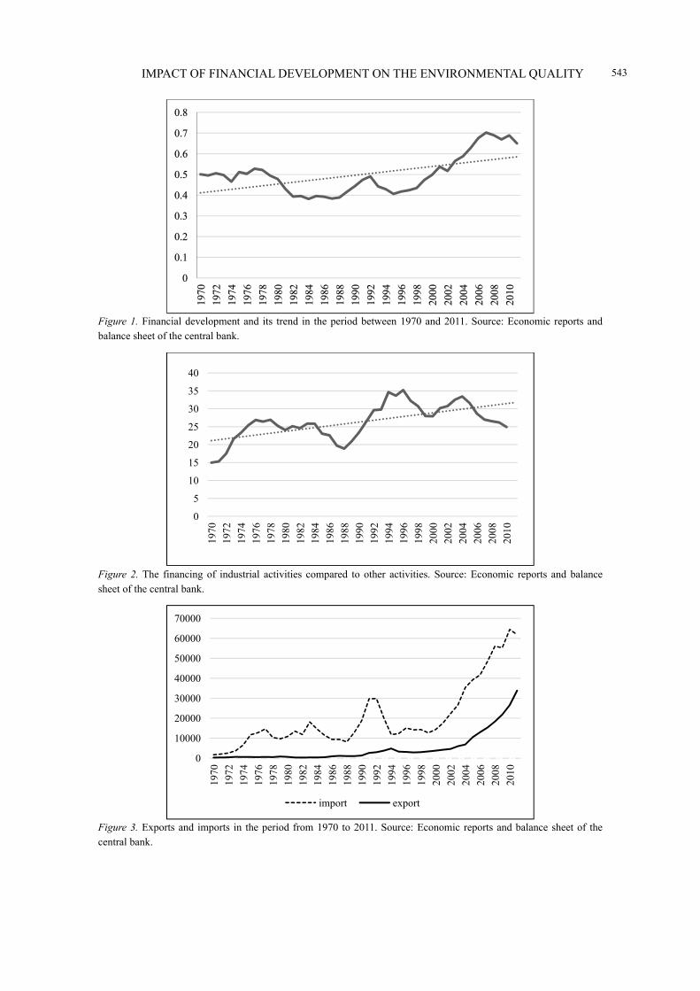
Financial Development and Trade in Iran
Figure 1 shows the trend of financial development in Iran. As shown in the period between 1970 and 2011,
financial development has declined and then increased due to imposed war. Overall financial development in
Iran has been increasing. However, the amount of financing for the industrial activities has increased over the
period. Figure 2 shows the amount of financing for the country’s industrial sector compared to other sectors and
activities with incremental growth, and shows that this sector has received more attention than other sectors in
financial development process.
Figure 3 shows the amount of exports and imports in Iran. Exports and imports have increased over the
years of the study.
Industries such as cement, glass, ceramics, iron and steel, pulp and paper, etc. apply a wide range of
environmental effects and release in the air plenty of oxides of Carbon, Sulfur, and Nitrogen.
According to Figure 4 and 5, exports of polluting goods have declined in the period between 1970 and
2011 and have a downward trend. However, the growth in imports of polluting goods compared to total
imported goods has risen. Therefore, the amount of pollutants produced during this period has a downward
trend.
IMPACT OF FINANCIAL DEVELOPMENT ON THE ENVIRONMENTAL QUALITY
543
Figure 1. Financial development and its trend in the period between 1970 and 2011. Source: Economic reports and balance sheet of the central bank.
Figure 2. The financing of industrial activities compared to other activities. Source: Economic reports and balance sheet of the central bank.
Figure 3. Exports and imports in the period from 1970 to 2011. Source: Economic reports and balance sheet of the central bank.
0
5
10
15
20
25
30
35
40
1970
1972
1974
1976
1978
1980
1982
1984
1986
1988
1990
1992
1994
1996
1998
2000
2002
2004
2006
2008
2010
0
10000
20000
30000
40000
50000
60000
70000
1970
1972
1974
1976
1978
1980
1982
1984
1986
1988
1990
1992
1994
1996
1998
2000
2002
2004
2006
2008
2010
import export

IMPACT OF FINANCIAL DEVELOPMENT ON THE ENVIRONMENTAL QUALITY
544
Figure 4. Trend of exporting polluting goods over the period from 1970 to 2011. Source: Economic reports and balance sheet of the central bank.
Figure 5. Trend of importing polluting goods over the period from 1970 to 2011. Source: Economic reports and balance sheet of the central bank.
Model
In this study, Autoregressive Distributed Lag Modeling Approach was employed which was proposed by
Pesaran and Shin (1999). Most of recent studies suggest that ARDL approach is preferable to other approaches
such as Engel-Granger, in examining the cointegration and long-run relationship among the variables. Whether
the variables in the model are I(0) or I(1), this approach is applicable, and in small samples it is relatively more
efficient than other approaches. ARDL Model is as follows:
, ∑ , ′ (2)
where
, 1 (3)
, 1, 2, … , (4)
In the above relationships Yt is the dependent variable and Xit is the independent variable. L is lag operator
and wt is a vector of categorical variables including predetermined variables in the model, such as intercept,
dummy variables, time trend, and other exogenous variables. P is the number of lags used for the dependent
0
5
10
15
20
25
1970
1972
1974
1976
1978
1980
1982
1984
1986
1988
1990
1992
1994
1996
1998
2000
2002
2004
2006
2008
2010
0
5
10
15
20
25
1970
1972
1974
1976
1978
1980
1982
1984
1986
1988
1990
1992
1994
1996
1998
2000
2002
2004
2006
2008
2010

IMPACT OF FINANCIAL DEVELOPMENT ON THE ENVIRONMENTAL QUALITY
545
variable and q is the number of lags used for the independent variables. Numbers of optimal lags for each of the
explanatory variables could be set by a measure of Akaike, Schwarz-Bayesian, Hanan-Queen, or adjusted
coefficient of determination. In this study, given the small size of the data set, Schwartz-Bayesian measure was
used. Long-run coefficients are calculated as follows:
,
,
1, 2 , …, (5)
ARDL approach consists of two steps to estimate the long-run relationships. First, the dynamic ARDL
model is tested for long-run relationship, and in the next step, long-run and short-run coefficients are estimated.
The second step is conducted only if the long-run relationship is verified in the first step. Having estimated
ARDL dynamic model, this paper tested the following hypothesis:
H ∑ 1 0
H ∑ 1 0 (6)
The null hypothesis implies the absence of a long-run relationship. Quantity t statistics requires to perform
the test as follows:
∑
∑ (7)
If t statistics obtained from the absolute critical values provided by Banerjee, Dolado, and Mester (2012) is
larger, then the null hypothesis based on absence of cointegration is rejected, and long-run relationship is
accepted (Nowferesti, 1999). In the second step, if the presence of cointegration is approved, the long-run
relationship would be estimated.
Study Results
Before the test, reliability of all variables is checked to ensure that none of the variables is I(2). If there is
any I(2) variable in the model, F statistics is not reliable. To ensure variables of time series used in the model
stationary or none-stationary, Augmented Dickey Fuller (ADF) test has been used. Table 1 shows the ADF
test’s results in the level for the variables. Usually the Schwarz Bayesian Criterion (SBC) saves the number of
lags. Therefore, in this study, the number of optimized lags is selected based on SBC criteria. OP variable in the
level, while without trend, is stationary, but for the variables of FD, FD2, GDP, and EN, Absolute Dickey Fuller
statistic in both cases is smaller than the critical values. Therefore, the variables in level are none-stationary and
the unit root hypothesis on the variables is not rejected.
Table 1
Results of Unit Root Tests in the Level
Variables With intercept and without trend * With intercept and trend **
Optimal lag ADF statistics Test results Optimal lag ADF statistics Test results
EN 0 -0.95 Non-stationary 0 -2.11 Non-stationary
FD 1 -0.74 Non-stationary 0 -2.79 Non-stationary
FD2 1 -0.72 Non-stationary 0 -2.44 Non-stationary
GDP 0 2.50 Non-stationary 5 0.25 Non-stationary
OP 9 -4.55 Stationary 9 -3.53 Non-stationary
Notes. * Critical value at the confidence level of 95% in cases without trend is -2.96; ** critical value at the confidence level of 95% in cases with trend is -3.56. Source: Research findings.

IMPACT OF FINANCIAL DEVELOPMENT ON THE ENVIRONMENTAL QUALITY
546
To find the stationary degree of the variables, ADF test was replicated for the first-order difference of the
variables. Test results showed that variables get stationary by making one deduction.
Table 2
Results of Unit Root Tests on the First Difference of the Variables
Variables With intercept and without trend * With intercept and trend **
Optimal lag ADF statistics Test results Optimal lag ADF statistics Test results
EN 0 -5.28 Stationary 0 -5.38 Stationary
FD 0 -3.94 Stationary 0 -3.71 Stationary
FD2 0 -3.84 Stationary 0 -3.60 Stationary
GDP 0 -3.81 Stationary 0 -4.24 Stationary
Notes. * Critical value at the confidence level of 95% in cases without trend is -2.96; ** critical value at the confidence level of 95% in cases with trend is -3.56. Source: Research findings.
Result of estimation of ARDL model is based on the three parts: dynamic, short-run, and long-run
relationships. The following equation as the dynamic relationships among variables can be specified and
estimated:
EN ∑ α EN ∑ FD ∑ FD ∑ GDP ∑ OP U (8)
To estimate the relationship, as the data are on annual basis, the maximum lags were taken two, and using
Schwarz-Bayesian criterion, dynamic relationships among variables were selected. The optimal lags for each of
the variables were set and the model was estimated as ARDL (1, 0, 0, 0, 0). To study the long-run relationship
of the variables, the value of computational statistics of Banerjee et al. (2012) is calculated in the following
way:
.
.3.78 (9)
The value of table of Banerjee et al. (2012) at confidence level of 90% for a model with intercept is equal
to -3.64; thus, the existence of long-run relationship among the variables is confirmed. Having ensured the
long-term relationship, results of estimation would be provided in Table 3.
Table 3
Result of Estimation of Long-run Relationship
Variables Coefficients Standard deviation t statistics Critical value
FD 14.55 6.33 2.30 0.028*
FD2 -0.11 0.06 -1.84 0.074**
GDP 20.84 3.14 6.63 0.000*
OP -38.81 8.56 -4.53 0.000*
Notes. * Significant at 95% confidence level; ** significant at 90% confidence level. Source: Research findings.
As the results of the classic test show the lack of successive correlation among components of disturbances,
properly specified equation and equal variance, the results of long-run relationship are reliable. Results
obtained from Table 3 show that all variables are significant at the 90% confidence interval. The positive
coefficient of GDP (20.84) shows that economic growth in Iran is primarily associated with emission increase.
Coefficient of financial development and trade liberalization is positive and negative respectively, which

IMPACT OF FINANCIAL DEVELOPMENT ON THE ENVIRONMENTAL QUALITY
547
implies that increase in financial development causes rise in environmental degradation; however, trade
increase promotes the quality of the environment. The coefficient of long term emissions relative to variable of
squared financial development is significant and negative (-0.11), which shows that the inverted U relationship
between financial development and environmental quality is true in Iran.
For a more detailed review of the results, changes in the environmental degradation index and financial
development could be estimated in the model according to the coefficients, and assuming that all other
conditions do not change, shown in Figure 6.
Figure 6. Inverted U relationship between financial development and environmental quality for Iran using Matlab. Sources: Research findings.
In this figure, the vertical axis and horizontal axis respectively represent the environmental emissions and
financial development. As it is seen, the curve for Iran is similar to an inverted U and the estimated model fully
meets the theoretical expectations. In the period between 1970 and 2011, Iran was in the first half of the curve,
and financial development for levels higher than 0.72 leads to improved environmental quality. The estimated
error correction model to study adjustment of short-run disequilibrium towards long-run equilibrium is
presented in Table 4.
Table 4
Results of the Estimation of Error Correction Model
Variables Coefficients Standard deviation T-statistics Critical value
dFD 7.76 3.79 2.04 0.049*
dFD2 -0.06 0.03 -1.71 0.096**
dGDP 11.12 3.25 3.42 0.002*
dOP -20.70 6.23 -3.32 0.002*
ECM(-1) -0.53 0.14 -3.80 0.001*
Notes. * Significant at 95% confidence level; ** significant at 90% confidence level. Source: Research findings.
The value of -0.53 was obtained for error correction coefficients in the model, which means a 53%
adjustment in each period to establish a long-run equilibrium. The results of CUSUM and CUSUMSQ tests for
evaluating the estimated coefficients and the results of stability test for short- and long-run coefficients over the
time were shown in Figure 7 and 8.

IMPACT OF FINANCIAL DEVELOPMENT ON THE ENVIRONMENTAL QUALITY
548
Figure 7. Plot of cumulative sum of recursive residuals. Sources: Research finding.
Figure 8. Plot of cumulative sum of squares of recursive residuals. Sources: Research finding.
As in both tests, the statistics were within the 95% confidence intervals, null hypothesis based on the
stability of the coefficients was accepted and at the confidence level of 95%, the obtained results are valid.
Conclusions
Economic growth is one of the most important concerns of human communities. Development process in
Iran, like other developing countries involves the use of the environment and at its degradation at the same
times. Financial intermediaries through financial development may increase technological innovation and
mobilize financial resources to identify the best production technology and make investments in projects
involving clean environment. Nevertheless, financial development may increase financing for industrial
activities which harm the environment.
Due to the different reliability degrees of the variables, long-run ARDL model was employed. The results
show that the coefficient of financial development is positive and significant at the 0.05% probability level, and
suggest that in addition to economic growth, financial development also affects environmental quality in Iran,
and has led to increase environmental pollution. Negative squared coefficient of financial development implies
that inverted U-shaped relationship between financial development and environmental quality is true for Iran.
Results show that Iran is on the upside half of curve and according to predictions made on the basis of the
IMPACT OF FINANCIAL DEVELOPMENT ON THE ENVIRONMENTAL QUALITY
549
financial development of approximately 0.72 in Iran, financial development will lead to improved
environmental quality. Given the high importance of development for developing countries, including Iran, to
support environmental policies is of low priority. Based on the Figure 2, in the years considered, financing for
industrial activity has increased compared to other activities and industries have been inefficient in protection
of the environment. Financial development has made way for destruction of environment. In fact, the
investments were only effective in increasing the size of the industrial activities and have not resulted in
technological advancement in the industry.
Results show that economic growth had a significant and positive impact on emissions. The study’s results
also suggest that increased trade openness has led to improvement of environmental quality in the country. This
could be due to that the goods which produce large quantities of pollutants in the manufacturing process are
imported from other countries like China. As a result, the pollution increases in the exporting countries, and in
Iran as an importing country, pollution reduces due to the reduction in production of polluting goods.
Furthermore, it might be due to decline in export of polluting goods, which reflects low production and reduced
pollution in Iran. The decline in the proportion of heavy polluting products’ export such as cement, glass,
ceramics, iron, and steel, which produce large amounts of pollutants in manufacturing process (Figure 5), and
increased proportion of imports (Figure 4) confirm the results of the model. In addition, economic openness
leads to an increase in imports of high tech intermediary and capital goods that create less pollution in
production process.
References Agheli, L., Velaei Yamchi, M., & Jangavar, H. (2010). Impacts of economic openness on environmental degradation in Iran.
Journal of Strategy, 19, 197-216. Alam, S., Fatima, A., & Butt, M. S. (2007). Sustainable development in Pakistan in the context of energy consumption demand
and environmental degradation. Journal of Asian Economics, 18(5), 825-837. Aldy, J. E. (2005). An environmental Kuznets curve analysis of U.S. state level carbon dioxide emission. Environment &
Development, 14, 48-72. Ang, J. B. (2007). CO2 emissions, energy consumption, and output in France. Energy Policy, 35(10), 4772-4778. Barqi Askooei, M. (2008). Effects of trade liberalization on greenhouse gas emission (carbon dioxide) in the environmental
Kuznets Curve. Journal of Economic Research, 82, 1-22. Barqi Askooei, M., Fallahi, F., & Zhande Khatibi, S. (2012). The effect of factory products and foreign direct investment on CO2
emissions in D8 Member countries. Journal of Economic Modeling, 4, 93-109. Behboodi, D., & Barghi Golazani, E. (2008). Environmental impacts of energy consumption and economic growth in Iran.
Journal of Value Economic, 5(4), 35-53. Behboodi, D., Fallahi, F., & Barghi Golazani, E. (2010). Social and economic factors effective on carbon dioxide emissions per
capita in Iran. Journal of Economic Research, 90, 1-17. Cole, M. A., Rayner, A. J., & Bates, J. M. (1997). The environmental Kuznets curve: An empirical analysis. Environment and
Development Economics, 2(4), 401-416. Fotros, M., & Maboodi, R. (2010). Causal relationship between energy consumption and urban population and environmental
pollution in Iran 1971-2006. Journal of Energy Economics Studies, 27, 1-17. Ghazali, S., & Zibaee, M. (2009). Analysis of the relationship between environmental pollution and economic growth
using panel data: A case study of carbon monoxide emissions. Journal of Economics and Agricultural Development, 2, 128-133.
Grossman, G., & Krueger, A. B. (1991). Environmental impact of a North American free trade agreement. NBER working paper, 3914, 1-57.
Halicioglu, F. (2009). An econometric study of CO2 emissions, energy consumption, income and foreign trade in Turkey. Energy Policy, 37(3), 1156-1164.

IMPACT OF FINANCIAL DEVELOPMENT ON THE ENVIRONMENTAL QUALITY
550
Iwata, H., Okada, K., & Samreth, S. (2010). Empirical study on the environmental Kuznets curve for CO2 in France: The role of nuclear energy. Energy Policy, 38(8), 4057-4063.
Jalil, A., & Feridun, M. (2011). The impact of growth, energy and financial development on the environment in China: A cointegration analysis. Energy Economics, 33(2), 284-291.
Levine, R. (2005). Finance and growth: Theory and evidence. Handbook of economic growth, 1, 865-934. Lieb, C. M. (2004). The environmental Kuznets curve and flow versus stock pollution: The neglect of future damages.
Enviromental and Resource Economics, 29, 483-506. Lotfalipour, M. R., Fallahi, M. A., & Ashena, M. (2010). The relationship between carbon dioxide emissions and economic
growth, energy and trade in Iran. Journal of Economic Researches, 94, 151-173. Lotfalipour, M. R., Fallahi, M. A., & Bastam, M. (2012). Environmental issues and forecasting the carbon dioxide emissions in
the Iran. Journal of Applied Economic Studies in Iran, 3, 81-109. Mowlayi, M., Kavosi Kalashemi, M. & Rafiei, H. (2010). The relationship between carbon dioxide emission and per capita
income and existing environmental Kuznets curve in Iran. Journal of Environmental Sciences, 1, 205-216. Nasrollahi, Z., & Ghaffari Goolak, M. (2009). Economic development and environmental pollution in Kyoto Pact countries and
the countries of Southeast Asia (with emphasis on the environmental Kuznets curve). Journal of Economic Sciences, 35, 105-125.
Nowferesti, M. (1999). Unit root and cointegration in econometrics. Tehran: Institute of Rasa Cultural Services. Ozturk, I., & Acaravci, A. (2013). The long-run and causal analysis of energy, growth, openness and financial development on
carbon emissions in Turkey. Energy Economics, 36, 262-267. Pao, H. T., & Tsai, C. M. (2011). Multivariate Granger causality between CO2 emissions, energy consumption, FDI (foreign
direct investment) and GDP (gross domestic product): Evidence from a panel of BRIC (Brazil, Russian Federation, India, and China) countries. Energy, 36(1), 685-693.
Pazhouan, J., & Moradhasel, N. (2007). Effects of economic growth on air pollution. Journal of Economic Research, 94(7), 141-160. Pesaran, M. H., & Shin, Y. (1999). An Autoregressive Distributed Lag Modeling Approach to cointegration analysis. In S. Strøm
(Ed.), Econometrics and economic theory in the twentieth century: The ragnar Frisch centennial symposium. Cambridge: Cambridge University Press.
Pourkazemi, M., & Ebrahimi, I. (2008). Evaluation of environmental Kuznets curve in the Middle East. Journal of Economic Research, 34, 57-71.
Sadeghi, S., & Feshari, M. (2010). An estimation of long-run relationship between exports and environmental quality index: A case study of Iran. Iranian Journal of Economic Research, 44, 67-83.
Sadeghi, S., Motafaker Azad, M., Pour Ebadelahan Kovich, M., & Shabaz Zade Kheyavi, A. (2012). The causal relationship between carbon dioxide emissions, foreign direct investment, GDP and per capita energy consumption in Iran. Journal of Energy and Environmental Economics, 4, 101-116.
Sadorsky, P. (2010). The impact of financial development on energy consumption in emerging economies. Energy Policy, 38(5), 2528-2535.
Salimifar, M., & Dehnavi, J. (2009). Comparing the environmental Kuznets curve in OECD member countries and developing countries: An analysis based on panel data. Journal of Knowledge and Development, 29(16), 181-200.
Selden, T. M., & Song, D. (1994). Environmental quality and development: Is there a Kuznets curve for air pollution emissions? Journal of Environmental Economics and Management, 27(2), 147-162.
Shafik, N. (1994). Economic development and environmental quality: An econometric analysis. Oxford Economic Papers, 46, 757-773.
Shahbaz, M., Hye, Q. M. A., Tiwari, A. K., & Leitão, N. C. (2013a). Economic growth, energy consumption, financial development, international trade and CO2 emissions in Indonesia. Renewable and Sustainable Energy Reviews, 25, 109-121.
Shahbaz, M., Solarin, S. A., Mahmood, H., & Arouri, M. (2013b). Does financial development reduce CO2 emissions in Malaysian economy? A time series analysis. Economic Modelling, 3, 145-152.
Sharzaei, G., & Haghani, M. (2009). Evaluation of causal relationship between carbon emissions and internal revenue, with emphasis on the role of energy. Journal of Economic Research, 68, 75-90.
Song, T., Zheng, T., & Tong, L. (2008). An empirical test of the environmental Kuznets curve in China: A panel cointegration approach. Economic Review, 19(3), 381-392.
Soytas, U., Sari, R., & Ewing, B. T. (2007). Energy consumption, income, and carbon emissions in the United States. Ecological Economics, 62(3-4), 482-489.

IMPACT OF FINANCIAL DEVELOPMENT ON THE ENVIRONMENTAL QUALITY
551
Tamazian, A., & Rao, B. (2010). Do economic, financial and institutional developments matter for environmental degradation? Evidence from transitional economies. Energy Economics, 32(1), 137-145.
Tamazian, A., Chousa, J. P., & Vadlamannati, K. C. (2009). Does higher economic and financial development lead to environmental degradation: Evidence from BRIC countries. Energy Policy, 37(1), 246-253.
Tol, S. J. W., Pacala, R., & Socolow, S. R. (2006). Understanding long term energy use and carbon dioxide emissions in the USA. Humborg: Humborg University Press .
United Nations. (1997). Kyoto Protocol to the United Nations framework convention on climate change. Retrieved from http://www.unfccc.int
Vaseghi, E., & Esmaeili, A. (2009). Evaluation of determining factors in CO2 emissions in Iran (application of environmental Kuznets). Journal of Ecology, 52, 99-110.
Yuxiang, K., & Chen, Z. (2010). Financial development and environmental performance: Evidence from china. Environment and Development Economics, 16, 1-19.
Zhang, Y. J. (2011). The impact of financial development on carbon emissions: An empirical analysis in China. Energy Policy, 39(4), 2197-2203.

Chinese Business Review, September 2014, Vol. 13, No. 9, 552-561 doi: 10.17265/1537-1506/2014.09.002
Sino-European Trade Competition in Latin
America and the Caribbean
Wioletta Nowak
University of Wroclaw, Wroclaw, Poland
The article studies trade in goods between China and the Latin American and Caribbean (LAC) countries and
between the European Union (EU) and LAC during the years from 2000 to 2013. From the beginning of the 21st
century, big changes in LAC’s trade patterns have been observed. The article contains possible explanation of them.
The analysis is based on the ECLAC (Economic Commission for Latin America and the Caribbean) data.
Merchandise trade between China and LAC grew significantly over the period from 2000 to 2013. In 2013, the
value of merchandise exports from China was higher than from the EU-28 in the case of 12 LAC countries. Chinese
imports of goods surpassed the European ones in five countries in the region. In order to increase its exports of
manufactured goods and imports of natural resources and agricultural commodities, China combines trade
arrangements with foreign aid policy. Besides, a rapid development of bilateral diplomatic ties between China and
LAC is observed. The EU-LAC trade relations have worsened during the last decade mainly due to financial crisis
and development of the EU-Asia trade relations.
Keywords: China, merchandise trade, foreign aid, European Union (EU)
Introduction
The European Union (EU) and China (after the United Sates) are the most important trading partners for
the Latin American and Caribbean (LAC). Since the beginning of the 21st century, a rapid expansion of
Sino-Latin trade and economic relations has been observed. China is likely to surpass the EU and be LAC’s
second largest trade partner in a few years. China’s ties with Latin America are not new. However, their
dynamics in recent years were really spectacular. The significant increase in trade between China and LAC
countries was observed after the beginning of the financial crisis. Besides, from 2008, China has become a
major source of financing for many countries in the region. China uses its loans to develop bilateral trade
relations with the LAC states.
After the financial crisis, the EU was mainly concentrated on the struggle against its effects. In order to
restore its economy, the EU developed closer economic and trade relations with Asia. At the same time, the
EU-LAC trade relations have worsened. Although, the EU increased its aid-for-trade with LAC countries, it has
been gradually losing its importance for LAC as a destination for exports and as a source for imports.
In the literature, trade relations between China and Latin America and between the EU and LAC are
mainly examined separately (Bárcena & Rosales, 2010; Bárcena, Prado, Rosales, & Pérez, 2012; Roy, 2012).
Wioletta Nowak, Ph.D., University of Wroclaw, Wroclaw, Poland. Correspondence concerning this article should be addressed to Wioletta Nowak, Institute of Economic Sciences, Uniwersytecka
22/26, 50-145 Wroclaw, Poland. E-mail: [email protected].
DAVID PUBLISHING
D

COMPETITION IN LATIN AMERICA AND THE CARIBBEAN
553
The aim of the paper is to study China-LAC and the EU-LAC trade relations in the first decade of the 21st
century using the same data set. The analysis is principally based on the EULAC data.
Development of China-LAC and the EU-LAC Trade Relations
Trade between China and Latin America is dated back to the 1560s. At that time, Chinese ships sailed to
Acapulco in Mexico via Manila. China exported mainly silk, cotton cloths, jewellery, and gun powder to Latin
America, and imported wine, olive, oil, soap, and food. In 1815, this “silk-road” on the sea between China and
Latin America was closed due to an implementation of the Chinese export control policy (Jiang, 2006, p. 69).
In the 19th century, Sino-Latin American relations took a different form. The basis of ties was the Chinese
immigration. Hundreds of thousands of Chinese workers migrated to the Latin American countries (Mexico,
Brazil, Chile, Panama, and Peru) where they mainly worked in mines and on plantations (Ratliff, 2009, p. 2).
After the proclamation of People’s Republic of China in 1949, economic cooperation between China and
LAC was still limited. Trade exchange was insignificant, not to mention investments. The situation was a
consequence of a lack of diplomatic contacts at high governmental levels between China and LAC states and
the poor condition of the Chinese economy.
In the 1950s, Sino-Latin American ties were restricted to visits of individual Latin Americans. LAC
countries began to establish diplomatic relations with China just in the 1970s. The first countries that
recognized People’s Republic of China in the region were Cuba and Chile. Cuba established diplomatic
relations with China in 19601 and Chile 10 years later. Then, other major countries in the region began to
recognize China.2 It happened mainly because of two significant events: In 1971, the government of People’s
Republic of China was recognised as the legal representative of China in the United Nations (UN) and was
given the permanent seat in the UN Security Council; in February 1972, President Richard Nixon visited China,
after which the pressure from the United States declined and Latin countries which were always in the orbit of
the American influence could begin to establish diplomatic relations with China.
China-LAC trade relations accelerated after Deng Xiaoping’s reforms in 1978. China’s rapid economic
growth and its constantly increasing demand for natural resources, food and new markets caused that it had to
find new trade partners. China, among others, turned to resource-rich Latin America.
Until now, China has got preferential access to three markets in the region (Table 1). It signed free trade
agreement (FTA) with Chile, Peru, and Costa Rica. FTAs cover items on the World Trade Organization’s new
trade agenda. It means that they concern not only the deregulation and liberalization of goods markets but also
services and investment. Besides, in 2012, China declared readiness to negotiate with Mercosur (Argentina,
Brazil, Paraguay, Uruguay, and Venezuela) on a free trade area.
Sino-Latin American trade relations are developed and strengthened also during high-level visits. A
significant increase in official visits to LAC by the highest Chinese authorities has been recorded since 2001.
Diplomatic relations were developed and maintained by Jiang Zemin and his successors Hu Jintao and Xi
Jinping (Table 2).
1 After the Sino-Soviet split in the 1960s, Cuba chose the Soviet Union and froze its relation with China. Both countries normalised relations after the collapse of the Soviet Union. 2 In 2014, People’s Republic of China was recognized by 21 LAC countries: Cuba (1960), Chile (1970), Peru (1971), Mexico (1972), Argentina (1972), Guyana (1972), Jamaica (1972), Trinidad and Tobago (1974), Venezuela (1974), Brazil (1974), Suriname (1976), Barbados (1977), Ecuador (1980), Colombia (1980), Antigua and Barbuda (1983), Bolivia (1985), Grenada (1985), Uruguay (1988), Bahamas (1997), Dominica (2004), and Costa Rica (2007).

COMPETITION IN LATIN AMERICA AND THE CARIBBEAN
554
Table 1
Trade Agreements Between China and the Latin American Countries
Agreement name Type Coverage Date of entry into force
Chile to China FTA & EIA Goods & Services 01-Oct-2006 (Goods), 01-Aug-2010 (Services)
China to Costa Rica FTA & EIA Goods & Services 01-Aug-2011
Peru to China FTA & EIA Goods & Services 01-Mar-2010
Note. EIA: Economic Integration Agreement. Source: Retrieved from http://rtais.wto.org/UI/PublicAllRTAList.aspx.
Table 2
Development of Bilateral Ties Between China and Latin America and the Caribbean in the Years 2001-2014
Year Chinese authority Visited LAC countries
2001, April President Jiang Zemin Chile, Argentina, Uruguay, Brazil, Cuba, Venezuela
2003, December Prime Minister Wen Jiabao Mexico
2004, November President Hu Jintao Chile, Brazil, Argentina, Cuba
2005, September President Hu Jintao Mexico
2008, November President Hu Jintao Peru, Costa Rica, Cuba
2009, February Vice President Xi Jinping Mexico, Jamaica, Colombia, Venezuela, Brazil
2010, April President Hu Jintao Brazil
2011, June Vice President Xi Jinping Cuba, Uruguay, Chile
2012, June Prime Minister Wen Jiabao Brazil, Uruguay, Argentina, Chile
2013, May/June President Xi Jinping Trinidad and Tobago, Costa Rica, Mexico,
2014, July President Xi Jinping Brazil, Argentina, Venezuela, Cuba
Moreover, the China Council for the promotion of international trade has initiated so far eight China-Latin
America business summits which are also an important platform for trade cooperation between China and LAC.
The first was held in Santiago, Chile (2007), the second in Harbin, China (2008), and the next in Bogota,
Colombia (2009), Chengdu, China (2010), Lima, Peru (2011), Hangzhou, China (2012), San Jose, Costa Rica
(2013), and Changsha, China (2014).
Europe and LAC are linked through historical, cultural, political, and economic ties which are dated back
to 1492. However, contemporary relations between the EU and LAC were regulated in 1999 during the first
EU-LAC summit which was held in Rio de Janeiro, Brazil. The main achievement of the summit was the
establishment of a strategic partnership between the EU and LAC. Since then, issues referring to a mutual
cooperation in the area of free trade between the regions are discussed during biannual EU-LAC summits. So
far six bi-regional summits have been held in Madrid, Spain (2002), Guadalajara, Mexico (2004), Vienna,
Austria (2006), Lima, Peru (2008), Madrid, Spain (2010), and Santiago, Chile (2013). The summits bring
together heads of state and government from both continents. In the years when the EU-LAC summits do not
take place, the EU and the Rio Group3 meet at ministerial level. In 2010, EU-LAC foundation was created in
order to assist in the implementation of main objectives of the strategic partnership between the regions. The
Foundation has 63 members: the 28 members of the EU, the 33 LAC states, and the EU institutions (Retrieved
from http://eulacfoundation.org/en/about-us).
The EU has privileged relations in trade with the Caribbean and countries of Central America. Besides, the 3 The Rio Group was established by Argentina, Brazil, Colombia, Mexico, Panama, Peru, Uruguay, and Venezuela in 1986. The Group eventually extended to 24 Latin American and Caribbean states.

COMPETITION IN LATIN AMERICA AND THE CARIBBEAN
555
EU signed special agreements with Mexico, Chile, Colombia, and Peru (Table 3). All trade agreements
between the EU and LAC relate to deregulation and liberalization of trade in goods and services.
Table 3
Trade Agreements Between the EU and LAC
Agreement name Type Coverage Date of entry into force
EU to CARIFORUM States EPA FTA & EIA Goods & Services 01-Nov-2008 EU to Central America (Costa Rica, El Salvador, Guatemala, Honduras, Nicaragua, and Panama)
FTA & EIA Goods & Services 01-Aug-2013
EU to Chile FTA & EIA Goods & Services 01-Feb-2003 (Goods)
01-Mar-2005 (Services)
EU to Colombia and Peru FTA & EIA Goods & Services 01-Mar-2013
EU to Mexico FTA & EIA Goods & Services 01-Jul-2000 (Goods)
01-Oct-2000 (Services)
Note. CARIFORUM includes 14 CARICOM members and the Dominican Republic. Source: Retrieved from http://rtais.wto.org/UI/PublicAllRTAList.aspx.
In 2000, the EU opened negotiations on free trade area with Mercosur. However, there are some obstacles
in negotiations concerning sectors which are sensitive for both sides. The EU protects its own production of
food via the common agricultural policy and Mercosur wants the access to the European market in agricultural
goods. In turn, Mercosur protects its own production of manufactured goods that are the EU’s basic export
commodities (Roy, 2012, p. 8).
Main Characteristics of Merchandise Trade Between China and LAC and Between the EU and LAC
Europe has been the second major trading partner (after the United States) for LAC for many years.
However, recently, an impressive increase in trade between China and LAC33 (33 countries) has been observed.
In the years 2000-2013, the value of China’s exports in goods to LAC33 increased about 19 times and Chinese
imports in goods from the region increased over 23 times. At that time, the value of the EU25 (25 countries)
exports in goods to LAC33 increased about three times. European merchandise imports increased 2.7 times.
Trends in merchandise trade between the EU25 and LAC33 and between China and LAC33 over the period
2000-2014 are presented in Figure 1.
In 2000, the value of European merchandise exports to LAC33 was 7.7 times higher than Chinese, but 14
years later only 1.2 times. At the beginning of the century, the value of European merchandise imports from
LAC33 was 9.3 higher than China’s imports from the region. In 2013, the EU25 imports value was merely 1.1
higher than the Chinese. The EU has been steadily losing its share in Latin American market to China. If the
average growth rate of Chinese trade with LAC will be maintained, China is likely to be the second important
trading partner for LAC in a few years.
After the beginning of global economic and financial crisis, both China and the EU decreased their trade
with LAC. In 2009 compared to 2008, the Chinese exports declined by 21% and imports by 10%. In the case of
the EU, the figures were respectively 24% and 31%.
The change in the Chinese merchandise trade with selected Latin American countries over the period from
2000 to 2013 is significantly higher. For instance, during last 14 years, the Chinese exports to Colombia and
Peru increased over 40 times. China’s imports from Venezuela and Colombia increased over 100 times. In the

COMPETITION IN LATIN AMERICA AND THE CARIBBEAN
556
case of Costa Rica, the increase in the Chinese imports was exceptionally high. In the considered years, the EU
increased its trade with the Latin American countries a few times (Table 4).
Figure 1. EU25 and China’s trade in goods with LAC33 in the years 2000-2013 (USD million). Source: Retrieved from http://www.cepal.org/comercio/ecdata2.
Table 4 Percentage Change in Value of China’s and the European Union’s Trade in Goods With Selected Latin American Countries in the Years 2000-2013
Country China EU25
Country China EU25
Exports Imports Exports Imports Exports Imports Exports Imports
Argentina 1,334% 554% 132% 111% Guatemala 964% 3,676% 132% 82%
Brazil 2,834% 3,249% 243% 155% Mexico 2,069% 1,997% 177% 242%
Chile 1,573% 1,447% 282% 149% Panama 752% 4,208% 153% 119%
Colombia 4,277% 11,158% 334% 356% Peru 4,188% 1,401% 387% 328%
Costa Rica 1,322% 46,041% 76% 116% Uruguay 856% 2,334% 182% 338%
Cuba 491% 522% 83% 71% Venezuela 2,264% 13,742% 96% 76%
Ecuador 3,863% 867% 509% 258%
Source: Retrieved from http://www.cepal.org/comercio/ecdata2.
The rise in the Chinese merchandise trade with selected Latin American countries is much more
impressive in longer period. During the last 20 years, China has been exponentially increased its trade with
countries in the region. China’s exports and imports of goods to its most important Latin American trading
partners are presented in Figure 2.
A fast growth of the merchandise exchange between China and LAC caused that China has already
overtaken the EU in trade with a few countries in the region. In 2013, China exported more commodities than
the EU to 12 Latin American countries: Chile, Panama, Venezuela, Peru, Uruguay, Guatemala, Paraguay,
Honduras, Jamaica, Nicaragua, Haiti, and Dominica. The Chinese imports value of goods was higher than the
European in the case of five countries: Brazil, Chile, Venezuela, Peru, and Uruguay.
Since the beginning of the 21st century, the importance of China as an export market significantly has
been increased in a few LAC countries (Table 5). In 2013, China absorbed almost one fourth of the Chilean
merchandise exports and one fifth of the Brazilian ones. Besides, over 17% of the Peruvian and 14% of the
Uruguayan exports were destined in China. A relatively big increase in the share of exports of goods to China
in total exports was also observed in the case of Colombia, Argentina, and Panama. China still became an
0
50000
100000
150000
200000
2000
2001
2002
2003
2004
2005
2006
2007
2008
2009
2010
2011
2012
2013
Exports of goods
E25 China
0
50000
100000
150000
200000
2000
2001
2002
2003
2004
2005
2006
2007
2008
2009
2010
2011
2012
2013
Imports of goods
E25 China

COMPETITION IN LATIN AMERICA AND THE CARIBBEAN
557
unexploited market for Bolivia, Costa Rica, Mexico, or Paraguay. Over the period from 2000 to 2013, China
substantially increased its importance as a source of imports for the LAC countries. In 2013, the most
dependent countries on Chinese commodities were Paraguay (28.3% of its imports came from China), Chile
(19.7%), and Peru (19.4%).
Figure 2. China’s exports and imports of goods to Brazil, Chile, Mexico, and Venezuela (USD million) in the years 1994-2013. Source: Retrieved from http://www.cepal.org/comercio/ecdata2.
Table 5
Merchandise Trade of Selected LAC Countries with China in 2000 and 2013 (Percentages of Total Trade)
Country Exports Imports
Country Exports Imports
2000 2013 2000 2013 2000 2013 2000 2013
Argentina 3.0 7.2 4.6 15.4 Ecuador 1.2 2.3 2.2 16.7
Bolivia 0.4 2.6 3.1 12.1 Mexico 0.2 1.7 1.6 16.1
Brazil 2.0 19.0 2.2 15.6 Panama 0.2 6.1 0.6 7.9
Chile 5.0 24.8 5.7 19.7 Paraguay 0.7 0.6 11.5 28.3
Colombia 0.2 8.7 3.0 17.5 Peru 6.4 17.5 3.9 19.4
Costa Rica 0.2 3.3 1.3 9.6 Uruguay 4.0 14.2 3.2 16.9
Source: Retrieved from http://www.cepal.org/comercio/ecdata2.
The EU is still an important export market for most of the LAC countries. For instance, in 2009 over 20%
of Brazil’s, Honduras’ or Panama’s exports were destined in EU27. However, in the years from 2000 to 2009, a
percentage increase in merchandise exports to EU27 was observed only in Ecuador, Honduras, Panama,
0
10000
20000
30000
40000
50000
60000
1994
1996
1998
2000
2002
2004
2006
2008
2010
2012
Brazil
Exports Imports
0
5000
10000
15000
20000
25000
1994
1996
1998
2000
2002
2004
2006
2008
2010
2012
Chile
Exports Imports
05000
100001500020000250003000035000
1994
1996
1998
2000
2002
2004
2006
2008
2010
2012
Mexico
Exports Imports
0
5000
10000
15000
2000019
94
1996
1998
2000
2002
2004
2006
2008
2010
2012
Venezuela
Exports Imports

COMPETITION IN LATIN AMERICA AND THE CARIBBEAN
558
Paraguay, Venezuela, and four Caribbean countries. In the case of 18 countries in the region, the share of
merchandise exports of goods to EU27 in their total exports decreased over the considered period (Bárcena &
Rosales, 2010, p. 13).
An analysis of the structure of China’s and Europe’s trade with LAC shows some similarities. Namely,
both sell to LAC mostly manufactured goods and LAC countries send to them mainly resources and raw
materials. China’s exports of goods to Latin America consist principally of electronics, components and parts,
machinery and equipment, textiles and apparel. In other words, China is a source of imports of cheap
manufactured goods for the region (Table 6).
Table 6
Top Five Latin American Trade Partners of China in 2013
China’s exports of goods China’s imports of goods
No. Country Goods No. Country Goods
1 Brazil Telecommunication equipment, optical instruments, electrical machinery
1 Brazil Iron ore and concentrates, seeds and oleaginous fruit, crude petroleum, pulp andwaste paper, sugar and honey
2 Mexico Telecommunication equipment, optical instruments, automatic data processing machines
2 Chile Copper, ores and concentrates of base metals, iron ore and concentrates
3 Chile Telecommunication equipment, footwear, cloths
3 Venezuela Crude petroleum and oils, petroleum products
4 Panama Petroleum products, ships, boats and floating structure
4 Mexico Ores and concentrates of base metals, passenger motor vehicles, microcircuits, transistors
5 Argentina Telecommunication equipment 5 Peru Ores and concentrates of base metals, iron ore and concentrates, copper
Source: Retrieved from http://www.cepal.org/comercio/ecdata2.
Table 7
Top Five Latin American Trade Partners of the European Union in 2013
EU25 exports of goods EU25 imports of goods
No. Country Goods No. Country Goods
1 Brazil
Medicinal and pharmaceutical products, motor vehicle parts and accessories, petroleum products, aircraft and associated equipment
1 Brazil Iron ore and concentrates, feeding stuff for animals, seeds and oleaginous fruit, coffee, crude petroleum
2 Mexico Petroleum products, medicinal and pharmaceutical products, motor vehicle parts and accessories
2 Mexico Crude petroleum and oils, telecommunication equipment, passenger motor vehicles
3 Argentina Petroleum products, motor vehicle parts and accessories, medicinal and pharmaceutical products
3 Chile Copper, ores and concentrates of base metals, fruit and nuts
4 Chile Aircraft and associated equipment, passenger motor vehicles, crude petroleum
4 Argentina Feeding stuff for animals, chemical products, ores and concentrates of base metals
5 Colombia Medicinal and pharmaceutical products, aircraft and associated equipment
5 Colombia Crude petroleum and oils, coal, fruit and nuts
Source: Retrieved from http://www.cepal.org/comercio/ecdata2.
Latin America is important destination for the European medicinal and pharmaceutical products, motor
vehicles and aircraft (Table 7). Latin American exports mainly copper, iron and steel, oil, natural gas, coal,

COMPETITION IN LATIN AMERICA AND THE CARIBBEAN
559
soya beans, beef, bananas, and coffee to China and the EU. On average, the LAC countries sell more different
products to the EU than to China (Bárcena et al., 2012, p. 40). Of the LAC countries, only Mexico exports more
technology-intensive products to China and the EU.
Foreign Aid as a Tool of Promoting Trade With LAC Countries
China uses different methods to increase its trade in goods with other countries. One of the most effective
tools is foreign aid. Depending on the region and country, China provides grants, interest-free loans or
concessional loans to countries with which it trades. In the case of the LAC countries, low-interest loans
dominated in the Chinese foreign aid policy. It is estimated that China offered about USD 100 billion to the
region in the years from 2005 to 2013 (Figure 3).
Figure 3. China’s lending to Latin America and the Caribbean in the years 2005-2013 (USD billion). Source: Gallagher, Irwin, and Koleski (2012).
Over 90% of China’s lending to LAC was pledged after 2007. In 2010, China’s loan commitments to the
region were more than combined loans of the Inter-American Development Bank, World Bank, and United
States Export-Import Bank to LAC (Gallagher et al., 2012, p. 1).
During the financial crisis, China provided low-interest loans mainly to four resource-rich countries in the
region: Venezuela (USD 50.6 billion), Argentina (USD 14.1 billion), Brazil (USD 13.4 billion), and Ecuador
(USD 9.9 billion). China was the last resort of financing for countries like Argentina, Ecuador, and Venezuela
that were not able to borrow easily in international capital markets. The data about Chinese lending to LAC in
the years from 2005 to 2013 are presented in Table 8.
Table 8
China’s Lending to Selected Latin American and Caribbean States in the Years 2005-2013 (USD Billion)
Country Value of loans Country Value of loans Country Value of loans
Argentina 14.1 Colombia 0.075 Peru 2.3
Bolivia 0.611 Costa Rica 0.789 Uruguay 0.01
Brazil 13.4 Ecuador 9.9 Venezuela 50.6
Chile 0.15 Mexico 2.4
Source: Gallagher et al. (2012).
Besides, in July 2014, Chinese President Xi Jinping announced additional USD seven billion to Argentina,
USD five billion to Brazil, and USD 5.7 billion in loan and USD five billion in credit line to Venezuela (Lee,
0.231 0
4.8 6.3
13.6
37
17.8
3.5
15
2005 2006 2007 2008 2009 2010 2011 2012 2013

COMPETITION IN LATIN AMERICA AND THE CARIBBEAN
560
2014). A sharp increase in the Chinese financing provided to LAC in the second half of the first decade of 21st
century coincided with the rise of trade in goods between China and countries in the region.
The EU members and institutions have been provided official development assistance to Latin America
and the Caribbean for many years. Since 2001, European grants and concessional loans have been more often
directed to trade-related projects and programmes4. The EU increased its aid-for-trade disbursements to LAC
countries after the Hong Kong WTO Ministerial Conference (Nowak, 2014, p. 77). The European aid-for-trade
to the region in the years 2002-2011 is presented in Figure 4.
Figure 4. The European Union’s aid-for-trade commitments to LAC (USD million, 2011 constant). Source: Retrieved from http://dx.doi.org/10.1787/aid_glance-2013-en.
From the report Aid for Trade at a Glance 2013, it follows that in 2010, the EU provided aid-for-trade to
25 LAC countries. The volumes of aid varied across the states. The EU supported trade-related projects mainly
in the poorest countries of the region: The major ones were Peru, Haiti, Honduras, and Jamaica (Figure 5).
Figure 5. The European Union’s aid-for-trade disbursements to selected LAC countries in 2010 (USD million, 2011 constant). Source: Retrieved from http://dx.doi.org/10.1787/aid_glance-2013-en.
The level of the European aid was lower than China’s aid. It is worth noting that in the years from 2005 to
2010, from 12 LAC countries to which China exported more commodities than the EU in 2013, only Chile and
Venezuela were not supported by the EU under the aid-for-trade program.
Conclusions
The LAC countries are not the most important trading partners for the EU and China. In 2013, the EU’s
exports to LAC represented only 6.7% of total and imports 6.0%. Exports and imports figures for China were
similar 6.0% and 6.5%, respectively (Retrieved from http://www.cepal.org/comercio/ecdata2). However, the
region became the area of Sino-European trade competition especially since the second half of the 21st
century. 4 In 2001, the Development Assistance Committee announced The DAC Guidelines Strengthening Trade Capacity for Development.
821.2 956.6
1,446.7
2002-2005 2006-2008 2009-2011
63.854.8
30.4 29.7 23.6 22.7 20.8 20
Peru Haiti Honduras Jamaica Dominican Rep.
Suriname El Salvador Nicaragua

COMPETITION IN LATIN AMERICA AND THE CARIBBEAN
561
A significant growth in trade between China and LAC countries has been observed since the beginning of
the global financial crisis. China, providing a huge amount of low-interest loans to LAC countries and
developing diplomatic relations with them, has been constantly increasing bilateral trade in goods with the
region. At the same time, the EU was also provided grants and concessional loans to support LAC’s efforts in
expanding its trade. However, the EU more concentrated on development of trade relations with the Asian than
LAC countries. As a result, the EU has been losing its priority for LAC.
References Bárcena, A., & Rosales, O. (2010). The People’s Republic of China and Latin America and the Caribbean: Towards a strategic
relationships (Economic Commission for Latin America and the Caribbean, Chile). Bárcena, A., Prado, A., Rosales, O., & Pérez, R. (2012). Latin America and the Caribbean and the European Union: Striving for
a renewed partnership (Economic Commission for Latin America and the Caribbean, Chile). Economic Commission for Latin America and the Caribbean. (2014). Statistics and indicators. Retrieved from
http://www.cepal.org/comercio/ecdata2 European Union-Latin America and Caribbean Foundation (EU-LAC Foundation). (2014). Retrieved from
http://eulacfoundation.org/en/about-us Gallagher, K. P., Irwin, A., & Koleski, K. (2012). The new banks in town: Chinese finance in Latin America. Retrieved from
http://www.thedialogue.org/PublicationFiles/TheNewBanksinTown-FullTextnewversion.pdf Jiang, S. (2006). A new look at the Chinese relations with Latin America. Retrieved from
http://www.nuso.org/upload/articulos/3351_2.pdf Lee, B. (2014). Chinese President Xi Jinping brings billions on visit to Latin America. Retrieved from
http://www.ibtimes.com/chinese-president-xi-jinping-brings-billions-visit-latin-america-1635626 Nowak, W. (2014). Development effectiveness of foreign assistance. Nierówności Społeczne a Wzrost Gospodarczy, 38(2), 74-84. Organisation for Economic Co-operation and Development., & World Trade Organization. (2013). Aid for trade at a glance 2013:
Connecting to value chains. Retrieved from http://dx.doi.org/10.1787/aid_glance-2013-en Ratliff, W. (2009). In search of a balanced relationship: China, Latin America, and the United States. Asian Politics & Policy, 1(1),
1-30. Roy, J. (2012). European Union-Latin American relations in a Turbolent Era. The Jean Monnet/Robert Schumann Paper Series,
12, 1-33. World Trade Organization. (2014). List of all RTAs. Retrieved from http://rtais.wto.org/UI/PublicAllRTAList.aspx

Chinese Business Review, September 2014, Vol. 13, No. 9, 562-577
doi: 10.17265/1537-1506/2014.09.003
Threshold Effects in the Capital Account Liberalization and
Foreign Direct Investment Relationship
Gammoudi Mouna, Cherif Mondher
Université de Reims, Région Champagne-Ardenne, France
This paper examines how capital account liberalization (CAL) affects foreign direct investment (FDI) inflows.
Authors use a dynamic panel model encompassing 14 Middle East countries over the period from 1985 to 2009. The
findings suggest that countries that are able to reap the benefits of the capital openness policy satisfy certain threshold
conditions regarding the level of financial development and institutional quality. Thus to promote FDI, governments
in this region should develop a set of policies that not only focus on financial openness, but also on the
improvement of the financial system and legal institutions.
Keywords: capital account liberalization (CAL), foreign direct investment (FDI), institutional quality, system GMM
estimator
Introduction
Capital account liberalization (CAL) has been one of the most important economic policies recommended
to developing countries for economic growth. Since the early 1990s, many countries in the Middle East have
established the measures of CAL to attract capital flows mainly foreign direct investment (FDI), which is
understood to be a major antecedent to economic development. Although, all members of them have witnessed
a substantial increase in the FDI inflows from 1985 to 2009 (Figure 1), it have been and continue to be poor in
comparison with the world and other developing regions. Furthermore, Figure 2 indicates a wide disparity in
FDI inflows and a notable difference in the process of CAL among Middle East countries. The question that
arises then is whether and under what conditions capital account policy promotes FDI. A few empirical studies
have been conducted to investigate this issue, which is still an open question until to date.
Studies have failed to establish a stable relation between capital account openness and FDI growth. Some
of them have found a positive impact of capital openness on FDI (Gastanaga, Nugent, & Pashamova, 1998) and
support the notion that countries with relatively liberalized capital accounts attracted more FDI inflows than
countries that are more closed. Butkiewicz and Yanikkaya (2008) reached the same result and concluded in
their study that capital restrictions reduce the benefits of FDI on growth in developing countries. Others have
doubted the robustness of this impact; Asiedu and Lien (2004) employed panel data for 96 countries over the
period from 1970 to 2000 and found that the impact of capital controls on FDI varies by region and has
Gammoudi Mouna, Ph.D. student in economics, Université de Reims, Région Champagne-Ardenne, France.
Cherif Mondher, Ph.D., professor, Université de Reims, Région Champagne-Ardenne, France.
Correspondence concerning this article should be addressed to Gammoudi Mouna, Université de Reims Champagne Ardenne
UFR des Sciences Economiques, Sociales et de Gestion 57 bis, rue Pierre Taittinger 51096 Reims Cedex, France. E-mail:
[email protected];[email protected].
DAVID PUBLISHING
D
LIBERALIZATION AND FOREIGN DIRECT INVESTMENT RELATIONSHIP
563
changed over time and proved that capital controls have no effect on FDI to Sub-Saharan Africa and the Middle
East, but affect FDI to East Asia and Latin America adversely. This controversy has prompted research on the
evaluation of the possible pre-conditions under which CAL may spur FDI. From a theoretical point of view,
countries must reach a certain threshold in terms of institutional and economic development before they can
expect to benefit the CAL (Chinn & Ito, 2008; Noy & Vu, 2007; Alfaro, Kalemli-Ozcan, & Volosovych, 2005).
Broadly speaking, the most important preconditions for moving to CAL are: financial market development,
institutional quality, and macroeconomic stability. However, very little attention has been paid by scholars to
this argument. Recently, some empirical studies conducted by (Noy & Vu, 2007, Cherif, Ben, Goaied, &
Kamer, 2011; Okada, 2013) examine how the role of institutional quality as a key factor in explaining the
mixed results in the effect of CAL on FDI inflows has reached more positive conclusions.
Figure 1. FDI net inflows (%GDP) and capital openness index, 1985-2009. Source: World Development Indicators
and author’s calculations, Chinn and Ito (2011).
This paper seeks to contribute to this emerging body of knowledge by investigating the possible existence
of macroeconomic stability, financial development, and institutional quality threshold effects in the relationship
between financial openness and FDI. This paper focused on the two influential articles; the first pivotal article
is given by Noy and Vu (2007) and the second article is proposed by Okada (2013). Noy and Vu (2007)
constructed an annual panel dataset for 62 developing and 21 developed countries from 1984 to 2000 and an
empirical analysis for each group separately, given that the factors that affect FDI inflows are different across
the two groups, using a standard FDI determination model with fixed effect and adding the capital control
variable. Furthermore, in order to examine whether the impact of capital controls on FDI inflows is sensitive to
different institutional factors like corruption, financial risk, and political stability, they included interaction
terms between capital openness and corruption. They underlined that the liberalization of the capital account is
not sufficient to generate increases in inflows unless it is accompanied by a lower level of corruption or a
02
46
FD
I
1985 1990 1995 2000 2005 2010year
.4.6
.81
1.2
1.4
KA
OP
EN
1985 1990 1995 2000 2005 2010year

LIBERALIZATION AND FOREIGN DIRECT INVESTMENT RELATIONSHIP
564
decrease in political risk. These results are obtained by using fixed effects and least squares estimators and
confirmed by GMM dynamic two-step panel estimator. Okada (2013) used a dynamic panel model to examine
how financial openness and institutional quality affect international capital inflows in the sample of 112
countries from 1985 to 2009. He found that while financial openness and institutional quality do not
individually have significant impacts on international capital inflows, their interaction effects are significant.
He confirmed the assumption that the partial effect of capital openness on FDI inflows is depending on the
level of institutional quality and concluded that capital account openness improves FDI inflow only in countries
with good institutional quality comparing to those with poor institutional quality. Furthermore, among
institutional factors, bureaucratic quality and law and order appear to play an important role in promoting FDI.
Figure 2. FDI net inflows (%GDP) and capital openness index in Middle East countries, 1985-2009 (Average). Source:
World Development Indicators and author’s calculations, Chinn and Ito (2008).
This paper complements previous studies that test the effects of CAL on FDI (Asiedu & Lien, 2004;
Alfaro, Chanda, Kalemli-Ozcan, & Sayek, 2004; Okada, 2013; Noy & Vu, 2007) and differs from researches of
Noy and Vu (2007) and Okada (2013) in two respects. Firstly, while Noy and Vu (2007) examined only one
aspect of institutional quality (corruption) and disregarded the role of other institutional quality which may be
important determinants of international capital inflows, this analysis is more comprehensive because the
measures of institutional quality reflect several characteristics of a country’s institutions, such as the
bureaucratic quality, law and order, government stability and investment profile. The second difference is that
although Okada (2013) disentangled how detailed components of institutions such as bureaucratic quality and
law and order can influence capital inflows, he disregarded the main role of financial development and
macroeconomic stability in promoting FDI. This study looks on the interaction effects between capital
openness and financial development on FDI inflows. The main contribution of the study is to investigate the
possible existence of macroeconomic stability, financial development, and institutional quality threshold effects
in the relationship between financial openness and FDI.
-50
51
01
5
Cyprus Egypt Iran Iraq Jordan Kuwait Lebanon Oman Qatar Saoudi Arabia Syria Turkey U.A.E Yemen
FDI KAOPEN

LIBERALIZATION AND FOREIGN DIRECT INVESTMENT RELATIONSHIP
565
Authors employ a panel data of 14 Middle East countries1 over the period from 1985 to 2009. Several
studies have found that lagged FDI is correlated with current FDI. Authors therefore use the system GMM
methodology for dynamic panel data proposed by Blundell and Bond (1998). This dynamic panel approach
enables to consider the presence of unobserved country-specific effects as well as to deal with the problem of
reverse causality or simultaneity2.
The remainder of the paper is organized as follows: Section 2 presents the empirical methodology and data,
Section 3 discusses estimation results, and section 4 concludes the paper.
Empirical Methodology and Data
Empirical Methodology
This paper uses a panel of 14 countries from the Middle East region, covers the period from 1985 to 2009,
and considers the following benchmark regression presented by Okada (2013):
FDI𝑖𝑡 = 𝛽𝑖 + 𝛽1KAOPEN𝑖𝑡 + 𝜌FDI𝑖𝑡−1 + 𝛽′𝐶𝑉𝑖𝑡 + 𝜀𝑖𝑡 (1)
where i refers to countries, t refers to time, βi is the country-specific effect, and εit is the error term for each
observation. FDI is net FDI/GDP, FDIit-1 is the lagged value, KAOPEN is the indicator of CAL developed by
Chinn and Ito (2008)3, CV is a vector of controlling variables drawn from the empirical literature of FDI
determinants. According to Moosa and Cardak (2006), market size (GDPpc), trade openness (Open) and
infrastructure quality (Tele) are the most robust determinants of FDI, thus these variables form part of the basic
set of controlling variables and appear in all model specifications. Economic literature suggests that countries
which are endowed with natural resources would receive more FDI. This paper therefore includes the share of
fuel in total merchandise exports to capture the availability of natural resource endowments (Nat). This measure
of natural resources has been employed in several studies, including Jeffrey and Andrew (1997) and Asiedu and
Lien (2011) among others and those which are available at World Development Indicators from World Bank.
Furthermore, in order to examine whether CAL promotes FDI only under certain conditions such as
macroeconomic stability, financial depth, and political stability, this paper introduces multiplicative terms
(KAOPEN*k) where k represents respectively inflation consumer price (INF), financial development (DC), and
institutional quality (INST). Therefore, KAOPEN INF is the interaction between capital openness and
inflation consumer price, KAOPEN*DC is the interaction between capital openness and private credit to the
domestic sector, and KAOPEN*INST is the interaction between capital openness and institutional quality.
FDI𝑖𝑡 = 𝛽𝑖+𝛽1KAOPEN𝑖𝑡 + 𝜌FDI𝑖𝑡−1 + 𝛽2𝑘𝑖𝑡 + 𝛽3 KAOPEN𝑖𝑡 𝑘𝑖𝑡 + 𝛽′𝐶𝑉𝑖𝑡 + 𝜀𝑖𝑡 (2)
As previously mentioned, equations (1) and (2) make up a dynamic panel data model, where the dependent
variable is partly explained by its past value. This model involves two econometric problems. The first one
results from the dynamic nature of the data, which can introduce some correlations between the lagged
depended variable and the error term εit or between some of the variables of the CV vector and the specific term
βi. The second issue results from the potential endogeneity of the explanatory variables. So, the application of
static panel data estimation methods would lead to biased estimates with dynamic panel data models. Considering
1 Cyprus, Egypt Arab Republic, Iran Islamic Republic, Iraq, Jordan, Kuwait, Lebanon, Oman, Qatar, Saudi Arabia, Syrian Arab
Republic, Turkey, United Arab Emirates, and Yemen. 2 The system GMM estimation allows to control for the potential endogeneity not only of FDI, but also of all other explanatory
variables. 3 This paper uses the KAOPEN index updated to 2011 which covers 181 countries from 1970 to 2011.

LIBERALIZATION AND FOREIGN DIRECT INVESTMENT RELATIONSHIP
566
these aspects, the appropriate methodology to use is the GMM estimator for dynamic panel data models
suggested by Arellano and Bond (1991), which provides consistent estimates for such models. This estimator
often referred to the difference, as GMM estimator takes the first difference of the data and then uses lagged
values of the endogenous variables as instruments. This allows to get rid of country specific effects and
eliminates any endogeneity that may be caused by the correlation of these country specific effects and the
explanatory variables.
This paper therefore lagged independent and control variables for one period, the first difference
transforms the first equation (1):
FDI𝑖𝑡 = 𝛽1KAOPEN𝑖𝑡 + 𝜌FDI𝑖𝑡−1 + 𝛽′𝐶𝑉𝑖𝑡 + 𝜀𝑖𝑡 (3)
FDI𝑖𝑡 − FDI𝑖𝑡−1 =
𝛽1(KAOPEN𝑖𝑡 − KAOPEN𝑖𝑡−1) + 𝜌(FDI𝑖𝑡−1 − FDI𝑖𝑡−2) + 𝛽′(𝐶𝑉𝑖𝑡 − 𝐶𝑉𝑖𝑡−1) + (𝜀𝑖𝑡 − 𝜀𝑖𝑡−1) (4)
Consequently, the GMM difference has eliminated the country fixed effect. However, the
first-differencing equation (1) induces a new bias by constructing the new error term Δεit, which is correlated
with the lagged dependent variable ΔFDIit, therefore suggests the following moment conditions:
E [FDIit-s (εi εit-1)] = 0, for s ≥ 2; t = 1…, T;
E [KAOPENit-s (εi εit-1)] = 0, for s ≥ 2; t = 1…, T;
E [CVit-s (εi εit-1)] = 0, for s ≥ 2; t = 1…, T.
However, as pointed out by Arellano and Bover (1995), when the explanatory variables are persistent time,
lagged levels are often poor instruments for first differences. Blundell and Bond (1998) proposed a more
efficient estimator, the system GMM estimator, which mitigates the poor instruments problem by using
additional moment conditions. In the Blundell and Bond’s GMM estimator, the instruments for the regression
in levels are the lagged differences of the corresponding variables and the instruments for the regression in
differences are the lagged levels. Thus, Blundell and Bond (1998) and Arellano and Bover (1995) set the
following additional moment conditions:
E [(FDIit-s FDIi ,t-s) (βi + εit)] = 0, for s = 1;
E [(KAOPENit-s KAOPENit-s) (βi + εit)] = 0, for s = 1;
E [(CVit-s CVit-s) (βi + εit)] = 0, for s = 1.
In the study, it uses the system GMM approach which generally produces more efficient and precise
estimates compared to difference GMM by improving precision and reducing the finite sample bias (Baltagi,
2008).
To verify the consistency of the GMM estimator, authors consider two specification tests: first, the Hansen
test (J-test) for over-identifying restrictions. The hypothesis being tested is that the chosen instruments are
uncorrelated with the residuals. If the null hypothesis is not rejected, the instruments are valid. Second, the
Arellano-Bond test for autocorrelation examines the null hypothesis of no order serial correlation in the
first-differenced residuals. Authors check for second-order correlation AR(2)4
which should be not rejected the
null hypothesis.
Data
Data on dependent variable (FDI/GDP) and control variables, including trade openness (% GDP), GDP
per capita (current U.S. dollars.), the number of telephone lines per 1,000 inhabitants, inflation consumer price
4 By construction, the differenced error term is probably first order serially correlated, even if the original error term is not.

LIBERALIZATION AND FOREIGN DIRECT INVESTMENT RELATIONSHIP
567
(annual %), domestic credit to the private sector (% GDP), and natural resource availability (share of fuel in
total merchandise exports) were collected from World Development Indicators published by the World Bank
(2011). Data on institutional quality were from the International Country Risk Guide (ICRG) published by the
Political Risk Services (PRS Group). ICRG ranges from zero to 100, the highest overall rating (theoretically,
100) indicates the lowest risk and the lowest score (theoretically, 0) indicates the highest risk. Furthermore, this
paper examines five unbundling institutional qualities among the subcomponents of political risk rating:
government stability, investment profile, corruption, law and order and bureaucracy quality. To ensure an easier
interpretation of the results, all indicators have been re-scaled to 0-1. The capital control measure (KAOPEN)
was taken from Chinn and Ito (2008) and updated to 2011. It is scaled in the range between -2.5 and 2.5, with
higher values standing for larger degrees of financial openness. One of the merits of the KAOPEN index is that
it refers to the intensity of capital controls, because it incorporates other types of restrictions such as current
account restrictions, not just capital account controls. The data were available for 181 developed and
developing countries from 1970 to 2008. Noting that the number of observations among countries is not steady,
it leads to an unbalanced panel data. Details on the variable definitions and data sources are available in
Appendix (Table A1 and A2).
Threshold Condition
The threshold effects are computed by using the partial differentiation of FDI on KAOPEN:
𝜕FDI𝑡𝜕KAOPEN𝑡
= 𝛽1 + 𝛽3𝑘𝑡
The positive effect of capital openness on FDI inflows is observed when:
𝛽1 + 𝛽3𝑘𝑡 > 0
Thus, the threshold effects in Middle Eastern countries can be computed as:
𝑘𝑡 > −𝛽1
𝛽3
The presence of the lagged depended variable in the model means that all the estimated beta coefficients
represent short period effects. The long period effects can be derived by dividing each of the betas by 1-, the
coefficient of the lagged depended variable.
Estimation Results
Descriptive statistics
Table 1 summarizes the descriptive statistics from the sample. For all variables, the cross-country variation
is very large, except openness to trade. The average of net inflows of FDI is 2.17% of GDP, with a standard
deviation of 3.66. The minimum value of net inflows of FDI concerns Yemen (-5.11 in 1995), whereas the
maximum value is for Jordan (23.53 in 2006). Concerning financial development, this paper observes that
average of domestic credit to the private sector is 45.66, with a standard deviation of 42.94. The minimum
reaches 1.8 (Iraq in 2004) and the maximum 269.66 (Cyprus in 2009). Macroeconomic instability seems critical
since the average of the annual percentage change of consumer prices equals to 12.75, with a standard deviation
of 20.5. The minimum value goes to Oman (-4 in 1987) and the maximum to Lebanon (99.8 in 1992). Cyprus
exhibits the highest value of institutional quality (highest scoring: 0.82), whereas the lowest index value is
observed in the Lebanon (lowest scoring: 0.1).

LIBERALIZATION AND FOREIGN DIRECT INVESTMENT RELATIONSHIP
568
Table 1
Summary Statistics
Variable Obs Mean Std. Dev. Min Max
FDI 318 2.17 3.66 -5.11 23.53
KAOPEN 320 0.78 1.71 -1.83 2.5
Open 271 78.65 32.10 5.39 170.64
INF 270 12.75 20.50 -4 99.80
DC 323 45.66 42.94 1.8 269.66
LGDPpc 264 8.19 1.14 6.09 10.30
LTle 347 2.49 0.79 0.52 3.86
Nat 266 50.64 39.72 0.0003 99.73
INST 345 0.595 0.142 0.10 0.82
GS 332 0.67 0.19 0 0.95
IP 334 0.58 0.21 0 1
COR 331 0.42 0.14 0.16 0.83
LO 331 0.61 0.21 0.16 1
BQ 331 0.48 0.20 0 1
Notes. Open: trade openness; infrastructure quality: Tele; INF: consumer price index; DC: domestic credit to the private sector,
LGDPpc = Log (current U.S. dollars), Ltl = Log (1 + number of telephone lines per 1,000 inhabitants); Nat: natural resource;
INST: political risk; GS: government stability; IP: investment profile; COR: corruption; LO: law and order; and BQ: bureaucracy
quality.
In the following, this paper reports results of the estimation using the system GMM estimator. Before
discussing the estimation results, the validity of the instruments must be confirmed. Indeed, the GMM system
regressions satisfy both the Hansen test of over-identifying restrictions and the second serial correlation test. In
all specifications of the Hansen test, this paper does not reject the null hypothesis that the instruments are valid.
Moreover, the AR(2) test fails to reject the null hypothesis that there is no second order correlation in the
first-differenced residuals. Then, the model seems correctly specified.
In Table 2, authors present results in which they take into consideration for macroeconomic instability (as
measured by inflation consumer price) and financial depth (as measured by domestic credit to private sector).
Table 3 provides results when taking into account of the institutional quality index. Table 4 summarizes the
results from the regressions running with five of the sub-components of the institutional quality index: law and
order, bureaucratic quality, corruption, government stability and investment profile both individually and
interactively.
Capital Account Policy, Macroeconomic Stability, Financial Development, and FDI
Column (1) in Table 2 shows the results of the benchmark equation where KAOPEN is the only
explanatory variable, authors control for lagged FDI, market size, trade openness, natural resource, and
infrastructure quality. It can be noted that ∂FDI/∂KAOPEN = β1 and therefore the parameter of interest is the
estimated coefficient of KAOPEN, β1, which is negative and significant at the 10% level suggesting that all else
equal, CAL has an adverse effect on FDI. One standard deviation increase in KAOPEN (sd = 1.71, see Table 1)
is expected to decrease FDI by about 1.52% points [∂FDI/∂KAOPEN = -0.892 1.71= -1.52]. This paper uses
an example to provide the reader with a better sense of the negative effect of KAOPEN on FDI in the region.
Specifically, it considers two countries in the Middle East countries that have extremely different levels of
capital openness Syria, and has the least capital openness country in the Middle East region and Qatar that has

LIBERALIZATION AND FOREIGN DIRECT INVESTMENT RELATIONSHIP
569
the highest capital openness. The average value of KAOPEN from 1985 to 2009 is about -1.83 in Syria and 2.5
for in Qatar. Then, the estimation result of the regression (Column 1) shows that all else equal, an increase in
KAOPEN from the level of Syria to the level of Qatar will increase FDI by about 3.86% points in the short run
and by about 17.78% points in the long run. This follows from the fact that the short-run effect of a change in
KAOPEN on FDI is given by (β1 ) and the long-run effect is (β1 )/(1 ρ): Where is β1 the estimated
coefficient of KAOPEN and ρ is the estimated coefficient of FDIit-1. Here, = [2.5 (-1.83)] and from Table 2
β1 = -0.892 and ρ = 0.783, then ∂FDI/∂KAOPEN = [-0.892 (2.5 (-1.83) = -3.86] in the short period and 92.4
[-0.892 (2.5 (-1.83))/(1 0.783) = -17.78] in the long period.
In column (2), KAOPEN is interacting with a MENA dummy to test whether the effects of KAOPEN
variable on FDI are the same for both MENA and non-MENA countries. It takes the value of one if the country
is located in the MENA and zero otherwise. It finds that the coefficient of the interaction terms is negative and
insignificant, that is to say that there is no difference between MENA and non-MENA countries in how capital
account openness affects FDI inflows.
Table 2
First Differences GMM Estimates: Capital Account Liberalization, Macroeconomic Stability and FDI From
1985 to 2009
Variables (1) (2) (3) (4) (5) (6)
Lagged FDI 0.783
(0.078)*
0.864
(0.000)***
0.688
(0.004)***
0.932
(0.000)***
0.952
(0.000)***
0.750
(0.000)***
LGDPpc 0.519
( 0.313 )
-0.347
(0.514)
-0.341
(0.019)**
-0.521
(0.005)
-0.321
(0.007)***
-0.981
(0.015)**
Open 0.019
( 0.033)**
0.016
(0.031)**
0.005
(0.99)
0.004
(0.521)
0.007
(0.249)
0.007
(0.190)
LTel -0.253
(0.663 )
0.258
(0.378)
0.35
(0.021)**
0.579
(0.003)***
0.071
(0.753)
-0.05
(0.889)
KAOPEN -0.892
(0.062 )*
0.20
(0.126)
-0.981
(0.015)**
INF -0.021
(0.062)*
-0.003
(0.827)
Nat 0.0014
(0.873)
-0.001
(0.755)
-0.014
(0.154)
-0.006
(0.268)
0.001
(0.661)
0.011
(0.058)*
INF*KAOPEN 0.008
(0.589)
DC 0.014
(0.002)***
0.032
(0.030)**
DC*KAOPEN 0.020
(0.030)**
MENA*KAOPEN -0.001
(0.998)
Serial correlation test (p-value)a p = 0.48 p = 0.5 p = 0.66 p = 0.61 p = 0.67 p = 0.49
Hansen J test (p-value)b p = 0.5 p = 0.5 p = 0.87 p = 0.61 p = 0.86 p = 0.78
Number of instruments 9 10 9 11 9 12
Countries 14 14 14 14 14 14
Observations 186 186 171 169 188 186
Mean 12.75 45.66
Threshold Level 49
Notse. P-values are in parenthesis; the dependent variable is FDI/GDP; the data on the political risk note index is normalized to lie
between zero and one; a higher number implies more stability; the model is estimated with the two-step Arellano-Bond GMM
dynamic panel methodology which is asymptotically efficient and robust for all kinds of heteroskedasticity; ***, **, and * refer to
the 1, 5, and 10% levels of significance respectively; a The null hypothesis is that the errors in the first difference regression exhibit
no second order correlation; b The null hypothesis is that the instruments are not correlated with the residuals.

LIBERALIZATION AND FOREIGN DIRECT INVESTMENT RELATIONSHIP
570
Table 3
First Differences GMM Estimates: Capital Account Liberalization, Political Stability and FDI From 1985 to
2009
Dependent variable: FDI/GDP (1) (2)
Lagged FDI 0.816
(0.000)***
0.767
(0.029)**
LGDPpc -0.378
(0.007)***
0.215
(0.628)
Open 0.014
(0.007)***
-0.015
(0.412)
LTel 0.237
(0.192)
0.713
(0.533)
Nat -0.005
(0.330)
-0.016
(0.176)
KAOPEN -13.989
(0.007)***
INST 2.43
(0.060)*
0.867
(0.901)
INST*KAOPEN 22.44
(0.007)***
Serial correlation test (p-value)a P = 0.6 P = 0.58
Hansen J-test ( p-value)b P = 0.34 P = 0.39
Number of instruments 9 12
Countries 14 14
Observations 188 186
Mean 0.59
Threshold Level 0.62
Notes. P-values are in parenthesis; the dependent variable is FDI/GDP; the data on the political risk note index is normalized to lie
between zero and one; a higher number implies more stability; the model is estimated with the two-step Arellano-Bond GMM
dynamic panel methodology which is asymptotically efficient and robust for all kinds of heteroskedasticity; ***, **, and * refer to
the 1, 5, and 10% levels of significance respectively; a. The null hypothesis is that the errors in the first difference regression
exhibit no second order correlation; b. The null hypothesis is that the instruments are not correlated with the residuals.
This paper now discusses the direct effect of macroeconomic instability and the level of financial
development in the host country on FDI. In column (3) and (5), it includes separately the consumer price index
(INF) and the domestic credit to the private sector (DC) as explanatory variables. As seen that, while the
inflation coefficient is negative and significant at the 10% level, the estimated coefficient of financial
development is positive and significant at the 1% level, indicating a partial support for the standard proposition
that a higher domestic credit increases the FDI inflows, then financial development promotes FDI in Middle
East region.
On one hand, column 3 shows that all else equal, a one standard deviation increase in INF (sd = 20.5 see
Table 1) will decrease FDI by about 0.43% points (∂FDI/∂INF = -0.021 20.5 = -0.43). On the other hand,
column 5 shows that all else equal, a one standard deviation increase in DC (sd = 42.94, see Table 1) will
increase FDI by about 0.6% points (∂FDI/∂DC = 0.014 42.94 = 0.6). Here, it provides an example to illustrate
the catalyzing and direct effect of financial development on FDI. Considering two countries in the Middle East
that differ significantly in terms of financial development, Iraq, a country with very poor financial development
and Cyprus, a country with the best financial development in Middle East, the average values of the measures
of financial (domestic credit to the private sector) from 1985 to 2009 for the two countries are 3.66 in Iraq and
Cyprus in 156.56 (Table 5). Then all else equal, an improvement in the financial development of the level of

LIBERALIZATION AND FOREIGN DIRECT INVESTMENT RELATIONSHIP
571
Iraq to the level of Cyprus will increase FDI by about 2.14% points [0.014 (156.56 3.66) = 2.14]. Ali, Fiess,
and MacDonald (2010) claimed that macroeconomic stability reduces the level of uncertainty encountered by
investors and increases the level of confidence in the economy, which encourages FDI.
Table 4
First Differences GMM Estimates: Capital Account Liberalization, Institutional Quality and FDI From 1985 to
2009
Dependent variable: FDI/GDP Law and order Bureaucracy quality Corruption Government
stability
Investment
profile
Lagged FDI 0.603
(0.000)***
0.970
(0.001)**
0.922
(0.002)***
0.562
(0.095)*
0.430
(0.021)**
LGDPpc -1.50
(0.006)***
-0.163
(0.798)
-0.187
(0.771)
0.672
(0.517)
-1.012
(0.149)
Open 0.024
(0.074)*
0.013
(0.427)
0.006
(0.553)
-0.00
(0.958)
-0.002
(0.820)
LTel 1.637
(0.047)**
0.307
(0.800)
0.108
(0.225)
0.478
(0.471)
0.16
(0.001)***
KAOPEN -5.25
(0.033)**
-7.94
(0.012)**
-4.53
(0.02)**
-7.88
(0.067)*
-2.90
(0.044)**
Nat -0.008
(0.392)
-0.016
(0.383)
0.012
(0.532)
-0.005
(0.747)
-0.014
(0.235)
INST 0.561
(0.856)
4.07
(0.576)
1.59
(0.750)
-3.01
(0.552)
-1.03
(0.676)
INST KAOPEN 8.20
(0.029)**
15.23
(0.009)***
9.78
(0.009)***
10.47
(0.05)**
5.44
(0.024)**
Serial correlation test (p-value)a p = 0.27 p = 0.18 p = 0.71 p = 0.3 p = 0.86
Hansen J test (p-value)b p =0.86 p = 0.84 p = 0.74 p = 0.22 p = 0.53
Number of instruments 12 12 11 6 12
Countries 14 14 14 14 14
Observations 186 186 186 186 186
Mean 0.61 0.48 0.42 0.67 0.58
Threshold Level 0.64 0.52 0.46 0.75 0.53
Notes. P-values are in parenthesis; the dependent variable is FDI/GDP; the data on the political risk note index is normalized to lie
between zero and one; a higher number implies more stability; the model is estimated with the two-step Arellano-Bond GMM
dynamic panel methodology which is asymptotically efficient and robust for all kinds of heteroskedasticity; ***, **, and * refer to
the 1, 5, and 10% levels of significance respectively; a The null hypothesis is that the errors in the first difference regression
exhibit no second order correlation; b The null hypothesis is that the instruments are not correlated with the residuals.
The results so far have shown that CAL and macroeconomic instability undermine FDI and that financial
development has had a direct and positive effect on FDI. This paper now tests whether an improvement in
financial development will result in a significant reduction in ∂FDI/∂KAOPEN. Here, it estimates equation (2)
and reports the results also in column 5 (see Table 2).
Noting that [∂FDI/∂KAOPEN = β1 + β3 DC], the parameters of interest are the estimated coefficient of
KAOPEN, β1, and the estimated coefficient of the interaction term, β3. Estimations show that β1 is negative and
significant at the 5% level and β3 is positive and significant at the 5% level, suggesting that financial
development significantly reduces the adverse effect of capital account openness on FDI.
The marginal impact of KAOPEN is:
𝜕FDI𝑡𝜕KAOPEN𝑡
= −0.981 + 0.02 𝐷𝐶

LIBERALIZATION AND FOREIGN DIRECT INVESTMENT RELATIONSHIP
572
Table 5
Countries Included in the Regressions
countries FDI KAOPEN Open LGDPpc Ltl Nat DC INF INST GS IP COR LO BQ
Cyprus 5.2 -0.31 100.14 9.32 3.62 2.57 156.56 3.42 0.71 0.68 0.80 0.67 0.73 0.90
Egypt 2.64 0.31 50.98 7.20 1.93 42.61 38.85 10.76 0.58 0.71 0.51 0.37 0.57 0.50
Iran 0.53 -1.09 39.24 7.33 2.45 81.96 24.54 20.24 0.54 0.63 0.44 0.50 0.60 0.46
Iraq 0.58 -0.80 na 6.79 1.51 89.37 3.66 na 0.33 0.53 0.39 0.25 0.27 0.10
Jordan 4.86 0.76 112.53 7.51 2.31 0.17 70.03 4.77 0.61 0.72 0.58 0.55 0.59 0.53
Kuwait 0.13 1.89 94.17 9.71 3.03 75.8 54.41 2.54 0.65 0.66 0.67 0.45 0.71 0.48
Lebanon 11.94 1.90 71.59 8.25 2.75 0.27 68.25 26.46 0.46 0.56 0.48 0.29 0.51 0.35
Oman 1.61 2.19 85.60 8.97 2.15 83.88 30.91 1.20 0.69 0.75 0.71 0.47 0.75 0.56
Qatar 2.34 2.50 89.02 na 3.17 86.23 38.47 3.52 0.65 0.73 0.66 0.35 0.77 0.43
Saoudi Arabia 1.44 1.89 72.35 9.13 2.49 89.91 26.19 0.35 0.61 0.70 0.68 0.35 0.78 0.57
Syria 1.13 -1.83 62.11 7.01 2.22 59.78 10.36 12.37 0.58 0.76 0.45 0.44 0.66 0.31
Turkey 0.92 -0.78 46.41 7.96 2.99 2.38 20.20 53.70 0.57 0.63 0.55 0.45 0.62 0.56
U.A.E 1.44 2.50 132.81 10.06 3.29 49.51 52.03 3.78 0.66 0.69 0.69 0.38 0.62 0.62
Yemen 1.63 2.06 78.48 6.22 1.05 88.57 5.88 27.96 0.60 0.73 0.58 0.43 0.42 0.35
Notes. na: indicates missing data; Open: trade openness; infrastructure quality: Tele; INF: consumer price index; DC: domestic
credit to the private sector, LGDPpc = Log (current U.S. dollars), Ltl = Log (1 + number of telephone lines per 1,000 inhabitants);
Nat: natural resource; INST: political risk; GS: government stability; IP: investment profile; COR: corruption; LO: law and order;
and BQ: bureaucracy quality.
Here again, it uses the sample of Iraq and Cyprus. It notes that the average value of financial development
is equal to 3.66 for Iraq and 156.65 for Cyprus. Then, the increase in KAOPEN by one standard deviation will
decrease FDI in Iraq by about 1.55% points [∂FDI/∂KAOPEN = (-0.981 + 0.02 3.66) 1.71= -1.55] (column
6). Now it supposes that Iraq implements policies lead to an improvement in its financial development, such
that the value of financial development increases to the level of Cyprus. Thus, a one standard deviation increase
in KAOPEN will increase FDI by 3.67% points [∂FDI/∂KAOPEN = (-0.981 + 0.02 156.65) 1.71 = 3.67].
It’s important to note that the estimated coefficient of financial development remains significant, suggesting
that financial development has a direct and indirect impact on FDI.
The total effect of one unit increase in KAOPEN for the Middle East region is calculated to be -0.067%
point using the average value of financial development in the Middle East region [∂FDI/∂KAOPEN = -0.981 +
(0.02 45.66) = -0.067]. The threshold level of financial development, separating negative and positive partial
impacts of KAOPEN on FDI inflows, is 49.05 [-(β1/β3) = -(-0.981/0.02) = 49.05]. Then, it can be concluded
that FDI inflows in countries with a sound domestic financial system benefit more from CAL than those in
countries with a fragile financial system. It appears that countries should first reform their domestic financial
system before liberalizing the capital account to allow for enlarged FDI inflows.
This paper also checks whether the impact of capital control on FDI inflows is sensitive to macroeconomic
instability, results show that the coefficient of the interaction term between the two variables is not statistically
significant, thus, macroeconomic instability does not seem to further the CAL-FDI relationship. The estimated
coefficient of lagged FDI is positive and significant in all regressions, an indication that FDI is persistent. It can
be concluded that dynamic GMM is an appropriate estimator (Baltagi, Demetriades, & Law, 2009). Per capita
GDP has perverse signs, showing significant negative effects on FDI inflows. Trade openness, as measured by
the trade-GDP ratio, has a positive and significant impact on FDI inflows, supporting the evidence that
LIBERALIZATION AND FOREIGN DIRECT INVESTMENT RELATIONSHIP
573
countries that are more open can attract more FDI inflows (Buchanan, Le, & Rishi, 2012). Results show also
that the infrastructure quality as measured by the number of telephone lines per thousand population plays a
significant role in absorbing FDI, this result of which is confirmed by Moosa and Cardak (2006) and Ali et al.
(2010).
Capital Account Policy, Institutions, and FDI
Table 3 reports the results of the regression analyzing the direct effect of institutional quality on FDI
inflows (column 1) and their influence on the role of capital account policy in promoting FDI inflows (column
2). As shown in column (1), institutional quality plays a significant role in determining FDI inflows by a
positive and significant coefficient on the institutional quality variable at the 10% level (k = INST). This
implies that FDI is attracted by the countries where institutions are solid. The result is in line with Ali et al.
(2010) who have stressed the importance of institutional quality in determining FDI inflows.
A one standard deviation increase in institutional quality (sd = 1.14, see Table 1) will increase FDI by
about 2.77% points (∂FDI/∂INST= 2.43 1.14 = 2.77). As a sample, this paper uses again the samples of
Cyprus and Iraq, which differ significantly in terms of institutional quality. The average values of the measures
of institutional quality from 1985 to 2009 of the two countries are INST—0.71 for Cyprus and 0.33 in Iraq (see
Table 5). Then all else equal, an improvement in institutional quality of the level of Iraq to the level of Cyprus
will increase FDI by about 0.92% points in the short period [2.43 (0.71 0.33) = 0.92] and by about 0.12%
points in the long period [2.43 (0.71 0.33)/1 0.81 = 0.12].
Then, this paper uses KAOPEN index and its interaction with the institutional quality variable to look for
whether institutional quality matters for FDI and CAL relationship. Regression in column (2) indicates that the
coefficient of KAOPEN, β1, is negative and significant at the 5% level and the estimated coefficient of the
interaction term, β3, is positive, suggesting that institutional quality as financial development significantly
reduces the adverse effect of capital account openness on FDI. Thus, the marginal effect of financial openness
on FDI increases with institutions, and the threshold level of institutions between the negative and positive
partial effect is 0.62 (13.989/22.44 = 0.62) which is 65th percentile in this sample. That is to say that, in the
sample, at most 35% (at least 65%) of the observations are greater (smaller) than 0.62. The negative effect of
capital openness on FDI in the Middle East countries is significant because of the low level of institutional
quality in the region, the average value of institutional quality in Middle East countries is 0.59 (see Table 3)
which is lower than the threshold levels (0.62).
Figure 2 presents a visual picture of the marginal effect of KAOPEN on FDI, based on each country’s
value of the political risk index for the Middle East countries. It indicates that countries, such as Cyprus, Oman,
and U.A.E that show positive effects of financial opening, have attained a threshold level of political stability,
whereas countries with underdeveloped institutional infrastructure may hamper the FDI inflows. So, the sample
countries can be categorized into two: Category A refers to countries where capital openness policy may
promote FDI and category B refers to countries where an increase in capital openness may not result in an
increase in FDI, and may possibly reduce FDI. Results reveal that 35% of countries in the sample lie above the
threshold of political risk index (0.62) and, then fall in category A, which are Kuwait, Oman, Qatar, U.A.E, and
Cyprus and 65% in the sample lie below the threshold level, which is Egypt, Iran, Iraq, Jordan, Lebanon, Syria,
Saudi Arabia, Turkey, and Yemen, these countries fall in category B.
Until now, institutional quality is discussed as a composite index of political risks comprising 12

LIBERALIZATION AND FOREIGN DIRECT INVESTMENT RELATIONSHIP
574
subcomponents, Okada (2013) asserted that this index is enabled to capture the appropriate effects on
international capital inflows thus, in the following, it is interesting to investigate the impact of the interaction
between the five main subcomponents of political risk and capital account openness on FDI inflows.
Specifically, it considers bureaucratic quality, law and order, corruption, government stability, and investment
profile which may be important determinants of international capital inflows. To ensure easier interpretation,
authors standardize all sub-indicators of the institutional index to range between 0 and 1 where a higher value
indicates a higher institutional quality, results are reported in Table 4. As seen in all specifications, the
coefficient interaction terms between financial openness and each sub-indicators of institutional quality are
significantly positive. This seems to confirm the finding and implies that the result is robust, that its
institutional quality matters for CAL and FDI inflows relationship, a result which is in the line with previous
studies by Noy and Vu (2007) and Okada (2013). However, in all cases, except in the specification where
investment profile is used as a proxy of institutional quality, Middle East region seems far from the threshold
(mean < threshold level). In panel (3), for example, the one unit increase in KAOPEN for the Middle East
region is expected to decrease FDI by 0.42% points, using the average value of corruption in Middle East
[∂FDI/∂KAOPEN = -4.53 + (9.78 0.42) = -0.42]. This is due to the high levels of corruption in the region.
Thereby, it can suggest that CAL is only efficient in generating more inflows of FDI in an environment of low
political risk (Noy & Vu, 2007).
Conclusions
By employing the data of 14 Middle East countries over the period from 1995 to 2009, this paper
investigates the effect of CAL on FDI inflows, taking into account the role of macroeconomic stability,
financial development level and institutional quality in each country. It finds that, while CAL has a negative
effect on FDI, good institutions and domestic financial developments (in particular, the domestic credit to
private sector) mitigate this adverse effect. It concludes that there are threshold levels of institutional quality
and financial development that are important determinants of the relationship between CAL and FDI. The
results reveal that capital openness facilities FDI in Kuwait, Oman, Qatar, U.A.E., and Cyprus, where political
risk is above the threshold level (0.62), but it has a negative effect on FDI in Egypt, Iran, Iraq, Jordan, Lebanon,
Syria, Saudi, Arabia, Turkey, and Yemen, where political risk is high and then below the threshold level. It
finds also, that although macroeconomic instability has a negative impact on FDI inflows, it does not seem to
further the CAL-FDI relationship.
With regard to policy, the results suggest that capital account policy in Middle East countries must be
embedded within a sound institutional and financial framework. Thus, governments in this region should
develop a set of policies that are not only focused on capital account openness but also on the improvement of
financial institution’s efficiency and political framework, which constitutes a necessary precondition for
successful the liberalization of the capital account and attracting foreign investors. Egypt, Iran, Iraq, Jordan,
Lebanon, Syria, Saudi, Arabia ,Turkey, and Yemen must undertake measures that can help to fight corruption,
enhance the protection of property rights, increase the respect for law and the impartiality of the legal system,
and improve other aspect of the institutional environment. The results are in line with Okada (2013) and Noy
and Vu (2007) who have stressed the importance of institutional quality in the CAL-FDI nexus. These results
have an important implication for countries in Middle East given that most of them are in dire need of FDI with
weak institutions.

LIBERALIZATION AND FOREIGN DIRECT INVESTMENT RELATIONSHIP
575
References
Alfaro, L., Chanda, A., Kalemli-Ozcan, S., & Sayek, S. (2004). FDI and economic growth: The role of local financial markets.
Journal of International Economics, 64, 89-112.
Alfaro, L., Kalemli-Ozcan, S., & Volosovych, V. (2005). Why doesn’t capital flow from rich to poor countries? An Empirical
Investigation (NBER Working Paper).
Ali, F. A., Fiess, N., & MacDonald, R. (2010). Do institutions matter for foreign direct investment? Open Economies Review, 21,
201-219.
Arellano, M., & Bond, S. (1991). Some tests of specification for panel data: Monte carlo evidence and an application to
employment equations. The Review of Economic Studies, 58, 277-297.
Arellano, M., & Bover, O. (1995). Another look at the instrumental variable estimation of error-components models. Journal of
Econometrics, 68, 29-51.
Asiedu, E., & Lien, D. (2004). Capital controls and foreign direct investment. World Development, 32, 479-490.
Asiedu, E., & Lien, D. (2011). Democracy, foreign direct investment and natural resources. Journal of International Economics,
84, 99-111.
Baltagi, B. (2008). Econometric analysis of panel data. Chichester: John Wiley & Sons.
Baltagi, B. H., Demetriades, P. O., & Law, S. H. (2009). Financial development and openness: Evidence from panel data. Journal
of Development Economics, 89, 285-296.
Blundell, R., & Bond, S. (1998). Initial conditions and moment restrictions in dynamic panel data models. Journal of
Econometrics, 87, 113-113.
Buchanan, B. G., Le, Q. V., & Rishi, M. (2012). Foreign direct investment and institutional quality: Some empirical evidence.
International Review of Financial Analysis, 21, 81-89.
Butkiewicz, J. L., & Yanikkaya, H. (2008). Capital account openness, international trade, and economic growth: A cross-country
empirical investigation. Emerging Markets Finance and Trade, 44, 15-38.
Cherif, M., Ben N. S., Goaied, M., & Kamer, B. (2011). Does capital account liberalization spur economic and financial
performance? New investigation for mena countries ( No. FEM33-06).
Chinn, M. D., & Ito, H. (2008). A new measure of financial openness. Journal of Comparative Policy Analysis: Research and
Practice, 10, 309-322.
Gastanaga, V. M., Nugent, J. B., & Pashamova, B. (1998). Host country reforms and FDI inflows: How much difference do they
make? World Development, 26, 1299-1314.
Jeffrey, D. S., & Andrew, M. W. (1997). Natural resource abundance and economic growth. Retrieved from
http://www.nber.org/papers/w5398.pdf
Moosa, I. A., & Cardak, B. A. (2006). The determinants of foreign direct investment: An extreme bounds analysis. Journal of
Multinational Financial Management, 16, 199-211.
Noy, I., & Vu, T. B. (2007). Capital account liberalization and foreign direct investment (Working Paper No. 200708, University
of Hawaii at Manoa, Department of Economics).
Okada, K. (2013). The interaction effects of financial openness and institutions on international capital flows. Journal of
Macroeconomics, 35, 131-143.

LIBERALIZATION AND FOREIGN DIRECT INVESTMENT RELATIONSHIP
576
Appendix
Table A1
Variables, Definitions and Sources
Variable Definition Source
FDI
Foreign direct investment, net inflows (% of GDP): Foreign direct investment is the net inflows
of investment to acquire a lasting management interest (10 percent or more of voting stock) in
an enterprise operating in an economy other than that of the investor. It is the sum of equity
capital, reinvestment of earnings, other long-term capital, and short-term capital as shown in
the balance of payments.
WDI5
GDPpc
GDP per capita is gross domestic product divided by midyear population. GDP is the sum of
gross value added by all resident producers in the economy plus any product taxes and minus
any subsidies not included in the value of the products. It is calculated without making
deductions for depreciation of fabricated assets or for depletion and degradation of natural
resources. Data are in current U.S. dollars.
WDI
Open Trade is the sum of exports and imports of goods and services measured as a share of gross
domestic product. WDI
Tel
Telephone lines are fixed telephone lines that connect a subscriber's terminal equipment to the
public switched telephone network and that have a port on a telephone exchange. Integrated
services digital network channels and fixed wireless subscribers are included.
WDI
INF
Inflation as measured by the consumer price index reflects the annual percentage change in the
cost to the average consumer of acquiring a basket of goods and services that may be fixed or
changed at specified intervals, such as yearly. The Laspeyres formula is generally used.
WDI
DC
Domestic credit to private sector (% of GDP) refers to financial resources provided to the
private sector, such as through loans, purchases of no equity securities, and trade credits and
other accounts receivable that establish a claim for repayment. For some countries these claims
include credit to public enterprises.
WDI
Nat Share of fuel in total merchandise exports WDI
KAOPEN Capital openness index measuring the extent of openness in capital account transactions Chinn-Ito6
INST
Political risk rating consists of the following 12 subcomponents: (A) Government Stability
(12points), (B) Socioeconomic Conditions (12points), (C) Investment Profile (12 points), (D)
Internal Conflict (12 points), (E) External Conflict (12 points), (F) Corruption (6 points), (G)
Military in Politics (6 points), (H) Religious Tensions (6 points), (I) Law and Order (6 points),
(J) Ethnic Tensions (6 points), (K) Democratic Accountability (6 points), (L) Bureaucracy
Quality (4points). Institutions which are defined as the sum of each component are ranged from
0 to 100 and a larger value means lower political risk.
PRS-ICRG7
5 World Development Indicators (2011) 6 Chinn- Ito (2011) 7 International Country Risk Guide
LIBERALIZATION AND FOREIGN DIRECT INVESTMENT RELATIONSHIP
577
Table A2
Variables, Definitions and Sources (Continued)
Variable Definition Source
Government
Stability
This is an assessment both of the government’s ability to carry out its declared programs,
and its ability to stay in office. The risk rating assigned is the sum of three factors
(Government Unity, Legislative Strength Popular Support) each of them with a maximum
score of four points and a minimum score of 0 points. Thus the government stability
scores from 0 to 12 and a higher values corresponding to “low risk levels".
PRS-ICRG
Investment
Profile:
This is an assessment of factors affecting the risk to investment that are not covered by
other political, economic, and financial risk components. It is the sum of three
subcomponents (contract viability/ expropriation, profit repartition and payment delays).
Each of them with a maximum score of four points and a minimum score of 0 points, so,
investment profile measured on a scale of 0 to 12, with 0 represent the highest risk levels
similarly 12 represent the lowest risk levels.
PRS-ICRG
Corruption
This index aims at evaluating the degree of corruption within the political system. It
indicates the opinion of analysts on each country regarding the extent to which high
government officials are likely to demand special payments, and illegal payments
generally expected throughout lower levels of government in the form of bribes connected
with import and export licenses, exchange controls, tax assessment, policy protection, or
loans. It ranks nations on a scale from 0 to 6. A score of 0 represents maximum corruption
level, while 6 indicates minimum corruption level.
PRS-ICRG
Law and Order
It ranges from 0 to 6, where a higher number indicates a better system of law and order.
This variable “reflects the degree to which the citizens of a country are willing to accept
the established institutions to make and implement laws and adjudicate disputes”. Higher
scores indicate: “sound political institutions, a strong court system, and provisions for an
orderly succession of power”. Lower scores indicate: “a tradition of depending on
physical force or illegal means to settle claims”. Upon changes in government new leaders
"may be less likely to accept the obligations of the previous regime.
PRS-ICRG
Bureaucracy
Quality
It ranges from 0 to 4. High scores indicate “an established mechanism for recruitment and
training”, “autonomy from political pressure”, and “strength and expertise to govern
without drastic changes in policy or interruptions in government services” when
governments change.
PRS-ICRG

Chinese Business Review, September 2014, Vol. 13, No. 9, 578-585
doi: 10.17265/1537-1506/2014.09.004
Cooperation Between Co-operative Business Organization and
Investor Owned Firm to Stimulate Economic Growth of a
Country: A Cooperative Advantage Approach
Chanchai Petchprapunkul
Kasetsart University, Bangkok, Thailand
This study elaborates that the economic growth of a country depending on not only the business performance of the
investor owned firms (IOFs), but also the business surplus of the cooperative organizations (Co-ops). The policy
maker should have the level of understanding and competence to blend five different factors related to
organizational structure and business model of the Co-ops and the IOFs to the five similarities factors on the
managerial approach of them into one marked. The study investigated five similarities factors and included into a
conceptual structural model with its six measurement models, economic growth model, general national factor
model, market and industry factors model, Co-ops/IOFs opportunities/threat model, Co-ops/IOFs strength
/weakness model, and lastly the Co-ops/IOFs firm dynamic/active: sales, profit, and lost model. Reliability of the
six similarities measurement models was tested by the Delphi technique with a sample of 33 respondents. The study
found that, apart from the six measurement models, it also has two intervening factor variables that will reduce the
power and magnitude of the economic growth which will come from mismanagement of policy maker: These
factors are the different in international culture among countries, and the global warming and natural disaster from
the excess consumption and excess production. These selfish, competition and economic greedy of people will lead
to economic, social, and natural disaster problems. To reduce the socioeconomic disadvantages and global disaster,
board’s committee, and Co-ops manager as well as chief executive officer (CEO) of the IOFs must have a good
understanding on these five similarities factors. Appropriate management of these five similarities factors will lead
the firms to reach their high managerial efficiency, customer value, firm value, and finally economic growth.
Keywords: Co-operatives, investor owned firms (IOFs), economic growth, not-for-profit firms, general national
factors, market industry factor, five forces, value chain
Introduction
It was accepted worldwide that the world economic real growth rate had a trend to reduce gradually,
according to the instability in the growth rate of both gross domestic product (GDP) and gross national product
(GNP). In addition, the economic growth was subtracted by the natural disaster and socioeconomic problem.
In order to stimulate economic growth of a country, the policy maker must have a good understanding on
Chanchai Petchprapunkul, Ph.D., senior lecturer, Department of Cooperatives, Faculty of Economics, Kasetsart University,
Bangkok, Thailand.
Correspondence concerning this article should be addressed to Chanchai Petchprapunkul, Faculty of Economics, Department of
Cooperatives, Kasetsart University, Bangkaen Campus, Bangkok 10900, Thailand. E-mail: [email protected].
DAVID PUBLISHING
D

A COOPERATIVE ADVANTAGE APPROACH
579
what the engines for the economic growth are. One giant mechanism is the higher productivities in the supply
side of the whole economy. In the same time, this mechanism was down-sized by many negative trickles down
multiplier effects. The way to increase and maintain the real growth rate is to pursue the better economic
growth concept that is the sustainable growth to create green and constructive economy.
Not only the investor owned firms (IOFs), but also the co-op business performance is encouraging the
growth of the economy. In the year 2012, the United Nation (UN) proclaimed that the philosophy of the
cooperative business organization and the way of Co-ops business operation can be promoted to assist the
world economy. Co-op business organization had a philosophy to cooperate together to create growth with
stability. The goal of the Co-op organization is not looking for profit but only surplus. They allocated all
surpluses to their members. Thus, their member can have higher quality of life, lower income inequality, and
higher welfare. Since the firm itself has not looked for business benefit, the firm has no risk burden. But, in the
same time, most of the Co-ops, especially in the developing country are small and have a narrow business
volume to help their member and have only small effects on their member’s way of life. The best way to
stimulate the real economic growth is to blend the advantage of these two kinds of the firms into one marked to
get both of the benefit of the two business philosophy.
Research Objective
The research objectives are as follows:
to elaborate that though the Co-ops and the IOF had the difference in their goal and objective of the
business philosophy, the cooperation between the Co-ops business organization and its management and the
IOF business organization and its management together will create the real and sustainable economic growth
rate;
to identify that the five different factors between the co-ops and the IOF are: organizational structure, goal,
and objective; ownership advantage and financing policy; investment policy; dividend payout policy; and social
and mutual aspect;
to indicate that the five similarities factors between the co-ops and the IOF are: general national variables;
market and industry variables; entrepreneurial opportunity or threat; entrepreneurial capacity:
strength/weakness; and business or firm dynamic-active: sale, profit and lost
Theoretical Concepts and Conceptual Framework
There are 10 measurements: Five of them are similarities factors and five of them are different factors
between the Co-ops firms and the IOF firms.
Five Different Factors
Different in organizational goal, objective, and structure. (1) Organizational goal and objective.
Cooperative goal is that a not-for-profit (NFP) (Cobia, 1989; Petchprapunkul, 2006) organization has its
business objective to service their members, while the IOF goal is that the general capitalism looks for the
profit maximization (PM). The former therefore did everything for their member benefit not their organization,
but the latter did everything for their share holder wealth.
(2) Organizational structure. Co-op organizational structure is composed of their general members and the
whole member elected a group of 15 members to be the board of director. One in the 15 will be chairman, the
leader of the board committee. Board committee will hire some professional managers to be the Co-ops
A COOPERATIVE ADVANTAGE APPROACH
580
manager, staff, and workers. Policy of the Co-ops mostly came from their annual general meeting. But the IOF
structure is composed of the share holder, executive board, and management.
Different in ownership advantage and financing policy. Co-ops share or stock is owned by their
member, called “member owner” principle controlled by their member or “member control” principle
distributing benefit to their member or “member benefit” principle (Cobia, 1989). The business ownership
within the Co-ops firms is owned by their members and administered by their elected board of member who
manage their businesses through the management team, but the ownership within the IOF is owned by the share
holders and managed by their executive officer hired by the company.
Different in the investment policy. The Co-op organization mostly has its investment policy to provide
service to their member, but the IOF investment policy is to find profit for the share owner. The investment
policy of the Co-op depends on the needs of their membership and the members’ economic and social problem.
For the IOF, their investment policy depends on the profit margin and the rate of return they can generate from
their cash inflow and income stream, which have to exceed their cost of financing.
Different in dividend payout policy. The board member of the cooperative at the year will allocate their
surplus to their member in the form of patronage refund and dividend payout as much as possible. But the IOF
firm will pay their profit to their share holder in the form of money return, according to the number of share or
stock they held. The Co-ops will not accumulate their surplus to their own organization but to their member,
because their investment is all for their member benefit, while the IOF is doing everything for the share holder
wealth.
Different in the social and mutual aspect. Co-op firm looks for member surplus and welfare, while the
IOF looks for the share holder wealth. The Co-op firm is always looking for the mutual aspect to reduce their
selfish. They are globally increasing their important role in local, regional, national, and international
socioeconomic development. But the IOF mostly looks for its own sides. They do not care the socialism but
mostly are concentrated on a perspective of the individualism, not collectivism.
All these five different factors are the measurement of why or how the Co-op was established and why and
how the IOF was established. These five different factors need five different approaches to identify and pursue
their business to reach the organizational goal or effectiveness. But from the past up to present, many weak
points to the economy can be seen, especially the income inequality and turbulence to the society and citizen.
Many of the policy makers in many countries in the world, not only the developed countries, but also the
developing countries, had made these mistakes. This is the most serious issue. The world had faced many
problems, both the nature and the socioeconomic ones, for examples, the global warming, the natural disaster,
over consumption of natural resource and excess consumption of economic resource, the inequality of income
distribution, and so on.
However, it still has five more similarity factors for the policy maker to blend and synthesize their
business managerial approach, to create their efficiency, to make their internal function meet their sale, revenue,
cost, profit, and lost.
Five Similarities Factors
It is the time to relocate misunderstanding and mis-policy management to turn the next decade into one
marked out by much faster and more sustainable growth of the corporation between the Co-op models and IOF
model to promote and carefully support the economic growth of every country. The solution is related to the

A COOPERATIVE ADVANTAGE APPROACH
581
adjustment of the five similarities mechanism of the engine of these two kinds of firms.
General national factors: S-P-E-L-T. These general national framework conditions are what and how to
scan the general environment in five dimensions: S = social, P = political, E = economic, L = legal, and T =
technology.
Aguilar (1967) proposed a concept of PEST and this concept had been added with one more L (L = legal).
Anyway, the policy maker has to scan these five dimensions to evaluate that the existing environment have
created or generated any opportunities or threats to the organizations. The general national factors: S-P-E-L-T
are as follows:
Social openness;
political/government policy;
economic and financial condition;
legal condition;
technology, Research & Development (R&D).
If the environment of these all five factor created an opportunity to the firm, it’s the time to penetrate the
business into the market to gain the market share. The next step is to look for and assess what will penetrate to
the new market with the existing product or the new product (Ansoft, 1965).
Market and industry factors. Porter (1979, 1980) suggested a “five forces” model: He explained that
every firm has to evaluate the density of the rivalry in the industry or the market structure when doing business.
This concept is to calculate the competitive advantage level, which will be based on the other four independent
variables: firstly, the new entry which will come into the industry with the excess supply to the industry;
secondly, the substitute product, whether the product would be replaced by the future substitute goods or
services, the market will be lost; the third and fourth variables are the bargaining power of supplier and buyer,
which will reduce the market share or create the higher cost of production. As competitive advantages, five
forces model are:
rivalry in the industry;
new entry;
substitute product;
bargaining power of supplier;
bargaining power of buyer.
Co-op/IOF business opportunity-threat. According to those two external factors: spelt and five forces
which the firms can not adjust or change them, the firms can only evaluate whether those external factors have
created opportunity or threat to the firm or not. Therefore, the firm has to scan their internal factor, to find out
that his firm has any strength or weakness to pursue his business policy and plan, to be market leader, and to
gain market share (Ansoft, 1965).
Co-op/IOF strength/weakness. This is the step of scanning the firm internal functions or structure that
has any positive or benefit or advantage over the competitors. If it has no any strengths, but weakness, it has to
prepare to prevent, protect, or adjust the business process as early as possible. The overall business process of a
firm has included overall activities which will create value chain to the firm and its customer. Therefore, the
management has to explore the strength or weakness in all of the functions.
Business/firm dynamic-active (sale, profit/lost). Porter (1985) suggested that a firm must have to create
its value chain to both the firm and customer. Every firm has two parts of activities. The first one is the primary

A COOPERATIVE ADVANTAGE APPROACH
582
activities and the second one is the secondary activities. Primary activities consisted of three parts. The first
part is the product interrelationship, the second part is marketing and sales, and the third part is service. Product
interrelationship is compost of inbound logistic, operation, out-bound logistics. Secondary activities are
composted of firm infrastructure, human resource management, technology development, and procurement.
Economic growth of a country. According to the measurement models, if a firm can manage, get, and
maintain the overall strength, it will reach the profit margin. Finally, this profit margin is both the Co-op and
the IOF surplus or profit respectively. At the same time, the growth of business sector will lead to demand for
labor or employment and economic growth from the supply side.
If policy makers of these two kinds of firms have a good understanding on both the differences and
similarities factors, by blending up them together, all these factors will generate the sustainable economic
growth to every country.
Business life cycle theory: Population ecology, resource dependence, institutionalism theory. How
those of firms can survive in the business arena depends on their competence and capability adapted in the
business and industry. According to the “population ecology” theory (Freeman & Hannan, 1977), if the firms
cannot adapt them, they will be dead after a short period of establishment or bird stage. After that, they have to
try to find access to some resources. According to the “resource dependent” theory, every firm has access to
some resource spent in their business and functions. If the firm can find the needed resources, they will then
expand their business, but if they cannot access to the needed resources, they will go to the contraction stage or
even the dead stage.
(1) Business at the birth stage: At this stage, the policy maker has to know or need to know that the firm
which will can survive in the industry must have and adjust its organization like an human being, the firm
which cannot adjust to the environment will not give a birth to itself in such market. This belongs to the
“population ecology” theory.
(2) Business at the stage of expansion: At this stage, the firm has to acquire resources such as capital for
investment and expand the market. If the firm cannot find the resources, they cannot be the market leader or
even challenger. This is the suggestion from the “resource dependence” theory.
Lastly, every firm has to know about the institutional theory, which explained that a well-systematic firm
has to challenge, adopt, or imitate the big firm to make themselves professionally as the general perfect institution.
Research Model
The researcher adopted the similarities factor together and constructed a research model as posited in
Figure 1. It can be elaborated that the successful Co-op and IOF performance will influence the economic
growth of a country depending on two groups of factors: The first group is the level of understanding on the
different structure, goal, objective; investment policy; dividend payout policy; and the social and mutual aspect,
which has to be managed as efficient as possible, matching the organizational goal and objective of the Co-op
and IOF case by case.
The second group of the variable is the management factors, as elaborated in the research model, if the
policy leader pertains their competence and can organize the five independent variables to explain the
dependent variable. The research model elaborated the structural equation modeling: SEM, which consists of
only one structural model and six measurement models. The structural model explained the five independent
measurement models and finally the economic growth of a country.
A COOPERATIVE ADVANTAGE APPROACH
583
Figure 1. Factors determine the Co-ops business performance and the IOFs business performance to economic growth.
Dependent Variable
In this study, the dependent variable measurement (economic growth) has totally three sub-measurements:
the GDP, jobs/employment, and low income gap. These mean that the all independent variables composed
together can explain the high level of GDP, explain high level of job employment, and create low income
inequality.
Independent Variables
Independent variables are shown as follows:
General national factors;
Market/industry factors: five forces (Porter, 1980) and STP-marketing (Borden, 1964);
Co-ops/IOFs business opportunities and threat;
Co-ops/IOFs business strength and weakness;
Co-ops/IOFs business dynamic-active (sales, profit, and lost).
Intervening Variable
In the model, they are also the intervening variables, which will change the relationship between the
dependent variable and the independent variables as the following:
International culture;
Global warming/natural disaster.
General
national
factors
Co-ops/IOFs opportunities/
Threat
Co-ops/IOFs strength/
weakness
Co-op/IOF
Firm
dynamic/active:
Sales, profit/
lost: Job/employ.
Low income gap
GDP/GNP
Jobs/employment
Busi
nes
s bir
ths
stag
e
Expan
sion s
tage
Contr
acti
on s
tage
Busi
nes
s dea
ths
stag
e
Tec
hnolo
gy/R
&D
Rel
ated
leg
al
Eco
nom
ic/F
inan
ce
Poli
tic/G
ovn
’t p
oli
cy
Soci
al o
pen
nes
s
Pri
mary
act
ivit
ies
Su
pp
ort
ive
acti
vit
ies
Economic
growth
Inte
rnat
ion
al c
ult
ure
Mar
ket
lea
der
Mar
ket
shar
e
Market and industry
factors
New
en
try
Su
bst
itu
te p
rod
uct
Bar
gai
nin
g p
ow
.er
of
sup
Bar
gai
nin
g p
ow
er
of
bu
y
Mar
ket
seg
men
tati
on
Tar
get
cu
sto
mer
Po
siti
on
ing
Glo
bal
war
min
g/n
atu
ral
dis
.

A COOPERATIVE ADVANTAGE APPROACH
584
Research Methodology
This study employed the Delphi Technique which is a systematic forecasting method involving structured
interaction among group of experts on a subject (Caplan, 1950). Delphi Technique typically includes at least
two rounds of experts answering questions and giving justification, providing the opportunity between rounds
for changes and revisions. The multiple rounds, which are stopped after a pre-defined criterion is reached,
enable the group of experts to arrive at a consensus forecast on the subject being discussed.
According to the literature review, the researcher had constructed an open-end questionnaire to ask for the
expert opinion on what should be the major factors contributed from Co-ops and IOFs performance to create
the economic growth.
Conclusions
According to the results from the first round survey, the overall 25 factors are gained. These 25 factors
were observed and classified into the six latent variables. These six latent variables match the co-operatives
theory and the IOFs theories as well (Table 1).
Table 1
Dependent and Independent Variables
Latent dependent variables with its measurement Independent variables with its measurement or observe variables
Economic growth (GNP/GDP, job employ, income gap) Firm dynamic/active: (1) sales; (2) profit/lost; (3) job employment
Co-ops/IOFs, firm dynamic/active: sales, profit/lost, job
employment (within four stages of business lifecycle)
Co-ops and IOFs’ business opportunities/threat
Co-ops and IOFs’ organizational strength/weakness
Co-ops and IOFs’ business opportunities/threat General national factor “S-P-E-L-T analysis factors”
Market and industry factor: (1) Five forces; (2) STP-marketing
Co-ops and IOFs organizational strength/weakness
Market and industry factor: (1) Five forces; (2) STP-marketing
Firm specific factors: (1) primary activities: inbound/operation/out
bound; marketing-sales-service. (2) supportive activities: infra
structure; technology; HRM; procurement
Apart from the first round, the researcher had contacted back again to the 33 persons who are the 11
lecturers in the area of cooperative economics, 11 doctoral international students, and 11 policy makers in the
Ministry of Agriculture and Co-operatives. This second round of survey comes up with the output of the study.
All of 33 respondents as posited in Table 2 reported that the overall 25 measurements influence both the
performance of Co-ops and IOFs firms.
Table 2
Types and Number of Respondents
Types Number %
Lecturer in the universities 11 33.33
Doctoral international students 11 33.33
Policy maker 11 33.33
Sum total 33 100.00
Even Co-ops are the social enterprise, they are different from the IOFs only in their goal, objective,
structure, and the way to do business. However, both of them were affected by the business factors.

A COOPERATIVE ADVANTAGE APPROACH
585
References
Ansoft, I. (1965). Corporate strategy. Pittsburgh: Carnegie-Mellon University Press.
Caplan, D. (1950). Delphi method, operation research. Santa Monica: Rand Corperation.
Cobia, D. (1989). Cooperatives in agriculture. Englewood Cliffs: Prentice Hall.
Aguilar, F. J. (1967). PEST analysis: Scanning the business environment. NewYork: Macmillan Publishers Ltd.
Freeman, J., & Hannan, M. (1977). Population ecology theory. American Journal of Sociology, 82(5), 929-964.
Porter, M. E. (1980). Competitive strategy: Techniques for analyzing industries and competitors. New York: Free Press
Porter, M. E. (1985). The competitive advantage: Creating and sustaining superior performance. New York: Free Press.
Porter, M. E. (1979). How competitive force shape strategy. Retrieved from http://www.docin.com/p-291884535.html
Borden, N. H. (1964) The concept of the marketing mix. Journal of Advertising Research, 4, 2-7.
Petchprapunkul, C. (2006). Performance of agricultural marketing cooperatives in Thailand. Saarbrücken: Lambert Academic
Publishing.
Chinese Business Review, September 2014, Vol. 13, No. 9, 586-597 doi: 10.17265/1537-1506/2014.09.005
Characteristics of Organizational Leadership and Motivation as a
Factor of Change in the Public Health System
Slobodanka Krivokapić
University Mediterranean, Podgorica, Montenegro
The purpose of this study is to investigate the characteristics of organizational leaders in the health system and the
factors that motivate health workers, in order to improve health care. The research was conducted in the public
health institutions in Montenegro. The objectives of the research were to investigate whether leaders affect the
motivation of employees in order to implement changes in the health system. The study was implemented through
the interview method on the representative sample of 603 employees in public health institutions. The factor
analysis revealed the latent characteristics of the organizational leader and the factors that motivate employees in
public health institutions. The result of study indicates that employees in public health perceive organizational
leadership to have a good quality. Result also exposes that the strongest motivation factor is a financial incentive.
Financial incentive is the main motivator for employees in the public health sector, while the participation in
decision-making was the least important motivational factor. The results obtained indicate that employees are
primarily focused on individual goals, which influence the acceptance of change within the health system. The role
of organizational leaders in motivating is poor because obtained factor scores are not correlated. The research has
shown that organizational leaders do not have a great impact on the motivation of employees in the public health
sector. This has effect on the process of accepting changes, where the roles of leaders are very important, especially
in providing support to employees.
Keywords: organizational leadership, characteristics of the leadership, motivation for change, change management,
public health
Introduction
Dynamic development of societies, development of science and technology require changes in the health
systems. Changes in the health systems are permanent, review the existing solutions, and also seek the new
ones that would effectively fulfill health needs. The reforms undertaken in the health care systems in transition
countries have limited effects in terms of realized measures and effect. There are numerous reasons for this, but
the main one is the inability of leaders to implement changes. Relatively insufficient research is conducted in
the public health sector that focuses on the characteristics of organizational leadership in the transition
countries that have a monopoly over the health system. The previous research conducted by UNDP shows that
beneficiaries of health services believe that the biggest obstacle in the implementation of reforms is a poor
Slobodanka Krivokapic, Ph.D., assistant professor at the Montenegro Business School, University Mediterranean, Podgorica,
Montenegro. Correspondence concerning this article should be addressed to Slobodanka Krivokapic, Podgorica, Vaka Djurovica bb,
Monenegro. E-mail: [email protected].
DAVID PUBLISHING
D

CHANGE IN THE PUBLIC HEALTH SYSTEM
587
motivation of the health care workers. Of the total number of surveyed beneficiaries, 17.8% of respondents
believe that the health care workers are not motivated for change (Retrived from http://www.me.undp.
org/content/dam/montenegro/docs/publications/DG/Corruption/Integrity%20Assessment%20of%20the%20Hea
lth%20Care%20System%20in%20Montenegro%20LOC.pdf). The analysis also shows that the implemented
reforms have not significantly changed the leadership style within the health care system. The health care
system of Montenegro consists of 31 public health institutions that serve 635,000 inhabitants of Montenegro.
The latest figure shows that there are 8,535 employees in the public health sector (Retrieved from
www.mostat.me). The health care system in Montenegro is a highly centralized and bureaucratically organized
structure, without the financial autonomy of health care organizations. The employees of public health
organizations cultivate a collectivist approach that includes a high level of formalization. The decision-making
process is centralized and any strategic decisions require involvement and confirmation of the highest
managerial level. There are not any relevant studies of organizational behaviour or quantitative research that
would highlight potential problems comparative to motivation of employees in the health care system.
In order to study the influence of organizational leadership on the motivation of employees within the
public health system, the research on the characteristics of leaders has been undertaken. It is particularly
important to emphasize that the characteristics of leaders have a special importance in the implementation of
organizational changes. These changes in the health system greatly depend on the characteristics of leaders at
all levels, as well as the motivation of employees to accept these changes. The perception of the beneficiaries of
health services regarding the implementation of reforms in the health system imposed a research problem,
which was defined within the research question. The starting point of the research question was to determine
what characteristics the organizational leaders have and to what extent they can motivate employees.
The objectives of the research were:
to determine the characteristics of organizational leaders within the public health system;
to consider the managerial variables which determine the problems within the health care institutions;
to examine the impact of health policy on the operation, autonomy and functioning of institutions;
to determine the motivational factors;
to investigate whether leaders affect the motivation of employees.
The research hypothesis was that organizational leadership motivates the employees in public health
institutions.
The importance of this topic is to determine how characteristics of the organizational leaders in the health
system for country in transition, impact quality of health care and overall system. By studying characteristics of
organizational leaders and motivation factors that impact employees, it can contribute to elements that reduce
resistance to change. At the same time, this will help in leading the activities in order to improve health services.
This is the first study that appears at characteristics of organizational leaders and factors of motivation in
Montenegro health system.
Literature Review
The literature in regards to organizational leadership and motivation suggests the existence of a large
number of theories, models, and theoretical approaches. Empirical analysis and research confirm or deny
certain theoretical positions. Most theories argue that individuals are different, but leaders’ behaviour plays a
significant role in motivating and enabling employees to perform effectively. Organizational leaders with

CHANGE IN THE PUBLIC HEALTH SYSTEM
588
different concepts on the same issue have different characteristics (Senge, 1990). The most attracting areas of
organizational science in recent year have been in the area of leadership and motivation (Ivanicevich, 2005,
Schermerhorn, 2005). Current research focuses on transactional leadership in which the leader directs or
motivates the followers towards the established goals. The motivation studies in the public sector raise the
question of the role played by the leadership (Moynihan & Pandey, 2007a). They also emphasize that managers
have varying degrees of influence over different aspects of work. Wright, Moynihan, and Pandey (2012, p. 206)
pointed out that leaders can influence public service motivation through several mechanisms, including
engaging employees, existing values, infusing jobs with meaning, highlighting, and rewarding public service
values. Studying the role of organizational leadership in motivating employees is of great importance in the
public health systems. The leader can affect the motivation through different mechanisms. Perry and
Hondeghem (2008, p. 308) pointed out that the specific challenges worth investigation include how leaders rise
the salience of collective identities and values in followers, self-concept, linking the organizational mission to
organizational members and client’s identities and values, and liking member’s job behaviours to their
identities and values.
The theory suggests that different factors contribute to increased motivation. Most researches on
motivation focus on individual differences among employees (Brewer, 2000). Attention is also given to the
information by which the employees can monitor their own progress (Ivancevich & McMahon, 1982). Robbins
and Coulter (2005) cited the Gallup study which found that the single most important thing subject to the
change of performances is the quality of relationship between employees and their direct supervisors, rather
than loyalty, wages, or work environment. Perry and Hondeghem (2008) pointed out on the motives and action
in the public domain that are intended to do good for others and shape the well-being of society.
The study of motivation in the public sector focuses on the employees and the organizational environment.
Wright (2001, p. 368) pointed out that the researchers generally make a mistake when they study motivation
while separating public and private sector. Contrary to this position, Alonso and Lewis (2001) pointed out that
the link between the motivation in the public sector and the performances is not so strong. Perry and Wise
(1990) defined the motivation in the public sector as an individual’s predisposition to respond to motives
grounded primarily or uniquely in public institutions and organizations.
The motivational context is the core content of organizational behaviour, institutional and environmental
factors, as well as individual motives. Houston (2000) stated that public sector motivation exists and those
employees attach greater importance to rewards at work, as well as the feelings of fulfilment, which represent
an important predictor of organizational performances.
Methodology
The research was conducted on a sample of 603 respondents through the interview method in 31 public
institutions in Montenegro. A specially designed questionnaire contained the demographic variables with 12
items, organizational variables with 16 items, characteristics of leaders with 11 items, influence of the Ministry
of Health on the work of health institutions with nine items, motivation factors with 12 items, demonization
factors with 12 items, autonomy and teamwork with seven items, interpersonal relationships and awareness
with seven items, and performance and satisfaction appraisal with two items. Assessment of the impact of
environmental factors has not been done, except for the impact of the Ministry of Health, as the emphasis has
been given on the internal factors of organizations.
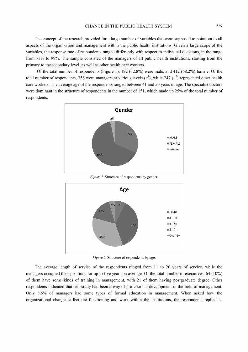
CHANGE IN THE PUBLIC HEALTH SYSTEM
589
The concept of the research provided for a large number of variables that were supposed to point out to all
aspects of the organization and management within the public health institutions. Given a large scope of the
variables, the response rate of respondents ranged differently with respect to individual questions, in the range
from 73% to 99%. The sample consisted of the managers of all public health institutions, starting from the
primary to the secondary level, as well as other health care workers.
Of the total number of respondents (Figure 1), 192 (32.8%) were male, and 412 (68.2%) female. Of the
total number of respondents, 356 were managers at various levels (n1), while 247 (n2) represented other health
care workers. The average age of the respondents ranged between 41 and 50 years of age. The specialist doctors
were dominant in the structure of respondents in the number of 151, which made up 25% of the total number of
respondents.
Figure 1. Structure of respondents by gender.
Figure 2. Structure of respondents by age.
The average length of service of the respondents ranged from 11 to 20 years of service, while the
managers occupied their positions for up to five years on average. Of the total number of executives, 64 (10%)
of them have some kinds of training in management, with 21 of them having postgraduate degree. Other
respondents indicated that self-study had been a way of professional development in the field of management.
Only 8.5% of managers had some types of formal education in management. When asked how the
organizational changes affect the functioning and work within the institutions, the respondents replied as

CHANGE IN THE PUBLIC HEALTH SYSTEM
590
follows: About 23% of them answered that they did not know, 20.4% of them responded that changes led to an
increase in employment and 19.2% responded that changes led to the reduction of the number of employees in
the institution.
Statistical Analysis
The statistical analysis of collected data was performed on the entire sample. The analysis was performed
with the help of the SPSS (statistical package for the social science) statistical programme within which the
specialized macros were used: Comfac2 and Spromax. The testing of scales from the questionnaire for the
nominal scale was carried out by the method of optimal scaling, and the method of latent dimensions was used
for ordinal scales. The discriminate analysis was used in the research at the project level, which attempted to
answer whether there are significant differences between managers at different levels and other health care
workers. The variance analysis was used to study the responses to scale questions. The studied characteristics
included nominal, ordinal, and five-point scale for the factors of motivation, demotivation, satisfaction, and
characteristics of organizational leaders. The variables included in the analysis were selected on the basis of the
expectations that they were related to the detected clustering and on the basis of their metric and statistical
characteristics.
A multivariate test was taken as the linear F-test > 2.00 with the inclusion of the cubic component at the
significance level = 0.05. The significance of the difference in pairs was determined by the modified LSD test
(Bonferroni test), which tested the difference among the pairs of arithmetic means. When checking the null
hypothesis, the t-test was used for parametric data and chi-square test for non-parametric data. The difference in
the distribution of respondents by individual characteristics was analysed by contingency tables. To test the
average canonical correlations among variables, the Cramer’s coefficient V (0 < V < 1) was used and V > 0.20
was considered; the contingency coefficient C > 0.30, with the significance level of p < 0.01 (highly
statistically significant) to p < 0.001(significant).
The analysis of hypothetical factors was performed with the confirmatory factor analysis, where the
analysis was based on the Proctrustean ProMax rotation, with the image analysis used as the starting solution,
but on the variables rescaled in the Harris Kaiser’s Matrix. It is believed that this analysis is the most
mathematically and statistically based method. The similarity of explorative and hypothetical factors was
checked by the correlation coefficient or the congruence coefficient.
Reduction of Characteristics
The number of items in the research was varied and dichotomous due to which the reduction was made by
the “image” method of the factor analysis with the direct oblimin method of oblique rotation. The number of
factors was determined by the Guttman-Kaiser criterion for the model image analysis. The choice of this
method was made because of the estimate of the statistical quality of selected variables which are of low
reliability. The image analysis served as a measure of belonging of a particular item to the analysed sample and
as a relative measure of the correlation amount before and after the Gutman-analysis, which is the obtaining of
the anti-image correlation. The factor analysis was performed using the method of principal components rotated
into the position, with the support of the “2macro-comfact2 software”.
The reduction process was carried out for the whole studied population, as well as for sub-samples. For the
purposes of this paper, the results on the whole sample are presented.

CHANGE IN THE PUBLIC HEALTH SYSTEM
591
The first phase included the processing of the total variance of items with the direct oblimin method of
oblique rotation as a method of factorization. Due to the large number of statistically significant factor loadings,
the factors whose factor loading is F > 10,401, and the characteristic values (eigen-value) > 0.60 (Meyer-Olkin
Kaiser-Measure of Sampling Adequacy) were selected for the analysis.
The second phase included testing and the validity of the measurement scales. In the case of ordinal
variables, the factor analysis was used and the factorization was not performed for the normalization of ordinal
variables, because the analyses did not indicate a need for this. These variables were subjected to an explorative
part of the SproMax macro, resulting in the orthoblique factors from the Harris-Kaiser’s image analysis.
The third phase involved the factoring of the obtained latent variables by the component model (principal
component analysis). Three factors were identified by the Guttman-Kaiser criterion and rotated by the direct
oblimin method.
The analysis was performed in data processing by health institutions, which showed that there were
significant differences in the evaluation of organizational leaders by health institutions, which was expressed as
highly significant (4.2) according to the F-test.
Characteristics of Organizational Leaders
The characteristics of organizational leaders were evaluated on the basis of 11 characteristics that identify
the organizational goals, ethics, communication, negotiation skills, communication skills, autonomy, and
respect from employees.
The characteristics were measured on the five-point scale, which included: from 1 (especially good) to 5
(extremelly unsatisfactory).
The arithmetic means of the observed characteristics of organizational leaders are about the average score
of two, which indicates that the leadership is good. A lack of structuring as a high correlation (shown in Table 1
which contains 474 cases) and the average score indicate that respondents were not discriminatory.
Table 1
Analysis of the Characteristics of Organizational Leaders
Variable Mean Standard deviation
Vision of managers (V) 2.21730 1.27309
Goal setting (G) 1.90717 1.12620
Ethics (E) 1.84177 1.11981
Autonomy in decision-making (AD) 2.09705 1.24701
Care for future managers (CM) 2.48101 1.36269
Communication skills (CS) 2.05274 1.27894
Negotiation skills (NS) 2.11603 1.29613
Encouraging the creativity of employees (EEC) 2.66878 1.44453
Giving an autonomy to employees (GAE) 2.33966 1.35490
Care for employees (CE) 2.15823 1.26352
Respect of employees (RE) 2.06962 1.20139
The analysis of variance characteristic of managers indicates that there are significant differences in the
evaluation of the characteristics of the managers by profession. The difference in the evaluation of the sense of
vision is the greatest (V = 1.8598). The best score was given by specialists and the worst by other health care
workers.

CHANGE IN THE PUBLIC HEALTH SYSTEM
592
When it comes to the characteristic regarding the goals of the institution, the difference among the
respondents by profession is V = 1.8598, which was also assessed best by specialist doctors and worst by other
health care workers with the high school diploma. The characteristic regarding ethics also shows the difference
by profession (V = 1.1473), and is best assessed by administrative workers (Mean = 2.0000). On the issue of
autonomy in decision-making, differences among professions are also evident (V = 1.6193) and the best
assessment was given by clinical specialists, which is also true for the characteristic taking care of future
leaders (V = 2.9558), while it was assessed worst by the medical technicians with high school diploma. The
characteristics of organizational leaders were generally assessed best by specialist doctors and worst by medical
technicians. An exception is the characteristic example for colleagues to follow which was assessed worst by
senior medical technicians (Mean = 1.7500).
Table 2
Correlation Matrix of the Characteristics of Organizational Leaders
V G E AD CM CS NS EEC GAE CE RE
V 1.00000
G 0.73221 1.0000
E 0.64702 0.66224 1.00000
AD 0.57797 0.47461 0.46219 1.00000
CM 0.61354 0.57882 0.51965 0.59081 1.00000
CS 0.64218 0.57292 0.56974 0.39977 0.53736 1.00000
NS 0.62531 0.60267 0.52249 0.43644 0.58718 0.82147 1.00000
EEC 0.65311 0.61005 0.54652 0.55189 0.67290 0.57021 0.61904 1.00000
GAE 0.55402 0.57769 0.57336 0.45844 0.54340 0.58747 0.58186 0.6251 1.00000
CE 0.67517 0.67447 0.68266 0.54440 0.61262 0.65682 0.64069 0.66628 0.67246 1.00000
RE 0.58032 0.63606 0.59437 0.49786 0.61745 0.64293 0.62613 0.57735 0.58419 0.70999 1.00000
Notes. Determinant of correlation matrix = 0.0002595; Kaiser-Meyer-Olkin measure of sampling adequacy = 0.93418; Bartlett test of Sphericity = 3868.2288; Significance = 0.00000.
The correlation analysis among 11 variables of the characteristic of organizational leaders is shown in the
Table 2 and all items highly correlate with each other from 0.39 to 0.82 (significant level p < 0.01). Negotiation
skills and communication skills have the highest correlation of 0.82, and then the respect from employees and
an example to follow, with 0.71.
Result of the factor analysis of these 11 factors of the characteristics of organizational leaders explained a
57% of variance which is shown in the Table 3. Features with these characteristics are called management
support. Communication skills have the bigest communality (0.73345), then example of conduct (0.70329),
while ethics in the work has the lowest communality (0.45599). These factor loadings and the variance
extracted confirm the convergent validity of the dimensions.
The obtained factor discriminates the respect of the manager and has a quantitative, rather than structural
significance in the analysis. The obtained factor represents a structural tool for the analysis of latent features
and the characteristics of managers.
The obtained factor represents a structural tool for the analysis of latent features and the characteristics of
managers. Crossing the factor scores obtained by the institutions is a significant difference in the responses,
especially for the variable “communication skills”, so that Phi = 0.50092, Cramer’s V = 0.25046 and
contigency coefficient = 0.44787, as well as “negotiation skills” (Phi = 0.53984; Cramer’s V = 0.26992;

CHANGE IN THE PUBLIC HEALTH SYSTEM
593
contigency coefficient = 0.47504) and “develop creative abilities of employees” (Phi = 0.53179; Cramer’s V =
0.26589, conigency coefficient = 0.46953). Similar differences in the characteristics of organizational leaders
occur at institutions in the variable “giving employees more autonomy” (Phi = 0.50877; Cramer’s V = 0.25438;
contigency coefficient = 0.45345). Highly significant multivariate F ratio was obtained in terms of the “vision
of the leaders” (F ratio = 4.130) and “goal settings” (F ratio = 3.8005). Researches showed significant
differences in assessment of profession leader’s characteristics on all variables. F ratio for the variable goals is
1.8598 where the differences are particularly manifested with medical specialists, as well as the ethics (F ratio
is 1.1473), encouraging the creativity of employees (F ratio = 2.9558), and ethic (F ratio = 2.1030).
Table 3
Results of the Factor Analysis for the Characteristics of Organization Leaders (12 Items)
Factor Variables F Communality
E = 6.99 Pct of V = 57.2% support management
Example of conduct 0.82353 0.70329
Vision of managers 0.79532 0.68513
Negotiation skills 0.79176 0.72534
Communication skills 0.78804 0.73345
Goal setting 0.77306 0.65045
Encouraging the creativity of employees 0.76783 0.64055
Respect from employees 0.76471 0.61748
Care for employees 0.72930 0.58658
Giving an autonomy to employees 0.72714 0.56426
Ethics at work 0.72607 0.57496
Autonomy in decision-making 0.61280 0.45599
Organizational leader’s at all hierarchical levels of the health system are determined by the higher
authority. Despite the formal announcement of the competition, all directors of public institutions are appointed
by the ministry. The following action is for directors of institutions (in consultation with the ministry) to place
managers at lower levels. Such a system of recruitment leads to a reduced influence of the leaders of on the
employees and their focus mainly on solving management problems, not the handling or initiating significant
change.
Motivational Factors
In this research, 12 factors were used to test the motivation, adapted to the situation in health system, and
measured by five-point scale. Motivational variables include salary, financial incentives, working conditions,
the affirmation in the profession, interpersonal relationship, status of the institutions, job security, participation
in decision making, the quality of management, the job by itself, acceptance of colleagues, and responsibility
which are shown in Table 4.
Analysis of mean of variables of work motivation shows that employees are highly motivated. Salary and
responsibility have the lowest arithmetic means and standard deviations, which the respondents consider the
best motivators, individual and univariate. The least important variable is participation in decision-making,
where at the same time the largest individual differences exist.
Correlation among 11 variables of work motivation (shown in Table 5) is positive and significantly
correlated to 0.06 at significant level of 0.55.

CHANGE IN THE PUBLIC HEALTH SYSTEM
594
Table 4
Analysis of Motivational Factors
Variables Mean Std. Dev
Salary (S) 1.15517 0.47273
Financial incentives (FI) 1.38314 0.78539
Working conditions (WC) 1.29310 0.59775
The affirmation in the profession (AP) 1.43870 0.68229
Interpersonal relationships (IR) 1.27011 0.52739
Status of the institution (SI) 1.60345 0.87722
Job security (JS) 1.40996 0.75154
Participation in decision-making (PDM) 2.11877 1.1929
The quality of management (QM) 1.32567 0.66245
The job by itself (JI) 1.51533 0.85670
Acceptance of colleagues (AC) 1.48276 0.68483
Responsibility (R) 1.20498 0.49385
Notes. Number of cases = 522; the boldface shows the highest mean and standard deviation.
Table 5
Correlation Matrix of Motivational Factors
S FI WC AP IR SI J S PDM QM J I AC R
S 1.00000
FI 0.55298 1.00000
WC 0.08327 0.18962 1.00000
AP 0.20510 0.31255 0.40887 1.00000
IR 0.0677 0.08794 0.38767 0.31014 1.00000
SI 0.19033 0.25996 0.34289 0.42591 0.37718 1.00000
J S 0.23659 0.27643 0.27035 0.26621 0.32540 4.7416 1.00000
PDM 0.13410 0.29361 0.30117 0.44546 0.30298 0.51675 0.43822 1.00000
QM 0.08961 0.12862 0.27228 0.28631 0.34106 0.31184 0.22093 0.38106 1.00000
JI 0.10549 0.09680 0.22922 0.28237 0.19261 0.31331 0.27641 0.37028 0.22117 1.00000
AC 0.10018 0.11223 0.24915 0.34279 0.39289 0.35762 0.31210 0.33866 0.45241 0.43884 1.00000
R 0.02792 0.12868 0.28373 0.27946 0.23654 0.27217 0.25409 0.20305 0.21798 0.28518 0.27437 1.0000
Notes. Determinant of corelation matrix= 0.04020535; Kaiser-Mayer Olkin measure of sampling adequacy = 0.83156; Bartlett test of Sphericity = 1635.6353; Significance = 0.00000.
The results of data processing showed that there were no significant differences between the groups
surveyed in respect of profession and the position occupied (managers and non-managerial staff) (V = 0.3182)
when it comes to motivational factors. Salaries and financial incentives are essentially important for all groups
of respondents, regardless of profession or position within the institution. The only significant difference occurs
in terms of the factor “status of the organization”, depending on the profession (V = 3.9711). The greatest
importance to this factor was given by specialist doctors (Mean = 1.6739) and the lowest by medical
technicians (Mean = 1.3913).
The image factors obtained from this group of variables are relatively weak, because the first factor
explains only 24% of the total variance and the other 4%, because the loadings of variables are relatively low.
The other factor called financial incentives is a variant that includes only two items, while other variables of the
motivator belong to the first factor. Direct correlation of factors is relatively low and amounts to 0.40. Low

CHANGE IN THE PUBLIC HEALTH SYSTEM
595
correlation is caused by reduced variability, because the Table 6 shows that all the factors are very important.
Salaries and financial incentives have emerged as two aspects of the same variable.
Table 6
Results of the Factor Analysis for Motivation
Factor Variables F Com.
Factor 1 E = 4.12 Interpersonal relationships Pct of Var = 24%
Acceptance of colleagues (AC) 0.59600 0.39211
Status of the institution (SI) 0.55757 0.41711
Interpersonal relationships (IR) 0.55311 0.31413
Participation in decision-making (PDM) 0.55046 0.43660
The quality of management (QM) 0.50980 0.29419
The affirmation in the profession (AP) 0.48435 0.36180
The job by Itself (JI) 0.47383 0.28523
Working conditions (WC) 0.46851 0.28077
Job security (JS) 0.44316 0.33934
Responsibility (R) 0.40472 0.18728 Factor 2 Financial incentives E = 1.49 Pct of Var = 4%
Financial incentives (FI) Salary (S)
0.52825 0.52318
0.38312 0.33989
Discussion
In practice, it is expected that leaders are the bearers and creators of change and that they possess a high
level of ethics and responsibility. It is particularly important that leaders in public health institutions are
mediators in relations with numerous stakeholders, among whom, the employees have special importance.
The results obtained indicate that respondents were not particularly discriminatory towards organizational
leaders, who received the average score of good, which does not indicate the specific characteristics of leaders.
Particular note is leader’s traits related to organizational behaviour, such as the autonomy of employees, the
attitude towards colleagues, ethics, and communication. Respondents with respect to these variables showed the
greatest differences both in institutions and occupation. This indicates a need to change organizational culture,
which is an important factor for improving existing practices and management styles.
Organizational leaders in the public health system have limited tools to motivate employees because of the
legal rules which do not allow the recognition of additional rewards, as an opportunity for increased
performance and achieved results.
The lack of structure, high correlation, and average scores (mean score is “good”) point to conclusion that
sample population was indiscriminative. The factors in Table 3 have quantitative meaning as oppose to
structural ones. The factors represent structural tools for analysis of potential characteristics and attributes of
organizational leaders. It is recommended to widen the scope of analysis of characteristics of organizational
leaders in order for more detailed representation.
When it comes to motivation, the perception of the employees is that interpersonal relationships and
financial motivators prevail. Within the interpersonal relationships, the most important factor is “acceptance
from colleagues” and from among the financial motivators, salaries make the strongest motivator. It is
recognized that due to the overall financial position of health care workers, the financial factors stand out and
dominate in relation to others, which results in low variability of other motivational factors.

CHANGE IN THE PUBLIC HEALTH SYSTEM
596
Encouraging and implementing changes within the health system and the implementation of strategic
decisions cannot take place without the charismatic organizational leadership, which will change the processes
within the system through the initiative and responsibility for the tasks performed. Building trust and good
working conditions leads to improved interpersonal relationships and satisfactory motivation. Moynihan and
Pandey (2007a) pointed out that effectiveness of leaders may depend even more on the ability to communicate,
persuade, and inspire. They also emphasised that managers have varying degrees of influence over different
aspects of work motivation, with grates influence over job satisfaction, noting that managers could influence
work motivation by changing the employees’ perception of organization (Moynihan & Pandey, 2007b).
Pandey and Wright (2006) raised the question of whether the public sector cultivates motivation.
Challenges of the environment present demands to organizational leaders to direct the employees and seek
the best ways to increase performances and achieve goals, regardless of whether it is the public system or
private health organizations. Perry and Wise (1990, p. 368) defined motivation in the public sector as an
individual’s predisposition to respond to motives grounded primarily or uniquely in public institutions and
organizations.
It should be particularly noted that changes in service organizations occur much harder and building trust
between leaders and employees has an enormous importance. Changes within the public health systems require
taking measures for greater involvement of employees in the decision-making process. This was rated low by
the respondents as a factor that can motivate them. Selection of appropriate organizational leaders with
authority could certainly improve the existing situation. The obtained results suggest that stronger leadership is
necessary to motivate public sector employees to accept organizational changes which would improve the
system of motivation and generally lead to an increase in performance.
Conclusions
Motivation and leadership are very important issues for the health care system and for the research of
organizational behaviour. The research has shown that organizational leaders in the public health care system of
transition countries have been given an average score of good by employees, and that they do not influence
motivation significantly.
Research has shown that there are significant differences in attitudes about characteristics of
organizational leaders, both between medical institutions and employees.
Financial incentives have proved to be the strongest motivational factor, which due to legal rules restricts
the ability of leaders to use this motivating factor. Participation in decision-making is rated lowest by
respondents, which puts them in a passive position when it comes to changes and their acceptance.
For the implementation of comprehensive organizational changes within the public health care system, it
is necessary to identify the motives for accepting new ideas, so that changes can be better received and spread
throughout the organization. In the process of accepting changes, the role of leaders is very important,
especially in providing support to employees. Support to employees includes explanations of what is expected
from changes and motivation of employees who can contribute to the successful change.
References Alonso, P., & Lewis, G. B. (2001). Pubblice service motivation and job performance: Evidence from the federal sector. American
Review of Public Administration, 31(4), 368-380. Brewer, G. S. (2000). Individual coneptions of public service motivation. Public Aministration Review, 60(3), 254-264.

CHANGE IN THE PUBLIC HEALTH SYSTEM
597
Houston, D. J. (2000). Publice service motivation: A multivariante test. Journal of Public Administration Research and Theory, 10(4), 713-727.
Ivancevich, J. M., & McMahon, J. T. (1982). The effects of goal setting, external feedback, and self-genearted feedback on oucome variables: A field experiment. Academy of Management Journal, 25(2), 359-372.
Ivanicevich, J. K. R. (2005). Organizational behaviour and management. Boston: McGraw Hill Irwin. MONSTAT. (2011). Census of population. Retrieved from www.mostat.me Moynihan, D. P., & Pandey, S. K. (2007a). The role of oranizations in fostering public service motivation. Public Administration
Rewiev, 67(1), 40-53. Moynihan, D. P., & Pandey, S. K. (2007b). Finding workable levers over work motivation: Comparing job satisfaction, job
involvement, and organizational commitment. Administration & Society, 39(7), 803-832. Pandey, S. K., & Wright, B. (2006). Conecting the dots in public management: Political environment, orgaizational goal
ambiguity and public manager’s role ambiguity. Journal of Public Administration Research and Theory, 16(4), 512-532. Pandey, S. K., Wright, B. E., & Moynihan, D. P. (2008). Public service motivation and interorganizational citizenship behavior:
Testing a preliminary model. Internationl Public management Journal, 11(1), 89-108. Perry, L. J., & Hondeghem, A. (2008). Motivation in public management: The call of public service. New York: Oxford
University Press. Perry, L. J., & Wise, L. R. (1990). The motivational bases of public service. Public Administration Review, 50(3), 367-373. Robbins, S. P., & Coulter, M. (2005). Management (8 ed.). Upper Saddle River: Pearson Education. Senge, P. (1990). The fifth discipline—The art & practice of leading organization. New York: Doubleday. United Nations Development Programme. (2011). Integrity assessment of health care system in Montenegro. Retrieved from
http://www.me.undp.org/content/dam/montenegro/docs/publications/DG/Corruption/Integrity%20Assessment%20of%20the%20Health%20Care%20System%20in%20Montenegro%20LOC.pdf
Wright, B. E. (2001). Public sector work motivation: Review of current literature and a revised conceptual model. Journal of Public Administration Research and Theory, 11(4), 559-586.
Wright, B. E., Moynihan, D. P., & Pandey, S. K. (2012). Pulling the levers: Transformational leadership, public service motivation and mission valence. Public Administration Review, 72(2), 206-215.