How Does Investing in Cheap Labour Countries Affect Performance at Home? France and Italy
Upload
mondodomaniCategory
view
1download
0
1.
Child labour and access to basicservices:
evidence from five countries
L. GuarcelloS. Lyon
F. C. Rosati
January 2004
Und
erst
andi
ng C
hild
ren’
s Wor
k Pr
ojec
t Wor
king
Pap
er S
erie
s, Ja
nuar
y 20
04


Child labour and access to basic services: evidence from five countries
L. Guarcello*
S. Lyon*
F. C. Rosati*
Working Paper January 2004
Understanding Children’s Work (UCW) Project
University of Rome “Tor Vergata” Faculty of Economics
V. Columbia 2 00133 Rome Tor Vergata
Tel: +39 06.7259.5618 Fax: +39 06.2020.687
Email: [email protected] As part of broader efforts toward durable solutions to child labor, the International Labour Organization (ILO), the United Nations Children’s Fund (UNICEF), and the World Bank initiated the interagency Understanding Children’s Work (UCW) project in December 2000. The project is guided by the Oslo Agenda for Action, which laid out the priorities for the international community in the fight against child labor. Through a variety of data collection, research, and assessment activities, the UCW project is broadly directed toward improving understanding of child labor, its causes and effects, how it can be measured, and effective policies for addressing it. For further information, see the project website at www.ucw-project.org.
This paper is part of the research carried out within UCW (Understanding Children's Work), a joint ILO, World Bank and UNICEF project. The views expressed here are those of the authors' and should not be attributed to the ILO, the World Bank, UNICEF or any of these agencies’ member countries.
* UCW-Project and University of Rome “Tor Vergata”

Child labour and access to basic services: evidence from five countries
Working Paper January 2004
ABSTRACT
Analyses of the determinants of child labour have largely neglected the role of access to basic services. The availability of these services can affect the value of children’s time and, concomitantly, household decisions concerning how this time is allocated between school and work. This paper investigates the link between child labour and water and electricity access in five countries – El Salvador, Ghana, Guatemala, Morocco and Yemen. Employing an econometric methodology based on propensity scores for dealing with the potential endogeneity of access to water and electricity, average treatment effects for water and electricity access on children’s activities are presented. The marginal effects of water and electricity access on children’s activities obtained by estimating a bivariate probit model are also examined. Finally, a sensitivity analysis is presented designed to check the robustness of the conclusions concerning the causal relationship between water and electricity access and children’s activities.
Child labour and access to basic services: evidence from five countries
Working Paper January 2004
CONTENTS
1. Introduction ........................................................................................................................... 1 2. Child activity status ............................................................................................................... 2 3. Child activity status and water/electricity access .............................................................. 4 4. Econometric methodology .................................................................................................. 8 5. ATT matching procedure: some results .......................................................................... 10 6. The effects of access to water and electricity on children’s school attendance and labour supply: a bivariate analysis ................................................................................................... 13 7. Sensitivity analysis ............................................................................................................... 15 8. Conclusion ............................................................................................................................ 17 Appendix A: Surveys and questions used to define variables for water and electricity access………...………………………………………………………………………………19 Appendix B: Detailed descriptive tables ............................................................................................... 21 Appendix C: Econometric methodology .............................................................................................. 24 Appendix D: Comparison of distributions of propensity scores for treated and control groups27
Propensity scores comparison for water access ....................................................................... 27
Propensity scores comparison for electricity access ................................................................ 29 Appendix E: Variable definitions and Results from bivariate probit estimates.............................. 31
Definitions of the main variables implied in the regression analysis .................................... 31
Marginal Effects results after Bivariate probit regression ....................................................... 33 Apependix F ............................................................................................................................................... 38 Appendix G: Average Treatment Effects for “Access to Water and Access to Electricity” for different values of the sensitivity parameters ....................................................................................... 46

1 UCW WORKING PAPER SERIES, JANUARY 2004
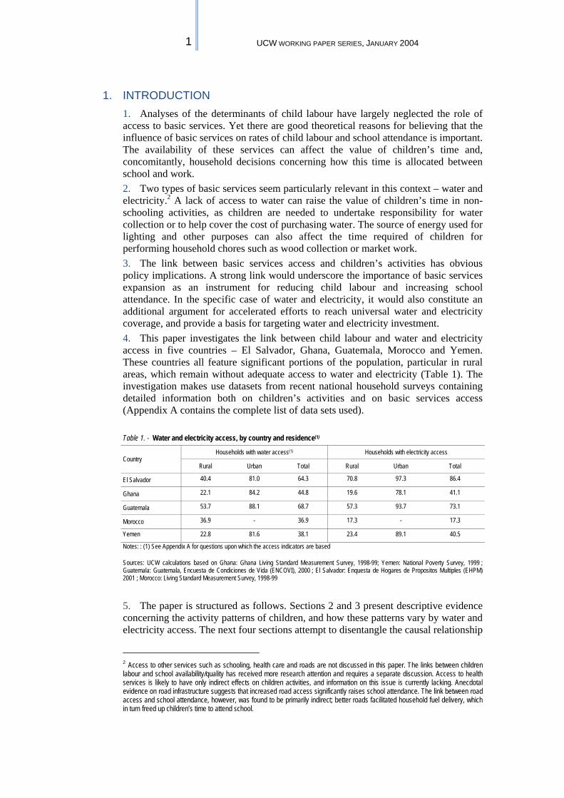
1. INTRODUCTION 1. Analyses of the determinants of child labour have largely neglected the role of access to basic services. Yet there are good theoretical reasons for believing that the influence of basic services on rates of child labour and school attendance is important. The availability of these services can affect the value of children’s time and, concomitantly, household decisions concerning how this time is allocated between school and work. 2. Two types of basic services seem particularly relevant in this context – water and electricity.2 A lack of access to water can raise the value of children’s time in non-schooling activities, as children are needed to undertake responsibility for water collection or to help cover the cost of purchasing water. The source of energy used for lighting and other purposes can also affect the time required of children for performing household chores such as wood collection or market work. 3. The link between basic services access and children’s activities has obvious policy implications. A strong link would underscore the importance of basic services expansion as an instrument for reducing child labour and increasing school attendance. In the specific case of water and electricity, it would also constitute an additional argument for accelerated efforts to reach universal water and electricity coverage, and provide a basis for targeting water and electricity investment. 4. This paper investigates the link between child labour and water and electricity access in five countries – El Salvador, Ghana, Guatemala, Morocco and Yemen. These countries all feature significant portions of the population, particular in rural areas, which remain without adequate access to water and electricity (Table 1). The investigation makes use datasets from recent national household surveys containing detailed information both on children’s activities and on basic services access (Appendix A contains the complete list of data sets used). Table 1. - Water and electricity access, by country and residence(1)
Country Households with water access(1) Households with electricity access
Rural Urban Total Rural Urban Total
El Salvador 40.4 81.0 64.3 70.8 97.3 86.4
Ghana 22.1 84.2 44.8 19.6 78.1 41.1
Guatemala 53.7 88.1 68.7 57.3 93.7 73.1
Morocco 36.9 - 36.9 17.3 - 17.3
Yemen 22.8 81.6 38.1 23.4 89.1 40.5
Notes: : (1) See Appendix A for questions upon which the access indicators are based Sources: UCW calculations based on Ghana: Ghana Living Standard Measurement Survey, 1998-99; Yemen: National Poverty Survey, 1999 ; Guatemala: Guatemala, Encuesta de Condiciones de Vida (ENCOVI), 2000 ; El Salvador: Enquesta de Hogares de Propositos Multiples (EHPM) 2001 ; Morocco: Living Standard Measurement Survey, 1998-99
5. The paper is structured as follows. Sections 2 and 3 present descriptive evidence concerning the activity patterns of children, and how these patterns vary by water and electricity access. The next four sections attempt to disentangle the causal relationship
2 Access to other services such as schooling, health care and roads are not discussed in this paper. The links between children labour and school availability/quality has received more research attention and requires a separate discussion. Access to health services is likely to have only indirect effects on children activities, and information on this issue is currently lacking. Anecdotal evidence on road infrastructure suggests that increased road access significantly raises school attendance. The link between road access and school attendance, however, was found to be primarily indirect; better roads facilitated household fuel delivery, which in turn freed up children’s time to attend school.
2 CHILD LABOUR AND ACCESS TO BASIC SERVICES: EVIDENCE FROM
FIVE COUNTRIES
between children’s activities and water and electricity access. Section 4 presents an econometric methodology based on propensity scores for dealing with the potential endogeneity of access to water and electricity. Section 5 then presents average treatment effects for water and electricity access on children’s activities, and Section 6 the marginal effects of water and electricity access on children’s activities obtained by estimating a bivariate probit model. Section 7 presents a sensitivity analysis designed to check the robustness of the conclusions concerning the causal relationship between water and electricity access and children’s activities. Section 8 concludes.
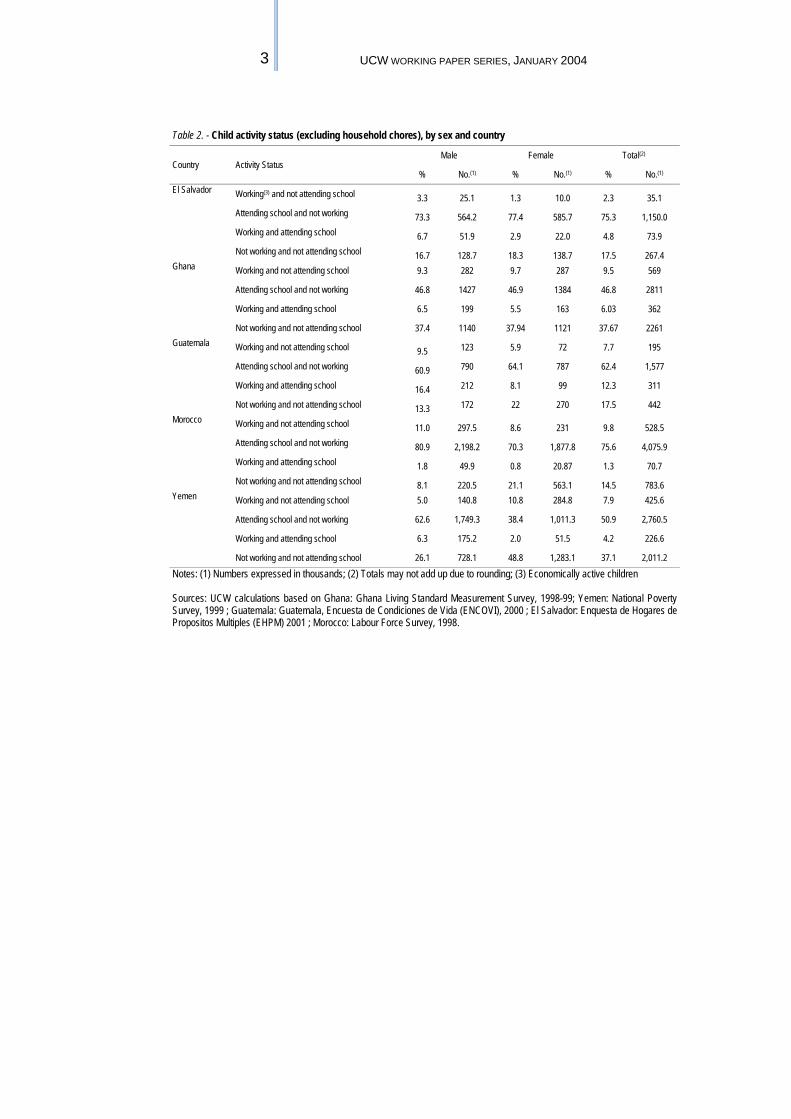
2. CHILD ACTIVITY STATUS 6. Children can be classified into four non-overlapping activity categories - those that work, those that attend school, those that both work and attend school, and those that do neither.3 The distribution of children across these activity categories varies somewhat in the five countries (Table 2). The proportion of children involved full-time in economic activities ranges from 10 percent in Morocco to two percent in El Salvador, and rates of full-time school attendance from 76 percent in Morocco to 51 percent in Yemen. The proportion of children combining school and economic activity varies from 12 percent in Guatemala to just one percent in Morocco. 7. All five countries feature a significant proportion of children absent from both school and work. More than one in three children in Ghana and Yemen, and almost one in five in El Salvador and Guatemala, are reportedly “idle”. In Morocco, reportedly idle children account for 15 percent of total 7-14 year-olds. These children require further investigation, but it is likely that many from this group contribute in some way to household welfare. Some may be engaged in unreported work,4 while others might not be economically active in a technical sense, but perform household chores – including water collection – that allow other household members to engage in productive activities.5
3 We use two alternative definitions of children’s work. The first classifies as workers all children aged between 7 and 14 years of age that carry out an economic activity for at least one hour a day. The second definition includes in the number of working children also those performing household chores for at least 28 hours a week. Data on hours spent on household chores are available only for El Salvador and Guatemala, hence the extended definition is applied only to these two countries. 4 Parents may falsely report their children as being idle instead of as working because (at best) work by children is forbidden or (at worst) because their children are engaged in illegal or dangerous activities. Alternatively, parents may misinterpret the survey question, and report a child as idle because he or she was not working at the time of the interview, although he or she may work during other periods. 5 A recent study of the phenomenon of “idle” children (UCW Project, ‘The Puzzle of Apparently Idle Children: Evidence for six countries’, October 2003) provides evidence suggesting that children can be absent from both school and economic activity because they are needed to perform household chores, because of their health, or because they are unable to find work after having left school. But the study indicated that a large proportion of children not in school or economic activity does not fall into any of these categories. In Guatemala, for example, one the countries included in the study, this “unexplained” portion of idle children population accounted for 70 percent of the total idle children.
3 UCW WORKING PAPER SERIES, JANUARY 2004
Table 2. - Child activity status (excluding household chores), by sex and country
Country Activity Status Male Female Total(2)
% No.(1) % No.(1) % No.(1) El Salvador Working(3) and not attending school 3.3 25.1 1.3 10.0 2.3 35.1
Attending school and not working 73.3 564.2 77.4 585.7 75.3 1,150.0 Working and attending school 6.7 51.9 2.9 22.0 4.8 73.9 Not working and not attending school 16.7 128.7 18.3 138.7 17.5 267.4
Ghana Working and not attending school 9.3 282 9.7 287 9.5 569
Attending school and not working 46.8 1427 46.9 1384 46.8 2811
Working and attending school 6.5 199 5.5 163 6.03 362
Not working and not attending school 37.4 1140 37.94 1121 37.67 2261 Guatemala Working and not attending school 9.5 123 5.9 72 7.7 195
Attending school and not working 60.9 790 64.1 787 62.4 1,577
Working and attending school 16.4 212 8.1 99 12.3 311
Not working and not attending school 13.3 172 22 270 17.5 442 Morocco Working and not attending school 11.0 297.5 8.6 231 9.8 528.5
Attending school and not working 80.9 2,198.2 70.3 1,877.8 75.6 4,075.9 Working and attending school 1.8 49.9 0.8 20.87 1.3 70.7 Not working and not attending school 8.1 220.5 21.1 563.1 14.5 783.6
Yemen Working and not attending school 5.0 140.8 10.8 284.8 7.9 425.6
Attending school and not working 62.6 1,749.3 38.4 1,011.3 50.9 2,760.5
Working and attending school 6.3 175.2 2.0 51.5 4.2 226.6
Not working and not attending school 26.1 728.1 48.8 1,283.1 37.1 2,011.2
Notes: (1) Numbers expressed in thousands; (2) Totals may not add up due to rounding; (3) Economically active children Sources: UCW calculations based on Ghana: Ghana Living Standard Measurement Survey, 1998-99; Yemen: National Poverty Survey, 1999 ; Guatemala: Guatemala, Encuesta de Condiciones de Vida (ENCOVI), 2000 ; El Salvador: Enquesta de Hogares de Propositos Multiples (EHPM) 2001 ; Morocco: Labour Force Survey, 1998.
4 CHILD LABOUR AND ACCESS TO BASIC SERVICES: EVIDENCE FROM
FIVE COUNTRIES
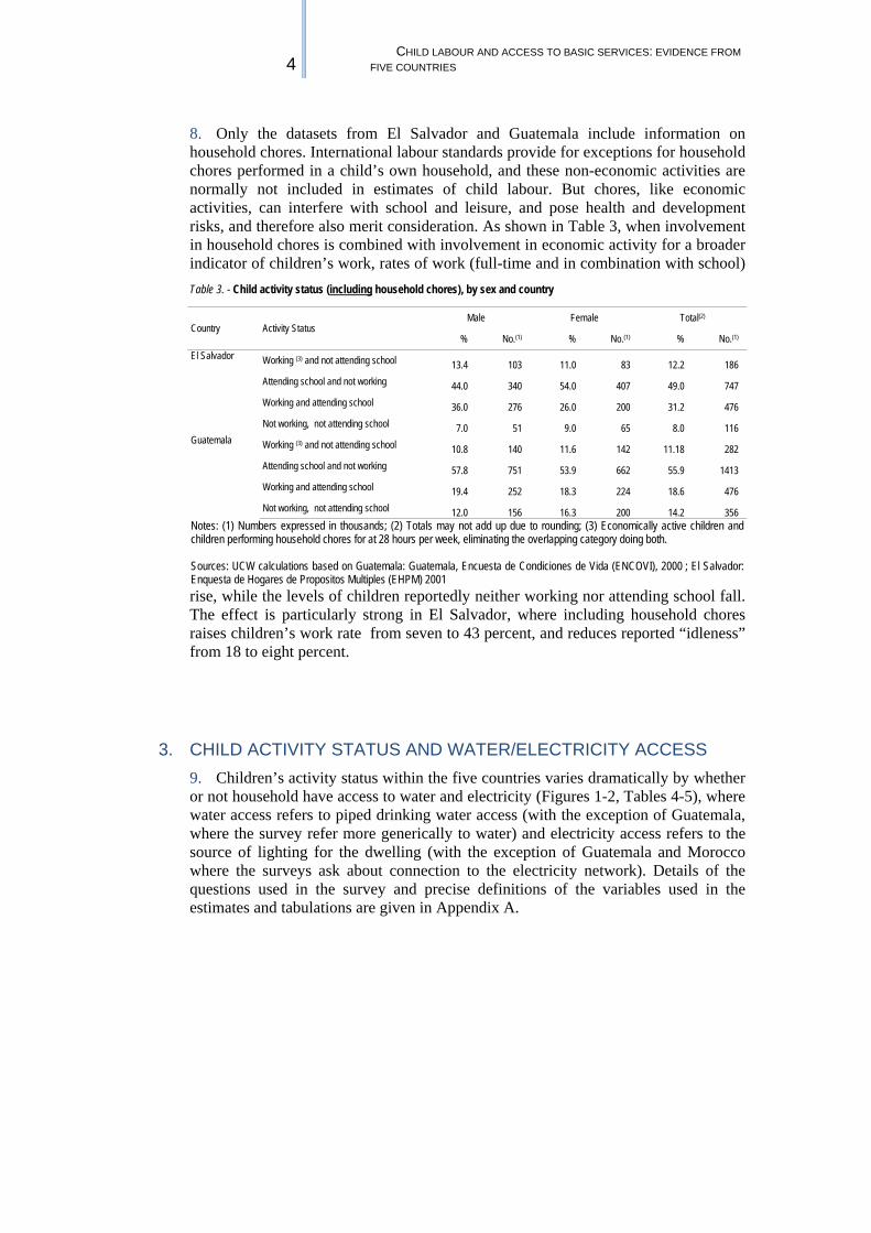
8. Only the datasets from El Salvador and Guatemala include information on household chores. International labour standards provide for exceptions for household chores performed in a child’s own household, and these non-economic activities are normally not included in estimates of child labour. But chores, like economic activities, can interfere with school and leisure, and pose health and development risks, and therefore also merit consideration. As shown in Table 3, when involvement in household chores is combined with involvement in economic activity for a broader indicator of children’s work, rates of work (full-time and in combination with school)
rise, while the levels of children reportedly neither working nor attending school fall. The effect is particularly strong in El Salvador, where including household chores raises children’s work rate from seven to 43 percent, and reduces reported “idleness” from 18 to eight percent.
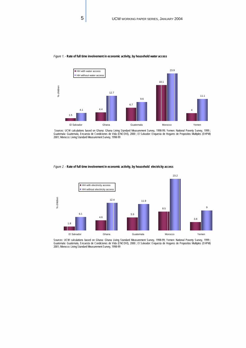
3. CHILD ACTIVITY STATUS AND WATER/ELECTRICITY ACCESS 9. Children’s activity status within the five countries varies dramatically by whether or not household have access to water and electricity (Figures 1-2, Tables 4-5), where water access refers to piped drinking water access (with the exception of Guatemala, where the survey refer more generically to water) and electricity access refers to the source of lighting for the dwelling (with the exception of Guatemala and Morocco where the surveys ask about connection to the electricity network). Details of the questions used in the survey and precise definitions of the variables used in the estimates and tabulations are given in Appendix A.
Table 3. - Child activity status (including household chores), by sex and country
Country Activity Status Male Female Total(2)
% No.(1) % No.(1) % No.(1) El Salvador Working (3) and not attending school 13.4 103 11.0 83 12.2 186
Attending school and not working 44.0 340 54.0 407 49.0 747 Working and attending school 36.0 276 26.0 200 31.2 476 Not working, not attending school 7.0 51 9.0 65 8.0 116
Guatemala Working (3) and not attending school 10.8 140 11.6 142 11.18 282 Attending school and not working 57.8 751 53.9 662 55.9 1413 Working and attending school 19.4 252 18.3 224 18.6 476 Not working, not attending school 12.0 156 16.3 200 14.2 356
Notes: (1) Numbers expressed in thousands; (2) Totals may not add up due to rounding; (3) Economically active children and children performing household chores for at 28 hours per week, eliminating the overlapping category doing both. Sources: UCW calculations based on Guatemala: Guatemala, Encuesta de Condiciones de Vida (ENCOVI), 2000 ; El Salvador: Enquesta de Hogares de Propositos Multiples (EHPM) 2001
5 UCW WORKING PAPER SERIES, JANUARY 2004
Figure 1. - Rate of full time involvement in economic activity, by household water access
1.5
4.4
6.7
18.1
44.1
12.7
9.6
23.9
11.1
El Salvador Ghana Guatemala Morocco Yemen
% c
hild
ren
HH with water access
HH without water access
Sources: UCW calculations based on Ghana: Ghana Living Standard Measurement Survey, 1998-99; Yemen: National Poverty Survey, 1999 ; Guatemala: Guatemala, Encuesta de Condiciones de Vida (ENCOVI), 2000 ; El Salvador: Enquesta de Hogares de Propositos Multiples (EHPM) 2001; Morocco: Living Standard Measurement Survey, 1998-99 Figure 2. - Rate of full time involvement in economic activity, by household electricity access
1.8
4.65.9
8.5
3.8
6.1
12.4 11.9
23.2
9
El Salvador Ghana Guatemala Morocco Yemen
% c
hild
ren
HH with electricity access
HH without electricity access
Sources: UCW calculations based on Ghana: Ghana Living Standard Measurement Survey, 1998-99; Yemen: National Poverty Survey, 1999 ; Guatemala: Guatemala, Encuesta de Condiciones de Vida (ENCOVI), 2000 ; El Salvador: Enquesta de Hogares de Propositos Multiples (EHPM) 2001; Morocco: Living Standard Measurement Survey, 1998-99

6 CHILD LABOUR AND ACCESS TO BASIC SERVICES: EVIDENCE FROM
FIVE COUNTRIES
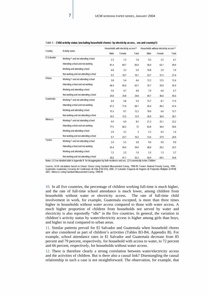
Table 4. - Child activity status (excluding household chores) by water access, sex and country(1)
Country Activity status Households with water access(2) Households without water access(2)
Male Female Total Male Female Total El Salvador Working(2) and not attending school 1.9 1.1 1.5 6.1 2.1 4.1
Attending school and not working 83.1 86.3 84.7 67.4 73.4 70.4 Working and attending school 6.3 3.4 4.9 9.2 3.0 6.1 Not working and not attending school 8.6 9.2 8.9 17.3 21.5 19.3
Ghana Working (2) and not attending school 2.8 5.9 4.4 13.0 12.4 12.7 Attending school and not working 66.8 63.8 65.2 34.9 35.0 35.0 Working and attending school 3.1 3.4 3.3 8.5 6.9 7.7 Not working and not attending school 27.3 26.9 27.1 43.6 45.8 44.6
Guatemala Working (2) and not attending school 7.8 5.5 6.7 12.8 6.4 9.6 Attending school and not working 65.9 68.2 67.0 51.1 57.1 54.1 Working and attending school 15.1 9.3 12.3 18.9 6.0 12.3 Not working and not attending school 11.3 17.0 14.0 17.2 30.5 24.0
Morocco(3) Working (2) and not attending school 15.9 20.3 18.1 23.2 24.6 23.9 Attending school and not working 63.2 38.6 51.1 66.4 41.1 54.3 Working and attending school 2.3 0.7 1.5 2.4 0.8 1.6 Not working and not attending school 18.6 40.4 29.4 8.1 33.5 20.2
Yemen Working (2) and not attending school 3.0 5.1 4.0 6.7 15.8 11.1 Attending school and not working 79.7 65.0 72.5 61.7 28.3 45.6 Working and attending school 4.9 1.7 3.3 8.3 2.5 5.5 Not working and not attending school 12.4 28.3 20.2 23.3 53.4 37.8
Sources: UCW calculations based on Ghana: Ghana Living Standard Measurement Survey, 1998-99; Yemen: National Poverty Survey, 1999 ; Guatemala: Guatemala, Encuesta de Condiciones de Vida (ENCOVI), 2000 ; El Salvador: Enquesta de Hogares de Propositos Multiples (EHPM) 2001; Morocco: Living Standard Measurement Survey, 1998-99
7 UCW WORKING PAPER SERIES, JANUARY 2004
Table 5. - Child activity status (excluding household chores) by electricity access, sex and country(1)
Country Activity status Households with electricity access(2) Households without electricity access(2)
Male Female Total Male Female Total El Salvador Working (2) and not attending school 2.3 1.3 1.8 9.5 2.5 6.1
Attending school and not working 81.4 84.7 83.0 56.0 63.1 59.4 Working and attending school 6.8 3.3 5.0 10.8 2.9 7.0 Not working and not attending school 9.5 10.7 10.1 23.7 31.5 27.4
Ghana Working (2) and not attending school 3.8 5.4 4.6 12.2 12.5 12.4 Attending school and not working 66.4 65.0 65.7 35.7 35.0 35.4 Working and attending school 5.0 4.7 4.8 7.4 6.0 6.7 Not working and not attending school 24.8 24.8 24.8 44.7 46.6 45.6
Guatemala Working (2) and not attending school 6.9 4.8 5.9 15.7 8.1 11.9 Attending school and not working 67.3 71.0 69.1 45.4 49.2 47.4 Working and attending school 15.3 8.7 12.2 18.9 6.6 12.7 Not working and not attending school 10.5 15.5 12.9 20.0 36.0 28.1
Morocco Working (2) and not attending school 9.9 6.9 8.5 21.3 25.1 23.2 Attending school and not working 77.5 66.2 72 63.8 36.4 50.6 Working and attending school 2.9 3.2 3 2.2 0.5 1.4 Not working and not attending school 9.7 23.7 16.5 12.6 37.9 24.9
Yemen Working (2) and not attending school 2.4 5.5 3.8 9.0 9.0 9.0 Attending school and not working 65.4 50.4 59.0 40.8 20.2 32.5 Working and attending school 1.5 2.3 1.9 5.3 1.3 3.7 Not working and not attending school 30.6 41.7 35.3 44.9 69.5 54.8
Notes: (1) See detailed table in Appendix B for disaggregation by both residence and sex; (2 Economically Active Children Sources: UCW calculations based on Ghana: Ghana Living Standard Measurement Survey, 1998-99; Yemen: National Poverty Survey, 1999 ; Guatemala: Guatemala, Encuesta de Condiciones de Vida (ENCOVI), 2000 ; El Salvador: Enquesta de Hogares de Propositos Multiples (EHPM) 2001 ; Morocco: Living Standard Measurement Survey, 1998-99
10. In all five countries, the percentage of children working full-time is much higher, and the rate of full-time school attendance is much lower, among children from households without water or electricity access. The rate of full-time child involvement in work, for example, Guatemala excepted, is more than three times higher in households without water access compared to those with water access. A much higher proportion of children from households not served by water and electricity is also reportedly “idle” in the five countries. In general, the variation in children’s activity status by water/electricity access is higher among girls than boys, and higher in rural compared to urban areas. 11. Similar patterns prevail for El Salvador and Guatemala when household chores are also considered as part of children’s activities (Tables B3-B4, Appendix B). For example, school attendance rates in El Salvador and Guatemala decrease from 85 percent and 79 percent, respectively, for household with access to water, to 72 percent and 66 percent, respectively, for households without water access. 12. There is therefore clearly a strong correlation between water/electricity access and the activities of children. But is there also a causal link? Disentangling the causal relationship in such a case is not straightforward. The observation, for example, that
8 CHILD LABOUR AND ACCESS TO BASIC SERVICES: EVIDENCE FROM
FIVE COUNTRIES
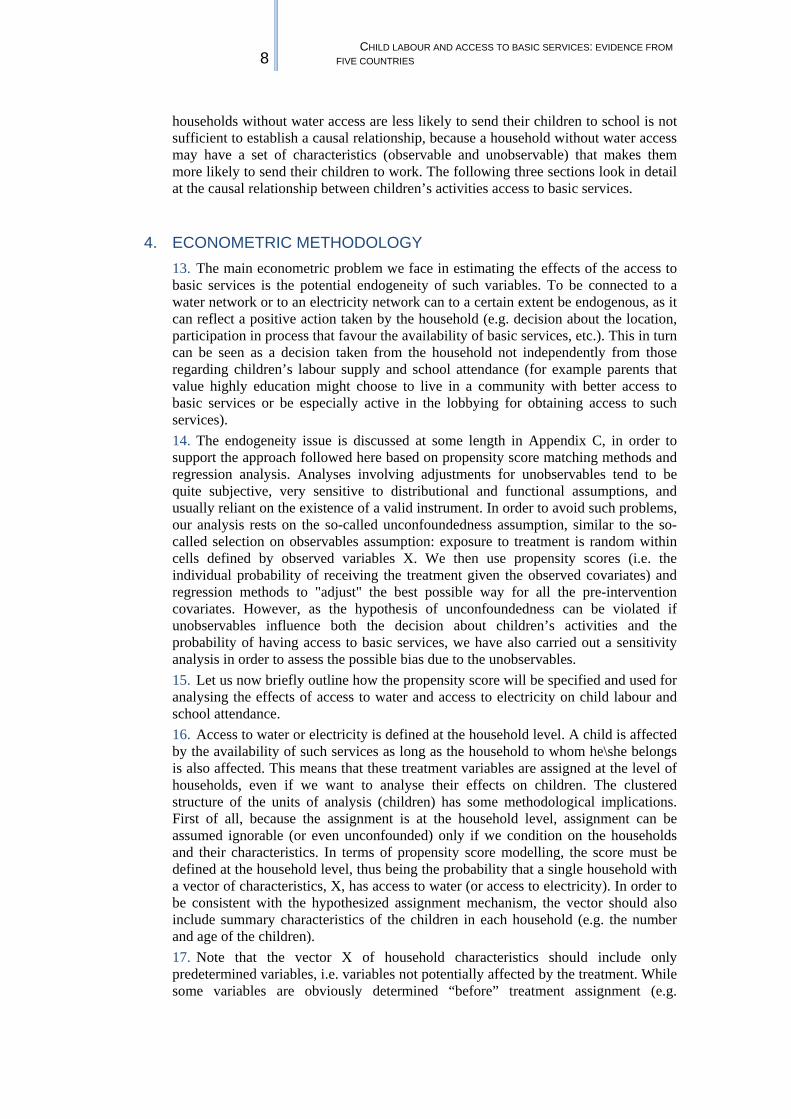
households without water access are less likely to send their children to school is not sufficient to establish a causal relationship, because a household without water access may have a set of characteristics (observable and unobservable) that makes them more likely to send their children to work. The following three sections look in detail at the causal relationship between children’s activities access to basic services.
4. ECONOMETRIC METHODOLOGY 13. The main econometric problem we face in estimating the effects of the access to basic services is the potential endogeneity of such variables. To be connected to a water network or to an electricity network can to a certain extent be endogenous, as it can reflect a positive action taken by the household (e.g. decision about the location, participation in process that favour the availability of basic services, etc.). This in turn can be seen as a decision taken from the household not independently from those regarding children’s labour supply and school attendance (for example parents that value highly education might choose to live in a community with better access to basic services or be especially active in the lobbying for obtaining access to such services). 14. The endogeneity issue is discussed at some length in Appendix C, in order to support the approach followed here based on propensity score matching methods and regression analysis. Analyses involving adjustments for unobservables tend to be quite subjective, very sensitive to distributional and functional assumptions, and usually reliant on the existence of a valid instrument. In order to avoid such problems, our analysis rests on the so-called unconfoundedness assumption, similar to the so-called selection on observables assumption: exposure to treatment is random within cells defined by observed variables X. We then use propensity scores (i.e. the individual probability of receiving the treatment given the observed covariates) and regression methods to "adjust" the best possible way for all the pre-intervention covariates. However, as the hypothesis of unconfoundedness can be violated if unobservables influence both the decision about children’s activities and the probability of having access to basic services, we have also carried out a sensitivity analysis in order to assess the possible bias due to the unobservables. 15. Let us now briefly outline how the propensity score will be specified and used for analysing the effects of access to water and access to electricity on child labour and school attendance. 16. Access to water or electricity is defined at the household level. A child is affected by the availability of such services as long as the household to whom he\she belongs is also affected. This means that these treatment variables are assigned at the level of households, even if we want to analyse their effects on children. The clustered structure of the units of analysis (children) has some methodological implications. First of all, because the assignment is at the household level, assignment can be assumed ignorable (or even unconfounded) only if we condition on the households and their characteristics. In terms of propensity score modelling, the score must be defined at the household level, thus being the probability that a single household with a vector of characteristics, X, has access to water (or access to electricity). In order to be consistent with the hypothesized assignment mechanism, the vector should also include summary characteristics of the children in each household (e.g. the number and age of the children). 17. Note that the vector X of household characteristics should include only predetermined variables, i.e. variables not potentially affected by the treatment. While some variables are obviously determined “before” treatment assignment (e.g.
9 UCW WORKING PAPER SERIES, JANUARY 2004
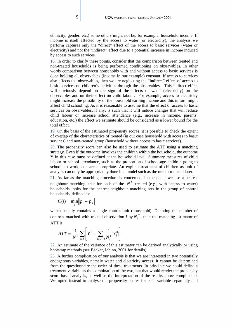
ethnicity, gender, etc.) some others might not be; for example, household income. If income is itself affected by the access to water (or electricity), the analysis we perform captures only the “direct” effect of the access to basic services (water or electricity) and not the “indirect” effect due to a potential increase in income induced by access to such services. 18. In order to clarify these points, consider that the comparison between treated and non-treated households is being performed conditioning on observables. In other words comparison between households with and without access to basic services is done holding all observables (income in our example) constant. If access to services also affects the observables, then we are neglecting the “indirect” effect of access to basic services on children’s activities through the observables. This indirect effect will obviously depend on the sign of the effects of water (electricity) on the observables and on their effect on child labour. For example, access to electricity might increase the possibility of the household earning income and this in turn might affect child schooling. As it is reasonable to assume that the effect of access to basic services on observables, if any, is such that it will induce changes that will reduce child labour or increase school attendance (e.g., increase in income, parents’ education, etc.) the effect we estimate should be considered as a lower bound for the total effect. 19. On the basis of the estimated propensity scores, it is possible to check the extent of overlap of the characteristics of treated (in our case household with access to basic services) and non-treated group (household without access to basic services). 20. The propensity score can also be used to estimate the ATT using a matching strategy. Even if the outcome involves the children within the household, the outcome Y in this case must be defined at the household level. Summary measures of child labour or school attendance, such as the proportion of school-age children going to school, to work, etc. are appropriate. An explicit treatment of children as unit of analysis can only be appropriately done in a model such as the one introduced later. 21. As far as the matching procedure is concerned, in the paper we use a nearest neighbour matching, that for each of the TN treated (e.g., with access to water) households looks for the nearest neighbour matching sets in the group of control households, defined as:
jijppiC −= min)(
which usually contains a single control unit (household). Denoting the number of controls matched with treated observation i by C
iN , then the matching estimator of ATT is
.11)(
01∑ ∑∈ ∈
⎥⎦
⎤⎢⎣
⎡−=
Ti iCjjT
iiT Y
NY
NTTA)
22. An estimate of the variance of this estimator can be derived analytically or using bootstrap methods (see Becker, Ichino, 2001 for details). 23. A further complication of our analysis is that we are interested in two potentially endogenous variables, namely water and electricity access. It cannot be determined from the questionnaire the order of these treatments. In principle we could define a treatment variable as the combination of the two, but that would render the propensity score based analysis, as well as the interpretation of the results, more complicated. We opted instead to analyse the propensity scores for each variable separately and

10 CHILD LABOUR AND ACCESS TO BASIC SERVICES: EVIDENCE FROM
FIVE COUNTRIES
derive separate estimates of their ATTs.6 Eventual interactions among these variables are then captured and analysed in the model specified subsequently. 24. Details of the methodology and of the results are reported in Appendix C.
5. ATT MATCHING PROCEDURE: SOME RESULTS 25. Propensity scores have been estimated as the probability that a household with characteristics X has access to water and electricity, respectively. In each case, specification of the propensity score was achieved by checking if the balancing property of the estimated propensity score was satisfied.7 Preliminary testing has 26. shown that by pooling together urban and rural areas it was very difficult to achieve “”balanced” estimates of the propensity scores. This result is not surprising given the structural differences between city and country and given that the effects of access to basic services is likely to be different across the area of residence. For this reason the propensity scores have been computed separately for urban and rural households. The estimated propensity score distributions are shown in Appendix D. 27. The distributions of the propensity scores for “treated” and “non-treated” groups of households overlap to a large extent for El Salvador (rural areas) and Guatemala (rural and urban areas) in the case of water access, and for Morocco (rural areas) in the case of electricity access, indicating that the characteristics of the two groups of households that have and do not have access to water (electricity) do not differ in a significant way. In the other cases, however, the “treated” and “non-treated” groups of households overlap to a much lesser extent, and therefore the analysis is more sensitive to our model specification. 28. Average Treatment Effects (ATT) have been computed using a nearest neighbour matching estimator; results appear in Tables 8 and 9. Caution should be exercised in interpreting the results, however, due to the potential endogeneity of the variables in question generated by unobserved variables, not taken into account in our analysis (see next section for a further discussion of this point). 29. The results obtained are very similar to those stemming from the regression analysis discussed in the next section. We leave, therefore, a detailed discussion for later and provide a short summary here. 30. Access to water in rural areas increases school attendance and reduces participation of children to economic activity and the number of children neither attending school nor working. The effects are differentiated somewhat by country, but they hold a similar pattern over the groups considered. In urban areas, the effect of access to water also has the same pattern, but it appears less well defined and not always significant. 31. Access to electricity has broadly similar effects, significantly increasing the proportion of children in school (El Salvador, Ghana, Morocco), and significantly reducing the proportion of economically active children (Morocco) and idle children (El Salvador, Ghana and Morocco). Again, with the exception of Guatemala, these effects appear to be less well defined in urban areas compared to rural ones.
6 Some preliminary testing supported our decision, as they show conditional independence of the occurrence of the three variables considered 7 To do this we used the procedure implemented in Stata by Becker and Ichino (2001).

11 UCW WORKING PAPER SERIES, JANUARY 2004
Table 6. - Average treatment effects for water access (results from matching procedure using water access as the treatment variable)
Country Outcome variable (2) Urban Rural
treat. contr. ATT t treat. contr. ATT t El Salvador Children attending school 1122 627 0.055 2.87 2887 570 0.028 1.028
Children working (1) 1122 627 -0.016 -1.131 2887 570 -0.027 -1.397 Working (2) and not attending school 1122 627 -0.007 -0.885 2887 570 -0.015 -1.12 Attending school and not working 1122 627 0.004 0.316 2887 570 -0.026 -1.55 Working and attending school 1122 627 0.05 2.347 2887 570 0.053 1.795 Not working and not attending school 1122 627 -0.047 -3.244 2887 570 -0.026 -1.55
Ghana Children attending school 876 174 0.043 0.658 400 319 0.068 1.772
Children working (1) 876 174 -0.096 -1.937 400 319 -0.088 -3.002
Working (2) and not attending school 876 174 -0.023 -0.693 400 319 -0.04 -1.754
Attending school and not working 876 174 -0.073 -1.938 400 319 -0.048 -2.543
Working and attending school 876 174 0.109 1.63 400 319 0.144 3.875
Not working and not attending school 876 174 -0.029 -0.47 400 319 -0.028 -0.748 Guatemala Children attending school 1516 171 -0.059 -1.411 1263 611 0.065 2.784
Children working (1) 1516 171 0.078 1.295 1263 611 0.015 0.74 Working (2) and not attending school 1516 171 -0.027 -1 1263 611 0.001 0.06 Attending school and not working 1516 171 0.112 1.776 1263 611 0.014 0.874 Working and attending school 1516 171 -0.032 -0.91 1263 611 0.051 2.084 Not working and not attending school 1516 171 -0.052 -0.961 1263 611 -0.066 -3.272
Morocco Children attending school -- -- -- -- 726 404 -0.021 0.032 Children working (1) -- -- -- -- 726 404 -0.053 0.027 Working (2) and not attending school -- -- -- -- 726 404 -0.046 0.025 Attending school and not working -- -- -- -- 726 404 -0.007 0.006 Working and attending school -- -- -- -- 726 404 -0.015 0.032 Not working and not attending school -- -- -- -- 726 404 0.067 0.026
Notes: (1) Economically Active; (2) The outcome variable is the proportion of children in each household involved in the reported activities. Sources: UCW calculations based on Ghana: Ghana Living Standard Measurement Survey, 1998-99; Yemen: National Poverty Survey, 1999 ; Guatemala: Guatemala, Encuesta de Condiciones de Vida (ENCOVI), 2000 ; El Salvador: Enquesta de Hogares de Propositos Multiples (EHPM) 2001 ; Morocco: Living Standard Measurement Survey, 1998-99

12 CHILD LABOUR AND ACCESS TO BASIC SERVICES: EVIDENCE FROM
FIVE COUNTRIES
Table 7. - Average treatment effects for electricity access (results from matching procedure using electricity access as the treatment variable)
Country Outcome variable (2) Urban Rural
treat. contr. ATT t treat. contr. ATT t El Salvador Children attending school 3598 125 0.011 0.09 1928 478 0.082 2.662
Children working (1) 3598 125 0.006 0.076 1928 478 -0.029 -1.347 Working (2) and not attending school 3598 125 -0.013 -0.186 1928 478 -0.01 -0.748 Attending school and not working 3598 125 0.08 0.639 1928 478 0.108 3.249 Working and attending school 3598 125 -0.073 -0.971 1928 478 -0.028 -1.345 Not working and not attending school 3598 125 -0.016 -0.168 1928 478 -0.075 -2.943
Ghana Children attending school 847 763 0.079 1.229 395 287 0.107 2.926 Children working (1) 847 163 -0.041 -0.868 395 287 -0.05 -1.708 Working (2) and not attending school 847 163 -0.031 -0.951 395 287 -0.031 -1.386 Attending school and not working 847 163 0.067 1.035 395 287 0.119 3.282 Working and attending school 847 163 -0.01 -0.298 395 287 -0.019 -0.946 Not working and not attending school 847 163 -0.066 -1.062 395 287 -0.077 -2.197
Guatemala Children attending school 1283 541 0.165 5.775 1557 140 0.168 1.887 Children working (1) 1283 541 0.022 0.912 1557 140 -0.059 -0.958 Working (2) and not attending school 1283 541 -0.028 -1.541 1557 140 -0.027 -0.554 Attending school and not working 1283 541 0.116 3.929 1557 140 0.2 2.255 Working and attending school 1283 541 0.05 2.727 1557 140 -0.032 -0.729 Not working and not attending school 1283 541 -0.131 -5.151 1557 140 -0.141 -1.727
Morocco Children attending school 393 361 0.189 4.859 Children working (1) 393 361 -0.115 -3.797 Working (2) and not attending school - - - - 393 361 -0.12 -3.926 Attending school and not working - - - - 393 361 0.183 4.631 Working and attending school - - - - 393 361 0.005 0.688 Not working and not attending school - - - - 393 361 -0.069 -2.145
Notes: (1) Economically active; (2) The outcome variable is the proportion of children in each household involved in the reported activities Sources: UCW calculations based on Ghana: Ghana Living Standard Measurement Survey, 1998-99; Yemen: National Poverty Survey, 1999 ; Guatemala: Guatemala, Encuesta de Condiciones de Vida (ENCOVI), 2000 ; El Salvador: Enquesta de Hogares de Propositos Multiples (EHPM) 2001 ; Morocco: Living Standard Measurement Survey, 1998-99
13 UCW WORKING PAPER SERIES, JANUARY 2004
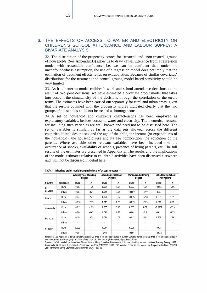
6. THE EFFECTS OF ACCESS TO WATER AND ELECTRICITY ON CHILDREN’S SCHOOL ATTENDANCE AND LABOUR SUPPLY: A BIVARIATE ANALYSIS 32. The distribution of the propensity scores for “treated” and “non-treated” groups of households (See Appendix D) allow us to draw causal inference from a regression model with reasonable confidence, i.e. we can be confident that, under the unconfoundedness assumption, the use of a regression model does not imply that the estimation of treatment effects relies on extrapolation. Because of similar covariates’ distributions for the treatment and control groups, model-based sensitivity should be very limited. 33. As it is better to model children’s work and school attendance decisions as the result of two joint decisions, we have estimated a bivariate probit model that takes into account the simultaneity of the decisions through the correlation of the errors terms. The estimates have been carried out separately for rural and urban areas, given that the results obtained with the propensity scores indicated clearly that the two groups of households could not be treated as homogeneous. 34. A set of household and children’s characteristics has been employed as explanatory variables, besides access to water and electricity. The theoretical reasons for including such variables are well known and need not to be discussed here. The set of variables is similar, as far as the data sets allowed, across the different countries. It includes the sex and the age of the child, the income (or expenditures of the household), the household size and its age composition, the education of the parents. Where available other relevant variables have been included like the occurrence of shocks, availability of schools, presence of living parents, etc. The full results of the estimates are presented in Appendix E. The results and the implications of the model estimates relative to children’s activities have been discussed elsewhere and will not be discussed in detail here. Table 8. - Bivariate probit model marginal effects of access to water (1)
Country Residence
Working(5) not attending school
Attending school not working
Working and attending school
Not attending school not working
dy/dx z dy/dx z dy/dx z dy/dx z
El Salvador
Rural -0.003 -1.36 0.054 4.71 0.003 1.34 -0.055 -5.06
Urban -0.004 -3.21 0.041 4.24 -0.007 -1.99 -0.03 -
Ghana
Rural -0.077 -7.47 0.074 3.02 -0.035 -5.98 0.039 1.59
Urban -0.016 -2.13 0.019 0.68 -0.019 -2.25 0.016 0.61
Guatemala
Rural -0.012 -1.99 0.035 2.43 0.003 0.32 -0.0262 -2.29
Urban -0.004 -0.67 0.016 0.73 -0.001 -0.1 -0.011 -0.73
Morocco
Rural -0.184 -5.28 0.094 1.06 -0.013 -4.98 0.103 1.16
Urban - - - - - - - -
Yemen(4)
Rural 0.002 - 0.014 - 0.006 - -0.021 -
Urban -0.004 - 0.04 - -0.001 - -0.034 - Notes: (1) See Appendix E for all control variables; (2) dy/dx is for discrete change in dummy variable from 0 to 1; (3) dy/dx is for discrete change in dummy variable from 0 to 1; (4) Simulated effects after bivariate probit; (5) Economically Active Children. Sources: UCW calculations based on Ghana: Ghana Living Standard Measurement Survey, 1998-99; Yemen: National Poverty Survey, 1999 ; Guatemala: Guatemala, Encuesta de Condiciones de Vida (ENCOVI), 2000 ; El Salvador: Enquesta de Hogares de Propositos Multiples (EHPM) 2001 ; Morocco: Living Standard Measurement Survey, 1998-99

14 CHILD LABOUR AND ACCESS TO BASIC SERVICES: EVIDENCE FROM
FIVE COUNTRIES
Table 9. - Bivariate probit model marginal effects of access to electricity (1)
Country Residence
Working(4) not attending school
Attending school not Working
Working and attending school
Not attending school not Working
dy/dx (2) z dy/dx(2) z dy/dx(2) z dy/dx(2) z
El Salvador Rural -0.01 -3.83 0.084 6.27 -0.004 -1.26 -0.07 -5.55
Urban -0.006 -2.08
0.081 3.87
-0.004 -0.61
-0.072 -
Ghana Rural 0.025 1.66 0.017 0.74 0.029 2.94 -0.071 -3.04
Urban -0.041 -3.96 0.145 4.93 -0.021 -2.44 -0.083 -2.98
Guatemala Rural -0.019 -3.06 0.075 4.82 0.031 3.42 -0.087 -7.02
Urban -0.024 -2.59 0.144 4.75 0.028 2.5 -0.149 -5.63
Morocco Rural -0.097 -4.36 0.188 5.43 0.002 0.46 -0.093 -3.24
Urban - - - - - - - -
Yemen(3) Rural -0.02 - 0.07 - 0.001 - -0.05 -
Urban -0.015 - 0.11 - -0.01 - -0.09 - Notes: (1) See Appendix E for all control variables; (2) dy/dx is for discrete change in dummy variable from 0 to 1; (3) Simulated effects after bivariate probit; (4) Economically Active Children. Sources: UCW calculations based on Ghana: Ghana Living Standard Measurement Survey, 1998-99; Yemen: National Poverty Survey, 1999 ; Guatemala: Guatemala, Encuesta de Condiciones de Vida (ENCOVI), 2000 ; El Salvador: Enquesta de Hogares de Propositos Multiples (EHPM) 2001 ; Morocco: Living Standard Measurement Survey, 1998-99
35. Table 10 presents the marginal effects for water and electricity access obtained by estimating the bivariate probit model; these marginal effects are computed for an “average” child (i.e. setting the value of the other variables at their mean value). 36. The effects of access to water and electricity are well defined and relatively large for almost all countries. Access to water in urban areas tends to increase the number of children that attend school only. This is normally associated with a reduction in the number of children performing economic activity or involved in no activities. The size of the effect varies across countries; access to water in urban areas is associated with an increase in the probability of attending school in the range of 2 (Ghana) to 10 (Yemen) percentage points. As just mentioned, while increased access to water is associated in all countries with an increase in school attendance, the effects on work or on the probability of being “idle” are differentiated by country. In El Salvador and Yemen increased water access is associated more with a reduction in the number of “idle” children, while in the other countries it is the number of working children that is reduced. 37. Access to water in rural areas shows a similar pattern; it induces an increase in the number of children attending school and a reduction in the number of children involved in economic activity or neither attending neither school nor working. Observe that the size of the effects in rural areas is in general larger than in urban areas. 38. The link between availability of electricity and children’s activities must be evaluated with more care than the case of access to water. In fact, as discussed in the previous section and shown in the graphs reported in the appendix, the distribution of treated and control group, obtained on the basis of the propensity scores, does show some dissimilarity. Unfortunately, a formal test to compare the two distributions is not available, but the difference they show in the case of electricity points to the need for some caution in evaluating the results. 39. Access to electricity increases school attendance in both urban and rural areas, with the exception of rural Ghana. The increase in school attendance is associated with a reduction of the number of both children working and of children neither attending school nor involved in economic activity. The size of the effect varies somewhat across countries, ranging from 18 percent in rural Morocco to seven
15 UCW WORKING PAPER SERIES, JANUARY 2004
percent in rural Yemen, and from 14 percent in urban Ghana to 11 percent in urban Yemen. 40. As mentioned in the preceding discussion, while the pattern of effects is similar across countries, the size of the effect is different. Given the nature of the data sets utilized and the different controls that are available for each country it is difficult to draw any conclusion from about the different size of the effects. The overall finding confirms, however, the important role that access to basic services has in determining household decisions concerning children activities. 41. It is also interesting to look at the effects of access to basic services (water and electricity) by age. The graphs reported in Appendix F show the simulated effect on children’s activities of access to water and electricity. Again, the patterns are generally similar across countries. We will hence comment only on the general pattern and make specific reference only to the exceptions. Let us start with the impact on school attendance. The effects of access to basic services are higher for relatively young and relatively old children. This seems to indicate that availability of water and electricity help both to increase school enrolment at younger ages and to reduce the drop out rate at later ages. The negative effect that access to basic services has on the participation of children to economic activity tends to be higher for relatively older children. “Idle” children seem to particularly benefit from access to basic services at a young age. The increase in enrolment seems therefore to be due to young children being withdrawn from full-time household chores or from being “idle” and brought into the education system. On the other hand, access to water and electricity appears to help retain in the school system children that would have otherwise dropped out to joint the labour market.
7. SENSITIVITY ANALYSIS 42. The previous discussion has highlighted the importance of access to basic services for reducing child labour and increasing school attendance. However, the presence of unobservables that influence both the decision relative to children’s activities and the access to basic service might invalidate the casual interpretation of the estimated relationship. For example, parents with stronger interest in education might decide to live in place where access to basic services, or might be more engaged in “lobbying” for the availability of such services. Even if the hypothesis of “exogeneity” of access to basic services seems reasonable to maintain, once we control for observables (as we did in the regression analysis and with the use of propensity scores), we nonetheless performed a sensitivity analysis to test the robustness of our results with respect to the presence of unobservables that are correlated both with children’s activities and with the availability of basic services. 43. In order to check how robust our causal conclusions are, we applied a method for sensitivity analysis, proposed by Rosenbaum and Rubin (1983) and extended here, for simplicity, to a multinomial outcome. In particular, this method allows us to assess the sensitivity of the causal effects with respect to assumptions about an unobserved binary covariate that is associated both with the treatments and with the response. 44. The unobservables are assumed to be summarized by a binary variable in order to simplify the analysis, although similar techniques could be used assuming other distributions for the unobservables. Note, however, that a Bernoulli distribution can be thought of as a discrete approximation to any distribution, and thus we believe that our distributional assumption will not severely restrict the generality of the results. 45. Suppose that treatment assignment is not unconfounded given a set of observable variables X, i.e.,
16 CHILD LABOUR AND ACCESS TO BASIC SERVICES: EVIDENCE FROM
FIVE COUNTRIES
P(T = 1|Y(0), Y(1), X) is not equal to P(T = 1| X)
but unconfoundedness holds given X and an unobserved binary covariate U, that is P(T = 1|Y(0), Y(1), X, U) is equal to P(T = 1| X, U).
46. We can then judge the sensitivity of conclusions to certain plausible variations in assumptions about the association of U with T, Y(0), Y(1) and X. If such conclusions are relatively insensitive over a range of plausible assumptions about U, then our causal inference is more defensible. 47. Since Y(0), Y(1) and T are conditionally independent given X and U, we can write the joint distribution of (Y(t), T, X, U) for t = 0, 1 as
Pr(Y(t), T, X, U) = Pr(Y(t)| X, U) Pr(T| X, U) Pr(U| X) Pr(X)
where, in our analysis, we assume that
Pr(U = 0|X) = Pr(U = 0) = π
Pr(T = 0| X, U) = (1+exp (γ’X + αU))-1
Pr(Y(t) = j| X, U) = exp(β’j X+ τj T+ δtjU) (1+ Σi exp(β’i X+ τi T+ δtiU)) –1
j=( Working only:W, Studying only: S, Working and Studying: WS, Idle Children: I)
π represents the proportion of individuals with U=0 in the population, and the distribution of U is assumed to be independent of X. This should render the sensitivity analysis more stringent, since, if U were associated with X, controlling for X should capture at least some of the effects of the unobservables. The sensitivity parameter α captures the effect of U on treatment receipt (e.g., credit rationing), while the δti,‘s are the effects of U on the outcome. 48. Given plausible but arbitrary values to the parameters π , α and δti, we estimated the parameters γ and βj by maximum likelihood and derived estimates of the ATT as follows:
[ ].ˆˆ1 01∑∈
−=Ti
iiT YYN
TTA)
where
)1,|)(r(P̂)1()0,|)(r(P̂)|)(r(P̂ˆ ==−+===== UXjtYUXjtYXjtYY ti ππ
49. These estimates of the ATT are comparable to the ones based on the propensity score based matching procedure and they are very similar to the marginal effects obtained. 50. In the following tables, the estimates of the ATT for water and electricity access in rural and urban areas, and different combinations of values for π, α and δti , are reported.
17 UCW WORKING PAPER SERIES, JANUARY 2004
51. As can be observed, the results of the estimates, reported in Appendix G for El Salvador and Guatemala,8 are not very sensitive to a range of plausible assumptions about U. Note that an α or δti of 0.5 almost doubles the odds of receiving the treatment or the odds of a certain value of the outcome. In addition, these values are larger than most of the coefficients of the estimated multinomial logit. Setting the values of the association parameter to larger numbers may change the obtained results. However, given the number of observed covariates already included in the models, the existence of a residual unobserved covariate so highly correlated with T and Y appears implausible. All this leads us to conclude that the results presented in this paper are robust also with respect to the existence of possible unobservables that influence both children’s activities and access to basic services. We can hence consider with some confidence the links identified in this paper between access to basic services and child labour as causal.
8. CONCLUSION 52. The time of adults and children are both inputs in the production of household welfare, both directly (through domestic production activities) and indirectly (through market activities). Allocation of household time across different activities can be thought of as the result of a rational choice taking into account the value of time of household members in the different activities. 53. Access to basic services (water and electricity in the case of our study) can modify the decision of the household concerning children activities through “price” and income effects. Easier access to water and electricity might reduce the value of children’s time in providing current resources to household income as opposed to investment in human capital accumulation. If water is available at or in the proximity of the household residence, the value of time spent by children outside school is reduced. Similarly, electricity availability, by influencing the mix of combustibles used by the household, can generate a similar effect. Moreover, the value of children’s time might be affected indirectly by access to basic services. The household could find it convenient to buy on the market water and/or other combustibles rather than produce them directly (by fetching water or wood, for example). In this case, access to basic services might produce a positive income effect that reduces the value of children’s time in contributing to current income. 54. While the theoretical underpinning of the potential effects of access to basic services are relatively easy to grasp (even if more attention should be given to the intra-household allocation of tasks), the questions that arise are mainly empirical. Are the effects of access to electricity on children’s activity present? Are they relevant? And finally can we be reasonably sure that the estimated effects reflect a causal relationship rather than, in the best scenario, just a covariation? 55. These are the issues that the present paper has tried to deal with employing a battery of methodological approaches. 56. To interpret the link between access to basic services and child labour as a causal relationship might be difficult, given that both observables and unobservables might be correlated both with the decision of the household about children’s activities and with the household access to water and electricity. Given the lack of good “instruments” in the data sets we have followed two different approaches to deal with possible spurious correlation arising from observables and unobservables. We have dealt with the potential role of observable household characteristics by making use of 8 Results for the other countries are available on request from the authors

18 CHILD LABOUR AND ACCESS TO BASIC SERVICES: EVIDENCE FROM
FIVE COUNTRIES
an approach based on propensity scores and matching strategy, based on the maintained hypothesis of unconfoundness. The role of unobservables has been assessed indirectly by using sensitivity analysis. 57. Both approaches followed that the estimated effects of access to basic services on child labour and school enrolment can be considered as reflecting a causal relationship with a sufficient degree of confidence. 58. The paper has shown that household with access to water and electricity are indeed more likely to send their children to school and less likely to send them to work or to keep them “idle”. This effect is not only present, but it is also sizable. The impact of water and electricity access varies from country to country, but is large with respect to those of other variables. Access to basic services improves children human capital accumulation especially in the rural areas, as one could expect. However, the effects in urban areas are far from negligible. 59. The effect of access to basic services is also clearly differentiated according to the age of the child. The availability of water and electricity help both to increase school enrolment at an early stage of life and to reduce the drop out rate at later ages. The impact of these services in reducing economic activity is stronger among older children, while their impact in reducing child “idleness” is stronger among younger children. The increase in enrolment seems hence to be due to young children being withdrawn from full-time household chores or from being “idle” and brought into the education system. On the other hand, access to water and electricity appears to help retain in the school system children that would have otherwise dropped out to join the labour market. 60. These findings highlight the importance of a cross-sectoral approach to dealing with the phenomenon of child labour. The results point in particular to the need to ensure that child labour considerations are mainstreamed into Government and donor policy in the water and electricity sectors. They underscore the importance of accelerating current Government efforts to expand electricity and water access, with a particular emphasis on communities where school attendance is low and child work rates are high. The results also illustrate how proper targeting and cross-sectoral considerations could be employed to increase the effectiveness of policies relating to basic services provision.

19 UCW WORKING PAPER SERIES, JANUARY 2004
APPENDIX A: SURVEYS AND QUESTIONS USED TO DEFINE VARIABLES FOR WATER AND ELECTRICITY ACCESS
Question used to define access to water Note: In bold positive response used to define the variable “Access to Water” Ghana Yemen Guatemala El Salvador Morocco (1) What is the source of drinking water for your household? Indoor plumbing ………………1 Inside standpipe… ……………2 Water vendor............................3 Water truck/tanker service……4 Neighbouring household ……….5 Private outside standpipe/tap….6 Public standpipe………………...7 Well with pump……………..…...8 Well without pump……………….9 River, lake spring, pond….……10 Rainwater……………..…………11 Other …………….…….………..….12
What is the source of drinking water for your household? Public net……………..….………1 Cooperative net…………….……2 Private net………………….……3 Well inside the dwelling………...4 Well outside the dwelling………...5 Spring………………………….….6 Covered pond……………………..7 An open pond……………………..8 Dam……………………………….9 Other………………………….....10
What is the main source of water used by the household? Pipe (network) inside the dwelling…………………………..1 Pipe, outside the dwelling but within the property………………………..2 Pipe from a public well……………………………….3 Public or private well…………….4 River, lake, stream………………..5 Water truck…………………….....6 Rain water………………………..7 Other (specify)…………………...8
What is the source of drinking water for your household? Pipe inside the dwelling ……….1 Pipe outside the dwelling but inside the property……………..2 Neighbour’s pipe………………..3 Fountain or public stream………..4 Cooperative stream..…………….5 Water truck……….……………..6 Private or cooperative well …….7 Lake, river, spring..……………..8 Other (specify)………………….9
What is the main source of drinking water in the “DOUAR”? Public network……..…………...1 Well………………………………2 Lake, river, spring………………..3 Hill dam…………………………..4 Water truck……………………….5 Other ……………………………..6 (1) Question applied to the rural questionnaire
Note: In bold positive response used to define the variable “Access to Electricity” Source: Ghana: Ghana Living Standard Measurement Survey, 1998-99; Yemen: National Poverty Survey, 1999 ; Guatemala: Guatemala, Encuesta de Condiciones de Vida (ENCOVI), 2000 ; El Salvador: Enquesta de Hogares de Propositos Multiples (EHPM) 2001 ; Morocco: Living Standard Measurement Survey, 1998-99

20 CHILD LABOUR AND ACCESS TO BASIC SERVICES: EVIDENCE FROM
FIVE COUNTRIES
Question used to define access to electricity Note: In bold positive response used to define the variable “Access to Electricity” Ghana
Yemen Guatemala El Salvador Morocco (1)
What is the main source of lighting for your dwelling? Electricity (mains)……………….1 Generator………………….……..2 Kerosene, Gas, Lamp…………….3 Candles/torches (flashlights)……..4
What is the main source of lighting in the house? Public net……….……………….1 Cooperation net………………...2 Private net………………………3 Household private generator…….4 Kerosene (gas)…………………..5 Gasoline torch…………………...6 Other (specify)…………………..7
This dwelling is connected to: An electrical energy distribution system? Yes…..1, No…..2
What is the main source of lighting in this house? Electricity……………………….1 Neighbour’s electricity connection..……………………..2 Kerosene (gas)…………………..3 Candle………….………………..4 Other………….………………….5
Is there any electricity in this “DOUAR” ? Yes…..1, No……2 (1) Question applied to the rural questionnaire
Note: In bold positive response used to define the variable “Access to Electricity” Source: Ghana: Ghana Living Standard Measurement Survey, 1998-99; Yemen: National Poverty Survey, 1999 ; Guatemala: Guatemala, Encuesta de Condiciones de Vida (ENCOVI), 2000 ; El Salvador: Enquesta de Hogares de Propositos Multiples (EHPM) 2001 ; Morocco: Living Standard Measurement Survey, 1998-99
21 UCW WORKING PAPER SERIES, JANUARY 2004
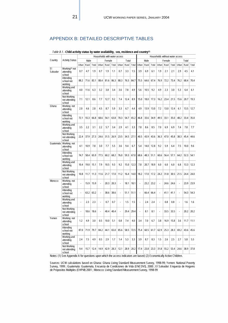
APPENDIX B: DETAILED DESCRIPTIVE TABLES
Table B.1. -Child activity status by water availability, sex, residence and country(1)
Country Activity Status Households with water access Households without water access
Male Female Total Male Female Total Urban Rural Total Urban Rural Total Urban Rural Total Urban Rural Total Urban Rural Total Urban Rural Total
El Salvador
Working(3) not attending school
0.7 4.7 1.9 0.7 1.9 1.1 0.7 3.3 1.5 3.9 6.9 6.1 1.9 2.1 2.1 2.9 4.5 4.1
Attending school not working
88.2 71.6 83.1 88.4 81.6 86.3 88.3 76.5 84.7 75.5 64.6 67.4 76.9 72.2 73.4 76.2 68.4 70.4
Working and attending school
4.0 11.6 6.3 3.2 3.8 3.4 3.6 7.8 4.9 5.6 10.5 9.2 4.9 2.3 3.0 5.3 6.4 6.1
Not Working not attending school
7.1 12.1 8.6 7.7 12.7 9.2 7.4 12.4 8.9 15.0 18.0 17.3 16.2 23.4 21.5 15.6 20.7 19.3
Ghana Working not attending school
2.0 4.6 2.8 4.5 8.7 5.9 3.3 6.7 4.4 4.9 13.9 13.0 7.2 13.0 12.4 6.1 13.5 12.7
Attending school not working
72.1 55.3 66.8 68.6 54.1 63.8 70.3 54.7 65.2 46.8 33.6 34.9 49.5 33.1 35.0 48.2 33.4 35.0
Working and attending school
3.5 2.2 3.1 2.2 5.7 3.4 2.9 4.1 3.3 7.8 8.6 8.5 7.0 6.9 6.9 7.4 7.8 7.7
Not Working not attending school
22.4 37.9 27.3 24.6 31.5 26.9 23.5 34.5 27.1 40.5 43.9 43.6 36.3 47.0 45.8 38.3 45.4 44.6
Guatemala Working not attending school
4.1 10.9 7.8 3.0 7.7 5.5 3.6 9.4 6.7 5.4 14.0 12.8 9.2 5.9 6.4 7.5 10.0 9.6
Attending school not working
74.7 58.4 65.9 77.5 60.2 68.2 76.0 59.3 67.0 68.6 48.3 51.1 60.6 56.4 57.1 64.2 52.3 54.1
Working and attending school
10.4 19.0 15.1 7.9 10.5 9.3 9.2 15.0 12.3 7.8 20.7 18.9 6.0 6.0 6.0 6.8 13.3 12.3
Not Working not attending school
10.8 11.7 11.3 11.6 21.7 17.0 11.2 16.4 14.0 18.2 17.0 17.2 24.2 31.8 30.5 21.5 24.4 24.0
Morocco Working not attending school
- 15.9 15.9 - 20.3 20.3 - 18.1 18.1 - 23.2 23.2 - 24.6 24.6 - 23.9 23.9
Attending school not working
- 63.2 63.2 - 38.6 38.6 - 51.1 51.1 - 66.4 66.4 - 41.1 41.1 - 54.3 54.3
Working and attending school
- 2.3 2.3 - 0.7 0.7 - 1.5 1.5 - 2.4 2.4 - 0.8 0.8 - 1.6 1.6
Not Working not attending school
- 18.6 18.6 - 40.4 40.4 - 29.4 29.4 - 8.1 8.1 - 33.5 33.5 - 20.2 20.2
Yemen Working not attending school
1.2 4.9 3.0 0.5 10.0 5.1 0.8 7.4 4.0 3.4 7.0 6.7 3.8 16.9 15.8 3.6 11.7 11.1
Attending school not working
87.0 71.9 79.7 84.2 44.1 65.0 85.6 58.5 72.5 75.4 60.5 61.7 62.9 25.3 28.3 69.2 43.6 45.6
Working and attending school
2.4 7.5 4.9 0.5 2.9 1.7 1.4 5.3 3.3 3.9 8.7 8.3 1.5 2.6 2.5 2.7 5.8 5.5
Not Working not attending school
9.4 15.7 12.4 14.9 42.9 28.3 12.1 28.9 20.2 17.4 23.8 23.3 31.8 55.2 53.4 24.6 38.9 37.8
Notes: (1) See Appendix A for questions upon which the access indicators are based; (2) Economically Active Children.
Sources: UCW calculations based on Ghana: Ghana Living Standard Measurement Survey, 1998-99; Yemen: National Poverty Survey, 1999 ; Guatemala: Guatemala, Encuesta de Condiciones de Vida (ENCOVI), 2000 ; El Salvador: Enquesta de Hogares de Propositos Multiples (EHPM) 2001 ; Morocco: Living Standard Measurement Survey, 1998-99

22 CHILD LABOUR AND ACCESS TO BASIC SERVICES: EVIDENCE FROM
FIVE COUNTRIES
Table B.2. - Child activity status by electricity access, sex, residence and country(1)
Country Activity Status
Households with electricity Households without electricity Male Female Total Male Female Total
Urban Rural Total Urban Rural Total Urban Rural Total Urban Rural Total Urban Rural Total Urban Rural Total El Salvador
Working(2) not attending school
1.1 4.3 2.3 0.9 1.8 1.3 1.0 3.1 1.8 8.4 9.6 9.5 1.8 2.5 2.5 5.2 6.3 6.1
Attending school not working
87.0 72.7 81.4 86.9 81.5 84.7 86.9 77.1 83.0 53.2 56.4 56.0 64.0 63.0 63.1 58.5 59.5 59.4
Working and attending school
4.2 10.8 6.8 3.5 3.0 3.3 3.8 6.9 5.0 8.0 11.1 10.8 4.5 2.7 2.9 6.3 7.1 7.0
Not Working not attending school
7.8 12.2 9.5 8.7 13.7 10.7 8.2 12.9 10.1 30.4 22.9 23.7 29.7 31.8 31.5 30.1 27.1 27.4
Ghana Working not attending school
1.7 8.1 3.8 4.4 7.4 5.4 3.1 7.8 4.6 5.3 13.1 12.2 7.1 13.4 12.5 6.3 13.2 12.4
Attending school not working
74.5 49.7 66.4 70.6 54.4 65.0 72.5 52.1 65.7 42.9 34.8 35.7 46.8 33.1 35.0 44.9 34.0 35.4
Working and attending school
3.2 8.8 5.0 2.5 8.9 4.7 2.8 8.8 4.8 8.2 7.2 7.4 5.3 6.1 6.0 6.7 6.7 6.7
Not Working not attending school
20.6 33.4 24.8 22.5 29.3 24.8 21.6 31.3 24.8 43.6 44.8 44.7 40.8 47.5 46.6 42.1 46.1 45.6
Guatemala Working not attending school
3.3 10.0 6.9 3.8 5.8 4.8 3.5 8.0 5.9 17.4 15.6 15.7 7.9 8.1 8.1 12.3 11.8 11.9
Attending school not working
75.5 60.3 67.3 78.6 64.1 71.0 77.0 62.1 69.1 51.2 44.9 45.4 29.7 51.2 49.2 39.5 48.1 47.4
Working and attending school
10.0 19.8 15.3 7.4 9.9 8.7 8.7 15.2 12.2 11.1 19.6 18.9 9.3 6.4 6.6 10.1 13.0 12.7
Not Working not attending school
11.2 9.9 10.5 10.3 20.2 15.5 10.7 14.7 12.9 20.4 19.9 20.0 53.0 34.3 36.0 38.1 27.1 28.1
Morocco Working not attending school
- 9.9 - - 6.9 - - 8.5 - - 21.3 21.3 - 25.1 25.1 - 23.2 23.2
Attending school not working
- 77.5 - - 66.2 - - 72 - - 63.8 63.8 - 36.4 36.4 - 50.6 50.6
Working and attending school
- 2.9 - - 3.2 - - 3 - - 2.2 2.2 - 0.5 0.5 - 1.4 1.4
Not Working not attending school
- 9.7 - - 23.7 - - 16.5 - - 12.6 12.6 - 37.9 37.9 - 24.9 24.9
Yemen Working not attending school
1.3 4.2 2.4 0.6 11.6 5.5 1.0 7.5 3.8 4.5 9.2 9.0 8.7 9.0 9.0 6.4 9.1 9.0
Attending school not working
68.1 61.3 65.4 57.9 41.1 50.4 64.0 52.2 59.0 44.1 40.6 40.8 20.3 20.2 20.2 33.1 32.5 32.5
Working and attending school
0.8 2.6 1.5 0.0 5.2 2.3 0.5 3.8 1.9 2.5 5.4 5.3 0.9 1.4 1.3 1.8 3.8 3.7
Not Working not attending school
29.8 31.9 30.6 41.5 42.1 41.7 34.5 36.5 35.3 48.9 44.7 44.9 70.1 69.5 69.5 58.7 54.5 54.8
Notes: (1) See Appendix A for questions upon which the access indicators are based; (2) Economically Active Children.
Sources: UCW calculations based on Ghana: Ghana Living Standard Measurement Survey, 1998-99; Yemen: National Poverty Survey, 1999 ; Guatemala: Guatemala, Encuesta de Condiciones de Vida (ENCOVI), 2000 ; El Salvador: Enquesta de Hogares de Propositos Multiples (EHPM) 2001 ; Morocco: Living Standard Measurement Survey, 1998-99

23 UCW WORKING PAPER SERIES, JANUARY 2004
Table B.3. - Child activity status (including household chores) by water access, sex and country(1)
Country Activity status
Households with water access(2) Households without water access(2)
Male Female Total Male Female Total El Salvador Working(2) and not attending school 10.39 8.85 9.63 18.05 14.34 16.2
Attending school not Working 45.25 55.58 50.36 42.52 51.28 46.88
Working and attending school 39.84 29.93 34.94 29.71 21.23 25.49
Not Working not attending school 4.52 5.64 5.07 9.72 13.15 11.43 Guatemala Working and not attending school 8.93 10.49 9.67 14.44 13.47 13.95
Attending school not Working 63.12 58.99 61.16 47.43 45.15 46.27
Working and attending school 17.81 18.46 18.12 22.55 17.9 20.19
Not Working not attending school 10.14 12.07 11.06 15.58 23.48 19.58 Notes: (1) See Appendix A for questions upon which the access indicators are based; (2) Economically Active Children. Sources: UCW calculations based on Ghana: Ghana Living Standard Measurement Survey, 1998-99; Yemen: National Poverty Survey, 1999 ; Guatemala: Guatemala, Encuesta de Condiciones de Vida (ENCOVI), 2000 ; El Salvador: Enquesta de Hogares de Propositos Multiples (EHPM) 2001 ; Morocco: Living Standard Measurement Survey, 1998-99
Table B.4. - Child activity status (including household chores) by electricity access, sex and country(1)
Country Activity status Households with electricity access(2) Households without electricity access(2)
Male Female Total Male Female Total El Salvador Working(2) and not attending school 10.98 9.55 10.27 24.8 18.5 21.78
Attending school not Working 45.98 55.78 50.87 35.73 44.22 39.81
Working and attending school 37.75 28.38 33.08 26.9 16.84 22.07
Not Working not attending school 5.29 6.28 5.79 12.56 20.43 16.35 Guatemala Working and not attending school 7.72 9.14 8.4 18.17 16.83 17.49
Attending school not Working 64.27 60.07 62.26 42.33 40.64 41.48
Working and attending school 18.33 19.65 18.96 22.01 15.24 18.59
Not Working not attending school 9.68 11.14 10.38 17.48 27.29 22.44 Notes: (1) See Appendix A for questions upon which the access indicators are based; (2) Economically Active Children Sources: UCW calculations based on Ghana: Ghana Living Standard Measurement Survey, 1998-99; Yemen: National Poverty Survey, 1999 ; Guatemala: Guatemala, Encuesta de Condiciones de Vida (ENCOVI), 2000 ; El Salvador: Enquesta de Hogares de Propositos Multiples (EHPM) 2001 ; Morocco: Living Standard Measurement Survey, 1998-99
24 CHILD LABOUR AND ACCESS TO BASIC SERVICES: EVIDENCE FROM
FIVE COUNTRIES
APPENDIX C: ECONOMETRIC METHODOLOGY
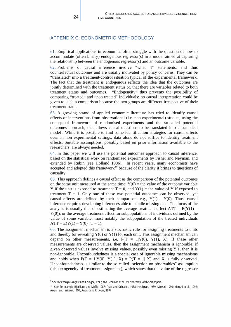
61. Empirical applications in economics often struggle with the question of how to accommodate (often binary) endogenous regressor(s) in a model aimed at capturing the relationship between the endogenous regressor(s) and an outcome variable. 62. Problems of causal inference involve “what if“ statements, and thus counterfactual outcomes and are usually motivated by policy concerns. They can be “translated” into a treatment-control situation typical of the experimental framework. The fact that the treatment is endogenous reflects the idea that the outcomes are jointly determined with the treatment status or, that there are variables related to both treatment status and outcomes. “Endogeneity” thus prevents the possibility of comparing “treated” and “non treated” individuals: no causal interpretation could be given to such a comparison because the two groups are different irrespective of their treatment status. 63. A growing strand of applied economic literature has tried to identify causal effects of interventions from observational (i.e. non experimental) studies, using the conceptual framework of randomised experiments and the so-called potential outcomes approach, that allows causal questions to be translated into a statistical model9. While it is possible to find some identification strategies for causal effects even in non experimental settings, data alone do not suffice to identify treatment effects. Suitable assumptions, possibly based on prior information available to the researchers, are always needed. 64. In this paper we will use the potential outcomes approach to causal inference, based on the statistical work on randomized experiments by Fisher and Neyman, and extended by Rubin (see Holland 1986). In recent years, many economists have accepted and adopted this framework10 because of the clarity it brings to questions of causality. 65. This approach defines a causal effect as the comparison of the potential outcomes on the same unit measured at the same time: Y(0) = the value of the outcome variable Y if the unit is exposed to treatment T = 0, and Y(1) = the value of Y if exposed to treatment T = 1. Only one of these two potential outcomes can be observed, yet causal effects are defined by their comparison, e.g., Y(1) - Y(0). Thus, causal inference requires developing inferences able to handle missing data. The focus of the analysis is usually that of estimating the average treatment effect ATT = E(Y(1) – Y(0)), or the average treatment effect for subpopulations of individuals defined by the value of some variable, most notably the subpopulation of the treated individuals ATT = E(Y(1) – Y(0) | T = 1). 66. The assignment mechanism is a stochastic rule for assigning treatments to units and thereby for revealing Y(0) or Y(1) for each unit. This assignment mechanism can depend on other measurements, i.e. P(T = 1|Y(0), Y(1), X). If these other measurements are observed values, then the assignment mechanism is ignorable; if given observed values involve missing values, possibly even missing Y’s, then it is non-ignorable. Unconfoundedness is a special case of ignorable missing mechanisms and holds when P(T = 1|Y(0), Y(1), X) = P(T = 1| X) and X is fully observed. Unconfoundedness is similar to the so called “selection on observables” assumption (also exogeneity of treatment assignment), which states that the value of the regressor
9 See for example Angrist and Krueger, 1999; and Heckman et al., 1999 for state-of-the-art papers. 10 See for example Bjorklund and Moffit, 1987; Pratt and Schlaifer, 1988; Heckman, 1989; Manski, 1990; Manski et al., 1992; Angrist and Imbens, 1995, Angrist and Krueger, 1999
25 UCW WORKING PAPER SERIES, JANUARY 2004
of interest is independent of potential outcomes after accounting for a set of observable characteristics X. This approach is equivalent to assuming that exposure to treatment is random within the cells defined by the variables X. Although very strong, the plausibility of these assumptions rely heavily on the amount and on the quality of the information on the individuals contained in X.
67. Under unconfoundedness one can identify the average treatment effect within subpopulations defined by the values of X: E(Y(1) – Y(0)| X = x) = E(Y(1) | X = x) - E(Y(0) | X = x) = = E(Y(1) | T = 1, X = x) - E(Y(0) | T = 0, X = x) and also the overall ATT as : E(Y(1) – Y(0)) = E(E(Y(1) – Y(0)| X = x)) where the outer expectation is over the distribution of X in the population. If we could simply divide the sample into subsamples, dependent on the exact value of the covariates X, we could then take the average of the within subsample estimates of the average treatment effects. Often the covariates are more or less continuous, so some smoothing techniques are in order: under unconfoundedness several estimation strategy can serve this purpose. One such strategy is regression modelling: usually a functional form for E(Y(t) | X = x) is assumed, for example a linear function in a vector of functions of the covariates E(Y(t) | X = x) = g(x)’ βt. Estimates of the parameters’ vectors βt (t = 0, 1) are usually obtained by least squares or maximum likelihood methods. Causal effects are rarely estimated, especially if the model is non linear, by the value of some parameters, unless some restrictions are imposed on the βt .11 68. Using regression models to “adjust” or “control for” pre-intervention covariates while being in principle a good strategy, it has some pitfalls. For example, if there are many covariates, it can be difficult to find an appropriate specification. In addition, regression modelling obscures information on the distribution of covariates in the two treatment groups. In principle, one would like to compare individuals that have the same values for all the covariates: unless there is a substantial overlap of the covariates’ distributions in the two groups, with a regression model one relies heavily on model specification, i.e. on extrapolation, for the estimation of treatment effects. 69. Therefore it is crucial to check the extent of the overlapping between the two distributions, and the “region of common support” for these distributions. When the number of covariates is large, this task is not an easy one. An approach that can be followed is to reduce the problem to a one-dimensional one by using the propensity score, that is, the individual probability of receiving the treatment given the observed covariates p(X) = P(T = 1| X). In fact, under unconfoundedness the following results hold (Rosenbaum and Rubin, 1983a)
T is independent of X given the propensity score p(X) Y(0) and Y(1) are independent of T given the propensity score
11 For example imposing that the treatment effect is constant, i.e. excluding the interaction terms of the treatment with the other covariates
26 CHILD LABOUR AND ACCESS TO BASIC SERVICES: EVIDENCE FROM
FIVE COUNTRIES
70. From (1) we can see that the propensity score has the so-called balancing property, i.e., observations with the same value of the propensity score have the same distribution of observable (and possibly unobservable) characteristics independently of the treatment status; from (2), exposure to treatment and control is random for a given value of the propensity score. These two properties allow us to a) use the propensity score as a univariate summary of all the X, to check the overlap of the distributions of X, because it is enough to check the distribution of the propensity score in the two groups, and b) use the propensity score in the ATE (or ATT) estimation procedure as the single covariate that needs to be adjusted for, as adjusting for the propensity score automatically controls for all observed covariates (at least in large samples). In this paper we will use the estimated propensity score to serve purpose a) to validate the regression results, and purpose b) by estimating the ATT with a propensity score based matching algorithm. 71. The analysis of the propensity score alone can be very informative because it reveals the extent of the overlap in the treatment and comparisons groups in terms of pre-intervention variables. The conclusion of this initial phase may be that treatment and control groups are too far apart to produce reliable estimates without heroic modelling assumptions. 72. The propensity score itself must be estimated: if the treatment is binary, any model for binary dependent variables can be used, although the balancing property should be used to choose the appropriate specification of the model, i.e. how the observed covariates enter the model. Some specification strategies are described in Becker and Ichino (2001) and Rubin (2002). Propensity score methods can be extended to include multiple treatments (Imbems, 2000; Lechner 2001). 73. The assumption that the treatment assignment is ignorable, or even unconfounded, underlies much of the recent economic policy intervention evaluation strategies (Jalan, Ravallion, 2001), so that one might have the impression that researchers no longer pay much attention to unobservables. The problem of the analyses involving adjustments for unobserved covariates, such as the Heckman’s type corrections (Heckman, Hotz, 1989), is that they tend to be quite subjective and very sensitive to distributional and functional specification. This has been shown in a series of theoretical and applied papers (Lalonde, 1986; Dehejia and Wahba, 1999; Copas and Li, 1997). The adjustment for unobserved variables, however, strongly relies on the existence of valid instruments, i.e. on variables that are correlated with T but are otherwise independent of the potential outcomes. If such variables exist, they can then be used as a source of exogenous variation to identify causal effects (Angrist, Imbens, 1995; Angrist, et al., 1996); the validity of a variable as an instrument, i.e., the validity of the exclusion restrictions, cannot be directly tested. In observational studies such variables are usually very hard to find, although there are some exceptions (see Angrist and Krueger, 1999, for some examples). 74. Thus, despite the strength of the unconfoundedness assumption, that, nevertheless, cannot be tested, it is very hard not to use it in observational studies: it is then crucial to adjust the “best” possible way for all observed covariates. Propensity score methods can help achieve this. The issue of unobserved covariates should then be addressed using models for sensitivity analysis (e.g. Rosenbaum and Rubin, 1983b) or using non parametric bounds for treatment effects (Manski, 1990; Manski et al., 1992).

27 UCW WORKING PAPER SERIES, JANUARY 2004
APPENDIX D: COMPARISON OF DISTRIBUTIONS OF PROPENSITY SCORES FOR TREATED AND CONTROL GROUPS
Propensity scores comparison for water access
(a) El Salvador (b) Guatemala
Urban
Urban
Den
sity
of A
cces
s to
W
ater
in U
rban
Are
a
Treated and Control group
Treated group Control group
.163316 .999241
.002751
3.15021
Den
sity
of A
cces
s to
wat
er in
Urb
an a
rea
Treated and Control group
Treated group Control group
.130206 .926275
.006121
5.13599
Rural
Rural
Den
sity
of A
cces
s to
W
ater
in R
ural
are
a
Treated and Control group
Treated group Control group
.112766 .736364
.009299
3.6211
Den
sity
of A
cces
s to
wat
er in
R
ural
are
a
Treated and Control group
Treated group Control group
.130206 .926275
.006121
5.13599

28 CHILD LABOUR AND ACCESS TO BASIC SERVICES: EVIDENCE FROM
FIVE COUNTRIES
(c) Ghana (d) Morocco
Urban
Urban
Den
sity
of a
cces
s to
wat
erin
Urb
an a
rea
Treated and Control group
Treated group Control group
.146494 .997828
.002215
4.71733
Rural
Rural
Den
sity
of A
cces
s to
wat
erin
Rur
al a
rea
Treated and Control group
Treated group Control group
.003898 .733835
.001447
3.68407
Den
sity
of A
cces
s to
Wat
er in
R
ural
Are
as
Treated and Control group
Treated group Control group
.000896 .547717.013318
40.4393

29 UCW WORKING PAPER SERIES, JANUARY 2004
Propensity scores comparison for electricity access
(a) El Salvador (b) Guatemala
Urban
Urban
Den
sity
of A
cces
s to
Ele
ctric
ity
in U
rban
are
a
Treated and Control group
Treated group
Control group
.370845 1.005357
32.937
Den
sity
of A
cces
s to
E
lect
ricity
in U
rban
are
a
Treated and Control group
Treated group Control group
.533275 .999253 .022905
8.62561
Rural
Rural
Den
sity
of A
cces
s to
Ele
ctric
ity
in R
ural
are
a
Treated and Control group
Treated group Control group
.070467 .999341.006981
2.60834
Den
sity
of A
cces
s to
El
ectri
city
in R
ural
Are
a
Treated and Control group
Treated group Control group
.050586 .992721 .016048
2.59615
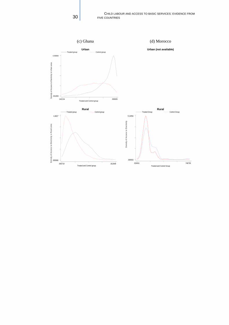
30 CHILD LABOUR AND ACCESS TO BASIC SERVICES: EVIDENCE FROM
FIVE COUNTRIES
(c) Ghana (d) Morocco
Urban
Urban (not available)
D
ensi
ty o
f Acc
ess
to E
lect
ricity
in U
rban
are
a
Treated and Control group
Treated group Control group
.042134 .999005
.001993
4.49494
Rural
Rural
Den
sity
of A
cces
s to
Ele
ctric
ity in
Rur
al a
rea
Treated and Control group
Treated group Control group
.000719 .812648
.000666
4.4817
Den
sity
of A
cces
s to
Ele
ctric
ity
Treated and Control Group
Treated Group Control Group
.024041 .746736
.000916
9.14054

31 UCW WORKING PAPER SERIES, JANUARY 2004
APPENDIX E: VARIABLE DEFINITIONS AND RESULTS FROM BIVARIATE PROBIT ESTIMATES
Definitions of the main variables implied in the regression analysis Child activities: Employment: 1 if individual currently works, 0 otherwise School Attendance: 1 if individual currently attends school, 0 otherwise Work only: 1 if individual currently works and do not attend school Study only: 1 if individual currently attends school and do not work Work and Study: 1 if individual currently works and attends school Neither: 1 if individual currently neither works nor attends school Access to basic services: Water 1 if household have access to public network, 0 otherwise Electricity 1 if household have access to public network, 0 otherwise Other variables: Female: 1 if female, 0 otherwise Household expenditures: logarithm of per capita household expenditure
Insurance: if at least one member of the household has a medical insurance, 0 otherwise
Credit: 1 if a household is credit rationed, 0 otherwise Father’s education: Fed_None: 1 if he has no completed education, 0 otherwise Fed_Primary: 1 if he has completed primary education, 0 otherwise Mother’s Education: Mother_None: 1 if she has no completed education, 0 otherwise Mother_ Primary: 1 if she has completed primary education, 0 otherwise (Secondary or higher education is the comparison group) Shocks:

32 CHILD LABOUR AND ACCESS TO BASIC SERVICES: EVIDENCE FROM
FIVE COUNTRIES
Collective 1 if a household reported experiencing at least a collective shock, 0 otherwise Individual 1 if a household reported experiencing at least a idiosyncratic shock, 0 otherwise
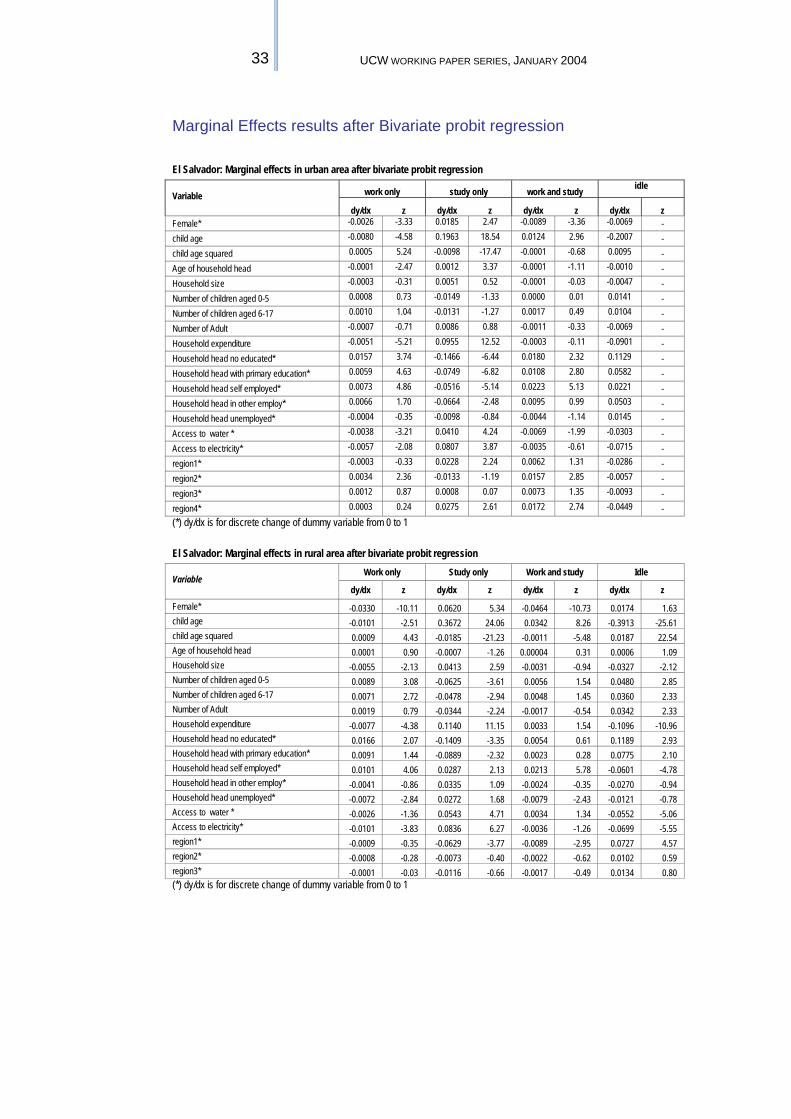
33 UCW WORKING PAPER SERIES, JANUARY 2004
Marginal Effects results after Bivariate probit regression El Salvador: Marginal effects in urban area after bivariate probit regression
Variable work only study only work and study idle
dy/dx z dy/dx z dy/dx z dy/dx z Female* -0.0026 -3.33 0.0185 2.47 -0.0089 -3.36 -0.0069 - child age -0.0080 -4.58 0.1963 18.54 0.0124 2.96 -0.2007 - child age squared 0.0005 5.24 -0.0098 -17.47 -0.0001 -0.68 0.0095 - Age of household head -0.0001 -2.47 0.0012 3.37 -0.0001 -1.11 -0.0010 - Household size -0.0003 -0.31 0.0051 0.52 -0.0001 -0.03 -0.0047 - Number of children aged 0-5 0.0008 0.73 -0.0149 -1.33 0.0000 0.01 0.0141 - Number of children aged 6-17 0.0010 1.04 -0.0131 -1.27 0.0017 0.49 0.0104 - Number of Adult -0.0007 -0.71 0.0086 0.88 -0.0011 -0.33 -0.0069 - Household expenditure -0.0051 -5.21 0.0955 12.52 -0.0003 -0.11 -0.0901 - Household head no educated* 0.0157 3.74 -0.1466 -6.44 0.0180 2.32 0.1129 - Household head with primary education* 0.0059 4.63 -0.0749 -6.82 0.0108 2.80 0.0582 - Household head self employed* 0.0073 4.86 -0.0516 -5.14 0.0223 5.13 0.0221 - Household head in other employ* 0.0066 1.70 -0.0664 -2.48 0.0095 0.99 0.0503 - Household head unemployed* -0.0004 -0.35 -0.0098 -0.84 -0.0044 -1.14 0.0145 - Access to water * -0.0038 -3.21 0.0410 4.24 -0.0069 -1.99 -0.0303 - Access to electricity* -0.0057 -2.08 0.0807 3.87 -0.0035 -0.61 -0.0715 - region1* -0.0003 -0.33 0.0228 2.24 0.0062 1.31 -0.0286 - region2* 0.0034 2.36 -0.0133 -1.19 0.0157 2.85 -0.0057 - region3* 0.0012 0.87 0.0008 0.07 0.0073 1.35 -0.0093 - region4* 0.0003 0.24 0.0275 2.61 0.0172 2.74 -0.0449 - (*) dy/dx is for discrete change of dummy variable from 0 to 1
El Salvador: Marginal effects in rural area after bivariate probit regression
Variable Work only Study only Work and study Idle
dy/dx z dy/dx z dy/dx z dy/dx z Female* -0.0330 -10.11 0.0620 5.34 -0.0464 -10.73 0.0174 1.63 child age -0.0101 -2.51 0.3672 24.06 0.0342 8.26 -0.3913 -25.61 child age squared 0.0009 4.43 -0.0185 -21.23 -0.0011 -5.48 0.0187 22.54 Age of household head 0.0001 0.90 -0.0007 -1.26 0.00004 0.31 0.0006 1.09 Household size -0.0055 -2.13 0.0413 2.59 -0.0031 -0.94 -0.0327 -2.12 Number of children aged 0-5 0.0089 3.08 -0.0625 -3.61 0.0056 1.54 0.0480 2.85 Number of children aged 6-17 0.0071 2.72 -0.0478 -2.94 0.0048 1.45 0.0360 2.33 Number of Adult 0.0019 0.79 -0.0344 -2.24 -0.0017 -0.54 0.0342 2.33 Household expenditure -0.0077 -4.38 0.1140 11.15 0.0033 1.54 -0.1096 -10.96 Household head no educated* 0.0166 2.07 -0.1409 -3.35 0.0054 0.61 0.1189 2.93 Household head with primary education* 0.0091 1.44 -0.0889 -2.32 0.0023 0.28 0.0775 2.10 Household head self employed* 0.0101 4.06 0.0287 2.13 0.0213 5.78 -0.0601 -4.78 Household head in other employ* -0.0041 -0.86 0.0335 1.09 -0.0024 -0.35 -0.0270 -0.94 Household head unemployed* -0.0072 -2.84 0.0272 1.68 -0.0079 -2.43 -0.0121 -0.78 Access to water * -0.0026 -1.36 0.0543 4.71 0.0034 1.34 -0.0552 -5.06 Access to electricity* -0.0101 -3.83 0.0836 6.27 -0.0036 -1.26 -0.0699 -5.55 region1* -0.0009 -0.35 -0.0629 -3.77 -0.0089 -2.95 0.0727 4.57 region2* -0.0008 -0.28 -0.0073 -0.40 -0.0022 -0.62 0.0102 0.59 region3* -0.0001 -0.03 -0.0116 -0.66 -0.0017 -0.49 0.0134 0.80 (*) dy/dx is for discrete change of dummy variable from 0 to 1

34 CHILD LABOUR AND ACCESS TO BASIC SERVICES: EVIDENCE FROM
FIVE COUNTRIES
Morocco: Marginal effects in rural area after bivariate probit regression Work only Study only Work and study No activities
Variable dy/dx z dy/dx z dy/dx z dy/dx z
female* 0.007 0.40 -0.275 -12.71 -0.027 -5.75 0.296 15.66
Hh size -0.022 -3.83 0.022 2.99 -0.001 -1.40 0.001 0.10
child age 0.069 2.01 0.170 3.88 0.022 4.15 -0.261 -6.53
child age squared -0.001 -0.41 -0.011 -5.46 -0.001 -4.10 0.013 6.89
household expenditures -0.080 -2.88 0.102 2.68 -0.001 -0.48 -0.020 -0.62
number of children aged 0-6 0.026 3.35 -0.031 -3.05 0.001 0.81 0.004 0.46
number of children aged 7-15 0.013 1.80 -0.008 -0.79 0.001 1.27 -0.006 -0.75
size of land holding 0.001 0.69 -0.002 -0.86 0.000 -0.21 0.001 0.49
presence of primary school* -0.068 -3.53 0.150 6.12 0.004 2.14 -0.087 -4.00
average travel time to school 0.002 2.19 -0.001 -1.26 0.000 1.26 0.000 -0.58
presence of public water network* -0.192 -5.78 0.134 1.52 -0.007 -3.70 0.065 0.74
presence of electricity* -0.103 -4.50 0.190 5.40 0.001 0.36 -0.088 -3.02
fathers' education -0.054 -5.22 0.071 5.43 -0.001 -0.71 -0.016 -1.34
mothers' education -0.074 -2.49 0.104 3.05 0.000 -0.14 -0.030 -0.90 * dy/dx is for a discreet change of dummy variable from 0 to 1 Source: UCW calculations based on Morocco LSMS 1998-99 Ghana: Marginal effects in urban area after bivariate probit regression
Work only Study only Work and study No activities
Variable dy/dx z dy/dx z dy/dx z dy/dx z
female* 0.0054 1.06 -0.0436 -1.94 0.0001 0.02 0.0381 1.79
Hh size 0.0050 2.85 -0.0354 -4.59 0.0008 0.47 0.0296 4.04
number of children aged 0-6 0.0071 2.19 -0.0318 -2.19 0.0041 1.23 0.0206 1.50
Number of adult 0.0014 0.51 0.0043 0.35 0.0025 0.88 -0.0082 -0.69
child age 0.0096 0.74 0.2438 4.53 0.0514 3.73 -0.3049 -5.94
child age squared -0.0004 -0.59 -0.0085 -3.35 -0.0018 -2.88 0.0106 4.41
Ln of Household expenditure -0.0115 -2.17 0.1022 4.64 0.0014 0.26 -0.0922 -4.42
Fathers’ education -0.0007 -0.31 0.0183 1.91 0.0021 0.95 -0.0197 -2.17
Mothers’ education -0.0010 -0.43 0.0393 3.74 0.0049 1.90 -0.0431 -4.33
Father not live* 0.0063 0.83 -0.0205 -0.62 0.0049 0.62 0.0094 0.30
Mother not live* 0.0129 1.71 -0.0825 -2.81 0.0025 0.36 0.0670 2.40
Access to water* -0.0161 -2.13 0.0190 0.68 -0.0186 -2.25 0.0157 0.61
Access to electricity* -0.0409 -3.96 0.1454 4.93 -0.0212 -2.44 -0.0833 -2.98 (*) dy/dx is for discrete change of dummy variable from 0 to 1

35 UCW WORKING PAPER SERIES, JANUARY 2004
Ghana: Marginal effects in rural area after bivariate probit regression
Variable Work only Study only Work and study Nothing
dy/dx z dy/dx z dy/dx z dy/dx z
female* -0.001 -0.16 -0.007 -0.46 -0.004 -0.71 0.012 0.78
Hh size 0.003 1.12 -0.008 -1.66 -0.001 -0.32 0.006 1.12
number of children aged 0-6 0.003 0.52 -0.016 -1.84 -0.004 -1.30 0.017 1.96
Number of adult 0.010 2.08 -0.043 -5.07 -0.008 -2.75 0.041 4.78
child age 0.014 0.65 0.142 3.89 0.061 4.98 -0.217 -5.83
child age squared 0.000 -0.21 -0.004 -2.34 -0.002 -2.79 0.006 3.33
Ln of Household expenditure -0.047 -5.90 0.107 7.60 0.002 0.47 -0.062 -4.38
Fathers’ education -0.013 -3.15 0.037 5.19 0.003 1.38 -0.027 -3.79
Mothers’ education -0.027 -5.15 0.063 7.13 0.002 0.54 -0.038 -4.16
Father not live* -0.046 -4.11 0.053 2.56 -0.017 -2.57 0.009 0.45
Mother not live* 0.016 1.39 -0.052 -2.70 -0.006 -1.00 0.042 2.10
Access to water* -0.077 -7.47 0.074 3.02 -0.035 -5.98 0.039 1.59
Access to electricity* 0.025 1.66 0.017 0.74 0.029 2.94 -0.071 -3.04 (*) dy/dx is for discrete change of dummy variable from 0 to 1

36 CHILD LABOUR AND ACCESS TO BASIC SERVICES: EVIDENCE FROM
FIVE COUNTRIES
Guatemala: Marginal effects in urban area after bivariate probit regression
Variable work only study only work and study Idle
dy/dx z dy/dx z dy/dx z dy/dx z Female* -0.0061 -1.36 0.0241 1.24 -0.0247 -2.10 0.0068 0.49
child age -0.0287 -3.48 0.1414 4.35 0.0641 2.98 -0.1768 -7.83
child age squared 0.0018 4.42 -0.0083 -5.37 -0.0017 -1.70 0.0082 7.72
Indigenous* 0.0145 2.82 -0.0587 -3.00 0.0368 2.82 0.0074 0.59
ln of household income -0.0115 -1.64 0.0533 1.76 0.0027 0.15 -0.0445 -2.07
Hh size -0.0041 -1.84 0.0178 1.86 -0.0058 -0.97 -0.0080 -1.20
number of children aged 0-6 0.0025 0.99 -0.0097 -0.88 0.0118 1.76 -0.0046 -0.60
number of children aged 7-14 0.0035 1.79 -0.0157 -1.88 0.0017 0.33 0.0105 1.84
Interaction Female-children 0-6 0.0003 0.11 -0.0034 -0.29 -0.0134 -1.80 0.0165 2.09
Father no educated* 0.0273 3.18 -0.1228 -4.13 -0.0041 -0.29 0.0997 4.13
Father with primary education* 0.0098 1.94 -0.0464 -2.16 -0.0065 -0.52 0.0431 2.72
Mother no educated none* 0.0284 3.42 -0.1137 -3.88 0.0348 1.94 0.0505 2.39
Mother with primary education* 0.0094 1.59 -0.0392 -1.60 0.0194 1.28 0.0104 0.59
Collective Shock* -0.0019 -0.37 0.0060 0.26 0.0364 2.23 -0.0405 -2.78
Individual shock* 0.0062 1.17 -0.0251 -1.16 0.0269 1.95 -0.0080 -0.55
Household Credit rationed* 0.0056 1.24 -0.0246 -1.29 0.0057 0.47 0.0133 1.02
Insurance* -0.0105 -2.85 0.0473 2.92 -0.0101 -1.00 -0.0268 -2.38
Inter. Credit rat.-individual shock* -0.0023 -0.35 0.0091 0.32 -0.0079 -0.47 0.0011 0.05
Inter. Credit rat.-collective shock* 0.0022 0.29 -0.0179 -0.52 -0.0174 -1.04 0.0331 1.20
Access to Water* -0.0036 -0.67 0.0163 0.73 -0.0014 -0.10 -0.0112 -0.73
Access to Electricity* -0.0236 -2.59 0.1437 4.75 0.0284 2.50 -0.1486 -5.63
Norte* -0.0167 -3.45 0.0838 3.04 -0.0184 -0.93 -0.0486 -3.10
Nororiente* -0.0050 -0.84 0.0140 0.47 0.0346 1.43 -0.0436 -3.12
Suroriente* -0.0135 -2.71 0.0369 1.17 0.0492 1.76 -0.0725 -6.39
Central* -0.0084 -1.53 -0.0147 -0.44 0.0998 3.26 -0.0767 -7.32
surroccidente* -0.0123 -2.44 0.0412 1.46 0.0397 1.66 -0.0686 -5.61
Noroccidente* -0.0150 -2.93 0.0613 2.06 0.0209 0.84 -0.0672 -5.10
Peten* -0.0035 -0.53 -0.0145 -0.41 0.0747 2.41 -0.0566 -4.56
(*) dy/dx is for discrete change of dummy variable from 0 to 1

37 UCW WORKING PAPER SERIES, JANUARY 2004
Guatemala: Marginal effects in rural area after bivariate probit regression
Variable Work only Study only work and study Idle
dy/dx z dy/dx z dy/dx z dy/dx z Female* -0.0496 -5.62 0.0729 3.17 -0.1339 -9.39 0.1106 6.28
child age -0.0787 -5.64 0.3003 9.39 0.1273 6.44 -0.3489 -13.88
child age squared 0.0051 7.47 -0.0171 -11.37 -0.0042 -4.59 0.0162 13.44
Indigenous* 0.0444 6.38 -0.0964 -5.70 0.0579 5.76 -0.0060 -0.45
ln of household income -0.0413 -2.77 0.1043 2.78 -0.0289 -1.32 -0.0341 -1.16
Hh size -0.0183 -4.11 0.0438 3.98 -0.0168 -2.58 -0.0087 -1.01
number of children aged 0-6 0.0128 2.96 -0.0267 -2.44 0.0189 2.99 -0.0050 -0.57
number of children aged 7-14 0.0077 2.19 -0.0167 -1.90 0.0101 1.94 -0.0010 -0.15
Interaction Female-children 0-6 -0.0027 -0.67 0.0056 0.55 -0.0041 -0.69 0.0012 0.15
Father no educated* 0.0699 4.21 -0.1841 -4.91 0.0182 0.83 0.0961 3.12
Father with primary education* 0.0429 2.89 -0.1103 -2.99 0.0247 1.15 0.0428 1.43
Mother no educated none* 0.0542 2.94 -0.1721 -3.41 -0.0198 -0.62 0.1377 3.52
Mother with primary education* 0.0492 2.06 -0.1337 -2.47 0.0027 0.09 0.0818 1.77
Collective Shock* 0.0316 3.36 -0.0651 -2.90 0.0473 3.50 -0.0139 -0.79
Individual shock* 0.0335 3.73 -0.0747 -3.41 0.0380 2.95 0.0032 0.18
Household Credit rationed* 0.0205 2.69 -0.0708 -3.63 -0.0207 -1.76 0.0710 4.70
Insurance* -0.0251 -3.63 0.0217 1.08 -0.0634 -6.78 0.0668 3.80
Inter. Credit rat.-individual shock* -0.0169 -1.61 0.0403 1.40 -0.0186 -1.16 -0.0048 -0.21
Inter. Credit rat.-collective shock* -0.0411 -4.70 0.1168 4.18 -0.0299 -1.93 -0.0458 -2.08
Access to Water* -0.0115 -1.99 0.0350 2.43 0.0027 0.32 -0.0262 -2.29
Access to Electricity* -0.0193 -3.06 0.0748 4.82 0.0311 3.42 -0.0865 -7.02
Norte* -0.0209 -1.18 0.0703 1.36 0.0355 0.93 -0.0849 -2.54
Nororiente* -0.0331 -2.18 0.1072 2.15 0.0008 0.02 -0.0748 -2.21
Suroriente* -0.0383 -2.68 0.1237 2.55 0.0339 0.91 -0.1193 -4.24
Central* -0.0135 -0.78 0.0499 1.01 0.0782 2.05 -0.1146 -3.88
surroccidente* -0.0531 -4.05 0.1732 4.09 0.0289 0.86 -0.1490 -5.58
Noroccidente* -0.0394 -2.39 0.1209 2.49 -0.0065 -0.21 -0.0750 -2.10
Peten* -0.0444 -3.43 0.1449 3.16 0.0236 0.65 -0.1241 -4.61
(*) dy/dx is for discrete change of dummy variable from 0 to 1
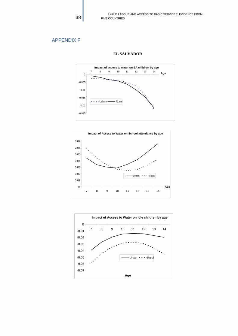
38 CHILD LABOUR AND ACCESS TO BASIC SERVICES: EVIDENCE FROM
FIVE COUNTRIES
APPENDIX F
EL SALVADOR
Impact of access to water on EA children by age
-0.025
-0.02
-0.015
-0.01
-0.005
07 8 9 10 11 12 13 14 Age
Urban Rural
Impact of Access to Water on School attendance by age
0 0.01
0.02
0.03
0.04
0.05
0.06
0.07
7 8 9 10 11 12 13 14Age
Urban Rural
Impact of Access to Water on Idle children by age
-0.07
-0.06
-0.05
-0.04
-0.03
-0.02
-0.01
07 8 9 10 11 12 13 14
Age
Urban Rural

39 UCW WORKING PAPER SERIES, JANUARY 2004
Impact of Access to Electricity on EA children by age
-0.06
-0.05
-0.04
-0.03
-0.02
-0.01
07 8 9 10 11 12 13 14
Age
Urban Rural
Impact of Access to Electricity on School attendance by age
0
0.01
0.02
0.03
0.04
0.05
0.06
0.07
0.08
0.09
0.1
7 8 9 10 11 12 13 14Age
Urban Rural
Impact of Access to Electricity on Idle children by age
-0.1
-0.09
-0.08
-0.07
-0.06
-0.05
-0.04
-0.03
-0.02
-0.01
07 8 9 10 11 12 13 14
Age
Urban Rural

40 CHILD LABOUR AND ACCESS TO BASIC SERVICES: EVIDENCE FROM
FIVE COUNTRIES
GUATEMALA
Impact of Access to Water on EA children by age
-0.03
-0.025
-0.02
-0.015
-0.01
-0.005
07 8 9 10 11 12 13 14
Age
Urban Rural
Impact of Access to Water on School attendance by age
0
0.005
0.01
0.015
0.02
0.025
0.03
0.035
0.04
7 8 9 10 11 12 13 14Age
Urban Rural
Impact of Access to Water on Idle children by age
-0.04
-0.035
-0.03
-0.025
-0.02
-0.015
-0.01
-0.005
07 8 9 10 11 12 13 14
Age
Urban Rural

41 UCW WORKING PAPER SERIES, JANUARY 2004
Impact of Access to Electricity on EA children by age
-0.08
-0.07
-0.06
-0.05
-0.04
-0.03
-0.02
-0.01
07 8 9 10 11 12 13 14
Age
Urban Rural
Impact of Access to Electricity on School attendance by age
00.020.040.060.080.1
0.120.140.160.180.2
7 8 9 10 11 12 13 14Age
Urban Rural
Impact of Access to Electricity on Idle children by age
-0.2-0.18-0.16-0.14-0.12-0.1
-0.08-0.06-0.04-0.02
07 8 9 10 11 12 13 14
Age
Urban Rural

42 CHILD LABOUR AND ACCESS TO BASIC SERVICES: EVIDENCE FROM
FIVE COUNTRIES
GHANA
Impact of Access to Water on EA by age
-0.090-0.080-0.070-0.060-0.050-0.040-0.030-0.020-0.0100.000
7 8 9 10 11 12 13 14Age
Urban Rural
Impact of Access to Water on School attendance by age
0.000
0.020
0.040
0.060
0.080
0.100
0.120
0.140
7 8 9 10 11 12 13 14Age
Urban Rural
Impact of Access to Electricity on Idle children by age
0.0000.0050.010
0.0150.0200.0250.030
0.0350.0400.045
7 8 9 10 11 12 13 14Age
UrbanRural

43 UCW WORKING PAPER SERIES, JANUARY 2004
Impact of Access to Electricity on EA children by age
-0.05
-0.04
-0.03
-0.02
-0.01
0
0.01
0.02
0.03
0.04
7 8 9 10 11 12 13 14Age
Urban Rural
Impact of Access to Electricity on School attendance by age
-0.04
-0.02
0
0.02
0.04
0.06
0.08
0.1
0.12
0.14
0.16
7 8 9 10 11 12 13 14Age
Urban Rural
Impact of Access to Electricity on Idle children by age
-0.1
-0.09
-0.08
-0.07
-0.06
-0.05
-0.04
-0.03
-0.02
-0.01
07 8 9 10 11 12 13 14
Age
Urban Rural

44 CHILD LABOUR AND ACCESS TO BASIC SERVICES: EVIDENCE FROM
FIVE COUNTRIES
YEMEN
Impact of Access to Electricity on EA children by age
-0.035
-0.03
-0.025
-0.02
-0.015
-0.01
-0.005
07 8 9 10 11 12 13 14
Age
UrbanRural
Impact of Access to Electricity on School attendance by age
0
0.05
0.1
0.15
0.2
7 8 9 10 11 12 13 14Age
UrbanRural
Impact of Access to Electricity on Idle children by age
-0.16
-0.14
-0.12
-0.1
-0.08
-0.06
-0.04
-0.02
07 8 9 10 11 12 13 14 Age
UrbanRural

45 UCW WORKING PAPER SERIES, JANUARY 2004
Impact of Access to Water on EA Children by age
-0.01
-0.008
-0.006
-0.004
-0.002
0
0.002
0.004
7 8 9 10 11 12 13 14Age
Urban Rural
Impact of Access to Water on School attendance by age
0
0.01
0.02
0.03
0.04
0.05
0.06
7 8 9 10 11 12 13 14
Age
UrbanRural
Impact of Access to Water on Idle children by age
-0.06
-0.05
-0.04
-0.03
-0.02
-0.01
07 8 9 10 11 12 13 14
AgeUrbanRural

46 CHILD LABOUR AND ACCESS TO BASIC SERVICES: EVIDENCE FROM
FIVE COUNTRIES
APPENDIX G: AVERAGE TREATMENT EFFECTS FOR “ACCESS TO WATER AND ACCESS TO ELECTRICITY” FOR DIFFERENT VALUES OF THE SENSITIVITY PARAMETERS Sensitivity analysis on the effect of access to water in Urban area ATT ���� �0W��1W�� ����� , ������ �0W��1W����� ����� , ������ �0W��1W����� ����� , ������ �0W��1W����� ����� , ������ �0W��1W�����
�0S��1S�� �0S��1S���� �0S��1S���� �0S��1S���� �0S��1S����
�0WS��1WS�� �0WS��1WS���� �0WS��1WS���� �0WS��1WS���� �0WS��1WS����
Working only -0.018 -0.018 -0.018 -0.018 -0.016
Studying only 0.107 0.107 0.106 0.103 0.097 Working and Studying -0.012 -0.012 -0.012 -0.012 -0.012
Idle Children -0.077 -0.077 -0.076 -0.073 -0.069
Sources: UCW calculations based on El Salvador: Enquesta de Hogares de Propositos Multiples (EHPM) 2001
Sensitivity analysis on the effect of access to water in Rural area ATT ���� �0W��1W�� ����� , ������ �0W��1W����� ����� , ������ �0W��1W����� ����� , ������ �0W��1W����� ����� , ������ �0W��1W�����
�0S��1S�� �0S��1S���� �0S��1S���� �0S��1S���� �0S��1S����
�0WS��1WS�� �0WS��1WS���� �0WS��1WS���� �0WS��1WS���� �0WS��1WS����
Working only -0.013 -0.013 -0.012 -0.013 -0.010
Studying only 0.074 0.071 0.072 0.071 0.063
Working and Studying 0.007 0.007 0.007 0.007 0.006
Idle Children -0.068 -0.065 -0.066 -0.065 -0.060
Sources: UCW calculations based on El Salvador: Enquesta de Hogares de Propositos Multiples (EHPM) 2001
Sensitivity analysis on the effect of access to electricity in Urban area ATT ���� �0W��1W�� ����� , ������ �0W��1W����� ����� , ������ �0W��1W����� ����� , ������ �0W��1W����� ����� , ������ �0W��1W�����
�0S��1S�� �0S��1S���� �0S��1S���� �0S��1S���� �0S��1S����
�0WS��1WS�� �0WS��1WS���� �0WS��1WS���� �0WS��1WS���� �0WS��1WS����
Working only -0.027 -0.027 -0.027 -0.026 -0.024
Studying only 0.220 0.220 0.218 0.205 0.206 Working and Studying -0.013 -0.013 -0.013 -0.013 -0.019
Idle Children -0.180 -0.180 -0.178 -0.166 -0.164
Sources: UCW calculations based on El Salvador: Enquesta de Hogares de Propositos Multiples (EHPM) 2001
Sensitivity analysis on the effect of access to electricity in Rural area ATT ���� �0W��1W�� ����� , ������ �0W��1W����� ����� , ������ �0W��1W����� ����� , ������ �0W��1W����� ����� , ������ �0W��1W�����
�0S��1S�� �0S��1S���� �0S��1S���� �0S��1S���� �0S��1S����
�0WS��1WS�� �0WS��1WS���� �0WS��1WS���� �0WS��1WS���� �0WS��1WS����
Working only -0.029 -0.029 -0.028 -0.029 -0.025
Studying only 0.141 0.140 0.138 0.140 0.129 Working and Studying -0.003 -0.003 -0.003 -0.003 -0.004
Idle Children -0.109 -0.108 -0.107 -0.108 -0.100
Sources: UCW calculations based on El Salvador: Enquesta de Hogares de Propositos Multiples (EHPM) 2001
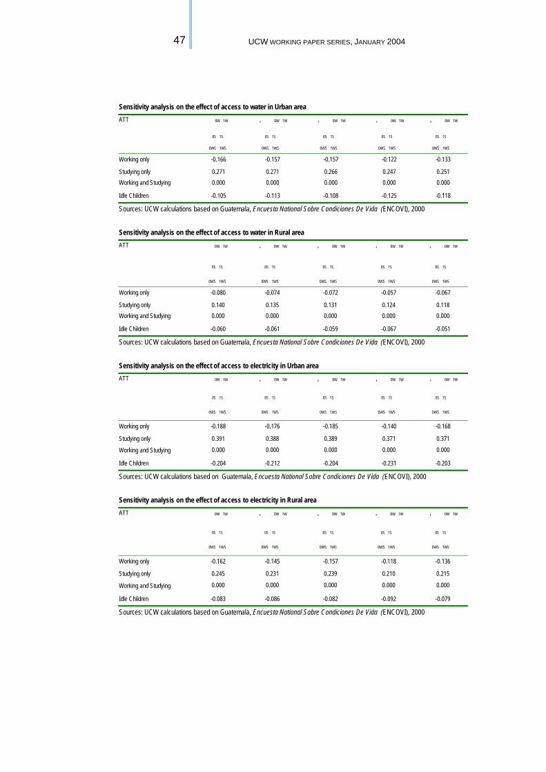
47 UCW WORKING PAPER SERIES, JANUARY 2004
Sensitivity analysis on the effect of access to water in Urban area ATT ���� �0W��1W�� ����� , ������ �0W��1W����� ����� , ������ �0W��1W����� ����� , ������ �0W��1W����� ����� , ������ �0W��1W�����
�0S��1S�� �0S��1S���� �0S��1S���� �0S��1S���� �0S��1S����
�0WS��1WS�� �0WS��1WS���� �0WS��1WS���� �0WS��1WS���� �0WS��1WS����
Working only -0.166 -0.157 -0.157 -0.122 -0.133
Studying only 0.271 0.271 0.266 0.247 0.251 Working and Studying 0.000 0.000 0.000 0.000 0.000
Idle Children -0.105 -0.113 -0.108 -0.125 -0.118
Sources: UCW calculations based on Guatemala, Encuesta National Sobre Condiciones De Vida (ENCOVI), 2000
Sensitivity analysis on the effect of access to water in Rural area ATT ���� �0W��1W�� ����� , ������ �0W��1W����� ����� , ������ �0W��1W����� ����� , ������ �0W��1W����� ����� , ������ �0W��1W�����
�0S��1S�� �0S��1S���� �0S��1S���� �0S��1S���� �0S��1S����
�0WS��1WS�� �0WS��1WS���� �0WS��1WS���� �0WS��1WS���� �0WS��1WS����
Working only -0.080 -0.074 -0.072 -0.057 -0.067
Studying only 0.140 0.135 0.131 0.124 0.118 Working and Studying 0.000 0.000 0.000 0.000 0.000
Idle Children -0.060 -0.061 -0.059 -0.067 -0.051
Sources: UCW calculations based on Guatemala, Encuesta National Sobre Condiciones De Vida (ENCOVI), 2000
Sensitivity analysis on the effect of access to electricity in Urban area ATT ���� �0W��1W�� ����� , ������ �0W��1W����� ����� , ������ �0W��1W����� ����� , ������ �0W��1W����� ����� , ������ �0W��1W�����
�0S��1S�� �0S��1S���� �0S��1S���� �0S��1S���� �0S��1S����
�0WS��1WS�� �0WS��1WS���� �0WS��1WS���� �0WS��1WS���� �0WS��1WS����
Working only -0.188 -0.176 -0.185 -0.140 -0.168
Studying only 0.391 0.388 0.389 0.371 0.371
Working and Studying 0.000 0.000 0.000 0.000 0.000
Idle Children -0.204 -0.212 -0.204 -0.231 -0.203
Sources: UCW calculations based on Guatemala, Encuesta National Sobre Condiciones De Vida (ENCOVI), 2000
Sensitivity analysis on the effect of access to electricity in Rural area ATT ���� �0W��1W�� ����� , ������ �0W��1W����� ����� , ������ �0W��1W����� ����� , ������ �0W��1W����� ����� , ������ �0W��1W�����
�0S��1S�� �0S��1S���� �0S��1S���� �0S��1S���� �0S��1S����
�0WS��1WS�� �0WS��1WS���� �0WS��1WS���� �0WS��1WS���� �0WS��1WS����
Working only -0.162 -0.145 -0.157 -0.118 -0.136
Studying only 0.245 0.231 0.239 0.210 0.215
Working and Studying 0.000 0.000 0.000 0.000 0.000
Idle Children -0.083 -0.086 -0.082 -0.092 -0.079
Sources: UCW calculations based on Guatemala, Encuesta National Sobre Condiciones De Vida (ENCOVI), 2000
Copyright © 2022 FDOKUMEN