PREPRINT VERSION - The original version of the manuscript can be found at http://pubs.rsc.org/

1

Chemical imaging of articular cartilage sections with Raman mapping,

employing uni- and multi-variate methods for data analysis

Alois Bonifacio,* a Claudia Beleites,

a Franco Vittur,

b Eleonora Marsich,

b Sabrina Semeraro,

b Sergio

Paolettib and Valter Sergo

a

5

Raman mapping in combination with uni- and multi-variate methods of data analysis is applied to

articular cartilage samples. Main differences in biochemical composition and collagen fibers

orientation between superficial, middle and deep zone of the tissue are readily observed in the 10

samples. Collagen, non-collagenous proteins, proteoglycans and nucleic acids can be distinguished

on the basis of their different spectral characteristics, and their relative abundance can be mapped

in the label-free tissue samples, at a so high resolution to permit the analysis at the level of single

cells. Differences between territorial and inter-territorial matrix, as well as inhomogeneities in the

inter-territorial matrix, are properly identified. Multivariate methods of data analysis prove to be 15

complementary to the univariate approach. In particular, our partial least squares regression model

gives a semiquantitative mapping of the biochemical costituents in agreement with average

composition found in literature. The combination of hierarchical and fuzzy cluster analysis

succeeds in detecting variations between different regions of the extra-cellular matrix. Because of

its characteristics as an imaging technique, Raman mapping could be a promising tool for studying 20

biochemical changes in cartilage occuring during aging or osteoarthritis.

Introduction

Hyaline cartilage is a highly specialized connective tissue

with remarkable biomechanical properties, which occurs at the 25

articulating surfaces of bones (articular cartilage) and within

the major airways1, 2. The function of articular cartilage is to

reduce friction between bones in joint articulation, and to

distribute loads across the joint surface. Cartilage tissue is

avascular and aneural, and consists of a relatively small 30

portion of a single type of cells (i.e. chondrocytes) embedded

in a large amount of extracellular matrix (ECM). The main

constituents of the ECM are collagen (50-60% of dry weight)

and proteoglycans (15-30% of dry weight)3. Most of the

collagen (90-95%) in the ECM is of type II, which forms a 35

network of fibres binding the proteoglycans and providing the

tissue with important mechanical properties such as toughness

and viscoelasticity. Most of the proteoglycans in cartilage are

complex molecular aggregates consisting of a core protein to

which one or more glycosaminoglycan chains (such as 40

chondroitin sulfate and keratan sulfate) are covalently

attached. The glycosaminoglycans (GAGs) form hydrophilic

gels which bind large amounts of water, bestowing

compressive strength properties to the tissue. However,

chondrocytes and main ECM costituents are not evenly 45

distributed within the tissue: in fact articular cartilage is

distinguished into superficial, middle and deep zones1-3

(Fig.1, left), according to the different shape of cells,

biochemical composition of the ECM and orientation of

collagen fibres. 50

Destruction of the ECM has been shown to be the initial

event during cartilage degradation in osteoarthritis,

rheumatoid arthritis as well as in other diseases4. Therefore,

considerable effort has been invested in studying cartilage.

Imaging techniques are valuable tools for investigating 55

tissues, and in particular magnetic resonance imaging (MRI)

is widely used for functional imaging of cartilage5. Besides

the efforts to improve the MRI performance, there is an

increasing interest in developing different imaging techniques

that can detect the biochemical changes in cartilage matrix to 60

diagnose, grade or investigate the molecular processes of

degerative joint diseases.

Vibrational spectroscopy has been successfully applied to

characterize tissues, and in particular Fourier-transform

infrared (FT-IR) imaging has been employed to study 65

cartilage specimens6, 7. This technique proved to be efficient

in imaging the distribution of collagen and proteglycans in

healthy and diseased cartilage. In spite of the considerable

work done by several groups on FT-IR imaging of cartilage,

the vibrational spectroscopy complementary to FT-IR, i.e. 70

Raman spectroscopy, has been only recently employed, in the

variant of Coherent Anti-Stokes Raman (CARS) for articular

cartilage imaging applications8. Raman spectroscopy is based

on the inelastic scattering of photons from a laser source by

the molecules constituting the sample9. It usually requires no 75

or little sample manipulation and below 2000 cm-1 water

yields a weak Raman signal: for these reasons Raman

spectroscopy is particularly apt for studying native tissues.

Moreover, Raman spectra can be recorded through fiber optic

probes10, suitable for in-vivo diagnostics. The coupling of a 80

2

Raman spectrometer with an optical microscope (usually

termed Raman microspectroscope) allows the analysis of

samples with a spatial resolution better than infrared

spectroscopy11. By using a motorized microscope stage, a

Raman spectrum can be collected from each point of an 5

arbitrary grid, obtaining a so-called Raman map of the

sample; the hyperspectral data set obtained can be processed

to yield images which show the distribution of the chemical

species present in the tissue. Raman micro-spectroscopic

studies have been reported for rabbit nasal12 and auricolar 10

cartilage13, for human bronchial tissue14 and for murine knee

joints15. To the best of our knowledge Raman mapping has not

yet been applied to articular cartilage and, hence, the aim of

this paper is to evaluate how Raman mapping can be applied

to charaterize articular cartilage, and what kind of information 15

can be retrieved from Raman maps of this tissue by uni- and

multivariate methods of data analysis. Univariate data analysis

is widely employed to process Raman maps, producing

images based on the absolute or integrated intensity at a

certain Raman shift. In this study, maps of areas from deep, 20

middle and superficial zones of articular cartilage (Fig.1,

right) have been collected, to evaluate the capability of the

univariate approach to distinguish the characteristic features

of each zone. However, univariate analysis considers only one

variable at a time. Conversely, multivariate methods, whose 25

are being increasingly applied to the analysis of Raman maps,

make use of larger parts of the spectra (or even the complete

spectrum) to produce an image, simultaneously taking into

account more variables. In this study, four different

multivariate techniques are used for the analysis of 30

hyperspectral data: principal component analysis (PCA)16,

partial least squares regression (PLSR)17, and two types of

cluster analysis18, hierarchical cluster analysis (HCA) and

fuzzy c-means cluster analysis (FCA).

Experimental 35

Chemicals and materials

CCl4, formalin, DNA, collagen (type II), concanavalin and

albumin were purchased from Sigma-Aldrich Italy (Milan,

Italy). Chondroitin sulfate sodium salt was purchased from

Wako Chemicals (Osaka, Japan). All chemicals employed 40

were used as provided by the suppliers, without further

purification. CaF2 microscope slides were purchased from

Crystal GmbH (Berlin, Germany).

Sample preparation

The humeral-scapular joint of a mature pig was collected at a 45

slaughterhouse and transferred in ice to the laboratory.

Articular cartilage was aseptically excised from the humeral

proximal head within 2 h from the sacrifice, and fixed in 4%

buffered formalin for 30 min. Formalin fixation is

recommended by the Histology Endpoint Committee of the 50

International Cartilage Repair Society (ICRS)19, and it does

not cause significant alterations in the Raman spectra of

tissues11, 20. Tissue slices approximately 100 m thick were

cut perpendicularly to the articular surface, rinsed with

distilled water and immediately mounted onto a CaF2 slide 55

while still wet. The samples were dried overnight in air at

room temperature, and then put under the Raman microscope

(without any cover slip) for data collection.

This study does not address the issue of inter-animal

variation of tissue composition or morphology, its scope being 60

that of evaluating the feasibility of Raman mapping on a

sample of articular cartilage. Therefore, large maps were

taken from different regions of only one sample.

Raman spectroscopy and mapping

Raman spectra and maps were collected in back scattering 65

geometry, with an InVia Raman microscope (Renishaw plc,

Wotton-under-Edge, UK) equipped with a 632.8 nm HeNe

laser (Melles-Griot, Voisins Le Bretonneaux, France)

delivering 15 mW of laser power at the sample. The laser was

polarized along the x-axis direction. The CaF2 slide 70

supporting the tissue samples was mounted on a ProScan II

motorized stage (Prior, Cambridge, UK) under the

microscope. A Leica 100x microscope objective (N.A. 0.95)

focused the laser on the sample into a spot of ~0.4 m

diamater. A 1800 l/mm grating yielded a spectral resolution of 75

4 cm-1. A thermoelectrically cooled charge coupled device

(CCD) camera was used for detection. The spectrograph

was calibrated using the lines of a Ne lamp. Instrumental

polarization effects were ruled out acquiring a spectrum of

CCl4 and comparing the recorded depolarization ratio with the 80

values derived from literature. Single spectra were collected

with an exposure time of 90 s. Mapping was achieved

Fig. 1 (left) Bright field micrograph of a section of articular cartilage, in

which the deep, middle and superficial zones are schematically shown;

(right) bright field micrographs of the areas of the deep, middle and

superficial zones which have been mapped with Raman

microspectroscopy

3

collecting spectra with steps of 1 m, with an exposure time

of 10 s for each spectrum. Spectra, consiting of 1272 data

points each, were obtained in the 600–1800 cm-1 region using

the synchro mode of the instrument software WiRETM 3.0

(Renishaw). In the synchro mode, the grating is continuously 5

moved to obtain Raman spectra of extended spectral regions.

The dimensions of the map depended on cartilage zone

investigated: 83×101 m, 83×40 m and 83×14 m for the

deep, transitional and superficial zones, respectively.

Data preprocessing and analysis 10

All data preprocessing and analysis was performed within the

R software environment for statistical computing and

graphics21. In particular, data import and export,

preprocessing and visualization were performed with the

hyperSpec package22 for R. 15

The preprocessing consisted of four steps: i) cosmic rays

identification and removal, ii) baseline correction, iii)

intensity vector-normalization and iv) outliers detection and

removal. For the baseline correction, a linear baseline was fit

automatically to the whole spectral range and was subtracted 20

from each spectrum of the dataset. Outliers detection was

done by identifying suspicious points on the PCA score maps

(see below) and inspecting the corresponding spectra. In the

Table 1 Raman shifts (cm-1) and assignments of the bands observed in the

average Raman spectra of cartilage. 25

Raman shifts Assignment

1670 collagen, amide I

1606 ν C=C aromatic ring (Phe, Tyr)

1586 ν C=C aromatic ring (Phe, Trp)

1557 ν C=C aromatic ring (Trp, Tyr)

1450 collagen - other proteins, C-H (CH2/CH3)

1424 glycosaminoglycans, s COO-

1380 glycosamin glycans, unassigned

1342 glycosaminoglycans, C-H (CH2)

1319 -

1269 collagen, amide III

1245 collagen, amide III

1208 Hyp, Tyr

1163 C-H (Tyr)

1127 proteins, C-N, C-C

1098 -

1068 glycosaminoglycans, s OSO3-

1033 Phe ring deformation

10 3 Phe ring deformation

940 collagen, ν C-C (protein backbone Pro)

920 collagen, ν C-C (Pro, Hyp)

876 collagen, ν C-C (Pro, Hyp)

857 collagen, ν C-C (Pro)

816 collagen – other proteins, ν C-C protein backbone

760 Trp ring deformation

725 -

644 yr ring deformation

622 Phe ring deformation

preprocessing stage, PCA is thus used as a method to identify

suspicious spectra, exploiting its sensitivity to outliers23.

These suspects were then individually examined before 30

deleting them.

PCA

PCA reduces the number of variables by condensing all the

spectral information contained in a large number of spectra 35

into a few latent variables (the principal components or PCs).

Hyperspectral data are thus decomposed by PCA into so-

called latent spectra (or “loadings”) and “scores”. This

approach is closely related to describing each spectrum in a

Raman map as a product between components concentrations 40

and pure costituents spectra, where the latent spectra are used

instead of those of the pure costituents, which are unknown23.

In the present study, PCA was performed on preprocessed

data, and the first two principal components PC 1 and PC 2,

which could be easily interpreted in terms of the biochemical 45

components of the tissue, were considered for discussion. The

loadings and score maps for the other principal components

are of more difficult interpretation, and are available as

Supplementary Information. PCA calculations were done

using the R function prcomp. 50

PLSR

In PLSR, a reference data set consisting of spectra with

600 800 1000 1200 1400 1600 1800

Pro

/Hy

p

Ph

e

CH

2 d

ef

amid

e II

I

1414

1275

998

939

881

1068

876 9

20

816

857

940

1004

1031

1380

1342

1271

1246 1451

(c)

(b)

(a)

collagen

Inte

nsi

ty (

a.u.)

Raman shift (cm-1)

chondroitin sulfate

1669

amid

e I

Fig. 2 Average spectra of the Raman maps taken from the (a) deep, (b)

middle and (c) superficial zones. Intensities are normalized (see

Experimental section). Most bands in the average spectra can be assigned

either to collagen or to chondroitin sulfate, whose Raman spectra are shown

for comparison (bottom, as thin line).

4

known analyte concentrations is used to build a calibration

model for these analytes. PLSR decomposes the calibration

data into scores and latent spectra. Instead of looking for the

variance in the spectra (as PCA), the co-variance between the

constituent concentrations and the spectra is used. However, 5

the purpose of the model used in this study is not quantitative

“prediction” of constituents concentrations as usually is the

case for PLSR, but only fitting of the spectra collected from

the cartilage sample.

For PLSR analysis, Raman spectra were subjected to a 10

loess24 smoothing interpolation. This was necessary as day-to-

day drift of the spectrograph requires the re-calibration of the

grating position, which in turn results in slightly different

Raman shifts for the measured data points of the model

substances compared to the tissue spectra. This procedure 15

improves also the signal-to-noise ratio. The spectra were

interpolated onto an evenly spaced Raman shift axis from 604

to 1800 cm-1 with data points spacing 4 cm-1.

The PLSR model was built using a calibration data set

comprising 10 spectra of each of the following pure 20

substances, each spectrum measured from a different sample

of the same pure substance: chondroitin sulfate (CS), DNA,

concanavalin and albumin; 20 collagen spectra were collected

from fibers oriented parallel and perpendicular with respect to

the laser polarization direction, since collagen Raman spectra 25

depend upon orientation25. Concanavalin and albumin were

taken as model compounds for proteins rich in β-sheets and α-

helices, respectively. Altogether, this reference data set of 60

spectra model the following groups of substances: collagen

(10 spectra for each fiber orientation), non-collagenous 30

protein (concanavalin and albumin), nucleic acids (DNA) and

GAGs (CS). The spectra of the reference data set are shown in

the Supplementary Information.

Strictly, since the reference spectra were normalized, the

PLSR models the spectral contribution of each group of 35

substances to the spectrum rather than the absolute

concentrations. However, the reference substances show

roughly equal overall Raman intensities and, hence, we

assumed that spectral contributions translate approximately to

the relative constituent concentrations. This approximation 40

does not take into account several factors such as different

sample densities and different Raman scatter cross-sections,

and therefore the results must be taken with care, in view of

the limits of our simplified model.

A PLSR model with 6 latent spectra was used, as suggested 45

by a 50-times iterated 10-fold cross validation (the cross

validation plot is available in the Supplementary Information).

PLSR calculations were made using the R package pls26.

HCA and FCA 50

In cluster analysis, spectra are segmented into groups (or

clusters) according to their resemblance, so that all spectra

belonging to one cluster have similar characterstics. In “hard”

clustering methods such as HCA, a spectrum esclusively

belongs to one cluster, whereas “soft” methods such as FCA 55

allow one spectrum to belong to more than one cluster at the

same time.

HCA produces a tree-like structure of clusterings, the

dendrogram. Its interpretation is somewhat similar to that of a

phylogenetic tree: the further one has to ascend the tree to 60

find a connection between two spectra (or species) of interest,

the less similar they are. This study uses an agglomerative

clustering approach. Initially, each spectrum is considered its

own cluster. Then, the two most similar spectra or clusters are

merged into one cluster, and the (dis)similarity or “distance” 65

between them is recorded. This is repeated until finally all

spectra end up in one cluster. The dendrogram depicts the

level of (dis)similarity for each such merging step. Finally,

the dendrogram is cut a certain level of (dis)similarity or

distance correspoding to a particular number of clusters. In a 70

pseudo-colour image, each spectrum is then coloured

according to its cluster.

In contrast to hard clustering, FCA uses continuous cluster

membership values rather than assigning one cluster for each

spectrum, so that each spectrum can partially belong to more 75

than one cluster. In FCA, the number of clusters is pre-

specified. The cluster means (or centroids) are initialized

either by randomly picked spectra or by spectra given by the

user. For each spetrum, the membership for each cluster is

calculated. The membership values are a measure of similarity 80

between the spectrum and the cluster mean (usually the

inverse of the distance) and are normalized to add up to 1 for

each spectrum.

600 800 1000 1200 1400 1600 1800

dna

Raman shift (cm-1)

St.

Dev

. In

tensi

ty (

a.u.)

(c)

(b)

(a)

1241

728

1099

1421 1

488

782

713

16741

656

1636

1578

1440

1421

1378

1335

1304

1243

1209

1070

782

1677

1451

1087

1488

1636

1578

13781335

1127

1087

1304

816

857

830

940

1053

1004

920

1244

1209 1

440

1685

1244

1336

1335

1372

Fig. 3 Normalized intensity standard deviations of the Raman maps taken

from the (a) deep, (b) middle and (c) superficial zones, corresponding to

the spectra in Fig.2. The band at 1087 cm-1 which is out of scale in the

spectrum (b) is due to calcium carbonate microcrystals (see Results and

Discussion). The Raman spectrum of DNA is reported for comparison

(bottom, thin line).

5

The cluster centroids are then updated to the average spectrum

weighted by the membership values for each cluster. These

two steps, updating the memberships and updating the cluster 5

centroids, are iterated until the algorithm converges to a stable

clustering. Prior to cluster analysis, the 5 th percentile of all

intensities (i.e. the intensity threshold below which 5% of all

spectra may be found27) at each Raman shift was subtracted

from all spectra in the data set to emphasize differences 10

between spectra. For HCA, we used Pearson’s distance

between all the spectra of a map, and then Ward's method to

determine the distance between clusters. The dendrogram is

available as Supplementary Information. HCA calculations

were done using the R function hclust and the function 15

pearson.dist from the hyperSpec package. Centroids obtained

by HCA were used as initial cluster centroids in FCA, instead

of a random selection. The “degree of fuzziness” parameter in

FCA was set to 1.4, encouraging a relatively “hard” outcome

of the cluster analysis. FCA calculations were done using 20

function cmean in R package e107128.

Results and Discussion

Characteristics of average Raman spectra

Figure 2 shows the average spectra of the Raman maps

collected from the deep, middle and superficial zones of 25

cartilage, corresponding to the areas shown in Fig.1. All

spectra have in common bands due to collagen and

proteoglycans (in particular CS), whose Raman spectra are

reported for reference in the lower part of Figure 2. Several

bands are also due to aromatic amino acids (i.e. Phe, Tyr and 30

Trp), which are efficient Raman scatterers29. A list of the

bands observed in the average spectra, together with their

assignments to vibrational modes, is shown in Table 1. In

particular, the two amide III band at 1246 and 1271 cm-1, the

groups of bands between 800 and 1000 cm-1 and the amide I 35

band at 1669 cm-1 are charactersitic of collagen, whereas the

bands at 1068, 1342 and 1380 cm-1 are typical of CS. This is

not unexpected, since collagen and CS are the main

constituents of articular cartilage, and their bands have

already been reported in Raman spectra collected from 40

cartilage tissues12-15. Besides the common features,

differences between the three zones are observed. In

agreement with previous studies on cartilage biochemical

composition1-3, the proteoglycans/collagen ratio is higher in

the deep zone than in the superficial zone, as clearly indicated 45

in the average spectra by the relative intensities of CS and

collagen associated Raman bands (Fig.2). Moreover, the

1669/1451 cm-1, 1246/1261 cm-1 and 920/940 cm-1 intensity

ratios are slightly different for the three cartilage zones. These

differences, however, likely reflect a variation in the 50

orientation of collagen fibrils rather than a change in chemical

composition of the tissue. Orientation effects in Raman

spectra of anisotropic samples are well known, and

differences in the intensity ratio similar to those observed

55

Fig. 4 Univariate images of the deep, middle and superficial zones of the cartilage tissue, based on the corresponding normalized Raman maps. Each

image maps the sum of intensities at Raman shifts which are characteristic of each different biochemical constituent. Pixels are colored according to a

linear red-yellow-green-blue color scale in which the red and blue correspond to the maximum and minimum value of an intensity sum, respectively. The

intensity sum is calculated over the intensities at 1578, 1488 and 782 cm-1 for DNA, at 1380, 1342 and 1068 cm-1 for chondroitin sulfate, at 1271, 1246,

920, 857 and 816 cm-1 for collagen and at 1555, 1127 and 1004 cm-1 for non-collagenous proteins. The two small white areas in the middle zone

correspond to the calcium carbonate microcrystals

6

among the spectra in Fig. 2 have been recently reported for

collagen fibers upon changes in sample orientation25. Indeed,

in the deep zone collagen fibrils are known to be oriented

perpendicular to the articular surface, whereas in the middle 5

and superficial zone they are oriented randomly and parallel,

respectively, to the surface1-3. The effects of this anisotropy

on polarized light microscopy and FT-IR imaging are known,

and have been exploited to study collagen orientation in

cartilage tissue30, 31. Although the effects of collagen 10

orientation in Raman spectra of cartilage have never been

reported, similar phenomena have been reported for osteonal

tissues32.

Further information about the variation of biochemical

species present in the cartilage sample is given by the 15

standard deviations in Raman intensity of the different maps

(Fig.3). For instance, the variation in Raman intensity at 1578

and 1488 cm-1 indicate the discontinuous presence of nucleic

acids, as expected for a tissue such as cartilage in which

groups of cells are scattered apart from each other in the 20

ECM. It should be noted that bands due to nucleic acids are

indistinguishable in the average spectra of Fig.2, buried under

the bands due to the more abundant ECM constituents, but are

clearly visible in the standard deviations.

A sharp band at 1087 cm-1 is also observed in the standard 25

deviations of the middle and superficial regions in Fig.3. This

band is particularly strong for the middle zone, and it is

attributed to the presence in the tissue of microscopic crystals

of calcium carbonate, CaCO3, which has indeed a

characteristic Raman band at 1087 cm-1 33. This attribution is 30

confirmed by the presence of a weaker band at 713 cm-1

(Fig.3b), which is also typical of this mineral. The occurrence

of calcium carbonate crystals in dry cartilage tissues has been

also reported by other studies12.

The intensity standard deviations in Fig.3 also show 35

interesting features in the amide I region between 1600 and

1700 cm-1. Variations of Raman intensity within the amide I

region suggest the occurrence of three or more bands with

maximum intensities at 1636, 1656 and above 1670 cm-1,

corresponding to different secondary protein structures. In 40

particular, the band at 1636 cm-1 is characteristic of the

collagen secondary structure, and is present as an evident

shoulder of the amide I band in the Raman spectrum of

collagen (Fig.2). The bands at 1656 cm-1 and above 1670 cm-1

are typical of -helical and -sheet secondary structures, 45

respectively29, 33.

In general, intensity standard deviations of the Raman maps

convey relevant spectral information that may otherwise

remain undetected in average spectra, and should be carefully

inspected. 50

800 1000 1200 1400 1600-0,12

-0,10

-0,08

-0,06

-0,04

-0,02

0,00

0,02

0,04

0,06

0,08

0,10

0,12

Raman shift (cm-1

)

PC

2 l

oad

ing

1271

726

1188

1578

1636

1677

1071

816 8

75 9

20

1432

1462

1378

1335

1243

800 1000 1200 1400 1600-0,12

-0,10

-0,08

-0,06

-0,04

-0,02

0,00

0,02

0,04

0,06

0,08

0,10

0,12

1271

782

1136

1161

1488

1578

1656

1636

1685

1070

1004

Raman shift (cm-1

)

PC

1 l

oad

ing

816

857

830

940

920

1440

1421

1378

1335

1304

1243

1209

Fig. 5 Loadings (top) for the first two principal components PC 1 and PC 2 of the deep zone Raman map, together with the PC 1 and PC 2 score maps

(bottom).

7

Univariate analysis of Raman maps

The images shown in Fig.4 depict the distribution of

several biochemical components in the three examined 5

regions of the articular cartilage sample. These images were

built by using a variant of the usual univariate imaging in

which a sum of the intensities at different Raman shifts, rather

than to a single one, is mapped. Although not strictly

univariate, this approach uses a number of variables (3 to 6) 10

which is very low compared to their total number (1272). This

vector of Raman shifts, whose intensity sum is imaged, was

built by considering the characteristic frequencies of each

biochemical component (for details see the caption of Fig.4).

According to the images in Fig.4, the positions of single 15

cells (clustered in so called “isogenous groups”) are readily

identified by imaging the distribution of the intensity of

characteristic DNA bands and they largely agree with the

morphological features observed in the conventional bright

field microscopy (Fig. 1). However, additional information is 20

conveyed by the Raman images since they allow the

identification of cells in areas where no morphological

features are present in bright field images. The small areas in

which DNA appears more dense are likely due to

chondrocytes’ nuclei. In the superficial zone, the position of 25

cells is very difficult to estimate from bright-field images,

whereas in Raman images the chondrocytes are readily

detected, having the flattened shape characteristic of this

region. Moreover, the absence of nucleic acids in cell-like

structures, such as those present in the bottom left region of 30

the deep zone in the bright field micrograph of Fig.4, readily

identifies lacunae (i.e. cavities in the ECM in which

chondrocytes are found), which are devoid of cells.

The images in Fig.4 also indicate that CS has a higher

concentration in the matrix immediately surrounding 35

chondrocytes (i.e. pericellular and territorial regions), whereas

collagen is most dense within the ECM or inter-territorial

matrix. This observation is in agreement with previous studies

on the biochemical studies on cartilage showing a higher

content of sulphated proteoglycans in the regions surrounding 40

the cells1, 2. Since proteoglycans are known to bind large

amounts of water, their density and thus their overall

concentration in wet tissues will be different than in the dry

tissues. However, their spatial distribution is unlikely to be

affected by the presence of water, as suggested by the 45

correlation of proteoglycans content between dehydrated and

hydrated cartilage sections as inferred from FT-IR and MRI

microscopy34. In the map of the deep zone, CS appears to be

denser in the pericellular and territorial regions of the groups

of cells in the upper part of the map. Since the regions 50

surrounding the cells are those more recently synthetized, a

possible interpretation for such diversity could be a difference

in the metabolism between the upper and the lower groups of

cells.

Non-collagenous proteins are detected upon mapping the 55

Fig. 6 Maps of the deep zone showing the relative spectral contribution (as %) of different constituents as fitted by the PLS model. For each pixel of the

map, the percentage of each component can be deduced by comparing the pixel color to the bar on the left. A and B indicate positions with spectra which

are representative of the inside of a chondrocyte and of the ECM, respectively.

8

intensity of Raman bands associated with aromatic amino

acids such as Phe, Tyr ad Trp, which are less present in

collagen than in other proteins (Fig. 4).Non-collagenous

proteins are denser within cells, pericellular and territorial 5

regions where collagen occurs in lower amounts. As expected,

in the inter-territorial matrix where collagen is the major

component, non-collagenous proteins are present in smaller

quantities.

All the images in Fig.4 have a lateral resolution of 1 m, 10

corresponding to the step with which the Raman map were

collected. Such a resolution is enough to yield information

about single cells with a detail much higher than that provided

by FT-IR imaging of cartilage (6 m)35. The maximum lateral

resolution attainable by Raman and FT-IR imaging is 15

physically restricted by the diffraction-limit of the radiation

used to investigate the sample. Therefore, Raman mapping

(for which visible light is usually employed) has a distinct

advantage over FT-IR imaging when studying tissues at the

scale of single-cells. Clearly, this improvement in lateral 20

resolution is achieved at the expense of the collection time,

which is much longer for Raman mapping. For these reasons,

Raman mapping is complementary to FT-IR imaging, and it is

particularly suited in studies where spatial resolution is

important, and single cells are to be resolved. 25

Multivariate analysis of Raman maps

The relatively simple approach based on univariate analysis

of Raman intensities in normalized spectra appears to be very

effective to localize the known main biochemical costituents 30

of the tissue, providing a qualitative description of the tissue

at a single-cell resolution. However, univariate analysis, in

case of complex samples such as tissues, can often lead to

partial or even incorrect information. Multivariate analysis

proved to be very effective in processing data for imaging 35

based on vibrational spectroscopies, and it is being widely

employed in Raman imaging of tissues and cells11, 36, 37.

For sake of brevity, the results of the multivariate analyses

are presented and discussed only for the deep zone map. It is

the largest map and includes the highest number of cells as 40

well as other morphological features (e.g. empty lacunae).

Moreover, its ECM appears to be more heterogeneous than

those of the other zones. The same analyses conducted on the

middle and superifcial zones were consistent with the results

obtained from the deep zone, and their multivariate images are 45

available as Supplementary Information.

PCA. PCA is very effective in differentiating between cells

and ECM, and between CS and collagen (Fig.5), at a low

computational cost. PC 1 shows intense positive loadings for 50

Raman shifts which are characteristic of ECM constituents

such as collagen (at 857, 920 and 940 cm-1) and CS (at 1070,

1378 cm-1), whereas the negative peaks of the loadings clearly

corresponds to Raman shifts of DNA (at 1578, 1488 and 782

cm-1) and non-collagenous proteins (at 1004 cm-1). Cells are 55

readily differentated from ECM in the score map for PC 1,

and are in agreement with the univariate images showing the

distribution of DNA and non-collagenous proteins. PC 2

shows intense negative loadings at 1071, 1335 and 1378 cm -1

which are very close to the Raman shifts of CS, while the 60

Fig. 7 Raman spectra (corresponding to the points A and B in fig.6 fitted with the PLS model, showing the spectral contributions of (a) DNA, (b) CS , (c)

non-collagenous proteins and (d) collagen to (e) the experimental spectra (circles), together with the reconstructed spectrum (line). The residuals,

calculated as the difference between the experimental and the reconstructed spectra, are shown superimposed to the y=0 line.

9

positive loadings are again at wavenumbers typical for

collagen (e.g 875, 920, 1243 and 1271 cm-1).

PLSR. Differently from the other methods employed in this

study, PLSR allows a quantitative analysis of the chemical 5

composition of the cartilage sample, in terms of its main

constituents. As we calibrated on spectral contribution rather

than concentration (see Experimental section), a semi-

quantitative analysis of the main costituents is presented. In

Fig.6, the images built with the PLSR model show the relative 10

contribution of each component included in the model to the

spectra of the Raman maps. According to the PLSR model,

the ECM is mainly constituted by collagen (50-60%) and

GAGs (20-30%), with a minor contribution from non-15

collagenous proteins (10-20%). These percentages are in

agreement with previous studies on the biochemical

composition of the different cartilage zones3. The pericellular

and territorial regions show an increased content of sulphated

proteoglycans (approximately 40%). As expected, nucleic 20

acids are virtually absent in the ECM, whereas they are

present up to 10-20%, together with 30-45% of non-

collagenous proteins, in regions corresponding to the cells.

The PLSR model can also distinguish between -helical

and -sheet proteins, as two distinct proteins, each having one 25

of these two secondary strucutres, were included in the model

(see Experimental section). According the PLSR, cells are

richer in -helical proteins, whereas -sheet proteins are

present in both cells and ECM (Fig.6). These results might be

tentatively interpreted considering that cells have nuclei rich 30

in a-helical proteins (e.g. histone proteins), whereas ECM

proteins such as fibronectin, tenascins and aggrecan proteins

are rich in β-sheet domains. However, since we fitted spectra

600 800 1000 1200 1400 1600 1800

15

78

(a)

(b)

(c)

Raman shift (cm-1

)

Inte

nsi

ty (

a.u

.)

16

74

16

36

14

40

14

21

13

78

13

35

13

04

12

43

12

091

00

4

85

7

94

09

20 1

07

0

Fig. 8 (a) average spectrum, (b) 5th percentile spectrum and (c) average of

the 5th percentile-subtracted spectra of the deep zone Raman map.

Fig. 9 False-color image of the deep zone map based on the hierarchical

cluster analysis (considering 7 clusters) of the Raman map after

subtraction of the 5th percentile spectrum from all spectra. Areas of

distinct colors have differences in biochemical composition as deduced

by the differences in their Raman spectra. Each cluster is also arbitrarily

identified with a number as indicated by the color code bar on the right.

600 800 1000 1200 1400 1600 1800

1674

1422

875

(2)

(1)

Raman shift (cm-1)

Inte

nsi

ty (

a.u

.)

1070

1636

1578

1378

1457

1127

1270

1304

816

857

830

940

1004

920

1244

1209

1440

1685

(3)

14881440

1578

(4)

782

1656

(7)

(6)

(5)

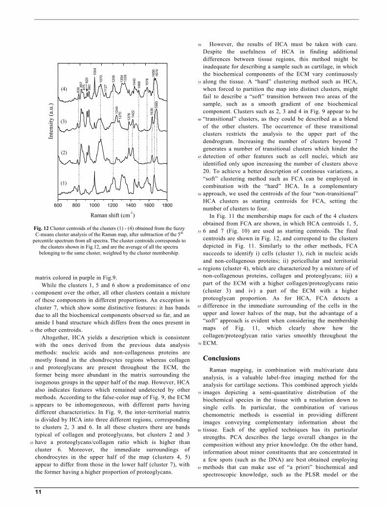
Fig. 10 Cluster centroids of the clusters (1) – (7) obtained from the

hierarchical cluster analysis of the Raman map after subtraction of the 5th

percentile spectrum from all spectra. The cluster centroids corresponds to

the clusters shown in Fig.10, and are the average of all the spectra having

the same cluster membership (i.e. the same color).

10

with albumin and concanavalin rather than with the proteins

mentioned above, this tentative interpretation must be taken

with great care.

The cellular regions of the map also show a high content of 5

collagen and proteoglycans. The presence of proteoglycans

and collagen inside the cells could be due partly to the

chondrocyte synthesis metabolism, and partly to the fact that

the Raman maps were collected in a non-confocal mode, so

that the ECM above or below the cells (along the z-axis) could 10

have contributed to the overall signal.

Fig.7 reports an example of PLSR analysis applied to two

spectra of the deep zone map: one (a) is taken from a cell and

the other one (b) from the ECM. Considering the limited

number of substances in our model and given the biochemical 15

complexity of a tissue, the residuals in Fig.7 suggest that the

PLSR model gives a reasonable fit of the experimental data. It

should be noted that the PLSR is meant to model mixtures

which consist completely of the components given in the

reference data set, which is only approximately the case for 20

cartilage. The residual spectrum shows a clear structure,

indicating that a model including more substances could help

to achieve a more accurate description of the tissue. For

instance, the fitting of the region around the sulfate vibration

of CS at 1068 cm-1 may be improved by adding other 25

sulphated GAGs to the model. On the other hand, the residual

intensity at 820 cm-1, in a spectral region which contains

characteristic collagen bands, could be explained with the fact

that we included in our model only one type of collagen,

whereas more than one type is present in the tissue. 30

HCA and FCA. Since cluster analysis looks for differences

between the spectra, the data pre-processing should emphasize

these differences. This could be accomplished by substracting

from all the data set the spectrum corresponding to the 35

biochemical composition that does not change over the whole

sample. Mathematically, this would be the “minimum

intensity spectrum”, i.e. the minimal intensity of all spectra

observed at each Raman shift. However, this approach may

cause problems: the minimum spectrum picks up the noise, 40

which may be not negligible in Raman spectra. Subtracting a

noisy spectrum will cause the result to be even more noisy.

Therefore, we rather subtracted the 5 th percentile of all

intensities at each Raman shift (fig. 8). This spectrum is still

very similar to the minimum spectrum, yet subject to much 45

less noise. Moreover, the 5th percentile-subtracted spectra

have positive intensity, whose interpretation is more

straightforward than that of the spectra with negative peaks

resulting from the subtraction of the mean spectrum. Indeed,

the application of HCA and FCA on 5th percentile-subtracted 50

spectra could distinguish spectral differences better than the

same analyses on un-subtracted data.

The use of a “hard” clustering method such as HCA on a

tissue Raman map leads to the partition of the map into

different areas, each area corresponding to a cluster of spectra. 55

Fig. 9 shows such a partition for the deep zone Raman map, in

which each cluster has been assigned a different color. The

number of clusters is chosen by the user according to several

issues, such as the dendrogram structure, the false-color maps

and the cluster centroids. Upon considering all these aspects, 60

we chose to divide the deep zone Raman map into 7 clusters.

Once clusters are formed, average spectra (centroids) can

be calculated for each cluster. Fig. 10 reports the centroids

corresponding to the clusters depicted in Fig. 9. As seen in

these two figures, HCA succeeds in differentiating between 65

cells, ECM immediately surronding cells which include

pericellular and territorial matrix, and inter-territorial ECM.

Cluster 1 (yellow areas in Fig. 9, corresponding to cells) has a

centroid with intense bands at 1578, 1488 and 782 cm -1 which

are characteristic of nucleic acids (Fig. 10). Moreover, bands 70

at 1656 and 1004 cm-1 suggests a high ratio of non-

collagenous proteins as well. On the other hand, the centroid

in Fig.10 corresponding to cluster 5 (brown areas surrounding

cells in the upper half of Fig. 9) shows bands at 1070 and

1378 cm-1, resembling the Raman spectrum of CS in Fig.2 and 75

indicating a high fraction of sulphated proteoglycans. The

centroid of cluster 6 (Fig. 10) presents features which are

distinctive of collagen, such as the quartet of bands at 857,

875, 920 and 940 cm-1, the amide III doublet at 1244 and 1270

cm-1, and the bands in the amide I region at 1636 and 1685 80

cm-1. This cluster corresponds to a part of the inter-territorial

Fig. 11 Cluster membership maps for clusters (1) - (4) as obtained from fuzzy C-means cluster analysis of the deep zone Raman map. The membership to

a certain cluster (i.e. the degree of belonging to a cluster, expressed as a coefficient from 0 to 1) for each spectrum is indicated by the color of the

corresponding pixel in the map, according to the color code bar on the right.

11

matrix colored in purple in Fig.9.

While the clusters 1, 5 and 6 show a predominance of one

component over the other, all other clusters contain a mixture 5

of these components in different proportions. An exception is

cluster 7, which show some distinctive features: it has bands

due to all the biochemical components observed so far, and an

amide I band structure which differs from the ones present in

the other centroids. 10

Altogether, HCA yields a description which is consistent

with the ones derived from the previous data analysis

methods: nucleic acids and non-collagenous proteins are

mostly found in the chondrocytes regions whereas collagen

and proteoglycans are present throughout the ECM, the 15

former being more abundant in the matrix surrounding the

isogenous groups in the upper half of the map. However, HCA

also indicates features which remained undetected by other

methods. According to the false-color map of Fig. 9, the ECM

appears to be inhomogeneous, with different parts having 20

different characteristics. In Fig. 9, the inter-territorial matrix

is divided by HCA into three different regions, corresponding

to clusters 2, 3 and 6. In all these clusters there are bands

typical of collagen and proteoglycans, but clusters 2 and 3

have a proteoglycans/collagen ratio which is higher than 25

cluster 6. Moreover, the immediate surroundings of

chondrocytes in the upper half of the map (clusters 4, 5)

appear to differ from those in the lower half (cluster 7), with

the former having a higher proportion of proteoglycans.

However, the results of HCA must be taken with care. 30

Despite the usefulness of HCA in finding additional

differences between tissue regions, this method might be

inadequate for describing a sample such as cartilage, in which

the biochemical components of the ECM vary continuously

along the tissue. A “hard” clustering method such as HCA, 35

when forced to partition the map into distinct clusters, might

fail to describe a “soft” transition between two areas of the

sample, such as a smooth gradient of one biochemical

component. Clusters such as 2, 3 and 4 in Fig. 9 appear to be

“transitional” clusters, as they could be described as a blend 40

of the other clusters. The occurrence of these transitional

clusters restricts the analysis to the upper part of the

dendrogram. Increasing the number of clusters beyond 7

generates a number of transitional clusters which hinder the

detection of other features such as cell nuclei, which are 45

identified only upon increasing the number of clusters above

20. To achieve a better description of continous variations, a

“soft” clustering method such as FCA can be employed in

combination with the “hard” HCA. In a complementary

approach, we used the centroids of the four “non-transitional” 50

HCA clusters as starting centroids for FCA, setting the

number of clusters to four.

In Fig. 11 the membership maps for each of the 4 clusters

obtained from FCA are shown, in which HCA centroids 1, 5,

6 and 7 (Fig. 10) are used as starting centroids. The final 55

centroids are shown in Fig. 12, and correspond to the clusters

depicted in Fig. 11. Similarly to the other methods, FCA

succeeds to identify i) cells (cluster 1), rich in nucleic acids

and non-collagenous proteins; ii) pericellular and territorial

regions (cluster 4), which are characterized by a mixture of of 60

non-collagenous proteins, collagen and proteoglycans; iii) a

part of the ECM with a higher collagen/proteoglycans ratio

(cluster 3) and iv) a part of the ECM with a higher

proteoglycan proportion. As for HCA, FCA detects a

difference in the immediate surrounding of the cells in the 65

upper and lower halves of the map, but the advantage of a

“soft” approach is evident when considering the membership

maps of Fig. 11, which clearly show how the

collagen/proteoglycan ratio varies smoothly throughout the

ECM. 70

Conclusions

Raman mapping, in combination with multivariate data

analysis, is a valuable label-free imaging method for the

analysis for cartilage sections. This combined approch yields

images depicting a semi-quantitative distribution of the 75

biochemical species in the tissue with a resolution down to

single cells. In particular, the combination of various

chemometric methods is essential in providing different

images conveying complementary information about the

tissue. Each of the applied techniques has its particular 80

strengths. PCA describes the large overall changes in the

composition without any prior knowledge. On the other hand,

information about minor constituents that are concentrated in

a few spots (such as the DNA) are best obtained employing

methods that can make use of “a priori” biochemical and 85

spectroscopic knowledge, such as the PLSR model or the

600 800 1000 1200 1400 1600 1800

(4)

Raman shift (cm-1)

Inte

nsi

ty (

a.u

.)

(1)

(2)

(3)

830 8

57

875

920

940

1004

1070

1127

1209

1304

1335

1440

1488

1578

1656

1674

1685

1636

1422

1378

12701244

Fig. 12 Cluster centroids of the clusters (1) - (4) obtained from the fuzzy

C-means cluster analysis of the Raman map, after subtraction of the 5th

percentile spectrum from all spectra. The cluster centroids corresponds to

the clusters shown in Fig.12, and are the average of all the spectra

belonging to the same cluster, weighted by the cluster membership.

12

"univariate" imaging of charactersitic bands. HCA easily

identifies small clusters among a majority of different spectra.

However, it cannot deal well with continuous concentration

gradients of biochemical costituents. These continous changes

are well described by FCA – that in turn has considerable 5

difficulties in finding small clusters with the usual random

initialization. The combination of the two cluster analysis

methods proved to be far more efficient than the two methods

used separately: transitions between the clusters are resolved

by partial membership, while the small clusters are correctly 10

retained.

Because of its capabilities, this combination of Raman

mapping and multivariate data analysis has an excellent

potential as a tool, complementary to other imaging

techniques, for studying biochemical and morphological 15

changes during cartilage degradation in processes as aging or

osteoarthritis.

Ackowledgements

AB and VS acknowleges partial support from FONDO

TRIESTE. AB thanks Anna Flamigni for helping in the 20

sample preparation.

Notes

*Corresponding Author

Addresses

aCENMAT Dept. of Materials and Natural Resources, University of 25

Trieste, Via Valerio 6a, 34100 Trieste, Italy. Fax: +39 040 572044 Tel:

+39 040 558 3768; E-mail: abonifacio@units.it b Dept. of Life Sciences, University of Trieste, Via Valerio 6a, 34100

Trieste, Italy.

References 30

1. C. A. Poole, J. Anat., 1997, 191, 1-13.

2. M. Huber, S. Trattnig and F. Lintner, Invest. Radiol., 2000, 35, 573-

580.

3. E. Kheir and D. Shaw, Orthopaed. Trauma, 2009, 23, 450-455.

4. T. Aigner and L. McKenna, Cell. Mol. Life Sci., 2002, 59, 5-18. 35

5. D. R. Jeffrey and I. Watt, Br. J. Radiol., 2003, 76, 777-787.

6. A. Boskey and N. Pleshko Camacho, Biomaterials, 2007, 28, 2465-

2478.

7. K. Potter, L. H. Kidder, I. W. Levin, E. N. Lewis and R. G. Spencer,

Arthritis. Rheum., 2001, 44, 846-855. 40

8. J. Mansfield, J. Yu, D. Attenburrow, J. Moger, U. Tirlapur, J. Urban,

Z. Cui and P. Winlove, J. Anat., 2009, 215, 682-691.

9. E. Smith and G. Dent, eds., Modern Raman Spectroscopy: A practical

approach, Wiley, Chichester, UK, 2005.

10. U. Utzinger and R. R. Richards-Kortum, J. Biomed. Opt., 2003, 8, 45

121-147.

11. R. Salzer and H. W. Siesler, eds., Infrared and Raman Spectroscopic

Imaging, Wiley-VCH, Weinheim, Germany, 2009.

12. N. Ignatieva, O. Zakharkina, G. Leroy, E. Sobol, N. Vorobieva and S.

Mordon, Laser Phys. Lett., 2007, 10, 749-753. 50

13. M. Heger, S. Mordon, G. Leroy, L. Fleurisse and C. Creusy, J.

Biomed. Opt., 2006, 11, 024003.

14. S. Koljenovic, T. C. Bakker Schut, J. P. van Meerbeeck, A. P. Maat,

S. A. Burgers, P. E. Zondervan, J. M. Kros and G. J. Puppels, J.

Biomed. Opt., 2004, 9, 1187-1197. 55

15. K. A. Dehring, N. J. Crane, A. R. Smukler, J. B. McHugh, B. J.

Roessler and M. D. Morris, Appl. Spectrosc., 2006, 60, 1134-1141.

16. P. Geladi, Spectrochim. Acta B Atomic Spectroscopy, 2003, 58, 767-

782.

17. S. Wold, M. Sjöström and L. Eriksson, Chemometr. Intell. Lab. Syst., 60

2001, 58, 109-130.

18. T. N. Tran, R. Wehrens and L. M. Buydens, Chemometr. Int. Lab.

Syst., 2005, 77, 3-17.

19. P. Mainil-Varlet, T. Aigner, M. Brittberg, P. Bullough, A. Hollander,

E. Hunziker, R. Kandel, S. Nehrer, K. Pritzker, S. Roberts and E. 65

Stauffer, J. Bone Joint Surg., 2003, 85, 45-57.

20. A. D. Meade, C. Clarke, F. Draux, G. D. Sockalingum, M. Manfait, F.

M. Lyng and H. J. Byrne, Anal. Bioanal. Chem., 2010, 396, 1781-

1791.

21. R Development Core Team, R:A language and environment for 70

statistical computing., (2010), R Foundation for Statistical

Computing, Vienna, Austria, url http://www.R-project.org

22. C. Beleites and V. Sergo, (in preparation), url

http://www.hyperSpec.r-forge.r-project.org.

23. I. T. Jolliffe, Principal Component Analysis, 2nd edn., Springer, New 75

York, 2002.

24. W. N. Venables and B. D. Ripley, Modern Applied Statistics with R,

Springer, New York, USA, 2002.

25. A. Bonifacio and V. Sergo, Vibr. Spectrosc., 2010, 53, 314-317.

26. R. Wehrens and B. Mevik, pls: Partial Least Squares Regression 80

(PLSR) and Principal Component Regression (PCR). R package

version 2.1-0., (2007); url http://mevik.net/work/software/pls.html

27. M. Longnecker and R. Ott, An introduction to statistical methods and

data analysis, 6th edn., Duxbury Press, Pacific Grove, USA, 2008.

28. E. Dimitriadou, K. Hornik, F. Leisch, D. Meyer and A. Weingessel, 85

e1071: Misc functions of the Department of Statistics, (2010) TU

Wien; url http://CRAN.R-project.org/package=e1071

29. R. Tuma, J. Raman spectrosc., 2005, 36, 307-319.

30. X. Bi, G. Li, S. B. Doty and N. P. Camacho, Osteoart. Cart., 2005,

13, 1050-1058. 90

31. D. P. Speer and L. Dahners, Clin. Orthopaed. Rel. Res., 1979, 139,

267-275.

32. M. Kazanci, P. Roschger, E. P. Paschalis, K. Klaushofer and P. Fratzl,

J. Struct. Biol., 2006, 156, 489-496.

33. G. Socrates, Infrared and Raman Characteristic Group Frequencies: 95

Tables and Charts Wiley, New York, 2004.

34. X. Bi, X. Yang, M. P. Bostrom, D. Bartusik, S. Ramaswamy, K. W.

Fishbein, R. G. Spencer and N. P. Camacho, Anal. Bioanal. Chem.,

2007, 387, 1601-1612.

35. X. Bi, X. Yang, M. P. Bostrom and N. P. Camacho, Biochim. 100

Biophys. Acta, 2006, 1758, 934-941.

36. P. Lasch and J. Kneipp, eds., Biomedical Vibrational Spectroscopy,

Wiley Interscience, Hoboken, New Jersey, 2008.

37. M. Diem, P. R. Griffiths and J. M. Chalmers, eds., Vibrational

Spectroscopy for Medical Diagnosis, Wiley, Chichester, UK, 2008. 105

13