Checking a process-based catchment model by artificial neural networks

HYDROLOGICAL PROCESSESHydrol. Process. 17, 265–277 (2003)Published online in Wiley InterScience (www.interscience.wiley.com). DOI: 10.1002/hyp.1123

Checking a process-based catchment model by artificialneural networks

Gunnar Lischeid1* and Stefan Uhlenbrook2

1 BITOK, Department of Hydrogeology, University of Bayreuth, Dr.-Hans-Frisch-Str. 1–3, D-95440 Bayreuth, Germany2 Institute of Hydrology, University of Freiburg, Fahnenbergplatz, D-79098 Freiburg, Germany

Abstract:

A process-based, conceptual runoff model, the tracer-aided catchment (TAC) model, is developed and applied to the40 km2 Brugga catchment in the Black Forest Mountains of southwest Germany. The model accounts for differentrunoff generation processes and runoff components. A lumped artificial neural network (ANN) model was also appliedusing the same data set. We compared the output from the two models in an effort to improve the efficiency of theTAC model and its model structure using physical and chemical data. Both approaches yielded comparably goodresults for daily discharge simulation. The TAC model, which uses spatially distributed input data, was superior tothe lumped ANN model in only one case. Dissolved silica concentration in catchment runoff was used to assess therunoff components mixing approach of the conceptual TAC model. The ANN simulation of silica time series wassuperior to that of the TAC model. However, using modelled discharge values instead of measured data markedlyweakened the silica predictions and resulted in a performance similar to the TAC model. We conclude that this reflectsthe inevitable non-linear error propagation within the TAC model. The ANN silica model improved substantially whenhourly data were used instead of daily data. According to the ANN, silica dynamics are characterized by hysteresisloops in the discharge–silica concentration relationship in the short term. In addition, this relationship depends on theantecedent moisture conditions in the medium term. About 87% of the hourly silica time series variance was explainedby non-linear regression with the hydrograph only. The implications of these findings are as follows. A simulation ofthe silica dynamics is possible using rather simple models that take into account the dynamics described above. In thisrespect, the TAC approach was confirmed by the ANN. However, an appropriate silica modelling time step must beshorter than daily values to be in line with the process time scale. Last but not least, the silica time series were assumedto reflect the spatial distribution of single hydrotopes to the catchment runoff during single storms, and thus to providean independent check for the spatially distributed model in addition to the hydrograph. This has proven wrong, as theinformation provided by the silica data is highly redundant to that of the hydrograph, illustrated by the fact that thesilica dynamics can be well described by the empirical model without requiring any spatial information. Copyright 2003 John Wiley & Sons, Ltd.

KEY WORDS rainfall runoff modelling; artificial neural network; runoff generation; dissolved silica; TAC model;model validation

INTRODUCTION

A variety of different processes influence runoff generation; for a review, see Bonell (1998). However,the dominant processes at a specific site and at a particular scale, and the causes for differences betweencatchments are still not well understood. We can identify runoff generation processes by: (i) interpretingfield observations of hydrological variables, i.e. ground water heads, soil water distributions or tracer data(e.g. McDonnell, 1990); (ii) simulating runoff processes with mathematical models (e.g. Bronstert, 2000);and (iii) combining both (e.g. Christophersen et al., 1990). Although the first approach is often restricted to

* Correspondence to: Gunnar Lischeid, BITOK, Department of Hydrogeology, University of Bayreuth, Dr.-Hans-Frisch-Str. 1–3, D-95440Bayreuth, Germany. E-mail: [email protected]

Received 31 January 2001Copyright 2003 John Wiley & Sons, Ltd. Accepted 2 January 2002

266 G. LISCHEID AND S. UHLENBROOK

the hillslope scale and small headwater catchment scale, the application of models offers the possibility toup-scale knowledge or to identify processes at larger scales.

While useful, application of physically based models as hypothesis testing tools may suffer from theneed, a priori, to define the processes used in the model. The conceptualization of these processes andtheir implementation in a certain model structure is problematic (Grayson et al., 1992). It is likely that, innature, different processes interact across different scales in a non-linear way. Such interactions are poorlyunderstood (Beven, 2001; Bloschl, 2001) and not well represented in today’s catchment models. Additionally,the performance of a model depends greatly on the quality of the input data. Every measurement is inevitablysubject to uncertainties and errors (Sherlock et al., 2001). Parameter values are often determined at a smallerscale than the scale of the model application, or cannot even be assessed directly in the field and must bedetermined by model calibration. The larger the parameter uncertainty, the less rigorous are the model teststhat can be performed and the more the model’s capacity for process identification is limited. Non-uniquenessof model solutions can also result in an infinite number of realizations of equivalent performance (e.g. Beven,1993; Oreskes et al., 1994).

Different runoff models commonly yield about the same performance in spite of substantially differentprinciples, e.g. detailed versus lumped physically based models, or even purely empirical models (e.g. Hsuet al., 1995; Maier and Dandy, 1996; Zealand et al., 1999). This result is due to the limited informationprovided by the shape of the hydrograph (Jakeman and Hornberger, 1993). Consequently, the challenge existsto include additional information in the model evaluation. Such a multiresponse validation could considerdischarge from sub-basins, ground water levels, snow heights, soil water contents, or tracer data. However,the use of additional data is not straightforward, as these data often cannot be used directly in the model unlessadditional routines, including (uncertain) model parameters, are implemented. Thus assessing the cost–benefitrelationship of increasing model complexity by identifying key variables out of a large set of candidatevariables becomes an inevitable prerequisite.

Natural tracers can provide important information about runoff generation processes at the catchment scale.Environmental isotopes (e.g. 18O, 2H, 3H) are widely used for age dating (e.g. Maloszewski and Zuber,1996) and to distinguish between event water and pre-event water during single events (e.g. Buttle, 1994).In combination with hydrochemical parameters such as the major anions and cations, geographic sourceareas and flow pathways can be determined (e.g. Hinton et al., 1994; Bazemore et al., 1994). Dissolvedsilica has also proved suitable for identifying runoff components from different origins (e.g. Pinder andJones, 1969; Hooper and Shoemaker, 1986; Hoeg et al., 2000). Compared with carbonate weathering, thechemical weathering of siliceous minerals is very slow (Wollast and Chou, 1988). In natural environments,the silica concentration of stream water and groundwater is likely to depend mainly on the size of thewater–rock surface and the contact time of the water with siliceous minerals. Consequently, different runoffcomponents can be distinguished if they differ in flowpaths and residence times but mix conservatively inthe stream. Thus, time series of silica concentration can be used to infer the varying spatial pattern of thecontribution of different runoff components. This might help considerably to evaluate spatially distributedrunoff models.

In this study, a process-oriented catchment model, the tracer-aided catchment (TAC) model (Uhlenbrook,1999) is applied to the Brugga basin. Time series of the concentration of dissolved silica in the catchmentrunoff are used as an additional constraint for the model as they are traced back to the varying spatialpatterns of different runoff components. This test becomes the more powerful the less the silica concen-tration is correlated with discharge, i.e. the more information the silica data provide in addition to thehydrograph. In this context, statistical dependence includes non-linear relationships and lag times betweendischarge and silica concentration. To summarize, the analysis of the TAC model focuses on the follow-ing questions:

1. Can the model structure be improved to reproduce better the observed time series of discharge and silicaconcentration? Does the model make efficient use of the information given by the input data set?

Copyright 2003 John Wiley & Sons, Ltd. Hydrol. Process. 17, 265–277 (2003)

CHECKING A PROCESS-BASED CATCHMENT MODEL 267

2. Can the parameterization of the model, given a certain structure, be improved with respect to simulate thetime series of discharge and silica concentration?

3. Are the time series of silica concentration statistically independent from the hydrograph?

STUDY SITE

Site description

The study was performed in the Brugga basin (40 km2) located in the southern Black Forest Mountains,southwestern Germany. It is a meso-scale mountainous catchment with elevation ranging from 438 to 1493 ma.m.s.l. and a snowmelt-driven runoff regime. The mean annual precipitation is approximately 1750 mm,generating a mean annual discharge of approximately 1220 mm. The bedrock consists of gneiss, covered bysoils developed in glacial and periglacial drift of varying depths (0–10 m). Soil permeability is generallyhigh. Saturated areas amount to 6Ð2% of the total basin area and do not differ much in their spatial extentin time (Guntner et al., 1999a,b). Saturated areas are mostly connected directly to the streams. The basin iswidely forested (75%) and the remaining area is pastureland; urban land use is less than 3%.

Previous experimental studies

The following detailed tracer investigations were carried out in the Brugga and neighbouring Zastlerbasins (18Ð4 km2): (i) hydrograph separations using 18O, chloride, and dissolved silica; (ii) artificial tracerexperiments at different hillslopes and in the river channel system; and (iii) residence time determinations using18O, tritium, and chloroflurocarbon (CFC) concentrations. These experiments led to the following conceptualmodel of runoff generation. Three main flow systems predominate in runoff generation.

1. Fast runoff components (near-surface runoff) are generated on impervious or saturated areas and on steephighly permeable slopes covered by boulder fields. The mean residence time of the near-surface runoffcomponent is hours to a few days, as shown by artificial tracer tests (Mehlhorn et al., 1998) and byhydrograph separations based on natural tracers during single events (Uhlenbrook, 1999; Hoeg et al., 2000).

2. Slow base-flow components (deep groundwater) originate from the fractured hard rock aquifer and thedeeper parts of the weathering zone. The mean residence time of the water is 6 to 9 years, as determinedby tritium and CFC measurements (Uhlenbrook, 1999; Uhlenbrook et al., 2002).

3. An intermediate flow system contributes mainly from the (peri-)glacial deposits above the saprolite (shallowgroundwater). The mean residence time of the water is 2 to 3 years, as determined by 18O measurements(Uhlenbrook, 1999; Uhlenbrook et al., 2002). In spite of the rather long mean residence time, this flowsystem dominates storm discharge. Springs draining these hillslopes show remarkable short-term dynamics.

The contributions of near-surface runoff, shallow groundwater, and deep groundwater to total runoff werecalculated for a period of 3 years using 18O and tritium measurements. These contribution rates weredetermined to be 11Ð1%, 69Ð4%, and 19Ð5% respectively (Uhlenbrook et al., 2002). Even if an uncertaintymust be assumed for these numbers, they demonstrate clearly the dominance of the shallow groundwatersystem and, consequently, the importance of shallow hillslope runoff for runoff generation at the test site.

MODELS

The process-based approach: the TAC model

The TAC model (for a detailed description see Uhlenbrook (1999) and Uhlenbrook and Leibundgut (2002))is a process-oriented conceptual rainfall runoff model with a modular structure. The spatial discretization isbased on a delineation of seven unit types, each with the same dominant runoff generation processes. For the



Brugga catchment, the units were obtained by overlaying different spatial information within a geographicalinformation system environment: a forest habitat map, a saturated area map (Guntner et al., 1999b), geologicmaps, a map of quaternary deposits, the drainage network, and a digital elevation model with a grid size of50 m ð 50 m. In addition, 100 m elevation zones account for the meteorological input variables (precipitation,temperature, and potential evapotranspiration) varying with altitude. The TAC model can be classified as semi-distributed, as it combines a hydrotope concept with elevation zones. Here, ‘hydrotopes’ refer to geographicunits of similar hydrologic characteristics and, consequently, similar dominant runoff generation processes. Thesnow routine and the soil modules were adapted from the HBV model (Bergstrom, 1976). The runoff generationmodule was developed for the Brugga basin based on results of experimental investigations, including detailedtracer studies (see section on previous experimental studies). For each unit type, a specific linear or non-linearreservoir concept was developed that conceptualizes the respective dominant runoff generation process. Thetotal basin runoff is equal to the superposition of the individual runoff components. An additional routingroutine is not used, as tracer tests showed that the water in the stream network reaches the outlet within themodelling time step of 1 day.

The runoff components generated in the different reservoir concepts can be assigned to the three mainflow systems according to the experimental investigations (see section on previous experimental studies).In addition, a specific concentration of dissolved silica can be assigned to each component (Uhlenbrook,1999). The model output consists of the simulated total discharge, the contribution of runoff components,and the simulated silica concentration in the total discharge. For the latter, the concentrations of all runoffcomponents of the different reservoir concepts are added, weighted by the discharge contribution of therespective hydrotopes.

The data-based approach: artificial neural networks (ANNs)

We applied ANNs using the same data set used for the TAC model. ANNs allow one to mimic anymathematical function with arbitrary accuracy (Hornik et al., 1989) and are used as a statistical tool to revealnon-linear regressions between different variables in a self-optimizing way, independently of any preselectedprocesses. If an ANN yields significantly better performance than the TAC model, this would provide strongevidence that either the TAC model structure (focus 1) or the TAC parameterization (focus 2) could beimproved. This objective has governed many studies of neural network modelling in hydrology (e.g. Frenchet al., 1992; Hsu et al., 1995; Campolo et al., 1999; Imrie et al., 2000).

In addition, key variables can be identified by neural networks (e.g. Luk et al., 2000; Gautam et al., 2000),which might provide a useful insight into whether the TAC model structure can be improved (focus 1). TheTAC model differs from many other catchment runoff models in that it explicitly accounts for spatial patternsof dominant runoff generation processes that can be identified with field investigations. However, the modelperformance is tested mainly by comparing time series of discharge and silica concentration (Uhlenbrook andLeibundgut, 2002). In this study, the spatial information used by the TAC model is not used in the ANNmodels; this is to test whether such spatial information is necessary to reproduce the observed patterns intime (focus 1).

Visualization of the non-linear regression hyperplanes revealed by the ANN can be used as a basis foridentifying the dominant processes at the given scale of observation, and can be compared with the processesimplemented in the physically based model (focus 1). The latter approach is seldomly undertaken, but hasshown its potential in prior studies (Lischeid, 2001a,b). Furthermore, statistical independence between thesilica time series and the hydrograph was confirmed if the ANN reveals additional driving variables for thesilica dynamics (focus 3). Although the ANN model cannot distinguish between coincidence and causality, itopens a new perspective on the data and might help to reveal new avenues for future investigations.

Multilayer perceptron-type networks are often used for time series simulation (Rumelhart and McClelland,1986). They consist of identical units called nodes that are arranged in subsequent layers (Figure 1, left).Every node of one layer is connected to every node of the preceding and subsequent layers. Each node in



the input layer corresponds to one of the input variables, and each of the output nodes corresponds to one ofthe output variables. In contrast, the number of hidden layers and the number of nodes in the hidden layerscan be chosen arbitrarily. Data are processed unidirectionally through the network. For every step, a tupleconsisting of data values for every input variable is needed. The data is fed into the input layer and passedto every node of the subsequent layer. In each node of this layer, all incoming values of the preceding layerare summed, passed through a non-linear activity function (here the logistic function that is identical for allnodes), transferred to the next layer, and so on. For every connection between nodes of subsequent layers, datavalues are multiplied by a weight factor specific for every connection. These weights are adjusted individuallyin order to map the input onto the output values in the best possible way in a ‘learning’ procedure. In addition,a bias is calibrated for every node of the hidden and the output layers to shift the most sensitive part of theactivity function, i.e. the part with the steepest gradient, toward the dominating range of the incoming values.Thus, the total number of parameters calibrated by the training procedure is equal to the number of nodes inthe hidden and the output layers, plus the sum of the products of the number of nodes in every two subsequentlayers. A widely accepted, and rather restrictive, rule of thumb is that the number of parameters should notexceed one-tenth of the number of tuples of the data set (Weigend et al., 1990). The ratio for the modelspresented in this paper is between 0Ð06 and 0Ð1.

In contrast to linear regression models, ANNs suffer from non-uniqueness of model solutions. This canbe partly compensated for by sophisticated methods of model optimization. However, any neural networksolution will necessarily still be an underestimation of the maximal model performance achievable with thegiven data set.

For simulation of time series that exhibit a pronounced ‘memory’, i.e. cross-correlation or autocorrelation,Elman-type networks are used (Elman, 1990). They differ from multilayer perceptrons in that the output ofevery hidden node or output node is also transferred to a so-called context node and passed back to every nodeof the respective layer in the subsequent step (Figure 1, right). The bias of the context nodes is not calibratedduring the learning procedure. The learning algorithm used in this study is the resilient propagation method(Riedmiller and Braun, 1993). We analysed the continuous time series of discharge using the Elman-typenetworks with two hidden layers. Multilayer perceptron-type networks with one hidden layer were used forthe silica model.

Following the common cross-validation approach, the data set was divided randomly into training,validation, and test data sets at a 2 : 1 : 1 ratio. This procedure was repeated ten times. Additionally, randominitialization of the weight matrix was performed another ten times for each set of data sets, yielding 100model runs.

The driving input variables were identified as follows. In a first step, the ANN was trained with tuplescomprising all independent variables that might contribute to explaining the observed variance. For the runoff

input layer

hidden layer

output layer

context nodes

Figure 1. Structure of a multilayer perceptron- (left) and of an Elman-type neural network (right)



and the silica model with a daily time step, daily mean values of discharge, air temperature, and potentialevapotranspiration and the daily sum of precipitation were selected. To account for a possible short-termmemory of the processes, values of the preceding time steps (1, 2, 3, 5, and 10 days prior to the samplingday) were included as input variables (see Luk et al., 2000). For the silica model with an hourly time step,discharge, air temperature, precipitation, radiation, and wind velocity were included as independent variables.Based on the experience of the preceding modelling exercise, a time delay was considered only for dischargeand air temperature (1, 2, 3, 6, and 12 h, and 1, 2, 3, and 5 days respectively prior to sampling). In the nextstep, the key variables were identified by skeletonization of the respective 100 models (Mozer and Smolensky,1989). This procedure yields a ranking of the independent variables sorted by relevance for the simulationof the target variable. The ANN was then trained with the first one, two, etc. of these independent variablesuntil the performance of the model did not increase further. Lischeid (2001a) described the procedure in moredetail. The software package SNNS (Stuttgart Neural Network Simulator) version 4Ð1 (Zell et al., 1995) wasused for the analysis.

Comparing different models

Daily precipitation, mean air temperature, and potential evapotranspiration data from the same periods wereused for both the TAC and the ANN calibration (15 July 1995–1 April 1997) and testing (2 April 1997–7October 1998). The data sets did differ slightly in that the TAC model was given data for a number ofelevation zones, but the ANN model was given only lumped values for calibration and testing. The sameset of daily mean silica concentration data from the Brugga outlet (July 1995–October 1998; 263 samples)were used for both models. In addition, hourly silica data were used for additional ANN analysis that partlyoverlapped with the daily silica concentration data (January 1998–July 1999; 329 samples).

The performance of the models is evaluated using the coefficient of determination r2 and the modelefficiency Reff, introduced by Nash and Sutcliffe (1970).

RESULTS

Runoff simulation

The ANN yielded similarly good results as the TAC model using precipitation, air temperature, and potentialevapotranspiration as input data (Table I). The number of hidden layers in the ANN was two, with four nodeseach. In spite of slightly better performance in the testing period, the ANN model was more likely tounderestimate the highest discharge peaks (Figure 2). However, a striking failure of the ANN model was itsunderestimation of the amount of precipitation stored in the snowpack at the beginning of 1996, when the dailymean air temperature was slightly below 0 °C. The discharge peak was predicted much too early. In contrast,the semi-distributed TAC model more closely predicted the onset of snowmelt, since it took into account thedependence of snow accumulation on temperature and elevation. It is important to note that this snowmeltevent was part of the training data set of the ANN, and that the remaining snowmelt-driven runoff peaks inthe 3 years of record were much better reproduced by the ANN (Figure 2, see Table I). Thus, failure of theANN in spring 1996 is ascribed to a particularly strong elevation gradient of snowmelt during that period.

Simulation of silica concentration

Silica concentration in the catchment runoff was simulated as a conservative mixture of the silicaconcentrations of different runoff components. These concentrations were determined by field measurementsand used without further calibration. Although the model results correspond well to the silica dynamics duringcertain periods (Uhlenbrook and Leibundgut, 1999, 2002), the model performance for the total period wasless satisfactory (Table II, first column). Based on the same silica data set, but using measured runoff data,the ANN tended to underestimate silica dynamics slightly, whereas the TAC tended to overestimate silica



01.01.96 01.07.96 01.01.97 01.07.97

Dis

char

ge [m

m d

ay-1

]

0

5

10

15

20

25

30

obs.TACANN

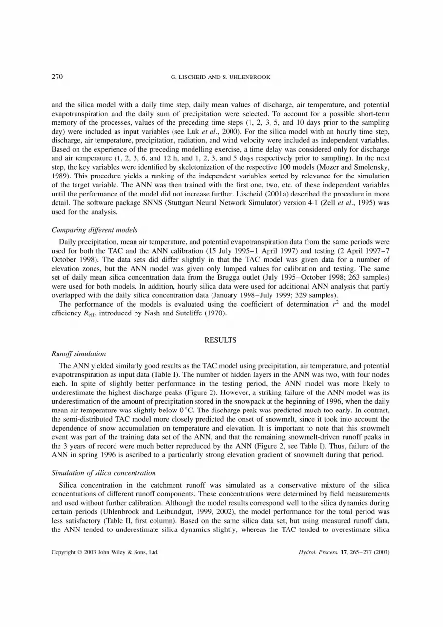
Figure 2. Observed and modelled hydrograph of the Brugga catchment runoff during the calibration period

Table I. Performance of different runoff models

TAC ANN

Calibration Testing Calibration Testing15/7/95–1/4/97 2/4/97–7/10/98 5/7/95–1/4/97 2/4/97–7/10/98

Reff 0Ð77 0Ð73 0Ð77 0Ð77r2 0Ð76 0Ð74 0Ð77 0Ð77

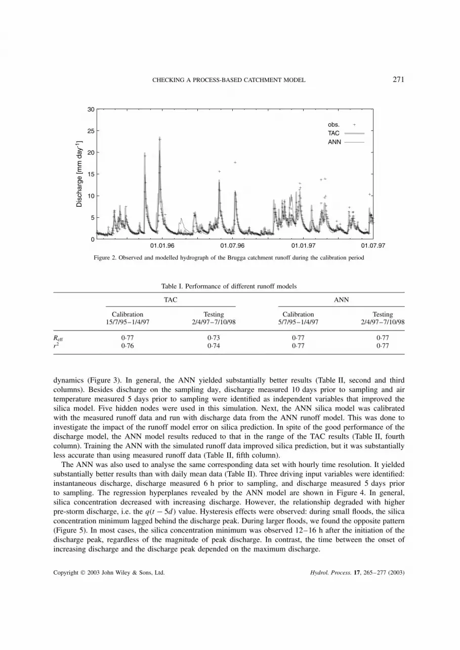
dynamics (Figure 3). In general, the ANN yielded substantially better results (Table II, second and thirdcolumns). Besides discharge on the sampling day, discharge measured 10 days prior to sampling and airtemperature measured 5 days prior to sampling were identified as independent variables that improved thesilica model. Five hidden nodes were used in this simulation. Next, the ANN silica model was calibratedwith the measured runoff data and run with discharge data from the ANN runoff model. This was done toinvestigate the impact of the runoff model error on silica prediction. In spite of the good performance of thedischarge model, the ANN model results reduced to that in the range of the TAC results (Table II, fourthcolumn). Training the ANN with the simulated runoff data improved silica prediction, but it was substantiallyless accurate than using measured runoff data (Table II, fifth column).

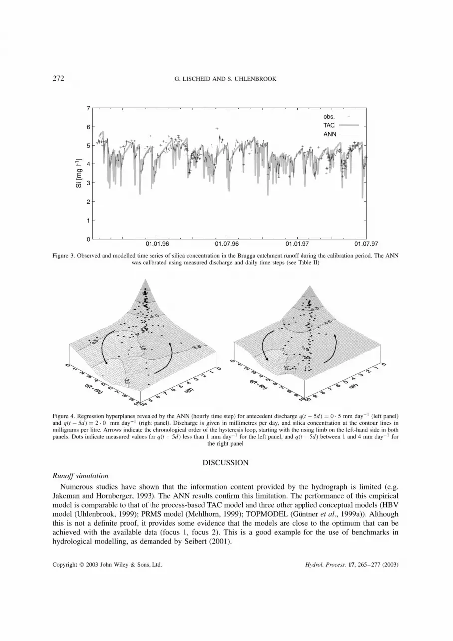
The ANN was also used to analyse the same corresponding data set with hourly time resolution. It yieldedsubstantially better results than with daily mean data (Table II). Three driving input variables were identified:instantaneous discharge, discharge measured 6 h prior to sampling, and discharge measured 5 days priorto sampling. The regression hyperplanes revealed by the ANN model are shown in Figure 4. In general,silica concentration decreased with increasing discharge. However, the relationship degraded with higherpre-storm discharge, i.e. the q�t � 5d� value. Hysteresis effects were observed: during small floods, the silicaconcentration minimum lagged behind the discharge peak. During larger floods, we found the opposite pattern(Figure 5). In most cases, the silica concentration minimum was observed 12–16 h after the initiation of thedischarge peak, regardless of the magnitude of peak discharge. In contrast, the time between the onset ofincreasing discharge and the discharge peak depended on the maximum discharge.



0

1

2

3

4

5

6

7

Si [

mg

l-1]

obs.TACANN

01.01.96 01.07.96 01.01.97 01.07.97

Figure 3. Observed and modelled time series of silica concentration in the Brugga catchment runoff during the calibration period. The ANNwas calibrated using measured discharge and daily time steps (see Table II)

Figure 4. Regression hyperplanes revealed by the ANN (hourly time step) for antecedent discharge q�t � 5d� D 0 Ð 5 mm day�1 (left panel)and q�t � 5d� D 2 Ð 0 mm day�1 (right panel). Discharge is given in millimetres per day, and silica concentration at the contour lines inmilligrams per litre. Arrows indicate the chronological order of the hysteresis loop, starting with the rising limb on the left-hand side in bothpanels. Dots indicate measured values for q�t � 5d� less than 1 mm day�1 for the left panel, and q�t � 5d� between 1 and 4 mm day�1 for

the right panel

DISCUSSION

Runoff simulation

Numerous studies have shown that the information content provided by the hydrograph is limited (e.g.Jakeman and Hornberger, 1993). The ANN results confirm this limitation. The performance of this empiricalmodel is comparable to that of the process-based TAC model and three other applied conceptual models (HBVmodel (Uhlenbrook, 1999); PRMS model (Mehlhorn, 1999); TOPMODEL (Guntner et al., 1999a)). Althoughthis is not a definite proof, it provides some evidence that the models are close to the optimum that can beachieved with the available data (focus 1, focus 2). This is a good example for the use of benchmarks inhydrological modelling, as demanded by Seibert (2001).



0

2

4

6

8

15/09

00:00

16/09

00:00

17/09

00:00

18/09

00:00

2

3

4

5

6

Si [

mg

l-1]

Dis

char

ge [m

3 s-

1 ]

0 2 4 6 82

3

4

5

6

Si [

mg

l-1]

Discharge [m3 s-1]

Dis

char

ge [m

3 s-

1 ]

Si [

mg

l-1]

Si [

mg

l-1]

Discharge [m3 s-1]

Dis

char

ge [m

3 s-

1 ]

Si [

mg

l-1]

Si [

mg

l-1]

Discharge [m3 s-1]

0

2

4

2

3

4

5

6

23/08

00:00

24/08

00:00

2

3

4

5

6

0 1 2 3 4 5

0

5

10

15

20

25

20/0200:00

23/0200:00

26/0200:00

01/0300:00

2

3

4

5

6

2

3

4

5

6

0 5 10 15 20 25

Figure 5. Time series of discharge and silica concentration (left panels) for three single events, and corresponding hysteresis loops (rightpanels; arrows indicate chronological order). Medium-sized stormflow event with high antecedent discharge (2Ð5 m3 s�1) in the upperline, medium-sized stormflow with low antecedent discharge (0Ð4 m3 s�1) in the middle, and a large event with low antecedent discharge(0Ð8 m3 s�1) in the lower line. Solid line: hydrograph; crosses: measured silica concentration; open squares: silica concentration simulated

by the ANN

The motivation for developing the TAC model was to link spatial patterns of zones with the samedominating runoff processes with the time series of discharge at the catchment outlet. Taking into accountelevation gradients of boundary fluxes (temperature, precipitation, and evapotranspiration) improved the modelsignificantly only during one single snowmelt event. Accounting for the spatial patterns of precipitation, e.g.during convective rainstorms, might have an even larger effect on model performance (Bell and Moore, 2000),but this has not been implemented in any of the Brugga runoff models so far.



Table II. Performance of different silica modelsa

TAC ANN ANN ANN

Calibrated with qsim (TAC) qobs qobs qsim (ANN)Applied to qsim (TAC) qobs qsim (ANN) qsim (ANN)

t D 1 day (July 1995–October 1998)Reff 0.29 0.70 0.29 0.46r2 0.36 0.70 0.31 0.47

t D 1 hour (January 1998–July 1999)Reff — 0.87 — —r2 — 0.87 — —

a qobs: measured runoff data; qsim: simulated runoff (respective runoff model given inbrackets).

Simulation of silica concentration

Testing of catchment models is often based solely on the comparison of simulated and observed discharge,although they often also simulate other fluxes and internal states. However, an extensive evaluation of a modelis the basis for carrying out further improvements of the model and for a better process identification. Toachieve the latter, additional data were integrated into catchment models. Kuczera and Mroczkowski (1998)demonstrated that the use of discharge salt content in addition to groundwater levels helped to increasethe confidence in a model significantly. The parameter uncertainty problem for a modified version of theHBV model was clearly reduced by considering groundwater levels in addition to discharge for modelcalibration and validation (Seibert, 2000). Franks et al. (1998) presented a means for reducing TOPMODEL’sparameter uncertainty by taking the spatial distribution of saturated areas into account. Guntner et al. (1999a)demonstrated that additional information could be used to identify invalid assumptions of the TOPMODELapproach for the Brugga basin. These examples also indicate the value of distributed data for processidentification and for evaluation of the process representation within the model.

Correspondingly, the TAC model simulated silica dynamics in the catchment runoff based on mixing thecontributions of different components to enable a check of the model in addition to discharge data. TheTAC silica approach worked well for several events. However, the performance of the TAC silica modelwas inferior to that of the lumped ANN that was calibrated with measured runoff data. It is not clear if themodel can be improved by improved parameterization (focus 2). The remarkable impact of using simulatedinstead of measured discharge data for the ANN silica model provides strong evidence that non-linear errorpropagation within the model plays an important role. This effect is traced back to the non-linear relationshipbetween discharge and silica concentration. The implications of error propagation within coupled models areseldomly taking into account, and it has not been investigated for the TAC model. However, it is very likelyto be of the same order of magnitude as shown for the ANN.

Visualization of the regression hyperplanes revealed by the ANN helped to identify the silica dynamics.According to the ANN results, antecedent soil moisture influences silica concentrations at the catchmentoutlet. The short-term dependence of the silica concentration on discharge is more pronounced during stormsafter extended base flow periods. The TAC model structure (focus 1) accounts for this, in that the fraction ofrunoff contribution from different hydrotopes depends on antecedent moisture conditions.

The ANN results clearly show that higher temporal resolution is a necessary step toward improving thesilica model (focus 1). Usually, a substantial decrease of silica concentration is observed for only a few hoursduring stormflow. As a consequence, daily mean values are dominated by high concentration data. Thus,aggregation of the data masks much of the silica dynamics.



The short-term silica dynamics are characterized by pronounced hysteresis loops of theconcentration–discharge relationship. Similar dynamics have often been observed elsewhere. For instance,Scanlon et al. (2001) used a spatially distributed model to explain the hysteresis in a forested headwatercatchment in Virginia. In contrast, 87% of the variance of the Brugga data set could be explained bythe ANN without using any spatially distributed information. This does not invalidate any approach usingspatially distributed data to explain the observed hysteresis. However, it emphasizes the urgent need to includeadditional data.

In addition, silica dynamics could be modelled using discharge data only. Thus, it is clear that the silica timeseries is highly redundant to the hydrograph and does not provide unambiguous information about the spatialdistribution of single runoff components (focus 3). Soil moisture conditions or groundwater heads within thewatershed are correlated with antecedent discharge. This is confirmed by a fair agreement between dischargeof two springs and basin discharge during some base and mean flow periods (Holko et al., 2002). Locationand size of the areas that contribute to runoff generation during single events depend on the catchment’smoisture conditions. Thus, there is a close relationship between the antecedent discharge and the fractionalcontribution to runoff by single hydrotopes each with specific silica concentration. As a consequence, silicaand discharge dynamics are closely related, and the silica time series cannot be used to identify clearly thecontribution of single hydrotopes at different locations within the catchment.

CONCLUSIONS

Running the process-based TAC model and ANNs with the same data set provided valuable informationconcerning the appropriate foci for further model development.

The ANN was only slightly superior to the TAC discharge model. Thus the hypothesis that the TAC modelis close to the optimum that is achievable with the given data set could not be falsified. However, the goodperformance of the simple lumped ANN approach confirms that the information provided by the hydrographonly cannot be used to identify different runoff components unambiguously.

Time series of silica concentrations in the catchment runoff were included and reproduced by the TACmodel by conservative mixing of different runoff components, each with a different silica concentration, ona daily basis. Performance of the ANN model was clearly superior to that of the TAC model when calibratedwith measured runoff data, and could be further improved by using hourly instead of daily aggregated data.Based on non-linear regressions and lag times performed by the ANN, 87% of the variance of the hourlysilica time series could be explained solely by the hydrograph.

The silica time series were assumed to reflect the spatial distribution of single hydrotopes to the catchmentrunoff during single storms, and thus to provide an independent check for the spatially distributed model inaddition to the hydrograph. This must be re-evaluated, as the information provided by the silica data is highlyredundant to that of the hydrograph, illustrated by the fact that the silica dynamics can be well described bythe empirical model without requiring any spatial information.

The implications of these findings are as follows. (i) A simulation of the silica dynamics is possibleusing rather simple models. In this respect, the TAC approach was confirmed by the ANN. (ii) Daily valuesdamped the silica dynamics too much. The appropriate modelling times step must be shorter to be in linewith the process time scale. (iii) There is strong evidence that minor mismatches of the runoff modellingresult in substantial errors of the silica model due to non-linear error propagation. This highlights principalshortcomings of coupled models that are rarely addressed. (iv) Additional spatially distributed data should beincluded to validate the model, as the silica data are too closely related to the hydrograph. (v) The chosenlevel of spatial resolution of the semi-distributed TAC model turned out not to be sufficient to make it clearlysuperior to the lumped ANN models, in terms of simulating discharge and silica concentrations at the basinexit. This does not imply that distributed models will not be superior to lumped models in every case. Instead,



in order to confine the model with additional spatially distributed data, it might be necessary to make it afully distributed model that takes into account the spatial distribution of single hydrotopes.

ACKNOWLEDGEMENTS

Part of this work was funded by the German Federal Ministry for Education, Science, Research and Technologyunder grant no. 0339476 C and by the Germany Research Foundation (DFG, Bonn) under grant no. Le 698/12-1. The authors wish to thank Jeff J. McDonnell for his help in improving the paper, Michael Hauhs and HolgerLange for helpful comments, and Kerstin Stahl and Kendall Watkins for language editing.

REFERENCES

Bazemore DE, Eshleman KN, Hollenbeck KJ. 1994. The role of soil water in stormflow generation in a forested headwater catchment:synthesis of natural tracer and hydrometric evidence. Journal of Hydrology 162: 47–75.

Bell VA, Moore RJ. 2000. The sensitivity of catchment runoff models to rainfall data at different spatial scales. Hydrology and Earth SystemSciences 4: 653–667.

Bergstrom S. 1976. Development and application of a conceptual runoff model for Scandinavian catchments. SMHI, Report No. RHO 7,Norrkoping, Sweden.

Beven KJ. 1993. Prophecy, reality and uncertainty in distributed hydrological modelling. Advances in Water Resources 16: 41–51.Beven KJ. 2001. How far can we go in distributed hydrological modelling? Hydrology and Earth Systems Sciences 5: 1–12.Bloschl G. 2001. Scaling in hydrology. Hydrological Processes 15(4): 709–711.Bonell M. 1998. Selected challenges in runoff generation research in forests from the hillslope to headwater drainage basin scale. Journal

of the American Water Resources Association 34(4): 765–785.Bronstert A. 2000. Capabilities and limitations of detailed hillslope hydrological modelling. Hydrological Processes 13(1): 21–48.Buttle JM. 1994. Isotope hydrograph separations and rapid delivery of pre-event water from drainage basins. Progress in Physical Geography

18(1): 16–41.Campolo M, Andreussi P, Soldati A. 1999. River flood forecasting with a neural network model. Water Resources Research 35: 1191–1197.Christophersen NC, Neal C, Hooper RP, Vogt RD, Andersen S. 1990. Modelling streamwater chemistry as a mixture of soilwater end-

members—a step towards second-generation acidification models. Journal of Hydrology 116: 307–320.Elman JL. 1990. Finding structure in time. Cognitive Science 14: 179–211.Franks S, Gineste P, Beven KJ, Merot P. 1998. On constraining the predictions of a distributed model: the incorporation of fuzzy estimates

of saturated areas into the calibration process. Water Resources Research 34(4): 787–797.French MN, Krajewski WF, Cuykendall RR. 1992. Rainfall forecasting in space and time using a neural network. Journal of Hydrology

137: 1–31.Gautam MR, Watanabe K, Saegusa H. 2000. Runoff analysis in humid forest catchment with artificial neural network. Journal of Hydrology

235: 117–136.Guntner A, Uhlenbrook S, Seibert J, Leibundgut Ch. 1999a. Multi-criterial validation of TOPMODEL in a mountainous catchment.

Hydrological Processes 13(11): 1603–1620.Guntner A, Uhlenbrook S, Seibert J, Leibundgut Ch. 1999b. Estimation of saturation excess overland flow areas—comparison of topographic

index calculations with field mapping. In Regionalization in Hydrology , Diekkruger B, Kirkby MJ, Schroder U (eds). IAHS Publication254. IAHS: Wallingford; 203–210.

Grayson RB, Moore ID, McMahon TA. 1992. Physically based hydrologic modeling, 2. Is the concept realistic? Water Resources Research26: 2659–2666.

Hinton MJ, Schiff SL, English MC. 1994. Examining the contributions of glacial till water to storm runoff using two- and three-componenthydrograph separations. Water Resources Research 30: 983–993.

Hoeg S, Uhlenbrook S, Leibundgut Ch. 2000. Hydrograph separation in a mountainous catchment—combining hydrochemical and isotopictracers. Hydrological Processes 14(7): 1199–1216.

Holko L, Herrmann A, Uhlenbrook S, Pfister L, Querner EP. 2002. Groundwater runoff separation—test of applicability of a simpleseparation method under varying natural conditions. IAHS Publication 274: 265–272.

Hooper RP, Shoemaker CA. 1986. A comparison of chemical and isotopic hydrograph separation. Water Resources Research 22(10):1444–1454.

Hornik K, Stinchcombe M, White H. 1989. Multilayer feedforward networks are universal approximators. Neural Networks 2: 359–366.Hsu K, Gupta HV, Sorooshian S. 1995. Artificial neural network modeling of the rainfall-runoff process. Water Resources Research 31:

2517–2530.Imrie CE, Durucan S, Korre A. 2000. River flow prediction using artificial neural networks: generalisation beyond the calibration range.

Journal of Hydrology 233: 138–153.Jakeman AJ, Hornberger GM. 1993. How much complexity is warranted in a rainfall-runoff model? Water Resources Research 29:

2637–2649.Kuczera G, Mroczkowski M. 1998. Assessment of hydrologic parameter uncertainty and the worth of data. Water Resources Research 34(6):

1481–1489.



Lischeid G. 2001a. Investigating short-term dynamics and long-term trends of SO4 in the runoff of a forested catchment using artificialneural networks. Journal of Hydrology 243: 31–42.

Lischeid G. 2001b. Investigating trends of hydrochemical time series of small catchments by artificial neural networks. Physics and Chemistryof the Earth, Part B 26(1): 15–18.

Luk KC, Ball JE, Sharma A. 2000. A study of optimal model lag and spatial inputs to artificial neural network for rainfall forecasting.Journal of Hydrology 227: 56–65.

Maier HR, Dandy GC. 1996. The use of artificial neural networks for the prediction of water quality parameters. Water Resources Research32: 1013–1022.

Maloszewski P, Zuber A. 1996. Lumped parameter models for interpretation of environmental tracer data. In IAEA TECDOC 910; 9–58.McDonnell JJ. 1990. A rationale for old water discharge through macropores in a steep, humid catchment. Water Resources Research 26:

2821–2832.Mehlhorn J. 1999. Verwendung von tracerhydrologischen Ansatzen in der Niederschlags-Abfluß-Modellierung (Use of tracer hydrological

approaches in rainfall runoff modelling). Freiburger Schriften zur Hydrologie, 8. University of Freiburg; 148.Mehlhorn J, Armbruster F, Uhlenbrook S, Leibundgut Ch. 1998. Determination of the geomorphological instantaneous unit hydrograph using

tracer experiments in a headwater basin. In Hydrology, Water Resources and Ecology in Headwaters , Kovar K, Tappeiner U, Peters NE,Craig RG (eds). IAHS Publication 248. IAHS: Wallingford; 327–335.

Mozer MC, Smolensky P. 1989. Skeletonization: a technique for trimming the fat from a network via relevance assessment. Advances inNeural Network Information Processing Systems 1: 107–115.

Nash JE, Sutcliffe JV. 1970. River flow forecasting through conceptual models, 1. A discussion of principles. Journal of Hydrology 10:282–290.

Oreskes N, Shrader-Frechette K, Belitz K. 1994. Verification, validation, and confirmation of numerical models in the earth sciences. Science263: 641–646.

Pinder GF, Jones JF. 1969. Determination of the groundwater component of peak discharge from the chemistry of total runoff. WaterResources Research 5: 438–445.

Riedmiller M, Braun H. 1993. A direct adaptive method for faster backpropagation learning: the Rprop algorithm. In Proceedings of IEEEInternational Conference on Neural Networks (ICNN), San Francisco; 586–591.

Rumelhart DE, McClelland JL. 1986. Parallel Distributed Processing: Explorations in the Microstructure of Cognition. Vol. 1: Foundations.Bradford, MIT Press: Cambridge MA.

Scanlon TM, Raffensperger JP, Hornberger GM. 2001. Modeling transport of dissolved silica in a forested headwater catchment: implicationsfor defining the hydrochemical response of observed flow pathways. Water Resources Research 37(4): 1071–1082.

Seibert J. 2000. Multi-criteria calibration of a conceptual runoff model using a generic algorithm. Hydrology and Earth System Sciences4(2): 215–224.

Seibert J. 2001. On the need for benchmarks in hydrological modelling. Hydrological Processes 15(6): 1063–1064.Sherlock MD, Chappell NA, McDonnell JJ. 2000. Effects of experimental uncertainty on the calculation of hillslope flow paths. Hydrological

Processes 14(14): 2457–2471.Uhlenbrook S. 1999. Untersuchung und Modellierung der Abflußbildung in einem mesoskaligen Einzugsgebiet (Examination and modelling

of the runoff generation in a mesoscale basin). Freiburger Schriften zur Hydrologie, 10. University of Freiburg, Germany; 202 (in German).Uhlenbrook S, Leibundgut Ch. 1999. Integration of tracer information into the development of a rainfall-runoff model. In Integrated Methods

in Catchment Hydrology—Tracer, Remote Sensing and New Hydrometric Techniques , Leibundgut Ch, McDonnell J, Schultz G (eds). IAHSPublication 258. IAHS: Wallingford; 93–100.

Uhlenbrook S, Leibundgut Ch. 2002. Process-oriented catchment modelling and multiple-response validation. Hydrological Processes 16:423–440.

Uhlenbrook S, Frey M, Leibundgut Ch, Maloszewski P. 2002. Residence time based hydrograph separations in a meso-scale mountainousbasin at event and seasonal time scales. Water Resources Research 38: 1–14.

Weigend AS, Huberman BA, Rumelhart DE. 1990. Predicting the future: a connectionist approach. International Journal of Neural Systems1(3): 193–209.

Wollast R, Chou L. 1988. Rate control of weathering of silicate minerals at room temperature and pressure. In: Physical and ChemicalWeathering in Geochemical Cycles , Lerman A, Meybeck M (eds). NATO ASI Series. Kluwer Academic Publishers: Dordrecht; 11–32.

Zealand CM, Burn DH, Simonovic SP. 1999. Short term streamflow forecasting using artificial neural networks. Journal of Hydrology 214:32–48.

Zell A, Mamier G, Vogt M, Mache N, Hubner R, Doring S, Herrmann K-U, Soyez T, Schmalzl M, Sommer T, Hatzigeorgiou A, Pos-selt D, Schreiner T, Kett B, Clemente G, Wieland J, Reczko M, Riedmiller M, Seemann M, Ritt M, DeCoster J, Biedermann J, Danz J,Wehrfritz C, Werner R, Berthold M, Orsier B. 1995. Stuttgart Neural Network Simulator user manual, Version 4Ð1. University of Stuttgart,Institute for Parallel and Distributed High Performance Systems, Report No. 6/95.


Checking a process-based catchment model by artificial neural networks

Documents

Transcript of Checking a process-based catchment model by artificial neural networks