Chapter 9 Markets for Labor

Microeconomics In Context – Sample Chapter for Early Release

DRAFT 1

CHAPTER 9: MARKETS FOR LABOR Jobs are not what they used to be. Various studies conclude that, at least in the United States, the pattern of employment is changing, with fewer jobs in manufacturing and more in the service sector. In many areas, “good” jobs—jobs that offer decent wages, job security, health care, and retirement benefits—are on the decline.1 According to a 2016 study, “tectonic changes are reshaping U.S. workplaces” that “are affecting the very nature of jobs.”2 One prominent example is the growth of the “gig” economy, where employment isn’t defined by a steady, full-time job, but by shorter-term freelance or contract projects.3 A 2021 analysis estimates that as many as one-third of U.S. workers are employed in the gig economy, with fewer people seeking traditional jobs during the economic recovery from COVID-19 lockdowns.4 A similar shift is occurring in most other countries. For example, China’s gig economy is also rapidly expanding, driven largely by food delivery and ride sharing work.5

A job isn’t just a means to a paycheck for most people. Work is often central to our sense of identity.6 When asked “What do you do?” the most common answer is a job title. Research shows that our jobs can have a significant influence on our well-being. Those who are more satisfied with their jobs tend to have higher life satisfaction, are more likely to experience positive emotions, and less likely to experience negative emotions.7 Meanwhile, being unemployed has significant negative impacts on one’s mental and physical health.8

In this chapter, we take a detailed look at labor markets. We will explore how labor markets function, including some factors that make labor markets unique. We will consider the reasons why some jobs provide higher salaries and better benefits than other jobs. Finally, we will survey several recent trends in labor markets in the United States and around the world, along with government policies that explain or respond to these trends.

1. ECONOMIC THEORY OF LABOR MARKETS

“The labor market” is a familiar phrase, but markets for labor are different from other markets in many ways. For a start, consider what is sold in a labor market. It is not human beings; slavery, one of the most despicable practices in human history, is illegal everywhere (although a 2019 analysis found that there are still over 40 million slaves throughout the world, including some in developed countries9). Rather, what is sold in labor markets is what is sometimes called “labor power”—that is, what a given person is able and willing to do in a given amount of time. An employer who hires a certain amount of labor power (X number of people working for Y hours) expects that it will produce a certain level of output. But it is not the actual output that is being purchased in this market—it is the contribution that employees make toward the production of output. This makes labor markets different from markets for the things that labor produces, such as sweaters, jet planes, or customer service over a telephone.

The neoclassical model of labor starts with a familiar idea—that the market is based on the interaction of supply and demand. We will shortly focus on differences, but in some ways labor markets are similar to markets for other things. The demand side of labor markets comprises firms seeking to maximize their profits. The supply side comprises people seeking to maximize their utility, in this case by exchanging their labor power for payment. The stylized utility-maximizing consumers who were


DRAFT 2

described in Chapter 8 are now simply dressed in overalls or suits and sent into the workplace, with the single goal of earning the money that will allow them to be consumers.

Like the neoclassical consumer model in Chapter 8, the neoclassical labor model makes a number of simplifying assumptions. On the demand side, the model assumes that all firms are forced by competition to maximize profits and minimize costs, that labor productivity can be easily measured, and that historical and social contexts can be ignored. On the supply side, people are assumed to seek employment purely in order to earn money, disregarding any intrinsic motivations or benefits associated with work.

Just like any other market model, the labor market model is used to study prices and quantities. Thus, we are concerned with how much labor will be supplied and purchased, and at what price (wage). To determine this, we need a theory both of the demand for and the supply of labor.

1.1 THE FIRM’S DECISION TO HIRE LABOR

On the demand side of the labor market, consider a firm seeking to hire a specific type of labor. What should guide the firm’s decisions about how much labor to hire? From the viewpoint of a profit-maximizing firm, an additional person-hour of labor will be desirable if it increases profits, but not otherwise. Hiring an additional person-hour does two contradictory things to the firm’s profit position:

• Costs are raised by the amount of the additional wages paid. • Revenue is increased by the value of the increase in output produced by the

additional hour of work.

Clearly, as long as the firm gets more additional revenue than it has to pay out in additional wages, it should keep hiring workers. But if it is getting less in additional revenue than it is paying out in additional wages, it should reduce the number of workers that it hires. The profit-maximizing decision rule for the firm can thus be expressed as hiring labor up to the point where:

MRPL = MFCL

where MRPL is the marginal revenue product of labor, or the amount that an additional unit of labor contributes to revenues, and MFCL is the marginal factor cost of labor, or the amount that the additional unit of labor adds to the firm’s costs. Note that hiring an additional unit of labor clearly adds to the wages the firm must pay, but it may also increase other costs, such as energy and supplies. For simplicity, we assume that the MFCL is just the additional wages, and that for the individual firm hiring another unit of labor doesn’t change the wages paid to any other workers. marginal revenue product of labor (MRPL): the amount that a unit of additional labor contributes to the revenues of the firm marginal factor cost of labor (MFCL): the amount that a unit of additional labor adds to the firm’s costs

In other words, the firm should hire additional units of labor until the marginal benefits just equal the marginal costs. We will see very similar reasoning in Chapter 16, concerning a firm’s decision about how much to produce—for exactly the same reasons. A formal derivation of this rule is described in the appendix to this chapter.


DRAFT 3

If the firm buys labor services in a competitive market, MFCL will simply be the competitively determined market wage, and the rule will simplify to:

MRPL = Wage

In most situations, the marginal revenue product of labor will decline as more workers are hired. A factory, for example, may be able to increase output by hiring more workers, but beyond a certain point additional workers will bring less benefit in terms of increased production. Further, the higher the market wage, the sooner a firm will reach the quantity of workers where MRPL equals the wage rate. Also, as the wage rate gets higher a firm is more likely to switch away from hiring labor towards other productive technologies, such as robot manufacturing or self-serve checkout counters. Overall, we expect these factors will create a downward-sloping demand curve for labor, as shown in Figure 9.1. Figure 9.1. An Individual Firm’s Labor Demand Curve

1.2 THE INDIVIDUAL’S DECISION TO SUPPLY LABOR

The traditional model of consumer behavior presented in Chapter 8, in which consumers seek to maximize their utility, can be reframed to apply to decisions about labor supply. Specifically, we can consider how much time an individual is willing to work, given different wage levels. Again, we assume that people seek to maximize their utility. In this simple model, the potential worker is (rather unrealistically) assumed to have perfect information regarding available jobs and wages, and to be free to vary his or her hours of paid work. However, the labor market model differs from the model of consumer choice in that here the “budget line” is defined according to the number of hours that the individual has available to “spend” on activities, rather than according to the amount of money that he, she, or they has to spend on goods. Whereas different people have different budget lines, everyone has the same amount of available time (i.e., 24 hours per day, 7 days per week, etc.).

In the neoclassical labor model, there are three different activities that an individual can spend his or her time on:

• paid work • unpaid work • leisure


DRAFT 4

Hours “spent” on paid labor result in wages, which in turn give opportunities for consumption. Hours spent on other activities yield utility either directly (as in the case of leisure) or indirectly through unpaid production such as cooking, cleaning, or even volunteer work. In this model, a paid job is itself generally assumed to yield no direct utility. Thus a potential worker must consider a trade-off between the benefits of earning an income against the lost utility from time spent working.

The Opportunity Cost of Paid Employment

As you might expect, the concept of opportunity cost is relevant for our labor market model. The opportunity costs of time spent working may include the following:

• Household production: A paid job may reduce the time that can be spent in productive but unpaid work at home—raising children, caring for elderly or sick relatives, cooking, cleaning, gardening, and the like.

• Education: As an alternative to seeking paid work immediately, individuals may decide to stay in school or return to school—either to prepare for better-paid future employment or simply to enjoy the life of a student.

• Self-employment: People can work for themselves rather than for someone else, starting a business such as opening a store or running a day care business in their home in order to make a profit. In this chapter, however, we focus only on people who work for wages or salaries.

• Leisure: Work cuts into the time available for leisure, whether playing music, fishing, camping, reading novels, watching sports, or whatever activities provide utility directly.

To the extent that you value any of these four pursuits and reduce the hours you devote to them when you take a paid job, that job has a “cost.” The cost is the lost opportunity for other activities. In addition to the opportunity costs associated with your time, you may incur direct monetary costs when taking a paid job, such as the costs of work-related clothing and commuting. You may incur increased monetary expenditures for things that otherwise might have been home-produced (using your time resources), such as childcare and meal preparation.

The Benefits of Paid Employment

At the same time, of course, paid jobs have many benefits. Most obvious is the fact that they are paid. Even if paid work is unpleasant, boring, stressful, or even demeaning, wages and salaries are strong extrinsic motivators that encourage individuals to supply their labor. In addition, paid work itself has great intrinsic significance in most people’s lives. Evidence from actual or possible lottery winners illustrates this point. According to a 2016 survey, 80 percent of American office workers would continue working even if they won the lottery.10 And among those who actually won the lottery, another study found that 85 percent continued to work despite winning an average of around $4 million, and most of them stayed at the same organization.11 Reasons for working other than money include friendships on the job, a feeling of contribution to a broader cause, and the sense of identity that comes from one’s work. As we noted above, however, the neoclassical model of labor markets considers pay to be the only relevant benefit of work. We will therefore maintain this assumption for our initial model of labor supply.


DRAFT 5

1.3 THE INDIVIDUAL SUPPLY CURVE FOR LABOR

We look at the decision of an individual to supply various amounts of work hours over a given time period, say a week, assuming, for the moment, that the worker can find a paid job meeting some minimum criteria of working conditions, commuting time, etc. For now, we do not consider a worker’s choices among different kinds of paid jobs, focusing only on the decision about how much time to put into an existing job. As we did in Chapter 3, we can conceptualize a supply curve that shows the relationship between price and quantity. In this case, price is the wage rate and quantity represents the number of hours of paid labor supplied. In other words, we are looking only at the effect of different wage levels on the individual’s willingness to supply labor to the market.

A reasonable first thought is that a labor supply curve will slope upward, just like all supply curves we have been looking at so far in the book. We show this in Figure 9.2, where the wage rate is on the vertical axis and the quantity of labor is on the horizontal axis. You might think of the wage rate as an hourly wage, as is common in many blue-collar and service jobs, or as a weekly or monthly salary that is common with professional and managerial jobs. Jobs may also pay in the form of tips, bonuses, or stock options, and they may provide fringe benefits such as health insurance. For our simple supply-and-demand analysis, we include all these in the concept of a “wage.” The quantity of labor is measured in time units, such as the number of hours one is willing to work per week.

This upward-sloping labor supply curve is supported by some simple economic logic: The higher the wage rate, the more attractive work is relative to other activities. We can think of a substitution effect, where workers substitute away from leisure and other activities, and toward more work, as the wage rate increases. We can also note that the opportunity cost of not working increases as the wage rate goes up. So, when offered a very low wage, an individual may be reluctant to join the labor market, or to supply many hours of work, because they may get more benefits from leisure, self-employment, or other activities. The higher the market wage rate, the more attractive it is to engage in additional paid labor instead of other activities.12 Figure 9.2. Upward-Sloping Labor Supply Curve

But we next need to think a little more deeply about the labor supply decision. Of course, one of the important reasons that an individual works is to earn an income,


DRAFT 6

which in turn is used to buy goods and services that they can then enjoy. Yet as one’s wage continues to rise, will the person always want to work more and more? Probably not. Economists explain this in terms of the fact that leisure pursuits (and perhaps other unpaid activities) are usually “normal goods,” in the sense explained in Chapter 4. As people earn higher incomes, they may also want more time to enjoy the fruits of their labor.

So, while the substitution effect described above suggests that a higher wage will result in more labor supplied, we also need to consider an income effect. Specifically, the higher the market wage, the more leisure (and other unpaid activities) people will want to “buy.” People may also have a target level of income in mind, beyond which they have less need for additional money. As we saw in Chapter 8, workers early in the industrial era often had such income targets. Increases in wages above the traditional level led individuals to take longer weekends and offer fewer hours of work the next week.

Imagine you are already making a good wage rate, and you get a raise. You may well decide to work less, rather than more, assuming you have the choice. In this case, a higher wage rate leads to a lower quantity of labor supplied, and a backwards-sloping labor supply curve!

Figure 9.3. Backward-Bending Individual Labor Supply Curve

Economists usually believe that, at relatively low wage rates, the substitution effect will dominate. But eventually, when wages rise enough, the income effect will dominate. The overall result is a backward-bending individual paid labor supply curve, as shown in Figure 9.3. So, the existence of the income effect means that the individual labor supply curve looks rather different from our normal supply curve in previous chapters.

backward-bending individual paid labor supply curve: a labor supply curve that arises because, beyond some level of wages, income effects outweigh substitution effects in determining individuals’ decisions about how much to work


DRAFT 7

1.4 THE MARKET SUPPLY CURVE FOR LABOR

We now broaden our thinking, moving from labor demand by an individual firm and labor supply by an individual worker, to the market level. We first extend our analysis of labor supply, and then consider market-level labor demand.

The supply of labor to a particular market, such as the national market for aerospace engineers or the market for restaurant wait staff in Chicago, can be thought of as the horizontal sum of the supply curves of those individuals who could participate in the market. Although the supply curves of some individuals might bend backward, the supply curve for a particular market can generally be assumed to have the usual upward slope, similar to Figure 9.1. This is because employers can obtain a larger quantity of labor in two ways. The first is by persuading workers already in the market to supply more hours. The second way is to attract more workers to enter the particular market, either by drawing them away from other jobs or by drawing them into the paid labor force from other activities. For most of these workers, we can assume that the substitution effect dominates, and so the supply curve will slope upward.

Market labor supply is relatively wage elastic if a variation in the wage brings a large change in the quantity of labor supplied. This could occur if the (upward-sloping sections of) individual worker’s supply curves are elastic. It also occurs when a rise in the wage readily draws more workers into the particular market. Markets for types of labor that use general or more easily acquired skills generally tend to have relatively elastic supply curves. If the local wage for restaurant wait staff rises, for example, people may leave jobs as salesclerks and delivery truck drivers in order to work at restaurants. If the wages paid by restaurants fall, wait staff may look for jobs as salesclerks and drivers.

Market labor supply is relatively wage inelastic, however, if a variation in the wage brings little change in the quantity of labor supplied. At the extreme, the supply of labor might be “fixed” for some occupations, at least in the short run. For example, there are only so many aerospace engineers in the United States at any point in time. (What slope would the supply curve have?) Raising the wage might draw a few engineers out of retirement or self-employment, but it cannot instantly produce a large quantity of new engineers, because obtaining the skills necessary for this job requires many years of education. A drop in the wage, similarly, might not much decrease the quantity of labor supplied in the short run, because the engineers’ specialized skills are not valued nearly as much in other markets. Changes in the quantity supplied will occur only over the long run, as high wages attract more students to train for the job or low wages cause more engineers to become dissatisfied and retrain for something else. The United States has also used immigration policies to increase the quantity of labor supplied in certain high-skilled areas where there are labor shortages. For a real-world example of a labor shortage, see Box 9.1.

We can also think of the supply of labor not just in terms of the market for a specific type of job, such as aerospace engineers, but with regard to the labor market for an entire region or country. In this case, we are considering the total number of people willing to supply their labor as a function of the average wage rate. Economists define the percentage of adults willing to work at current wages as the labor force participation rate. In the United States, the labor force participation rate in 2021 was about 62 percent. That is lower than it was in the 2000s and 2010s, but higher than it was in the 1950s and 1960s.13 We will discuss trends in labor force participation later in the chapter.


DRAFT 8

labor force participation rate: the percentage of the adult, noninstitutionalized population that is either working at a paid job or seeking paid work

The elasticity of labor supply at this broadest level considers how the labor force

participation rate changes as average real wages change. Based on the results of dozens of studies from the United States and Europe, labor force participation tends to be relatively wage-inelastic.20 Most estimated elasticities are between 0.05 and 0.60, indicating that higher real wages do increase labor force participation rates, but only modestly. Labor participation tends to be somewhat more wage elastic for females.

In addition to considering the elasticity of labor supply, it is important to note that labor supply curves can also shift in response to nonprice factors, just like the shifts in other supply curves that we studied in Chapter 3. For the economy as a whole, for example, labor supply curves tend to shift outward over time because of population growth. Changes in gender norms and household technology have resulted in outward shifts in labor supply curves for professions such as law and medicine as increasing numbers of women have entered those fields. The COVID-19 pandemic, in contrast, reduced the supply of people willing to work in jobs such as health care and teaching.

BOX 9.1 A SHORTAGE OF DOCTORS

A shortage of doctors in the United States is only expected to get worse, due to changes on both the demand and supply side. According to a 2021 study, the shortfall of doctors is predicted to be between 38,000 and 124,000 by 2034.14 The most important change on the demand side is the aging of the American population, given that health care needs generally increase with age. By 2034 the number of Americans over age 65 is predicted to increase by over 40 percent, with even larger growth (74 percent) for those age 75 and over.

On the supply side, one problem is that the supply of doctors is relatively inelastic in the short term. It commonly takes about 10 to 15 years from the time an undergraduate decides to become a doctor to the time when they can actually start practicing. Thus, the labor market for doctors is an example of a market that can persist in a condition of disequilibrium for many years.15

The COVID-19 pandemic has had multiple impacts on the market for doctors. While illnesses from COVID-19 have increased the demand for medical care, the number of patients undergoing routine procedures such as colonoscopies has declined.16 On the supply side, the pandemic has caused many doctors to leave the profession, primarily through early retirement.17 About one-third of doctors are over age 60, and the pandemic increased stress, the risk of infection, and costs such as protective equipment.18 The COVID-19 pandemic also magnified already-existing inequalities in the U.S. health care system, and addressing those inequalities would create an even greater shortage of doctors:

The COVID-19 pandemic has only exacerbated our nation’s doctor shortages. Furthermore, it shined a spotlight on already profound inequities in health care access. [We estimate] that if all insurance-, place-, and race-based inequities in health care access were eliminated, then the country would need an additional 180,400 physicians.19


DRAFT 9

Changes in one labor market may also have repercussions in other markets. For example, a rise in the wages of salesclerks (a movement along the supply curve for salesclerks) might decrease the supply of wait staff (that is, shift the supply curve for wait staff back), as people exit the wait staff market in order to take advantage of the higher wages now being offered for salesclerks.

1.5 MARKET DEMAND CURVES

The demand curve for paid labor—whether for a specific job or for the entire labor market—can generally be thought of as downward-sloping, like the demand curves we examined in previous chapters. When wages are high, employers have incentives to economize on the use of labor. They may cut back on production or try to substitute other inputs (e.g., another type of labor, machinery, or computerization) for the type of labor whose wage is high. But when wages are low, employers may be able to expand production or substitute relatively cheap labor for other inputs. In terms of the marginal revenue product logic discussed above, we can say that firms are willing to accept a lower marginal revenue product of labor when wages are low but will insist on a high marginal revenue product when wages are high.

Labor demand will tend to be relatively wage elastic if there are good substitute inputs available and if the wage bill is a large proportion of total production costs (so that the employers are motivated to seek out substitutes). Labor demand will tend to be relatively inelastic if no good substitute inputs are available and the wage bill is a small proportion of total costs. A 2015 meta-analysis based on over 100 studies from all regions of the world finds that labor demand tends to be inelastic, averaging around 0.20 in the short run and 0.40 in the long run.21 We would expect labor demand to be more elastic in the long run as employers have more time to find substitutes for relatively expensive labor. The article also found that demand is more elastic for low-skilled workers, as it is easier to find substitutes for workers without specialized skills.

The labor demand curve may shift if there is a change in the demand for the good or service that it is used to produce, if technological developments alter the production process, if the number of employers changes, or if the price or availability of other inputs changes. For example, when an organization experiences a fall in demand for its products, its labor demand curve will shift back as well.

1.6 MARKET ADJUSTMENT

Still using the same simplifying assumptions as in Chapter 3 about how markets work, we can examine how market forces might influence wage rates and the quantity of labor employed.

For example, Figure 9.4 depicts a stylized labor market for real estate agents in the United States. In the early 2000s, home sales were booming, and demand for the services of real estate agents was high, as depicted by demand curve D1. Stories in the newspapers at the time touted the fat salaries real estate agents could make as many people were buying homes in order to “flip” them in a short time period at a profit.

When the housing bubble burst during 2006 and 2007, home sales declined by about half, and the demand for real estate agents similarly declined. The labor market for real estate agents went from boom to bust. We can think of this as the demand curve shifting to D2.

Comparing equilibrium E1 to equilibrium E2, we can see that the model predicts that the number of real estate agents will fall and that the wage will fall as well. In fact,


DRAFT 10

employment for real estate agents declined by more than 25 percent during the Great Recession and real wages declined as well.22

Figure 9.4. The Labor Market for Real Estate Agents

Labor market adjustment takes time—the movement from E1 to E2 is not instantaneous. It takes time for workers to change their career plans and for employers to adjust wages and salaries, which may be set by labor contracts. Given that labor market conditions are constantly changing, it may be unclear whether a particular labor market is in equilibrium. Much of the recent labor economics research has focused on the persistence of “friction” in labor markets, which slows the transition of workers from one job to another. In particular, unemployed workers may spend considerable time searching for a job that meets their specific requirements.

The existence of labor market friction means that a significant number of job openings typically exist, even during periods of unemployment. For example, in February 2022 the unemployment rate was 3.8 percent in the United States and 6.3 million people were unemployed. Yet there were also 11.3 million job openings.

Discussion Questions

1 Suppose that your college or university substantially raises the wages that it offers to pay students who tend computer laboratories, monitoring the equipment and answering questions. What do you think would happen to the quantity of labor supplied? Why? Where would the extra labor hours come from? Do you think the supply of this kind of labor is elastic or inelastic? Why?

2 Opticians fit people who have poor eyesight with glasses or contact lenses, prescribed by an optometrist. Beginning in the 1990s, technological developments in laser eye surgery made surgery an increasingly popular way of correcting bad eyesight. What effect do you think this development had on the market for opticians? Draw a graph, carefully showing whether the shift is in demand or supply and showing the resulting predicted changes in the quantity of labor demanded and in the wage.


DRAFT 11

2. EXPLAINING VARIATIONS IN WAGES

Among the things that economists are especially eager to understand about labor markets is differences in wages. Why do professional basketball players (average annual salary over $8 million in 202223) make so much more than aerospace engineers (average salary of $121,000), who in turn earn so much more than preschool teachers (average salary of $37,000)?24 In addition, within the same job definition it is possible to find workers who receive very different compensation, even though they seem to have equivalent qualifications and are hired from the same job market. Women in the United States are paid, on average, only 82 percent of what men make on average.25 Are such patterns of wage differentials determined by the logic of markets? If not, what other forces affect them? 2.1 WAGE VARIATIONS IN THE NEOCLASSICAL LABOR MODEL

Some economists stress productivity differences as nearly the sole source of wage variation over the long run. This emphasis requires a number of restrictive assumptions: that people behave in a rational, self-interested way, that market forces are strong, and that markets are perfectly competitive. A high wage, in this view, is merely a sign that an individual is making a highly valued contribution.

In the neoclassical labor model, the demand for labor—the employers’ willingness to pay for different types of labor services—is solely a function of how productive workers are. Employers are not willing to pay their workers more than the value that each one contributes to what the employer finally sells—what we have called the marginal revenue product of labor. Employers who can get away with paying workers less than their MRPL are motivated to do so in order to minimize costs and therefore to maximize profits. Theoretically, this should not be possible, if the labor market is truly competitive. In that case, workers who do not receive a “fair” wage from one employer (a wage equal to their MRPL) can find another employer who will offer the wage that actually represents the worker’s contribution. In the neoclassical model, the main reason for variations in labor productivity, and hence in wages, is human capital, which consists of people’s knowledge and skills. Human capital is mostly affected by:

• formal education and job-related training • informal education and job-related experience • innate talents • the physical and mental health of the worker26

Obviously, different kinds of jobs require different kinds of human capital. Different levels of human capital often result from different levels of investment, in terms of education and training. The wages for skilled occupations, such as aerospace engineers (e.g., compared to farm manual laborers), reflect in part the fact that aerospace engineers have specific formal training, whereas farm laborers use more common skills that many people possess.

We can see the impact of education levels in Figure 9.5, which shows median earnings by education level in the United States. Those with a master’s degree earn about 18 percent more than those with just a bachelor’s degree, and those with a bachelor’s degree earn 67 percent more than those with just a high school diploma.

The income benefits associated with education increased in recent decades. According to analysis by the U.S. Census Bureau, the increase in the economic benefits of education


DRAFT 12

may be explained by both the supply of labor and the demand for skilled workers. In the 1970s, the premiums paid to college graduates dropped because of an increase in their numbers, which kept the relative earnings range among the educational attainment levels rather narrow. Recently, however, technological changes favoring more skilled (and educated) workers have tended to increase earnings among working adults with higher educational attainment, while, simultaneously, the decline of labor unions and a decline in the minimum wage in constant dollars have contributed to a relative drop in the wages of less educated workers.27

Of course, educational attainment is one factor employers look at when evaluating potential employees. A firm that is seeking to employ an aerospace engineer would look for someone with the appropriate degree. A college degree is a common screening method that employers use to limit their job search to specific candidates. Other screening methods used by employers include requirements that applicants have a minimum number of years of work experience, or certification that they have been trained to do specific tasks.

Figure 9.5. Median Weekly Earnings of U.S. Workers, by Educational Attainment, 2021

Source: U.S. Bureau of Labor Statistics, 2021a.

Note: Professional degrees include medical, dentistry, veterinarian, and law degrees beyond the bachelor’s level.

screening methods: approaches used by employers to limit their job search to specific candidates

In a subtler, but also common, example, firms may require credentials such as a college degree, or even a graduate degree, not because they are convinced that the undergraduate or graduate education has directly provided essential knowledge or skills but because the possession of the degree signals that the person is a certain kind of worker. The signaling theory of the value of education suggests that the value


DRAFT 13

of a college education may be not so much in the way it creates human capital as in how it solves information problems for employers, signaling that a potential employee has the organization and self-discipline needed to complete a college degree—qualities that will also be essential in the workplace.

signaling theory: a theory of the value of an education that suggests that an educational credential signals to an employer that a potential worker has desired character traits and work habits

In the neoclassical framework, a worker’s productivity, and consequently his or her wages, may depend on other factors besides human capital. One example is the level of work effort, such as the pace at which a worker works, and the attention paid to a task. This not only depends on the worker’s motivation, but also on employer management practices, which could include both positive reinforcement or encouragement and negative reinforcement or discipline. In some jobs, workers are paid on a “piecework” system, meaning a fixed amount for each unit produced, so that greater productivity means higher income.

Finally, a worker’s productivity depends on the quantity and characteristics of the resources available to them. In the simplest terms, those who work with more, newer, and better equipment and technology are more productive and, according to the neoclassical model, likely to receive a higher wage.

2.2 SOCIAL NORMS, BARGAINING POWER, AND LABOR UNIONS

As suggested by some of the examples that we have already mentioned the neoclassical labor model does not explain all variations in wages across occupations and across workers. We now turn to various other factors that influence wages.

As we saw in Chapter 5, wages may be prevented from reaching equilibrium due to minimum wage laws. But even well above the relevant minimum wage, social norms may prevent wages from adjusting downward due to market forces. According to the neoclassical labor model, wages should adjust downward when demand decreases or supply increases. In reality, employers are usually slow to offer significant wage reductions, and people will resist taking the offers if made, because the social norm is for wages to adjust upward, not downward, over time.

In addition to norms, an essential aspect of most labor markets is the bargaining power on each side. One obvious situation that allows a firm to keep wages low is if it is the only employer to whom a certain group of workers can look for work. This is called a condition of monopsony. In the 1900s, for example, some manufacturing companies (including Hershey’s for chocolate and Pullman for railway cars) set up “company towns” in which they were the sole major employer. Remote mining towns and logging camps are other examples. In such cases, workers may have to accept the company’s low wages as the price of keeping their jobs—unless they have the ability and the determination to leave the area. Immigrant workers today are often in the position of being bound to a single employer, perhaps because the employer has impounded their passports or, if they lack proper documentation, has threatened to report them to immigration authorities.

monopsony: a situation in which there is only one buyer but many sellers. This situation occurs in a labor market in which there are many potential workers but only one employer


DRAFT 14

More common in labor markets are cases of oligopsony, in which there are just a few buyers. For example, if someone is looking for work as a supermarket stocker or salesclerk, there are just a few major supermarket chains, giving these large employers considerable power in setting wages. In theory, even a few large employers could compete against each other for employees, thereby bidding wages up, but in situations where the employees do not have specialized skills this is unlikely.

oligopsony: a situation in which there are only a few major buyers but many sellers. This situation occurs in a labor market when there are many potential workers but just a few large employers

Labor unions are legally recognized organizations that collectively bargain for

their members regarding wages, benefits, and working conditions. Unions first appeared in the mid-nineteenth century, but they were not legally recognized in the United States until 1935. As seen in Figure 9.6, membership in labor unions in the United States peaked in the mid-1950s, when over one-third of all wage and salary workers were unionized. Since then, membership in unions has gradually but steadily declined. In 2020, less than 11 percent of workers in the United States belonged to a union. Labor union membership is much higher in the public sector than the private sector. About 35 percent of government employees, but only 6 percent of private sector workers, belong to a union. labor unions: legally recognized organizations that collectively bargain for their members (workers) regarding wages, benefits, and working conditions Figure 9.6. Union Membership in the United States, 1950–2020

Source: U.S. Bureau of Labor Statistics, 2021b.

One of the reasons for the decline in union membership in recent decades has been an anti-union regulatory environment. Perhaps most famously, in 1981 President Ronald Reagan responded to an illegal strike by air traffic controllers, who were federal


DRAFT 15

employees, by giving them 48 hours to return to work or face termination, resulting in many losing their jobs permanently. More recently, since 2011 states such as Wisconsin and Indiana have passed new laws limiting the power of labor unions. Another reason for the decline of labor unions has been a shift in employment from traditional unionized occupations such as manufacturing to service occupations in which it is more difficult to unionize, such as retail and restaurant workers.

Union membership rates are higher in most other industrialized countries. For example, union membership is 14 percent in Australia, 24 percent in the United Kingdom, 33 percent in Italy, 50 percent in Norway, and 65 percent in Sweden.28 However, even in most of these countries union membership rates have been declining in recent years.

Labor unions have been effective at providing well-paying jobs for their members. According to the U.S. Bureau of Labor Statistics, the average weekly earnings of unionized private sector workers in 2020 were $1,144 per week, compared to earnings of $958 for non-union workers.29 Union workers are also more likely to have employer-provided benefits such as health insurance and paid vacations.

Some economists argue that unions push wages to above-market levels.30 According to this view, while unions were probably necessary to counter the excessive power of corporations in much of the twentieth century, they have more recently become a source of market inefficiency. Other economists see labor unions as a necessary way for workers to bargain on an equal footing with management. The decline of unions is widely considered a contributing factor in the rise of economic inequality in the United States, which we discuss in more detail in Chapter 10. Also, the benefits of unions may extend beyond those who actually belong to them:

[Unions] affect non-union pay and practices [by instituting] norms and practices that have become more widespread throughout the economy, thereby improving pay and working conditions for the entire workforce. . . . Many fringe benefits, such as pensions and health insurance, were first provided in the union sector and then became more commonplace. Union grievance procedures, which provide due process in the workplace, have been adapted to many non-union workplaces. . . . [Unions] remain a source of innovation in work practices (e.g., training and worker participation) and in benefits (e.g., childcare, work-time flexibility, and sick leave).31

2.3 EFFICIENCY WAGES AND DUAL LABOR MARKETS

Economists have theorized that employers may sometimes pay wages somewhat above the market-determined level as a way of motivating and retaining workers. Efficiency wage theory proposes that workers will work harder and “smarter” when they know that their employer is paying them more than they could receive elsewhere. Because these wages are above the market-clearing level, there is likely to be a queue of potential workers who would like to get the relatively high wages. This fact adds to employee motivation, because they understand that if they were to shirk and be fired there would be plenty of applicants for their position. Employees may also be motivated by a sense of gratitude, or identification with the firm, because we tend to like people who treat us well. Thus, it is theorized that efficiency wages can be profit maximizing: The cost to the firm of the extra wages may be more than made up for by the superior work effort and loyalty that they elicit. (See Box 9.2 for more on the potential benefits of efficiency wages.)


DRAFT 16

efficiency wage theory: the theory that an employer can motivate workers to put forth more effort by paying them somewhat more than they could get elsewhere BOX 9.2 GOOD JOBS ARE GOOD FOR BUSINESS

According to a recent study,32 providing employees with “good” jobs and paying efficiency wages can frequently be good for business, too. This idea runs counter to prevailing notions of cost minimization.

The conventional wisdom is that many companies have no choice but to offer “bad” jobs—especially retailers whose business models entail competition by offering low prices. If retailers invest more in employees, customers will have to pay more, so the assumption goes. Several businesses in the study provide their employees with “good” jobs, including Trader Joe’s and Costco. Trader Joe’s starting salary of around $40,000 per year is about twice what many of its competitors offer. Costco’s wages are about 40 percent higher than those of their main competitor, Walmart’s Sam’s Clubs. Both Trader Joe’s and Costco also offer good opportunities for advancement. Turnover at these companies is low, and employee morale is relatively high. They are both also known for high-quality customer service.

The study found that, rather than hurting these firms’ profits, they actually financially outperform their competitors. For example, annual revenues per square foot are $986 at Costco, but only $588 at Sam’s Club. Sales per square foot at Trader Joe’s are about three times that of a typical U.S. supermarket. Companies offering well-paying jobs also typically institute policies that promote worker efficiency, including training workers for a variety of tasks and allowing them to make relatively small decisions on their own. The study concludes:

Today many retail managers believe that there is a tradeoff between investing in employees and offering the lowest prices. That is false. Retailers that persist in believing in it forgo the opportunity to improve their own performance and contribute the kind of jobs the U.S. economy urgently needs. When backed up with a specific set of operating practices, investing in employees can boost customer experience and decrease costs. Companies can compete successfully on the basis of low prices and simultaneously keep their customers and employees happy.33

Of course, not all workers benefit from efficiency wages. The theory of dual

labor markets is based on the idea that there can be different sectors within a labor market. Workers in the “primary” sector of a labor market receive high (possibly efficiency) wages, opportunities for advancement, job security, and perhaps other favorable working conditions. Employment in the “secondary” sector, by contrast, is more closely driven by market conditions. These workers generally receive lower wages, enjoy few opportunities for advancement (even if they increase their human capital), and have little job security. dual labor markets: a situation in which primary sector workers enjoy high wages, opportunities for advancement, and job security, while secondary sector workers are generally hired with low wages, no opportunities for advancement, and little job security


DRAFT 17

Such labor market segmentation may take place across firms. A primary sector

of large, established firms may exist side-by-side with a secondary sector of smaller organizations that are more subject to competitive pressures. Dual labor markets may also exist within a single organization. For example, a firm may employ regular workers with health and retirement benefits and, alongside them, hire temporary workers on short contracts with no benefits. In many colleges and universities, tenured faculty constitute the “primary” workforce. Lecturers, adjuncts, and research associates, who constitute a secondary workforce, are hired as the need arises—and let go when the need falls. Such a structure allows an employer to keep a loyal core of employees and to avoid making new long-term commitments in times of temporary high demand. But individual workers may become stuck in the secondary sector as they have fewer opportunities to build up human capital and may quickly develop an “unstable-looking” work history.

An extreme type of dual labor market is what some economists call a “winner-take-all” market, such as the one for star athletes, famous actors, and top corporate executives. In such markets, the rewards for being in first place are vastly greater than the rewards for being a step down, even if the actual difference in talents and skills between the top tier and the next is small. Welfare analysis applied to such markets would find significant inefficiency. Very few people can actually get into the top tier in, for example, Olympic sports or an acting career. Yet the rewards for winning are so appealing that many individuals devote huge amounts of time and effort trying to “reach for the gold.” Except in cases in which the effort to be the best is rewarding in itself, those who unsuccessfully devote their lives to the effort would probably have happier, more productive lives working toward different goals.

2.4 DISCRIMINATION

Labor market discrimination exists when, among similarly qualified people, some are treated disadvantageously in employment on the basis of race, sex, age, sexual preference, physical appearance, or disability. Workers who belong to disfavored groups may be paid less for the same work, may be denied promotions, or may simply be excluded from higher-paying and higher-status occupations. labor market discrimination: a condition that exists when, among similarly qualified people, some are treated disadvantageously in employment on the basis of race, sex, age, sexual preference, physical appearance, or disability

Historically, much labor market discrimination, particularly against African Americans and other minorities, was based on racist beliefs that certain groups were innately inferior. Some discrimination against women was similarly based on sexist notions of inferiority. Gender discrimination is also historically rooted in social norms that reserved better-paying jobs for men (who were assumed to be supporting families), while making women (who were assumed to have husbands to rely on) solely responsible for providing unpaid household labor and family care.

Discriminatory attitudes are not just held by employers. They may also be held by customers or co-workers, which can pose a dilemma for employers, even if they themselves are not prejudiced. For example, suppose that a law firm hires a skilled minority lawyer, but racially biased clients prefer to be represented by European-American lawyers. The firm may find that the new lawyer attracts little business to the firm, and thus may receive lower pay and not be considered for promotion. Such


DRAFT 18

discrimination can be eliminated only by socially coordinated action or major changes in social norms.

In Figure 9.7 we compare median weekly earnings in the United States of fulltime, year-round workers in various groups, using government data from 2021. Median earnings are at a level where half the people in the group make more and half less. We see that median earnings vary significantly by both race and sex. The median earnings of black male workers were only 75 percent of the earnings of their white male counterparts, and the median earnings of Hispanic male workers were only 70 percent of white male earnings. Disparities among female workers of different races also exist, although the differences are somewhat less pronounced. White female workers only earn 82 percent of the earnings of their white male counterparts. Gender disparities are also evident among male and female workers of other races.

The data in Figure 9.7 are not necessarily evidence of wage discrimination. Some variations in wages may be due to factors outside the labor market itself, such as differences in experience, education, and occupational choice (although some of these differences may also be a result of discrimination and outdated social norms). For example, we saw earlier in the chapter that educational attainment can have a significant impact on earnings. Education levels vary by race. About 40 percent of white individuals over age 25 have a bachelor’s degree or higher, but only 26 percent of black and 19 percent of Hispanic individuals have at least a bachelor’s degree.34 So differences in education levels may explain the variation in wages by race, rather than discrimination. But again, differences in educational attainment may be a result of past, and current, discrimination not in the labor market but in terms of access to education.

Figure 9.7. Median Weekly Earnings, Select Groups of U.S. Workers, Age 25 and Over, 2021

Source: U.S. Bureau of Labor Statistics, 2021d.

Educational attainment does not vary significantly by gender in the United States (actually, a slightly higher percentage of women have a college degree or higher).35 So the differences in earnings between male and female workers in Figure


DRAFT 19

9.7 cannot be attributed to differences in education. Part of the explanation for women’s lower earnings is that women have traditionally had less work experience than men, on average. Men as a group have tended to work more continuously at their jobs, whereas, given social norms and, sometimes, individual preferences or requirements concerning family responsibilities, many mothers participate in the labor market less than full-time or not at all when their children are young, leading to reduced advancement opportunities.

Another important factor in explaining earnings differences by gender is occupational segregation—the tendency of men and women to be found in different kinds of jobs. For example, in the United States, jobs like bookkeeper, dental hygienist, child-care worker, registered nurse, and preschool teacher are held overwhelmingly by women. Meanwhile, men dominate in occupations such as construction trades, metal working, truck driving, and engineering. Occupational segregation could be a result of differences in preferences, or it could also reflect discrimination. For example, existing stereotypes may lead more women to become nurses while doctors are more likely to be men. occupational segregation: the tendency of men and women to be employed in different occupations gender wage gap: the difference in average wages between men and women; women are paid, on average, less than men

The gender wage gap—the difference in average wages between men and women—has declined in the United States in recent decades, as shown in Figure 9.8 (which repeats the figure from Chapter 0).36 In 1970 women’s average wages were only 58 percent of men’s wages. By 2020 the ratio had increased substantially, although even then women earned only 82 percent of men’s wages. Figure 9.8 shows that the gender wage ratio tended to rise prior to 2000, remain somewhat constant in the 2000s, and rise again during the 2010s. According to a comprehensive 2016 analysis, about half of the difference between men’s and women’s pay in the United States is associated with differences in industry and occupation choice.37 The study also concludes that workforce interruptions, such as taking time off to raise children or care for family members, also help explain why women earn less than men, on average. However, even after accounting for gender differences in education, experience, occupational choice, and other variables, about 40 percent of the gender pay gap remains unexplained. At least part of this unexplained difference can most likely be attributed to discrimination.

According to the International Labour Organization, women are paid about 16 percent less than men globally.38 While data are not available for all countries, the gender wage gap is the highest, above 30 percent, in India, Pakistan, and South Korea. Developed countries with a comparatively low gender wage gap include Australia (13 percent), Italy (8 percent), and Belgium (7 percent). Women are paid more than men, on average, in more than a dozen countries including Argentina, Costa Rica, Thailand, Bangladesh, and the Philippines.


DRAFT 20

Figure 9.8. The Gender Pay Gap in the United States, 1970-2020

Source: U.S. Census Bureau, 2022.

As shown in Figure 9.7, the gap in wages based on race is larger than the gap based on gender. While some progress has been made in reducing gender wage gaps, wage differences based on race may actually be increasing. A 2020 analysis finds that the gap in wages between black and white workers in the U.S. has steadily increased since 2000.39 A 2013 article finds that differences in formal education are important in explaining the gap, but at least one-third of the gap is due to discrimination.40 The analysis also finds that black job seekers tend be offered, and accept, lower wages than white workers. Interestingly, race-based wage gaps decrease over time if black workers stay at the same job. According to one of the authors, “As an employer I may discriminate against you by offering a lower wage when I first hire you, but over time as you work for me, I come to know how good you really are as an individual, and I adjust your wage accordingly.”41

Researchers also study race-based discrimination using creative experimental studies that explore how employers respond to job applicants with “minority-sounding” names. In these studies, researchers respond to job advertisements with fictitious resumes that are exactly the same in all respects except the applicant’s name. A classic 2003 study, for example, found that applicants with names like Emily and Greg were 50 percent more likely to receive an interview request than applicants with names like Lakisha and Jamal.42 A similar 2016 study found that applicants with black-sounding names were 14 percent less likely to receive interview requests than those with white-sounding names. Also, the degree of discrimination increased the more likely the job involved interaction with customers.43 A 2021 analysis suggests that some progress has been made in reducing racial hiring discrimination.44 Based on sending fictitious resumes to 108 large U.S. firms, applicants with black-sounding names were 2 percent less likely to be contacted by employers, with 85 firms displaying no racial bias.

A 2017 paper that reviewed the results of 28 such studies found that applicants with white-sounding names receive, on average, 36 percent more call-backs than black applicants and 24 percent more call-backs than Latinos.45 The results also indicate that the degree of discrimination against black applicants has not declined


DRAFT 21

since 1989 but has declined slightly for Latinos. The authors conclude that the “results document a striking persistence of racial discrimination in U.S. labor markets.”

Experiments testing for racial discrimination in hiring have been conducted in other countries besides the United States. A 2016 article reviewed the results of 43 discrimination studies, with 28 conducted in Europe, 12 in the United States, and 3 in other countries.46 Across all studies, ethnic and racial minorities were 49 percent less likely to be invited for an interview, with discrimination slightly more prevalent in Europe than in the U.S. However, discrimination is relatively lower in German-speaking countries, which is attributed to requiring detailed job applications that include records such as school transcripts and diplomas, even for entry-level positions. The authors suggest that this additional information better documents an applicant’s qualifications, reducing the prevalence of discrimination.

Discussion Questions

1 According to the U.S. Bureau of Labor Statistics, the hourly median wage in 2020 was $13.59 for home health aides, $25.24 for firefighters, $42.88 for computer programmers, $61.03 for lawyers, and $78.85 for dentists.47 Based on the information in this section, try to explain why the wages for these various occupations differ. Do you think these wage differences are justified based on market forces? Also, do you think these wage differences are fair, based on the social contribution of each job?

2 What do you think society should be doing, if anything, to reduce labor market discrimination? Do you have any experience with discrimination in the workplace?

3. CONTEMPORARY LABOR ISSUES AND POLICIES

For the remainder of this chapter, we consider several labor issues that reflect recent changes in labor markets. We also discuss labor market polices, with a focus on policies that can enhance human well-being rather than just maximize profits or incomes. The six topics covered in this section are:

1. changes in labor force participation rates 2. labor market flexibility 3. labor markets and immigration 4. cooperatives 5. work–life balance 6. labor markets, inequality, and power

3.1 LABOR FORCE PARTICIPATION RATES

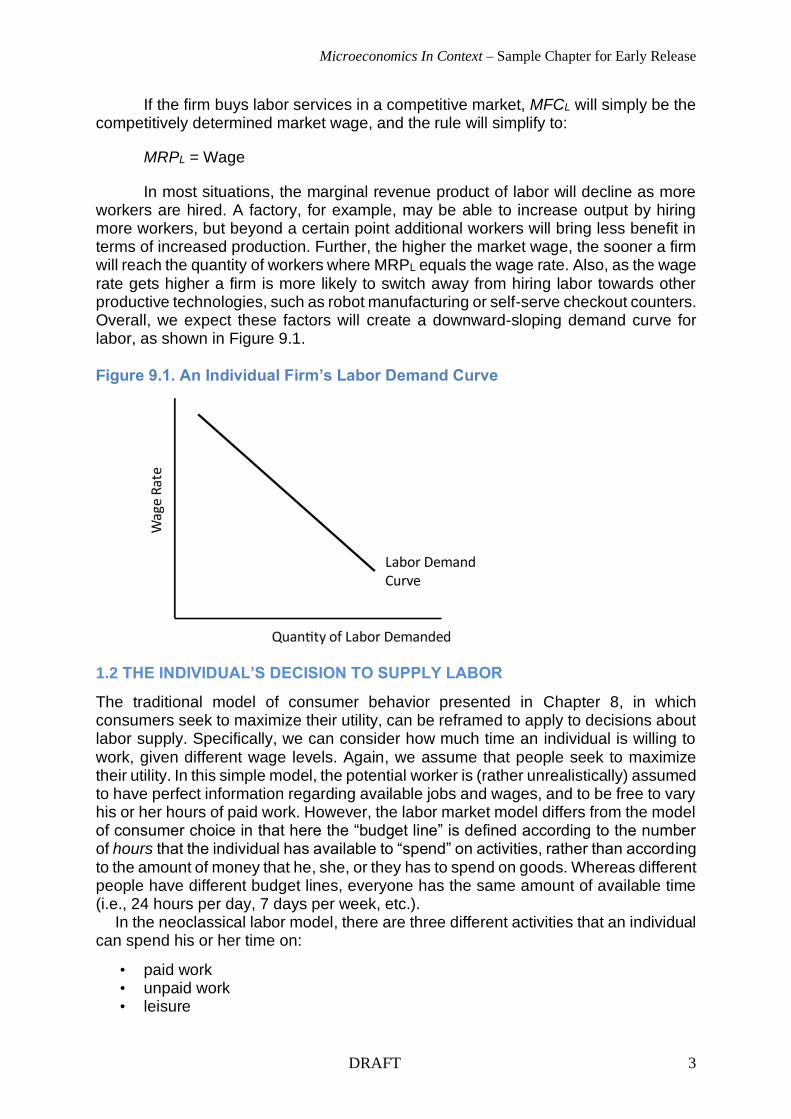
As discussed earlier in the chapter, the labor force participation rate is the percentage of noninstitutionalized adults that are either working or seeking a job. Of course, many people, such as students, retirees, or those taking time off from working for personal reasons such as childcare or health concerns don’t want – or may not need – a job. The U.S. labor force participation rate in 2021 was 61 percent but looking at Figure 9.9 we see that this rate differs between men and women over time. Male labor force participation has been steadily declining since 1960, while that of females steadily increased up to 2000 before leveling off. It has since also been declining, albeit less sharply than for males.


DRAFT 22

Figure 9.9. Labor Force Participation Rates in the United States, 1960–2021

Source: U.S. Bureau of Labor Statistics, 2021e.

What explains these trends? The increase in female labor participation up to 2000 largely reflects increased work opportunities for females. Reduction in the gender pay gap meant that the opportunity cost to females of not working increased, thus increasing female labor supply. To some extent, the decline in male labor force participation in the 1960s and 1970s can also be attributed to a greater gender balance in paid work within families. But more recently, labor force participation has been declining for both men and women, particularly after the Great Recession and during the COVID-19 pandemic. The reduction in labor market participation due to the pandemic has been greater for women, particularly black and Hispanic women as many lost jobs in the leisure and service sectors.48

Over the last several decades the United States has gone from having one of the highest labor force participation rates among industrialized countries to one of the lowest.49 Economists attribute this recent decline to two main factors: that many people have dropped out of the labor force due to frustration when looking for acceptable jobs and other difficulties; and that demographic changes are putting downward pressure on labor force participation.50 The demographic changes include an aging population and higher average educational attainment. An increasing share of Americans are retired, and thus voluntarily out of the labor force (although this group could include some who involuntarily retired early due to lack of job opportunities). Also, a higher proportion of young (and some older) people are attending college and graduate school, also voluntarily removing themselves from the labor force for a time.

Economists are more concerned about people dropping out of the labor force due to frustration at not finding employment or other difficulties. The U.S. Bureau of Labor Statistics measures the number of “discouraged workers”—those who have looked for a job within the last year but stopped because they believed there were no jobs available matching their skills.51 The number of discouraged workers in the United States decreased steadily during the 2010s, but more than doubled during the peak of the COVID-19 pandemic.52


DRAFT 23

Currently, some labor market researchers have shifted their attention to the opioid crisis as an explanation for the decline in labor force participation, particularly among males of prime working age (aged 25–54) with lower education levels. A 2018 paper finds a significant negative relationship between opioid prescription rates and labor market participation.53 The authors estimate that resolving the opioid crisis would increase labor market participation among prime-aged males by four percentage points.

3.2 LABOR MARKET FLEXIBILITY

For most of the twentieth century, Americans generally thought of “a job” (or at least a good job) as something that you typically did Monday through Friday, 40 hours a week, for a wage or salary and benefits (such as health insurance and pension plans). People often expected to stay in the same job for years or even decades. In recent years, however, it has become popular to talk about how employment is becoming more “flexible.” But the term “flexibility” has two very different meanings, depending on whether it is considered from the point of view of the worker or the employer.

One meaning of “flexible” work is that it is more suited to workers’ varying needs. Such work arrangements include flexibility in setting hours, job sharing, and the ability to work from home at times. Workers may be able to adjust their starting and quitting times, for example to make commuting or dropping off a child at school or day care easier. They may also be able to “compress” a standard workweek by working longer daily hours and taking a weekday off every week or every other week. Job sharing typically means that two employees work part-time, essentially sharing a full-time job between them. Working from home, even if only occasionally, reduces commuting time and costs, and allows workers to care for children or other relatives at home. Research shows that not only are flexible workers more satisfied with their jobs, but they also tend to be more productive and take sick leave less often.54

As a result of the COVID-19 pandemic, many workers worked from home to reduce their exposure to illness. But a 2021 survey by the U.S. Census Bureau finds that the ability to telework varies significantly by income level.55 While 73 percent of workers making more than $200,000 per year were able to switch to working at home during the pandemic, 32 percent of those making between $50,000 and $75,000 were able to make the switch, and only 13 percent of those making less than $25,000.

A somewhat different type of employment flexibility from the perspective of workers are “gig” jobs. These are jobs, part-time or full-time, that involve working under short-term contracts doing consulting, freelance, project-based, or other work. A common example is drivers for ride services such as Uber and Lyft who work when they want to and are needed. As mentioned at the start of this chapter, an increasing number of workers in the U.S. and elsewhere participate in the gig economy, either by choice or necessity. Gig workers in the U.S. are disproportionately minority and young, with relatively low incomes. While most gig workers describe their work as a side job, more than half say the extra income is “essential” or “important” for meeting their basic needs.56 The majority of gig workers in the U.S. are satisfied with their work, but gig workers are less likely to have employment benefits such as paid vacations and health care.57 The COVID-19 pandemic led to a significant increase in the number of gig workers, as the demand for services such as food delivery increased. For more on the impact of the pandemic on labor markets, see Box 9.3.

Employment “flexibility” from the perspective of the employer generally refers to having more control over setting workers’ hours and pay, offering few or no benefits, and being able to terminate employees quickly and without fuss. Laws that regulate


DRAFT 24

how easy it is to terminate employees can affect a firm’s hiring decisions. For example, labor law changes instituted in France in 2016 gave firms greater discretion when laying off or firing employees.58 The rationale was that it had become so difficult to terminate employees in France that firms were hesitant to hire new workers, especially in response to temporary economic improvements that might necessitate layoffs later.

It is likely that a desire for flexibility from the employer perspective is driving the gig economy at least as much as the demand side by workers. By hiring contract workers, employers avoid providing benefits such as health care and retirement plans. Workers paid as consultants bear the full burden of social insurance taxes, while firms must contribute half of these taxes for regular workers. Firms can also adjust the hours of gig workers, or terminate them, as economic conditions change, much easier than with traditional employees. BOX 9.3. THE GREAT RESIGNATION

Starting in early 2021 unprecedented numbers of workers in the United States, Germany, the United Kingdom, China, and other countries began quitting their jobs. Over 40 percent of the global workforce considered leaving their jobs in 2021, an effect dubbed “the Great Resignation.”59 Some of the resignations represent people who wanted to quit during the depths of the COVID-19 pandemic but were hesitant given uncertainty about the future. But the main factor seems to be that many workers are rethinking what they want out of their jobs as the economy recovers from the pandemic.60 Employees in many sectors became accustomed to the advantages of remote work during the pandemic and are refusing to return to in-person jobs. Many women, in particular, are seeking long-term jobs where they can combine telework with household production such as raising children. Other workers are quitting as a result of stress and burnout during the pandemic and are seeking a better work-life balance.

The Great Resignation is not universal throughout the workforce. In the United States, it is being driven by middle-aged workers, while resignation rates are actually down for the youngest and oldest workers. Resignation rates are also down in the manufacturing sector, but up significantly in the retail, health care, and technology sectors. Preliminary data suggest that blue-collar workers are quitting largely to seek higher wages, while white-collar workers are quitting to seek more flexible work arrangements.61

While it’s unclear yet whether resignation rates will remain at historically high levels, most labor experts believe the COVID-19 pandemic has produced long-term changes in labor markets. Professor Isabell Welpe, of the Technical University of Munich, states that “how we organize work and work together will not return to the way it was before the pandemic.” She sees a large-scale transition towards hybrid work, where employees might come to an office only one or two days per week, while working remotely the majority of the time.62

3.3 LABOR MARKETS AND IMMIGRATION

One of the most controversial topics in discussions of labor markets and wages is the impact of immigration, particularly the immigration of workers seeking low-wage jobs. According to the neoclassical labor model, an influx of unskilled workers willing to work for relatively low wages (an increase in labor supply) will drive down equilibrium wages in markets for unskilled labor and displace some domestic workers. But greater labor


DRAFT 25

supply may also increase economic output and productivity. Another question is whether immigrants contribute sufficient tax revenue to finance their use of public services.

Most economists find that immigration into the United States does not have a negative impact on the wages of most U.S.-born workers.63 In many cases, immigrants and native-born workers do not compete for the same jobs and may actually complement each other. For example, low-skilled immigrants tend to be concentrated in sectors such as agriculture and hospitality, with native-born workers concentrated in other sectors of the economy. Also, immigrants’ demand for goods and services supports many jobs, driving up wages in some labor markets. Overall, most economists conclude that immigration leads to a slight increase in wages for U.S.-born workers, although some studies find a negative impact for U.S.-born workers without a high school degree.

According to researchers at the University of Pennsylvania, immigration into the United States has the following impacts on the economy, workers, and taxes:64

• Immigrants mainly compete in labor markets with other immigrants. Thus, while wages for U.S.-born workers do not decrease, an influx of immigration drives down wages for those immigrants already in the country.

• Overall, immigrants increase innovation as they account for a disproportionate share of patents, science graduates, and senior positions at top venture capital firms.

• For the entire nation, immigration (including undocumented immigration) improves the government’s fiscal balance as immigrants pay more in taxes than they consume in government services. However, some states with a large concentration of low-skilled immigrants are negatively impacted, as such immigrants pay less in taxes and use more public services, particularly education.

Perhaps the most comprehensive analysis of the impact of immigration on the U.S. economy is a 2017 report by the National Academies of Science, Engineering, and Medicine.65 Over 600 pages in length, it reviews hundreds of studies on the topic. Like the above studies, it concludes that immigration has little impact on the wages or employment levels of native-born Americans. Low-skilled immigrants reduce prices for consumers in certain sectors, including childcare, construction, and house cleaning. As immigrants tend to be younger than average Americans, they also help balance the overall aging of the American population.

A recent consensus has also emerged that educated immigrants actually increase the wages of native-born workers, based on the productivity gains resulting from innovation and worker interactions. Current immigrants tend to be, on average, more educated than earlier waves of immigrants. The report concludes that the “prospects for long-run economic growth in the United States would be considerably dimmed without the contributions of high-skilled immigrants.”66

Note that the above analyses consider immigration as a whole, both documented and undocumented. Much of the political debate on immigration, in contrast, focuses almost exclusively on undocumented immigrants. Economic research has found that undocumented immigrants depress the wages of native-born workers without a high school degree, by between 1 and 7 percent.67 But the net impact on the country is generally positive, for several reasons. With undocumented workers concentrated in low-skilled positions, other workers focus on higher-productivity tasks. According to the Congressional Budget Office, between 50 and 75


DRAFT 26

percent of undocumented workers pay taxes.68 The consensus among economists is that undocumented workers pay more in taxes than they receive in public services. At the federal level, they clearly subsidize Social Security, contributing about $15 billion per year but receiving only about $1 billion, as most are ineligible for Social Security benefits.69 But undocumented workers impose net costs on state and local governments, mainly due to education and health care spending. The CBO concludes, however, that spending by state and local governments on undocumented workers “represents a small percentage of the total amount spent by those governments to provide such services to residents in their jurisdictions.”70

3.4 COOPERATIVES

Much of the discussion in this chapter has assumed a working arrangement in which the goals of the “employee” do not necessarily align with those of the “employer.” For example, we discussed how “flexibility” can mean very different things to employees and employers. In most companies, top executives seek to maintain (or increase) worker productivity while lowering wage costs, as it leads to higher profits. From the perspective of workers, however, increases in wages are seen as desirable, and workers may have little concern for the profitability of the company.

Worker cooperatives are an alternative kind of firm organization that seeks to reduce or eliminate the potential for labor conflicts by arranging that the owners of the enterprise are the workers themselves. Worker cooperatives are sometimes viewed as a “third way” of labor organization, in contrast to for-profit companies and government-run enterprises. The organizational structure of worker cooperatives can vary, but in a typical cooperative every worker is also an owner. Worker cooperatives normally do seek to make a profit, and any profits are distributed among the worker-owners (in addition to receiving wages or a salary). Some workers may hold more ownership shares than others and thus receive a greater share of profits, perhaps because of seniority, but in many cooperatives all workers have equal ownership shares. Important decisions are generally voted upon by all worker-owners, including decisions about wages, working hours, and benefits. Despite any differences in ownership shares, decisions are typically made on a “one person, one vote” basis.

worker cooperatives: a labor arrangement in which the owners of an enterprise are the workers themselves

Worker cooperatives arose as an alternative labor framework during the Industrial Revolution. Cooperatives are found throughout the world, the most famous being the Mondragón Cooperative Corporation in the Basque region of Spain, founded in 1956. Mondragón consists of more than 250 separate cooperatives with a total of about 75,000 worker-owners.71 Some of the differences between Mondragón and a typical capitalist company can be described as follows:

One of the co-operatively and democratically adopted rules governing [Mondragón] limits top-paid worker-members to earning 6.5 times the lowest-paid workers. Nothing more dramatically demonstrates the differences distinguishing this from the capitalist alternative organization of enterprises. . . . [I]ts pay equity rules can and do contribute to a larger society with far greater income and wealth equality than is typical in societies that have chosen capitalist organizations of enterprises. Over 43 percent of members are women, whose equal powers with male members likewise influence gender relations in society different from capitalist enterprises.72


DRAFT 27

Italy has about 8,000 worker cooperatives, and France has nearly 2,000. In India, the India Coffee House is a cooperative restaurant chain with nearly 400 locations.73 In the United States, the U.S. Federation of Worker Cooperatives, whose membership comprises nearly 100 cooperatives representing 6,000 workers, promotes cooperative formation, advocacy, and development.74 One example of a successful worker cooperative in the United States is the Evergreen Cooperatives in Cleveland, OH, based in a low-income neighborhood and providing living wage jobs. The cooperative’s main business is an environmentally conscious laundry facility that provides service to local hospitals.75

Based solely on economic performance such as worker productivity, the evidence suggests that worker cooperatives can perform at least as well as traditional capitalist companies.76 According to a 2011 paper that studied Mondragón, cooperative member-owners tend to be better paid than their peers in comparable firms, with greater opportunities for involvement and training.77 Although the cooperative labor framework is a “viable and possibly even superior alternative” to the traditional capitalist firm, it is not a “universal panacea” either. For example, job satisfaction was lower in cooperatives than traditional firms, perhaps a reflection of higher worker expectations. Obviously, estimating the overall impact of worker cooperatives on well-being requires a multifaceted analysis in which all factors cannot be easily quantified.

3.5 WORK–LIFE BALANCE

Paid work can both enhance and reduce well-being. But even for those who truly enjoy their work, a balance is needed between working and other activities that enhance well-being. Various recent studies demonstrate a positive correlation between work-life balance and subjective wellbeing. For example, a 2018 study asked over 30,000 workers in South Korea how well their work hours fit in with their commitments outside of work.78 Those with a better work-life balance reported higher subjective wellbeing. A 2019 study of workers in Pakistan also found that those who were more satisfied with their work-life balance reported higher average subjective wellbeing.79 Similarly, a positive correlation between work-life balance and SWB has been obtained in the United Kingdom,80 China,81 and Indonesia.82

Recall from Box 1.2 that work-life balance is one of the 11 dimensions included in the Better Life Index. The BLI measures work-life balance using two variables: the percent of employees that work very long hours (50 or more hours per week) and the daily amount of time full-time workers devote to personal care (sleeping, eating, etc.) and leisure. The share of workers that work more than 50 hours per week is 25 percent in South Korea, 18 percent in Japan, 11 percent in the United States, 4 percent in Germany, and only 1 percent in Sweden. The top five countries ranked by work-life balance are the Netherlands, Italy, Denmark, Spain and France, with the United States ranking 29th out of 40 countries.

Another variable commonly used to assess work-life balance is the average amount of time a worker spends working. In the United States, workers spend an average of about 35 hours per week on the job.83 While workers in low- and middle-income countries tend to work the most hours per year, Americans work more hours per year, on average, than most other industrialized countries, as shown in Figure 9.10. Americans work, on average, about 120 hours more per year than Canadian workers, 370 hours more than French workers, and 440 hours more than German workers. Note that the difference between American and German workers equates to 11 full 40-hour workweeks per year!


DRAFT 28

National policies regarding paid vacation and holidays explain much of the differences shown in Figure 9.10. The United States is the only OECD nation, and one of the only countries globally, that does not require employers to provide any paid vacation time or holidays. Meanwhile, national laws entitle all employees to at least 13 paid days off per year in Mexico, 16 days in China, 22 days in Brazil, 30 days in Germany, and 36 days in France.84 Movements in Europe toward shorter standard working hours have often been motivated by macroeconomic considerations, with the goal of reducing unemployment. Also, unions tend to be more prominent in European countries, effectively advocating for workers’ rights.

Even when American workers are able to take paid vacations, many do not fully utilize them over concerns about falling behind or appearing unproductive. According to one survey, more than half of U.S. workers who receive vacation days use half or less of their available time off. And even when Americans do take time off, most indicate that they end up doing some work during their vacations.85 Research has shown that the well-being benefits of vacations include reduced stress, lower risk of heart disease, improved mental health, and even better relationships.86

Figure 9.10. Average Annual Hours Worked, Select Countries, 2020

Source: OECD, OECD.Data, “Hours Worked.”

The United States is also the only industrialized nation that does not mandate employers to provide paid leave to new parents. According to the Family and Medical Leave Act of 1993, U.S. workers are entitled to up to 12 weeks of unpaid time off to care for a new child, or for a personal or family medical reason. But workers in other nations receive paid time off for these reasons, and for much longer periods. For example, in France new mothers are entitled to 42 weeks of leave at an average of 45 percent of their normal salary. In Germany new mothers receive 58 weeks off at 73 percent of their normal salary.87 Many nations also allocate some paid parental leave specifically to fathers. Japan entitles new fathers up to 30 weeks of paid parental leave, while Norway, Portugal, and Iceland provide them with around two months of paid leave.88


DRAFT 29

3.6 LABOR MARKETS, INEQUALITY, AND POWER

In Section 2 we explored various theories regarding wage differences across workers and occupations. In this final section, we consider labor markets in a broader context of the business sphere and political power. For example, how much do firms pay their workers as compared to what they pay to top executives, and how much do they claim in profits?

Figure 9.11 repeats a graph that we presented in Chapter 0, showing the time trend for real (inflation-adjusted) median weekly wages and corporate profits in the United States from 1980 to 2020. After adjusting for inflation, median weekly wages in 2020, around $980, were only about 20 percent higher than they were in 1980. Meanwhile, corporate profits (also adjusted for inflation) nearly tripled, reaching more than $2 trillion.

One interpretation of Figure 9.11 is that the economic gains in the business sphere over the last several decades were almost entirely “captured” as profits to corporations rather than wage increases for workers. Some rough calculations suggest that if half of the increase in corporate profits from 1980 to 2020 had instead been allocated to increasing employees’ wages, workers’ incomes would be at least 10 percent higher than they are today. As we will see in the next chapter, the stagnation of workers’ wages is a leading reason for the increase in economic inequality in the United States since the 1970s.

Historical data indicate that American workers fared much better earlier in the twentieth century. According to the U.S. Census Bureau, real average annual earnings increased by a factor of about four between 1900 and 1970.89 During the 1970s real earnings essentially stopped increasing. Household income continued to increase slightly beyond the 1970s, only because more people per household entered the labor force. Figure 9.11. Real Median Weekly Wages Versus Real Corporate Profits, United States, 1980–2020

Sources: Federal Reserve Bank of St. Louis, Federal Reserve Economic Data.


DRAFT 30

Figure 9.11 suggests that corporations have effectively been able to increase their profits dramatically in the past few decades without having to pay their workers higher wages and salaries. Meanwhile, the incomes of management executives, particularly those at the very top, have soared. The average compensation of chief executive officers (CEOs) of large U.S. corporations in 1965 was 20 times the pay of an average worker. But in 2020, CEO average compensation stood at 351 times the pay of an average worker!90

Are CEOs really worth so much more today than they were 50 years ago, as a result of an increase in their marginal revenue product? Nobel Prize-winning economist Joseph Stiglitz notes that the evidence for extremely high CEO incomes accurately reflecting the marginal revenue increases the executives earn for their companies “remains thin.”91 It is much more likely that these trends indicate a shift in economic power, away from workers and toward corporate profits and executive compensation. American workers have lost economic power as a result of various factors, including globalization and technological change. Globalization has allowed corporations to outsource labor needs to low-wage countries such as China, India, and Bangladesh, reducing the demand for domestic workers. Similarly, technological changes have also reduced the demand for some workers, as many tasks can now be done by robots or computers. In the next chapter we will further discuss the role of globalization, technological change, and labor unions in explaining recent trends in economic inequality.

Economic power is closely related to political power. Prior to the 1970s, corporate influence on American politics was more limited, with lobbying by corporations that was partly balanced by the efforts of labor unions and organizations advocating for broader public interests. But the balance of political power began to shift dramatically in the 1970s and 1980s as corporations ramped up their lobbying efforts:

[B]usiness lobbying has built itself up over time, and the self-reinforcing quality of corporate lobbying has increasingly come to overwhelm every other potentially countervailing force. It has also fundamentally changed how corporations interact with government—rather than trying to keep government out of its business (as they did for a long time), companies are now increasingly bringing government in as a partner, looking to see what the country can do for them.92

Thus, the explanation for the stagnation of median wages in Figure 9.11 is found in a mix of both market forces and political power. Both sides of the political spectrum discuss the importance of increasing wages for “middle-class Americans.” But what policies could be instituted to foster broadly shared wage growth?

According to a 2015 paper, “the potential has existed for adequate, widespread wage growth over the last three-and-a-half decades, but these economic gains have not trickled down to the vast majority.”93 The authors conclude that this unequal distribution of economic gains is primarily a result of various policies, and that reversing this trend will necessitate policy changes, including:

• Increased public infrastructure investment: It is widely recognized that the United States faces a shortfall of investment in transportation, research, education, and other infrastructure. Public spending on such projects could create many well-paying jobs.


DRAFT 31

• Targeted employment programs: Low wages and high unemployment are concentrated in certain regions of the United States, normally with large minority populations. Government policies to create decent jobs could be focused on such regions.

• Raising the minimum wage: Adjusted for inflation, the minimum wage in the United States is about 30 percent below its 1968 level! We will further discuss the debate about the minimum wage in the next chapter.

• Policies that strengthen rights to collective bargaining: The authors conclude that the decline of collective bargaining power by labor unions is the “single largest factor suppressing wage growth for middle-wage workers over the last few decades.”

• Increasing the rights of undocumented workers: As undocumented workers are often subject to exploitation and low wages, the authors suggest that expanding their rights, including a path to citizenship, would lead to higher wages.

• Providing more paid leave: As we saw earlier in the chapter, the United States lags far behind most other nations in providing workers paid time off for parental leave.

• Reducing race and gender wage inequality: The authors argue for stronger enforcement of anti-discrimination laws regarding the hiring, promotion, and wages of women and minority workers.

These or other policies aimed at increasing equity and raising wages involve a number of different areas of economic analysis. In the next chapter we look in more detail at the overall issue of economic inequality. In Chapter 11 we focus on taxes, which have a significant impact on income distribution. And we return to the issue of corporate power in Chapter 17, where we look at the relationship between market power and profit maximization. Discussion Questions

1 What evidence have you seen—in your own experience, others’ experiences, or through the media—of increasing “flexibility” in labor markets? Do you think that these changes have been beneficial, harmful, or both?

2 Do you think that the relative wages of average workers and top executives reflect their respective marginal revenue product? What kinds of policies would you favor regarding worker pay and executive compensation?

REVIEW QUESTIONS

1. In the neoclassical labor model, how does a firm decide on the quantity of labor to hire?

2. What are some of the opportunity costs of paid employment? 3. Why might the individual labor supply curve bend backward? 4. Why can we generally assume that market labor supply curves will slope upward? 5. In what types of labor markets might labor supply be relatively wage elastic? In

what types of markets might labor supply be relatively wage inelastic? 6. How can we use a supply-and-demand graph to illustrate the operation of a labor

market? 7. How does the neoclassical labor model explain variations in wages? 8. How is human capital important in explaining wage variations? 9. What is monopsony?


DRAFT 32

10. What is oligopsony? 11. What is efficiency wage theory? 12. What are dual labor markets? 13. How can we identify labor discrimination? 14. What is occupational segregation? 15. How has labor market participation changed in the United States in recent

decades? 16. What is employment flexibility from the perspective of workers? From the

perspective of employers? 17. What is the economic evidence about how immigration affects wages? 18. What are worker cooperatives, and how do they differ from traditional firms in terms

of labor organization? 19. How do average work hours per year in the United States compare to most other

countries? 20. How do paid vacation and leave policies in the United States compare to most

other countries? 21. What has been the trend in median wages in the United States in the past few

decades? How does this compare with the trend in corporate profits? 22. What is the role of political power in explaining the stagnation of median wages in

the United States in recent decades? EXERCISES

1. Reviewing Chapters 3 and 4 if necessary, illustrate on a labor market graph the following examples that were described in the text.

a. A relatively elastic supply curve for wait staff. b. A virtually “fixed” supply of aerospace engineers, in the short run. c. The effect on the supply of lawyers of the reduction of barriers to women’s

participation in the practice of the law. d. The effect on the market for wait staff of a rise in the wage of salesclerks.

2. Draw labor market graphs illustrating the following examples that were mentioned in the text.

a. A labor demand curve, when very good substitutes for labor in the production process exist.

b. The effect of a drop in demand for the organization’s product. c. The effect of a rise in the price of other inputs that have been used as

substitutes for labor.

3. Suppose that you observe that the wages for accountants in your town have gone up and that the number of accountants employed has also gone up. Which one of the following conditions could explain this? Illustrate your answer with a graph and explain in a brief paragraph.

a. Businesses are failing, reducing the need for accountants. b. Many accountants are leaving the field in order to train to become financial

analysts instead. c. A rash of business scandals has increased the demand for auditing services

performed by accountants. d. The local university has just graduated an unusually large group of

accountants.


DRAFT 33

4. The U.S. Bureau of Labor Statistics keeps track of the average wages and number of workers involved in various occupations over time and also makes projections about what jobs may show the most growth in the future. Using data available at the bureau’s Web site, www.bls.gov, try to look up information on an occupation that interests you. How does it pay, compared to other jobs? Is demand projected to rise in the future?

5. Match each concept in Column A with an example in Column B.

Column A Column B

a. An alternative to wage employment b.The income effect on individual labor supply c. A cause of a shift in the demand for professors d. A cause of a shift in the supply of professors e. Using education as a “signal” f. Labor market monopoly g. Labor market monopsony h. Cooperatives i. Occupational segregation j. Efficiency wages

1. “Insurance adjustor” jobs are traditionally given to men while “insurance representative” jobs go to women

2. Isabella cuts back her hours at her job after she gets a raise

3. Many professors reach retirement age

4. Acme Corp. hires only college graduates for sales jobs, but doesn’t care about their majors

5. Acme Corp. pays above prevailing market wages to motivate and retain its employees

6. Westinghouse is the major employer in the county

7. Marshall is the only person who knows how to run his company’s antiquated database

8. Household production 9. Workers are owners of the business 10. A rising college-student-age population

REFERENCES

Adobe. 2016. Work in Progress. May 2016. http://www.adobe.com/content/dam/acom/en/aboutadobe/pdfs/Future-of-Work-2016.pdf.

Aliprantis, Dionissi, and Mark E. Schweitzer. 2018. “Opioids and the Labor Market.” Working Paper 18-07, Federal Reserve Bank of Cleveland. May.

Anderson, Monica, Colleen McClain, Michelle Faverio, and Risa Gelles-Watnick. 2021. The State of Gig Work in 2021. Pew Research Center, December 8.

Anonymous. 2021. “The Next Great Disruption Is Hybrid Work – Are We Ready?” The Work Trend Index, Microsoft WorkLab, March 22. https://www.microsoft.com/en-us/worklab/work-trend-index/hybrid-work.

Anonymous. 2016. “The Effects of Immigration on the United States’ Economy,” Budget Model Background Brief, Penn Wharton, University of Pennsylvania, June 27.

Anonymous. 2014. “Statistics that Hurt: Racial Discrimination Still Affects Minority Wages.” Kellogg Insight, Kellogg School of Management at Northwestern University, January 8.

http://www.adobe.com/content/dam/acom/en/aboutadobe/pdfs/Future-of-Work-2016.pdf

http://www.adobe.com/content/dam/acom/en/aboutadobe/pdfs/Future-of-Work-2016.pdf


DRAFT 34

Arando, Saioa, Monica Gago, Derek C. Jones, and Takao Kato. 2011. “Efficiency in Employee-Owned Enterprises: An Econometric Case Study of Mondragon.” IZA Discussion Paper No. 5711, Bonn, Germany, May 2011.

Arias, Maria A., and Restrepo-Echavarria Paulina. 2016. “Demographics Help Explain the Fall in the Labor Force Participation Rate.” The Regional Economist, 24(4):16–18.

Arvey, Richard D., Itzhak Harpaz, and Hui Liao. 2004. “Work Centrality and Post-award Work Behavior of Lottery Winners.” The Journal of Psychology, 138(5):404–420.

Association of American Medical Colleges (AAMC). 2021. The Complexities of Physician Supply and Demand: Projections From 2019 to 2034. Washington, D.C., June.

Bargain, Olivier, Kristian Orsini, and Andreas Peichl. 2011. “Labor Supply Elasticities in Europe and the US.” IZA Discussion Paper No. 5820, June 2011, Bonn, Germany.

Bertrand, Marianne, and Sendhil Mullainathan. 2003. “Are Emily and Greg More Employable than Lakisha and Jamal? A Field Experiment on Labor Market Discrimination.” National Bureau of Economic Research, Working Paper 9873, Washington, DC, July.

Blau, Francine D., and Christopher Mackie (editors). 2017. “The Economic and Fiscal Consequences of Immigration.” Panel on the Economic and Fiscal Consequences of Immigration, The National Academies of Science, Engineering, and Medicine, Washington, DC.

Blau, Francine D., and Lawrence M. Kahn. 2016. “The Gender Wage Gap: Extent, Trends, and Explanations.” National Bureau of Economic Research, Working Paper 21913, Washington, DC, January.

Bowling, Nathan A., Kevin J. Eschleman, and Qiang Wang. 2010. “A Meta-analytic Examination of the Relationship between Job Satisfaction and Subjective Well-Being.” Journal of Occupational and Organizational Psychology, 83:915–934.

Calfas, Jennifer. 2017. “Why Most Americans Aren’t Using All of their Vacation Days.” Time, May 29.

Center on Budget and Policy Priorities. 2017. “Chart Book: The Legacy of the Great Recession.” September 12.

Chugh, Abhinav. 2021. “What Is ‘the Great Resignation’? An Expert Explains.” World Economic Forum, November 29.

Congressional Budget Office (CBO). 2007. “The Impact of Unauthorized Immigrants on the Budgets of State and Local Governments.” December 2007.

Cook, Ian. 2021. “Who Is Driving the Great Resignation?” Harvard Business Review, September 15.

Davidson, Adam. 2013. “Do Illegal Immigrants Actually Hurt the U.S. Economy?” The New York Times, February 12.

Day, Jennifer Cheeseman, and Eric C. Newburger. 2002. “The Big Payoff: Educational Attainment and Synthetic Estimates of Work–Life Earnings.” U.S. Census Bureau, Current Population Reports, P23–210.

Dill, Michael. 2021. “We Already Needed More Doctors. Then COVID-19 Hit.” AAMC Insights. June 17. https://www.aamc.org/news-insights/we-already-needed-more-doctors-then-covid-19-hit.

Doucouliagos, Chris. 1995. “Worker Participation and Productivity in Labor-Managed and Participatory Capitalist Firms: A Meta-Analysis.” Industrial and Labor Relations Review, 49(1):58–77.

https://www.aamc.org/news-insights/we-already-needed-more-doctors-then-covid-19-hit

https://www.aamc.org/news-insights/we-already-needed-more-doctors-then-covid-19-hit


DRAFT 35

Drutman, Lee. 2015. “How Corporate Lobbyists Conquered American Democracy.” The Atlantic, April 20.

Editorial Board. 2013. “Nevada Must Get Creative Solutions for Doctor Shortages.” Reno Gazette-Journal, August 3.

Edo, Anthony. 2019. “The Impact of Immigration on the Labor Market.” Journal of Economic Surveys, 33(3):922-948.

Fan, Jialin, and Andrew P. Smith. 2017. “Positive Well-Being and Work-Life Balance among UK Railway Staff.” Open Journal of Social Sciences, 5(6):1-6.

Ferguson, Jill L.2017. “Health Benefits of Taking a Vacation.” Huffpost, March 5. Fryer, Roland G., Jr., Devah Pager, and Jörg L. Spenkuch. 2013. “Racial Disparities

in Job Finding and Offered Wages.” Journal of Law and Economics, 56:633–689. Gardiner, Alistair. 2021. “COVID’s Effects on Doctor Supply and Demand, According

to Experts.” MDLinx, January 28. https://www.mdlinx.com/article/covid-s-effects-on-doctor-supply-and-demand-according-to-experts/4XhjJ2d46b8HZrScVK9T91.

Gaskell, Adi. 2016. “Why a Flexible Worker Is a Happy and Productive Worker.” Forbes, January 15.

Goldsmith, Arthur, and Timothy Diette. 2012. “Exploring the Link between Unemployment and Mental Health Outcomes.” The Socioeconomic Status Indicator (American Psychological Association), April.

Gould, Elise. 2020. “Black-white Wage Gaps Are Worse Today than in 2000.” Economic Policy Institute, Working Economics Blog, February 27.

Greenstone, Michael, and Adam Looney. 2012. “What Immigration Means for U.S. Employment and Wages.” The Hamilton Project, May 4.

Gunawan, G., Y. Nugraha, M. Sulastiana, and D. Harding. 2020. “Work-Life Balance and Subjective Well-Being among Employees on Life Science Company in Indonesia” in Advances in Business, Management, and Entrepreneurship. CRC Press, London.

Hodel, Kate. 2019. “How Many Slaves Are There Today, and Who Are They?” The Guardian, February 25.

International Labour Organization (ILO). 2018. Global Wage Report 2018/19: What Lies behind Gender Pay Gaps. Geneva.

Jones, Janelle. 2021. “5 Facts About the State of the Gender Pay Gap.” U.S. Department of Labor Blog, March 19.

Judge, Timothy A., and Ryan Klinger. 2008. “Job Satisfaction: Subjective Well-Being at Work,” in The Science of Subjective Well-Being (Michael Eid and Randy J. Larsen, editors). The Guilford Press, New York.

Kelly, Joshua. 2016. “France Wants to Make It Easier to Fire Workers so Employers Will Stop Harassing Them into Quitting.” PRI (Public Radio International), May 13.

Kline, Patrick M., Evan K. Rose, and Christopher R. Walters. 2021. “Systemic Discrimination among Large U.S. Employers.” National Bureau of Economic Research, Working Paper 29053, August.

Kochhar, Rakesh, and Jesse Bennett. 2021. “U.S. Labor Market Inches Back from the COVID-19 Shock, but Recovery Is Far from Complete.” Pew Research Center, April 14.

Krause, Eleanor, and Isabel Sawhill. 2017. “What We Know and Don’t Know About Declining Labor Force Participation: A Review.” The Brookings Institution, May.

Lichter, Andreas, Andreas Peichl, and Sebastian Siegloch. 2015. “The Own-wage Elasticity of Labor Demand: A Meta-regression Analysis.” European Economic Review, 80: 94–119.


DRAFT 36

Livingston, Gretchen. 2016. “Among 41 Nations, U.S. Is the Outlier when it Comes to Paid Parental Leave.” Pew Research Center, September 26.

Lufkin, Bryan. 2021. “What We’re Getting Wrong about the ‘Great Resignation’.” BBC, WorkLife, October 28.

Marshall, Joey, Charlynn Burd, and Michael Burrows. 2021. “Those Who Switched to Telework Have Higher Income, Education, and Better Health.” U.S. Census Bureau, March 31.

Martikainen, Pekka, and Tapani Valkonen. 1996. “Excess Mortality of Unemployed Men and Women during a Period of Rapidly Increasing Unemployment.” The Lancet, 348(9032):909–912.

Medical Group Management Association (MGMA). 2021. “Measuring the Toll COVID-19 Took on the Physician Workforce.” March 4. https://www.mgma.com/data/data-stories/measuring-the-toll-covid-19-took-on-the-physician.

Mishel, Lawrence, and Jori Kandra. 2021. “CEO Pay Has Skyrocketed 1,322% since 1978.” Economic Policy Institute, August 10.

Mishel, Lawrence. 2012. “Unions, Inequality, and Faltering Middle-Class Wages.” Economic Policy Institute, Issue Brief #342. Washington, DC.

Mishel, Lawrence, and Ross Eisenbrey. 2015. “How to Raise Wages: Policies That Work and Policies That Don’t.” Economic Policy Institute, Briefing Paper #391, March 19.

MOB Partners. 2021. 11th Annual State of Independence in America: Data Highlights and Preview. August.

Molla, Rani. 2021. “More Americans Are Taking Jobs without Employer Benefits Like Health Care or Paid Vacation.” Vox, September 3.

Nunley, John M., Adam Pugh, Nicholas Romero, and Richard Alan Seals, Jr. 2014. “An Examination of Racial Discrimination in the Labor Market for Recent College Graduates: Estimates from the Field.” Auburn University, Department of Economics, Working Paper AUWP 2014-06, March 24.

Organisation for Economic Co-operation and Development (OECD). 2017. Key Characteristics of Parental Leave Systems. OECD Family Database. http://www.oecd.org/els/family/database.htm.

Pew Research Center. 2016. The State of American Jobs. October. Picchi, Aimee. 2017. “America’s Job Problem: Low-Wage Work Is Growing Fastest.”

CBS News, August 4. Quillian, Lincoln, Devah Pager, Ole Hexel, and Arnfinn H. Midtbøen. 2017. “Meta-

analysis of Field Experiments Shows No Change in Racial Discrimination in Hiring over Time.” Proceedings of the National Academy of Sciences, 114(41):10870-10875.

Schmitt, John, and Janelle Jones. 2012. “Where Have All the Good Jobs Gone?” Center for Economic and Policy Research, Washington, DC, July.

Shams, Khadija, and Alexander Kadow. 2019. “The Relationship Between Subjective Well-being and Work-Life Balance Among Labourers in Pakistan.” Journal of Family and Economic Issues, 40:681-690.

Stiglitz, Joseph E.2011. “Of the 1%, By the 1%, For the 1%.” Vanity Fair, March 31. Ton, Zeynep. 2012. “Why Good Jobs Are Good for Retailers.” Harvard Business

Review, 90(1-2):124. U.S. Bureau of Labor Statistics. 2021a. "Earnings and Unemployment Rates by

Educational Attainment." April 21. U.S. Bureau of Labor Statistics. 2021b. "Union Affiliation Data from the Current

Population Survey." Online data tools.

https://www.mgma.com/data/data-stories/measuring-the-toll-covid-19-took-on-the-physician

https://www.mgma.com/data/data-stories/measuring-the-toll-covid-19-took-on-the-physician


DRAFT 37

U.S. Bureau of Labor Statistics. 2021c. “Union Members Summary.” Economic News Release, January 22.

U.S. Bureau of Labor Statistics. 2021d. “Usual Weekly Earnings of Wage and Salary Workers, First Quarter 2021.” Economic News Release, April 16.

U.S. Bureau of Labor Statistics. 2021e. Labor Force Statistics from the Current Population Survey. BLS Data Series.

U.S. Bureau of Labor Statistics. 2021f. Average Weekly Hours and Overtime of All Employees on Private Nonfarm Payrolls by Industry Sector, Seasonally Adjusted. Table B-2, Economic News Release. December.

U.S. Census Bureau. 2022. “Equal Pay Day: March 15, 2022.” Release Number CB22-SFS.33. March 15.

U.S. Census Bureau. 2020. Educational Attainment in the United States: 2019. March 30.

U.S. Census Bureau. 1976. Bicentennial Edition: Historical Statistics of the United States, Colonial Times to 1970.Washington, DC.

U.S. Census Bureau. 1982. Statistical Abstract of the United States 1982–1983.Washington, DC.

Wartzman, Rick. 2017. The End of Loyalty: The Rise and Fall of Goods Jobs in America. Public Affairs, New York.

Watchner, Michael. 2007. “The Rise and Decline of Unions.” The Washington Post, July 18.

Weller, Torsten. 2021. “What’s Next for China’s Gig Economy?” China-Britain Business Focus, June 28. https://focus.cbbc.org/whats-next-for-chinas-gig-economy/#.Yaa1esfMI2w.

Wolff, Richard. 2012. “Yes, There Is an Alternative to Capitalism: Mondragon Shows the Way.” The Guardian, June 24.

Wong, Ka Po, Fion Choi Hung Lee, Pei-Lee The, and Alan Hoi Shou Chan. 2021. “The Interplay of Socioecological Determinants of Work-Life Balance, Subjective Well-Being and Employee Wellbeing.” International Journal of Environmental Research and Public Health, 18(9):4525.

Yang, Jae Won, Chunchui Suh, Chae Kwan Lee, and Byung Chul Son. 2018. “The Work-Life Balance and Psychosocial Well-being of South Korean Workers.” Annals of Occupational and Environmental Medicine, 30:38.

Zschirnt, Eva, and Didier Ruedin. 2016. “Ethnic Discrimination in Hiring Decisions: A Meta-analysis of Correspondence Tests 1990–2015.” Journal of Ethnic and Migration Studies, 42(7):1115–1134.

APPENDIX: A FORMAL MODEL OF A FIRM’S HIRING DECISION

Suppose that a firm produces disposable razors. Holding all other inputs fixed, the relationship between the number of workers (the “quantity of labor”) hired and the number of razors that can be produced in a day is given in the first two columns of Table 9.1. From these first two columns, the marginal physical product of labor (MPPL) of each additional worker can be computed. For example, one worker can produce 5 razors, but adding an additional worker makes possible the production of 12 razors, so the marginal physical product of the second worker is 7 razors. Note that the marginal physical product of labor first rises and then falls. marginal physical product of labor (MPPL): the amount that a unit of additional labor contributes to the physical product of a firm

https://focus.cbbc.org/whats-next-for-chinas-gig-economy/#.Yaa1esfMI2w

https://focus.cbbc.org/whats-next-for-chinas-gig-economy/#.Yaa1esfMI2w


DRAFT 38

We further assume that the firm sells razors in a competitive market and that

the price received per razor is constant at $3. Hence the marginal revenue product of labor (MRPL), the monetary value of the additional physical production, is always just $3 × MPPL. We assume that the firm buys labor in a perfectly competitive labor market, at a constant wage of $12. Hence the marginal factor cost of labor (MFCL) is constant at $12.

Table 9.1. Labor Analysis of Hypothetical Razor Firm

Quantity of labor Quantity of razors mppl mrpl mfcl

L 5 5 15 12

2 12 7 21 12

3 18 6 18 12

4 23 5 15 12

5 27 4 12 12

6 30 3 9 12

7 32 2 6 12

8 33 1 3 12

Figure 9.12. Marginal Revenue Product of Labor and Marginal Factor Cost of Labor

The MRPL and MFCL curves are graphed in Figure 9.12. The MRPL curve has an initial hump, because the MPPL initially increases and then declines. For all workers up to the fifth worker, hiring the additional worker adds more to revenues than to costs. The profit-maximizing firm should stop hiring workers when MRPL = MFCL, at an employment level of five workers.


DRAFT 39

NOTES

1 See, for example, Wartzman, 2017, Pew Research Center, 2016, and Schmitt and Jones, 2012. 2 Pew Research Center, 2016. 3 Mulcahy, 2016. 4 MOB Partners, 2021. 5 Weller, 2021. 6 Judge and Klinger, 2008. 7 Bowling et al., 2010. 8 Goldsmith and Diette, 2012; Martikainen and Valkonen, 1996. 9 Hodel, 2019. 10 Adobe, 2016. 11 Arvey et al., 2004. 12 We are assuming that the potential worker can enjoy at least a minimal standard of living from activities other than market work when the wage is too low to make market work attractive. In situations of dire poverty, however, this may not be the case, and people may need to work two or three jobs at extremely low wages just to maintain subsistence. 13 U.S. Bureau of Labor Statistics, Labor Force Participation Rate series from the Current Population Survey. 14 AAMC, 2021. 15 Editorial Board, 2013. 16 Gardiner, 2021. 17 MGMA, 2021. 18 Gardiner, 2021. 19 Dill, 2021. 20 Bargain et al., 2011. 21 Lichter et al., 2015. 22 Employment and wage data from the U.S. Bureau of Labor Statistics online database. 23 https://runrepeat.com/salary-analysis-in-the-nba-1991-2019. 24 Average annual salaries for aerospace engineers and preschool teachers from the U.S. Bureau of Labor Statistics, May 2020 National Occupational Employment and Wage Estimates. 25 Jones, 2021. 26 The last determinant of human capital is sometimes overlooked. However, malnourishment and mental or physical ill-health can seriously affect a worker’s energy, motivation, and general capacity to use his or her knowledge and skills. 27 Day and Newburger, 2002, p. 3. 28 OECD, Trade Union Dataset, OECD.Stat. 29 U.S. Bureau of Labor Statistics, 2021c. 30 See, for example, Watchner, 2007. 31 Mishel, 2012, p. 9. 32 Ton, 2012. 33 Ibid, online version, no page provided. 34 U.S. Census Bureau, 2020. 35 Ibid. 36 Brown and Patten, 2017. 37 Blau and Kahn, 2016. 38 ILO, 2018. 39 Gould, 2020. 40 Fryer et al., 2013. 41 Anonymous, 2014. 42 Bertrand and Mullainathan, 2003. 43 Nunley et al., 2014. 44 Kline et al., 2021. 45 Quillian et al., 2017. 46 Zschirnt and Ruedin, 2016. 47 https://www.bls.gov/oes/current/oes_nat.htm. 48 Kochhar and Bennett, 2021. 49 Krause and Sawhill, 2017. 50 Arias and Restrepo-Echavarria, 2016.

https://runrepeat.com/salary-analysis-in-the-nba-1991-2019


DRAFT 40

51 https://www.bls.gov/bls/glossary.litm. 52 U.S. Bureau of Labor Statistics, Labor Force Statistics from the Current Population Survey, https://data.bls.gov/timeseries/LNS15026645. 53 Aliprantis and Schweitzer, 2018. 54 Gaskell, 2016. 55 Marshall et al., 2021. 56 Anderson et al., 2021. 57 Molla, 2021. 58 Kelly, 2016. 59 Anonymous, 2021. 60 Cook, 2021. 61 Lufkin, 2021. 62 Chugh, 2021. 63 Greenstone and Looney, 2012; Edo, 2019. 64 Anonymous, 2016. 65 Blau and Mackie, 2017. 66 Ibid, pp. 6-7. 67 Davidson, 2013. 68 CBO, 2007. 69 Davidson, 2013. 70 CBO, 2007, p. 3. 71 https://en.wikipedia.org/wiki/Mondragon_Corporation. 72 Wolff, 2012, no page provided. 73 https://en.wikipedia.org/wiki/Worker_cooperative. 74 https://usworker.coop/home/. 75 http://www.evgoh.com/. 76 Doucouliagos, 1995. 77 Arando et al., 2011. 78 Yang et al., 2018. 79 Shams and Kadow, 2019. 80 Fan and Smith, 2017. 81 Wong et al., 2021. 82 Gunawan, 2020. 83 U.S. Bureau of Labor Statistics, 2021f. 84 Wikipedia, “List of Minimum Annual Leave by Country,” https://en.wikipedia.org/wiki/List_of_minimum_annual_leave_by_country. 85 Calf as, 2017. 86 Ferguson, 2017. 87 OECD, 2017. 88 Livingston, 2016. 89 U.S. Census Bureau, 1976, Series D; U.S. Census Bureau, 1982, Table 667. 90 Mishel and Kandra, 2021. 91 Stiglitz, 2011. 92 Drutman, 2015, no page provided. 93 Mishel and Eisenbrey, 2015, p. 2.

https://data.bls.gov/timeseries/LNS15026645

Chapter 9 Markets for Labor

Documents

Transcript of Chapter 9 Markets for Labor