CHAPTER 14 - Biblioteca Digital do IPB

386 Single and Two-Phase Flows on Chemical and Biomedical Engineering, 2012, 386-411

Ricardo Dias, Antonio A. Martins, Rui Lima and Teresa M. Mata (Eds) All rights reserved-© 2012 Bentham Science Publishers

CHAPTER 14

Mass Transfer Models for Oxygen-Water Co-Current Flow in Vertical Bubble Columns

Valdemar Garcia1 and João Sobrinho Teixeira2,*

1Instituto Politécnico de Bragança, Escola Superior de Tecnologia e de Gestão, Quinta de Santa Apolónia, 5300-999 Bragança, Portugal and 2Instituto Politécnico de Bragança, Escola Superior Agrária, Quinta de Santa Apolónia, 5301-857 Bragança, Portugal

Abstract: The present work reports a theoretical and experimental study of mass transfer for oxygen-water co-current flow in vertical bubble columns. The axial dispersion of liquid phase was also studied. Experiments were carried out in a 32 mm internal diameter and 5.35 and 5.37 m height columns. The superficial liquid velocity ranged from 0.3 to 0.8 m/s and volumetric flow rate ratio of gas to liquid ranged from 0.015 to 0.25. Mathematical models were developed to predict concentration of gas dissolved in the liquid as function of different physical and dynamic variables for two-phase co-current downflow and upflow. We obtained for the ratio of the liquid side mass transfer coefficient to initial bubbles radius, kL/r0=0.12 s-1.

Keywords: Vertical bubble columns, gas-liquid bubble flow, oxygen-water flow, oxygen-water mass transfer, mass transfer models, gas-liquid co-current downflow, gas-liquid co-current upflow, mass transfer coefficient, axial dispersion, liquid axial dispersion coefficient, U tube.

INTRODUCTION

The simultaneous gas and liquid flow frequently occurs in several situations and in many industrial applications such as distillation columns, chemical and nuclear reactors, pipelines for hydrocarbon mixtures transport, solar collectors, mass transfer equipments like bubble columns, packed columns, air lifts pumps, among others. Bubble columns, equipment where the gas phase is dispersed in small bubbles in continuous liquid phase, have been used as gas-liquid contactors

*Address correspondence to João Sobrinho Teixeira: Instituto Politécnico de Bragança, Escola Superior Agrária, Quinta de Santa Apolónia, 5301-857 Bragança, Portugal. E-mail: [email protected].

Mass Transfer Models for Oxygen-Water STP Flows on Chemical and Biomedical Engineering 387

devices, like as absorbers and/or strippers, chemical reactors for hydrogenation, oxidation or chlorination of organic liquids such as fermenters in wastewater biological treatment units.

Particularly, the air/oxygen-water flow can be found in areas where the water oxygenation is very important, like the aquaculture and the water treatment units (drinking, waste and river). The simultaneous flow of oxygen and water in co-current bubbly regime, first in downflow and then in upflow, occurs in a U tube, device with applications on referred areas [1-6].

The liquid mixing or axial dispersion is one of the parameters that can influence the process of mass transfer of gas to liquid and therefore must be known. The literature on liquid axial dispersion for bubble columns, especially for the air-water system, is extensive. Many empirical [7, 8] and theoretical [9-11] equations have been developed in order to predict the axial dispersion coefficient.

In the present work, the liquid phase mass transfer coefficients and the axial mixing (axial dispersion coefficients) of the liquid phase of vertical bubble columns operating with co-current downflow and upflow were determined for the oxygen-water system.

EXPERIMENTAL

The experiments were performed on two vertical bubble columns, linked in the bottom in U tube form, operating with co-current downflow and upflow of gas and liquid. The columns are respectively, 5.37 and 5.35 m height and 32 mm inside diameter.

Gas Absorption

The absorption experiments were performed in acrylic glass tubes. The liquid, tap water, was circulated in the tubes by a centrifugal pump and was introduced at the top of test section. The water flow rate was measured by a calibrated rotameter and was regulated by a ball valve. The gas used for all experiments was pure oxygen supplied by a high pressure bottle. The oxygen was introduced into the test column through a porous gas distributor installed at the top of the test section. The porous gas distributor allowed the formation of small diameter bubbles (about

388 STP Flows on Chemical and Biomedical Engineering Garcia and Teixeira

2-4 mm). The volumetric oxygen flow rate was determined with an electronic flow meter.

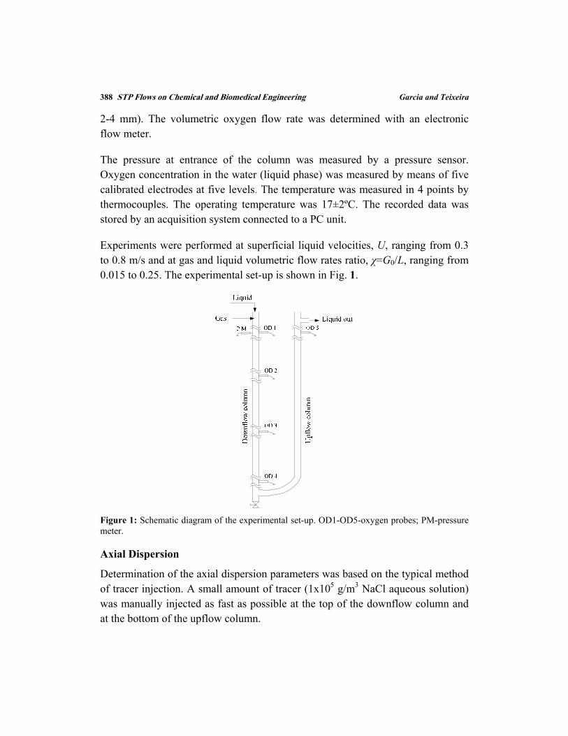
The pressure at entrance of the column was measured by a pressure sensor. Oxygen concentration in the water (liquid phase) was measured by means of five calibrated electrodes at five levels. The temperature was measured in 4 points by thermocouples. The operating temperature was 17±2ºC. The recorded data was stored by an acquisition system connected to a PC unit.

Experiments were performed at superficial liquid velocities, U, ranging from 0.3 to 0.8 m/s and at gas and liquid volumetric flow rates ratio, χ=G0/L, ranging from 0.015 to 0.25. The experimental set-up is shown in Fig. 1.

Figure 1: Schematic diagram of the experimental set-up. OD1-OD5-oxygen probes; PM-pressure meter.

Axial Dispersion

Determination of the axial dispersion parameters was based on the typical method of tracer injection. A small amount of tracer (1x105 g/m3 NaCl aqueous solution) was manually injected as fast as possible at the top of the downflow column and at the bottom of the upflow column.


The system response, consisting in the detection of the tracer concentration variation with the time, was obtained with two conductivity probes, made of a pair of platinum cells, located at distances of 4.26 m and 3.95 m from the tracer injection points. The conductivity probes, connected to a conductimeter and to a computer, were used to follow this time variation. The experimental set-up is shown in Fig. 2.

Figure 2: Experimental set-up for determination of the axial dispersion parameters.

THEORY

Axial Dispersion

Liquid mixing in a bubble column is usually described on the basis of the one-dimensional axial dispersion model, particularly if the ratio between length and diameter of the column is large.

A mass balance to the tracer, in the infinitesimal "slice" situated between the quotas x and x+dx of a column, with volume S x (see Fig. 3), leads to the equation that represents the model of axial dispersion:

2*

2 1A A A

L

C C CUD

t x x

(1)


where *LD represents the liquid axial dispersion coefficient, S is the column cross

sectional area, is the gas holdup, U is the superficial liquid velocity and CA is the concentration of tracer in the liquid at position x of column and at time t.

Response - Measurement of tracer

concentration

Tracer - Pulse input

GL

l

xx+dx

CACA +d CA

S

x

Figure 3: Schematic representation for the mass balance of the tracer in a bubble column.

Introducing the following variables:

m ; ; with

1m L

x t l lZ t

Ul t U

where l represents the axial distance between tracer injection point and tracer response point in the column, mt is the mean residence time that represents the ratio between the liquid volume in length l of column and the volumetric liquid flow rate what goes through it and LU is the real liquid velocity. equation (1) can be rewritten in the form:

2

2

1A A AC C C

Pe Z Z

(2)

where Pe represents the Peclet adimensional number for simultaneous gas and liquid flow:


* *

1 L

L L

Ul U l

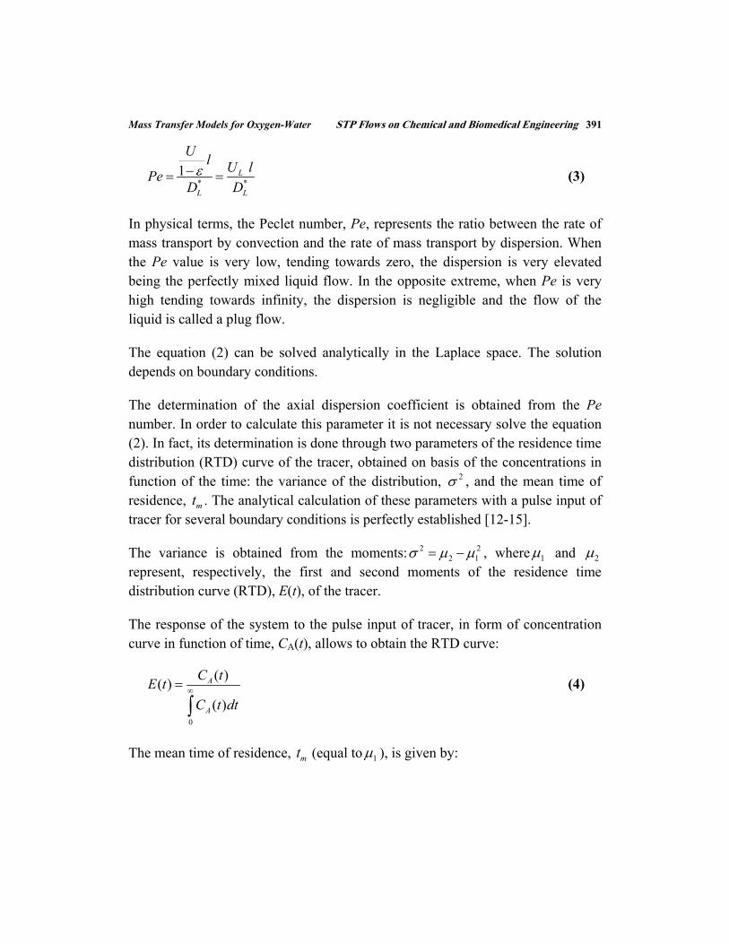
PeD D (3)

In physical terms, the Peclet number, Pe, represents the ratio between the rate of mass transport by convection and the rate of mass transport by dispersion. When the Pe value is very low, tending towards zero, the dispersion is very elevated being the perfectly mixed liquid flow. In the opposite extreme, when Pe is very high tending towards infinity, the dispersion is negligible and the flow of the liquid is called a plug flow.

The equation (2) can be solved analytically in the Laplace space. The solution depends on boundary conditions.

The determination of the axial dispersion coefficient is obtained from the Pe number. In order to calculate this parameter it is not necessary solve the equation (2). In fact, its determination is done through two parameters of the residence time distribution (RTD) curve of the tracer, obtained on basis of the concentrations in function of the time: the variance of the distribution, 2 , and the mean time of residence, mt . The analytical calculation of these parameters with a pulse input of tracer for several boundary conditions is perfectly established [12-15].

The variance is obtained from the moments: 2 22 1 , where 1 and 2

represent, respectively, the first and second moments of the residence time distribution curve (RTD), E(t), of the tracer.

The response of the system to the pulse input of tracer, in form of concentration curve in function of time, CA(t), allows to obtain the RTD curve:

0

( )( )

( )

A

A

C tE t

C t dt

(4)

The mean time of residence, mt (equal to 1 ), is given by:


0

0

0

( )

( )

( )

A i Ai ii

mAi i

A i

tC t dt t C tt tE t dt

C tC t dt

(5)

The variance of the E(t) curve is given by:

2 2

2 2 2 2 20

0

0

( )

( )

( )

A i Ai ii

m m mAi i

A i

t C t dt t C tt E t dt t t t

C tC t dt

(6)

Since injection of the tracer has been effectuated in a point below entrance the fluids in the column and the response, in terms of tracer concentration, has been obtained in a point before the end of the column, the system is considered "open" type [13, 15, 16], as shown in Fig. 3. Assuming that the bubble column is open to the liquid dispersion, the Peclet number is calculated using the following equation [13-15]:

2

2 2

2 8

mt Pe Pe

(7)

where tm and 2 are calculated for each experimental condition from the experimental values of tracer concentration AC vs. time, with equations (5) and (6), respectively. Therefore, the liquid axial dispersion coefficient *

LD can be determined by equation (3).

Mass Transfer Models

The oxygen transfer from the bubbles to the water in a co-current gas-liquid flow leads to a continuous increase of the dissolved oxygen concentration along the column, and can be applied a one-dimensional theoretical model to describe the mass transfer process.

The concentration profile along the tube can be obtained for a given operating condition (values of gas and liquid flow rate) when knowing the values of


variables and parameters at the tube entrance. In the model that we develop, we use as operating variables, the superficial liquid velocity, U, and the ratio of volumetric gas/liquid flow rate at entrance, . The values of variables and parameters at entrance that is necessary to know are: the pressure, P0, concentration, C0, the temperature, T, the Henry's constant, H, the density of water, , and the tube height, l.

We will present two models to describe the process of mass transfer from gas to liquid: one takes into account the axial dispersion of liquid and the other not.

Models without dispersion

Downflow

For an infinitesimally length dx, as shown in Fig. 4, the material balance in steady state for the dissolved oxygen in the liquid gives

*L ( ) d ( d ) k a C C S x L C C L C (8)

where a is the interfacial area per unit of column volume, C is the local concentration of oxygen solute dissolved in liquid, kL is the liquid side mass transfer coefficient, S is the column cross sectional area, L is the liquid (water) volumetric flow rate and C* is the solubility of gas solute in liquid (saturation concentration). This equation gives, after rearrangement, the basic equation of the model

*Ld ( )d

SC k a C C x

L (9)

In this model it is admitted, for each flow rate of water and of oxygen, that the bubbles that are formed in the inlet of the gas in the column are all of the same size, spherical, with equal velocity and the gas holdup is constant at entrance of the column. While the fluids go down in the tube, all the bubbles decrease in size equally with the increase of the pressure, so that in a determined section x, the bubbles take the same size and the gas holdup and the interfacial area per unit of column volume are constant.


GL

xx+dx

C

S

x

C +dC

x=0; P0; C0

Ub

Figure 4: Schematic representation of a gas-liquid downflow, initial point and scheme for the mass balance.

For a given volumetric gas flow rate, G, the total number of bubbles that crosses a section of column per unit of time, nt, is given by:

t / b b bn G V n S U (10)

where Vb represents the volume of a bubble, nb is the number of bubbles per unit of column volume and Ub is the bubbles velocity. Being a = nbAb, where Ab is the superficial area of a bubble, and combining with equation (10) we obtain:

3 1

b

Ga

r S U (11)

where r is the radius of a bubble. The retention of gas or gas holdup, , at any point of the column and Ub are obtained by the expressions of Nicklin [17]:

b

G

S U (12)

0 b

L GU U

S S (13)

where U0 represents the bubbles velocity in stagnant medium. This parameter, although it is dependent of operating variables, can be taken approximately


constant, being used in this model the reference value of U0=0.20 m/s, recommended by several authors as Deckwer [16] and Whalley [18]. In our experiments we obtained values of U0 in the range 0.16 to 0.23 m/s with an average of 0.19 m/s.

The equilibrium concentration at the interface can be calculated by Henry's law. If the gas phase is only formed by the gas to dissolve, then:

* P H C (14)

where P is the total operation pressure and H is the Henry’s law constant.

The pressure variation is given by:

m

dPg

dx (15)

where m is the mixture density given by:

(1 )m (16)

In the development of the model, we have into account the pressure variation and the oxygen consummation as result of its transfer for the liquid and, consequently, the variation of G and r, variables that have values of G0 and r0, respectively, at tube entrance. Therefore, the parameters a, and m are also variable. P increases along the tube, C* increases, Vb decreases and consequently r and G. Thus, while the fluids go down in the tube, a and will decrease. Gas consumption enhances the effect of the increase of P in these variables.

Considering behaviour of ideal gas for the oxygen, the bubbles volume in a determined point of the tube it is calculated by:

0

0 0( )1 b b

t

P L C CV V T

P P n

(17)

where the subscript (0) represents the value of variables at the tube inlet, i.e., x=0, the negative term of right side of the equation represents the reduction of the bubbles volume due its transfer for the liquid (or the consumption of oxygen), is the gas


constant and T is the temperature. Taking into account the equation (10), nt=G/Vb=G0/Vb0, so the volumetric gas flow rate at any point of the column, is given by:

0 00

( )

P L C CG G T

P P

(18)

Similarly we obtain the bubbles volume and its radius:

0

3 3 0 0

0

( )4 4

3 3

P C Cr r T

GP PL

(19)

and

1/3

0 00

( )

P C Cr r T

P P

(20)

where is the ratio between gas and liquid volumetric flow rates at the tube entrance, =G0/L.

Equation (12) can be manipulated taking into account the equations (13) and (18), obtaining for gas holdup:

0 0

0 00

1

P C CU U T

P PP C C

U T UP P

(21)

where U is the superficial liquid velocity, U=L/S.

The interfacial area is obtained by equation (11) taking into account the equations (13), (20) and (21):

1/3

0 0

0

( )3 P C Ca T

r P P

(22)

The pressure variation with x is obtained from the manipulation of equation (15) taking into account the equation (21):


0

0 00

U UdP

gdx U U C CU

P TP

(23)

The basic equation of the model, equation (9), can be manipulated taking into account the equations (14), (21) and (22) that, whit ( )dx f dP obtained from equation (23), gives:

2 /3 1/32 /30 0

0

0

1 0

3 L

U U C C dC Pg P T C P

k dP Hr

(24)

The profile of pressure and concentration along the column is then given by solving simultaneous equations system (23) and (24) [19]. The solution can be obtained by numerical integration, for example by the Runge-Kutta method, with the boundary condition 0C C for 0P P and 0x .

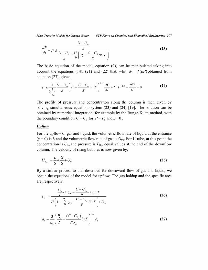
Upflow

For the upflow of gas and liquid, the volumetric flow rate of liquid at the entrance (y = 0) is L and the volumetric flow rate of gas is G0u. For U-tube, at this point the concentration is C0u and pressure is P0u, equal values at the end of the downflow column. The velocity of rising bubbles is now given by:

0 ub

L GU U

S S (25)

By a similar process to that described for downward flow of gas and liquid, we obtain the equations of the model for upflow. The gas holdup and the specific area are, respectively:

0 0

0 00

1

u u

u u

u

u

u

P C CU U T

P PP C C

U T UP P

(26)

1/3

0 0

0

( )3u u

u

u uu

P C Ca T

r P P

(27)


The differential equation for the pressure variation is:

0

000

u

u

u

u u

U U

dPg

C Cdy U U UP T

P

(28)

where 0u

u

G

L .

The basic equation of the model, equation (9), now for upflow, after rearrangement gives:

2/3 1/30 2/30

0

0

1 0

3

u

u

uL u u

u

C CU U dC Pg P T C P

k dP H

r

(29)

The profile of pressure and concentration along the column is given by solving the simultaneous set of equations (28) and (29) [19]. The solution can be obtained by numerical integration, for example by the Runge-Kutta method, with the boundary condition 0u

C C for 0uP P and 0y .

Models with Dispersion

We will now develop a model for mass transfer which, in addition to the assumptions of previous model, includes the axial dispersion.

From a mass balance of dissolved oxygen in the liquid contained in a infinitesimal "slice" located between the coordinates x and x + dx, with volume Sdx , whit *

LD and S constants, we obtain for the steady state, the following equation:

* * * (1 ) ( ) ( ) (1 ) ( )L L Lx x dx

dC dCD S L C x k a S dx C C D S L C x dx

dx dx

(30)

where C, *C and a represent, respectively, the concentration of dissolved oxygen in liquid at level x, the saturation concentration at same level and interfacial area


per unit volume of column. From equation (30) we obtain the basic equation of the model:

* *(1 ) ( ) 0L L

d dC dCD U k a C C

dx dx dx

(31)

For the downflow column, the pressure variation is still given by equation (23), the gas holdup by the equation (21) and the interfacial area per unit volume by the equation (22). In order to solve equation (31) can be used the following change of variable:

(1 )dC

vdx

(32)

With this change of variable, making 0'a r a and taking into account the Henry's law, equation (31) can be rewritten in the following form:

*

0

' 01

LL

kdv U PD v a C

dx r H

(33)

where 'a is calculated by the following equation:

1

30 0' 3

P C Ca T

P P

(34)

The profiles of concentration and pressure along the column and the fitting

parameter0

Lk

r (Eq. (33)) are obtained by solving the following set of differential

equations:

0*

'1

L

L

k P Ua C v

r Hdv

dx D

(35)

1 d

dC v

dx

(36)


0

0 001

L

U UdPg

P C CdxU T U

P P

(37)

The resolution of this system of differential equations was performed using a numerical integrator of problems with boundary conditions at two points ( 0x and 4.94 x m) using the Lobatto-Runge-Kutta formula [19].

In addition to the points used as boundary conditions provided also the experimental value of the concentration of dissolved oxygen in water in two other measuring points located at 1.6 and 3.25 m from the entrance, thus determining the fitting parameter kL/r0. In the optimization of this parameter was used the Levenberg-Marquardt subroutine.

For the upflow column the model involves a number of equations analogous to the downflow column. The basic equation is equal to equation (31), with the axial coordinate y, the gas holdup u and the interfacial area per unit of volume ua

* *(1 ) ( ) 0uL u L u

d dC dCD U k a C C

dy dy dy

(38)

The gas holdup, u , is given by equation (26) and the interfacial area, ua , is

obtained by equation (27). Making a change of variable similar to the equation

(32), (1 )u

dC

dy , also considering the change '

0uu ua r a and the Henry's law,

equation (38) becomes:

* '

0

01

u

u

LL u

u

kd U PD a C

dy r H

(39)

where 'ua is calculated by the following equation:

1

30 0' 3 u u

u uu

P C Ca T

P P

(40)


The pressure variation is given by equation (28). The resolution process is identical to that used for the downward flow, and now to the boundary condition

0y the pressure is 0uP and concentration is 0u

C . For the U-tube, we consider the values of variables at the upflow column entrance equal to the values at the end of downflow column, at the same operating conditions.

RESULTS AND DISCUSSION

Axial Dispersion

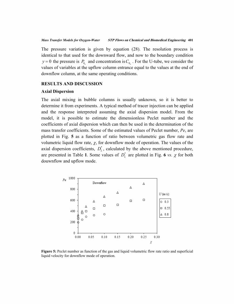
The axial mixing in bubble columns is usually unknown, so it is better to determine it from experiments. A typical method of tracer injection can be applied and the response interpreted assuming the axial dispersion model. From the model, it is possible to estimate the dimensionless Peclet number and the coefficients of axial dispersion which can then be used in the determination of the mass transfer coefficients. Some of the estimated values of Peclet number, Pe, are plotted in Fig. 5 as a function of ratio between volumetric gas flow rate and volumetric liquid flow rate, , for downflow mode of operation. The values of the axial dispersion coefficients, *

LD , calculated by the above mentioned procedure, are presented in Table 1. Some values of *

LD are plotted in Fig. 6 vs. for both douwnflow and upflow mode.

Figure 5: Peclet number as function of the gas and liquid volumetric flow rate ratio and superficial liquid velocity for downflow mode of operation.


Figure 6: Liquid axial dispersion coefficient as function of the gas and liquid volumetric flow rate ratio and superficial liquid velocity for downflow and upflow mode of operation.

Under the applied experimental conditions, the values of *LD are in the range of

41.3 x10-4 and 87.0 x10-4 m2s-1. For the same operating conditions, these values are consistent with those provided by two correlations often cited in literature: the correlation of Joshi [9] and correlation of Field and Davidson [10].

It can be seen in Fig. 5, which in the range of values of gas and liquid flow rates tested, with the column operating under bubble regime, Pe increases with and U, which means we move towards plug flow. The increase of Pe with the liquid flow rate is consistent with studies by several authors for different diameter columns, different ways of introducing the gas stream and various values of flow of liquid and gas, whether the system is homogeneous, transition or heterogeneous. The increase of Pe with U can be explained by the fact that increasing the velocity of fluid elements, the residence time in the column is reduced. The increase of Pe with can be explained similarly: more bubbles in the column increases the effective velocity of the elements of fluid, reducing their time of residence. The variation of Pe with (or gas superficial velocity, G/S, since U is fixed) is in agreement with results obtained by authors such as


Zahradníck and Fialová [20], when the bubble regime was homogeneous, as was the case in which most part of our experiments took place. In this regime, the bubbles have approximately equal sizes, which make them move with similar velocities. Several authors [20-23] obtained an opposite result, i.e., Pe decreases with G/S when operating conditions in column originated transition or heterogeneous bubble regime. The type of regime is one of the factors with significant influence on the liquid mixture.

As can be seen in Fig. 6, the variation of *LD with the liquid superficial velocity

and with the volumetric flow rate of gas/liquid is similar for downflow and upflow bubble columns.

Gas Absorption

In the presented model, the ratio of the mass transfer coefficient and the initial bubbles radius, kL/r0, from equation (24) can be obtained from the experimental data, being a fitting parameter of model. The curves that best approximate the experimental data (presented as C=C-C0 vs. x) are shown in Fig. 7 for U = 0.38 m/s and in Fig. 8 for U = 0.64 m/s, to flow downward and then upward in the U tube.

Figure 7: Comparison between the predicted liquid phase oxygen concentration profiles and the experimental data at U=0.38 m/s for downflow and upflow bubble columns of U tube.


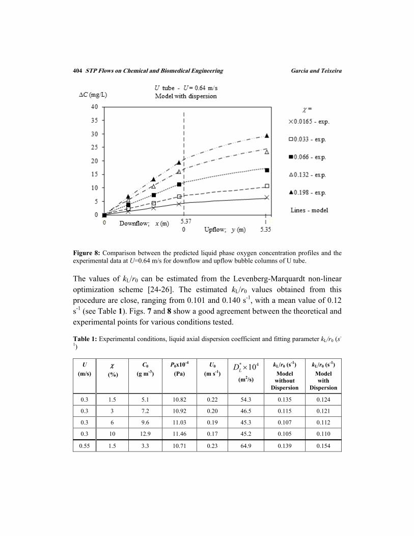
Figure 8: Comparison between the predicted liquid phase oxygen concentration profiles and the experimental data at U=0.64 m/s for downflow and upflow bubble columns of U tube.

The values of kL/r0 can be estimated from the Levenberg-Marquardt non-linear optimization scheme [24-26]. The estimated kL/r0 values obtained from this procedure are close, ranging from 0.101 and 0.140 s-1, with a mean value of 0.12 s-1 (see Table 1). Figs. 7 and 8 show a good agreement between the theoretical and experimental points for various conditions tested.

Table 1: Experimental conditions, liquid axial dispersion coefficient and fitting parameter kL/r0 (s-

1)

U

(m/s)

(%)

C0

(g m-3)

P0x10-4

(Pa)

U0

(m s-1)

* 410LD

(m2/s)

kL/r0 (s-1)

Model without

Dispersion

kL/r0 (s-1)

Model with

Dispersion

0.3 1.5 5.1 10.82 0.22 54.3 0.135 0.124

0.3 3 7.2 10.92 0.20 46.5 0.115 0.121

0.3 6 9.6 11.03 0.19 45.3 0.107 0.112

0.3 10 12.9 11.46 0.17 45.2 0.105 0.110

0.55 1.5 3.3 10.71 0.23 64.9 0.139 0.154


Table 1: cont…

0.55 3 4.1 10.75 0.21 61.3 0.133 0.145

0.55 6 5.1 10.91 0.20 56.9 0.125 0.133

0.55 10 6.5 11.07 0.18 53.5 0.122 0.126

0.55 15 8.2 11.24 0.17 53.0 0.123 0.128

0.55 20 9.8 11.34 0.16 51.0 0.120 0.123

0.55 25 8.5 11.40 0.16 52.2 0.112 0.110

0.8 1.5 3.2 10.90 0.23 87.0 0.140 0.153

0.8 3 5.8 10.95 0.22 73.2 0.139 0.154

0.8 6 4.8 11.02 0.20 63.1 0.127 0.141

0.8 10 5.7 11.10 0.19 57.8 0.112 0.116

0.8 15 6.6 11.18 0.17 54.7 0.104 0.110

0.8 20 7.5 11.28 0.17 51.2 0.103 0.106

0.8 25 8.6 11.44 0.16 49.6 0.101 0.114

Mass transfer coefficient can be calculated for each operating condition through one of several correlations existing in literature. We suggest and use in this study the Hugmark’s correlation [27] because it was specifically obtained with gas-liquid bubble columns operating whit air-water and oxygen-water:

0.1160.546 0.779 1/3

2/3

(2 ) (2 ) (2 )2 0.0187L Rr k r U r g

D D D

(41)

where D is the diffusivity of solute in the liquid, is the viscosity of the liquid and UR is the relative velocity of two fluid phases (modulus of difference between the real velocities of gas and liquid).

This equation can be rearranged, allowing explicit kL/r0 for downward flow:

0.779

0 0

000.233

0.37667 0.0386671/3 0.035

0 2 1.1050 0 0 00 0

1

0.017387L

P C CU U T

P PUU U

k DD g

r P C C P C CT r T r

P P P P

(42)


We obtain an identical equation for upward flow simply by replacing the term U-U0 by U+U0.

This equation can be used with the differential equation of the model, equation (24), implying that the fitting parameter is the radius of the bubble at tube entrance, r0. If this value is known then the model predicts the concentration at any point in the column known initial values of all variables.

Analysing equation (41), can be concluded that for high values of the bubbles radius, the second term on the right side is dominant, so the value of the transfer coefficient is approximately constant for a given operating condition. Thus, given the values of the bubbles radius in the bubble columns, with values greater than 0.1 mm, all r values are high and kL is approximately constant. This is in agreement with the values of kL/r0 presented in Table 1.

Figure 9: Comparison between predicted concentration values obtained with kL/r0=0.12 s-1 and variable kL/r0 for a downflow 20m column at four operating conditions.

Simulations with the model show that the concentration profile does not vary much whether you use the constant value of 0.12 s-1 for kL/r0, whether to use variable values along the column obtained with equation (42), as shown in Fig. 9,

0

5

10

15

20

25

0 5 10 15 20

Sé…Sé…

x (m)

C(mg/L)

kL/r0=0.12 s-1

kL/r0 variable

U=0.3 m/s; =0.015r0=1.5 mm

0

20

40

60

80

100

0 5 10 15 20

U=0.3 m/s; =0.10r0=1.5 mm

C(mg/L)

kL/r0=0.12 s-1

kL/r0 variable

x (m)

0

2

4

6

8

10

0 5 10 15 20

Série1Série2

x (m)

U=0.8 m/s; =0.015r0=1.5 mm

C(mg/L)

kL/r0=0.12 s-1

kL/r0 variable0

20

40

60

80

100

0 5 10 15 20

U=0.8 m/s; =0.30r0=1.5 mm

C(mg/L)

kL/r0=0.12 s-1

kL/r0 variable

x (m)


and therefore the model is not very sensitive to variations in the kL/r0 value. Variation of concentration as a function of axial distance in a 20 m downflow column is obtained from the model for various operating conditions, according to Fig. 9. It was used in all simulations the following values for the variables: C0=0, P0=101325 Pa, U0=0.20 m/s, T=288.15 K, H=2.0765x106 J/kg, =999.1 kg/m3, =1.149x10-3 Pa s and D=1.88x10-9 m2/s.

Under the experimental conditions tested, Fig. 10 shows, for four operating conditions of Fig. 9, that the parameter kL/r0 and therefore the mass transfer coefficient kL, have a small change along the column, being obtained with equation (42) kL/r0 values near 0.12s-1. This value can be used in most practical situations, except in the operating conditions in which the gas volumetric flow rate is very small.

Figure 10: Variation of kL/r0 parameter with axial coordinate in downflow 20 m column for several operating conditions.

CONCLUSIONS

Models are presented for mass transfer in bubble columns with simultaneous flow of gas and liquid in downflow and upflow co-current bubbly regime. The models developed for steady state take into account: the variation of pressure along the tube, the variation of bubbles size and the variation of gas volumetric flow rate, either by pressure variation or by consumption of solute absorbed by the liquid. Models that include the axial dispersion are also presented.

0.00

0.02

0.04

0.06

0.08

0.10

0.12

0.14

0 5 10 15 20

kL/r0

( s-1)

U=0.3 m/s; =0.015

U=0.3 m/s; =0.10

U=0.8 m/s; =0.015

U=0.8 m/s; =0.30r0=1.5 mm

x (m)


The results obtained with the models are in good agreement with the experimental results obtained with the oxygen-water system.

The parameter that results from the ratio of the mass transfer coefficient and the initial bubbles radius, and therefore the mass transfer coefficient, kL, in most practical situations of interest, have a small change with the bubbles radius along the column. Therefore we can use a constant value of kL/r0=0.12 s-1, mean value obtained with the fit of the experimental data to the model and that is close of the value obtained with the correlation of Hugmark.

Under tested conditions, axial dispersion had no influence on mass transfer process.

CONFLICT OF INTEREST

None declare.

ACKNOWLEDGEMENT

None declare.

NOTATION

a -interfacial area per unit of column volume, m-1

Ab -area of a bubble, m2

C -concentration of gas solute dissolved in liquid (liquid-phase oxygen concentration), kg m-3

C0 -concentration of gas solute dissolved in liquid at tube entrance (x=0), kg m-

3

C* -solubility of gas solute in liquid, kg m-3

CA -tracer (NaCl) concentration in the liquid, kg m-3

db -bubble diameter, m


D -molecular diffusion coefficient of gas in liquid, m2 s-1

*LD -liquid axial dispersion coefficient, m2 s-1

G -acceleration due to gravity, m s-2

G -gas volumetric flow rate, m3 s-1

G0 -gas volumetric flow rate at tube entrance (x=0), m3 s-1

H -Henry’s law constant, J kg-1

kL -liquid phase mass transfer coefficient, m s-1

L -liquid volumetric flow rate, m3 s-1

P -total pressure, Pa

P0 -pressure at x=0, Pa

Pe -Peclet number, see equation 3

R -bubble radius, m

r0 -bubble radius at column entrance (x=0), m

-gas constant, J kg-1 K-1

S -column cross sectional area, m2

T -temperature, K

Ub -bubbles velocity, m s-1

U -liquid superficial velocity, m s-1

U0 -rise velocity of bubbles in stagnant medium, m s-1

UR -relative velocity between the moving phases = [(G/S)-(L/(1-)S)], m s-1


Vb -bubble volume, m3

x -vertical (axial) coordinate for downflow system, m

y -vertical (axial) coordinate for upflow system, m

-ratio of gas flow rate and liquid flow rate (=G0/L)

-liquid viscosity, Pa s

-density of the liquid, kg m-3

m -density of gas-liquid mixture, kg m-3

REFERENCES

[1] Boyd CE, Watten B. Aeration systems in aquaculture. Rev Aquat Sci 1989; 1(3): 425-72. [2] Petit J. Water supply, treatment, and recycling in aquaculture. In Barnabe G editor.

Aquaculture, volume 1, Ellis Horwood Series in Aquaculture and fisheries support, Ellis Horwood 1990; pp 63-196.

[3] Speece RE. Oxygen supplementation by U-Tube to the Tombigbee river. Water Sci Technol 1996; 34(12): 83-90.

[4] Roustan M, Liné A, Wable O. Modeling of vertical downward gas-liquid flow for the design of a new contactor. Chem Eng Sci 1992; 47(13): 3681-8.

[5] Teixeira JAS. Oxigenação em aquicultura: o sistema do Tubo em U. PhD in Chemical Engineering. Faculty of Engineering: Porto University; 1998 (in Portuguese).

[6] Garcia VRR, 2006. Oxigenação em Borbulhadores Verticais e Inclinados. PhD in Chemical Engineering. Faculty of Engineering: Porto University; 2006 (in Portuguese).

[7] Deckwer WD, Burckhart R, Zoll G. Mixing and mass transfer in tall bubble columns. Chem Eng Sci 1974; 29(11): 2177-88.

[8] Hikita H, Kikukawa H. Liquid-phase mixing in bubble columns: Effect of liquid properties. The Chem Eng J 1974; 8(3): 191-7.

[9] Joshi JB. Axial mixing in multiphase contactors-A unified correlation. Trans Inst Chem Eng 1980; 58(3): 155-65.

[10] Field RW, Davidson JF. Axial dispersion in bubble columns. Trans Inst Chem Eng 1980; 58: 228-35.

[11] Kawase Y, Moo-Young M. Liquid phase mixing in bubble columns with Newtonian and non-Newtonian fluids. Chem Eng Sci 1986; 41(8): 1969-77.

[12] Levenspiel O, Smith WK. Notes on the diffusion-type model for longitudinal mixing of fluids in flow. Chem Eng Sci 1957; 6(4-5): 227-33.

[13] Levenspiel O, Ed. Chemical Reaction Engineering. 2nd ed. New York: John Wiley & Sons 1972.


[14] Westerterp KR, van Swaaij WPM, Beenackers AACM. Chemical reactor design and operation. Student edition Netherlands: John Wiley & Sons 1987.

[15] Fogler HS. Elements of Chemical Reaction Engineering. 2nd ed. New York: Prentice Hall Inter.Edit. 1992.

[16] Deckwer WD. Bubble Column Reactors. Chichester: John Wiley & Sons 1991. [17] Nicklin DJ. 1962. Two-phase bubble flow. Chem Eng Sci 1962; 17(9): 693-702. [18] Whalley PB. Boiling, Condensation and Gas-Liquid Flow. Oxford: Oxford University Press

1987. [19] Cash JR, Wright MH. A deferred correction method for nonlinear two-point boundary

value problems. SIAM J Sci Stat Comput 1991; 12(4): 971-89. [20] Zahradník J, Fialová JA. The effect of bubbling regime on gas and liquid phase mixing in

bubble column reactors. Chem Eng Sci 1996; 51(10): 2491-500. [21] Hebrard G, Bastoul D, Roustan M, Comte MP, Beck C. Characterization of axial liquid

dispersion in gas-liquid and gas-liquid-solid reactors. Chem Eng J 1999; 72(2): 109-16. [22] Moustiri S, Hebrard G, Thakre SS, Roustan M. A unified correlation for predicting liquid

axial dispersion coefficient in bubble columns. Chem Eng Sci 2001; 56(3): 1041-7. [23] Moustiri S, Hebrard G, Roustan M. Effect of a new high porosity packing on

hydrodynamics of bubble columns. Chem Eng Process 2002; 41(5): 419-26. [24] Levenberg K. A method for the solution of certain non-linear problems in least squares.

Quart Appl Math 1944; 2(2): 164-8. [25] Marquardt DW. An algorithm for least-squares estimation of nonlinear parameters. SIAM J

Appl Math 1963; 11(2): 431-41. [26] Brown KM, Dennis JE. Derivative free analogues of the Levenberg-Marquardt and Gauss

algorithms for nonlinear least squares approximations. Numer Math 1972; 18(4): 289-97. [27] Hugmark GA. Holdup and mass transfer in bubble columns. Ind Eng Chem Proc Des Dev

1967; 6(2): 218-20.

CHAPTER 14 - Biblioteca Digital do IPB

Documents

Transcript of CHAPTER 14 - Biblioteca Digital do IPB