Nonlinear Dyn (2006) 46:337–348DOI 10.1007/s11071-005-9004-x

O R I G I N A L A R T I C L E

Changing the representation and improving stability intime-stepping analysis of structural non-linear dynamics

S. Lopez

Accepted: 30 September 2005 / Published online: 13 September 2006C© Springer Science + Business Media B.V. 2006

Abstract In the present paper, we propose a change inthe representation of the discrete motion equations instructural non-linear dynamics to obtain an improve-ment in the stability of time numerical integrations. Inparticular, natural local state variables are indicated fora finite-element approach to beam problems. The re-sults, relative to Newmark approximations for the vari-ations in the displacement and velocity vectors, showa significant increase in the range of stability of thetime-integration process and a reduction in the numberof Newton iterations required in the time-integrationsteps. It is also shown that the proposed approachinherently obeys the law of conservation of energy.

Keywords Change of representation · Numericalstability · Structural finite-element non-lineardynamics

1. Introduction

Non-linear elastodynamics is an important field instructural analysis, and in the last 30 years, therehas been extensive research into time-integration al-gorithms. In particular, stability is a dominant topicbecause, while unconditionally stable schemes can be

S. LopezDipartimento di Strutture, Universita della Calabria, 87030Rende, Italye-mail: salvatore.lopez@labmec.unical.it

recovered in linear dynamics, numerical instability fre-quently appears in non-linear regimes.

In order to obtain stable solutions, schemes that de-mand the conservation or decrease in the total energyof the Hamiltonian system within each time step are ex-tensively used. Energy-conserving algorithms in elas-todynamics have already appeared in the works of Be-lytschko and Schoeberle [1] and Hughes et al. [2]. Theenergy–momentum method introduced by Simo andTarnow [3, 4] preserves energy, as well as linear andangular momentum, in the time interval. Conservationproperties are enforced into the equation of motion viaLagrange multipliers. Adaptive time-stepping proce-dures [5] and controllable numerical dissipation [6, 7]can also be introduced to permit larger time steps and,consequently, to obtain better computational efficiency.

Although finite difference methods appear to prevailin the literature on the numerical treatment of initial-value problems, a number of alternative finite-elementmethods have been developed for the temporal dis-cretization process. Weighted residual statement andthe Galerkin finite-element approach for the numericalsolution of the equations of motion has been employedby Zienkiewicz et al. [8], and by Lasaint and Raviart[9]. More recently, time finite elements, where the New-mark family formulae can be recovered by the choiceof representative constants and the algorithmic energyconservation is implicitly preserved, have been carriedout (see [10] and related bibliography).

In all cases, it seems that an appropriate representa-tion and discretization of the motion equation leads

Springer

338 Nonlinear Dyn (2006) 46:337–348

to an appreciable difference in the time-integrationschemes with regard to stability. Argyris et al. [11], inparticular, noted a significant increase in the range ofstability of the classical Newmark method if the natu-ral mode finite-element discretization and lumped massmatrices are used. Of course, all the above mentionedtime-stepping algorithms can take additional advantageof these opportune representations.

In this paper, we consider the behaviour of the aver-age acceleration Newmark scheme in the application tomotion equations represented in two different sets ofstate variables. While the first representation followsthe typical Cartesian coordinates, the second one is ob-tained by adding further local variables. The objectiveis to write the motion equations in a less non-linearform. In effect, it appears that rational expressions ofthe internal forces in the structural system can be sub-stituted by analytical trigonometric versions. This leadsto a significant increase in the range of stability ofthe time-integration process. The increase in computa-tional effort due to the introduction of new unknownsand the loss of symmetry in the iteration matrix is bal-anced by the reduction in the number of Newton itera-tions required in the time-integration steps.

In particular, the choice of additional local variablesis strictly linked to the representation of the internal en-ergy and its consequent internal forces. These expres-sions are generically governed by a misure of strains. Itseem opportune to consider such misures by the intro-duction of new unknowns and related motion equations.In effect, in such a way, in one way internal strains canbe expressed more simply being written in their intrin-sic reference system. In another way, the new motionequations express the evolution of linear as well as an-gular momentum in a less non-linear form.

The remainder of the paper is organized as fol-lows. In Section 2, discrete motion equations and thechange in the representation of the internal forces aredescribed. Section 3 gives examples of application ofthe proposed method. In particular, finite-element co-rotational formulation, and the resulting choice of thelocal variables are presented for beam problems. Somefinal conclusions are drawn in Section 4.

2. Discrete motion equations and the change

in representation

We refer to dynamic systems with V (u(x, t)) inter-nal energy, T (u(x, t)) kinetic energy and L(u(x))(t)

external work, where u are the displacements and uthe velocities. The dot denotes time derivative and xand t are the spatial and time coordinates, respec-tively. u denote the accelerations, while u∗ and u∗

represent the initial displacements and initial veloci-ties, respectively. The semi-discrete formulation of theequation of motion can be written, after spatial dis-cretization and inclusion of boundary conditions, in theform:

Mu(t) + N(u(t)) − P(t) = 0, u(0) = u∗,

u(0) = u∗. (1)

In (1), we have:

Mu(t) = ∂

∂t∂T (u(t))

∂u, N(u(t)) = ∂V (u(t))

∂u,

P(t) = ∂L(u)(t)∂u

, (2)

where Mu(t) are the inertia forces, N(u(t)) the internalforce and P(t) the external forces.

For the time integration of the semi-discrete initialvalue problem (1), we refer to the constant time step�t = tn+1 − tn . By assuming the state variables un , un ,un , as known at the time tn and making the externalforces P(t) for all t , the time integration is restrictedto the successive solution of the state variables at theend of each step un+1, un+1, un+1. In order to realizethis step-by-step integration, the set of variables is re-duced to the displacements un+1 only by the Newmarkapproximations:

un+1 = γ

β�t(un+1 − un) +

(1 − γ

β

)un

+(

1 − γ

2β

)�t un, (3)

un+1 = 1

β�t2(un+1 − un) − 1

β�tun

+(

1 − 1

2β

)un. (4)

In the following, we use the average accelerationscheme by adopting γ = 1/2 and β = 1/4.

Springer

Nonlinear Dyn (2006) 46:337–348 339

By inserting relations (??) and (4) in Equation (1),we arrive at the non-linear equation of the form:

F(un+1) = 0. (5)

This represents the non-linear system of algebraicequations defined at the tn+1 time with the un+1 vectorunknown. The velocities and accelerations at the end ofthe time step can then be obtained by relations (??) and(4), respectively. Newton-like iterative methods can beused to solve system (5) by linearization

F(u

(k+1)n+1

) = F(u

(k)n+1

) + ∂F(u

(k)n+1

)∂un+1

(u

(k+1)n+1 − u

(k)n+1

)+O(�t2) = 0. (6)

The iterative process is initialized here by choosingu

(0)n+1 as the linear extrapolation of the previously com-

puted un and un−1 vectors when n > 0, while the for-mula u

(0)1 = u0 + �t u∗ is used when n = 0. By choos-

ing the fixed tolerance η = 10−8, the formula∥∥u(k+1)n+1 − u

(k)n+1

∥∥/∥∥u(k+1)n+1 − un

∥∥ ≤ η (7)

is adopted as convergence criterion.At this point, Nu indicating the number of compo-

nents of the state vector u(t), we introduce additionalNq state variables of the q(t) vector. In the follow-ing, we assume that the components of u(t) follow theCartesian coordinates, while components of q(t) followa suitable local frame. We require that q(t) = q(u(t))and that internal energy V (u(x, t)) can be expressed interms of local variables as V (q(u(x, t))). The adopteddefinition of internal force is now:

N(q(t)) = ∂V (q(t))∂q

∂q(u(t))∂u

∣∣∣∣u(t)=u(q(t))

(8)

where we assume the well-posed inverse relationu(t) = u(q(t)). System (1) is then defined by Nu + Nq

unknowns, where Nu equations are

Mu(t) + N(q(t)) − P(t) = 0, (9)

and the remaining Nq equations aim to satisfy theq(t) = q(u(t)) relation by introducing second deriva-tive q(t).

Initial conditions are defined by q(t) = q(u(t)),q(t) = (∂q(u)/∂u)u(t) and q(t) = (∂q(u)/∂u)u2(t) re-lations. The time-integration scheme follows, as out-lined above, in the Nu + Nq space (u(t), q(t)), whereapproximations (??) and (4) are also used for the qn

and qn definitions.

3. Numerical tests

A set of numerical examples is chosen to show theapplication of the discussed method for the time inte-gration of the motion equations.

Stable behaviour of the time-integration schemes,in the absence of numerical dissipation, is verified byreferring to the condition

�E = Vn+1 − Vn + Tn+1 − Tn − �L = 0, (10)

as a sufficient stability condition in the non-linearregime (see e.g., [1]). Equation (10) express the con-servation of the total energy �E , where Vn+1 and Vn

represent the internal energy at the end and the begin-ning of the time step, Tn+1 and Tn are the correspondingkinetic energies and �L symbolizes the work done byexternal forces within the time step. We use the trape-zoidal rule to calculate the work of the external forces:

�L = 1

2(un+1 − un)T(Pn+1 + Pn). (11)

As regards to consistency, note that as in the numer-ical tests, for such a �t in which both representationshave a stable behaviour, kinematic quantities of interestproves to have the same values. Therefore, the methodshows to be second-order accurate.

3.1. Motion of a dumbbell

We investigate the motion of a dumbbell modelled as atwo-body problem and defined in the two-dimensionalambient space (x, y). Additional background materialon the motion of a several particles system in a potentialfield can be found in standard books on classical me-chanics, see e.g. [12] and [13]. By referring toFig.1, we assume m1 = m2 = 1 with uT ={u1 v1 u2 v2}. The initial conditions are givenby uT

0 = {0 0 0 1} and uT0 = {5 0 10 0}. The interaction

of the two bodies is assumed to be governed by a

Springer

340 Nonlinear Dyn (2006) 46:337–348

Fig. 1 Dumbbell: Initial configuration and problem definition

Leonard–Jones potential, which is often employed inmolecular dynamic simulations:

V (r ) = A

[(σ

r

)5

−(

σ

r

)3]

. (12)

In (12), r is the distance between the centers of the twobodies. We make σ = (3/5)1/2, such that r = 1 char-acterizes the internal force free configuration. Accord-ingly, if r < 1, the resulting force is repulsive, whereasr > 1 implies attraction of the two bodies. We can referto [14] and [15] for the numerical instabilities, whichare introduced in such dynamic systems.

In addition to the Nu = 4 components of the statevector u, we introduce Nq = 2 local variables qT ={r α}. These latter are defined through the relations

r = [(u2 − u1)2 + (v2 − v1)2]1/2,

α = arctan

(v2 − v1

u2 − u1

), (13)

and the respective inverses expressed as

u2 − u1 = r cos(α), v2 − v1 = r sin(α). (14)

Note how the introduced variables r and α representthe distance between the two masses and the angle thattheir conjunction forms with the x-axis, respectively.

Simple mathematical manipulations show that, by(8) and (12)–(14), we obtain

Nu1 (q) = ∂V (r )

∂u1= −∂V (r )

∂rcos(α), (15)

Nv1 (q) = ∂V (r )

∂v1= −∂V (r )

∂rsin(α), (16)

Nu2 (q) = ∂V (r )

∂u2= ∂V (r )

∂rcos(α), (17)

Nv2 (q) = ∂V (r )

∂v2= ∂V (r )

∂rsin(α), (18)

and that, also, we can write the extra equations

r − r α2 = (u2 − u1) cos(α)

+(v2 − v1) sin(α), (19)

r α + 2r α = −(u2 − u1) sin(α)

+(v2 − v1) cos(α). (20)

The system in the (u, q) space, with dimension 6, is thenexpressed by Equation (9) and relations (19)–(20).

We investigate the quasi-rigid case related to A =106 and applications of (u) and (u, q) representationsfor increasing values of the time step �t . Let stepsbe the number of time steps effected by the integra-tion process to analyze the behaviour for t = 0, . . . , T .Table1 reports the mean value of the Nwi Newton

Table 1 Dumbbell: Mean value Nwm

of the Newton iterations

�t u-repr. u, q-repr.

0.01 3.995 2.0000.02 5.020 2.0000.03 div 2.0150.04 2.0200.05 2.0250.06 2.0290.07 2.0340.08 2.0400.09 2.0430.1 2.050

t = 0, . . . , 2

Springer

Nonlinear Dyn (2006) 46:337–348 341

iterations in the i th step

Nwm =step∑i=1

Nwi/steps, (21)

carried out, unless it becomes unstable (div), in theprocess for T = 2 in the (u(t)) and (u(t), q(t)) repre-sentations.

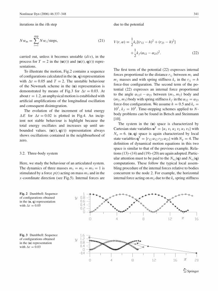
To illustrate the motion, Fig.2 contains a sequenceof configurations calculated in the (u, q) representationwith �t = 0.05 and T = 2. The unstable behaviourof the Newmark scheme in the (u) representation isdemonstrated by means of Fig.3 for �t = 0.03. Atabout t = 1.2, an unphysical motion is established withartificial amplifications of the longitudinal oscillationand consequent disintegration.

The evolution of the increment of total energy�E for �t = 0.02 is plotted in Fig.4. An incip-ient not stable behaviour is highlight because thetotal energy oscillates and increases up until un-bounded values. (u(t), q(t)) representation alwaysshows oscillations contained in the neighbourhood ofzero.

3.2. Three-body system

Here, we study the behaviour of an articulated system.The dynamics of three masses m1 = m2 = m3 = 1 isstimulated by a force p(t) acting on mass m3 and in thex-coordinate direction (see Fig.5). Internal forces are

due to the potential

V (r, α) = 1

2ke[(r12 − h)2 + (r23 − h)2]

+1

2k f (α12 − α23)2. (22)

The first term of the potential (22) expresses internalforces proportional to the distance ri j between mi andm j masses and with spring stiffness ke in the ri j = hforce-free configuration. The second term of the po-tential (22) expresses an internal force proportionalto the angle α12s − α23 between (m1, m2) body and(m2, m3) body with spring stiffness k f in the α12 = α23

force-free configuration. We assume h = 0.5 and ke =107, k f = 103. Time-stepping schemes applied to N -body problems can be found in Betsch and Steinmann[10].

The system in the (u) space is characterized byCartesian state variables uT = {u1 v1 u2 v2 u3 v3} withNu = 6. (u, q) space is again characterized by localstate variables qT = {r12 α12 r23 α23} with Nq = 4. Thedefinition of dynamical motion equations in this twospace is similar to that of the previous example. Rela-tions (13)–(14) and (19)–(20) are again adopted. Partic-ular attention must to be paid to the Nu2 (q) and Nv2 (q)computations. These follow the typical local assem-bling procedure of the internal forces relative to bodiesconcurrent to the node 2. For example, the horizontalinternal force acting on m2 due to the ke spring stiffness

Fig. 2 Dumbbell: Sequenceof configurations obtainedin the (u, q) representationwith �t = 0.05

Fig. 3 Dumbbell: Sequenceof configurations obtainedin the (u) representationwith �t = 0.03

Springer

342 Nonlinear Dyn (2006) 46:337–348

Fig. 4 Dumbbell: Totalenergy increment �Eversus time t for �t = 0.02:continuous line for (u(t))and dotted line for(u(t), q(t)) representations,respectively

Fig. 5 Three-body system: Initial configuration and problem definition

is computed by the sum

∂V∂r12

∂r12

∂u2

∣∣∣∣ u2 − u1 = r12 cos(α12)v2 − v1 = r12 sin(α12)

+ ∂V∂r23

∂r23

∂u2

∣∣∣∣ u3 − u2 = r23 cos(α23)v3 − v2 = r23 sin(α23)

. (23)

For completeness, we give the explicit formulae

Nu2 (q) = ke(r12 − h) cos(α12) − ke(r23 − h) cos(α23)

+k f (α23 − α12)1

r12sin(α12)

+k f (α23 − α12)1

r23sin(α23), (24)

Springer

Nonlinear Dyn (2006) 46:337–348 343

Nv2 (q) = ke(r12 − h) sin(α12) − ke(r23 − h) sin(α23)

−k f (α23 − α12)1

r12cos(α12)

−k f (α23 − α12)1

r23cos(α23). (25)

Applications of (u) and (u, q) representations forincreasing values of the time step �t are investigated.Table2 reports the Nwm values performed in the time-integration process for T = 1.

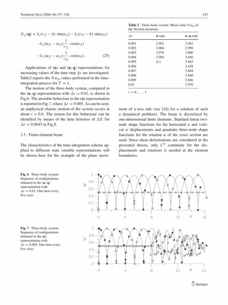
The motion of the three-body system, computed inthe (u, q) representation with �t = 0.01, is shown inFig.6. The unstable behaviour in the (u) representationis reported in Fig.7, where �t = 0.005. As can be seen,an unphysical chaotic motion of the system occurs atabout t = 0.6. The reason for this behaviour can beidentified by means of the time histories of �E for�t = 0.0045 in Fig.8.

3.3. Finite-element beam

The characteristics of the time-integration scheme ap-plied to different state variable representations willbe shown here for the example of the plane move-

Table 2 Three-body system: Mean value Nwm ofthe Newton iterations

�t u-repr. u, q-repr.

0.001 2.992 2.9820.002 3.004 2.9980.003 3.970 3.0000.004 3.984 3.0400.005 div 3.4650.006 3.6580.007 3.8040.008 3.8400.009 3.8660.01 3.930

t = 0, . . . , 1

ment of a toss rule (see [16] for a solution of sucha dynamical problem). The beam is discretized byone-dimensional finite elements. Standard linear two-node shape functions for the horizontal u and verti-cal w displacements and quadratic three-node shapefunctions for the rotation α of the cross section areused. Since shear deformations are considered in thepresented theory, only C0 continuity for the dis-placements and rotations is needed at the elementboundaries.

Fig. 6 Three-body system:Sequence of configurationsobtained in the (u, q)representation with�t = 0.01. One item everyfive steps

Fig. 7 Three-body system:Sequence of configurationsobtained in the (u)representation with�t = 0.005. One item everyfive steps

Springer

344 Nonlinear Dyn (2006) 46:337–348

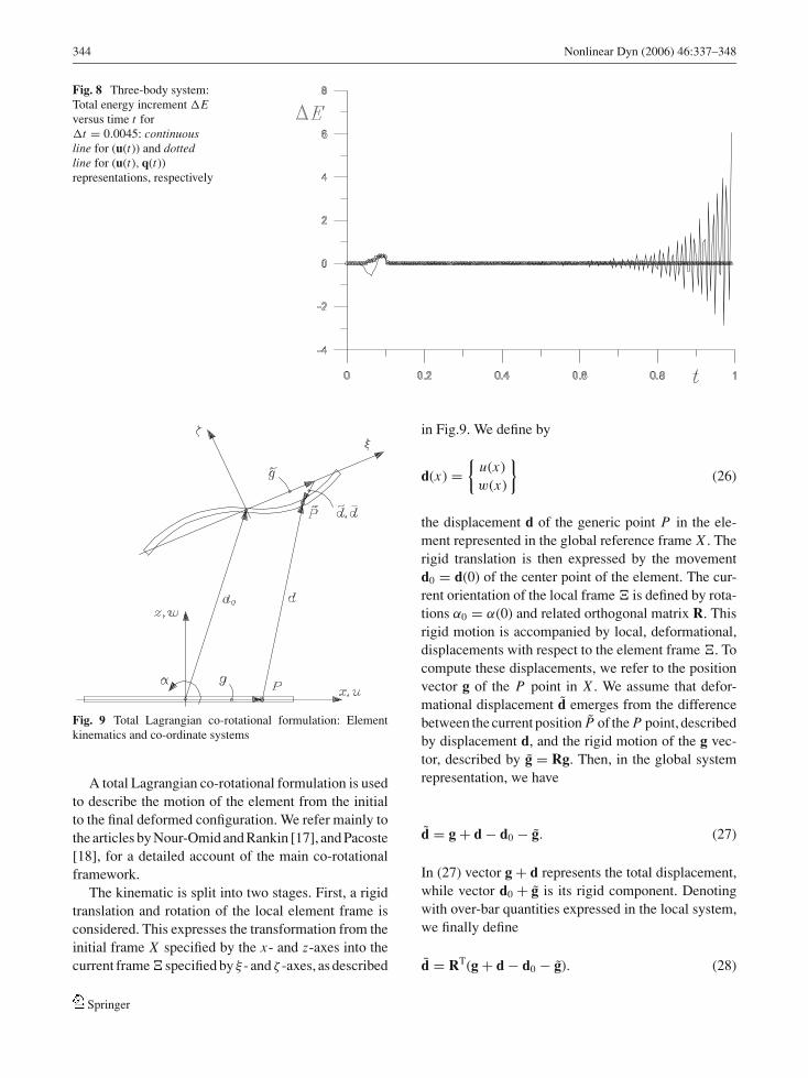
Fig. 8 Three-body system:Total energy increment �Eversus time t for�t = 0.0045: continuousline for (u(t)) and dottedline for (u(t), q(t))representations, respectively

Fig. 9 Total Lagrangian co-rotational formulation: Elementkinematics and co-ordinate systems

A total Lagrangian co-rotational formulation is usedto describe the motion of the element from the initialto the final deformed configuration. We refer mainly tothe articles by Nour-Omid and Rankin [17], and Pacoste[18], for a detailed account of the main co-rotationalframework.

The kinematic is split into two stages. First, a rigidtranslation and rotation of the local element frame isconsidered. This expresses the transformation from theinitial frame X specified by the x- and z-axes into thecurrent frame specified by ξ - and ζ -axes, as described

in Fig.9. We define by

d(x) ={

u(x)w(x)

}(26)

the displacement d of the generic point P in the ele-ment represented in the global reference frame X . Therigid translation is then expressed by the movementd0 = d(0) of the center point of the element. The cur-rent orientation of the local frame is defined by rota-tions α0 = α(0) and related orthogonal matrix R. Thisrigid motion is accompanied by local, deformational,displacements with respect to the element frame . Tocompute these displacements, we refer to the positionvector g of the P point in X . We assume that defor-mational displacement d emerges from the differencebetween the current position P of the P point, describedby displacement d, and the rigid motion of the g vec-tor, described by g = Rg. Then, in the global systemrepresentation, we have

d = g + d − d0 − g. (27)

In (27) vector g + d represents the total displacement,while vector d0 + g is its rigid component. Denotingwith over-bar quantities expressed in the local system,we finally define

d = RT(g + d − d0 − g). (28)

Springer

Nonlinear Dyn (2006) 46:337–348 345

By referring to the displacements expressed in the localsystem, the total deformation energy V is then obtainedfrom

V = 1

2

∫ h

−h(E Aε2 + G Aγ 2 + E Jχ2)dx (29)

where 2h is the length of the element and E A, G A andE J represent the axial, shear and flexural rigidities, re-spectively. Measurements of the axial ε and transversalγ strain, together with the usual definition of the cur-vature χ , are formulated by the following expressions:

ε = d1′, γ = d2

′, χ = α′, (30)

where the prime denotes differentiation with respect tox .

In the u(x, t)T = {u(x, t) v(x, t) α(x, t)} state vari-able representation, the explicit expressions of the

strains are therefore:

ε = (1 + u′ − cos(α0)) cos(α0)

+(w′ − sin(α0)) sin(α0), (31)

γ = −(1 + u′ − cos(α0)) sin(α0)

+(w′ − sin(α0)) cos(α0). (32)

We refer to an element with nodes i and j at the bound-aries and node o at the centre. The elemental forcevector is then derived from the differentiation of po-tential (29) with respect to the nodal parameters ui (t),u j (t), wi (t), w j (t), αi (t), α0(t), α j (t), in the u(x, t)interpolation.

The state variable representation (u(x, t), q(x, t) ishere obtained by the interpolations

u(x) = u0 + xh

(r0 cos(α0) − h) − xh

s0 sin(α0), (33)

w(x) = w0 + xh

r0 sin(α0) + xh

s0 cos(α0). (34)

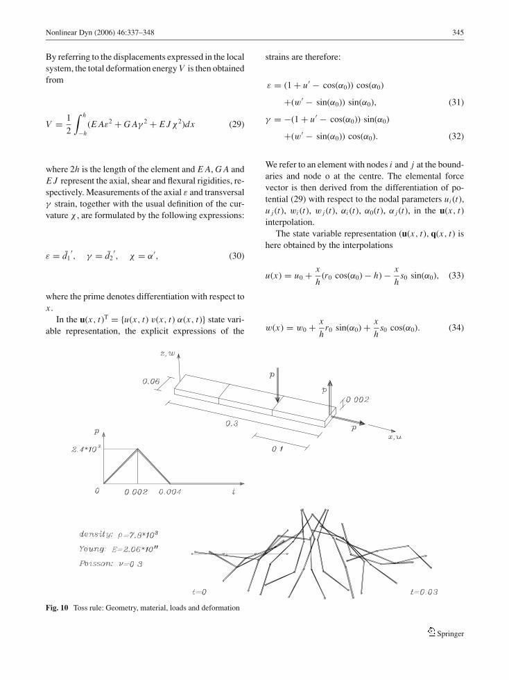
Fig. 10 Toss rule: Geometry, material, loads and deformation

Springer

346 Nonlinear Dyn (2006) 46:337–348

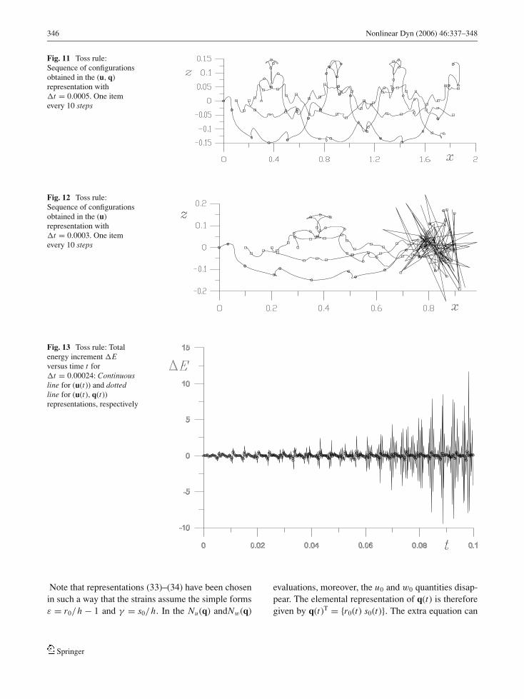
Fig. 11 Toss rule:Sequence of configurationsobtained in the (u, q)representation with�t = 0.0005. One itemevery 10 steps

Fig. 12 Toss rule:Sequence of configurationsobtained in the (u)representation with�t = 0.0003. One itemevery 10 steps

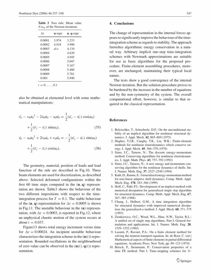
Fig. 13 Toss rule: Totalenergy increment �Eversus time t for�t = 0.00024: Continuousline for (u(t)) and dottedline for (u(t), q(t))representations, respectively

Note that representations (33)–(34) have been chosenin such a way that the strains assume the simple formsε = r0/h − 1 and γ = s0/h. In the Nu(q) andNw(q)

evaluations, moreover, the u0 and w0 quantities disap-pear. The elemental representation of q(t) is thereforegiven by q(t)T = {r0(t) s0(t)}. The extra equation can

Springer

Nonlinear Dyn (2006) 46:337–348 347

Table 3 Toss rule: Mean valueNwm of the Newton iterations

�t u-repr. u, q-repr.

0.0001 3.974 3.2330.0002 4.918 3.9900.0003 div 4.1340.0004 4.6200.0005 4.9450.0006 5.0470.0007 5.1670.0008 5.4800.0009 5.7810.001 5.940

t = 0, . . . , 0.1

also be obtained at elemental level with some mathe-matical manipulations:

r0 − r0α02 − 2s0α0 − s0α0 = 1

2(u j − ui ) cos(α0)

+1

2(v j − vi ) sin(α0), (35)

s0 − s0α02 + 2r0α0 + r0α0 = −1

2(u j − ui ) sin(α0)

+1

2(v j − vi ) cos(α0). (36)

The geometry, material, position of loads and loadfunction of the rule are described in Fig.10. Threebeam elements are used for discretization, as describedabove. Selected deformed configurations within thefirst 60 time steps computed in the (u, q) represen-tation are shown. Table3 shows the behaviour of thetwo different impositions with respect to the time-integration process for T = 0.1. The stable behaviourof the (u, q) representation for �t = 0.0005 is shownin Fig.11. The unstable behaviour in the (u) represen-tation, with �t = 0.0003, is reported in Fig.12, wherean unphysical chaotic motion of the system occurs atabout t = 0.037.

Figure13 shows total energy increment versus timefor �t = 0.00024. An incipient unstable behaviourcharacterizes the integration scheme in the (u(t)) repre-sentation. Bounded oscillations in the neighbourhoodof zero value can be observed in the (u(t), q(t)) repre-sentation.

4. Conclusions

The change of representation in the internal forces ap-pears to significantly improve the behaviour of the time-integration scheme as regards to stability. The approachfurnishes algorithmic energy conservation in a natu-ral way. Arbitrary implicit one-step time-integrationschemes with Newmark approximations are suitablefor use as basic algorithms for the proposed pro-cedure. Finite-element assembling procedures, more-over, are unchanged, maintaining their typical localnature.

The tests show a good convergence of the internalNewton iteration. But the solution procedure proves tobe burdened by the increase in the number of equationsand by the non-symmetry of the system. The overallcomputational effort, however, is similar to that re-quired in the classical representation.

References

1. Belytschko, T., Schoeberle, D.F.: On the unconditional sta-bility of an implicit algorithm for nonlinear structural dy-namics. J. Appl. Mech. 42, 865–869 (1975)

2. Hughes, T.J.R., Caughy, T.K., Liu, W.K.: Finite-elementmethods for nonlinear elastodynamics which conserve en-ergy. J. Appl. Mech. 45, 366–370 (1978)

3. Simo, J.C., Tarnow, N.: The discrete energy–momentummethod. Conserving algorithms for nonlinear elastodynam-ics. J. Appl. Math. Phys. 43, 757–792 (1992)

4. Simo, J.C., Tarnow, N.: A new energy and momentum con-serving algorithm for the nonlinear dynamics of shells. Int.J. Numer. Meth. Eng. 37, 2527–2549 (1994)

5. Kuhl, D., Ramm, E.: Generalized energy-momentum methodfor non-linear adaptive shell dynamics. Comp. Meth. Appl.Mech. Eng. 178, 343–366 (1999)

6. Hoff, C., Pahl, P.J.: Development of an implicit method withnumerical dissipation for generalized single step algorithmfor structural dynamics. Comp. Meth. Appl. Mech. Eng. 67,367–385 (1988)

7. Chung, J., Hulbert, G.M.: A time integration algorithmfor structural dynamics with improved numerical dissipa-tion: the generalized-a method. J. Appl. Mech. 60, 371–375(1993)

8. Zienkiewicz, O.C., Wood, W.L., Hine, N.W., Taylor, R.L.:A unified set of single step algorithms. Part I. General for-mulation and applications. Int. J. Numer. Meth. Eng. 20,1529–1552 (1984)

9. Lasaint, P., Raviart, P.A.: On a finite element method forsolving the neutron transport equation. In: de Boor, C. (ed.)Mathemetical aspects of finite elements in partial differentialequations, Academic Press, New York, pp. 89–123 (1974)

10. Betsch, P., Steinmann, P.: Conservation properties of atime FE method. Part I. Time-stepping schemes for N -

Springer

348 Nonlinear Dyn (2006) 46:337–348

body problems. Int. J. Numer. Meth. Eng. 49, 599–638(2000)

11. Argyris, J., Papadrakakis, M., Mauroutis, Z.S.: Nonlineardynamic analysis of shells with the triangular element TRIC.Comp. Meth. Appl. Mech. Eng. 192, 3005–3038 (2003)

12. Goldstein, H.: Classical Mechanics. Addison-Wesley, Read-ing, Massachusetts (1980)

13. Arnold, V.I., Mathematical Methods of Classical Mechanics.Prentice-Hall, Englewood Cliffs, NJ (1989)

14. Gonzales, O., Simo, J.C.: On the stability of symplectic andenergy–momentum algorithms for non-linear Hamiltoniansystems with symmetry. Comp. Meth. Appl. Mech. Eng. 134,197–222 (1996)

15. Crisfield, M.A., Shi, J.: An energy conserving co-rotationalprocedure for non-linear dynamics with finite elements. Non-linear Dyn. 9, 37–52 (1996)

16. Kuhl, D., Ramm, E.: Constraint energy momentum al-gorithm and its application to non-linear dynamics ofshells. Comp. Meth. Appl. Mech. Eng. 136, 293–315(1996)

17. Nour-Omid, B., Rankin, C.C.: Finite rotation analysis andconsistent linearization using projectors. Comp. Meth. Appl.Mech. Eng. 93, 353–384 (1991)

18. Pacoste, C.: Co-rotational flat facet triangular elements forshell instability analyses. Comp. Meth. Appl. Mech. Eng.156, 75–110 (1998)

Springer