ch for more information On Algebraic Graph Theory and the Dynamics of Innovation Networks

arX

iv:0

712.

2752

v1 [

phys

ics.

soc-

ph]

17

Dec

200

7M. D. Konig, S. Battiston, M. Napoletano, F. Schweitzer:

On Algebraic Graph Theory and the Dynamics of Innovation NetworksNetworks and Heterogeneous Media (2007, submitted)

See http://www.sg.ethz.ch for more information

On Algebraic Graph Theory and theDynamics of Innovation Networks

M. D. Konig⋆, S. Battiston, M. Napoletano and F. Schweitzer

Chair of Systems Design, ETH Zurich, Kreuzplatz 5, 8032 Zurich, Switzerland

⋆ corresponding author, email: [email protected]

Abstract

We investigate some of the properties and extensions of a dynamic innovation network

model recently introduced in [36]. In the model, the set of efficient graphs ranges, depending

on the cost for maintaining a link, from the complete graph to the (quasi-) star, varying

within a well defined class of graphs. However, the interplay between dynamics on the nodes

and topology of the network leads to equilibrium networks which are typically not efficient

and are characterized, as observed in empirical studies of R&D networks, by sparseness,

presence of clusters and heterogeneity of degree. In this paper, we analyze the relation

between the growth rate of the knowledge stock of the agents from R&D collaborations

and the properties of the adjacency matrix associated with the network of collaborations.

By means of computer simulations we further investigate how the equilibrium network is

affected by increasing the evaluation time τ over which agents evaluate whether to maintain

a link or not. We show that only if τ is long enough, efficient networks can be obtained by

the selfish link formation process of agents, otherwise the equilibrium network is inefficient.

This work should assist in building a theoretical framework of R&D networks from which

policies can be derived that aim at fostering efficient innovation networks.

Keywords: Innovation Networks, R&D Collaborations, Network Formation

1 Introduction

The field of Network Theory has only recently focused its attention on the study of dynamic

models in which the topology of the network endogeneously drives the evolution of the network.

These models assume that the evolution of the links in the network is driven by the dynamics

of a state variable, associated to each node, which depends, through the network, on the state

variable of the other nodes [22, 45]. Such an interplay is crucial in many biological systems and

especially in socio-economic systems. In biological systems, a Darwinian selection mechanism

usually works at a global level: for instance in the context of networks, one can think of a

mechanism in which the least fit nodes are replaced (together with their connections) with

new nodes that are randomly connected to the remaining nodes[6, 32, 33]. In socio-economic

networks, besides the global selection mechanism, there exists a “local” selection mechanism: the

1/23

http://arXiv.org/abs/0712.2752v1

http://www.sg.ethz.ch

[email protected]

M. D. Konig, S. Battiston, M. Napoletano, F. Schweitzer:On Algebraic Graph Theory and the Dynamics of Innovation Networks

Networks and Heterogeneous Media (2007, submitted)


nodes in fact represent agents that form or delete links with other agents, based on the utility

that those links may provide to them [8, 27].

The foregoing issue has also attracted researchers in computer science [11, 18, 38] as well as

social scientists and economists [1, 2, 24, 25, 31] In particular, the study of networks has become

increasingly important in the literature on R&D networks [12, 17, 21]. Here, the evolution of the

network is of interest for the investigation of the efficiency and stability of networks of agents

exchanging knowledge in R&D collaborations. In such a context, we have recently introduced a

new model of network evolution in which the topology and the state variable of nodes co-evolve

[36, 37]. The nodes of the network are associated with a dynamical state variable, representing

the utility of the agent, that depends on the links (the R&D collaborations) and the utility of

the other agents. The network then evolves according to a prescribed link formation rule, which,

in turn, depends on the expected increase of utility of the agents.

Independently of the co-evolution of the network and the utility of the agents, we determine

exactly the efficient graphs (in which the aggregate utility of the agents is maximized) and we

show that there are stable equilibria which are not efficient. This implies that, if the network

evolves through the selfish linking behavior of agents, it may not reach an efficient equilibrium.

This result is of interest for policy design questions how to establish incentive mechanisms and

legal frameworks in order to help the system to reach its efficient equilibrium. Interestingly, the

model is also able to reproduce some of the main stylized facts of empirical studies on R&D

networks [12, 26, 40] - namely that such networks are sparse, clustered and heterogeneous in

degree - and therefore offers a candidate framework to explain the formation of these networks.

In this paper, we consider the same model of [36] and we investigate further some of its prop-

erties, in particular, the relation between the utility of the agents and the properties of the

adjacency matrix of the network. In addition, here we also introduce a time delay τ in the de-

cision about keeping or removing a link and we investigate by means of computer simulation

how the equilibrium reached by the network is affected by increasing τ . The result is interesting

in view of more realistic models for the design of policies that may facilitate the formation of

efficient innovation networks.

The paper is organized as follows. First (sec. 2), we introduce the dynamics of knowledge ex-

change on a static network. Then we review some results from algebraic graph theory and we

discuss their implications for our model (sec. 3). We proceed by showing the existence of ineffi-

cient equilibria (sec. 4-6). We finally report the results of computer simulations of the evolution

of the network, in particular, with respect to impact of the evaluation time of the links (sec. 7).

We finally summarize the results and draw some conclusions (sec. 8).

2/23





2 Knowledge Dynamics and Utility Function of the Agents

In this section we describe the dynamics of the state variable of the nodes in a static network.

In section 5 we extend our studies to the endogeneous evolution of the network whereby we

introduce the rules for the formation of links.

Consider a set of agents, N = {1, ..., n}, represented as nodes of an undirected graph G, with an

associated variable xi representing the knowledge of agent i. A link ij, represents the transfer

of knowledge between agent i and agent j. Knowledge is shared among an individual’s direct

and indirect acquaintances and the knowledge level of an agent is proportional to the knowledge

levels of its neighbors. We assume that knowledge x = (x1, ..., xn) grows, starting from positive

values, xi(0) > 0 ∀i, according to the following linear ordinary differential equation

xi =

n∑

j=1

aijxj (1)

where aij = {0, 1} are the elements of the adjacency matrix A of the graph G. In vector notation

we have x = Ax. In the following we will use the terms network and graph as synonyms.

Similar to Carayol and Roux [7] we assume that the gross return of agent i is proportional to

her knowledge growth rate, with proportionality constant set to 1 for sake of simplicity. We also

assume that maintaining a link induces a constant cost c ≥ 0 for both agents connected by the

link. Therefore the net return ρi of agent i is given by

ρi(t) =xi(t)

xi(t)− cdi (2)

where di denotes the degree of agent i. We assume that the utility function of an agent in a

given network is her asymptotic net return ui = limt→∞ ρi(t) . As we will show in the next

section, limt→∞xi(t)xi(t)

= λPF(Ci) where λPF is the spectral radius of the block (sub-) matrix in

A corresponding to the connected component Ci to which i belongs to. Therefore, the utility

function of agent i in a given network is

ui(t) = λPF(Ci) − cdi (3)

As we will see later on, the evolution of the network stems from each agent trying independently

to increase her utility by forming or deleting links. Of course when she does so, this affects the

utility of the other agents which will react by forming or removing other links. However, before

describing the evolution of the network, we want to discuss some implications of our assumptions

on the growth of knowledge and the utility function of the agents.

3 Knowledge Growth and Properties of the Adjacency Matrix

Since the knowledge dynamics is linear and the utility function is proportional to the largest real

eigenvalue of the graph, there are many mathematical properties immediately available for the

3/23





static part of the model. In this section we review the implications of some well known results

for matrices and graphs on the dynamics of knowledge growth in the model. We will only focus

on undirected graphs and symmetric matrices respectively.

First of all, since the adjacency matrix in (1) is non-negative and in particular it is a Metzler

matrix, the vectorial space Rn+ is invariant for the linear operator A. It follows that for non-

negative initial values (as assumed in the model), it is x(t) ≥ 0 and x(t) ≥ 0, ∀t > 0 [43]. This

ensures the following property:

Proposition 1 The values of knowledge x in (1) are non-negative for all times.

For convenience of the reader we report below some facts and definitions that we need in the

succeeding sections.

A walk in the graph is an alternating sequence of nodes and links. The k-power of the adjacency

matrix is related to walks of length k in the graph. In particular,(

Ak)

ijgives the number of walks

of length k from node i to node j [20]. A connected component of a graph is a maximal subgraph

in which there exists a walk from every node to every other node. The graph is connected when

the only connected component is the graph itself. If the adjacency matrix can be decomposed

in blocks, each block corresponds to a connected component.

An n × n matrix A is said to be a reducible matrix if and only if for some permutation matrix

P , the matrix P T AP is block upper triangular. If a square matrix is not reducible, it is said

to be an irreducible matrix. The adjacency matrix of a connected graph is always irreducible

[29] and in particular it cannot be decomposed in multiple blocks. Irreducible matrices can be

primitive or cyclic (imprimitive) [43]. This distinction is important because some result about

the convergence of the knowledge values holds only for graphs with primitive adjacency matrix.

For a primitive, non-negative matrix A it is Ak > 0 for some positive integer k ≤ (n − 1)nn

[29]. This means that, A is primitive if, for some k, there is a walk of length k from every

node to every other node. Notice that this definition is a much more restrictive than the one of

irreducible (or connected) graph in which it is required that there exits a walk from every node

to every other node, but not necessarily of the same length. A graph is said to be primitive if

its associated adjacency matrix is primitive.

The general solution [4, 29, 34] of the system of linear ordinary differential equations in Eq. (1)

is

x(t) = eAtx(0) (4)

where x(0) is the initial state and eA =∑∞

n=0A

n

n! is the matrix exponential. The matrix exponen-

tial can be easily computed in terms of the Jordan form of the matrix. Once the Jordan form is

known J = SAS−1, where S is a non-singular matrix, the matrix exponential is eAt = SeJtS−1.

We can then rewrite the solution of the system as

x(t) = SeJtS−1x(0) (5)

4/23





For each component i of the vector x we get

xi(t) =k

∑

j=1

pj(t)eλj t (6)

where pj(t) is a polynomial in t of degree µj equal to the number of linearly independent

eigenvectors with eigenvalue λj (its geometric multiplicity). µj is strictly smaller than the order

mj of the Jordan block corresponding to the eigenvalue λj of the matrix A.

If the graph is connected, then the largest real eigenvalue is present in the exponent for each

component i in Eq. (6). Since the matrix A ≥ 0 is non-negative, this eigenvalue coinidides

with the spectral radius and with the Perron-Frobenius eigenvalue, λPF (see below). Thus, it is

straightforward to see that the ratio xi

xiis dominated, for t → ∞, by λPF,

limt→∞

xi

xi

= λPF (7)

If the graph is disconnected, the agents in disconnected components Ci have uncoupled equations

of the form (1) that can be solved separately. Let G = (V,E) be a graph with connected

components C1, C2, ..., Cl. The set of eigenvalues of G, i.e. the spectrum of G, is the union of

sets of eigenvalues of the components. Thus, λPF(G) = maxj{λPF(Cj)} [10, 41].

In the following, we repeat here the Perron-Frobenius theorem in a formulation convenient to

our context Seneta [43].

Theorem 2 (The Perron-Frobenius Theorem) Let A be a non-negative matrix. Then (1)

the spectral radius is an eigenvalue, (called λPF) and all other eigenvalues are smaller or equal

in absolute value; (2) λPF is associated to one or more non-negative eigenvectors and, (3) λPF

is bounded from below and above as follows: mini

∑

j aij ≤ λPF ≤ maxi

∑

j aij.

If, in addition, A is an irreducible matrix, then (4) λPF has multiplicity 1 and (5) the associated

eigenvector is positive.

If, in addition, A is a primitive matrix, then (6) λPF is strictly greater in absolute value than

all other eigenvalues.

Notice that, going from non-negative to irreducible matrices the eigenspace of λPF reduces from

several non-negative eigenvectors to only one positive eigenvector. In the limit of large t, the

terms related to the largest real eigenvalues will dominate in Eq. (6). In particular, it can be

shown that for large t, the vector x(t) converges (in direction) to a linear combination of Perron

eigenvectors (associated to the Perron eigenvalue λPF) [29], where the specific linear combination

may depend on the initial conditions. In particular, if the adjacency matrix is primitive, the

Perron eigenvector is unique and there is a unique stable attractor. Interpreting the result in

our model, one can say that

5/23





Proposition 3 If the graph of interaction between agents is primitive, there is a unique asymp-

totic distribution of relative values of knowledge x/∑n

j=1 xj given by the Perron eigenvector of

the adjacency matrix A.

If the assumption of primitivity of the matrix falls, in particular if the matrix is non-negative but

not irreducible, then there are, in general, several Perron eigenvectors and thus several possible

equilibria for the relative values of knowledge, depending on the initial condition.

It is useful to look at an alternative but equivalent way to characterize a primitive graph. A

graph G is primitive if and only if it is connected and the greatest common divisor of the set of

length of all cycles in G is 1 [47]. This means, for instance, that the connected graph consisting of

two connected nodes is not primitive as the only cycle has lenght 2 (since the link is undirected

a walk can go forward and backward along the link). Similarly, a chain or a tree is also not

primitive, since all cycles have only even length. However, if we add one link in order to form

a triangle, the graph becomes primitive. The same is true, if we add links in order to form any

cycle of odd length. We can state the following result.

Proposition 4 If the graph G is connected, the presence of one cycle of odd lenght is a suffi-

cient condition for the primitivity of G and hence for the uniqueness of the relative knowledge

distribution x/∑n

j=1 xj given by the Perron eigenvector.

We now discuss the relation between walks in the graph and growth rate of knowledge. In our

model, a walk in the graph corresponds to a sequence of agents contributing to their individual

knowledge to their neighbors in the walk in order to generate a sequence of recombined knowl-

edge. As mentioned in the beginning, each component of the power k of the adjacency matrix,(

Ak)

ij, gives the number of walks of length k from node i to node j. Considering the vector

u = (1, ..., 1), we have that nk := uTAku is the number of all walks of length k among all

nodes in G. Since the adjacency matrix is symmetric we have that u =∑

aiwi where wi is the

eigenvector of A associated with the eigenvalue λi. It follows that nk =∑

i |ai|2λki . For large k,

we have approximately nk ∼ λkPF [9], and we get

nk − nk−1

nk−1∼ λPF − 1 (8)

Thus, the largest real eigenvalue λPF of the graph measures the growth rate of the number of

walks of length k when the length increases by one. as well as the growth factor of the number of

knowledge recombinations in the network of collaborations. As we have seen in the first part of

this section, λPF coincides also with the asymptotic growth rate of knowledge in time. Therefore,

the faster the number of walks in the graph (and thus of knowledge recombinations) grows with

the length of the walks, the faster also grows in time the knowledge of the agents involved. One

should not confuse the two growth rates, one in time and the other with respect to walk length

(which does not vary in time, as we are analyzing a static network).

6/23





A similar interpretation comes from the Rayleigh-Ritz theorem [29] which states that:

λPF = maxx 6=0

xTAx

xT x(9)

where the maximum is obtained for the Perron eigenvector associated with λPF. Here, x can be

any vector in Rn. xixj can be interpreted as the result of the recombination of the knowledge of

agents i and j if they are connected. Accordingly, one can interpret the right-hand side of Eq. (9)

as the maximum number of total knowledge recombinations, xT Ax =∑

i,j xiaijxj, normalized

to the absolute total knowledge, xT x =∑n

i=1 x2i . Some other results relate λPF to the number of

links or the degree of the nodes in the graph. For instance, the Perron-Frobenius theorem states

that λPF is bounded from below and above by the minimum and maximum degree respectively

(di =∑

j aij is the degree of node i). This means, that the higher (minimum or maximum) the

degree of the nodes in the graph, the higher λPF and thus the knowledge growth rate. We denote

the maximum degree in G by ∆. Then, a better lower bound holds so that√

∆ ≤ λPF(G) ≤ ∆.

We refer to Cvetkovic et al. [14], Cvetkovic and Rowlinson [15] for other inequalities involving

λPF.

There is also a result about the inequality of the growth rate of knowledge across agents. For a

primitive matrix A one can show [3] that the Perron-Frobenius eigenvector associated with the

eigenvalue λPF is the solution to the following optimization problem

maxx>0

min1≤i≤n

∑nj=1 aijxj

xi

(10)

where∑n

j=1 aijxj = (Ax)i = xi. The Perron eigenvector is the vector that maximizes the

minimum growth factor over all agents i and also minimizes the maximum growth factor. By

maximizing the minimum growth factor we obtain balanced growth [3]. In terms of our model:

Proposition 5 If the graph G is primitive, the unique stable distribution of relative knowledge

values x/∑n

j=1 xj to which the dynamics (1) converges, is also the distribution that minimizes

the difference between maximum and minimum growth rates across agents.

From the results above we can conclude that the utility function of agent i in Eq. (3) increases

with the number of walks in the connected component to which agent i belongs to. On the other

hand the utility decrease with the degree of the agent. Therefore it is best for an agent to be able

to reach the other agents through many walks but to have not too many links. We now compare

this utility function with other similar utility functions in the literature on innovation networks

that depend on the position of an agent in the network. For instance, the utility function of

Jackson and Wolinsky [31] is given by

ui =

n∑

i=1

δd(i,j) − cdi (11)

7/23





where 0 ≤ δ ≤ 1 and d(i, j) is the length of the shortest path from node i to node j. Other

examples are those introduced by Carvalho and Iori [8], Holme and Ghoshal [27] and Corbo and

Parkes [11], Fabrikant et al. [18].

The cost term in our utility function (3) is the same as in (11). The difference is in the benefit

term: while the latter utility function only considers the shortest path we take into account all

walks across. It has been argued that that knowledge gets transferred not only along the shortest

path but also along all other paths in the network [46]. Accordingly, all agents to which agent

i is indirectly connected to, contribute to the utility of agent i in our model. Bala and Goyal

[1], Kim and Wong [35] introduce a utility function of the form

ui = |Ci| − cdi (12)

where |Ci| is the size of the connected component of agent i ∈ Ci, that is the number of agents

who can be reached by agent i in the network G. This utility function takes into account all agents

that agent i can reach and it is higher the more agents there are in its connected component. The

difference between (12) and our utility function (3) is that, in our model, not only the number

of agents that can be reached (size of the connected component |Ci|) but also the structure of

the component contributes to the utility of the agent.

4 Efficiency

In this section we define the efficiency of the system (the social optimum for all agents) and

we show that if cost is not too high (c < 1/2), the complete graph is efficient. In the following

section (6) we show that however, during the evolution, the system does not necessarily reach

the efficient network and can very well stabilize in inefficient networks. For the investigation of

the set of efficient graphs in the whole range of cost, see [36]

Definition 6 The performance Π(G) of the network G is defined as the sum of the individual

utilityΠ(G) =

∑ni=1 ui

=∑n

i=1 (λPF(Ci) − cdi)

=∑n

i=1 λPF(Ci) − 2mc

(13)

where m denotes the number of edges in G and Ci is the connected component to which agent i

belongs.

If G is connected, then there is obviously only one component. The idea of definition (13) is

that, in order to maximize the performance of the system, one has to maximize total knowledge

growth while minimizing the total cost. Π is given by the sum of the individual asymptotic net

returns, which is just the sum of the asymptotic individual knowledge growth rates xi

ximinus

the total cost for all links.

8/23





The network G∗ is called efficient, if it maximizes Π over the set of all possible graphs with a

given number of nodes:

G∗ = argmaxG

{Π(G) : |V (G)| = n} (14)

Following Cvetkovic and Rowlinson [15] , we will denote the star with n nodes (and n−1 edges)

as K1,n−1 and the complete graph with n nodes as Kn.

We can immediately determine the efficient network, in the special case of null costs, c = 0. The

case c < 1/2 requires some more work.

Proposition 7 If costs are zero, c = 0, then the complete graph Kn is the efficient graph. Its

performance is given by Π(Kn) = nλPF(Kn) = n(n − 1).

Proof. If costs are zero, then total asymptotic net returns are Π = nλPF. The graph with the

highest eigenvalue is the complete graph Kn with λPF(Kn) = n − 1 [28]. 2

Proposition 8 The complete graph Kn is efficient for c < 12 . For costs c ≥ n the empty graph

is efficient.

Proof. Since for the complete graph it is λPF = n − 1 and m = n(n−1)2 , its performance is

Π(Kn) = n(n − 1) − 2n(n−1)2 c = n(n − 1)(1 − c).

On the other hand, the largest real eigenvalue λPF of a graph G with m edges is bounded from

above so that λPF ≤ 12(√

8m + 1 − 1) [44]. For the performance of the system we then have

Π =

n∑

i=1

λPF(Gi) − 2mc ≤ n max1≤i≤n

λPF(Gi) − 2mc ≤ n

2(√

8m + 1 − 1) − 2cm := b(n,m, c) (15)

with n ≤ m ≤(

n2

)

. For fixed cost c and number of nodes n, the number of edges maximizing

Eq. (15) is given by m∗ = n2−c2

8c2if n2−c2

8c2<

(

n2

)

and m∗ = n(n−1)2 if n2−c2

8c2>

(

n2

)

. The graph with

the latter number of edges is the complete graph. Inserting m∗ into Eq. (15) yields

b(n,m∗, c) =

n2 (

√

n2−c2

c2+ 1 − 1) − n2−c2

4cc > n

2n−1

n(n − 1)(1 − c) = Π(Kn) c < n2n−1

(16)

The bound for c ≤ n2n−1 ∼ 1

2 coincides with the performance of the complete graph, Kn which

is therefore the efficient graph. If instead c = n then m∗ = 0 and the efficient graph is the

empty graph. This concludes the proof. Notice that a similar result can be obtained using an

alternative bound for connected graphs, λPF ≤√

2m − n + 1 due to [28]. 2

9/23





0 0.2 0.4 0.6 0.8 1 1.2 1.4 1.6 1.8 21000

2000

3000

4000

5000

6000

7000

8000

9000

10000

← Kn

b(n,m

∗,c

)

c

Figure 1: Upper bound b(n,m∗, c) of Eq. (16) for n = 100 and varying costs c. For c ≤ n2n−1

the upper bound is given by the complete graph Kn.

5 Network Evolution

In our model we assume that agents have a certain inertia for creating new links and evaluating

their existing ones. The rate at which links are formed is much slower than the rate at which

knowledge flows (and the knowledge stocks of agents change). In other words, there are two

different time scales in our dynamical system: the fast dynamics of the knowledge levels and

returns and the slow evolution of the network. The returns immediately reach their quasi-

equilibrium state, whereas the network remains unchanged during this short adaptation time.

One can say that the variables with the fast dynamics are “slaved” by the variables with the

slow dynamics [23] (see Gross and Blasius [22] for a review)1. We assume that the knowledge

growth rate has got very close to its asymptotic value when agents create new links.

In the network evolution process, pairs of agents are asynchronously updated. Let T count the

number of such updates. At every network update T the following steps are taken: (1) Two

agents, not already connected, are uniformly selected at random to form a link and the creation

time T (birth date) is recorded for that link. (2) All links that have been previously created and

that are as old as τ are evaluated (with τ as an exogenous parameter). For the evaluation of a

link, the incident agents compare their current utility at T with the utility before the creation

at T − (τ + 1), i.e. before the birth date of the link. The link is maintained only if both agents

strictly increase their utility2, otherwise the link is removed. (3) Finally. the age of all links is

1This principle has been used e.g by Jain and Krishna [32, 33] in the context of evolutionary biology. Subse-

quently Saurabh and Cowan [42] have applied their model to an innovation system.2Note that in the mean time the network and also the neighbors of the agents that are evaluating the link

may have different knowledge values which in turn affects the utility of the agents. This means that the utility

of the agents may have increased due to different reasons than the link that is currently evaluated. In our model

agents do not distinguish which of their links is responsible for an increase or decrease in their utility separately

but they rather observe the overall effect on their utility by all their links at the same time.

10/23





increased by one, T → T + 1. This process is represented in the following algorithm.

1 Initialization: empty graph

2 quasi-equilibrium (fast knowledge growth/decline):

With A fixed, the knowledge grows according to Eq. (1) to reach constant growth rates

(“balanced” growth).

3 perturbation: network update (slow network evolution)

(i) A pair of agents is randomly chosen to create a link.

(ii) The performance of the links attaining an age of τ is evaluated3:

if both utilities have increased → keep the link

otherwise → remove the link

4 Stop the evolution if the network is stable4, otherwise T → T + 1 and go to 2

initialization

xi reach

quasi-equilibrium

perturbation

of aij

In the version of the model analyzed here the links that pass the evaluation τ network updates

after their creation remain in the graph forever. Some of the results presented here still hold if

this hypothesis is relaxed and links are evaluated again in the future and possibly deleted, but

we do not consider this case in the present paper. The local process of formation and deletion of

links described above intends to mimic the process by which selfish agents improve their utility

through a trial and error method.

6 Stability

In this section we first give a definition of stability as a stationary network resulting from the

network formation process described in the previous section. We then give two examples of stable

networks that are not efficient, the star K1,n−1 and the clique Kn. Finally we derive an upper

bound for the cost of links above which the complete graph is not reachable (and for costs c < 12

3If τ = 1 the link that is created is immediately evaluated afterwards.4The notion of stability is defined in (9)

11/23





101

2

3

4

5

6

7

8

9 (i)(ii)

(iii)

1

Figure 2: A star K1,8 and an additional edge, appended either from an isolated node to the

nodes in the star or between two nodes in the star.

it is the efficient network). In the proofs of this section we assume an evaluation period of τ = 1.

This means that links are evaluated immediatley after they are created.

The network evolution is in a stable equilibrium if it is bilaterally stable. A network G is

bilaterally stable if and only if no pair of agents, i and j, can create a bilateral connection such

that the utilities of both agents at the evaluation period τ are higher than the current utilities.

More formally,

Definition 9 For a fixed value of τ G is bilaterally stable at time t if there does not exist a pair

i, j such that both ui(t + τ) > ui(t) and uj(t + τ) > uj(t).

This definition is similar to the notion of pairwise stability introduced earlier by Jackson [30].

Let G+uv denote the graph obtained by adding a link uv to the existing graph G. The addition

of one edge uv leads to a change in the individual utility ui (cf. Eq. (3))

∆ui = ui(G + uv) − ui(G)

= λPF(G + uv) − c(di + 1) − (λPF(G) − cdi)

= ∆λPF − c

(17)

Proposition 10 For τ = 1 and any value of cost c, there exists a number of nodes n such that

the star K1,n−1 is bilaterally stable .

Proof. We consider a graph with consisting in the star K1,n−1 as a subgraph and some isolated

nodes and we show that if n is large enough, the benefit of any additional link is smaller than

a given cost c. As shown in Fig. 2, there are only three types of links that can be added, either

between the nodes of the star or by attaching a disconnected node.

• By adding a leaf to the central node of the star K1,n−1, (link (iii) in Fig. 2), the change

in eigenvalue is ∆λPF =√

n −√

n − 1 which is monotonically decreasing with n > 0. For

any given c if√

n −√

n − 1 < c then no new node will be attached to K1,n−1.

12/23





• If a link is created from a disconnected node to a peripheral node in the star (link (i) in

Fig. 2), then the resulting eigenvalue is smaller than the eigenvalue obtained from the link

created to the central node in the star. This comes from the fact that the former adjacency

matrix is not stepwise while the latter is, see Brualdi and Solheid [5].

• The case of a link between two nodes in the star (link (i) in Fig. 2) requires a little more

work. We use an upper bound due to Maas [39] on the increase of the largest real eigenvalue

∆λPF of a connected undirected graph G, if an edge ij is added. The upper bound depends

on the component i and j of the eigenvector x associated to λPF:

λPF(G + ij) − λPF(G) < 1 + δ − δ(1 + δ)(2 + δ)

(xi + xj)2 + δ(2 + δ + 2xixj)(18)

where δ denotes the minimum degree in the graph G. With this upper bound we can

compute the change in individual utility by the addition of an edge, ∆ui = ∆λPF − c.

The characteristic polynomial of the star K1,n−1 is given by (λ2 − (n − 1))λn−2. Thus

the largest real eigenvalue is λPF =√

n − 1. The corresponding normalized eigenvector

is given by 12(n−1)(1, ..., 1,

√n − 1, 1, ..., 1)T . Applying Eq. (18) to the star K1,n−1 gives

∆λPF = (λPF(K1,n−1 + ij) − λPF(K1,n−1)) < 2 − 4n2

1+2n2 which leads to ∆ui < 21+2n2 − c.

For n ≥√

2−c2c

, ∆ui becomes negative and therefore adding the link is not profitable.

Combining the results above, and noticing that√

n −√

n − 1 > 22n2+1

, we can conclude that,

for any c, no link of either one of the three types is added to the star for n large enough. 2

Notice that the bound of Maas [39] which we used in the first part of the previous proposition

holds only for connected graphs and cannot be used when adding a link that connects a graph

to a previously disconnected node. For the next proofs we will use a bound on the increase of

the largest real eigenvalue ∆λPF when a link is added, which depends only on the number of

links and nodes in the graph, regardless of the structure of the links.

Proposition 11 The change in the largest real eigenvalue, ∆λPF of a graph G with m edges

and n nodes, by adding one edge to the graph is bounded as follows

∆λPF ≤ 1

2(−1 +

√

1 + 8(m + 1)) − 2m

n(19)

Proof. The average degree of the graph is d = 2mn

. A lower bound on the largest real eigenvalue

is given by λPF ≥ d [15]. An upper bound on the largest real eigenvalue is given by λPF ≤12(−1 +

√1 + 8m) [44]. Combining the two bounds yields the proposition. 2

13/23





101

2

3

4

5

6

7

8

91

Figure 3: A complete graph K9 and a node appended.

Proposition 12 For τ = 1 and any value of cost c, there exists a number of nodes n such the

clique Kn is bilaterally stable.

Proof. We consider the graph G′ obtained by connecting a clique Kn and an isolated node

via and edge (see Fig. 3). We consider the increase of the largest real eigenvalue, ∆λPF =

λPF(G′)− λPF(Kn) and we apply the bound of prop. 11. Since d = n− 1 in the clique, we have

∆λPF ≤ 12(−1 +

√

1 + 8(m + 1))− (n− 1) which is smaller than c for n > n∗ = 2+c(1+c)2c

, as one

can check solving the inequality for m = n(n−1)2 + 1. 2

There is another bound on the change of λPF for bilateral link deletion or creation: if the

undirected connected graphs G and G′ differ in only one edge then |λPF(G)−λPF(G′)| ≤ 1 [16].

This bound is weaker than the ones previously introduced, but it is still useful to derive the

following proposition.

Proposition 13 If costs are higher than one, c > 1, and τ = 1, then no agent will create any

link. Any graph is bilaterally stable and in particular, the empty graph is bilaterally stable.

Since Eq. (1) implicitly assumes benefit equal 1 from a collaboration, the case c > 1 is somehow

an extreme case, because the cost of a link is higher than the benefit and therefore the result

above is not surprising.

We now prove that the efficient graph is not necessarily reached by the evolution (see also Fig.

4).

Proposition 14 For τ = 1 and cost c < 1/2 the efficient, complete graph Kn of size n ≥ 2c

cannot be reached by the network formation process.

Proof. We apply the bound of proposition (11) on the change in the largest real eigenvalue,

∆λPF, by adding an edge to the graph G with m edges. Solving the equation ∆λPF = c for m

14/23





0 5 10 15 20 25 30 35 40 45 500

0.1

0.2

0.3

0.4

0.5

0.6

0.7

0.8

0.9

1

n

c∗ ∄Kn

Figure 4: Maximal value of cost c for which the complete graph can be obtained as an equilib-

rium network.

yields the maximal number m∗ of edges that can be added to a graph of n nodes when the cost

is c, m∗(n, c) = n4 (−1 − 2c + n +

√

n2 + 9 − 2n(1 + 2c)). Notice that m∗(n, c) decreases with

increasing cost c. Imposing now this expression to be equal to one edge less than the number of

edges in a complete graph Kn of n nodes,(

n2

)

− 1 = n(n−1)2 − 1, we get c∗ = 2

n. Thus, if costs

exceed this value then the increase in eigenvalue corresponding to the creation of the link that

would make the graph complete, is smaller than the cost. Notice that c∗ decreases with n and

tends to 0 for large n, as plotted in Fig. 4, and therefore for any given c there is an n large

enough such that the complete graph cannot be reached.2

Similar to previous works of other authors [1, 11, 31] we find stars and cliques to be stable

structures for a given value of cost for the links. However, in this model, there is a limit size

above which these networks can be stable. Moreover, for a same level of cost, one can obtain

both a star or a complete graph (with different n) as stable equilibria of the dynamics. This

points to the existence of multiple equilibria, as investigated more thoroughly in [36]

7 Simulation Studies of Network Evolution

For multiple realizations (simulations) we study the evolution of the network and the stable equi-

librium networks reached by this evolution. In order to characterize the networks, we introduce

some simple network measures:

(i) The network density s(G) of a graph G is defined as the number of links m divided by

the maximum number of links n(n−1)2 , i.e. s(G) := 2m

n(n−1) . s(G) measures how sparse a

network is.

15/23





(ii) The relative performance π(G) := Π(G)Π(Kn) = Π(G)

n(n−1)(1−c) . π(G) measures the relative per-

formance of a network compared to the complete graph. In section 4 we have shown that

for costs c < 12 the complete graph is efficient. Thus, a value of the relative performance

smaller than one is a measure of the inefficiency of the network.

(iii) The local clustering coefficient, Cl, measures the fraction of an agent’s neighbors that are

also neighbors of each other. The global clustering coefficient, Cg, is the average of the

local clustering coefficient of all agents in the network. The global clustering coefficient is

at most one.

We first study the networks obtained with an evaluation period τ = 1, which means that agents

evaluate their links immediately after reaching their balanced growth rates. We then investigate

the density and efficiency of the stable equilibrium networks that are reached, if τ is longer than

1. This means that agents are evaluating their bilateral links after several other agents may have

created bilateral links.

In Fig. (5), the evolution of the network measures mentioned above (the network density, the

relative performance, average degree and the global clustering coefficient) is shown for some

particular realizations with n = 30 agents and different values of cost, c ∈ {0.01, 0.2, 0.5},c ≤ 0.5. The values we measure are relative quantities with respect to the complete graph which

is in this reange of cost also the efficient graph. One can see that for c = 0.2 and c = 0.5, the

stable equilibrium network is inefficient, sparse and highly clustered. It is important to notice

that those agents with high degree, which bear the cost of many interactions, have smaller utility

than those with a smaller degree. This is also indicated by the colors of the nodes in Fig. (6).

The agents with small degree are benefiting to a larger extent than the high degree agents. This

comes from the properties of the largest real eigenvalue of the adjacency matrix. The eigenvalue

of the network, which determines the positive contribution to the individual growth rates, is

the same for all the agents in the same component, but the costs are depending on the degree.

Accordingly, the nodes with high degree have the same return as the nodes with small degree

from the network but they have to incur higher costs.

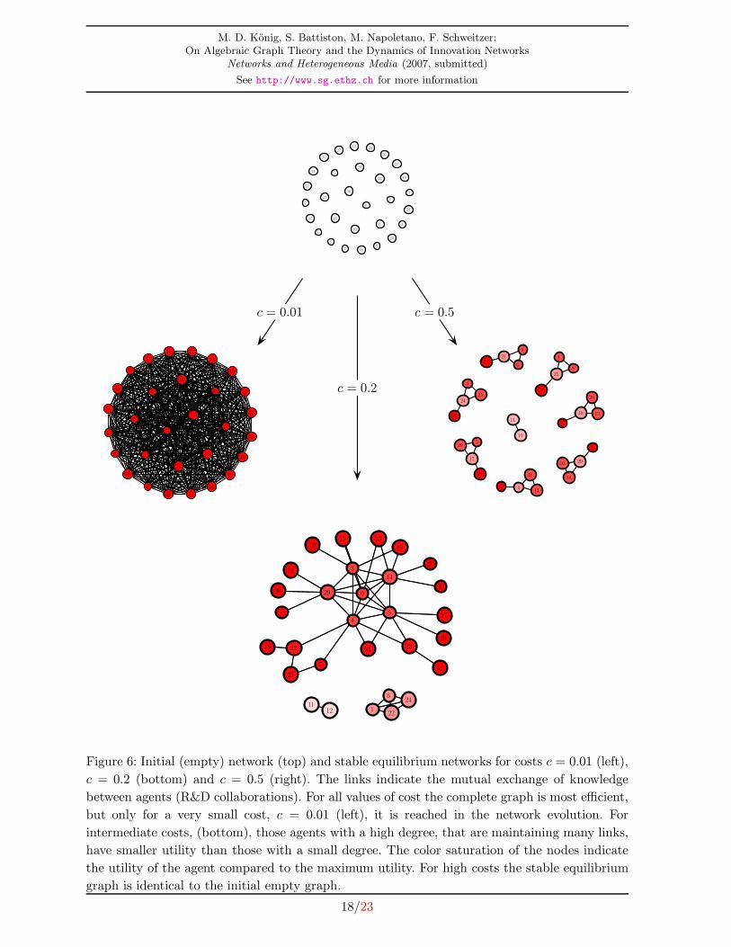
In Fig. (6)5 the stable equilibrium networks for 30 agents and three different values of the cost

are shown. For small costs, c = 0.1, the complete and efficient graph is reached. For intermediate

costs, c = 0.2, a sparse and highly clustered graph with a highly heterogeneous degree distribu-

tion is obtained. For high costs, c = 0.5, the stable equilibrium network consists of many small

clusters. One can see that by decreasing the cost the size of the connected components grows.

This is consistent with what has been observed in a recent study by Hanaki et al. [26] on R&D

collaborations of firms in the IT industry.

In Fig. (7) network density s(G) and relative performance π(G) are shown for increasing values of

the evaluation period τ (10 realizations for every value of τ) for n = 30 agents and intermediate

5The graphs were plotted with a network layout algorithm introduced by Geipel [19].

16/23





0 500 1000 1500 2000 2500−0.2

0

0.2

0.4

0.6

0.8

1

1.2

c=0.01c=0.20c=0.50π

T0 500 1000 1500 2000 2500

0

0.1

0.2

0.3

0.4

0.5

0.6

0.7

0.8

0.9

1

c=0.01c=0.20c=0.50

s

T

0 500 1000 1500 2000 25000

5

10

15

20

25

30

c=0.01c=0.20c=0.50〈d

〉

T0 500 1000 1500 2000 2500

0

0.1

0.2

0.3

0.4

0.5

0.6

0.7

0.8

0.9

1

c=0.01c=0.20c=0.50C

g

T

Figure 5: Evolution of the network starting from an empty graph until reaching its stable

equilibrium configuration, Fig. (6 bottom). The stable equilibrium network for intermediate

costs c = 0.2 is inefficient, sparse and is highly clustered, while for small costs c = 0.01 the

efficient complete graph is realized.

17/23





15

20

1

2

13

4

21

3

24

26

7

8

11

29

17

19

9

27

18

12

14

23

226

25

5

28

10

0

16

15

20

1

2

13

4

21

3

24

26

7

8

11

29

17

19

9

27

18

12

14

23

226

25

5

28

10

0

16

15

20

1

2

13

4

21

3

24

26

7

8

11

29

17

19

9

27

18

12

14

23

22

6

255

28

10

0

16

15

20

1

2

13

4

21

3

24

26

7

8

11

29

17

19

9

27

18

12

14

23

22

6

255

28

10

0

16

15

20

1

2

13

4

21

3

24

26

7

8

11

29

17

19

9

2718

12

14

23

22

6

25

5

28

10

0

16

15

20

1

2

13

4

21

3

24

26

7

8

11

29

17

19

9

2718

12

14

23

22

6

25

5

28

10

0

16

15

20

1

2

134

21

3

2426

7

8

11

2917

19

9

27

18 12

1423

22

6

25

5

28

10

0

16

15

20

1

2

134

21

3

2426

7

8

11

2917

19

9

27

18 12

1423

22

6

25

5

28

10

0

16

c = 0.01

c = 0.2

c = 0.5

Figure 6: Initial (empty) network (top) and stable equilibrium networks for costs c = 0.01 (left),

c = 0.2 (bottom) and c = 0.5 (right). The links indicate the mutual exchange of knowledge

between agents (R&D collaborations). For all values of cost the complete graph is most efficient,

but only for a very small cost, c = 0.01 (left), it is reached in the network evolution. For

intermediate costs, (bottom), those agents with a high degree, that are maintaining many links,

have smaller utility than those with a small degree. The color saturation of the nodes indicate

the utility of the agent compared to the maximum utility. For high costs the stable equilibrium

graph is identical to the initial empty graph.

18/23





costs c = 0.2. If the evaluation period is long enough, the efficient graph, i.e. the complete

graph, can be reached. Thus, if agents are evaluating their interactions in the long-term, the

performance of the system can be increased up to the efficient state.

−5 0 5 10 15 20 250

0.2

0.4

0.6

0.8

1

τ

s

a

−5 0 5 10 15 20 250

0.2

0.4

0.6

0.8

1

τπ

b

Figure 7: Density (a) and relative performance (b) for the stable equilibrium networks with

cost c = 0.2, n = 30 agents and 10 realizations for every evaluation period τ ∈ [0, 20]. By

increasing the evaluation period τ , the efficient graph, Kn, is reached.

8 Conclusion

In this paper, we consider the economic model of network evolution introduced in [36] in the

context of innovation and R&D collaborations. The model is characterized by two time scales:

there is a fast dynamics on the state variable of the nodes, representing their knowledge, and

a slow dynamics on the links of the graph. Since the fast dynamics is linear and occurs on a

static graph, there is a number of well known results form the theory of matrices that can be

applied to the model and we have reviewed the most important of them. For what concerns

the evolution of the network we have used some results from the theory of graph spectra to

derive some propositions on the efficiency and stability of the network. In particular, we have

provided a simple proof of the existence of equilibria, like the star and the clique, that for

c < 1/2 are not efficient but are stable. The existence of inefficient equilibria is of interest to

economists because it raises the issue of how to design appropriate policies to help the system

to reach the efficient equilibria. Our simulations confirm the analytical results and show that

the interplay between dynamics on the nodes and topology of the network leads in many cases

to equilibrium networks which are not efficient and are characterized, as observed in empirical

studies of R&D networks, by sparseness, presence of clusters and heterogeneity of degree. In

particular, we observe subgraphs of finite size and highly heterogeneous degree distribution

among which there are only a few connections. These properties have been observed in empirical

19/23





studies of innovation networks [13, 26] (for a more systematic comparison with the stylized facts

on innovation networks, see [36]).

As an new element, in this paper we also introduce a time τ after which agents evaluate whether

to keep or delete a link and we investigate by means of computer simulation how the equilibrium

reached by the network is affected by increasing the time τ . If agents evaluate their interactions

on a long-term, then they are able to reach an efficient state, which, on the other hand, is not

reachable, when collaborations are evaluated in the short-term. In other words, a short-sighted

rational behavior in the agents can give rise to inefficient networks, as often happens in reality.

Appropriate policy measures could be designed to support economic agents in maintaining in-

teractions even when, in the short run, they may be unprofitable. Our model may serve as a first

step towards both a theoretical explanation for the empirical regularities in a R&D networks

and a very simple test bed for policy design.

9 Acknowledgments

We are particularly grateful to Hans Haller for his astute comments and perceptive suggestions.

Morover we are in debted to Koen Frenken, Giorgio Fagiolo, Matthias Feiler, Kerstin Press, Jan

Lorentz and Nicolas Carayol for clarifying discussions and helpful comments. Finally we would

like to thank the critical audiences at the 5th International EMAEE Conference on Innovation

in Manchester, 2007, and the audience at the European Conference on Complex Systems in

Dresden, 2007.

References

[1] Bala, V.; Goyal, S. (2000). A Noncooperative Model of Network Formation. Econometrica

68(5), 1181–1230.

[2] Ballester, C.; Calvo-Armengol, A.; Zenou, Y. (2006). Who’s Who in Networks. Wanted:

The Key Player. Econometrica 74(5), 1403–1417.

[3] Boyd, S. (2006). Linear Dynamical Systems. Lecture Notes, Stanford University.

[4] Braun, M. (1993). Differential Equations and Their Applications. Texts in Applied Math-

ematics, Springer, 4th edn.

[5] Brualdi, R. A.; Solheid, Ernie, S. (1986). On the Spectral Radius of Connected Graphs.

Publications de l’ Institute Mathmatique 53, 45–54.

[6] Caldarelli, G.; Capocci, A.; Garlaschelli, D. (2007). Self–organized network evolution cou-

pled to extremal dynamics. Nature Physics .

20/23





[7] Carayol, N.; Roux, P. (2003). Self-Organizing Innovation Networks: When do Small Worlds

Emerge? Working Papers of GRES - Cahiers du GRES 2003-8, Groupement de Recherches

Economiques et Sociales.

[8] Carvalho, R.; Iori, G. (2007). Socioeconomic Networks with Long-Range Interactions. ArXiv

e-prints 706.

[9] Chung, F.; Lu, L. (2007). Complex Graphs and Networks. American Mathematical Society.

[10] Chung, Fan, R. (1997). Spectral Graph Theory. Regional Conference Series in Mathematics,

Conference Board of the Mathematical Sciences.

[11] Corbo, J.; Parkes, D. (2005). The price of selfish behavior in bilateral network formation.

In: PODC ’05: Proceedings of the twenty-fourth annual ACM symposium on Principles of

distributed computing. New York, NY, USA: ACM Press, pp. 99–107.

[12] Cowan, R.; Jonard, N. (2004). Network Structure and the Diffusion of Knowledge. Journal

of Economic Dynamics and Control 28, 1557–1575.

[13] Cowan, R.; Jonard, N.; Ozman, M. (2004). Knowledge Dynamics in a Network Industry.

Technological Forecasting and Social Change 71(5), 469–484.

[14] Cvetkovic, D.; Doob, M.; Sachs, H. (1995). Spectra of Graphs: Theory and Applications.

Johann Ambrosius Barth.

[15] Cvetkovic, D.; Rowlinson, P. (1990). The Largest Eigenvalue of a Graph: A Survey. Linear

and Multinilear Algebra 28, 3–33.

[16] Cvetkovic, D.; Rowlinson, P.; Simic, S. (1997). Eigenspaces of Graphs, vol. 66. Cambridge

University Press, Encyclopedia of Mathematics.

[17] Ehrhardt, G. C. M. A.; Marsili, M.; Vega-Redondo, F. (2006). Phenomenological Models

of Socio-Economic Network Dynamics.

[18] Fabrikant, A.; Luthra, A.; Maneva, E.; Papadimitriou, C. H.; Shenker, S. (2003). On a

network creation game. In: PODC ’03: Proceedings of the twenty-second annual symposium

on Principles of distributed computing. New York, NY, USA: ACM Press, pp. 347–351.

ISBN 1-58113-708-7.

[19] Geipel, M. (2007). Self-Organization applied to Dynamic Network Layout. International

Journal of Modern Physics C Forthcoming.

[20] Godsil, C. D.; Royle, G. F. (2001). Algebraic Graph Theory. Springer.

[21] Goyal, S.; Moraga-Gonzalez, J. L. (2001). R&D Networks. RAND Journal of Economics

32, 686–707.

21/23





[22] Gross, T.; Blasius, G. (2007). Adaptive Coevolutionary Networks - A Review. Eprint arXiv:

0709.1858.

[23] Haken, H. (1977). Synergetics - An Introduction; Nonequilibrium Phase Transitions and

Self-Organization in Physics, Chemistry and Biology. Springer.

[24] Haller, H.; Kamphorst, J.; Sarangi, S. (2007). (Non-)existence and scope of Nash networks.

Economic Theory 31, 597–604.

[25] Haller, H.; Sarangi, S. (2005). Nash Networks with Heterogeneous Links. Mathematical

Social Sciences 50, 181–201.

[26] Hanaki, N.; Nakajima, R.; Ogura, Y. (2007). The Dynamics of R&D Collaboration in the

IT Industry. Working Paper.

[27] Holme, P.; Ghoshal, G. (2006). Dynamics of Networking Agents Competing for High Cen-

trality and Low Degree. Physical Review Letters 96(098701).

[28] Hong, Y. (1993). Bounds of eigenvalues of graphs. Discrete Math. 123, 65–74.

[29] Horn, R. A.; Johnson, C. R. (1990). Matrix Analysis. Cambridge University Press.

[30] Jackson, M. O. (2003). A survey of models of network formation: Stability and efficiency.

Working Papers 1161, California Institute of Technology, Division of the Humanities and

Social Sciences.

[31] Jackson, M. O.; Wolinsky, A. (1996). A Strategic Model of Social and Economic Networks.

Journal of Economic Theory 71(1), 44–74.

[32] Jain, S.; Krishna, S. (1998). Autocatalytic Sets and the Growth of Complexity in an

Evolutionary model. Physical Review Letters 81(25), 5684–5687.

[33] Jain, S.; Krishna, S. (2001). A model for the emergence of cooperation, interdependence,

and structure in evolving networks. Proceedings of the National Academy of Sciences 98(2),

543–547.

[34] Khalil, H. K. (2002). Nonlinear Systems. Prentice Hall.

[35] Kim, C.; Wong, K.-C. (2007). Network formation and stable equilibrium. Journal of

Economic Theory 133, 536–549.

[36] Konig, M. D.; Battiston, S.; Napoletano, M.; Schweitzer, F. (2007). Efficiency and Stability

of Dynamic Innovation Networks. Forthcoming.

[37] Konig, M. D.; Battiston, S.; Schweitzer, F. (2007). Innovation Networks - New Approaches

in Modeling and Analyzing, Springer Complexity Series, chap. Modeling Evolving Innova-

tion Networks.

22/23





[38] Koutsoupias, E.; Papadimitriou, C. H. (1999). Worst-case equilibria. Lecture Notes in

Computer Science 1563, 404–413.

[39] Maas, C. (1987). Perturbation results for the adjacency spectrum of a graph. ZAMM 67,

428–430.

[40] Powell, W. W.; White, D. R.; Koput, K. W.; Owen-Smith, J. (2005). Network Dynamics

and Field Evolution: The Growth of Interorganizational Collaboration in the Life Sciences.

American Journal of Sociology 110, 1132–1205.

[41] Robinson, R.; Foulds, L. (1980). Digraphs: Theory and Techniques. Gordon and Breach

Science Publishers.

[42] Saurabh, A.; Cowan, R. (2004). The Growth of Knowledge and Complexity in an Evolv-

ing Network Model of Technological Innovation. Tech. rep., UNU-INTECH and MERIT,

University of Maastricht, The Netherlands. Paper presented at “Organisations, Innovation

and Complexity: New Perspectives on the Knowledge Economy”, 9th-10th September 2004,

CRIC, University of Manchester, Manchester,England, UK.

[43] Seneta, E. (2006). Non-negative Matrices And Markov Chains. Springer.

[44] Stanley, R. P. (1987). A Bound on the Spectral Radius of Graphs with e Edges. Linear

Algebra and its Applications 87, 267–269.

[45] Stewart, I. (2004). Networking opportunity. Nature 427, 601–604.

[46] Wasserman, S.; Faust, K. (1994). Social Network Analysis: Methods and Applications.

Cambridge University Press.

[47] Xu, J. (2003). Theory and Application of Graphs. Kluwer Academic Publishers.

23/23


ch for more information On Algebraic Graph Theory and the Dynamics of Innovation Networks

Documents

Transcript of ch for more information On Algebraic Graph Theory and the Dynamics of Innovation Networks