1. IntroductionDevelopment has been

an important concept sincethe definition of ‘econo-my’ was provided for thefirst time. Yet, method-ological evaluation of de-velopment and its relation-ship with growth has ac-quired greater emphasis s-ince the World War II. Inaddition, four periods ofdevelopment have beenobserved which displaysignificant features (Duttand Ros 2008).– 1945-1950: Low savings,

high population growth,less willingness to invest,intensive production in a-griculture and limited in-dustry orientation.

– 1950 - Late 1960s: massprotectionism and importsubstitution, as no focuson export was needed.

– Late 1960s-1980s: Re-birth of the neo-classicalapproach. Extended focuson integration of coun-tries, emphasis on theoverdependence school.

– 1980 - Present: Measure-ment of economic devel-opment by mathematicaleconomics. Interpreta-tion of the effects of economic development on distribu-tion, income and preferences started with integration ofmicro-theory with macro-theory.

As a result, the factorsunderlying economic de-velopment and the effectsof development on wel-fare have been broadly in-vestigated, specifically s-ince the 1990s. In addi-tion to growth modelsstemming from produc-tion function and capitalstock, index studies meas-uring total and marginalproductivity and growthaccounting models werebrought into use in the in-ternational literature (Oy-eranti 2000, Knowles andMcCombie 2002).

Factor productivity s-tudies focusing on theCobb-Douglas productionfunction developed bySolow (1957) and K-endrick (1961), whichtakes employment as areference production fac-tor, were widely observedin the literature. These s-tudies were also refer-enced as growth account-ing studies, and includedoutput growth against in-put growth. Generally,growth refers to technicalchange when it dependson all production factors,while it is called partial

factor productivity when it depends on the efficiency of a s-ingle factor. The main convergence studies focussed on thewelfare effect of increased commercial activities (Balassa1971, Chenery 1962, Chenery and Eckstein 1970, Wilhelm2008) and on changes in total and partial factor productivi-ty levels (Balassa and Bertrand 1970, Hayami and Ruttan1970, Komlos 1988, Dowrick and Nyguen 1989).

Agricultural Value Added and Economic Growthin the European Union Accession Process

RAHMIYE FIGEN CEYLAN*, BURHAN ÖZKAN*

AbstractThe aim of this paper is to analyse the impact of agricultural income within theframework of the European Union integration process using an extended Solowgrowth model and panel data analysis tools. The effects of per capita agriculturalvalue added on per capita income were examined using two samples of 25 and 30EU member and candidate states respectively for the periods 1995-2007 and 2002-2007. A dummy variable representing EU membership status and a composite riskvariable computed by the PRS Group, which provided information on structuralproperties of the economies of relevant countries, were used as independent vari-ables. According to the two-way random effects estimation results, the agricultur-al value added elasticity of per capita income was 0.025 for the 1995-2007 period,and 0.22 for the 2002-2007 period. It was estimated that average per capita in-come is 5.6 % higher among EU members. With a change representing a 1 pointrise in composite risk, which means a reduction of the risk faced by the countryconcerned, it was demonstrated that per capita income rose 1% during both peri-ods. The results also showed that agriculture retains its economic importance, andthat average per capita income among EU members is higher than among non-members due to exogenous factors.

Keywords: European Union, integration, Solow growth, agricultural value added, risk.

RésuméL’objectif de cet article est d’analyser l’impact du revenu agricole dans le cadre duprocessus d’intégration dans l’Union européenne, en utilisant une extension du mo-dèle de Solow et des outils d’analyse des données de panel. Les effets de la valeurajoutée agricole par habitant sur le revenu par habitant ont été examinés en s’ap-puyant sur deux échantillons de 25 et 30 États membres et Pays candidats, respec-tivement pour les périodes 1995-2007 et 2002-2007. Une variable nominale repré-sentant le statut de membre de l’UE et une variable de risque composite, calculéepar PRS Group, fournissant des informations sur les propriétés structurelles deséconomies des pays concernés, ont été utilisées comme variables indépendantes.Selon les résultats du modèle à effets aléatoires bidirectionnel, l’élasticité de la va-leur ajoutée agricole du revenu par habitant est égale à 0,025 pour la période 1995-2007 et à 0,22 pour la période 2002-2007. Il a été estimé que le revenu moyen parhabitant est 5,6% plus élevé dans les pays membres de l’UE. Avec un changementreprésentant 1 point de hausse de la valeur du risque composite, ce qui signifie uneréduction du risque auquel le pays fait face, il a été démontré que le revenu par ha-bitant a augmenté de 1% dans les deux périodes. Les résultats indiquent égalementque l’agriculture garde son importance économique et que le revenu moyen par ha-bitant dans les pays de l’UE est plus élevé par rapport aux pays non-membres enraison de certains facteurs exogènes.

Mots-clés: Union européenne, intégration, modèle de Solow, valeur ajoutée, risque.

62

*Akdeniz University, Faculty of Agriculture Department of Agricul-tural Economics, Antalya - TURKEY.

Jel Classification: E25, F43, O47, Q18

NEW MEDIT N. 4/2013

However, the convergence of countries has been testedbased on the utilization of production functions. By way ofexample, Pittau and Zelli (2006) measured regional conver-gence within the EU between 1977 and 1996 and found thatconvergence from poor regions to rich regions was rela-tively low. Mayawala (2007) analysed the effects of agri-culture on economic growth for 71 countries in three groups(developed – developing – less developed) between 1984and 2004, with the inclusion of economic and social struc-tural variables. The study revealed that both the capitalstructure and the rise in exports affected growth positivelyin all countries, while investment risk affected inverselymedium income level countries. Government instability af-fected growth positively in the top two groups.

Indeed, structural convergence has been an important re-search topic in recent years. In their push studies focusingon commercial gains across the EU member states, Lejouret al., (2009) found that EU membership increased com-mercial relationships by 33 % when considered alone andby 55 % when changes in the structure of economic institu-tions were also taken into consideration. Moreover, incomelevels of candidate countries were expected to rise between31% and 43 % in the long run after they had became EUmembers.

Another study investigating the single sector neo-classi-cal growth model also incorporated an exogenous agricul-ture sector, and aimed to clarify the reasons behind the lateindustrial development of some countries regardless of re-source abundance (Gollin et al., 2002). Research on 62 de-veloping countries in the period 1960-1990 demonstrated asignificant rise in agricultural efficiency when interpretingthe uprising trend of GDP per capita. Later, the same studyfound that agriculture cannot be substituted for the relevanteconomies.

Another important question addressed has been whetheragriculture, having inelastic production factors, affects eco-nomic growth and per capita income. Therefore, a surveyon the effects that agriculture has on economic growth canbe important to assess the productivity of the sector and thesupportive financial transfers to the sector. The EuropeanUnion (EU) integration process involves specific tools andproduces certain outcomes for economies, and one of themain impacts of the integration process has been recordedin agriculture. The aim of this paper is to analyse the ef-fects of agriculture on economic growth within a sample ofEU member and candidate countries.

By analysing the impact of agriculture on the national e-conomies, it seems possible to provide information on theproductivity of the sector and on efficiency change accord-ing to the time considered and the countries involved.Therefore the impact of agricultural value added on percapita income has been estimated using a version of theSolow growth model extended with structural coherencevariables to cover the European Union member and candi-date countries in two reference periods, 1995-2007 and

2002-2007, taking into account the accession process. Sam-ples were constructed according to data availability and thenumber of member states. The analysis was based onto t-wo samples to include more candidate and new member s-tates specifically for the 2002–2007 sampling period.Therefore, the main objective of the study was to under-stand the effect of the relationship between agriculture andgrowth levels through differences in per capita GDP ac-cording to the membership status of the countries with re-spect to the European Union.2. MaterialsDescription of the model and variables

The Extended Solow Growth Model was applied usingpanel data analysis for two periods between 1995 and 2007.By the year 2013 there will be 28 EU members and 4 can-didates. While it was possible to acquire data for Iceland,Turkey, no data was available for Macedonia and Montene-gro. Therefore, 30 countries were included in the study.

Within the scope of the study, an analysis was made tomeasure the impacts of agricultural value added, specificmacroeconomic variables and indices representing socialand institutional structure over per capita income as growthindicator. Most of the fundamental economic indicatorsused were retrieved from World Development Indicatorsand Global Development Finance (Anonymous, 2011a). Inaddition, structural coherence indices retrieved from the In-ternational Country Risk Guide (ICRG) were used in theanalyses in order to represent the institutional and socialstructures of the countries.Political, economic and financial risk

The composite risk score is the arithmetic mean of polit-ical (100 points), economic (50 points) and financial (50points) risk scores. The composite risk score is divided in-to the following rating categories: too low (80-100) and toohigh (0-49.9) according to ICRG methodology (Hoti,2003).

A new basket composed of government stability, socio-e-conomic conditions, investment profile, openness for demo-cratic control and bureaucratic quality was established,and the scores were indexed to 100 points for political risk.The components of economic risk are per capita GDP risk(ratio of the Dollar-based national income to the average in-come of all countries), real GDP growth risk (growth ratecalculated relating to 1990 prices), annual inflation risk(non-weighted Consumer Price Index), budget balance risk(budget balance of the country with domestic currency tothe overall GDP) and current account risk (balance of pay-ments in Dollars to the GDP of the country).

Financial risk components are external debt risk (debt toGDP ratio), external debt service risk (current account totalto Dollar value of exported goods and services) net inter-national liquidity risk (Dollar value of official annual re-serves to monthly Dollar value of import cost of goods) andexchange rate stability risk (depreciation or appreciation of

63

NEW MEDIT N. 4/2013

the national currency). For this study, the economic and fi-nancial risk components indexed for 50 points were adjust-ed to a 100 points scale. The average of the three risk scoresis treated as the composite risk variable in the growth mod-el implemented.3. MethodMeasurement of economic development usingpanel data

For the empirical analysis of economic development,time series analysis can be preferred as a methodology, withthe utilization of measures retrieved from a unique datasource for different time periods. However, panel data stud-ies are preferred when measuring time and place variationsof growth, and when comparing the growth performancesof different countries (Ederveen et al., 2006, Islam 2003,Chenery and Taylor 1968). Panel data analyses are also pre-ferred in cross-country macro-economic studies due to theshort time series (Olofin et al., 2009, Lloyd et al., 2001).

Panel data may be estimated with the Least Squares(OLS) or Maximum Likelihood (ML) methods. Yet, what ismore important in panel data analysis is whether the esti-mation could be bound to time series and/or cross sectionalpoints. Due to the decision made on this extended model,panel estimation, fixed effects or random effects estimationmethodology is selected (Arellano, 2003). In order to selectthe proper estimation method, it is important to test the sta-tionarity of a series using the specification tests. After de-termining whether the series analysed are stationary ini-tially or after being differentiated, it is also important to de-termine whether the series could be estimated with a co-in-tegration procedure or not. After co-integration was definedas a specific field of study in 1995, many different testswere developed. In our study, Pedroni’s (1999) four-statis-tic test is used. This test was developed by investigation ofρ and t statistics in the panel and in the group of series.

Panel estimation incorporates OLS estimation which dis-regards cross-sectional and time effects for the valuation ofthe model. In case of models for which panel estimation isnot suitable, the one-way error components model, whichrefers to the inclusion of unobserved cross-sectional effects,or the two-way error components model involving unob-served time effects as well, are considered to be the appro-priate estimation model. In order to understand whether theset could be estimated in the form of a panel, it is importantto first implement a cross-sectional dependency test. If wereach a concrete result according to which cross-sectionalvariables are independent of neglected fixed effects andrandom effects, then utilization of unified panel regressionproduces more accurate estimation results.

The first testing methodology proposed for a panel serieswas the Breusch-Pagan Lagrange Multiplier (LM) test (Ko-rkmaz et al., 2010; Berke, 2009). The LM test gives accu-rate results when the number of time related data points (T)is larger than the number of cross-section related datapoints (N). By contrast, when there are more cross-section-

al observation points, other proposed tests should also beconsidered (Hoyos and Sarafidis, 2006). The Pesaran CDtest, which also depends on the Lagrange Multipliermethodology, is appropriate for situations where T is small-er than N, and when there is a balanced panel (Hoyos andSarafidis, 2006; Pesaran, 2004). In addition, the non-para-metric statistic of Friedman (1937), which relies on the S-pearman rank correlation coefficient and Frees statistic(1995, 2004) depending on the square of the correlation co-efficient, can be used for the measurement of cross-section-al dependence (Hoyos and Sarafidis, 2006).

All three tests assume cross-sectional independence.When independence is inapplicable, it is clear that the mod-el fits best the random effects estimation. In this situation,it is necessary to implement the Hausman specification testto determine whether to use random effects or fixed effectsestimation methodology (Baltagi, 2005). In this test, the hcoefficient retrieved after taking differences of the regres-sors with respect to cross-sections and time series can beused to test whether the random effects model is preferredto fixed effects or not (Arellano, 2003). This test focuses oncorrelations of independent variables with random groupeffect variables. If this correlation is equal to 0, the randomeffects model is preferred. At the opposite end of the scale,the fixed effects model is preferred (Lloyd et al., 2001,Washington et al., 2003; Kunst, 2009).Panel data analysis methods - Two-way errorcomponent regression model

When the objective is to measure the impact of an unob-served time series variable, as well as the unobserved cross-sectional variable in panel data analysis, it is necessary toimplement a two-way error components regression model.Accordingly, the error term takes the following form (Balt-agi 2005).

Here, while µi is the unobserved cross-sectional effect, λτis the unobserved time series effect. In addition, λτ is inde-pendent of the cross-section and provides information onall time-related data excluded from the regression.

In a two-way fixed effects analysis, when µι and λτ areinterpreted as constant parameters to be estimated, νit is thetwo-way error term [1]. Statistical inference depends on thevalues that N observation points take during definite timeperiods (Baltagi, 2005). Then the function takes the follow-ing form in this situation [2].

The main assumption for random effects estimation isthat µi, λτ and νit components have independent distribu-tions with 0 mean and constant variance (Wooldridge,2002). Inference with random effects analysis gives gener-al information on the population from which the sample is

[2]

i=1,……,N; t=1,…..,T [1]

NEW MEDIT N. 4/2013

64

constructed (Baltagi, 2005). In this analysis, it is assumedthat the error terms have constant variance for all i and t asvar By contrast, covariance of er-ror terms is σ2

µ for the same cross-sections (i=j) and for dif-ferent time periods (t≠s) and is σ2

λ for the same time peri-od (t=s) and different observation periods (i≠j) and 0 other-wise.

In addition, random effects estimation allows inferenceon three different error components for the population fromwhich that sample is collected. Accordingly, random ef-fects estimation is referred as the error components analy-sis in the literature as well.

The two-way error components model is preferred whenthe data set and degrees of freedom are available. Yet, whenno cross-sectional dependence is detected, it is more appro-priate to estimate the data set in a simplified way.Model Structure – The effect of agriculture andEuropean Union Membership on economic growth

This study implies a specifically modified Solow GrowthModel. The model is extended with sector productivityvariables and social and economic indicators.

The Solow Growth Model stemming from the productionfunction is turned into the following general form [3] afterincluding agriculture, exports and inflation (Hwa, 1988).

where: Y.

= average annual GDP growth rate; K.= average

annual capital stock growth rate; L.

= average annual labourgrowth rate; A

.= average annual agricultural growth rate; X

.

= average annual export growth rate; P.= average annual in-

flation growth rate.Humphries and Knowles (1998) included non-farm

labour, education and health expenditures variables in thissystem, while Barro (1991) extended the model with eco-nomic and structural coherence variables. Since the aim ofthis study was to measure the impacts of integration to theUnion’s social and economic structures on economicgrowth in the EU member and candidate countries, the fol-lowing extended form [5] of the Solow Growth Model wasapplied.

The main variables for the model were the following:Yit : Per capita income in country i and time tAVAit : Per capita agricultural value added in country i

and time tCSit : Per capita capital stock in country i and time tEit Per capita education expenditure amount in coun-

try i and time tEUit : EU membership condition in country i and time t

(member=1; non-member=0)CRit : Per capita composite institutional quality index

value

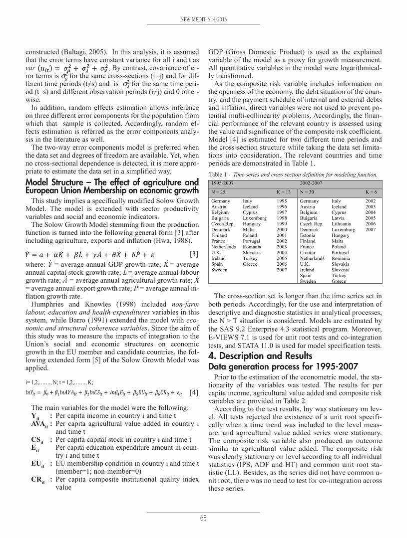
GDP (Gross Domestic Product) is used as the explainedvariable of the model as a proxy for growth measurement.All quantitative variables in the model were logarithmical-ly transformed.

As the composite risk variable includes information onthe openness of the economy, the debt situation of the coun-try, and the payment schedule of internal and external debtsand inflation, direct variables were not used to prevent po-tential multi-collinearity problems. Accordingly, the finan-cial performance of the relevant country is assessed usingthe value and significance of the composite risk coefficient.Model [4] is estimated for two different time periods andthe cross-section structure while taking the data set limita-tions into consideration. The relevant countries and timeperiods are demonstrated in Table 1.

The cross-section set is longer than the time series set inboth periods. Accordingly, for the use and interpretation ofdescriptive and diagnostic statistics in analytical processes,the N > T situation is considered. Models are estimated bythe SAS 9.2 Enterprise 4.3 statistical program. Moreover,E-VIEWS 7.1 is used for unit root tests and co-integrationtests, and STATA 11.0 is used for model specification tests.4. Description and ResultsData generation process for 1995-2007

Prior to the estimation of the econometric model, the sta-tionarity of the variables was tested. The results for percapita income, agricultural value added and composite riskvariables are provided in Table 2.

According to the test results, lny was stationary on lev-el. All tests rejected the existence of a unit root specifi-cally when a time trend was included to the level meas-ure, and agricultural value added series were stationary.The composite risk variable also produced an outcomesimilar to agricultural value added. The composite riskwas clearly stationary on level according to all individualstatistics (IPS, ADF and HT) and common unit root sta-tistic (LL). Besides, as the series did not have common u-nit root, there was no need to test for co-integration acrossthese series.

[3]

1995-2007 2002-2007

N = 25 K = 13 N = 30 K = 6

Germany

Austria

Belgium

Bulgaria

Czech Rep.

Denmark

Finland

France

Netherlands

U.K.

Ireland

Spain

Sweden

Italy

Iceland

Cyprus

Luxemburg

Hungary

Malta

Poland

Portugal

Romania

Slovakia

Turkey

Greece

1995

1996

1997

1998

1999

2000

2001

2002

2003

2004

2005

2006

2007

Germany

Austria

Belgium

Bulgaria

Czech Rep.

Denmark

Estonia

Finland

France

Croatia

Netherlands

U.K.

Ireland

Spain

Sweden

Italy

Iceland

Cyprus

Latvia

Lithuania

Luxemburg

Hungary

Malta

Poland

Portugal

Romania

Slovakia

Slovenia

Turkey

Greece

2002

2003

2004

2005

2006

2007

Table 1 - Time series and cross section definition for modeling function.

i= 1,2,……., N; t = 1,2,……., K;

[4]

NEW MEDIT N. 4/2013

65

.

NEW MEDIT N. 4/2013

66

lnYit N: 25 K: 13

Test statistic Hypothesis Level +

Drift

!1 Time

trend

!

IPS H0: All panels have unit roots 5,65 1,00 0,73 0,77

LL H0: Panel has a unit root -2,242 0,01** -9,90 0,00**

Fisher – ADF2

H0: All panels have unit roots 3,2948 < 0,01** 3,29 < 0,01**

HT H0: All panels have unit roots 1,01 1,00 0,7510 1,00

lnAVAit N: 25 K: 13

Test statistic Hypothesis Level +

Drift

! Time

trend

!

IPS H0: All panels have unit roots 1,75 0,96 -4,44 0,00**

LL H0: Panel has a unit root -0,79 0,21 -7,06 0,00**

Fisher – ADF H0: All panels have unit roots 6,57 0,00** 2,51 < 0,01**

HT H0: All panels have unit roots 0,81 0,68 0,28 < 0,01**

CRit N: 25 K: 13

Test statistic Hypothesis Level +

Drift

! Time

trend

!

IPS H0: All panels have unit roots -2,66 < 0,01** -1,18 0,12

LL H0: Panel has a unit root -10,71 0,00** -9,97 0,00**

Fisher – ADF H0: All panels have unit roots 12,16 0,00** 2,31 0,00**

HT H0: All panels have unit roots 0,67 < 0,01** 0,51 0,56

Estimation results for 1995-2007Due to one-way error components estimation outputs

shown in Table 3, Frees, Peseran CD and Friedman RAVEtests indicated that the model had cross-sectional depend-ence, and that the data could not be estimated in panel form.However, the Hausman specification test results showedthat one-way random effects estimation would produce bi-ased results. However, as the parameter estimate of percapita agricultural value added did not comply with eco-nomic expectations, and as the length of the series was longenough, it was decided to execute comparative estimationfor two-way error components. The outputs of the two-wayerror components estimation are provided in Table 4.

Initially, considering the FRE and B-P statistics it wasclear that the model had cross-sectional dependence. As theFrees test was developed by evaluation of Friedman and Pe-

seran statistics, the test result was used to reject cross-sec-tional independence. In any case, the difference between ingroup (0.86) and total (0.37) goodness of fit (R2) values re-trieved from the two way random effects estimation also in-dicated that the data could not be estimated using joint pan-el (Kunst, 2009). What is more, the Hausman statistic,which compares the fixed effects model with the randomeffects model, was not significant with a 0.98 p-value. Ac-cordingly, it was found that the random effects modelwould lead to more significant and unbiased results whencompared with the fixed effects model.

While all parameter estimates were significant in the pan-el solution, the per capita agricultural value added parame-ter estimate was not significant in the random and fixed ef-fects solutions. Even so, the Wald parameter significancetest1 indicated that the parameter estimates of random ef-fects had common significance. The parameters were joint-ly significant due to the 0 p-value of the Wald statistic. Fur-thermore, the 37% total goodness of fit (R2) indicated thatexplanatory variables could explain the 37% variation inthe dependent variable.

Prior to interpretation of the findings, diagnostic testswere implemented to understand whether there was someautocorrelation in error terms, and whether the error vari-ance was homoscedastic. As a result of the Wooldridge au-tocorrelation test results, the null hypothesis of ‘no auto-correlation’ was rejected. In any case, the likelihood ratiobased Wald heteroscedasticity test rejected ‘no het-eroscedasticity’ hypothesis. Accordingly, the model was re-estimated using the White error correction methodology.The test findings and consistent parameter estimates areprovided in Table 5.

Independent

Variable

OLS One Way Random

Effect

One Way Fixed Effect

lnAVAit 0,5493 (0,00) -0,2857 (0,00) -0,3418 (0,00)

CRit 0,0658 (0,00) 0,0139 (0,00) 0,0122 (0,00)

EUit 0,5285 (0,00) 0,1720 (0,00) 0,1647 (0,00)

Constant 0,8140 (0,02) 10,013 (0,00) 10,48 (0,00)

N 25 25 25

K*N 325 325 325

R2

0,77

In-group: 0,65

Between groups: 0,04

Total: 0,05

In-group: 0,66

Between groups: 0,003

Total: 0,0099

F TestF (3,321):

362,45 (0,00)

F (3,297):

188,06 (0,00)

Wald Parameter

Test("2(3))

409,63 (0,00)

B-P CSD3

Test

("2(1))

80,21 (0,00)

FRE CSD Test 4

5,471 (0,00)

RAVE CSD Test 108,253 (0,00)

Peseran CD Test 18,227 (0,00)

Hausman S. T.

("2(3))

16,53 (< 0,01)

Wooldridge Test

(F(1,24))271,63 (0,00)

Wald Test ("2(3)) 2.045,24 (0,00)

Table 3 - One-way error component estimation results (1995-2007).

3 CSD = Cross Sectional Dependence.4 Q values 0,10: 0,1984; 0,05: 0,2620; 0,01: 0,3901.

Independent

Variable

OLS Two-Way Random

Effect

Two-Way Fixed Effect

lnAVAit 0,5493 (0,00) 0,0245 (0,41) -0,0019 (0,94)

CRit 0,0658 (0,00) 0,0081 (0,00) 0,0075 (0,00)

EUit 0,5285 (0,00) 0,0561 (0,00) 0,0549 (0,00)

Constant 0,8140 (0,02) 8,5247 (0,00) 8,7348 (0,00)

N 25 25 25

K*N 325 325 325

R2

0,77

In group: 0,86

Between groups: 0,83

Total: 0,37

In group: 0,86

Between groups: 0,73

Total: 0,29

F TestF (3,321):

362,45 (0,00)

F (15,285):

112,57 (0,00)

Wald Parameter

Test ("2(15))

1279,94 (0,00)

B-P CSD

Test("2(1))

831,25 (0,00)

FRE CSD Test5

7,056 (0,00)

RAVE CSD Test 1,899 (1,00)

Peseran CD -1,966 (1,95)

Hausman S. T.

("2(15))

6,06 (0,9788)

Wooldridge Test

(F(1,24))271,63 (0,00)

Wald Test ("2(12)) 5,42*e

16(0,00)

Table 4 - Two-way error component estimation results (1995-2007).

1 Degrees of freedom for the statistic (k-1): 13 years + 3 explanatoryvariables - 1.

lnYit N: 25 K: 13

Test statistic Hypothesis Level +

Drift

1 Time

trend

IPS H0: All panels have unit roots 5,65 1,00 0,73 0,77

LL H0: Panel has a unit root -2,242 0,01** -9,90 0,00**

Fisher – ADF2

H0: All panels have unit roots 3,2948 < 0,01** 3,29 < 0,01**

HT H0: All panels have unit roots 1,01 1,00 0,7510 1,00

lnAVAit N: 25 K: 13

Test statistic Hypothesis Level +

Drift

Time

trend

IPS H0: All panels have unit roots 1,75 0,96 -4,44 0,00**

LL H0: Panel has a unit root -0,79 0,21 -7,06 0,00**

Fisher – ADF H0: All panels have unit roots 6,57 0,00** 2,51 < 0,01**

HT H0: All panels have unit roots 0,81 0,68 0,28 < 0,01**

CRit N: 25 K: 13

Test statistic Hypothesis Level +

Drift

Time

trend

IPS H0: All panels have unit roots -2,66 < 0,01** -1,18 0,12

LL H0: Panel has a unit root -10,71 0,00** -9,97 0,00**

Fisher – ADF H0: All panels have unit roots 12,16 0,00** 2,31 0,00**

HT H0: All panels have unit roots 0,67 < 0,01** 0,51 0,56

Table 2 - Stationarity test results for 1995-2007 period.

1 Null hypothesis is rejected on* 0,05 and on** 0,01 significance level.2 Statistic computation for Fisher ADF with time trend does not involve drift.

5 Q values 0,10: 0,1984; 0,05: 0,2620; 0,01: 0,3901.

Consequently, the agricultural value added elasticity ofper capita national income proves to be 0.0245. Per capitaincome rises by almost 1% (0.08 %) due to a 1 point in-crease in the composite risk variable, which means an ap-preciation of the risk position of the country. Consequent-ly, the composite risk semi-elasticity of per capita incomeis 1% as semi-elasticity refers to the parameter estimatesdirectly in variables taking numerical values (Gujarati,2003).

The EU dummy variable parameter estimate of 0.0561 in-dicates, after taking the anti-log, that average per capita in-come is around 1 Dollar higher in EU member countries.Like the composite risk interpretation, the EU membershipsemi-elasticity of per capita income is 0.057. The semi-e-lasticity for categorical variables is calculated by taking theanti-log of the parameter estimate and deducting 1 in semi-logarithmic models as demonstrated by Halvorsen andPalmquist (1980) (Gujarati, 2003).

Following this calculation, almost the same value is reachedusing the parameter estimate. Accordingly, being a member ofthe European Union leads to a 0.057 % rise in per capita in-come. Also, time has a significant effect on per capita incomerise. Average per capita income rises with time.Data generation process for 2002-2007

The same unit root tests were applied as in the previousperiod in order to test whether the variables were stationaryor not. Stationary test results are indicated in Table 6 for percapita national income, agricultural value added and com-posite risk variables.

According to results with time trend, the Fisher ADF test in-dicated that per capita income variable in logarithmic formwas stationary. Accordingly, lny was stationary with trend onlevel. The per capita agricultural value added series was sta-tionary for LL and Fisher ADF statistics. However, the sameseries was not stationary according to the IPS and HT statis-tics. Even so, when interpreted with trend on level, the percapita agricultural value added series was found to be station-ary using the Fisher ADF and HT statistics. In contrast, thecomposite risk variable was stationary on level due to the LLand Fisher ADF statistics and it was found to be non-station-ary with trend. Accordingly, the series were found to be sta-tionary on level, and investigating co-integrating relationshipamong the series was considered to be unnecessary.Estimation results for 2002-2007

As for the 1995-2007 period, an initial comparativeanalysis was made between the one-way error componentand the panel LS estimation outputs.

NEW MEDIT N. 4/2013

67

Independent Variable Two-Way Random Effects

lnAVAit 0,0245 (0,79)

CRit 0,0081 (0,00)

EUit 0,0561 (0,07)

Constant 8,5247 (0,00)

1996 0,01 (0,16)

1997 0,02 (0,10)

1998 0,05 (0,00)

1999 0,09 (0,00)

2001 0,13 (0,00)

2001 0,15 (0,00)

2002 0,15 (0,00)

2003 0,17 (0,00)

2004 0,18 (0,00)

2005 0,21 (0,00)

2006 0,25 (0,00)

2007 0,29 (0,00)

N 25

K*N 325

R2

In group: 0,86

Between groups: 0,83

Total: 0,37

Wald Parameter Test ("2(15)) 807,47 (0,00)

Table 5. Two-way random effects estimates with consistent standard er-rors for 1995-2007 period.

lnYit N: 25 K: 6

Test statistic Hypothesis Level +

Drift

!6 Time

trend

!

IPS H0: All panels have unit roots 13,82 1,00

LL H0: Panel has a unit root 3,57 0,99

Fisher – ADF7

H0: All panels have unit roots -2,63 0,99 21,08 0,00**

HT H0: All panels have unit roots 1,05 1,00 0,24 0,98

lnAVAit N: 25 K: 6

Test statistic Hypothesis Level +

Drift

!8 Time

trend

!

IPS H0: All panels have unit roots 0,84 0,79

LL H0: Panel has a unit root -4,09 0,00**

Fisher – ADF H0: All panels have unit roots 6,02 0,00** 14,94 0,00**

HT H0: All panels have unit roots 0,47 0,09 -0,31 0,01**

CRit N: 25 K: 6

Test statistic Hypothesis Level +

Drift!9 Time

trend!

IPS H0: All panels have unit roots 1,12 0,87

LL H0: Panel has a unit root -24,26 0,00**

Fisher – ADF H0: All panels have unit roots 5,27 0,00** -1,42 0,92

HT H0: All panels have unit roots 0,51 0,22 0,30 0,99

Table 6 - Stationarity test results for 2002-2007 period.

6 * Null hypothesis is rejected on 95 %, ** null hypothesis is rejected on 99%.7 Fisher ADF statistic with time trend does not include drift.8 * Null hypothesis is rejected on 95 %, ** null hypothesis is rejected on 99%.9 * Null hypothesis is rejected on 95 %, ** null hypothesis is rejected on 99%.

Independent Variable OLS One Way Random

Effect

One Way Fixed Effect

lnAVAit 0,6068 (0,00) 0,0102 (0,88) -0,1524 (<0,01)

CRit-1 0,0856 (0,00) 0,0116 (< 0,01) 0,0029 (0,32)

EUit 0,3908 (0,00) 0,1868 (0,00) 0,1691 (0,00)

Constant -1,0854 (0,00) 8,3212 (0,00) 9,9651 (0,00)

N 30 30 30

K*N 180 180 180

R2

0,83

In-group: 0,28

Between groups: 0,70

Total: 0,62

In-group: 0,65

Between groups: 0,04

Total: 0,05

F TestF (3,176):

290,10 (0,00)

F (3,147):

27,46 (0,00)

Wald Parameter Test ("2(3)) 56,48 (0,00)

B-P CSD Test ("2(1)) 169,80 (0,00)

FRE CSD Test 10

7,025 (0,00)

RAVE CSD Test 90,819 (0,00)

Peseran CD Test 26,215 (0,00)

Hausman S.T. ("2(3)) 34,30 (0,00)

Wooldridge Test (F(1,29)) 1783,356 (0,00)

Wald Test ("2(3)) 2669,03 (0,00)

Table 7 - One way error component estimation findings (2002-2007).

10 Q values 0,10: 0,4127; 0,05: 0,5676; 0,01: 0,9027.

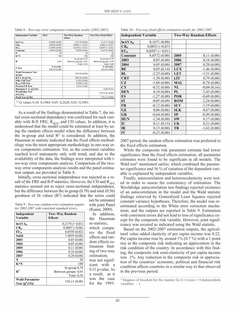
As a result of the findings demonstrated in Table 7, the ini-tial cross-sectional dependency was confirmed for each vari-able with B-P, FRE, RAVE, and CD values. In addition, it isunderstood that the model could be estimated at least by us-ing the random effects model when the difference betweenthe in-group and total R2 is considered. In addition, theHausman m statistic indicated that the fixed effects method-ology was the most appropriate methodology in one-way er-ror components estimation. Yet, as the concerned variablesreached level stationarity only with trend, and due to theavailability of the data, the findings were interpreted with t-wo-way error components analysis. Comparison of the two-way error components analysis results and the panel estima-tion outputs are provided in Table 8.

Initially, cross-sectional independence was rejected as a re-sult of the FRE and B-P statistics. However, the CD and RAVEstatistics seemed not to reject cross-sectional independence,but the difference between the in-group (0.78) and total (0.56)goodness of fit values (R2) indicated that the series could

not be estimatedwith joint Panel(Kunst, 2009).

In addition,the Hausmanm-statistic,which compa-res the fixedeffects and ran-dom effects es-timation find-ing of two-wayestimation,was not signif-icant with a0.31 p-value. Asa result, as itwas the casefor the 1995-

2007 period, the random effects estimation was preferred tothe fixed effects estimation.

While the composite risk parameter estimate had lowersignificance than the fixed effects estimation, all parameterestimates were found to be significant in all models. TheWald test2 mentioned earlier, which combined the parame-ter significance and 56 % of variation of the dependent vari-able is explained by independent variables.

Finally, autocorrelation and heteroscedasticity were test-ed in order to assess the consistency of estimation. TheWooldridge autocorrelation test findings rejected existenceof an autocorrelation in the model and the Wald statisticfindings retrieved by Generalized Least Squares rejectedconstant variance hypotheses. Therefore, the model was re-estimated according to the White error correction mecha-nism, and the outputs are reported in Table 9. Estimationwith consistent errors did not lead to loss of significance ex-cept for the composite risk variable. However, joint signif-icance was secured as indicated using the Wald statistic.

Based on the 2002-2007 estimation outputs, the agricul-tural value added elasticity of per capita income was 0.22.Per capita income rose by around 1% (0.7 %) with a 1 pointrise in the composite risk indicating an appreciation in therisk condition of the country. In accordance with this find-ing, the composite risk semi-elasticity of per capita incomewas 1%. Any reduction in the composite risk or apprecia-tion of the countries’ economic, political and financial riskcondition affects countries in a similar way to that observedin the previous period.

Independent Variable OLS Two-Way Random

Effect

Two-Way Fixed Effect

lnAVAit 0,6068 (0,00) 0,2178 (0,00) 0,1671 (0,00)

CRit 0,0856 (0,00) 0,0067 (< 0,01) 0,0033 (<0,07)

EUit 0,3908 (0,00) 0,0558 (< 0,01) 0,0507 (< 0,01)

Constant -1,0854 (0,00) 7,4859 (0,00) 8,0572 (0,00)

N 30 30 30

K*N 180 180 180

R2

0,83

In-group: 0,78

Between groups: 0,65

Total: 0,56

In-group: 0,79

Between groups: 0,59

Total: 0,46

F TestF (3,176):

290,10 (0,00)

F (29,142):

422,86 (0,00)

Wald Parameter Test

("2(8))

303,96 (0,00)

B-P C-D ("2(1)) 200,36 (0,00)

FRE CSD Test11

8,395 (0,00)

RAVE CSD Test -0,950 (1,66)

Peseran CD Test 2,533 (1,00)

Hausman S. T. ("2(15)) 9,44 (0,31)

Wooldridge Test

(F(1,29))1783,356 (0,00)

Wald Test ("2(8)) 156,11 (0,00)

Table 8 - Two-way error component estimation results (2002-2007).

11 Q values 0,10: 0,1984; 0,05: 0,2620; 0,01: 0,3901.

Table 10 - Two-way fixed effects estimation results for 2002-2007.Independent Variable Two-Way Random Effects

lnAVAit 0,1671 (0,00)

CRit 0,0033 (<0,07)

EUit 0,0507 (< 0,01)

Constant 8,0572 (0,00) 2005 0,11 (0,00)

2003 0,03 (0,00) 2006 0,16 (0,00)

2004 0,05 (0,00) 2007 0,20 (0,00)

BE 0,05 (0,14) LUX -1,46 (0,00)

BL -2,25 (0,00) LET -1,51 (0,00)

CRT -1,30 (0,00) L#T 0,79 (0,00)

CZ -1,68 (0,00) MAL -0,78 (0,00)

CY -0,52 (0,00) NL -0,04 (0,16)

DEN 0,18 (0,00) PL -1,43 (0,00)

ES -1,27 (0,00) POR -0,69 (0,00)

F# -0,05 (0,09) ROM -2,24 (0,00)

FR -0,12 (0,00) SLV -1,19 (0,00)

GE 0,06 (0,06) SLK -0,67 (0,00)

GR -0,64 (0,00) SP -0,49 (0,00)

HUN -1,34 (0,00) SW 0,17 (0,00)

IC 0,11 (0,15) UK 0,21 (0,00)

IR 0,13 (0,00) TR -1,62 (0,00)

IT -0,23 (0,00)

Independent

Variable

Two--Way Random

Effects

lnAVAit 0,2178 (< 0,01)

CRit 0,0067 (<0,06)

EUit 0,0558 (0,02)

Sabit 7.4859 (0,00)

2003 0,03 (0,00)

2004 0,05 (0,00)

2005 0,11 (0,00)

2006 0,16 (0,00)

2007 0,20 (0,00)

N 30

K*N 180

R2

In-group 0,78

Between groups: 0,65

Total: 0,56

Wald Parameter

Test ("2(15))

156,11 (0,00)

Table 9 - Two-way random error estimation outputsfor 2002-2007 with consistent standard errors.

2 Degrees of freedom for the statistic (k-1): 6 years + 3 independentvariables - 1.

NEW MEDIT N. 4/2013

68

As for the 1995-2007 sampling period, the average percapita income was around 1 Dollar (1.0574) higher in EUmember countries, and at the same time the EU member-ship elasticity of per capita income was 0.057.

After assessing the estimation results, the objective wasto interpret the two-way fixed effects estimation results for2002-2007 to conform to the economic expectations andquantitative proximity to random effects estimates. Themain reason was to evaluate the country parameter esti-mates. The estimates, in accordance with this aim, are re-ported in Table 10.

Considering the estimation outputs from which the Aus-trian data for 2002 is taken as a base, the average per capi-ta GDP shows changes according to the countries con-cerned. In 22 countries from the sample of 29 countries (ex-cluding Belgium, Denmark, Iceland, Ireland, Latvia, Swe-den and the United Kingdom), the semi-elasticity of percapita income with reference to Austria and year 2002 isnegative. Alternatively said, the average per capita incomein these 22 countries is lower than the 2002 average percapita income level of Austria. The reduction rate forTurkey was 0.81 % when the antilog of the parameter esti-mate (-1.62) was taken. As with Turkey, the average percapita income reduction was higher in Poland, Bulgaria,Romania and the Czech Republic. This finding is compati-ble with the economic expectations of recent new membercountries from Central and Eastern Europe.

The analysis of the impacts of agricultural value added,composite risk and EU membership on per capita incomein two different samples considering different time di-mensions were completed accordingly. The fundamentalfindings indicated that contribution of agricultural valueadded to per capita income has increased over the 2002-2007 analysis period when the 5th enlargement has beencompleted. In addition, EU membership and appreciationin the risk position has affected per capita income posi-tively.5. Discussion

The objective of this study was to investigate the impactof agriculture on national economies within a sample con-structed from member and candidate countries of the Euro-pean Union. The study focused on panel data estimation ofthe effect of agricultural value added on per capita incomeby applying empirical methods to two sub-samples. An ex-tended form of the Solow Growth Model was applied to 25countries in the period ranging from 1995 to 2007, and to30 countries between 2002 and 2007.

The model used was an extension of the Solow GrowthModel, and per capita income was used as a growth indica-tor. The impacts of per capita agricultural value added, andthe composite risk variable determined through economicand social risk indicators pre-calculated by the PRS groupwere used as explanatory variables. In addition, the effectof EU membership was measured by a dummy variableused as an explanatory variable.

As regards the two-way random effects estimation resultsfor 25 countries between 1995 and 2007, the agriculturalvalue added elasticity of per capita income was found to be0.025, and it was clear that 1 point appreciation of compos-ite risk leads to a 1% rise in per capita income. Also, aver-age per capita income proved to be 5.6 % higher in EUmember countries.

Following the two-way random effects estimation resultsfor 30 countries between 2002 and 2007, the agriculturalvalue added elasticity of per capita income was found to be0.22, and it was again clear that a 1 point appreciation ofcomposite risk leads to a 1% rise in per capita income.However, the average per capita rise due to EU membershipwas the same as in the previous period i.e. 5.6%.

Hence, the agricultural value added and the rise in agri-cultural value added contributed to the average per capitaincome in the two sub-periods. The reason why the quanti-tative effect of agricultural value added was higher in thesecond period seems to be related with the accession ofCentral and Eastern European countries, which proceededfrom low equilibrium to equilibrium during the 2002-2007period. This explains why the above countries display ahigher population density compared to former membersand their range of economic activity is less diversified. Fi-nally, EU membership, which is measured categorically, al-so contributed to the rise in average per capita income.Therefore, EU membership affects per capita income exter-nally as an independent factor for the period. In otherwords, it is estimated that if different countries have thesame factor endowments, if they have institutional struc-tures in conformity with each other, and if they are likely tohave more open economic structures, they will have com-paratively higher per capita income levels. Consequently,EU membership contributed to average per capita incomeby 5.6% in both the reviewed periods.

Appreciation of economic, financial and political riskconditions also leads to positive improvements in averageper capita income. The composite risk score is taken as theaverage of political risk, meaning the institutional qualityand administrative capacity of a country, economic risk,meaning the economic stability of an economy, and finan-cial risk, meaning the economic openness and commercialcapacity of an economy. A one point rise in this average s-core, or a one point appreciation of the economic, financialand political situation of a country resulted in an almost 1%rise in per capita income in both periods.

The findings of the relevant reviewed periods and sam-ples indicate that EU membership and appreciation of thecomposite risk score leads to positive improvements in percapita income. Moreover, in order to measure inter-countrydifferences, a two-way fixed effects model was also esti-mated for the 2002-2007 period. Based on these findings,an average per capita income reduction was observed in 22countries with reference to the 2002 Austrian data. The re-duction measured for Turkey was 0.81 %.

NEW MEDIT N. 4/2013

69

NEW MEDIT N. 4/2013

The following inferences are reached regarding the EUaccession process, and the impacts of this process on agri-culture and economic growth due to the analytical findings.

The findings demonstrate that per capita income is high-er in EU member countries compared to non-member coun-tries. One of the main factors explaining this condition isthe effect of the free movement of goods, services, personsand capital, and the specific implementation provisions de-veloped in accordance with these principles.

Specifically, the free movement of persons allowed moreopportunities to gain access to income generating activities inthe 12 countries which had completed the accession process,without considering Bulgaria, Romania and Cyprus. In addi-tion, the procedures used for cross-border movement of goodsprovided specific commercial advantages to recently devel-oping new member countries, as well as to developed mem-ber countries. From this perspective, the external contributionof European Union membership to per capita income level asan indicator of economic growth can be inferred.

Agriculture secures its importance in terms of contribu-tion to the economy of both member and candidate coun-tries of the European Union. Specifically, when new mem-ber countries that have a significant rural population ratedespite being over-populated and Mediterranean membercountries, where agricultural trade continues to be a funda-mental economic activity, are considered, agriculture can-not be evaluated as a sector that should be kept out of theintegration process. Basically, the positive impact of agri-cultural value added on per capita income in the two peri-ods under investigation confirms the evidence-based per-spective of the European Union, according to which agri-culture has to be considered an important sector.References

Anonymous. (2011a). World Bank World DevelopmentIndicators: data.worldbank.org

Arellano, M. (2003). Panel Data Econometrics. OxfordUniversity Press, New York, 231 Ss.

Washington, S. P., Karlaftis M. G. And Mannering F. L.(2003). Statistical and Econometric Methods for Transporta-tion Data Analysis. Chapman & Hall/Crc, Boca Raton, Fl.

Berke, B. (2009). Public Debt Stock and Inflation Relation-ship in the European Monetary Union: Panel Data Analysis.Ekonometri ve�statistik (Econometrics and Statistics) 9, 30-55.

Balassa, B. and Bertand, T.J. (1970). Growth Perform-ance of Eastern European Economies and ComparableWestern European Countries. The American Economic Re-view, Vol. 60, No. 2, Papers and Proceedings of the Eighty-second Annual Meeting of the American Economic Associ-ation (May, 1970): 314-320.

Balassa, B. (1971). Trade Policies in Developing Countries.The American Economic Review, Vol. 61, No. 2, Papers andProceedings of the Eighty-Third Annual Meeting of theAmerican Economic Association (May, 1971): 178-187.

Baltagi, H. B. (2005). Econometric Analysis of Panel Da-ta. John Wiley & Sons Ltd., 3rd Ed. UK: 302 pages.

Barro, R. J. (1991). Economic Growth in A Cross SectionOf Countries. The Quarterly Journal Of Economics 106,407-43.

Beck, N. and Kazt, J. N. (1995). What To Do (And NotTo Do) With Time-Series Cross-Section Data. The Ameri-can Political Science Review, 89 (3):634-647.Chenery, H.B. 1962. Development Policies for Southern Italy. TheQuarterly Journal of Economics, Vol. 76, No. 4 (Nov.,1962): 515-547.

Chenery, H. B. And Taylor, L. 1968. Development Pat-terns: Among Countries and Over Time. The Review of E-conomics And Statistics, Vol. 50:4, 391-416.

Chenery, H. B. and Eckstein, P. 1970. Development Al-ternatives for Latin America. The Journal of Political Econ-omy, Vol. 78, No. 4, Part 2: Key Problems of EconomicPolicy in Latin America (Jul. - Aug., 1970): 966-1006.

Dowrick, S. and Nyugen, D-T. (1989). OECD Compara-tive Economic Growth 1950-85: Catch-Up and Conver-gence. The American Economic Review, Vol. 79, No. 5(Dec., 1989): 1010-1030.

Drukker, D. M. (2003) Testing For Serial Correlation InLinear Panel-Data Models. The Stata Journal (2003): 3-2,168-177.

Dutt, A. K. and Ros J. (2008). (ed) International Hand-book of Development Economics. Volumes 1 and 2. Ed-ward Elgar Publishing.

Ederveen, S., de Groot, H. L. F., Nahuis, R. (2006). Fer-tile Soil for Structural Funds? A Panel Data Analysis OfThe Conditional Effectiveness Of European Cohesion Pol-icy. Kyklos, 59-1, 17-42.

Frees, E.W. (1995). Assessing Cross-Sectional Correla-tion in Panel Data. Journal of Econometrics 69, 393-414.

Frees, E.W. (2004). Longitudinal and Panel Data: Analy-sis and Applications in the Social Sciences. Cambridge U-niversity Press.

Friedman, M. (1937). The Use of Ranks To Avoid TheAssumption of Normality Implicit in the Analysis of Vari-ance, Journal of The American Statistical Association, 32,675-701.

Gollin, D., Parente, S. and Rogerson, R. (2002). The Roleof Agriculture in Development. The American EconomicReview, Vol. 92, No. 2, Papers and Proceedings of the OneHundred Fourteenth Annual Meeting of the American Eco-nomic Association (May, 2002): 160-164.

Gujarati, D. (2003). Basic Econometrics. McGraw Hill,4th Edition. New York. 1002 pages.

Halvorsen, R. And Palmquist, R. (1980). The Interpreta-tion of Dummy Variables in Semilogarithmic Equations.American Economic Review, 70-3, 474-475.

Hayami, Y. and Ruttan, V. W. (1970). Agricultural Pro-ductivity Differences among Countries. The American Eco-nomic Review, Vol. 60 (5 -Dec., 1970): 895-911.

Hoti, S. (2003). The International Country Risk Guide:An Empirical Evaluation. Modelling and Simulation Socie-

70

NEW MEDIT N. 4/2013

ty Of Australia And New Zealand Index. 3/09.http://www.mssanz.org.au/modsim03/volume_03/b09/04

_hoti_international.pdf. (Approach 02.12.2011).Hoyos, de, R. E. and Sarafidis, V. (2006). Testing for

Cross–Sectional Dependence In Panel–Data Models. The S-tata Journal 6(4): 482-496.

Humphries, H. And Knowles, S. (1998). Does AgricultureContribute to Economic Growth? Some Empirical Evi-dence. Applied Economics 30, 775-81.

Hwa, E-C. (1988). The Contribution of Agriculture to E-conomic Growth: Some Empirical Evidence. World Devel-opment, 16, 1329-39.

Islam, N. (2003). Growth Empirics: A Panel Data Ap-proach. The Quarterly Journal of Economics 110 (1995),1127-70.

Kendrick, J. W. (1961). Productivity trends in the UnitedStates, Princeton University Press, pp: 630.

Knowles, S. and McCombıe, J., (2002). Erkin Bairam:1958-2001, His contribution to economics. The Universityof Otago, Economics discussion papers, no: 0212: 22pp.

Komlos, J. (1988). Agricultural Productivity in Americaand Eastern Europe: A Comment. The Journal of Econom-ic History, 48 (3 - Sep., 1988): 655-664.

Korkmaz, T. Yildiz, B. and Gökbulut, R.I. (2010). TestingValidity of Asset Pricing Model in Istanbul Stock Exchange100 Index IMKB with Panel Data Analysis. Istanbul Uni-versity Journal of Business Faculty 39:1, 95-105.

Kunst, R. M. (2009). Econometric Methods for Panel Da-ta – Part II. Unpublished, University of Vienna,http://homepage.univie.ac.at/robert.kunst/panels2e.pdf(Approach 02.12.2011).

Lejour, A. M., Solanic, V. and Tang, P. J. G. (2009). EUAccession and Income Growth: An Empirical Approach.Transition Studies Review, 16 (1): 127-144.

Lloyd, T., Morrisey, O. and Osei, R. (2001). Problemswith Pooling in Panel Data Analysis for Developing Coun-

tries: The Case of Aid and Trade Relationships. Centre forResearch In Economic Development (Credit), UniversityOf Nottingham Research Paper No. 01/14.

Olofin, S. O., Kouassi, E. and Salisu, A. A. (2009). Test-ing for Heteroscedasticity and Serial Correlation in a Two-Way Error Component Model. Paper Presented in 14 An-nual Conference On Econometric Modelling For Africa, 8-10th July 2009, Abuja, Nigeria.

Oyerantı, O. A. 2000. “Concept and Measurement of Pro-ductivity” in Productivity and Capacity Building in Nigeria.Proceedings of the Ninth Annual Conference of the ZonalResearch Units of the Central Bank of Nigeria, 12th-16thJune, Abeokuta: 16-35.

Pedroni, P. (1999). Critical Values for Cointegration Testsin Heterogeneous Panels With Multiple Repressors. OxfordBulletin Of Economics And Statistics, Special Issue, 0305– 9049.

Peseran, M.H. (2004). General Diagnostic Tests for CrossSection Dependence in Panels. Cambridge Working Papersin Economics No. 0435, Faculty of Economics, UniversityOf Cambridge.

Solow, R., M. (1957). Technical Change and the Aggre-gate Production Function. The Review of Economics andStatistics, Vol. 39, No. 3 (Aug., 1957): 312-320.

Washington, S. P., Karlaftis M. G. and Mannering F. L.(2003). Statistical and Econometric Methods for Transporta-tion Data Analysis. Chapman & Hall/Crc, Boca Raton, Fl.

Wılhelm, S. (2008). Croissance tunisienne et importa-tions agricoles: une analyse longitudinale. New Medit, vol7, n. 2: 50-56

Wooldridge, J. M. (2003). Econometric Analysis of CrossSection and Panel Data. The MIT Press, Massachusetts, 752pages.

71