Cerberus’08 Team Report

H. Levent Akın1

Cetin Mericli1

Tekin Mericli1

Barıs Gokce1

Ergin Ozkucur1

Can Kavaklıoglu1

Olcay Taner Yıldız2

1Artificial Intelligence LaboratoryDepartment of Computer Engineering

Bogazici University

34342 Bebek, Istanbul, Turkey

2Department of Computer EngineeringIsık University

Sile, Istanbul, Turkey{akin, cetin.mericli, tekin.mericli}@boun.edu.tr

{sozbilir, nezih.ozkucur, can.kavaklioglu}@boun.edu.trolcaytaner@isikun.edu.tr

November 1, 2008

Contents

1

1 Introduction 2

2 Software Architecture 32.1 BOUNLib . . . . . . . . . . . . . . . . . . . . . . . . . . . . . 32.2 Cerberus Station . . . . . . . . . . . . . . . . . . . . . . . . . 32.3 Cerberus Player . . . . . . . . . . . . . . . . . . . . . . . . . . 4

2.3.1 Common library . . . . . . . . . . . . . . . . . . . . . 42.3.2 Vision library . . . . . . . . . . . . . . . . . . . . . . . 52.3.3 Planner library . . . . . . . . . . . . . . . . . . . . . . 52.3.4 Robot specific elements . . . . . . . . . . . . . . . . . 52.3.5 Cerberus Player Module on Nao . . . . . . . . . . . . 5

3 Vision 103.1 Image Processing and Perception . . . . . . . . . . . . . . . . 10

3.1.1 Color Classification . . . . . . . . . . . . . . . . . . . . 103.2 Scanline Based Perception Framework . . . . . . . . . . . . . 12

3.2.1 Vision Object . . . . . . . . . . . . . . . . . . . . . . . 123.2.2 Goal Perception . . . . . . . . . . . . . . . . . . . . . 123.2.3 Line Perception . . . . . . . . . . . . . . . . . . . . . . 163.2.4 Goal Target Perception . . . . . . . . . . . . . . . . . 173.2.5 “On Goal Line” Perception . . . . . . . . . . . . . . . 173.2.6 Distance Calculations . . . . . . . . . . . . . . . . . . 18

4 Localization 194.1 World Modeling and Short Term Observation Memory . . . . 204.2 Localization . . . . . . . . . . . . . . . . . . . . . . . . . . . . 21

5 Motion 255.1 Motion Engine . . . . . . . . . . . . . . . . . . . . . . . . . . 255.2 Implemented Biped Walking Algorithms . . . . . . . . . . . . 26

5.2.1 Static Walking with CoM Criterion . . . . . . . . . . . 275.2.2 Dynamic Walking with CPG Method . . . . . . . . . 27

i

6 Planning and Behaviors 37

1

Chapter 1

Introduction

The Cerberus team made its debut in RoboCup 2001 competition. Thiswas the first international team participating in the league as a result of thejoint research effort of a group of students and their professors from BogaziciUniversity (BU), Istanbul, Turkey and Technical University Sofia, Plovdivbranch (TUSP), Plovdiv, Bulgaria. The team competed in Robocup 2001-2008 except the year 2004. Currently Bogazici University is maintaining theteam. In 2005, despite the fact that it was the only team competing withERS-210s (not ERS210As), Cerberus won the first place in the technicalchallenges. In the Robocup 2008 organization [1], a new league, named theStandard Platform League (SPL) [2], was introduced. In this league, theNao humanoid robots manufactured by Aldebaran Robotics [3] are used asthe standard robot platform and no hardware modifications are allowed aswas the case for the 4-Legged League with Aibo robots. Cerberus competedin both the 4-legged and the 2-legged categories of the SPL in 2008 andmade it to the quarterfinals, losing to the eventual champion in the 4-leggedcategory.

The organization of the rest of the report is as follows. The softwarearchitecture is described in Chapter 2. In Chapter 3, the algorithms behindthe vision module are explained. The main localization algorithm is given inChapter 4. The planning module is described in Chapter 6. The locomotionmodule and gait optimization methods used are explained in Chapter 5.

2

Chapter 2

Software Architecture

Software architecture of Cerberus has been completely rewritten in 2008.The existing modular architecture was transformed into a more general li-brary architecture, where the code repository is separated into levels in termsof generality. Similar to the well known Model-View-Control architecture,the main goal of this new approach was to organize our code base into logicalsections all of which are easy to access, manipulate and debug. The rewriteprocess was originally targeting the Aibo platform but the well designedarchitecture has made our initial development on Nao painless and quick.

Software architecture of Cerberus consists of mainly three parts:

• BOUNLib

• Cerberus Player

• Cerberus Station

2.1 BOUNLib

Past experience has demonstrated the previous modular approach to be sub-optimal in some cases. Especially considering issues such as reuse of sourcecode for multiple architectures and also multiple purposes, making specificmodifications to the special purpose modules becomes very time consumingand error prone.

We have started collecting general parts of our code base in a librarystructure called BOUNLib. Using this library will enable us to easily codefor different platforms or different robots by reusing most of our code base.

2.2 Cerberus Station

BOUNLib library includes a versatile input output interface, called BOUNio,providing essential connectivity services to the higher level processes such

3

as reliable UDP protocol, file logging, and TCP connections. Connectionsare made seamlessly to the sender, thus there is no need to write specificcode for any application or test case.

Using BOUNio library enabled us to implement a very general version ofour previous Cerberus Station using Trolltech’s Qt Development Framework[4]. Using the well structured architecture of our runtime code and CerberusStation, it is very easy to test new features to be added to the robot, whichis a very vital resource for any research experiment.

Cerberus Station is designed to have the same features of old CerberusStation and more, mainly aimed at visualizing the new library based coderepository, some of which are listed below:

1. Record and replay facilities providing an easy to use test bed for ourtest case implementations without deploying the code on the robot foreach run.

2. A set of monitors which enable visualizing several phases of imageprocessing, localization, and locomotion information.

3. Recording live images, classified images, intermediate output of severalvision phases, objects perceived and estimated pose on the field in realtime.

4. Log to file and replay at different speeds or frame by frame.

5. Locomotion test unit in which all parameters of the motion engine andspecial actions can be specified and tested remotely.

2.3 Cerberus Player

Following the same design pattern, Cerberus Player code base was alsoswitched to a more robust library structure instead of the previous staticmodular approach. The new design consists of four main elements:

• Common library

• Vision library

• Planner library

• Robot specific elements

2.3.1 Common library

The Common library is dedicated to containing robot data and their primi-tive functions such as serialization/deserialization. The primary element ofthe Common library is the Robot class, which defines the data elements a

4

robot needs to keep track of in the run time. The Robot class can be con-sidered as the state vector of the robot at a time. Using this single sourceof data greatly simplifies some of the architectural constraints. Other ele-ments of the Common library include, sensor related, vision related classesand configuration related classes.

2.3.2 Vision library

The Vision library is designed to accommodate multiple vision algorithmsseamlessly. Using such a standard interface provides a great visual researchplatform, where any new algorithm can be tested easily and thoroughly.Using our new approach, it will be possible to test our existing vision algo-rithms against the new scanline alternatives, providing us a very fruitful testenvironment to compare multiple techniques and reach precise conclusionswith thorough analysis.

2.3.3 Planner library

The Planner library is refactored with the new architecture. Having a Plan-ner library enables us to use the implemented planning facilities on otherplatforms as well.

2.3.4 Robot specific elements

Any general code requires a point of connection to a specific architecture.Robot specific elements provide the bindings between the library compo-nents and the robot hardware.

2.3.5 Cerberus Player Module on Nao

There are two ways for a controller to use (or communicate with) NaoQi onthe Nao robot.

• The first way is to develop a different executable other than MainBro-ker which runs as a separate process and communicates with Main-Broker over network (Figure 2.1).

• The second way is to develop a new module and loading it along withthe MainBroker. This way, function calls are faster (Figure 2.2).

The user modules which are loaded with MainBroker are less safe thana separate process. If an exception occurs, all the hardware controller wouldcrash and cause hardware damage. However, this method is faster thanseparate process.

A soccer playing system is very complicated and there is always a highpossibility of getting run time exceptions especially during development.

5

Figure 2.1: Safe user controller and MainBroker.

Figure 2.2: Unsafe but faster user controller and MainBroker.

6

On the other hand, such a system should be as fast as possible. Afterconsidering the circumstances, we developed our system to support bothexecution methods. The separate process method is used frequently in earlydevelopment of system components, and module loading method is used fortestings in real time.

Our soccer playing system is basically a module which uses other mod-ules. Except actual soccer related components, this module has two mainjobs for hardware management; image synchronization and the motion man-agement.

Image Synchronization Process

Current Nao platform has one camera. The camera can provide 5, 15 or 30frames in one seconds optionally. The raw format of the image is YUV422.In the YUV422 format, the colors are represented with three channels asY U and V. Each consecutive two pixels share same U and V values. InFigure 2.3, the memory layout of the image format is given.

Figure 2.3: Memory layout of the YUV422 image format.

To take images from the camera, first a proxy is created and connected toALVision module. Before taking images, camera settings are set, which arein our case 15 frames per second, YUV422 image format, 320x240 resolutionand auto white balance disabled. After setting the parameters, a new threadis created which will constantly request an image from the ALVision moduleand process all related works. After process is finished, instead of immediaterequest of the new image, the thread is put to sleep state. The sleep time isestimated as in the algorithm given in Figure 2.4.

Motion Manager Process

Motion manager process is a separate thread and is responsible for con-stantly sending the most recent servo commands to the ALMotion module.

Synchronization of Image and Motion Manager Process

There is a constant data exchange between the motion management pro-cess and the image fetching process. The planning algorithm (explained inChapter 6) sends motion commands to the motion manager and in turn itsends the odometry values to the localization algorithm. Note that both the

7

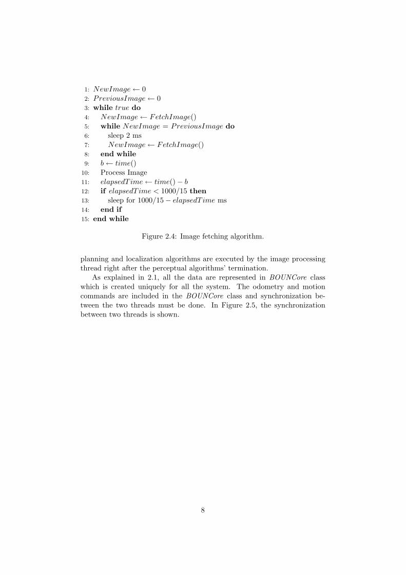
1: NewImage← 02: PreviousImage← 03: while true do4: NewImage← FetchImage()5: while NewImage = PreviousImage do6: sleep 2 ms7: NewImage← FetchImage()8: end while9: b← time()

10: Process Image11: elapsedT ime← time()− b12: if elapsedT ime < 1000/15 then13: sleep for 1000/15− elapsedT ime ms14: end if15: end while

Figure 2.4: Image fetching algorithm.

planning and localization algorithms are executed by the image processingthread right after the perceptual algorithms’ termination.

As explained in 2.1, all the data are represented in BOUNCore classwhich is created uniquely for all the system. The odometry and motioncommands are included in the BOUNCore class and synchronization be-tween the two threads must be done. In Figure 2.5, the synchronizationbetween two threads is shown.

8

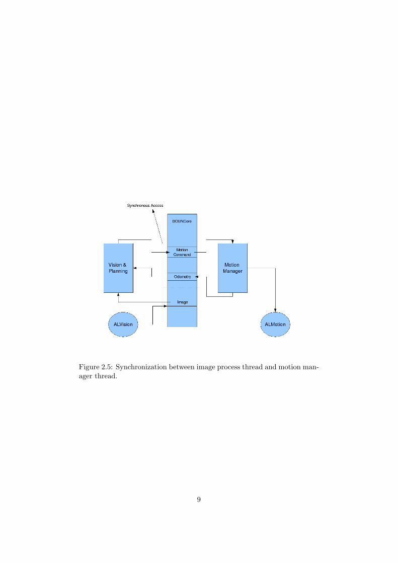
Figure 2.5: Synchronization between image process thread and motion man-ager thread.

9

Chapter 3

Vision

3.1 Image Processing and Perception

The purpose of the perception module is to process the raw image andextract available object features from the image (bearing and range if avail-able). The input to the module is the image in YUV422 format as explainedin 2.3.5 and the output is the range and bearing features of seen objects onthe field. The two main parts of this module are color classification andperception.

3.1.1 Color Classification

In the raw image format, each pixel is represented with a three-byte valueand can be one of the 2553 values. Since it is impossible to efficiently operateon such an input space, the colors are classified into fewer color groups. Eachgroup represents a possible color on the environment. These are white,green, yellow, blue, robot-blue, orange, and red. There is actually one moregroup which stands for none of the groups and noted as the “ignore” group.

To summarize the problem, we have an image with a resolution of320x240, where each pixel has a range of 2553 values and we want to assigneach pixel to one of the eight color groups. This is a regression problemand we used Generalized Regression Neural Network (GRNN) to solve thisproblem [5]. GRNN is a neural network which can approximate a function(linear or nonlinear) with n dimensional domain to m dimensional outputdomain.

In our problem, input space has three dimensions and output space haseight dimensions. In the output, the value with index of the target colorgroup has the value of one while all other values have value of zero. Toreduce the complexity of the algorithm, we omitted two bits from Y channelsand four bits from U and V channels. The new input space is still threedimensional but has a range of 2× 6× 24 ∗ 24.

10

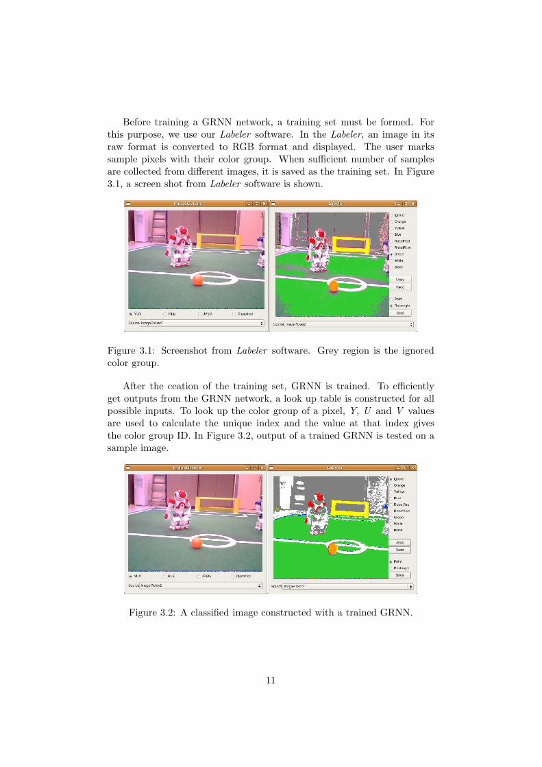
Before training a GRNN network, a training set must be formed. Forthis purpose, we use our Labeler software. In the Labeler, an image in itsraw format is converted to RGB format and displayed. The user markssample pixels with their color group. When sufficient number of samplesare collected from different images, it is saved as the training set. In Figure3.1, a screen shot from Labeler software is shown.

Figure 3.1: Screenshot from Labeler software. Grey region is the ignoredcolor group.

After the ceation of the training set, GRNN is trained. To efficientlyget outputs from the GRNN network, a look up table is constructed for allpossible inputs. To look up the color group of a pixel, Y, U and V valuesare used to calculate the unique index and the value at that index givesthe color group ID. In Figure 3.2, output of a trained GRNN is tested on asample image.

Figure 3.2: A classified image constructed with a trained GRNN.

11

3.2 Scanline Based Perception Framework

Scanline based vision framework was introduced this year to exploit sev-eral advantages of scanline based perception systems over blob based visionsystems.

The most significant improvement over blob based systems is the in-creased reasoning possibilities. Using a single scanline it is possible to de-tect a line segment by simply tracking the change in color of the pixels onthe scanline. Furthermore, it is possible to combine information gained bymultiple scanlines providing further spatial information about the structuresavailable in the current image. In our previous blob based perception systemsuch extensive and precise reasoning was not possible.

Scanline perception framework is also more scalable. The complexityof the system can be changed automatically in run time, by adjusting thenumber of scanlines per image. Since only the pixels on the scanlines aresegmented, segmentation overhead of the blob based systems can also beavoided.

Inspecting a region of the image with a set of scanlines can provide a fastand accurate method of reasoning about the confidence of the perception.Such confidence values are very crucial for the performances of higher levelmodules. Further probabilistic methods will be employed to increase utilityof these confidence values in the future.

In the following parts of this section, the implemented scanline basedperception methods will be described in detail.

3.2.1 Vision Object

The Vision object instantiates other perception methods after generatingsome information which is required by all of the specialized perceptionclasses.

The image received from robot’s camera is first scanned with severalscanlines. The number of these scanlines can be altered according to theviewing angle of the camera, however currently this feature is left as futurework.

Once pixels corresponding to the scanlines are segmented, this segmentedand ordered set of pixels are traversed once for important points, definedby each specialized perception method. Selected subsets of the segmentedpixels are then sent to specialized perception classes for further processingand object detection.

3.2.2 Goal Perception

This section describes the most extensive specialized perception class, whichis designed for goal perception. Processing starts with the input of the vision

12

object, indicating the important points for this specialized perception class.The goal of the scanline based goal perception is to detect the goal bars

individually so that multiple landmarks can be perceived from a single goal.A four stage procedure is designed to achieve this purpose, which can be usedto perceive left and right goal bars individually. Due to the generic design ofthe perception stages and the underlying scanline framework, implementingtop and bottom bars is only a task of mirroring left and right bar perceptors.Similarly beacon perception will be only a variation of the bar perception.

Tests of the perceptor are done using the new version of the CerberusStation, a screen shot of which is shown Figure 3.2.2. Using this visual toolgreatly enhances the testing procedure. Employing the BOUNio library itis possible to observe run time performance as well as to inspect recordedlogs within the goal perception tester tool.

Figure 3.3: Cerberus Station Goal Perception Test Tool.

The goal perception task is divided between several classes, namely mainvision object, goal perceptor, goal bar perceptor, and bar perceptor. Thebar perceptor performs the four stage bar perception procedure, the goalbar perceptor investigates if the found bar is the correct bar, and the mainvision object initiates the procedure.

Initially the main vision class runs a series of scanlines perpendicular tothe horizon plane and classifies the YUV image along these scanlines (see

13

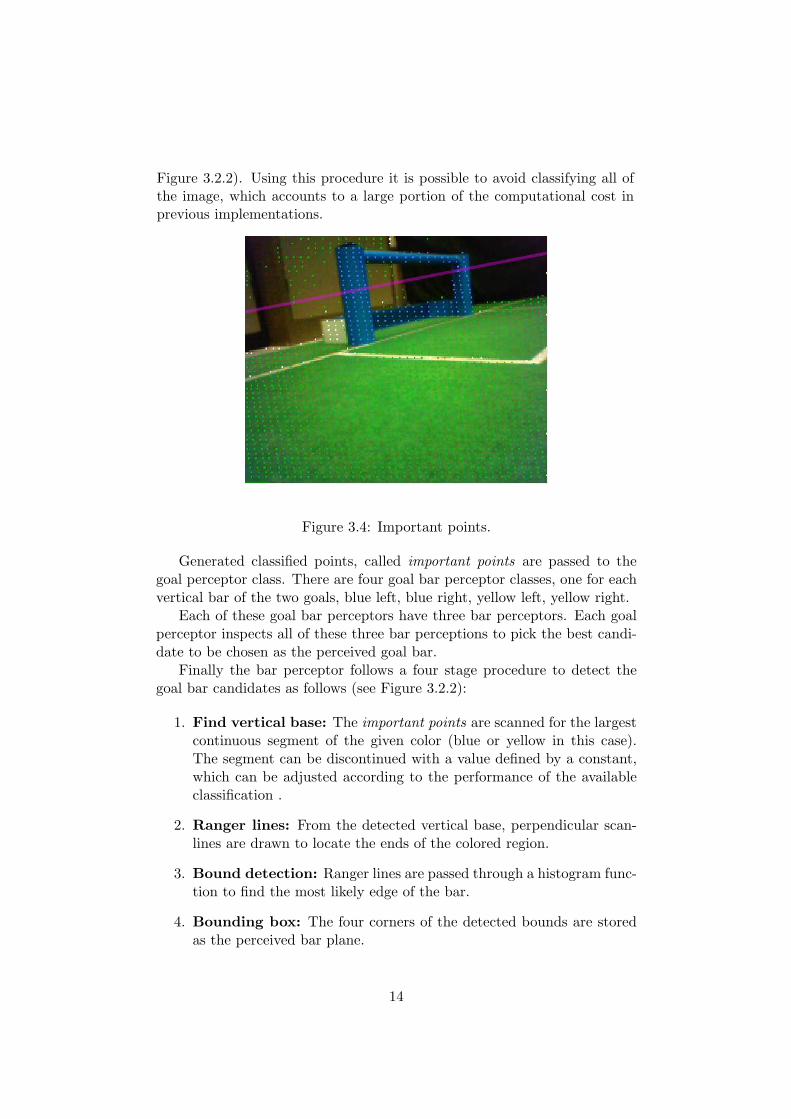
Figure 3.2.2). Using this procedure it is possible to avoid classifying all ofthe image, which accounts to a large portion of the computational cost inprevious implementations.

Figure 3.4: Important points.

Generated classified points, called important points are passed to thegoal perceptor class. There are four goal bar perceptor classes, one for eachvertical bar of the two goals, blue left, blue right, yellow left, yellow right.

Each of these goal bar perceptors have three bar perceptors. Each goalperceptor inspects all of these three bar perceptions to pick the best candi-date to be chosen as the perceived goal bar.

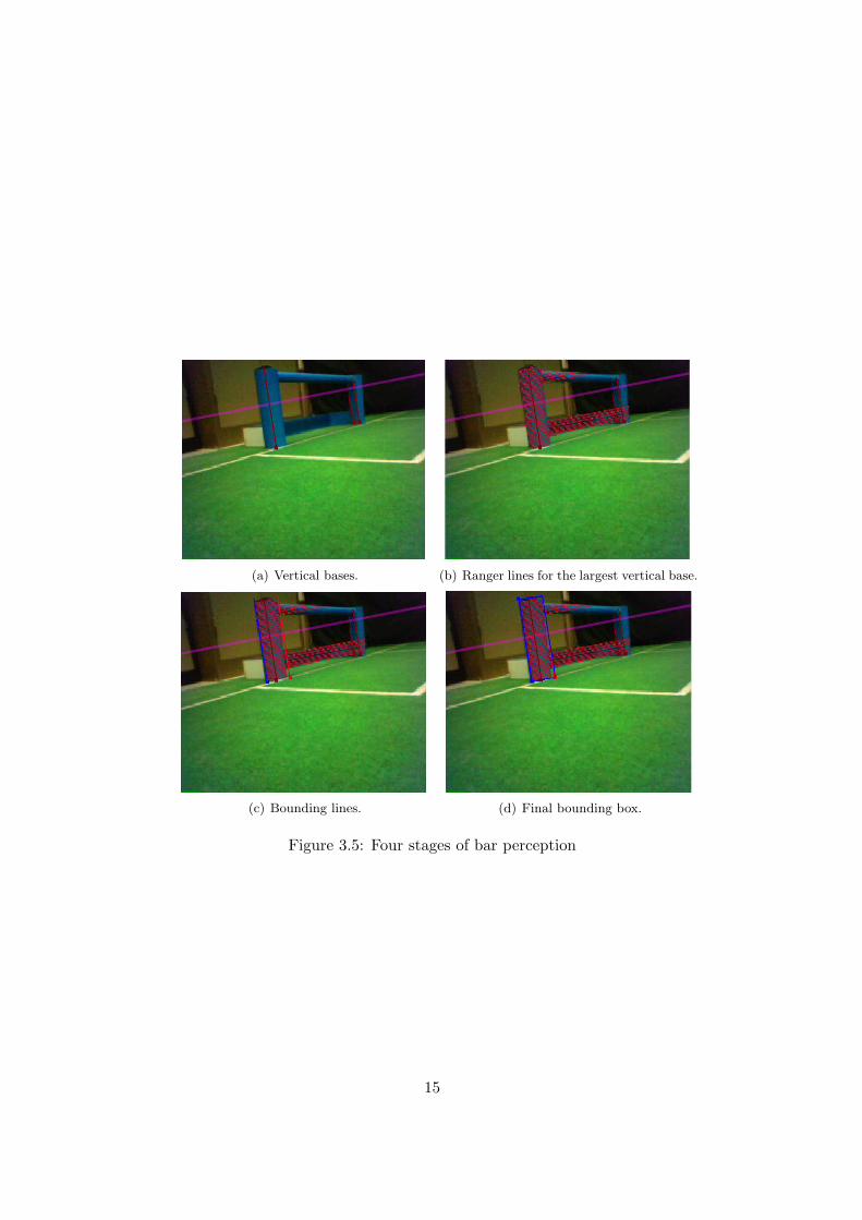
Finally the bar perceptor follows a four stage procedure to detect thegoal bar candidates as follows (see Figure 3.2.2):

1. Find vertical base: The important points are scanned for the largestcontinuous segment of the given color (blue or yellow in this case).The segment can be discontinued with a value defined by a constant,which can be adjusted according to the performance of the availableclassification .

2. Ranger lines: From the detected vertical base, perpendicular scan-lines are drawn to locate the ends of the colored region.

3. Bound detection: Ranger lines are passed through a histogram func-tion to find the most likely edge of the bar.

4. Bounding box: The four corners of the detected bounds are storedas the perceived bar plane.

14

(a) Vertical bases. (b) Ranger lines for the largest vertical base.

(c) Bounding lines. (d) Final bounding box.

Figure 3.5: Four stages of bar perception

15

Once candidate bars are generated, respective goal bar perceptors searchfor the best available vertical goal bar of their respective colors. To achievequantified confidence results, goal bar perceptors draw squares, scaled tothe size of the perceived bar, around the expected positions of the coloredregions, as shown in Figure 3.2.2a. Within these squares scanlines are run todetect the ratio of pixels with the requested color. Figure 3.2.2b shows theresulting confidence values. Observations indicate false positive frequencyis very low with confidence values greater than 0.5.

(a) Confidence regions drawn for all possibleleft blue vertical goal bars.

(b) Final confidence values for left and rightblue vertical goal bars.

Figure 3.6: Final perception.

3.2.3 Line Perception

Line perception is implemented in a similar fashion with the goal targetperception. The main vision object supplies the important points for the lineperception, which is, in this case, defined as the mid point of a green-whitetransition and a consecutive white-green transition on a single scanline.

First, the best possible fitting lines are found for the current importantpoints with least squares line fitting. Using these lines a circle detectionalgorithm runs, trying to find the center circle of the field. In case themiddle circle is found, no further processing is done. Since there are manyintersection points on the center circle lines, proceeding further with cornerdetection gives false positive results. Besides, finding the center circle is veryinformative as it is.

In case the center circle is not found, corner detection algorithm is runto find the corners formed by the detected lines. After several sanity checks,the found corners are marked as the perceived corners.

16

3.2.4 Goal Target Perception

Using the available scanline perception framework it is quite easy to im-plement simple perceptions quickly having all the robust properties of thescanline vision technique. Goal target perception presents a good examplefor such a case.

In order to score a goal, a goal target perception is required, so that therobot can shoot at the correct spot. Localization can generally be reliedupon to figure out the direction of the goal, however it can not be trustedfor precise shooting due to high level of noise.

This perception method provides a more limited but more accurate ap-proach to be used as a precise goal target on the perceived image, once therobot is assumed to be actually facing the goal. There are sanity checks inplace to avoid shooting in case the robot does not actually face the goal.

The important points for this very specialized perception are the pointscolored with the opponent team’s goal color. These points are traversed forthe largest continuous region obeying the sanity checks. If no such region isfound, goal target perception can set goal target to be unknown and avoidshooting to a completely obstructed goal or even worse to any other randomdirection. If the region is found as an appropriate goal target, its center ismarked as the goal target.

3.2.5 “On Goal Line” Perception

The most specialized perception is “on goal line” perception which providesa signal to the goal keeper to help the robot with its localization. Oncethe goal keeper roughly gets around the goal line, it can be quite hardto get localized precisely. Since the opponent goal is quite far away andgenerally obstructed, it can rarely be used in localization, which degradesthe performance of the localization.

To help the goal keeper in such situations, “on goal line” perceptionsignals the goal keeper that it is standing on the goal line. The plannermodule of the goal keeper turns the robot’s head from one side to the otherall the time, searching for a possible ball to save. This behavior frequentlyresults in a particular sequence of perceptions when the goal keeper is onthe goal line, which are the own goal bar perception - corner perception -corner perception - own goal bar perception, respectively.

“On goal line” perception looks for such sequences and generates a signalindicating the goal keeper is on the goal line, which can be used to align thegoal keeper more precisely to improve chances for a better goal saving andlocalization performance.

17

3.2.6 Distance Calculations

To calculate the distance of a visually observed object, either a stereo visionsystem or using consecutive frames of single camera as stereo vision is needed[6]. The Nao robot has a single camera but the sizes of the objects in theenvironment are fixed and known. The distances of objects can be inferredby the size feature of the objects. In visual observations, the size of an objectcan be measured by the width or height of the object in pixels. As the objectgets closer, the size of the object in the image increases and this increasehas a nonlinear relationship with the actual distance of the object. In ourapproach, we represent this relationship with the function y = a× (xb) + cwhere y is the distance, x is the width or height of the object in pixels, anda, b and c are parameters of the function.

Now the problem is reduced to finding the three optimal values for a, band c. To optimize these parameters, a training set is collected from the en-vironment and the parameters are estimated with the least squares method.The pixel widths are found from the classified image, so this training proce-dure is repeated for each object type and after each color calibration processwhich was explained in section 3.1.1.

18

Chapter 4

Localization

Currently, Cerberus employs three different localization engines. The firstengine is an inhouse developed localization module called Simple Localiza-tion (S-LOC) [7]. S-LOC is based on triangulation of the landmarks seen.Since it is unlikely to see more than two landmarks at a time in the currentsetup of the field, S-LOC keeps the history of the percepts seen and modifiesthe history according to the received odometry feedback. The perceptionupdate of the S-Loc depends on the perception of landmarks and the pre-vious pose estimate. Even if the initial pose estimate is provided wrong, itacts as a kidnapping problem and is not a big problem as S-Loc will convergeto the actual pose in a short period of time if enough perception could bemade during this period.

The second one is a vision based Monte Carlo Localization with a setof practical extensions (X-MCL) [8]. The first extension to overcome theseproblems and compensate for the errors in sensor readings is using inter-percept distance as a similarity measure in addition to the distances andorientations of individual percepts (static objects with known world framecoordinates on the field). Another extension is to use the number of per-ceived objects to adjust confidences of particles. The calculated confidenceis reduced when the number of perceived objects is small and increased whenthe number of percepts is high. Since the overall confidence of a particle iscalculated as the multiplication of likelihoods of individual perceptions, thisadjustment prevents a particle from being assigned with a smaller confidencevalue calculated from a cascade of highly confident perceptions where a sin-gle perception with lower confidence would have a higher confidence value.The third extension is related with the resampling phase. The number ofparticles in successor sample set is determined proportional to the last cal-culated confidence of the estimated pose. Finally, the window size in whichthe particles are spread into is inversely proportional to the confidence ofestimated pose. This engine was used in both Aibo and Nao games.

The third engine is a novel contribution of our lab to the literature,

19

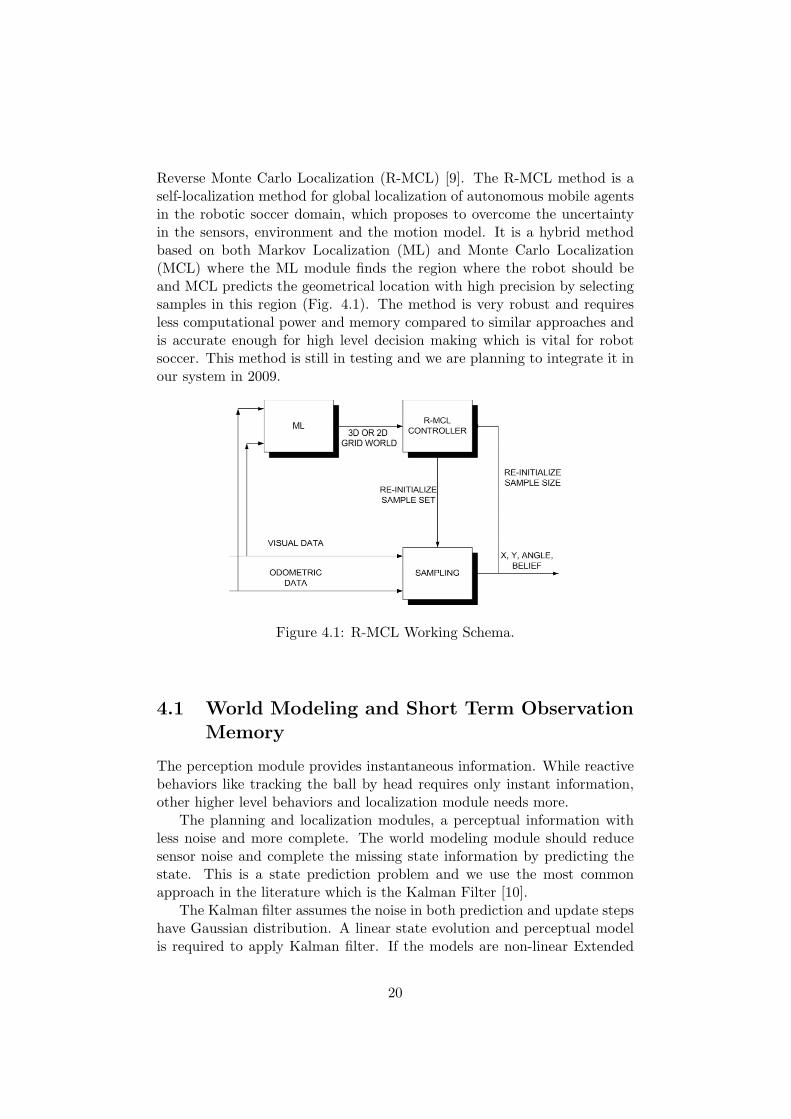
Reverse Monte Carlo Localization (R-MCL) [9]. The R-MCL method is aself-localization method for global localization of autonomous mobile agentsin the robotic soccer domain, which proposes to overcome the uncertaintyin the sensors, environment and the motion model. It is a hybrid methodbased on both Markov Localization (ML) and Monte Carlo Localization(MCL) where the ML module finds the region where the robot should beand MCL predicts the geometrical location with high precision by selectingsamples in this region (Fig. 4.1). The method is very robust and requiresless computational power and memory compared to similar approaches andis accurate enough for high level decision making which is vital for robotsoccer. This method is still in testing and we are planning to integrate it inour system in 2009.

Figure 4.1: R-MCL Working Schema.

4.1 World Modeling and Short Term ObservationMemory

The perception module provides instantaneous information. While reactivebehaviors like tracking the ball by head requires only instant information,other higher level behaviors and localization module needs more.

The planning and localization modules, a perceptual information withless noise and more complete. The world modeling module should reducesensor noise and complete the missing state information by predicting thestate. This is a state prediction problem and we use the most commonapproach in the literature which is the Kalman Filter [10].

The Kalman filter assumes the noise in both prediction and update stepshave Gaussian distribution. A linear state evolution and perceptual modelis required to apply Kalman filter. If the models are non-linear Extended

20

Kalman Filter can be used where models are linearized by Taylor Series.In our problem, the observations are distance and the bearing of the

objects with respect to robot origin. And the state we want to know is actualdistance and bearing informations. In addition for the dynamic objects likethe ball, the state vector also includes distance change and bearing changeinformation to ease prediction.

For any object, the observation is z = {d, θ} where d and θ are distanceand bearing respectively to the robot origin. For the stationary objects stateis m = {d, θ} and the state evolution model is m1

k+1 = I∗mk and zk = I∗mk

where k is time and I is the unit matrix.For the dynamic objects, the observation is the same but state is repre-

sented as m = {d, θ, dd, dθ} where dd is the change in distance in one timestep and dθ is the change in bearing likewise. The state evolution model is:

dk+1

θk+1

dd,k+1

dθ,k+1

=

1 0 1 00 1 0 10 0 1 00 0 0 1

dk

θk

dd,k

dθ,k

and observation model is:

(dk+1

θk+1

)=

(1 0 0 00 1 0 0

)

dk

θk

dd,k

dθ,k

As can be observed from the model specifications, we omit the correlationbetween objects and separately execute filter equations for each object. Ifan object is not observed for more than a pre-specified time step, the beliefstate is reset and the object is reported as unknown. For our case this timestep is 270 frames for stationary objects and 90 frames for dynamic objects.

In the update steps, the odometry readings are used. The odometryreading is u = {dx, dy, dθ} where dx and dy are displacements in egocentriccoordinate frame and dθ is the change in orientation. When an odometryreading is received, all the state vectors of known objects are geometricallyre calculated and the uncertainty is increased.

The most clear effect of using a Kalman Filter is that the disadvantageof limited field of view is reduced. In the Figure 4.2, a robot spins its headand is aware of three distinct landmarks at the same time.

4.2 Localization

In the previous years in SPL, a simple goal box seeking action was enoughto score or even win matches. However, in recent years, the score intentedactions of the robot are highly dependent on self pose information. The

21

Figure 4.2: A robot spins its head and is aware of three distinct landmarksat the same time.

problem of estimating the self pose has also become harder due to the de-creased number of landmarks and increased field size.

The localization problem is a self pose estimation problem like in section4.1, and the widely used approach is the Monte Carlo Localization (MCL)algorithm [11]. In this problem, the state to be estimated is µ = {x, y, θ},where x and y are global coordinates and θ is orientation of the robot.

In MCL algorithm, belief state is represented by a particle set and eachelement represents a possible pose of the robot. In Figure 4.3, a samplebelief state is given.

In the MCL algorithm, an importance weight is calculated for each par-ticle which shows how suitable a particle to the observations. All the parti-cles are copied to the next belief state set with respect to their importanceweight. To calculate importance weights, the observations are taken from theoutput of the world modeling algorithm as described in section 4.1. Only theknown stationary objects are used in calculations. The importance weightsis calculated by difference of expected bearing and predicted bearings andlikely if the distance is known, expected distance and predicted distance. InFigure 4.4, an example belief state is given, where both distance and bearingis known for a single landmark.

While importance weight and resampling steps are the correction stepof the MCL, prediction step is done with odometry readings. In prediction,each particle is updated with geometrically recalculating the position andadding a small random noise which represents increase in uncertainty. Toavoid kidnapping situations, in the resampling step, some of the particlesare randomly generated.sampling steps are the correction step of the MCL,prediction step is done with odometry readings. In prediction, each particleis updated with geometrically recalculating the position and adding a small

22

Figure 4.3: Belief state of the robot in MCL algorithm.

Figure 4.4: An example belief state is given, where both distance and bearingis known for a single landmark. The particles are grouped over an arc aroundtrue position of the object.

23

random noise which represents increase in uncertainty. To avoid kidnap-ping situations, in the resampling step, some of the particles are randomlygenerated.

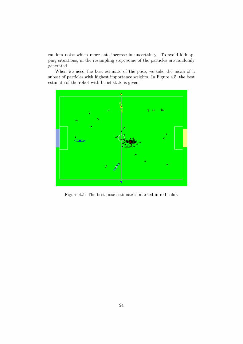
When we need the best estimate of the pose, we take the mean of asubset of particles with highest importance weights. In Figure 4.5, the bestestimate of the robot with belief state is given.

Figure 4.5: The best pose estimate is marked in red color.

24

Chapter 5

Motion

For our team, the most important component of transition from quadrupedrobots to biped robots was the locomotion module. Fast and robust lo-comotion is a vital capability that a mobile robot should have, especiallyif the robot is expected to play soccer. Cerberus has a significant researchbackground in different mobility configurations including wheeled and leggedlocomotion. The rest of this section provides information about our researchon bipedal locomotion.

5.1 Motion Engine

Our motion engine has three different representation infrastructures, whichallow different levels of abstractions.

The first infrastructure contains a data structure, named “Body”, whichstores the physical properties of the robot as well as the functions used forperforming related calculations. The “Body” is composed of several “Link”s,which are data structures for storing the joint positions, angles, and relatedkinematic description parameters. Being platform independent and generic,this infrastructure makes it possible to define new robot platforms via someconfiguration files and allows controlling the joints of the robot platformeasily.

The second infrastructure is a hierarchical one. A root engine is definedat the very top level and the common properties and functions of eachdifferent motion engine are included in it. Different motion engines areinherited from the root engine, and platform and motion algorithm specificparts are defined. For Nao, four main features are implemented. The firstone is to make the robot perform a static walking in which the robot tries tokeep the ground projection of its Center of Mass (CoM) inside the supportpolygon. In addition to the static walking feature, a dynamic walking featureis also implemented. A signal generation-based algorithm, which is verysimilar to Central Pattern Generator [12] is used. The motion of the head

25

is separated from the motion of the rest of the body and implemented asthe third feature. The last feature is the motion player, which reads thesequential joint angles from pose definition files and plays them to realizesome special actions, such as kicking the ball and standing up from a fallenposition.

The third infrastructure is a container for some common motion-relatedfunctions. In addition to the matrix operations which are necessary forkinematics calculations, implementations to read configuration files are alsoincluded as common functions.

5.2 Implemented Biped Walking Algorithms

Walking algorithms can be classified into two main groups; static walkingand dynamic walking. The main principle of static walking is to preservestability all the time during the motion, which guarantees that the robotwill not fall unless there is an external force to push the robot to fall. Themost common method for static walking is based on keeping the CoM insidethe support polygon. Although static walking is advantageous in terms ofmaintaining the balance continuously, the length of each step is very limitedbecause of the concerns related to keeping the CoM inside the support poly-gon. Therefore, it is not possible to achieve a fast walk using static walkingtechniques. On the other hand dynamic walking is based on maintainingthe balance by using dynamic properties of the motion. There are mainlythree different methodologies;

• Zero-Moment Point (ZMP) Criterion [13] is very similar to CoMbased static walking. The only difference is that holding ZMP insidethe support polygon is enough to maintain the balance. Although itis a very common method, it is computationally very expensive.

• Passive-Dynamic Walking (PDW) [14] where CoM is carried alongthe motion direction, and the body moves along the motion directionbecause of the gravity. The important point is the timing of the footcontact of the swinging leg with the ground.

• Central Pattern Generators (CPGs) [12] method is based on the syn-chronous movement patterns of the joints. For this purpose, a signalis assigned for each joint, and the system is trained for synchronouspatterns and balanced locomotion as a whole.

We implemented static walking with CoM criterion and a dynamic walk-ing with CPG method [15] to be used on our Nao robots.

26

5.2.1 Static Walking with CoM Criterion

As a static walking example we implemented finite state machine basedbiped walking whose main criterion is to keep the CoM inside the supportpolygon. The implementation is essentially a combination of three differentmotions. The first motion is to shift the CoM into the sole of the supportfoot. This motion is generated on the sagittal plane and in the directionof the motion in order to prevent CoM from being left behind or beyond.By this way, it is provided that the ground projection of the CoM is keptinside the sole of the support foot. Foot pressure sensors (FPSs) are usedfor feedback. When it is guaranteed that the weight of the body is carriedby the support foot, swinging leg is shortened. During this motion, thebody is moved along the walking direction by the joints at the ankle of thesupport foot until the ground projection of the CoM is on the boundariesof the support foot. This makes it possible to use a longer step. As the lastmotion, swinging leg is moved in the direction of motion and landed on theground. This point is where the robot is in its most unstable state. In orderto maintain the stability of the robot, the landing speed of the foot andreactiveness to be aware of the landing moment of the swinging leg shouldbe controlled. If the landing is too fast, the landing will not be noticedon time and the state transition would not be accomplished properly. Thisdisturbs the balance through the support leg and the robot falls down onthe support leg. On the other hand, if the landing is too slow, the motionwill be very slow and inefficient. For these purposes, forward kinematics isused in addition to the FPSs. Using forward kinematics, relative locationsof the feet are calculated and swinging foot is landed fast enough while itis horizontally far away from the support foot. When the vertical distancebetween swinging foot and the ground is small, landing speed is slowed downand FPSs are used to determine whether the swinging foot is landed or not.Because of the symmetric nature of the biped walking, after the swinging legis landed, the roles are switched between legs and same motion is repeatedfor the other leg.

5.2.2 Dynamic Walking with CPG Method

As a dynamic walking example, a walking method based on that of thechampion of the Humanoid League in the RoboCup07, NimbRo [15], is im-plemented. They defined three important features for each leg; leg extension,leg angle, and foot angle. Leg extension is the distance between hip jointand ankle joint. It determines the height of the robot while moving. Legangle is the angle between the pelvis plate and the line from hip to ankle.It has three components; roll, pitch, and yaw. The third feature, foot an-gle, is defined as the angle between foot plate and pelvis plate. It has onlytwo components; roll and pitch. Using these features helps us to have more

27

abstract calculations for the motion.Before finding motion features, a central clock (φtrunk) is generated for

the trunk which is between −π and π. Each leg is fed with a different clock(φleg) with ls× π/2 phase shift where ls represents leg sign and it is −1 forthe left leg while +1 for the right leg. The synchronization of the legs canbe preserved in this way. In the calculations of motion features at a giventime, the corresponding phase value is considered and the values for featuresare calculated by using these phase values.

In order to find the leg angle and foot angle features, motion at eachstep is divided into five sub-motions; shifting, shortening, loading, swinging,and balance. In shifting sub-motion, lateral shifting of the CoM is handled.For this purpose, a sinusoidal signal is used:

θshift = ls× ashift × sin(φleg) (5.1)

where ashift is a constant to determine the shift amount. This shift signal isapplied to the leg and the foot with different magnitudes. While it is appliedto the leg as it is, only the half of the value with a negation is applied tothe foot:

θLegShift = θshift (5.2)

θFootShift = −0.5× θshift (5.3)

. The second important sub-motion is shortening signal and it is not alwaysapplied. Phase value for shortening is calculated with

φshort = vshort × (φleg + π/2 + oshort) (5.4)

. where vshort is a constant to determine the shortening duration, and oshort

is also a constant for the phase shift of shortening relative to the shiftingsub-motion. During shortening state, both a joint angle for the foot and aleg extension value are calculated by

γshort = { −ashort × 0.5× (cos(φshort) + 1) if − π ≤ φshort < π0 otherwise

(5.5)

and

θfootShort = { 0.5× (cos(φshort) + 1) if − π ≤ φshort < π0 otherwise

(5.6)

The third sub-motion of the step is loading which is also not always applied.The function of the corresponding phase value is given as

φload = vload × piCut(φleg + π/2− π/vshort + oshort)− π (5.7)

28

. where vload is a constant to determine the load duration, and piCut is afunction which maps the value of the parameter to a value between −π andπ. In this phase, only a part of the leg extension is calculated as

γload = { −0.5× aload × cos(φload) + 1) if − π ≤ φload < π0 otherwise

(5.8)

where aload is determined according to the motion speed. Swinging is themost important part of the motion. In this part, the leg is unloaded, short-ened and moved along the way of motion which reduces the stability ofthe system considerably. This movement has effects on each component ofthe leg and the foot angle features of the motion. Because the behavior ofthe θswing is changed during the swinging process, another clock signal iscalculated as

φswing = vswing × φleg + π/2 + oswing (5.9)

. where vswing is a constant to determine the swinging duration, and oswing isalso a constant for a phase shift of swinging sub-motion. θswing is calculatedby the equation:

θswing = {sin(φswing) if − π/2 ≤ φswing < π/2

b× (φswing − π/2 + 1) π/2 ≤ φswing

b× (φswing + π/2− 1) otherwise(5.10)

where b = −(2/(2× π × vswing − π).According to the speed and direction of the motion, θswing is distributed

to the components of leg and foot angle features as

θlegSwingr = ls× v0 × θswing (5.11)

.θlegSwingp = v1 × θswing (5.12)

.θlegSwingy = ls× v2 × θswing (5.13)

.θfootSwingr = ls× 0.25× v0 × θswing (5.14)

.θfootSwingp = 0.25× v1 × θswing (5.15)

.As the last component of the step, balance, correction values for the

deviations of the other operations are added to the system from the footangle feature and the rolling component of the leg angle feature. Correctionequations are:

θfootBalancer = ls× 0.5×0 ×cos(φleg + 0.35) (5.16)

29

.

θfootBalancep = 0.02 + 0.08× v1 − 0.04× v1 × cos(2.0× φleg + 0.7); (5.17)

.θlegBalancer = 0.01 + ls× v0 + |v0|+ 0.1× v2 (5.18)

. At the end, the corresponding parts of the motion features can be com-bined. Equations to combine corresponding parts are given as

θlegr = θlegSwingr + θlegShift + θlegBalancer (5.19)

.θlegp = θlegSwingp (5.20)

.θlegy = θlegSwingy (5.21)

.θfootr = θfootSwingr + θfootShift + θfootBalancer (5.22)

.θfootp = θfootSwingp + θfootShort + θfootBalancep (5.23)

.γ = γshort + γload (5.24)

. There is a direct relation between the joints of the robot and these motionfeatures. In other words, by using these features, the values for hip, knee,and ankle joints can be calculated easily using the following rules:

1. Since there is only one feature which changes the distance between thehip and ankle which is the leg extension, the knee joint is determinedaccording to only the value of the leg extension feature of the motion.From five sub-motions of a step, the leg extension feature is calculatedand its value is in between −1 and 0. While calculating the valueof the knee joint from the extension, the normalized leg length, n, iscalculated as n = 1 + (1 − nmin) × γ, where nmin = 0.875. The kneejoint value is directly proportional to the arc cosine of the length ofthe leg; θknee = −2× acos(n).

2. Another special case for the motion is its turn component. If we con-sider the physical construction of the robot, there is only one jointdedicated for this motion; hip yaw joint. So, the turn component ofthe motion directly determines the value for the hip yaw joint whichmeans θhipy = θlegy .

30

3. There are two more joints at the hip. By definition, roll and pitchcomponents of the leg angle feature directly determine the values ofthe hip joints. This means that θhipr = θlegr and θhipp = θlegp . Inorder to compensate for the effects of the leg extension on the pitchcomponent of the leg angle feature, half of the value of the knee jointangle should be rotated around the turn component of the motion andadded to the hip pitch and roll joints. In other words, pitch and rollcomponents of the hip joints can be calculated by

(θhipr

θhipp

)=

(θlegr

θlegp

)+ Rθhipy ×

(0

−0.5× θknee

)(5.25)

4. The values of the ankle joints are calculated by applying the inverse ofthe rotation around the turn component of the motion to the differencebetween the leg and the foot angle features. In order to compensate forthe effects of the leg extension on the pitch component of the foot anglefeature, half of the value of the knee joint angle should also be addedto the ankle pitch joint. In other words, pitch and roll components ofthe ankle joints can be calculated by(

θankler

θanklep

)=

(0

−0.5× θknee

)+R−1

θhipy×

(θfootr − θlegr

θfootp − θlegp

)(5.26)

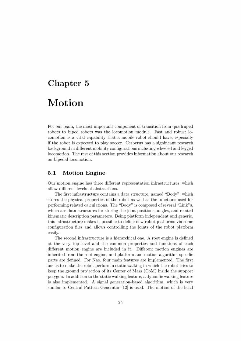
The resulting signals of each joint of a leg are given in figures 5.1, 5.2,5.3, 5.4, 5.5, 5.6 for forward walking direction.

Figure 5.1: Signal for controlling the hip yaw joint for forward walking.

Aside from the implementation inspired from the work of the NimbRoteam, we have also developed a custom algorithm for bipedal walking, which

31

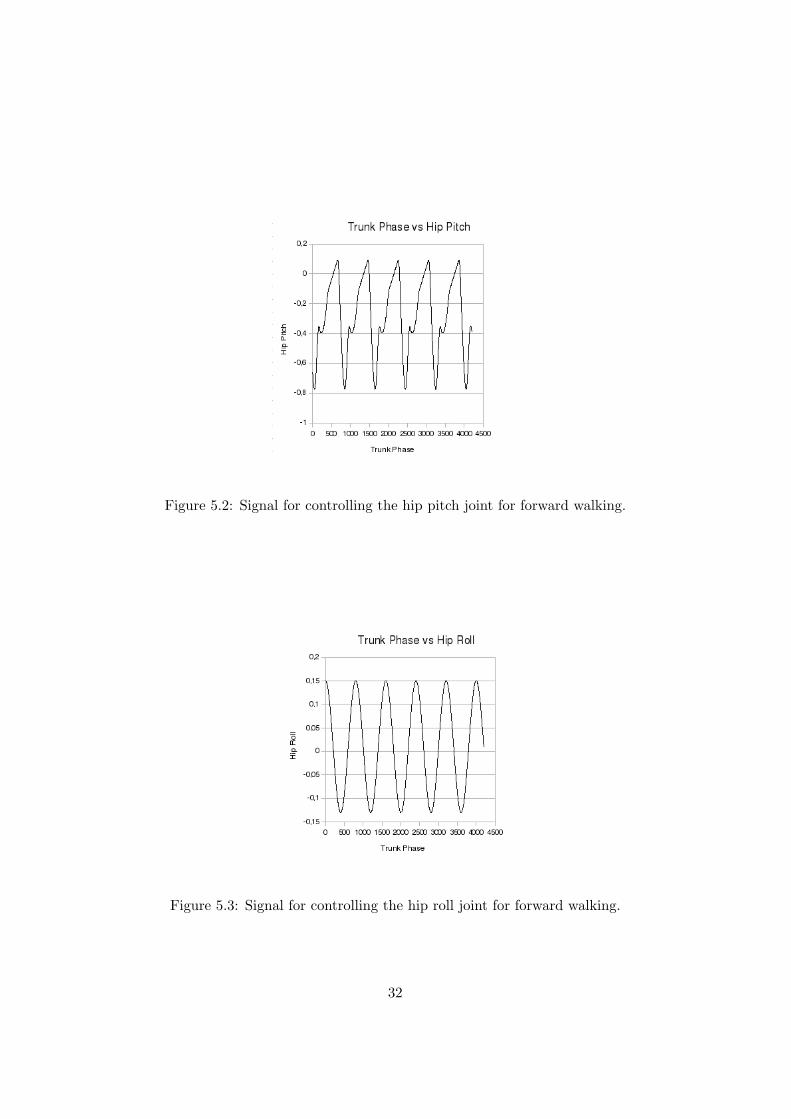
Figure 5.2: Signal for controlling the hip pitch joint for forward walking.

Figure 5.3: Signal for controlling the hip roll joint for forward walking.

32

Figure 5.4: Signal for controlling the knee joint for forward walking.

Figure 5.5: Signal for controlling the ankle pitch joint for forward walking.

33

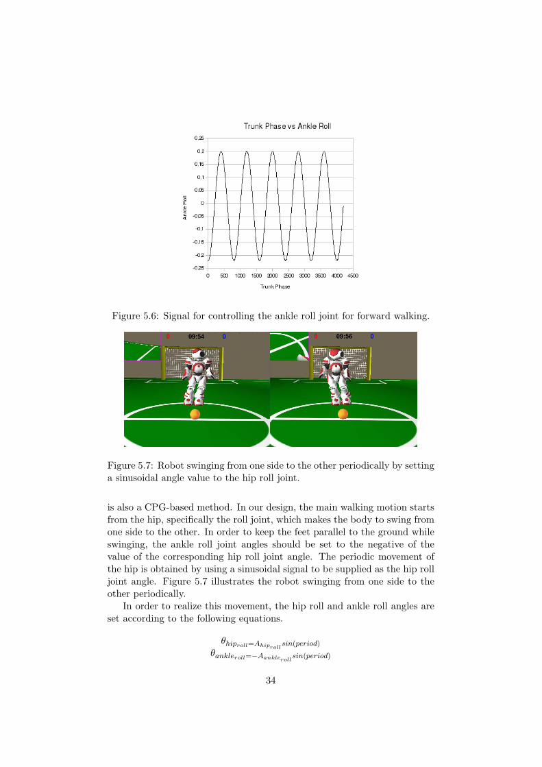
Figure 5.6: Signal for controlling the ankle roll joint for forward walking.

Figure 5.7: Robot swinging from one side to the other periodically by settinga sinusoidal angle value to the hip roll joint.

is also a CPG-based method. In our design, the main walking motion startsfrom the hip, specifically the roll joint, which makes the body to swing fromone side to the other. In order to keep the feet parallel to the ground whileswinging, the ankle roll joint angles should be set to the negative of thevalue of the corresponding hip roll joint angle. The periodic movement ofthe hip is obtained by using a sinusoidal signal to be supplied as the hip rolljoint angle. Figure 5.7 illustrates the robot swinging from one side to theother periodically.

In order to realize this movement, the hip roll and ankle roll angles areset according to the following equations.

θhiproll=Ahiprollsin(period)

θankleroll=−Aanklerollsin(period)

34

This motion is the basis of the entire walking since it passes the projectionof the center of mass from one foot to the other periodically, letting the idlefoot to move according to the requested motion command.

In order to make the robot perform a stepping motion, the pitch angles onthe leg chain should be set. These angles again take sinusoidal values whichare consistent with the hip roll angle. The following equations illustrate howthe values of these angles are computed.

θhippitch= Apitchsin(period) + θhiprest

pitch

θkneepitch= −2Apitchsin(period) + θkneerest

pitch

θanklepitch= Apitchsin(period) + θanklerest

pitch

The Apitch value determines how big the step is going to be. Figure5.8 shows the robot walking forwards. Obtaining backwards walk does notrequire much work but just reversing the iteration of the period value, whichis defined as 0 < period < 2π.

Similarly, making the robot move laterally is possible by setting the rollangles instead of the pitch angles together with the knee pitch, while turningaround is possible by setting the hipY awPitch joint angles properly. Theamplitudes Apitch, Aroll, Ayaw are multiplied with the corresponding motioncomponent, namely forward, left, turn which are normalized in the inter-val [−1, 1], to manipulate the velocity of the motion. In order to make therobot move omnidirectionally, the sinusoidal signals that are computed in-dividually for each motion component are summed up and the final jointangle values obtained in that way. For instance, it is possible to make therobot walk diagonally in the north-west direction by simply assigning posi-tive values to both the forward and the left components.

35

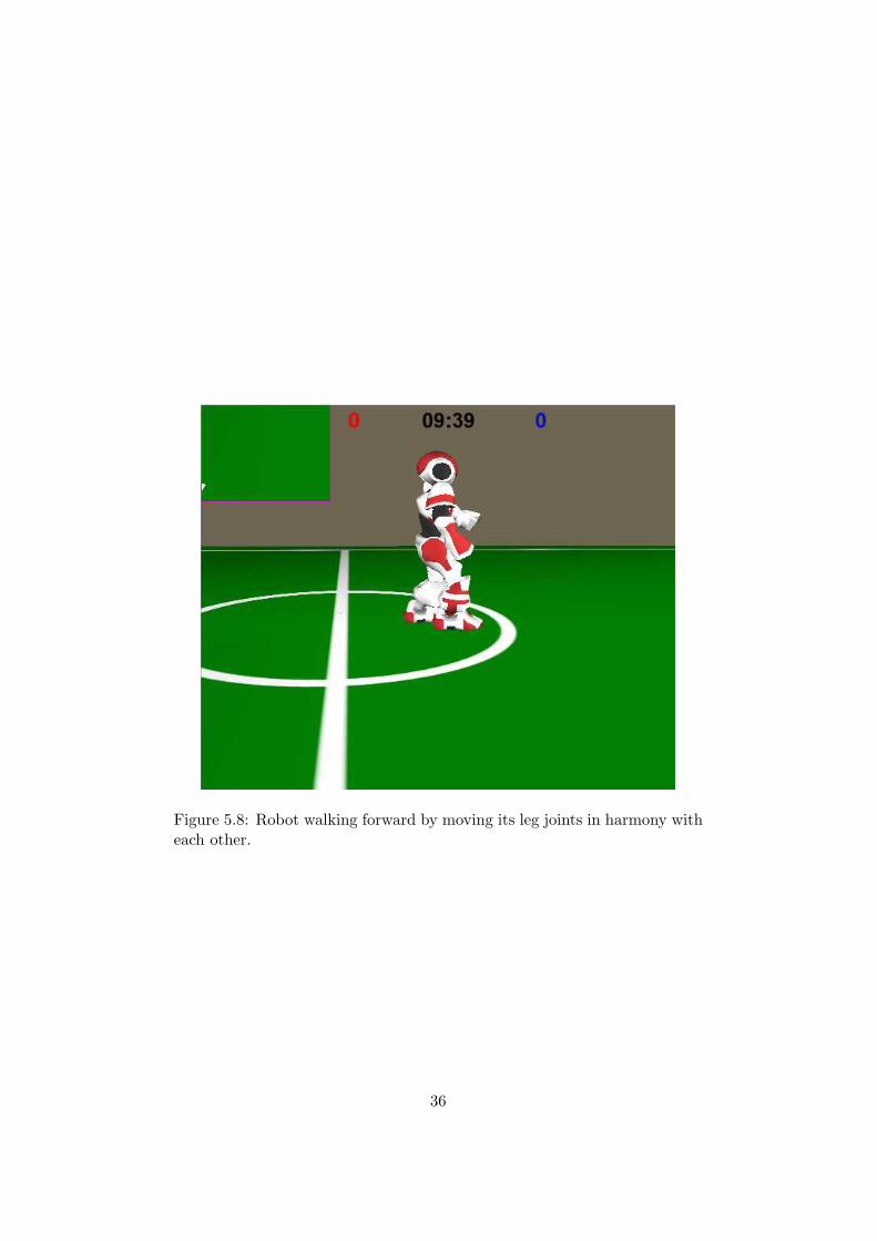
Figure 5.8: Robot walking forward by moving its leg joints in harmony witheach other.

36

Chapter 6

Planning and Behaviors

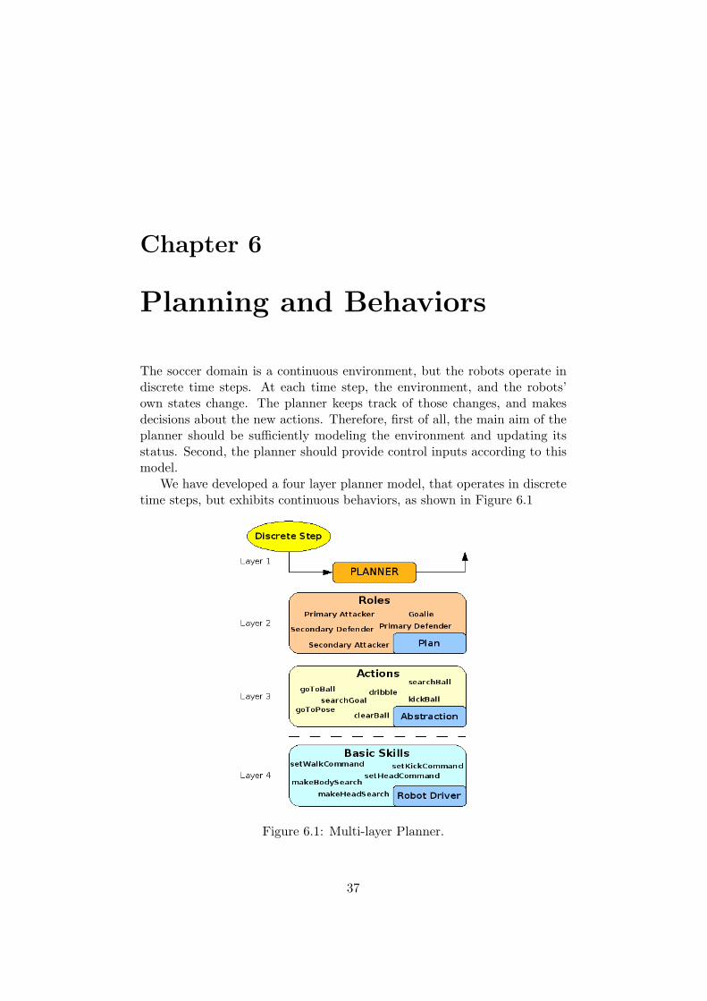
The soccer domain is a continuous environment, but the robots operate indiscrete time steps. At each time step, the environment, and the robots’own states change. The planner keeps track of those changes, and makesdecisions about the new actions. Therefore, first of all, the main aim of theplanner should be sufficiently modeling the environment and updating itsstatus. Second, the planner should provide control inputs according to thismodel.

We have developed a four layer planner model, that operates in discretetime steps, but exhibits continuous behaviors, as shown in Figure 6.1

Figure 6.1: Multi-layer Planner.

37

The topmost layer provides a unified interface to the planner object.The second layer deals with different roles that a robot can take. Eachrole incorporates an “Actor” using the behaviors called “Actions” that thethird layer provides. Finally, the fourth layer contains basic skills that theactions of the third layer are built upon. A set of well-known software designconcepts like Factory Design Pattern[16], Chain of Responsibility DesignPattern [17] and Aspect Oriented Programming [18].

Figure 6.2: Flowchart for task assignment.

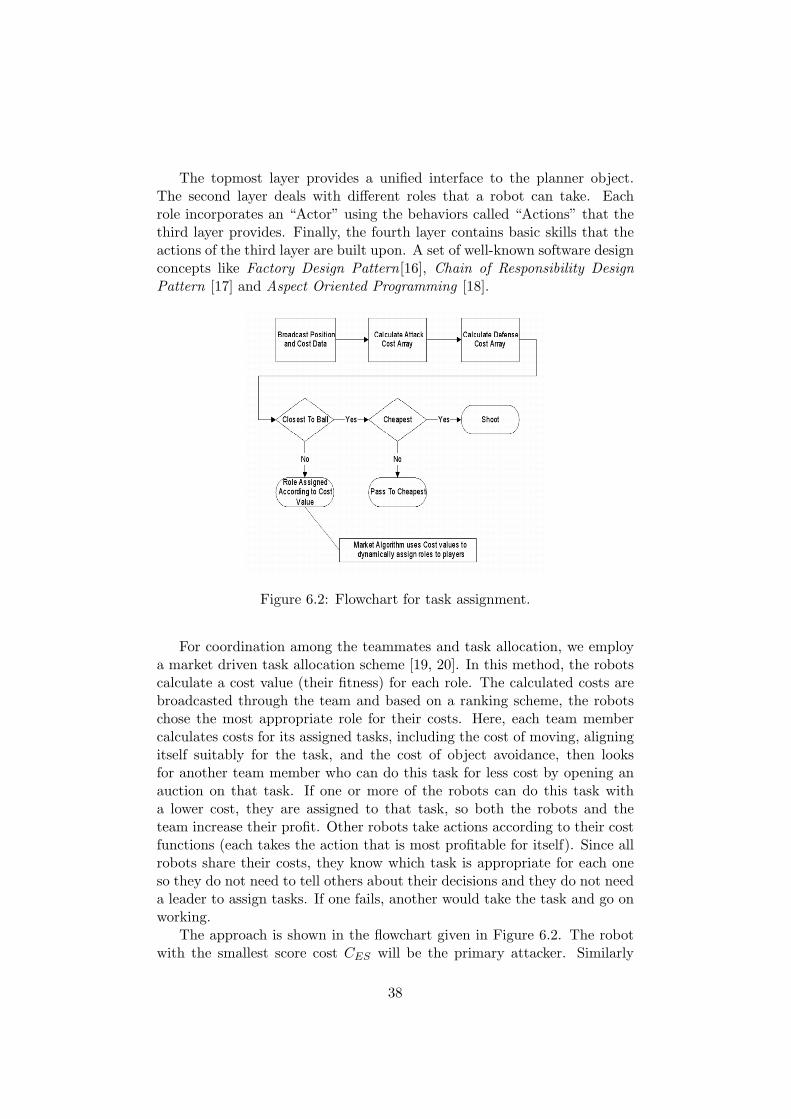
For coordination among the teammates and task allocation, we employa market driven task allocation scheme [19, 20]. In this method, the robotscalculate a cost value (their fitness) for each role. The calculated costs arebroadcasted through the team and based on a ranking scheme, the robotschose the most appropriate role for their costs. Here, each team membercalculates costs for its assigned tasks, including the cost of moving, aligningitself suitably for the task, and the cost of object avoidance, then looksfor another team member who can do this task for less cost by opening anauction on that task. If one or more of the robots can do this task witha lower cost, they are assigned to that task, so both the robots and theteam increase their profit. Other robots take actions according to their costfunctions (each takes the action that is most profitable for itself). Since allrobots share their costs, they know which task is appropriate for each oneso they do not need to tell others about their decisions and they do not needa leader to assign tasks. If one fails, another would take the task and go onworking.

The approach is shown in the flowchart given in Figure 6.2. The robotwith the smallest score cost CES will be the primary attacker. Similarly

38

the robot, except the primary attacker, with the smallest Cdefender cost willbe the defender. If Cauctioneer is higher than all passing costs (Cbidder(i))then the attacker will shoot, else, it will pass the ball to the robot with thelowest Cbidder(i) value. The cost functions used in the implementations areas follows:

CES = µ1.tdist + µ2.talign + µ3.cleargoal(6.1)Cbidder(i) = µ1.tdist + µ2.talign + µ3.clearteammate(i) + CES(i), i 6= robotid(6.2)

Cauctioneer = CES(robotid)(6.3)Cdefender = µ5.tdist + µ6.talign + µ7.cleardefense(6.4)

where robotid is the id of the robot, tdist is the time required to move forspecified distance, talign is the time required to align for specified amount, µi

are the weights of several parameters to emphasize their relative importancein the total cost function, cleargoal is the clearance from the robot to goalarea-for object avoidance, cleardefense is the clearance from the robot to themiddle point on the line between the middle point of own goal and the ball-for object avoidance, and similarly clearteammate(i) is the clearance from therobot to the position of a teammate. Each robot should know its teammatesscore and defense costs. In our study each agent broadcasts its score anddefense costs. Since the auctioneer knows the positions of its teammates, itcan calculate the Cbidder(id=robotid) value for its teammates.

The game strategy can easily be changed by changing the cost functionsin order to define the relative importance of defensive behavior over offensivebehavior, and this yields greater flexibility in planning, which is not generallypossible.

39

Acknowledgements

This work is supported by Bogazici University Research Fund throughproject 06HA102 and TUBITAK Project 106E172.

40

Bibliography

[1] Robocup. www.robocup.org/.

[2] SPL. Robocup standard platform league www.tzi.de/spl/.

[3] Aldebaran-Nao. http://www.aldebaran-robotics.com/eng/nao.php.

[4] Trolltech’s Qt Development Framework.http://trolltech.com/products.

[5] Ethem Alpaydın. Machine Learning. MIT Press, 2004.

[6] Thomas Lemaire, Cyrille Berger, Il-Kyun Jung, and Simon Lacroix.Vision-based slam: Stereo and monocular approaches. Int. J. Comput.Vision, 74(3):343–364, 2007.

[7] H. Kose, B. Celik, and H. L. Akın. Comparison of localization methodsfor a robot soccer team. International Journal of Advanced RoboticSystems, 3(4):295–302, 2006.

[8] K. Kaplan, B. Celik, T. Mericli, C. Mericli, and H. L. Akın. Practicalextensions to vision-based monte carlo localization methods for robotsoccer domain. RoboCup 2005: Robot Soccer World Cup IX, LNCS,4020:420–427, 2006.

[9] H. Kose and H. L. Akın. The reverse monte carlo localization algorithm.Robotics and Autonomous Systems, 55(6):480–489, 2007.

[10] Greg Welch and Gary Bishop. An introduction to the kalman filter.Technical report, Chapel Hill, NC, USA, 1995.

[11] Sebastian Thrun, Dieter Fox, Wolfram Burgard, and Frank Dellaert.Robust monte carlo localization for mobile robots. Artificial Intelli-gence, 128(1-2):99–141, 2001.

[12] C. Pinto and M. Golubitsky. Central pattern generators for bipedallocomotion. J Math Biol, 2006.

[13] M. Vukobratovic and D. Juricic. Contribution to the synthesis of bipedgait. IEEE Transactions on Bio-Medical Engineering, 1969.

41

[14] Tad McGeer. Passive dynamic walking. The International Journal ofRobotics Research, 9:62–82, April 1990.

[15] Sven Behnke. Online trajectory generation for omnidirectional bipedwalking. 2006.

[16] Wikipedia Anonymous. Factory method pattern, 2007.

[17] Wikipedia Anonymous. Chain-of-responsibility pattern, 2007.

[18] Wikipedia Anonymous. Aspect-oriented programming, 2007.

[19] H. Kose, C. Mericli, K. Kaplan, and H. L. Akın. All bids for one and onedoes for all: Market-driven multi-agent collaboration in robot soccerdomain. Computer and Information Sciences-ISCIS 2003, 18th Inter-national Symposium Antalya, Turkey, Proceedings LNCS 2869, pages529–536, 2003.

[20] H. Kose, K. Kaplan, C. Mericli, U. Tatlıdede, and H. L. Akın. Market-driven multi-agent collaboration in robot soccer domain. Cutting EdgeRobotics, pages 407–416, 2005.

42