Centro de Investigación Científica de Yucatán, AC

Centro de Investigación Científica de Yucatán, A.C.

Posgrado en Ciencias Biológicas

VARIACIÓN SUCESIONAL Y ESPACIAL DECARACTERES Y GRUPOS FUNCIONALES DE

PLANTAS LEÑOSAS EN UN BOSQUE TROPICALSECO

Tesis que presenta

LUCÍA SANAPHRE VILLANUEVA

En opción al título de

DOCTOR EN CIENCIAS (Ciencias Biológicas: OpciónRecursos Naturales)

Mérida, Yucatán (Agosto 2016)

CENTRO DE INVESTIGACIÓN CIENTÍFICA DE YUCATÁN, A. C.

POSGRADO EN CIENCIAS BIOLÓGICAS

RECONOCIMIENTO

Por medio de la presente, hago constar que el trabajo de tesis de Lucía Sanaphre

Villanueva titulado “Variación sucesional y espacial de caracteres y grupos funcionales de

plantas leñosas en un bosque tropical seco” fue realizado en la Unidad de Recursos

Naturales, en la línea de investigación Cambio Global en Ecosistemas Neo-tropicales,

Laboratorio de Ecología, del Centro de Investigación Científica de Yucatán, A.C. bajo la

dirección del Dr. Juan Manuel Dupuy Rada y del Dr. José Luis Andrade Torres, dentro de

la opción de Recursos Naturales, perteneciente al Programa de Posgrado en Ciencias

Biológicas de este Centro.

Atentamente.

Mérida, Yucatán, México, a 2 de agosto de 2016.

DECLARACIÓN DE PROPIEDAD

Declaro que la información contenida en la sección de Materiales y Métodos

Experimentales, los Resultados y Discusión de este documento proviene de las

actividades de experimentación realizadas durante el período que se me asignó para

desarrollar mi trabajo de tesis, en las Unidades y Laboratorios del Centro de Investigación

Científica de Yucatán, A.C., y que a razón de lo anterior y en contraprestación de los

servicios educativos o de apoyo que me fueron brindados, dicha información, en términos

de la Ley Federal del Derecho de Autor y la Ley de la Propiedad Industrial, le pertenece

patrimonialmente a dicho Centro de Investigación. Por otra parte, en virtud de lo ya

manifestado, reconozco que de igual manera los productos intelectuales o desarrollos

tecnológicos que deriven o pudieran derivar de lo correspondiente a dicha información, le

pertenecen patrimonialmente al Centro de Investigación Científica de Yucatán, A.C., y en

el mismo tenor, reconozco que si derivaren de este trabajo productos intelectuales o

desarrollos tecnológicos, en lo especial, estos se regirán en todo caso por lo dispuesto por

la Ley Federal del Derecho de Autor y la Ley de la Propiedad Industrial, en el tenor de lo

expuesto en la presente Declaración.

Firma: ________________________________

Nombre: Lucía Sanaphre Vilanueva

AGRADECIMIENTOS

A los doctores Juan Manuel Dupuy Rada y José Luis Andrade Torres por haber dirigido

este trabajo con gran paciencia, por haberme enseñado tanto y por todo su apoyo.

A los doctores Casandra Reyes, Paula Jackson y Horacio Paz por sus valiosos

comentarios para la construcción, reconstrucción y mejora de este trabajo.

A los doctores Jorge Meave, Luz María Calvo Irabién, Roger Orellana y José Luis

Hernández por sus valiosas aportaciones.

A Filogonio May Pat y a Santos Uc Uc por su ayuda en la colecta de muestras de plantas

y suelo.

A Luis Simá Gómez y al Ing. Roberth Us Santamaría por su apoyo en la medición de

datos ambientales.

Al Ing.James Callaghan por todas las facilidades para hacer uso de las instalaciones de la

Reserva Biocultural Xaxil Kiuic.

Al doctor Arturo Alvarado Segura y su familia, por recibirme durante una semana de

muestreos en su casa en Oxcutzcab, Yucatán.

A Erika Tetetla Rangel, Nahlleli Civi Chilpa Galván y Karla Esther Almanza Rodríguez por

recibirme generosamente en su casa cuando lo necesité.

A Alejandra Arceo García y Landy Rodríguez Solís por su trabajo siempre eficiente y

amable.

Al CICY por las facilidades académicas y de infraestructura para elaborar este trabajo.

Al CONACYT por la beca 169510 sin la cual nada de esto habría sido posible.

DEDICATORIA

A Maxi y Alfredo, por ser la mejor experiencia de mi vida, y por su apoyo y amor

incondicional.

A mis padres Manuel y Teresita, por su amor, su presencia permanente y porque aún

ahora, siguen apoyándome en todo.

A mis hermanos, cuñado y sobrinos, por su cariño.

A Juan Manuel Dupuy, por contar siempre con sus conocimientos, solidaridad, ayuda y

por su amistad.

A José Luis Andrade, por su amistad y apoyo en los momentos difíciles.

A Don Filos, por su generosidad compartiendo la cultura maya y el conocimiento de la

vegetación, por su amistad y por su ayuda en campo.

A Santos Uc Uc, de quien aprendí tanto y cuyo conocimiento de la vegetación hizo posible

mis muestreos. Además, su inteligencia, buena disposición y buen sentido del humor los

hizo rápidos, eficientes y amenos.

A mis compañeros y amigos de Recursos Naturales, por hacer de esta experiencia algo

más enriquecedor y entrañable.

i

ÍNDICE

LISTADO DE ANEXOS .....................................................................................................V

LISTADO DE ABREVIATURAS....................................................................................... VI

LISTADO DE FIGURAS ..................................................................................................VII

LISTADO DE CUADROS ............................................................................................... VIII

RESUMEN........................................................................................................................ IX

SUMMARY ....................................................................................................................... XI

INTRODUCCIÓN............................................................................................................... 1

CAPÍTULO 1. .................................................................................................................... 3

1.1 ANTECEDENTES ............................................................................................................. 31.1.1 Los caracteres funcionales en plantas leñosas y sus asociaciones.................................. 3

1.1.2 El papel del filtrado ambiental y la competencia en el ensamblaje de las comunidades de

plantas leñosas.................................................................................................................. 8

1.1.3 El bosque tropical seco.................................................................................................... 11

1.1.4 Estrategias de vida de las plantas del bosque seco en relación a la sucesión secundaria

y a la topografía............................................................................................................... 12

1.1.5 El bosque tropical de la Península de Yucatán y el papel del disturbio .......................... 14

1.2 JUSTIFICACIÓN............................................................................................................. 15

1.3 PREGUNTAS DE INVESTIGACIÓN .............................................................................. 16

1.4 OBJETIVO GENERAL.................................................................................................... 16

1.5 OBJETIVOS ESPECÍFICOS........................................................................................... 16

1.6 HIPÓTESIS ..................................................................................................................... 17

ii

1.7 BIBLIOGRAFÍA............................................................................................................... 18

CAPÍTULO 2. WHAT MAKES A WOODY PLANT A GENERALIST OR ASPECIALIST? A FUNCTIONAL TRAIT ANALYSIS IN A SECONDARY TROPICAL DRYFOREST 31

2.1 ABSTRACT..................................................................................................................... 31

2.2 INTRODUCTION............................................................................................................. 32

2.3 MATERIALS AND METHODS........................................................................................ 342.3.1 Study site ......................................................................................................................... 34

2.3.2 Sampling design............................................................................................................... 35

2.3.3 Species selection ............................................................................................................. 35

2.3.4 Functional traits................................................................................................................ 35

2.3.5 Statistical analyses .......................................................................................................... 36

2.4 RESULTS........................................................................................................................ 38

2.5 DISCUSSION .................................................................................................................. 47

2.6 CONCLUSIONS.............................................................................................................. 50

2.7 ACKNOWLEDGEMENTS............................................................................................... 51

2.8 REFERENCES................................................................................................................ 51

CAPÍTULO 3. FUNCTIONAL DIVERSITY OF SMALL AND LARGE TREES ALONGSECONDARY SUCCESSION IN A TROPICAL DRY FOREST....................................... 61

3.1 ABSTRACT..................................................................................................................... 61

3.2 INTRODUCTION............................................................................................................. 62

3.3 MATERIALS AND METHODS........................................................................................ 653.3.1 Study site ......................................................................................................................... 65




3.4 RESULTS........................................................................................................................ 723.4.1 Functional indices ............................................................................................................ 72

3.4.2 Null models ...................................................................................................................... 72

3.5 DISCUSSION .................................................................................................................. 75

3.6 CONCLUSIONS.............................................................................................................. 79

3.7 ACKNOWLEDGMENTS ................................................................................................. 80

3.8 REFERENCES................................................................................................................ 80

CAPÍTULO 4. AMONG AND WITHIN-COMMUNITIES PLANT TRAIT ASSOCIATIONSIN A NEOTROPICAL DRY FOREST............................................................................... 89

4.1 ABSTRACT..................................................................................................................... 89

4.1.1 INTRODUCTION............................................................................................................. 90

4.2 MATERIALS AND METHODS........................................................................................ 933.3.1 Sampling design............................................................................................................... 93



3.3.4 Environmental variables................................................................................................... 95


4.3 RESULTS........................................................................................................................ 98

4.4 DISCUSSION ................................................................................................................ 106

4.5 CONCLUSIONS............................................................................................................ 111

4.6 ACKNOWLEDGEMENTS............................................................................................. 111

4.7 REFERENCES.............................................................................................................. 112

CAPÍTULO 5. DISCUSIÓN GENERAL...................................................................... 120

iv

5.1 EL CAMBIO SUCESIONAL DE LOS GRUPOS FUNCIONALES DE PLANTASLEÑOSAS 120

5.2 DIFERENCIACIÓN FUNCIONAL DE LAS ESPECIES EN LA ESCALA LOCAL Y DEPAISAJE 124

5.3 CONCLUSIONES Y PERSPECTIVAS ........................................................................ 1275.3.1 Conclusiones.................................................................................................................. 127

5.3.2 Perspectivas................................................................................................................... 128

CAPÍTULO 6. BIBLIOGRAFÍA.................................................................................. 131

CAPÍTULO 7. ANEXOS ............................................................................................ 156

v

LISTADO DE ANEXOS

Appendix 8.1 Mean canopy height per successional age category and mean height of

trees included in our analysis per size. .......................................................................... 156

Appendix 8.2 Total species richness and species included per plot.............................. 157

Appendix 8.3 Observed and null model values of Functional Indices and Standard Effect

Sizes per plot. Plots in blank are those with 3 or less species........................................ 162

Appendix 8.4 Mean leaf area, petiole length and mean seed volume per species. ...... 169

Appendix 8.5 Null models of alpha and beta components and trait correlations............ 173

Appendix 8.6 Principal Component Analysis of topography, soil variables and forest stand

age. ............................................................................................................................... 184

Appendix 8.7 Reduced multiple linear regressions models of plot mean trait values with

successional age and environmental variables. For each trait the minimum model is

shown, according to akaike criterion and hypothesis testing procedures........................ 186

vi

LISTADO DE ABREVIATURAS

Dis Dispersal syndrome

Ex Plant exudates

FDiv Functional Divergence

FEve Functional Eveness

FRic Functional Richness

FS Flat-site specialist

G Generalist

HS Hill specialist

LA Leaf area

LC Leaf compoundness

LD Leaf deciduousness

LDMC Leaf dry matter content

LP Leaf petiole

LPb Leaf pubescence

LPulv Leaf pulvination

MPU Minimal photosyntethic

unit

OG Old-growth forest

specialist

SG Second-growth forest

specialist

SES Standard Effect Sizes

SLA Specific leaf area

Sp Plant spininess

TGA Trait Gradient Analysis

WSG Wood specific gravity

vii

LISTADO DE FIGURAS

Figure 2.1 PCA of species according to their functional traits. ......................................... 42

Figure 2.2 Box plot of continuous traits for generalist and specialist species a) in the

successional gradient and b) in the topographical gradient. ............................................. 44

Figure 2.3 Proportion of species with particular attributes of different binary traits for

generalists and specialists a) in the successional gradient and b) in the topographical

gradient............................................................................................................................ 45

Figure 2.4 Change in relative abundance of generalists and specialists a) in the

successional gradient and b) in the topographical gradient. ............................................. 47

Figure 3.1 Variation of functional diversity components in relation to successional age. (a)

Functional Richness (FRic) of small trees; (b) Functional Richness of large trees; (c)

Functional Divergence (FDiv) of small trees; (d) Functional Divergence of large trees; (e)

Functional Evenness (FEve) of small trees; (f) Functional Evenness of large trees.

Regression coefficients and significance values are shown. ............................................ 74

Figure 3.2 Mean Standardized Effect Size (SES) of observed functional diversity

components (and standard error) in relation to null model randomizations by successional

age category. (a) FRic SES of small trees; (b) FRic SES of large trees; (c) FDiv SES of

small trees; (d) FDiv SES of large trees; (e) FEve SES of small trees; (f) FEve SES of

large trees........................................................................................................................ 74

Figure 4.1 Scatterplot of species trait values (ti) vs. abundance weighted plot mean trait

values (Pj) for Leaf Dry Matter Content (LDMC) of woody plant communities of a tropical

dry forest in the Yucatan Peninsula.................................................................................. 96

Figure 4.2 Scatter diagrams of the species mean trait values and plot mean trait values for

the six functional traits a) Wood Specific Gravity (WSG); b) Leaf Dry Matter Content

(LDMC); c) Specific Leaf Area (SLA); d) Petiole Length (PL, log10); e) Leaf or Leaflet Area

(LA, log10) and f) Seed Volume (SV, log10). ................................................................... 99

Figure 4.3 Pearson´s correlations for Pj, βi, α and ts values........................................... 101

Figure 4.4 Average of plot mean trait values (± SE) by successional age category.. ..... 105

viii

LISTADO DE CUADROS

Cuadro 1.1 Caracteres funcionales de plantas comúnmente medidos. ............................. 4

Table 2.1 Species classification according to successional gradient and topographical

position as specialists (YS = young secondary forest specialist; OG = old-growth forest

specialist; FS = flat-site specialist; HS = hill specialist), generalists (G) and too rare to

classify (Too rare). ........................................................................................................... 39

Table 3.1 Functional traits employed in this study and their functional role...................... 68

Table 3.2 Functional diversity measures employed in this study and their ecological

interpretation.................................................................................................................... 69

Table 3.3 Wilcoxon signed-rank tests evaluating differences between mean null model and

mean expected values (Z) of large and small trees for each functional index and

successional age/ topographic class................................................................................ 75

Table 4.1 Statistics of trait gradient analysis (TGA) for six functional traits across a

successional gradient in a semideciduous forest of the Yucatan Peninsula, Mexico. ....... 98

Table 4.2 Reduced multiple linear regressions models of plot mean trait values with

successional age and environmental variables. For each trait the minimum model is

shown, according to Akaike criterion and hypothesis testing procedures (* = p < 0.05; ** =

p < 0.01; *** = p < 0.001). .............................................................................................. 105

Table 4.3 Relative importance of regressors on variance explained of reduced multiple

linear regressions models, obtained by R2 partitioning averaging sequential sums of

squares over all orderings of explanatory variables. ...................................................... 106

ix

RESUMEN

Los caracteres funcionales de las especies constituyen una herramienta útil para explicar

su distribución y para entender el efecto que tiene el ambiente en el ensamblaje de sus

comunidades a diferentes escalas espaciales. La finalidad de este trabajo fue obtener,

mediante el uso de los caracteres funcionales, una aproximación sobre cuáles

características de las plantas leñosas son clave para su coexistencia y dominancia en un

gradiente de sucesión y topografía en la Península de Yucatán. Esto se realizó en tres

etapas: (1) Se analizó qué caracteres funcionales distinguen a los grupos de especies

leñosas especialistas y generalistas en ambos gradientes. Las especies pioneras sólo se

diferenciaron de las tardías y las generalistas por la presencia de pulvinos (característica

asociada al control de la temperatura) y las pioneras de las tardías por el hábito deciduo

de las primeras. Las especies generalistas fueron más similares a las especies tardías,

con hojas o foliolos pequeños y perennes. Las generalistas dominaron en todas las

edades sucesionales, lo que reflejaría la historia de disturbio de la zona o un gradiente

ambiental muy pequeño. Las especies tardías co-dominaron con generalistas en edades

sucesionales tardías únicamente en cerros. (2) A partir del análisis de la diversidad

funcional se determinó que la fase de regeneración (brinzales) es susceptible a procesos

de filtrado ambiental en todas las edades de la sucesión y en los cerros. Los adultos, por

el contrario, fueron favorecidos por las condiciones de edades sucesionales jóvenes e

intermedias, en donde mostraron una alta riqueza funcional; asimismo, mostraron filtrado

ambiental sólo en la edad sucesional más tardía en cerros. También se encontró

evidencia de competencia en etapas jóvenes de la sucesión en la fase regenerativa, y

ninguna señal en adultos. (3) El análisis del gradiente de caracteres permitó establecer

que la co-variación de caracteres de adultos (y por ende la diferenciación funcional de las

especies) es mínima entre parcelas, lo que sugiere la ausencia de filtros ambientales que

produzcan un recambio funcional entre diferentes edades de sucesión u otros gradientes

del paisaje. Por el contrario, la diferenciación funcional ocurre al interior de las

comunidades. La conclusión general es que en el bosque semideciduo estudiado los

procesos de filtrado ambiental y competencia son determinantes en el ensamblaje de las

comunidades de plantas leñosas más jóvenes, y su efecto se incrementa hacia las

edades más avanzadas de la sucesión. En las plantas adultas existe un continuo de

variación en estrategias ecológicas en las plantas leñosas, pero ésta obedece

x

principalmente a factores locales (que es necesario investigar) y no a diferencias

ambientales o de otro tipo a escala de paisaje.

xi

SUMMARY

Functional traits of species, i.e. measurable features affecting their fitness in a given

environment, provide insights into how species are distributed, and how the environment

shapes plant community assembly at different spatial scales. Secondary succession is one

of the most important scenarios in which these processes can be analyzed from a

functional perspective. The objective of this study was to obtain, through the use of

functional traits, a better understanding of which traits are key for plant coexistence and

dominance over successional and topographical gradients in the Yucatan Peninsula. We

achieved this through three different approaches: (1) We characterized functionally

generalist and specialist plant species found along successional and topographic (flat sites

vs hills) gradients. We found scarce differentiation between these groups. Early-

successional species differed from late-successional and generalists in having pulvinated

leaves (a trait related to temperature control) and from late-successional species because

the former were deciduous. Generalists showed the greatest functional variation, but they

were more similar to late successional species by sharing small perennial leaves or

leaflets. Generalists were dominant in all successional stages, probably reflecting the long

history of disturbance of the area. (2) Functional diversity analysis showed that the

regenerative phase (saplings) was the only one that suffered an increasing reduction of

trait range by environmental filtering during succession on flat sites and hills. In contrast,

adults showed an increased range of traits, indicating favourable conditions and a more

complete use of resources than expected by chance at early and intermediate

successional ages. Besides, adults showed environmental filtering only in the oldest plots

on hills. We also found evidence of competition for saplings at early successional age, and

no evidence for adults. (3) Trait gradient analysis showed that trait covariation of adults (or

species functional differentiation) occurred mainly within communities, indicating that the

successional/topographical gradient do not result in a strong functional differentiation

among species in this forest. The general conclusion is that environmental filtering and

competition drives community assembly of saplings in this semideciduous forest, with an

increasing effect towards late successional stands. For adult plants there is a functional

continuum of variation that is driven by local factors (which deserve further investigation)

and not by environmental differences at the landscape scale.

CAPÍTULO I

1

INTRODUCCIÓN

La sucesión secundaria inicia con un cambio drástico en las condiciones biológicas y

ambientales con respecto a las que existían antes del disturbio, y ocasiona cambios

dinámicos en la composición de la vegetación a lo largo del tiempo; en consequencia, la

sucesión representa una oportunidad ideal para investigar el ensamblaje de las

comunidades (Lasky et al., 2014). Las plantas son entidades dinámicas que interactúan

entre sí, procesan los recursos y se adecuan a su ambiente. Algunas de estas

interacciones y procesos pueden analizarse mediante sus caracteres funcionales, es

decir, aquellas características morfológicas, fisiológicas o de historia de vida con valor

adaptativo (Violle et al., 2007). Los caracteres funcionales son una herramienta que

permite inferir muchas de las interacciones entre las especies (competencia, facilitación,

herbivoría), determinan su capacidad para establecerse, crecer, sobrevivir y reproducirse

bajo ciertas condiciones ambientales e influyen en los procesos ecosistémicos, como la

producción primaria y los ciclos biogeoquímicos del carbono, agua y nutrimentos, entre

otros (Lavorel, 2013; Westoby y Wright, 2006).

Existen caracteres funcionales vegetales que co-varían negativamente entre muchas

especies, y que reflejan la baja disponibilidad de recursos limitantes como el agua, la luz o

los nutrimentos, por lo que las plantas pueden maximizar únicamente ciertas funciones a

costa de limitar otras (Reich, 2014). Debido a que estas disyuntivas influyen en su

estrategia ecológica y distribución (Kneitel y Chase, 2004), los análisis de comunidades

de plantas basados en caracteres funcionales tienen un poder explicativo mucho mayor

que aquellos que analizan las especies y su diversidad (Keddy, 1992a; Reich et al., 2003;

Tilman et al., 1997). Por esto, los estudios de la sucesión secundaria basados en

caracteres funcionales se han convertido en una herramienta fundamental para su

entendimiento (Buzzard et al., 2015; Lohbeck et al., 2015; Zhang et al., 2015).

Los análisis funcionales permiten inferir porqué las especies que se establecen en fases

iniciales de la sucesión lo hacen, y porqué son reemplazadas por otras en fases

intermedias y tardías, en relación al cambio ambiental que ocurre simultáneamente como

consecuencia del desarrollo de la vegetación (Lebrija-Trejos et al., 2010a). Pero los

estudios funcionales no se limitan al entendimiento de la dinámica de la comunidad;

también permiten predecir el comportamiento en términos de resistencia y resiliencia de

CAPÍTULO I

2

los ecosistemas ante eventos locales de perturbación (asociados principalmente con las

actividades humanas y ante cambios de escala global, McGill et al., 2006) y los servicios

ambientales que aportan (Lavorel, 2013; Lavorel y Grigulis, 2012). Por esto, su aplicación

en bosques tropicales secos es muy adecuado por ser un ecosistema que ha sido poco

estudiado en comparación con los bosques tropicales húmedos, y que está altamente

amenazado debido al uso intensivo, transformación y degradación históricos de la que ha

sido objeto (Portillo-Quintero y Sánchez-Azofeifa, 2010; Miles et al., 2006).

Utilizando como herramienta una aproximación basada en caracteres funcionales en un

bosque tropical semideciduo de Yucatán, en este trabajo se analizaron las estrategias

ecológicas de especies especialistas y generalistas tanto en el gradiente ambiental

asociado a la sucesión secundaria (bosque joven y viejo) como el asociado con la

topografía (sitios planos o en cerros), y los posibles procesos de ensamblaje de estas

comunidades.

CAPÍTULO I

3

CAPÍTULO 1.

1.1 ANTECEDENTES

1.1.1 Los caracteres funcionales en plantas leñosas y sus asociaciones

Los caracteres funcionales de las plantas (Cuadro 1.1) son aquellas características

morfológicas, fisiológicas o fenológicas medibles a nivel de individuo, que impactan de

forma indirecta la adecuación de la especie a tavés de sus efectos en la biomasa

vegetativa, la reproducción o la supervivencia de la planta (Violle et al., 2007). En

múltiples especies se han descrito las correlaciones de los caracteres funcionales que

determinan la estrategia ecológica de las plantas, siendo ésta la manera en que las

especies mantienen sus poblaciones bajo una variedad de ambientes, con la presencia de

competidores y bajo procesos de disturbio que determinan su coexistencia (Westoby,

1998). Estas correlaciones obedecen a dos tipos de fenómenos: 1) limitantes físicas,

fisiológicas o de desarrollo que limitan la evolución independiente de los caracteres, y 2)

procesos de selección natural que favorecieron ciertas combinaciones de caracteres

sobre otras (Wright et al., 2007). Las disyuntivas o interacciones funcionales negativas

(trade-offs), en las que los patrones de asignación de recursos en una función ocurre a

expensas del funcionamiento de otra (Kneitel y Chase, 2004; Semenova y van der Maarel,

2000), son de interés particular por su papel en la diferenciación de nicho, en la

coexistencia de las especies y en el recambio de especies en gradientes ambientales

(Wright et al., 2007). Las disyuntivas pueden analizarse conforme a su papel en la historia

de vida de las plantas: aquellas asociadas con la adquisición, procesamiento y

conservación de recursos (eje económico) y aquellas asociadas con la reproducción.

Dentro del primer eje, se encuentran aquellas disyuntivas relacionadas con caracteres

funcionales de hojas, tallos y raíces. Por ejemplo, las especies que fotosintetizan más por

unidad de peso de N en hojas (es decir, que tienen alta eficiencia del uso fotosintético del

nitrógeno o PNUE) tienden a tener altas tasas de crecimiento y a distribuirse en sitios

perturbados o hábitats altamente productivos (Hikosaka, 2004). El PNUE se correlaciona

de forma negativa con el peso foliar por unidad de área (LMA por sus siglas en inglés).

Las especies con alto LMA y bajo PNUE se encuentran en hábitats poco productivos o

extremosos, y se caracterizan por tener hojas de longevidad larga pero con bajas

CAPÍTULO I

4

concentraciones de nitrógeno y bajas tasas fotosintéticas por unidad de peso (Amass), con

láminas gruesas, venas protuberantes, alta densidad de los tejidos o alguna combinación

de esas características. La disyuntiva entre PNUE y LMA se debe a que, para producir

hojas más duras, la planta requiere asignar más biomasa y nitrógeno para formar paredes

celulares gruesas, reduciendo la conductancia del mesófilo y la asignación de N al

aparato fotosintético. Dado que las plantas no pueden maximizar tanto PNUE como LMA,

hay una disyuntiva entre fotosíntesis y persistencia de las hojas (Hikosaka, 2004).

Cuadro 1.1 Caracteres funcionales de plantas comúnmente medidos.

Abreviaturaen inglés Descripción Obtención y/o unidades

H Altura mSA Área de la albura cm2

SLA Área foliar específica Área hoja en fresco / peso seco hoja(cm2 g-1)

LA o LSz Área o tamaño de la hoja cm2

LDMC Contenido seco foliar 100 x peso hoja desecada / peso hojasaturado (%)

ρwood Densidad de madera Peso seco / volumen verde (g cm-3)PNUE Eficiencia del uso fotosintético del

nitrógenoIncremento en biomasa por unidad deN tomado o perdido (Kg mol-1)

WSG Gravedad específica de la madera Densidad madera / Densidad agua (sinunidades)

LA/SA Inverso del valor de Huber, Área total dehojas/Área de la albura

cm2

LL Longevidad foliar (meses)PL Longitud peciolo cmNarea o LNCa Nitrógeno por unidad de área foliar LNCm / SLA (mg cm-2)Nmass o LNCm Nitrógeno por unidad de peso o

Contenido de Nitrógeno foliar%

Seedmass Peso de la semilla gLMA Peso foliar por unidad de área 1 / SLA; peso seco hoja / área hoja en

fresco (g-1 cm2)Ψmin Potencial hídrico estacional mínimo MPaLNP Productividad de nitrógeno foliar Tasa de incremento en peso seco por

unidad de N en hoja por unidad detiempo (g g–1 día–1)

Sz Tamaño de la semilla cm3

NAR o ULR Tasa de asimilación neta Incremento en biomasa por área dehoja (g m-2 día-1)

RGR Tasa de crecimiento relativo NAR X LAR(g g-1 día-1)

CAPÍTULO I

5

Abreviaturaen inglés Descripción Obtención y/o unidades

Aarea Tasa fotosintética foliar por unidad deárea foliar

μmol m-2 s-1

Amass Tasa fotosintética foliar por unidad depeso foliar

μmol g-1 s-1

De una forma similar, se ha descrito la disyuntiva entre la asignación de biomasa a fibras,

rayos o paredes celulares de vasos y traqueidas (lo que confiere una resistencia

mecánica mayor a la madera pero menor área de conducción de agua), o la de favorecer

su almacenamiento y conducción (Chave et al., 2009). Se ha encontrado que árboles de

bosques tropicales con alta capacidad de almacenamiento de agua en la albura (es decir,

en parénquima, espacios capilares y vasos y traqueidas) mantienen tasas máximas de

transpiración por una fracción mayor del día que otros árboles con menor capacidad de

almacenar agua (Goldstein et al., 1998). También se ha demostrado que la capacitancia

de la albura disminuye a medida que se incrementa la densidad de la madera (Meinzer et

al., 2003). A su vez, las fuertes relaciones entre el aporte de agua a las hojas y la

capacidad fotosintética máxima (Amax), sugieren que esta capacidad está limitada por el

aporte del sistema vascular (Brodribb y Feild, 2000; Santiago et al., 2004), por lo que la

densidad de la madera se asocia inversamente con las tasas de crecimiento, fotosíntesis

y el área foliar específica (SLA por sus siglas en inglés, Cuadro 1.1) (Ishida et al., 2008;

Bucci et al., 2004; Reich et al., 1997). Con base en estas relaciones, se ha propuesto una

disyuntiva entre la eficiencia hidráulica del tallo y la seguridad (Pineda-García et al., 2013;

Tyree y Sperry, 1989). Las especies muy eficientes en la conducción de agua, que

pueden sostener altas tasas fotosintéticas y que en general son deciduas, son altamente

susceptibles a la cavitación. (Pineda-García et al., 2013; Méndez-Alonzo et al., 2012;

Markesteijn et al., 2011; Sobrado, 1997, 1993). Por el contrario, las especies perennifolias

que tienen una capacidad más reducida de transporte de agua y de fotosíntesis, pueden

funcionar con potenciales hídricos del suelo mucho más bajos antes de que ocurra la

formación de émbolos que obstruyan el movimiento del agua en el xilema (Pineda-García

et al., 2013; Méndez-Alonzo et al., 2012; Markesteijn et al., 2011; Sobrado, 1997, 1993).

Aparentemente, la combinación de dos mecanismos para evitar la sequía, el

almacenamiento de agua en la albura (asociado con una baja densidad de madera) y el

CAPÍTULO I

6

hábito deciduo de las hojas, permiten desacoplar a las especies de potenciales muy

negativos del suelo (Pineda-García et al., 2013). El almacenamiento de agua en la albura,

asociado principalmente con especies de fases tardías de la sucesión en el bosque

tropical seco, están a su vez asociadas con raíces someras (Paz et al., 2015). Por el

contrario, las especies de fases tempranas de la sucesión, sometidas a condiciones más

rigurosas de sequía, y que en general presentan baja capacidad de almacenar agua en la

albura pero alta resistencia a la cavitación, muestran un sistema de raíces de mayor

longitud y de mayor profundidad (Paz et al., 2015). Tales relaciones sugieren una

disyuntiva entre la profundidad de las raíces y la capacidad de almacenamiento de agua

en la albura (Paz et al., 2015).

Finalmente, en lo que respecta a la reproducción, múltiples estudios han propuesto una

disyuntiva entre el tamaño de las semillas y su número, pues se ha encontrado que la

producción de semillas se correlaciona de forma negativa con su peso (Westoby, 1998;

Westoby et al., 2002; Weiher et al., 1999). Además, se ha descrito en diversos estudios

que las plántulas de especies con semillas más grandes tienden a tener mayores reservas

en relación a las partes autótrofas en funcionamiento de la plántula, por lo que pueden

mantener la respiración por un tiempo más largo bajo déficit de carbono (Westoby et al.,

2002). La supervivencia de las plántulas también se relaciona positivamente con el

tamaño de las semillas porque las plántulas provenientes de semillas grandes pueden

competir mejor con otras plantas ya establecidas, pueden emerger después de estar

enterradas en suelo u hojarasca y pueden resistir mejor la sequía (Westoby et al., 2002;

Leishman y Westoby, 1994; Moles y Westoby, 2004). Dado que las especies con semillas

pequeñas tienen alta fecundidad, y las plántulas de las especies que provienen de

semillas grandes mayor habilidad competitiva y/o tolerancia a diversas condiciones

estresantes, se ha propuesto la disyuntiva entre fecundidad y habilidad competitiva

(Tilman, 1994). Esta disyuntiva plantea que las especies competitivas tienen fecundidad

baja, por lo que las semillas pueden llegar a un número reducido de parches; en cambio,

las especies poco competitivas producen un número grande de semillas, lo que les

permite colonizar un gran número de parches y sobrevivir en aquellos en los que no haya

especies competitivas (Tilman, 1994). Sin embargo, la evidencia empírica y modelos

matemáticos han demostrado que la coexistencia mediada por esta disyuntiva es

inconsistente, pues para explicar la coexistencia de las especies se requiere de una fuerte

CAPÍTULO I

7

asimetría en habilidad competitiva (Muller-Landau, 2010; Coomes y Grubb, 2003). Debido

a que al parecer la ventaja de las semillas grandes radica en su mayor tolerancia al estrés

producido por la sequía o la sombra, recientemente se ha propuesto la disyuntiva entre

tolerancia y fecundidad como mecanismo de explicación para la coexistencia de las

especies con diferentes tamaños de semilla. De acuerdo con esta hipótesis, las especies

más tolerantes (con semillas grandes) se establecerán en todos los sitios con condiciones

estresantes, mientras que las no tolerantes (con semillas pequeñas) serían más exitosas

en los sitios menos estresantes. Este mecanismo permitiría la coexistencia de un gran

número de especies (Muller-Landau, 2010).

En el continuo de variación funcional de las plantas, las disyuntivas en hojas, tallos y

raíces permiten identificar bajo diferentes condiciones y regímenes de disturbio un

espectro económico rápido-lento de adquisición, uso y conservación de recursos (Reich,

2014). Esto quiere decir que la coordinación entre los caracteres y recursos resulta en

especies con estrategia ecológica lenta o rápida, sin importar si el factor limitante principal

es la luz, el agua, la temperatura, el nitrógeno o el fósforo (Reich, 2014). La estrategia

rápida, también descrita como adquisitiva o productiva, comprende aquellas especies que

adquieren y utilizan de forma acelerada recursos como el agua, los nutrimentos o la luz

mediante órganos de bajo costo. Por ejemplo, hojas con alto contenido de nitrógeno en

aparato fotosintético pero bajo contenido de carbono, o un tronco con alta conductividad

hidráulica pero con alta susceptibilidad a la cavitación y daño mecánico. Esta estrategia

es favorecida bajo condiciones de alta disponibilidad de recursos. Por el contrario, cuando

los recursos son limitantes, predomina la estrategia lenta, conservadora o tolerante al

estrés, con especies que adquieren de forma lenta los recursos, pero que los retienen por

largos periodos de tiempo. Por ejemplo, este tipo de especies tienen hojas con baja

productividad pero larga longevidad o troncos con baja conductividad hidráulica pero con

alta densidad de la madera, asociada a una alta resistencia a la cavitación y al daño

mecánico (Reich, 2014). El reconocimiento de este continuo ayuda a comprender el

recambio de especies que ocurre en gradientes ambientales en respuesta a la

disponibilidad diferencial de los recursos más limitantes, el ensamblaje de sus

comunidades y el funcionamiento de los ecosistemas (Reich, 2014).

CAPÍTULO I

8

1.1.2 El papel del filtrado ambiental y la competencia en el ensamblaje de lascomunidades de plantas leñosas

El ensamblaje de las comunidades de plantas está determinado por limitantes a la

dispersión (Hubbell, 1999), procesos neutrales (Hubbell, 2005), facilitación (Michalet y

Pugnaire, 2016), competencia (Tilman, 1987) y filtrado ambiental (Weiher y Keddy, 1995).

El concepto de filtro ambiental se refiere a las condiciones abióticas que previenen el

establecimiento o la permanencia de una especie en un sitio determinado (Kraft et al.,

2015), y actúan de forma jerárquica, pues seleccionan de forma progresiva a las especies

mejor adaptadas a las condiciones locales conforme a sus caracteres funcionales (De

Bello et al., 2013). Las variables ambientales que varían a gran escala, como la

elevación, precipitación o la temperatura, actúan como el primer filtro y determinan la

presencia-ausencia de las especies (Toledo et al., 2012; Kraft et al., 2008); de forma

subsecuente otros factores ambientales con variación más local, como la radiación,

topografía o pendiente eliminan especies con menor adecuación, hasta que quedan

únicamente las más adaptadas (De Bello et al., 2013). Finalmente, los filtros que varían

en escalas cada vez más finas, como el microclima, actúan predominantemente sobre los

caracteres que diferencian a las especies, y tienen efectos en su abundancia y

dominancia (De Bello et al., 2013). Desde esta perspectiva, el ambiente actúa como una

fuerza selectiva, y las especies que coexisten en las comunidades comparten caracteres

funcionales que reflejan su tolerancia al ambiente (Kraft et al., 2015). Esto ha generado

una línea de investigación en la que se asume la existencia del filtrado ambiental si se

detecta la convergencia de caracteres en ejes funcionales clave en relación a un modelo

nulo, basado en el muestreo aleatorio del conjunto de especies del área de estudio (Kraft

et al., 2008; Cornwell et al., 2006).

El principio de exclusión competitiva, por otra parte, establece que dos especies

ecológicamente idénticas no pueden coexistir indefinidamente (Macarthur y Levins, 1967).

Con base en este principio, la teoría de nicho explica la coexistencia de un gran número

de especies de plantas al establecer que la coexistencia en un espacio y tiempo

determinados es posible porque las especies se diferencian en la forma en como usan y

adquieren los recursos que utilizan, y esa diferenciación se refleja en sus caracteres

funcionales (Schwilk y Ackerly, 2005). Así, mientras qe los filtros ambientales producirían

una mayor similitud funcional entre las especies, la exclusión competitiva por el contrario

CAPÍTULO I

9

incrementaría la diferenciación funcional entre las mismas (Villéger et al., 2008). Sin

embargo, otros mecanismos han sido propuestos para explicar la coexistencia de una alta

diversidad de especies. El efecto de almacenamiento o storage effect en particular

(Warner y Chesson, 1985) ha sido considerado cada vez más en los últimos años

(Mayfield y Levine, 2010). La teoría del efecto de almacenamiento aplica en particular a

las situaciones en las que las condiciones ambientales favorecen a diferentes especies en

diferentes tipos de parches (conectados éstos por dispersión), y en donde ocurre la

competencia por recursos; así, las altas tasas de crecimiento poblacional en los parches

con condiciones favorables compensan por las bajas tasas de crecimiento en los que

tienen condiciones desfavorables (Sears y Chesson, 2007). De forma similar, a lo largo

del tiempo los bancos de semillas o los adultos de vida larga “almacenan” los efectos

positivos de los años favorables, y amortiguan los efectos negativos de los años malos

cuando las poblaciones comienzan a declinar (Sears y Chesson, 2007). Esto significa que

el efecto de almacenamiento promoviendo la coexistencia es posible únicamente cuando

hay diferencias ecológicas entre las especies (i. e. de nicho) y una covariación entre las

respuestas de las plantas al ambiente y la competencia (Warner y Chesson, 1985).

Los análsis más actuales de la coexistencia de las especies han apuntado a que ésta es

posible bajo dos tipos de diferencias entre las especies: de nicho y de jerarquía

competitiva, y ambas se reflejan en las diferencias de caracteres funcionales entre las

especies (Mayfield y Levine, 2010). Cuando dos especies A y B difieren en el nicho

ecológico que ocupan, y las condiciones ambientales favorecen a la especie A, la

competencia intraespecífica de A tiene más importancia que la interespecífica con B

(Chesson, 2000). Esto permite que las diferencias de nicho faciliten la coexistencia al

favorecer a las especies que llegan a tener bajas densidades (Chesson, 2000). Por el

contrario, cuando las especies A y B no difieren en el nicho que ocupan, pero sí difieren

en su habilidad competitiva, el resultado es la exclusión de la menos competitiva,

independientemente de la abundancia de ambas (Chesson, 2000).La coexistencia ocurre

por tanto entre especies con poca diferenciación de nicho y poca diferencia en habilidad

competitiva, o entre especies con nichos muy diferentes y una gran diferencia de habilidad

competitiva (Mayfield y Levine, 2010). Si la habilidad competitiva está asociada con

caracteres funcionales particulares, la exclusión competitiva (y no sólo el filtrado

ambiental) puede producir la convergencia de caracteres en relación a un modelo nulo

CAPÍTULO I

10

(Kraft et al., 2015; Kunstler et al., 2012; Mayfield y Levine, 2010). Por ello, se ha sugerido

ampliar el concepto de filtrado ambiental, de modo que incluya la exclusión competitiva

basada en diferencias de habilidad o jerarquía competitiva entre las especies (Mayfield y

Levine, 2010).

Por otra parte, aunque recientemente han surgido estudios que tratan de explicar la

coexistencia y el ensamblaje de algunas comunidades de plantas con base en la teoría

reciente (Lasky et al., 2014; Kunstler et al., 2012), existe información muy limitada en

cuanto a la variación de los procesos de ensamblaje en relación a los diferentes estadios

ontogénicos de la plantas. Diversos estudios han mostrado que las fases más

susceptibles a los filtros ambientales son la de las plántulas (Scholz et al., 2011) y los

brinzales (Punchi-Manage et al., 2013; Kanagaraj et al., 2011), por lo que las condiciones

ambientales experimentadas en ese periodo pueden influir fuertemente en la composición

de las comunidades. Por ejemplo, la interacción de sombra y sequía tiene un efecto

negativo mayor en plántulas y brinzales que en árboles adultos (Niinemets, 2010).

También se ha observado que en plantas de bosque tropical seco, la fase de brinzal es

altamente susceptible a reducciones de la precipitación, probablemente porque la

capacitancia de las plantas de brinzales es inferior (a veces menos de la mitad) que la de

los adultos (Wolfe y Kursar, 2015). Esto es un indicio de que la competencia por el agua,

recurso más limitante en los bosques secos, pudiera ser asimétrica entre adultos y

brinzales, lo que ocurriría si el potencial hídrico del tallo o ramas depende del tamaño de

la planta (Schwinning y Weiner, 1998). Diferencias en capacitancia entre plantas adultas y

jóvenes, como muestra el trabajo de Wolfe y Kursar (2015), podría significar diferencias

en potencial hídrico asociado al tamaño, pues se ha descrito previamente una asociación

directa entre capacitancia y potencial hídrico de las ramas en múltiples plantas de

bosques tropicales y sabana (Scholz et al., 2011). Sin embargo son necesarios estudios,

especialmente en plantas de bosques tropicales secos.

Aunque la competencia por agua no ha sido medido de forma directa (Craine y Dybzinski,

2013)., se considera probable que ocurra mediante dos procesos distintos: a)

considerando que no hay gradientes de concentración del agua en el suelo, las especies

más competitivas serían aquéllas capaces de tomarla más rápidamente, y b) cuando hay

un gradiente de mayor a menor concentración de agua entre el suelo lejano a la raíz y el

CAPÍTULO I

11

que está circundante a la misma, las especies más competitivas serían aquellas capaces

de producir numerosas raíces de mayor longitud, logrando apropiarse del recurso antes

de que llegue a estar en contacto con un competidor (preemption) (Craine y Dybzinski,

2013). En el caso de este último mecanismo, y asumiendo que la biomasa aérea se

correlaciona de forma directa con la biomasa subterránea, es posible que las plantas de

menor tamaño pudieran sufrir un mayor estrés hídrico. Además, este filtrado por

competencia podría acentuarse con la sucesión, pues hay un importante incremento en la

biomasa aérea y de raíces finas con el desarrollo de la vegetación a medida que

transcurre la sucesión (Hernández-Stefanoni et al., 2011; Vargas et al., 2008). Sin

embargo, los estudios de competencia por agua son muy escasos, y queda mucho por

investigar en esta área (Craine y Dybzinski, 2013).

1.1.3 El bosque tropical seco

El bosque tropical seco (BTS) se caracteriza por un periodo de sequía de por lo menos 5

meses al año, una precipitación que varía entre los 400 y 1700 mm, y por una razón entre

la precipitación y la evapotranspiración potencial menor a 1 (Pennington et al., 2006;

Gerhardt y Hytteborn, 1992; Murphy y Lugo, 1986). Durante la época seca, la

precipitación es menor a 10 mm al mes, mientras que en la época de lluvia se rebasan los

100 mm (Maass y Burgos, 2011). La precipitación ocurre con una alta variabilidad

interanual pero también intraestacional, pues dentro de una misma estación lluviosa

ocurren múltiples eventos de pequeñas lluvias con menos de 20 mm de agua, y sólo unas

cuantas tormentas con más de 50 mm que pueden contribuir con casi el 50% de la

precipitación total anual (Maass y Burgos, 2011). Además, también se presentan periodos

cortos de sequía dentro del periodo de lluvias, iguales o mayores a 10 días sin

precipitación, que afectan el reclutamiento de las especies (Engelbrecht et al., 2006).

Los procesos ecológicos también son fuertemente estacionales. La vegetación está

dominada por al menos un 50% de especies deciduas en respuesta a la sequía (Portillo-

Quintero y Sánchez-Azofeifa, 2010), y el crecimiento de todas las plantas y la producción

de hojas ocurre durante la época de lluvias, mientras que la floración es más variable

(Valdez-Hernández et al., 2010; Borchert et al., 2004). La disminución del índice de área

foliar durante los meses de escasa precipitación permite la penetración de la luz al

CAPÍTULO I

12

sotobosque y la acumulación de materia orgánica en el suelo, que se descompone

durante el periodo de lluvia (Pennington et al., 2006). Los suelos de los BTS suelen ser

ricos en nutrimentos y la estacionalidad disminuye su pérdida por lixiviación, facilita el uso

del fuego para control de malezas y disminuye las poblaciones de insectos, lo que les

confiere un alto valor para la agricultura (Pennington et al., 2006). En México, hasta el

2009 se había perdido más del 70 % de la cobertura potencial de estos bosques por

efecto de diversos usos, lo que ha generado un mosaico de fragmentos con diferentes

edades de sucesión (Portillo-Quintero y Sánchez-Azofeifa, 2010).

1.1.4 Estrategias de vida de las plantas del bosque seco en relación a la sucesiónsecundaria y a la topografía

La variación temporal y espacial de la disponibilidad de agua es uno de los principales

factores que determinan la distribución y diversificación ecológica de las especies (Toledo

et al., 2012; Engelbrecht et al., 2007). Tanto la sucesión secundaria como la topografía,

que producen cambios locales en su disponibilidad, inciden por tanto en el recambio

funcional de las especies (Lasky et al., 2014; Méndez-Alonzo et al., 2013; Kraft y Ackerly,

2010; Lebrija-Trejos et al., 2010a).

Existe un número muy reducido de estudios en los que se haya medido la variación

promedio de condiciones y recursos entre diferentes edades de sucesión en los bosques

tropicales secos (BTS) (Buzzard et al., 2015; Pineda-García et al., 2013; Lebrija-Trejos et

al., 2011). Esos estudios describen el ambiente en edades tempranas de la sucesión

como seco, soleado y con altas temperaturas en el suelo y en el aire, condiciones que

favorecen la pérdida de agua por transpiración en las plantas (Bhaskar y Ackerly, 2006).

Un reducido número de especies pueden establecerse bajo estas condiciones

(especialistas de bosque joven o pioneras), y generalmente poseen caracteres asociados

con una estrategia conservadora de recursos, como raíces que penetran profundamente

en el suelo (Paz et al., 2015) u hojas grandes pero compuestas con foliolos muy

pequeños, deciduas y en ocasiones con pulvinos, que les permiten evitar la carga de

irradiancia y el control de la temperatura minimizando la transpiración (Lohbeck et al.,

2015; Lebrija-Trejos et al., 2010a). Durante los primeros años de sucesión, las

comunidades de leñosas están consituidas por plantas de estatura relativamente baja,

área basal reducida, con bajas densidades de especies e individuos, con bajo índice de

CAPÍTULO I

13

área foliar y con una cobertura en parches (Alvarez-Añorve et al., 2012; Williams-Linera et

al., 2011; Lebrija-Trejos et al., 2010b; Madeira et al., 2009; Kennard, 2002). En algunos

bosques secos se ha descrito que el reclutamiento mediante rebrote también tiene su

mayor importancia en edades sucesionales tempranas, sobre todo cuando el fuego

empleado en la agricultura es de baja intensidad (Kennard et al., 2002).

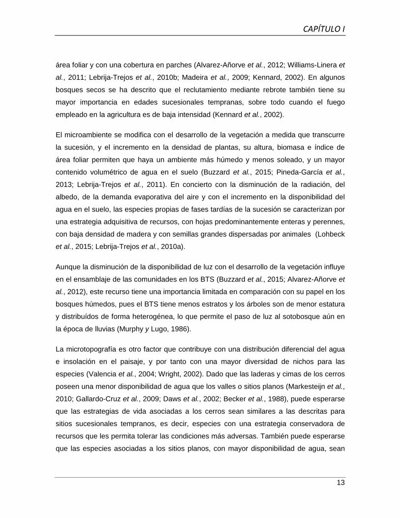
El microambiente se modifica con el desarrollo de la vegetación a medida que transcurre

la sucesión, y el incremento en la densidad de plantas, su altura, biomasa e índice de

área foliar permiten que haya un ambiente más húmedo y menos soleado, y un mayor

contenido volumétrico de agua en el suelo (Buzzard et al., 2015; Pineda-García et al.,

2013; Lebrija-Trejos et al., 2011). En concierto con la disminución de la radiación, del

albedo, de la demanda evaporativa del aire y con el incremento en la disponibilidad del

agua en el suelo, las especies propias de fases tardías de la sucesión se caracterizan por

una estrategia adquisitiva de recursos, con hojas predominantemente enteras y perennes,

con baja densidad de madera y con semillas grandes dispersadas por animales (Lohbeck

et al., 2015; Lebrija-Trejos et al., 2010a).

Aunque la disminución de la disponibilidad de luz con el desarrollo de la vegetación influye

en el ensamblaje de las comunidades en los BTS (Buzzard et al., 2015; Alvarez-Añorve et

al., 2012), este recurso tiene una importancia limitada en comparación con su papel en los

bosques húmedos, pues el BTS tiene menos estratos y los árboles son de menor estatura

y distribuídos de forma heterogénea, lo que permite el paso de luz al sotobosque aún en

la época de lluvias (Murphy y Lugo, 1986).

La microtopografía es otro factor que contribuye con una distribución diferencial del agua

e insolación en el paisaje, y por tanto con una mayor diversidad de nichos para las

especies (Valencia et al., 2004; Wright, 2002). Dado que las laderas y cimas de los cerros

poseen una menor disponibilidad de agua que los valles o sitios planos (Markesteijn et al.,

2010; Gallardo-Cruz et al., 2009; Daws et al., 2002; Becker et al., 1988), puede esperarse

que las estrategias de vida asociadas a los cerros sean similares a las descritas para

sitios sucesionales tempranos, es decir, especies con una estrategia conservadora de

recursos que les permita tolerar las condiciones más adversas. También puede esperarse

que las especies asociadas a los sitios planos, con mayor disponibilidad de agua, sean

CAPÍTULO I

14

más similares a las descritas para fases sucesionales tardías, con caracteres funcionales

asociados a la adquisición de recursos. Efectivamente, estudios previos en bosques

secos muestran que las especies que predominan en cerros tienden a tener madera de

alta densidad, con baja capacidad para almacenar agua pero alta resistencia a la

cavitación y hojas deciduas, mientras que en sitios planos predominan especies con

densidad de la madera media o baja que pueden almacenar agua y con hojas perennes

(Méndez-Alonzo et al., 2013; Borchert, 1994).

1.1.5 El bosque tropical de la Península de Yucatán y el papel del disturbio

Debido al gradiente de precipitación que se incrementa dede el noroeste hacia el sureste

de la Península, en el estado de Yucatán se presentan varios tipos de bosques como el

bajo caducifolio, el mediano subcaducifolio o el bajo inundable (Flores et al. 2010).

Estudios previos en los bosques medianos subcaducifolios de la Península han mostrado

que existe una similitud relativamente alta entre comunidades de plantas leñosas de

edades sucesionales distintas (Dupuy et al., 2012a; Schultz, 2003; Rico-Gray y García-

Franco, 1992). Algunos autores han propuesto que esa similitud se debe a que la

vegetación se encuentra en un estado de sucesión detenida, producto del uso recurrente

de la vegetación por más de 2000 años, desde los mayas pre-colombinos hasta los

habitantes actuales (Schultz, 2003; González-Iturbe et al., 2002; Mizrahi et al., 1997; Rico-

Gray y García-Franco, 1992). El disturbio crónico del bosque es consecuencia

principalmente de la agricultura de roza-tumba y quema, pero también de la eliminación

de especies consideradas como indeseables; de la extracción, selección y propagación de

otras con usos maderables, medicinales, alimenticios o de construcción; de la cacería, y

más recientemente de la agricultura, la ganadería y el crecimiento urbano (Dupuy et al.,

2015; Zamora Crescencio et al., 2009; Rico-Gray y García-Franco, 1992). Además, no se

puede dejar de considerar el disturbio que ocurre de forma natural en la península por el

impacto de los huracanes, aunque aparentemente éste tiene un impacto mucho menor

(Bonilla-Moheno, 2012; Whigham et al., 1991). En particular, el bosque tropical

subcaducifolio que constituye el área de estudio se ubica en la región Puuc, cerca de la

Sierrita de Ticul, por lo que se presentan zonas planas donde se realiza preferentemente

la agricultura, y pequeños lomeríos. La zona también tiene una larga historia de uso: la

más antigua se remonta al año 600 a. C. con un asentamiento maya de varios kilómetros;

más recientemente, a la comunidad de San Sebastián (mediados del siglo XVI)

CAPÍTULO I

15

(http://www.kaxilkiuic.org.mx) y actualmente a pueblos cercanos como Yaxhachen,

Xkobenhaltún o Xul, que aprovechan los recursos del área con actividades como cacería,

agricultura, producción de miel, construcción y usos medicinales (obs. pers.).

1.2 JUSTIFICACIÓN

A pesar del manejo reciente e histórico y a la perturbación recurrente en los bosques de la

península de Yucatán, se han publicado relativamente pocos estudios que expliquen los

cambios en la estructura de la comunidad vegetal durante la sucesión secundaria, en

relación a características ambientales, geográficas y de configuración del paisaje (Dupuy

et al., 2012; Hernández-Stefanoni et al., 2011; Schultz, 2003; González-Iturbe et al., 2002;

Turner II et al. 2001; Rico_Grey y García-Franco, 1992). En particular, el bosque mediano

subcaducifolio es el ecosistema terrestre más importante el Estado de Yucatán, con una

extensión aproximada de 1,264,568.9 ha (Secretaría de Desarrollo Urbano y Medio

Ambiente, 2007). Sin embargo, no se ha efectuado ningún análisis de la ecología

funcional de este ecosistema, a pesar de que es sabido que los caracteres funcionales

ofrecen un método altamente promisorio para entender cómo cambian las propiedades de

la vegetación en relación a gradientes físicos y geográficos (Westoby y Wright, 2006). Es

más, sólo recientemente se han iniciado en México los estudios de bosques tropicales

secos desde un punto de vista funcional, que caracterizan funcionalmente las especies

pioneras y tardías, o que analizan la variación de los caracteres funcionales de las

comunidades en relación con el tiempo de sucesión y sus condiciones microambientales

(Paz et al., 2015; Pineda-García et al., 2015, 2013, 2011; Lohbeck et al., 2013; Méndez-

Alonzo et al., 2013; Lebrija-Trejos et al., 2010a).

En este trabajo se hizo un análisis funcional de las comunidades de plantas leñosas en un

bosque tropical subcaducifolio de Yucatán, con la finalidad de obtener información sobre

cómo responden las plantas leñosas ante un gradiente sucesional y topográfico,

información fundamental para hacer un manejo y uso racional de las especies (Grime,

2006). Este estudio podrá ser base para generar nuevas líneas de investigación con

aplicaciones futuras, por ejemplo para la selección de especies en programas de

restauración ecológica, de reforestación o en la evaluación de servicios ecosistémicos

(Chazdon et al., 2010; Franks et al., 2009; Brown 2004).

CAPÍTULO I

16

1.3 PREGUNTAS DE INVESTIGACIÓN

¿Qué características funcionales distiguen a los grupos de plantas leñosas

especialistas -de etapas tempranas o tardías de la sucesión y de sitios planos y

cerros- de las especies generalistas? ¿las especies generalistas dominan a lo

largo de la sucesión y en diferentes posiciones topográficas en este bosque

sometido a largos procesos de disturbio?

¿Cómo varían los procesos de ensamblaje de las comunidades (filtrado ambiental

vs competencia) durante la sucesión secundaria y en relación a la posición

topográfica? ¿Varía la importancia relativa de estos procesos entre los brinzales y

las plantas adultas leñosas?

¿El filtrado ambiental local (i. e. dentro de las comunidades) y el asociado al

gradiente sucesional (i. e. entre comunidades) han favorecido asociaciones

particulares de caracteres en las plantas leñosas?

¿En qué medida la variación de los caracteres funcionales entre comunidades

ocurre en respuesta a los gradientes ambientales asociados a la edad sucesional y

a las características del suelo?

1.4 OBJETIVO GENERAL

Cuantifcar para las especies más dominantes de plantas leñosas de un bosque tropical

subcaducifolio de la Península de Yucatán algunos caracteres funcionales clave para su

coexistencia, para inferir los procesos de ensamblaje de esas comunidades y la variación

de estrategias ecológicas en respuesta a los gradientes asociados con la sucesión

secundaria y la topografía.

1.5 OBJETIVOS ESPECÍFICOS

Identificar los caracteres funcionales que distinguen a las especies que se

establecen en todo el gradiente sucesional y los de aquellas especies que se

especializan en porciones particulares del mismo.

CAPÍTULO I

17

Analizar cómo varían en importancia los procesos de filtrado ambiental y

competencia en las comunidades de brinzales y adultos de especies leñosas

durante la sucesión secundaria.

Analizar cómo co-varían los caracteres funcionales dentro y entre las comunidades

de plantas leñosas, y qué variables ambientales asociadas con la sucesión

secundaria, el suelo o la topografía explican esa variación.

1.6 HIPÓTESIS

a) Se encontrarán dos grupos generales de especies: aquellas especialistas,

es decir que se ven favorecidas (en términos de abundancia) en porciones restringidas

del gradiente sucesional (pioneras o tardías) o posición topográfica (sitios planos vs

cerros), y las generalistas o especies capaces de establecerse y llegar a ser dominantes

en todo el gradiente ambiental.

b) Como las condiciones de menor disponibilidad de agua ocurren al inicio de

la sucesión o en cerros, las especialistas de esos sitios presentarán caracteres

funcionales de hojas y tallos que les permitan evitar o resistir la sequía (por ejemplo hojas

compuestas y deciduas, pulvinos, alta densidad de la madera), mientras que las

especialistas de bosques viejos o de sitios planos presentarán caracteres asociados con

ambientes más mésicos (como hojas enteras y perennes, baja densidad de la madera).

c) Considerando la capacidad de las especies generalistas de establecerse

pronto en la sucesión y persistir hasta edades tardías, se espera que las generalistas

muestren una posición funcional intermedia entre las especialistas de bosque joven/

cerros y las especialistas de bosque maduro/sitios planos, aunque siendo más similares a

las primeras.

d) El aprovechamiento de la vegetación en diversos ecosistemas y sus usos

ha favorecido la proliferación de especies capaces de establecerse en amplios rangos de

variación ambiental (generalistas), y desfavorecido a aquellas especies con

requerimientos más estrechos para completar su ciclo de vida (especialistas) (Dar y

Reshi, 2014; Devictor et al., 2008; Vellend et al., 2007; McKinney, 2006; Smart et al.,

2006; Rooney et al., 2004; McKinney y Lockwood, 1999). Dada la larga historia de manejo

de este bosque, se espera que las generalistas sean el elemento dominante en todas las

edades sucesionales y posiciones topográficas.

CAPÍTULO I

18

e) El filtrado ambiental (observado como baja riqueza funcional) determinará

de forma principal el ensamblaje de las comunidades en fases tempranas de la sucesión y

en cerros, como resultado de un microambiente menos favorable en estas condiciones, tal

como se ha descrito en otros bosques secos.

f) El efecto de filtrado ambiental será más fuerte en los brinzales que en los

adultos, dado que la fase regenerativa es mucho más susceptible a condiciones

desfavorables.

g) Los procesos de competencia (observados como una alta divergencia y alta

equitatividad funcional) serán más importantes en edades sucesionales intermedias y

tardías, debido a que la competencia por recursos limitantes como el agua puede

incrementarse con el mayor desarrollo de raíces finas de individuos de mayor tamaño.

h) Los procesos competitivos limitarán más a los brinzales, pues es posible

que enfrenten una competencia asimétrica por el agua con los adultos.

i) Debido a que las comunidades (i. e. parcelas) de diferente edad sucesional

poseen distintas condiciones ambientales y de competencia como consecuencia del

desarrollo de la vegetación, se encontrarán a nivel de paisaje (entre parcelas)

asociaciones de caracteres funcionales que reflejen el recambio de especies de una

estrategia conservadora en parcelas jóvenes a una estrategia adquisitiva de recursos en

parcelas de edad más avanzada.

j) Por el contrario, debido a que se espera que las condiciones ambientales

dentro de las comunidades sean más homogéneas que entre las parcelas de diferente

edad sucesional, las asociaciones de caracteres serán más débiles o estarán ausentes

dentro de las comunidades.

k) Finalmente, se espera que el suelo explique una proporción similar de la

covariación de los caracteres funcionales que la edad de sucesión, pues las propiedades

del suelo varían en respuesta a los cambios de la vegetación que ocurren con la sucesión

secundaria.

1.7 BIBLIOGRAFÍA

Alvarez-Añorve, M.Y., Quesada, M., Sanchez-Azofeifa, G.A., Avila-Cabadilla, L.D., y

Gamon, J.A. (2012). Functional regeneration and spectral reflectance of trees

CAPÍTULO I

19

during succession in a highly diverse tropical dry forest ecosystem. Am. J. Bot.

99, 816–826.

Becker, P., Rabenold, P.E., Idol, J.R., y Smith, A.P. (1988). Water potential gradients for

gaps and slopes in a Panamanian tropical moist forest’s dry season. J. Trop.

Ecol. 4, 173–184.

Bhaskar, R., y Ackerly, D.D. (2006). Ecological relevance of minimum seasonal water

potentials. Physiol. Plant. 127, 353–359.

Bonilla-Moheno, M. (2012). Damage and recovery of forest structure and composition after

two subsequent hurricanes in the Yucatan Peninsula. Caribb. J. Sci. 46, 240–248.

Borchert, R. (1994). Soil and Stem Water Storage Determine Phenology and Distribution

of Tropical Dry Forest Trees. Ecology 75, 1437.

Borchert, R., Meyer, S.A., Felger, R.S., y Porter-Bolland, L. (2004). Environmental control

of flowering periodicity in Costa Rican and Mexican tropical dry forests. Glob.

Ecol. Biogeogr. 13, 409–425.

Brodribb, T.J., y Feild, T.S. (2000). Stem hydraulic supply is linked to leaf photosynthetic

capacity: evidence from New Caledonian and Tasmanian rainforests. Plant Cell

Environ. 23, 1381–1388.

Bucci, S.J., Goldstein, G., Meinzer, F.C., Scholz, F.G., Franco, A.C., y Bustamante, M.

(2004). Functional convergence in hydraulic architecture and water relations of

tropical savanna trees: from leaf to whole plant. Tree Physiol. 24, 891–899.

Buzzard, V., Hulshof, C.M., Birt, T., Violle, C., and Enquist, B.J. (2016). Re-growing a

tropical dry forest: functional plant trait composition and community assembly

during succession. Functional Ecology 30, 1006–1013.

Chave, J., Coomes, D., Jansen, S., Lewis, S.L., Swenson, N.G., y Zanne, A.E. (2009).

Towards a worldwide wood economics spectrum. Ecol. Lett. 12, 351–366.

CAPÍTULO I

20

Chesson, P. (2000). Mechanisms of maintenance of species diversity. Annu. Rev. Ecol.

Syst. 343–366.

Coomes, D.A., y Grubb, P.J. (2003). Colonization, tolerance, competition and seed-size

variation within functional groups. Trends Ecol. Evol. 18, 283–291.

Cornwell, W.K., Schwilk, D.W., y Ackerly, D.D. (2006). A trait-based test for habitat

filtering: convex hull volume. Ecology 87, 1465–1471.

Craine, J.M., y Dybzinski, R. (2013). Mechanisms of plant competition for nutrients, water

and light. Funct. Ecol. 27, 833–840.

Dar, P.A., y Reshi, Z.A. (2014). Components, processes and consequences of biotic

homogenization: A review. Contemp. Probl. Ecol. 7, 123–136.

Daws, M.I., Mullins, C.E., Burslem, D.F., Paton, S.R., y Dalling, J.W. (2002). Topographic

position affects the water regime in a semideciduous tropical forest in Panama.

Plant Soil 238, 79–89.

De Bello, F., Lavorel, S., Lavergne, S., Albert, C.H., Boulangeat, I., Mazel, F., y Thuiller,

W. (2013). Hierarchical effects of environmental filters on the functional structure

of plant communities: a case study in the French Alps. Ecography 36, 393–402.

Devictor, V., Julliard, R., y Jiguet, F. (2008). Distribution of specialist and generalist

species along spatial gradients of habitat disturbance and fragmentation. Oikos 0,

080211051304426–0.

Dupuy, J.M., Hernández-Stefanoni, J.L., Hernández-Juárez, R.A., Tetetla-Rangel, E.,

López-Martínez, J.O., Leyequién-Abarca, E., Tun-Dzul, F.J., y May-Pat, F. (2012).

Patterns and Correlates of Tropical Dry Forest Structure and Composition in a

Highly Replicated Chronosequence in Yucatan, Mexico. Biotropica 44, 151–162.

Dupuy, J.M., Durán-García, R., García-Contreras, G., Arellano Morín, J., Acosta Lugo, E.,

Méndez-González, M.E., y Andrade Hernández, M. (2015). Chapter 8.

Conservation and use. En Biodiversity and Conservation of the Yucatán

CAPÍTULO I

21

Peninsula, G.A. Islebe, S. Calmé, J.L. León-Cortés, y B. Schmook, eds. (Cham:

Springer International Publishing), p.

Engelbrecht, B.M.J., Dalling, J.W., Pearson, T.R.H., Wolf, R.L., Gálvez, D.A., Koehler, T.,

Tyree, M.T., y Kursar, T.A. (2006). Short dry spells in the wet season increase

mortality of tropical pioneer seedlings. Oecologia 148, 258–269.

Engelbrecht, B.M.J., Comita, L.S., Condit, R., Kursar, T.A., Tyree, M.T., Turner, B.L., y

Hubbell, S.P. (2007). Drought sensitivity shapes species distribution patterns in

tropical forests. Nature 447, 80–82.

Gallardo-Cruz, J.A., Pérez-García, E.A., y Meave, J.A. (2009). β-Diversity and vegetation

structure as influenced by slope aspect and altitude in a seasonally dry tropical

landscape. Landsc. Ecol. 24, 473–482.

Gerhardt, K., y Hytteborn, H. (1992). Natural dynamics and regeneration methods in

tropical dry forests - an introduction. J. Veg. Sci. 3, 361–364.

Goldstein, G., Andrade, J.L., Meinzer, F.C., Holbrook, N.M., Cavelier, J., Jackson, P., y

Celis, A. (1998). Stem water storage and diurnal patterns of water use in tropical

forest canopy trees. Plant Cell Environ. 21, 397–406.

González-Iturbe, J.A., Olmsted, I., y Tun-Dzul, F. (2002). Tropical dry forest recovery after

long term Henequen (sisal, Agave fourcroydes Lem.) plantation in northern

Yucatan, Mexico. For. Ecol. Manag. 167, 67–82.

Grime, J.P. (2006). Trait convergence and trait divergence in herbaceous plant

communities: mechanisms and consequences. J. Veg. Sci. 17, 255–260.

Hernández-Stefanoni, J.L., Dupuy, J.M., Tun-Dzul, F., y May-Pat, F. (2011). Influence of

landscape structure and stand age on species density and biomass of a tropical

dry forest across spatial scales. Landsc. Ecol. 26, 355–370.

Hikosaka, K. (2004). Interspecific difference in the photosynthesis-nitrogen relationship:

patterns, physiological causes, and ecological importance. J. Plant Res. 117,

481–494.

CAPÍTULO I

22

Hubbell, S.P. (1999). Light-Gap Disturbances, Recruitment Limitation, and Tree Diversity

in a Neotropical Forest. Science 283, 554–557.

Hubbell, S.P. (2005). Neutral theory in community ecology and the hypothesis of functional

equivalence. Funct. Ecol. 19, 166–172.

Ishida, A., Nakano, T., Yazaki, K., Matsuki, S., Koike, N., Lauenstein, D.L., Shimizu, M., y

Yamashita, N. (2008). Coordination between leaf and stem traits related to leaf

carbon gain and hydraulics across 32 drought-tolerant angiosperms. Oecologia

156, 193–202.

Kanagaraj, R., Wiegand, T., Comita, L.S., y Huth, A. (2011). Tropical tree species

assemblages in topographical habitats change in time and with life stage: Habitat-

driven tree species assemblages. J. Ecol. 99, 1441–1452.

Kennard, D.K. (2002). Secondary forest succession in a tropical dry forest: patterns of

development across a 50-year chronosequence in lowland Bolivia. J. Trop. Ecol.

18, 53–66.

Kennard, D.K., Gould, K., Putz, F.E., Fredericksen, T.S., y Morales, F. (2002). Effect of

disturbance intensity on regeneration mechanisms in a tropical dry forest. For.

Ecol. Manag. 162, 197–208.

Kneitel, J.M., y Chase, J.M. (2004). Trade-offs in community ecology: linking spatial scales

and species coexistence. Ecol. Lett. 7, 69–80.

Kraft, N.J., y Ackerly, D.D. (2010). Functional trait and phylogenetic tests of community

assembly across spatial scales in an Amazonian forest. Ecol. Monogr. 80, 401–

422.

Kraft, N.J.B., Valencia, R., y Ackerly, D.D. (2008). Functional Traits and Niche-Based Tree

Community Assembly in an Amazonian Forest. Science 322, 580–582.

Kraft, N.J.B., Adler, P.B., Godoy, O., James, E.C., Fuller, S., y Levine, J.M. (2015).

Community assembly, coexistence and the environmental filtering metaphor.

Funct. Ecol. 29, 592–599.

CAPÍTULO I

23

Kunstler, G., Lavergne, S., Courbaud, B., Thuiller, W., Vieilledent, G., Zimmermann, N.E.,

Kattge, J., y Coomes, D.A. (2012). Competitive interactions between forest trees

are driven by species’ trait hierarchy, not phylogenetic or functional similarity:

implications for forest community assembly. Ecol. Lett. 15, 831–840.

Lasky, J.R., Uriarte, M., Boukili, V.K., y Chazdon, R.L. (2014). Trait-mediated assembly

processes predict successional changes in community diversity of tropical forests.

Proc. Natl. Acad. Sci. 111, 5616–5621.

Lebrija-Trejos, E., Pérez-García, E.A., Meave, J.A., Bongers, F., y Poorter, L. (2010a).

Functional traits and environmental filtering drive community assembly in a

species-rich tropical system. Ecology 91, 386–398.

Lebrija-Trejos, E., Meave, J.A., Poorter, L., Pérez-García, E.A., y Bongers, F. (2010b).

Pathways, mechanisms and predictability of vegetation change during tropical dry

forest succession. Perspect. Plant Ecol. Evol. Syst. 12, 267–275.

Lebrija-Trejos, E., Pérez-García, E.A., Meave, J.A., Poorter, L., y Bongers, F. (2011).

Environmental changes during secondary succession in a tropical dry forest in

Mexico. J. Trop. Ecol. 27, 477–489.

Leishman, M.R., y Westoby, M. (1994). The Role of Seed Size in Seedling Establishment

in Dry Soil Conditions -- Experimental Evidence from Semi-Arid Species. J. Ecol.

82, 249.

Lohbeck, M., Poorter, L., Lebrija-Trejos, E., Martínez-Ramos, M., Meave, J.A., Paz, H.,

Pérez-García, E.A., Romero-Pérez, I.E., Tauro, A., y Bongers, F. (2013).

Successional changes in functional composition contrast for dry and wet tropical

forest. Ecology 94, 1211–1216.

Lohbeck, M., Lebrija-Trejos, E., Martínez-Ramos, M., Meave, J.A., Poorter, L., y Bongers,

F. (2015). Functional trait strategies of trees in dry and wet tropical forests are

similar but differ in their consequences for succession. Plos One 10, e0123741.

CAPÍTULO I

24

Maass, M., y Burgos, A. (2011). Chapter 9. Water dynamics at the ecosystem level in

seasonally dry tropical forests. En Seasonally Dry Tropical Forests: Ecology and

Conservation, R. Dirzo, H.S. Young, H.A. Mooney, y G. Ceballos, eds.

(Washington: Island Press), pp. 141–156.

Macarthur, R., y Levins, R. (1967). The Limiting Similarity, Convergence, and Divergence

of Coexisting Species. Am. Nat. 101, 377–385.

Madeira, B.G., Espírito-Santo, M.M., Neto, S.D., Nunes, Y.R.F., Arturo Sánchez Azofeifa,

G., Wilson Fernandes, G., y Quesada, M. (2009). Changes in tree and liana

communities along a successional gradient in a tropical dry forest in south-

eastern Brazil. Plant Ecol. 201, 291–304.

Markesteijn, L., Iraipi, J., Bongers, F., y Poorter, L. (2010). Seasonal variation in soil and

plant water potentials in a Bolivian tropical moist and dry forest. J. Trop. Ecol. 26,

497–508.

Markesteijn, L., Poorter, L., Paz, H., Sack, L., y Bongers, F. (2011). Ecological

differentiation in xylem cavitation resistance is associated with stem and leaf

structural traits. Plant Cell Environ. 34, 137–148.

Mayfield, M.M., y Levine, J.M. (2010). Opposing effects of competitive exclusion on the

phylogenetic structure of communities: Phylogeny and coexistence. Ecol. Lett. 13,

1085–1093.

McKinney, M.L. (2006). Urbanization as a major cause of biotic homogenization. Biol.

Conserv. 127, 247–260.

McKinney, M.L., y Lockwood, J.L. (1999). Biotic homogeneization_a few winners replacing

many losers in the next mass extinction.pdf. TREE 14, 450–453.

Meinzer, F.C., James, S.A., Goldstein, G., y Woodruff, D. (2003). Whole-tree water

transport scales with sapwood capacitance in tropical forest canopy trees. Plant

Cell Environ. 26, 1147–1155.

CAPÍTULO I

25

Méndez-Alonzo, R., Paz, H., Zuluaga, R.C., Rosell, J.A., y Olson, M.E. (2012).

Coordinated evolution of leaf and stem economics in tropical dry forest trees.

Ecology 93, 2397–2406.

Méndez-Alonzo, R., Pineda-García, F., Paz, H., Rosell, J.A., y Olson, M.E. (2013). Leaf

phenology is associated with soil water availability and xylem traits in a tropical

dry forest. Trees 27, 745–754.

Michalet, R., y Pugnaire, F.I. (2016). Facilitation in communities: underlying mechanisms,

community and ecosystem implications. Funct. Ecol. 30, 3–9.

Mizrahi, A., Ramos Prado, J., y Jiménez-Osornio, J. (1997). Composition, structure, and

management potential of secondary dry tropical vegetation in two abandoned

henequen plantations of Yucatan, Mexico. For. Ecol. Manag. 96, 273–282.

Moles, A.T., y Westoby, M. (2004). Seedling survival and seed size: a synthesis of the

literature. J. Ecol. 92, 372–383.

Muller-Landau, H.C. (2010). The tolerance-fecundity trade-off and the maintenance of

diversity in seed size. Proc. Natl. Acad. Sci. 107, 4242–4247.

Murphy, P.G., y Lugo, A.E. (1986). Ecology of tropical dry forest. Annu. Rev. Ecol. Syst.

67–88.

Niinemets, Ü. (2010). Responses of forest trees to single and multiple environmental

stresses from seedlings to mature plants: Past stress history, stress interactions,

tolerance and acclimation. For. Ecol. Manag. 260, 1623–1639.

Paz, H., Pineda-García, F., y Pinzón-Pérez, L.F. (2015). Root depth and morphology in

response to soil drought: comparing ecological groups along the secondary

succession in a tropical dry forest. Oecologia 179, 551–561.

Pennington, R.T., Lewis, G.P., y Ratter, J.A. (2006). Chapter 1. An overview of the plant

diversity, biogeography and conservation of neotropical savannas and seasonally

dry forests. En Neotropical Savannas and Seasonally Dry Forests: Plant Diversity,

CAPÍTULO I

26

Biogeography, and Conservation, R.T. Pennington, J.A. Ratter, y G.P. Lewis, eds.

(Boca Raton, FL: CRC press), p. 491.

Pineda-García, F., Paz, H., y Tinoco-Ojanguren, C. (2011). Morphological and

physiological differentiation of seedlings between dry and wet habitats in a tropical

dry forest: Water-use strategies of TDF tree seedlings. Plant Cell Environ. 34,

1536–1547.

Pineda-García, F., Paz, H., y Meinzer, F.C. (2013). Drought resistance in early and late

secondary successional species from a tropical dry forest: the interplay between

xylem resistance to embolism, sapwood water storage and leaf shedding. Plant

Cell Environ. 36, 405–418.

Pineda-García, F., Paz, H., Meinzer, F.C., y Angeles, G. (2015). Exploiting water versus

tolerating drought: water-use strategies of trees in a secondary successional

tropical dry forest. Tree Physiol. tpv124.

Portillo-Quintero, C.A., y Sánchez-Azofeifa, G.A. (2010). Extent and conservation of

tropical dry forests in the Americas. Biol. Conserv. 143, 144–155.

Punchi-Manage, R., Getzin, S., Wiegand, T., Kanagaraj, R., Savitri Gunatilleke, C.V.,

Nimal Gunatilleke, I.A.U., Wiegand, K., y Huth, A. (2013). Effects of topography

on structuring local species assemblages in a Sri Lankan mixed dipterocarp

forest. J. Ecol. 101, 149–160.

Reich, P.B. (2014). The world-wide “fast–slow” plant economics spectrum: a traits

manifesto. J. Ecol. 102, 275–301.

Reich, P.B., Walters, M.B., y Ellsworth, D.S. (1997). From tropics to tundra: global

convergence in plant functioning. Proc. Natl. Acad. Sci. 94, 13730–13734.

Rico-Gray, V., y García-Franco, J.G. (1992). Vegetation and soil seed bank of

successional stages in tropical lowland deciduous forest. J. Veg. Sci. 3, 617–624.

CAPÍTULO I

27

Rooney, T.P., Wiegmann, S.M., Rogers, D.A., y Waller, D.M. (2004). Biotic

Impoverishment and Homogenization in Unfragmented Forest Understory

Communities. Conserv. Biol. 18, 787–798.

Santiago, L.S., Goldstein, G., Meinzer, F.C., Fisher, J.B., Machado, K., Woodruff, D., y

Jones, T. (2004). Leaf photosynthetic traits scale with hydraulic conductivity and

wood density in Panamanian forest canopy trees. Oecologia 140.

Scholz, F.G., Phillips, N.G., Bucci, S.J., Meinzer, F.C., y Goldstein, G. (2011). Chapter 13.

Hydraulic Capacitance: Biophysics and Functional Significance of Internal Water

Sources in Relation to Tree Size. En Size- and Age-Related Changes in Tree

Structure and Function, F.C. Meinzer, B. Lachenbruch, y T.E. Dawson, eds.

(Dordrecht: Springer Netherlands), pp. 341–362.

Schultz, G.P. (2003). Chapter 6. Structure and diversity of the forests at The Eden

ecological reserve. En The Lowland Maya Area: Three Millennia at the Human-

Wildland Interface, A. Gómez-Pompa, M.F. Allen, S.L. Fedick, y J.J. Jiménez-

Osornio, eds. (The Haworth Press, Inc.), pp. 91–114.

Schwilk, D.W., y Ackerly, D.D. (2005). Limiting similarity and functional diversity along

environmental gradients: Diversity and gradients. Ecol. Lett. 8, 272–281.

Schwinning, S., y Weiner, J. (1998). Mechanisms Determining the Degree of Size

Asymmetry in Competition among Plants. Oecologia 113, 447–455.

Sears, A.L.W., y Chesson, P. (2007). New methods for quantifying the spatial storage

effect: an illustration with desert annuals. Ecology 88, 2240–2247.

Semenova, G., V., y van der Maarel, E. (2000). Plant functional types - a strategic

perspective. J. Veg. Sci. 11, 917–922.

Smart, S.M., Thompson, K., Marrs, R.H., Le Duc, M.G., Maskell, L.C., y Firbank, L.G.

(2006). Biotic homogenization and changes in species diversity across human-

modified ecosystems. Proc. R. Soc. B Biol. Sci. 273, 2659–2665.

CAPÍTULO I

28

Sobrado, M.A. (1993). Trade-off between water transport efficiency and leaf life-span in a

tropical dry forest. Oecologia 96, 19–23.

Sobrado, M.A. (1997). Embolism vulnerability in drought-deciduous and evergreen species

of a tropical dry forest. Acta Oecologica 18, 383–391.

Tilman, D. (1987). The importance of the mechanisms of interspecific competition. Am.

Nat. 769–774.

Tilman, D. (1994). Competition and biodiversity in spatially structured habitats. Ecology 75,

2–16.

Toledo, M., Peña-Claros, M., Bongers, F., Alarcón, A., Balcázar, J., Chuviña, J., Leaño,

C., Licona, J.C., y Poorter, L. (2012). Distribution patterns of tropical woody

species in response to climatic and edaphic gradients: Environmental responses

of tropical trees. J. Ecol. 100, 253–263.

Tyree, M.T., y Sperry, J.S. (1989). Vulnerability of xylem to cavitation and embolism. Annu.

Rev. Plant Biol. 40, 19–36.

Valdez-Hernández, M., Andrade, J.L., Jackson, P.C., y Rebolledo-Vieyra, M. (2010).

Phenology of five tree species of a tropical dry forest in Yucatan, Mexico: effects

of environmental and physiological factors. Plant Soil 329, 155–171.

Valencia, R., Foster, R.B., Villa, G., Condit, R., Svenning, J.-C., Hernández, C.,

Romoleroux, K., Losos, E., Magard, E., y Balslev, H. (2004). Tree species

distributions and local habitat variation in the Amazon: large forest plot in eastern

Ecuador. J. Ecol. 92, 214–229.

Vargas, R., Allen, M.F., y Allen, E.B. (2008). Biomass and carbon accumulation in a fire

chronosequence of a seasonally dry tropical forest. Glob. Change Biol. 0, 109–

124.

Vellend, M., Verheyen, K., Flinn, K.M., Jacquemyn, H., Kolb, A., Van Calster, H., Peterken,

G., Graae, B.J., Bellemare, J., Honnay, O., et al. (2007). Homogenization of forest

CAPÍTULO I

29

plant communities and weakening of species-environment relationships via

agricultural land use. J. Ecol. 95, 565–573.

Villéger, S., Mason, N.W., y Mouillot, D. (2008). New multidimensional functional diversity

indices for a multifaceted framework in functional ecology. Ecology 89, 2290–

2301.

Violle, C., Navas, M.-L., Vile, D., Kazakou, E., Fortunel, C., Hummel, I., y Garnier, E.

(2007). Let the concept of trait be functional! Oikos 116, 882–892.

Warner, R.R., y Chesson, P.L. (1985). Coexistence mediated by recruitment fluctuations: a

field guide to the storage effect. Am. Nat. 769–787.

Weiher, E., y Keddy, P.A. (1995). Assembly Rules, Null Models, and Trait Dispersion: New

Questions from Old Patterns. Oikos 74, 159.

Weiher, E., van der Werf, A., Thompson, K., Roderick, M., Garnier, E., y Eriksson, O.

(1999). Challenging Theophrastus: A common core list of plant traits for functional

ecology. J. Veg. Sci. 10, 609–620.

Westoby, M. (1998). A leaf-height-seed (LHS) plant ecology strategy scheme. Plant Soil

199, 213–227.

Westoby, M., Falster, D.S., Moles, A.T., Vesk, P.A., y Wright, I.J. (2002). Plant Ecological

Strategies: Some Leading Dimensions of Variation Between Species. Annu. Rev.

Ecol. Syst. 33, 125–159.

Whigham, D.F., Olmsted, I., Cabrera Cano, E., y Harmon, M.E. (1991). The impact of

Hurricane Gilbert on trees, litterfall, and woody debris in a dry tropical forest in the

northeastern Yucatan Peninsula. Biotropica 23, 434–441.

Williams-Linera, G., Alvarez-Aquino, C., Hernández-Ascención, E., y Toledo, M. (2011).

Early successional sites and the recovery of vegetation structure and tree species

of the tropical dry forest in Veracruz, Mexico. New For. 42, 131–148.

CAPÍTULO I

30

Wolfe, B.T., y Kursar, T.A. (2015). Diverse patterns of stored water use among saplings in

seasonally dry tropical forests. Oecologia 179, 925–936.

Wright, J.S. (2002). Plant diversity in tropical forests: a review of mechanisms of species

coexistence. Oecologia 130, 1–14.

Wright, I.J., Ackerly, D.D., Bongers, F., Harms, K.E., Ibarra-Manriquez, G., Martinez-

Ramos, M., Mazer, S.J., Muller-Landau, H.C., Paz, H., Pitman, N.C.A., et al.

(2007). Relationships Among Ecologically Important Dimensions of Plant Trait

Variation in Seven Neotropical Forests. Ann. Bot. 99, 1003–1015.

Zamora Crescencio, P., Flores Guido, J.S., y Ruenes Morales, R. (2009). Flora útil y su

manejo en el Cono Sur del estado de Yucatan, México. Polibotánica 227–250.

CAPÍTULO II

31

CAPÍTULO 2.WHAT MAKES A WOODY PLANT A GENERALIST OR A SPECIALIST? AFUNCTIONAL TRAIT ANALYSIS IN A SECONDARY TROPICAL DRY FOREST

Artículo en preparación.

Lucía Sanaphre-Villanueva *a, Juan Manuel Dupuy a, José Luis Andrade a, Casandra Reyes-

García a, Paula C. Jackson b and Horacio Paz c

a Unidad de Recursos Naturales, Centro de Investigación Científica de Yucatán (CICY), Mérida,

Yucatán, México.

b Department of Ecology, Evolution, and Organismal Biology, Kennesaw State University,

Kennesaw, GA, USA.

c Instituto de Investigaciones en Ecosistemas y Sustentabilidad, Universidad Nacional Autónoma

de México, Morelia, Michoacán, México.

* Corresponding author: [email protected]

Heading: Plant generalists and specialists in a dry forest

2.1 ABSTRACT

1. Tropical dry forests are being strongly impacted by human activities, and the human-

induced environmental changes may result in the spread of common, generalist species,

capable of surviving in a wide range of environmental conditions.

2. Our objective is to assess if generalist and specialist plant species within a successional

gradient and among different topographical positions display different constellations of

functional traits, and if generalists are the predominant component of a tropical dry forest

landscape with a long history of human disturbance.

3. Using a multinomial model based on relative abundances of woody species in 273 plots,

from the sixty five most abundant species 10 were classified as old growth forest

specialists (old specialists), 6 species as young secondary forest specialists (young

specialists), 27 species as generalists and 22 species as too rare to classify with

confidence. Those same species were clasified according to topography, and we found

12 flat area specialists, 9 hill specialists, 23 generalists and 21 Too rare.

CAPÍTULO II

32

4. Most of the young forest specialists were also flat sites specialists, and most of the old

forest specialists were also hill specialists. PERMANOVA analysis using 13 functional

traits for the 65 most abundant species revealed significant differences among groups.

Leaf shedding was the main mechanism allowing young and flat specialists to avoid

hydraulic failure, while old and hill specialists use different mechanisms to cope with

drought.

5. Generalist species were more similar to old and hill specialists, and tended to be more

abundant than young and old specialists accross the successional gradient, and as

abundant as flat and hill specialists on topographical positions.

6. A more thorough functional analysis is needed to determine which traits confer

generalists competitive advantages over old specialists in flat areas, since both groups

are functionally similar. Reproductive traits or resprouting may offer new insights.

Key-words. Hill, homogenization, pioneer, slash and burn agriculture, slope, succession,

tolerant, Yucatan.

2.2 INTRODUCTION

As the current natural environments are increasingly threaten by human activities, it becomes

more important to define the characteristics that differentiate a generalist from a specialist

species (Chazdon et al., 2011), under the rationale that the former one will be more plastic in its

response to disturbance and will less likely become locally extinct. Forest conversion to

agriculture, livestock pastures, urban areas, etc., has caused the loss of more than 70% of

tropical forest cover in the last 15 years (Keenan et al., 2015). Human-induced environmental

change impose new filters on species, resulting in the spread of common, generalist species,

capable of surviving in a wide range of environmental conditions, and a decline of specialist

species, which leads to an increased similarity among communities (i.e. biotic homogenization),

along with diminished diversity (Smart et al., 2006; McKinney and Lockwood, 1999). Tropical dry

forests are among the most threatened ecosystems in the world, because they are easily

cleared and woody regeneration is effortlessly eliminated with fire; besides, the severe dry

season suppresses pest and weed populations, facilitates the use of fire and slows soil

degradation –characteristics that are highly valuable for agriculture and other land uses

(Donfack et al., 1995; Janzen, 1988).

The few functional and microenvironmental studies conducted on tropical dry forests show that

elevated temperature and water vapour pressure deficit that result from higher radiation loads

CAPÍTULO II

33

during the dry season can be the main drivers of functional differentiation in recently abandoned

lands after agriculture (Lebrija-Trejos et al., 2010). In the dry environments of these early stages

of succession, dominating species are those with functional traits associated with irradiance load

avoidance through leaf or leaflet movement, hydraulic failure avoidance through leaf shedding,

high cavitation resistance and deeper root foraging capacity (Paz et al., 2015; Méndez-Alonzo et

al., 2013; Pineda-García et al., 2011; Lebrija-Trejos et al., 2010a), i.e. young secondary forest

specialists, such as many legume species (Lebrija-Trejos et al., 2010; Romero-Duque et al.,

2007; Gillespie et al., 2000). At latter successional stages, when vegetation starts to recover, the

increase in density of individuals and foliage modifies the microenvironment making it more

shaded and humid, and such autogenic changes favor species capable of withstanding lower

light availability, i. e. old growth forest specialists (Lebrija-Trejos et al., 2010).

Topography is another important variable producing changes in vegetation structure and

composition. Differences in soil water availability (lowest on hill-tops, intermediate on slopes and

highest in valleys) have been previously reported (Pineda-García et al., 2013; Lebrija-Trejos et

al., 2011; Markesteijn et al., 2010; Gallardo-Cruz et al., 2009; Becker et al., 1988). For example,

deciduous trees with high wood density and water-storing trees with low wood density are

predominantly distributed in upland dry forests, while evergreen with high and low wood

densities trees are confined to more humid lowland sites (Méndez-Alonzo et al., 2013; Borchert,

1994).

Few functional studies on tropical forest succession or in topographical gradients have focused

on the functional differentiation between young secondary and old-growth forest specialists

(Letcher et al., 2015; Lasky et al., 2014; Alvarez-Añorve et al., 2012; Lebrija-Trejos et al., 2010)

or between upland and lowland specialists (Méndez-Alonzo et al., 2013; Borchert, 1994), but do

not address the functional traits that may facilitate the establishment and survival of generalist

species along the complete successional gradient.

Previous studies in forests of the Yucatan Peninsula, which have been managed for millennia,

have found that patterns of plant species composition and structure are mainly determined by

successional age and topography (López-Martínez et al., 2013; Dupuy et al., 2012a, 2012b;

White and Hood, 2004). Therefore, the aim of this study is to assess if secondary succession

and the mild topography present in our study area differentiate species into generalists and

specialists, and to answer the following questions: Do generalist and specialist species display

CAPÍTULO II

34

different constellations of traits? Are generalists dominant (more abundant) over the whole

successional age gradient?

We expect that: 1) successional age and topography will differentiate species into generalist and

specialists –either or both in young successional forest stands vs older stands and/or in hills vs

flat areas. 2) specialists in young forest stands and in hills will show leaf and stem traits

associated with drought resistance or avoidance (e.g. high wood specific gravity,

deciduousness, compound leaves and pulvination), while the old growth forest and flat area

specialists will show traits associated with more mesic environments, such as low wood specific

gravity, evergreens and simple leaves. 3) Considering the capacity of generalists to establish

early in succession but also to persist through latter successional ages, we expect that

generalists would show an intermediate functional position between young seconday/hill-

specialists and old growth/flat area specialist species but would be more similar to the former. 4)

Finally, given the millenial history of management of our studied forest, we expect that generalist

species will be more abundant than specialist species across all successional ages and

topographical positions.

2.3 MATERIALS AND METHODS

2.3.1 Study site

The study area covers a 352 km2 landscape of semi-deciduous tropical forest in the central part

of the Yucatan Peninsula, Mexico (20° 01´07” to 20° 09´ 36” N latitude, and 89° 35´59” to 89°

23´31” W longitude), and includes the Biocultural Reserve Xaxil Kiuic. The region is

characterized by a sub humid warm climate -AW1 according to the modified Köppen system

(García, 1981)- with summer rains and a sharp dry season from November to April; mean

annual temperature is 26°C and mean annual precipitation ranges between 900 and 1100 mm.

The landscape consists of flat areas with relatively deep (40–100 cm) clayey Luvisols and

Cambisols and small limestone hills (elevations between 60 and 190 m asl) with shallow (5–20

cm) rocky Lithosols and Rendzines (Flores and Espejel 1994; Bautista-Zúñiga et al. 2003). Soil

depth is greater in flat areas than on slopes (Bautista-Zúñiga et al., 2003), while soil fertility

shows the opposite pattern (Dupuy et al., 2012a). The predominant land use has been

traditional slash and burn agriculture, practiced by the Mayan people for over 2000 years (Rico-

Gray and García-Franco, 1991). Consequently the vegetation is a shifting mosaic of small

agricultural fields and forests of different successional ages.

CAPÍTULO II

35

2.3.2 Sampling design

A Spot 5 satellite image acquired on January 2005 was used for a supervised classification in

the following vegetation classes 1) 3 to 8 years of secondary succession, 2) 9 to 15 years, 3) >

15 years on flat areas, and 4) > 15 years on hills. Vegetation classes 1 and 2 occurred mostly in

flat areas, since these are generally preferred by local farmers (Hernández-Stefanoni and

Dupuy, 2008). In the summers of 2008 and 2009, twenty three 1 Km2 landscape units were

selected that encompassed the range of landscape conditions of disturbance and fragmentation.

At each unit 12 sampling plots (3 in each vegetation class) were established (276 plots in total):

Stand age of each plot was determined from interviews with local residents who lived in the area

for 40 years and owned or worked the land. Mayan farmers have a keen empirical knowledge of

forest succession, and their own detailed system of classifying and distinguishing several

successional stages based on their knowledge of the local disturbance regime, and the

presence and size of certain species, which makes their determination of forest stand age

reliable (González-Cruz et al., 2014; Hernández-Stefanoni et al., 2006). Each plot consisted of a

circular 200 m2 area where all woody plants with a diameter at breast height (DBH, measured at

1.3 m height) > 5 cm were measured (for a detailed description of sampling design see

(Hernández-Stefanoni et al., 2011).

2.3.3 Species selection

We calculated the relative importance value (RIV) of all species in the four vegetation classes

described earlier. The RIV of each species in each class was the sum of its relative abundance,

frequency and basal area. For each vegetation class and separately for trees, lianas and shrubs,

we selected those species that constituted at least 90% of the cumulative RIV, and obtained a

total of 72 species covering all vegetation classes. However, we only include in the analyses 65

species for which we were able to collect material from at least 5 individuals, which represent

90% ± 10% (mean ± standard deviation) of the total richness per plot; 45 species are trees, 11

species are shrubs, and 9 species are lianas.

2.3.4 Functional traits

Samples were collected from at least 5 individuals per species (14 individuals per species on

average, total 934) during the rainy months of 2011 (from August to November) and 2012 (from

September to November). We obtained 3 to 5 young, healthy and completely expanded leaves

from sun-exposed branches from each individual. Fresh weight was determined to 0.001 g using

CAPÍTULO II

36

a digital scale (Mettler Toledo PB4002-S/FACT, OH, USA) and samples were digitized using a

flatbed scanner, oven-dried at ~60°C for three days, and weighed again. We measured petiole

length (PL) and leaf or leaflet area (as an average of ten leaflets) with the software ImageJ

1.47b (Rasband, 2014). We separately quantified total leaf area (LA), which represents the leaf

and petiole area for species with simple leaves and the sum of the area of all the leaflets and

petiole for species with compound leaves, from the minimum photosynthetic unit (MPU) that

represents the leaf area for the former and the average leaflet area for the latter. Specific leaf

area (SLA) and leaf dry matter content (LDMC) were calculated using standard methods

(Cornelissen et al., 2003).

We obtained wood specific gravity (WSG) from 4 individuals per species with the largest DBH,

which on average was 3.2 cm for lianas, 4.1 cm for shrubs and 16.4 cm for trees. Lianas were

sampled with a knife by taking a 4 to 5 cm long and 1 cm wide slice from the trunk, tapering

longitudinally towards the pith. We peeled off only bark that could be retrieved by hand. We

proceeded in the same way with shrubs when there was a clearly defined trunk at least 4 cm

wide. Otherwise we cut one branch at the first ramification and took a 4 to 5 cm long section. For

trees, we took a sample from cortex to pit at breast height using a 5 mm diameter core borer,

and samples were cut every centimetre. Green volume was measured using the water

displacement method. Samples were oven dried at 100°C and weighed on an analytical scale

(Ohaus Adventurer AP 2140, NJ, USA). Dry weight of each sample was divided over its green

volume to obtain wood specific gravity. A weighted average per sampled tree was calculated

weighting each core section by the cross-sectional area of the corresponding trunk (Muller-

Landau, 2004).

From field specimens and bibliography, we determined some binary traits: leaf compoundness

(LC; 0 = simple, 1 = compound); leaf pulvination (LPulv; 0 = absent, 1 = present); leaf

pubescence (LPb; 0 = absent, 1 = present), dispersal syndrome (Dis; 0 = abiotic, 1 = biotic);

plant exudates (Ex; 0 = absent, 1 = present), and plant spininess (Sp; 0 = absent, 1 = present).

From parataxonomist Filogonio May Pat and bibliography we also determined leaf

deciduousness (LD; 0 = evergreen, 1 = deciduous).

2.3.5 Statistical analyses

We classified woody plant species in our forest using a multinomial model based on estimated

species relative abundances in early and late successional habitats (Chazdon et al., 2011).

Since the multinomial model classify species only between two habitats, we performed two

CAPÍTULO II

37

analyses to identify specialist and generalist species, one considering the successional gradient,

and another considering the topographical gradient.

In the first analysis, we compared plots of vegetation classes 1 and 2 (plots from 3 to 15 years of

secondary succession) as representative of young forests, versus plots of vegetation classes 3

and 4 (plots older than 15 years of succession on flat areas and hills) as representative of older

vegetation. The criteria to define the vegetation classes was based on their spectral signal,

which allowed us to separate them under a supervised classification of SPOT 5 satellite imagery

(see Hernández-Stefanoni and Dupuy, 2008). Although forests older than 15 years (and less

than 80 years old) do not necessarily represent mature vegetation, the long history of human

occupancy and millennial use of the vegetation in the Yucatan make it difficult to find older,

mature-forest fragments. Besides, a previous study in the same area with 168 plots showed

significant differences in species composition among the same vegetation classes (Dupuy et al.,

2012a) that we corroborated with a PERMANOVA analysis with our 273 plots (root squared

transformation on abundance matrix of species, and Bray Curtis similarity; pseudo F = 15.908, p

< 0.0001).

The model distinguished four groups of species: generalists, young secondary forest specialist

(hereafter refered to as young specialists), old growth forest specialists (hereafter old specialists)

and too rare to classify with confidence (hereafter too rare). When a species is shared among

old-growth and young secondary forests, the multinomial model uses a threshold to determine if

a species is classified as old specialists or young specialists. We used a conservative threshold

of k = 2/3. This means that a species was considered as old specialist if its relative abundance in

old-growth forests was twice its relative abundance in young secondary forests, while a species

was considered as young specialists if its relative abundance in young secondary forest was

twice its relative abundance in old growth forests. A one-sided statistical test was then

performed to determine the minimum number of individuals of a species in old-growth (Xi) or in

young secondary forest (Yi) necessary to obtain a significant result at particular values of k and

p. Those minimum values (Xmin and Ymin) are used as thresholds to differentiate generalists from

young specialists and old specialists, and all these categories from Too rare. We used 40 as a

minimum value to perform the classification, with p = 0.05/40 = 0.00125 (Chazdon et al., 2011).

We performed a second analysis where we compared plots on flat areas (vegetation classes 1

to 3, plots of all successional ages on flat sites) vs plots on hills (vegetation class 4, plots older

than 15 years on hills). Although the ideal approach would include young plots on hills as well,

CAPÍTULO II

38

agriculture is established mainly on flat areas, and we could not find enough replicates in this

condition. We decided not to limit the analysis to plots older than 15 years on flat areas vs hills

(vegetation classes 3 and 4) because removing younger plots reduced the observed proportion

on flat areas for many species, and the multinomial model is very susceptible to total

abundance. The model distinguished four groups of species: generalists, hill specialists, flat

areas specialists (hereafter flat specialists) and too rare. Since the multinomial model is based

on relative abundances of species, we used the total number of species registered (n = 137

species, 273 plots) for both analyses. For all other analyses, we included only the 65 species

(that represent more than 90% of total richness per plot) for which we determined functional trait

information. The multinomial model was performed with vegan package (Oksanen et al., 2016)

in R software (R Development Core Team, 2015).

To determine if there were functional differences between generalists and specialists, we

performed a PERMANOVA based on a matrix of dissimilarity obtained with euclidean distances

of the 13 standardized functional traits in PRIMER v. 6.1.18 and PERMANOVA+ v. 1.08. In order

to visualize which traits were associated with generalists and specialists, we performed a

Principal Component Analysis (PCA) on the 13 traits. To test whether the proportion of attributes

of binary traits differed among groups, we applied chi-square analyses and Tukey-type multiple

comparison tests (Zar, 1999). In the case of continuous traits, we preformed a separate ANOVA

for each trait and Tukey’s post hoc analyses in InfoStat software (Di Rienzo et al., 2013).

Finally, to determine if there were significant differences in relative abundance of generalists and

specialists per plot in relation to successional age and topographic position, we performed the

non-parametric Kruskal-Wallis test and paired comparisons among means of the ranks in

InfoStat software (Di Rienzo et al. 2013) among the four vegetation classes: 1) 3 to 8 years of

secondary succession on flat areas (n = 48 plots), 2) 9 to 15 years on flat areas (78), 3) > 15

years on flat areas (84), and 4) > 15 years on hills (63).

2.4 RESULTS

In the successional gradient, the multinomial model classified 10 species as old specialists, 6

species as young specialists, 27 species as generalists and 22 species as too rare. According to

topography, we found 12 flat specialists, 9 hill specialists, 23 generalists and 21 too rare (Table

2.1).

CAPÍTULO II

39

Table 2.1 Species classification according to successional gradient and topographical position as

specialists (YS = young forest specialist; OS = old forest specialist; FS = flat site specialist; HS = hill

specialist), generalists (G) and too rare to classify (Too rare).

Species Family Lifeform

Succession Topography

Bauhinia ungulata Fabaceae Tree G FS

Bourreria pulchra Boraginaceae Tree G G

Bursera simaruba Burseraceae Tree G G

Caesalpinia gaumeri Fabaceae Tree G G

Calyptranthes pallens Myrtaceae Tree G G

Chloroleucon mangense Fabaceae Tree G G

Coccoloba spicata Polygonaceae Tree G G

Cochlospermum vitifolium Bixaceae Tree G FS

Croton reflexifolius Euphorbiaceae Tree G G

Diospyros anisandra Ebenaceae Tree G G

Diospyros yucatanensis ssp yucatanensis Ebenaceae Tree G G

Eugenia axillaris Myrtaceae Tree G FS

Exostema caribaeum Rubiaceae Tree G HS

Guettarda elliptica Rubiaceae Tree G G

Gymnopodium floribundum Polygonaceae Tree G G

Jatropha gaumeri Euphorbiaceae Tree G G

Luehea speciosa Malvaceae Tree G FS

Lysiloma latisiliquum Fabaceae Tree G G

Malpighia glabra Malpighiaceae Tree G G

Neomillspaughia emarginata Polygonaceae Tree G FS

Piscidia piscipula Fabaceae Tree G FS

Platymiscium yucatanum Fabaceae Tree G G

Psidium sartorianum Myrtaceae Tree G FS

Semialarium mexicanum Celastraceae Tree G G

Senna racemosa Fabaceae Tree G G

Tabebuia chrysantha Bignoniaceae Tree G G

Vitex gaumeri Lamiaceae Tree G G

Diospyros tetrasperma Ebenaceae Tree OG HS

CAPÍTULO II

40



Erythroxylum rotundifolium Erythroxylaceae Tree OG G

Karwinskia humboldtiana Rhamnaceae Tree OG HS

Lonchocarpus guatemalensis Fabaceae Tree OG HS

Machaonia lindeniana Rubiaceae Tree OG G

Neea psychotrioides Nyctaginaceae Tree OG HS

Senegalia gaumeri Fabaceae Tree OG HS

Sideroxylon obtusifolium Sapotaceae Tree OG HS

Talisia oliviformis Sapindaceae Tree OG HS

Thouinia paucidentata Sapindaceae Tree OG HS

Acacia pennatula Fabaceae Tree YS G

Heliocarpus donnell-smithii Malvaceae Tree YS FS

Leucaena leucocephala Fabaceae Tree YS FS

Lonchocarpus rugosus Fabaceae Tree YS FS

Mimosa bahamensis Fabaceae Tree YS FS

Senna atomaria Fabaceae Tree YS FS

Amphilophium paniculatum var molle Bignoniaceae Liana Too rare Too rare

Aphelandra scabra Acanthaceae Shrub Too rare Too rare

Arrabidaea pubescens Bignoniaceae Liana Too rare Too rare

Bauhinia divaricata Fabaceae Shrub Too rare Too rare

Bunchosia swartziana Malpighiaceae Shrub Too rare Too rare

Cardiospermum corindum Sapindaceae Liana Too rare Too rare

Cnidoscolus aconitifolius Euphorbiaceae Shrub Too rare Too rare

Coccoloba acapulcensis Polygonaceae Tree Too rare Too rare

Crossopetalum rhacoma Celastraceae Shrub Too rare Too rare

Cydista diversifolia Bignoniaceae Liana Too rare Too rare

Cydista potosina Bignoniaceae Liana Too rare Too rare

Dalbergia glabra Fabaceae Liana Too rare Too rare

Eugenia buxifolia Myrtaceae Tree Too rare G

Heteropterys brachiata Malpighiaceae Liana Too rare Too rare

Lasianthaea fruticosa Asteraceae Shrub Too rare Too rare

Mansoa verrucifera Bignoniaceae Liana Too rare Too rare

CAPÍTULO II

41



Pisonia aculeata Nyctaginaceae Liana Too rare Too rare

Randia truncata Rubiaceae Shrub Too rare Too rare

Samyda yucatanensis Salicaceae Shrub Too rare Too rare

Tabernaemontana alba Apocynaceae Shrub Too rare Too rare

Ximenia americana Olacaceae Shrub Too rare Too rare

Zapoteca formosa Fabaceae Shrub Too rare Too rare

CAPÍTULO II

42

Figure 2.1 PCA of species according to their functional traits. Symbols correspond to Plant Functional Type (PFT). Symbols represent species

classification by the multinomial model: OS = old forest specialist, YS = young forest specialist; HS = hill specialist; FS = flat site specialist; G =

generalist, and Too rare = too rare to classify with confidence. Functional traits are: LA = Leaf area; LP = Leaf petiole; MPU = Minimal

photosynthetic unit; LDMC = Leaf dry matter content; SLA = Specific leaf area; LC = Leaf compoundness (0 = simple; 1 = compound); LD = Leaf

deciduousness (0 = evergreen; 1 = deciduous); LPulv = Leaf pulvination (0 = absent; 1 = present); LPb = Leaf pubescence (0 = absent; 1 =

CAPÍTULO II

43

present); WSG = Wood specific gravity; Ex = Plant exudates (0 = absent; 1 = present); Sp = Plant spininess (0 = absent; 1 = present), and Dis =

Dispersal syndrome (0 = abiotic; 1 = biotic).

Species (in italics and abbreviated) are: Ac.pen, Acacia pennatula; Am.pan, Amphilophium paniculatum var molle; Ap.sca, Aphelandra scabra;

Ar.pub, Arrabidaea pubescens; Ba.div, Bauhinia divaricata; Ba.ung, B. ungulata; Bo.pul, Bourreria pulchra; Bu.sim, Bunchosia swartziana; Bu.swa,

Bursera simaruba; Ca.gau, Caesalpinia gaumeri; Ca.pal, Calyptranthes pallens; Ca.cor, Cardiospermum corindum; Ch.man, Chloroleucon

mangense; Cn.aco, Cnidoscolus aconitifolius; Co.aca, Coccoloba acapulcensis; Co.spi, Coccoloba spicata; Co.vit, Cochlospermum vitifolium;

Cr.rha, Crossopetalum rhacoma; Cr.ref, Croton reflexifolius; Cy.div, Cydista diversifolia; Cy.pot, Cydista potosina; Da.gla, Dalbergia glabra; Di.ani,

Diospyros anisandra; Di.tet, Diospyros tetrasperma; Di.yuc, Diospyros yucatanensis ssp. yucatanensis; Er.rot, Erythroxylum rotundifolium; Eu.axi,

Eugenia axillaris; Eu.bux, Eugenia buxifolia; Ex.car, Exostema caribaeum; Gu.ell, Guettarda elliptica; Gy.flo, Gymnopodium floribundum; He.don,

Heliocarpus donnellsmithii; He.bra, Heteropterys brachiata; Ja.gau, Jatropha gaumeri; Ka.hum, Karwinskia humboldtiana; La.fru, Lasianthaea

fruticosa; Le.leu, Leucaena leucocephala; Lo.rug, Lonchocarpus rugosus; Lo.gua, L. guatemalensis; Lu.spe, Luehea speciosa; Ly.lat, Lysiloma

latisiliquum; Ma.lin, Machaonia lindeniana; Ma.gla, Malpighia glabra; Ma.ver, Mansoa verrucifera; Mi.bah, Mimosa bahamensis; Ne.psy, Neea

psychotrioides; Ne.ema, Neomillspaughia emarginata; Pi.pis, Piscidia piscipula; Pi.acu, Pisonia aculeata; Pl.yuc, Platymiscium yucatanum; Ps.sar,

Psidium sartorianum; Ra.tru, Randia truncata; Sa.yuc, Samyda yucatanensis; Se.mex, Semialarium mexicanum; Se.gau, Senegalia gaumeri;

Se.ato, Senna atomaria; Se.rac, S. racemosa; Si.obt, Sideroxylon obtusifolium; Ta.chr, Tabebuia chrysantha ssp. chrysantha; Ta.alb,

Tabernaemontana alba; Ta.oli, Talisia oliviformis; Th.pau, Thouinia paucidentata; Vi.gau, Vitex gaumeri; Xi.ame, Ximenia americana; Za.for,

Zapoteca formosa spp. formosa.

CAPÍTULO II

44

PERMANOVA analysis showed that in the successional gradient, young specialists were

significantly different from generalists (t = 1618, p = 0.0291) and from old specialists (t =

1.7596, p = 0.0467). We also found a significant functional difference between hill and flat

specialists (t = 1.4671, p = 0.0454). The first two component axes of the PCA accounted

for 50.8% of species variation (Figure 2.1). The first axis (which explained 28.1 % of

variation) was largely related to the leaf and stem economics spectrum, as it tended to

separate species with big leaves, long petioles, high specific leaf area, low wood specific

gravity and abiotic dispersal from species with opposite traits. The second axis (that

explained 22.7% of variation) was associated with traits related to leaf temperature control

and defense, as it separated deciduous species, mainly with compound leaves, high leaf

dry matter content, very small minimal photosynthetic unit, pulvinii and spines, from

species with high specific leaf area, mostly simple leaves without pulvination and

exudates.

a) b)

Figure 2.2 Box plot of continuous traits for generalist and specialist species a) in the successional

gradient and b) in the topographical gradient. Significantly different means among PFT are shown

with different letters (p < 0.05). OS = old growth forest specialist, YS = young forest specialist; HS =

hill specialist; FS = flat site specialist, and G = generalist. Significantly different means are shown

CAPÍTULO II

45

with different letters (p < 0.05). Only leaf area, leaf decidiousness and leaf pulvination significantly

differ between young specialists and generalists, while specific leaf area, minimal photosynthetic

unit and leaf pulvination significantly differ between young and old specialists. With respect to

topography, only leaf deciduousness and leaf pubescence differed between flat and hill specialists

(Figure 2.1).

a)

b)

Figure 2.3 Proportion of species with particular attributes of different binary traits for generalists and

specialists a) in the successional gradient and b) in the topographical gradient. Different letters

show the proportions that are significantly different among PFT with (p < 0.05) based on Tukey-type

multiple comparison testing. OS = old growth forest specialist, YS = young forest specialist; HS =

hill specialist; FS = flat site specialist, and G = generalist.

When analyzed separately, several functional traits distinguished the groups: young

specialists comprised species with higher specific leaf area (F2,40 = 3.39, p = 0.0437) and

CAPÍTULO II

46

lower minimum photosynthetic unit (F2,40 = 4.15, p = 0.0231) than generalists (Figure 2.2

a). Young specialists also had more deciduous (q = 4.410, p < 0.01) and pulvinated

species (q = 3.398, p < 0.05) with bigger total leaf area (F2,40 = 3.84, p = 0.0298) than old

specialists. Regarding topography, flat specialists showed more deciduous species (q =

3.921, p < 0.05) and more pubescent leaves than hill specialists (q = 3.598, p < 0.05)

(Figure 2.3 b).

Finally, we found significant differences in dominance among groups along the

successional gradient (H = 578.12, p < 0.0001) and according to topographical position (H

= 365.96, p < 0.0001). In the successional gradient (Figure 2.4 a), generalists were

dominant over the other functional groups in all vegetation classes except 4 (> 15 years on

hills), where they co-dominated with old specialists. Regarding topography, generalists

were co-dominant with flat specialists in flat sites and with hill specialists in hill sites

(Figure 2.4 b).

CAPÍTULO II

47

Figure 2.4 Change in relative abundance of generalists and specialists a) in the successional

gradient and b) in the topographical gradient. Secondary succession categories: 1 = 3 to 8 years of

secondary succession on flat areas (n = 48 plots), 2 = 9 to 15 years (78) on flat areas, 3 = > 15

years on flat areas (84) and 4 = > 15 years on hills (63). Significantly different means are shown

with different letters (p < 0.05). OG = old-growth forest specialist, SG = second-growth forest

specialist; HS = hill specialist; FS = flat site specialist, and G = generalist.

2.5 DISCUSSION

Our results clearly show that secondary succession and topography are important

elements influencing functional variation of woody plants in our study site, and

differentiating young from old forest as well as hill from flat area specialists, in accordance

with our first prediction.

On the other hand, we found only partial support for our second prediction: that specialist

species would display different constellations of traits, with young specialists and hill

specialists showing leaf and stem traits associated with drought resistance and avoidance,

while old specialists and flat specialists would show traits associated with more mesic

environments. Our results show that desiccation avoidance is indeed a key element in this

semideciduous forest. Desiccation avoidance can be achieved via increased access to

water (through deep roots or water storage in stems and roots) or via reduced water loss

(through leaf shedding or stomatal control) (Larcher, 2003). As predicted, young

specialists have drought avoidance traits, such as deciduous leaves that evade hydraulic

failure when trees experience water stress (Reich and Borchert, 1984) and pulvinar

movement that reduces irradiance load through fine-tuned changes in leaf orientation

(Bielenberg et al., 2003). A larger total leaf area found in young specialists than in old

specialists (Figure 2.3 a) allow an increment in light harvest (Niinemets et al., 2004;

Takenaka, 1994), while pulvini and deciduousness prevent excesive water loss by

transpiration (Bielenberg et al., 2003; Sobrado, 1993). Although a big leaf area may seem

surprising early in succession in a dry forest, as this trait declines with increasing insolation

(Ackerly et al., 2002), a similar result has been found in other Mexican dry forests

(Lohbeck et al., 2013). Besides, most of our young specialists are legumes, and have

compound leaves, that in combination with deciduousness allow pioneer plants to low leaf

temperature minimizing water loss by transpiration, and a rapid acquisition of light for

CAPÍTULO II

48

photosynthesis during the rainy season prior to leaf shedding (Sobrado, 1993). In contrast,

small perennial leaves are associated with a more conservative strategy, with a lower

acquisition of light (Sobrado, 1993).

Contrary to our expectations, however, young specialists were functionally more similar to

flat specialists; while old were more similar to hill specialists (Figure 2.1). Indeed, eight out

of the ten old specialists were also hill specialists, while five out the six young specialists

were also flat specialists (Table 2.1). The association between old and hill specialists was

particularly strong, since only one out of the nine hill specialists was not an old specialist,

whereas seven out of twelve flat were not young specialists. These results may reflect our

unbalanced sampling design, since we did not include young secondary forest plots on

hills. However, the scant occurrence of this combination of conditions in our study area

clearly reflects the preference of Mayan farmers (with a millenial history of traditional

slash-and-burn agriculture http://www.kiuic.org/research.html; Dupuy et al. 2012b) for flat

areas. Thus, the oldest and least disturbed forest stands, harbouring old-growth

specialists, are expected to occur on hills, while flat areas have likely been subjected to

recurrent land conversion to agriculture, and are therefore dominated by generalists and

young specialists.

Surprisingly, flat specialists differed from hill specialists only in two functional traits (leaf

deciduousness and leaf pubescence) and in the opposite direction we predicted –

deciduousness was more common among the former (Figure 2b). Previous studies on

tropical dry forests have analyzed the role of leaf deciduousness as a strategy to cope with

drougth (Pineda-García et al., 2013; Hasselquist et al., 2010; Markesteijn et al., 2010;

Sobrado, 1997, 1995, 1993, 1991). As mentioned before, our results could be an artefact

of our unbalanced sampling design. Alternatively, since deciduous species tend to be

more susceptible to cavitation and loss of function, but also have higher assimilation rates

and water and nitrogen use efficiency than perennial species (Hasselquist et al., 2010;

Sobrado, 1997, 1993, 1991), deciduous species could be more common on dryer sites

such as slopes and ridges, because they maximize light and water use for rapid

assimilation during the rainy season and subsequently shed their disposable leaves during

dry season, thus avoiding hydraulic failure. In contrast, evergreen species could be more

common on moister sites, where they can afford to produce costly leaves and keep them

during dry season through a stem that is more resistant to cavitation (Méndez-Alonzo et

CAPÍTULO II

49

al., 2013). Multiple studies have shown that slopes and hill-tops represent more stressful

sites in terms of soil water availability (Markesteijn et al., 2010; Daws et al., 2005, 2002;

Bellingham and Tanner, 2000; Becker et al., 1988); it is therefore possible that evergreen

species on hills in our study site are accessing deeper sources of water. Previous studies

in the Yucatan have shown that tree roots take water from subsurface soil-filled cavities

and in the porous limestone bedrock at approximately 2 m depth (Hasselquist et al., 2010;

Querejeta et al., 2007); however, further studies are required to elucidate the sources of

water used by perennial and deciduous species on hills and in flat sites in our study area.

Interestingly, functional groups were not differentiated by wood specific gravity (WSG)

even though this trait has been directly associated with higher cavitation resistance

(Méndez-Alonzo et al., 2012; Markesteijn et al., 2011; Chave et al., 2009). Previous

studies in other dry forests have shown that woody plants have multiple strategies to face

drought resulting from the interplay among LD, WSG, stem water storage capacity and

root depth (Paz et al., 2015; Pineda-García et al., 2013; Sobrado, 1997). For example,

species that are susceptible to drought may get established in drought-prone early

successional stages or on hills through an increased capacity of roots to forage deeper for

water (Paz et al., 2015). An alternative strategy involves the decoupling of plant-tissue

from soil hydric status through water storage in stems and roots, which can allow plants to

maintain their water potential above soil levels as drought intensifies (Méndez-Alonzo et

al., 2013; Pineda-García et al., 2013). Finally, leaf shedding may be key to avoid hydraulic

failure in species that are highly susceptible to cavitation (Choat et al., 2005; Sobrado,

1993), and has generally been associated with low WSG (Méndez-Alonzo et al., 2012;

Markesteijn et al., 2011), but also with a high proportion of non-conductive heartwood for

the particular case of legume species (Reyes-García et al., 2012).

Interestingly, we found that generalist species are highly variable functionally, and we were

unable to identify a set of traits that could account for their success. Moreover, and

contrary to our third prediction, generalist species were neither restricted to an

intermediate functional position among young-secondary/hill-specialists and late-

successional/flat-specialist species nor closer to the former. Although Pineda-García et al.

(2013) proposed that generalists may show high resistance to soil drought based on high

resistance of xylem to embolism making them capable of establishing during early stages

of secondary succession, we found that generalists exhibited the entire range of wood

CAPÍTULO II

50

specific gravity (Méndez-Alonzo et al., 2012; Markesteijn et al., 2011). It is possible that

other functional traits that we did not consider may prove to be more relevant for defining

generalist species. In particular, traits associated with reproduction and seed dispersal

capacity in open or disturbed habitats may be important, since generalists have been

characterized as having high fecundity, long distance dispersal primarily by wind and

abiotic pollination (Wiegmann and Waller, 2006; McKinney and Lockwood, 1999). The

predominance of generalist species may also be related to sprouting capacity -an

important functional trait that was not included in this study. Stem and root sprouting can

be an important regeneration mechanism (Kammesheidt, 1999), especially in a context of

recurrent, but spaced and low-intensity shifting cultivation, where small agricultural fields

are surrounded by second growth or old-growth forests, as occurs in our study area

(Dupuy et al., 2012a, 2012b) Woody plant species capable of sprouting can circumvent the

vicissitudes of regeneration from seed, including pollination and dispersal failure, seedling

mortality from litterfall or herbivory, and asymetric competition (Bond and Midgley, 2003).

Sprouts have a well-developed root system stored with reserves, which gives them a

competitive advantage over seedlings, since sprouts can occupy a larger portion of

available growing space because they are taller, have larger crown area and larger basal

diameter than seedlings (Kennard et al., 2002; Miller and Kauffman, 1998). According to

local people with a deep empirical knowledge of vegetation and extensive practice of

slash-and-burn agriculture, all 65 species included in our analyses are capable of

sprouting after slash and after slash-and-burn agriculture, but further studies on sprouting

capacity are needed to assess the importance of this trait in defining the generalist

syndrome.

Finally, our fourth prediction that generalists would dominate accross succession and

topography was supported only for the successional gradient. Our results show that

generalists are more competitive under more mesic conditions: at intermediate-aged and

old plots on flat sites (Pineda-García et al., 2013; Lebrija-Trejos et al., 2011; Markesteijn et

al., 2010). The importance of generalists in this forest deserves a more thorough functional

analysis, to determine which sets of functional traits (apart from the ones included in this

study) confer them competitive advantages over old forest specialists on flat sites.

2.6 CONCLUSIONS

CAPÍTULO II

51

Our results suggest that in our study site leaf shedding is the main mechanism allowing

young forest specialist species to avoid hydraulic failure, while old forest specialists retain

their leaves and consequently must use different mechanisms to cope with drought.

Besides, we found that generalist species were functionally more similar to old forest and

hill specialists, and consequently became highly dominant at older plots both on flat sites

and on hills. In the more mesic conditions of flat sites, generalists dominate over old forest

specialists, while in the more stressful conditions on hills they are co-dominant with hill-

specialists. Given the millennial history of management of our study area, and the

preference by Mayan farmers for flat areas to establish slash-and-burn agriculture, we

hypothesize that hills may constitute important reservoirs for old forest specialists, which

are likely most vulnerable to local extinction due to recurrent and pervasive human

disturbance.

2.7 ACKNOWLEDGEMENTS

We thank the communities of Xkobenhaltún, Xul and Yaxhachén for allowing us to work in

their lands. James Callaghan and Kaxil Kiuic A.C. provided logistic support. We are

grateful to Filogonio May-Pat, Roberth Armando Us Santamaría and Luis Simá Gómez for

their help with fieldwork, and to Santos Uc Uc for his help with species identification and

fieldwork. LSV acknowledges CONACYT, Mexico, for the grant awarded (169510).

2.8 REFERENCES

Ackerly, D., Knight, C., Weiss, S., Barton, K. & Starmer, K. (2002) Leaf size, specific leaf

area and microhabitat distribution of chaparral woody plants: contrasting patterns

in species level and community level analyses. Oecologia, 130, 449–457.

Alvarez-Añorve, M.Y., Quesada, M., Sanchez-Azofeifa, G.A., Avila-Cabadilla, L.D. &

Gamon, J.A. (2012) Functional regeneration and spectral reflectance of trees

during succession in a highly diverse tropical dry forest ecosystem. American

Journal of Botany, 99, 816–826.

Bautista-Zúñiga, F., Batllori-Sampedro, E., Ortiz-Pérez, M.A., Palacio-Aponte, G. &

Castillo-González, M. (2003) Geoformas, agua y suelo en la Península de

Yucatán. Naturaleza y sociedad en el área maya: Pasado, Presente y Futuro (eds

CAPÍTULO II

52

P. Colunga & A. Larque), pp. 21–35. Academia Mexicana de Ciencias y Centro

de Investigación Científica de Yucatán, Mérida, Yucatán, México.

Becker, P., Rabenold, P.E., Idol, J.R. & Smith, A.P. (1988) Water potential gradients for

gaps and slopes in a Panamanian tropical moist forest’s dry season. Journal of

Tropical Ecology, 4, 173–184.

Bellingham, P.J. & Tanner, E.V.J. (2000) The Influence of Topography on Tree Growth,

Mortality, and Recruitment in a Tropical Montane Forest. BIOTROPICA, 32, 378.

Bielenberg, D.G., Miller, J.D. & Berg, V.S. (2003) Paraheliotropism in two Phaseolus

species: combined effects of photon flux density and pulvinus temperature, and

consequences for leaf gas exchange. Environmental and Experimental Botany,

49, 95–105.

Bond, W.J. & Midgley, J.J. (2003) The evolutionary ecology of sprouting in woody plants.

International Journal of Plant Sciences, 164, S103–S114.

Borchert, R. (1994) Soil and Stem Water Storage Determine Phenology and Distribution of

Tropical Dry Forest Trees. Ecology, 75, 1437.

Chave, J., Coomes, D., Jansen, S., Lewis, S.L., Swenson, N.G. & Zanne, A.E. (2009)

Towards a worldwide wood economics spectrum. Ecology Letters, 12, 351–366.

Chazdon, R.L., Chao, A., Colwell, R.K., Lin, S.-Y., Norden, N., Letcher, S.G., Clark, D.B.,

Finegan, B. & Arroyo, J.P. (2011) A novel statistical method for classifying habitat

generalists and specialists. Ecology, 92, 1332–1343.

Choat, B., Ball, M.C., Luly, J.G. & Holtum, J.A.M. (2005) Hydraulic architecture of

deciduous and evergreen dry rainforest tree species from north-eastern Australia.

Trees, 19, 305–311.

Cornelissen, J.H.C., Lavorel, S., Garnier, E., Díaz, S., Buchmann, N., Gurvich, D.E.,

Reich, P.B., Steege, H. ter, Morgan, H.D., van der Heijden, M.G.A., Pausas, J.G.

& Poorter, H. (2003) A handbook of protocols for standardised and easy

CAPÍTULO II

53

measurement of plant functional traits worldwide. Australian Journal of Botany,

51, 335–380.

Daws, M.I., Mullins, C.E., Burslem, D.F., Paton, S.R. & Dalling, J.W. (2002) Topographic


Plant and Soil, 238, 79–89.

Daws, M.I., Pearson, T.R.H., Burslem, D.F.R.P., Mullins, C.E. & Dalling, J.W. (2005)

Effects of topographic position, leaf litter and seed size on seedling demography

in a semi-deciduous tropical forest in Panamá. Plant Ecology, 179, 93–105.

Di Rienzo, J.A., Casanoves, F., Balzarini, M.G., Gonzalez, L., Tablada, M. & Robledo,

C.W. (2013) InfoStat. Grupo InfoStat, FCA, Universidad Nacional de Córdoba,

Argentina.

Donfack, P., Floret, C. & Pontanier, R. (1995) Secondary succession in abandoned fields

of dry tropical Northern Cameroon. Journal of Vegetation Science, 6, 499–508.

Dupuy, J.M., Hernández-Stefanoni, J.L., Hernández, R., Juárez, F.T.D. & Pat, F.M.

(2012a) Efectos del cambio de uso del suelo en la biomasa y diversidad de

plantas leñosas en un paisaje de bosque tropical seco en Yucatán. Investigación

Ambiental. Ciencia y política pública., 4, 130–140.


López-Martínez, J.O., Leyequién-Abarca, E., Tun-Dzul, F.J. & May-Pat, F.

(2012b) Patterns and Correlates of Tropical Dry Forest Structure and Composition

in a Highly Replicated Chronosequence in Yucatan, Mexico. Biotropica, 44, 151–

162.

Flores, J.S. & Espejel, I. (1994) Tipos de Vegetación de La Península de Yucatán (ed JS

Flores). Universidad Autónoma de Yucatán, Mérida, Yucatán, México.

Gallardo-Cruz, J.A., Pérez-García, E.A. & Meave, J.A. (2009) β-Diversity and vegetation


landscape. Landscape Ecology, 24, 473–482.

CAPÍTULO II

54

García, E. (1981) Modificaciones Al Sistema de Clasificación Climática de Köppen (Para

Adaptarlo a Las Condiciones de La República Mexicana). Instituto de Geografía

Universidad Nacional Autónoma de México, Mexico D. F.

Gillespie, T.W., Grijalva, A. & Farris, C.N. (2000) Diversity, composition, and structure of

tropical dry forests in Central America. Plant ecology, 147, 37–47.

González-Cruz, G., García-Frapolli, E., Fernández, A.C. & Rada, J.M.D. (2014)

Conocimiento tradicional maya sobre la dinámica sucesional de la selva. Un caso

de estudio en la Península de Yucatán. Etnobiología, 12, 60–67.

Hasselquist, N.J., Allen, M.F. & Santiago, L.S. (2010) Water relations of evergreen and

drought-deciduous trees along a seasonally dry tropical forest chronosequence.

Oecologia, 164, 881–890.

Hernández-Stefanoni, J.L. & Dupuy, J.M. (2008) Effects of landscape patterns on species

density and abundance of trees in a tropical subdeciduous forest of the Yucatan

Peninsula. Forest Ecology and Management, 255, 3797–3805.

Hernández-Stefanoni, J.L., Dupuy, J.M., Tun-Dzul, F. & May-Pat, F. (2011) Influence of


dry forest across spatial scales. Landscape Ecology, 26, 355–370.

Hernández-Stefanoni, J.L., Pineda, J.B. & Valdes-Valadez, G. (2006) Comparing the Use

of Indigenous Knowledge with Classification and Ordination Techniques for

Assessing the Species Composition and Structure of Vegetation in a Tropical

Forest. Environmental Management, 37, 686–702.

Janzen, D.H. (1988) Chapter 14. Tropical dry forests. Biodiversity (eds E.O. Wilson & F.M.

Peter), pp. 130–137. National Academy Press, Washington, DC.

Kammesheidt, L. (1999) Forest recovery by root suckers and above-ground sprouts after

slash-and-burn agriculture, fire and logging in Paraguay and Venezuela. Journal

of Tropical Ecology, 15, 143–157.

CAPÍTULO II

55

Keenan, R.J., Reams, G.A., Achard, F., de Freitas, J.V., Grainger, A. & Lindquist, E.

(2015) Dynamics of global forest area: Results from the FAO Global Forest

Resources Assessment 2015. Forest Ecology and Management, 352, 9–20.

Kennard, D.K., Gould, K., Putz, F.E., Fredericksen, T.S. & Morales, F. (2002) Effect of

disturbance intensity on regeneration mechanisms in a tropical dry forest. Forest

Ecology and Management, 162, 197–208.

Larcher, W. (2003) Physiological Plant Ecology, 4th ed. Springer, Berlin, Germany.

Lasky, J.R., Uriarte, M., Boukili, V.K. & Chazdon, R.L. (2014) Trait-mediated assembly


Proceedings of the National Academy of Sciences, 111, 5616–5621.

Lebrija-Trejos, E., Pérez-García, E.A., Meave, J.A., Bongers, F. & Poorter, L. (2010)


species-rich tropical system. Ecology, 91, 386–398.

Lebrija-Trejos, E., Pérez-García, E.A., Meave, J.A., Poorter, L. & Bongers, F. (2011)


Mexico. Journal of Tropical Ecology, 27, 477–489.

Letcher, S.G., Lasky, J.R., Chazdon, R.L., Norden, N., Wright, S.J., Meave, J.A., Pérez-

García, E.A., Muñoz, R., Romero-Pérez, E., Andrade, A., Andrade, J.L.,

Balvanera, P., Becknell, J.M., Bentos, T.V., Bhaskar, R., Bongers, F., Boukili, V.,

Brancalion, P.H.S., César, R.G., Clark, D.A., Clark, D.B., Craven, D.,

DeFrancesco, A., Dupuy, J.M., Finegan, B., González-Jiménez, E., Hall, J.S.,

Harms, K.E., Hernández-Stefanoni, J.L., Hietz, P., Kennard, D., Killeen, T.J.,

Laurance, S.G., Lebrija-Trejos, E.E., Lohbeck, M., Martínez-Ramos, M., Massoca,

P.E.S., Mesquita, R.C.G., Mora, F., Muscarella, R., Paz, H., Pineda-García, F.,

Powers, J.S., Quesada-Monge, R., Rodrigues, R.R., Sandor, M.E., Sanaphre-

Villanueva, L., Schüller, E., Swenson, N.G., Tauro, A., Uriarte, M., van Breugel,

M., Vargas-Ramírez, O., Viani, R.A.G., Wendt, A.L. & Williamson, G.B. (2015)

Environmental gradients and the evolution of successional habitat specialization:

CAPÍTULO II

56

a test case with 14 Neotropical forest sites (ed S Zhou). Journal of Ecology, 103,

1276–1290.


Pérez-García, E.A., Romero-Pérez, I.E., Tauro, A. & Bongers, F. (2013)


forest. Ecology, 94, 1211–1216.

López-Martínez, J.O., Sanaphre-Villanueva, L., Dupuy, J.M., Hernández-Stefanoni, J.L.,

Meave, J.A. & Gallardo-Cruz, J.A. (2013) β-Diversity of Functional Groups of

Woody Plants in a Tropical Dry Forest in Yucatan (ed J Chave). Plos One, 8,

e73660.

Markesteijn, L., Iraipi, J., Bongers, F. & Poorter, L. (2010) Seasonal variation in soil and

plant water potentials in a Bolivian tropical moist and dry forest. Journal of

Tropical Ecology, 26, 497–508.

Markesteijn, L., Poorter, L., Paz, H., Sack, L. & Bongers, F. (2011) Ecological


structural traits. Plant, Cell & Environment, 34, 137–148.

McKinney, M.L. & Lockwood, J.L. (1999) Biotic homogeneization_a few winners replacing

many losers in the next mass extinction.pdf. TREE, 14, 450–453.

Méndez-Alonzo, R., Paz, H., Zuluaga, R.C., Rosell, J.A. & Olson, M.E. (2012) Coordinated

evolution of leaf and stem economics in tropical dry forest trees. Ecology, 93,

2397–2406.

Méndez-Alonzo, R., Pineda-García, F., Paz, H., Rosell, J.A. & Olson, M.E. (2013) Leaf


dry forest. Trees, 27, 745–754.

Miller, P.M. & Kauffman, J.B. (1998) Seedling and Sprout Response to Slash-and-Burn

Agriculture in a Tropical Deciduous Forest. Biotropica, 30, 538–546.

CAPÍTULO II

57

Muller-Landau, H.C. (2004) Interspecific and inter-site variation in wood specific gravity of

tropical trees. Biotropica, 36, 20–32.

Niinemets, Ü., Al Afas, N., Cescatti, A., Pellis, A. & Ceulemans, R. (2004) Petiole length

and biomass investment in support modify light interception efficiency in dense

poplar plantations. Tree physiology, 24, 141–154.

Oksanen, J., Blanchet, F.G., Kindt, R., Legendre, P., Minchin, P.R., O’Hara, R.B.,

Simpson, G.L., Solymos, P., Stevens, M.H.H. & Wagner, H. (2016) Package

‘vegan’.

Paz, H., Pineda-García, F. & Pinzón-Pérez, L.F. (2015) Root depth and morphology in


succession in a tropical dry forest. Oecologia, 179, 551–561.

Pineda-García, F., Paz, H. & Meinzer, F.C. (2013) Drought resistance in early and late


xylem resistance to embolism, sapwood water storage and leaf shedding. Plant,

Cell & Environment, 36, 405–418.

Pineda-García, F., Paz, H. & Tinoco-Ojanguren, C. (2011) Morphological and physiological

differentiation of seedlings between dry and wet habitats in a tropical dry forest:

Water-use strategies of TDF tree seedlings. Plant, Cell & Environment, 34, 1536–

1547.

Querejeta, J.I., Estrada-Medina, H., Allen, M.F. & Jiménez-Osornio, J.J. (2007) Water

source partitioning among trees growing on shallow karst soils in a seasonally dry

tropical climate. Oecologia, 152, 26–36.

R Development Core Team. (2015) R: A Language and Environment for Statistical

Computing. R Foundation for Statistical Computing, Viena, Austria.

Rasband, W.S. (2014) ImageJ. Java 1.6.0_20 (64-bit), National Institutes of Health,

Bethesda, Maryland, USA.

CAPÍTULO II

58

Reich, P.B. & Borchert, R. (1984) Water stress and tree phenology in a tropical dry forest

in the lowlands of Costa Rica. The Journal of Ecology, 61–74.

Reyes-García, C., Andrade, J.L., Simá, J.L., Us-Santamaría, R. & Jackson, P.C. (2012)

Sapwood to heartwood ratio affects whole-tree water use in dry forest legume and

non-legume trees. Trees, 26, 1317–1330.

Rico-Gray, V. & García-Franco, J.G. (1991) The Maya and the vegetation of the Yucatan

Peninsula. Journal of Ethnobiology, 11, 135–142.

Romero-Duque, L.P., Jaramillo, V.J. & Pérez-Jiménez, A. (2007) Structure and diversity of

secondary tropical dry forests in Mexico, differing in their prior land-use history.

Forest Ecology and Management, 253, 38–47.

Smart, S.M., Thompson, K., Marrs, R.H., Le Duc, M.G., Maskell, L.C. & Firbank, L.G.

(2006) Biotic homogenization and changes in species diversity across human-

modified ecosystems. Proceedings of the Royal Society B: Biological Sciences,

273, 2659–2665.

Sobrado, M.A. (1991) Cost-Benefit Relationships in Deciduous and Evergreen Leaves of

Tropical Dry Forest Species. Functional Ecology, 5, 608.

Sobrado, M.A. (1993) Trade-off between water transport efficiency and leaf life-span in a

tropical dry forest. Oecologia, 96, 19–23.

Sobrado, M.A. (1995) Seasonal differences in nitrogen storage in deciduous and

evergreen species of a tropical dry forest. Biologia plantarum, 37, 291–295.

Sobrado, M.A. (1997) Embolism vulnerability in drought-deciduous and evergreen species

of a tropical dry forest. Acta Oecologica, 18, 383–391.

Takenaka, A. (1994) Effects of leaf blade narrowness and petiole length on the light

capture efficiency of a shoot. Ecological Research, 9, 109–114.

CAPÍTULO II

59

White, D.A. & Hood, C.S. (2004) Vegetation patterns and environmental gradients in

tropical dry forests of the northern Yucatan Peninsula. Journal of vegetation

science, 15, 151–160.

Wiegmann, S.M. & Waller, D.M. (2006) Fifty years of change in northern upland forest

understories: Identity and traits of ‘winner’ and ‘loser’ plant species. Biological

Conservation, 129, 109–123.

Zar, J., H. (1999) Biostatistical Analysis, 4th ed. Prentice Hall, Inc., New Jersey, USA.

CAPÍTULO II

60

CAPÍTULO III

61

CAPÍTULO 3.FUNCTIONAL DIVERSITY OF SMALL AND LARGE TREES ALONGSECONDARY SUCCESSION IN A TROPICAL DRY FOREST

Forests 2016, 7(8), 163-178; doi: 10.3390/f7080163

Lucía Sanaphre-Villanueva1, Juan Manuel Dupuy 1*, José Luis Andrade1, Casandra

Reyes-García1, Horacio Paz2, Paula C. Jackson3

1Unidad de Recursos Naturales, Centro de Investigación Científica de Yucatán (CICY),

Mérida, Yucatán, México; [email protected]; [email protected]; [email protected]

2Instituto de Investigaciones en Ecosistemas y Sustentabilidad, Morelia, Michoacán,

México; [email protected]

3Department of Ecology, Evolution, and Organismal Biology, Kennesaw State University,

Kennesaw, GA, USA; [email protected]

*Correspondence: [email protected]; Tel.: 52-999-942-83-30

3.1 ABSTRACT

Functional Diversity is considered an important driver of community assembly in

environmental and successional gradients. To understand tree assembly processes in a

semideciduous tropical forest, we analyzed the variation of Functional Richness (FRic),

Functional Divergence (FDiv), and Functional Evenness (FEve) of small vs large trees in

relation to fallow age after slash-and-burn agriculture and topographical position (flat sites

vs hills). FRic of small trees was lower than null model predicted values across the

successional gradient, and decreased unexpectedly in older successional ages. FRic of

large trees was higher than null model predictions early in succession and lower in late-

successional stands on hills. Dominant species were more similar (low FDiv) in early and

intermediate successional stands for small trees, and on hills for large trees, suggesting

that species that are best adapted to harsh conditions share similar traits. We also found

evidence of competitive exclusion among similar species (high FEve) for small trees in

early successional stands. Overall, our results indicate that community assembly of small

trees is strongly affected by the changing biotic and abiotic conditions along the

CAPÍTULO III

62

successional and topographical gradient. For large trees, hills may represent the most

stressful conditions in this landscape.

Keywords: Competitive exclusion, environmental filtering, null models, plant functional

traits, topographic position, Yucatan.

3.2 INTRODUCTION

Tropical dry forests (TDF), characterized by a dry period of several months, a mean

annual rainfall between 400 and 1700 mm, and a ratio of rainfall to potential

evapotranspiration greater than unity, is one of the most extensive ecosystems in the

tropics (Gerhardt and Hytteborn, 1992; Murphy and Lugo, 1986). However, because the

severe dry season facilitates vegetation removal with fire and the suppression of pests and

weeds (Miles et al., 2006; Sanchez-Azofeifa et al., 2005; Murphy and Lugo, 1986) it is also

one of the ecosystems most threatened by land conversion. This land use change has

produced a mosaic of tropical dry forest patches of different successional ages, which may

offer an opportunity to further our understanding of assembly patterns and processes

during secondary succession in this human-modified system (Quesada et al., 2009).

Young successional forest stands are dry, sunny, and hot, because early plant

communities have small stature and offer little cover, have small basal area and a small

leaf area index (Alvarez-Añorve et al., 2012; Williams-Linera et al., 2011; Lebrija-Trejos et

al., 2010b; Madeira et al., 2009; Kennard, 2002). The increase in plant density, height,

above-ground biomass and leaf area index modifies the environment over time into one

that is relatively cooler and moister at later successional stages (Buzzard et al., 2015;

Lebrija-Trejos et al., 2011). Although an increasing number of studies have analysed the

recovery of species richness, and the change of structural and functional traits during

secondary succession in TDF, only few have measured some of the environmental

gradients involved (Buzzard et al., 2015; Pineda-García et al., 2013; Lebrija-Trejos et al.,

2011). In particular, soil water availability (Buzzard et al., 2015) and air temperature

(Lebrija-Trejos et al., 2010a) have been described among the main filters limiting plant

establishment and growth of species associated with young plots. Light may also play a

role in community assembly (Buzzard et al., 2015; Alvarez-Añorve et al., 2012) although to

a lesser extent than in wet forests, because tropical dry forests are less stratified, possess

CAPÍTULO III

63

short statured trees and have a patchy distribution of canopy that can allow higher light

availability in the understory (Murphy and Lugo, 1986).

As a consequence of the harsh environmental conditions at the beginning of succession, a

reduced number of species with functional traits associated with maximizing photo-

protection and heat dissipation dominate (i.e. the TDF pioneer guild) (Lohbeck et al., 2013;

Alvarez-Añorve et al., 2012; Lebrija-Trejos et al., 2010b). These species are characterized

by conservative traits associated with high water stress tolerance and slow growth

(Buzzard et al., 2015; Lohbeck et al., 2015). As the environment changes, pioneers

decline and other species with acquisitive traits associated with fast growth can establish

and compete for resources (i.e. the TDF mature forest guild) (Buzzard et al., 2015;

Lohbeck et al., 2015). These changes from conservative to acquisitive strategies suggest

that abiotic filtering is an important process in community assembly early in TDF

succession, whereas the relative importance of competitive exclusion appears to increase

at later successional stages (Purschke et al., 2013).

Besides succession, another source of variation in forests is topography, which covaries

with multiple environmental factors (Gallardo-Cruz et al., 2009; Becker et al., 1988).

Several studies in TDF have shown that soil water availability is lower on slopes and hill-

tops compared to valleys (Markesteijn et al., 2010; Gallardo-Cruz et al., 2009).

Environmental variation associated with topographic position may result in shifts in TDF

plant species composition that are analogous to those observed along secondary

succession. Thus, environmental filtering can be expected to select species with

conservative traits on slopes and hill-tops, while some species having acquisitive traits

may competitively exclude other species in valleys. Moreover, the effects of environmental

filtering and competition along succession and across topographic positions may be size

dependent, since plant function (e.g. water transport capacity or light harvest), plant

responses to the environment, and plant-plant interactions (e.g. competition or facilitation)

are also size dependent (Schwinning and Weiner, 1998).

The distribution of functional traits in a community (Mason et al., 2008; Cavender-Bares et

al., 2004), and the magnitude of their differences among species, or functional diversity

(Mouchet et al., 2010) can shed light on the relative influence of environmental filtering

(Weiher and Keddy, 1995) and competition (Tilman, 1987). Assessment of functional

CAPÍTULO III

64

organization of communities requires a multifaceted approach, and several functional

diversity indices have been proposed as indicators of the processes that govern

community assembly (Ricotta et al., 2014; Villéger et al., 2008; Mason et al., 2005). Here,

we consider three functional diversity indices: (1) Functional Richness (FRic), which

measures the functional trait space occupied by species based on their position on trait

axes, independently of their abundance; (2) Functional Evenness (FEve), which reflects

the regularity in the distribution of species abundances, or the regularity in their pairwise

functional dissimilarities, and (3) Functional Divergence (FDiv), which measures functional

distance among the most abundant species (Villéger et al., 2008). Since environmental

filtering is expected to reduce the range of successful strategies among coexisting species

(Weiher et al., 1998; Keddy, 1992b), and FRic can be considered as a multivariate range

of functional traits; low values of FRic can be interpreted as the result of environmental

filtering (Cornwell et al., 2006). FEve gauges how thoroughly the resources available are

being exploited by the community (Ricotta et al., 2014), and increases when the strategies

of co-occurring species are evenly distributed in relation to resource use, which can be

interpreted as an indication of niche partitioning by competitive exclusion (Kraft et al.,

2008). Finally, FDiv measures how species abundances are spread along functional axes,

and is low when the most dominant species have low functional trait differentiation, which

occurs when environmental filters favor a narrow range of functional traits (Villéger et al.,

2008). Conversely, high FDiv may be an indication of an increase in competitive

interactions (Villéger et al., 2008; Mason et al., 2005), since competition may set a limit to

the similarity of coexisting species (Macarthur and Levins, 1967).

The aim of this study was to use a trait-based approach to assess how environmental

filtering and competition influence the assembly of large and small-sized tree communities

during succession, and if this influence differs in flat areas and on hills of a tropical

semideciduous forest. Specifically, we aimed to answer the following questions: (1) how do

different functional diversity components (FRic, FDiv and FEve) vary along secondary

succession after slash and burn agriculture, and between flat areas and hills? (2) Do

functional diversity responses to successional age and topographic position differ between

large- and small-sized trees? We hypothesize that abiotic conditions early in succession

and on hills may represent strong filters allowing the establishment of mostly stress

tolerant slow-growing species that conserve resources for longer periods of time (Lohbeck

CAPÍTULO III

65

et al., 2013). Conversely, later in succession and in flat areas, where water availability is

relatively less limiting, acquisitive faster-growing plants with low water use efficiencies and

high photosynthetic rates may dominate, and competitively exclude other species

(Alvarez-Añorve et al., 2012). Therefore, we predict (1) lower FRic in early successional

ages and on hills, reflecting stronger environmental filtering under these conditions

compared to later successional ages and flat areas. We also expect (2) lower FRic values

for small than for large trees, because the strongest filters to species establishment are

known to occur at early life stages when plants are smaller (Grubb, 1977). (3) We predict

that FEve and FDiv would be higher at intermediate- and late-successional ages, reflecting

increasing competition, as the number of individuals and/or their size increase with

successional age. Finally, (4) we predict that, compared to large trees, small trees will

show higher FEve and FDiv values due to asymmetric competition for limiting resources,

especially at intermediate and late-successional ages and in flat areas, where they can be

suppressed by large canopy trees (Schwinning and Weiner, 1998).


3.3.1 Study site

The study area covers a 352 km2 landscape of semi-deciduous tropical forest (50-75% of

trees shed their leaves during the dry season) in the central part of the Yucatan Peninsula,

Mexico (20° 01´07” to 20° 09´ 36” N latitude, and 89° 35´59” to 89° 23´31” W longitude).

The region is characterized by a warm sub humid climate -AW1 according to the modified

Köppen system (García, 1981)- with summer rains and a marked dry season from

November to April. Mean annual temperature is 26°C and mean annual precipitation

ranges between 1000 and 1200 mm (Orellana et al., 2003). The landscape consists of

valleys or flat areas with relatively deep (40–100 cm) clayey Luvisols and Cambisols and

low limestone hills (elevations between 60 and 190 m asl) with shallow (5–20 cm) rocky

Lithosols and Rendzines (Bautista-Zúñiga et al., 2003; Flores and Espejel, 1994). Soil

depth is greater in flat areas than on slopes (Bautista-Zúñiga et al., 2003) whereas soil

fertility shows the opposite pattern (Dupuy et al., 2012a). The predominant land use has

been traditional slash and burn agriculture, in which all trees are cut to grow corn, squash

and beans for one or two years, followed by a fallow period; this system has been

practiced by the Mayan people throughout the studied landscape for over 2000 years

CAPÍTULO III

66

(Rico-Gray and García-Franco, 1991). Consequently the vegetation is a shifting mosaic of

different successional ages.


As part of a study relating forest structure and diversity to landscape patterns of habitat

types based on a supervised classification of satellite imagery (Hernández-Stefanoni and

Dupuy, 2008), in the summer of 2008 and 2009 twenty three 1 km2 landscape units were

selected that encompassed the range of landscape conditions of disturbance and

fragmentation of the area. At each unit, 12 sampling sites were established spanning four

vegetation classes that could be differentiated using remote sensing: 1) 3 to 8 years of

secondary succession, 2) 9 to 15 years, 3) > 15 years on flat areas and 4) > 15 years on

hills –three sites per vegetation class where possible, depending on the availability of

stands of each class in each landscape unit. Stand age was determined from interviews

with local residents who lived in the area for at least 40 years and owned or worked on the

land. Mayan farmers have a keen empirical knowledge of forest succession, and their own

detailed system of classifying and distinguishing several successional stages based on

their knowledge of the local disturbance regime, and the presence and size of certain

species, which makes their determination of forest stand age reliable (Hernández-

Stefanoni et al., 2006). In total, there were 276 plots consisting of two concentric circular

areas, one of 200 m2 where all tress with a diameter at breast height (DBH; 1.3 m height)

> 5 cm were measured, and the other one of 50 m2 where all plants of tree species with

DBH between 1 and 5 cm were measured (for a detailed description of sampling and

vegetation characterization see (Hernández-Stefanoni et al., 2011)). From this inventory,

and considering only plants with DBH > 5 cm, we calculated for each vegetation class the

importance value (I.V.) of each species as:

I.V. = (relative basal area + relative density + relative frequency)/3 x 100

For trait sampling we selected a total of 45 tree species (out of a total of 120) that

constituted at least 80% of the cumulative I.V. in each vegetation classes. However, for

this study, we categorized sites into different successional-age classes, based on a

previous study in the Yucatan Peninsula, which found that abandoned agricultural fields

reached a tree species composition indistinguishable from that of mature forests after

CAPÍTULO III

67

about 25 years of succession (Turner II et al., 2001): 1) 3 to 10 years old (early-

successional), 2) 11 to 25 years old (intermediate), 3) 26 to 70 years old (late-

successional). For the last two categories we distinguished between plots on flat sites and

on hills. No sites were sampled in early-successional forest stands on hills because such

stands are rare in our study area, since local farmers generally prefer flat areas for slash

and burn agriculture. Since the environment that plants experience and competitive

interactions are influenced by plant size, and to maximize the detection of size-dependent

signals of assembly processes, we restricted our analysis to data from individuals with 1 to

2.5 cm in DBH (hereafter called small trees), and individuals with DBH > 5 cm (hereafter

called large trees). These groups differed significantly in height (Mann Whitney, p <

0.0001, Appendix 8.1). The group of small trees corresponds mostly to the sapling or

juvenile ontogenetic phase, while the group of large trees comprises adult trees and some

juveniles.

For large trees, the selected species represent 90.95 % ± 9.48 (mean ± standard

deviation) of the total richness per plot (Pakeman and Quested, 2007), whereas for small

trees they represent 83.81 % ± 11.87 (Appendix 8.2). To explore the potential effect of

unrepresentative samples, we performed a second analysis for small trees including only

those plots with at least 80% of species (159 plots), and obtained qualitatively similar

results, so we present results from all plots (236 for small trees and 264 for large trees

excluding all plots with less than 3 species, which is the minimum size required to

calculate the functional indices).


Regardless of vegetation class, during the rainy months (August-November) of 2011 and

2012 we obtained samples from at least 5 individuals per species (15 individuals per

species on average, 664 individuals in total). We collected 3 to 5 young, healthy, and

completely expanded leaves from sun-exposed branches of each individual. Fresh weight

of each leaf was determined to 0.001 g using a digital scale (Mettler Toledo PB4002-

S/FACT, OH, USA), and each leaf was digitized using a flatbed scanner, oven-dried at

~60°C for three days, and weighed again. Petiole length and minimal photosynthetic unit

(leaf or leaflet area as an average of ten leaflets) were measured with the software ImageJ

1.47b (Rasband, 2014). Specific leaf area (leaf area/dry matter) and leaf dry matter

CAPÍTULO III

68

content (leaf dry mass/leaf fresh mass) were calculated using standard methods


Wood specific gravity was obtained from 4 individuals per species regardless of vegetation

class (average DBH was 16.4 cm). A sample was taken from cortex to pith at 1.3 m height

using a 5 mm diameter core borer, and samples were cut every centimeter for a more

accurate calculation (Williamson and Wiemann, 2010). Green volume was measured using

the water displacement method. Samples were oven dried at 100°C and weighed on an

analytical scale (Ohaus Adventurer AP 2140, NJ, USA). Dry weight of each sample was

divided over its green volume to obtain wood specific gravity. A weighted average per

sampled tree was calculated weighing each core section by the cross-sectional area of the

corresponding trunk (Muller-Landau, 2004; Williamson and Wiemann, 2010).

In addition, we obtained the following traits from field specimens, from a parataxonomist

and from the literature: leaf compoundness (0 = simple, 1 = compound); leaf pulvination (0

= absent, 1 = present); leaf pubescence (0 = absent, 1 = present), dispersal syndrome (0 =

abiotic, 1 = biotic); plant exudates (0 = absent, 1 = present), plant spininess (0 = absent, 1

= present) and leaf deciduousness (0 = evergreen, 1 = deciduous). The functional role of

all traits is shown in Table 3.1.

Table 3.1 Functional traits employed in this study and their functional role.

Plant trait Functional role

Minimal photosyntethic unit Leaf cooling

Leaf petiole Light capture efficiency

Leaf dry matter content Leaf cost, leaf life span, herbivory defense

Specific leaf area Growth rate, photosynthetic rate

Leaf compoundness Leaf cooling

Leaf deciduousness Drought avoidance

Leaf pulvination Photo-damage and water loss by transpirationminimization

Leaf pubescence Herbivory defense

Wood specific gravity Growth rate, hydraulic conductivity and safety,mechanical resistance

CAPÍTULO III

69

Plant trait Functional role

Plant exudates Herbivory defense

Plant spininess Herbivory defense

Dispersal syndrome Biotic interactions, dispersal


Functional indices

Functional Richness (FRic) is the volume delimited by the smallest convex hull drawn

around the species positioned on trait axes according to their trait values (Cornwell et al.,

2006). Functional Divergence (FDiv) is the functional distance among the most abundant

species (Villéger et al., 2008). Functional Evenness (FEve) is the degree to which the

biomass of a community is distributed in niche space (Ricotta et al., 2014) (see Table 3.2

for details).

Table 3.2 Functional diversity measures employed in this study and their ecological interpretation.

Functionalcomponent Formula Ecological interpretation

Positive values1 Negativevalues1

Richness (FRic)(Cornwell et al.,2006; Villéger etal., 2008)

Quickhull algorithm. Volume of theminimal convex hull which includesall the species considered in thecommunity.

Favorable conditionsthat allow multiplecombinations of traitsand a more thoroughuse of the resourcesavailable (Villéger etal., 2008; Cornwell etal., 2006).

Environmentalfiltering favoringa narrow rangeof functionaltraits (Villéger etal., 2008;Cornwell et al.,2006).

Divergence (FDiv)

(abundance-weighted) (Villégeret al., 2008)

dGd

dGdFDiv

where d is the sum of abundance-weighted deviances from the center

of gravity;d

is the absoluteabundance-weighted deviances from

the center of gravity, and dG is the

The most abundantspecies have extremefunctional trait values,reflecting either nichepartitioning bycompetitive exclusion,or local environmentalheterogeneityfavoring differentecological strategies

Environmentalfiltering favoringa narrow rangeof functionaltraits, resultingin little functionaldifferentiationamong dominantspecies (Villégeret al., 2008).

CAPÍTULO III

70

Functionalcomponent Formula Ecological interpretation

Positive values1 Negativevalues1

mean distance of the S species to thecenter of gravity.

(Mason et al., 2005)

Evenness (FEve)

(Abundance-weighted) (Ricottaet al., 2014)

The average community uniquenessU is the expected dissimilaritybetween one individual of species ichosen at random from a givencommunity and all other j species inthe community:

dpp

pUpU ij

N

iji

jN

iii

N

iji

1

Where dij is the functionaldissimilarity between species i and j;p is the relative abundance ofspecies i or j, and U+ is the weighteddissimilarity between species i and allother species in the community.

Functional evenness is the regularityin the distribution of single speciescontributions to U. With the relativecontribution of species i to U ( ), theregularity in the distributions of iscalculated with the index of Bulla:

= min , 1

An even dispersion ofthe strategies of co-occurring species inrelation to resourceuse, it can beinterpreted as anindication of nichepartitioning bycompetitive exclusion(Kraft et al., 2008)

Environmentalfilters favoringone or fewstrategies, sothe species thatsurvive arefunctionallymore similarthan expectedby chance(Mouchet et al.,2010; Grime,2006).

1 Compared to a null model of random assembly of species.

Before calculating functional indices, we applied a log10 transformation to those traits that

departed from normality (minimal photosynthetic unit and petiole length) as recommended

by Swenson (Swenson, 2014). Because all traits considered were numeric, we

standardized trait values and obtained Euclidean distances among species from a species

x traits matrix. FEve was calculated using this distance matrix. The calculation of the

convex hull for FRic and FDiv requires more points (species) than dimensions (traits).

CAPÍTULO III

71

Since this was not always the case for every plot, we used principal coordinate analysis

(PCoA) with a correction for negative eigenvalues (Cailliez, 1983), and used PCoA axes

as traits, to reduce their number (Laliberté and Legendre, 2010). The number of PCoA

axes used as traits (T) was:

T = Smin -1

Where Smin is the number of species in the community with the fewest species. This entails

a reduction in dimensionality, and a concomitant loss of information, which was quantified

via the R2-like ratio in PCoA (Laliberté and Legendre, 2010).

The three diversity measures were calculated separately for large trees (plants > 5 cm

DBH) and small trees (DBH between 1 and 2.5 cm). All diversity indices were based on

the number of selected species per plot, which was tightly correlated with the total number

of species per plot (Pearson correlation 0.97, p< 0.0001). We calculated functional

richness (FRic) (Cornwell et al., 2006) and functional divergence (FDiv) (Villéger et al.,

2008) with FD package (Laliberté et al., 2014), and FEve (Ricotta et al., 2014) with

function FeveR in R software (R Development Core Team, 2015).

To evaluate how functional components vary as a function of secondary succession, we

performed linear or logarithmic regressions with successional age. We selected as the

best model the one with the highest R2. When the difference was less than 1 %, we

selected the linear model.

Null models

To account for variation in species richness among plots and vegetation classes, and to

assess if functional indices obtained per plot differed from random, we constructed null

models (by shuffling species names on the trait data matrix) and re-calculated functional

components 999 times. These null models maintained the observed patterns of trait co-

variance, and changed only the trait matrix, keeping the number of species and their

abundance in each plot. To assess if the observed FRic, FDiv and FEve differed

significantly from random variation among plots of different successional age and

topographical position, we used the two-tailed Wilcoxon signed-ranks test per vegetation

class to test our empirical data against the expectation from the null model. To assess the

direction of the deviation of observed values from those expected by chance, while

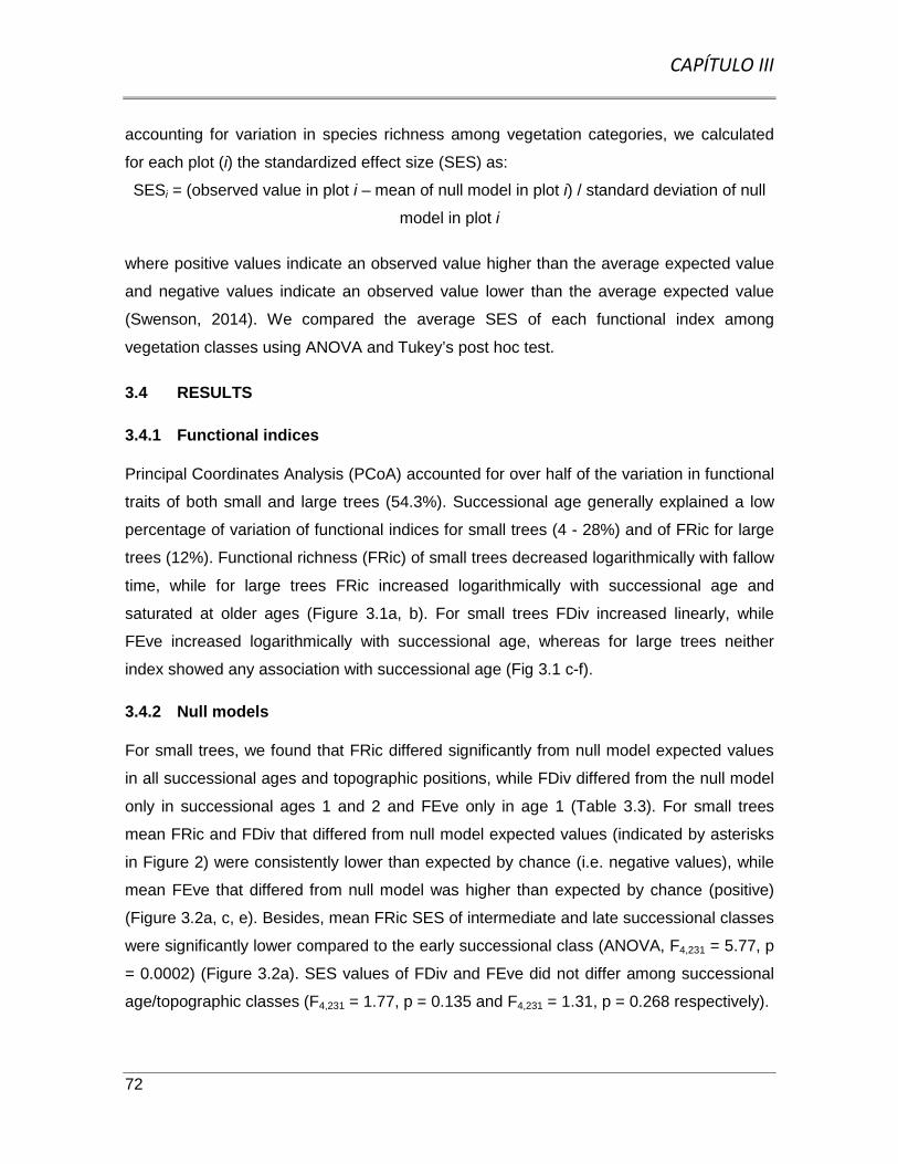
CAPÍTULO III

72

accounting for variation in species richness among vegetation categories, we calculated

for each plot (i) the standardized effect size (SES) as:

SESi = (observed value in plot i – mean of null model in plot i) / standard deviation of null

model in plot i

where positive values indicate an observed value higher than the average expected value

and negative values indicate an observed value lower than the average expected value

(Swenson, 2014). We compared the average SES of each functional index among

vegetation classes using ANOVA and Tukey’s post hoc test.

3.4 RESULTS

3.4.1 Functional indices

Principal Coordinates Analysis (PCoA) accounted for over half of the variation in functional

traits of both small and large trees (54.3%). Successional age generally explained a low

percentage of variation of functional indices for small trees (4 - 28%) and of FRic for large

trees (12%). Functional richness (FRic) of small trees decreased logarithmically with fallow

time, while for large trees FRic increased logarithmically with successional age and

saturated at older ages (Figure 3.1a, b). For small trees FDiv increased linearly, while

FEve increased logarithmically with successional age, whereas for large trees neither

index showed any association with successional age (Fig 3.1 c-f).

3.4.2 Null models

For small trees, we found that FRic differed significantly from null model expected values

in all successional ages and topographic positions, while FDiv differed from the null model

only in successional ages 1 and 2 and FEve only in age 1 (Table 3.3). For small trees

mean FRic and FDiv that differed from null model expected values (indicated by asterisks

in Figure 2) were consistently lower than expected by chance (i.e. negative values), while

mean FEve that differed from null model was higher than expected by chance (positive)

(Figure 3.2a, c, e). Besides, mean FRic SES of intermediate and late successional classes

were significantly lower compared to the early successional class (ANOVA, F4,231 = 5.77, p

= 0.0002) (Figure 3.2a). SES values of FDiv and FEve did not differ among successional

age/topographic classes (F4,231 = 1.77, p = 0.135 and F4,231 = 1.31, p = 0.268 respectively).

CAPÍTULO III

73

For large trees, mean FRic differed significantly from null model values in early and

intermediate successional classes on flat sites, and in the late successional class on hills

(Table 3.3, Figure 3.2b). Mean FDiv only differed significantly from null model values in the

late successional class on hills (Table 3.3, Figure 3.2d), while mean FEve did not differ

from null model values in any successional class (Figure 3.2f). Mean FRic SES values that

differed from null model (indicated by asterisks in Figure 3.2b) were higher than expected

by chance at early and intermediate age classes, but lower than expected by chance in the

late successional class on hills (and differed significantly among classes, ANOVA, F4,258 =

3.26, p = 0.013, Figure 3.2b). Mean FDiv SES values were significantly lower than

expected by chance (Figure 3.2d) only in the late successional class on hills (Figure 3.2d).

Mean functional indices and SES per plot can be found in Appendix 8.3.

CAPÍTULO III

74

Figure 3.1 Variation of functional diversity components in relation to successional age. (a)

Functional Richness (FRic) of small trees; (b) Functional Richness of large trees; (c) Functional

Divergence (FDiv) of small trees; (d) Functional Divergence of large trees; (e) Functional Evenness

(FEve) of small trees; (f) Functional Evenness of large trees. Regression coefficients and

significance values are shown.

Figure 3.2 Mean Standardized Effect Size (SES) of observed functional diversity components (and

standard error) in relation to null model randomizations by successional age category. (a) FRic SES

of small trees; (b) FRic SES of large trees; (c) FDiv SES of small trees; (d) FDiv SES of large trees;

(e) FEve SES of small trees; (f) FEve SES of large trees. Means with different letters are

significantly different (p < 0.05). Horizontal lines indicate mean Standardized Effect Size (SES)

CAPÍTULO III

75

equal to zero (the mean of 999 randomizations). Successional age category and number of plots for

small/large trees: 1 Flat (3 to 10 years) = 85/83; 2 Flat (11 to 25 years) = 52/66; 2 Hill (11 to 25

years) = 29/30; 3 Flat (26 to 70 years) = 39/52; 3 Hill (26 to 60 years) = 31/32. Asterisks denote

mean FRic, FDiv or FEve (not SES) values that differ significantly from null models (see Table 3.3).

Table 3.3 Wilcoxon signed-rank tests evaluating differences between mean null model and mean

expected values (Z) of large and small trees for each functional index and successional age/

topographic class.

Successional age/

Topographic class

Functional

indexZ p Z p

Large trees Small trees

1 Flat FRic 1.9659 0.049 -3.148 0.002

2 Flat 2.4179 0.016 -5.155 0.000

2 Hill 0.0514 ns1 -4.054 0.000

3 Flat -0.7012 ns -4.577 0.000

3 Hill -1.9821 0.046 -4.253 0.000

1 Flat FDiv -0.7991 ns -4.800 0.000

2 Flat -0.2076 ns -2.914 0.004

2 Hill 0.0103 ns -2.065 0.037

3 Flat -0.4007 ns -1.200 ns

3 Hill -2.0756 0.037 -1.215 ns

1 Flat FEve 0.5085 ns 2.776 0.006

2 Flat -1.4597 ns 1.239 ns

2 Hill -1.1210 ns 1.784 ns

3 Flat -0.3916 ns 1.730 ns

3 Hill -1.4959 ns 0.137 ns1 ns = not significant (p > 0.05). Sample sizes (n) per age/topographic class: 1 Flat = 83, 2 Flat = 66,2 Hill = 30, 3 Flat = 52, 3 Hill = 32.

3.5 DISCUSSION

CAPÍTULO III

76

We found that variation in functional diversity of trees in the tropical dry forest studied was

influenced by successional age and topographic position, and that patterns of functional

variation differed between small (DBH 1–2.5 cm) and large trees (DBH > 5 cm), depending

on the functional component considered. Examining SES values and their departure from

null models (Figure 2), our results generally do not support our first prediction that FRic

would be lower early in succession and on hills than in late successional forests and in flat

areas. This prediction was based on previous findings in tropical dry forests showing that,

(1) compared to late-successional forests, early successional stages experience higher

irradiance, and warmer and drier conditions, (Pineda-García et al., 2013; Lebrija-Trejos et

al., 2011); and (2) hill tops and slopes have lower water availability than flat areas

(Markesteijn et al., 2010; Gallardo-Cruz et al., 2009; Becker et al., 1988). We found

evidence of environmental filtering only for large trees in late-successional forests on hills

(Figure 2b), probably due to the effect of lower soil water availability (Markesteijn et al.,

2010; Gallardo-Cruz et al., 2009; Becker et al., 1988). However, our results also suggest a

thorough use of resources by large trees in early successional and intermediate forests (3

to 25 years old) on flat sites, reflecting maximum variation in ecological strategies and

positive FRic values (Figure 2b), probably due to the coexistence of pioneers, generalists

and (resprouts of) old-growth forest specialists. Moreover, small trees face unfavorable

conditions (negative FRic SES values) in the complete successional/topographical

gradient, and a stronger signal of environmental filtering at intermediate and late

successional ages (Figure 2a). We believe that this successional trend may have resulted

from two possibilities:

1) Relatively higher FRic values early in succession may reflect the coexistence of

acquisitive and conservative species that show different constellations of functional

traits in young stands. Pioneers (which represent the conservative strategy in dry

forests) may establish from seeds of nearby forests (since slash-and-burn

agriculture may destroy the seed bank) (Dalling and Denslow, 1998), whereas

more acquisitive shade-tolerant species may avoid unfavorable conditions for seed

establishment by getting established mainly from resprouts (Kammesheidt, 1999).

The subsequent reduction in FRic over succession may result from environmental

filtering associated with lower light and air evaporative demand, which would

decrease the success of the conservative species (Lebrija-Trejos et al., 2010a).

CAPÍTULO III

77

2) Alternatively, modern coexistence theory states that functional convergence results

not only form environmental filtering, but also from competitive exclusion based on

hierarchical competitive abilities among species (Kraft et al., 2015; Mayfield and

Levine, 2010). The Functional Richness index may thus reflect the combined effect

of both environmental filtering and competitive processes (Mayfield and Levine,

2010). In line with this, early in succession negative FRic values of small trees may

reflect the effect of environmental filters (high irradiance load, air temperature and

evaporative demand), whereas at latter successional ages the lower FRic values

may reflect the elimination of poor competitors (Mayfield and Levine, 2010).

Competitive hierarchy of species can be determined by multiple factors, but in a dry

forests it may be defined mostly by water availability, which is the most limiting

resource (Murphy and Lugo, 1986). Previous studies of microenvironment in

tropical dry forests have shown that soil water content increases with successional

age, as radiation load and air evaporative demand decrease with canopy

development (Buzzard et al., 2015; Pineda-García et al., 2013; Lebrija-Trejos et al.,

2011). However, other studies have found a steady and sometimes marked

increase in fine root biomass along succession (Vargas et al., 2008; Deans et al.,

1996; but see Powers and Peréz-Aviles, 2013), and a decrease in soil water

potential (Lebrija-Trejos et al., 2011). Theoretically, the increasing importance of

soil drying by transpiration as canopy closes and forests mature (Marthews et al.,

2008) could be a sign of stronger competitive processes, if plants pre-empt water

supply from coming in contact with other species (which may be considered as a

filter), or if they reduce soil water potential to low levels (Craine and Dybzinski,

2013). The effect of below-ground competition on soil water availability has been

poorly quantified (Craine and Dybzinski, 2013). The relative importance of soil

drying by evaporation vs. transpiration during dry forests succession, and its effects

on tree community assembly need further investigation.

In agreement with our second prediction, FRic SES values were consistently lower for

small trees than for large trees (see values of y axes in Figure 2a,b). The latter result also

agrees with previous findings showing that the strongest filters to species establishment

occur at early life stages when plants are smaller (Poorter, 2007), although our small tree

category corresponds to saplings and juveniles, which are not the most sensitive

CAPÍTULO III

78

ontogenetic stage (i.e., seedlings). Differences in tree size may represent differences both

in microenvironments and in competitive abilities, with smaller plants being most

susceptible to both. Larger individuals are better equipped to cope with competitors and

fluctuating unfavorable conditions, such as dry spells, through a more developed root

system, enabling them to forage in larger areas and to store more water and nutrients, as

well as a bigger trunk allowing them to store more water and to harvest more light

(Niinemets, 2010). Alternatively, differences in FRic between small and large trees can

arise from temporal fluctuations in environmental conditions suitable for reproduction and

recruitment of species (i.e., the storage effect; Warner and Chesson, 1985). Favorable

conditions could produce a strong recruitment that results in a cohort of reproductive large

trees (Warner and Chesson, 1985). Under unfavorable conditions, many small trees could

be filtered out (reducing their FRic), whereas large trees may be able to survive for many

years and reproduce when more favorable conditions occur. In other words, lower FRic for

small trees than for large ones would be expected under the storage effect, because large

trees may comprise a larger number of cohorts. Resprouting capacity, which is

generalized among the species studied (LSV pers. obs.) likely also plays a role

(Kammesheidt, 1999).

Contrary to our third prediction (that competitive processes would be more important at

intermediate and latter successional ages), FDiv showed partial evidence of environmental

filtering (negative values, see Table 2) instead of competition. Negative FDiv values

suggest a scarce functional differentiation of dominant species. Small trees showed

negative FDiv SES values in early and intermediate successional forests suggesting that

the small-sized trees capable of establishing and becoming dominant at these

successional stages may share similar traits, probably associated with avoiding water loss,

such as pinnate, deciduous, leaves (Lohbeck et al., 2013). Large trees showed negative

FDiv in late successional stages on hills, suggesting that environmental filtering may

reduce the functional strategies present in this environment, which is also in line with the

negative values of FRic found there.

In agreement with our fourth prediction, we found signs of competition only for small trees

in early successional ages. Positive FEve SES values in the youngest successional class

(Figure 2e) suggest that species with functional strategies that survive the filters disperse

CAPÍTULO III

79

evenly in relation to resource use, which can be interpreted as niche partitioning by

competitive exclusion. Environmental filtering is usually conceived aside of competitive

processes; nonetheless both factors interact dynamically to drive community patterns

(Kraft et al., 2015). Moreover, although neither FEve nor FDiv departed from null model

predictions in late successional ages (contrary to our third prediction), hierarchical

competitive ability (reflected by low FRic values especially at late successional ages)

cannot de discarded (Mayfield and Levine, 2010).

Finally, our results, especially those of FDiv and FEve, should be taken with caution, since

competition in tropical dry forests is expected to be strongest for below-ground resources

(water and nutrients), which are most limiting, yet we did not consider any below-ground

functional traits in this study. Further studies are needed to assess the relative importance

of above-ground (light availability, air temperature) vs. below-ground (water, nutrients)

resources on assembly of tree communities in tropical dry forests.

3.6 CONCLUSIONS

Our results clearly show that assembly patterns differ between plants of different sizes.

While small-sized trees showed evidence of environmental filtering and/or competition at

all successional ages and topographical positions, large-sized trees showed evidence of

these assembly processes only in late successional forests on hills, indicating that the

former represent a more susceptible phase of development, and that small-sized tree

communities are strongly affected by the changing biotic and abiotic conditions along the

successional and topographical gradient. For larger plants, late successional forests on

hills represent the most stressful conditions in this landscape. Moreover, small trees

showed the strongest environmental filtering (lowest functional richness) in late

successional forest stands, although the few studies in tropical dry forests that have

analyzed microenvironmental differences during succession suggest that the most

stressful conditions (hot and dry environment) occur during the early stages of succession.

Our results suggest that the functional richness index may actually reflect the combined

effect of both environmental filtering and hierarchical competitive ability. Future research

should test this and the possibility that relatively high soil drying by transpiration in late

successional forest stands may exert a stronger effect on tree community assembly than

relatively low evaporative demand.

CAPÍTULO III

80

3.7 ACKNOWLEDGMENTS





fieldwork. We thank two anonymous reviewers for their insightful comments that greatly

improved this paper. Financial support was provided by FOMIX-Yucatán (YUC-2008-C06-

108863); LSV also acknowledges CONACYT, Mexico, for the grant awarded (169510).

3.8 REFERENCES

Alvarez-Añorve, M.Y., Quesada, M., Sanchez-Azofeifa, G.A., Avila-Cabadilla, L.D., and



99, 816–826.

Bautista-Zúñiga, F., Batllori-Sampedro, E., Ortiz-Pérez, M.A., Palacio-Aponte, G., and

Castillo-González, M. (2003). Geoformas, agua y suelo en la Península de

Yucatán. In Naturaleza Y Sociedad En El Área Maya: Pasado, Presente Y Futuro,

P. Colunga, and A. Larque, eds. (Mérida, Yucatán, México: Academia Mexicana

de Ciencias y Centro de Investigación Científica de Yucatán), pp. 21–35.

Becker, P., Rabenold, P.E., Idol, J.R., and Smith, A.P. (1988). Water potential gradients

for gaps and slopes in a Panamanian tropical moist forest’s dry season. J. Trop.

Ecol. 4, 173–184.

Buzzard, V., Hulshof, C.M., Birt, T., Violle, C., and Enquist, B.J. (2016). Re-growing a

tropical dry forest: functional plant trait composition and community assembly

during succession. Functional Ecology 30, 1006–1013.

Cailliez, F. (1983). The analytical solution of the additive constant problem. Psychometrika

48, 305–308.

CAPÍTULO III

81

Cavender-Bares, J., Kitajima, K., and Bazzaz, F.A. (2004). Multiple trait associations in

relation to habitat differentiation among 17 Floridian oak species. Ecol. Monogr.

74, 635–662.


Reich, P.B., Steege, H. ter, Morgan, H.D., van der Heijden, M.G.A., et al. (2003).

A handbook of protocols for standardised and easy measurement of plant

functional traits worldwide. Aust. J. Bot. 51, 335–380.

Cornwell, W.K., Schwilk, D.W., and Ackerly, D.D. (2006). A trait-based test for habitat


Craine, J.M., and Dybzinski, R. (2013). Mechanisms of plant competition for nutrients,

water and light. Funct. Ecol. 27, 833–840.

Dalling, J.W., and Denslow, J.S. (1998). Soil seed bank composition along a forest

chronosequence in seasonally moist tropical forest, Panama. J. Veg. Sci. 9, 669–

678.

Deans, J.D., Moran, J., and Grace, J. (1996). Biomass relationships for tree species in

regenerating semi-deciduous tropical moist forest in Cameroon. For. Ecol. Manag.

88, 215–225.


López-Martínez, J.O., Leyequién-Abarca, E., Tun-Dzul, F.J., and May-Pat, F.

(2012). Patterns and Correlates of Tropical Dry Forest Structure and Composition

in a Highly Replicated Chronosequence in Yucatan, Mexico. Biotropica 44, 151–

162.

Flores, J.S., and Espejel, I. (1994). Tipos de vegetación de la Península de Yucatán

(Mérida, Yucatán, México: Universidad Autónoma de Yucatán).

Gallardo-Cruz, J.A., Pérez-García, E.A., and Meave, J.A. (2009). β-Diversity and

vegetation structure as influenced by slope aspect and altitude in a seasonally dry

tropical landscape. Landsc. Ecol. 24, 473–482.

CAPÍTULO III

82

García, E. (1981). Modificaciones al sistema de clasificación climática de Köppen (para

adaptarlo a las condiciones de la República Mexicana) (Mexico D. F.: Instituto de

Geografía Universidad Nacional Autónoma de México).

Gerhardt, K., and Hytteborn, H. (1992). Natural dynamics and regeneration methods in




Grubb, P.J. (1977). The maintenance of species-richness in plant communities: the

importance of the regeneration niche. Biol. Rev. 52, 107–145.

Hernández-Stefanoni, J.L., and Dupuy, J.M. (2008). Effects of landscape patterns on

species density and abundance of trees in a tropical subdeciduous forest of the

Yucatan Peninsula. For. Ecol. Manag. 255, 3797–3805.

Hernández-Stefanoni, J.L., Pineda, J.B., and Valdes-Valadez, G. (2006). Comparing the

Use of Indigenous Knowledge with Classification and Ordination Techniques for


Forest. Environ. Manage. 37, 686–702.

Hernández-Stefanoni, J.L., Dupuy, J.M., Tun-Dzul, F., and May-Pat, F. (2011). Influence of



Kammesheidt, L. (1999). Forest recovery by root suckers and above-ground sprouts after

slash-and-burn agriculture, fire and logging in Paraguay and Venezuela. J. Trop.

Ecol. 15, 143–157.

Keddy, P.A. (1992). Assembly and response rules: two goals for predictive community




18, 53–66.

CAPÍTULO III

83

Kraft, N.J.B., Valencia, R., and Ackerly, D.D. (2008). Functional Traits and Niche-Based

Tree Community Assembly in an Amazonian Forest. Science 322, 580–582.

Kraft, N.J.B., Adler, P.B., Godoy, O., James, E.C., Fuller, S., and Levine, J.M. (2015).


Funct. Ecol. 29, 592–599.

Laliberté, E., and Legendre, P. (2010). A distance-based framework for measuring

functional diversity from multiple traits. Ecology 91, 299–305.

Laliberté, E., Legendre, P., and Shipley, B. (2014). FD: measuring functional diversity

from multiple traits, and other tools for functional ecology.

Lebrija-Trejos, E., Meave, J.A., Poorter, L., Pérez-García, E.A., and Bongers, F. (2010a).



Lebrija-Trejos, E., Pérez-García, E.A., Meave, J.A., Bongers, F., and Poorter, L. (2010b).



Lebrija-Trejos, E., Pérez-García, E.A., Meave, J.A., Poorter, L., and Bongers, F. (2011).




Pérez-García, E.A., Romero-Pérez, I.E., Tauro, A., and Bongers, F. (2013).



Lohbeck, M., Lebrija-Trejos, E., Martínez-Ramos, M., Meave, J.A., Poorter, L., and

Bongers, F. (2015). Functional trait strategies of trees in dry and wet tropical

forests are similar but differ in their consequences for succession. Plos One 10,

e0123741.

CAPÍTULO III

84

Macarthur, R., and Levins, R. (1967). The Limiting Similarity, Convergence, and

Divergence of Coexisting Species. Am. Nat. 101, 377–385.


G., Wilson Fernandes, G., and Quesada, M. (2009). Changes in tree and liana



Markesteijn, L., Iraipi, J., Bongers, F., and Poorter, L. (2010). Seasonal variation in soil

and plant water potentials in a Bolivian tropical moist and dry forest. J. Trop. Ecol.

26, 497–508.

Marthews, T.R., Burslem, D.F.R.P., Paton, S.R., Yangüez, F., and Mullins, C.E. (2008).

Soil drying in a tropical forest: three distinct environments controlled by gap size.

Ecol. Model. 216, 369–384.

Mason, N.W., Mouillot, D., Lee, W.G., and Wilson, J.B. (2005). Functional richness,

functional evenness and functional divergence: the primary components of

functional diversity. Oikos 111, 112–118.

Mason, N.W.H., Lanoiselée, C., Mouillot, D., Wilson, J.B., and Argillier, C. (2008). Does

niche overlap control relative abundance in French lacustrine fish communities? A

new method incorporating functional traits. J. Anim. Ecol. 77, 661–669.

Mayfield, M.M., and Levine, J.M. (2010). Opposing effects of competitive exclusion on the


1085–1093.

Miles, L., Newton, A.C., DeFries, R.S., Ravilious, C., May, I., Blyth, S., Kapos, V., and

Gordon, J.E. (2006). A global overview of the conservation status of tropical dry

forests. J. Biogeogr. 33, 491–505.

Mouchet, M.A., Villéger, S., Mason, N.W.H., and Mouillot, D. (2010). Functional diversity

measures: an overview of their redundancy and their ability to discriminate

community assembly rules. Funct. Ecol. 24, 867–876.

CAPÍTULO III

85

Muller-Landau, H.C. (2004). Interspecific and inter-site variation in wood specific gravity of

tropical trees. Biotropica 36, 20–32.

Murphy, P.G., and Lugo, A.E. (1986). Ecology of tropical dry forest. Annu. Rev. Ecol. Syst.

67–88.




Orellana, R., Islebe, G.A., and González-Iturbe, J.A. (2003). Presente, pasado y futuro de

los climas de la Península de Yucatán. In Naturaleza y Sociedad en el Área

Maya, P. Colunga-García Marín, and A. Larqué Saavedra, eds. (Mérida, Yucatán,

México: Academia Mexicana de Ciencias, Centro de Investigación Científica de

Yucatán.), pp. 37–52.

Pakeman, R.J., and Quested, H.M. (2007). Sampling plant functional traits: What

proportion of the species need to be measured? Appl. Veg. Sci. 10, 91.

Pineda-García, F., Paz, H., and Meinzer, F.C. (2013). Drought resistance in early and late




Powers, J.S., and Peréz-Aviles, D. (2013). Edaphic factors are a more important control on

surface fine roots than stand age in secondary tropical dry forests. Biotropica 45,

1–9.

Purschke, O., Schmid, B.C., Sykes, M.T., Poschlod, P., Michalski, S.G., Durka, W., Kühn,

I., Winter, M., and Prentice, H.C. (2013). Contrasting changes in taxonomic,

phylogenetic and functional diversity during a long-term succession: insights into

assembly processes. J. Ecol. 101, 857–866.

Quesada, M., Sanchez-Azofeifa, G.A., Alvarez-Añorve, M., Stoner, K.E., Avila-Cabadilla,

L., Calvo-Alvarado, J., Castillo, A., Espírito-Santo, M.M., Fagundes, M.,

Fernandes, G.W., et al. (2009). Succession and management of tropical dry

CAPÍTULO III

86

forests in the Americas: Review and new perspectives. For. Ecol. Manag. 258,

1014–1024.

R Development Core Team (2015). R: A language and environment for statistical

computing (Viena, Austria.: R Foundation for Statistical Computing).

Rasband, W.S. (2014). ImageJ (Bethesda, Maryland, USA: National Institutes of Health).

Rico-Gray, V., and García-Franco, J.G. (1991). The Maya and the vegetation of the

Yucatan Peninsula. J. Ethnobiol. 11, 135–142.

Ricotta, C., Bacaro, G., and Moretti, M. (2014). A New Measure of Functional Evenness

and Some of Its Properties. Plos One 9, e104060.

Sanchez-Azofeifa, G.A., Quesada, M., Rodriguez, J.P., Nassar, J.M., Stoner, K.E.,

Castillo, A., Garvin, T., Zent, E.L., Calvo-Alvarado, J.C., Kalacska, M.E.R., et al.

(2005). Research Priorities for Neotropical Dry Forests. Biotropica 37, 477–485.

Schwinning, S., and Weiner, J. (1998). Mechanisms Determining the Degree of Size


Swenson, N.G. (2014). Functional and Phylogenetic Ecology in R (New York, NY:

Springer).


Nat. 769–774.

Turner II, B.L., Villar, S.C., Foster, D., Geoghegan, J., Keys, E., Klepeis, P., Lawrence, D.,

Mendoza, P.M., Manson, S., Ogneva-Himmelberger, Y., et al. (2001).

Deforestation in the southern Yucatán peninsular region: An integrative approach.

For. Ecol. Manag. 154, 353–370.

Vargas, R., Allen, M.F., and Allen, E.B. (2008). Biomass and carbon accumulation in a fire


124.

CAPÍTULO III

87

Villéger, S., Mason, N.W., and Mouillot, D. (2008). New multidimensional functional

diversity indices for a multifaceted framework in functional ecology. Ecology 89,

2290–2301.

Warner, R.R., and Chesson, P.L. (1985). Coexistence mediated by recruitment

fluctuations: a field guide to the storage effect. Am. Nat. 769–787.

Weiher, E., and Keddy, P.A. (1995). Assembly Rules, Null Models, and Trait Dispersion:

New Questions from Old Patterns. Oikos 74, 159.

Weiher, E., Clarke, G.D.P., and Keddy, P.A. (1998). Community Assembly Rules,

Morphological Dispersion, and the Coexistence of Plant Species. Oikos 81, 309.

Williams-Linera, G., Alvarez-Aquino, C., Hernández-Ascención, E., and Toledo, M. (2011).



Williamson, G.B., and Wiemann, M.C. (2010). Measuring wood specific gravity...Correctly.

Am. J. Bot. 97, 519–524.

CAPÍTULO III

88

CAPÍTULO IV

89

CAPÍTULO 4.AMONG AND WITHIN-COMMUNITIES PLANT TRAIT ASSOCIATIONS IN ANEOTROPICAL DRY FOREST

Artículo en preparación.

Lucía Sanaphre-Villanueva a, Juan Manuel Dupuy * a, José Luis Andrade a, Casandra

Reyes-García a, Paula C. Jackson b and Horacio Paz c

a Unidad de Recursos Naturales, Centro de Investigación Científica de Yucatán (CICY),

Mérida, Yucatán, México.

b Department of Ecology, Evolution, and Organismal Biology, Kennesaw State University,

Kennesaw, GA, USA.

c Centro de Investigaciones en Ecosistemas, Universidad Nacional Autónoma de México,

Morelia, Michoacán, México.

* Corresponding author: [email protected]

Running headline: Among and within communities plant trait variation.

4.1 ABSTRACT

Question(s): How do and which plant functional traits correlate at the plot scale (within

plots) and at the landscape scale (among plots)? Are trait correlations at the landscape

scale explained by the environmental gradient formed by soil properties, topographic

position and successional age? What is the relative contribution of these three factors to

explaining variation in plot trait values (community abundance-weighted means)?

Location: The Yucatan Peninsula, Mexico.

Methods: We used Trait Gradient Analysis to decompose species’ functional traits into

values representing the position of the species along a gradient defined by community-

level mean trait values (beta values), and values representing the difference between trait

values of a species and the mean of co-occurring species (alpha values). To identify trait

covariation at the landscape scale (among β values) and at the plot scale (among α

CAPÍTULO IV

90

values), we determined α and β components for six functional traits (leaf area, petiole

length, specific leaf area, leaf dry matter content, wood specific gravity and seed volume)

of 65 woody plant species in a tropical dry forest in the Yucatan Peninsula. We also

investigated the relative contribution of environmental factors (successional age,

topographical position, soil properties) to explaining variation in plot trait values

(community abundance-weighted means).

Results: Within plots, alpha trait correlations segregated species into the rapid-slow

continuum. At the landscape scale, mean trait averages of plots where each species was

present (β values) were similar among species, resulting in few β trait correlations –mostlt

not different from random species assembly. This may be due to recurrent slash and burn

agriculture leading to the selection and dominance of species capable of thriving under

recurrent fire disturbance and of establishing in a wide range of conditions. Little variation

in plot abundance-weighted traits was explained by environmental factors.

Conclusions: Alpha trait correlations suggest that, within plots, local environmental

heterogeneity (likely resulting from recurrent small-scale disturbance), and possibly

species competition, may play a key role in the assembly of these communities. At the

landscape scale, disturbance has resulted in functionally homogeneous vegetation almost

decoupled from the environment.

Key-words. Biotic homogenization; community abundance-weighted mean trait values;

fire; functional variation within and among communities; plant community assembly;

recurrent disturbance; scale; soil properties; Trait gradient analysis; Yucatan Peninsula.

4.1.1 INTRODUCTION

Because functional traits affect plant fitness and mediate species responses to the

environment, analysis of variation in functional traits can shed light on the factors and

processes that drive community assembly (Kraft et al., 2007; Weiher et al., 1998). A

common approach to understanding community assembly is the use of community

weighted trait means (CWM) (Cornwell and Ackerly, 2009; Cingolani et al., 2007; Garnier

et al., 2004). These reflect the functional traits of dominant species, and are directly

related to the mass ratio hypothesis of Grime (1998), which postulates that the traits of the

most abundant species largely determine community structure and ecosystem processes.

CAPÍTULO IV

91

This approach has been used to explore patterns of variation in plant strategies along

environmental gradients considering the covariation of single and multiple traits with

environmental variables (De Bello et al., 2013; Lebrija-Trejos et al., 2010a; Garnier et al.,

2004). For example, CWM of specific leaf area (SLA: leaf area/dry matter) and leaf area

(LA) have been found to be positively correlated in response to environmental filtering

associated with rainfall and soil phosphorus gradients (McDonald et al., 2003; Fonseca et

al., 2000; Ackerly et al., 2002).

Dominant trait values in plant communities are driven by large-scale filters such as climate

and temperature (Moles et al., 2014), and, at finer scales, by disturbance regime and local

factors such as topographic-edaphic conditions, microenvironment and biotic interactions

(De Bello et al., 2013; Lebrija-Trejos et al., 2010a; Diaz et al., 1998; Keddy, 1992b).

Because spatial variation of these factors can be structured at different scales, a better

understanding of community assembly using functional traits can be obtained with the

explicit analysis of trait-environment covariation at different scales. Trait gradient analysis

(TGA; Ackerly & Cornwell 2007) was developed as a tool for the combined analysis of

functional trait variation among communities at the landscape or regional level and among

species within communities. This is achieved through the decomposition of the species

mean trait values (t) into beta (among communities) and alpha (within community) values.

Thus, for species i, the beta value represents the average of the CWM where i species

occurs. Since individual traits influence plant dispersal, establishment and persistence,

CWMs reflect the integrated effects of disturbance, dispersal limitation and environmental

filters on dominant species, and consequently β values reveal the similarities or

differences among species in the environmental conditions where each species exists.

Therefore, β values represent the functional position of each species within the functional

space of the pool of species in the landscape or region, i.e. in the trait gradient (Ackerly &

Cornwell 2007). Ecologically similar species in similar environments are expected to have

similar traits, so significant correlations of beta values of different traits would reflect the

turnover of species among communities in response to environmental gradients. Applying

TGA to plant communities along the California Coast (USA), values of SLA were

positively associated with LA and maximum plant height (max height); while all three traits

were negatively associated with wood density (WD) –likely in response to environmental

filtering associated with soil moisture availability (Ackerly and Cornwell, 2007). Similarly, in

CAPÍTULO IV

92

an Australian subtropical rain forest, trait values of LA, seed size, WD and max height

co-varied significantly in parallel to the dominant abiotic gradients formed by soil,

topography, elevation and large natural disturbances (Kooyman et al., 2010).

A simple way of measuring functional differentiation of species within communities is to

determine if traits of species i are above or below the average values of co-occurring

species in the communities where it is most abundant. In TGA this value is named the

alpha component, and is calculated for each i species by subtracting the beta from the

species mean trait value (ti). Correlations between α values of different traits can arise

from parallel co-variation of multiple traits, reflecting morfo-physiological restrictions at the

species level, that allow fine partitioning of microsites and/or resources within

communities. Conversely, lack of correlations between α values is expected when species

in a particular position in the gradient differentiate functionally from co-occurring species in

different ways than other species in other parts of the gradient (for example when plants

from different vegetation types are included in the analysis). Since TGA is scale

dependent, we expect the first outcome if analyzing short environmental gradients where

communities are more similar, while the second would be more likely in large

environmental gradients with a strong species turnover, such as those sampled in the

above-mentioned studies by Ackerly & Cornwell (2007) and Kooyman et al. (2010). In both

studies, the lack of correlations between α values was attributed to independent axes of

ecological differentiation and coexistence of species.

TGA allows capturing the signature of ecological filters that act on plant strategies at

different spatial scales, and the specific correlations of CWM with environmental variables

can result in a better understanding of the fit between species and the habitat they use.

This approach can be particularly useful when studying species assembly in complex

swidden agricultural landscapes with a dynamic mosaic of old growth and secondary

forests.

Several functional studies in tropical dry forests have found that during secondary

succession, species turnover occur in response to the autogenic environmental change

produced by early successional species, that show a conservative strategy characterized

by traits that avoid loss of water (compound, deciduous leaves, with small area and

pulvini) (Lohbeck et al., 2015; Pineda-García et al., 2013; Lebrija-Trejos et al., 2010).

CAPÍTULO IV

93

Towards older stages, conservative species are replaced by others with an acquisitive

strategy, with high sapwood storage capacity, and large, perennial leaves and large seeds

(Lohbeck et al., 2015; Pineda-García et al., 2013; Lebrija-Trejos et al., 2010a). The aim of

this study is to evaluate through TGA the trait co-variation of woody plants at two scales:

landscape (i.e. among communities, CWM and β values) and local (i.e. within

communities, α values) in a tropical dry forest in the Yucatan Peninsula, which has been

subjected to long-term (over 2000 years) and recurrent slash and burn agriculture (Rico-

Gray & García-Franco 1991). We expect strong β and CWM associations (i.e. among

communities, landscape scale) reflecting the functional turnover of species associated with

secondary succession, and weaker or absent trait associations of α values (i.e. inside

communities, local scale), as a result of a scarce local environmental heterogeneity. We

also expected that successional age and soil properties would explain a similar proportion

of trait variation, because the gradient of soil nutrients is expected to vary with

successional age (Becknell and Powers, 2014).


3.3.1 Sampling design

In the summer of 2008 and 2009, 23 landscape units (1 km2) were selected encompassing

the range of disturbance and fragmentation conditions of the area. In each unit, we

established 12 sampling plots differing in successional age after slash and burn agriculture

and/or topographic position: 3-8 year-old, 9-15 year-old, > 15 year-old on flat areas and >

15 year-old on hills. Forest stand age was determined from interviews with local residents

who lived in the area for at least 40 years and owned or worked the land. A total of 276

plots were established consisting of two concentric circular areas: 200 m2 for all woody

plants with a diameter at breast height (DBH; 1.3 m) > 5 cm, and 50 m2 for all woody

plants 1-5 cm DBH (for a detailed description of sampling see Hernández-Stefanoni et al.

et al. 2011).


We used data from 273 plots having individuals with DBH > 5 cm to calculate the relative

importance value (RIV) of all species in each stand age-topographic position category as

the sum of the species’ relative abundance, frequency and basal area. For each category

CAPÍTULO IV

94

and separately for trees, lianas and shrubs, we selected those species representing 90%

of the cumulative RIV, and obtained a total of 72 species. However, only 65 species were

included for which we could collect leaf and wood samples from at least 5 individuals. Of

these, 45 species were trees, 11 shrubs and 9 lianas. We could obtain seeds of only 55

species: 40 trees, 9 shrubs and 7 lianas.


Samples were collected from at least 5 individuals per species (14 individuals per species

on average; see Appendix 8.4) during the rainy season (August-November) of 2011 and

2012. The following functional traits, reflecting key components of plant function, were

selected: specific leaf area, SLA; leaf dry matter content, LDMC; petiole length, PL; leaf

area, LA; wood specific gravity, WSG and seed volume, SV.

We obtained 3-5 young, healthy and completely expanded leaves from sun-exposed

branches from each individual. For each leaf, fresh weight was determined to 0.001 g

using a digital scale (Mettler Toledo PB4002-S/FACT, OH, USA) and samples were

digitized using a scanner, oven-dried at 60°C for three days, and weighed again. Petiole

length (PL) and leaf or leaflet area (the average of ten leaflets) were measured using

ImageJ 1.47b (Rasband, 2014). SLA and LDMC were calculated using standard methods


Wood specific gravity (WSG) was obtained from individuals with the largest DBH: 3.2 cm

on average for lianas, 4.1 cm for shrubs, and 16.4 cm for trees. For lianas, a 4-5 cm long

and 1 cm wide slice was taken from the trunk, after taking off the bark that could be

manually removed. A similar procedure was used for shrubs when they had a trunk ≥ 4 cm

DBH; otherwise we cut one branch at the first ramification and took a 4-5 cm long section.

For trees, a sample was taken at breast height from cortex to pith from 4 individuals per

species using a 5 mm diameter core borer. Green volume was measured using the water

displacement method. Samples were oven dried at 100°C and weighed with an analytical

scale (Ohaus Adventurer AP 2140, NJ, USA). Wood specific gravity of each sample was

obtained by dividing dry weight over green volume (Williamson and Wiemann, 2010;

Muller-Landau, 2004).

CAPÍTULO IV

95

Ripe fruits or seeds for 40 species were collected, in most cases from just one individual.

Specimens from the Herbarium at CICY were also used to obtain fruit or seed

measurements for some species. Seed volume was used as a proxy for seed mass.

Height, width and length of at least 3 (and in most cases 10) seeds per individual were

measured using a Vernier or obtained from botanical descriptions. Seed volume (SV) was

calculated using the ellipsoid formula [(4/3) π (length * width * height) / 8)].

3.3.4 Environmental variables

Three 10 cm-deep soil samples (ca. 400 g each) were taken in 2008 and 2009 at the

center, northern and southern limits of each plot, and subsequently pooled to obtain a

single compound sample. The following variables were obtained: pH in water (1:2 ratio),

soil organic matter (combustion or Walkley-Black), cation exchange capacity (Olsen),

electric conductivity (1:5 extracts), total nitrogen (Kjeldahl), available phosphorus (Bray)

and interchangeable potassium (ammonium acetate). Altitude and slope were obtained

using a digital elevation model (spatial resolution: 30 m) from the Mexican National

Institute of Statistics, Geography and Informatics.


Trait Gradient Analysis

According to Ackerly & Cornwell (2007), the abundance-weighted plot mean trait value,

equivalent to the widely used community abundance-weighted trait mean is:

Pj=∑ aijtijS

i=1∑ aijSi=1

(1)

The species mean trait value is defined as:

ti̅=∑ aijtijP

j=1∑ aijPj=1

(2)

Where tij is defined as the trait value of species i in plot j, aij is the abundance of species i

in plot j; S is the number of species in the study and P is the number of plots. The values

of Pj constitute the gradient in community structure defined by species traits (Figure 4.1),

since Pj is an integrated measure of the abiotic and biotic environment that may influence

CAPÍTULO IV

96

community assembly. The range of Pj values of occupied plots represents the niche

breadth (Ri) of the species along the gradient (Ackerly and Cornwell, 2007).

βi is the species’ mean location along the trait gradient, defined as the abundance-

weighted mean of for those plots occupied by the species (Ackerly and Cornwell, 2007):

= ∑∑ (3)

The αi value of species i is a measure of the deviation of the mean trait value of the

species from the co-occurring species in the community, and it is defined as the difference

between the species mean trait value and its βi value (Figure 4.1) (Ackerly and Cornwell,

2007).

Figure 4.1 Scatterplot of species trait values (ti) vs. abundance weighted plot mean trait values (Pj)

for Leaf Dry Matter Content (LDMC) of woody plant communities of a tropical dry forest in the

Yucatan Peninsula. The small gray circles represent species occurrences, and the dashed line

represents abundance-weighted least squares regression. The vertical alignment of gray circles

represents the species found in each plot. TGA parameters are illustrated for Cochlospermum

vitifolium (Willd.) Spreng. The solid squares represent the 75 plots occupied by this species, and

CAPÍTULO IV

97

their range, from 0.3 to 0.42, defines the species’ niche breadth (Ri) = 0.12 (black horizontal hair-

line). The open square represents the intersection of this species’s beta value (open circle on the

abscissa; βi = 0.38) and its mean trait value (open circle on the ordinate; ti = 0.27). The β value

indicates that this species is more abundant towards the mid-higher portion of the gradient. The

negative α value (the difference between β and the regression or dashed line = -0.11), indicates

that LDMC of this generalist species is below the values of other co-ocurring species with a more

conservative or slow strategy.

Two independent trait gradient analyses (TGA) were performed: one for SV using data

from 55 species, and another for the other 5 traits (PL, LA, LDMC, SLA and WSG) using

all 65 species. Trait data were log10-transformed when necessary. To test the potential

role of habitat filtering in community assembly, we constructed a null model in which

species were randomly assembled within plots, keeping species richness of each plot, and

the association of species with their traits values (Ackerly and Cornwell, 2007), but not

abundances. Species-trait associations were kept, because they represent the minimum

possible functional differentiation among species. Both analyses were performed on R

software (R Development Core Team, 2008) using Ackerly & Cornwell’s (2007) script.

Pearson correlations of Pj and beta- (landscape scale) or alpha values (plot scale) were

performed to evaluate trait associations at each scale. Correlations among species mean

trait values were used to infer if Pj and beta trait correlations reflect species trait

associations, or if traits are sorted independently by ecological filters.

Multiple regression models were performed to evaluate the relative contribution of soil

properties, topographic variables and forest stand age to explaining variation in Pj values.

The log10[y+1] transformation was used for altitude and CE, and the logit transformation

(Warton and Hui, 2011) for percentage variables (slope, stoniness, soil total nitrogen and

soil matter content). For each trait, all possible subsets of independent variables were

tested and the best model was selected using Akaike´s criterion and hypothesis testing

procedures with Infostat software (Di Rienzo et al., 2013). The relative importance of

explanatory variables was gauged by R2 partitioning averaging sequential sums of squares

over all orderings of explanatory variables with R package relaimpo (version 2.2)

(Grömping, 2006).

CAPÍTULO IV

98

Finally, ANOVA was used to assess differences in functional traits among stand age-

topography categories, while a principal component analysis of stand age, soil properties

and topographic variables was performed to understand the relationships among

environmental variables and to help interpret trait-environment associations.

4.3 RESULTS

The range of alpha values exceeded the range of beta values for all traits, indicating that

species vary more in their trait values relative to co-occurring species compared to the

mean trait values of plots in which they occur (Table 4.1). Niche breadths (Ri) relative to

the overall range in ts values were lower for specific leaf area (SLA) and leaf dry matter

content (LDMC) than for the other traits analyzed (Table 4.1, Figure 4.2).

Table 4.1 Statistics of trait gradient analysis (TGA) for six functional traits across a successional

gradient in a semideciduous forest of the Yucatan Peninsula, Mexico.

LA SLA PL LDMC WSG SV(cm2, log10) (cm2gr-1) (cm, log10) (gr gr-1) [gr cm3

(gr cm3)-1] (cm3, log10)

Species characteristics

ts min -2.00 67.2 -0.60 0.15 0.23 -3.52ts max 2.40 295.7 1.28 0.49 1.09 -0.17ts mean 1.11 137.3 0.22 0.37 0.72 -1.64βs min 0.29 103.0 -0.10 0.32 0.60 -2.61βs max 1.77 165.6 0.54 0.40 0.89 -1.24βs range 1.48 62.62 0.64 0.08 0.29 1.37βs mean 1.08 124.5 0.21 0.38 0.78 -1.85αs min -2.88 -52.4 -0.78 -0.21 -0.51 -1.92αs max 1.38 170.5 0.98 0.13 0.28 1.62αs range 4.26 222.95 1.77 0.34 0.78 3.53αs mean 0.03 12.8 0.01 -0.02 -0.06 0.21Rs mean 1.00 37.0 0.62 0.06 0.22 1.01Rs min 0 0 0 0 0 0Rs max 2.13 105.6 1.16 0.14 0.59 1.75Rs mean / tsrange 0.23 0.16 0.33 0.18 0.25 0.30

Plot characteristics

Ps mean 1.01 124.4 0.24 0.38 0.78 -1.85

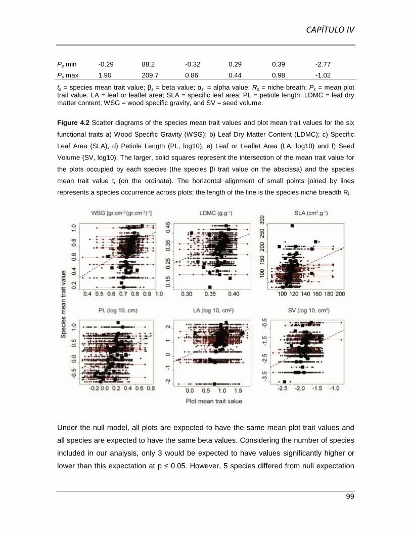
CAPÍTULO IV

99

Ps min -0.29 88.2 -0.32 0.29 0.39 -2.77Ps max 1.90 209.7 0.86 0.44 0.98 -1.02

ts = species mean trait value; βs = beta value; αs = alpha value; Rs = niche breath; Ps = mean plottrait value. LA = leaf or leaflet area; SLA = specific leaf area; PL = petiole length; LDMC = leaf drymatter content; WSG = wood specific gravity, and SV = seed volume.

Figure 4.2 Scatter diagrams of the species mean trait values and plot mean trait values for the six

functional traits a) Wood Specific Gravity (WSG); b) Leaf Dry Matter Content (LDMC); c) Specific

Leaf Area (SLA); d) Petiole Length (PL, log10); e) Leaf or Leaflet Area (LA, log10) and f) Seed

Volume (SV, log10). The larger, solid squares represent the intersection of the mean trait value for

the plots occupied by each species (the species βi trait value on the abscissa) and the species

mean trait value ti (on the ordinate). The horizontal alignment of small points joined by lines

represents a species occurrence across plots; the length of the line is the species niche breadth Ri.

Under the null model, all plots are expected to have the same mean plot trait values and

all species are expected to have the same beta values. Considering the number of species

included in our analysis, only 3 would be expected to have values significantly higher or

lower than this expectation at p ≤ 0.05. However, 5 species differed from null expectation

CAPÍTULO IV

100

for wood specific gravity (WSG) and leaf area (LA), 14 for LDMC, 18 for petiole length

(PL), 12 for SLA and 13 for seed volume (SV), so the null model was rejected for all traits

(Appendix 8.5).

Contrary to our expectations, trait correlations were in general stronger within plots (alpha

values) than among plots (plot mean trait values, Pj,, and beta values; Figure 4.3). At the

plot scale (alpha values), we found a negative correlation of WSG with LA and SLA, and a

positive correlation between LA and PL (Figure 4.3 c). At the landscape scale, for Pj, and

beta values, we found a negative correlation of SLA with LA, and for Pj, values a positive

correlation between SV and PL. Only four out of eight correlations found among Pj, values

were also found among beta values (Figure 4.3 a, b). We found no associations of WSG

with LA or SLA among Pj, values or beta values. At both scales (Pj, values and alpha

values) we found negative correlations of LDMC values with SLA, LA and PL; SLA with

SV; and WSG with PL; and a positive correlation between WSG and LDMC (Figure 4.3 a,

c).

We found no association of SV with LA, WSG, or LDMC, or between SLA and PL at either

scale. It is notable that correlations of species trait values (ti) showed almost the same

associations and patterns as alpha values (Figure 4.3 c, d). Only the SLA-SV correlation

among beta values was significantly different from null-model expectations.

Pj values differed significantly among successional-age/topographic-position categories,

although stand-age/topography explained a low percentage of variation (Figure 4.4). WSG,

SV, LA and LDMC had lower values in the youngest plots (3-8 year-old), while PL showed

its highest values in older plots (> 15 year-old) on flat sites and hills (Figure 4.4). The

lowest values of SLA wdere found in older plots on flat sites (Figure 4.4).

According to PCA, most of the overall variation in predictor variables was related to soil

properties (first axis), mainly soil total nitrogen (N), organic matter (SOM), cation exchange

capacity (CEC) and stoniness (Ston; Appendix 8.6). Some additional variation (second

axis) was independently associated with soil phosphorus (P), and potassium (K), altitude

and forest stand age (Appendix 8.6).

We found significant associations of functional traits with topography, soil properties and

forest stand age, although the amount of variation explained was low (R2: 0.02 - 0.27),

CAPÍTULO IV

101

particularly for WSG, SLA and LDMC (Table 4.2, Appendix 8.7). LDMC and WSG were

associated with CEC. PL varied with stand age, P, slope, N, SOM and Ston. LA and SLA

varied with stand age, pH and N. Finally, SV was associated with stoniness, SOM, P and

K. Overall, forest stand age was the main variable explaining variation in LA, LDMC and

PL, while soil properties and topography were more important for SLA, SV and WSG

(Table 4.3).

Figure 4.3 Pearson´s correlations for Pj, βi, α and ts values.. These expected correlations of the

alpha and beta components, across traits, are generally close to the correlation of the species trait

values (column d). LA = leaf or leaflet area; PL = petiole length; SLA = specific leaf area; LDMC =

leaf dry matter content; WSG = wood specific gravity, and SV = seed volume. Seed volume was

obtained as an abundance-weighted average considering data from only 55 species. The rest of

functional traits were obtained as an abundance-weighted average considering data from 65

species. * = p < 0.05; ** = p < 0.01; *** = p < 0.001.

CAPÍTULO IV

102

CAPÍTULO IV

103

CAPÍTULO IV

104

CAPÍTULO IV

105

Figure 4.4 Average of plot mean trait values (± SE) by successional age category. Different letters

indicate significantly different means (p < 0.05) according to ANOVA and Tukey’s post hoc analysis.

Successional age categories: 1 = 3 to 8 years of secondary succession (n = 51), 2 = 9 to 15 years

(86), 3 = > 15 years on flat areas (74) and 4 = > 15 years on hills (62). Seed volume was obtained

as an abundance-weighted average considering only data from 55 species. The rest of functional

traits were obtained as an abundance-weighted average considering data from 65 species.

Table 4.2 Reduced multiple linear regressions models of plot mean trait values with successional

age and environmental variables. For each trait the minimum model is shown, according to Akaike

criterion and hypothesis testing procedures (* = p < 0.05; ** = p < 0.01; *** = p < 0.001).

Trait R² Adj. R² Age pH N CEC P Slope SOM Ston K

LA 0.1 0.09 *** * ***

LDMC 0.08 0.07 *** *

PL 0.27 0.25 *** * * ** * *

SLA 0.08 0.07 ** *** **

SV 0.23 0.22 *** * *** **

WSG 0.02 0.02 *

PL = petiole length; LA = leaf or leaflet area; LDMC = leaf dry matter content; SLA = specific leaf

area, WSG = wood specific gravity, SV = seed volume. Age = Fallow time after slash and burn

agriculture; CEC= cation exchange capacity; K = interchangeable potassium; N = Soil total nitrogen;

Ston = Stoniness; SOM = Soil Matter Content; P = available phosphorus. Variables where

transformed, but original names are used for clarity. n= 263.

CAPÍTULO IV

106

Table 4.3 Relative importance of regressors on variance explained of reduced multiple linear

regressions models, obtained by R2 partitioning averaging sequential sums of squares over all

orderings of explanatory variables.

Trait

% ofvariance

explainedby themodel

Age CEC K N P pH Slope SOM Ston

LA 9.55 0.74 0.19 0.07

LDMC 7.86 0.87 0.13

PL 26.89 0.70 0.07 0.10 0.06 0.04 0.03

SLA 8.52 0.21 0.13 0.66

SV 23.35 0.06 0.12 0.28 0.53

WSG 1.97 1.00

See abbreviations meanings on Table 4.2.

4.4 DISCUSSION

We evaluated through TGA the trait co-variation of woody plants at two scales: landscape

(i.e. among communities, CWM and β values) and local (i.e. within communities, α values).

We found partial support for our prediction that, at the landscape scale, beta and plot

mean (Pj) values of functional traits would be strongly correlated, reflecting turnover of

functionally distinct species associated with microenvironmental change during

succession; whereas, at the plot scale, alpha values would show weaker correlations, as a

result of a scarce local environmental heterogeneity. We found nine functional trait

correlations between alpha values, and fewer correlations between beta (four) or Pj (eight)

values (Figure 4.3). Although null-model tests on beta values were rejected for all traits

(Appendix 8.5), indicating that species were aggregated in plots with other species with

similar trait values –which is consistent with habitat filtering (Ackerly and Cornwell, 2007;

Cornwell et al., 2006), this rejection was based on a reduced number of species.

Consequently, only one trait correlation (involving beta values, specific leaf area-seed

volume) did not differ from null model expectations. We found weak trait correlations

associated with the segregation of species into the rapid-slow continuum at the plot scale

(i. e. αi values), and only some correlations at landscape scale (i. e. Pj, and βi values). By

CAPÍTULO IV

107

rapid species we mean species that have great growth potential because they have “high

capacity to move water and to acquire and use nutrients and light to fix carbon, but build

flimsy, disposable tissues and are less tolerant to low resources” (Reich, 2014). Rapid

species have been directly related with high specific leaf area (SLA) (Poorter and Garnier,

2007; Poorter and Bongers, 2006), or high leaf area (LA) and petiole length (PL)

(Niinemets et al., 2004; Poorter, 2009) and inversely with wood specific gravity (WSG)

(Poorter and Bongers, 2006; Brodribb and Feild, 2000) and leaf dry matter content (LDMC)

(Hodgson et al., 2011; Wilson et al., 1999).

Because in the null models species were assigned to plots at random, but the species-

traits associations were maintained, the expected correlations of the αi and βi components

across traits in the null model are close to the traits correlations in the species (Ackerly

and Cornwell, 2007). Surprisingly, we found that only one trait correlation (SLA-SV) at the

landscape (βi values) was not different from null model expectation. This means that

nearly all trait correlations we found among and inside plots did not differ from a random

assembly of species. Therefore, αi correlations indicate that, inside plots, species

segregation may be the result of two possible processes: species morpho-physiological

constraints that allow them to take advantage of fine-scale environmental heterogeneity,

favoring species with ecological strategies that require or tolerate different levels of

resources, and species competition that establishes a limit in species similarity (de Bello et

al., 2013). This fine-scale environmental heterogeneity may be partly the result of local

disturbance. Firewood harvest, cutting of small trees for construction of Mayan houses,

and poaching are common daily activities we witnessed during sampling, and which occur

in all successional ages and topographic positions.

The correlations between αi values allow to distinguish two groups of species with

particular trait combinations that appear to segregate within plots: one group of species

with low LDMC, WSG and SV, high SLA and variable PL and LA, and the other with low

LDMC and WSG, high LA and PL and variable SV. While this combinations of traits

corresponds to acquisitive or rapid species, opposite trait correlations (i.e. high LDMC and

WSG, and low SLA or LA) correspond mainly to conservative or slow species. Our results

suggest that the segregation of these species occurs within plots regardless of topographic

position or forest stand age, which agrees with previous findings showing a high similarity

CAPÍTULO IV

108

in species composition, and the coexistence of generalist, pioneer and late-successional

species in all successional stages, probably as a result of the long history of disturbance in

this forest (Dupuy et al., 2012a; Mizrahi et al., 1997; Rico-Gray and García-Franco, 1992).

Trait correlations we obtained among αi values of WSG, LA, SLA and LDMC result from

well-known associations; for example, local differentiation in relation to WSG may be the

result of drought tolerance, since a relationship between high WSG and low xylem

susceptibility to cavitation as has been extensively documented (Chave et al., 2009). Low

WSG is correlated with high water storage capacity or with high hydraulic conductivity

(Poorter et al., 2010; Chave et al., 2009; Borchert, 1994) and with high SLA or LA,

because these traits are associated with high carbon assimilation that depends on water

supply (Ishida et al., 2008; Santiago et al., 2004). Furthermore, rapid acquisition of water

and minerals that results in high photosynthetic and growth rates are associated with low

LDMC (Reich, 2014). The αi LA-PL association result from an allometric scaling

relationship between these two traits (assuming PL is directly related with petiole mass),

because stronger petioles are required to support bigger leaves (Li et al., 2008; Niinemets

et al., 2007).

That βi correlations did not differ from a random assembly is an indication that species with

particular trait combinations segregate among plots, and that this segregation is unrelated

to environmental differences among plots. Thus, species with particular trait associations

may become dominant in some plots just because they have rapid growth, or high

fecundity or are highly competitive (Kneitel and Chase, 2004). The rapid species capable

of dominating in plots are those with either disposable leaves (i. e. low LDMC) and high

SLA, or with low LDMC and long petioles, or with high SLA and low LA. All these trait

associations are related to high photosynthetic rates (tightly associated with SLA) or

efficient light capture (long petioles and big leaves), which may be an indication that light

and/or moisture plays an important role in species dominance. An association of SLA and

species abundance has been reported before in other systems (Cornwell and Ackerly,

2010; Cingolani et al., 2007). WSG was unrelated to other traits (especially SLA and LA),

probably as a consequence of the interplay between plant drought resistance vs drought

avoidance mechanisms, which are fundamental in dry forests. Apart from xylem

vulnerability to embolism and sapwood water reserves (both associated with WSG), other

CAPÍTULO IV

109

traits, such as leaf shedding, root depth or leaf movement (paraheliotropism) may increase

water use efficiency (Pineda-García et al., 2013; Hasselquist et al., 2010; Brodribb and

Holbrook, 2003; Koller, 2000). For example, Fabace harbors more individuals (35% in 17

species) that any other family in our study site; these plants can achieve a more efficient

use of water than other species irrespective of their wood density through a combination of

small LA, leaf shedding and fine regulation of leaf movement by pulvini (Reyes-García et

al., 2012).

We found weaker trait correlations at landscape scale, and only half of them among βi

values, sometimes in opposite direction with Pj values. While Pj values reflect the

integrated effects of disturbance, dispersal limitation and environmental filters on dominant

species, βi values reveal the similarities or differences among species in the environmental

conditions (biotic and abiotic) where each species exists. In a disturbed forest as ours,

many of the species are capable of establishing along most of the gradient (i.e. in most of

the plots; see niche breadth as horizontal lines on Figure 4.2), and consequently the

average traits of these plots (i.e. their βi values) are similar among species, which

canceled out many βi values correlations. However, few correlations among βi values can

be also an indication that the environmental gradient among plots of different successional

age is not enough to filter out specific functional strategies. This has been found previously

in seedlings in a tropical dry forest (Pineda-García et al., 2015). Other studies in

Amazonian forests have found that species that are generalists at one scale (hundreds of

square meters, Pitman et al., 1999) are specialists at a bigger scale (thousands of square

meters, Toledo et al., 2012). Probably many of our species would show clear

environmental preferences at a larger scale, as many of them distribute in geographic

ranges of thousands of square kilometers, which exceeds widely the possible

environmental variation of our study area.

Just one trait correlation differed from null model, and can therefore be attributed to

environmental filtering: SLA-SV (Figure 4.3b). The negative correlation between SLA and

SV (among βi values) suggests the existence of filters among plots that favor species with

high SLA and small seeds on one extreme, and the opposite values on the other. Species

with high SLA and small seeds are associated with high photosynthetic rates and low

drought tolerance (Poorter and Rose, 2005; Daws et al., 2008; Baker, 1972), and they may

CAPÍTULO IV

110

be favored by the environmental gradient associated to secondary succession after slash

and burn agriculture.

Environmental variables explained a low proportion of variation in plot mean functional

traits (R2: 0.02 - 0.27; Table 4.3), and we found complex relationships between functional

traits of dominant species and environmental variables, and partial support to our

prediction that slope and soil properties would be as influential as successional age due to

their co-variation. All traits (except WSG) were associated both with soil/topographic

variables and with successional age; however, variation in SLA, SV and WSG was

associated mostly with soil/topographic variables, whereas variation in LA, LP and LDMC

was mainly associated with successional age (Table 4.4). PL has been directly associated

with light capture efficiency (Niinemets et al., 2004; Takenaka, 1994) suggesting that light

availability, which decreases with vegetation development during succession, may be the

main factor affecting this trait. In contrast, LA and LDMC were directly related to

successional age, possibly reflecting greater water deficit in early successional stages

(Lebrija-Trejos et al. 2010).

SLA was associated with the two main orthogonal axes in the landscape: total nitrogen

(N), soil organic matter (SOM) and cation exchange capacity (CEC) on the one hand; and

available phosphorous (P), interchangeable potassium (K) and forest stand age on the

other (Table 4.3, Appendix 8.6). This is in agreement with previous findings that associate

SLA with soil nutrients (Ordoñez et al., 2009) and stand age (Becknell and Powers, 2014;

Lebrija-Trejos et al., 2010a). SV was associated with SOM, stoniness, P and K. These

variables were indirectly related both with topographic position (SOM and stoniness are

higher on hills than on flat areas) and with successional age (as P and K covary with stand

age). Besides, mean values of SV differed between young plots in flat areas and older

plots on hills (categories 1 and 4; Table 4.2), suggesting that both successional age and

topographic position may indirectly and simultaneously influence SV.

The only variable that was significantly associated with WSG was CEC (Table 4.3), which

is positively associated with soil fertility. However, this association explained very little

variation (R2 = 0.02), and it is unlikely that high fertility per se favors species with high

WSG. Other variables associated with topographic position (besides CEC) may be

involved, since WSG was the only trait showing significant differences between hills and

flat areas (categories 3 and 4; Table 4.2). In particular, water deficit may be an important

CAPÍTULO IV

111

stressor, especially on hill tops and slopes, favoring species with high values of WSG

(Markesteijn et al., 2011; Choat et al., 2005). Soil water potential has been found to be

more negative (indicating lower water availability for plants) on hills or slopes than in

valleys (Markesteijn et al., 2010; Daws et al., 2002; Becker et al., 1988).

The low percentage of variation explained by topography, succession-related

environmental conditions and soil properties, coupled with the results of null models of trait

correlations, suggest that either recurrent human disturbance may have resulted in a

decoupling of woody plant assembly from some environmental filters, or that the

environmental factors that filter out species occur at larger scales. Further investigation is

needed to determine if the scarce functional turnover seen at the landscape scale is

associated with a low environmental variability among successional stages and

topographical positions.

4.5 CONCLUSIONS

Our results suggest that, at the plot scale, assembly of species, as gauged by leaf, trunk

and seed functional traits, is determined by local environmental heterogeneity, partially

associated with fine-scale heterogeneity and/or by interspecific competition. At the

landscape scale, most of species where capable of establishing in a wide range of

conditions. Consequently, most trait correlations involving the functional environment of

each species (i.e the trait average of those plots where each species is present) did not

differ from randomness. Further investigation is needed to determine if the scarce

functional turnover seen at the landscape scale is associated with a low environmental

variability among successional stages and topographical positions, or from a long term

management of vegetation.

4.6 ACKNOWLEDGEMENTS





fieldwork. LSV acknowledges CONACYT, Mexico, for the grant awarded (169510).

CAPÍTULO IV

112

4.7 REFERENCES

Ackerly, D.D., and Cornwell, W.K. (2007). A trait-based approach to community assembly:

partitioning of species trait values into within- and among-community components.

Ecol. Lett. 10, 135–145.

Ackerly, D., Knight, C., Weiss, S., Barton, K., and Starmer, K. (2002). Leaf size, specific

leaf area and microhabitat distribution of chaparral woody plants: contrasting

patterns in species level and community level analyses. Oecologia 130, 449–457.

Baker, H.G. (1972). Seed Weight in Relation to Environmental Conditions in California.

Ecology 53, 997–1010.

Becker, P., Rabenold, P.E., Idol, J.R., and Smith, A.P. (1988). Water potential gradients

for gaps and slopes in a Panamanian tropical moist forest’s dry season. J. Trop.

Ecol. 4, 173–184.

Becknell, J.M., and Powers, J.S. (2014). Stand age and soils as drivers of plant functional

traits and aboveground biomass in secondary tropical dry forest. Can. J. For. Res.

44, 604–613.

de Bello, F., Vandewalle, M., Reitalu, T., Lepš, J., Prentice, H.C., Lavorel, S., and Sykes,

M.T. (2013). Evidence for scale- and disturbance-dependent trait assembly

patterns in dry semi-natural grasslands. J. Ecol. 101, 1237–1244.



Brodribb, T.J., and Feild, T.S. (2000). Stem hydraulic supply is linked to leaf

photosynthetic capacity: evidence from New Caledonian and Tasmanian

rainforests. Plant Cell Environ. 23, 1381–1388.

CAPÍTULO IV

113

Brodribb, T.J., and Holbrook, N.M. (2003). Changes in leaf hydraulic conductance during

leaf shedding in seasonally dry tropical forest. New Phytol. 158, 295–303.

Chave, J., Coomes, D., Jansen, S., Lewis, S.L., Swenson, N.G., and Zanne, A.E. (2009).


Choat, B., Ball, M.C., Luly, J.G., and Holtum, J.A.M. (2005). Hydraulic architecture of


Trees 19, 305–311.

Cingolani, A.M., Cabido, M., Gurvich, D.E., Renison, D., and Díaz, S. (2007). Filtering

processes in the assembly of plant communities: Are species presence and

abundance driven by the same traits? J. Veg. Sci. 18, 911–920.





Cornwell, W.K., and Ackerly, D.D. (2009). Community assembly and shifts in plant trait

distributions across an environmental gradient in coastal California. Ecol. Monogr.

79, 109–126.

Cornwell, W.K., and Ackerly, D.D. (2010). A link between plant traits and abundance:

evidence from coastal California woody plants: Abundance, rarity and plant traits.

J. Ecol. 98, 814–821.

Cornwell, W.K., Schwilk, D.W., and Ackerly, D.D. (2006). A trait-based test for habitat


Daws, M.I., Mullins, C.E., Burslem, D.F., Paton, S.R., and Dalling, J.W. (2002).

Topographic position affects the water regime in a semideciduous tropical forest

in Panama. Plant Soil 238, 79–89.

CAPÍTULO IV

114

Daws, M.I., Crabtree, L.M., Dalling, J.W., Mullins, C.E., and Burslem, D.F.R.P. (2008).

Germination Responses to Water Potential in Neotropical Pioneers Suggest

Large-seeded Species Take More Risks. Ann. Bot. 102, 945–951.

De Bello, F., Lavorel, S., Lavergne, S., Albert, C.H., Boulangeat, I., Mazel, F., and Thuiller,



Di Rienzo, J.A., Casanoves, F., Balzarini, M.G., Gonzalez, L., Tablada, M., and Robledo,

C.W. (2013). InfoStat (Argentina: Grupo InfoStat, FCA, Universidad Nacional de

Córdoba).

Diaz, S., Cabido, M., and Casanoves, F. (1998). Plant functional traits and environmental

filters at a regional scale. J. Veg. Sci. 9, 113–122.


López-Martínez, J.O., Leyequién-Abarca, E., Tun-Dzul, F.J., and May-Pat, F.

(2012). Patterns and Correlates of Tropical Dry Forest Structure and Composition

in a Highly Replicated Chronosequence in Yucatan, Mexico. Biotropica 44, 151–

162.

Fonseca, C.R., Overton, J.M., Collins, B., and Westoby, M. (2000). Shifts in trait-

combinations along rainfall and phosphorus gradients. J. Ecol. 88, 964–977.

Garnier, E., Cortez, J., Billès, G., Navas, M.-L., Roumet, C., Debussche, M., Laurent, G.,

Blanchard, A., Aubry, D., Bellmann, A., et al. (2004). Plant functional markers

capture ecosystem properties during secondary succession. Ecology 85, 2630–

2637.

Grömping, U. (2006). Relative Importance for Linear Regression in R: The Package

relaimpo. J. Stat. Softw. Vol 1 Issue 1 2007.

Hasselquist, N.J., Allen, M.F., and Santiago, L.S. (2010). Water relations of evergreen and


Oecologia 164, 881–890.

CAPÍTULO IV

115

Hodgson, J.G., Montserrat-Marti, G., Charles, M., Jones, G., Wilson, P., Shipley, B.,

Sharafi, M., Cerabolini, B.E.L., Cornelissen, J.H.C., Band, S.R., et al. (2011). Is

leaf dry matter content a better predictor of soil fertility than specific leaf area?

Ann. Bot. 108, 1337–1345.

Ishida, A., Nakano, T., Yazaki, K., Matsuki, S., Koike, N., Lauenstein, D.L., Shimizu, M.,

and Yamashita, N. (2008). Coordination between leaf and stem traits related to

leaf carbon gain and hydraulics across 32 drought-tolerant angiosperms.

Oecologia 156, 193–202.

Keddy, P.A. (1992). Assembly and response rules: two goals for predictive community


Kneitel, J.M., and Chase, J.M. (2004). Trade-offs in community ecology: linking spatial

scales and species coexistence. Ecol. Lett. 7, 69–80.

Koller, D. (2000). Plants in search of sunlight. In Advances in Botanical Research, pp. 35–

131.

Kooyman, R., Cornwell, W., and Westoby, M. (2010). Plant functional traits in Australian

subtropical rain forest: partitioning within-community from cross-landscape

variation. J. Ecol. 98, 517–525.

Kraft, N.J., Cornwell, W.K., Webb, C.O., and Ackerly, D.D. (2007). Trait evolution,

community assembly, and the phylogenetic structure of ecological communities.

Am. Nat. 170, 271–283.

Lebrija-Trejos, E., Pérez-García, E.A., Meave, J.A., Bongers, F., and Poorter, L. (2010).



Li, G., Yang, D., and Sun, S. (2008). Allometric relationships between lamina area, lamina

mass and petiole mass of 93 temperate woody species vary with leaf habit, leaf

form and altitude. Funct. Ecol. 22, 557–564.

CAPÍTULO IV

116

Lohbeck, M., Lebrija-Trejos, E., Martínez-Ramos, M., Meave, J.A., Poorter, L., and

Bongers, F. (2015). Functional trait strategies of trees in dry and wet tropical

forests are similar but differ in their consequences for succession. Plos One 10,

e0123741.

Markesteijn, L., Iraipi, J., Bongers, F., and Poorter, L. (2010). Seasonal variation in soil

and plant water potentials in a Bolivian tropical moist and dry forest. J. Trop. Ecol.

26, 497–508.

Markesteijn, L., Poorter, L., Paz, H., Sack, L., and Bongers, F. (2011). Ecological



McDonald, P.G., Fonseca, C.R., Overton, J., and Westoby, M. (2003). Leaf-size

divergence along rainfall and soil-nutrient gradients: is the method of size

reduction common among clades? Funct. Ecol. 17, 50–57.

Mizrahi, A., Ramos Prado, J., and Jiménez-Osornio, J. (1997). Composition, structure, and



Moles, A.T., Perkins, S.E., Laffan, S.W., Flores-Moreno, H., Awasthy, M., Tindall, M.L.,

Sack, L., Pitman, A., Kattge, J., Aarssen, L.W., et al. (2014). Which is a better

predictor of plant traits: temperature or precipitation? J. Veg. Sci. 25, 1167–1180.



Niinemets, Ü., Al Afas, N., Cescatti, A., Pellis, A., and Ceulemans, R. (2004). Petiole

length and biomass investment in support modify light interception efficiency in

dense poplar plantations. Tree Physiol. 24, 141–154.

Niinemets, U., Portsmuth, A., Tena, D., Tobias, M., Matesanz, S., and Valladares, F.

(2007). Do we Underestimate the Importance of Leaf Size in Plant Economics?

Disproportional Scaling of Support Costs Within the Spectrum of Leaf

Physiognomy. Ann. Bot. 100, 283–303.

CAPÍTULO IV

117

Ordoñez, J.C., van Bodegom, P.M., Witte, J.-P.M., Wright, I.J., Reich, P.B., and Aerts, R.

(2009). A global study of relationships between leaf traits, climate and soil

measures of nutrient fertility. Glob. Ecol. Biogeogr. 18, 137–149.

Pineda-García, F., Paz, H., and Meinzer, F.C. (2013). Drought resistance in early and late




Pineda-García, F., Paz, H., Meinzer, F.C., and Angeles, G. (2015). Exploiting water versus



Pitman, N.C.A., Terborgh, J., Silman, M.R., and V., P.N. (1999). Tree Species

Distributions in an Upper Amazonian Forest. Ecology 80, 2651.

Poorter, L. (2009). Leaf traits show different relationships with shade tolerance in moist

versus dry tropical forests. New Phytol. 181, 890–900.

Poorter, H., and Garnier, E. (2007). Ecological Significance of Inherent Variation in

Relative Growth Rate and Its Components. In Functional Plant Ecology, Francisco

I. Pugnaire, and F. Valladares, eds. (Boca Raton, FL: CRC Press), pp. 67–100.

Poorter, L., and Bongers, F. (2006). Leaf traits are good predictors of plant performance

across 53 rain forest species. Ecology 87, 1733–1743.

Poorter, L., and Rose, S.A. (2005). Light-dependent changes in the relationship between

seed mass and seedling traits: a meta-analysis for rain forest tree species.

Oecologia 142, 378–387.

Poorter, L., McDonald, I., Alarcón, A., Fichtler, E., Licona, J.-C., Peña-Claros, M., Sterck,

F., Villegas, Z., and Sass-Klaassen, U. (2010). The importance of wood traits and

hydraulic conductance for the performance and life history strategies of 42

rainforest tree species. New Phytol. 185, 481–492.


CAPÍTULO IV

118



Reyes-García, C., Andrade, J.L., Simá, J.L., Us-Santamaría, R., and Jackson, P.C.

(2012). Sapwood to heartwood ratio affects whole-tree water use in dry forest

legume and non-legume trees. Trees 26, 1317–1330.

Rico-Gray, V., and García-Franco, J.G. (1992). Vegetation and soil seed bank of


Santiago, L.S., Goldstein, G., Meinzer, F.C., Fisher, J.B., Machado, K., Woodruff, D., and



Takenaka, A. (1994). Effects of leaf blade narrowness and petiole length on the light

capture efficiency of a shoot. Ecol. Res. 9, 109–114.


C., Licona, J.C., and Poorter, L. (2012). Distribution patterns of tropical woody



Warton, D.I., and Hui, F.K. (2011). The arcsine is asinine: the analysis of proportions in

ecology. Ecology 92, 3–10.

Weiher, E., Clarke, G.D.P., and Keddy, P.A. (1998). Community Assembly Rules,


Williamson, G.B., and Wiemann, M.C. (2010). Measuring wood specific gravity...Correctly.

Am. J. Bot. 97, 519–524.

Wilson, P.J., Thompson, K.E.N., and Hodgson, J.G. (1999). Specific leaf area and leaf dry

matter content as alternative predictors of plant strategies. New Phytol. 143, 155–

162.

CAPÍTULO IV

119

CAPÍTULO V

120

CAPÍTULO 5.DISCUSIÓN GENERAL

La sucesión secundaria es uno de los escenarios más importantes para analizar los

procesos que determinan el ensamblaje de las comunidades, y que permiten entender

porqué las especies se establecen en donde lo hacen, en términos de tiempo y espacio.

Mientras que la sucesión secundaria ha sido ampliamente descrita para bosques

tropicales húmedos, los estudios en los bosques secos son más escasos (Portillo-

Quintero y Sánchez-Azofeifa, 2010), y en particular los estudios que analizan la sucesión

secundaria desde un punto de vista funcional. Esto ha limitado el análisis de los

mecanismos sucesionales en estos sistemas, aún cuando representan el 42% de la

vegetación tropical y subtropical del planeta (Murphy y Lugo, 1986), y cuando están bajo

enorme presión por cambios de uso de suelo y altas tasas de deforestación (Keenan et

al., 2015; Miles et al., 2006; Janzen, 1988).

En este contexto, la finalidad de este trabajo fue obtener, mediante el uso de caracteres

funcionales de tallos, hojas y semillas, una aproximación de las características de las

plantas leñosas que son clave para su coexistencia y dominancia en un paisaje particular

de la Península de Yucatán, en donde los gradientes ambientales principalmente

estudiados en la sucesión secundaria han sido las características del suelo y la topografía

(Dupuy et al., 2012a; López-Martínez et al., 2012; Hernández-Stefanoni y Dupuy, 2008;

White y Hood, 2004; Rico-Gray y García-Franco, 1992). Este análisis partió de tres

aproximaciones distintas que se analizan en los siguientes apartados.

5.1 EL CAMBIO SUCESIONAL DE LOS GRUPOS FUNCIONALES DE PLANTASLEÑOSAS

Con base en los pocos estudios disponibles para bosques secos, podemos describir los

sitios sucesionales tempranos como lugares con una alta demanda evaporativa por la

elevada irradiación y albedo, lo que produce un incremento en la temperatura del aire y

una pérdida de agua superficial del suelo (Lebrija-Trejos et al., 2011; Pineda-García et al.,

2011; Hasselquist et al., 2010). De igual forma, los lugares situados en cerros, ya sea en

la cima o en la pendiente, tienen una menor disponibilidad de agua en el suelo que los

lugares ubicados en valles, pues por gravedad el líquido se mueve hacia las partes más

CAPÍTULO V

121

bajas (Markesteijn et al., 2010; Gallardo-Cruz et al., 2009; Becker et al., 1988). Estas

condiciones, tanto en las parcelas jóvenes como en los cerros, pueden llegar a ser

severas, y producir una diferenciación de nicho que permita el establecimiento de distintos

grupos de especies en cada ambiente (Chazdon et al., 2010; Kraft et al., 2008; Valencia et

al., 2004). En el sitio de estudio, se confirmó mediante un modelo multinomial basado en

la estimación de las abundancias relativas de las especies, que al inicio de la sucesión en

este bosque coexisten especialistas de bosque joven (< 15 años), de sitios planos y

generalistas.

Se confirmó sólo parcialmente la hipótesis de que las especialistas de bosques jóvenes y

cerros presentarían caracteres funcionales de hojas y tallos asociados con la evitación o

con la tolerancia a la sequía, y que las especialistas de bosques viejos y sitios planos

presentarían caracteres asociados con ambientes más mésicos (hipótesis b). En realidad,

los grupos de especialistas más similares entre sí fueron los de bosque joven y sitios

planos por un lado, y los grupos de especialistas de bosque viejo y cerros por el otro

(Figura 2.1, capítulo 2).

Las plantas especialistas de bosque joven, de forma similar a lo descrito previamente en

otros bosques secos (Pineda-García et al., 2013; Lebrija-Trejos et al., 2010a; Sobrado,

1993), mostraron caracteres primordialmente asociados al control de la temperatura en

hojas mediante el movimiento a través de pulvinos, y a evitar el embolismo mediante la

pérdida de hojas durante la sequía (capítulo 2), lo cual en otros trabajos se ha descrito

que ocurre cuando el potencial hídrico en la planta alcanza niveles tan bajos que ponen

en riesgo su integridad (Sobrado, 1993; Reich y Borchert, 1984). Las especies

especialistas de sitios planos únicamente se distinguieron por tener hojas deciduas. El

reducido número de caracteres altamente eficientes en las primeras etapas sucesionales

(pulvinos, foliolos reducidos, hábito deciduo) explica porqué el índice de Divergencia

Funcional de los brinzales en parcelas jóvenes e intermedias (3 a 10 y 11 a 25 años de

edad respectivamente) mostró valores más negativos de lo esperado por azar (capítulo 3),

lo cual sugiere la dominancia de un reducido número de estrategias funcionales.

Las especies generalistas no mostraron una posición funcional intermedia entre las

especialistas de bosque joven o de cerros y las especialistas de bosque maduro o de

sitios planos, ni son más similares a las primeras (contrariamente a lo esperado en la

CAPÍTULO V

122

hipótesis c). Aunque las especies generalistas son altamente variables funcionalmente,

con un número de combinaciones de caracteres propios de todos los grupos de

especialistas, la mayoría fueron más similares a las especialistas de cerros y de bosque

tardío. A pesar de eso, son mucho más abundantes en edades sucesionales tempranas

que las especies clasificadas como especialistas de bosque joven. De esta forma los 13

caracteres funcionales empleados no resultaron suficientes o relevantes para comprender

el éxito (en términos de abundancia) de estas especies, probablemente poque no se

relacionan con procesos como la reproducción (las generalistas se han descrito como

especies de alta fecundidad, y con dispersión y polinización abiótica; Wiegmann y Waller,

2006; McKinney y Lockwood, 1999) y la adquisición y almacenamiento de recursos

subterráneos.

Algunos estudios han establecido que, en bosques secos en los que las condiciones

durante la época de sequía son altamente estresantes, la sombra producida por el

crecimiento de la vegetación (por hojas de especies perennes y por ramas de especies

deciduas) representa un elemento facilitador para la supervivencia de las plántulas de

bosque tardío durante la época seca (Lebrija-Trejos et al., 2010b; McLaren y McDonald,

2003b; Gerhardt, 1996). Sin embargo, el análisis de diversidad funcional (capítulo 3)

mostró el efecto del filtrado ambiental en los brinzales en todas las edades de sucesión.

Aunque el menor efecto negativo del ambiente ocurre en etapas iniciales de la sucesión,

los valores negativos de la divergencia funcional (FDiv) en esas edades también muestran

que hay condiciones ambientales favoreciendo sólo ciertas combinaciones de caracteres,

pues este índice muestra que las especies son más similares de lo esperado por el azar.

También se detectaron procesos de competencia en los brinzales en las edades más

tempranas de sucesión, lo que indica que mientras los filtros ambientales restringen las

estrategias funcionales, los procesos competitivos limitan la similitud entre las especies

que sobreviven a esos filtros. Esta competencia pudiera asociarse con una alta densidad

de individuos jóvenes que ocurre en esta fase (Dupuy et al., 2012a).

La riqueza funcional (FRic) de los árboles adultos (significativamente superior de lo

esperado por azar) mostró que las condiciones de las parcelas de edades sucesionales

jóvenes e intermedias, que comprenden edades de 3 a 25 años, son las más favorables

para la coexistencia del máximo número de estrategias funcionales en esta fase

ontogénica. El análisis de especialistas y generalistas (capítulo 2) mostró que es en el

CAPÍTULO V

123

rango de 9 a 15 años de edad sucesional cuando coexisten especies generalistas, tardías

y pioneras, lo que explicaría la mayor riqueza funcional. Estos patrones son similares a lo

que se esperarían bajo la hipótesis del disturbio intermedio (Connell, 1978).

A medida que continúa el desarrollo de la vegetación, las condiciones se tornan más

húmedas y menos soleadas (Pineda-García et al., 2013; Lebrija-Trejos et al., 2011), y las

especies más dominantes son las generalistas y las especialistas de bosque maduro y

cerros (capítulo 2). Estas últimas (las especialistas) se caracterizan por tener hojas

perennes, lo que las asocia con una estrategia de captura de recursos lenta sensu Reich

2014, y su conservación por un tiempo mayor (Sobrado, 1993), pero con múltiples

variaciones en las combinaciones de otros caracteres. Esto conduce a pensar que las

estrategias de estas especies varían entre aquellas que evitan la sequía (por ejemplo

mediante raíces profundas o mediante el almacenamiento de agua en sus tejidos, lo que

les permitiría desacoplar transitoriamente su estado hídrico comparado con el del suelo;

Pineda-García et al., 2013) y las tolerantes a la sequía (con alta densidad de madera,

asociada con el mantenimiento del funcionamiento de la planta a bajos potenciales

hídricos y con una alta resistencia a la cavitación; Méndez-Alonzo et al., 2012a;

Markesteijn et al., 2011; Maherali et al., 2004).

Con el análisis de diversidad funcional (capítulo 3) se obtuvo que el efecto negativo del

ambiente en el establecimiento o persistencia de las especies (o filtrado ambiental) es

mayor en esta etapa de la sucesión (i. e. tardía) aunque sólo para los brinzales (mediante

un valor de FRic menor del que se esperaría por azar) tanto en sitios planos como en

cerros (Figure 3.2a). En consecuencia, se comprobó el efecto de filtros ambientales en los

cerros (hipótesis e), pero no en las primeras etapas sucesionales. También se corroboró

la mayor susceptibilidad de los brinzales a condiciones desfavorables en comparación con

los adultos (hipótesis f). La disminución de la FRic de brinzales en edades avanzadas de

la sucesión puede deberse a que, a medida que continúa el desarrollo de la vegetación, la

demanda de agua se incrementa y la disminución del potencial hídrico del suelo

superficial obedece ya no a la evaporación como en fases iniciales, sino a la transpiración

(Lebrija-Trejos et al., 2010a; Marthews et al., 2008). La luz también es un recurso limitante

a medida que se desarrolla la vegetación con el tiempo (Buzzard et al., 2015; Alvarez-

Añorve et al., 2012), a pesar de que se ha descrito como un factor menos importante

porque los bosques más secos tienen una mayor apertura del dosel y es un recurso

CAPÍTULO V

124

variable espacial y temporalmente (Lebrija-Trejos et al., 2011; Huante y Rincón, 1997).

Sin embargo, el área de estudio es un bosque subcaducifolio (es decir, en el extremo

menos seco de los bosques estacionales), en el que un estudio reciente del

microambiente muestró que durante la época de lluvias la densidad de flujo de fotones

disminuye drásticamente a alturas del dosel de 3.5 y 1.5 m (de la Rosa-Manzano et al.,

2015), sugiriendo que la luz puede ser un filtro importante para los brinzales. Lo anterior

permite suponer que, contrariamente a lo esperado, en este bosque las condiciones más

limitantes para las plantas jóvenes ocurren en rodales de edad sucesional avanzada,

tanto en sitios planos como en cerros. No puede descartarse además, que los bajos

valores de riqueza funcional de brinzales en edades avanzadas reflejen también

diferencias en habilidad competitiva de las especies y no sólo del filtrado ambiental (ver

sección 1.1.2; Mayfield y Levine, 2010).

Por otra parte, se esperaba que los procesos de competencia (observados como una alta

divergencia y equitatividad funcional) serían más importantes en edades sucesionales

intermedias y tardías y en brinzales, debido a que la competencia por recursos limitantes

como el agua podría incrementarse con el mayor desarrollo de raíces finas de individuos

cada vez de mayor tamaño (hipótesis f y g). Sin embargo, no se enontraron indicios de

competencia en esas etapas de la sucesión ni en brinzales ni en adultos (figura 3.2 e, f).

Al parecer las condiciones más adversas para los adultos ocurren en las edades

sucesionales más avanzadas en cerros, pues se obtuvieron especies funcionalmente más

similares de lo esperado por azar en esa posición topográfica (bajos valores de FDiv).

Como ya se mencionó antes, probablemente la competencia por el agua en este bosque

ocurra por diferencias en jerarquía competitiva, lo que sería detectado mediante una

reducción en la FRic, y no por exclusión competitiva, lo que se reflejaría en una mayor

FEve (Mayfield y Levine, 2010). También es posible que los caracteres funcionales

asociados más directamente con la competencia por agua, como los de raíces, no fueron

considerados en los análisis (Craine y Dybzinski, 2013)

5.2 DIFERENCIACIÓN FUNCIONAL DE LAS ESPECIES EN LA ESCALA LOCAL YDE PAISAJE

Múltiples asociaciones de caracteres funcionales y disyuntivas se han descrito como parte

de los mecanismos que permiten la coexistencia de las especies vegetales (Reich, 2014;

CAPÍTULO V

125

Wright et al., 2010, 2004; Chave et al., 2009). En lo que se refiere a la economía de los

recursos de las plantas (como el agua, la luz o los nutrientes), algunas de esas

asociaciones forman un espectro o eje de variación alrededor de 4 elementos clave: las

hojas, el tallo, las raíces y las semillas. Con la finalidad de analizar la variación conjunta

entre pares de caracteres funcionales asociados con las hojas, el tallo, y las semillas, y

compararla tanto en la escala de paisaje (entre parcelas) como en la local (dentro de las

parcelas), se utilizó el método del Análisis del Gradiente de Caracteres (Trait Gradien

Analysis, TGA, capítulo 4) (Ackerly y Cornwell, 2007).

Teóricamente, las limitantes en la dispersión, el filtrado ambiental o la exclusión

competitiva a lo largo del gradiente considerado (en este caso entre parcelas de diferente

edad de sucesión y posición topográfica) producirían un recambio de estrategias

funcionales, lo que sería capturado en el TGA como un gradiente de los caracteres

funcionales a escala de paisaje (en unidades de cada caracter, no en unidades

geográficas) (Ackerly y Cornwell, 2007). Analizando las correlaciones de los valores beta,

que representan el promedio del gradiente en donde cada especie es más abundante, se

puede inferir si existe co-variación entre pares de caracteres funcionales y por tanto un

recambio funcional en ejes de variación específicos. En este trabajo, se buscaba

encontrar correlaciones de caracteres que mostraran el recambio de especies de una

estrategia conservadora en parcelas jóvenes a una estrategia adquisitiva de recursos en

parcelas de edad más avanzada (hipótesis i). Contrariamente a lo esperado, se

encontraron escasas correlaciones de valores beta. Es muy posible que los largos

períodos de manejo de la vegetación hayan favorecido especies generalistas capaces de

establecerse en la mayor parte del gradiente ambiental, debido a disturbios continuos a

una escala local que permitan la coexistencia de estrategias de crecimiento rápido, lento e

intermedio en todas las edades sucesionales (capítulo 2).

Sin embargo, no fue posible probar esta hipótesis por la ausencia de vegetación que

realmente pudiera considerarse “madura” como referencia. No puede descartarse además

otra posibilidad importante: el método de TGA se ha utilizado para analizar el recambio

funcional en áreas con una fuerte diferenciación ambiental y de tipos de vegetación

(Kooyman et al., 2010; Ackerly y Cornwell, 2007). Así, el gradiente ambiental del paisaje

en el área de estudio puede ser muy poco contrastante, lo que también explicaría que la

mayoría de las especies sean capaces de establecerse en cualquier sitio, y la escasa

CAPÍTULO V

126

relación entre las variables edáficas y de edad sucesional con los valores promedio de los

caracteres por parcela (Figura 4.3). Tampoco puede descartarse la capacidad de las

especies de plantas de establecerse y sobrevivir en ambientes subóptimos. Un estudio

previo en bosque seco ha mostrado que las plántulas de especies pioneras y tardías no

muestran una diferenciación clara a lo largo del eje de variación funcional de explotación

de agua-tolerancia a la sequía, lo que sugiere que el gradiente de disponibilidad de agua

entre sitios de diferente edad de sucesión no es suficiente para filtrar estrategias

fisiológicas con un uso diferencial de la misma (Pineda-García et al., 2015). Hallazgos

parecidos fueron descritos para un área de 400 Km2 de bosque tropical húmedo del

Amazonas, en donde el 88% de las especies se describieron como generalistas, pues

eran capaces de establecerse en tres tipos de vegetación y dos etapas sucesionales

(Pitman et al., 1999). Sin embargo, cuando esas mismas especies fueron analizadas en

un área de 160, 000 Km2, las especies respondieron claramente a gradientes climáticos y

del suelo (Toledo et al., 2012). Este último trabajo mostró que las especies de plantas son

capaces de distribuirse en condiciones subóptimas, pero es posible capturar sus

preferencias por condiciones ambientales particulares cuando se analiza el factor

ambiental adecuado a la escala correcta (Toledo et al., 2012). Esto indica que es probable

que las especies aparentemente generalistas en el área de estudio de este trabajo, que

son la mayoría, pudieran ser especialistas al considerar un gradiente ambiental en

extensiones geográficas más amplias.

Los resultados del TGA también sugieren que en este bosque la co-variación de

caracteres funcionales que ocurre dentro de las parcelas puede ser igual o más fuerte que

la que podría esperarse entre diferentes edades de sucesión o posiciones topográficas

(es decir, entre parcelas, contrariamente a lo esperado en la hipótesis j). Estudios previos

han demostrado patrones similares (De Bello et al., 2009; Pavoine y Dolédec, 2005;

Westoby et al., 2002). Westoby y coautores (2002) propusieron que tal patrón puede ser

producido por tres procesos: a) una heterogeneidad ambiental local muy amplia; b)

procesos de inmigración de lugares con condiciones distintas, o, mucho más probable, c)

algún proceso denso-dependiente como el efecto de almacenamiento (“storage effect”),

en el que la variación temporal y espacial de las condiciones favorables permite un

reclutamiento diferenciado en tiempo y espacio para especies con estrategias

divergentes, además de una alterancia entre la importancia de la competencia intra vs

CAPÍTULO V

127

interespecífica, lo cual permite el mantenimiento de la diversidad a lo largo del tiempo

(Chesson, 2000).

5.3 CONCLUSIONES Y PERSPECTIVAS

5.3.1 Conclusiones

Los principales hallazgos de este estudio son:

1. Se analizaron los caracteres funcionales y las diferencias funcionales entre

estrategias ecológicas de plantas leñosas incluyendo no sólo a especies

especialistas, sino también (por primera vez en bosques secos) a las generalistas,

que tienen una gran importancia en los bosques sometidos a procesos recurrentes

de disturbio como los de la Península de Yucatán. Se determinó que las especies

generalistas tienden a mostrar caracteres funcionales más similares a los de las

especies tardías.

2. Como en otros bosques secos, en las fases iniciales de la sucesión las

condiciones de alta irradiancia, alta temperatura del suelo y del aire y alta

demanda evaporativa, favorecen caracteres funcionales asociados con la

disminución de la pérdida de agua por transpiración y el fotodaño en las especies

especialistas de bosque joven. Estas especies difieren de las generalistas en que

tienen mayor área foliar específica, una unidad mínima fotosintética reducida y la

presencia de pulvinos, mientras que difieren de las especialistas de bosque viejo

en el hábito deciduo en las primeras.

3. Contrariamente a lo señalado en otros bosques secos, los procesos de filtrado

ambiental afectan a los brinzales durante toda la sucesión, pero incrementan

fuertemente hacia las fases tardías, donde aparentemente las condiciones son

más mésicas. En los adultos, las condiciones más desfavorables ocurren

únicamente en edades tardías sobre cerros. Es probable que el principal filtro esté

asociado con una desecación del suelo mediante la transpiración para los

brinzales, y a una menor disponibilidad de agua relacionada a la posición

topográfica en los adultos, aunque en ambos casos no puede descartarse un

posible efecto de la disminución de la luz.

CAPÍTULO V

128

4. Se detectaron efectos de competencia en edades tempranas de la sucesión sólo

para los brinzales. Sin embargo, no puede descartarse que la reducción en la

riqueza funcional en brinzales y adultos también muestre procesos de

competencia, pues la exclusión competitiva entre especies que difieren en

jerarquía competitiva también produce una reducción en el rango multivariado de

los caracteres funcionales.

5. La fase regenerativa mostró ser más suceptible al filtrado ambiental y a la

competencia que los adultos. Esto sugiere que los adultos tienen una mayor

capacidad para competir y para afrontar peligros tales como la baja disponibilidad

de recursos, daños mecánicos o el ataque de herbivoros.

6. Mediante el análisis de gradientes de caracteres, se observó que las diferencias

funcionales son mayores al interior de las parcelas que entre ellas. Esto sugiere

que procesos denso-dependientes, inmigración, la heterogeneidad ambiental local

o el disturbio recurrente definen de forma más importante el funcionamiento de

estas comunidades que el gradiente sucesional o topográfico.

5.3.2 Perspectivas

De acuerdo con los resultados de este estudio, se requieren varias aproximaciones de

investigación adicionales para poder entender la diferenciación funcional descrita en este

bosque, ya sea a nivel de estrategias ecológicas, de diversidad funcional o de covariación

de caracteres a diferentes escalas:

Micro y meso ambiente. Es necesario hacer una caracterización fina de por lo

menos dos recursos que al parecer son los más relevantes en este sistema: la

disponibilidad de agua en el suelo y la luz. Conocer cómo es la variación del

contenido volumétrico del agua y el potencial hídrico en el suelo a diferentes

profundidades, tanto en sitios planos como en laderas, o la medición mediante

isótopos estables de la profundidad a la cual las especies adquieren el agua,

podría ser de gran utilidad para entender la manera en la que se reparte este

recurso (Kulmatiski y Beard, 2013). Además, conocer cómo difiere la disponibilidad

de la luz localmente y en diferentes edades de sucesión y posiciones topográficas

podría ayudar a explicar los patrones de filtrado ambental descritos para los

brinzales, o el incremento de la riqueza funcional de los adultos. También

CAPÍTULO V

129

permitiría dilucidar si lo que está produciendo la diferenciación funcional dentro de

las comunidades se relaciona con la heterogeneidad de recursos a escala local, o

si otros procesos denso-dependientes son los que influyen en la diversidad

funcional en este sistema.

La inclusión de caracteres funcionales asociados al aprovechamiento de recursos

subterráneos también es un elemento clave para entender este ecosistema. Si los

patrones de filtrado ambiental en edades sucesionales jóvenes y tardías están

relacionados con la capacidad de las plantas de apropiarse del recurso agua y

limitar su disponibilidad a plantas vecinas (“preemption”), la competitividad de las

especies podría depender de la longitud o densidad de las raíces, o de su

distribución vertical (Craine y Dybzinski, 2013; Querejeta et al., 2007).

Debido a que el rebrote se ha considerado como un caracter funcional que es

clave en la regeneración de los bosques secos (McLaren y McDonald, 2003a), es

necesario investigar si tiene un papel relevante en el ensamblaje de las

comunidades. Por ejemplo, si el reclutamiento de brinzales de especies tardías en

parcelas jóvenes está dado por este mecanismo; si el rebrote permite el

crecimiento de las especies en ambientes que serían poco propicios para la

regeneración por semilla o si se asocia con algún grupo particular de plantas (i.e.

con cierta estrategia funcional) o es una característica generalizada.

El análisis de la diversidad funcional sugirió que el filtrado ambiental es un proceso

de ensamblaje importante en plantas de menor tamaño. El uso de índices con

múltiples caracteres impide saber cuáles son los que están teniendo un papel más

importante, e incluso podrían obscurecer patrones que se detectan en análisis de

caracteres individuales (Bhaskar et al., 2014). Por esto, es necesario hacer un

análisis de la diversidad funcional de los caracteres más importantes por

separado, lo que permitiría una mejor comparación con estudios previos en otros

sistemas. También sería de utilidad analizar la variación de la diversidad funcional

para los grupos de plantas con estrategia similar (i.e. especialistas y generalistas),

pues sus procesos de ensamblaje difieren en diferentes etapas de la sucesión

(Lebrija-Trejos et al., 2010b).

El papel del disturbio es otro tema importante por analizar. Aunque difícilmente

puede medirse plenamente su impacto porque la vegetación más antigua de la

CAPÍTULO V

130

región no podría considerarse prístina (dada la larga historia de ocupación de la

Península y del área de estudio), sí pueden practicarse diferentes tipos de

disturbio o de daño controlado (o monitorear el que ya existe) para evaluar su

efecto en las especies y la relación entre su estrategia funcional con su capacidad

de recuperación. También puede analizarse la capacidad de recuperación a nivel

de las comunidades. Sin embargo, permanecerá como una incógnita si las

actividades humanas han seleccionado durante milenios las especies capaces de

establecerse en amplios rangos ambientales, y si esto ha influido en la similitud

entre comunidades del bosque en la Península.

BIBLIOGRAFÍA

131

CAPÍTULO 6.BIBLIOGRAFÍA

Ackerly, D.D., y Cornwell, W.K. (2007). A trait-based approach to community assembly:

partitioning of species trait values into within- and among-community components.

Ecol. Lett. 10, 135–145.

Ackerly, D., Knight, C., Weiss, S., Barton, K., y Starmer, K. (2002). Leaf size, specific leaf

area and microhabitat distribution of chaparral woody plants: contrasting patterns

in species level and community level analyses. Oecologia 130, 449–457.

Alvarez-Añorve, M.Y., Quesada, M., Sanchez-Azofeifa, G.A., Avila-Cabadilla, L.D., y



99, 816–826.

Baker, H.G. (1972). Seed Weight in Relation to Environmental Conditions in California.

Ecology 53, 997–1010.

Bautista-Zúñiga, F., Batllori-Sampedro, E., Ortiz-Pérez, M.A., Palacio-Aponte, G., and

Castillo-González, M. (2003). Geoformas, agua y suelo en la Península de

Yucatán. En Naturaleza y Sociedad en el Área Maya: Pasado, Presente y Futuro,

P. Colunga, y A. Larque, eds. (Mérida, Yucatán, México: Academia Mexicana de

Ciencias y Centro de Investigación Científica de Yucatán), pp. 21–35.

Becker, P., Rabenold, P.E., Idol, J.R., y Smith, A.P. (1988). Water potential gradients for

gaps and slopes in a Panamanian tropical moist forest’s dry season. J. Trop.

Ecol. 4, 173–184.

Becknell, J.M., y Powers, J.S. (2014). Stand age and soils as drivers of plant functional

traits and aboveground biomass in secondary tropical dry forest. Can. J. For. Res.

44, 604–613.

Bellingham, P.J., y Tanner, E.V.J. (2000). The Influence of Topography on Tree Growth,

Mortality, and Recruitment in a Tropical Montane Forest. BIOTROPICA 32, 378.

BIBLIOGRAFÍA

132

de Bello, F., Vandewalle, M., Reitalu, T., Lepš, J., Prentice, H.C., Lavorel, S., y Sykes,

M.T. (2013). Evidence for scale- and disturbance-dependent trait assembly

patterns in dry semi-natural grasslands. J. Ecol. 101, 1237–1244.

Bhaskar, R., y Ackerly, D.D. (2006). Ecological relevance of minimum seasonal water

potentials. Physiol. Plant. 127, 353–359.

Bhaskar, R., Dawson, T.E., y Balvanera, P. (2014). Community assembly and functional

diversity along succession post-management. Funct. Ecol. 28, 1256–1265.

Bielenberg, D.G., Miller, J.D., y Berg, V.S. (2003). Paraheliotropism in two Phaseolus

species: combined effects of photon flux density and pulvinus temperature, and

consequences for leaf gas exchange. Environ. Exp. Bot. 49, 95–105.

Bond, W.J., y Midgley, J.J. (2003). The evolutionary ecology of sprouting in woody plants.

Int. J. Plant Sci. 164, S103–S114.

Bonilla-Moheno, M. (2012). Damage and recovery of forest structure and composition after

two subsequent hurricanes in the Yucatan Peninsula. Caribb. J. Sci. 46, 240–248.



Borchert, R., Meyer, S.A., Felger, R.S., y Porter-Bolland, L. (2004). Environmental control

of flowering periodicity in Costa Rican and Mexican tropical dry forests. Glob.

Ecol. Biogeogr. 13, 409–425.

Brodribb, T.J., y Feild, T.S. (2000). Stem hydraulic supply is linked to leaf photosynthetic

capacity: evidence from New Caledonian and Tasmanian rainforests. Plant Cell

Environ. 23, 1381–1388.

Brodribb, T.J., y Holbrook, N.M. (2003). Changes in leaf hydraulic conductance during leaf

shedding in seasonally dry tropical forest. New Phytol. 158, 295–303.

BIBLIOGRAFÍA

133

Bucci, S.J., Goldstein, G., Meinzer, F.C., Scholz, F.G., Franco, A.C., y Bustamante, M.

(2004). Functional convergence in hydraulic architecture and water relations of

tropical savanna trees: from leaf to whole plant. Tree Physiol. 24, 891–899.

Buzzard, V., Hulshof, C.M., Birt, T., Violle, C., y Enquist, B.J. (2015). Re-growing a tropical

dry forest: functional plant trait composition and community assembly during

succession. Funct. Ecol. 30, 1006–1013.

Cailliez, F. (1983). The analytical solution of the additive constant problem. Psychometrika

48, 305–308.

Cavender-Bares, J., Kitajima, K., y Bazzaz, F.A. (2004). Multiple trait associations in

relation to habitat differentiation among 17 Floridian oak species. Ecol. Monogr.

74, 635–662.

Chave, J., Coomes, D., Jansen, S., Lewis, S.L., Swenson, N.G., y Zanne, A.E. (2009).


Chazdon, R.L., Finegan, B., Capers, R.S., Salgado-Negret, B., Casanoves, F., Boukili, V.,

y Norden, N. (2010). Composition and Dynamics of Functional Groups of Trees

During Tropical Forest Succession in Northeastern Costa Rica: Functional Groups

of Trees. Biotropica 42, 31–40.

Chazdon, R.L., Chao, A., Colwell, R.K., Lin, S.-Y., Norden, N., Letcher, S.G., Clark, D.B.,

Finegan, B., y Arroyo, J.P. (2011). A novel statistical method for classifying

habitat generalists and specialists. Ecology 92, 1332–1343.

Chesson, P. (2000). Mechanisms of maintenance of species diversity. Annu. Rev. Ecol.

Syst. 343–366.

Choat, B., Ball, M.C., Luly, J.G., y Holtum, J.A.M. (2005). Hydraulic architecture of


Trees 19, 305–311.

BIBLIOGRAFÍA

134

Cingolani, A.M., Cabido, M., Gurvich, D.E., Renison, D., y Díaz, S. (2007). Filtering

processes in the assembly of plant communities: Are species presence and

abundance driven by the same traits? J. Veg. Sci. 18, 911–920.

Connell, J.H. (1978). Diversity in Tropical Rain Forests and Coral Reefs. Science 199,

1302–1310.

Coomes, D.A., y Grubb, P.J. (2003). Colonization, tolerance, competition and seed-size

variation within functional groups. Trends Ecol. Evol. 18, 283–291.





Cornwell, W.K., y Ackerly, D.D. (2009). Community assembly and shifts in plant trait

distributions across an environmental gradient in coastal California. Ecol. Monogr.

79, 109–126.

Cornwell, W.K., y Ackerly, D.D. (2010). A link between plant traits and abundance:

evidence from coastal California woody plants: Abundance, rarity and plant traits.

J. Ecol. 98, 814–821.

Cornwell, W.K., Schwilk, D.W., y Ackerly, D.D. (2006). A trait-based test for habitat


Craine, J.M., y Dybzinski, R. (2013). Mechanisms of plant competition for nutrients, water

and light. Funct. Ecol. 27, 833–840.

Dalling, J.W., y Denslow, J.S. (1998). Soil seed bank composition along a forest

chronosequence in seasonally moist tropical forest, Panama. J. Veg. Sci. 9, 669–

678.

Dar, P.A., y Reshi, Z.A. (2014). Components, processes and consequences of biotic

homogenization: A review. Contemp. Probl. Ecol. 7, 123–136.

BIBLIOGRAFÍA

135

Daws, M.I., Mullins, C.E., Burslem, D.F., Paton, S.R., y Dalling, J.W. (2002). Topographic


Plant Soil 238, 79–89.

Daws, M.I., Pearson, T.R.H., Burslem, D.F.R.P., Mullins, C.E., y Dalling, J.W. (2005).

Effects of topographic position, leaf litter and seed size on seedling demography

in a semi-deciduous tropical forest in Panamá. Plant Ecol. 179, 93–105.

Daws, M.I., Crabtree, L.M., Dalling, J.W., Mullins, C.E., y Burslem, D.F.R.P. (2008).

Germination Responses to Water Potential in Neotropical Pioneers Suggest

Large-seeded Species Take More Risks. Ann. Bot. 102, 945–951.

De Bello, F., Thuiller, W., Lepš, J., Choler, P., Clément, J.-C., Macek, P., Sebastià, M.-T.,

y Lavorel, S. (2009). Partitioning of functional diversity reveals the scale and

extent of trait convergence and divergence. J. Veg. Sci. 20, 475–486.

De Bello, F., Lavorel, S., Lavergne, S., Albert, C.H., Boulangeat, I., Mazel, F., y Thuiller,



Deans, J.D., Moran, J., y Grace, J. (1996). Biomass relationships for tree species in

regenerating semi-deciduous tropical moist forest in Cameroon. For. Ecol. Manag.

88, 215–225.

Devictor, V., Julliard, R., y Jiguet, F. (2008). Distribution of specialist and generalist

species along spatial gradients of habitat disturbance and fragmentation. Oikos 0,

080211051304426–0.

Di Rienzo, J.A., Casanoves, F., Balzarini, M.G., Gonzalez, L., Tablada, M., y Robledo,

C.W. (2013). InfoStat (Argentina: Grupo InfoStat, FCA, Universidad Nacional de

Córdoba).

Diaz, S., Cabido, M., y Casanoves, F. (1998). Plant functional traits and environmental

filters at a regional scale. J. Veg. Sci. 9, 113–122.

BIBLIOGRAFÍA

136

Donfack, P., Floret, C., y Pontanier, R. (1995). Secondary succession in abandoned fields

of dry tropical Northern Cameroon. J. Veg. Sci. 6, 499–508.


López-Martínez, J.O., Leyequién-Abarca, E., Tun-Dzul, F.J., y May-Pat, F.

(2012a). Patterns and Correlates of Tropical Dry Forest Structure and

Composition in a Highly Replicated Chronosequence in Yucatan, Mexico.

Biotropica 44, 151–162.

Dupuy, J.M., Hernández-Stefanoni, J.L., Hernández, R., Juárez, F.T.D., y Pat, F.M.

(2012b). Efectos del cambio de uso del suelo en la biomasa y diversidad de

plantas leñosas en un paisaje de bosque tropical seco en Yucatán. Investig.

Ambient. Cienc. Política Pública 4, 130–140.

Dupuy, J.M., Durán-García, R., García-Contreras, G., Arellano Morín, J., Acosta Lugo, E.,

Méndez-González, M.E., y Andrade Hernández, M. (2015). Chapter 8.

Conservation and use. En Biodiversity and Conservation of the Yucatán

Peninsula, G.A. Islebe, S. Calmé, J.L. León-Cortés, y B. Schmook, eds. (Cham:

Springer International Publishing), p.

Engelbrecht, B.M.J., Dalling, J.W., Pearson, T.R.H., Wolf, R.L., Gálvez, D.A., Koehler, T.,

Tyree, M.T., y Kursar, T.A. (2006). Short dry spells in the wet season increase

mortality of tropical pioneer seedlings. Oecologia 148, 258–269.

Engelbrecht, B.M.J., Comita, L.S., Condit, R., Kursar, T.A., Tyree, M.T., Turner, B.L., y

Hubbell, S.P. (2007). Drought sensitivity shapes species distribution patterns in

tropical forests. Nature 447, 80–82.

Flores, J.S., y Espejel, I. (1994). Tipos de vegetación de la Península de Yucatán (Mérida,

Yucatán, México: Universidad Autónoma de Yucatán).

Fonseca, C.R., Overton, J.M., Collins, B., y Westoby, M. (2000). Shifts in trait-

combinations along rainfall and phosphorus gradients. J. Ecol. 88, 964–977.

BIBLIOGRAFÍA

137

Gallardo-Cruz, J.A., Pérez-García, E.A., y Meave, J.A. (2009). β-Diversity and vegetation


landscape. Landsc. Ecol. 24, 473–482.

García, E. (1981). Modificaciones al sistema de clasificación climática de Köppen (para

adaptarlo a las condiciones de la República Mexicana) (Mexico D. F.: Instituto de

Geografía Universidad Nacional Autónoma de México).

Garnier, E., Cortez, J., Billès, G., Navas, M.-L., Roumet, C., Debussche, M., Laurent, G.,

Blanchard, A., Aubry, D., Bellmann, A., et al. (2004). Plant functional markers

capture ecosystem properties during secondary succession. Ecology 85, 2630–

2637.

Gerhardt, K. (1996). Effects of root competition and canopy openness on survival and

growth of tree seedlings in a tropical seasonal dry forest. For. Ecol. Manag. 82,

33–48.

Gerhardt, K., y Hytteborn, H. (1992). Natural dynamics and regeneration methods in


Gillespie, T.W., Grijalva, A., y Farris, C.N. (2000). Diversity, composition, and structure of

tropical dry forests in Central America. Plant Ecol. 147, 37–47.

Goldstein, G., Andrade, J.L., Meinzer, F.C., Holbrook, N.M., Cavelier, J., Jackson, P., y

Celis, A. (1998). Stem water storage and diurnal patterns of water use in tropical

forest canopy trees. Plant Cell Environ. 21, 397–406.

González-Cruz, G., García-Frapolli, E., Fernández, A.C., y Rada, J.M.D. (2014).

Conocimiento tradicional maya sobre la dinámica sucesional de la selva. Un caso

de estudio en la Península de Yucatán. Etnobiología 12, 60–67.

González-Iturbe, J.A., Olmsted, I., y Tun-Dzul, F. (2002). Tropical dry forest recovery after

long term Henequen (sisal, Agave fourcroydes Lem.) plantation in northern

Yucatan, Mexico. For. Ecol. Manag. 167, 67–82.

BIBLIOGRAFÍA

138



Grömping, U. (2006). Relative Importance for Linear Regression in R: The Package

relaimpo. J. Stat. Softw. Vol 1 Issue 1 2007.

Grubb, P.J. (1977). The maintenance of species-richness in plant communities: the

importance of the regeneration niche. Biol. Rev. 52, 107–145.

Hasselquist, N.J., Allen, M.F., y Santiago, L.S. (2010). Water relations of evergreen and


Oecologia 164, 881–890.

Hernández-Stefanoni, J.L., y Dupuy, J.M. (2008). Effects of landscape patterns on species

density and abundance of trees in a tropical subdeciduous forest of the Yucatan

Peninsula. For. Ecol. Manag. 255, 3797–3805.

Hernández-Stefanoni, J.L., Pineda, J.B., y Valdes-Valadez, G. (2006). Comparing the Use

of Indigenous Knowledge with Classification and Ordination Techniques for


Forest. Environ. Manage. 37, 686–702.

Hernández-Stefanoni, J.L., Dupuy, J.M., Tun-Dzul, F., y May-Pat, F. (2011). Influence of



Hikosaka, K. (2004). Interspecific difference in the photosynthesis-nitrogen relationship:

patterns, physiological causes, and ecological importance. J. Plant Res. 117,

481–494.

Hodgson, J.G., Montserrat-Marti, G., Charles, M., Jones, G., Wilson, P., Shipley, B.,

Sharafi, M., Cerabolini, B.E.L., Cornelissen, J.H.C., Band, S.R., et al. (2011). Is

leaf dry matter content a better predictor of soil fertility than specific leaf area?

Ann. Bot. 108, 1337–1345.

BIBLIOGRAFÍA

139

Huante, P., y Rincón, E. (1997). Responses to light changes in tropical deciduous woody

seedlings with contrasting growth rates. Oecologia 113, 53–66.

Hubbell, S.P. (1999). Light-Gap Disturbances, Recruitment Limitation, and Tree Diversity

in a Neotropical Forest. Science 283, 554–557.

Hubbell, S.P. (2005). Neutral theory in community ecology and the hypothesis of functional

equivalence. Funct. Ecol. 19, 166–172.

Ishida, A., Nakano, T., Yazaki, K., Matsuki, S., Koike, N., Lauenstein, D.L., Shimizu, M., y

Yamashita, N. (2008). Coordination between leaf and stem traits related to leaf

carbon gain and hydraulics across 32 drought-tolerant angiosperms. Oecologia

156, 193–202.

Janzen, D.H. (1988). Chapter 14. Tropical dry forests. En Biodiversity, E.O. Wilson, y F.M.

Peter, eds. (Washington, DC: National Academy Press), pp. 130–137.

Kammesheidt, L. (1999). Forest recovery by root suckers and above-ground sprouts after

slash-and-burn agriculture, fire and logging in Paraguay and Venezuela. J. Trop.

Ecol. 15, 143–157.

Kanagaraj, R., Wiegand, T., Comita, L.S., y Huth, A. (2011). Tropical tree species

assemblages in topographical habitats change in time and with life stage: Habitat-

driven tree species assemblages. J. Ecol. 99, 1441–1452.

Keddy, P.A. (1992a). A Pragmatic Approach to Functional Ecology. Funct. Ecol. 6, 621.

Keddy, P.A. (1992b). Assembly and response rules: two goals for predictive community


Keenan, R.J., Reams, G.A., Achard, F., de Freitas, J.V., Grainger, A., y Lindquist, E.

(2015). Dynamics of global forest area: Results from the FAO Global Forest

Resources Assessment 2015. For. Ecol. Manag. 352, 9–20.

BIBLIOGRAFÍA

140



18, 53–66.

Kennard, D.K., Gould, K., Putz, F.E., Fredericksen, T.S., y Morales, F. (2002). Effect of

disturbance intensity on regeneration mechanisms in a tropical dry forest. For.

Ecol. Manag. 162, 197–208.

Kneitel, J.M., y Chase, J.M. (2004). Trade-offs in community ecology: linking spatial scales

and species coexistence. Ecol. Lett. 7, 69–80.

Koller, D. (2000). Plants in search of sunlight. En Advances in Botanical Research, pp. 35–

131.

Kooyman, R., Cornwell, W., y Westoby, M. (2010). Plant functional traits in Australian

subtropical rain forest: partitioning within-community from cross-landscape

variation. J. Ecol. 98, 517–525.

Kraft, N.J., y Ackerly, D.D. (2010). Functional trait and phylogenetic tests of community

assembly across spatial scales in an Amazonian forest. Ecol. Monogr. 80, 401–

422.

Kraft, N.J., Cornwell, W.K., Webb, C.O., y Ackerly, D.D. (2007). Trait evolution, community

assembly, and the phylogenetic structure of ecological communities. Am. Nat.

170, 271–283.

Kraft, N.J.B., Valencia, R., y Ackerly, D.D. (2008). Functional Traits and Niche-Based Tree

Community Assembly in an Amazonian Forest. Science 322, 580–582.

Kraft, N.J.B., Adler, P.B., Godoy, O., James, E.C., Fuller, S., y Levine, J.M. (2015).


Funct. Ecol. 29, 592–599.

Kulmatiski, A., y Beard, K.H. (2013). Root niche partitioning among grasses, saplings, and

trees measured using a tracer technique. Oecologia 171, 25–37.

BIBLIOGRAFÍA

141

Kunstler, G., Lavergne, S., Courbaud, B., Thuiller, W., Vieilledent, G., Zimmermann, N.E.,

Kattge, J., y Coomes, D.A. (2012). Competitive interactions between forest trees

are driven by species’ trait hierarchy, not phylogenetic or functional similarity:

implications for forest community assembly. Ecol. Lett. 15, 831–840.

Laliberté, E., y Legendre, P. (2010). A distance-based framework for measuring functional

diversity from multiple traits. Ecology 91, 299–305.

Laliberté, E., Legendre, P., y Shipley, B. (2014). FD: measuring functional diversity from

multiple traits, and other tools for functional ecology.

Larcher, W. (2003). Physiological Plant Ecology (Berlin, Germany: Springer).

Lasky, J.R., Uriarte, M., Boukili, V.K., y Chazdon, R.L. (2014). Trait-mediated assembly


Proc. Natl. Acad. Sci. 111, 5616–5621.

Lavorel, S. (2013). Plant functional effects on ecosystem services. J. Ecol. 101, 4–8.

Lavorel, S., y Grigulis, K. (2012). How fundamental plant functional trait relationships

scale-up to trade-offs and synergies in ecosystem services. J. Ecol. 100, 128–

140.

Lebrija-Trejos, E., Pérez-García, E.A., Meave, J.A., Bongers, F., y Poorter, L. (2010a).



Lebrija-Trejos, E., Meave, J.A., Poorter, L., Pérez-García, E.A., y Bongers, F. (2010b).



Lebrija-Trejos, E., Pérez-García, E.A., Meave, J.A., Poorter, L., y Bongers, F. (2011).



BIBLIOGRAFÍA

142

Leishman, M.R., y Westoby, M. (1994). The Role of Seed Size in Seedling Establishment

in Dry Soil Conditions -- Experimental Evidence from Semi-Arid Species. J. Ecol.

82, 249.

Letcher, S.G., Lasky, J.R., Chazdon, R.L., Norden, N., Wright, S.J., Meave, J.A., Pérez-

García, E.A., Muñoz, R., Romero-Pérez, E., Andrade, A., et al. (2015).

Environmental gradients and the evolution of successional habitat specialization:

a test case with 14 Neotropical forest sites. J. Ecol. 103, 1276–1290.

Li, G., Yang, D., y Sun, S. (2008). Allometric relationships between lamina area, lamina

mass and petiole mass of 93 temperate woody species vary with leaf habit, leaf

form and altitude. Funct. Ecol. 22, 557–564.


Pérez-García, E.A., Romero-Pérez, I.E., Tauro, A., y Bongers, F. (2013).



Lohbeck, M., Lebrija-Trejos, E., Martínez-Ramos, M., Meave, J.A., Poorter, L., y Bongers,

F. (2015). Functional trait strategies of trees in dry and wet tropical forests are

similar but differ in their consequences for succession. Plos One 10, e0123741.

López-Martínez, J.O., Hernández-Stefanoni, J.L., Dupuy, J.M., y Meave, J.A. (2012).

Partitioning the variation of woody plant β-diversity in a landscape of secondary

tropical dry forests across spatial scales. J. Veg. Sci. 24, 33–45.

López-Martínez, J.O., Sanaphre-Villanueva, L., Dupuy, J.M., Hernández-Stefanoni, J.L.,

Meave, J.A., y Gallardo-Cruz, J.A. (2013). β-Diversity of Functional Groups of

Woody Plants in a Tropical Dry Forest in Yucatan. Plos One 8, e73660.

Maass, M., y Burgos, A. (2011). Chapter 9. Water dynamics at the ecosystem level in

seasonally dry tropical forests. En Seasonally Dry Tropical Forests: Ecology and

Conservation, R. Dirzo, H.S. Young, H.A. Mooney, y G. Ceballos, eds.

(Washington: Island Press), pp. 141–156.

BIBLIOGRAFÍA

143

Macarthur, R., y Levins, R. (1967). The Limiting Similarity, Convergence, and Divergence

of Coexisting Species. Am. Nat. 101, 377–385.


G., Wilson Fernandes, G., y Quesada, M. (2009). Changes in tree and liana



Maherali, H., Pockman, W.T., y Jackson, R.B. (2004). Adaptive variation in the

vulnerability of woody plants to xylem cavitation. Ecology 85, 2184–2199.

Markesteijn, L., Iraipi, J., Bongers, F., y Poorter, L. (2010). Seasonal variation in soil and

plant water potentials in a Bolivian tropical moist and dry forest. J. Trop. Ecol. 26,

497–508.

Markesteijn, L., Poorter, L., Paz, H., Sack, L., y Bongers, F. (2011). Ecological



Marthews, T.R., Burslem, D.F.R.P., Paton, S.R., Yangüez, F., y Mullins, C.E. (2008). Soil

drying in a tropical forest: three distinct environments controlled by gap size. Ecol.

Model. 216, 369–384.

Mason, N.W., Mouillot, D., Lee, W.G., y Wilson, J.B. (2005). Functional richness,

functional evenness and functional divergence: the primary components of

functional diversity. Oikos 111, 112–118.

Mason, N.W.H., Lanoiselée, C., Mouillot, D., Wilson, J.B., y Argillier, C. (2008). Does niche

overlap control relative abundance in French lacustrine fish communities? A new

method incorporating functional traits. J. Anim. Ecol. 77, 661–669.

Mayfield, M.M., y Levine, J.M. (2010). Opposing effects of competitive exclusion on the


1085–1093.

BIBLIOGRAFÍA

144

McDonald, P.G., Fonseca, C.R., Overton, J., y Westoby, M. (2003). Leaf-size divergence

along rainfall and soil-nutrient gradients: is the method of size reduction common

among clades? Funct. Ecol. 17, 50–57.

McGill, B.J., Enquist, B., Weiher, E., y Westoby, M. (2006). Rebuilding community ecology

from functional traits. Trends Ecol. Evol. 21, 178–185.

McKinney, M.L. (2006). Urbanization as a major cause of biotic homogenization. Biol.

Conserv. 127, 247–260.

McKinney, M.L., y Lockwood, J.L. (1999). Biotic homogeneization_a few winners replacing

many losers in the next mass extinction.pdf. TREE 14, 450–453.

McLaren, K.., y McDonald, M.. (2003a). Coppice regrowth in a disturbed tropical dry

limestone forest in Jamaica. For. Ecol. Manag. 180, 99–111.

McLaren, K.P., y McDonald, M.A. (2003b). The effects of moisture and shade on seed

germination and seedling survival in a tropical dry forest in Jamaica. For. Ecol.

Manag. 183, 61–75.

Meinzer, F.C., James, S.A., Goldstein, G., y Woodruff, D. (2003). Whole-tree water

transport scales with sapwood capacitance in tropical forest canopy trees. Plant

Cell Environ. 26, 1147–1155.

Méndez-Alonzo, R., Paz, H., Zuluaga, R.C., Rosell, J.A., y Olson, M.E. (2012).

Coordinated evolution of leaf and stem economics in tropical dry forest trees.

Ecology 93, 2397–2406.

Méndez-Alonzo, R., Pineda-García, F., Paz, H., Rosell, J.A., y Olson, M.E. (2013). Leaf


dry forest. Trees 27, 745–754.

Michalet, R., y Pugnaire, F.I. (2016). Facilitation in communities: underlying mechanisms,

community and ecosystem implications. Funct. Ecol. 30, 3–9.

BIBLIOGRAFÍA

145

Miles, L., Newton, A.C., DeFries, R.S., Ravilious, C., May, I., Blyth, S., Kapos, V., y

Gordon, J.E. (2006). A global overview of the conservation status of tropical dry

forests. J. Biogeogr. 33, 491–505.

Miller, P.M., y Kauffman, J.B. (1998). Seedling and Sprout Response to Slash-and-Burn

Agriculture in a Tropical Deciduous Forest. Biotropica 30, 538–546.

Mizrahi, A., Ramos Prado, J., y Jiménez-Osornio, J. (1997). Composition, structure, and



Moles, A.T., y Westoby, M. (2004). Seedling survival and seed size: a synthesis of the

literature. J. Ecol. 92, 372–383.

Moles, A.T., Perkins, S.E., Laffan, S.W., Flores-Moreno, H., Awasthy, M., Tindall, M.L.,

Sack, L., Pitman, A., Kattge, J., Aarssen, L.W., et al. (2014). Which is a better

predictor of plant traits: temperature or precipitation? J. Veg. Sci. 25, 1167–1180.

Mouchet, M.A., Villéger, S., Mason, N.W.H., y Mouillot, D. (2010). Functional diversity

measures: an overview of their redundancy and their ability to discriminate

community assembly rules. Funct. Ecol. 24, 867–876.



Muller-Landau, H.C. (2010). The tolerance-fecundity trade-off and the maintenance of

diversity in seed size. Proc. Natl. Acad. Sci. 107, 4242–4247.

Murphy, P.G., y Lugo, A.E. (1986). Ecology of tropical dry forest. Annu. Rev. Ecol. Syst.

67–88.




BIBLIOGRAFÍA

146

Niinemets, Ü., Al Afas, N., Cescatti, A., Pellis, A., y Ceulemans, R. (2004). Petiole length

and biomass investment in support modify light interception efficiency in dense

poplar plantations. Tree Physiol. 24, 141–154.

Niinemets, U., Portsmuth, A., Tena, D., Tobias, M., Matesanz, S., y Valladares, F. (2007).

Do we Underestimate the Importance of Leaf Size in Plant Economics?

Disproportional Scaling of Support Costs Within the Spectrum of Leaf

Physiognomy. Ann. Bot. 100, 283–303.

Oksanen, J., Blanchet, F.G., Kindt, R., Legendre, P., Minchin, P.R., O’Hara, R.B.,

Simpson, G.L., Solymos, P., Stevens, M.H.H., y Wagner, H. (2016). Package

“vegan.”

Ordoñez, J.C., van Bodegom, P.M., Witte, J.-P.M., Wright, I.J., Reich, P.B., y Aerts, R.

(2009). A global study of relationships between leaf traits, climate and soil

measures of nutrient fertility. Glob. Ecol. Biogeogr. 18, 137–149.

Orellana, R., Islebe, G.A., y González-Iturbe, J.A. (2003). Presente, pasado y futuro de los

climas de la Península de Yucatán. En Naturaleza y sociedad en el área maya, P.

Colunga-García Marín, y A. Larqué Saavedra, eds. (Mérida, Yucatán, México:

Academia Mexicana de Ciencias, Centro de Investigación Científica de Yucatán.),

pp. 37–52.

Pakeman, R.J., y Quested, H.M. (2007). Sampling plant functional traits: What proportion

of the species need to be measured? Appl. Veg. Sci. 10, 91.

Pavoine, S., y Dolédec, S. (2005). The apportionment of quadratic entropy: a useful

alternative for partitioning diversity in ecological data. Environ. Ecol. Stat. 12,

125–138.

Paz, H., Pineda-García, F., y Pinzón-Pérez, L.F. (2015). Root depth and morphology in


succession in a tropical dry forest. Oecologia 179, 551–561.

Pennington, R.T., Lewis, G.P., y Ratter, J.A. (2006). Chapter 1. An overview of the plant

diversity, biogeography and conservation of neotropical savannas and seasonally

BIBLIOGRAFÍA

147

dry forests. En Neotropical Savannas and Seasonally Dry Forests: Plant Diversity,

Biogeography, and Conservation, R.T. Pennington, J.A. Ratter, y G.P. Lewis, eds.

(Boca Raton, FL: CRC press), p. 491.

Pineda-García, F., Paz, H., y Tinoco-Ojanguren, C. (2011). Morphological and

physiological differentiation of seedlings between dry and wet habitats in a tropical

dry forest: Water-use strategies of TDF tree seedlings. Plant Cell Environ. 34,

1536–1547.

Pineda-García, F., Paz, H., y Meinzer, F.C. (2013). Drought resistance in early and late




Pineda-García, F., Paz, H., Meinzer, F.C., y Angeles, G. (2015). Exploiting water versus



Pitman, N.C.A., Terborgh, J., Silman, M.R., y V., P.N. (1999). Tree Species Distributions in

an Upper Amazonian Forest. Ecology 80, 2651.

Poorter, L. (2007). Are Species Adapted to Their Regeneration Niche, Adult Niche, or

Both? Am. Nat. 169, 433–442.

Poorter, L. (2009). Leaf traits show different relationships with shade tolerance in moist

versus dry tropical forests. New Phytol. 181, 890–900.

Poorter, H., y Garnier, E. (2007). Ecological Significance of Inherent Variation in Relative

Growth Rate and Its Components. En Functional Plant Ecology, Francisco I.

Pugnaire, y F. Valladares, eds. (Boca Raton, FL: CRC Press), pp. 67–100.

Poorter, L., y Bongers, F. (2006). Leaf traits are good predictors of plant performance

across 53 rain forest species. Ecology 87, 1733–1743.

BIBLIOGRAFÍA

148

Poorter, L., y Rose, S.A. (2005). Light-dependent changes in the relationship between

seed mass and seedling traits: a meta-analysis for rain forest tree species.

Oecologia 142, 378–387.

Poorter, L., McDonald, I., Alarcón, A., Fichtler, E., Licona, J.-C., Peña-Claros, M., Sterck,

F., Villegas, Z., y Sass-Klaassen, U. (2010). The importance of wood traits and

hydraulic conductance for the performance and life history strategies of 42

rainforest tree species. New Phytol. 185, 481–492.

Portillo-Quintero, C.A., y Sánchez-Azofeifa, G.A. (2010). Extent and conservation of

tropical dry forests in the Americas. Biol. Conserv. 143, 144–155.

Powers, J.S., y Peréz-Aviles, D. (2013). Edaphic factors are a more important control on

surface fine roots than stand age in secondary tropical dry forests. Biotropica 45,

1–9.

Punchi-Manage, R., Getzin, S., Wiegand, T., Kanagaraj, R., Savitri Gunatilleke, C.V.,

Nimal Gunatilleke, I.A.U., Wiegand, K., y Huth, A. (2013). Effects of topography

on structuring local species assemblages in a Sri Lankan mixed dipterocarp

forest. J. Ecol. 101, 149–160.

Purschke, O., Schmid, B.C., Sykes, M.T., Poschlod, P., Michalski, S.G., Durka, W., Kühn,

I., Winter, M., y Prentice, H.C. (2013). Contrasting changes in taxonomic,

phylogenetic and functional diversity during a long-term succession: insights into

assembly processes. J. Ecol. 101, 857–866.

Querejeta, J.I., Estrada-Medina, H., Allen, M.F., y Jiménez-Osornio, J.J. (2007). Water

source partitioning among trees growing on shallow karst soils in a seasonally dry

tropical climate. Oecologia 152, 26–36.

Quesada, M., Sanchez-Azofeifa, G.A., Alvarez-Añorve, M., Stoner, K.E., Avila-Cabadilla,

L., Calvo-Alvarado, J., Castillo, A., Espírito-Santo, M.M., Fagundes, M.,

Fernandes, G.W., et al. (2009). Succession and management of tropical dry

forests in the Americas: Review and new perspectives. For. Ecol. Manag. 258,

1014–1024.

BIBLIOGRAFÍA

149

R Development Core Team (2015). R: A language and environment for statistical

computing (Viena, Austria.: R Foundation for Statistical Computing).




Reich, P.B., y Borchert, R. (1984). Water stress and tree phenology in a tropical dry forest

in the lowlands of Costa Rica. J. Ecol. 61–74.

Reich, P.B., Walters, M.B., y Ellsworth, D.S. (1997). From tropics to tundra: global

convergence in plant functioning. Proc. Natl. Acad. Sci. 94, 13730–13734.

Reich, P.B., Wright, I.J., Cavender-Bares, J., Craine, J.M., Oleksyn, J., Westoby, M., y

Walters, M.B. (2003). The evolution of plant functional variation: traits, spectra,

and strategies. Int. J. Plant Sci. 164, S143–S164.

Reyes-García, C., Andrade, J.L., Simá, J.L., Us-Santamaría, R., y Jackson, P.C. (2012).

Sapwood to heartwood ratio affects whole-tree water use in dry forest legume and

non-legume trees. Trees 26, 1317–1330.

Rico-Gray, V., y García-Franco, J.G. (1991). The Maya and the vegetation of the Yucatan

Peninsula. J. Ethnobiol. 11, 135–142.

Rico-Gray, V., y García-Franco, J.G. (1992). Vegetation and soil seed bank of


Ricotta, C., Bacaro, G., y Moretti, M. (2014). A New Measure of Functional Evenness and

Some of Its Properties. Plos One 9, e104060.

Romero-Duque, L.P., Jaramillo, V.J., y Pérez-Jiménez, A. (2007). Structure and diversity

of secondary tropical dry forests in Mexico, differing in their prior land-use history.

For. Ecol. Manag. 253, 38–47.

BIBLIOGRAFÍA

150

Rooney, T.P., Wiegmann, S.M., Rogers, D.A., y Waller, D.M. (2004). Biotic

Impoverishment and Homogenization in Unfragmented Forest Understory

Communities. Conserv. Biol. 18, 787–798.

de la Rosa-Manzano, E., Andrade, J.L., García-Mendoza, E., Zotz, G., y Reyes-García, C.

(2015). Photoprotection related to xanthophyll cycle pigments in epiphytic orchids

acclimated at different light microenvironments in two tropical dry forests of the

Yucatan Peninsula, Mexico. Planta 242, 1425–1438.

Sanchez-Azofeifa, G.A., Quesada, M., Rodriguez, J.P., Nassar, J.M., Stoner, K.E.,

Castillo, A., Garvin, T., Zent, E.L., Calvo-Alvarado, J.C., Kalacska, M.E.R., et al.

(2005). Research Priorities for Neotropical Dry Forests. Biotropica 37, 477–485.

Santiago, L.S., Goldstein, G., Meinzer, F.C., Fisher, J.B., Machado, K., Woodruff, D., y



Scholz, F.G., Phillips, N.G., Bucci, S.J., Meinzer, F.C., y Goldstein, G. (2011). Chapter 13.

Hydraulic Capacitance: Biophysics and Functional Significance of Internal Water

Sources in Relation to Tree Size. En Size- and Age-Related Changes in Tree

Structure and Function, F.C. Meinzer, B. Lachenbruch, y T.E. Dawson, eds.

(Dordrecht: Springer Netherlands), pp. 341–362.

Schultz, G.P. (2003). Chapter 6. Structure and diversity of the forests at The Eden

ecological reserve. En The Lowland Maya Area: Three Millennia at the Human-

Wildland Interface, A. Gómez-Pompa, M.F. Allen, S.L. Fedick, y J.J. Jiménez-

Osornio, eds. (The Haworth Press, Inc.), pp. 91–114.

Schwilk, D.W., y Ackerly, D.D. (2005). Limiting similarity and functional diversity along

environmental gradients: Diversity and gradients. Ecol. Lett. 8, 272–281.

Schwinning, S., y Weiner, J. (1998). Mechanisms Determining the Degree of Size


Sears, A.L.W., y Chesson, P. (2007). New methods for quantifying the spatial storage

effect: an illustration with desert annuals. Ecology 88, 2240–2247.

BIBLIOGRAFÍA

151

Semenova, G., V., y van der Maarel, E. (2000). Plant functional types - a strategic

perspective. J. Veg. Sci. 11, 917–922.

Smart, S.M., Thompson, K., Marrs, R.H., Le Duc, M.G., Maskell, L.C., y Firbank, L.G.

(2006). Biotic homogenization and changes in species diversity across human-

modified ecosystems. Proc. R. Soc. B Biol. Sci. 273, 2659–2665.

Sobrado, M.A. (1991). Cost-Benefit Relationships in Deciduous and Evergreen Leaves of

Tropical Dry Forest Species. Funct. Ecol. 5, 608.

Sobrado, M.A. (1993). Trade-off between water transport efficiency and leaf life-span in a

tropical dry forest. Oecologia 96, 19–23.

Sobrado, M.A. (1995). Seasonal differences in nitrogen storage in deciduous and

evergreen species of a tropical dry forest. Biol. Plant. 37, 291–295.

Sobrado, M.A. (1997). Embolism vulnerability in drought-deciduous and evergreen species

of a tropical dry forest. Acta Oecologica 18, 383–391.

Swenson, N.G. (2014). Functional and Phylogenetic Ecology in R (New York, NY:

Springer).

Takenaka, A. (1994). Effects of leaf blade narrowness and petiole length on the light

capture efficiency of a shoot. Ecol. Res. 9, 109–114.


Nat. 769–774.

Tilman, D. (1994). Competition and biodiversity in spatially structured habitats. Ecology 75,

2–16.

Tilman, D., Knops, J., Wedin, D., Reich, P., Ritchie, M., y Siemann, E. (1997). The

influence of functional diversity and composition on ecosystem processes.

Science 277, 1300–1302.


C., Licona, J.C., y Poorter, L. (2012). Distribution patterns of tropical woody

BIBLIOGRAFÍA

152



Turner II, B.L., Villar, S.C., Foster, D., Geoghegan, J., Keys, E., Klepeis, P., Lawrence, D.,

Mendoza, P.M., Manson, S., Ogneva-Himmelberger, Y., et al. (2001).

Deforestation in the southern Yucatán peninsular region: An integrative approach.

For. Ecol. Manag. 154, 353–370.

Tyree, M.T., y Sperry, J.S. (1989). Vulnerability of xylem to cavitation and embolism. Annu.

Rev. Plant Biol. 40, 19–36.

Valdez-Hernández, M., Andrade, J.L., Jackson, P.C., y Rebolledo-Vieyra, M. (2010).

Phenology of five tree species of a tropical dry forest in Yucatan, Mexico: effects

of environmental and physiological factors. Plant Soil 329, 155–171.

Valencia, R., Foster, R.B., Villa, G., Condit, R., Svenning, J.-C., Hernández, C.,

Romoleroux, K., Losos, E., Magard, E., y Balslev, H. (2004). Tree species

distributions and local habitat variation in the Amazon: large forest plot in eastern

Ecuador. J. Ecol. 92, 214–229.

Vargas, R., Allen, M.F., y Allen, E.B. (2008). Biomass and carbon accumulation in a fire


124.

Vellend, M., Verheyen, K., Flinn, K.M., Jacquemyn, H., Kolb, A., Van Calster, H., Peterken,

G., Graae, B.J., Bellemare, J., Honnay, O., et al. (2007). Homogenization of forest

plant communities and weakening of species-environment relationships via

agricultural land use. J. Ecol. 95, 565–573.

Villéger, S., Mason, N.W., y Mouillot, D. (2008). New multidimensional functional diversity

indices for a multifaceted framework in functional ecology. Ecology 89, 2290–

2301.

Violle, C., Navas, M.-L., Vile, D., Kazakou, E., Fortunel, C., Hummel, I., y Garnier, E.

(2007). Let the concept of trait be functional! Oikos 116, 882–892.

BIBLIOGRAFÍA

153

Warner, R.R., y Chesson, P.L. (1985). Coexistence mediated by recruitment fluctuations: a

field guide to the storage effect. Am. Nat. 769–787.

Warton, D.I., y Hui, F.K. (2011). The arcsine is asinine: the analysis of proportions in

ecology. Ecology 92, 3–10.

Weiher, E., y Keddy, P.A. (1995). Assembly Rules, Null Models, and Trait Dispersion: New

Questions from Old Patterns. Oikos 74, 159.

Weiher, E., Clarke, G.D.P., y Keddy, P.A. (1998). Community Assembly Rules,


Weiher, E., van der Werf, A., Thompson, K., Roderick, M., Garnier, E., y Eriksson, O.

(1999). Challenging Theophrastus: A common core list of plant traits for functional


Westoby, M. (1998). A leaf-height-seed (LHS) plant ecology strategy scheme. Plant Soil

199, 213–227.

Westoby, M., y Wright, I.J. (2006). Land-plant ecology on the basis of functional traits.

Trends Ecol. Evol. 21, 261–268.

Westoby, M., Falster, D.S., Moles, A.T., Vesk, P.A., y Wright, I.J. (2002). Plant Ecological

Strategies: Some Leading Dimensions of Variation Between Species. Annu. Rev.

Ecol. Syst. 33, 125–159.

Whigham, D.F., Olmsted, I., Cabrera Cano, E., y Harmon, M.E. (1991). The impact of

Hurricane Gilbert on trees, litterfall, and woody debris in a dry tropical forest in the

northeastern Yucatan Peninsula. Biotropica 23, 434–441.

White, D.A., y Hood, C.S. (2004). Vegetation patterns and environmental gradients in

tropical dry forests of the northern Yucatan Peninsula. J. Veg. Sci. 15, 151–160.

Wiegmann, S.M., y Waller, D.M. (2006). Fifty years of change in northern upland forest

understories: Identity and traits of “winner” and “loser” plant species. Biol.

Conserv. 129, 109–123.

BIBLIOGRAFÍA

154

Williams-Linera, G., Alvarez-Aquino, C., Hernández-Ascención, E., y Toledo, M. (2011).



Williamson, G.B., y Wiemann, M.C. (2010). Measuring wood specific gravity...Correctly.

Am. J. Bot. 97, 519–524.

Wilson, P.J., Thompson, K.E.N., y Hodgson, J.G. (1999). Specific leaf area and leaf dry

matter content as alternative predictors of plant strategies. New Phytol. 143, 155–

162.

Wolfe, B.T., y Kursar, T.A. (2015). Diverse patterns of stored water use among saplings in

seasonally dry tropical forests. Oecologia 179, 925–936.

Wright, J.S. (2002). Plant diversity in tropical forests: a review of mechanisms of species

coexistence. Oecologia 130, 1–14.

Wright, I.J., Reich, P.B., Westoby, M., Ackerly, D.D., Baruch, Z., Bongers, F., Cavender-

Bares, J., Chapin, T., Cornelissen, J.H., Diemer, M., et al. (2004). The worldwide

leaf economics spectrum. Nature 428, 821–827.

Wright, I.J., Ackerly, D.D., Bongers, F., Harms, K.E., Ibarra-Manriquez, G., Martinez-

Ramos, M., Mazer, S.J., Muller-Landau, H.C., Paz, H., Pitman, N.C.A., et al.

(2007). Relationships Among Ecologically Important Dimensions of Plant Trait

Variation in Seven Neotropical Forests. Ann. Bot. 99, 1003–1015.

Wright, S.J., Kitajima, K., Kraft, N.J., Reich, P.B., Wright, I.J., Bunker, D.E., Condit, R.,

Dalling, J.W., Davies, S.J., Díaz, S., et al. (2010). Functional traits and the

growth-mortality trade-off in tropical trees. Ecology 91, 3664–3674.

Zamora Crescencio, P., Flores Guido, J.S., y Ruenes Morales, R. (2009). Flora útil y su

manejo en el Cono Sur del estado de Yucatan, México. Polibotánica 227–250.

Zar, J., H. (1999). Biostatistical analysis (New Jersey, USA: Prentice Hall, Inc.).

BIBLIOGRAFÍA

155

Zhang, H., Qi, W., John, R., Wang, W., Song, F., y Zhou, S. (2015). Using functional trait

diversity to evaluate the contribution of multiple ecological processes to

community assembly during succession. Ecography 38, 1176–1186.

ANEXOS

156

CAPÍTULO 7.ANEXOS

Appendix 7.1 Mean canopy height per successional age category and mean height of trees included in our analysis per size.

Tree size Successionalage category

Topographicalposition

Canopy height(m)1

SD Tree speciesmean height (m)

SD

Small 1 Flat 7.32 1.64 3.97 0.59

2 Flat 10.22 1.65 4.32 0.57

3 Flat 11.86 1.76 4.33 0.75

2 Hill 9.84 1.73 4.5 0.72

3 Hill 10.36 1.97 4.32 0.57

Large 1 Flat 7.32 1.64 6.41 1.06

2 Flat 10.22 1.65 7.93 1.01

3 Flat 11.86 1.76 8.8 0.93

2 Hill 9.84 1.73 7.74 1.04

3 Hill 10.36 1.97 7.84 1.191Average of the 10 largest individuals per plot.

ANEXOS

157

Appendix 7.2 Total species richness and species included per plot.Pl

ot

Succ

essi

onal

age

cate

gory

Topo

grap

hy

Age

Tota

l spe

cies

smal

l

Tree

spe

cies

incl

uded

sm

all

%sp

ecie

sin

clud

ed s

mal

l

Tota

l spe

cies

larg

e

Tree

spe

cies

incl

uded

larg

e

%sp

ecie

sin

clud

ed la

rge

Plot

Succ

essi

onal

age

cate

gory

Topo

grap

hy

Age

Tota

l spe

cies

smal

l

Tree

spe

cies

incl

uded

sm

all

%sp

ecie

sin

clud

ed s

mal

l

Tota

l spe

cies

larg

e

Tree

spec

ies

incl

uded

larg

e

%sp

ecie

sin

clud

ed la

rge

101 1 Flat 10 5 4 80 15 12 80 1601 1 Flat 8 9 6 66.67 12 11 91.67

102 1 Flat 7 4 4 100 8 7 87.5 1602 3 Flat 50 4 4 100 8 7 87.5

103 3 Flat 60 8 6 75 10 7 70 1603 3 Hill 40 7 6 85.71 11 10 90.91

104 3 Hill 30 12 9 75 80 13 72.22 1604 1 Flat 5 3 3 100 1 1 100

105 3 Hill 40 5 4 80 20 14 70 1605 3 Hill 40 4 3 75 17 14 82.35

106 3 Flat 40 4 4 100 13 10 76.92 1606 1 Flat 8 4 4 100 4 4 100

107 2 Hill 20 5 5 100 17 17 100 1607 1 Flat 9 6 6 100 4 4 100

108 1 Flat 7 6 5 83.33 6 5 83.33 1608 3 Hill 40 7 6 85.71 15 15 100

109 3 Flat 60 5 5 100 13 9 69.23 1609 2 Flat 12 3 3 100 9 9 100

201 2 Flat 12 6 6 100 10 10 100 1701 3 Flat 60 9 5 55.56 14 12 85.71

202 2 Flat 20 6 5 83.33 8 7 87.5 1702 2 Flat 4 3 75 8 8 100

203 3 Hill 40 8 7 87.5 14 13 92.86 1703 3 Hill 40 6 6 100 11 10 90.91

204 2 Flat 13 2 1 50 7 7 100 1704 1 Flat 8 7 7 100 5 5 100

205 2 Flat 13 1 1 100 8 8 100 1705 1 Flat 10 8 6 75 8 8 100

206 3 Flat 40 3 2 66.67 7 6 85.71 1706 3 Flat 70 3 3 100 8 8 100

207 1 Flat 8 7 5 71.43 4 4 100 1707 3 Hill 30 11 6 54.55 11 11 100

208 1 Flat 8 4 3 75 5 4 80 1708 1 Flat 6 8 6 75 4 4 100

209 2 Hill 20 8 6 75 14 14 100 1709 1 Flat 10 3 2 66.67 4 4 100

301 1 Flat 10 4 2 50 8 7 87.5 1801 3 Hill 40 9 7 77.78 12 12 100

302 1 Flat 10 3 3 100 6 6 100 1802 3 Hill 45 4 4 100 19 16 84.21

303 2 Hill 20 8 6 75 10 6 60 1803 3 Flat 60 6 4 66.67 10 9 90

304 2 Hill 20 14 13 92.86 7 7 100 1804 3 Flat 30 7 7 100 9 8 88.89

ANEXOS

158

305 1 Flat 6 9 8 88.89 8 4 50 1805 3 Flat 60 4 4 100 9 8 88.89

306 2 Flat 25 11 6 54.55 14 11 78.57 1806 3 Hill 60 2 1 50 11 9 81.82

307 1 Flat 8 5 5 100 7 6 85.71 1807 3 Flat 50 2 1 50 10 9 90

308 2 Flat 25 15 12 80 15 14 93.33 1808 3 Hill 40 4 3 75 13 13 100

309 2 Flat 25 8 7 87.5 18 17 94.44 1809 3 Flat 50 5 4 80 10 10 100

401 2 Flat 12 8 6 75 11 11 100 1901 3 Flat 30 3 3 100 9 9 100

402 3 Flat 50 7 5 71.43 13 12 92.31 1902 2 Hill 20 2 2 100 16 14 87.5

403 3 Hill 50 6 5 83.33 18 15 83.33 1903 3 Flat 30 7 5 71.43 13 13 100

404 3 Flat 50 6 5 83.33 9 9 100 1904 1 Flat 8 5 4 80 3 3 100

405 3 Flat 50 6 5 83.33 17 15 88.24 1905 2 Flat 12 4 3 75 7 7 100

406 3 Flat 50 10 9 90 11 11 100 1906 1 Flat 9 9 6 66.67 8 6 75

407 3 Hill 50 10 8 80 13 12 92.31 1907 2 Hill 20 10 7 70 13 10 76.92

408 3 Flat 50 4 2 50 14 13 92.86 1908 1 Flat 7 7 5 71.43 4 4 100

409 3 Hill 50 6 5 83.33 15 14 93.33 1909 1 Flat 7 5 3 60 5 5 100

501 3 Hill 60 6 5 83.33 15 12 80 2001 2 Hill 25 7 7 100 15 14 93.33

502 3 Hill 60 10 8 80 15 13 86.67 2002 1 Flat 5 7 6 85.71 2 2 100

503 1 Flat 10 9 8 88.89 13 11 84.62 2003 2 Flat 15 6 4 66.67 8 7 87.5

504 2 Flat 12 15 13 86.67 11 10 90.91 2004 1 Flat 3 8 6 75 1 1 100

505 1 Flat 6 14 13 92.86 4 4 100 2005 1 Flat 10 4 1 25 8 7 87.5

506 3 Hill 60 10 10 100 17 14 82.35 2006 3 Hill 35 10 6 60 9 9 100

507 3 Hill 60 11 9 81.82 19 16 84.21 2007 3 Hill 35 6 4 66.67 13 12 92.31

508 3 Flat 60 8 6 75 17 14 82.35 2008 1 Flat 10 8 5 62.5 8 5 62.5

509 1 Flat 10 14 12 85.71 7 7 100 2009 2 Flat 25 8 7 87.5 13 12 92.31

601 1 Flat 5 8 7 87.5 4 3 75 2010 2 Hill 20 7 6 85.71 15 14 93.33

602 2 Flat 15 6 5 83.33 7 6 85.71 2011 3 Flat 40 4 3 75 10 10 100

603 2 Flat 18 5 3 60 12 11 91.67 2012 2 Flat 20 7 5 71.43 13 12 92.31

604 2 Hill 18 10 8 80 10 9 90 2101 3 Flat 30 6 6 100 14 13 92.86

605 1 Flat 6 15 12 80 6 5 83.33 2102 2 Flat 14 9 9 100 13 13 100

606 3 Flat 30 13 11 84.62 13 12 92.31 2103 2 Flat 14 3 2 66.67 9 8 88.89

ANEXOS

159

607 1 Flat 7 4 4 100 2 2 100 2104 2 Hill 20 6 6 100 13 13 100

608 2 Hill 20 8 7 87.5 11 9 81.82 2105 1 Flat 9 8 8 100 14 14 100

609 2 Flat 20 12 10 83.33 12 10 83.33 2106 2 Hill 20 7 6 85.71 16 15 93.75

701 2 Hill 20 9 7 77.78 12 12 100 2107 3 Hill 40 10 7 70 15 14 93.33

702 2 Hill 20 8 5 62.5 17 14 82.35 2108 3 Flat 40 9 7 77.78 15 12 80

703 1 Flat 7 5 5 100 4 4 100 2109 3 Flat 35 10 8 80 12 11 91.67

704 2 Flat 16 3 2 66.67 15 14 93.33 2201 1 Flat 8 9 7 77.78 7 5 71.43

705 2 Hill 16 10 8 80 15 13 86.67 2202 1 Flat 8 8 5 62.5 7 6 85.71

706 1 Flat 7 12 11 91.67 9 9 100 2203 2 Flat 20 3 2 66.67 8 8 100

707 2 Flat 14 8 8 100 15 14 93.33 2204 1 Flat 7 3 2 66.67 0 0 ND

708 2 Hill 16 11 10 90.91 9 8 88.89 2205 1 Flat 7 4 2 50 0 0 ND

709 2 Flat 17 9 8 88.89 14 14 100 2206 1 Flat 10 10 9 90 11 10 90.91

801 1 Flat 7 12 11 91.67 6 6 100 2207 1 Flat 7 4 4 100 3 3 100

802 2 Flat 12 11 9 81.82 11 10 90.91 2208 1 Flat 10 12 10 83.33 7 7 100

803 2 Flat 25 9 6 66.67 13 12 92.31 2209 1 Flat 7 10 9 90 2 2 100

804 2 Hill 17 8 7 87.5 17 15 88.24 2301 3 Flat 50 11 9 81.82 12 11 91.67

805 2 Flat 15 14 12 85.71 14 11 78.57 2302 3 Hill 50 5 5 100 13 13 100

806 1 Flat 10 2 2 100 7 5 71.43 2303 3 Flat 60 10 7 70 12 12 100

807 1 Flat 5 5 3 60 1 1 100 2304 2 Flat 15 5 4 80 11 11 100

808 3 Flat 30 2 2 100 7 7 100 2305 2 Flat 15 3 2 66.67 10 9 90

809 2 Flat 15 10 8 80 11 10 90.91 2306 2 Flat 15 6 5 83.33 10 10 100

901 1 Flat 10 7 5 71.43 5 5 100 2307 2 Flat 15 6 6 100 11 10 90.91

902 2 Flat 16 4 3 75 14 14 100 2308 3 Hill 30 10 8 80 22 19 86.36

903 2 Flat 20 4 3 75 13 13 100 2309 3 Flat 60 9 6 66.67 12 10 83.33

904 1 Flat 4 8 7 87.5 4 2 50 3010 2 Hill 20 7 6 85.71 7 7 100

905 1 Flat 10 6 5 83.33 15 12 80 3011 1 Flat 10 3 2 66.67 7 6 85.71

906 2 Flat 15 4 4 100 7 7 100 3012 1 Flat 8 4 3 75 10 9 90

907 2 Flat 20 5 4 80 11 10 90.91 4010 3 Hill 50 5 4 80 16 15 93.75

908 2 Flat 15 6 5 83.33 14 14 100 4011 3 Flat 50 6 4 66.67 9 8 88.89

ANEXOS

160

909 1 Flat 8 5 4 80 8 8 100 4012 3 Flat 50 4 4 100 11 10 90.91

1001 3 Hill 30 15 11 73.33 18 16 88.89 5010 1 Flat 10 14 11 78.57 11 11 100

1002 1 Flat 10 6 6 100 8 8 100 5011 1 Flat 8 10 9 90 5 5 100

1003 2 Flat 18 12 11 91.67 12 12 100 5012 1 Flat 6 8 7 87.5 3 3 100

1004 3 Hill 30 10 9 90 15 14 93.33 6010 1 Flat 10 11 9 81.82 10 8 80

1005 1 Flat 6 6 5 83.33 6 6 100 6011 2 Hill 13 10 9 90 14 14 100

1006 2 Hill 20 8 7 87.5 16 14 87.5 6012 2 Flat 13 1 1 100 8 8 100

1007 3 Flat 30 12 10 83.33 16 15 93.75 7010 2 Flat 16 7 7 100 16 15 93.75

1008 2 Flat 11 5 5 100 15 12 80 7011 3 Flat 40 7 5 71.43 8 7 87.5

1009 1 Flat 8 7 6 85.71 6 5 83.33 7012 1 Flat 6 11 10 90.91 6 5 83.33

1010 3 Flat 30 5 4 80 10 7 70 8010 2 Flat 20 7 4 57.14 4 3 75

1011 1 Flat 6 8 7 87.5 5 3 60 8011 1 Flat 4 13 13 100 6 6 100

1012 1 Flat 6 4 4 100 8 7 87.5 8012 1 Flat 8 14 12 85.71 9 8 88.89

1101 2 Flat 11 2 2 100 8 8 100 9010 2 Flat 14 4 4 100 8 8 100

1102 2 Hill 20 9 8 88.89 16 13 81.25 9011 1 Flat 10 4 4 100 15 12 80

1103 1 Flat 10 8 8 100 9 9 100 9012 2 Flat 20 2 2 100 7 6 85.71

1104 2 Hill 18 7 5 71.43 10 10 100 10010 2 Flat 20 7 7 100 14 14 100

1105 3 Flat 35 4 3 75 12 12 100 10011 1 Flat 7 7 6 85.71 7 6 85.71

1106 1 Flat 10 8 8 100 10 8 80 10012 2 Flat 25 9 7 77.78 14 12 85.71

1107 2 Flat 20 4 2 50 11 9 81.82 11010 1 Flat 10 5 4 80 8 8 100

1108 2 Flat 20 7 5 71.43 14 12 85.71 11011 1 Flat 10 5 5 100 10 8 80

1109 1 Flat 9 2 2 100 8 8 100 11012 1 Flat 9 5 5 100 6 6 100

1201 3 Flat 40 8 6 75 9 9 100 12010 2 Flat 15 2 2 100 8 7 87.5

1202 1 Flat 10 4 3 75 9 8 88.89 12011 3 Flat 35 3 3 100 12 12 100

1203 1 Flat 6 5 4 80 1 1 100 12012 3 Flat 40 6 2 33.33 9 5 55.56

1204 1 Flat 8 4 3 75 4 4 100 13010 1 Flat 10 7 6 85.71 9 9 100

1205 2 Hill 16 7 6 85.71 7 6 85.71 13011 2 Flat 25 8 4 50 16 14 87.5

1206 2 Hill 20 14 11 78.57 18 17 94.44 13012 2 Hill 16 13 11 84.62 7 7 100

1207 3 Flat 60 9 7 77.78 17 17 100 14010 1 Flat 6 7 6 85.71 3 3 100

ANEXOS

161

1208 2 Hill 16 5 5 100 14 12 85.71 14011 1 Flat 9 9 8 88.89 10 9 90

1209 1 Flat 10 2 2 100 7 7 100 14012 1 Flat 6 4 4 100 9 9 100

1301 2 Flat 25 7 5 71.43 8 6 75 15010 2 Flat 25 6 5 83.33 16 13 81.25

1302 2 Hill 17 4 4 100 13 11 84.62 15011 1 Flat 6 8 8 100 6 6 100

1303 2 Hill 20 7 6 85.71 17 16 94.12 15012 1 Flat 10 6 4 66.67 7 7 100

1304 2 Flat 14 8 8 100 14 13 92.86 16010 3 Flat 50 1 1 100 13 12 92.31

1305 1 Flat 10 9 8 88.89 14 12 85.71 16011 1 Flat 10 7 5 71.43 5 5 100

1306 1 Flat 9 3 3 100 9 8 88.89 16012 3 Flat 60 5 2 40 8 8 100

1307 2 Flat 20 10 7 70 9 9 100 17010 3 Hill 40 7 6 85.71 9 8 88.89

1308 2 Flat 16 2 2 100 13 9 69.23 17011 3 Flat 35 4 2 50 7 6 85.71

1309 1 Flat 9 11 10 90.91 13 12 92.31 17012 1 Flat 8 5 5 100 6 6 100

1401 2 Flat 20 3 2 66.67 9 9 100 18010 3 Flat 60 11 7 63.64 12 11 91.67

1402 2 Flat 15 3 3 100 8 8 100 18011 3 Flat 60 5 4 80 12 10 83.33

1403 1 Flat 6 12 9 75 3 3 100 18012 3 Flat 40 3 2 66.67 11 10 90.91

1404 2 Hill 18 8 7 87.5 11 9 81.82 19010 1 Flat 10 8 7 87.5 5 5 100

1405 2 Flat 25 11 9 81.82 15 15 100 19011 2 Hill 25 2 2 100 13 12 92.31

1406 2 Flat 25 8 7 87.5 12 12 100 19012 3 Flat 40 2 2 100 13 11 84.62

1407 2 Flat 18 4 3 75 8 8 100 20010 3 Flat 40 2 2 100 15 13 86.67

1408 2 Flat 12 10 8 80 12 9 75 20011 3 Flat 30 4 2 50 6 6 100

1409 2 Flat 12 8 7 87.5 13 11 84.62 20012 1 Flat 6 5 4 80 1 1 100

1501 2 Hill 25 9 7 77.78 18 15 83.33 21010 2 Flat 20 8 5 62.5 12 11 91.67

1502 3 Hill 30 15 11 73.33 14 13 92.86 21011 1 Flat 8 4 3 75 12 11 91.67

1503 3 Flat 30 5 2 40 10 9 90 21012 3 Flat 30 9 8 88.89 14 12 85.71

1504 2 Flat 12 3 2 66.67 8 7 87.5 22010 1 Flat 10 11 7 63.64 6 5 83.33

1505 1 Flat 10 12 11 91.67 16 16 100 22011 2 Flat 11 13 12 92.31 9 7 77.78

1506 3 Hill 30 8 7 87.5 16 12 75 22012 2 Flat 12 10 8 80 7 6 85.71

1507 3 Flat 50 8 6 75 11 11 100 23010 3 Hill 30 8 6 75 15 12 80

1508 1 Flat 6 9 9 100 5 5 100 23011 3 Flat 35 4 3 75 10 10 100

1509 1 Flat 10 8 7 87.5 11 10 90.91 23012 3 Hill 40 11 10 90.91 15 13 86.67

ANEXOS

162

Appendix 7.3 Observed and null model values of Functional Indices and Standard Effect Sizes per plot. Plots in blank are those with 3 or

less species.

Site

Succ

essi

onal

age

Topo

grap

hy

Age

FRic

sm

all

FDiv

smal

l

FEve

sm

all

SES

FRic

smal

l

SES

FDiv

smal

l

SES

FEve

smal

l

FRic

sm

all

mea

nnul

l

FDiv

sm

all

mea

nnul

l

FEve

sm

all

mea

nnul

l

FRic

larg

e

FDiv

larg

e

FEve

larg

e

FRic

larg

eSES

FDiv

larg

eSES

FEve

larg

eSES

FRic

larg

em

eann

ull

FDiv

larg

em

eann

ull

FEve

larg

em

eann

ull

101 1 Flat 10 1.15 0.74 0.73 -1.01 -0.18 -1.63 5.48 0.76 0.79 14.76 0.84 0.66 -0.57 0.97 0.46 17.4 0.74 0.65102 1 Flat 7 3.35 0.58 0.36 -0.5 -1.02 0.8 5.54 0.77 0.35 12.32 0.75 0.54 0.19 -0.05 0.09 11.35 0.76 0.54103 3 Flat 60 3.71 0.63 0.62 -1.17 -1.06 -0.29 9.47 0.76 0.63 15.81 0.74 0.65 0.85 -0.15 0.05 11.39 0.75 0.65104 3 Hill 30 15.57 0.79 0.8 0.27 0.55 1.99 14.23 0.75 0.75 13.34 0.7 0.6 -1.06 -0.43 -1.83 18.33 0.74 0.64105 3 Hill 40 1.09 0.79 0.67 -0.98 0.2 0.44 5.16 0.76 0.64 16.51 0.68 0.59 -0.53 -0.54 -1.07 18.95 0.74 0.62106 3 Flat 40 2.48 0.7 0.92 -0.68 -0.71 1.84 5.31 0.76 0.86 13.33 0.86 0.58 -0.37 0.96 -0.2 15.16 0.75 0.58107 2 Hill 20 6.83 0.47 0.31 -0.15 -1.59 -0.44 7.53 0.77 0.31 18.6 0.74 0.52 -0.55 -0.03 -0.77 20.86 0.75 0.54108 1 Flat 7 5.69 0.48 0.2 -0.44 -1.21 0.78 7.82 0.76 0.19 7.03 0.61 0.56 -0.2 -1.03 1.1 7.97 0.76 0.54109 3 Flat 60 13.93 0.56 0.71 1.31 -2.06 -0.12 7.68 0.76 0.72 17.77 0.77 0.54 0.69 0.22 -0.61 14.28 0.75 0.56201 2 Flat 12 5.55 0.32 0.52 -0.85 -3.13 0.79 9.74 0.77 0.49 19.05 0.71 0.52 0.73 -0.32 -1.89 15.37 0.75 0.57202 2 Flat 20 9.3 0.77 0.95 0.3 0.15 0.52 7.87 0.76 0.93 10.61 0.87 0.57 -0.12 0.89 -0.24 11.22 0.75 0.58203 3 Hill 40 6.18 0.83 0.7 -0.99 0.77 -0.73 11.27 0.75 0.72 13.52 0.77 0.59 -0.99 0.27 -0.38 18.25 0.74 0.6204 2 Flat 13 14.06 0.86 0.68 0.51 1.21 -0.96 11.44 0.75 0.71205 2 Flat 13 15.52 0.74 0.7 0.54 -0.18 0.08 12.81 0.75 0.7206 3 Flat 40 10 0.67 0.48 0.06 -0.55 -1.05 9.7 0.75 0.52207 1 Flat 8 3.68 0.67 0.69 -0.85 -0.87 0.57 7.64 0.76 0.67 6.15 0.71 0.7 0.15 -0.43 1.21 5.5 0.76 0.64208 1 Flat 8 0.43 0.97 0.07 -0.7 0.75 -0.96 2.73 0.78 0.07 3.65 0.42 0.64 -0.34 -2.45 1.56 4.98 0.77 0.59209 2 Hill 20 2.82 0.8 0.66 -1.34 0.42 -1.21 9.49 0.76 0.7 18.18 0.81 0.7 -0.19 0.75 -0.57 19.02 0.75 0.71301 1 Flat 10 12.15 0.85 0.55 0.15 0.69 -0.67 11.39 0.76 0.57302 1 Flat 10 3.24 0.59 0.13 0.1 -0.75 0.68 2.88 0.77 0.13 9.15 0.75 0.67 -0.1 -0.09 0.56 9.66 0.76 0.66303 2 Hill 20 10.09 0.61 0.5 0.1 -0.78 1.85 9.59 0.75 0.46 10.75 0.85 0.5 0.25 0.61 -0.73 9.5 0.76 0.53304 2 Hill 20 22.73 0.65 0.65 1.02 -0.98 1.28 18.13 0.74 0.62 15.42 0.73 0.67 0.81 -0.25 -0.69 11.28 0.75 0.69305 1 Flat 6 15.08 0.74 0.71 0.48 -0.13 0.3 12.7 0.75 0.7 5.85 0.57 0.84 0.1 -2.04 1.36 5.44 0.76 0.79306 2 Flat 25 5.25 0.86 0.65 -0.89 1.08 -1.23 9.65 0.76 0.69 19.55 0.7 0.67 0.64 -0.56 0.16 16.42 0.75 0.66307 1 Flat 8 4.5 0.61 0.54 -0.67 -1.04 -0.04 7.73 0.76 0.54 9.05 0.74 0.59 -0.08 -0.12 -0.2 9.42 0.75 0.59308 2 Flat 25 17.02 0.56 0.78 -0.08 -2.35 1.82 17.39 0.74 0.73 20.23 0.68 0.58 0.25 -0.7 -0.28 19.07 0.74 0.59309 2 Flat 25 6.56 0.89 0.73 -0.92 1.78 -0.98 11.04 0.75 0.76 20.45 0.71 0.67 -0.11 -0.51 -0.82 20.92 0.74 0.68401 2 Flat 12 3.67 0.74 0.71 -1.15 -0.09 0.46 9.31 0.75 0.69 19.63 0.54 0.58 0.7 -1.72 1.29 16.2 0.74 0.54402 3 Flat 50 0.92 0.56 0.43 -1.41 -1.28 -1.67 7.99 0.77 0.46 15.03 0.72 0.68 -0.51 -0.29 0.79 17.44 0.74 0.66403 3 Hill 50 2.88 0.73 0.73 -1 -0.32 0.16 7.47 0.76 0.72 16.62 0.73 0.6 -0.68 -0.14 -0.94 19.61 0.75 0.62404 3 Flat 50 1.25 0.87 0.69 -1.35 1.2 -1.06 7.54 0.76 0.73 7.8 0.74 0.75 -1.24 -0.12 1.02 14.05 0.75 0.73

ANEXOS

163

405 3 Flat 50 1.01 0.73 0.81 -1.38 -0.31 1.09 7.8 0.76 0.77 13.12 0.81 0.57 -1.67 0.78 -1.17 19.92 0.74 0.6406 3 Flat 50 7.86 0.76 0.72 -1.25 0.14 -1.25 14.21 0.75 0.75 15.04 0.48 0.66 -0.27 -2.59 0.85 16.35 0.75 0.64407 3 Hill 50 3.43 0.91 0.58 -1.87 1.44 -0.76 12.79 0.76 0.6 17.38 0.65 0.6 0.02 -0.84 0.53 17.28 0.75 0.58408 3 Flat 50 18.18 0.69 0.72 -0.01 -0.76 1.31 18.23 0.75 0.69409 3 Hill 50 5.5 0.61 0.53 -0.43 -0.93 0.77 7.55 0.76 0.51 16.51 0.64 0.43 -0.52 -0.65 -1.36 18.89 0.74 0.46501 3 Hill 60 3.97 0.67 0.85 -0.76 -1.3 -2.9 7.56 0.76 0.93 16.51 0.68 0.7 -0.16 -0.66 0.58 17.3 0.74 0.69502 3 Hill 60 10.23 0.75 0.75 -0.53 -0.06 -1.13 12.9 0.75 0.78 8.41 0.78 0.52 -2.19 0.29 -0.01 18.33 0.75 0.52503 1 Flat 10 15.93 0.52 0.43 0.68 -1.46 0.15 12.57 0.75 0.43 19.28 0.86 0.58 0.6 0.88 0.01 16.42 0.75 0.58504 2 Flat 12 14.44 0.53 0.57 -0.81 -2.3 0.12 17.98 0.75 0.56 18.35 0.67 0.71 0.56 -0.88 0.16 15.58 0.75 0.71505 1 Flat 6 17.53 0.71 0.58 -0.14 -0.33 -0.8 18.17 0.74 0.6 7.29 0.8 0.79 0.54 0.4 0.09 5.13 0.76 0.78506 3 Hill 60 7.03 0.66 0.52 -1.68 -0.66 -0.23 15.39 0.75 0.52 18.23 0.67 0.62 -0.14 -0.94 -0.86 18.85 0.74 0.63507 3 Hill 60 7.07 0.63 0.69 -1.43 -1.47 0.05 14.15 0.75 0.69 26.62 0.7 0.73 1.5 -0.73 0.25 20.41 0.74 0.72508 3 Flat 60 9.16 0.68 0.87 -0.06 -1.02 1.09 9.44 0.76 0.84 17.6 0.79 0.73 -0.33 0.74 -0.97 19.08 0.74 0.75509 1 Flat 10 14.91 0.61 0.74 -0.53 -1.8 1.41 17.36 0.75 0.7 5.42 0.68 0.52 -1.15 -0.63 -0.32 11.27 0.76 0.54601 1 Flat 5 11.27 0.54 0.32 -0.02 -1.13 0.71 11.34 0.77 0.32 0.94 0.67 0.93 -0.55 -1.55 -0.06 2.52 0.77 0.93602 2 Flat 15 4.15 0.41 0.21 -0.73 -1.5 1.04 7.52 0.76 0.21 12.79 0.84 0.73 0.65 0.89 -0.32 9.57 0.75 0.74603 2 Flat 18 0.46 0.86 0.42 -0.74 0.51 -0.38 2.66 0.78 0.43 23.11 0.69 0.58 1.35 -0.43 -0.05 16.49 0.75 0.58604 2 Hill 18 2.88 0.71 0.55 -1.96 -0.35 2.75 12.65 0.76 0.46 18.6 0.77 0.58 0.94 0.2 -0.18 13.9 0.75 0.59605 1 Flat 6 11.98 0.63 0.62 -1.17 -1.24 -0.54 17.39 0.75 0.63 3.79 0.8 0.77 -0.82 0.48 1.16 7.51 0.75 0.72606 3 Flat 30 15.51 0.75 0.68 -0.15 0.01 -1.29 16.23 0.75 0.71 16.52 0.89 0.53 -0.16 1.17 0.79 17.31 0.74 0.51607 1 Flat 7 1.74 0.77 0.44 -0.88 0.01 -0.62 5.13 0.77 0.46608 2 Hill 20 9.2 0.62 0.5 -0.44 -0.91 0.18 11.41 0.76 0.49 9.13 0.7 0.7 -0.98 -0.53 -0.22 14 0.75 0.7609 2 Flat 20 7.97 0.82 0.75 -1.52 1.05 -1.55 15.22 0.75 0.78 15.32 0.86 0.54 0.02 0.94 -0.47 15.23 0.75 0.55701 2 Hill 20 2.7 0.88 0.64 -1.68 1.28 -1.43 11.24 0.75 0.69 21.95 0.7 0.74 0.98 -0.6 0.94 17.37 0.75 0.72702 2 Hill 20 6.14 0.69 0.76 -0.3 -0.73 -0.53 7.58 0.76 0.78 21.2 0.75 0.71 0.5 0.15 -0.24 18.93 0.74 0.72703 1 Flat 7 8.01 0.68 0.62 0.04 -0.63 0.96 7.8 0.76 0.59 2.65 0.67 0.81 -0.62 -0.96 0.48 5.22 0.76 0.8704 2 Flat 16 16.27 0.88 0.57 -0.59 1.49 -1.97 18.95 0.74 0.62705 2 Hill 16 3.4 0.81 0.79 -1.87 0.74 0.97 12.79 0.76 0.77 18.44 0.75 0.52 0.1 -0.05 -0.37 17.96 0.75 0.53706 1 Flat 7 19.08 0.77 0.76 0.53 0.3 0.38 16.57 0.75 0.75 21.11 0.59 0.56 1.44 -1.18 0.67 14.01 0.76 0.55707 2 Flat 14 9.91 0.52 0.42 -0.57 -1.45 0.4 12.86 0.77 0.41 22.48 0.75 0.67 0.79 0.01 0.22 18.87 0.75 0.66708 2 Hill 16 3.91 0.63 0.48 -2.3 -0.93 -0.97 15.23 0.75 0.51 19.03 0.81 0.61 1.32 0.59 -0.33 12.68 0.75 0.62709 2 Flat 17 9.32 0.59 0.64 -0.74 -1.62 0.4 13.07 0.76 0.63 23.42 0.75 0.57 1.02 -0.06 0.11 18.86 0.75 0.57801 1 Flat 7 21.98 0.4 0.45 1.24 -2.13 1.64 16.24 0.76 0.41 18.47 0.58 0.43 1.81 -1.28 -0.32 9.51 0.76 0.45802 2 Flat 12 10.96 0.52 0.55 -0.62 -1.93 0.35 14.12 0.76 0.54 17.14 0.74 0.62 0.44 -0.14 0.1 14.96 0.75 0.61803 2 Flat 25 2.8 0.68 0.54 -1.4 -0.54 1.53 9.71 0.76 0.47 19.9 0.76 0.68 0.59 0.13 -0.36 17.08 0.75 0.69804 2 Hill 17 6.45 0.86 0.72 -0.94 1.15 -0.12 11.27 0.75 0.72 19.28 0.91 0.52 -0.09 1.18 -0.72 19.65 0.75 0.53805 2 Flat 15 7.79 0.81 0.54 -2.02 0.5 1.37 17.41 0.75 0.5 17.08 0.77 0.58 0.17 0.24 -1.15 16.26 0.75 0.61806 1 Flat 10 4.96 0.79 0.68 -0.57 0.25 2.77 7.64 0.76 0.6807 1 Flat 5 0.62 0.76 0.5 -0.67 -0.08 -0.16 2.76 0.77 0.5808 3 Flat 30 16.75 0.79 0.47 1.08 0.26 -0.38 11.3 0.75 0.48809 2 Flat 15 9.91 0.78 0.74 -0.57 0.34 1.3 12.76 0.75 0.7 19.6 0.79 0.54 0.92 0.38 0.14 15.17 0.75 0.54

ANEXOS

164

901 1 Flat 10 7.04 0.48 0.52 -0.08 -1.81 0.81 7.44 0.77 0.5 9.35 0.87 0.52 0.42 0.8 -0.72 7.42 0.75 0.54902 2 Flat 16 3.58 0.82 0.35 0.34 0.22 0.07 2.55 0.78 0.35 16.06 0.82 0.53 -0.61 0.72 0.3 18.85 0.75 0.53903 2 Flat 20 0.03 0.87 0.47 -0.89 0.71 -2.97 2.51 0.77 0.55 17.38 0.54 0.5 -0.12 -1.57 0.26 17.91 0.75 0.5904 1 Flat 4 12.78 0.84 0.56 0.26 0.62 0.49 11.45 0.75 0.55905 1 Flat 10 1.26 0.64 0.55 -1.35 -0.9 -0.6 7.57 0.76 0.57 19.16 0.79 0.48 0.41 0.32 -0.91 17.23 0.75 0.51906 2 Flat 15 2 0.62 0.56 -0.8 -0.9 1.57 5.58 0.76 0.5 8.95 0.84 0.65 -0.47 0.7 1.34 11.3 0.76 0.61907 2 Flat 20 3.88 0.61 0.68 -0.33 -1.37 0.04 5.29 0.76 0.68 17.59 0.85 0.64 0.47 0.82 1.56 15.21 0.74 0.6908 2 Flat 15 1.57 0.77 0.63 -1.33 0.16 -3.07 7.47 0.76 0.74 14.81 0.72 0.62 -0.9 -0.29 0.86 18.9 0.75 0.6909 1 Flat 8 2.54 0.18 0.23 -0.68 -2.69 1.46 5.39 0.77 0.22 7.97 0.46 0.55 -0.99 -1.95 1.34 12.95 0.75 0.53

1001 3 Hill 30 12.84 0.55 0.44 -0.67 -1.19 -0.46 16.13 0.75 0.44 17.6 0.78 0.59 -0.63 0.32 0.84 20.3 0.75 0.581002 1 Flat 10 4.47 0.42 0.26 -1.03 -1.64 0.94 9.75 0.77 0.26 21.1 0.75 0.8 1.69 0.02 0.82 12.73 0.75 0.791003 2 Flat 18 12.91 0.61 0.73 -0.72 -1.88 0.55 16.37 0.75 0.72 19.58 0.62 0.63 0.52 -1.29 0.8 17.14 0.75 0.621004 3 Hill 30 6.02 0.77 0.84 -1.57 0.31 1.36 14.08 0.75 0.81 20.75 0.81 0.57 0.37 0.71 -1.22 19.06 0.75 0.591005 1 Flat 6 17.14 0.68 0.5 1.98 -0.53 -0.95 7.75 0.76 0.53 5.18 0.77 0.44 -0.87 0.09 -0.71 9.47 0.75 0.471006 2 Hill 20 4.9 0.63 0.7 -1.3 -1.39 -0.05 11.35 0.76 0.7 18.79 0.7 0.69 0 -0.5 0.53 18.78 0.74 0.681007 3 Flat 30 3.93 0.85 0.67 -2.28 1.21 0 15.2 0.75 0.67 17.27 0.86 0.53 -0.52 1.28 -1.38 19.51 0.75 0.571008 2 Flat 11 4.86 0.66 0.38 -0.59 -0.6 0.55 7.55 0.77 0.37 15.28 0.77 0.6 -0.43 0.35 -1.72 17.32 0.74 0.641009 1 Flat 8 20.46 0.46 0.34 2.16 -1.58 0.58 9.69 0.76 0.33 7.76 0.84 0.54 0.03 0.47 -0.02 7.62 0.77 0.541010 3 Flat 30 5.7 0.63 0.55 0.08 -0.92 0.54 5.36 0.77 0.53 13 0.84 0.58 0.29 0.72 -0.22 11.46 0.75 0.591011 1 Flat 6 10.42 0.34 0.22 -0.23 -1.94 1.1 11.59 0.76 0.21 2.42 0.67 0.76 -0.05 -1.01 0.64 2.57 0.77 0.731012 1 Flat 6 2.67 0.52 0.3 -0.62 -1.33 0.66 5.32 0.78 0.29 11.44 0.85 0.51 -0.01 0.84 -1.04 11.47 0.75 0.551101 2 Flat 11 17.84 0.6 0.62 0.92 -1.3 0.34 13.06 0.75 0.611102 2 Hill 20 15.18 0.66 0.66 0.54 -0.91 -0.38 12.53 0.75 0.67 11.5 0.84 0.56 -1.47 1.02 -0.5 18.37 0.75 0.571103 1 Flat 10 3.95 0.61 0.7 -1.72 -1.47 0.2 12.77 0.76 0.69 13.02 0.83 0.55 -0.25 0.79 -1.63 14.24 0.75 0.591104 2 Hill 18 1.88 0.71 0.77 -1.23 -0.48 1.52 7.5 0.76 0.72 13.34 0.73 0.6 -0.41 -0.23 -1.08 15.4 0.75 0.621105 3 Flat 35 7.49 0.92 0.33 1.63 0.77 -0.22 2.61 0.78 0.33 20.51 0.79 0.62 0.64 0.43 -0.32 17.32 0.75 0.631106 1 Flat 10 8 0.6 0.72 -0.94 -1.79 0.71 12.78 0.75 0.7 12.64 0.64 0.68 -0.01 -1.28 0.43 12.69 0.75 0.671107 2 Flat 20 13.41 0.61 0.7 -0.13 -1.61 0.06 14.08 0.75 0.71108 2 Flat 20 2.15 0.76 0.46 -1.14 0.01 -0.83 7.52 0.76 0.49 17.1 0.59 0.62 -0.02 -1.84 -1.01 17.18 0.74 0.641109 1 Flat 9 14.93 0.5 0.52 0.36 -1.62 1.38 13.07 0.75 0.491201 3 Flat 40 1.99 0.54 0.74 -1.63 -2.48 -0.03 9.97 0.76 0.74 15.63 0.62 0.75 0.26 -1.6 2.55 14.29 0.75 0.681202 1 Flat 10 2.96 0.5 0.28 0.09 -1.35 0.81 2.69 0.78 0.27 17.76 0.85 0.59 0.91 0.96 -0.73 12.98 0.75 0.611203 1 Flat 6 4.59 0.96 0.28 -0.18 0.91 -0.16 5.32 0.78 0.281204 1 Flat 8 3.24 0.64 0.28 0.1 -0.61 0.45 2.88 0.77 0.28 2.49 0.84 0.61 -0.64 0.58 -0.49 5.07 0.76 0.631205 2 Hill 16 3.79 0.67 0.69 -1.09 -0.76 2.13 9.44 0.76 0.6 17.84 0.59 0.66 1.68 -1.49 0.43 9.54 0.76 0.641206 2 Hill 20 14.82 0.58 0.58 -0.29 -1.38 -0.13 16.28 0.75 0.58 19.74 0.66 0.7 -0.3 -1.12 0.41 20.99 0.74 0.691207 3 Flat 60 3.61 0.83 0.8 -1.56 1.01 0.1 11.42 0.75 0.8 9.59 0.71 0.66 -2.74 -0.4 0.8 20.82 0.74 0.651208 2 Hill 16 6.72 0.43 0.24 -0.15 -1.41 0.27 7.45 0.75 0.24 18.23 0.67 0.56 0.21 -0.7 -0.15 17.25 0.75 0.561209 1 Flat 10 9.11 0.87 0.6 -0.45 0.91 0.61 11.39 0.75 0.591301 2 Flat 25 1.62 0.84 0.78 -1.31 1.03 -1.47 7.76 0.76 0.83 4.18 0.81 0.61 -1.14 0.47 -0.39 9.68 0.76 0.631302 2 Hill 17 1.76 0.66 0.74 -0.82 -0.91 0.4 5.29 0.76 0.73 18.03 0.77 0.6 0.35 0.22 -0.42 16.35 0.74 0.6

ANEXOS

165

1303 2 Hill 20 4.98 0.96 0.28 -0.9 0.96 0.04 9.39 0.76 0.28 11.75 0.86 0.58 -2.08 1.29 -0.1 20.51 0.74 0.581304 2 Flat 14 3.06 0.8 0.76 -1.95 0.64 -0.2 12.89 0.75 0.77 17.21 0.87 0.6 -0.2 1.11 -0.64 18.14 0.73 0.611305 1 Flat 10 5.8 0.85 0.49 -1.39 0.77 -0.03 12.64 0.76 0.49 19.25 0.66 0.54 0.43 -0.9 -0.28 17.24 0.75 0.541306 1 Flat 9 0.74 0.98 0.18 -0.63 0.85 0.87 2.65 0.78 0.18 14.51 0.73 0.55 0.33 -0.22 -0.79 12.82 0.75 0.571307 2 Flat 20 1.96 0.73 0.7 -1.86 -0.29 0.98 11.61 0.76 0.67 19.9 0.83 0.64 1.18 0.9 -0.73 14 0.75 0.661308 2 Flat 16 11.62 0.56 0.71 -0.5 -2.25 0.41 14.12 0.75 0.71309 1 Flat 9 5.01 0.86 0.62 -2.05 1.22 -0.72 15.25 0.75 0.64 23.09 0.85 0.63 1.25 1 -0.12 17.28 0.75 0.631401 2 Flat 20 16.36 0.64 0.73 0.43 -1.26 0.17 14.18 0.75 0.731402 2 Flat 15 1.94 0.56 0.13 -0.26 -0.97 0.75 2.73 0.79 0.13 15.31 0.67 0.56 0.48 -0.72 0.04 12.88 0.76 0.561403 1 Flat 6 6.87 0.82 0.48 -1.51 0.55 -0.45 14.09 0.75 0.49 1.24 0.78 0.76 -0.47 0.03 0.37 2.55 0.77 0.751404 2 Hill 18 5.82 0.64 0.49 -1.1 -0.81 0.3 11.31 0.75 0.48 9.91 0.74 0.56 -0.78 -0.11 0.31 14.02 0.75 0.551405 2 Flat 25 9.59 0.6 0.65 -0.95 -1.54 0.07 14.29 0.75 0.65 21.39 0.72 0.57 0.39 -0.31 -0.19 19.68 0.75 0.581406 2 Flat 25 6.98 0.75 0.78 -0.87 0.02 0.7 11.26 0.75 0.76 11.93 0.8 0.69 -1.14 0.62 -0.55 17.37 0.74 0.691407 2 Flat 18 1.83 0.51 0.39 -0.27 -1.46 1.51 2.66 0.78 0.38 16.56 0.53 0.68 0.74 -1.88 1.31 12.74 0.75 0.641408 2 Flat 12 7.29 0.78 0.78 -1.09 0.43 0.4 12.71 0.75 0.76 18.02 0.72 0.62 0.77 -0.34 0.58 14.12 0.75 0.61409 2 Flat 12 10.99 0.81 0.73 -0.05 0.54 0.26 11.24 0.75 0.72 18.34 0.88 0.6 0.45 1.36 -0.48 16.16 0.75 0.611501 2 Hill 25 5.3 0.83 0.75 -1.2 0.95 0.58 11.18 0.75 0.73 17.76 0.65 0.6 -0.47 -0.77 0.23 19.77 0.74 0.591502 3 Hill 30 12.72 0.75 0.84 -0.7 0.08 0.72 16.12 0.75 0.82 17.55 0.82 0.56 -0.17 0.72 -0.26 18.34 0.75 0.561503 3 Flat 30 15.6 0.79 0.53 0.27 0.36 -0.65 14.25 0.74 0.551504 2 Flat 12 8.37 0.59 0.58 -0.6 -1.48 -0.53 11.45 0.75 0.61505 1 Flat 10 11.74 0.6 0.6 -0.96 -1.54 0 16.36 0.75 0.6 12.81 0.9 0.53 -1.88 1.33 -1.27 20.65 0.75 0.561506 3 Hill 30 5.42 0.78 0.72 -1.15 0.26 0.51 11.2 0.75 0.7 13.34 0.72 0.72 -0.82 -0.27 -0.61 17.26 0.74 0.731507 3 Flat 50 3.58 0.74 0.95 -1.16 -0.29 0.62 9.36 0.76 0.93 13.65 0.79 0.57 -0.62 0.41 -0.85 16.55 0.74 0.61508 1 Flat 6 8.94 0.55 0.38 -1.02 -1.08 0.05 14.2 0.75 0.38 4.18 0.64 0.67 -0.71 -1.1 0.83 7.57 0.76 0.631509 1 Flat 10 5.63 0.89 0.62 -1.07 1.31 -0.38 11.07 0.75 0.63 15.6 0.7 0.8 0.04 -0.65 1.13 15.42 0.75 0.781601 1 Flat 8 8.75 0.64 0.5 -0.2 -0.8 0.85 9.74 0.75 0.46 13.96 0.65 0.69 -0.49 -1.27 -0.13 16.26 0.75 0.691602 3 Flat 50 1.49 0.51 0.66 -0.91 -2.16 0.18 5.35 0.76 0.65 8.81 0.52 0.44 -0.47 -1.34 0.63 11.25 0.76 0.431603 3 Hill 40 2.34 0.81 0.79 -1.45 0.58 0.95 9.58 0.76 0.76 17.13 0.43 0.58 0.39 -2.5 0.32 15.1 0.75 0.571604 1 Flat 5 4.15 0.96 0.69 0.51 1.73 -0.47 2.6 0.77 0.711605 3 Hill 40 2.23 0.92 0.47 -0.1 0.97 -1.42 2.53 0.77 0.5 18.89 0.68 0.59 0.04 -0.83 0.72 18.72 0.75 0.571606 1 Flat 8 7.31 0.69 0.23 0.45 -0.39 0.3 5.37 0.77 0.23 9.17 0.71 0.59 0.87 -0.45 0.61 5.38 0.77 0.581607 1 Flat 9 6.51 0.77 0.76 -0.61 0.11 -0.13 9.48 0.76 0.76 9.14 0.87 0.53 0.9 0.66 0.22 5.33 0.77 0.521608 3 Hill 40 4.78 0.43 0.59 -0.94 -2.34 1.32 9.61 0.76 0.56 17.38 0.71 0.61 -0.52 -0.5 -0.36 19.61 0.75 0.621609 2 Flat 12 1.25 0.87 0.38 -0.44 0.5 0.32 2.61 0.78 0.38 15.81 0.72 0.69 0.33 -0.27 0.35 14.12 0.75 0.681701 3 Flat 60 1.42 0.8 0.83 -1.28 0.5 0.21 7.3 0.76 0.82 13.57 0.86 0.56 -0.8 1.21 -1 17.4 0.74 0.591702 2 Flat 1.17 0.44 0.44 -0.51 -1.9 0.37 2.79 0.77 0.43 18.8 0.75 0.59 1.19 0.09 -0.5 12.79 0.74 0.61703 3 Hill 40 2.71 0.87 0.47 -1.32 0.69 -1.43 9.37 0.76 0.5 16.62 0.81 0.64 0.26 0.64 0.15 15.32 0.75 0.631704 1 Flat 8 10.86 0.33 0.34 -0.1 -2.17 1.1 11.37 0.76 0.32 9.48 0.93 0.42 0.4 0.99 -0.77 7.6 0.77 0.451705 1 Flat 10 4.95 0.52 0.31 -0.95 -1.2 0.76 9.69 0.77 0.3 21.87 0.84 0.45 1.84 0.52 -1.38 12.72 0.76 0.481706 3 Flat 70 0.11 0.81 0.78 -0.85 0.53 -0.41 2.75 0.77 0.81 10.25 0.78 0.47 -0.49 0.26 -1.01 12.78 0.75 0.51707 3 Hill 30 4.08 0.78 0.71 -1.08 0.34 -1.54 9.42 0.76 0.76 17.27 0.81 0.59 0.21 0.56 -0.07 16.24 0.74 0.59

ANEXOS

166

1708 1 Flat 6 10.36 0.7 0.3 0.08 -0.33 -0.47 9.96 0.76 0.31 4.91 0.8 0.62 -0.13 0.28 -0.31 5.47 0.76 0.631709 1 Flat 10 5.7 0.71 0.58 0.12 -0.38 -0.28 5.2 0.76 0.591801 3 Hill 40 3.82 0.8 0.71 -1.41 0.55 -0.48 10.88 0.76 0.72 8.94 0.54 0.51 -1.73 -1.53 1.46 17.21 0.75 0.471802 3 Hill 45 0.95 0.72 0.82 -1.05 -0.48 0.88 5.1 0.76 0.78 18.89 0.71 0.73 -0.34 -0.47 0.59 20.34 0.74 0.721803 3 Flat 60 1.72 0.52 0.62 -0.84 -1.71 1.24 5.32 0.76 0.59 15.9 0.64 0.71 0.33 -1.43 0.5 14.22 0.75 0.71804 3 Flat 30 9.9 0.83 0.86 -0.29 1.16 0.24 11.36 0.75 0.86 21.15 0.68 0.72 1.67 -0.83 0.42 12.68 0.75 0.711805 3 Flat 60 6.04 0.86 0.84 0.18 1.08 1.3 5.3 0.76 0.79 14.21 0.83 0.59 0.27 0.58 1.55 12.89 0.75 0.541806 3 Hill 60 10.25 0.68 0.73 -0.81 -1.04 -0.65 14.18 0.75 0.751807 3 Flat 50 15.19 0.86 0.61 0.26 0.97 -0.86 13.89 0.75 0.641808 3 Hill 40 3.8 0.83 0.65 0.36 0.62 -2.37 2.67 0.77 0.75 17.38 0.72 0.6 -0.14 -0.39 -1.03 18.03 0.75 0.621809 3 Flat 50 3.29 0.65 0.95 -0.46 -1.5 0.57 5.06 0.77 0.93 21.49 0.86 0.4 1.24 0.57 0.5 15.41 0.75 0.41901 3 Flat 30 2.86 0.55 0.29 0.05 -1.15 1.63 2.72 0.79 0.27 11.1 0.68 0.65 -0.62 -0.68 -0.05 14.2 0.75 0.651902 2 Hill 20 16.62 0.76 0.6 -0.49 0.23 0.81 18.91 0.74 0.581903 3 Flat 30 6.56 0.68 0.83 -0.24 -0.94 0.97 7.69 0.76 0.79 12.23 0.74 0.69 -1.3 0.01 -0.14 18.28 0.74 0.691904 1 Flat 8 4.02 0.98 0.16 -0.35 0.87 -0.38 5.54 0.77 0.16 1.61 0.71 0.64 -0.28 -0.51 -0.08 2.41 0.78 0.641905 2 Flat 12 1.23 0.65 0.78 -0.49 -1.18 0.77 2.77 0.77 0.75 15.6 0.78 0.66 0.83 0.27 -0.93 11.41 0.75 0.691906 1 Flat 9 8.16 0.82 0.84 -0.3 0.88 -0.19 9.63 0.76 0.84 15.99 0.69 0.49 1.31 -0.41 0.76 9.68 0.75 0.471907 2 Hill 20 2.19 0.75 0.88 -1.82 0.03 0.82 11.22 0.75 0.86 17.65 0.76 0.68 0.45 0.17 -0.7 15.39 0.75 0.71908 1 Flat 7 4.41 0.71 0.76 -0.67 -0.54 0.45 7.5 0.76 0.74 4.6 0.78 0.49 -0.2 0.09 0.42 5.47 0.76 0.491909 1 Flat 7 2.83 0.3 0.28 0.06 -2.32 1.01 2.65 0.78 0.27 8.75 0.86 0.39 0.21 0.59 -0.53 7.79 0.76 0.42001 2 Hill 25 6.89 0.71 0.65 -0.89 -0.36 0.34 11.33 0.75 0.64 24.63 0.81 0.57 1.3 0.61 -0.37 18.84 0.75 0.582002 1 Flat 5 2.5 0.25 0.29 -1.42 -2.47 1.64 9.59 0.76 0.282003 2 Flat 15 1.46 0.49 0.46 -0.91 -1.63 0.81 5.3 0.76 0.45 17.14 0.75 0.6 1.14 0.02 -0.5 11.36 0.75 0.622004 1 Flat 3 14.46 0.9 0.46 0.96 0.95 -1.3 9.75 0.76 0.52005 1 Flat 10 17.14 0.82 0.56 1.15 0.52 -0.44 11.34 0.75 0.582006 3 Hill 35 16.1 0.44 0.62 1.31 -2.69 0.99 9.68 0.76 0.58 17.33 0.7 0.69 0.59 -0.59 0.05 14.36 0.75 0.682007 3 Hill 35 1.61 0.6 0.48 -0.9 -0.91 -0.02 5.34 0.75 0.48 26.23 0.68 0.71 1.85 -0.92 0.22 17.45 0.75 0.72008 1 Flat 10 2.46 0.87 0.74 -1.12 1.08 0.81 7.82 0.76 0.71 4.14 0.51 0.77 -0.77 -1.9 3.49 7.73 0.75 0.632009 2 Flat 25 16.06 0.71 0.86 0.92 -0.65 -0.06 11.32 0.75 0.86 24.33 0.79 0.6 1.49 0.54 -0.41 17.37 0.74 0.612010 2 Hill 20 5.55 0.84 0.72 -0.8 0.97 -0.06 9.36 0.76 0.73 15.38 0.81 0.49 -0.81 0.4 -0.84 18.96 0.76 0.512011 3 Flat 40 0.15 0.63 0.75 -0.82 -1.32 0.51 2.65 0.77 0.73 18.75 0.56 0.58 0.65 -1.93 -0.28 15.45 0.75 0.592012 2 Flat 20 12.36 0.8 0.72 1.01 0.49 -1.57 7.65 0.76 0.79 20.03 0.84 0.56 0.53 0.93 -1.21 17.41 0.74 0.592101 3 Flat 30 2.18 0.86 0.68 -1.5 1.07 -1.36 9.47 0.76 0.73 14.42 0.79 0.61 -0.83 0.41 -0.67 18.23 0.75 0.632102 2 Flat 14 10.37 0.65 0.7 -0.71 -1.27 0.53 13.94 0.75 0.69 18.79 0.78 0.72 0.09 0.49 -0.53 18.36 0.74 0.732103 2 Flat 14 15.81 0.53 0.56 0.6 -1.7 0.25 12.71 0.75 0.552104 2 Hill 20 4.58 0.65 0.75 -0.98 -1.05 -0.08 9.4 0.75 0.75 15.59 0.64 0.68 -0.52 -1.23 1.09 18.07 0.75 0.652105 1 Flat 9 15.73 0.43 0.43 0.57 -2.03 0.63 12.86 0.77 0.42 17.78 0.63 0.65 -0.29 -1.37 -0.58 19.13 0.74 0.662106 2 Hill 20 5.23 0.7 0.53 -0.91 -0.34 0.95 9.8 0.76 0.5 20.95 0.63 0.62 0.27 -1.42 0.05 19.78 0.75 0.622107 3 Hill 40 5.16 0.72 0.86 -1.19 -0.4 1.58 11.02 0.75 0.81 17.38 0.58 0.52 -0.35 -1.54 -0.06 18.93 0.75 0.532108 3 Flat 40 2.51 0.64 0.82 -1.73 -1.25 1.59 11.32 0.75 0.77 14.7 0.77 0.72 -0.57 0.38 -0.1 17.31 0.75 0.722109 3 Flat 35 4.32 0.69 0.68 -1.67 -0.68 0.58 12.91 0.75 0.67 15.56 0.59 0.73 -0.19 -1.95 0.74 16.5 0.75 0.71

ANEXOS

167

2201 1 Flat 8 13.05 0.49 0.47 0.35 -1.66 0.35 11.35 0.76 0.46 8.25 0.69 0.65 0.12 -0.67 -0.07 7.68 0.76 0.652202 1 Flat 8 17.45 0.49 0.51 2.2 -1.88 0.06 7.51 0.76 0.5 9.76 0.64 0.62 0.02 -1.09 -0.37 9.68 0.76 0.632203 2 Flat 20 11.35 0.76 0.73 -0.3 0.1 0.23 12.87 0.75 0.722204 1 Flat 72205 1 Flat 72206 1 Flat 10 9.08 0.7 0.38 -1.01 -0.29 -0.06 14.22 0.75 0.39 20.82 0.63 0.6 1.15 -0.99 0.06 15.24 0.74 0.62207 1 Flat 7 8.18 0.29 0.12 0.69 -1.93 1 5.33 0.77 0.12 7.31 0.89 0.77 1.56 1.26 0.6 2.54 0.77 0.752208 1 Flat 10 11.25 0.77 0.65 -0.81 0.3 -0.07 15.26 0.75 0.65 14.84 0.47 0.66 0.69 -2.66 1 11.36 0.75 0.632209 1 Flat 7 14.41 0.58 0.47 0.08 -1.34 0.32 14.04 0.76 0.452301 3 Flat 50 8.61 0.86 0.5 -1.13 0.72 -0.31 14.4 0.75 0.51 17.04 0.77 0.63 0.15 0.27 -0.37 16.27 0.75 0.642302 3 Hill 50 2.75 0.83 0.72 -1.02 0.71 0.08 7.49 0.76 0.72 17.4 0.83 0.65 -0.19 0.97 -1.73 18.26 0.74 0.682303 3 Flat 60 4.98 0.8 0.84 -1.2 0.7 1.19 11.16 0.75 0.8 17.21 0.77 0.68 -0.03 0.32 -0.51 17.36 0.74 0.692304 2 Flat 15 9.17 0.47 0.35 0.99 -1.5 -0.2 5.12 0.77 0.35 18.8 0.66 0.62 0.48 -0.7 1.38 16.45 0.75 0.582305 2 Flat 15 22.88 0.75 0.66 1.69 0.04 -1.06 14.12 0.75 0.692306 2 Flat 15 6.03 0.66 0.71 -0.34 -1.07 0.12 7.64 0.76 0.7 10.27 0.85 0.66 -1.01 0.97 -0.89 15.26 0.75 0.682307 2 Flat 15 7.15 0.61 0.6 -0.49 -1.11 0.75 9.69 0.76 0.58 17.23 0.63 0.6 0.34 -1.19 0.12 15.55 0.75 0.592308 3 Hill 30 5.39 0.69 0.65 -1.51 -0.6 -0.41 12.79 0.75 0.66 18.85 0.66 0.72 -0.82 -1.31 -0.73 22.03 0.74 0.732309 3 Flat 60 6.29 0.83 0.71 -0.67 0.74 -0.02 9.58 0.76 0.71 17.81 0.67 0.59 0.52 -0.6 -0.11 15.28 0.74 0.593010 2 Hill 20 9.6 0.87 0.75 0.02 1.22 0.1 9.5 0.75 0.75 6.57 0.7 0.7 -0.95 -0.59 -0.16 11.52 0.75 0.73011 1 Flat 10 12.79 0.65 0.67 0.6 -1.09 0.48 9.67 0.76 0.663012 1 Flat 8 4.53 0.98 0.16 0.57 0.83 -0.76 2.7 0.78 0.16 10.38 0.74 0.71 -0.77 -0.12 1.28 14.1 0.75 0.674010 3 Hill 50 7.23 0.72 0.93 0.48 -0.54 -0.09 5.34 0.76 0.93 13.95 0.71 0.75 -1.37 -0.6 -0.09 19.77 0.75 0.764011 3 Flat 50 1.64 0.82 0.64 -0.86 0.42 -0.41 5.31 0.77 0.65 17.39 0.7 0.43 0.89 -0.38 -0.28 12.88 0.76 0.434012 3 Flat 50 0.26 0.74 0.73 -1.21 -0.13 0.27 5.16 0.75 0.71 17.7 0.79 0.66 0.46 0.45 1.19 15.49 0.75 0.635010 1 Flat 10 5.49 0.87 0.5 -2.32 0.76 0.56 16.47 0.75 0.49 23.38 0.67 0.62 1.44 -0.86 0.48 16.37 0.75 0.615011 1 Flat 8 10.21 0.64 0.58 -0.78 -1.02 0 14.15 0.76 0.58 13.86 0.84 0.69 1.37 0.77 -0.16 7.55 0.76 0.695012 1 Flat 6 12.35 0.81 0.77 0.21 0.59 0.24 11.28 0.75 0.76 1.24 0.83 0.3 -0.47 0.23 0.22 2.55 0.78 0.36010 1 Flat 10 8.89 0.6 0.58 -1.09 -1.49 0.19 14.22 0.75 0.58 15.74 0.8 0.85 0.59 0.78 1.36 12.74 0.75 0.826011 2 Hill 13 11.91 0.63 0.52 -0.44 -0.82 0.61 14.13 0.75 0.51 20.4 0.79 0.67 0.37 0.64 1.05 18.71 0.74 0.666012 2 Flat 13 12.59 0.79 0.67 -0.07 0.44 0.02 12.93 0.75 0.677010 2 Flat 16 2.27 0.83 0.83 -1.79 0.99 2.17 11.19 0.76 0.76 14.01 0.73 0.6 -1.38 -0.11 -0.01 19.82 0.74 0.67011 3 Flat 40 7.74 0.94 0.71 0.05 1.66 -0.28 7.48 0.76 0.71 7.1 0.7 0.51 -0.86 -0.37 1.02 11.32 0.76 0.497012 1 Flat 6 23.04 0.57 0.68 1.56 -1.76 2.37 15.62 0.75 0.62 7.76 0.67 0.76 0.06 -0.99 -0.25 7.45 0.75 0.778010 2 Flat 20 1.99 0.86 0.35 -0.79 0.48 -0.89 5.47 0.76 0.36 2.11 0.8 0.78 -0.13 0.3 -0.81 2.5 0.78 0.818011 1 Flat 4 11.77 0.79 0.61 -1.45 0.58 -0.8 18.32 0.74 0.63 9.19 0.96 0.45 -0.04 1.33 0.17 9.4 0.76 0.458012 1 Flat 8 14.23 0.53 0.58 -0.64 -1.57 0.99 17.27 0.75 0.56 22.43 0.69 0.73 1.95 -0.68 1.2 12.76 0.75 0.699010 2 Flat 14 3.12 0.61 0.42 -0.5 -0.94 0.9 5.2 0.78 0.4 10.75 0.84 0.61 -0.43 0.83 0.93 12.93 0.75 0.599011 1 Flat 10 3.88 0.94 0.33 -0.33 0.85 -0.82 5.29 0.77 0.34 23.45 0.8 0.36 1.36 0.3 0.13 17.14 0.74 0.369012 2 Flat 20 6.98 0.84 0.64 -0.54 0.77 0.45 9.68 0.76 0.6310010 2 Flat 20 4.06 0.74 0.58 -1.41 -0.1 -0.35 11.14 0.76 0.59 22.11 0.7 0.68 0.73 -0.59 0.53 18.83 0.75 0.6710011 1 Flat 7 6.51 0.78 0.64 -0.64 0.16 -0.39 9.66 0.76 0.65 7.34 0.8 0.61 -0.47 0.36 0.31 9.63 0.76 0.6

ANEXOS

168

10012 2 Flat 25 6.14 0.51 0.43 -0.99 -1.44 -0.14 11.16 0.76 0.43 14.37 0.6 0.69 -0.62 -1.77 0.43 17.37 0.75 0.6811010 1 Flat 10 17.45 0.31 0.32 2.95 -2.31 1.37 5.17 0.77 0.31 17.75 0.71 0.55 0.9 -0.34 -0.54 13.05 0.75 0.5611011 1 Flat 10 1.88 0.85 0.22 -1.25 0.34 -0.05 7.88 0.77 0.22 9.51 0.85 0.59 -0.67 0.9 -0.7 12.9 0.75 0.6111012 1 Flat 9 7.49 0.49 0.17 -0.06 -1.17 1.4 7.79 0.77 0.17 8.78 0.74 0.67 -0.18 -0.1 -0.39 9.68 0.75 0.6812010 2 Flat 15 6.08 0.71 0.69 -1.04 -0.51 -0.83 11.35 0.75 0.7112011 3 Flat 35 2.06 0.63 0.85 -0.19 -1.63 0.89 2.67 0.77 0.8 10.67 0.61 0.66 -1.51 -1.54 -0.18 17.67 0.75 0.6612012 3 Flat 40 12.28 0.8 0.84 1.01 0.57 0.59 7.55 0.75 0.8213010 1 Flat 10 7.9 0.48 0.44 -0.36 -1.81 -0.06 9.73 0.77 0.44 11.55 0.84 0.73 -0.49 1.15 -0.91 14 0.75 0.7513011 2 Flat 25 5.1 0.75 0.53 -0.06 -0.09 1.17 5.35 0.76 0.5 17.5 0.91 0.57 -0.35 1.81 -1.13 19.09 0.75 0.613012 2 Hill 16 16.11 0.78 0.58 -0.05 0.26 1.2 16.37 0.75 0.55 14.59 0.77 0.58 0.64 0.07 0.26 11.32 0.76 0.5714010 1 Flat 6 17.45 0.42 0.41 1.61 -1.89 0.45 9.63 0.76 0.4 3.02 0.81 0.71 0.21 0.42 -1.01 2.43 0.77 0.7514011 1 Flat 9 16.15 0.48 0.51 0.72 -1.78 0.23 12.7 0.75 0.5 21.98 0.84 0.56 1.6 0.72 0.36 14.07 0.75 0.5514012 1 Flat 6 1.82 0.69 0.22 -0.84 -0.38 1.2 5.39 0.77 0.21 13.71 0.81 0.59 -0.09 0.51 -0.51 14.19 0.76 0.6115010 2 Flat 25 1.49 0.66 0.77 -1.33 -1.22 -1.18 7.54 0.76 0.81 18.98 0.84 0.71 0.15 1.26 0.06 18.27 0.75 0.7115011 1 Flat 6 8.61 0.47 0.18 -0.85 -1.31 0.47 12.91 0.77 0.17 4.71 0.69 0.75 -0.99 -0.72 -0.39 9.56 0.75 0.7615012 1 Flat 10 14.06 0.41 0.39 2.03 -1.84 1.69 5.38 0.76 0.37 14.3 0.59 0.68 0.54 -1.65 0.25 11.5 0.75 0.6716010 3 Flat 50 19.07 0.57 0.6 0.35 -1.63 0.06 17.39 0.75 0.616011 1 Flat 10 6.08 0.7 0.29 -0.37 -0.3 -0.27 7.95 0.77 0.29 10.78 0.74 0.6 0.68 -0.15 -1.98 7.62 0.76 0.6616012 3 Flat 60 14.3 0.79 0.55 0.24 0.37 -0.97 13.05 0.75 0.5817010 3 Hill 40 4.58 0.66 0.66 -0.98 -0.87 -0.62 9.28 0.76 0.68 17.38 0.77 0.72 0.93 0.2 -0.58 12.63 0.75 0.7417011 3 Flat 35 14.14 0.91 0.49 0.92 1.2 -0.64 9.55 0.75 0.5217012 1 Flat 8 6.28 0.56 0.27 -0.27 -1.08 1.13 7.6 0.78 0.26 10.85 0.57 0.6 0.21 -1.54 0.58 9.8 0.75 0.5818010 3 Flat 60 4.68 0.71 0.88 -1.36 -0.72 1.06 11.24 0.76 0.86 12.76 0.8 0.6 -0.78 0.45 0.42 16.42 0.75 0.5918011 3 Flat 60 2.1 0.97 0.8 -0.79 2.22 0.05 5.22 0.77 0.8 15.05 0.69 0.82 -0.02 -0.99 -0.28 15.16 0.75 0.8318012 3 Flat 40 10.57 0.59 0.58 -0.95 -1.58 0.23 15.12 0.74 0.5819010 1 Flat 10 5.8 0.56 0.74 -1.1 -1.94 0.71 11.26 0.75 0.72 7.87 0.94 0.6 -0.02 1.45 -0.7 7.98 0.76 0.6219011 2 Hill 25 22.71 0.46 0.53 1.13 -2.01 0.6 17.33 0.75 0.5219012 3 Flat 40 10.33 0.44 0.48 -1.26 -2.07 0.81 16.46 0.76 0.4620010 3 Flat 40 21.5 0.77 0.8 0.77 0.55 0.02 17.99 0.74 0.820011 3 Flat 30 6.69 0.79 0.73 -0.57 0.32 -0.4 9.57 0.76 0.7420012 1 Flat 6 3.25 0.72 0.16 -0.49 -0.19 1 5.3 0.77 0.1621010 2 Flat 20 4.02 0.91 0.39 -0.73 0.82 -1.53 7.38 0.76 0.42 18.59 0.7 0.64 0.49 -0.56 0.35 16.16 0.75 0.6321011 1 Flat 8 0.05 0.98 0.08 -0.84 0.71 -0.1 2.68 0.79 0.08 19.7 0.85 0.68 0.66 1.27 -1.14 16.44 0.75 0.7121012 3 Flat 30 7.54 0.77 0.71 -1.04 0.24 0.81 12.82 0.75 0.68 12.76 0.87 0.55 -0.9 1.27 -0.66 17.17 0.75 0.5622010 1 Flat 10 9.21 0.77 0.72 -0.42 0.18 0.93 11.3 0.75 0.69 15.01 0.79 0.79 1.63 0.37 0.01 7.45 0.76 0.7922011 2 Flat 11 17.51 0.8 0.67 0.06 0.71 -0.11 17.22 0.74 0.67 16.02 0.93 0.5 0.9 1.4 -0.46 11.33 0.75 0.5122012 2 Flat 12 7.3 0.64 0.5 -1.09 -0.96 -0.75 12.85 0.76 0.52 8.52 0.93 0.41 -0.23 0.98 -1.08 9.7 0.76 0.4223010 3 Hill 30 3.5 0.72 0.73 -1.19 -0.27 0.22 9.4 0.75 0.72 17.38 0.91 0.6 0.03 1.76 -2.06 17.25 0.75 0.6423011 3 Flat 35 0.11 0.73 0.74 -0.81 -0.53 -0.35 2.67 0.78 0.75 18.82 0.66 0.71 0.66 -1.05 1.26 15.5 0.75 0.6823012 3 Hill 40 4.86 0.67 0.77 -2.04 -1.1 0.91 15.22 0.75 0.74 15.68 0.69 0.73 -0.53 -0.78 1.67 18.14 0.75 0.69

ANEXOS

169

Appendix 7.4 Mean leaf area, petiole length and mean seed volume per species.

Mean leaf area and petiole length per species

Species Author Family Life form n Petiole Length(cm)

Leaf Area(cm2)

Acacia pennatula (Schltdl. & Cham.) Benth. Fabaceae Tree 5 0.88 0.01Amphilophium paniculatum var molle (Schltdl. & Cham.) Standl. Bignoniaceae Liana 13 3.16 14.54Aphelandra scabra (Vahl) Sm. Acanthaceae Shrub 21 0.96 39.47Arrabidaea pubescens (L.) A.H. Gentry Bignoniaceae Liana 17 3.02 14.31Bauhinia divaricata L. Fabaceae Shrub 14 2.70 45.41Bauhinia ungulata L. Fabaceae Tree 13 1.81 33.28Bourreria pulchra (Millsp.) Millsp. Boraginaceae Tree 17 4.78 78.68Bunchosia swartziana Griseb. Malpighiaceae Shrub 17 0.47 11.84Bursera simaruba (L.) Sarg. Burseraceae Tree 19 7.14 24.74Caesalpinia gaumeri Greenm. Fabaceae Tree 16 2.35 2.01Calyptranthes pallens Griseb. Myrtaceae Tree 18 0.70 17.25Cardiospermum corindum L. Sapindaceae Liana 14 2.75 7.75Chloroleucon mangense (Jacq.) Britton & Rose Fabaceae Tree 8 1.59 0.47Cnidoscolus aconitifolius (Mill.) I.M. Johnst. Euphorbiaceae Shrub 5 19.12 250.50Coccoloba acapulcensis Standl. Polygonaceae Tree 11 2.28 37.94Coccoloba spicata Lundell Polygonaceae Tree 17 2.65 108.78Cochlospermum vitifolium (Willd.) Spreng. Bixaceae Tree 15 13.83 188.20Crossopetalum rhacoma Crantz Celastraceae Shrub 12 0.86 21.04Croton reflexifolius Kunth Euphorbiaceae Tree 16 3.83 60.54Cydista diversifolia (Kunth) Miers Bignoniaceae Liana 14 2.61 34.59Cydista potosina (K. Schum. & Loes.) Loes. Bignoniaceae Liana 17 1.84 33.15Dalbergia glabra (Mill.) Standl. Fabaceae Liana 10 1.52 4.84Diospyros anisandra S.F. Blake Ebenaceae Tree 18 0.25 8.01Diospyros tetrasperma Sw. Ebenaceae Tree 19 0.45 18.30Diospyros yucatanensis ssp.yucatanensis

Lundell Ebenaceae Tree 26 0.78 14.55

Erythroxylum rotundifolium Lunan Erythroxylaceae Tree 12 0.30 2.77Eugenia axillaris (Sw.) Willd. Myrtaceae Tree 18 0.34 9.30Eugenia buxifolia Lam. Myrtaceae Tree 14 0.47 8.14Exostema caribaeum (Jacq.) Schult. Rubiaceae Tree 15 1.31 14.75Guettarda elliptica Sw. Rubiaceae Tree 17 0.58 12.77Gymnopodium floribundum Rolfe Polygonaceae Tree 19 0.34 12.71Heliocarpus donnellsmithii Rose Malvaceae Tree 13 3.73 57.28Heteropterys brachiata (L.) DC. Malpighiaceae Liana 10 0.54 14.81Jatropha gaumeri Greenm. Euphorbiaceae Tree 17 0.89 10.46

ANEXOS

170

Karwinskia humboldtiana (Schult.) Zucc. Rhamnaceae Tree 11 1.39 44.44Lasianthaea fruticosa (L.) K.M. Becker Asteraceae Shrub 8 3.01 0.51Leucaena leucocephala (Lam.) de Wit Fabaceae Tree 7 4.63 11.98Lonchocarpus rugosus Benth. Fabaceae Tree 14 2.52 10.48Lonchocarpus guatemalensis Lundell Fabaceae Tree 17 1.16 122.36Luehea speciosa Willd. Malvaceae Tree 14 6.00 0.35Lysiloma latisiliquum (L.) Benth. Fabaceae Tree 15 0.38 6.57Machaonia lindeniana Baill. Rubiaceae Tree 13 0.50 12.00Malpighia glabra L. Malpighiaceae Tree 15 6.48 46.30Mansoa verrucifera (Schltdl.) A.H. Gentry Bignoniaceae Liana 15 1.27 0.59Mimosa bahamensis Benth. Fabaceae Tree 15 1.24 19.97Neea psychotrioides Donn. Sm. Nyctaginaceae Tree 17 2.57 62.37Neomillspaughia emarginata (H. Gross) S.F. Blake Polygonaceae Tree 13 4.11 20.89Piscidia piscipula (L.) Sarg. Fabaceae Tree 12 2.14 20.30Pisonia aculeata L. Nyctaginaceae Liana 15 3.39 45.42Platymiscium yucatanum Standl. Fabaceae Tree 10 0.45 9.40Psidium sartorianum (O. Berg) Nied. Myrtaceae Tree 17 0.70 5.62Randia truncata Greenm. & C.H. Thomps. Rubiaceae Shrub 16 0.36 9.20Samyda yucatanensis Standl. Salicaceae Shrub 18 0.90 50.59Semialarium mexicanum (Miers) Mennega Celastraceae Tree 16 7.60 82.00Senegalia gaumeri (S.F. Blake) Britton & Rose Fabaceae Tree 10 2.69 0.42Senna atomaria (L.) H.S. Irwin & Barneby Fabaceae Tree 13 5.09 23.33Senna racemosa (Mill.) H.S. Irwin & Barneby Fabaceae Tree 13 2.90 5.67Sideroxylon obtusifolium (Humb. ex Roem. & Schult.) T.D. Penn. Sapotaceae Tree 17 0.93 13.69Tabebuia chrysantha ssp.chrysantha

(Jacq.) G. Nicholson Bignoniaceae Tree 10 8.00 30.02

Tabernaemontana alba Mill. Apocynaceae Shrub 15 1.24 37.35Talisia oliviformis (Kunth) Radlk. Sapindaceae Tree 14 2.60 17.84Thouinia paucidentata Radlk. Sapindaceae Tree 19 3.03 8.13Vitex gaumeri Greenm. Lamiaceae Tree 19 8.60 36.32Ximenia americana L. Olacaceae Shrub 10 0.29 6.82Zapoteca formosa spp. formosa (Kunth) H.M. Hern. Fabaceae Shrub 9 2.42 3.20

ANEXOS

171

Mean seed volume per species and sources of information.

Species Author Family Lifeform

SeedVolume(cm3)

n(individuals)

Source of information

Acacia pennatula (Schltdl. & Cham.)Benth.

Fabaceae Tree 0.023 1 Field samples

Amphilophium paniculatumvar molle

(Schltdl. & Cham.)Standl.

Bignoniaceae Liana 0.001 Gentry A. H. (1982) Bignoniaceae. Flora deVeracruz (eds A. Gómez-Pompa & V. Sosa), p 26.Instituto Nacional de Investigaciones sobreRecursos Bióticos. Veracruz, Mexico.

Aphelandra scabra (Vahl) Sm. Acanthaceae Shrub 0.006 3 CICY herbariumArrabidaea pubescens (L.) A.H. Gentry Bignoniaceae Liana 0.002 3 CICY herbariumBauhinia divaricata L. Fabaceae Shrub 0.049 1 Field samplesBauhinia ungulata L. Fabaceae Tree 0.018 1 Field samplesBourreria pulchra (Millsp.) Millsp. Boraginaceae Tree 0.017 1 Field samplesBunchosia swartziana Griseb. Malpighiaceae Shrub 0.024 P. A. González Gutiérrez (2010) A revision of Cuban

Bunchosia (Malpighiaceae), with description of anew subspecies from Hispaniola. Willdenowia 40(1):55-61.

Bursera simaruba (L.) Sarg. Burseraceae Tree 0.072 3 Field and CICY herbarium samplesCaesalpinia gaumeri Greenm. Fabaceae Tree 0.113 1 Field samplesCalyptranthes pallens Griseb. Myrtaceae Tree 0.018 2 Field samplesCardiospermum corindum L. Sapindaceae Liana 0.026 3 Field samplesChloroleucon mangense (Jacq.) Britton &

RoseFabaceae Tree 0.049 Flora de Nicaragua (Trópicos):

http://www.tropicos.org/name/13008139?projectid=7Cnidoscolus aconitifolius (Mill.) I.M. Johnst. Euphorbiaceae Shrub 0.054 3 Field samplesCoccoloba acapulcensis Standl. Polygonaceae Tree 0.197 3 Field samplesCoccoloba spicata Lundell Polygonaceae Tree 0.110 2 Field samplesCochlospermum vitifolium (Willd.) Spreng. Bixaceae Tree 0.020 1 Field samplesCrossopetalum rhacoma Crantz Celastraceae Shrub 0.096 3 Field samplesCydista diversifolia (Kunth) Miers Bignoniaceae Liana 0.001 1 CICY herbariumCydista potosina (K. Schum. & Loes.)

Loes.Bignoniaceae Liana 0.037 2 CICY herbarium

Diospyros anisandra S.F. Blake Ebenaceae Tree 0.088 3 Field and CICY herbarium samplesDiospyros tetrasperma Sw. Ebenaceae Tree 0.135 1 CICY herbariumDiospyros yucatanensisssp. yucatanensis

Lundell Ebenaceae Tree 0.126 2 Field

Erythroxylum rotundifolium Lunan Erythroxylaceae Tree 0.008 1 CICY herbariumEugenia axillaris (Sw.) Willd. Myrtaceae Tree 0.084 3 Field samplesEugenia buxifolia Lam. Myrtaceae Tree 0.065 Flora Mesoamericana (Trópicos)

ANEXOS

172


SeedVolume(cm3)

n(individuals)


http://www.tropicos.org/Name/22101731?projectid=3Guettarda elliptica Sw. Rubiaceae Tree 0.044 3 Field samplesGymnopodium floribundum Rolfe Polygonaceae Tree 0.001 1 Field samplesHeliocarpus donnellsmithii Rose Malvaceae Tree 0.001 3 Field samplesJatropha gaumeri Greenm. Euphorbiaceae Tree 0.456 1 Field samplesKarwinskia humboldtiana (Schult.) Zucc. Rhamnaceae Tree 0.051 3 Field samplesLasianthaea fruticosa (L.) K.M. Becker Asteraceae Shrub 0.0003 1 Field samplesLeucaena leucocephala (Lam.) de Wit Fabaceae Tree 0.017 2 Field samplesLuehea speciosa Willd. Malvaceae Tree 0.004 2 Field samplesLysiloma latisiliquum (L.) Benth. Fabaceae Tree 0.009 3 Field samplesMachaonia lindeniana Baill. Rubiaceae Tree 0.001 2 Field samplesMalpighia glabra L. Malpighiaceae Tree 0.014 1 Field samplesMansoa verrucifera (Schltdl.) A.H. Gentry Bignoniaceae Liana 0.072 3 Field and CICY herbarium samplesMimosa bahamensis Benth. Fabaceae Tree 0.009 1 Field samplesNeea psychotrioides Donn. Sm. Nyctaginaceae Tree 0.026 1 Field samplesNeomillspaughiaemarginata

(H. Gross) S.F. Blake Polygonaceae Tree 0.004 3 Field samples

Piscidia piscipula (L.) Sarg. Fabaceae Tree 0.013 2 Field samplesPisonia aculeata L. Nyctaginaceae Liana 0.096 Fay J. F. (1980) Nyctaginaceae. Flora de Veracruz

(eds A. Gómez-Pompa & V. Sosa), p 42. InstitutoNacional de Investigaciones sobreRecursos Bióticos. Veracruz, Mexico.

Psidium sartorianum (O. Berg) Nied. Myrtaceae Tree 0.021 3 Field samplesRandia truncata Greenm. & C.H.

Thomps.Rubiaceae Shrub 0.223 1 Field samples

Semialarium mexicanum (Miers) Mennega Celastraceae Tree 0.048 3 Field and CICY herbarium samplesSenegalia gaumeri (S.F. Blake) Britton &

RoseFabaceae Tree 0.015 3 Field samples

Senna atomaria (L.) H.S. Irwin &Barneby

Fabaceae Tree 0.019 P. Ubiergo & M. Lapp. (2007) Caracterizaciónmorfológica de semillas de algunas especies de losgéneros Cassia L. y Senna Mill. (LeguminosaeJuss.) Revista de la Facultad de Agronomía 24:426-441.

Sideroxylon obtusifolium (Humb. ex Roem. &Schult.) T.D. Penn.

Sapotaceae Tree 0.123 1 Field samples

Tabebuia chrysantha ssp.chrysantha

(Jacq.) G. Nicholson Bignoniaceae Tree 0.001 1 CICY herbarium

Tabernaemontana alba Mill. Apocynaceae Shrub 0.033 1 Field samplesTalisia oliviformis (Kunth) Radlk. Sapindaceae Tree 0.524 G. E. Kantak (1979) Observations on Some Fruit-

ANEXOS

173


SeedVolume(cm3)

n(individuals)


Eating Birds in Mexico. The Auk 96(1): 183-186.Thouinia paucidentata Radlk. Sapindaceae Tree 0.008 3 Field samplesVitex gaumeri Greenm. Lamiaceae Tree 0.670 1 Field samplesZapoteca formosa spp.formosa

(Kunth) H.M. Hern. Fabaceae Shrub 0.014 2 Field samples

Appendix 7.5 Null models of alpha and beta components and trait correlations.

Null models of alpha and beta components.

"In the null model, species and their associated trait values were randomly assembled into local plots, and the trait gradient

analysis was then repeated 999 times. The vector of plot numbers was resampled without replacement in the full matrix of 273

plot-species-trait observations. This approach maintained the distribution of plot diversity, the number of occurrences per

species, and the intraspecific distribution of abundance” (Supplementary material of Ackerly & Cornwell 2007).

Under the null, the expectation of plot mean trait values was the same for all plots so expected beta values were the same for

all species. At p < 0.05, only 3 species would be expected to have beta values that were significantly higher or lower than this

shared expectation. Because alpha and beta are a linear decomposition of the trait value, either both quantities can differ

significantly from the null expectation, or neither, for each species (Ackerly and Cornwell 2007).

Mean beta and alpha values confidece limits (CL) are shown, result from 999 iterations of null model. Also beta and alpha

values result from our data are shown. If our values were above or under confident limits, they were considered significant (sig).

Otherwise were not significant (ns).

ANEXOS

174

Species Trait Beta.025 CL Beta.975_CL Alpha.025_CL AlphaT.975_CL Beta_our data Alpha_our data Beta_test Alpha_testSENGAU WSG 0.78 0.82 0.08 0.12 0.80 0.10 ns nsACAPEN WSG 0.77 0.83 0.23 0.29 0.78 0.28 ns nsAMPPA1 WSG 0.63 0.78 -0.27 -0.12 0.71 -0.20 ns nsAPHSCA WSG 0.59 0.86 -0.36 -0.09 0.80 -0.30 ns nsARRPUB WSG 0.65 0.79 -0.26 -0.12 0.76 -0.23 ns nsBAUDIV WSG 0.70 0.83 -0.08 0.05 0.77 -0.02 ns nsBAUUNG WSG 0.79 0.85 0.09 0.15 0.84 0.10 ns nsBOUPUL WSG 0.76 0.80 -0.02 0.02 0.80 -0.02 ns nsBUNSWA WSG 0.70 0.80 -0.22 -0.12 0.76 -0.18 ns nsBURSIM WSG 0.70 0.73 -0.37 -0.34 0.73 -0.37 ns nsCAEGAU WSG 0.78 0.82 0.08 0.12 0.79 0.11 ns nsCALPAL WSG 0.77 0.83 0.03 0.09 0.82 0.04 ns nsCARCOR WSG 0.56 0.88 -0.41 -0.09 0.85 -0.38 ns nsCHLMAN WSG 0.72 0.81 -0.22 -0.13 0.75 -0.16 ns nsCNIACO WSG 0.54 0.87 -0.58 -0.25 0.72 -0.43 ns nsCOCACA WSG 0.71 0.82 -0.17 -0.06 0.76 -0.11 ns nsCOCSPI WSG 0.78 0.82 0.04 0.08 0.81 0.05 ns nsCOCVIT WSG 0.66 0.75 -0.52 -0.43 0.74 -0.51 ns nsCROREF WSG 0.85 0.93 0.16 0.24 0.89 0.20 ns nsCRORHA WSG 0.58 0.90 -0.18 0.14 0.81 -0.09 ns nsCYDDIV WSG 0.57 0.90 -0.39 -0.06 0.79 -0.28 ns nsCYDPOT WSG 0.57 0.89 -0.38 -0.06 0.71 -0.20 ns nsDALGLA WSG 0.65 0.87 -0.40 -0.18 0.76 -0.29 ns nsDIOANI WSG 0.80 0.85 0.09 0.14 0.83 0.11 ns nsDIOTET WSG 0.78 0.81 0.01 0.04 0.78 0.04 ns nsDIOYUC WSG 0.75 0.81 -0.03 0.03 0.80 -0.02 ns nsERYROT WSG 0.76 0.83 0.07 0.14 0.77 0.13 ns nsEUGAXI WSG 0.75 0.80 -0.03 0.02 0.78 -0.01 ns nsEUGBUX WSG 0.76 0.85 0.06 0.15 0.84 0.07 ns nsEXOCAR WSG 0.79 0.82 0.06 0.09 0.81 0.07 ns nsGUEELL WSG 0.75 0.82 0.01 0.08 0.80 0.03 ns nsGYMFLO WSG 0.78 0.80 -0.01 0.01 0.79 0.00 ns nsHELDON WSG 0.66 0.78 -0.41 -0.29 0.74 -0.37 ns nsHETBRA WSG 0.55 0.85 -0.32 -0.02 0.73 -0.20 ns nsJATGAU WSG 0.71 0.80 -0.37 -0.28 0.76 -0.33 ns nsKARHUM WSG 0.73 0.83 0.03 0.13 0.80 0.06 ns nsLASFRU WSG 0.59 0.86 -0.36 -0.09 0.64 -0.14 ns nsLEULEU WSG 0.75 0.80 -0.04 0.01 0.73 0.03 sig sigLONRUG WSG 0.79 0.86 0.09 0.16 0.86 0.09 ns nsLONGUA WSG 0.79 0.81 0.01 0.03 0.80 0.02 ns nsLUESPE WSG 0.75 0.80 -0.08 -0.03 0.77 -0.05 ns ns

ANEXOS

175

Species Trait Beta.025 CL Beta.975_CL Alpha.025_CL AlphaT.975_CL Beta_our data Alpha_our data Beta_test Alpha_testLYSLAT WSG 0.73 0.77 -0.22 -0.18 0.77 -0.22 sig sigMACLIN WSG 0.78 0.85 0.14 0.21 0.83 0.16 ns nsMALGLA WSG 0.78 0.84 0.07 0.13 0.81 0.10 ns nsMANVER WSG 0.56 0.90 -0.40 -0.06 0.78 -0.28 ns nsMIMBAH WSG 0.81 0.83 0.08 0.10 0.80 0.11 sig sigNEEPSY WSG 0.75 0.79 -0.08 -0.04 0.80 -0.09 sig sigNEOEMA WSG 0.79 0.80 0.00 0.01 0.79 0.01 ns nsPISACU WSG 0.69 0.84 -0.41 -0.26 0.79 -0.36 ns nsPISPIS WSG 0.77 0.80 -0.02 0.01 0.79 -0.01 ns nsPLAYUC WSG 0.75 0.82 0.08 0.15 0.78 0.12 ns nsPSISAR WSG 0.77 0.82 0.03 0.08 0.78 0.07 ns nsRANTRU WSG 0.65 0.88 -0.08 0.15 0.72 0.08 ns nsSAMYUC WSG 0.67 0.85 -0.13 0.05 0.82 -0.10 ns nsSEMMEX WSG 0.75 0.79 -0.05 -0.01 0.78 -0.04 ns nsSENATO WSG 0.73 0.81 -0.11 -0.03 0.76 -0.06 ns nsSENRAC WSG 0.72 0.81 -0.13 -0.04 0.77 -0.09 ns nsSIDOBT WSG 0.79 0.84 0.23 0.28 0.83 0.24 ns nsTABALB WSG 0.56 0.88 -0.43 -0.11 0.80 -0.35 ns nsTABCHR WSG 0.73 0.82 -0.07 0.02 0.81 -0.06 ns nsTALOLI WSG 0.73 0.81 -0.10 -0.02 0.80 -0.09 ns nsTHOPAU WSG 0.80 0.83 0.11 0.14 0.81 0.13 ns nsVITGAU WSG 0.75 0.80 -0.15 -0.10 0.76 -0.11 ns nsXIMAME WSG 0.64 0.85 -0.19 0.02 0.60 0.06 sig sigZAPFOR WSG 0.67 0.86 -0.19 0.00 0.77 -0.10 ns nsSENGAU LA 0.74 0.98 -1.35 -1.12 0.91 -1.28 ns nsACAPEN LA 0.62 1.00 -3.00 -2.62 0.88 -2.88 ns nsAMPPA1 LA 0.76 1.37 -0.21 0.40 1.25 -0.09 ns nsAPHSCA LA 0.39 1.62 -0.02 1.21 0.94 0.66 ns nsARRPUB LA 0.81 1.32 -0.16 0.35 1.07 0.09 ns nsBAUDIV LA 0.82 1.39 0.27 0.83 1.02 0.64 ns nsBAUUNG LA 0.99 1.29 0.24 0.53 1.16 0.37 ns nsBOUPUL LA 1.00 1.23 0.67 0.90 1.11 0.78 ns nsBUNSWA LA 0.81 1.25 -0.18 0.26 1.07 0.00 ns nsBURSIM LA 1.03 1.14 0.25 0.36 1.02 0.37 sig sigCAEGAU LA 0.83 1.03 -0.73 -0.53 0.94 -0.63 ns nsCALPAL LA 0.93 1.21 0.02 0.31 1.13 0.11 ns nsCARCOR LA 0.18 1.66 -0.77 0.71 1.13 -0.24 ns nsCHLMAN LA 0.66 1.17 -1.50 -0.99 0.80 -1.12 ns nsCNIACO LA 0.34 1.74 0.65 2.06 1.25 1.14 ns nsCOCACA LA 0.76 1.33 0.25 0.82 1.12 0.46 ns nsCOCSPI LA 1.14 1.38 0.66 0.89 1.27 0.77 ns ns

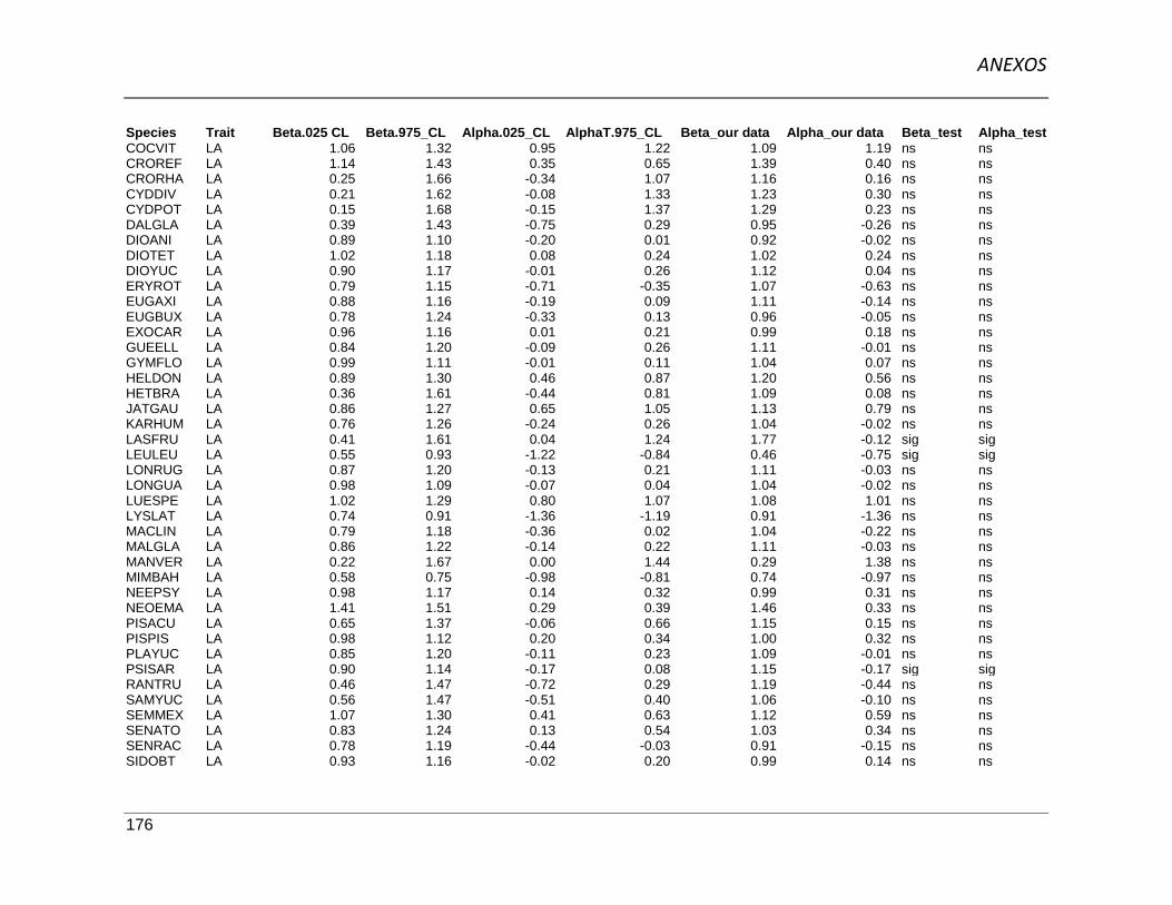
ANEXOS

176

Species Trait Beta.025 CL Beta.975_CL Alpha.025_CL AlphaT.975_CL Beta_our data Alpha_our data Beta_test Alpha_testCOCVIT LA 1.06 1.32 0.95 1.22 1.09 1.19 ns nsCROREF LA 1.14 1.43 0.35 0.65 1.39 0.40 ns nsCRORHA LA 0.25 1.66 -0.34 1.07 1.16 0.16 ns nsCYDDIV LA 0.21 1.62 -0.08 1.33 1.23 0.30 ns nsCYDPOT LA 0.15 1.68 -0.15 1.37 1.29 0.23 ns nsDALGLA LA 0.39 1.43 -0.75 0.29 0.95 -0.26 ns nsDIOANI LA 0.89 1.10 -0.20 0.01 0.92 -0.02 ns nsDIOTET LA 1.02 1.18 0.08 0.24 1.02 0.24 ns nsDIOYUC LA 0.90 1.17 -0.01 0.26 1.12 0.04 ns nsERYROT LA 0.79 1.15 -0.71 -0.35 1.07 -0.63 ns nsEUGAXI LA 0.88 1.16 -0.19 0.09 1.11 -0.14 ns nsEUGBUX LA 0.78 1.24 -0.33 0.13 0.96 -0.05 ns nsEXOCAR LA 0.96 1.16 0.01 0.21 0.99 0.18 ns nsGUEELL LA 0.84 1.20 -0.09 0.26 1.11 -0.01 ns nsGYMFLO LA 0.99 1.11 -0.01 0.11 1.04 0.07 ns nsHELDON LA 0.89 1.30 0.46 0.87 1.20 0.56 ns nsHETBRA LA 0.36 1.61 -0.44 0.81 1.09 0.08 ns nsJATGAU LA 0.86 1.27 0.65 1.05 1.13 0.79 ns nsKARHUM LA 0.76 1.26 -0.24 0.26 1.04 -0.02 ns nsLASFRU LA 0.41 1.61 0.04 1.24 1.77 -0.12 sig sigLEULEU LA 0.55 0.93 -1.22 -0.84 0.46 -0.75 sig sigLONRUG LA 0.87 1.20 -0.13 0.21 1.11 -0.03 ns nsLONGUA LA 0.98 1.09 -0.07 0.04 1.04 -0.02 ns nsLUESPE LA 1.02 1.29 0.80 1.07 1.08 1.01 ns nsLYSLAT LA 0.74 0.91 -1.36 -1.19 0.91 -1.36 ns nsMACLIN LA 0.79 1.18 -0.36 0.02 1.04 -0.22 ns nsMALGLA LA 0.86 1.22 -0.14 0.22 1.11 -0.03 ns nsMANVER LA 0.22 1.67 0.00 1.44 0.29 1.38 ns nsMIMBAH LA 0.58 0.75 -0.98 -0.81 0.74 -0.97 ns nsNEEPSY LA 0.98 1.17 0.14 0.32 0.99 0.31 ns nsNEOEMA LA 1.41 1.51 0.29 0.39 1.46 0.33 ns nsPISACU LA 0.65 1.37 -0.06 0.66 1.15 0.15 ns nsPISPIS LA 0.98 1.12 0.20 0.34 1.00 0.32 ns nsPLAYUC LA 0.85 1.20 -0.11 0.23 1.09 -0.01 ns nsPSISAR LA 0.90 1.14 -0.17 0.08 1.15 -0.17 sig sigRANTRU LA 0.46 1.47 -0.72 0.29 1.19 -0.44 ns nsSAMYUC LA 0.56 1.47 -0.51 0.40 1.06 -0.10 ns nsSEMMEX LA 1.07 1.30 0.41 0.63 1.12 0.59 ns nsSENATO LA 0.83 1.24 0.13 0.54 1.03 0.34 ns nsSENRAC LA 0.78 1.19 -0.44 -0.03 0.91 -0.15 ns nsSIDOBT LA 0.93 1.16 -0.02 0.20 0.99 0.14 ns ns

ANEXOS

177

Species Trait Beta.025 CL Beta.975_CL Alpha.025_CL AlphaT.975_CL Beta_our data Alpha_our data Beta_test Alpha_testTABALB LA 0.26 1.69 -0.12 1.31 1.72 -0.15 sig sigTABCHR LA 0.85 1.28 0.20 0.63 1.05 0.43 ns nsTALOLI LA 0.86 1.23 0.02 0.39 1.01 0.24 ns nsTHOPAU LA 0.93 1.09 -0.18 -0.02 1.01 -0.10 ns nsVITGAU LA 0.92 1.16 0.40 0.64 1.08 0.48 ns nsXIMAME LA 0.45 1.45 -0.62 0.39 1.24 -0.41 ns nsZAPFOR LA 0.50 1.41 -0.91 0.00 1.14 -0.64 ns nsSENGAU LDMC 0.38 0.39 0.01 0.02 0.39 0.01 ns nsACAPEN LDMC 0.38 0.39 0.04 0.05 0.38 0.05 ns nsAMPPA1 LDMC 0.37 0.40 0.00 0.03 0.40 0.00 ns nsAPHSCA LDMC 0.32 0.40 -0.13 -0.05 0.38 -0.11 ns nsARRPUB LDMC 0.37 0.40 0.00 0.03 0.40 0.00 sig sigBAUDIV LDMC 0.37 0.41 0.02 0.06 0.40 0.03 ns nsBAUUNG LDMC 0.38 0.40 0.01 0.03 0.40 0.01 sig sigBOUPUL LDMC 0.36 0.38 -0.10 -0.08 0.39 -0.11 sig sigBUNSWA LDMC 0.37 0.39 -0.02 0.00 0.38 -0.01 ns nsBURSIM LDMC 0.37 0.38 -0.07 -0.06 0.38 -0.07 sig sigCAEGAU LDMC 0.39 0.40 0.07 0.08 0.40 0.07 ns nsCALPAL LDMC 0.37 0.39 -0.02 0.00 0.38 -0.01 ns nsCARCOR LDMC 0.32 0.41 -0.18 -0.09 0.36 -0.13 ns nsCHLMAN LDMC 0.37 0.40 0.04 0.07 0.39 0.05 ns nsCNIACO LDMC 0.30 0.40 -0.25 -0.15 0.36 -0.21 ns nsCOCACA LDMC 0.36 0.40 -0.04 0.00 0.39 -0.03 ns nsCOCSPI LDMC 0.38 0.39 -0.01 0.00 0.37 0.01 sig sigCOCVIT LDMC 0.36 0.38 -0.11 -0.09 0.38 -0.11 sig sigCROREF LDMC 0.33 0.36 -0.08 -0.05 0.35 -0.07 ns nsCRORHA LDMC 0.33 0.42 -0.03 0.06 0.39 0.00 ns nsCYDDIV LDMC 0.33 0.42 -0.04 0.05 0.36 0.02 ns nsCYDPOT LDMC 0.34 0.42 -0.02 0.06 0.38 0.02 ns nsDALGLA LDMC 0.35 0.41 -0.06 0.00 0.40 -0.05 ns nsDIOANI LDMC 0.38 0.40 0.01 0.03 0.39 0.02 ns nsDIOTET LDMC 0.37 0.38 -0.01 0.00 0.38 -0.01 ns nsDIOYUC LDMC 0.38 0.40 0.05 0.07 0.39 0.06 ns nsERYROT LDMC 0.38 0.40 0.04 0.06 0.39 0.05 ns nsEUGAXI LDMC 0.38 0.40 0.01 0.03 0.39 0.02 ns nsEUGBUX LDMC 0.38 0.40 0.02 0.04 0.40 0.02 ns nsEXOCAR LDMC 0.37 0.38 -0.03 -0.02 0.38 -0.03 sig sigGUEELL LDMC 0.37 0.39 0.00 0.02 0.39 0.00 ns nsGYMFLO LDMC 0.39 0.39 0.01 0.01 0.39 0.01 ns nsHELDON LDMC 0.34 0.38 -0.16 -0.12 0.38 -0.16 sig sigHETBRA LDMC 0.35 0.41 -0.02 0.04 0.39 0.00 ns ns

ANEXOS

178

Species Trait Beta.025 CL Beta.975_CL Alpha.025_CL AlphaT.975_CL Beta_our data Alpha_our data Beta_test Alpha_testJATGAU LDMC 0.36 0.39 -0.15 -0.12 0.38 -0.14 ns nsKARHUM LDMC 0.37 0.40 0.01 0.04 0.39 0.02 ns nsLASFRU LDMC 0.32 0.40 -0.14 -0.06 0.35 -0.09 ns nsLEULEU LDMC 0.35 0.37 -0.08 -0.06 0.34 -0.05 sig sigLONRUG LDMC 0.37 0.39 -0.01 0.01 0.39 -0.01 ns nsLONGUA LDMC 0.38 0.39 -0.01 0.00 0.38 0.00 ns nsLUESPE LDMC 0.38 0.39 0.00 0.01 0.38 0.01 ns nsLYSLAT LDMC 0.39 0.40 0.05 0.06 0.38 0.07 sig sigMACLIN LDMC 0.36 0.38 -0.05 -0.03 0.38 -0.05 ns nsMALGLA LDMC 0.37 0.39 -0.03 -0.01 0.38 -0.02 ns nsMANVER LDMC 0.33 0.42 0.03 0.12 0.32 0.13 sig sigMIMBAH LDMC 0.39 0.39 0.02 0.02 0.39 0.02 ns nsNEEPSY LDMC 0.38 0.39 -0.02 -0.01 0.39 -0.02 sig sigNEOEMA LDMC 0.40 0.40 0.01 0.01 0.40 0.01 ns nsPISACU LDMC 0.36 0.40 -0.11 -0.07 0.39 -0.10 ns nsPISPIS LDMC 0.37 0.38 -0.05 -0.04 0.38 -0.05 ns nsPLAYUC LDMC 0.37 0.39 0.03 0.05 0.37 0.05 sig sigPSISAR LDMC 0.38 0.40 0.02 0.04 0.40 0.02 ns nsRANTRU LDMC 0.35 0.40 -0.02 0.03 0.39 -0.01 ns nsSAMYUC LDMC 0.35 0.40 -0.08 -0.03 0.39 -0.07 ns nsSEMMEX LDMC 0.37 0.38 -0.04 -0.03 0.37 -0.03 ns nsSENATO LDMC 0.36 0.39 -0.10 -0.07 0.38 -0.09 ns nsSENRAC LDMC 0.36 0.39 -0.06 -0.03 0.37 -0.04 ns nsSIDOBT LDMC 0.38 0.40 0.04 0.06 0.39 0.05 ns nsTABALB LDMC 0.31 0.40 -0.20 -0.11 0.40 -0.20 ns nsTABCHR LDMC 0.37 0.39 -0.03 -0.01 0.39 -0.03 ns nsTALOLI LDMC 0.38 0.40 0.09 0.11 0.40 0.09 ns nsTHOPAU LDMC 0.38 0.39 0.01 0.02 0.38 0.02 ns nsVITGAU LDMC 0.37 0.39 -0.03 -0.01 0.37 -0.01 ns nsXIMAME LDMC 0.36 0.42 0.02 0.08 0.36 0.08 sig sigZAPFOR LDMC 0.36 0.41 0.02 0.07 0.39 0.04 ns nsSENGAU LP 0.20 0.30 0.13 0.23 0.14 0.28 sig sigACAPEN LP 0.14 0.29 -0.34 -0.20 0.31 -0.36 sig sigAMPPA1 LP 0.10 0.46 0.04 0.40 0.12 0.38 ns nsAPHSCA LP -0.16 0.49 -0.51 0.14 0.21 -0.22 ns nsARRPUB LP 0.12 0.42 0.06 0.36 0.23 0.25 ns nsBAUDIV LP 0.07 0.42 0.01 0.35 0.27 0.16 ns nsBAUUNG LP 0.14 0.31 -0.06 0.12 0.28 -0.03 ns nsBOUPUL LP 0.21 0.34 0.34 0.47 0.27 0.41 ns nsBUNSWA LP 0.02 0.28 -0.61 -0.35 0.05 -0.38 ns nsBURSIM LP 0.29 0.37 0.49 0.57 0.28 0.58 sig sig

ANEXOS

179

Species Trait Beta.025 CL Beta.975_CL Alpha.025_CL AlphaT.975_CL Beta_our data Alpha_our data Beta_test Alpha_testCAEGAU LP 0.20 0.30 0.07 0.17 0.26 0.11 ns nsCALPAL LP 0.06 0.23 -0.38 -0.21 0.15 -0.31 ns nsCARCOR LP -0.19 0.57 -0.13 0.63 0.54 -0.10 ns nsCHLMAN LP 0.09 0.34 -0.14 0.11 0.18 0.02 ns nsCNIACO LP -0.16 0.73 0.55 1.44 0.30 0.98 ns nsCOCACA LP 0.07 0.38 -0.02 0.28 0.19 0.17 ns nsCOCSPI LP 0.20 0.33 0.09 0.22 0.34 0.08 sig sigCOCVIT LP 0.26 0.44 0.70 0.88 0.38 0.76 ns nsCROREF LP 0.26 0.43 0.15 0.32 0.39 0.19 ns nsCRORHA LP -0.23 0.57 -0.64 0.16 0.37 -0.44 ns nsCYDDIV LP -0.23 0.64 -0.22 0.64 0.19 0.22 ns nsCYDPOT LP -0.23 0.59 -0.33 0.50 0.43 -0.17 ns nsDALGLA LP -0.09 0.51 -0.33 0.27 0.36 -0.18 ns nsDIOANI LP -0.07 0.09 -0.69 -0.53 0.00 -0.60 ns nsDIOTET LP -0.01 0.11 -0.46 -0.34 0.15 -0.49 sig sigDIOYUC LP 0.10 0.26 -0.37 -0.21 0.19 -0.30 ns nsERYROT LP 0.05 0.26 -0.78 -0.57 0.04 -0.57 sig sigEUGAXI LP -0.04 0.14 -0.61 -0.43 -0.03 -0.44 ns nsEUGBUX LP -0.03 0.24 -0.57 -0.30 -0.08 -0.25 sig sigEXOCAR LP 0.14 0.26 -0.14 -0.03 0.13 -0.01 sig sigGUEELL LP 0.08 0.29 -0.53 -0.32 0.09 -0.33 ns nsGYMFLO LP -0.02 0.07 -0.53 -0.45 -0.01 -0.46 ns nsHELDON LP 0.15 0.39 0.19 0.43 0.34 0.23 ns nsHETBRA LP -0.27 0.42 -0.68 0.00 0.22 -0.49 ns nsJATGAU LP 0.15 0.39 0.49 0.73 0.04 0.84 sig sigKARHUM LP 0.08 0.35 -0.40 -0.13 0.17 -0.22 ns nsLASFRU LP -0.16 0.51 -0.37 0.31 0.23 -0.09 ns nsLEULEU LP 0.20 0.36 0.12 0.28 0.42 0.06 sig sigLONRUG LP 0.24 0.44 0.23 0.43 0.37 0.30 ns nsLONGUA LP 0.27 0.33 0.07 0.13 0.28 0.12 ns nsLUESPE LP 0.13 0.28 -0.22 -0.07 0.12 -0.06 sig sigLYSLAT LP 0.26 0.35 0.43 0.51 0.27 0.51 ns nsMACLIN LP 0.00 0.22 -0.64 -0.42 -0.10 -0.32 sig sigMALGLA LP 0.00 0.22 -0.52 -0.30 -0.06 -0.24 sig sigMANVER LP -0.21 0.67 0.14 1.03 0.48 0.33 ns nsMIMBAH LP 0.16 0.22 -0.12 -0.05 0.27 -0.17 sig sigNEEPSY LP 0.15 0.26 -0.17 -0.05 0.14 -0.05 sig sigNEOEMA LP 0.30 0.35 0.06 0.11 0.36 0.05 sig sigPISACU LP 0.02 0.44 -0.10 0.31 0.17 0.16 ns nsPISPIS LP 0.23 0.31 0.30 0.39 0.30 0.31 ns nsPLAYUC LP 0.14 0.35 0.19 0.39 0.29 0.24 ns ns

ANEXOS

180

Species Trait Beta.025 CL Beta.975_CL Alpha.025_CL AlphaT.975_CL Beta_our data Alpha_our data Beta_test Alpha_testPSISAR LP 0.02 0.17 -0.52 -0.36 0.00 -0.35 sig sigRANTRU LP -0.13 0.42 -0.58 -0.03 0.12 -0.28 ns nsSAMYUC LP -0.09 0.40 -0.85 -0.36 0.05 -0.50 ns nsSEMMEX LP 0.10 0.23 -0.27 -0.14 0.21 -0.26 ns nsSENATO LP 0.13 0.38 0.33 0.57 0.25 0.45 ns nsSENRAC LP 0.13 0.36 0.10 0.33 0.27 0.19 ns nsSIDOBT LP 0.13 0.26 -0.29 -0.16 0.15 -0.18 ns nsTABALB LP -0.23 0.57 -0.48 0.33 0.37 -0.28 ns nsTABCHR LP 0.18 0.45 0.46 0.73 0.29 0.62 ns nsTALOLI LP 0.13 0.35 0.07 0.28 0.14 0.27 ns nsTHOPAU LP 0.23 0.32 0.16 0.25 0.23 0.25 sig sigVITGAU LP 0.19 0.33 0.60 0.75 0.31 0.63 ns nsXIMAME LP -0.24 0.35 -0.89 -0.29 0.24 -0.78 ns nsZAPFOR LP -0.04 0.45 -0.07 0.43 0.23 0.15 ns nsSENGAU SLA 126.38 133.27 44.70 51.59 128.08 49.89 ns nsACAPEN SLA 119.41 128.02 -2.46 6.15 123.16 2.40 ns nsAMPPA1 SLA 115.16 133.82 -6.71 11.95 126.35 0.76 ns nsAPHSCA SLA 111.65 156.88 36.90 82.13 133.36 60.42 ns nsARRPUB SLA 115.95 132.35 -6.96 9.44 124.80 0.59 ns nsBAUDIV SLA 116.23 135.19 1.65 20.61 117.47 19.37 ns nsBAUUNG SLA 127.27 139.25 26.30 38.28 131.08 34.47 ns nsBOUPUL SLA 119.37 126.60 -6.39 0.84 122.38 -2.17 ns nsBUNSWA SLA 115.49 128.82 -16.88 -3.55 121.64 -9.70 ns nsBURSIM SLA 120.53 124.08 -7.49 -3.94 122.17 -5.58 ns nsCAEGAU SLA 118.84 124.32 -13.78 -8.30 121.43 -10.89 ns nsCALPAL SLA 113.68 123.46 -23.55 -13.77 114.55 -14.64 ns nsCARCOR SLA 111.25 169.28 126.45 184.48 125.19 170.54 ns nsCHLMAN SLA 116.45 129.62 -1.10 12.07 130.77 -2.25 sig sigCNIACO SLA 105.67 158.69 60.03 113.05 102.97 115.75 sig sigCOCACA SLA 116.59 134.93 23.80 42.14 123.44 35.29 ns nsCOCSPI SLA 105.84 115.71 -48.47 -38.60 109.57 -42.33 ns nsCOCVIT SLA 122.79 130.68 17.22 25.11 129.85 18.05 ns nsCROREF SLA 125.61 134.95 9.03 18.37 119.75 24.23 sig sigCRORHA SLA 95.98 146.37 -68.41 -18.02 115.35 -37.39 ns nsCYDDIV SLA 99.84 148.86 -1.94 47.08 110.65 36.27 ns nsCYDPOT SLA 99.09 151.48 -16.01 36.38 117.86 17.61 ns nsDALGLA SLA 107.45 143.13 19.64 55.32 129.52 33.25 ns nsDIOANI SLA 123.22 129.72 4.33 10.83 127.44 6.61 ns nsDIOTET SLA 118.36 123.48 -9.03 -3.91 121.64 -7.19 ns nsDIOYUC SLA 114.65 124.38 -30.97 -21.24 118.17 -24.76 ns nsERYROT SLA 119.43 131.10 11.20 22.87 124.42 17.88 ns ns

ANEXOS

181

Species Trait Beta.025 CL Beta.975_CL Alpha.025_CL AlphaT.975_CL Beta_our data Alpha_our data Beta_test Alpha_testEUGAXI SLA 115.92 123.87 -15.91 -7.96 115.79 -7.83 sig sigEUGBUX SLA 103.52 121.95 -51.93 -33.50 122.43 -52.41 sig sigEXOCAR SLA 121.89 128.12 2.09 8.32 126.19 4.02 ns nsGUEELL SLA 118.61 130.73 3.45 15.57 123.83 10.35 ns nsGYMFLO SLA 124.26 127.70 3.99 7.43 125.70 5.99 ns nsHELDON SLA 126.26 149.89 69.39 93.02 131.41 87.87 ns nsHETBRA SLA 112.13 157.44 17.59 62.90 113.46 61.57 ns nsJATGAU SLA 118.20 132.17 18.46 32.43 125.27 25.36 ns nsKARHUM SLA 117.18 132.35 8.36 23.53 120.00 20.71 ns nsLASFRU SLA 114.12 164.40 71.88 122.16 165.58 70.70 sig sigLEULEU SLA 135.29 152.06 57.59 74.36 159.09 50.56 sig sigLONRUG SLA 114.40 125.02 -16.51 -5.89 121.82 -13.31 ns nsLONGUA SLA 129.04 132.84 8.10 11.90 126.77 14.17 sig sigLUESPE SLA 122.92 131.08 21.21 29.37 134.17 18.12 sig sigLYSLAT SLA 116.75 121.58 -28.37 -23.54 120.94 -27.73 ns nsMACLIN SLA 128.03 142.39 46.48 60.84 130.79 58.08 ns nsMALGLA SLA 116.05 126.84 -12.90 -2.11 122.13 -8.19 ns nsMANVER SLA 97.51 148.14 -29.07 21.56 158.89 -39.82 sig sigMIMBAH SLA 125.95 129.45 7.89 11.39 127.00 10.34 ns nsNEEPSY SLA 117.13 123.47 -20.08 -13.74 124.15 -20.76 sig sigNEOEMA SLA 118.90 121.45 -4.14 -1.59 121.22 -3.91 ns nsPISACU SLA 111.47 134.99 8.26 31.78 118.33 24.92 ns nsPISPIS SLA 117.34 121.89 -33.66 -29.11 121.40 -33.17 ns nsPLAYUC SLA 117.29 128.53 -15.57 -4.33 122.45 -9.49 ns nsPSISAR SLA 116.46 124.38 -14.58 -6.66 121.93 -12.13 ns nsRANTRU SLA 111.60 142.24 5.49 36.13 125.58 22.15 ns nsSAMYUC SLA 113.58 147.06 47.64 81.12 133.16 61.54 ns nsSEMMEX SLA 109.41 117.95 -36.61 -28.07 116.13 -34.79 ns nsSENATO SLA 117.79 130.28 0.81 13.30 124.74 6.35 ns nsSENRAC SLA 119.45 131.97 9.78 22.30 123.20 18.55 ns nsSIDOBT SLA 112.63 121.40 -50.08 -41.31 122.30 -50.98 sig sigTABALB SLA 105.54 155.23 34.68 84.37 120.73 69.18 ns nsTABCHR SLA 118.93 132.78 7.80 21.65 127.48 13.10 ns nsTALOLI SLA 114.43 127.36 -31.10 -18.17 122.94 -26.68 ns nsTHOPAU SLA 123.93 128.77 8.90 13.74 125.86 11.81 ns nsVITGAU SLA 118.62 126.51 -21.39 -13.50 120.00 -14.88 ns nsXIMAME SLA 105.01 137.97 -32.73 0.23 113.31 -8.07 ns nsZAPFOR SLA 111.39 139.54 27.36 55.51 122.22 44.68 ns nsSENGAU SV -1.80 -1.68 -0.15 -0.03 -1.71 -0.12 ns nsACAPEN SV -1.79 -1.64 0.00 0.15 -1.74 0.10 ns nsAMPPA1 SV -2.18 -1.53 -1.47 -0.82 -1.97 -1.03 ns ns

ANEXOS

182

Species Trait Beta.025 CL Beta.975_CL Alpha.025_CL AlphaT.975_CL Beta_our data Alpha_our data Beta_test Alpha_testAPHSCA SV -2.14 -1.38 -0.84 -0.08 -1.63 -0.59 ns nsARRPUB SV -1.98 -1.61 -1.09 -0.72 -1.78 -0.92 ns nsBAUDIV SV -1.87 -1.50 0.19 0.56 -1.72 0.41 ns nsBAUUNG SV -1.84 -1.61 -0.14 0.10 -1.88 0.14 sig sigBOUPUL SV -1.79 -1.65 -0.12 0.02 -1.74 -0.03 ns nsBUNSWA SV -1.87 -1.56 -0.06 0.25 -1.63 0.01 ns nsBURSIM SV -1.64 -1.56 0.41 0.49 -1.68 0.53 sig sigCAEGAU SV -1.65 -1.52 0.57 0.70 -1.67 0.72 sig sigCALPAL SV -1.84 -1.60 -0.15 0.10 -1.56 -0.19 sig sigCARCOR SV -2.25 -1.20 -0.39 0.67 -1.88 0.29 ns nsCHLMAN SV -1.78 -1.57 0.26 0.47 -1.69 0.38 ns nsCNIACO SV -2.22 -1.18 -0.09 0.95 -1.27 0.00 ns nsCOCACA SV -1.79 -1.50 0.79 1.08 -1.66 0.96 ns nsCOCSPI SV -1.61 -1.44 0.48 0.65 -1.46 0.50 ns nsCOCVIT SV -1.78 -1.65 -0.05 0.08 -1.82 0.12 sig sigCRORHA SV -2.23 -1.11 0.09 1.21 -1.29 0.27 ns nsCYDDIV SV -2.47 -1.31 -1.69 -0.53 -1.74 -1.26 ns nsCYDPOT SV -2.28 -1.20 -0.23 0.85 -1.68 0.24 ns nsDIOANI SV -1.74 -1.59 0.53 0.68 -1.71 0.65 ns nsDIOTET SV -1.65 -1.50 0.63 0.78 -1.55 0.68 ns nsDIOYUC SV -1.73 -1.54 0.64 0.84 -1.63 0.73 ns nsERYROT SV -1.88 -1.65 -0.44 -0.22 -1.82 -0.27 ns nsEUGAXI SV -1.73 -1.53 0.45 0.65 -1.63 0.56 ns nsEUGBUX SV -1.86 -1.51 0.32 0.67 -1.77 0.58 ns nsGUEELL SV -1.79 -1.58 0.22 0.44 -1.81 0.45 sig sigGYMFLO SV -2.07 -1.96 -1.04 -0.93 -1.92 -1.08 sig sigHELDON SV -1.97 -1.75 -1.25 -1.03 -1.94 -1.06 ns nsJATGAU SV -1.74 -1.49 1.15 1.40 -1.78 1.44 sig sigKARHUM SV -1.82 -1.53 0.24 0.53 -1.64 0.35 ns nsLASFRU SV -2.25 -1.50 -2.02 -1.27 -2.30 -1.23 sig sigLEULEU SV -1.82 -1.64 -0.13 0.06 -1.72 -0.05 ns nsLUESPE SV -1.90 -1.73 -0.66 -0.49 -1.83 -0.57 ns nsLYSLAT SV -1.84 -1.76 -0.29 -0.20 -1.70 -0.35 sig sigMACLIN SV -2.02 -1.77 -1.23 -0.98 -1.94 -1.06 ns nsMALGLA SV -1.84 -1.64 -0.22 -0.01 -1.86 0.01 sig sigMANVER SV -2.25 -1.17 0.03 1.11 -1.77 0.63 ns nsMIMBAH SV -1.83 -1.74 -0.31 -0.22 -1.83 -0.22 sig sigNEEPSY SV -1.77 -1.64 0.06 0.19 -1.70 0.11 ns nsNEOEMA SV -1.95 -1.82 -0.58 -0.45 -1.95 -0.45 ns nsPISACU SV -1.92 -1.39 0.37 0.91 -1.54 0.52 ns nsPISPIS SV -1.78 -1.70 -0.18 -0.11 -1.75 -0.14 ns ns

ANEXOS

183

Species Trait Beta.025 CL Beta.975_CL Alpha.025_CL AlphaT.975_CL Beta_our data Alpha_our data Beta_test Alpha_testPSISAR SV -1.81 -1.63 -0.05 0.13 -1.69 0.01 ns nsRANTRU SV -2.05 -1.26 0.60 1.40 -1.99 1.34 ns nsSEMMEX SV -1.74 -1.59 0.27 0.43 -1.60 0.29 ns nsSENATO SV -1.76 -1.51 0.79 1.04 -1.73 1.02 ns nsSIDOBT SV -1.71 -1.56 0.65 0.80 -1.68 0.77 ns nsTABALB SV -2.26 -1.20 -0.28 0.78 -2.10 0.62 ns nsTABCHR SV -1.95 -1.69 -1.31 -1.05 -1.89 -1.11 ns nsTALOLI SV -1.70 -1.44 1.16 1.42 -1.57 1.29 ns nsTHOPAU SV -1.84 -1.74 -0.35 -0.25 -1.69 -0.41 sig sigVITGAU SV -1.66 -1.50 1.33 1.49 -1.53 1.36 ns nsZAPFOR SV -2.04 -1.43 -0.42 0.19 -1.64 -0.22 ns ns

Null models of trait correlations.

Summary data from trait correlations result from 999 iterations of null model. Correlation of our data are also shown. If our

values were below percentile 2.5 or above percentile 97.5, they were considered significant (sig). Otherwise were not significant

(ns).

Traits Variable Media D.E. Mín Máx Percentil 2.5 Percentil 97.5 Our data pLDMC-LA Alpha -0.432 0.043 -0.599 -0.266 -0.514 -0.348 -0.3245 nsLDMC-LP Alpha -0.357 0.046 -0.497 -0.218 -0.441 -0.267 -0.3086 nsLP-LA Alpha 0.29 0.039 0.166 0.407 0.212 0.365 0.3424 nsSLA-LA Alpha 0.042 0.05 -0.12 0.211 -0.054 0.145 -0.0179 nsSLA-LDMC Alpha -0.619 0.027 -0.702 -0.481 -0.664 -0.562 -0.6319 nsSLA-LP Alpha 0.117 0.051 -0.046 0.271 0.017 0.223 0.0705 nsSLA-WSG Alpha -0.41 0.039 -0.542 -0.275 -0.477 -0.32 -0.4145 nsSV-LA Alpha 0.025 0.038 -0.109 0.207 -0.05 0.097 0.019 nsSV-LDMC Alpha 0.114 0.043 -0.033 0.243 0.023 0.196 0.0787 nsSV-LP Alpha 0.051 0.041 -0.084 0.194 -0.024 0.137 0.0642 nsSV-SLA Alpha -0.361 0.037 -0.465 -0.23 -0.434 -0.285 -0.2908 nsSV-WSG Alpha 0.077 0.04 -0.105 0.179 -0.006 0.153 0.0439 nsWSG-LA Alpha -0.397 0.037 -0.511 -0.263 -0.471 -0.326 -0.3998 nsWSG-LDMC Alpha 0.53 0.036 0.346 0.622 0.452 0.59 0.5364 nsWSG-LP Alpha -0.446 0.037 -0.564 -0.303 -0.514 -0.371 -0.4259 nsLDMC-LA Beta -0.212 0.169 -0.77 0.398 -0.525 0.117 0.1997 nsLDMC-LP Beta -0.269 0.152 -0.74 0.183 -0.563 0.054 -0.366 ns

ANEXOS

184

LP-LA Beta 0.171 0.141 -0.362 0.566 -0.12 0.442 -0.0004 nsSLA-LA Beta -0.251 0.159 -0.709 0.524 -0.543 0.072 -0.3108 nsSLA-LDMC Beta -0.368 0.162 -0.851 0.13 -0.666 -0.055 -0.4011 nsSLA-LP Beta 0.068 0.162 -0.373 0.706 -0.23 0.38 0.1084 nsSLA-WSG Beta -0.006 0.178 -0.654 0.485 -0.41 0.338 -0.1635 nsSV-LA Beta 0.148 0.178 -0.374 0.606 -0.216 0.485 -0.182 nsSV-LDMC Beta -0.126 0.189 -0.567 0.52 -0.475 0.264 0.2055 nsSV-LP Beta 0.269 0.185 -0.399 0.706 -0.133 0.589 0.1286 nsSV-SLA Beta -0.353 0.162 -0.778 0.24 -0.649 -0.006 -0.651 <0.05SV-WSG Beta -0.14 0.184 -0.599 0.46 -0.481 0.235 0.1331 nsWSG-LA Beta -0.099 0.161 -0.624 0.49 -0.383 0.219 -0.1671 nsWSG-LDMC Beta 0.252 0.212 -0.424 0.886 -0.189 0.64 0.1823 nsWSG-LP Beta -0.296 0.162 -0.726 0.328 -0.599 0.052 -0.0837 ns

Appendix 7.6 Principal Component Analysis of topography, soil variables and forest stand age.

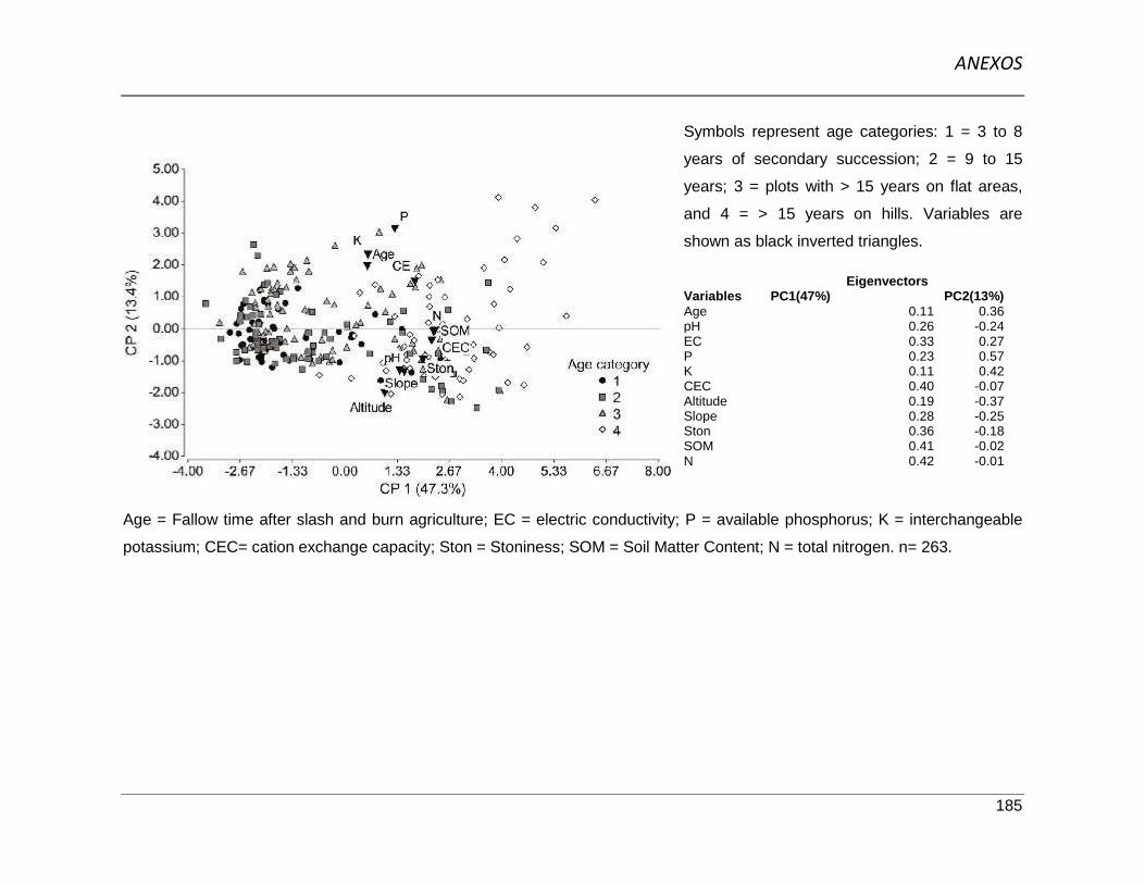
ANEXOS

185

Symbols represent age categories: 1 = 3 to 8

years of secondary succession; 2 = 9 to 15

years; 3 = plots with > 15 years on flat areas,

and 4 = > 15 years on hills. Variables are

shown as black inverted triangles.

EigenvectorsVariables PC1(47%) PC2(13%)Age 0.11 0.36pH 0.26 -0.24EC 0.33 0.27P 0.23 0.57K 0.11 0.42CEC 0.40 -0.07Altitude 0.19 -0.37Slope 0.28 -0.25Ston 0.36 -0.18SOM 0.41 -0.02N 0.42 -0.01

Age = Fallow time after slash and burn agriculture; EC = electric conductivity; P = available phosphorus; K = interchangeable

potassium; CEC= cation exchange capacity; Ston = Stoniness; SOM = Soil Matter Content; N = total nitrogen. n= 263.

ANEXOS

186

Appendix 7.7 Reduced multiple linear regressions models of plot mean trait values with successional age and environmental variables.

For each trait the minimum model is shown, according to akaike criterion and hypothesis testing procedures.

Trait R² Adj. R² AIC Coef Est. SE T p-value

LA 0.1 0.09 240.67 const -3.64 1.56 -2.34 0.0199

Age 0.41 0.08 5.05 <0.0001

pH 3.84 1.58 2.44 0.0156

N -0.17 0.05 -3.39 0.0008

LDMC 0.08 0.07 -1258.16 const 0.39 0.01 27.56 <0.0001

Age 0.02 0.0044 4.56 <0.0001

CEC -0.02 0.01 -2.19 0.0293

PL 0.27 0.25 -110.49 const -0.02 0.25 -0.09 0.9275

Age -0.32 0.04 -7.74 <0.0001

P -0.08 0.04 -2.11 0.0358

Slope -0.22 0.09 -2.6 0.0100

SOM 0.06 0.03 2.28 0.0236

N -0.13 0.06 -2.34 0.0198

Ston 0.23 0.11 2.12 0.0352

SLA 0.08 0.07 2130.41 const 379.57 56.51 6.72 <0.0001

Age -8.4 2.91 -2.88 0.0040

pH -256.99 57.29 -4.49 <0.0001

N 4.81 1.86 2.58 0.0100

SV 0.23 0.22 175.59 const -1.76 0.1 -17.81 <0.0001

ANEXOS

187

Trait R² Adj. R² AIC Coef Est. SE T p-value

P -0.27 0.07 -3.8 0.0002

K 0.26 0.09 2.83 0.0050

Ston 0.73 0.17 4.26 <0.0001

SOM 0.06 0.03 1.98 0.0490

WSG 0.02 0.02 -647.04 const 0.68 0.04 15.1 <0.0001

CEC 0.06 0.03 2.3 0.0200

PL = petiole length; LA = leaf or leaflet area; LDMC = leaf dry matter content; SLA = specific leaf area, WSG = wood specific gravity, SV =

seed volume. Age = Fallow time after slash and burn agriculture; CEC= cation exchange capacity; K = interchangeable potassium; N = Soil

total nitrogen; Ston = Stoniness; SOM = Soil Matter Content; P = available phosphorus. Variables where transformed, but original names are

used for clarity. n= 263.

Centro de Investigación Científica de Yucatán, AC

Documents

Transcript of Centro de Investigación Científica de Yucatán, AC