Commodity prices, money and inflation - European Central Bank
Upload
khangminh22Category
view
3download
0
CEREMCENTRAL EUROPEAN REVIEW
OF ECONOMICS AND MANAGEMENT
WSB University in Wrocław
Vol.2, No.1, March 2018 ISSN 2543-9472e-ISSN 2544-0365

CENTRAL EUROPEAN REVIEW OF ECONOMICS AND MANAGEMENT
Volume 2, Number 1 March 2018
Wydawnictwo: Wyższa Szkoła Bankowa we Wrocławiu, ul. Fabryczna 29-31, 53-609 Wrocław
Vol. 2, No. 1
Editors:
Francisco Vargas and Ali Emrouznejad
Applications of Data Envelopment Analysis in Developing
Countries

3
Editor-in-chief: Prof. Johannes (Joost) Platje, [email protected]
Secretary of editorial board: Dr. Tomasz Rólczyński, [email protected]
Members of editorial board: Prof. Michael Wheeler, Harvard Business School, USA; Prof.
John Hall, University of Pretoria, South Africa; Prof. Petr Polák, University of Brunei
Darussalam, Brunei; Prof. Yanping Zhao, Ocean University in Qingdao, China; Dr Corrado
Topi, University of York, England; Dr. Wim Westerman, University of Groningen, The
Netherlands; Dr. Ynte van Dam, University of Wageningen, The Netherlands; Prof. Francisco
Vargas, University of Sonora, Mexico; Prof. Mike Ellenbecker, University of Massachusetts
Lowell, USA; Prof. Diana Pociovalisteanu, “Constantin Brancusi” University of Targu-Jiu,
Romania; Prof. Thomas Weith, Leibniz-Zentrum für Agrarlandschaftsforschung e.V.,
Germany; Prof. Barbara Despiney-Żochowska, University Paris 1 Pantheon-Sorbonne,
France; Prof. Walter Leal Filho, Hamburg University of Applied Sciences, Germany; Prof.
Tatjana Tambovceva, Riga Technical University, Latvia; Prof. Osvaldo Quelhas, Federal
Fluminense Universidade, Brazil; Prof. Valentina Pidlisnyuk, Jan Evangelista Purkyne
University, Czech Republic; Dr. Les Duckers, University of Coventry, United Kingdom; Dr.
Wytze van der Gaast, JIN Climate and Sustainability, Netherlands; Prof. Jena Laage-
Hellmann, Chalmers University of Technology, Sweden; Prof. Vasilij Szwec, Mining
University in Dniepropietrovsk, Ukraine; Prof. Jan Vachal, VSTE v Ceskich Budejovicach,
Czech Republic; Prof Ali Emrouznejad, Aston University, United Kingdom; Prof. Marian
Noga, WSB University in Wrocław, Poland; Prof. Aniela Styś, WSB University in Wrocław,
Poland; Prof. Piotr Migoń, The University of Wrocław, Poland; Prof. Marek Bugdol,
Jagiellonian University, Poland.
Advisory board: Prof. Stefan Forlicz, WSB University in Wrocław, Poland; Prof. Jacek
Mercik, WSB University in Wrocław, Poland; Prof. Jaroslav Nenadal, Technical University
of Ostrava, Czech Republic; Dr. Wim Lambrechts, Open University of The Netherlands, The
Netherlands; Dr. Luis Velazquez, University of Sonora, Mexico; Prof. Jana Brauweiler,
University of Applied Science Zittau/Görlitz, Germany; Prof. Jarl Kampen, University of
Anwerp, Belgium; Prof. Ralph Wrobel, Westsaxonian University of Applied Science,
Germany; Prof. Diana Cibulskiene, Siauliai University, Lithuania; Prof. Stanisław Styś, WSB
University in Wrocław, Poland; Prof. Krzysztof Łobos, WSB University in Wrocław, Poland;
Prof. Jacek Unold, WSB University in Wrocław, Poland; Prof. Maciej Jasiński, WSB
University in Wrocław, Poland; Dr Bolesław Goranczewski, WSB University in Wrocław,
Faculty of Economics in Opole, Poland; Prof. Piotr Jedynak, Jagiellonian University, Poland;
Prof. Andrzej Bujak, WSB University in Wrocław, Poland.
Contact: Tomasz Rólczyński, [email protected], +48 71 376 23 43, ul. Fabryczna
29-31, 53-609 Wrocław, Poland
The journal is reviewed according to the principle of double blind peer review, as well as in
compliance with the standards of the Polish Ministry of Science and Higher Education.
CEREM is a continuation of the WSB University in Wrocłąw Research Journal (Zeszyty
Naukowe WSB we Wrocławiu – ISSN 1643-7772; eISSN 2392-1153), which is included in B
list of the Polish Ministry of Science and Higher Education from 23.12.2015 (8 points).
CEREM is registered in the IC Journal Master List, and indexed in CEJSH, Index Copernicus
and BazEkon
Copyright by Wyższa Szkoła Bankowa we Wrocławiu
ISSN 2543-9472; eISSN 2544-0365
Cover and logo design: Sebprojekt.pl Wydawnictwo: Wyższa Szkoła Bankowa we Wrocławiu, ul. Fabryczna 29-31, 53-609, Wrocław.

4

5
CONTENTS
1. Francisco VARGAS, Ali EMROUZNEJAD, Editorial ............................. 7
2. Swati RAJU, Assessing the Efficiency of Urban Co-operative Banks in
India ………………………………………………………………………. 11
3. Alexandra Maria RIOS CABRAL, Francisco S. RAMOS, Efficiency
container ports in Brazil: A DEA and FDH approach ……………………. 43
4. Berna H. Ulutas, Efficiency analysis of airports in Turkey considering
environmental effects …………………………………………………….. 65
5. Rajani Neeraj MATHUR, Swati RAJU RAMNATH, Efficiency in Food
Grains Production in India using DEA and SFA …………………………. 79
6. Anoop SINGH, DEA Based Approach to Set Energy Efficiency Target
Under PAT Framework: A Case of Indian Cement Industry …………… 103
7. Cees Johannes GELDERMAN, Jelle DE JONGE, Jos SCHIJNS, Janjaap
SEMEIJN, Investigating Cooperative Purchasing Performance - a survey of
purchasing professionals in Dutch hospitals ……………………………. 133
8. Peter SCHOLTZ, David GROSSMANN, Sinan KRUECKEBERG, Better
the Devil You Know that the Devil You don’t – financial crises between
ambiguity aversion and selective perception ……………………………. 155
9. Anna MOTYLSKA – KUŹMA, Alternative Finance and Sustainable
Development …………………………………………………………….. 175

CENTRAL EUROPEAN REVIEW OF ECONOMICS AND MANAGEMENT ISSN 2543-9472; eISSN 2544-0365
www.cerem-review.eu
www.ojs.wsb.wroclaw.pl Vol. 2, No. 1, 7-11, March 2018
Correspondence address: Ali Emrouznejad, Aston Business School, Aston University, Birmingham B4
7ET, UK. E-mail: [email protected].
© 2018 WSB UNIVERSITY IN WROCŁAW
EDITORIAL - Applications of Data Envelopment
Analysis in developing dountries
Francisco VARGAS
University of Sonora, Hermosillo, Mexico
Ali EMROUZNEJAD
Aston University, UK
The Central European Review of Economics and Management (CEREM) has
been recognized for the cutting edge and pertinence of topics selected for
publication. In the previous issue, Data Envelopment Analysis (DEA) has been
widely used in measuring efficiency in developing countries. This issue follows the
same topic with five papers on DEA, analyzing analyze a variety of themes of
efficiency matters in developing countries. In addition to the five DEA articles, there
are three more papers that, respectively, refer to the performance of the cooperative
purchasing in healthcare, the emotional bias decisions during financial crises, and
the alternative finance of sustainable development.
The paper by Swati Raju examined the efficiency of co-operative banks in India
using both Stochastic Frontier Analysis (SFA) and DEA analysis. The study finds
moderate to high efficiency in banking activities. Deposits and loans disbursed
emerge as major determinant of efficiency for core banking activities. Off balanced
activities also showed a considerable degree of efficiency.
In an interesting article Anoop Singh and Bharat Sharma present a DEA based
approach to set an energy efficiency target in the cement industry in India. The study
proposes an alternative target setting a method based on DEA, which takes into
account technical and operational differences across the industrial plants. Within

Francisco VARGAS, Ali EMROUZNEJAD
8
Perform, Achieve, and Trade (PAT) framework, the authors highlight the efficacy of
DEA methodology in implementing the PAT scheme.
Alexandra María Ríos Cabral and Francisco S. Ramos, in their contribution, aim
to evaluate the technical efficiency of 44 Brazilian port terminals that handled
containers during 2016. For this purpose, the authors applied output oriented DEA
and Free Disposal Hull (FDH) models. The main result show that half of the
terminals have an inefficient infrastructure with idle capacity. Additionally, a strong
relationship between terminal size and degree of specialization with efficiency was
found.
This is followed by the next paper by Berna H. Ulutas that refers to efficiency
evaluation of “green airports” in Turkey. The author introduces a DEA model to
assess the efficiency of 22 airports in Turkey with pollutant emissions as an
undesirable output. Airport location shows up as a critical factor on environment
pollution. Likewise, the weather and proximity to tall buildings or hills have a
significant impact on environmental quality.
In their paper, Rajani Neraj Mathur and Swati Raju Ramanath, seek to analyze
efficiency in production of food grains for India using data for the period 1960-1961
and 2013-2014. Using DEA and SFA, the authors maintain that the problem of food
security lies not in shortage but in an imbalance in distribution. In addition, the
authors argue that food security requires more than one strategy to transform the
current patterns and practices of production, distribution and consumption of food.
The main purpose of the study by Cees Johannes Gelderman, Jelle De Jonge, Jos
Schijns and Janjaap Semeijn, is to find an explanation for performance of co-
operative purchasing in healthcare. By investigating the roll of trust, commitment,
organizational factors and interpersonal skills, the authors developed a conceptual
model for performance of co-operative purchasing. The model has been empirically
validated using a survey of 88 Dutch hospital purchasing professionals. Such
analysis showed a significant impact of trust and commitment in cooperative
purchasing groups on performance. Although proper IT support is often neglected
in healthcare organizations, efforts to improve IT systems facilitate the tactical
cooperative purchasing process.

EDITORIAL
9
Peter Scholz, David Grossmann, Sinan Krueckeberg present a paper in which
they hypothesize that during financial crisis market participants are presumably
prone to emotional bias decisions. The authors use the economic policy uncertainty
indicator, the Dow Jones Industrial Average and the Nikkei 225 GARCH volatilities
to test the ambiguity aversion and selective perception of investors. For most crises,
the authors found a significant link between uncertainty and market volatility.
However, as far as ambiguity aversion is concerned, the causality differs between
crises indicating that investors not always are driven by uncertainty.
The paper by Anna Motylska-Kuzma aims to evaluate alternative finance for
implementation of basic assumptions and goals of sustainable development. The
author uses comparative analysis of the common methods of alternative finance. The
results show that despite many features that indicate the inclusion of alternative
finance, the basic assumptions and goals of sustainable development are arbitrary.
Finally, the editorial team of CEREM ratifies its commitment to provide the
reader with a newly generated knowledge. We hope the readers will find the present
content useful. Likewise, we are grateful to all authors and the many reviewers who
helped us to make the current issue a reality. Specially, Prof. Joost (Johannes) Platje,
Editor in-Chief, who kindly guided and supported us in every task that preparation
of this issue required.

CENTRAL EUROPEAN REVIEW OF ECONOMICS AND MANAGEMENT ISSN 2543-9472; eISSN 2544-0365
www.cerem-review.eu
www.ojs.wsb.wroclaw.pl Vol. 2, No. 1, 11-42, March 2018
Correspondence address: Swati Raju, Mumbai School of Economics and Public Policy, University of
Mumbai, Mumbai 400 098. India. E-mail: [email protected].
Received: 15-09-2017, Revised: 19-12-2017, Revised: 12-01-2018, Accepted: 17-01-2018
doi: http://dx.doi.org/10.29015/cerem.550
© 2018 WSB UNIVERSITY IN WROCŁAW
Assessing the efficiency of urban co-operative
banks in India
Swati RAJU
Mumbai School of Economics and Public Policy, University of Mumbai, India
Abstract:
Aim: Urban Co-operative Banks are a small albeit significant constituent in the multi-stage credit delivery mechanism of the banking sector in India. These banks have an organisational, managerial and regulatory structure different from commercial banks. It is, therefore, of interest to study the efficiency with which these banks perform their core banking and off balance sheet activities. This paper focuses on the measurement of efficiency in the conduct of core banking and off balance sheet activities for the period 2013-14 to 2015-16.
Design / Research methods: The main idea is to employ the parametric Stochastic Frontier Analysis and the non-parametric Data Envelopment Analysis to measure the efficiency of Urban Co-operative Banks. We estimate two models for both the frontier methods, Model A examines the efficiency in core banking activity and Model B for the off balance sheet activities. The analysis of super efficiency undertaken helps identify the most efficient bank while the quartile analysis provides an insight into the distribution of efficiency (for both Models A and B). A Tobit model (for both Models A and B) has also been estimated to identify the determinants of efficiency.
Conclusions / findings: We find that Urban Co-operative banks display a higher mean efficiency in core banking activities (Model A) as compared to the off-balance sheet activities (Model B) and this finding has been reiterated by the frequency distribution of efficiency for both the frontier methods. The difference in the mean efficiency obtained for Models A and B is much wider under the stochastic frontier analysis. The analysis of super efficiency points out that of the three banks efficient under Model A and five efficient banks under Model only one bank is common to both the models. The quartile analysis highlights that 38.9 percent of the UCBs are ranked in the lower two quartiles of efficiency. The Tobit regression model has identified deposits and loans disbursed as significant determinants of efficiency for both models.
Originality / value of the article: This study contributes significantly to the existent gap in the literature on efficiency measurement of banks in India by focusing on efficiency measurement among urban co-operative banks who play an important role in urban financial inclusion.
Implications of the research: This study is the only study that has measured the efficiency in operations of Urban Co-operative Banks and can hence provide an insight into the operations of these banks. It can also help individual banks in taking appropriate measures to improve efficiency. Key words: urban co-operative banks; efficiency, super efficiency JEL: E5, C6.

Swati RAJU
12
1. Introduction
Banks in India can be broadly classified into commercial and co-operative
banks. Both these groups of banks are also known as scheduled banks as they are
included in the Second Schedule of the Banking Regulation Act, 1965. Co-operative
banks are organized in the co-operative sector and operate in urban and rural areas.
There is no formal definition of Urban Co-operative Banks (UCBs) and the
reference is to primary co-operative banks located in urban and semi-urban areas.
These banks have traditionally focused on communities, localities, and workplace
groups, and play a crucial role in mobilising resources from lower and middle
income groups in urban areas. They essentially lend to small borrowers and
businesses. A benefit that UCBs possess is the low cost structure and the flexibility
they can provide to the local community by being more responsive to their needs.
UCBs in India are registered as co-operative societies under the provisions of State
(Provincial) Co-operative Societies Acts or Multi State (Province) Co-operative
Societies Acts and are licensed to undertake the business of banking under
provisions of the Banking Regulation Act, 1949. UCBs, in turn, are further classified
into scheduled and non-scheduled. Scheduled UCBs are those which have a deposit
base exceeding INR 1,000 million and can avail of a borrowing/loan facility from
the Reserve Bank of India. This facility is not available to non-scheduled UCBs.
The beginnings of co-operative banking in India goes back to the end-nineteenth
century and was consequent to the successful co-operative experiments in Britain
and Germany. The problems of rural indebtedness towards the end of the 19th
century also created an environment conducive to the growth of chit funds and co-
operative societies. Co-operatives are based on the tenets of mutual help, democratic
decision making, and open membership. The first known co-operative bank or
mutual aid society in the country was the "Anyonya Sahakari Mandali" established
in the princely State of Baroda in 1889. As the movement gained strength, it led to
the enactment of the Co-operative Credit Societies Act, 1904, and later to a more
comprehensive Co-operative Societies Act, 1912. The Government of India Act in
1919 transferred the subject of "Co-operation" from itself to the Provincial
Governments. The Government of Bombay passed the first State Co-operative

ASSESSING THE EFFICIENCY OF URBAN CO-OPERATIVE BANKS IN INDIA
13
Societies Act in 1925 which led to an important phase in the evolution of co-
operative credit institutions in the country. The Multi-Unit Co-operative Societies
Act, 1942, was enacted to cover societies with membership from more than one
province. The emergence of several national federations of co-operative societies in
various functional areas along with several different laws governing the same type
of societies led to the consolidation of the laws governing co-operative societies
under a comprehensive Central legislation - the Multi-State Co-operative Societies
Act, 1984, which covered banks with a presence in several States (provinces). From
March 1, 1966, co-operative banks that had a paid-up share capital and reserves of
Rs. 1 Lakh and more were brought under the purview of the Banking Regulation
Act, 1949, and hence under the supervisory control of the Reserve Bank of India.
The deposits of UCBs are covered under Deposit Insurance from 1968 up to Rs. 1
Lakh only.
It is pertinent to note that although commercial banks form the mainstay of the
banking system in India, the role played by co-operative banks cannot be
underestimated and these banks constitute a vital component in the multi-stage
credit delivery mechanism in rural as well as urban areas (Chakrabarty 2003). There
has been a tremendous increase in the total number of UCBs in the country from
1,307 in 1991 to 1,574 as of end-March 2016 accompanied by a humungous
increase in the deposits and advances of UCBs. Of the 1,574 UCBs, 52 are
categorised as Scheduled UCBs and 1,522 as Non-Scheduled UCBs. Deposits
increased by 38.61 times from INR 101570 million in end March 1991 to INR
3,92,1794 million as of end March 2016. Advances given by UCBs also increased
by 30.61 times from INR 80030 million to INR 24,50,125 million in March 2016.
Although the deposits and advances of UCBs have seen a manifold increase over
time, their share in the overall deposits and advances of the banking system in India
as of end-March 2016 is at a mere 3.5 percent and 3.1 percent respectively
(Appendix Table 1). Further, UCB presence is geographically skewed with
concentration in a few regions and States (provinces). The regional distribution of
UCBs as of end March 2016 indicates a concentration of UCBs in the Western and
Southern regions which together account for 81.8 percent of the total UCBs in the
country (Appendix Table 2). Within the dominant regions, States (provinces) such

Swati RAJU
14
as Maharashtra, Gujarat, Karnataka, Andhra Pradesh, and Tamil Nadu account for
more than 80 percent of the UCBs (Appendix Table 3). The concentration in these
States can be attributed to the prevalence of a strong co-operative movement and
emergence of a strong co-operative leadership (Chakrabarty 2009).
Despite being a small segment of the banking system, UCBs play a vital role in
urban financial inclusion. The Census of India 2011 has highlighted the fast pace of
urbanization in the country which has increased from 27.81 percent in 2001 to 31.16
percent in 2011. The Census 2011 has also noted that for the first time since
Independence, the absolute increase in population in urban areas has been greater
than the increase in rural areas. UCBs, with their well-established connections with
specific communities, enjoy the trust of small savers and borrowers. The local nature
of their operations and the intermingling with the local community provide a natural
advantage in achieving wider urban financial inclusion. The High Power Committee
on Urban Co-operative Banks constituted by the RBI in 1999 recognized the critical
role played by UCBs in urban financial inclusion -‘the co-operative credit endeavour
was the first ever attempt at micro credit dispensation in India’ (Chakrabarty 2009).
UCBs predominantly offer banking services to businessmen, small traders, artisans,
factory workers, and salaried people in urban and semi-urban areas. Several artisans
and small businessmen are under-banked and often find it difficult to access large
commercial banks. UCBs cater to the needs of this population and hence can emerge
as major players in urban financial inclusion through their outreach and provision of
customized services (Reserve Bank of India 2005).
Efficiency studies relating to banks in India have focused mainly on the
performance of scheduled commercial banks along with a comparison of the
performance of private and foreign banks. Studies that measure the efficiency of co-
operative banks and particularly UCBs are few and this paper seeks to contribute to
the literature on efficiency measurement of scheduled UCBs in India. Section II of
the paper presents a brief discussion on the different approaches to measure bank
efficiency. Section III presents a brief review of efficiency studies with reference to
Indian banks including the literature concerning co-operative banks in India. Section
IV discusses the methodology, and the empirical evidence is presented in Section V.
Section VI concludes the paper.

ASSESSING THE EFFICIENCY OF URBAN CO-OPERATIVE BANKS IN INDIA
15
2. Approaches to measure banking efficiency
The literature on banking efficiency identifies two approaches to study and
measure efficiency, namely the production approach and the intermediation
approach (Humphrey 1985; Hjalmarsson et al. 2000). The production approach, first
discussed by Benston (1965), views banks as entities that provide services to
customers such as loans and other financial services. The focus is the number and
type of transactions and/or services provided by a bank over a given period of time.
Data on such details is often difficult to obtain in the public domain and a common
proxy often used is the number of deposits and loan accounts. This approach centres
on operating costs and includes physical variables and their costs. The
intermediation approach discussed by Sealey and Lindley (1977) views banks as
financial intermediaries who transfer funds from one set of agents (depositors) to
another set of agents (creditors). Assets created by the bank through loans and
advances, securities, and investments generate income while deposits of the bank are
liabilities and interest has to be paid by the bank. This approach considers interest as
well as operating costs.
Berger and Humphrey (1977) have pointed out that the intermediation approach
is better suited to examine bank-level efficiency as at the bank level the focus is
often on being cost efficient whereas the production approach is apt for studying
branch-level efficiency. Processing of transactions normally takes place at the
branch level and hence efficiency measurement in processing transactions and
services, the focus of the production approach, is best studied at the branch level.
3. Review of efficiency studies relating to banks in India
The literature on efficiency measurement of banks, internationally and in India,
is extensive. The review, consequently, concentrates on major studies that have used
frontier methods to examine the efficiency of banks in India including a few studies
on co-operative banks in the country. Table 1 presents the details of these studies.
The focus of these studies has been a comparative assessment of different types of

Swati RAJU
16
efficiency among commercial banks in India viz. technical, cost, revenue, and profit
efficiency. Table 1, thus, highlights the paucity of work on efficiency measurement
of co-operative banks and more so of urban co-operative banks. This study seeks to
fill this gap in the measurement of efficiency of urban co-operative banks in India by
analysing technical efficiency for the period 2013-14 to 2015-16.
Table 1. Major studies on banking efficiency in India
Author(s) Method
Used
Focus of the
Study
Period
of Study
Findings
Bhattacharya et
al. (1997)
DEA
and
SFA
Productive/Tec
hnical
efficiency of
commercial
banks
1986-
1991
Public sector banks were most efficient
followed by foreign banks and private
banks.
Sathye (2003) DEA Productive
efficiency of
commercial
banks
1997-
1998
Efficiency of public and private sector
banks was comparable to the efficiency
of foreign banks in India. Public sector
banks were found to be more efficient
than private sector banks.
Shanmugam,
Das (2004)
SFA Technical
efficiency of
commercial
banks
1992-
1999
Wide variations observed across bank
groups in raising interest margins and
non-interest income. Efficiency in
raising interest margins was time
invariant while that of non-interest
income was time varying. The State
Bank group and foreign banks
performed better than the nationalized
banks and private sector banks.
Das, Ghosh
(2006)
DEA Technical
efficiency of
commercial
banks
1992-
2002
Wide variation in the technical
efficiency of banks and medium-sized
public sector banks operated at higher
levels of efficiency. More efficient
banks were seen to have lower non-
performing assets.
Bhattacharya,
Pal (2013)
SFA Impact of
financial sector
reforms on
technical
efficiency of
commercial
banks
1989-
2009
Impact of financial sector reforms on
technical efficiency was mixed.
Decline in efficiency observed for
public sector and private sector banks
for a large part of the post reform
period. Public sector banks displayed
higher efficiency as compared to
private sector banks and foreign banks.

ASSESSING THE EFFICIENCY OF URBAN CO-OPERATIVE BANKS IN INDIA
17
Table 1. Cont. Author(s) Method
Used
Focus of the
Study
Period
of Study
Findings
Kumbhakar,
Sarkar (2003)
SFA Cost
efficiency of
commercial
banks
1986-
2000
Improvement in cost efficiency over
the time period. Cost efficiency in
private sector banks was higher than
public sector banks. Decline in
inefficiency was slower in the post
deregulation period compared to the
pre-deregulation period.
Das et al. (2005) DEA Technical
efficiency,
cost
efficiency,
revenue
efficiency,
and profit
efficiency of
commercial
banks
1997-
2003
Improvement in the median efficiency
scores of Indian banks, in general, and
particularly of bigger banks. No major
difference observed for technical and
cost efficiency whereas sharp
differences were observed for revenue
and profit efficiency.
Sensarma
(2005)
SFA Cost and
profit
efficiency of
commercial
banks
1986-
2003
Improvement in cost efficiency and a
decline in profit efficiency observed
during the period. Domestic banks
(public sector and private sector) were
found to be more efficient than foreign
banks. Public sector banks showed
greater cost efficiency while private
sector banks showed higher profit
efficiency.
Kumar, Gulati
(2010)
DEA Cost,
technical, and
allocative
efficiency of
public sector
banks in India
1993-
2008
Deregulation had a positive impact on
the cost efficiency of banks. An upward
trend observed for technical efficiency
whereas a declining trend seen for
allocative efficiency. Cost inefficiency
of banks was largely due to technical
inefficiency rather than allocative
inefficiency. Alpha and beta
convergence was observed for cost
efficiency.
Mahesh, Bhide
(2008)
SFA Impact of
financial
sector reforms
on cost, profit,
and loan
efficiency of
commercial
banks
1985-
2004
Competition in the post de-regulation
period had a significant impact on cost
and profit efficiencies while loan
efficiency did not display significant
improvement. Wide variations seen
across different bank groups.

Swati RAJU
18
Table 1. Cont. Author(s) Metho
d
Used
Focus of the
Study
Period
of Study
Findings
Studies pertaining to Co-operative Banks in India
Ramesh, Patel
(1999)
Growth
performance
of urban co-
operative
banks
1975-
1994
A phenomenal growth seen in the
number of bank branches, membership,
share capital, reserves, deposits and
advances. This growth was, however,
accompanied by a huge increase in
borrowings by UCBs.
Shah (2001,
2007)
Performance
of rural co-
operative
credit
institutions in
Maharashtra
1981-
2003
A slowdown in growth of membership
and institutional financing, rapid
increase in outstanding against loan
advances. Major challenges include
high transactions costs, poor repayment
record, growing non-performing assets
and wilful default.
Chander,
Chandel
(2010)
Financial
ratio
analysis
Evaluate
performance
of four
District
Central Co-
operative
Banks in
Haryana
1998-
2009.
All four banks in the bankruptcy zone
which could be attributed to financial
mismanagement and underutilization of
resources.
Bhatt, Bhat
(2013)
DEA Technical
efficiency of
eight co-
operative
banks in
Jammu &
Kashmir and
identify
factors which
influence
efficiency
2001-07 3 of the 8 banks were found to be
efficient under CRS-DEA model while
5 of 8 banks were efficient under the
VRS-DEA model. Better management
of deposits, loan recovery, investment
and improving skill of staff could
improve efficiency.
Gaurav,
Krishnan
(2017)
DEA and
SFA
Technical
efficiency of
District
Central Co-
operative
Banks in India
2002-14 Substantial variation in the efficiency
of District Central Co-operative Banks
across States. Adoption of better
technology and improvement in
management can help improve
efficiency.
Note: Commercial banks refers to public sector, private sector, and foreign banks in India.

ASSESSING THE EFFICIENCY OF URBAN CO-OPERATIVE BANKS IN INDIA
19
4. Methodology
Bank performance has been traditionally measured using financial ratio analysis.
The drawback of this approach is that it tends to aggregate several aspects of
performance and can be misleading as it depends on an arbitrary benchmark ratio
both of which may not help assess the long term performance of banks (Sherman,
Gold 1985; Yeh 1986). Sherman and Gold (1985) were the first study to apply
frontier methods to measure banking efficiency. The non-parametric Data
Envelopment Analysis (DEA) and the parametric Stochastic Frontier Analysis
(SFA) have been extensively employed in efficiency measurement in recent times.
Other frontier methods used are the free disposal hull, thick frontier, and the
distribution free approaches (Sathye 2003). The parametric SFA requires the
specification of a functional form whereas the nonparametric DEA uses
mathematical programming. Seiford and Thrall (1990) write ‘that the kind of
mathematical programming procedure used by DEA for efficient frontier estimation
is comparatively robust’. The mathematical formulations of the DEA models can be
converted to simpler formulations which are easier to estimate using the linear
programming (LP) procedure to estimate relative efficiency in decision making units
(DMUs) and can be used to calculate the best practice production frontier for firms
(Ali, Seiford 1993). A main property of DEA is that it does not require any a priori
assumptions about the functional form and the distribution of the error term (Coelli
1995).
Efficiency of a DMU, in this case a bank, can be defined as the ability with
which it can convert inputs to outputs and is calculated as the ratio of outputs to
inputs. Efficiency can also be defined as the ratio of minimum costs that would have
to be incurred to the actual costs incurred to produce a given level of output and
efficiency measures always lie between 0 and 1.
4.1. Stochastic frontier analysis
Stochastic Frontier Analysis (SFA) was developed by Aigner et al. (1977) and
Meeusen and Van den Broeck (1977). The approach requires that a functional form
be specified for the frontier production function. An advantage of SFA over DEA is

Swati RAJU
20
that it takes into account measurement errors and other noise in the data (Latruffe et
al. 2004).
Suppose a producer has a production function f(xi, a). In a world with no
inefficiency, the firm i would produce
(1)
where, iy = output; xi = vector of inputs ; a = vector of parameters to be estimated.
A fundamental element of SFA is that each firm can potentially produce less than its
maximum capacity due to inefficiency which renders the production function as:
1.....i N (2)
where, i i ie v u , is a composite of two error terms:
(i) vi is a normally distributed error term representing measurement and specification
error or noise and represents factors beyond the control of the firm;
(ii) ui is a one sided error term which represents inefficiency i.e. the inability to
produce the maximum level of output given the inputs used. The component ui is
assumed to be distributed independently of vi and to satisfy ui ≥ 0. The non-
negativity of the technical inefficiency term reflects the fact that if ui ≥ 0 the unit
(firm or country or state) will not produce at the maximum attainable level. The
generalization of the specification of ui by Battese and Coelli (1988) is given by
or .
A measure of inefficiency can be obtained by means of the parameter γ which is
defined as
(3)
where, 2
v and 2
u are the variances of the noise and inefficiency effects
respectively.
The value of γ lies between 0 and 1. If it is close to zero then deviations from the
frontier can be attributed to noise, while if the value of γ is close to 1, then
deviations from the frontier can be attributed to technical inefficiency (Battese,
Corra 1977; Tran et al. 2008; Coelli et al. 2005).
Another measure of inefficiency can be obtained from the parameter λ (Aigner
et al. 1977) which is computed as:

ASSESSING THE EFFICIENCY OF URBAN CO-OPERATIVE BANKS IN INDIA
21
02
2
2 v
u
(4)
4.2. Data Envelopment Analysis
The Data Envelopment Analysis (DEA) method allows the generalization of the
single output/input technical efficiency measure to multiple outputs/inputs by
constructing a relative efficiency measure. DEA models can be estimated either
under constant returns to scale or variable returns to scale. The Constant Returns to
Scale (CRS) efficiency is obtained by solving the Charnes, Cooper and Rhodes
(CCR) model. The CRS model estimates the gross efficiency of a DMU which
reflects technical and scale efficiency. The efficiency of transforming inputs into
output denotes technical efficiency while scale efficiency estimates that most
productive scale size which is the scale at which efficiency is 100 percent. The
Banker, Charnes and Cooper (BCC) model measures the Variable Returns to Scale
(VRS) efficiency. This model takes into consideration the variation in efficiency
with respect to the scale of operation and therefore measures pure technical
efficiency. The scale efficiency of a DMU can be calculated as the ratio of its CRS
to VRS efficiency. The CRS efficiency of a firm is always less than or equal to its
VRS efficiency. Thus, other things being equal, the VRS model gives the highest
efficiency score while the CRS model gives the lowest score. The focus in DEA
models on variable returns is mainly to ascertain whether a DMU exhibits
decreasing, increasing, or constant returns to scale rather than to quantify the degree
of returns to scale (Fukuyama 2000).
Depending on the orientation, DEA models can be expressed either as output-
oriented (maximization) or input-oriented (minimization) models. The output-
oriented DEA model seeks to maximize output production for a given level of
resources whereas the input-oriented envelopment model aims to produce the
observed output with minimum inputs. Thus, the dual of the output-maximizing
DEA model is the input-oriented envelopment model and vice versa (Ramanathan
2003).
An input-oriented CRS-DEA model of cost efficiency for a bank can be
expressed as (Färe, Grosskopf 1985):

Swati RAJU
22
(5)
where, wi denotes the vector of input prices for bank i; the first condition states that
the output of bank i cannot be less than a linear combination λi of the output of all
banks Y; the second inequality states that the input vector of bank i cannot be greater
than a linear combination λi of the input vectors of all banks X. Solving the above
equation gives the minimum costs and a comparison of minimum costs to actual
costs gives an estimate of cost efficiency.
The measure of technical inefficiency obtained from the input-oriented DEA
models corresponds to Farell’s input-based measure of technical inefficiency. The
estimates of efficiency obtained from the input-oriented and output-oriented
measures would be similar under the CRS model but are unequal for the VRS model
as the CRS-DEA model is only appropriate when all firms are operating at optimal
scale. However, due to imperfect competition or constraints on finance, firms may
not operate at the optimal scale and hence an input-oriented variable return to scale
may be used to calculate technical efficiency. Further, the choice of orientation
(input or output) is dependent on which quantities (inputs or outputs) the DMU has
most control over and are the unit’s primary decision variables (Coelli et al. 2005).
Coelli and Perelman (1999) point out that the choice of orientation has only a minor
influence on the scores obtained. Coelli et al. (2005: 181) also note that ‘the output
and input oriented DEA models will estimate exactly the same frontier and
therefore, by definition, identify the same set of firms as being efficient. It is only
the inefficiency measures associated with the inefficient firms that may differ
between the two methods’.

ASSESSING THE EFFICIENCY OF URBAN CO-OPERATIVE BANKS IN INDIA
23
5. Empirical evidence
This paper seeks to measure the efficiency of UCBs in India in the framework of
the intermediation approach for the period 2013-14 to 2015-16. Efficiency has been
measured using both the frontier methods, namely stochastic frontier and data
envelopment analysis. There were 1,574 UCBs in India as of end-March 2016. Of
these, 52 banks are categorised as scheduled UCBs and 1,522 as non-scheduled
UCBs. The focus of the paper is on the efficiency of scheduled UCBs and data has
been obtained from Primary (Urban) Co-operative Bank Outlook, Reserve Bank of
India. Sathye (2003) writes, ‘the choice of inputs and outputs in DEA is a matter of
long standing debate’. The total income of a bank comprises of net interest income
and non-interest income. Although the average non-interest income of all UCBs
taken together during the period under consideration (2013-14 to 2015-16)
constituted only 10 percent of its total income, there exist huge variations among
individual banks and it contributes 16 to 20 percent of total income in some
scheduled UCBs. Besides, in recent times UCBs have expanded their off-balance
sheet activities and not taking into consideration non-interest income may not
provide a correct estimate of efficiency. This paper, therefore, considers two
separate models for the two output variables – net interest income (Model A) and
non-interest income (Model B). Model A has a single output variable - net interest
income and three input variables have been considered which reflect physical
capital, labour, and loanable funds which are proxied by the expenditure incurred on
fixed assets, labour. Interest paid is a critical variable especially for UCBs as most
co-operative banks offer a higher interest rate on deposits as compared to their
counterparts such as scheduled commercial banks. Model B concerns the non-
interest income that accrues to a bank from off-balance sheet activities. Most of
these activities are in the nature of provision of services for which the bank charges
a fee or commission and hence the input variables included are the expenditure
incurred on fixed assets and labour. All variables are values in logs.
Three of the 52 scheduled UCBs were not considered for efficiency estimation
as data for two banks – Vasai Vikas Sahakari Bank Limited and Vasavi Co-
operative Urban Bank Limited was not reported for all the years under consideration

Swati RAJU
24
while the net interest income of Rupee Co-operative Bank Limited was negative
during the period under consideration. Since no major year to year variations were
seen in either the output or input variables for the time period under consideration, it
was decided to measure efficiency by taking the average value of the output and
input variables. A brief description of the variables used in the estimation is in Table
2.
Table 2. Description of variables used in the empirical analysis
Variable Description
Output Variables
Net Interest Income (LNETINTINC)
Interest Earned–Interest Expended (Paid) refers
to the income earned from traditional/core
banking activities such as accepting deposits,
lending and investment in government and other
securities; interest paid by banks on deposits and
interest paid on borrowings from the RBI and
other agencies
Non-Interest Income
(LNONINTINC)
Income from off–balance sheet activities and
includes fees, commissions, exchange and
brokerage; profit & loss from foreign exchange
operations; trading and sale of securities; sale of
fixed and other assets and dividend income
Input Variables
Price of Physical Capital or Fixed
Assets (LFXDASSET)
Rent, taxes and lighting, printing and stationery,
depreciation on bank’s property, repairs and
maintenance and insurance
Price of labour (LSAL) Payments and provisions for employees
Price of loanable funds (LINTPD) Interest paid on deposits and borrowings from
the Reserve Bank of India and other agencies
Note: All variables are expressed in INR million and expressed as natural logs in
estimation. Source: Author’s own elaboration.
Table 3 presents the descriptive statistics of the variables used in the estimation
of the DEA and SFA models and in the Tobit regression model. It can be seen that
the least average input cost/expenditure is on fixed assets followed by salary and
payments to staff. Among output variables, the average for non-interest income is
much higher than that of net interest income. A comparison of the standard deviation
of both these output variables indicates that the variations in non-interest income
among UCBs is much higher than for net interest income given that there exists a

ASSESSING THE EFFICIENCY OF URBAN CO-OPERATIVE BANKS IN INDIA
25
huge peer pressure among UCBs to maintain a similarity in interest rates offered on
deposits. The wide range observed in share capital, deposits, investments, and loans
also points to the vast heterogeneity in the operations of scheduled UCBs.
Table 3. Descriptive statistics of variables (INR Million)
Statistic Mean Minimum Maximum Standard
Deviation
Net Interest Income 1020 82 6179 1168
Non- Interest Income 3484 204 26460 4763
Interest Paid 2464 122 20280 3614
Expenditure Incurred on Fixed Assets 206 13 1292 280
Expenditure Incurred on Salary and
Payments to Staff
385 36 2997 478
Share Capital 620 74 3351 598
Deposits 33013 1452 275354 47462
Investments 10580 865 83105 14865
Loans 21350 689.9 178781 31381
Source: Author’s own elaboration.
5.1 Results of stochastic frontier analysis
The variables considered in the stochastic frontier model are similar to the
output and input variables considered for DEA (described in Table 2). The results of
the SFA models are given in Table 4. The dependent variable in Model A is log of
net interest income while expenditure incurred on fixed assets, salary and other
payments, and interest paid are the explanatory variables. It can be observed that
interest paid by a bank has a statistically significant impact (at 1 percent level of
significance) on the net interest income earned by the bank. The relationship
between the expenditure incurred on fixed assets such a rent etc. although positive is
not statistically significant while a negative albeit not significant relationship is seen
between the expenditure incurred on labour and the net interest income of a bank.
The lambda (λ) parameter is 0.64 and statistically significant at 5 percent clearly
indicating that the existence of technical inefficiency and deviations from the
frontier are not entirely due to noise. Inefficiency contributes on average almost 64
percent to the value of λ over this period.

Swati RAJU
26
Table 4. Results of stochastic frontier analysis
Model A Model B
constant 0.22
(0.52)
2.25***
(6.9)
LFXDASSET 0.04
(0.48)
0.48***
(5.61)
LSAL -0.07
(-0.54)
0.61***
(5.32)
LINTPD 0.91***
(6.96) --
λ 0.64**
(1.64)
1.70**
(2.09)
p- values are in parentheses. *** = p < 0.01; ** = p < 0.05; * = p < 0.10
λ is the estimate of the term in equation (4) Source: Author’s own elaboration.
Model B seeks to capture the efficiency of scheduled UCBs in off-balance sheet
activities and the explanatory variables considered are the expenditure incurred on
fixed assets and salary and other payments. Both these explanatory variables are
positive and statistically significant at 1 percent level. Further, the statistically
significant λ (lambda) statistic reveals high inefficiency in off-balance sheet
activities undertaken by the scheduled UCBs. A comparison of the λ statistic for
Models A and B indicates that scheduled UCBs display inefficiency in both core
banking activity as well as in their expanded non-core off-balance sheet activities.
Further, the inefficiency is much higher (170 percent) in the non-core operations. A
frequency distribution of efficiency for Models A and B along with the respective
mean efficiency is presented in Table 5 which shows that the mean efficiency of
Model A is higher than that of Model B implying thereby that scheduled UCBs are
generally more efficient in traditional/core banking activities as compared to off-
balance sheet activities. A comparison of the frequency distribution of banks across
the efficiency range for Models A and B reiterates the finding. It can be observed
that all the 49 banks were in the efficiency range of 0.7 and above for Model A.
Further, 48 banks (98 percent) were in the efficiency range of 0.8 to 1 while only 1
bank was in the low efficiency range of 0.7 to 0.8.

ASSESSING THE EFFICIENCY OF URBAN CO-OPERATIVE BANKS IN INDIA
27
Table 5. Frequency distribution of efficiency scores – SFA Model
Model A
Model B
Efficiency
Range
No. of
Banks
Percent of
Banks
Efficiency
Range
No. of
Banks
Percent of
Banks
0.4 ≤ E < 0.5 -- -- 0.4 ≤ E < 0.5 2 4.08
0.5 ≤ E < 0.6 -- -- 0.5 ≤ E < 0.6 1 2.04
0.6 ≤ E < 0.7 -- -- 0.6 ≤ E < 0.7 5 10.20
0.7 ≤ E < 0.8 1 2.04 0.7 ≤ E < 0.8 18 36.73
0.8 ≤ E < 0.9 25 51.02 0.8 ≤ E < 0.9 18 36.73
0.9 ≤ E < 1 23 46.94 0.9 ≤ E < 1 5 10.20
Total 49 100.00 49 100.00
Mean
Efficiency 0.895 0.778 Source: Author’s own elaboration.
The frequency distribution for Model B shows a higher percentage of banks in
the lower ranges of efficiency - 26 banks (53.1 percent) were in the lower efficiency
range of 0.4 to 0.8 whereas only 23 banks (46.9 percent) were in the efficiency range
0.8 to 1. Of these, only 5 banks were in the highest efficiency range greater than 0.9.
5.2 Results of Data Envelopment Analysis
A two-stage input-oriented model was estimated to measure the efficiency in
banking operations of scheduled UCBs for the period 2013-14 to 2015-16. Given
that the time period under consideration is very short, a CRS-DEA model was better
suited to capture the overall efficiency. Both Models A and B have a single output
and three and two input variables respectively. Like in the case of the SFA model,
efficiency was computed for 49 of the 52 scheduled UCBs. Pastor and Ruiz (2007)
discuss DEA models such as the translation invariant model, Seiford and Zhu’s
(2002) posteriori approach, directional distance models, range directional models
and weighted additive models that allow for the inclusion of DMUs with negative
output (as in the case of Rupee Co-operative Bank which had negative net interest
income in all the three years). Most of these studies with negative data are for
models with variable returns to scale and it can be inferred that the constant returns
to scale (CCR) model cannot be used for negative data. Consequently, as per usual

Swati RAJU
28
practice, this paper does not take banks which have a negative output variable into
consideration. The efficiency estimates for both models is presented in Table 6.
Table 6. Summary of efficiency estimates: input oriented CRS- DEA Model Statistic Model A Model B
Mean 0.929 0.924
Minimum 0.804 0.800
Maximum 1 1
Standard deviation 0.040 0.050 Source: Author’s own elaboration.
The DEA models estimated indicate that the average overall efficiency as given
by the CRS-DEA model is quite high for both Model A (0.929) and Model B
(0.924). The standard deviation for both models is not very high indicating small
variations in performance among scheduled UCBs. Further, the range of efficiency
is marginally wider for banks under Model B. Given the high mean efficiency
displayed by scheduled UCBs, it would be of interest to study the distribution in
efficiency. Table 7 presents the frequency distribution of the efficiency of the CRS-
DEA model.
Table 7. Frequency distribution of technical efficiency Model A Model B
Efficiency Range
No of
Banks
Percent of
Banks No of Banks
Percent of
Banks
0.8 ≤ E < 0.9 10 20.4 16 33
0.9 ≤ E < 1 36 73.5 28 57
E = 1 3 6.1 5 10 Source: Author’s own elaboration.
It can be observed that a fifth of the scheduled UCBs have an efficiency score
that is below 0.9 (90 percent) and only 3 banks (6.1 percent) have an efficiency
score of 1 in the traditional and core banking activity (Model A). For Model B, more
than one-third of the banks have an efficiency score less than 0.9 and 5 banks (10
percent) have an efficiency score of 1. Besides, the number of banks with an
efficiency score between 0.9 and 1 is higher under Model A.

ASSESSING THE EFFICIENCY OF URBAN CO-OPERATIVE BANKS IN INDIA
29
5.3 Super efficiency and quartile analysis of efficiency
All efficient DMUs need not necessarily have the same performance level and a
disaggregation of the efficiency scores (super efficiency) of the efficient DMUs can
reveal the extent of efficiency among the efficient units. The Andersen and Petersen
(1993) super efficiency approach has been employed to obtain the estimates of super
efficiency. Table 8 presents the scores of efficiency and super efficiency for the
efficient scheduled UCBs and it can be seen that all efficient banks had feasible
solutions for Models A and B.
Table 8. Super efficiency scores of efficient banks
Model A Model B
Bank Efficiency
Score
Super
Efficiency
Score
Bank Efficiency
Score
Super
Efficiency
Score
Gopinath Patil
Parsik Janata
Sahakari Bank
Ltd.
1 1.01 Bharati Sahakari
Bank Ltd. 1 1.00
Nasik
Merchant's
Co-operative
Bank Ltd.
1 1.04
Indian Mercantile
Co-operative
Bank Ltd.
1 1.01
Sardar
Bhiladwala
Pardi Peoples
Co-operative
Bank Ltd
1 1.15
Janalaxmi Co-
operative Bank
Ltd.,
1 1.00
Mehsana Urban
Co-operative
Bank Ltd.
1 1.00
Sardar
Bhiladwala Pardi
Peoples Co-
operative Bank
Ltd.
1 1.05
Source: Author’s own elaboration.
The super efficiency scores revealed that in the case of Model A the efficiency
score of 1 actually ranged between 1.15 and 1.01 while for Model B, 3 of the 5
efficient banks had a super efficiency score of 1 itself and the highest super

Swati RAJU
30
efficiency score was 1.05 for Sardar Bhiladwala Pardi Peoples Co-operative Bank
Ltd. This bank is the only scheduled UCB that features as an efficient bank both for
Models A and B.
A quartile analysis of efficiency performance by banks revealed that all the three
efficient banks under Model A are in the best-performing fourth quartile whereas for
Model B only two banks - Mehsana Urban Co-operative Bank Ltd. and Sardar
Bhiladwala Pardi Peoples Co-operative Bank Ltd are in the fourth quartile for both
the SFA and DEA models. Using DEA analysis for Model B, the other 3 efficient
banks, however, showed huge variations in efficiency under the SFA model and
were not necessarily in the highest fourth quartile. The details of individual bank
efficiency (DEA and SFA) along with the quartile analysis is in Appendix Table 4.
Table 9. Banks with lower efficiency in model A and model B Abhyudaya Co-operative Bank Ltd.,
Mumbai Nagpur Nagrik Sahakari Bank Ltd.
Amanath Co-operative Bank Ltd.
Bangalore NKGSB Co-operative Bank Ltd., Mumbai
Bharat Co-operative Bank (Mumbai) Ltd.,
Mumbai
Nutan Nagarik Sahakari Bank Ltd.,
Ahmedabad
Cosmos Co-operative Urban Bank Ltd. Pravara Sahakari Bank Ltd.
Greater Bombay Co-operative Bank
Limited
Saraswat Co-operative Bank Ltd., Bombay
Janakalyan Sahakari Bank Ltd., Mumbai
Shamrao Vithal Co-operative Bank Ltd.
Janata Sahakari Bank Ltd., Pune.
Shikshak Sahakari Bank Ltd., Nagpur.
Kalyan Janata Sahakari Bank Ltd., Kalyan
The Akola Urban Co-operative Bank Ltd.,
Akola.
Karad Urban Co-operative Bank Ltd.
The Kapol Co-operative Bank Ltd.,
Mumbai
Mapusa Urban Co-operative Bank of Goa
Ltd., Total = 19 Scheduled UCBs
Source: Author’s own elaboration.
From a policy perspective, it is imperative to identify banks that display low
levels of efficiency in both core banking activity as well as in off-balance sheet
activities. Table 9 records 19 (38.9 percent) scheduled UCBs in the lower first two
quartiles of efficiency by either the DEA or the SFA analysis for both Models A and

ASSESSING THE EFFICIENCY OF URBAN CO-OPERATIVE BANKS IN INDIA
31
B. It is pertinent to note that there are other banks in quartiles 1 and 2 but not
included in Table 9 as they are not common to both Models A and B.
5.4 Input slacks
Input slacks are indicators of the potential areas of improvement. Table 12
presents the mean input slack for each of the input variables. The mean input slack
was almost similar for salary payments and interest paid by banks and marginally
higher on expenditure incurred by banks on fixed assets for Model A. Further, an
almost equal number of banks had a slack on each of these inputs. The analysis on
slacks also indicated that 3 banks – Goa Urban Co-operative Bank Limited, Nagpur
Nagrik Sahakari Bank Limited, and Saraswat Co-operative Bank Limited, Bombay –
had no input slacks while 46 of the 49 scheduled UCBs face a slack on at least one
input variable.
Table 10. Mean input slack values and percentage of banks having input slacks
Model A Model B
Mean Slack
Value
No. of Banks
With Slack
Mean Slack
Value
No. of
Banks With
Slack
LSAL 0.09 19 (38.8) 0.004 1 (2.0)
LFXDASSET 0.14 20 (40.8) 0.08 11 (22.5)
LINTPD 0.08 19 (38.8) -- --
No. of Banks with
Zero Slack 3 banks 6.12 percent 37 banks 75.5 percent
No. of Banks with at
least 1 Slack 46 banks 93.88 percent 12 banks 24.5 percent
Figures in parentheses indicate percentage of banks with slack
Source: Author’s own elaboration.
As concerns Model B, the average input slack on fixed assets was higher than on
salary payments. Further, 11 banks (22.5 percent) witnessed a slack on fixed assets
whereas only 1 bank (Mapusa Urban Co-operation Bank of Goa, Limited) showed a
slack on salary. Also, 75.5 percent banks had zero slack and only 24.5 percent banks
saw just one input slack.

Swati RAJU
32
5.5 Results of the Tobit Model
The second step of the two stage DEA was the Tobit model to identify the
determinants of efficiency. Variables that can influence efficiency like amount of
share capital, deposits, investments, and loans have been considered. Here too, the
explanatory variables were considered as average values of the period and
transformed to natural logs. The choice of explanatory variables took into
consideration the impact these variables had on core banking activity (Model A) as
well as the off-balance sheet activities (Model B). Share capital and reserve funds
represent the funds owned by a bank and together constitute a major component of
the working capital. These variables also determine the borrowing capacity of co-
operative banks. While share capital impacted the lending capacity of an UCB,
reserve funds formed the buffer for contingencies, if any. Other important
constituents of working capital are deposits and borrowings and reflect borrowed or
not–owned funds of a bank. A large deposit base or an increase in the deposit base
and reserves funds would point to a greater reliance of a bank on its own funds.
Although reserve funds and borrowings are important in lending activity, the Tobit
model estimated does not include reserve funds as 4 of the 49 banks (Amanath Co-
operative Bank Limited, Bangalore; Indian Mercantile Co-operative Bank Ltd.,
Lucknow; Mapusa Urban Co-operative Bank of Goa Limited and The Kapol Co-
operative Bank Limited, Mumbai) considered in the sample showed negative
reserves in all the three years. Borrowings of banks was also not included as almost
50 percent of the banks considered in the sample show zero borrowings.
The results of the Tobit model (Table 11) indicated deposits and loans disbursed
by a bank to be significant determinants of efficiency for both Models A and B.
Shanmugan and Das (2004) also reported deposits to be a major determinant of
efficiency. A negative and statistically significant co-efficient on deposits, however,
points to an inverse relationship between the increase in deposits and the efficiency
achieved as regards net interest income earned by the bank. The positive and
significant co-efficient of loans would imply that an increase in loans can positively
influence the efficiency obtained on net interest income. The significance of the
loans variable for Model B may be interpreted as customers of a bank who have
obtained a loan from the bank may also approach it for the services of non-core

ASSESSING THE EFFICIENCY OF URBAN CO-OPERATIVE BANKS IN INDIA
33
activities, given that customers of UCBs are often under banked. Further,
investments made by the bank would generate revenue for the bank and hence the
positive and significant relationship observed between efficiency and investments.
Share capital has a positive impact on non-interest income efficiency. These results
of the Tobit model, however, need to be considered with care given that the reserve
funds and borrowings were not included in the Tobit estimation.
Table 11. Results of the Tobit Model
Model A Model B
Variable Co-efficient Co-efficient
Constant 1.07***
(14.67)
1.32 ***
(13.90)
lshare -0.003
(-0.24)
0.02@
(1.78)
ldep -0.13*
(-2.35)
-0.24**
(-3.26)
linvst 0.06*
(2.01)
0.06
(1.47)
lloans 0.07@
(1.87)
0.14**
(3.02)
t- values are in parentheses.
*** -- p < 0.001; ** -- p < 0.01; * -- p < 0.05 @ -- p=0.1 Source: Author’s own elaboration.
5. Conclusion
UCBs, thus, constitute a heterogeneous group in terms of geographical spread,
area of operation, size and in terms of individual performance. The regional
distribution of UCBs pointed to a concentration in the Western and Southern regions
of the country. The States of Maharashtra, Gujarat, Karnataka, Andhra Pradesh, and
Tamil Nadu account for more than 80 percent of the UCBs in the country as of end
March 2016. There has been an impressive increase in deposits and advances of
UCBs since 1991. UCBs form a miniscule albeit important segment of the banking
sector in the country particularly with regard to urban financial inclusion. The paper
has examined the efficiency for 49 of the 52 scheduled UCBs in both the

Swati RAJU
34
traditional/core banking activities as well as in off-balance sheet activities using
both stochastic frontier and data envelopment analysis for the period 2013-14 to
2015-16. The results point to a high mean efficiency in core banking activities as
compared to the non-core/off-balance sheet activities. This finding has been
reiterated by the frequency distribution of efficiency for banks. An analysis of super
efficiency indicated only one Scheduled UCB - Sardar Bhiladwala Pardi Peoples
Co-operative Bank Ltd.- common to both Models A and B for both the frontier
methods. The quartile analysis highlights that 38.9 percent of the UCBs were ranked
in the lower two quartiles of efficiency and the Tobit regression model has identified
deposits and loans disbursed as significant determinants of efficiency.
The high efficiency displayed by UCBs in core banking as well as off-balance
sheet activities during the three year period must be interpreted with caution as they
may not hold if efficiency is estimated for a longer period of time. Further, UCBs
are faced with several challenges that range from poor financial health to
governance issues. UCBs, in general, tend to borrow from each other and the
collapse of a UCB has the potential to destabilise the UCB sector. Such UCB
failures have led to serious concerns about the systemic risk posed by these banks.
Another major concern is the financial health of UCBs. The gross non-performing
assets as a percent of gross advances of UCBs increased from 5.7 percent in 2013-14
to 6.6 percent in 2015-16. The percentage of UCBs under the highest rated category
‘A’ under the CAMELS model declined from 28.4 per cent in 2014-15 to 25.8 per
cent in 2015-16. The Capital to Risk Weighted Assets Ratio (CRAR) of scheduled
UCBs was 5.85 percent as of end March 2015. The Reserve Bank of India’s
requirement of strict compliance with capital adequacy norms also creates problems
for UCBs as these banks cannot raise share capital from the public. The other
challenges faced by UCBs are duality of control between the Reserve Bank of India
and respective State governments, the low level of professionalism, apprehensions
about the credentials of promoters of some new UCBs, and lack of training among
both lower staff and top management which has led to serious problems of
governance. Several measures have been taken by the Reserve Bank of India to
ensure their financial health and better corporate governance.

ASSESSING THE EFFICIENCY OF URBAN CO-OPERATIVE BANKS IN INDIA
35
APPENDIX
Table 1. Urban co-operative banks: some statistics (End March, INR Million) Year No of Banks Deposits Advances
1991 1,307 101,570 80,030
2001 1,618 808,400 543,890
2011 1,645 2119000 1365000
2015 1,579 3,551,359 2,243,286
2016 1,574 3,921,794 2,450,125
Source: Reserve Bank of India. (several publications)
Table 2. Regional distribution of UCBs (end March 2016)
Region No. of UCBs Region Percent to Total
Northern 72 4.6
North Eastern 16 1.0
Eastern 58 3.7
Central 135 8.5
Western 738 46.7
Southern 555 35.1
Total 1574 100 Source: Reserve Bank of India, Primary (Urban) Co-operative Bank Outlook, 2015-16.
Table 3. State-wise distribution of UCBs in major regions (end March 2016)
Western Region Southern Region
States No. of UCBs States No. of UCBs
Goa 6 Andhra Pradesh 48
Gujarat 224 Karnataka 265
Maharashtra 508 Kerala 60
Region Total 738 Tamil Nadu 129
Telangana 52
Puducherry 1
Region Total 555
Source: Reserve Bank of India, Primary (Urban) Co-operative Bank Outlook, 2015-16.

Swati RAJU
36
Table 4. Individual bank efficiency score – DEA and SFA models with quartiles
Model A
Net Interest Income Model B
Non-Interest Income
Sr.
No Bank Name DEA Quartile SFA Quartile DEA Quartile SFA Quartile
1
Abhyudaya Co-operative
Bank Ltd.,
Mumbai 0.8965 1 0.88445 2 0.8643 1 0.72603 1
2
Ahmedabad
Mercantile
Co-Op Bank Ltd. 0.9747 4 0.92953 4 0.9241 3 0.82434 3
3
Amanath Co-
operative Bank Ltd.
Bangalore 0.9052 1 0.89451 2 0.8268 1 0.46812 1
4
Andhra
Pradesh Mahesh Co-
Operative
Urban Bank Ltd. 0.9405 3 0.91325 4 0.94 3 0.81311 3
5
Bassein
Catholic Co-operative
Bank Ltd. 0.9845 4 0.92352 4 0.9688 4 0.91633 4
6
Bharat Co-
operative Bank
(Mumbai)
Ltd., Mumbai 0.9223 2 0.90711 3 0.8923 1 0.81773 3
7
Bharati
Sahakari
Bank Limited. 0.9659 4 0.88604 2 1 4 0.8492 3
8
Bombay
Mercantile
Co-operative Bank Limited 0.9371 3 0.92112 4 0.8007 1 0.51437 1
9
Citizen Credit
Co-operative Bank Ltd.,
Mumbai 0.9364 3 0.91519 4 0.8928 1 0.78641 2
10
Cosmos Co-operative
Urban Bank
Ltd. 0.9052 1 0.87444 1 0.9178 2 0.86661 4
11
Dombivli
Nagari
Sahakari
Bank Ltd. 0.9605 3 0.90232 3 0.964 3 0.87826 4

ASSESSING THE EFFICIENCY OF URBAN CO-OPERATIVE BANKS IN INDIA
37
Table 4. Cont.
Model A
Net Interest Income Model B
Non-Interest Income
Sr.
No Bank Name DEA Quartile SFA Quartile DEA Quartile SFA Quartile
12
Goa Urban Co-operative
Bank
Limited. 0.9241 2 0.8941 2 0.95 3 0.85799 4
13
Gopinath
Patil Parsik
Janata Sahakari
Bank Ltd.,
Thane 1 4 0.94564 4 0.8803 1 0.6847 1
14
Greater
Bombay Co-
operative Bank Limited 0.8818 1 0.87228 1 0.8751 1 0.66452 1
15
Indian
Mercantile
Co-operative Bank
Ltd.,Lucknow 0.9271 2 0.86918 1 1 4 0.80211 3
16
Jalgaon Janata
Sahakari
Bank Ltd. 0.9062 2 0.88676 2 0.9415 3 0.79513 3
17
Janakalyan Sahakari
Bank Ltd.,
Mumbai 0.8919 1 0.87766 1 0.8937 2 0.78782 2
18
Janalaxmi
Co-operative
Bank Ltd., Nashik 0.9611 4 0.90573 3 1 4 0.70755 1
19
Janata
Sahakari
Bank Ltd., Pune. 0.9088 2 0.89461 2 0.9067 2 0.87963 4
20
Kallappanna
Awade Ichalkaranji
Janata
Sahakari Bank Ltd. 0.9449 3 0.87611 1 0.9799 4 0.84345 3
21
Kalupur
Commercial Coop.Bank
Ltd. 0.9554 3 0.91549 4 0.9493 3 0.90326 4
22
Kalyan Janata
Sahakari Bank Ltd.,
Kalyan 0.9188 2 0.9006 3 0.9109 2 0.72819 1

Swati RAJU
38
Table 4. Cont.
Model A
Net Interest Income Model B
Non-Interest Income
Sr.
No Bank Name DEA Quartile SFA Quartile DEA Quartile SFA Quartile
23
Karad Urban Co-operative
Bank Ltd. 0.8933 1 0.88007 1 0.9074 2 0.78777 2
24
Mahanagar Co-operative
Bank Ltd.,
Mumbai 0.9295 3 0.91017 3 0.9052 2 0.76391 2
25
Mapusa Urban Co-
operative Bank of Goa
Ltd., Mapusa 0.8777 1 0.86097 1 0.9562 3 0.7594 2
26
Mehsana
Urban Co-Op Bank Ltd. 0.9802 4 0.89288 2 1 4 0.92206 4
27
Nagar Urban
Co-operative Bank Ltd.,
Ahmednagar 0.9785 4 0.91324 3 0.9809 4 0.8895 4
28
Nagpur
Nagrik Sahakari
Bank Ltd. 0.9186 2 0.90259 3 0.8774 1 0.63465 1
29
Nasik Merchant's
Co-operative
Bank Ltd. 1 4 0.94178 4 0.9673 3 0.87865 4
30
New India Co-operative
Bank Ltd.,
Mumbai 0.9635 4 0.88361 1 0.9846 4 0.75547 2
31
NKGSB Co-
operative
Bank Ltd., Mumbai 0.9082 2 0.89288 2 0.9002 2 0.79306 2
32
Nutan
Nagarik Sahakari
Bank Ltd.,
Ahmedabad 0.8917 1 0.87593 1 0.9243 3 0.78284 2
33
Pravara Sahakari
Bank Ltd. 0.9204 2 0.88529 2 0.9723 4 0.73772 2
34
Punjab &
Maharashtra
Co-operative
Bank Ltd. 0.9374 3 0.91275 3 0.9232 2 0.73524 2
35
Rajkot Nagrik
Sahakari
Bank Ltd. 0.9466 3 0.87935 1 0.974 4 0.90844 4

ASSESSING THE EFFICIENCY OF URBAN CO-OPERATIVE BANKS IN INDIA
39
Table 4. Cont.
Model A
Net Interest Income Model B
Non-Interest Income
Sr.
No Bank Name DEA Quartile SFA Quartile DEA Quartile SFA Quartile
36
Sangli Urban Co-operative
Bank Ltd.,
Sangli 0.8898 1 0.86952 1 0.935 3 0.83842 3
37
Saraswat Co-
operative
Bank Ltd., Bombay 0.8945 1 0.88513 2 0.8456 1 0.77294 2
38
Sardar
Bhiladwala Pardi Peoples
Coop Bank
Ltd. 1 4 0.9307 4 1 4 0.87232 4
39
Shamrao Vithal Co-
operative
Bank Ltd. 0.9017 1 0.88759 2 0.8756 1 0.74782 2
40
Shikshak
Sahakari
Bank Ltd., Nagpur. 0.9089 2 0.89406 2 0.8992 2 0.69989 1
41
Solapur
Janata
Sahakari Bank Ltd. 0.9366 3 0.91228 3 0.9103 2 0.81069 3
42
Surat Peoples
Coop Bank
Ltd. 0.9672 4 0.92499 4 0.9486 3 0.91403 4
43
Thane Bharat
Sahakari
Bank Ltd. 0.9101 2 0.89679 3 0.8878 1 0.64328 1
44
The Akola
Janata
Commercial Co-operative
Bank Ltd.,
Akola. 0.9238 2 0.90447 3 0.8986 2 0.74928 2
45
The Akola
Urban Co-
operative Bank Ltd.,
Akola. 0.8292 1 0.80586 1 0.8888 1 0.73044 1
46
The Kapol
Co-operative
Bank Ltd.,
Mumbai 0.8044 1 0.79567 1 0.8083 1 0.45184 1
47
The Khamgaon
Urban Co-
operative Bank Ltd.,
Khamgaon. 0.9659 4 0.92086 4 0.9578 3 0.81484 3

Swati RAJU
40
Table 4. Cont.
Model A
Net Interest Income Model B
Non-Interest Income
Sr.
No Bank Name DEA Quartile SFA Quartile DEA Quartile SFA Quartile
48
TJSB Sahakari
Bank 0.9329 3 0.91037 3 0.9231 2 0.80631 3
49
Zoroastrian Co-operative
Bank Ltd.,
Bombay 0.9601 3 0.91513 4 0.9684 4 0.82414 3
Quartile 1 0.9052 0.88361 0.8928 0.73524
Quartile 2 0.9271 0.89461 0.9232 0.79306
Quartile 3 0.9605 0.91324 0.9673 0.8492
Quartile 4 1 0.94564 1 0.92206
References
Aigner D.J., Lovell C.A.K., Schmidt P. (1977), Formulation and estimation of stochastic frontier
production models, „Journal of Econometrics”, vol. 6 no. 1, pp. 21-37.
Ali A.I., Seiford L.M. (1993), The mathematical programming approach to efficiency analysis, in: The
Measurement of Productive Efficiency. Techniques and Applications, ed. Fried H.O., Schmidt S.S.,
Oxford Scholarship Press, Oxford UK, pp. 120-159.
Battese G.E., Corra G.S. (1977), Estimation of a production frontier model with application to the
pastoral zone of Eastern Australia, „Australian Journal of Agricultural Economics”, vol. 21 no. 3, pp.
169-179.
Battese G.E., Coelli T.J. (1988), Prediction of firm level technical efficiencies with a generalized
frontier production function and panel data, „Journal of Econometrics”, vol. 38 no. 3, pp. 387-399.
Battese G.E., Coelli T.J. (1995), A model for technical inefficiency effects in a stochastic frontier
production function for panel data, „Empirical Economics”, vol. 20, pp. 325-332,
http://pages.stern.nyu.edu/~wgreene/FrontierModeling/Reference-Papers/Battese-Coelli-1995.pdf
[10.02.2018].
Berger A.N., Humphrey D.B. (1997), Efficiency of financial institutions. International survey and
directions for future research, „European Journal of Operational Research”, vol. 98 no. 2, pp. 175-212.
Benston G.J. (1965), Branch banking and economies of scale, „Journal of Finance”, vol. 20 no.2, pp.
312-331.
Bhatt M.S., Bhat S.A. (2013), Financial performance and efficiency of cooperative banks in Jammu &
Kashmir (India), „Journal of Co-operative Accounting and Reporting”, vol. 2 no. 1, pp. 16-36.
Bhattacharyya A., Lovell C.A.K., Sahay P. (1997), the impact of liberalization on the productive
efficiency of Indian commercial banks, „European Journal of Operational Research”, vol. 98 no. 2, pp.
332-345.

ASSESSING THE EFFICIENCY OF URBAN CO-OPERATIVE BANKS IN INDIA
41
Bhattacharyya A., Pal S. (2013), Financial reforms and technical efficiency in Indian commercial
banking. A generalized stochastic frontier analysis, „Review of Financial Economics”, vol. 22 no. 3,
pp. 109-117, https://ssrn.com/abstract=2465322 [10.02.2018].
Chakrabarty T.K. (2003), Rural income. Some evidence of effect of rural credit during last three
decades, „Reserve Bank of India Occasional Papers”, vol. 24 no. 3, pp 225-239.
Chander R., Chandel J.K. (2010), Financial viability of an Apex Cooperative Credit Institution. A case
study of the HARCO Bank, „Asia-Pacific Business Review”, vol. 6 no. 2, pp. 61-70.
Coelli T.J., Perelman S. (1999), A comparison of parametric and non-parametric distance functions.
With application to European railways, „European Journal of Operational Research”, vol. 117 no. 2,
pp. 326-339.
Coelli T.J., Rao D.S.P., O’Donell C.J., Battese G.E. (2005), An introduction to efficiency and
productivity analysis, 2nd edition, Springer, New York.
Das A., Nag A., Ray S.C. (2005), Liberalization, ownership and efficiency in Indian banking. A
nonparametric analysis, „Economic and Political Weekly”, vol. 40 no.12, pp. 1190-1197.
Das A., Ghosh S. (2006), Financial deregulation and efficiency. An empirical analysis of Indian banks
during post-reforms period, „Review of Financial Economics”, vol. 15 no. 3, pp. 193-221.
Färe R., Grosskopf S. (1985), A non-parametric cost approach to scale efficiency, „Scandinavian
Journal of Economics”, vol. 87 no.4, pp. 594-604.
Fukuyama H. (2000), Returns to scale and scale elasticity in data envelopment analysis, „European
Journal of Operational Research”, vol. 125 no. 1, pp. 93-112.
Gaurav S., Krishnan J. (2017), How efficient are India’s Cooperative Banks? Evidence from DCCBs,
„Economic and Political Weekly”, vol. 52 no.12, pp.115-124.
Hjalmarsson L., Andersson I., Mlima A. (2000), Swedish banking efficiency and productivity in an
international perspective, „Government Inquiry on the International Competitiveness of the Swedish
Financial Sector”, Supplement no. 28.
Humphrey D.B. (1985), Cost and scale economies in bank intermediation, in: Handbook of Banking
Strategy, ed. Aspinwall R.C., Eisenbeis R.A., John Wiley and Sons, New York, pp. 745-783.
Kumar S., Gulati R. (2010), Dynamics of cost efficiency in Indian public sector banks. A post-
deregulation experience. Paper presented at Twelfth Annual Conference on Money and Finance in the
Indian Economy, March 11-12, http://202.54.18.156/conf/money1/mfc-
12/Dynamics%20of%20cost%20efficiency_sunil%20kumar.pdf [10.02.2018].
Kumbhakar S.C., Sarkar S. (2003), Deregulation, Ownership and productivity growth in the banking
industry. Evidence from India, „Journal of Money, Credit and Banking”, vol. 35 no.3, pp. 403-424.
Latruffe L., Balcombe K., Davidova S. (2004), Determinants of technical efficiency of crop and
livestock farms in Poland, „Applied Economics”, vol. 36 no. 12, pp. 1255-1263.

Swati RAJU
42
Mahesh H.P., Bhide S. (2008), Do financial sector reforms make commercial banks more efficient? A
parametric exploration of the Indian case, „Margin. The Journal of Applied Economic Research”, vol. 2
no. 4, pp. 415-441.
Meeusen W., van Den Broeck J. (1977), Efficiency estimation from Cobb-Douglas production
functions with composed error, „International Economic Review”, vol. 18 no. 2, pp. 435-444.
Ramanathan R. (2003), An introduction to data envelopment analysis. A tool for performance
measurement, Sage Publishers, New Delhi.
Ramesh B., Patel M.R. (1999), Performance evaluation of Urban Co-operative Banks in India, „Asian
Economic Review”, vol. 41 no. 2, pp. 323-330.
National Bank for Agriculture and Rural Development (2005), Report of task force on revival of rural
cooperative credit institutions” (Long Term - Vaidyanathan Committee). https://www.nabard.org/demo/auth/writereaddata/File/DCRR%20-%20Annexures.pdf
Reserve Bank of India (1999), High Powered Committee to review the performance of Urban Co-
operative Banks (Madhavrao
Committee).https://www.rbi.org.in/scripts/PublicationReportDetails.aspx?UrlPage=&ID=129

CENTRAL EUROPEAN REVIEW OF ECONOMICS AND MANAGEMENT ISSN 2543-9472; eISSN 2544-0365
www.cerem-review.eu
www.ojs.wsb.wroclaw.pl Vol. 2, No. 1, 43-64, March 2018
Correspondence address: Francisco S. Ramos, Federal University of Pernambuco, Av. Prof. Moraes
Rego, 1235 - Cidade Universitária, Recife - PE - CEP: 50670-901, Brazil. E-mail: [email protected].
Received: 30-09-2017, Revised: 15-12-2017, Accepted: 30-12-2017
http://dx.doi.org/10.29015/cerem.579
© 2018 WSB UNIVERSITY IN WROCŁAW
Efficiency container ports in Brazil: A DEA and
FDH approach
Alexandra Maria RIOS CABRAL
Federal University of Alagoas, Brazil
Francisco S. RAMOS
Federal University of Pernambuco, Brazil
Abstract:
Aim: This study aims to evaluate the technical efficiency of 44 Brazilian port terminals that handled containers in 2016. The evaluation will first proceed by identifying the main benchmarks. It will then provide an analysis of variables that may have an effect on technical efficiency as well as the nature of their relationship with the latter – namely: container movement and specialized terminals.
Design / Research methods: In this work, we apply the techniques of Data Envelopment Analysis and Free Disposal Hull. Output-oriented models were constructed, using three inputs – berth depth, berth length and number of berths; and three outputs – number of containers handled, medium board measured in container handled per hour of mooring, and medium consignment rate measured in container throughput per ship.
Conclusions / findings: The main results show that half of the terminals have an inefficient infrastructure, with a capacity larger than necessary to meet current demand for transportation of containers. In addition, there is a strong relationship between the efficiency and size of a terminal port and between the efficiency and degree of specialization. Moreover, the private use terminal (TUP) of Itacal and the public quay of OCRIM can serve as benchmarks for most of the terminals.
Originality / value of the article: Relatively few studies in the literature have tried to measure technical efficiency for developing countries. Moreover, none of the studies found regarding Brazilian ports have shown the scenario after promulgation of the Port Law in 2013, and only a few have used container cargo as their focus. This article is of interest for scientists in the transportation sector, exporters/importers, and Brazilian Government officers interested in observing the effects of public policies aimed at the sector. We also suggest future work concerning the sector’s improvements, which can follow from our findings.
Key words: DEA, FDH, container terminal, Brazilian ports, port efficiency, technical
efficiency. JEL: R42, O18, L95, N76

Alexandra Maria RIOS CABRAL, Francisco S. RAMOS
44
1. Introduction
Disseminated and efficient infrastructure is crucial for ensuring the effective
functioning of the economy. It is a substantial factor in selecting the location of
economic activity and the types of business or sectors that can develop within a
country. Well-developed infrastructure minimizes the effect of distance between
regions, integrating the national market and connecting it at low cost to markets in
other nations and regions. Moreover, the quality and vastness of infrastructure
networks significantly influence economic growth and reduce income inequalities
and poverty in a variety of ways. A well-developed transport and communications
infrastructure network is a prerequisite for the access of less-developed communities
to core economic activities and services (World Economic Forum 2014: 135).
Also, efficient modes of transport – including quality railroads, roads, ports, and
air transport – allow managers to get their goods and services to market in a secure
and timely manner and facilitate the movement of workers to the most suitable jobs.
In this sense, reducing the inefficiency of port logistics, either through the
expectation of greater participation of the private initiative in port operations or
through public investments, is something expected by economic agents in Brazil.
Brazilian ports are far from the world references of efficiency and productivity.
In a ranking of 144 countries by the World Economic Forum, Brazil ranks 122th in
the item on quality of ports in a report released for 2014-2015 (World Economic
Forum 2014: 135).
The Brazilian government is concerned about the problems faced by the port
sector. In 2013, it sanctioned the Law of Ports (Brazil 2013), which has been
causing profound changes in the sector, allowing the private sector to operate ports,
offering a better service and cheaper rates.
The debate about the importance and efficiency of ports is not new. In Brazil,
98.6% of Brazilian exports were shipped by Brazilian ports in 2015 (MDIC 2015),
and there are numerous bottlenecks in this sector.
This particularity and others indicate the need for Brazil to have an excellent
port infrastructure, as the ports are the only access route to the international market
for most products exported by Brazil.

EFFICIENCY CONTAINER PORTS IN BRAZIL: A DEA AND FDH APPROACH
45
In Brazil, the total cargo movement in 2016 amounted to 998 million tonnes, of
which 63% was dry bulk cargo, 22% was liquid bulk, 10% was container cargo, and
5% was general cargo (ANTAQ 2016).
In the last decade alone, the global traffic of containerized cargo has grown at a
rate of 7.3% per year, from 69 million TEUs1 in 2000 to 139 million in 2010.
Between 2000 and 2010, the proportion of international shipping in tonnes of loaded
containers carried increased from 10.5% to 16%, with an estimated growth rate for
this segment of approximately 6.6% per year until 2015. In all, approximately 1.3
billion tonnes were transported by containers in 2010 and that loading showed a gain
of 12.9% over 2009; i.e., one of the strongest growth rates in the history of
containerization (UNCTAD 2011: 213).
In the case of container cargo, Brazilian ports and private use terminals (TUP)
handled 8.8 million TEUs in 2016. The port of Santos itself accounted for 31.5% of
the total, and the five largest ports accounted for 64.9% of the total, or 5,719,158
TEUs. In terms of weight, 100 million tonnes in containerized cargo were shipped in
2016 compared with 74.1 million tonnes in 2010, a growth of 35% (ANTAQ 2016).
A retrospective analysis shows that maritime transport is not only the most
widely used means of cargo transport worldwide but also the fastest growing in
recent years, indicating an overall trend of increased participation in the transport
matrix of exports.
The purpose of this study is, therefore, to measure and evaluate the technical
efficiency of the Brazilian port terminals that facilitated movement of containerized
cargo in 2016. To conduct this study, we employed the technique of Data
Envelopment Analysis (DEA) and the Free Disposal Hull approach (FDH), using
information provided by ports and TUPs and data provided by the National
Waterway Transportation Agency (ANTAQ). The work was restricted to terminals
that handled the movement of containers in 2016 and that participated in research on
port performance by ANTAQ’s accountability board in that year.
Although several studies have tried to calculate the technical efficiency of
Brazilian ports, none of them have shown the scenario after promulgation of the Port
1 One TEU is the load capacity of a standard shipping container: 20 feet long by 8 feet wide by 8 feet
high. It is a standard measurement used to calculate its volume.

Alexandra Maria RIOS CABRAL, Francisco S. RAMOS
46
Law in 2013. In 2012, for example, there were only 06 TUPs and 20 ports with
container movement. In 2016, we noted the presence of 12 TUPs and 18 ports.
These 12 TUPs (all constructed outside Port’s area) were responsible for all the
increases in container cargo in 2012–2016. We have also noted that several ports are
renting their areas to private players to improve their efficiency and competitiveness.
Therefore, it is very important to follow all the changes in this sector.
This article is of interest for scientists of the transportation sector,
exporters/importers, and the Brazilian Government, which can observe the effects of
public policies aimed at the sector.
Future work needs to be done to look at the sector’s behavior and identify the
ports that either deserve greater investment input or need to be restructured
internally.
2. Methodology
The non-parametric DEA model allows for a comparative analysis of processes
characterized by different scales, with the aid of a production frontier that enables
ranking of processes according to a predetermined performance criterion. The
objective of DEA is to identify Decision Making Units (DMUs) as either efficient or
inefficient and to determine procedures that can be used to adjust the inputs and
outputs of inefficient DMUs to achieve efficiency.
The DEA technique has been widely used to evaluate the technical efficiency of
ports. Technical efficiency is used to evaluate relative productivity over time, space,
or both. It is a measure that can be improved through better allocation and use of
different inputs to produce desired outputs (Itoh 2002).
Wang and Cullinane (2006) analyzed the efficiency of 104 container ports in 29
countries in Europe using DEA. Their main conclusions were that inefficiency
permeates most of the ports and that large-scale production tends to be associated
with high efficiency.
DEA models had already been used by other authors, such as Roll and Hayuth
(1993), who worked with a hypothetical numerical example of twenty ports;

EFFICIENCY CONTAINER PORTS IN BRAZIL: A DEA AND FDH APPROACH
47
Martinez-Budria, Diaz-Armas, Navarro-Ibanez, and Ravelo-Mesa (1999) and Díaz-
Hernández, Martínez-Budría, and Jara-Díaz (2008), who worked with Spanish ports;
Tongzon (2001), who focused on four Australian ports and 12 other international
container ports; Valentine and Gray (2001), who studied 31 container ports from a
list of the top 100 container ports worldwide for 1998; Itoh (2002), who studied the
eight major Japanese ports in the 1990s; Barros (2003), who analyzed the technical
efficiency and technological change of Portuguese seaports; Barros and Athanassiou
(2004), who compared the efficiency of Greek and Portuguese seaports; Park and De
(2004), who examined the applicability of DEA to seaport efficiency measurement
using eleven Korean seaport as DMUs; Barros (2006) who evaluated the
performance of Italian seaports from 2002 to 2003, combining operational and
financial variables; Simões and Marques (2010) who studied congestion and
technical efficiency of 41 European seaports for 2005; and Wu, Yan, and Liu (2010)
who performed a sensitivity analysis in the input and output variables of 77 global
container ports.
Studies of Brazilian ports include Sousa Junior (2010) and Bertoloto (2010),
who used as inputs the total length of berths (in meters) and maximum draft (in
meters) of ports; Acosta (2008), who included “total port storage area” as an
additional input; Fontes (2006), who worked only with the extent of the quay as an
input; Wanke, Barbastefano, and Hijjar (2011), who analyzed the technical
efficiency of 25 Brazilian terminals for 2008 using terminal area (in square meters),
size of parking lot for incoming trucks (in number of trucks), and number of
shipping berths as inputs; and Rios and Maçada (2006), who measured the technical
efficiency of container terminals of Mercosul from 2002 to 2004.
The latter authors included the largest number of variables in their model, with a
total of seven variables, as follows: number of cranes, number of berths, number of
employees, terminal area, and the quantity of equipment in yard as inputs; and TEUs
handled and average number of containers handled by hour/vessel as outputs. Their
work stands out because it was the only one that focused exclusively on Brazilian
container terminals, while other Brazilian authors used aggregate data to the input
(entirely port, not specific terminals) and outputs (sum of two or more types of
cargo).

Alexandra Maria RIOS CABRAL, Francisco S. RAMOS
48
Pallis, Vitsounis, and De Langen (2010) reviewed 395 relevant journal papers
on ports that were published during 1997-2008. As one of the results, their work
showed that only two articles involving Brazilian ports were published. This
underscores the importance of our article on port research.
DEA models may admit constant returns to scale (DEA-CCR) or variable
returns to scale (DEA-BCC and FDH); they can also be either input-oriented or
output-oriented. Briefly, input-oriented models minimize the resources used without
changing the production level, and output-oriented models aim to improve products
without modifying the resources used.
The DEA-CCR model was designed by Charnes, Cooper, and Rhodes (1978),
while the DEA-BCC model was conceived later, in 1984, by Banker, Charnes, and
Cooper (1984). By assuming a convex border, the BCC model allows DMUs that
operate with low levels of inputs to have increasing returns of scale and those that
operate with high levels of inputs to have decreasing returns of scale.
Measures of technical efficiency derived from DEA-CCR and DEA-BCC are
frequently used to obtain measures of scale efficiency, as shown in equation (1)
(Cooper et al. 2007):
*
_
*
_
*
_
*
_
/1
/1
jBCC
jCCR
jBCC
jCCR
j orSE
(1)
where jSE represents the scale efficiency of the jth DMU, while *
_ jCCR and
*
_/1 jCCR are the technical efficiencies obtained by DEA-CCR (for input-oriented
models and output-oriented models, respectively). *
_ jBCC and *
_/1 jBCC are
obtained by DEA-BCC models. If 1jSE , the jth DMU has scale efficiency, i.e.,
constant returns to scale prevail for the jth firm. If 1jSE , then the jth DMU has
variable returns to scale (increasing or decreasing).
The non-parametric FDH model, designed by Deprins, Simar, and Tulkens
(2006), excludes the condition of local convexity, i.e., only actual existing
observations (not linear combinations of observations) are taken into account in the
efficiency comparisons (Panayides et al. 2009). This model maintains only the

EFFICIENCY CONTAINER PORTS IN BRAZIL: A DEA AND FDH APPROACH
49
assumption of free disposal and is, therefore, less constrained than are the other
models (Da Conceição, Ramos 1999).
Formally, the efficiency measurement used in FDH models is obtained from:
ro
n
j
rjj
sr y
y1
,...2,1
* minmax
, such that 11
n
j
j , 1) ,0(j . (2)
The production frontier is obtained under this method by comparing inputs and
outputs to establish the dominant DMUs. It is obtained by observing a dominant
firm that produces a greater quantity of output using either a smaller or an equal
quantity of inputs than used by other firms. An observation is declared inefficient if
it is dominated by at least one other observation.
Figure 1 shows the boundaries DEA-CCR, DEA-BCC and FDH, clearly in
accord with the hypothesis of convexity. The boundary of the production set linked
to the DEA-CCR is given by the segment OF. Excluding the origin, the boundary of
the production set is given by the VABCD segment corresponding to the DEA-BCC
variant incorporating variable returns to scale. Finally, the FDH frontier is given by
the segment VAEBGHJCD.
Figure 1. Alternative forms of construction of the non-parametric production
frontier
Source: Tulkens (1990).
Note: Pa = DEA-CCR; Pb = DEA-BCC; Pc = FDH.

Alexandra Maria RIOS CABRAL, Francisco S. RAMOS
50
Note that point E would not be efficient under the DEA-CCR or DEA-BCC
approach, but it represents a point of technical efficiency according to FDH. This
allows us to assert that a relationship exists between these boundaries, making
possible an ordering of the indices of efficiency associated with the DEA and FDH
methods, such that 10 *
_
*
_
*
_ jFDHjBCCjCCR (inequality FGL with the
FDH index, , included) (Da Conceição, Ramos 1999).
Thus, a DMU considered efficient under the DEA-CCR method would be
efficient under all other methodologies. At the same time, a DMU deemed
inefficient under the technical FDH would also be deemed inefficient under all other
methodologies.
3. Construction of the DEA and FDH models for port efficiency analysis
Depending on the type of cargo moved in a port, different combinations of
inputs would be needed to obtain a given output; i.e., the need for a given input may
be either larger or smaller depending on the type of load handled: liquid bulk, dry
bulk, general cargo, containerized or not. This is the first difficulty that one
encounters in formulating a production function for each scenario. Other problems
could also be enumerated; for example, the relevant information is not always
available, a problem that is even worse if one wishes to compare ports in different
countries.2
If we consider studies of Brazilian researchers, it will be noted that they have
tried to adapt available information from websites of port authorities for the chosen
inputs and have used secondary research on Brazilian official sources for outputs.
Unfortunately, Brazil does not have uniform information available to the general
public. Indeed, it is common to find that data sets on port terminals are insufficiently
detailed.
Given the available information, the inputs and outputs selected are shown in
Tab. 1. The first output relates to the unit amounts of containers handled at given
2 In some cases, an indicator that exists for one country is unavailable for another country, making
comparison impossible.

EFFICIENCY CONTAINER PORTS IN BRAZIL: A DEA AND FDH APPROACH
51
terminals. Almost all previous studies have included this variable in their models,
because it is closely related to the need for facilities for cargo handling. In addition,
this variable is the main basis for comparison of container terminals, especially in
relation to their size (scale), the magnitude of investments made by the port, and the
activity levels practiced. Some authors view this variable as the most appropriate
and most analytically tractable indicator of the productive efficiency of a port.
Table 1. Input and output variables
Variables Description Source
Outputs
Throughput
(units of Containers)
In amounts of units of 20’ and 40’ containers per
terminal, indicating intensity of use of each
terminal
ANTAQ
Medium board
(units of Containers/h)
Average productivity of the terminal with respect
to berthing time of ships ANTAQ
Medium consignment rate
(units of containers/ship)
Indicates the characteristic size of ships that
frequent the port, for each type of cargo or goods
at each terminal
ANTAQ
Inputs
Berth length (m) Total length of berth(s) belonging to a particular
terminal that features container handling Ports’ Website
Berth depth (m) Average depth of berth(s) that moves containers
from a particular port terminal Ports’ Website
N. of berths (units) Number of berths that move containers at a
particular port terminal Ports’ Website
Source: Authors’ elaboration.
The medium board, the second output of the model, indicates the average
productivity of each terminal compared to the time of berthing of ships, taken as
service time. It is expected that this indicator will be as large as possible because
both a decrease in berthing time and an increase in cargo handled imply a reduction
in costs for ships and enables port agents to increase the number of vessels berthed,
generating more revenue for the port.
This work additionally uses a third output, the medium consignment rate, which
indicates the characteristic size of a ship that arrives at the container terminal. As it
represents a measure of the total number of units of containers moved by the number
of ships, the higher the rate, the lower the cost of port services for a higher capacity
ship. This is because less time would be spent by the agent port and vessels on

Alexandra Maria RIOS CABRAL, Francisco S. RAMOS
52
paperwork, and less time would be used for berthing and loading/unloading of goods
for a given quantity of goods that are distributed between two ships instead of just
one.
It is important to emphasize that only ports with deep access channels can be
used for larger vessels. This is a way of optimizing the port infrastructure and
increasing the amount of cargo handled by making better use of all berths. There is,
therefore, a gain on both sides (port and client) at these terminals, and it is thus very
important to include the final output (medium consignment rate) of the model if one
wishes to measure the efficiency of a particular terminal.
The data source for the output variables is ANTAQ. We had access to the
available baseline information in the last official report of the Port Services
Operational Performance. This report provides various operational and statistical
indicators based on data and information obtained from the Administrations of
Organized Ports and Private Use Terminals about vessels operations – loading and
unloading – that take place in each of the port facilities in Brazil. The reference year
2016 was the last to be provided by ANTAQ. It is important to emphasize that the
DMU in this work is not the port as a whole but specific terminals in each port that
operate with containers and that have provided ANTAQ with information about
such operations.
Regarding port operation facilities, a variety of inputs are needed. A priori
information about manpower, capital goods, and land would be needed. However,
given that reliable data on manpower are not always available, information about
this input may be obtained from a pre-determined relationship, given the strong
correlation between manpower and terminal facilities. Specifically, the number of
cranes and berths and the amount of terminal area can be used to estimate the
number of employees (Wang et al. 2003).
Thus, we created a database with the input variables “terminal berth depth”,
“terminal berth length”, and “terminal berth number”. These inputs were found for
most of the terminals in the sample, using the terminals’ websites as the data source.
It is worth commenting that none of the previously constructed models for
Brazilian ports/terminals included these three inputs simultaneously. Bertoloto

EFFICIENCY CONTAINER PORTS IN BRAZIL: A DEA AND FDH APPROACH
53
(2010) is the only one that uses length of berth and depth of berth as inputs;
however, the focus of this work was not restricted to containerized cargo.
Some terminals had to be removed from the sample because it was not possible
to obtain input data for them. In addition, the Tecon and the TEV terminals (both
belonging to the port of Santos) had to be aggregated because we did not find
disaggregated information for them. However, removed terminals accounted for
only 0.02% of containers handled, which does not represent a significant loss for our
analysis.
Altogether, the sample included 44 Brazilian port terminals belonging to 17
ports and 11 TUPs, responsible for approximately 99,98% of containers handled in
Brazil in 2016, with six variables in total. So, we followed the recommendations in
the literature with regard to sample size, that says: it is advised to have a sample at
least three and preferably four times the total number of inputs and outputs. (Sarkis
2007).
4. Proposed models
DEA models can be distinguished by their orientation. Input-oriented models are
closely related to operational and management issues, while output-oriented models
are more closely related to planning and macroeconomic strategies. Both
orientations have their uses in the context of the container port industry (Cullinane et
al. 2006).
The decision to work with an output-oriented model was made because our
focus was on discovering the following: a) whether Brazilian terminals’ existing
facilities are fully utilized, and b) whether production (outputs) at these terminals is
maximized, given the available resources (Cullinane et al. 2006). The results may
show the need to either build a new terminal or increase the capacity of ports such as
the port of Santos (SP) and other large Brazilian ports operating near their
production capacity.
In this work, we chose to develop three non-parametric models: DEA-CCR,
DEA-BCC, and FDH. All three are output-oriented, in view of increasing growth

Alexandra Maria RIOS CABRAL, Francisco S. RAMOS
54
rates observed in intermodal container shipping. The choice of the DEA-CCR and
DEA-BCC models is justified because it is unknown whether there are a priori
economies of scale at the terminals in the sample. Thus, these models can also
determine which terminals are the most efficient of all terminals. The FDH model,
in turn, will indicate which terminals are the most inefficient among all the
terminals.
It is important to emphasize that, although there have been several studies of
Brazilian ports, none follow the FDH approach in their modelling, which further
reinforces the importance of this study.
5. Empirical results and analysis
To calculate the efficiency index of terminals and their benchmarks, we used the
EMS software, version 1.3. To determine returns, efficiencies of scale, and slacks,
and to perform some statistical tests, we used the software R. Without prior
knowledge of the existence of economies of scale in the production function of the
terminals analyzed, it was necessary to work with the DEA-CCR model initially. If
it was verified that constant returns applied to certain terminals, the efficiency scale
would be unity.
The DEA-CCR model was found to be the one with the smallest number of port
terminals considered efficient, with only six (06) terminals, a consequence of the
restrictive assumptions assumed under this approach. The DEA-BCC and FDH
approaches found 7 and 22 terminals, respectively, to be efficient. Considering that a
terminal regarded as effective in the DEA-CCR approach is effective for any other
approach, it may safely be said from the results that these terminals have a
performance superior to the others. In contrast, terminals found to be inefficient
under the FDH methodology would undeniably have poor performance. Both the
more efficient and the most inefficient terminals are shown in Tab. 2.

EFFICIENCY CONTAINER PORTS IN BRAZIL: A DEA AND FDH APPROACH
55
Table 2. Terminal Efficiency under the DEA-CCR, DEA-BCC, and FDH
models (efficient terminal = 1; inefficient terminal <1)
DMU – Port/TUP Terminal DEA
FDH Scale
Efficiency
Returns
of scale CCR BCC
Fortaleza-CE Commercial quay 1.00 1.00 1.00 1.00 CTE
Fortaleza-CE Oil tanker pier 1.00 1.00 1.00 1.00 CTE
Santos-SP BTP 1.00 1.00 1.00 1.00 CTE
Santos-SP Tecon + TEV 1.00 1.00 1.00 1.00 CTE
TUP Embraport-SP Embraport 1.00 1.00 1.00 1.00 CTE
TUP Itacal-AM Itacal 1.00 1.00 1.00 1.00 CTE
TUP Chibatão-AM Chibatão 0.86 1.00 1.00 1.57 INCR
Vitoria-ES Peiu 0.05 0.06 1.00 0.83 DECR
Rio de Janeiro-RJ Rollon/off Terminal 0.12 0.12 1.00 1.00 CTE
Belem-PA Public Quay 0.33 0.38 1.00 0.43 DECR
Belem-PA Public Quay of
Ocrim 0.41 0.52 1.00 0.72 DECR
TUP J. F. de Oliveira -
AM
J F of Oliveira
Manaus 0.53 0.53 1.00 1.00 CTE
Salvador-BA Tecon 0.58 0.59 1.00 0.86 DECR
Rio de Janeiro-RJ Libra T1 0.60 0.61 1.00 0.94 DECR
Itaguai-RJ Tecon 0.78 0.78 1.00 0.95 DECR
TUP Itapoa Terminais
Portuarios-SC Itapoa 0.83 0.84 1.00 1.03 INCR
TUP Portonave
Terminais Portuarios de
Navegantes-SC
Portonave 0.87 0.88 1.00 0.96 DECR
Itajai-SC Leased pier 0.85 0.89 1.00 1.26 INCR
Vitoria-ES TVV 0.88 0.90 1.00 1.20 INCR
Santos-SP Libra Terminal S/A 0.91 0.91 1.00 0.99 DECR
Imbituba-SC Public Quay 0.93 0.96 1.00 0.77 DECR
Paranagua-PR TCP 0.94 0.96 1.00 0.84 DECR
São Francisco do Sul-SC Public Quay 0.64 0.74 0.99 1.90 INCR
Rio de Janeiro-RJ Multi-Rio T2 0.64 0.64 0.93 0.95 DECR
Rio Grande-RS Tecon 0.60 0.60 0.82 1.06 INCR

Alexandra Maria RIOS CABRAL, Francisco S. RAMOS
56
Suape-PE Tecon Suape 0.55 0.58 0.77 1.10 INCR
Vila do Conde-PA Multiple use
terminal 1 0.42 0.47 0.69 1.85 INCR
Natal-RN Commercial Quay 0.50 0.56 0.69 1.72 INCR
Santos-SP Public Quay Saboo 0.27 0.28 0.48 0.73 DECR
TUP Super Terminais
Comercio e Industria-
AM
Super Terminais
Commerce and
Industry
0.21 0.37 0.42 2.00 INCR
TUP Terminal Portuario
de Pecem-CE Pecem 0.36 0.39 0.40 1.57 INCR
Belem-PA Outeiro 0.05 0.05 0.30 0.78 DECR
São Sebastiao-SP Public Quay 0.02 0.02 0.25 1.00 CTE
TUP Intermoor of
Brazil-RJ Intermoor of Brazil 0.04 0.04 0.25 1.00 CTE
Paranagua-PR Public Quay 0.01 0.01 0.21 0.80 DECR
TUP Terminal Portuario
da Gloria-TPG-ES TPG 0.02 0.03 0.21 0.41 DECR
Rio de Janeiro-RJ Public Quay 0.02 0.02 0.17 1.21 INCR
Salvador-BA Public Quay 0.05 0.05 0.12 1.26 INCR
TUP Teporti-SC Teporti 0.01 0.01 0.09 0.84 DECR
Vitoria-ES Capuaba 0.02 0.02 0.08 0.59 DECR
Santos-SP Ecoporto Santos S/A 0.04 0.04 0.07 0.88 DECR
Vitoria-ES Commercial Quay 0.03 0.03 0.04 1.12 INCR
Itaqui-MA Public Quay 0.00 0.01 0.02 1.28 INCR
Rio Grande-RS Public Quay 0.01 0.01 0.01 1.93 INCR
AVERAGE 0.48 0.50 0.68 1.08
Source: Authors’ calculations.
Note: TUP = Private Use Terminal, CTE = constant, INCR = increasing, DECR = decreasing
Once the efficiencies were determined, we applied a nonparametric test, the
Wilcoxon Rank Sum Test (Cooper et al. 2007), to examine whether there are
significant differences between efficiencies calculated in two different situations
(Díaz-Hernández et al. 2008): a) terminals with above-average traffic versus
terminals with below-average traffic, and b) specialized terminals versus
unspecialized ones.

EFFICIENCY CONTAINER PORTS IN BRAZIL: A DEA AND FDH APPROACH
57
The null hypothesis of this test was rejected at the 0.01 significance level in both
scenarios. This suggests that the medians are not statistically equal in both cases;
i.e., there are significant differences in the efficiencies of the terminals, according to
either size or level of expertise. In other words, terminals with great container
movement tend to be more efficient than are other terminals that work with diverse
types of cargos, and specialized terminals tend to be more efficient than are multiple
use terminals.
We also applied the Spearman rank correlation test to see if there was any
relationship between cargo moved and the efficiencies calculated by the all three
models. The results obtained were 0.77, 0.77, and 0.61 for the DEA-CCR, DEA-
BCC, and FDH models, respectively, all statistically significant at the 0.01
significance level. The high values for the Spearman correlation coefficients suggest
that the efficiency of a terminal is significantly affected by its size. This may
indicate that ports that benefit from economies of scale are necessarily more
efficient than are those with low volumes of movement of containerized goods.
6. Economies of scale, slacks, and projection values
Of the 22 inefficient terminals shown in Table 2, only two exhibit constant
returns to scale, twelve show increasing returns, and only eight have decreasing
returns to scale. This means that it is possible achieve efficiency in fourteen
terminals, getting better their productivity indicators and/or more containers
movement.
Under the FDH approach, most of the slacks are found in the variables number
of berths, berth length, number of containers handled, and medium board. In other
words, at most of the terminals, only a portion of the quay and/or berth was
necessary and a smaller depth is really required; even then, their best use would
allow for increased cargo handling (number of containers) with faster
loading/unloading times to achieve efficiency.
Tab. 3 shows all slacks pointed by the FDH approach. TUP Pecém, located in
the state of Ceará, while moving other types of non-containerized cargo, can be

Alexandra Maria RIOS CABRAL, Francisco S. RAMOS
58
efficient if it captures six times more than its actual number of containers movement,
and increases its productivity from 26.8 to 34.2 containers/hour. For that, this
terminal does not even need to use all 04 berths (03 of them would be enough) with
a draft that exceeds its needs by 1 meter, and a quay extension that is 2 meters more
than necessary.
Table 3. Targets for an inefficient terminal become efficient (FDH approach)
Source: Authors’ calculations.
Note: EXT = berth extension (m); BD = Depth of berth (m); NB = Number of berths (units); C =
number of containers handled (container units); MB = Medium board (containers / hour); TC =
Consignment rate (containers / ship)
Also in Tab. 3, Tecon Suape terminal, which is located in the state of
Pernambuco and is specialized in container handling, needs small changes to
improve its productivity indicators if it wants to achieve maximum efficiency. The

EFFICIENCY CONTAINER PORTS IN BRAZIL: A DEA AND FDH APPROACH
59
“average board” indicator needs to increase from 49.2 to 56.7 container/hour (15%
growth), and its consignment rate should increase from 448 to 463 per
container/ship, an approximate increase of only 3%.
Therefore, in general, for inefficient terminals under the FDH approach, it is
possible to raise production by approximately 134% of the number of containers
handled, using only a portion of their infrastructure and achieving better use of their
facilities. As for the rest – 22 efficient terminals – it may be necessary to review
their production capacity, in the case of higher container demand, once their
facilities have been fully utilized.
7. Benchmarks
Under the DEA-BCC model, the main benchmarks were the TUP Embraport,
TUP Itacal, and the Tecon + TEV terminals (both in Port of Santos/SP), with 35, 31,
and 22 citations, respectively. All benchmarks are specialized terminals and were
responsible in 2016 for 1.346.289 units of containers, or 22.902.634 tons of
container cargo.
Under the FDH approach, the Itacal terminal emerges as dominant for twelve
inefficient terminals (Tab. 4). The public quay OCRIM of the port of Belém/PA
emerges as the second most important benchmark, dominating the other seven
terminals.
It is important to emphasize that FDH methodology is more suitable for
identifying the most obvious cases of inefficiency than for identifying cases of
efficiency, as already noted (Da Conceição, Ramos 1999). Therefore, the DEA-BCC
methodology is better for identifying benchmarks than is the FDH methodology.
Tab. 4 is self-explanatory when it is easily observed that the main benchmark
identified by the FDH methodology presents either equal or smaller values for the
inputs than for the other terminals dominated by it. At the same time, it achieves
better results for all outputs than do the other terminals listed in the table.

Alexandra Maria RIOS CABRAL, Francisco S. RAMOS
60
Table 4. TUP Itacal as benchmark and dominated terminals
Location Terminal FDH INPUTS OUTPUTS
EXT BD NB C MB CR
TUP ITACAL 1.00 11 2 1 1,921 4 33
Port of Belém/PA Outeiro 0.30 255 10 1 58 2 29
Port of Itaqui/MA Public quay 0.02 446 12 2 12 0 2
Port of Paranagua/PR Public quay 0.21 122 9 1 7 0 7
Port of Rio de Janeiro/RJ Public quay 0.17 450 10 2 33 0 17
Port of Rio Grande/RS Public quay 0.01 1,115 9 4 145 0 7
Port of Santos/SP EcoPort Santos
S/A 0.07 704 13 3 336 3 31
Port of São Sebastiao/SP Public quay 0.25 150 9 1 6 1 6
Port of Vitoria/ES Commercial quay 0.04 465 8 2 92 0 18
Port of Vitoria/ES Capuaba 0.08 204 10 1 4 1 4
TUP Intermoor of
Brasil/RJ Intermoor of Brasil 0.25 90 10 1 237 1 2
TUP Teporti/SC Teporti 0.09 150 9 1 7 0.04 3
TUP da Gloria/ES TPG 0.21 70 5 1 147 0.3 7
Source: Authors’ calculations.
Note: EXT = berth extension (m); BD = Depth of berth (m); NB = Number of berths (units); C =
number of containers handled (container units); MB = Medium board (containers / hour); TC =
Consignment rate (containers / ship)
8. Concluding remarks
This article analyses the technical efficiency of 44 maritime terminals using
information provided by ANTAQ about the movement of cargo containers in 2016.
The approach taken was to verify whether such terminals were prepared to handle
increased demand for their services. To this end, we investigated whether current
infrastructure is being fully utilized and whether production (output) indicators have
been maximized, given the existing resources.
The main results show that half of the terminals in the sample have an
inefficient infrastructure, one that is larger than necessary to meet the current
demand for transportation of containers. In other words, if containers were handled
only at these terminals (some terminals also handle other types of load), capacity
would exist to handle a larger movement of containers than is currently handled –

EFFICIENCY CONTAINER PORTS IN BRAZIL: A DEA AND FDH APPROACH
61
approximately 134% of the volume handled in 2016 – using only a portion of their
infrastructure.
We also observed that there is a strong relationship between efficiency and the
size of a terminal port. Putting together all the 22 efficient terminals, they were
responsible for 81% of all container movement (5.7 million of units) in 2016. In
contrast, the other half of the container terminals accounted for only 19% of the
remaining cargo.
Nevertheless, a strong relationship between the technical efficiency of terminals
and their degree of specialization was identified in containerized cargo.
In this study, two terminals have excelled, serving as a benchmark for most of
the terminals, according to the DEA-BCC and FDH models. These are the TUP
Embraport (DEA-BCC approach) and TUP Itacal (FDH approach), both of which
are specialized terminals.
It is important to investigate port efficiency using a more realistic model that
may include the handling of other types of loads at the same terminals. Perhaps this
new type of analysis allows a better verification of the use of inputs and ports and
gets to the conclusion that slacks were fully fulfilled and poised to capture the non-
containerized cargo.
The DEA-BCC and FDH approaches allow researchers to identify ports that
either deserve greater investment input or need to be restructured internally.
Furthermore, it is necessary to observe the sector’s behavior since the Port Law
opened the market for private players.
The Federal Government has been carrying out important public investments in
partnership with the private sector (agents responsible for the maintenance and
operation of port terminals). The Growth Acceleration Plan (PAC) foresaw many of
the port infrastructure bottlenecks, including the construction/expansion of access
channels for goods disposal, dredging, and dock works, and the management of
surveillance, security, and logistics intelligence services.
The PAC was created in 2007, but, unfortunately, it has been practically stopped
since 2016. Among the dredging works planned for 2015-2018 (from a total of 11),
only one was completed by June/2017 (Brazil 2017).

Alexandra Maria RIOS CABRAL, Francisco S. RAMOS
62
Without the resumption of PAC’s investments, it is expected that the port
inefficiency will not decline, pushing Brazil even further away from the countries
that are better positioned in the ranking created by the World Economic Forum
(World Economic Forum 2014: 135).
Therefore, we must continue to observe the technical efficiency of the ports in
the next few years, as a subsidy for the implementation of new public policies aimed
at the sector and the contribution of new investments.
We can also suggest another kind of investigation using other inputs: number of
RTG cranes and PT cranes, total storage area, number of reach stackers, terminal
tractors, and forklifts for loaded and empty containers. Unfortunately, it is very
difficult to find this type of information for Brazilian terminals.
References
Acosta C.M.M. (2008), Uma proposta de metodologia para análise de eficiência em Ports brasileiros: a
técnica de análise envoltória de dados (DEA) (A proposed methodology for efficiency analysis in
Brazilian ports: the technique of data envelopment analysis (DEA), Master’s thesis, Universidade
Federal do Rio Grande, Rio Grande, RS.
ANTAQ (2016), Anuário estatístico aquaviário (Waterway statistical yearbook),
http://web.antaq.gov.br/Anuario/ [17.02.2018].
Banker R.D., Charnes A., Cooper W.W. (1984), Some models for estimating technical and scale
inefficiencies in data envelopment analysis, „Management Science”, vol. 30 no. 9, pp. 1078-1092.
Barros C.P. (2003), The measurement of efficiency of Portuguese seaport authorities with DEA,
„International Journal of Transport Economics”, vol. 30 no. 3, pp. 335-354,
http://trid.trb.org/view.aspx?id=686569 [17.02.2018].
Barros C.P. (2006), A benchmark analysis of Italian seaports using data envelopment analysis,
„Maritime Economics Logistics”, vol. 8 no. 4, pp. 347-365.
Barros C.P., Athanassiou M. (2004), Efficiency in European seaports with DEA. Evidence from Greece
and Portugal, „Maritime Economics & Logistics”, vol. 6 no. 2, pp. 122-140.
Bertoloto R.F. (2010), Eficiência de Ports e terminais privativos brasileiros com características distintas
(Efficiency of Brazilian ports and private terminals with different characteristics), Master’s thesis,
Universidade Federal Fluminense, Rio de Janeiro, RJ.
Brazil (2013), Lei nº 12.815 de 5 de Junho de 2013 (Law 12.815 of 5 June 2013),
http://www.planalto.gov.br/ccivil_03/_ato2011-2014/2013/lei/l12815.htm [17.02.2018].

EFFICIENCY CONTAINER PORTS IN BRAZIL: A DEA AND FDH APPROACH
63
Brazil (2017), 5º Balanço do PAC – 2015-2018 (5th PAC Balance – 2015-2018), pp. 21-22,
http://www.pac.gov.br/pub/up/relatorio/5b9fe99fd9d00dc167187bebbe6654ff.pdf [17.02.2018].
Charnes A., Cooper W.W., Rhodes E. (1978), Measuring the efficiency of decision making units,
„European Journal of Operational Research”, vol. 2 no. 6, pp. 429-444.
Cooper W.W., Seiford L.M., Tone K. (2007), Data envelopment analysis. A comprehensive text with
models, applications, references and DEA-solver software, Springer, New York.
Cullinane K., Wang T.-F., Song D.-W., Ji P. (2006), The technical efficiency of container ports.
Comparing data envelopment analysis and stochastic frontier analysis, „Transportation Research. Part
A: Policy and Practice”, vol. 40 no. 4, pp. 354-374.
Deprins D., Simar L., Tulkens H. (2006), Measuring labor-efficiency in post offices, in: Public goods,
environmental externalities and fiscal competition, ed. Chander P., Drèze J., Lovell C.K., Mintz J.,
Springer, New York, pp. 285-309.
Díaz-Hernández J.J., Martínez-Budría E., Jara-Díaz S. (2008), Productivity in cargo handling in
Spanish ports during a period of regulatory reforms, „Networks and Spatial Economics”, vol. 8 no. 2,
pp. 287-295.
Fontes O.H.P.M. (2006), Avaliação da eficiência portuária através de uma modelagem DEA (Review
of port efficiency through DEA modeling), Master’s thesis, Universidade Federal Fluminense, Rio de
Janeiro, RJ.
Itoh H. (2002), Efficiency changes at major container ports in Japan. A window application of data
envelopment analysis, „Review of Urban and Regional Development Studies”, vol. 14 no. 2, pp. 133-
152.
MDIC (2015), Portos do Brasil movimentam 98,6% das exportações em 2015 (Brazilian ports handle
98.6% of exports in 2015), http://www.portosdobrasil.gov.br/home-1/noticias/portos-do-brasil-
movimentam-98-6-das-exportacoes-em-2015 [17.02.2018].
Martinez-Budria E., Diaz-Armas R., Navarro-Ibanez M., Ravelo-Mesa T. (1999), A study of the
efficiency of Spanish port authorities using data envelopment analysis, „International Journal of
Transport Economics”, vol. 26 no. 2, pp. 237-253, http://trid.trb.org/view.aspx?id=514631
[17.02.2018].
Pallis A.A., Vitsounis T.K., De Langen P.W. (2010), Port economics, policy and management. Review
of an emerging research field, „Transport Reviews”, vol. 30 no. 1, pp. 115-161.
Panayides P.M., Maxoulis C.N., Wang T., Ng K.Y.A. (2009), A critical analysis of DEA applications
to seaport economic efficiency measurement, „Transport Reviews”, vol. 29 no. 2, pp. 183-206.
Park R.-K., De P. (2004), An alternative approach to efficiency measurement of seaports, „Maritime
Economics & Logistics”, vol. 6 no. 1, pp. 53-69.
Rios L.R., Maçada A.C.G. (2006), Analysing the relative efficiency of container terminals of mercosur
using DEA, „Maritime Economics & Logistics”, vol. 8 no. 4, pp. 331-346.
Alexandra Maria RIOS CABRAL, Francisco S. RAMOS
64
Roll Y., Hayuth Y. (1993), Port performance comparison applying data envelopment analysis (DEA),
„Maritime Policy & Management”, vol. 20 no. 2, pp. 153-161.
Sarkis J. (2007), Preparing your data for DEA, in: Modeling data irregularities and structural
complexities in data envelopment analysis, ed. Zhu J., Cook W.D., Springer, New York, pp. 305-320.
Simões P., Marques R.C. (2010), Influence of congestion efficiency on the European seaports
performance. Does it matter?, „Transport Reviews”, vol. 30 no. 4, pp. 517-539.
Sousa Junior J.N.C. (2010), Avaliação da eficiência dos Ports utilizando análise envoltória de dados.
Estudo de caso dos Ports da região nordeste do Brasil (Evaluation of port efficiency using data
envelopment analysis. A case study of the ports of northeastern Brazil), Master’s thesis, Universidade
Federal do Ceará, Fortaleza, CE.
Da Conceição Sampaio de Sousa M., Ramos F.S. (1999), Eficiência técnica e retornos de escala na
produção de serviços públicos municipais. O caso do nordeste e do sudeste brasileiros (Technical
efficiency and returns to scale in the production of local public services. The case of the northeastern
and southeastern Brazil), „Revista Brasileira de Economia”, vol. 53 no. 4, 433–461.
Tongzon J. (2001), Eficiency measurement of selected Australian and other international ports using
data envelopment analysis, „Transportation Research. Part A: Policy and Practice”, vol. 35 no. 2, pp.
107-122.
Tulkens H. (1990), The measurement of productive efficiency by FDH frontiers, Université Catholic de
Louvain, Louvain-la-Neuve.
UNCTAD (2011), Review of maritime transport 2010, http://unctad.org/en/docs/rmt2011_en.pdf
[17.02.2018].
Valentine V.F., Gray R. (2001), The measurement of port efficiency using data envelopment analysis,
paper presented at the Ninth World Conference on Transport Research, Seoul [unpublished work].
Wang T., Cullinane K., Song D.-W. (2003), Container port production efficiency. A comparative study
of DEA and FDH approaches, „Journal of Eastern Asian Society for Transportation Studies”, no. 5, pp.
698-713, http://www.easts.info/2003journal/papers/0698.pdf [17.02.2018].
Wang T.-F., Cullinane K. (2006), The efficiency of European container terminals and implications for
supply chain management, „Maritime Economics & Logistics”, vol. 8 no. 1, pp. 82-99.
Wanke P.F., Barbastefano R.G., Hijjar M.F. (2011), Determinants of efficiency at major Brazilian port
terminals, „Transport Reviews”, vol. 31 no. 5, pp. 653-677.
World Economic Forum (2014), The Global Competitiveness Report 2014-2015,
http://www3.weforum.org/docs/WEF_GlobalCompetitivenessReport_2014-15.pdf [17.02.2018].
Wu J., Yan H., Liu J. (2010), DEA models for identifying sensitive performance measures in container
port evaluation, „Maritime Economics & Logistics”, vol. 12 no. 3, pp. 215-236.

CENTRAL EUROPEAN REVIEW OF ECONOMICS AND MANAGEMENT ISSN 2543-9472; eISSN 2544-0365
www.cerem-review.eu
www.ojs.wsb.wroclaw.pl Vol. 2, No. 1, 65-78, March 2018
Correspondence address: Berna H. Ulutas, Eskisesehir Osmangazi University, Büyükdere Mahallesi,
Meşelik Yerleşkesi, 26040 Odunpazarı/Eskişehir, Turkey. E-mail: [email protected].
Received: 15-10-2017, Revised: 05-12-2017, Revised: 24-01-2018, Revised: 02-02-2018, Accepted: 08-
02-2018
doi: http://dx.doi.org/10.29015/cerem.583
© 2018 WSB UNIVERSITY IN WROCŁAW
Efficiency analysis of airports in Turkey
considering environmental effects
Berna H. ULUTAS
Eskisehir Osmangazi University, Turkey
Abstract:
Aim: This paper aims to attract attention to the “green airport” term that is basically related with
environmental legislations.
Design / Research methods: A Data Envelopment Analysis (DEA) model is introduced to assess the
efficiency of 22 airports in Turkey with the definition of undesirable output as emission values.
Conclusions / findings: Results illustrate that only two airports are efficient based on the considered
outputs and undesirable output.
Originality / value of the article: Up-to-best knowledge, green gas emission data of airports in Turkey
are considered in a DEA model for the first time. To minimize the undesirable output, it is considered as
a desirable input in the model. Results are expected to support official authorities during decision
making.
Limitations of the study: Data for noise levels and the exposed area and/or number of exposed people and buildings were not available for the airports in concern.
Key words: airport efficiency, data envelopment analysis, undesired outputs, environmental factors,
noise level, handicap friendly airport, green airport JEL: L93, L98, O18, O44, Q53, R11, R15
1. Introduction
Air transportation is becoming one of the most popular transportation
alternatives due to the changing life style of people. On the other hand, assessing
airport performance has several dimensions, therefore the problem is still critical for
decision makers. There are several studies in the literature to cope with the issues of

Berna H. ULUTAS
66
airport inefficiency and poor profitability. Managerial efficiency aims to identify the
airports that perform better compared to other airports. Recently, Cavaignac and
Petiot (2017) analyze 461 articles dealing with the application of Data Envelopment
Analysis in the transport sector (1989-2016). It is stated that 40% of the articles deal
with the air transportation. Among these articles 63% deal with airport and 36%
with airlines. Forsyth (2007) states that it is more difficult to develop satisfactory
models for air transport due to the particular problems of ensuring comparability and
of defining output which are not encountered in other sectors.
Single European Sky ATM Research (SESAR) state the two main
environmental issues associated with aviation are emissions and noise (SESAR,
2017). Global emissions are related to climate change since aircraft emit gases and
particles in direct proportion to the quantity of fuel burned directly into the upper
troposphere and lower stratosphere; CO2 is also emitted at airports through various
airport operations, such as ground support vehicles and passenger surface transport
vehicles. Air Transport Action Group (ATAG) declare that globally, the aviation
industry accounts for around 2% of all human-induced CO2 emissions (ATAG
2017). Local emissions refer to aircraft operations at airports (landing and taking off,
taxiing, fuel storage, engine testing and the use of auxiliary power units) that impact
on local air quality through pollutants emitted during these operations. Additionally,
other airport operations, such as the use of ground support equipment, airport air-
conditioning, passenger cars, and many others, also affect local air quality.
Generally aircraft noise is influenced by particular factors such as the number of
flights, their timing, the type of aircraft, and the flight path.
It is important to consider desirable outputs as passengers and aircraft
movements, and undesirable outputs as aircraft noise and pollutants when evaluating
the efficiency of airports. On the other hand, it is critical to consider urban
development impact factors around the site.
Mahashabde et al. (2011) aim to address shortcomings in current decision-
making practices for aviation environmental policies in terms of noise, air quality,
and climate impacts of aviation. Püschel and Evangelinos (2012) estimate airport
noise annoyance cost around Düsseldorf, Germany. Sari et al. (2013) determine the
affected areas around the airports, the topographical information in the study area,

EFFICIENCY ANALYSIS OF AIRPORTS IN TURKEY
67
the geographical structure and population database were used to create geo database
for Antalya airport and Van Ferit Melen airport. Ozkurt et al. (2014) calculate the
level of aircraft noise exposure around Istanbul Ataturk Airport, Turkey according to
the European Noise Directive. Ozkurt (2014) model noise exposure levels at
surrounding areas of Esenboga Airport, Turkey. Ozkurt et al. (2015) calculate noise
levels for the day, evening and night time periods around Izmir Adnan Menderes
Airport. Hamamci et al. (2017) form noise maps of four international airports in
Turkey by using SoundPlan Software and identify the lands affected by noise
pollution by overlaying noise maps and CORINE dataset in Geographic Information
System (GIS) environment. Layers are typified by four main classes with type codes
as; residential, green and agriculture areas, industrial and commercial use, road and
railways.
Wolfe et al. (2014) model the net cost and distribution of environmental
damages and state that populations living at airport boundaries face damages of
$100-400 per person per year from aircraft noise and between $5-16 per person per
year from climate damages (in 2006 dollars). Gasco et al. (2017) provide a literature
review and shows the increasing importance of communicating noise information
from aircraft and the variety of indicators used to communicate with the public.
Rodríguez-Díaz et al. (2017) review the literature concerning the noise reduction
problem around airports from the Air Traffic Control (ATC) perspective.
Lawton and Fujiwara (2016) state that airport expansion is an issue of intense
public debate due to the potential impacts on climate change and the quality of life
of affected local communities. This paper is the first study to analyze the
relationships between airports and multiple subjective wellbeing measures, by
merging national-level population statistics with noise measurement maps for
seventeen English airports. Recently, Fujiwara et al. (2017) analyze the association
between subjective wellbeing reported in the moment and aviation, in terms of
airport location, aircraft noise, and activities within airports and results state that
Being within areas of high levels of aircraft noise is associated with lower levels of
happiness and relaxation. Grampella et al. (2017) focus on the amounts of different
pollutants and the noise annoyance levels generated by an airport in a period of time.

Berna H. ULUTAS
68
Based on the accessible literature, it can be claimed that there is currently no
study to assess the efficiency of airports in Turkey considering airport locations and
emissions. Therefore, to fill the gap in the literature, the paper is structured as
follows: second section provides basics of DEA and common input and output
factors used in the literature. In the third section, the data obtained from General
Directorate of State Airports Authority (DHMI, Devlet Hava Meydanları Isletmesi)
is evaluated by the defined input and output factors. Results are discussed in the
fourth section and the last section of the paper concludes the study and provides
directions for future research.
2. Data Envelopment Analysis for airport assessment
DEA, originally proposed by Charnes et al. (1978) is a nonparametric method
implemented to measure the productive efficiency of Decision Making Units
(DMUs). The envelope of the observed DMUs’ input and output levels is calculated
by linear programming and can be considered as a best-practice frontier (Cooper et
al. 2000). Seiford (1997) reviews DEA studies for 1978-1996, and recently,
Emrouznejad and Yang (2017) report an extensive listing of DEA-related articles
including theory and methodology developments and “real” applications in
diversified scenarios from 1978 to end of 2016. Cavaignac and Petiot (2017) present
a comprehensive bibliometric analysis of 461 articles dealing with the application of
DEA in the transport sector (1989-2016).
2.1. Determination of decision making units
There is no certain rule for the number of DMUs, inputs and outputs. Golany
and Roll (1989) state that the number of DMUs should be greater or equal to twice
the product of the number of inputs and the number of outputs and Banker et al.,
(1989) suggest that the number of DMUs should be at least three times the number
of inputs and outputs together

EFFICIENCY ANALYSIS OF AIRPORTS IN TURKEY
69
2.2. Defining input and outputs
Several input and output criteria can be defined for performance evaluation in
profit and non-profit organizations by means of DEA. Certain factors that can be
grouped as physical and technical are considered in literature. However, the
determination of specific factors depends on the problem type and also the
experience of the researcher. There is no certain input or output factors defined for
any problem.
Outputs are considered as the benefits gained from the performance of the
decision making units. Inputs for a DEA study are determined as the resources or the
factors that may affect the performance of decision making units. Aircraft require
airspace, runways, and other terminal capacity such as apron stands. Therefore, staff
costs, costs for airport access, runway area, commercial revenues, passenger’s air
traffic movements and cargo traffic should be optimized. The number of counters, x-
ray machines, parking area for cars in an airport, number of boarded and embarked
passengers, number of domestic flight passengers, intensity of passengers, and
number of flights are defined as outputs in some of the papers. Likewise, apron area,
departure lounge area, check-in counter, curb frontage, parking area, baggage claim
area, average number of workers, terminal area, runway length, number of gates are
defined as inputs.
Gillen and Lall (1997) consider data for 1989-1992 to assess performance of 21
USA airports. Melchor and Carmen (1999) work on the efficiency of Spanish
airports by use of Malmquist index. Sarkis (2000) utilized DEA for 44 USA airports.
Adler and Berechman (2001) develop a model to evaluate relative efficiency and
service quality. Martin and Roman (2001) use DEA to assess efficiency of 37
Spanish airports after privation for 1997 data. Inputs are defined as labor, capital and
material cost, outputs are air traffic, number of passengers, and cargo (tons). Pels et
al. (2001) assess air cargo and passenger transportation efficiency of European
airports for 1995-1997. Pels et al. (2003) utilize physical capacity data of European
airport to identify inefficiencies. Oum and Yu (2003) compare efficiencies, unit
costs and financial results. Fernandes and Pacheco (2002) consider 35 airports in
Brasil. Authors define six input as apron area, departure lounge area, number of

Berna H. ULUTAS
70
check-in counter, curb frontage, number of parking slots, baggage claim area and
output as total number of boarded and disembarked passenger
Bazargan and Vasigh (2003) assess 45 airports in USA by CCR method.
Pacheco and Fernandes (2003) evaluate 35 airports in Brasil by BCC method by use
of 1998 data. Yoshida and Fujimoto (2004) consider 67 airports in Japan and use
2000 data to benchmark with DEA. Sarkis and Talluri (2004), use 5 years data to
assess 44 airports in USA. Holvard and Graham (2004) apply DEA for airports in
UK. Wang, et al. (2004) analysis the operational performance of 10 major airports in
Taiwan. Yu (2004) consider 14 domestic Taiwan airports and focus on
environmental effects. Noise (in 1000 New Taiwan dollars) is defined as the
undesired output.
Ulutas (2008) assess airports in Turkey by using the data of years 2000-2005
from DHMİ annual statistics. The inputs that effect performance are defined as
number of personnel, operating costs, annual passenger capacity, and annual plane
capacity and outputs are defined as passenger / area, cargo flow, total plane flow /
number of runways, and operating revenue. By taking the airports as a reference set
for the inefficient ones, actual and target values for each is calculated and discussed.
Further Ulutas and Ulutas (2009) suggest an analytical hierarchy model to prioritize
the input and output to be used in the DEA model.
3. Assessing airports in Turkey
Republic of Turkey General Directorate of State Airports Authority (Devlet
Hava Meydanları Isletmesi, DHMI) is responsible for operating the airports as well
as air navigation services in Turkey. To evaluate efficiency using a DEA framework,
data for 55 airports in Turkey are collected for 2017 from the official web site of
Airport Authority. However, the airports that are managed by private companies
(Zonguldak Caycuma, Gazipasa Alanya, Zafer and Aydın Cildir, Istanbul Sabiha
Gokcen) and Eskisehir Anadolu University School of Civil Aviation (Eskisehir
Hasan Polatkan) are not considered within the scope of this study. Available data for
49 airports are the population of the city, distance to city, terminal area, parking

EFFICIENCY ANALYSIS OF AIRPORTS IN TURKEY
71
area, period of service, and total number of flights (passenger and cargo). Currently,
33 airports in Turkey are accredited as “handicap friendly airports” based on
meeting the criteria or counter and terminal area interior design, parking area
availability etc. 29 airports in Turkey have “green airport” certificate and the amount
of emission for these airports are declared on their web site. This study considers 22
homogenous airports that are accredited as “handicap friendly” and “green” airport.
3.1. Defining factors for analysis
Terminal area, terminal aircraft capacity, and total number of flights are
considered as outputs in many of the DEA studies in the literature. These factors are
known to be related managerial issues. Depending on the demand, there may be a
necessity of expansion of the terminal or runways. On the other hand, based on the
period of service (year), maintenance may be required for the terminal requiring
several new investments. The transportation policies, also marketing strategies of
airline companies have attracted attention of the passengers to the airline transport in
Turkey, especially for the last decade. Therefore, outputs are considered as Terminal
area, m2 (O1), Terminal airplane capacity (O2), and Total number of air traffic (O3)
in this study.
The accreditation for disabled people mainly considers inner design of the
terminal and the parking area. On the other hand, the distance to closest city center
should be reasonable to enable accessibility (should not be located too far).
However, when the terminal is too close to the city center, noise exposure and also
total emission can be considered as undesired factors. Distance to the city, km (O4)
is considered as an output. Considering amount of emission is the undesired output.
Emission values stated in the web sites of the airports that are accredited as “green”
are utilized in this study. There are possible strategies to deal with undesired factors
(as defined in the following section). As suggested by Liu et al. (2010), the
undesirable output, emission value, is considered as a desirable input. Tab.1
provides the data for the DMUs considered in this study.
Table 2 presents the correlation matrix for the data in concern. It can be stated
that data for emission has a high positive correlation with terminal area, terminal
airplane capacity, and total number of air traffic.

Berna H. ULUTAS
72
Table 1. Data for the DMUs in concern
DMU O 1 O 2 O 3 O 4 I 1
Adıyaman 23780 5 1711 22 3671.852
Balıkesir Merkez 330 1 156 5.5 129.682
Bursa Yenisehir 12716 6 6856 50 4643.000
Canakkale 12500 5 4595 5 919.002
Denizli Cardak 18739 4 6270 63 5554.000
Diyarbakır 95691 10 14309 10 18818.700
Elazıg 16400 1 7094 12 4740.980
Hatay 43688 6 9606 23 14465.800
Isparta S. Demirel 5400 5 23372 30 3924.020
Kapadokya 3500 5 3726 30 5617.223
Kars Harakani 35946 1 3220 6 5954.610
Kastamonu 3740 2 834 13 1794.475
Kayseri 22000 9 15048 5 21104.231
Konya 23650 8 8727 18 1279.209
Mugla Dalaman 118005 38 33654 6 44165.632
Mus 2490 3 2492 17 3906.121
Samsun Çarşamba 11500 10 17097 25 18740.185
Sivas Nuri Demirag 20047 11 4259 23 6857.360
Sanlıurfa Gap 12000 11 5754 35 10723.442
Tokat 560 1 1177 20 743.238
Trabzon 23745 18 25391 6 36255.097
Usak 1460 1 1800 7 657.000
Source: author’s own elaboration.
Table 2. Correlation matrix for the data
I 1 O 1 O 2 O 3 O 4
I 1 1 0.705 0.883 0.853 -0.246
O 1 0.705 1 0.736 0.606 -0.238
O 2 0.883 0.736 1 0.807 -0.151
O 3 0.853 0.606 0.807 1 -0.134
O 4 -0.246 -0.238 -0.151 -0.134 1
Source: author’s own elaboration.

EFFICIENCY ANALYSIS OF AIRPORTS IN TURKEY
73
3.2. Results for the proposed DEA model
It is known that desirable output should be increased and undesirable output
should be reduced to improve the performance. Three main approaches to model
undesirable outputs in a DEA are summarized in Dyckhoff and Allen (2001) as
follows:
The undesirable output is modelled as being desirable by using the
reciprocal of the undesirable output as DEA output
The undesirable output is modelled in DEA as input. Both CCR and BCC
DEA models can be used, depending on the operational scale of the DMUs.
Adding to the reciprocal additive transformation of the undesirable output a
positive scalar, big enough, so that the final values are positive for each DMU
(values translation). This approach is stated to be valid for BCC and additive DEA
models.
As a new approach, Gomes and Lins (2008) define the undesirable output
emission as input and model undesirable outputs based on the zero sum gains DEA
models (ZSG-DEA). In this paper, amount of emission data is considered as an
input.
Tab.3 represents the efficiency values obtained by the CCR-I model. Among 22
airports in concern, Balıkesir Merkez and Konya airports (=9.09%) are identified as
the most efficient airports. The average efficiency value of the airports is calculated
as 0.3852 that is a quite low value. Results illustrate the importance of considering
emission values because as the population of the city that is close to the airport
increase, the risk for the number of people who are affected by emissions caused by
emissions may also increase. However, it should be kept in mind that the
efficient/inefficient DMUs may change if the airports that have heavy air traffic (i.e.,
Istanbul Ataturk, Ankara Esenboga) are considered in the model. Although,
operation of airports are influenced by several factors, the results of this study may
be considered as a prior information for the official authority in decision making.

Berna H. ULUTAS
74
Table 3. Results for the DEA
Rank DMU Efficiency score Rank DMU Efficiency score
1 Balıkesir Merkez 1 12 Sivas Nuri Demirağ 0.2356
2 Konya 1 13 Kastamonu 0.2333
3 Isparta S. Demirel 0.8731 14 Elazığ 0.2193
4 Çanakkale 0.8414 15 Kapadokya 0.1792
5 Tokat 0.7198 16 Hatay 0.1634
6 Uşak 0.5048 17 Muş 0.1561
7 Bursa Yenişehir 0.3758 18 Şanlıurfa Gap 0.1452
8 Adıyaman 0.3729 19 Muğla Dalaman 0.1445
9 Denizli Çardak 0.3695 20 Samsun Çarşamba 0.1337
10 Kars Harakani 0.3265 21 Kayseri 0.1045
11 Diyarbakır 0.275 22 Trabzon 0.1027
Source: author’s own elaboration.
Table 4 represents the projection values for emission values. To minimize the
adverse effect of emissions, takeoff and landing (aircraft moves) can be planned
accordingly. It is not possible to move an airport to another location. Therefore,
these results may aid decision makers to avoid costly investments for the airports
that are close to the city center.
Table 4. Projection values for emission values
Rank Data Projection Diff.(%) Rank Data Projection Diff.(%)
1 129.68 129.68 0 12 6857.36 1615.41 -76.5
2 1279.21 1279.21 0 13 1794.48 418.63 -76.67
3 3924.02 3425.88 -12.69 14 4740.98 1039.84 -78.07
4 919.00 773.26 -15.86 15 5617.22 1006.47 -82.08
5 743.24 535.00 -28.02 16 14465.80 2363.05 -83.66
6 657.00 331.66 -49.52 17 3906.12 609.93 -84.38
7 4643.00 1744.65 -62.42 18 10723.40 1557.03 -85.48
8 3671.85 1369.36 -62.71 19 44165.60 6382.79 -85.55
9 5554.00 2051.99 -63.05 20 18740.20 2506.09 -86.63
10 5954.61 1944.29 -67.35 21 21104.20 2205.75 -89.55
11 18818.70 5175.85 -72.49 22 36255.10 3721.83 -89.73
Source: author’s own elaboration.

EFFICIENCY ANALYSIS OF AIRPORTS IN TURKEY
75
Environmental impact of airports can also be assessed based on noise. The
studies to determine noise level of the airports in Turkey are executed by an
accredited organization. Within the scope of the project, measurements are assessed
in three noise bands (55 dBA, 65 dBA, and 75 dBA) for different time intervals
(overall-Lgag, day-Ld, evening-Le, and night-Ln). Future studies may consider
noise exposure area, households, population, number of school, and number of
hospital when data are shared with public.
4. Concluding remarks
It is important to measure emission and also consider noise levels constantly to
analyze the effect of an airport to the environment. This study aims to attract
attention to the importance of this topic and evaluate efficiency of airports in Turkey
with relevant available data.
The results are obtained by an input oriented model that assumes the managers
cannot influence the traffic level in the short run. It is clear that the location of the
airports has a high impact on the operations and environmental effect. Available
land may constrain the development of the airport. Once the airport is constructed,
the cost of construction or expansion of the airport in future years depends critically
on its location. Weather and the proximity of tall buildings or of hills have impact on
environmental factors.
Several DEA studies in the accessible literature focus the economic aspects of
the airport efficiency problem. However, the factors defined in this study is critical
from the environmental point of view. Also, accessibility and “design for everyone”
concepts are critical for the social impact. The factors discussed in this paper can
also be used to assess the efficiency of airports in other countries by use of related
data.

Berna H. ULUTAS
76
References
Air Transport Acion Group (ATAG) (2017), www.atag.org [02.03.2018].
Banker R.D. (1992), Estimation of returns to scale using Data Envelopment Analysis, „European
Journal of Operations Research”, vol. 62 no. 1, pp. 74-84.
Banker R.D., Charnes A., Cooper W.W., Swarts J., Thomas D. (1989), An introduction to Data
Envelopment Analysis with some of its models and their uses, „Research in Governmental and Non-
Profit Accounting”, vol. 5, pp. 125-163.
Cavaignac L., Petiot R. (2017), A quarter century of Data Envelopment Analysis applied to the
transport sector. A bibliometric analysis, „Socio-Economic Planning Sciences”, vol. 57C, pp. 84-96.
Charnes A., Cooper W.W., Rhodes E. (1978), Measuring the efficiency of decision making units,
„European Journal of Operational Research”, vol. 2 no. 6, pp. 429-444.
Cooper W.W., Seiford M.L., Tone K. (2000), Data Envelopment Analysis, Kluwer Academic
Publishers, Boston.
Dyckhoff H., Allen K. (2001), Measuring ecological efficiency with Data Envelopment Analysis
(DEA), „European Journal of Operational Research”, vol. 132 no. 2, pp. 312-325.
Emrouznejad A., Yang G. (2018), A survey and analysis of the first 40 years of scholarly literature in
DEA: 1978-2016, „Socio-Economic Planning Sciences”, vol. 61, pp. 4-8.
Fernandes E., Pacheco R.R. (2002), Efficient use of airport capacity, „Transportation Research Part A:
Policy and Practice”, vol. 36 no. 3, pp. 225-238.
Forsyth P. (2007), Models of airport performance, in: Handbook of Transport Modelling (Handbooks
in Transport), ed. Hensher D.A., Button K.J., vol. 1, Elsevier, Amsterdam, pp. 715-727.
Fujiwara D., Lawton R.N., MacKerron G. (2017), Experience sampling in and around airports.
Momentary subjective wellbeing, airports, and aviation noise in England, „Transportation Research.
Part D: Transport and Environment”, vol. 56, pp. 43-54.
Gasco L., Asensio C., de Arcas G. (2017), Communicating airport noise emission data to the general
public, „Science of the Total Environment”, vol. 586, pp. 836-848.
Gillen D., Lall A. (1997), Developing measures of airport productivity and performance. An
application of Data Envelopment Analysis, „Transportation Research. Part E: Logistics and
Transportation Review”, vol. 33 no. 4, pp. 261-273.
Golany B., Roll Y. (1989), An application procedure for DEA, „Omega”, vol. 17 no. 3, pp. 237-250.
Grampella M., Martini G., Scotti D., Tassan F., Zambon G. (2017), Determinants of airports’
environmental effects, „Transportation Research. Part D: Transport and Environment”, vol. 50, pp.
327-344.
EFFICIENCY ANALYSIS OF AIRPORTS IN TURKEY
77
Gomes E.G., Lins M.P.E. (2008), Modelling undesirable outputs with zero sum gains data envelopment
analysis models, „Journal of the Operational Research Society”, vol. 59 no. 5, pp. 616-623.
Hamamci S.F., Dogru A.O., Sari D., Ozkurt N., Seker D.Z. (2017), Determining characteristics of
lands affected by noise pollution of airports, „Fresenius Environmental Bulletin”, vol. 26 no. 1, pp. 69-
74.
Holvad T., Graham A. (2004), Efficiency measurement for UK airports. An application of Data
Envelopment Analysis, „The Empirical Economics Letter”, vol. 3 no. 1, pp. 29-39.
Lawton R.N., Fujiwara D. (2016), Living with aircraft noise. Airport proximity, aviation noise and
subjective wellbeing in England, „Transportation Research. Part D: Transport and Environment”, vol.
42, pp. 104-118.
Liu W.B., Meng W., Li X.X., Zhang D.Q. (2010), DEA models with undesirable inputs and outputs,
„Annals of Operations Research”, vol. 173 no. 1, pp. 177-194.
Mahashabde A., Wolfe P., Ashok A., Dorbian C., He Q., Fan A., Lukachko S., Mozdzanowska A.,
Wollersheim C., Barrett S.R.H., Locke M., Waitz I.A. (2011), Assessing the environmental impacts of
aircraft noise and emissions, „Progress in Aerospace Sciences”, vol. 47, pp. 15-52.
Martín C.J., Román C. (2001), An application of DEA to measure the efficiency of Spanish airports
prior to privatization, „Journal of Air Transport Management”, vol. 7 no. 3, pp. 149-157.
Oum T.H., Yu C., Fu X. (2003), A comparative analysis of productivity performance of the world’s
major airports. Summary report of the ATRS global airport benchmarking research report 2002,
„Journal of Air Transport Management”, vol. 9 no. 5, pp. 285-297.
Ozkurt N. (2014), Current assessment and future projections of noise pollution at Ankara Esenboga
Airport, Turkey, „Transportation Research. Part D: Transport and Environment”, vol. 32, pp. 120-128.
Ozkurt N., Hamamci S.F., Sari D. (2015), Estimation of airport noise impacts on public health. A case
study of Izmir Adnan Menderes Airport, „Transportation Research. Part D: Transport and
Environment”, vol. 36, pp. 152-159.
Ozkurt N., Sari D. , Akdag A., Kutukoglu M., Gurarslan A. (2014), Modeling of noise pollution and
estimated human exposure around İstanbul Atatürk Airport in Turkey, „Science of the Total
Environment”, vol. 482 no. 483, pp. 486-492.
Pacheco R.R, Fernandes E. (2003), Managerial efficiency of Brazilian airports, „Transportation
Research. Part A: Policy and Practice”, vol. 37 no. 8, pp. 667-680.
Pels E., Nijkamp P., Rietveld P. (2003), Inefficiencies and scale economies of European airport
operations, „Transportation Research. Part E: Logistics and Transportation Review”, vol. 39 no. 5, pp.
341-361.
Püschel R., Evangelinos C. (2012), Evaluating noise annoyance cost recovery at Düsseldorf
International Airport, „Transportation Research. Part D: Transport and Environment”, vol. 17, pp. 598-
604.

Berna H. ULUTAS
78
Republic of Turkey General Directorate of State Airports Authority (Devlet Hava Meydanları
İşletmesi, DHMI), http://www.dhmi.gov.tr [02.03.2018].
Rodríguez-Díaz A., Adenso-Díaz B., González-Torre P.L. (2017), A review of the impact of noise
restrictions at airports, „Transportation Research. Part D: Transport and Environment”, vol. 50, pp.
144-153.
Sari D., Hamamci S.F., Akdag A., Kutukoglu M., Ozkurt N. (2013), Havalimanlarında gürültü
haritalama çalışmaları, Türkiye’den örnekler (Airport noise map studies. Examples from Turkey), 10.
Ulusal Akustik Kongresi Yıldız Teknik Üniversitesi Oditoryumu, İstanbul, 16-17 December 2013,
https://www.researchgate.net/publication/308983742_HAVALIMANLARINDA_GURULTU_HARIT
ALAMA_CALISMALARI-_TURKIYE'DEN_ORNEKLER [03.03.2018].
Sarkis J., Talluri S. (2004), Performance based clustering for benchmarking of US airports,
„Transportation Research. Part A: Policy and Practice”, vol. 38 no. 5, pp. 329-346.
Sarkis J. (2000), An analysis of the operational efficiency of major airports in the United States
„Journal of Operations Management”, vol. 18 no. 3, pp. 335-351.
Seiford L.M. (1997), A bibliography for Data Envelopment Analysis (1978-1996), „Annals of
Operations Research”, vol. 73, pp. 393-438.
Single European Sky ATM Research (SESAR) (2017), www.sesarju.eu [02.03.2018].
Ulutas B.B. (2008), Türkiye’deki Havalimanı Etkinliklerinin Veri Zarflama Analizi ile
Değerlendirilmesi (Assessing efficiency of airports in Turkey by Data Envelopment Analysis), Master
Thesis, Eskisehir Osmangazi Üniversity.
Ulutas B.B., Ulutas B. (2009), An analytic network process combined data envelopment analysis
methodology to evaluate the performance of airports in Turkey, in: Proceedings of the 10th
International Symposium on the Analytic Hierarchy/Network Process, July 29-August 1, University of
Pittsburgh, Pittsburgh, PA.
Wang T.R., Ho T.C., Feng M.C., Yang K.Y. (2004), A comparative analysis of the operational
performance of Taiwan's major airports, „Journal of Air Transport Management”, vol. 10 no. 5, pp.
353-360.
Wolfe P.J., Yim S.H.L., Lee G., Ashok A., Barrett S.R.H., Waitz I.A. (2014), Near-airport distribution
of the environmental costs of aviation, „Transport Policy”, vol. 34, pp. 102-108.
Yoshida Y., Fujimoto H. (2004), Japanese-airport benchmarking with the DEA and endogenous-weight
TFP methods. Testing the criticism of overinvestment in Japanese regional airports, „Transportation
Research. Part E: Logistics and Transportation Review”, vol. 40 no. 6, pp. 533-546.
Yu M.M. (2004), Measuring physical efficiency of domestic airports in Taiwan with undesirable
outputs and environmental factors, „Journal of Air Transport Management”, vol. 10 no. 5, pp. 295-303.
Reserve Bank of India (1999), High Powered Committee to review the performance of urban co-
operative banks (Madhavrao Committee),
https://rbi.org.in/scripts/PublicationReportDetails.aspx?UrlPage=&ID=822 [02.03.2018].

CENTRAL EUROPEAN REVIEW OF ECONOMICS AND MANAGEMENT ISSN 2543-9472; eISSN 2544-0365
www.cerem-review.eu
www.ojs.wsb.wroclaw.pl Vol. 2, No. 1, 79-101, March 2018
Correspondence address: Tajani Neeraj Mahur, SIES Lane, Jain Society, Sion West, Mumbai,
Maharashtra 400022, India. E-mail: [email protected].
Received: 23-10-2017, Revised: 29-12-2017; Revised: 05-02-2018, Accepted: 16-02-2018
doi: http://dx.doi.org/10.29015/cerem.589
© 2018 WSB UNIVERSITY IN WROCŁAW
Efficiency in food grains production in India using
DEA and SFA
Rajani Mathur
SIES College of Arts, Science and Commerce, India
Swati RAJU RAMNATH
Mumbai University, India
Abstract:
Aim: Food security is a multi-dimensional issue and is concerned with aspects such as availability, access and utilisation. It would require major interventions that will transform the current patterns and practices of food production, distribution and consumption. Food security can be attained by increasing the level of agricultural productivity and efficiency and improvements in agricultural efficiency are at the core of the quest for food security. This paper seeks to examine the efficiency in food grains production in India for the period 1960-61 to 2013-14.
Design / Research methods: The key idea is to employ the non-parametric Data Envelopment Analysis and the parametric Stochastic Frontier Analysis to measure the efficiency of food grains production in India. We have estimated an input oriented single output, multi – input DEA models (CRS – DEA and VRS- DEA) of agricultural production to measure the efficiency in food grains production for two time periods 1960-61 to 1989-90 and 1991-92 to 2013-14. The analysis of super efficiency was conducted for both these time periods helped identify the years in which food grains production was most efficient.
Conclusions / findings: We find high average efficiency in farming operations for both the frontier methods. However, the range of efficiency obtained varies considerably for the different frontier methods. The period after 1990 has witnessed improved agricultural performance as can be inferred from the frequency distribution of the efficiency scores which indicates that during this period the overall efficiency scores have been higher and there was not a single year in which the efficiency levels have been less than 0.9. The analysis of super efficiency also indicates the improved performance of the agricultural sector in the post 1990 periods as greater number of years recorded an efficiency score greater than 1 as compared to the previous period. However, the super efficiency scores recorded in the period 1961-1990 were higher than those in the post 1990 years suggesting thereby that there could be a tapering of the positive impact of the Green Revolution. Efficiency estimates obtained by the SFA model are marginally lower than that of the DEA model and the results of the SFA model indicate net sown area, net irrigated area and pesticides to be statistically significant inputs.
Originality / value of the article: This study contributes significantly to the literature on efficiency measurement of agricultural production in India by focussing on efficiency measurement of food grains. Most studies focus on farm level data and /or on individual crops.

Rajani Neeraj MAHUR, Swati RAJU RAMNATH
80
Implications of the research: The results of this study have implications for the issue of food security in India. Its results indicate a need to expand irrigation facilities and net sown area to improve efficiency in food grain production which is vital for the issue of food security. Key words: agriculture efficiency, food grains production, food security JEL: C6, Q18.
1. Introduction
The Food and Agriculture Organisation’s (FAO) vision of a world without
hunger is one in which “most people are able, by themselves, to obtain the food they
need for an active and healthy life, and where social safety nets ensure that those
who lack resources still get enough to eat” (FAO/WHO 2007). Food security is a
multi-dimensional concept and includes aspects such as availability (associated with
production and trade), access (associated with income and wealth) and utilisation
(associated with health and nutrition) (Asenso-Okyere et al. 1997). The Planning
Commission Government of India (9th Five Year Plan, vol. II) has also noted that
the essential elements of food security encompass adequate availability of food,
efficient distribution through trade and / or public distribution system, and
availability of adequate purchasing power in the hands of the people. Asenso-
Okyere et al. (1997) point out the significance of food security to human welfare and
an indicator reflecting changes in human life which has an impact on the food and
nutritional situation at the global, national, and household and individual level. From
the individual and house hold point of view, food security is concerned with both
physical (supply) and economic access to adequate food for all members.
The multiple challenges to food security are rising food prices, population
growth, rapid dietary transitions, threats to agricultural production, inefficient
production practices and supply chains and a declining investment in agriculture in
almost all countries and more so in developing countries. At the global level, food
production is adequate to avoid famine and malnutrition but there are wide regional
disparities in availability, access and utilization. Further, the overall positive trend at
the global level has disguised the disparities in production and distribution of food
between regions (Rosegrant et al. 1995; Rosegrant et al. 1997). Consequently, the
provision of food security would require major interventions and involve more than

Efficiency in food grains production in India using DEA and SFA
81
one strategy to transform the current patterns and practices of food production,
distribution and consumption.
While access to food (which covers the systems and programmes of making
food available at affordable prices to citizens) is extremely important; of equal
significance are measures that aim at increasing production and improving yields.
Increasing production and yields with the available inputs would be the first step in
tackling the availability issue in food security. The POST note (2006) examines the
causes of food insecurity in developing countries points out that it is not agricultural
development alone but also institutional and industrial development that are needed
to successfully reduce poverty and food insecurity, but no country has achieved
reduction in poverty and food insecurity without first increasing agricultural
productivity.
Since Independence the government in India has sought to ensure and maintain
food security in the country and a range of policies were implemented to increase
the domestic production of food grains along with adequate procurement and storage
facilities, maintenance of buffer stocks, provision of minimum support price, an
effective public distribution system accompanied by open market sales and periodic
import of food grains. One of the major policy initiatives in this direction is The
National Food Security Act, 2013 (also Right to Food Act) passed by the parliament
of India with the objective of providing subsidized food grains to approximately two
thirds of India’s 1.2 billion people. The above act makes into legal entitlements for
existing food security programmes of the Government of India. The schemes
covered in the programme are the Midday Meal Scheme, Integrated Child
Development Scheme, and distribution System, and also the maternity entitlements.
The Midday Meal Scheme and the Integrated Child Development Services Scheme
are universal in nature whereas the PDS will reach about two-thirds of the
population (75% in rural areas and 50% in urban areas). However, in spite of all
these efforts, (FAO 2015) notes that India is still home to the highest (194.6 million
or 15.2 per cent of the population) undernourished people in the world.
An important aspect of food security is increasing the level of agricultural
productivity and efficiency. In other words, improvements in agricultural efficiency
form the core of food security and aspects that would need attention are output per

Rajani Neeraj MAHUR, Swati RAJU RAMNATH
82
hectare, regional variations, technological backwardness, remunerative prices,
marketing and delivery systems, low and faulty input uses.
The crucial need to address efficiency in Indian agriculture stems from the fact
that it is a sector that almost weaves the economic and social fabric of the country.
Pilz and Wilmshofer (2015) emphasise a three point argument supporting the key
importance of agriculture in India -first, nearly three-quarters of India’s families
depend on rural incomes; second rural areas account for a very large majority of
India’s poor (some 770 million people or about 70 percent); lastly India’s food
security requires increasing production of cereal crops, as well as that of fruits,
vegetables and milk to meet the demands of a growing population with rising
incomes. In India, even today almost half of the workforce are dependent on the
agricultural sector, but this workforce receives a very small share in the GDP, such
that the poor in agriculture have incomes much that lower than their counterparts in
industry or services sector. Therefore, it is without doubt that improved performance
and incomes in agriculture would impact the fate of the largest proportion of the
low-income population in India.
FAO (2009) further points out that by 2050 agriculture would be required to
feed 9.1 billion people while at the same time managing issues of climate change,
land degradation, bioenergy. The provision of food, feed and fibre, as well as
incomes and employment place immense pressure on the agriculture sector.
Measuring the efficiency of existing agricultural set- ups would therefore be an
important step in maintaining the synergies between agriculture development and
food security.
Measuring the efficiency of agricultural production is an important issue in a
developing country like India as it is linked to incidence of poverty and nutrition. A
time series evidence on rural poverty in India shows that the incidence of poverty
fluctuates in response to variations in real agricultural output per head, but there is
no significant time trend. There is a statistically significant inverse relationship
between rural poverty and agricultural performance for India as a whole, suggesting
that agricultural growth by itself tends to reduce the incidence of poverty (Ahluwalia
1978).

Efficiency in food grains production in India using DEA and SFA
83
The present study therefore is an attempt to examine efficiency in agricultural
productivity in India.
2. Review of literature
This section contains studies which examine agricultural efficiency in
developing countries and also those related to India. The focus of some studies has
been on the efficient use of resources by farmers given the existing agricultural
practices (i.e. technical efficiency) while some studies have examined whether farms
are operating at the optimal size that guarantee production at the minimum average
cost (i.e. scale efficiency) using the non-parametric Data Envelopment Analysis,
parametric Stochastic Frontier Analysis and Indexing methods.
Bhatia (1967) constructed an index of agricultural efficiency for 47 districts in
Uttar Pradesh for the year 1960-61 for 11 crops. Agricultural efficiency was stated
to be a function of various factors that included the physical (climate and soil),
socio-economic (size of holding and type of farming), and technical organization
(crop rotation, irrigation and mechanization). Data on 11 crops for the period 1960-
1961 obtained from official sources was considered. An analysis of spatial variations
in efficiency indicated that regions in the north of the State coinciding with the Terai
displayed extremely low levels of efficiency while the high agricultural efficiency
zone comprised of a long narrow belt running from west to southeast. The results
also demonstrated wide disparity in efficiency levels both across crops in a given
region as well as across regions within the State. The paper found that high and very
low efficiency regions in the State were continuous belts while the medium and low
efficiency areas enveloped the high efficiency areas in a somewhat irregular manner.
Coelli and Battese (1996) estimated a SFA model to determine efficiency in
production for farm-level data for three villages in the state of Andhra Pradesh, in
India. Results indicated substantial variations in farm level efficiencies in the three
villages along with a general upward trend in the levels of mean efficiency over the
sample period in all three villages. The high variability of the mean efficiencies for
the villages at the beginning of the study were contrasted by the convergence in

Rajani Neeraj MAHUR, Swati RAJU RAMNATH
84
values towards the end of the ten-year period. Factors that influenced efficiency
included farm size, age and level of education.
Jha et al. (2000) applied DEA to examine allocative and technical efficiency on
a sample of 300 wheat farms in Punjab, India for the years 1981-82 and 1982-83.
The findings of the study emphasized that both at the aggregate and individual tehsil
level farm size mattered and that aggregate technical and allocative efficiency was
greater on large farms as compared to small farms. The paper further suggested that
land fragmentation in Punjab needed to be avoided if efficiency was to be improved.
Thiam et al. (2001) conducted a meta-analysis to review empirical estimates of
technical efficiency of agriculture in developing countries. A data set of 51
observations of technical efficiency from 32 studies was analyzed in order to
ascertain if data specific characteristics and econometric specifications applied in the
various studies explained for systematic differences in the efficiency estimates. The
Tobit procedure indicated that modelling factors such as primal versus dual, number
of fixed inputs and number of variable inputs influenced average technical
efficiency estimates. Other factors such as the number of variables in the model,
crop type, stochastic versus deterministic frontiers and sample size did not seem to
significantly affect estimates of technical efficiency across studies.
Coelli et al. (2002) studied efficiency in farming in Bangladesh during 1997
using a sample of 406 rice farms across 21 villages. Output was measured as
kilograms of rice harvested and the input variables considered were land under rice
cultivation, family and hired labour, fertiliser, seed and number of draft animals
employed. The study observed that though the adoption of rice based green
revolution resulted in an increase in rice output from 11,504 thousand metric tonnes
in 1968-70 to 18,211 thousand metric tonnes in 1992-94 it has stagnated ever since
signifying the need to develop new varieties and improve the efficiencies of the
existing technologies. The paper noted that the overuse of fertilizers and labour have
resulted in allocative inefficiency. Further, units with better access to input markets
and doing less off- farm work tended to be more efficient.
Pujari (2005) estimated DEA as well as SFA models and the Malmquist index to
calculate technical efficiency and total factor productivity for cereal crops in Indian
agriculture using district level data over twenty-five years 1966-67 to 1994-95 from

Efficiency in food grains production in India using DEA and SFA
85
thirteen major States. Wide inter-State variations in efficiency were observed for all
cereal crops. The results showed that irrigation, bullock, fertilizers, tractors had a
positive impact on yield whereas labour in all crops showed a negative impact on
yields. The results also pointed to the importance of availability of infrastructure
facilities like market density, road density, and rural bank branch and literacy rate in
improving efficiency of cereal production.
Murthy et al. (2009) estimated technical and scale efficiencies using DEA and
log linear regression models for tomato-producing farms in Kolar and Bangalore
rural districts of Karnataka. Three farm sizes, viz. small, medium and large were
considered. Technical inefficiency was pervasive across farms irrespective of the
size of holding. The medium farms exhibited highest level of technical efficiency
which could be explained by factors such as land and labour productivity and
education. Small farms, on the other hand, were price-efficient in terms of lower
cost on production (Rs1.72/kg compared to Rs2.01 in medium farms and Rs1.85 in
large farms) and hence enjoyed higher unit profit. The existence of increasing
returns to scale in a majority of farms pointed to the potential for expanding
production and productivity and thereby increasing technical efficiency. The paper
found that the inability of the farmers to fully exploit the available technologies as
the major cause for low productivity.
Poudel et al. (2011) used DEA to measure technical efficiency in a random
sample of 240 coffee growers (120 conventional and 120 organic farmers) in two
districts of Nepal. The paper indicated no major difference in mean technical
efficiency scores of organic (0.89) and conventional (0.83) farmers. The results of
the Tobit regression indicate that the differences in technical efficiency were related
to education, farm experience and training/extension services and access to credit.
Besides, technical efficiency was positively correlated to household size, farm
experiences in input/output use, credit for investment and adoption of technical
know-how on farming system management.
Ray and Ghose (2014) applied Data Envelopment Analysis to obtain Pareto-
Koopmans measures of technical efficiency for a multi-output, multi-input model of
agricultural production covering food grains and non-food grains for 17 States in
India for the period 1970-71 to 2000-01. The output variable was the production of

Rajani Neeraj MAHUR, Swati RAJU RAMNATH
86
food grains and non-food grains while inputs included were land, fertilizers,
irrigated area, pump sets, tractors, electricity and labour. The disaggregated input
and output efficiencies showed a declining trend over time. The paper found that
though the adoption of modern technology necessitated increased use of fertilizers
and agricultural machinery, the potential benefits of the technological revolution
remain largely unrealized because of the inabilities for the productive utilization of
the inputs.
3. Methodology
Most studies which examine and analyze efficiency have used a combination of
different methods such as the index methods, Data Envelopment Analysis,
Stochastic Frontier Analysis along with Tobit models and Two Stage Least Squares
(2SLS). The economic theory on which efficiency analysis is based derives from the
seminal work of Koopmans (1951) and Debreu (1951) on activity analysis and on
Farrell (1957) influential The Measurement of Productive Efficiency. Farrell was
highly influenced by the measure of technical efficiency developed by Koopmans
and Debreu and further proposed that technical efficiency of a firm can be
decomposed into - pure technical efficiency (TE) which would reflect the ability of a
firm to obtain maximum output from a given set of inputs under a given technology
and allocative efficiency (AE) which would reflect the ability of a firm to use its
inputs in optimal proportions, given their respective prices and the production
technology. These two measures of efficiency can then be combined to provide a
measure of total economic efficiency. Thus, in the Farrell approach, inefficiency of a
productive unit can either be because it is obtaining less than the maximum output
available from a determined group of inputs (technically inefficient) or by not
purchasing the best combination of inputs given their prices and marginal
productivities (allocative inefficiency). Most recent studies have measured
performance using frontier functions either parametric or non-parametric.

Efficiency in food grains production in India using DEA and SFA
87
Data Envelopment Analysis (DEA) is a non-parametric linear programming
technique that measures the efficiency of a decision-making unit (DMU) such as a
firm or a public-sector agency and identifies the best practice frontier, first
introduced into the operations research literature by (Charnes et al. 1978) to evaluate
non-profit and public sector organizations. A major advantage of DEA is that it does
not require the specification of a functional relationship between inputs and outputs
and other restrictions though it may not necessarily account for statistical noise and
has the ability to simultaneously handle multiple inputs and multiple outputs without
any specifications of their relative importance. Performance measures that study
multiple input and output models are of importance to policy makers since it
indicates the extent to which a particular industry or company can be expected to
increase its multiple output and decrease its input levels by merely improving its
efficiency (Zhu 2000). The DEA model initially developed by Charnes Cooper and
Rhodes and known as the CCR model assumed that operations follow constant
returns to scale and was modified by (Banker et al. 1984) to handle variable returns
to scale. The modified models are referred to as the BCC DEA models. The CRR
and BCC models enable a distinction to be made between two kinds of efficiencies-
technical and scale efficiencies given that each of these models have a different set
of assumptions. The CRR model provides estimates of gross efficiency of a DMU
under the assumption of constant returns-to-scale (CRS) and the efficiency measure
is known as overall technical efficiency (OTE). The OTE can further be
decomposed into two mutually exclusive and non-additive components - pure
technical efficiency (PTE) and scale efficiency (SE). Pure technical efficiency
describes the efficiency in converting inputs to output, while scale efficiency
recognizes that economies of scale cannot be achieved at all possible scales of
production and that there is one most productive scale size, where the scale
efficiency is 100 percent. The technical efficiency of a DMU is therefore a
comparative measure of how well it actually processes inputs to achieve its outputs,
as compared to its maximum potential for doing so, which is given by the
production possibility frontier (Barros, Mascarenhas 2005). A DMU, thus, will be
deemed as technically inefficient if it operates below the frontier. The BCC model
captures the variation in efficiency considering the scale of operation under a less

Rajani Neeraj MAHUR, Swati RAJU RAMNATH
88
restrictive variable returns to scale (VRS) technology (VRS), and provides an
alternative measure of technical efficiency referred to as the VRS efficiency and is
given by the ratio of OTE to PTE (Dhungana et al. 2004). The PTE can be measured
from the efficient frontier under the assumption of variable returns-to-scale.
Let x and y represent inputs and outputs and i and j represent particular inputs
and outputs respectively. Hence, xi and yj would imply the ith input and jth output
of a decision making unit (DMU). The total number of inputs and outputs are
represented by I and J where I, J > 0.
A general output oriented CCR DEA model can be represented as:
.,......2,1;,.....2,1;,
,....2,1;0
1
..
max
11
1
1
JjIiuv
Mmxuyv
xu
ts
yvz
imjm
im
I
i
imjm
J
j
jm
im
I
i
im
jm
J
j
jm
(1)
A general input oriented CCR DEA model can be represented as:
.,.........2,1;,........2,1;,
,.......2,1;0''
1'
..
''min
11
1
1
JjIiuv
Mmxuyv
yv
ts
xuz
imjm
im
I
i
imjm
J
j
jm
jm
J
j
jm
im
I
i
im
(2)

Efficiency in food grains production in India using DEA and SFA
89
Variable returns to scale – BCC Model
The VRS formulation was first suggested by Banker et al. (1984) and hence is
referred to as the BCC DEA or VRS DEA model. This model can be represented as
follows:
.0
1
'
..
''min
1
11
1
1
M
m
M
m
immim
M
m
jmmjm
M
m
im
I
i
im
m
xux
yy
ts
xuz
(3)
The Constant Returns to Scale (CRS) efficiency is obtained by removing the
convexity constraints from equation 3. The CRS model estimates gross efficiency of
a DMU which is a composite of technical and scale efficiency. The efficiency of
transforming inputs into output denotes technical efficiency while scale efficiency
estimates that most productive scale size where the scale at which efficiency is 100
percent. The BCC model measures Variable Returns to Scale (VRS) efficiency. This
model takes into consideration the variation in efficiency with respect to the scale of
operation and therefore measures pure technical efficiency. The scale efficiency of a
DMU can be calculated as the ratio of its CRS to VRS efficiency.
In the CRS model the inputs and outputs will be scaled up and down with the
same proportions whereas in the VRS a scaling up of inputs may not lead to an equi-
proportionate increase in output. Scale efficiency can be used to measure the loss
from not operating at optimal scale size (Bogetoft, Otto 2011).
Stochastic frontier analysis
Given a general production function of the form , then in the absence of
any inefficiency the output of the firm would be represented by

Rajani Neeraj MAHUR, Swati RAJU RAMNATH
90
(4)
Where; = output = vector of inputs and is a vector of parameters to be
estimated.
Hence the level of output given by equation (9) would represent technically the
maximum potential output that can be achieved by the firm.
The Stochastic Frontier Model (SFA) model takes into account the effects of
inefficiency and hence a given firm maybe actually be producing less than the
optimal level and the production function may then be represented as:
(5)
where , is a composite of two terms:
(i) vi is a normally distributed error term representing measurement and specification
error or noise and represents factors beyond the control of the firm;
(ii) ui is a one-sided error term which represents inefficiency i.e. the inability to
produce the maximum level of output given the inputs used. The component ui is
assumed to be distributed independently of vi and to satisfy ui ≥ 0. The non-
negativity of the technical inefficiency term reflects the fact that if ui > 0 the unit
(firm or country or state) will not produce at the maximum attainable level. The
generalization of the specification of ui by Battese and Coelli (1988) is given by
U ~ N[0,σ2u].
A measure of inefficiency can be obtained by means of the parameter γ which is
defined as
(6)
where, and are the variances of the noise and inefficiency effects,
respectively.
The value of γ lies between 0 and 1. If it is close to zero then deviations from the
frontier can be attributed to noise, while, if the value of γ is close to 1, then
deviations from the frontier can be attributed to technical inefficiency (Battese,
Corra 1977; Coelli et al. 2005).
Another measure of inefficiency discussed by is given by (Aigner et al. 1977) is
lambda.
i.e λ2=
(7)
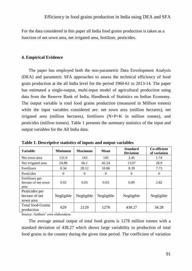
Efficiency in food grains production in India using DEA and SFA
91
For the data considered in this paper all India food grains production is taken as a
function of net sown area, net irrigated area, fertilizer, pesticides.
4. Empirical Evidence
The paper has employed both the non-parametric Data Envelopment Analysis
(DEA) and parametric SFA approaches to assess the technical efficiency of food
grain production at the all India level for the period 1960-61 to 2013-14. The paper
has estimated a single-output, multi-input model of agricultural production using
data from the Reserve Bank of India, Handbook of Statistics on Indian Economy.
The output variable is total food grains production (measured in Million tonnes)
while the input variables considered are: net sown area (million hectares), net
irrigated area (million hectares), fertilizers (N+P+K in million tonnes), and
pesticides (million tonnes). Table 1 presents the summary statistics of the input and
output variables for the All India data.
Table 1. Descriptive statistics of inputs and output variables
Variable Minimum Maximum Mean Standard
Deviation
Co-efficient
of variation
Net sown area 131.9 143 145 2.45 1.74
Net irrigated area 24.88 66.1 45.24 13.07 28.9
Fertilizers 0.34 28.12 10.86 8.39 7.73
Pesticides 0 0 0 0 0
Fertilizers per
hectare of net sown
area
0.02 0.05 0.03 0.09 2.82
Pesticides per
hectare of net
sown area
Negligible Negligible Negligible Negligible Negligible
Total food-Grains
production 629 2129 1278 438.27 34.28
Source: Authors’ own elaboration.
The average annual output of total food grains is 1278 million tonnes with a
standard deviation of 438.27 which shows large variability in production of total
food grains in the country during the given time period. The coefficient of variation

Rajani Neeraj MAHUR, Swati RAJU RAMNATH
92
of total food grains output is 34.28. The above results also indicate that on an
average fertilizer is an input which records maximum consumption at 108.58 lakh
tonnes whereas pesticides use is an average of 44.36 thousand tonnes. However, no
major difference can be observed between average fertilizer consumption and
pesticide consumption per hectare of net sown area which is at 0.322 lakh tonnes
and 0.3154 thousand tonnes per net sown area. The average net irrigated area is also
very low at 45.24 million hectares for the entire country and which actually amounts
to 32.23 percent of net sown area.
4.1 Results of DEA
The input oriented DEA model seeks to answer the question: By how much can
inputs be reduced to produce the same level of output? A summary of efficiency
estimates obtained from the DEA and SFA models is presented in Table 2.
Table 2. Summary of efficiency estimates: DEA Models
Statistic VRS-DEA CRS-DEA
Mean 0.98 0.95
Minimum 0.95 0.82
Maximum 1 1
Standard Deviation 0.02 0.04
Co-efficient of Variation 15.31 4.39
Skewness -0.14 -0.81
Source: Authors’ own elaboration.
The summary of efficiency estimates for the all India data on total food grains
production indicates that for the VRS and CRS models, the mean technical
efficiencies are 0.98 and 0.95 respectively and the corresponding standard deviations
are 0.01 and 0.04 indicating thereby the presence of considerable efficiency in
farming operations. In order to better understand the variations in agricultural
efficiency the entire period 1960-61 to 2013-14 has been divided two phases to
coincide with the pre-reforms (1960-61 to 1990-91) and post -reforms period (1991-
92 to 2013-14). Such an analysis would help examine changes in efficiency, if any,
in the country’s agriculture sector and would also provide better insights into the

Efficiency in food grains production in India using DEA and SFA
93
factors influencing agricultural productivity in India. The results of the DEA
estimation for the two periods is presented in Table 3.
Table 3. Summary of efficiency estimates of the DEA Models
1961-62 to 1990-91 1990-91 to 2013-14
Statistic CRS-DEA VRS-DEA CRS-DEA VRS-DEA
Mean 0.95 0.99 0.96 0.99
Minimum 0.84 0.95 0.96 0.96
Maximum 1 1 1 1
Median 0.97 0.99 0.96 1
Source: Authors’ own elaboration.
The above table indicates that the productive efficiency in Indian agriculture is
marginally higher in the post reforms period where the mean VRS efficiency at
0.994 is higher than that in the previous period where the same is at 0.985. Further,
the median score in the second-time frame is higher at 1 as compared to 0.98 for the
corresponding VRS score in the earlier time period. It therefore appears that the
post-reforms phase has registered an improvement in agriculture from the
productivity and efficiency perspective.
An in-depth analysis of the efficiency can be obtained from the frequency
distribution of technical efficiency scores for each of the two periods (Table 4)
Table 4. Frequency distribution of technical efficiency – DEA Models
1961-62 to 1990-1991 1990-91 to 2013-14
Efficiency
Range
CRS DEA (No of
years, %)
VRS DEA (No of
years, %)
CRS DEA (No of
years, %)
VRS DEA (No of
years, %)
0.8<=E<0.9 3 (10) Nil Nil Nil
0.9<=E 18 (62) 20 (69) 18 (75) 11 (46)
E=1 8 (28) 9 (31) 6 (25) 13 (54)
Source: Authors’ own elaboration.
It can be observed that in the period after 1990, the overall efficiency scores are
better and there is not a single year in which the efficiency levels have been less than
0.9. The post reforms era can thus be seen as that of improved agricultural

Rajani Neeraj MAHUR, Swati RAJU RAMNATH
94
performance and efficiency scores attaining a higher minimum level. The CRS DEA
indicates that for 18 years (75%) from a total of 29 years considered the technical
efficiency is seen to be greater than or at least equal to 0.9. Similarly, for the same
period 13 years are indicative of hundred percent efficiency in productivity under
the VRS DEA. In contrast the earlier time phase up to 1990 speaks of relatively
lesser performance in agriculture sector since only a total of 9 years (31%) report a
technical efficiency level of 100% under the VRS DEA.
A graphical presentation of the efficiency achieved in each year of the pre-and
post-reform period is presented in Figures 1 and 2.
Figure 1. VRS efficiency: 1962-1990
Source: Authors’ own elaboration.
An analysis of the efficiency scores shows that efficiency in food grain
production is low in 1974 and similar levels of efficiency can be observed are seen
in 1982, 1983. These years of low efficiency also coincide with drought years in the
country. The years 1962, 1971, 1976, 1988 to 1990 are seen as periods of relatively
good efficiency in performance.

Efficiency in food grains production in India using DEA and SFA
95
Figure 2. VRS efficiency: 1991-2014
Source: Authors’ own elaboration.
In the post reforms era, up to 1995 there has been hundred percent efficiency in
agriculture at the all India level. However, the years 1998 and 1999 have also
witnessed a steep decline in efficiency. Likewise, in the period after 2000, 2009
being a drought year has seen a decline in efficiency. –Besides, the period 2009 -
2012 also indicate a decline in the efficiency scores. A comparison of the efficiency
scores in the two periods – pre-and post-reform shows a wide variation in efficiency
in the pre-reform period and only 9 of the 29 years (a third of the years) show an
efficiency of 1 whereas greater uniformity in efficiency is observed in the post
reform period 14 of the 24 (58 percent of the years) years show an efficiency score
of 1 in food grains production in the country.
The standard DEA approach classifies DMUs as efficient or inefficient based on
the efficiency score obtained by the DMU. All DMUs with a score of unity are
classified as efficient, however, all efficient DMUs may not have the same
performance level. Hence a disaggregation of the efficiency scores of the efficient
DMUs can be done using different methods such as the super efficiency approach
(Andersen, Petersen 1993); cross evaluation (Green et al. 1996) or assurance regions
method (Cooper et al. 1999). Such methods of decomposing the efficiency score of
the optimal units were developed initially by Banker and Gifford (1988), and Banker
et al. (1989). Super efficiency estimates consider the possibility of a DMU

Rajani Neeraj MAHUR, Swati RAJU RAMNATH
96
increasing its inputs and/or reducing its outputs without becoming inefficient. Such
an approach will help rank the efficient DMUs. The super efficiencies help
determine the difference in efficiency among the efficient DMUs. For the years of
greater efficiency in performance the super efficiencies would extend beyond one.
For the data that we have considered, the years and the corresponding super
efficiency scores are presented in the table below.
Table 5. Super efficiency scores
Year Super Efficiency Year Super Efficiency
1962 1.66 1991 1.04
1965 1.15 1992 1
1968 1.01 1993 1.02
1971 1.15 1994 1.03
1976 1.19 1995 1
1984 1.02 1997 1.02
1988 1.05 2002 1.04
1989 1.09 2003 1.07
1990 Inf 2004 1.01
2005 1.03
2007 1.03
2013 Inf
2014 1.02
Source: Authors’ own elaboration.
Table 5 shows that in the period after 1991, greater number of years record
super efficiencies in agricultural production as compared years before 1991. The
highest level of super efficiency is recorded in the year 1962 at 1.66 Also, the range
for the super efficiency is much lesser in the period after the 1990s while the range
is much greater for the period until 1990 indicating a stable level of performance at a
higher level in the period after 1990.
For the post reforms data, the super efficiency reaches a peak level of near 1.07
in 1991. For the years 1992-1995 also efficiencies are greater than one. The years
2003-2005 also indicate super efficiency in production.

Efficiency in food grains production in India using DEA and SFA
97
4.2 Results of SFA
The mean efficiency measure of the SFA model at 0.94 is closer to the
efficiency achieved under CRS DEA. Further the mean efficiency under VRS DEA
is greater than that obtained from the SFA model and from the CRS DEA approach.
The highest variability in technical efficiency scores is observed in the VRS DEA
model. Further, the DEA models exhibit a higher variability than the SFA model.
Table 6. Summary statistics: SFA Model
Statistic
Mean 0.94
Minimum 0.80
Maximum 0.99
Standard Deviation 0.04
Co-efficient of Variation 4.69
Skewness -6118
Source: Authors’ own elaboration.
Technical efficiency under all three models shows a wide range of variation
among the respondents – the VRS (0.44 to 1), CRS (0.052 to 1) and SFA (0.15 to
0.98) with the largest variation for the CRS model.
Table 7. Results of the SFA Model
Variable Co-efficient Z values
Constant -1.56 -1.36
Net sown area 0.99 *** 5.28
Net irrigated area 1.07*** 8.41
Fertilizers 0.05 1.05
Pesticides -0.11 -3.94
Gamma 1.00*** 206.32
σ2 0.01
Log likelihood 94.64
*** = z < 0.001; ** = z< 0.01; * = z< 0.05 and.= p <0.1
Source: Authors’ own elaboration.

Rajani Neeraj MAHUR, Swati RAJU RAMNATH
98
The maximum likelihood estimates of the stochastic frontier model are given in
Table 7. The results indicate that four inputs, namely, net sown area, net irrigated
area and pesticides are statistically significant. The positive and statistically
significant co-efficient for net sown area, net irrigated area indicate that a 1 percent
increase in net sown area would increase output by almost 1 percent, while a one
percent increase in net irrigated area would increase output by another one percent.
The negative and significant co-efficient on pesticides point towards an inverse
relationship between output and this input. Thus, a decline in pesticides would
positively increase total food grains production. The value of gamma is one which
suggests that inefficiency in agriculture is purely on account of technical
inefficiency and the impact of statistical noise is zero.
6. Conclusion
The paper has measured efficiency in agricultural production in India for the
period 1960-61 to 2013-14. The results indicated to the presence of considerable
efficiency in farming operations for both the frontier methods. The mean efficiency
obtained under the SFA model was closer to the efficiency achieved under CRS
DEA model. A wide variation in efficiency was also seen for the different frontier
methods and the largest variation was observed for the CRS model over this period.
The analysis of efficiency under the DEA model for the two sub periods – 1960-61
to 1989-90 and 1990-91 to 2013-14 indicated to a marginal increase in productive
efficiency in food grains production in the period 1990-91 to 2013-14. Further, the
period after 1991 witnessed super efficiencies for a greater number of years. The
results of the SFA model pointed out net sown area, net irrigated area and pesticides
to be statistically significant inputs. The results indicated a negative and significant
coefficient for pesticides thereby indicating that a possible reduction in pesticide
may help increase efficiency. It can, thus, be concluded, that the effects of the Green
Revolution which significantly improved efficiency in agriculture during the mid-
1960s seem to be tapering off. An improvement in agricultural efficiency can take
place from increased investments in irrigation for the country as a whole since only

Efficiency in food grains production in India using DEA and SFA
99
32 percent of the net sown area is currently irrigated. The Prime Minister’s initiative
to improve and upgrade irrigation and make every drop useful through the Sinchai
Yojana can provide the much-needed boost to agricultural production in the country.
Improvements in efficiency and productivity will have a positive impact on food
security.
References
Ahluwalia M.S. (1978), Rural poverty and agricultural performance in India, „The Journal of
Development Studies”, vol. 14 no. 3, pp. 298-323.
Aigner D., Lovell C.A.K., Schmidt P. (1977), Formulation and estimation of stochastic frontier
production function models, „Journal of Econometrics”, vol. 6 no. 1, pp. 21-37.
Andersen P., Petersen N.C. (1993), A procedure for ranking efficient units in data envelopment
analysis, „Management Science”, vol. 39 no. 10, pp. 1261-1264.
Asenso-Okyere W.K., Benneh G., Tims W. (1997), Sustainable food security in West Africa, Kluwer
Academic Publishers, Boston.
Banker R.D., Charnes A., Cooper W.W. (1984), Some models for estimating technical and scale
inefficiencies in data envelopment analysis, „Management Science”, vol. 30 no. 9, pp. 1078-1092.
Banker R.D., Charnes A., Cooper W.W., Swarts J., Thomas D.A. (1989), An introduction to data
envelopment analysis with some of its models and their uses, „Research in Governmental and
Nonprofit Accounting”, vol. 5, pp.125-163.
Banker R.D., Gifford J.L. (1988), A relative efficiency model for the evaluation of public health nurse
productivity, Carnegie Mellon University, Pittsburgh.
Barros C.P., Mascarenhas M.J. (2005), Technical and allocative efficiency in a chain of small hotels,
„International Journal of Hospitality Management”, vol. 24 no. 3, pp. 415-436.
Battese G.E., Coelli T.J. (1988), Prediction of firm-level technical efficiencies with a generalized
frontier production function and panel data, „Journal of Econometrics”, vol. 38 no. 3, pp. 387-399.
Battese G.E., Corra G.S. (1977), Estimation of a production frontier model. With application to the
pastoral zone of Eastern Australia, „Australian Journal of Agricultural and Resource Economics”, vol.
21 no. 3, pp.169-179.
Bhatia S.S. (1967), Spatial variations, changes and trends in agricultural efficiency in Uttar Pradesh,
1953-1963, „Indian Journal of Agricultural Economics”, vol. 22 no. 1, pp. 66-80,
https://ageconsearch.umn.edu/bitstream/231978/2/Agricultural%20Efficiency%20in%20Uttar%20Prad
esh.pdf [03.03.2018].
Charnes A., Cooper W.W., Rhodes E. (1978), Measuring the efficiency of decision making units,
„European Journal of Operational Research”, vol. 2 no. 6, pp. 429-444.

Rajani Neeraj MAHUR, Swati RAJU RAMNATH
100
Coelli T.J. et al. (2005), An introduction to efficiency and productivity analysis, Springer, New York.
Coelli T.J., Battese G.E. (1996), Identification of factors which influence the technical inefficiency of
Indian farmers, „Australian Journal of Agricultural Economics”, vol. 40 no. 2, pp. 103-128.
Coelli T.J., Rahman S., Thirtle C. (2002), Technical, allocative, cost and scale efficiencies in
Bangladesh rice cultivation. A non-parametric approach, „Journal of Agricultural Economics”, vol. 53
no. 3, pp. 607-626.
Cooper W.W., Park K.S., Yu G. (1999), IDEA and AR-IDEA. Models for dealing with imprecise data
in DEA, „Management Science”, vol. 45 no. 4, pp. 597-607.
Debreu G. (1951), The coefficient of resource utilization, „Econometrica. Journal of the Econometric
Society”, vol. 19 no. 3, pp. 273-292.
Dhungana B.R., Nuthall P.L., Nartea G.V. (2004), Measuring the economic inefficiency of Nepalese
rice farms using data envelopment analysis, „Australian Journal of Agricultural and Resource
Economics”, vol. 48 no. 2, pp. 347-369.
FAO (2009), How to feed the world in 2050. Insights from an expert meeting at FAO,
http://www.fao.org/fileadmin/templates/wsfs/docs/expert_paper/How_to_Feed_the_World_in_2050.pd
f [02.03.2018].
FAO/WHO (2007), The state of food and agriculture. Paying farmers for environmental services,
http://www.fao.org/publications/sofa/2007/en/ [02.03.2018].
FAO (2015), Status of the World’s Soil Resources (SWSR) – Main Report. Food and Agriculture
Organization of the United Nations and Intergovernmental Technical Panel on Soils,
http://www.fao.org/3/a-i5199e.pdf [02.03.2018].
Farrell M.J. (1957), The measurement of productive efficiency, „Journal of the Royal Statistical
Society. Series A (General)”, vol. 120 no. 3, pp. 253-290.
Green R.H., Doyle J.R., Cook W.D. (1996), Preference voting and project ranking using DEA and
cross-evaluation, „European Journal of Operational Research”, vol. 90 no. 3, pp. 461-472.
Jha R., Chitkara P., Gupta S. (2000), Productivity, technical and allocative efficiency and farm size in
wheat farming in India. A DEA approach, „Applied Economics Letters”, vol. 7 no. 1, pp. 1-5.
Koopmans T.C. (1951), Efficient allocation of resources, „Econometrica. Journal of the Econometric
Society”, vol. 19 no. 4, pp.455–465.
Murthy Sreenivasa D., Sudha M., Hedge M.R., Dakshinamoorthy V. (2009), Technical efficiency and
its determinants in tomato production in Karnataka, India. Data envelopment analysis (DEA) approach,
„Agricultural Economics Research Review”, vol. 22 no. 2, pp. 215-224.
Pilz M., Wilmshofer S. (2015), Formal, nonformal, and informal learning in rural India. The case of
fishing families on the Chilika Lagoon, „Prospects”, vol. 45 no. 2, pp. 231-243.

Efficiency in food grains production in India using DEA and SFA
101
POSTnote (2006), Food security in developing countries, „The Parliamentary Office of Science and
Technology”, no. 274, pp. 1-4, http://www.parliament.uk/documents/post/postpn274.pdf [02.03.2018].
Poudel K.L., Yamamoto N., Johnson T.G. (2011), Comparing technical efficiency of organic and
conventional coffee farms in Nepal using data envelopment analysis (DEA) approach, in: 85rd Annual
Conference of the Agricultural Economics Society,
https://ageconsearch.umn.edu/bitstream/108949/2/14Poudel_Yamamoto_Sugimoto_Nishiwak_Kano.p
df [02.03.2018].
Pujari A.K. (2005), Efficiency and productivity in Indian agriculture. A stochastic frontier approach,
https://papers.ssrn.com/sol3/papers.cfm?abstract_id=713321 [02.03.2018].
Ray S.C., Ghose A. (2014), Production efficiency in Indian agriculture. An assessment of the post
green revolution years, „Omega”, vol. 44, pp. 58-69.
Rosegrant M.W., Agcaoili-Sombilla M.C., Perez N.D. (1995), Global food projections to 2020:
Implications for investment, International Food Policy Research Institute,
https://books.google.pl/books?id=XwQJorWEPT0C&printsec=frontcover&hl=pl&source=gbs_ge_sum
mary_r&cad=0#v=onepage&q&f=false [02.03.2018].
Rosegrant M.W., Ringler C., Gerpacio R.V. (1997), Water and land resources and global food supply,
International Association of Agricultural Economists Conference, August 10-16, 1997, Sacramento,
California.
Thiam A., Bravo-Ureta B.E., Rivas T.E. (2001), Technical efficiency in developing country
agriculture. A meta-analysis, „Agricultural Economics”, vol. 25 no. 2-3, pp. 235-243,
https://ageconsearch.umn.edu/bitstream/177163/2/agec2001v025i002-003a012.pdf [02.03.2018].
Zhu J. (2000), Multi-factor performance measure model with an application to Fortune 500 companies,
„European Journal of Operational Research”, vol. 123 no. 1, pp. 105-124.

CENTRAL EUROPEAN REVIEW OF ECONOMICS AND MANAGEMENT ISSN 2543-9472; eISSN 2544-0365
www.cerem-review.eu
www.ojs.wsb.wroclaw.pl Vol. 2, No. 1, 103-132, March 2018
Correspondence address: Anoop Singh, Department of Industrial and Management Engineering, Indian
Institute of Technology Kanpur, India. E-mail: [email protected]
Received: 15-09-2017, Revised: 14-02-2018, Revised: 27-02-2018, Accepted: 27-02-2018
doi: http://dx.doi.org/10.29015/cerem.552
© 2018 WSB UNIVERSITY IN WROCŁAW
DEA based approach to set energy efficiency target
under PAT Framework: A case of Indian cement
industry
Anoop SINGH, Bharat SHARMA
Indian Institute of Technology Kanpur, India
Abstract:
Aim: Propose a Data Envelopment Analysis (DEA) based approach to set energy efficiency targets under the Perform, Achieve and Trade (PAT) framework of the Bureau of Energy Efficiency (BEE)
Design / Research methods: We adopt input-oriented non-controllable DEA model with variable return to scale DEA
Conclusions / findings: Due to the implication of in-house energy conversion, we estimate separate energy efficiency targets based on “purchased energy” as well as “process energy”. The later accounts for energy finally used in the production process after in-house energy conversion.
Originality / value of the article: The Bureau of Energy Efficiency (BEE) in India has introduced a market based energy efficiency mechanism under the Perform, Achieve and Trade (PAT) framework. Under this mechanism, energy efficiency certificates can be traded across eight identified sectors thus bringing cost effectiveness to achieve the energy efficiency targets. To implement the scheme, differentiated energy efficiency targets have been set using baseline specific energy consumption. This approach does not account for technical and operational aspects like vintage, scale, output mix and input mix. This study proposes an alternative target setting method based on Data Envelopment Analysis (DEA) which takes into account some of the above mentioned technical and operational differences across the industrial plants. A comparative assessment highlights the efficacy of DEA methodology in implementation of the PAT scheme. We estimate energy efficiency targets based on “purchased energy” as well as “process energy”, i.e. that used finally in the production process.
Implications of the research: BEE may adopt the suggested approach to set energy efficiency targets for subsequent cycles under the Perform, Achieve and Trade (PAT) framework. Key words: energy efficiency target, PAT framework, Data Envelopment Analysis, Indian cement industry JEL: Q48, Q49 .

Anoop SINGH, Bharat SHARMA
104
1. Introduction
There is a continuous challenge to balance the tripod of environment,
development and resource utilization. Energy efficiency offers a strong case to be
pursued for in order to attain this balance. The growing requirement of energy,
constrained access to the resources, questions pertaining to energy security,
environmental concerns and increasing competitiveness in global markets has driven
the urgency to layout strategies to attain higher efficiency in energy utilization.
Policy framework in India has given increasing importance to energy efficiency
across different sectors and has addressed it time and again. The Energy
Conservation Act, 2001 provides for the various measures to improve energy
efficiency in the country. The Act identifies 15 energy intensive industries and
establishments as Designated Consumers (DCs) for targeting energy efficiency
efforts. The Act led to setting up of the Bureau of Energy Efficiency (BEE), and
entrusted it with both promotional and regulatory functions.
While working with the international community on the challenges of global
warming, India identified the need for measures and actions at national level to
adapt to climate change and to develop in an ecologically sustainable manner. The
Prime Minister of India released the National Action Plan on Climate Change
(NAPCC) on 30th June 2008. Out of these eight missions, National Mission for
Enhanced Energy Efficiency (NMEEE) and National Mission for Sustainable
Habitat (NMSH) are related to energy efficiency. NMSH advances the sustainability
of human habitats primarily in urban regions by improving energy efficiency in
buildings, solid waste management and promoting a modal shift to public transport.
Apart from the previously running programs on energy efficiency by the BEE,
NMEEE suggested four more initiatives namely the Market Transformation for
Energy Efficiency (MTEE), the Energy Efficiency Financing Platform (EEFP), the
Framework for Energy Efficient Economic Development (FEEED) and the Perform
Achieve & Trade (PAT). The PAT mechanism is being implemented under the
institutional structure of the BEE. PAT targets the Designated Consumers (DCs) in
the industrial sectors which accounts for about 25% of the nation’s GDP and 45% of
the commercial energy consumption in India (Bureau of Energy Efficiency 2012: 1-

DEA BASED APPROACH TO SET ENERGY EFFICIENCY TARGET UNDER PAT …
105
4). Out of the fifteen energy intensive industries notified in the Act, eight industrial
sectors are included in first PAT cycle. In 2010, Energy Conservation Act
Amendment Bill was passed. This allows the government to issue Energy Saving
Certificates (ESCerts) and also allows purchase of these certificated by DCs which
fail to meet the targets set under the PAT framework. A penalty would be imposed
for the DCs which fail to comply with the energy consumption targets.
The first PAT cycle was rolled out for the financial year 2012-13 to 2014-15. In
the first cycle, 478 DCs were included across eight energy intensive sectors. In the
second PAT cycle, the depth and width of PAT has been increased. The total
number of DCs has been increased to 621 and three more sectors are included viz.
Petroleum refinery, railways and electricity distribution companies. While the
second PAT cycle had been rolled out, it continues to retain its original flavour.
This paper discusses the methodology adopted under PAT mechanism for target
setting for DCs and attempts to provide a Data Envelopment Analysis (DEA) based
alternate approach for target setting. DEA is a non-parametric linear programming
method in operations research, which builds an efficiency frontier and provides a
performance based ranking for the Decision Making Units (DMUs). DEA is a
widely applied tool used in different fields including the energy sector. The next
section briefly discuss the industrial energy consumption scenario in India. Section 3
presents a review of the PAT framework including the methodology for efficiency
target setting for the first cycle and discussion thereof. A brief review of the
literature covering application of the DEA in the context of energy efficiency, is
presented in section 4. Section 5 discusses the methodology adopted in the paper and
results thereof.
2. Industrial energy consumption in India
India consumes about 4.5% of the world’s industrial energy (International
Energy Agency 2016). With increasing industrialization and a push for
manufacturing, energy consumption is bound to increase. Table 1 shows the sector-
wise energy consumption in the Indian economy from year 2010-11 to 2014-15.

Anoop SINGH, Bharat SHARMA
106
Industrial energy consumption in India is around 50% of the total energy
consumption of the country and, later, remains a focus for energy efficiency
improvement.
Table 1. Energy consumption across sectors in Indian economy
2010-11 2011-12 2012-13 2013-14 2014-15
Sector Energy
(kTOE)
Sector
%
Energy
(kTOE)
Sector
%
Energy
(kTOE)
Sector
%
Energy
(kTOE)
Sector
%
Energy
(kTOE)
Sector
%
Industry 163282 33.05 131962 46.97 167250 50.24 223805 52.72 270641 55.92
Transport 58003.5 11.74 19387 6.90 25314 7.60 29104 6.86 114126 23.58
Others
(Residential, Services,
Agri., etc.)
239693 48.51 129584 46.13 122614 36.83 136501 32.16 72343 14.94
Non-Energy
use 33105.9 6.70 - - 17757 5.33 35098 8.27 26841 5.54
TOTAL 494084.4 280933 332935 424508 483951
Source: GOI (2012, 2013, 2014, 2015, 2016).
2.1 Energy use pattern in Indian industry
Energy consumption across various industrial sectors depends on the energy
density of the sector in the overall feel of industrial activity. Table 2 shows the
distribution of energy consumption across various industrial sectors in India (GOI
2012, 2013, 2014, 2015, 2016).
Energy consumption across the industrial sectors varies depending on
technological aspects governing output mix and input mix. Further adoption of
captive power generation, internal waste heat recovery and co-generation of
electricity and steam also differentiate energy consumption pattern across similar
plants. Cement industries one of the large energy consuming sectors, followed by
iron and steel sector.

DEA BASED APPROACH TO SET ENERGY EFFICIENCY TARGET UNDER PAT …
107
Table 2. Energy consumption across various industrial sectors in India
Industrial Sector 2010-11 2011-12 2012-13 2013-14 2014-
15
Iron and steel 25924.5 28261 37735 40793 54758
Chemical and petrochemical 5811.9 5897 15954 12423 12595
Non-ferrous metals 524.5 3670 12816 125 20
Non-metallic minerals$ 7329.3 - 2 18 -
Transport equipment 11848.9 171 11 8 -
Machinery 35 1578 77 17 264
Mining and quarrying 2797.6 1307 1110 903 141
Food & Tobacco - 137 - - -
Paper, pulp and print 1189.2 2280 1435 1288 1195
Construction 109.4 12172 11009 27742 26217
Textile and leather 930.8 868 451 937 1004
Non-specified (industry) 106781 75621 86650 139551 174448
Total Industrial Energy
Consumption (PJ) 163282.1 131962 167250 223805 270641
Source: GOI (2012, 2013, 2014, 2015, 2016).
Note: $ – including cement industry
2.2 Cement
The Indian cement industry is the second largest producer in the world after
China and is also a very efficient one. By converting from wet process plants to dry
and semi dry process plants, cement industry in India has achieved economy in fuel
and power consumption. Of the 13 types of cement produced in India, Ordinary
Portland Cement (OPC), Portland Pozzolana Cement (PPC) and Portland blast
furnace Slag Cement (PSC) accounted for 39%, 52% and 8% of the total production
respectively in the year 2007 (Lawrence Berkeley National Laboratory 2010).
In India, thermal energy consumption for clinker production in the year 2005-06
was averaged to 725 kcal/kg and electricity consumption for cement production was
averaged to 82 kWh/MT (Planning Commission 2008). A total primary energy
consumption of Indian cement Industry was estimated at 700 PJ in the year 2007. Of
the total final energy consumption of 580 PJ, coal constituted 91% and electricity
share was 9%. Thermal energy intensity for producing 174 MT of cement in the year

Anoop SINGH, Bharat SHARMA
108
2007 was 3.03 GJ/MT and electrical energy intensity was 0.3 GJ/MT (Lawrence
Berkeley National Laboratory 2010).
Coal consumption in the cement industry peaked at 18.097 MT in 2005 while it
was 15.08 MT in 2011 with a growth of 2.86% from the previous year. Electricity
consumption was 15311 GWh in 2011 with a decrement of 7.42%. CAGR of coal
and electricity consumption from 2006 to 2011 were 1.95% and 5.09% respectively
(CEIC 2013). Table 3 shows the specific energy consumption for cement sector in
different countries including India.
Table 3. Specific energy consumption in cement industry – an international
comparison
Country Specific Electrical Energy
Consumption (kWh/ton of cement)
Specific Thermal Energy
Consumption (kcal/kg of cement)
India 82 725
Spain 92 836
Germany 100 836
Japan 100 836
Brazil 110 884
Italy 112 908
China 118 956
Mexico 118 1003
Canada 140 1075
USA 141 1099
World Average 100-110 850-860
World Best 65 649
Source: Gielen, Taylor (2009); International Energy Agency (2007); Madlool et al. (2011).
The specific energy consumptions of the plants in India were observed to be
more than 20-30% of that of the plants in Japan in 1990 (Singh 2000). After
adapting and adopting several measures and continuous improvements, presently
Indian cement industry is the most energy efficient in the world (Gielen, Taylor
2009; International Energy Agency 2007). But there is scope for improvement as
compared to the best plants in the world and within the country.
3. Perform, Achieve & Trade (PAT) mechanism
PAT is developed as an institutional and regulatory framework to incentivize
energy saving and to give a push to the energy efficient industrial production in

DEA BASED APPROACH TO SET ENERGY EFFICIENCY TARGET UNDER PAT …
109
India. It will support use of energy efficient technologies in industries. Under this
framework, each designated consumer (DC) is given a “unit specific” specific
energy consumption reduction target in terms of percentage reduction in the specific
energy consumption (SEC). The tenets followed in PAT framework are
accountability, predictability, transparency, consistency, simplicity and adaptability.
3.1 PAT mechanism
BEE sets the sectorial targets and unit specific targets for the plants. BEE issues
energy saving certificates EScerts to the DCs who overachieve their targets based on
the PAD (PAT assessment Document) approved by accredited Designated Energy
Agencies (DENA). It coordinates with various state designated agencies (SDAs) for
the verification and implementation of the PAT scheme.
These SDAs coordinate with BEE to decentralise the work of monitoring and
verification. The SDAs are normally the state level renewable energy agencies. They
monitor the compliances by the DCs and levy penalty on them in case of non-
compliances. DENA is the independent energy auditor accredited by BEE which
verifies and audits the PAD submitted by the DCs for assessment of compliance.
The DENA shares the audit report with the SDAs and the BEE.
The DCs have to comply with the target approved by the BEE. It’s also the
responsibility of the DCs to prepare PAD and appoint an independent DENA. After
approval of PAD, a DC request for the issuance of EScerts in case of
overachievement or penalty is levied on in case of failure of compliance. After that,
to compensate its shortfall DC has to purchase EScert from the power exchanges
(PXn) or may sell EScerts to enjoy monetary benefits or may put them in the
banking to be used in the next PAT cycle.
3.2 PAT Target Setting methodology
In the target setting phase, data was collected from different DCs for the
duration of 5 years from year 2005-2006 to year 2009-2010. A baseline data for the
baseline year 2009-10 was prepared taking the average of three years from 2007-
2008 to 2009-2010. Target for each DC was specified through public notification.
Commencement of the first PAT cycle was from 1st April 2012 for duration of three

Anoop SINGH, Bharat SHARMA
110
years. During this period, DCs were to achieve the target. Monitoring and
verification started after April 2013. Based on the cross-verification report, DCs
would be issued EScerts or a penalty would be levied. The quantity of
underachieved target is to be paid at the prevailing oil prices. For the SEC target
setting in subsequent cycles, data for the previous three years is to be collected. The
duration of the second PAT cycle is from 2016-17 to 2018-19.
Rule 4 published in The Gazette of India, Extraordinary, Part II, section 3, sub-
section (i) vide-notification number G.S.R. 269 (E) dated the 30th March, 2012
provides the procedures for establishing energy consumption norms and standards
i.e. about SEC calculations and target setting. The sub-sections in the Rule 4 give
guidelines for “Normalisation” by considering factors affecting the energy
consumption viz. capacity utilization, mix of captive and grid electricity etc.
Normalized SEC = f (Reported SEC, Normalisation Factor) (1)
The normalising statistical procedures are to be applied to SEC during baseline
and target periods only if capacity utilization (or plant load factor for thermal power
plants) has a deviation from baseline year due to uncontrollable factors specified in
the Rule 4 viz. natural disasters, rioting or social unrest, changes in government
policies and environmental standards and impact of market (sales or shortage of raw
materials).
Target setting in PAT is a two-tier process. First, a sector-level target is set
based on the overall energy consumption in the sector. Thereafter, a plant-specific
target is set for the DC. Due to factors like difference in technology adopted, output
mix and raw material mix, plants show a wide range of specific energy
consumption. This range is defined as the bandwidth of the sector. Sub-groups are
defined based on process or output. A relative SEC is calculated with respect to the
most efficient plant of that group. The target reduction of the DC is set as a
multiplier for the respective SEC in that group.
We provide a detailed explanation for target setting in the cement sector and
juxtapose the same with PAT targets for the first cycle. For each DC in the sector,
all types of cement products and exported clinker were converted into an equivalent

DEA BASED APPROACH TO SET ENERGY EFFICIENCY TARGET UNDER PAT …
111
major product using appropriate conversion factors. Following the approach adopted
in Singh et al. (2010), the final Gate to Gate (GtG) energy is calculated by taking
count of all the thermal energy imported, converting the electrical energy into
thermal equivalent, subtracting the electricity exported to the grid and taking count
of notional energy for import and export of clinkers. The cement sector had to
achieve a reduction of 4.28% of their consumption during the first PAT cycle. There
are seven groups in the cement sector based on the type of major products and
processes. Figure 1 shows these groups on the plotted SEC of 85 cement DCs.
Figure 1. Groups in cement sector
Source: Authors’ own elaboration.
Group 1 has 55 plants having major product as PPC. Group 2 is for the 16 plants
which have OPC cement as the major product. Group 3 has 7 plants having Portland
Slag cement as the major product. Group 4 has 2 white cement plants. Group 5 has 2
wet process based cement plants. Group 6 has 2 plants with only grinding units.
Group 7 has only 1 plant which is a “Clinkerization unit”.
The energy saving target for a DC will be the product of baseline production
and SEC reduction target (Equation 3). The SEC reduction target is the difference of

Anoop SINGH, Bharat SHARMA
112
SEC calculated for the baseline and the target SEC. The percentage reduction of
SEC is product of a multiplier X and the relative SEC (Equation 5). Energy saving
by all DCs, when summed up would be equal to the sectoral energy saving target.
Following equations are used to calculate the energy saving target for a DC:
(2)
(3)
(4)
(5)
Where, = Baseline SEC of DC (MTOE)
= Target SEC for DC (MTOE)
= Relative SEC of DC (MTOE)
= Baseline SEC of the most efficient DC
X = Multiplying Factor
= Baseline output of DC (tonnes)
= Energy saving by a DC
= Total energy saving in the sector
3.3 PAT critique
PAT offers a compliance flexibility similar to the emission trading schemes.
Excess ECerts, allocated to a DC towards energy saving beyond their SEC target,
can be sold via the existing power exchanges (PXs) in the country. DCs, with a
target shortfall, can purchase the required number of ECerts to fulfil their reduction
target. Anyways Edward shortfall would attract a penalty which is linked to the
prevailing oil prices. However, the level of penalty is not enough to dis-incentivise
the shortfall in meeting the energy efficiency targets. The methodological approach
adopted under the first PAT cycle continues to be saddled with shortcomings. Target
energy efficiencies compared to the average annual rate of energy efficiency
improvement in the sector. If the target is lesser than the average annual rate of
energy efficiency improvement, the actions under PAT mechanism will tend to
counter-productive as it will lead to significantly higher supply of ECerts and
separating the demand thereof. Based on the oversupply, and the policy for banking,

DEA BASED APPROACH TO SET ENERGY EFFICIENCY TARGET UNDER PAT …
113
this effect will also be carried onward to the subsequent PAT cycles. Subdued prices
for Ecerts would, in turn, dis-incentivise long-term investment in efficiency
improvement.
The sectoral target for SEC set by BEE is rather lenient. As per IEA data for
India from 1991 to 2001, the specific energy consumption in cement sector based on
total primary energy supply reduced with CAGR of 4.05% in that duration
(International Energy Agency 2007). The historical reductions in SEC of the cement
sector is much more than the relaxed target of 4.28% (equivalent to 1.43% per
annum) decided by BEE for the first PAT cycle of three-year duration.
Internationally, countries have succeeded to achieve annual SEC reduction rates
from 1.1% in Germany to 1.9% in China. Clearly, the targets set by BEE for the first
PAT cycle seems to be lenient.
The benefits from a merit based mechanism like PAT arise due to trade of
ECerts between sector DCs with different marginal cost of energy efficiency
improvement. For example, the marginal cost curve for aluminium sector is steeper
than paper and pulp sector, and would be steeper for DCs with relatively higher
energy efficiency i.e. low SEC. The ESCert generated in paper and pulp sector does
not represent the same cost and technological advancement required as to the ESCert
generated in aluminium sector.
The wide range of specific energy consumption within a sector indicates the
potential for the energy saving. It also indicates the variation of plants on factors like
vintage, product and raw material mix, technology etc. Acknowledging these
variations, BEE has opted for a unit specific target energy reduction instead for a
single benchmark. It is evident that it is not feasible to achieve a single benchmark
by the unit having highest SEC and unit having lowest SEC. This approach does not
completely justify the primary purpose of enhancing energy efficiency in the
industrial sector. On the contrary, target setting under PAT framework seems to take
a rather lenient view of highly inefficient plants. It also doesn’t follow a model with
strong theoretical considerations that can compare DCs based on variations on
account of output mix and input mix. This can be addressed by the use of Data
Envelopment Analysis. Instead of comparing and target setting based on the plant
having least SEC, it is more prudent to set the target based on a peer-to-peer

Anoop SINGH, Bharat SHARMA
114
comparison among plants having similar performance characteristic like scale,
energy input etc.
4. Energy efficiency and DEA: A literature review
Energy efficiency has been extensively researched and examined based on the
requirements in different research domains (engineering, resource management,
economics, policy etc.). Greening et al. categorised the employed analytical
techniques in four different types (Greening et al. 2007). First, econometric methods
used to assess the demand outcome of energy based on prices or energy taxes (e.g.
Oh, Lee 2004; Lescaroux 2008). Second, simulation and optimization models based
on top-down and bottom-up approach to study the interplay of technology and
energy consumption (e.g. Bohringer, Rutherford 2008; Frei et al. 2003). Third are
the industry and process specific microeconomic analyses based on simulation,
optimization and statistical techniques (e.g., Babusiaux, Pierru 2007; Henning,
Trygg 2008; Singh et al. 2010). Fourth type are the decomposition methods like
index decomposition analysis (IDA), used to study the effects of morphological
change and energy efficiency in the aggregate energy use in a sector or overall for a
country (e.g. Alcantara, Duarte 2004; Ang, Zhang 2000; Unander 2004).
Bhattacharya and Paul used the decomposition technique to understand the sectorial
changes in energy consumption and intensity in India for the duration of year 1980-
95 (Shyamal, Bhattacharya 2004). Nag and Parikh used decomposition method to
understand the impact of structural changes, activity levels, fuel mix, and fuel
quality and energy intensity on the carbon emission intensity from commercial
energy use in India (Nag, Parikh 2000).
The IDA based approach uses the energy intensity as a proxy for energy
efficiency and analyses the variations in intensity because of different factors.
However, IDA cannot be directly applied to energy efficiency target setting. The
benefit of the non-parametric approach of DEA lies in the fact that it uses all factors
simultaneously in a total factor framework. DEA uses the concept of efficiency as
defined in Farrel (1957) and applies the evaluation methodology as developed by

DEA BASED APPROACH TO SET ENERGY EFFICIENCY TARGET UNDER PAT …
115
Charles et al. (Charnes et al. 1978), thereby avoids the use of imperfect proxies like
energy intensity. DEA has received attention in the field of energy and
environmental studies. A detailed survey of over 100 such studies has been provided
by Zhou et al. (2008). Ramanathan compared energy efficiency of different transport
modes in the Indian context using DEA (Ramanathan 2008). In another paper,
Ramanathan studied efficiency with respect to energy consumption and CO2
emission in North Africa and countries of Middle East (Ramanathan 2005).
Mukherjee presented several DEA models for analysis of used energy efficiency in
US manufacturing firms (Mukherjee 2008). DEA has been also used for
benchmarking the electric utilities in Europe and northern Europe (Jamasb, Pollitt
2003; Edvardsen, Førsund 2003).
DEA was applied Boyd and Pang examined the relationship between
productivity and energy efficiency for glass industry (Boyd, Pong 2000). Blomberg
et al. (2012) used DEA to assess policy implications on energy efficiency in
Swedish pulp and paper industry. Lee (2008) applied DEA with regression for
benchmarking energy efficiency of government buildings in Taiwan. Lee and Lee
(2009) used regression with 2-stage DEA for benchmarking the performance of
building management system with climate adjusted energy consumption. Kim
compared the energy consumption efficiency of Asia-Pacific countries using DEA
(Taeho 2008). Hu and Kao used DEA for setting energy saving targets for APEC
countries with capital stock, labour employment and energy consumption as inputs
and GDP as output (Hu, Kao 2007). Onut and Soner used input oriented CRS DEA
for energy efficiency assessment for the Antalya regions of hotel in Turkey with
occupancy rates and annual total revenue as outputs (Onut, Soner 2006). Energy
efficiency development of non-energy-intensive industries in Germany and
Columbia was studied by Martinez with CO2 emissions as undesirable output and
using three different DEA model viz. CCR, cost minimization and slack based
model with undesirable output (Martínez 2011). Mandal and Madheshwaran (2011)
measured energy use efficiency with undesirable outputs for Indian cement industry.
Yang and Pollitt used four different methods based on DEA accompanied with other
techniques like SFA, regression and Tobit regression to incorporate undesirable
output and incontrollable variables in order to evaluate the performance of Chinese

Anoop SINGH, Bharat SHARMA
116
coal-fired power plants (Yang, Pollitt 2009). Most of the above-mentioned studies
were conducted from an academic perspective and were not aimed at developing an
alternate implementable approach to target setting. In contrast, this paper assesses
the applicable methodology for energy efficiency target setting and suggests
development of a methodological approach based on data envelopment analysis
(DEA).
5. Data collection and description
All of the data was obtained from the Annual report and Directors’ report of the
respective firms. This was accessed through the CAPITALINE database which
gather this information Cement Manufacturers’ Assocoation’s publication “Cement
Statistics” for the duration from year 2007 to 2010 was also used to get relevant
plant/firm level information. The information on the process involved (wet or dry)
was confirmed from the respective websites of firms.
The data collected for the cement producing firms includes raw material
consumed, power and fuel consumed, power and fuel expenditure, finished products
and capacity and energy consumption per unit production. The important criteria for
data collection was the continuity of data from year 2007 to 2010. Data for a total of
31 firms was collected. Energy information required special focus in order to avoid
double counting of the purchased fuel used for electricity generation and as thermal
fuel. Cement to be traded was not mentioned clearly into the raw materials, and was
matched from the finished products data from their annual reports. For study
involving energy consumption, plant-level data is most apt. But because of its
unavailability, firm level data was collected. Plant level data could not be accessed
from BEE.
Detailed information about the input and output consists of the quantity of the
fuel (coal, diesel, furnace oil and gaseous fuels) and for in-house electricity
generated from diesel generators and steam turbines, quantity of the raw material
(limestone, slag, fly-ash, and other materials including pozzolana material, laterite
etc.) purchased/consumed and its unit price and total cost, total clinker production

DEA BASED APPROACH TO SET ENERGY EFFICIENCY TARGET UNDER PAT …
117
(only for a few firms) and clinker sold, cement production and capacity. For
aggregating the fuel consumption, all of the fuels were converted into energy in
MTOE (metric tonne of oil equivalent). Since the quality of the fuels used and their
respective calorific values were not provided, the conversion was done on the basis
of the calorific values as constant as per the Sub Ordinate 394 (E) by the Ministry of
Power. To back-track the coal consumption by the steam turbines, heat rate was
assumed at 2717 kCal/kWh as specified in the PAT booklet. To back-track the diesel
consumption in diesel generators, the specific fuel consumption was assumed to be
0.16 kg/kWh.
Since quality of coal can vary, exercise was done to identify the quality of the
coal consumed based on the unit cost to the firm. Almost all firms reported a coal
quality of Grade-A for respective year. A constant GCV (gross calorific value) of
3.8 million kCal/MT was assumed for all of the plants showing a coal of Grade-A
quality. As for the firms showing coal quality different from Grade-A, their
respective calorific values were used. For other firms a coal constant was used to
ascertain coal quality wherever feasible.
To calculate the SEC for the cement production, the energy consumed for the
clinker that was sold was deducted from the overall calculation of SEC. Similarly,
limestone consumed in the sold clinker was also deducted from the total limestone
consumption on a proportionate basis.
From the compiled data, baseline data was prepared as per the BEE
methodology for PAT. For preparing baseline data, an average of three years data
was used i.e. for years 2008, 2009 and 2010. Wherever data for any of these years
was incongruent or unavailable, data from year 2007 was included. The firms for
which only one or two year data was available out of four years, the mean for the
baseline was calculated by including those one or two year observations only. The
sample consists of the plants having dry manufacturing process.

Anoop SINGH, Bharat SHARMA
118
6. Suggested methodology
The methodology proposed for calculating target Specific Energy Consumption
(SEC) consists of a 2-stage process. For the first stage, a method close to the
approach adopted by BEE for target setting under the PAT mechanism to set Sector
Energy Reduction Target (SERT), with a slight variation is described in the sub-
section below. In the second stage, reduction targets for individual firms are set
based on an alternate approach developed using DEA. Further, a differentiation is
also made between the energy purchased by the plant against the energy finally
consumed in the process after any conversion (for e.g. use of oil or coal to produce
electricity). Thus, final SEC targets are estimated for “purchased energy” as well as
for “process energy”.
6.1. Stage 1- Sector Energy Reduction Target (SERT)
BEE assigned a reduction target of 0.62 million MTOE/year for the cement
sector, which had a total energy consumption of 14.48 million MTOE/year in the
baseline year 2009-2010, to be achieved at the end of first PAT cycle in March
2015. This is equivalent to a sectorial reduction target of 4.28% on a pro-rata basis.
We have applied the same percentage reduction target to the total energy
consumption of the sample of firms in our dataset.
Energy saving targets for the DCs, under the PAT mechanism is given as a
percentage reduction from the baseline SEC for the respective DC. Based on the
analysis done on the notified targets of the DCs in the cement sector and the
information given in PAT consultation document (Bureau of Energy Efficiency
2011), it is inferred that this percentage reduction target for individual DCs is the
product of relative SEC and a common “multiplying factor”. This multiplying factor
is different for each sub-sector as the reduction target is different for every
respective sub-sector. We apply this approach for the sample of dry process cement
manufacturing plants as a sub-sector of the cement sector. However, we do not
further divide our sample in sub-sectors as all the data corresponds to dry process.
Target energy reduction for the sample, SEC for each firm and the multiplying
factor are calculated using estimated baseline data as follows in equation (6) to (8).

DEA BASED APPROACH TO SET ENERGY EFFICIENCY TARGET UNDER PAT …
119
(6)
(7)
Using equation (7) in equation (6) yields the following relation:
(8)
Where, n being number of firms in the sample
X = Multiplying Factor
ET = Total energy consumption in the sample (MTOE)
ES = Total energy saving target for sample (MTOE)
Oi = Output of the firm (tonnes)
SECi = Specific energy consumption of the firm (MTOE/tonne)
SECit = Target Specific energy consumption
SECir = Relative SEC i.e. ratio of firm’s SEC to lowest SEC in sample.
Total energy consumption by the firms in our sample is 7136156.13 MTOE. The
target energy saving for this sample, based on the BEE’s percentage target reduction
for the sector would be 305427.48 MTOE (4.28% of total energy consumption). For
the sample of 31 firms in our study, the calculated value of the multiplying factor
comes out to be 2.494 when purchased energy is considered and 3.406 when the
process energy input is considered. Based on the BEE’s approach, the firm with the
least SEC is given a percentage reduction of 2.494% or 3.406%, depending on the
energy input consideration, and all other units will have a reduction target higher
than this value.
A deviation from the BEE methodology has been adopted for the energy
consumption target. Instead of different reduction target for different firms, a
common minimum percentage reduction target has been set for all firms at Stage-1,
which is equal to the target set under BEE methodology for the firm having least
SEC. This is to ensure a minimum reduction in energy consumption even for those
firms which will be technically efficient and will form efficiency frontier in the
DEA analysis.

Anoop SINGH, Bharat SHARMA
120
6.2 Stage 2- DEA based Target Setting for individual firms
SECs of DCs vary depending on a number of controllable and non-controllable
factors. Controllable factors include input mix, technology, operational practises,
output mix, etc. Non-controllable factors include ambient conditions, market
conditions, regulations etc. We include some of the controllable factors in DEA.
DEA results provide targets for the controllable factors such as quantities of inputs
(or output) variables by a firm to reach the efficiency frontier. For our study, only
targets for energy consumption are counted for. The use of other inputs in DEA
analysis gives overall efficiency scores which result in identification of energy
saving potential for the firms in a holistic manner. Achieving the overall efficiency
may or may not contribute to the purpose of energy saving in a market based
environment and in an economically viable way. Hence, the targets are set only for
energy consumption, not for other inputs.
After equal percentage energy reduction target for each DC in stage-1, the
remaining sectorial reduction target to be achieved in stage-2 is allocated to the DCs
based on potential energy saving projections from DEA application. The remaining
stage-2 reductions are distributed amongst the inefficient DCs on a pro-rata basis of
the total energy saving projection from the DEA. The DCs which form the
efficiency frontier have zero additional energy reduction target and hence, don’t
have any reduction targets in stage-2. This is different from the BEE methodology
where only one DC can have the least reduction target in a sector/sub-sector.
6.3. DEA model
Input and output variables for DEA are selected by considering the purpose of
the study and the information availability. The purpose of the DEA application here
is to find out the target reduction for SEC of a plant based on the performance of its
peers by forming an efficiency frontier.
Cement production (in tonnes) of the plant is used as the only output variable in
the study. Cement plants in India produce a mix of cements like OPC, PPC, etc.
Although more than one output can be used in DEA, we use only one because of the
non-availability of data.

DEA BASED APPROACH TO SET ENERGY EFFICIENCY TARGET UNDER PAT …
121
Plant capacity affects the efficiency of the plant, which is not always because of
economies of scale. Setting the capacity is mostly an economic decision which is
dependent on various non-managerial and market variables, and other environmental
factors such as availability of raw material at the plant-site. It can also be considered
as a proxy for net assets of a plant and for the technology incorporated which can’t
be changed significantly in the short run. Hence capacity is considered and used as a
non-controllable variable for study.
Another variable which is of importance is the vintage of the plant which is the
year of establishment of the plant. Although it is assumed that the vintage adversely
affects the efficiency of the plant due to old technologies and wear-tear, but plants
do improve their machinery and replace the old ones with the more productive and
efficient ones. Hence, true effect of vintage is difficult to measure. For
benchmarking studies where one plant is compared with another, consideration of
vintage will result in undue advantage to inefficiency and regressive approach to
modernization. Therefore, vintage is not included as an environmental variable or
non-controllable variable. The data does not give any information on the age of the
plant but only of the registration date of the firm. This data about firm does not give
any proxy for vintage.
The total energy consumption of the plant is calculated by converting all
energy inputs into tonnes of oil equivalent. Distinction is made to identify the
“purchased energy” input and the “production energy” input. The former refers to
the energy inputs purchased and later accounts for energy conversion, for e.g. by
converting oil or coal to electricity. This allows us to analyse and set energy
efficiency targets based on these two perspectives. Plants generate electricity for
their own consumption from the primary energy inputs. This distinction will help us
identify thermal energy and electricity requirements separately. Therefore, four
types of energy input baskets are considered for DEA. These are described later in
the section.
The objective of setting targets is to reduce input energy. Hence, an input
oriented approach is adopted for DEA. Capacity considered as a non-controllable
variable. Hence, an “input-oriented non-controllable model with variable return to
scale” DEA model is adopted. It is described as follows,

Anoop SINGH, Bharat SHARMA
122
Minimize (9)
Subject to,
(i = 1,2)
(10)
(λ1, λ2,…. λn)
Here P is the production output matrix-vector, L is the limestone consumption
matrix vector, λ is a non-negative vector, ‘n’ denotes the number of firms and C is
the capacity matrix-vector (for a non-controllable variable). Ei is the energy
consumption input matrix-vector where ‘i’ denotes the types of energy input as
electricity, fuel or as total energy input. For any DMU0 to be evaluated, ei0, l0, c0 and
p0 are the corresponding vectors for the observed values of energy consumption,
limestone consumption, capacity and production of the DMU under consideration,
respectively. Four alternate energy input formulations are used giving four different
versions of the model as given in next table:
Table 4. Energy input formulations
Source: Authors’ own elaboration.
In case 1, there is one energy variable where E represents total energy
purchased. In case 2, there are two energy variables where E1 represents purchased
electricity and E2 represents purchased fuel. With one input variable in case 3, E
represents total energy used for production process which is the sum of purchased
electricity and electricity that generated in-house, and other fuels (in tonnes of oil
equivalent) excluding fuel used for generation of electricity. For Case 4, E1
represents total electricity consumed and E2 represents fuels consumed only in
Case Energy Input Formulation (MTOE)
Number of
Energy
Inputs
E E1 E2 Limestone
1 Total energy purchased 1 ̶ ̶
2 Purchased electricity and purchased fuels 2 ̶
3 Total energy consumed for production
process 1 ̶ ̶
4 Total electricity used in production process
and fuels consumed in production process 2 ̶

DEA BASED APPROACH TO SET ENERGY EFFICIENCY TARGET UNDER PAT …
123
production process excluding the amount used in electricity generation. Total
Electricity includes purchased and electricity generated in-house.
7. Results and Discussions
Following table summarises the results of the adopted DEA based methodology
(with all energy input scenarios). It also gives a comparison of the targets adopting
BEE’s methodology. Since the BEE focuses only on the energy efficiency targets,
we have not included the Limestone reduction targets in our result analysis.
As per BEE methodology, the highest percentage SEC reduction target is for
unit CD_031 having SEC of 0.108 MTOE/tonnes and relative SEC of 2.824 and
having target reduction of 7.05%. For Case-1, 13 DCs form the efficiency frontier
having least and highest SEC reduction target to be 2.49% and 17.86%. For Case-2,
efficiency frontier is formed by 14 DMUs. The highest SEC % reduction target is
19.044%.
For Case-3, the efficiency frontier is formed by 11 DCs. The SEC % reduction
target for the firms forming efficiency frontier, based on the process energy based
SEC, is 3.41%. But when the reduction targets were converted on the purchased
energy based SEC, the SEC % reduction targets came out to be different for the
firms forming efficiency frontier. Maximum target is of 12.37% and minimum is
2.27%, based on purchased energy based SEC. For Case-4, the efficiency frontier in
this case is formed by 14 DMUs. The DEA SEC reduction targets vary from a
highest of 15.32% 013 to a lowest of 2.27%.
An important observation in Case-3 and Case-4 is that some of the firms are
having final targets less than 3.41% (e.g. 2.27% for CD_015 and 2.63% for
CD_002), which is corresponding to the minimum target from the BEE
methodology for the process energy based SEC. When total energy input is
segregated into type of energy used viz. electricity and fuel, in most of the units, the
energy consumption calculated based on the purchased energy input comes out to be
higher than that of the energy consumption based on process energy input. This
difference is accounted to the conversion inefficiencies from the losses in making
electricity from fuel.

Anoop SINGH, Bharat SHARMA
124
Table 5. SEC reduction targets for different energy inputs
Unit
Code
Limestone per tonne
of cement
production
(Tonnes)
SEC (Purchased
Energy)
(MTOE/
Tonnes)
SEC (Process
Energy)
(MTOE/
Tonnes)
Share of
purchased electricity in
total
electricity
consumption
SEC Reduction Target (%)
BEE Methodology
DEA
based Case-
1
DEA
based Case-
2
DEA
based Case-
3
DEA
based Case-
4
CD_001 0.848 0.070 0.070 100.00 4.57 12.13 11.97 9.09 9.07
CD_002 1.068 0.055 0.042 10.79 3.60 2.59 2.49 2.63 2.63
CD_003 1.149 0.057 0.056 87.26 3.75 2.49 2.49 5.76 5.66
CD_004 1.050 0.061 0.050 30.79 3.96 2.49 2.49 2.79 2.79
CD_005 1.152 0.064 0.049 26.71 4.16 2.49 2.49 2.61 2.61
CD_006 0.612 0.068 0.056 21.96 4.45 2.49 2.49 2.82 2.82
CD_007 0.762 0.071 0.065 74.20 4.64 8.37 8.96 6.52 7.48
CD_008 1.131 0.058 0.048 41.41 3.82 4.76 4.84 4.72 5.39
CD_009 1.176 0.053 0.043 32.22 3.49 2.49 2.49 3.72 3.81
CD_010 0.945 0.038 0.038 100.00 2.49 2.49 2.49 3.41 3.41
CD_011 1.447 0.074 0.062 33.83 4.87 14.21 13.14 8.33 7.46
CD_012 0.069 0.070 0.070 95.32 4.60 2.49 2.49 3.39 3.39
CD_013 1.330 0.094 0.090 72.33 6.14 17.68 18.97 12.37 15.32
CD_014 1.320 0.099 0.089 43.39 6.45 13.75 16.01 7.83 9.06
CD_015 1.190 0.058 0.038 5.36 3.76 2.49 2.49 2.27 2.27
CD_016 1.297 0.073 0.063 16.54 4.76 14.78 10.28 8.31 9.52
CD_017 1.321 0.064 0.055 45.94 4.20 2.49 2.49 3.91 2.93
CD_018 0.928 0.058 0.058 100.00 3.77 9.13 7.11 7.25 3.41
CD_019 0.896 0.059 0.059 99.40 3.84 2.49 2.49 3.40 3.40
CD_020 1.263 0.076 0.071 75.71 4.94 17.13 14.78 10.67 9.52
CD_021 1.269 0.094 0.094 100.00 6.13 16.99 16.64 11.75 13.10
CD_022 1.353 0.084 0.084 99.91 5.46 15.39 16.26 10.91 12.47
CD_023 0.997 0.057 0.053 63.27 3.76 9.99 6.72 6.49 7.20
CD_024 1.332 0.088 0.088 100.00 5.73 17.86 19.04 12.27 14.56
CD_025 1.090 0.062 0.060 99.67 4.08 7.92 7.54 10.18 10.65
CD_026 2.054 0.094 0.094 99.85 6.15 5.68 5.60 6.48 3.41
CD_027 0.932 0.063 0.063 99.15 4.11 2.49 2.49 3.40 3.40
CD_028 1.022 0.063 0.062 96.30 4.10 7.75 8.03 6.22 7.13
CD_029 1.396 0.057 0.048 40.43 3.70 2.49 2.49 2.89 2.89
CD_030 0.617 0.053 0.051 91.76 3.45 2.49 2.49 3.31 3.31
CD_031 1.639 0.108 0.107 98.60 7.05 7.95 6.64 6.48 8.37
Source: Authors’ own elaboration.
The inefficiencies in generation are reflected in energy consumptions of the
plants. The electricity produced through a Captive Power Plant (CPP) saves
Transmission and Distribution (T&D) losses, which otherwise would be borne at
system level purchases by other consumers. This gives rise to two important
considerations. One, the inefficiencies in generations are required to be reduced, but

DEA BASED APPROACH TO SET ENERGY EFFICIENCY TARGET UNDER PAT …
125
only after being accounted with the savings in T&D losses at the power system
level. Second, a direct comparison between plants with and without a CPP cannot be
a right approach.
Figure 2. SEC (purchased energy) vs. BEE methodology based SEC reduction
%
Source: Authors’ own elaboration.
Figure 3. SEC (purchased energy) vs. Case-1 SEC reduction %
Source: Authors’ own elaboration.

Anoop SINGH, Bharat SHARMA
126
Figure 4. SEC (purchased energy) vs. Case-2 SEC reduction %
Source: Authors’ own elaboration.
Figure 5. SEC (purchased energy) vs. Case-3 SEC reduction %
Source: Authors’ own elaboration.

DEA BASED APPROACH TO SET ENERGY EFFICIENCY TARGET UNDER PAT …
127
Figure 6. SEC (purchased energy) vs. Case-4 SEC reduction %
Source: Authors’ own elaboration.
Figure 7. SEC (process energy) vs. Case-3 SEC reduction %
Source: Authors’ own elaboration.

Anoop SINGH, Bharat SHARMA
128
Figure 8. SEC (process energy) vs. Case-4 SEC reduction %
Source: Authors’ own elaboration.
Figure 2 shows a strong positive correlation with value of correlation coefficient
to be 1 between SEC reduction percentages based on BEE methodology and
purchased energy SEC. Figure 3 and Figure 4 shows Case-1 and Case-2 SEC
reduction percentages with purchased energy SEC showing moderately positive
correlation and having values of correlation coefficients to be 0.65 and 0.69
respectively. Figure 5 and Figure 6 shows Case-3 and Case-4 SEC reduction
percentages with purchased energy SEC showing moderately positive correlation
and having values of correlation coefficients to be 0.65 and 0.64 respectively. Figure
7 and Figure.8 shows Case-3 and Case-4 SEC reduction percentages with process
energy SEC showing moderately positive correlation and having values of
correlation coefficients to be 0.69 and 0.68 respectively. Overall, the DEA based
method showed a moderately positive correlation for different cases and having
maximum values for process based energy inputs and process energy based SEC.

DEA BASED APPROACH TO SET ENERGY EFFICIENCY TARGET UNDER PAT …
129
8. Conclusion
Energy efficiency plays an important role in achieving energy security and
addressing environmental concerns of the country. PAT is an ambitious market
based measure for improving energy efficiency in India’s energy-intensive industrial
sectors. The cement plants in India are the most efficient in world country-wise, but
there is still a great scope of improvement as compared to the world benchmarks.
The DEA method adopted for this paper gives energy saving target not just on
the basis of SEC, but also considers other criteria like capacity and raw material.
The methodology does not always set high targets for the plants having high specific
energy consumption, as it also considers the DEA based technical efficiency for
target setting. DEA encompasses other factors and sets the targets holistically. The
methodology adopted by BEE ignores the impact of factors like raw material
composition and quality, internal consumption of products by the plant itself, in-
house energy conversion etc. These factors can’t be ignored while setting the targets.
As BEE sets plant-specific targets, it also gives importance to the factors like
vintage and the old technology used in the plants. Older plants are less efficient and
there has been a sympathetic look towards them in target setting. This should not be
the case as it can be considered as a reward for inefficiencies and obsoleteness. Such
older inefficient plants used appropriate targets to incentivize in technological
improvement. It is desirable to implement a credible mechanism for target setting
for energy efficiency and strict compliance for the same.
Another important issue is the comparatively short duration of the three-year for
the PAT cycle, resulting in adoption of easy-fix methods adopted by the plants.
Long term regulated certainty under the PAT mechanism supported with more
stringent targets would provide incentives for adopting a long term strategy for
energy efficiency improvement. Blending fly-ash and slag reduces the SEC, but
does not help the plants in the long run. The target accomplishment should be
sufficient to make economic investments profitable in the long run. Therefore, the
duration of PAT cycle should be increased.
Unavailability of plant level data remains a limitation of this study is that of the
data. The firm-level data does not give the information about the pattern and

Anoop SINGH, Bharat SHARMA
130
behaviour of the plants. As the firm-level data covers the overall energy expenditure
across multiple plants, plant level differences could not be investigated.
The energy efficiency regulator i.e. BEE needs to take a broader perspective to
make data accessible so that areas for improvement in PAT methodology can be
identified. Data access can be provided by without revealing the true identity of the
plants. Given a fairly large number of DCs in each sector, a fair degree of anonymity
can still be ensured.
References
Alacantara V., Duarte R. (2004), Comparison of energy intensities in European Union countries.
Results of a structural decomposition analysis, „Energy Policy”, vol. 32 no. 2, pp. 177-189.
Ang B.W., Zhang F.Q. (2000), A survey of index decomposition analysis in energy and environmental
studies, „Energy”, vol. 25 no. 12, pp. 1149-1176.
Babusiaux D., Pierru A. (2007), Modelling and allocation of CO2 emissions in a multiproduct industry.
The case of oil refining, „Applied Energy”, vol. 84 no. 7, pp. 828-841.
Blomberg J., Henriksson E., Lundmark R. (2012), Energy efficiency and policy in Swedish pulp and
paper mills. A data envelopment analysis approach, „Energy Policy”, vol. 42, pp. 569-579.
Bohringer C., Rutherford T.F. (2008), Combining bottom-up and top-down, „Energy Economics”, vol.
30 no. 2, pp. 574-596.
Boyd G.A., Pang J.X. (2000), Estimating the linkage between energy efficiency and productivity,
„Energy Policy”, vol. 28 no. 5, pp. 289-296.
Bureau of Energy Efficiency (2011), PAT consultation document,
http://220.156.189.23/NMEEE/PAT%20Consultation%20Document_10Jan2011.pdf [10.02.2018].
Bureau of Energy Efficiency (2012), PAT Booklet, „PAT Perform, Achieve and Trade”,
https://beeindia.gov.in/sites/default/files/PAT%20PPT_0.pdf [July 2012]
CEIC (2013), India Premium Database, https://www.ceicdata.com/en/blog/expansion-population-data-
india-premium-database [10.03.2018].
Charnes A., Cooper W.W., Rhodes E. (1978), Measuring the efficiency of decision making units,
„European Journal of Operational Research”, vol. 2 no. 6, pp. 429-444.
Edvardsen D.F., Førsund F.R. (2003), International benchmarking of electricity distribution utilities,
„Resource and Energy Economics”, vol. 25 no. 4, pp. 353-371.
Farrell M.J. (1957), The measurement of productive efficiency, „Journal of the Royal Statistical
Society”, vol. 120 no. 3, pp. 253-290.

DEA BASED APPROACH TO SET ENERGY EFFICIENCY TARGET UNDER PAT …
131
Frei C.W., Haldi P.H., Sarlos G. (2003), Dynamic formulation of a top-down and bottom-up merging
energy policy model, „Energy Policy”, vol. 31 no. 10, pp. 1017-1031.
Gielen D., Taylor P. (2009), Indicators for industrial energy efficiency in India, „Energy”, vol. 34 no.
2, pp. 962-969.
Greening L.A., Boyd G., Roop J.M. (2007), Modeling of industrial energy consumption. An
introduction and context, „Energy Economics”, vol. 29 no. 4, pp. 599-608.
Henning D., Trygg L. (2008), Reduction of electricity use in Swedish industry and its impact on
national power supply and European CO2 emissions, „Energy Policy”, vol. 36 no. 7, pp. 2330-2350.
Hu J.L., Kao C.H. (2007), Efficient energy-saving targets for APEC economies, „Energy Policy”, vol.
35 no. 1, pp. 373-382.
International Energy Agency (2007), Tracking industrial energy efficiency and CO2 emissions,
https://www.iea.org/publications/freepublications/publication/tracking_emissions.pdf, pp. 140-163
[10.03.2018].
International Energy Agency (2016), World Energy Statistics 2016,
http://www.oecd.org/publications/world-energy-statistics-25183885.htm, pp. II.6-II.320 [10.03.2018].
Jamasb T., Pollitt M. (2003), International benchmarking and regulation. An application to European
electricity distribution utilities, „Energy Policy”, vol. 31 no. 15, pp. 1609-1622.
Lawrence Berkeley National Laboratory (2010), Strategies for low carbon growth in India. Industry
and non-residential sectors, https://ies.lbl.gov/sites/all/files/low-co-growth-india-2011.pdf
[10.03.2018].
Lee W.S. (2008), Benchmarking the energy efficiency of government buildings with data envelopment
analysis', „Energy and Buildings, vol. 40, pp. 891–895.
Lee W.S., Lee K.P. (2009), Benchmarking the performance of building energy management using data
envelopment analysis, „Applied Thermal Engineering”, vol. 29 no. 16, pp. 3269-3273.
Lescaroux F. (2008), Decomposition of US manufacturing energy intensity and elasticities of
components with respect to energy prices, „Energy Economics”, vol. 30 no. 3, pp. 1068-1080.
Madlool N.A., Saidur R., Hossain M.S., Rahim N.A. (2011), A critical review on energy use and
savings in the cement industries, „Renewable and Sustainable Energy Reviews”, vol. 15 no. 4, pp.
2042-2060.
Mandal S.K., Madheswaran S. (2011), Energy use efficiency of Indian cement companies. A data
envelopment analysis, „Energy Efficiency”, vol. 4 no. 1, pp. 57-73.
Martínez C.I.P. (2011), Energy efficiency development in German and Colombian non-energy-
intensive sectors. A non-parametric analysis, „Energy Efficiency”, vol. 4 no. 1, pp. 115-131.
GOI (2012, 2013, 2014, 2015, 2016), Energy Statistics, Ministry of Statistics & Programme
Implementation (MOSPI), Government of India, New Delhi.

Anoop SINGH, Bharat SHARMA
132
Mukherjee K. (2008), Energy use efficiency in US manufacturing. A nonparametric analysis, „Energy
Economics”, vol. 30 no.1, pp.76-96.
Nag B., Parikh J. (2000), Indicators of carbon emission intensity from commercial energy use in India,
„Energy Economics”, vol. 22 no.4, pp. 441-461.
Oh W., Lee K. (2004), Causal relationship between energy consumption and GDP revisited. The case
of Korea 1970-1999, „Energy Economics”, vol. 26 no. 1, pp. 51-59.
Onut S., Soner S. (2006), Energy efficiency assessment for the Antalya Region hotels in Turkey,
„Energy and Buildings”, vol. 38 no. 8, pp. 964-971.
Planning Commission (2008), Cement Task Force Reports for the Eleventh Five Year Plan (2007-
2012), http://planningcommission.nic.in/plans/planrel/11thf.htm [10.03.2018].
Ramanathan R. (2000), A holistic approach to compare energy efficiencies of different transport
modes, „Energy Policy”, vol. 28 no. 11, pp. 743-747.
Ramanathan R. (2005), An analysis of energy consumption and carbon dioxide emissions in countries
of the Middle East and North Africa, „Energy”, vol. 30 no. 15, pp. 2831-2842.
Shyamal P., Bhattacharya R.N. (2004), Causality between energy consumption and economic growth
in India. A note on conflicting results, „Energy Economics”, vol. 26 no. 6, pp. 977-983.
Singh A. (2000), Energy efficiency and CO2 emissions mitigation potential in Indian cement industry,
Working Paper No. 78, United Nations University/Institute for Advanced Studies (UNU/IAS), Tokyo.
Singh A., Parikh K.S., Parikh J. (2010), Inter-fuel substitution, industrial energy demand and carbon
emissions. An analysis using firm/plant-level data for 14 industrial sectors in India, VDM Verlag Dr.
Müller, Saarbrücken.
Taeho K. (2008), Efficiency at energy industry. A comparison of energy consumption efficiency
among Asian Pacific countries, „Asian Journal on Quality”, vol. 9 no. 3, pp. 113-121.
Unander F. (2004), Decomposition of manufacturing energy-use in IEA countries. How do recent
developments compare with historical long-term trends, „Applied Energy”, vol. 84 no. 7, pp. 771-780.
Yang H., Pollitt M. (2009), Incorporating both undesirable outputs and uncontrollable variables into
DEA: The performance of Chinese coal-fired power plants, „European Journal of Operational
Research”, vol. 197 no. 3, pp. 1095-1105.
Zhou P., Ang B.W., Poh K.L. (2008), Measuring environmental performance under different
environmental DEA technologies, „Energy Economics”, vol. 30 no.1, pp. 1-14.

CENTRAL EUROPEAN REVIEW OF ECONOMICS AND MANAGEMENT ISSN 2543-9472; eISSN 2544-0365
www.cerem-review.eu
www.ojs.wsb.wroclaw.pl Vol. 2, No. 1, 133-153, March 2018
Correspondence address: Cees Johannes Gelderman, Open University of The Netherlands, PO Box 2960,
6401 DL Heerlen, the Netherlands. E-mail: [email protected]
Received: 22-09-2017, Accepted: 01-12-2017
doi: http://dx.doi.org/10.29015/cerem.568
© 2018 WSB UNIVERSITY IN WROCŁAW
Investigating cooperative purchasing performance -
a survey of purchasing professionals in Dutch
hospitals
Cees Johannes GELDERMAN, Jelle De JONGE, Jos SCHIJNS, Janjaap
SEMEIJN
Open University of the Netherlands, The Netherlands
Abstract:
Aim: Cooperative purchasing is considered a promising area for lowering the cost in the health care
sector, although recent initiatives show mixed results. The purpose of this study is to find a thorough
explanation for the performance of cooperative purchasing in healthcare by investigating the role of
trust, commitment, organizational factors (i.e. group formality, and IT system effectiveness) and
interpersonal skills (i.e. teamwork skills, and communication).
Design / Research methods: A conceptual model for the performance of cooperative purchasing was developed. This model was empirically validated using a survey of 88 Dutch hospital purchasing professionals.
Conclusions / findings: Analysis shows a significant impact of trust and commitment in cooperative purchasing groups on performance. Group formality and teamwork skills appear to be essential for achieving trust and cooperative purchasing performance. We also found a positive impact of IT system effectiveness on commitment, not on trust. Positive feelings about the group and positive expectation about the continuity of the group can be stimulated through effective IT systems. Since proper IT support is often neglected in many healthcare organizations, management efforts to improve IT systems could truly facilitate the tactical purchasing process of cooperative purchasing in hospitals.
Originality / value of the article: Many cooperative purchasing initiatives suffer from conflicts over the allocation of savings, time, and costs. Despite the growing importance of cooperative purchasing, few empirical studies have explored the effects on hospital performance. Our study extends previous research by investigating the relationships between trust, commitment, and the performance of cooperative purchasing (1) and the impact of organizational factors and interpersonal skills on trust and commitment in purchasing groups within a healthcare context (2).
Key words: cooperative purchasing, healthcare, trust, commitment, cooperative purchasing performance JEL: M1

Cees Johannes GELDERMAN et al.
134
1. Introduction
Most OECD countries are faced with a continuous growth in health expenditures
as a share of GDP, which has resulted in a collective concern for controls of costs
and systems efficiency (Rego et al. 2014). The United States currently spends
approximately 18% of the national GDP on health services with projected increases
of up to 20% by 2021 (e.g. Spaulding et al. 2014; Elmuti et al. 2013). The life
expectancy of people in developed countries is rising fast. The expenses on health
and welfare costs have increased significantly in the last ten years. This growth is
largely attributed to the general aging of the world population and the growing
number of age-related health problems (e.g. Schut, Van den Berg 2010; Lovelock
2010). As the population ages, people require more health care. Another reason is
the expansion of healthcare offerings and the improved technology (Van Ewijk et al.
2013). Healthcare costs are continuously increasing, and healthcare providers are
more and more under cost and quality pressures (Chakraborty et al. 2014) and
efficiency has emerged as the central goal to the operations of health care
organizations (Al-Amin et al. 2016). Political choices must be made concerning
access to healthcare, and also how to finance healthcare. These problems are easier
to handle when healthcare is delivered in a more efficient and cost-effective way
(e.g. Gelderman, Albronda 2017). Therefore, all options to achieve efficiency gains
should be addressed.
Procurement is considered to be a promising area for lowering the costs in the
health care sector (Walker et al. 2013). Horizontal collaborative purchasing has
often been cited as a way for hospitals to address the challenges of the rising
healthcare costs (e.g. Essig 2000; Burns, Lee 2008). However, empirical evidence
regarding the effects of cooperation on hospital performance is scarce (Büchner et
al. 2015), while initiatives of Dutch hospitals have had mixed results (Kusters,
Versendaal 2013). Collaborating organizations struggle to develop and maintain
sustainable inter-organizational relationships (Schotanus et al. 2010). For instance,
trust and commitment are commonly considered key success factors for cooperative
purchasing. However, in empirical studies trust does not always appear to have a

INVESTIGATING COOPERATIVE PURCHASING PERFORMANCE
135
significant impact on cooperative purchasing performance (e.g. Schotanus et al.
2010), while commitment was not always found effective (e.g. Muhwezi 2010).
These relation-specific factors are particularly relevant for cooperative
purchasing in healthcare, since members of different institutions need to work
together. It is important that members are prepared to invest in the continuity of the
purchasing group (commitment) and that they can rely on a fair allocation of costs
and savings (trust). We investigate trust and commitment as outcome (dependent)
variables which is not uncommon in collaboration research (e.g. Kwon, Suh 2004).
In turn, trust and commitment in cooperative purchasing are influenced by different
antecedents. This study investigates the impact of organizational factors (i.e. group
formality, and IT system effectiveness) and interpersonal skills (i.e. teamwork skills,
and communication) on trust and commitment in cooperative purchasing groups.
Our study extends previous research by investigating the relationships between
trust, commitment, and the performance of cooperative purchasing. In addition, we
examine the impact of organizational factors and interpersonal skills on trust and
commitment in purchasing groups within a healthcare context. A conceptual model
for the performance of cooperative purchasing was developed. This model was
empirically validated using a survey of 88 Dutch hospital purchasing professionals.
2 Literature review
2.1 Cooperative purchasing in healthcare
Procurement in healthcare is an important area where the efficiency can or
should be increased (Walker et al. 2013) and cooperative purchasing is considered a
promising venue for lowering the procurement costs in this sector (Nollet, Beaulieu
2005). The procurement function in Dutch healthcare is characterized by centralized
purchasing and loose cross-unit coordination (Ruiter et al. 2011). Getting
compliance from internal users is a challenging and a crucial task for purchasing in
healthcare. Top management support is important (e.g. Birken et al. 2015), although
physicians (e.g. surgeons) have a major influence on the purchase of a variety of
expensive products (Schneller 2009). The selection of suppliers is often determined

Cees Johannes GELDERMAN et al.
136
by a physician’s preference (Chen et al. 2013). Therefore, purchasers must generate
support and consensus for their purchasing projects, typically through cross-
functional teams (Ruiter et al. 2011). These teams are not only needed, but often
required by the government due to the risk factors involved. Commodities and
standardized items seem better suited for cooperative procurement. Moreover, most
hospitals lack sufficient IT support for the tactical purchasing process (Ruiter et al.
2011).
Cooperative purchasing can be defined as “the cooperation between two or more
organizations in a purchasing group in one or more steps of the purchasing process
by sharing and/or bundling their purchasing volumes, information and/or resources”
(Schotanus, Telgen 2007: 53). This definition takes into account typical motives for
cooperative purchasing: the bundling of purchasing volume, the distribution of
resources, and the sharing of information (Tella, Virolainen 2005). Furthermore, the
definition is not limited to mere contracting, but includes all the possible steps of the
purchasing process (for example, bidding and negotiating); it also takes various
forms of purchasing groups into account. In this study, the joined purchasing activity
will be called ‘cooperative purchasing’ and the entity of the group where this
activity is taking place will be referred to as ‘purchasing group’. The buyers of a
purchasing group have to define and combine their individual requirements.
Activities such as supplier selection, negotiation and contract management are most
commonly transferred to the purchasing group (Gobbi, Hsuan 2015).
Cooperative purchasing is considered to be especially interesting for public
organizations, since they usually do not consider themselves competitors
(Schotanus, Telgen 2007). Cooperative purchasing has been practiced intensively by
hospitals which usually have similar requirements (Gobbi, Hsuan 2015). Hospital
pooling alliances were found successful in purchasing commodity and
pharmaceutical items (Burns, Lee 2008). Still, many public organizations have
difficulties in sustaining interorganizational relationships in the form of purchasing
collaborations (Schotanus et al. 2011). Due to the specific characteristics of the
healthcare sector, these initiatives are faced with considerable problems (Rego et al.
2014). Although coordination efforts are made, no cost reduction and quality
improvement program appears to align the entire health care supply chain from

INVESTIGATING COOPERATIVE PURCHASING PERFORMANCE
137
providers to purchasers (Ford, Scanlon 2007). The supply chain is managed through
a complex line of command, balancing power relationships among various
professional groups (De Vries et al. 1999; Rego et al. 2014). A specific challenge for
cooperative purchasing of medical products is handling supplier lock-in situations
due to the medical training of specialists (Carrera et al. 2015).
Nollet and Beaulieu (2005) described two different possible governance
structures for cooperative purchasing in healthcare. The first is the “cooperative
structure”, where the purchases to be performed by the group are distributed among
members. In this structure, the members have more influence and, thus, there is
more room for customer-specific requirements. This makes this structure suitable for
medical product categories (Meijer 2014). Second, there is the “third party
structure”, which is a distinct organization negotiating and writing contracts
according to a mandate given by the members. This structure is suitable for
procuring standard products and services (Meijer 2014). Most purchasing groups in
the Netherlands are cooperative structure groups, while in other countries, such as
Germany, USA and Canada, the third party structure is most commonly applied
(Schneller 2000).
2.2 Performance of cooperative purchasing
All studies face the difficulty of evaluating the performance of alliances
(Hoffmann, Schlosser 2001). It is difficult to objectively measure the performance
of cooperative purchasing, as it depends on the objectives of the specific group. The
most important objectives found by Tella and Virolainen (2005) were the expected
cost savings due to negotiating power, the efficiency gains, and the information
exchange between members about price levels and suppliers. The rationale behind
cooperative purchasing is to have more volume and to share workload to reduce
costs (Schneller 2000). Bundling volume is called consolidation; consolidation is a
procurement practice used to transfer activities to a central entity such as bidding,
supplier evaluation, negotiation, and contract management. A purchasing group
usually provides additional power to the members of the group in their negotiations
with suppliers. Consequently, members should get more favorable conditions than
they would have obtained individually. The average saving for hospitals that

Cees Johannes GELDERMAN et al.
138
participate in cooperative purchasing has been estimated between 10%-25%
(Cleverley, Nutt 1984; Nollet, Beaulieu 2003, 2005). The hospitals in the Intrakoop
initiative reported an average saving of 31% for the purchase of pacemakers
(Carrera et al. 2015).
In addition to better contractual conditions there are other important reasons for
joining a purchasing group. As the negotiation process is performed by only one
organization, instead of many, joining a purchasing group also reduces
administrative costs (Essig 2000). In their study of the motives for joining
purchasing groups, Tella and Virolainen (2005) found that, in addition to the cost
savings, information sharing between organizations was another important motive.
Individual companies valued the information of suppliers and market prices. Next to
cost savings, cooperative purchasing is also valued for its indirect benefits in terms
of process optimization and knowledge sharing (Carrera et al. 2015). Walker et al.
(2013) found that product innovation and ensuring supply are important themes for
health care providers. In a general sense, the performance of purchasing groups is
determined by the degree of achieving their hard and soft objectives (Schotanus et
al. 2010).
2.3 Development of hypotheses
Trust has been widely used in studies on buyer-supplier relationships. Trust is
considered central to all relational exchanges (Morgan, Hunt 1994). Trust is
believed to be a crucial factor for achieving cooperation between parties. In the
organizational economics and transaction cost literature, trust has been theorized to
reduce opportunistic behavior and thereby to reduce the need for control and
transaction costs (e.g. Dyer 1997; Hofmann, Schlosser 2001). According to
Williamson (1979), relations that feature personal trust will survive greater stress
and display greater adaptability. Transaction costs are supposed to be lower in cases
of high levels of trust, since less monitoring, control, and cooperative agreements
are necessary. Therefore, trust can be considered an important antecedent of
cooperative purchasing performance (cf. Schotanus et al. 2010).
Zaheer et al. (1998) defined trust as the expectation that an actor can be relied
on to fulfill obligations (1), will behave in a predictable manner (2), and will act and

INVESTIGATING COOPERATIVE PURCHASING PERFORMANCE
139
negotiate fairly when the possibility for opportunism is present (3). In cooperative
purchasing, all three elements are likely to be important for successful cooperation.
The third element seems to be particularly relevant for cooperative purchasing, since
fair allocation of cost savings between the members is critical for the performance of
cooperative purchasing (Gobbi, Hsuan 2015). The workload is divided among group
members, for instance negotiating the terms for buying a specific product category.
Members need to trust their negotiator to act in the best interest of the entire group,
instead of pursuing their own (short-term) interests. Empirical studies indicate that
the development of (mutual) trust is critical for cooperative purchasing, promoting
savings, transparency and simplification (Gobbi, Hsuan 2015). We hypothesize:
(H1) Trust has a positive impact on the performance of cooperative purchasing
in healthcare.
Commitment is also central to all relational exchanges between partners.
Morgan and Hunt (1994: 23) defined commitment as “an exchange partner believing
that an ongoing relationship with another is so important as to warrant maximum
efforts at maintaining it; that is, the committed party believes the relationship is
worth working on to ensure that it endures indefinitely”. Commitment causes
entities to make short-term sacrifices for the long-term good. When commitment is
high, partners in the collaboration want to continue their relationship, which reduces
opportunism (Muhwezi 2010).
Group members must believe that the group is worth working in (Schotanus et
al. 2010; Coun et al. 2015). The performance of cooperative purchasing apparently
depends on the willingness of the group members to continue and invest in ‘their’
purchasing group (Kumar et al. 1995). Walker et al. (2013) found commitment to be
the most important enabler of cooperative purchasing among the healthcare
respondents. Furthermore, in healthcare, there is no shareholder pressure for direct
results and the long-term view prevails over the short-term results. Establishing
cooperation requires much energy and time from numerous individuals from
different organizations. These set-up costs, and the partner scarcity, are likely to
reduce short-term opportunism. We hypothesize:
(H2) Commitment has a positive impact on the performance of cooperative
purchasing in healthcare.

Cees Johannes GELDERMAN et al.
140
Formality refers to organizational structures, such as rules, regulations, and the
division of labor. Some argue that less formality is necessary in relationships with
high levels of trust and commitment (e.g. Klein Woolthuis 1999) or even that formal
written agreements between parties are not very important for cooperative behaviors
(e.g. Hendrick 1996). However, in order to minimize uncertainty and conflicts, it is
also argued that purchasing groups need formal agreements on important decisions
(Schotanus et al. 2010). Agreements have to be made on decision making and on
reporting group performance. Other formality aspects are regular organized
meetings and the use of several procedures and rules, such as joining and leaving
rules, duties and rights (Schotanus, Telgen 2007). The formality aspects of the group
refer to the rules of the game necessary to reduce uncertainties and possible
opportunistic behavior. Hoffmann and Schlosser (2001) found that ‘a precise
definition of rights and duties’ is the most important factor.
We propose that purchasing groups have a need for formal structures and rules.
In collaboration we expect that group formality contributes to the levels of trust and
commitment. This leads to the following hypotheses:
(H3) Group formality has a positive impact on trust (3a) and on commitment
(3b) in cooperative purchasing in healthcare.
Interfirm communication includes sharing of meaningful and timely information
between firms (Anderson, Narus 1990). Inter-organizational communication has
been documented as a critical factor in promoting strategic collaboration among
firms (Paulraj et al. 2008). In cooperative purchasing literature this importance is
also recognized. In spite of this recognized importance, communication was almost
uniformly viewed as the one area which consortia had failed to manage effectively
(Liang, Cotton 1997). In addition, information sharing reduces information
asymmetry as well as the potential for opportunism, this in turn reduces transaction
costs (Dyer 1997). Purchasing professionals should demonstrate communications
skills for inter- and intra-organizational collaboration (e.g. Prajogo, Sohal 2013).
Communication fosters trust and commitment by assisting in resolving disputes and
aligning perceptions and expectations (e.g. Morgan, Hunt 1994). Communication
between group members can be considered an antecedent and necessary condition
for achieving trust and commitment in purchasing groups. Communication, in terms

INVESTIGATING COOPERATIVE PURCHASING PERFORMANCE
141
of knowledge-sharing, enables collaboration in collaborative procurement (Walker
et al. 2013). This leads to the following hypothesis:
(H4) Communication has a positive impact on trust (4a) and on commitment
(4b) in cooperative purchasing in healthcare.
The support of IT systems in the tactical purchasing process in healthcare lags
behind other sectors, and is still in its first phase of maturity (Ruiter et al. 2011;
Collum et al. 2016). Walker et al. (2013) found perceived problems with a lack of a
common coding system, lack of data, and having to rely on suppliers for data. Many
have raised the importance of adopting IT supporting tools in collaborative
healthcare groups for communication and contracting purposes (e.g. Gobbi, Hsuan
2015). The supposition in this study is that to be successful in cooperative
purchasing, information and product data need to be shared, and compared
effectively. The exchange of information is important not only during the initial
selecting, and contracting phase, but also during the “contract life” for interventions
and evaluation causes, like contract management, supplier performance
improvement and compliance measurement. Information sharing reduces
information asymmetry as well as the potential for opportunism, this in turn reduces
transaction costs (Dyer 1997). The collaborative process and communication in
purchasing groups can be improved by using effective IT systems. Concerns about
losing control of the process can be reduced with IT programs that show real time
progress and that enhance the transparency for all members about the behavior of a
lead buyer (Kusters, Versendaal 2013). These benefits of effective IT systems are
likely to contribute to the trust and commitment of members within collaborative
purchasing groups. We hypothesize:
(H5) Effective information systems have a positive impact on trust (5a) and on
commitment (5b) in cooperative purchasing in healthcare.
Increasingly purchasing is done in cross-functional teams (e.g. Driedonks et al.
2014), also in healthcare (Ruiter et al. 2011). Giunipero and Pearcy (2000)
introduced the “world-class skill set” which includes the ten most important
purchasing skills. One of these skills refers to the ability to work in teams. Studies
indicate that the ability to work effectively in groups/teams is considered a critical
skill for supply chain professionals (e.g. Prajogo, Sohal 2013). Working in cross-

Cees Johannes GELDERMAN et al.
142
functional sourcing teams requires combining knowledge and skills from people
with different functional backgrounds (Driedonks 2011). Based on an extensive
literature review, Stevens and Campion (1994) identified generic skills and abilities
necessary for teamwork by individual members. Teamwork skills include
interpersonal skills (e.g. conflict resolution, problem-solving) and self-management
skills (e.g. goal-setting, planning, task coordination).
Cross-functional purchasing in healthcare requires regulations due to the risk
factor of medical technology and also to gain compliance with internal users.
Purchasing professionals in healthcare act within a system with many stakeholders
(e.g. patients, insurance companies, suppliers, physicians, technicians) and have to
balance different interests and influences. Healthcare purchasing is highly dependent
on physicians, due to their internal power position and their preferences for specific
materials and expensive products (e.g. Rego et al. 2014; Schneller 2009). Due to
these characteristics, it is even more important that purchasing professionals possess
teamwork skills for their work in a cooperative purchasing teams. This leads to the
following hypotheses.
(H6) Teamwork skills have a positive impact on trust (6a) and on commitment
(6b) in cooperative purchasing in healthcare.
3. Research method
The hypotheses were tested using a survey administered in two rounds to all
purchasing professionals who have experience in cooperative purchasing, employed
in Dutch hospitals. Based on their experience and position in purchasing groups,
they appear appropriate to study factors explaining the performance of cooperative
purchasing. An e-mail invitation was sent to the public e-mail address of each
purchasing department of 69 hospitals, reaching a total number of 396 purchasing
professionals. The invitation gave access to an online questionnaire. After two
weeks, a reminder was sent and a link was placed in a newsletter of the Dutch
purchasing association (NEVI).

INVESTIGATING COOPERATIVE PURCHASING PERFORMANCE
143
In order to stimulate response, the research design included a special incentive:
for each valid response, €5 was donated to the CliniClowns foundation that sends
clowns to bring joy and distraction for sick or disabled children. Another incentive
was that the respondents were promised to receive a summary of the study results.
The questionnaire was pretested to improve readability, question order and to
improve ambiguous questions. A total number of 88 completed questionnaires were
received, which resulted in an effective response rate of 22.2% (88/396). Some 25%
of the respondents have ‘Purchasing director’ as their job title. The other
professional purchasers were purchasing managers (14.8%), senior buyers (21.6%)
and buyers (33.0%). Remaining respondents were mainly (senior) purchasing
advisors.
The variables in the hypotheses were measured as multiple-item constructs on 5-
point Likert-scales. All operationalizations were derived from measurement scales
used and validated in other academic studies. The performance of cooperative
purchasing was measured by using the eight items from Rozemeijer (2000). This
study recognized the benefits that are directly related to the results of purchasing
cooperation initiatives. The first, fixed part of the items read ‘cooperative
purchasing has led to the following benefits in our organization, that were otherwise
not possible’. The items were related to various benefits, such as cost savings, value
creation, supplier and parts reduction, purchasing professionalism, and new product
development. The trust construct was measured by the seven items used in Doney
and Cannon (1997), including the credibility and the benevolence of the purchasing
partners. The commitment construct was based on the operationalization of Kumar et
al. (1995). The six items covered the willingness to continue and to invest in the
purchasing group. The group formality is measured by two items from De Jong et al.
(2001) that include a question about procedures and rules, and a question concerning
the goals and objectives. The construct refers to the “rules of the game”, necessary
to reduce uncertainties and to enhance efficiency. To measure the IT system
construct, the six items from Davis (1989) were used, covering effectiveness and
efficiency of the IT system that was used in the purchasing group. Teamwork skills
are important for cross-functional purchasing teams that need to combine knowledge
and skills from members with different functional backgrounds (Driedonks 2011).

Cees Johannes GELDERMAN et al.
144
This study has used four items, based on Tasa et al. (2007) and Stevens and
Campion (1994), emphasizing skills for involving participants in group activities
and skills for conflict resolution. The communication construct is measured by six
items, obtained from Paulraj et al. (2008). The items refer to sharing and exchanging
information by members of the purchasing group.
4. Results
First we examine the reliability and validity measures for the measurement
models (4.1). Then we evaluate the structural model (4.2).
4.1 Evaluation of measurement models
Examining Indicator Loadings
In our study, both Cronbach’s alpha values and composite reliability values are
well above the threshold values of 0.60 and 0.70 respectively (Hair et al. 2014),
suggesting that internal consistency reliability of each reflective latent variable is
acceptable. All Average Variance Extracted (AVE) values are above 0.50,
demonstrating unidimensionality and suggesting that convergent validity of each
latent factor is acceptable. Another measure of convergent validity of the
measurement models is found by computing the standardized loadings for indicators
and generating Bootstrap t-statistics for their significance. In our study all
standardized loadings are found significant at a significance level of 0.001,
confirming convergent validity.
To determine the discriminant validity of our indicators, we first look at the
matrix of loadings and cross-loadings for all reflective items in the model. The
loadings of the items should be greater for the latent variable to which they
theoretically belong than for any other latent variable (cf. Lowry, Gaskin 2014).
With the exception of two indicators from the teamwork skills construct, we found
no cross loadings that exceed the indicators’ outer loadings. Thus, there is
considerable indication that discriminant validity is met. We conclude that all

INVESTIGATING COOPERATIVE PURCHASING PERFORMANCE
145
constructs show evidence for acceptable internal consistency reliability, convergent
validity and discriminant validity.
4.2 Evaluation of the structural model
To assess and evaluate the structural model estimates we looked at collinearity,
size and significance of path coefficients, and R2 values. The estimation of path
coefficients in the structural model is based on OLS regressions of each endogenous
latent variable on its corresponding predecessor constructs. Therefore, the path
coefficients might be biased if the estimation involves significant collinearity among
the predictor constructs and make them quite unstable and thus not generalizable
(Hair et al. 2014). A measure of collinearity is the variance inflation factor (VIF). To
assess collinearity, we consider VIF values above 5 in the predictor constructs as
indicative of a potential collinearity problem. VIF values in our study are well below
the threshold value of 5, indicating that collinearity is not an issue.
Table 1 presents the estimates of path coefficients of the proposed model and
respective t-values, significances and confidence intervals. Five of the eleven
hypothesized paths are statistically significant. Figure 1 shows the structural model
including the size and significance of path coefficients, as well as R2 values.
Table 1. Size and significance of the Structural Model Path Coefficients
Path Path
Coefficients
t
Values
Sign.
Levels p Values
95% C.I.
(low)
95% C.I.
(high)
Commitment ->
Performance 0.309 2.613 ** 0.009 0.059 0.502
Communication ->
Commitment -0.013 0.105 N.S. 0.916 -0.278 0.227
Communication -> Trust -0.073 0.702 N.S. 0.483 -0.261 0.155
Group formality ->
Commitment 0.129 1.109 N.S. 0.267 -0.095 0.353
Group formality -> Trust 0.491 4.802 *** 0.000 0.280 0.679
IT systems -> Commitment 0.457 4.416 *** 0.000 0.239 0.649

Cees Johannes GELDERMAN et al.
146
Table 1. Cont.
Path Path
Coefficients
t
Values
Sign.
Levels p Values
95% C.I.
(low)
95% C.I.
(high)
IT systems -> Trust 0.098 0.923 N.S. 0.356 -0.093 0.315
TW skills -> Commitment 0.085 0.626 N.S. 0.531 -0.179 0.350
TW skills -> Trust 0.270 2.170 * 0.030 0.018 0.505
Trust -> Commitment 0.160 1.428 N.S. 0.153 -0.045 0.396
Trust -> Performance 0.508 4.878 *** 0.000 0.331 0.734
Note: N.S. = not significant; *p ≤ 0.050; **p ≤ 0.010; ***p ≤ 0.001; C.I. = Confidence Interval
Source: authors’ own elaboration.
Figure 1. Empirically validated model
Source: authors’ own elaboration.

INVESTIGATING COOPERATIVE PURCHASING PERFORMANCE
147
5. Discussion and recommendations for further research
Our results confirm that trust and (to a lesser extent) commitment have a
positive impact on performance. These findings were expected, although the results
are not always found in other empirical studies (e.g. Muhwezi 2010; Schotanus et al.
2010). The results suggest that cooperative purchasing groups should focus on
developing trust and commitment. Purchasing professionals should pay attention to
their own credibility and the benevolence toward other members. Although the
findings on teamwork skills and IT systems appear to be valid, these variables were
not included in previous studies on cooperative purchasing performance.
The findings of our study contradict publications that consider formal
agreements and procedures are not very important for cooperative behaviour (e.g.
Hendrick 1996; Schotanus et al. 2010), especially in relationships with high levels of
trust and commitment (e.g. Klein Woolthuis 1999). The results of our study indicate
that we have to make a distinction between the impact on trust and the impact on
commitment. Group formality is positively associated with trust, not with
commitment. Group formality might be more important for commitment and
performance in cooperative purchasing among private companies because of their
competitive environments and the pursuit of profits (Hoffman, Schloesser 2001).
Many hospitals must deal with supplier lock-in relations as a result of the
preferences of medical specialist for certain materials, equipment and services
(Carrera et al. 2015). Our study was limited to a sample of the professional
purchasers. Future studies could incorporate the views and experiences of specific
stakeholders, especially the powerful physicians.
The operationalization of communication in our study strongly focusses on
sharing and exchanging information. The teamwork skills construct in our study also
covers elements of interpersonal communication, e.g. involving other members in
group discussions and group activities such as developing team strategies for team
goals. The impact of communication on trust could be covered by the teamwork
skills construct. Future studies could elaborate on other dimensions of
communication and their influence on cooperative purchasing groups. The same

Cees Johannes GELDERMAN et al.
148
argument applies for group formality that includes elements of communication, e.g.
items that refer to rules, procedures, and the setting of goals and objectives.
Our model includes trust and commitment as antecedents for cooperative
purchasing performance. Obviously, many other factors may contribute to the
success of joint procurement, for instance the institutional context and the
organizational culture (cf. Tátrai 2015). Future research could include the financial
accountability of clinical managers and the alignment between professional values
and organizational requirements (cf. Macinati, Rizzo 2016). Reaching collective
agreement can be a struggle by healthcare purchasing groups (e.g. Gobbi, Hsuan
2015). Future studies could investigate the impact of supplier management on the
(different elements of) cooperative purchasing performance. Other critical elements
of inter-organizational collaboration in healthcare are the content of the cooperation,
the details of responsibility, and the compulsory or voluntary nature of participation
of group members. Joint public procurement does not automatically yield cheaper
and more efficient procurement (Tátrai 2015).
6. Practical implications
Cooperative purchasing has often been mentioned as a viable way for hospitals
to efficiency and higher performance, although many initiatives typically fail.
Studies report unclear and mixed findings on the variables that could explain the
(lack of) success of cooperative purchasing in health care. We found direct effects of
trust and commitment on cooperative purchasing performance. In addition, trust
appears to be positively influenced by group formality and teamwork skills.
Organizations should acknowledge that teamwork skills for conflict resolution and
involving participants are important for achieving trust and performance. Analysis
showed a significant impact of IT systems effectiveness on commitment, not on
trust. Managers should invest in a workable, update IT system able to connect all
participants. Purchasing group members should lobby for an effective IT system.
Apparently, trust does not depend on IT systems to facilitate collaboration. Trust

INVESTIGATING COOPERATIVE PURCHASING PERFORMANCE
149
appears to be a behavioral factor that is not associated with the quality of supportive
IT systems.
For successful management of a purchasing group good and effective IT
systems for the tactical purchasing process for cooperative purchasing groups must
be in place. Opportunities for management of successful cooperative purchasing are
IT solutions for tendering, e-auctions, data management, spend analyzing,
performance measuring, group decision support, etc.
Balancing the interests within and between participating hospitals requires
special teamwork skills from all purchasing professionals involved. The analysis
shows that involving members in group activities and solving potential conflicts are
indeed essential skills for achieving the required level of trust within inter-
organizational purchasing teams. It is thus very important to appropriately address
conflicts as they arise. Training and selecting purchasing professionals on
interpersonal skills, and especially in conflict resolution also seems to be an obvious
route to increase trust and performance in cooperative purchasing.
References
Anderson J.C., Narus A. (1990), A model of distributor firm and manufacturer firm working
partnerships, „Journal of Marketing”, vol. 54 no. 1, pp. 42-58.
Al-Amin M., Makarem S.C., Rosko M. (2016), Efficiency and hospital effectiveness in improving
Hospital Consumer Assessment of Healthcare Providers and Systems ratings, „Health Care
Management Review”, vol. 41 no 4, pp. 296-305.
Bagozzi R.P. (1994), Principles of marketing research, Blackwell, Cambridge, MA.
Birken S.A., Lee S.Y.D., Weiner B.J., Chin M.H., Chiu M., Schaefer C.T. (2015), From strategy to
action. How top managers’ support increases middle managers’ commitment to innovation
implementation in health care organization, „Health Care Management Review”, vol. 40 no. 2, pp. 159-
168.
Büchner V.A., Hinz V., Schreyögg J. (2015), Cooperation for a competitive position. The impact of
hospital cooperation behavior on organizational performance, „Health Care Management Review”, vol.
40 no. 3, pp. 214-224.
Burns L.R., Lee J.A. (2008), Hospital purchasing alliances. Utilization, services, and performance,
„Health Care Management Review”, vol. 33 no. 3, pp. 203-215.

Cees Johannes GELDERMAN et al.
150
Carrera P.M., Katik S., Schotanus F. (2015), Cooperative purchasing of pacemakers by Dutch
hospitals. What are the determinants, cost-savings and perceived non-monetary benefits?, „Proceedings
of the 24th IPSERA Conference”, Amsterdam.
Chakraborty S., Bhattacharya S., Dobrzykowski D.D. (2014), Impact of supply chain collaboration on
value co-creation and firm performance. A healthcare service sector perspective, „Procedia Economics
and Finance”, vol. 11, pp. 676-694.
Chen D.Q., Preston D.S., Xia W. (2013), Enhancing hospital supply chain performance. A relational
view and empirical test, „Journal of Operations Management”, vol. 31 no. 6, pp. 391-408.
Collum T.H., Menachemi N., Sen B. (2016), Does electronic health record use improve hospital
financial performance? Evidence from panel data, „Health Care Management Review”, vol. 41 no. 3,
pp. 267-274.
Coun M.J.H., Gelderman C.J., Pérez Arendsen J. (2015), Gedeeld leiderschap en proactiviteit in Het
Nieuwe Werken (Shared leadership and proactivity in the New Ways of Working), “Gedrag en
Organisatie”, vol. 28, no 4, pp. 356-379.
Cleverley W.O., Nutt P.C. (1984), The effectiveness of group purchasing organizations. “Health
Services Research”, vol. 19 no. 1, pp. 65-81.
Davis F.D. (1989), Perceived usefulness, perceived ease of use, and user acceptance of information
technology, „MIS Quarterly”, vol. 13 no. 3, pp. 319-340.
De Jong A., De Ruyter K., Streukens S., Ouwersloot, H. (2001), Perceived uncertainty in self-managed
service teams: an empirical assessment, “International Journal of Service Industry Management”, vol.
12 no. 2, pp. 158-183.
De Vries G., Bertrand J.W.M., Vissers J.M.H. (1999), Design requirements for health care production
and control systems, „Production Planning and Control. The Management of Operations”, vol. 10 no. 6,
pp. 559-569.
Doney P.M., Cannon J.P. (1997), An examination of the nature of trust in buyer-seller relationships,
„Journal of Marketing”, vol. 61 no. 2, pp. 35-51.
Driedonks B.A. (2011), Sourcing team success. Team studies in a purchasing and supply management
context, dissertation, Eindhoven University of Technology, Eindhoven.
Driedonks B.A., Gevers J.M., Van Weele A.J. (2014), Success factors for sourcing teams. How to
foster sourcing team effectiveness, „European Management Journal”, vol. 32 no. 2, pp. 288-304.
Dyer J.H. (1997), Effective interim collaboration. How firms minimize transaction costs and maximize
transaction value, „Strategic Management Journal”, vol. 18 no. 7, pp. 535-556.
Elmuti D., Khoury G., Omran O., Aboud-Zaid A.S. (2013), Challenges and opportunities of health care
supply chain management in the United States, „Health Marketing Quarterly”, vol. 30 no. 2, pp. 128-
143.

INVESTIGATING COOPERATIVE PURCHASING PERFORMANCE
151
Essig M. (2000), Purchasing consortia as symbiotic relationships: developing the concept of
„consortium sourcing”, „European Journal of Purchasing and Supply Management”, vol. 6 no. 1, pp.
13-22.
Eriksson P.E., Westerberg M. (2010), Effects of cooperative procurement procedures in construction
project performance: a conceptual framework, „International Journal of Project Management”, vol. 29
no. 2, pp. 197-208.
Ford E.E., Scanlon D.P. (2007), Promise and problems with supply management approaches to health
care purchasing, „Health Care Management Review”, vol. 32 no. 3, pp. 192-202.
Gelderman C.J., Albronda B.J. (2017), Professioneel inkopen (Professional purchasing), 5th edition,
Noordhoff Uitgevers, Groningen.
Giunipero L.C., Pearcy D.H. (2000), World-class purchasing skills. An empirical investigation,
„Journal of Supply Chain Management”, vol. 36 no. 4, pp. 4-15.
Gobbi C., Hsuan J. (2015), Collaborative purchasing of complex technologies in healthcare –
implications for alignment strategies, „International Journal of Operations and Production
Management”, vol. 35 no. 3, pp. 430-455.
Hair J.F., Hult G.T.M., Ringle C.M., Sarstedt, M. (2014), A primer on partial least squares structural
equation modeling (PLS-SEM), Sage, Thousand Oaks.
Hendrick T.E. (1996), Purchasing consortiums. Horizontal alliances among firms buying common
goods and services: What? who? why? how?, Center for Advanced Purchasing Studies, Tempe, AZ.
Hoffmann W.H., Schlosser R. (2001), Success factors of strategic alliances in small and medium-sized
enterprises. An empirical survey, „Long Range Planning”, vol. 34 no. 3, pp. 357-381.
Klein Woolthuis R.J.A. (1999), Sleeping with the enemy. Trust, dependence and contract in
interorganisational relationships, dissertation, University of Twente, Enschede.
Kumar N., Scheer L.K., Steenkamp J.B.E. (1995), The effects of perceived interdependence on dealer
attitudes, „Journal of Marketing Research”, vol. 32 no. 3, pp. 348-356.
Kusters R.J.G., Versendaal J. (2013), Horizontal collaborative e-purchasing for hospitals. IT for
addressing collaborative purchasing impediments, „Journal of International Technology and
Information Management”, vol. 22 no. 1, pp. 64-83.
Kwon I.W.G., Suh T. (2004), Factors affecting the level of trust and commitment in supply chain
relationships, „Journal of Supply Chain Management”, vol. 40 no. 1, pp. 4-14.
Liang A., Cotton S. (1997), Patterns of inter-organizational purchasing. Evolution of consortia-based
purchasing amongst GP fund holders, „European Journal of Purchasing and Supply Management”, vol.
3 no. 2, pp. 83-91.
Lovelock, B. (2010), Disability and going green: a comparison of the environmental values and
behaviours of persons with and without disability, “Disability and Society” vol. 25 no. 4, pp. 467-484.

Cees Johannes GELDERMAN et al.
152
Lowry P.B., Gaskin J. (2014), Partial Least Squares (PLS) Structural Equation Modeling (SEM) for
building and testing behavioral causal theory. When to choose it and how to use it, „IEEE Transactions
on Professional Communication”, vol. 57 no. 2, pp. 123-146.
Macinati M.S., Rizzo M.G. (2016), Exploring the link between clinical managers involvement in
budgeting and performance. Insights from the Italian public health care sector, „Health Care
Management Review”, vol. 41 no. 3, pp. 213-223.
Meijer J. (2014), Effectieve inkoopsamenwerking met autonomie- en confederatiestructuren (Effective
purchasing collaboration with autonomy and confederation structures), Nyenrode Business University,
Breukelen,
https://www.pianoo.nl/sites/default/files/documents/documents/samenvattingproefschrifteffectieveinko
opsamenwerkingmetautonomie-enconfederatiestructuren.pdf [11.02.2018].
Morgan R.M., Hunt S.D. (1994), The commitment-trust theory of relationship marketing, „Journal of
Marketing”, vol. 58 no. 3, pp. 20-38.
Muhwezi M. (2010), Horizontal purchasing collaboration in developing countries. Behavioral issues in
public units in Uganda, dissertation, University of Twente, Enschede.
Nollet J., Beaulieu M. (2003), The development of group purchasing. An empirical study in the
healthcare sector, „Journal of Purchasing and Supply Management”, vol. 9 no. 1, pp. 3-10.
Nollet J., Beaulieu M. (2005), Should an organisation join a purchasing group?, „Supply Chain
Management. An International Journal”, vol. 10 no. 1, pp. 11-17.
Paulraj A., Lado A.A., Chen I.J. (2008), Inter-organizational communication as a relational
competency. Antecedents and performance outcomes in collaborative buyer–supplier relationships,
„Journal of Operations Management”, vol. 26 no. 1, pp. 45-64.
Prajogo D., Sohal A. (2013), Supply chain professionals. A study of competences, use of technologies,
and future challenges, „International Journal of Operations and Production Management”, vol. 33 no.
11-12, pp. 1532-1554.
Rego N., Claro J., Pinho de Sousa J. (2014), A hybrid approach for integrated healthcare cooperative
purchasing and supply chain configuration, „Health Care Management Science”, vol. 17 no. 4, pp. 303-
320.
Rozemeijer F.A. (2000), Creating corporate advantage in purchasing, dissertation, Eindhoven
University of Technology, Eindhoven.
Ruiter H., Buijs S., Bakker E., Van den Bemd L. (2011), Inkoop in anno 2011 de zorg (Purchasing in
healthcare in 2011, best practices), Berenschot/NEVI, Utrecht.
Schneller E.S. (2000), The value of group purchasing in the health care supply chain, School of Health
Administration and Policy, Arizona State University College of Business, Tempe, AZ.
Schneller E. S. (2009), The value of group purchasing-2009. Meeting the needs for strategic savings, a
study conducted by Health Care Sector Advances Inc., Scottsdale, AZ,
https://c.ymcdn.com/sites/www.supplychainassociation.org/resource/resmgr/research/schneller.pdf
[11.02.2018].

INVESTIGATING COOPERATIVE PURCHASING PERFORMANCE
153
Schotanus F., Telgen J. (2007), Developing a typology of organizational forms of cooperative
purchasing, „Journal of Purchasing and Supply Management”, vol. 13 no. 1, pp. 53-68.
Schotanus F., Telgen J., De Boer L.D. (2010), Critical success factors for managing purchasing groups,
„Journal of Purchasing and Supply Management”, vol. 16 no. 1, pp. 51-60.
Schut F.T., Van den Berg B. (2010), Sustainability of comprehensive universal long-term care
insurance in the Netherlands, „Social Policy & Administration”, vol. 44 no. 4, pp. 411-435.
Spaulding A., Zhao M., Haley D.R. (2014), Value-based purchasing and hospital acquired conditions.
Are we seeing improvement?, „Health Policy”, vol. 118 no. 3, pp. 413-421.
Stevens M.J., Campion M.A. (1994), The knowledge, skill, and ability requirements for teamwork.
Implications for human resource management, „Journal of Management”, vol. 20 no. 2, pp. 503-530.
Tasa K., Taggar S., Seijts G.H. (2007), The development of collective efficacy in teams. A multilevel
and longitudinal perspective, „Journal of Applied Psychology”, vol. 92 no. 1, pp. 17-27.
Tátrai T. (2015), Joint public procurement, „ERA Forum”, vol. 16 no. 1, pp. 7-24.
Tella E., Virolainen V.M. (2005), Motives behind purchasing consortia, „International Journal of
Production Economics”, vol. 93-94 no. 1, pp. 161-168.
Van Ewijk C., Van der Horst A., Besseling P. (2013), Gezondheid loont. Tussen keuze en solidariteit,
toekomst voor de zorg (Health pays off. Between choice and solidarity, a future for healthcare), CPB,
The Hague, https://www.cpb.nl/sites/default/files/publicaties/download/cpb-boek-7-toekomst-voor-de-
zorg.pdf [11.02.2018].
Walker H., Schotanus F., Bakker E., Harland, C. (2013), Collaborative procurement. A relational view
of buyer–buyer relationships, „Public Administration Review”, vol. 73 no. 4, pp. 588-598.
Williamson O.E. (1979), Transaction-cost economics. The governance of contractual relations,
„Journal of Law and Economics”, vol. 22 no. 2, pp. 233-261.
Zaheer A., McEvily B., Perrone V. (1998), Does trust matter? Exploring the effects of
interorganizational and interpersonal trust on performance, „Organization Science”, vol. 9 no. 2, pp.
141-159.

CENTRAL EUROPEAN REVIEW OF ECONOMICS AND MANAGEMENT ISSN 2543-9472; eISSN 2544-0365
www.cerem-review.eu
www.ojs.wsb.wroclaw.pl Vol. 2, No. 1, 155-174, March 2018
Correspondence address: Peter Scholz, Hamburg School of Business Administration, Alter Wall 38,
20457 Hamburg, Germany E-mail: [email protected]
Received: 16-06-2017, Revised: 28-01-2018, Accepted: 12-02-2018
doi: http://dx.doi.org/10.29015/cerem.498
© 2018 WSB UNIVERSITY IN WROCŁAW
Better the devil you know than the devil you don’t
– financial crises between ambiguity aversion and
selective perception
Peter SCHOLZ, Sinan KRUECKEBERG
Hamburg School of Business Administration, Germany
David GROSSMANN
Andrássy University, Hungary, Claussen-Simon Graduate Centre at HSBA,
Germany
Abstract:
Aim: Financial crises are dangerous and frightening events with potentially severe consequences for investors, financial systems and even whole economies. Hence, we suppose that market participants show increased proneness to emotionally biased decisions during times of market distress. We test our hypothesis by analyzing two well-known behavioral effects: ambiguity aversion and selective perception.
Design / Research methods: First, we use GARCH volatilities of major stock indices as a measure of market distress and monthly data from the Economic Policy Uncertainty Indicator (EPUI) as a proxy for the level of market uncertainty. By estimating the Granger causality, we test whether uncertainty causally influences market volatility, which could be interpreted as a sign of ambiguity aversion of market participants. Second, we use sub-indices of the EPUI regarding financial regulation, monetary policy, and economic policy as a proxy for market awareness of these topics. By regressing on GARCH volatilities, which serve again as the measure for crises, we analyze if investors’ attention differs depending on market distress due to selective perception
Conclusions / findings: Overall, we find mixed results. For ambiguity aversion, we find causality for the total sample as well as for the subsamples of the first oil crisis, the Latin America crisis, the Asian crisis, and the subprime crisis. For selective perception, we find significant results for the total sample as well, as for the Dot.Com bubble and the subprime crisis.
Originality / value of the article: We add value by examining specific severe financial crises with respect to behavioral aspects of market participants. We want to learn whether the awareness of investors regarding important topics like monetary policy, financial regulation, and economic policy is stable over time and if uncertainty drives the market distress or vice versa. This knowledge is important to investors and policy makers.

Peter SCHOLZ, David GROSSMANN, Sinan KRUECKERBERG
156
Implications of the research: Investors and decision-makers need to focus e.g. on current discussions regarding financial regulation not only in times of distress but also in normal times. Otherwise, policy makers will be forced to react in times of pressure and cannot proactively devise regulation. Limitations of the research: First, we did not check for spill-over effects. The question if volatility creates subsequent ripple effects in our framework is left for future research. Second, for the Japanese crisis we did not find causality in our ambiguity aversion analysis. The question whether the link between levels of uncertainty and volatility is stronger once a bubble bursts on domestic soil remains unanswered in our paper.
Key words: ambiguity aversion, economic policy, financial crisis, financial regulation, monetary policy, selective perception, uncertainty. JEL: G01, G02, G15, N22.
1. Introduction
Financial crises are frightening events, which may have disastrous consequences
for market participants and therefore are presumably linked to emotional decision
making. In this paper, we examine two different behavioral effects, which are
potentially related to financial crises: ambiguity aversion and selective perception.
First, we focus on the relationship between uncertainty and volatility to explore if
investor behavior expresses ambiguity aversion during financial crises. Investors are
expected to seek “safe havens” for their investments in case of increasing degrees of
uncertainty in financial markets, leading to heightened volatility. This behavior
could be referred to as ambiguity aversion, a heuristic, which assumes investors to
prefer quantifiable risks over non-measurable uncertainty. The distinction between
risk and uncertainty has first been made by Knight (1921) and Ellsberg (1961).
Ellsberg was the first one to analyze the significance of the behavioral aspect. In
case of ambiguous information on an asset, investors expect higher returns and may
cause excess volatility (Epstein, Schneider 2008; Daxhammer, Facsar 2012). We use
monthly data from the Economic Policy Uncertainty Indicator (EPUI) to analyze its
impact on the monthly GARCH volatility of the Dow Jones Industrial Average
(DJIA) and Nikkei 225 during several distinctive financial crises (see table 1) to test
for ambiguity aversion. Since the EPUI measures the frequency of newspaper
articles covering the conjoined terms economy, policy, and uncertainty, it serves as a
proxy for the uncertainty level in the economy. Based on Granger causality tests, we
find that uncertainty indeed drives volatility in the overall sample. For individual

Better the devil you know than the devil you don’t …
157
crises, however, this is not generally the case. For the regression analysis, we use a
96-year time series of the U.S. EPUI and the DJIA; and 23 years of the Japanese
EPUI and Nikkei 225.
Table 1. Analyzed crises
Uncertainty Index Crisis Bubble
Burst Analyzed Period
EP
UI
Black Thursday 1929 1926 - 1932
1st Oil Crisis 1973 1970 - 1976
2nd Oil Crisis 1979 1976 - 1982
Latin America Crisis 1982 1979 - 1985
Black Monday 1987 1984 - 1990
EP
UI
& S
ub
-
Ind
ices
Japan Asset Price Bubble 1990 1987 - 1993
Asian Financial Crisis 1997 1994 - 2000
Dot.Com Crisis 2000 1997 - 2003
Subprime Crisis 2008 2005 - 2011
Notes: Selection of financial crises included in the analyses.
Source: Based on Kindleberger, Aliber (2015) as well as own research interest.
Second, we use the corresponding sub-indices of the U.S. EPUI to test if market
participants are fooled by selective perception with respect to financial regulation,
monetary policy, and economic policy. To the best of our knowledge, selective
perception traces back to Bruner and Postman (1949). It describes the behavior that
investors subliminally neglect information, which does not fit to their investment
story. Generally, market participants should be aware of financial regulation and
monetary as well as economic policy at all times, but we suspect that during crises,
people are seeking for a “lender of last resort” and care more about regulation and
economic policy than in “good times”. Against this background, we use the
corresponding sub-indices of the EPUI as a proxy for media coverage and market
attention with respect to the subject’s financial regulation, monetary policy, and
economic policy to test for selective perception. The DJIA GARCH volatility serves
as a measure for the course of a crisis. Due to limited data availability for the EPUI
sub-indices to 23 years and U.S. only, we regress the EPUI sub-indices on monthly

Peter SCHOLZ, David GROSSMANN, Sinan KRUECKERBERG
158
DJIA GARCH volatilities for this specific timeframe. For the Dot.Com and
subprime crises, we find a statistically significant relation between stock market
volatility and uncertainty sub-indices. By contrast, there is no significant relation for
the Japanese and Asian crises and U.S. equity volatility.
2. Literature Review
Research into factors of uncertainty and their effects on economic and financial
variables has steadily been gaining interest and relevance. Commencing with
Bernanke’s (1983) seminal paper on firm-level investment timing decisions under
uncertainty, followed by an analysis of macro uncertainty shocks by Bloom (2009),
the field has developed several statistical indicators in order to quantify uncertainty,
among others the EPUI as devised by Baker et al. (2016).
This literature in general and the EPUI as a quantitative indicator in particular
have frequently been employed for inquiry into the dependency between uncertainty
and the economy. Several strands of research are developing, which will be
reviewed hereafter in ascending order of relevance to this paper.
Studies have focused on geographical spill-over effects of uncertainty as laid out
by Colombo (2013) and the IMF (2013), who show that significant spillover does
occur, both between the EU and the U.S. as well as emanating from these
geographies outward. The European Commission (2013) and European Central
Bank (2013) shed light onto the dependency between economic policy uncertainty
and economic activity, highlighting the negative correlation between uncertainty and
real economic variables such as investment, employment and real GDP. An
extensive body of literature has developed analyzing both correlations and causality
between policy uncertainty and stock returns. Antonakakis et al. (2012) discover
time-varying correlations between policy uncertainty and stock returns, Brogaard
and Detzel (2015) show that economic policy uncertainty can be used as a proxy for
forecasting excess market returns, while Balcilar et al. (2016) find causal
relationships between economic policy uncertainty and stock returns in sub-periods
of rolling-window tests.

Better the devil you know than the devil you don’t …
159
Nodari (2013), Pastor and Veronesi (2013) show that political uncertainty
commands a risk premium, leads to increased correlation between equities and most
interestingly, causes heightened market volatility. Further research into the
dependency between uncertainty and volatility is undertaken by Amengual and
Dacheng (2013), who find evidence for significant downward volatility jumps
following a reduction of policy uncertainty. Baker et al. (2016) show a significant
impact of uncertainty onto future volatility by regressing the VIX, an index of the
30-day option-implied volatility of the S&P 500, against different sub-components
of policy uncertainty.
We take up this general thrust of research into directional dependencies between
policy uncertainty and volatility. However, where preceding analyses have utilized
proxies for implied future volatility, we deviate in employing realized historical
GARCH sigma time series. Furthermore, we contribute to existing literature in
analyzing various financial crises sequentially over multiple decades. In regressing
our volatility estimates against the EPUI and its different sub-indices, we thus close
a methodological gap of immediate interest in focusing on realized volatilities in
dependence on policy uncertainty levels in times of significant financial market
stress. Our research aims are therefore twofold: first, realized volatility regressed
against the historical EPUI in the U.S. and Japan will test for ambiguity aversion and
its supposed direct consequence, a “risk-off approach” and “flight to safe havens” on
the part of market participants. Second, it will be analyzed whether the prevalence of
particular terms in media publications related to interventions, quantified by
different U.S. EPUI sub-indices, indeed leads to heightened volatility highlighting
the occurrence of selective perception in market participants.
3. Dataset
Our proxies for uncertainty are monthly data points of the Economic Policy
Uncertainty Indicator and multiple sub-indicators, following Baker et al. (2016).
This includes the general historical time series of policy uncertainty for the U.S.
(available from 1900 onwards), which are employed in analyses regarding

Peter SCHOLZ, David GROSSMANN, Sinan KRUECKERBERG
160
ambiguity aversion as well as the differentiated sub-indicators “Financial
Regulation”, “Economic Policy”, and “Monetary Policy” (available starting 1985) to
test for selective perception. Selection of the differentiated sub-indicators is based
on our interest regarding market participants’ perception and behavioral reactions to
supposed intervention around financial crises.
The EPUI calculation is based on counting the monthly publication frequency of
articles containing three specific terms within ten leading American newspapers.
Articles are counted when containing terms related to the three fields “economy”,
“policy”, and “uncertainty”. The article count is then scaled through averaging over
the number of articles per paper per month. The resulting data are standardized to
unit standard deviation and averaged over all ten newspapers by month, as well as
normalized to a mean of 100 regarding the timeframe 1985 to 2009. For specific
sub-indicators, an additional search term relevant to the specific field (e.g. “QE” for
quantitative easing) is added into the process (Baker et al. 2016).
As a measure for realized market reactions to shifts in the various measures of
policy uncertainty in times of crises, we choose monthly closing prices of the Dow
Jones Industrial Average (dataset: 1915 to 2017) as well as the Nikkei 225 (dataset:
1988 to 2017).
In the selection of specific time periods for further analyses, we are motivated
by Kindleberger’s wave model (cf. Kindleberger, Aliber 2015) as a reference for
significant financial crises. To populate our model, resulting relevant time series are
chosen in a way to include the preceding and following three years with reference to
the date of the outbreak of a crisis. For analyses employing the historical uncertainty
indicator for the U.S., we thus study a wide range of crises comprising the Great
Depression with Black Thursday (dataset: 1926 to 1932), the first oil crisis (1970 to
1976), the second oil crisis (1976 to 1982), the Latin America crisis (1979 to 1985),
the turbulences around Black Monday (1984 to 1990), the Japan crisis (1987 to
1993), the Asian financial crisis (1994 to 2000), the Dot.Com bubble (1997 to
2003), and the subprime crisis (2005 to 2011). In order to analyze the intervention
specific sub-indicators of policy uncertainty, i.e. financial regulation, economic
policy, and monetary policy, we run additional regression analyses for the Japan

Better the devil you know than the devil you don’t …
161
crisis, the Asian financial crisis, the Dot.Com bubble and the subprime crisis,
spanning the date ranges mentioned above.
4. Methods
To reach conclusions as to the explanatory power of policy uncertainty for
market volatility, we use a panel regression approach. The model is estimated as
follows:
(1)
We use as a constant, as the coefficient of four different uncertainty
indices we aim to estimate, with = 1 to T for the time, and epsilon () as the error
term of the model (Wooldridge 2002).
As the dependent variable, we feed monthly returns of both the DJIA as well as
the Nikkei 225 into a standard GARCH(1,1) process, incorporating the most recent
observations for both the continuously compounded return and the variance rate. For
a technical description of GARCH models see Bollerslev (1986) and Hull (2014).
From this, the natural logarithms of the GARCH(1,1) sigma values are extracted as
the estimate for realized volatility. For the regression models, multiple GARCH(1,1)
sigma time series are calculated to address the different time horizons of the
uncertainty indices. First, a time series starting from January 1915 until January
2017 is used. Second, time series spanning from January 1985 until January 2017
(DJIA) as well as one spanning from June 1988 to January 2017 (Nikkei 225) are
calculated. The GARCH calculations consider the timeframe until 2017 to
incorporate the latest stock market returns, even if the regression models end with
the subprime crisis in 2011. For the independent variables, the natural logarithms of
the respective uncertainty indices are used.
For the first analyses, the time series GARCH(1,1) U.S. Sigma 1915 and the
U.S. EPUI as well as the GARCH(1,1) Japan Sigma 1988 and the Japanese EPUI
are chosen. In addition, the Granger (1969) causality, used as a robustness check for
ambiguity aversion, tests if one variable can forecast another variable. The causality

Peter SCHOLZ, David GROSSMANN, Sinan KRUECKERBERG
162
tests are used for each regression pair of individual time series. The estimates are
sensitive to the choice of lag-length (Thornton, Batten 1985). For robustness
purposes, only the tendencies of the estimates are considered and a lag-length of
three is chosen. The general outcomes are similar if shorter (1) or longer (4) lag-
lengths are calculated (cf. Thurman, Fisher 1988). For the second analyses, the time
series GARCH(1,1) U.S. Sigma 1985 and the U.S. sub-indicators are selected.
5. Statistics and results
We aim to analyze different periods of financial distress. For that reason,
regression models for the EPUI as well as regression models for sub-indices of the
EPUI are calculated for up to nine different crises. The descriptive statistics for the
dependent and independent variables are shown in table 2. An exemplary time series
starting in 1970 with the first oil crisis for the dependent variable GARCH(1,1)
Sigma 1915 and the independent variable U.S. EPUI can be seen in Appendix I.
All non-logarithmized variables can reject the null hypothesis of a Jarque-Bera
test (p-value 0.000) and are therefore non-normally distributed. A Pearson’s chi-
squared test of independence is applied for the estimated combinations between the
dependent and independent variables. All tested combinations cannot reject the null
hypothesis (all p-values close to 0.240) and are therefore independent of each other.
It can be doubted that a unit root for the time series exist, since the null-hypothesis
of stationarity based on a KPSS test (Kwiatkowski et al., 1992) cannot be rejected
for all but two subsamples. A possible explanation could be “that most economic
time series are not very informative about whether or not there is a unit root”
(Kwiatkowski et al. 1992: 160). The trend stationary results are shown in
Appendix III.

Better the devil you know than the devil you don’t …
163
Table 2. Descriptive statistics
Variable Mean Median St. Dev. Min. Max. 1st
Quant.
3rd
Quant.
U.S. Sigma
1915 0.049 0.043 0.021 0.027 0.183 0.037 0.052
U.S. Sigma
1985 0.044 0.042 0.012 0.025 0.091 0.034 0.050
Japan Sigma
1988 0.060 0.0582 0.011 0.048 0.126 0.053 0.064
U.S. EPUI
1915 116.19 114.21 47.37 29.62 317.39 79.67 143.82
Japan EPUI
1988 97.54 92.31 32.11 29.92 204.73 71.59 116.44
Financial Reg. 100.60 55.85 122.72 0.000 877.55 30.56 113.24
Economic
Policy 100.06 89.80 41.53 37.27 271.83 69.23 120.59
Monetary
Policy 99.82 84.20 60.93 16.57 407.94 57.52 126.37
Notes: The table shows the descriptive statistics for the variables from the beginning of the time series
until January 2011. The dependent variables are U.S. and Japanese Sigma calculates, which are based
on a standard GARCH(1,1) process of the monthly returns for the Dow Jones Industrial Average Index
and the Nikkei 225. The independent variables are the U.S. and Japanese EPUI as well as U.S. sub-
indicators for financial regulation, economic policy, and monetary policy.
Source: EPUI data based on Baker et al. (2016).
6. Ambiguity Aversion
Different approaches can be used for the chosen panel regression methodology
to test for ambiguity aversion. The models can be based on a random effects (RE) or
a fixed effects (FE) approach. We statistically test for the appropriate model based
on the total period for both time series. The FE approach, which considers
unobserved effects that can be correlated with the independent variables, is chosen
because both models reject the null hypotheses of a Hausman test. Furthermore,
based on a F-test for individual effects, an ordinary least squares (OLS) and a FE
approach are examined, which cannot reject the null hypothesis. However, it is

Peter SCHOLZ, David GROSSMANN, Sinan KRUECKERBERG
164
doubted that no individual effects exist during the timeframe. Therefore, FE
regressions are used.
The coefficients of the U.S. EPUI, which are presented in table 3, show positive
statistically significant relationships for the Black Thursday crash, the first oil crisis,
Black Monday, the Asian state crisis, the Dot.Com crash, the subprime crisis, and
the total period. The U.S. EPUI seems to have an impact on the mentioned crises.
Table 3. Ambiguity aversion regressions - U.S.
Dependent: GARCH(1,1)
U.S. Sigma 1915
Black
Thursday
1929
1st Oil
Crisis
1973
2nd Oil
Crisis
1979
Latin
America
1982
Black
Monday
1987
U.S. EPUI 0.843***
(0.141)
0.354***
(0.115)
-0.237***
(0.077)
0.014
(0.082)
0.445**
(0.162)
Adjusted R² 0.323 0.114 0.115 0.000 0.165
F-Test (p-value) 0.000 0.003 0.003 0.867 0.010
Observations 73 73 73 73 37
Granger Causality No Yes No Yes No
Dependent: GARCH(1,1)
U.S. Sigma 1915
Japan
Crisis
1990
Asian
Crisis
1997
Dot.Com
Bubble
2000
Subprime
Crisis
2008
Total
Period
U.S. EPUI 0.089
(0.121)
0.391***
(0.140)
0.204***
(0.058)
0.675***
(0.095)
0.250***
(0.021)
Adjusted R² 0.007 0.096 0.397 0.167 0.114
F-Test (p-value) 0.464 0.007 0.000 0.000 0.000
Observations 73 73 73 73 1,153
Granger Causality No Yes No Yes Yes
Notes: The dependent variable is the log of the GARCH(1,1) U.S. volatility 1915. The independent
variable is the log U.S. EPUI. The periods for analyzing the crisis consider three years before and after
the crisis started, e.g. the asset or financial bubble burst. Except for the Black Monday regression,
which analyzes three years after the stock market crash. The overall period for monthly observations is
January 1915 until January 2011. Standard errors in parenthesis. The Granger causality states if the
uncertainty index can predict the volatility.
Level of significance: *** p<0.01, ** p<0.05, * p<0.10.
Source: EPUI data based on Baker et al. (2016).
Both, the Latin America crisis and the Japan crisis have positive albeit not
significant coefficients of uncertainty. In the set of the crisis, the Black Monday
crash of 1987 stands out because it has not been created by a burst of a financial

Better the devil you know than the devil you don’t …
165
bubble. Instead, computerized trading programs most probably caused the stock
market crash. Therefore, only the years following the Black Monday market crash
are shown in table 3. If the period for analyzing the Black Monday spans the years
1984 until 1990, the coefficient for the U.S. EPUI would account for 0.039 (standard
error 0.155) with a p-value of 0.867. The second oil crisis is the only crisis that
displays a negative statistically significant link. However, the second oil crisis of
1979 started shortly before the Latin America crisis of 1982. The years analyzed
before 1982 overlap with the years after the 1979 crisis. If both crises are portrayed
together for the years 1976 until 1985, the estimate displays a negative coefficient of
0.182 (0.062) and a p-value of 0.004. For the second oil crisis and the Latin America
crisis, the uncertainty index seems to have a negative impact on the volatility of the
DJIA.
The results for Granger causality estimates for the crises are indifferent. For the
total period, the Asian state crisis, and the subprime crisis, the variables can forecast
each other because the direction of causality between the variables is in both
directions (cf. Granger 1969). That means, the uncertainty index can forecast a crisis
but at the same time the crisis can predict a level of uncertainty. The Granger tests
indicate a true, one-way causal relation only for the first oil crisis and the Latin
American crisis, with the uncertainty index influencing the volatility. Furthermore,
for Black Thursday, Black Monday, and the Dot.Com crash, we find a one-way
causal link from the volatility towards the EPUI. Appendix II shows all results for
Granger causalities.
The coefficient of the U.S. EPUI does not show a statistically significant
link during the Japan crisis. The result indicates that the level of uncertainty in the
U.S. does not seem to have influenced the Japan crisis and vise-versa. As a
robustness check, the relationship between the Japanese uncertainty index, starting
in June 1988 as the earliest available date, and a GARCH(1,1) sigma time series for
the Nikkei 225 is tested. We find a positive, statistically significant relation of
0.339*** (standard error 0.080) from 1988 to 1993. For the total period from 1988
to 2011, a positive coefficient of 0.178*** (0.027) is found. A Granger causal link
between the level of uncertainty and volatility cannot be found for the Japan crisis.
However, we find that the volatility of the Nikkei can predict the Japanese EPUI for

Peter SCHOLZ, David GROSSMANN, Sinan KRUECKERBERG
166
the total period. Overall, the U.S. and Japanese results during the Japan crisis
indicate that a link between the level of uncertainty and volatility might be strongest
if the financial bubble bursts on home soil. We leave the investigation of this
assumption up for future research.
Table 4. Ambiguity aversion regressions - Japan
Dependent: GARCH(1,1)
Japan Sigma 1988
Japan
Crisis
1990
Total
Period
Japanese EPUI 0.339***
(0.080)
0.178***
(0.027)
Adjusted R² 0.237 0.140
F-Test (p-value) 0.000 0.000
Observations 56 272
Granger Causality No No
Notes: The dependent variable is the log of the GARCH(1,1) volatility for the Nikkei 225. The
independent variable is the log Japanese EPUI. The Granger causality states if the EPUI can predict the
volatility. Level of significance:
*** p<0.01, ** p<0.05, * p<0.10.
Source: EPUI data based on Baker et al. (2016).
7. Selective perception
For the test of selective perception, three indices dating back to 1985 are used as
independent variables to analyze the impact on the volatility. The volatility is
estimated based on the above-described GARCH(1,1) approach starting from 1985.
The results for the uncertainty of financial regulation are displayed in table 5. The
uncertainty of financial regulation seems to have an impact on the Dot.Com bubble
and subprime crisis as well as on the total examined period since the coefficients are
positive and significant. For the Japan and Asian state crises, the coefficients are
positive, but not statistically significant. Especially for the subprime crisis, with the
highest coefficient of 0.248*** and adjusted R-squared of 0.608 for the investigated
crisis, new financial regulatory actions, such the implementation of Basel II in the

Better the devil you know than the devil you don’t …
167
U.S. before the crisis or Basel III after the Lehman Brothers collapse, were publicly
discussed and might have led to selective perception of market participants.
Table 5. Financial regulation uncertainty
Dependent: GARCH(1,1)
U.S. Sigma 1985
Japan
Crisis
1990
Asian
Crisis
1997
Dot.Com
Bubble
2000
Subprime
Crisis
2008
Total
Period
Financial Regulation 0.042
(0.037)
0.038
(0.036)
0.048***
(0.017)
0.248***
(0.022)
0.115***
(0.013)
Adjusted R² 0.018 0.015 0.096 0.608 0.197
F-Test (p-value) 0.256 0.291 0.007 0.000 0.000
Observations 73 73 73 73 309
Notes: The dependent variable is the log of the GARCH U.S. volatility 1985. The independent variable
is the log of the sub-index financial regulation. The periods for analyzing the crisis consider three years
before and after the crisis started, e.g. the asset or financial bubbles burst. The overall period for
monthly observations is January 1985 until January 2011. Standard errors in parenthesis.
Level of significance: *** p<0.01, ** p<0.05, * p<0.10.
Source: EPUI data based on Baker et al. (2016).
The impact of economic policy uncertainty on crises in the U.S. is reported in
table 6. It can be seen that the uncertainty of economic policy seems to have an
influence on the Dot.Com bubble, the subprime crisis, and on the total timeframe.
The results for the sub-index are in line with Baker et al. (2016), who find a positive
impact of 0.432*** on the logarithmized 30-day implied volatility of the S&P 500
for a time horizon from 1996 to 2012. The negative coefficients for the Japan and
Asian state crises are not significant. Again, the coefficient of 0.534*** and adjusted
R-squared of 0.545 for the subprime crisis are highest. A possible explanation could
be publicly discussed economic policy acts before and after the crisis, such as tax
cuts, trade agreements, and the intended reform of the social security system during
the Bush administration or the stimulus debate and the Troubled Asset Relief
Program (TARP) after 2008.

Peter SCHOLZ, David GROSSMANN, Sinan KRUECKERBERG
168
Table 6. Economic policy uncertainty
Dependent: GARCH(1,1)
U.S. Sigma 1985
Japan
Crisis
1990
Asian
Crisis
1997
Dot.Com
Bubble
2000
Subprime
Crisis
2008
Total
Period
Economic Policy -0.029
(0.084)
-0.108
(0.095)
0.133***
(0.041)
0.534***
(0.055)
0.245***
(0.035)
Adjusted R² 0.002 0.017 0.126 0.545 0.138
F-Test (p-value) 0.728 0.261 0.002 0.000 0.000
Observations 73 73 73 73 313
Notes: The dependent variable is the log of the GARCH U.S. volatility 1985. The independent variable
is the log of the sub-index economic policy. The periods for analyzing the crisis consider three years
before and after the crisis started, e.g. the asset or financial bubbles burst. The overall period for
monthly observations is January 1985 until January 2011. Standard errors in parenthesis.
Level of significance: *** p<0.01, ** p<0.05, * p<0.10.
Source: EPUI data based on Baker et al. (2016).
Table 7. Monetary policy uncertainty
Dependent:
GARCH(1,1)
U.S. Sigma 1985
Japan
Crisis
1990
Asian
Crisis
1997
Dot.Com
Bubble
2000
Subprime
Crisis
2008
Total
Period
Monetary Policy 0.044
(0.049)
0.030
(0.047)
0.077***
(0.026)
0.151**
(0.069)
0.114***
(0.025)
Adjusted R² 0.011 0.006 0.106 0.062 0.063
F-Test (p-value) 0.375 0.526 0.004 0.031 0.000
Observations 73 73 73 73 313
Notes: The dependent variable is the log of the GARCH U.S. volatility 1985. The independent variable
is the log of the sub-index monetary policy. The periods for analyzing the crisis consider three years
before and after the crisis started, e.g. the asset or financial bubbles burst. The overall period for
monthly observations is January 1985 until January 2011. Standard errors in parenthesis.
Level of significance: *** p<0.01, ** p<0.05, * p<0.10.
Source: EPUI data based on Baker et al. (2016).
The last reported index in table 7 is the sub-index monetary policy. The
uncertainty of monetary policy actions seems to have a positive statistically
significant impact on the Dot.Com crisis and the subprime crisis. Furthermore, the
total period also displays a strong positive coefficient. As with the other two indices,
the Japan and Asian state crises seem not to be affected by uncertainty in the U.S.
Comparable to the financial regulation and economic policy sub-indices, the
uncertainty of monetary policy actions of 0.151** is highest for the subprime crisis.

Better the devil you know than the devil you don’t …
169
Surprisingly, the level of uncertainty is not as high as for the other two examined
indices, which might be triggered by the overall low-interest rate level in the U.S.
following the monetary policy of the Fed and Alan Greenspan after 2002. In this
context, the uncertainty about the rise of the United States Fed Funds Rate in the
years 2004 to 2006, which is one of the reasons for the bursting of the bubble, does
not seem to have a particularly high impact on the volatility of the DJIA. Market
participants might have neglected the information about the overall low-interest rate
level as a future factor for the burst of the subprime bubble.
8. Conclusion
Are investors making emotionally biased decisions during financial crises? At
least with respect to ambiguity aversion and selective perception, we find mixed
results. For most crises, there is a significant link between uncertainty as measured
by the EPUI and stock market volatility. The Granger causality test, however, only
indicates for about half of the crises that uncertainty drives market volatility, which
would be a sign of ambiguity aversion. During many other crises, it also seems
possible that market volatility triggers uncertainty. Our findings are subject to the
assumption that the EPUI really measures “Knight uncertainty”. If so, considering
behavioral aspects in the restoration of confidence in markets should prove to be a
valuable supplementary measure alongside traditional efforts, such as the injection
of liquidity into markets. Possibly, this might contribute to tackling the causes of
rampant volatility in times of crisis at their root, in the behavior of market
participants.
Regarding selective perception, we find a significant link between newspaper
coverage of topics like financial regulation, monetary policy, and economic policy
on the one hand and stock market volatility as a measure for the course of a crisis on
the other hand. This link only holds true for the Dot.Com bubble and the subprime
crisis, but not for the Japanese asset bubble and the Asian crisis. We suspect that
from the domestic U.S. perspective, the Japanese and Asian crises did not trigger a
call for a U.S. “lender of last resort” and therefore did not raise too much attention

Peter SCHOLZ, David GROSSMANN, Sinan KRUECKERBERG
170
of U.S. market participants to domestic financial regulation or monetary policy. For
U.S. crises, however, there seems to be selective perception with respect to terms
like financial regulation, monetary policy, and economic policy. In the face of
financial crises, it therefore seems advisable to act swiftly and decisively to ease
media attention on issues around policy and regulation with the aim to preclude the
possible impact selective perception can develop. Furthermore, in preparation to
counter the behavioral routines outlined above, it should be assured that policy
makers and market participants do not only react to crises in an ad-hoc manner but
proactively adjust to monetary and economic policy as well as regulation.
References
Amengual D., Dacheng X. (2013), Resolution of policy uncertainty and sudden declines in volatility,
„Chicago Booth Research Paper”, no. 13-78, “Fama-Miller Working Paper”,
https://ssrn.com/abstract=2348137 [02.03.2018].
Antonakakis N., Chatziantoniou I., Filis G. (2012), Dynamic co-movements between stock market
returns and policy uncertainty, „MPRA Paper”, no. 42905, http://mpra.ub.uni-muenchen.de/42905
[02.03.2018].
Baker S.R., Bloom N., Davis S.J. (2016), Measuring economic policy uncertainty, „Quarterly Journal
of Economics”, vol. 131 no. 4, pp. 1593-1636.
Balcilar M., Chang T., Gupta R., Li X.-l. (2016), The causal relationship between economic policy
uncertainty and stock returns in China and India. Evidence from a bootstrap rolling-window approach,
„Emerging Markets Finance and Trade”, vol. 52 no. 3, pp. 674-689.
Bernanke B.S. (1983), Irreversibility, uncertainty, and cyclical investment, „The Quarterly Journal of
Economics”, vol. 98 no. 1, pp. 85-106.
Bloom N. (2009), The impact of uncertainty shocks, „Econometrica”, vol. 77 no. 3, pp. 623-685.
Bollerslev T. (1986), Generalized autoregressive conditional heteroskedasticity, „Journal of
Econometrics”, vol. 31 no. 3, pp. 307-327.
Bruner J.S., Postman L. (1949), On the perception of incongruity. A paradigm, „Journal of
Personality”, vol. 18 no. 2, pp. 206-223.
Brogaard J., Detzel A. (2015), The asset pricing implications of government economic policy
uncertainty, „Management Science”, vol. 61 no. 1, pp. 3-18.
Colombo V. (2013), Economic policy uncertainty in the US. Does it matter for the Euro area?,
„Economics Letters”, vol. 121 no. 1, pp. 39-42.

Better the devil you know than the devil you don’t …
171
Daxhammer R.J., Facsar M. (2012), Behavioral finance, UVK, Konstanz.
Ellsberg D. (1961), Risk, ambiguity, and the savage axioms, „The Quarterly Journal of Economics”,
vol. 75 no. 4, pp. 643-669.
Epstein L.G., Schneider M. (2008), Ambiguity, information quality and asset pricing, „The Journal of
Finance”, vol. 63 no. 1, pp. 197-228.
European Central Bank (2013), Monthly Bulletin. How has macroeconomic uncertainty in the euro
area evolved recently?, European Central Bank, Frankfurt.
European Commission (2013), EU quarterly report on the Euro Area. Assessing the impact of
uncertainty on consumption and investment, European Commission, Brussels.
Granger C.W.J. (1969), Investigating causal relations by econometric models and cross-spectral
models, „Econometrica”, vol. 37 no. 3, pp. 424-438.
Hull J.C. (2014), Options, futures and other derivatives, 9th edition, Pearson, Boston, MA.
International Monetary Fund (IMF) (2013), World economic outlook. Hopes, realities, risks,
International Monetary Fund, Washington, DC,
https://www.imf.org/en/Publications/WEO/Issues/2016/12/31/World-Economic-Outlook-April-2013-
Hopes-Realities-Risks-40201 [02.03.2018].
Kindleberger C.P., Aliber R.Z. (2015), Manias, panics and crashes. A history of financial crises, 7th
edition, Palgrave Macmillan, New York.
Knight F.H. (1921), Risk, uncertainty, and profit (Reprints of Economic Classics from 1964), Augustus
M. Kelley, New York.
Kwiatkowski D., Phillips P.C.B., Schmidt P., Shin Y. (1992), Testing the null hypothesis of stationarity
against the alternative of a unit root. How sure are we that economic time series have a unit root?,
„Journal of Econometrics”, vol. 54 no. 1-3, pp. 159-178.
Nodari G. (2013), Financial regulation, policy uncertainty and credit spreads in the US, „Journal of
Macroeconomics”, vol. 41 no. C, pp. 122-132.
Pastor L., Veronesi P. (2013), Political uncertainty and risk premia, „Journal of Financial Economics”,
vol. 110 no. 3, pp. 520-545.
Thornton D.L., Batten D.S. (1985), Lag-length selection and tests of Granger causality between money
and income, „Journal of Money, Credit and Banking”, vol. 17 no. 2, pp. 164-178.
Thurman W., Fisher M. (1988), Chicken, eggs, and causality, or which came first?, „American Journal
of Agricultural Economics”, vol. 70 no. 2, pp. 237-238.
Wooldridge J.M. (2002), Econometric analysis of cross-section and panel data, MIT Press, Cambridge,
MA.

Peter SCHOLZ, David GROSSMANN, Sinan KRUECKERBERG
172
Appendix I.
Figure 1: Times series of variables.
Notes: The graph shows the time series of the monthly GARCH(1,1) volatility of the Dow Jones
Industrial Average Index (blue) and the U.S. Economic Policy Uncertainty Index (red) from 1970 until
2011
Source: EPUI data based on Baker et al. (2016).

Better the devil you know than the devil you don’t …
173
Appendix II.
Table 8 Granger causality - U.S.
Granger Causality Test Reverse Granger Causality Test
Variable 1 Variable 2 p-value Variable 1 Variable 2 p-value
Sigma 1915
(1915-2011) U.S. EPUI 0.013 U.S. EPUI
Sigma 1915
(1915-2011) 0.091
Sigma 1915
(1929) U.S. EPUI 0.775 U.S. EPUI
Sigma 1915
(1929) 0.000
Sigma 1915
(1973) U.S. EPUI 0.000 U.S. EPUI
Sigma 1915
(1973) 0.499
Sigma 1915
(1979) U.S. EPUI 0.784 U.S. EPUI
Sigma 1915
(1979) 0.268
Sigma 1915
(1982) U.S. EPUI 0.078 U.S. EPUI
Sigma 1915
(1982) 0.569
Sigma 1915
(1987) U.S. EPUI 0.713 U.S. EPUI
Sigma 1915
(1987) 0.039
Sigma 1915
(1990) U.S. EPUI 0.538 U.S. EPUI
Sigma 1915
(1990) 0.251
Sigma 1915
(1997) U.S. EPUI 0.095 U.S. EPUI
Sigma 1915
(1997) 0.087
Sigma 1915
(2000) U.S. EPUI 0.338 U.S. EPUI
Sigma 1915
(2000) 0.028
Sigma 1915
(2008) U.S. EPUI 0.082 U.S. EPUI
Sigma 1915
(2008) 0.028
Notes: A Granger causality test and the reverse test to analyze if variable 1 can predict the other
variable 2. The order of lags is three. If the p-value is below 0.1, the null hypotheses of “no Granger
causality exists” can be rejected. Blue shading: uncertainty index can predict volatility. Green shading:
both variables can predict each other. Red shading: volatility can predict uncertainty index.
Source: EPUI data based on Baker et al. (2016).
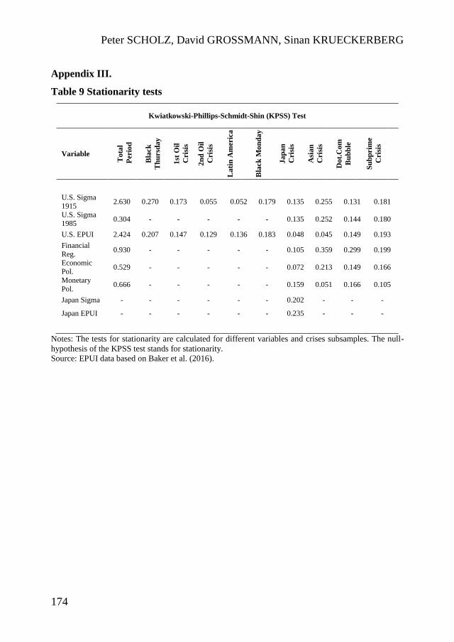
Peter SCHOLZ, David GROSSMANN, Sinan KRUECKERBERG
174
Appendix III.
Table 9 Stationarity tests
Kwiatkowski-Phillips-Schmidt-Shin (KPSS) Test
Variable
To
tal
Peri
od
Bla
ck
Th
ursd
ay
1st
Oil
Cris
is
2n
d O
il
Cris
is
La
tin
Am
eric
a
Bla
ck
Mo
nd
ay
Ja
pa
n
Cris
is
Asi
an
Cris
is
Do
t.C
om
Bu
bb
le
Su
bp
rim
e
Cris
is
U.S. Sigma
1915 2.630 0.270 0.173 0.055 0.052 0.179 0.135 0.255 0.131 0.181
U.S. Sigma
1985 0.304 - - - - - 0.135 0.252 0.144 0.180
U.S. EPUI 2.424 0.207 0.147 0.129 0.136 0.183 0.048 0.045 0.149 0.193
Financial
Reg. 0.930 - - - - - 0.105 0.359 0.299 0.199
Economic Pol.
0.529 - - - - - 0.072 0.213 0.149 0.166
Monetary
Pol. 0.666 - - - - - 0.159 0.051 0.166 0.105
Japan Sigma - - - - - - 0.202 - - -
Japan EPUI - - - - - - 0.235 - - -
Notes: The tests for stationarity are calculated for different variables and crises subsamples. The null-
hypothesis of the KPSS test stands for stationarity.
Source: EPUI data based on Baker et al. (2016).

CENTRAL EUROPEAN REVIEW OF ECONOMICS AND MANAGEMENT ISSN 2543-9472; eISSN 2544-0365
www.cerem-review.eu
www.ojs.wsb.wroclaw.pl Vol. 2, No. 1, 175-187, March 2018
Correspondence address: Anna Motylska-Kuźma, WSB University in Wrocław, ul. Fabryczna 29-31, 53-
609 Wrocław, Poland. E-mail: . [email protected]
Received: 12-07-2017, Revised: 27-10-2017, Revision: 16.01.2018, Accepted: 17-01-2018
doi: http://dx.doi.org/10.29015/cerem.511
© 2018 WSB UNIVERSITY IN WROCŁAW
Alternative finance and sustainable development
Anna MOTYLSKA-KUŹMA
WSB University in Wrocław, Poland
Abstract:
Aim: The aim of this article is to evaluate alternative finance for the implementation of the basic assumptions and goals of sustainable development.
Design / Research methods: Using the comparative analysis the most frequent mentioned forms of alternative finance have been assessed. The analysis took into account both the assumptions and the basic goals of sustainable development.
Conclusions / findings: The conducted analysis show that despite many features that indicate the inclusion of alternative finance in philosophy of sustainable development, the implementation of the basic assumptions and goals are arbitrary. Many of the alternative forms do almost realized nothing.
Originality / value of the article: An juxtaposition of sources of financing with the concept of sustainable development is usually carried out when analyzing the funding opportunities for relevant initiatives. However, in this case, the assessment is concentrating on the sources of financing and implementation by them of the adopted sustainability assumptions and goals.
Key words: alternative finance, sustainable development. JEL: G23, G24, G30, G32, O30.
1. Introduction
The financial crisis of 2008 exposed the weakness of the traditional banking
system and financial markets. In response to growing problems, governments and
regulators in many countries have introduced additional restrictions that
significantly hinder access to capital. This situation particularly affected the SME
sector and newly emerging enterprises. These entities, therefore, began looking for
other alternative financing methods. Taking into account the fact that the SME
sector makes a significant contribution to the economic development of all countries

Anna MOTYLSKA-KUŹMA
176
(e.g. in Poland it generates about 50% of GDP), and growth as such cannot be
achieved without innovation, the actions restricting access to capital were not only a
serious blow to the economic operators themselves, but also translated into a
slowdown observed for a very long time.
By adopting a Declaration of Action for Sustainable Development in Rio de
Janeiro, the signatory countries have committed themselves to respecting the
principles and achieving the objectives set. Hence, the question arises whether the
financial crisis and the resulting lack of access to capital and the above declarations
go hand in hand and whether the resulting alternatives are the answer to the
emerging problems.
The aim of this article is to evaluate alternative sources of finance for the
implementation of the basic assumptions and goals of sustainable development.
The article is divided into three sections. The first of them discusses the basic
concepts of sustainable development. Particular attention has been paid to the
assumptions and goals adopted by many countries within the framework of this
concept. The second section deals with alternative finances, the origins of their
growing popularity and their basic forms. The final section analyzes and evaluates
the implementation of sustainable development policies by individual forms of
alternative finance. The most important conclusions flowing from the analysis are
contained in the summary which also offers further indication of research
opportunities.
2. Sustainable development – basic concepts, objectives and directions of action
Sustainable development has been defined in many ways, but the most common
and frequently quoted definition is from “Our Common Future” – “Sustainable
development is development that meets the needs of the present without
compromising the ability of future generations to meet their own needs.”
The concept of sustainable development is associated primarily with the United
Nations Conference on Environment and Development organized in Rio de Janeiro
in 1992 (the so-called Earth Summit). At the meeting, government representatives

ALTERNATIVE FINANCE AND SUSTAINABLE DEVELOPMENT
177
from 170 countries, including Poland, declared their support for the idea of
environmentally sensitive economic development. During the Conference, as well as
later, a number of different types of treaties were signed, which have been put into
effect with greater or lesser success. Unfortunately, the implementation of the idea
of sustainable development met with very sharp criticism. This is a normative
concept of conscious and active shaping of social relations and human-environment
relations. It requires, therefore, a difficult axiological understanding that is contrary
to the ruling, ubiquitous liberal democracy. So if most ethical values are
subordinated to economic values, and not vice versa, the realization of sustainable
development will remain only a utopia.
This concept has enormous scientific and research potential, especially from an
interdisciplinary perspective. It offers the opportunity to compile and combine the
perspectives of different academic disciplines, such as linking ecology, ethics,
economics, research, sociology and many other disciplines. In addition, research on
sustainable development provides the basis for formulating recommendations for
social policy, identifying ways to improve the quality of life and the state of the
environment (Rokicka, Woźniak 2016).
Sustainable development assumes that economic growth is supposed to lead to
greater social cohesion (including reduce social stratification, equalize opportunities,
counteract marginalization and discrimination) and improving the quality of the
environment through limiting the harmful impact of production and consumption on
the state of the environment, the protection of natural resources (Kuraszko 2009).
Sustainable development refers to the social and economic development of an
enterprise, which enables the implementation of the strategy and the attainment of
its objectives without interfering with its future realization (Witek-Crabb 2005).
Therefore, the development of an enterprise should be carried out in such a way that
it does not interfere with the future development potential, also on the basis of
building a competitive advantage.
Implementing such a development requires not only the knowledge of internal
procedures and capabilities but also a very detailed knowledge of the conditions and
environment in which it operates. Mutual relationships and ways of interacting are
of great importance here. It is quite common for managers to seek solutions that

Anna MOTYLSKA-KUŹMA
178
should reconcile conflicting interests of different parties. Hence, it is necessary to
harmonize economic objectives with social and environmental objectives.
Looking at sustainability research, it is noteworthy that some authors
interchangeably use the terms sustainability and business responsibility (Laszlo
2008). This is in some way justified, because sustainable development involves the
use and conservation of natural resources and the orientation of technology and
institutions in order to achieve and sustain the fulfillment of the human needs of
present and future generations. This understanding, which preserves soil, water
resources, plants and genetic resources of animals, does not degrade the
environment and uses technologies, is economically viable and socially acceptable
(Kuciński 2009).
Regardless of whether these concepts are considered the same or not, they
certainly have common assumptions. Their focus is on external effects and
distribution problems related to the economic activity of enterprises.
Key elements of sustainable development, according to the Brundtland Report
(Brundtland 1987), were:
Recovery of economic growth
Changing the quality of economic growth
Satisfying basic needs such as jobs, food, water, access to sanitation, health
care
Ensuring a sustainable level of production
Protecting and improving the natural resource base
Technology reorientation and risk management
Merging the environment and economy in the decision-making process
Reorientation of international economic relations.
In 2015 the Goals for Sustainable Development were established, which were
included in the UN’s Development Agenda 2030. They contain 17 basic objectives:
No poverty, Zero Hunger, Good health and well – being, Quality education, Gender
equality, Clean water and sanitation, Affordable and clean energy, Decent work and
economic growth, Industry, innovation and infrastructure, Reduced inequalities,
Sustainable cities and communities, Responsible consumption and production,

ALTERNATIVE FINANCE AND SUSTAINABLE DEVELOPMENT
179
Climate action, Life below water, Life on land, Peace, justice and strong institutions,
Partnership for the goals.
3. Alternative finance
Alternative Finance (AF) is an innovative segment of financial market, aimed at
providing consumer loans, startup financing, providing capital to the SME sector
through the use of new technologies – online platforms and social networking sites
(Waszkiewicz 2016). In the broader context, alternative finance serves to stimulate
economies and to fund charity or socially important actions (Wardrop et al. 2015).
The new segment operates outside the traditional banking and capital markets
(Baeck et al. 2014), so it is a part of shadow banking, defined by the Financial
Stability Board (FSB 2011) and European Commission in the Green Book (EC
2012). Also Goldman Sachs (Nash, Beardsley 2015) speaks similarly about
alternative finance.
The most frequently mentioned forms of alternative finance include: P2P
Consumer Lending, P2P Business Lending, Donation Crowdfunding, Reward
Crowdfunding, Equity Crowdfunding, Invoice Trading, Debt – Based Securities,
Community Share/Microfinance, Pension – led Funding. Among the most popular,
however, are mainly P2P loan platforms and crowdfunding platforms.
The P2P lending platforms are divided into two groups according to the type of
“customers” that use these solutions: P2P consumer lending and P2P business. The
first group offers access to loans given and taken by individuals. The interest rate is
determined in the auction, i.e. the appropriate statement of the borrower's offer with
the offer of the lender. Hence, the rate is generally lower than the market rate of
credit and credit lines, but at the same time higher than the market offering of
deposit instruments, taking into account the corresponding period of time. The
second group refers to operations where the borrower has an economic entity, while
the lender may be represented by other entities and individuals (Baeck et al. 2014).
The first P2P platform was launched in the UK in 2005, but the idea quickly
spread around the world. However, the cradle of this form of alternative finance

Anna MOTYLSKA-KUŹMA
180
remains the UK, as it is the place where most of these loans are offered. According
to the NESTA research (Baeck et al. 2014) in 2014 £749m has been lent in P2P
business lending and £547m in P2P customer lending.
Crowdfunding is the use of the internet community and networks to raise capital
for a variety of ideas. It is a typical collection of money (smaller or larger amounts)
through the internet for the purpose one chooses. Due to the way of payment to the
donors, we distinguish four types of crowdfunding (Motylska-Kuźma 2016):
donation – projects are non-profit, usually associated with charity, so for the
money paid the donor does not receive anything in return;
reward – in return for donations, donors receive rewards, but their nature is
very often dependent on the amount of payment. The prize could be the
prototypes of products, tickets for an event organized, etc.
lending – this kind of crowdfunding is very similar to business P2P lending,
so these forms are often identified with each other. However, P2P is
supposed to transfer financial surpluses from lenders to borrowers and it is
not necessarily a specific purpose here. In the case of lending crowdfunding,
the purpose must be specifically defined;
equity – investors acquire shares in companies, later using dividends,
distributions of profit or redemptions at initial prices.
Invoice trading is the purchase by investors of the sales invoices with discount,
using ICT (Wardrop et al. 2015). So it can be said that it is some sort of factoring,
although not institutionalized. It is increasingly called microfactoring.
Microfinance refers to loans granted to a very specific group of SMEs, namely
those who are in financial trouble or for some reason are excluded from the
traditional banking system. Community shares, however, are the transfer of certain
amounts to charity (Wardrop et al. 2015).
In case of debt-based securities, the borrower receives the funds for the
indicated purpose and, in return, issues an unsecured debt instrument for a specified
period of time (Waszkiewicz 2016). This is similar to the issue of bonds, but
because it is outside the traditional banking system, the instrument received is not
only not secured, but very often the legal capacity of its debt collection is very
limited.

ALTERNATIVE FINANCE AND SUSTAINABLE DEVELOPMENT
181
Pension-led funding is the financing of the SME sector from the funds accrued
from the pension funds of the project promoter. Intellectual property serves
frequently as security, and the method itself is developed only in the UK (Wardrop
et al. 2015).
The market for alternative finance can boast a very dynamic development.
According to the NESTA research (Baeck et al. 2014), between 2012 and 2014, in
the UK alone, the following growth rates were recorded:
Equity crowdfunding – 410%
P2P business lending – 250%
Rewards crowdfunding – 206%
Invoice trading – 174%
Debt – based securities – 117%
P2P consumer lending – 108%
Community shares – 95%
Donation crowdfunding – 77%
Pension – led funding – 5%.
4. Alternative finance and sustainable development
Table 1 below provides a comparative analysis of all forms of alternative
finance and assesses the level of achievement of the assumptions and the goals of
sustainable development. Each of the alternative finance forms listed in Chapter 3
was rated 1 to 3, where 1 means that no objective or assumption was covered by the
form of financing analyzed, 3 – full implementation. Ratings are given subjectively,
based on the definitions and descriptions in Chapter 3. Because all the assumptions
and objectives of sustainable development are considered equivalent, no weights
which are responsible for the priority were introduced into the analysis. The sum of
the rates received reflects the degree of coherence of a given form of financing with
the ideas of sustainable development.

Anna MOTYLSKA-KUŹMA
182
Table 1. Assessment of alternative finance
Rule/Goal of
sustainable
development
P2P
consum
er
lending
P2P
business
lending
Donatio
n
crowdfu
nding
Reward
crowd-
funding
Equity
crowd-
funding
Invoice
trading
Debt –
based
securities
Comm
unity
shares
Pension –
led
funding
Average
The Rules:
Recovery of
economic
growth
2 3 1 2 3 3 3 2 2 2.33
Changing the
quality of
economic
growth
2 3 1 2 3 2 3 1 1 2.00
Satisfying
basic needs 1 3 2 2 3 3 3 2 1 2.00
Ensuring a
sustainable
level of
production
1 2 1 2 3 2 2 2 2 1.89
Protecting
and
improving the
natural
resource base
1 2 2 2 2 2 2 2 2 1.89
Technology
reorientation
and risk
management
1 2 1 3 3 2 3 2 2 2.11
Merging the
environment
and economy
in the
decision-
making
process
1 2 2 2 2 2 2 2 2 1.89

ALTERNATIVE FINANCE AND SUSTAINABLE DEVELOPMENT
183
Table 1. Cont.
Rule/Goal of
sustainable
development
P2P
consum
er
lending
P2P
business
lending
Donatio
n
crowdfu
nding
Reward
crowd-
funding
Equity
crowd-
funding
Invoice
trading
Debt –
based
securities
Comm
unity
shares
Pension –
led
funding
Average
Reorientation
of
international
economic
relations
1 1 1 1 1 1 1 1 1 1.00
The goals:
No poverty 2 2 2 2 2 2 2 2 2 2.00
Zero hunger 2 1 2 1 1 1 1 2 1 1.33
Good health
and well–
being
1 1 2 2 1 1 1 1 1 1.22
Quality
education 1 1 1 1 1 1 1 1 1 1.00
Gender
equality 3 3 3 3 3 3 3 3 3 3.00
Clean water
and sanitation 1 1 2 1 1 1 1 1 1 1.11
Affordable
and clean
energy
1 1 1 1 1 1 1 1 1 1.00
Decent work
and economic
growth
2 3 2 3 3 3 3 3 3 2.78
Industry,
innovation
and
infrastructure
2 3 2 3 3 3 3 3 3 2.78
Reduced
inequalities 3 3 2 2 2 2 2 2 2 2.22
Sustainable
cities and
communities
2 2 2 2 2 2 2 2 2 2.00

Anna MOTYLSKA-KUŹMA
184
Table 1. Cont.
Rule/Goal of
sustainable
development
P2P
consum
er
lending
P2P
business
lending
Donatio
n
crowdfu
nding
Reward
crowd-
funding
Equity
crowd-
funding
Invoice
trading
Debt –
based
securities
Comm
unity
shares
Pension –
led
funding
Average
Responsible
consumption
and
production
2 3 2 3 3 3 3 3 3 2.78
Climate
action 1 1 1 1 1 1 1 1 1 1.00
Life below
water 1 1 1 1 1 1 1 1 1 1.00
Life on land 1 1 1 1 1 1 1 1 1 1.00
Peace, justice
and strong
institutions
1 1 1 1 1 1 1 1 1 1.00
Partnerships
for the goals 1 1 1 1 1 1 1 1 1 1.00
Total: 27 29 28 29 28 28 28 29 28
Percentage
[%]: 36.0 38.7 37.3 38.7 37.3 37.3 37.3 38.7 37.3
Source: author’s own assessment
As can be seen in Table 1, the principle of economic growth is best
implemented, and among the goals – “gender equality”, “decent work and economic
growth”, “industry, innovation and infrastructure” and “responsible consumption
and production”. The “reorientation of international economic relations” was
completely omitted. Alternative financing is indeed transnational, as most platforms
work for people not necessarily associated with a given country. On the other hand,
however, this is not a sufficient argument to consider them to be capable of affecting
the economic relations between individual countries. Some sustainability targets
have also been omitted. Firstly, alternative finance does not meet the goal “quality
education”. Some of the analyzed forms of funding may be sources of capital needed
to meet the goals of improving the quality of education. However, the financing
model alone does not meet the above objective. Another unrealized goal is
“affordable and clean energy”. As in the case of quality of education, projects

ALTERNATIVE FINANCE AND SUSTAINABLE DEVELOPMENT
185
funded through obtained capital may involve renewable energy sources, but the
source of financing alone does not contribute to this objective. A similar situation
also applies to goals such as “climate action”, “life below water”, “life on land”,
“peace, justice and strong institutions” and “partnership for the goals”.
However, by observing the summary estimates of all the alternative forms of
financing analyzed, it can be seen that they do not differ significantly. In fact, some
of the assumptions or goals are pursued by selected models better and others worse.
However, on average, these ratings remain on a very similar level. It is between 27
and 29 points, i.e. on average 37.6% of the maximum number of points.
It is worth noting that the sum of all points can be between 25 and 75. The
lowest value is a situation in which a given form of financing does not pursue any of
the assumptions and goals of sustainable development (receives a rating 1
everywhere). The highest value – all objectives and assumptions are fully
implemented. When comparing this theoretical framework with the results obtained,
it could be concluded that alternative financing is unlikely to support the objectives
of sustainability and its assumptions, although it would seem at first glance that they
favor a responsible business and fight against inequalities that are one of the
fundamental concepts associated with sustainable development.
5. Summary
It should be noted that the market of alternative finance is no longer just a
response to the crisis, but an increasingly rapidly growing segment of the modern
financial market. And while this is still a market niche compared to European credit
assets, the AF market has a huge potential for growth.
Alternative finance is mainly used to finance the SME sector, including
innovative solutions, charitable donations or microfinance. It has limited procedures,
transaction transparency, control capabilities, and high quality customer service. The
primary benefit is either reduced cost or favorable interest rates as well as satisfying
individual social needs.

Anna MOTYLSKA-KUŹMA
186
However, from the point of view of implementing the principles and objectives
of sustainable development, alternative finance does not seem to respond directly to
the much needed changes. Brief evaluation of the different forms of funding can
lead to erroneous conclusions that they especially fight with social differences,
stimulate “healthy” growth because they promote socially acceptable activities. A
more detailed analysis demonstrates, however, that the first impression is wrong. It
is true that alternative finance certainly contributes to the realization of many
projects that are more or less in line with the assumptions and goals of sustainable
development, but the funding models themselves do not serve them.
The above analysis has several limitations. First, the assessment is subjective.
This means that it is not based on credible research, but on subjective judgment of
the author, made on the basis of definitions and descriptions of the forms of
alternative funding and the principles and goals of sustainable development.
Nevertheless, it points to some interesting insights that may be the basis for further
research.
Secondly, the evaluation included only the concept of the funding model itself.
As mentioned above, adding to the analysis the characteristics of the projects being
implemented could in greater detail determine whether alternative finance
contributes to achieving the principles and goals of sustainable development or not.
It should not only evaluate the projects themselves, but to examine their scope and
nature of their impact on the environment and society.
In conclusion, consumer awareness and ubiquitous technology have led to the
creation of a certain sensitivity on the part of enterprises towards aspects of social
responsibility that have a direct impact on sustainability. Alternative finance has a
role to play here, which will be appreciated both by donors and by capital recipients.
References
Baeck P., Collins L., Zhang B. (2014), Understanding alternative finance. The UK Alternative Finance
Industry Report, University of Cambridge, https://www.nesta.org.uk/sites/default/files/understanding-
alternative-finance-2014.pdf [11.02.2018].
Brundtland and World Commission on Environment and Development (1987), Our common future.
Report of the World Commission on Environment and Development, Oxford University,
http://www.un-documents.net/our-common-future.pdf [11.02.2018].

ALTERNATIVE FINANCE AND SUSTAINABLE DEVELOPMENT
187
Financial Stability Board (FSB) (2011), Shadow banking. Strengthening oversight and regulation
recommendations of the Financial Stability Board, http://www.fsb.org/wp-
content/uploads/r_111027a.pdf?page_moved=1 [11.02.2018].
European Commission (EC) (2012), Green Paper. Shadow banking,
http://ec.europa.eu/internal_market/bank/docs/shadow/green-paper_en.pdf [11.02.2018].
Kuciński K. (ed.) (2009), Strategie przedsiębiorstw wobec wymogów zrównoważonego rozwoju
(Enterprises’ strategies and the requirements of sustainable develompent), Oficyna Wydawnicza SGH,
Warszawa.
Kuraszko I. (2009), Zrównoważony rozwój (Sustainable development), Forum Odpowiedzialnego
Biznesu, http://odpowiedzialnybiznes.pl/artykuly/zrownowazony-rozwoj/ [11.02.2018].
Laszlo Ch. (2008), Firma zrównoważonego rozwoju (The sustainable company), Studio EMKA,
Warszawa.
Motylska-Kuźma A. (2016), The cost of crowdfunding capital, in: 3rd International Multidisciplinary
Scientific Conference on Social Science & Arts, SGEM 2016, Conference Proceedings, Book 2, Vol.
III, pp. 601-612, DOI: 10.5593/SGEMSOCIAL2016/B23/S06.076.
Rokicka E., Woźniak W. (2016), W kierunku zrównoważonego rozwoju. Koncepcje, interpretacje,
konteksty, Katedra Socjologii Ogólnej (Towards sustainable development. Ideas, interpretations,
contexts), Wydział Ekonomiczno-Socjologiczny, Uniwersytet Łódzki,
http://socjologia.uni.lodz.pl/pliki/32-w_kierunku_zrownowazonego_rozwoju.pdf [11.02.2018].
Nash R.M., Beardsley E. (2015), The future of finance. Part 3: The rise of the new Shadow Bank,
Goldman Sachs Global Investment Research,
https://www.betandbetter.com/photos_forum/1425585417.pdf [11.02.2018].
Waszkiewicz A. (2016), Finanse alternatywne – elektroniczne innowacje finansowe (Finance
alternatives – electronic financial innovation), „Acta Universitatis Lodziensis. Folia Oeconomica”, vol.
319 no. 2, pp.135-152.
Wardrop R., Zhang B., Rau R., Gray M. (2015), Moving Mainstream. The European Alternative
Finance Benchmarking Report, University of Cambridge and EY,
http://www.ey.com/Publication/vwLUAssets/EY-and-university-of-cambridge/$FILE/EY-cambridge-
alternative-finance-report.pdf [11.02.2018].
Witek-Crabb A. (2005), Zrównoważony rozwój przedsiębiorstw – więcej niż ekorozwój (Sustainable
development of enterprises – beyond eco-development), in: Zrównoważony rozwój przedsiębiorstwa a
relacje z interesariuszami ekorozwój (Sustainable development of enterprises and relationships with
stakeholders), ed. Brdulak H., Oficyna Wydawnicza SGH, Warszawa, pp. 561-568.
Copyright © 2022 FDOKUMEN