Causative mechanisms for the occurrence of a triplelayered mesospheric inversion eventover low latitudesK. Ramesh1, S. Sridharan2, and S. Vijaya Bhaskara Rao1

1Department of Physics, Sri Venkateswara University, Tirupati, India, 2National Atmospheric Research Laboratory, Gadanki, India

Abstract The temperature profile obtained from the space borne instrument “Sounding of Atmosphere byBroadband Emission Radiometry” instrument onboard “Thermosphere Ionosphere Mesosphere Energetics andDynamics” shows a triple layered mesospheric inversion event on the night of 23 September 2011, when thereis an overpass near the low-latitude sites Gadanki (13.5°N, 79.2°E) and Tirunelveli (8.7°N, 77.8°E). The threemesospheric inversion layers (MILs) are formed in the height region around ~70 (lower), ~80 (middle), and~90 km (upper) with amplitudes ~11, ~44, and ~109K and thickness of 3.4, 4.9, and 6.6 km, respectively. Theformation of the lower and middle MILs can only be observed in the Rayleigh lidar temperature profiles overGadanki due to upper height limitation of the system. Nearly all the dominant causative mechanisms areexamined for the occurrence of the MIL event. The lower MIL at ~70km is inferred to be due to planetary wavedissipation, as there is a sudden decrease of planetary wave activity above 70 km. Further, it is demonstratedthat the middle MIL at ~80 km is due to the turbulence generated by gravity wave breaking which is in turndue to gravity wave-semi-diurnal tidal interaction, though the height of the middle MIL descends at the rateof ~1km/h, which is nearly the vertical phase speed of diurnal tide, whereas the upper MIL at above 90 km isdue to the large chemical heating rate (~45 K/day) generated by the dominant exothermic reactionO+O+M→O2+M.

1. Introduction

The term “mesospheric inversion layer” (MIL) refers to the inversion of temperature gradient from negative topositive superposed upon the characteristically decreasing mesospheric thermal structure with the positivelapse rate at the bottom. The thickness and amplitude of the MIL can reach up to ~10 km and ~100K,respectively, depending on the season and latitude. This is a striking and poorly understood feature of the MLT(mesosphere and lower thermosphere) region explored bymany researchers from different sites using a varietyof instrumental techniques. After Schmidlin [1976], who was the first to report the MIL, there have been severaldetailed reports on their occurrence characteristics using lidars, radars, rocketsondes, and satellites overdifferent geographic locations [Hauchecorne et al., 1987; Jenkins et al., 1987;Meriwether et al., 1998; Thomas et al.,2001; Siva Kumar et al., 2001, 2006; Sridharan et al., 2008, 2010; She et al., 1995; States and Gardner, 1998; Chenet al., 2000; Clancy and Rusch, 1989; Clancy et al., 1994; Leblanc and Hauchecorne, 1997; Venkat Ratnam et al.,2003; Fadnavis and Beig, 2004;Meriwether and Gerrard, 2004; Lehmacher et al., 2006; Ramesh and Sridharan, 2012;Szewczyk et al., 2013; Ramesh et al., 2013a, 2013b]. TheMILs can be found (spanning ~50–120 km) at all latitudesduring all the seasons, but they can be found more frequently during winter months at midlatitudes [Leblancand Hauchecorne, 1997] and in equinox months at low latitudes [Siva Kumar et al., 2001]. They can normallybe classified into lower and upper MILs. The lower MILs, which occur in the lower height region of ~65–80 kmare believed to be due to planetary wave (PW) breaking. When the phase speed of the PW matches thebackground zonal wind speed u� c ¼ 0ð Þ, a critical level is formed, leading to PW dissipation which normallyoccurs at the altitudes of ~65–80 km [Sassi et al., 2002; Meriwether and Gerrard, 2004]. Salby et al. [2002]explained the relationship of PW activity with the temperature inversions in the mesosphere. The mesosphericinversions are associated with the PW phase shift which causes the wave temperature out of phase with thewave geopotential. The turbulence created by the gravity wave breaking may also alter the vertical structure ofthe PW and cause their absorption just above the inversion region [Ramesh et al., 2013a]. Gan et al. [2012]studied the global distribution and seasonal variation of lower MIL characteristics using Sounding ofAtmosphere by Broadband Emission Radiometry (SABER) temperature data. They found that the occurrencerate of lower MILs peaks in spring and autumn at low latitudes and during winter at midlatitudes.

RAMESH ET AL. ©2014. American Geophysical Union. All Rights Reserved. 3930

PUBLICATIONSJournal of Geophysical Research: Space Physics

RESEARCH ARTICLE10.1002/2013JA019750

Key Points:• Demonstrated causativemechanisms fora triple-layered mesospheric inversions

• Lower and middle layers due toPW breaking and GW-tidalinteraction respectively

• Upper layer is formed due to thechemical reaction between twooxygen atoms

Correspondence to:S. Sridharan,susridharan@narl.gov.in

Citation:Ramesh, K., S. Sridharan, and S. VijayaBhaskara Rao (2014), Causativemechanisms for the occurrence of a triplelayered mesospheric inversion eventover low latitudes, J. Geophys. Res. SpacePhysics, 119, 3930–3943, doi:10.1002/2013JA019750.

Received 30 DEC 2013Accepted 23 APR 2014Accepted article online 29 APR 2014Published online 19 MAY 2014

The upper MILs which occur at higher altitudes between 85 and 100 km have been suggested to be dueto gravity wave (GW) tidal interactions [Meriwether and Gerrard, 2004]. GWs play a vital role in transporting theheat energy and momentum flux from their sources in the lower atmosphere and thereby affect the generalcirculation, thermal structure, and the energy budget of the middle and upper atmosphere. According tolinear saturation theory [Lindzen, 1981], in the absence of damping, the GWs generated in troposphere[Fritts and Nastrom, 1992] propagate vertically upward with increasing amplitude in response to decreasingatmospheric density in proportion to ez/2H (z=height, H= scale height) and break at a particular heightwhere they become convectively (N2< 0, Ri< 0; N=Brunt-Väisälä frequency, Ri=Richardson number) ordynamically (Ri< 0.25) unstable. The amplitude of the waves saturates above this “breaking level” byirreversible extraction of energy from the wave leads to the production of turbulence [Hodges, 1967, 1969],which prevents further wave growth with height. The wave-induced acceleration begins to deceleratethe background winds resulting in critical level, where the horizontal phase speed of the wave matchesthe background wind u� c ¼ 0ð Þ. The turbulence heating arising from the wave breaking could form theinversion layer, and it provides a feedback mechanism reducing the stability that can maintain the MIL[Meriwether and Gardner, 2000].

Walterscheid [1981] suggested that the interactions of GWs with tides can significantly modulate the tidalamplitudes and affect the turbulent intensity. The interaction can also impact the distribution of O, O3, OH,and NO by modulating the eddy diffusivity in the MLT region. The interaction between the gravity wavesand thermal tides strongly modifies the momentum, heat flux, and the stability structure of the gravitywave and enhances the temperature amplitude which in turn maintains an inversion layer in the mesosphere[Liu and Hagan, 1998; Sridharan et al., 2008]. The observed effects of gravity wave-tidal interaction include (i)the modulation of amplitude and phase of the tide in response to the gravity wave momentum deposition,and (ii) the modulation of gravity wave fluxes at tidal periods as a result of critical level interactions [Frittsand Vincent, 1987; Thayaparan et al., 1995; Williams et al., 1999]. Nakamura et al. [1997] studied the variabilityof diurnal tidal amplitudes and phases during gravity wave-tidal interactions at equatorial and subtropicallatitudes. They suggested that the amplitude of diurnal tide is maximum during equinoxes and solstices inthe MLT region and the interaction between gravity waves and tides modulates the gravity wave momentumfluxes which provide the feedback for the tidal amplitude and phase structures. Sica et al. [2002] found goodcorrelation between gravity wave variance and semi-diurnal tides and showed poor correlation between gravitywave variance and diurnal tides during a MIL event at midlatitudes. The formation of MILs due to gravity wave-tidal interaction can be identified by (i) the presence of two cooling regions of amplitude ~10–30K above andbelow the inversion layer, and (ii) the downward progression of gravity wave breaking region (heating/coolingregion) at the rate of tidal phase speed [Meriwether et al., 1998; Liu and Hagan, 1998; Liu et al., 2000].

Along with dynamics, chemical heating also plays a dominant role for the occurrence of upper mesosphericinversion layers. This includes the heat energy released by several exothermic chemical reactions between H,O, O2, O3, OH, and HO2 [Mlynczak and Solomon, 1991; Meriwether and Mlynczak, 1995; Meriwether andGardner, 2000;Meriwether and Gerrard, 2004; Ramesh et al., 2013b].Meriwether and Mlynczak [1995] illustratedthe importance of chemical heating in causing the MILs between 80 and 95 km by the mesosphericphotochemistry with the dynamical transport of long-lived chemical species. Fadnavis and Beig [2004]discussed the relationship of inversion layers with the seven exothermic chemical reactions which areresponsible for significant heating in the mesosphere over Indian tropical region. They observed semi-annualoscillation in the inversion amplitudes, ozone concentrations, and the frequency of occurrence with maximaduring May and November and minima during July and January. The correlation between the inversionamplitudes and the ozone mixing ratios suggests the importance of ozone concentration in the formationof MILs. Ramesh et al. [2013b] discussed the dominance of chemical heating over dynamics for the largeMILs in the height region of ~80–85 km. It was demonstrated that the occurrence of large MILs could bedue to the large ozone mixing ratios which in turn caused large chemical heating rates (~50%) mainlythrough the reaction, H +O3→OH+O2.

A triple layered MIL event is observed with each layer having different amplitudes on the night of 23September 2011 in the temperature profiles obtained from Sounding of Atmosphere by Broadband EmissionRadiometry (SABER) instrument onboard Thermosphere Ionosphere Mesosphere Energetics and Dynamics(TIMED) satellite when it over passed near Gadanki (13.5°N, 79.2°E) and Tirunelveli (8.7°N, 77.8°E). The three

Journal of Geophysical Research: Space Physics 10.1002/2013JA019750

RAMESH ET AL. ©2014. American Geophysical Union. All Rights Reserved. 3931

layers are observed in the height region around 70, 80, and 90 km, respectively. Though the roles of gravitywaves, planetary waves, and chemical heating have been discussed in the earlier studies [Ramesh andSridharan, 2012; Ramesh et al., 2013a, 2013b], the present study addresses the influence of gravity wave-tidalinteraction for the occurrence of the MIL. In this study, along with gravity wave-tidal interaction, theother causative mechanisms namely planetary wave dissipation and chemical heating are also discussed forthis ideal case of triple layered mesospheric inversion event. In the present study, it is inferred that the threeinversion layers (lower at 70, middle at 80, and upper at 90 km) could predominantly be due to planetarywave dissipation, gravity wave-tidal interaction, and chemical heating, respectively. Though the mesosphericinversions observed at ~80–85 km are dominantly due to the exothermic reaction between H and O3

[Ramesh et al., 2013b], it is inferred in the present study that the inversion occurred above ~90 km is mainlydue to the large heat energy released by the exothermic reaction, O +O+M→O2+M.

2. Instrumentation and Data Analysis2.1. Rayleigh Lidar Temperature Measurements Over Gadanki

The Rayleigh lidar observations have been carried out in the height region of ~30–90 km at the NationalAtmospheric Research Laboratory (NARL), Gadanki (13.5°N, 79.2°E) with Nd:YAG laser transmitter that emitted600mJ energy per pulse with a repetition frequency of 50 Hz. The clear-sky vertical density profiles in thephoton count mode are obtained by transmitting the 532 nm laser beam in zenith direction, and thebackscattered photons integrated for 12,500 transmitted pulses corresponding to a temporal resolutionof 250 s are collected by a 75 cm diameter Newtonian telescope at the height resolution of 300m. The detailsof NARL lidar system are included in Siva Kumar et al. [2003] and Ramesh and Sridharan [2012]. The molecularbackscattered photons are used to derive temperature profiles using the method given by Hauchecorne andChanin [1980]. Considering the atmosphere is in hydrostatic equilibrium, the pressure value is seeded atthe top of the height range (90 km), and by applying the ideal gas equation, the vertical temperature profilesT(z) are obtained using the expression given by

T zið Þ ¼ Mg zið ÞΔzRLog 1þ Xð Þ where X ¼ ρ zið Þg zið ÞΔz

P zi þ Δz=2ð Þ (1)

and the uncertainty in the measurement of temperature is given by

δT zið ÞT zið Þ ¼ δLog 1þ Xð Þ

Log 1þ Xð Þ ¼ δX1þ Xð ÞLog 1þ Xð Þ (2)

2.2. Thermosphere Ionosphere Mesosphere Energetics and Dynamics—Sounding of the AtmosphereUsing Broadband Emission Radiometry Data Sets

The Sounding of the Atmosphere using Broadband Emission Radiometry (SABER) is a space-borne instrumentonboard the Thermosphere-Ionosphere-Mesosphere Energetics and Dynamics (TIMED) satellite, and itprovides the vertical profiles of temperature, ozone volume mixing ratio, chemical heating rates due tovarious exothermic chemical reactions among H, O, O2, O3, OH, OH2, and volume emission rates ofdifferent species. The SABER level-2A files of version-1.07 (V1.07) have the vertical profiles of temperature,number density, volume mixing ratio of ozone (O3), and the volume emission rates of O2 and OH andlevel-2A files of version-2.0 (V2.0) have atomic oxygen (O) and atomic hydrogen (H) profiles. The SABERlevel-2B files have the upper mesospheric and lower thermospheric cooling and heating rates of differentexothermic chemical reactions. The errors in the SABER version-1.07 temperatures are 2 K below 70 km, 1.8 Kat 80 km, and 6.7 K at 100 km [Remsberg et al., 2008; Gan et al., 2012]. The SABER V2.0 nighttime verticalprofiles (after 19:30 h IST; Indian Standard Time is 5:30 h ahead of Universal Time) of temperature, ozonemixing ratio (9.6μm channel), and chemical heating rates due to six exothermic reactions (given in Table 1)are downloaded from http://saber.gats-inc.com/ for September 2011 averaged between 10.0°N–15.0°N and60.0°E–90.0°E used for the present study. More details on SABER instrument and different datasets can befound in Remsberg et al. [2003], Mlynczak et al. [2007], and Gan et al. [2012].

2.3. Medium Frequency Radar Observations Over Tirunelveli

The Medium Frequency (MF) radar at Equatorial Geophysical Research Laboratory (EGRL), Indian Institute ofGeomagnetism, Tirunelveli (8.7°N, 77.8°E) has been operating with the frequency of 1.98MHz and providing

Journal of Geophysical Research: Space Physics 10.1002/2013JA019750

RAMESH ET AL. ©2014. American Geophysical Union. All Rights Reserved. 3932

the vertical profiles of zonal andmeridional winds in the height range of ~78–98 kmwith 2 kmheight resolutionand 2min time resolution. More details of this MF radar can be obtained from Rajaram and Gurubaran [1998].The MF radar zonal and meridional winds for September 2011 are used for the present study.

3. Observations and Results3.1. Rayleigh Lidar and TIMED-SABER Temperature Inversions

Figure 1 shows the nightly mean (20:31–00:47h IST) of Rayleigh lidar temperature profiles over Gadanki, theTIMED-SABER temperature profiles corresponding to the locations (11.8°N, 72.5°E) and (9.2°N, 72.9°E), which areclose to as well as representing Gadanki and Tirunelveli, respectively, and the MSIS-E-90 model temperatureprofiles for 23 September 2011. The observed uncertainties in lidar temperatures are 0.1–2.0 K at 30–70 K,2.0–11.0K at 70–85km, and 11.0–18.0K at 85–89km. The high power laser (~30W) made it possible to achievethe temperature profile up to ~90km with relatively less uncertainties. The lidar temperature profile shows two

inversion layers at ~70 and ~80km with amplitudes of 16.2and 52.1K and thicknesses of 2.7 and 3.9 km, respectively.Here the amplitude and thickness of the inversion layer aredefined respectively as the differences in temperature andheights of top and bottom of the inversion layer [Leblanc andHauchecorne, 1997]. The SABER temperature profile showsthree inversion layers at ~69–70km (lower MIL), ~79–80km(middle MIL), and ~90.5 km (upper MIL) with the amplitudesof 11, 44, and 109K and thicknesses of 3.4, 4.9, and 6.6 km,respectively, over Gadanki. Due to low signal-to-noise ratio,the upper inversion layer cannot be observed in the lidartemperature profile. The three inversion layers can also beobserved near Tirunelveli in the SABER temperatureprofile shown in this figure. It can also be observed from thisfigure that the middle MIL at ~80km is sandwiched betweentwo cooling regions (defined as negative deviation of theobserved temperatures from the model temperatures) withamplitudes of 11 and 48K, respectively, over Gadanki.

3.2. Lower MIL Due to Planetary Wave Activity

Meriwether and Gerrard [2004] suggested that the MILsgenerated in the height region of ~65–80 km could bedue to PW breaking during equinox and winter solsticeconditions. In order to verify the relationship of PW activityin the formation of lower MIL at ~70 km over Gadanki on23 September 2011, the SABER temperature perturbations

Figure 1. The Rayleigh lidar nightly mean (20:31–00:47 h IST) temperature profile for 23 September2011 over Gadanki. The TIMED-SABER nighttimetemperatures corresponding to the locations(11.8°N, 72.5°E) and (9.2°N, 72.9°E), which are closeto as well as representing Gadanki and Tirunelveli,respectively. The corresponding MSIS-90 modeltemperature profile is also shown for comparison.

Table 1. The Dominant Exothermic Reactions Responsible for Upper Mesospheric and Lower Thermospheric ChemicalHeating Rates From TIMED-SABER V2.0a

Serial Number Reaction

Maximum Heating Rate (K/day)

At 82.3 km At 95.3 km

R1 O+OH→H+O2 2.0 1.46R2 H+O2+M→HO2+M 0.25 0.007R3 H+O3→OH+O2 7.5 5.54R4 O+HO2→OH+O2 0.27 0.008R5 O+O+M→O2+M 0.52 44.2R6 O+O2+M→O3+M 3.0 2.2R7 O+O3→O2+O2 – –

Total heating rate: 13.54 53.41

aNote: Heating rates for R7 are not available.

Journal of Geophysical Research: Space Physics 10.1002/2013JA019750

RAMESH ET AL. ©2014. American Geophysical Union. All Rights Reserved. 3933

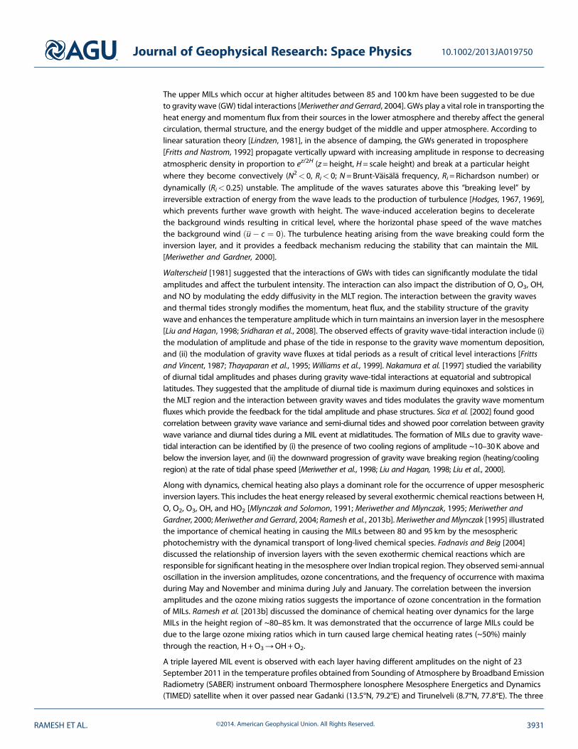
(deviation from monthly mean) averagedbetween 10.0°N–15.0°N and 60.0°E–90.0°Eare subjected to wavelet (Morlet) analysisas shown in Figure 2. It can be observedfrom this figure the presence of 2 day PWduring 20–25 September 2011 overGadanki location. The 2 day wave is aprominent and ubiquitous PW feature,which is stronger during low-latitudewinter [Gurubaran et al., 2001], and it hasnormally been identified as a westwardpropagating PW of zonal wavenumber2–5 [Palo et al., 1999]. The amplitude ofthe PW increases while propagatingupward from the lower atmosphere(~34 km) and peaks above 65 km. Above65 km, the wave amplitude decreasesgradually and dissipates at ~69–70 km.The PW dissipation may be either due towave transience or due to critical levelinteraction [Charney and Drazin, 1961].However, background wind observationsare required to confirm this. It can beinferred from the decrease of planetarywave activity that the lower MIL couldbe due to planetary wave dissipation.

3.3. Middle MIL Due to Gravity Wave-Tidal Interaction

As mentioned in sub-section 3.1, Figure 3 shows the Rayleigh lidar relative temperature perturbations (%)

calculated as T�ToTo

� 100 (where T and To are the half an hour and nightly mean (~4 h) temperature profiles)

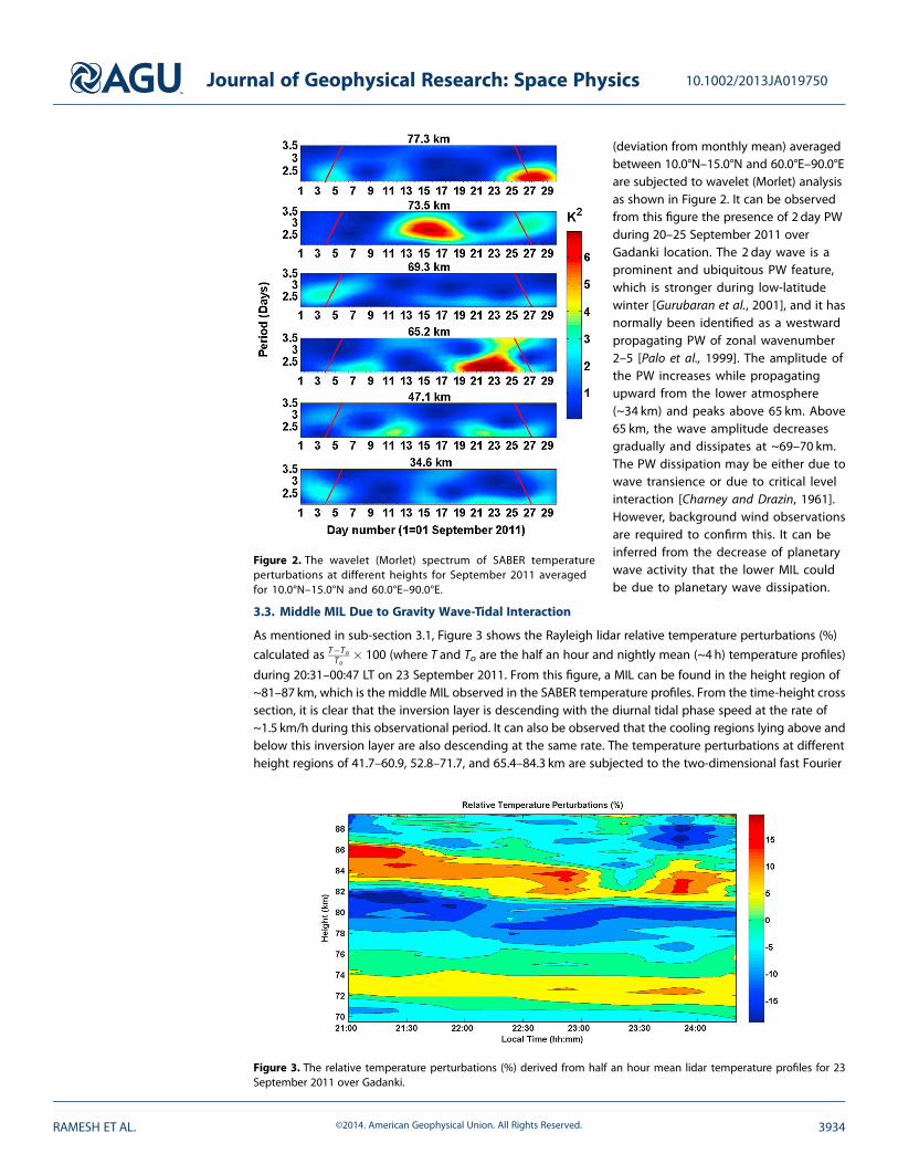
during 20:31–00:47 LT on 23 September 2011. From this figure, a MIL can be found in the height region of~81–87 km, which is the middle MIL observed in the SABER temperature profiles. From the time-height crosssection, it is clear that the inversion layer is descending with the diurnal tidal phase speed at the rate of~1.5 km/h during this observational period. It can also be observed that the cooling regions lying above andbelow this inversion layer are also descending at the same rate. The temperature perturbations at differentheight regions of 41.7–60.9, 52.8–71.7, and 65.4–84.3 km are subjected to the two-dimensional fast Fourier

Figure 3. The relative temperature perturbations (%) derived from half an hour mean lidar temperature profiles for 23September 2011 over Gadanki.

Figure 2. The wavelet (Morlet) spectrum of SABER temperatureperturbations at different heights for September 2011 averagedfor 10.0°N–15.0°N and 60.0°E–90.0°E.

Journal of Geophysical Research: Space Physics 10.1002/2013JA019750

RAMESH ET AL. ©2014. American Geophysical Union. All Rights Reserved. 3934

transform (FFT) analysis in order to inferthe dominant period and verticalwavelength of gravity waves. From thespectrum shown in Figure 4, we can inferthe presence of gravity waves of differentperiods and vertical wavelengths. Inparticular, gravity waves of verticalwavelengths 3.84, 6.4, and 9.6 km withperiods 22.2, 20.5, and ~53–65min,respectively, are dominantly present. Thevertical and horizontal phase speeds of thedominant gravity waves are calculated fromthe gravity wave dispersion relation and arefound to be ~3.0, ~5.2, and ~3.0m/s and~27.8, ~43.6, and ~63.3m/s, respectively,above ~80 km.

The Brunt-Väisälä frequency squaredvalues (N2) are calculated from Rayleighlidar nightly mean temperature profiles forthe convective instability using thefollowing equation:

N2 zð Þ ¼ g zð ÞTo zð Þ

dTo zð Þdz

þ g zð ÞCp

� �(3)

where g(z) is the acceleration due togravity, To(z) is the nightly mean vertical

temperature profile from lidar temperatures, and Cp is the specific heat at constant pressure(Cp= 1004 JK�1kg�1). Figure 5a shows the vertical profile of N2 calculated from Rayleigh lidar temperaturesfor 23 September 2011. The error bars shown in the figure are the standard errors of hourly profiles of N2.From this figure it can be observed that the gravity wave attains the convective instability (N2< 0) above theinversion region at ~85–86 km from which it can be inferred that the gravity wave propagates upward withincreasing amplitude and breaks in the inversion region (~80–86 km) due to tidal modulation of gravity waveamplitude. Liu et al. [2000] suggested that the stability of the background atmosphere which includes thezonal mean, diurnal wind, and temperature structures can influence the gravity wave breaking level.According to gravity wave-tidal interaction model proposed by Fritts and Vincent [1987], the gravity waveshaving phase velocities in the direction of tidal wind u� c < 0ð Þ will reduce in amplitude or be removed bycritical level absorption, and those waves having phase velocities opposite to the direction of tidal wind fieldu� c > 0ð Þ will increase in amplitude [Nakamura et al., 1997]. Figure 5b shows the vertical profile of meanzonal wind, which is westerly at ~80 km where the gravity wave energy is larger (Figure 4) and becomeseasterly at ~84 km. There is a reduction in total wind shear (refer to equation (4)) in the height region of82–86 km. Above 86 km, there is no much variation in the zonal winds and total wind shear. The verticalprofiles of N2 computed from SABER temperature profiles representing Gadanki and Tirunelveli also show thenegative values above 84 km (Figure 5c), confirming the presence of convective instability. The Richardsonnumber is estimated using the following relation

Ri ¼ N2

Totalwindshearð Þ2 (4)

where the total wind shear can be given asffiffiffiffiffiffiffiffiffiffiffiffiffiffiffiffiffiffiffiffiffiffiffiffiffiffidudz

� �2 þ dvdz

� �2qwith du

dz ;dvdz are the mean zonal and meridional

wind shears respectively.

The height profile of Ri (Figure 5d) shows negative values above 84 km, revealing that the necessary conditionfor convective instability is satisfied.

As the amplitude of the gravity wave is limited tou’ ¼ u� c, the condition for gravity wave saturation is verifiedby calculating the saturation ratio (R) which is defined as the ratio between gravity wave amplitude (T ′) to its

Figure 4. Two-dimensional spectra of Rayleigh lidar temperature per-turbations showing the dominant period and vertical wavelengths on23 September 2011 over Gadanki for the height regions of 41.7–60.9,52.8–71.7, and 65.4–84.3 km.

Journal of Geophysical Research: Space Physics 10.1002/2013JA019750

RAMESH ET AL. ©2014. American Geophysical Union. All Rights Reserved. 3935

saturation value T ′s

� �. The gravity wave saturation ratio given by Hauchecorne et al. [1987] is calculated using the

following equation:

R ¼ T ′

T ′swith T ′s ¼ NT

u� cð Þg

(5)

Figures 6a–6c show the height profiles of R for the three dominant gravity waves mentioned above (Figure 4).The error bars shown in the figure denote the standard error of hourly values of R. From the figure, it canbe observed that for the gravity wave of period 22.2min and vertical wavelength 3.84 km, the R valueincreases with height above ~80 km in the inversion region and becomes greater than unity at ~84 km, andabove this height, its value decreases, revealing that the wave gets saturated. For the other two waves, Rvalues do not attain unity, indicating that the waves do not get saturated in the inversion region.

As suggested by Liu et al. [2000], the gravity wave stability depends upon the potential temperature gradient,vertical wind shear, zonal mean state, and tidal structures. The gravity wave interacting with mean flowcan change the temperature, mean wind, and chemical structures when the wave becomes unstable andbreaks. Thayaparan et al. [1995] suggested that the wave stress due to gravity wave-tidal interactions affects

Figure 5. The vertical profiles of (a) Brunt-Väisälä frequency square (N2) computed from Rayleigh lidar observations overGadanki, (b) mean zonal wind and total wind shear over Tirunelveli, (c) Brunt-Väisälä frequency square (N2), and (d)Richardson number computed from SABER temperatures close to Gadanki and Tirunelveli for 23 September 2011.

Figure 6. The height profiles of saturation ratio (R) for the gravity waves of different periods and vertical wavelengths.

Journal of Geophysical Research: Space Physics 10.1002/2013JA019750

RAMESH ET AL. ©2014. American Geophysical Union. All Rights Reserved. 3936

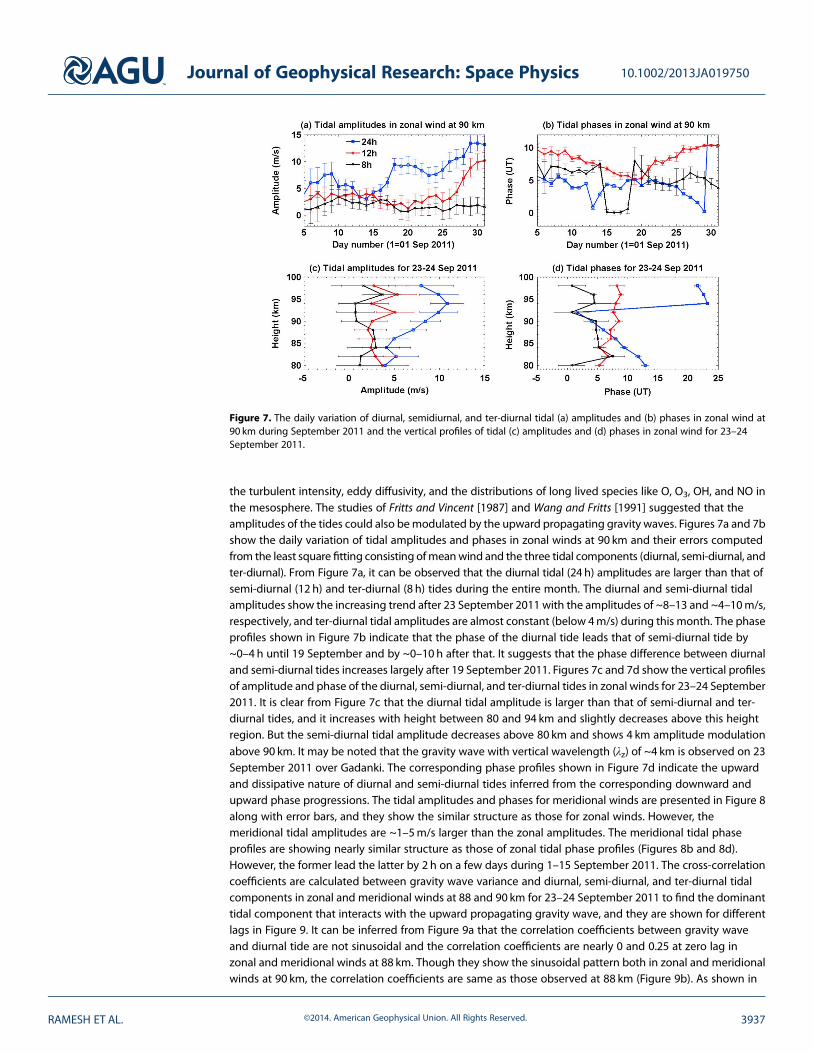
the turbulent intensity, eddy diffusivity, and the distributions of long lived species like O, O3, OH, and NO inthe mesosphere. The studies of Fritts and Vincent [1987] and Wang and Fritts [1991] suggested that theamplitudes of the tides could also bemodulated by the upward propagating gravity waves. Figures 7a and 7bshow the daily variation of tidal amplitudes and phases in zonal winds at 90 km and their errors computedfrom the least square fitting consisting ofmeanwind and the three tidal components (diurnal, semi-diurnal, andter-diurnal). From Figure 7a, it can be observed that the diurnal tidal (24 h) amplitudes are larger than that ofsemi-diurnal (12 h) and ter-diurnal (8 h) tides during the entire month. The diurnal and semi-diurnal tidalamplitudes show the increasing trend after 23 September 2011 with the amplitudes of ~8–13 and ~4–10m/s,respectively, and ter-diurnal tidal amplitudes are almost constant (below 4m/s) during this month. The phaseprofiles shown in Figure 7b indicate that the phase of the diurnal tide leads that of semi-diurnal tide by~0–4 h until 19 September and by ~0–10 h after that. It suggests that the phase difference between diurnaland semi-diurnal tides increases largely after 19 September 2011. Figures 7c and 7d show the vertical profilesof amplitude and phase of the diurnal, semi-diurnal, and ter-diurnal tides in zonal winds for 23–24 September2011. It is clear from Figure 7c that the diurnal tidal amplitude is larger than that of semi-diurnal and ter-diurnal tides, and it increases with height between 80 and 94 km and slightly decreases above this heightregion. But the semi-diurnal tidal amplitude decreases above 80 km and shows 4 km amplitude modulationabove 90 km. It may be noted that the gravity wave with vertical wavelength (λz) of ~4 km is observed on 23September 2011 over Gadanki. The corresponding phase profiles shown in Figure 7d indicate the upwardand dissipative nature of diurnal and semi-diurnal tides inferred from the corresponding downward andupward phase progressions. The tidal amplitudes and phases for meridional winds are presented in Figure 8along with error bars, and they show the similar structure as those for zonal winds. However, themeridional tidal amplitudes are ~1–5m/s larger than the zonal amplitudes. The meridional tidal phaseprofiles are showing nearly similar structure as those of zonal tidal phase profiles (Figures 8b and 8d).However, the former lead the latter by 2 h on a few days during 1–15 September 2011. The cross-correlationcoefficients are calculated between gravity wave variance and diurnal, semi-diurnal, and ter-diurnal tidalcomponents in zonal and meridional winds at 88 and 90 km for 23–24 September 2011 to find the dominanttidal component that interacts with the upward propagating gravity wave, and they are shown for differentlags in Figure 9. It can be inferred from Figure 9a that the correlation coefficients between gravity waveand diurnal tide are not sinusoidal and the correlation coefficients are nearly 0 and 0.25 at zero lag inzonal and meridional winds at 88 km. Though they show the sinusoidal pattern both in zonal and meridionalwinds at 90 km, the correlation coefficients are same as those observed at 88 km (Figure 9b). As shown in

Figure 7. The daily variation of diurnal, semidiurnal, and ter-diurnal tidal (a) amplitudes and (b) phases in zonal wind at90 km during September 2011 and the vertical profiles of tidal (c) amplitudes and (d) phases in zonal wind for 23–24September 2011.

Journal of Geophysical Research: Space Physics 10.1002/2013JA019750

RAMESH ET AL. ©2014. American Geophysical Union. All Rights Reserved. 3937

Figures 9c and 9d, the correlation coefficients between gravity wave variance and semi-diurnal tidalcomponents display the sinusoidal pattern, and the correlation coefficients at zero lag are 0.3 and 0.55 at88 km and 0.25 and 0.3 at 90 km, respectively, in zonal andmeridional winds. The correlation between gravitywave and semi-diurnal tide decreases with height from 88 to 90 km which suggests that the interactionbetween them does not occur at higher heights. It can be observed from Figures 9e and 9f that the crosscorrelations are not pure sinusoidal variations and the correlation coefficients between gravity wave and ter-diurnal tide at zero lag are 0.08 and 0.1 at 88 km in zonal andmeridional winds respectively and zero at 90 kmin both wind components. Thus, the larger correlation coefficient between gravity wave and semi-diurnaltide (0.55) emphasizes the occurrence of gravity wave interaction with semi-diurnal tide rather than withother tidal components (diurnal and ter-diurnal) during the large mesospheric temperature inversion in theheight region of ~80–85 km. Liu and Hagan [1998] suggested that there exists cooling in the gravity breakingregion and heating right below it, and the cooling is mostly due to the dominance of horizontal advectionover the vertical advection and the heating is due to both the effect of advection and turbulence. Liu et al.

Figure 8. Same as Figure 7 but in meridional winds.

Figure 9. The cross-correlation coefficients between (a) diurnal, (c) semi-diurnal, and (e) ter-diurnal tides and gravity wavesin zonal and meridional winds at 88 km, and Figures 9b, 9d, and 9f same as Figures 9a, 9c, and 9e, but in zonal and meri-dional winds at 90 km.

Journal of Geophysical Research: Space Physics 10.1002/2013JA019750

RAMESH ET AL. ©2014. American Geophysical Union. All Rights Reserved. 3938

[2000] suggested that the gravity wave breaking level is affected by the stability of the backgroundatmosphere which is influenced by the zonal mean plus diurnal tidal wind and background temperature. Liuand Hagan [1998] also illustrated the schematic mechanism involving the gravity wave-tidal interaction andsuggested that, in the region of dynamical cooling, the gravity wave becomes unstable and breaks. When thegravity wave breaks, the momentum flux carried by the wave will be deposited on the background and thismomentum deposition accelerates the mean flow. This acceleration increases the background wind shearbelow the cooling region and increases the downward heat flux which is developed as an inversion layer. Thecooling/heating rates due to gravity wave breaking are calculated using the following equation given by Liuand Meriwether [2004]:

∂T∂t

¼ 4� 3ηð Þ To zbð Þg λzj j N2Deddy (6)

where λz is the gravity wave vertical wavelength, To(zb) is the temperature at the wave breaking height, N2 is theBrunt–Väisälä frequency square, η is the measure of turbulence taken as 0.2, and Deddy is the mean eddydiffusion coefficient calculated from the equation given by Lindzen [1981]. Figure 10 shows the calculatedcooling/heating rates from the equation (6) for the gravity wave of λz = 3.84 km and T=22.2min which issaturated at ~84 km (Figure 6a) using half-an-hour integrated lidar temperature profiles. It can be observed fromthis figure that themagnitude of heating rate is ~15.5 K/h at the initial stage of gravity wave breaking (21:00 LT),and its value increases up to ~33.7K/h at around 22:00 LTand again decreases to ~15K/h by 24:00 LT. It can alsobe observed from this figure that the heating rate descends with the diurnal tidal phase speed at the rate of~1.3 km/h between 80 and 84 km. It is also clear from this figure that the cooling rates above (~17K/h) andbelow (~10K/h) the inversion layer are descending at the same rate. Therefore, the local heating and coolingassociated with the gravity wave breaking are modulated by the diurnal tidal structure.

3.4. Upper MIL Predominantly Due to Chemical Heating

Ramesh et al. [2013b] illustrated the dominance of chemical heating over dynamics for the occurrenceof a few large MILs observed in the height region of ~80–85 km over Gadanki during January–February2011. Relatively large enhancements in the concentrations of ozone (O3) and atomic oxygen (O)have been observed in the inversion region during those MIL events. The large heating rates morethan ~15 K/day (~50–60%) by the reaction between H and O3 dominate that by the other reactions at80–85 km during those MIL events. The energy budget in the upper mesospheric region is mainly due toUV absorption by O3 at 80–85 km, chemical heating due to the reaction between odd hydrogen andodd oxygen at 85–95 km and the UV absorption by O2 above 95–100 km. In the present study, alongwith the lower and middle MILs at ~70 and 80 km, a large inversion layer is observed in the uppermesosphere lower thermospheric (UMLT) region at ~90–98 km on 23 September 2011 in SABERtemperature over Gadanki (Figure 1). The upper inversion layer starts at ~90–91 km and peaks at 98 km

Figure 10. The height and time variation of cooling/heating rates for 23 September 2011.

Journal of Geophysical Research: Space Physics 10.1002/2013JA019750

RAMESH ET AL. ©2014. American Geophysical Union. All Rights Reserved. 3939

with the maximum temperature of ~250 K, and the temperature decreases up to ~105 km and againincreases above this height. Hence, the mesopause height is observed to be at lower heights (~90 km),as earlier reported by Venkat Ratnam et al. [2010] during September. Both chemistry and dynamics playa major role for the heating/cooling effects in the upper mesosphere and lower thermospheric region(~90–100 km), and it is difficult to find the dominance of any of these mechanisms for the accumulation ofchemical species in this height region. The diurnal tidal amplitudes are larger above ~90 km, and they shouldbecome unstable and break above this height region over the tropical latitudes [Lindzen, 1967, 1981; Garcia andSolomon, 1985]. Due to their high phase velocities, the tides deposit the energy and momentum in thebackground, thereby affecting the thermal structure in theMLT region. The large heating rates generated due todifferent exothermic reactions between the chemical species O, O2, O3, and H could influence the UMLT thermalstructure. The chemical heating occurs depending on the law of mass action, and more abundance of reactivespecies (O, H, andO3) causesmore chemical heating [Meriwether andMlynczak, 1995]. Figures 11a–11c show thevertical profiles of volume mixing ratios of O, O3, and H, respectively, downloaded from TIMED-SABER version2.0 (V2.0) data sets for the night of 23 September 2011 over the Gadanki region. It can be observed from thesefigures that the mixing ratios of O, O3, and H begin to increase from ~80 km and peaks at ~101, ~93.6, and~100km, respectively, in the UMLT region. The increase in the atomic oxygen mixing ratio could be due todownward transport from the middle thermosphere where its abundance is large and its photochemicaldestruction rate is slow [Garcia and Solomon, 1985]. The atomic oxygen reacts with molecular oxygen and

causes the maximum ozone mixing ratios in this heightregion. The increase in ozone mixing ratio also depends onthe loss rate of this constituent through the reaction withatomic hydrogen which is maximum due to the advectivetransport of H2O in the upper mesosphere. The verticalprofiles of SABER V2.0 chemical heating rates due to the sixpotential exothermic reactions (given in Table 1) for thenight of 23 September 2011 are shown in Figure 12. It canbe observed from this figure that the heating rate due to thereaction between H and O3 (R3: H+O3→OH+O2) peaks(~7.5K/day) at ~82.3 km where the maximum total heatingrate due to all the reactions is ~13.6K/day which is muchless than those discussed in Ramesh et al. [2013b]. But theheating rate due to the reaction between O and O (R5:O+O+M→O2+M) dominates all other reactions with themaximum value of ~44.3 K/day at ~95.3 km, and the totalheating rate due to all the six reactions is observed to be~53.5 K/day at this height region. The heating rates due tothese six reactions at 82.3 and 95.3 km are mentioned inTable 1. From the table, we can infer that the largetemperature inversion layer at ~90–98km shown in Figure 1could be due to the large chemical heating rates producedjointly by the six exothermic reactions.

Figure 11. The SABER volume mixing ratios (unitless) of (a) atomic oxygen, (b) ozone, and (c) atomic hydrogen for 23September 2011 over the Gadanki location.

Figure 12. The SABER-V2.0 chemical heating ratesdue to the dominant six exothermic reactionsbetween O+OH, H+O2+M, H+O3, O+HO2,O+O+M, and O+O2+M for 23 September 2011over the Gadanki location.

Journal of Geophysical Research: Space Physics 10.1002/2013JA019750

RAMESH ET AL. ©2014. American Geophysical Union. All Rights Reserved. 3940

4. Discussion and Conclusions

In the present study, the causative mechanisms of the three inversion layers observed at different heightsaround ~70, ~80, and ~90 km on the night of 23 September 2011 over the Gadanki region have beeninvestigated. It is found that the dissipation of 2 day PW propagating from lower atmosphere caused thelower MIL at ~70 km. The descending structure of the inversion layer at the rate of ~1 km/h suggests that theinteraction between GW and tides could occur during the large MIL observed at ~80 km. The two-dimensional FFT analysis of lidar temperature perturbations shows the presence of an internal gravity waveof vertical wavelength ~4 km and period ~22.2min which propagates upward with increasing amplitude inresponse to the decreasing atmospheric density. The good correlation (~0.55) between semi-diurnal tide andgravity wave suggests the occurrence of interaction between these wave structures during this inversionevent. It is found that the amplitude of the semi-diurnal tide decreases with height and shows ~4 km verticalmodulation due to its interaction with gravity wave above ~80 km whereas the diurnal tidal amplitudeincreases with height above this height level. The gravity wave attains the convective instability (N2< 0,Ri< 0) above 80 km due to its interaction with semi-diurnal tide and breaks above the top of the inversionlayer (~84–85 km). When the gravity wave breaks at a particular height, the energy carried by the wavewill be deposited in the background, and thus the enhancement in the temperature is maintained as aninversion layer. It is also observed that this inversion layer is sandwiched between two cooling regions, andthe calculated heating and cooling rates (~33 and 15 K/h) descend with height at the rate of ~1.3 km/h whichsuggests the influence of tides on the occurrence of this inversion layer. As suggested by Liu and Hagan[1998], when the gravity wave becomes unstable and breaks, the momentum flux carried by the wave will bedeposited in the background and accelerates the mean flow. This acceleration increases the positive shearbelow the breaking level and increases the downward heat flux at the bottom of the inversion layer. Thisdownward heat flux produces heating at the bottom and cooling at the top of the inversion layer. Theyalso suggested that the cooling could be due to the dominance of horizontal advection over the verticaladvection, and the heating could be due to both the advection and turbulence. It is also observed that thetotal chemical heating rate due to the six exothermic reactions given in Table 1 peaks at ~83 km with thevalue of 13.5 K/day. However, the reaction between H and O3 dominates (~50–60%) all other reactions at theheating rate of 7.5 K/day. Ramesh et al. [2013b] showed that the total heating rate is above ~30 K/daybetween 80 and 85 km during the large MIL events observed in January–February 2011 over the Gadankiregion. This value is much larger than that obtained in the present study (13.5 K/day), indicating the minorrole of chemical heating for the formation of the middle MIL. In this case, the gravity wave-tidal (semi-diurnal)interaction plays a dominant role over chemical heating for the occurrence of the middle MIL observed at~80–84 km on 23 September 2011 over Gadanki.

The SABER temperature profile shows another large inversion layer with an amplitude of ~100 K observedat the upper mesospheric and lower thermospheric height region (~90–98 km). The total chemical heatingrate (~54 K/day) due to the six exothermic reactions peaks at ~95 km and this large chemical heating ratecould be the reason for the occurrence of this upper inversion layer. It should be noted that the reactionbetween O and O (R5) dominates with the maximum heating rate of ~44 K/day and contributes nearly 81% ofthe total heating rates during this inversion event. This large heating rate is observed to be in proportion tothe large mixing ratio of atomic oxygen above this height region. As shown in Figures 7c and 8c, the diurnaltidal amplitude increases with height above ~80 km and decreases slightly above ~92–94 km in zonal andmeridional winds. The changes in chemical composition due to dynamics could lead to the changes in theheating rates that provide the positive or negative feedback to damp or accelerate the original dynamicalperturbations [Marsh, 2011]. The temperatures due to the large chemical heating rates accelerate thebackground wind and the wind shear due to this acceleration generates the critical level u� c ¼ 0ð Þ for theupward propagating diurnal tide so that the amplitude of the diurnal tide decreases above ~92–94 km.

The important conclusions drawn from the present study are described as follows:

1. All the possible causative mechanisms for the occurrence of the mesospheric inversion layers namelyPW critical level interaction/dissipation, gravity wave-tidal interaction, and chemical heating have beendiscussed for the occurrence of this triple layered MIL event.

2. The lower MIL, which occurs at ~70 km, could be due to planetary wave dissipation, as it is observed thatthere is a significant reduction in the PW amplitudes.

Journal of Geophysical Research: Space Physics 10.1002/2013JA019750

RAMESH ET AL. ©2014. American Geophysical Union. All Rights Reserved. 3941

3. Though the diurnal tidal amplitudes are larger compared with other tidal components, the correlationbetween semi-diurnal tide and gravity waves suggests the occurrence of interaction between thesetwo wave structures, which might have caused the middle MIL observed at ~80–84 km.

4. Though there is a strong interaction between semi-diurnal tide and gravity wave, the height of the inver-sion layer and heating/cooling region descends at the rate of diurnal tidal phase speed (~1 km/h) insteadof semi-diurnal tidal phase speed (> 8 km/h).

5. The heat energy liberated due to the exothermic chemical reaction, O+O+M→O2+M dominates theother reactions for the occurrence of the upper MIL observed above 90 km, though the earlier studynoted that the chemical heating rate due to the reaction H+O3→OH+O2 dominated the other reactionsand other dynamical processes in causing the MILs, which occurred at relatively lower heights between80 and 85 km [Ramesh et al., 2013b].

ReferencesCharney, J. G., and P. G. Drazin (1961), Propagation of planetary-scale disturbances from the lower into the upper atmosphere, J. Geophys.

Res., 66, 83–109.Chen, S., H. Zhilin, M. A. White, H. Chen, D. A. Kruger, and C. Y. She (2000), Lidar observations of seasonal variation of diurnal mean tem-

perature in the mesopause region over Fort Collins, Colorado (41˚N, 105˚W), J. Geophys. Res., 105, 12,371–12,379.Clancy, R. T., and D. W. Rusch (1989), Climatology and trends of mesospheric (58-90) temperatures based upon 1982-1986 SME limb scat-

tering profiles, J. Geophys. Res., 94, 3377–3393.Clancy, R. T., D. W. Rusch, andM. T. Callan (1994), Temperatureminima in the average thermal structure of the middle atmosphere (70-80 km)

from analysis of 40 to 92 km SME global temperature profiles, J. Geophys. Res., 99, 19,001–19,020.Fadnavis, S., and G. Beig (2004), Mesospheric temperature inversions over the Indian tropical region, Ann. Geophys., 22, 3375–3383.Fritts, D. C., and G. D. Nastrom (1992), Sources of mesoscale variability of gravity waves. Part II, frontal, convective, and jet stream excitation,

J. Atmos. Sci., 49, 111–127.Fritts, D. C., and R. A. Vincent (1987), Mesospheric momentum flux studies at Adelaide, Australia: Observations and a Gravity wave-tidal

interaction model, J. Atmos. Sci., 44, 605–619.Gan, Q., S. D. Zhang, and F. Yi (2012), TIMED/SABER observations of lower mesospheric inversion layers at low and middle latitudes,

J. Geophys. Res., 117, D07109, doi:10.1029/2012JD017455.Garcia, R. R., and S. Solomon (1985), The effect of breaking gravity waves on the dynamics and chemical composition of the mesosphere and

lower thermosphere, J. Geophys. Res., 90, 3850–3868.Gurubaran, S., S. Sridharan, T. K. Ramkumar, and R. Rajaram (2001), The mesospheric quasi-2-day wave over Tirunelveli (8.7°N), J. Atmos. Sol.

Terr. Phys., 63, 975–985.Hauchecorne, A., and M. L. Chanin (1980), Density and temperature profiles obtained by lidar between 35 and 70 km, Geophys. Res. Lett., 7,

565–568.Hauchecorne, A., M. L. Chanin, and R. Wilson (1987), Mesospheric temperature inversion and gravity wave dynamics, Geophys. Res. Lett., 14,

935–939.Hodges, R. R. (1967), Generation of turbulence in the upper atmosphere by internal gravity waves, J. Geophys. Res., 72, 3455–3458.Hodges, R. R. (1969), Eddy diffusion coefficients due to instabilities in internal gravity waves, J. Geophys. Res., 74, 4087–4090.Jenkins, D. B., D. P. Wareing, L. Thomas, and G. Vaughan (1987), Upper stratospheric and mesospheric temperatures derived from lidar

observations at Aberystwyth, J. Atmos. Sol. Terr. Phys., 49, 287–298.Leblanc, T., and A. Hauchecorne (1997), Recent observations of mesospheric temperature inversions, J. Geophys. Res., 102, 19,471–19,482.Lehmacher, G. A., C. L. Croskey, J. D. Mitchell, M. Friedrich, F.-J. Lübken, M. Rapp, E. Kudeki, and D. C. Fritts (2006), Intense turbulence observed

above a mesospheric temperature inversion at equatorial latitudes, Geophys. Res. Lett., 33, L08808, doi:10.1029/2005GL024345.Lindzen, R. S. (1967), Thermally driven diurnal tide in the atmosphere, Q. J. R. Meteorol. Soc., 93, 18–42.Lindzen, R. S. (1981), Turbulence and stress owing to gravity wave and tidal breakdown, J. Geophys. Res., 86, 9707–9714.Liu, H. L., and J. W. Meriwether (2004), Analysis of a temperature inversion event in the lower mesosphere, J. Geophys. Res., 109, D02S07,

doi:10.1029/2002JD003026.Liu, H. L., and M. E. Hagan (1998), Local heating/cooling of the mesosphere due to gravity wave modulated by the diurnal tide breaking,

Geophys. Res. Lett., 25, 2941–2944.Liu, H. L., M. E. Hagan, and R. G. Roble (2000), Local mean state changes due to gravity wave breaking modulated by the diurnal tide,

J. Geophys. Res., 105, 12,381–12,396.Marsh, D. R. (2011), Chemical–dynamical coupling in the mesosphere and lower thermosphere, in Aeronomy of the Earth’s Atmosphere and

Ionosphere, IAGA Special Sopron Book Series, vol. 2, edited by M. A. Abdu et al., pp. 3–17, Springer, Houten, Netherlands, doi:10.1007/978-94-007-0326-1.

Meriwether, J. W., and C. S. Gardner (2000), A review of the mesospheric inversion layer phenomenon, J. Geophys. Res., 105, 12,405–12,416.Meriwether, J. W., and A. J. Gerrard (2004), Mesosphere inversion layers and stratosphere temperature enhancements, Rev. Geophys., 42,

RG3003, doi:10.1029/2003RG000133.Meriwether, J. W., andM. G.Mlynczak (1995), Is chemical heating amajor cause of themesosphere inversion layer?, J. Geophys. Res., 100, 1379–1387.Meriwether, J. W., X. Gao, V. Wickwar, T. Wilkerson, K. Beissner, S. Collins, and M. Hagan (1998), Observed coupling of the mesospheric

inversion layer to the thermal tidal structure, Geophys. Res. Lett., 25, 1479–1482.Mlynczak, M. G., and S. Solomon (1991), Middle atmosphere heating by exothermic chemical reactions involving odd-hydrogen species,

Geophys. Res. Lett., 18, 37–40.Mlynczak, M. G., B. T. Marshall, F. J. Martin-Torres, J. M. Russell III, R. E. Thompson, E. E. Remsberg, and L. L. Gordley (2007), Sounding of the

Atmosphere using Broadband Emission Radiometry observations of daytime mesospheric O2(1Δ) 1.27 μm emission and derivation of

ozone, atomic oxygen, and solar and chemical energy deposition rates, J. Geophys. Res., 112, D15306, doi:10.1029/2006JD008355.Nakamura, T., D. C. Fritts, J. R. Isler, T. Tsuda, R. A. Vincent, and I. M. Reid (1997), Short-period fluctuations of the diurnal tide observed with

low-latitude MF and meteor radars during CADRE: Evidence for gravity wave/tidal interactions, J. Geophys. Res., 102, 26,225–26,238.

AcknowledgmentsThe authors are thankful to Dr. K.Raghunath and technical staff for oper-ating and maintaining the Rayleigh lidarsystem at NARL, Gadanki. They greatlyacknowledge the EGRL, Indian Instituteof Geomagnetism, Tirunelveli for pro-viding the necessary MF radar winddata used in this study. They are alsogreatly thankful to TIMED-SABER teamfor providing necessary data throughthe website: http://saber.gats-inc.com/.They are thankful to their Editor and thetwo Reviewers for their comments andsuggestions, which greatly helped themto improve the manuscript. The lidarand radar data used in this manuscriptcan be made available to anyoneon request.

Alan Rodger thanks the reviewers fortheir assistance in evaluating this paper.

Journal of Geophysical Research: Space Physics 10.1002/2013JA019750

RAMESH ET AL. ©2014. American Geophysical Union. All Rights Reserved. 3942

Palo, S. E., R. G. Roble, and M. E. Hagan (1999), Middle atmosphere effects of the quasi-two-day wave determined from a general circulationmodel, Earth Planets Space, 51, 629–647.

Rajaram, R., and S. Gurubaran (1998), Seasonal variabilities of low latitude mesospheric winds, Ann. Geophys., 16, 197–204.Ramesh, K., and S. Sridharan (2012), Large mesospheric inversion layer due to breaking of small-scale gravity waves: Evidence from Rayleigh

lidar observations over Gadanki (13.5˚N, 79.2˚E), J. Atmos. Sol. Terr. Phys., 89, 90–97.Ramesh, K., S. Sridharan, K. Raghunath, S. Vijaya Bhaskara Rao, and Y. Bhavani Kumar (2013a), Planetary wave–gravity wave interactions

during mesospheric inversion layer events, J. Geophys. Res. Space Physics, 118, 4503–4515, doi:10.1002/jgra.50379.Ramesh, K., S. Sridharan, and S. Vijaya Bhaskara Rao (2013b), Dominance of chemical heating over dynamics in causing a few large meso-

spheric inversion layer events during January-February 2011, J. Geophys. Res. Space Physics, 118, 6751–6765, doi:10.1002/jgra.50601.Remsberg, E., G. Lingenfelser, V. L. Harvey, W. Grose, J. Russell III, M. Mlynczak, L. Gordley, and B.T. Marshall (2003), On the verification of the

quality of SABER temperature, geopotential height, and wind fields by comparison with Met Office assimilated analyses, J. Geophys. Res.,108(D19), 4628, doi:10.1029/2003JD003720.

Remsberg, E. E., et al. (2008), Assessment of the quality of the Version 1.07 temperature-versus-pressure profiles in the middle atmospherefrom TIMED/SABER, J. Geophys. Res., 113, D17101, doi:10.1029/2008JD010013.

Salby, M., F. Sassi, P. Callaghan, D. Wu, P. Keckhut, and A. Hauchecorne (2002), Mesospheric inversions and their relationship to planetarywave structure, J. Geophys. Res., 107(D4), 4041, doi:10.1029/2001JD000756.

Sassi, F., R. R. Garcia, B. A. Boville, and H. Liu (2002), On temperature inversions and the mesospheric surf zone, J. Geophys. Res., 107(D19),4380, doi:10.1029/2001JD001525.

Schmidlin, F. J. (1976), Temperature inversions near 75 km, Geophys. Res. Lett., 3, 173–176.She, C. Y., J. R. Yu, R. Roble, P. Keckhut, A. Hauchecorne, and M. L. Chanin (1995), Vertical structure of the midlatitude temperature from

stratosphere to mesopause (30-105 km), Geophys. Res. Lett., 22, 377–380.Sica, R. J., T. Thayaparan, P. S. Argall, A. T. Russell, and W. K. Hocking (2002), Modulation of upper mesospheric temperature inversions due to

tidal-gravity wave interactions, J. Atmos. Sol. Terr. Phys., 64, 915–622.Siva Kumar, V., Y. Bhavani Kumar, K. Raghunath, P. B. Rao, M. Krishnaiah, K. Mizutani, T. Aoki, M. Yasui, and T. Itabe (2001), Lidar measurements

of mesospheric temperature inversions at a low latitude, Ann. Geophys., 19, 1039–1044.Siva Kumar, V., P. B. Rao, and H. Bencherif (2006), Lidar observations of middle atmospheric gravity wave activity over a low-latitude site

(Gadanki, 13.5˚N, 79.2˚E), Ann. Geophys., 24, 823–834.Siva Kumar, V., P. B. Rao, and M. Krishnaiah (2003), Lidar measurements of stratosphere-mesosphere thermal structure at low latitude:

Comparison with satellite data and models, J. Geophys. Res., 108(D11), 4342, doi:10.1029/2002JD003029.Sridharan, S., S. Sathish Kumar, and S. Gurubaran (2008), Influence of gravity waves and tides on mesospheric temperature inversion layers:

simultaneous Rayleigh lidar and MF radar observations, Ann. Geophys., 26, 3731–3739.Sridharan, S., K. Raghunath, S. Sathish Kumar, and D. Nath (2010), First results of warm mesospheric temperature over Gadanki (13.5˚N, 79.2˚E)

during the sudden stratospheric warming of 2009, J. Atmos. Sol. Terr. Phys., 72, 1139–1146.States, R. J., and C. S. Gardner (1998), Influence of the diurnal tide and thermospheric heat sources on the formation of mesospheric tem-

perature inversion layers, Geophys. Res. Lett., 25, 1483–1486.Szewczyk, A., B. Strelnikov, M. Rapp, I. Strelnikova, G. Baumgarten, N. Kaifler, T. Dunker, and U.-P. Hoppe (2013), Simultaneous observations of

a mesospheric inversion layer and turbulence during the ECOMA-2010 rocket campaign, Ann. Geophys., 31, 775–785.Thayaparan, T., W. K. Hocking, and J. MacDougall (1995), Observational evidence of tidal/gravity wave interactions using the UWO 2MHz

radar, Geophys. Res. Lett., 22, 373–376.Thomas, J. D., D. P. Sipler, J. E. Salah, and J. W. Meriwether (2001), Rayleigh lidar observations of a mesospheric inversion layer during night

and day, Geophys. Res. Lett., 28, 3597–3600.Venkat Ratnam, M., J. B. Nee, W. N. Chen, V. Siva Kumar, and P. B. Rao (2003), Recent observations of mesospheric temperature inversions

over a tropical station (13.5˚N, 79.2˚E), J. Atmos. Sol. Terr. Phys., 65, 323–334.Venkat Ratnam, M., A. K. Patra, and B. V. Krishna Murthy (2010), Tropical mesopause: Is it always close to 100 km?, J. Geophys. Res., 115,

D06106, doi:10.1029/2009JD012531.Walterscheid, R. L. (1981), Dynamical cooling induced by dissipating internal gravity waves, Geophys. Res. Lett., 8, 1235–1238.Wang, D. Y., and D. C. Fritts (1991), Evidence of Gravity wave-tidal interaction observed near the summer mesopause at Poker Flat, Alaska,

J. Atmos. Sci., 48, 572–583.Williams, P. J. S., N. J. Mitchell, A. G. Beard, V. S. C. Howells, and H. G. Muller (1999), The coupling of Planetary waves, Tides and Gravity waves in

the mesosphere and lower thermosphere, Adv. Space Res., 24, 1571–1576.

Journal of Geophysical Research: Space Physics 10.1002/2013JA019750

RAMESH ET AL. ©2014. American Geophysical Union. All Rights Reserved. 3943