case study of north gujarat agroclimatic zone

CLIMATEOROLOGICAL ANALYSIS

FOR

WATER RESOURCES AND IRRIGATION PLANNING:

CASE STUDY OF NORTH GUJARAT AGROCLIMATIC ZONE

A Thesis Submitted to

The Maharaja Sayajirao University of Baroda in fulfillment of the requirements

for the award of degree of

DOCTOR OF PHILOSOPHY IN

CIVIL ENGINEERING GUIDE By Prof. D.T.Shete N. R. Patel Ph.D. in Civil Engineering M.E. (Civil) in W.R.E. F.I.E. (I) A.I.E. (I) F.I.W.R.S. M.I.W.R.S. F.I.S.H. M.I.S.H.

WATER RESOURCES ENGINEERING AND MANAGEMENT INSTITUTE FACULTY OF TECHNOLOGY AND ENGINEERING

THE MAHARAJA SAYAJIRAO UNIVERSITY OF BARODA SAMIALA – 391 410 OCTOBER – 2011

http://www.pdfcomplete.com/cms/hppl/tabid/108/Default.aspx?r=q8b3uige22

CERTIFICATE

This is to certify that the thesis entitled “Climateorological

Analysis For Water Resources And Irrigation Planning: Case Study Of

North Gujarat Agroclimatic Zone” which is being submitted to The

Maharaja Sayajirao University of Baroda in fulfillment of the

requirements for the award of degree of Doctor of Philosophy in Civil

Engineering by Ms. Neha R. Patel has been written by her under my

supervision and guidance. This is an original work carried out by her

independently. The matter presented in this thesis has not been

submitted for the award of any other degree.

(Prof. D.T.Shete) Guide (Prof. A.S. Patel) I/C Director, Dean, Water Resources Engineering & Faculty of Tech. & Engg., Management Institute, The M.S.Univeristy of Baroda Faculty of Tech. & Engg., The M.S.Univeristy of Baroda


CONTENTS ACKNOWLEDGEMENT i PREFACE v ABSTRACT vii NOTATIONS xi LIST OF MAPS xvii LIST OF PLATES xvii LIST OF TABLES xviii LIST OF FIGURES xxxi

CHAPTER NO.

TOPIC PAGE NO.

1

INTRODUCTION

1

1.1 General 1

1.2 Climate Parameter Basics 2

1.3 Climate of India 3

1.4 Climate of Gujarat 5

1.5 Study Area 6

1.6 Objectives of Present Study 8

1.7 Overview 9

2.

LITERATURE REVIEW

11

2.1 General 11

2.2 Literature Review 11

2.2.1 Missing data 12

2.2.2 Probability distribution 18

2.2.3 Development of regression relationships 20

2.2.4 Characteristics of climate data 21

2.2.5 Regionalization based on spatial and temporal

behaviour of rainfall 27

2.2.6 Design storm from rainfall depths 29

2.2.7 Drought analysis 30

2.2.8 Crop planning for rainfed agriculture 32


3

STUDY AREA

40

3.1 General 40

3.2 Study Area 40

3.2.1 Agriculture scenario 45

3.2.2 Water resources 45

3.2.3 Soil resources 46

3.2.4 Cropping pattern 47

4

DATA COLLECTION

48

4.1 General 48

4.2 Collection of Data 48

4.2.1 Climate data 48

4.2.2 Details of water resources projects 59

4.2.3 Soil type data 61

4.2.4 Crop data 65

5

METHODOLOGY

68

5.1 General 68

5.2 Missing Climate Data 69

5.3 Probability Distribution 77

5.4 Development of Regression Relationships 80

5.5 Characteristics of Climate Data 85

5.6 Regionalizing Based on Spatial and Temporal Patterns of

Daily Rainfall

90

5.7 Design Storm for Study Period 95

5.8 Drought Analysis 101

5.9 Crop Planning for Rainfed Agriculture 104

5.9.1 Climate classification 104

5.9.2 Dry spell analysis 109

5.9.3 Climatic Index (CI) 111

5.9.4 Crop period based on onset and cessation of monsoon 112


6

RESULTS AND ANALYSIS

115

6.1 General 115

6.2 Missing Climate Data 115

6.3 Probability Distribution 125

6.4 Regression Relationships 166

6.5 Characteristics of Climate Data 178

6.6 Regionalization Based on Spatial and Temporal Rainfall

Patterns 214

6.7 Design Storm for Hathmati Catchment Area 221

6.8 Drought Analysis 229

6.9 Crop Planning for Rainfed Agriculture 241

6.9.1 Climate classification 241

6.9.2 Dry spell 243

6.9.3 Climatic indices 255

6.9.4 Onset, cessation and length of growing period 262

7

CONCLUSIONS AND RECOMMENDATIONS

285

7.1 General 285

7.2 Conclusions 285

7.2.1 Missing climate data 285

7.2.2 Probability distributions 286

7.2.3 Development of regression relationships 288

7.2.4 Characteristics of climate data 290

7.2.5 Regionalization based on spatial and temporal rainfall

patterns 292

7.2.6 Design storm for Hathmati catchment area 292

7.2.7 Drought analysis 293

7.2.8 Crop planning for rainfed agriculture 295

7.3 Recommendations 297

7.4 Future Scope of Work 299

REFERENCES

300


i

ACKNOWLEDGEMENT

At the end of a four years journey it is necessary to stop, look back,

analyze what happened and recognize the help rendered by the people who

helped to complete the journey. This thesis is the culmination of my sincere

efforts in obtaining my Doctoral degree in Civil Engineering. I have not traveled in

a vacuum in this journey. There are some people who made this journey easier

with words of encouragement and by offering different places to look to rest for

expanding my theories and ideas.

I express my gratitude to The Maharaja Sayajirao University of Baroda

for providing me opportunity to pursue Doctorate degree in Civil Engineering

possible. I will put my best efforts to add to the glory of The M.S. University.

First and foremost, it is my great pleasure and proud privilege to express

my deep sense of gratitude to my Guide, Dr. D.T. Shete, Professor and Former

Director, Water Resources Engineering and Management Institute (WREMI),

Samiala, for his excellent guidance, constant inspiration, positive criticism and

unparalleled support throughout the whole journey of my work. His comments on

chapter drafts are themselves a course in critical thought upon which I will always

draw. I could not have imagined having a better advisor and mentor for my Ph.D.

study. He is and will be the most valued person in my life.

I am grateful to Dr. R.C. Maheswari, Vice Chancellor, Sardar Krushinagar

Dantiwada Agriculture University, for his kind help rendered in providing the

details regarding the crops grown in the area.

I express my sincere appreciation and thanks to Dr. A. S. Patel, Professor

and I/C Director, WREMI for his kind support and encouragement.

I am deeply grateful to Prof. A.C. Pandya, Former Project Manager of ES

CAAP / UNDP, Philiphines, Former Director, GEDA, Former Director, CIAE,

Bhopal and Former Director, NDDB, for extending his helping hand in providing

the required data and constantly inspiring to achieve my goal.

I am thankful to Dr. F.P. Parekh, Associate Professor, WREMI, for her

kind support whenever needed for.


ii

I warmly thank Dr. U.C. Kothyari, Professor, Department of Civil

Engineering, Indian Institute of Technology, Roorkee. It was my privilege to

discuss the findings of my work with him and his suggestions were highly

valuable for improving the thesis content and presentation.

I wish to express my warm and sincere thanks to Prof. Vyas Pandey,

Head, Meterological division, GAU, Anand for his guidance related to the crop

planning, during my work.

I am thankful to Dr. B.S. Patel, Chief Agronomist, AICRP on Integrated

Farming Systems, Sardar Krushinagar Dantiwada Agriculture University, for

providing the details regarding the crops grown in the area.

I am thankful to Shri M.K. Dixit, Superintending Engineer and Shri

A.G.Shah, Assistant Engineer, State Water Data Centre, Gandhinagar for

providing the data regarding the raingauge stations situated in the study area.

I am very much grateful to Shri M. G. Golwala, Superintending Engineer

(Hydro), Central Design Organization, Gandhinagar for providing the information

and maps related to the major irrigation projects in the study area. I am thankful

for the assistance given by his Executive Engineers (Shri Gohil and Shri Bhatt), for the same.

I am grateful to the Librarians of Indian Institute of Technology, Guwahati,

Faculty of Technology and Engineering, The M.S. University of Baroda and

Sardar Krushinagar, Dantiwada Agriculture University for assisting me in

providing the required reference material for carrying out the research work.

My warm thanks are due to Ms. M.R. Khatri, Ms. A.V. Nadar, Mr. K.B.

Patel, Ms. S.C. Parmar, Ms. N.A. Bhatia, Mr. P.G. Joshi, Ms. D.B. Joshi and

Ms. N.G. Tiwari, former and present Temporary Teaching Assistants of WREMI,

who were always ready to help.

My sincere thanks are due to Shri G.K. Patel, Lab Assistant, Shri J.D. Vyas, Computer operator, Shri R.G. Prajapati, Temporary Technical Assistant,

Shri A.D. Choksi, Senior Clerk, Shri G.J. Darji, Clerk; the staff of WREMI who

always helped and who were co-operative during my work.


iii

I am thankful to Shri S. J. Chauhan, Shri L. G. Rabari and Shri M.K. Rohit, former and present peons, WREMI for their help and support during the

time of my research work.

I express my sincere thanks to all my graduate and post graduate students who were always concerned and curious about the research work

which always motivated me to work even more hard to successfully complete the

thesis work.

I wish to thank my best friends in high school, Shraddha & Jyoti; my best

friend in undergraduate and graduate level, Heta & Gautam; my good friend and

colleague Bhumi; and my childhood friend, Gayatri; for helping me get through

the difficult times and for all the emotional support, camaraderie, entertainment,

and caring they provided.

I am also very much thankful to my Sir, my colleague and my one of the

most dearest friends, Dr. T.M.V. Suryanarayana, Assistant Professor, WREMI

who always inspired me to work hard and helped me a lot during my research

work which will always be the most valuable to me. I don’t have any words to

express his kindness, supportive nature and positive criticism during my work.

Thanks a lot Sir……..

For her continuous nurture and parental concern, always kind and friendly

words of encouragement, I take this opportunity to thank, Dr. V.D. Shete, for

always being there and making me feel comfortable. Her constant motherly

caring and love have made things much easier and motivated me the most to

work hard.

Lastly I want to thank everyone, who helped me directly or indirectly in my

research work, which I may be missing to mention here inadvertently.

It was my great fortune that during the completion of my research journey I

met my life partner, Nimish, whose loving, encouraging, patient and faithful

support during the final stages of this Ph.D. is highly appreciated. I show my

gratitude to his family too specially my mother in law, and my wonderful three


iv

sisters in law for being there and believing in me that I could successfully

complete my work in time. I thank them all for their understanding.

Finally and most importantly, I am thankful to my brother Jiten for always

being a biggest moral support and my mother Heena, without whom I may not be

here. For her love, concern, support, wishes and bearing me in my good and bad

moods, understanding me and having faith in me, not only during my work but

throughout my whole life till now. My mother is as solid as black rock. The

creativity, determination and sense of conscientiousness with which she

responded to life’s challenges have led me to seek this in myself. I dedicate this

Thesis to her. My father, Rashmikant for being there spiritually. Again I would

like to thank both of my families for helping and supporting me directly or

indirectly for successful completion of my work. It was under the blessing of God

I gained so much drive and an ability to tackle challenges head on.

Place: Vadodara

Date: 4th October 2011 (N. R. Patel)


v

PREFACE

Science has made enormous inroads in understanding climate and its causes.

This understanding is crucial because it allows decision makers to place climate

change in the context of other large challenges facing the nation and the world.

There are still some uncertainties, and these always will be, in understanding a

complex system like Earth’s climate. The improvements in dealing with these

understandings are increasingly reflected in the performance of the operational

hydrological models used for forecasting the impacts of floods, droughts and

other environmental hazards. A key consideration with hydrometeorological

forecasts is that the information provided is usually used for operational decision-

making.

The climate of India defies easy generalisation, comprising a wide range of

weather conditions across a large geographic extent and varied topography.

India's unique geography and geology strongly influence its climate; this is

particularly true of the Himalayas in the north and the Thar Desert in the

northwest. As in much of the tropics, monsoonal and other weather conditions in

India are unstable: major droughts, floods, cyclones and other natural disasters

are sporadic, but have killed or displaced millions. India's long-term climatic

stability is further threatened by global warming. Climatic diversity in India makes

the analysis of these issues complex.

The revelation by the India Meteorological Department (IMD, 2008) that eight of

the 10 warmest years on record since 1901 have been in the last one decade

and that all years since 1993, barring one, have clocked higher than normal

temperature established beyond doubt that India's climate has already changed

on account of global warming–and this is irrespective of whether the warming is

on the long-term ascendant or cyclical in nature. Some earlier studies conclude

that temperatures in India would soar by 30 C to 60 C and monsoon rainfall would

be up by 15 % to 50 % by the end of the 21st century. What is equally unnerving

is that overall farm production is forecast to drop by 10 % to 40 % due to the

temperature rise by the end of the century, making the agriculture sector the

worst sufferer though its contribution to global warming is relatively meagre.


http://en.wikipedia.org/wiki/Geography_of_India

http://en.wikipedia.org/wiki/Geology_of_India

http://en.wikipedia.org/wiki/Himalayas

http://en.wikipedia.org/wiki/Thar_Desert

http://en.wikipedia.org/wiki/Global_warming

vi

Research to increase food production requires detailed knowledge of the

characteristics of the climate within which the farmer must work

It has been my earnest desire to acquire more knowledge in the field of climate

and share the same with the other engineers. Recognizing the importance of

climate studies and the effects of global warming, I took up the present study with

a view to develop a knowledge regarding the climate of the study area affected

by the change. The identified study area was found to be the one of the most

affected water scarce area. Therefore I decided to study the climate of the North

Gujarat Agroclimatic Zone in order to assist the water resources and irrigation

activities in the region. The analysis is based on the climate data obtained for the

period of 1961 to 2008.

The study determines the maximum rainfall depths, which could assist in

planning a new and re-examining an existing water resources project using a

probabilistic approach. The study characterizes the climate parameters. The

spatial variability of rainfall in the area is investigated. Even the magnitude and

intensity of drought in the area is studied using standardized precipitation index

for preliminary information regarding planning and managing the extreme

scenarios. The main focus of study is to identify the optimum onset dates of

monsoon for planning the agricultural activities in the region through improved

techniques, so that the rainfed agriculture could be made more dependable.

The development of this research is enriched and motivated by indirect

suggestions provided by the reviewers through the research publications related

to the subject matter. It is a pleasure to acknowledge the substantial help and

guidance I received from my Guide. He has always encouraged and supported

me from the very initiation of my interest in the topic, which was even before my

registration to my Ph.D.

I hope that this research work may be useful especially to the practicing

Hydrologists, Engineers, Agriculturists, Agronomists and Farmers in the region

for planning the water resources and agricultural activities.


vii

ABSTRACT

Climatology is the scientific study of climate, including the causes and long–term

effects of variation in regional and global climates. Climatology also studies how

climate changes over time and is affected by human actions. Climate models are

used for a variety of purposes from study of the dynamics of the weather and

climate system to projections of future climate.

For a country like India, which is still largely dependent upon rain–fed agriculture,

availability of freshwater is one of the foremost concerns for the future. Most of

Indian plains receive about 80% of their annual quota of rain from the southwest

monsoon during the four months, June to September. The coastal areas in

peninsular India receive rain from the northeast monsoon during October to

December, which includes cyclonic storms.

Gujarat State experiences diverse climate conditions In terms of the standard

climatic types, tropical climates viz., sub–humid, arid and semi–arid, are spread

over different regions of the state. Out of total area of the state 58.60 % fall under

arid and semi–arid climatic zone. The arid zone contributes 24.94 %, while the

semi–arid zone forms 33.66 % of the total area of the state.

Gujarat is divided into eight agroclimatic zones. For the present study north

Gujarat agroclimatic zone is considered. The major objectives of present study

are to investigate the climate in the area to plan the water resources and to plan

rainfed agriculture in the region. For the present study daily rainfall data from 167

raingauge stations for 48 years (1961–2008) and climate data from 5 climate

stations are obtained and analyzed.

The present study deals with the methodology to fill the missing data using only

one rainguage station and to identify the same. Amongst the different methods,

the closest station, non linear regression and ANN are used, as other methods

require more than one rainguage station. To determine the best method for filling

the missing daily rainfall data different forecast verification as well as model

verification parameters are used and presented in the study. Cluster analysis is

used for forming the clusters of raingauge stations. Overall it is concluded that

the model having the ANN method using the generalized regression network is


viii

the best model for filling the missing daily rainfall data, as out of 68 models this

model gives exact results in 39 cases and within 10% error in additional 19

cases.

Various probability distributions and transformations can be applied to estimate

one day and 2 to 7 & 10 consecutive days maximum rainfall of various return

periods. In the present study 16 different types of continuous probability

distributions were tested using Akaike Information Criterion (AIC) and Bayesian

Information Criterion (BIC) for goodness of fit of an estimated statistical model for

north Gujarat agroclimatic zone. Inverse Gaussian distribution is best fitted to

one day and consecutive 2 to 7 & 10 days maximum rainfall dataset by both the

AIC and BIC criteria.

Regression analysis is carried out to determine one day and consecutive 2 to 7 &

10 days maximum rainfall at required return period. It has been concluded that

the relationship between the return period and one day maximum rainfall,

consecutive two, three, four, five, six, seven and ten days maximum rainfall are

logarithmic. The relationship is nearly perfect i.e. r is greater than 0.9976. It is

established that a linear relationship exists between one day maximum rainfall

and consecutive two, three, four, five, six, seven and ten days maximum rainfall.

The relationship is nearly perfect with r greater than 0.9979. It is established that

the relationships developed can be used for design or review of various hydraulic

structures for planning and managing the resources in the region.

The characteristics of the rainfall and climate data representing the mean,

median, standard deviation, coefficient of variation and the quartile values were

determined. The mean annual rainfall varies from 350 mm to 900 mm for the

region. The other climate parameters are also studied. It can be observed that

the available climate data indicates significant effects of variation on the

temperature and precipitation patterns. The maximum temperature is significantly

following increasing trend for available climate stations. The annual rainfall

pattern for all the 73 raingauge stations is either increasing or decreasing.

The present study methodologically attempts to determine the structure of the

accumulated rainfall amounts contributed by the accumulated number of rainfall

days using concentration index, COIN, to represent the distribution and intensity


http://en.wikipedia.org/wiki/Statistical_model

ix

of the rainfall. The COIN values are ranging from 0.54 to 0.66 with an average

value of 0.60. It can be concluded that a concentration index, defined on the

basis of the exponential curves, enables the evaluation of contrast or

concentration of the different daily amounts of the rainfall by regionalizing the

study area into lower and higher variability.

A detailed hydrometeorological study for the Hathmati catchment having an area

of about 595 km2 has been made in order to provide estimates of the design

storm rainfalls for different return periods and the Probable Maximum

Precipitation (PMP) likely to be experienced by the catchment using rainfall data

for the period 1961 to 2008. The analysis revealed that the PMP estimates over

the catchment for 1, 2, 3, 4 and 5 day duration have been found to be 28.5 cm,

37 cm, 55.5 cm, 64.7 cm and 70 cm respectively by adjusting the envelope

Depth–Duration (DD) raindepths with appropriate moisture maximization factors.

Design storm raindepths given in the study will be useful in the planning and

design of new water resources projects as well as in re-examining the spillways

of existing water control devices.

A new approach to determine the Standardized Precipitation Index (SPI) using

the best fitted distribution and comparing it with the conventional approach (using

unfitted i.e. in its original form or gamma distribution) is presented. Different time

scales of 4, 12 and 24 months are adopted for short and long duration drought

predictions. It is identified that the area is drought affected.

An improved technique for analyzing wet and dry spells using Markov Chain is

presented. The performance of zero, first and second order Markov chain models

are studied based on AIC and BIC. It is found that the zero-order model is

superior to the first and second order models in representing the probabilities of

dry spell length of 7 to 14 days. Climatic indices are determined on monthly and

weekly basis. It is found that the July and August are most reliable for rainfed

agriculture. The detailed analysis for the weekly CI and Kci values indicated that,

crops can be taken up starting from 25th standard meteorological week (18th

June) till the end of 37th standard meteorological week (16th September).

The onset is identified by using water balance technique for the raingauge

stations. The identified onset is presented in the form of dependable probability


x

of exceedance levels which are quite valuable for planning of rainfed agricultural

activities. The suggested average onset dates are 17th June, 29th June and 13th

July which are earliest, normal and latest onset dates respectively. The average

cessation dates obtained are 13th September, 14th September and 16th

September for the respective earliest, normal and latest onset dates. The

average length of growing season is 88 days, 78 days and 65 days for early,

normal and late onset respectively.

In the present study, the sowing dates are suggested for the 73 raingauge based

on the results obtained by analyzing dry spell length, the climate indices, the

onset, the cessation and length of growing period. It is recommended to adopt

normal onset date to be the sowing date for rainfed crops in the region. When

one considers the earliest or latest onset dates, supplemental irrigation will be

required for the crops which are not able to withstand the long dry spell of 7 to 10

days. In general, one can conclude for Pearl millet, one of the major crops grown

in the region, that the excess amount of water requirement may be maximum

around 52 % to 20 % of total water requirement, for dry spell length of 7 to 10

days respectively.


xi

NOTATIONS

1D One day

A Number of event forecasts that correspond to event observations

Area

AEHDSL Annual extreme hydrologic dry spell length

AET Actual evapotranspiration

AIC Akaike's information criterion

ANCOVA Analysis of covariance

ANFIS Adaptive neuro fuzzy inference system

ANN Artificial neural network

ARMA Autoregressive or models

AWC Available water content

A Constant

B Number of event forecasts that do not correspond to observed

events

BHS Bright hours of sunshine

BIAS Bias score

BIC Bayesian’s information criterion

BS–slope Bootstrap–based slope

B Constant

C Number of no–event forecasts corresponding to observed events

C1 Constant

C2 Constant

C3 Constant

C4 Constant

Cv Coefficient of variation

C10D Consecutive 10 days






A ′


xii


CANN The cluster–based ANN

CDO Central design organization

CFNN Counterpropagation fuzzy-neural network

CI Climate index

CLIGEN Climate generator

COIN Concentration index

CS Closest station

CWPF–PDs Crop–water production functions

C Constant

D Number of no–event forecasts corresponding to no events observed

DAC Divide and conquer

DD Depth–duration

DWT Discrete wavelet transform

D Index of agreement

Ej Coefficient of efficiency

EOF Empirical orthogonal functions

Eta Actual evapotranspiration

Etc Crop evapotranspiration

ETo Reference crop evapotranspiration

ETS Equitable threat score

EV2 Extreme value type II

E Standard error

FA Factor analysis

FAO Food and agriculture organization

FAR False alarm ratio

FC Fraction of correct

G Gamma

GA Genetic algorithm

GCMs Global circulation models

GDD Growing degree days

GPD Generalized Pareto distribution

GRNN

Generalized regression neural network


xiii

H0 Null hypothesis

HDI Hybrid drought index

HK Hanssen Kuipers

I Inverse Gaussian

IDM De Martonne aridity index

IDP Incremental dynamic programming

IDRP Intensity–duration–return period

IM Inter–monsoon

IMD India meteorological department

IUK Iterative universal kriging

JC Johansson continentality

Kc Crop coefficients

Kc–adj Adjusted crop coefficient

Kcb Basal crop coefficient

Kci Initial crop coefficient

Ke Surface evaporation

KOI Kerner oceanity index

Ks Water stress coefficient

K No. of parameters

L Maximized value of the likelihood function for the estimated model

LLJ Low–level jet

M Model preparation data

M3 Third moment about mean

M4 Fourth moment about mean

M.S.L. Mean sea level

MAE Mean absolute error

MAF Moisture adjustment factor

MAI Moisture availability index

MK Mann–Kendall

ML Maximum likelihood

MLP–ANN Multi–layer perceptron form of ANN

MMF Moisture maximization factor

MOK Monsoon onset over Kerala

Multi–channel singular spectrum analysis


xiv

M–SSA

M Slope of the regression line

Mt Number of groups of tied ranks

N Minimum acceptable length of records

NEM Northeast monsoon

NLR Non linear regression

NRC Normalized rainfall curves

N No. of observations

Ni Frequencies in each class obtained from the observed rainfall

O Original

Average of the observed data points

Oi Observed data points

Orig–PDSI Original Palmer drought severity index

P Probability of occurrence of a rainfall

Pi Rainfall amount of the ith month

P.M. Penman–Monteith

P3 Pearson type III

PANN Periodic ANN

PCA Principal component analysis

PCI Precipitation concentration index

PCR Principal component regression

Pdf Probability density function

PDSI Palmer’s drought severity index

Pe Effective rainfall

PET Potential evapotranspiration

PMF Probable maximum flood

PMP Probable maximum precipitation

PMS Probable maximum storm

POD Probability of detection

PV Pinna combinative

PW Pre–whitening

pi Predicted data points

R Ratio of 100 years maximum event to 2 years maximum event

Coefficient of determination

O


xv

R2

R1 One day maximum rainfall

Ri Ranks of observations xi of the time series

Rj Ranks of observations

Rmod Ratio of 100 years maximum event to 2 years maximum event of a

fitted distribution

Rx Consecutive 2 to 7 & 10 days maximum rainfall

RAW Readily available soil water

RBN Radial basis network

RCM Regional climate model

RH Relative humidity

RMSE Root mean square error

RSS Residual sum of squares

R Coefficient of correlation

S’ Area between the equidistribution line and polygonal line

Sr Standard error of the estimate

St Standard deviation

SC–PDSI Self–calibrated version of Palmer drought severity index

SIC Schwarz information criterion

SMW Standard meteorological week

SOI Southern oscillation index

SPI Standardized precipitation index

SPImod Modified standardized precipitation index

SPS Standard project storm

SSA Singular spectrum analysis

SW Southwest

SWDC State water data centre

SWI Soil water index

SWM Southwest monsoon

T Return period / recurrence interval

TANN Threshold–based ANN

TAW Total available water

TGD Three gorges dam

Maximum temperature


xvi

Tmax

Tmin Minimum temperature

t10 Student “t” value at 90% significance level and {n – 6} degrees of

freedom

tj Tied observations

U Inequality coefficient

Uz Standardized variable

UAE United Arab Emirates

V Model validation data

Maximum dew point

Precipitable water corresponding to the storm dew point

X

Accumulated percentage of days

ipX Fitted probability of rainfall at ith observation

x Rainfall data from the selected station for finding missing record

Mean of the data set

px Mean of probability

xj Rainfall time series

Y Accumulated percentage of rainfall

y Missing rainfall record from the station in question

Z Standard normal variate

α Desired significance level

μ Mean / scale parameter

λ Shape parameter

ν Variance

σ Standard deviation

pσ Standard deviation of probability

MW

sWi

x

x


xvii

LIST OF MAPS

Sr. No. Map Title Page No. 1 1.1 India Climatic Zone 4

2 1.2 State of Gujarat, India 5

3 1.3 Study Area 6

LIST OF PLATES

Sr. No. Plate Title Location 1 1 Map showing details of Hathmati catchment area Folder 1

2 2 Dendrogram of 167 raingauge stations in north

Gujarat agroclimatic zone Folder 2


xviii

LIST OF TABLES

Sr. No.

Table Title Page No

1 1.1 Agroclimatic Zones in Gujarat State 6 2 3.1 List of Talukas under Study 41 3 4.1 Details of Climate Stations Available for the Study 49 4 4.2 Details of Raingauge Stations Situated in North Gujarat

Region 51

5 4.3 Details of 73 Raingauge Stations in North Gujarat Agroclimatic Zone 54

6 4.4 Major Irrigation Schemes in North Gujarat Region 59 7 4.5 Total Available Water (TAW) in the 0.25 m Soil Profile. 64 8 4.6 Details of Pearl Millet with Effective Root Zone Depth of 30

cm 65

9 4.7 Details of Maize with Effective Root Zone Depth of 50 cm 66 10 4.8 Details of Groundnut with Effective Root Zone Depth of 45

cm 66

11 4.9 Details of Cotton with Effective Root Zone Depth of 75 cm 66 12 4.10 Details of Sesame with Effective Root Zone Depth of 60 cm 67 13 4.11 Details of Mung Bean with Effective Root Zone Depth of 45

cm 67

14 4.12 Details of Guar with Effective Root Zone Depth of 60 cm 67 15 5.1 Different Types of Distance Measures for Clustering 71 16 5.2 Linkage Rules for Determining Clusters 72 17 5.3 A 2 x 2 Contingency Matrix for Conditional / Categorical

Statistics 74

18 5.4 Details of Conditional / Categorical Statistics 75 19 5.5 Details of Goodness of Fit Parameters for Validating Model

Amounts 76

20 5.6 Continuous Probability Distributions used in the Present Study 79

21 5.7 Threshold Values for Coefficient of Variation 87 22 5.8 Frequency Distribution, Accumulated Percentage of Rainy

Days and Accumulated Percentage of Rainfall Amount for Aslali Raingauge Station

92

23 5.9 Modified SPI Classifications by Agnew (2000) for Drought 103 24 5.10 Climate Types based on Mean Monthly Temperatures 105 25 5.11 Classification of Climate for Dryland Agricultural Productivity 105 26 6.1 Cophen Coefficient Value for Various Combinations of

Distance Measures and Linkage Rules 115

27 6.2 Bias Score for ANN, CS and NLR Methods for Model Preparation and Validation 119

28 6.3 Frequency Distribution for POD, FAR, ETS and HK Scores for Model Preparation 121

29 6.4 Frequency Distribution for POD, FAR, ETS and HK Scores for Model Validation 122


xix

30 6.5 Frequency Distribution for RMSE for Model Preparation and Validation 124

31 6.6 Frequency Distribution for MAE for Model Preparation and Validation 124

32 6.7 Results for the Models Developed Using the ANN, Closest Station and Non Linear Regression Methods 125

33 6.8 AIC for Aslali Raingauge Station, Ahmedabad District 136 34 6.9 BIC for Aslali Raingauge Station, Ahmedabad District 136 35 6.10 AIC for Bareja Raingauge Station, Ahmedabad District CD 36 6.11 BIC for Bareja Raingauge Station, Ahmedabad District CD 37 6.12 AIC for Barejadi Raingauge Station, Ahmedabad District CD 38 6.13 BIC for Barejadi Raingauge Station, Ahmedabad District CD 39 6.14 AIC for Chandola Raingauge Station, Ahmedabad District CD 40 6.15 BIC for Chandola Raingauge Station, Ahmedabad District CD 41 6.16 AIC for Dehgam Raingauge Station, Ahmedabad District CD 42 6.17 BIC for Dehgam Raingauge Station, Ahmedabad District CD 43 6.18 AIC for Nal Lake Raingauge Station, Ahmedabad District CD 44 6.19 BIC for Nal Lake Raingauge Station, Ahmedabad District CD 45 6.20 AIC for Sanand Raingauge Station, Ahmedabad District CD 46 6.21 BIC for Sanand Raingauge Station, Ahmedabad District CD 47 6.22 AIC for Wasai Raingauge Station, Ahmedabad District CD 48 6.23 BIC for Wasai Raingauge Station, Ahmedabad District CD 49 6.24 AIC for Ambaji Raingauge Station, Banaskantha District CD 50 6.25 BIC for Ambaji Raingauge Station, Banaskantha District CD 51 6.26 AIC for Amirgadh Raingauge Station, Banaskantha District CD 52 6.27 BIC for Amirgadh Raingauge Station, Banaskantha District CD 53 6.28 AIC for Bapla Raingauge Station, Banaskantha District CD 54 6.29 BIC for Bapla Raingauge Station, Banaskantha District CD 55 6.30 AIC for Chandisar Raingauge Station, Banaskantha District CD 56 6.31 BIC for Chandisar Raingauge Station, Banaskantha District CD 57 6.32 AIC for Chitrasani Raingauge Station, Banaskantha District CD 58 6.33 BIC for Chitrasani Raingauge Station, Banaskantha District CD 59 6.34 AIC for Danta Raingauge Station, Banaskantha District CD 60 6.35 BIC for Danta Raingauge Station, Banaskantha District CD 61 6.36 AIC for Dantiwada Raingauge Station, Banaskantha District CD 62 6.37 BIC for Dantiwada Raingauge Station, Banaskantha District CD 63 6.38 AIC for Deesa Raingauge Station, Banaskantha District CD 64 6.39 BIC for Deesa Raingauge Station, Banaskantha District CD 65 6.40 AIC for Dhanera Raingauge Station, Banaskantha District CD 66 6.41 BIC for Dhanera Raingauge Station, Banaskantha District CD 67 6.42 AIC for Gadh Raingauge Station, Banaskantha District CD 68 6.43 BIC for Gadh Raingauge Station, Banaskantha District CD 69 6.44 AIC for Hadad Raingauge Station, Banaskantha District CD 70 6.45 BIC for Hadad Raingauge Station, Banaskantha District CD 71 6.46 AIC for Junisarotri Raingauge Station, Banaskantha District CD 72 6.47 BIC for Junisarotri Raingauge Station, Banaskantha District CD 73 6.48 AIC for Nava Raingauge Station, Banaskantha District CD 74 6.49 BIC for Nava Raingauge Station, Banaskantha District CD


xx

75 6.50 AIC for Palanpur Raingauge Station, Banaskantha District CD 76 6.51 BIC for Palanpur Raingauge Station, Banaskantha District CD 77 6.52 AIC for Panthawada Raingauge Station, Banaskantha

District CD

78 6.53 BIC for Panthawada Raingauge Station, Banaskantha District CD

79 6.54 AIC for Sanali Ashram Raingauge Station, Banaskantha District CD

80 6.55 BIC for Sanali Ashram Raingauge Station, Banaskantha District CD

81 6.56 AIC for Wadgam Raingauge Station, Banaskantha District CD 82 6.57 BIC for Wadgam Raingauge Station, Banaskantha District CD 83 6.58 AIC for Mansa Raingauge Station, Gandhinagar District CD 84 6.59 BIC for Mansa Raingauge Station, Gandhinagar District CD 85 6.60 AIC for Raipur weir Raingauge Station, Gandhinagar District CD 86 6.61 BIC for Raipur weir Raingauge Station, Gandhinagar District CD 87 6.62 AIC for Balasinor Raingauge Station, Kheda District CD 88 6.63 BIC for Balasinor Raingauge Station, Kheda District CD 89 6.64 AIC for Dakor Raingauge Station, Kheda District CD 90 6.65 BIC for Dakor Raingauge Station, Kheda District CD 91 6.66 AIC for Kapadwanj Raingauge Station, Kheda District CD 92 6.67 BIC for Kapadwanj Raingauge Station, Kheda District CD 93 6.68 AIC for Kathlal Raingauge Station, Kheda District CD 94 6.69 BIC for Kathlal Raingauge Station, Kheda District CD 95 6.70 AIC for Kheda Raingauge Station, Kheda District CD 96 6.71 BIC for Kheda Raingauge Station, Kheda District CD 97 6.72 AIC for Mahemadabad Raingauge Station, Kheda District CD 98 6.73 BIC for Mahemadabad Raingauge Station, Kheda District CD 99 6.74 AIC for Mahisa Raingauge Station, Kheda District CD 100 6.75 BIC for Mahisa Raingauge Station, Kheda District CD 101 6.76 AIC for Nadiad Raingauge Station, Kheda District CD 102 6.77 BIC for Nadiad Raingauge Station, Kheda District CD 103 6.78 AIC for Pinglaj Raingauge Station, Kheda District CD 104 6.79 BIC for Pinglaj Raingauge Station, Kheda District CD 105 6.80 AIC for Savli Tank Raingauge Station, Kheda District CD 106 6.81 BIC for Savli Tank Raingauge Station, Kheda District CD 107 6.82 AIC for Vadol Raingauge Station, Kheda District CD 108 6.83 BIC for Vadol Raingauge Station, Kheda District CD 109 6.84 AIC for Vaghroli Tank Raingauge Station, Kheda District CD 110 6.85 BIC for Vaghroli Tank Raingauge Station, Kheda District CD 111 6.86 AIC for Ambaliyasan Raingauge Station, Mehsana District CD 112 6.87 BIC for Ambaliyasan Raingauge Station, Mehsana District CD 113 6.88 AIC for Dharoi Raingauge Station, Mehsana District CD 114 6.89 BIC for Dharoi Raingauge Station, Mehsana District CD 115 6.90 AIC for Kadi Raingauge Station, Mehsana District CD 116 6.91 BIC for Kadi Raingauge Station, Mehsana District CD 117 6.92 AIC for Kalol Raingauge Station, Mehsana District CD 118 6.93 BIC for Kalol Raingauge Station, Mehsana District CD


xxi

119 6.94 AIC for Katosan Raingauge Station, Mehsana District CD 120 6.95 BIC for Katosan Raingauge Station, Mehsana District CD 121 6.96 AIC for Kheralu Raingauge Station, Mehsana District CD 122 6.97 BIC for Kheralu Raingauge Station, Mehsana District CD 123 6.98 AIC for Mehsana Raingauge Station, Mehsana District CD 124 6.99 BIC for Mehsana Raingauge Station, Mehsana District CD 125 6.100 AIC for Ransipur Raingauge Station, Mehsana District CD 126 6.101 BIC for Ransipur Raingauge Station, Mehsana District CD 127 6.102 AIC for Thol Raingauge Station, Mehsana District CD 128 6.103 BIC for Thol Raingauge Station, Mehsana District CD 129 6.104 AIC for Unjha Raingauge Station, Mehsana District CD 130 6.105 BIC for Unjha Raingauge Station, Mehsana District CD 131 6.106 AIC for Vijapur Raingauge Station, Mehsana District CD 132 6.107 BIC for Vijapur Raingauge Station, Mehsana District CD 133 6.108 AIC for Visnagar Raingauge Station, Mehsana District CD 134 6.109 BIC for Visnagar Raingauge Station, Mehsana District CD 135 6.110 AIC for Patan Raingauge Station, Patan District CD 136 6.111 BIC for Patan Raingauge Station, Patan District CD 137 6.112 AIC for Sidhpur Raingauge Station, Patan District CD 138 6.113 BIC for Sidhpur Raingauge Station, Patan District CD 139 6.114 AIC for Wagdod Raingauge Station, Patan District CD 140 6.115 BIC for Wagdod Raingauge Station, Patan District CD 141 6.116 AIC for Badoli Raingauge Station, Sabarkantha District CD 142 6.117 BIC for Badoli Raingauge Station, Sabarkantha District CD 143 6.118 AIC for Bayad Raingauge Station, Sabarkantha District CD 144 6.119 BIC for Bayad Raingauge Station, Sabarkantha District CD 145 6.120 AIC for Bhiloda Raingauge Station, Sabarkantha District CD 146 6.121 BIC for Bhiloda Raingauge Station, Sabarkantha District CD 147 6.122 AIC for Dantral Raingauge Station, Sabarkantha District CD 148 6.123 BIC for Dantral Raingauge Station, Sabarkantha District CD 149 6.124 AIC for Himmatnagar Raingauge Station, Sabarkantha

District CD

150 6.125 BIC for Himmatnagar Raingauge Station, Sabarkantha District CD

151 6.126 AIC for Idar Raingauge Station, Sabarkantha District CD 152 6.127 BIC for Idar Raingauge Station, Sabarkantha District CD 153 6.128 AIC for Khedbrahma Raingauge Station, Sabarkantha

District CD

154 6.129 BIC for Khedbrahma Raingauge Station, Sabarkantha District CD

155 6.130 AIC for Kundlacampo Raingauge Station, Sabarkantha District CD

156 6.131 BIC for Kundlacampo Raingauge Station, Sabarkantha District CD

157 6.132 AIC for Limla Dam Raingauge Station, Sabarkantha District CD 158 6.133 BIC for Limla Dam Raingauge Station, Sabarkantha District CD 159 6.134 AIC for Malpur Raingauge Station, Sabarkantha District CD 160 6.135 BIC for Malpur Raingauge Station, Sabarkantha District CD


xxii

161 6.136 AIC for Meghraj Raingauge Station, Sabarkantha District CD 162 6.137 BIC for Meghraj Raingauge Station, Sabarkantha District CD 163 6.138 AIC for Modasa Raingauge Station, Sabarkantha District CD 164 6.139 BIC for Modasa Raingauge Station, Sabarkantha District CD 165 6.140 AIC for Pal Raingauge Station, Sabarkantha District CD 166 6.141 BIC for Pal Raingauge Station, Sabarkantha District CD 167 6.142 AIC for Prantij Raingauge Station, Sabarkantha District CD 168 6.143 BIC for Prantij Raingauge Station, Sabarkantha District CD 169 6.144 AIC for Sabli Raingauge Station, Sabarkantha District CD 170 6.145 BIC for Sabli Raingauge Station, Sabarkantha District CD 171 6.146 AIC for Shamlaji Raingauge Station, Sabarkantha District CD 172 6.147 BIC for Shamlaji Raingauge Station, Sabarkantha District CD 173 6.148 AIC for Vadgam Raingauge Station, Sabarkantha District CD 174 6.149 BIC for Vadgam Raingauge Station, Sabarkantha District CD 175 6.150 AIC for Vijaynagar Raingauge Station, Sabarkantha District CD 176 6.151 BIC for Vijaynagar Raingauge Station, Sabarkantha District CD 177 6.152 AIC for Virpur Raingauge Station, Sabarkantha District CD 178 6.153 BIC for Virpur Raingauge Station, Sabarkantha District CD 179 6.154 Logarithmic and Linear Relationship for 73 Raingauge

Stations of North Gujarat Agroclimatic Zone 170

180 6.155 Summary of Average Value of Parameters for Logarithmic Relationship between Return Period and One Day, Consecutive 2 to 7 & 10 Days Maximum Rainfall in North Gujarat Agroclimatic Zone

176

181 6.156 Summary of Average Value of Parameters for Linear Relationship between One Day and Consecutive 2 to 7 & 10 Days Maximum Rainfall in North Gujarat Agroclimatic Zone

177

182 6.157 Length of Records Required for the 73 Raingauge Stations in North Gujarat Agroclimatic Zone 178

183 6.158 Characteristics of Annual Rainfall Data for 73 Raingauge Stations in North Gujarat Agroclimatic Zone 180

184 6.159 Annual Trends for 73 Raingauge Stations of North Gujarat Agroclimatic Zone 193

185 6.160 Characteristics of Climate of Ahmedabad, Ahmedabad District 194

186 6.161 Characteristics of Climate of Deesa, Banaskantha District 198 187 6.162 Characteristics of Climate of Dantiwada, Banaskantha

District 202

188 6.163 Characteristics of Climate of Vallabh Vidyanagar, Kheda District 206

189 6.164 Characteristics of Climate of Idar, Sabarkantha District 209 190 6.165 COIN for 73 Raingauge Stations and Percentage of Total

Rainfall Amount for 25% of Rainy Days Observed in North Gujarat Agroclimatic Zone

215

191 6.166 Severe Rainstorms Observed at Hatmati Catchment Area 222 192 6.167 Observed One Day to Consecutive 2 to 5 Days Raindepths

for Hathmati Catchment Area 223

193 6.168 1,2,3,4 and 5 Day Rainfall at Different Return Period for Hathmati Water Resources Project 224


xxiii

194 6.169 Parameters used for Working out MMFs 225 195 6.170 Drought Intensity Classification Events (Percentages) for

SPI4, SPI12 and SPI24 in Ahmedabad District 230

196 6.171 Drought Intensity Classification Events (Percentages) for SPI4, SPI12 and SPI24 in Banaskantha District 232

197 6.172 Drought Intensity Classification Events (Percentages) for SPI4, SPI12 and SPI24 in Gandhinagar District 233

198 6.173 Drought Intensity Classification Events (Percentages) for SPI4, SPI12 and SPI24 in Kheda District 234

199 6.174 Drought Intensity Classification Events (Percentages) for SPI4, SPI12 and SPI24 in Mehsana District 235

200 6.175 Drought Intensity Classification Events (Percentages) for SPI4, SPI12 and SPI24 in Patan District 236

201 6.176 Drought Intensity Classification Events (Percentages) for SPI4, SPI12 and SPI24 in Sabarkantha District 237

202 6.177 All India and Gujarat State Drought Years Analyzed by Gore and Ponkshe, (2004) 240

203 6.178 Climate Classification Based on MAI for North Gujarat Agroclimatic zone. 242

204 6.179 Details of Rainy Days Observed from 1961 to 2008 for 73 Raingauges in the North Gujarat Agroclimatic Zone 244

205 6.180 Fitted Probability of Occurrence of Event from 15th June to 14th October for Aslali, Ahmedabad District, with 2.5 mm Threshold Value

246

206 6.181 AIC and BIC Values for Model Fit 248 207 6.182 Model Selection with Akaike Weights 249 208 6.183 Fitted Probability of Occurrence of Event from 15th June to

14th October for Aslali, Ahmedabad District, with 8 mm Threshold Value

251

209 6.184 Monthly CI Values for North Gujarat Agroclimatic Zone 256 210 6.185 Weekly CI Values for North Gujarat Agroclimatic Zone 257 211 6.186 Monthly Kci Values for North Gujarat Agroclimatic Zone 259 212 6.187 Weekly Kci Values for North Gujarat Agroclimatic Zone 260 213 6.188 Onset (Suggested Sowing Dates), Cessation and Length of

Growing Season for North Gujarat Agroclimatic Zone 265

214 6.189 Probability of Dry Spell for Aslali Raingauge Station Using 2.5 mm Threshold Value 268

215 6.190 Probability of Dry Spell for Aslali Raingauge Station Using 8 mm Threshold Value 268

216 6.191 Probability of Dry Spell for Bareja Raingauge Station Using 2.5 mm Threshold Value CD

217 6.192 Probability of Dry Spell for Bareja Raingauge Station Using 8 mm Threshold Value CD

218 6.193 Probability of Dry Spell for Barejadi Raingauge Station Using 2.5 mm Threshold Value CD

219 6.194 Probability of Dry Spell for Barejadi Raingauge Station Using 8 mm Threshold Value CD

220 6.195 Probability of Dry Spell for Chandola Raingauge Station Using 2.5 mm Threshold Value CD


xxiv

221 6.196 Probability of Dry Spell for Chandola Raingauge Station Using 8 mm Threshold Value CD

222 6.197 Probability of Dry Spell for Dehgam Raingauge Station Using 2.5 mm Threshold Value CD

223 6.198 Probability of Dry Spell for Dehgam Raingauge Station Using 8 mm Threshold Value CD

224 6.199 Probability of Dry Spell for Nal Lake Raingauge Station Using 2.5 mm Threshold Value CD

225 6.200 Probability of Dry Spell for Nal Lake Raingauge Station Using 8 mm Threshold Value CD

226 6.201 Probability of Dry Spell for Sanand Raingauge Station Using 2.5 mm Threshold Value CD

227 6.202 Probability of Dry Spell for Sanand Raingauge Station Using 8 mm Threshold Value CD

228 6.203 Probability of Dry Spell for Wasai Raingauge Station Using 2.5 mm Threshold Value CD

229 6.204 Probability of Dry Spell for Wasai Raingauge Station Using 8 mm Threshold Value CD

230 6.205 Probability of Dry Spell for Ambaji Raingauge Station Using 2.5 mm Threshold Value CD

231 6.206 Probability of Dry Spell for Ambaji Raingauge Station Using 8 mm Threshold Value CD

232 6.207 Probability of Dry Spell for Amirgadh Raingauge Station Using 2.5 mm Threshold Value CD

233 6.208 Probability of Dry Spell for Amirgadh Raingauge Station Using 8 mm Threshold Value CD

234 6.209 Probability of Dry Spell for Bapla Raingauge Station Using 2.5 mm Threshold Value CD

235 6.210 Probability of Dry Spell for Bapla Raingauge Station Using 8 mm Threshold Value CD

236 6.211 Probability of Dry Spell for Chandisar Raingauge Station Using 2.5 mm Threshold Value CD

237 6.212 Probability of Dry Spell for Chandisar Raingauge Station Using 8 mm Threshold Value CD

238 6.213 Probability of Dry Spell for Chitrasani Raingauge Station Using 2.5 mm Threshold Value CD

239 6.214 Probability of Dry Spell for Chitrasani Raingauge Station Using 8 mm Threshold Value CD

240 6.215 Probability of Dry Spell for Danta Raingauge Station Using 2.5 mm Threshold Value CD

241 6.216 Probability of Dry Spell for Danta Raingauge Station Using 8 mm Threshold Value CD

242 6.217 Probability of Dry Spell for Dantiwada Raingauge Station Using 2.5 mm Threshold Value CD

243 6.218 Probability of Dry Spell for Dantiwada Raingauge Station Using 8 mm Threshold Value CD

244 6.219 Probability of Dry Spell for Deesa Raingauge Station Using 2.5 mm Threshold Value CD


xxv

245 6.220 Probability of Dry Spell for Deesa Raingauge Station Using 8 mm Threshold Value

CD

246 6.221 Probability of Dry Spell for Dhanera Raingauge Station Using 2.5 mm Threshold Value

CD

247 6.222 Probability of Dry Spell for Dhanera Raingauge Station Using 8 mm Threshold Value

CD

248 6.223 Probability of Dry Spell for Gadh Raingauge Station Using 2.5 mm Threshold Value

CD

249 6.224 Probability of Dry Spell for Gadh Raingauge Station Using 8 mm Threshold Value

CD

250 6.225 Probability of Dry Spell for Hadad Raingauge Station Using 2.5 mm Threshold Value

CD

251 6.226 Probability of Dry Spell for Hadad Raingauge Station Using 8 mm Threshold Value

CD

252 6.227 Probability of Dry Spell for Junisarotri Raingauge Station Using 2.5 mm Threshold Value

CD

253 6.228 Probability of Dry Spell for Junisarotri Raingauge Station Using 8 mm Threshold Value

CD

254 6.229 Probability of Dry Spell for Nava Raingauge Station Using 2.5 mm Threshold Value

CD

255 6.230 Probability of Dry Spell for Nava Raingauge Station Using 8 mm Threshold Value

CD

256 6.231 Probability of Dry Spell for Palanpur Raingauge Station Using 2.5 mm Threshold Value

CD

257 6.232 Probability of Dry Spell for Palanpur Raingauge Station Using 8 mm Threshold Value

CD

258 6.233 Probability of Dry Spell for Panthawada Raingauge Station Using 2.5 mm Threshold Value

CD

259 6.234 Probability of Dry Spell for Panthawada Raingauge Station Using 8 mm Threshold Value

CD

260 6.235 Probability of Dry Spell for Sanali Ashram Raingauge Station Using 2.5 mm Threshold Value

CD

261 6.236 Probability of Dry Spell for Sanali Ashram Raingauge Station Using 8 mm Threshold Value

CD

262 6.237 Probability of Dry Spell for Wadgam Raingauge Station Using 2.5 mm Threshold Value

CD

263 6.238 Probability of Dry Spell for Wadgam Raingauge Station Using 8 mm Threshold Value

CD

264 6.239 Probability of Dry Spell for Mansa Raingauge Station Using 2.5 mm Threshold Value

CD

265 6.240 Probability of Dry Spell for Mansa Raingauge Station Using 8 mm Threshold Value

CD

266 6.241 Probability of Dry Spell for Raipur Weir Raingauge Station Using 2.5 mm Threshold Value

CD

267 6.242 Probability of Dry Spell for Raipur Weir Raingauge Station Using 8 mm Threshold Value

CD

268 6.243 Probability of Dry Spell for Balasinor Raingauge Station Using 2.5 mm Threshold Value

CD


xxvi

269 6.244 Probability of Dry Spell for Balasinor Raingauge Station

Using 8 mm Threshold Value CD

270 6.245 Probability of Dry Spell for Dakor Raingauge Station Using 2.5 mm Threshold Value

CD

271 6.246 Probability of Dry Spell for Dakor Raingauge Station Using 8 mm Threshold Value

CD

272 6.247 Probability of Dry Spell for Kapadwanj Raingauge Station Using 2.5 mm Threshold Value

CD

273 6.248 Probability of Dry Spell for Kapadwanj Raingauge Station Using 8 mm Threshold Value

CD

274 6.249 Probability of Dry Spell for Kathlal Raingauge Station Using 2.5 mm Threshold Value

CD

275 6.250 Probability of Dry Spell for Kathlal Raingauge Station Using 8 mm Threshold Value

CD

276 6.251 Probability of Dry Spell for Kheda Raingauge Station Using 2.5 mm Threshold Value

CD

277 6.252 Probability of Dry Spell for Kheda Raingauge Station Using 8 mm Threshold Value

CD

278 6.253 Probability of Dry Spell for Mahemadabad Raingauge Station Using 2.5 mm Threshold Value

CD

279 6.254 Probability of Dry Spell for Mahemadabad Raingauge Station Using 8 mm Threshold Value

CD

280 6.255 Probability of Dry Spell for Mahisa Raingauge Station Using 2.5 mm Threshold Value

CD

281 6.256 Probability of Dry Spell for Mahisa Raingauge Station Using 8 mm Threshold Value

CD

282 6.257 Probability of Dry Spell for Nadiad Raingauge Station Using 2.5 mm Threshold Value

CD

283 6.258 Probability of Dry Spell for Nadiad Raingauge Station Using 8 mm Threshold Value

CD

284 6.259 Probability of Dry Spell for Pinglaj Raingauge Station Using 2.5 mm Threshold Value

CD

285 6.260 Probability of Dry Spell for Pinglaj Raingauge Station Using 8 mm Threshold Value

CD

286 6.261 Probability of Dry Spell for Savli Tank Raingauge Station Using 2.5 mm Threshold Value

CD

287 6.262 Probability of Dry Spell for Savli Tank Raingauge Station Using 8 mm Threshold Value

CD

288 6.263 Probability of Dry Spell for Vadol Raingauge Station Using 2.5 mm Threshold Value

CD

289 6.264 Probability of Dry Spell for Vadol Raingauge Station Using 8 mm Threshold Value

CD

290 6.265 Probability of Dry Spell for Vaghroli Tank Raingauge Station Using 2.5 mm Threshold Value

CD

291 6.266 Probability of Dry Spell for Vaghroli Tank Raingauge Station Using 8 mm Threshold Value

CD

292 6.267 Probability of Dry Spell for Ambaliyasan Raingauge Station Using 2.5 mm Threshold Value

CD


xxvii

293 6.268 Probability of Dry Spell for Ambaliyasan Raingauge Station Using 8 mm Threshold Value

CD

294 6.269 Probability of Dry Spell for Dharoi Raingauge Station Using 2.5 mm Threshold Value

CD

295 6.270 Probability of Dry Spell for Dharoi Raingauge Station Using 8 mm Threshold Value

CD

296 6.271 Probability of Dry Spell for Kadi Raingauge Station Using 2.5 mm Threshold Value

CD

297 6.272 Probability of Dry Spell for Kadi Raingauge Station Using 8 mm Threshold Value

CD

298 6.273 Probability of Dry Spell for Kalol Raingauge Station Using 2.5 mm Threshold Value

CD

299 6.274 Probability of Dry Spell for Kalol Raingauge Station Using 8 mm Threshold Value

CD

300 6.275 Probability of Dry Spell for Katosan Raingauge Station Using 2.5 mm Threshold Value

CD

301 6.276 Probability of Dry Spell for Katosan Raingauge Station Using 8 mm Threshold Value

CD

302 6.277 Probability of Dry Spell for Kheralu Raingauge Station Using 2.5 mm Threshold Value

CD

303 6.278 Probability of Dry Spell for Kheralu Raingauge Station Using 8 mm Threshold Value

CD

304 6.279 Probability of Dry Spell for Mehsana Raingauge Station Using 2.5 mm Threshold Value

CD

305 6.280 Probability of Dry Spell for Mehsana Raingauge Station Using 8 mm Threshold Value

CD

306 6.281 Probability of Dry Spell for Ransipur Raingauge Station Using 2.5 mm Threshold Value

CD

307 6.282 Probability of Dry Spell for Ransipur Raingauge Station Using 8 mm Threshold Value

CD

308 6.283 Probability of Dry Spell for Thol Raingauge Station Using 2.5 mm Threshold Value

CD

309 6.284 Probability of Dry Spell for Thol Raingauge Station Using 8 mm Threshold Value

CD

310 6.285 Probability of Dry Spell for Unjha Raingauge Station Using 2.5 mm Threshold Value

CD

311 6.286 Probability of Dry Spell for Unjha Raingauge Station Using 8 mm Threshold Value

CD

312 6.287 Probability of Dry Spell for Vijapur Raingauge Station Using 2.5 mm Threshold Value

CD

313 6.288 Probability of Dry Spell for Vijapur Raingauge Station Using 8 mm Threshold Value

CD

314 6.289 Probability of Dry Spell for Visnagar Raingauge Station Using 2.5 mm Threshold Value

CD

315 6.290 Probability of Dry Spell for Visnagar Raingauge Station Using 8 mm Threshold Value

CD

316 6.291 Probability of Dry Spell for Patan Raingauge Station Using 2.5 mm Threshold Value

CD


xxviii

317 6.292 Probability of Dry Spell for Patan Raingauge Station Using 8 mm Threshold Value

CD

318 6.293 Probability of Dry Spell for Sidhpur Raingauge Station Using 2.5 mm Threshold Value

CD

319 6.294 Probability of Dry Spell for Sidhpur Raingauge Station Using 8 mm Threshold Value

CD

320 6.295 Probability of Dry Spell for Wagdod Raingauge Station Using 2.5 mm Threshold Value

CD

321 6.296 Probability of Dry Spell for Wagdod Raingauge Station Using 8 mm Threshold Value

CD

322 6.297 Probability of Dry Spell for Badoli Raingauge Station Using 2.5 mm Threshold Value

CD

323 6.298 Probability of Dry Spell for Badoli Raingauge Station Using 8 mm Threshold Value

CD

324 6.299 Probability of Dry Spell for Bayad Raingauge Station Using 2.5 mm Threshold Value

CD

325 6.300 Probability of Dry Spell for Bayad Raingauge Station Using 8 mm Threshold Value

CD

326 6.301 Probability of Dry Spell for Bhiloda Raingauge Station Using 2.5 mm Threshold Value

CD

327 6.302 Probability of Dry Spell for Bhiloda Raingauge Station Using 8 mm Threshold Value

CD

328 6.303 Probability of Dry Spell for Dantral Raingauge Station Using 2.5 mm Threshold Value

CD

329 6.304 Probability of Dry Spell for Dantral Raingauge Station Using 8 mm Threshold Value

CD

330 6.305 Probability of Dry Spell for Himmatnagar Raingauge Station Using 2.5 mm Threshold Value

CD

331 6.306 Probability of Dry Spell for Himmatnagar Raingauge Station Using 8 mm Threshold Value

CD

332 6.307 Probability of Dry Spell for Idar Raingauge Station Using 2.5 mm Threshold Value

CD

333 6.308 Probability of Dry Spell for Idar Raingauge Station Using 8 mm Threshold Value

CD

334 6.309 Probability of Dry Spell for Khedbrahma Raingauge Station Using 2.5 mm Threshold Value

CD

335 6.310 Probability of Dry Spell for Khedbrahma Raingauge Station Using 8 mm Threshold Value

CD

336 6.311 Probability of Dry Spell for Kundlacampo Raingauge Station Using 2.5 mm Threshold Value

CD

337 6.312 Probability of Dry Spell for Kundlacampo Raingauge Station Using 8 mm Threshold Value

CD

338 6.313 Probability of Dry Spell for Limla Dam Raingauge Station Using 2.5 mm Threshold Value

CD

339 6.314 Probability of Dry Spell for Limla Dam Raingauge Station Using 8 mm Threshold Value

CD

340 6.315 Probability of Dry Spell for Malpur Raingauge Station Using 2.5 mm Threshold Value

CD


xxix

341 6.316 Probability of Dry Spell for Malpur Raingauge Station Using

8 mm Threshold Value CD

342 6.317 Probability of Dry Spell for Meghraj Raingauge Station Using 2.5 mm Threshold Value

CD

343 6.318 Probability of Dry Spell for Meghraj Raingauge Station Using 8 mm Threshold Value

CD

344 6.319 Probability of Dry Spell for Modasa Raingauge Station Using 2.5 mm Threshold Value

CD

345 6.320 Probability of Dry Spell for Modasa Raingauge Station Using 8 mm Threshold Value

CD

346 6.321 Probability of Dry Spell for Pal Raingauge Station Using 2.5 mm Threshold Value

CD

347 6.322 Probability of Dry Spell for Pal Raingauge Station Using 8 mm Threshold Value

CD

348 6.323 Probability of Dry Spell for Prantij Raingauge Station Using 2.5 mm Threshold Value

CD

349 6.324 Probability of Dry Spell for Prantij Raingauge Station Using 8 mm Threshold Value

CD

350 6.325 Probability of Dry Spell for Sabli Raingauge Station Using 2.5 mm Threshold Value

CD

351 6.326 Probability of Dry Spell for Sabli Raingauge Station Using 8 mm Threshold Value

CD

352 6.327 Probability of Dry Spell for Shamlaji Raingauge Station Using 2.5 mm Threshold Value

CD

353 6.328 Probability of Dry Spell for Shamlaji Raingauge Station Using 8 mm Threshold Value

CD

354 6.329 Probability of Dry Spell for Vadgam Raingauge Station Using 2.5 mm Threshold Value

CD

355 6.330 Probability of Dry Spell for Vadgam Raingauge Station Using 8 mm Threshold Value

CD

356 6.331 Probability of Dry Spell for Vijaynagar Raingauge Station Using 2.5 mm Threshold Value

CD

357 6.332 Probability of Dry Spell for Vijaynagar Raingauge Station Using 8 mm Threshold Value

CD

358 6.333 Probability of Dry Spell for Virpur Raingauge Station Using 2.5 mm Threshold Value

CD

359 6.334 Probability of Dry Spell for Virpur Raingauge Station Using 8 mm Threshold Value

CD

360 6.335 Trend Values for Onset Dates 269 361 6.336 Maximum Amount of Supplemental Irrigation Water

Required for Pearl Millet Crop Considering Sowing Date to be Early Onset Date for Ahmedabad District

272

362 6.337 Maximum Amount of Supplemental Irrigation Water Required for Pearl Millet Crop Considering Sowing Date to be Late Onset Date for Ahmedabad District

273

363 6.338 Maximum Amount of Supplemental Irrigation Water Required for Pearl Millet Crop Considering Sowing Date to be Early Onset Date for Banaskantha District

CD


xxx

364 6.339 Maximum Amount of Supplemental Irrigation Water Required for Pearl Millet Crop Considering Sowing Date to be Late Onset Date for Banaskantha District

CD

365 6.340 Maximum Amount of Supplemental Irrigation Water Required for Pearl Millet Crop Considering Sowing Date to be Early Onset Date for Gandhinagar District

CD

366 6.341 Maximum Amount of Supplemental Irrigation Water Required for Pearl Millet Crop Considering Sowing Date to be Late Onset Date for Gandhinagar District

CD

367 6.342 Maximum Amount of Supplemental Irrigation Water Required for Pearl Millet Crop Considering Sowing Date to be Early Onset Date for Kheda District

CD

368 6.343 Maximum Amount of Supplemental Irrigation Water Required for Pearl Millet Crop Considering Sowing Date to be Late Onset Date for Kheda District

CD

369 6.344 Maximum Amount of Supplemental Irrigation Water Required for Pearl Millet Crop Considering Sowing Date to be Early Onset Date for Mehsana District

CD

370 6.345 Maximum Amount of Supplemental Irrigation Water Required for Pearl Millet Crop Considering Sowing Date to be Late Onset Date for Mehsana District

CD

371 6.346 Maximum Amount of Supplemental Irrigation Water Required for Pearl Millet Crop Considering Sowing Date to be Early Onset Date for Patan District

CD

372 6.347 Maximum Amount of Supplemental Irrigation Water Required for Pearl Millet Crop Considering Sowing Date to be Late Onset Date for Patan District

CD

373 6.348 Maximum Amount of Supplemental Irrigation Water Required for Pearl Millet Crop Considering Sowing Date to be Early Onset Date for Sabarkantha District

CD

374 6.349 Maximum Amount of Supplemental Irrigation Water Required for Pearl Millet Crop Considering Sowing Date to be Late Onset Date for Sabarkantha District

CD


xxxi

LIST OF FIGURES

Sr. No.

Figure No.

Title Page No.

1 4.1 Meteorological data for Ahmedabad climate station 50 2 4.2 Annual rainfall for the raingauge stations in Ahmedabad

district 56

3 4.3 Annual rainfall for the raingauge stations in Banaskantha district

56

4 4.4 Annual rainfall for the raingauge stations in Gandhinagar district

57

5 4.5 Annual rainfall for the raingauge stations in Kheda district 57 6 4.6 Annual rainfall for the raingauge stations in Mehsana district 58 7 4.7 Annual rainfall for the raingauge stations in Patan district 58 8 4.8 Annual rainfall for the raingauge stations in Sabarkantha

district 59

9 5.1 Illustration for computing consecutive 2 days maximum rainfall 78 10 5.2 Illustration for computing consecutive 3 days maximum rainfall 78 11 5.3 Normalized rainfall curve (NRC) for Aslali raingauge station 92 12 5.4 Normalized rainfall curve (NRC) for Pal and Aslali raingauge

stations 93

13 5.5 Pseudo–adiabatic diagram for dew point reduction to 1000 mb 99 14 5.6 Precipitable water above 1000 mb assuming saturation with

pseudo adiabatic lapse rate for the indicated surface temperature

100

15 5.7 Diagrammatic representation of equiprobability transformation from a fitted distribution to the standard normal distribution for determining SPI

102

16 5.8 Kc values using FAO Penman Monteith method 107 17 5.9 Kc values using dual crop coefficient approach 107 18 5.10 Flowchart of processes carried out in the study 110 19 5.11 Average Kci as related to the level of ETo and the interval

between irrigations and/or significant rain during the initial growth stage for all soil types when wetting events are light to medium (3-10 mm per event)

112

20 6.1 Part of dendrogram of 167 raingauge stations of north Gujarat region

117

21 6.2 Network architecture of generalized regression neural network for one of the model out of 68

118

22 6.3 Box plot of the bias score for model preparation and validation 120 23 6.4 Box plot for POD, FAR, ETS and HK scores for model

preparation and validation 123

24 6.5 Box plot for RMSE and MAE scores for model preparation and validation data

124

25 6.6 One day maximum rainfall range, minimum, maximum, mean and standard deviation for raingauge stations in north Gujarat agroclimatic zone

126


xxxii

26 6.7 Consecutive 2 days maximum rainfall range, minimum, maximum, mean and standard deviation for raingauge stations in north Gujarat agroclimatic zone

127


128


129


130


131


132


133

33 6.14 One day to consecutive 2 to 7 & 10 days maximum rainfall for Visnagar raingauge station

134

34 6.15 One day to consecutive 2 to 7 & 10 days maximum rainfall for Dhanera raingauge station

135

35 6.16 First and sixteenth ranked probability distribution to the one day and consecutive 2 to 4 days maximum rainfall series of Aslali raingauge station

138

36 6.17 First and sixteenth ranked probability distribution to the consecutive 5 to 7 and 10 days maximum rainfall series of Aslali raingauge station

139

37 6.18 Mean µ for one day and consecutive 2 to 7 & 10 days for raingauge stations situated in Ahmedabad district

140

38 6.19 Shape parameter, λ for one day and consecutive 2 to 7 & 10 days for raingauge stations situated in Ahmedabad district

140

39 6.20 Mean µ for one day and consecutive 2 to 7 & 10 days for raingauge stations situated in Banaskantha district

141

40 6.21 Shape parameter, λ for one day and consecutive 2 to 7 & 10 days for raingauge stations situated in Banaskantha district

141

41 6.22 Mean µ for one day and consecutive 2 to 7 & 10 days for raingauge stations situated in Gandhinagar district

142

42 6.23 Shape parameter, λ for one day and consecutive 2 to 7 & 10 days for raingauge stations situated in Gandhinagar district

142

43 6.24 Mean µ for one day and consecutive 2 to 7 & 10 days for raingauge stations situated in Kheda district

143

44 6.25 Shape parameter, λ for one day and consecutive 2 to 7 & 10 days for raingauge stations situated in Kheda district

143

45 6.26 Mean µ for one day and consecutive 2 to 7 & 10 days for raingauge stations situated in Mehsana district

144


xxxiii

46 6.27 Shape parameter, λ for one day and consecutive 2 to 7 & 10 days for raingauge stations situated in Mehsana district

144

47 6.28 Mean µ for one day and consecutive 2 to 7 & 10 days for raingauge stations situated in Patan district

145

48 6.29 Shape parameter, λ for one day and consecutive 2 to 7 & 10 days for raingauge stations situated in Patan district

145

49 6.30 Mean µ for one day and consecutive 2 to 7 & 10 days for raingauge stations situated in Sabarkantha district

146

50 6.31 Shape parameter, λ for one day and consecutive 2 to 7 & 10 days for raingauge stations situated in Sabarkantha district

146

51 6.32 Rainfall depth–duration–return period relations for Aslali, Bareja, Barejadi, Chandola, Dehgam, Nal Lake, Sanand and Wasai raingauge stations in Ahmedabad district.

147

52 6.33 Rainfall depth–duration–return period relations for Ambaji, Amirgadh, Bapla, Chandisar, Chitrasani and Danta raingauge stations in Banaskantha district

149

53 6.34 Rainfall depth–duration–return period relations for Dantiwada, Deesa, Dhanera, Gadh, Hadad and Junisarotri raingauge stations in Banaskantha district

150

54 6.35 Rainfall depth–duration–return period relations for Nava, Palanpur, Panthawada, Sanali Ashram and Wadgam raingauge stations in Banaskantha district.

151

55 6.36 Rainfall depth–duration–return period relations for Mansa and Raipur Weir raingauge stations in Gandhinagar district

152

56 6.37 Rainfall depth–duration–return period relations for Balasinor, Dakor, Kapadwanj, Kathlal, Kheda and Mahisa raingauge stations in Kheda district

154

57 6.38 Rainfall depth–duration–return period relations for Mahemadabad, Nadiad, Pinglaj, Savli Tank, Vadol and Vaghroli Tank raingauge stations in Kheda district

155

58 6.39 Rainfall depth–duration–return period relations for Ambaliyasan, Dharoi, Kadi, Kalol, Katosan and Kheralu raingauge stations in Mehsana district

157

59 6.40 Rainfall depth–duration–return period relations for Mehsana, Ransipur, Thol, Unjha, Vijapur and Visnagar raingauge stations in Mehsana district

158

60 6.41 Rainfall depth–duration–return period relations for Patan, Sidhpur and Wagdod raingauge stations in Patan district

160

61 6.42 Rainfall depth–duration–return period relations for Badoli, Bayad, Bhiloda, Dantral, Himmatnagar, Idar, Khedbrahma and Kundlacampo raingauge stations in Sabarkantha district

161

62 6.43 Rainfall depth–duration–return period relations for Limla Dam, Malpur, Meghraj, Modasa, Pal, Prantij, Sabli and Shamlaji raingauge stations in Sabarkantha district

162

63 6.44 Rainfall depth–duration–return period relations for Vadagam, Vijaynagar and Virpur raingauge stations in Sabarkantha district

163


xxxiv

64 6.45 Logarithmic relationship between return period and one day and consecutive 2 to 7 & 10 days rainfall for Aslali raingauge station in Ahmedabad district

167

65 6.46 Linear relationship between one day and consecutive 2 to 7 & 10 days rainfall for Aslali raingauge station in Ahmedabad district

169

66 6.47 Normal and average rainfall for 73 raingauges in north Gujarat agroclimatic zone

183

67 6.48 Box plot of annual time series of rainfall for raingauge stations situated in Ahmedabad district

185

68 6.49 Box plot of annual time series of rainfall for raingauge stations situated in Banaskantha district

187

69 6.50 Box plot of annual time series of rainfall for raingauge stations situated in Gandhinagar district

188

70 6.51 Box plot of annual time series of rainfall for raingauge stations situated in Kheda district

189

71 6.52 Box plot of annual time series of rainfall for raingauge stations situated in Mehsana district

190

72 6.53 Box plot of annual time series of rainfall for raingauge stations situated in Patan district

191

73 6.54 Box plot of annual time series of rainfall for raingauge stations situated in Sabarkantha district

192

74 6.55 Monthly minimum, maximum and average climate of Ahmedabad, Ahmedabad district

195

75 6.56 Annual trend of climatic parameters of Ahmedabad, Ahmedabad district

197

76 6.57 Monthly minimum, maximum and average climate of Deesa, Banaskantha district

200

77 6.58 Annual trend of climatic parameters of Deesa, Banaskantha district

201

78 6.59 Monthly minimum, maximum and average climate of Dantiwada, Banaskantha district

203

79 6.60 Annual trend of climatic parameters of Dantiwada, Banaskantha district

204

80 6.61 Monthly minimum, maximum and average climate of Vallabh Vidyanagar, Kheda district

207

81 6.62 Annual trend of climatic parameters of Vallabh Vidyanagar, Kheda district

208

82 6.63 Monthly minimum, maximum and average climate of Idar, Sabarkantha district

210

83 6.64 Annual trend of climatic parameters of Idar, Sabarkantha district

211

84 6.65 PCI for raingauge stations in Ahmedabad district 213 85 6.66 PCI for raingauge stations in Banaskantha district CD 86 6.67 PCI for raingauge stations in Gandhinagar district CD 87 6.68 PCI for raingauge stations in Kheda district CD 88 6.69 PCI for raingauge stations in Mehsana district CD 89 6.70 PCI for raingauge stations in Patan district CD 90 6.71 PCI for raingauge stations in Sabarkantha district CD


xxxv

91 6.72 Isopleth map of COIN for north Gujarat agroclimatic zone 217 92 6.73 Satellite images for the lower portion of the area consisting of

Bareja, Kathlal, Kheda, Mehmadabad, Nal Lake (Nal sarovar), Kadi, Kalol, Prantij, Vijapur etc

218

93 6.74 Satellite images for the upper portion of the region consisting of Ambaji, Amirgadh, Chandisar, Danta, Dantiwada, Shamlaji, Bhiloda, Prantij, Vijaynagar, etc.

219

94 6.75 Annual rainfall over the Hathmati catchment area 221 95 6.76 Actual maximum rainfall observed at Hathmati catchment

area 222

96 6.77 Depth duration (DD) and envelope curve for Hathmati catchment area

223

97 6.78 SPI4, SPI12, SPI24 for Aslali raingauge station, Ahmedabad district

231

98 6.79 SPI4, SPI12, SPI24 for Bareja raingauge station, Ahmedabad district

CD

99 6.80 SPI4, SPI12, SPI24 for Barejadi raingauge station, Ahmedabad district

CD

100 6.81 SPI4, SPI12, SPI24 for Chandola raingauge station, Ahmedabad district

CD

101 6.82 SPI4, SPI12, SPI24 for Dehgam raingauge station, Ahmedabad district

CD

102 6.83 SPI4, SPI12, SPI24 for Nal Lake raingauge station, Ahmedabad district

CD

103 6.84 SPI4, SPI12, SPI24 for Sanand raingauge station, Ahmedabad district

CD

104 6.85 SPI4, SPI12, SPI24 for Wasai raingauge station, Ahmedabad district

CD

105 6.86 SPI4, SPI12, SPI24 for Ambaji raingauge station, Banaskantha district

CD

106 6.87 SPI4, SPI12, SPI24 for Amirgadh raingauge station, Banaskantha district

CD

107 6.88 SPI4, SPI12, SPI24 for Bapla raingauge station, Banaskantha district

CD

108 6.89 SPI4, SPI12, SPI24 for Chandisar raingauge station, Banaskantha district

CD

109 6.90 SPI4, SPI12, SPI24 for Chitrasani raingauge station, Banaskantha district

CD

110 6.91 SPI4, SPI12, SPI24 for Danta raingauge station, Banaskantha district

CD

111 6.92 SPI4, SPI12, SPI24 for Dantiwada raingauge station, Banaskantha district

CD

112 6.93 SPI4, SPI12, SPI24 for Deesa raingauge station, Banaskantha district

CD

113 6.94 SPI4, SPI12, SPI24 for Dhanera raingauge station, Banaskantha district

CD

114 6.95 SPI4, SPI12, SPI24 for Gadh raingauge station, Banaskantha district

CD


xxxvi

115 6.96 SPI4, SPI12, SPI24 for Hadad raingauge station, Banaskantha district

CD

116 6.97 SPI4, SPI12, SPI24 for Junisarotri raingauge station, Banaskantha district

CD

117 6.98 SPI4, SPI12, SPI24 for Nava raingauge station, Banaskantha district

CD

118 6.99 SPI4, SPI12, SPI24 for Palanpur raingauge station, Banaskantha district

CD

119 6.100 SPI4, SPI12, SPI24 for Panthawada raingauge station, Banaskantha district

CD

120 6.101 SPI4, SPI12, SPI24 for Sanali Ashram raingauge station, Banaskantha district

CD

121 6.102 SPI4, SPI12, SPI24 for Wadgam raingauge station, Banaskantha district

CD

122 6.103 SPI4, SPI12, SPI24 for Mansa raingauge station, Gandhinagar district

CD

123 6.104 SPI4, SPI12, SPI24 for Raipur Weir raingauge station, Gandhinagar district

CD

124 6.105 SPI4, SPI12, SPI24 for Balasinor raingauge station, Kheda district

CD

125 6.106 SPI4, SPI12, SPI24 for Dakor raingauge station, Kheda district

CD

126 6.107 SPI4, SPI12, SPI24 for Kapadwanj raingauge station, Kheda district

CD

127 6.108 SPI4, SPI12, SPI24 for Kathlal raingauge station, Kheda district

CD

128 6.109 SPI4, SPI12, SPI24 for Kheda raingauge station, Kheda district

CD

129 6.110 SPI4, SPI12, SPI24 for Mahemadabad raingauge station, Kheda district

CD

130 6.111 SPI4, SPI12, SPI24 for Mahisa raingauge station, Kheda district

CD

131 6.112 SPI4, SPI12, SPI24 for Nadiad raingauge station, Kheda district

CD

132 6.113 SPI4, SPI12, SPI24 for Pinglaj raingauge station, Kheda district

CD

133 6.114 SPI4, SPI12, SPI24 for Savli Tank raingauge station, Kheda district

CD

134 6.115 SPI4, SPI12, SPI24 for Vadol raingauge station, Kheda district

CD

135 6.116 SPI4, SPI12, SPI24 for Vaghroli Tank raingauge station, Kheda district

CD

136 6.117 SPI4, SPI12, SPI24 for Ambaliyasan raingauge station, Mehsana district

CD

137 6.118 SPI4, SPI12, SPI24 for Dharoi raingauge station, Mehsana district

CD

138 6.119 SPI4, SPI12, SPI24 for Kadi raingauge station, Mehsana district

CD


xxxvii

139 6.120 SPI4, SPI12, SPI24 for Kalol raingauge station, Mehsana district

CD

140 6.121 SPI4, SPI12, SPI24 for Katosan raingauge station, Mehsana district

CD

141 6.122 SPI4, SPI12, SPI24 for Kheralu raingauge station, Mehsana district

CD

142 6.123 SPI4, SPI12, SPI24 for Mehsana raingauge station, Mehsana district

CD

143 6.124 SPI4, SPI12, SPI24 for Ransipur raingauge station, Mehsana district

CD

144 6.125 SPI4, SPI12, SPI24 for Thol raingauge station, Mehsana district

CD

145 6.126 SPI4, SPI12, SPI24 for Unjha raingauge station, Mehsana district

CD

146 6.127 SPI4, SPI12, SPI24 for Vijapur raingauge station, Mehsana district

CD

147 6.128 SPI4, SPI12, SPI24 for Visnagar raingauge station, Mehsana district

CD

148 6.129 SPI4, SPI12, SPI24 for Patan raingauge station, Patan district CD 149 6.130 SPI4, SPI12, SPI24 for Sidhpur raingauge station, Patan

district CD

150 6.131 SPI4, SPI12, SPI24 for Wagdod raingauge station, Patan district

CD

151 6.132 SPI4, SPI12, SPI24 for Badoli raingauge station, Sabarkantha district

CD

152 6.133 SPI4, SPI12, SPI24 for Bayad raingauge station, Sabarkantha district

CD

153 6.134 SPI4, SPI12, SPI24 for Bhiloda raingauge station, Sabarkantha district

CD

154 6.135 SPI4, SPI12, SPI24 for Dantral raingauge station, Sabarkantha district

CD

155 6.136 SPI4, SPI12, SPI24 for Himmatnagar raingauge station, Sabarkantha district

CD

156 6.137 SPI4, SPI12, SPI24 for Idar raingauge station, Sabarkantha district

CD

157 6.138 SPI4, SPI12, SPI24 for Khedbrahma raingauge station, Sabarkantha district

CD

158 6.139 SPI4, SPI12, SPI24 for Kundlacampo raingauge station, Sabarkantha district

CD

159 6.140 SPI4, SPI12, SPI24 for Limla Dam raingauge station, Sabarkantha district

CD

160 6.141 SPI4, SPI12, SPI24 for Malpur raingauge station, Sabarkantha district

CD

161 6.142 SPI4, SPI12, SPI24 for Meghraj raingauge station, Sabarkantha district

CD

162 6.143 SPI4, SPI12, SPI24 for Modasa raingauge station, Sabarkantha district

CD

163 6.144 SPI4, SPI12, SPI24 for Pal raingauge station, Sabarkantha district

CD


xxxviii

164 6.145 SPI4, SPI12, SPI24 for Prantij raingauge station, Sabarkantha district

CD

165 6.146 SPI4, SPI12, SPI24 for Sabli raingauge station, Sabarkantha district

CD

166 6.147 SPI4, SPI12, SPI24 for Shamlaji raingauge station, Sabarkantha district

CD

167 6.148 SPI4, SPI12, SPI24 for Vadgam raingauge station, Sabarkantha district

CD

168 6.149 SPI4, SPI12, SPI24 for Vijaynagar raingauge station, Sabarkantha district

CD

169 6.150 SPI4, SPI12, SPI24 for Virpur raingauge station, Sabarkantha district

CD

170 6.151 Percentage of raingauge stations experiencing drought in north Gujarat agroclimatic zone during the study period (1961 to 2008)

239

171 6.152 Zero order Markov model fitted to rain event with 2.5 mm threshold rainfall

249

172 6.153 Probability of dry spell length of 7 to 14 days using zero order Markov model with 2.5 mm threshold rainfall

250

173 6.154 Zero order Markov model fitted to rain event with 8 mm threshold rainfall

254

174 6.155 Probability of dry spell length of 7 to 14 days using zero order Markov model with 8 mm threshold rainfall

254

175 6. 156 Monthly and weekly CI and Kci for Aslali raingauge station 256 176 6.157 Onset dates observed for Aslali, Ahmedabad district 263 177 6.158 Trend of onset of monsoon for north Gujarat agroclimatic

zone. 271

178 6.159 Early onset dates in Julian days starting from 1st January for north Gujarat agroclimatic zone

274

179 6.160 Normal onset dates in Julian days starting from 1st January for north Gujarat agroclimatic zone

275

180 6.161 Late onset dates in Julian days starting from 1st January for north Gujarat agroclimatic zone

276

181 6. 162 Early cessation dates in Julian days starting from 1st January for north Gujarat agroclimatic zone

277

182 6. 163 Normal cessation dates in Julian days starting from 1st January for north Gujarat agroclimatic zone

278

183 6.164 Late cessation dates in Julian days starting from 1st January for north Gujarat agroclimatic zone

279

184 6.165 Early length of growing period for north Gujarat agroclimatic zone

281

185 6.166 Normal length of growing period for north Gujarat agroclimatic zone

282

186 6.167 Late length of growing period for north Gujarat agroclimatic zone

283


1

CHAPTER 1

INTRODUCTION

1.1 GENERAL

Climate (from Ancient Greek klima, meaning inclination) is commonly defined as

the weather averaged over a long period of time. Climate encompasses the

statistics of temperature, humidity, wind, rainfall, atmospheric pressure,

atmospheric particle count and numerous other meteorological parameters in a

given region over long periods of time. The standard averaging period is 30

years, but other periods may be used depending on the purpose. Climate also

includes statistics other than the average, such as the magnitudes of day–to–day

or year–to–year variations.

The climate of a location is affected by its latitude, terrain, altitude, ice or snow

cover, as well as nearby water bodies and their currents. Climates can be

classified according to the average and typical ranges of different variables, most

commonly temperature and precipitation. The widely used classification criteria is

the one originally developed by Wladimir Koppen. The Thornthwaite system, in

use since 1948, incorporates evapotranspiration in addition to temperature and

precipitation information and is used in studying the potential impacts of climate

changes. The Bergeron and spatial synoptic classification systems focus on the

origin of air masses defining the climate for certain areas.

Climate can be contrasted to weather, which is the present condition of climate

parameters over periods upto two weeks. Meteorology is the interdisciplinary

scientific study of the atmosphere that focuses on weather processes and

forecasting. Studies in the field stretch back millennia, though significant

progress in meteorology did not occur until the eighteenth century. The

nineteenth century saw breakthroughs occur after observing networks developed

across several countries. Breakthroughs in weather forecasting were achieved in

the latter half of the twentieth century, after the development of the computers.

Meteorological phenomena are observable weather events which illuminate and

are explained by the science of meteorology. These events are bound by the


http://en.wikipedia.org/wiki/Ancient_Greek

2

variables that exist in Earth's atmosphere: These are temperature, air, water

vapour, the gradients & interactions of each variable, and how they change in

time. The majority of Earth's observed weather is located in the troposphere.

Different spatial scales are studied to determine how systems on local, regional,

and global levels impact weather and climatology. Meteorology, climatology,

atmospheric physics, and atmospheric chemistry are sub–disciplines of the

atmospheric sciences. Meteorology and hydrology compose the interdisciplinary

field of hydrometeorology. Meteorology has application in many diverse fields

such as the water resources, agriculture, construction, military, energy

production, transport, etc.

Climatology is the scientific study of climate, including the causes and long–term

effects of variation in regional and global climates. Climatology also studies how

climate changes over time and is affected by human actions. Climate models are

used for a variety of purposes from study of the dynamics of the weather and

climate system to projections of future climate.

1.2 CLIMATE PARAMETER BASICS

As climatology deals with aggregates of weather properties, statistics are used to

reduce a vast array of recorded properties into one or a few understandable

numbers. For example if one wished to calculate the daily mean temperature at a

given place, through a number of methods, first one can take all recorded

temperatures throughout the day add them together and then divide the same by

the total number of observations. As an example one can take all hourly

recordings of temperature sum them and divide by 24. This will yield an average

temperature for the day.

A much simpler but less accurate method of calculating the daily mean

temperature is actually the one that is in vogue. A simple average is calculated

for the maximum and minimum temperatures recorded for the day. This method

is the one most commonly employed because in the days before computers were

used to measure and record temperature, special thermometers that operated on

the principle of a bathtub ring were able to leave a mark at the highest and lowest

temperature experienced since the last time that thermometer was reset. Each

day human observers would be able to determine the maximum and minimum


3

temperature for the previous 24 hours, but they would not know any of the other

temperatures that occurred over that time span. Thus, for most of the period of

weather records, only the maximum and the minimum daily temperatures are

known. Of course the numerical average calculated by the maximum–minimum

method will differ somewhat from the one obtained by taking all hourly

temperatures and dividing by 24. Even though computers are available now that

can measure and record temperatures every second, one do not calculate mean

daily temperatures using this more accurate method because this may change

the method of calculating the means in the middle of our long term weather

records. What would happen if the temperatures began to rise abruptly at the

same point in the period of record that the method of calculating the mean

temperature changed? One would not be able to know whether the change

represented an actual change in climate or was just an artifact of a change in the

method of calculating the mean temperature.

1.3 CLIMATE OF INDIA

The climate of India defies easy generalisation, comprising a wide range of

weather conditions across a large geographic scale and varied topography. India

is home to an extraordinary variety of climatic regions, ranging from tropical in

the south to temperate and alpine in the Himalayan north, where elevated

regions receive sustained winter snowfall. The nation's climate is strongly

influenced by the Himalayas and the Thar Desert. Four major climatic groupings

predominate, into which fall seven climatic zones that, as designated by experts,

are defined on the basis of such traits as temperature and precipitation.

Groupings are assigned codes according to the Köppen climate classification

system as presented in Map 1.1.

The India Meteorological Department (IMD) designates four official seasons:

Winter, occurs during January to February. Summer or pre–monsoon

season lasts from March to May (April to July in northwestern India). In

western and southern regions, the hottest month is April; for northern

regions, May is the hottest month. Temperatures average around 32–40°C

in most of the interior.


4

Map 1.1 India Climatic Zone

Monsoon or rainy season occurs from June to September. The season is

dominated by the humid southwest summer monsoon, which slowly

sweeps across the country beginning in late May or early June. July is the

wettest month. Average daily temperature ranges between 16° C and

28° C.

Post–monsoon season lasts from October to December. South India

typically receives more precipitation. Monsoon rains begin to recede from

north India at the beginning of October. In northwestern India, October

and November are usually cloudless. Parts of the country experience the

dry northeast monsoon. Average temperature of the season is 17°C.


5

For a country like India, which is still largely dependent upon rain–fed agriculture,

availability of freshwater is one of the foremost concerns for the future. Most of

Indian plains receive about 80% of their annual quota of rain from the southwest

monsoon during the four months, June to September. The coastal areas in

peninsular India receive rain from the northeast monsoon during October to

December, which includes cyclonic storms.

1.4 CLIMATE OF GUJARAT

Gujarat State (Map 1.2) experiences diverse climate conditions In terms of the

standard climatic types, tropical climates viz., sub–humid, arid and semi–arid, are

spread over different regions of the state. Out of total area of the state 58.60 %

fall under arid and semi–arid climatic zone. The arid zone contributes 24.94 %,

while the semi–arid zone forms 33.66 % of the total area of the state. The

regions in the extreme north comprising the district of Kachchh and the western

parts of Banaskantha and Mehsana, the northern fringe of Saurashtra

(Jamnagar) and its western part have arid climate and the rest of the State has

semi–arid climate. The districts of Valsad, Dangs, Surat, Vadodara and Kheda

have sub–humid climate. The principal weather parameters that build the climate

of the State are rainfall and temperature, although others like humidity,

cloudiness, dew and fog are also important from the agricultural point of view.

Map 1.2 State of Gujarat, India


6

1.5 STUDY AREA

Gujarat is divided into eight agroclimatic zones (Map 1.3). Table 1.1 gives the

details of the agroclimatic zones prevailing in Gujarat. For the present study north

Gujarat agroclimatic zone is considered.

Map 1.3 Study Area

Table 1.1 Agroclimatic Zones in Gujarat State Sr. No.

Agro–climatic

zone

Area (districts and talukas)

Type of soil Crops grown

1 South

Gujarat

(heavy

rain area)

Area south of river Ambica

(1) Whole of Dang district

(2) Part of Valsad district (excluding Navsari and

Gandevi talukas)

(3) Part of Surat district (Valod, Vyara, Uchchhal,

Songadh and Mahuva)

Deep black soil

with patches of

coastal alluvial,

laterite and

medium black

soil

Cotton, pearl

millet, paddy,

vegetables,

horticultural

crops and

sugarcane

2 South

Gujarat

Area between rivers Abmica and Narmada

(1) Part of Valsad district (Navsari and Gandevi

talukas)

(2) Part of Surat district (kamrej, Nizar, Palsana,

BardoliI, Mangrol and Mandavi talukas)

(3) Part of Bharuch district (Ankleshwar, Valia,

Junagadh, Rajpipla, Dediapada and sagabara

talukas)

Deep black

clayey soils

Cotton, pearl

millet, wheat,

vegetables,

horticultural

crops and

sugarcane

3 Middle Area between rivers Narmada and Vishwamitri Deep black, Cotton, pearl


7

Gujarat including Panchmahals district

(1) Whole of Panchmahals district

(2) Whole of Vadodara district

(3) Part of Bharuch district (Bharuch, Amod and

Jambusar talukas)

(4) Borsad taluka of Kheda district

medium black to

loamy sand

soils

millet,great

millet, tobacco,

pulses, wheat,

paddy, maize,

and sugarcane

4 North

Gujarat

Area between rivers Vishwamitri and Sabarmati

and part of Mehsana, Ahmedabad and

Banaskantha districts

(1) Whole of Sabarkantha district

(2) Part of Ahmedabad district (includes Dehgam,

DasKroi and Sanand talukas)

(3) Whole of Kheda district except Borsad and

part of Khambhat and Matar talukas

(4) Whole of Mehsana district and some parts of

Patan (except Chanasama, Sami & Harij talukas

(5) Part of Banaskantha district (Deesa, Dhanera,

Palanpur, Danta and Wadgam talukas)

Sandy loam to

sandy soils

Tobacco,

wheat, great

millet,

vegetables,

spices and

condiments,

oilseeds

5 Bhal and

coastal

areas

Area around the gulf of Khambhat and Bhal

and coastal region in Bharuch and Surat

districts

(1) Olpad taluka of Surat district,

(2) Hansot & Wagra talukas of Bharuch district

(3) Dholka and Dhandhuka talukas of

Ahmedabad district

(4) Vallabhipur and Bhavnagar talukas of

Bhavnagar district

(5) Limbdi talukas of Surendranagar district

Medium

black,poorly

drained and

saline soil

Groundnut,

cotton, pearl

millet,dry

wheat pulse

and great

millet

6 South

Saurasthra

(1) Whole of Junagadh district

(2) Part of Bhavanagar district (Sihor, Ghogha,

Savarkundla, Gariadhar, Palitana, Talaja and

Mahuva talukas)

(3) Part of Amreli district (Dhari, Kodinar, Rajula,

Jafrabad, Khambha, Amreli, Babra, Lilia, Lathi

and Kunkavav talukas)

(4) Part of Rajkot district (Jetpur, Dhoraji Upleta

and Gondal talukas)

Shallow

medium black

calcareous

soils

Groundnut,

cotton, pulses,

wheat, pearl

millet, great

millet,

sugarcane

7 North (1) Whole of Jamnagar district Shallow Groundnut,


8

Saurasthra (2) Part of Rajkot district (Padadhari, Lodhika,

Jasdan, Rajkot, Wakaner, Morvi,

Jamkandorna, Kotda and Sangani talukas)

(3) Part of Surendranagar district (Wadhvan, Muli,

Chotila and Sagalay talukas)

(4) Part of Bhavnagar district (Gadhada, Umrala

and Botad talukas)

medium black

soil

cotton, wheat,

pearl millet,

great millet,

sugarcane

8 North west

zone

(1) Whole of Kachchh district

(2) Malia taluka of Rajkot district

(3) Halvad, Dhangadhra and Dasada talukas of

Surendranagar district

(4) Sami, Harij and Chanasama talukas of

Mehsana district

(5) Santalpur, Radhanpur, Kankrej, Diyodar Vav

and Tharad talukas of Banaskantha district

(6) Viramgam and Daskroi city of Ahmedabad

district

Sandy and

saline soil

Groundnut,

cotton, wheat,

pearl millet,

great millet,

Source: http://agri.gujarat.gov.in/informations/agro–climatic.htm

1.6 OBJECTIVES OF PRESENT STUDY

The goal of the present study is to analyse the climate data for water resources

and irrigation plannings for the irrigation projects in the north Gujarat agroclimatic

zone.

The objectives of the present study are

1. To fill the missing climate data.

2. To determine the best fitted probability distributions for the given rainfall

data set in order to ascertain the design rainfall at required return period

for the region using the probabilistic approach.

3. To develop relationship between return period and one day and

consecutive 2 to 7 & 10 days maximum rainfall to determine design rainfall

at required return period for planning or re-examining various hydraulic

stuructures and to determine the drainage coefficient for the region.

4. To develop relationship between one day and consecutive 2 to 7 & 10

days maximum rainfall to determine design rainfall given maximum one

day rainfall.


9

5. To study the rainfall pattern and intensity of its concentration spatially in

the region.

6. To study the drought pattern using improved technique of determining

standardized precipitation index in order to predict the magnitude of

droughts.

7. To evaluate the design storm raindepths by hydrometeorological and

statistical studies for the catchment in the study area.

8. To determine climatic suitability of growing crops.

9. To determine the probabilities of dry spell lengths by evaluating different

orders of Markov chain for planning the agriculture activities in the region.

10. To determine onset & withdrawal of monsoon and length of growing period

using water balance approach.

11. To determine the sowing dates for the rainfed crops in the region.

1.7 OVERVIEW

The subsequent text of the thesis has been organised in the following chapters:

Chapter II deals with the literature review pertaining to the objectives of the

present study. For achieving the foresaid objectives various literatures have been

reviewed and presented here. Numerous research papers have been reviewed

from various international and national journals, proceedings of conferences/

seminars/symposiums/workshops, covering various sections such as missing

data, probability distributions, development of regression relationships,

characteristics of climate data, regionalization based on spatial and temporal

behaviour of rainfall, design storm from rainfall depths, drought analysis and crop

planning for rainfed agriculture. Total 312, papers, books etc. are reviewed.

Chapter III presents the details of study area. North Gujarat agroclimatic zone is

spread over seven districts namely Ahmedabad, Banaskantha, Gandhinagar,

Kheda, Mehsana, Patan and Sabarkantha. Information related to the agriculture

scenario, water resources, soil resources and cropping pattern is presented.

Chapter IV deals with the data collection. The climate data i.e. minimum and

maximum temperatures, relative humidity, wind speed, sunshine hours and

rainfall are collected. For agricultural analysis, data regarding onset of monsoon


10

and crop details are collected. For water resources project analysis, data of the

major and minor irrigation schemes in north Gujarat region are obtained.

Chapter V discusses the methodology adopted for analyzing the climate data in

the study area. A detailed description of the approach for planning / re-examining

the water resources and agricultural activities, in the region, for conducting the

research as well as the analytical procedure in order to draw conclusions based

on the climate data obtained, will be presented.

Chapter VI presents the results and analysis obtained using above mentioned

methodology. A detailed analysis of the research, the explanation and findings

are discussed.

Chapter VII concludes the thesis by discussing the overall contribution of the

research in the context of related work in the area. It also presents

recommendations for further research and development work.


11

CHAPTER 2

LITERATURE REVIEW

2.1 GENERAL

The objectives of the study in general are to analyze the climate parameters for

planning various water resources structures and irrigation activities. For

achieving the aforesaid objectives various literatures have been reviewed and

presented here.

2.2 LITERATURE REVIEW

Numerous research papers have been reviewed from various international and

national journals, proceedings of seminars/conferences/symposiums/workshops,

either in print or through electronic search engines via internet, etc. Total 312 are

reviewed. Literature review of 54 papers are presented herein and the remaining

258 are enclosed in CD.

To assist the objectives of the study, the literature review carried out is divided

into various sections as follows:

1. Missing data

2. Probability distributions

3. Development of regression relationships

4. Characteristics of climate data

5. Regionalization based on spatial and temporal behaviour of rainfall

6. Design storm from rainfall depths

7. Drought analysis

8. Crop planning for rainfed agriculture


12

2.2.1 Missing Data

Missing data related to rainfall

Missing data related to climate parameters other than rainfall

Missing data related to other parameters

Missing data related to forecasting models

Missing data related to rainfall

(1) The objectives of the study by Mair and Fares (2010) were to examine records

from long–term rain gauges in Makaha Valley for data homogeneity and to

compare methods of estimating missing data. Double mass analysis was used to

investigate data homogeneity. Four methods for estimating missing daily rainfall

data were tested using index gauges selected from a network of 21 active rain

gauges. The number of index gauges and their order of selection were varied

according to proximity and correlation. Selection by correlation significantly

improved the performance of the station average and inverse distance methods

for most cases, as well as the normal ratio method for the case when only one

gauge is used. The normal ratio method produced the lowest error when two to

five index gauges were used; the inverse distance method yielded the lowest

error when six or seven index gauges were used. Direct substitution produced

better accuracy than the normal ratio method when using only one index gauge.

Problems related to multicollinearity, heteroscedasticity, and assumptions of data

normality preclude the use of multiple linear regression.

(2) Precipitation data are one of the most important inputs in rainfall–runoff models.

Long records often contain gaps which are to be filled. Linear regression and

multiple linear regression techniques were applied for the estimation of monthly

precipitation by Villazon and Willems (2010). For the multiple linear regressions

technique the tool called HEC4 developed by the U.S. Corps of Engineers was

used. The disaccumulation from monthly to daily time scales was carried out

assuming that each station has the same distribution of daily precipitation

intensities as the recording station with the highest correlation. The study area

considered for this study was part of the Pirai River basin located in Santa Cruz–

Bolivia, which is a tributary of the Amazon River. The available data were from 33

daily rainfall stations where 8 had more than 25 years of recorded data. These


13

data were collected by the regional meteorological and hydrological services

Senamhi and Searpi. The spatial distribution and the range of altitudes of the

stations were quite high (334 a.m.s.l. to 1875 a.m.s.l.). The rain gauge density for

the study area was 81.97 km2 per station. The gap filling techniques were

evaluated based on 32 months extracted from the recorded data. The evaluation

was carried out for 6 days, 3 days and 1 day of disaccumulation period. The

multiple linear regression technique applied for the monthly rainfall estimation

gave an important reduction (36%) in the standard deviation and root mean

squared error over the linear regression. It was observed that the accuracy of the

disaccumulated results decreased when the period of accumulation was smaller.

At the daily time scale, the multiple linear and linear regression methods had

similar performance.

(3) Accurate estimate of missing daily precipitation data remains a difficult task

particularly for large watersheds with coarse rain gauge network. Reliable and

representative precipitation time series are essential for any rainfall–runoff model

calibration as well as for setting–up any downscaling model for hydrologic impact

study of climate change. Coulibaly and Evora (2007) investigated six different

types of artificial neural networks namely the multilayer perceptron (MLP)

network and its variations (the time–lagged feedforward network (TLFN)), the

generalized radial basis function (RBF) network, the recurrent neural network

(RNN) and its variations (the time delay recurrent neural network (TDRNN)), and

the counterpropagation fuzzy–neural network (CFNN) along with different

optimization methods for infilling missing daily total precipitation records and daily

extreme temperature series. Daily precipitation and temperature records from 15

weather stations located within the Gatineau watershed in northeastern Canada,

were used to evaluate the accuracy of the different models for filling data gaps of

daily precipitation and daily extreme temperatures. The experiment results

suggested that the MLP, the TLFN and the CFNN provided the most accurate

estimates of the missing precipitation values. However, overall, the MLP

appeared the most effective at filling missing daily precipitation values.

Furthermore, the MLP also appears the most suitable for filling missing daily

maximum and minimum temperature values. The CFNN was similar to the MLP

at filling missing daily maximum temperature, however, it was less effective at

estimating minimum temperature. The experiment results show that the


14

dynamically driven networks (RNN and TDRNN) were less suitable for filling the

gaps in both the daily precipitation and the extreme temperature records,

whereas the RBF appeared fairly suitable only for estimating maximum and

minimum temperature.

Missing data related to climate parameters other than rainfall

(1) Solar radiation is a primary driver for many physical, chemical and biological

processes on the earth’s surface, and complete & accurate solar radiation data at

a specific region are quite indispensable to the solar energy related researches.

Wu et al. (2007), using Nanchang station, China, as a case study, aimed to

calibrate existing models and develop new models for estimating missing global

solar radiation data using commonly measured meteorological data and

proposed a strategy for selecting the optimal models under different situations of

available meteorological data. Using daily global radiation, sunshine hours,

temperature, total precipitation and dew point data covering the years from 1994

to 2005, calibrated or developed and evaluated seven existing models and two

new models. Validation criteria included intercept, slope, coefficient of

determination, mean bias error and root mean square error. The best result (R2 =

0.93) was derived from Chen model 2, which used sunshine hours and

temperature as predictors. The Bahel model, which only used sunshine hours,

was almost as good, explaining 92% of the solar radiation variance. Temperature

based models (Bristow and Campbell, Allen, Hargreaves and Chen 1 models)

provided less accurate results, of which the best one (R2 = 0.69) was the Bristow

and Campbell model. The temperature based models were improved by adding

other variables (daily mean total precipitation and mean dew point). Two such

models could explain 77% (Wu model 1) and 80% (Wu model 2) of the solar

radiation variance. A strategy for selecting an optimal method for calculating

missing daily values of global solar radiation: (1) when sunshine hour and

temperature data were available, use Chen model 2; (2) when only sunshine

hour data were available, use Bahel model; (3) when temperature, total

precipitation and dew point data were available but not sunshine hours, use Wu

model 2; (4) when only temperature and total precipitation were available, use

Wu model 1; and (5) when only temperature data were available, use Bristow

and Campbell model.


15

(2) A rainfall simulator was developed by Lavergnat and Gole (2005) based on

simple assumptions on the release of raindrops from cloud bases and on a

previously found model of raindrop inter arrival time and size distributions at

ground level. The simulator was designed so that the main characteristics of rain

observed on the ground were preserved: size distribution, inter arrival time

distribution and autocovariance of drop sizes. Results showed that derived

characteristics of rain, such as rain rate, were in good agreement with

observations.

(3) Typical approaches to climate signal estimation from data are susceptible to

biases if the instrument records are incomplete, cover differing periods, if

instruments change over time, or if coverage is poor. A method (Iterative

Universal Kriging, or IUK) was presented by Sherwood (2001) for obtaining

unbiased, maximumlikelihood (ML) estimates of the climatology, trends, and/or

other desired climatic quantities given the available data are from an array of

fixed observing stations that report sporadically. The conceptually straightforward

method followed a mixed model approach, making use of well known data

analysis concepts, and avoided gridding the data. It was resistant to missing data

problems, including “selection bias,” and also in dealing with common data

heterogeneity issues and gross errors. Perhaps most importantly, the method

facilitated quantitative error analysis of the signal being sought, assessing

variability directly from the data without the need for any auxiliary model. The

method was applied to raw insonde data to examine weak meridional winds in

the equatorial lower stratosphere, providing some improvements on existing

climatologies.

Missing data related to other parameters

(1) An improved methodology for the determination of missing values in a

spatiotemporal database was presented by Sorjamaa et al. (2010). This

methodology performed denoising projection in order to accurately fill the missing

values in the database. The improved methodology was called empirical

orthogonal functions (EOF) pruning, and it was based on an original linear

projection method called empirical orthogonal functions (EOF). The experiments

demonstrated the performance of the improved methodology and presented a


16

comparison with the original EOF and with a widely used optimal interpolation

method called objective analysis.

(2) Ng et al. (2009) evaluated the performance of different estimation techniques for

the infilling of missing observations in extreme daily hydrologic series.

Generalized regression neural networks (GRNNs) were proposed for the

estimation of missing observations with their input configuration determined

through an optimization approach of genetic algorithm (GA). The efficacy of the

GRNN–GA technique was obtained through comparative performance analyses

of the proposed technique to existing techniques. Based on the results of such

comparative analyses, especially in the case of the English River (Canada), the

GRNN–GA technique was found to be a highly competitive technique when

compared to the existing artificial neural networks techniques. In addition, based

on the criteria of mean square and absolute errors, a detailed comparative

analysis involving the GRNN–GA, k–nearest neighbors, and multiple imputation

for the infilling of missing records of the Saugeen River (Canada), also found the

GRNN–GA technique to be superior when evaluated against other competing

techniques.

(3) Bustami et al. (2007) aimed to improve water level prediction at Bedup River

with estimations made to missing precipitation data, using Artificial Neural

Network (ANN). Studies to predict water level in the state of Sarawak, Malaysia

had been actively carried out. However, among problem faced was modeling

precipitation readings, which inevitably affected water level precipitation

accuracies. A Backpropagation property of ANN was used in the study to predict

both missing precipitation and water level. ANN model developed in this study

successfully estimated missing precipitation data of a recorder in Bedup River,

Sarawak with 96.4% accuracy. The predicted values of precipitation were then

used to forecast water level of the same gauging station and yielded accuracy

value of 85.3%, compared to only 71.1% accuracy of water level prediction with

no estimation made to its missing precipitation data. These results showed that

ANN was an effective tool in forecasting both missing precipitation and water

level data, which are utmost essential to hydrologists around the globe.


17

Missing data related to forecasting models

(1) Partal and Cigizoglu (2009) aimed to predict the daily precipitation from

meteorological data of Turkey using the wavelet–neural network method, which

combined two methods: discrete wavelet transform (DWT) and artificial neural

networks (ANN). The wavelet–ANN model provided a good fit with the observed

data, in particular for zero precipitation in the summer months, and for the peaks

in the testing period. The results indicated that wavelet–ANN model estimations

were significantly superior to those obtained by either a conventional ANN model

or a multi linear regression model. In particular, the improvement provided by the

new approach in estimating the peak values had a noticeably high positive effect

on the performance evaluation criteria. Inclusion of the summed sub–series in

the ANN input layer brought a new perspective to the discussions related to the

physics involved in the ANN structure.

(2) For better and sustainable output, timely and necessary input is the basic

requirement. This is also true in case of monsoon rainfall. At present farmers do

not know the availability of rainfall either date wise or quantity wise in the forth

coming monsoon. Further, the trends of monsoon, onset, dry spell, wet spell,

withdrawal, heavy to very heavy rain spells etc. are also completely unknown.

Even with the latest developments in meteorological instruments, super

computers satellite images media communication the agricultural community is

able to receive weather information 2–3 days in advance only but not well before.

In this regard an attempt was made by Shah (2008) to establish a model for

forecasting daily trend of summer monsoon behaviour well in advance in its due

course from the onset to withdrawal phases. The model was very unconventional

with respect to its input parameters.

(3) Weather generators were widely used in hydrological, ecological, and crop–yield

modeling. CLIGEN was a frequently adopted weather generator. According to

Kou et al. (2007) although CLIGEN was tested in many parts of the world, still

before being applied to the Loess Plateau, China, it was needed to be validated

because of the unique climate of the region. Only the generated daily

precipitation were validated, for it was assumed to be the most important climatic

factor affecting the precision of SWAT, which was selected as the main tool to do


18

a regional assessment of soil erosion. Five sites, which had 30 years of relatively

complete daily precipitation records along an aridity gradient, were selected for

the validation of CLIGEN. The main purposes of the study were to test the

usefulness of CLIGEN in precipitation simulation and to determine whether the

performance varied with the aridity gradient. Means and standard deviations of

five rainfall variables between measured and each of the 10 sets of CLIGEN

generated precipitation were compared for each site. The precipitation variables

analyzed were: yearly total precipitation, yearly number of rainy days, monthly

total precipitation, log–transformed monthly average wet–spell length, and log–

transformed monthly average dry–spell length. T–tests and F–tests were used to

determine if there were significant differences in the means and standard

deviations, respectively, between observed data and CLIGEN–generated data.

Results showed that CLIGEN preserved the means quite well, and preserved

standard deviations reasonably well, although there were considerable variations

among sites, among precipitation variables, and among seasons. There was no

obvious trend of performance along the aridity gradient.

2.2.2 Probability Distribution

(1) Daily point rainfall records at Agrometeorological observatory of Assam

Agricultural University, Jorhat for a period of 36 years were analysed by Bora et al. (2010) for their statistical behaviour. Daily extreme annual events as well as 2

to 5 consecutive day rainfalls have been determined from the records. Weibul’ws

plotting position formula was used to determine the probabilities of these extreme

values from 1972 to 2007. Commonly used extreme value distribution functions

such as Gumbel, Log Pearson Type III and Log Normal were used to test the

fitness for regeneration. These were tested against the observed records with the

help of Chi Square goodness of fit. It was found that Gumbel extreme value

distribution function was better to regenerate the records at 84% probability level

and much better than Log Pearson Type III (21%) and Log Normal (6.6%)

distribution.

(2) Probability distributions were determined by Barkotulla et al. (2009) to predict

rainfall status of various return period estimating one day and two to seven

consecutive days annual maximum rainfall of Boalia, Rajshahi, Bangladesh.


19

Three commonly used probability distributions (viz: Normal, Log Normal and

Gamma distribution) were tested to determine the best fit probability distribution

using the comparison of chi–square values. Results showed that the log–normal

distribution was the best fit probability distribution for one day and two to seven

consecutive days annual maximum rainfall for the region. Based on the best fit

probability distribution the maximum rainfall of 116.15 mm, 161.09 mm, 190.14

mm, 205.96 mm, 220.37 mm, 234.66 mm and 245.21 mm was expected to

occur 1, 2, 3, 4, 5, 6 and 7 days respectively at Boalia (Rajshahi City Corporation

and surrounding areas) every two years. For a recurrence interval of 100 years,

the maximum rainfall expected in 1, 2, 3, 4, 5, 6 and 7 days were 290.24 mm,

406.49 mm, 544.08 mm, 558.56 mm, 600.33 mm, 631.28 mm and 633.89 mm

respectively. The results of this study would be useful for agricultural scientists,

decision makers, policy planners and researchers in order to identify the areas

where agricultural development and construction of drainage systems in Boalia

as one of the major factors causing flooding should be focused as a long–term

environmental strategy for Bangladesh.

(3) Dabral et al. (2009) presented a study of excess – deficit analysis of rainfall for

Umaiam (Barapani) Meghalya, India. Three commonly used probability

distribution function (normal, lognormal and gamma) were tested on weekly

rainfall and evaporation data by comparing the chi–square values. For weekly

rainfall and evaporation data, all three distributions were found to be best fitted

for different weeks. At 60 % and 90 % probability levels expected rainfall was

scarce in week nos. 1 to 12 and 43 to 52. For 10 % to 50 % probability level

expected rainfall was not scarce. Expected value of evaporation varied from 3.7

mm to 57.1 mm at 10 % probability levels and from 1.8 mm to 27.9 mm at 90 %

probability levels for all the weeks. From water management planning point of

view 30 % and 40 % risk levels can be adopted. At 30 % risk level, there was

deficit of rainfall from week nos. 1 to 21, 24, 26, 28, 30 to 33 and 46 to 52. Total

computed deficit was 126.2 mm. At 40 % risk levels there was deficit of rainfall in

week nos. 1 to 17, 19–22, 23, 26, 28, 40–52. Total computed deficit was 434.4

mm. Excess of rainfall was in week nos. 18, 22, 24, 25, 27, 29 to 39. Therefore,

drainage was required during that period. Total computed excess rainfall was

169.1 mm. In order to minimize the risk of crop failure due to lack of rain in the

region, it is advisable that irrigation schedule is planned at 30 % risk level.


20

Irrigation planning based on 30 % risk level may increase the irrigation losses but

will have less risk of crop failure.

2.2.3 Development of Regression Relationships

(1) In the study by Patel and Shete (2008a) 45 years (1961–2005) data of 42

raingauge stations in Sabarkantha district of north Gujarat Region were used to

predict consecutive day’s rainfall from one day rainfall for given recurrence

interval from 1 to 50 years. The recurrence interval (return period) was calculated

using Gringorten’s plotting position. Models were developed from the first 30

years and were validated for the rest of the 15 years. From the study carried out

it was evident that the polynomial regression models best fitted to the given data

with coefficient of correlation ranging from 0.858 to 0.999 with negligible RMSE.

For a recurrence interval of 50 years, the maximum rainfall expected in 1 day &

2, 3, 4, 5 and 6 consecutive days was 818 mm, 1,162 mm, 1,462 mm, 1,628 mm,

1,761 mm and 1,835 mm respectively. For the Sabarkantha district of north

Gujarat region, one can use the models provided in the study to predict 2–6

consecutive days rainfall from one day rainfall at a given recurrence interval

accurately for the design of various hydrologic structures.

(2) Annual one day maximum rainfall and two to five consecutive day’s maximum

rainfall corresponding to a return period of 2 to 100 years has been conducted for

Accra, Ghana by Kwaku and Duke (2007). Three commonly used probability

distributions; normal, lognormal and gamma distributions were tested to

determine the best fit probability distribution that described the annual one day

maximum and two to five consecutive days’ maximum rainfall series by

comparing with the Chi–square value. The results revealed that the log–normal

distribution was the best fit probability distribution for one day annual maximum

as well as two to five consecutive days’ maximum rainfall for the region. Based

on the best fit probability distribution a maximum of 84.05 mm in 1 day, 91.60

mm in 2 days, 100.40 mm in 3 days, 105.67 mm in 4 days and 109.47 mm in 5

days was expected to occur at Accra every two years. Similarly a maximum

rainfall of 230.97 mm, 240.49, 272.77 mm, 292.07 mm and 296.54 mm was

expected to occur in 1 day, 2, 3, 4 and 5 days respectively every 100 years. The

results from the study could be used as a rough guide by engineers and


21

hydrologists during the design and construction of drainage systems in the Accra

metropolis as poor drainage has been identified as one of the major factors

causing flooding in Accra.

(3) Nadar et al. (2007) predicted drainage coefficient using Gumbel’s probability

analysis theory. The area considered under study was Devgadhbaria rain gauge

station in Panchmahals district. The daily rainfall data from 1961–2005 were

taken into consideration. Maximum rainfall of various consecutive days e.g. one

day, two days, three days and so on for each year under consideration were

computed. The maximum amount of rainfall at different probability levels was

studied by model studies using Curve Expert 1.3 software. The drainage co–

efficient at different probability levels were computed using Gumbel’s probability

distribution, which comes out to be maximum for 1–day maximum rainfall and

minimum for 7–days maximum rainfall considered for any of the probability

levels. The minimum drainage co–efficient for the area taken under study was

71.893 mm / day at 60% probability level and the maximum drainage co–efficient

was 368.771 mm / day at 80% probability level.

2.2.4 Characteristics of Climate Data

Determining statistical parameters in general

Trends related to temperature

Trends related to rainfall

Trends related to other parameters

Determining statistical parameters in general

(1) Clarke (2010) discussed four areas where, statistical methods were misused in

reporting results of hydro–climatological research. They were: (i) the use of the

same data set both to suggest a hypothesis (commonly of trend over time) and to

test it; (ii) failure to use an appropriate significance level for tests in which a

number of hypotheses were tested, even when the data sets used were mutually

uncorrelated; (iii) failure to account for spatial correlations between variables,

whether these were explanatory or response variables; and (iv) exaggerated

importance given to statistical tests of significance, in particular to the 5% and

1% significance levels.


22

(2) Trends and periodic movements in climatic series were treated as non–stationary

components. A time series model and Bayesian statistics were combined through

a Markov chain Monte Carlo procedure by Kottegoda et al. (2007). Gibbs

sampling was used in the Monte Carlo application. Monthly series of river flow,

rainfall and temperature from northern Italy were used. Some late temperature

rises were noted, otherwise there were no systematic increases or decreases in

the series. Changes in periodicity were also of a random nature. From the results

it was also possible to compare these properties between different locations and

climatic indicators.

(3) In this two–part series, the ASCE (2000a) investigated the role of artificial neural

networks (ANNs) in hydrology. ANNs are gaining popularity, as was evidenced

by the increasing number of papers on this topic appearing in hydrology journals,

especially over the last decade. In terms of hydrologic applications, this modeling

tool is still in its nascent stages. The practicing hydrologic community is just

becoming aware of the potential of ANNs as an alternative modeling tool. This

paper was intended to serve as an introduction to ANNs for hydrologists. Apart

from descriptions of various aspects of ANNs and some guidelines on their

usage, the paper offered a brief comparison of the nature of ANNs and other

modeling philosophies in hydrology. A discussion on the strengths and limitations

of ANNs brought out the similarities they had with other modeling approaches,

such as the physical model.

Trends related to temperature

(1) The temporal and spatial characteristics of trends in extreme indices over Korea

between 1971 and 2010 were investigated by Im et al. (2010) using daily

minimum (Tmin) and maximum (Tmax) temperatures and precipitation data from

a regional climate projection at 20 km grid spacing. Five temperature–based

indices and five precipitation–based indices were selected to comprehensively

consider the frequency, intensity, and persistence of extreme events. In addition,

Mann–Kendall tests were used to detect the statistical significance of trends in

these indices. For validation during the reference period (1971–2000), the model

reasonably simulated the temporal and spatial pattern of the trend. The model

captured observed direction and magnitude well in various types of extremes.

Indices based on Tmin showed a considerable change towards warmer climate


23

conditions while indices based on Tmax did not reveal any distinct trend, implying

an asymmetric response of Tmin and Tmax to global warming. Indices of the

frequency and intensity of heavy precipitation showed a significant increase,

whereas the duration of dry and wet consecutive days showed no change. For

future projections, the temperature–based indices exhibited a much more

significant and consistent trend than the precipitation–based indices, with

statistical significance at the 95% confidence level for all indices. The frequency

and intensity of heavy precipitation were projected to increase in the 21st century,

continuing the trend of the reference climate. Although the future projected

changes in the duration of consecutive dry and wet days were not statistically

significant, the signal became more pronounced with respect to the reference

simulation.

(2) The daily rainfall and temperature data 1969–2000 of Jhansi were analyzed to

know seasonal and annual variability. Three distinct crop growth seasons kharif

(26–40 SMW), rabi (42–15 SMW) and summer (16–25 SMW) were characterized

for seasonal trends by Singh et al. (2009b). The stable rainfall period was

worked out. The annual and Kharif rainfall showed a decrease in recent decade

(1984–1993). Trend analysis on rainfall reflected a decrease of 0.89 and 1.12

mm per year in annual and kharif season during past 35 years whereas no such

specific trend was observed for rabi and summer seasons. The temperature

variability was small indicating only minor year to year variations. However during

recent decade, the minimum temperature showed an increase of 0.050 C and

0.130 C per year during annual and kharif season.

(3) According to Haris et al. (2008) climatic variability combining with human–

induced emission of greenhouse gases resulted in an increase of global mean

temperature which in turn, lead to higher evaporative demand and accelerated

the hydrological cycle. In changing climatic scenarios variable rainfall

characteristics directly affected ecosystem, agricultural practices and water

resource management. In the present study, the changing trends of rainfall,

temperature and potential evapotranspiration (PET) were investigated for

monthly and annual basis for some centers of Bihar in Eastern India. The results

showed that the highest and lowest average rainfall was observed at Pusa during

July and December months respectively to the tune of 324.52 mm and 3.80 mm

and coefficient of variation ranges from 0.53 to 2.08 for Pusan and from 0.38 to


24

2.34 for Sabour. At Sabour (Bihar agroecological zone IIIA), increasing trend in

rainfall was observed for all months, although this increase was significant for

April to June only. In majority of the cases except during January and April–June,

maximum and minimum temperatures showed an increasing trend, potential

evapotranspiration showed a decreasing trend in all months except during July–

October. At Pusa (Bihar agroecologcial zone I), an increase in minimum

temperature and rainfall and decrease in maximum temperature and PET was

observed. Four months (July–October) out of 12 showed a downward trend in

rainfall but upward trend for the rest of months and annual rainfall. However, this

increase was significant for April, November and December and decrease was

significant for March and September months. Maximum temperature showed

decreasing trend from January–June and annually but from July–December and

increasing trend was observed. In general, minimum temperature showed an

increasing trend and this was significant for all of the cases except during March.

During first six months (January–June) potential evapotranspiration observed an

increasing trend while decreasing trend in remaining six months, however annual

PET showed a decreasing trend.

Trends related to rainfall

(1) Annual, seasonal and monthly rainfall trends from 1961 to 2006 period were

analysed in the study by Rio et al. (2010) applying various statistical tools to data

from 553 Spanish weather stations. The magnitude of the trends was derived

from the slopes of the regression lines using the least squares method, while the

statistical significance was determined using the non–parametric Mann–Kendall

test. Geostatistical interpolation techniques were applied to generate rainfall

trend surfaces. Combining classic trends tests and spatially interpolated

precipitation permits the spatio–temporal visualization of detected trends.

Updated trends revealed that rainfall is generally decreasing in January,

February, March, April, and June. Around 61, 44 and 12% of the whole territory

was evidencing significant negative trends in February, June and March,

respectively. Significant precipitation decreases are also noted in more than 28%

of Spain in summer and winter. On the contrary, rainfall was significantly

increasing in October in more than 21% of Spain and areas mainly located in

north–western areas. May, August, September and autumn also showed

significant positive trends in the period 1961–2006, although the percentages


25

were lower than for negative trends. Finally, the annual precipitation was

significantly decreasing in 11% of the territory.

(2) The daily rainfall data of Akola for last 36 (1971–2006) years were analyzed by

Tupe et al. (2010) to study its variability. The mean annual rainfall was 790 mm

with 27 % variability. The contribution from winter, summer, pre monsoon,

monsoon and post monsoon periods to total rainfall was 2.48, 3.09, 81.55, 9.23

and 3.65 %. Each standard meteorological week (SMW) from 24th to 40th

received a rainfall of above 20 mm, indicating the crop growing period from June

3rd week to October 1st week. The monthly mean rainfall was observed to be

11.8, 144, 195.7, 209.7, 115.1 and 53.2 mm for May, June, July, August,

September and October respectively.

(3) In order to investigate the behaviour of climatic and hydrological variables,

several statistical and stochastic techniques were currently applied to time series.

A statistical analysis of annual and seasonal precipitation was performed over

109 cumulated rainfall series with more than 50 years of data observed in a

region of Southern Italy (Calabria) by Caloiero et al. (2009). Trend analyses had

been made by using both nonparametric (Mann–Kendall test) and parametric

(linear regression analysis) procedures. The long historical series of monthly

rainfall data employed in this work had been previously processed through a pre–

whitening (PW) technique in order to reduce the autocorrelation of rainfall series

and its effects on outcomes of trend detection. The application of the above

mentioned procedures had shown a decreasing trend for annual and winter–

autumn rainfall and an increasing trend for summer precipitation. Moreover the

Mann–Whitney test was used to identify the possible change points in the data.

The higher percentages of rainfall series showed possible year changes during

decade 1960–1970 for almost all of the temporal aggregation rainfall.

Trends related to other parameters

(1) Changes in sunshine duration in association with total cloud amount, rainy days

and good visibility days over India were examined by Jaswal (2009) for 1970–

2006. Climatologically, annual total sunshine duration over west Rajasthan and

adjoining Gujarat was more than 3100 hours which is ideal for harnessing solar

energy over these regions. The trend analysis indicated significant decrease in


26

sunshine duration over the country for all months (except June) and the

maximum decrease took place in January (–0.44 hour / decade) followed by

December (–0.39 hour / decade). Seasonally, decline in sunshine hours was

highest in winter and post monsoon (4 % per decade) and lowest in monsoon (3

% per decade). Decadal variations indicated maximum decrease in sunshine

over the Indo–Gangetic plains and south peninsula during 1990–1999. Spatially,

the decreasing trends in sunshine hours are highest in Indo–Gangetic plains and

south peninsula while regions over Rajasthan and Gujarat had lowest decrease.

Out of 40 stations under study, the maximum decrease in sunshine occurred at

New Delhi (winter at 13 % per decade and post monsoon at 10 % per decade)

and Varanasi (summer and monsoon at 7 % per decade). Correlation analysis of

sunshine duration with total cloud amount, rainy days and good visibility days

indicated regional and seasonal variations in factors explaining the long term

trends in sunshine duration over the country.

(2) A stochastic model for weekly water deficit series, using 28 years climatological

data, under climatic condition of S.K.Nagar was been developed by Deora and Singh (2009). The turning point test and Kendall’s rank correlation test were

applied for detecting the trend. Correlogram technique was used to detect the

periodicity, which was then analyzed by Fourier series method. Significant

harmonics were also identified. The statistical properties of the generated water

deficit series were compared with observed series. The developed model was

validated by predicting two years ahead and compared with the observed water

deficit series, the test results indicated the high degree of model fitness. The

developed model may be used for representing the time–based structure of the

water deficit time series.

(3) The subject of trend detection in hydrologic data has received a great deal of

attention lately, especially in connection with the anticipated changes in global

climate. However, climatic variability, which is reflected in hydrologic data, can

adversely affect trend test results. The scaling hypothesis has been recently

proposed for modeling such variability in hydrologic data. The Mann–Kendall

test, which is widely used to detect trends in hydrologic data, was modified to

account for the effect of scaling by Hamed (2008). Exact expressions for the

mean and variance of the test statistic were derived under the scaling

hypothesis, and the normal distribution was shown to remain a reasonable


27

approximation. A procedure for estimating the modified variance from observed

data was also outlined. The modified test was applied to a group of 57 worldwide

total annual river flow time series from the database of the Global Runoff Data

Centre in Koblenz, Germany, that were shown in an earlier study to exhibit

significant trends in annual maximum flow. The results showed a considerable

reduction in the number of stations with significant trends when the effect of

scaling was taken into account. These results indicated that the evidence of real

trends in hydrologic data was even weaker than suggested by earlier studies,

although highly significant increasing trends seemed to be more common than

negative ones. It was also shown that admitting scaling in the modified test

helped to avoid discrepancies found in some previous studies, such as the

existence of significant opposite trends in neighboring stations, or in different

segments of the same time series.

2.2.5 Regionalization Based on Spatial and Temporal Behaviour of Rainfall

(1) Cheval et al. (2011) contributed to better understanding of the precipitation data,

analyzing several measurement errors in Romania. Based on the influence of

wind speed, solid precipitation rate, and wetting losses, the monthly amounts

registered at 159 weather stations through 1961–2006 were adjusted. The

results emphasized distinct temporal and spatial distributions of the adjusted

magnitude. In general, the correction factors increased with altitude and they had

high values in the cold season, as they highly depended on wind speed and solid

precipitation percentage. In Romania, bias corrections increased monthly

precipitation by less than 10% from June to September, by 10–20% in the

transition months, and by higher values during the winter.

(2) The study by Deniz et al. (2010) investigated the spatial variability of the

continentality, oceanity and aridity indices in Turkey. Four indices were

calculated using the climatic data from 229 meteorological stations in Turkey.

The nature of the indices expressed general climatic features such as

continentality, marine influences and aridity. The climatic indices used were the

Johansson Continentality (JC) Index, the Kerner Oceanity Index (KOI), the De

Martonne Aridity Index (IDM) and the Pinna Combinative (PV) Index.

Furthermore, aridity characteristics in Turkey were examined using the two


28

separate periods (1960–1990 and 1991–2006). To assess the temperature and

precipitation patterns in Turkey, the climatic indices were calculated by using

monthly temperature and precipitation for the period 1960–2006. According to

the results of the KOI, marine climates characteristics were dominant in the Black

Sea region than in its Aegean and Mediterranean region. The JC index was used

for the climatic classification between continental and oceanic climates. The

continental effect was found across 25% of the country. The maximum

continentality with a score of 71.5 was found in the eastern Anatolia.

Furthermore, semi–dry areas were increasing in the 1991–2006 period compared

to 1960–1990. A significant correlation was found between the values of the JC

index and the KOI. The JC index gave reasonable results for Turkey. The

continental effect was found across 25% of the country. The analysis may be of

benefit for the explanation of landscape characteristics and the rational utilization

of water resources, agriculture and energy scenarios for the region in many

areas of Turkey.

(3) The analysis carried out by Wickramagamage (2010) was based on monthly

means of rainfall at a dense network of gauging stations in Sri Lanka. The mean

monthly values of rainfall at 646 stations were used as variables to characterize

the individual stations. These variables showed a significant correlation among

most of them. The highest correlations were found between months within the

same meteorological season, with one exception. The exception was that of

October which was a higher correlation with months of southwest monsoon

(SWM) than with the inter–monsoon (IM) months. The IM months and November

had moderate values of correlation with the months of SWM. All three months of

northeast monsoon (NEM) were strongly correlated and form a clearly defined

group. This pattern of correlation explained the spatial distribution of rainfall of

the 12 months. The strongly correlated months had a similar spatial pattern. This

indicated that the number of distinct spatial modes of rainfall was less than 12.

To discover these modes, principal component analysis (PCA) and factor

analysis (FA) were applied on the data set. Of the two ordination methods, FA

produced more easily interpretable results than PCA. The factor solution

identified four spatiotemporal rainfall modes–weak southwest (SW) mode

(March–April), strong SW mode (May–October), strong NEM mode (December–


29

February) and mixed mode (November). These modes have strong similarity to

the monthly rainfall surfaces created using the original data of the same periods.

2.2.6 Design Storm from Rainfall Depths

(1) The objective of the study by Lu and Yamamoto (2008) was to develop a new

method for deriving statistical distribution of maximum discharge from the

distribution of annual maximum daily rainfall by using a random cascade model.

This model was used to probabilistically downscale daily rainfall into hyetographs

in which the daily rainfall was randomly generated according to its probabilistic

distribution. Then maximum discharge was calculated from downscaled

hyetograph by means of a rainfall–runoff model. Finally, the distribution of

maximum discharge was derived numerically. This technique was applied to the

Doki River Basin, a small basin in Japan, where the influence of human activities

was limited. The observed annual maximum discharge data from 1976 to 1998

were used to verify the calculated distribution of maximum discharge. It was

shown that the distribution of maximum discharge was well reproduced.

(2) Information about the incidence of heaviest 1, 2 and 3–day rainfall events and

their spatial patterns over the Indian region were useful for different hydrological

analysis and design purposes. Keeping this in view, Mandal et al. (2005)

prepared spatial patterns maps of heaviest 1, 2 and 3–day rainfall over the

contiguous Indian region using 643 long period (1901–1991) rainfall stations data

uniformly distributed over the country. Catalogue of exceptionally heavy falls of

rain in 1, 2 and 3–day duration were presented in tabular form and their

meteorological causes had been briefly discussed. Trend analysis had been

attempted to know whether there was any increasing or decreasing trends in the

extreme 1, 2 and 3–day rainfall over the Indian region.

(3) The hydrological studies including the design flood studies for the major projects

in Gujarat were carried out due to 1973 unprecedented floods occurred in the

major rivers, namely, the Banas, the Sabarmati, the Mahi, the Narmada, the Tapi

and the Damanganga flowing through the Gujarat State. This necessitated the

revision of design flood studies carried out in the past. Keeping the devastating

effects of the floods in view, an attempt was made by Mistry (1988) to bring out

the facts which necessitated the revision of design flood, the problems arising out


30

of the upward revision of the design flood and the points required to be analysed

by the concerned authorities for planning the river valley development keeping in

view the experience gained from the existing reservoirs and the modern methods

available due to advancement made in the techinal as well as meterological

spheres.

2.2.7 Drought Analysis

(1) Mavromatis (2010) presented a methodology for making use of drought indices

in climate change impact assessment studies. To achieve this goal: (1) linear

relationships between drought indices and satellite soil moisture information,

derived from the ERS scatterometer [Soil Water Index, (SWI)] for the years

1992–2000, were developed by employing [analysis of covariance (ANCOVA)]

and (2) the vulnerability of soil water content to climate change was assessed

using regional climate model (RCM) projections. Several drought indices were

evaluated for their abilities to monitor SWI, on a monthly basis, at nine locations

in Greece. The original Palmer Drought Severity Index (Orig–PDSI) and its self–

calibrated version (SC–PDSI) correlated best with SWI in three stations each and

precipitation in two. The degree of agreement, however, varied substantially

among the sites. Seasonality had a significant effect on the relationship between

the SWI and the two afore mentioned drought indices (Orig–PDSI, SC–PDSI),

presenting a bimodal pattern that fluctuated markedly during the year. ANCOVA

had proved to be a useful method for measuring the agreement between SWI

and the drought indices (r2 ranged from 46.2% to 79.9%), implying that drought

indices were an important information source for detecting and monitoring

drought. 11 different RCM runs were compared for their abilities to reproduce

present climate mean and variability of temperature and precipitation. Orig–PDSI

was not sensitive to the much warmer future climate change scenarios

constructed and, therefore, was not suggested for climate change impacts

assessment studies. SC–PDSI, on the other hand, it had the potential to be used;

however, its responses depended on the time period on which the climate

characteristics and duration factors were computed from.

(2) Droughts are an inevitable consequence of meteorological variability, and the

design of water resource infrastructure and management strategies to mitigate


31

their effects, requires assessment of the risk. Crucial characteristics of droughts

are related to their peak intensities, durations, and severities. According to Wong et al. (2010) these variables were typically correlated and copulas provided a

versatile means to model their dependence structure. In Australia, for example,

drought severity was associated with the El–Niño Southern Oscillation. Data from

two rainfall districts in New South Wales, one on the east and the other on the

west of the Great Dividing Range, were considered. These rainfall data were

categorized into three states, El–Niño, Neutral, and La–Niña, according to the

prevailing Southern Oscillation Index. Gumbel Hougaard copulas and t–copulas

were fitted to the droughts in the three states. The copula parameters were

estimated separately for each state, and the differences were analyzed. The

goodness–of–fit of the Gumbel–Hougaard and t–copulas were compared, and

the limitations of the two copula models were discussed. The times between

drought events were also analyzed according to the El–Niño Southern Oscillation

state they occur in. The fitted copulas were used to estimate annual recurrence

intervals of at least one of the three variables, and of all three variables,

exceeding critical values taking into account of the mixture of states.

(3) Chen et al. (2009) investigated historical trends of meteorological drought in

Taiwan by means of longterm precipitation records. Information on local climate

change over the last century was also presented. Monthly and daily precipitation

data for roughly 100 years, collected by 22 weather stations, were used as the

study database. Meteorological droughts of different levels of severity were

represented by the standardized precipitation index (SPI) at a three–monthly time

scale. Additionally, change–point detection was used to identify meteorological

drought trends in the SPI series. Results of the analysis indicate that the

incidence of meteorological drought has decreased in northeastern Taiwan since

around 1960, and increased in central and southern Taiwan. Long–term daily

precipitation series show an increasing trend for dry days all over Taiwan. Finally,

frequency analysis was performed to obtain further information on trends of

return periods of drought characteristics.


32

2.2.8 Crop Planning for Rainfed Agriculture

Climate classification

Onset and withdrawal of monsoon

Evapotranspiration rate

Dry spell analysis for crop planning

Crop planning

Climate classification

(1) The work by Khan et al. (2010) dealt with the climates of Pakistan. It was based

on the study and analysis of the data regarding temperature, rainfall, number of

rainy days, humidity, wind speed and direction, pressure, evapotranspiration,

sunshine, and also with the classification of climates. The factors bringing

variation in the climates of Pakistan were latitudinal location, proximity to sea

level, rough topography, continentility, marine influence in the extreme south,

vegetation cover, and soil contents. On the basis of temperature, Pakistan had

been classified into five regions i.e. hot, warm, mild, cool, and cold. The southern

parts of Pakistan had high temperature (28oC at Hyderabad) that decreased

toward north upto 10oC at Astore. Four rainfall regions had been identified i.e.

arid, semi–arid, sub humid, and humid. The rainfall concentration decreased from

171.4 cm at Murree in the north to 3.4 cm at Nokkundi in the south. The eastern

part of Pakistan received heavy rains during summer, from southwesterly

currents, called monsoon, whereas the western parts had high rains in winter,

from southwesterly winds, called western disturbances. The extreme north of the

country had heavy rains from local thunderstorms caused by convectional

uplifting of air parcel due to local heating. Pakistan experienced four rainy

seasons i.e. winter rainfall, pre–monsoon rainfall, monsoon rainfall, and post

monsoon rainfall. The winter and monsoon were the moistest seasons, while the

other two constituted the driest seasons of the country. The highest annual

number of rainy days was 91.3 at Murree in the north, while it decreased to 4 at

Nokkundi in the south. The relative humidity of Pakistan was above 70 % at

Makran coast and less than 40 % in southwestern Balochistan, and in the

extreme north, while the rest of Pakistan was 40 % to 70 %. The lower latitudes

of the country along with coastal belt had a recorded wind speed of above 6

knots, while it decreased to 2 knots in the northern mountainous region. The


33

lower Indus plain and southwestern Balochistan recorded low pressure in

summer, while a ridge of high pressure developed over Himalayas in winter. The

Makran coast and parts of Balochistan and Sind had sunshine duration above 8

h / day, which reduced to 7 h / day toward northern mountainous region. Most of

the plain had evapotranspiration above 3mm, while it decreased to 2 mm in

highland. Due to its sub–tropical location, Pakistan had two main seasons i.e.

summer and winter. The summer season of the country lasted for seven months

in plain and for four months in highland, while the winter season varies for five

months in plain and seven months in highland. These two main seasons of

Pakistan were further sub–divided into four sub–seasons i.e. cold, hot, monsoon,

and warm. The cold season varied from mid–November to mid April, hot season

from mid April to June, and monsoon season from July to mid September and

warm season from mid September to mid November. On the basis of distribution

and variation of weather elements, Pakistan could be divided into five macro

regions, which were further sub–divided into 18 meso and 46 micro climatic

types.

(2) Long term monthly and annual averages of mean temperature were regressed

against corresponding elevation data. A good correlation was observed between

annual mean temperature and elevation. These monthly spatial variation of mean

temperatures was used for computation of spatial potential based on Thornwaite

and Mather method (1957). Different agroclimatic indices were worked out using

climatic parameters by Goswami (2008). The values refered to the agroclimatic

indices which expressed the relationship between climate and agricultural

production in quantitative terms. The information collected on the climatic

characteristics had been integrated with information on present land use

practices and AWC and soil information to characterize the climate. The study

tried to demonstrate the use of new tools to characterize the agroclimate in hilly

areas of north eastern Region of India.

(3) Peel et al. (2007) produced a new global map of climate using the Köppen–

Geiger system based on a large global data set of long–term monthly

precipitation and temperature station time series. Climatic variables used in the

Köppen–Geiger system were calculated at each station and interpolated between

stations using a two dimensional (latitude and longitude) thin plate spline with

tension onto a 0.1°×0.1° grid for each continent. A problem in dealing with sites


34

that were not uniquely classified into one climate type by the Köppen–Geiger

system and assess the outcomes on a continent by continent basis was also

discussed. Globally the most common climate type by land area is BWh (14.2%,

Hot desert) followed by Aw (11.5%, Tropical savannah). The updated world

Köppen–Geiger climate map is freely available electronically.

Onset and withdrawal of monsoon

(1) Asian summer monsoon is the predominant climate system in Myanmar and

nearly 90% of total rainfalls are from summer monsoon. The timing of monsoon

onset is of importance to the agricultural sector and water replenishment.

However, there is a lack of systematic method to detect the climatological

monsoon onset dates of Myanmar. The climatology of the summer monsoon

onset over Myanmar was defined by Htway and Matsumoto (2011) using the

mean pentad precipitation data of 29 stations from 1968 to 2000. As a result, the

climatological monsoon onset dates over Myanmar were on 18th May (the middle

date of pentad number 28) in the southern and central Myanmar and on 28th May

(the middle date of pentad number 30) in the northern Myanmar. These

climatological onset dates in two areas of Myanmar were confirmed by examining

seven meteorological parameters of the observed station data and ERA40 re–

analysis data during the period between 21st April and 9th June.

(2) Studies were undertaken to identify the quantum and distribution of rainfall with

the frequency of dry spell occurrence during monsoon at Giridih, Jharkhand

state, India by Banik and Sharma (2009). Rainfall at different confidence levels

was calculated using mixed gamma distribution. The normal onset of monsoon at

Giridih was 24th standard meteorological week (SMW) and the mean monsoon

rainfall was 1112 mm. If monsoon onsets was two weeks earlier (22nd SMW) than

the normal (24th SMW), the total monsoonal rainfall was more than the normal

with increased number of dry spells. The coefficient of variation of June and

September rainfall was very high. Moisture availability index (MAI) indicated

possibility of rice cultivation from 25th SMW and the flowering stage of rice

completed within 39th SMW (normal withdraw of monsoon). Thus to minimize

crop failure, conventional cultivation of 135 ± 10 days rice could be replaced by

95 ± 10 days one, particularly in upland (without bund, direct seeded rice) and

medium land (low bund land) situation.


35

(3) The summer monsoon onset over Kerala (MOK) marks the beginning of the rainy

season for the country. Associated with the MOK, significant transitions of large

scale atmospheric and oceanic circulation patterns are observed over the Asia–

Pacific region. A new method for the objective identification of MOK, based on

large scale circulation features and rainfall over Kerala, was discussed by Pai and Nair (2009). Further, a set of empirical models based on the principal

component regression (PCR) technique was developed for the prediction of the

date of MOK by keeping in mind the IMD’s operational forecasting service

requirements. Predictors for the models were derived using correlation analysis

from the thermal, convective and circulation patterns. Only five predictors

pertaining to the second half of April were used in the first model (Model–1) so

that the prediction of MOK can be prepared by the end of April itself. The second

model (Model–2) used four additional predictors pertaining up to the first half of

May along with two predictors used in the Model–1 for update prediction at the

end of the first half of May. To develop each of the PCR models, Principal

Components Analysis (PCA) of the respective predictor data was carried out

followed by regression analysis of first two principal components (PCs) with the

date of MOK. Both these models showed good skill in predicting the date of MOK

during the independent test period of 1997–2007. The root mean square error

(RMSE) of the predictions from both the models during the independent test

period was about four days which was nearly half the RMSE of the predictions

based on climatology.

Evapotranspiration rate

(1) The study by Tripathi and Chintamanie (2010) analyzed the weather data [X1

as cloud cover (okta), X2 as minimum temperature (oC), X3 as maximum

temperature (oC), X4 as wind velocity (km/day), X5 as wind direction (o), X6 as

maximum RH (%) and X7 as minimum RH (%)] collected at Roorkee during 2006

& 2007. Result showed that the pan evaporation equal to USWB pan could be

calculated using the regression equation;

( )76

54321avg

0.032X0.034X 0.022X0.37X0.09X0.13X0.05X1.55mm/dayEp

−−

−++++= (2.1)


36

whereas the Penman–Monteith could be made comparable to Modified Penman

and radiation methods by providing some adjustment factor or developing fresh

Kc values for its own use.

(2) The Penman–Monteith (P.M.) equation with its new definition of reference crop

evapotranspiration (ETo) was recommended by FAO as the standard method of

crop water requirement calculation. The ETo component of the CROPWAT

model, which was based on the P.M. equation, was examined for sensitivity to

errors in input data under the environment of a semi–humid sub tropic region of

Bangladesh by Ali et al. (2009). The results showed that the ETo estimates were

most sensitive to maximum temperature and least sensitive to minimum

temperature. The order of sensitivity noticed was maximum temperature >

relative humidity > sunshine duration > wind speed > minimum temperature. The

sensitivity coefficients showed seasonal variation. The model parameters

‘Angstrom’s coefficient’ showed sensitivity to errors in single or pair values. The

implications of sensitivity to ETo estimates and in selecting appropriate method

for ETo estimation in a data–short environment were discussed.

(3) Long term changes of reference evapotranspiration and crop water requirements

with climate can have a great effect on agricultural production as well as water

resources management. The objective of the research by Li et al. (2008) was to

analysis the effect of climate change and variability on reference

evapotranspiration crop water requirements. Based on the historical meteorology

data Penman–Monteith equation and approaches recommended by FAO

reference evapotranspiration (ETo ) and crop water requirements which derived

by ETo times crop coefficients, were calculated, and its change trends and

causes were analyzed also for winter wheat and maize in Hebei Province, China

during 1965–1999. The results showed that reference evapotranspiration and

crop water requirement have decreased with time. The main reason for the

decreasing of ETo and crop water requirements was the reducing of sunshine

hours and wind speeds.

Dry spell analysis for crop planning

(1) According to Patel and Shete (2010) Indian agriculture solely depends on the

distribution pattern and amount of rainfall. Analysis based on average annual


37

rainfall is not useful in predicting the start of rains, wet and dry spells for deciding

cropping pattern,etc. It is observed that probabilities of a particular day being wet

or dry assist in planning agricultural activities for a region. For the present study

Markov models of zero, first and second orders are utilized to predict the

probabilities of wet and dry days using Instat climatic guide. The analysis is

based on rainfall data of 45 years (1961-2005) obtained from 42 raingauge

stations in Sabarkantha district of Gujarat, India. The optimum order of the

Markov Chain for the wet and dry spells for Sabarkantha District are analyzed

using Akaike Information Criteria (AIC) and Bayesian Information Criteria (BIC).

From the results it is found that generally the most parsimonious models are

those of first order (winter) or zero order (summer). Overall, the BIC yields less

ambiguous results than the AIC, and thus, a higher level of model confidence is

achieved when using the BIC as the model-order selection criteria. It is found that

the zero-order model is superior to the first and second order models in

representing the probabilities of dry spell length of 7, 10 and 14 days in

Sabarkantha district, Gujarat, India. Markov type models can assist in analyzing

the occurrence of wet and dry spells for crop planning and water resources

management.

(2) The study of the temporal–spatial variability of dry sequences and the probability

of their occurrence are particularly important in understanding the impact of

climate change on droughts. Llano and Penalba (2011) analysed the different

properties of dry sequences, focussing on extreme condition, analysing their

degree of spatial coherence, and their temporal variability. For the study, daily

precipitation data were used for the period 1961–2000 throughout Argentina. The

region north of 40 0S was divided in two from the meridian of 63 0W with highly

differentiated dry properties. The eastern region was more homogeneous where

mean dry sequences last less than six days and long sequences of about 60

days. The Andean region showed a marked east–west gradient in any of the

above properties, with extreme values of over 10 days (mean sequences) and

150 days (the longest sequences). At the seasonal level the above properties

reflected a differential pattern according to the time of year under study. In the

case of summer, when the dry sequences were more harmful to crops, the

maximum duration in the Pampa region could extend to about 25 days. Owing to

the problems that dry sequences of over 30 days could produce in the different


38

ecosystems and based on the above findings, the temporal–spatial variability

was analysed, and variability over the years, together with a progressive

decrease in the occurrence of such events, was found. The study of extreme dry

events provided useful tools that could be applied to different hydrological and

agricultural needs.

(3) The aim of the study by Mathlouthi and Lebdi (2009) was to derive operation

rules for small reservoirs during dry events. The approach was illustrated by the

case study of Ghézala Dam, located in the north of Tunisia. The following data

were available: daily rainfall for the period from 1968 to 2005 and hydrological

data from 1985 to 2002. As a first step, events of dry periods were analysed,

according to a predetermined threshold. A dry event was considered to consist of

a series of dry days separated by rainfall events, each defined as an

uninterrupted series of rainfall days comprising at least one day with precipitation

exceeding a threshold of 4 mm. A specific procedure was followed to generate

synthetic sequences of dry and wet events, of lengths corresponding to a

hydrological year. These data were routed through a simple rainfall–runoff model

to obtain synthetic streamflow series. Each generated data set was subject to

deterministic optimization using incremental dynamic programming (IDP).

Operation rules were derived by means of multiple regression analysis, and

appeared to perform most satisfactorily for different predetermined levels of

available reservoir storage. The practical utility of these rules was demonstrated

for simulated dry, intermediate and wet years, respectively.

Crop planning

(1) Based on the result of an experiment conducted for three years from 1997–1999

during Kharif, under rainfed conditions, a model was generated by Patil and Puttanna (2009) for relating crop coefficient of ragi with time at Bangalore. The

peak value of crop coefficient was found to be 1.02 on 66th day after sowing. The

multiple regression equation was also generated based on the accumulated

values of actual evapotranspiration (AET), growing degree days (GDD) and

bright hours of Sunshine (BHS) from sowing to physiological maturity, using the

field experimental data for the period 1998–2005. This multiple regression

equation could be applied to forecast the yield of finger millet under rainfed

conditions. This model was validated for the crop grown during Kharif 2005.


39

(2) There was a change in cropping systems across the state of Kerala as the index

in foodgrain crops was declining while increasing in index of non–foodgrain crops

as mentioned by Rao et al. (2008a). It was also evident that there was a change

in climate as rainfall during the southwest monsoon was declining and

temperature rise was projected in tune with global warming. The occurrence of

floods and droughts as evident in 2007 (floods due to excess monsoon rainfall by

41% against normal) and summer 2004 (drought due to significant rainfall from

November, 2006 to May 2004), adversely affected food crops like paddy and

plantation crops production to a considerable extent. Deforestation, shift in

cropping systems, decline in wetlands and depletion of surface water resources

and groundwater may aggravate the intensity of floods and droughts in excess

and deficit rainfall events. The frequency of weather abnormalities was likely to

be high as projected across the country. At the same time, climate change/

variability may lead to shift in crop boundaries which were thermosensitive and

aversely affected crop production to a considerable extent, reflecting on State’s

economy. It was more so across mid and high ranges of kerala, where

thermosensitive crops were grown.

(3) The long term rainfall data for Sali rice season (June – November) of Jaintia Hills

district, Meghalaya had been analysed to estimate expected weekly rainfall at

various probability levels by Goswami et al. (2008). Based on expected rainfall

at 50 and 75 % probability levels and water requirement, a crop calendar for Sali

rice had been prepared for the district. The calendar was assumed to be

applicable for the whole district irrespective of terrain differences as rice was

mostly grown in comparatively plain lands in bunded condition. 22nd to 24th

meteorological weeks had been suggested best for sowing / transplanting to

avoid any kind of water stress during the critical growth periods. Amount of water

required to maintain at least 5 cm of standing water in the field up to the dough

stage had also been calculated.


40

CHAPTER 3

STUDY AREA

3.1 GENERAL

Gujarat, has an area of 1,96,077 km² with a coast line of 1,600 km, most of which

lies on the Kathiawar peninsula and a population of 6,03,83,682 as per the 2011

census data. The state is bordered by Rajasthan to the north, Maharashtra to the

south, Madhya Pradesh to the east and the Arabian Sea as well as the Pakistani

province of Sindh on the west (Map 1.2). Its capital is Gandhinagar, while its

largest city is Ahmedabad.

3.2 STUDY AREA

Gujarat is divided into eight agroclimatic zones as mentioned in chapter 1 (Map

1.3 and Table 1.1). North Gujarat agroclimatic zone is selected amongst all the

eight agroclimatic zones for the present study (Map 1.3). North Gujarat

agroclimatic zone is partly or fully spread over seven districts namely

Ahmedabad, Banaskantha, Gandhinagar, Kheda, Mehsana, Patan and

Sabarkantha (Table 1.1). There are 48 talukas under the study area as given in

Table 3.1. It covers 12 % (196.12 lac ha) geographical and 21 % (94.99 lac ha)

cultivated area of the State.


41

Table 3.1 List of Talukas under Study Sr. No.

District Taluka Taluka under study

1

Ahmedabad

Ahmedabad Ahmedabad 2 Barvala Dascroi 3 Bavla Mandal 4 Daskroi Sanand 5 Dhandhuka Viramgam 6 Dholka 7 Mandal 8 Rampur 9 Ranpura

10 Sanand 11 Viramgam 12

Banaskantha

Amirgadh Deesa 13 Bhabharnava Dhanera 14 Danta Palanpur 15 Dantiwada Wadgam 16 Deesa 17 Dhanera 18 Diodar 19 Kankrej 20 Palanpur 21 Tharad 22 Wadgam 23 Vav 24

Gandhinagar

Dehgam Dehgam 25 Gandhingar Gandhingar 26 Kalol Kalol 27 Mansa Mansa 28

Kheda

Balasinor Balasinor 29 Kapadwanj Kapadwanj 30 Kathlal Kathlal 31 Kheda Kheda 32 Mahudha Mahudha 33 Matar Mehmdabad 34 Mehmdabad Nadiad 35 Nadiad Thasra 36 Thasra Virpur 37 Virpur 38

Mehsana

Bechraji Bechraji 39 Kadi Kadi 40 Kheralu Kheralu 41 Mehsana Mehsana 42 Satlasana Satlasana 43 Unjha Unjha 44 Vadnagar Vadnagar 45 Vijapur Vijapur 46 Visnagar Visnagar


42

47

Patan

Chanasma Patan 48 Harij Radhanpur 49 Patan Santalpur 50 Radhanpur Sidhpur 51 Sami 52 Santalpur 53 Sidhpur 54

Sabarkantha

Bayad Bayad 55 Bhiloda Bhiloda 56 Dhansura Dhansura 57 Himatnagar Himatnagar 58 Idar Idar 59 Khedbramha Khedbramha 60 Malpur Malpur 61 Meghraj Meghraj 62 Modasa Modasa 63 Prantij Prantij 64 Talod Talod 65 Vadali Vadali 66 Vijaynagar Vijaynagar

Ahmedabad District

Ahmedabad is located at 23.00º N and 72.58º E. Ahmedabad is the largest city in

Gujarat. It is the seventh largest city and seventh largest metropolitan area of

India. The city spans an area of 205 km2.

Ahmedabad experiences extreme climate. There is great difference between the

temperatures of days and nights. Summers start from the month of March and

end by June. Winters are cool and dry and period includes the month of

November to February. Monsoons are from July to September. The annual

rainfall varies between 85 mm to 1,549 mm for a period from 1961 to 2008.

Banaskantha District

The Banaskantha district is situated between the parallels of latitude 23.81° N

and 24.70° N and the meridians of longitude 71.10° E and 73.00° E. The area

covered by the district is 10,757 km2. The rank of the district is 4th in area of the

State. It is in the north western part of the Gujarat State.The district is surrounded

by Rajasthan state to the north, Sabarkantha district to the east, Patan district to

the south–east and Kachchh district to the west.

The climate of this district is characterized by a hot summer and dryness in the

non rainy seasons. The cold season from December to February is followed by


43

the hot season from March to May. The south-west monsoon season is from

June to September, October and November form the post monsoon season. The

annual rainfall varies between 214 mm to 1,801 mm for a period from 1961 to

2008.

Gandhinagar District

The district extends from 20.00º N to 23.36º N latitude and 71.10ºE to 72.66ºE

longitude and has an area of 2,163.48 sq km. Gandhinagar district is located in

central portion of Gujarat state, surrounded by Mehsana district to the north,

Sabarkantha district to the north–east, Ahmedabad district to the south & west

and Kheda to the south–east.

In Gandhinagar district, the region has extreme climate with mean maximum

temperature of 45o C and mean minimum temperature of 9o C. The annual rainfall

varies between 144 mm to 1,469 mm for a period from 1961 to 2008.

Kheda District

Kheda is located at 22.75° N and 72.68° E. It has an average elevation of 21 m.

It has a population of 2,024,216 of which 20.08% were urban as of 2001. It

covers an area of 3,943 km². Kheda city is the administrative headquarters of the

district. The district has over 600 villages. It is bounded by the districts of

Gandhinagar and Sabarkantha to the north, Panchmahal to the east,

Ahmedabad to the west, and Anand and Vadodara to the south.

The climate of the Kheda district is characterized by a hot summer and general

dryness except during the south–west monsoon. The period from March to May

is one of continuous increase in temperature. The weather is intensely hot in

summer and particularly in the month of May the day temperature reaches 430 C

or even above. January is generally the coldest month when temperature goes

down to 80 C to 90 C during nights. The annual rainfall varies from 103 mm to

1,992 mm for a period from 1961 to 2008.


http://en.wikipedia.org/wiki/Kheda

http://en.wikipedia.org/wiki/Gandhinagar

http://en.wikipedia.org/wiki/Sabarkantha

http://en.wikipedia.org/wiki/Panchmahal

http://en.wikipedia.org/wiki/Ahmedabad

http://en.wikipedia.org/wiki/Anand,_Gujarat

http://en.wikipedia.org/wiki/Vadodara

44

Mehsana District

The Mehsana district has an area of 4376.38 km2. The forest area is of 50.22

km2, the irrigated area is of 1930.79 km2 and unirrigated area accounts for

1467.67 km2. Mehsana district is surrounded by Banaskantha district to the

north, Sabarkantha district to the east, Gandhinagar district to the south–east,

Ahmedabad to the south–west and Patan district to the west.

The climate of the Mehsana district is moderate with mean daily maximum

temperature of 41º C and the mean daily minimum temperature of 11º C. The

annual rainfall varies between 36 mm to 2,603 mm for a period from 1961 to

2008.

Patan District

The Patan District has an area of 5,742.59 km2. The forest area is of 438.36 km2,

the irrigated area is of 1,012.62 km2 and unirrigated area accounts for 2,966.41

km2. The district is surrounded by Banaskantha district to the north, Mehsana

district to the east, Surendranagar district to the south and Kachchh district to the

west.

The climate of this district is characterized by a hot summer and general dryness

in the major part of the year. Summer is very hot and winter is too cold. The cold

season is from December to February. After February there is rapid increase in

the temperature. May is the hottest month. The mean daily maximum

temperature is about 410 C and the minimum is about 80 C. After October both

the day and night temperature decreases at a rapid rate. January is the coldest

month. The annual rainfall varies between 59 mm to 1,713 mm for a period from

1961 to 2008.

Sabarkantha District

The Sabarkantha district is the part of Gujarat plains and lies between 72º 43' to

73º 39' E and 23º 03' to 24º 30' N, covering an area of 7,259.60 km2. It is

surrounded by Banaskantha and Mehsana districts in the west; Ahmedabad,

Gandhinagar, Kheda and Panchmahals districts in the south and Sirohi, Udaipur

and Dungarpur districts (Rajasthan) in the north and east.


45

The climate of Sabarkantha district is characterized by a hot summer with

general dryness except in the monsoon season. The annual rainfall varies

between 45 mm to 2,462 mm for a period from 1961 to 2008.

3.2.1 Agriculture Scenario

North Gujarat is described as arid and semi arid region with high temperatures

and limited growth period (LGP) of less than 100 days. The rainy season being

short (July–August), the biggest problem in both agriculture and daily life is

water. The water is very precious due to scarce and bad quality of ground water.

The high temperatures, sandy soils, scarce water and high wind velocity

combined together make very precarious agricultural situation in the region that

often leads to water stress during post–anthesis and grain development period in

Kharif crops. Contrarily, high temperatures, both during seeding and maturity, are

the main yield–limiting factors in Rabi crops. The summer and spring crops are

feasible only where water is available. As such the selection of crop depends

primarily on quantum and distribution of rainfall, water availability, appropriate

temperature window and such other natural resources.

Agriculture is highly diversified in the region. Pearl millet is the most dominant

crop followed by cotton, rapeseed, mustard, wheat, castor, guar, mungbean,

maize, sesamum and cumin. Isabgol is the main source of natural fibre. The

productivity of castor, potato, guar, cotton and wheat have evinsaged significant

enhancement. All the technological revolutions in seed production of cotton

inclusive of Hybrid cotton technology and BT Cotton Technology belong to north

Gujarat.

3.2.2 Water Resources

North Gujarat constitutes 23 percent area of Gujarat state where 34 percent of

population lives. The biggest problem in agriculture and domestic life is “Water”

for drinking and irrigation. Average rainfall of the whole region is 600 mm. It

varies a lot and is the highest (around 900 mm) in eastern part of north Gujarat. It

reduces as one proceeds towards west. The agricultural situations in north

Gujarat are marked by erratic rains in quantum and space that often leads to


46

scarcity conditions especially in less rain endowed areas like Banaskantha,

Sabarkantha and part of Patan.

Despite proportion of irrigated area of cultivated land in north Gujarat is more

(49%) than Gujarat (32%) yet it faces severe scarcity of water availability as

compared to other regions of Gujarat. Major source of irrigation is ground water.

Dug wells and tube wells are the major source of irrigation and consummately

cover over 88 % of the irrigation resources as compared to 80% irrigation water

supply through wells in Gujarat. Only 15 % of the rainfall percolates in the soil

there by storing over 225 crore cubic meters of rain water annually as ground

water. The rest flows away as runoff every year creating lot of soil erosion and

depletion of soil nutrition. The withdrawal of ground water is 350 crore cubic

meters per annum thereby creating an average annual deficit of ground water as

125 crore cubic meters. Surface water availability per capita in north Gujarat is

124 cubic meters per year as compared to 735 and 274 cubic meters per year in

South & Central Gujarat and Saurashtra, respectively. Thus north Gujarat is the

most stigmatic for the over withdrawal of ground water with water lift in many

talukas particularly in Mehsana district having approached critical level of over

500 m. Due to over withdrawal of ground water, ground water table has been

going down by 2 to 4 meters per year. As such the digging of the wells is not

advisable in such dark zones. The energy required for pumping water is also

enormous and generally motor horse power required is 50 hp.

3.2.3 Soil Resources

The north Gujarat can be divided into two major parts (i) with loamy sandy soil

and has rainfall of around 700 mm that encompases Mehsana, Gandhinagar and

Sabarkanth districts having pearlmillet or cotton based cropping system and (ii)

with sandy soil having lesser average rainfall (450 mm) spread over the

remaining land. The salinity problem is menacing and the ingression has been

intimidating at a rate of 0.5 km/year due to which the fertile lands are becoming

unproductive.

Soils of north Gujarat exhibit considerable variability in their characteristics and

productivity. The soils are shallow to very depp (> 30 m), moderate to

excessively drained and gently sloping. The typical aridity of the region leads to


47

scarce vegetation and low level of organic carbon (< 0.5%) in soil. Most of these

soils have low N (< 250 kg/ha), low to medium P2O5 (12–54 kg/ha) and medium

to high K2O (170–300 kg/ha), which reflects poor soil fertility culminating in lower

productivity. Most of the soils are also deficient in sultphur (< 10 mg/kg), iron (< 5

mg/kg) and zinc (< 0.5 mg/kg). The status of manganese (> 10 mg/kg) and

copper (> 0.4 mg/kg) is adequate in soils of all the districts. High infiltration rate

and low water holding capacity are the major production constraints.

3.2.4 Cropping Pattern

Agriculture in north Gujarat predominantly hovers around non–food crop

economy with local preference for crops like castor, groundnut, spices, cotton,

tobacco, vegetables and fruits. The region is fast catapulting into “Oil Bowl” with

more than 25% area i.e 7.8 lac ha under oilseeds.

In north Gujarat pearlmillet is the most dominant crop (20%), followed by cotton

(12%), rape seed and mustard (12%), wheat (9%), castor (9%), Guar (7%),

mungbean (6%), maize (5%), sesame (4%) and cumin (4%). Pearl millet covers

around 59.2 percent of the area under pearlmillet in Gujarat (9.26 lac ha).

Mustard, castor and guar have lot of industrial utility and are predominantly

grown in north Gujarat occupying 73.7, 96.2 and 98.4 % of the acreage under

those crops in the state, respectively. Similarly mung, bean, cumin, moth bean,

potato, isabgol and fennel are also predominantly grown in north Gujarat

constituting 84.0, 48.0, 90.0, 76.6, 92.2 and 86.2 percent of the area under

respective crop in the State, respectively.


48

CHAPTER 4

DATA COLLECTION

4.1 GENERAL

To facilitate achieving the objectives of the study the climate data i.e. minimum

and maximum temperatures, relative humidity, wind speed, sunshine hours and

rainfall are collected. For agricultural analysis, data regarding onset of monsoon

and crop details are collected. For water resources project analysis data of the

major and minor irrigation schemes in north Gujarat region are obtained.

4.2 COLLECTION OF DATA

For planning the irrigation activities and water resources projects in the area data

regarding long term climate parameters, soil analysis and crop data are

necessary. Above mentioned data are collected from various Government and

private agencies. The various data collected and source of data are enlisted as

follows:

4.2.1 Climate Data

Climate data comprises of major five variables namely, minimum & maximum

temperatures, relative humidity, bright sunshine hours and wind speed. These

five basic climate dataset are the minimum requirement for planning of any water

resources or agricultural planning. The above mentioned climate parameters are

available from the meteorological stations established in and around the area.

Meteorological Data:

Source:

1. India Meteorological Department, Pune.

2. Sardar Krushinagar Agriculture University, Dantiwada, Banaskantha.

Data:

(1) Rainfall.

(2) Evaporation.


49

(3) Temperature.

(4) Wind velocity.

(5) Average relative humidity.

(6) Sunshine hours.

(7) Dew point temperature.

The weekly climate data i.e. minimum and maximum temperatures,

averagerelative humidity, wind speed, sunshine hours and rainfall are collected

from IMD, Pune. Details of climate stations are presented in Table 4.1.

Table 4.1 Details of Climate Stations Available for the Study Station Name Latitude Longitude Altitude From To

N E m Ahmedabad 22°04'00" 72°38'00" 55 1969 2005 Deesa 24°15'30" 72°10'20" 136 1969 2005 Idar 23°50'40" 73°00'30" 219 1969 2005 VallabhVidhyanagar 22°34'00" 72°56'00" 44 1969 2005 Gandhinagar 23°13'00" 72°42'00" 82 1973 1978 Sardar Krushinagar 24°19'10" 72°20'15" 572 1982 2008

As the climate stations are very few in the region the 28 years of available data

are also utilized. But 6 years of available weekly data of Gandhinagar has not

been considered for the study. Thus there are 5 climate stations available. The

sample data for Ahmedabad climate station are represented in Fig. 4.1.

In order to improve the analysis involving only rainfall data, raingauge networks

wherein only daily rainfall data are measured, are considered. These daily rainfall

dataset are obtained from State Water Data Centre (SWDC), Gandhinagar.

The rainfall data for the entire north Gujarat region comprising of 7 districts viz.

Ahmedabad, Banaskantha, Gandhinagar, Kheda, Mehsana, Patan and

Sabarkantha are collected. There are 167 raingauge stations established in

these 7 districts. The details are presented in Table 4.2 below. The data contains

missing records from few days to several years. The data availability is from

1961 onwards.


50

Fig. 4.1 Meteorological data for Ahmedabad climate station.


51

Table 4.2 Details of Raingauge Stations Situated in North Gujarat Region Sr. no.

Name of raingauge station

Taluka District Latitude N

Longitude E

From To Years

1 Ahmedabad Ahmedabad Ahmedabad 22°04'00" 72°38'00" 1961 2005 45 2 Aslali Dascroi Ahmedabad 22°55'00" 72°35'40" 1961 2005 45 3 Bagodra Dholka Ahmedabad 22°38'30" 72°12'10" 1969 2005 37 4 Bareja Dascroi Ahmedabad 22°50'50" 72°35'30" 1961 2005 45 5 Barejadi Dascroi Ahmedabad 22°53'40" 72°40'30" 1962 2005 44 6 Bavla Bavla Ahmedabad 22°49'40" 72°22'40" 1966 2005 40 7 Bhankoda Viramnagar Ahmedabad 23°16'40" 72°09'30" 1967 2005 39 8 Chandola Dascroi Ahmedabad 22°59'20" 72°36'30" 1962 2005 44 9 Changodar Dholka Ahmedabad 22°55'40" 72°26'50" 1966 2005 40 10 Dehgam Dehgam Ahmedabad 23°10'00" 72°49'30" 1962 2005 44 11 Dhandhuka Dhandhuka Ahmedabad 22°23'00" 71°59'20" 1961 2005 45 12 Dholera Dhandhuka Ahmedabad 22°14'30" 72°14'10" 1961 2002 42 13 Dholka Dholka Ahmedabad 22°43'40" 72°26'30" 1961 2005 45 14 Mandal (A) Mandal Ahmedabad 23°12'00" 71°50'00" 2001 2005 5 15 Mithapur Dholka Ahmedabad 22°36'50" 72°07'30" 1970 1998 29 16 Nal Lake Sanand Ahmedabad 22°49'10" 72°03'50" 1970 2005 36 17 Sadra Dehgam Ahmedabad 23°20'20" 72°46'20" 1967 1998 32 18 Sanand Sanand Ahmedabad 22°59'20" 72°23'00" 1967 2005 39 19 Sitapur Viramnagar Ahmedabad 23°27'20" 71°50'40" 1967 2005 39 20 Wasai Dascroi Ahmedabad 22°51'30" 72°32'40" 1971 2005 35 21 Viramgam Viramnagar Ahmedabad 23°07'20" 72°02'50" 1962 2005 44 22 Warna Dholka Ahmedabad 22°30'00" 72°24'10" 1967 2005 39 23 Ambaji Danta Banaskantha 24°20'10" 72°51'00" 1971 2005 35 24 Amirgadh Palanpur Banaskantha 24°24'50" 72°38'50" 1967 2005 39 25 Balundra Palanpur Banaskantha 24°21'22" 72°32'02" 1998 2005 8 26 Bapla Dhanera Banaskantha 24°34'04" 72°13'12" 1965 2005 41 27 Bhabhar Bhabhar Banaskantha 24°03'55" 71°36'00" 2000 2005 6 28 Bhilda Danta Banaskantha 24°31'05" 72°25'05" 2000 2005 6 29 Bhildi Bhildi Banaskantha 24°11'34" 72°00'39" 1999 2000 2 30 Chandisar Palanpur Banaskantha 24°13'55" 72°18'40" 1969 2005 37 31 Chitrasani Palanpur Banaskantha 24°16'00" 72°30'00" 1967 2005 39 32 Danta Danta Banaskantha 24°11'36" 72°45'45" 1961 2005 45 33 Dantiwada Dhanera Banaskantha 24°19'10" 72°20'15" 1964 2005 42 34 Deesa Deesa Banaskantha 24°15'30" 72°10'20" 1961 2005 45 35 Deodar Deodar Banaskantha 24°06'30" 71°46'10" 1962 2005 44 36 Dhanera Dhanera Banaskantha 24°30'40" 72°01'45" 1961 2005 45 37 Gadh Palanpur Banaskantha 24°07'17" 72°15'31" 1971 2005 35 38 Hadad Danta Banaskantha 24°15'45" 72°58'30" 1968 2005 38 39 Hathindra Palanpur Banaskantha 24°13'35" 72°35'55" 1971 1999 29 40 Jhajham Santalpur Banaskantha 23°56'50" 71°20'05" 1967 2005 39 41 Junisarotri Palanpur Banaskantha 24°21'40" 72°32'45" 1971 2005 35 42 Kankrej Shihori Banaskantha 24°02'10" 71°56'36" 1962 1977 16 43 Kanodar Palanpur Banaskantha 24°05'20" 72°24'10" 1993 2005 13 44 Kansari Deesa Banaskantha 24°19'40" 72°08'05" 1981 2005 25 45 Wadgam Wadgam Banaskantha 24°04'21" 72°29'35" 1961 2005 45 46 Khara Palanpur Banaskantha 24°22'25" 72°26'45" 1971 1992 22 47 Mandal Dhanera Banaskantha 24°34'00" 72°14'00" 1993 1998 6 48 Marwada Palanpur Banaskantha 24°21'55" 72°21'05" 1971 1992 22 49 Mavsari Wav Banaskantha 24°36'50" 71°21'55" 1964 2005 42 50 Mukteshwar Wadgam Banaskantha 24°02'21" 72°37'51" 1984 2005 22 51 Naroli Tharad Banaskantha 24°37'15" 71°38'25" 1964 2005 42 52 Nava Deesa Banaskantha 24°07'49" 72°10'17" 1971 2005 35 53 Navavas Danta Banaskantha 23°59'55" 72°42'16" 2000 2005 6 54 Palanpur Palanpur Banaskantha 24°10'14" 72°26'10" 1962 2005 44 55 Panthawada Dhanera Banaskantha 24°29'20" 72°18'05" 1967 2005 39 56 Paswadal Palanpur Banaskantha 23°59'00" 72°25'00" 1970 1998 29


52

57 Pilucha Wadgam Banaskantha 23°58'50" 72°31'50" 2000 2005 6 58 Radhanpur Radhanpur Banaskantha 23°50'00" 71°36'19" 1961 2005 45 59 Rajapuria Palanpur Banaskantha 24°18'08" 72°30'44" 1971 1992 22 60 Rasana Palanpur Banaskantha 24°13'13" 72°14'51" 1973 2005 33 61 Ratanpur Palanpur Banaskantha 24°09'20" 72°28'15" 1999 2005 7 62 Samau Palanpur Banaskantha 24°05'16" 72°06'00" 1971 2000 30 63 Sanali Ashram Danta Banaskantha 24°12'20" 72°57'30" 1970 2000 31 64 Santalpur Santalpur Banaskantha 23°45'52" 71°10'05" 1961 2005 45 65 Sipu Dam Dantiwada Banaskantha 24°23'30" 72°18'10" 1999 2005 7 66 Suigam Wav Banaskantha 24°08'00" 71°22'00" 1967 2005 39 67 Tharad Tharad Banaskantha 24°23'30" 71°37'20" 1961 2005 45 68 Umbari Kankarej Banaskantha 24°03'10" 72°00'15" 2000 2005 6 69 Varahi Santalpur Banaskantha 23°47'35" 71°26'30" 1961 1998 38 70 Virampur Palanpur Banaskantha 24°16'10" 72°39'42" 1971 1992 22 71 Wav Wav Banaskantha 24°21'55" 71°31'30" 1962 2005 44 72 Zerda Deesa Banaskantha 24°22'10" 72°03'23" 1998 2005 8 73 Gandhinagar Gandhinagar Gandhinagar 23°13'00" 72°42'00" 1974 2005 32 74 Mansa Mansa Gandhinagar 23°25'30" 72°42'00" 1967 2005 39 75 Raipur weir Dehgam Gandhinagar 23°06'30" 72°43'45" 1971 2005 35 76 Sevalia Thasara Kheda 22°48'16" 73°21'29" 1983 2001 19 77 Balasinor Balasinor Kheda 22°57'25" 73°15'13" 1961 2005 45 78 Betawada Kapadwanj Kheda 23°05'08" 73°03'20" 1999 2005 7 79 Bilodra Nadida Kheda 22°44'45" 72°52'34" 1968 2005 38 80 Dakor Thasara Kheda 22°45'10" 73°08'50" 1974 2005 32 81 Kapadwanj Kapadwanj Kheda 23°02'00" 73°04'30" 1968 2005 38 82 Kathlal Kapadwanj Kheda 22°54'50" 72°59'10" 1969 2005 37 83 Kheda Kheda Kheda 22°45'00" 72°41'10" 1967 2005 39 84 Limbasi Matar Kheda 22°36'40" 72°37'30" 1973 2005 33 85 Mahemdabad Mahemdabad Kheda 22°49'30" 72°45'30" 1969 2005 37 86 Mahij Mahemdabad Kheda 22°52'30" 72°39'05" 1967 2005 39 87 Mahisa Maudha Kheda 22°51'20" 73°03'40" 1971 2005 35 88 Mahudha Nadiad Kheda 22°49'20" 72°56'30" 1967 2005 39 89 Matar Matar Kheda 22°42'20" 72°39'40" 1993 2005 13 90 Nadiad Nadiad Kheda 22°41'40" 72°52'10" 1970 2005 36 91 Pinglaj Kheda Kheda 22°48'50" 72°36'20" 1962 2005 44 92 Rasikpura Kheda Kheda 22°42'10" 72°31'10" 1967 2005 39 93 Savli tank Balasinor Kheda 22°57'40" 73°06'50" 1965 2005 41 94 Sayat tank Nadiad Kheda 22°47'00" 73°05'00" 1967 2005 39 95 Thasara Thasara Kheda 22°47'40" 73°12'50" 1998 2005 8 96 Vadol Kapadwanj Kheda 22°58'30" 73°12'00" 1968 2005 38 97 Vaghroli Tank Thasara Kheda 22°53'00" 73°17'30" 1968 1987 20 98 Kalol Kalol Mehsana 23°15'00" 72°29'40" 1961 2005 45 99 Ambaliyasan Mehsana Mehsana 23°27'30" 72°27'00" 1970 2003 34 100 Baspa Sami Mehsana 23°43'35" 71°40'35" 1981 2003 23 101 Becharaji Becahraji Mehsana 23°32'40" 72°06'30" 1961 1961 1 102 Dharoi Kheralu Mehsana 24°00'00" 72°51'15" 1962 2004 43 103 Dhinoj Chansma Mehsana 23°39'40" 72°16'50" 1964 2003 40 104 Kadi Kadi Mehsana 23°18'00" 72°22'10" 1962 2005 44 105 Katosan Mehsana Mehsana 23°27'00" 72°13'00" 1937 2003 67 106 Khandosan Visnagar Mehsana 23°43'09" 72°27'39" 1993 2003 11 107 Kheralu Kheralu Mehsana 23°53'10" 72°37'20" 1967 1998 32 108 Mehsana Mehsana Mehsana 23°36'30" 72°24'40" 1961 1999 39 109 Ransipur Vijapur Mehsana 23°44'10" 72°48'00" 1967 2005 39 110 Ranuj Patan Mehsana 23°45'40" 72°13'50" 1970 2003 34 111 Red Laxmi Vadnagar Mehsana 23°49'20" 72°41'20" 2001 2003 3 112 Sudasana Kheralu Mehsana 23°49'30" 72°48'30" 1967 1998 32 113 Taranga hill Kheralu Mehsana 23°58'00" 72°45'30" 1967 1998 32 114 Thol Kadi Mehsana 23°07'40" 72°22'40" 1972 2005 34 115 Unjha Unjha Mehsana 23°48'15" 72°23'45" 1965 2003 39 116 Vijapur Vijapur Mehsana 23°33'30" 72°45'15" 1967 2005 39


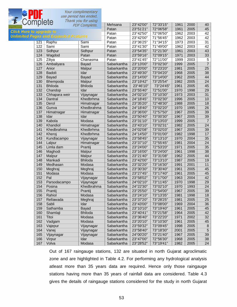
53

117 Visanagar Visnagar Mehsana 23°42'00" 72°33'15" 1961 2000 40 118 Patan Patan Patan 23°51'21" 72°06'58" 1961 2005 45 119 Chanasma Chanasma Patan 23°42'50" 72°06'50" 1962 2003 42 120 Harij Harij Patan 23°42'00" 71°56'45" 1962 2003 42 121 Raphu Sami Patan 23°36'25" 71°34'15" 1973 2003 31 122 Sami Sami Patan 23°41'30" 71°49'00" 1962 2003 42 123 Sidhpur Sidhpur Patan 23°54'35" 72°21'30" 1961 2003 43 124 Wagdod Patan Patan 23°59'16" 72°09'15" 1971 2003 33 125 Ziliya Chanasma Patan 23°41'45" 72°11'00" 1999 2003 5 126 Ambaliyara Bayad Sabarkantha 23°13'00" 73°02'30" 1999 2005 7 127 Anior Malpur Sabarkantha 23°20'00" 73°23'20" 1981 2005 25 128 Badoli Idar Sabarkantha 23°49'30" 73°04'20" 1968 2005 38 129 Bayad Bayad Sabarkantha 23°14'00" 73°14'00" 1962 2005 44 130 Bhempoda Malpur Sabarkantha 23°19'42" 73°25'54" 1982 2005 24 131 Bhiloda Bhiloda Sabarkantha 23°46'10" 73°24'45" 1961 2005 45 132 Chandop Idar Sabarkantha 23°55'40" 72°51'00" 1970 1998 29 133 Chhapara weir Vijaynagar Sabarkantha 24°02'10" 73°10'30" 1973 2003 31 134 Dantral Khedbrhma Sabarkantha 24°18'45" 73°02'30" 1996 2005 10 135 Derol Himatnagar Sabarkantha 23°35'20" 72°48'30" 1988 2005 18 136 Gunva Khedbrahma Sabarkantha 24°18'40" 73°02'20" 1970 1995 26 137 Himatnagar Himatnagar Sabarkantha 23°36'00" 72°57'50" 1967 2005 39 138 Idar Idar Sabarkantha 23°50'40" 73°00'30" 1967 2005 39 139 Kabola Modasa Sabarkantha 23°31'10" 73°13'03" 1999 2005 7 140 Khandiol Himatnagar Sabarkantha 23°43'10" 73°02'31" 1982 2005 24 141 Khedbrahma Khedbrhma Sabarkantha 24°02'08" 73°02'03" 1967 2005 39 142 Kheroj Khedbrhma Sabarkantha 24°14'50" 73°01'00" 1982 1998 17 143 Kundlacampo Vijaynagar Sabarkantha 23°58'45" 73°13'10" 1970 2004 35 144 Lalpur Himatnagar Sabarkantha 23°37'10" 72°55'45" 1981 2004 24 145 Limla dam Prantij Sabarkantha 23°24'00" 72°53'20" 1971 2005 35 146 Maghodi Malpur Sabarkantha 23°16'00" 73°24'00" 1961 1998 38 147 Malpur Malpur Sabarkantha 23°21'40" 73°31'08" 1962 2005 44 148 Mankadi Bhiloda Sabarkantha 23°42'00" 73°13'10" 1987 2005 19 149 Medhasan Modasa Sabarkantha 23°32'20" 73°16'30" 1991 2001 11 150 Meghraj Meghraj Sabarkantha 23°30'30" 73°30'40" 1961 2005 45 151 Modasa Modasa Sabarkantha 23°27'45" 73°17'40" 1961 2005 45 152 Pal Vijaynagar Sabarkantha 23°58'02" 73°17'00" 1963 2004 42 153 Parsodacampo Vijaynagar Sabarkantha 24°02'10" 73°11'45" 1970 1998 29 154 Posina Khedbrahma Sabarkantha 24°22'30" 73°02'10" 1970 1993 24 155 Prantij Prantij Sabarkantha 23°25'50" 72°54'00" 1967 2005 39 156 Rahiol Modasa Sabarkantha 23°24'10" 73°13'35" 1981 1998 18 157 Rellawada Meghraj Sabarkantha 23°37'20" 73°28'25" 1981 2005 25 158 Sabli Idar Sabarkantha 23°43'00" 73°08'00" 1969 2004 36 159 Sathamba Bayad Sabarkantha 23°10'10" 73°19'40" 1961 2005 45 160 Shamlaji Bhiloda Sabarkantha 23°40'41" 73°21'58" 1964 2005 42 161 Titoi Modasa Sabarkantha 23°36'40" 73°22'20" 1971 2002 32 162 Vadgam Modasa Sabarkantha 23°20'10" 73°10'30" 1961 2005 45 163 Vajepur Vijaynagar Sabarkantha 23°59'32" 73°09'45" 1998 2005 8 164 Vanej Vijaynagar Sabarkantha 23°58'40" 73°18'30" 2001 2005 5 165 Vijaynagar Vijaynagar Sabarkantha 24°00'20" 73°21'40" 1967 2005 39 166 Virpur Idar Sabarkantha 23°47'00" 72°56'30" 1968 2005 38 167 Volva Modasa Sabarkantha 23°28'52" 73°19'41" 1982 2005 24

Out of 167 raingauge stations, 132 are situated in north Gujarat agroclimatic

zone and are highlighted in Table 4.2. For performing any hydrological analysis

atleast more than 35 years data are required. Hence only those raingauge

stations having more than 35 years of rainfall data are considered. Table 4.3

gives the details of raingauge stations considered for the study in north Gujarat


54

agroclimatic zone. The highlighted station contains missing records ranging from

few days to one year.

Table 4.3 Details of 73 Raingauge Stations in North Gujarat Agroclimatic Zone Sr. No.

Name of station Taluka District Latitude N

Longitude E

Data available From To

1 Aslali Dascroi

Ahmedabad

22°55'00" 72°35'40" 1961 2008 2 Bareja Dascroi 22°50'50" 72°35'30" 1971 2008 3 Barejadi Dascroi 22°53'40" 72°40'30" 1971 2005 4 Chandola Dascroi 22°59'20" 72°36'30" 1971 2008 5 Dehgam Dehgam 23°10'00" 72°49'30" 1962 2006 6 Nal Lake Sanand 22°49'10" 72°03'50" 1970 2008 7 Sanand Sanand 22°59'20" 72°23'00" 1967 2008 8 Wasai Dascroi 22°51'30" 72°32'40" 1971 2008 9 Ambaji Danta

Banaskantha

24°20'10" 72°51'00" 1971 2008 10 Amirgadh Palanpur 24°24'50" 72°38'50" 1967 2008 11 Bapla Dhanera 24°34'04" 72°13'12" 1965 2008 12 Chandisar Palanpur 24°13'55" 72°18'40" 1969 2008 13 Chitrasani Palanpur 24°16'00" 72°30'00" 1967 2008 14 Danta Danta 24°11'36" 72°45'45" 1961 2008 15 Dantiwada Dhanera 24°19'10" 72°20'15" 1964 2008 16 Deesa Deesa 24°15'30" 72°10'20" 1961 2008 17 Dhanera Dhanera 24°30'40" 72°01'45" 1961 2008 18 Gadh Palanpur 24°07'17" 72°15'31" 1971 2008 19 Hadad Danta 24°15'45" 72°58'30" 1968 2008 20 Junisarotri Palanpur 24°21'40" 72°32'45" 1971 2008 21 Nava Deesa 24°07'49" 72°10'17" 1971 2006 22 Palanpur Palanpur 24°10'14" 72°26'10" 1962 2008 23 Panthawada Dhanera 24°29'20" 72°18'05" 1967 2008 24 Sanali Ashram Danta 24°12'20" 72°57'30" 1970 2004 25 Wadgam Wadgam 24°04'21" 72°29'35" 1961 2008 26 Mansa Mansa

Gandhinagar 23°25'30" 72°42'00" 1967 2008

27 Raipur weir Dehgam 23°06'30" 72°43'45" 1971 2008 28 Balasinor Balasinor

Kheda

22°57'25" 73°15'13" 1961 2008 29 Dakor Thasara 22°45'10" 73°08'50" 1974 2008 30 Kapadwanj Kapadwanj 23°02'00" 73°04'30" 1968 2008 31 Kathlal Kapadwanj 22°54'50" 72°59'10" 1969 2008 32 Kheda Kheda 22°45'00" 72°41'10" 1967 2008 33 Mahemdabad Mahemdabad 22°49'30" 72°45'30" 1967 2008 34 Mahisa Maudha 22°51'20" 73°03'40" 1970 2005 35 Nadiad Nadiad 22°41'40" 72°52'10" 1965 2008 36 Pinglaj Kheda 22°48'50" 72°36'20" 1967 2005 37 Savli tank Balasinor 22°57'40" 73°06'50" 1968 2008 38 Vadol Kapadwanj 22°58'30" 73°12'00" 1970 2005 39 Vaghroli Tank Thasara 22°53'00" 73°17'30" 1973 2008 40 Ambaliyasan Mehsana

Mehsana

23°27'30" 72°27'00" 1970 2008 41 Kalol Kalol 23°15'00" 72°29'40" 1961 2008 42 Dharoi Kheralu 24°00'00" 72°51'15" 1968 2008 43 Kadi Kadi 23°18'00" 72°22'10" 1962 2006 44 Katosan Mehsana 23°27'00" 72°13'00" 1967 2008 45 Kheralu Kheralu 23°53'10" 72°37'20" 1967 2008


55

46 Mehsana Mehsana 23°36'30" 72°24'40" 1961 2005 47 Ransipur Vijapur 23°44'10" 72°48'00" 1967 2005 48 Thol Kadi 23°07'40" 72°22'40" 1972 2008 49 Unjha Unjha 23°48'15" 72°23'45" 1965 2003 50 Vijapur Vijapur 23°33'30" 72°45'15" 1967 2008 51 Visanagar Visnagar 23°42'00" 72°33'15" 1961 2008 52 Patan Patan

Patan 23°51'21" 72°06'58" 1961 2008

53 Sidhpur Sidhpur 23°54'35" 72°21'30" 1961 2008 54 Wagdod Patan 23°59'16" 72°09'15" 1971 2005 55 Badoli Idar

Sabarkantha

23°49'30" 73°04'20" 1968 2008 56 Bayad Bayad 23°14'00" 73°14'00" 1962 2008 57 Bhiloda Bhiloda 23°46'10" 73°24'45" 1961 2008 58 Dantral Khedbrahma 24°18'45" 73°02'30" 1970 2008 59 Himatnagar Himatnagar 23°36'00" 72°57'50" 1967 2008 60 Idar Idar 23°50'40" 73°00'30" 1967 2008 61 Khedbrahma Khedbrahma 24°02'08" 73°02'03" 1967 2008 62 Kundlacampo Vijaynagar 23°58'45" 73°13'10" 1970 2004 63 Limla dam Prantij 23°24'00" 72°53'20" 1971 2008 64 Malpur Malpur 23°21'40" 73°31'08" 1962 2008 65 Meghraj Meghraj 23°30'30" 73°30'40" 1961 2008 66 Modasa Modasa 23°27'45" 73°17'40" 1961 2008 67 Pal Vijaynagar 23°58'02" 73°17'00" 1961 2005 68 Prantij Prantij 23°25'50" 72°54'00" 1967 2008 69 Sabli Idar 23°43'00" 73°08'00" 1969 2004 70 Shamlaji Bhiloda 23°40'41" 73°21'58" 1964 2005 71 Vadgam Modasa 23°20'10" 73°10'30" 1961 2008 72 Vijaynagar Vijaynagar 24°00'20" 73°21'40" 1967 2008 73 Virpur Idar 23°47'00" 72°56'30" 1970 2005

The maximum and minimum annual rainfall during the study period (1961 to

2008) for the above raingauge stations are presented districtwise in Figs. 4.2 to

4.8.


56

Fig. 4.2 Annual rainfall for the raingauge stations in Ahmedabad district

Fig. 4.3 Annual rainfall for the raingauge stations in Banaskantha district


57

Fig. 4.4 Annual rainfall for the raingauge stations in Gandhinagar district

Fig. 4.5 Annual rainfall for the raingauge stations in Kheda district


58

Fig. 4.6 Annual rainfall for the raingauge stations in Mehsana district

Fig. 4.7 Annual rainfall for the raingauge stations in Patan district


59

Fig. 4.8 Annual rainfall for the raingauge stations in Sabarkantha district

4.2.2 Details of Water Resources Projects

The north Gujarat region consists of major, medium and minor irrigation projects.

There are 7 major irrigation schemes as given in Table 4.4.

Table 4.4 Major Irrigation Schemes in North Gujarat Region Sr. No.

Scheme name District

1 Dantiwada Banaskantha 2 Dharoi Mehsana 3 Fatehwadi Ahmedabad 4 Hathmati Sabarkantha 5 Meshwo Sabarkantha 6 Sipu Banaskantha 7 Vatrak Sabarkantha

The details of each major irrigation schemes are obtained from Central Design

Organization (CDO), Gandhinagar. From the catchment area details obtained for

these schemes it was observed except for Hathmati reservoir, the other six

catchment area included the adjoining state of Rajasthan. As the catchment area

of Hathmati reservoir entirely lies in Gujarat State, for the present study it is


60

considered for design storm analysis the details of which are presented as below.

The map showing the catchment area is given in Plate 1.

Location Vill: Fatepur, Ta: Bhiloda, Dist:

Sabarkantha

Purpose Irrigation & flood control

River Hathmati

Area of catchment 595 km2

Mean annual runoff in the catchment 123 Mm3

Mean annual rainfall 864 mm

Year of commencement of construction

work

1959

Year of completion 1971

Dam :

Type Earthen

Maximum height above the lowest point

of foundation

23.62 m

Length at the top of the dam 933 m

Total Volume Content:

Earthwork 1.2 Mm3

Spillway Details:

Type Waste weir

Length 241 m

Energy dissipater Stilling basin apron

Maximum discharge 2943 m3/s

Type, Nos. and size of gate Ungated

Reservoir:

Area at full reservoir level 32.36 Km2

Gross storage capacity 161 Mm3


61

Effective storage capacity 153 Mm3

Area under submergence

a) Forest : NIL b) Waste land : NA c) Culturable : 3750 ha

No. of villages under submergence 14 partial ,6 full (Source: http://guj–nwrws.gujarat.gov.in)

4.2.3 Soil Type Data

The general properties of soil in the study area were mentioned in Chapter 3. For

the analysis of onset of monsoon, the soil moisture holding capacity data are

required. The characteristics of the top soil found in the study area are obtained

from various soil survey reports, prepared by various soil survey divisions in the

state, as mentioned below. These are indicative values which are obtained by

conducting borehole log test. These values are then analyzed for top 0.25 m soil

layer for the study for all the raingauge stations and presented in Table 4.5.

Source:

1. November 2000, Land Irrigability appraisal report for the area under the

command of Hadmatiya Reservoir Project , Taluka: Dantiwada, District :

Banaskantha, Soil survey division, Ahmadabad, Narmada Water resources

and water supply department, Govt. of Gujarat.

2. July 1998, Land Irrigability appraisal report for the area under the command

of Mahdevpura water Resources Project , Taluka: Kapadwanj, District :

Kheda, S.E., Soils, Drainage & Reclamation Circle, Vadodara, Narmada

Water resources and water supply department, Govt. of Gujarat.

3. May 1993, Land Irrigability appraisal report for the area under the command

of Kadiyara water resources project, District : Sabarkantha, S.E. Soils,

Drainage & Reclamation Circle, Vadodara, Narmada & Water Resources

Department, Govt. of Gujarat.

4. December 2000, Land Irrigability appraisal report for the area under the

command of Kharicut Irrigation Scheme, Taluka : City, District : Ahmedabad,

Soils Survey Division, Ahmedabad, Narmada Water resources and water

supply department, Govt. of Gujarat.


62

5. November 1998, Land Irrigability appraisal report for the area under the

command of Godhada Water Resources Project, Taluka : Danta, District:

Banaskantha, S.E. Soils and Drainage and Reclamation Circle, Vadodara,

Narmada Water resources and water supply department, Govt. of Gujarat.

6. August 1988, 3 Decades of Soil Survey Organisation, S.E. Soils and

Drainage and Reclamation Circle, Vadodara, Narmada Water resources and

water supply department, Govt. of Gujarat.

7. Land Irrigability Appraisal Report for the area under the command of Sipu

Reservoir Project, Taluka : Dantiwada, District : Banaskantha, Soils Survey

Division, Ahmedabad, Narmada Water resources and water supply

department, Govt. of Gujarat.

8. August 1998, Detailed Soil Survey Report for the Area under the command of

Balaram Water Resources Project, Taluka : Palanpur, District : Banaskantha,

S.E. Soils and Drainage and Reclamation Circle, Vadodara, Narmada Water

resources and water supply department, Govt. of Gujarat.

9. October 2000, Land Irrigability Appraisal Report for the area under the

command of Sipu Reservoir Project, Taluka : Dantiwada, District :

Banaskantha, Soils Survey Division, Ahmedabad, Narmada Water resources

and water supply department, Govt. of Gujarat.

10. November 1990, Mahadevpura water resources project, Taluka: Kapadwanj,

District : Kheda, S.E. Soils and Drainage and Reclamation Circle, Vadodara,

Narmada Water resources and water supply department, Govt. of Gujarat.

11. November 1990, Revised detailed soil survey report for the area under the

command of varanasi irrigation scheme, Taluka: Kapadwanj, District : Kheda,

S.E. Soils and Drainage and Reclamation Circle, Vadodara, Narmada Water

resources and water supply department, Govt. of Gujarat.

12. March 1988, Detailed soil survey report of Galab Irrigation Scheme, Taluka:

Thasara and Kapadwanj, District : Kheda, S.E. Soils and Drainage and

Reclamation Circle, Vadodara, Narmada Water resources and water supply

department, Govt. of Gujarat.

13. May 1994, Land Irrigability appraisal report for the area under the command

of Vadgam Water Resources Project, Taluka : Modasa, District: Sabarkantha,

S.E. Soils and Drainage and Reclamation Circle, Vadodara, Narmada &

Water Resources Department, Govt. of Gujarat.


63

14. May 1983, Soil Survey Report for the Area under the Command of Rolla

Irrigation Scheme, Taluka : Megharaj, District: Sabarkantha, S.E. Soils and

Drainage and Reclamation Circle, Vadodara, Narmada & Water Resources


15. November 1979, Soil Survey Report for the Area under the Command of

Hathmati Reservoir Project, District : Sabarkantha, Soils Survey Division,

(W.R.I.), Ahmedabad, Govt. of Gujarat.

16. Soil Survey Report for the Area under the Command of Watrak Irrigation

Scheme, Taluka: Malpur, District : Sabarkantha, Soils Survey Division,

Ahmedabad, Govt. of Gujarat.

17. January 2001, Land Irrigability Appraisal Report for the Area under the

Extended Command of Sabarmati Reservoir Project, Volume I, S.E. Soils and

Drainage and Reclamation Circle, Vadodara, Narmada Water Resources and

Water Supply Department, Govt. of Gujarat.

18. March 2006, Land Irrigability Appraisal Report for the Area under the

Command of Mukteshwar Water Resources Project, Taluka: Wadgam,

District: Banaskantha, Soil Survey Division : Gandhinagar, Soils, Drainage &

Reclamation circle, Vadodara, Narmada Water Resources Water Supply and

Kalpsar Department, Govt. of Gujarat.

19. May 1994, Land Irrigability Appraisal Report for the Area under the Command

of Pal Water Resources Project, Taluka: Vijaynagar, District: Sabarkantha,

Soils, Drainage & Reclamation circle, Vadodara, Narmada & Water

Resources Department, Govt. of Gujarat.

20. May 1993, Detailed Soil Survey Report for the area under the command of

Chandrana Water Resources Project, District : Sabarkantha, S.E., Soils ,

Drainage & Reclamation, Vadodara, Narmada & Water Resources



64

Table 4.5 Total Available Water (TAW) in the 0.25 m Soil Profile

Sr. No. District Station Depth,

mm/0.25 m soil depth 1

Ahmedabad

Aslali 37 2 Bareja 31 3 Barejadi 40 4 Chandola 40 5 Dehgam 37 6 Sanand 40 7 Nal Lake 40 8 Wasai 40 9

Banaskantha

Ambaji 40 10 amirgadh 25 11 Bapla 30 12 Chandisar 25 13 Chitrasani 25 14 Danta 40 15 Dantiwada 30 16 Deesa 30 17 Dhanera 30 18 Gadh 25 19 Hadad 40 20 Junisarotri 25 21 Nava 30 22 Palanpur 25 23 Panthawada 30 24 Sanali Ashram 40 25 Wadgam 30 26 Gandhinagar mansa 40 27 Raipur weir 37 28

Kheda

Balasinor 37 29 Dakor 37 30 Kapadwanj 37 31 Kathlal 37 32 Kheda 37 33 Mahemdabad 37 34 Mahisa 37 35 Nadiad 37 36 Pinglaj 37 37 Savli tank 37 38 Vadol 37 39 Vaghroli Tank 37 40

Mehsana

Ambaliyasan 40 41 Kalol 40 42 Dharoi 40 43 Kadi 40 44 Katosan 40 45 Kheralu 40 46 Mehsana 40 47 Ransipur 40 48 Thol 40 49 Unjha 30 50 Vijapur 40 51 Visanagar 40 52

Patan Patan 40

53 Sidhpur 25 54 Wagdod 40


65

55

Sabarkantha

Badoli 31 56 Bayad 37 57 Bhiloda 32 58 Dantral 30 59 Himmatnagar 30 60 Idar 31 61 Khedbhrama 37 62 Kundlacampo 37 63 Limla dam 27 64 Malpur 32 65 Meghraj 32 66 Modasa 32 67 Pal 37 68 Prantij 27 69 Sabli 31 70 Shamlaji 32 71 Vadgam 32 72 Vijaynagar 37 73 Virpur 31

4.2.4 Crop Data

The details regarding the cropping pattern and major crops grown in the study

area are obtained from the following sources.

1. Department of Agriculture, Krishi Bhavan, Gandhinagar.

2. Sardar Krushinagar Agriculture University, Dantiwada, Banaskantha.

Anand Agriculture University, Anand.

The details of crop, crop length period, crop growth stages of certain major crops

considered for the analysis are presented in Table 4.6 to 4.10.

Table 4.6 Details of Pearl Millet with Effective Root Zone Depth of 30 cm

Name of

variety Date of sowing

Length of

growing period, days

Crop development stages Critical growth stages

Stage Days Stage Days

GHB 558

On set of monsoon (June 3rd

week to July 1st week)

90–100 1. Emergence 04–05 1.Tillering 30

GHB 538

2. Seedling 15–30 2. Flowering 50

GHB 577

3.Tillering 30–35 3. Milking 70 4. Panicle initiation 45–50 4. Soft dough 80 5. Flowering 50–60 6. Milking 65–75 7. Soft dough 75–85 8. Dry husk 85–100


66

Table 4.7 Details of Maize with Effective Root Zone Depth of 50 cm

Name of variety

Date of sowing

Length of

growing period, days



GM 4 Onset of monsoon (June 3rd week to July 1st

week)

85–90 1. Emergence 5 1. Knee high 30 Narmada

Moti 85–90 2. Seedling 15–25 2.Tasseling 45

GM 6 75–80 3. Knee high 25–30 3. Silking 55 4. Tasseling 45–50 4. Milky 70 5. Silking 57–60 6. Milky 65–70 7. Grain development 70–75 8. Dry husk 75–80

Table 4.8 Details of Groundnut with Effective Root Zone Depth of 45 cm

Name of variety

Date of sowing

Length of growing period, days



GG 2 Onset of monsoon (June 3rd

week to July 2nd week)

100-110 1. Emergence 7-10 1. Flowering 30-45 GG 5 2. Branching 15-35 2. Peg formation 31-51 GG 7 3. Flowering 30-45 3. Pod formation 40-60

GG 20 Onset of monsoon (June 2nd

week to end of June)

120-130 4. Peg formation 31-51 4.Pod development 50-90 GG 10 5. Pod formation 40-60 GG 11 6. Pod development 50-90 GG 12

Table 4.9 Details of Cotton with Effective Root Zone Depth of 75 cm Name of variety

Date of sowing

Length of

growing Period,

days

Crop development stages Critical growth stages Stage Days Stage Days

Rainfed Cotton GC 11 On set of

monsoon (June 3rd

week to July 3rd

week)

230–250 1. Germination 04–05 1. Branching 50 GC 13 2. Seedling 30–40 2. Square 85 GC 21 3. Branching 40–60 3. Flowering 95 GC 23 4. Square 85 3. Boll formation 120

5. Flower 95 5. Boll formation 120 6. Boll bursting 160 7. First peaking 180

Irrigated Cotton Govt approved Bt cotton

3rd week of May to 1st week of July

180–230 1. Germination 04–05 1. Branching 40 2. Seedling 20–30 2. Square 60 3. Branching 30–50 3. Flowering 70 4. Square initiation 60 3. Boll formation 90 5. Flower initiation 70 6. Boll development 100 5. Boll formation 90 7. Boll bursting 120 6. Boll development 100 7. First peaking 140 7. Boll bursting 120 8. First peaking 140


67

Table 4.10 Details of Sesame with Effective Root Zone Depth of 60 cm

Name of variety

Date of sowing



Stage Days Stage Days GT 1 On set of

monsoon (June 3rd

week to July 1st week)

85-90 1. Emergence 4 1. Vegetative 25 GT 2 85-90 2. Vegetative 10-30 2. Branching 35 GT 20 90-95 3. Branching 30-40 3. Flowering 50

4. Flowering 40-60 4. Pod filling 70

Purva 1 Mid August 120 5. Pod filling 60-75

Table 4.11 Details of Mung Bean with Effective Root Zone Depth of 45 cm

Name of variety

Date of sowing




K 851 Onset of monsoon (June 3rd

week to July 2nd week)

61-68 1. Emergence 4 1. Branching 30 GM 4 2. Branching 25-30 2. Flowering 35-45

3. Flowering 35-45 3. Pod development 50-55 4. Pod development

Table 4.12 Details of Guar with Effective Root Zone Depth of 60 cm

Name of

variety

Date of sowing

Length of growing Period,

days



GG 1 2nd week of July to 4th week of July

100-110 1. Emergence 4 1. Branching 25 GG 2 95-100 2. Branching 25 2. Flowering 35-50

3. Flowering 35-50 3. Pod development 45-60 4. Pod development 45-60


68

CHAPTER 5

METHODOLOGY

5.1 GENERAL

Daily rainfall data for 73 raingauge stations, weekly minimum & maximum

temperatures, relative humidities, sunshine hours, dew point temperature and

wind speed for greater than or equal to 35 years in the north Gujarat agroclimatic

zone are collected from various sources mentioned in the Chapter 4.

Generally, it is observed that the dataset obtained is seldom continuous. For

performing the analysis one requires a complete data set. Therefore the missing

data have to be filled up using an appropriate method. It is a known fact that the

climatic parameters except the rainfall are recorded for all the 365 days on daily

basis while rainfall is recorded only when it occurs i.e. for the monsoon period on

daily basis. For Gujarat it is observed that 94% of annual rainfall occurs in the

monsoon season. From the dataset of rainfall it is observed that for the

premonsoon (March to May), postmonsoon (October and November) and winter

(December to February) seasons the daily values are zero for more than 98% of

years except in some cases of the month of October. Thus for determining

missing daily rainfall June to October months are considered. For other climatic

parameters all 365 days values are considered. For the parameters other than

rainfall the missing dataset is filled in using the linear trend followed by the values

obtained from the past.

Hydrologic modeling and water resources assessments depend upon knowledge

of the form and amount of rainfall occurring in a region of concern over a time

period of interest. Rainfall varies spatially and temporally. It should be

understood that both spatial and temporal variations in rainfall are important in

hydrologic studies as well as in water resources planning and in agriculture

planning.


69

5.2 MISSING CLIMATE DATA

In order to compute the missing daily rainfall data the latitudes and longitudes of

the different raingauge stations are converted to x and y co–ordinates using the

Franson Coord Trans V 2.2. The raingauge stations in and around study area are

utilized for forming the groups of stations to compute the missing data using

cluster analysis.

Cluster Analysis

Cluster analysis is one of the statistical techniques often used in meteorology

and climatology to identify homogeneous climate groups and for climate

classification. The aim of the cluster analysis is to group the raingauge stations

into clusters for filling in missing data. It is performed by clustering algorithms. All

the clustering algorithms follow the basic four steps routine to identify

homogeneous groups

(i) Calculation of the specified distance between all the raingauge stations.

(ii) Formation of a new cluster merging from the two closest entries, based on

a defined criterion.

(iii) Recalculation of the distance between all the entries, and

(iv) Repetition of steps (ii) and (iii) until all entries merge into one cluster.

Data clustering algorithms can be of different types such as joining (tree

clustering), two way joining (block clustering) and k–means clustering. The

purpose of this joining algorithm is to join together objects into successively

larger clusters, using some measure of similarity or distance. A typical result of

this type of clustering is the hierarchical tree. While for other types of analyses

the research question of interest is usually expressed in terms of cases

(observations) or variables. It turns out that the clustering of both may yield

useful results. For example, imagine a study where a researcher has gathered

data on different measures of climate parameters (variables) for a sample of

tropical climate (cases). The researcher may want to cluster cases (parameters)

to detect clusters of parameters with similar characteristics. At the same time, the

researcher may want to cluster variables (sub climate category) to detect clusters

of measures that appear to tap similar sub climate characteristics. This type of

problems uses two way joining algorithms. This method of clustering is very

different from the joining (tree clustering) and two–way joining. Suppose that one


http://www.statsoft.com/textbook/cluster-analysis/

70

already has hypothesis concerning the number of clusters in ones cases or

variables. One may want to "tell" the computer to form exactly 3 clusters that are

to be as distinct as possible. This is the type of research question that can be

addressed by the k–means clustering algorithm. For the present study the joining

algorithm is of concern as forming the groups of raingauge stations are required

based on the distances. Also one cannot be biased and conclude that some n

number of clusters are required for grouping the stations so the k–means will not

be useful and the two way joining is out of choice as ones goal for forming the

groups is based on the single parameter distance between the stations. Thus for

the cluster analysis joining algorithm is appropriate and hence adopted.

Hierarchical tree is a way to investigate grouping in data, simultaneously over a

variety of scales, by creating a cluster tree called a dendrogram. The tree is not a

single set of clusters, but rather a multi–level hierarchy, where clusters at one

level are joined as clusters at the next higher level. Hierarchical tree can be

agglomerative ("bottom–up") or divisive ("top–down"). Agglomerative algorithms

begin with each element as a separate cluster and merge them into successively

larger clusters. Divisive algorithms begin with the whole set and proceed to divide

it into successively smaller clusters.

The joining or tree clustering method uses the dissimilarities/similarities or

distances between objects when forming the clusters. Similarities are a set of

rules that serve as criteria for grouping or separating items. The distances

(similarities) can be based on a single dimension or multiple dimensions, with

each dimension representing a rule or condition for grouping objects. The most

straightforward way of computing distances between objects in a multi–

dimensional space is to compute Euclidean distances. If one has a two– or

three–dimensional space this measure is the actual geometric distance between

objects in the space (i.e., as if measured with a ruler). However, the joining

algorithm does not "care" whether the distances that are "fed" to it are actual real

distances, or some other derived measure of distance that is more meaningful to

the researcher; and it is up to the researcher to select the right method for her

specific application. There are different distance measures available for

clustering which are used in the present study given in Table 5.1.


http://www.statsoft.com/textbook/statistics-glossary/a.aspx?button=a

http://en.wikipedia.org/wiki/Dendrogram

71

Table 5.1 Different Types of Distance Measures for Clustering Distance measure

Equation Remark

Euclidean ( )

21

2 y)(x, distance

−= ∑i

ii yx Euclidean distance

Square Euclidean distance (Seuclidean)

( )

V y)(x, distance

2∑ −= i

ii yx

Each coordinate in the sum of squares is inversely weighted by the sample variance, v, of that coordinate

Mahalanobis distance

Corrects data for different scales and correlations in the variables

City block metric ∑ −=

iii yx y)(x, distance ---

Minikowski metric

---

cosine

One minus the cosine of the included angle between points (treated as vectors)

correlation distance = 1 – r; where r = Z(x)·Z(y)/n One minus the sample correlation between points (treated as sequences of values)

Hamming distance --- The percentage of

coordinates that differ Jaccard

---

One minus the Jaccard coefficient (based on similarity), the percentage of nonzero coordinates that differ

Chebychev distance ii yx maximum y)(x, distance −= Maximum coordinate

difference

When each object represents its own cluster, the distances between those

objects are defined by the chosen distance measure. One then needs a linkage

or amalgamation (aggregate) rule to determine when two clusters are sufficiently

similar to be linked together. There are various possibilities as presented in Table

5.2. For example, link two clusters together when any two objects in the two

clusters are closer together than the respective linkage distance.

MATLAB software is used for forming the clusters. Different combinations using

the distance measures and linkage rules are evaluated by Cophen coefficient

feature available. This measure is used to compare alternative cluster solutions

obtained using different combinations of distance measures and linkage rules

presented in Tables 5.1 and 5.2. Based on the groups formed using the cluster

analysis, further calculations are carried out.


72

Table 5.2 Linkage Rules for Determining Clusters Linkage rules Remarks

Single The distance between two clusters is determined by the distance of the two closest objects (nearest neighbors) in the different clusters. This rule will, in a sense, string objects together to form clusters, and the resulting clusters tend to represent long "chains."

Complete In this method, the distances between clusters are determined by the greatest distance between any two objects in the different clusters (i.e., by the "farthest neighbors"). This method usually performs quite well in cases when the objects actually form naturally distinct "clumps." If the clusters tend to be somehow elongated or of a "chain" type nature, then this method is inappropriate.

Average In this method, the distance between two clusters is calculated as the average distance between all pairs of objects in the two different clusters. This method is also very efficient when the objects form natural distinct "clumps," however, it performs equally well with elongated, "chain" type clusters. It is also called as unweighted pair–group method using arithmetic averages.

Weighted This method is identical to the unweighted pair–group average method, except that in the computations, the size of the respective clusters (i.e., the number of objects contained in them) is used as a weight. Thus, this method (rather than the previous method) should be used when the cluster sizes are suspected to be greatly uneven. It is also known as weighted pair–group method using arithmetic averages.

Centroid The centroid of a cluster is the average point in the multidimensional space defined by the dimensions. In a sense, it is the center of gravity for the respective cluster. In this method, the distance between two clusters is determined as the difference between centroids. It is also called as unweighted pair–group method using the centroid average.

Median This method is identical to the previous one, except that weighting is introduced into the computations to take into consideration, differences in cluster sizes (i.e., the number of objects contained in them). Thus, when there are (or one suspects there to be) considerable differences in cluster sizes, this method is preferable to the previous one. It is also known as weighted pair–group method using the centroid average.

Ward This method is distinct from all other methods because it uses an analysis of variance approach to evaluate the distances between clusters. In short, this method attempts to minimize the sum of squares of any two (hypothetical) clusters that can be formed at each step. In general, this method is regarded as very efficient; however, it tends to create clusters of small size.

Though there are number of raingauge stations in the vicinity of the raingauge

station where missing data are to be calculated, it happens rarely that there is

more than one station where complete data are available, for filling the missing

data. An attempt is made to fill the missing data using only one rainguage station

and to identify the same. Amongst the different methods available, the artificial

neural network (ANN), the closest station and the non linear regression methods

are used, as other methods require more than one rainguage station. After

forming the groups of the raingauge stations the missing data are calculated

using the ANN method, closest station method and non linear regression

method.


73

Missing data of the selected station are to be filled in using the best method

among the ANN, closest station (CS) and non linear regression (NLR) methods

with one raingauge station as input. Different ANN networks such as

competitivecascade–forward backpropagation, Elman backpropagation, feed–

forward backpropagation, feed–forward input–delay backpropagation,

generalized regression, Hopfield recurrent, linear layer, perceptron, probabilistic

neural and radial basis are explored in case for filling missing data using ANN

method. For closest station method the missing data are filled in with the same

set of data as present in the nearby raingauge station. While in case for non

linear regression method the selected regression equation provides zero value

output given the zero value input. This is required for the representation of no

rain events. Thus the gamma model as presented in Eq. 5.1 is used for non

linear regression models.

Gamma Model: exp(a/b)/b)(xay cm ⋅⋅= (5.1)

where,

y = missing rainfall record from the station in question

xm = rainfall data from the selected station for finding missing record

a, b, c = constants

A nearby raingauge station (having complete data for a period which is found

missing in the raingauge station in question) to the raingauge station in question,

is selected as an input station. If the nearest station contained the same missing

records then the next nearby station containining the complete dataset is

selected as input station. When there are more than one nearby stations having

complete dataset then the input station is determined based on the higher

correlation coefficient value between the input station and the missing data

raingauge station. Thus the groups of the raingauge stations are explored for

determining the input station.

After determining the input station for filling in missing data of the raingauge

station, the set of complete data (100%) in both the input and the raingauge

station in question are utilized for model analysis. From these 100% dataset,

70% data are utilized for forecast and model preparation and the remaining 30%


74

are used to test and validate the model based on different forecast and model

parameters.

In order to investigate the best method based on the forecasted events, the

categorical or conditional statistics quantifying the skill in the prediction of the

occurrence of rain based on the familiar 2 × 2 (yes/no) contingency Table is

used. A contingency Table presented in Table 5.3 is a matrix showing the

frequencies of predicted and/or observed events, such as "rain" and "no rain". It

gives information about the types of errors occurring in the forecast.

Table 5.3 A 2 x 2 Contingency Matrix for Conditional / Categorical Statistics Event observed

Yes No

Event forecast Yes A B No C D

The value of "A" is the number of event forecasts that correspond to event

observations, or the number of hits. Value of "B" is the number of event forecasts

that do not correspond to observed events, or the number of false alarms. Value

of "C" is the number of no–event forecasts corresponding to observed events, or

the number of misses and value of "D" is the number of no–event forecasts

corresponding to no events observed, or the number of correct rejections. This

2 x 2 table will be referred in the definitions of a number of performance

measures formulated for the 2 x 2 verification problem. For example based on

the method for determining missing rainfall, a certain value is obtained which will

be referred to the case yes for the event forecasted. Then the next step will be to

choose either A or B based on the actual data observed. If the rain actually

occurred then A is chosen and if not then B. Thus for the 2 x 2 contingency table

the alphabets A, B, C and D will be replaced by the numeric values by

categorizing each value obtained. Based on the values obtained Table 5.4

presents the definitions and equations of conditional / categorical statistics for

verification of the forecasted values obtained using ANN, CS and NLR methods

Akaike's information criterion (AIC) and Bayesian’s Information Criterion (BIC) of

selecting the optimum model are considered for selection of the method to be

used. Akaike (1974) proposed AIC as a measure of the goodness of fit of an

estimated statistical model. It is based on the concept of entropy, in effect

offering a relative measure of the information lost when a given model is used to


http://www.swpc.noaa.gov/forecast_verification/Glossary.html




75

describe reality and can be said to describe the tradeoff between bias and

variance in model construction, or that of precision and complexity of the model.

The AIC is not a test on the model in the sense of hypothesis testing; rather it is a

tool for model selection.

Table 5.4 Details of Conditional / Categorical Statistics Conditional / categorial statistics

Equation Limits Perfect score Remarks

Bias Score, BIAS

A BBIASA C

+=

+

0 to infinity

1 A perfect bias score indicates the predicted rainfall area (frequency) is the same as was observed. Value less than one underforecasts rainfall. Value greater than one overforecasts rainfall.

Probability of Detection, POD

APODA C

=+

0 to 1 1 The POD is sensitive only to missed events, not false alarms. POD can be increased by issuing a larger number of rain forecasts on the assumption that a greater number will be correct, usually at the cost of more false alarms.

False Alarm Ratio, FAR

BFARA B

=+

0 to 1 0 FAR is sensitive only to false predictions, and not to missed events. This score can always be decreased by underforecasting the number of severe events, but only at the cost of more missed events.

Equitable Threat Score, ETS

( ) ( )( ) ( )

DxA BxCETS

B C xN DxA BxC−

=+ + −

min. value is 1/3

– The ETS is a modification to the CSI that takes into account the number of correct forecasts of events (hits) that would be expected purely due to chance

Hanssen and Kuipers Score, HK ( ) ( )

DxA BxCHKD B x C A

−=

+ +

–1 to 1 1 The HK score has the advantage that it is independent of the distribution of events and non–events in the sample set. Put another way, for measuring the skill of the model, the HK score is appropriate because it does not depend on whether there happened to be more wet or dry days in the sample set (provided the sample set is large enough to yield stable statistics). This is why it is often called the "true skill statistic."


76

Given a data set, several competing models may be ranked according to their

AIC, with the one having the lowest AIC being the best. 2 [ln(2 / ) 1]AIC k n RSS nπ= + + (5.2)

where k is the no. of parameters, n the no. of observations and RSS is the

residual sum of squares given as

( )2

1

n

i iiRSS p o

== −∑

(5.3)

where pi is the predicted data points and oi is the observed data points.

In parametric methods, there might be various candidate models with different

number of parameters to represent a dataset. The number of parameters in a

model plays an important role. The likelihood of the training data is increased

when the number of parameters in the model is increased but it might result in

overtraining problem, if the number of parameters is too large. In order to

overcome this problem, one can use BIC (parametric method) which is also one

of the statistical criteria for model selection. The BIC is sometimes also named

the Schwarz Criterion or Schwarz Information Criterion (SIC). It is so named

because Schwarz (1978) gave a Bayesian argument for adopting it.

ln ln( )RSSBIC n k nn

= + (5.4)

where k is the no. of parameters, n is the no. of observations and RSS is the

residual sum of squares.

For validating the model amounts obtained in conjunction to AIC and BIC, two

more parameters presented in Table 5.5 will be used, as these are the basic

parameters for testing the model amounts.

Table 5.5 Details of Goodness of Fit Parameters for Validating Model Amounts Goodness of fit

parameter Equation Remarks

Root mean square error, RMSE

( ) 5.0

1

2

−= ∑

=

n

i npiOiRMSE

It is appropriate to quantify the error in terms of the units of the variable. Both RMSE and MAE indicate errors in the model amounts obtained.

Mean absolute error, MAE

1

1 n

i iiMAE o p

n =

= −∑

The missing sunshine hours are determined using the CROPWAT 8.0 software

based on the FAO 56 guidelines. The method is derived from the air temperature

(minimum and maximum temperatures) differences which are related to the


77

degree of cloud cover in a location as an indicator of the fraction of

extraterrestrial radiation that reaches the earth’s surface. The Hargreaves’

radiation formula adjusted and validated at several weather stations, is available

in CROPWAT 8.0 and hence used.

For other climatic parameters such as minimum temperature, maximum

temperature, relative humidity, wind speed, etc., the missing data are filled in

using the SPSS software. Here the data are filled in using linear trend, observed

for the study period, for each parameter under consideration.

5.3 PROBABILITY DISTRIBUTION

Probability distribution arises from experiments where the outcome is subjected

to chance. The nature of the experiment dictates which probability distribution

may be appropriate for modeling the resulting random outcomes. There are two

types of probability distribution–continuous and discrete. Using a probability

model does not allow one to predict the result of any individual experiment but

one can determine the probability that a given outcome will fall inside a specific

range of values. The rainfall data is a collection of continuous random variable as

it can take on any value within a finite range. The complete daily point rainfall

dataset thus obtained is used for the analysis by converting it to consecutive 2, 3,

4, 5, 6, 7 and 10 days rainfall. Fig. 5.1 and 5.2 shows the illustration for

determining consecutive 2 and 3 days maximum rainfall total. Similar procedure

is adopted for determining consecutive 4, 5, 6, 7 and 10 days maximum rainfall

total.


78

Date 1 2 3 4 5 6 7 8 9 10 11 12 13 14 15

Rainfall, mm 1 15 5 20 56 66 22 15 0 6 10 27 33 5 3 Consecutive 2 days 16 25 122 37 6 37 38

Moving 2 day total

16 20

25 122

88 37

15 6

16 37

60

38

8 Maximum 2 day total 122

Fig. 5.1 Illustration for computing consecutive 2 days maximum rainfall.

Date 1 2 3 4 5 6 7 8 9 10 11 12 13 14 15 Rainfall, mm 1 15 5 20 56 66 22 15 0 6 10 27 33 5 3

Moving 3 day total

21 142 37 43 41 21

40 81 142 144 103 37 21 16 43 65 65 41

Maximum 3 day total 144 Fig. 5.2 Illustration for computing consecutive 3 days maximum rainfall.

There are numerous continuous probability distributions available. The selection

of best fitted probability distribution will be based on AIC and BIC using the

maximum likelihood method. The available sixteen continuous probability

distributions are checked for the rainfall dataset (1961–2008) of north Gujarat

agroclimatic zone and are given in Table 5.6.


79

Table 5.6 Continuous Probability Distributions used in the Present Study

Sr. no.

Type of continuous probability distribution

Probability density function

1 Birnbaum–Saunders

2 Exponential

3 Extreme value

4 Gamma

5 Generalized

extreme value

6 Generalized

Pareto

7 Inverse

Gaussian

8 Logistic

9 Log–Logistic The variable x has a loglogistic distribution with location parameter µ and scale

parameter σ > 0 if ln x has a logistic distribution with parameters µ and σ. 10 Lognormal

11 Nakagami

12 Normal

13 Rayleigh

14 Rician


80

15 t location–scale

16 Weibull

An effort has been made to determine the best fitted probability distribution for

the given rainfall dataset in order to evaluate the rainfall characteristics of the

region. The complete daily rainfall dataset obtained is used for the analysis by

converting it to consecutive 2, 3, 4, 5, 6, 7 and 10 days rainfall. The backward

moving window is used to obtain the consecutive 2, 3, 4, 5, 6, 7 and 10 days

rainfall data. 16 different probabilities presented in Table 5.6 are applied to the

dataset of one and consecutive 2, 3, 4, 5, 6, 7 & 10 days rainfall.

The AIC for probability distribution fittings is different from the Eq. 5.2 and is

given as,

2In(L)2kAIC −= (5.5)

where k is the number of parameters in the statistical model, and L is the

maximized value of the likelihood function for the estimated model.

Similarly BIC is an asymptotic result derived under the assumptions that the data

distribution is in the exponential family.

The BIC is expressed as:

ln(n)k Lln 2BIC +−= (5.6)

where n is the number of observations, or equivalently, the sample size; k is the

number of free parameters to be estimated and L is the maximized value of the

likelihood function for the estimated model.

5.4 DEVELOPMENT OF REGRESSION RELATIONSHIPS

Using the fitted distribution the probability of rainfall and the respective return

period will be obtained and regression models will be developed for the rainfall of

different amounts applicable for water resources planning which is discussed in

the following text.


http://en.wikipedia.org/wiki/Exponential_family

http://en.wikipedia.org/wiki/Observation

http://en.wikipedia.org/wiki/Parameter

http://en.wikipedia.org/wiki/Likelihood

81

The following regression relationship have been developed

Regression models for one day to ten consecutive days of annual

maximum rainfall corresponding to one to 1000 years of return period.

Regression relationships of two to ten consecutive days of maximum

annual rainfall with one day annual maximum rainfall.

Regression relationship for the prediction of consecutive days of maximum

rainfall from one day maximum rainfall and consecutive days ranging from

two to seven and ten.

Based on the fitted distribution, the probability of occurrence of a rainfall denoted

by P, whose magnitude is equal to or in excess of a specified magnitude X is

obtained. The recurrence interval (return period) T is given by,

P1 T = (5.7)

Thus the rainfall amount for a recurrence interval from 1–10 years in steps of 1

year, 15, 20, 25, 50, 75 and 100 years are determined using the best probability

distribution fitted to the dataset, for application in drainage coefficient, design of

water harvesting system, etc.

The consecutive two to seven and ten days rainfall and the recurrence interval

for each of the combinations will be investigated based on the fitted probability.

For the development of regression models a dataset consisting of 100 samples

are selected. The sample consists of 1–65 years in steps of 1 year, 70–200 in

steps of 5 years, 250–500 in step of 50 years, 750 and 1000 years. Out of these

100 values model formulation are carried out using 70% data (70 values) and the

remaining 30% data are used to validate the model. The selection of 70 values

out of 100 values is a random selection. This selection iteration procedure is

carried out 35 times. Thus 35 different random models are developed and the

best model based on the goodness of fit parameters is considered.

Regression relationships of two to seven and ten consecutive days of maximum

annual rainfall with one day annual maximum rainfall are developed using the

same approach.


82

Goodness of Fit Test Parameters

Coefficient of correlation, r

Measure of the "goodness of fit" is the coefficient of correlation, r. To explain the

meaning of this measure, one has to define the standard deviation, which

quantifies the spread of the data around the mean:

( )2

1

n

t iis o o

== −∑ (5.8)

where st is the standard deviation, oi is the observed data points and O is the

average of the observed data points given by

1

1 n

iio o

n −= ∑ (5.9)

The quantity st considers the spread around a constant line (the mean) as

opposed to the spread around the regression model. This is the uncertainty of

the dependent variable prior to regression. One also defines the deviation from

the fitting curve as

( )2

1

n

r i iis o p

== −∑ (5.10)

where sr is the deviation from the fitting curve, pi is the predicted data points.

Note the similarity of this expression to the standard error of the estimate given in

Eq. 5.9; this quantity likewise measures the spread of the points around the fitting

function. Thus, the improvement (or error reduction) due to describing the data in

terms of a regression model can be quantified by subtracting the two quantities.

Because the magnitude of the quantity is dependent on the scale of the data, this

difference is normalized to yield

t

rt

sss

r−

= (5.11)

where r is defined as the coefficient of correlation. As the regression model starts

improving describing the data, the correlation coefficient approaches unity. For a

perfect fit, the standard error of the estimate will approach sr = 0 and the

correlation coefficient will approach r = 1.

Legates and McCabe (1999) evaluated the correlation and correlation based

measures widely used to examine the goodness of fit of hydrologic and

hydroclimatic models. According to them these measures are oversensitive to


83

extreme values and are insensitive to additive and proportional differences

between model predictions and observations. Because of these limitations,

correlation–based measures can indicate that a model is good predictor, even

when it is not. In the present study three basic parameters (the coefficient of

determination R2, the coefficient of Efficiency, E and the Index of Agreement, d)

are used for model validation.

Coefficient of determination, R2

The coefficient of determination is the square of the Pearson’s Product Moment

coefficient of correlation (R2 = r2) and describes the proportion of the total

variance in the observed data that can be explained by the model. It ranges from

0.0 (poor model) to 1.0 (perfect model) and is given by

( )( )

( ) ( )0.5n

1i

2

i

0.5n

1i

2

i

n

1iiii

2

ppoo

pppoR

−

−

−−=

∑∑

∑

==

= (5.12)

where oi and pi are the observed and predicted data points and oand p are the

mean of the observed and predicted data points.

Coefficient of efficiency, E

Nash and Sutcliffe (1970) defined the Coefficient of Efficiency, which ranges from

minus infinity (poor model) to 1.0 (perfect model), as

1

1

1.0

n j

i ii

jn

ii

o pEj

o o=

=

−∑= −

−∑ (5.13)

where Ej is the coefficient of efficiency. E is the ratio of the Mean Square Error

(MAE) to the variance in the observed data, subtracted from unity. For example,

if the square of the differences between the model simulations and the

observations is as large as the variability in the observed data, then E=0.0 and if

it exceeds it, then E<0.0 (i.e., the observed mean is a better predictor than pi).

Thus, a value of zero for the coefficient of efficiency indicates that the observed

mean, O, is as good a predictor as the model while negative values indicate that

the observed mean is a better predictor than the model (Wilcox et al., 1990). The

coefficient of efficiency represents an improvement over the coefficient of

determination for model evaluation purposes because it is sensitive to


84

differences in the observed and model–simulated means and variances; that is, if

E decreases as A and B vary from 1.0 and 0.0, respectively. Due to the squared

differences, however, E is more sensitive to extreme values, as is R2. The

coefficient of efficiency has been widely used to evaluate the performance of

hydrologic models (Leavesley et al., 1983). Wilcox et al. (1990) used coefficient

of efficiency to evaluate the performance of hydrologic models.

Index of agreement, d

Willmott (1981) sought to overcome the insensitivity of correlation–based

measures to differences in the observed and model–simulated means and

variances by developing the Index of Agreement, given by

( )1

1

1.0

n

i iijn

i i i ii

o pdj

p o o o=

=

−∑= −

− + −∑ (5.14)

where dj is the index of agreement. The Index of Agreement varies from 0.0

(poor model) to 1.0 (perfect model) which is similar to the interpretation of the

coefficient of determination, R2. Willmott (1984) argued that the Index of

agreement represented the ratio between the MSE and the "potential error".

Potential error was defined as the sum of the squared absolute values of the

distances from pi to o to oi and represents the largest value that can attain for

each observation/model–simulation pair. As with the coefficient of efficiency, the

index of agreement represents a decided improvement over the coefficient of

determination but also is sensitive to extreme values, owing to the squared

differences.

The value of j in the Eq. 5.13 and Eq. 5.14 considered for the present study and

as suggested by Willmott (1981) is one. The statistic E1 termed as the modified

coefficient of efficiency has the desired properties not inflated by squared values

and is commensurate with d1 termed as the modified index of agreement. In

addition, it is appropriate to quantify the error in terms of the units of the variable.

Inequality coefficient, U

The inequality coefficient is a simulation statistics related to the RMSE, defined

as under


85

0.5 0.52 2

1 1

n n

i ii i

RMSEUo p

n n= =

= ∑ ∑ +

(5.15)

The numerator is the root mean square error. If U=0 then p = o and there is a

perfect fit. If U=1, then p ≠ o and it lacks predicative value.

These measures, or absolute error measures (non–negative statistics that have

no upper bound), include the square–root of the mean square error or RMSE

(RMSE = MSE0.5) and the mean absolute error, MAE, presented in Eqs. 5.16 and

5.17 , which describe the difference between the model simulations and

observations in the units of the variable. Experience using MAE and RMSE

shows that in general, RMSE > MAE for the range of most values. The degree to

which RMSE exceeds MAE is an indicator of the extent to which outliers (or

variance in the differences between the modeled and observed values) exist in

the data. (Legates and McCabe, 1999).

( ) 5.0

1

2

−= ∑

=

n

i npiOiRMSE (5.16)

1

1 n

i iiMAE o p

n =

= −∑ (5.17)

The models developed present the relationship between the return period and

the rainfall of different amount of interest applicable for water resources planning.

For agricultural planning particularly for determining the drainage coefficients for

the study area it is assumed that 15 % of the rainfall infiltrates into the soil and

the remaining 85 % constitutes the runoff (Source: Technical Advisory Report

2009, Sardar Krushinagar Dantiwada Agriculture University). The drainage

coefficients is computed for the study area based on the models developed.

5.5 CHARACTERISTICS OF CLIMATIC DATA

Analysis related to the numerical values is the basis of statistical analysis. The

statistical analysis of all the climatic parameters is performed to determine the

general characteristics of the data. The available daily data for each climate

parameter is thus converted to different time scales such as weekly, decadal,


86

monthly, seasonal and annual for further analysis. For monsoon period June,

July, August and September months are considered.

Rainfall Data

Rainfall is a variable parameter with respect to time and location. Any type of

analysis based on the past record would not represent the climate accurately

unless the length of the record is adequate. Mockus (1960) presented an

equation for evaluating the adequacy of the length of record for a given level of

significance

( ) 6 R log t4.3 N 210 += (5.18)

where,

N = minimum acceptable length of records,

t10 = Student– t value at 90% significance level and (N – 6) degrees of freedom,

R = Ratio of 100 years maximum event to 2 years maximum event

The Mockus equation is a nonlinear equation with unknown N on both sides of

equal sign. The calculation of the minimum acceptable length of record is

possible through an iterative search through the Eq. 5.18.

The above equation parameters are modified by determining the R value above

using the fitted distribution values obtained for respective raingauge stations. The

length obtained using the modified equation will be compared with the Mockus

equation.

( ) 6 R log t4.3 N 2mod10 += (5.19)

where,


t10 = Student–t value at 90% significance level and (N – 6) degrees of freedom,

Rmod = Ratio of 100 years maximum event to 2 years maximum event for the

fitted distribution

Coefficient of variation, Cv

Xσ=vC (5.20)

where σ = the standard deviation and

X = the mean of the data points.


87

Cv measures the variability of rainfall. This measure is indicative of dependability

of rainfall expressed in percentage. The threshold levels for CV for any

interpretation are presented in Table 5.7.

Table 5.7 Threshold Values for Coefficient of Variation Timescale Threshold value Daily < 250 % Weekly < 150% Monthly <100% Seasonal <50 % Yearly <25%

If CV is within the threshold limits of variability, it is considered that the rainfall is

dependable (Singh et al. 2004b).

The symmetry of the rainfall distribution curve is measured as its skewness and

given as 2

33

Mskewness

ν=

(5.21)

where M3 is the third moment about mean and ν is the variance.

The peakedness or flatness of the rainfall distribution curve is observed through

its kurtosis

42

Mkurtosis

ν=

(5.22)

where M4 is the fourth moment about mean.

In order to study the heterogeneity of rainfall amounts over an area, a modified

version of Oliver’s (1980) Precipitation Concentration Index (PCI) is used. This

index is described as

( )

122

1212

1

100i

i

ii

PPCI x

P

=

=

∑=

∑ (5.23)

where Pi is the rainfall amount of the ith month and annually calculated for each of

the raingauge stations. The PCI denotes uniformity of monthly distribution in a

year over a particular station or the interannual variability. PCI values below 10

indicate a uniform, monthly rainfall distribution in a year. Values from 11 to 20

denote seasonality and values above 20 correspond to climates with substantial

monthly variability (Oliver, 1980).


88

Trend Analysis

Trend analysis on annual climate series of rainfall, minimum and maximum

temperatures, minimum and maximum relative humidities, sunshine hours and

average wind speed are carried out. Trend in the climate parameter at a

particular station is examined by applying the Kendall rank correlation test and

the regression analysis.

The Mann–Kendall trend test (Mann, 1945; Kendall, 1975) is based on the

correlation between the ranks of a time series and their time order. For a time

series X = {x1, x2, . . ., xn}, the test statistic is given by Kendall rank statistic

which is computed as

∑>

=ji

ijaS (5.24)

where

>=

==

<=

−=−=

ji

ji

ji

ijjiij

x x 1- x x 0

x x 1

)Rsign(R)xsign(xa (5.25)

and Ri and Rj are the ranks of observations xi and xj of the time series,

respectively.

As can be seen from Eq. 5.25, the test statistic depends only on the ranks of the

observations, rather than their actual values, resulting in a distribution free test

statistic. This is true because if data were to be transformed to any distribution,

the ranks of the observations would remain the same. Distribution–free tests

have the advantage that their power and significance are not affected by the

actual distribution of the data. Under the assumption that the data are

independent and identically distributed, the mean and variance of the S statistic

in Eq. 5.24 above are given by (Kendall, 1975) as

0E(S) = (5.26)

and

5)/181)(2nn(n(S)V 0 +−= (5.27)

where, n is the number of observations. The existence of tied ranks (equal

observations) in the data results in a reduction of the variance of S to become


89

∑=

+−+−=mt

1jjjj

*0 5)/181)(2t(tt-5)/181)(2nn(n(S)V (5.28)

where,

mt = number of groups of tied ranks, each with tj tied observations.

Kendall (1975) also shows that the distribution of S tends to normality as the

number of observations becomes large. The significance of trends can be tested

by comparing the standardized variable Uz in Eq. 5.29 with the standard normal

variate z at the desired significance level α, where the subtraction or addition of

unity in Eq. 5.29 is a continuity correction.

<+

=

==

>=

=

0S (S)V

1S

0S 0

0S (S)V

1-S

U

*0

*0

z (5.29)

When there is an absence of a trend in the data series, the value of Uz lies

between the limits ± 1.64 at the 95% level of confidence.

Regression analysis is conducted with time as the independent variable and

annual series of respective climate parameter as the dependent variable. A linear

equation,

Y = m X + c (5.30)

is fitted by regression. Slope of the regression line, m indicates per year increase

or decrease in rainfall. Significance of the slope is tested by determining the

t–value with the following equation

21

2

rNrt−

−= (5.31)

where r is the correlation coefficient between Y and X. The null hypothesis (H0:

Slope, m is not significantly different from zero) is rejected if calculated value of t

is more than the tabulated value (t1–α/2, degrees of freedom) obtained from the

standard, t distribution Tables.


90

5.6 REGIONALIZING BASED ON SPATIAL AND TEMPORAL PATTERNS OF

DAILY RAINFALL

The World is facing severe problems of floods and droughts due to the effect of

climate change. Daily predictions and intensity of rainfall would help in planning

the measures to be adopted, for overcoming the same. The analysis of

concentration of intensity of rainfall also helps in water resources planning. The

concentration of rainfall intensity at a particular region will help in identifying the

areas of high and low intensities. Then it will facilitate to regulate the flows from

high intensity areas towards low intensity ones.

In statistical terms the daily rainfall distribution of its amount and frequencies are

generally represented by negative exponential distributions. This is so because,

in classifying and tabulating the daily rainfall amounts by length, their frequencies

decrease exponentially, starting with the lowest class. Therefore, in a given

period and place where many small daily amounts of rainfall occur, few large

daily amounts of rainfall are also observed. These sparse large amounts may,

however, have a considerable weight, i.e. they represent a notable percentage in

the total amount of rainfall at the given place. Consequently, their occurrence in

any given year may have a decisive effect on hydrologic input. In order to

determine the relative or percentage impact of the different classes of daily

rainfall and, especially, to evaluate the weight of the largest amounts in the total

amount, the study analyses the accumulated percentage of rainfall Y contributed

by the accumulated percentage of days X on which it took place. These

percentages are related to positive exponential curves, termed normalized

rainfall curves (NRC). Such functions are of the kind

( )X bexp X aY = (5.32)

where a and b are constants.

Soman and Kumar (1990) analysed the daily rainfall at 365 Indian stations for the

80 year period, 1901–1980. The rainfall data relate to the south–west monsoon

season from June to September (122 days), which accounts for the major part of

the annual rainfall over most parts of the country. For each of the station the

rain–days are arranged in ascending order of rain amount, and the association

between the cumulated percentage rain amount (Y) and the cumulated


91

percentage number of rain days (X), designated as the normalized rainfall curve,

is calculated. It has been shown that X and Y are related by the equation

( )[ ]cX100bexp XY −−= (5.33)

where b and c are empirical constants that depend on the coefficient of variation

(Cv) of the rainfall series.

The statistical structure of daily precipitation can be analyzed by the means of

concentration curves that relate the accumulated percentage of precipitation Y

contributed by the accumulated percentage of rain days X on which it took place,

(Martin – Vide, 2004). These curves are adjustable through exponential functions

such as Eq. 5.32. A concentration index (COIN), defined on these curves

enables the contrast or concentration of the different daily amounts to be

evaluated. COIN is used to represent the distribution and intensity of rainfall. This

index, which is supported by exponential curves of the type given by Eq. 5.32,

evaluates the differences between the rainfall percentages contributed by the

different classes. The present study methodologically attempts to determine the

structure of the accumulated rainfall amounts contributed by the accumulated

number of rainfall days.

In terms of climatology, the term rain day indicates a day on which a measurable

amount of rain i.e 0.1 mm or more has been recorded at any station. This is

different from what is known as rainy day by Indian Meteorological Department

(IMD) which defines a day with a rain amount of 2.5 mm or more. The relation

between these two parameters was dealt with by Soman and Kumar (1990),

which will also be studied for the present area.

The present study deals with the detailed study regarding the spatial and

temporal distribution of rainfall at 73 raingauge stations having varying rainfall in

intensity and amounts. As an example consider a hypothetical raingauge station

to understand the methodology for calculating the COIN. The rainfall data are

distributed among different classes from 0.1–0.9 mm with class interval of 1 and

are presented in Table 5.8. The frequencies in each class are obtained from the

observed rainfall during the study period and denoted as ni.

From Table 5.8 one can learn that there are total 205 rainy days observed during

the study period amounting to 2281.50 mm of rainfall. 14 days were recorded


92

with 0.1 to 0.9 mm of rainfall representing 5.36 % of total 205 rainy days and

having just 0.31 % of total rainfall. Highest frequency of 37 days (i.e 24.88 – 6.83

= 18.05 %) was recorded for rainfall amount of 1 to 1.9 mm. Maximum rainiest

day is observed in the class of 216.0–216.9 with frequency of one. Fig. 5.3

represents a normalized rainfall curve for some Aslali raingauge station.

Fig. 5.3 Normalized rainfall curve (NRC) for Aslali raingauge station

Table 5.8 Frequency Distribution, Accumulated Percentage of Rainy Days and

Accumulated Percentage of Rainfall Amount for Aslali Raingauge Station Class Midpoint ni ∑ni Pi ∑Pi ∑ni (%) = X ∑Pi ( %) = Y

1 2 3 4 5=2x3 6 7 8 0.10 – 0.90 0.50 14.00 14.00 7.00 7.00 6.83 0.31 1.00 – 1.90 1.50 37.00 51.00 55.50 62.50 24.88 2.74 2.00 – 2.90 2.50 32.00 83.00 80.00 142.50 40.49 6.25 3.00 – 3.90 3.50 12.00 95.00 42.00 184.50 46.34 8.09 4.00 – 4.90 4.50 13.00 108.00 58.50 243.00 52.68 10.65 5.00 – 5.90 5.50 9.00 117.00 49.50 292.50 57.07 12.82 6.00 – 6.90 6.50 12.00 129.00 78.00 370.50 62.93 16.24 7.00 – 7.90 7.50 8.00 137.00 60.00 430.50 66.83 18.87 8.00 – 8.90 8.50 4.00 141.00 34.00 464.50 68.78 20.36 9.00 – 9.90 9.50 5.00 146.00 47.50 512.00 71.22 22.44

10.00 – 10.90 10.50 6.00 152.00 63.00 575.00 74.15 25.20 11.00 – 11.90 11.50 7.00 159.00 80.50 655.50 77.56 28.73 12.00 – 12.90 12.50 7.00 166.00 87.50 743.00 80.98 32.57 13.00 – 13.90 13.50 1.00 167.00 13.50 756.50 81.46 33.16 14.00 – 14.90 14.50 5.00 172.00 72.50 829.00 83.90 36.34 15.00 – 15.90 15.50 1.00 173.00 15.50 844.50 84.39 37.02 16.00 – 16.90 16.50 5.00 178.00 82.50 927.00 86.83 40.63 17.00 – 17.90 17.50 3.00 181.00 52.50 979.50 88.29 42.93 18.00 – 18.90 18.50 3.00 184.00 55.50 1035.00 89.76 45.36 19.00 – 19.90 19.50 6.00 190.00 117.00 1152.00 92.68 50.49 20.00 – 20.90 20.50 3.00 193.00 61.50 1213.50 94.15 53.19 30.00 – 30.90 30.50 1.00 194.00 30.50 1244.00 94.63 54.53 40.00 – 40.90 40.50 1.00 195.00 40.50 1284.50 95.12 56.30 50.00 – 50.90 50.50 2.00 197.00 101.00 1385.50 96.10 60.73 66.00 – 66.90 66.50 2.00 199.00 133.00 1518.50 97.07 66.56


93

67.00 – 67.90 67.50 1.00 200.00 67.50 1586.00 97.56 69.52 92.00 – 92.90 92.50 1.00 201.00 92.50 1678.50 98.05 73.57 99.00 – 99.90 99.50 1.00 202.00 99.50 1778.00 98.54 77.93

116.00 – 116.90 116.50 1.00 203.00 116.50 1894.50 99.02 83.04 170.00 – 170.90 170.50 1.00 204.00 170.50 2065.00 99.51 90.51 216.00 – 216.90 216.50 1.00 205.00 216.50 2281.50 100.00 100.00

Total 205.00 2281.50 29136.00 2407.81 1277.06

Now for a NRC, a bisector of a quadrant is termed as an equidistribution line

representing an ideal case, having the perfect distribution of the daily rainfall. The

concentration (or daily irregularity) can be considered to be a function of the

relative separation of the equidistribution line. For comparing the raingauge

stations consider another raingauge station named Pal.

Fig. 5.4 Normalized rainfall curve (NRC) for Pal and Aslali raingauge stations

From Fig. 5.4, it can be said that Aslali station’s polygonal line represents a

region with greater concentration or irregularity than that of Pal. Also comparing

total amount of the rainfall for 10% of the rainiest days, it is 41% and 47.91% of

the total amount of the rainfall in case of Pal and Aslali respectively. Also

comparing total amount of the rainfall for 70% of the rainiest days it is 95 % and

96.93 % of the total amount of the rainfall in case of Pal and Aslali respectively

Thus in general it can be concluded that at Aslali for any given percentage of the

rainiest days a higher percentage of the total annual rainfall amount occurs

compared to the percentage of the total annual rainfall amount at Pal for the


94

same given percentage of the rainiest days. The above mentioned polygonal line

is also termed as concentration curve or Lorenz curve, widely used in many

areas (Martin–Vide, 2004).

The area enclosed by the bisector of the quadrant is denoted as S and the

polygonal line provides a measure of concentration, because the greater the

area, the greater is the concentration. The Gini concentration index will serve to

quantify it and is defined by

000 ,10/2index Gini S= (5.34)

The concentration curve of the Aslali station is presented in Fig. 5.3. Now the

above–mentioned method can be improved by substituting the polygonal lines by

the exponential curves of the type given in Eq. (5.32). The determination of

constants a and b, by means of the least–squares method, is as follows:

( )∑ ∑∑ ∑ ∑ ∑ ∑ ∑∑∑∑

−

−−+= 22

ii2

ii2i

N

Yln Xln Xln Yln aln

ii

iiiiii

XX

XXXXXXX(5.35)

( )∑ ∑∑ ∑ ∑ ∑ ∑ ∑

−

−−+= 22

i

iiii

XN

Y lnX lnXln Yln

i

iiii

X

XXNXXNb

(5.36)

After determining the constants, the definite integral of the exponential curve

between 0 and 100 represents the area A′under the curve 100

0

bx

b1xe

baA

−=′ (5.37)

The area between the equidistribution line and polygonal line is S’ and the area

between the equidistribution line and X = 100 is the difference between 10,000/2

and A′ .

Thus A2000 10,S ′−=′ (5.38)

From this value, daily rainfall concentration index, which resembles that of Gini

index, can be defined as

COIN = 2S’/10,000 or simply COIN = S’/5,000 (5.39)


95

5.7 DESIGN STORM FOR STUDY PERIOD

In the design of any hydrologic project related with irrigation, hydropower or flood

control, it is necessary to determine the areal and time distribution of the greatest

rainfall associated with a rainstorm and to evaluate the average depth of rainfall

over a specified area during the storm. The specified area for such a hydrologic

project is the natural drainage basin which is called a river catchment. By

definition, a design storm of a catchment is an estimate of the highest rainfall of a

specified recurrence interval over the catchment which is accepted for use in

determining the spillway design flood.

Three types of design storms are commonly used for deriving spillway design

floods: (i) Standard Project Storm (SPS), (ii) Probable Maximum Storm (PMS) or

Probable Maximum Precipitation (PMP), and (iii) Frequency based storms.

The Standard Project Storm (SPS) is the most severe rainstorm that has actually

occurred over the catchment during the period of available records. It is used in

the design of all water projects where not much risk is involved and economic

considerations are taken into account. The probable maximum storm, also called

the probable maximum precipitation (PMP), over a river basin refers to that

amount of rainfall depth that is close to the physical upper limit for a given

duration over a particular drainage area. WMO (1986) defines PMP as the

greatest depth of precipitation for a given duration that is physically possible over

a particular area and geographical location at a certain time of the year.

Estimates of PMP are required for calculating the resulting probable maximum

flood (PMF) hydrograph which is the design flood for spillways of large dams,

where no risk of failure can be accepted. An estimate of PMP is made either by a

statistical method in which a very large return period value of rainfall depth is

calculated or by the physical method in which major historical rainstorms are

moisture maximized. It is generally determined from the greatest storm rainfall

depths associated with severe rainstorms and from increasing this rainfall in

accordance with meteorologically possible increases in the atmospheric factors

that contribute to storm rainfall. A design flood can be estimated using a

frequency based method or rainfall runoff method. The former involves a

frequency analysis of long–term streamflow data at a site of interest. When such

data are not available, then a frequency analysis of rainfall data is performed and


96

coupled with a rainfall–runoff model to get the design flood. The rainfall runoff

model can be empirical, conceptual, or physically based. On the other hand,

regional frequency analysis can also be employed to obtain the design flood. The

index method is one of the most popular regional frequency analysis methods.

The derivation of design storm rainfall for a drainage catchment requires use of

long period rainfall data and other meteorological data for stations in and around

the catchment. The index and catchment area maps are required to identify the

number of raingauge stations in and around the catchment area. A detailed

hydrometeorological study for the catchment of the Hathmati major irrigation

project and Guhai Medium Irrigation Project in north Gujarat region are carried

out to provide estimates of the design storm rainfalls for different return periods

and the Probable Maximum Precipitation (PMP) likely to be experienced by the

catchment using rainfall data for the period 1961 to 2008. The PMP rain depths

are used to check the adequacy of the current spillway capacity of the dams

constructed. The results of this study are useful for assessing the flood behaviour

of a river as well as in many hydrologic design problems or are useful in

evaluating the existing hydraulic structures and the effect of climate change if

any.

Runoff in the catchment is mainly generated from rainfall occurring in the

catchment during June to September. The assessment of total rainfall over the

catchment during the individual months and the year as a whole is of vital

importance to determine the net availability of water that runs off into the river.

Mean monthly, seasonal and annual rainfall and number of rainy days over the

catchment upto the dam site have been estimated by Theissen polygon method.

An attempt has been made to determine the highest areal rainfalls for the whole

catchment for 1 to 5 days durations. For this purpose the daily rainfall data of the

stations in the catchments are analyzed for the period 1961 to 2008 and for each

year one heaviest rainstorm that was sustained for 3 to 5 days is selected.

Storm selection

For determining design storm depths, only pertinent storms are selected for

analysis. The storm selection is facilitated by a detailed meteorologic study of

major storms in the region of the project watershed. As a guideline, a value of 2.5


97

cm may be appropriate for watersheds in semiarid regions, and a value of 5 cm

for watersheds in humid regions . Only the storms with a daily rainfall equal to or

greater than the threshold value are selected for further analysis. Sometimes a

heavy storm may be preceded or followed by another storm just short of the

threshold value. If the total rainfall depth of the two storms on 2 days equals or

exceeds the 2 day threshold value, then both storms are included in the analysis.

After obtaining a suitable severe rainstorm data base, the following four methods

are generally used for estimation of the SPS or PMP design storm rainfall

(i) Depth–Duration analysis

(ii) Depth–Area–Duration analysis

(iii) Storm transposition

(iv) Statistical method

The main objective of these methods is to estimate the highest rainfall that might

occur over the catchment. In estimating the PMP, the highest observed rainfall is

maximized for a moisture maximization factor (MMF). For the present study the

depth–duration method and statistical method are considered for estimating the

highest rainfall. In case of statistical method, for different return periods from 2 to

100 years using annual maximum rainfall series of the catchment by applying the

methodology given in sections 5.3 and 5.4, the one day and consecutive 1 to 5

days’ maximum rainfalls are determined.

Depth duration method

Frequency of occurrence of 48 (from 1961 to 2008) heavy rainspells which

affected the catchment are observed. Daily aerial rainfall during each of these 48

rainstorms are worked out and among them 10 severe rainstorms are considered

for further analysis. The maximum point rainfalls for 1 to 5 days durations for

these 10 severe rainstorms will be used to determine the isohyetal maps. With a

view to obtaining the highest areal rain depths for different durations over the

catchment, the areal average rain depths are plotted against their duration. Such

a curve is called the depth–duration (DD) curve. The curve enveloping all such

curves is then drawn. The enveloping curve gives design storm rainfall for

different durations over the catchment.


98

Storm maximization

The purpose of storm maximization is to determine the amount of increase in

rainfall of a storm due to physically possible alterations in the meteorological

factors producing the storm. The physical factors can be distinguished as

1. Mechanisms causing atmospheric moisture to precipitate and

2. The moisture content of the air mass responsible for the storm.

In general, it is difficult to manipulate physical mechanisms for increased

precipitation or increase mechanical efficiency of a storm. In practice, storm

maximization therefore is not carried out in this way. Furthermore, the

mechanisms producing intense rainfall can be reasonably assumed to be highly

efficient and may likely be near maximum efficiency. Storms are therefore,

maximized for moisture content of the air mass.

The PMP for different durations over an area is derived by maximizing the

highest rainfalls obtained for major historical rainstorms that have occurred over

the area. This maximization consists of simply multiplying the highest rainfall

values by the moisture maximization factor (MMF). The MMF is a ratio of the

highest amount of moisture recorded in the study area during the period when

the storm occurred to the amount of moisture recorded during the storm. The

objective of maximization is to determine the physical upper limit of rainfall which

would result if the moisture available to the storm is maximum. Obviously, the

most important factor in the moisture maximization is the estimation of moisture

or precipitable water available in the atmosphere.

The MMF therefore is determined on the basis of 12–hour or 24–hour maximum

persisting storm and the maximum ever recorded persisting dew point for the

area. Both storm and maximum dew points are reduced pseudo–adiabatically to

the 1000 mb level by means of Fig. 5.5 so that dew points obtained at different

elevations are comparable. Figure 5.6 gives values of precipitable water (mm)

between 1000 mb surface and various pressure levels up to 200 mb in a

saturated pseudo–adiabatic atmosphere as a function of the 1000 mb dew point.


99

Fig. 5.5 Pseudo–adiabatic diagram for dew point reduction to 1000 mb.

Storm dew point and maximum dew point

Because the storm occurs for several hours, it is desirable to compute the most

persistent value of the dew point from observations made at regular intervals of

time. In practice, the highest storm dew point persisting over 12 hours or 24

hours is used; this could also be an average value over that time period.

The maximum dew point is obtained from an analysis of historical data. The

calendar period of 15 days during which the storm has occurred is marked. The

dew point data corresponding to this period is gathered for each of 25 to 30

years. The highest persisting dew point of each year for the selected period is

noted. Then the highest of these dew point values is chosen for storm

maximization.


100

Fig. 5.6 Precipitable water above 1000 mb assuming saturation with pseudo

adiabatic lapse rate for the indicated surface temperature.

Moisture adjustment

The standard project storm depths, obtained from depth duration analysis, are

multiplied by moisture adjustment factor (MAF). The MAF is defined as the ratio

of the precipitable water corresponding to the maximum dew point, MW , to the

precipitable water corresponding to the storm dew point, sW

s

M

WW

MAF = (5.40)

Thus multiplying the MAF and the rainfall depths obtained from the depth– area–

duration the PMP for 1 to 5 days are estimated.

Comparison between physical and statistical methods

The annual maximum catchment rain depths for the 48 year period for 1 to 5

days’ duration are subjected to the best fitted distribution. The maximum rainfall

depths for the different return periods are determined by the frequency factor


101

method. The design storm obtained by the hydrometerological study is then

compared with the frequency factor method and the return period close to the

value obtained by the hydrometerological study is identified. Thus the study

compares the statistical and hydrometerological analysis for finding the design

storm for a catchment in consideration.

5.8 DROUGHT ANALYSIS

Drought indicates water scarcity resulted due to insufficient precipitation, high

evapotranspiration, and over–exploitation of water resources or combination of

these parameters. Drought indices are important elements of drought monitoring

and assessment since they simplify complex interrelationships between many

climate and climate related parameters. There are various methods and indices

for drought analysis which identify and classify drought based on the parameters

used to determine it. Along the various indices proposed for characterization of

meteorological drought two are widely accepted and used according to Tsakiris

and Vangelis (2005) namely the Palmer’s Drought Severity Index (PDSI) and the

standardized precipitation index (SPI). The PDSI uses precipitation evaporation

and soil moisture conditions as key determinants. PDSI is useful for drought

assessment but not sensitive enough for being used in monitoring of drought.

While the SPI is using precipitation as the only determinant describing the water

deficit and effective for monitoring drought. The SPI is a relatively new drought

index based only on precipitation. It is an index based on the probability of

precipitation for any time scale.

The SPI was formulated by Mckee et al. in 1993. The purpose of SPI is to assign

a single numeric value to the precipitation that can be compared across regions

with markedly different climates. Many researchers have studied the SPI

considering it to be fitted to normal distribution by converting it to standard

normal variate. For the present study the best fitted distribution are identified and

the data are then converted to the standard normal variable. Fig. 5.7 shows the

diagrammatic representation of the proposed methodology.


102

Fig.5.7 Diagrammatic representation of equiprobability transformation from a

fitted distribution to the standard normal distribution for determining SPI

The monthly time scale totals are used. Instead of 3 month time scale a 4 month

time scale is used as the south west monsoon in India is for 4 months from June

to September. The monthly data are then converted to 4, 12 and 24 months

totals for determining SPI4, SPI12 and SPI24 respectively. Thus for the present

study SPI4 is considered for short term or seasonal variation of drought for 4

months period as it reflects short–term and medium–term moisture conditions. It

is important to compare the 4–month SPI with longer time scales. A relatively

normal 4–month period could occur in the middle of a long–term drought that

would only be visible at longer time scales. Looking at longer time scales would

prevent a misinterpretation that any "drought" might be over. For average and

long term drought index duration of 12 months and 24 months are studied

respectively. A 12–month SPI is a comparison of the rainfall for 12 consecutive

months with the same 12 consecutive months during all the previous years of

available data. The SPI at these time scales reflect long–term rainfall patterns.

Because these time scales are the cumulative result of shorter periods that may

be above or below normal, the longer SPIs tend toward zero unless a specific

trend is taking place. SPIs of 24–month are probably tied to streamflows,

reservoir levels, and even groundwater levels at the longer time scales.

Evaluations for each station are being determined by the same methodology.

According to Agnew (2000) as per McKee’s classification for drought all negative

indices (SPI) are taken to indicate the occurrence of drought; this means for 50%

of the time, drought is occurring which is not correct. The SPI drought thresholds

recommended by Agnew correspond to 5%, 10%, and 20% probabilities. Hence


103

drought is only expected 2 in 10 years and extreme drought only 1 in 20 years.

This, it is believed, is a more realistic drought frequency and it corresponds to the

employment of the term abnormal occurrence, as used in other branches of

environmental science. Therefore the modified SPI classification proposed by

Agnew is adopted. Table 5.9 presents the drought intensity classification

according to Agnew.

SPI is the ratio of difference between precipitation and mean at a selected period

to standard deviation.

σxxSPI i −

= (5.41)

where ix is the precipitation for ith observation, x mean of the data set and σ

standard deviation.

Table 5.9 Modified SPI Classifications by Agnew (2000) for Drought SPI Probability of

occurrence McKee et al. (1995)

drought classes Modified drought classes

by Agnew (2000) Less than –2.00 0.023 Extremely wet Less than –1.65 0.050 Extremely wet Less than –1.50 0.067 Severely wet Less than –1.28 0.100 Severely wet Less than –1.00 0.159 Moderately wet Less than –0.84 0.201 Moderately wet Less than –0.50 0.309 No drought Less than 0.00 0.500 Mild drought No drought Less than –0.50 0.309 No drought Less than –0.84 0.201 Moderate drought Less than –1.00 0.159 Moderate drought Less than –1.28 0.100 Severe drought Less than –1.50 0.067 Severe drought Less than –1.65 0.050 Extreme drought Less than –2.00 0.023 Extreme drought

A newer approach for determining the SPI is introduced. Based on the

methodology presented in section 5.3 the best distribution is fitted to the rainfall

dataset of 4, 12 and 24 months time series. The probabilities are then obtained

for the respective rainfall values. The SPI given by Eq. (5.41) is modified as

p

pipmod

xXSPI

σ−

= (5.42)

where

ipX = fitted probability of rainfall at ith observation; px = mean of probability; pσ =

standard deviation of probability


104

5.9 CROP PLANNING FOR RAINFED AGRICULTURE

From analysis of the measured historical data it is possible to get some insight

into problems related to the amount of crop water requirement available. If

planning of water resources development is to be successful, improved estimates

of probable rainfall and its characteristics and timing are critical. Strategic

management is needed by analyzing the time series, start of rainy season and

water balance of the long historical data for the prediction of a season to be a wet

or dry. Techniques like Markov chain can be very helpful for estimation of the risk

of dry spells. The information can assist farmers in selecting drought resistant

varieties, selecting best sowing date by avoiding the period of high risk of long

dry spell. Also the farmer is to be aware of supplementary irrigation and sowing

strategies.

Prediction and modeling of rainfall is an important problem in atmospheric

sciences and agriculture. It is often addressed using statistical learning methods

since global circulation and climate change models are inaccurate to capture

characteristics of precipitation for a specific location. Problem of modeling

precipitation occurrence for a network of rain stations should capture a number of

data properties, e.g. spatial dependencies between pairs of rain stations, the

temporal (e.g. run–length) distribution of the wet and dry spell lengths, inter

annual variability in the number of rainy days per season, etc. A prolonged dry

spell following the “false start” of the rains could affect seed germination and

consequently lead to crop failure. Thus, a study of the start of the rainy season is

very crucial for crop production.

5.9.1 Climate Classification

Hargreaves (1977) reviewed various classifications of climate and definitions of

drought and concluded that, although no simple classification can include all the

variations, use of some rather simple generalizations would significantly improve

the science of agro technology transfer. A more refined breakdown is required for

most specific crops. The climate types based upon mean monthly temperatures

were proposed and are given in Table 5.10. Each temperature zone was

subdivided using seven criteria, relating to adequacy or excess of precipitation


105

for agricultural production. These classifications are given in Table 5.11 where

MAI is determined as

EToPMAI = (5.43)

where

P is the amount of rainfall for 75% probability level

ETo is the amount of reference crop evapotranspiration for 75 % probability level.

Table 5.10 Climate Types based on Mean Monthly Temperatures Climatic type Criteria Polar All months < 10°C Boreal 1–3 months > 10°C Sub temperate 4–5 months > 10°C Temperate 6–9 months > 10°C Subtropical 10–12 months > 10°C Tropical All months ≥17°C

Table 5.11 Classification of Climate for Dryland Agricultural Productivity Criteria Climate

classification Productivity classification

All months with MAI of 0.00– 0.33

Very arid Not suited for rainfed agriculture

1 or 2 months with MAI of 0.34 or above

Arid Limited suitability for rainfed agriculture

3 or 4 months with MAI of 0.34 or above

Semiarid Production possible for crops requiring a 3–4 month growing season

5 or more consecutive months with MAI of 0.34 or above

Wet–dry Production possible for crops requiring a good supply of water during 5 or more months

1 or 2 months with MAI above 1.33

Somewhat wet Natural or artificial drainage required for good production

3 or 5 months with MAI above 1.33

Moderately wet Good drainage required for normal agricultural production

6 or more months with MAI above 1.33

Very wet Very good drainage required for normal agricultural production

Evapotranspiration

The FAO expert consultation in 1990 reached unanimous agreement in

recommending the Penman–Monteith approach as the best performing method

to estimate evapotranspiration of a reference crop ETo and adopted the

estimates for bulk surface and aerodynamic resistance as elaborated by Allen et

al. (1989) as standard values for the reference crop. Many studies on various

crops have shown, however, that the crop resistance factor, which represents the

stomatal behaviour of the crop, is affected by climatic conditions. Solar radiation,

air temperature, vapour pressure deficit, day length and wind have all been found

to affect the crop resistance in different degrees and directions.


106

The adoption of fixed values for crop surface resistance and crop height required

an adjustment of the concept of reference evapotranspiration which was

redefined as follows:

Reference evapotranspiration is the rate of evapotranspiration from a

hypothetical reference crop with an assumed crop height (12 cm), a fixed

crop surface resistance (70 s m–1 ) and albedo (0.23), closely resembling

the evapotranspiration from an extensive surface of green grass cover of

uniform height, actively growing, completely shading the ground and with

adequate water.

To further standardize the use of the FAO Penman–Monteith method, studies

were undertaken to provide recommendations when limited meteorological data

are available. Procedures were developed to estimate values for vapour

pressure, solar radiation and wind speed. This allowed the use of the Penman–

Monteith even if only the temperature data are available. This excluded the need

to maintain any other empirical ETo estimation method as a standard, and only

one method for estimating ETc is presently recommended, which has largely

contributed to the transparency and consistency in reference evapotranspiration

and crop water requirement studies.

Irrigation & Drainage (I&D) Paper No. 56 (Allen et al., 1998) provides detailed

procedures for the calculation of ETo with different time steps, ranging from

hours to months, and includes computations by hand with the help of a

calculation sheet, or by means of a computer. The Penman–Monteith method is

used for the estimation of the evapotranspiration of a hypothetical reference crop

with fixed crop parameters, i.e. ETo. Experimentally determined ratios of

ETc/ETo, called crop coefficients (Kc) are used to relate ETc to ETo or

ETc=Kc x ETo (5.44)

This is referred to as the ETc using single crop coefficient.

Difference in leaf anatomy, stomata characteristics, aerodynamic properties and

even albedo causes the crop transpiration to differ from the reference crop

evapotranspiration under the same climatic conditions. Due to variations in the

crop characteristics throughout its growing season, Kc for a given crop changes

from sowing till harvest. A review of crop coefficients resulted in an update of Kc

values to be applied to the FAO Penman–Monteith method and procedures to


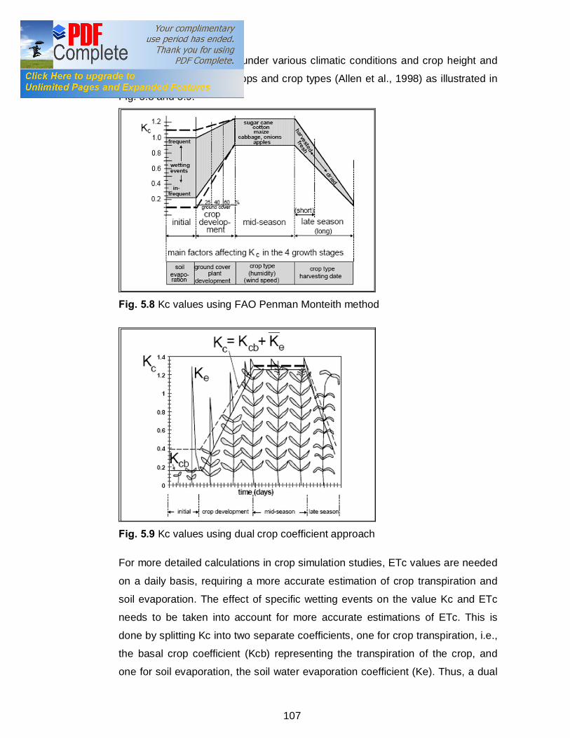
107

arrive at better estimates under various climatic conditions and crop height and

expanding the range of crops and crop types (Allen et al., 1998) as illustrated in

Fig. 5.8 and 5.9.

Fig. 5.8 Kc values using FAO Penman Monteith method

Fig. 5.9 Kc values using dual crop coefficient approach

For more detailed calculations in crop simulation studies, ETc values are needed

on a daily basis, requiring a more accurate estimation of crop transpiration and

soil evaporation. The effect of specific wetting events on the value Kc and ETc

needs to be taken into account for more accurate estimations of ETc. This is

done by splitting Kc into two separate coefficients, one for crop transpiration, i.e.,

the basal crop coefficient (Kcb) representing the transpiration of the crop, and

one for soil evaporation, the soil water evaporation coefficient (Ke). Thus, a dual


108

crop coefficient approach was introduced for ETc as ETc = (Kcb+Ke) ETo. (Allen

et al. 1998)

The dual crop coefficient approach is more complicated and more

computationally intensive than the single crop coefficient approach. The

procedure is conducted on a daily basis and intended for applications using

computers. This approach is recommended to be followed when improved

estimates for Kc are needed, for example to schedule irrigation for individual

fields on a daily basis.

The calculation procedure for ETc using dual crop coefficient approach consists

of:

1. Identifying the lengths of crop growth stages, and selecting the

corresponding Kcb coefficient;

2. Adjusting the selected Kcb coefficients for climatic conditions during the

growth stage;

3. Constructing the basal crop coefficient curve (allowing one to determine

Kcb values for any period during the growing period);

4. Determining daily Ke values for surface evaporation; and

5. Calculating ETc as the product of ETo and (Kcb+Ke).

Standard values of revised Kc and Kcb for crop stages initial, mid–season and

end–season are given in Allen et al. (1998).The concept of dual crop coefficient

is taken into consideration but in a different manner by performing the irrigation

scheduling, wherein the maximum evapotranspiration rate (ETc = ETm) is

obtained by multiplying Kc into ETo, where Kc is considered to be the single crop

coefficient. ETc becomes actual evapotranspiration (ETc = ETa) when there are

stress conditions due to lack of moisture during rainfed farming. Thus when ETc

becomes ETa the Kc value is determined by the ratio of ETa to ETo which is

denoted as Kc–adj. Thus Kc–adj is obtained for all such conditions for

determining the exact values for rainfed farming.


109

5.9.2 Dry Spell Analysis

In mathematics, a Markov chain, named after Andrey Markov, is a discrete–time

stochastic process with the Markov property. The Markov property means the

next state solely depends on the present state and doesn't directly depend on the

previous states. There are n numbers of order for preparing Markov models.

Considering just two categories of dry and wet is called a zero order Markov

chain. A zero order chain is one that has no memory. The fact that yesterday was

dry does not affect the chance of rain (wet) today. First order Markov chain

consists of four categories of days namely ‘dry & dry’, ‘dry & rain’, ‘rain & dry’ and

‘rain & rain’. A first order chain has only one day of memory. If the chain is first

order, then the fact that yesterday was dry may affect (i.e. change the probability)

that today is rainy. However, with a first order chain, the extra information that the

day before yesterday was also dry does not further change the probability of rain

today. With a second order Markov chain the memory extends two days, but no

more. And so on.

The modeling approach consists of two stages of analysis. Stage 1: Preparation,

Stage 2: Fit the model. Stage 1 summaries the data for the model fitting. As

defined by India Meteorological Department, a day with more than 2.5 mm

rainfall has been considered as wet and that with less than 2.5 mm rainfall as

dry. Stage 2 determines the model probabilities. One has to specify the

complexity of the initial model and a previous fitting. Thus the second stage is to

fit the model to produce the fitted probabilities. Fig. 5.10 represents the flow chart

of the modeling process carried out.

The daily rainfall data are analyzed to determine the observed / actual

probabilities. The actual probabilities are determined as

events ofnumber Total observed eventsrain ofNumber =rain ofy Probabilit (5.45)

For example if one has to determine the probability of rain on 15th June for a

period of 45 years of analysis. One has to determine the actual no. of rain events

observed during the 45 years. Say the number of rain events observed are 32

then the actual probability of rain is 32 / 45 i.e. 71 %. The probability of a day

being dry is one minus the probability of rain. 29th February is an exceptional to


110

the above as the total no. of events will not be 45 instead it will be 11 as it occurs

11 times only within the study period of 45 years.

Fig. 5.10 Flowchart of processes carried out in the study

To obtain the optimum order of the Markov chain, Akaike's information criterion

(AIC) and Bayesian’s Information Criterion (BIC) given by Eq. 5.2 and 5.4 for

selecting the optimum model are considered. Further to ensure how much

optimum is the model selected the Akaike weights are determined. After

determining the optimum order of the model, it is used to determine the

probabilities of occurrence of dry spell length from 7 to 14 consecutive days over

a period of 30 days. The probabilities thus obtained will be utilized for crop

planning in the study area.


111

The same modeling approach is applied using 8 mm threshold value. A day with

more than 8 mm rainfall has been considered as wet and that with less than 8

mm rainfall as dry. Rainfall upto 8 mm/day may all lost by evaporation with a dry

soil surface and little or no vegetative cover. (Doorenbos and Pruitt, 1977).

Therefore this 8 mm threshold value is considered in view of agriculture planning.

5.9.3 Climatic Index (CI)

A study to determine the suitability of crops to be grown at suitable periods of the

year based on a proposed “climatic index” considering the availability of water

from rainfall as well as the loss of water through evapotranspiration in the rainfed

area of north Gujarat agroclimatic zone is carried out.

The water requirement of crop should be less than or equal to the water available

from rainfall for a crop to be grown in a particular field. For climatic suitability, the

value of crop coefficient (Kc / Kc–adj) obtained from the above methodology

should therefore be less than the ratio of two climatic factors effective rainfall and

ETo at each stage of crop growth. At a stage of water balance, when the

effective rain and crop evapotranspiration are same, the value of Kc is equal to

the ratio of two climatic factors namely effective rainfall and ETo. This ratio of two

climatic parameters may be termed as climatic index for effective representation

of climatic factors in calculation of water balance.

CI = Pe/ETo (5.46)

Where

Pe = effective rainfall

ETo = reference evapotranspiration

The effective rainfall is determined based on the irrigation scheduling performed

using soil water balance method. The reference evapotranspiration (ETo) is

estimated using FAO Penman Monteith method with help of the FAO CropWat

8.0. The weekly values of climatic factors i.e effective rainfall & ETo and climatic

index for the 36 years are developed.

The monthly values of the climatic index as the ratio of effective rainfall and ETo

are calculated and are analysed to plan for best suited crop and cropping period,

for the values of the crop coefficient Kc should be less than or equal to the values


112

of CI at each stage of crop growth for optimal crop growth. The 80% dependable

value of CI for each month is calculated expecting to have it in 4 out of 5 years.

Kci is a function of wetting interval, evaporating power of the atmosphere and

magnitude of the wetting event during the initial periods and is estimatd from Fig.

5.11 for light to medium (3-10 mm per event) wetting events as suggested by

Allen et al. (1998) in FAO Irrigation and Drainage 56.

Fig. 5.11 Average Kci as related to the level of ETo and the interval between

irrigations and/or significant rain during the initial growth stage for all soil types

when wetting events are light to medium (3-10 mm per event)

Once the monthly CI and Kci are obtained then further weekly values of climatic

index may be determined and analyzed to plan for best suited crop and cropping

period. A CI and Kc curve for all the weeks are drawn out of the average values

of CI and Kci for each week.

5.9.4 Crop Period based on Onset and Cessation of Monsoon

At the surface, monsoon onset is recognized as a rapid substantial and sustained

increase in rainfall. Over India, monsoon onset occurs initially across the south

peninsula in early June, when heavy rains lash south peninsula after the cross–

equatorial low–level jet (LLJ) is established across the Somali coast into the


113

near–equatorial Arabian Sea. This phenomenon is usually accompanied by the

formation of a mid–troposphere shear zone across the Bay of Bengal to the

south–east Arabian Sea in which a cyclonic vortex may be embedded. By middle

of July, monsoon covers the whole country.

Onset criteria

Onset is quantified by the Depth method described by Raes et al. (2004). It

considers a cumulative rainfall depth that will bring the top 0.25 m of the soil

profile to field capacity during a maximum of 4 days. The corresponding

threshold rainfall quantifies the field inspection method by farmers to determine

whether conditions are favorable for wet sowing. This is achieved by digging a

test hole, usually a day after a rain event. The logic is to allow the rain to reach

deeper layers of the soil, forming a recognisable wetting front. The total available

soil water (TAW) during the initial stage for annual crops, for the major soils in

the study area are used to determine the amount of rainfall required to raise the

soil water content from wilting point to field capacity. Since TAW values may vary

from one soil type to another an average TAW is considered. A mean threshold

value of rainfall is obtained by upgrading the TAW values by 20% to take care of

losses by surface runoff, non–uniform wetting, and soil evaporation. Thus the

obtained threshold value of rainfall depth is considered for predicting the onset of

monsoon.

For each station, the date having a probability of at least 20% that the root zone

has adequate soil moisture is regarded as the date after which the onset criteria

apply. The 20% probability level is commonly considered as acceptable when

evaluating rainfed agriculture (Kipkorir et al., 2007). If 40 mm depth of water

rained in one day the amount of runoff would also be more. So a date with only

one day among the 4 days having 40 mm or more rainfall available is not

appropriate in view for crop planning. Therefore a search for onset date with a

condition of rainy days has to be introduced. Thus atleast 2 out of 4 days must be

rainy is applied for searching the onset dates. The date having a probability of at

least 20% that the root zone has adequate soil moisture was regarded as the

date after which the onset criteria apply. The 20% probability level is commonly

considered as acceptable when evaluating rainfed agriculture. (Mugalavai et al.

2008). Starting from the initial search date the onset is taken to be the date on


114

which the criteria is first satisfied or exceeded (Stewart, 1990; Kipkorir et al.,

2004).

Cessation criteria

Cessation is quantified by considering the date on which the water stress in the

root zone of a crop under consideration exceeds a threshold value. For each of

the stations and for each of the 48 years of period that daily rainfall data is

available the soil water content in the root zone is simulated with help of the soil

water balance. The maximum rooting depth for the crop and readily available soil

water (RAW) of 50% of TAW is considered in the study. Water stress is assessed

by means of the water stress coefficient Ks (Allen et al., 1998). As long as a

fraction of RAW remains available in the root zone, there is no water stress and

Ks is 1. When water stress occurs, Ks decreases linearly with the soil water

content and becomes zero when wilting point is reached. The cessation of the

rainy season is assumed when Ks drops below 0.40 within the cessation window.

The cessation is taken to be the date on which the criterion was first satisfied or

exceeded. If in case during the crop period the threshold value is not observed

then the next season crop is considered for the cessation with the same criteria.

Length of growing season

The length of the growing season (days) for a particular year is taken as the

difference between the Julian day numbers of the determined onset date and the

determined cessation date and of that year.

Statistical analysis

Probabilities of exceedance of the onset dates (specified as julian day numbers)

are calculated using the probability distribution function. The 80, 50 and 20%

probabilities of exceedance are determined and used as indicators of early,

normal and late onset respectively.

Overall information regarding the climate type, dry spell length, climatic index and

crop period based on onset and cessation criteria when analysed in correlation

with each other will be useful for the planning of irrigation and agricultural

activities in the area.


115

CHAPTER 6

RESULTS AND ANALYSIS

6.1 GENERAL

north Gujarat agroclimatic zone is fully or partly spread over seven districts

namely Ahmedabad, Banaskantha, Gandhinagar, Kheda, Mehsana, Patan and

Sabarkantha of Gujarat. For the study, 167 raingaguge stations and 5 climate

stations situated in and around the north Gujarat agroclimatic zone are selected,

various studies are carried out and numerous models are developed. The main

objective of the present study is to plan the water resources and irrigation

management based on climate parameters. The results obtained and analysis

carried out during the study of the north Gujarat agroclimatic zone are presented

here.

6.2 MISSING CLIMATE DATA

For determining the nearest input station cluster analysis is applied. Various

combinations of distance measures and linkage rules are evaluated using

Cophen coefficient. Table 6.1 depicts the results obtained. The square

Euclidean–distance measure using average–linkage rule is found to be the best

for forming the clusters as the Cophen coefficient of 0.671 is the highest.

Table 6.1 Cophen Coefficient Value for Various Combinations of Distance

Measures and Linkage Rules. Linkage rule Distance measure

Single Complete Average Weighted Centroid Median Ward

Euclidean 0.457 0.643 0.665 0.634 0.658 0.613 0.618 Square Euclidean 0.486 0.633 0.671 0.619 0.664 0.613 0.628 Mahalanobis 0.498 0.607 0.607 0.642 0.652 0.664 0.597 Cityblock 0.444 0.607 0.669 0.606 0.640 0.531 0.604 Minkowski 0.457 0.643 0.665 0.634 0.658 0.613 0.618 Cosine 0.605 0.576 0.607 0.605 0.607 0.609 0.604 Correlation 0.522 0.574 0.617 0.655 0.079 0.130 0.042 Hamming 0.100 0.100 0.100 0.100 0.000 0.000 0.000 Jaccard 0.100 0.100 0.100 0.100 0.000 0.000 0.000 Chebychev 0.454 0.613 0.655 0.621 0.657 0.646 0.621


116

Clusters are formed using 167 raingauge stations in and around the study area.

The raingauge stations are coded from 1 to 167 numbers. Fig. 6.1 presents a

part of the whole cluster formed for the analysis. The whole cluster is presented

in Plate 2. The input to the raingauge station having missing daily data are

determined using the cluster analysis. For example consider station having code

No. 52 with missing records, in Fig. 6.1. From Fig. 6.1 it is evident that station 52

is nearer to station 62. Therefore for determining missing records of station 52,

the input station selected is the station 62. In many cases it is found that the

immediate nearer station also has the missing records. Then for such cases the

next nearer station is explored for determining complete records. For example

the missing records of station 52 are from 1975 to 1980. As discussed earlier one

selects station 62 as the input station for determining missing records. But it is

found that the station 62 has 1980 year as missing. Then in this case, the next

nearer station 124 is explored and if the station 124 contains 1980 year as

missing then either station 29 or 42 is explored till complete set of missing

records are filled with the data from such nearer stations. The extent of exploring

the outer loops for considering the missing records is limited to 0.5 units of the

distance measure statistics obtained as one needs to analyse nearer stations. It

is observed that the farthest distance within this limit is within 30 km and nearest

is around 4 km. For cases where no such station with all the data is available for

the corresponding set of missing records then two different models are

developed for different years. For example based on the previous illustration

when one finds that station 62 contains 1980 year missing then the model for

determining the missing records for the year 1975 to 1979 is developed and for

1980 separate input station i.e. station 124 is used. Thus for determining the

missing records of one station two separate models based on the availability of

input station are developed. In the present study the total number of raingauge

stations containing missing daily data is 47. The total numbers of models

developed are 68.


117

Fig. 6.1 Part of dendrogram of 167 raingauge stations of north Gujarat region

While considering ANN method different neural networks are explored for

determining the best network. It is found that for competitive neural network the

output for any input data is either one or zero. For cascade back propogation,

elman back propogation, feed–forward backpropagation, feed–forward input–

delay backpropagation etc., the network output yields one random constant value

for all the inputs. Hopfield recurrent, linear layer, perceptron and probabilistic

neural networks are found infeasible to the present input data. Generalized

regression neural network (GRNN) and radial basis network yield some realistic

results. Amongst the two the radial basis network does not give any value for

input of three digits while the generalized regression performs well. Thus

generalized regression network is used for ANN models amongst the different

types of ANN networks studied. The network architecture of one of the model out

of the 68 different GRNNs created is presented in Fig. 6.2. The input varies

according to the data availability but is equal to or greater than 3,535 (70% of the

total number of sample) number for model preparation.


118

Fig. 6.2 Network architecture of generalized regression neural network for one of

the model out of 68

Table 6.2 presents the frequency distribution for Bias score. In case of Bias

values for model preparation data, it is observed that out of 68 models prepared

by the ANN method, 45 are in the range of 0.81 to 1.19. Out of these 45, 14 are

in the range of 0.81 to 0.98 i.e. these are underforecasting, 27 are in the range of

1.02 to 1.19 i.e. these are overforecasting. In the range of 0.99 to 1.01 there are

4 models which are more or less perfect. Similarly, in case of models prepared

by the closest station method, 52 are in the range of 0.81 to 1.19. Out of these

52, 23 are underforecasting and 27 are overforecasting. 2 models are more or

less perfect i.e between 0.99 to 1.01 range. In case of models prepared by the

non linear regression method, 35 are in the range of 0.81 to 1.19. Out of these,

13 are underforecasting and 19 are overforecasting. 3 models are more or less

perfect. If one can see the models in the range of 0.96 to 1.04 then there are 6, 5

and 8 models prepared by the ANN, closest station and non linear regression

methods respectively.


119

Table 6.2 Bias Score for ANN, CS and NLR Methods for Model Preparation and

Validation Frequency

class Frequency

ANN Closest station (CS) Non linear regression (NLR) Preparation Validation Preparation Validation Preparation Validation

0.01-0.20 0 0 0 0 0 0 0.21-0.40 0 0 0 0 0 0 0.41-0.60 0 1 0 1 0 2 0.61-0.80 0 4 1 5 2 3 0.81-0.98 14 14 23 20 13 13 0.99-1.01 4 7 2 2 3 2 1.02-1.19 27 11 27 19 19 10 1.21-1.40 15 18 8 13 18 17 1.41-1.60 6 9 5 3 5 7 1.61-1.80 1 3 1 4 3 6 1.81-2.00 1 0 0 0 1 2 2.01-2.20 0 0 1 1 2 1 2.21-2.40 0 0 0 0 0 1 2.41-2.60 0 1 0 0 0 0

Total 68 68 68 68 66 66

In case of Bias values for model validation data, it is observed that out of 68

models prepared by the ANN method and tested for Bias, 32 are in the range of

0.81 to 1.19. Out of these 32, 14 are in the range of 0.81 to 0.98 and are

underforecasting, 11 are in the range of 1.02 to 1.19 and are overforecasting. In

the range of 0.99 to 1.01 there are 7 models which are more or less perfect.

Similarly, in case of models prepared by the closest station method and tested

for Bias, 41 are in the range of 0.81 to 1.19. Out of these 41, 20 are

underforecasting and 19 are overforecasting. 2 models are more or less perfect.

In case of models prepared by the non linear regression method and tested for

Bias, 25 are in the range of 0.81 to 1.19. Out of these, 13 are underforecasting

and 10 are overforecasting. 2 models are more or less perfect. If one can see the

models in the range of 0.96 to 1.04 then there are 11, 4 and 6 models prepared

by the ANN, closest station and non linear regression methods respectively.

Thus looking to the maximum number of models in the range nearer to 1, it can

be said that the ANN method is the best method for forecasting and validating

the models on the basis of Bias.

Fig. 6.3 shows the box plot for the Bias scores obtained during the model

preparation and validation. For all the further boxplot figures ANN, CS and NLR

denotes the Artificial Neural Network, the closest station and the non linear

regression methods respectively and the alphabets M and V denote model

preparation data and validation data respectively. Thus ANN_M presents the plot


120

of ANN method using model preparation data and ANN_V presents the plot of

ANN method using model validation data. The box plot indicates the minimum,

the maximum, the 25th, 50th (median) and the 75th percentile data values. The

interquartile range is the difference between the 25th and the 75th percentile

values. From the Fig. 6.3 it is clear that the range of data points is the largest in

case of non linear regression method using model validation data indicating more

variation. The range of data points is the smallest in case of closest station

method using model preparation data indicating less variation. But there are

more outliers (data points having values greater that one third of the interquartile

range) in case of the closest station and the non linear regression methods

compared to the ANN method for both the model preparation and model

validation dataset.

Fig. 6.3 Box plot of the bias score for model preparation and validation

Table 6.3 and Table 6.4 represent the POD, FAR, ETS and HK scores for model

preparation and model validation data respectively. For the POD score greater

than 0.70 the ANN method has frequency of 31 and 30 for model preparation and

model validation data respectively, as compared to the closest station and the

non linear regression methods having frequency of 22 and 26 respectively for

model preparation data and 16 and 33 for model validation data respectively. The

frequency of the ANN method is higher than that of the closest station and the

non linear regression methods for preparation of the models and is just less than

3 compared to non linear regression and greater than 4 for closest station for


121

validating the models. Therefore it can be said that the ANN method, is the best

for model preparation and validation on the basis of POD.

Table 6.3 Frequency Distribution for POD, FAR, ETS and HK Scores for Model

Preparation Frequency

classes Frequency

POD FAR ETS HK ANN CS NLR ANN CS NLR ANN CS NLR ANN CS NLR

0.01 - 0.05 0 0 0 0 0 0 0 0 0 0 0 0 0.06 - 0.10 0 0 0 1 0 0 0 0 5 0 0 3 0.11 - 0.15 0 0 0 0 0 0 0 0 0 0 0 1 0.16 - 0.20 0 0 0 1 1 0 0 0 1 0 0 1 0.21 - 0.25 0 0 4 1 2 4 3 5 5 0 0 0 0.26 - 0.30 0 0 0 6 6 5 6 4 8 0 0 1 0.31 - 0.35 0 0 1 8 10 1 11 14 20 0 0 0 0.36 - 0.40 0 0 1 11 11 9 29 27 15 1 3 2 0.41 - 0.45 1 1 0 16 15 16 7 8 2 4 4 3 0.46 - 0.50 2 3 2 15 14 6 4 2 3 4 8 7 0.51 - 0.55 1 4 3 6 7 10 2 3 2 17 16 15 0.56 - 0.60 6 13 6 2 1 7 5 5 5 11 15 16 0.61 - 0.65 18 14 10 0 0 2 0 0 0 18 12 8 0.66 - 0.70 9 11 23 1 1 1 0 0 0 7 5 4 0.71 - 0.75 20 12 7 0 0 4 0 0 0 4 4 3 0.76 - 0.80 8 8 4 0 0 1 0 0 0 1 1 2 0.81 - 0.85 2 2 5 0 0 0 0 0 0 0 0 0 0.86 - 0.90 0 0 0 0 0 0 0 0 0 0 0 0 0.91 - 0.95 0 0 0 0 0 0 1 0 0 0 0 0 0.96 – 1.00 1 0 0 0 0 0 0 0 0 1 0 0

Total 68 68 66 68 68 66 68 68 66 68 68 66

For FAR values less than or equal to 0.3 the ANN, closest station and non linear

regression methods give the frequency of 9 each for preparing the models and

14, 18 & 12 while validating the models respectively. It is observed that in case of

model preparation all the methods have same frequency but in case of validation

of models, the closest station method has the highest frequency.

The values of ETS and HK also indicate the effectiveness of the ANN method by

having maximum frequency for best values. The ANN, closest station and non

linear regression methods have the frequency of 1, 0 and 0 respectively with

respect to greater than 0.7 value of ETS while preparing and frequency of 2, 1

and 1 respectively while validating the model. For HK 70% data give 6, 5 and 5

frequency for values greater than 0.7 in case of the ANN, closest station and non

linear regression methods respectively. When the results for 30% data are

obtained it is observed that the frequency for the same is 8, 8 and 7 for the ANN,

closest station and non linear regression methods respectively. Thus it can be


122

said that ANN method is the best for model preparation and validation on the

basis of ETS and HK scores.

Table 6.4 Frequency Distribution for POD, FAR, ETS and HK Scores for Model

Validation Frequency

classes Frequency

POD FAR ETS HK ANN CS NLR ANN CS NLR ANN CS NLR ANN CS NLR

0.01 - 0.05 0 0 0 1 0 0 1 0 8 1 0 7 0.06 - 0.10 0 0 3 0 0 0 0 0 0 0 0 1 0.11 - 0.15 0 0 2 0 0 0 0 0 0 0 0 0 0.16 - 0.20 1 0 2 1 2 3 0 1 1 0 0 0 0.21 - 0.25 0 0 1 5 8 4 4 1 1 0 0 0 0.26 - 0.30 0 0 0 7 8 5 13 11 8 0 0 0 0.31 - 0.35 0 0 0 7 6 7 10 15 10 1 1 1 0.36 - 0.40 0 1 0 9 12 8 16 12 14 3 3 3 0.41 - 0.45 2 1 2 8 7 5 7 12 9 6 5 1 0.46 - 0.50 4 5 2 17 12 9 10 8 9 7 9 2 0.51 - 0.55 6 5 1 5 6 11 3 4 3 7 5 7 0.56 - 0.60 6 9 5 5 6 3 1 1 1 10 18 5 0.61 - 0.65 11 7 5 1 0 2 0 1 0 17 14 17 0.66 - 0.70 8 14 10 1 1 0 1 1 1 8 5 15 0.71 - 0.75 16 17 7 0 0 1 1 1 1 3 4 3 0.76 - 0.80 7 4 13 0 0 1 0 0 0 2 1 1 0.81 - 0.85 3 2 9 0 0 3 0 0 0 1 2 2 0.86 - 0.90 2 2 3 1 0 1 0 0 0 1 1 1 0.91 - 0.95 1 1 1 0 0 2 0 0 0 0 0 0 0.96 - 1.00 1 0 0 0 0 1 1 0 0 1 0 0

Total 68 68 66 68 68 66 68 68 66 68 68 66

Fig. 6.4 shows the box plot of the POD, FAR, ETS and HK scores. For all the

parameters the non linear regression method has the largest range of data set

hence there is more variation in the parameters obtained. Therefore non linear

regression is not preferred for filling in missing records due to the greater

variability of the forecast verification parameters. From the point of view of the

box plot either ANN or closest station is suitable when considering forecast and

verification parameters.


123

Fig. 6.4 Box plot for POD, FAR, ETS and HK scores for model preparation and

validation

Tables 6.5 and 6.6 presents the RMSE and MAE values for model preparation

and model validation data. The RMSE value for ANN method obtained is the

lowest upto 20 mm, compared to the CS and NLR method. The NLR method

gives the highest RMSE value in the range of 81 to 85 mm. The MAE obtained is

the least for ANN method. All the models, except one in case for model

preparation and ten in case for model validation, are having MAE values less

than equal to 5 mm. As the ANN method yields less error for both the RMSE and

MAE, it is the best.


124

Table 6.5 Frequency Distribution for RMSE for Model Preparation and Validation Frequency

class, mm

Frequency ANN CS NLR

Preparation Validation Preparation Validation Preparation Validation 01-05 0 0 0 0 0 0 06-10 17 8 4 9 3 4 11-15 47 31 24 22 6 7 16-20 4 25 36 33 8 6 21-25 0 3 4 4 13 5 26-30 0 1 0 0 5 13 31-35 0 0 0 0 8 6 36-40 0 0 0 0 9 3 41-45 0 0 0 0 3 6 46-50 0 0 0 0 1 6 51-55 0 0 0 0 2 3 56-60 0 0 0 0 3 2 61-65 0 0 0 0 1 2 66-70 0 0 0 0 1 1 71-75 0 0 0 0 2 0 76-80 0 0 0 0 0 0 81-85 0 0 0 0 0 1 Total 68 68 68 68 66 66

Table 6.6 Frequency Distribution for MAE for Model Preparation and Validation Frequency

class, mm

Frequency ANN CS NLR

Preparation Validation Preparation Validation Preparation Validation 01-05 67 58 54 49 14 14 06-10 1 10 14 19 29 29 11-15 0 0 0 0 16 13 16-20 0 0 0 0 6 7 21-25 0 0 0 0 1 2 26-30 0 0 0 0 0 1 Total 68 68 68 68 66 66

From Fig. 6.5 one can observe that the data range and the interquartile range for

ANN method is the smallest when preparing model while it is the largest for non

linear regression method while validating the model for both the RMSE and MAE

scores. Thus it is clear from the box plots that ANN method is best suited for the

present dataset.

Fig. 6.5 Box plot for RMSE and MAE scores for model preparation and validation

data.


125

Table 6.7 depicts the summary of 68 best models selected considering the AIC

and BIC, alongwith the other conditional / categorical statistics as discussed

earlier, for both model preparation and validation. From the Table 6.7 one can

say that 66 models out of 68 have ANN method as the best. 2 models out of 68

have closest station method as the best while no model shows non linear

regression as the best method for the model preparation. In case for model

validation, 39 models show ANN, 26 models show closest station and 3 models

show non linear regression method as the best.

Table 6.7 Results for the Models Developed Using the ANN, Closest Station and

Non Linear Regression Methods

Model preparation data

Model validation data Total ANN Closest

station Non linear regression

ANN 39 24 03 66 Closest station 00 02 0 02 Non linear regression 00 00 0 0 Total 39 26 03 68

In a nutshell, it can be concluded that the ANN method is the best to fill in the

missing daily rainfall data.

6.3 PROBABILITY DISTRIBUTION

The statistical measures of the dataset for one and consecutive 2 to 7 & 10 days

maximum rainfall i.e. mean, minimum, maximum, range, etc. are calculated for

the 48 years (1961 to 2008) and the results are presented in the Fig.s 6.6 to

6.13.

From the Fig.s 6.6 to 6.13 it is observed that Visnagar raingauge station received

the highest maximum, one day to consecutive 2 to 7 & 10 days maximum rainfall

(indicated by green line in Figs. 6.6 to 6.13). The maximum value of one day to

consecutive 2 to 7 & 10 days rainfall observed are 834 mm (25th June 1997),

1,042 mm, 1,166 mm, 1,180 mm, 1,187 mm, 1,193 mm, 1,193 mm and 1,193

mm respectively. This maximum values observed for 73 raingauge stations are

observed for the same 1997 year. But for other raingauge stations the storm

years are different. For 73 raingauge stations the maximum value plot shows

many fluctuations.


126

Fig. 6.6 One day maximum rainfall range, minimum, maximum, mean and standard deviation for raingauge stations in north Gujarat agroclimatic zone


127

Fig. 6.7 Consecutive 2 days maximum rainfall range, minimum, maximum, mean and standard deviation for raingauge stations in north Gujarat agroclimatic zone


128



129



130



131



132



133



134

If one superimposes the maximum value line (indicated by green colour in

Figs. 6.6 to 6.13), the pattern differs from one to 2 and 2 to 3 but remains

almost constant for 3 to 7 days for a given raingauge station. Thus one can

say in general that the storms affecting the total rainfall value are observed for

one to consecutive 2 and 3 days. For consecutive 4 to 7 days the

accumulated rainfall value increases but with less impact on the total amount

which does not affect the maximum rainfall pattern line. For consecutive 10

days the accumulated rainfall value shows considerable increase in the total

amount of rainfall obtained. Fig. 6.14 shows the plot of one day and

consecutive 2 to 7 & 10 days maximum rainfall for Visnagar raingauge station.

The linear trend line (indicated by black line in Fig. 6.14) shows increasing

trend for one day and consecutive 2 to 7 & 10 days maximum rainfall.

Fig. 6.14 One day to consecutive 2 to 7 & 10 days maximum rainfall for

Visnagar raingauge station.

If one observes the minimum values (indicated by yellow line in Figs. 6.6 to

6.13), Dhanera raingauge station show the lowest value of 7 mm (29th June

1987) each for maximum one day to consecutive 2 to 7 & 10 days. The


135

fluctuation for minimum value is less compared to the maximum value. Fig.

6.15 shows the plot of one day and consecutive 2 to 7 & 10 days maximum

rainfall for Dhanera raingauge station.

Fig. 6.15 One day to consecutive 2 to 7 & 10 days maximum rainfall for

Dhanera raingauge station.

The highest mean value (indicated by black line in Figs. 6.6 to 6.13) of one

day and consecutive 2 to 7 & 10 days maximum rainfall is obtained for

Vaghroli tank with 153 mm, 200 mm, 233 mm, 255 mm, 270 mm, 285 mm,

304 mm and 359 mm respectively. Lowest mean value of 93 mm and 124 mm

for one day and consecutive 2 days rainfall respectively, is observed at Sanali

Ashram. At Panthawada the lowest mean value observed for consecutive 3,

4, 5, 6 & 7 days maximum rainfall are 140 mm, 150 mm, 157 mm, 166 mm

and 176 mm respectively. At Unjha the same for consecutive 10 days

maximum rainfall of 190 mm is observed. The standard deviation varies from

45.07 mm at Vijaynagar raingauge station to 221.02 mm at Visnagar

considering all the raingauge stations for all 584 (= 73 x 8) datasets. The

mean and standard deviation lines show less fluctuation.


136

Thus this extreme event needs to be studied for proper planning of the water

resources systems in and around the region consisting of diverse rainfall

pattern. Tables 6.8 and 6.9 present the results obtained by determining best

probability function for one of the raingauge station, Aslali situated in

Ahmedabad district. Similar results are obtained for other 72 raingauge

stations, and presented in Tables 6.10 to 6.153 and are provided in the CD.

Table 6.8 AIC for Aslali Raingauge Station, Ahmedabad District Name of probability distribution 1D C2D C3D C4D C5D C6D C7D C10D Birnbaum–Saunders 525 553 568 576 582 588 594 612 Exponential 554 584 598 607 613 617 622 636 Extreme value 571 594 598 601 605 614 621 633 Gamma 527 555 567 574 580 586 592 609 Generalized extreme value 527 556 570 577 583 589 594 612 Generalized Pareto 549 576 574 578 584 591 598 614 Inverse Gaussian 437 465 480 488 494 500 506 525 Log–Logistic 525 555 569 577 582 588 594 612 Logistic 539 566 576 583 588 595 601 618 Lognormal 525 553 568 576 581 587 593 611 Nakagami 533 559 570 576 582 588 594 609 Normal 545 570 578 583 589 596 602 617 Rayleigh 531 557 568 575 580 586 592 608 Rician 533 559 570 577 582 588 594 610 t location–scale 536 567 578 585 591 597 603 619 Weibull 532 559 570 576 582 588 594 610

Table 6.9 BIC for Aslali Raingauge Station, Ahmedabad District Name of probability distribution 1D C2D C3D C4D C5D C6D C7D C10D Birnbaum–Saunders 529 557 572 579 585 591 597 616 Exponential 556 586 599 608 615 619 623 638 Extreme value 575 597 601 605 609 617 625 637 Gamma 531 559 571 578 584 590 595 613 Generalized extreme value 533 562 576 583 588 594 600 617 Generalized Pareto 555 582 580 584 590 597 604 620 Inverse Gaussian 441 469 484 491 498 504 510 528 Log–Logistic 529 559 573 580 586 592 597 616 Logistic 543 570 580 587 592 599 604 621 Lognormal 529 557 572 579 585 591 597 615 Nakagami 536 563 573 580 585 592 597 613 Normal 549 574 582 587 592 600 606 620 Rayleigh 533 559 570 576 582 588 594 609 Rician 537 563 574 580 586 592 598 613 t location–scale 542 572 584 591 596 603 608 624 Weibull 536 563 574 580 586 592 598 613

Note: 1D–One day; C2D–Consecutive 2 days; C3D–Consecutive 3 days; C4D–Consecutive 4 days; C5D–Consecutive 5 days; C6D–Consecutive 6 days; C7D–Consecutive 7 days; C10D– Consecutive 10 days


137

Based on AIC and BIC values presented in Table 6.8 to 6.153, one can say

that Inverse Gaussian is the best fitted distribution for all the stations for one

day and consecutive 2 to7 & 10 days maximum rainfall. The probability

density function (pdf) for the fitted distribution is

(6.1)

Where

μ (mu) = scale parameter; µ>0 is the mean of the distribution

λ (lambda) = shape parameter

It is observed that the second ranking probability distributions differ when

comparing AIC and BIC. According to AIC ranking, Birnbaum–Saunders for

176 (30.1 %) datasets, Rayleigh for 110 (18.8 %) datasets, Log Logistic for 98

(16.8 %) dataset, Lognormal for 54 (9.2 %) dataset, Generalized Extreme for

17 (2.9 %), Generalized Pareto for 32 (9.2 %), Gamma for 88 (15.1 %),

Nakagami for 3 (0.5%) and Weibull, Logistic and Exponential for 2 (0.3 %)

each, are at second position, out of 584 dataset.

According to BIC ranking, Rayleigh for 206 (35 %) datasets, Birnbaum–

Saunders for 168 (29 %) dataset, Log Logistic for 94 (16 %) dataset,

Lognormal for 53 (9 %) dataset and Generalized Pareto for 15 (3 %), Gamma

for 37 (6 %) dataset, Generalized Extreme for 7 (1 %) dataset, Logistic for 2

(0.3 %) dataset and Weibull and Exponential for 1 (0.2 %) dataset, are at

second position out of 584 dataset.

Though these distributions are second ranked the difference between the AIC

and BIC values of the best distribution i.e. inverse Gaussian and the second

best distribution is very large in the range of 69–193 units. While the

difference between the second best distribution and distributions ranking third

to sixteen are in the range of 1–29. Thus the first best distribution is

considered for further analysis.

Extreme value and exponential probability distributions are commonly used

for hydrological analysis by many practicing researchers and hydrologists. It is


138

observed that extreme value probability distribution ranked 16th (i.e. last)

among the 16 distributions in 357 (61.1 %) datasets out of 584 datasets and

exponential distribution ranked 16th for 223 (38.2 %) cases while for rest 4

(0.7 %) cases Birnbaum–Saunders ranked 16th based on AIC values. Based

on BIC values it is observed that extreme value probability distribution ranked

16th (i.e. last) among the 16 distributions in 213 (36.5 %) datasets, exponential

distribution ranked 16th for 366 (62.7 %) cases and Birnbaum–Saunders

ranked 16th for rest of the 5 (0.9 %) cases out of 584 datasets. Figs. 6.16 and

6.17 represents the first ranked and sixteen ranked probability distribution

respectively to the dataset for Aslali raingauge station.

Fig. 6.16 First and sixteenth ranked probability distribution to the one day and

consecutive 2 to 4 days maximum rainfall series of Aslali raingauge station


139

Fig. 6.17 First and sixteenth ranked probability distribution to the consecutive

5 to 7 and 10 days maximum rainfall series of Aslali raingauge station

Each station has eight dataset (one day and consecutive 2 to 7 &10 days

maximum rainfall). Thus 584 different datasets have been analyzed for 73

raingauge stations. One can say that though there are different datasets for

different raingauge stations the best fitted distribution at the first place is

unique (i.e. Inverse Gaussian) according to both AIC and BIC. For the same

distribution, there are varying populations described by the 584 different

datasets having different values of the distribution parameters, µ and λ

presented in Figs 6.18 to 6.31. The value of µ ranges from 92.88 to 358.09 for

the raingauge stations in the study area while that for λ ranges from 108.50 to

1647.06. From Figs. 6.18 to 6.31 one can observe that the plots for µ values

for the districts are parallel to each other while those for λ are varying and

lines are intersecting each other. A shape parameter affects the shape of a

distribution rather than simply shifting it (as a location parameter does) or

stretching/shrinking it (as a scale parameter does). Therefore the intersecting

lines for λ indicate the varying shapes in the population of the rainfall data of

the region indicating no uniform pattern.


140

Fig. 6.18 Mean µ for one day and consecutive 2 to 7 & 10 days for raingauge

stations situated in Ahmedabad district

Fig. 6.19 Shape parameter, λ for one day and consecutive 2 to 7 & 10 days

for raingauge stations situated in Ahmedabad district


141


stations situated in Banaskantha district


for raingauge stations situated in Banaskantha district


142


stations situated in Gandhinagar district


for raingauge stations situated in Gandhinagar district


143


stations situated in Kheda district


for raingauge stations situated in Kheda district


144

Fig. 6.26 Mean, µ for one day and consecutive 2 to 7 & 10 days for raingauge

stations situated in Mehsana district


for raingauge stations situated in Mehsana district


145


stations situated in Patan district


for raingauge stations situated in Patan district


146


stations situated in Sabarkantha district


for raingauge stations situated in Sabarkantha district


147

Fig. 6.32 Rainfall depth–duration–return period relations for Aslali, Bareja,

Barejadi, Chandola, Dehgam, Nal Lake, Sanand and Wasai raingauge

stations in Ahmedabad district


148

Bhakar et al. (2006a) recommended that 2–100 yea is a sufficient return

period for soil and water conservation measures, construction of dams,

irrigation and drainage works. The rainfall depth–duration–return periods for

all the 73 raingaguge stations are presented from Figs. 6.32 to 6.424.

Based on the best fit probability distribution for the raingauge stations situated

in Ahmedabad district the maximum rainfall of 88 mm, 118 mm, 134 mm, 146

mm, 153 mm, 161 mm, 167 mm and 188 mm is expected to occur every two

years for one day and consecutive 2 to 7 & 10 days respectively at Nal Lake

raingauge station. It is observed that this rainfall depth is the lowest amongst

the eight raingauge stations in the Ahmedabad district. The highest maximum

rainfall of 115 mm, 201 mm, 212 mm, 223 mm, 234 mm and 275 mm is

expected to occur every two years for one day & consecutive 4, 5, 6, 7 & 10

days respectively at Barejadi raingauge station. The highest maximum rainfall

of 158 mm and 177 mm is expected to occur every two years for consecutive

2 and 3 days respectively at wasai raingauge station.

The maximum rainfall of 339 mm, 474 mm, 520 mm, 594 mm, 612 mm, 625

mm, 653 mm and 797 mm is expected to occur every 100 years for one day

and consecutive 2 to 7 & 10 days respectively at Sanand, Aslali, Barejadi,

Aslali, Barejadi, Dehgam, Dehgam and Barejadi raingauge stations. It is

observed that these rainfall depths are the lowest in the Ahmedabad district.

The highest maximum rainfall of 438 mm, 583 mm, 691 mm and 755 mm are

expected to occur every 100 years for one day & consecutive 2, 3 & 4 days

respectively at Chandola raingauge station. The highest maximum rainfall of

770 mm, 834 mm, 884 mm and 1,048 mm are expected to occur every 100

years for consecutive 5, 6, 7 and 10 days respectively at Bareja raingauge

station.


149

Fig 6.33 Rainfall depth–duration–return period relations for Ambaji, Amirgadh,

Bapla, Chandisar, Chitrasani and Danta raingauge stations in Banaskantha

district


150

Fig 6.34 Rainfall depth–duration–return period relations for Dantiwada,

Deesa, Dhanera, Gadh, Hadad and Junisarotri raingauge stations in

Banaskantha district


151

Fig 6.35 Rainfall depth–duration–return period relations for Nava, Palanpur,

Panthawada, Sanali Ashram and Wadgam raingauge stations in Banaskantha

district

For Banaskantha district the maximum rainfall of 69 mm and 91 mm is

expected to occur every two years for one day and consecutive 2 days

respectively at Nava raingauge station while 105 mm, 111 mm, 116 mm, 121

mm, 125 mm and 136 mm is expected to occur every two years for one day


152

and consecutive 3 to 7 & 10 days respectively at Dhanera raingauge station. It

is observed that this rainfall depth is the lowest amongst the seventeen

raingauge stations in the Banaskantha district. The highest maximum rainfall

of 103 mm, 135 mm, 159 mm, 177 mm, 189 mm, 199 mm, 214 mm and 251

mm is expected to occur every two years for one day & consecutive 2 to 7 &

10 days respectively at Danta raingauge station.



and consecutive 2 to 7 & 10 days respectively at Sanali Ashram raingauge

station. It is observed that this rainfall depth is the lowest amongst the

seventeen raingauge stations in the Banaskantha district. The highest

maximum rainfall of 534 mm is expected to occur every 100 years for one day

at Ambaji raingauge station. The highest maximum rainfall of 682 mm, 775

mm, 851 mm, 911 mm, 964 mm, 998 mm and 1,220 mm is expected to occur

every 100 years for consecutive 2 to 7 & 10 days respectively at Chitrasani

raingauge station.

Fig 6.36 Rainfall depth–duration–return period relations for Mansa and Raipur

Weir raingauge stations in Gandhinagar district

For Gandhinagar district the maximum rainfall of 112 mm, 150, 175 mm, 194

mm, 209 mm, 218 mm, 227 mm and 254 mm is expected to occur every two

years for one day and consecutive 2 to 7 & 10 days respectively at Mansa

raingauge station. It is observed that this rainfall depth is the lowest amongst

the two raingauge stations in the Gandhinagar district. The highest maximum


153

rainfall of 115 mm, 154 mm, 180 mm, 201 mm, 212 mm, 223 mm, 234 mm

and 275 mm is expected to occur every two years for one day & consecutive

2 to 7 & 10 days respectively at Raipur weir raingauge station.

The maximum rainfall of 329 mm, 479 mm and 579 mm is expected to occur

every 100 years for one day and consecutive 2 & 3 days respectively at

Mansa raingauge station. The maximum rainfall of 597 mm, 612 mm, 643

mm, 675 mm and 797 mm is expected to occur every 100 years for

consecutive 4 to 7 & 10 days respectively at Raipur weir raingauge station.

These rainfall depths are the lowest amongst the two available raingauge

stations in the Gandhinagar district. The highest maximum rainfall of 385 mm,

583 mm and 584 mm is expected to occur every 100 years for one day and

consecutive 2 & 3 days respectively at Raipur weir raingauge station. The

highest maximum rainfall of 634 mm, 677 mm, 698 mm, 721 mm and 864 mm

is expected to occur every 100 years for consecutive 4 to 7 & 10 days

respectively at Mansa station.


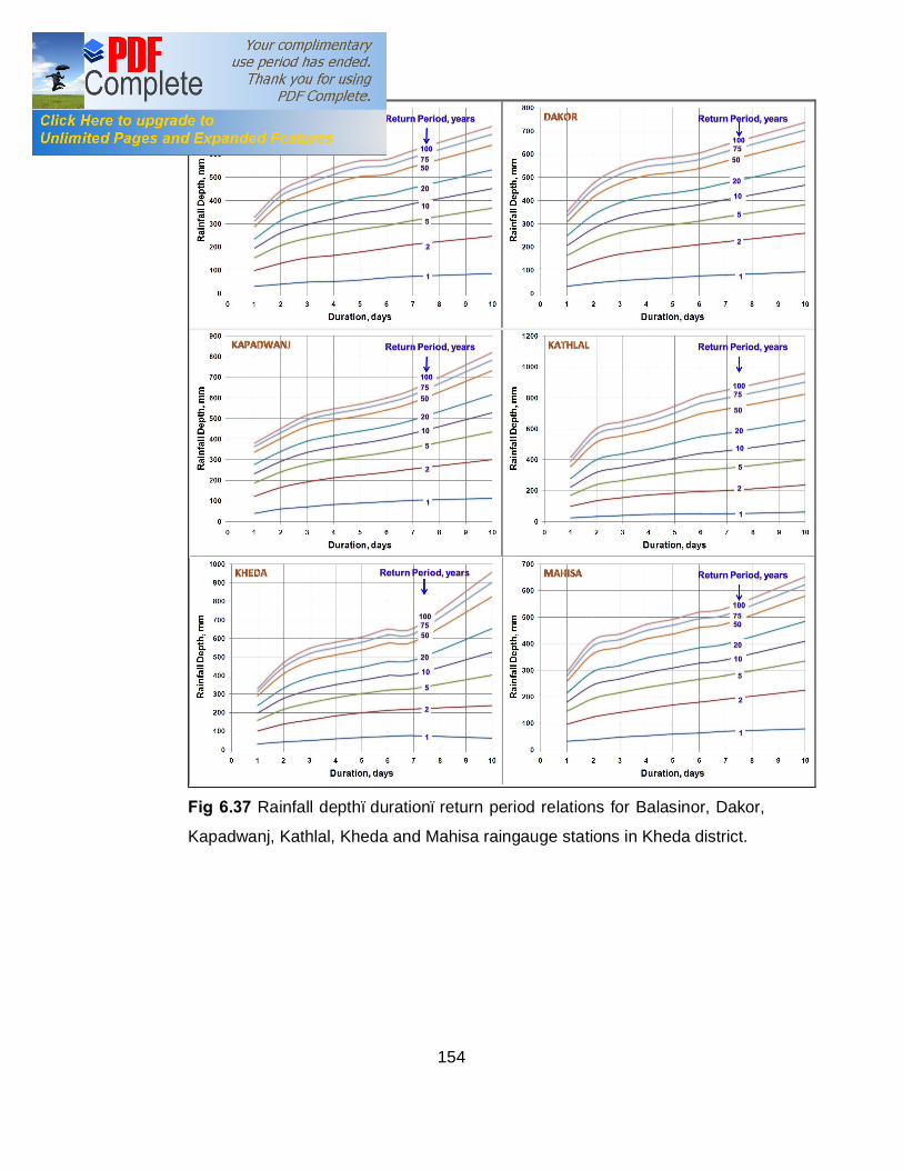
154

Fig 6.37 Rainfall depth–duration–return period relations for Balasinor, Dakor,

Kapadwanj, Kathlal, Kheda and Mahisa raingauge stations in Kheda district.


155

Fig 6.38 Rainfall depth–duration–return period relations for Mahemadabad,

Nadiad, Pinglaj, Savli Tank, Vadol and Vaghroli Tank raingauge stations in

Kheda district

For the raingauge stations situated in Kheda district the maximum rainfall of

97 mm, 125, 142 mm, 156 mm, 170 mm, 180 mm, 192 mm and 226 mm is

expected to occur every two years for one day and consecutive 2 to 7 & 10

days respectively at Mahisa raingauge station. It is observed that this rainfall

depth is the lowest amongst the twelve raingauge stations in the Kheda


156

district. The highest maximum rainfall of 144 mm, 193 mm, 217 mm, 238 mm,

253 mm, 266 mm, 280 mm and 328 mm is expected to occur every two years

for one day & consecutive 2 to 7 & 10 days respectively at Mahemadabad

raingauge station.


mm and 654 mm is expected to occur every 100 years for one day and

consecutive 3 to 7 & 10 days respectively at Mahisa raingauge station. The

maximum rainfall of 404 mm is expected to occur every 100 years for

consecutive 2 days at Savali tank raingauge station. These rainfall depths are

the lowest amongst the twelve available raingauge stations in the Kheda

district. The highest maximum rainfall of 451 mm, 619 mm, 677 mm, 715 mm,

757 mm, 824 mm, 852 mm and 976 mm is expected to occur every 100 years

for one day and consecutive 2 to 7 & 10 days respectively at Nadiad

raingauge station.


157

Fig 6.39 Rainfall depth–duration–return period relations for Ambaliyasan,

Dharoi, Kadi, Kalol, Katosan and Kheralu raingauge stations in Mehsana

district


158

Fig 6.40 Rainfall depth–duration–return period relations for Mehsana,

Ransipur, Thol, Unjha, Vijapur and Visnagar raingauge stations in Mehsana

district


mm, 171 mm and 195 mm is expected to occur every two years for one day

and consecutive 2 to 7 & 10 days respectively at Mehsana raingauge station.

It is observed that this rainfall depth is the lowest amongst the eleven

raingauge stations in the Mehsana district. The highest maximum rainfall of


159

115 mm, 216mm and 226 mm is expected to occur every two years for one

day & consecutive 6 and 7 days respectively at Visnagar raingauge station.

The highest maximum rainfall of 150 mm, 173 mm and 190 mm is expected to

occur every two years for consecutive 2, 3 and 4 days respectively at Kadi

raingauge station every two year. The highest maximum rainfall of 205 mm is

expected to occur consecutive 5 days at Kalol raingauge station and 261 mm

is expected to occur every two years for consecutive 10 days at Dharoi

raingauge station.

For a recurrence interval of 100 years, the lowest maximum rainfall expected

in one day and consecutive 2 to 7 & 10 days are 325 mm, 481 mm, 543 mm,

591 mm, 577 mm, 594 mm, 623 mm and 677 mm respectively at Dharoi,

Ambaliyasan, Thol, Thol, Ambaliyasan, Ambaliyasan, Kadi and Kadi

raingauge stations respectively. It is observed that this rainfall depth is the

lowest amongst the eleven raingauge stations. The highest maximum rainfall

of 580 mm, 768 mm, 851 mm, 894 mm, 951 mm, 903 mm, 931 mm and 1,063

mm is expected to occur at interval of 100 years for one day and consecutive

2 to 7 & 10 days respectively at Vijapur raingauge station.

For the raingauge stations situated in Patan district the maximum rainfall of 82

mm, 106, 118 mm, 130 mm, 139 mm, 147 mm, 154 mm and 172 mm is


days respectively at Patan raingauge station. It is observed that this rainfall

depth is the lowest amongst the three raingauge stations in the Patan district.

The highest maximum rainfall of 85 mm, 115 mm, 132 mm, 145 mm, 157 mm,

167 mm, 177 mm and 200 mm is expected to occur every two years for one

day & consecutive 2 to 7 & 10 days respectively at Sidhpur raingauge station.



and consecutive 2 to 7 & 10 days respectively at Patan raingauge station.

These rainfall depths are the lowest amongst the three available raingauge

stations in the Patan district. The highest maximum rainfall of 487 mm, 726

mm, 847 mm, 868 mm, 886 mm, 900 mm, 954 mm and 1178 mm is expected


160

to occur every 100 years for one day and consecutive 2 to 7 & 10 days

respectively at Wagdod raingauge station.

Fig 6.41 Rainfall depth–duration–return period relations for Patan, Sidhpur

and Wagdod raingauge stations in Patan district

For the raingauge stations situated in Sabarkantha district the maximum

rainfall of 87 mm, 118 mm, 138 mm, 154 mm, 172 mm, 184 mm, 194 mm and

222 mm is expected to occur every two years for one day and consecutive 2

to 7 & 10 days respectively at Vijaynagar raingauge station. It is observed that

this rainfall depth is the lowest amongst the nineteen raingauge stations in the

Sabarkantha district. The highest maximum rainfall of 128 mm at Dantral, 163

mm, 184 mm, 209 mm, 223 mm, 235 mm, 252 mm and 295 mm is expected

to occur every two years for one day & consecutive 2 to 7 & 10 days

respectively at Bhiloda raingauge station.


161

Fig 6.42 Rainfall depth–duration–return period relations for Badoli, Bayad,

Bhiloda, Dantral, Himmatnagar, Idar, Khedbrahma and Kundlacampo

raingauge stations in Sabarkantha district


162

Fig. 6.43 Rainfall depth–duration–return period relations for Limla Dam,

Malpur, Meghraj, Modasa, Pal, Prantij, Sabli and Shamlaji raingauge stations

in Sabarkantha district


163

Fig 6.44 Rainfall depth–duration–return period relations for Vadgam,

Vijaynagar and Virpur raingauge stations in Sabarkantha district.

The maximum rainfall of 270 mm, 369 mm, 488 mm, 532 mm and 571 mm is

expected to occur every 100 years for one day and consecutive 2, 5, 6 & 7

days respectively at Vijaynagar raingauge station. The maximum rainfall of

428 mm and 461 mm is expected to occur every 100 years for consecutive 3

& 4 days respectively at Meghraj raingauge station. The maximum rainfall of

655 mm is expected to occur every 100 years for consecutive 10 days at Pal

raingauge station. These rainfall depths are the lowest amongst the nineteen

available raingauge stations in the Sabarkantha district. The highest

maximum rainfall of 410 mm, 770 mm, 780 mm, 873 mm and 1104 mm is

expected to occur every 100 years for one day and consecutive 5 to 7 & 10

days respectively at Idar raingauge station. The highest maximum rainfall of

608 mm and 682 mm is expected to occur every 100 years for consecutive 2

& 3 days respectively at Shamlaji raingauge station. The highest maximum

rainfall of 720 mm is expected to occur every 100 years for consecutive 4

days at Kundlacampo raingauge station.


164

Overall for north Gujarat agroclimatic zone, for a recurrence interval of 2 years

the maximum rainfall of 69 mm and 91 mm is expected to occur every two

years for one day and consecutive 2 days respectively at Nava raingauge

station while 105 mm, 111 mm, 116 mm, 121 mm, 125 mm and 136 mm is


days respectively at Dhanera raingauge station of Banaskantha district. It is

observed that this rainfall depth is the lowest amongst the 73 raingauge

stations in the north Gujarat agroclimatic zone. The highest maximum rainfall

of 144 mm, 193 mm, 217 mm, 238 mm, 253 mm, 266 mm, 280 mm and 328

mm is expected to occur every two years for one day & consecutive 2 to 7 &

10 days respectively at Mahemadabad raingauge station of Kheda district.

For a recurrence interval of 100 years, the lowest maximum rainfall of 270 mm

is expected to occur every 100 years for one day at Vijaynagar raingauge

station of Sabarkantha district. The lowest maximum rainfall of 361 mm, 395

mm, 441 mm, 476 mm, 482 mm, 512 mm and 606 mm and consecutive 2 to 7

& 10 days respectively at Sanali Ashram raingauge station. It is observed that

this rainfall depth is the lowest amongst the 73 raingauge stations in the north

Gujarat agroclimatic zone. The highest maximum rainfall of 580 mm, 768 mm,

851 mm, 894 mm and 951 mm is expected to occur at interval of 100 years

for one day and consecutive 2 to 5 days respectively at Vijapur raingauge

station of Mehsana district. The highest maximum rainfall of 964 mm, 998 mm

and 1,220 mm is expected to occur every 100 years for consecutive 6, 7 & 10

days respectively at Chitrasani raingauge station.

As mentioned earlier it is assumed that 15 % of the rainfall infiltrates into the

soil and the remaining 85 % constitutes the runoff (Source: Technical

Advisory Report 2009, Sardar Krushinagar Dantiwada Agriculture University).

Thus the drainage coefficient for north Gujarat agroclimatic zone of 58.65

mm/day (=65x0.85), 38.68 mm/day (=91x0.85/2), 29.75 mm/day

(=105x0.85/3), 23.60 mm/day (=111x0.85/4), 19.72 mm/day (=116x0.85/5),

17.14 mm/day (=121x0.85/6), 15.17 mm/day (=125x0.85/7) and 11.56

mm/day (=136x0.85/10) is expected to occur every two years for the crop

grown and having tolerance of one day and consecutive 2 to 7 & 10 days


165

respectively. It is observed that the drainage coefficients are the lowest

amongst the 73 raingauge stations in the north Gujarat agroclimatic zone.

Similarly the highest drainage coefficient obtained for the region are of 122.40

mm/day, 82.02 mm/day, 61.48 mm/day, 50.57 mm/day, 43.01 mm/day, 37.68

mm/day, 34.00 mm/day and 27.88 mm/day is expected to occur every two

years for one day & consecutive 2 to 7 & 10 days respectively at

Mahemadabad raingauge station of Kheda district.

For a recurrence interval of 100 years, the lowest drainage coefficient of

229.50 mm/day, 153.43 mm/day, 111.92 mm/day, 93.71 mm/day, 80.92

mm/day, 68.28 mm/day, 62.17 mm/day and 51.51 mm/day for the crop grown

and having tolerance of one day and consecutive 2 to 7 & 10 days

respectively is determined. The highest drainage coefficient of 493 mm/day,


mm/day, 121.19 mm/day and 103.70 mm/day is expected to occur at interval

of 100 years for the crop grown and having tolerance of one day and

consecutive 2 to 7 and 10 days respectively for north Gujarat agroclimatic

zone.

Hence based on the sample data of 73 raingauge stations, the 16 different

distribution functions describing the population were determined. Thus it can

be concluded that all the 16 distributions fitted the dataset of 73 raingauge

stations and a unique distribution was identified at the first place as the best fit

according to AIC and BIC. Birnbaum–Saunders, Rayleigh, Log Logistic,

Lognormal, Generalized Pareto & Gamma distributions were the second best

distributions among the dataset analyzed. The commonly used extreme value

and exponential distributions were the least ranked amongst the 16

distributions. For the design of the hydraulic and water conservation

structures the required amount of rainfall depth (design rainfall) for the

intended design return period can be obtained by considering 15 % runoff for

economical considerations. Hence the rainfall depth–duration–return periods

for all the 73 raingauge stations developed can be used as a guideline for

planning the water resources in the area. In particular, these values could be

very beneficial during the construction of drainage systems in the area as


166

poor drainage has been identified as one of the major factors causing

flooding.

6.4 REGRESSION RELATIONSHIPS

Curve expert 1.4 software was used to develop relationship between return

period and one day & consecutive 2 to 7 & 10 days maximum rainfall.

Amongst the different relationships obtained based on the maximum

correlation value of more than 0.98, it is evident that the logarithmic

relationship exists between the return period and one day and consecutive 2

to 7 & 10 days maximum rainfall. The regression equation is of the type

Rx = C1 + C2 ln(T) (6.2)

where

Rx = one day maximum rainfall; consecutive 2 to 7 & 10 days

maximum rainfall; mm

x = 1 to 7 & 10

T = return period, years

C1, C2 = constants

Fig. 6.45 depicts the relationships developed for Aslali raingaguge stations.

Similar relationships are obtained for other raingauge stations in the study

area. Table 6.154 presents the equation to determine the constants C1 and

C2. This equation is valid for predicting one day and consecutive 2 to 7 & 10

day over the recurrence interval of 2 to 1000 years for the data used.


167

Fig. 6.45 Logarithmic relationship between return period and one day and

consecutive 2 to 7 & 10 days rainfall for Aslali raingauge station in

Ahmedabad district


168

There exists a linear relationship between one day maximum rainfall and

consecutive 2 to 7 & 10 days maximum rainfall. Fig. 6.46 depicts the

relationships developed for Aslali raingaguge stations. The model developed

is of the type

Rx = C3 + C4 (R1) (6.3)

where,

Rx = consecutive 2 to 7 &10 days maximum rainfall, mm;

X = 2 to 7 & 10

R1 = one day maximum rainfall in mm;

C3, C4 = constants

Table 6.154 presents the equation to determine the constants C3 and C4. This

equation is valid for predicting consecutive day rainfall for 2 to 7 & 10 day over

the recurrence interval of 2 to 1000 years for the data used.

For obtaining both the equations 6.1 and 6.2 the respective dataset of 73

raingauge station are randomized and analyzed 35 times to obtain the best

results.


169

Fig. 6.46 Linear relationship between one day and consecutive 2 to 7 & 10

days rainfall for Aslali raingauge station in Ahmedabad district


170

Table 6.154 Logarithmic and Linear Relationship for 73 Raingauge Stations of

North Gujarat Agroclimatic Zone Name of

raingauge station

Rx= C1+C2ln(T) Rx = C3+C4(R1) C1 C2 C3 C4

Aslali (-0.01x6 + 0.32x5 - 3.75x4 + 21.72x3 - 67.68x2 + 120.80x - 24.71)

(0.01x6 - 0.28x5 + 3.21x4 - 17.19x3 + 42.33x2 - 26.31x + 65.98)

-0.03x6 + 0.91x5 - 9.7557x4 + 48.258x3 - 107.17x2 + 78.075x + 25.018

0.0006x5 - 0.02x4 + 0.21x3 - 1.13x2 + 2.95x - 1.49

Bareja

-0.03x6 + 1.10x5 - 12.57x4 + 69.73x3 - 197.53x2 + 279.08x - 92.05

0.05x6 - 1.52x5 + 15.57x4 - 73.20x3 + 157.12x2 - 113.51x + 95.23

0.09x6 - 3.22x5 + 45.07x4 - 321.02x3 + 1,216.45x2 - 2,299.66x + 1,677.72

-0.0005x6 + 0.01x5 - 0.24x4 + 1.75x3 - 6.73x2 + 13.08x - 8.50

Barejadi

-0.07x6 + 2.32x5 - 26.52x4 + 146.59x3 - 407.91x2 + 549.88x - 200.98

-0.02x6 + 0.76x5 - 9.29x4 + 56.26x3 - 178.57x2 + 282.91x - 81.99

0.06x6 - 2.37x5 + 33.10x4 - 235.58x3 + 894.13x2 - 1,680.09x + 1,210.09

-0.0002x6 + 0.0062x5 - 0.09x4 + 0.74x3 - 3.13x2 + 6.59x - 3.94

Chandola

-0.16x6 + 4.60x5 - 49.21x4 + 252.21x3 - 645.76x2 + 792.01x - 323.18

0.09x6 - 2.67x5 + 28.18x4 - 140.31x3 + 338.19x2 - 346.60x + 211.53

-0.39x6 + 12.13x5 - 146.22x4 + 892.22x3 - 2,902.46x2 + 4,759.78x - 3,059.73

0.003x6 - 0.08x5 + 0.99x4 - 6.11x3 + 20.04x2 - 32.83x + 22.28

Dehgam 0.012x6 - 0.33x5 + 3.25x4 - 14.52x3 + 30.54x2 - 16.93x + 34.23

-0.01x6 + 0.31x5 - 3.40x4 + 18.55x3 - 57.01x2 + 109.05x + 0.78

0.05x6 - 1.69x5 + 20.45x4 - 125.42x3 + 415.92x2 - 704.59x + 470.54

-0.0001x6 + 0.0035x5 - 0.03x4 + 0.17x3 - 0.50x2 + 1.03x + 0.38

Nal Lake

-0.06x6 + 1.96x5 - 22.07x4 + 119.75x3 - 325.10x2 + 407.70x - 155.27

0.03x6 - 1.06x5 + 11.47x4 - 58.11x3 + 138.90x2 - 115.32x + 97.53

0.06x6 - 2.23x5 + 32.47x4 - 238.88x3 + 930.22x2 - 1,805.46x + 1,332.77

-0.0002x6 + 0.01x5 - 0.14x4 + 1.15x3 - 4.82x2 + 10.12x - 6.64

Sanand -0.0075x6 + 0.24x5 - 3.16x4 + 20.44x3 - 68.21x2 + 116.14x - 6.58

0.006x6 - 0.20x5 + 2.46x4 - 14.11x3 + 35.46x2 - 11.99x + 49.32

0.03x6 - 1.15x5 + 15.11x4 - 102.14x3 + 376.97x2 - 721.24x + 532.69

-0.0005x6 + 0.01x5 - 0.21x4 + 1.43x3 - 5.25x2 + 10.08x - 6.28

Wasai

-0.05x6 + 1.58x5 - 17.62x4 + 96.02x3 - 268.99x2 + 376.43x - 134.16

0.02x6 - 0.68x5 + 7.40x4 - 37.46x3 + 87.57x2 - 62.11x + 82.01

0.09x6 - 3.39x5 + 48.23x4 - 347.10x3 + 1,325.09x2 - 2,521.07x + 1,854.03

-0.0006x6 + 0.02x5 - 0.29x4 + 2.09x3 - 7.90x2 + 15.18x - 9.99

Ambaji -0.007x6 + 0.24x5 - 2.95x4 + 18.24x3 - 60.85x2 + 118.20x - 118.82

0.01x6 - 0.39x5 + 3.91x4 - 17.66x3 + 33.57x2 - 4.55x + 111.33

0.06x6 - 2.00x5 + 24.31x4 - 148.03x3 + 474.34x2 - 735.94x + 462.79

-0.0001x5 + 0.0030x4 - 0.02x3 + 0.11x2 - 0.09x + 1.08

Amirgadh 0.02x6 - 0.70x5 + 8.75x4 - 53.69x3 + 167.18x2 - 225.13x + 154.61

-0.004x6 + 0.14x5 - 2.003x4 + 14.67x3 - 59.65x2 + 128.84x - 24.25

0.06x6 - 1.97x5 + 26.06x4 - 175.67x3 + 633.01x2 - 1,133.87x + 770.64

-0.0005x6 + 0.01x5 - 0.21x4 + 1.48x3 - 5.44x2 + 10.21x - 6.07

Bapla -0.001x6 + 0.11x5 - 2.47x4 + 21.52x3 - 86.41x2 + 155.61x - 74.52

0.002x6 - 0.10x5 + 1.713x4 - 12.48x3 + 41.59x2 - 45.56x + 90.72

-0.07x6 + 2.57x5 - 34.78x4 + 237.43x3 - 858.24x2 + 1,544.84x - 1,067.20

0.0009x6 - 0.02x5 + 0.37x4 - 2.50x3 + 8.78x2 - 15.21x + 11.34


171

Chandisar

-0.04x6 + 1.37x5 - 17.51x4 + 108.54x3 - 338.43x2 + 498.50x - 223.02

-0.06x6 + 1.89x5 - 20.68x4 + 113.69x3 - 333.59x2 + 499.00x - 193.11

0.20x6 - 6.58x5 + 83.09x4 - 536.67x3 + 1,866.41x2 - 3,282.98x + 2,248.57

-0.002x6 + 0.08x5 - 0.98x4 + 6.18x3 - 20.84x2 + 35.86x - 22.93

Chitrasani 0.02x6 - 0.60x5 + 8.10x4 - 55.40x3 + 198.65x2 - 353.70x + 210.64

-0.01x6 + 0.48x5 - 6.58x4 + 45.66x3 - 169.32x2 + 336.09x - 113.46

= -0.01x6 + 0.40x5 - 4.33x4 + 21.66x3 - 46.85x2 + 13.47x + 2.88

0.0001x6 - 0.004x5 + 0.05x4 - 0.28x3 + 0.85x2 - 0.95x + 1.80

Danta -0.01x6 + 0.37x5 - 3.10x4 + 8.46x3 + 10.90x2 - 67.04x + 78.75

-0.001x6 + 0.09x5 - 1.95x4 + 17.97x3 - 82.96x2 + 192.86x - 36.68

0.03x6 - 1.24x5 + 17.54x4 - 124.62x3 + 463.83x2 - 839.15x + 552.33

-0.0003x6 + 0.009x5 - 0.12x4 + 0.84x3 - 3.1072x2 + 5.87x - 2.88

Dantiwada -0.006x6 + 0.21x5 - 2.88x4 + 18.15x3 - 55.32x2 + 77.07x - 1.87

-0.001x6 + 0.06x5 - 0.87x4 + 7.02x3 - 33.63x2 + 93.83x + 1.11

0.04x6 - 1.38x5 + 17.73x4 - 116.20x3 + 411.77x2 - 746.71x + 520.17

-0.0001x6 + 0.004x5 - 0.05x4 + 0.34x3 - 1.32x2 + 2.79x - 0.91

Deesa -0.006x6 + 0.18x5 - 2.21x4 + 12.91x3 - 36.45x2 + 47.30x + 14.52

-0.002x6 + 0.06x5 - 0.94x4 + 7.84x3 - 37.01x2 + 99.54x - 2.20

0.01x6 - 0.26x5 + 3.27x4 - 21.49x3 + 78.78x2 - 153.40x + 105.47

0.0035x3 - 0.05x2 + 0.38x + 0.88

Dhanera -0.04x6 + 1.06x5 - 12.61x4 + 72.96x3 - 212.14x2 + 277.13x - 166.16

0.03x6 - 0.91x5 + 10.57x4 - 58.90x3 + 161.81x2 - 179.28x + 176.36

0.04x6 - 1.34x5 + 18.03x4 - 123.14x3 + 448.48x2 - 822.80x + 593.50

-0.0003x6 + 0.009x5 - 0.12x4 + 0.90x3 - 3.50x2 + 7.01x - 4.27

Gadh -0.03x6 + 0.82x5 - 8.80x4 + 46.18x3 - 123.70x2 + 157.11x - 59.83

0.003x6 - 0.03x5 - 0.27x4 + 6.17x3 - 37.14x2 + 107.68x + 13.81

-0.10x6 + 3.3762x5 - 41.80x4 + 263.13x3 - 888.53x2 + 1,520.05x - 1,028.35

0.001x6 - 0.03x5 + 0.41x4 - 2.65x3 + 9.13x2 - 15.67x + 11.82

Hadad 0.003x6 - 0.06x5 + 0.31x4 + 0.49x3 - 7.77x2 + 28.94x + 23.88

-0.01x6 + 0.37x5 - 4.12x4 + 22.79x3 - 68.88x2 + 118.76x - 12.28

0.19x6 - 6.31x5 + 79.99x4 - 514.05x3 + 1,767.35x2 - 3,068.45x + 2,085.02

-0.001x6 + 0.04x5 - 0.60x4 + 3.88x3 - 13.32x2 + 23.30x - 14.76

Junisarotri 0.01x6 - 0.41x5 + 4.89x4 - 28.35x3 + 83.18x2 - 108.80x + 86.66

-0.01x6 + 0.32x5 - 3.98x4 + 24.82x3 - 84.52x2 + 164.41x - 28.04

0.06x6 - 2.08x5 + 26.07x4 - 164.80x3 + 553.97x2 - 939.34x + 613.39

-0.0004x6 + 0.01x5 - 0.14x4 + 0.90x3 - 3.11x2 + 5.67x - 2.73

Nava

0.06x6 - 2.09x5 + 25.10x4 - 149.11x3 + 456.42x2 - 662.05x + 312.77

-0.05x6 + 1.52x5 - 18.28x4 + 109.18x3 - 340.26x2 + 526.36x - 187.95

-0.11x6 + 3.96x5 - 54.32x4 + 380.58x3 - 1,432.10x2 + 2,734.83x - 2,051.96

0.001x6 - 0.04x5 + 0.63x4 - 4.30x3 + 15.60x2 - 28.48x + 21.72

Palanpur

-0.10x6 + 3.05x5 - 34.90x4 + 191.35x3 - 514.26x2 + 623.69x - 281.86

0.05x6 - 1.47x5 + 16.46x4 - 86.01x3 + 209.02x2 - 186.37x + 158.75

0.23x6 - 7.95x5 + 107.10x4 - 737.13x3 + 2,719.09x2 - 5,037.19x + 3,612.58

-0.001x6 + 0.04x5 - 0.59x4 + 4.12x3 - 15.22x2 + 28.40x - 19.27

Panthawada 0.02x6 - 0.67x5 + 7.16x4 - 36.28x3 + 88.82x2 - 89.34x + 45.65

-0.02x6 + 0.75x5 - 8.33x4 + 45.58x3 - 130.05x2 + 193.41x - 31.74

-0.02x6 + 1.10x5 - 16.90x4 + 129.02x3 - 515.31x2 + 1,015.09x - 754.68

0.0002x6 - 0.008x5 + 0.13x4 - 1.00x3 + 3.97x2 - 7.60x + 6.75

Sanali Ashram 0.02x6 - 0.65x5 + 7.23x4 - 38.09x3 + 97.74x2 - 98.47x + 72.86

-0.02x6 + 0.85x5 - 9.71x4 + 54.37x3 - 156.21x2 + 223.53x - 61.15

0.10x6 - 3.30x5 + 39.95x4 - 242.51x3 + 776.48x2 - 1,238.35x + 777.89

-0.001x6 + 0.03x5 - 0.34x4 + 2.08x3 - 6.59x2 + 10.54x - 5.43


172

Wadgam

-0.07x6 + 2.10x5 - 23.90x4 + 132.83x3 - 371.81x2 + 496.25x - 218.62

0.05x6 - 1.46x5 + 16.52x4 - 90.20x3 + 242.27x2 - 276.67x + 192.77

0.16x6 - 5.40x5 + 72.10x4 - 504.46x3 + 1,865.43x2 - 3,461.63x + 2,501.76

-0.001x6 + 0.03x5 - 0.45x4 + 3.18x3 - 11.95x2 + 22.78x - 15.64

Mansa -0.02x6 + 0.57x5 - 6.40x4 + 34.97x3 - 96.96x2 + 141.68x + 0.74

0.005x6 - 0.15x5 + 1.65x4 - 8.44x3 + 15.73x2 + 20.42x + 26.17

0.08x6 - 2.96x5 + 41.83x4 - 300.35x3 + 1,146.32x2 - 2,180.34x + 1,598.70

0.001x5 - 0.04x4 + 0.44x3 - 2.20x2 + 5.20x - 3.13

Raipur Weir 0.006x6 - 0.26x5 + 4.50x4 - 36.55x3 + 144.50x2 - 232.43x + 183.61

-0.02x6 + 0.69x5 - 9.36x4 + 63.92x3 - 230.04x2 + 404.55x - 159.82

-0.01x6 + 0.25x5 - 2.50x4 + 12.17x3 - 40.73x2 + 134.95x - 208.67

0.0002x6 - 0.007x5 + 0.09x4 - 0.58x3 + 2.02x2 - 3.69x + 4.34

Balasinor 0.04x6 - 1.20x5 + 13.62x4 - 74.37x3 + 202.58x2 - 239.68x + 153.34

-0.02x6 + 0.82x5 - 9.34x4 + 52.48x3 - 153.71x2 + 231.48x - 61.70

0.02x6 - 0.46x5 + 2.74x4 + 6.38x3 - 112.01x2 + 357.74x - 351.45

-0.001x5 + 0.03x4 - 0.38x3 + 1.82x2 - 3.81x + 4.22

Dakor 0.04x6 - 1.34x5 + 15.42x4 - 86.16x3 + 240.26x2 - 284.68x + 170.96

-0.01x6 + 0.34x5 - 3.89x4 + 22.09x3 - 69.10x2 + 121.85x - 6.02

-0.02x6 + 0.86x5 - 13.11x4 + 99.16x3 - 391.91x2 + 777.48x - 590.23

0.0002x6 - 0.006x5 + 0.08x4 - 0.60x3 + 2.19x2 - 3.73x + 3.66

Kapadwanj 0.03x6 - 0.90x5 + 10.30x4 - 56.12x3 + 144.81x2 - 126.19x + 104.44

0.002x6 - 0.07x5 + 0.95x4 - 6.22x3 + 19.66x2 - 21.72x + 74.02

-0.01x6 + 0.37x5 - 4.63x4 + 28.70x3 - 95.90x2 + 177.74x - 100.89

-0.001x4 + 0.02x3 - 0.17x2 + 0.66x + 0.30

Kathlal -0.02x6 + 0.63x5 - 5.73x4 + 21.64x3 - 27.08x2 - 0.51x + 39.95

0.004x6 - 0.04x5 - 0.92x4 + 15.96x3 - 87.37x2 + 205.50x - 48.67

-0.02x6 + 0.50x5 - 4.62x4 + 17.10x3 - 19.41x2 - 4.60x - 5.14

0.0001x6 - 0.003x5 + 0.02x4 - 0.05x3 - 0.14x2 + 0.78x + 0.61

Kheda -0.04x6 + 1.19x5 - 13.44x4 + 73.61x3 - 202.42x2 + 275.26x - 75.36

0.03x6 - 0.83x5 + 8.99x4 - 46.39x3 + 113.44x2 - 100.22x + 84.46

-0.03x6 + 0.94x5 - 8.54x4 + 29.52x3 - 1.09x2 - 176.81x + 220.36

0.0005x6 - 0.01x5 + 0.17x4 - 0.92x3 + 2.41x2 - 2.57x + 2.03

Mahemadabad 0.004x6 - 0.09x5 + 0.68x4 - 0.76x3 - 11.41x2 + 59.67x + 22.20

-0.02x6 + 0.57x5 - 6.55x4 + 37.10x3 - 110.50x2 + 173.09x - 29.55

0.01x6 - 0.20x5 + 0.83x4 + 7.35x3 - 71.78x2 + 210.07x - 194.60

-0.0001x6 + 0.002x5 - 0.01x4 - 0.0003x3 + 0.31x2 - 0.92x + 2.06

Mahisa 0.01x6 - 0.54x5 + 6.53x4 - 39.16x3 + 120.28x2 - 161.12x + 135.85

-0.01x6 + 0.50x5 - 6.30x4 + 39.96x3 - 133.61x2 + 225.06x - 74.72

-0.13x6 + 4.47x5 - 57.42x4 + 375.12x3 - 1,313.55x2 + 2,340.31x - 1,664.57

0.001x6 - 0.03x5 + 0.40x4 - 2.67x3 + 9.39x2 - 16.61x + 12.95

Nadiad -0.03x6 + 0.83x5 - 8.42x4 + 39.08x3 - 83.23x2 + 81.33x - 1.23

0.02x6 - 0.51x5 + 4.72x4 - 17.77x3 + 15.89x2 + 56.24x + 33.47

-0.12x6 + 3.75x5 - 45.09x4 + 272.52x3 - 875.06x2 + 1,432.97x - 944.22

0.0008x6 - 0.02x5 + 0.28x4 - 1.69x3 + 5.40x2 - 8.54x + 6.64

Pinglaj -0.01x6 + 0.34x5 - 4.13x4 + 24.47x3 - 74.18x2 + 126.40x - 48.02

-0.004x6 + 0.12x5 - 1.49x4 + 9.65x3 - 38.16x2 + 86.13x + 29.57

-0.08x6 + 2.62x5 - 33.75x4 + 219.52x3 - 760.90x2 + 1,346.01x - 926.09

0.0005x6 - 0.01x5 + 0.22x4 - 1.46x3 + 5.08x2 - 8.74x + 7.07

Savli tank -0.01x6 + 0.36x5 - 4.49x4 + 27.45x3 - 85.64x2 + 142.67x - 11.01

-0.002x6 + 0.05x5 - 0.42x4 + 1.87x3 - 8.34x2 + 32.52x + 26.74

0.02x6 - 0.68x5 + 8.60x4 - 57.19x3 + 213.09x2 - 406.82x + 302.18

-0.0001x6 + 0.002x5 - 0.02x4 + 0.13x3 - 0.50x2 + 1.24x + 0.07


173

Vadol -0.01x6 + 0.57x5 - 6.61x4 + 37.07x3 - 105.09x2 + 162.31x - 61.18

0.01x6 - 0.37x5 + 4.26x4 - 22.06x3 + 49.82x2 - 30.97x + 87.39

-0.07x6 + 2.43x5 - 31.05x4 + 199.45x3 - 679.57x2 + 1,182.98x - 800.03

0.0006x6 - 0.01x5 + 0.23x4 - 1.49x3 + 4.94x2 - 8.13x + 6.39

Vaghroli 0.07x6 - 2.28x5 + 26.54x4 - 150.02x3 + 421.78x2 - 514.56x + 289.99

-0.03x6 + 1.05x5 - 12.15x4 + 68.45x3 - 197.35x2 + 282.08x - 59.77

-0.05x6 + 1.84x5 - 26.10x4 + 189.41x3 - 738.65x2 + 1,462.81x - 1,108.45

0.0003x6 - 0.01x5 + 0.13x4 - 0.98x3 + 3.80x2 - 7.20x + 6.41

Ambaliyasan

-0.11x6 + 3.70x5 - 45.93x4 + 285.27x3 - 929.97x2 + 1515.60x - 913.75

0.03x6 - 1.16x5 + 15.28x4 - 98.75x3 + 325.30x2 - 502.44x + 376.87

-0.04x6 + 1.61x5 - 21.77x4 + 149.47x3 - 551.98x2 + 1,057.15x - 652.69

-0.0002x5 + 0.003x4 - 0.01x3 - 0.08x2 + 0.60x - 0.08

Dharoi

-0.01x5 + 0.43x4 - 4.62x3 + 20.81x2 - 27.16x + 76.56

-0.001x6 + 0.04x5 - 0.96x4 + 9.48x3 - 47.84x2 + 126.60x - 31.07

0.30x6 - 10.15x5 + 134.35x4 - 906.62x3 + 3,277.64x2 - 5,981.80x + 4,230.79

-0.002x6 + 0.07x5 - 0.92x4 + 6.15x3 - 22.03x2 + 40.07x - 26.98

Kadi

-0.004x6 + 0.14x5 - 1.81x4 + 9.31x3 - 15.72x2 + 13.78x - 16.40

-0.01x6 + 0.27x5 - 3.45x4 + 23.31x3 - 90.96x2 + 189.60x + 5.56

-0.12x6 + 4.00x5 - 50.97x4 + 326.69x3 - 1,108.86x2 + 1,911.20x - 1,286.77

0.0004x6 - 0.01x5 + 0.15x4 - 1.01x3 + 3.42x2 - 5.71x + 4.97

Kalol

0.005x6 - 0.14x5 + 1.72x4 - 10.26x3 + 30.36x2 - 18.16x + 53.60

-0.02x6 + 0.61x5 - 7.42x4 + 45.26x3 - 148.14x2 + 250.96x - 76.46

-0.09x6 + 3.09x5 - 41.36x4 + 280.72x3 - 1,019.19x2 + 1,884.03x - 1,373.77

0.0009x6 - 0.03x5 + 0.40x4 - 2.73x3 + 9.78x2 - 17.49x + 13.63

Katosan

-0.03x6 + 0.91x5 - 11.52x4 + 71.25x3 - 218.97x2 + 304.32x - 117.34

0.02x6 - 0.66x5 + 8.00x4 - 46.05x3 + 125.70x2 - 122.07x + 114.63

0.13x6 - 4.29x5 + 55.33x4 - 363.98x3 + 1,290.45x2 - 2,334.23x + 1,650.57

-0.0007x6 + 0.02x5 - 0.31x4 + 2.14x3 - 7.87x2 + 14.96x - 9.82

Kheralu

-0.06x6 + 1.80x5 - 19.87x4 + 104.50x3 - 267.45x2 + 306.99x - 118.25

0.03x6 - 0.91x5 + 9.99x4 - 50.67x3 + 117.24x2 - 82.32x + 105.67

-0.04x6 + 1.27x5 - 15.08x4 + 87.59x3 - 262.00x2 + 391.65x - 240.84

0.0004x6 - 0.01x5 + 0.14x4 - 0.81x3 + 2.37x2 - 3.14x + 2.79

Mehsana

-0.02x6 + 0.96x5 - 13.07x4 + 84.81x3 - 263.59x2 + 340.13x - 159.16

0.004x6 - 0.19x5 + 3.22x4 - 22.50x3 + 62.69x2 - 19.51x + 73.81

-0.04x6 + 1.58x5 - 20.99x4 + 137.89x3 - 462.34x2 + 733.97x - 454.46

0.0005x6 - 0.01x5 + 0.23x4 - 1.55x3 + 5.28x2 - 8.45x + 6.51

Ransipur

0.06x6 - 1.73x5 + 18.60x4 - 95.08x3 + 241.00x2 - 285.39x + 152.77

-0.04x6 + 1.22x5 - 13.23x4 + 69.11x3 - 186.44x2 + 271.60x - 66.37

0.11x6 - 3.28x5 + 37.21x4 - 206.96x3 + 595.02x2 - 852.89x + 473.05

-0.0006x6 + 0.01x5 - 0.20x4 + 1.11x3 - 3.12x2 + 4.66x - 1.55

Thol

-0.0015x6 + 0.03x5 - 0.29x4 + 1.38x3 - 5.86x2 + 21.81x + 28.77

-0.004x6 + 0.15x5 - 2.33x4 + 17.05x3 - 64.48x2 + 131.40x - 15.97

0.01x6 - 0.59x5 + 8.52x4 - 60.08x3 + 218.88x2 - 393.14x + 264.53

-0.0004x6 + 0.013x5 - 0.18x4 + 1.24x3 - 4.42x2 + 8.07x - 4.43

Unjha

0.001x6 - 0.03x5 + 0.41x4 - 2.07x3 + 2.59x2 + 13.73x + 6.76

-0.0006x6 + 0.01x5 - 0.004x4 - 0.56x3 + 1.45x2 + 14.76x + 58.22

0.02x6 - 0.85x5 + 11.04x4 - 71.42x3 + 243.34x2 - 408.39x + 272.62

-0.0003x6 + 0.01x5 - 0.12x4 + 0.77x3 - 2.71x2 + 4.98x - 2.49


174

Vijapur

-0.01x6 + 0.3152x5 - 3.27x4 + 15.25x3 - 28.31x2 + 19.55x + 43.05

0.015x6 - 0.44x5 + 4.77x4 - 23.14x3 + 44.48x2 + 4.99x + 55.37

0.22x6 - 7.48x5 + 98.14x4 - 655.34x3 + 2,344.29x2 - 4,222.97x + 2,949.64

-0.001x6 + 0.04x5 - 0.60x4 + 4.02x3 - 14.50x2 + 26.53x - 17.62

Visnagar

-0.09x6 + 3.01x5 - 35.36x4 + 202.04x3 - 572.53x2 + 731.02x - 386.35

0.003x6 - 0.11x5 + 1.53x4 - 8.67x3 + 12.24x2 + 48.42x + 85.70

-0.01x6 + 0.50x5 - 7.48x4 + 55.58x3 - 216.53x2 + 429.55x - 327.38

-0.0004x6 + 0.01x5 - 0.13x4 + 0.79x3 - 2.61x2 + 4.54x - 1.88

Patan

-0.03x6 + 1.08x5 - 12.29x4 + 66.76x3 - 179.31x2 + 229.36x - 103.78

0.01x6 - 0.38x5 + 3.98x4 - 18.40x3 + 33.08x2 + 2.27x + 67.42

0.02x6 - 0.97x5 + 14.41x4 - 108.49x3 + 432.39x2 - 841.41x + 624.95

-0.0002x6 + 0.006x5 - 0.08x4 + 0.63x3 - 2.57x2 + 5.19x - 2.77

Sidhpur

-0.07x6 + 2.07x5 - 23.09x4 + 125.05x3 - 343.30x2 + 459.25x - 226.54

0.05x6 - 1.58x5 + 17.414 - 91.97x3 + 239.71x2 - 271.96x + 204.93

-0.05x6 + 1.51x5 - 17.30x4 + 97.69x3 - 286.19x2 + 424.79x - 234.86

0.0004x6 - 0.01x5 + 0.10x4 - 0.44x3 + 0.77x2 + 0.04x + 0.22

Wagdod

0.01x6 - 0.03x5 - 0.43x4 + 3.70x3 + 7.65x2 - 96.88x + 58.41

0.007x6 - 0.22x5 + 2.74x4 - 13.45x3 + 13.13x2 + 84.81x + 25.12

0.17x6 - 5.54x5 + 71.14x4 - 466.80x3 + 1,652.79x2 - 2,981.32x + 2,078.63

-0.0008x6 + 0.02x5 - 0.32x4 + 2.17x3 - 7.89x2 + 14.85x - 9.49

Badoli

0.05x6 - 1.57x5 + 18.06x4 - 102.31x3 + 292.97x2 - 368.60x + 210.43

-0.05x6 + 1.59x5 - 18.23x4 + 103.10x3 - 299.88x2 + 422.89x - 136.76

0.02x6 - 0.39x5 + 0.83x4 + 26.31x3 - 219.13x2 + 650.07x - 627.32

-0.002x5 + 0.05x4 - 0.60x3 + 2.98x2 - 6.78x + 6.85

Bayad

0.02x6 - 0.77x5 + 9.88x4 - 61.81x3 + 191.16x2 - 243.85x + 172.94

0.07x5 - 1.94x4 + 19.05x3 - 84.12x2 + 168.42x - 33.67

0.04x6 - 1.58x5 + 22.77x4 - 164.68x3 + 620.21x2 - 1,126.06x + 772.38

-0.0001x6 + 0.005x5 - 0.08x4 + 0.69x3 - 2.84x2 + 5.61x - 2.86

Bhiloda

0.02x5 - 0.54x4 + 6.25x3 - 34.29x2 + 100.96x + 6.36

-0.03x6 + 0.98x5 - 10.98x4 + 59.46x3 - 162.79x2 + 220.86x - 43.58

-0.17x6 + 5.94x5 - 78.98x4 + 534.91x3 - 1,938.25x2 + 3,541.01x - 2,506.58

0.001x6 - 0.05x5 + 0.70x4 - 4.80x3 + 17.43x2 - 31.69x + 23.53

Dantral

-0.02x6 + 0.47x5 - 4.72x4 + 22.70x3 - 56.10x2 + 76.58x + 4.25

0.05x5 - 1.29x4 + 12.10x3 - 52.07x2 + 114.01x - 18.22

-0.10x6 + 3.17x5 - 38.97x4 + 243.01x3 - 814.71x2 + 1,388.42x - 944.35

0.0005x6 - 0.01x5 + 0.18x4 - 1.11x3 + 3.63x2 - 5.86x + 5.06

Himmatnagar

-0.02x6 + 0.65x5 - 7.20x4 + 38.85x3 - 106.40x2 + 149.19x - 36.95

0.03x6 - 0.82x5 + 9.17x4 - 49.01x3 + 124.95x2 - 116.38x + 107.40

0.15x6 - 4.45x5 + 50.31x4 - 289.15x3 + 898.76x2 - 1,432.32x + 909.42

-0.001x6 + 0.04x5 - 0.46x4 + 2.75x3 - 8.94x2 + 15.20x - 9.06

Idar

0.03x6 - 0.79x5 + 8.51x4 - 44.18x3 + 114.37x2 - 126.27x + 102.81

-0.05x6 + 1.46x5 - 16.24x4 + 89.05x3 - 254.06x2 + 372.92x - 115.78

0.22x6 - 6.98x5 + 86.26x4 - 539.05x3 + 1,798.93x2 - 3,037.55x + 2,011.35

-0.001x6 + 0.04x5 - 0.49x4 + 3.00x3 - 9.73x2 + 16.17x - 9.32

Khebhrama

-0.02x6 + 0.59x5 - 5.98x4 + 28.33x3 - 66.19x2 + 92.27x - 3.98

0.01x6 - 0.32x5 + 2.54x4 - 6.29x3 - 10.95x2 + 69.72x + 16.83

0.002x6 - 0.21x5 + 4.87x4 - 44.73x3 + 191.66x2 - 358.09x + 241.33

-0.0003x6 + 0.01x5 - 0.16x4 + 1.18x3 - 4.54x2 + 8.58x - 4.93


175

Kundlacampo

0.02x6 - 0.45x5 + 4.93x4 - 27.15x3 + 80.75x2 - 111.52x + 104.17

-0.01x6 + 0.26x5 - 3.30x4 + 22.05x3 - 85.74x2 + 188.69x - 46.88

-0.10x6 + 3.31x5 - 43.34x4 + 285.74x3 - 993.72x2 + 1,726.22x - 1,198.62

0.0008x6 - 0.02x5 + 0.34x4 - 2.25x3 + 7.74x2 - 13.04x + 10.04

Limladam

0.05x6 - 1.62x5 + 18.46x4 - 102.21x3 + 282.81x2 - 339.09x + 219.88

-0.01x6 + 0.41x5 - 4.40x4 + 23.52x3 - 69.45x2 + 122.96x - 25.06

0.08x6 - 2.47x5 + 30.58x4 - 192.33x3 + 654.54x2 - 1,143.11x + 773.62

-0.0009x6 + 0.02x5 - 0.34x4 + 2.22x3 - 7.76x2 + 14.18x - 8.86

Malpur

0.02x6 - 0.58x5 + 7.18x4 - 43.99x3 + 138.99x2 - 193.63x + 156.40

0.03x5 - 1.00x4 + 11.33x3 - 60.17x2 + 152.80x - 34.54

-0.30x6 + 9.89x5 - 126.89x4 + 825.68x3 - 2,866.48x2 + 5,028.82x - 3,496.51

0.002x6 - 0.06x5 + 0.87x4 - 5.67x3 + 19.49x2 - 33.58x + 24.15

Meghraj

0.06x6 - 1.75x5 + 20.29x4 - 114.12x3 + 318.11x2 - 375.81x + 214.49

-0.02x6 + 0.73x5 - 8.67x4 + 51.55x3 - 158.41x2 + 236.03x - 65.88

-0.03x6 + 1.14x5 - 15.38x4 + 105.62x3 - 394.19x2 + 771.80x - 583.57

0.0003x6 - 0.01x5 + 0.12x4 - 0.86x3 + 3.13x2 - 5.80x + 5.42

Modasa

0.04x6 - 1.23x5 + 14.02x4 - 76.79x3 + 204.91x2 - 221.99x + 164.20

0.01x5 - 0.31x4 + 3.36x3 - 18.17x2 + 54.91x + 2.53

-0.008x6 + 0.21x5 - 2.05x4 + 7.25x3 + 2.05x2 - 67.52x + 86.72

0.0006x5 - 0.01x4 + 0.19x3 - 1.03x2 + 2.81x - 1.30

Pal

0.02x6 - 0.64x5 + 6.88x4 - 35.32x3 + 88.87x2 - 84.57x + 79.59

-0.02x6 + 0.59x5 - 6.62x4 + 36.28x3 - 103.94x2 + 157.74x - 36.01

-0.006x6 + 0.34x5 - 6.54x4 + 57.39x3 - 250.50x2 + 524.89x - 412.60

-0.001x5 + 0.04x4 - 0.38x3 + 1.76x2 - 3.55x + 3.92

Prantij

0.02x6 - 0.59x5 + 6.74x4 - 38.44x3 + 117.02x2 - 166.79x + 155.41

0.01x5 - 0.37x4 + 5.10x3 - 35.24x2 + 117.96x - 22.72

0.36x6 - 11.70x5 + 152.13x4 - 1,008.64x3 + 3,588.77x2 - 6,462.60x + 4,508.81

-0.001x6 + 0.05x5 - 0.66x4 + 4.43x3 - 15.89x2 + 29.14x - 19.37

Sabli

-0.03x6 + 0.94x5 - 10.41x4 + 56.17x3 - 155.65x2 + 222.79x - 68.78

0.04x6 - 1.07x5 + 12.33x4 - 68.78x3 + 190.92x2 - 226.66x + 160.13

-0.05x6 + 1.37x5 - 14.77x4 + 75.86x3 - 187.99x2 + 199.13x - 50.37

0.0007x6 - 0.02x5 + 0.25x4 - 1.47x3 + 4.40x2 - 6.09x + 4.23

Shamlaji

0.02x6 - 0.40x5 + 3.68x4 - 16.12x3 + 38.00x2 - 41.84x + 61.42

0.01x6 - 0.34x5 + 3.50x4 - 14.74x3 + 12.87x2 + 65.65x + 11.33

-0.34x6 + 11.31x5 - 146.85x4 + 964.33x3 - 3,362.46x2 + 5,884.77x - 4,047.87

0.0008x6 - 0.02x5 + 0.30x4 - 1.90x3 + 6.17x2 - 9.72x + 7.41

Wadgam

-0.02x6 + 0.57x5 - 6.74x4 + 38.27x3 - 106.35x2 + 140.55x + 6.86

0.02x6 - 0.65x5 + 7.71x4 - 44.48x3 + 125.75x2 - 146.21x + 122.66

-0.0607x6 + 1.89x5 - 22.99x4 + 137.33x3 - 415.45x2 + 590.03x - 330.14

0.0003x6 - 0.008x5 + 0.08x4 - 0.46x3 + 1.06x2 - 0.43x + 0.71

Vijaynagar

-0.01x6 + 0.46x5 - 6.21x4 + 40.63x3 - 132.88x2 + 214.55x - 62.60

0.01x6 - 0.22x5 + 3.01x4 - 19.25x3 + 57.43x2 - 59.77x + 65.86

-0.35x6 + 11.5x5 - 148.68x4 + 970.14x3 - 3,360.69x2 + 5,837.36x - 3,961.33

0.003x6 - 0.10x5 + 1.35x4 - 8.82x3 + 30.55x2 - 52.81x + 36.88

Virpur

0.02x6 - 0.64x5 + 7.32x4 - 40.76x3 + 111.48x2 - 115.65x + 80.25

-0.05x6 + 1.40x5 - 16.22x4 + 92.28x3 - 270.04x2 + 386.47x - 130.32

-0.04x6 + 1.58x5 - 23.64x4 + 179.01x3 - 721.23x2 + 1,464.78x - 1,135.75

0.0002x6 - 0.01x5 + 0.16x4 - 1.31x3 + 5.49x2 - 11.24x + 10.00


176

The values of C1, C2, C3 and C4 are predicted using the respective equation

presented in Table 6.154 corresponding to one day and consecutive 2 to 7 &

10 days maximum rainfall for each of the chosen return period. These values

are compared with the observed values to evaluate the performance of the

equations determined. The absolute difference between the observed and

predicted values for constants is not more than 5 % in any case. Moreover the

prediction in case for C3 and C4 are 98 % accurate because the absolute

differences between predicted and observed values are well below 2 %. Thus

the relationships developed are almost exact for predicting the constants C1,

C2, C3 and C4.

The constants obtained and the equations developed are validated using

different goodness of fit parameters. Tables 6.155 and 6.156 present the

summary of average values for the parameters obtained for the relationships

developed.

Table 6.155 Summary of Average Value of Parameters for Logarithmic

Relationship between Return Period and One Day, Consecutive 2 to 7 & 10

Days Maximum Rainfall in North Gujarat Agroclimatic Zone Day

maximum rainfall

Constants Data type r R2 E1 d1 U RMSE MAE

C1 C2

mm mm One

35.39 75.66 M 0.9983 0.9983 0.9638 0.9819 0.0000 4.8202 2.8944 V 0.9991 0.9995 0.9672 0.9835 0.0000 3.0734 2.3839

Two 43.55 106.94

M 0.9988 0.9988 0.9659 0.9830 0.0000 6.4640 3.8623 V 0.9994 0.9996 0.9701 0.9850 0.0000 4.4059 3.3588

Three 57.63 115.26

M 0.9976 0.9985 0.9584 0.9795 0.0000 6.6108 3.5422 V 0.9982 0.9999 0.9545 0.9769 0.0000 4.1341 2.7025

Four 71.35 119.79

M 0.9984 0.9987 0.9634 0.9817 0.0000 7.5217 4.3606 V 0.9991 0.9997 0.9668 0.9834 0.0000 4.6649 3.6575

Five 80.47 124.98

M 0.9986 0.9986 0.9657 0.9829 0.0000 7.5115 4.1057 V 0.9994 0.9998 0.9697 0.9849 0.0000 4.3891 3.3770

Six 87.62 130.18

M 0.9985 0.9985 0.9642 0.9822 0.0000 7.9077 4.3555 V 0.9994 0.9998 0.9686 0.9843 0.0000 4.6992 3.6323

Seven 92.47 137.58

M 0.9985 0.9985 0.9643 0.9822 0.0000 8.3775 4.5896 V 0.9994 0.9997 0.9689 0.9845 0.0000 4.9243 3.8387

Ten 96.50 167.14

M 0.9987 0.9987 0.9655 0.9828 0.0000 9.8171 5.5631 V 0.9994 0.9997 0.9699 0.9850 0.0000 6.1080 4.6819


177

Table 6.156 Summary of Average Value of Parameters for Linear

Relationship between One Day and Consecutive 2 to 7 & 10 Days Maximum

Rainfall in North Gujarat Agroclimatic Zone Day

maximum rainfall

Constants Data type r R2 E1 d1 U RMSE MAE C3 C4

mm mm

Two -2.28 1.37

M 0.9993 0.9993 0.9870 0.9936 0.0000 2.0131 1.2760 V 0.9996 0.9996 0.9883 0.9944 0.0000 1.4098 1.1206

Three 2.80 1.54 M 0.9989 0.9998 0.9816 0.9907 0.0000 2.4869 1.4285 V 0.9979 0.9999 0.9755 0.9884 0.0000 1.7676 1.2729

Four 12.12 1.62

M 0.9993 0.9993 0.9836 0.9920 0.0000 2.9715 1.8538 V 0.9995 0.9997 0.9840 0.9920 0.0000 1.9547 1.5626

Five 19.50 1.67

M 0.9992 0.9992 0.9810 0.9908 0.0000 3.4220 2.1177 V 0.9996 0.9997 0.9824 0.9915 0.0000 2.1550 1.7467

Six 23.83 1.75

M 0.9991 0.9991 0.9802 0.9903 0.0000 3.6302 2.2313 V 0.9996 0.9997 0.9822 0.9911 0.0000 2.3774 1.8553

Seven 24.76 1.85

M 0.9992 0.9992 0.9794 0.9900 0.0000 4.1206 2.5356 V 0.9992 0.9997 0.9786 0.9896 0.0000 2.5619 2.1392

Ten 13.00 2.25

M 0.9992 0.9992 0.9801 0.9900 0.0000 5.0300 3.0726 V 0.9995 0.9996 0.9814 0.9906 0.0000 3.2491 2.6047

For all the goodness parameters obtained it is observed that the lowest value

of coefficient of efficiency (E1) corresponds to the model having lowest

correlation coefficient (r) value. The highest RMSE and MAE values

correspond to the lowest correlation coefficient value. Physically coefficient of

Efficiency is the ratio of the MAE to the variance in the observed data,

subtracted from unity. Thus as the correlation coefficient improves the

efficiency is increased and error is minimized. Thus based on the above

goodness of fit parameters the relationship obtained for each of the 73

raingauge stations is the best.

Therefore it can be concluded that the relationship between the return period

and one day maximum rainfall, consecutive two, three, four, five, six, seven

and ten days maximum rainfall, are logarithmic. While a linear relationship

exists between one day maximum rainfall and consecutive two, three, four,

five, six, seven and ten days maximum rainfall. The relationships developed

are accurate upto 95% for return period from 2 to 1000 years.


178

The relationships can be used for determining the design rainfall required at

desired return period used for planning the various components of water

resources and irrigation projects in the region.

6.5 CHARACTERISTICS OF CLIMATIC DATA

Any type of statistical analysis based on the past record would not represent

the climate accurately unless the length of the record is adequate. Therefore

the rainfall data are tested for the length of records and the results are

presented in Table 6.157.

Table 6.157 Length of Records Required for the 73 Raingauge Stations in

North Gujarat Agroclimatic Zone

Sr. no.

Name of Available length of

record

Length of record required Annual rainfall raingauge station Original Fitted Maximum, Minimum,

data data mm mm

1 Aslali 48 12 17 1521 141 2 Bareja 38 11 17 1549 143 3 Barejadi 38 11 16 1372 185 4 Chandola 38 12 19 1372 162 5 Dehgam 47 13 18 1474 144 6 Nal Lake 39 13 19 1374 85 7 Sanand 42 11 15 1394 181 8 Wasai 38 11 17 1531 189 9 Ambaji 38 13 27 1801 174 10 Amirgadh 42 13 16 1467 114 11 Bapla 44 14 21 1580 49 12 Chandisar 40 13 18 1213 84 13 Chitrasani 42 13 21 1356 16 14 Danta 46 11 19 1571 95 15 Dantiwada 45 13 18 1357 36 16 Deesa 48 12 18 1189 59 17 Dhanera 48 14 27 1067 7 18 Gadh 38 14 21 1627 30 19 Hadad 41 11 16 1254 214 20 Junisarotri 38 12 18 1447 95 21 Nava 38 15 25 1587 16 22 Palanpur 47 12 24 1374 32 23 Panthawada 42 14 20 1350 41 24 Sanali Ashram 39 11 16 1132 104 25 Wadgam 41 13 20 1701 113 26 Mansa 42 12 17 1469 144 27 Raipur weir 38 11 16 1433 190 28 Balasinor 48 12 16 1547 240 29 Dakor 35 11 16 1439 121


179

30 Kapadwanj 41 12 15 1671 256 31 Kathlal 40 11 19 1433 134 32 Kheda 38 12 15 1905 226 33 Mahemdabad 42 11 15 1596 219 34 Mahisa 39 11 14 1624 103 35 Nadiad 41 12 19 1992 146 36 Pinglaj 42 12 20 1280 119 37 Savli tank 41 11 14 1226 209 38 Vadol 39 12 19 1329 177 39 Vaghroli Tank 36 10 16 1577 232 40 Ambaliyasan 39 12 20 1370 123 41 Kalol 48 13 16 2603 195 42 Dharoi 41 12 15 1898 198 43 Kadi 47 13 23 1966 156 44 Katosan 42 13 19 1324 54 45 Kheralu 42 12 22 1489 140 46 Mehsana 48 15 23 2362 78 47 Ransipur 42 13 19 1519 87 48 Thol 37 12 17 1233 69 49 Unjha 44 13 20 1322 36 50 Vijapur 42 12 18 1593 226 51 Visanagar 48 15 28 2003 91 52 Patan 48 14 22 1713 73 53 Sidhpur 47 13 23 1529 87 54 Wagdod 38 14 25 1535 59 55 Badoli 41 11 17 1526 137 56 Bayad 47 12 15 1758 311 57 Bhiloda 48 11 15 1926 291 58 Dantral 39 11 19 1339 106 59 Himatnagar 39 12 18 1523 106 60 Idar 42 12 17 2077 206 61 Khedbrahma 42 11 17 1669 127 62 Kundlacampo 42 11 17 1793 170 63 Limla dam 38 11 13 1364 197 64 Malpur 47 13 15 2163 299 65 Meghraj 48 11 15 1853 226 66 Modasa 48 11 12 2462 294 67 Pal 46 11 15 1285 161 68 Prantij 42 12 15 1535 220 69 Sabli 36 11 17 1183 165 70 Shamlaji 42 12 17 1699 45 71 Vadgam 48 12 14 1811 250 72 Vijaynagar 42 11 15 1625 91 73 Virpur 38 11 17 1321 245

The annual dataset are analyzed in two ways, first without fitting it to any

distribution and secondly by fitting it to the best distribution (Inverse

Gaussian). The dataset is fitted to Inverse Gaussian distribution and the

probabilities at required return periods of 2 and 100 years are obtained for the

analysis. The length of records are determined for both, original and fitted

dataset. It is observed that the lengths of record for the fitted data in all case


180

are more than the data in its original form. Hence the adequacy of length of

records must be determined by fitting the dataset to the best probability

distribution. From Table 6.157 it is observed that the length of record available

is adequate for statistical analysis. Table 6.158 presents the characteristics of

annual rainfall data for 73 raingauge stations of north Gujarat agroclimatic

zone.

Table 6.158 Characteristics of Annual Rainfall Data for 73 Raingauge

Stations in North Gujarat Agroclimatic Zone

Sr. No.

Name of raingauge

station Sample

size Mean Standard

deviation Cv Skewness Kurtosis

mm mm % Statistic Std. error Statistic Std.

error 1 Aslali 48 692.49 328.37 47 0.516 0.343 -0.292 0.674 2 Bareja 38 781.12 343.83 44 0.250 0.383 -0.191 0.750 3 Barejadi 38 754.98 306.11 41 0.339 0.383 -0.742 0.750 4 Chandola 38 683.76 325.32 48 0.400 0.383 -0.471 0.750 5 Dehgam 47 647.92 347.37 54 0.598 0.347 -0.487 0.681 6 Nal Lake 39 530.96 291.84 55 0.726 0.378 0.604 0.741 7 Sanand 42 674.92 282.39 42 0.188 0.365 -0.192 0.717 8 Wasai 38 753.87 317.78 42 0.516 0.383 0.139 0.750 9 Ambaji 38 722.93 382.09 53 0.757 0.383 0.236 0.750

10 Amirgadh 42 649.33 359.51 55 0.948 0.365 -0.032 0.717 11 Bapla 44 457.08 293.24 64 1.620 0.357 4.083 0.702 12 Chandisar 40 508.22 275.38 54 0.665 0.374 -0.115 0.733 13 Chitrasani 42 627.99 340.26 54 0.614 0.365 -0.145 0.717 14 Danta 46 756.52 351.72 46 0.503 0.350 -0.338 0.688 15 Dantiwada 45 532.92 286.77 54 0.985 0.354 1.073 0.695 16 Deesa 48 523.40 269.10 51 0.479 0.343 -0.217 0.674 17 Dhanera 48 473.10 280.87 59 0.515 0.343 -0.466 0.674 18 Gadh 38 579.72 342.66 59 1.014 0.383 1.194 0.750 19 Hadad 41 632.98 290.78 46 0.458 0.369 -0.475 0.724 20 Junisarotri 38 657.65 330.66 50 0.671 0.383 0.196 0.750 21 Nava 38 477.60 314.46 66 1.485 0.383 3.323 0.750 22 Palanpur 47 610.71 313.85 51 0.602 0.347 -0.275 0.681 23 Panthawada 42 461.29 290.42 63 1.212 0.365 1.345 0.717 24 Sanali Ashram 39 558.60 243.62 44 0.352 0.378 -0.393 0.741 25 Wadgam 41 644.50 365.80 57 0.943 0.369 0.634 0.724 26 Mansa 42 687.82 338.00 49 0.678 0.365 -0.426 0.717 27 Raipur weir 38 681.00 311.17 46 0.440 0.383 -0.659 0.750 28 Balasinor 48 742.76 349.49 47 0.663 0.343 -0.398 0.674 29 Dakor 35 724.86 312.81 43 0.328 0.398 0.113 0.778 30 Kapadwanj 41 847.29 403.18 48 0.302 0.369 -1.028 0.724 31 Kathlal 40 720.15 323.58 45 0.062 0.374 -0.650 0.733 32 Kheda 38 778.05 362.89 47 0.890 0.383 1.043 0.750 33 Mahemdabad 42 763.03 347.78 46 0.656 0.365 -0.221 0.717


181

34 Mahisa 39 672.10 277.16 41 0.933 0.378 2.812 0.741 35 Nadiad 41 796.07 416.17 52 0.821 0.369 1.507 0.724 36 Pinglaj 42 648.96 303.23 47 0.440 0.365 -0.460 0.717 37 Savli tank 41 667.07 303.83 46 0.307 0.369 -1.218 0.724 38 Vadol 39 671.71 323.42 48 0.586 0.378 -0.501 0.741 39 Vaghroli Tank 36 861.37 343.68 40 0.293 0.393 -0.536 0.768 40 Ambaliyasan 39 616.77 320.57 52 0.550 0.378 -0.322 0.741 41 Kalol 48 729.21 416.76 57 2.251 0.343 7.936 0.674 42 Dharoi 41 755.53 358.96 48 0.850 0.369 1.166 0.724 43 Kadi 47 702.95 374.40 53 1.184 0.347 2.011 0.681 44 Katosan 42 587.18 328.70 56 0.351 0.365 -0.671 0.717 45 Kheralu 42 680.44 355.11 52 0.602 0.365 -0.309 0.717 46 Mehsana 48 623.92 415.03 67 2.012 0.343 6.028 0.674 47 Ransipur 42 633.49 340.41 54 1.035 0.365 0.835 0.717 48 Thol 37 531.42 274.27 52 0.620 0.388 0.208 0.759 49 Unjha 44 470.62 256.51 55 1.367 0.357 2.836 0.702 50 Vijapur 42 751.26 379.20 50 0.463 0.365 -0.906 0.717 51 Visanagar 48 606.09 416.47 69 1.713 0.343 3.179 0.674 52 Patan 48 524.93 320.86 61 1.403 0.343 3.131 0.674 53 Sidhpur 47 581.82 313.21 54 0.920 0.347 0.852 0.681 54 Wagdod 38 540.62 345.18 64 0.986 0.383 1.061 0.750 55 Badoli 41 734.30 308.13 42 0.452 0.369 -0.077 0.724 56 Bayad 47 793.70 369.45 47 0.734 0.347 -0.203 0.681 57 Bhiloda 48 863.60 384.05 44 0.933 0.343 0.593 0.674 58 Dantral 39 663.71 285.90 43 0.190 0.378 -0.416 0.741 59 Himatnagar 39 738.28 344.67 47 0.396 0.378 -0.631 0.741 60 Idar 42 847.78 412.10 49 0.870 0.365 1.124 0.717 61 Khedbrahma 42 740.95 320.96 43 0.589 0.365 0.499 0.717 62 Kundlacampo 42 860.99 361.89 42 0.668 0.365 0.227 0.717 63 Limla dam 38 725.77 336.00 46 0.466 0.383 -0.976 0.750 64 Malpur 47 798.43 420.51 53 1.436 0.347 2.174 0.681 65 Meghraj 48 742.25 334.02 45 0.975 0.343 1.332 0.674 66 Modasa 48 796.64 402.45 51 1.980 0.343 5.753 0.674 67 Pal 46 679.26 283.63 42 0.596 0.350 -0.340 0.688 68 Prantij 42 805.23 379.26 47 0.320 0.365 -1.044 0.717 69 Sabli 36 684.82 277.69 41 0.184 0.393 -0.635 0.768 70 Shamlaji 42 767.08 360.32 47 0.696 0.365 0.550 0.717 71 Vadgam 48 694.79 353.59 51 0.973 0.343 0.719 0.674 72 Vijaynagar 42 742.12 336.09 45 0.469 0.365 0.035 0.717 73 Virpur 38 644.47 297.25 46 0.494 0.383 -0.675 0.750

The mean annual rainfall for the north Gujarat agroclimatic zone ranges from

457.08 mm at Bapla to 863.60 mm at Bhiloda. The standard deviation ranges

from 243.62 mm at Sanali ashram to 420.51 mm at Malpur. The annual data

for all the 73 raingauges are positively skewed with a range of 0.062 to 2.251.

Positive skewness indicates a distribution with an asymmetric tail extending

towards more positive values. Values of 2 times standard error of skewness


182

or more (regardless of sign) are probably skewed to a significant degree and

are indicated by shaded portions in Table 6.158. 25 stations out of 73 are

significantly positively skewed. On a norm–referenced test, the existence of

skewed distributions as indicated by the skewness statistic is important which

may reduce the reliability of the test. Thus for a skewed distribution a criterion

referenced test gives desirable results.

The kurtosis ranges from -1.218 to 7.936. Kurtosis characterizes the relative

peakedness or flatness of a distribution compared to the normal distribution.

Negative kurtosis indicates a relatively flat distribution. Positive kurtosis

indicates a relatively peaked distribution. Since a value greater than two times

of the standard error indicates significant kurtosis. The existence of flat or

peaked distribution indicates violations of the assumption of normality that

underlies many of the other statistics like correlation coefficients, t – tests etc.

used to study the validity of the test. The shaded value in Table 6.158

indicates significant kurtosis. 11 stations out of 73 have significant kurtosis.

The coefficient of variation for annual rainfall is greater than the threshold limit

of 25% (Singh et al. 2004b), for all the raingauge stations and ranges from

40 % to 67 %, hence not dependable. According to Foster 1949, gauging

stations receiving scanty rainfall have greater value of coefficient of variations.

Therefore the raingauges situated in north Gujarat agroclimatic zone receives

scanty rainfall based on coefficient of variation.

The average annual rainfall for 3 thirty year period (normal rainfall) i.e. first

from 1961 to 1990, second from 1971 to 2000 and third from 1981 to 2008, for

the different raingauges are calculated and represented in Fig. 6.47. Overall

average value for the period from 1961 to 2008 is also depicted in Fig. 6.47. It

is observed that the normal rainfall pattern is varied for all the raingauges. No

unique pattern can be observed for the study period (1961 to 2008).


183

Fig. 6.47 Normal and average rainfall for 73 raingauges in north Gujarat agroclimatic zone


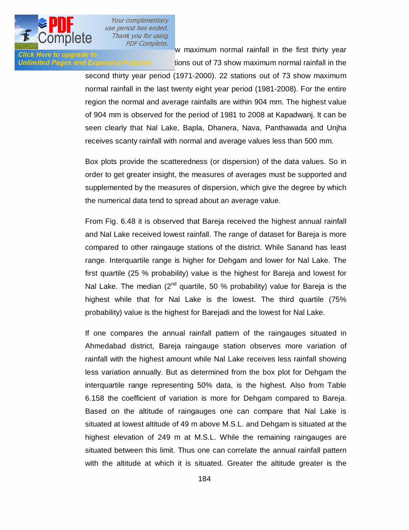
184

18 stations out of 73 show maximum normal rainfall in the first thirty year

period (1961-1990). 30 stations out of 73 show maximum normal rainfall in the

second thirty year period (1971-2000). 22 stations out of 73 show maximum

normal rainfall in the last twenty eight year period (1981-2008). For the entire

region the normal and average rainfalls are within 904 mm. The highest value

of 904 mm is observed for the period of 1981 to 2008 at Kapadwanj. It can be

seen clearly that Nal Lake, Bapla, Dhanera, Nava, Panthawada and Unjha

receives scanty rainfall with normal and average values less than 500 mm.

Box plots provide the scatteredness (or dispersion) of the data values. So in

order to get greater insight, the measures of averages must be supported and

supplemented by the measures of dispersion, which give the degree by which

the numerical data tend to spread about an average value.

From Fig. 6.48 it is observed that Bareja received the highest annual rainfall

and Nal Lake received lowest rainfall. The range of dataset for Bareja is more

compared to other raingauge stations of the district. While Sanand has least

range. Interquartile range is higher for Dehgam and lower for Nal Lake. The

first quartile (25 % probability) value is the highest for Bareja and lowest for

Nal Lake. The median (2nd quartile, 50 % probability) value for Bareja is the

highest while that for Nal Lake is the lowest. The third quartile (75%

probability) value is the highest for Barejadi and the lowest for Nal Lake.

If one compares the annual rainfall pattern of the raingauges situated in

Ahmedabad district, Bareja raingauge station observes more variation of

rainfall with the highest amount while Nal Lake receives less rainfall showing

less variation annually. But as determined from the box plot for Dehgam the

interquartile range representing 50% data, is the highest. Also from Table

6.158 the coefficient of variation is more for Dehgam compared to Bareja.

Based on the altitude of raingauges one can compare that Nal Lake is

situated at lowest altitude of 49 m above M.S.L. and Dehgam is situated at the

highest elevation of 249 m at M.S.L. While the remaining raingauges are

situated between this limit. Thus one can correlate the annual rainfall pattern

with the altitude at which it is situated. Greater the altitude greater is the


185

variation in annual rainfall for a set of raingauges into consideration. Similar

observations can be drawn for the box plots of other districts.

Fig.6.48 Box plot of annual time series of rainfall for raingauge stations

situated in Ahmedabad district

If one compares the annual rainfall pattern of the raingauges situated in

Ahmedabad district, Bareja raingauge station observes more variation of

rainfall with the highest amount while Nal Lake receives less rainfall showing

less variation annually. But as determined from the box plot for Dehgam the

interquartile range representing 50% data, is the highest. Also from Table

6.158 the coefficient of variation is more for Dehgam compared to Bareja.

Based on the altitude of raingauges one can compare that Nal Lake is

situated at lowest altitude of 49 m above M.S.L. and Dehgam is situated at the

highest elevation of 249 m at M.S.L. While the remaining raingauges are

situated between this limit. Thus one can correlate the annual rainfall pattern

with the altitude at which it is situated. Greater the altitude greater is the


186

variation in annual rainfall for a set of raingauges into consideration. Similar

observations can be drawn for the box plots of other districts.

Fig. 6.49 illustrates the box plot for Banaskantha district. It is observed that

Ambaji received the highest annual rainfall and Dhanera received lowest

rainfall. The range of dataset for Ambaji is more compared to other raingauge

stations of the district, with greater variation in annual amounts. Bapla has

least range, with lesser variation of annual rainfall. Interquartile range

indicating 50% of data are higher for Ambaji and lower for Bapla. The first

quartile (25 % probability) value is the highest for Danta which is nearer to

Ambaji compared to the lowest observed at Nava. The median (2nd quartile,

50 % probability) value for Ambaji is the highest while that for Panthawada is

the lowest. The third quartile (75 % probability) value is the highest for Ambaji

and the lowest for Bapla. As discussed earlier for Ahmedabad district, the

same is observed for Banaskantha district too. Ambaji is situated at the

highest elevation of 1,495 m above M.S.L. compared to the remaining stations

in the district. Thus Ambaji observes greater variations in annual rainfall with

the highest amounts for all the statistics calculated. Comparing the coefficient

of variation values, Bapla, Nava and Panthawada station have higher values

of 64 %, 66 % & 63 % respectively, indicating scanty rainfall, showing lesser

variations in the statistics determined.


187

Fig. 6.49 Box plot of annual time series of rainfall for raingauge stations

situated in Banaskantha district

For Gandhinagar district there are only two raingauges available for analysis.

Fig. 6.50 shows the box plot for Gandhinagar district. Based on the altitude

values, Mansa is situated at 338 m and Raipur weir at 215 m above M.S.L. It

is observed that Mansa received the highest and lowest annual rainfall. Here

the range of dataset is also more than Raipur weir. Interquartile range is

higher for Mansa. The first quartile (25 % probability) value is the similar for

both the raingauge stations. The second and third quartile value for Mansa is

greater than Raipur Weir.


188

Fig.6.50 Box plot of annual time series of rainfall for raingauge stations

situated in Gandhinagar district

Fig. 6.51 shows the box plot for raingauges situated in Kheda district. One

can observe that Kapadwanj and Mahisa received the highest and lowest

annual rainfall respectively. The range of dataset and interquartile range for

Kapadwanj is larger than other raingauge stations in the district. The first

quartile (25 % probability) value is the highest for Vaghroli tank and lowest for

Savli tank. The median (2nd quartile, 50 % probability) and the third quartile

(75 % probability) value for Kapadwanj is the highest while that for Vadol and

Mahisa respectively is the lowest. If one recalls the plot of normal rainfalls for

73 raingauge stations then it can be clearly seen that Kapadwanj depicts the

highest normal rainfall value of 904 mm for the period from 1981 to 2008.

Thus the rainfall for the last 28 years has changed the overall pattern for

Kapadwanj raingauge station influencing the rainfall extremes. The altitude of

Kapdawanj is 366 m and is the highest amongst the set of raingauges in the

district. Thus it shows greater variations in the annual rainfall amounts.


189


situated in Kheda district

From Fig. 6.52 it is observed that Kadi and Vijapur raingauge station received

the highest rainfall and Unjha received lowest rainfall. The range of dataset for

Kadi raingauge station is larger than other raingauge stations in the district.

Interquartile range is higher for Vijapur. The first quartile (25 % probability)

value is the highest for Kalol and lowest for Unjha. The median (2nd quartile,

50 % probability) value for Vijapur and Kadi is the highest while that for Unjha

is the lowest. The third quartile (75 % probability) value is the highest for

Vijapur and the lowest for Unjha. Here no specific observations can be made

based on the altitude of the raingaues. Kheralu is situated at the highest

elevation of 557 m above M.S.L. While Kadi and Vijapur observing the

variations in annual rainfall values are situated at 512 m and 416 m above

M.S.L. Based on the normal rainfall value plot Unjha recieved scanty rainfall

throughtout the study period for all the 3 thirty years periods from 1961 to


190

2008 as shown in Fig. 6.47. Thus the lowest value for each of the statistics in

the box plot is obtained for Unjha. But no specific observations can be made

for the highest amounts observed in the district. Though Visnagar, observes

the highest one day and consecutive 2 to 7 & 10 days maximum rainfall but it

does not influence the annual amounts. Hence overall scenario in case of

annual rainfall does not depend on the extreme events observed and on the

elevation at which it is measured.


situated in Mehsana district

Fig. 6.53 represents the box plot for raingaguges situated in Patan district. It is

observed that Wagdod raingauge station received the highest & lowest annual

rainfall. The range of dataset for Wagdod raingauge station is larger than

other raingauge stations in the district. The first quartile (25 % probability)

value is the highest for Sidhpur and lowest for Patan. The median (2nd


191

quartile, 50 % probability) value for Sidhpur is the highest while that for

Wagdod is the lowest. The third quartile (75 % probability) value is the highest

for Sidhpur and the lowest for Patan. Sidhpur is situated at the highest

elevation of 406 m above M.S.L. Thus for Patan district one can conclude

similar observations as seen for previous districts except Mehsana. Sidhpur

shows much variation in annual amounts which is influenced by the altitude at

which it is situated.


situated in Patan district

Fig. 6.54 shows the box plot for raingauges located at Sabarkantha district.

The highest amount of annual rainfall is observed at Shamlaji, while

Vijaynagar received lowest rainfall. The range of dataset for Shamlaji

raingauge station is larger than other raingauge stations in the district.

Interquartile range is higher for Prantij. The first quartile (25 % probability)

value is the highest for Idar and lowest for Vadgam. The median (2nd quartile,

50 % probability) value for Kundlacampo is the highest while that for Vadgam

is the lowest. The third quartile (75 % probability) value is the highest for


192

Prantij and the lowest for Dantral. For the raingauges situated in Sabarkantha

district greater variations for annual rainfall is observed with no specific

observations to be made with respect to altitude. Kundlacampo observes

maximum normal rainfall for the period of 1961 to 1990 which has influenced

the highest value obtained for the 50 % of the probability.


situated in Sabarkantha district

Table 6.159 presents the annual trend of 73 raingauge stations of north

Gujarat agroclimatic zone. From Table 6.30 it is observed that an increasing

trend is observed for 38 out of 73 (52 %) raingauge stations. The trend value

ranges from 0.17 mm / year at Malpur to 9.74 mm / year at Kapadwanj. Rest

of the 35 (48%) raingauge stations observe decreasing trend ranging from

0.03 mm / year at Savali tank to 10.25 mm / year at Ambaji. These trend

values are significant at Ambaji, Dhanera, Junisarotri and Kapadwanj. The 25

stations having normal rainfall value greater for the period from 1981 to 2008

show positive trends. Thus one can conclude that the rainfall for this period

has influenced the trend values indicating a change in the rainfall pattern.


193

Thus from the normal rainfall plots and trend values one can study the pattern

of rainfall affecting the climate scenario now a days.

Table 6.159 Annual Trends for 73 Raingague Stations of North Gujarat

Agroclimatic Zone. Sr. no.


Trend mm/ year

Sr. no.

Name of Raingauge

station

Trend mm/ year

Sr. no.

Name of raingauge

station

Trend mm/ year

1 Aslali -4.46 25 Sanali Ashram -4.64 49 Thol 4.08 2 Bareja 3.10 26 Mansa 3.70 50 Unjha -0.36 3 Barejadi -2.79 27 Raipur weir -1.04 51 Vijapur 4.28 4 Chandola 3.01 28 Balasinor 4.43 52 Visanagar 2.32 5 Dehgam 1.96 29 Dakor -6.03 53 Sidhpur 3.97 6 Nal Lake 4.66 30 Kapadwanj 9.74 + 54 Wagdod -3.77 7 Sanand 5.46 31 Kathlal 6.30 55 Badoli -1.76 8 Wasai -1.53 32 Kheda 3.58 56 Bayad 3.98 9 Ambaji -10.24 + 33 Mahemdabad -5.03 57 Bhiloda 1.09

10 Amirgadh 2.00 34 Mahisa 2.23 58 Dantral -6.99 11 Bapla -1.73 35 Nadiad 0.66 59 Himatnagar -1.38 12 Chandisar -2.26 36 Pinglaj -1.69 60 Idar 4.21 13 Chitrasani -0.70 37 Savli tank -0.03 61 Khedbrahma -0.53 14 Danta -2.99 38 Vadol 6.58 62 Kundlacampo -0.48 15 Dantiwada -0.62 39 Vaghroli Tank 2.35 63 Limla dam 6.42 16 Deesa 0.95 40 Ambaliyasan -4.81 64 Malpur 0.17 17 Dhanera 6.44 * 41 Kalol -1.06 65 Meghraj 2.94 18 Gadh -2.99 42 Dharoi -1.18 66 Modasa 1.43 19 Hadad -1.66 43 Kadi 1.72 67 Pal -2.53 20 Junisarotri -7.81 + 44 Katosan 3.56 68 Prantij 2.39 21 Wadgam 0.21 45 Kheralu 2.06 69 Sabli -2.07 22 Nava -4.28 46 Mehsana -3.15 70 Shamlaji 0.76 23 Palanpur 2.04 47 Patan 3.46 71 Vadgam 2.56 24 Panthawada -0.64 48 Ransipur 3.13 72 Vijaynagar -0.80

73 Virpur -4.23

The descriptive statistics are designed to assist the distributions of the data

based on values obtained. Skewness characterizes the degree of asymmetry

of a distribution around its mean. Normal distributions produce a skewness

statistic of about zero. The characteristics of climate data are also analyzed.

Table 6.160 presents the characteristics of Ahmedabad climate station.

From Table 6.160 it is observed that the coefficient of variation is more in

case of wind speed and least for maximum temperature. For annual rainfall

the coefficient of variation is above the threshold limit of 25 % and hence not

dependable. Rainy days, total rainfall, rainfall intensity, maximum

temperature, average relative humidity and wind speed are positively skewed

which indicate a distribution with an asymmetric tail extending towards more


194

positive values. Minimum temperature and sunshine hours are negatively

skewed, indicating a distribution with an asymmetric tail extending towards

more negative values. Values of 2 times standard error of skewness or more

(regardless of sign) are probably skewed to a significant degree. Thus the

sunshine hours are significantly negatively skewed. Kurtosis characterizes the

relative peakedness or flatness of a distribution compared to the normal

distribution. Normal distributions produce a kurtosis statistic of about zero

called mesokurtic. Positive kurtosis indicates a relatively peaked distribution.

Negative kurtosis indicates a relatively flat distribution. Values of 2 times

standard errors of kurtosis or more (regardless of sign) probably differ from

mesokurtic to a significant degree. Thus rainfall intensity and sunshine hours

have significant kurtosis indicating violations of the assumption of normality

that underlies many of the other statistics like correlation coefficients, t-tests,

etc. used to study test validity. For the other parameters the kurtosis is within

the expected range of chance fluctuations in the statistic, which further

indicates a distribution with no significant kurtosis problem.

Table 6.160 Characteristics of Climate of Ahmedabad, Ahmedabad District Parameter Mean Minimum Maximum Cv Skewness Kurtosis Trend Rainy days, days / year 30.00 12.00 53.00 35 0.36 -0.51 -0.33

Annual rainfall, mm 749.00 215.00 1284.00 41 0.38 -0.92 -1.67 Rainfall intensity, mm/day 25.05 12.50 48.50 30 1.08* 1.51* 0.05

Minimum temperature,0C 20.80 3.50 32.80 27 -0.54 -0.90 0.02

Maximum temperature,0C 34.40 19.40 47.50 14 0.12 -0.61 0.01

Average relative humidity, % 53.80 7.00 100.00 34 0.28 -0.56 -0.07

Wind speed, Kmph 8.67 2.40 36.00 55 0.47 0.57 -0.01***

Sunshine hours, h / day 8.30 1.80 13.40 37 -1.40* 0.97* -0.01*

Note:- *Significant according to standard error e where,

kurtosisfor N24e skeweness;for

N6e ==

N = no. of sample

**Significant at 5% level; ***Significance at 10% level


195

Fig.6.55 Monthly minimum, maximum and average climate of Ahmedabad,

Ahmedabad district


196

Fig. 6.55 represents monthly minimum, maximum and average values of the

climate parameters observed at Ahmedabad climate station. It is observed

that the minimum and maximum temperatures are higher in the month of June

and May respectively. The average relative humidity is the highest in the

month of July. Also the windspeed observed in the months of May and June is

the highest. The sunshine hours are more in the months from March to May

indicating higher maximum temperatures and relative humidity. The sunshine

hours are lowest in the months of higher rainy days. Thus based on the

climate parameters one can correlate the climate of the area and observe its

impact on the parameters measured.

Fig. 6.56 illustrates the trend for rainfall and other climatic parameters. Based

on trend values obtained it is observed that trend is decreasing for rainy days,

total rainfall and wind speed while it is increasing for rainfall intensity,

minimum and maximum temperatures. An increasing trend in minimum and

maximum temperatures and rainfall can be observed. While decreasing trend

is observed for rainy days, total rainfall and wind speed. The average relative

humidity and sunshine hours show no significant trend.

All the trend values except for wind speed are non significant at 5% level of

significance. Thus increasing rainfall intensity and decreasing rainfall amounts

indicate the effect of climate change observed now–a–days. But for increase

in minimum and maximum temperatures, the sunshine hours should also be

increased accordingly, which is not much evident from the available data.


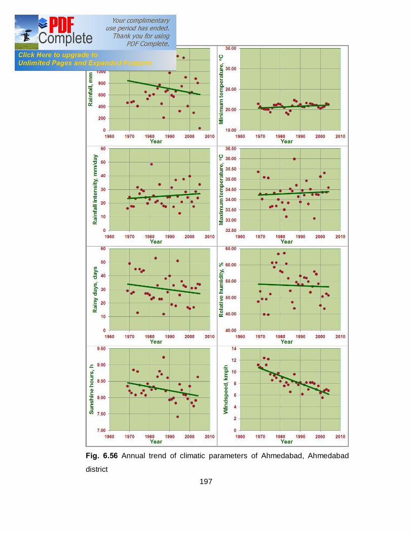
197

Fig. 6.56 Annual trend of climatic parameters of Ahmedabad, Ahmedabad

district


198

Table 6.161 depicts the characteristics of climate of Deesa climate station. It

is observed that the coefficient of variation is most in case of wind speed and

least for maximum temperature. For annual rainfall the coefficient of variation

is above the threshold limit of 25 % and hence not dependable. Rainy days,

total rainfall, rainfall intensity, average relative humidity and wind speed are

positively skewed which indicate a distribution with an asymmetric tail

extending towards more positive values. Minimum temperature, maximum

temperature and sunshine hours are negatively skewed, indicating a

distribution with an asymmetric tail extending towards more negative values.

Minimum temperature, maximum temperature, average relative humidity, wind

speed and sunshine hours are significantly skewed. Positive kurtosis indicates

a relatively peaked distribution. Negative kurtosis indicates a relatively flat

distribution. Minimum temperature, maximum temperature, average relative

humidity, wind speed and sunshine hours have significant kurtosis indicating

violations of the assumption of normality that underlies many of the other

statistics like correlation coefficients, t-tests, etc. used to study test validity.

Skewness and kurtosis are within the expected range of chance fluctuations

in the statistic, which further indicate a distribution with no significant

skewness or kurtosis problem.

Table 6.161 Characteristics of Climate of Deesa, Banaskantha District Parameter Mean Minimum Maximum Cv Skewness Kurtosis Trend

Rainy days, days / year 22.00 4.00 41.00 41.98 0.17 -0.42 -0.125 Annual rainfall, mm 472.48 50.10 1010.80 55.98 0.29 -0.81 -1.968 Rainfall intensity, mm/day 21.42 4.94 50.52 43.18 0.65 1.47 0.065

Minimum temperature,0C 19.42 5.10 29.20 30.79 -0.47* -1.06* 0.003 Maximum temperature,0C 33.98 22.00 44.40 13.23 -0.11* -0.71* 0.031***

Average relative humidity, % 53.56 19.00 95.00 28.08 0.46* -0.29* 0.022

Wind speed, kmph 4.70 2.40 21.60 66.14 0.65* 1.11* -0.135*** Sunshine hours, hours/day 9.25 3.10 14.00 23.34 -0.86* 0.42* 0.018



N6e ==

N = no. of sample; **Significant at 5% level; *** Significant at 10% level


199

Fig. 6.57 depicts monthly minimum, maximum and average values of the

climate parameters observed at Deesa climate station. It is observed that the

minimum and maximum temperatures are higher in the month of June and

May respectively. The average relative humidity is the highest in the month of

August. Also the windspeed observed in the month of June is the highest. The

sunshine hours are more in the month of March. When the sunshine hours

are lowest, for those months the rainfall is observed.

Here one can say that the increasing trend in sunshine hours may tend to

increase the trend of maximum and minimum temperatures which can be

seen from Fig. 6.56. Also the decrease in rainfall and rainy day indicates that

the rainfall for the area is decreasing with increase in sunshine hours and

daytime temperatures.

Fig. 6.58 represents the trend for the climatic parameters. One can observe

the increasing trend in minimum & maximum temperatures, sunshine hours

and relative humidity. Decreasing trend in rainy days, rainfall and wind speed

are observed. According to Mann Kendall test maximum temperature and

wind speed have significant trend value at 10 % significance level.


200

Fig.6.57 Monthly minimum, maximum and average climate of Deesa,



201

Fig. 6.58 Annual trend of climatic parameters of Deesa, Banaskantha district


202

Table 6.162 summarizes the characteristics of Dantiwada climate station. The

coefficient of variation is most in case of rainfall intensity & wind speed and

least for maximum temperature. For annual rainfall the coefficient of variation

is above the threshold limit of 25 % and hence not dependable. Rainy days,

minimum and maximum temperatures and sunshine hours are negatively

skewed which indicate a distribution with an asymmetric tail extending

towards more negative values. Annual rainfall, rainfall intensity, average

relative humidity and wind speed are positively skewed, indicating a

distribution with an asymmetric tail extending towards more positive values.

Rainy days and annual rainfall are within the expected range of chance

fluctuations in the statistic for skewness and kurtosis, which further indicates a

distribution with no significant skewness or kurtosis problem. Thus other

parameters except the annual rainfall and rainy days, have significant

skewness and kurtosis indicating violations of the assumption of normality that

underlies many of the other statistics like correlation coefficients, t-tests, etc.

used to study test validity.

Table 6.162 Characteristics of Climate of Dantiwada, Banaskantha District Parameter Mean Minimum Maximum Cv Skewness Kurtosis Trend Rainy days, days / year 19.00 2.00 32.00 41.60 -0.30 -0.61 0.249

Annual rainfall, mm 522.00 36.00 1357.00 59.47 1.00 1.04 2.800 Rainfall intensity, mm/day 29.39 11.36 101.81 71.98 2.57* 6.59* -0.300

Minimum temperature,0C 19.05 5.90 36.90 34.38 -0.40* -1.08* 0.011

Maximum temperature,0C 33.84 10.10 47.20 13.91 -0.18* -0.45* -0.005

Average relative humidity, % 54.13 7.80 100.00 30.34 0.21* -0.24* 0.134

Wind speed, kmph 5.59 2.40 36.00 71.60 1.31* 1.80* -0.015 Sunshine hours, hours/day 8.32 1.30 39.20 34.74 -1.28* 2.46* -0.079***



N6e ==

N = no. of sample

**Significant at 5% level; *** Significant at 10% level


203

Fig. 6.59 Monthly minimum, maximum and average climate of Dantiwada,



204

Fig. 6.60 Annual trend of climatic parameters of Dantiwada, Banaskantha

district


205


climate parameters observed at Dantiwada climate station. It is observed that

the minimum and maximum temperatures are higher in the month of June and

May respectively. The average relative humidity is the highest in the month of

June. Also the highest windspeed is observed in the month of June. The

sunshine hours are higher in the month of May. It is observed that when the

sunshine hours are lowest the rainfalls are observed in those months.

Fig. 6.60 represents the trend for rainfall and other climatic parameters. One

can observe the opposite scenario for the annual averages for this station

compared to the other two discussed earlier. An increasing trend in minimum

temperature, relative humidity, rainy days and rainfall amounts is observed.

Decreasing trend in maximum temperature, sunshine hours, wind speed and

rainfall intensity are observed. According to Mann Kendall test these trend

values are not significant except for sunshine hours. The period of average

calculation considered is from 1982 to 2008 which may be one of the reasons.

While for other stations it is averaged over the period from 1969 to 2005.

From Table 6.163 it is observed that the coefficient of variation is most in case

of wind speed and least for maximum temperature. For annual rainfall the

coefficient of variation is above the threshold limit of 25 % and hence not

dependable. Rainy days, rainfall, rainfall intensity, maximum temperatures,

average relative humidity and wind speed are positively skewed which

indicates a distribution with an asymmetric tail extending towards more

positive values. Minimum temperature and sunshine hours are negatively


more negative values. Annual rainfall, rainfall intensity and rainy days are

within the expected range of chance fluctuations in the statistic for skewness

and kurtosis, which further indicates a distribution with no significant

skewness or kurtosis problem. Thus other parameters except the annual

rainfall, rainfall intensity and rainy days, have significant skewness and

kurtosis indicating violations of the assumption of normality that underlies

many of the other statistics like correlation coefficients, t-tests, etc. used to

study test validity.


206

Table 6.163 Characteristics of Climate of Vallabh Vidyanagar, Kheda District Parameter Mean Minimum Maximum Cv Skewness Kurtosis Trend Rainy days, days / year 29.00 8.00 53.00 35.77 0.07 0.09 -0.008

Annual rainfall, mm 752.34 226.35 1,904.80 48.00 1.07 1.59 -3.294

Rainfall intensity, mm/day 25.78 11.93 51.49 32.08 0.89 1.20 -0.086

Minimum temperature,0C 19.57 7.40 28.60 22.52 -0.60* -0.24* 0.011

Maximum temperature,0C 33.40 22.50 41.10 10.48 0.33* 0.25* 0.021

Average relative humidity, % 62.90 28.50 97.00 21.67 0.11* 0.08* 0.150**

Wind speed, kmph 3.57 0.51 14.40 63.06 0.73* 1.45* -0.098***

Sunshine hours, hours/day 8.70 1.30 14.30 24.97 -0.57* 0.07* 0.017**



N6e ==

N = no. of sample

**Significant at 5% level; *** Significance at 10% level


climate parameters observed at Vallabh Vidyanagar climate station. It is

observed that the minimum & maximum temperatures and sunshine hours are

the highest in the month of May. The average relative humidity is the highest

in the month of July. Also the windspeed observed for the month of June is

the highest. The highest rainfall is observed in the month of July where the

numbers of rainy days are also more.

Fig. 6.62 represents the trend for rainfall and other climatic parameters. An

increasing trend in minimum and maximum temperatures and relative

humidity, sunshine hours is observed. Decreasing trends for rainfall and wind

speed are observed. The data for rainfall intensity and rainy days are not

available, hence not plotted. According to Mann Kendall test these trend

values are significant for average relative humidity, wind speed and sunshine

hours at 5 %, 10 % & 5 % significance level respectively.


207

Fig. 6.61 Monthly minimum, maximum and average climate of Vallabh

Vidyanagar, Kheda district


208

Fig. 6.62 Annual trend of climatic parameters of Vallabh Vidyanagar, Kheda

district

Table 6.164 illustrates the characteristics of Idar climate station. It is observed

that the coefficient of variation is most in case of rainfall and least for

maximum temperature. Rainy days, rainfall, maximum temperature, wind

speed and sunshine hours are positively skewed which indicate a distribution

with an asymmetric tail extending towards more positive values. Rainfall


209

intensity, minimum temperature and average relative humidity are negatively


more negative values. Minimum temperature is within chance of fluctuation for

skewness. Rainy days, rainfall, rainfall intensity and maximum temperature

have negative kurtosis indicating relatively flat distribution. Other parameters

show positive kurtosis indicating peaked distribution. Minimum temperature is

within the acceptable chance of fluctuation for kurtosis.

Table 6.164 Characteristics of Climate of Idar, Sabarkantha District Parameter Mean Minimum Maximum Cv Skewness Kurtosis Trend Rainy days, days / year 32.00 14.00 58.00 34.00 0.44* -0.28* -0.12

Annual rainfall, mm 797.00 205.00 1,065.00 44.00 0.29* -0.14* -2.29

Rainfall intensity, mm/day 24.00 12.00 37.00 27.00 -0.02* -0.73* -0.07

Minimum temperature,0C 21.00 17.00 22.00 5.00 -1.72 6.20 0.01

Maximum temperature,0C 34.00 33.00 36.00 2.00 0.36* -0.51* 0.04**

Average relative humidity, % 46.00 37.00 56.00 10.00 -0.12* 0.22* 0.08

Wind speed, kmph 2.66 2.40 16.80 38.97 4.68* 3.55* -0.01

Sunshine hours, hours/day 8.36 7.44 10.35 6.00 1.18* 4.39* 0.01



N6e ==

N = no. of sample

**Significant at 5% level

Fig. 6.63 represents the trend for rainfall and other climatic parameters. One

can observe the increasing trend in minimum and maximum temperatures,

average relative humidity and sunshine hours and decreasing trend for rainy

days, total rainfall, rainfall intensity and wind speed. Based on trend values

obtained it is observed that trend is decreasing for rainy days, total rainfall

amount and rainfall intensity while it is increasing for minimum and maximum

temperatures, average relative humidity and sunshine hours.


210

Fig. 6.63 Monthly minimum, maximum and average climate of Idar,

Sabarkantha district


211

Fig. 6.64 Annual trend of climatic parameters of Idar, Sabarkantha district


212

For Fig. 6.64 all the trend values except for maximum rainfall are non

significant at 5% level of significance. Thus while relating the rainfall and other

climate parameters one can say that as the other climate parameter values

increase for given annual time series for Idar, the rainfall intensity decrease.

This is due to the climatic changes because of global warming effect. Further

variation effects can be achieved if one explores the climate data if available

at each raingauge network.

From the statistics obtained for all the five climate stations general

observations can be made. The findings relate to the study funded by NASA

indicating the amount of solar radiation the sun emits, during times of quiet

sunspot activity, has increased since 1970’s with a rate of 0.05 percent per

decade.(http://www.nasa.gov/home/hqnews/2003/mar/HP_news_03106. html)

Richard Willson, a researcher affiliated with NASA's Goddard Institute for

Space Studies and Columbia University's Earth Institute, New York said that

this trend was important because, if sustained over many decades, it could

cause significant climate change. He was the lead author of the study recently

published in Geophysical Research Letters. Historical records of solar activity

indicated that solar radiation has been increasing since the late 19th century.

He mentioned that if a trend, comparable to the one found in his study,

persisted throughout the 20th century, it would had provided a significant

component of the global warming the Intergovernmental Panel on Climate

Change reports to have occurred over the past 100 years.

In order to study the heterogeneity of rainfall amounts over an area, a

modified version of Oliver’s (1980) Precipitation Concentration Index (PCI) is

used as explained in the methodology. The PCI for 73 raingaguge stations

have been calculated and presented in Figs. 6.65 to 6.70. Fig. 6.65 presents

the plot for Ahmedabad district and the remaining plots are provided in Figs.

6.66 to 6.71 for Banaskantha, Gandhinagar, Kheda, Mehsana, Patan and

Sabarkantha districts, which are given in CD. For all the raingauge stations

the Precipitation Concentration Index (PCI) values are above 20 which

correspond to climates with substantial monthly variability. The average PCI


213

for all the stations is around 40 %. Thus for the north Gujarat agroclimatic

region the monthly rainfall is substantially variable.

Fig. 6.65 PCI for raingauge stations in Ahmedabad district


214

Thus based on the different statistical characteristics of the climate

parameters discussed, one can conclude that the climate of the present study

area is varying and needs to be analyzed in detail for planning the water

resources and agricultural activities.

6.6 REGIONALIZATION BASED ON SPATIAL AND TEMPORAL RAINFALL

PATTERNS

The concentration indices (COIN) for 73 raingauges, the constants a & b and

the percentage of rainfall amount for 25 % of rainiest days are presented in

Table 6.165. From Table 6.165 it can be observed that if one considers a

period of 48 years from 1961 to 2008 then more than 60% of the total rain fell

in 25% of rainiest days in the region. During the past 48 years, Prantij has

experienced maximum of 77 % of total rainfall within 25 % of rainiest days.

While Mahisa has experienced 63 % of total rainfall within 25 % of rainiest

days. It can be observed that Mahisa, Savli tank and Vadol have minimum

COIN of 0.54 while Dharoi and Prantij have maximum COIN of 0.66 and the

average COIN for north Gujarat agroclimatic zone is 0.60. The COIN value for

73 raingauge stations in north Gujarat agroclimatic zone varies from 0.54 to

0.66 with standard deviation of 0.03. This 12% variation is significant

according to Kolmogrov Smirnov one sample test statistic at 0.01 significance

level. Fig. 6.69 illustrates the distribution of the concentration of rainfall in the

study area.


215

Table 6.165 COIN for 73 Raingauge Stations and Percentage of Total Rainfall Amount for 25% of Rainy Days Observed in North Gujarat Agroclimatic Zone

Sr. no.


a b COIN Percentage of total rainfall amount for

25% of rainiest days 1 Aslali 0.0589 0.0275 0.56 65 2 Bareja 0.0678 0.0258 0.55 66 3 Barejadi 0.0506 0.0287 0.58 68 4 Chandola 0.0584 0.0272 0.57 67 5 Dehgam 0.0406 0.0309 0.60 70 6 Nal Lake 0.0627 0.0267 0.56 65 7 Sanand 0.0330 0.0331 0.61 71 8 Wasai 0.0707 0.0254 0.55 67 9 Ambaji 0.0593 0.0271 0.57 67

10 Amirgadh 0.0345 0.0323 0.62 72 11 Bapla 0.0504 0.0285 0.59 69 12 Chandisar 0.0415 0.0304 0.61 70 13 Chitrasani 0.0474 0.0291 0.60 70 14 Danta 0.0438 0.0300 0.60 70 15 Dantiwada 0.0292 0.0339 0.63 73 16 Deesa 0.0242 0.0358 0.65 75 17 Dhanera 0.0308 0.0335 0.63 72 18 Gadh 0.0429 0.0300 0.61 71 19 Hadad 0.0393 0.0311 0.61 71 20 Junisarotri 0.0366 0.0318 0.61 72 21 Nava 0.0670 0.0261 0.55 65 22 Palanpur 0.0417 0.0302 0.61 72 23 Panthawada 0.0396 0.0309 0.61 72 24 Sanali Ashram 0.0478 0.0293 0.59 69 25 Wadgam 0.0532 0.0281 0.58 68 26 Mansa 0.0344 0.0323 0.62 66 27 Raipur Weir 0.0574 0.0276 0.56 73 28 Balasinor 0.0414 0.0309 0.59 69 29 Dakor 0.0425 0.0308 0.59 68 30 Kapadwanj 0.0528 0.0285 0.57 67 31 Kathlal 0.0452 0.0300 0.59 68 32 Kheda 0.0458 0.0298 0.59 69 33 Mahemadabad 0.0317 0.0332 0.63 73 34 Mahisa 0.0685 0.0260 0.54 63 35 Nadiad 0.0360 0.0318 0.62 72 36 Pinglaj 0.0632 0.0264 0.57 68 37 Savli tank 0.0690 0.0260 0.54 64 38 Vadol 0.0766 0.0247 0.54 64 39 Vaghroli 0.0678 0.0258 0.55 65 40 Ambaliyasan 0.0415 0.0306 0.60 70 41 Dharoi 0.0201 0.0378 0.66 75 42 Kadi 0.0374 0.0313 0.62 72 43 Kalol 0.0373 0.0316 0.61 72


216

44 Katosan 0.0416 0.0305 0.60 70 45 Kheralu 0.0387 0.0309 0.62 72 46 Mehsana 0.0363 0.0315 0.63 73 47 Ransipur 0.0498 0.0287 0.59 70 48 Thol 0.0508 0.0286 0.58 68 49 Unjha 0.0517 0.0286 0.58 67 50 Vijapur 0.0306 0.0334 0.63 73 51 Visnagar 0.0381 0.0310 0.62 73 52 Patan 0.0369 0.0314 0.62 73 53 Sidhpur 0.0396 0.0307 0.62 72 54 Wagdod 0.0528 0.0281 0.59 68 55 Badoli 0.0407 0.0308 0.60 70 56 Bayad 0.0308 0.0335 0.63 73 57 Bhiloda 0.0321 0.0330 0.63 73 58 Dantral 0.0406 0.0300 0.63 71 59 Himmatnagar 0.0323 0.0330 0.62 72 60 Idar 0.0437 0.0301 0.60 70 61 Khebhrama 0.0348 0.0323 0.62 72 62 Kundlacampo 0.0474 0.0292 0.59 69 63 Limladam 0.0439 0.0301 0.60 70 64 Malpur 0.0246 0.0355 0.65 75 65 Meghraj 0.0341 0.0327 0.61 73 66 Modasa 0.0292 0.0339 0.63 74 67 Pal 0.0602 0.0270 0.56 66 68 Prantij 0.0181 0.0388 0.66 77 69 Sabli 0.0480 0.0292 0.59 69 70 Shamlaji 0.0373 0.0314 0.62 72 71 Vadgam 0.0317 0.0334 0.62 72 72 Vijaynagar 0.0476 0.0295 0.58 68 73 Virpur 0.0427 0.0304 0.60 70

Fig. 6.72 indicates the COIN for north Gujarat agroclimatic zone. It is

observed that the overall concentration of rainfall in most of the region is

nearer to the average value of 0.600 indicated by the green colour. The

average value obtained, divides the area into two different parts indicating

higher and lower concentration of rainfall with reference to the average value

obtained. Also there are some of the closed contours observed in the area. If

one observes the lower portion of the area the COIN value builds up from

lower to higher and achieves peak at 0.595. Further moving from the peak the

COIN value decreases forming depression cones near the Nal Lake, Wasai,

Savali tank, Vaghroli tank and Mahisa areas.


217

Fig. 6.72 Isopleth map of COIN for north Gujarat agroclimatic zone.

Observing the satellite images from the google maps, the terrain is somewhat

flatter at and around these areas. Observing the google earth images the

depression areas are less dense compared to the other area, although Nal

Lake is situated nearer to the water body. Thus one may say that it is not

necessary to believe that the concentration of rainfall is more nearer to the

water bodies.


218

Fig. 6.73 Satellite images for the lower portion of the area consisting of Bareja, Kathlal, Kheda, Mehmadabad, Nal Lake (Nal

sarovar), Kadi, Kalol, Prantij, Vijapur, etc. .


219

Fig. 6.74 Satellite images for the upper portion of the region consisting of Ambaji,

Amirgadh, Chandisar, Danta, Dantiwada, Shamlaji, Bhiloda, Prantij, Vijaynagar,

etc.


220

The rainfall concentration may build up away from the water body which may be

influenced due to the altitude at which it is situated. While it is known by now that

many changes in the environment have their impact on climate. But at least one

can study the behaviour spatial variability of rainfall by the concentration indices

and plan for the water resources and agricultural management. Fig. 6.73 shows

the satellite images of the lower portion of the study area consisting of lower

concentration compared to the upper portion of the area.

As one observes the upper portion of the area, the concentration of the rainfall is

at or above the average value of 0.60 except at Ambaji, Wadgam and Nava. If

one observes the satellite images available from the google maps, the area is

surrounded by mountainous regions. Hence the concentration of rainfall is higher

due to the hilly region attracting more rains. Most of the central portion too

observes the same scenario of average or above average concentration of

rainfall with closed increasing contours at Kadi, Prantij and Malpur. Fig. 6.74

shows the satellite images of the upper portion of the study area consisting of

higher concentration compared to the lower portion. The distribution of rainfall

varies spatially in the region dividing the region into two parts with higher and

lower concentrations with respect to the mean value. Hence as one moves from

north towards south the variability of rainfall decreases. Most of the areas within

the region observes greater variability with respect to the concentration of daily

rainfall amount as the COIN value in any case is not more than 0.66 (as the

COIN value of 1.00 gives the most uniform amount of rainfall for uniform number

of rainy days).

The region receives most of the rainfall with fewer rainy days indicating the

higher intensity of the rainfall. From the agriculture point of view, higher intensity

of rainfall is less useful compared to the lesser intensity of rainfall. The high

intensity of rainfall is incapable to fully infiltrate the soil due to lesser time of

concentration resulting in more runoff. Thus the water harvesting (runoff

harvesting) structures must be planned for storage of heavy rains which can be


221

used afterwards during the long dry spell periods, which are often observed in

the region and confirmed by the further studies on dry spell analysis carried out

for the region.

6.7 DESIGN STORM FOR HATHMATI CATCHMENT AREA

Nine raingauge stations fall in the Hathmati catchment area. This stations are

Badoli, Bhiloda, Idar, Kundlacampo, Modasa, Pal, Sabli,Shamlaji and Vijaynagar.

The aerial rainfall is determined using Theissen polygon formed using the other

adjacent raingauge stations. The annual rainfall for the Hathmati catchment area

is as represented in Fig. 6.75. The maximum value of 1573 mm is observed in

2006. Lowest annual rainfall of 202 mm is observed in 1987. The average rainfall

over the catchment is 740 mm. The trend line indicated by black colour in the Fig.

6.75 do not show any increase or decrease in the annual rainfall amounts.

Fig. 6.75 Annual rainfall over the Hathmati catchment area


222

Occurrence of 48 heavy rainspells which affected the Hathmati catchment are

presented in Fig. 6.76. Daily aerial rainfalls during each of these 48 rainstorms

have been worked out and among them 10 severe rainstorms are given in Table

6.166. The maximum rainfalls for 1 to 5 days durations have been determined

from the Table 6.166.

Fig. 6.76 Actual maximum rainfall observed at Hathmati catchment area

Table 6.166 Severe Rainstorms Observed at Hathmati Catchment Area Sr. No. Date of rainstorm Daily rainfall, mm Total

Mm 1 2 3 4 5 1 29 Aug–2 Sep 1973 25.45 56.46 151.16 174.30 41.84 449.21 2 16 Aug–20 Aug 2006 182.83 44.58 2.79 156.45 43.28 429.94 3 30 Jul –3 Aug 1968 57.58 153.14 145.67 58.48 3.67 418.55 4 8 Jul–11 Jul 1993 76.08 151.71 41.72 77.31 --- 346.82 5 23 Jul–27 Jul 1982 70.48 86.90 126.79 31.13 28.69 344.00 6 24 Jun–27 Jun 1997 18.27 150.99 137.09 19.11 --- 325.46 7 3 Aug–6 Aug 1984 25.65 103.57 129.22 14.16 --- 272.60 8 22 Jul–26 Jul 1991 44.71 57.52 13.77 62.92 89.23 268.15 9 3 Jul–7 Jul 1990 28.74 69.45 75.80 60.49 19.06 253.54 10 17 Jul–18 Jul 1993 71.69 164.90 --- --- --- 236.59


223

To obtain envelope raindepths over the catchment, the raindepths for 1,2,3,4 and

5 day durations were plotted as depth-duration (DD) curves (see Fig. 6.77). DD

analysis has shown that the catchment received as high as 182.83 mm, 236.59

mm, 356.39 mm, 414.87 mm and 449.21 mm in 1, 2,3,4 and 5 day durations

respectively as depicted in Table 6.167

Table 6.167 Observed One Day to Consecutive 2 to 5 Days Raindepths for

Hathmati Catchment Area Sr. no. Year 1D C2D C3D C4D C5D

1 1973 25.45 81.91 233.07 407.37 449.21 2 2006 182.83 227.41 230.20 386.65 429.93 3 1968 57.58 210.72 356.39 414.87 418.54 4 1993 76.08 227.79 269.51 346.82 346.82 5 1982 70.48 157.38 284.17 315.30 343.99 6 1997 18.27 169.26 306.35 325.46 325.46 7 1984 25.65 129.22 258.44 272.60 272.60 8 1991 44.71 102.23 116.00 178.92 268.15 9 1990 28.74 98.19 173.99 234.48 253.54 10 1993 71.69 236.59 236.59 236.59 236.59

Fig. 6.77 Depth duration (DD) and envelope curve for Hathmati catchment area


224

Design rainfall by statisitcal method

In order to determine the design raindepths by the statistical method, the annual

maximum catchment raindepths for the 48 years period (1961–2008) for 1,2,3,4

and 5 day durations have been subjected to the best fitted Inverse Gaussian

distribution. Table 6.168 gives the design storm rainfalls for 1,2,3,4 and 5 day

durations for return period from 2 to 1000 years. This Table shows that the

highest raindepths obtained by DD method (Table 6.167) for 1–day (182.83 mm)

is close to 23 years, 2–day is close to 14 years, 3–day is close to 60 years,

4–day is close to 54 years and 5–day is close to 60 years.

Table 6.168 1,2,3,4 and 5 Day Rainfall at Different Return Period for Hathmati

Water Resources Project Return period 1–day 2–day 3–day 4–day 5–day

Years mm mm mm mm mm 2 78 116 138 159 174 5 119 175 202 236 255 10 149 216 246 289 310 20 177 256 289 341 364 50 215 309 345 408 434 60 223 320 356 422 448 70 229 329 365 433 459 80 235 336 373 443 470 90 240 343 380 451 479

100 244 349 387 459 487 500 312 443 484 578 608 750 329 466 508 607 639

1000 341 483 526 629 661

In evaluating the probable maximum precipitation (PMP) for the Hathmati

catchment, the envelope curve obtained by DD method are maximized with the

moisture maximization factors (MMFs). The MMF is a ratio of the highest amount

of moisture recorded over the catchment during the period when the rainstorm

occurred to that recorded in the rainstorm. The moisture in an air mass from

which large precipitation occurs, can be estimated from the surface dew points

decreasing with height at a the pseudo-adiabatic lapse rate.


225

For long duration rainstorms, the maximum 24 hour persisting dew point value is

used. The MMF has therefore been worked out on the basis of maximum

persisting rainstorm and the maximum persisting dew point for the catchement.

The maximum 24 hour persisting dew point temperature for the catchment in July

and August months have been observed.

The maximum 12 hours persisting dew point temperature for the Hathmati

Catchment has been found to be 27.6 0 C. The storm dew point temperatures for

the selected 10 rainstorms have been obtained. The elevation of the catchment

is 202 m. The dew point temperatures obtained above are reduced to the mean

sea level from Fig. 5.5. Table 6.169 gives the values of parameters used for

evaluating the MMFs where the dew points are expressed in their 1000 mb

equivalents using Fig. 5.6.

Table 6.169 Parameters used for Working out MMFs Rainstorm period Storm dew point 0 C Precipitable

water

mm

Maximum dew point for the Hathmati catchment

0 C

Precipitable water

mm

MMF Observed Reduced

to mean sea level

29 Aug–2 Sep 1973 24.8 25.2 88 28.5 94 1.07 16 Aug–20 Aug 2006 --- --- --- 28.5 94 --- 30 Jul–3 Aug 1968 --- --- --- 28.5 94 --- 8 Jul–11 Jul 1993 23.2 24.0 60 28.5 94 1.56 23 Jul–27 Jul 1982 24.8 25.2 88 28.5 94 1.07 24 Jun–27 Jun 1997 --- --- --- 28.5 94 --- 3 Aug–6 Aug 1984 25.0 25.8 74 28.5 94 1.27 22 Jul–26 Jul 1991 25.0 25.8 74 28.5 94 1.27 3Jul–7 Jul 1990 23.7 24.2 66 28.5 94 1.42 17 Jul–18 Jul 1993 23.2 24.0 60 28.5 94 1.56

The MMFs obtained for the 10 severe rainstorms have been found and

presented in Table 6.169. A maximum value of 1.56 is observed for two severe

rainstorms analyzed. Thus a value of 1.56 is the obtained MAF for determining

the PMPs for the catchment.


226

PMP for the Hathmati catchment

The following estimates of PMP have been obtained by adjusting the DD rain

depths by the appropriate MMFs factors:

Equivalent to Return period calculated by

statistical method, years

1–day mm 2851.56 183 ≈×= 250

2–day mm 3701.56237 ≈×= 145

3–day mm 5551.56356 ≈×= 1530

4–day mm 6471.56415 ≈×= 1220

5–day mm 7001.56449 ≈×= 1750

The estimates of PMP for 1,2,3,4 and 5 day durations for the Hathmati catchment

have been found to be 285 mm, 370 mm, 555 mm, 647 mm and 700 mm

respectively. These PMP raindepths can be used for calculation of the PMF

hydrograph for the Hathmati dam.

From the design storm analysis of the Hathmati Water Resources Project

following results have been emerged:

The average annual rainfall in the catchment is about 74 cm with a standard

deviation of 29 cm.

The coefficient of variability of annual rainfall is about 39%. July month has the

lowest variability of 51% among the four months while June has about 100%,

August has about 61% and September has about 105% variability of rainfall.

10 severe rainstorms have occurred over the catchment during the 48 year

period. Out of these 10 rainstorms, 5 were observed in July, 4 in August and 1 in

June. The heavy intensity of storms were observed in the years 1968, 1973,

1982, 1984, 1990, 1991, 1993, 1997 and 2006.


227

The annual maximum catchment rain depths for the 48 year period for 1,2,3,4

and 5 days durations have been subjected to best fitted Inverse Gaussian

distribution. The highest observed rain depths obtained by DD method for 1-day

duration (i.e. 182.83 mm) is close to 23 years, 2–day duration (i.e. 236.59 mm) is

close to 14 years, 3–day duration (i.e. 356.39 mm) is close to 60 years, 4–day

duration (i.e. 414.87 mm) is close to 54 years and 5–day duration (i.e. 449.21

mm) is close to 60 year return period estimated by statistical (probability

distribution) method.

The estimates of PMP using hydrometeorological method, for 1,2,3,4 and 5 day

durations for the Hathmati catchment have been found to be 285 mm, 370 mm,

555 mm, 647 mm and 700 mm respectively. This PMP estimates are equivalent

to 250, 145, 1530, 1220 and 1750 years of return period estimated by statistical

(probability distribution) method.

The findings above can be supported by the study carried out by Mistry (1988)

emphasizing the review of design floods for some of the major river valley

projects in Gujarat state. He mentioned that the hydrological aspects, viz.,

availability of water, design flood, etc. were estimated on the basis of a few years

observed discharge data available at that time or by using the rational empirical

formulae for runoff and floods. The design floods for the projects were estimated

by applying suitable factor of safety, to the observed maximum flood at the site or

at nearby site on the same stream depending on the judgement of the designer.

Attemps were also made to estimate the magnitude of the design flood by using

the slope area method and observed flood marks of the highest experienced

flood from local inquiry. All these above mentioned methods were based on the

past available records of floods in the concerned regions. At the time of preparing

the project report, the design flood derived by the above methods is based on the

data available, then the design flood may be subjected to revision.

The construction of Hathmati dam was completed in Year 1971. Mistry (1988)

has mentioned in his report that unprecedented floods occurred in the year 1973


228

over the Sabarmati basin. Also it should be noted that the year 2006 observed

major one day storm as can be observed from the analysis carried out. This

necessitated the revision of design flood study carried out in past. Keeping the

devastating effects of the floods in view, an attempt was made for revision of the

design flood which will be useful in the planning and design of new water

resources projects as well as in re–examining the spillways of the existing water

control devices.

The design discharge capacity of spillway of existing Hathmati dam is 2,943 m3/s.

Its catchment area is 595 km2. Based on the hydrometerological method the

design raindepth over the catchment observed for one day is 285 mm. Therefore

the design flood considering 85 % runoff, comes out to be 1,668.27 m3/s. When

one considers the statistical frequency distribution method, then 1000 year return

period rainfall depth is considered for spillway designs. The rainfall depth using

statistical method obtained is 341 mm and the design flood calculated is 1,996.07

m3/s. Thus the design flood obtained for the period from 1961 to 2008 is reduced

to 43 % and 32 % in case for hydrometerological and statistical method

respectively, than the design discharge of the existing spillway capacity. This

design discharge capacity of 2,943 m3/s was determined considering the

maximum flood observed in 1927. If in case for further analysis period in future a

need may arise to re-examining the design storm the statistical method can be

recommended. In case of Kadana dam, it was completed in 1979 with main

spillway capacity of 31,400 m3/s. Considering the rainfall in 1973 the design

discharge was revised and an additional spillway of 18,097 m3/s was

constructed.

Overall it can be said that probable maximum precipitation estimates by

statistical method are well comparable with values obtained by the

hydrometeorological method for different durations. As the hydrometeorological

method involves additional data for dew point temperatures and lengthy


229

calculation, PMP by statistical method can be easily used with appropriate return

period for planning purposes.

6.8 DROUGHT ANALYSIS

By using the monthly rainfall data of 73 raingauge stations, standardized

precipitation index (SPI) values are calculated for 4, 12 and 24 months period.

Based on AIC and BIC the best distribution fitted to the dataset of 4 months, 12

months and 24 months rainfall for all the raingauge stations obtained is inverse

Gaussian and hence used for further analysis. The drought intensity is classified

as discussed in methodology using Table 5.9 and the results are presented in

Tables 6.70 to 6.176 The number of events and percentage out of total number

of years of analysis is calculated for all the three types of data viz. original one

(O), gamma fitted (G) and best fitted inverse Gaussian (I).

From Table 6.170 it is observed that the total drought events for 4 month time

scale using gamma and inverse Gaussian distribution are equal for Bareja,

Chandola, Dehgam, Sanand and Nal Lake raingauge stations in Ahmedabad

district. For 12 month time scale (SPI12) Aslali, Barejadi, Sanand and Nal Lake

have same drought events for gamma and inverse Gaussian while it is more for

gamma distribution in case for Bareja, Chandola, Dehgam and Vasai. For 24

months time scale (SPI24) all the raingauges give equal events except Dehgam.

The total drought events for SPI4, SPI12 and SPI24 using original dataset are

less than or equal to the gamma and inverse Gaussian distributions. Though the

total drought events for most of the stations are equal for gamma and inverse

Gaussian distribution, the later predicts more extreme drought events.It is

observed that for smaller time scales the gamma and inverse Gaussian gives

similar results. But as the time scale increases the results may vary. Thus

extreme events are more categorized by the best fitted inverse Gaussian

distribution.


230

Table 6.170 Drought Intensity Classification Events (Percentages) for SPI4, SPI12 and SPI24 in Ahmedabad

District Rain - gauge Station

Type Moderate drought Severe drought Extreme drought Total drought

SPI4 SPI12 SPI24 SPI4 SPI12 SPI24 SPI4 SPI12 SPI24 SPI4 SPI12 SPI24 No. % No. % No. % No. % No. % No. % No. % No. % No. % No. % No. % No. %

Aslali O 8 17 7 15 6 13 3 6 3 6 4 9 1 2 1 2 0 0 12 25 11 23 10 21 G 6 13 6 13 5 11 6 13 5 10 7 15 1 2 1 2 0 0 13 27 12 25 12 26 I 4 8 5 10 5 11 5 10 3 6 5 11 3 6 4 8 2 4 12 25 12 25 12 26

Bareja O 4 11 3 8 2 5 2 5 3 8 3 8 2 5 2 5 1 3 8 21 8 21 6 16 G 3 8 3 8 6 16 4 11 3 8 2 5 2 5 3 8 2 5 9 24 9 24 10 27 I 3 8 2 5 6 16 2 5 1 3 1 3 4 11 5 13 3 8 9 24 8 21 10 27

Barejadi O 7 18 5 13 5 14 1 3 3 8 3 8 1 3 1 3 1 3 9 24 9 24 9 24 G 7 18 4 11 5 14 4 11 4 11 4 11 0 0 1 3 0 0 11 29 9 24 9 24 I 4 11 4 11 5 14 4 11 4 11 3 8 1 3 1 3 1 3 9 24 9 24 9 24

Chandola O 6 16 7 18 7 19 3 8 3 8 1 3 0 0 0 0 1 3 9 24 10 26 9 24 G 6 16 7 18 9 24 4 11 1 3 2 5 1 3 3 8 0 0 11 29 11 29 11 30 I 6 16 5 13 6 16 4 11 2 5 3 8 1 3 3 8 1 3 11 29 10 26 10 27

Dehgam O 6 13 5 11 5 11 3 6 4 9 3 7 0 0 0 0 2 4 9 19 9 19 10 22 G 2 4 6 13 5 11 8 17 6 13 4 9 0 0 0 0 2 4 10 21 12 26 11 24 I 2 4 5 11 5 11 7 15 4 9 2 4 1 2 2 4 4 9 10 21 11 23 11 24

Nal Lake O 6 15 4 10 7 18 3 8 4 10 0 0 0 0 0 0 1 3 9 23 8 21 8 21 G 3 8 0 0 5 13 4 10 6 15 2 5 2 5 2 5 1 3 9 23 8 21 8 21 I 3 8 0 0 4 11 2 5 4 10 3 8 4 10 4 10 1 3 9 23 8 21 8 21

Sanand O 2 5 4 10 4 10 5 12 3 7 1 2 2 5 2 5 2 5 9 21 9 21 7 17 G 1 2 1 2 4 10 5 12 5 12 2 5 3 7 3 7 3 7 9 21 9 21 9 22 I 1 2 1 2 4 10 3 7 3 7 2 5 5 12 5 12 3 7 9 21 9 21 9 22

Wasai O 4 11 2 5 5 14 1 3 3 8 1 3 2 5 1 3 1 3 7 18 6 16 7 19 G 5 13 6 16 6 16 3 8 1 3 3 8 2 5 3 8 1 3 10 26 10 26 10 27 I 4 11 5 13 5 14 2 5 0 0 2 5 3 8 4 11 2 5 9 24 9 24 9 24


231

Figs. 6.78 depict the SPI for different timescales using inverse Gaussian

distribution for Aslali raingauge station, Ahmedabad district. Remaining 72

raingauge stations plots are presented from Figs 6.79 to to 6.150 and enclosed in

CD.

Fig. 6.78 SPI4, SPI12, SPI24 for Aslali raingauge station, Ahmedabad district

For shorter period of 4 months the switching of SPI between positive and

negative values are more frequent. In longer periods it is seen that the duration

of wet or dry periods are longer. Both of these situations can be interpreted in

different approaches according to different water users. For example, the soil

moisture is influenced much during the 4 months base period and agricultural

studies must be carried with more caution. Longer periods of drought affect the

ground water and river flows. In the planning of water resources these aspects

should also be considered

While analyzing the different time scales of SPI values, it is observed that when

the timescale increases from 4 to 24 months the drought intensity events

decrease for all the stations. As observed from the results of Tables 6.169 to

6.175 for original data, gamma fitted data and best fitted (inverse Gaussian) data,

one can say that the total events observed for most of the raingauge stations is

almost same. But for the extreme events the number observed in case for best

fitted distribution are more compared to the original and gamma fitted data. The

same is observed for all the other districts too.


232

Table 6.171 Drought Intensity Classification Events (Percentages) for SPI4, SPI12 and SPI24 in Banaskantha District Rain - gauge station

Type Moderate drought Severe drought Extreme drought Total drought SPI4 SPI12 SPI24 SPI4 SPI12 SPI24 SPI4 SPI12 SPI24 SPI4 SPI12 SPI24

No. % No. % No. % No. % No. % No. % No. % No. % No. % No. % No. % No. %

Ambaji O 5 13 7 18 9 24 3 8 1 3 1 3 0 0 0 0 1 3 8 21 8 21 11 30 G 5 13 6 16 7 19 5 13 5 13 4 11 0 0 0 0 0 0 10 26 11 29 11 30 I 3 8 4 11 7 19 3 8 4 11 4 11 2 5 1 3 0 0 8 21 9 24 11 30

Amirgadh O 6 14 6 14 5 12 1 2 1 2 2 5 0 0 0 0 1 2 7 17 7 17 8 20 G 7 17 6 14 8 20 5 12 5 12 4 10 0 0 0 0 0 0 12 29 11 26 12 29 I 6 14 4 10 6 15 3 7 5 12 4 10 2 5 1 2 1 2 11 26 10 24 11 27

Bapla O 6 14 6 14 3 7 2 5 2 5 2 5 0 0 0 0 1 2 8 18 8 18 6 14 G 5 11 6 14 4 9 4 9 3 7 4 9 2 5 2 5 2 5 11 25 11 25 10 23 I 4 9 4 9 3 7 4 9 3 7 3 7 3 7 3 7 3 7 11 25 10 23 9 21

Chandisar O 6 15 8 20 3 7 3 8 2 5 1 2 0 0 0 0 2 5 9 23 10 25 6 15 G 5 13 5 13 3 7 4 10 5 13 2 5 1 3 1 3 3 7 10 25 11 28 8 20 I 3 8 3 8 2 5 4 10 5 13 1 2 3 8 2 5 4 10 10 25 10 25 7 17

Chitrasani O 4 10 5 12 2 5 2 5 2 5 3 7 1 2 1 2 2 5 7 17 8 19 7 17 G 6 14 3 7 3 7 1 2 4 10 4 10 3 7 2 5 2 5 10 24 9 21 9 22 I 2 5 3 7 3 7 0 0 1 2 2 5 4 10 3 7 4 10 6 14 7 17 9 22

Danta O 5 11 6 13 5 11 3 7 2 4 2 4 1 2 1 2 2 4 9 20 9 20 9 20 G 6 13 8 17 7 16 3 7 2 4 2 4 2 4 2 4 3 7 11 24 12 26 12 27 I 5 11 5 11 7 16 1 2 3 7 1 2 4 9 3 7 4 9 10 22 11 24 12 27

Dantiwada O 4 9 6 13 1 2 2 4 1 2 3 7 1 2 1 2 1 2 7 16 8 18 5 11 G 3 7 4 9 2 5 3 7 4 9 0 0 3 7 2 4 4 9 9 20 10 22 6 14 I 2 4 3 7 2 5 3 7 3 7 0 0 3 7 3 7 4 9 8 18 9 20 6 14

Deesa O 9 19 9 19 4 9 1 2 1 2 2 4 2 4 2 4 3 6 12 25 12 25 9 19 G 8 17 7 15 6 13 2 4 2 4 1 2 3 6 3 6 5 11 13 27 12 25 12 26 I 7 15 6 13 6 13 2 4 3 6 1 2 3 6 3 6 5 11 12 25 12 25 12 26

Dhanera O 6 13 8 17 5 11 4 8 2 4 2 4 0 0 1 2 2 4 10 21 11 23 9 19 G 5 10 7 15 5 11 3 6 3 6 2 4 3 6 2 4 3 6 11 23 12 25 10 21 I 4 8 4 8 4 9 1 2 1 2 1 2 4 8 4 8 4 9 9 19 9 19 9 19


233

Gadh O 5 13 5 13 3 8 2 5 2 5 2 5 0 0 0 0 1 3 7 18 7 18 6 16 G 4 11 7 18 2 5 2 5 2 5 4 11 2 5 2 5 2 5 8 21 11 29 8 22 I 3 8 3 8 1 3 0 0 1 3 3 8 4 11 3 8 3 8 7 18 7 18 7 19

Hadad O 6 15 6 15 6 15 4 10 4 10 1 3 0 0 0 0 2 5 10 24 10 24 9 23 G 2 5 2 5 3 8 8 20 8 20 4 10 0 0 0 0 2 5 10 24 10 24 9 23 I 2 5 2 5 2 5 7 17 6 15 5 13 1 2 2 5 2 5 10 24 10 24 9 23

Junisarotri O 5 13 4 11 4 11 3 8 2 5 2 5 1 3 1 3 1 3 9 24 7 18 7 19 G 4 11 3 8 1 3 4 11 4 11 6 16 2 5 2 5 1 3 10 26 9 24 8 22 I 2 5 2 5 0 0 3 8 2 5 5 14 4 11 4 11 2 5 9 24 8 21 7 19

Nava O 6 16 6 16 2 5 1 3 1 3 2 5 0 0 0 0 1 3 7 18 7 18 5 14 G 4 11 5 13 2 5 4 11 4 11 2 5 1 3 1 3 3 8 9 24 10 26 7 19 I 3 8 3 8 2 5 3 8 3 8 1 3 2 5 2 5 4 11 8 21 8 21 7 19

Palanpur O 5 11 9 19 4 9 2 4 1 2 3 7 1 2 1 2 2 4 8 17 11 23 9 20 G 7 15 7 15 4 9 5 11 5 11 4 9 1 2 1 2 2 4 13 28 13 28 10 22 I 4 9 5 11 4 9 3 6 3 6 3 7 3 6 3 6 3 7 10 21 11 23 10 22

Panthawada O 4 10 6 14 3 7 2 5 1 2 2 5 0 0 0 0 1 2 6 14 7 17 6 15 G 6 14 6 14 4 10 1 2 3 7 2 5 2 5 1 2 2 5 9 21 10 24 8 20 I 1 2 1 2 4 10 3 7 3 7 1 2 3 7 3 7 3 7 7 17 7 17 8 20

Sanali Ashram

O 7 18 6 15 3 8 2 5 2 5 1 3 1 3 1 3 2 5 10 26 9 23 6 16 G 5 13 4 10 3 8 4 10 4 10 3 8 1 3 1 3 2 5 10 26 9 23 8 21 I 3 8 4 10 3 8 4 10 2 5 3 8 3 8 3 8 2 5 10 26 9 23 8 21

Wadgam O 6 15 9 22 3 7 2 5 1 2 2 5 0 0 0 0 1 2 8 20 10 24 6 15 G 8 20 8 20 5 12 4 10 4 10 4 10 0 0 0 0 0 0 12 29 12 29 9 22 I 8 20 7 17 4 10 1 2 3 7 3 7 3 7 1 2 2 5 12 29 11 27 9 22

Table 6.172 Drought Intensity Classification Events (Percentages) for SPI4, SPI12 and SPI24 in Gandhinagar District Rain - gauge station

Type Moderate drought Severe drought Extreme drought Total drought SPI4 SPI12 SPI24 SPI4 SPI12 SPI24 SPI4 SPI12 SPI24 SPI4 SPI12 SPI24


Mansa O 7 17 6 14 2 5 2 5 1 2 6 15 0 0 0 0 0 0 9 21 7 17 8 20 G 5 12 7 17 1 2 5 12 4 10 7 17 0 0 0 0 0 0 10 24 11 26 8 20 I 3 7 4 10 1 2 5 12 5 12 7 17 1 2 1 2 0 0 9 21 10 24 8 20

Raipur Weir

O 6 16 7 18 4 11 3 8 2 5 3 8 0 0 0 0 1 3 9 24 9 24 8 22 G 5 13 3 8 4 11 5 13 6 16 4 11 0 0 0 0 1 3 10 26 9 24 9 24 I 3 8 3 8 3 8 6 16 4 11 3 8 1 3 2 5 3 8 10 26 9 24 9 24


234

Table 6.173 Drought Intensity Classification Events (Percentages) for SPI4, SPI12 and SPI24 in Kheda District

Rain - gauge station Type

Moderate drought Severe drought Extreme drought Total drought SPI4 SPI12 SPI24 SPI4 SPI12 SPI24 SPI4 SPI12 SPI24 SPI4 SPI12 SPI24


Balasinor O 5 10 8 17 9 19 4 8 2 4 1 2 0 0 0 0 0 0 9 19 10 21 10 21 G 3 6 7 15 7 15 7 15 6 13 5 11 0 0 0 0 0 0 10 21 13 27 12 26 I 3 6 7 15 7 15 7 15 6 13 5 11 0 0 0 0 0 0 10 21 13 27 12 26

Dakor O 6 17 1 3 3 9 1 3 5 14 1 3 1 3 1 3 1 3 8 23 7 20 5 15 G 1 3 1 3 5 15 6 17 6 17 2 6 1 3 1 3 1 3 8 23 8 23 8 24 I 1 3 0 0 5 15 6 17 3 9 2 6 1 3 4 11 1 3 8 23 7 20 8 24

Kapadwanj O 7 17 8 20 5 13 4 10 3 7 4 10 0 0 0 0 0 0 11 27 11 27 9 23 G 7 17 7 17 3 8 6 15 5 12 7 18 0 0 0 0 0 0 13 32 12 29 10 25 I 5 12 6 15 2 5 6 15 5 12 6 15 0 0 0 0 1 3 11 27 11 27 9 23

Kathlal O 1 3 2 5 5 13 6 15 5 13 1 3 1 3 1 3 2 5 8 20 8 20 8 21 G 2 5 4 10 4 10 7 18 5 13 3 8 1 3 2 5 2 5 10 25 11 28 9 23 I 0 0 2 5 4 10 3 8 2 5 2 5 5 13 5 13 3 8 8 20 9 23 9 23

Kheda O 5 13 5 13 6 16 3 8 3 8 3 8 0 0 0 0 0 0 8 21 8 21 9 24 G 6 16 7 18 6 16 4 11 4 11 5 14 0 0 0 0 0 0 10 26 11 29 11 30 I 5 13 7 18 6 16 4 11 2 5 4 11 1 3 2 5 1 3 10 26 11 29 11 30

Mahemadabad O 8 19 6 14 5 12 2 5 3 7 2 5 0 0 0 0 1 2 10 24 9 21 8 20 G 6 14 8 19 4 10 5 12 4 10 6 15 0 0 0 0 1 2 11 26 12 29 11 27 I 5 12 5 12 3 7 4 10 5 12 6 15 2 5 1 2 1 2 11 26 11 26 10 24

Mahisa O 4 10 3 8 2 5 3 8 2 5 2 5 1 3 1 3 2 5 8 21 6 15 6 16 G 2 5 2 5 2 5 3 8 2 5 4 11 3 8 3 8 2 5 8 21 7 18 8 21 I 2 5 1 3 2 5 2 5 2 5 3 8 4 10 3 8 3 8 8 21 6 15 8 21

Nadiad O 5 13 7 18 9 24 3 8 1 3 1 3 0 0 0 0 1 3 8 21 8 21 11 30 G 5 13 6 16 7 19 5 13 5 13 4 11 0 0 0 0 0 0 10 26 11 29 11 30 I 3 8 4 11 7 19 3 8 4 11 4 11 2 5 1 3 0 0 8 21 9 24 11 30

Pinglaj O 2 5 5 12 5 12 5 12 3 7 3 7 2 5 1 2 0 0 9 21 9 21 8 20 G 1 2 5 12 4 10 5 12 3 7 7 17 3 7 2 5 0 0 9 21 10 24 11 27 I 1 2 4 10 4 10 3 7 2 5 7 17 5 12 4 10 0 0 9 21 10 24 11 27

Savli tank O 8 20 8 20 6 15 2 5 3 7 4 10 1 2 0 0 1 3 11 27 11 27 11 28 G 9 22 9 22 5 13 4 10 4 10 6 15 0 0 0 0 1 3 13 32 13 32 12 30 I 6 15 7 17 5 13 5 12 6 15 6 15 1 2 0 0 1 3 12 29 13 32 12 30


235

Vadol O 4 10 5 13 2 5 1 3 3 8 4 11 2 5 0 0 1 3 7 18 8 21 7 18 G 4 10 4 10 1 3 3 8 5 13 1 3 2 5 0 0 5 13 9 23 9 23 7 18 I 3 8 3 8 1 3 2 5 4 10 1 3 3 8 2 5 5 13 8 21 9 23 7 18

Vaghroli tank O 3 8 4 11 6 17 3 8 2 6 1 3 1 3 1 3 2 6 7 19 7 19 9 26 G 4 11 6 17 4 11 3 8 2 6 3 9 1 3 1 3 2 6 8 22 9 25 9 26 I 4 11 4 11 4 11 0 0 1 3 3 9 4 11 3 8 2 6 8 22 8 22 9 26

Table 6.174 Drought Intensity Classification Events (Percentages) for SPI4, SPI12 and SPI24 in Mehsana District

Rain - gauge station Type

Moderate drought Severe drought Extreme drought Total drought SPI4 SPI12 SPI24 SPI4 SPI12 SPI24 SPI4 SPI12 SPI24 SPI4 SPI12 SPI24


Ambaliyasan O 4 10 6 15 4 11 4 10 3 8 2 5 0 0 0 0 1 3 8 21 9 23 7 18 G 4 10 5 13 5 13 6 15 5 13 1 3 0 0 0 0 2 5 10 26 10 26 8 21 I 3 8 4 10 4 11 2 5 3 8 1 3 4 10 3 8 3 8 9 23 10 26 8 21

Dharoi O 6 15 9 22 4 10 3 7 1 2 3 8 0 0 0 0 1 3 9 22 10 24 8 20 G 6 15 6 15 6 15 7 17 7 17 3 8 0 0 0 0 2 5 13 32 13 32 11 28 I 5 12 5 12 6 15 6 15 6 15 2 5 1 2 1 2 3 8 12 29 12 29 11 28

Kadi O 7 15 7 15 6 13 2 4 2 4 2 4 0 0 0 0 0 0 9 19 9 19 8 17 G 5 11 4 9 6 13 7 15 6 13 5 11 0 0 1 2 1 2 12 26 11 23 12 26 I 3 6 4 9 6 13 5 11 3 6 5 11 3 6 4 9 1 2 11 23 11 23 12 26

Kalol O 9 19 6 13 6 13 2 4 1 2 3 6 0 0 0 0 0 0 11 23 7 15 9 19 G 8 17 4 8 6 13 6 13 6 13 6 13 0 0 1 2 0 0 14 29 11 23 12 26 I 8 17 4 8 6 13 6 13 5 10 5 11 0 0 2 4 1 2 14 29 11 23 12 26

Katosan O 5 12 4 10 1 2 5 12 5 12 2 5 0 0 0 0 3 7 10 24 9 21 6 15 G 6 14 4 10 4 10 5 12 6 14 1 2 1 2 1 2 4 10 12 29 11 26 9 22 I 2 5 2 5 3 7 5 12 2 5 0 0 3 7 5 11 5 12 10 24 9 21 8 20

Kheralu O 7 17 7 17 5 12 3 7 2 5 1 2 0 0 0 0 2 5 10 24 9 21 8 20 G 4 10 6 14 2 5 6 14 6 14 5 12 0 0 0 0 1 2 10 24 12 29 8 20 I 4 10 6 14 2 5 3 7 4 10 3 7 3 7 2 5 3 7 10 24 12 29 8 20

Mehsana O 6 13 7 15 5 11 1 2 1 2 3 6 0 0 0 0 0 0 7 15 8 17 8 17 G 4 8 5 10 3 6 4 8 3 6 5 11 2 4 2 4 2 4 10 21 10 21 10 21 I 4 8 4 8 3 6 1 2 2 4 4 9 5 10 4 8 3 6 10 21 10 21 10 21

Ransipur O 6 14 5 12 7 17 1 2 2 5 1 2 0 0 0 0 1 2 7 17 7 17 9 22 G 4 10 4 10 3 7 5 12 4 10 6 15 1 2 1 2 1 2 10 24 9 21 10 24 I 3 7 4 10 3 7 4 10 2 5 6 15 2 5 3 7 1 2 9 21 9 21 10 24


236

Thol O 3 8 4 11 5 14 3 8 3 8 3 8 1 3 1 3 1 3 7 18 8 22 9 24 G 4 11 4 11 8 22 2 5 3 8 4 11 4 11 2 5 0 0 10 26 9 24 12 32 I 2 5 2 5 6 16 1 3 2 5 6 16 4 11 4 11 0 0 7 18 8 22 12 32

Unjha O 5 11 6 14 4 9 3 7 1 2 1 2 0 0 1 2 2 5 8 18 8 18 7 16 G 4 9 5 11 4 9 2 5 3 7 1 2 3 7 2 5 3 7 9 20 10 23 8 19 I 3 7 1 2 4 9 1 2 5 11 1 2 4 9 2 5 3 7 8 18 8 18 8 19

Vijapur O 9 21 8 19 3 7 1 2 3 7 3 7 0 0 0 0 3 7 10 24 11 26 9 22 G 7 17 7 17 3 7 5 12 4 10 4 10 0 0 0 0 3 7 12 29 11 26 10 24 I 5 12 2 5 2 5 6 14 9 21 4 10 0 0 0 0 3 7 11 26 11 26 9 22

Visnagar O 9 19 8 17 4 9 0 0 0 0 2 4 0 0 0 0 0 0 9 19 8 17 6 13 G 9 19 5 10 9 19 5 10 6 13 2 4 0 0 1 2 0 0 14 29 12 25 11 23 I 5 10 4 8 9 19 5 10 6 13 3 6 3 6 2 4 1 2 13 27 12 25 13 28

Table 6.175 Drought Intensity Classification Events (Percentages) for SPI4, SPI12 and SPI24 in Patan District Rain - gauge station

Type Moderate drought Severe drought Extreme drought Total drought


Patan O 7 15 8 17 2 4 3 6 3 6 4 9 0 0 0 0 0 0 10 21 11 23 6 13 G 6 13 4 8 2 4 3 6 5 10 1 2 3 6 3 6 4 9 12 25 12 25 7 15 I 6 13 1 2 0 0 3 6 7 15 2 4 3 6 3 6 4 9 12 25 11 23 6 13

Sidhpur O 5 10 6 13 2 4 2 4 2 4 3 6 1 2 1 2 2 4 8 17 9 19 7 15 G 6 13 8 17 6 13 2 4 2 4 2 4 3 6 3 6 3 6 11 23 13 27 11 23 I 3 6 4 8 6 13 1 2 0 0 0 0 4 8 4 8 5 11 8 17 8 17 11 23

Wagdod O 5 13 6 16 3 8 3 8 2 5 4 11 0 0 0 0 0 0 8 21 8 21 7 19 G 6 16 7 18 2 5 3 8 3 8 3 8 1 3 1 3 3 8 10 26 11 29 8 22 I 4 11 3 8 1 3 0 0 2 5 2 5 4 11 4 11 4 11 8 21 9 24 7 19


237

Table 6.176 Drought Intensity Classification Events (Percentages) for SPI4, SPI12 and SPI24 in Sabarkantha District Rain - gauge

Station Type Moderate drought Severe drought Extreme drought Total drought


Badoli O 2 5 5 12 2 5 4 10 2 5 3 8 1 2 1 2 2 5 7 17 8 20 7 18 G 2 5 5 12 3 8 5 12 5 12 2 5 2 5 1 2 3 8 9 22 11 27 8 20 I 1 2 4 10 3 8 4 10 3 7 2 5 3 7 3 7 3 8 8 20 10 24 8 20

Bayad O 13 28 13 28 6 13 1 2 1 2 4 9 0 0 0 0 0 0 14 30 14 30 10 22 G 12 26 12 26 5 11 4 9 4 9 7 15 0 0 0 0 0 0 16 34 16 34 12 26 I 9 19 11 23 4 9 6 13 5 11 8 17 0 0 0 0 0 0 15 32 16 34 12 26

Bhiloda O 9 19 9 19 6 13 2 4 2 4 2 4 0 0 0 0 2 4 11 23 11 23 10 21 G 7 15 9 19 8 17 5 10 4 8 3 6 0 0 0 0 2 4 12 25 13 27 13 28 I 6 13 6 13 8 17 5 10 5 10 3 6 1 2 2 4 2 4 12 25 13 27 13 28

Dantral O 6 15 8 21 4 11 3 8 1 3 2 5 1 3 0 0 0 0 10 26 9 23 6 16 G 6 15 5 13 8 21 4 10 4 10 2 5 1 3 1 3 0 0 11 28 10 26 10 26 I 5 13 4 10 8 21 2 5 2 5 0 0 4 10 3 8 2 5 11 28 9 23 10 26

Himmatnagar O 5 13 7 18 7 18 3 8 1 3 2 5 1 3 1 3 1 3 9 23 9 23 10 26 G 5 13 5 13 5 13 4 10 4 10 5 13 1 3 1 3 1 3 10 26 10 26 11 29 I 4 10 5 13 5 13 2 5 3 8 5 13 3 8 2 5 1 3 9 23 10 26 11 29

Idar O 6 14 5 12 4 10 3 7 3 7 1 2 0 0 1 2 2 5 9 21 9 21 7 17 G 1 2 1 2 3 7 6 14 6 14 3 7 2 5 2 5 3 7 9 21 9 21 9 22 I 1 2 1 2 3 7 3 7 4 10 3 7 5 12 4 10 3 7 9 21 9 21 9 22

Khedbrahma O 3 7 4 10 5 12 3 7 2 5 3 7 1 2 1 2 1 2 7 17 7 17 9 22 G 2 5 4 10 5 12 6 14 4 10 3 7 1 2 2 5 3 7 9 21 10 24 11 27 I 1 2 2 5 4 10 4 10 3 7 3 7 3 7 3 7 3 7 8 19 8 19 10 24

Kundlacampo O 7 17 8 19 5 12 1 2 1 2 2 5 1 2 1 2 1 2 9 21 10 24 8 20 G 6 14 10 24 6 15 4 10 2 5 3 7 1 2 1 2 1 2 11 26 13 31 10 24 I 5 12 9 21 5 12 3 7 2 5 4 10 2 5 2 5 1 2 10 24 13 31 10 24

Limla dam O 8 21 8 21 3 8 2 5 2 5 3 8 0 0 0 0 1 3 10 26 10 26 7 19 G 3 8 2 5 4 11 6 16 6 16 0 0 2 5 2 5 4 11 11 29 10 26 8 22 I 3 8 2 5 3 8 8 21 8 21 1 3 0 0 0 0 4 11 11 29 10 26 8 22

Malpur O 8 17 9 19 7 15 0 0 0 0 3 7 0 0 0 0 0 0 8 17 9 19 10 22 G 11 23 8 17 5 11 3 6 5 11 6 13 0 0 0 0 0 0 14 30 13 28 11 24 I 10 21 8 17 4 9 4 9 5 11 7 15 0 0 0 0 0 0 14 30 13 28 11 24


238

Meghraj O 8 17 6 13 8 17 2 4 2 4 3 6 0 0 0 0 0 0 10 21 8 17 11 23 G 10 21 8 17 7 15 4 8 6 13 6 13 1 2 0 0 0 0 15 31 14 29 13 28 I 9 19 7 15 6 13 4 8 5 10 7 15 2 4 2 4 0 0 15 31 14 29 13 28

Modasa O 6 13 9 19 7 15 1 2 0 0 2 4 0 0 0 0 0 0 7 15 9 19 9 19 G 8 17 9 19 6 13 4 8 4 8 6 13 0 0 0 0 0 0 12 25 13 27 12 26 I 6 13 8 17 5 11 4 8 5 10 7 15 2 4 0 0 0 0 12 25 13 27 12 26

Pal O 4 9 7 15 5 11 1 2 2 4 4 9 2 4 1 2 1 2 7 15 10 22 10 22 G 9 19 8 17 6 13 4 9 1 2 6 13 0 0 2 4 0 0 13 28 11 24 12 27 I 8 17 8 17 6 13 2 4 0 0 5 11 3 6 3 7 1 2 13 28 11 24 12 27

Prantij O 6 14 6 14 3 7 4 10 3 7 3 7 0 0 0 0 1 2 10 24 9 21 7 17 G 4 10 6 14 3 7 6 14 5 12 7 17 0 0 0 0 0 0 10 24 11 26 10 24 I 4 10 3 7 3 7 4 10 5 12 3 7 2 5 2 5 4 10 10 24 10 24 10 24

Sabli O 6 17 5 14 2 6 2 6 2 6 0 0 1 3 2 6 2 6 9 25 9 25 4 11 G 5 14 5 14 2 6 4 11 3 8 2 6 1 3 2 6 2 6 10 28 10 28 6 17 I 3 8 4 11 2 6 4 11 3 8 0 0 2 6 2 6 4 11 9 25 9 25 6 17

Shamlaji O 5 12 7 17 2 5 2 5 1 2 2 5 1 2 1 2 2 5 8 19 9 21 6 15 G 9 21 9 21 4 10 1 2 2 5 4 10 3 7 2 5 2 5 13 31 13 31 10 24 I 5 12 6 14 3 7 1 2 2 5 2 5 3 7 2 5 4 10 9 21 10 24 9 22

Vadgam O 11 23 10 21 4 9 1 2 0 0 5 11 0 0 0 0 0 0 12 25 10 21 9 19 G 7 15 6 13 4 9 5 10 6 13 7 15 0 0 0 0 0 0 12 25 12 25 11 23 I 5 10 6 13 3 6 7 15 6 13 3 6 0 0 0 0 4 9 12 25 12 25 10 21

Vijaynagar O 8 19 8 19 5 12 1 2 1 2 1 2 2 5 2 5 3 7 11 26 11 26 9 22 G 7 17 7 17 7 17 2 5 2 5 2 5 2 5 2 5 3 7 11 26 11 26 12 29 I 7 17 7 17 7 17 1 2 1 2 2 5 3 7 3 7 3 7 11 26 11 26 12 29

Virpur O 8 21 7 18 1 3 2 5 2 5 4 11 0 0 0 0 2 5 10 26 9 24 7 19 G 8 21 9 24 2 5 6 16 5 13 5 14 0 0 0 0 2 5 14 37 14 37 9 24 I 6 16 8 21 1 3 6 16 5 13 4 11 0 0 0 0 3 8 12 32 13 34 8 22


239

Thus there are differences in number observed for moderate, severe and

extreme events for all the three types of data analyzed. As one already knows

that any statistical data are rarely following normal distribution and the

commonly used gamma distribution is not the best fitted one for the present

data analyzed, thus the discussion related to the results obtained based on

inverse Gaussian distribution is dealt with.

The most obvious characteristics of the drought events observed in all the

Figures are that drought category changes as the time scale changes. At

longer time scales drought becomes less frequent and of longer duration. For

all the stations it is observed that the total drought events are more than 20%

for the period under study. Thus based on SPI analysis the area can be

categorized as drought affected according to the IMD classification. Observing

the moderate, severe and extreme drought events the most frequently

affected years observing all the 73 raingauge stations is presented in Fig.

6.151.

Fig. 6.151 Percentage of raingauge stations experiencing drought in north

Gujarat agroclimatic zone during the study period (1961 to 2008)


240

From Fig. 6.151 one can say that the year 1987 observed extreme drought

event for around 80% (59 out of 73) raingauge stations for SPI24 which is the

highest. Observing the moderate, severe and extreme drought events for all

the 73 raingauge stations, years 1974, 1985 to 1988 and 1999 to 2002 are the

most droughts affected one. The frequency of extreme drought is higher for all

over north Gujarat agroclimatic zone. One can observe that almost every year

with only few exceptions the region experiences drought of different

magnitudes and time scales.

The study carried out by Gore and Sinha Ray (2002), using aridity index for

drought classification for Gujarat state for the period of 1901 to 1999, is in

accordance with the findings obtained by using the modified SPI classification.

Aridity index used by the authors categorized 27 drought years as worst

droughts when the area affected by it exceeded 50% of the total area. For the

period from 1961 to 1999, the years 1962, 1966, 1968, 1972, 1974, 1982,

1985, 1986, 1987, 1991, 1995 and 1999 are the worst droughts mentioned.

Similar results are obtained using SPI too for the present study region.

The above results obtained can also be confirmed by the study carried out by

Chopra (2006). The author stated that the drought of 1987 was one of the

worst in the century. The monsoon rainfall was normal only in 14 out of 35

meteorological sub–division in the country (India). Also Gujarat was one such

state where drought occurred with unfailing regularity. All India and Gujarat

state drought years were analysed and presented in Table 6.177 referring the

study by Gore and Ponkshe (2004). In addition, drought index results agree

with the historical record for the duration of drought (12–24 month) with some

exceptions.

Table 6.177 All India and Gujarat State Drought Years Analyzed by Gore and Ponkshe (2004)

1961-1970 1971-1980 1981-1990 1991-2000 Gujarat state 1962, 1963, 1965, 1966,1968

1972, 1973, 1974 1982, 1985, 1986, 1987, 1990

1991, 1993, 1995, 1998, 1999

All India 1965, 1966, 1968 1972, 1974, 1979 1982, 1987


241

Overall the drought study concludes that the inverse Gaussian distribution is

best fitted to the rainfall data in the study area for different time scales of 4, 12

and 24 months. The total drought events are nearly same for gamma and best

fitted distribution. The original data gives less drought events compared to the

gamma and inverse Gaussian distributions. It can be concluded that inverse

Gaussian can be used for further studies for classifying the drought intensities

for the region. Further the area is drought prone as more than 20% years the

drought is experienced during the study period from 1961 to 2008. The SPI

values show that when time scale increases drought occurs less frequently

but has longer duration. Also when the time scale is short the shift between

positive and negative values are seen more frequently and when the time

scale increases it is observed that the SPI values respond to the varying

precipitation conditions slower.

In a nutshell drought analysis carried out by the standardized precipitation

index is vital for the study area experiencing frequent drought events.

6.9 Crop Planning for Rainfed Agriculture

6.9.1 Climate classification

Climate classification analysis is carried out for the five climate stations and

analysed for crop planning. The distribution of these 5 climate stations among

the 73 raingauge stations are performed using Theissen polygon method.

Table 6.178 represents the moisture availability index (MAI) for monsoon

season (June to September). Based on the climate classification the MAI for

all the years is is greater than or equal to 1.33 for atleast 1 or 2 months. Thus

the clilmate is either arid or somewhat wet (as per Table 5.11). The MAI

values are satisfactory for crop production for two months in a year i.e. July

and August receiving major amount of total rainfall. The same was supported

by the climate data analysis presented in section 6.4.


242

Table 6.178 Climate Classification Based on MAI for North Gujarat

Agroclimatic zone.

Sr. No. Name of raingauge station

MAI Climate classification June July August September 1 Aslali 0.17 1.39 1.35 0.13 Somewhat wet 2 Bareja 0.28 1.41 1.56 0.14 Somewhat wet 3 Barejadi 0.24 1.40 1.68 0.07 Somewhat wet 4 Chandola 0.23 1.67 1.27 0.04 Somewhat wet 5 Dehgam 0.21 1.39 0.97 0.08 Somewhat wet 6 Nal Lake 0.11 0.87 0.61 0.00 Arid 7 Sanand 0.32 1.36 0.98 0.17 Somewhat wet 8 Vasai 0.18 1.35 1.22 0.12 Somewhat wet 9 Ambaji 0.22 1.18 0.82 0.19 Arid 10 Amirgadh 0.17 1.20 0.86 0.10 Arid 11 Bapla 0.05 0.89 0.62 0.08 Arid 12 Chandisar 0.02 0.79 0.73 0.04 Arid 13 Chitrasani 0.13 1.01 0.67 0.16 Arid 14 Danta 0.07 1.52 1.18 0.13 Somewhat wet 15 Dantiwada 0.03 0.88 0.67 0.05 Arid 16 Deesa 0.07 0.83 0.50 0.11 Arid 17 Dhanera 0.06 0.60 0.52 0.10 Arid 18 Gadh 0.09 0.88 0.58 0.04 Arid 19 Hadad 0.09 1.18 1.03 0.17 Arid 20 Junisarotri 0.01 1.59 0.58 0.17 Somewhat wet 21 Nava 0.06 0.62 0.50 0.00 Arid 22 Palanpur 0.13 1.27 0.72 0.21 Arid 23 Panthawada 0.02 0.90 0.48 0.00 Arid 24 Sanali Ashram 0.10 1.10 0.84 0.19 Arid 25 Wadgam 0.16 1.16 0.71 0.15 Arid 26 Mansa 0.12 1.40 1.15 0.05 Somewhat wet 27 Raipurweir 0.19 1.43 1.33 0.05 Somewhat wet 28 Balasinor 0.22 1.20 0.94 0.13 Arid 29 Dakor 0.25 1.03 1.66 0.00 Somewhat wet 30 Kapadwanj 0.15 1.92 1.41 0.17 Somewhat wet 31 Kathlal 0.04 1.00 1.09 0.03 Arid 32 Kheda 0.14 1.49 1.84 0.07 Somewhat wet 33 Mahemdabad 0.37 1.15 1.29 0.18 Arid 34 Mahisa 0.14 1.16 1.30 0.01 Arid 35 Nadiad 0.29 1.05 1.20 0.08 Arid 36 Pinglaj 0.07 1.14 1.35 0.20 Somewhat wet 37 Savli tank 0.19 1.19 0.96 0.00 Arid 38 Vadol 0.09 0.93 1.12 0.13 Arid 39 Vaghroli Tank 0.33 1.24 1.28 0.12 Arid 40 Ambaliyasan 0.13 1.11 0.91 0.10 Arid 41 Dharoi 0.26 1.41 1.15 0.15 Somewhat wet 42 Kadi 0.28 1.47 0.96 0.10 Somewhat wet 43 Kalol 0.14 1.59 0.97 0.08 Somewhat wet 44 Katosan 0.18 1.08 0.45 0.00 Arid 45 Kheralu 0.13 0.99 1.06 0.15 Arid 46 Mehsana 0.11 1.14 0.94 0.05 Arid 47 Ransipur 0.13 1.10 0.96 0.07 Arid 48 Thol 0.08 0.79 0.92 0.00 Arid 49 Unjha 0.00 1.10 0.44 0.00 Arid 50 Vijapur 0.22 1.25 1.08 0.11 Arid 51 Visnagar 0.21 1.03 0.61 0.08 Arid


243

52 Patan 0.04 0.57 0.43 0.05 Arid 53 Sidhpur 0.10 1.02 0.74 0.01 Arid 54 Wagdod 0.06 0.59 0.41 0.00 Arid 55 Badoli 0.14 1.40 1.27 0.26 Somewhat wet 56 Bayad 0.31 1.47 1.35 0.20 Somewhat wet 57 Bhiloda 0.35 1.86 1.79 0.39 Somewhat wet 58 Dantral 0.25 1.22 1.16 0.04 Arid 59 Himatnagar 0.15 1.29 1.06 0.13 Arid 60 Idar 0.35 1.30 1.26 0.22 Arid 61 Khedbrahma 0.15 1.34 1.35 0.31 Somewhat wet 62 Kundlacampo 0.19 1.69 1.48 0.15 Somewhat wet 63 Limla dam 0.08 1.38 0.98 0.08 Somewhat wet 64 Malpur 0.28 1.25 1.41 0.16 Somewhat wet 65 Meghraj 0.22 1.44 1.32 0.16 Somewhat wet 66 Modasa 0.35 1.12 1.25 0.24 Arid 67 Pal 0.18 1.33 1.29 0.27 Arid 68 Prantij 0.22 1.56 1.26 0.07 Somewhat wet 69 Sabli 0.09 1.07 1.15 0.04 Arid 70 Shamlaji 0.20 1.50 1.66 0.18 Somewhat wet 71 Vadgam 0.15 1.08 1.02 0.05 Arid 72 Vijaynagar 0.26 1.53 1.37 0.08 Somewhat wet 73 Virpur 0.13 1.27 1.17 0.13 Arid

If one analyzes the climate in the region, it is mostly arid except few stations

observing somewhat wet climate. 29 out of 73 stations observed somewhat

wet climate. Most of these stations are situated in Ahmedabad and

Sabarkantha districts, which are situated at the southern and south east

portions of the region. Therefore one can conclude that the region is

experiencing two types of climate. The arid climate is experienced mostly over

the region baring certain areas of southern and south east portions

experiencing somewhat wet climate.

Arid climate has limited suitability for rainfed agriculture, which has to be

therefore planned for optimum utilization of rainfall. Somewhat wet climate

requires natural or artificial drainage for good production. It can be said that

though the raingauge stations are situated in one agroclimatic zone, two

different types of climate are observed.

6.9.2 Dry Spell

Markov chain model is investigated for predicting the behaviour of dry spells

for the monsoon season. The fitted model is used to estimate the risk of long

dry spell lengths. Data of 73 raingauge stations are analyzed and the

probability of dry spell is obtained. According to IMD classification, a day with


244

more than 2.5 mm of rainfall is considered to be a rainy day. Table 6.179

presents the details of the rainy days observed during the period from 1961 to

2008 for 73 raingauges in the region.

Table 6.179 Details of Rainy Days Observed from 1961 to 2008 for 73

Raingauges in the North Gujarat Agroclimatic Zone

Sr. No. Station Rainy Days % of Wet Days Maximum Minimum Average 1 Aslali 50 6 27 22.13 2 Bareja 48 7 29 23.77 3 Barejadi 44 7 27 22.13 4 Chandola 44 9 26 21.31 5 Dehgam 54 9 27 22.13 6 Sanand 39 7 26 21.31 7 Nal Lake 34 6 21 17.21 8 Vasai 49 10 27 22.13 9 Ambaji 67 13 32 26.23

10 amirgadh 49 10 25 20.49 11 Bapla 43 3 19 15.57 12 Chandisar 45 5 22 18.03 13 Chitrasani 50 1 25 20.49 14 Danta 62 9 31 25.41 15 Dantiwada 43 2 21 17.21 16 Deesa 48 6 22 18.03 17 Dhanera 38 1 19 15.57 18 Gadh 44 2 23 18.85 19 Hadad 56 10 29 23.77 20 Junisarotri 51 11 26 21.31 21 Nava 41 2 20 16.39 22 Palanpur 56 5 26 21.31 23 Panthawada 43 3 20 16.39 24 Sanali Ashram 48 8 27 22.13 25 Wadgam 55 8 26 21.31 26 mansa 49 8 26 21.31 27 Raipur weir 43 9 24 19.67 28 Balasinor 57 11 30 24.59 29 Dakor 50 3 27 22.13 30 Kapadwanj 52 7 29 23.77 31 Kathlal 50 6 26 21.31 32 Kheda 53 8 30 24.59 33 Mahemdabad 49 12 29 23.77 34 Mahisa 48 4 27 22.13 35 Nadiad 54 7 31 25.41 36 Pinglaj 54 8 26 21.31 37 Savli tank 44 6 25 20.49 38 Vadol 48 11 26 21.31 39 Vaghroli Tank 54 10 29 23.77 40 Ambaliyasan 46 6 25 20.49 41 Kalol 53 10 27 22.13 42 Dharoi 55 12 29 23.77 43 Kadi 46 11 26 21.31 44 Katosan 41 5 21 17.21 45 Kheralu 51 8 28 22.95


245

46 Mehsana 63 5 26 21.31 47 Ransipur 65 10 26 21.31 48 Thol 44 2 21 17.21 49 Unjha 38 3 17 13.93 50 Vijapur 47 11 27 22.13 51 Visanagar 50 4 26 21.31 52 Patan 42 6 22 18.03 53 Sidhpur 53 9 25 20.49 54 Wagdod 41 6 18 14.75 55 Badoli 53 11 30 24.59 56 Bayad 49 12 30 24.59 57 Bhiloda 56 15 33 27.05 58 Dantral 55 7 31 25.41 59 Himmatnagar 48 10 29 23.77 60 Idar 58 12 32 26.23 61 Khedbhrama 51 10 31 25.41 62 Kundlacampo 61 16 37 30.33 63 Limla dam 46 11 26 21.31 64 Malpur 51 15 30 24.59 65 Meghraj 55 14 32 26.23 66 Modasa 52 14 31 25.41 67 Pal 56 8 32 26.23 68 Prantij 50 10 30 24.59 69 Sabli 52 14 29 23.77 70 Shamlaji 64 4 32 26.23 71 Vadgam 52 13 28 22.95 72 Vijaynagar 64 4 33 27.05 73 Virpur 49 13 28 22.95

The percentage of wet days is calculated considering 122 days (June to

September) of monsoon season. It is observed that the percentage of wet

days ranges from 13.93 to 30.33 i.e. corresponding to 17 and 37 days

respectively. The lowest value is observed at Unjha and highest at

Kundlacampo.

Analysis of 48 years of rainfall showing the fitted probability of an event in

case of zero, first and second orders of Markov chain from 15th June to 14th

October is presented in Table 6.180. From Table 6.180 one can say that the

highest probability of a day being wet is 36% for the period from 30th July to

6th August (day 212 to 219). The highest probability of a day being wet given

the previous day is wet (Rain & Rain) is 62% for the period from 12th July to

22nd July (day 194 to 204). The highest probability of a day being wet given

the previous two days are wet (Rain, Rain & Rain) is 63% from 19th June to

23rd June (161 to 175). Thus as the order of the Markov chain increases the

probability also increases. In case of zero order as it does not depend on any


246

previous value the probability is less compared to the first and second order

where the previous day’s consideration increases the probability value.

The probability of day being dry is one minus the probability of day being wet.

Thus for period having 36% probability of wet has 64% probability of day

being dry. Similarly from the probability of day being wet given the previous

day being dry is obtained as one minus the probability of day being dry given

the previous day is wet and so on for third order results.

Table 6.180 Fitted Probability of Occurrence of Event from 15th June to 14th

October for Aslali, Ahmedabad District, with 2.5 mm Threshold Value

Date

Probability of occurrence of an event Zero order First order Second order

Rain Rain & dry Rain & rain

Rain, dry & dry

Rain, dry & rain

Rain, rain &

dry

Rain, rain & rain

15-Jun 0.09 0.06 0.29 0.05 0.08 0.30 0.62 16-Jun 0.09 0.06 0.31 0.06 0.08 0.32 0.62 17-Jun 0.09 0.07 0.32 0.06 0.09 0.33 0.62 18-Jun 0.10 0.07 0.34 0.06 0.10 0.35 0.62 19-Jun 0.11 0.07 0.36 0.06 0.11 0.36 0.63 20-Jun 0.11 0.08 0.37 0.07 0.12 0.38 0.63 21-Jun 0.12 0.08 0.39 0.07 0.13 0.39 0.63 22-Jun 0.12 0.08 0.40 0.07 0.14 0.41 0.63 23-Jun 0.13 0.09 0.42 0.08 0.15 0.42 0.63 24-Jun 0.14 0.09 0.44 0.08 0.16 0.44 0.62 25-Jun 0.14 0.09 0.45 0.08 0.17 0.45 0.62 26-Jun 0.15 0.10 0.47 0.08 0.18 0.47 0.62 27-Jun 0.16 0.10 0.48 0.09 0.19 0.48 0.62 28-Jun 0.16 0.11 0.50 0.09 0.20 0.50 0.62 29-Jun 0.17 0.11 0.51 0.10 0.21 0.51 0.62 30-Jun 0.18 0.12 0.52 0.10 0.22 0.52 0.62 1-Jul 0.19 0.12 0.54 0.10 0.23 0.53 0.61 2-Jul 0.19 0.12 0.55 0.11 0.24 0.54 0.61 3-Jul 0.20 0.13 0.56 0.11 0.25 0.55 0.61 4-Jul 0.21 0.13 0.57 0.11 0.26 0.56 0.61 5-Jul 0.22 0.14 0.58 0.12 0.27 0.57 0.61 6-Jul 0.23 0.14 0.59 0.12 0.28 0.58 0.60 7-Jul 0.23 0.15 0.59 0.12 0.29 0.59 0.60 8-Jul 0.24 0.15 0.60 0.13 0.30 0.59 0.60 9-Jul 0.25 0.15 0.60 0.13 0.31 0.60 0.60 10-Jul 0.26 0.16 0.61 0.14 0.32 0.61 0.59 11-Jul 0.26 0.16 0.61 0.14 0.32 0.61 0.59 12-Jul 0.27 0.17 0.62 0.14 0.33 0.61 0.59 13-Jul 0.28 0.17 0.62 0.15 0.34 0.62 0.59 14-Jul 0.29 0.17 0.62 0.15 0.34 0.62 0.58 15-Jul 0.29 0.18 0.62 0.15 0.35 0.62 0.58 16-Jul 0.30 0.18 0.62 0.16 0.36 0.62 0.58 17-Jul 0.31 0.19 0.62 0.16 0.36 0.62 0.58


247

18-Jul 0.31 0.19 0.62 0.16 0.36 0.62 0.57 19-Jul 0.32 0.19 0.62 0.16 0.37 0.62 0.57 20-Jul 0.32 0.19 0.62 0.17 0.37 0.62 0.57 21-Jul 0.33 0.20 0.62 0.17 0.38 0.62 0.57 22-Jul 0.33 0.20 0.62 0.17 0.38 0.62 0.57 23-Jul 0.34 0.20 0.61 0.17 0.38 0.62 0.56 24-Jul 0.34 0.20 0.61 0.17 0.38 0.62 0.56 25-Jul 0.34 0.21 0.61 0.18 0.39 0.61 0.56 26-Jul 0.35 0.21 0.60 0.18 0.39 0.61 0.56 27-Jul 0.35 0.21 0.60 0.18 0.39 0.61 0.56 28-Jul 0.35 0.21 0.60 0.18 0.39 0.60 0.56 29-Jul 0.35 0.21 0.59 0.18 0.39 0.60 0.55 30-Jul 0.36 0.21 0.59 0.18 0.39 0.60 0.55 31-Jul 0.36 0.21 0.58 0.18 0.39 0.59 0.55 1-Aug 0.36 0.21 0.58 0.18 0.39 0.59 0.55 2-Aug 0.36 0.21 0.57 0.18 0.38 0.58 0.55 3-Aug 0.36 0.21 0.57 0.18 0.38 0.58 0.55 4-Aug 0.36 0.21 0.56 0.18 0.38 0.58 0.55 5-Aug 0.36 0.21 0.56 0.18 0.38 0.57 0.55 6-Aug 0.36 0.21 0.56 0.18 0.38 0.57 0.55 7-Aug 0.35 0.20 0.55 0.17 0.37 0.57 0.55 8-Aug 0.35 0.20 0.55 0.17 0.37 0.56 0.55 9-Aug 0.35 0.20 0.54 0.17 0.37 0.56 0.55 10-Aug 0.35 0.20 0.54 0.17 0.36 0.55 0.55 11-Aug 0.34 0.19 0.54 0.17 0.36 0.55 0.55 12-Aug 0.34 0.19 0.53 0.16 0.36 0.55 0.55 13-Aug 0.34 0.19 0.53 0.16 0.35 0.54 0.55 14-Aug 0.33 0.19 0.53 0.16 0.35 0.54 0.55 15-Aug 0.33 0.18 0.53 0.16 0.34 0.54 0.55 16-Aug 0.32 0.18 0.53 0.15 0.34 0.54 0.56 17-Aug 0.32 0.17 0.52 0.15 0.33 0.54 0.56 18-Aug 0.31 0.17 0.52 0.15 0.33 0.53 0.56 19-Aug 0.30 0.17 0.52 0.14 0.32 0.53 0.56 20-Aug 0.30 0.16 0.52 0.14 0.32 0.53 0.56 21-Aug 0.29 0.16 0.52 0.14 0.31 0.53 0.56 22-Aug 0.28 0.15 0.52 0.13 0.31 0.53 0.56 23-Aug 0.28 0.15 0.52 0.13 0.30 0.53 0.56 24-Aug 0.27 0.15 0.52 0.12 0.30 0.53 0.57 25-Aug 0.26 0.14 0.52 0.12 0.29 0.52 0.57 26-Aug 0.25 0.14 0.53 0.12 0.29 0.52 0.57 27-Aug 0.25 0.13 0.53 0.11 0.28 0.52 0.57 28-Aug 0.24 0.13 0.53 0.11 0.28 0.52 0.57 29-Aug 0.23 0.12 0.53 0.11 0.27 0.52 0.57 30-Aug 0.22 0.12 0.53 0.10 0.26 0.52 0.57 31-Aug 0.22 0.11 0.53 0.10 0.26 0.52 0.58 1-Sep 0.21 0.11 0.54 0.09 0.25 0.52 0.58 2-Sep 0.20 0.11 0.54 0.09 0.25 0.52 0.58 3-Sep 0.19 0.10 0.54 0.09 0.24 0.52 0.58 4-Sep 0.18 0.10 0.54 0.08 0.24 0.52 0.58 5-Sep 0.18 0.09 0.55 0.08 0.23 0.52 0.58 6-Sep 0.17 0.09 0.55 0.08 0.23 0.52 0.58 7-Sep 0.16 0.09 0.55 0.07 0.22 0.52 0.58 8-Sep 0.15 0.08 0.55 0.07 0.22 0.52 0.58 9-Sep 0.15 0.08 0.55 0.07 0.21 0.51 0.58 10-Sep 0.14 0.07 0.55 0.06 0.21 0.51 0.58 11-Sep 0.13 0.07 0.55 0.06 0.20 0.51 0.58


248

12-Sep 0.13 0.07 0.55 0.06 0.20 0.51 0.58 13-Sep 0.12 0.06 0.55 0.06 0.19 0.50 0.58 14-Sep 0.11 0.06 0.55 0.05 0.19 0.50 0.58 15-Sep 0.11 0.06 0.55 0.05 0.18 0.50 0.58 16-Sep 0.10 0.06 0.55 0.05 0.18 0.49 0.58 17-Sep 0.10 0.05 0.55 0.05 0.17 0.49 0.58 18-Sep 0.09 0.05 0.54 0.04 0.17 0.48 0.58 19-Sep 0.09 0.05 0.54 0.04 0.16 0.47 0.57 20-Sep 0.08 0.05 0.54 0.04 0.16 0.47 0.57 21-Sep 0.08 0.04 0.53 0.04 0.15 0.46 0.57 22-Sep 0.07 0.04 0.53 0.04 0.15 0.45 0.56 23-Sep 0.07 0.04 0.52 0.03 0.15 0.45 0.56 24-Sep 0.07 0.04 0.51 0.03 0.14 0.44 0.56 25-Sep 0.06 0.04 0.50 0.03 0.14 0.43 0.55 26-Sep 0.06 0.03 0.49 0.03 0.13 0.42 0.55 27-Sep 0.06 0.03 0.48 0.03 0.13 0.41 0.54 28-Sep 0.05 0.03 0.47 0.03 0.13 0.40 0.54 29-Sep 0.05 0.03 0.46 0.02 0.12 0.39 0.53 30-Sep 0.05 0.03 0.45 0.02 0.12 0.37 0.52 1-Oct 0.04 0.03 0.44 0.02 0.11 0.36 0.51 2-Oct 0.04 0.02 0.42 0.02 0.11 0.35 0.51 3-Oct 0.04 0.02 0.41 0.02 0.11 0.34 0.50 4-Oct 0.04 0.02 0.39 0.02 0.10 0.33 0.49 5-Oct 0.03 0.02 0.38 0.02 0.10 0.31 0.48 6-Oct 0.03 0.02 0.36 0.02 0.10 0.30 0.47 7-Oct 0.03 0.02 0.35 0.02 0.09 0.29 0.46 8-Oct 0.03 0.02 0.33 0.02 0.09 0.28 0.45 9-Oct 0.03 0.02 0.31 0.02 0.09 0.27 0.44 10-Oct 0.03 0.02 0.30 0.01 0.08 0.25 0.42 11-Oct 0.02 0.02 0.28 0.01 0.08 0.24 0.41 12-Oct 0.02 0.02 0.26 0.01 0.08 0.23 0.40 13-Oct 0.02 0.01 0.25 0.01 0.07 0.22 0.39 14-Oct 0.02 0.01 0.23 0.01 0.07 0.21 0.37

The three different orders of Markov chain models are evaluated based on the

AIC & BIC as calculated using the Eqs. 5.2 & 5.4. The fitted model consists of

8 parameters in case of zero order, and 6 each in case of first and second

order. Table 6.181 depicts the results obtained. The sample size (N) is 366 as

daily probabilities are calculated considering the 29th February.

Table 6.181 AIC and BIC Values for Model Fit Sr. No. Model order RSS N k AIC BIC

1 Zero 0.44 366 5 -1409.75 -2417.01 2 First 0.75 366 5 -1262.37 -2277.43 3 Second 0.68 366 6 -1253.25 -2268.31


249

Table 6.182 Model Selection with Akaike Weights

Sr. No. Model order Δi Exp(-0.5 x Δi) Weight 1 Zero 0.00

{ })75.1409(75.1409 −−−=

1.00 1.00

2 First 147.38

{ })37.1262(75.1409 −−−=

0.00 0.00

3 Second 156.50

{ })25.1253(75.1409 −−−=

0.00 0.00

Sum = 1.00

The AIC and the BIC values in case of zero order model are less compared to

first and second orders. Further applying Akaike weights as depicted in Table

6.182 for selection between models; zero order is 100 times better than the

first and second orders. Based on the AIC and BIC values zero order model is

the best fitted one and therefore considered for further analysis. Fig. 6.152

shows the model fit for zero order Markov chain. Fig. 6.153 depicts the dry

spell length for 7 to 14 days using 2.5 mm of threshold value.

FIG. 6.152 Zero order Markov model fitted to rain event with 2.5 mm threshold

rainfall


250

Fig. 6.153 Probability of dry spell length of 7 to 14 days using zero order Markov model with 2.5 mm threshold rainfall

The spell lengths of 7 to 14 days over periods of 30 days are calculated &

given in Table 6.153. The results show that the probability of a dry spell of 7

days, within the 30 days following sowing, has dropped to 0.5 by 7th July (day

189). Similarly, for a dry spell of 10 days within the 30 days following sowing,

has dropped to 0.5 by 20th June (day 172). For a dry spell of 14 days within

the 30 days following sowing, has dropped to 0.5 by 14th June (day 166). This

information in correlation with the onset dates will be most important for

agricultural planning.

Similar analysis is carried out for threshold value of 8 mm in view for

agricultural planning. Table 6.183 presents the probabilities for zero, first and

second order Markov models. Fig. 6.154 shows the model fit for zero order

Markov chain.


251

Table 6.183 Fitted Probability of Occurrence of the Event from 15th June to 14th October for Aslali, Ahmedabad District, with 8 mm Threshold Value

Date

Probability of occurrence of an event Zero order First order Second order

rain Rain & dry Rain & rain

Rain, dry & dry

Rain, dry & rain

Rain, rain &

dry Rain, rain

& rain

15-Jun 0.05 0.04 0.26 0.02 0.21 0.41 0.60 16-Jun 0.06 0.04 0.27 0.03 0.22 0.41 0.59 17-Jun 0.06 0.04 0.28 0.03 0.22 0.41 0.59 18-Jun 0.07 0.05 0.29 0.03 0.23 0.40 0.58 19-Jun 0.07 0.05 0.31 0.03 0.23 0.40 0.58 20-Jun 0.07 0.05 0.32 0.03 0.23 0.40 0.57 21-Jun 0.08 0.05 0.33 0.03 0.24 0.40 0.57 22-Jun 0.08 0.06 0.34 0.04 0.24 0.40 0.56 23-Jun 0.09 0.06 0.36 0.04 0.24 0.40 0.56 24-Jun 0.09 0.06 0.37 0.04 0.25 0.40 0.55 25-Jun 0.10 0.07 0.38 0.04 0.25 0.40 0.54 26-Jun 0.10 0.07 0.39 0.05 0.25 0.40 0.54 27-Jun 0.11 0.08 0.41 0.05 0.25 0.40 0.53 28-Jun 0.11 0.08 0.42 0.05 0.26 0.40 0.53 29-Jun 0.12 0.08 0.43 0.05 0.26 0.40 0.52 30-Jun 0.13 0.09 0.44 0.06 0.26 0.40 0.51 1-Jul 0.13 0.09 0.45 0.06 0.26 0.41 0.51 2-Jul 0.14 0.10 0.46 0.06 0.26 0.41 0.50 3-Jul 0.15 0.10 0.47 0.07 0.26 0.41 0.50 4-Jul 0.15 0.11 0.48 0.07 0.26 0.41 0.49 5-Jul 0.16 0.11 0.48 0.08 0.26 0.42 0.48 6-Jul 0.17 0.12 0.49 0.08 0.26 0.42 0.48 7-Jul 0.18 0.12 0.50 0.08 0.26 0.42 0.47 8-Jul 0.18 0.13 0.50 0.09 0.26 0.43 0.47 9-Jul 0.19 0.13 0.51 0.09 0.26 0.43 0.46 10-Jul 0.20 0.14 0.51 0.10 0.26 0.44 0.46 11-Jul 0.20 0.14 0.51 0.10 0.26 0.44 0.45 12-Jul 0.21 0.15 0.52 0.10 0.26 0.44 0.45 13-Jul 0.22 0.15 0.52 0.11 0.26 0.45 0.44 14-Jul 0.23 0.16 0.52 0.11 0.26 0.45 0.44 15-Jul 0.23 0.16 0.52 0.12 0.26 0.46 0.43 16-Jul 0.24 0.17 0.52 0.12 0.25 0.46 0.43 17-Jul 0.25 0.17 0.52 0.12 0.25 0.46 0.42 18-Jul 0.25 0.18 0.51 0.13 0.25 0.47 0.42 19-Jul 0.26 0.18 0.51 0.13 0.25 0.47 0.42 20-Jul 0.26 0.19 0.51 0.14 0.25 0.48 0.41 21-Jul 0.27 0.19 0.51 0.14 0.25 0.48 0.41 22-Jul 0.27 0.19 0.50 0.14 0.25 0.48 0.41 23-Jul 0.28 0.20 0.50 0.15 0.24 0.49 0.41 24-Jul 0.28 0.20 0.49 0.15 0.24 0.49 0.40 25-Jul 0.29 0.20 0.49 0.15 0.24 0.49 0.40 26-Jul 0.29 0.21 0.48 0.16 0.24 0.50 0.40 27-Jul 0.29 0.21 0.48 0.16 0.24 0.50 0.40 28-Jul 0.30 0.21 0.47 0.16 0.24 0.50 0.40 29-Jul 0.30 0.21 0.47 0.16 0.24 0.51 0.40 30-Jul 0.30 0.21 0.46 0.17 0.23 0.51 0.40 31-Jul 0.30 0.21 0.46 0.17 0.23 0.51 0.40 1-Aug 0.30 0.21 0.45 0.17 0.23 0.51 0.40


252

2-Aug 0.30 0.21 0.45 0.17 0.23 0.51 0.40 3-Aug 0.30 0.21 0.44 0.17 0.23 0.52 0.40 4-Aug 0.30 0.21 0.44 0.17 0.23 0.52 0.40 5-Aug 0.30 0.21 0.43 0.17 0.23 0.52 0.40 6-Aug 0.30 0.21 0.43 0.17 0.23 0.52 0.40 7-Aug 0.30 0.21 0.42 0.17 0.22 0.52 0.40 8-Aug 0.29 0.21 0.42 0.17 0.22 0.52 0.40 9-Aug 0.29 0.20 0.42 0.17 0.22 0.52 0.40 10-Aug 0.29 0.20 0.41 0.17 0.22 0.52 0.41 11-Aug 0.28 0.20 0.41 0.17 0.22 0.52 0.41 12-Aug 0.28 0.19 0.41 0.17 0.22 0.52 0.41 13-Aug 0.27 0.19 0.40 0.16 0.22 0.52 0.41 14-Aug 0.27 0.19 0.40 0.16 0.22 0.52 0.42 15-Aug 0.26 0.18 0.40 0.16 0.22 0.51 0.42 16-Aug 0.26 0.18 0.40 0.16 0.22 0.51 0.42 17-Aug 0.25 0.17 0.40 0.15 0.22 0.51 0.42 18-Aug 0.25 0.17 0.40 0.15 0.22 0.51 0.43 19-Aug 0.24 0.16 0.40 0.15 0.22 0.50 0.43 20-Aug 0.23 0.16 0.40 0.14 0.22 0.50 0.43 21-Aug 0.23 0.15 0.40 0.14 0.22 0.50 0.44 22-Aug 0.22 0.15 0.40 0.14 0.22 0.49 0.44 23-Aug 0.21 0.14 0.40 0.13 0.22 0.49 0.44 24-Aug 0.21 0.14 0.40 0.13 0.22 0.49 0.45 25-Aug 0.20 0.13 0.40 0.12 0.22 0.48 0.45 26-Aug 0.19 0.13 0.40 0.12 0.22 0.48 0.45 27-Aug 0.18 0.12 0.41 0.12 0.22 0.47 0.46 28-Aug 0.18 0.12 0.41 0.11 0.22 0.47 0.46 29-Aug 0.17 0.11 0.41 0.11 0.22 0.46 0.46 30-Aug 0.16 0.11 0.42 0.10 0.22 0.46 0.47 31-Aug 0.15 0.10 0.42 0.10 0.22 0.45 0.47 1-Sep 0.15 0.10 0.42 0.10 0.22 0.45 0.47 2-Sep 0.14 0.09 0.42 0.09 0.22 0.44 0.48 3-Sep 0.13 0.09 0.43 0.09 0.22 0.43 0.48 4-Sep 0.13 0.08 0.43 0.08 0.22 0.43 0.48 5-Sep 0.12 0.08 0.43 0.08 0.22 0.42 0.48 6-Sep 0.12 0.08 0.44 0.08 0.22 0.41 0.48 7-Sep 0.11 0.07 0.44 0.07 0.22 0.41 0.49 8-Sep 0.10 0.07 0.44 0.07 0.22 0.40 0.49 9-Sep 0.10 0.06 0.44 0.06 0.22 0.39 0.49 10-Sep 0.09 0.06 0.44 0.06 0.22 0.39 0.49 11-Sep 0.09 0.06 0.45 0.06 0.22 0.38 0.49 12-Sep 0.08 0.05 0.45 0.06 0.22 0.37 0.49 13-Sep 0.08 0.05 0.45 0.05 0.22 0.37 0.49 14-Sep 0.08 0.05 0.45 0.05 0.22 0.36 0.49 15-Sep 0.07 0.05 0.45 0.05 0.22 0.35 0.48 16-Sep 0.07 0.04 0.44 0.04 0.21 0.35 0.48 17-Sep 0.06 0.04 0.44 0.04 0.21 0.34 0.48 18-Sep 0.06 0.04 0.44 0.04 0.21 0.34 0.48 19-Sep 0.06 0.04 0.44 0.04 0.21 0.33 0.47 20-Sep 0.05 0.03 0.43 0.03 0.21 0.32 0.47 21-Sep 0.05 0.03 0.43 0.03 0.21 0.32 0.46 22-Sep 0.05 0.03 0.42 0.03 0.21 0.31 0.46 23-Sep 0.05 0.03 0.41 0.03 0.21 0.31 0.45 24-Sep 0.04 0.03 0.41 0.03 0.21 0.30 0.45 25-Sep 0.04 0.03 0.40 0.03 0.20 0.30 0.44 26-Sep 0.04 0.03 0.39 0.02 0.20 0.29 0.43


253

27-Sep 0.04 0.02 0.38 0.02 0.20 0.29 0.42 28-Sep 0.03 0.02 0.37 0.02 0.20 0.28 0.41 29-Sep 0.03 0.02 0.36 0.02 0.20 0.28 0.40 30-Sep 0.03 0.02 0.34 0.02 0.19 0.28 0.39 1-Oct 0.03 0.02 0.33 0.02 0.19 0.27 0.38 2-Oct 0.03 0.02 0.32 0.02 0.19 0.27 0.37 3-Oct 0.03 0.02 0.30 0.02 0.18 0.27 0.36 4-Oct 0.03 0.02 0.29 0.01 0.18 0.26 0.35 5-Oct 0.02 0.02 0.27 0.01 0.18 0.26 0.34 6-Oct 0.02 0.02 0.26 0.01 0.17 0.26 0.32 7-Oct 0.02 0.02 0.24 0.01 0.17 0.26 0.31 8-Oct 0.02 0.01 0.23 0.01 0.17 0.26 0.29 9-Oct 0.02 0.01 0.22 0.01 0.16 0.26 0.28 10-Oct 0.02 0.01 0.20 0.01 0.16 0.26 0.27 11-Oct 0.02 0.01 0.19 0.01 0.15 0.26 0.25 12-Oct 0.02 0.01 0.17 0.01 0.15 0.26 0.24 13-Oct 0.02 0.01 0.16 0.01 0.14 0.26 0.22 14-Oct 0.02 0.01 0.15 0.01 0.14 0.26 0.21

From the Table 6.183, one can say that the highest probability of a day being

wet is 30%, which was 36% with 2.5 mm threshold value, from to 28th July to

7th August (210 to 220). The highest probability of a day being wet given the

previous day is wet was 62% with 2.5 mm threshold value, which is now 52%

from 12th July to 17th July (164 to 169). The highest probability of a day being

wet given the previous two days are wet was 63 % with 2.5 mm threshold

value, which is now 59 % from 15th June to 17th June (167 to 169).

Figs. 6.154 present the dry spell length of 7 to 14 days using 8 mm of

threshold value. From the Fig. 6.154 one can say that the overall probabilities

obtained are less compared to the one observed for the 2.5 mm threshold

value. The spell lengths of 7 to 14 days over period of 30 days are calculated

as shown in Fig. 6.152. The results show that the lowest probability of a dry

spell of 7 days, within the 30 days following sowing, has dropped to 0.59 by

29th July (day 211). A dry spell of 10 days over the 30 days period has

dropped to 0.21 by 17th July (day 199). A dry spell of 14 days over the 30

days has dropped to 0.04 by 18th July (day 200).


254

Fig. 6.154 Zero order Markov model fitted to rain event with 8 mm threshold

rainfall

Fig. 6.155 Probability of dry spell length of 7 to 14 days using zero order

Markov model with 8 mm threshold rainfall


255

One can conclude that the probability increases as the order of the Markov

chain increases from zero to second. When one compares the probability of

occurrence for 2.5 mm and 8 mm threshold value, it is found that the

probability for later one is less than the former threshold value.

Thus by changing and increasing the threshold value of rainfall, the

probabilities of wet spell are reduced. Also for both the cases one can

observe that as the dry spell length increases from 7 to 14 days the probability

of occurrence decreases. Thus more the length of dry spell more is the

probability of getting wet spell for a choosen period. Therefore the onset dates

must be planned such that the critical growth stages requiring water coincides

with the maximum probability values of wet spell obtained for the respective

stations. This will be correlated once the onset dates are obtained. Similar

observations can be made based on the probability plots of dry spell length of

7 to 14 days for 2.5 mm and 8 mm threshold values for remaining 72

raingauge stations.

6.9.3 Climatic Indices

The climatic indices (CI) are worked out for planning of the crops to be grown

in the area. The indices determined can be used to select the crop based on

crop coefficient (Kci) value which is below the CI value. The indices are

initially calculated on monthly basis which are presented in Table 6.184. It is

observed that as the area is receiving rainfall during the monsoon months

(June to September) only, the CI values for rest of the months are zero. So it

is very much evident that during these four months the rainfed agriculture is

possible. But this information is too rough and detailed rainfed period needs to

be analyzed. Therefore the indices are calculated on weekly basis too. Table

6.185 presents the weekly CI values. Fig. 6.156 depicts the monthly and

weekly CI and Kci for Aslali raingauge station.


256

Fig. 6.156 Monthly and weekly CI and Kci for Aslali raingauge station.

Table 6.184 Monthly CI Values for North Gujarat Agroclimatic Zone Station Jan Feb Mar Apr May Jun Jul Aug Sep Oct Nov Dec Aslali 0.00 0.00 0.00 0.00 0.00 0.46 1.75 1.68 0.37 0.00 0.00 0.00 Bareja 0.00 0.00 0.00 0.00 0.00 0.48 1.87 2.30 0.36 0.00 0.00 0.00 Barejadi 0.00 0.00 0.00 0.00 0.00 0.52 2.08 2.11 0.56 0.00 0.00 0.00 Chandola 0.00 0.00 0.00 0.00 0.00 0.28 2.11 1.88 0.36 0.00 0.00 0.00 Dehgam 0.00 0.00 0.00 0.00 0.00 0.51 1.82 1.73 0.42 0.00 0.00 0.00 Sanand 0.00 0.00 0.00 0.00 0.00 0.48 1.76 1.94 0.50 0.00 0.00 0.00 Nal Lake 0.00 0.00 0.00 0.00 0.00 0.31 1.24 1.23 0.22 0.00 0.00 0.00 Vasai 0.00 0.00 0.00 0.00 0.00 0.33 2.40 2.03 0.53 0.00 0.00 0.00 Ambaji 0.00 0.00 0.00 0.00 0.00 0.40 2.08 1.57 0.55 0.00 0.00 0.00 Amirgadh 0.00 0.00 0.00 0.00 0.00 0.37 2.06 1.85 0.35 0.00 0.00 0.00 Bapla 0.00 0.00 0.00 0.00 0.00 0.12 1.37 1.10 0.24 0.00 0.00 0.00 Chandisar 0.00 0.00 0.00 0.00 0.00 0.17 1.52 1.11 0.34 0.00 0.00 0.00 Chitrasani 0.00 0.00 0.00 0.00 0.00 0.24 1.59 1.41 0.39 0.00 0.00 0.00 Danta 0.00 0.00 0.00 0.00 0.00 0.49 2.37 1.72 0.52 0.00 0.00 0.00 Dantiwada 0.00 0.00 0.00 0.00 0.00 0.24 1.54 1.24 0.40 0.00 0.00 0.00 Deesa 0.00 0.00 0.00 0.00 0.00 0.41 1.23 1.21 0.23 0.00 0.00 0.00 Dhanera 0.00 0.00 0.00 0.00 0.00 0.13 1.21 1.30 0.24 0.00 0.00 0.00 Gadh 0.00 0.00 0.00 0.00 0.00 0.17 1.26 1.08 0.22 0.00 0.00 0.00 Hadad 0.00 0.00 0.00 0.00 0.00 0.36 1.86 1.55 0.35 0.00 0.00 0.00 Junisarotri 0.00 0.00 0.00 0.00 0.00 0.18 1.86 1.81 0.46 0.00 0.00 0.00 Nava 0.00 0.00 0.00 0.00 0.00 0.20 1.13 1.12 0.20 0.00 0.00 0.00 Palanpur 0.00 0.00 0.00 0.00 0.00 0.36 1.71 1.36 0.38 0.00 0.00 0.00 Panthawada 0.00 0.00 0.00 0.00 0.00 0.14 1.19 1.35 0.22 0.00 0.00 0.00 Sanali ashram 0.00 0.00 0.00 0.00 0.00 0.28 1.43 1.52 0.49 0.00 0.00 0.00 Wadgam 0.00 0.00 0.00 0.00 0.00 0.42 2.00 1.35 0.29 0.00 0.00 0.00 Mansa 0.00 0.00 0.00 0.00 0.00 0.39 2.10 1.67 0.27 0.00 0.00 0.00 Raipur weir 0.00 0.00 0.00 0.00 0.00 0.41 1.98 1.69 0.26 0.00 0.00 0.00 Balasinor 0.00 0.00 0.00 0.00 0.00 0.59 2.04 1.55 0.42 0.00 0.00 0.00 Dakor 0.00 0.00 0.00 0.00 0.00 0.52 1.74 1.89 0.29 0.00 0.00 0.00 Kapadwanj 0.00 0.00 0.00 0.00 0.00 0.60 2.42 2.17 0.56 0.00 0.00 0.00 Kathlal 0.00 0.00 0.00 0.00 0.00 0.53 1.65 1.41 0.42 0.00 0.00 0.00 Kheda 0.00 0.00 0.00 0.00 0.00 0.42 2.01 2.30 0.52 0.00 0.00 0.00 Mahemdabad 0.00 0.00 0.00 0.00 0.00 0.58 1.59 1.77 0.78 0.00 0.00 0.00 Mahisa 0.00 0.00 0.00 0.00 0.00 0.60 1.63 1.79 0.47 0.00 0.00 0.00 Nadiad 0.00 0.00 0.00 0.00 0.00 0.60 1.73 1.76 0.47 0.00 0.00 0.00 Pinglaj 0.00 0.00 0.00 0.00 0.00 0.29 1.74 1.93 0.61 0.00 0.00 0.00 Savli tank 0.00 0.00 0.00 0.00 0.00 0.55 1.76 1.61 0.38 0.00 0.00 0.00


257

Vadol 0.00 0.00 0.00 0.00 0.00 0.37 1.51 1.71 0.24 0.00 0.00 0.00 Vaghroli tank 0.00 0.00 0.00 0.00 0.00 0.71 2.00 1.83 0.46 0.00 0.00 0.00 Ambaliyasan 0.00 0.00 0.00 0.00 0.00 0.41 1.74 1.72 0.39 0.00 0.00 0.00 Dharoi 0.00 0.00 0.00 0.00 0.00 0.52 1.81 1.77 0.57 0.00 0.00 0.00 Kadi 0.00 0.00 0.00 0.00 0.00 0.55 1.91 1.72 0.37 0.00 0.00 0.00 Kalol 0.00 0.00 0.00 0.00 0.00 0.35 2.10 1.89 0.33 0.00 0.00 0.00 Katosan 0.00 0.00 0.00 0.00 0.00 0.57 1.78 1.14 0.33 0.00 0.00 0.00 Kheralu 0.00 0.00 0.00 0.00 0.00 0.38 1.68 1.61 0.43 0.00 0.00 0.00 Mehsana 0.00 0.00 0.00 0.00 0.00 0.28 1.65 1.35 0.40 0.00 0.00 0.00 Ransipur 0.00 0.00 0.00 0.00 0.00 0.37 1.52 1.59 0.46 0.00 0.00 0.00 Thol 0.00 0.00 0.00 0.00 0.00 0.24 1.29 1.95 0.16 0.00 0.00 0.00 Unjha 0.00 0.00 0.00 0.00 0.00 0.15 1.31 1.06 0.09 0.00 0.00 0.00 Vijapur 0.00 0.00 0.00 0.00 0.00 0.45 1.74 1.62 0.54 0.00 0.00 0.00 Visnagar 0.00 0.00 0.00 0.00 0.00 0.33 1.54 0.95 0.41 0.00 0.00 0.00 Patan 0.00 0.00 0.00 0.00 0.00 0.17 1.26 1.11 0.31 0.00 0.00 0.00 Sidhpur 0.00 0.00 0.00 0.00 0.00 0.27 1.48 1.43 0.28 0.00 0.00 0.00 Wagdod 0.00 0.00 0.00 0.00 0.00 0.23 1.23 1.17 0.07 0.00 0.00 0.00 Badoli 0.00 0.00 0.00 0.00 0.00 0.25 2.26 1.94 0.51 0.00 0.00 0.00 Bayad 0.00 0.00 0.00 0.00 0.00 0.69 1.90 2.15 0.68 0.00 0.00 0.00 Bhiloda 0.00 0.00 0.00 0.00 0.00 0.57 2.23 2.16 0.69 0.00 0.00 0.00 Dantral 0.00 0.00 0.00 0.00 0.00 0.58 2.01 1.74 0.32 0.00 0.00 0.00 Himmatnagar 0.00 0.00 0.00 0.00 0.00 0.60 1.92 1.75 0.52 0.00 0.00 0.00 Idar 0.00 0.00 0.00 0.00 0.00 0.56 1.90 2.05 0.69 0.00 0.00 0.00 Khedbhrama 0.00 0.00 0.00 0.00 0.00 0.35 1.85 2.14 0.79 0.00 0.00 0.00 Kundlacampo 0.00 0.00 0.00 0.00 0.00 0.35 2.48 2.47 0.87 0.00 0.00 0.00 Limla dam 0.00 0.00 0.00 0.00 0.00 0.35 1.97 1.98 0.45 0.00 0.00 0.00 Malpur 0.00 0.00 0.00 0.00 0.00 0.65 1.92 2.83 0.65 0.00 0.00 0.00 Meghraj 0.00 0.00 0.00 0.00 0.00 0.46 2.06 2.07 0.50 0.00 0.00 0.00 Modasa 0.00 0.00 0.00 0.00 0.00 0.58 2.07 2.16 0.53 0.00 0.00 0.00 Pal 0.00 0.00 0.00 0.00 0.00 0.34 1.95 2.04 0.77 0.00 0.00 0.00 Prantij 0.00 0.00 0.00 0.00 0.00 0.65 2.01 2.26 0.48 0.00 0.00 0.00 Sabli 0.00 0.00 0.00 0.00 0.00 0.25 1.62 1.95 0.53 0.00 0.00 0.00 Shamlaji 0.00 0.00 0.00 0.00 0.00 0.50 2.56 2.06 0.61 0.00 0.00 0.00 Vadgam 0.00 0.00 0.00 0.00 0.00 0.44 1.88 1.83 0.55 0.00 0.00 0.00 Vijaynagar 0.00 0.00 0.00 0.00 0.00 0.45 2.18 1.82 0.56 0.00 0.00 0.00 Virpur 0.00 0.00 0.00 0.00 0.00 0.38 1.67 1.83 0.45 0.00 0.00 0.00

Table 6.185 Weekly CI Values for North Gujarat Agroclimatic Zone Station W25 W26 W27 W28 W29 W30 W31 W32 W33 W34 W35 W36 W37 Aslali 0.00 0.70 0.40 1.30 1.70 1.70 1.20 0.90 0.70 0.50 0.40 0.00 0.00 Bareja 0.90 0.60 0.60 0.70 1.30 1.40 2.20 1.60 0.70 0.60 0.50 0.00 0.00 Barejadi 0.20 0.80 0.50 1.60 1.70 0.80 2.30 1.20 0.60 0.60 0.50 0.00 0.00 Chandola 0.60 0.90 0.20 1.40 1.20 0.50 1.40 0.70 0.60 0.40 0.40 0.00 0.00 Dehgam 0.00 0.60 0.90 0.60 1.50 0.90 1.20 1.80 0.80 0.50 0.40 0.20 0.00 Sanand 0.20 0.60 1.90 0.60 0.70 0.60 1.30 0.70 0.50 0.40 0.30 0.20 0.20 Nal Lake 0.70 0.40 1.00 0.30 0.50 0.30 1.20 0.60 0.00 0.00 0.30 0.00 0.00 Vasai 0.00 1.00 0.40 0.90 1.10 1.00 2.00 2.00 0.50 0.70 0.50 0.20 0.00 Ambaji 0.00 0.30 0.60 1.80 1.30 2.20 1.90 1.90 0.80 0.80 1.00 0.00 0.00 Amirgadh 0.30 0.20 0.30 0.50 1.40 3.10 2.60 1.60 0.70 0.60 0.20 0.20 0.00 Bapla 0.00 0.40 0.30 0.20 1.40 2.40 2.30 0.80 0.80 0.80 0.20 0.00 0.00 Chandisar 0.00 0.00 0.30 0.20 1.40 2.40 2.30 0.80 0.80 0.80 0.20 0.00 0.00 Chitrasani 0.00 1.00 0.80 0.40 1.60 1.80 1.90 1.30 0.40 0.20 0.20 0.80 0.60 Danta 0.00 0.20 0.70 0.90 1.80 1.70 2.60 1.30 0.90 0.70 0.70 0.10 0.00 Dantiwada 0.00 0.00 0.40 0.40 1.20 1.40 1.80 1.20 0.30 0.20 0.10 0.40 0.00


258

Deesa 0.00 0.80 0.40 0.40 1.60 0.80 1.00 0.80 0.30 0.30 0.60 0.00 0.00 Dhanera 0.00 0.00 0.90 0.10 1.10 0.90 1.60 0.80 0.10 0.20 0.30 0.10 0.00 Gadh 0.00 0.20 0.40 0.60 0.60 0.80 1.30 0.60 0.20 0.80 0.40 0.00 0.00 Hadad 0.00 0.20 0.50 1.30 1.50 1.60 1.90 0.90 0.80 0.60 0.50 0.10 0.00 Junisarotri 0.00 0.50 0.50 0.50 0.70 1.50 1.30 1.60 0.40 0.40 0.60 0.00 0.00 Nava 0.00 0.00 0.20 0.20 0.90 0.70 0.70 0.60 0.00 0.00 0.00 0.00 0.00 Palanpur 0.00 0.20 0.90 0.50 1.20 3.00 2.50 1.20 0.40 0.20 0.50 0.60 0.00 Panthawada 0.00 0.60 0.20 0.30 0.60 0.90 2.40 0.80 0.90 0.10 0.30 0.00 0.00 Sanali ashram 0.00 0.20 0.40 1.50 1.10 1.50 1.50 1.60 0.70 0.60 0.40 0.00 0.00 Wadgam 0.00 0.50 1.20 0.60 1.60 1.70 2.20 0.90 0.40 0.90 0.20 0.00 0.00 Mansa 0.00 0.30 1.50 1.80 1.30 1.00 1.50 1.00 0.50 0.40 0.30 0.10 0.00 Raipur weir 0.00 0.20 0.80 1.30 1.00 0.80 1.10 0.70 0.60 0.30 0.50 0.00 0.00 Balasinor 0.60 0.70 1.00 1.30 1.90 1.40 1.90 1.20 0.50 0.80 0.40 0.10 0.00 Dakor 0.00 0.50 0.10 1.00 1.00 0.50 1.40 0.90 0.90 0.60 0.00 0.00 0.00 Kapadwanj 0.00 0.50 0.80 1.50 1.20 2.40 1.70 1.20 1.00 0.40 0.80 0.00 0.00 Kathlal 0.00 0.50 0.50 1.10 0.80 1.50 1.40 0.90 1.00 0.40 0.60 0.10 0.00 Kheda 0.00 0.60 1.40 1.10 0.90 1.00 1.10 0.70 1.00 0.60 0.50 0.20 0.00 Mahemdabad 0.00 0.40 1.30 0.90 1.40 1.10 1.40 1.20 1.10 0.80 1.00 0.20 0.00 Mahisa 0.00 0.40 0.60 1.00 0.80 1.70 1.40 0.90 0.50 0.70 0.80 0.00 0.00 Nadiad 0.10 0.70 0.90 1.00 1.40 1.60 1.70 1.40 0.80 0.40 0.60 0.30 0.00 Pinglaj 0.00 0.30 0.40 0.90 1.30 0.80 1.60 0.80 0.80 0.60 0.80 0.20 0.00 Savli tank 0.00 0.30 0.80 1.10 0.90 1.40 1.60 0.90 0.80 0.40 0.50 0.00 0.00 Vadol 0.00 0.20 0.20 0.70 0.90 1.60 1.10 1.20 0.50 0.80 0.40 0.00 0.00 Vaghroli tank 0.10 0.80 0.60 1.20 1.10 1.60 2.10 1.20 0.90 0.50 0.20 0.00 0.00 Ambaliyasan 0.00 0.00 0.60 0.60 0.50 0.90 0.70 1.00 0.70 0.60 0.30 0.30 0.00 Dharoi 0.10 0.20 0.90 1.50 1.30 1.40 1.80 1.40 1.00 0.70 0.70 0.10 0.10 Kadi 0.00 0.50 1.00 1.00 1.20 0.70 0.80 0.60 0.50 0.40 0.50 0.00 0.00 Kalol 0.10 0.40 0.70 1.00 1.20 1.10 1.60 1.00 0.70 0.50 0.20 0.00 0.00 Katosan 0.00 0.50 1.00 1.00 1.20 0.70 0.80 0.60 0.50 0.40 0.50 0.00 0.00 Kheralu 0.10 0.20 0.60 1.00 0.50 1.20 1.50 1.10 0.70 0.40 0.70 0.00 0.00 Mehsana 0.00 0.50 1.00 1.00 1.20 0.70 0.80 0.60 0.50 0.40 0.50 0.00 0.00 Ransipur 0.00 0.30 0.90 1.20 1.40 1.10 1.60 1.10 0.40 0.50 0.80 0.00 0.00 Thol 0.00 0.10 0.50 0.40 0.30 0.50 0.80 0.40 0.80 0.10 0.10 0.20 0.00 Unjha 0.00 0.00 0.60 0.10 1.20 1.10 0.80 0.40 0.00 0.10 0.00 0.00 0.00 Vijapur 0.00 0.80 0.80 1.30 1.50 1.10 1.90 0.90 0.40 0.60 1.10 0.00 0.00 Visnagar 0.00 0.30 0.80 0.80 1.20 0.60 0.80 0.80 0.50 0.30 0.20 0.00 0.00 Patan 0.00 0.10 0.40 0.60 0.50 0.50 1.20 0.40 0.30 0.20 0.30 0.00 0.00 Sidhpur 0.00 0.20 1.10 0.50 0.80 1.50 2.10 0.90 0.70 0.30 0.30 0.00 0.00 Wagdod 0.00 0.40 0.30 0.50 0.80 0.70 0.70 0.50 0.20 0.00 0.00 0.00 0.00 Badoli 0.10 0.50 0.10 1.60 1.90 1.80 2.40 1.70 1.50 0.90 0.80 0.50 0.10 Bayad 0.00 0.10 0.80 0.50 1.10 1.40 1.90 1.50 2.10 0.90 0.50 0.80 0.20 Bhiloda 0.10 0.40 1.00 1.80 2.00 2.10 2.20 1.60 1.00 0.80 1.00 0.20 0.00 Dantral 0.40 0.80 1.30 1.40 1.30 1.30 1.20 1.20 1.30 0.50 0.30 0.00 0.00 Himmatnagar 0.10 0.10 0.70 1.30 1.60 1.40 2.10 1.60 0.60 0.60 1.20 0.00 0.10 Idar 0.10 0.80 0.20 1.10 1.60 1.60 2.60 1.50 1.80 0.90 1.40 0.40 0.00 Khedbhrama 0.00 0.40 1.00 1.00 1.40 1.30 2.20 1.50 1.20 0.90 0.70 0.10 0.00 Kundlacampo 0.10 0.40 0.90 1.80 2.00 2.10 2.90 1.90 2.10 1.00 1.00 0.10 0.20 Limla dam 0.00 0.10 1.10 0.50 1.50 1.10 1.20 0.80 0.70 0.50 0.60 0.00 0.00 Malpur 0.40 0.40 0.80 1.20 1.20 1.70 1.40 1.70 1.10 1.00 0.60 0.30 0.30 Meghraj 0.00 0.60 0.70 1.20 1.60 1.30 1.60 1.80 0.80 1.00 0.50 0.30 0.20 Modasa 0.00 0.70 0.40 1.20 2.00 1.50 1.70 1.20 1.40 1.10 1.00 0.20 0.00 Pal 0.10 0.60 0.50 1.30 2.00 1.30 2.20 1.50 1.20 0.80 1.00 0.20 0.20 Prantij 0.10 0.30 1.30 1.10 2.10 1.50 1.30 1.30 0.60 0.50 0.70 0.10 0.00 Sabli 0.00 0.20 0.90 1.40 1.20 1.50 2.00 1.30 1.20 0.60 0.50 0.20 0.00


259

Shamlaji 0.20 0.60 0.60 1.80 1.40 2.00 1.90 1.90 1.70 1.20 0.60 0.40 0.00 Vadgam 0.00 0.50 0.60 1.00 1.50 1.30 1.10 1.30 1.00 0.50 1.20 0.10 0.00 Vijaynagar 0.10 0.50 0.90 1.40 1.10 1.80 1.40 1.40 1.60 1.30 1.20 0.00 0.00 Virpur 0.50 1.00 1.60 1.20 1.10 1.60 1.50 0.80 0.80 0.70 0.30 0.10 0.00

Once the indices are obtained, the Kci values are determined for the region as

explained in section 5.9.3. Table 6.186 depicts the monthly Kci values

corresponding to monthly CI. Table 6.187 presents the weekly Kci values

corresponding to weekly CI.

Table 6.186 Monthly Kci Values for North Gujarat Agroclimatic Zone Station Jan Feb Mar Apr May Jun Jul Aug Sep Oct Nov Dec Aslali 0.20 0.16 0.22 0.12 0.11 0.31 0.96 1.00 0.53 0.30 0.43 0.21 Bareja 0.20 0.16 0.14 0.12 0.16 0.31 0.96 1.00 0.53 0.23 0.43 0.21 Barejadi 0.20 0.16 0.14 0.12 0.19 0.31 0.96 1.00 0.53 0.23 0.37 0.21 Chandola 0.20 0.16 0.14 0.12 0.19 0.31 0.96 1.00 0.53 0.30 0.39 0.21 Dehgam 0.20 0.16 0.14 0.12 0.16 0.43 0.96 1.00 0.43 0.23 0.39 0.21 Sanand 0.20 0.16 0.14 0.12 0.16 0.37 0.96 1.00 0.43 0.23 0.18 0.21 Nal Lake 0.20 0.16 0.29 0.12 0.16 0.53 0.96 1.00 0.53 0.30 0.43 0.21 Vasai 0.20 0.16 0.14 0.12 0.11 0.37 0.96 1.00 0.53 0.23 0.43 0.21 Ambaji 0.23 0.17 0.14 0.12 0.11 0.43 0.89 0.94 0.56 0.34 0.47 0.23 Amirgadh 0.20 0.16 0.14 0.12 0.16 0.30 0.94 1.00 0.55 0.30 0.38 0.21 Bapla 0.20 0.16 0.14 0.12 0.11 0.22 0.94 1.00 0.37 0.23 0.18 0.21 Chandisar 0.20 0.16 0.14 0.12 0.11 0.22 0.94 1.00 0.37 0.23 0.38 0.21 Chitrasani 0.20 0.16 0.14 0.12 0.11 0.22 0.94 1.00 0.55 0.23 0.38 0.21 Danta 0.23 0.17 0.30 0.12 0.11 0.46 0.89 0.94 0.56 0.34 0.46 0.23 Dantiwada 0.20 0.31 0.22 0.12 0.16 0.30 0.94 1.00 0.45 0.23 0.38 0.51 Deesa 0.51 0.16 0.13 0.22 0.11 0.29 0.88 0.92 0.44 0.31 0.42 0.17 Dhanera 0.20 0.16 0.39 0.12 0.11 0.22 0.94 1.00 0.37 0.23 0.38 0.21 Gadh 0.21 0.31 0.13 0.12 0.19 0.29 0.88 0.92 0.37 0.31 0.42 0.17 Hadad 0.23 0.17 0.14 0.12 0.74 0.46 0.89 0.94 0.56 0.27 0.47 0.23 Junisarotri 0.20 0.37 0.14 0.12 0.19 0.22 0.96 1.00 0.53 0.42 0.18 0.21 Nava 0.21 0.16 0.13 0.12 0.16 0.21 0.88 0.92 0.37 0.31 0.42 0.17 Palanpur 0.20 0.16 0.14 0.12 0.16 0.30 0.94 1.00 0.55 0.30 0.18 0.51 Panthawada 0.20 0.16 0.14 0.12 0.11 0.22 0.94 1.00 0.45 0.30 0.18 0.21 Sanali ashram 0.23 0.17 0.14 0.12 0.11 0.30 0.89 0.94 0.56 0.34 0.20 0.23 Wadgam 0.20 0.16 0.14 0.12 0.11 0.30 0.94 1.00 0.55 0.30 0.18 0.21 Mansa 0.20 0.16 0.40 0.12 0.11 0.31 0.96 1.00 0.53 0.23 0.18 0.21 Raipur weir 0.20 0.16 0.14 0.12 0.19 0.22 0.96 1.00 0.53 0.23 0.18 0.21 Balasinor 0.18 0.15 0.26 0.30 0.20 0.56 0.88 0.92 0.62 0.30 0.17 0.19 Dakor 0.18 0.15 0.13 0.11 0.11 0.30 0.88 0.92 0.54 0.30 0.38 0.19 Kapadwanj 0.20 0.16 0.14 0.12 0.11 0.45 0.96 1.00 0.53 0.23 0.43 0.21 Kathlal 0.18 0.15 0.13 0.11 0.11 0.43 0.88 0.92 0.54 0.23 0.17 0.19 Kheda 0.20 0.16 0.22 0.12 0.19 0.43 0.96 1.00 0.53 0.30 0.43 0.51 Mahemdabad 0.18 0.27 0.20 0.11 0.20 0.56 0.88 0.92 0.54 0.23 0.38 0.19 Mahisa 0.18 0.15 0.13 0.11 0.11 0.30 0.88 0.92 0.45 0.14 0.34 0.19 Nadiad 0.18 0.15 0.13 0.11 0.11 0.53 0.88 0.92 0.54 0.30 0.38 0.19 Pinglaj 0.20 0.16 0.29 0.12 0.19 0.45 0.96 1.00 0.53 0.23 0.43 0.21 Savli tank 0.18 0.15 0.13 0.11 0.16 0.21 0.88 0.92 0.54 0.23 0.38 0.19 Vadol 0.18 0.15 0.13 0.11 0.16 0.30 0.88 0.92 0.45 0.23 0.17 0.19 Vaghroli tank 0.18 0.15 0.13 0.11 0.38 0.45 0.88 0.92 0.54 0.23 0.17 0.19 Ambaliyasan 0.20 0.16 0.14 0.12 0.11 0.31 0.96 1.00 0.43 0.23 0.43 0.21


260

Dharoi 0.23 0.17 0.14 0.12 0.17 0.55 0.89 0.94 0.56 0.34 0.47 0.23 Kadi 0.47 0.16 0.14 0.12 0.16 0.45 0.96 1.00 0.43 0.23 0.43 0.51 Kalol 0.20 0.16 0.14 0.12 0.16 0.31 0.96 1.00 0.53 0.30 0.43 0.21 Katosan 0.20 0.16 0.14 0.12 0.11 0.45 0.96 1.00 0.37 0.30 0.18 0.21 Kheralu 0.23 0.17 0.30 0.12 0.17 0.43 0.89 0.94 0.56 0.34 0.46 0.23 Mehsana 0.20 0.16 0.29 0.12 0.16 0.31 0.96 1.00 0.53 0.30 0.39 0.21 Ransipur 0.23 0.17 0.14 0.12 0.11 0.30 0.89 0.94 0.46 0.27 0.20 0.23 Thol 0.20 0.16 0.14 0.12 0.19 0.31 0.96 1.00 0.43 0.23 0.39 0.21 Unjha 0.48 0.16 0.14 0.12 0.20 0.30 0.94 1.00 0.37 0.14 0.18 0.21 Vijapur 0.23 0.17 0.30 0.12 0.11 0.30 0.89 0.94 0.56 0.27 0.47 0.59 Visnagar 0.57 0.17 0.23 0.12 0.17 0.30 0.89 0.94 0.56 0.34 0.53 0.59 Patan 0.51 0.16 0.27 0.12 0.11 0.29 0.88 0.92 0.44 0.43 0.42 0.40 Sidhpur 0.20 0.31 0.39 0.12 0.20 0.30 0.94 1.00 0.45 0.30 0.42 0.21 Wagdod 0.21 0.16 0.13 0.12 0.11 0.21 0.88 0.92 0.37 0.24 0.42 0.17 Badoli 0.23 0.17 0.14 0.12 0.11 0.30 0.89 0.94 0.64 0.27 0.39 0.23 Bayad 0.23 0.17 0.30 0.12 0.21 0.30 0.89 0.94 0.56 0.34 0.20 0.23 Bhiloda 0.23 0.17 0.39 0.12 0.21 0.54 0.89 0.94 0.64 0.34 0.46 0.23 Dantral 0.23 0.17 0.14 0.12 0.21 0.54 0.89 0.94 0.56 0.34 0.20 0.23 Himmatnagar 0.23 0.17 0.30 0.12 0.17 0.30 0.89 0.94 0.56 0.34 0.46 0.23 Idar 0.23 0.17 0.43 0.12 0.11 0.30 0.89 0.94 0.56 0.34 0.47 0.23 Khedbhrama 0.23 0.17 0.39 0.12 0.11 0.46 0.89 0.94 0.56 0.34 0.46 0.59 Kundlacampo 0.23 0.17 0.14 0.12 0.21 0.46 0.89 0.94 0.64 0.34 0.20 0.23 Limla dam 0.23 0.17 0.14 0.12 0.17 0.30 0.89 0.94 0.56 0.34 0.20 0.23 Malpur 0.23 0.17 0.30 0.12 0.21 0.46 0.89 0.94 0.56 0.34 0.47 0.23 Meghraj 0.23 0.17 0.14 0.12 0.17 0.46 0.89 0.94 0.64 0.34 0.47 0.23 Modasa 0.23 0.17 0.14 0.12 0.17 0.56 0.89 0.94 0.64 0.34 0.46 0.23 Pal 0.23 0.17 0.14 0.12 0.11 0.30 0.89 0.94 0.56 0.34 0.20 0.23 Prantij 0.23 0.17 0.30 0.12 0.17 0.55 0.89 0.94 0.64 0.34 0.46 0.23 Sabli 0.23 0.17 0.14 0.12 0.11 0.30 0.89 0.94 0.56 0.34 0.20 0.23 Shamlaji 0.23 0.17 0.14 0.12 0.11 0.56 0.89 0.94 0.64 0.34 0.46 0.23 Vadgam 0.23 0.17 0.30 0.12 0.17 0.46 0.89 0.94 0.56 0.27 0.47 0.59 Vijaynagar 0.23 0.17 0.39 0.12 0.17 0.55 0.89 0.94 0.64 0.34 0.47 0.23 Virpur 0.23 0.17 0.14 0.12 0.11 0.30 0.89 0.94 0.64 0.27 0.20 0.23

Table 6.187 Weekly Kci Values for North Gujarat Agroclimatic Zone Station W25 W26 W27 W28 W29 W30 W31 W32 W33 W34 W35 W36 W37 Aslali 0.31 0.31 0.96 0.96 0.96 0.96 1.00 1.00 1.00 1.00 0.53 0.53 0.53 Bareja 0.31 0.31 0.96 0.96 0.96 0.96 1.00 1.00 1.00 1.00 0.53 0.53 0.53 Barejadi 0.31 0.31 0.96 0.96 0.96 0.96 1.00 1.00 1.00 1.00 0.53 0.53 0.53 Chandola 0.31 0.31 0.96 0.96 0.96 0.96 1.00 1.00 1.00 1.00 0.53 0.53 0.53 Dehgam 0.43 0.43 0.96 0.96 0.96 0.96 1.00 1.00 1.00 1.00 0.43 0.43 0.43 Sanand 0.37 0.37 0.96 0.96 0.96 0.96 1.00 1.00 1.00 1.00 0.43 0.43 0.43 Nal Lake 0.53 0.53 0.96 0.96 0.96 0.96 1.00 1.00 1.00 1.00 0.53 0.53 0.53 Vasai 0.37 0.37 0.96 0.96 0.96 0.96 1.00 1.00 1.00 1.00 0.53 0.53 0.53 Ambaji 0.43 0.43 0.89 0.89 0.89 0.89 0.94 0.94 0.94 0.94 0.56 0.56 0.56 Amirgadh 0.30 0.30 0.94 0.94 0.94 0.94 1.00 1.00 1.00 1.00 0.55 0.55 0.55 Bapla 0.22 0.22 0.94 0.94 0.94 0.94 1.00 1.00 1.00 1.00 0.37 0.37 0.37 Chandisar 0.22 0.22 0.94 0.94 0.94 0.94 1.00 1.00 1.00 1.00 0.37 0.37 0.37 Chitrasani 0.22 0.22 0.94 0.94 0.94 0.94 1.00 1.00 1.00 1.00 0.55 0.55 0.55 Danta 0.46 0.46 0.89 0.89 0.89 0.89 0.94 0.94 0.94 0.94 0.56 0.56 0.56 Dantiwada 0.30 0.30 0.94 0.94 0.94 0.94 1.00 1.00 1.00 1.00 0.45 0.45 0.45 Deesa 0.29 0.29 0.88 0.88 0.88 0.88 0.92 0.92 0.92 0.92 0.44 0.44 0.44 Dhanera 0.22 0.22 0.94 0.94 0.94 0.94 1.00 1.00 1.00 1.00 0.37 0.37 0.37 Gadh 0.29 0.29 0.88 0.88 0.88 0.88 0.92 0.92 0.92 0.92 0.37 0.37 0.37


261

Hadad 0.46 0.46 0.89 0.89 0.89 0.89 0.94 0.94 0.94 0.94 0.56 0.56 0.56 Junisarotri 0.22 0.22 0.96 0.96 0.96 0.96 1.00 1.00 1.00 1.00 0.53 0.53 0.53 Nava 0.21 0.21 0.88 0.88 0.88 0.88 0.92 0.92 0.92 0.92 0.37 0.37 0.37 Palanpur 0.30 0.30 0.94 0.94 0.94 0.94 1.00 1.00 1.00 1.00 0.55 0.55 0.55 Panthawada 0.22 0.22 0.94 0.94 0.94 0.94 1.00 1.00 1.00 1.00 0.45 0.45 0.45 Sanali ashram 0.30 0.30 0.89 0.89 0.89 0.89 0.94 0.94 0.94 0.94 0.56 0.56 0.56 Wadgam 0.30 0.30 0.94 0.94 0.94 0.94 1.00 1.00 1.00 1.00 0.55 0.55 0.55 Mansa 0.31 0.31 0.96 0.96 0.96 0.96 1.00 1.00 1.00 1.00 0.53 0.53 0.53 Raipur weir 0.22 0.22 0.96 0.96 0.96 0.96 1.00 1.00 1.00 1.00 0.53 0.53 0.53 Balasinor 0.56 0.56 0.88 0.88 0.88 0.88 0.92 0.92 0.92 0.92 0.62 0.62 0.62 Dakor 0.30 0.30 0.88 0.88 0.88 0.88 0.92 0.92 0.92 0.92 0.54 0.54 0.54 Kapadwanj 0.45 0.45 0.96 0.96 0.96 0.96 1.00 1.00 1.00 1.00 0.53 0.53 0.53 Kathlal 0.43 0.43 0.88 0.88 0.88 0.88 0.92 0.92 0.92 0.92 0.54 0.54 0.54 Kheda 0.43 0.43 0.96 0.96 0.96 0.96 1.00 1.00 1.00 1.00 0.53 0.53 0.53 Mahemdabad 0.56 0.56 0.88 0.88 0.88 0.88 0.92 0.92 0.92 0.92 0.54 0.54 0.54 Mahisa 0.30 0.30 0.88 0.88 0.88 0.88 0.92 0.92 0.92 0.92 0.45 0.45 0.45 Nadiad 0.53 0.53 0.88 0.88 0.88 0.88 0.92 0.92 0.92 0.92 0.54 0.54 0.54 Pinglaj 0.45 0.45 0.96 0.96 0.96 0.96 1.00 1.00 1.00 1.00 0.53 0.53 0.53 Savli tank 0.21 0.21 0.88 0.88 0.88 0.88 0.92 0.92 0.92 0.92 0.54 0.54 0.54 Vadol 0.30 0.30 0.88 0.88 0.88 0.88 0.92 0.92 0.92 0.92 0.45 0.45 0.45 Vaghroli tank 0.45 0.45 0.88 0.88 0.88 0.88 0.92 0.92 0.92 0.92 0.54 0.54 0.54 Ambaliyasan 0.31 0.31 0.96 0.96 0.96 0.96 1.00 1.00 1.00 1.00 0.43 0.43 0.43 Dharoi 0.55 0.55 0.89 0.89 0.89 0.89 0.94 0.94 0.94 0.94 0.56 0.56 0.56 Kadi 0.45 0.45 0.96 0.96 0.96 0.96 1.00 1.00 1.00 1.00 0.43 0.43 0.43 Kalol 0.31 0.31 0.96 0.96 0.96 0.96 1.00 1.00 1.00 1.00 0.53 0.53 0.53 Katosan 0.45 0.45 0.96 0.96 0.96 0.96 1.00 1.00 1.00 1.00 0.37 0.37 0.37 Kheralu 0.43 0.43 0.89 0.89 0.89 0.89 0.94 0.94 0.94 0.94 0.56 0.56 0.56 Mehsana 0.31 0.31 0.96 0.96 0.96 0.96 1.00 1.00 1.00 1.00 0.53 0.53 0.53 Ransipur 0.30 0.30 0.89 0.89 0.89 0.89 0.94 0.94 0.94 0.94 0.46 0.46 0.46 Thol 0.31 0.31 0.96 0.96 0.96 0.96 1.00 1.00 1.00 1.00 0.43 0.43 0.43 Unjha 0.30 0.30 0.94 0.94 0.94 0.94 1.00 1.00 1.00 1.00 0.37 0.37 0.37 Vijapur 0.30 0.30 0.89 0.89 0.89 0.89 0.94 0.94 0.94 0.94 0.56 0.56 0.56 Visnagar 0.30 0.30 0.89 0.89 0.89 0.89 0.94 0.94 0.94 0.94 0.56 0.56 0.56 Patan 0.29 0.29 0.88 0.88 0.88 0.88 0.92 0.92 0.92 0.92 0.44 0.44 0.44 Sidhpur 0.30 0.30 0.94 0.94 0.94 0.94 1.00 1.00 1.00 1.00 0.45 0.45 0.45 Wagdod 0.21 0.21 0.88 0.88 0.88 0.88 0.92 0.92 0.92 0.92 0.37 0.37 0.37 Badoli 0.30 0.30 0.89 0.89 0.89 0.89 0.94 0.94 0.94 0.94 0.64 0.64 0.64 Bayad 0.30 0.30 0.89 0.89 0.89 0.89 0.94 0.94 0.94 0.94 0.56 0.56 0.56 Bhiloda 0.54 0.54 0.89 0.89 0.89 0.89 0.94 0.94 0.94 0.94 0.64 0.64 0.64 Dantral 0.54 0.54 0.89 0.89 0.89 0.89 0.94 0.94 0.94 0.94 0.56 0.56 0.56 Himmatnagar 0.30 0.30 0.89 0.89 0.89 0.89 0.94 0.94 0.94 0.94 0.56 0.56 0.56 Idar 0.30 0.30 0.89 0.89 0.89 0.89 0.94 0.94 0.94 0.94 0.56 0.56 0.56 Khedbhrama 0.46 0.46 0.89 0.89 0.89 0.89 0.94 0.94 0.94 0.94 0.56 0.56 0.56 Kundlacampo 0.46 0.46 0.89 0.89 0.89 0.89 0.94 0.94 0.94 0.94 0.64 0.64 0.64 Limla dam 0.30 0.30 0.89 0.89 0.89 0.89 0.94 0.94 0.94 0.94 0.56 0.56 0.56 Malpur 0.46 0.46 0.89 0.89 0.89 0.89 0.94 0.94 0.94 0.94 0.56 0.56 0.56 Meghraj 0.46 0.46 0.89 0.89 0.89 0.89 0.94 0.94 0.94 0.94 0.64 0.64 0.64 Modasa 0.56 0.56 0.89 0.89 0.89 0.89 0.94 0.94 0.94 0.94 0.64 0.64 0.64 Pal 0.30 0.30 0.89 0.89 0.89 0.89 0.94 0.94 0.94 0.94 0.56 0.56 0.56 Prantij 0.55 0.55 0.89 0.89 0.89 0.89 0.94 0.94 0.94 0.94 0.64 0.64 0.64 Sabli 0.30 0.30 0.89 0.89 0.89 0.89 0.94 0.94 0.94 0.94 0.56 0.56 0.56 Shamlaji 0.56 0.56 0.89 0.89 0.89 0.89 0.94 0.94 0.94 0.94 0.64 0.64 0.64 Vadgam 0.46 0.46 0.89 0.89 0.89 0.89 0.94 0.94 0.94 0.94 0.56 0.56 0.56 Vijaynagar 0.55 0.55 0.89 0.89 0.89 0.89 0.94 0.94 0.94 0.94 0.64 0.64 0.64 Virpur 0.30 0.30 0.89 0.89 0.89 0.89 0.94 0.94 0.94 0.94 0.64 0.64 0.64


262

The analysis for the weekly CI and Kci values indicates that, crops can be

taken up starting from 25th standard meteorological week (18th June) till the

end of 37th standard meteorological week (16th September). Based on the

initial information obtained from the above results related to dry spell and

climatic indices the further analysis for onset, cessation and growth lengths

are carried out for aid in planning rainfed irrigation in the region.

6.9.4 Onset, Cessation and Length of Growing Period

Probabilities of exceedance of the onset dates (specified as julian day

numbers) are calculated using the Inverse Gaussian distribution. The 80, 50

and 20% probabilities of exceedance are determined and used as indicators

of early, normal and late onset respectively.

Onset

According to the data available, the soil analysis involved 2 test samples one

from 0 to 15 cm and the other from 15 to 30 cm. The depth of water in each

case is determined. The sum of 0 to 15 and 15 to 30 cm gives the total depth

of water available for 30 cm of depth. This depth of water obtained is then

used to determine the total available water (TAW) for 25 cm of depth and

considered as the threshold limit for analysis. For evaluation of onset criteria,

a threshold value obtained as given in Table 4.5 for 4 consecutive days is

appropriate for the study area (Raes et al 2004). Based on the above

threshold value the actual onset and cessation dates for each year are

determined. To eliminate the problems of early showers, which are followed

by long dry spells, an appropriate initial search date and the corresponding

onset are selected starting from June.


263

Fig. 6.157 Onset dates observed for Aslali, Ahmedabad district

The date having a probability of at least 20% or more that the root zone has

adequate soil moisture was regarded as the date after which the onset criteria

apply. The 20% probability level is commonly considered as acceptable while

evaluating rainfed agriculture (Mugalavai et al. 2008). Starting from the initial

search date the onset was taken to be the date on which the criteria was first

satisfied or exceeded. Fig. 6.157 depicts the onset dates obtained for Aslali

raingauge station. Similar results are obtained for remaining 72 raingauge

stations. This different onset dates further analyzed for determining early,

normal and late onset dates corresponding to 80, 50 and 20 percentages. A

threshold value of rainfall is obtained for all the 73 raingauge stations and

presented in Table 6.188. The onset dates obtained are suggested as the

sowing date for the region.


264

Cessation

For each of the 73 stations and for each of the 35-48 years of period that daily

rainfall data is available the soil water content in the root zone is simulated

with help of the soil water balance module in the Instat software. The Pearl

millet crop is selected since it is the major crop grown in the region. The

maximum rooting depth for Pearl millet is 0.30 m. Water stress is assessed by

means of the water stress coefficient Ks (Allen et al., 1998). When water

stress occurs, Ks decreases linearly with the soil water content and becomes

zero when wilting point is reached. The cessation of the rainy season is

assumed when Ks drops below 0.40 (Mugalavai et al. 2008). At that moment

the crop experiences severe water stress and early canopy senescence is

likely to be triggered. This simple approach eliminates the unrealistic long

back-ends to the growing season. The cessation is taken to be the date on

which the criterion was first satisfied or exceeded. The date having a

probability of at least 20% that the root zone has adequate soil moisture (i.e.,

Ks is 1) is regarded as the date before which the cessation criteria apply

corresponding to the early, normal and late onset dates.

Length of growing season

The length of the growing season (days) for a particular year is taken as the

difference between the Julian day numbers of the determined for onset and

the cessation dates.

The onset dates are obtained for 73 raingaguge stations. The calculated

early, normal and late onset and cessation dates and length of growing

season for the rainy season are presented in Table 6.188.


265

Table 6.188 Onset (Suggested Sowing Dates), Cessation and Length of

Growing Season for North Gujarat Agroclimatic Zone

Raingauge Station

Depth Onset (suggested sowing dates) Cessation Length

Early Normal Late Early Normal Late Early Normal Late Aslali 37 17-Jun 29-Jun 13-Jul 16-Sep 13-Sep 13-Sep 91 76 62 Bareja 31 18-Jun 26-Jun 12-Jul 5-Sep 9-Sep 12-Sep 79 75 62 Barejadi 40 18-Jun 27-Jun 5-Jul 17-Sep 13-Sep 13-Sep 91 78 70 Chandola 40 20-Jun 29-Jun 13-Jul 13-Sep 11-Sep 12-Sep 85 74 61 Dehgam 37 19-Jun 27-Jun 14-Jul 6-Sep 6-Sep 13-Sep 79 71 61 Sanand 40 17-Jun 25-Jun 14-Jul 7-Sep 6-Sep 19-Sep 82 73 67 Nal Lake 40 22-Jun 29-Jun 17-Jul 2-Sep 4-Sep 12-Sep 72 67 57 Wasai 40 20-Jun 3-Jul 12-Jul 14-Sep 12-Sep 14-Sep 86 71 64 Ambaji 40 19-Jun 30-Jun 14-Jul 9-Sep 12-Sep 1-Sep 82 74 49 amirgadh 25 16-Jun 27-Jun 13-Jul 20-Sep 23-Sep 23-Sep 96 88 72 Bapla 30 25-Jun 2-Jul 14-Jul 7-Sep 8-Sep 13-Sep 74 68 61 Chandisar 25 22-Jun 3-Jul 23-Jul 16-Sep 15-Sep 20-Sep 86 74 59 Chitrasani 25 16-Jun 30-Jun 13-Jul 19-Sep 18-Sep 21-Sep 95 80 70 Danta 40 16-Jun 28-Jun 14-Jul 16-Sep 15-Sep 12-Sep 92 79 60 Dantiwada 30 22-Jun 5-Jul 14-Jul 6-Sep 10-Sep 18-Sep 76 67 66 Deesa 30 14-Jun 30-Jun 16-Jul 27-Aug 4-Sep 10-Sep 74 66 56 Dhanera 30 13-Jun 6-Jul 18-Jul 12-Sep 13-Sep 19-Sep 91 69 63 Gadh 25 14-Jun 29-Jun 16-Jul 9-Sep 1-Sep 10-Sep 87 64 56 Hadad 40 25-Jun 4-Jul 15-Jul 17-Sep 5-Sep 1-Sep 84 63 48 Junisarotri 25 19-Jun 2-Jul 16-Jul 18-Sep 13-Sep 13-Sep 91 73 59 Nava 30 17-Jun 3-Jul 18-Jul 23-Aug 7-Sep 12-Sep 67 66 56 Palanpur 25 13-Jun 29-Jun 6-Jul 15-Sep 17-Sep 17-Sep 94 80 73 Panthawada 30 22-Jun 3-Jul 16-Jul 5-Sep 9-Sep 16-Sep 75 68 62 Sanali Ashram 40 21-Jun 1-Jul 14-Jul 10-Sep 10-Sep 10-Sep 81 71 58 Wadgam 30 19-Jun 30-Jun 16-Jul 11-Sep 9-Sep 23-Sep 84 71 69 mansa 40 19-Jun 29-Jun 12-Jul 10-Sep 8-Sep 13-Sep 83 71 63 Raipur weir 37 18-Jun 2-Jul 13-Jul 22-Sep 12-Sep 13-Sep 96 72 62 Balasinor 37 13-Jun 26-Jun 15-Jul 15-Sep 9-Sep 25-Sep 94 75 72 Dakor 37 17-Jun 25-Jun 7-Jul 22-Sep 17-Sep 16-Sep 97 84 71 Kapadwanj 37 16-Jun 26-Jun 12-Jul 16-Sep 14-Sep 14-Sep 92 80 64 Kathlal 37 17-Jun 30-Jun 12-Jul 12-Sep 23-Sep 18-Sep 87 85 68 Kheda 37 18-Jun 26-Jun 6-Jul 20-Sep 14-Sep 15-Sep 94 80 71 Mahemdabad 37 10-Jun 20-Jun 6-Jul 24-Sep 24-Sep 24-Sep 106 96 80 Mahisa 37 19-Jun 27-Jun 15-Jul 17-Sep 22-Sep 20-Sep 90 87 67 Nadiad 37 18-Jun 27-Jun 13-Jul 18-Sep 19-Sep 19-Sep 92 84 68 Pinglaj 37 17-Jun 3-Jul 18-Jul 15-Sep 13-Sep 17-Sep 90 72 61 Savli tank 37 16-Jun 27-Jun 15-Jul 11-Sep 22-Sep 21-Sep 87 87 68 Vadol 37 21-Jun 27-Jun 13-Jul 19-Sep 25-Sep 22-Sep 90 90 71 Vaghroli Tank 37 13-Jun 26-Jun 13-Jul 17-Sep 20-Sep 19-Sep 96 86 68 Ambaliyasan 40 23-Jun 2-Jul 18-Jul 8-Sep 8-Sep 14-Sep 77 68 58 Dharoi 40 15-Jun 25-Jun 13-Jul 20-Sep 17-Sep 5-Sep 97 84 54 Kadi 40 15-Jun 27-Jun 15-Jul 11-Sep 10-Sep 14-Sep 88 75 61 Kalol 40 17-Jun 1-Jul 15-Jul 17-Sep 8-Sep 13-Sep 92 69 60 Katosan 40 20-Jun 29-Jun 13-Jul 8-Sep 9-Sep 10-Sep 80 72 59 Kheralu 40 22-Jun 3-Jul 13-Jul 18-Sep 18-Sep 19-Sep 88 77 68 Mehsana 40 15-Jun 4-Jul 18-Jul 4-Sep 10-Sep 15-Sep 81 68 59 Ransipur 40 22-Jun 12-Jul 13-Jul 13-Sep 18-Sep 17-Sep 83 68 66 Thol 40 18-Jun 3-Jul 25-Jul 6-Sep 7-Sep 16-Sep 80 66 53 Unjha 30 17-Jun 1-Jul 17-Jul 9-Sep 14-Sep 17-Sep 84 75 62


266

Vijapur 40 16-Jun 28-Jun 7-Jul 17-Sep 13-Sep 20-Sep 93 77 75 Visanagar 40 23-Jun 1-Jul 16-Jul 2-Sep 9-Sep 17-Sep 71 70 63 Patan 40 23-Jun 6-Jul 21-Jul 30-Aug 6-Sep 13-Sep 68 62 54 Sidhpur 25 13-Jun 27-Jun 7-Jul 8-Sep 12-Sep 15-Sep 87 77 70 Wagdod 40 16-Jun 29-Jun 21-Jul 23-Aug 25-Aug 13-Sep 68 57 54 Badoli 31 22-Jun 1-Jul 14-Jul 21-Sep 19-Sep 19-Sep 91 80 67 Bayad 37 15-Jun 26-Jun 6-Jul 21-Sep 2-Oct 25-Sep 98 98 81 Bhiloda 32 12-Jun 20-Jun 5-Jul 15-Sep 25-Sep 23-Sep 95 97 80 Dantral 30 18-Jun 28-Jun 9-Jul 11-Sep 8-Sep 13-Sep 85 72 66 Himmatnagar 30 10-Jun 27-Jun 14-Jul 13-Sep 17-Sep 20-Sep 95 82 68 Idar 31 16-Jun 25-Jun 2-Jul 17-Sep 30-Sep 17-Sep 93 97 77 Khedbhrama 37 20-Jun 2-Jul 14-Jul 19-Sep 19-Sep 19-Sep 91 79 67 Kundlacampo 37 17-Jun 28-Jun 12-Jul 22-Sep 25-Sep 22-Sep 97 89 72 Limla dam 27 21-Jun 29-Jun 8-Jul 20-Sep 15-Sep 17-Sep 91 78 71 Malpur 32 16-Jun 25-Jun 14-Jul 21-Sep 25-Sep 20-Sep 97 92 68 Meghraj 32 17-Jun 27-Jun 9-Jul 17-Sep 25-Sep 20-Sep 92 90 73 Modasa 32 12-Jun 24-Jun 8-Jul 17-Sep 24-Sep 18-Sep 97 92 72 Pal 37 22-Jun 3-Jul 12-Jul 21-Sep 4-Oct 22-Sep 91 93 72 Prantij 27 13-Jun 25-Jun 4-Jul 10-Sep 23-Sep 19-Sep 89 90 77 Sabli 31 24-Jun 3-Jul 18-Jul 26-Sep 16-Sep 26-Sep 94 75 70 Shamlaji 32 17-Jun 26-Jun 11-Jul 21-Sep 24-Sep 19-Sep 96 90 70 Vadgam 32 19-Jun 29-Jun 12-Jul 16-Sep 22-Sep 15-Sep 89 85 65 Vijaynagar 37 16-Jun 23-Jun 8-Jul 17-Sep 14-Sep 15-Sep 93 83 69 Virpur 31 16-Jun 30-Jun 13-Jul 17-Sep 14-Sep 18-Sep 93 76 67

At Aslali raingauge station, the earliest onset obtained on 17th of June, normal

onset obtained on 29th June and latest onset obtained on 13th July. The

probability of dry spell length during the onset dates, 30 days and 50 days

following onset are presented in Tables 6.189 and 6.190 for Aslali raingauge

stations.

From Table 6.189 one can see that for early onset the spell length of 7 days

gives maximum probability of 89 %. As the spell length increases the

probability decreases. For spell length of 14 days the maximum probability is

24 %. This means that for a crop sown on 17th June the probability of dry spell

of 7 days over a period of 30 days is 89% and it decreases as the spell length

increases to 14 days upto 24%. Therefore for a crop which can withstand 7

days dryspell during initial sowing period, irrigation has to be provided as the

probability of wet spell is only 11 %. But for a crop which is able to withstand

14 days of dry spell during initial sowing period, no supplemental irrigation is

required as the probability of wet spell is 76 %. The 30th and 50th days

following sowing are having maximum probability of 41 % and 62 %

respectively. The first critical growth period of 30th day following sowing date

is appropriate as the probabilities are more than 41 %. While for second


267

critical growth period of 50th day following sowing date is appropriate for spell

lengths of equal to or more than 8 days with maximum probability of 46 %.

Thus initial irrigation if provided the crop grown on 17th June can survive

during the critical growth stages for spell length of more than 8 days where

the probability is greater than 50%.

For the normal onset date of 29th of June, the probability of crop having spell

length of 7 days is 65 % and for 14 days it is 7 %. Initial irrigation may be

required in case for dry spell length of 7 days, the probability for dry spell

length of 8 or more days is greater than 50 % so it may not require inital

irrigation. The 1st critical growth stage is falling in the range of 2 to 47 % for 14

to 7 days respectively. While for the 2nd critical growth stage the range is from

21 to 86 % for 14 to 7 days respectively. For dry spell of 11 or more days the

50th day following sowing has probability of less than 42 %. But for 7 to 10

days dry spell the probability is more than 50 %. Therefore irrigation has to be

provided for the second critical growth period for the crop which cannot to

withstand a dry spell length of 7 to 10 days over a period of 30 days.

For late onset date of 13th July, the probability of sowing date having 7 days

dry spell over a period of 30 days period is 43 % and is the maximum. The

first critical growth stage is having 75 % probability for 7 days dry spell over a

period of 30 days. While for second critical growth stage the probability

increases to 99% and is greater than 50 % for all the dry spell length from 7 to

14 days. Therefore irrigation has to be provided. There is no need during

initial sowing period but irrigation is must when the second critical growth

stage is arrived after 50 days following sowing. For the first critical growth

stage irrigation is required for dry spell length of 7 and 8 days and for more

than 8 days the wet spell probability is more than 50 %, hence indicating no

irrigation requirement.


268

Table 6.189 Probability of Dry Spell for Aslali Raingauge Station Using 2.5

mm Threshold Value

Date Dry Spell Length

7 8 9 10 11 12 13 14 Early onset 17th Jun 0.82 0.70 0.57 0.46 0.36 0.28 0.21 0.16 30th day following onset 17th Jul 0.41 0.27 0.17 0.11 0.07 0.04 0.03 0.02 50th day following onset 6th Aug 0.62 0.46 0.34 0.24 0.17 0.12 0.08 0.06 Normal onset 29th Jun 0.65 0.50 0.38 0.27 0.20 0.14 0.10 0.07 30th day following onset 29th Jul 0.47 0.33 0.22 0.15 0.09 0.06 0.04 0.02 50th day following onset 18th Aug 0.86 0.75 0.64 0.53 0.42 0.34 0.26 0.21 Late onset 13th Jul 0.43 0.29 0.19 0.12 0.08 0.05 0.03 0.02 30th day following onset 12th Aug 0.75 0.61 0.48 0.37 0.28 0.20 0.15 0.11 50th day following onset 1st Sep 0.99 0.96 0.92 0.86 0.80 0.72 0.65 0.57

Table 6.190 Probability of Dry Spell for Aslali Raingauge Station Using 8 mm

Threshold Value

Date Dry Spell Length

7 8 9 10 11 12 13 14 Early onset 17th Jun 0.89 0.79 0.68 0.57 0.47 0.38 0.30 0.24 30th day following onset 17th Jul 0.59 0.43 0.31 0.21 0.15 0.10 0.07 0.05 50th day following onset 6th Aug 0.80 0.67 0.55 0.43 0.34 0.26 0.19 0.14 Normal onset 29th Jun 0.82 0.70 0.57 0.46 0.36 0.28 0.21 0.16 30th day following onset 29th Jul 0.67 0.52 0.39 0.28 0.20 0.14 0.10 0.07 50th day following onset 18th Aug 0.58 0.43 0.31 0.21 0.15 0.10 0.07 0.04 Late onset 13th Jul 0.61 0.45 0.33 0.23 0.16 0.11 0.08 0.05 30th day following onset 12th Aug 0.89 0.80 0.70 0.59 0.49 0.39 0.32 0.25 50th day following onset 1st Sep 1.00 0.99 0.97 0.95 0.91 0.87 0.82 0.76

Overall the three onset dates can be considered for a crop which can

withstand a dry spell length of more than 11 days. But a dry spell length of 7

to 10 days is critical for a crop then in case for early onset and 50th day

following the latest onset irrigation needs to be provided.

When one considers 8 mm threshold value the situation becomes more

critical as can be seen from Table 6.190. Crops withstanding a long dry spell

of 11 to 14 days are only advisible except for the 50th day following latest

onset date, where the probabilities are more than 76%. Hence requires

irrigation facilities similar to the 2.5 mm threshold value results. For other spell

length of 7 to 10 days supplemental irrigation is must as the maximum

probabilities are more than 50 %.

Similar results are obtained for the other stations. Tables 6.191 to Table 6.334

represents the probability of dry spell for remaining 72 raingauge stations


269

using 2.5 mm and 8 mm threshold value. These Tables 6.191 to 6.334 are

given in CD. The results of the onset and probability of dry spell length can be

used for planning the crops within the area into consideration.

To confirm that the selected onset and cessation dates for each station are

representative of the current climatic conditions, a homogeneity test based on

cumulative deviation from the mean is carried out. The results for the

homogeneity test reveals that the generated onset and cessation dates are

homogeneous over the past 35–48 years for each of the 73 stations. This

indicates that there is no shift in onset and cessation in the past 35-48 years;

however, continuous monitoring should be carried out to detect any shift if it

arises in the future. The Mann Kendall trend analysis is also performed to

determine any trend if present in the onset dates obtained. Table 6.335

presents the results obtained.

Table 6.335 Trend Values for Onset Dates Sr. no.

Name of raingauge

station

Trend value day / year

Sr. no.

Name of raingauge

station


Sr. no.

Name of raingauge

station


1 Aslali -0.06 26 Mansa -0.06 51 Visnagar 0.03 2 Bareja 0.14 27 Raipurweir 0.36 52 Patan 0.16 3 Barejadi 0.00 28 Balasinor -0.24 53 Sidhpur -0.20 4 Chandola 0.27 29 Dakor 0.16 54 Wagdod * 0.73 5 Dehgam 0.13 30 Kapadwanj -0.09 55 Badoli 0.16 6 Nal Lake -0.11 31 Kathlal 0.20 56 Bayad -0.04 7 Sanand 0.00 32 Kheda 0.00 57 Bhiloda 0.00 8 Vasai 0.27 33 Mahemdabad * 0.43 58 Dantral 0.00 9 Ambaji 0.07 34 Mahisa + 0.35 59 Himatnagar 0.00 10 Amirgadh -0.25 35 Nadiad 0.30 60 Idar + 0.31 11 Bapla -0.16 36 Pinglaj 0.31 61 Khedbrahma + -0.35 12 Chandisar -0.06 37 Savli tank 0.20 62 Kundlacampo 0.00 13 Chitrasani -0.20 38 Vadol -0.20 63 Limla dam 0.00 14 Danta -0.26 39 Vaghroli Tank -0.22 64 Malpur -0.07 15 Dantiwada + -0.31 40 Ambaliyasan 0.00 65 Meghraj 0.00 16 Deesa -0.19 41 Dharoi * -0.29 66 Modasa -0.03 17 Dhanera -0.06 42 Kadi 0.00 67 Pal -0.23 18 Gadh -0.12 43 Kalol + -0.36 68 Prantij -0.09 19 Hadad -0.18 44 Katosan -0.09 69 Sabli -0.05 20 Junisarotri 0.25 45 Kheralu -0.21 70 Shamlaji -0.21 21 Nava *** -0.73 46 Mehsana 0.00 71 Vadgam 0.00 22 Palanpur -0.10 47 Ransipur 0.00 72 Vijaynagar 0.04 23 Panthawada -0.19 48 Thol -0.24 73 Virpur 0.18 24 Sanali Ashram -0.33 49 Unjha -0.11 25 Wadgam -0.10 50 Vijapur -0.03

Note: + Significance at 10 % level; * Significance at 5 % level; *** Significance at 1 % level


270

From Table 6.335 it can be observed that Barejadi, Sanand, Kheda,

Ambaliyasan, Mehsana, Ransipur, Bhiloda, Dantral, Himmatnagar,

Kundalcampo, Limla dam, Meghraj and Vadgam stations have uniform onset

dates indicated by zero trend value. All other raingauge stations have either

increasing or decreasing trend with no significance level except Dantiwada,

Nava, Mahemadabad, Mahisa, Dharoi, Kalol, Wagdod, Idar and Khedbrahma

stations. The maximum increasing trend of 0.73 day per year is observed at

Wagdod while maximum decreasing trend is observed at Nava of 0.73 day

per year. Fig. 6.158 presents the plot of trend values for the region. The onset

and cessation dates and the length of growing season are plotted as

isochrones in Figs. 6.159 to 6.167.

From Fig. 6.158 one can say that the trend of onset of monsoon observed in

the south is increasing and it decreases as one moves from south to north.

Most of the area experiences decreasing trend indicating green colour.


271

Fig. 6.158 Trend of onset of monsoon for north Gujarat agroclimatic zone.

The amount of supplemental irrigation water required based on the

information of probability of dry spell and the onset dates in case for early and

late dates for one of the major crops (i.e Pearl millet) are determined for 36

years (1969–2005). The maximum values observed during 36 years in each

case are given in Tables 6.336 and 6.337 respectively for the raingauge

stations in Ahmedabad district. Overall for north Gujarat agroclimatic zone if

one considers the early onset date to be the sowing date, the total water


272

requirement ranges from 331.62 mm to 501.81mm with an average value of

384.12 mm. When one considers the late onset date to be the sowing date,

the total water requirement ranges from 314.16 mm to 472.25 mm with an

average value of 368.40 mm.

Table 6.336 Maximum Amount of Supplemental Irrigation Water Required for

Pearl Millet Crop Considering Sowing Date to be Early Onset Date for

Ahmedabad District

Station Total water requirement

Using 2.5 mm threshold value and dry spell length

Using 8 mm threshold value and dry spell length

7 8 9 10 7 8 9 10

Aslali 436.67 108.28 56.46 43.56 24.28 225.94 86.26 60.93 55.27 Bareja 501.81 127.19 59.92 32.08 0.00 254.70 254.70 164.17 74.50 Barejadi 431.83 79.53 53.27 37.75 15.77 212.21 212.21 105.47 53.27 Chandola 418.32 93.51 53.41 36.29 12.08 209.27 209.27 209.27 100.62 Dehgam 422.80 72.33 47.79 41.24 23.41 187.77 187.77 187.77 90.98 Nal Lake 402.15 181.57 170.72 81.65 35.50 181.57 181.57 181.57 170.72 Sanand 419.19 131.08 64.30 41.40 15.72 213.11 213.11 213.11 100.12 Wasai 425.94 84.33 53.97 28.81 12.08 216.21 216.21 158.58 79.48

From Table 6.336 for 2.5 mm threshold value it can be observed that as the

number of dry spell length increases the amount of water required in excess

of rainfall decreases. Overall it can be said that the maximum amount of water

required in case for 7 days dry spell length is about 45.15 % (i.e. 181.57 /

402.15 ) of the total water requirement and decreases to 2.8 % ( 12.08 /

418.32) of the total water requirement for 10 days dry spell length.

From Table 6.337 for 8 mm threshold value it can be observed that as the

number of dry spell length increases the amount of water required excess of

rainfall decreases. Overall it can be said that the maximum amount of water

required in case for 7 days dry spell length is about 51.74 % (= 225.94 /

436.67 ) of the total water requirement and decreases to 12.33 % (=53.27 /


When one considers the late onset date to be the sowing date, then the total

maximum water requirement for Pearl millet varies over the raingauges in the

district and ranges from 407.21 mm at Aslali to 472.25 mm at Bareja.


273

From Table 6.337 for 2.5 mm threshold value it can be observed that as the




407.21 ) of the total water requirement and decreases to 9.75 % (= 41.66 /


Table 6.337 Maximum Amount of Supplemental Irrigation Water Required for

Pearl Millet Crop Considering Sowing Date to be Late Onset Date in

Ahmedabad District

Station Total water requirement

Using 2.5 mm threshold value and dry spell length

using 8 mm threshold value and dry spell length

7 8 9 10 7 8 9 10

Aslali 407.21 186.52 135.37 117.68 109.28 132.08 111.73 94.68 80.27 Bareja 472.25 133.58 105.20 78.66 64.44 221.19 221.19 155.27 124.60 Barejadi 427.06 140.76 93.18 69.82 41.66 174.62 174.62 132.00 93.18 Chandola 420.77 135.60 116.79 98.74 76.83 173.60 173.60 173.60 132.62 Dehgam 409.36 136.55 115.90 102.67 86.06 172.81 172.81 172.81 125.56 Nal Lake 417.67 157.34 144.11 125.98 114.73 157.34 157.34 157.34 144.11 Sanand 411.70 139.99 116.51 104.21 89.09 161.57 161.57 161.57 137.87 Wasai 418.48 133.95 114.43 94.35 74.78 171.12 171.12 141.26 123.77

From Table 6.337 for 8 mm threshold value it can be observed that as the




472.25 ) of the total water requirement and decreases to 19.70 % (= 80.27 /

407.21) of the total water requirement for 10 days dry spell length. Table

6.338 to 6.349 represents the amount of supplemental irrigation water

required for Pearl Millet crop for Banaskantha, Gandhinagar, Kheda,

Mehsana, Patan and Sabarkantha districts and are given in CD.

From Fig. 6.159 one can say that monsoon hits the southern part first and

travels from south to north in the region. Late showers are observed in the

western portion consisting Patan district and some parts of Mehsana district.

Even the northern part of Banaskantha consisting of Bapla, Panthawada and

Dantiwada regions receives rainfall later compared to other regions. For the


274

early rains the onset dates ranges from 10th June to 25th June with an average

date of 17th June. In a year with an early onset, the onset over the region

generally shows a gradual progression from the southern part of the region

towards the north, however, it shows a general southwesterly progression.

Since this is the period when the south-east (SE) monsoon sets in, the

monsoon onset approaches from two ends one progressing from south east

and the other with stronger south easterly progression. The two arms then

gradually move northwards.

Fig. 6. 159 Early onset dates in Julian days starting from 1st January for north

Gujarat Agroclimatic zone


275

Figs. 6.160 and 6.161 drawn for normal and late onset dates, depticts the

same pattern as observed for the early onset date. The normal and late onset

ranges are larger compared to the early onset one. The normal onset dates

ranges from 20th June at Bhiloda to 12th July at Ransipur with an average

value of 29th June. For late onset the range is between 2nd July and 25th July

observed at Idar and Thol respectively with an average value of 13th July.

Fig. 6.160 Normal onset dates in Julian days starting from 1st January for

north Gujarat agroclimatic zone


276

Thus overall one can observe that in all the three cases of early, normal and

late onsets, the rain first starts in the Kheda region and travels simultaneously

from two ends one travelling from Ahmedabad to Gandhinagar and other

travelling from eastern part of Sabarkantha. Both the arms then meet and the

rains then progress from Mehsana to Banaskantha and Patan regions.

Fig. 6.161 Late onset dates in Julian days starting from 1st January for north

Gujarat agroclimatic zone


277

Fig. 6.162 Early cessation dates in Julian days starting from 1st January for


Results indicate that the recession pattern is opposite to that observed for the

onset one. From Fig. 6.162, the rain first receeds from Patan and north

western part consisting areas in Banaskantha district and then receeds from

Mehsana, then Sabarkantha then Gandhinagar, then Ahmedabad and then

lastly from Kheda and some parts of Sabarkantha district. Thus the length of

growing period will be more as one travels from south to north in the region


278

which is shown in Fig. 6.165. The cessation ranges from 23rd August at

Wagdod to 26th September at Sabli with an average value of 13th September.

Fig. 6.163 Normal cessation dates in Julian days starting from 1st January for


Fig. 6.163 shows normal cessation dates which follows similar pattern as the

early cessation ones. The data range is more compared to the early

cessation. Monsoon starts receeding from north western part and lastly

recedes from the south eastern part as can be seen from Fig. 6.163 in the


279

region. The cessation ranges from 25th August to 4th October observed at

Wagdod and Pal respectively. The average cessation date is 14th September.

Fig. 6.164 Late cessation dates in Julian days starting from 1st January for


From Fig. 6.164 the late cessation dates are denser compared to earliest and

latest. The pattern of recession slightly differs from the earlier two isochrones.

The rain starts receeding from north central parts consisting of some parts of

Banaskantha district and also it starts receeding from western part consisting


280

of Mehsana district. The late cessation ranges from 1st September at Hadad

to 26th September at Sabli with an average value of 16th September.

Figs. 6.165 to 6.166 show the isochrones for length of growing period. The

three plots show similarity with its respective cessation plots. The early length

of growing period ranges from 67 to 106 days with an average period of 88

days. The lowest value corresponds to Deesa raingauge station and the

highest is observed at Mahemadabad raingauge station. The normal length of

growing period ranges from 57 to 98 days with an average period of 78 days.

The lowest value corresponds to Wagdod raingauge station and the highest is

observed at Bayad raingauge station. The late length of growing period

ranges from 48 to 81 days with an average period of 65 days. The lowest

value corresponds to Hadad raingauge station and the highest is observed at

Bayad raingauge station.


281

Fig. 6.165 Early length of growing period for north Gujarat agroclimatic zone


282

Fig. 6.166 Normal length of growing period for north Gujarat agroclimatic zone


283

Fig. 6.167 Late length of growing period for north Gujarat agroclimatic zone


284

Thus one can conclude that the dry spell length, the climatic indices, the

onset, the cessation and length of growing period, are helpful in planning the

agriculture activities in the region. Crops like pearl millet, sesame, groundnut,

maize, mung bean, cotton and gaur are major crops grown in the area.

Observing their critical stages which in most of the cases are at the 30th and

50th day following sowing date, the rainfed agriculture is possible if one

considers normal onset date as the sowing dates. When one considers the

earliest or latest onset dates as sowing dates, supplemental irrigation, will be

required for the crops which cannot to withstand the long dry spell of 7 to 10

days respectively. This value observed for the Ahmedabad district comes to

maximum around 52 % to 20 % of total water requirement for 7 to 10 days dry

spell respectively. The area is suitable for the crops which are able to

withstand a long dry spell of more than 10 days for all the three onset dates.

Thus the above information can be utilized judiciously for crop planning in the

region.


285

CHAPTER 7 CONCLUSIONS AND RECOMMENDATIONS

7.1 GENERAL

Based on the results obtained and the analysis performed, following

conclusions can be summarized on the overall research work carried out.

7.2 CONCLUSIONS

7.2.1 Missing Climate Data

Cluster analysis was used for forming groups of nearby raingauge stations.

The square Euclidean distance measure using average–linkage rule was

found to be the best for forming the clusters based on highest Cophen

coefficient value of 0.671. The farthest distance within the clusters formed

was 30 km and the nearest was around 4 km.

To determine the best method for filling in the daily missing rainfall data the

performance of three methods viz, artificial neural network (ANN), closest

station method (CS) and non linear regression (NLR), were evaluated based

on various forecast verification (i.e. Bias, Probability of Detection, False Alarm

Ratio, Equitable Threat Score and Hanssen and Kuipers score) and model

verification (i.e. RMSE, MAE, AIC and BIC) parameters.

Total 68 models were developed and validated. The frequency distribution

and box plots presented for Bias, Probability of Detection, False Alarm Ratio,

Equitable Threat Score, Hanssen & Kuipers score, RMSE and MAE

parameters indicated the superiority of ANN method over CS and NLR

methods. For models validated using ANN method, it is concluded that

forecast verification parameters were improved over model formulation

values.


286

The RMSE value for the models formulated using ANN method was observed

upto 20 mm while MAE was within 5 mm. The model developed using NLR

method gave the highest RMSE value ranging from 81 to 85 mm and MAE

value upto 30 mm.

Based on AIC and BIC, 66 models out of 68 had ANN method as the best. 2

models out of 68 had closest station method as the best while no model

showed non linear regression method as the best during model formulation.

The model validation showed 39, 26 and 3 models as the best using ANN, CS

and NLR methods based on AIC and BIC values.

The ANN model developed in this study was the most efficient. It was able to

generate daily climate data from the nearest available input station. Both the

forecast verification and model verification parameters depict the superiority of

the ANN method over the CS and NLR methods.

7.2.2 Probability Distributions

The highest observed one day, consecutive 2 to 7 & 10 days maximum

rainfall for the period from 1961 to 2008 was 834 mm, 1042 mm, 1166 mm,

1180 mm, 1193 mm, 1193 mm and 1193 mm respectively at Visnagar

raingauge station in Mehsana district in the year 1997. The lowest value of

one day, consecutive 2 to 7 & 10 days maximum rainfall was observed to be 7

mm in the year 1987 at Dhanera raingauge station in Banaskantha district.

The storms affecting the total rainfall value are observed for one to

consecutive 2 to 3 days. For consecutive 4 to 7 days the accumulated rainfall

value increased but with less impact on the total amount. For consecutive 10

days the accumulated rainfall showed considerable increase in the value

obtained.


287

The one day and consecutive 2 to 7 and 10 days maximum rainfall showed

increasing trend.

In the present study 16 different probability distributions were analyzed for

584 rainfall series. The computed AIC and BIC values for 16 different

probability distributions revealed that inverse Gaussian is the best for one day

and consecutive 2 to 7 and 10 days maximum rainfall series of 73 raingauge

stations. Birnbaum-Saunders, Rayleigh, Log Logistic, Lognormal, Generalized

Pareto & Gamma distributions were the second best distributions among the

various 16 distributions analyzed. The commonly used extreme value and

exponential distributions were the least ranked amongst the various 16

distributions.

The parameters of the inverse Gaussain distribution, µ and λ were obtained

for all the 584 dataset of rainfall series. The value of µ ranged from 92.88 to

358.09 and that for λ ranged from 108.50 to 1647.06.

Considering the rainfall depth–duration–return period for a recurrence interval

of 2 years the lowest value of maximum rainfall of 69 mm, 91 mm, 105 mm,

111 mm, 116 mm, 121 mm, 125 mm and 136 mm is expected to occur every

two years for one day and consecutive 2 to 7 & 10 days respectively. The

highest value of maximum rainfall of 144 mm, 193 mm, 217 mm, 238 mm, 253

mm, 266 mm, 280 mm and 328 mm is expected to occur every 2 years for

one day & consecutive 2 to 7 & 10 days.

For a recurrence interval of 100 years the lowest value of maximum rainfall of

270 mm, 361 mm, 395 mm, 441 mm, 476 mm, 482 mm, 512 mm and 606 mm

is expected to occur every 100 years for one day maximum and consecutive 2

to 7 & 10 days respectively. The highest maximum rainfall of 580 mm, 768

mm, 851 mm, 894 mm and 951 mm, 964 mm, 998 mm and 1,220 mm is

expected to occur at interval of 100 years for one day and consecutive 2 to 7

and 10 days respectively.


288

The drainage coefficient for north Gujarat agroclimatic zone of 58.65 mm/day,

38.68 mm/day, 29.75 mm/day, 23.60 mm/day, 19.72 mm/day, 17.14 mm/day,

15.17 mm/day and 11.56 mm/day is expected to occur every two years for the

crop grown and having tolerance of one day and consecutive 2 to 7 & 10 days

respectively. It is observed that the drainage coefficients are the lowest

amongst the 73 raingauge stations in the north Gujarat agroclimatic zone.

Similarly the highest drainage coefficient obtained for the region are of 122.40

mm/day, 82.02 mm/day, 61.48 mm/day, 50.57 mm/day, 43.01 mm/day, 37.68

mm/day, 34.00 mm/day and 27.88 mm/day is expected to occur every two

years for one day & consecutive 2 to 7 & 10 days respectively at

Mahemadabad raingauge station of Kheda district.

For a recurrence interval of 100 years, the lowest drainage coefficient of


mm/day, 68.28 mm/day, 62.17 mm/day and 51.51 mm/day for the crop grown

and having tolerance of one day and consecutive 2 to 7 & 10 days

respectively is determined. The highest drainage coefficient of 493 mm/day,


mm/day, 121.19 mm/day and 103.70 mm/day is expected to occur at interval

of 100 years for the crop grown and having tolerance of one day and

consecutive 2 to 7 and 10 days respectively for north Gujarat agroclimatic

zone.

7.2.3 Development of Regression Relationships

From Table 6.155, it is seen that for all the 73 raingauge stations the

correlation between the return period and one day and consecutive 2 to 7 &

10 days maximum rainfall obtained by the regression analysis is excellent and

i.e. r is greater than 0.9976. The relationship developed is logarithmic of the

type


289

Rx = C1 + C2 ln(T) (7.1)

where

Rx = one day maximum rainfall; consecutive 2 to 7 & 10 days

maximum rainfall; mm

x = 1 to 7 & 10

T = return period, years

C1, C2 = constants

With reference to Table 6.156 it is proved that for all the 73 raingauge stations

the correlation between one day and consecutive 2 to 7 and 10 days

maximum rainfall is excellent i.e r is greater than 0.9979. The relationship

developed is linear of the type

Rx = C3 + C4 (R1) (7.2)

where,

Rx = consecutive 2 to 7 &10 days maximum rainfall, mm;

x = 2 to 7 & 10

R1 = one day maximum rainfall in mm;

C3, C4 = constants

The regression relationship developed are formulated and validated using

various goodness of fit parameters such as correlation coefficient, r,

coefficient of determination, R2, coefficient of efficiency, E1, index of

agreement, d1, inequality coefficient, U, root mean square error, RMSE and

maximum absolute error, MAE. The r, R2, E1 and d1 for the models

developed were nearly perfect with the values greater than 0.96 for model

formulation. The r, R2, E1 and d1 are nearly perfect and greater than 0.98 for

model validation. The RMSE is less than 9.8171 mm and MAE is less than

5.5600 mm for model formulation. In case for model validation, RMSE is less

than 5.03 mm and MAE is less than 3.07 mm. The inequality coefficient is

nearly zero indicating perfect models.


290

The relationships developed are accurate upto 95 % for return period from 2

to 1000 years. The relationships developed can be used for design or review

of various hydraulic structures for planning and managing the resources in the

region.

7.2.4 Characteristics of Climate Data

An attempt was made to modify the Mockus equation using the fitted

probability distribution value. The modified form of Mockus equation is given

as

( ) 6 R log t4.3 N 2mod10 += (7.3)

where,


t10 = Student “t” value at 90% significance level and (N – 6) degrees of

freedom,

Rmod = Ratio of 100 years maximum event to 2 years maximum event for the

fitted distribution

The length of record obtained by the above equation is more than that

obtained by the original equation.

From Table 6.157, the length of record available is adequate for statistical

analysis. It is concluded that the modified form of Mockus equation is to be

used for determining the length of records.

The mean annual rainfall for the region ranges from 457.08 mm to 863.00

mm. It is proved that the annual rainfall series are positively skewed indicating

an asymmetric tail extending towards more positive values. 25 stations are

significantly positively skewed. It is seen that the kurtosis ranges from -1.218

to 7.936 indicating the relative flat or peaked distribution. Both the skewness

and kurtosis obtained concluded that the annual rainfall series violates the

assumptions of normality that underlies many of the statistics like correlation


291

coefficient, t-tests, etc. Therefore the criterion based tests are used for model

selection.

The coefficient of variation is greater than 25 % and ranges from 40 % to 67

% and hence not dependable. According to Foster (1949), the raingauge

stations receive scanty rainfall.

It is concluded from Fig. 6.47 that the normal rainfall pattern is varied for all

the raingauge stations. From Figs. 6.48 to 6.54 it can be seen that the annual

rainfall pattern varies with the altitude of the raingauge stations for

Ahmedabad, Banaskantha, Gandhinagar, Kheda and Patan districts.

Mehsana and Sabarkantha districts show no specific observations with

respect to altitude of the raingauge stations.

It is concluded that 38 out of 73 raingauge stations observed increasing trend

ranging from 0.17 mm / year to 9.74 mm / year. Rest 35 raingauges observed

decreasing trend ranging from 0.03 mm / year to 10.25 mm / year.

Similar descriptive statistics for the climate stations are also determined and

overall it can be concluded that the maximum and minimum temperature,

average relative humidity and sunshine hours showed increasing trends

except for Dantiwada climate station, which consists of different time period

dataset from 1982 to 2008. Decreasing trend for wind speed was observed for

all the climate stations

Based on precipitation concentration index it can be concluded that there is

substantial variability in the monthly rainfall series. The average precipitation

concentration index is around 40 % as can be seen from Figs. 6.65 to 6.70.

Therefore it can be concluded that different statistical parameters computed

indicate erratic behaviour of climate parameters with respect to time and

space in the region.


292

7.2.5 Regionalization Based on Spatial and Temporal Rainfall Patterns

The normalized rainfall curves can be represented by the exponential curves

giving the concentration indices (COIN) value. The COIN value obtained for

73 raingauge stations show 12 % variation which is significant one at 0.01.

The COIN values are ranging from 0.54 to 0.66 with an average value of 0.60.

It is concluded that this average value divides the entire region into higher and

lower concentration of rainfall.

It is observed that the raingauge stations with higher values of COIN observe

higher amounts of daily rainfall, increasing the variability of daily concentration

of rainfall.

It is concluded that as one move from north towards south the variability of

rainfall decreases. The upper part of north Gujarat agroclimatic zone

consisting of Banaskantha, Patan and some parts of Mehsana districts the

concentration of rainfall is higher compared to the lower part of the zone

consisting of Kheda, Ahmedabad and some parts of Sabarkantha districts.

Therefore a COIN, defined on the basis of the exponential curves, enables the

contrast or concentration of the different daily amounts to be evaluated for the

region.

It is observed that the region receives most of the rainfall with fewer rainy

days indicating the need for water storing structures for high intensity of

rainfall.

7.2.6 Design Storm for Hathmati Catchment Area

From the design storm analysis of the Hathmati Water Resources Project

following conclusions have been emerged:


293

The average annual rainfall in the catchment was about 740 mm with a

standard deviation of 290 mm. The coefficient of variability of annual rainfall

was about 39%. July month has the lowest variability of 51% among the four

months while June has about 100%, August has about 61% and September

has about 105%, variability.

10 severe rainstorms had occurred over the catchment during the 48 year

period. Out of these 10 rainstorms, 5 were observed in July, 4 in August and 1

in June. This very heavy intensity of rainfall depths were observed in the

years 1968, 1973, 1982, 1984, 1990, 1991, 1993, 1997, 2005 and 2006.

The highest rain depths obtained by DD method for 1-day duration was close

to 23 years, 2-day duration was close to 14 years, 3-day duration was close to

60 years, 4-day duration was close to 54 years and 5-day duration was close

to 60 year return period estimated by statistical method.

The estimates of PMP for 1,2,3,4 and 5 day durations for the Hathmati

catchment have been found to be 285 mm, 370 mm, 555 mm, 647 mm and

700 mm respectively.

It was found that probable maximum precipitation estimates by statistical

method were well comparable with values obtained by the hydro

meteorological method for different durations. As the hydrometeorological

method involves additional data for dew point temperatures and lengthy

calculation, PMP by statistical method can be easily used with appropriate

return period for planning purposes.

7.2.7 Drought Analysis

The modified SPI classification presented by Agnew (2000) was used for

categorizing moderate, severe and extreme drought events. Further the SPI

equation is modified using newer approach of fitting the dataset to the best

probability distribution i.e. Inverse Gaussian and given as


294

p

pipmod

xXSPI

σ−

= (7.4)

where

ipX = fitted probability of rainfall at ith observation

px = mean of probability

pσ = standard deviation of probability

The results were compared with the conventional approach of using unfitted

(i.e. in its original form) and gamma fitted dataset. Different time scales of 4,

12 and 24 months were adopted. Instead of 3 month time scale a 4 month

time scale was adopted for predicting seasonal variation of drought. For

average and long term drought, duration of 12 and 24 months were studied

respectively.

The area is drought prone as in more than 20% years the drought is

experienced for the period from 1961 to 2008.

From Figs. 6.78 to 6.150 one can conclude that the drought category changes

as the time scale changes from 4 to 24 months. At longer time scale such as

24 months the drought becomes less frequent.

The original data give less number of drought events compared to the gamma

and inverse Gaussian distributions. The total drought events are nearly same

for gamma and inverse Gaussian distribution. But the numbers of individual

drought intensity events differ. The extreme events observed are more for the

inverse Gaussian distribution compared to original and gamma fitted

distribution. It can be concluded that the best fitted inverse Gaussian

distribution used for classifying the drought intensities for the region give more

realistic results.


295

7.2.8 Crop Planning for Rainfed Agriculture

The climate of the region is classified using the moisture availability index

(MAI). One or two months observed MAI values equal to or greater than 1.33.

Arid climate has limited suitability for rainfed agriculture, which has to be

therefore planned for optimum utilization of rainfall. Somewhat wet climate

requires natural or artificial drainage for good production. It is concluded that

the region experiences arid climate for most of the raingauges analysed. It is

proved that though the north Gujarat is in one agroclimatic zone, two different

types of climate are observed in the region.

An improved technique for analyzing wet and dry spells using three orders of

Markov Chain was presented. Two threshold values for categorizing rain and

dry day were used. The one used was according to the IMD classification of

adopting 2.5 mm from meterological point of view and the second one was

introducted based on the consideration of initial abstraction value of 8 mm as

per Doorenbos and Pruitt (1977) from agriculture point of view. The

performance of zero, first and second order Markov chain models were

studied based on AIC and BIC. It was found that the zero order model is the

best model for representing the probabilities of dry spell length of 7 to 14

days.

Climatic indices were determined on monthly and weekly basis. It was found

that the July and August are most reliable for rainfed agriculture. The detailed

analysis for the weekly CI and Kci values indicated that, crops can be taken

up starting from 25th standard meteorological week (18th June) till the end of

37th standard meteorological week (16th September). Crops like pearl millet,

sesame, groundnut, maize, mung bean, cotton and gaur are major crops

grown in the area. Observing their critical stages, which in most of the case

for all the crops are nearer to the 30th and 50th day following sowing dates, the

rainfed agriculture is possible if one considers normal onset date as the

sowing date.


296

Based on the initial information obtained from the results related to dry spell

and climatic indices the further analysis for onset, cessation and growth

lengths was carried out for detailed planning of rainfed agriculture in the

region.

The onset was identified by using water balance technique for the raingauge

station. The identified onset was presented in the form of dependable

probability of exceedance levels which are quite valuable for planning of

rainfed agricultural activities. This approach was further modified by

introducing the condition of rainy days for obtaining more realistic onset value.

Thus a search for onset date with atleast 2 out of 4 days must be rainy was

applied.

The suggested average onset dates are 17th June, 29th June and 13th July

which are earliest, normal and latest respectively. The average cessation

dates obtained are 13th September, 14th September and 16th September for

the respective earliest, normal and latest onset dates. The average length of

growing season is 88 days, 78 days and 65 days for early, normal and late

onset respectively.

This information is very important to the farmers in the region for crop

selection and planning sowing dates based on suggested onset dates.

In the present study the sowing dates are suggested for the 73 raingauge and

presented in Table 6.188. Further evaluation of successful rainfed irrigation is

carried out and discussed based on the results obtained by analyzing dry

spell length, the climatic indices, the onset, the cessation and length of

growing period.

When one considers the earliest or latest onset dates, supplemental irrigation

will be required for the crops which cannot withstand the long dry spell of 7 to

10 days. In general one can conclude for Pearl millet, one of the major crop

grown in the region, that the additional amount of water required may be


297

maximum upto 52 % to 20 % of total water requirement, for dry spell length of

7 to 10 days respectively.

For crops which can withstand long dry spell of more than 10 days, sowing

can be considered using any of the three onset dates suggested in Table

6.188 for respective stations.

7.3 RECOMMENDATIONS

AIC and BIC are recommended over the goodness of fit test (Kolmogrov

Smirnov, Chi–square and Anderson Darling) for model selection.

In addition of correlation coefficient r, coefficient of determination R2 and

RMSE, it is recommended to report the performance of other goodness of fit

parameters such as coefficient of efficiency, index of agreement, inequality

coefficient and maximum absolute ratio for model validation.

Overall, the best models identified for filling in daily missing rainfall series offer

a new framework for meteorological data reconstruction. These models can

be extended to other context in which the objective is to fill gaps in recorded

meteorological data.

The inverse Gaussian probability distribution identified is recommended to

obtain the probability of rainfall series for north Gujarat agroclimatic zone.

For soil and water conservation measures, construction of dams, irrigation

and drainage works the rainfall depth–duration–return period and regression

relationships are recommended, to determine the design rainfall depth.

To determine the design storm for a catchement, statistical frequency method

with appropriate return period is recommended over the hydrometorological

studies involving lengthy and numerous input parameters.


298

It is recommended to monitor the climate data using the statistical techniques

for investigating the climate change scenarios for combating the future

extreme events which are observed now a days.

Modified standardized precipitation index proposed in the study and the

Agnew (2000) classification for drought magnitude are recommended for

drought studies.

It is observed that the classification of drought varies according to the dataset

considered. Therefore it is recommended to transform the rainfall series to its

best distribution and use modified SPI equation for drought studies.

It is recommended to use zero order Markov type models to describe the

occurrence of wet and dry spells for crop planning and water resources

management.

Based on the purpose of study it is recommended to use appropriate

threshold value for wet and dry days classification as it affects the overall

results obtained.

It is recommended to use the modified water balance approach considering

rainy days condition presented, for determining the onset and cessation

dates.

The Kci values developed on weekly basis and presented in Table 6.187 are

recommended for selection of crops in the area.

The normal onset dates suggested in Table 6.188 for sowing of rainfed crops

in the region are recommended.

If one adopts early or late onset dates, suggested in Table 6.188, to be the

sowing dates, supplemental irrigation maximum upto 52 % of total water


299

requirement, either during early or later growth stages, are recommened for

crops which cannot withstand a long dry spell of 7 to 10 days.

Crops which can withstand a dryspell of more than 10 days are suitable for

rainfed irrigation in the region and hence, it is recommended to develop more

varities for the same.

7.4 FUTURE SCOPE OF WORK

One can predict the incomplete rainfall series using the time series models

(i.e. autoregressive, integrated and moving models) and compare it with the

approach presented in the study.

One can utilize the complete rainfall series for other climate studies for the

north Gujarat agroclimatic zone.

One can re-examine the design storm for the remaining major irrigation

projects in the region using the similar methodology.

Both modified fourier index and precipitation concentration index calculated

from monthly rainfall data over a number of successive years can be used in

the same north Gujarat agroclimatic region and compared with the

concentration indices (COIN) to characterize rainfall zones.

The present methodology can be suggested for planning water resources and

irrigation activities for the remaining seven agroclimatic zones and compare

the climate scenarios observed.


300

REFERENCES

1. Abdullah, A., and Al-Mazroui, M.A. (1998). “Climatological study of the

southwestern region of Saudi Arabia. I. rainfall analysis.” Climate Research, 9,

213–223.

2. Abebe, A.J., Solomatine, D.P., and Venneker, R.G.W. (2000). “Application of

adaptive fuzzy rule-based models for reconstruction of missing precipitation

events”, Hydrological Sciences J., 45(3), 425–436.

3. Adlouni, S.E., Bobee, B., and Ouarda, T.B.M.J. (2008). “On the tails of

extreme event distributions in hydrology”, J. of Hydrology, 355, 16–33.

4. Aghajani, G. (2007). “Agronomical analysis of the characteristics of the

precipitation (case study: Sabzevar, Iran)”, Pakistan J. of Biological Sciences,

10(8), 1353–1358.

5. Agnew, C.T. (2000). “Using the SPI to identify drought.” Drought Network

News, 12(1), 6–12.

6. Ahmed, A., Ould, C., Yasuda, H., Hattori, K., and Nagasawa R. (2008).

“Analysis of rainfall records (1923–2004) in Atar-Mauritania”, Geofizika, 25(1),

53–64.

7. Akaike, H. (1974). “A new look at the statistical model identification.” IEEE

Transactions on Automatic Control, 19(6), 716–723.

8. Akinyemi, J.O., and Akinyemi, M.L. (2006). “Rainfall analyses for irrigation

management in Ibadan southwestern Nigeria.”, ASAE Annual Meeting, The

American Society of Agricultural and Biological Engineers, St. Joseph,

Michigan, www.asabe.org Paper number 062031.

9. Ali, M.H., Adham, A.K.M., Rahman, M.M., and Islam, A.K.M.R. (2009).

“Sensitivity of Penman – Monteith estimates of reference evapotranspiration

to errors in input climatic data”, J. of Agrometeorology, 11(1), 1–8.


http://en.wikipedia.org/wiki/Hirotsugu_Akaike

301

10. Allen, R.G.; Jensen, M.E.; Wright, J.L.; Burman, R.D. (1989). “Operational

estimates of evapotranspiration.” Agronomy J., Madison, 81, 650-662.

11. Allen, R. G., Pereira, L. S., Raes, D., and Smith, M. (1998). “Crop

evapotranspiration: Guidelines for computing crop requirements.” Irrigation

and Drainage Paper No. 56, FAO, Rome, Italy.

12. Allen, R.G., Pereira, L.S., Smith, M., Raes, D., and Wright, J.I. (2005). “FAO-

56 dual crop coefficient method for estimating evaporation from soil and

application extensions”, J. of Irrigation and Drainage Engineering, 131(1), 2–

13.

13. Ananthakrishnan, R., and Soman, M.K. (1989). “Statistical distribution of daily

rainfall and its association with the coefficient of variation of rainfall series.”

Int. J. of Climatology, 9(5), 485–500.

14. Anctil, F., Lauzon, N., Andreassian, V., Oudin L., and Perrin, C. (2006).

“Improvement of rainfall-runoff forecasts through mean areal rainfall

optimization.” J. of Hydrology, 328, 717–725.

15. Apaydin, H., Erpul, G., Bayramin, I., and Gabriels, D. (2006). “Evaluation of

indices for characterizing the distribution and concentration of precipitation: A

case for the region of Southeastern Anatolia project, Turkey.” J. of Hydrology,

328, 726–732.

16. Arora, M., Goel, N.K., and Singh, P. (2005). “Evaluation of temperature trends

over India.” Hydrological Sciences J., 50(1), 81–93.

17. ASCE. (2000a). “Artificial neural networks in hydrology. I: preliminary

concepts.” J. of Hydrologic Engineering, 5(2), 115–123.

18. ASCE. (2000b). “Artificial neural networks in hydrology. II: hydrologic

application.” J. of Hydrologic Engineering, 5(2), 124–137.


http://www3.interscience.wiley.com/journal/113491179/issue

302

19. Babu, R., Dhayani, B.L., Kumar N., and Tamradhwaj (2003). “Rainfall

intensity–duration–return period equations and nomographs for Andhra

Pradesh.”, J. of Agrometeorology, 5(1), 35–45.

20. Bacanli, U.G., Dikbas, F., and Baran, T. (2008). “Drought analysis and a

sample study of Aegean region.” Proc. of Sixth Int. Conference on Ethics and

Environmental Policies Ethics and Climate Change. Scenarios for Justice and

Sustainability, Padova, 1–10.

21. Balasubramanian, T.N., Nambi, A.A., and Ganesan, M. (2007). “Study on the

effective growing period (EGP) using FAO model for the selected districts of

Andhra Pradesh and Rajasthan.” J. of Agrometeorology, 9 (2), 279–281.

22. Banik, P., Mandal, A., and Rahman M. S. (2002). “Markov chain analysis of

weekly rainfall data in determining drought-proneness.” Discrete Dynamics in

Nature and Society, 7(4), 231–239.

23. Banik, P., and Sharma, R.C. (2009). “Rainfall pattern and moisture availability

index in relation to rice (oryza sativa I.) crop planning in eastern plateau

region in India.” J. of Agrometeorology, 11(1), 54–58.

24. Barker, P. A., Wilby, R. L., and Borrows, J. (2004). “A 200-year precipitation

index for the central English Lake district.”, Hydrological Sciences J., 49(5),

769–785.

25. Barkotulla, M. A. B., Rahman, M. S., and Rahman, M. M. (2009).

“Characterization and frequency analysis of consecutive days maximum

rainfall at Boalia, Rajshahi and Bangladesh”, J. of Development and

Agricultural Economics, 1(5), 121–126.

26. Basile, R.M., and Corbin S.W. (1969). “A graphical method for determining

Thornthwaite climate classifications”, Annals of the Association of American

Geographers, 59(3), 561–572.


http://www.hindawi.com/34918457.html



303

27. Bayazit, M., and Bulu, A. (1991). “Generalized probability distribution of

reservoir capacity.” J. of Hydrology, 126, 195–205.

28. Bayazit, M., and Onoz, B. (2005). “Probabilities and return periods of multisite

droughts.” Hydrological Sciences J., 50(4), 605–615.

29. Ben-Gai, T., Bitan, A., Manes, A., Alpert, P. and Rubin, S. (1998). “Spatial and

temporal changes in rainfall frequency distribution patterns in Israel.” Theor.

Appl. Climatol. 61, 177–190.

30. Bhakar, S. R., Bansal A. K., Chhajed, N., and Purohit, R. C. (2006a).

“Frequency analysis of consecutive days maximum rainfall at Banswara,

Rajasthan, India.” ARPN J. of Engineering and Applied Sciences, Asian

Research Publishing Network (ARPN), 1(3), 64–67.

31. Bhakar, S. R., Bansal, A. K., Chhajed, N. and. Singh, R.V. (2006b). “Rainfall

analysis for drought estimation of Udaipur region.” J. of Agricultural

Engineering, 43(3), 40–43.

32. Bhattacharya, B., Shrestha, D.L., and Solomatine, D. P., (2003). “Neural

networks in reconstructing missing wave data in sedimentation modelling.”

Proc. of the XXXth IAHR Congress, Thessaloniki, Greece.

33. Bhuiyan, C. (2004). “Various drought indices for monitoring drought condition

In Aravalli terrain of India.” Proc. of XXth ISPRS Congress, 243-248.

34. Bhuiyan, C., Singh, R.P., and Kogan, F.N. (2006). “Monitoring drought

dynamics in the Aravalli region (India) using different indices based on ground

and remote sensing data”, Int. J. of Applied Earth Observation and

Geoinformation, 8(4), 289–302.

35. Biamah, E.K., Sterk, G., and Sharma, T.C. (2004). “Analysis of agricultural

drought in Iiuni, eastern Kenya: application of a Markov model.”, Hydrological

Processes, 19(6), 1307–1322.

36. Boni G., Parodi A., and Rudari R. (2006) “Extreme rainfall events: learning

from raingauge time series.” J. of Hydrology 327, 304–314.


http://www3.interscience.wiley.com/cgi-bin/jhome/4125

http://www3.interscience.wiley.com/cgi-bin/jhome/4125

http://www3.interscience.wiley.com/cgi-bin/jissue/110431073

304

37. Bora, P.K., Deka, R.L., and Nath, K.K. (2010). “Probabilistic annual maximum

rainfall for Jorhat, Assam.” Agrometeorological Services for Farmers,

Department of Agricultural Meteorology, Anand, 133–137.

38. Brumbelow, K., and Georgakakos A. (2007). “Consideration of climate

variability and change in agricultural water resources planning”, J. of Water

Resources Planning and Management, 133(3), 275–285.

39. Buishand, T.A. (1978). “Some remarks on the use of daily rainfall models.” J.

of Hydrology, 36, 295–308.

40. Burgueno, A., Martínez, M.D., Lana, X. and. Serra, C. (2005). “Statistical

distributions of the daily rainfall regime in Catalonia (Northeastern Spain) for

the years 1950-2000.”, Int. J. of Climatology, 25(10), 1381–1403.

41. Burgueno, A., Serra, C., and Lana, X. (2004). “Monthly and annual statistical

distributions of daily rainfall at the Fabra Observatory (Barcelona, NE Spain)

for the years 1917–1999.”, Theoretical and Applied Climatology, 77(1–2), 57–

75.

42. Bustami, R., Bessaih, N., Bong, C. and Suhaili, S. (2007). “Artificial neural

network for precipitation and water level predictions of Bedup river.” IAENG

Int. J. of Computer Science, 34(2).

43. Caloiero, T., Coscarelli, R., Ferrari, E., and Mancini, M. (2009). “Trend

detection of annual and seasonal rainfall in Calabria (southern Italy).” Int. J.

Climatol., 31, 44–56.

44. Chang, J.H. (1955). “The climate of China according to the new Thornthwaite

classification.” Annals of the Association of American Geographers, 45(4),

393–403.

45. Chaudhari, K.N., and Dadhwal, V.K. (2004). “Assessment of impact of drought

– 2002 on the production of major Kharif and rabi crops using standardized

precipitation index.” J. of Agrometeorology, 6(Sp. Issue), 10–15.


305

46. Chen, S.T., Kuo, C.C., Yu, P.S. (2009). “Historical trends and variability of

meteorological droughts in Taiwan.” Hydrological Sciences J., 54(3), 430–

441.

47. Cheung, W.H., Senay, G.B., and Singh, A. (2008). “Trends and spatial

distribution of annual and seasonal rainfall in Ethiopia.” Int. J. of Climatology,

28(13), 1723–1734.

48. Cheval, S., Baciu, M., Dumitrescu, A., Breza, T., Legates D.R., and Chende,

V. (2011). “Climatologic adjustments to monthly precipitation in Romania”, Int.

J. of Climatology, 31(5), 704–714.

49. Chopra, P. (2006). “Drought risk assessment using remote sensing and GIS :

A case study of Gujarat.” M.S. thesis, Geo–information Science and Earth

Observation in Hazard and Risk Analysis, Int. Institute of Geo–information

Science and Earth Observation, Netherlands.

50. Chung, C.H., and Salas, J. D. (2000). “Drought occurrence probabilities and

risks of dependent hydrologic processes.” J. of Hydrologic Engineering, 5(3),

259–268.

51. Clarke, R. T. (2010). “On the (mis)use of statistical methods in hydro-

climatological research.” Hydrological Sciences J., 55(2), 139–144.

52. Colaizzi, P.D., Barnes, E.M., Clarke, T. R., Choi, C.Y., and Waller, P.M.

(2003). “Estimating soil moisture under low frequency surface irrigation using

crop water stress index.” J. of Irrigation and Drainage Engineering, 129(1),

27–35.

53. Coulibaly, P., and Evora, N.D. (2007). “Comparison of neural network

methods for infilling missing daily weather records.” J. of Hydrology, 341(1–2),

27–41.

54. Dabral, P.P. and Jhajjaria, D. (2005). “Rainfall analysis for Doimukh (Itanagar)

Arunachal Pradesh.” J. of Indian Water Resources Society, 25(3), 9–14.


http://www.sciencedirect.com/science/journal/00221694

http://www.sciencedirect.com/science?_ob=PublicationURL&_tockey=%23TOC%235811%232007%23996589998%23661849%23FLA%23&_cdi=5811&_pubType=J&_auth=y&_acct=C000053881&_version=1&_urlVersion=0&_userid=1583010&md5=35ad221aae75b8d176ea7e33ff050713

306

55. Dabral, P.P., Pandey, P., Debnath, S., Tado, S. and Singh, R.P. (2009).

“Excess-deficit analysis of rainfall for Umaiam (Barapani), Meghalaya.” J. of

Indian Water Resources Society, 29(3), 15–22.

56. Dalezios, N.R., Loukas A., Vasiliades L., and Liakopoulos, E. (2000).

“Severity-duration-frequency analysis of droughts and wet periods in Greece”,

Hydrological Sciences J., 45(5), 751–769.

57. Das, A.D., and Mukhopadhyay, S.K. (1996). “A study on effective monsoon

and dry spells of short return periods during monsoon months in two north

Bengal districts.” Mausam, 47(2), 145–148.

58. Delleur, J.W., Chang, T.J., and Kavvas, M.L. (1989). “Simulation models of

sequences of dry and wet days”, J. of Irrigation and Drainage Engineering,

115(3), 344–357.

59. Demuth, S., and Heinrich, B. (1997). “Temporal and spatial behaviour of

drought in south Germany.” Proc. of the Postojna, Slovenia, IAHS Publ. no.

246, 151–157.

60. Deniz, A., Toros, H., and Incecik, S. (2010). “Spatial variations of climate

indices in Turkey.” Int. J. of Climatology, 31(3), 394–403.

61. Deora, B.S., and Singh, R.V. (2009). “Stochastic modelling of water deficit.” J.

of Agrometeorology, 11(1), 19–28.

62. Dhar, O.N., Kulkarni, B.D., and Nandargi, S.S. (1991). “Design storm

estimation for Waingang basin upto Dhapewada dam site - A brief appraisal.”

J. of Applied Hydrology, 4(1 & 2), 43–49.

63. Dixit, P., Rodriguez, D., and Chen, D. (2004). “Spatial modelling of extreme

temperatures in The Southern Mallee of Victoria.” Proc. of the 4th Int. Crop

Science Congress, Brisbane, Australia.

64. Doorenbos, J. and Pruitt W.O. (1977) “Guidelines for predicting crop water

requirements.” FAO Irrigation and Drainage Paper No. 24, FAO, Rome, Italy


307

65. Dubey, D.P., and Dubey, R. (2008). “Climate change induced

thermoprecipitatory attributes with respect to crop production under dryland

conditions of Kymore plateau.” Int. Symposium on Agrometeorology and Food

Security, Hyderabad, 24.

66. Edwards, C., Daniel, C., McKee, T.B., Doesken, N.J., and Kleist, J. (1997).

“Historical analysis of drought in the United States.” Proc. of 7th Conference

on Climate Variations, Center Long Beach.

67. Elshamy, M.E., Wheater, H.S., Gedney, N., and Huntingford C. (2006).

“Evaluation of the rainfall component of a weather generator for climate

impact studies.” J. of Hydrology, 326, 1–24.

68. Elshorbagy, A.A., Panu, U.S., and Simonovic, S.P. (2000a). “Group-based

estimation of missing hydrological data: I. approach and general

methodology.” Hydrological Sciences J., 45(6), 849–866.

69. Elshorbagy, A.A., Panu, U.S., and Simonovic, S.P. (2000b). “Group-based

estimation of missing hydrological data: II. application to streamflows.”


70. Fasullo, J., and Webster, P.J. (2003). “A hydrological definition of Indian

monsoon onset and withdrawal”, J. of Climate, 6, 3200–3211.

71. Feddema, J.J. (2005). “A revised Thornthwaite-type global climate

classification”, Physical Geography, 26(6), 442–466.

72. Fernandez, L.B., and Vergara, G. A. (1998). “Risk of scarcity of monthly

precipitation and streamflows in semiarid.” Hydrological Sciences J., 43(5),

759–773.

73. Fernando, D.A.K., and Jayawardena, A.W. (1994). “Generation and

forecasting of monsoon rainfall data.” Proc. of 20th WEDC Conference on

Affordable Water Supply and Sanitation, Colombo, Sri Lanka.

74. Ferro V., and Porto P. (2006). “Flood frequency analysis for Sicily, Italy,” J. of

Hydrologic Engineering, 11(2), 110–122.


308

75. Foster, S.E. (1949). “Rainfall and runoff.” The Macmillan Company, New York

76. Gabriel, K.R., and Neumann, J. (1962). “A Markov chain model for daily

rainfall occurrence at Tel Aviv.” Quarterly J. of the Royal Meteorological

Society, 88(375), 90–95.

77. Garcia, B.I.L., Sentelhas, P.C., Tapil, L., and Sparovek, G. (2006). “Filling in

missing rainfall data in the Andes region of Venezuela, based on a cluster

analysis approach.” 14(2), 225–233.

78. Giuseppe, E.D., Vento, D., Epifani, C., and Esposito, S. (2005). “Analysis of

dry and wet spells from 1870 to 2000 in four Italian sites.” Geophysical

Research Abstracts, 7, SRef-ID: 1607-7962/gra/EGU05-A-07712.

79. Goddard, L., Mason, S.J., Zebiak, S.E., Ropelewski, C.F., Basher, R., and

Cane, M.A., (2001). “Current approaches to seasonal to interannual climate

predictions”, Int. J. of Climatology, 21(9), 1111–1152.

80. Gommes, R., and Petrassi, F. (1996). “Rainfall variability and drought in sub-

saharan Africa.” FAO agrometeorology series working paper No. 9.

81. Gore, P.G. and Ponkshe, A.S. (2004). “Drought in Gujarat districts and state

as key indicators to all India drought.”, J. of Agrometeorology, 6 (1), 47-54.

82. Gore, P.G., and Sinha Ray, K.C. (2002). “Droughts and aridity over districts of

Gujarat.” J. of Agrometeorology 4 (1), 75–85.

83. Goswami, B., Singh, O.P., Satapathi, K.K., and Saikia, U.S. (2008). “Rainfall

analysis in relation to rice crop for Jaintia Hills district of Meghalaya.” J. of

Agrometerology, 10(2), 188–192.

84. Goswami, J. (2008). “Geomatics–based agroclimatic characterization of

Meghalaya”, J. of Agrometeorology, Special Issue–Part I: 164–168.



309

85. Goswami, P., and Gouda, K.C. (2007). “Advance forecasting of the date of

onset of monsoon rainfall over India.” Research Report RR CM 0716, CSIR,

Bangalore

86. Green, J.R. (1965). “Two probability models for sequences of wet or dry

days.” Monthly Weather Review, 93(3), 157–157.

87. Griffis, V.W., and Stedinger, J.R. (2007a). “Log-Pearson type 3 distribution

and its application in flood frequency analysis. II: parameter estimation

methods.” J. of Hydrologic Engineering, 12(5), 492–500.

88. Griffis, V.W., and Stedinger, J.R. (2007b) “Log–Pearson type 3 distribution

and its application in flood frequency analysis. I: distribution characteristics.”

J. of Hydrologic Engineering, 12(5), 482–491.

89. Guhathakurta, P., and Rajeevan, M. (2008). “Trends in the rainfall pattern

over India.” Int. J. of Climatology, 28(11), 1453–1469.

90. Habib, Z. (2001). “Monthly spatial rainfall correlation functions and

interpretations for Turkey.” Hydrological Sciences J., 46(4), 525–535.

91. Haider, S.F, and Hussain, M.Y. (1989). “Statistical distribution of rainfall data

and probabilities of the number of rainy days.” J. of Islamic Academy of

Sciences, 2(4), 299–302.

92. Hajjam, S., Yusefi, N., and Irannejad, P. (2006). “A blended model for

estimating of missing precipitation data (Case study of Tehran - Mehrabad

station).” BIABAN (Desert J.), 11(2), 49–55.

93. Haktanir, T. (1996). “Probability – weighted moments without plotting position

formula.” J. of Hydrologic Engineering, 1(2), 89–91.

94. Hamed, K.H. (2008). “Trend detection in hydrologic data: the Mann–Kendall

trend test under the scaling hypothesis.” J. of Hydrology, 349, 350–363.

95. Hargreaves, G. H. (1977). “World water for agriculture.” Agency for Int.

Development, Washington, D.C.


http://scitation.aip.org/vsearch/servlet/VerityServlet?KEY=ASCERL&possible1=Griffis%2C+V.+W.&possible1zone=author&maxdisp=25&smode=strresults&aqs=true

http://scitation.aip.org/vsearch/servlet/VerityServlet?KEY=ASCERL&possible1=Stedinger%2C+J.+R.&possible1zone=author&maxdisp=25&smode=strresults&aqs=true

http://scitation.aip.org/vsearch/servlet/VerityServlet?KEY=ASCERL&possible1=Griffis%2C+V.+W.&possible1zone=author&maxdisp=25&smode=strresults&aqs=true

http://scitation.aip.org/vsearch/servlet/VerityServlet?KEY=ASCERL&possible1=Stedinger%2C+J.+R.&possible1zone=author&maxdisp=25&smode=strresults&aqs=true

310

96. Hargreaves, G. H. and Samani, Z.A. (1991). “Irrigation scheduling.” Las

Cruces: Editts., 46

97. Haris, A., Elanchezian, A. Chhabra, R.V. and Sikka, A.K. (2008). “Trend

analysis of climatic parameters for some agroecological regions of Bihar.” Int.

Symposium on Agrometeorology and Food Security, Hyderabad, 22.

98. Harmsen, E.W., Miller, N.L., Schlegel, N.J., and Gonzalez, J.E. (2007).

“Downscaled climate change impacts on reference evapotranspiration and

rainfall deficits in Puerto Rico.” Proc. of World Environmental and Water

Resources Congress 2007: Restoring our Natural Habitat.

99. Haylock, M. and Nicholls, N. (2000). “Trends in extreme rainfall indices for an

updated high quality data set for Australia, 1910–1998.” Int. J. of Climatology,

20, 1533–1541.

100. Heo, J.H., Kho, Y.W., Shin, H., Kim, S., and Kim, T. (2008). “Regression

equations of probability plot correlation coefficient test statistics from several

probability distributions.” J. of Hydrology, 355, 1–15.

101. Hernandez, C.J.J., and Gaskin, S.J. (2007). “Spatio temporal analysis of daily

precipitation and temperature in the basin of Mexico.” J. of Hydrology, 336(3–

4), 231–249.

102. Ho, C.H., Kim, J.H., Lau, K.M., Kim, K.M., Gong, D., and Lee, Y.B. (2005).

“Interdecadal changes in heavy rainfall in China during the northern summer.”

TAO, 16(5), 1163–1176.

103. Hong, W., Hayes, M.J., Wilhite, D.A., and Svoboda, M.D. (2005). “The effect

of the length of record on the standardized precipitation index calculation.” Int.

J. of climatology, 25(4), 505–520.

104. Hote, Y.L. (1985). “Verification of rainfall data quality and homogeneity

through the method of annual rainfall indices vector.” Proc. of lnternational

Workshop on the Correction of Precipitation Measurements, Zurich.


http://scitation.aip.org/vsearch/servlet/VerityServlet?KEY=ASCERL&possible1=Harmsen%2C+Eric+W.&possible1zone=author&maxdisp=25&smode=strresults&aqs=true

http://scitation.aip.org/vsearch/servlet/VerityServlet?KEY=ASCERL&possible1=Miller%2C+Norman+L.&possible1zone=author&maxdisp=25&smode=strresults&aqs=true

http://scitation.aip.org/vsearch/servlet/VerityServlet?KEY=ASCERL&possible1=Schlegel%2C+Nicole+J.&possible1zone=author&maxdisp=25&smode=strresults&aqs=true

http://scitation.aip.org/vsearch/servlet/VerityServlet?KEY=ASCERL&possible1=Gonzalez%2C+J.+E.&possible1zone=author&maxdisp=25&smode=strresults&aqs=true

311

105. Hote, Y.L., Mahe, G., Some, B., and Triboulet, J.P. (2002). “Analysis of a

Sahelian annual rainfall index from 1896 to 2000; the drought continues.”


106. Htway, O., and Matsumoto, J. (2011). “Climatological onset dates of summer

monsoon over Myanmar.” Int. J. of Climatology, 31(3), 382–393.

107. Hu, T.S., Lam, K.C., and Ng, S.T. (2005). “A modified neural network for

improving river flow prediction.” Hydrological Sciences J., 50(2), 299–318.

108. Hughes, D.A. (2006). “Comparison of satellite rainfall data with observations

from gauging station networks.” J. of Hydrology, 327 (3 & 4), 399–410.

109. Hutchinson, P. (1985). “Rainfall analysis of the Sahelian drought in the

Gambia.” Int. J. of Climatology, 5(6), 665–672.

110. Im, E.S., Jung, I.W., and Bae, D.H. (2010). “The temporal and spatial

structures of recent and future trends in extreme indices over Korea from a

regional climate projection.” Int. J. of Climatology, 31(1), 72–86.

111. IMD (2008). “Effects of warming”. Business Standard, New Delhi ,

http://www.business-standard.com/india/news/editorial-effectswarming

/322887/

112. Izumi, O., Kuniyuki, S., and Toshirou, K. (2004). “Effects of rising temperature

on growth, yield and dry-matter production of rice grown in the paddy field.”

Proc. of the 4th Int. Crop Science Congress Brisbane, Australia.

113. Jackson, I.G. (1986). “Relationships between raindays, mean daily intensity

and monthly rainfall in the tropics.” Int. J. of Climatology, 6(2), 117–134.

114. Jaswal, A.K. (2009). “Sunshine duration climatology and trends in association

with other climatic factors over India for 1970-2006.” Mausam, 60(4), 437–

454.

115. Jat, M.L., Sharma, S.K. Jain, L.K. Sharma, R.K. and Balyan, J.K. (2008).

“Cropping pattern and crop diversification in response to change in climate in


312

Udaipur region.” Int. Symposium on Agrometeorology and Food Security,

Hyderabad, 28.

116. Jayasree, V. (2008). “Spatial distribution of daily precipitation in the Bhadra

river, Karnataka.” J. of Applied Hydrology, 21(1 & 2), 56–64.

117. Jhajharia, D., Kithan, S.B., and Fancon, A.K. (2006). “Correlation between

pan evaporation and meteorological parameters under the climatic conditions

of Jorhat (Assam).” J. of Indian Water Resources Society, 26(1–2), 39–41.

118. Kaledhonkar, M.J., Kamra, S.K., Yadav R.K., and Tiwari, K.N. (1996).

“Probabilities of historic droughts for south western Orissa in India.” J. of


119. Kappus, U., Bleek, J.M., and Blair, S.H. (1978). “Rainfall frequencies for the

persian gulf coast of Iran.” Hydrological Sciences-Bulletin, 23(1), 119–129.

120. Kalogirou, S., Neocleous, C., Michaelides, S.C. and Schizas, C.N. (1997). “A

time series reconstruction of precipitation records using artificial neural

networks.” Fifth European Congress on Intelligent Techniques and Soft

Computing, EUFIT 97, Aaachen, Germany.

121. Kar, G., and Kumar, A. (2007). “Agroclimate characterization for sustainable

rainfed crop planning in KBK districts of Orissa.” J. of Agrometeorology, 9(2),

185–195.

122. Kar, G., and Mohanty, S. (2002). “Prediction of extreme rainfall events for mid

central table zone of Orissa.” J. of Agrometeorology, 4(2), 137–142.

123. Karamouz M., Rasouli K., and Nazif S. (2009). “Development of a hybrid

index for drought prediction: case study.” J. of Hydrologic Engineering, 14(6),

617–627.

124. Keller, A. A. (1982). “Development and analysis of an irrigation scheduling

program with emphasis on forecasting consumptive use.” M.S. thesis,

Agricultural and Irrigation Engineering Department, Utah State University,

Logan


313

125. Keller, A. A. (1987). “Modeling command area demand and response to water

delivered by the main system.” Ph.D. dissertation, Agricultural and Irrigation

Engineering Department, Utah State University, Logan.

126. Kendall, M. G., (1975). “Rank correlation methods.” 4th ed., Charles Griffin:

London.

127. Keskin, M.E., Terzi, O., and Taylan, D. (2004). “Fuzzy logic model

approaches to daily pan evaporation estimation in western Turkey.”


128. Khan, S.U., Hasan, M. U., Khan, F.K., and Bari, A. (2010). “Climate

classification of Pakistan.” BALWOIS 2010 – Ohrid, Republic of Macedonia.

129. Khandelwal, M.K., Nayak, A.K., Rao, G.G., Chinchmlatpure, A.R., Nath A. and

Munshi, H.Y. (2002) “Assessment of irrigation and drainage requirement

based on rainfall analysis for Bara Tract of Gujarat.” J. of Agrometeorology,

4(2), 127–136.

130. Khichar, M.I., Niwas R. and Pal S. (2000). “Markov chain model for use in

analysis of southwest monsoon rainfall of arid zone in Haryana.” J. of Applied

Hydrology, 13(3 & 4), 60–65.

131. Khullar, N.K., Soni, A., Singh, J., and Jaggi, A.K. (1999). “Selection of rainfall

frequency distribution model for Punjab.” J. of Applied Hydrology, 12(4), 22–

28.

132. Kim, T.W., Valde, J.B., Nijssen, B., and Roncayolo, D. (2006). “Quantification

of linkages between large-scale climatic patterns and precipitation in the

Colorado river basin.” J. of Hydrology, 321, 173–186.

133. Kingumbi, A., Bargaoui, Z., and Hubert, P. (2005). “Investigation of the rainfall

variability in central Tunisia.” Hydrological Sciences J., 50(3), 493–508.


314

134. Kipkorir, E.C., Raes, D., Bargerei, R.J. and Mugalavai, E.M. (2007).

“Evaluation of two risk assessment methods for sowing maize in Kenya.”

Agric. For. Meteorol., 144, 193–199.

135. Klemes, V. (2000a). “Tall tales about tails of hydrological distributions I.” J. of


136. Klemes, V. (2000b). “Tall tales about tails of hydrological distributions II.” J. of


137. Kondrashov, D., and Ghil, M. (2006). “Spatio-temporal filling of missing points

in geophysical data sets.” Nonlinear Processes in Geophysics, 13, 151–159.

138. Kothari, A.K., Kumar V., Jain P.M. and Purohit R.C. (2008). “A modified

approach for determination of onset and withdrawal of monsoon.” J. of

Agrometerology, 10(2), 178–183.

139. Kottegoda, N.T., Natale, L., and Raiteri, E. (2007). “Gibbs sampling of climatic

trends and periodicities.” J. of Hydrology, 339(1–2), 54–64.

140. Kou, X., Ge, J., Wang, Y., and Zhang, C. (2007). “Validation of the weather

generator CLIGEN with daily precipitation data from the Loess Plateau,

China.” J. of Hydrology, 347, 347–357.

141. Koutrouvelis, I.A., and Canavos, G.C. (1999). “Estimation in the pearson type

3 distribution.” Water Resources Research, 35(9), 2693–2704.

142. Koutsoyiannis, D. (2004a). “Statistics of extremes and estimation of extreme

rainfall: I. theoretical investigation.” Hydrological Sciences J., 49(4), 575–590.

143. Koutsoyiannis, D. (2004b). “Statistics of extremes and estimation of extreme

rainfall: II. empirical investigation of long rainfall records.” Hydrological

Sciences J., 49(4), 591–610.

144. Krajewski, W.F., Ciach, G.J., and Habib, E. (2003). “An analysis of smallscale

rainfall variability in different climatic regimes.” Hydrological Sciences J.,

48(2), 151–162.


315

145. Kulkarni, B.D., Mandal, B.N., Mulye, S.S., and Deshpande, N.R. (2004).

“Estimation of design storm for the Manjra catchment.” J. of Applied

Hydrology, 17(2 & 3), 52–59.

146. Kulshrestha, M.S., George, R.K., and Shekh, A.M. (2007). “Weekly rainfall

probability analysis by gamma distribution and artificial network.” J. of

Agrometeorology, 9(2), 196–202.

147. Kumar, K.K., and Da Silva, J.A.T. (1996). “Evaluation of crop growing periods

at some stations in northeast Brazil.” Mausam, 47(2), 179–184.

148. Kumar, V. (2003). “Rainfall characteristics of Shimla district (H.P.).” J. of


149. Kumar, Y., and Kumar, S. (2001). “Rainfall analysis of district Rampur of Uttar

Pradesh for crop irrigation planning.” J. of Indian Water Resources Society.

21(4), 162–167.

150. Kwaku, X.S., and Duke, O. (2007). “Characterization and frequency analysis

of one day annual maximum and two to five consecutive days’ maximum

rainfall of Accra, Ghana.” ARPN J. of Engineering and Applied Sciences, 2(5),

27–31.

151. Lavergnat, J., and Gole, P. (2005). “A stochastic model of raindrop release:

application to the simulation of point rain observations.” J. of Hydrology, 328,

8– 19.

152. Leavesley, G.H., Lichty R.W., Troutman B.M. and Saindon, L.G. (1983).

“Precipitation-runoff modeling system user's manual.” United States

Geological Survey Water Resources Investigations Report 83-4238, Reston,

Virginia.

153. Lee, C.Y. (2005). “Application of rainfall frequency analysis on studying

rainfall distribution characteristics of Chia-Nan plain area in southern Taiwan.”

Crop, Environment & Bioinformatics, 2, 31–38.


316

154. Lefebvre, M., and Guilbault, L. (2007). “Statistical models for the errors in

precipitation forecasts.” ARPN J. of Engineering and Applied Sciences, Asian

Research Publishing Network, 2(6), 27–28.

155. Legates, D.R., and McCabe, G.J. (1999). “Evaluating the use of "goodness of

fit" measures in hydrologic and hydroclimatic model validation.” Water

Resources Research, 35, 233–241.

156. Lennox, S., Dunn, P.K., Power, B., and DeVoil, P. (2004). “A statistical

distribution for modeling rainfall with promising applications in crop science”, Proc. of the 4th Int. Crop Science Congress, Brisbane, Australia.

157. Leonard, M., Metcalfe, A., and Lambert, M. (2008). “Frequency analysis of

rainfall and streamflow extremes accounting for seasonal and climatic

partitions.” J. of Hydrology, 348, 135–147.

158. Li, C., Li, B., and Hong K. (2008). “Climate change and its effects on

reference evapotranspiration and crop water requirements in Hebei province,

China during 1965-1999.” Proc. Int. Symposium on Agrometeorology and

Food Security, Hyderabad, 19.

159. Liebmann, B., Camargo, S.J., Seth, A., Marengo, J.A.C., Leha, M., Allured,

D., Fu, R. and Vera, C.S. (2007). “Onset and end of the rainy season in south

America in observations and the ECHAM 4.5 atmospheric general circulation

model.” J. of Climate 20, 2037–2050.

160. Llano, M.P., and Penalba, O.C. (2011). “A climatic analysis of dry sequences

in Argentina.” Int. J. of Climatology, 31(4), 504–513.

161. Lloyd-Hughes, B. and Saunders, M.A. (2002). “A drought climatology for

Europe.” Int. J. of Climatology, 22, 1571–1592.

162. Longobardi, A., and Villani, P. (2009). “Trend analysis of annual and seasonal

rainfall time series in the mediterranean area.” Int. J. of Climatology, 30(10),

1538–1546.


317

163. Lough, J.M. (1993). “Variations of some seasonal rainfall characteristics in

Queensland, Australia: 1921-1987.” Int. J. of Climatology, 13(4), 391–409.

164. Lu, M., and Yamamoto, T. (2008). “Application of random cascade model to

estimation of design flood from rainfall data.” J. of Hydologic Engineering,

13(5), 385–391.

165. Mahale, D. and Dhane, S.S. (2003). “Rainfall analysis in relation to paddy

crop in coastal saline soils at Panvel.” J. of Agrometeorology 5(1), 89–92.

166. Mair, A., and Fares, A. (2010). “Assessing rainfall data homogeneity and

estimating missing records in Mākaha valley, O‘ahu, Hawai‘I.” J. of Hydrologic


167. Mandal, B.N., Deshpande, N.R., Kulkarni, B.D. and Sangam, R.B. (2002).

“Spatial patterns of highest observed 1 to 3 –day point rainfall over the Indian

region.” J. of Applied Hydrology, 18(1&2), 77–87.

168. Mandal, B.N., Deshpande, N.R., Sangam, R.B. and Kulkarni, B.D. (2005).

“Estimation of design storm raindepths for the Krishna catchment above

Srisailam dam.” Proc. of Int. Conference on Hydrology and Watershed

Management with a focal theme on water quality and conservation for

sustainable development, Centre for water resources, Institute of

Postgraduate studies & Research, Jawaharlal Nehru Technological

University, Hyderabad, 419–426.

169. Mann, H. B., (1945). “Non-parametric test against trend.” Econometrica, 13,

245-259.

170. Manorama, K., Ravichandran, G., and Joseph, T.A. (2007). “Rainfall analysis

and crop planning for the Nilgiris.” J. of Agrometeorology, 9(2), 209–215.

171. Martin–Vide, J. (2004). “Spatial distribution of a daily precipitation

concentration index in Peninsular Spain.” Int. J. of Climatology, 24 (8), 959–

971.


318

172. Mathlouthi, M., and Lebdi, F. (2009). “Use of generated time series of dry

events for the optimization of small reservoir operation.” Hydrological

Sciences J., 54(5), 841–851.

173. Mavromatis, T. (2010). “Use of drought indices in climate change impact

assessment studies: an application to Greece.” Int. J. of Climatology, 30(9),

1336–1348.

174. McKee, T.B., Doesken, N.J., and Kleist, J. (1993). “The relationship of drought

frequency and duration to time scales.” Proc. of Eighth Conference on Applied

Climatology, Anaheim, California.

175. McKee, T. B.; Doesken; N. J. and Kleist. J. (1995). “Drought monitoring with

multiple time scales.” Proc. of the Ninth Conference on Applied Climatology;

American Meteorological Society, Boston, 233–236.

176. Mebrhatu, M.T., Tsubo, M., and Walker, S. (2004). “The characteristics of

daily and monthly rainfall for a decision support system.” Proc. of the 4th Int.

Crop Science Congress, Brisbane, Australia.

177. Meshram, D.T., Roa, V.V.A., Bagle, B.G., and Dhandhar, D.G. (2006).

“Frequency analysis for one to five consecutive days annual maximum rainfall

for Panchmahals of central Gujarat.” J. of Agrometeorology, 8(2), 237–242.

178. Michaelides, S.C., Neocleous, C., and Schizas, C.N. (1995). “Artificial neural

networks and multiple linear regression in estimating missing rainfall records.”

Proc. of Int. Conference on Digital Signal Processing, Limassol, Cyprus.

179. Michaelides, S.C., Pattichis, C. S., and Kleovoulou, G. (1998) “Classification

of climatic variability using artificial neural networks.” Proc. of Conference on

Applied Mathematical Modeling, Limassol, Cyprus.

180. Miroslava, U. (1992). “Extreme value distribution of rainfall data at Belgrade,

Yuglslavia.” Atmosfera, 5 (1), 47–56.


319

181. Mishra, K.K. and Satyanarayan, T. (1987). “Effect of extreme events on

statistical parmeters of rainfall at Kharagpur, west Bengal.” J. of Agriculture

Engineering. ISAE, 24(1), 74–86.

182. Mishra, A.K., Desai, V.R., and Singh, V.P. (2007). “Drought forecasting using

a hybrid stochastic and neural network model.” J. of Hydrologic Engineering,

12(6), 626–638.

183. Mishra, A.K., Gnanaseelan, C., and Seetaramayya, P. (2004). “A study of

rainfall along the west coast of India in relation to low level jet and air–sea

interactions over the Arabian sea.” Current Science, 87(4), 475–485.

184. Mistry, J.F. (1988). “Important aspects of river valley projects, Vol. I:

Hydrology and Water Planning.” Mahajan Book Distributors, 40-50

185. Mobassher, A., Safiullah, M.A., Paul, D.P., and Hoque, M.M. (1996). “Some

climatological characteristics of relative humidity in Bangladesh.” Mausam

47(2), 149–156.

186. Mockus, V. (1960). “Selecting a flood frequency method.” Trans. ASAE, 3(54),

48-51.

187. Modarres, R. (2007). “Streamflow drought time series forecasting.” J. of

Stochastic Environmental Research and Risk Assessment (SERRA), 21(3),

223–233.

188. Moreira, E.E., Coelho, C.A, Paulo, A.A., Pereira, L.S., and Mexia, J.T. (2008).

“SPI-based drought category prediction using loglinear models.” J. of

Hydrology, 354, 116–130.

189. Moreira E.E., Paulo A.A., Pereira L.S., and Mexia J.T. (2006). “Analysis of SPI

drought class transitions using loglinear models.” J. of Hydrology, 331(1–2),

349–359.

190. Mourato, S., Moreira, M., and Corte–Real J. (2009). “Interannual variability of

precipitation distribution patterns in southern Portugal.” Int. J. of Climatology,

30(12), 1784–1794.


http://scitation.aip.org/vsearch/servlet/VerityServlet?KEY=ASCERL&possible1=Mishra%2C+A.+K.&possible1zone=author&maxdisp=25&smode=strresults&aqs=true

http://scitation.aip.org/vsearch/servlet/VerityServlet?KEY=ASCERL&possible1=Desai%2C+V.+R.&possible1zone=author&maxdisp=25&smode=strresults&aqs=true

http://scitation.aip.org/vsearch/servlet/VerityServlet?KEY=ASCERL&possible1=Singh%2C+V.+P.&possible1zone=author&maxdisp=25&smode=strresults&aqs=true

320

191. Mugalavai, E.M., Kipkorir, E.C., Raes, D., and Rao, M.S. (2008). “Analysis of

rainfall onset, cessation and length of growing season for western Kenya.”

Agricultural and Forest Meteorology, 148, 1123–1135.

192. Muhammad, F., and Nabi, G. (1991). “A markov chain model for rainfall

occurrence in Pakistan.” J. of Islamic Academy of Sciences, 4(2), 173–178.

193. Mukhopadhav, S.K., Bhowmik, D. and Bhattacharya, B. (2004). “Mixed

gamma probability distribution model for weekly monsoon rainfall at a farm in

Nadia”, J. of Interacademicia, 8(4), 618–626.

194. Muller, A., Arnaud, P., Lang, M., and Lavabre, J. (2009). “Uncertainties of

extreme rainfall quantiles estimated by a stochastic rainfall model and by a

generalized pareto distribution.” Hydrological Sciences J., 54(3), 417–429.

195. Murthy, B.R.K. and Venkatraman P. (1999). “Stochastic analysis of hydrologic

drought in Pennar basin.” J. of Indian Water Resources Society, 19(5), 19–22.

196. Murty, N.S., Sah, S. and Singh, R.K. (2008). “Climate and its variability over

the western Himalaya.” Int. Symposium on Agrometeorology and Food


197. Nadar, A.V., Suryanarayana, T.M.V. and Shete, D.T. (2007), “Prediction of

drainage coefficient by probability analysis.” Proc. of National Conference on

Hydraulics and Water Resources, Surat, 107-113.

198. Nadarajah, S., and Choi, D. (2007). “Maximum daily rainfall in South Korea”,

J. of Earth System Science, 116 (4), 311–320.

199. Naidu, C. V., Srinivasa, R.B.R., and Bhaskar, R.DV. (1999). “Climatic trends

and periodicities of annual rainfall over India.” Meteorological Applications,

6(4), 395–404.

200. Nain, A.S., Kersebaum, K.C., Mirschel, W. (2005). “Are meteorological

parameters based drought indices enough for agricultural drought monitoring:

a comparative study of drought monitoring with SPI and crop simulation


321

model.” Proc. of ICID 21st European Regional Conference, Frankfurt (Oder)

and Slubice - Germany and Poland, 1–9.

201. Nath, K.K. and Deka, R.L. (2002). “Perturbations of climatic elements of

Jorhat, Assam.” J. of Agrometeorology, 4 (1), 87–91.

202. Nash, J.E. and. Sutcliffe J.V. (1970). “River flow forecasting through

conceptual models: Part I–A discussion of principles.” J. Hydrol., 10, 282–290.

203. Nayak, P.C., Sudheer, K.P., Rangan, D.M., and Ramasastri, K.S. (2004). “A

neuro-fuzzy computing technique for modeling hydrological time series.” J. of

Hydrology, 291, 52 – 66.

204. Ng, W.W., Panu, U.S., and Lennox, W.C. (2009). “Comparative studies in

problems of missing extreme daily streamflow records.” J. of Hydrologic


205. Norbiato D., Borga M., Sangati M., and Zanon F. (2007). “Regional frequency

analysis of extreme precipitation in the eastern Italian Alps and the august 29,

2003 Flash Flood”, J. of Hydrology, 345, 149 – 166.

206. Ochola, W.O., and Kerkides, P. (2003). “A Markov chain simulation model for

predicting critical wet and dry spells in Kenya: analysing rainfall events in the

Kano Plains.” Irrigation and Drainage, 52(4), 327–342.

207. Oliver, J.E. (1980). “Monthly precipitation distribution: a comparative index.”

Professional Geographer, 32, 300–309.

208. Onibon, H., Ouarda, T.B.M.J., Barbet, M., St-Hilaire, A., Bobee, B., and

Bruneau, P. (2004). “Regional frequency analysis of annual maximum daily

precipitation in Quebec, Canada.” Hydrological Sciences J., 49(4), 717–735.

209. Onof, C., Faulkner, D., and Wheater, H.S. (1996). “Design rainfall modelling in

the Thames catchment.” Hydrological Sciences J., 41(5), 715–733.

210. Pai, D.S., and Nair, R.M. (2009). “Summer monsoon onset over Kerala: New

definition and prediction.” J. Earth Syst. Sci., 118(2), 123–135.


http://www3.interscience.wiley.com/cgi-bin/jissue/106560687

322

211. Pai, D.S., and Rajeevan, M. (2007). “Indian summer monsoon onset:

variability and prediction.” NCC Research Report, National Climate Centre,

IMD, Pune.

212. Palynchuk, B., and Guo. Y., (2008). “Threshold analysis of rainstorm depth

and duration statistics at Toronto, Canada.” J. of Hydrology, 348, 535–545.

213. Pandey, R.P., and Ramasastri, K.S. (2002). “Incidence of droughts in different

climatic regions.” Hydrological Sciences J., 47(S), S31–S40.

214. Panigrahi D., Acharya M. and Senapati P.C.(2007) “Climatic suitability of

growing food crops in the Khandhamal district of Orissa”, J. of Indian Water

Resources Society, 27(1–2), 35–42.

215. Parmar, R.S., Akula, B., Shekh, A.M., and Jhala, A.J. (2005). “Climatic

variability in Gujarat State (India).” J. of Agrometeorology, 7(2), 214–219.

216. Partal, T., and Cigizoglu, H.K. (2009). “Prediction of daily precipitation using

wavelet–neural networks.” Hydrological Sciences J., 54(2), 234–246.

217. Parthasarathy, B., Sontakke, N.A., Monot, A.A., and Kothawale, D.R. (1987).

“Droughts/floods in the summer monsoon season over different

meteorological subdivisions of India for the period 1871–1984.” Int. J. of

Climatology, 7(1), 57–70.

218. Patel, N.R. and Shete, D.T. (2007a). “Rainfall analysis for drought estimation

of Sabarkantha district of north Gujarat region, India.” Proc. of South Asian

Conference on Water in Agriculture: Management Options for Increasing Crop

Productivity Per Drop of Water, India.

219. Patel, N.R., and Shete, D.T. (2007b). “Probability distribution analysis of

consecutive days rainfall data for Sabarkantha district of north Gujarat region,

India.” ISH J. of Hydraulic Engineering, 14(3), 43–55.


323

220. Patel, N.R., and Shete, D.T. (2008a). “Predicting consecutive days rainfall

from one day rainfall using regression models for Sabarkantha district of North

Gujarat region, India”, J. of Applied Hydrology, 12 (1 & 2), 137–143.

221. Patel, N.R., and Shete, D.T. (2008b). “Predicting consecutive day’s maximum

rainfall by probabilistic approach for Sabarkantha district of Gujarat, India.”

Shri Vasantrao Naik Memorial National Agriculture Seminar on "Livelihood

Security Through Rainwater Management, Nagpur

222. Patel, N.R. and Shete, D.T. (2008c). “Markov zero order model for dry and

wet spells for Sabarkantha district, Gujarat, India.” Int. Symposium on

Agrometeorology and Food Security, Hyderabad.

223. Patel, N.R. and Shete, D.T. (2010). “Selection of optimum order of markov

chain for sabarkantha district, gujarat, India.” Int. J. of Water Resources and

Environmental Management, 2(1), 103-115.

224. Patel, K.I., Chaudhari, G.B., Pandey, V. and Shekh, A.M. (2004). “Rainfall

climatology of Gujarat State.” J. of Agrometeorology, 6(Sp. Issue), 252–257.

225. Patel, S.R., Sastri, A.S.R.A.S., Singh, R., and Naidu D. (2008). “Annual and

seasonal rainfall variability in different Districts of Chhatisgrah in Central

India.” Int. Symposium on Agrometeorology and Food Security, Hyderabad,

37.

226. Patil, C.S., and Puttanna, B. (2009). “Influence of actual evapotranspiration,

growing degree days and bright sunshine hours on yield of finger millet.”

Mausam, 60(3), 343–348.

227. Paturel, J.E., Servat E., Delattre, M.O., and Lubes-Niel H. (1998). “Analysis of

rainfall long series in non-Sahelian west and central Africa within a context of

climate variability.” Hydrological Sciences J., 43(6), 937–946.

228. Paulo, A.A., and Pereira, L.S. (2007). “Prediction of SPI drought class

transitions using Markov chains.” Water Resources Management, Springer

Netherlands, 21(10), 1573–1650.


324

229. Peel, M.C., Finlayson, B.L. and McMahon, T.A., (2007). “Updated world map

of the Köppen-Geiger climate classification.” Hydrol. Earth Syst. Sci., 11,

1633–1644.

230. Phien, H.N., Arbhabhirama, A. and Sunchindah, A. (1980). “Rainfall

distribution in Northeastern Thailand.” Hydrological Sciences-Bulletin, 25(2),

167–182.

231. Philip, N.S., and Joseph, B.K. (2003). “A neural network tool for analyzing

trends in rainfall.” Computers & Geosciences, 29(2), 215–223.

232. Ponce, V.M., Pandey, R.P., and Ercan, S. (2000). “Characterization of

drought across climatic spectrum.” J. of Hydrologic Engineering, 5(2), 222–

224.

233. Qian, G., Sural, S., Gu, Y., and Pramanik, S. (2004). “Similarity between

euclidean and cosine angle distance for nearest neighbor queries.” Proc. of

The 2004 ACM Symposium on Applied Computing, ACM.

234. Quiring, S.M., and Papakryiakou, T.N. (2003). “An evaluation of agricultural

drought indices for the Canadian prairies.” Agriculture and Forest

Meteorology, 118, 49–62.

235. Raes, D., Sithole, A., Makaru, A. and Millford, J. (2004). “Evaluation of first

planting dates recommended by criteria currently used in Zimbabwe.” Agric.

For. Meteorol., 125, 177–185.

236. Rai, S.K., and Singh, K.A. (2009). “Rainfall variability and probability for crop

planning at Madhepura in Bihar.” J. of Agrometerology, 11(1), 42–46.

237. Rajegowda, M.B., Babu, R.B.T., Janardhanagowda, N.A. and Muralidhara

K.S. (2008). “Impact of climate change on Agriculture in Karnataka State,

India.” Int. Symposium on Agrometeorology and Food Security, Hyderabad,

34.


325

238. Rakhecha, P.R. and Clark, C. (1999). “Revised estimates of one-day probable

maximum precipitation (PMP) for India.” Meteorological Applications, 6(4),

343–350.

239. Rakhecha, P.R., Deshpande, N.R., Soman, M.K. (1991). “Estimation of

probable maximum precipitation and maximum rainfall for different recurrence

intervals for 2-day duration over Gujarat.” J. of Applied Hydrology, 4(3 & 4),

51–59.

240. Raman, H., Elango, K., Mohan, S. and Rao, M.V. (1993). Stochastic analysis

of droughts in Adyar basin.” J. of Indian Water Resources Society, 13(3&4),

192–197.

241. Ramesh, K.J. and Iyengar, G.R., (1999). “Characteristics of medium range

rainfall forecasts of the Asian summer monsoon.” Int. J. of Climatology, 19(6),

627–637.

242. Rao, A.V.M.S., Rao, G.G.S.N., Rao, V.U.M., Chowdary, P.S., Manikandhan,

N. and Ramakrishna, Y.S. (2008). “Temperature trends over India.” Int.

Symposium on Agrometeorology and Food Security, Hyderabad, 22.

243. Rao, D.V.B., Naidu, C.V., Rao, B.R.S., and Bhagyalakshmi, R. (1998).

“Variability of summer monsoon rainfall over India.” J. of Applied Hydrology,

11 (1), 49–57.

244. Rao, G.S.L.H.V. Prasada, Ram Mohan H.S. Gopakumar C.S. and

Krishnakumar K.N. (2008a) “Climate change and cropping systems over

Kerala in the humid tropics”, Int. Symposium on Agrometeorology and Food


245. Rao, N.H., Sarma, P.B.S., and Chander, S. (1988). “Irrigation scheduling

under a limited water supply.” Agricultural Water Management, 15(2), 165–

175.

246. Ravindrababu, B.T., Janardhan Gowda, N.A., Jagadeesha N., Rajashekhar

K.R. and Rajegowda, M.B. (2007). “Application of weather based



326

agroadvisories in eastern dry zone of Karnataka.” J. of Agrometeorology, 9(2),

259–264.

247. Ray, K., and Butala, P.P. (2005). “Rainfall based parameters and yields of

major kharif crops of Gujarat state.” J. of Agrometeorology, 7(1), 21–28.

248. Raziei, T., Arasteh, P.D., Saghfi, B. (2005). “Annual rainfall trend in arid and

semi-arid regions of Iran.” Proc. of ICID 21st European Regional Conference

2005, Frankfurt (Oder) and Slubice - Germany and Poland.

249. Reddy, D.R., Sreenivas, G., Mahadevappoa, S.G., MadhaviLata, A., Rao,

S.B.S.N., and Varma, N.R.G. (2007). “Rainfall variability and its impacts on

agriculture in north Telangana regions of Andhra Pradesh.” J. of


250. Rio, S.D., Herrero, L., Fraile, R., and Penas, A. (2010). “Spatial distribution of

recent rainfall trends in Spain (1961-2006).” Int. J. of Climatology, 31(5), 656–

667.

251. Rizvi, R.H., Singh, R., Kareemulla, K., and Dadhwal, K.S. (2003). “Prediction

of consecutive days rainfall from one day rainfall for Bundelkhand region

during monsoon season.” J. of Agrometerology, 5(2), 77–81.

252. Runtunuwu, E. and Kondoh, A. (2008). “Assessing global climate variability

under coldest and warmest periods at different Latitudinal regions.”

Indoenseian J. of agriucltural science, 9(1), 7–18.

253. Saf, B. (2009). “Regional flood frequency analysis using L moments for the

Buyuk and Kucuk menderes river basins of Turkey.” J. of Hydrologic

Engineering, 14(8), 783–794.

254. Saha, S. and Biswal, G.C. (2004). “Rainfall variability at different locations of

coastal Orissa in relation to crop planning.” J. of Agrometeorology, 6(Sp.

Issue), 220–226.


327

255. Saha, A., and Sarkar, C. (2005). “An assessment of climatic risk involved in

growing rainfed rabi crops in different agroclimatic zone of West Bengal.” J. of

Agrometeorology 7(1), 36–43.

256. Saha, R., and Mishra, V. K. (2005). “Probability analysis of rainfall at

Meghalaya, India for crop planning.” Indian J. of Soil Conservation, 33(1), 86–

87.

257. Saikia, U.S., Satapathy, K.K., Goswami, B., Singh, R.K., and Rao, B.K.

(2007). “Trend of rainfall and temperature change at Umiam, Meghalaya.” J.

of Agrometeorology, 9 (2), 203–208.

258. Saleh, A.F.M. and Bhuiyan, S.I. (1996). “Analysis of agricultural drought in a

rainfed lowland rice system: A case study in north-west Bangladesh.” J. of


259. Samani, Z. (2000). “Estimating solar radiation and evapotranspiration using

minimum climatological data.” J. of Irrigation and Drainage Engineering,

126(4), 265–267.

260. Sambou, S. (2004). “Frequency analysis of daily rainfall in the Sahelian area:

case of the upstream basin of the Senegal River.” Hydrological Sciences J.,

49(1), 115–129.

261. Sarma, V.V.J. (2005). “Rainfall pattern in the coastal zone of Krishna

Godavary basin Andhra Pradesh India.” J. of Applied Hydrology, 17(1 & 2), 1–

11.

262. Savva, A.P. and Frenken K. (2002). “Crop water requirement and irrigation

scheduling.” Irrigation Manual, Module 4.

263. Saxena, R., and Aggarwal, P.K. (2008). “Climate change impact on wheat

farmers in Northern and central India.” Int. Symposium on Agrometeorology

and Food Security, Hyderabad, 34.


328

264. Schneider, T. (2001). “Analysis of Incomplete Climate Data: Estimation of

Mean Values and Covariance Matrices and Imputation of Missing Values.” J.

of Climate, 14, 853–871.

265. Selvaraju, R., Meinke, H. and Hansen, J. (2004). “Climate information

contributes to better water management of irrigated cropping systems in

southern India”, New directions for a diverse planet.” Proc. of the 4th Int. Crop

Science Congress, Brisbane, Australia.

266. Sen, Z., and Eljadid, A.G. (1999) “Rainfall Distribution Function for Libya and

Rainfall Prediction.” Hydrological Sciences J., 44(5), 665–680.

267. Shah, D. (2008). “Innovative model for forecasting daily trend of monsoon

rainfall.” J. of Agrometeorology, special issue–part I: 55–57.

268. Shahid, S. (2009) “Rainfall variability and the trends of wet and dry periods in

Bangladesh.” Int. J. of Climatology, 30(12), 2299–2313.

269. Sharma, K.N., Pujhari, K.L., Panigrahi, B., and Sharma, S.D. (1991).

“Probability analysis of annual rainfall of Orissa.” J. of Applied Hydrology, 4(3

& 4), 21–26.

270. Shelat, R.B., and Shete, D.T. (2008). “Probability distribution analysis of

consecutive days rainfall data for Patan district of Gujarat, India.” J. of

Agrometeorology, 10(special issue-Part II), 494–497.

271. Sherif, M., Akram, S., and Shetty, A. (2009). “Rainfall analysis for the

Northern Wadis of United Arab Emirates: A case study.” J. of Hydrologic

Engineering, 14(6), 535–544.

272. Sherwood, S.C. (2001). “Climate signals from station arrays with missing

data, and an application to winds.” Climate signals: J. of Geophysics

Research, 1–14.

273. Sheth, M.P. and Shete, D.T. (2008). “Study of daily normal rainfall pattern for

Dahod district of Gujarat, India”, Int. Symposium on Agrometeorology and



329

274. Sinaki, J.M., Heravan, E.M., Shirani, R.A.H., Noormohammadi, G., and Zarei,

G. (2007). “The Effects of Water Deficit During Growth Stages of Canola

(Brassica napus L.).” American-Eurasian J. Agric. & Environ. Sci., 2 (4), 417–

422.

275. Singh, P.K. (2005). “Rainfall variability and crop planning in Sabour region of

Bihar.” J.of Agrometeorology 7 (2), pp. 284 – 290.

276. Singh, S.V. and Kripalani, R.H. (2007). “Analysis of persistence in daily

monsoon rainfall over India.” Int. J. of Climatology, 6(6), 625 – 639.

277. Singh, S.P., Hundal, S.S., and Aujla, M.S. (2004a). “Dry and wet spell

sequences for crop planning at Bathinda, Punjab – A Markov Chain

approach”, J. of Agrometeorology 6(Sp. Issue), 242 – 246.

278. Singh, S., Nag, A.K., and Gill, O.P. (2004b). “Rainfall Characteristics of

Rajasthan State”, J. of Agrometeorology, 6(Sp. Issue), 247 – 251.

279. Singh, R.S., Rao, A.S., and Mall, R.K. (2008). “Rainfall changes and drought

assessment over arid western Rajasthan.” Int. Symposium on

Agrometeorology and Food Security, Hyderabad, 33.

280. Singh, P.K., Rathore, L.S., Singh, K.K. and Baxla, A.K. (2009a). “Rainfall

characteristics of northwest alluvial plain zone of Bihar.” J. of


281. Singh, P.K., Singh, K.K., Rathore, L.S., and Baxla, A.K. (2009b). “Climatic

variability in Jhansi region of Uttar Pradesh.” J. of Agrometeorology, 11(1),

51–53.

282. Sirdas, S., and Sen, Z. (2003). “Spatio-temporal drought analysis in the

Trakya region, Turkey.” Hydrological Sciences J., 48(5), 809–820.

283. Sivakumar, B., Liong, S., Liaw, C., and Phoon, K. (1999). “Singapore rainfall

behavior: chaotic?” J. of Hydrologic Engineering, 4(1), 38–48.



330

284. Sivasami, K.S. (2000). “Droughts and rainfall pattern, 1877-1999.” Economic

and Political Weekly, 1991–1992.

285. Soman, M.K., and Kumar, K.K. (1990). “Some aspects of daily rainfall

distribution over India during the south-west monsoon season.” Int. J. of

Climatology, 10(3), 299–311.

286. Sorjamaa, A., Amaury, L., Yves, C., and Eric, D. (2010). “An improved

methodology for filling missing values in spatiotemporal climate data set.” J. of

Computational Geosciences, 14(1), 55–64.

287. Sperber, K.R., Slingo, J.M., and Annamalai, H. (2006). “Predictability and the

relationship between subseasonal and interannual variability during the asian

summer monsoon.” Int. J. of Climatology, 126(568), 2545–2574.

288. Srikalra, N., and Tanprasert, C. (2006). “Rainfall prediction for Chao Phraya

river using neural networks with online data collection.” Proc. of the 2nd IMT-

GT Regional Conference on Mathematics, Statistics and Applications,

University Sains, Malaysia.

289. Srivastava, A.K., and Yadav, R.L. (2008). “Analysis of long-term weather

trends in central Uttar Pradesh.” Int. Symposium on Agrometeorology and


290. Stewart, J.I. (1990). “Principles and performance of response farming. In:

Russell C., Bellammy, J.A. (Eds.).” Climatic Risk in Crop Production.

Brisbane, Australia, 361–382.

291. Subbaramayya, I. and Naidu, C.V. (1992). “Spatial variations and trends in the

Indian monsoon rainfall.” Int. J. of Climatology, 12(6), 597–609.

292. Sudheer, K.P., Gosain, A.K., and Ramasastri, K.S. (2003). “Estimating actual

evapotranspiration from limited climatic data using neural computing

technique.” J. of Irrigation and Drainage Engineering, 129(3),214–218.



331

293. Suhaila, J., and Jemain, A.A. (2008). “Fitting the statistical distribution for daily

rainfall in Peninsular Malaysia based on AIC criterion.” J. of Applied Sciences

Research, 4(12), 1846–1857.

294. Suppiah, R., and Hennessy, K.J. (1998). “Trends in total rainfall, heavy rain

events and number of dry days in Australia 1910-1990.” Int. J. of Climatology,

18(10), 1141–1164.

295. Suryanarayana, T.M.V., Nadar, A.V., and Shete, D.T. (2008). “Drainage

coefficient by gumbel’s probability analysis of Surendranagar district, Gujarat.”

Proc. of Shri Vasantrao Naik Memorial National Agriculture Seminar on

"Livelihood Security Through Rainwater Management”, Nagpur.

296. Tambile, R.H., Deshmukh, U.G., Acharya, H.S., and Mantri, A.R. (1991).

“Probability analysis of annual rainfall data at Parbhani (Maharashtra) for crop

planning.” J. of Indian Water Resources Society, 11(2), 33–35.

297. Thipperudrappa, N.M., and Putty, M.R.Y. (2007). “Rainfall variation over the

last two decades a comparison between two districts of Karnataka.” ISH J. of

Hydraulic Engineering, 13(2), 93–107.

298. Thompson, C.S., Thomson, P.J. and Zheng, X. (2007). “Fitting a multisite daily

rainfall model to New Zealand data”, J. of Hydrology, 340(1–2), 25–39.

299. Thornthwaite, C.W. (1948). “An approach toward a rational classification of

climate.” Geographical Review, 38(1), 55–94.

300. Trajkovic, S. (2005). “Temperature-based approaches for estimating

reference evapotranspiration.” J. of Irrigation and Drainage Engineering,

131(4), 316–323.

301. Trajkovic, S., Todorovic, B., and Stankovic, M. (2003). “Forecasting of

reference evapotranspiration by artificial neural networks.” J. of Irrigation and

Drainage Engineering, 129(6), 454–457.

302. Tripathi, R.P. (1992). “Probability of sequences of wet and dry days at

Pantanagar.” J. of Indian Water Resources Society, 12(1 & 2), 85–88.



332

303. Tripathi, S.K., Singh, M., and Pandey, A. (2007). “Agroclimatic variability

analysis of Roorkee, Uttarkhand.” J. of Indian Water Resources Society,

27(3–4), 24–30.

304. Tripathi, S.K., and Chintamanie (2010). “Comparative analysis of

evapotranspiration of reference crop calculated for south west plains of

Uttarakhand”, Agrometeorological Services for Farmers, Department of

Agricultural Meteorology, Anand, 126–132.

305. Tsakiris, G. (1988). “Stochastic modeling of rainfall occurrences in continuous

time”, Hydrological Sciences J., 33(5), 437–447.

306. Tsakiris, G. and Vangelis, H. (2005). “Establishing drought index incorporating

evapotranspiration.” European Water, 9(10), 3–11.

307. Tupe, A.R., Wanjari, S.S., and Bhale, V.M. (2010). “Rainfall variability analysis

for crop planning at Akola (Western Vidarbha).” Agrometeorological Services

for Farmers, Department of Agricultural Meteorology, Anand, 46–50.

308. Vaidya, V.B., Karande, B.I., Pandey, V., Lunagaria, M.M., and Shekh, A.M.

(2008). “Rainfall probability analysis for crop planning in Gujarat State.” J. of

Agrometeorlogy, 10(Special Issue-Part I), 183 –185

309. Van Den Brink H.W., Van D., and Konnen, G.P. (2009). “Estimating 10000-

year return values from short time series.” Int. J. of Climatology, 3, 561–572.

310. Varshavian, V., Ghahrman, N., Khalili, A., and Hajjam, S. (2008). “Risk

analysis of agrometeorological indices of climate change in several regions of

Iran.” Int. Symposium on Agrometeorology and Food Security, Hyderabad,

38.

311. Venkataraman, S. (1995). “Agrometeorological determination of the optimal

distribution of total water requirement of crops.” Int. J. of Ecology and

Environmental Sciences, 21, 251–261.


333

312. Venkataraman, S. (2001). “A simple and rational agroclimatic method for

rainfall zonations in dryland areas.” Indian J. Environ. & Ecoplan. 5(3), 431–

436.

313. Venkataraman, S. (2002). “Homogenous dryland rainfall zones of Andhra

Pradesh.” J. Curr. Sci., 2(1), 19–25

314. Venkataraman S. (2005). “Climatic influences on water use–efficiencies in

irrigated wheat in India.” J. Curr. Sci., 7(1), 277–280.

315. Vicente-Serrano, S.M., González-Hidalgo, J.C., Luis M.D., and Raventos, J.

(2004). “Drought patterns in the mediterranean area: the Valencia region

(eastern Spain).”, Climate Research, 26, 5–15.

316. Villazon, M.F., and Willems, P. (2010). “Filling gaps and daily disaccumulation

of precipitation data for rainfall-runoff model.” BALWOIS 2010-Ohrid, Republic

of Macedonia – 25.

317. Viswanadh, G.K., and Sanjeeva, D. (2002). “Rainfall prediction through auto –

regressive models.” Proc. of Int. Conference on Hydrology and Watershed

Management with a Focal Theme on Water Quality and Conservation for

Sustainable Development, Centre for Water Resources, Institute of

Postgraduate Studies & Research, Jawaharlal Nehru Technological

University, Hyderabad, 447–458.

318. Vivekananadan, N. (2009). “Comparison of T-year rainfall using frequency

analysis approach.” J. of Indian Water Resources Society, 29(1), 22–27.

319. Vivekanadan, N. (2004). “Estimation of design flood of a river by frequency

analysis- a case study.” J. of App. Hydrology, 17(2 & 3), 15–19.

320. Wang, W., Van Gelder, P.H.A.J.M., Vrijling J.K., and Ma, J. (2006)

“Forecasting daily streamflow using hybrid ANN models”, J. of Hydrology 324,

(1–4), 383–399.

321. Weglarczyk, S., Strupczewski, W.G., and Singh, V.P. (2002a). “A note on the

applicability of log-gumbel and log-logistic probability distributions in


334

hydrological analyses: II. assumed PDF.” Hydrological Sciences J., 47(1),

123–137.

322. Weglarczyk, S., Strupczewski, W.G., and Singh, V.P. (2002b). “A note on the

applicability of log-gumbel and log-logistic probability distributions in

hydrological analyses: II. Assumed PDF.” Hydrological Sciences J., 47(1),

123–137.

323. Wickramagamage, P. (2010). “Seasonality and spatial pattern of rainfall of Sri

Lanka: exploratory factor analysis.” Int. J. of Climatology, 30(8), 1235–1245.

324. Wilcox, B.P., W.J. Rawls, D.L. Brakensiek, and J.R. Wight, (1990). “Predicting

runoff from rangeland catchments: A comparison of two models.” Water

Resour. Res., 26, 2401-2410.

325. Willmott, C.J. (1981). “On the validation of models.” Phys. Geog., 2, 184-194.

326. Willmott, C.J., (1984). “On the evaluation of model performance in physical

geography.” Spatial statistics and models, Gaile, G.L. and C.J. Willmott (eds.),

D. Reidel, Dordrecht, 443-460.

327. Wilson, P. S., and Toumi, R. (2005) “A fundamental probability distribution for

heavy rainfall.” Geophys. Res. Lett., 32.

328. Wong, C.L., Venneker, R., Uhlenbrook, S., Jamil, A.B.M., and Zhou, Y.

(2009). “Variability of rainfall in Peninsular Malaysia.” Hydrology and Earth

System Sciences Discuss, 6, 5471–5503.

329. WMO. (1986). “Guidelines on the selection of Reference Climatological

Stations (RCSs) from the existing climatological station network.” WMO/TD-

No.130. World Meteorological Organization, Geneva.

330. Wong, G., Lambert, M.F., Leonard, M., and Metcalfe, A.V. (2010).“Drought

analysis using trivariate copulas conditional on climatic states.” J. of


331. Wu G., Liu, Y., and Wang, T. (2007). “Methods and strategy for modeling daily

global solar radiation with measured meteorological data – A case study in


335

Nanchang station, China”, Energy Conversion and Management 48, 2447–

2452.

332. Xiao, C., Yu, R., and Fu Y. (2009). “Precipitation characteristics in the Three

Gorges dam vicinity.” Int. J. of Climatology, 30(13), 2021–2024.

333. Yoo, C. (2006), “Long term analysis of wet and dry years in Seoul Korea”, J.

of Hydrology, Vol. 318, Issues: 1 – 4, pp. 24 – 36.

334. Yoo, C., Kim, K., and Park, M.J. (2007). “Estimation of areal reduction factors

using a mixed gamma distribution.” J. of Hydrology, 335(3–4), 271–284.

335. Yoo, C., Lee, J.S., and Yoon, Y.N. (2001). “Climatological thresholds of daily

rainfall.” J. of Hydrologic Engineering, 6 (5), 436–441.

336. Yu, P.S., Chen, S.T., Wu, C.C., and Lin, S.C. (2004). “Comparison of grey

and phase-space rainfall forecasting models using a fuzzy decision method.”

Hydrological Sciences J., 49(4), 655-672.

337. Yue, S. (2000). “Joint probability distribution of annual maximum storm peaks

and amounts as represented by daily rainfalls.” Hydrological Sciences J.,

45(2), 315–326.

338. Yue, S., and Pilon, P. (2004). “A comparison of the power of the t test, Mann-

Kendall and bootstrap tests for trend detection.” Hydrological Sciences J.,

49(1), 21–37.

339. Zhang, Q., Xu, C.Y., Zhang, Z., Chen, Y. D., Liu, C.L., Lin, H. (2008). “Spatial

and temporal variability of precipitation maxima during 1960–2005 in the

Yangtze River basin and possible association with large-scale circulation.” J.

of Hydrology, 353, 215– 227.


case study of north gujarat agroclimatic zone

Documents

Transcript of case study of north gujarat agroclimatic zone