International Funding Methodologies Final Report - University ...
Upload
khangminh22Category
view
0download
0
1

Editors
I
Editors Ma Jun (Special Advisor to PBC Governor; Chair of the NGFS workstream “Supervision”; Director of Research Center for Green Finance Development at Tsinghua University) Ben Caldecott (Director, Oxford Sustainable Finance Programme & Associate Professor, University of Oxford; COP26 Strategy Advisor for Finance, Cabinet Office, UK Government) Ulrich Volz (Director of the SOAS Centre for Sustainable Finance & Reader in Economics, SOAS, University of London; Senior Research Fellow at the German Development Institute)

Disclaimer
II
Disclaimer With the exception of chapter 1, the views and opinions expressed in this volume are those of the authors alone and do not reflect those of the Central Banks and Supervisors Network for Greening the Financial System (NGFS) or the editors.

Table of Contents
III
Table of Contents
Table of Contents
IV

Table of Contents
V

List of acronyms
VI
List of acronyms AAL Average Annual Loss
BAU Business-as-Usual
BCBS The Basel Committee on Banking Supervision
BGS Brown-Green-Score
BMBF German Federal Ministry of Education and Research
BMG Brown-Minus-Green
CARIMA Carbon Risk Management
CGE Computable General Equilibrium
COGs Cost of Goods Sold
DSCR Debt Service Coverage Ratio
EAD Exposure at Default
EBITDA Earnings Before Interests, Taxes, Depreciation and Amortization
EL Expected Loss
EP Exceedance Probability
EPR Extended Producer Responsibility
ERA Environmental Risk Analysis
ESG Environmental, Social and Governance
EVs Electric Vehicles
FIs Financial Institutions
GIZ The Deutsche Gesellschaft für Internationale Zusammenarbeit GmbH
IAMs Integrated Assessment Models
IAIS International Association of Insurance Supervisor
ICBC Industrial and Commence Bank of China
IEA International Energy Agency
IIASA The International Institute for Applied Systems Analysis
IOs International Organizations

List of acronyms
VII
IPCC Intergovernmental Panel on Climate Change
IPSF International Platforms for Sustainable Finance
IRB Internal Ratings Based Approach
JGCRI Joint Global Change Research Institute
KRI Key Risk Indicators
LGD Loss Given Default
LTV Loan-to-Value
NCD Natural Capital Declaration
NCRA Natural Capital Risk Assessment
NGFS The Network of Central Banks and Supervisors for Greening the Financial System
NPLs Non-Performing Loans
OECD Organization for Economic Co-operation and Development
PD Probability of Default
PIK Potsdam Institute for Climate Research
RCRA Resource Conversation and Recovery Act
RMS Risk Management Solutions
RCP Representative Concentration Pathway
SSPs Shared Socioeconomic Pathways
TCFD Task Force on Climate-related Financial Disclosures
TEV Total Economic Value
UNEP United Nations Environment Programme
VaR Value-at-Risk
VfU Verein für Umweltmanagement und Nachhaltigkeit in Finanzinstituten e.V. / German Association for Environmental Management and Sustainability in Financial Institutions

Glossary
VIII
Glossary1 Business-as-usual (BAU)
Also referred as Baseline or Reference, describing scenarios based on the assumption that no mitigation policies or measures will be implemented
beyond those that are already in force or legislated or will be adopted.2
Collateral An asset or third-party commitment used by a collateral provider to
secure an obligation vis-à-vis a collateral taker.3
Credit risk The potential that a bank borrower or counterparty will fail to meet its
obligations in accordance with agreed terms.4
Environmentally unsustainable asset
Polluting or high carbon asset, according to the terminology commonly used in the financial industry.
ESG integration An SRI strategy that aims at enhancing traditional financial (risk) analysis by systematically including ESG criteria in the investment analysis to
enhance risk-adjusted returns.5
ESG scoring The scoring methodologies assessing a company’s performance in environmental, social and governance aspects based on different approaches, such as generating a final numeric score based on weighted
scores of indicators in the three dimensions.6
Exposure The inventory of elements/assets exposed to a hazard or risk.7
Green asset Asset that provides environmental benefits in the broader context of
environmentally sustainable development.8
1 Definitions, unless otherwise indicated, are taken from the occasional papers or this report. 2 Adapted from IPCC reports (Allen, M. R., Barros, V. R., Broome, J., Cramer, W., Christ, R., Church, J. A., Dubash, N. K. (2014).
IPCC fifth assessment synthesis report-climate change 2014 synthesis report. Intergovernmental Panel on Climate Change,
Geneva, Switzerland.). Note that BAU is defined at a general conceptual level here, thus the acute definition of it depends
on the purposes of the studies and varies in terms of detailed assumptions. 3 Adapted from glossary of online database of European Central Bank (2020), All Glossary Entries, retrieved April 2020 from
https://www.ecb.europa.eu/home/glossary/html/glossc.en.html 4 Adapted from BCBS. (2000). Principles for the Management of Credit Risk. 5 Adapted from NGFS. (2019). A sustainable and responsible investment guide for central bank's portfolio management. 6 Note that ESG scoring methodologies vary according to users and purposes, thus the definition here is a general
conclusion based on some ESG scoring practices by institutions like AXA Investment Managers (2020), Our framework and
scoring methodology. retrieved from https://www.axa-im.com/responsible-investing/framework-and-scoring-
methodology 7 Adapted from background papers commissioned by the Global Commission on Adaptation to inform its 2019 flagship
report: Stadtmueller, D., Jarzabkowski, P., Iyahen, E., Chalkias, K., Clarke, D., & Zwick, A. (2019). Insurance for Climate
Adaptation: Opportunities and Limitations. 8 Adapted from the definition of “green finance” in the report by Green Finance Study Group (2016). Please note that the
scope and definition of “green” now still varies across institutions according to different purposes (See OECD publication:
Inderst, G., Kaminker, C., & Stewart, F. (2012). Defining and measuring green investments: Implications for Institutional
Investors' Asset Allocations.).

Glossary
IX
Hazard Potential events with possibilities of occurrence and severity of any particular potential disaster, such as a tropical storm or flood, at a given
location, within a specified time period.9
Legal risk The risk of a loss being incurred from unexpected application of a law or
regulations or a contract that cannot be enforced.10
Liquidity risk The risk that the firm will not be able to meet efficiently both expected and unexpected current and future cash flow and collateral needs without affecting either daily operations or the financial condition of the
firm.11
Market risk The risk of losses arising from movements in market prices of assets, including but not limited to equities, bonds, foreign exchanges, and
commodities.12
Non-performing loans (NPLs)
Loans that satisfy either or both of the following criteria: (a) material exposures which are more than 90 days past due; (b) the debtor is assessed as unlikely to pay its credit obligations in full without realization of collateral, regardless of the existence of any past-due amount or of the
number of days past due.13
Operational risk The risk of losses resulting from inadequate or failed internal processes, people and systems or from events, including legal risks, but excluding
strategic and reputational risks.14
Physical risks
Economic costs and financial losses resulting from the increasing severity and frequency of extreme climate change-related weather events (such as heat waves, landslides, floods, wildfires and storms) as well as longer term progressive shifts of the climate (such as changes in precipitation, extreme weather variability, ocean acidification, and rising sea levels and average temperatures), and rises in sea levels. In addition, losses of ecosystem services (e.g., desertification, water shortage, degradation of soil quality or marine ecology), as well as environmental incidents (e.g., major chemical leakages or oil spills to air, soil and water/ocean) also fall
into the category of physical risks.15
9 Adapted from background papers commissioned by the Global Commission on Adaptation to inform its 2019 flagship
report: Stadtmueller, D., Jarzabkowski, P., Iyahen, E., Chalkias, K., Clarke, D., & Zwick, A. (2019). Insurance for Climate
Adaptation: Opportunities and Limitations. 10 Adapted from glossary of online database of European Central Bank (2020). All Glossary Entries. Retrieved April 2020
https://www.ecb.europa.eu/home/glossary/html/glossc.en.html 11 Adapted from BCBS. (2008). Principles for Sound Liquidity Risk Management and Supervision. 12 Adapted from BCBS. (2016). Minimum capital requirements for market risk. 13 Adapted from glossary of online database of European Central Bank (2020). All Glossary Entries. Retrieved April 2020
https://www.ecb.europa.eu/home/glossary/html/glossc.en.html 14 Adapted from publication of BCBS. (2011). Principles for the Sound Management of Operational Risk. 15 Partly adopted from NGFS. (2019). First comprehensive report: A call for action: Climate change as a source of financial
risk. Note that the definitions of physical and transition risks in this work are slightly different from (i.e., broader than) the
definitions provided in the NGFS first comprehensive report where physical and transition risks only focus on climate-
related impacts, while in this report both environment and climate related risks/impacts are taken into account.
Glossary
X
Representative Concentration Pathway (RCP)
Scenarios that include time series of emissions and concentrations of the full suite of greenhouse gases (GHGs) and aerosols and chemically active gases, as well as land use/land cover. The word representative signifies that each RCP provides only one of many possible scenarios that would lead to the specific radiative forcing characteristics. The term pathway emphasizes that not only the long-term concentration levels are of
interest, but also the trajectory taken over time to reach that outcome.16
Stress test The evaluation of an FI’s financial position under a severe but plausible scenario to assist in decision making within the FI. The term “stress testing” is also used to refer not only to the mechanics of applying specific individual tests, but also to the wider environment within which the tests
are developed, evaluated and used within the decision-making process.17
Transition risks The risks relate to the process of adjustment towards a low-carbon economy. The process of reducing emissions is likely to have significant
impact on all sectors of the economy affecting financial assets values.18
Underwriting risk The loss on underwriting activity in the insurance or securities industry19.
For the insurance industry, is the risk that an insurance company will suffer losses because the economic situations or the occurring rate of incidents have changed contrary to the forecast made at the time when
a premium rate was set.20
Vulnerability The level of damage which would be expected at different levels of intensity of a hazard. For example, when a storm surge hits an area with weak building regulations and few flood mitigation measures, it is more vulnerable to loss compared to an area with strong flood control infrastructure and strong building regulations. Vulnerability assessment
may include secondary impacts such as business interruption.21
16 Adapted by IPCC (2014), AR5 Climate Change 2014: Mitigation of Climate Change; TCFD (2017), Final Report:
Recommendations of the Task Force on Climate-related Financial Disclosure. 17 Adapted from BCBS. (2009). Principles for sound stress testing practices and supervision. 18 Adapted from NGFS. (2019). First comprehensive report: A call for action: Climate change as a source of financial risk. In
its work, the NGFS has incorporated the risk associated with emerging legal cases related to climate change for
governments, firms and investors, e.g. liability risks, as a subset of physical and transition risks. See also footnote 15. 19 Adapted from Kumar, R. (2014). Strategies of banks and other financial institutions: Theories and cases: Elsevier. 20 Adapted from FSA Japan. (2020). Insurance Underwriting Risk Checklist and Manual. 21 Adapted from background papers commissioned by the Global Commission on Adaptation to inform its 2019 flagship
report: Stadtmueller, D., Jarzabkowski, P., Iyahen, E., Chalkias, K., Clarke, D., & Zwick, A. (2019). Insurance for Climate
Adaptation: Opportunities and Limitations.

Preface
XI
Preface
by
Frank Elderson, Chair of the NGFS
Dr. Ma Jun, Chair of the NGFS workstream “Supervision”
Over the last few years, the idea that environment‐related risks can strand assets in different sectors of the global economy has become much more widely accepted. The threat of stranded assets, particularly from climate‐related physical and transition risks, has spurred work by financial supervisors and central banks. NGFS members have announced new supervisory expectations and climate stress tests to help improve the solvency of individual financial institutions, as well as the resilience of the financial system as a whole.
We know we must act. But financial institutions and their supervisors are still at an early stage in developing and deploying suitable datasets, models, and tools. We urgently need better data and analysis in order to properly measure and manage exposures to environment‐related risks.
There are barriers that need to be overcome and we know what these are: poor availability of consistent, comparable, and trusted data; costs of data and accessing resources to conduct analysis; missing standards and norms that hinder the use and flow of data; a lack of transparency into data and methods used, resulting in a trust deficit among users; and underdeveloped internal capabilities to analyse and interpret data and analysis to aid decision making.
The NGFS is committed to helping the entire global financial system quickly overcome these barriers, so environment‐related risks can be properly measured and managed, and that is why we are excited to see the publication of our first NGFS Occasional Paper, Case Studies of Environmental Risk Analysis Methodologies.
This anthology contains dozens of examples of environmental risk analysis in practice, with chapters written by a wide range of different research providers and practitioners. The methods and tools they describe can be used by wide range of different financial institutions, including banks, asset managers and insurance companies. While we are not recommending any particular service or provider, the point of the paper is to showcase the scale and pace of innovation currently underway.
The Occasional Paper is relevant to all central banks, NGFS members, as well as non‐members. It offers valuable insight into the state of environmental risk analysis and many technical details that will be helpful for financial institutions and supervisors. The fact that it showcases the adoption of environmental risk analysis by some financial institutions in the world will also serve as an important inspiration for many others to follow suit. The views expressed in the Occasional Paper are those of the individual authors, and do not necessarily reflect the views of the members and observers of the NGFS.
Finally, we would like to thank all those that contributed to this report, particularly the editors of this Occasional Paper—Prof. Ben Caldecott and Prof. Ulrich Volz—as well the NGFS

Preface
XII
Secretariat and Dr. Ma’s team including Dr. Sun Tianyin, Dr. Li Jing, and Zhu Yun for their great efforts in organizing the participating authors and editing this volume.

Synopsis of Environmental Risk Analysis by Financial Institutions
1
Synopsis of Environmental Risk Analysis by Financial Institutions
By
Central Banks and Supervisors’ Network for Greening the Financial System1
1 Introduction
This NGFS Occasional Paper, Case Studies of Environmental Risk Analysis Methodologies, aims to provide a comprehensive review of the tools and methodologies for Environmental Risk Analysis (ERA) used by a few dozen financial institutions (FIs) including banks, asset managers and insurance companies. The term “environmental risks” used in this document refers to both environment- and climate-related risks. Climate-related risks are a subset of the broader category of environmental risks.
As stated in the April 2019 NGFS Comprehensive Report, environment-related risks refer to risks (credit, market, operational and legal risks, etc.) posed by the exposure of financial firms and/or the financial sector to activities that may potentially cause or be affected by environmental degradation (such as air pollution, water pollution and scarcity of fresh water, land contamination, reduced biodiversity and deforestation) and actions to address these environmental challenges. Climate-related risks refer to risks posed by the exposure of financial firms and/or the financial sector to physical or transition risks caused by or related to climate change (such as damage caused by extreme weather events or a decline in the asset values of carbon intensive sectors).
Environment- and climate-related risks associated with environmentally unsustainable assets are still underestimated by many FIs, while many green and low-carbon investment opportunities are under-appreciated by them, causing an excessive allocation of financial resources to environmentally unsustainable assets and under-deployment of financial resources to green assets. This misallocation of resources reflects many institutional, policy and technical problems that contribute to the difficulties in measuring and pricing environmental externalities. In areas of green finance, these problems include, to name a few, the lack of clear definitions of green and environmentally unsustainable assets, inadequate or lack of user friendly environmental and climate data, the lack of public knowledge and capacity to conduct ERA, and the lack of policy and regulatory incentives for green financial activities.
Based on the detailed case studies contained in the following chapters, this introduction provides an accessible review of the tools and methodologies developed by FIs, third-party service providers, research institutions and NGOs. These tools and methodologies cover a wide-range of environmental/climate scenario analyses and stress tests as well as environmental, social and governance (ESG) analysis and natural capital risk assessment, that can be used to analyze the potential impact on FIs from transition and physical risks associated with climate and other environmental factors. This introduction also identifies major barriers
1 This chapter is a condensed version of NGFS publication on Overview of Environmental Risk Analysis by Financial Institutions.
Link: https://www.ngfs.net/sites/default/files/medias/documents/overview_of_environmental_risk_analysis_by_financial_ins
titutions.pdf

Chapter 1
2
to the wider adoptions of ERA by the financial services industry and concludes by recommending several steps for stakeholders to help enhance the awareness of the need for ERA, develop capacities and ERA datasets, support pilot projects, and promote the disclosures of ERA results (including stress tests and scenario analyses).
The rest of this introduction is divided into four sections. Section 1 presents a taxonomy of environmental risks, explains how these risks may translate into credit, market, underwriting, and operational risks for FIs, and highlights the importance of these risks by reviewing literature on the potential magnitude of financial losses they may cause. Section 2 reviews the ERA tools and methodologies that have been developed by financial institutions, third party services providers, research institutions, and NGOs. Section 3 discusses the major gaps between research and application of ERA tools. Section 4 presents a number of recommendations for stakeholders, including FIs, central banks and regulators, industrial associations, NGOs and academic institutions on how to promote ERA in the financial industry.
Classification of environmental risks According to the G20 Green Finance Study Group (2017), NGFS (2019a), and other literatures such as Ma et al. (2018), the environmental and climatic sources of financial risks can be
mapped to two key risk categories – physical and transition risks2:
1) Physical risks that arise from the impact of extreme climatic events (such as exacerbated extreme weather events), rises in sea levels, losses of ecosystem services (e.g., desertification, water shortage, degradation of soil quality or marine ecology), as well as environmental incidents (e.g., major chemical leaks or oil spills to air, soil, water or ocean);
2) Transition risks that arise from human efforts to address environmental and climate challenges, including changes in public policies, technological breakthroughs, shifts in investor or public sentiments and disruptive business model innovations.
Physical and transition risks have many categories and subcategories. For instance, “extreme weather events” as physical risks include tropical cyclones and typhoons, floods, winter storms, heat waves, droughts and hailstorms, among others. Public policy changes, as a category of transition risks, include carbon trading systems, carbon taxes, subsidies for renewable energy or electric vehicles (EVs) and energy saving projects. There are numerous examples of physical and transition risks that may have financial implications for firms and the financial institutions that finance their operations. Table 1-1 presents a brief taxonomy of environmental and climatic sources of risks under the headings of physical and transition risks.
2 Note that the following descriptions of physical and transition risks are broader than those used in the NGFS
Comprehensive Report (NGFS, 2019a), as we now cover both environment-related physical and transition risks and
climate-related physical and transition risks, while the NGFS (2019a) report focused only on climate-related risks.

Synopsis of Environmental Risk Analysis by Financial Institutions
3
Table 1-1 Sources of environmental risks
Physical Risks Sub-categories/examples
Extreme weather events Tropical cyclones/typhoons, floods, winter storms, heat waves, droughts, wildfires, hailstorms
Ecosystem pollution Soil pollution and degradation, air pollution, water pollution, marine pollution, environmental accidents
Sea-level rise Chronic sea-level rise or sea surges
Water scarcity Droughts or insufficient supply of water
Deforestation/desertification Deforestations leading to extinctions of species, changes to climatic conditions, desertification, and displacement of populations
Transition Risks Sub-categories/examples
Public policy changes Energy transition policies, pollution control regulations, resource conservation regulations
Technological changes Clean energy technologies, energy saving technologies, clean transportation, and other green technologies
Shifting sentiment Changes in consumer preferences for certain products, changes in investor sentiments on certain asset classes
Disruptive business models
New ways to run businesses that can rapidly gain market shares from traditional businesses (e.g., virtual meetings that significantly reduce business travels; vertical farming that challenges traditional farming)
Source: Caldecott et al. (2013); CICERO (2017); G20 Green Finance Study Group (2017); Ma et al. (2018); NGFS (2019a)
Transmission from environmental risks to financial risks As an essential task of FIs, risk management forms the basis of financial stability. Conventionally, FIs manage risks through a framework often under regulated prudential
requirements. They include credit risk, liquidity risk, market risk, underwriting risk 3 and
operational risk. Risks arising from environmental factors have not been seriously considered or even recognized by many FIs, especially those in developing countries, and are therefore not yet properly priced. One reason for the lack of ERA and management is the limited understanding of the transmission mechanism between environmental and financial risks. This section elaborates on how financial firms’ exposures to environmental and climate risks are transmitted to financial risks.
While FIs may have direct exposures to environmental risks (e.g., headquarters of some FIs may be located in coastal areas under risks of a sea-level rise), most exposures are indirect and arise from their clients’ and investees’ exposures to these risks. As illustrated in Figure 1-1 (NGFS, 2020c), transition risks will affect the operations of businesses and the wealth of households, creating financial risks for lenders and investors. They will also affect the broader macroeconomy through investment, productivity and relative price channels, particularly if the transition leads to stranded assets. Physical risks affect the economy in two ways. Acute
3 The definition of underwriting risks could be referred to publications by FSA Japan (2020); Kumar (2014).

Chapter 1
4
impacts from extreme weather events can lead to business disruption and damages to property: historically these impacts were considered transient, but this will change with increased global warming. These events can increase underwriting risks for insurers and impair asset values. Chronic impacts, particularly from increased temperatures, sea levels rise and precipitation, may affect labor, capital and agriculture productivity. These changes will require a significant level of investment and adaptation by companies, households and governments.
Figure 1-1 Schematic illustration of transmission from environmental risks to financial risks
Source: Adapted from NGFS (2020c)
Table 1-2 describes 24 categories and sub-categories of environmental risks. Each may result in financial risks such as credit (default) risk, market risk (valuation loss), and liquidity risk, as
well as operational risk with FIs.4 There are therefore numerous scenarios for environmental
risks to transmit to financial risks. Table 1-2 shows almost 100 possible scenarios of environmental risk transmission to financial risks; we select 10 cases to illustrate how such transmissions could work. Note that these are just examples of how physical and transition risks may result in selected financial risks and operational risks. This does not mean that these events could not result also in the other types of risks. For instance, typhoons and floods may have implications at the same time for credit, market, liquidity and operational risks of financial institutions.
4 For formal definitions of these financial risks, please see BCBS (2000, 2008, 2011, 2016).

Synopsis of Environmental Risk Analysis by Financial Institutions
5
Table 1‐2 Examples of environmental risks transmitted to FI financial risks
Financial risks For FIs Environmental risks
Market risk
Credit risk
Liquidity risk
Other risks
Physical Risks Sub‐categories
Extreme weather events
Tropical cyclones/Typhoons
Floods
Winter storms
Heat waves
Droughts
Wildfires
Hailstorms
Ecosystems pollutions
Soil degradation and pollution
Water pollution
Marine pollution
Environmental accidents
Sea‐level rise
Water scarcity
Deforestation
Desertification
Transition Risks Sub‐categories
Public policy change
Energy transition policies
Pollution control regulation
Polices on resource conservation
Technological changes
Clean energy technologies
Energy saving technologies
Clean transportation
Other green technologies
Shifting sentiment
Disruptive business model
Sources: adapted from G20 Green Finance Study Group (2017); NGFS (2019a); Ma et al (2018); CICERO (2017); Caldecott et al. (2013); EIOPA (2019).
Note: Examples of other risks include operational risk, legal risk, underwriting risk and liability risk.5

Chapter 1
6
Case 1: Transmission from tropical cyclone/typhoon risk to market risk, credit risk and underwriting risk
1) Climate change exacerbates the intensity and frequency of tropical cyclones/typhoons (physical risk);
2) Higher intensity and frequency of tropical cyclones/typhoons lead to more severe damages to real estate assets located in coastal areas, reducing the value of properties (market risk);
3) Lower property values reduce collateral values of mortgage loans, and increase loss given default (LGD);
4) Lower collateral values of mortgage loans and disruption to economic activities (e.g., income) due to extreme weather events increase mortgage default rates, and higher default rates and LGD increase expected losses of banks (credit risk) (Sun & Ma, 2020);
5) For insurers that provide property insurance for real estate assets in coastal areas, larger than expected damage losses of property could result in unexpectedly high
claims (underwriting risk).6
Case 2: Transmission from flood risk to operational risk, credit risk and liquidity risk 1) Climate change will result in more severe and frequent floods (physical risk) (Blöschl
et al., 2019);
2) Floods disrupt supply chains and plant operations of some non-financial firms (e.g., due to power and transportation disruption) that are banks’ clients, or threaten banks’ business continuity by damaging their buildings (operational risk);
3) Business disruptions reduce revenues and increase repair/maintenance costs, thus reduce profit of the affected non-financial firms;
4) Reduced revenues and profits of these firms weaken their ability to repay bank loans and increase loan default rates and LGD (credit risk);
5) Insurers that provide flood insurance may be under pressure to liquidate assets at a loss to cover claims due to major flooding (liquidity risk).
Case 3: Transmission from high temperatures/heat waves to credit risk and operational risk
1) Climate change results in longer, more frequent and more dangerous heatwaves (physical risk) (Pierre-Louis, 2019);
2) Heatwaves decrease labor productivity (Deryugina & Hsiang, 2014), and may disrupt transportation, power generation (e.g., due to a lack of cooling water) of non-financial firms that are banks’ clients;
5 Note that legal risk is included in the definition of operation risk by the Basel Committee (BCBS, 2011, Page 3). For liability
risk, please see the report of Bank of England (2015). 6 Hurricane Andrew in 1992 in Florida, caused an estimated $15.5 billion (1992 dollars) in total insured losses, resulted in
the insolvency of 11 insurance companies, link: https://www.air-worldwide.com/news-and-events/press-releases/Twenty-
Five-Years-after-Hurricane-Andrew--AIR-Analyzes-the-Impact-if-it-Were-to--Strike-Again-Today/

Synopsis of Environmental Risk Analysis by Financial Institutions
7
3) Decline in productivity and business disruptions reduce revenues and increase facility maintenance and repair costs of these non-financial firms;
4) Reduction in profitability of these firms will increase default rates and LGD for banks (credit risk);
5) Damages to transportation and power facilities may cause disruption of banking services (operational risk) (Euronews, 2019).
Case 4: Transmission from drought to credit risk 1) Climate change causes more severe drought conditions and water shortages (physical
risk) (Calanca, 2007; Loukas et al., 2008);
2) Water scarcity may lead to power shortages;
3) Water scarcity and power shortages reduce revenues and increase operating costs of non-financial firms that depend heavily on water (such as those in agriculture, food manufacturing, textile & dyeing, and other water intensive industries) and power;
4) These changes in revenue and cost of non-financial firms may result in higher default rates of loans to the companies (credit risk).
Case 5: Transmission from wildfire to legal risk and credit risk 1) Climate change leads to global warming and more frequent and intensive droughts
(Herrera et al., 2017);
2) Exacerbated droughts increase the probability of wildfires (physical risk);
3) Wildfires destroy infrastructure and equipment, thus lowering productivity and revenues of some non-financial firms. Wildfires may also increase their repayment costs;
4) Losses incurred from more wildfires could also be in the form government penalties or legal claims to liable companies that caused or exacerbated the wildfires;
5) From a lender’s perspective, higher cost, lower revenue and impairment of collaterals could reduce the affected non-financial firms’ ability to repay bank loans and increase default rates and LGD (credit risk).
Case 6: Transmission from soil degradation to credit risk 1) Land degradation (physical risk) lowers agricultural yields (UNDP, 2019; Young, 1994);
2) Expenditure for remediation measures lead to lower profitability of agricultural firms;
3) For banks lending to these agricultural firms, lower firm profitability may result in higher default rates and LGD (credit risk) (Ascui & Cojoianu, 2019; UNEP FI, 2018b).
Case 7: Transmission from environmental accidents to legal risk and market risk 1) Environmental accidents by non-financial firms (e.g., BP’s oil spill) may result in serious
water and land pollution (physical risk);
2) Litigation may result in heavy penalties for these companies and associated reputation risk;

Chapter 1
8
3) Lawsuits and penalties lead to extra costs and tarnish these companies’ reputation and reduce their future sales;
4) From an investor/lender’s perspective, the above-mentioned changes in revenue and cost as well as reputational losses of the non-financial firms could lead to a fall in their valuation (market risk) and an increase in the probability of loan defaults and LGD (credit risk);
5) From an insurer’s perspective, these could result in an increase in environment-related
claims under liability policies (liability risk).7
Case 8: Transmission from energy transition policies to market and credit risks 1) Energy transition policies may include measures (e.g., carbon tax/pricing scheme) to
limit utilization of fossil fuels (transition risk);
2) These measures may result in higher costs for oil & gas companies, coal mining companies, and coal-fired power producers, reducing demand for their products;
3) Higher costs and reduced revenues cut profits and reduce future cash flows of these companies;
4) From a FI perspective, these result in lower asset valuation (market risk) and/or higher loan default rates and LGD of carbon-intensive companies (credit risk).
Case 9: Transmission from technological changes to market risk and credit risk 1) Technological innovation that results in a decline in renewable energy costs (transition
risk) reduces market share and pricing power of “environmentally unsustainable companies” such as oil & gas companies, coal mining companies, and coal-fired power producers;
2) From a FI perspective, the reduced sales and profits of “environmentally unsustainable” companies lead to decreased asset value (market risk) and/or higher default rates and LGD (credit risk).
Case 10: Transmission from shift in market sentiment to market, credit and liquidity risks
1) Market sentiment towards carbon-intensive assets could change suddenly (transition risk) due to introduction of new climate policies such as carbon taxes, carbon trading mechanisms, reduction in quota for fossil fuel energy, and regulatory restrictions on fossil fuel financing, and new technology development in the form of a sharp decline in renewable energy costs and energy saving technologies;
2) For FIs, such sentiment shifts could lead to a sudden decline in price/valuation of carbon-intensive assets they hold (market risk); for banks, such a decline in price/valuation could increase the default risk and LGD if these assets are held as loan collaterals (credit risk); it may also result in difficulties in selling such assets by FIs (liquidity risk).
7 For details, refer to Bank of England (2015).

Synopsis of Environmental Risk Analysis by Financial Institutions
9
Financial significance of environmental risks The lack of recognition and pricing of environmental risks could lead to significant financial losses of corporates and FIs that provide financing for those exposed to such risks. It also implies an under-estimation of the potential costs (or externalities) of financing or investing in environmentally unsustainable assets (including polluting and high carbon assets) by FIs, thus leading to excessive allocation of capital into environmentally unsustainable sectors and delaying the green transition of the global economy.
To convince senior managers of FIs to take action to manage environmental risks, it is critical for them to get a sense of the potential magnitude of the financial impact of their FIs’ exposure to environmental risks. This section reviews literatures that estimate the potential financial losses that may be caused by environmental risks.
As stated earlier, physical risks such as sea level rises and extreme weather events could seriously damage or destroy physical assets like real estate in coastal areas, leading to declines in property valuation, increases in non-performing Loans (NPLs), and heavy insurance losses. Examples of such losses estimated in the literatures are:
1) A Blackrock study estimates that the financial losses of 15 US cities could amount to US$8 trillion due largely to sea level increase and more frequent extreme weather events, as a result of climate change (BlackRock, 2019);
2) An EIU study estimates that, from a private sector investor’s perspective, global warming of around 4°C could result in a present value loss of US$4.2 trillion of financial assets globally, 5°C warming could result in a present value loss of US$7 trillion, while 6°C of warming could lead to a present value loss of US$13.8 trillion. These losses are caused by direct and indirect harms to portfolios’ growth and returns derived from more destructive floods, droughts and severe storms. However, from the public-sector perspective, which implies the employment of a lower discount rate, 6°C of warming could lead to a present value loss of US$43 trillion (EIU, 2015);
3) A DNB report entitled ‘Waterproof’ estimates that, in case of 1.5°C to 3.5°C of warming, the number of claims on property insurance in 2085 would rise to 131% of that in 2016 (Regelink et al., 2017);
4) Swiss Re estimated insured losses in 2016 amounted to less than one-third of the approximately US$175 billion in total disaster-related losses, leaving a protection gap
of US$121 billion. The global protection gap has widened by about 20%8 over the past
25 years (EESI, 2018; Swiss Re, 2016).
Transition risks, arising from the process of policy- and technology-driven adjustments towards a greener and low-carbon economy, could take the following forms:
1) Technology innovation, leading to a sharp fall in renewable energy costs and thus reduced pricing power and market share for fossil fuels. For example, Bloomberg New Energy Finance (Bloomberg NEF, 2019) estimates that the global average wind and solar power costs would fall to 87% of coal fired power prices by 2027 and to 73% by 2030;
8 The protection gap here refers to the ratio of total uninsured losses to total economic losses.

Chapter 1
10
2) Policy changes, including those leading to a sharp increase in carbon prices. Based on World Bank estimate (Ramstein et al., 2019) current global average carbon price is at US$2 a ton, a mere fraction of the estimated US$75 a ton in 2030 required to achieve a 2-degree target;
3) Changes in consumer preference: According to an Accenture survey in 2019 (Long et al., 2019), around 72% of respondents indicate that they are currently buying more environmentally friendly products than they were five years ago, and this shift in consumer preference will likely strengthen going forward.
These significant transition forces will likely lead to very sizeable financial impact on carbon intensive assets in many countries and markets. According to the IEA’s 2012 World Energy Outlook (Van der Hoeven, 2013), it was estimated to have a 50% chance of limiting the rise in global temperature to 2°C, only a third of current fossil fuel reserves can be burned before 2050. Another study published in Nature Climate Change (McGlade & Ekins, 2015), globally, a third of oil reserves, half of gas reserves and over 80% of current coal reserves should remain unused from 2010 to 2050 in order to meet the target of 2°C. In other words, if the world is to meet the Paris climate targets, these unburnable fossil fuels must become stranded assets. An example of such a risk is the potential sharp decline in demand for coal-fired power generation in a few years when renewable energy prices become even more competitive, undercutting the economics of new as well as existing coal fired power plants and resulting in stranded assets in the coal mining and coal-fired power sectors. The following summarizes the preliminary findings of several studies on the financial impact of transition risks:
1 A study by Tsinghua University estimates that the non-performing loan ratio of representative coal-fired power companies could exceed 20% by 2030, up from the current level of less than 3%, due to the expected fall in clean energy costs and the resulting downward pressure on pricing power of the coal-fired power companies, the rise in carbon prices, a decline in demand, and an increase in funding costs for pollution and carbon intensive companies (Ma & Sun, 2020);
2 A study by HSBC Global Research estimates that unburnable fossil fuels may result in a 40%~60% decrease in enterprise valuations EBITDA for some major resource-focused global companies, including Shell, BP, Total and Statoil (Robins et al., 2013);
3 Studies on the transition risks of climate change have estimated the potential for losses as ranging from US$ 1-4 trillion when considering the energy sector alone Mercure et al., 2018, or up to US$ 20 trillion when looking at the economy more broadly (NGFS, 2019a);
4 Summarizing the results of 31 models, the IPCC concludes that the mitigation costs of limiting warming to 2°C, including consumption losses due to risks of food and water security, loss of livelihoods and income, breakdown of infrastructure networks and critical services and alike, would be between 1-4% of global aggregate consumption by 2030 compared to current economic forecasts under cost-effective scenarios with all key mitigation technologies available and no delay of mitigation (Allen et al., 2014);
5 A climate stress-test of the financial system that examines the impact of transition risk for the top 20 listed banks in Europe finds, even focusing only on the banks’ portfolio of equity holdings, the Value at Risk amounts to about 1% of the banks’ regulatory capital, while losses vary between 8% to over 30% of capital across banks under “severe” scenarios (Battiston et al. 2017).

Synopsis of Environmental Risk Analysis by Financial Institutions
11
2 Overview of ERA tools for financial institutions
This section reviews the framework for ERA and various ERA methodologies. Many of these methodologies are developed by specialized third-party vendors and research institutions and are used by FIs on a pilot basis due to their complexity and resource intensity.
Three aspects of the ERA methodologies and their applications are reviewed:9 first, the major
steps for analyzing environmental and climate-related risks are summarized; second, the methodologies for scenarios analysis and stress test are classified by the types of users including banks, asset managers and insurance companies, and by the types of risks including physical and transition risks; third, alternative methodologies used by FIs in measuring environmental risks and opportunities are presented, including ESG ratings and the natural capital risk assessment approach. This section also includes a few boxes that describe technical details of several ERA methodologies, including frequently used climate scenarios.
Steps for environmental risk analysis and management
The framework for environmental risks analysis and management typically involves four
steps:10
• Risk identification: conducting strategic assessment of the types of environmental factors that may cause financial risks (e.g., value impairment from sea-level increases, extreme weather events, declining demand for or prices of fossil fuels, devaluation of associated infrastructure, interruption of supply chains, increased natural capital costs, and increased emission and pollution costs);
• Risk exposure: measuring the sizes of FIs’ exposures to these risks (e.g., 15% loans exposed to certain risks);
• Risk assessment: estimating probabilities and magnitudes of financial losses arising from these risks (using ERA methods such as scenario analysis and stress test). The results of these ERA could feed into risk pricing;
• Risk mitigation: taking actions to reduce risks via introducing internal policies and processes that discourage exposures to environmentally risky assets. For example, FIs can reduce their exposures to carbon-intensive infrastructure assets now to avoid carbon lock-in and the risks of holding stranded assets in the longer term; they can also assist the green transition and environmental risk management of non-financial companies via more active shareholder engagement, requesting better information disclosure and providing risk management products.
Models used for assessing different types of risks This subsection reviews the various models used to assess, on a forward-looking basis, the financial impact of environmental risks in the forms of scenario analysis and stress tests.
Models for assessing physical risks Most ERA models assessing physical risks first capture the impact on companies’ financials due to environmental risks. The financial impact, such as declining revenues or rising costs, can be
9 There could be more dimensions for classifying the ERA methodologies, e.g., by micro/sectoral/macro perspective, or by
dynamic/static approach. 10 As indicated by the “Guide to climate scenario analysis for central banks and supervisors, NGFS (2020b)”, it must be
recognized that this field is still relatively in its infancy and that there is no universally agreed approach.

Chapter 1
12
the direct result of environmental or climate events that cause property and other damages, or an indirect or secondary effect of physical events. The most common secondary impact is business interruptions and reduced economic activities. Examples include electricity outages, disruptions to supply chains and declining demand for the company’s products due to an economic slowdown. The resulting changes in financial statements are then integrated into financial models (e.g., probability of default (PD) and LGD models or securities’ valuation models) to quantify the financial risks (e.g., credit risks for lenders and market risks for institutional investors) both on a portfolio basis and individual transaction/client basis. Results of these analyses are typically presented as a scenario analysis or a stress test. Examples of physical risks analyses include Tsinghua University’s modelling framework for assessing the impact of future trajectories of typhoons on default probabilities of mortgage loans in Chinese coastal cities under various climate scenarios in Chapter 6, and VfU’s analysis of the impact of water stress on corporate bonds’ credit risks, in Chapter 9. Similar approaches should be applicable to analyzing impact on stocks and other securities.
Models for assessing transition risks Like physical risk models, typical ERA models assessing transition risks try to first capture the financial statement impact of policy and technological changes at the company level driven by environmental and climatic factors under various scenarios.
In a climate-related transition risk analysis, the typical first step is the creation of temperature-based or event-based scenarios using underlying models, such as sector-specific models, macroeconomic models or Integrated Assessment Models (IAM). Given these scenarios, the financial models can then quantify the impact of energy transition policies (e.g., increasing carbon prices and contracting demand for fossil fuel products) and technology changes (e.g., causing downward pressure on the sales and prices of fossil fuel products) on companies’ revenues and costs in carbon-intensive sectors such as oil & gas, coal mining, coal-fired power generation, steel, cement and transportation. These changes in corporate financial statements are then integrated into risk models by FIs to assess financial risks (e.g., credit and market risks) both on a portfolio basis and an individual transaction/client basis.
A major challenge in modelling climate-related transition risks is handling the interactions between economic variables, energy sector parameters and corporate reactions. IAM provide input to tackle these challenges. Among many methodologies incorporating IAM included in the Occasional Paper, two examples are CLIMAFIN methodology in Chapter 4 that explains how to use the outputs of IAM (across scenarios) to assess transition risks for investor portfolios (Battiston et al. 2017), and the methodology in Chapter 11 that uses an IAM – incorporating both energy and land-use systems into a macro model – to translate the assumptions under different transition scenarios into key economic variables. The IAM approach produces a series of outputs on the energy sector, which are then used to translate scenario outputs into shocks on the real economy. Shocks are divided into two types: direct shocks (such as carbon price increases), which affect asset value streams through a company’s operations or costs, and indirect shocks (such as a decline in demand and a resulting change in commodity prices), which affect asset value streams through changes in demand or selling prices.
ERA methods have also been developed to analyze the financial impact of other environment-related transition risks (such as pollution and water stress), although the number of such studies are significantly fewer than those on climate-related risks. For pollution-related transition risk analysis, a typical first step is to construct scenarios related to environmental policy and regulatory changes, which would have an impact on the costs and/or revenues for companies in high-polluting sectors. For example, an ICBC environmental stress test models

Synopsis of Environmental Risk Analysis by Financial Institutions
13
the impact of possible increases in government levies on air pollution. The impact of such policy changes on companies’ financial statements are estimated, and the resulting changes in financial variables, such as costs, revenues, profits, and asset/liability ratios are fed into valuation models or PD models to quantify the changes in market and credit risks of the affected companies and/or investment portfolios (in Chapter 5).
Models used by different types of FIs
Models used by banks Most ERA models for commercial banking businesses assess the impact of environmental factors on credit risk metrics, such as PD and LGD (see for example the UNEP FI’s pilot project for banks, (UNEP FI, 2018a, 2018b). These models – including transition risk models and physical risk models – work by first estimating the environment-related losses or changes of some metrics that constitute explanatory variables for the loan-related risk models, then using these results as inputs for banks’ credit risk models to generate adjusted risk measures including PD, LGD and credit ratings. Thus, the adjusted risk metrics produced from the second step have incorporated environmental factors, i.e., translated environmental risks into credit risks.
The above-mentioned ERA methodologies apply to banks’ lending business. Banks engaged in securities and investment businesses also apply ERA models to analyze the impact of various environmental and climate factors on the performance of bonds, equities, other securities and their portfolios. These models are in principle the same as those described in the following subsection on models used by asset managers.
Models used by asset managers ERA models for asset management first estimate the changes induced by environmental risks or factors to metrics that later constitute the determinant variables of valuation models of assets such as equities, bonds, real estate and infrastructure. Very often, the direct determinant variables of valuation models are dividends or cash flows. In a typical ERA model used by asset managers, environmental factors (e.g., energy transition policies) lead to declining revenues and increasing costs for a carbon-intensive company or portfolio, which in turn reduce the present values of their future dividends or cash flows. The estimated changes in the valuation of a security, an asset (e.g., stock, bond, property or infrastructure) or a portfolio under various scenarios are the typical “output” of the ERA model.
Other outputs of the ERA exercise could take the forms of Value-at-Risk metrics (e.g., 5% probability of over y% drawdown) as illustrated in Chapter 23 of this report by AVIVA or a sensitivity analysis (e.g., a x% share/bond price decline for a 1% increase in carbon price) as introduced in Chapter 16 by CUFE.
Some researchers have used regressions to derive “Carbon-Beta” to capture the “risks and opportunities” of stocks or other assets arising from the climate transition, based on stock market prices and carefully constructed “environmentally unsustainable” and “green” portfolios. The Carbon Beta estimates the impacts or effects on firms, and their values or stock prices, of possible changes in expectations that may occur as the present economy moves towards a green economy (see for example the CARIMA approach in Chapter 34). The Carbon Beta can be determined for different asset classes such as stocks, corporate bonds, loans, portfolios, and funds. In portfolio management, the Carbon Beta can be integrated into investment strategies, such as Factor Investing and Best-in-class approaches, and can be used for hedging carbon risks.

Chapter 1
14
Models used by insurance companies Insurers’ business consists of two categories: (i) underwriting business providing insurance services and solutions to policyholders; and (ii) investment business acting as a major institutional investor. For the underwriting business, insurance companies mainly face risks of increased liabilities from physical risks, such as more frequent and severe weather events. Most ERA methodologies applied to the insurance sector (especially by property & casualty insurance and re-insurance companies) in this context use catastrophe models to estimate potential loss and price premia, see for example case studies by RMS in Chapter 24. They also integrate forward-looking climate scenarios in such models to represent the changed patterns of possible future losses compared to historical records.
Other methodologies Two alternative methodologies are also used in ERA by FIs. One is ESG scoring and integration, used mainly by institutional investors in assessing the “current” ESG performances of the issuers of securities, which may have forward-looking implications. The second, natural capital risk assessment, focuses on assessing risk factors that fall into the ecological category, such as water availability and soil quality, and how these risks may impact financial performances of borrowers or other corporates.
ESG scoring and integration ERA methodologies, often presenting results in the form of scenario analysis and stress tests, focus on forward-looking assessments of the financial implications of environment- and climate-related risks. Investment managers and banks also evaluate the ESG performance of their clients or assets held to facilitate investment/lending decision-making. Some empirical studies show that the ESG performance of listed companies and bond issuers has a positive correlation with their long-term financial performance.
ESG scoring and integration methodology can be considered as another major category of tools for assessing environmental risks for investment holdings. The assessment of ESG performance is typically summarized in ESG scores of the securities (e.g., stocks and bonds), which are usually estimated by specialized ESG rating providers. The ESG scores are used (integrated) in the investment management practices for selecting securities with a view to managing the relevant financial risk exposure (e.g., by excluding stocks and bonds of lower ESG scores in the portfolio) and/or capturing upside opportunities (e.g., by giving preferences to selecting stocks and bonds with higher ESG scores in the portfolio).
Major credit rating agencies have incorporated “material” ESG factors in their credit analysis (see Chapters 26, 27). “Material” factors are those that increase the likelihood of default and credit loss currently or potentially in the future. Several financial data service providers such as MSCI and Bloomberg have developed ESG databases that cover most listed companies and bonds. Many asset managers use ESG indicators provided by these data vendors, but some asset managers also developed their proprietary methodologies for ESG scoring and integration. For example, one asset manager constructed an ESG scoring methodology that considered six aspects of environmental performance, including “emissions and energy management”, “environmental impact of production”, “water management”, “reputation risk”, “emission reduction initiatives” and “measures of environmental impact”. A growing number of banks has initiated ESG analysis of their loan applicants and other clients.
The increasing demand for reliable and timely ESG data has given rise to ESG data providers that use technology – such as artificial intelligence and machine learning algorithms – to screen vast quantities of unstructured data from sources external to a company, such as news articles, NGO reports, social media and other sources. Automated search tools using pre-

Synopsis of Environmental Risk Analysis by Financial Institutions
15
defined keywords linked to specific ESG issues (e.g., climate change, water scarcity, labor relations, corporate governance) can scan vast quantities of data to identify risk incidents and controversies related to a company’s ESG performance and sustainability. These data can then be used to compile ESG scores and metrics, which are used by banks, institutional investors and investment managers for due diligence and risk management (RepRisk’s Chapter 30).
Natural capital risk assessment In 2016, a coalition including environmental NGOs, companies and accounting organizations published the natural capital protocol, which called for the application of the natural capital risk assessment (NCRA). NCRA is a toolkit to help businesses measure and value the natural services that they rely on and their natural capital liabilities, which include the environmental damage that may result from their operations. Natural capital in this context refers to factors that fall into the ecological category that may have an impact on production activities, such as the quantity of natural capital (e.g., water availability, soil depth), quality of natural capital (e.g., water, air or soil quality) or the availability of ecosystem services (e.g. water filtration or pollination).
The aim of natural capital risk assessment is to identify the natural capital risks likely to be material to corporates and investments in securities. Currently, the most relevant and studied sector is agriculture, given its relevance to both the impacts and dependencies on natural capital. As in the case of National Australian Bank, the risk assessment model in this sector evaluates the future trend of these natural capital risks and their potential impacts on agricultural production, which in turn could determine farmers’ profitability and therefore ability to repay their loans, see Chapter 8. The result of NCRA could take the form of a ‘traffic lights’ system which classified loan applicants’ natural capital risks into high, medium, and low risks. These risk measures can be factored into a bank’s overall loan decision-making process.
3 Gaps in ERA analysis and applications
While an increasing number of financial supervisors and FIs have recognized the significance of ERA for ensuring financial stability and the resilience of FIs to environment- and climate-related risks, its applications remain limited. Consultation meetings with a few dozen FIs indicate that only a fraction of large FIs in OECD countries and China have begun to utilize some ERA methods for assessing environmental risks and many of these applications remain at the experimental stage. Many FIs are not yet engaged, and most small FIs, especially in developing countries, have limited awareness of ERA. This finding is also consistent with the NGFS Status Report on Financial Institutions Experiences from working with green, non-green and environmentally unsustainable financial assets and a potential risk differential. The barriers to wider ERA applications may include the following:
1) A lack of awareness of environmental risks and appreciation of their relevance Many FIs, especially those in developing countries, remain unaware of the significance of environmental risks and their potential implications of these risks on their operations. This is in part due to the lack of public knowledge, such as media coverage and education, and clear and explicit expectations from central banks and other regulators. In recent years, many FIs in OECD countries have gained awareness of climate-related risks, in part due to the efforts of the NGFS, but some of them remain largely unconcerned, partly because their investee companies or borrowers have yet to be significantly impacted by these risks, and partly because such risks are perceived to be distant and imprecise.
2) Inadequate environmental data

Chapter 1
16
Effective ERA requires granular data that describe the environmental aspects of companies and securities, historical patterns of environmental and climate changes, associated losses, forward-looking scenarios and assumptions for future environmental and climate changes and losses, as well as impacts of such changes on economies, sectors and companies. To a varying degree, the lack of appropriate data forms another barrier to ERA applications.
In some jurisdictions where corporates and FIs look to regulators for developing or recommending specific unsustainable finance taxonomies, the absence of such taxonomies becomes a key bottleneck for ERA. Without taxonomies, corporates and FIs are unable to clearly define and measure their green and environmentally unsustainable activities, and FIs are therefore unable to clearly quantify their green and environmentally unsustainable exposures which make it more difficult to conduct ERA.
In some jurisdictions, there is a lack of regulatory guidance and standards for ESG information disclosure. While other jurisdictions have disclosure requirements, the reported data are not sufficiently granular nor appropriate for risk assessment purposes. There are many sources of publicly available environmental information (G20 GFSG, 2017), but many of them are not presented in a usable or friendly format for FIs, or are not easily accessible to FIs.
3) Limited capacity to develop ERA methodologies For a typical financial firm, the development of ERA tools and models requires significant resources, including researchers specializing in economics, finance, environment, climate and statistics, and spending on manpower, data, and consultants. When the urgency or future benefits of such analysis remains unclear, the high cost of development, which is immediate, tends to deter many FIs from investing in such an effort. Another explanation for the lack of investment in ERA methodologies is that many ERA components are public goods eventually to be used widely, but there are no mechanisms for sharing the R&D spending or access to data.
4) Limited application to environment-related risks and emerging market economies Compared with the methodologies for assessing climate risks, risk metrics and ERA methods for assessing environment-related risks (e.g., pollution, water risk, and biodiversity losses) – which are of greater concerns in many developing countries than in OECD countries, are less developed. While many developing countries (e.g., some African and ASEAN countries) are facing greater challenges due to climate change and environmental degradation, their financial sectors’ awareness of environmental risks and capacities for conducting ERA are much more limited than those of OECD countries.
5) Gaps in methodologies and data quality a. Most ERA methodologies available today focus on the transmission of environmental
risks to financial risks via the corporate channel, by working out the impact of environmental/climate scenarios on financial statement and using the results for quantifying the credit and market risks for investments/loans in financial models. These approaches tend to ignore the macroeconomic feedback loop despite that environmental and climate changes may well impact many macroeconomic and macro-financial variables affecting a company’s performance. The lack of “feedback” analysis reflects the underdevelopment of methodologies for capturing the complex mechanisms of risk transmission between the real economy, energy sector and the financial system.
b. Very few transition risk analyses have taken into account future adaptive measures of the affected entities in estimating their future financial performance (e.g., energy

Synopsis of Environmental Risk Analysis by Financial Institutions
17
companies’ internal efforts to allocate resources to renewable energies). This problem may result in some overestimation of financial risks arising from FIs’ exposure to such entities.
c. Most physical risk analyses focus on direct physical damages of properties, infrastructure and agriculture assets, with limited reference to impact of climate events on variables affecting firms’ operating environment. For example, it has been challenging for these analyses to quantify the relationships between natural disasters and the resulting damages to local economic growth, household income, unemployment rate, and supply chain conditions.
d. Most ERA studies by NGOs and academic institutions focus on listed equities and publicly traded bonds, as data for these securities are more readily available. This also means that environment- and climate-related risks are under-researched in sectors such as commercial banking, private equity, real estate and infrastructure.
e. The baseline, business-as-usual (BAU) scenario selected in many models directly impacts the magnitude of results under the policy or transition scenario. Selecting a baseline scenario requires an implicit assumption on the current level of policy and technical developments, which directly affects results. The fact that there is currently no widely accepted baseline scenario makes it difficult to compare results from different studies.
f. On ESG ratings, one major issue is the inconsistency in data definitions between different data vendors. A related issue is the lack of transparency on the methodologies used to develop ESG ratings. A study published by MIT and University of Zurich found that “measurement divergence” (i.e., the different ways ESG criteria are measured) explains more than 50 percent of the variations across ESG ratings (Berg et al., 2019). In terms of data used, many ESG data vendors rely heavily on counterparties’ self-reported information that may not be sufficiently reliable.
4 Options for mainstreaming ERA
Given the growing recognition by NGFS members of the significance of environmental and climate-related risks to the resilience of the financial system, and the usefulness of ERA approaches in helping FIs to identify and manage such risks, some collective efforts are needed – by FIs, industry associations, central banks and financial supervisors, NGFS, international organizations (IOs), third-party vendors, and academic institutions – to promote ERA applications in the financial sector. We recommend the following actions to the abovementioned stakeholders, some of which have appeared in other NGFS publications, such as A Call for Action: Climate Change as a Source of Financial Risk (NGFS, 2019a), Macroeconomic and Financial Stability Implications of Climate Change (NGFS, 2019b), Guide for Supervisors – Integrating Climate-related and Environmental Risks into Prudential Supervision (NGFS, 2020a), and A Status Report on Financial Institutions’ Experiences Working with Green, Non-green and Brown Financial Assets and a Potential Risk Differential (NGFS, 2020d).
Enhancing awareness of the need for ERA Central banks and financial supervisors should strive to enhance ERA awareness among FIs, including by: conducting ERA themselves to assess the impact of environmental factors on financial stability; clarifying the expectations for FIs to assess and manage environment- and

Chapter 1
18
climate-related risks; sending policy signals that FIs’ disclosures of ERA results could be made a semi-compulsory or compulsory requirement in the future (NGFS, 2020a).
Industry associations servicing the financial community, NGOs and academic institutions and the media can also help to raise awareness by advocating the relevance of environment- and climate-related risks to financial stability and the green transition of the financial system via publications, seminars, and public-private sector dialogues. Such public efforts should highlight that the impact of many transition risks (e.g., those associated with energy transition) could be felt much earlier and risk hedging and mitigation are feasible even as many physical risks associated with climate change may be visible only in the longer term.
Developing analytical capacity and databases Industry associations, central banks and supervisors, IOs, NGOs and academic institutions could organize seminars and training activities on ERA methodologies, with some results delivered as public goods to the financial industry. These organizations could host or signpost ERA-related information on their websites, including working papers, case studies, as well as publicly available environmental data, models and tools. In developing ERA tools for internal use, FIs, central banks and supervisors that lack internal resources could work with external vendors, academic institutions and NGOs that have invested substantially in this area.
Supporting demonstration projects The NGFS, IOs, central banks and supervisors should consider supporting (by organizing and/or mobilizing research grants for) a few demonstration ERA projects in key sectors such as banking, insurance and asset management, and for key regions exposed to substantial environment- and climate-related risks. For example, an ERA demonstration project for analyzing transition risks to carbon-intensive assets may prove useful to a wide range of FI users. Demonstration projects for analyzing risks associated with water shortages, pollution and biodiversity losses could also help speed up methodological progress and enhance capacities in these areas. It may also be useful to support some case studies, especially in developing countries, to understand with more granularity the potential impact of physical and transition risks on regions highly vulnerable to environment- and climate-related risks (e.g., those with heavy dependence on fossil fuels or subject to higher risks of droughts and extreme weather events).
Encouraging disclosures of environmental risk exposures and ERA results As stated in NGFS (2019a), the NGFS emphasizes the importance of a robust and internationally consistent climate and environmental disclosure framework. In countries where tools and capacity are relatively more developed, central banks and supervisors can encourage disclosures of FIs’ exposures to environment- and climate-related risks (e.g., percentages of portfolios in high carbon assets and in heavily-polluting industries) and their ERA results (including environmental stress tests and scenario analyses) in line with TCFD recommendations. Semi-compulsory (e.g., the “comply or explain” requirement) or compulsory disclosures can be considered when capacities are further enhanced.
As FIs’ abilities to produce decision-useful disclosures depend critically on disclosures by firms in the real economy, central banks and financial supervisors could work with securities regulators and exchanges as well as environmental ministries to improve corporate level reporting on environmental and climate-related information and to ensure the reported information is user-friendly to FIs and market participants. Industry associations and NGOs can also organize pilot projects for environmental information disclosures by corporates and FIs for demonstration purposes.

Synopsis of Environmental Risk Analysis by Financial Institutions
19
Developing Key Risk Indicators (KRI) and statistics The NGFS and relevant IOs can conduct research and encourage market bodies and academic institutions to develop key risk indicators to identify and measure the most important environmental and climate-related risks with financial implications and enable data comparability and aggregation. Such indicators could be developed along sector lines (e.g., commercial banking, asset management, and insurance). Once developed, these indictors can be used as the basis for compiling environmental risk statistics for the financial sector at both country and global levels. Such statistics will be useful for monitoring and assessing the levels and changes of environment- and climate -related risks a country or the global financial sector is exposed to, and will enable forward looking risk analysis on an aggregate basis. They could also contribute to better understanding of risk classifications, potential mitigants and recommended actions.
Supporting development and adoption of unsustainable finance taxonomies NGFS (2019a) called for policymakers to bring together the relevant stakeholders and experts to develop a taxonomy that enhances the transparency around which economic activities contribute to the transition to a green and low-carbon economy and are more exposed to environment- and climate-related risks (both physical and transition). In jurisdictions where the lack of unsustainable finance taxonomies forms a barrier to green finance development and environment- and climate-related risk analysis, regulators could take initiatives in developing such taxonomies or encouraging the adoption of certain international taxonomies already available. For jurisdictions that need help in taxonomy development, IOs and NGOs could provide assistance. International platforms and relevant IOs, such as the International Platforms for Sustainable Finance (IPSF) and the ISO Technical Committee on Sustainable Finance, could explore options for harmonizing sustainable finance taxonomies.
5 Organization of this Occasional Paper
The rest of this Occasional Paper, consisting of 36 chapters, is organized as follows. Part I includes chapters on ERA methodologies that are or can be potentially applied by commercial banks, with a focus on analyzing credit risk implications of environment- and climate-related physical and transition risks. Part II includes chapters on ERA methodologies that are or can be potentially applied by asset managers to analyze market and credit risks of environment- and climate-related physical and transition risks, as well as methodologies developed by or for insurance companies to assess liability risks arising from their climate-related exposures. The tools and methodologies presented in most of the chapters in Parts I and II take the form of scenario analysis and stress testing and thus provide forward-looking assessments of future impact of environment- and climate-related risks facing FIs. Part III includes chapters on ESG index and rating methodologies already adopted by some asset managers to quantifying the current exposure of ESG risks of investment portfolios. Part IV includes chapters on a number of cross-cutting issues, including methodology comparison, scenario assumptions, and carbon risk assessment tools.

Chapter 1
20
Bibliography
Allen, M. R., Barros, V. R., Broome, J., Cramer, W., Christ, R., Church, J. A., Dubash, N. K. (2014). IPCC fifth assessment synthesis report-climate change 2014 synthesis report. Intergovernmental Panel on Climate Change, Geneva, Switzerland.
Ascui, F., & Cojoianu, T. (2019). Natural capital credit risk assessment. NGFS ERA Occasional Paper.
Bank of England. (2015). The impact of climate change on the UK insurance sector. https://www.bankofengland.co.uk/-/media/boe/files/prudential-regulation/publication/impact-of-climate-change-on-the-uk-insurance-sector.pdf
Battiston, S., Mandel, A., Monasterolo, I., Schütze, F., & Visentin, G. (2017). A Climate stress-test of the financial system. Nature Climate Change, 7(4), 283–288.
BCBS. (2000). Principles for the management of credit risk. https://www.bis.org/publ/bcbs75.htm
BCBS. (2008). Principles for sound liquidity risk management and supervision. https://www.bis.org/publ/bcbs144.htm
BCBS. (2009). Principles for sound stress testing practices and supervision. https://www.bis.org/publ/bcbs155.pdf
BCBS. (2011). Principles for the sound Management of operational Risk. https://www.bis.org/publ/bcbs155.pdf
BCBS. (2016). Minimum capital requirements for market risk. Berg, F., Koelbel, J. F., & Rigobon, R. (2019). Aggregate Confusion: The Divergence of ESG
Ratings. Working paper. Massachusetts Institute of Technology. BlackRock. (2019). Getting physical: Scenario analysis for assessing climate-related risks.
https://www.blackrock.com/ch/individual/en/insights/physical-climate-risks BloombergNEF. (2019). Price Trends of New Energies Retrieved Feburary, 2020.
https://about.bnef.com/new-energy-outlook/ Blöschl, G., Hall, J., Viglione, A., Perdigão, R. A., Parajka, J., Merz, B., Bilibashi, A. (2019).
Changing climate both increases and decreases European river floods. Nature, 573(7772), 108-111.
Calanca, P. (2007). Climate change and drought occurrence in the Alpine region: how severe are becoming the extremes? Global and Planetary Change, 57(1-2), 151-160.
Caldecott, B., Howarth, N., & McSharry, P. (2013). Stranded assets in agriculture: Protecting value from environment-related risks.
CICERO. (2017). Shades of Climate Risk. Categorizing climate risk for investors. https://pub.cicero.oslo.no/cicero-xmlui/handle/11250/2430660
Deryugina, T., & Hsiang, S. M. (2014). Does the environment still matter? Daily temperature and income in the United States. https://www.nber.org/papers/w20750.pdf
EESI. (2018). Fact Sheet: Strengthening Financial Resilience to Climate Change - The Role of Insurance. Retrieved from https://www.eesi.org/papers/view/fact-sheet-strengthening-financial-resilience-to-climate-change.
EIU. (2015). The cost of inaction: Recognising the value at risk from climate change. https://eiuperspectives.economist.com/sites/default/files/The%20cost%20of%20inaction_0.pdf
Euronews. (2019). Faced with increasing heat waves frequency, European cities need to adapt. Retrieved from Euronews: Sci-tech website: https://www.euronews.com/2019/09/23/faced-with-increasing-heat-waves-frequency-european-cities-need-to-adapt
FSA Japan. (2020). Insurance Underwriting Risk Checklist and Manual. https://www.fsa.go.jp/en/refer/manual/hoken_e/hoken-e.htm

Synopsis of Environmental Risk Analysis by Financial Institutions
21
G20 Green Finance Study Group. (2017). G20 Green Finance Synthesis Report 2017. http://unepinquiry.org/wp-content/uploads/2017/07/2017_GFSG_Synthesis_Report_EN.pdf
Glauber, A., & Gunawan, I. (2016). The cost of fire: An economic analysis of Indonesia's 2015 fire crisis. The World Bank. http://pubdocs.worldbank.org/en/643781465442350600/Indonesia-forest-fire-notes. pdf.
Herrera, D. A., Ault, T., Fasullo, J., & Carrillo, C. M. (2017). Is climate change intensifying the drying-trend in the Caribbean? Paper presented at the AGU Fall Meeting Abstracts.
Kumar, R. (2014). Strategies of banks and other financial institutions: Theories and cases: Elsevier.
Lloyd's. (2014). Catastrophe Modelling and Climate Change. https://www.lloyds.com/~/media/lloyds/reports/emerging-risk-reports/cc-and-modelling-template-v6.pdf
Long, J., Hart, M., & Guerriero, S. (2019). Chemical (Re)action: Growth in a circular economy. Loukas, A., Vasiliades, L., & Tzabiras, J. (2008). Climate change effects on drought severity.
Advances in Geosciences, 17. Ma, J., Zhou, Y., & Yin, H. (2018). Environmental Risk Analysis by Financial Institutions. China
Financial Publishing House, Beijing. Ma, J., & Sun, T. Y.(2020). Quantitative modelling approches for climate transition and
physical risks and their applications in thermal power sector and mortgage loans. Tsinghua Financial Review.
McGlade, C., & Ekins, P. (2015). The geographical distribution of fossil fuels unused when limiting global warming to 2 C. Nature, 517(7533), 187.
Mercure, J. F., Pollitt, H., Viñuales, J. E., Edwards, N. R., Holden, P. B., Chewpreecha, U., Salas, P., Sognnaes, I., Lam, A., & Knobloch, F. (2018). Macroeconomic impact of stranded fossil fuel assets. Nature Climate Change, 8(7), 588-593.
Munich Re. (2020). Wildfires: Clear indicators that climate change is changing the risks. https://www.munichre.com/en/risks/natural-disasters-losses-are-trending-upwards/wildfires-as-the-climate-changes-so-do-the-risks.html
NGFS. (2019a). A call for action: Climate change as a source of financial risk. https://www.ngfs.net/sites/default/files/medias/documents/synthese_ngfs-2019_-_17042019_0.pdf
NGFS. (2019b). Macroeconomic and financial stability Implications of climate change. https://www.ngfs.net/sites/default/files/medias/documents/ngfs_research_priorities_final.pdf
NGFS. (2019c). A sustainable and responsibel investment guide for central bank's portfolio management. https://www.ngfs.net/sites/default/files/medias/documents/ngfs-a-sustainable-and-responsible-investment-guide.pdf
NGFS. (2020a). Guide for supervisors: Integrating climate-related and environmental risks into prudential supervision. https://www.ngfs.net/sites/default/files/medias/documents/ngfs_guide_for_supervisors.pdf
NGFS. (2020b). Guide to climate scenario analysis for central banks and supervisors. https://www.ngfs.net/sites/default/files/medias/documents/ngfs_guide_scenario_analysis_final.pdf
NGFS. (2020c). NGFS Climate Scenarios for central banks and supervisors. https://www.ngfs.net/sites/default/files/medias/documents/820184_ngfs_scenarios_final_version_v6.pdf

Chapter 1
22
NGFS. (2020d). A status report on Financial Institutions’ experiences working with green, non-green and brown financial assets and a potential risk differential. https://www.ngfs.net/sites/default/files/medias/documents/ngfs_status_report.pdf
Pierre-Louis, K. (2019). Heat Waves in the Age of Climate Change: Longer, More Frequent and More Dangerous. Retrieved from The New York Times: Climate website: https://www.nytimes.com/2019/07/18/climate/heatwave-climate-change.html
Ramstein, C., Dominioni, G., Ettehad, S., Lam, L., Quant, M., Zhang, J., Leuschner, P. (2019). State and Trends of Carbon Pricing 2019. The World Bank.
Regelink, M., Reinders, H. J., & van de Wiel, M. V. e. I. (2017). An exploration of climate-related risks for the Dutch financial sector.
Robins, N., Mehta, K., & Spedding, P. (2013). Oil & Carbon Revisited: Value at Risk from Unburnable Reserves. HSBC Global Research.
Swiss Re. (2016). Natural catastrophes and man-made disasters in 2015: Asia suffers substantial losses. sigma, 1, 2016.
UNDP. (2019). Combatting land degradation - securing a sustainable future. Retrieved from UNDP: Sustainable land manangement website: https://www.undp.org/content/undp/en/home/librarypage/environment-energy/sustainable_land_management/combatting-land-degradation---securing-a-sustainable-future.html
UNEP FI. (2018a). EXTENDING OUR HORIZONS -- Assessing credit risk and opportunity in a changing climate: Outputs of a working group of 16 banks -- piloting the TCFD Recommendations PART 1: Transition-related risks & opportunities.
UNEP FI. (2018b). Navigating a New Climate: Assessing Credit Risk and Opportunity in a Changing Climate: Outputs of a Working Group of 16 Banks Piloting the TCFD Recommendations PART 2: Physical risks and opportunities, UNEP Financial Initiative & Acclimatise. Publication: Geneva, Switzerland.
Van der Hoeven, M. (2013). World energy outlook 2012. International Energy Agency: Tokyo, Japan. https://www.iea.org/reports/world-energy-outlook-2012
Young, A. (1994). Land degradation in South Asia: its severity, causes and effects upon the people: FAO.

23
Part I ERA for Banks

Chapter 2
24
An Approach to Measuring Physical Climate Risk in Bank Loan Portfolios
by
Four Twenty Seven, a Moody’s affiliate1
Abstract
Banks’ exposures to physical climate risk are largely determined by extreme weather events and chronic changes to climatic patterns at the location of the assets underlying their loan portfolios. Banks can leverage forward-looking climate data from global climate models to identify and manage this emerging risk. Key elements of an effective physical climate risk assessment include mapping assets and assessing each asset’s projected risk using the best available science, capturing relative change for each location, and incorporating multiple datasets to capture different dimensions of risk across hazards. Four Twenty Seven’s analysis includes climate risk scores for heat stress, floods, hurricanes & typhoons, sea level rise and water stress, leveraging the downscaled outputs of global climate models alongside other environmental datasets. These scores are based on the precise location of assets, but the consistent methodology allows for global comparison of risk. Once credit analysts have a view of the risk exposure of the assets underlying a mortgage or commercial loan portfolio, for example, this knowledge can inform due diligence and annual mortgage review processes. The impacts of climate hazards on clients’ probabilities of default depends on many factors including an asset’s sensitivity to the hazards to which it is exposed, as well as asset-level and regional resilience efforts. Credit analysts can use forward-looking climate risk scores to ask informed questions around sensitivity and resilience to help clients and potential clients to mitigate these risks.
Keywords: physical risk, climate risk, resilience, credit risk, banks, asset-level risk
1 Introduction
Banks are under increasing pressure from regulators to integrate climate change considerations into their risk management driven by concern about systemic exposure to climate change through their loan portfolios (NGFS, 2019a). Banks’ exposure to risks from the physical impacts of climate change are in part based on the physical locations of the assets underlying the loans or projects they finance. This chapter will present an approach to assessing physical climate risk exposures for real assets and provide examples of how credit analysts can leverage these data. This process can be used to assess and manage climate risk exposure across asset types, including mortgages and real estate investments or debt financing, corporations, and infrastructure finance.
1 This chapter is written by Natalie Ambrosio, director of communications, Four Twenty Seven (now a Moody’s affiliate),
email: [email protected]; Emilie Mazzacurati, founder and CEO of Four Twenty Seven; Jing Zhang, Managing Director
and Global Head of Research & Modelling at Moody's Analytics; Nik Steinberg, Director of Analytics, Four Twenty Seven.

An Approach to Measuring Physical Climate Risk in Bank Loan Portfolios
25
2 Purpose: leverage climate data to assess risk exposure for banks
From climate risk to credit risk Climate hazards can affect credit risks through direct and indirect impacts on the assets underlying a loan, including through impacts on real assets, operations, supply chains, and markets, 2 which in turn affect credit indicators such as cash flows, capital expenditure, profitability, demand, and liabilities. Corporations’ credit risks are driven by climate change impacts on corporate facilities and across the value chain, while infrastructure finance and mortgages are directly affected by the exposures of the assets underlying the loan.
To manage their exposures to physical climate risks, banks must first assess to which climate hazards the assets underlying their loan portfolios may be exposed. Working from the location of the assets underlying their lending portfolios, lenders can obtain forward-looking data from global climate models for relevant locations. Banks should strive to use data that is consistent and comparable using the most accurate, up-to-date information on projected climate changes. The methodology described in the next few sections illustrates how Four Twenty Seven recommends banks use climate data to understand and mitigate climate risks in their lending portfolios.
3 Physical climate risk assessment overview
Map assets The relevance and potential impacts of climate change will depend on the physical locations of the assets. Different regions have different elevations, topography and sensitivities and will thus be affected differently as the climate changes. It is essential for credit analysts to obtain the specific location and features of assets underlying their lending portfolios, including the asset type, to factor in the sensitivity of the asset to climate-related hazards.
In addition to the asset-level view of risk exposure, whenever possible, it is also valuable to have a view of how an asset is exposed to climate risk throughout its value chain (Hubert et al., 2018). For example, a port may be exposed to increasing hurricanes or typhoons which increase repair costs that necessitate reallocations of the budget. However, this port’s revenue may rely on transport of crops from agricultural land whose productivity is falling due to enduring droughts. Or it may export goods that travel by freight on a coastal railway that will experience chronic flooding due to its coastal location. Likewise, operations and revenues at corporate facilities often depend on supply chains with wide-reaching global footprints and varying exposure to climate hazards. For analysts to obtain a thorough view on the climate risk exposure in the value chain, they must understand the underlying geographic locations that underpin an asset’s value chain. When available, this information can be leveraged to provide a more informed view of how an asset may be exposed to credit risk from climate risk (Stiroh, 2016).
Assess forward-looking risk Working with climate models can be challenging – dozens of different models exist, with different granularity and time horizons (Flato et al., 2014). Four Twenty Seven recommends banks strive to use data that is consistent and comparable – indeed, climate risk assessments need to be systematic and comparable across assets to allow for the comparison of risk among assets across regions. The data should also lean on best-available science. As climate science
2 Harnish, Molly. Central Banks and Climate Risks. Federal Reserve Bank of Richmond. 2019.
https://www.richmondfed.org/publications/research/econ_focus/2019/q2-3/feature1

Chapter 2
26
develops, the precision of characterizing changes in different risks will improve. Thus, it is important to base climate risk assessments on the best-available, peer-reviewed science. Leveraging adaptable, science-driven inputs to inform their risk assessments allows analysts’ understanding of their underlying climate risk exposure to grow as the science develops.
Capturing relative change As each region is acclimated to specific historical climate conditions, the same extremity of event can have different impacts on economies and assets in different locations (Gershunov & Guirguis, 2012). For example, the summer of 2019 saw record high temperatures around the globe, but these temperatures looked significantly different in different places, with Anchorage sweltering at 32C and Paris seeking relief at 43C (Baker, 2019). Anchorage’s high temperatures would have caused less disruptions in Paris. Locations that experience the greatest relative changes are often the most vulnerable, even if the absolute temperature, for example, is not the highest. Those areas that do not yet experience significant heat waves or severe storms are likely to be less prepared for their occurrences than those that have at least some experience with these severe conditions.
Four Twenty Seven’s methodology takes into account the projected relative change, compared to a location-specific historical baseline. For example, extreme heat alerts that are based on a set temperature, rather than location-specific health thresholds tend to trigger alerts at higher temperatures than those systems based on temperatures at which the local population experiences adverse health impacts. Thus, when projecting exposures to extreme heat, assessments are most effective when leveraging thresholds that indicate when the local population is likely to be affected (Steinberg et al., 2018).
Incorporating multiple datasets Four Twenty Seven’s methodology integrates a diverse set of climate and environmental datasets to capture different elements of changing conditions. Understanding different types of climate hazards requires different types of data. While global climate models can be downscaled to provide informative projections of temperature and precipitation changes, other phenomenon such as floods and droughts are also affected by other interacting factors. Having a view on the different dimensions of risk exposure for each hazard, and how each of these elements may change over time, provides for a more nuanced risk assessment.
Identify hotspots The results of this systematic climate risk screening are rescaled from 0-100 and communicated in standardized metrics that can inform decision-making. The most important element is that data are applicable to a specific location but conveyed in metrics that are comparable across the world. Four Twenty Seven’s analysis captures different dimensions of risk from climate hazards including floods, heat stress, hurricanes and typhoons, sea level rise, and water stress. Communicating the results with rescaled metrics, allows credit analysts to compare risks across a set of assets based on indicators that have different raw values. Credit analysts can leverage both standardized values communicating risk to each hazard, as well as raw measure values for the underlying risk indicators that can inform further analysis of what is driving an asset’s risk.
Since different levels of exposures have different implications depending on the hazard in question, identifying different risk exposure thresholds can help analysts understand what a risk value may mean for the asset in question. Four Twenty Seven identifies five risk exposure thresholds defined based on the characteristics of the particular hazard to account for differences in potential disruption caused by different severities or frequencies of an event. Risk thresholds are described in more detail below.

An Approach to Measuring Physical Climate Risk in Bank Loan Portfolios
27
How can asset managers assess their exposure to physical climate risks?
Asset managers can also leverage science-driven climate risk assessments to understand and mitigate exposure to climate risk in their investment portfolios. While this chapter focuses on the ways in which banks can leverage Four Twenty Seven’s physical climate risk data, asset managers are exposed to the impacts of climate change through the ways in which climate hazards impact the corporations in which they invest and can also leverage forward-looking data to understand this risk. Corporate exposures to climate risk are driven by the exposures and sensitivities of their facilities to climate hazards and the businesses’ supply chains and markets in which they rely on for sales. As discussed above, corporations can experience disruptions due to climate impacts on each element of their value chains. Four Twenty Seven also provides science-driven climate risk data that provides a view on companies’ risk based on the exposure of their global facilities. This enables asset managers to identify and manage the climate risks in their portfolios. They can leverage quantitative risk scores to identify hotspots in their portfolios, such as corporations with above-average climate risk exposures compared to others in the sector, or corporations that have high exposures to specific hazards in multiple regions. This can allow for more thorough climate risk disclosures by investors (EBRD & GCA, 2018), can feed into passive investment strategies that hedge against climate risk, and can guide shareholder engagement around risk disclosures and resilience (LaManna, 2018).
4 Detailed methodology: location-based physical climate risk scores
Climate data Four Twenty Seven’s methodology currently includes five major physical climate hazards associated with climate change: heat stress, floods, hurricanes & typhoons, sea level rise and water stress.
For temperature and precipitation-based indicators, we currently use outputs from statistically downscaled Coupled Model Intercomparison Project Phase 5 (CMIP5) models and indicator results are based on an ensemble average of the models.
Each model provides projections which begin in 2020 and extend to at least 2100, with slight variations depending on the indicator. We look at the period of 1975-2005 as a historical benchmark,3 and project future states in 2030-2040 under the “Business as Usual” scenario (RCP 8.5 concentration pathway). While there are ongoing discussions about which RCP most accurately reflects long-term conditions based on “business as usual,”(Hausfather & Peters, 2020) we believe this scenario is the most valid for business purposes because any potential policy actions will only have a discernable impact on climate change by around 2050 (Steinberg et al., 2018).
3 This is the standard historical baseline used in climate modeling and provides a perspective on what society’s
infrastructure and physiological acclimation is prepared for.

Chapter 2
28
Figure 2-1 Hazards included in Four Twenty Seven’s physical climate risk application
*Wildfires forthcoming
Risk indicators For each hazard we identify indicators that capture shifts in tail-end distributions, including both absolute and relative changes in conditions, and assess exposure at a specific site location. Indicator values are rescaled and normalized so that measures can be aggregated into facility risk scores that are comparable globally, despite the different units of the raw values.
Heat Stress The heat stress score measures the relative change over time in both the frequency and severity of hot days, as well as average temperatures. It includes three different temperature indicators based on climate projections. This data is downscaled to a resolution of 25 x 25km. We derive heat stress indicators using data from global climate models that are part of CMIP5, overseen by the Intergovernmental Panel on Climate Change4 and downscaled by the National Aeronautics and Space Administration (NASA). 5
Floods The flood score measures the severity and frequency of historical floods (both rainfall- and riverine-based flooding), the frequency of future heavy rainfall events, and the intensity of prolonged periods of heavy rainfall. It includes climate projections for precipitation changes, as well as modeled data on historical inundation and simulated extremes that could occur in the future based on local rainfall and topography. Flood risk is at a resolution of 90 x 90m. We use global climate models for the precipitation data used in our flood scores, alongside historical and simulated flood data from Fathom,6 a flood risks analytics firm.
Hurricanes & Typhoons The hurricane & typhoon score captures geographical exposure to hurricanes and typhoons, also known as tropical cyclones. Because climate models cannot predict specific instances of hurricanes & typhoons, we analyze historical data on wind speed and barometric pressure for
4 https://www.ipcc.ch/ 5 https://www.nasa.gov/ 6 https://www.fathom.global/

An Approach to Measuring Physical Climate Risk in Bank Loan Portfolios
29
1200 hurricanes & typhoons from 1984-2017, from the World Meteorological Organization7. This tells us which areas have been most exposed to cyclones historically, and therefore will be most exposed to future increases in cyclone frequency and intensity.
Sea Level Rise The sea level rise score estimates the absolute and relative increase in the frequency of coastal floods. It includes high-resolution digital elevation model data, as well as estimates of local storm surge and sea level rise. The resolution is 90 x 90m. We use data from weather and climate data provider CLIMsystems8 for sea level rise.
Water Stress The water stress score measures the projected changes in drought-like patterns over time, including changes in water supply and demand. To assess water stress risk we leverage climate projections for precipitation changes, and also include data on current water scarcity and projected water demand changes in the area, from the World Resources Institute9. The data are at the watershed level.
Sensitivity factors Four Twenty Seven adjusts some risk scores to consider the differing sensitivities of different facility types to certain climate hazards. A facility’s heat stress and water stress score will be partially determined by its dependence on resources affected by climate change such as water and energy, or its reliance on labor. For example, a data center is more energy intensive than an office and will thus be more sensitive to increasing temperatures’ effects on energy supplies. As a result, an office would receive a lower heat stress score than a data center in the same area. We use peer-reviewed research to identify which types of facilities receive adjustments for heat and water stress, based on a facility’s industry. For example, to determine adjustments to heat stress scores for facilities that are supported by outdoor labor or operate in non-climate controlled conditions, we reference the article, “Temperature and the allocation of time: Implications for climate change,” in the Journal of Labor Economics (Graff Zivin & Neidell, 2014).
Exposure thresholds After a facility receives a score for each climate hazard, we assign to it a risk rating. There are five risk ratings based on thresholds ranging from “no risk” to “red flag.” For heat stress and water stress, the thresholds are based on relative statistical thresholds referring to how exposed an asset is compared to other assets in Four Twenty Seven’s database of over a million corporate facilities. Floods, cyclones, and sea level rise are based on absolute thresholds due to the binary nature of risk for these hazards, where an asset is either susceptible or not to flooding due to its elevation or proximity to waterways, for example.
5 Translating climate risk to credit risk
As discussed previously, an ultimate goal for banks in incorporating climate assessment is to understand the credit consequence of climate factors. We discuss how we can achieve this by combining the insights discussed in the previous sections with the well-established credit risk modelling techniques for various asset classes.
7 https://public.wmo.int/en 8 http://www.climsystems.com/ 9 https://www.wri.org/

Chapter 2
30
Publicly Traded Firms The so-called structured model framework, first developed by Merton, Black and Scholes in the 1970s, further developed and commercialized by KMV Corporation and later bought by Moody’s, is widely considered as the industry standard for assessing the credit risk of listed firms (Nazeran & Dwyer, 2015). In Moody’s Expected Default Frequency™ (EDF™) framework, the initial asset value of an entity can take on many different paths over time, and it captures the probability of these asset values falling below the default point (See Figure 2-2).
Figure 2-2 Normal course of asset values over time for a particular entity
Based on this framework, we acknowledge that negative climate shocks are characterized by uncertainty of timing, differential impacts across locations, and variations in the magnitudes of depreciation across different entities and assets, affecting an entity’s overall asset value. With acute weather events, asset value is more likely to be lower than expected, increasing future asset volatility and increasing default risk (Figure 2-3 illustrates different asset value paths).
Figure 2-3 Adjusted asset value paths due to acute weather event
We can incorporate physical climate risks as one dimension affecting an entity’s asset value due to extreme weather events. To estimate the frequency and magnitude of these uncertain negative shocks, and ultimately their effect on credit risk, we undertake the following steps:
• Leverage standard Integrated Assessment Models (IAMs) to estimate expected worldwide damage due to physical climate risk under 2 degrees and 4 degrees warming scenarios.

An Approach to Measuring Physical Climate Risk in Bank Loan Portfolios
31
• Employ Four Twenty Seven’s climate risk scores to estimate how this global damage is distributed to locations with different climate exposure.
• To calibrate how much an extreme weather event of a certain magnitude affects the asset value of an entity, observed asset depreciations due to past extreme weather events are used as a proxy for the negative shocks associated with future events.
• Based on an entity’s location, we have a distribution of the frequencies of extreme weather events facing the firm in the future. Combining this with the calibrated distribution of the extent an event reduces the firm’s asset value, we increase our forecast of asset volatility in the EDF model to reflect this additional source of risk.
As asset volatility is a main driver of probability of default in the EDF model, the climate-adjusted asset volatility forecasts result in climate-adjusted PD term structures for each firm.
Sovereign and Muni The spread on a sovereign—either the spread in the CDS market or the difference between the sovereign yield and the risk-free rate—is closely linked with the sovereign's credit risk, as reflected by the rating. Climate change will affect the rating of a sovereign in many ways: weaker economic activity and infrastructure damage will reduce GDP growth while increasing growth uncertainty. Natural disasters will tax institutional and fiscal strengths of a sovereign. Demographic shifts could reduce a country’s tax base while at the same time contributing to political tension. Well established approaches to converting a rating into a Through the Cycle PD and LGD as well as on credit spread exist.
We can create a climate risk adjusted PD for a sovereign as follows: Integrated Assessment models (IAMs) models provide estimates of the reductions in GDP growth. Four Twenty Seven’s climate scores reflect the vulnerability to heat stress, water stress, sea level rise, floods, and hurricanes / typhoons as well as the strength of the economy and social institutions, which Moody’s will leverage to determine the impact of climate change on institutional, infrastructure and fiscal strength and the corresponding impact on rating at the country level. We will use these scores and outputs from the IAMs models to assign the reduction in GDP to the countries that are most vulnerable to climate change. With the adjusted GDP growth, we will compute the relevant climate adjusted financial metrics. The reductions then enable estimation of the impact on the rating, the probability of default, and other corresponding risk factors.
The municipal market includes local government, water and sewer, higher education, public power, housing, not-for-profit, airport, state governments, toll facilitates and ports. Like sovereigns, municipal issuers’ ratings are shaped by exposures to heat stress, water stress, sea level rise, and extreme events as well as the strengths of the economies and social institutions. Quantitative models of muni bonds (e.g., Moody’s Qrate Model)10 estimate the rating as a function of the economic strength of the municipal issuers using measures like “airline payments per passenger,” “per capita GDP,” “operating cash flow,” “age distribution of population,” “debt as a percent of revenues,” and “population growth.” Key to evaluating climate change impacts on municipal issuers will be linking the municipal issuer’s climate scores and credit rating risk drivers. Once these linkages are established, we can estimate the impact on the rating, the probability of default, and other corresponding risk factors.
10 QRATE (Quantitative Ratings Estimator). Moody’s Analytics. https://www.moodysanalytics.com/product-list/qrate-
quantitative-ratings-estimator

Chapter 2
32
Infrastructure Infrastructure is exposed to construction risk, country risk, counterparty risk, market risk and operational risk. Infrastructure investment ratings are also influenced by a suite of climate hazards as well as the strength of the economy and social institutions. Risk drivers for infrastructure investments include revenue and cost stability, political risk, debt service coverage, and construction risk. Establishing the impacts of climate change on infrastructure investments necessitates linking project climate scores to credit-rating risk drivers. These linkages then enable the estimation of rating impacts, the probability of default, and other corresponding risk factors.
Commercial Real Estate Commercial property performance is subject to environmental influences on revenue generation potential, operating costs, and ultimately, collateral asset valuation. The potential impacts of climate change on real estate assets can occur through several channels. Acute physical risks, such as hurricanes and floods, represent catastrophic events that can cause considerable property damages. Long-term chronic physical risks, like sea-level rise and changing precipitation patterns have the potential to impact both supply and demand for real estate. Under the most pessimistic climate scenarios such risks are projected to grow in frequency and severity during this century. Optimistic climate projections are predicated on the assumed adoption of aggressive global decarbonization practices. The transition away from carbon sources of energy will require changes in policy and regulation, technological investment, as well as market adaptation. Real estate is also subject to these transition risks via uncertain future tax policies, environmental and efficiency standards, and changing consumer preferences for environmentally conscientious products.
An accurate assessment of the net income potential for a given property is vital for lenders. Typically, these assessments do not account for the impact that environmental factors may have on key operating revenue and cost drivers. In this context, a property may face revenue headwinds from downtime and business disruptions as a result of a catastrophic climate event. Similarly, demand could suffer if tenants prefer space in buildings with improved energy efficiency or other green infrastructure. Several significant cost drivers could also be at play in a changing climate: higher operating costs, capital expenditure and maintenance costs, and higher insurance premiums could impact a borrower’s debt service coverage. The impact on collateral is also important, as asset values can shift in climate change effected areas, potentially resulting in decreased liquidity in those markets.
The above-mentioned climate change impacts on properties’ net operating income (NOI) and value can be translated into key ratios such as DSCR and LTV, which serve as the most critical inputs to real estate loans’ credit risk assessment framework, including Moody’s Commercial Mortgage Metrics™ (CMM™) or most internal credit risk models (Chen & Zhang, 2011). The end results for this integrated analysis framework can be compared to assess various climate change scenarios.
6 Case studies: evaluating the climate risk exposure of loans
Physical climate risk data can be systematically integrated into lending decisions through loan origination, annual review processes, and risk management and reporting. The case studies below provide examples of how credit analysts can leverage Four Twenty Seven’s physical climate risk application.

An Approach to Measuring Physical Climate Risk in Bank Loan Portfolios
33
Mortgage portfolios The annual review process for mortgage portfolios is a good case of application of this methodology, because they often contain millions of rows of properties that analysts cannot feasibly assess individually. As credit analysts typically have the address underlying each mortgage, they can easily upload the portfolio locations into Four Twenty Seven’s physical climate risk scoring application to receive risk scores for all the properties. Users need to input each asset’s location (street address or latitude/longitude), as well as the facility activity (i.e., shopping center or manufacturing facility). Climate risk scores can help analysts by informing an initial, automated hotspot analysis that identifies locations above a certain risk threshold or have high exposure to multiple hazards. Analysts can then explore the risks at these high-risk sites more thoroughly.
The case study below considers a sample mortgage portfolio that has been screened for its climate risk exposure11. Given the impacts of flooding on residential real estate and the ways in which repeated inundation, insurance costs, and repair expenses, can affect mortgage repayments and property values, a mortgage analyst may be particularly interested in the properties’ flood risk. After uploading the spreadsheet of mortgage locations and scoring the portfolio, the analyst can sort the assets based on their flood risk scores to identify properties with the highest risk exposure.
In this portfolio there are two properties with red flags for flood risk and six properties with high risk (Figure 2-4). Properties with red flags for floods are susceptible to high frequency of flooding and/or high flooding severity during events that have a 1% chance of occurring annually. Likewise, properties with high flood risk are also exposed to some inundation during flood events. Even a single severe flood can significantly damage real estate and lead to significant costs for homeowners. In the portfolio below, there is one asset with red flags for floods, hurricanes & typhoons, and sea level rise, suggesting that this asset carries substantial exposure to climate risk. The manifestation of this risk exposure into financial loss will be influenced by how structurally prepared both the home and the surrounding area are for floods and high winds. Exploring the different dimensions of risk underlying each asset’s exposure, alongside any site-specific preparedness efforts and regional climate adaptation, will help the analyst obtain a more thorough view of whether the asset’s physical risk exposure may affect the chances of mortgage default.
11 The data and visuals used in these case studies are from Four Twenty Seven’s climate risk application.

Chapter 2
34
Figure 2-4 The exposure of assets in a sample mortgage portfolio sorted based on their exposure to flooding
Source: Four Twenty Seven
Promoting Equitable Climate Resilience
Making lending decisions based on quantitative climate risk scores does have the potential to lead to a disproportionate impact on low-income families or other vulnerable households that are frequently among the most exposed to climate hazards due to many interacting economic and social factors. A lending strategy that prevents loans to low-income populations would not contribute to systemic resilience but may rather perpetuate vulnerabilities. However, banks can engage with mortgage applicants around the physical climate risks they’ve identified, helping families to understand and mitigate risk exposure that they may otherwise not be aware of if the risks were not disclosed. Banks can also identify resources for families striving to mitigate their exposure and encourage loan applicants to work with insurers or contractors to implement resilience-measures.
Banks also have an opportunity to use a forward-looking view of climate risk exposure to ensure that new homes are not built in areas largely exposed to sea level rise or on the edges of drought prone forests vulnerable to wildfires, for example. Reducing new development in such exposed areas will help to mitigate the climate risk that leads to stranded assets and has detrimental impacts on financial systems and communities globally.

An Approach to Measuring Physical Climate Risk in Bank Loan Portfolios
35
Commercial Real Estate
Figure 2-5 Sites of commercial real estate highly exposed to floods in Europe
Source: Four Twenty Seven
Analysts can also integrate climate risk into their due diligence processes, such as for commercial loans. Unlike mortgage portfolios, this process may involve fewer assets and may allow for a more thorough view of climate risk exposure at each asset. By inputting the address of the assets underlying potential loans, analysts can obtain climate risk scores for each asset, as well as more detailed information on the underlying indicators. This informs the due diligence process by showing regional trends, based on the geographic distribution of assets and climate hazards, and provides insight on the risk drivers at each potential asset. By combining this information with the bank’s knowledge of the life of each loan, and the activities at each facility, the analyst can make more informed lending decisions to manage the bank’s risk.
In this case study, a credit analyst uploaded a commercial loan portfolio with assets across Europe (Figure 2-5) and started by exploring the assets’ exposure to floods. Four Twenty Seven’s climate risk scoring application allows users to switch between table and map view to identify regional trends. In this case, viewing the assets mapped by their location and colored based on their flood risk allowed the analyst to see that there are several assets that are highly exposed to floods, while some are less exposed. The analyst may want to review the risk exposure of the highly exposed assets in more detail to understand what drives risk at each site and identify if these facilities are highly exposed to other hazards. The analyst may start with the freight logistics facility in Milan (Figure 2-6), clicking on its location to review the other risks at this facility, revealing that it also a high exposure to heat stress and water stress.

Chapter 2
36
Figure 2-6 Climate risk scores for one of the most exposed assets in a commercial real estate portfolio*
*This freight logistics facility in Milan has a red flag for floods and high exposure to heat stress and water stress.
Source: Four Twenty Seven
The analyst may flag this site as one to examine more thoroughly during the due diligence process to understand what drives this facility’s exposure. This asset’s flood risk shows that it experiences relatively frequent flooding and is likely to experience more severe flooding moving forward. Analysts can use their understanding of the activities of the asset underlying a potential loan, alongside their information on the lifetime of the loan, to guide their interpretation of the climate risk assessment. For example, logistics facilities often rely on industrial equipment which can incur costly damage during flood events, and operations relying on specific equipment and facilities can be easily disrupted due to inundation. Likewise, this facility also relies on regional transportation infrastructure to receive and distribute goods. Thus, flooding may be particularly significant for this facility since it is likely to experience disruptions if regional infrastructure is inundated even when its own equipment may not be damaged. This data highlights the importance of flood preparedness at this asset, as well as the preparedness of regional transportation infrastructure to withstand increasing extreme precipitation. The analyst may also note the asset’s high exposure to heat stress and water stress, since these are applicable due to the energy-intensive nature of freight logistics facilities and their reliance on outdoor labor. After exploring the underlying risk drivers at the asset, the credit analyst can discuss this risk with the loan applicant to understand if and how the applicant is preparing for these impacts and reducing the risk. Analysts’ well-rounded understanding of how an asset is exposed to changing conditions in the next several decades can inform their client engagement around risk and resilience, so they can build a thorough view on how this risk exposure may translate into credit impacts.

An Approach to Measuring Physical Climate Risk in Bank Loan Portfolios
37
7 Limitations and need for further research
Four Twenty Seven’s climate risk scoring methodology is based on the specific location of assets, which provides the projection of how assets may be affected by changing climate hazards. However, banks do not currently have complete records of the exact locations underlying their loans. This data gap makes it challenging for some banks to leverage this category of data12.
The primary output of this physical climate risk assessment is forward-looking exposure to several physical climate hazards out to mid-century, accounting for the sensitivity of different asset types. However, the impact of climate hazards on an entity’s credit worthiness depends not only on exposure and sensitivity, but also on preparedness. For example, a home that is elevated or an office that has elevated its electronics and put tiled floor on the ground floor, are less likely to incur costly flood damages than a home that sits on the ground in the floodplain and the office without flood defense. Preparedness is a key aspect for credit analysts to investigate if they find an asset has high exposure to climate risk.
An asset’s preparedness will depend both on its own structural resilience to extreme events, as well as the resilience of the surrounding region which it depends upon for resources and employees or clients (Ambrosio & Kim, 2019). This information is highly specific to the characteristics of each asset, but is an essential element in forming a comprehensive understanding of the potential material impacts of climate change on an asset or the organization that it is part of. There is a need for continued research around systematic, context-specific approaches to assessing resilience at scale. In the meantime, credit analysts can improve their understanding of their clients’ risks by leveraging the findings from physical climate risk assessments to engage with clients or potential clients about the exposure of their assets, asking specific questions about an asset’s operations, supply chain dependencies, resource use, market positioning, and other elements that will influence how likely a loan is to be impacted by the exposure of its underlying asset.
Four Twenty Seven currently provides an assessment of physical exposure, and is working with its parent company, Moody’s Corporation, to provide a quantitative estimate of the financial value at risk for each asset class.
Because banks have not traditionally consistently integrated climate risk into their credit evaluation processes, it is challenging to systemically project potential impacts in monetary terms. However, as described above, performing systematic climate risk screening is the first step from which to build a more sophisticated understanding of credit risk exposure and develop new financial metrics that connect financial risk to climate risk. As banks begin to integrate climate risk data more systematically into their processes, they have an opportunity to translate this information into indicators that speak to traditional financial reporting, such as Probability of Default and Loss Given Default.
Likewise, location-specific climate data can be used to develop scenario analysis, that considers the uncertainty of modeling the future. By leveraging science-driven data that shows different potential outcomes based on different climate futures, banks can develop approaches to understand the range of their risk under different scenarios. This can help informed a more nuanced view of loans’ risk exposure and also support growing reporting requirements. Four Twenty Seven recommends an approach to scenario analysis that accounts
12 GeoAsset. Spatial Finance Initiative. https://spatialfinanceinitiative.com/geoasset-project/

Chapter 2
38
for the variations in projected physical impacts due to scientific uncertainty (Steinberg et al., 2019).
After obtaining forward-looking, location-specific projections that capture the potential impacts from a changing climate, banks also need capacity building to help analysts understand these impacts and respond accordingly. While it is essential to start with scientifically grounded, forward-looking data, the users of this data need to be trained to understand what potential impacts can mean for credit risk. As mentioned above, each climate hazard can affect corporate facilities, real estate and infrastructure assets, by increasing operating or repair costs and decreasing revenue due to business disruptions. These impacts can reduce funding reserves or lead to below-target revenues, with implications for loan repayment. Credit analysts need to understand these risk pathways so they can make informed decisions based on climate risk data. They also need to understand the uncertainty inherent in climate projections, the ways in which impacts vary in different regions and sectors, and the ways climate risks interact with other credit factors.
An Approach to Measuring Physical Climate Risk in Bank Loan Portfolios
39
Bibliography
Ambrosio, N., & Kim, Y. (2019). Community Resilience and Adaptive Capacity: A Meaningful Investment Across Assets. October 17. Federal Reserve Bank of San Francisco Community Development Innovation Review. https://www.frbsf.org/community-development/publications/community-development-investment-review/2019/october/community-resilience-and-adaptive-capacity-a-meaningful-investment-across-assets/
Baker, M. (2019). Anchorage Had Never Reached 90 degrees. That Changed This Week. The New York Times. July 4. https://www.nytimes.com/2019/07/04/us/alaska-heat-anchorage-fireworks.html
Chen, J., & Zhang, J. (2011). Modeling Commercial Real Estate Loan Credit Risk: An Overview. Version 2.0. Moody’s Analytics. May. https://www.moodysanalytics.com/-/media/whitepaper/2011/11-03-05-modeling-cre-loan-credit-risk-an-overview.pdf
EBRD, & GCA. (2018). Advancing TCFD Guidance on Physical Climate Risk and Opportunities. Flato, G., Marotzke, J., Abiodun, B., Braconnot, P., Chou, S. C., Collins, W., Eyring, V. (2014).
Evaluation of climate models. In Climate change 2013: the physical science basis. Contribution of Working Group I to the Fifth Assessment Report of the Intergovernmental Panel on Climate Change (pp. 741-866): Cambridge University Press.
Gershunov, A., & Guirguis, K. (2012). California heat waves in the present and future. Geophysical Research Letters, 39(18).
Graff Zivin, J., & Neidell, M. (2014). Temperature and the allocation of time: Implications for climate change. Journal of Labor Economics, 32(1), 1-26.
Hausfather, Z., & Peters, G. P. (2020). Emissions–the ‘business as usual’story is misleading. In: Nature Publishing Group.
Hubert, R., Evain, J., & Nicol, M. (2018). Getting started on physical climate risk analysis in finance – Available approaches and the way forward.
LaManna, M. (2018). From Risk to Resilience: Engaging with Corporates to Build Adaptive Capacity.
Nazeran, Pooya and Dwyer, Douglas. Credit Risk Modeling of Public Firms: EDF9. Moody’s Analytics. June 2015. https://www.moodysanalytics.com/-/media/whitepaper/2015/2012-28-06-public-edf-methodology.pdf
NGFS. (2019). A call for action – Climate change as a source of financial risk. Network for Greening the Financial System first comprehensive report, April 2019, link: https://www.banque-france.fr/sites/default/files/media/2019/04/17/ngfs_first_comprehensive_report_-_17042019_0.pdf
Steinberg, N. C., Mazzacurati, E., Turner, J., Colin, G., Dickinson, R., Snyder, M., & Trasher, B. (2018). Preparing public health officials for climate change: a decision support tool. California’s Fourth Climate Change Assessment.
Steinberg, N. C., Turner, J. C., Gannon, C. (2019). Demystifying Climate Scenario Analysis for Financial Stakeholders. Four Twenty Seven. December. http://427mt.com/wp-content/uploads/2019/12/Demystifying-Scenario-Analysis_427_2019.pdf
Stiroh, K. (2016). Kevin Stiroh: Opening remarks at the GARP Global Risk Forum.

Chapter 3
40
Assessing Credit Risk in a Changing Climate: Transition-Related Risks in Corporate Lending Portfolios
By
Oliver Wyman1
Abstract
The methodology described in this chapter is designed to assess the impact of climate transition scenarios on the creditworthiness of corporate counterparties. In the absence of historical data, any credible climate impact assessment requires a form of bottom-up analysis. The methodology is anchored in the climate science and is a combination of top-down and bottom-up modules to optimize the trade-off between workload and analytical rigour. For the most material and/or representative exposures, we condition the financials and cashflows of the counterparties before re-assessing their creditworthiness (bottom-up module). We then extrapolate the results of the bottom-up approach based on relevant customer characteristics to cover the remainder of the portfolio (top-down module). The bottom-up module allows to gain a deep knowledge of the potential impact of climate scenarios while the top-down module enables institutions to perform a portfolio-wide climate stress-testing, even in the context of limitations in data or time and resources. The scope, depth, and complexity of the analysis is tailored to be proportionate to the materiality of the exposures
Keywords: climate risk, transition risk, TCFD, climate scenario analysis, sustainable finance, climate stress test
1 Introduction
Increasingly, climate change is being recognized as an issue not just for governments and civil society but one that the financial sector needs to understand and address. Climate change represents a set of risks for banks (such as potential credit losses on borrowers who are no longer competitive in the transition to a low carbon economy) as well as opportunities (such as lending to new categories of borrowers). Climate scenario analysis is an important tool for understanding and integrating climate risks into a bank’s broader risk management framework. Climate scenario analysis can be thought of as a “what-if” analysis of one potential state of the world under a specific climate scenario that allows institutions to assess their climate-related exposures; for example, a scenario under which a low-carbon transition materialises. A scenario is therefore a plausible “hypothetical construct” of the future, not a precise forecast. Climate scenario analysis helps an institution to explore and better understand their potential exposures to climate-related risks.
1 This chapter is written by John Colas, Partner & Vice Chairman, Financial Services Americas, email:
[email protected]; Ilya Khaykin, Partner, email: [email protected]; Alban Pyanet, Principal, email:

Assessing Credit Risk in a Changing Climate
41
2 Purpose
The key aim of our methodology is to help financial institutions assess the transition-related exposures to climate risks in their corporate loan portfolios where they may have concerns about the impacts of a low-carbon transition (for instance due to change in policies, technology, or market sentiment), as well as an appetite to explore and capture the associated opportunities. Corporate loan portfolios are short-term compared to the time horizon of a low-carbon transition, providing financial institutions with the flexibility to adjust such portfolios over time. However, financial institutions should not wait to assess the potential impacts and opportunities of climate change, because:
• The transition may unfold in a disorderly manner, for instance triggered by a sudden regulatory response, leaving little time for financial institutions and their clients to adjust, and potentially creating a “climate-driven Minsky moment”;2
• Even if the transition happens in an orderly manner, changing the exposures and risk profile of a corporate loan portfolio takes time: assessing risks and growth prospects, developing a coherent strategy, and building capabilities and relationships to affect the profile of the client base require advanced action;
• Finally, understanding climate risks and opportunities will allow financial institutions to engage with their customers to help them manage the transition to a low-carbon future and establish themselves as trusted advisors.
The purpose is to comprehensively assess the impact of orderly and disorderly transition scenarios on the creditworthiness of wholesale clients across all sectors and geographies: it helps build awareness of climate risks and can be used not only by risk practitioners and sustainability teams at financial institutions, but also by the business sector, supervisors, and investors.
Given the end goal is to integrate climate risks into the broader risk management framework and within decision-making processes, we believe it is important to leverage existing metrics such as probability of default or expected loss, rather than use a standalone, climate-specific metric such as a climate score. This will facilitate understanding of the results by stakeholders and allow the outputs to be more readily evaluated within the organization’s existing business processes.
The methodology described in this chapter is designed to be compatible with a wide range of climate scenarios. While it is focused on credit exposures and risks, the same methodology can be applied for other asset classes, such as equity investments, and outside of the financial services industry, for instance by corporates who would like to quantify their business exposure to climate transition risk.
3 Methodology
Our methodology to perform scenario analysis is composed of three modules (Figure 3-1):
• The climate transition scenarios (both orderly and disorderly);
2 Bank of England Prudential Regulation Authority (2018), Transition in Thinking: The impact of climate change on the UK
banking sector.

Chapter 3
42
• A “bottom-up” module, which assesses the impact of transition risk scenarios on a set of representative exposures; and
• A “top-down” module, which extrapolates the name-level information to the remainder of the portfolio.
Figure 3-1 Scenario analysis methodology – overview
The rationale for developing both a top-down and a bottom-up module is to balance accuracy, comprehensiveness, and workload. The bottom-up module is critical to driving a deep understanding of the risks in the absence of historical data, while the top-down module makes its application across the portfolio more practical, for instance when data or time and resources are not sufficient to run a bottom-up analysis for all counterparties. In practice, a detailed, counterparty-level analysis can be performed on a sample of companies in each sector to evaluate the drivers and estimate the impact of the scenario on corporate performance. The size of the required sample depends on the homogeneity of the portfolio. The top-down module then extrapolates the impact to other companies in the portfolio. This technique reduces both the required time and resources, while maintaining integrity and accuracy of the analysis.
The three modules are further detailed in the following.
Climate scenarios Scenario analysis methodologies need to be compatible with a range of climate scenarios so that financial institutions can test several plausible “hypothetical constructs” of the future, and make strategic decisions based on this analysis. When performing scenario analysis, we use two types of climate transition scenarios – temperature-based scenarios and event-based scenarios (see Figure 3-2) – which we then apply to specific companies to evaluate their impact.
Borrower characteristics
(e.g. rating)
Intermediary
outputOutputInput
Climate
scenarios Top down module
Bottom up module
Clim
ate
sce
nari
o m
od
els
Impact on probability of
default
Evolution of risk factors (by sector/geography)
Revenue
Low-carbon capex
Emissions cost
Climate credit
quality index
(by sector/geography)
The top-down module systematically applies
the scenario across the portfolio and drives
consistency and repeatability
Bottom-up analysis of select borrowers is used
to calibrate the impact of cost and revenue
drivers on credit ratings
Borrower –level analysis
A
A-
BBB
AAA
Time
The impact of the scenario on all
borrowers is assessed through a
Merton-type model
Legend

Assessing Credit Risk in a Changing Climate
43
Figure 3-2 Temperature and Event-based climate transition scenarios
Temperature-based scenarios are holistic scenarios used by researchers, policymakers, and, increasingly, corporations to analyze how the world might achieve a particular change in average global temperature. They are essential for understanding and quantifying how the economy could evolve. Advanced models to develop these scenarios already exist and can be leveraged by financial institutions (Figure 3-3).
Figure 3-3 Climate scenario models - Representative model structure
Source: Potsdam Institute for Climate Impact Research (PIK)
The most sophisticated scenario models, such as the ones used by the Intergovernmental Panel on Climate Change (IPCC), are intended as energy-economy-climate models with policy and research applications, leading to three issues:
Temperature-based / Integrated scenario
2040
50
21000
20202000 20802060
100
150
• Scenarios focused on potential impact of one triggering
event (e.g. carbon price regulation)
• Focus on understanding current portfolio exposure
to the specific event – timing considered as “near-term”
for simplification of analysis
CO2 emission trajectory and corresponding climate
change scenarios
~4.5°C
No action
~3°C
Business as usual
Paris pledges
~2°C Two-degree~1.5°C
Rapid energy
transition
GT
CO
2e
/ye
ar
Event-based scenarios / Disorderly transition scenarios
Triggering event Type of risk Key metric
Exampleexposed
sector
Carbon price regulation
Transition (policy)
Carbon price Oil & Gas
Breakthrough in energy storage
Transition (technology)
Battery capacity
Car manufacturers
• Holistic scenarios/cross-sector
• Often developed for policy purposes to describe an
orderly transition, not a stress scenario
• Requires long-term modeling and assumptions
• Explicitly refers to the TCFD and the 2°C scenario
Orderly
transition
scenarios
Representative model structure
Emissions and
climate forcing
• Greenhouse gases
• Air pollutants
• Land-use change
• Atmospheric changes
Climate impacts
• Agriculture and food
production
• Water availability
• Floods, droughts, storms
• Sea level rise
• Economic damages
Socio-demographic
and economic
• Population growth
• Economic development
• Technology
• Policies
• Energy use
• Land use
Climate projections
• Temperature
• Precipitation
• Glacier and ice melting
• Extreme weather
Transition risk modules Physical risk modules
Common transition
scenario outputs
• Energy demand
• Energy prices
• Land use
• Emissions
• Investments
• Carbon price
• Macroeconomic impacts
Scenario
models
Source: Potsdam Institute for Climate Impact Research (PIK)

Chapter 3
44
• First, they often describe a smooth and orderly transition to a low-carbon economy, which is optimized to minimize the costs on the economy. In the other words, they often depict a best-case scenario, rather than stress scenario (such as a disorderly transition to a low-carbon economy).
• Second, critical outputs for financial analysis are often unpublished or unavailable, forcing financial institutions to develop their own variables, further interpret some of the results, and pilot the analysis on a sample of their exposures.
• Third, from a model risk management perspective, financial institutions need to get comfortable with the modelling assumptions made by scientists in a field they are often unfamiliar with.
Event-based scenarios are scenarios focused on the potential short-term impact of one trigger event, such as the sudden implementation of a major carbon price regulation. This type of scenario can be used to model aspects of an abrupt or a disorderly transition to a low-carbon economy. At this stage, the industry at large is moving towards longer-term, orderly transition scenarios (Figure 3-4). However, from risk and stress testing perspectives, we also see value in modelling shorter-term, disorderly transition scenarios as they may tie to near-term decisions and highlight different risks.
Abrupt or disorderly transition scenarios are not as well understood, but may create additional risks for institutions as, by definition, an abrupt or a disorderly transition would be less optimal for the economy. These types of scenarios are therefore useful candidates for climate stress testing and have been highlighted by regulators.

Assessing Credit Risk in a Changing Climate
45
Figure 3-4 Climate scenarios used in the industry3
Source: “Climate Change, Managing A New Financial Risk,” IACPM and Oliver Wyman, 2019
The remainder of this section describes how we use the variables from the climate scenarios to assess the potential credit losses. Note the methodology is compatible with all climate scenarios that provide the relevant output variables.
Bottom-up module The purpose of the bottom-up module is to assess the impact of the climate scenarios on the creditworthiness of a sample of companies. To this end, we build a linkage between climate scenarios, key drivers, and company-level financial statements at the counterparty level for all segments, as depicted in Figure 3-5.
3 For more information on climate scenarios, please refer to:
- www.climatescenarios.org/primer/
- db1.ene.iiasa.ac.at/CDLINKSDB/
- www.iea.org/reports/world-energy-outlook-2019
Which climate scenarios do you use (or plan to use) for climate
scenario analysis/stress testing? [several responses possible]
# of respondents
What is the time horizon of the climate scenarios
you are using (or plan to use) for climate
scenario analysis/stress testing?
# of respondents
8
9
4
8
6
3
5
3
5
Internal
scenario
2DS REMIND
CD-
LINKS
1.5°C
IEA 450 IEA
B2DS
REMIND
CD-
LINKS
2°C
RCP IEA SDS Other
5
8
16
Short to
medium term
Medium to
long term
Long term
Some institutions plan to disclose
under different scenarios
Orderly transition scenarios
Typically orderly transition scenarios

Chapter 3
46
Figure 3-5 Bottom-up module overview
We begin by assessing the evolution of key business drivers under a transition scenario (volume, unit cost, price, capital expenditure) for each segment. Table 3-1 shows an example of how the various drivers can be adjusted for oil and gas producers under a carbon tax scenario (where the tax is applied to producers). Figure 3-6 illustrates how the resulting profit margin of oil and gas upstream companies can be adjusted.
Credit rating model
Intermediary
outputOutputInput
Company financials
Scenario-adjusted PD
(sample)
Credit rating model
Key drivers
Volume
Price
Unit cost
Capital expenditure
2
Company-level financial
statements (scenario-adjusted)
Income Statement
Cash Flow Statement
Balance SheetClim
ate
sc
en
ari
os
Asset value
Second, we develop scenario-adjusted financial statements based
on the key drivers
Lastly, we create a linkage between rating model metrics and the scenario-
adjusted financial statements and re-run
the rating model
First, we identify and assess key drivers to translate the impact of a
scenario on a company’s financial
statements

Assessing Credit Risk in a Changing Climate
47
Table 3-1 Expected scenario impact on key drivers – Oil and gas Exploration and Production
Driver Expected Scenario Impact Modelling approach
Volume Some of the additional costs borne by the producers due to the tax will be passed onto the consumers; increased prices will lead to a decrease in demand/production
Decrease volume of high cost producers to reflect the decreasing demand
Unit Cost The marginal cost of extraction will be impacted by the cost of emissions: Released when oil and natural gas products are used Generated during the production process
Shift cost curves upwards to reflect the additional costs of emissions due to the carbon tax
Price The price paid by consumers will increase due to the carbon tax, however the margin for the producer will become smaller
Assess scenario price and demand based on carbon intensity and elasticities of the sector
Capital Expenditure
Capital expenditure is expected to decrease reflecting the lower demand Represents investments to maintain current production or grow future production
Link level of capital expenditure to prices
Asset value Some high-cost oil and gas reserves will become uneconomical under the scenario due to lower demand and negative margins (sometimes referred to as “stranded assets”)
Apply impairment on balance sheet of borrowers with high cost reserves to account for the decreasing demand
Figure 3-6 Illustration of unit cost adjustment – Oil and gas Exploration and Production
Once the key drivers have been estimated, we link them to the financials of each company, including income statement, cash flow statement, and balance sheet (Figure 3-7). The output of this step is scenario-adjusted financials, which can then be re-run through the business-as-
0
5
10
15
20
25
30
35
40
45
50
55
60
65
70
Scenario unit costBaseline unit cost Carbon price for CO2
emissions from oil and
natural gas products
Carbon price for CO2
emissions generated
during production process
Change in cost of
oil field services
The scenario price is higher than the
baseline price (due to the shift in supply),
as producers pass through some of the
costs of the carbon price
Baseline price
Scenario price
Baseline margin
Scenario margin
Unit cost - carbon tax levied on producers
USD/boe; carbon price scenario; Illustrative
Cost of emissions that will be
released when oil and natural gas
products are used (only if the
carbon tax is levied on producers)
Cost of emissions
generated during the
production processDecrease in the cost of
oil field services due to
lack in demand

Chapter 3
48
usual credit rating model, to get to scenario-adjusted ratings and probability of default for each counterparty.
Figure 3-7 Linkage of business drivers to company financial statement
Top-down module A top-down extrapolation approach is a useful complement to the bottom-up analysis since it enables institutions to perform a portfolio-wide climate stress test, even when data or time and resources are not sufficient to run a bottom-up analysis for all counterparties. In practice, we extrapolate the results of the bottom-up analysis based on relevant customer characteristics to cover the remainder of the portfolio.
Depending on the portfolio and the institution in question, various approaches can be considered for extrapolating the results from the counterparty-level analysis and for developing a generalisable relationship between credit impact and scenario variables for each segment in-scope. Typically, a regression-based “rule of thumb” that uses company data and scenario variables as independent variables is calibrated based on the bottom-up analysis to predict changes in credit quality. The company data allow to estimate differentiated impacts across firms based on initial characteristics (e.g., starting rating, geography), while the scenario variables allow to estimate the impact for a range of scenarios and therefore to run recurrent and flexible portfolio stress-testing without comprehensive update of counterparty-level impact analysis.
4 Case study and implications
The methodology allows an institution to estimate the potential financial impact of various climate scenarios. An example output is shown in Figure 3-8. The methodology provides the scenario-adjusted rating and probability of default for the analyzed companies. Even in a high-
Cash Flow Statement
Cash Flows from Operations
Cash Flows from Investing
Cash Flows from Financing
Volume
Unit cost
Price
Capital expenditure
Income Statement
Revenue
Expenses
Balance Sheet
Assets
Liabilities
Shareholder’s EquityAsset value
Borrower’s adaptation plans
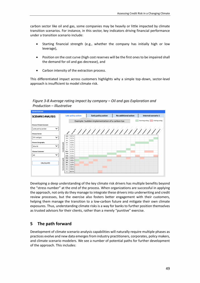
Assessing Credit Risk in a Changing Climate
49
carbon sector like oil and gas, some companies may be heavily or little impacted by climate transition scenarios. For instance, in this sector, key indicators driving financial performance under a transition scenario include:
• Starting financial strength (e.g., whether the company has initially high or low leverage),
• Position on the cost curve (high cost reserves will be the first ones to be impaired shall the demand for oil and gas decrease), and
• Carbon intensity of the extraction process.
This differentiated impact across customers highlights why a simple top-down, sector-level approach is insufficient to model climate risk.
Figure 3-8 Average rating impact by company – Oil and gas Exploration and Production – Illustrative
Developing a deep understanding of the key climate risk drivers has multiple benefits beyond the “stress number” at the end of the process. When organizations are successful in applying the approach, not only do they manage to integrate these drivers into underwriting and credit review processes, but the exercise also fosters better engagement with their customers, helping them manage the transition to a low-carbon future and mitigate their own climate exposures. Thus, understanding climate risks is a way for banks to further position themselves as trusted advisors for their clients, rather than a merely “punitive” exercise.
5 The path forward
Development of climate scenario analysis capabilities will naturally require multiple phases as practices evolve and new data emerges from industry practitioners, corporates, policy makers, and climate scenario modelers. We see a number of potential paths for further development of the approach. This includes:
TRANSITION RISK
Average changes in credit ratings by scenario
SCENARIO ANALYSIS
Choose Sector
Choose Geography
CALCULATE
Oil and gas
World
Choose Customer
All
Late policy action Early policy action No additional action Internal scenario 1
Late policy action
Choose Climate Scenario
Starting rating Ending ratingExample: Sudden implementation of a carbon tax

Chapter 3
50
• Creating financially oriented transition scenarios tailored to the vulnerabilities of individual institutions,
• Integrating transition risk assessment within organizations, and
• Building out climate scenario models to support financial risk analysis.
Most publicly available scenarios are primarily intended for a different purpose from financial risk assessment. The most sophisticated scenario models, such as the ones assessed in IPCC reports, are intended as energy-economy-climate models with policy and research applications, not for financial analysis. As a result, critical outputs for financial analysis are often unpublished or unavailable. Over the past few years, significant advancements have been made toward building a bridge between the scenario modelling practices of the scientific community and the credit risk analysis practices of the financial sector. For instance, the SENSES project, in which Oliver Wyman is participating, gathers the climate scenario modelers and various stakeholders (such as finance practitioners, policymakers, and corporates) to develop the new generation of climate change scenarios.4 This process highlighted a number of areas for future development, which include:
• New types of scenarios (such as disorderly transition scenarios),
• Improved model granularity,
• Ex post calculations to generate new financial risk variables, and
• Redesign of model reporting and outputs to track additional sector variables.
Integration of transition risk assessment in the organization The methodology outlined in this chapter provides for scenario-based assessment of transition risk. However, institutions need to go beyond risk assessment and disclosure to properly manage transition risks. As climate risks materialize, institutions would benefit from their broader incorporation into a range of business management and risk management processes at financial institutions.5 While specifics may differ across institutions depending on particular profiles, potential examples of areas for integration include:
• Integration of transition risk measurement across other risk measurement processes including physical risk,
• Embedding into risk identification processes,
• Incorporation of climate risk considerations in underwriting and credit rating processes,
• Consideration of climate-related limits and exposure monitoring,
4 For more information, please refer to: http://senses-project.org 5 For more details on the integration of climate-related considerations into traditional risk management frameworks, please
refer to “Climate Change, Managing A New Financial Risk,” IACPM and Oliver Wyman

Assessing Credit Risk in a Changing Climate
51
• Climate risk-related portfolio management and structuring,
• Consideration within business planning, strategic planning, and pricing,
• Adjustment of governance and organization, and
• Capturing climate risk in the risk appetite.
6 Conclusion
The potential disruption and financial implications of climate change are imminent. As the impact of climate change prompts high financial stakes and substantial structural adjustments to the global economy, financial institutions will face both climate risks and opportunities. Financial institutions need to treat climate risks as a financial risk, not just a reputational one, and integrate climate considerations into their financial risk management frameworks. The measurement management of climate risks is a new exercise and will continue to evolve. In helping financial institutions assess climate risks, we count on the compounding effect of these efforts. As the financial services industry adopts sound, analytical approaches for understanding climate risks, we believe it will become a significant governance and risk management topic. Investors will respond in kind, as the information created by climate disclosures drives their own capital allocations. A richer data environment can fuel more efficient capital markets. Through all these changes, increasing awareness of climate risks within the financial services industry will ultimately generate broad-based benefits for other industries and the society as a whole.

Chapter 4
52
Assessing Forward-Looking Climate Risks in Financial Portfolios: A Science-Based Approach for
Investors and Supervisors
By
Irene Monasterolo and Stefano Battiston1
Abstract
Climate risk is a new source of financial risk characterized by deep uncertainty, non-linearity, and endogeneity. Neglecting these characteristics leads to a severe underestimation of potential financial losses and gains. We present the CLIMAFIN methodology designed to help investors and financial institutions to address this challenge and to embed climate risk into pricing models and stress-tests. The method builds on the Climate Stress-test by Battiston et al. (2017), which has become over the years a reference tool for academics and practitioners. CLIMAFIN allows to translate forward-looking climate transition scenarios into financial shocks and to provide investors and financial supervisors with scenario-adjusted risk metrics and models (e.g. Climate Value at Risk, Climate Spread, Climate Stress-test). The chapter describes the technical details of the methodology and some recent policy applications carried out in collaboration with leading financial institutions.
Keywords: climate scenarios, climate transition risk, financial risk, risk management strategy, climate VaR, climate spread, climate stress-test, financial stability
1 Introduction
There is a growing consensus among scientists, central bank officials and financial supervisors that climate change is a new source of risks for the economy and financial stability, at both individual institution and system levels (Battiston et al., 2017). Climate-related financial losses can result from the misalignment of investments in the economy and finance with the climate and energy transition targets. It is broadly recognized that massively scaling up investments in low-carbon firms and sectors and phasing-out those in fossil-fuel power plants and carbon-intensive sectors are both needed to achieve climate targets laid out in the Paris Agreement (New Climate Economy, 2018).
In recent years, many central banks and academic institutions began to analyze climate-related financial risks that could stem from a disorderly transition to a low-carbon economy, consisting
1 This chapter is written by Irene Monasterolo (corresponding author, IM) and Stefano Battiston (SB). IM is an assistant
professor at Vienna University of Economics and Business, and visiting research fellow at Boston University’s Global
Development Policy Center, email: [email protected]. SB is SNF Professor of Banking at the University of Zurich,
and professor of Political Economy at Ca’Foscari University of Venice, email: [email protected]. The authors (IM
and SB) would like to thank Antoine Mandel (Paris School of Economics), Bas van Ruijven and Keywan Riahi (IIASA), Petr
Jakubik (EIOPA) for the useful comments and collaboration on the application of the methodology. We acknowledge the
support of the INSPIRE grant and of the FET H2020 project CLIMEX (Grant number 851876). IM acknowledges the support
of the Klimafonds+ project GreenFin, the H2020 CASCADES project (Grant number 821010) and of the OeNB’s Maria
Schaumeyer habilitationsstipendium, while SB recognizes the support of the Schwyzer Winiker Stiftung.
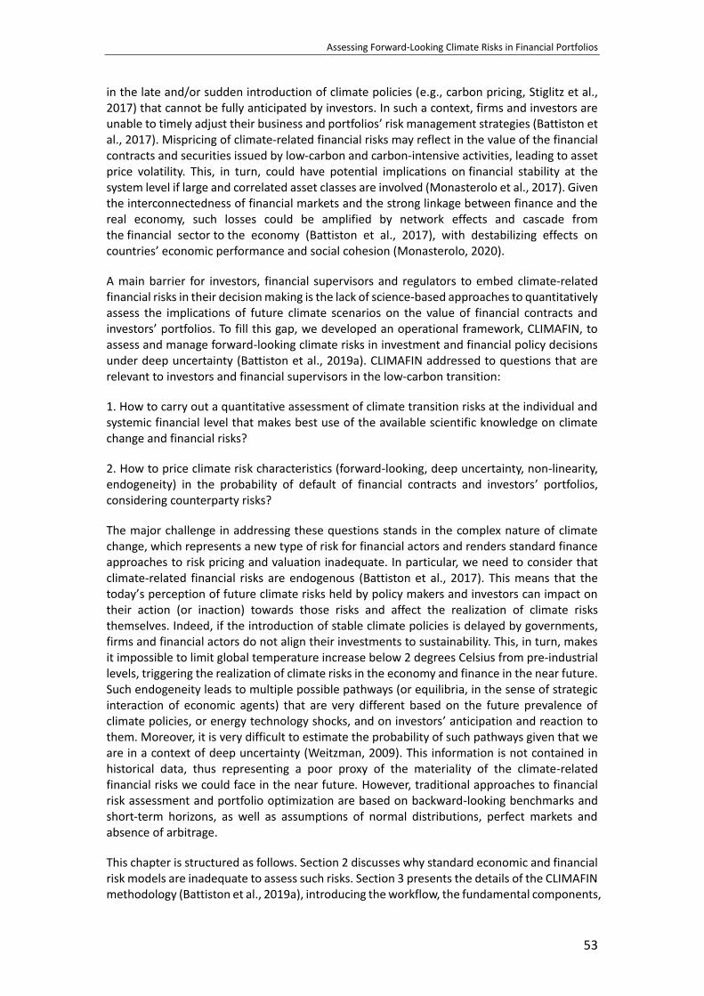
Assessing Forward-Looking Climate Risks in Financial Portfolios
53
in the late and/or sudden introduction of climate policies (e.g., carbon pricing, Stiglitz et al., 2017) that cannot be fully anticipated by investors. In such a context, firms and investors are unable to timely adjust their business and portfolios’ risk management strategies (Battiston et al., 2017). Mispricing of climate-related financial risks may reflect in the value of the financial contracts and securities issued by low-carbon and carbon-intensive activities, leading to asset price volatility. This, in turn, could have potential implications on financial stability at the system level if large and correlated asset classes are involved (Monasterolo et al., 2017). Given the interconnectedness of financial markets and the strong linkage between finance and the real economy, such losses could be amplified by network effects and cascade from the financial sector to the economy (Battiston et al., 2017), with destabilizing effects on countries’ economic performance and social cohesion (Monasterolo, 2020).
A main barrier for investors, financial supervisors and regulators to embed climate-related financial risks in their decision making is the lack of science-based approaches to quantitatively assess the implications of future climate scenarios on the value of financial contracts and investors’ portfolios. To fill this gap, we developed an operational framework, CLIMAFIN, to assess and manage forward-looking climate risks in investment and financial policy decisions under deep uncertainty (Battiston et al., 2019a). CLIMAFIN addressed to questions that are relevant to investors and financial supervisors in the low-carbon transition:
1. How to carry out a quantitative assessment of climate transition risks at the individual and systemic financial level that makes best use of the available scientific knowledge on climate change and financial risks?
2. How to price climate risk characteristics (forward-looking, deep uncertainty, non-linearity, endogeneity) in the probability of default of financial contracts and investors’ portfolios, considering counterparty risks?
The major challenge in addressing these questions stands in the complex nature of climate change, which represents a new type of risk for financial actors and renders standard finance approaches to risk pricing and valuation inadequate. In particular, we need to consider that climate-related financial risks are endogenous (Battiston et al., 2017). This means that the today’s perception of future climate risks held by policy makers and investors can impact on their action (or inaction) towards those risks and affect the realization of climate risks themselves. Indeed, if the introduction of stable climate policies is delayed by governments, firms and financial actors do not align their investments to sustainability. This, in turn, makes it impossible to limit global temperature increase below 2 degrees Celsius from pre-industrial levels, triggering the realization of climate risks in the economy and finance in the near future. Such endogeneity leads to multiple possible pathways (or equilibria, in the sense of strategic interaction of economic agents) that are very different based on the future prevalence of climate policies, or energy technology shocks, and on investors’ anticipation and reaction to them. Moreover, it is very difficult to estimate the probability of such pathways given that we are in a context of deep uncertainty (Weitzman, 2009). This information is not contained in historical data, thus representing a poor proxy of the materiality of the climate-related financial risks we could face in the near future. However, traditional approaches to financial risk assessment and portfolio optimization are based on backward-looking benchmarks and short-term horizons, as well as assumptions of normal distributions, perfect markets and absence of arbitrage.
This chapter is structured as follows. Section 2 discusses why standard economic and financial risk models are inadequate to assess such risks. Section 3 presents the details of the CLIMAFIN methodology (Battiston et al., 2019a), introducing the workflow, the fundamental components,

Chapter 4
54
input metrics and data used. Section 4 illustrates the output of the CLIMAFIN methodology (Climate Spread, the Climate Value at Risk (VaR) and the Climate Stress-test) as applied to equity holdings, corporate and sovereign bond portfolios held by financial institutions, in collaboration with central banks (e.g., Austrian National Bank (OeNB), Banco de Mexico (BdM)) and financial regulators (e.g., European Insurance and Occupational Pension Funds Authority (EIOPA)). In section 5, we conclude by discussing the applicability of science-based climate-financial risk metrics and methods to inform investors’ risk management strategies, and to support financial supervisors in identifying systemic climate-related financial risks and the designing prudential measures to mitigate them.
2 Climate change as a new type of risks for financial analysis
Climate change represents a new type of risk for financial actors and decision makers, because it is characterized by:
• Deep uncertainty: Due to the nature of the earth system, climate change is characterized by deep uncertainties in forecasting its realization and impact on humans and ecosystems. This is in part due to the presence of tail events (Weitzman, 2009) and tipping points after which the characteristics of the system change abruptly (Solomon et al., 2009). The more the system gets closer to such tipping points, the more the possibility of irreversible changes in the human-environmental system to occur, and with that the possibility of crossing of the planetary boundaries (Steffen et al. 2018) and of triggering domino effects (Lenton et al., 2019). Other sources of uncertainty refer to the assumptions on agents’ utility function, future productivity growth rate, and intertemporal discount rate used in cost-benefit analyses of climate change.
• Non-linearity: Recent research showed that the distribution of extreme climate-related events (heat/cold waves) is highly non-linear (Ackerman, 2017). Fourteen of the 15 hottest years on record were since 2000, while 2015-2019 was the hottest five-year period on record (WMO, 2019).
• Forward-looking nature of risk: The impacts of climate change are on the time scale of two decades or longer, while the time horizon of financial markets is much shorter (few months).
• Endogeneity: Climate-change risks are endogenous and depend on the risk perceptions of the agents involved. Indeed, the achievement of the climate targets depends on governments’ and firms’ investment decisions. But both types of decisions depend on their perceptions of the risks involved, which differ across the possible transition scenarios and trajectories (Battiston, 2019). Thus, the endogeneity between policies choices and investors’ expectations on the financial risks resulting from these policies generates the possibility of multiple equilibria. Green perception is likely to lead to green climate policy and green portfolio.
Climate change is expected to impact the economy and finance via physical and transition risks
(Carney 2015). However, while climate physical risks will be more visible in the medium-to-
long term, climate transition risks could happen earlier and be more financially relevant.
Further, it is now well recognized that in assessing climate-related financial risks, one should
not only consider the characteristics of climate risks, but also those of financial risks. Research
developed following the Great Financial Crisis highlighted the key role of financial complexity

Assessing Forward-Looking Climate Risks in Financial Portfolios
55
and financial actors’ interconnectedness in amplifying shocks via the reverberation of losses
within the financial network (Battiston et al. 2012, 2016) and in contributing to the building
up of systemic risk (Battiston et al. 2012).
These elements challenge the traditional approaches to financial risk assessment used by
investors and financial supervisors because they require a rethinking of the notion of
materiality of risks and, connected to that, the notion of time horizons, benchmarks and
coordination problems in investment decisions. Indeed, standard approaches to economic
and financial risk assessment stand on the identification of the most likely scenarios, on the
computation of expected values and on the calculation of risk metrics (e.g., volatility) based
on the historical values of market prices. In addition, they rely on strong assumptions of
market conditions and agents’ behaviors, including perfect information, normal distributions,
and a lack of arbitrage (Black & Scholes, 1973). These assumptions and characteristics are
clearly at odds with the characteristics of climate risks (and financial risks) and could lead to
underestimating the impact of climate change in risk assessment models, with relevant
implications on policy recommendations (DeFries et al., 2019).
3 The CLIMAFIN framework
CLIMAFIN methodology is a transparent and science-based approach to quantitatively assessing and pricing forward-looking climate risks and their characteristics (i.e., deep uncertainty, non-linearity and endogeneity) in the value of individual financial contracts and investors’ portfolio. More specifically, we can embed forward-looking climate transition scenarios provided by climate science and climate economic models (e.g., Integrated Assessment Models, IAMs) in:
• Probabilities of defaults of contracts and securities (i.e., introducing climate in financial pricing models for equity holdings, corporate and sovereign bonds)
• Quantitative metrics of financial risks used by investors, central banks and financial regulators (e.g., climate VaR, climate spread)
• A full-fledged Climate Stress-test rooted in financial network models.
Table 4-1 summarizes the purpose of CLIMAFIN and its characteristics along key dimensions such as coverage of scenarios, risk types and financial instrument types.

Chapter 4
56
Table 4-1: Purpose and characteristics of CLIMAFIN
Purpose
To enable investors, central banks and financial regulators to assess forward-looking climate risks (transition, physical) and opportunities in financial portfolios and identify drivers at the individual and system level.
Target users
CLIMAFIN can be customized for both private and public financial institutions, portfolios and types of financial contracts (e.g. equity holdings, corporate and sovereign bonds, loans). Existing applications have involved development finance institutions (e.g. China Development Bank), national central banks (e.g. OeNB, BdM), financial regulators (EIOPA) and commercial banks (European and US banks).
Climate scenarios covered
CLIMAFIN covers 2°C-aligned climate transition scenarios, including those characterized by a disorderly low-carbon transition (e.g., late and sudden introduction of climate policies and lack of full anticipation by investors). CLIMAFIN builds on the IEA Technological Roadmap as well as scenarios of emissions targets, energy technology trajectories and national contributions produced by IAMs used by the IPCC (2014, 2018), and their scenario databases, such as LIMITS Database 2 and Socio-Economic Shared Pathways and the most recent CD-Links3.
Risk types covered
The methodology allows users to compute the probability of default (PD) for individual financial contracts, the Climate Value at Risk (Climate VaR) and Expected Shortfall (ES), and the climate stress-test under forward-looking climate transition scenarios (including a disorderly transition) aligned to the 2°C target. The sectors covered, such as energy, utility, manufacturing and transportation, are those in the IEA technological roadmap and in the EU Reference Scenarios.
Risk transmission channels
CLIMAFIN has focused so far on transition risks arising from asset value adjustments according to the types of climate risks, the financial risk characteristics of the investors and their expectations of the impact of climate policies. Adjustments include economic and financial gains/losses (Gross Value Added (GVA), Probability of Default (PD)) due to i), exposures to high/low carbon activities (classified in Climate Policy Relevant Sectors (CPRS) and ii), delayed and disorderly alignment with climate targets that investors do not fully anticipate. If climate policies are credible, stable and anticipatable by investors, the portfolios will not experience large price volatilities that require asset revaluation. Our team is working to include physical risk transmissions. Recent application has focused on climate physical risk stemming from floods and sea-level rise.
Financial contracts covered
The methodology applies to loans, corporate and sovereign bonds and equity holdings, and cat bonds. Our team is working to integrate derivatives.
Granularity of the analysis
Risks at the firm level can be aggregated to the portfolio level and incorporated into standard financial risk metrics (see Climate VaR by Battiston et al., 2017). The level of granularity required depends on the depth of analysis and would normally include project and/or counterparty data.
2 The LIMITS Scenario Database is operated by the International Institute for Applied Systems Analysis (IIASA)
https://tntcat.iiasa.ac.at/LIMITSDB/dsd?Action=htmlpage&page=about 3 https://data.ene.iiasa.ac.at/iamc-1.5c-explorer/#/login?redirect=%2Fworkspaces

Assessing Forward-Looking Climate Risks in Financial Portfolios
57
Country-specific risks
We elaborate a dataset of proprietary trajectories based on country and sector specific progress towards their Nationally Determined Contributions (NDCs) and climate targets in order to incorporate country-level transition risks into standard metrics of sovereign risks (see the Climate Spread in Battiston & Monasterolo, 2019). The team is working to incorporate country-specific exposures to climate physical risks.
The CLIMAFIN framework provides a quantitative assessment arranged in a workflow of four modules. Figure 4-1 shows the interplay of the four modules in the CLIMAFIN workflow. Module 1 gathers and consolidates a database of climate science scenarios and climate transition scenarios, e.g., those provided by the IPCC (2018) and the NGFS (2019).
Module 2 uses the information from Module 1 to generate a large set of forward-looking climate transition scenarios that imply a shock on the low-carbon and carbon-intensive economic activities (respectively positive and negative) based on their energy technologies (i.e., specific renewable energy or fossil fuels based). Depending on the assumptions on the climate economic model used (e.g. IAMs) and the introduction of the policy (e.g. the value of the carbon tax), the policy shock can be computed either as difference across trajectories (Monasterolo et al., 2018) or as difference along time steps in the same trajectory (Battiston et al., 2017). when moving from the initial state of the economy, i.e., the Business as Usual (B), to a specific policy scenario (P). Using climate economics models (e.g., the IAMs), we calculate economic shocks (market share, Gross Value Added (GVA)) by region and sector of economic activity (e.g., low-carbon or carbon-intensive), conditioned to each scenario. The core of the feedback mechanism is as follows: the forward-looking climate transition scenarios imply a shock to the low-carbon and carbon-intensive economic activities (respectively positive and negative) based on their energy technologies (i.e., renewable energy or fossil fuels based). To associate a climate financial risk profile to the sectors of economic activities, Battiston et al. (2017) introduced the Climate Policy Relevant Sectors (CPRS), i.e., fossil fuels, low/high-carbon utility, low/high-carbon transportation, energy intensive manufacturing, housing.
Module 3 provides the information set of a risk-averse investor and carries out a valuation adjustment and a risk adjustment of individual financial contracts, i.e., in their Probability of Default (PD) based on the scenarios of economic shocks (by activity and its energy technology) obtained from Module 2. In particular, Module 3 uses the outcome of the economic shock on each economic activity and assets, and prices it in the PD and value of the financial contracts (equity holdings, corporate and sovereign bonds) issued by the activity, or in the loans associated to that.
Module 4 uses information on repricing of the contracts and computes distributions that allow to consider non-linearity and deep uncertainty of climate change in climate financial risk metrics (e.g. Climate VaR) and the Climate Stress-test. Rooted on financial valuation in network models, the Climate Stress-test allows to assess the largest losses for individual portfolios conditioned to climate scenarios, considering risk amplification and reverberation driven by financial interconnectedness, considering losses generated by direct and indirect exposures (second round losses, Battiston et al., 2017, Roncoroni et al., 2019).

Chapter 4
58
Figure 4-1 CLIMAFIN framework for climate financial risk assessment under deep uncertainty
Module 1 provides the information set combining science-based knowledge and market data to be used by financial supervisors and investors. Module 2 provides information on the economic shocks (positive and negative) associated with climate transition scenarios, at the level of economic activity. Modules 3 and 4 provide metrics and methods of financial risks to support investment and policy decision making in the transition to a carbon-neutral economy. Source: Battiston et al. (2019a)
Module 1. Database of climate science scenarios and climate economics scenarios
Module 1 gathers and consolidates the following sets of information:
• Sets of future climate change scenarios, as from the IPCC reports (IPCC, 2014, IPCC
2018), forecasts of GHG emission concentrations, temperature changes and socioeconomic impacts of climate change conditioned to the scenarios.
• Sets of economic trajectories under climate policy scenarios as provided by well-established economic models of climate change, e.g., IAMs 4 , partial or general economic equilibrium models that consider GHG emission targets and any physical damages resulting from climate change. For instance, the LIMITS database and the new CD-Links database provides scenarios of the evolution of different economic sectors’ output under various policy scenarios as computed by IAMs developed by leading academic institutions such as IIASA, PIK, and CMCC.
For instance, in the climate risk assessment of the sovereign bond portfolios of insurance companies in the European Union (EU), Battiston et al. (2019a) used the climate policy scenarios aligned to the 2°C target developed by the international science community and reviewed by the IPCC. They considered the stabilization concentration of CO2 at the end of
4 Note that IAMs consider only in very stylized way, if at all, the impact of climate change on the socioeconomic system. It
can be argued that the convex damage function used in this literature cannot account for the essential characteristics of
climate risks such as tail risk and climate tipping points. The approach presented here can be adapted to use trajectories
from economic models that would also account for these effects.
Value at Risk à
M2: SHOCKS ON SECTORS’ FORWARD-LOOKING TRAJECTORIES (market shares, GVA)
M1: CLIMATE SCENARIOS (EMISSIONS TARGETS)
M3: SHOCK ON FIRM’S CASH FLOWS AND FISCAL REVENUES
(IPCC 2014)
3 TWh from coal
7 TWh from renewables
Utility: 10TWh generation
M4: CLIMATE VAR AND CLIMATE STRESS TEST CONDITIONED TO CLIMATE SCENARIOS
M3: SHOCKS ON PD AND PRICE OF FINANCIAL CONTRACTS
Country
WITCH:
bond
shock
(%)
WITCH:
yield
shock
(%)
Austria 1,3 -0,16
Australia -17,36 2,45
Canada -5,21 0,67
Norway -14,82 2,05
Poland -12,85 1,75
Sources: Battiston & Monasterolo2019, Monasteroloea 2018
FEEDBACK ONECONOMIC STRUCTURE

Assessing Forward-Looking Climate Risks in Financial Portfolios
59
century consistent with the 2°C pledge under the Paris Agreement (i.e., 450 and 500 parts per million (ppm)). These are associated with two different policy implementation scenarios, i.e., Reference Policy (RefPol) and Strong Policy (StrPol) in the exercise conducted by LIMITS IAMs (Kriegler et al., 2013). RefPol assumes a weak near-term target by 2020 with fragmented countries’ actions to achieve emissions reduction by 2050, while StrPol assumes a stringent near-term target by 2020. The 500 and 450 ppm scenarios are associated with a probability of exceeding the 2°C target by 35-59% and 20-41% respectively. A change in climate policy (e.g. in the value of the carbon tax every five years) implies a change in the sectors' macroeconomic trajectory, thus a change in the market shares of primary and secondary energy sources. Currently, CLIMAFIN’s new analyses use the CD-Links post-Paris Agreement Scenarios.
Table 4-2 provides an overview of the scenarios and their comparisons (See Battiston & Monasterolo, 2019).
Table 4-2 LIMITS scenarios’ characteristics
Source: Table based on Kriegler et al. (2013), adapted in Battiston and Monasterolo (2019)
Module 2. Climate transition shock scenarios This module derives scenarios of economic shocks (positive or negative) at the level of economic activities, based on their energy technology and relevance for climate policy implementation from the information provided by Module 1.
First, based on climate science evidence from Module 1, we construct an event tree for the main possible scenarios relevant for climate transition risk, in a mid-term horizon of 2025-2030 or in a long-term horizon (2050), following the 5 years calculations of the IAMs. In particular, we provide an argument for how the current socioeconomic dynamics of opposing vested interests increases the likelihood of a disorderly low-carbon transition. This event tree can be defined for the zero-carbon energy transition needed to achieve the climate targets (IPCC, 2018) as in Figure 4-2:
No policy Base Baseline None N/A None
RefPol Reference Weak 2100 None
StrPol Reference Stringent 2100 None
450 Benchmark None N/A 450 ppm
500 Benchmark None N/A 500 ppm
Delayed Policy RefPol-450 Climate Policy Weak 2020 450 ppm
Delayed Policy StrPol-450 Climate Policy Stringent 2020 500 ppm
Delayed Policy RefPol-500 Climate Policy Weak 2020 500 ppm
Delayed Policy StrPol-500 Climate Policy Stringent 2020 500 ppm
Delayed Action RefPol2030-500 Climate Policy Weak 2030 501 ppm
Fragmented action
Immediate action
Scenario class Scenario name Scenario type
Level of ambition
(near term)
Level of ambition
(long term)
Level of international
cooperation

Chapter 4
60
Figure 4-2 Low-carbon transition’s main transition scenarios: chain of events in the transmission of economic and financial shocks
Second, based on the economic trajectories from Module 1, we derive a set of economic shocks (on output, market share and GVA) by region and sector of the economic activities (low-carbon and carbon-intensive). These shocks can be computed either across climate transition trajectories (Monasterolo et al. 2018), or within the same trajectory across years (Battiston et al. 2017). Since the current classifications of economic activities (e.g. NACE 4 digit) do not provide information on the sector’s exposure to climate risks, we classify economic activities relevant to climate transition risks into CPRS. These include fossil fuel, utility, energy-intensive, transport, housing, infrastructure, identified based on: the direct and indirect contributions of economic activities (classified at the NACE 4-digit level) to GHG emissions (Scope 1, 2, 3); their sensitivities to climate policy implementation (e.g. the EU carbon leakage directive 2003/87/EC); the technology mix of the activities and their role in the energy value chain; their investment plans, particularly the climate relevant part (e.g. CAPEX in Battiston et al., 2017). Doing so allows us to identify activities and sectors that will have the most impact on achieving climate targets and will also be impacted by climate transition risks. The CPRS classification was used by the European Central Bank (20195) and by EIOPA (20186) to assess financial actors’ exposure to climate transition risks in the EU.
Third, we consider the transition of the economy from a business-as-usual (BAU) trajectory to a given policy trajectory (P) compatible with a 1.5°C or a 2°C target:
• Shocks are obtained as differences in sectors’ output between the BAU and the climate policy shock trajectories (P) for the same model (e.g., IAMs7 ) that can be calculated either across trajectories or across years (2020 to 2100) within the same trajectory;
5 https://www.ecb.europa.eu/pub/financial-stability/fsr/special/html/ecb.fsrart201905_1~47cf778cc1.en.html#toc5 6 https://register.eiopa.europa.eu/Publications/Reports/EIOPA%20FSR%20December%202018.pdf 7 Note that other climate economic models could be used to provide shocks on output. We opted for IAMs because they
are the models reviewed by the IPCC report and used to inform climate policy discussion.
Orderly
Disorderly
Low-carbon transition scenarios: economic and financial shocks transmission tree
After 2030/never
Governments introducetimely and coordinatedclimate policies aimed toachieve the 2˚C target(e.g. a carbon tax alignedto Stiglitz et al. 2017)
The pathway is predictable.Market players cananticipate the shift fromfossil fuel to renewableenergy sources and price itin their business models
No aggregate shocks on assetprices. While there isidiosyncratic risk related toindividual firms’performances, there is nosystemic risks.
Governments cannot (ormay want not) introducetimely and coordinatedclimate policies. Thetransition may take placebut it will be disorderly.
Aggregate shocks on asset prices (volatility) could occur triggering potential individual and systemic risks. These, in turn, could affect financial stability.
Uncertainty characterisesthe transition. Marketplayers can anticipate theshift from fossil fuel torenewable energy and priceit in their business models.
Temperature increases for centuries, leading to irreversible changes to the earth system (tipping points, domino effects)
Climate policies are never introduced. The energy transition never takes place.
Large shocks on GDP drivenby resource scarcity and shock on productivity andprofitability trigger systemic financial risk.

Assessing Forward-Looking Climate Risks in Financial Portfolios
61
• We need to depart from the idea of “most likely/feasible scenario” and consider sets of several scenarios (see Table 4-2) to be able to determine (in Module 4) how wrong could an investor be in computing the Climate VaR of her portfolio.
• The disorderly transition is thus intended as a temporary out-of-equilibrium shift of the economy between two separate equilibrium trajectories based on the energy technology that drives the transition. This formulation makes the exercise familiar to economists because they are consistent with traditional economic models’ rationale.
Module 3. Shock scenario-adjusted financial pricing and risk valuation This module integrates forward-looking climate transition risk scenarios in financial risk-pricing models and quantitative financial risk metrics used by investors and financial supervisors, such as Climate Spread (Battiston & Monasterolo, 2019) and Climate VaR (Battiston et al., 2017). The Climate Spread is defined as the change in the spread of a corporate or sovereign bond contract conditional on a given Climate Policy Shock Scenario, thus introducing future climate risks in the assessment of firms or countries’ financial solvency. The Climate VaR can be defined as the “worst-case loss” conditioned to future climate shock scenarios given a certain confidence level.
From the sectorial economic shock trajectories based on climate transition scenarios (Module 2), we compute the financial shocks on the cashflows of individual economic activities comprising the sector. We then translate the shock on the cashflows in the adjustments of PDs of individual firms and sovereign governments, and in the adjustment of risks and values of the individual risky financial contracts (equity holdings, corporate and sovereign and bonds). In this step, we develop climate-based financial pricing models and financial risk metrics (e.g. Climate Spread, Climate VaR) embedded in the forward-looking climate shock trajectories, accounting for the deep uncertainties of climate risks.
Our approach stands on the definition of the Information Set of a risk-averse investor who aims to minimize the largest climate-related losses to her portfolio. We define an information set that can accommodate incomplete information and deep uncertainty (Greenwald & Stiglitz, 1986) and can cover a time horizon that is relevant both for investment strategies and for the low-carbon transition (e.g. from 2020 to 2050). The investor’s information set comprises (Battiston et al., 2019a):
• Climate policy scenarios corresponding to Greenhouse Gases (GHG) emission reduction target across regions), provided e.g. by IPCC reports;
• Future economic trajectories for carbon-intensive and low-carbon activities conditioned to climate scenarios, provided by climate economic models (e.g., IAMs);
• Forward-looking Climate Policy Shock Scenarios intended as a disorderly transition from B (Business as Usual) to P (a given climate policy scenario). These can be computed either across trajectories or across years within the same trajectory;
• Climate Policy Shocks on the economic output of low-carbon/carbon-intensive activities, on their Gross Value Added (GVA) and their contribution to the fiscal revenues of the sovereign government. The policy shocks are under transition scenarios and in a specific climate economic model.

Chapter 4
62
3.3.1 Pricing forward-looking climate risks into equity holdings We introduce a valuation model where 𝑡0 denotes the time at which valuation is carried out and E denotes a generic equity contract. In the absence of climate policies, we assume that all relevant information is captured by the expected future flow of dividends.
Following Gordon's formulation (Gordon 1959), we further consider that dividends grow at a
constant rate 𝑔(𝐵) so that for all 𝑡 ≥ 𝑡0; 𝑑𝑖𝑣(𝑡 + 1) = (1 + 𝑔(𝐵))𝑑𝑖𝑣(𝑡)
Denoting by 𝑟 the cost of risky capital, the value of equity is then determined as the net
present value of future dividends equal to 𝑉𝐸𝐵,𝑡0:
Where
𝑑𝑖𝑣 (B) = 𝑑𝑖𝑣(𝑡0).
If we assume a climate policy shock to occur at time 𝑡∗, dividend is assumed to shift to 𝑑𝑖𝑣(P) and the growth rate of dividends to 𝑔(𝑃) where P identifies a specific climate policy scenario.
The value of equity is then determined as 𝑉𝐸𝑃,𝑡∗
If the climate policy shock occurs at valuation time, i.e., 𝑡∗ = 𝑡0, we have
In a climate policy scenario P, it is expected that 𝑑𝑖𝑣(P) and 𝑔(𝑃) decrease for carbon- intensive economic activities and increase for low-carbon economic activities.
From the equity valuation under climate scenarios, we can then assess:
The change of valuation in the case of a disorderly transition occurring at time 𝑡∗ given by
𝑉𝐸𝐵,𝑡0 - 𝑉𝐸
𝑃,𝑡∗
Given a probability distribution P on the time of occurrence and/or the impact of the policy scenarios, we can compute Climate VaR associated with an equity contract. Climate VaR is a quantile of loss distributions conditioned to climate policy shocks scenarios, which could be either characterized by physical or transition risks (Battiston et al., 2017), in a given time. The Climate VaR, then, defines the largest losses (usually in USD) in the value of a risky asset (e.g., equity holdings and bonds) or portfolio that the investor should withstand, conditioned to a given scenario, confidence level and time. Thus, the Climate VaR is a measure of risk of investment under forward-looking climate scenarios. The Climate VaR Management Strategy can be written as:

Assessing Forward-Looking Climate Risks in Financial Portfolios
63
The VaR, despite being well known and used by investors, has two main limitations in this
context. First, VaR is computed assuming knowing how the loss will be distributed, and this leads to model risk. Second, VaR depends linearly on the PD of underlying assets, thus
implying that small errors have small consequences. However, the PD of leveraged investor depends non-linearly on PD of underlying assets, thus implying small errors can have big consequences. But, importantly, VaR does not consider leverage. This means that to assess the financial risk implications of climate change, we need to go beyond VaR and consider interconnected financial actors, leverage financial agents with overlapping portfolios, i.e., the conditions for systemic risk in financial networks (Battiston et al., 2016). This is a main feature of CLIMAFIN, as well as the possibility to be applied to other risk metrics, such as the Expected Shorfall (ES). This is the average of all the losses above the VaR (i.e., the largest losses), and gives us a measure of what we can expect in terms of losses on our portfolio.
For a complete explanation of the pricing of forward-looking climate transition risks in the value of equity holdings, see Battiston and Monasterolo (2019).
3.3.2 Pricing forward-looking climate risks into corporate and sovereign bonds We consider a risky (defaultable) bond issued by a corporate issuer j, issued at 𝑡0 with maturity T. The value of the defaultable bond at time T, with R being the Recovery Rate of the corporate bond (i.e., the percentage of notional recovered upon default), and LGD being the Loss-Given-Default (i.e., the percentage loss), can be written as:
𝑣𝑗(𝑇) = {𝑅𝑗 = (1 − 𝐿𝐺𝐷𝑗) 𝑖𝑓 𝑗 𝑑𝑒𝑓𝑎𝑢𝑙𝑡𝑠 (𝑤𝑖𝑡ℎ 𝑝𝑟𝑜𝑏𝑎𝑏𝑖𝑙𝑖𝑡𝑦 𝑄𝑗)
1 𝑒𝑙𝑠𝑒 (𝑤𝑖𝑡ℎ 𝑝𝑟𝑜𝑏𝑎𝑏𝑖𝑙𝑖𝑡𝑦 1 − 𝑄𝑗)
The unitary price 𝑃𝑗(𝑡) of the bond at time 𝑡 < 𝑇 and 𝑡 > 𝑡0 follows the usual definition of
discounted expected value at the maturity:
𝑃𝑗(𝑡) = exp(−𝑟𝑓(𝑇 − 𝑡)) 𝐸[𝑣𝑗(𝑇)]= exp (−𝑟𝑓(𝑇 − 𝑡)) (1 − 𝑄 𝐿𝐺𝐷)
The bond price 𝑣𝑗∗ is equal to the bond discounted expected value, with 𝑦𝑓 risk-free rate, i.e.,
the yield of the bond facing no default risk (e.g. the German bond in the case of sovereign bonds, see Battiston & Monasterolo, 2019). The cumulative probability of default Q is related
to the probability of default at t as follows: Q = 1 – (1 − q)(𝑇−𝑡). The formula can be used to determine, from the market price, the value of the annual default probability q (i.e., q implied) for a given risk-free rate and LGD. In the case of a multi-coupon bond, the formula gets more complicated since one must sum up the expected value of the coupons, but the logic remains the same. For each coupon k, the coupon amount is assumed to be paid only if j has not defaulted before.
The bond price is defined implicitly by the yield 𝑦𝑗 of bond j (under risk neutral measure) as
follows:
𝑣𝑗∗ = 𝑒−𝑦𝑗𝑇
We can define the Probability of Default (PD) 𝑞𝑗(𝑃) of the corporate bonds’ issuer j under
Climate Policy Scenario P as:
𝑞𝑗(𝑃) = 𝒫 (𝜂𝑗 < 𝜃𝑗(𝑃)) = ∫ 𝜙(𝑃)(𝜂𝑗)𝑑𝜂𝑗𝜃𝑗(𝑃)
𝜂𝑖𝑛𝑓

Chapter 4
64
where 𝜙(𝑃)(𝜂𝑗) is the probability distribution of idiosyncratic shock 𝜂𝑗, and 𝜂𝑖𝑛𝑓 is the lower
bound of the range of the value of 𝜂𝑗.
We report a result on the PD adjustment. In simple terms, conditioned to the climate policy shock, there is a shift ∆𝑞 in the probability distribution of the small productivity shocks and thus in the default probability of issuer j:
∆𝑞𝑗(𝑃)= 𝑞𝑗(𝑃) - 𝑞𝑗(𝐵) = ∫ 𝜙(𝜂𝑗)𝑑𝜂𝑗𝜃𝑗(𝑃)
𝜂𝑖𝑛𝑓, with 𝜃𝑗(𝑃) = 𝜃𝑗(𝐵) - 𝜉𝑗(𝑃)
Thus, assuming that the climate policy shock on the fiscal revenues of the firm (and thus of the sovereign) is proportional to the shock on the GVA of low-carbon and carbon-intensive
sectors, i.e., 𝜉𝑗 = 𝜒𝑗𝑢𝑗,𝑠𝐺𝑉𝐴(P), with elasticity 𝜒𝑗 , then the adjustment ∆𝑞𝑗(𝑃), the PD of j in a
Climate Policy Shock Scenario:
• Increases with the GVA shock magnitude |𝑢𝑗,𝑠𝐺𝑉𝐴(P)| if 𝑢𝑗,𝑠
𝐺𝑉𝐴(P)<0, decreases vice versa;
• Is proportional to the GVA shocks on CPRS (in the limit of small Climate Policy Shocks).
The bond spread can be defined then as:
𝑠𝑗 =𝑦𝑗−𝑦𝑓, with 𝑒−𝑦𝑗𝑇 = 1 − 𝑞𝑗 𝐿𝐺𝐷𝑗
The Climate Spread Δ𝑠𝑗 is defined as the change in the spread of a bond contract conditional
upon a Climate Policy Shock Scenario:
For a complete explanation of the pricing of forward-looking climate transition risks in the value of corporate and sovereign bonds, see Battiston and Monasterolo (2019).
Required input data From the perspective of the user, the application of the CLIMAFIN methodology requires the following information on the portfolio of investments to be collected and analyzed:
• Financial securities (listed equities, corporate and sovereign bonds): identifier of the financial security, e.g. ISIN code, TICKER and LEI of the issuer;
• Financial securities (unlisted equities and loans): LEI of the firm, full legal name, location of incorporation. Same information for the parent company;
• The NACE sector of the economic activities of the firm that issue the contract (at 4-digit level, if possible);
• The composition of financial actors’ investments in financial securities (i.e., their exposure);
• Information on the characteristics of the financial securities and time series data (e.g., duration, maturity, coupon, term, prices, etc.).
All financial information (except loans) can be collected using financial data providers (e.g., Bloomberg, Thomson Reuters Eikon, etc.).

Assessing Forward-Looking Climate Risks in Financial Portfolios
65
In addition to the financial input data, the following climate and energy data are needed:
• Measures of economic shocks associated with climate scenarios and provided by IAMs (Kriegler et al., 2013; McCollum et al., 2018);
• Contributions from fossil fuels and renewable energy sectors to the individual countries’ GVA (e.g. Eurostat, IEA);
• Data on country’s macroeconomic and financial aggregates (e.g., debt/GDP, deficit, etc.) provided by national or international statistical offices (e.g., Eurostat, OECD).
4 Applications to portfolios of financial institutions
In this section, we present several applications of the CLIMAFIN approach to the risk analysis of investment portfolios.
Climate risk assessment of insurance companies’ sovereign bond portfolio The CLIMAFIN framework was recently applied to a forward-looking climate transition risk assessment of sovereign bond portfolios of insurance companies in Europe, as a result of the first collaboration between climate economists, climate financial risk modelers and financial regulators (Battiston et al., 2019b). The analysis considers forward-looking scenarios characterized by a disorderly introduction of climate policies (i.e., carbon pricing) and lack of full anticipation and pricing by investors.
The authors first computed the shocks on market shares and profitability of carbon-intensive and low-carbon activities that contribute to the GVA and fiscal revenues of the EU countries, which in turn issue the sovereign bonds that are held in the portfolios of European insurers. The shocks are calculated with climate economic models that provide climate transition trajectories for fossil fuel and renewable energy and electricity sectors, conditioned to 2°C-aligned climate policy scenarios. After defining the climate risk management strategy under uncertainty for a risk averse investor (insurer) that aims to minimize the largest losses in her sovereign bonds’ portfolio, the authors price the climate transition scenarios in the PD of the individual sovereign bonds and in the bonds’ climate spread. The results (see e.g., Figure 4-3) show that the impact of a disorderly transition to the low-carbon economy on the sovereign bonds’ portfolios of European insurers, under 2°C-aligned climate policy scenarios, are moderate but non-negligible. In particular, shocks on bonds’ value are heterogeneous across countries and reflect the progress towards decarbonization of countries’ economies. Most negative impacts affect the portfolios of insurance solos exposed to Polish sovereign bonds.
Two dimensions drive the magnitude of the impact of climate shocks on bonds’ portfolios. First, for each sovereign bond, negative shocks (e.g., on primary energy fossil sector) can be possibly compensated by positive shocks (e.g., on secondary energy electricity based on renewable sources). Second, in a portfolio of sovereign bonds issued by several countries, negative aggregate shocks from a less climate-aligned sovereign can be possibly compensated by positive shocks from another more climate-aligned sovereign. These two dimensions contribute to limit the magnitude of the median value of the portfolio impact in the chart.

Chapter 4
66
Figure 4-3 Distribution of impact on sovereign holdings of European insurers
Note: The length of the bars represents the heterogeneity of impacts on insurers domiciled in the given country (wider distribution). Y-axis represents negative impact (percentage of the original value of government portfolios) of climate policy shocks on the value of sovereign bonds (e.g. 100% expresses 0% impact, 97% corresponds to drop of 3%). The estimated impact is based on the country of the holder (issuing country), across climate policy shock scenarios and under the scenario of adverse market conditions. Source: Battiston et al. (2019b)
This work aims to raise the awareness of climate risks to insurers as well as of regulators and financial supervisors, and provide an approach to include climate risks into their risk assessment frameworks. This requires moving from the backward-looking nature of traditional financial risk assessment to a forward-looking assessment that considers both climate uncertainty and financial complexity.
Climate risk assessment of sovereign bond portfolio of the Austrian National Bank (OeNB)
Battiston and Monasterolo (2019) assessed the climate risk exposure of OeNB’s portfolio of sovereign bonds issued by OECD countries (10 years, zero coupon). They considered forward-looking climate transition trajectories produced by two climate economic models (used to calculate energy and electricity trajectories consistent with the 2°C targets and used by the IPCC report, i.e., GCAM and WITCH8 ), conditioned to several mild and tight climate policy scenarios characterized by carbon pricing (Kriegler et al., 2013). They then modelled the impact of the change in low-carbon and carbon-intensive sectors’ profitability on the GVA and fiscal revenues of each individual OECD country. Finally, they priced the shock on the fiscal revenues in the PD of the sovereign bond of the issuing country, on the bond price and yield, i.e., the Climate Spread. Results show that the level of (mis)alignment of a country’s economy with low-carbon transition, under feasible climate transition scenarios, can be priced in the sovereign bond and affect the country’s financial risk position. In particular, as Table 4-3 shows, the largest negative shocks on the value of individual sovereign bonds are on countries where fossil fuel-based primary and secondary energy sources represent a large contribution to GVA and national GDP, e.g., Australia and Poland. In contrast, sovereign bonds of countries with
8 The Global Change Assessment Model (GCAM) is the IAM developed by the Joint Global Change Research Institute in
Maryland to explore the dynamics of the coupled human-Earth system and the response of this system to global change
(http://www.globalchange.umd.edu/gcam/). WITCH is the IAM global dynamic model integrating the interactions between
the economy, the technological options, and climate change. It is developed at the RFF-CMCC-EIEE European Institute on
Economics and the Environment in Milan (IT): www.witchmodel.org
95%
96%
97%
98%
99%
100%
101%
PL HU DE SK AT GR BE SI LV IT UK ES PT NL LT EE DK FI LU FR IE NO BG MT LI CY HR CZ SE
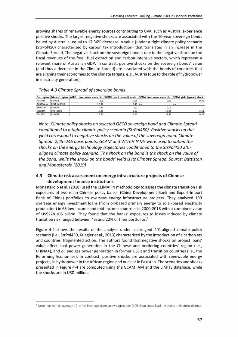
Assessing Forward-Looking Climate Risks in Financial Portfolios
67
growing shares of renewable energy sources contributing to GVA, such as Austria, experience positive shocks. The largest negative shocks are associated with the 10-year sovereign bonds issued by Australia, equal to 17.36% decrease in value (under a tight climate policy scenario (StrPol450) characterized by carbon tax introduction) that translates in an increase in the Climate Spread. The negative shock on the sovereign bond is due to the negative shock on the fiscal revenues of the fossil fuel extraction and carbon-intensive sectors, which represent a relevant share of Australian GDP. In contrast, positive shocks on the sovereign bonds’ value (and thus a decrease in the Climate Spread) are associated with the bonds of countries that are aligning their economies to the climate targets, e.g., Austria (due to the role of hydropower in electricity generation).
Table 4-3 Climate Spread of sovereign bonds
Note: Climate policy shocks on selected OECD sovereign bond and Climate Spread conditioned to a tight climate policy scenario (StrPol450). Positive shocks on the yield correspond to negative shocks on the value of the sovereign bond. Climate Spread: 2,45=245 basis points. GCAM and WITCH IAMs were used to obtain the shocks on the energy technology trajectories conditioned to the StrPol450 2°C-aligned climate policy scenario. The shock on the bond is the shock on the value of the bond, while the shock on the bonds’ yield is its Climate Spread. Source: Battiston and Monasterolo (2019)
Climate risk assessment on energy infrastructure projects of Chinese development finance institutions
Monasterolo et al. (2018) used the CLIMAFIN methodology to assess the climate transition risk exposures of two main Chinese policy banks’ (China Development Bank and Export-Import Bank of China) portfolios to overseas energy infrastructure projects. They analyzed 199 overseas energy investment loans (from oil-based primary energy to solar-based electricity production) in 63 low-income and mid-income countries in 2000-2018 with a combined value of US$228.105 billion. They found that the banks’ exposures to losses induced by climate transition risk ranged between 4% and 22% of their portfolios.9
Figure 4-4 shows the results of the analysis under a stringent 2°C-aligned climate policy scenario (i.e., StrPol450, Kriegler et al., 2013) characterized by the introduction of a carbon tax and countries' fragmented action. The authors found that negative shocks on project loans’ value affect coal power generation in the Chinese and bordering countries' region (i.e., CHINA+), and oil and gas power generation in former USSR and transition countries (i.e., the Reforming Economies). In contrast, positive shocks are associated with renewable energy projects, in hydropower in the African region and nuclear in Pakistan. The scenarios and shocks presented in Figure 4-4 are computed using the GCAM IAM and the LIMITS database, while the shocks are in USD million.
9 Note that with an average 12-times leverage, even an average shock (10% circa) could lead the banks to financial distress.
Geo region Models’ region WITCH: bond value shock (%) WITCH: yield (spread) shock GCAM: bond value shock (%) GCAM: yield (spread) shock
AUSTRIA EUROPE 1,3 -0,16 0,13 -0,02
AUSTRALIA REST_WORLD -17,36 2,45 n.a. n.a.
BELGIUM EUROPE 0,84 -0,1 0,03 0
CANADA PAC_OECD -5,21 0,67 -18,29 2,61
POLAND EUROPE -12,85 1,75 -2,49 0,32

Chapter 4
68
Figure 4-4 Climate financial risk assessment of Chinese overseas energy projects
Note: Projected gains and losses of China Development Bank and Export-Import Bank of China’s overseas energy loans portfolio (project based) conditioned to stringent 2°C-aligned climate policy scenarios (in million USD). Source: Monasterolo et al. (2018)
Climate Stress-test of the financial system In 2017, Battiston et al. (2017) published a Climate Stress-test exercise that provides an application of financial valuation in network models to the analysis of equity portfolios of banks exposed to climate transition risks. First, the authors assessed investors’ exposure to climate transition risk using the CPRS classification. Then, with the climate stress-test, they assessed the first and second-round losses of investors’ portfolios conditioned to climate transition scenarios, i.e., the indirect losses due to devaluation of counterparties' debt obligations on the interbank market, using the DebtRank10. They further calculated the Climate VaR, conditioned to different climate transition scenarios provided by IAMs and under low-carbon or high-carbon investment strategies, of the 20 most exposed banks in the EU and US (Figure 4-5).
The authors found that the exposure of institutional investors to climate transition risk is largely heterogenous and amplified by network effects. In particular, the exposures of pension and investment funds to CPRS reached 43-45% of equity portfolios, and the potential losses could be amplified by the mutual exposures of financial actors (e.g., pension funds and investment funds). Roncoroni et al. (2019) further developed the climate stress-test applied to Banco de Mexico’s portfolio using the Asset Network Valuation Framework (NEVA) approach (Barucca et al., 2019).
Battiston et al. (2017)’s Climate Stress-test considered micro-level climate transition risks, i.e., the exposures of individual banks to individual financial contracts (equity holdings) and computed the Climate VaR (VaR 95, i.e., 5%) on largest EU and US banks’ portfolios, assessing the impact of a disorderly transition on banks’ capital. They found that banks with a “environmentally unsustainable” investment strategy (i.e., those mostly exposed to fossil fuel and carbon intensive firms) incur large losses (Figure 4-5 left chart) in comparison to banks with a greener investment strategy (Figure 4-5 right chart). Moreover, the losses via first round (i.e., due to direct effects, dark colors) are amplified by risk reverberation and contagion of
10 The DebtRank is a reference measure of systemic financial impact developed by Battiston et al. (2012).It is inspired by
feedback-centrality and allows to determine the systemically important nodes in a network to assess drivers of systemic
financial risk.

Assessing Forward-Looking Climate Risks in Financial Portfolios
69
intra-financial contracts (i.e., the indirect effects, lighter colors). For instance, with regards to the two most exposed banks, Deutsche Bank’s losses on capital are driven by direct effects, while Credit Agricole’s losses are driven by indirect effects. This means that the largest banks are heterogeneously exposed to climate transition risk and the related losses could be amplified by financial interconnectedness, with implications on asset price volatility and financial stability (Monasterolo et al., 2017).
Figure 4-5 Climate Value at Risk (VaR) of EU largest banks conditioned to low-carbon or high-carbon investment strategy
Note: The Climate VaR (5%) analysis is conducted on the equity holdings of 20 most severely affected banks, under scenario of renewable (green, left chart) and fossil fuel and carbon intensive (brown, right chart) investment strategies, in USD million. Dark (light) color represents first (second) round losses. The analysis is based on the financial network model by Battiston et al. (2012) that introduced the DebtRank. Source: Battiston et al. (2017)
5 Conclusion
In this chapter, we presented CLIMAFIN, a transparent and science-based approach vetted by academics and practitioners. CLIMAFIN allows to translate forward-looking climate transition scenarios into financial shocks and to provide investors and financial supervisors with scenario-adjusted risk metrics and models (i.e., Climate Spread, Climate VaR and Climate Stress-testing).
The innovative approach of CLIMAFIN supports private and public financial institutions in their portfolio risk management strategies. It also provides financial supervisors with a methodology, independent from the ones developed by the industry, in order to inform the design of regulations to foster financial stability in the low-carbon transition.
Embedding climate risk into financial risk metrics requires to connect areas of knowledge which have remained separated so far and developed in parallel by climate scientists, climate

Chapter 4
70
economists, financial risk and network experts. Moreover, this interdisciplinary endeavor would not be possible without the long-term dedication of academic researchers.
The CLIMAFIN applications addresses three important elements of climate-financial risk assessment. First, the temporal scale of the problem and its uncertainty compel us to move from a stress-test approach based on a single type of scenarios to a set of scenarios, to be able to compute the Climate VaR conditioned to the uncertainty that characterizes the scenarios. Second, the assumptions of the scenarios matter for their use in financial assessment. New generation of climate scenarios assumes that countries are on track to deliver on their 2030 climate pledges, and do not consider the role of finance nor its complexity in achieving the scenarios, implying that funds for undertaking even massive investments in energy technology (and change the energy technology composition) are always available with no frictions. However, in reality, financing (in particular to low-carbon energy investments) is constrained and affects the likelihood of the transition scenarios. Third, the information gaps at firm level (e.g., the energy technology and emissions profile) mean imperfect information for investors about their exposure to climate risks via firms’ contracts (e.g., stocks, bonds, or loans). Greenhouse gases (GHG) emissions accounting suffers from limited availability, comparability and relevance for climate policy (Monasterolo et al., 2017). In contrast, in the definition of the activities that are exposed to transition risk, i.e., the CPRS, CLIMAFIN considers not only GHG direct and indirect emissions of activities but also their relevance for climate policy implementation, their role in the energy value chain, and firms’ future investment plan (e.g. CAPEX). CLIMAFIN has been applied to several portfolios (e.g., equity holdings of EU and US largest banks, sovereign bonds’ portfolios of European insurance firms and central banks, syndicated loans of US banks, etc.) and is supporting several central banks and financial regulators’ climate financial risk assessment exercises. CLIMAFIN has been recently extended to the analysis of the exposure of US banks’ loans to climate physical risks (storms and floods) impacting on firms and sectors’ capital intensity, at a granular geographical level, and computing the Value-
at-Risk (95 and 99 percentile by Battiston et al., 2020).
The result indicates that under several climate scenarios, the potential impact of a disorderly transition to a low-carbon economy on financial actors (e.g., pension funds, investment funds and insurers, development banks) is considerable. In addition, investors’ exposures to climate risks are large and can be amplified by financial complexity, potentially creating new sources of risk for economic and financial stability.
Regarding climate transition risks, current CLIMAFIN’s developments focus on the refinement of the disorderly transition scenarios in collaboration with the IAM community, including SSPs and Post-Paris Agreement scenarios, and the analysis of the feedbacks of the climate financial
shocks Battiston et al., 2020. Regarding the climate physical risk scenarios, the CLIMAFIN team
is working at the refinement of the shocks’ transmission to the individual firms at a granular geo-localized level, in collaboration with development finance institutions (e.g., the World Bank), using microlevel data.

Assessing Forward-Looking Climate Risks in Financial Portfolios
71
Bibliography
Ackerman, F. (2017). Worst-Case Economics: Extreme Events in Climate and Finance: Anthem Press.
Barucca, P., Bardoscia, M., Caccioli, F., D'Errico, M., Visentin, G., Battiston, S., & Caldarelli, G. (2019). Network valuation in financial systems. Mathematical Finance.
Battiston, S., Mandel, A., & Monasterolo, I. (2020). CLIMAFIN Assessing climate physical risk for banks. UNEPFI Pilot project on implementing TCFD recommendations for banks.
Battiston, S. (2019). The importance of being forward-looking: managing financial stability in the face of climate risk. Banque de France's Financial Stability Review(23), 39-48.
Battiston, S., Mandel, A., & Monasterolo, I. (2019a). CLIMAFIN handbook: pricing forward-looking climate risks under uncertainty. Working Paper available at SSRN http://dx.doi.org/10.2139/ssrn.3476586
Battiston, S., Jakubik, P., Monasterolo, I., Riahi, K., and van Ruijven B. (2019b). Climate risk assessment of sovereign bonds’ portfolio of European insurers. In: European Insurance and Occupational Pension Authority (EIOPA) Financial Stability Report,
https://www.eiopa.europa.eu/sites/default/files/publications/eiopa_financial_stabilty_report_-_december_2019.pdf
Battiston, S., & Monasterolo, I. (2019). A climate risk assessment of sovereign bonds’ portfolio. Working Paper available at SSRN https://papers.ssrn.com/sol3/papers.cfm?abstract_id=3376218
Battiston, S., Mandel, A., Monasterolo, I., Schütze, F., & Visentin, G. (2017). A climate stress-test of the financial system. Nature Climate Change, 7(4), 283-288.
Battiston, S., Caldarelli, G., May, R. M., Roukny, T., & Stiglitz, J. E. (2016). The price of complexity in financial networks. Proceedings of the national academy of sciences, 113(36), 10031-10036.
Battiston, S., Puliga, M., Kaushik, R., Tasca, P., & Caldarelli, G. (2012). Debtrank: Too central to fail? financial networks, the fed and systemic risk. Scientific reports, 2, 541.
Black, F., & Scholes, M. (1973). The pricing of options and corporate liabilities. Journal of political economy, 81(3), 637-654.
Carney, M. (2015). Breaking the Tragedy of the Horizon–climate change and financial stability. Speech given at Lloyd’s of London, 29, 220-230.
DeFries, R. S., Edenhofer, O., Halliday, A. N., Heal, G. M., Lenton, T., Puma, M., . . . Schellnhuber, H. J. (2019). The missing economic risks in assessments of climate change impacts.
Greenwald, B. C., & Stiglitz, J. E. (1986). Externalities in economies with imperfect information and incomplete markets. The quarterly journal of economics, 101(2), 229-264.
IPCC. (2018). Global Warming of 1.5◦C - Summary for Policymakers. Technical Report Intergovernmental Panel on Climate Change.
IPCC. (2014). Climate change 2014: synthesis report. Contribution of Working Groups I. II and III to the fifth assessment report of the Intergovernmental Panel on Climate Change, 151.
Kriegler, E., Tavoni, M., Aboumahboub, T., Luderer, G., Calvin, K., Demaere, G., . . . Schaeffer, M. (2013). What does the 2 C target imply for a global climate agreement in 2020? The LIMITS study on Durban Platform scenarios. Climate Change Economics, 4(04), 1340008.
McCollum, D. L., Zhou, W., Bertram, C., De Boer, H.-S., Bosetti, V., Busch, S., . . . Fay, M. (2018). Energy investment needs for fulfilling the Paris Agreement and achieving the Sustainable Development Goals. Nature Energy, 3(7), 589-599.
Monasterolo, I. (2020). Climate change and the financial system. Annual Review of Resource Economics, Vol 12, forthcoming.

Chapter 4
72
Monasterolo, I., Battiston, S., Janetos, A. C., & Zheng, Z. (2017). Vulnerable yet relevant: the two dimensions of climate-related financial disclosure. Climatic Change, 145(3-4), 495-507.
Monasterolo, I., Zheng, J. I., & Battiston, S. (2018). Climate Transition Risk and Development Finance: A Carbon Risk Assessment of China's Overseas Energy Portfolios. China & World Economy, 26(6), 116-142.
New Climate Economy. (2018). Unlocking the inclusive growth story of the 21st century: Accelerating climate action in urgent times.
NGFS. (2019). First comprehensive report: A call for action, April 17, 2019. Roncoroni, A., Battiston, S., Farfàn, E., Leonardo, L. O., & Martinez Jaramillo, S. (2019).
Climate risk and financial stability in the network of banks and investment funds. Available at SSRN 3356459.
Solomon, S., Plattner, G.-K., Knutti, R., & Friedlingstein, P. (2009). Irreversible climate change due to carbon dioxide emissions. Proceedings of the national academy of sciences, 106(6), 1704-1709.
Stiglitz, J. E., Stern, N., Duan, M., Edenhofer, O., Giraud, G., Heal, G. M., . . . Pangestu, M. (2017). Report of the high-level commission on carbon prices.
Weitzman, M. L. (2009). On modeling and interpreting the economics of catastrophic climate change. The Review of Economics and Statistics, 91(1), 1-19.
WMO. (2019). July matched, and maybe broke, the record for the hottest month since analysis began. Retrieved from https://public.wmo.int/en/media/news/july-matched-and-maybe-broke-record-hottest-month-analysis-began

Environmental Stress-Testing on Banks’ Credit Risks
73
Environmental Stress-Testing on Banks’ Credit Risks
by
Industrial and Commercial Bank of China1
Abstract
The benefits of the positive externalities of an unpolluted environment and stable climate are enjoyed by all economic actors. Conversely, the costs of the negative externalities of the pollution and emissions that damage the environment and cause climate change have historically not affected individual firms. However, both positive and negative externalities can be internalized by a firm with the introduction of relevant policy- and market-based mechanisms. For the first time for a Chinese financial institution, this paper discusses the impact of internalizing environmental costs onto a firm’s balance sheet and the consequent risks this creates for commercial banks. A relevant theoretical framework, transmission mechanisms and analytical methodologies are established to assess the impact of tightening environmental protection standards and climate change policies, joint and several liabilities that banks are exposed to via their customers’ activities and changes in the bank’s reputational standing in the eyes of its shareholders and depositors. Two industries, namely thermal power and cement production, are selected for stress testing against a range of high, medium and low stress scenarios and the impact on their financial performance and credit ratings is assessed as a result. Actionable responses to this analysis are put forward. This bank-led approach to research in this focused field (i.e., assessing the impact of environmental factors on credit risk of commercial banks) is pioneering in China.
Keywords: environmental Factors, credit Risk, stress testing, commercial banks
1 Introduction
In recent years, the international community has increasingly recognized that commercial activities, including pollutant discharges and the exploitation of natural resources, are accelerating environmental degradation, testing the planet’s carrying capacity (Bank of England, 2015). In response, government, public and non-governmental organizations have proposed ever tighter restrictions on companies’ environmental footprints. These restrictions in turn have forced businesses to assume more costs associated with environmental protection and face growing challenges for managing environmental and social risks. Consequently, commercial banks and other lenders have had to reconsider risks on the loans they provide to businesses, including risks of default due to rising costs of complying with environmental regulations, of being liable for pollution, of third-party claims for damage compensations, and of losses of reputation and market shares due to non-compliance.
1 This chapter is written by Yin Hong, Deputy Director of Morden Finance Research Institute, email: [email protected];
Ma Suhong, Head of strategy and development department, ICBC Credit Suisse Asset Management Co.,Ltd.; Le Yu, Yang
Xing, Lv Zhenyan, Qiu Muyuan, Zhang Jingwen from ICBC.

Chapter 5
74
In response to these rising environmental risks, ICBC set up a research group to study how environmental factors impact risks faced by commercial banks since 2015. In this chapter, we first point out that both positive and negative externalities of a firm’s impact on the environment can be converted into endogenous variables in the firm’s financial performance by policy, market or legal factors. We then apply stress test approaches to analyze how the impact of environmental protection policies on firms’ costs translates to credit risks for commercial banks and how significant that impact on credit risks may be. It is noteworthy that due to business confidentiality, we have not disclosed the quantitative outcomes of the stress-test exercises led by ICBC.
2 Basic framework of ICBC’s environmental stress-testing
A traditional stress-testing consists of six steps: 1) select the portfolios to be tested; 2) select the stress factors and indicators to be applied; 3) select stress-bearing objects and determine stress-bearing indicators; 4) build scenarios; 5) construct the transmission model; 6) perform the stress-testing and analyze results (see Figure 5-1, Peria et al., 2001; Berge & Lindquist, 2007). In this section, we set out the detail of our approach to environmental stress-testing using this process.
Figure 5-1 Flow chart of stress-testing
Stress-bearing objects and indicators Stress-bearing objects refer to targets under the stress-testing, while stress-bearing indicators represent the performance of stress-bearing objects in specific aspects. The main businesses of commercial banks in China relate to deposits and loans, therefore stress-testing should target the impact on credit and business indicators of depositors and borrowers. We classify the stress-bearing objects of bank credit risk tests into debtors or counterparties, portfolios and macro objects. Debtors or counterparties refer to individuals, portfolios can be further divided by different standards, such as by product, industry, customer and region, while macro objects refer to the banks overall, focusing on the bank’s entire assets and overall risk.
Based on ICBC’s experience, there are two types of stress-bearing indicators commonly used at the portfolio level, namely technical indicators and management indicators. The former represents risks of losses, such as probability of default (PD), loss given default (LGD), expected loss, unexpected loss and risk exposure, all closely related to the day-to-day operations of financial institutions including commercial banks. Management indicators include capital

Environmental Stress-Testing on Banks’ Credit Risks
75
adequacy ratio (CAR), non-performing loan (NPL) ratio, economic capital, and profit margin, which are usually the focus of regulatory authorities and governments (see Table 4-1).
Table 5-1 Commonly used stress-bearing indicators
Through this environment stress-testing, ICBC developed a bottom-up approach, which started with one factor and one industry at the basic-level impact to multiple targets with more complex implications. For the first step, major polluting industries -combined discharged pollutants account for more than half of the country’s total, such as thermal power generation, cement, iron and steel, nonferrous metals, chemical engineering and paper making, were selected as the priority for analysis and research.
We took the bottom-up approach because the different production technology, resource consumption and discharge indicators in various industries necessitate different stress-bearing capabilities under environmental protection policies. Placing the entire economy under the stress-testing initially would have made it difficult to ensure the soundness of the results. Industries such as thermal power and cement have not only been the main source of manufacturing-related environmental pollution, but also the focus of environmental protection policies. Selecting these industries as the pilot industries for environmental stress-testing also ensures that the analysis and results are inclusive. Further, the selected stress-bearing indicators are those representing firms’ long-term operating capacities because the impact of environmental risks on firms is a long-term variable subject to market conditions. The indicators selected according to a more traditional stress-testing might have been insufficient to wholly capture the impact of environmental factors and are likely to generate biases in formulating policies.
3 Stress factors under environmental stress-testing
Policy standards and enforcement Tightened environmental regulations add costs and affect firms’ profitability. Increased regulatory standards and enforcement may affect the debt-paying capabilities of those in high-pollution and high-emissions industries, thereby impacting the credit and solvency of the lenders. In recent years, the Chinese government has introduced a slew of environmental protection policies aiming to improve environmental standards and strengthen law enforcement.
On Jan 1, 2015, the Environmental Protection Law was formally enacted with the purpose to promote ecological awareness and promote a sustainable socioeconomic development, establishing the principle of harmony between man and nature and prioritizing protection.
Technical indicators Management indicators
PD CAR
LGD NPL ratio
Duration Economic capital
Gap CAR
EL Profit margin
Loan loss Industry profitability
Provision

Chapter 5
76
Since 2013, China has steadily implemented regulations to increase protection of air, water and soil. A range of guidelines have been introduced, such as pollution control technologies on the production of cement, iron and steel, sulfuric acid, and volatile organic compounds (VOCs), as well as drawing up ecological protection red lines.
Price factors Changes in balance sheets and income statements due to price variations have always been the focus of stress-testing. In the Chinese economy, price factors impacted by environmental protection policies are mainly carbon trading, pollution rights trading and carbon taxes. As important economic means to internalize environmental and social costs, the three factors have been so widely used in developed countries that mature and practical experiences have accumulated. China is also actively pushing for related reform in this respect to facilitate its economic transition, efforts that will add costs and test the repayment capacities of firms engaged in highly polluting and energy-intensive activities.
Impact of natural disasters Climate change is posing unprecedented threats to human societies. The increased frequency, scale and spread of natural disasters such as droughts and floods have added risks to firms and financial institutions and therefore need to be incorporated into the range of stress-testing to be performed.
Scenario setting The next step scenario setting concerns the ranges of stress factors. Common scenarios fall into three types: historical, hypothetical, mixed. A historical scenario refers to stressors set pursuant to historical data. A hypothetical scenario is subjectively selected by risk managers, allowing more flexibility and the ability to simulate hypothetical events. The most common is the combination of a historical and a hypothetical scenario, the so-called mixed scenario, which contains historical information and has the flexibility to hypothesize. The last type of scenario is strongly advocated by regulatory authorities as it can prevent risk managers from being too divergent in their scenario analysis and it is also forward-looking.
In setting scenarios, the first step is considering future trends of environmental protection policies and the small-probability events. Traditional stress-testing focuses on the evaluation of small-probability events (Goldstein, 2015; Hahn, 2007; Weber et al., 2008). Risks from macroeconomic volatilities have generally been accounted for in the financial system through robust risk-reduction arrangements and countermeasures. The major difference is that commercial banks have not made adequate preparations for environmental risks. Even Basel I,II,III (Carney, 2015; CISL & UNEP FI, 2014) , the latest risk management standard for the banking industry, failed to explicitly address environmental factors (CISL & UNEP FI, 2014). Therefore, environmental policy factors must first be considered in scenario setting.
Transmission path Modeling how the stressors bring about financial impact is the core of the stress-testing. Stress-testing for different risks, such as those related to the market, credit, liquidity and operations, adopt different transmission mechanisms. For some credit risk types, the stress transmission mechanism is relatively clear and easily described by the adoption of a financial model. For a macro stress-testing on credit risks, however, the transmission process might be difficult to describe due to the complicated impact of the macroeconomy on many individuals at the micro level. In such cases, it is more suitable to describe the transmission mechanism through an econometric model. The modelling methods can include a top-down centralized model, a subsection model, a structural model and a simplified model. For those more ordinary stress-testing, the target assets, stress-bearing objects and indicators are all quite

Environmental Stress-Testing on Banks’ Credit Risks
77
clear. However, for those uncommon stress-testing, the objects under tests may not be clearly definable. For environmental stress-testing, one needs to factor in the wide-ranging impact of environmental risks on the firms’ balance sheets, cash flows and income statements, and the transition mechanism needs to address costs profits and risks.
4 Stress-testing on impact of environmental factors on bank credit
risk: thermal power and cement industries
ICBC selected two industries, thermal power and cement, and included 437 and 80 companies respectively, for first-round stress-testing. The main steps were as follows:
Identify environmental stress The research group first worked out the stress-transmission diagrams for environmental factors in the thermal power and cement industries (see Figure 5-2 and Figure 5-3). Our research found at the end of 2013, 91.6% thermal power plants in China were installed with desulfurization facilities while 50% were equipped with denigration. The adoption of dust removal facilities had only recently begun, so the proportion of dust-removal-fitted units in service stood at 20% only, with much potential for energy saving. In the future, the thermal power industry will see more changes responding to environmental protection policies. One is the heightened atmospheric pollution emissions limits. The emission limit of nitrogen oxides will be tightened to 100mg/m3 from 450mg/m3, stricter than the standards of the US (135 mg/ m3) and EU (200mg/m3). The allowed limit for SO2 will be restricted to 100-200mg/m3 from 400mg/m3 (higher than that of the US (184mg/ m3) and EU (200mg/m3). The standard for smoke dust will be reduced to 30-20mg/m3 from 50mg/m3, matching those of the US and EU. Another policy is the higher pollutant discharge fees, which raised the standards for major polluting firms and regions. After a transition period, firms’ discharge fees are expected to increase by as much as three times2.
2 Different regions have different transition periods. E.g., the transition period is one year for Beijing, three years for Hebei
and five for Shanghai.
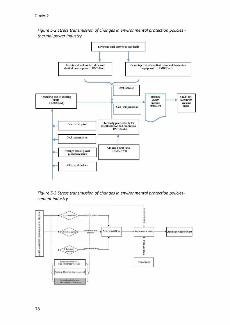
Chapter 5
78
Figure 5-2 Stress transmission of changes in environmental protection policies - thermal power industry
Figure 5-3 Stress transmission of changes in environmental protection policies- cement industry
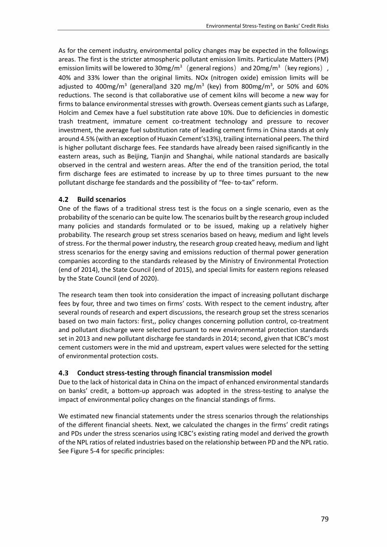
Environmental Stress-Testing on Banks’ Credit Risks
79
As for the cement industry, environmental policy changes may be expected in the followings areas. The first is the stricter atmospheric pollutant emission limits. Particulate Matters (PM) emission limits will be lowered to 30mg/m3(general regions)and 20mg/m3(key regions),
40% and 33% lower than the original limits. NOx (nitrogen oxide) emission limits will be adjusted to 400mg/m3 (general)and 320 mg/m3 (key) from 800mg/m3, or 50% and 60% reductions. The second is that collaborative use of cement kilns will become a new way for firms to balance environmental stresses with growth. Overseas cement giants such as Lafarge, Holcim and Cemex have a fuel substitution rate above 10%. Due to deficiencies in domestic trash treatment, immature cement co-treatment technology and pressure to recover investment, the average fuel substitution rate of leading cement firms in China stands at only around 4.5% (with an exception of Huaxin Cement’s13%), trailing international peers. The third is higher pollutant discharge fees. Fee standards have already been raised significantly in the eastern areas, such as Beijing, Tianjin and Shanghai, while national standards are basically observed in the central and western areas. After the end of the transition period, the total firm discharge fees are estimated to increase by up to three times pursuant to the new pollutant discharge fee standards and the possibility of “fee- to-tax” reform.
Build scenarios One of the flaws of a traditional stress test is the focus on a single scenario, even as the probability of the scenario can be quite low. The scenarios built by the research group included many policies and standards formulated or to be issued, making up a relatively higher probability. The research group set stress scenarios based on heavy, medium and light levels of stress. For the thermal power industry, the research group created heavy, medium and light stress scenarios for the energy saving and emissions reduction of thermal power generation companies according to the standards released by the Ministry of Environmental Protection (end of 2014), the State Council (end of 2015), and special limits for eastern regions released by the State Council (end of 2020).
The research team then took into consideration the impact of increasing pollutant discharge fees by four, three and two times on firms’ costs. With respect to the cement industry, after several rounds of research and expert discussions, the research group set the stress scenarios based on two main factors: first,, policy changes concerning pollution control, co-treatment and pollutant discharge were selected pursuant to new environmental protection standards set in 2013 and new pollutant discharge fee standards in 2014; second, given that ICBC’s most cement customers were in the mid and upstream, expert values were selected for the setting of environmental protection costs.
Conduct stress-testing through financial transmission model Due to the lack of historical data in China on the impact of enhanced environmental standards on banks’ credit, a bottom-up approach was adopted in the stress-testing to analyse the impact of environmental policy changes on the financial standings of firms.
We estimated new financial statements under the stress scenarios through the relationships of the different financial sheets. Next, we calculated the changes in the firms’ credit ratings and PDs under the stress scenarios using ICBC’s existing rating model and derived the growth of the NPL ratios of related industries based on the relationship between PD and the NPL ratio. See Figure 5-4 for specific principles:

Chapter 5
80
Figure 5-4 Schematic diagram of financial transmission model
Step 1 Set the function of the impact of changes in environmental protection standards on financial indicators of firms: C=f , where C indicates the change in a firm’s cost and f
denotes environmental protection standards. For thermal power companies, the annual power generated was estimated according to prime operating revenue and on-grid power tariffs, while the increase in the amount of prime operating cost was then calculated based on the increased cost per kilowatt*hour under the stress scenarios. For cement producers, the prime operating costs under the stress scenarios were calculated by prime operating costs and the percentage increases.
Step 2 Calculate main indicators for balance sheet and income statement according to changes in prime operating costs and financial statement articulation.
When applying stress on the financial position of a sample firm, we paid attention primarily to two indicators in the income statement: revenue and cost of goods sold (COGS). Correspondingly, other accounts in the income statement would also change, thus affecting profit and retained earnings in the balance sheet.
We assumed △ B = percentage of cost change, △ P = percentage of price change, and △ Q = percentage of quantity change. After accounting for changes in cost, price and quantity we arrived at revenue, COGS and profit from the equations below:
△ R=(1+ △ P)(1+ △ Q) - 1
△ COGS=(1+ △ B)(1+ △ Q) - 1
△ Profit= △ R -△ COGS
Here △ R= revenue change in percentage, △ COGS= COGS change in percentage, △ Profit= profit change in percentage.
1) Income statement under stress conditions The prime operating revenue and income in the income statement were directly impacted and adjusted accordingly.

Environmental Stress-Testing on Banks’ Credit Risks
81
2) Balance sheet under stress conditions A decrease in net profit in the income statement leads to decrease of the owner’s equity in the balance sheet. We adjusted the current assets and liabilities according to the cash flow cycle while maintaining other assumptions.
Similar changes in the income statements can have different impact on the balance sheets of different borrowers. We translated the impact into a reduction in retained earnings on the balance sheet, with the understanding that no general rules were applicable to all borrowers. One limitation of such a simple approach is that it does not account for individual companies’ adjustments to their own financing structures responding to the decline in revenue. As well, cash flow cycle may deteriorate under stress conditions. However, given that cash flow cycle has no significant weighting in the customer credit rating model, we believed that results based on this simplified approach were sufficient to deduce a credit rating migration matrix.
Step 3 Input above financial indicators into the corresponding score sheets. At ICBC, different corporate customer credit ratings and evaluation models were applied to thermal power and cement companies. The evaluation model consisted of quantitative and qualitative evaluations. To be prudent, we assumed that scores on qualitative and quantitative evaluations declined by the same proportion.
From the change in a firm’s evaluation score we obtained the change in its credit rating, which through relationship mapping allowed us to estimate the change in PD. Raising the environmental protection standards for firms would cause their profits to decline, reducing their solvency and causing declining credit standings and rising PDs.
Step 4 Construct credit rating transition matrices for the industries that the companies were in by summarizing changes in credit ratings of firms; further analyze changes in loan quality in related industries based on the relationship between the PD and the NPL ratio.
Main findings of stress-testing and policy recommendations
Thermal power firms Stricter environmental protection standards will impose great cost pressure on the thermal power industry, but the industry will maintain stable given steady economic growth and rising demand for electricity as China furthers industrialization. Enhanced environmental protection standards will nonetheless have major structural impact on the thermal power industry.
Policy recommendations
• Maintain existing AAA customers while continuing to attract high-quality customers from the five major power companies.
• Pay attention to the impact of changes in environmental protection policies on the financial cost and credit risk of firms with AA+ ratings and below, especially corporate customers that may be degraded to BBB+ or below.
• Recognize opportunities to grant loans to firms with energy-saving and emission- reduction plans.
• Recognize new upstream and downstream segments resulted from environmental technologies, such as solid waste treatment.
• Strictly prevent thermal power firms violating environmental protection laws and regulations from obtaining funding.

Chapter 5
82
Cement industry The cement industry will by and large enter a slow-growth stage under pressure to reduce capacity. Raised environmental protection standards will impose obvious financial pressure.
Policy recommendations
• Guard against risks faced by small and medium-sized cement firms as they adapt to the green economy.
• Keep track of possible credit risks from industry capacity reduction.
• Select companies strong on desulfurization, denitration and dust removal and help them expand given growth potential.
• Monitor mergers, acquisitions and reorganizations in the industry and improve bank’s customer quality by seizing appropriate environmental improvement opportunities.
• Use ICBC’s financial portfolio products to focus on the development of the industrial solid waste market and lend more support to cement co-treatment projects.
• Grant loans to firms well-positioned in the green transformation of the cement industry, support companies with the potential to go global.
Further development of environmental stress-testing In our research, the first problem was data availability and accuracy, so relevant ministries and commissions are advised to implement requirement on companies for mandatory disclosures of environmental data. Our research group is strengthening cooperation with the Ministry of Environmental Protection in a bid to improve the accuracy of estimates for the internalization of environmental cost.
As ICBC sets high standard for high-polluting and high-energy-consuming industries to access its business, the customers selected for this stress-testing were mainly large and medium- sized companies, which likely produced above-average results. These test results therefore are more indicative of ICBC customers and do not reflect the entire industry. The quality of the stress-testing would have been much improved if data representing the whole industry had been obtained.
These stress-testing targeted thermal power and cement industries. We plan to cover other polluting industries including iron and steel, nonferrous metals, chemical and paper. The methods will be enhanced to include prices, regions and climate change, with the goal to yield quantitative results. For example, stress-testing concerning the impact of environmental factors on the credit risks of commercial banks will be conducted from the perspective of pricing (carbon trading), the sustainable rating (ESG) for firms will be explored, and the feasibility of incorporating environmental factors into the bank customer credit rating system will be considered to help research and develop an “ICBC Green Index”, prioritizing loans to and investment in green firms and fields.
5 Conclusion and recommendations
Environmental risks have become an important factor impacting the daily operations of commercial banks, therefore environmental stress-testing should be incorporated into bank credit risk rating systems and processes. This will improve the ability of the banking sector to

Environmental Stress-Testing on Banks’ Credit Risks
83
identify environmental risks and the customers most able to contribute to sustainable development, thereby enhancing the ability of the banking system to continuously support the green economy, while also becoming resilient to environmental risks itself. In our opinion, stress-testing the impact of environmental factors is important for commercial banks for the following four reasons: first, stress-testing can help precisely estimate and quantify the impact of more extreme environmental factors on a bank’s credit risks, improving the capacity of a bank’s environmental risk management processes; second, environmental risk factors can be included in the customer credit rating system, enabling environmental risk measurement to form a basis for the pricing of credit products; third, stress-testing leads to rational arrangement of bank loans and investment portfolios, thus actively promote the adjustment of credit and investment structures; fourth, stress-testing could be taken as a reference point for banks and regulators in their future considerations of environmental factors and risks.
ICBC has stayed at the forefront exploring the impact of environmental risks through stress-testing analysis. The following are the highlights of our stress-testing:
• The scenarios constructed by ICBC accounted for many complex factors with a series of policies and standards formulated or due to be released.
• A number of aspects of the environmental stress-testing methodology developed by ICBC may be innovative in China or globally, such as the transmission mechanism from environment protection policies to firm impacts to bank impacts, the formulation of scenarios despite the complexity faced and the forecasting methodology based on ICBC’s big data.
• ICBC started the stress test on a single industry and gradually extended to multiple industries, an innovative and practical approach to developing the research methodology.
• Both first-round and corresponding feedback effects were accounted for. For example, in stress-testing thermal power companies, the impact from changes in the on-grid power tariffs was considered; for the cement industry, the study discussed subsequent improvement measures that firms could take in response to environmental protection policies, including co-treatment operations
• The approach of expanding coverage from one to many factors and from one to many industries created a path for the banking industry to intensify its capabilities on stress-testing.
We believe the construction of this market-oriented mechanism can greatly help reduce the impact of economic development on the environment. To improve the efficacy of this method, we make the following recommendations:
• The authorities should actively and collaboratively promote research on fiscal policy, financial policy and industrial policy and develop a whole set of policy support systems for the internalization of environmental costs.
• Emissions standards should be tightened with strict supervision and implementation, additional pollutant discharge taxes should be collected from polluting firms, and companies should be encouraged to make green investments and upgrade technologies through tax reductions, discounts, government procurement.

Chapter 5
84
• Voluntary agreements and tradable permits should be introduced to establish a well-running carbon trading market.
• Special re-lending policy for “environmental protection fields “should be formulated, along with positive development of green bonds and green insurance, to reduce the operating cost of firms through a market-oriented approach supporting green investment.
• Intermediary service system should be actively cultivated, and policies on the open and transparent disclosure of environmental information should be enacted.
• Policy and market signals should both aim to enhance the value of preserving natural resources and reduce the value of carbon intensive investments to spur the transformations of the industrial structures and companies toward a green economy.
Table 5-2 China major environmental laws & regulations since 2013
Title Issued by Issued in Main content
Pollution Prevention and Control Techniques in the industries of cement steel, sulfuric acid, volatile organic compounds (VOCs)
Ministry of Environmental Protection
May 2013
Cement: Key pollutants to be effectively controlled in 2015, with NOx emissions kept below 1.5 million tons and particulate matter emissions (including unorganized emissions) below 2 million tons and full control will be in place in 2020. Steel: Sintering fume should be fully desulfurized. Blast furnace gas (BFG) dry dedusting is encouraged. Low-sulfur fuel, regenerative combustion and low-nitrogen combustion technologies are encouraged for steel-rolling industrial furnaces. Sulfuric acid: The pickling process shall be employed for acid production in iron-sulfur plants and acid production from smelting fume; acidic wastewater and cooling water shall be treated separately. The water reuse ratio shall not be lower than 90%. Volatile organic compounds (VOCs): VOCs prevention and control system will be established in key areas in 2015; emissions reduction will be basically materialized from raw materials to final products and from production and consumption in 2020.
Circular of the State Council on
State Council September 2013
Overall air quality to be improve, heavy pollution days to be reduced significantly, by 2017, the concentration of inhalable

Environmental Stress-Testing on Banks’ Credit Risks
85
Issuing the Action Plan for Air Pollution Prevention and Control (G.F. [2013] No. 37)
particulate matters to fall by over 10% from 2012 in prefectural or higher-level cities. Air quality to improve notably in the Beijing- Tianjin-Hebei region, the Yangtze River Delta and the Pearl River Delta. The concentration of fine particulate matters to fall by 25%, 20% and 15% in the above three regions.
Environmental Protection Law
National People’s Congress
April 2014
Establish a sound system of environment and health monitoring, investigation and risk assessment, and create a mechanism for public monitoring and early warning of environmental pollution; define red lines for ecological protection in key ecological protection zones, ecologically sensitive areas and ecologically vulnerable areas to maintain strict protection; expand the scope of complainants in environment-related public interest litigations so that all social organizations that are registered with the civil affairs department of the people’s government at or above the level of city divided into districts, are specialized in environmental protection activities in public interests for more than five years and maintain good reputation are eligible for lodging a lawsuit with the people’s court. Firms that discharge pollutants illegally and refuse to take corrective actions can be fined for successive days in the amount of initial fine.
Action Plan for Water Pollution Prevention and Control
State Council April 2015
Close down 10 categories of small firms. Close down all product projects of small paper making, leather making, dyeing, dye making, coking, sulfur refining, arsenic refining, oil refining, electroplating and pesticide firm that will seriously contaminate water bodies. Launch crackdown on 10 key industries. Develop pollution crackdown plans for paper making, coking, nitrogen fertilizers, nonferrous metals, dyeing, agricultural and sideline foodstuffs processing, active pharmaceutical ingredient (API) manufacturing, leather making, pesticide and electroplating industries and implement cleaner upgrading. Implement equivalent or reduction replacement of main pollutant emissions from new,

Chapter 5
86
alteration and expansion projects in the above industries. In 2020, over 70% of water bodies in seven key drainage basins (Yangtze River, Yellow River, Pear River, Songhua River, Huaihe River, Haihe River and Liaohe River) will reach or exceed Class III. Black-and-malodorous water bodies will be controlled within 10% in developed areas of cities at the prefectural and higher levels. In 2030, over 75% of water bodies in seven key drainage basins will reach or exceed Class III. Black-and- malodorous water bodies in developed urban areas will be basically removed. About 95% of centralized drinking water sources in urban areas will reach or exceed Class III.
Technical Guide to Delimitation of Bio-protection Red Line (Trial) (H.F. [2014] No. 10)
Ministry of Environmental Protection
May 2015
Areas that are very important to water conservation are included within the bio- protection red line according to results of water conservation function assessment and classification. Grade 1 and Grade 1 protected areas of important drinking water sources are included within the bio-protection red line. The specific method shall be as set forth in HJ/T338.
Highly sensitive areas are included within the bio- protection red line according to the results of soil erosion sensitivity assessment and classification. Zones of key soil erosion prevention and protection areas that pose a relatively significant risk of soil erosion also shall be included within the bio-protection red line.
Assess the materiality of biological diversity preservation function.
Soil Environmental Quality Standard for Agricultural Land (2nd Exposure
Ministry of Environmental Protection
August 2015
10 soil contaminants (i.e., total manganese, total cobalt, total selenium, total vanadium, total antimony, total thallium, fluoride (water soluble fluorine), benzoapyrene, total petroleum hydrocarbon and total phthalic acid esters) are added to the test options according to relevant foreign standards

Environmental Stress-Testing on Banks’ Credit Risks
87
Draft) (revision of GB15618-1995)
and Risk Screening Guideline Values for Soil Contamination of Development Land (2nd Exposure Draft) (supplement to HJ 25.3-2014)
and China’s National Technical Rules for Evaluation of Soil Contamination Status, which are applicable to soil contamination investigation and evaluation in specified areas. The soil pH level of 6.5 or below under the original standard is further divided into
two levels: pH ≤ 5.5 and 5.5 < pH ≤ 6.5,
with different limits applied to the two
levels, so that the three levels (pH ≤ 6.5,
6.5 7.5) under the original standard are
increased to four levels (pH ≤ 5.5,5.5 <
pH ≤ 6.5, 6.5< pH ≤ 7.5,pH>7.5).
The limit on lead content of soil in agricultural land is lowered to 80 mg/kg. The original standard prescribes three limit levels according to pH value according to the impact of lead on crop growth: 250mg/kg (pH<6.5), 300mg/kg (pH6.5-7.5) and 350mg/kg (pH>7.5).
The limit on HCH and DDT contents of soil is lowered to 0.1 mg/kg from the original standard of 0.5mg/kg.

Chapter 5
88
Bibliography
Bank of England. (2015). The impact of climate change on the UK insurance sector. Berge, T.O., & Lindquist, K.G. (2007). A suite-of-models approach to stress-testing financial
stability, preliminary paper presented at the "2nd Expert Forum on Advanced Techniques on Stress-testing: Applications for Supervisors", IMF and DNB, Amsterdam, October 23-24.
Carney, M. (2015). Breaking the Tragedy of the Horizon–climate change and financial stability. Speech given at Lloyd’s of London, 29, 220-230.
CISL, & UNEP FI. (2014). Stability and Sustainability in Banking Reform: Are Environmental Risks Missing in Basel III?
Goldstein, M. (2015). Bank Stress-testing and Financial Stability: Lessons from the 2009-14 US and EU_Wide Tests for Asian Emerging Economies. Peterson Institute for International Economics Working Paper.
Hahn, F. R. (2007). Environmental determinants of banking efficiency in Austria. Empirica, 34(3), 231-245.
Peria, M. M. S. M., Majnoni, M. G., Jones, M. M. T., & Blaschke, M. W. (2001). Stress testing of financial systems: an overview of issues, methodologies, and FSAP experiences: International Monetary Fund.
Weber, O., Fenchel, M., & Scholz, R. W. (2008). Empirical analysis of the integration of environmental risks into the credit risk management process of European banks. Business Strategy and the Environment, 17(3), 149-159.

Quantifying the Impact of Physical Risks on Probabilities of Bank Loan Defaults
89
Quantifying the Impact of Physical Risks on Probabilities of Bank Loan Defaults
By
Research Center for Green Finance Development, Tsinghua University1
Abstract
In this chapter, we present an analytical framework and the methodologies for measuring the impact of climate-related physical risks on the default risks of bank loans. The framework consists of the setting of climate scenarios and a suite of catastrophe models and financial models. For the case study, we analyzed the impacts of climate change on typhoons’ intensity and frequency and on credit risk metrics (e.g. PD and LGD) of mortgage loans in China’s coastal cities. The model shows that, under an extreme scenario (RCP8.5 with extreme exacerbation effect on typhoons), the expected annual credit loss of mortgage loans could rise nearly three fold in 2050 compared with the baseline scenario which assumes no change in typhoons’ occurrence pattern. This framework can also be applied to estimate potential climate exacerbated impacts of other natural disasters including floods, heatwaves, drought and wildfires on financial risk metrics such as default probability and valuation of assets.
Keywords: climate-related physical risks, typhoon, mortgage loan, default probability, quantitative
1 Introduction
A growing consensus among the scientific community is that global warming will lead to changes in the occurring patterns of future weather and climate events, such as typhoons, floods and heat waves. These climate-related physical risks can cause considerable damages, many of which unexpected, to the real economy and the financial sector that provides funding for economic activities. The losses to the real economy and the associated impact on the financial sector can be enormous as estimated by several central banks and research institutions (EIU, 2015; PRA Bank of England, 2015; Regelink et al., 2017).
Against this backdrop, the international financial community has called for attention and actions to integrate climate-related physical risks into financial decision making by financial institutions. For example, the G20 Green Finance Study Group, the Central Banks and Supervisors’ Network for Greening the Financial System (NGFS, 2019) and the Taskforce for Climate-Related Financial Disclosure (TCFD, 2017) have advised financial regulators and institutions to conduct environmental risk analysis (ERA) and disclosing information related to climate-risk exposures and the resulting financial risks. To manage these environmental and climate risks, the primary step is to quantify these risks. Many literatures, including other
1 The primary authors of this chapter are Dr. SUN Tianyin, Senior Research Fellow, email: [email protected], and
Dr. MA Jun, Director, Research Center for Green Finance Development at Tsinghua University, email:
[email protected]. The authors would like to thank Dr Gabriela Aznar Siguan, Prof David Bresch and Eberenz
Samuel from ETH Zurich, ZHU Yun and MENG Tingyi from Tsinghua University and WANG Jiayi and ZHAO Xinran from
UIBE for their advices and contributions. The authors acknowledge the support of the INSPIRE grant.

Chapter 6
90
chapters in this Occasional Paper, have discussed the methodologies for quantifying transition risks and their impact on banks’ and institutional investors’ exposures.
In this chapter, we present an analytical framework and the methodologies for measuring the impact of climate-related physical risks on credit risk metrics of bank loans. In a case study using this framework, we quantify the increase in the probabilities of default (PD) and Loss-Given-Default (LGD) of mortgage loans for properties in coastal cities of China, caused by the increased intensities and frequencies of typhoons under various climate change scenarios.
The remainder of this chapter is organized as follows: Section 2 introduces the applications of the proposed analytical approach; Section 3 presents the general analytical framework, the modules within the framework, and several modelling details; Section 4 presents the results of a case study that shows the quantitative estimates of the impact of typhoons on the PD and LGD of mortgage loans in coastal cities of China; Section 5 discusses the limitations of the current methodologies and outlines future work for our research.
2 Applications
This climate physical risk analysis framework is mainly developed for financial institutions, especially banks, to analyze the financial risks arising from the impact of physical risks under various climate scenarios. The framework could be applied to a wide range of hazards including typhoons, floods, heat waves, droughts etc., and various sectors, especially those vulnerable to natural disasters such as housing, agriculture, energy and transportation. The rationale of these risks translating into credit risks and most affected sectors are briefly described in the following Table 6-1.

Quantifying the Impact of Physical Risks on Probabilities of Bank Loan Defaults
91
Table 6-1 Examples of physical risks’ impact on credit risks
Climate-related physical risks
Mechanism for translating into credit risks Most exposed sectors
Typhoons/hurricanes
Higher intensities and frequencies of typhoons/hurricanes cause severer destruction to properties and assets, and consequently reduce their values and lead to higher default rates for loans to these sectors
Real estate Transportation Agriculture Power
Floods
More frequent floods cause severer destruction to properties and assets and interrupt business operations, impacting financial performance of the firms affected, and leading to higher default rates on loans to these sectors
Transportation Real estate Mining Manufacturing
Droughts
More severe and frequent droughts reduce water supply to sectors heavily relying on water and affect production activity and revenues. Droughts also push up water prices and consequently operational expenses while reduce profitability, leading to more loan defaults
Agriculture Food and beverage Textile and dying Steel Power Mining
Heat waves
Increasing frequency, severity and length of heatwaves cause more wildfires, reduce labor productivity and lower agricultural production; heatwaves also raise temperatures of cooling water for power plants and cause cable outages, interrupting power production and transmission. These lead to worse financial performance of affected firms and higher rates of loan defaults.
Agriculture Forestry Energy Transportation All labor-intensive sectors
Sea-level rise
Rising sea levels cause irreparable destruction of properties and assets located in coastal areas, leading to higher loan default rates
All sectors deploying assets and facilities along the coastal area
Source: Compiled by authors
This framework can also be used by local governments to assess the financial and fiscal impact of climate physical risks to cities and regions. For example, a coastal city prone to typhoons can apply this methodology to quantify the potential financial destruction caused by future typhoons (e.g., reduction in property values) and the needed expenditure for repairment. This analysis could be used to derive the financial risks facing a local government (e.g., the reduction in value of government-owned properties), the future increase in fiscal expenditure (for repairment and disaster relief) and the resulting government debt obligations and debt risks (assuming that the government will need to borrow to meet its additional expenditure needs).

Chapter 6
92
3 Analytical framework and methodologies
In this section we describe the general framework of our analysis and the methodologies used in the four modules of the disaster loss and the financial models.
Analytical framework The general analytical framework consists of two major components: a disaster loss model and a group of financial models, as illustrated in Figure 6-1.
Figure 6-1 General physical risk assessment framework
The disaster loss model is used to estimate the value losses from physical property damages, economic losses (e.g., decline in GDP or income), and/or financial losses due to business interruptions by natural disasters. The output of the disaster model is then used as an input into the financial models to adjust the estimated financial statements of an entity (e.g., a company), such as assets, liabilities, revenues, costs and profits/losses. These adjusted variables are later used to calculate various financial ratios such as the loan-to-value, return-on- equity, asset/liability and interest coverage.
The disaster loss model itself is made up of four major modules. These are the climate exacerbation module, the hazard module, the asset exposure module and the vulnerability module. The financial models used in the analysis could include the insurance actuarial model, the PD and LGD models, and the valuation model for asset management, depending on the type of financial business and the underlying assets affected by disasters. The two components of the analytic framework are interconnected by several economic and financial variables including GDP, household income, revenues, costs, and the loan-to-value ratio (LTV).
The modules In this subsection we describe the specific modules used in the disaster loss model and the financial models.
3.2.1 Disaster loss model The disaster loss model within this framework is largely built on the on-going python package CLIMADA developed by a group of researchers at ETH Zurich (Aznar Siguan & Bresch, 2019).

Quantifying the Impact of Physical Risks on Probabilities of Bank Loan Defaults
93
The exacerbation module produces the exacerbation effect of climate change on the occurrence pattern and intensity of historical disaster events. The hazard module describes a hazard’s historical intensity and occurrence probability in a specific region. These two modules are together used to predict the profile of future typhoons. The asset exposure module describes the geographical distribution of assets being affected to coordinate with the geographical locations of a hazard. The vulnerability module combines hazard and asset modules translating the intensity of a hazard’s damages to assets.
Exacerbation module The exacerbation module addresses the exacerbated effect of global warming on typhoons’ and other natural disasters’ intensities and frequencies. Specifically, it correlates the incremental change of intensity and occurrence probability of a hazard and a rise in temperature caused by higher carbon concentration in the atmosphere. Depending on the ocean basins investigated, many studies show considerable discrepancy of predicted changes in typhoons’ speed and frequency derived from climate change (Knutson et al., 2019). For any given location, there is a high amount of uncertainty in climate change-exacerbation effect on typhoon i.e., the probability distribution of the impact on typhoons’ intensity and frequency caused by climate change has fat tails. In our study presented later in this chapter, we use the mean, 90th percentile and the 99th percentile of the statistical distribution of exacerbation effects from these studies for parameterization, which form respectively our mild, severe and extreme scenarios.
Hazard module The hazard module models future hazard profiles under climate scenarios defined by IPCC (Allen et al., 2014). For our case study, this is done through combining historical typhoons’ tracks obtained from the National Oceanic and Atmospheric Administration (NOAA) and the output of climate exacerbation module. More specifically, the data of typhoon tracks along the coast of China are provided in the International Best Track Archive for Climate Stewardship (IBTrACS) project of the NOAA (NOAA, 2019). The IBTrACS project is a centralized database providing historical tropical cyclone track data to aid the understanding of the distribution, frequencies, and intensities of tropical cyclones worldwide. The database pools data from all the Regional Specialized Meteorological Centers and other international centers and individuals, creating a global best track dataset that merges information from multiple centers into one product and archive for public use.
Asset exposure module The asset exposure module describes the geographical locations and value distribution of the concerned assets/properties potentially exposed to natural disaster events. These are often expressed by the latitudes, longitudes and altitudes of the assets/properties and their corresponding monetary values at specific sites. Depending on the specific assets being investigated, this information can be obtained from data providers or asset owners.
Vulnerability module The vulnerability module addresses the correlation between the magnitude of damages to assets and the intensity of a hazard. The data used for determining the correlation are empirical studies and expert judgement. This relationship is often depicted by a damage function curve, as Figure 6-2 shows. Here the x axis indicates the intensity of the hazard and the y axis the magnitude of damage that the assets suffer in a monetary context as a percentage of their initial values. In Figure 6-2, the lines of different colors represent the damage curves for various assets for the same hazard. This is because different assets (e.g., buildings, power plants and bridges) with different physical structures and qualities demonstrate varied responses (i.e., sustaining different levels of damage) while bearing the

Chapter 6
94
same level of shocks from the hazards. The damage curve for a specific asset against a hazard is determined by several critical points on the curve. For example, the critical points on the property damage curve include (1) the threshold intensity point at which the wind speed of typhoon starts to cause damages and (2) the full damage intensity point at which the wind speed of typhoon causes 100% damage. These critical points determining the damage curve are based on empirical studies of historical records (Emanuel, 2011).
Figure 6-2 Schematic damage function curves of a natural disaster for different assets
3.2.2 Financial models As mentioned earlier, many financial models could be used to analyze the impact of disasters on financial variables related to insurance, asset management and banking operations, taking the output of the “disaster loss model” as inputs.
In this study, we adopt the Expected Loss (EL) model widely used by banks to estimate credit risks. Typically, EL is expressed as the product of three individual risk-measure components, namely Probability of Default (PD), Exposure at Default (EAD) and Loss Given Default (LGD) as suggested in BCBS, 2017 and other studies (Hull, 2012):
∑ 𝐸𝐿𝑖 = ∑ 𝑃𝐷𝑖 ∗ 𝐿𝐺𝐷𝑖 ∗ 𝐸𝐴𝐷𝑖 … … … … … … … … … … [1]
As we assume banks’ future exposure (EAD) (the real estate properties in the coastal areas) is unchanged for the purpose of this study, so only impacts of typhoons on PD and LGD need to be evaluated to derive future disasters’ impact on EL. The models estimating the PD and LGD are integrated to calculate the expected loss fraction of asset 𝑖, expressed as a percentage of EAD:
𝑃𝑒𝑟𝑐𝑒𝑛𝑡𝑎𝑔𝑒 𝐿𝑜𝑠𝑠 𝑜𝑓 𝐸𝐴𝐷𝑖 = 𝑃𝐷𝑖 ∗ 𝐿𝐺𝐷𝑖 … … … … … … . … [2].

Quantifying the Impact of Physical Risks on Probabilities of Bank Loan Defaults
95
In a typical PD model for mortgage loans, the dependent variable is the probability of a default by a borrower, and the explanatory variables may include household income, mortgage loan interest rates, risk-free rates, loan-to-value ratios (LTV), and loan maturity (Tian, 2014; Xu et al., 2010). In our case study, we identify the LTV and household income as the two principal “directly impacted” variables, which bridge the disaster loss model and the PD model. These variables translate increased property losses and declined household income to PD’s incremental change (the delta PD). The logic is that the property impairment and household income decline due to disasters would increase the LTV and damage the borrower’s repayment capacity, which tends to increase the incentive and risk for the borrower to default. In this case, we also use per capita GDP growth as a proxy for household income growth, assuming the disaster’s impact on GDP is proportional to its impact on household income.
For a typical LGD model, its explanatory variables could be categorized into contract characteristics, borrower characteristics, differences across industry and industry conditions, and macroeconomic systematic risk factors (Qi & Yang, 2009). Among these variables, the Loan-to-value (LTV) ratio is often considered as a key driver of LGD (Calem & LaCour-Little, 2004; Hou et al., 2019; Leow & Mues, 2012; Lu, 2014). It can bridge the disaster loss model and LGD model by translating the property impairment to incremental LGD (the delta LGD). The logic behind this is that an increase in LTV implies that the impaired value of collateral is less likely to cover the outstanding loans at default.
Using the PD and LGD estimates produced by the two models above, we can assess the expected percentage loss of EAD by equation [2]. In the current case study which is for illustrative purposes, we consider only the household income and LTV as the links between hazard damage and the PD, and LTV as the link between hazard damage and the LGD. It doesn’t mean that other explanatory variables in the PD model and LGD model are completely irrelevant, although they are less important from the perspective of climate risk analysis.
4 Case study: quantifying typhoon impact on EL of mortgage loans
In the following, we present some methodological details on how to apply the framework to estimate the impact of increased intensity and frequency of typhoons on the EL of mortgage loans for properties in China’s coastal cities. This application involves the following seven steps:
Step 1: Select the cities In this study, we select 40 Chinese coastal cities in eight provinces frequently exposed to typhoons according to geographical locations and historical typhoon landfall records. In the period 2004-2016, properties located in these eight provinces suffered 85% of the direct economic losses from typhoons according to our own analysis based multiple sources of loss data on historical typhoon events2. A full list of these cities is shown in Table 6-2 below.
2 Data sources: China Meteorological Administration, link: www.tcdata.typhoon.gov.cn China Meteorological
Administration: Yearbook of Meteorological Disasters (2004-2016); YIN Jie et al: A study on the relationship between
typhoon intensity grade and disaster loss in China (2013); and other press releases.

Chapter 6
96
Table 6-2 40 Chinese coastal cities selected in our case study
Index Coastal Cities Provinces
1 Binzhou
Shandong
2 Weifang
3 Weihai
4 Yantai
5 Qingdao
6 Rizhao
7 Lianyungang
Jiangsu 8 Yancheng
9 Nantong
10 Suzhou
11 Shanghai Shanghai
12 Jiaxing
Zhejiang
13 Hangzhou
14 Shaoxing
15 Zhoushan
16 Ningbo
17 Taizhou
18 Wenzhou
19 Ningde
Fujian
20 Fuzhou
21 Putian
22 Quanzhou
23 Xiamen
24 Zhangzhou
25 Chaozhou
Guangdong
26 Shantou
27 Jieyang
28 Huizhou
29 Shenzhen
30 Dongguan
31 Guangzhou
32 Zhongshan
33 Zhuhai
34 Jiangmen
35 Maoming
36 Zhanjiang
37 Foshan
38 Qingyuan
39 Beihai Guangxi
40 Haikou Hainan

Quantifying the Impact of Physical Risks on Probabilities of Bank Loan Defaults
97
Step 2: Estimate outstanding mortgage loans The next step is collecting/estimating data on the mortgage loans of these cities. However, few municipalities at the district administrative level reported such data, which would have provided the required geographical resolution for our analysis. Therefore, we scaled the 2018 national mortgage loan data to district municipality level using the share of each district’s GDP of the national total, arriving at an estimate of the district’s outstanding mortgage loans. The underlying assumption, validated by our study using many samples, is that the ratio of a district’s outstanding mortgage loans to the national aggregate is similar to the ratio of the district’s GDP to the national GDP.
Step 3: Identify the locations of properties Another important data point we need for the analysis is the geographical locations of the district level properties (assets), so that the potential disaster damages could be mapped accordingly. We apply an online tool to geocode the center of municipal districts as the location of the properties in a specific municipal district. The output includes the latitudes and longitudes for the properties in the municipal districts of the 40 cities (see Figure 6-3).
Figure 6-3 Distribution of properties (and values) along the coast of China
Source: authors’ estimates

Chapter 6
98
Step 4: Generate typhoons’ future profiles under various climate scenarios The historical track data of the typhoons used in our case study are extracted from the NOAA’s IBTRACS database, which to our best knowledge provides the most complete record of historical tropical cyclone tracks worldwide. From this database, all the recorded tracks of historical typhoons landed on the 40 Chinese coastal cities are selected for our modelling. The historical data of typhoon tracks, together with the exacerbation effects induced by global warming estimated and summarized by NOAA climate researcher Thomas R. Knutson (Knutson et al., 2019), are used in the hazard module, which generates the future typhoon profiles under several IPCC’s climate scenarios, as shown by Figure 6-4.
Figure 6-4 Locations and intensities of typhoons along Chinese coast
Source: Authors’ simulations
Step 5: Develop vulnerability curves for properties in each district Our case study takes Emanuel’s vulnerability curve (Emanuel, 2011) as the basis and adjusts its parameters, namely the threshold velocity and half damage velocity which determine the final shape of the curve, to match the historical records of typhoons’ impact on the selected cities in China (Sun, 2019). The historical records of impact are derived from the data of China’s provincial and municipal economic losses caused by typhoon, provided by a professional research data provider CSMAR3. The final vulnerability curve of properties against typhoons is shown in Figure 6-5. This procedure is also applicable for defining the vulnerability curve of GDP of the Chinese coastal cities. The only difference is that the vulnerability curve of GDP is
3 Data used are derived from CSMAR, historical records of economic losses caused by typhoons in China, 2019, link:
http://www.gtarsc.com

Quantifying the Impact of Physical Risks on Probabilities of Bank Loan Defaults
99
calibrated with data sources contained in empirical studies on economic losses due to typhoons (Liu, 2017; Ma, 2016; Wang et al., 2019; J.-y. Zhang et al., 2013; Q. Zhang et al., 2009).
Figure 6-5 Property value loss as a function of winds speed (in %)
Source: authors’ estimates
Step 6: Estimate property value losses (value reduction in collaterals) under two climate scenarios We use the disaster loss model to estimate the potential annual value losses of properties (used as collaterals for mortgage loans) and impact on GDP (taken as proxy to the decline in household income), under two IPCC’s climate scenarios and three levels of climate exacerbation effects as shown in Table 6-3. The two climate scenarios are represented by two Representative Concentration Pathways (RCPs). An RCP is a greenhouse gas concentration trajectory adopted by the IPCC in its Fifth Assessment Report (AR5) in 2014. The RCPs describe possible climate future scenarios depending on the volume of greenhouse gases (GHG) emitted in the decades to come. According to IPCC’s Fifth Assessment Report (AR5) (IPCC, 2014), the four RCPs, namely RCP2.6, RCP4.5, RCP6.0, and RCP8.5, are labelled after a possible range of radiative forcing values in the year 2100 (2.6, 4.5, 6.0, and 8.5 W/m2, respectively).
In our case study, we focus on RCP 6.0 and RCP8.5, the two scenarios that we believe are more likely to occur than others based on the observed trend of human mitigation efforts (Berg et al., 2018). In addition, three levels of climate exacerbation effects on typhoons are considered for each of the two IPCC’s climate scenarios. The first considers the average (i.e., 50th percentile of the statistical distribution of) exacerbation effect (“mean case”). The second incorporates the 90th percentile exacerbation effects (“severe case”). The third incorporates the 99th percentile exacerbation effect (“extreme case”). There are thus six combinations of two climate scenarios and three levels of exacerbation effects (see Table 6-3). As a comparison, the baseline scenario is one that assumes historical typhoon occurrence pattern remains unchanged in the future.

Chapter 6
100
Table 6-3 shows that, under the baseline scenario the estimated annual value losses of properties (physical loss in the table) in the 40 cities will be around RMB100billion (0.65% of total value) in 2030 and 2050. The value losses would surge to RMB210billion (1.36% of total value) and 443 billion (2.87% of total value) in 2030 and 2050 respectively under the RCP8.5 extreme case. As for the impact on GDP, 1% of annual loss is expected under the baseline scenario from 2030 and 2050, while under RCP8.5 extreme case the GDP loss would amount to 2.2% in 2030 and 5.0% in 2050.
Table 6-3 Estimated annual value losses of collaterals and GDP in 40 Chinese coastal cities due to typhoons
Source: authors’ estimates
2030 2035 2040 2045 2050
Physical loss 101 101 101 101 101
GDP loss 62 62 62 62 62
Exacerbation Climate
Physical loss 109 110 112 114 116
GDP loss 67 69 70 71 73
Physical loss 113 117 121 125 130
GDP loss 71 74 77 80 83
Physical loss 134 142 150 160 172
GDP loss 80 85 91 98 105
Physical loss 157 179 203 231 261
GDP loss 96 110 126 146 167
Physical loss 163 178 194 217 240
GDP loss 104 114 126 142 159
Physical loss 210 256 308 371 443
GDP loss 137 170 208 255 310
2030 2035 2040 2045 2050
Physical loss 0.65% 0.65% 0.65% 0.65% 0.65%
GDP loss 1.00% 1.00% 1.00% 1.00% 1.00%
Exacerbation Climate
Physical loss 0.70% 0.71% 0.72% 0.74% 0.75%
GDP loss 1.09% 1.11% 1.13% 1.15% 1.18%
Physical loss 0.73% 0.76% 0.78% 0.81% 0.84%
GDP loss 1.15% 1.20% 1.24% 1.30% 1.35%
Physical loss 0.87% 0.92% 0.97% 1.04% 1.11%
GDP loss 1.30% 1.38% 1.47% 1.58% 1.71%
Physical loss 1.02% 1.16% 1.31% 1.49% 1.69%
GDP loss 1.55% 1.78% 2.05% 2.36% 2.71%
Physical loss 1.05% 1.15% 1.26% 1.40% 1.56%
GDP loss 1.68% 1.85% 2.04% 2.29% 2.57%
Physical loss 1.36% 1.66% 1.99% 2.40% 2.87%
GDP loss 2.21% 2.75% 3.37% 4.14% 5.02%
Scenarios
Scenarios
Extreme
RCP6.0(≈ Δ1.3℃ in 2050)
RCP8.5(≈ Δ2.0℃ in 2050)
Estimated annual value losses (Billion Yuan)
Mean
RCP6.0(≈ Δ1.3℃ in 2050)
RCP8.5(≈ Δ2.0℃ in 2050)
Severe
RCP6.0(≈ Δ1.3℃ in 2050)
RCP8.5(≈ Δ2.0℃ in 2050)
Baseline
Estimated annual value losses (%)
Extreme
RCP6.0(≈ Δ1.3℃ in 2050)
RCP8.5(≈ Δ2.0℃ in 2050)
Severe
RCP6.0(≈ Δ1.3℃ in 2050)
RCP8.5(≈ Δ2.0℃ in 2050)
Baseline
Mean
RCP6.0(≈ Δ1.3℃ in 2050)
RCP8.5(≈ Δ2.0℃ in 2050)

Quantifying the Impact of Physical Risks on Probabilities of Bank Loan Defaults
101
Step 7: Estimate changes in PD, LGD, and EL of mortgage loans due to typhoons In this step, we estimate the impact of future typhoons on key credit risk metrics, including PD, LGD, and EL, of mortgage loans in the 40 Chinese cities under various climate scenarios with different exacerbation effects. The key to estimating the change in PD as a result of changes in LTV and Payment-to-Income Ratio (PTIR) is identifying the elasticity of change in PD to change in LTV, and the elasticity of change in PD to change in PTIR. These coefficients are estimated or calibrated based on relevant empirical studies such as (Tian, 2014) and (Fu, 2005).
𝛥𝑃𝐷 ≈ 𝛼 × (1 − 𝑑𝑜𝑤𝑛 𝑝𝑎𝑦𝑚𝑒𝑛𝑡
1 − ∆𝑐𝑜𝑙𝑙𝑎𝑡𝑒𝑟𝑎𝑙 𝑉𝑎𝑙𝑢𝑒− (1 − 𝑑𝑜𝑤𝑛 𝑝𝑎𝑦𝑚𝑒𝑛𝑡))
+ 𝛽 × (𝑝𝑎𝑦𝑚𝑒𝑛𝑡
𝛥ℎ𝑜𝑢𝑠𝑒ℎ𝑜𝑙𝑑 𝑖𝑛𝑐𝑜𝑚𝑒) … … … … … … … [5]
The changes in PD (probability of default in a year) under the six scenarios (2 IPCC scenarios × 3 exacerbation effects) are estimated and shown in Table 6-4 below. The delta PD (i.e., change in PD) shown in Table 6-4 refers to the increase (in percentage points) of the PD of mortgage loans in any given year due to the heightened typhoon risks compared with the baseline level for the same year. For example, under the “extreme case” (RCP8.5 with extreme exacerbation), the PD for 2050 would increase by 0.97ppts (to 1.37%) from the baseline level of 0.4%. The estimated results for the increase of LGD are shown in Table 6-5. Compared to the impact on PDs, the changes to LGD caused by heightened typhoon risks are significantly smaller, with the highest increment of 1.58ppts in 2050 under the extreme case (RCP8.5 with extreme exacerbation), from the baseline LGD value of 27%.

Chapter 6
102
Table 6-4 Estimated increase in PD under various typhoon scenarios (in ppts)
Source: authors’ estimates
Note: the unit of all figures in the table, unless otherwise indicated, is percentage point.
Table 6-5 Estimated increase in LGD under various typhoon scenarios (in ppts)4
Source: authors’ estimates
Note: the unit of all figures in the table, unless otherwise indicated, is percentage point.
2030 2035 2040 2045 2050
Base PD 0.40% 0.40% 0.40% 0.40% 0.40%
Exacerbation Climate
delta PD from LTV 0.01 0.01 0.01 0.02 0.02
delta PD from Income 0.01 0.01 0.02 0.02 0.02
Total delta PD 0.02 0.03 0.03 0.04 0.04
delta PD from LTV 0.02 0.02 0.03 0.03 0.04
delta PD from Income 0.04 0.05 0.06 0.07 0.09
Total delta PD 0.05 0.07 0.08 0.11 0.13
delta PD from LTV 0.04 0.05 0.06 0.08 0.09
delta PD from Income 0.04 0.05 0.06 0.07 0.09
Total delta PD 0.08 0.10 0.12 0.15 0.18
delta PD from LTV 0.07 0.10 0.14 0.17 0.21
delta PD from Income 0.07 0.10 0.13 0.17 0.21
Total delta PD 0.14 0.20 0.27 0.34 0.43
delta PD from LTV 0.08 0.10 0.12 0.15 0.19
delta PD from Income 0.08 0.11 0.13 0.16 0.20
Total delta PD 0.17 0.21 0.25 0.32 0.38
delta PD from LTV 0.15 0.21 0.28 0.36 0.46
delta PD from Income 0.15 0.22 0.30 0.39 0.50
Total delta PD 0.30 0.43 0.57 0.76 0.97
Scenarios
Extreme
RCP6.0(≈ Δ1.3℃ in 2050)
RCP8.5(≈ Δ2.0℃ in 2050)
Estimated delta PD induced by future typhoons
Mean
RCP6.0(≈ Δ1.3℃ in 2050)
Severe
RCP8.5(≈ Δ2.0℃ in 2050)
RCP6.0(≈ Δ1.3℃ in 2050)
RCP8.5(≈ Δ2.0℃ in 2050)
Baseline
2030 2035 2040 2045 2050
Base LGD 27% 27% 27% 27% 27%
Exacerbation Climate
RCP6.0(≈ Δ1.3℃ in 2050)
delta LGD 0.03 0.04 0.05 0.06 0.07
RCP8.5(≈ Δ2.0℃ in 2050)
delta LGD 0.06 0.07 0.09 0.11 0.13
RCP6.0(≈ Δ1.3℃ in 2050)
delta LGD 0.15 0.18 0.22 0.27 0.32
RCP8.5(≈ Δ2.0℃ in 2050)
delta LGD 0.25 0.35 0.46 0.59 0.73
RCP6.0(≈ Δ1.3℃ in 2050)
delta LGD 0.28 0.35 0.43 0.53 0.64
RCP8.5(≈ Δ2.0℃ in 2050)
delta LGD 0.50 0.71 0.95 1.25 1.58
Scenarios
Extreme
Estimated delta LGD induced by future typhoons
Baseline
Mean
Severe

Quantifying the Impact of Physical Risks on Probabilities of Bank Loan Defaults
103
After obtaining the estimated changes in PD and LGD under various scenarios, these results are used to calculate the percentage change in EL of banks’ mortgage assets at exposure. The results are shown in Table 6-6 and Figure 6-6. The expected loss ratio (ratio of EL to exposure) under the baseline scenario remains at 0.11% from 2030-2050 assuming no change in climate conditions. Under the extreme case (RCP8.5 with extreme exacerbation), the heightened typhoon risk could add another 0.28ppts (to 0.39%) to the expected loss ratio in 2050, compared with baseline level of 0.11%.
Table 6-6 Estimated change of EL (Expected Loss) fraction under various scenarios (in ppts)
Source: authors’ estimates
Note: the unit of all figures in the table, unless otherwise indicated, is percentage point.
4 The base LGD value is derived from Lu (2014).
2030 2035 2040 2045 2050
Base EL 0.11% 0.11% 0.11% 0.11% 0.11%
Exacerbation Climate
RCP6.0(≈ Δ1.3℃ in 2050)
delta % EL 0.01 0.01 0.01 0.01 0.01
RCP8.5(≈ Δ2.0℃ in 2050)
delta % EL 0.01 0.02 0.02 0.03 0.03
RCP6.0(≈ Δ1.3℃ in 2050)
delta % EL 0.02 0.03 0.03 0.04 0.05
RCP8.5(≈ Δ2.0℃ in 2050)
delta % EL 0.04 0.06 0.08 0.10 0.12
RCP6.0(≈ Δ1.3℃ in 2050)
delta % EL 0.05 0.06 0.07 0.09 0.11
RCP8.5(≈ Δ2.0℃ in 2050)
delta % EL 0.08 0.12 0.16 0.22 0.28
Scenarios
Mean
Severe
Extreme
Baseline
Estimated delta fraction of Expected Loss (EL) induced by future typhoons

Chapter 6
104
Figure 6-6 Development of estimated EL (Expected Loss) fraction under various scenarios (2020-2050)
Source: authors’ estimates
5 Limitations and future research
This chapter presents a framework for quantifying the impact of climate physical risks (e.g., natural disasters) on banks’ credit risk metrics. We illustrate the approach with an application of the various modules in a case study, in which we assess the impact of future typhoon scenarios on the PD, LGD and EL of mortgage loans in China’s coastal cities. The preliminary finding shows that the PD of mortgage loans could rise by several folds due to intensified typhoon risks under severe and extreme scenarios.
The case study presented here is a simplified, illustrative example intending to show the mechanics of how different modules work in the framework, and the quantitative results should be interpreted with cautions for several reasons. First, there are two channels of damages from typhoons, wind and flood surge, while our case study only considered damages from heightened wind risk. Second, the impact of typhoons on economic variables such as household income in our model is derived from an approximation to historical direct damage loss. A more sophisticated economic-disaster model could be constructed to capture possible interruptions to broader economic activities and rising unemployment as well as their indirect impact on household income.
The potential applications of this analytical framework are not limited to assessing the impact of typhoons on mortgage loan PDs. It could be used to analyze the impact of many other types of environmental and climate risks –e.g., droughts, floods, heatwaves, winter storms, wildfires, deforestation and environmental accidents – on financial indicators such as valuations and VAR of investment portfolios, in addition to credit risk metrics. The most critical work needed for the various applications lies in better understanding sector-specific issues, such as the reliance of agriculture firms on water supply and the climate impact on water supply and water prices.

Quantifying the Impact of Physical Risks on Probabilities of Bank Loan Defaults
105
Bibliography
Allen, M. R., Barros, V. R., Broome, J., Cramer, W., Christ, R., Church, J. A., . . . Dubash, N. K. (2014). IPCC fifth assessment synthesis report-climate change 2014 synthesis report. Intergovernmental Panel on Climate Change, Geneva, Switzerland.
Aznar Siguan, G., & Bresch, D. N. (2019). CLIMADA v1: a global weather and climate risk assessment platform. Geoscientific Model Development, 12, 3085-3097.
BCBS. (2017). Basel III: international regulatory framework for banks. Bank for International Settlements. URL: https://www.bis. org/bcbs/basel3. htm (Accessed 2018-02-22).
Berg, A. O., Clapp, C., Lannoo, E., & Peters, G. (2018). Climate scenarios demystified. A climate scenario guide for investors. CICERO Report.
Calem, P. S., & LaCour-Little, M. (2004). Risk-based capital requirements for mortgage loans. Journal of Banking & Finance, 28(3), 647-672.
EIU. (2015). The cost of inaction: Recognising the value at risk from climate change. Emanuel, K. (2011). Global warming effects on US hurricane damage. Weather, Climate, and
Society, 3(4), 261-268. Fu, G. (2005). An empirical study on the credit risk model of household's mortgage loan.
Hunan University, Hou, T., Huang, H., & Wang, C. (2019). Study of Explanatary Variables for Loss Given Default.
Journal of Regional Financial Research No.3, 39-46. Hull, J. (2012). Risk management and financial institutions,+ Web Site (Vol. 733): John Wiley
& Sons. IPCC. (2014). AR5 Climate Change 2014: Mitigation of Climate Change. Knutson, T., Camargo, S. J., Chan, J. C., Emanuel, K., Ho, C.-H., Kossin, J., . . . Walsh, K. (2019).
Tropical cyclones and climate change assessment: Part II. Projected response to anthropogenic warming. Bulletin of the American Meteorological Society(2019).
Leow, M., & Mues, C. (2012). Predicting loss given default (LGD) for residential mortgage loans: A two-stage model and empirical evidence for UK bank data. International Journal of Forecasting, 28(1), 183-195.
Liu, J. (2017). Evaluation of correlation between typhoon and regional economic loss: a case study of guangxi. Technoeconomics & Management Research(11), 120-125.
Lu, H. (2014). A Study of Loss-Given-Default Prediction Model for Residential Mortgage Loan. Paper presented at the Finance Forum.
Ma, h. (2016). Economic loss assessment of typhoon disaster in coastal areas. Guangdong University of Foreign Studies,
NGFS. (2019). A call for action Climate change as a source of financial risk. NOAA. (2019). International Best Track Archive for Climate Stewardship (IBTrACS). Retrieved
from https://www.ncdc.noaa.gov/ibtracs/ PRA Bank of England. (2015). The impact of climate change on the UK insurance sector. Qi, M., & Yang, X. (2009). Loss given default of high loan-to-value residential mortgages.
Journal of Banking & Finance, 33(5), 788-799. Regelink, M., Reinders, H. J., & van de Wiel, M. V. e. I. (2017). An exploration of climate-
related risks for the Dutch financial sector. Sun, T. (2019). Historical impacts of Tythoon in Chinese cities. Research Center for Green
Finance Development. Tsinghua University. TCFD. (2017). The Use of Scenario Analysis in Disclosure of Climate-Related Risks and
Opportunities Tian, B. (2014). An empirical study on the factors affecting the default risk of mortgage
loans. Economic Research Guide(28), 108-110. Wang, H., Xu, M., Onyejuruwa, A., Wang, Y., Wen, S., Gao, A. E., & Li, Y. (2019). Tropical
cyclone damages in Mainland China over 2005–2016: losses analysis and implications. Environment, Development and Sustainability, 21(6), 3077-3092.

Chapter 6
106
Xu, P., Hou, J., & Xue, Q. (2010). An empirical study on credit risk of individual housing loan based on Logistic model -- taking the data of shaanxi construction bank as an example. Financial Theory & Practice(11), 52-56.
Zhang, J.-y., Wu, L.-g., & Zhang, Q. (2013). TROPICAL CYCLONE DAMAGES IN CHINA UNDER GLOBAL WARMING. Journal of Tropical Meteorology, 19(2).
Zhang, Q., Liu, Q., & Wu, L. (2009). Tropical Cyclone Damages in China 1983–2006. Bulletin of the American Meteorological Society, 90(4), 489-495.

Assessing the Impact of Climate-Related Transition on Default Probabilities of Thermal Power Companies
107
Assessing the Impact of Climate-Related Transition on Default Probabilities of Thermal Power
Companies
By
Research Center for Green Finance Development, Tsinghua University1
Abstract
This chapter presents an analytical framework for measuring the impact of key transition factors (e.g., demand reduction, development of renewable energy technologies, carbon price increases, and funding cost increases) on the credit risks of thermal power companies. We apply this framework to the estimation of average probability of default (PD) of representative Chinese companies in the thermal power sector under various climate-related transition scenarios. We find that under a 2-degree scenario, the average PD of major thermal power companies could rise to 10% in 2025 and 23% in 2030, up from about 3% in 2020. We also conclude from our case study that compared with demand reduction and carbon price increases, price competition from renewables will likely be the most significant driver for the growing credit risks of Chinese thermal power companies.
Keywords: transition risk, thermal power, probability of default, credit risk
1 Background
Climate transition and its financial impact The financial risks associated with climate change have attracted considerable attentions and sparked extensive discussions recently in the financial sector (Bank of England, 2018; Jun Ma et al., 2017; Jun Ma et al., 2018; NGFS, 2019). These risks include potential financial losses from climate-related physical events (e.g., extreme weather events and sea level rises) as well as climate-related transition factors, including public policies and technological changes facilitating the transition to a low-carbon economy. Climate-related transition risks mainly result from human efforts to prevent or mitigate climate change.
In the climate transition process, actions to mitigate climate change could result in wide-ranging impacts on companies in industries such as energy, transportation, manufacturing and construction. These impacts on the sectors of the real economy could be transmitted to financial institutions (FIs) engaged in financial transactions with them, thus lead to financial risks and losses. These losses and impacts received by the financial sectors could be enormous as estimated by several central banks and research institutions (EIU, 2015; PRA Bank of England, 2015; Regelink et al., 2017). From a financial stability perspective, to better anticipate
1 The authors of this chapter are Dr. MA Jun, Director of Research Center for Green Finance Development at Tsinghua
University, email: [email protected]; Dr. SUN Tianyin, Senior Research Fellow, email: [email protected];
ZHU Yun, Economist, email: [email protected]. The authors would like to thank PENG Weijian from Tsinghua
University and Dr. QI Yuandong from University of Maryland for their contributions.

Chapter 7
108
and mitigate the potential risks and losses resulting from climate transition, the international financial community has called for actions to have FIs integrate these risks into financial decision-making. The most noticeable efforts are the G20 Green Finance Study Group (G20 GFSG, 2017), the Network for Greening the Financial System (NGFS, 2019) and the Taskforce for Climate-Related Financial Disclosures (TCFD Financial Stability Board, 2016).
Recent developments in methodologies To effectively manage climate-related transition risks, the key step is to quantify the impacts of climate transition on financial risk metrics, such as the probability of default (PD) of loans and bonds and the valuation of securities, properties, and infrastructure assets. PD, as a crucial risk indicator for banks and bond investors, describes the probability that a borrower will be unable to meet its debt obligations.
Battiston et al. (2017) conducted a stress-test study and assessed the potential losses in banks’ equities for major European banks by mapping the assets, which the banks hold and are exposed to fossil fuel production sectors and energy-intensive sectors, to the potential devaluation impacts under various climate scenarios (Battiston et al., 2017). By accounting both a bank’s direct exposure to these sectors and the indirect exposures from holding financial products exposed to the aforementioned sectors issued by other institutions, they find that for the 20 most-severely affected EU listed banks, 8% to 33% equity losses could be expected.
Commissioned by the UNEP Financial Initiative, Oliver Wyman (OW) developed a transition risk analytical approach, having been trial-used, by 16 international banks to analyze their transition risks (UNEP FI, 2018). Based on data from a subgroup of these 16 banks, the research shows that the PD for bank loans to the energy utility sector under the “2 degrees (2DS) by 2040” scenario could be 2.3-2.4 times greater than under a baseline scenario (no efforts taken to mitigate climate change). The University of Cambridge Institute for Sustainability Leadership (CISL) also developed a transition risk analytical framework for asset management (ClimateWise, 2019).
Researchers of 2 Degrees Investment Initiative(2ii) developed a framework for measuring the impact of abrupt late economic decarbonization scenarios. They incorporate disorderly transition scenarios that do not strictly follow the conventional “smooth” transition scenarios generated by Integrated Assessment Models (IAMs) (Hayne et al., 2019). They find that probabilities of default of bonds issued by climate-sensitive sectors in 2035 could rise by 2-3 folds under a “too late, too sudden” transition against to that of business-as-usual scenario.
Our approach: incorporating price competition and funding cost increases as additional risk drivers
Most studies in this area attempt to estimate the changes to revenues and costs of the affected companies or assets due to demand reduction and carbon price increase during the transition of energy sources. These estimated changes are then used to derive changes in valuation of securities and/or credit risk metrics. However, these studies have not explicitly considered declines in renewable energy prices (which put downward pressure on fossil fuel prices) and increases in funding costs (due to credit rating downgraded, changing regulations and banks’ internal credit polices). We believe that these factors (price competition and funding cost increases) are highly relevant, and possibly more important than carbon price increases, to companies’ financials and the resulting increase in credit risks. Failures to consider these factors may lead to significant underestimation of the financial risks faced by banks and investors.

Assessing the Impact of Climate-Related Transition on Default Probabilities of Thermal Power Companies
109
In our analysis presented in this chapter, we explicitly modelled the impact of price competition and funding cost increases, in addition to the usual transition drivers such as demand reduction and carbon price increases, on financial performance and credit risks of Chinese coal-fired power generation (hereafter thermal power) companies under various climate-related transition scenarios.
The remainder of this chapter is organized as follows: Section 2 introduces the methodology and general framework of our analysis and its modules, Section 3 presents a detailed case study on Chinese thermal power companies, and discusses the results, while Section 4 concludes with comments on policy implications and future work.
2 Methodology
Risk drivers In this study, we took a comprehensive approach to analyzing the credit risk impact of climate transition on Chinese coal-fired power generation companies (hereafter thermal power companies). Our analysis considered five risk drivers in assessing the financial impact on thermal power companies and their credit risks during the transition to achieve a 2-degree climate outcome:
First, the impact of climate-related transition on demand for thermal power companies. Compared to baseline scenario that assumes no changes in current policies and technologies, the 2DS scenario requires a substantial reduction in the consumption of electricity generated by coal-fired power plants. This reduced demand will affect future revenues of thermal power companies.
Second, the impact of renewable technology changes on thermal power tariffs. We expect that due to technology progress, the cost (per kW) of renewable energies such as solar and wind will continue to decline rapidly in the foreseeable future. This will exert competitive downward pressure on thermal power tariffs, thus reducing revenues of thermal power companies.
Third, the impact of carbon prices on the costs of energy firms. China’s national carbon emission trading system (EST) is expected to cover all major thermal power companies in 1-2 years and all major oil & gas companies in the next 2-4 years. According to IEA forecast, under the 2-degree scenario, China’s carbon price will have to rise by about 10 times in the 10 years through 2030 (IEA, 2019). As a result, these companies will have to pay for carbon emissions at a rapidly rising price for a growing proportion of their output.
Fourth, the impact of financial deterioration on funding costs of the affected companies. Due to the declining revenues and rising costs caused by reasons stated above, these companies’ financial metrics (such as cash-flow) will deteriorate and thus their credit ratings will likely be downgraded by banks and credit-rating agencies. Such rating downgrades will result in higher funding costs for the firms.
Fifth, the impact of a possible increase in risk weight for environmentally unsustainable assets on funding costs of the affected companies. As mentioned earlier, the on-going policy discussions in China of changing risk weights for bank loans to “environmentally unsustainable” and “green” companies may also result in higher borrowing rates for fossil fuel companies. We estimate that a 50-percentage-point increase in risk weight (from 100% to 150%) for

Chapter 7
110
“environmentally unsustainable companies” could lead to an increase in average lending rate of about 50bps for companies in thermal power industry.
Framework of climate transition risk analysis Our analytical framework for climate transition risk assessment integrates the following drivers of energy transition that impact companies in the thermal power industry: changing demand, progress in renewable technology, changing carbon price and rising funding cost. We use this framework to quantify the impact of energy transition on Chinese thermal power companies under the baseline scenario and the 2DS climate scenario. More specifically, we apply this analytical approach to estimating the differences in companies’ financials among alternative climate mitigation scenarios and the changes in probability of default (PD) of these companies receiving financing from banks and the bond market.
As shown in Figure 7-1, our framework of climate transition risk analysis consists of four steps, with three of which referred to as “modules”. These four steps are: setting climate scenarios, transition impact evaluation, corporate impact analysis, and financial risk assessment. In the following section, we provide a detailed description of these steps and the linkages between the modules.
Figure 7-1 Framework of climate transition risk assessment model
2.2.1 Setting climate scenarios A climate risk analysis requires first setting the various climate scenarios of future annual global emissions targets and the corresponding public policies are set to achieve them. Here we consider two climate scenarios: the baseline and the 2-degree scenario. The baseline scenario assumes that current climate measures taken in China will remain unchanged, i.e., no further mitigation efforts to curb demand, no changes in carbon prices, no further development of renewable and energy-savings technologies, and no changes in funding costs for thermal power firms. It serves as a benchmark for other scenarios to evaluate the variables under study. For the 2-degree scenario, we adopt the IEA ETP’s definition and estimates of future demand for coal-fired power generation, changes in carbon prices, and future market shares of renewable energies (International Energy Agency, 2017).

Assessing the Impact of Climate-Related Transition on Default Probabilities of Thermal Power Companies
111
2.2.2 Transition impact evaluation module The transition impact module describes a sector’s potentially changing performance under a set climate scenario or pathway compared to that under the baseline scenario. The so-called sector performance includes changes in demand, changes in production costs and sales prices under given climate scenarios. For example, under IEA ETP’s 2DS scenario, coal-fired power generation is estimated to drop nearly 50% from its current volume in 2020-2030. In this study, we adopt the modelling output of IEA’s ETP-TIMES supply model to parameterize the demand or production changes of coal-fired power generation and renewables (wind and solar power), which are further fed as inputs into the analysis in the corporate impact module.
In addition to the impact of energy-policy changes on demand for fossil fuel energy, climate transition may also involve regulatory changes in the financial sector. In China, Dr. Ma Jun, one of the authors of this chapter and a member of the Monetary Policy Committee of the People’s Bank of China, proposed explicitly that regulators should consider adjusting the risk weights to differentiate policies for green and environmentally unsustainable loans, as Chinese bank data clearly show that the default probability of green loans has been much lower than that of environmentally unsustainable loans. In 2019, the French bank Natixis announced that it had launched an internal approach to raise the analytical risk weights for environmentally unsustainable loans and reduce analytical risk weights for green loans based on internal risk models. We believe that other banks may follow suit and some countries’ regulators may also adopt such policies. These policies will result in higher funding costs for environmentally unsustainable companies (such as fossil fuel companies) while reducing costs for green companies.
In applying the transition impact module to our case study, we considered the impacts of demand reduction and carbon price increases, based on the results of the ETP-TIMES model, the impact of price competition from renewables, and the impact of funding cost increases, partly based on the assumption of a risk weight increase for “environmentally unsustainable companies” and partly reflecting the growing credit risk premium charged by banks or bond investors. These impacts were then fed into the corporate impact module to quantify the changes in the company financials.
2.2.3 Corporate impact module The corporate impact module integrates the impacts of climate scenarios (e.g., impacts on demand and funding costs) into company financial analyses, and derive the changes in financial indicators, such as revenues, costs, profits, assets, liabilities, and equities and various financial ratios of the affected companies. Specifically, it involves modelling the three financial statements to reflect the direct financial effects of climate-related transition. These outputs will then be used as inputs or explanatory variables in financial risk models such as PD models and valuation models to gauge impacts on banks and investors.
2.2.4 Financial risk module The financial risk module could utilize various financial models, such as logit/probit PD models, Merton-based default risk model as well as valuation models (e.g., DCF model), and risk analysis tools such as VAR model. These models are used to quantify the impacts of the climate transition shocks on credit or market risks facing financial assets (e.g., loans, bonds, stocks, real estate and infrastructure assets), by integrating the results from the corporate impact module. For example, changes in the financial ratios of the affected companies, together with the economic impacts estimated by the transition impact evaluation module, can be used as inputs in this module to feed the financial risk models such as a PD and/or LGD model. The PD model estimates the change in the default risk of a loan or a bond due to factors driven by

Chapter 7
112
climate transition. In our case study, we apply a PD model to estimate the impact of climate transition on default rates of thermal power companies in China.
3 Case study of Chinese thermal power companies
We apply the above-mentioned transition risk analytical framework to estimating the impact of climate-related transition on the PD of loans to three large representative Chinese thermal power companies under the 2DS scenario. This is a typical scenario analysis to simulate what would happen to thermal power companies and to associated banks once new policies and technologies are introduced to mitigate climate change and to achieve 2DS target. The contents below are organized in the following four sections: 1) description of transition scenarios; 2) financial impact on the companies; 3) the PD model; and 4) the results.
Description of transition scenarios In this case study, we consider two climate scenarios: the baseline scenario and the 2DS scenario. The baseline scenario considers the current commitments by the government to limit emissions and improve energy efficiency, including the NDCs pledged under the Paris Agreement, but assumes no additional efforts going forward. The 2DS scenario incorporates the further government actions and technological progress necessary to mitigate climate change and to meet the 2DS climate target.
From the perspective of the thermal power sector, we identify the following critical impact factors under the 2DS scenario, namely market demand, power tariffs, carbon price, and funding costs. The first two factors will affect a company’s revenue, and the last two factors will largely impact the costs of the company. Table 7-1 summarizes the assumptions that we use for these impact factors under the baseline and 2DS scenario.

Assessing the Impact of Climate-Related Transition on Default Probabilities of Thermal Power Companies
113
Table 7-1 Summary of impact factors under various climate scenarios
Year Impact factors
2020 2025 2030 Data Sources/Comments
Demand change (%)
Baseline scenario 0% 4% 2% Five-year cumulative change (in %) in demand for coal-fired power generation. Source: Gross electricity generation by coal in China, IEA ETP 2017.
2DS scenario 0% -
16% -30%
Carbon Price (RMB/tonne)
Baseline scenario 45 45 45 Mean carbon price in China in 2019 taken from www.tanpaifang.com
2DS scenario 80 294 508 Forecasts by IEA: IEA WEO 2019 Documentation Table 5 (P.18); World Bank (2019): State and Trends of Carbon Pricing. P.10
Power tariff (in RMB/KW)
Baseline scenario 0.33 0.33 0.33 Tariff of thermal power in Shanxi, China Source: Development and Reform Commission of Shanxi Province, 2017
2DS scenario
Elasticity of thermal power tariff to change in renewable power tariff
7% 44% 80%
The decline in renewable power tariffs (due to technology progress) is assumed to exert downward pressure on coal-fired power tariffs with an elasticity shown in the table. For example, a 1% drop in renewable energy tariff would lead to a 0.07% drop in coal fired power tariff from baseline in 2020; and a 1% drop in renewable energy tariff would lead to a 0.8% drop in coal fired power tariff from baseline in 2030. Projection of China renewable power tariffs for 2020-2030 are provided by Bloomberg New Energy Finance.
Tariff 0.33 0.27 0.20
Funding cost increase reflecting change in credit risk
Due to the revenue declines and cost increases caused by transition drivers listed above, these companies’ financial metrics will deteriorate and thus their credit ratings will be downgraded by banks and credit rating agencies. Such rating downgrades will result in higher funding costs for the firms.
Funding cost increase due to increase in risk weight for environmentally unsustainable assets
We assume Chinese banks or bank regulators will adopt some form of “environmentally unsustainable” penalizing policy (e.g., an increase in risk weight for environmentally unsustainable assets from 100% to 150%), which will lead to an increase in average funding cost by 50bps for companies in thermal power industry.
Based on the above impact factors, we selected six transition scenarios for our analysis. The main reason for developing these transition scenarios is that changes to these factors may not occur simultaneously, as some of them affect each other (e.g., a carbon price increase will result in a demand contraction, so demand reduction should not be considered as an independent factor if a large carbon price shock is assumed). A detailed description of each scenario is shown in Table 7-2.
Table 7-2 Six transition scenarios for our case study
Risk drivers Transition Scenarios
Demand change Carbon
Price Power Tariff Funding Costs
NDC 2DS-
aligned Carbon
price shock Renewable price shock
PD impact
on interest
rate
Rate rise on environmentally
unsustainable assets
Baseline √
2DS
Carbon price √ √ √ √
Demand drop √ √ √
Impact from renewables
√
√ √ √
Carbon + Renewables √ √ √ √ √
Demand + Renewables √ √ √ √

Chapter 7
114
1) Baseline scenario
This scenario assumes no changes to carbon price, the current trajectory of demand for thermal power, renewable technologies, and funding costs in the future.
2) 2DS sub-scenarios:
Under the 2DS scenario, we consider five sub-scenarios. All of these sub-scenarios incorporate the impact of financial deterioration on funding costs (i.e., an increase in funding cost for a year due to the change in estimated PD based on data of the previous year) and the impact of a risk weight increase for environmentally unsustainable assets on funding costs. The difference among the sub-scenarios is that some of them consider one or two risk factors from the three non-financial factors (demand, carbon price, and impact from renewables). There are certainly other possible combinations of these factors, but we present only five to illustrate.
i. Carbon price
Under this sub-scenario, only the carbon price is assumed to change (based on IEA and World Bank projection of carbon prices for China), while thermal power demand and its tariff remain the same as in the baseline scenario.
ii. Demand drop
Under this sub-scenario, only demand for thermal power is assumed to change (based on IEA ETP’s projection under 2DS scenario for China), while the carbon price and power tariff remain the same as in the baseline scenario.
iii. Impact from renewables
Under this sub-scenario, the thermal power tariff is assumed to decline due to competitive pressure from lower prices of renewable energy, while thermal power demand and the carbon price remain the same as in the baseline scenario. We assume a gradual increase in price elasticity (from about 0.1 in 2020 to 0.8 in 2030) between thermal power tariff and the weighted-average renewable energy price (wind and solar), and derive thermal power tariff projections based on tariff projections for renewables provided by Bloomberg New Energy Finance.
iv. Carbon + Renewables
Under this sub-scenario, we assume a carbon price increase along with a power tariff decline due to competitive pressure from renewables, but demand for thermal power remains the same as in the baseline scenario.
v. Demand + Renewables
Under this sub-scenario, we assume a demand drop for thermal power along with a power tariff decline due to competitive pressure from renewables, but the carbon price will remain the same as in the baseline scenario.
Impact on financial performance of thermal power companies To reflect the aforementioned factors into the climate risk analysis of the thermal power sector, we selected three representative Chinese coal-fired power generation companies for a case study. These companies are large publicly listed firms and derive their majority revenues from

Assessing the Impact of Climate-Related Transition on Default Probabilities of Thermal Power Companies
115
coal-fired power generation and sales. Table 7-3 summarizes our estimates of these companies’ key financial ratios, including asset/liability ratio, return on assets (ROA), total revenue growth, current ratio, operating margin and return on capital employed (ROCE), under the baseline scenario and the five 2DS sub-scenarios. The results show that, under all 2DS sub-scenarios, all financial ratios will worsen over time compared to their initial values (in 2020) and against those of the baseline scenario in the same year. This suggests that every climate risk driver will have a negative impact on the financial performance of the thermal power sector in the coming decade.
Table 7-3 Key financial ratios of thermal power companies under various scenarios2
2 The impacts of financial deterioration and a possible risk weight increase for “environmentally unsustainable” assets on
funding costs of the affected companies are implicitly included in all the cases of 2DS scenario.
2020 2025 2030 2020 2025 2030 2020 2025 2030
0.84 0.82 0.80 0.74 0.69 0.64 0.73 0.69 0.64
Carbon price 0.84 0.91 1.19 0.74 0.79 1.15 0.73 0.74 0.97Demand drop 0.84 0.90 1.09 0.74 0.79 1.06 0.73 0.74 0.87
Renewables impact 0.84 0.95 1.28 0.74 0.85 1.36 0.73 0.76 0.99Carbon + Renewables 0.84 1.04 1.70 0.74 0.98 1.95 0.73 0.84 1.42
Demand + Renewables /Demand + price
0.84 1.01 1.47 0.74 0.95 1.64 0.73 0.82 1.19
3% 4% 4% 4% 5% 5% 4% 5% 5%
Carbon price 3% 0% -5% 4% -1% -10% 4% 1% -7%Demand drop 3% 1% -2% 3% 0% -6% 4% 1% -2%
Renewables impact 3% -1% -5% 3% -4% -13% 4% 0% -6%Carbon + Renewables 3% -4% -14% 3% -10% -30% 4% -4% -18%
Demand + Renewables /Demand + price
3% -2% -7% 3% -7% -17% 3% -2% -9%
1% 1% 0% 1% 1% 0% 1% 1% 0%
Carbon price 1% 1% 0% 1% 1% 0% 1% 1% 0%Demand drop -2% -5% -8% -2% -5% -8% -2% -5% -8%
Renewables impact -1% -5% -7% -1% -5% -7% -1% -5% -7%Carbon + Renewables -1% -5% -7% -1% -5% -7% -1% -5% -7%
Demand + Renewables /Demand + price
-3% -10% -15% -3% -10% -15% -3% -10% -15%
0.51 0.47 0.47 0.47 0.61 0.81 0.35 0.65 1.00
Carbon price 0.50 0.47 0.47 0.47 0.35 0.36 0.35 0.35 0.21Demand drop 0.50 0.37 0.26 0.46 0.28 0.19 0.34 0.36 0.11
Renewables impact 0.50 0.38 0.28 0.46 0.29 0.21 0.34 0.27 0.12Carbon + Renewables 0.49 0.38 0.28 0.45 0.29 0.21 0.34 0.17 0.12
Demand + Renewables /Demand + price
0.49 0.30 0.15 0.44 0.22 0.12 0.33 0.13 0.07
15% 17% 17% 9% 11% 12% 17% 19% 20%
Carbon price 14% 2% -22% 8% -2% -23% 16% 3% -24%Demand drop 14% 7% -12% 8% -1% -24% 16% 7% -16%
Renewables impact 14% -3% -39% 7% -10% -48% 16% 0% -34%Carbon + Renewables 13% -21% -105% 7% -26% -106% 15% -20% -109%
Demand + Renewables /Demand + price
13% -15% -88% 6% -24% -108% 15% -14% -95%
5% 5% 5% 5% 5% 5% 5% 5% 5%
Carbon price 5% 1% -7% 4% -1% -12% 5% 1% -8%Demand drop 5% 2% -2% 4% 0% -7% 5% 2% -3%
Renewables impact 5% -1% -8% 4% -4% -16% 5% 0% -7%Carbon + Renewables 4% -6% -21% 3% -11% -35% 4% -5% -23%
Demand + Renewables /Demand + price
4% -4% -11% 3% -9% -20% 4% -3% -11%
Key financial ratiosClimate
scenariosRisk drivers
Thermal power sector
Company A Company B Company C
Debt ratio
Base
2DS
Return on assets (ROA)
Base
2DS
Total revenue growth
Base
2DS
Current ratio
Base
2DS
Operating margin
Base
2DS
Return on capitalemployed
(ROCE)
Base
2DS

Chapter 7
116
Impact on probability of default These ratios estimated in the above analysis are then taken as inputs into our PD model for estimating the probabilities of default of these companies under various scenarios. Our logistic PD model is constructed as follows:
𝑃(𝐷𝑒𝑓𝑎𝑢𝑙𝑡)𝑖 = 𝛽0 + ∑ 𝛽𝑖𝑋𝑖 + 𝜖
Where Xi is the bond and firm characteristics affecting bond default probability, including variables such as interest coverage ratio, ROA, asset/liability ratio, current ratio and total revenue growth, as well as dummies on state ownership and sector characteristics. These explanatory variables above are selected based on the advice from finance experts and preliminary model results. The main purpose of this econometric model is to provide numeric interpretations of the effect of changing certain factors on the probability of a bond default. The model parameters are estimated using five-year data on all Chinese firms that have issued bonds in the domestic market.
Using the same set of variables, we build a machine learning (ML) model where the aforementioned logistic regression serves as the base model to make predictions for future defaults. Given that the proportion of default observations is low in historical data, to ensure the predictive performance of our ML model, we oversample our data before splitting it into training and testing sets for model building. By oversampling, we use a bootstrap method to draw observations from the minority class (default bonds) with replacement. We keep doing this until the minority (default) and majority (non-default) become balanced (equal-sized). We utilize recall, which is defined as (true positive)/(true positive + false positive), to measure our model’s predictive performance, which turns out to be reasonably good.
Results PDs under various scenarios Figure 7-2 shows the estimated annual PD values averaged from the three Chinese thermal power companies under various scenarios. In all 2DS sub-scenarios, these companies’ PDs rise sharply from 2020 to 2030, indicating the negative impact of each of the transition risk drivers on credit risks facing banks and/or bond investors with exposures to thermal power companies. Similarly, the PD estimates in 2025 and 2030 under all 2DS sub-scenarios are significantly higher than those under the baseline scenario for the same years.
Under the 2DS sub-scenario of “carbon + renewables”, which takes into account both the carbon price increase and price competition from renewables in addition to funding cost increase, the average of estimated annual PD values of the three companies surge from about 3% in 2020 to 10% in 2025 and 23% in 2030, representing a nearly four-fold increase during 2020-2025 and more than eight-fold increase during 2020-2030. Under the other 2DS sub-scenarios, including that considering only price competition (carbon price increase) from renewables, the average of estimated PDs still rises sharply from about 3% in 2020 to around 6% (5%) in 2025 and around 13% (10%) in 2030. The clear conclusion is that regardless of the technical assumptions characterizing the 2DS transition, the likelihood of credit default will become extremely high and unbearable in 5-10 years for thermal power companies.

Assessing the Impact of Climate-Related Transition on Default Probabilities of Thermal Power Companies
117
Figure 7-2 Average PD estimates of Chinese thermal power companies under different scenarios
Relative significance of climate risk drivers Our quantitative analysis under various 2DS sub-scenarios allows us to compare the relative significance of several energy transition factors in driving the deterioration of company financials and the rise in credit risks. This analysis may help companies and FIs to identify and prepare responses to the main sources of the climate-related risks and help governments and regulators to understand the most effective ways to facilitate the energy transition.
In this section, we focus on quantifying and comparing the magnitude of the credit risk impact of each of the following factors: demand contraction (for coal-fired power generation), change in carbon price, and price competition from renewable energies. The impacts of these three factors can be measured by taking the difference between the PD estimate for 2030 and the PD estimate for 2020 in the three 2DS sub-scenarios: 2DS (demand drop), 2DS (carbon price), and 2DS (price competition from renewables). Note that in each of these three sub-scenarios funding cost increases are built-in assumptions.

Chapter 7
118
Figure 7-3 Increase in PD as a result of risk drivers during 2020-30 (in ppts)
Source: Authors’ calculation
Figure 7-3 shows the price competition from renewable energies is the most significant driver for the increase in credit risks of thermal power companies. Along with funding cost increases, it could raise the PD by as much as 9.9 ppts between 2020 and 2030, while that impact from carbon price increase and demand drop may drive 7.5 ppts and 6.0 ppts respective during the same period. One implication of this result is that technology progress in the renewables sector probably deserves more attention than it currently gets from policy makers who would like to see a faster pace of energy transition.
4 Conclusion
We presented a framework for analyzing the impact of climate transition on thermal power companies and the quantitative results using data on selected Chinese companies. Our model takes into account not only the commonly assumed transition factors such as carbon price increase and demand contraction for coal-fired power generation, but also three other factors that we believe will become increasingly more important risk determinants: 1) price competition from renewable energies that will experience a rapid decline in costs, 2) upward pressure on funding costs due to the deterioration of company financials, and 3) upward pressure on funding costs as banks or/or regulators begin to tighten credit policies against or raise risk weights for environmentally unsustainable assets.
Our findings suggest the estimated PDs for the thermal power companies will rise sharply (by three-to-eight fold) in the coming ten years under various transition scenarios. It is a clear warning to FIs that exposures to environmentally unsustainable assets such as loans or bonds issued by thermal power companies pose significant credit risks for them in the medium- to longer term. Actions need to be taken soon to reduce the exposures to such risks or adopt

Assessing the Impact of Climate-Related Transition on Default Probabilities of Thermal Power Companies
119
appropriate hedging strategies to offset these risks. For thermal power companies, they must immediately move toward green transformation, i.e., shifting their businesses away from coal-fired power generation and increase investments in green energies. Without embarking on an aggressive green transformation, many of them will likely fall into financial distress five years from now.
Although this chapter only presents a case study on thermal power companies, the research approach that we developed can be applied to energy companies and carbon-intensive companies in many sectors. Our next project is an application to analyze credit risks of Chinese oil and gas companies. We will also continue to refine our methodologies by working on more granular aspects of the scenario settings, macro-micro feedback mechanisms, as well as company-level responses to climate transition shocks.

Chapter 7
120
Bibliography
Bank of England. (2018). Transition in thinking: The impact of climate change on the UK banking sector.
Battiston, S., Mandel, A., Monasterolo, I., Schütze, F., & Visentin, G. (2017). A climate stress-test of the financial system. Nature Climate Change, 7(4), 283-288.
ClimateWise. (2019). Transition risk framework: Managing the impacts of the low carbon transition on infrastructure investments.
EIU. (2015). The cost of inaction: Recognising the value at risk from climate change. G20 GFSG. (2017). G20 Green Finance Synthesis Report 2017. Hayne, M., Ralite, S., Thomä, J., & Koopman, D. (2019). Factoring transition risks into
regulatory stress-tests: The case for a standardized framework for climate stress testing and measuring impact tolerance to abrupt late and sudden economic decarbonization ACRN Journal of Finance and Risk Perspectives, 8, 206-222.
IEA. (2019). World Energy Model Documentation. International Energy Agency. (2017). Energy Technology Perspectives 2017. Ma, J., Henderson, I., Gilbert, S., & Cheng, L. (2017). Improving the availability and usefulness
of publicly available environmental data for financial analysis. Ma, J., Zhou, Y., & Yin, H. (2018). Environmental Risk Analysis by Financial Institutions.
Beijing. NGFS. (2019). A call for action Climate change as a source of financial risk. PRA Bank of England. (2015). The impact of climate change on the UK insurance sector. Regelink, M., Reinders, H. J., & van de Wiel, M. V. e. I. (2017). An exploration of climate-
related risks for the Dutch financial sector. TCFD Financial Stability Board. (2016). Recommendations of the task force on climate-
related financial disclosures. Financial Stability Board, Basel, Switzerland. UNEP FI. (2018). EXTENDING OUR HORIZONS -- Assessing credit risk and opportunity in a
changing climate: Outputs of a working group of 16 banks -- piloting the TCFD Recommendations PART 1: Transition-related risks & opportunities.

Natural Capital Credit Risk Assessment
121
Natural Capital Credit Risk Assessment
By
Francisco Ascui and Theodor F. Cojoianu1
Abstract
In recent years, the financial sector has become increasingly aware of the implications of its impacts and dependencies on natural capital. Typically, these impacts and dependencies are indirect, mediated through the direct exposures of the companies and other entities to which the financial sector provides services such as lending, investment and insurance. This implies a need for the financial sector to develop new methods and tools for conducting these activities. This chapter outlines recent developments in taking natural capital considerations into account in commercial bank lending, through the credit risk assessment process. It situates natural capital credit risk assessment (NCCRA) within the context of the earlier development of environmental credit risk assessment (ECRA) and provides a detailed explanation of how NCCRA can be conducted in practice. Various studies have now demonstrated that NCCRA is feasible, using a combination of quantitative and qualitative inputs. Implementation challenges include the complexity and interconnectedness of natural capital processes, data availability and cost, spatial data analytical capacity and the need for transformational change, both within lending organisations and across the banking sector.
Keywords: natural capital; risk; credit risk assessment; environmental credit risk; lending
1 Introduction
In recent years, the financial sector has become increasingly aware of the implications of its impacts and dependencies on natural capital – the stocks of the world’s renewable and non-renewable natural assets (e.g. natural resources and ecosystems) that yield flows of environmental goods and services (e.g. timber, food, flood mitigation) which directly and indirectly underpin the global economy and human wellbeing (Ascui & Cojoianu, 2019b; Bebbington & Gray, 1993; Costanza et al., 1997; Costanza & Daly, 1992; Pearce, 1988; Schumacher, 1973). An impact can be defined as “[t]he negative or positive effect of business activity on natural capital” while a dependency is “[a] business reliance on or use of natural capital” (Natural Capital Coalition, 2016, pp. 16-17). Typically, the majority of the financial sector’s impacts and dependencies on natural capital are indirect, i.e. mediated through exposures to the companies and other entities to which the financial sector provides services (e.g. lending, investment and insurance). Historically, many of these impacts and dependencies, and the risks that flow from them, have been overlooked. Despite its importance, natural capital rarely appears on the balance sheets of corporations and has usually been ignored in financial decision-making. Ignoring natural capital ultimately translates into unpriced material risks for financial institutions that may emerge at either local or
1 Francisco Ascui is an Associate Professor in Business and Climate Change at the University of Edinburgh and an independent consultant; email: [email protected]. Theodor F. Cojoianu is an Assistant Professor of Finance, Queen's University Belfast and a Member of the Platform on Sustainable Finance at the European Commission, email: [email protected].

Chapter 8
122
systemic levels. A corollary of this is that opportunities exist for competitive advantage for those institutions that are better able to assess and manage natural capital risks, and for benefits to flow to society from improved management of natural capital (Cojoianu et al., 2015; Mulder et al., 2013; Natural Capital Coalition, 2018; UNEP, 2015).
In 2012, around 40 international financial institutions signed the Natural Capital Declaration, committing to integrate natural capital considerations into their financial products, and their accounting and reporting frameworks, by 2020 (Mulder et al., 2013). In this chapter, we focus on developments in a single financial sector activity: commercial lending. A founding signatory of the Natural Capital Declaration, National Australia Bank (NAB), has declared an intention to “manage our natural capital with the same diligence that we manage our financial capital” (Henry, 2016). However, they acknowledge that this will require a “significant step-change” in credit decision-making and the development of entirely new credit risk assessment methods, because “[t]o date, credit decisions to agribusiness customers have been based on standard banking considerations like cash flow, assets, risk analyses and banker-customer relationships” (NAB, 2018). This echoes broader feedback from across the financial sector that consideration of natural capital credit risks has been held back by a lack of natural capital credit risk assessment (NCCRA) methods and tools (Cojoianu et al., 2015). However, in the last few years, a number of new guidance documents, methods and tools for natural capital risk assessment have been developed. This chapter will review the current state of these. First, however, we place NCCRA in the context of earlier work on environmental credit risk assessment (ECRA) in the financial sector.
2 From ECRA to NCCRA
Credit risk can be defined as “the risk of an economic loss from the failure of a counterparty to fulfil its contractual obligations” (Mengze & Wei, 2015, p. 159). Credit risk assessment traditionally involves quantitative and/or qualitative assessment of information on borrower characteristics – such as reputation, leverage, earnings and collateral – as well as other contextual factors which are considered to influence the risk of borrower default (Altman & Saunders, 1997; Caouette et al., 2010).
Banks started incorporating some environmental risks into their credit risk assessment processes in the early 1990s (Coulson, 2002; Weber et al., 2008), driven by legislation such as the Comprehensive Environmental Response, Compensation and Liability Act 1980 in the United States, which imposed remediation liabilities on the owners of contaminated sites. Such legislation created a direct risk for banks taking possession of contaminated land which had been used as security for a loan (Coulson & Dixon, 1995). Banks also began to appreciate that they were exposed indirectly to environmental risks affecting the borrower, which could increase the risk of default on the loan. Finally, banks became aware of the reputational risk associated with lending to industries or activities attracting negative publicity because of environmental issues.
Each of these types of risk – direct, indirect and reputational – is different in nature, requiring a distinct approach to risk assessment and management. Banks responded to the legal imposition of direct risks by undertaking rigorous environmental risk assessments of sites associated with borrowers in polluting industries; becoming more cautious in their lending; and requiring borrowers to provide additional security, guarantees or insurance to protect the lender from future liabilities (Coulson & Dixon, 1995; Delamaide, 2008). The existence of a direct risk to the lender is usually something that can be relatively easily determined and quantified (assigned a probability of occurrence and potential financial impact). Indirect risk,

Natural Capital Credit Risk Assessment
123
on the other hand, requires a different type of borrower-specific analysis that is potentially much wider-ranging in nature, reflecting the diversity of environmental risks affecting businesses in general (Dobler et al., 2014; James, 1994). Finally, reputational risk is usually addressed through high-level responsible lending policies, rather than via explicit measurement procedures (Dell’Atti & Trotta, 2016; Mukherjee et al., 2013).
Environmental credit risk assessment (ECRA) has evolved in the past three decades, although the evidence suggests that, aside from consideration of direct risk, it is not yet highly sophisticated in practice. For example, a survey of 50 European banks in the mid-2000s found that they generally claimed to take environmental risks into account in the credit rating stage, but “there is still a lack of a systematic and quantitative integration of these kinds of risk in all phases of the credit risk management process” (Weber et al., 2008, p. 157). In addition, the survey found considerable variation in approaches taken by banks, from a single assessment question to applying sophisticated risk evaluation tools (in a minority of cases). Furthermore, within the vast scope of indirect risks, banks tended to concentrate on just two areas: the impacts of mandatory environmental regulations, and changes in buyer or consumer attitudes (Thompson & Cowton, 2004; Weber et al., 2008). Both of these areas relate primarily to the environmental impacts of borrower companies, and the possibility that these impacts could result in adverse financial outcomes for those companies, which in these examples could occur as a result of government regulation or consumer disapproval (or what we term a ‘societal response’ in Figure 8-1 below).
The turn towards ‘natural capital’ thinking in the financial sector since 2012 (Natural Capital Declaration, 2012) significantly extends the scope from environmental impacts to include dependencies. We use the term ‘natural capital credit risk assessment’ (NCCRA) to denote this enlarged scope, which primarily involves evaluating indirect risk for the lender, arising from financial impacts on the borrower. Figure 8-1 below illustrates the ways in which a borrower company can be exposed, either directly or through its supply chain, to adverse financial outcomes as a result of its impacts or dependencies on natural capital (note that each pathway is a simplification of actual causal pathways, which may contain many intermediate steps, as well as interactions with other causal pathways). Under this framing, contaminated land can be viewed as a typical example of a negative impact on natural capital (potentially affecting the quality of soil, water and ecosystems/biodiversity) as a result of pollution discharge as an impact driver, which can result in a financial impact on the business (e.g. through the societal response of legally-imposed remediation obligations). Dependencies are quite different, and often taken for granted: businesses may depend on inputs of natural capital in the form of land, water, energy or materials, as well as a vast range of ecosystem services, such as climate regulation, pollination, flood protection and waste assimilation. Exogenous environmental or social changes, such as climate change or deforestation, or even the company’s own impacts on natural capital (via the ‘ecosystem response’ pathway in Figure 8-1), may threaten the availability or quality of these dependencies in future. Where these inputs and services are priced (either in markets or through regulation), they may feature in existing risk assessment metrics; but the problem is that many natural capital dependencies are either not priced at all, or not priced at their full social cost (Helm, 2014; van den Belt & Blake, 2015). Such dependencies – as well as similarly mispriced impacts – may therefore carry a risk of being priced or otherwise affecting the business in future, whether directly, indirectly or through the supply chain, thus translating into indirect risk for a lender.

Chapter 8
124
Figure 8‐1: Natural capital impact and dependency pathways
Source: Adapted by the authors from concepts in Natural Capital Coalition (2016) and PwC (2015).
The sectors most likely to be both highly dependent on natural capital, and with high potential for impacts on natural capital, are typically primary production industries such as agriculture, fisheries and forestry (KPMG, 2014; Natural Capital Coalition, 2016; van den Belt & Blake, 2015). Unfortunately, these sectors also have highly complex and diverse natural capital impacts and dependencies, which have received relatively little attention from ESG analysts: a survey of 66 financial research providers in 2015 (Cojoianu et al., 2015) found that only nine claimed to have any methodological expertise in assessing natural capital risks in agriculture and 13 in forestry; furthermore, this expertise was limited to whole-sector analysis, rather than the ability to provide more granular assessment of risks at the individual asset level. We now turn to consider the new guidance documents, methods and tools that have been developed in recent years that are relevant to assisting financial institutions with conducting NCCRA.
Natural capital risk assessment guides, methods and toolsThe Natural Capital Coalition was launched in 2012 as a global platform to support the development of methods for natural and social capital valuation in business. A key objective of the Coalition was to develop a standardised framework for businesses to measure and value their direct and indirect impacts and dependencies on natural capital. This came to fruition with the 2016 release of the Natural Capital Protocol (Natural Capital Coalition, 2016). The Natural Capital Protocol is a generic decision-support framework for businesses to identify, measure, and value their impacts and/or dependencies on natural capital, covering all types of natural capital assessment for all types of business, operating in any geography, at any organisational level. The framework is a step-by-step guide arranged in four stages, each helping to answer a fundamental question: ‘Why’ (framing the purpose of conducting a natural capital assessment), ‘What’ (determining the objectives and scope), ‘How’ (measuring and valuing impacts and/or dependencies) and ‘What next’ (interpreting results and taking action). As a generic framework, its direct relevance for implementing NCCRA in practice is limited. However, it serves to establish an important common platform of concepts, terminology and a standardised process for businesses to follow in assessing their own impacts and dependencies on natural capital, which should in turn make it easier for the financial sector to evaluate their indirect exposure.2
2 A number of sector-specific supplements to the Protocol have subsequently been produced, including one for the financial sector (produced in partnership with the Natural Capital Finance Alliance): Connecting Finance and Natural Capital: A Supplement to the Natural Capital Protocol (Natural Capital Coalition, 2018). Again, this is a generic framework, covering
Environmental or social change
Change in natural capital
Change in ecosystem services
Company or supply chain
Impact driverChange in
natural capitalSocietal impact
Impact pathwayDependency pathway
Societal response
Ecosystem response

Natural Capital Credit Risk Assessment
125
In 2018, the Natural Capital Finance Alliance issued Integrating natural capital in risk assessments: A step‐by‐step guide for banks (Natural Capital Finance Alliance & PwC, 2018). This document provides a guide for banks to undertake rapid assessment of natural capital risks across a lending portfolio, and is supplemented with the online tool ENCORE (Exploring Natural Capital Opportunities, Risks and Exposure).3 Both the guide and ENCORE focus on natural capital dependency risks only.4 A key rationale for developing the guide and online tool was that in the past, environmental risk has tended to be assessed only at the transaction level, whereas natural capital dependencies may give rise to systemic risks that only become apparent at portfolio level, such as regional concentration risk or process concentration risk (Natural Capital Finance Alliance & PwC, 2018). Potential applications of this approach include supporting discussions with borrowers about risk management measures, and monitoring risks in a given region or market segment. A parallel report by the Natural Capital Finance Alliance and PwC (2018) notes that there are at least two broad options for a bank to integrate natural capital considerations into their decision-making: either to embed it within their organisation-level environmental, social and governance (ESG) management frameworks; or to integrate it into their credit risk assessment processes. The guide and ENCORE provide a more specific set of resources for banks to understand their exposure to natural capital risks, but with an emphasis on portfolio screening rather than individual transaction credit risk assessment.
In 2019, the Natural Capital Finance Alliance launched Natural Capital Credit Risk Assessment in Agricultural Lending: An Approach Based on the Natural Capital Protocol (Ascui & Cojoianu, 2019b). This is the first guide to focus specifically on how to conduct NCCRA, based on and consistent with the Natural Capital Protocol. Although its principles can be applied to credit risk assessment in any sector, it focusses on a particularly challenging sector: agriculture. Having a standardised method for NCCRA in agricultural lending is important for two main reasons. The first is that agriculture is a front-line sector in terms of both its impacts and dependencies on natural capital. Agriculture is a major driver of global land-use change, which is estimated to cause losses of ecosystem services worth US$4.3-20 trillion/year (Costanza et al., 2014). The FAO (2015) estimates the cost of the combined impacts on natural capital of eight major cereal crops and livestock production systems at over US$2.3 trillion/year, or 150% of their measured production value. At the same time, agriculture is fundamentally dependent on a range of both renewable and non-renewable natural capital inputs, from soil and water to nutrients and pollination services. A study by the Natural Capital Finance Alliance and UN Environment World Conservation Monitoring Centre (2018) found that large-scale agriculture topped the list of all primary industry sectors in terms of its exposure to material natural capital dependency risks.
Secondly, the agricultural sector needs substantial flows of new investment, on top of the approx. USD 436 billion currently invested every year (Donckt & Chan, 2019), in order to increase production by 60-100% on 2005 levels to feed a growing global population by 2050 (Alexandratos & Bruinsma, 2012; Tilman et al., 2011). Commercial bank lending has an important role to play in scaling up agricultural investment, both for larger companies and for the many small to medium sized enterprises (SMEs) that dominate the sector, with over 90% of farms world-wide being family-owned (Graeub et al., 2016; Lowder et al., 2016). For many such SMEs, commercial bank lending may be the only available source of external finance, aside from government or donor grants. Until now, however, secured lending – particularly at
all financial services (e.g. investment, lending, insurance etc.) provided to all sectors of the economy. It provides a common platform for the financial sector, but it does not provide any specific guidance on how to undertake NCCRA. 3 https://encore.naturalcapital.finance/ (accessed 3 June 2019). 4 At the time of writing (June 2020), impact drivers have recently been added to the ENCORE tool, but it does not yet provide any assessment of the level of risk associated with these.

Chapter 8
126
the relatively small scale typical of loans to farmers – is an asset class that has been relatively overlooked in the shift towards greater awareness of natural capital issues across the finance sector. The most widely applied ESG risk management framework for debt is the Equator Principles, which were launched in 2003 and as of March 2020 have been adopted by 104 financial institutions from 38 countries, covering the majority of project finance debt in developed and emerging markets.5 However, the Equator Principles are targeted at project finance transactions over US$10 million, or project-related corporate loans over US$100 million, and are therefore not normally applied to the smaller-scale lending that is more typical in the agricultural sector. In addition, the Equator Principles focus mainly on environmental impacts, not broader risks arising from dependencies on natural capital, and they do not provide any specific guidance for credit risk assessment (Equator Principles, 2013).
Natural capital credit risk assessment in practiceIn this section we outline the key steps in carrying out NCCRA, drawing principally on the NCFA guide (Ascui & Cojoianu, 2019b), supplemented with the authors’ experience of carrying out NCCRA studies across a number of sectors, including livestock and dairy farming, cropping and forestry.
2.2.1 Stage 1: Frame The Frame Stage helps a user establish why they would conduct a natural capital credit risk assessment. This involves, first of all, understanding key natural capital concepts and the business case for undertaking a NCCRA. The Natural Capital Protocol provides extensive guidance on this, which we will not replicate here. It is up to each lender to clarify their own reasons for undertaking NCCRA. For example, NAB realised that they faced commercial risks and opportunities related to natural capital degradation, as the largest lender to agribusiness in Australia, and that their credit exposure to agriculture was in fact larger than it was to the mining sector. Through surveying 10,000 agribusiness customers over four years, they also realised that natural capital was important to their customers, and that perceptions of NAB’s level of environmental commitment made a significant difference to customer satisfaction with the company (NAB, 2018).
2.2.2 Stage 2: Scope The Scope Stage involves defining what should be included in an assessment. This in turn should be informed by defining the objectives and target audience for the assessment. A number of technical decisions need to be made about the scope of the assessment: for example whether to focus on impacts and/or dependencies, which value perspective to take (e.g. that of the lender, the borrower, the community or society in general), and where to set spatial and temporal boundaries. The guide also recommends considering whether the scope of boundaries should be ‘attributional’ or ‘consequential’ in nature: an attributional analysis measures impacts according to a defined scope of responsibility, while a consequential analysis measures the total system-wide impacts resulting from a decision or action (Brander & Ascui, 2015; Finnveden et al., 2009). The two approaches can yield quite different conclusions, for example about whether biofuels increase or decrease global greenhouse gas emissions (Searchinger et al., 2008).
The last and most important step in the Scope Stage is to conduct a materiality assessment, in order to limit the scope of potential risks that need to be considered and measured in an individual assessment. This is particularly important for NCCRA in the agricultural sector, as a distinctive and challenging feature of the sector is that relevant natural capital impacts and dependencies vary considerably across geographies and agricultural sub-sectors (e.g. different
5 http://equator-principles.com/members-reporting/

Natural Capital Credit Risk Assessment
127
crops and livestock production systems). For example, a soil condition that is harmful for one crop type can be tolerated by another, and even the same crop grown on the same soil under different climatic conditions can require very different inputs. However, limiting the scope of potential risks to those which are most likely to be material is an important step for NCCRA in any sector.6
An important concept to clarify in any risk assessment exercise is that of risk itself. Risk can be regarded as referring to uncertainty of outcomes that are significantly different to expectations, whether in a positive or negative direction (Hardaker, 2000). However, common usage tends to focus on the probability of outcomes that are negative or worse than expectations, or ‘downside risks’. This also fits with credit as a form of financing that is mainly exposed to downside risks, in contrast to equity investment which is exposed to both positive and negative outcomes. Nevertheless, even in the context of lending, the concept of ‘opportunities’ can be employed to consider broader positive outcomes, beyond the improved performance of a specific loan, that may eventuate from extending credit to a borrower, such as the possibility of accessing a new market or improving the lender’s reputation. The concept of ‘resilience’ (Darnhofer, 2014) can also be useful as a way of conceptualising the value of lower risk.
Materiality is another key concept that can be interpreted in many ways. The NCFA NCCRA guide, in line with the Natural Capital Protocol, defines materiality broadly, as “anything that has reasonable potential to significantly alter the decisions being taken” (Ascui & Cojoianu, 2019b, p. 11). Each lender will have to determine what it considers to be the threshold for ‘reasonable potential’ (in the definition of materiality), bearing in mind that the significance of a risk is the product of its probability of occurrence and its impact. The most significant risks are those which are highly likely to occur and the impact of which is also high (high-probability/high-impact), whereas low-probability/low-impact risks can often safely be accepted (subject to periodic monitoring, in case the probability of occurrence or degree of impact should change in future). It is important to be aware of low-probability/high-impact risks, as they may be mitigated by suitable preparation, insurance or other forms of portfolio-level diversification. Likewise, high-probability/low-impact risks should be flagged as opportunities for management intervention, and checked to ensure that they do not aggregate to higher impacts at portfolio level.
For NCCRA in the agriculture sector, the NCFA guide provides a simplified high-level framework or categorisation of likely material risk areas for agriculture in general, for use as a starting point in sector/region scoping. An updated version of this is provided in Table 8-1 below. The term ‘risk area’ is used for groups of related risk factors, which in turn are grouped under six thematic areas: water; weather and climate; land and soil; biodiversity and ecosystems; energy; and air (emissions). These risk areas cover both potential impact and dependency risks that have been found to be material through bottom-up analysis across a number of different agricultural sub-sectors, from large-scale cropping to livestock production (Ascui & Cojoianu, 2017, 2019a, 2019b; Cojoianu & Ascui, 2018). It should be noted that the example impact risks describe only the potential impacts on natural capital – the likelihood that these might in turn
6 The NCFA guide recommends that a two-stage approach is taken, in which the key potential risks are first scoped at sector/region level (e.g. for wheat farming in Australia) to establish a framework within which loan-specific assessments, for that sector and region, can then be made. The first stage is similar to scoping for a portfolio-level assessment (Natural Capital Finance Alliance & PwC, 2018). The NCFA ENCORE tool provides one option for this. A bank can select a sector (one of 11 high-level sectors as defined in the Global Industry Classification Standard (GICS)) and, if desired, one of 157 sub-sectors, in some cases further sub-divided by production processes within the sub-sector; and then obtain a materiality assessment for relevant ecosystem services and natural capital stocks that the sector depends on. However, it is worth noting that the ENCORE tool only covers natural capital dependency risks, and furthermore, materiality has been assessed at a generic, global level rather than at any more specific level.

Chapter 8
128
result in adverse financial outcomes for the borrower company (via the societal or ecosystem response pathways shown in Figure 8-1) would need to be evaluated based on the specific context.
Table 8‐1 Example key natural capital risk areas for agricultural loan natural capital risk assessment
Thematic area Example natural capital risk areas
Example impact risk Example dependency risk
Water
Water use/ availability
Water used is non-renewable, extracted beyond its renewal rate, or diverted from other ecosystem uses.
Mortality, lower productivity and/or increased costs due to insufficient water being available to meet target production levels. Availability has a quantity dimension (how much water is available), a temporal dimension (when water is available), and a reliability dimension (how likely it is to be available when required). Too much water can be as problematic as too little water. Risks may also be associated with the reliability of water supply infrastructure, e.g. for irrigated crops; water rights and pricing; and efficiency of water use.
Water quality Negative effects on the quality of surface or sub-surface water.
Mortality, lower productivity and/or increased costs due to sub-optimal water quality. Relevant aspects of water quality will vary according to the agricultural system (e.g. livestock vs. crops).
Weather and climate
Temperature
Not generally applicable, although certain activities can affect local micro-climates and/or contribute to larger-scale effects, e.g. through changing the albedo of land surfaces.
Mortality, lower productivity and/or increased costs due to exposure to sub-optimal temperature patterns, such as hot and/or cold temperature extremes.
Extreme weather
Not generally applicable, although certain activities can exacerbate or mitigate the effects of extreme weather-related events.
Mortality, lower productivity and/or increased costs due to exposure to extreme weather-related events such as floods, bushfires and storms.
Land and soil
Soil quality Negative effects on soil properties.
Mortality, lower productivity and/or increased costs due to sub-optimal soil quality. Relevant aspects of soil quality as a dependency will vary according to the agricultural system.
Fertiliser
Inputs to fertiliser production are non-renewable, extracted beyond their renewal rate, or diverted from other ecosystem uses. Fertiliser use is also a driver of other impacts (e.g. on soil quality, water quality and greenhouse gas emissions) which can be assessed separately.
Mortality, lower productivity and/or increased costs due to deficiency of key nutrients.

Natural Capital Credit Risk Assessment
129
Waste Wastes produced are improperly disposed, harmful, or exceed assimilative capacity .
Not generally applicable, although certain farming activities may depend on inputs which are considered wastes elsewhere, e.g. application of treated effluent as a fertiliser.
Biodiversity and ecosystems
Biodiversity Negative effects on biodiversity, habitats or ecosystems.
Mortality, lower productivity and/or increased costs due to loss of ecosystem services such as pollination.
Weeds, pests and diseases
Increased incidence of weeds. Mortality, lower productivity and/or increased costs due to increased incidence of weeds.
Animal welfare Negative effects on welfare of farmed animals.
Mortality, lower productivity and/or increased costs due to poor animal welfare.
Energy Energy use
Energy inputs are non-renewable, extracted beyond their renewal rate, or diverted from other ecosystem uses. The use of energy derived from fossil fuels is also a driver of greenhouse gas emissions, which can be assessed separately.
Mortality, lower productivity and/or increased costs due to inadequate availability or inefficient use of energy.
Air
Greenhouse gas emissions
Emissions of greenhouse gases may be regulated or priced at higher levels in future.
Generally not applicable, as even though plants depend on carbon dioxide for their growth, it is generally not limited in supply, and hence not relevant as a dependency, except for crops grown in greenhouses.
Other air emissions
Negative effects from other air emissions (e.g. particulates, drift from pesticide/herbicide application).
Generally not applicable, although there could be examples of one form of agriculture depending on emissions from another, e.g. wind erosion depositing soil nutrients from one location to another.
Source: Adapted by the authors from Ascui and Cojoianu (2019b) and Ascui and Cojoianu (2019a)
2.2.3 Stage 3: Measure and Value (Assess) The NCFA NCCRA guide proposes the following model for credit risk assessment (Figure 8-2), which proposes that the overall risk level for a given risk factor is a product of the current (historical) risk level, the likely future trend over the relevant timescale(s), the probability of the risk being priced (if relevant) and the borrower’s ability to mitigate the risk. The current (historical) risk level for natural capital risks is analogous to a borrower’s financial credit history: it provides a strong indication of the borrower’s fundamental vulnerability to expected natural capital risks. In the absence of a method (such as this framework) for assessing natural capital risk at the level of the individual transaction, historical natural capital risks may have been partially reflected in the lender’s overall risk premium for the sector. However, what is not necessarily currently taken into account is what will happen to the risk level over time, in physical terms (the future trend) and in economic terms (the probability of the risk being priced). Many physical risks translate directly into impacts on farm financial performance (e.g. by reducing yields or increasing input prices) and therefore do not require separate assessment of the probability of being priced, but some (often regarded as ‘externalities’) come about through being priced in some way, for example by government regulation or changes in consumer demand. Assessments of the current (historical) situation and future

Chapter 8
130
projection need to be considered in combination with an assessment of the borrower’s ability to manage the given risk (step 2c), in order to evaluate the overall risk (step 3).
Figure 8‐2: Risk assessment model
Source: Adapted from Ascui and Cojoianu (2019b).
The next step is to measure or assess each of these components of risk. First of all, it is important to understand what the example risk areas shown in Table 8-1 mean in terms of specific risks for the relevant sector or sub-sector. For example, ‘water availability’ may be associated with different risks in different sectors and geographies. When considering Australian wheat production, which is predominantly rain-fed, ‘water availability’ primarily concerns the availability of soil moisture derived from rainfall, whereas for Australian horticulture, access to sufficient supplies of irrigation water would be the key issue (and in some areas this would imply risks associated with dependency on surface water flows, whereas other areas would depend on groundwater resources). Each of these specific risks could be assessed with reference to different indicators, such as a variability-adjusted precipitation metric or the trend in groundwater resource levels.
Identifying specific risks and indicators is an art that should be informed by science. From a lender’s perspective, credit risk is primarily concerned with the possibility of default or delay in repayment by the borrower. Material natural capital related risks are, therefore, those outcomes that are significantly negative in terms of the borrower’s future financial performance (a secondary consideration would be outcomes that are significantly negative in terms of the value of the underlying asset (such as land) offered as security). In the case of agriculture, the main determinants of financial performance of a typical farm are input costs, yields or productivity, and output prices; therefore, material risks can be identified as those factors which could produce a significant adverse variation in any of these (increased input costs, lower yields or productivity, or lower output prices). In the case of water availability for Australian wheat production, there is a strong correlation between plant water use and grain yield. Lower yields could therefore come about either if the average amount of plant available water reduces in future, or if available water becomes less reliable. This suggests that suitable risk indicators would include a quantity measure and a variability measure. In general, across the regions of southern Australia, which make up the bulk of Australian wheat production, wheat is a winter crop which relies mainly on rainfall received during the growing season (as opposed to northern Australia, where winter crops rely mainly on stored soil moisture from summer rainfall). Therefore, for most Australian wheat cropping regions, the amount and variability of rainfall received during the growing season could be suitable indicators of water availability risk (French & Schultz, 1984). Highly detailed historical data is available from the Australian Bureau of Meteorology, and climate forecasts can provide an assessment of likely
Step 1:
Assess current situation
Step 2a:
Estimate likely future trend
Step 2b:
Estimate probability of risk being priced (where relevant)
Step 2c:
Assess borrower's ability to mitigate
risk
Step 3:
Evaluate overall risk

Natural Capital Credit Risk Assessment
131
future trends in these indicators. In general, future trends for most risk indicators could assessed using a variety of different methods, including simple extrapolation from historical trends, modelling and expert judgement. The borrower’s ability to mitigate risk can be considered part of overall assessment of management capability, which lenders already undertake as part of agricultural credit risk assessment. Table 8-2 provides examples of potential specific risks, indicators and data sources for assessing natural capital credit risks for Australian wheat production.
Table 8‐2: Example risk factors, possible indicators and potential data sources for wheat farming in Australia
Thematic area
Risk area Risk factor Indicator
Data sources (current or historical situation)
Data sources (future
projection or pricing)
Risk mitigation evidence
Water
Water availability
Growing season rainfall
Millimetres of rainfall during growing season for the region (historical average)
Regional rainfall datasets
Regional outputs from long-term climatic models
Farmer’s ability to use rainfall prediction tools and adapt accordingly
Rainfall reliability
Variability index for the above
Water use Water use efficiency
Total annual millimetres of rainfall divided by tonnes of wheat yield (historical averages)
Regional or farm-specific rainfall datasets combined with farm-specific yield records
Extrapolation of historical trend
Farmer’s ability to improve water use efficiency
Water quality7
Not applicable
Not applicable Not applicable Not applicable
Not applicable
Weather and climate
Temperature extremes
Heat stress
Total annual high degree hours (historical average)
Regional or farm-specific temperature records
Regional outputs from long-term climatic models
Farmer’s ability to use temperature prediction tools and adapt accordingly
Frost damage
Total annual frost days (historical average)
Extreme weather
Floods, cyclones, hailstorms, bushfires, drought
Number of significant events in last 10 years
Regional data from government agencies or insurers, or farm-specific records
Regional outputs from long-term climatic models
Farmer’s ability to use extreme event prediction tools and adapt accordingly
7 Not considered applicable in this particular example, because wheat farming in Australia is primarily rain-fed and there are no significant risks associated with the quality of this water input. Nevertheless, water quality could be a relevant risk factor for irrigated wheat farms, and it is highly likely to be relevant for any livestock farming. Agricultural activities may also impact on water quality; however, in the case of wheat farming, the main water quality impact risk is of fertiliser run-off, which is considered separately under ‘Fertiliser use’.

Chapter 8
132
Land and soil
Soil quality
Soil acidity Percentage of crop area with soil pH <4.5
Farm-specific soil samples
Extrapolation of historical trend
Farmer’s ability to monitor and actively manage these risks
Soil salinity
Percentage of crop area with soil salinity >100mM/L
Soil organic carbon
Percentage of crop area with soil organic carbon <1% in top 10cm
Soil erosion Percentage of farm with ground cover <50%
Farmer observations (e.g. photos); ground cover maps derived from satellite data
Fertiliser
Fertiliser use
Total tonnes of fertiliser used divided by application area (historical average)
Farm-specific records
Extrapolation of historical trend
Farmer’s ability to monitor and actively manage these risks
Fertiliser cost as % of total farm costs
Farm-specific records or analyst reports
Fertiliser application
Partial Nutrient Balance (kg nutrient removed from soil/kg applied)
Farm-specific soil samples combined with farm-specific application records
Partial Factor Productivity (kg yield/kg nutrient applied)
Kilogrammes of nitrates released to surface water
Farm-specific records and/or environmental protection agency water quality monitoring data
Biodiversity and
ecosystems Biodiversity
Extent and/or quality of biodiversity
% of land set aside for biodiversity/native vegetation
Farm-specific records and/or satellite data
Scientific assessments of likely future changes in ecosystems and biodiversity; or extrapolation
Farmer’s awareness of biodiversity and implementation of conservation strategies
Quality of biodiversity
Biodiversity maps, e.g. Atlas of Living Australia

Natural Capital Credit Risk Assessment
133
of historical trend
Weeds, pests and diseases
Rate and/or severity of incidents
Cost per hectare of weeds, pests and diseases control (historical average)
Farm-specific or regional records
Scientific assessments of likely future changes in weeds, pests and diseases incidence; or extrapolation of historical trend
Farmer’s capacity and equipment to respond to weeds, pests or diseases outbreaks
Animal welfare8
Not applicable
Not applicable Not applicable Not applicable
Not applicable
Energy Energy use
Energy use efficiency
Total energy used divided by tonnes of wheat yield (historical averages)
Farm-specific records
Extrapolation of historical trend
Farmer’s ability to monitor energy consumption and implement energy efficiency measures
Energy cost Energy cost as % of total farm costs
Analysts’ energy cost projections
Air
Greenhouse gas emissions
Carbon intensity
Total tonnes of greenhouse gas emissions (in CO2 equivalent) divided by tonnes of wheat yield (historical averages)
Farm-specific records
Extrapolation of historical trend
Farmer’s ability to monitor greenhouse gas emissions and implement emission reduction measures Cost of
carbon
Greenhouse gas emissions cost as % of total farm costs
Analysts’ carbon price projections
Other air emissions
Other emissions intensity
Total tonnes of other air emissions divided by tonnes of wheat yield
Farm-specific records
Extrapolation of historical trend
Farmer’s ability to monitor other air emissions and implement emission reduction measures
Source: Adapted by the authors from Ascui and Cojoianu (2019b).
Having identified suitable risk factors and obtained data on indicators, the next step is to evaluate what that information means in terms of risk levels. Given the challenges of natural capital data collection and assessing the uncertainty of future conditions, quantitative or monetary valuations are unlikely to be feasible in many circumstances. The exceptions might be for certain narrowly defined risks (e.g. if legislation might be passed which would introduce
8 Not considered applicable in this particular example, because it focuses only on the activity of growing wheat. However, in Australia, wheat farming is often combined with livestock farming, in which case animal welfare would be a relevant risk factor for the latter activity.

Chapter 8
134
a specific cost of carbon for certain on-farm emissions which were previously unregulated, this risk could be quantified and assigned a monetary value, which could in turn be added as a cost in a model of the farm’s financial situation). In many other cases, however, a qualitative assessment, based on a combination of quantitative and qualitative inputs from the measurement stage, will be feasible in order to assign a risk level to each risk factor. Ideally, over time, such qualitative assessments would be validated by back-testing against quantitative performance data, enabling the development of more robust and replicable metrics.
A variety of techniques can be used to convert information gathered through the measurement stage into assessed risk levels. If data is available across a portfolio of loans, then one way of assigning risk levels may be on the basis of benchmarking against peers, with risk levels assigned to percentiles. For example, water use efficiency could be assigned the following risk levels, based on performance relative to peers:
High risk = below 40th percentile;
Medium risk = between 40th and 60th percentiles;
Low risk = above 60th percentile.
The chosen percentile ranges should be based on evidence of impacts, such as historical information showing that the lowest 40% of farms have significantly lower yields than the upper 40%.
Use of percentiles is particularly appropriate when the risk factor has a linear relationship with impacts or dependencies. For example, water availability risk, measured as millimetres of rainfall during the late growing season, was found to have a linear relationship with wheat yields in New South Wales, Australia (CelsiusPro AG, 2010). However, risks may have a variety of relationships with indicators. For example, a risk may increase sharply at certain thresholds (a stepped relationship, as described in the case of soil acidity below), or it may increase exponentially towards some limit (such as total crop failure or death of livestock). These relationships are illustrated conceptually in Figure 8-3. However, it should be noted that many other relationships are possible. The type of relationship and its critical parameters (e.g. threshold levels) may vary by sector/region. They may also depend on the materiality criteria (what level of impact or dependency is considered to be significant). Furthermore, it should be noted that in some cases the critical parameters or their relationships may be unknown, or imperfectly understood.
Figure 8‐3: Types of risk relationship
Source: Ascui and Cojoianu (2019b).

Natural Capital Credit Risk Assessment
135
Example: risk thresholds for soil acidity – wheat farming in Australia
Soil acidification is a slowly occurring natural process accelerated by agriculture, mainly due to excessive use of ammonium-based fertilisers, and partly because the product removed (e.g. grains or other crops) is alkaline. Nitrogen in ammonium-based fertilisers is readily converted to nitrate and hydrogen ions in the soil. As acidity increases, aluminium becomes more soluble, resulting in poor root growth, which in turn restricts access to water and nutrients. Acidification can also make nutrients chemically unavailable, and negatively affect soil microbial activity.
It is estimated that approximately 50% of Australia’s agricultural soils are affected by soil acidity, which results in over A$1.5/year in lost production (de Caritat et al., 2011; Hajkowicz & Young, 2005).The optimal pH range for wheat is around or above pH 5.5 in the topsoil and 4.8 in the subsurface – key thresholds below which aluminium begins to dissolve and starts to affect root growth (Gazey & Andrew, 2009). One technique to help overcome this risk is to apply lime, which can help increase grain yield when soil pH is a constraint.
Figure 8‐4 Key thresholds for soil pH for wheat
Source: Wheatbelt NRM (2013)
While the existence of these biophysical thresholds provides a relatively clear identification of risk levels at the level of a specific soil sample site (e.g. High risk = pH<4.5, Medium risk = 4.5<pH<5.5 and Low risk = pH>5.5), further steps are required to convert data from soil samples to a risk assessment for the farm as a whole. If sampling has been done correctly, it should be possible to infer the proportions of the farm’s arable land that fall into the above three risk categories. Quantification of the yield penalty and/or cost of liming could be used to derive rules for converting these proportions into an overall risk assessment.
The risk assessment model in Figure 8-2 proposes that the overall risk is a product of the risk level of the current (historical) situation, the expected future trend (including the probability of pricing, where relevant) and the farmer’s ability to mitigate the risk. The question therefore arises, how should the latter factors be considered to alter the current risk level?
One approach is to use expert judgement to evaluate each stage iteratively, on its own merits. For example, let us assume that the current risk level for a given risk factor is assessed as being medium. Reputable forecasts project that the risk will increase in future, but an expert (either the assessor themselves, or a third party) judges that the risk level is still best described as

Chapter 8
136
medium. Based on the farmer’s demonstrated capability to manage the risk, however, an expert (again either the assessor themselves, or a third party) judges that the overall risk is best described as low.
Another alternative, which may be used in the absence of a basis for expert judgement, is to construct a risk logic table or algorithm to determine how risk assessments for each stage will be combined into an overall risk assessment. An example is given in Table 8-3, in which the assessment at each stage moderates the preceding risk level (up, down or keeps it the same). Similar tables can be constructed for assessments with more risk levels or stages. Tables such as these, or algorithms built on their logic, can help automate the overall risk assessment, but care should always be taken to ensure that they do not inhibit better judgement, where it is available. In other words, it should always be possible to over-ride the automated process, where the assessor has good reason to believe the overall risk should be assessed otherwise.
Table 8‐3: Example risk logic table
Current (historical) risk Future projection Risk mitigation Overall risk
Low Decrease Ineffective Low
Low Decrease Moderately Effective Low
Low Decrease Highly Effective Low
Low Stay the same Ineffective Medium
Low Stay the same Moderately Effective Low
Low Stay the same Highly Effective Low
Low Increase Ineffective High
Low Increase Moderately Effective Medium
Low Increase Highly Effective Low
Medium Decrease Ineffective Medium
Medium Decrease Moderately Effective Low
Medium Decrease Highly Effective Low
Medium Stay the same Ineffective High
Medium Stay the same Moderately Effective Medium
Medium Stay the same Highly Effective Low
Medium Increase Ineffective High
Medium Increase Moderately Effective High
Medium Increase Highly Effective Medium
High Decrease Ineffective High
High Decrease Moderately Effective Medium
High Decrease Highly Effective Low
High Stay the same Ineffective High
High Stay the same Moderately Effective High
High Stay the same Highly Effective Medium
High Increase Ineffective High
High Increase Moderately Effective High
High Increase Highly Effective High
Source: Adapted from Ascui & Cojoianu (2019b).

Natural Capital Credit Risk Assessment
137
2.2.4 Stage 4: Apply The Apply Stage provides guidance on how to validate and verify the results of an assessment, and the actions a user could take to apply results and integrate them into existing processes. The end result of conducting the risk assessment may be a set of ‘traffic lights’ as illustrated in Table 4. This may be sufficient for the assessor to factor into their overall judgement (along with other qualitative inputs, such as an assessment of the farmer’s financial management ability) in order to make a decision about whether or not to offer credit to the applicant. Alternatively, a further step could involve assigning weights (for example based on expert judgement) to the different risk factors and risk levels, in order to calculate an overall risk assessment automatically. As with combining current, future projection and risk mitigation assessments into an overall risk assessment for single risk factors, any automated overall risk assessment for the applicant entity as a whole should be treated with caution, and not allowed to inhibit better judgement, where it is available.
Table 8‐4: Example overall risk assessment
Thematic area
Risk area Risk factor Current
(historical) risk
Future projection
Risk mitigation
Overall risk
Water
Water availability
Growing season rainfall
Rainfall reliability
Medium Increase Highly
effective Medium
Water use Water use efficiency
Medium Stay the same
Highly effective
Low
Water quality
Not applicable
Not applicable
Not applicable
Not applicable
Not applicable
Weather and climate
Temperature extremes
Heat stress
Frost damage
High Increase Moderately effective
High
Extreme weather
Floods, cyclones, hailstorms, bushfires, drought
High Increase Moderately effective
High
Soil
Soil quality
Soil acidity
Soil salinity Soil organic carbon
Soil erosion
Low Stay the same
Moderately effective
Low
Fertiliser use
Fertiliser use
efficiency Fertiliser cost
High Stay the same
Highly effective
Medium

Chapter 8
138
Fertiliser application Fertiliser run-off
Biodiversity and
ecosystems
Biodiversity
Extent and/or
quality of biodiversity
Low Increase Ineffective High
Weeds, pests and diseases
Rate and/or severity of incidents
High Increase Moderately effective
High
Animal welfare
Not applicable
Not applicable
Not applicable
Not applicable
Not applicable
Energy Energy use
Energy use efficiency
Energy cost
Medium Decrease Highly
effective Low
Air emissions
Greenhouse gas
emissions
Carbon intensity
Cost of carbon
Medium Increase Moderately effective
High
Other air emissions
Other emissions intensity
Low Stay the same
Moderately effective
Low
Source: Ascui and Cojoianu (2019b).
Once a risk assessment framework has been constructed for a given sector/region, it should be validated, reviewed and continuously improved. Validation can take many different forms. One option could take the form of an expert review. Alternatively, a quantitative validation could be based on applying the framework to a set of loans and then comparing the performance of those loans with a control sample, over a suitable period of time. It may be possible to conduct a hypothetical risk assessment exercise on a set of historical loans (i.e. backtesting), in order to avoid the problem of having to wait a long time to see the effect of natural capital risk factors on performance.
3 Conclusions
An increasing awareness of natural capital across the financial sector is driving the development of new methods and tools for integrating NCCRA into financial services activities. This chapter has outlined recent developments in taking natural capital considerations into account in commercial bank lending, through the credit risk assessment process, with a detailed review of the guidance now available for NCCRA in agricultural lending. Whilst that guidance focuses on agriculture, the framework can easily be adapted for secured lending in other sectors, particularly other primary industries such as forestry, fisheries and aquaculture.
Incorporating natural capital considerations into the credit assessment process addresses a gap in the ESG landscape around smaller-scale secured lending, and is an important step for financial institutions to meet their commitments under the Natural Capital Declaration (Mulder et al., 2013; Natural Capital Declaration, 2012). The objective of systematically assessing natural capital risks is to improve financial institutions’ overall assessments of credit risks. NCCRA extends the scope of ECRA to include consideration of risks associated with

Natural Capital Credit Risk Assessment
139
natural capital dependencies, in addition to impacts. An improved understanding of a borrower’s risk profile is likely to enable improved allocation of capital and enhance overall loan performance, thus allowing increased finance to flow towards more sustainable activities in future. One of the benefits of a standardised procedure is that it reduces the risk of each lender developing different measurement and valuation approaches to natural capital risks, thereby obtaining different results. There is a distinct ‘public good’ advantage to the standardisation of methods as far as is practicable. It is therefore to be hoped that banks will continue to collaborate on further methodological development of the framework.
Detailed studies of natural capital risks in relation to specific sectors and geographies (Ascui & Cojoianu, 2017, 2019a; Cojoianu & Ascui, 2018) have demonstrated that NCCRA is feasible, using a combination of quantitative and qualitative inputs. Many challenges to implementing NCCRA in practice remain, however. In the agricultural sector in particular, natural capital impacts and dependencies are often difficult to define and measure, because they are complex, multi-dimensional and interconnected (and sometimes still poorly understood). Identifying suitable risk measures is therefore a matter of balancing complexity and comprehensiveness with practicality: a mix of art and science. There is no definitive ‘right’ answer to the question of how to measure a particular risk, but studies have shown that there are, for nearly all of the identified risks, some options currently available to begin assessment (Ascui & Cojoianu, 2017, 2019a; Cojoianu & Ascui, 2018). Only by starting to collect such information, and then comparing it with loan performance, will lenders be able to evaluate quantitatively the effectiveness of different metrics and measurement options (Katchova & Barry, 2005).
There is of course a trade-off between the cost of obtaining and analysing information, and the associated benefit – and at present, neither side of this equation has been adequately measured, with respect to sector- and geography-specific NCCRA. This is an important area for further research (Weber, 2012; Weber et al., 2010). The benefit should not only consider the lender’s improved ability to identify, avoid and/or price natural capital risk due to a reduction in information asymmetry (Akerlof, 1970), but also the potential benefits for the borrower that could result from understanding risks, and mitigation options or best practices, of which they might not previously have been aware. In general, more research is required that explores the links between natural capital impacts and dependencies, and borrower financial performance.
Another challenge is that credit risk assessment is by its very nature a forward-looking process that requires judgements to be made about an unknown future. NCCRA therefore differs fundamentally from backward-looking natural capital accounting, for example as practiced under the UN System of Environmental-Economic Accounting, or SEEA (European Commission et al., 2013). Nevertheless, a forward-looking risk assessment can start from an assessment of the historical situation, and convergence with frameworks such as SEEA (for example by sharing concepts and definitions, thus promoting consistency of data) is certainly desirable.
Other areas for further research and development include:
Developing and refining natural capital risk factors, indicators and thresholds for different sectors and regions;
Validating the application of the framework against loan performance;
Quantifying the impact of risk mitigation on overall risk impact;
Developing methods for dealing with interlinked risks;

Chapter 8
140
Developing methods for weighting and combining risks into an overall risk assessment – as opposed to relying on credit officers’ subjective integration;
Developing methods for aggregation at different levels (e.g. diversified operations, regions or lending portfolios); and
Extending the framework for use in ongoing monitoring and client engagement.
In order to implement NCCRA effectively, banks and/or research providers will need to start investing in spatial ‘Big Data’ capabilities, for example using Geographical Information Systems (GIS), which have not yet been widely adopted in the financial sector (Cojoianu et al., 2015). Many existing natural capital datasets are already GIS-based (e.g. rainfall and other climatic data, soil maps etc.), and by collecting and collating their own data, elicited through the lending application process (Goss & Roberts, 2011), banks may begin to benefit from the ability to detect systemic risks (and opportunities) across a portfolio, in a bottom-up manner as opposed to the top-down assessment currently offered by tools such as ENCORE. Such systemic effects are likely to be relevant because many natural capital and sustainability issues involve long-term, large-scale processes, where systemic understanding is still emergent. Ideally some form of data-sharing process – such as various initiatives underway in the area of product sustainability claims (Gale et al., 2017) – would develop, so that such information would not remain siloed within individual lenders, where its potential utility is significantly decreased. Data integration platforms could potentially integrate data from multiple external sources (such as meteorological data, soil quality, satellite data) as well as holding borrower data in confidence, which the borrower could then elect to release to different lenders or other parties as required. The Natural Capital Coalition is working with a variety of partners to address natural capital data issues through its Data Information Flow project.9
Finally, truly valuing natural capital will require radical transformations in awareness and culture both within lending organisations and across the banking sector. At present, only a handful of the world’s banks have signed up to the Natural Capital Declaration. It is likely that, as experienced in the past with environmental risk, banks may be concerned that asking their customers too many difficult questions may result in them being competitively disadvantaged (Coulson, 2002, 2009). Furthermore, at the level of individual credit assessment officers, focussing primarily on financial information is a powerful mind-set which will need to be actively transformed to a new framing that is inclusive of natural capital impacts and dependencies. There is an urgent need for both critical and empirical social science research which addresses the many challenges associated with achieving this transformation, if the goal of managing our natural capital with the same diligence that we manage our financial capital is to be achieved, in the relatively short time before that natural capital is irrevocably depreciated.
9 See https://naturalcapitalcoalition.org/projects/data-kit/

Natural Capital Credit Risk Assessment
141
Acknowledgements
Parts of this chapter have been reproduced or adapted with permission from Ascui, F. and Cojoianu, T. F. (2019) ‘Implementing natural capital credit risk assessment in agricultural lending’, Business Strategy and the Environment, 28(6), pp. 1234–1249 © 2019 John Wiley & Sons, Ltd and ERP Environment; and Ascui, F., & Cojoianu, T. F. (2019) Natural Capital Credit Risk Assessment in Agricultural Lending: An Approach Based on the Natural Capital Protocol. Oxford: Natural Capital Finance Alliance.

Chapter 8
142
Bibliography
Akerlof, G. A. (1970). The Market for “Lemons”: Quality Uncertainty and the Market Mechanism. The Quarterly Journal of Economics, 84(3), 488.
Alexandratos, N., & Bruinsma, J. (2012). World agriculture towards 2030/2050: The 2012 revision. Rome: Food and Agriculture Organization of the United Nations.
Altman, E. I., & Saunders, A. (1997). Credit risk measurement: Developments over the last 20 years. Journal of Banking & Finance, 2(11-12), 1721–1742.
Ascui, F., & Cojoianu, T. F. (2017). Assessing environmental and natural capital risks in lending to Australian agriculture. Hobart: University of Tasmania.
Ascui, F., & Cojoianu, T. F. (2019a). Implementing natural capital credit risk assessment in agricultural lending. Business Strategy and the Environment, 28(6), 1234–1249.
Ascui, F., & Cojoianu, T. F. (2019b). Natural Capital Credit Risk Assessment in Agricultural Lending: An Approach Based on the Natural Capital Protocol. Oxford: Natural Capital Finance Alliance.
Bebbington, J., & Gray, R. (1993). Corporate accountability and the physical environment: social responsibility and accounting beyond profit. Business Strategy and the Environment, 2(2), 1-11.
Brander, M., & Ascui, F. (2015). The attributional-consequential distinction and its applicability to corporate carbon accounting. In S. Schaltegger, D. Zvezdov, I. Alvarez, M. Csutora, & E. Günther (Eds.). Corporate Carbon and Climate Accounting, 99-120.
Caouette, J. B., Altman, E. I., Narayanan, P., & Nimmo, R. (Eds.). (2010). Managing Credit Risk: The Great Challenge for the Global Financial Markets. (2nd ed.). Hoboken, NJ: John Wiley & Sons.
CelsiusPro AG. (2010). Weather Dependency of Wheat Yields in NSW, Australia: Hedging Wheat Yields with Weather Derivatives.
Cojoianu, T. F., & Ascui, F. (2018). Developing an evidence base for assessing natural capital risks and dependencies in lending to Australian wheat farms. Journal of Sustainable Finance & Investment, 8(2), 95-113.
Cojoianu, T. F., Hoepner, A. G., Rajagopalan, R. D., & Borth, D. S. (2015). Towards including natural resource risks in cost of capital: State of play and the way forward. Oxford: Natural Capital Declaration.
Costanza, R., d'Arge, R., de Groot, R., Farber, S., Grasso, M., Hannon, B., . . . van den Belt, M. (1997). The value of the world's ecosystem services and natural capital. Nature, 387(6630), 253-260.
Costanza, R., & Daly, H. E. (1992). Natural capital and sustainable development. Conservation Biology, 6(1), 37-46.
Costanza, R., de Groot, R., Sutton, P., van der Ploeg, S., Anderson, S. J., Kubiszewski, I., . . . Turner, R. K. (2014). Changes in the global value of ecosystem services. Global environmental change, 26, 152-158.
Coulson, A. B. (2002). A Benchmarking Study: Environmental Credit Risk Factors in the Pan‐European Banking Sector. London: ISIS Asset Management.
Coulson, A. B. (2009). How should banks govern the environment? Challenging the construction of action versus veto. Business Strategy and the Environment, 18(3), 149-161.
Coulson, A. B., & Dixon, R. (1995). Environmental risk and management strategy: the implications for financial institutions. International Journal of Bank Marketing, 13(2), 22-29.
Darnhofer, I. (2014). Resilience and why it matters for farm management. European Review of Agricultural Economics, 41(3), 461–484.
de Caritat, P., Cooper, M., & Wilford, J. (2011). The pH of Australian soils: field results from a national survey. Soil Research, 49(2), 173–182.

Natural Capital Credit Risk Assessment
143
Delamaide, D. (2008). Environmental risk management: A Growing Trend in Commercial Lending. The Secured Lender, 64(3), 56–58.
Dell’Atti, S., & Trotta, A. (Eds.). (2016). Managing Reputation in The Banking Industry: Theory and Practice. Cham: Springer.
Dobler, M., Lajili, K., & Zéghal, D. (2014). Environmental Performance, Environmental Risk and Risk Management. Business Strategy and the Environment, 23(1), 1-17.
Donckt, M. V., & Chan, P. (2019). The new FAO global database on agriculture investment and capital stock. Rome: Food and Agriculture Organization of the United Nations.
Equator Principles. (2013). Equator Principles III. The Equator Principles Association. European Commission, OECD, United Nations, & World Bank. (2013). System of
Environmental‐Economic Accounting 2012: Experimental Ecosystem Accounting. New York: United Nations.
FAO. (2015). Natural Capital Impacts in Agriculture: Supporting Better Business Decision‐Making.
Finnveden, G., Hauschild, M. Z., Ekvall, T., Guinée, J., Heijungs, R., Hellweg, S., . . . Suh, S. (2009). Recent Developments in Life Cycle Assessment. Journal of Environmental Management, 91(1), 1-21.
French, R., & Schultz, J. (1984). Water use efficiency of wheat in a Mediterranean-type environment. I: The relation between yield, water use and climate. Australian Journal of Agricultural Research, 35(6), 743-764.
Gale, F., Ascui, F., & Lovell, H. (2017). Sensing reality? New monitoring technologies for global sustainability standards. Global Environmental Politics, 17(2), 65-83.
Gazey, C., & Andrew, J. (Eds.). (2009). Soil pH in northern and southern areas of the WA wheatbelt. Perth, Western Australia: Department of Agriculture and Food, Government of Western Australia.
Goss, A., & Roberts, G. S. (2011). The impact of corporate social responsibility on the cost of bank loans. Journal of Banking & Finance, 35(7), 1794–1810.
Graeub, B. E., Chappell, M. J., Wittman, H., Ledermann, S., Kerr, R. B., & Gemmill-Herren, B. (2016). The State of Family Farms in the World. World Development(87), 1–15.
Hajkowicz, S., & Young, M. (2005). Costing yield loss from acidity, sodicity and dryland salinity to Australian agriculture. Land Degradation & Development, 16(5), 417–433.
Hardaker, J. B. (2000). Some issues in dealing with risk in agriculture. Armidale: University of New England Graduate School of Agricultural and Resource Economics.
Helm, D. (2014). Taking natural capital seriously. Oxford Review of Economic Policy, 30(1), 109-125.
Henry, K. (2016). Dr Ken Henry AC Speech – Advancing Australia’s Natural Capital. http://news.nab.com.au/dr-ken-henry-ac-speech-advancing-australias-natural-capital/
James, P. (1994). Business environmental performance measurement. Business Strategy and the Environment, 3(2), 59–67.
Katchova, A. L., & Barry, P. J. (2005). Credit risk models and agricultural lending. American Journal of Agricultural Economics, 87(1), 194-205.
KPMG. (2014). Natural Capital at Risk. KPMG. Lowder, S. K., Skoet, J., & Raney, T. J. W. D. (2016). The number, size, and distribution of
farms, smallholder farms, and family farms worldwide. World Development, 87, 16-29.
Mengze, H., & Wei, L. (2015). A comparative study on environment credit risk management of commercial banks in the Asia-Pacific region. Business Strategy and the Environment, 24(3), 159-174.
Mukherjee, N., Zambon, S., & Lucius, H. (2013). Do banks manage reputational risk? A case study of European Investment Bank. Dublin: The Society of Actuaries in Ireland.

Chapter 8
144
Mulder, I., Mitchell, A., Peirao, P., Habtegaber, K., Cruickshank, P., Scott, G., & Meneses, L. (2013). The NCD Roadmap: implementing the four commitments of the Natural Capital Declaration. Geneva and Oxford: UNEP Finance Initiative and Global Canopy Programme.
NAB (2018). Natural Value @ NAB. Melbourne: National Australia Bank. Natural Capital Coalition. (2016). Natural Capital Protocol. London: Natural Capital Coalition. Natural Capital Coalition (2018). Connecting Finance and Natural Capital: A Supplement to
the Natural Capital Protocol. London: Natural Capital Coalition. Natural Capital Declaration. (2012). The Natural Capital Declaration. Oxford: Natural Capital
Declaration. Natural Capital Finance Alliance, & PwC. (2018). Integrating natural capital in risk
assessments: A step‐by‐step guide for banks. Oxford, Geneva and London: Natural Capital Finance Alliance and PricewaterhouseCoopers.
Natural Capital Finance Alliance, & UN Environment World Conservation Monitoring Centre. (2018). Exploring natural capital opportunities, risks and exposure: A practical guide for financial institutions. Oxford, Geneva and Cambridge: Natural Capital Finance Alliance.
Pearce, D. (1988). Economics, equity and sustainable development. Futures, 20(6), 598-605. PwC. (2015). Valuing corporate environmental impacts: PwC methodology document.
London: PricewaterhouseCoopers. Schumacher, E. F. (1973). Small is Beautiful: a Study of Economics As If People Mattered.
New York: Harper & Row. Searchinger, T., Heimlich, R., Houghton, R. A., Dong, F., Elobeid, A., Fabiosa, J., . . . Yu, T.-H. J.
S. (2008). Use of U.S. croplands for biofuels increases greenhouse gases through emissions from land-use change. Science, 319(5867), 1238-1240.
Thompson, P., & Cowton, C. J. (2004). Bringing the environment into bank lending: implications for environmental reporting. The British Accounting Review, 36(2), 197-218.
Tilman, D., Balzer, C., Hill, J., & Befort, B. L. (2011). Global food demand and the sustainable intensification of agriculture. Proceedings of the National Academy of Sciences of the United States of America, 108(5), 20260–20264.
UNEP. (2015). The financial system we need: Aligning the financial system with sustainable development. The UNEP Inquiry Report. United Nations Environment Programme. Geneva: United Nations Environment Programme.
van den Belt, M., & Blake, D. (2015). Investing in natural capital and getting returns: an ecosystem service approach. Business Strategy and the Environment, 24(7), 667-677.
Weber, O. (2012). Environmental credit risk management in banks and financial service institutions. Business Strategy and the Environment, 21(4), 248-263.
Weber, O., Fenchel, M., & Scholz, R. W. (2008). Empirical analysis of the integration of environmental risks into the credit risk management process of European banks. Business Strategy and the Environment, 17(3), 149-159.
Weber, O., Scholz, R., & G, M. (2010). Incorporating sustainability criteria into credit risk management Business Strategy and the Environment, 19(1), 39-50.
Wheatbelt NRM. (2013). Soil Acidity. Northam, Western Australia: Wheatbelt Natural Resource Management. https://www.wheatbeltnrm.org.au/sites/default/files/basic_page/files/Acidsoils.pdf

A Model to Integrate Water Stress into Corporate Bond Credit Analysis
145
A Model to Integrate Water Stress into Corporate Bond Credit Analysis1,2
by
Henrik Ohlsen and Michael Ridley
Abstract
Water stress is perhaps the most tangible aspect of climate change and involved in almost all companies’ production processes. Companies that depend on water and operate where water withdrawals are high relative to available supply are exposed to water risk. The costs for a firm to obtain water needed to sustain its operations may rise abruptly or gradually, impacting its profitability, competitiveness and the ability to repay debt. Combining data on the corporate water usage per production location with costs based on site-specific water supply and demand conditions, our tool for integrating water stress into corporate bond credit- risk analysis (Corporate Bonds Water Credit Risk Tool) allows financial analysts to quantify corporate water risk, assess the potential impact of water stress on a company’s credit ratios and conduct company-specific scenario analysis. Fixed-income analysts and portfolio managers can further use his tool to benchmark companies and assets in water- intensive industries, such as mining, power and beverage, on exposures to water stress. In a 2015 study, we applied the model across 24 companies in three sectors and found: 1) water stress levels in many regions are high and increasing; 2) companies will face pressure to internalize costs; 3) financial ratios of companies in some sectors or regions may be negatively impacted; 4) financial institutions face potential risks from companies receiving their funding while having production in water-stressed areas.
Keywords: shadow water price, water stress, additional OPEX, additional CAPEX, physical risk, credit risk
1 Introduction
Water Stress and Financial Analyses For many companies, the access to enough water for operations is becoming increasingly costly, especially in water-stressed regions. On the supply side, the continuous overuse of water sources, ecosystem degradation and changing climate patterns with more frequent and severe droughts are making water an increasingly scarce resource. On the demand side, population growth is contributing to rising demand from households and agriculture, and competition for water resources is growing within and between water- dependent economic sectors. As a result of these growing supply and demand pressure, water-related capital
1 This chapter was re-written and edited by Henrik Ohlsen, Managing Director of VfU, email: [email protected] and Michael
Ridley, Director, Senior Responsible Investment Specialist, HSBC GAM, email: [email protected]. 2 It is a short version of the 2015 final project report ´Integrating Water Stress into Corporate Bond Credit Analysis´,
authored by Michael Ridley and David Boland and edited by Liesel van Ast, Simone Dettling, Anders Nordheim, and Henrik
Ohlsen. The project was commissioned by the German Federal Ministry for Economic Cooperation and Development (BMZ)
in 2014 and jointly led by Global Canopy Programme; UN Environment Programme Finance Initiative (UNEP FI); and
German Association for Environmental Management and Sustainability in Financial Institutions (VfU).

Chapter 9
146
expenditure is rising amongst companies that directly withdraw water in catchments with scarce or over-allocated resources. Water tariffs are increasing as utilities attempt to recover higher expenditure to secure supplies. Water shortages have prompted authorities in economies including the U.S. state of California and the Brazilian state of Sao Paulo to introduce demand management and restrictions, which can limit production. Increasingly uncertain water supply and rising water costs affect the financials of companies, e.g., in mining, power and beverage industries. Additional capital expenditures to secure water supply (e.g., through investment in desalination), higher operating expenditures due to increasing water prices, production losses resulting from restricted access to water or the loss of a company’s social license to operate as it competes for scarce water resources with the local community, can lead to lower-than-expected earnings, restricted growth, and unfavorable financial ratios impacting credit analysis.
2 General Principle of the Water Credit Risk Tool
This tool incorporates openly available data from the World Resources Institute on water stress at any location into a traditional financial model, thereby enabling users to integrate a company’s exposure to water stress into credit risk analysis.
To achieve this purpose, the model uses a shadow price for water as a proxy for exposure to potentially increasing costs for water resulting from water stress. Our analysis, as described in the next section, found no statistical correlation between urban water tariffs and water scarcity. In the absence of market prices that reflect resource constraints, shadow prices provide a proxy for the magnitude of exposure to water stress.
The calculation of these shadow prices is based on a total economic value (TEV) concept – a concept taken from environmental economics. Shadow water prices are calculated by considering the value of the alternative uses of the water were it not used by the companies analyzed (opportunity costs). Where location-specific water use data are unavailable for a company, shadow water prices across a company’s assets are weighted by production or assets in each location in order to derive a company-weighted shadow water price to reflect its overall risk profile. A higher company-specific shadow price indicates higher potential exposure to water stress across its operations. By using the shadow price to calculate a company’s potential water use costs, water risk is introduced into the company’s financial model via operating expenditures. This allows the user to measure the potential impact of increasing water costs on key financial ratios used in credit assessments.
The TEV concept is used to estimate the shadow water price to provide an ‘upper bound’ with which the model is able to gauge the magnitude of direct potential exposure for a company, and to test the company’s financials against this exposure. The market price of water may not reach the shadow price, however the costs of water constraints can be internalized through both market and non-market mechanisms, including capital expenditure (capex), physical shortages leading to lower production, and asset stranding caused by loss of water rights.

A Model to Integrate Water Stress into Corporate Bond Credit Analysis
147
Figure 9-1 Shadow price increases with water stress
When the model introduces water as a factor into the credit analysis of companies, the two parameters that determine estimates of how a firm’s credit is impacted are the amount of water the firm uses and the shadow water prices that the firm faces depending on the locations where it produces. These two factors, coupled with the financial strength and business risk profile of each company, determine the extent to which firms are impacted by water stress in the model.
To illustrate the efficacy of the model, the full report of the project3 also presents analysis undertaken on 24 companies, eight each from mining, power and beverage industries. We apply the Excel-based model4 to investigate how these firms’ credit ratios could be impacted by water stress, based on the potential costs associated with their water use under current and projected water supply conditions.
The model calculates company credit ratios before and after integrating the shadow price of the water used at their production locations. For some firms, using the full value of water use accounting for scarcity and population factors could significantly impact their credit ratios, which could lead to a rating downgrade and an adjustment in the value of their bonds.
3 Methodology
Estimating shadow water price The financial model provided is an open-source Microsoft Excel-based tool. It extends traditional credit analysis, which evaluates firms’ business and financial risks, to include water stress. Our model calculates five credit ratios for companies, but unlike traditional credit analysis tools, the Corporate Bonds Water Credit Risk Tool (CBWCR Tool) can also model firms
3 See the report (GIZ/NCD/VfU, 2016) at http://vfu-mediathek.de/mediathek/entry/2492/#gv-entry-reviews. 4 See the excel-based model (GIZ/NCD/VfU, 2016) at http://vfu-mediathek.de/mediathek/entry/3527/#gv-entry-reviews.

Chapter 9
148
being impacted by TEV associated with the water used for business operations, defined in this case as the ‘shadow price’.
Water prices are a lagging indicator of water risk. Water governance is highly politicized and current water tariffs are not a reliable indicator for local supply-demand dynamics. The price of municipal water for 355 cities around the world ranged from US$0.0/m3 to US$4.5/ m3 in 2014, according to a Water Tariff Survey published by Global Water Intelligence (2014). Our analysis found no statistical correlation between these urban water tariffs and water scarcity levels at the 355 locations, based on data from the World Resources Institute. Current water costs are inadequate as indicators of exposures to water risk. The location-specific shadow water price provides an appropriate proxy for water stress, as depicted in Figure 9-2.
Figure 9-2 Estimated shadow prices of water in global cities providing a proxy for water stress across geographies
Source:WRI Aqueduct. Shadow water prices from DBRM Associates.
Our model aims to overcome this by using the TEV concept to capture the full economic value of water to reflect supply constraints and demand pressures. The evaluation of alternative allocations of water among competing users requires costs and benefits to be expressed in monetary terms, using prices and quantities. The TEV concept covers the external benefits that water provides to society and ecology, in addition to the private benefits enjoyed by water consumers. Since observed prices for water often fail to reflect actual economic values, for example, due to government regulations and subsidies, observed market prices need to be adjusted to accommodate distortions.5 In some cases, there may be no market price, so the value must be estimated.
The TEV concept6 attempts to capture the benefits that water provides, in addition to the private benefits enjoyed directly by water consumers. We estimate the use value of four different “services” provided by water, namely water’s value for agriculture, domestic supply, human health and environmental services
Figure 9-3 shows how we capture the total economic value. The four services agricultural values, domestic supply values, human health impacts and environmental impacts are the four
5 UN Department of Economic and Social Affairs, Statistics Division, System of Environmental-Economic Accounting for
Water,2012. 6 See Appendix A in the full report (Ridley & Boland, 2015).
Copenhagen$ 7.38/m³
(TEV: $3.99)
Mumbai$ 0.22/m³
(TEV: $13.58)
Mexico-City$ 0.95/m³
(TEV: $8.66)
Vancouver$ 2.22/m³
(TEV: $2.01)
Sao Paulo $ 1.28/m³
(TEV: $5.33)

A Model to Integrate Water Stress into Corporate Bond Credit Analysis
149
dependent variables in the TEV equation (Table 9-1). The values for domestic supply are calculated on a simple assumption that value increases with water scarcity. The two independent variables of the TEV are water stress and population.
Figure 9-3 Components of the shadow Water Price
Source: Ridley, M. and D. Boland (2015)
The model sums these four values to arrive at an overall shadow water price:
Shadow Water Price = (2W/5) + P(4/5(W + 1)) + PD((2 x 10↑ - 8W↑ 2 + 10↑ - 8W + 10 ↑ - 7)) + P(W/10) x (0.031W ↑2 + 0.015W)7
’8
The population weighting and average value of a DALY are in the model itself and can be adjusted by the user as required.
7 Abbreviations: W = baseline water stress score, PD = population density, P = population weight, D = value of DALY
(disease-adjusted life years) 8 For more details of how this formula is derived, please refer to the full report (Ridley & Boland, 2015).
Water Stress
Agriculturalvalues
Domestic supplyvalues
Human health impacts
Environmentalimpacts
Population weighting

Chapter 9
150
Table 9-1 Explanation of the dependent variables in our TEV calculation
Dependent variables
Types of water use
Equation Independent variables impacting dependent variable
Method for calculating
Agricultural value
Consumptive (2W/5) Baseline water stress
Meta-analysis based on estimates of value of agricultural water use from study sites in published research, to infer values for agricultural water use at new locations (“benefits transfer”). To minimise variation across methods and significant uncertainty in values normalized across years for inflation and pricing parity, the research was restricted to studies published from 2000 to 2015.
Domestic supply price
Non- consumptive
P (4/5(W+1)) Baseline water stress, population
The values of domestic supply are calculated on an assumption that value increases with water scarcity, with values ranging from US$0/m3 to US$5/m3. Values are based on the range of urban prices in the Global Water Intelligence 2014 tariff survey data
Human health Non- consumptive
PD (2x10⁻⁸ xW2 + 10-8 x W+ 10-7)
Baseline water stress, population
Calculated using life-cycle analysis impact factors developed by Pfister et al (2009). Includes a value for
‘disability adjusted life years’ (DALY), per m3 of water consumption.
Environmental impact
Non- consumptive
P (W/10) x (0.031W2 + 0.015W)
Baseline water stress, population
Calculated using life cycle analysis impact factors developed by Pfister et al (2009).
Water stress, the “W” in the equation, is one of the two independent variables in our calculation of shadow water price. The second independent variable is population size within a 50-kilometer (km) radius. Areas that have high levels of water stress and are densely populated will have relatively high shadow water prices, reflecting expectations of increased costs to secure supplies and greater competition for resources.
Using the TEV concept to calculate the US$/m3 shadow water price, indexed to water stress, is a systematic approach to integrating water risk into financial analysis (Equarius Risk Analytics, 2015).
The model includes the shadow water price to estimate the potential scale of the financial impact of water constraints on companies with operations in water-stressed catchments.
Integrating shadow prices of water in CBWCR tool The CBWCR tool calculates company credit ratios before and after integrating the shadow price of the water used at production locations.

A Model to Integrate Water Stress into Corporate Bond Credit Analysis
151
In a 2015 study, we analyzed 24 companies from three different industries – eight each from the mining, power and beverage. Each company analyzed in the model is shown on a separate sheet in the Excel file. The top half of each Excel sheet is a standard credit analyst’s company model. The model contains Profit and Loss, Cash Flow and Balance Sheet information for each company for 2013-2017. These three interlinked statements generate five key credit ratios used to estimate the credit strength of the company.9 Calculating these adjusted credit ratios, on the assumption that the firms were being asked to pay a higher price for water in line with the shadow price at their main locations, allowed credit analysts to see by how much the firms’ credit ratios might deteriorate over 2013-2017. This allowed analysts to consider whether this might lead the rating agencies to downgrade the companies’ credit ratings, or lead to a fall in the value of the firms’ bonds.
What is novel about this model is the inclusion of location-specific information about the firms’ operations and water use. This is found in the lower part of each company sheet. The model pulls in data on water stress held by the World Resources Institute (WRI) and applies a formula to calculate shadow prices at different locations around the world, in the years 2010, 2020, 2030 and 2040. The tool enables users to calculate the shadow water price at all land-based locations for these years.
With the mining companies, we ascertain the location of all their main mines, while for the power industry we identify the location of power generation plants. Based on the longitude and latitude of each site, the model identifies the level of water stress at that location using WRI data, and then calculates the shadow water price to identify the value of water linked to water stress at that specific location.
The shadow water price at all of a firm’s main locations is then weighted by the amount of water each company uses at each location, so that the model calculates a blended or average shadow water price for each company. Suppose a mining company uses 60 percent of its water at mine A (where the shadow price is US$10.00/m3) and 40 percent of its water at mine B (where the shadow price is US$2.00/m3), the company’s blended shadow price would be (US$10 x 0.6) + (US$2 x 0.4) = US$6.80.
Most firms only discloses information about their overall aggregate water use per annum: most do not break down water use by location. So, for many companies we use proxies such as reserves for mining, installed capacity for power utilities and production data for beverages to estimate the blended shadow water prices relevant to the companies’ operations (for further details on this see Appendix B of the full report). Users of the tool may wish to use alternative production-related proxies to estimate the breakdown of water use by location.
The blended shadow price for each company is then multiplied by the amount of water that the company uses in a year. This calculates each company’s total shadow water costs to reflect both its exposure to water-stressed areas and its dependence on access to water resources. This shadow water cost appears as a new “water OPEX line” on the company’s Profit and Loss account and thus affects the credit ratios. The overall process is sketched out in Figure 9-4.
9 For a full description see Appendix B of the full report (Ridley & Boland, 2015).

Chapter 9
152
Figure 9-4 Three sources of data to introduce TEV of water into corporate bond credit analysis
Location-level vs. country-level water price The model uses a slightly different methodology for beverage companies, largely because they operate so many production sites, bottling plants, distilleries and breweries around the world. So rather than accounting for the exact locations of all these operations, their blended shadow water price is calculated at a country level. Analysts assess the proportion of their operations in different countries, then assign a country-specific shadow price (as opposed to a locational price to the site). This approach reflects the time constraints that analysts are likely to face, but the model could be adjusted to create a more granular, site-specific evaluation in countries with significant production sites and areas under water stress.
This shadow price is then weighted according to one of the following criteria, based on a hierarchy of information:
• How much product, in terms of hectolitres, does the company produce per country?
• If the above information is not available, the weighting is based on the number of factories or distilleries or breweries operated per country.
• If neither piece of information is provided, the weighting is based on the breakdown of annual revenues by country.
This simplified approach enables a high-level benchmarking on exposure to water stress. Further sub-national research could then be conducted where a company is identified as at risk from water stress. Of the eight beverage companies analyzed, two firms, namely A-Busch and Heineken, specify the amount of product they produce by country in terms of hectolitres. One firm, namely Nestle, specifies the number of production sites it operates in each country. The remaining five firms break down their sales by country. For further guidance on how to use the model, see Appendix B in the full report.

A Model to Integrate Water Stress into Corporate Bond Credit Analysis
153
4 Case studies
Assessment of exposure to water stress For the 24 companies in mining, power and beverage industries analyzed in our project, we found that there was a large difference in how exposed they might be to water stress. Many of the firms operate in regions of water stress. Results of the model’s application do not provide a forecast of actual impacts on the financials of specific companies or timings of costs being internalized. They provide a proxy to benchmark companies on their exposure to localized water stress across their operations worldwide, with risk aggregated at a company level so that it can be integrated into credit analysis.
The model increases the operating expenditure (OPEX) that each firm faces annually, on the assumption that the firm must pay to access water at all of its main operating sites, at a cost in line with our estimate of the shadow water price at these locations. Given this assumption, the firm faces higher OPEX costs every year; this reduces their free cash flows and their key credit ratios like Net debt/EBITDA can deteriorate.
Six of the mining companies analyzed are investment-grade and two are non-investment-grade – Fortescue and Vedanta. Six of the power companies are investment-grade, while two, Consol Energy and Eskom, are non-investment-grade. All the beverage companies were investment-grade.10
10Based on data as of June 2015.

Chapter 9
154
Table 9-2 Ratings of 24 companies from three industrial sectors, as at 17 July 2015
Sector Company B'berg Equity (Ticker) HQ Market Moody’s
(Cap. Billion) S&P
Mining Anglo American
AAL_LN Equity London, UK £12.4 Baa2 Neg BBB-
Mining Barrick Gold ABX_US Equity Toronto, Canada $10.7 Baa2 Neg BBB-
Mining BHP Billiton BHP_US Equity Melbourne, Australia
£67.3 A1 A+ Neg
Mining Fortescue Metals
FMG_AU Equity Perth, Australia AUD 5.3 Ba2 Neg BB Neg
Mining Glencore GLEN_LN Equity Zug, Switzerland £31.9 NR BBB
Mining Rio Tinto RIO_LN Equity London, UK £47.4 A3 A-
Mining Vale VALE_US Equity Rio de Janeiro, Brazil
$27.4 Baa2 Neg BBB Neg
Mining Vedanta VED_LN Equity Mumbai, India £1.3 Ba3 Neg BB- Neg
Power Consol Energy CNX_US Equity Canonsburg, PA, USA
$4.2 B1 BB
Power EdF EDF_FP Equity Paris, France £40.2 A1 Neg A+ Neg
Power Eskom 1001Z_SJ Equity South Africa Not listed Ba1 BB+ Neg
Power GdF GSZ_FP Equity Paris, France £43.2 A1 Neg A
Power RWE RWE_GY Equity Dusseldorf, Germany
£12.1 Baa1 Neg BBB+ Neg
Power Sempra Energy
SRE_US Equity San Diego, USA $25.7 Baa1 BBB+
Power Southern Company
SO_US Equity Atlanta, GA, USA $39.9 Baa1 A Cwn
Power Vattenfall VATT_SS Equity Stockholm, Sweden
Not listed A3 A-
Beverages Anheuser-Busch
ABI_BB Equity Leuven, Belgium £190.5 A2 Pos A
Beverages Carlsberg CARLB_DC Equity Copenhagen, Denmark
DKK 96.8 Baa2 Neg NR
Beverages Diageo DGE_LN Equity London, UK £48.7 A3 A-
Beverages FEMSA FEMSAUBD_MM Equity Monterrey, Mexico
MXN 512.9
NR A-
Beverages Heineken HEIA_NA Equity Amsterdam, Netherlands
£42.2 Baa1 BBB+
Beverages Nestlé NESN_VX Equity Vevey, Switzerland
CHF 232 Aa2 AA
Beverages Pernod Ricard RI_FP Equity Paris, France £29.2 Baa3 Pos BBB-
Beverages SAB Miller SAB_LN Equity London, UK £56.8 A3 A-
Source: Company Reports, Bloomberg
When we introduce water as a factor into the credit analysis of companies, the two parameters that determine how a firm’s credit is impacted are the amount of water the firm uses, and the overall blended shadow water price that applies to the water used across the firm’s sites.

A Model to Integrate Water Stress into Corporate Bond Credit Analysis
155
Table 9-3 Data on the 24 firms’ water use in 2013 and the changes of blended shadow prices between 2010 and 2040
Source: Company Reports, Bloomberg, GIZ/NCD/VfU/DBRM Associates
Table 9-3 sets out the amount of water the firms used in thousand cubic metres, in 2013 (column 3) and the blended shadow water prices using 2010 and 2040 scarcities for each company in 2013 (columns 4 and 5).
The companies in Table 9-3 are ranked in terms of the sizes of their annual 2013 water consumption. This shows a wide range in the amount of water used by the 24 companies, from Glencore, which used 969 million cubic meters (m3) in 2013, to Pernod Ricard, which used 2.4 million m3. Two other companies used 500 million m3 or more in 2013 – Rio Tinto and EDF. Fifteen of the 24 firms used more than 100 million m3 of water in 2013. Together, the 24 companies use more than 5.3 billion cubic meters of water annually, almost as much as the annual freshwater withdrawals of a country such as Norway (6.4 billion m3/annum) (Bank, 2020).
EDF is one of the top three companies in water consumption. This is significant because the model only considers consumptive water use, while many utilities including EDF also use a great deal of water in a non-consumptive way. For example, for cooling power plants, where water is extracted from rivers or seas, run over power plants and pipes, and then returned to water courses. The model only applies shadow prices to consumptive water use, meaning water that is not returned to the rivers or seas. None of the beverage firms directly used more than 65 million cubic meters in 2013.
Since the majority of the beverage firms’ water use is through their supply chains, they may be indirectly exposed to water stress through the products that they buy (e.g., sugar, fruit, barley, packaging) (Water Footprint Network, 2019). The model only integrates annual direct water use by companies themselves, as reported by the companies (Ethical Consumer, 2013).
Company Sector Water Use 2013 TEV 2010 TEV 2040 %age Change Between
Thousand Cubic Metres $/m3 $/m3 2010 and 2040 TEVs
Glencore Mining 939,000 4.33 5.41 24.9%
Rio Tinto Mining 731,000 8.67 8.70 0.3%
EdF Power 500,000 4.10 4.38 6.8%
Southern Power 388,269 2.62 2.73 4.2%
Vale Mining 373,800 1.08 1.13 4.6%
BHP Billiton Mining 347,500 6.41 6.44 0.5%
Vedanta Mining 344,849 2.46 3.76 52.8%
Eskom Power 334,275 4.61 5.25 13.9%
RWE Power 314,900 3.55 3.84 8.2%
Anglo American Mining 201,490 1.41 1.89 34.0%
Vattenfall Power 162,000 4.30 4.28 -0.5%
Fortescue Mining 139,420 0.66 0.66 0.0%
GdF Power 132,600 5.80 6.39 10.2%
Sempra Power 120,760 8.81 8.62 -2.2%
Barrick Gold Mining 100,909 4.16 4.55 9.4%
SAB Beverages 62,100 3.24 3.68 13.6%
Nestle Beverages 61,065 4.44 4.82 8.6%
A Busch Beverages 39,447 4.15 4.46 7.5%
Heineken Beverages 27,670 3.42 3.79 10.8%
Consol Power 16,473 3.67 4.03 9.8%
Femsa Beverages 14,950 4.67 5.38 15.2%
Carlsberg Beverages 14,300 4.23 4.58 8.3%
Diageo Beverages 5,581 4.56 4.95 8.6%
Pernod Ricard Beverages 2,406 4.40 4.66 5.9%

Chapter 9
156
Whereas most of the water used by mining and power companies is directly consumed in operations, direct water use may represent just 1 percent of total water use by beverage companies. Since beverage companies do not disclose the volumes of water used by their suppliers, we have not included this in the analysis. The model excludes indirect water use because this would need to use modelled estimates based on industry averages. The analysis may therefore underestimate the level of water risk in the beverage industry.
Company-wide shadow prices calculated for the firms in 2010 range from US$0.66/m3 for Fortescue Metals to US$8.81/m3 for Sempra Energy. Thirteen of the companies face weighted average shadow prices above US$4.00/m3. The distribution of the 2010 shadow prices within the mining industry is wide. Large mining companies such as Rio Tinto and BHP Billiton face high estimated shadow prices of US$8.67/m3 and US$6.41/m3 respectively, while the 2010 shadow price for Anglo American is estimated at US$1.41/m3.
Beverage companies’ 2010 shadow prices are found in the middle or towards the top of Table 3. The 2010 shadow price ranges narrowly from US$4.67/m3 for Femsa to US$3.24/ m3 for SAB Miller. Given the large number of sites operated by beverage companies, the blended shadow prices in this industry are based on average country-level water stress data, which may mask variations in site-specific water stress within countries.
For 22 of the companies analyzed, the blended shadow water price rises between 2010 and 2040. The shadow prices tend to be higher in 2040 than in 2010, because water stress and population are projected over time to rise in many locations. Water stress may be exacerbated in some regions as climate change leads to changes in rainfall patterns and more frequent and severe droughts. However, water availability is projected to increase in some locations as rainfall patterns change over time.
Scenario analysis to model current and future risks In our study, we model the potential implications of three scenarios for the 24 companies:
1. Exposure to current water stress: firms pay the 2010 shadow prices in 2014, 2015, 2016 and 2017;
2. Exposure to future water stress: firms pay the 2040 shadow prices in 2014, 2015, 2016 and 2017;
3. Business as usual (BAU) without water stress: companies do not face the shadow prices of water.
In all three scenarios, we assume all of the companies see their annual revenues grow by 3 percent per year, and their general annual COGS (cost of goods sold) rise by 2 percent per annum. We also assume that water use grows at 2 percent per annum and water prices grow at 3 percent per annum.11
Scenarios 1 and 2 model the impacts of shadow prices of water on the financial ratio projections for these firms, compared to Scenario 3. The firms’ Net Debt/EBITDA ratios have increased (deteriorated), as they become more leveraged; their EBITDA/Revenue ratios have fallen (deteriorated) as their margins shrink.
11 These assumptions are made for all the three scenarios in case business grows as business as usual.

A Model to Integrate Water Stress into Corporate Bond Credit Analysis
157
Net Debt/EBITDA ratios estimated to be significantly exposed to the internalization of shadow prices for water include four mining companies: Barrick Gold, Vedanta, Rio Tinto and Glencore, and four power companies namely Eskom, RWE, Sempra and Southern.
Although credit ratios are important, there is no direct or one-to-one relationship between credit ratios and credit ratings. Credit ratios are only one part of the way in which credit analysts rate companies. Credit analysis involves financial risk analysis, looking at credit ratios, as well as business risk analysis, which involves looking at the competitiveness of an industry in which a firm operates. How strong a company’s credit ratios need to be to achieve a particular credit rating depends in part on the business risks that it faces; this in turn is largely shaped by the industrial sector in which a firm operates.
How do the mining, power and beverage industries compare on business risks? Mining is viewed as moderately high-risk, given the industry’s high cyclicality and the fairly intense level of competition. By contrast, utilities tend to be low- risk, due to their industry’s low cyclicality and their natural monopoly status. The beverage industry lies between mining and utilities in terms of business risk, given its low cyclicality and low competition.
Because mining firms face greater business risks than both beverage firms and utilities, mining firms need to have strong credit ratios to earn the same credit rating as either a beverage firm or a utility. In the mining space, companies probably need to have a Net Debt/EBITDA ratio of below 4.0x to be rated investment-grade. A mining company would probably need a Net Debt/EBITDA ratio of below 2.0x to be rated in the Single A rating category.
In contrast, it can be assumed that power companies with Net Debt/EBITDA above 5.5x, are not likely to be investment-grade, and that utilities with Net Debt/EBITDA above 3.5x are likely to be rated below the Single A rating category.

Chapter 9
158
Table 9-4 Estimation of the firms net debt/EBITDA in 2017 in three scenarios
Source: GIZ/NCD/VfU Corporate Bonds Water Credit Risk Tool
5 Conclusion
Applications The CBWCR tool is applicable to both credit analysts and portfolio managers in the bond markets on both buy and sell sides.
Credit analysts can use the tool to cover mining, power and beverage companies or other industries heavily dependent on water with outstanding bonds. Analysts can source corporate location-specific water data and apply the tool to analyze specific companies, potentially extending or adjusting quantitative analysis. Results can be used for selecting companies or issues for engagement, or to follow up with further research on the company’s water management.
Other bond professionals in origination and syndication could use the tool to analyze the potential impact of water scarcity on the issuers. Rating agencies may use the tool to consider

A Model to Integrate Water Stress into Corporate Bond Credit Analysis
159
the potential impact of water stress on credit ratings, while credit risk managers can apply it to analyzing whole portfolios of bonds.
Environmental, Social and Governance (ESG) analysts can use the tool to identify and engage firms “at risk” from water stress by encouraging more disclosures and management practices on water. The model could provoke research into regulatory frameworks, water policies and infrastructure relevant to preparedness for water scarcity.
Companies themselves could use the tool to consider the potential impact of water stress on their own credit ratings. They should be able to source good data on water usage, the location of their operations, water prices, and data about capex responses to higher water prices.
Limitations and outlook There are three basic limitations in the model’s current form. First, it only considers direct water usage. Because firms in the mining and power industries are heavy users of water, the model works well when analyzing these firms. But in other sector like retail, where direct water use levels are low, there is a significant reliance on water usage higher up the supply chain. Currently the model does not take this type of indirect water usage into account.
A second limitation is that the model relies on firm providing information on the geographic locations of their main operating sites, and their annual water consumption. This information is difficult to find in some industries, such as data centers. Data centers can use significant power and water, but information on their location and water use can be difficult to obtain.
The third shortfall is that it only assumes firms are impacted by having to pay a higher price for water over time. However, in some extreme circumstances, firms could be denied access to water completely if there was a falling-out with the population around an operating site, or if water reserves became unavailable.
As the investment community becomes more aware of water as an issue of stewardship,12 there are more areas and aspects in which the methodology discussed in this article can be applied and improved.
12 A new investor initiative, named “Valuing Water Finance Task Force”, online at https://www.ceres.org/valuing-water-
finance-task-force, was founded in early 2020 with the goal to engage with corporate leaders on sustainable water
practices.

Chapter 9
160
Bibliography
Equarius Risk Analytics, http://www.equariusrisk.com/2015/01/24/business-water-risk-can-shadow-risk-pricing-inform-capital-markets/ accessed 23 June 2015.
Ethical Consumer, The water footprint of soft drinks, Sector Report on the Soft Drinks Industry, 2013 - Economic Accounting for Water
GIZ/NCD/VfU (2016) Integrating Water Stress in Corporate Bond Analysis, full report, available online at http://vfu-mediathek.de/mediathek/entry/2492/#gv-entry-reviews
GIZ/NCD/VfU (2016) Integrating Water Stress in Corporate Bond Analysis, full report, available online at http://vfu-mediathek.de/mediathek/entry/3527/#gv-entry-reviews
Ridley, M. and D. Boland (2015). "Integrating water stress into corporate bond credit analysis." German Federal Ministry for Economic Cooperation and Development (BMZ). https://vfu. de/ressourcen/publikationen/integrating-water-stress-report-summary_final.pdf
Global Water Intelligence (2014), Water for Mining in Latin America. Water Footprint Network, http://temp.waterfootprint.org/?page=files/Softdrinks, accessed
23 June, 2020. Water Valuing Finance Task Force, https://www.ceres.org/valuing-water-finance-task-force,
accessed 23 June, 2020. The World Bank Data Bank, online at http://data.worldbank.org/indicator/ER.H2O.FWTL.K3 Water Footprint Network, http://temp.waterfootprint.org/?page=files/Softdrinks accessed
23 June, 2020. UN Department of Economic and Social Affairs, Statistics Division (2012), System of
Environmental-Economic Accounting for Water.

A Model to Integrate Water Stress into Corporate Bond Credit Analysis
161
Disclaimer
The authors, editors and affiliates will not accept any liability for damage arising from the use of the report or Corporate Bonds Water Credit Risk Tool, and make no representation regarding the advisability or suitability of specific investment decisions. A decision to invest in any company or vehicle should not be made in reliance on any of the statements set forth in this article or the original report. The contents of this report do not constitute recommendations to buy, sell, or hold such security, nor are they considered to be investment advice. All market data included in this report are derived from third parties as at 1 July 2015.

Chapter 10
162
Integration of Climate Change Risk within RAF and ESG Assessment in Credit Risk Models
by
Banca Intesa Sanpaolo1
Abstract
With rising awareness of how climate change and related risks affect financial stability, financial institutions and firms are integrating climate change risks into their risk appetite framework (RAF) and process of decision-making as well. To help build a climate-conscious culture, Banca Intesa Sanpaolo as a leading bank group in Italy, has been following the guidance by organizations like the Task Force on Climate-related Financial Disclosures (TCFD) and working on developing approaches to minimize the impact of such risks. These approaches are developed through the streams of Management of Intesa Sanpaolo’s direct exposure to ESG risks, identification and evaluation of business related ESG risks, and evaluation of ESG linked business opportunities.
Keywords: climate change risk, risk appetite framework, ESG assessment, credit risk model
1 Environmental risk analysis in Banca Intesa Sanpaolo: recent
developments
Background The Paris Agreement on Climate Change, together with the UN 2030 Agenda for Sustainable Development, have laid the foundations for a more sustainable future. Sustainability and transition to a low-carbon economy, which are more efficient in terms of resources and circularity, are key elements of a specific action plan for ensuring the long-term competitiveness of the European Union.
Governments, firms and financial institutions are facing the catastrophic and unpredictable consequences of climate change and resource depletion. In particular, the financial system has already undergone several reforms during the past years to integrate the lessons learnt from the recent financial crisis, but it is ready to contribute to a greener and more sustainable economy. In this context, the European Union is committed to promoting more sustainable economic growth, to ensure the stability of the financial system and to promote greater transparency with a long-term view of the economy. In January 2018, the High-Level Expert Group (HLEG) on Sustainable Finance appointed by the European Commission in 2016 published a final report with a series of recommendations on key priority actions to develop an EU sustainable financial strategy. Some of the priorities highlighted by the HLEG have been
1 This chapter is written by Fiorella Salvucci, Head of Credit Risk - Corporate, Sovereign and Financial Institutions portfolio
at Intesa Sanpaolo, email: [email protected]; Fabio Garzaniti, Head of Internal Model Development Unit
- Corporate, Sovereign and Financial Institutions portfolios at Intesa Sanpaolo, email: [email protected];
Andrey Karpov, Credit Risk Model Developer – Credit Risk Department at Intesa Sanpaolo; Fabio Verachi, Enterprise Risk
Manager – Enterprise Risk Department at Intesa Sanpaolo.

Integration of Climate Change Risk within RAF and ESG Assessment in Credit Risk Models
163
included in the 2018 European Commission’s Action Plan for Financing Sustainable Growth, which was launched in March 2018.
With reference to financial markets, the European Commission aims at improving financial stability by integrating environmental, social and governance (ESG) factors into the investment decision-making process. The environmental aspects, such as the mitigation of climate change and adaptation solutions in response to global warming are specially taken into consideration by the EU. In fact, the inclusion of ESG factors in the decision-making process of public and
private institutions play a fundamental role in European Commission’s Action Plan.2 The EU
Action Plan for Financing Sustainable Growth aims at:
1. Redirecting capital flows towards sustainable investments, to achieve sustainable and inclusive growth;
2. Managing financial risks deriving from climate change, resource depletion, environmental degradation and social issues;
3. Promoting transparency and long-term vision in economic and financial activities.
ESG factors and governance improvements in the banking sector The contribution of the banking sector to sustainable economic growth will depend on the ability of banking institutions to adapt their business models to the new needs emerging from environmental transformations. Banca Intesa Sanpaolo, in order to assess its ability to compete on the market and to develop in balanced conditions its economic-financial assets, is trying to integrate the results of the financial statements with an articulated and complex series of qualitative information, such as the products and services offered, the markets of reference, the sector structure, the degree of competition, the trend in demand, the technology used, the corporate governance and the quality of management.
The Board of Directors (BoD) and top management of Banca Intesa Sanpaolo take responsibility for promoting the risk culture and its inclusion in the strategy. Middle management is required to supervise the development of an adequate risk culture and create mechanisms for implementing the risk appetite. Following these principles, Intesa Sanpaolo is developing internal skills and a framework that would allow for the recognition of the ESG risks, thus adopting the recommendations of the Task Force on Climate-related Financial Disclosure (TCFD) as well as other provisions on sustainable finance (ESG, SDGs, EU Action Plan, etc.). The new competitive scenario, where the Bank operates, is generating a twofold effect:
• On the one hand, regulation is becoming more intrusive (e.g., through the possible introduction of a capital requirement for the risks associated with climate and other environmental factors);
• On the other hand, for some time now, the regulator has started to directly monitor the quality (viability and sustainability) of the banks’ business models (conduct, compliance, enterprise risk management models, corporate governance, etc.).
2 As an example, managers’ remuneration or the various incentives to protect stakeholder’s rights are tools aimed at
guaranteeing the equality among the various interested parts of a company.

Chapter 10
164
The TCFD and its main implications on the Group Risk Appetite Framework In June 2017, following the publication of the final report of the TCFD recommendations, some gaps emerged that had to be filled in the context of the management of ESG risks. Regarding climate risks, the analysis showed that the BoD should define and describe the governance and culture of ESG risks. Furthermore, the governance of financial intermediaries should
define the roles and responsibilities regarding the purpose of its monitoring and evaluation.3
Intesa Sanpaolo is implementing this kind of guidelines. Indeed, the management responsibilities include the definition, approval and implementation of the overall business strategy and the related overall risk strategy. The Institution’s key policies, within the applicable legal and regulatory framework, include the risk appetite that must consider the
benefits in the medium term and the solvency.4
The BoD maintains direct responsibility of this topic. The information related to climate change is provided to the BoD at least once a year and it is considered in defining the strategy, risk management, business objectives and investment policies. In light of this analysis, Intesa Sanpaolo has created a task force focused on corporate social responsibility (CSR) and the integration of ESG risks in the risk management framework, supporting the Risk Committee and the top management in its supervisory functions related to the monitoring of current and future overall risk strategy of the Bank.
The intensification of these discussions requires an improvement in the relationship with other internal risk processes, especially with the risk appetite framework (RAF), Internal Capital Adequacy Assessment Process (ICAAP), stress test and strategic planning. In fact, it is well known that risk and capital planning are an indispensable and integral component of strategic planning and the related documentary outputs merge with the business plan.5
Following the June 2017 TCFD recommendations, the key activities of the risk management department concern:
• Identification, assessment and measurement of climatic risks (transition risk and physical risk) of the Bank;
• Implementation, development and monitoring of a corporate-level risk governance framework, including risk culture, risk appetite and bank risk limits.
Moreover, the Chief Risk Officer Area, has the new task of identifying, assessing, measuring, monitoring and adequately managing all the risks related to climate risk (both transition and physical risk), guaranteeing that the identification and evaluation are not based solely on qualitative information but also take into account quantitative aspects and results of internal
models.6
3 The climate risk for finance in Italy, Report of the Working Group 3 of the Italian Observatory on sustainable finance, 4
March 2019. 4 This approach is described in the report of the CoSo Framework: Enterprise Risk Management, Applying enterprise risk
management to environmental, social and governance-related risks in CoSo, February 2018. In addition, the functioning
of the board in the management of ESG risks is also in line with the CONSOB Report "Non-Financial Information as a driver
of transformation", published on 25 March 2018. 5 See M. Baravelli, Sapienza University of Rome, M. Di Antonio, University of Genoa - The new regulatory model: how
strategic planning changes in banks, Bancaria (2018). 6 In the credit risk internal rating model, with reference to climate risk, the Bank utilizes a qualitative questionnaire to assess
the exposure of socio-environmental risks as well as environmental certifications are taken into consideration.

Integration of Climate Change Risk within RAF and ESG Assessment in Credit Risk Models
165
Within the Chief Risk Officer Area, the Enterprise Risk Management Head Office Department is becoming more and more involved in the ESG risk management process. These recent evolutions envisage that ESG risks should be identified, analyzed and managed in an integrated and cross-view way, involving all corporate functions, and that risk logics also become part of strategic decision-making processes. Although there is a regulatory pressure for improving internal governance to oversight these risks, the integration process is slightly slow compared to what is expected by regulators, because of the poor data quality and of difficulties in modeling the scenarios and adopt changes in the risk models.
In September 2019, the European Supervisory Authorities (European Banking Authority, EBA; European Securities and Markets Authority, ESMA; European Insurance and Occupational Pensions Authority, EIOPA) stressed in a joint report on “Risks and vulnerabilities in the EU financial system” that financial intermediaries should incorporate ESG risks and, in particular, climate risks in the risk governance framework.
As a consequence, the Bank is even more committed to identifying, monitoring and incorporating these risks within its RAF. For instance, the calibration of the RAF metrics, the risk appetite, risk tolerance and risk capacity calibration activities are mainly addressed by the Enterprise Risk Management department which considers the analysis of the evolution of the business strategy, the prudential regulation and the stress scenarios, formulate the proposals to be submitted to the Board. In this context, particular attention is dedicated to methodologies and tools to model the Most Significant Transactions (MST): the priority is to evaluate ex ante the impact at least on the main RAF indicators of big tickets and to check, by using what if analysis, what risk position the Bank would put in place in case the transaction is actually implemented (compared to the RAF thresholds in force). Shortcomings in this sense can compromise the ability to critically evaluate the risk/return profile and understand the main profits drivers.
The RAF is approved by the BoD and reviewed, for possible modifications, at least once a year. The Enterprise Risk Management function is strongly involved in its formulation as well as in the other already mentioned cross-functional processes (ICAAP and stress test). Furthermore, recent developments show that EU supervisors aim to review the Capital Requirements Regulation and Directive framework through a potential inclusion of ESG risks in the Supervisory Review Evaluation Process, including wider considerations on the second pillar such as risk management activities and stress tests.
Regulators are encouraging financial institutions to take ESG factors into consideration in their analyses. In fact, the speed at which these changes are taking place (just think of the European Commission activism in giving substance to its Action Plan for Sustainable Finance) could underestimate the fact that the financial sector cannot yet fully guarantee an effective and appropriate climate risk management. These difficulties derive above all from the already mentioned lack of hypotheses, models and scenarios capable of generating a large number of detailed information to be summarized in significant key performance indicators and/or key risk indicators.
2 Environmental Risk Analysis in a commercial bank: Intesa
Sanpaolo’s approach
Intesa Sanpaolo, a leading banking group in Italy in all the market segments, is aware of its significant impact on the social and environmental context, thus choosing to act not only on the basis of profit, but also with the aim of creating long-term value not only for the Bank’s

Chapter 10
166
shareholder, but also for its employees, customers, the community as a whole and last but not least, the environment.
Given both the macroeconomic scenario and the Group’s risk profile, the Intesa Sanpaolo risk management framework aims to achieve a complete and consistent overview of risks, by continuously improving the assessment and representation of the risk level of the Group’s activities and fostering a culture of risk-awareness. Proper risk management and control are essential conditions to ensure reliable and sustainable creation of value and protect the Group’s financial soundness and reputation. Therefore, with specific reference to the management of ESG risks, the Bank’s approach has been developed within the following streams:
• Management of Intesa Sanpaolo’s direct exposure to ESG risks;
• Identification and evaluation of business related ESG risks;
• Evaluation of ESG linked business opportunities.
Intesa Sanpaolo considers environment and, more specifically, climate change as a fundamental part of a wider management model of social and environmental strategy. To this end the Bank has joined important international initiatives and standards such as the United Nations Global Compact, the Principles on Responsible Banking of the United Nations Environment Finance Initiative (UNEP FI), the TCFD recommendations and CDP, aimed at promoting dialogue among firms, international organizations and society in general and to pursue with respect for the environment. Moreover, the Bank has developed and issued specific internal policies in this area (Group’s “Rules for the environmental and energy policy”).
To address more specifically the management of its direct exposure and reduce its direct ecological footprint, Intesa Sanpaolo has developed a Climate Change Action Plan, applied technological innovations for the modernization of its buildings and introduced more energy-efficient systems, promoted the purchase of electricity from renewable sources and has developed mobility management initiatives that reduce emissions due to commuting and business meetings.
The identification and evaluation of business-related environmental risks at present is performed mainly through:
• Risk clearing activities established within Intesa Sanpaolo’s Risk Management Framework aimed at granting a qualitative evaluation of ESG risks related to transactions, loans and counterparties belonging to sensitive sectors (e.g. mining, power & utilities);
• The adoption of Equator Principles (EP) guidelines for the assessment of social and environmental risks for project finance;
• Credit risk models that include “social” and “environmental” information in the qualitative and quantitative components of the corporate rating model (as discussed in the following sections).
Risk clearing activities have a strong focus on evaluating environmental risks, currently dealing with:

Integration of Climate Change Risk within RAF and ESG Assessment in Credit Risk Models
167
• MSTs, as defined in the internal Guidelines for the Governance of the Group’s Most Significant Transactions;
• Credit transactions with corporate clients, within the decision-making autonomy of the parent company;
• New partnerships related to financial and non-financial initiatives;
• Suppliers selections.
The risk clearing activity includes the evaluation, in line with the EP guidelines, of the technical forms of project finance from US$10 million and project-related corporate loans from US$100 million.
The risk assessment is performed through a qualitative analysis of the operation and the counterparty, taking under considerations relevant items of the reputational dimensions. Special attention is given to the evaluation of the counterparty’s ESG risk profiles. The analysis is carried out by means of specialized info providers, public data, information gathered by the business functions that eventually propose further insights. The methodology (qualitative metrics) is tailored on the type of operation (e.g., credit transactions vs suppliers’ selection).
The risk clearing structure issues an advisory opinion resulting from the risk assessment, which assigns to the operation/counterparty a risk class and contributes to the decision-making process, empowering the appropriate evaluation of this type of risks. The risk clearing activity is supported by the ongoing implementation of self-regulated policies for the assessment and management of the social and environmental risks in sensitive sectors.
In order to strengthen its management of ESG risks and to ensure a constant and precautionary monitoring of possible changes to national and European regulations, Intesa Sanpaolo is presently involved in a number of international industry working groups on climate change issues. Furthermore, international studies show that climate change may also be a business opportunity. As an example, in order to achieve the EU’s climate and energy targets for 2030, the European Commission’s Action Plan on Sustainable Finance estimates supplementary investment of 180 billion euros per year. To this end, Intesa Sanpaolo is active in assisting its customers committed to reducing their environmental impact with green products and services.
In light of the above, Intesa Sanpaolo issued its first Green Bond for 500 million euros in 2017 and among the objectives of the 2018-2021 Business Plan, it included the support to the production system with an environmental perspective, with a specific plafond of up to 5 billion euros, aimed at companies which adopt a circular economy model.
Finally, the current framework for the governance of ESG risks and opportunities will be further developed in line with Intesa Sanpaolo’s adhesion to TCFD and the ongoing EU regulatory developments in the field of sustainable finance and climate change risk. Key enhancements to be implemented will therefore include:
• Consolidation and mapping of ESG risks to properly enrich ESG information available on counterparties/transactions and development of a common infrastructure (data and tools), thus enabling and supporting reporting, strategic planning and decision-making processes;

Chapter 10
168
• Widening of the scope of the ESG risk clearing activities and strengthening of climate change risk evaluation within the decision-making process;
• Further enhancement of the ESG governance framework (e.g. RAF, roles and responsibilities).
3 ESG assessment in credit risk models
Internal ratings for the corporate portfolio The analysis of ESG risk factors in credit risk models is an important element in the overall risk management framework and their relevance is bound to assume an increasing importance in the years to come. At the beginning of 2009, with the introduction of the first foundation internal ratings-based approach (FIRB) corporate rating models, the evaluation of ESG risk factors was incorporated by Intesa Sanpaolo in the “qualitative” component of the PD models. Given the absence of readily available ESG data at the time (both at counterparty and aggregated level) that could be used to statistically analyze the robustness of correlation with credit risk, the ESG risks were incorporated in the rating models through a set of specific questions to be answered in the qualitative assessment section. Rating analysts had to fill the questionnaire during the rating attribution process, based on expert judgment and specific guidelines. The latter were necessary in order to render the answers based on specialist evaluation homogeneous across different assessments.
A practical consequence of this choice was that all the answers provided by the rating analysts could be stored in order to accumulate a sufficiently long time series of ESG risk factors assessments. Indeed, as mentioned before, one of the major challenges in ESG risks analysis is data availability: it could be difficult to observe an actual correlation with the corporate defaults in the past and the available data could be insufficient to produce robust conclusions. Unexpectedly, it is possible that the most environmentally unsustainable corporates, from the environmental point of view, have always been the best payers, given their high profitability.
Among the other sources of uncertainty was the absence of a clear and uniformly acknowledged taxonomy to identify which corporates can be defined “green” and which are certainly “environmentally unsustainable”, as well as to the level with respect to which the ESG risks should be assessed (e.g., counterparty vs. asset/loan level). Moreover, some ESG risks could be more relevant for large corporates with sophisticated business structure covering multiple economic sectors and industries. Therefore, the same counterparty could be simultaneously considered “green” and “environmentally unsustainable”, depending on the branch of business under evaluation. At the same time, the corporate credit risk models are usually developed at counterparty level. As a consequence, the statistical analysis based on historical perspective could be potentially biased and not representative of the future dynamics However, the analysis of default rates behavior for each answer to the relevant question could give a first insight on the correlation of the ESG risks with the credit risk of a certain counterparty.
Even though the qualitative questionnaire is considered to be an auxiliary element in the overall evaluation of the creditworthiness of corporate obligors (the main sources of credit risk assessment is balance sheet and internal/external behavioral information), it is essential for a correct and comprehensive analysis of all the characteristics of a certain counterparty that cannot be deduced from financial data and other traditionally used information.

Integration of Climate Change Risk within RAF and ESG Assessment in Credit Risk Models
169
One of such examples is the exposure to ESG risk factors that could influence in a relevant way the capability of a certain obligor to pay his debt in a duly manner:
• Environmental credit issues:7 (i) transition risks can impact, for example, the utilities,
carbon-intensive industries and transportation sectors, as they could be affected by tightening emissions regulation; (ii) physical risks, such as damage to hydroelectric power stations and gas pipelines, as well as oil spills and disruptions from extreme weather events, are more common for the sectors dependent on natural resources, including land and water, and the industries with a high level of fixed assets (e.g. energy generation, materials and buildings, agriculture and forestry enterprises);
• Social credit issues: demographic and health-related shifts in consumer preferences and regulation could affect the performance of the food, beverage and tobacco sectors, while the tightening of the healthcare regulation could affect the drug pricing in the pharmaceuticals industry;
• Governance credit issues: risks deriving from lawsuits, tax litigations, social security and environmental disputes, incidents of alleged corruption, fraud and other violations, management structure stability and general governance issues.
In order to evaluate the correlation between a given risk factor and the risk of default, a time series of historically registered data is needed. When available, a traditional estimation approach can be applied to study the discriminatory power of ESG risk factors. This means that you should analyze different sets of information collected at a given point in time (T) and connect them to the observed default frequency over the next period (usually equal to 12 months, between T and T+1). The data collected by mean of qualitative questionnaire can be used for this purpose.
An example of the application of the above approach with respect to the answers to the question about the exposure of corporate counterparties to social and environmental is shown in Table 10-1. Notice, that the answers “b” and “c” (there exists a certain exposure to social/environmental risks in terms of harmful substances emission, negative environmental impact, job safety issues, respect of human rights etc.) show a higher riskiness, as the default rates observed for these answers are higher than the portfolio average.
7 For additional reference, see “Implementing the Recommendations of the Task Force on Climate-related Financial
Disclosures” by TCFD, June 2017.

Chapter 10
170
Table 10-1 Question about the exposure to social/environmental risks – Default rates distribution
Question - Exposure to social/environmental risks % Population distribution
% Index of riskiness8
a) No exposure 59% 96%
b) Yes, but the company operates in compliance with the regulations by adopting forms of protection
39% 104%
c) Yes, potential social/environmental risks 2% 132%
Total 100% 100%
Environmental certifications and implications on riskiness The subsequent corporate rating models releases occurred in 2010 (transition to AIRB approach) and in 2014, highlighted a satisfactory predictive ability of the risk drivers aimed at assessing ESG risks: all the previous qualitative questions were confirmed in terms of their statistical significance, based on the time series of observed default rates.
Given the ever-rising worldwide awareness of the importance of ESG risks evaluation in general and climate change risks analysis in particular, the last change of the corporate rating models in April 2017 was accompanied with further enhancement of the above risks evaluation. In addition to some new questions added to the qualitative questionnaire, the social and environmental information analysis was included for the first time into the quantitative section of the model.
Regarding the new questions, the presence of business interruption or credit payment insurance against negative events, that could hinder the obligor’s solvency and the continuity of business activity enriches the qualitative questionnaire to be compiled by a rating analyst. In particular, the presence of an insurance against catastrophic events (wildfire, earthquakes, floods etc.) could be considered as a mitigating factor protecting the obligor against physical risks.
As for the quantitative section, the presence/absence of certain certificates (quality, environmental, occupational health, information security etc.) was included as an independent risk driver into the regression model, aimed at predicting the default target variable. The regression parameters were then estimated on the time series of annual data, where at each reference date T the presence of certificates was indicated at counterparty level. Table 10-2 shows the default rates distribution observed during the model estimation sample. Note that the presence of each type of certification is associated to a lower riskiness.
8 The observed level of risk is expressed in terms of an index number with respect to the 100% base set equal to the average
portfolio default rate.

Integration of Climate Change Risk within RAF and ESG Assessment in Credit Risk Models
171
Table 10-2 Presence of environmental certificates – default rates distribution
Certification ISO 140009 % Population distribution % Index of riskiness
No 97% 101%
Yes 3% 62%
Total 100% 100%
EMAS10 Distribution % % Index of riskiness
No 99.7% 100%
Yes 0.3% 71%
Total 100% 100%
FSC 11 Distribution % % Index of riskiness
No 99% 100%
Yes 1% 64%
Total 100% 100%
Organic Certification 12 Distribution % % Index of riskiness
No 98% 101%
Yes 2% 63%
Total 100% 100%
Finally, it’s worth to underline that in general the possibility to include some risk factors into the rating model through a quantitative approach is highly dependent on the availability of data and of a representative sample: these are essential for the estimation of the relationship of hypothetical risk drivers with a given target variable, as well as for the analysis of the correlation intensity in terms of discriminatory power. A qualitative approach can be used instead as a data collection instrument, which is fundamental during the transition towards the quantitative approach. Moreover, the collected data can be also used for an ex-post validation of the judgmentally assigned factor weights, eventually adjusting the initial assumptions.
As for the future developments, the Intesa Sanpaolo Group is going to further reinforce the risk management practices on ESG and climate related issues, in line with the European Commission’s Action Plan on Financing Sustainable Growth, as well as with EBA’s initial policy recommendations that are currently under development. Using the accumulated historical experience, the Group is committed to enhance climate risk awareness and to guarantee sound risk management practices on climate related issues in order to reduce the potential impact of climate change implications and to protect its reputation, its business and its investors. The climate change risk analysis is being incorporated in its risk management framework, with particular reference to credit risk and reputational risk, while the climate change sensitive exposures monitoring of credit portfolio is being included in the RAF
9 Certification ISO 14001 is a certification of a family of standards related to environmental management that exists to help
organizations minimize how their operations negatively affect the environment (energy efficiency, efficiency in the use of
materials and water, correct management of waste, emissions etc.). 10 EMAS is the EU’s Eco-Management and Audit Scheme. It is similar to ISO 14001, but considered by some analysts to be
more rigorous. 11 FSC (Forest Stewardship Council): certification concerning the purchase of forest products of which we know the origin
and good management on an environmental level. It is used by companies in the wood / paper / furniture industry. 12 Organic certification: specific certifications on cultivation methods (in the case of farms) or the origin of the raw material
(in the case of food companies).

Chapter 10
172
framework, in order to integrate the long-term time horizon dimension and ESG analysis in the business relationships with corporates.
This would also allow to play an important role to raise awareness amongst corporates about long-term challenges and incentivize them to increase the shift towards sustainable business models.
In order to guarantee a prudent management of risks and opportunities connected to climate change, the introduction of elements connected to climate change within the RFA is being analyzed.
With regard to the credit risk models, a set of new ESG risk drivers (suggested by the ever-enriching methodological literature and the industry best practices) will be tested in a regression analysis framework in order to study their correlation with the default event in terms of discriminatory power. Based on statistical evidence, the introduction of a stand-alone ESG scorecard within the rating model will be considered.
4 Conclusion
As described in this chapter, Intesa Sanpaolo aims at creating a climate-conscious culture to minimize the potential impact of climate change. To guarantee a healthy and prudent management of risks and opportunities connected to this topic, we are integrating climate change risk considerations into the RAF.
The perimeter definition of the ESG area relevant sectors must also be accompanied by a coherent integration of the information set available, especially with regards to counterparties subject to evaluation and monitoring. Therefore, a specific analysis aimed at classifying corporate counterparties in terms of belonging to some specific sectors should be carried out. This assessment of reputational/ESG/climate change risks is particularly useful in order to:
• Allow monitoring of exposure to these sectors;
• Integrate the counterparty reputational, ESG and climate change risk estimation activities in the cross-functional internal processes.
These short considerations highlight the importance of these first piloting evaluations, which must be followed by other relevant developments, especially in terms of external disclosure and in the context of the adoption and application of ESG policies. With this aim, the Bank launched an inter-functional working group that is in charge for the design of the reference framework and the information/process solution to be implemented.
173
Part II ERA for Institutional Investors and Insurers

Chapter 11
174
Quantifying Value Impairment through Transition Risk Analysis
By
Vivid Economics1
Abstract
Vivid’s Climate Risk Toolkit uses climate scenario analysis to quantify the transition risks associated with different climate policy pathways, in line with TCFD recommendations. These estimates can inform financial institutions’ investment decision making and help align strategic decisions with the expected state of climate policy. As climate risks become increasingly apparent, the use of climate scenario analysis in supporting investors’ decisions will become more valuable. By quantifying the impacts associated with climate change transition risk, our methodology can guide investment decisions in the coming period of uncertainty.
Keywords: scenario analysis, transition risk, financial value impairment, TCFD recommendations, asset-level modelling, quantitative analysis, climate change
1 Introduction
In holding large portfolios, most institutional investors face exposure to climate-related risk across sectors, geographies and financial instruments, while at the same time financing the development of the real economy. The longer time horizons of their asset and liability management, as well as their exposure to equity and debt, further highlight the importance of considering climate change in strategic decisions. However, the extent of investors’ exposure to climate change can be particularly difficult to assess given the size and diversification of their portfolios.
Vivid’s methodology quantifies the value impairment and risk impacts of different climate scenarios on a range of financial assets. The climate risk toolkit can quantify impacts on financial assets under different climate scenarios and provides a clear narrative as to the drivers of these impacts. This information can inform investors and regulators of the exposure of various portfolios and individual assets to the transition risk associated with these climate scenarios.
2 Methodology
Our climate risk toolkit consists of four key modelling components, as detailed in Figure 11-1:
1) Scenario pathway The scenario modelling component produces the transition risk narrative to be explored and translates this into scenario outputs through modelling.
1 This chapter is written by authors: Josh Cowley, Economist, email: [email protected]; Jason Eis,
Executive Director, email: [email protected]; Thomas Nielsen, Engagement Manager, email:

Quantifying Value Impairment Through Transition Risk Analysis
175
2) Economic shocks The economic shock modelling component translates outputs from the scenario modelling stage into real economic shocks, the impact of which can then be quantified in the asset modelling component. Shocks are divided into two types: direct and indirect. Direct shocks are those that inflict immediate costs on companies, while indirect shocks affect companies streams through secondary channels, such as changes in demand for a company’s products.
3) Asset value streams The asset value streams component quantifies the annual value stream impacts of identified shocks on financial assets. It does so by first examining financial asset exposure to shocks, for example, through the markets in which companies are currently active. The next step is then to model company actions in response to shocks, such as implementation of abatement opportunities. Finally, competition dynamics such as exit, or costs pass through to consumers is modelled by considering relative exposure and action across the market.
4) Financial impacts This final modelling component consolidates annual impacts from the asset-level modelling into valuation impacts. The asset-level modelling is consistent across all asset classes, but there are differences in financial modelling across asset classes. Financial modelling generally follows a discounted cash flow approach with additional elements for some asset classes.
This chapter describes the four modelling components and is structured accordingly.
Figure 11-1 The Net-Zero Toolkit consists of four modelling components
Source: Vivid Economics
Scenario pathways Climate scenarios are plausible, distinctive, consistent, challenging and relevant descriptions of future outcomes that should enable investors to better understand how investments might perform under different climate policy pathways. Thus, scenarios need to present a range of

Chapter 11
176
possible outcomes across key risk and opportunity factors, covering a variety of alternative plausible future states under a given set of assumptions and constraints.
To ensure comparability across scenarios, they depend on a consistent set of inputs to convert to outputs (Table 11-1). Climate risk scenarios must define inputs such as climate policy stringency and timing, and the potential for abatement associated with various low-carbon technologies in a consistent way. In addition, parameters which are consistent across scenarios such as GDP projections, population growth and current policies will affect scenario outputs.
Table 11-1 Key inputs required for transition risk scenario modelling
Inputs Description
Climate policy stringency Regional carbon budgets over time
Policy timing Year of climate policy introduction and rate of increase in stringency
Changes in relative technology costs Changes in abatement costs based on feasible technological improvements
Behavioural change parameters Changes in demand for existing goods and ease of adoption for key goods such as heating and beef
Baseline economic parameters (constant across scenarios)
GDP, population, current CO2 emissions and climate policies
Source: Vivid Economics
Vivid’s methodology can incorporate a wide range of publicly available scenarios. Any publicly available scenario providing the scenario outputs listed in Table 11-2 can be used. For example, these include the 1.5°C scenarios underpinning the IPCC’s Special Report on Global Warming of 1.5°C hosted by the International Institute of Applied Systems Analysis (IIASA).2 The scenarios in this database cover some of the key dimensions of uncertainty, including level of warming, emissions overshoot, and socioeconomic assumptions through different Shared Socioeconomic Pathways (SSP).
At the same time, Vivid’s ability to design and incorporate bespoke scenarios can be useful for generating valuation impacts that are transparent and aligned with investors’ own views on transition risk. Publicly available scenarios may require taking on assumptions that may be unclear or at odds with investors’ views of climate action. Bespoke scenario design allows control over the underlying assumptions and full alignment between an internal view of climate risks and the scenario modelled. For example, Vivid constructed the Forecast Policy Scenario (FPS) under the IPR project, which aligned with a disorderly transition of climate policy – this is detailed further in Section 0.
Vivid Economics’ scenario design starts with a set of core factors underpinning each climate change scenario, which our scenario modelling then uses to estimate key economic and energy
2 IAMC 1.5°C Scenario Explorer hosted by IIASA (release 2.0)
https://vivideconomics.sharepoint.com/:p:/s/projects/190703CPP/ESW_9U3EzLVPoiG8VKXlw0QBzt7LoqPcHXE-
P4srZC9oyQ?e=vkgBwh

Quantifying Value Impairment Through Transition Risk Analysis
177
system variables. To describe plausible future pathways, scenarios are consistently based on the set of inputs outlined in Table 11-1 that can be translated into the outputs required to conduct asset-level analysis.
Transition risk scenario modelling estimates key economic and energy system variables across each scenario, through energy systems modelling. A high-level summary of the scenario modelling approach is shown in Figure 11-2 below. Vivid Economics uses integrated assessment modelling (IAM) – incorporating both energy and land-use systems – to translate the assumptions under each low-carbon transition scenario into key economic variables.
Figure 11-2 Overview of the scenario modelling process
Source: Vivid Economics
The integrated assessment modelling produces a series of outputs which are used in the economic shocks component. The scenario outputs used to assess firm level outcomes in the asset value stream methodology are detailed in Table 11-2.
Table 11-2 Example outputs required from transition risk scenario modelling
Output Example
Implicit carbon price pathways Carbon price values implied by climate policy action (annual, to 2050)
Gross power capacity additions and total generation and storage
Deployment of renewable energy by technology (annual, to 2050)
Fossil fuel and other commodities demand
Demand for oil, gas and coal (annual, to 2050)
Demand for energy and land-related end-use technologies
Capacity additions (new sales) of all major road transport vehicles by type (annual, to 2050)
Source: Vivid Economics
Chapter 11
178
Economic shocks The economic shock modelling component translates scenario outputs into shocks on the real economy, the impact of which can then be quantified in the asset value streams modelling component. Shocks are divided into two types: direct, which affect asset value streams through a company’s operations or costs, and indirect, which affect asset value streams through changes in demand for a company’s products.
The primary direct shock to assets from transition risk is implicit carbon pricing. Implicit carbon prices – which include carbon taxes, market-based carbon prices or the cost of complying with other climate change regulations – represent a significant cost shock for emissions intensive companies. Whether prices are imposed through carbon taxes, ETS, clean technology subsidies, or other policy mechanisms, they can be summarized by a single carbon price signal. This price then assigns a cost to the company’s emissions and to its carbon-intensive inputs.
Low carbon transition scenarios also produce indirect shocks through changes in demand for a company’s products and resulting changes in commodity prices. Climate policy pricing emissions and technology shifts make low carbon products less costly for consumers compared to products with high emissions intensities, affecting demand in both types of markets. As a result, while demand for fossil fuels, which are emissions intensive in use, is expected to decline, demand for clean technology alternatives (like renewables) or green commodities (like lithium) is expected to grow. These changes in demand will affect prices for products in these markets.
Vivid’s methodology supplements scenario outputs on demand contractions with modelling of commodity price changes, as these will determine which assets different companies continue to operate. For example, climate policies such as implicit carbon pricing raise the costs associated with consuming a barrel of oil, tonne of coal or cubic metre of natural gas. Vivid’s methodology finds the new global price faced by suppliers using the global supply curve for each fossil fuel, mineral, manufacturing and downstream sectors, such as vehicle production or petroleum refining.
3 Asset value streams
The asset-level modelling component calculates the impacts of the economic shocks on assets. This component identifies asset exposure to each of the direct and indirect shocks, and then assesses what actions companies will take to mitigate exposure. Exposure depends on what markets a company is active in, as well as company emissions intensity, while response depends on available abatement options. Finally, dynamic competition takes the exposure and response modules as inputs and calculates the equilibrium outcome on firms within each market.
Company exposure The exposure of financial assets to market level risks is identified through financial data on revenue flows. Asset-level modelling is implemented at the business segment level, based on individual markets. Companies in the model can operate in several markets, with exposure estimated based on company segmentation.
Carbon cost exposure is calculated using asset-level emissions data. The direct cost burden from transition risk can be quantified for individual assets using scope 1, while scope 2 and 3 emissions capture indirect cost burdens. Scope 1 emissions are direct emissions from owned

Quantifying Value Impairment Through Transition Risk Analysis
179
or operationally controlled sources, while scope 2 & scope 3 emissions are supply chain emissions, including purchased energy and materials.
In addition, demand-side impacts for transition-sensitive sectors are modelled in additional detail. Transition-sensitive sectors are those which are expected to experience significant indirect impacts from transition risk. For example, demand destruction in the oil sector associated with climate policy, and demand creation for low-carbon markets such as EV production is calculated based on scenario modelling outputs.
Company action The action component models company response to risk exposure that is independent of their competitors’ actions. Vivid’s ‘action’ modelling component focuses on company responses that are independent of competitors’ actions. Independently of competitors, companies can realise effective abatement opportunities to reduce emissions and exposure to direct carbon costs.
The direct carbon pricing impact of transition risk will lead firms to consider which abatement options are available to reduce the cost burden. Vivid’s abatement cost database is sufficiently granular to differentiate between abatement potential and cost.
Vivid’s competition modelling component examines the interplay between exposure and action in the context of the market. This involves aggregating direct and indirect impacts on each company and examining what costs companies can pass through to consumers.
The combination of cost estimates from transition risk modelling and cost pass-through rates is used to estimate secondary changes in market demand and firm-level profit margin changes. These results are then used to estimate the final impacts on firm-level profits. Market share across firms will adjust, and company revenues, profits and emissions are estimated after such adjustments.
4 Financial impacts
Cashflow estimates from asset modelling are discounted to net present value (NPV) terms to estimate financial valuation impacts as illustrated in Figure 11-3. This fundamental approach forms the basis of valuation calculations for each asset class, which ensures comparability across results by asset class. There are some additional asset class specific modelling steps required for fixed income and real assets. This section outlines the specific approaches for equities, fixed income assets, and real estate and infrastructure, while the case study details some results from the Inevitable Policy Response (IPR) project which followed this methodology.

Chapter 11
180
Figure 11-3 Discounted Cash Flow modelling is used to translate annual profit impacts into changes in current valuation
Source: Vivid Economics
Equities The net present value (NPV) of firm profits is used to measure value impairment for equities. The asset-level modelling produces annual cashflow estimates under each climate scenario. These cash flows are then aggregated to the company level and discounted back to net present value (NPV) terms. The model uses company-level discount rates if available, or standard discount rates otherwise. Value impairment for an equity under each scenario is defined as the percentage of change in NPV profits compared to the chosen reference scenario which is assumed to be ‘priced in’ to the current valuation of the equity.
Corporate debt Corporate debt impacts are estimated by translating changes in equity valuations to changes in fixed income instrument default risk. Historical data on expected mortality loss rates by credit rating through time is combined with changes in credit ratings under each transition scenario compared to the reference scenario. Results can be calculated for all publicly listed bond instruments currently outstanding (data permitting).
The corporate debt modelling approach is summarized in Figure 11-4. Changes in future cash flows calculated from the value stream modelling are converted into estimates on default risks, which are considered through the lens of credit rating changes. The impact on default risk are translated into a new security valuation through the standard bond valuation model.

Quantifying Value Impairment Through Transition Risk Analysis
181
Figure 11-4 Corporate debt modelling summary
Source: Vivid Economics
Real estate and infrastructure Value impairment for real estate and infrastructure is assessed using a common methodology. This section sets out the approach based on real estate, with key differences for infrastructure outlined where relevant. The approach for real assets is also based on a discounted cash flow approach, with some conceptual adjustments. The relevant asset-level modelling elements for real estate and infrastructure are exposure to direct carbon costs, as well as the owners’ response in terms of abatement. Vivid’s modelling is flexible to incorporating more asset-level data where available in specific markets or for specific portfolios.
The competition modelling for real assets determines the share of total costs that can be abated or passed through to tenants or consumers. The share of costs from direct transition risk impacts that is passed through to tenants is modelled using the cost pass through modelling described above. Infrastructure cost pass through rates vary by sector and region, depending on the availability of alternative assets. For some large infrastructure assets with clearly identifiable sources of demand, changes in demand are estimated based on changes in underlying gas demand and increases in pipeline costs.
The real estate modelling approach is summarized in Figure 11-5. Value impairment for real estate under each scenario is defined as the % change in NPV of scenario rental profits compared to the reference scenario, which is assumed to be ‘priced in’ to the current valuation. The approach for infrastructure is the same, except with cost pass through based on the dynamic between infrastructure owners and consumers rather than owners and tenants in real estate.

Chapter 11
182
Figure 11-5 Real estate modelling summary
Source: Vivid Economics
Case study – Inevitable Policy Response (IPR) The IPR project defined a Forecast Policy Scenario (FPS) which is consistent with a disorderly transition.3 The FPS defines a series of policy actions that are likely to occur in the period to 2050 as the realities of climate change become clear, and pressure on governments from all angles increase. The disorderly nature of the scenario means that the macro and sector level impacts of policy forecasts take effect around the time of a 2025 ‘ratchet’ on policy stringency.
While the impact on current value is modest in percentage terms, it implies that $1.6 trillion (over half of UK GDP) would be wiped off the MSCI ACWI (Figure 11-6). The total negative impact of the FPS is 3.1% of the current index value. Broken out by value stream, demand destruction for transition-sensitive sectors such fossil fuels and ICEs reduce index value by 2.8%. This is offset somewhat by growth in demand for renewables, EVs and other cleantech, which increases index value by 1%. The remaining 1.2% reduction is attributed to costs from carbon pricing and associated competition impacts.
3 For more information on the design of the IPR scenario, see https://www.unpri.org/inevitable-policy-response/what-is-
the-inevitable-policy-response/4787.article
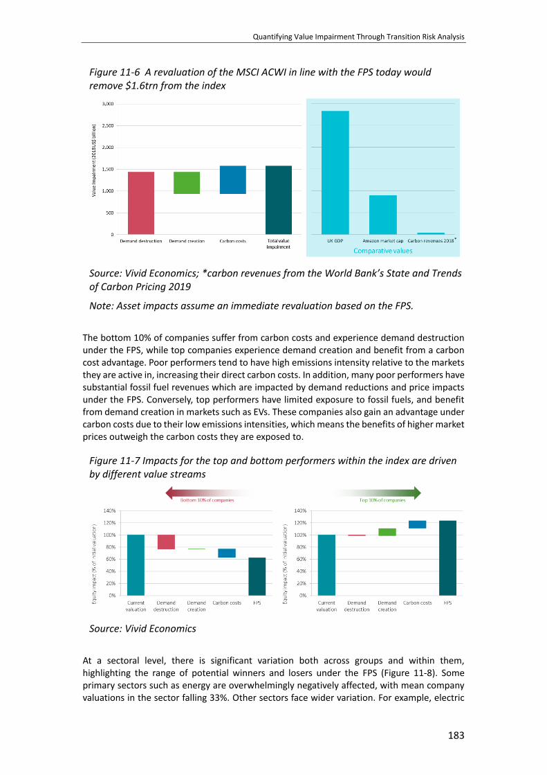
Quantifying Value Impairment Through Transition Risk Analysis
183
Figure 11-6 A revaluation of the MSCI ACWI in line with the FPS today would remove $1.6trn from the index
Source: Vivid Economics; *carbon revenues from the World Bank’s State and Trends of Carbon Pricing 2019
Note: Asset impacts assume an immediate revaluation based on the FPS.
The bottom 10% of companies suffer from carbon costs and experience demand destruction under the FPS, while top companies experience demand creation and benefit from a carbon cost advantage. Poor performers tend to have high emissions intensity relative to the markets they are active in, increasing their direct carbon costs. In addition, many poor performers have substantial fossil fuel revenues which are impacted by demand reductions and price impacts under the FPS. Conversely, top performers have limited exposure to fossil fuels, and benefit from demand creation in markets such as EVs. These companies also gain an advantage under carbon costs due to their low emissions intensities, which means the benefits of higher market prices outweigh the carbon costs they are exposed to.
Figure 11-7 Impacts for the top and bottom performers within the index are driven by different value streams
Source: Vivid Economics
At a sectoral level, there is significant variation both across groups and within them, highlighting the range of potential winners and losers under the FPS (Figure 11-8). Some primary sectors such as energy are overwhelmingly negatively affected, with mean company valuations in the sector falling 33%. Other sectors face wider variation. For example, electric

Chapter 11
184
utilities with the strongest renewables strategy could see valuation double (104 percent), while laggards could see valuations fall by two-thirds (-66 percent).
Figure 11-8 Within-sector variation can be significant, particularly for the most impacted sectors in the index
Source: Vivid Economics
Note: Error bars indicate the 10th and 90th percentiles of companies in each sector.
Detailed results on the IPR asset impacts are available on the Principles for Responsible Investment website.
5 Limitations & areas for development
While the Climate risk toolkit can be used to assess risk for a wide range of asset classes and at a high level of granularity, there remains some outstanding developments that will improve the level of analysis offered in the future. Some limitations of the current approach to scenario analysis are outlined below.
• The baseline scenario selected directly impacts the magnitude of results under the policy scenario. Selecting a baseline scenario requires an implicit assumption on the current level of policy and technical developments, which directly affects results. While our approach offers the choice between a BAU scenario that reflects current policy announcements or a scenario which continues historical trends, there is currently no widely accepted baseline scenario.
• The methodology limits interactions between physical and transition risks. The climate risk toolkit has developed to be capable of analyzing physical risks alongside transition risks since the IPR project. However, there could be further interaction between the physical and transition effects in future renditions of the climate risk toolkit.
• A focus on listed equities means some sectors and regions are underrepresented in results. Analysis focuses on listed equities and the sectors and regions these represent. This means not all risks are captured as many fossil fuel producers are not listed, such as Middle Eastern national oil companies. In addition, while Europe and

Quantifying Value Impairment Through Transition Risk Analysis
185
the US are well represented due to a high level of listed equities, there are fewer Chinese equities listed for example. This can be overcome if private equity information is incorporated for a desired region or sector.
6 Conclusion
Climate scenario analysis can inform financial institutions’ investment decisions and help align strategic decisions with the expected state of climate policy. As climate risks become increasingly apparent, the use of climate scenario analysis in supporting investors’ decisions will become ever more valuable. By quantifying the impacts associated with climate change transition risk, our methodology can guide investment decisions in the coming period of uncertainty.

Chapter 12
186
Financial Climate-related Transition Risks: Integrated Assessment Across the Finance and
Investment Universe
By
Dr. Nicole Röttmer1
PricewaterhouseCoopers GmbH Wirtschaftsprüfungsgesellschaft, Germany
Abstract
Financial institutions are facing a potentially significant disruption in the real economy, reflecting on their balance sheets, business models, and portfolios. Quickly understanding and integrating this understanding of potential regulatory, market, and technology dynamics into standard operating procedures is key for smoothly managing potential risks and capturing the arising opportunities. This chapter outlines a pathway for capturing the key risk and opportunity drivers at the right level of detail, and for integrating them across institution types, functions and in specific roles.
Keywords: transition, risk, opportunity, climate excellence, investment, banking, insurance, real estate, project finance, risk management, analyst, portfolio management
1 Purpose and approach
Why to leverage scenario analysis? The climate transition the world might undergo to limit global warming will test the resilience of business models, while at the same time creating significant potential for value. Increasing awareness of the potential impact of the transition is fostering regulator, supervisor and stakeholder attention, and insufficient action and communication by financial institutions might reflect on their license to operate.
Scenario analysis is a method of choice when historical trends and datasets can no longer be used to accurately forecast the future (e.g. in the case of accelerating or disruptive change, as in a climate transformation), and effects are likely to play out over the medium to long term.
Scenario analysis is a powerful tool, enabling users to directly understand the impact of climate change on sectors, specific companies, or even entire portfolios. Per scenario, it allows for the modelling of a variety of impacts that can be interrelated and interact positively or negatively with one another. For example, it not only connects changes in oil demand from the automotive industry (resulting from the introduction of more electric vehicles) with impacts on oil prices and refinery performance, but also with the impact on demand for renewable
1 This chapter is written by Dr. Nicole Röttmer, Partner, PricewaterhouseCoopers GmbH Wirtschaftsprüfungsgesellschaft
GmbH Germany, email: [email protected].

Financial Climate-related Transition Risks: Integrated Assessment Across the Finance and Investment Universe
187
power generation and the potential for alternative fuels to boost financial performance in other sectors.
Infobox Scenario: "A scenario describes a development path that leads to a specific result. [...] It should be noted that scenarios are hypothetical constructs; they are not forecasts or predictions, nor are they sensitivity analyses "(TCFD, 2017d). Scenarios describe conceivable, inherently consistent future worlds instead of, for example, a change in individual parameters such as an interest rate. In simple terms, a scenario is a consistent series of "what-if" questions.
Due to these characteristics, scenario analysis can deliver valuable insights to any user interested in learning about the potential impact of climate-related risks and opportunities on their own performance, from an investor curious about how a portfolio of investments would perform under the assumptions of climate change, to an insurance company striving to understand the impact of climate-related risks on their policies and their business. Its insights inform risk management and link well with upcoming supervisory stress-tests, as demonstrated for example by the launch of market-wide insurance climate stress tests in early 2019 by the Prudential Regulatory Authority (PRA) in the United Kingdom.2
An example by The CO-Firm and Kepler Cheuvreux illustrates, why this scenario view might extend our current understanding of risks and opportunities. Their research shows that under the 2°C and 2.7°C climate pathways (scenarios, for the sake of easy understanding) by the International Energy Agency (IEA) 3 , companies today might be significantly over- or undervalued (Figure 12-1).4 Capital markets thus might not fully account for them yet(The CO-Firm & Kepler Cheuvreux, 2018c, p. 36).
2 Bank of England, Prudential Regulatory Authority (2019) Insurance Stress Test 2019, 18.06.2019. See
https://www.bankofengland.co.uk/-/media/boe/files/prudential-regulation/letter/2019/insurance-stress-test-
2019.pdf?la=en&hash=2F9F25800465DFF2AFA24C5C230D8ADCE6BA5810 3 The Scenarios that form the basis for the assessment of climate-related risks build on 1) the International Energy Agency
(IEA) Energy Technology Perspectives (ETP) and 2) the IEA World Energy Outlook (WEO). The ETP 2017 2°C Scenario (2DS)
and the WEO 2016 450 Scenario form the basis for the 2°C scenario. The ETP 2017 Reference Technology Scenario (RTS)
and the WEO 2018 New Policies Scenario (NPS) – once available – form the basis for the 2.7°C Scenario. 4 For an analysis of the automotive, steel and electric utility sectors, please refer to publications of the CO-firm. (The CO-
Firm & Kepler Cheuvreux, 2018b, 2018c, 2018).

Chapter 12
188
Figure 12-1 Illustrative steel company valuation impact in a 2°C and a 2.7°C scenario, assuming an average adaptation (Market) as well as “beating the marking” (Beat-the-market) relative to a consensus baseline(The CO-Firm & Kepler Cheuvreux, 2018d)
Thus, scenario analyses can support existing risk, financing, investment, or underwriting processes by answering the following questions:
• How material are climate-related risks, i.e., to what extent do they affect the financial performance of investments, products, companies, sectors and countries?
• What drives climate-related risks and opportunities, i.e., changing energy prices, competitive new technologies, changing demand patterns?
• What do I need to believe for these risks and opportunities to materialize? I.e., will oil heating be prohibited, do synthetic fuels enter the market at reasonable cost, or will the renewable build-out take place?
• How resilient is my portfolio, and potentially the companies’ business lines and projects, given the potential to strategically adapt (technology investments, product or value chain changes)?
Such findings can be used by different groups of actors within financial institutions, for a variety of purposes. Some examples are to support the selection of financing or investment objects, to validate risk parameters and modelling, to adjust portfolio or fund allocation, to focus exposure to companies according to their risk, and to support reporting (Röttmer, 2018, pp. 269-282).
Why think about a fundamental modelling logic for climate transition risks? Scenarios allow for capturing interdependent sector dynamics, such as the impact of an electrification of cars on electricity demand, housing infrastructure, the oil market, input prices for the chemical industry and so on. Only a fundamental analysis allows for capturing these effects, as the following example illustrates:
0
10
20
30
40
50
60
70
80
90
100
Ind
exe
d s
um
of
cu
mu
lative
dis
cou
nte
d
cash
flo
ws (
Baselin
e =
100)
"Consensus"
baseline
2.7 C Beat-
the-Market
2.7 C
Market
2 C Beat-
the-Market
2 C Market
PerpetuityFirst 5 years Years 2023 -2050

Financial Climate-related Transition Risks: Integrated Assessment Across the Finance and Investment Universe
189
There is a widespread belief that the climate transition risks and opportunities can largely be described through carbon prices. However, this is not reflecting the fundamental changes in the economy that will – in an interdependent manner – influence demand, technology cost curves, resource availability, etc. Figure 12-2 provides an example, illustrating the global revenue of three large electric utility companies under a under possible 2.0°C climate scenario. Despite their comparable size in terms of power generation capacity, the three companies have significantly different carbon footprints. The company with the lowest footprint shows the lowest revenue growth potential in the scenario and is outperformed by the company with the biggest carbon footprint over time.
Figure 12-2 Global revenue development for power generation of three large electric utility companies in a 2.0°C scenario
Source: The CO-Firm and Kepler Cheuvreux (2018b)
Another fundamental belief relates to the assumption that sector dynamics are indicative of company dynamics (the same holds true for specific physical assets, such as real estate). Research by The CO-Firm (The CO-Firm & Kepler Cheuvreux, 2018c) shows that average financial effects on sectors are barely indicative of individual company’s performance. Rather, for example, companies within the automotive sector, exhibit significantly different financial impacts (positive and negative), based on specific company characteristics and geographic footprints. In the automotive sector, for example, regional demand trends (e.g. vehicle fleet growth driven by developing markets) and technological diversity (plug-in hybrid, electric or conventional vehicles) drive company EBITDA performance: “The main differentiators between winners and losers are regional and technological exposure, and diversity, relative to the peer group” (The CO-Firm & Kepler Cheuvreux, 2018c), as can be seen in Figure 12-3 below.

Chapter 12
190
Figure 12-3 EBITDA impact on individual companies in an exemplary 2.0°C IEA-based climate scenario analysis.
Source: The CO-Firm and Kepler Cheuvreux (2018c)
These dynamics require an increasingly thorough understanding of drivers of direct and indirect climate-related risks and opportunities as well as the ability to quantify and manage their potential financial impact. This can be achieved by treating this type of risk and opportunity along the existing mechanisms, from sector outlooks to risk models.
Purpose of the fundamental Climate Excellence methodology In this context, the purpose of the Climate Excellence methodology and tool is to financially assess climate-related transition risks and opportunities. It quantifies the risks and opportunities arising from the transition towards a lower carbon economy using scenario analysis. It builds on a bottom-up approach, focusing on the drivers of financial performance for plants, products, projects and technologies under a changing market, price, technology and regulatory environment, thus lending itself to the analysis for the real economy and the financial sector. For the financial sector, it can be conducted across a multitude of use cases with a defined real asset underlying the financial instrument, such as bank portfolios and individual loans, equity portfolios/funds, bonds, real estate, infrastructure and other project financing mechanisms, and insurance premium impact calculations.
Transition risks could alter the risk-return profile of financial assets. Climate Excellence leverages different publicly available, scientific and integrated future climate pathways and energy system models. It leverages their assumptions on technology, market (demand, price), and regulatory changes in a fundamental model, translating them into specific impacts on physical assets such as products and technologies, plants, real estate and infrastructure, companies, and sectors in their relevant geographies. It derives country-level impacts on that basis.
This approach mirrors the work typically performed by chief economists, sector analysts, and financial analysts (e.g. research analysts, equity/ credit analysts or actuaries) and supplements it with specific climate-related, financially relevant insights. Given the fundamental approach, it can provide all types of metrics for integration into standard modelling approaches (e.g. for asset management, discounted cash flow (DCF) or multiples models). Its bottom-up approach provides one pathway for integrating climate-related risks (and opportunities) into the standard risk categories used by regulators.
-100
-50
0
50
100
150
200
EB
ITD
A (
ch
an
ge %
vs.
2016)
2020 2030 2040 2050
Individual companies*
Individual companies‘ performance
Financial Climate-related Transition Risks: Integrated Assessment Across the Finance and Investment Universe
191
Chapter approach This chapter illustrates how fundamental scenario analysis can be used as a practical tool for analyzing transition risks and opportunities. Using the example of asset management and the scenarios provided by the International Energy Agency, this paper presents the methodology and demonstrates the application of scenario analysis with a real-life case study.
Three key characteristics describe the methodology embedded in the Climate Excellence tool:
- Extending the current financial sector view on risk and opportunity, with a forward-looking, materiality-based financial assessment of climate-related risks and opportunities:
- Scenarios describe plausible development paths towards a lower carbon economy (without providing any probability), leading to a specific global warming target or carbon particle concentration. The methodology is inherently forward-looking due to the application of scenarios, and allows for a materiality-based, quantitative financial assessment of climate-related risks and opportunities.
- Comprehensive coverage of scenario impacts, due to fundamental analysis and market-based assessment:
- The analysis enables an integrated understanding across scenario-specific climate risk drivers, addressing the suggestion of the TCFD (2017b). It thus reflects the full potential financial impact from changing demand, competitive environments, input prices and new technologies, as well as regulation, and not only single factors.
- It is based on the underlying, sector-specific market dynamics, enabling the integration of climate analyses into existing risk, valuation, credit or underwriting processes, as well as internal macroeconomic outlooks and microeconomic views.
- It allows for a consistent assessment of risks and opportunities across financial instruments and underlying assets (e.g. real estate, infrastructure, projects, companies, plants or products, countries)
- Reflective of strategic choices of companies (adaptive capacity), providing a more true and fair view on the specific risk position of the real economy counterpart:
- “Financial modelling of climate risk must consider companies’ ability to anticipate transition risks and develop mitigation strategies, as it impacts future asset development and companies’ financial performance. Adaptive capacity allows a true and fair view of risks and opportunities to be presented. Not considering it might lead to the overestimation of climate risks” (The CO-Firm & Kepler Cheuvreux, 2018a, p. 33).
2 Which questions does transition scenario analysis answer for
financial institutions?
For financial institutions, there are various use cases for the results and learnings from scenario analysis. Three broad distinctions can be made: Use cases by institution, by function within an organization, and within functions, such as equity analysis, building on the specific methodologies and proxies used.

Chapter 12
192
Questions answered for asset managers/owners, for banks and insurance companies
Different financial institutions’ characteristics require different foci when performing scenario analyses, as the TCFD illustrates in their supplemental disclosure guidance for asset owners and asset managers, banks, and insurance companies (TCFD, 2017a).
Scenario analysis provides different financial institutions with a common foundation of insights on overall materiality, risk (opportunity) drivers, changing macroeconomic and sector environment. These are:
1. Order of magnitude financial impacts within and across scenarios;
2. Sector- and scenario- or even geography-specific risk drivers with significant financial impacts based on changes to revenues, cost, and capex;
3. Understanding of the company-, project-, plant- or product-specific characteristics that imply vulnerability relative to the risk drivers;
4. An interpretation of the changes described by the scenario that imply the change in the risk profile;
5. Potentially a range of KPIs for approximating the potential risk position.
Institutions tend to have different approaches to integrating scenario learnings into their operations.
Asset Manager/Asset Owner Key Question: Could climate change have a material impact on my investment analysis?
While the TCFD distinguishes between asset managers and asset owners, both have the same goal: to optimize value (risk return) for their investors and stakeholders. Given their role in the financial system, they strive to outperform the market, identify new and attractive financing opportunities, and, depending on the institution, potentially guide the energy transition. Relevant insights extend across the five points illustrated above, depending on the respective audience within the institution. A relevant cross-check consists of extending the frame of the analysis to longer timeframes, checking whether any risks (opportunities) occurring after ten years might already impact the performance of assets currently invested in. One example is the real estate sector, where an intention to sell in 10 years’ time might meet a demand which then already incorporates a view to the next 10 years – thus, 20 years would be the appropriate timeline for assessing risks. In the risk integration, the focus is on the key risk drivers.
Banks Key question: Could climate change impact my counterparties’ probability of default?
While banks tend to leverage the same underlying basis and findings of scenario analysis, they tend to apply a higher materiality threshold (apart from for distressed entities). Also, when integrating the learnings in the standard processes, they tend to leverage the few key risk drivers per sector and geography. Standard portfolio indicators are of less relevance currently. In risk integration, the focus is on the key risk drivers.

Financial Climate-related Transition Risks: Integrated Assessment Across the Finance and Investment Universe
193
Insurance companies Key question: How does climate change affect my underwriting and investment activities across business lines?
Scenario analysis allows for a forward-looking integration of climate-related risks into investment and underwriting activities, complementing traditional stress testing. On the underwriting side, scenario analysis supports a better understanding of climate-related impacts on claims and premiums. Insurance premiums, for example, could be affected by climate-related transitions risk due to changes in the amount of insurance policies sold. There could be different potential implications. A reduction in premium revenues could impact overall profitability and, in turn, also impact capital requirements. Scenario analysis provides insights into which sectors within the underwriting portfolio across different business lines could be most affected.
Questions answered by function of a financial institution A number of needs by different functions can be addressed by scenario analysis, for example within asset management. Some of the objectives of scenario analysis by user group were derived from the TCFD‘s supplementary notes for the financial sector (TCFD, 2017a).
Table 12-1 Objectives of scenario analysis for the asset manager user group5
User groups
User Questions that can be answered with Scenario Analysis
Market
Equity Analyst (PRI, 2018)
● Who could be winners and losers - structurally, including adaptive
capacity?
● What are the material impacts of climate change on existing risk
factors? Have new risk factors been identified?
Product development (PRI, 2018, p. 37)
● Where do new investment needs arise (and existing needs
diminish)?
● How can this be reflected in new products or during the transition
of existing products?
Portfolio Manager
● How could climate change affect the relative risk-return profile of
specific sectors?
● To what extent can security selection influence the average sector
risk?
● Can the sector actively manage its risks and opportunities?
● What are the material impacts of climate change on existing risk
factors? Have new risk factors been identified?
Risk controlling
Risk Manager ● Would new risk factors or a change in the materiality of risk factors
imply a need for reflection in general risk management?
Sustainability Department
CSR Manager
● Which metrics should be retrieved from the specialist
departments for the disclosure of climate risks?
● Qualitative vs. quantitative: Which financial indicators should be
mapped?
5 Adapted from PwC (2019) in TCFD Think Tank (2019, pp. 14-15). The criteria considered here are followed by
presentations and discussions in the TCFD Think Tank in Q1 and Q2 2019. For further criteria and parameters see Technical
Supplement publications of TCFD (2017c, p. 9).

Chapter 12
194
Integration example: Asset owner analyst While the second line of defense is regulated in its risk modelling, there is flexibility in investment analysis with regard to model used. While some analysts use multiple-based models, others build on, for example, discounted cash flow models. Some analysts build distinct models per company, reflecting corporate assets and investment plans, while others work primarily with financial reporting and derive additional insights qualitatively.
Once the potential financial materiality of climate-related risks and opportunities and their timing has been analyzed and an analyst chooses to integrate these findings, the analyst has different pathways for doing so. Using the example of a discounted cash flow model, climate-related insights might find reflection in the growth potential or risk profile of specific securities. If changes in cash flows are to be reflected, the results will depend on whether the analyst is interested in the business impacts at a specific point in time or in a trend. Results from the analysis of a specific time frame can be used to extend the forecasting horizon of specific cash flows. If the analysis shows business impact changes in a trend, the terminal growth rate can be adjusted. Also, the specific short-term calculation could integrate climate-related impacts on cash flows (the same holds true for capex).
Similar degrees of freedom exist for the reflection of risk. An illustrative issue tree is shown below (Figure 12-4).
Figure 12-4 How to integrate scenario analysis into company valuations
Source: The CO-Firm and Kepler Cheuvreux (2018a)
3 Methodology & data
This chapter outlines the method and data used to assess climate-related risks & opportunities with Climate Excellence, using the example of individual companies. Our method for modelling is unique in that it:
• provides forward-looking and financial impacts;
• builds on fundamental analysis, enabling the assessment of risks from market and competitive dynamics, and enabling an easy integration into existing analysis practices;
Do you want to integrate these
results of scenario analysis into
financial modelling?
Use the results in multi-criteria or
other type of analysis
Do you want to reflect changes in
cash flows or changes in the risk
profile?
Do you want to be able to reflect the
business impact of transition risks at
a specific point in time or are you
more interested in the trend?
Do you want to understand the
potential risks in specific scenarios
or integrate scenario risk into the
central valuation model?
Extend the forecasting
horizon or specific cash
flows (option 1)
Adjust the terminal
growth rate (option 2)
Calculate the implied risk
premium and its variance under
different adaptive capacity
scenarios (option 3)
Adjust the discount rate to
reflect the required rate of
return to take up additional
transition risk
(option 4)
No Yes
Growth profile Risk profile
Risk to baseline scenarioTrendPoint in Time Risk within transition scenario

Financial Climate-related Transition Risks: Integrated Assessment Across the Finance and Investment Universe
195
• includes adaptive capacity, i.e., the capacity of companies to adjust their strategies if financially relevant;
• builds on bottom-up asset-level modelling, allowing integrated insights on a plant, technology, company, country and sector level;
• builds on geographic granularity corresponding to specific sector characteristics;
The approach has been co-developed with leading financial institutions, inputs/ modelling been academically validated and tested with companies over several years.6
Two approaches are most discussed in modelling climate-related financial impacts: top-down and bottom-up modelling. We have chosen the bottom-up approach for the quantitative assessment of climate-related financial risks and opportunities, as we have seen that corporate characteristics within a sector lead to significantly different financial impacts.
Understanding the financial implications of climate scenarios We calculate the financial impact (FI) for an individual company i for a given year t>0 under a given climate scenario SC as follows.
Formula 12-1 Financial impact calculation, example: Company
𝐹𝐼𝑆𝐶,𝑖,𝑡>0 = (∑ 𝐶𝐴𝐵𝑖,𝑡,𝑗,𝑘 × 𝐵𝐹𝐼𝑆𝐶,𝑖,𝑡,𝑗,𝑘
𝑗,𝑘
) × (∑ 𝐶𝐴𝐵𝑖,𝑡=0,𝑗,𝑘 × 𝐵𝐹𝐼𝑆𝐶,𝑖,𝑡=0,𝑗,𝑘
𝑗,𝑘
)
−1
Where
𝐹𝐼𝑆𝐶,𝑖,𝑡>0 is the financial impact in terms of EBITDA, EBIT or sales relative to the start year
𝐶𝐴𝐵𝑖,𝑡,,𝑗,𝑘 is the company activity breakdown that splits revenue shares to the bottom level, summarizing the activity j in a geography (e.g. country or region) k
𝐵𝐹𝐼𝑆𝐶,𝑖,𝑡,,𝑗,𝑘 is the financial impact in terms of absolute EBITDA, EBIT or sales under the scenario SC for the bottom-level activity j in geography k for company i
Formula 12-1 shows that the breaking down of an individual company’s economic activity into meaningful climate-impact entities (based on industry standard classification systems, such as NACE - as used in the EU Taxonomy - or NAICS)7 to which we can map a specific climate-related
6 See, for example: University of Cambridge Institute for Sustainability Leadership (CISL, 2016) and The Energy Transition
Risks & Opportunities (ET Risk) research consortium seeks to provide research and tools to assess the financial risks and
opportunities associated with the transition to a low-carbon economy. Please refer to: http://et-risk.eu/, as well as G20
Green Finance Study Group (2017). 7 NACE - Statistical classification of economic activities in the European Community, NACE is derived from the French
Nomenclature statistique des activités économiques dans la Communauté européenne; NAICS - North American Industry
Classification System

Chapter 12
196
financial impact for this individual activity and in its geography. To do this, in a first step, we cluster economic activities by profit drivers (is the key determinant the value chain performance, the operations performance, or product differentiation). Then, we break down a company segment by key operations from a climate-related view (per geographic region).
Climate Excellence then uses functional impact relations for mapping climate scenario parameters such as demand changes, relative price changes, availability of raw materials, etc. to the profit and loss divers along the companies’ structural criteria. This is a materiality-driven approach, looking at the extent of climate risks and opportunities relative to the average margin and margin volatility. This mapping results in individual cost, margin, and/ or volume impacts. The overview illustrates that an understanding of the sector and partially geographic market dynamics is key in providing a true and fair view of the impacts.
Fundamental market modelling to calculate the financial impact of climate scenarios
In the previous chapter we broke down company economic activities into climate-impact homogeneous entities, based on NACE codes. We analyzed their profit drivers, identified the relevant transmission mechanisms that illustrate their impact by climate scenarios, and gained an understanding of the competitive situation.
We now assume that we are looking at a sector in which financial performance is driven by operations efficiency, and that operations efficiency is linked to the technology, capacity, and efficiency status of specific plants owned by the company. This would, for example, be the case for sectors such as cement, steel, and utilities. In this case, Figure 12-5 (subsequent numbering is consistent with the chart8) illustrates our modelling approach:
Data on current plant ownership by a company (2) in different geographies is mapped with the scenario-based, geographic changes to demand, prices, etc. (1), and, reflecting future developments, the potential for companies to technologically improve their assets and pass through additional cost (3). Building on the investment plans announced by companies, and the improvement potential, the fundamental market model (5) then dynamically models the relative competitive position of plants as it changes due to relative geographic demand trends, changing input costs, etc.
The market model allocates scenario-specific relative margin and volume impacts to the different plants. This approach is further detailed in the subsequent paragraphs and described in detail in the “Investor primer to transition risk analysis” report by The CO-Firm and Kepler Cheuvreux (2018a).
8 For more general information on each of the following steps, please refer to publications of The CO-Firm and Kepler
Cheuvreux (2018a).

Financial Climate-related Transition Risks: Integrated Assessment Across the Finance and Investment Universe
197
Figure 12-5 Fundamental market modelling approach to quantify financial impacts from climate scenarios
1. Derive the key risk drivers to translate a scenario into a narrative. First, develop a holistic
transition narrative by extending scenario data with consistent transition drivers. This can include a) Breaking down country-specific technology pathways by region and country based on scenario data; or b) deriving information on regulatory interventions (e.g. quotas and subsidies) by region and by scenario based on current and announced regulatory regime, climate targets, envisaged technology pathways.
2. Build an asset-level database with financial information on individual economic activity in geographies. The analysis builds on data on corporate assets, such as power generation plants (e.g. wind turbines) or steel and cement plants, and technologies, efficiencies, production cost of each entity.
3. Conduct a techno-economic assessment of risk mitigation measures (“adaptive capacity”). Financial modeling of climate risk must consider companies’ ability to anticipate transition risks and develop mitigation strategies. The potential effectiveness of such measures is comprised under adaptive capacity. Analyzing risk mitigation must take into account a variety of aspects such as the scenario applied (e.g. 2.0°C), the current technology base of a company, e.g. type, location, and age of technologies, investment and CAPEX and the risk-return profile of the market. Measures comprise cost pass-through, technological upgrades and shifts, etc.
4. Incorporate three assumptions for companies’, i.e., asset development. Three potential pathways form part of the analysis: FROZEN freezes the current asset portfolio over time. This hypothetical assumption is used to identify the cost of inaction under climate scenarios. MAINSTREAM assumes that company changes or adapts its asset portfolio in line with the overall market trend under the scenario. BEAT THE MARKET assumes that a company takes all financially profitable means to adjust based on its financial prowess, anticipating changes, beating the market.
5. Develop a fundamental market model based on the demand and supply developments to derive prices and asset-specific profit in the scenarios. At the example of an asset-centric sector, steps 1. to 4. allow for identifying the production costs per asset and company under different scenarios over time, forming a merit order. The intersection of the merit-order with the demand given by the scenario indicates the commodity price. The difference between this price and the production costs indicates the financial impact:

Chapter 12
198
𝐵𝐹𝐼𝑆𝐶,𝑖,𝑡,,𝑗,𝑘 is the financial impact in terms of absolute EBITDA, EBIT or sales under the scenario SC for the bottom-level activity j in geography k for company i
6. Derive financial impacts on companies. Aggregating the resulting absolute profit changes results in profit impact on company level.
Deep dive on data required for climate scenario analysis
Transition scenarios (1) While a climate scenario illustrates the carbon (equivalent) emissions still available to sustain a certain global warming level with a specific likelihood, transition scenarios that lend themselves to scenario modelling tend to provide insights into potential allocations of carbon budgets to, for example industrial sectors, and the choices these sectors need to take to achieve such an overarching global warming pathway. Regulation, technology mix, and changes in demand and prices can be drivers. Also transition scenarios can build on the impact of, for example, choices already taken, i.e., by regulators.
Figure 12-6 Illustrative relationship between climate scenarios, carbon budget and sector
Given the fundamental modelling approach, Climate Excellence can operate with a range of scenarios. For illustrative purposes, the following case examples build on publications by the IEA, and their integrated energy system models.
Scenarios can provide a set of parameters that describe future world in most cases, covering:
• Economic activity by sector/ geography
• Population growth
• Energy demand
• Climate policy
• Fossil fuel generation, renewable share in power generation
• Carbon capture and storage assumptions, bio-energy shares, syn fuels
• Oil and gas demand
2.250GtCO2
1.890 GtCO2
2.950GtCO2
Cumulative
emissions
already
released
1.5°
Remaining
budget
2.0°
What is available?
Source: PwC based on Shell scenario
Sector impacts
• Product
demand
• Production
technology
change
• Energy use
and CO2
emissions
• Change of
input-/output prices
Company Impacts
Product
portfolio
Company
impact
Financial
impact
Strategic
impact
Margins Business
models
Production
technologies
Geographic
exposure
Earnings
Capex
Business
segments
Assets
The Present The Path The Future

Financial Climate-related Transition Risks: Integrated Assessment Across the Finance and Investment Universe
199
• GHG emissions
Asset-level data (2) Chapter 3 illustrated the value of detailed and complete data on corporate assets in adequately assessing climate-related risks and opportunities. Similarly, Caldecott et al. point out that analysis using asset-level data is typically9:
• Bottom-Up: Asset-level exposure is aggregated up to the company level rather than inferred from company-level reporting;
• Fundamental: Fundamental asset attributes (e.g., location, technology, and age) inform analysis rather than disclosed metrics (for example, carbon intensity), enabling more sophisticated and flexible analysis;
• Comparable: Standardization can ensure accurate company comparisons and avoids embedded methodological assumptions;
• Forward-looking: Asset attributes (such as age) can enhance the analysis of future company performance and enable validation of company projections.
• Efficient: It can significantly reduce reporting burdens and reduce time and money spent on assuring voluntary disclosures;
• Timely: Asset-level data can be updated in real time as events occur (like mergers or asset commissioning) rather than according to annual reporting cycles;
• Transparent: Asset attributes are transparent and are based on real observational data, giving stakeholders access to the same data as company executives;
• Scalable: The marginal costs of data acquisition and analysis decrease with scale of the dataset;
• Science-driven: Asset-level data unlocks scientific approaches to analysis which are repeatable and testable;
• Unbiased: Assessments of environmental factors informed by asset-level data do not rely on the (non-expert) opinions of corporate boards.
• Self-improving: Science and technology-driven risk analysis and data acquisition improve continuously with new generations of technology and research. Costs are also reduced over time.
For Climate Excellence, among others, third-party asset level data used comprises more than 230,000 physical assets in over 50 countries, providing information such as technologies used, capacities, production volumes, location, and other sector-specific information.
9 Based on article of Caldecott et al. (2018).

Chapter 12
200
Risk mitigation measures (3) As an additional step, the analysis covers ~130 general technical measures for improving energy and carbon efficiency, as well as commercial measures companies can take to respond to changing input costs, in case taking these measures is business case positive.
4 Impact examples: Climate-related transition risks:
The following paragraphs illustrate climate-related transition risks for two distinct sectors. This assumes that the financial institution has reviewed whether and in which sectors climate-related risks and opportunities might become financially material in a first step. In a second step, in sectors potentially materially affected, the following analyses can be applied.
The first example is for power generation, illustrating that climate-related impacts on single companies can substantially differ from the respective sector average. The second example shows that risk and opportunity drivers impact corporations activities differently, despite them operating in the same sector.
Power generation: Global EBITDA implications and relative company performance
Looking at the sub-sector average for power generation, both climate scenarios exhibit positive EBITDA developments relative to today (see Figure 12-7), in the business line power generation.
Relative to a 2.7°C IEA scenario, IEA’s 2.0°C scenario reflects higher CO2 prices, more investments in renewable energy sources and power grids, as well as a higher power demand in general through electrification (e.g. e-mobility). Thus, globally, the 2.0°C scenario shows stronger EBITDA growth until 2030. However, not all power generation companies profit from these developments at the same manner. The scatter plot shows a heterogeneous picture with some companies outperforming the global average growth trend, while others - under the scenario - cannot maintain their current financial performance.
Performing this type of analysis across sectors can provide material insights for portfolio management, as it illustrates the growth implications per (i.e., invested) sector, which might differ substantially between sectors. The distribution of growth potential among the companies in the sector can provide guidance to analyst security selection within the limits set by portfolio management.

Financial Climate-related Transition Risks: Integrated Assessment Across the Finance and Investment Universe
201
Figure 12-7 The financial impact of climate risks usually affects individual companies heterogeneously, even within the same sector. Both figures show MAINSTREAM adaptive capacity
Source: The CO-Firm and Kepler Cheuvreux (2018b)
A steel example illustrates the risk and opportunity driver analysis.
Steel manufacturing: Valuation insights, the cost of inaction, and characteristics of successful companies
The example on power generation showed heterogenous impact on companies, even within the same sector. Figure 12-8 illustrates the cumulative discounted cash flows of three steel companies along three-time horizons, focusing on their steel segments. An analysis by Kepler Cheuvreux and The CO-Firm revealed that all three steel companies would lose relative to a consensus baseline with a perpetuity view under both a 2.0°C or 2.7°C climate scenario compared to baseline evaluation.10 In particular, steel company B could lose ~ 60% in a 2.7°C world, and ~50% in a 2.7°C world, and ~70% in a 2.0°C world, even under the assumption that company B invests proactively (in a business case positive manner) and aggressively in those technologies and markets with highest EBITDA potential (strategy: “BEAT THE MARKET”). Steel company A and C would be significantly less impacted by the climate scenarios.
This type of analysis illustrates the potential materiality of climate scenarios relative to a baseline as it could currently be applied by analysts and illustrates the time horizons in which different cash flow assumptions would materialize.
10 With regard to the choice of a baseline for company valuation, the valuation estimates from climate change scenarios
are compared with a market ‘consensus’ baseline, based on Bloomberg consensus data and the terminal growth rate and
discount rate applied from Kepler Cheuvreux’ own equity analysts (The CO-Firm & Kepler Cheuvreux, 2018d).
Weighted average global power generation
0
50
100
150
2015 2020 2025 2030 2035 2040 2045 2050
EB
ITD
A (
ch
an
ge %
vs.
tod
ay)
EB
ITD
A (
ch
an
ge %
vs.
tod
ay)
Individual power generation companies in 2°C scenario
(100)
(50)
0
50
100
150
200
2.0°C
2.7°C
2025 2030 2040 2050

Chapter 12
202
Figure 12-8 The discounted cash flow from steel manufacturing would be significantly reduced for all three steel companies along a 2.7°C and 2.0°C warming pathway11
Often, climate-related risks and opportunities are considered a medium- to long-term effect. Figure 12-9 illustrates the impact of companies seizing to invest beyond what they have planned for the next three to five years (“frozen” strategy). This would already reduce EBITDA in the short-term.
Were the companies to adjust along the scenario-based developments in their respective geographic markets and in line with their technological experience, and their financial means (generated in the steel segment), company A could generate a positive trend. This is even more true if the company proactively “beats the market” (Figure 12-9).
11 With regard to the choice of a baseline for company valuation, the valuation estimates from climate change scenarios
are compared with a market ‘consensus’ baseline, based on Bloomberg consensus data and the terminal growth rate and
discount rate applied from Kepler Chevreux’ own equity analysts (The CO-Firm & Kepler Cheuvreux, 2018d).
0
10
20
30
40
50
60
70
80
90
100
"Consensus"
baseline
Ind
exe
d s
um
of
cu
mu
lative
dis
cou
nte
d
cash
flo
ws (
Baselin
e =
100)
2.7 C
Beat-the-
Market
2.0 C
Beat-the-
Market
PerpetuityYears 2023 -2050First 5 years
0
10
20
30
40
50
60
70
80
90
100
Ind
exe
d s
um
of
cu
mu
lative
dis
cou
nte
d
cash
flo
ws (
Baselin
e =
100)
2.7 C
Beat-the-
Market
"Consensus"
baseline
2.0 C
Beat-the-
Market
0
10
20
30
40
50
60
70
80
90
100
Ind
exe
d s
um
of
cu
mu
lative
dis
cou
nte
d
cash
flo
ws (
Baselin
e =
100)
"Consensus"
baseline
2.7 C
Beat-the-
Market
2.0 C
Beat-the-
Market
Steel Company A Steel Company B Steel Company C

Financial Climate-related Transition Risks: Integrated Assessment Across the Finance and Investment Universe
203
Figure 12-9 EBITDA development of three steel companies with three strategic assumptions under a 2.0°C climate scenario12
What drives such differences in the financial performance of companies and their ability to adapt to climate scenarios? The companies’ current technology portfolios and geographic footprints provide explanations. For a better understanding of the results, it is worthwhile to note that there are three main technology routes for steel manufacturing: coal-based (Blast Oxygen Furnace (BOF)), electricity-based (Electric Arc Furnace (EAF)), and gas-based (Direct Reduced Iron (DRI)). All routes have different characteristics regarding raw materials, investments and GHG emissions. Figure 12-10 shows the EBITDA breakdown according the three technology routes and the geographical footprint for the main regions and countries. Company A has a globally and technology diversified portfolio which can level-out climate-related impacts. Company C has invested in two routes in two regions. Only Company B has focused on one route in one country. Company A benefits from its diversified portfolio, which levels out climate-related impacts through the different route characteristics and different climate impacts among regions. Additionally, it profits from further investment in the electric-based and gas-based production routes regions, benefiting from the route’s inherent characteristics (e.g. North America). Steel company C can also profit from its early investment in the gas-based route in the United States. However, steel company B’s portfolio focuses on the coal-based production route in one country. The costs for the coal-based route to adapt to climate-related impacts are significantly higher compared to the other technologies and investment only pays off under high CO2 prices which occur in the 2.0°C only after 2030. Until then, the competitive disadvantage of coal-based steel production results in decreasing financial performance.
12 With regard to the choice of a baseline for company valuation, the valuation estimates from climate change scenarios
are compared with a market ‘consensus’ baseline, based on Bloomberg consensus data and the terminal growth rate and
discount rate applied from Kepler Chevreux’ own equity analysts (The CO-Firm & Kepler Cheuvreux, 2018).
EB
ITD
A (
change %
vs.
2016)
EB
ITD
A (
change %
vs.
2016)
EB
ITD
A (
change %
vs.
2016)
20402020 2030 2050
-50%
0%
50%
100%
-50%
20502020 2030 2040
0%
50%
100%
2020 2030 2040 2050
-50%
0%
100%
50%
FROZEN MARKET BEAT THE MARKET
Steel Company A Steel Company B Steel Company C

Chapter 12
204
Figure 12-10 Today's asset and geographic portfolio and the adaptive strategy influence the ability of companies to succeed under 2.0°C climate scenario13
5 How to apply scenario analysis
Scenario analysis of climate-related financial risks and opportunities can integrate smoothly into existing processes and practices. Using the example of investment, climate scenarios can be mapped against an investor’s own macroeconomic outlook, in the case of IEA, regarding population growth and economic growth. The sector-specific scenario developments can be mapped with the institutions’ own sector-specific outlooks, leading to a delta analysis which helps to understand where and how risk and opportunity drivers might change or new ones might arise, and allows the internal experts to review the order of magnitude impacts based on their experience. The same holds true for the company level, building on the companies’ structural characteristics (Figure 12-11).
13 With regard to the choice of a baseline for company valuation, the valuation estimates from climate change scenarios
are compared with a market ‘consensus’ baseline, based on Bloomberg consensus data and the terminal growth rate and
discount rate applied from Kepler Chevreux’ own equity analysts (The CO-Firm & Kepler Cheuvreux, 2018d).

Financial Climate-related Transition Risks: Integrated Assessment Across the Finance and Investment Universe
205
Figure 12-11 Scenario analysis insights lend themselves to easy integration into existing financial institution practices (example investment)
Source: PwC (2019) Own elaboration
For the specific integration into existing valuation approaches, Figure 12-11 provides a first methodological overview. Figure 12-12 provides a schematic example for an integration of climate-related factors into real estate valuation, based on an income approach.
Figure 12-12 Illustrative approach on how to integrate climate-related risks in real estate evaluation
Source: Valuation of Carbon Performance Project (2019)
6 Conclusions and outlook The purpose of this study is to describe one pathway to analyzing climate-related risks and opportunities, based on the Climate Excellence methodology and tool, and using the example of asset management and scenarios provided by the International Energy Agency (others can be applied in a similar fashion). The paper underlined the insights that can be generated by using climate scenario analyses, and showcased different use cases for different financial institutions and their functions. The underlying modelling and data needs were explained and the application of scenario analysis with a real-life case study was demonstrated.
Illustrative picture of value determination with the income approach
Multiple
…
Annual income
Av. Rent/m2
Annual cost
Occupancy Rate
(m2)x
Maintenance &
repair cost
(Opex)
Admin cost
(Opex)
Int. interest rate/
riskyield
Residual life/
annuity multiple
Potential climate-related value driver
To be paid by
tenant
To be paid by
landlord
Operating
licence: EPC
level
Exchange duties
(heating…)
Energy price
increase
Internal CSR/CO2
targets/priceEE Renew ables
Future value
projection:
adjustment factors
(+/-) based on
comperative data
Required Invest
Projected renov.
cost (Capex)
Capital cost-
+ +x +
+
x
-
%
%
SCHEMATIC
Carbon pricing: Increased energy
tax/carbon price for Non-ETS
Ordinance law : define tight EE
standards for building stock
Demand side: Market pressure
increase by tenants/occupiers
National (sub)sector climate targets
define max „risk“
Technologies get cheaper due to
learning curves and/or subsidies

Chapter 12
206
There are a few key conclusions that can be derived from this overview:
• Focusing exclusively on carbon and carbon regulation might jump too short in providing a true and fair view of potential climate-related risks and opportunities.
• In line with the recommendations by the (TCFD, 2017b), it is valuable to look not only into the next couple of years, as investment or product decisions taken today may face significantly negative impacts during their lifetime, creating lock-ins or avoidable losses
• Only focusing on sector-centric analysis means losing out on the potential to improve portfolios by active securities selection, as company performance within sectors in the same scenario tends to vary significantly.
• At the same time, scenario analysis allows for deriving clear and distinct risk and opportunity drivers on a sector-, and – depending on sector characteristics - potentially geography-level. They can be mapped to distinct company characteristics. This provides ample space for the easy integration of climate-related risk and opportunity analyses, all the way to a quantitative integration into valuation, probability of default, or premium calculations.
Voluntary disclosure, such as the Principles for Responsible Investment (PRI) and the Carbon Disclosure Project (CDP), as well as regulatory activities connected with the disclosure of climate-related risks and opportunities, and supervisory activities indicate that scenario-based climate-related disclosure is there to stay. At the same time, scenario analysis still tends to be a weaker point in current disclosure related to the TCFD recommendations 14 , as are the integration into strategy and risk management. These points are closely connected – without a clear view on underlying dynamics and risk and opportunity drivers, it is hard to formulate a strategy or integrate numbers without their underlying rationale into a risk framework.
With increasing work on and with climate scenarios and by contrasting specific results with one another, and increasing disclosure, it can be expected that the dialogue will increasingly center on key scenario assumptions, such as on the key decarbonizing engines of the energy system (i.e., carbon capture and storage or usage), and the transmission of these assumptions to the financial performance of individual business models, products, customers and suppliers, etc. The same holds true for commercial actors’ strategic responses and adaptive capacities. These dynamics pave the way for a better understanding of the strategic choices we are facing regarding climate change, their economic impacts across assets, companies, sectors, societies, a call for meaningful data, and a smarter dialogue between users and preparers.
14 According to the TCFD status report, information related to Strategy c), “describe the resilience of the organization’s
strategy, taking into consideration different climate-related scenarios, including a 2°C or lower scenario”, had the lowest
levels of disclosure (TCFD, 2019).

Financial Climate-related Transition Risks: Integrated Assessment Across the Finance and Investment Universe
207
Bibliography
Caldecott, B., Dericks, G., Bouveret, G., Schumacher, K., Pfeiffer, A., TULLOCH, D., . . . MCCARTEN, M. J. U. o. O., Sustainable Finance Programme accessed. (2018). Asset-Level Data and the Energy Transition: Findings from ET Risk Work Package 2. 19.
CISL. (2016). Feeling the heat: An investors’ guide to measuring business risk from carbon and energy regulation. Cambridge, UK.
G20 Green Finance Study Group. (2017). G20 Green Finance Synthesis Report 2017. PRI. (2018). Implementing the Task Force on Climate-related Financial Disclosures (TCFD)
Recommendations - A guide for Asset Owners, p. 37ff. https://www.unpri.org/download?ac=4652
Röttmer, N. (2018). Szenarioanalysen und TCFD - ein Beitrag zum Risikomanagement und zur Finanzierungs- bzw. Investitionsstrategie? . In Stapelfeld, M., Granzow, M. and Kopp, M.. Greening Finance. Der Weg in eine nachhaltige Finanzwirtschaft.
TCFD. (2017a). Implementing the Recommendations of the Task Force on Climate-related Financial Disclosures.
TCFD. (2017b). Recommendations of the Task Force on Climate-related Financial Disclosures. TCFD. (2017c). Technical Supplement: The Use of Scenario Analysis in Disclosure of Climate-
Related Risks and Opportunities. In: Task Force on Climate-Related Financial Disclosures.
TCFD. (2017d). The Use of Scenario Analysis in Disclosure of Climate-Related Risks and Opportunities
TCFD. (2019). 2019 Status report, https://www.fsb-tcfd.org/wp-content/uploads/2019/06/2019-TCFD-Status-Report-FINAL-053119.pdf
TCFD Think Tank. (2019). User Guidance on TCFD Recommendations. Implementing TCFD step by step in your company. https://gsfc-germany.com/wp-content/uploads/2019/08/190820_TCFD_Handreichungen_EN-1.pdf
The CO-Firm, & Kepler Cheuvreux. (2018a). Investor Primer to Transition Risk Analysis, http://et-risk.eu/investor-primer-to-transition-risk-analysis/
The CO-Firm, & Kepler Cheuvreux. (2018b). Transition risk for electric utilities, http://et-risk.eu/electric-utilities/
The CO-Firm, & Kepler Cheuvreux. (2018c). Transition risks in the automotive sector. http://et-risk.eu/auto_risk/
The CO-Firm, & Kepler Cheuvreux. (2018d). Transition risks in the steel sector, http://et-risk.eu/wp-content/uploads/2018/07/Transition-risks-for-steel.pdf

Chapter 13
208
A Physical Climate Risk Analytical Toolkit for Banks and Investors
By
Acclimatise and Vivid Economics1
Abstract
The Acclimatise-Vivid Economics physical climate risk analytical toolkit offers a joined-up top down and bottom up approach to assessing physical risks in financial portfolios. Acclimatise draws on extensive experience in interpreting physical climate risk data to provide detailed analysis of how climate hazards can impact clients’ holdings. Vivid Economics brings understanding of state-of-the-art modelling techniques to shed light on the macroeconomic climate impacts facing banks and investors. Here we share an overview of the Acclimatise-Vivid Economics analytical toolkit, which is a suite of integrated tools and services that can be customised to clients’ evolving needs. The analytical toolkit is based on a layered approach, which first provides a high-level climate risk assessment at the portfolio level, followed by deep dive analyses where material risks are identified. The toolkit provides qualitative risk scores for the portfolio-wide heatmapping, and quantitative financial metrics at the second (‘deep dive’) stage.
Keywords: physical climate risk, natural disasters, changes in asset values, financial impacts
1 Purpose of the analytical toolkit
Climate change risks have the potential to disrupt financial markets, and are of growing importance for the finance sector. The Task Force for Climate-related Financial Disclosures (TCFD), and the Network for Greening the Financial System (NGFS) have highlighted the financial risks from climate change, and called for the integration of climate risk into asset management and investment practices. Having an investment portfolio which is resilient to potential future climate scenarios is of vital importance.
Acclimatise and Vivid Economics have partnered to develop an analytical toolkit for banks and investors, to assess physical climate risks and opportunities under future climate scenarios. Acclimatise is an advisory and analytics company specialised in physical climate risk assessment and climate change adaptation. Vivid Economics is a strategic economics consultancy with a focus on climate change analysis, public and private climate change strategies, and the quantification of risks and opportunities.
Our analytical toolkit assesses the impacts of climate change-related physical risks and opportunities on a portfolio by combining climate hazard models with sector and asset-level vulnerability data, value stream impact models and financial modelling, to assess impact on
1 This chapter is written by Richenda Connell, email: [email protected], CTO and Co-founder of Acclimatise;
Robin Hamaker-Taylor, email: [email protected], Financial services climate risk consultant at
Acclimatise; Xianfu Lu, email: [email protected], Head of Analytics at Acclimatise; Eis, Jason, email:
[email protected], Executive Director of Vivid Economics.

A Physical Climate Risk Analytical Toolkit for Banks and Investors
209
key financial metrics. It can serve various business functions within a financial institution including strategic portfolio management, informing lending decisions and asset allocation, disclosure, and internal or external engagement. It can be delivered with a menu-driven interface.
2 Intended users and application
Our toolkit has been designed for use by banks and investors to evaluate forward-looking physical climate risks based on scenarios. Within banks, the toolkit caters to a variety of functions, including:
• Risk management teams,
• Credit risk departments,
• Investment officers, and
• Lending officers.
Within the investment community, the target users are asset managers and investors, also across a variety of functions, including:
• Risk management teams,
• Investment officers, and
• Stewardship teams.
The toolkit has broad applicability as it can be used globally, across most sectors. Furthermore, it can be applied to most asset classes, and supports analyses for a wide range of acute and chronic climate hazards. More detail is provided in Section 3 below.
3 Fundamental components
Overview Our toolkit performs both portfolio-wide and asset-level assessment of physical risks and opportunities with its phased, layered approach. After secure data collection of asset level information, (including location, sector and sub-sector information, and details of the underlying physical assets2), the first phase is a high-level portfolio-wide assessment, resulting in a heatmap. The second phase involves quantification for a selection of assets. This involves ‘deep dive’ asset-specific analyses for higher risk areas identified from the Phase 1 heatmap. See Figure 14-1 for an overview of the toolkit’s fundamental components.
2 To the extent this information is available. This includes, for example: construction type, number of stories, age of physical
asset, etc.

Chapter 13
210
Figure 13-1 Overview of fundamental components of the Acclimatise-Vivid Economics analytical toolkit for physical climate risks
Source: Acclimatise and Vivid Economics
Coverage Our toolkit has global coverage and covers all sectors and sub-sectors which can be vulnerable to physical climate risks. See Figure 14-2 for a sample of sectors typically assessed by users of the toolkit.
Figure 13-2 Non-exhaustive sample of economic sectors covered in the Acclimatise-Vivid Economics toolkit
The toolkit draws on the latest climate science on potential changes in key climate hazards, both acute and chronic, from a wide range of global and regional climate model outputs. Specifically, the toolkit leveraging:
• The full suite of climate models participating in the World Climate Research Programme’s (WCRP) fifth phase of the Climate Model Inter-comparison Project, known as ‘CMIP5’; and

A Physical Climate Risk Analytical Toolkit for Banks and Investors
211
• Some of the regional climate model outputs from WCRP’s Coordinated Regional Climate Downscaling Experiment (CORDEX).
Figure 13-3 provides an overview of the climate science used in the analytical toolkit.
Figure 13-3 The toolkit employs robust climate science on potential changes to key climate hazards
Source: Acclimatise and Vivid Economics
Hazards listed under “chronic” and “acute” hazards are variables that are entirely dependent on climatic or hydrometeorological conditions (hence can be quantified by either climate models directly or by combining more than one variable directly simulated by climate models). The “climate-related” variables/phenomenon are often also dependent on other non-climatic parameters (e.g. water stress is dependent on population and economic activities, landslide dependent on topography etc.).
The toolkit covers a range of time periods, from the present day up to 2100, with most financial institutions applying it on investment timescales up to mid-century. It provides data for a range of climate scenarios, though typically the representative concentration pathway (RCP) scenarios 2.6 and 8.5 are used to span a range of future physical risks, roughly corresponding to 2oC and 4°C warming by the end of the 21st century.3
The financial effects of physical climate risks can be quantified with the toolkit for a full range of asset classes and risks. It is designed to assess debt, equity, real estate and infrastructure investments. See Figure 14-4 for an overview of asset classes covered by the toolkit.
3 Source: IPCC, 2014: Climate Change 2014: Synthesis Report. Contribution of Working Groups I, II and III to the Fifth
Assessment Report of the Intergovernmental Panel on Climate Change [Core Writing Team, R.K. Pachauri and L.A. Meyer
(eds.)]. IPCC, Geneva, Switzerland, 151 pp. Table 2.1. Available from:
https://www.ipcc.ch/site/assets/uploads/2018/05/SYR_AR5_FINAL_full_wcover.pdf

Chapter 13
212
Figure 13-4 The financial effects of climate change can be quantified for a full range of asset classes and risks with the analytical toolkit
Source: Acclimatise and Vivid Economics
4 Detailed methodology
Our toolkit performs both portfolio-wide and asset-level assessment of physical risks and opportunities with its phased, layered approach. This draws on good practice in risk management, which suggests that a broad screening of risks should be conducted, before determining which areas to focus on for in-depth analysis. The heatmapping approach has multiple benefits, in that it:
• Provides an early indication of where higher risks may lie within the portfolio,
• Is comprehensive in scope, covering all relevant sectors, sub-sectors and geographies,
• Is undertaken quickly and efficiently, and
• Highlights ‘hotspots’ of physical risk in the portfolio, which can then be the focus for deep-dive analysis or investor engagement.
This section reviews the two phases of the analytical toolkit in more detail, highlighting how the heatmapping exercise is a first stage that feeds in to the second deep-dive stage. These phases are separate, relying on distinct methodologies, as described in Sections 4.1 and 4.2.
Portfolio-wide physical risk heatmapping The first phase identifies key areas of physical risk by screening a portfolio for vulnerability to a full range of climate impacts. Inputs for this are covered under Section 5.1 of this chapter, but include portfolio composition information on sectors in locations of interest to the client. For this phase, spatial data on climate hazards under various scenarios are combined with sector vulnerability indicators and applied to the portfolio. This produces a heatmap which helps identify priority portfolio segments for deeper analysis.
This phase assesses the vulnerability of a portfolio – by sector and sub-sector – to climate and climate-related hazards. Vulnerability to climate change of each sub-sector is assessed using a

A Physical Climate Risk Analytical Toolkit for Banks and Investors
213
suite of eight vulnerability indicators covering the whole value chain, including for example, reliance on climate-sensitive supplies, transportation route, market demand, etc.
Each sub-sector is assigned a vulnerability indicator weighting score within the toolkit, according to the relative importance of the indicator to a particular sub-sector. This score represents the extent to which that vulnerability indicator will affect the value of any holding in that sub-sector when subject to a specific combination of hazards. These vulnerability indicators have been developed by Acclimatise over a decade, drawing on a broad base of empirical analysis and peer-reviewed literature, as well as Acclimatise’s work with clients in those sectors and geographies most prone to climate risk. They capture a wide range of impact channels through which climate and climate-related hazards can affect holdings in a sub-sector. The indicators are designed to provide comprehensive coverage of potential risk areas, and enable financial institutions to have a full picture of the factors that might affect the value of their portfolios.
Within the toolkit, the hazard data and vulnerability indicators are combined to assess physical risks facing a financial institution’s sub-sectors by geography. Impacts are assessed across all vulnerability indicators that are important to a specific sub-sector, and utilising hazard data sets that are relevant to the sub-sector. Sets of relevant climate/weather data (e.g. temperature or precipitation), and climate/weather-related events data (e.g. landslide or wildfire risk) are linked to each vulnerability indicator. The underlying hazard data are assigned scores, to indicate the presence, absence and severity of individual hazards.
A set of physical risk heatmaps are produced in this phase, per climate scenario and time period, providing banks and investors with a picture across the portfolio of which segments face higher physical climate risks. The heatmaps can be provided based on sector and sub-sector categories, asset classes and geographies as specified by the client. The heatmaps are typically delivered in Excel so they can be readily disseminated. An illustrative heatmap output, showing risk scores by sector, sub-sector and geography is provided in the ‘Input and output metrics/data’ section (Section 5).
Quantification of physical risk in financial metrics The second phase takes portfolio segments identified as at high risk in the heatmapping phase and employs data on climate hazards (present-day and future), value stream impact models and financial modelling to assess impacts on key financial metrics. The analytical approach is summarized in Figure 14-5. It applies data analytics to evaluate value stream impacts at two levels:
• Economy and sector-level effects of physical climate change, deploying a Computation General Equilibrium (CGE) model to estimate the effects of slow-onset climate change for a large number of countries and sectors. This models the wider demand shifts caused by physical climate change, and the interdependencies between sectors.
• Company-specific value chain analysis of physical climate risk, applying climate hazard data to quantify impacts on the physical assets and supply chains of companies in the sector.

Chapter 13
214
Figure 13-5 Overview of analytical approach to quantifying the financial effects of physical climate risk
Source: Acclimatise and Vivid Economics
Economy and sector-level modelling We deploy a computational general equilibrium (CGE) model to assess the interactions between economic sectors and between countries/regions. It provides an understanding not just of ‘first-order’ climate change impacts but also how climate change shocks feed through the entire economic system, sector by sector. Compared to other similar models, it provides a higher level of geographic and sector disaggregation, and hence a more nuanced view of climate change effects than models which are limited to a handful of regions and sectors.
Detailed climate change impact functions are used to model the relationships between temperature increases and economic outcomes at sector- and country-levels. Impact functions provide a means to translate between physical and economic impacts, providing information on the magnitude of economic impact for any given temperature rise. These impact functions draw on the latest academic research and cover a range of effects, including impacts of increased temperatures on labor productivity, reductions in availability of land caused by sea level rise and changes in the demand for specific sectors. These risks are quantified and used as an input into financial asset modelling.
Modelling impacts on value chains We model physical climate risks to value chains for key impact channels: changes in facility-level production, physical asset damage, business interruption and supply chain disruption. These risks are quantified and used as an input into financial asset modelling.
• Facility-level production: Changes in climatic variables can have a direct impact on the
productive capacity of assets. We maintain an in-house database of sensitivity functions, which
describe the relationships between climatic factors and production, based on latest academic
literature and empirical evidence. Combining sensitivity functions, asset locations and climate
models generate estimates of changes in production at the facility level between present day
and under future climate change scenarios.
• Facility-level extreme weather damages: We maintain a database of damage functions which
describe the relationships between hazard intensity and physical damage to assets for many
major asset classes. Combining these with archetypal asset and hazard intensity data for asset
locations provides estimates of facility-level losses.

A Physical Climate Risk Analytical Toolkit for Banks and Investors
215
• Facility-level business and supply chain interruptions: We maintain a model of business
downtime caused by extreme climate events. The model combines empirical data on business
interruptions caused by extreme weather events with hazard maps, to evaluate associated
production losses. In parallel, data on sector supply chains are combined with data on extreme
events at key supply locations for the sector, to estimate potential supply chain disruption and
associated lost production across the sector.
Financial modelling Discounted cash flow models are used to estimate the combined effects of the above value stream impacts on valuations of financial assets. For each financial entity, we aggregate the cash flow impacts of changes in sector size with facility-level impacts on productivity, damages, and business and supply chain interruptions. These cash flows are discounted over time using a company-specific discount rate in order to estimate valuation impacts. The same approach is used for corporate bonds, factoring in the impacts of cash flow changes on probability of default.
5 Input and output metrics/data
Inputs Databases integrated into the toolkit include:
• Acute and chronic climate and climate-related hazard data, for present-day and future time periods under climate change scenarios,
• Country economic data, covering a range of social accounting matrices,
• Input-output data and international trade data,
• Data on listed companies, including financial metrics, geographic and product segmentation, and
• Sectoral databases.
Other databases can be integrated into the toolkit depending on client requirements.
Clients provide portfolio data in a matrix of sub-sector and geography for the first phase of analysis (portfolio-wide heatmapping). Sub-sector descriptions are mapped onto standard industry classifications. For the second phase (quantified deep dives), core financial information for counterparties is required, if they are not listed companies or if data are not publicly available.
Outputs The toolkit provides qualitative risk scores at the first stage: portfolio-wide heatmapping, and quantitative financial metrics at the second stage: ‘deep dive’ analysis. Providing qualitative metrics is a strength of the toolkit, as the heatmapping can be used to facilitate internal dialogue around the climate ‘hot spots’ across a portfolio and help raise awareness. The qualitative risk score gives clear direction and focus for the quantitative assessment, so that data- and resource-intensive quantitative analysis is only performed where warranted.
The first phase produces a heatmap output, as shown in Figure 13-6. Outputs can be displayed aggregated by asset type, portfolio sub-sectors and geographies. Vulnerability to all hazards
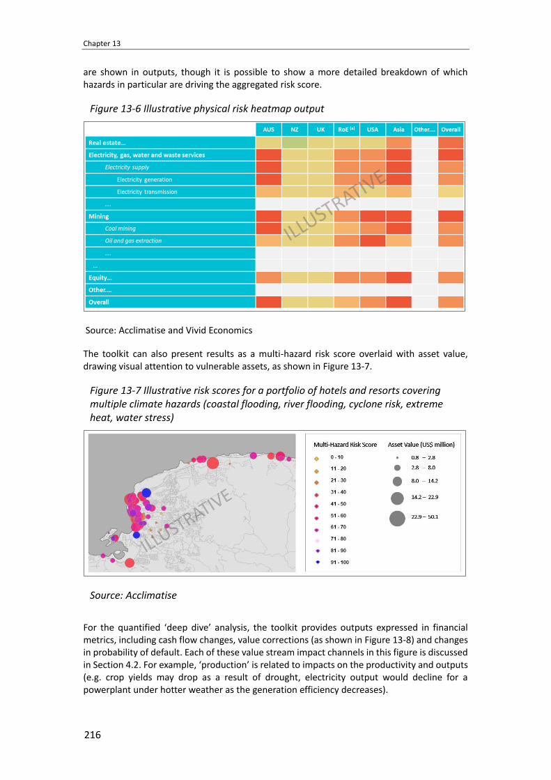
Chapter 13
216
are shown in outputs, though it is possible to show a more detailed breakdown of which hazards in particular are driving the aggregated risk score.
Figure 13-6 Illustrative physical risk heatmap output
Source: Acclimatise and Vivid Economics
The toolkit can also present results as a multi-hazard risk score overlaid with asset value, drawing visual attention to vulnerable assets, as shown in Figure 13-7.
Figure 13-7 Illustrative risk scores for a portfolio of hotels and resorts covering multiple climate hazards (coastal flooding, river flooding, cyclone risk, extreme heat, water stress)
Source: Acclimatise
For the quantified ‘deep dive’ analysis, the toolkit provides outputs expressed in financial metrics, including cash flow changes, value corrections (as shown in Figure 13-8) and changes in probability of default. Each of these value stream impact channels in this figure is discussed in Section 4.2. For example, ‘production’ is related to impacts on the productivity and outputs (e.g. crop yields may drop as a result of drought, electricity output would decline for a powerplant under hotter weather as the generation efficiency decreases).

A Physical Climate Risk Analytical Toolkit for Banks and Investors
217
Figure 13-8 Illustrative example of change in asset value, decomposed into value stream impact channels
Source: Acclimatise and Vivid Economics
6 Limitations of the current approach, outlook/future development
A key feature of the toolkit is its layered approach, which first provides a high-level climate risk assessment at the portfolio level, followed by deep dive analyses where material risks are identified. The toolkit provides qualitative risk scores for the portfolio-wide heatmapping, and quantitative financial metrics at the second (‘deep dive’) stage. Providing qualitative metrics may be seen by some as a weakness. However, the tool developers perceive this to be a strength, as the heatmapping can be used to facilitate internal dialogue around the climate ‘hot spots’ across a portfolio and help raise awareness. The qualitative risk score gives clear direction and focus for the quantitative assessment, so that data- and resource-intensive quantitative analysis is only performed where warranted.
The heatmapping analytics are based on the most recent best-in-class and peer-reviewed climate-related data. Many of the climate variables are reliant on the Coupled Modelled Intercomparison Project (CMIP) for climate projections data. Phase 5 of Coupled Modelled Intercomparison Project, ‘CMIP5’ is currently the most recent iteration for which climate model output data are fully available, and these data are included in the current version of our heatmapping analytics. The next generation, CMIP6, is being carried out by the scientific community. CMIP6 data are expected to be made available in 2021, when Acclimatise will integrate them into our analytics.
For other impact data sets (which may continue to use CMIP5 as their data inputs for the near future), commercial and research organizations release data periodically, which we horizon-scan for suitability for use in the heatmapping. Our internal refresh plan includes an annual review of new/updated datasets that we consider will benefit the heatmapping and notification to clients of the timescales for adding the new datasets. After each such data refresh, the heatmapping analytics are presented as an updated version to the market.

Chapter 14
218
Understanding and Mitigating Risks from a Global Low Carbon Transition: A Micro-Based Approach
to Assessing Climate Transition Risk
by
Climate Policy Initiative Energy Finance1
Abstract
Climate transition risk is an increasingly important object of concern for central bankers and policymakers with financial stability mandates. However, managing the financial stability implications of climate transition risk cannot be done using traditional macroeconomic modelling tools alone. Micro-level, bottom-up modelling is required for effective identification of the drivers, timing and magnitude of climate transition risk. An analysis of the potential impact of climate transition risk on financial stability also requires a mapping of risk transmission channels, including the extent to which risk mitigation activity by companies and financial institutions can pass risk to public balance sheets. CPI Energy Finance has developed an analytical approach which assesses these issues and calculates climate transition value-at-risk metrics for physical fossil fuel and industrial assets, companies and tax revenues. This chapter explains the analytical approach by reference to our recent case study in South Africa, which showed that climate transition risk, if not well managed, could pose a threat to South Africa’s sovereign credit rating. While the chapter focuses on the application of this analysis by those with financial stability mandates, the modelling also has important applications in risk management activities of development financial institutions, fossil fuel and industrial companies and financial institutions.
Keywords: climate transition risk, financial stability, value-at-risk metrics, contingent liabilities, South Africa, sovereign credit rating, modelling, bottom up
1 Introduction
This chapter sets out the approach that Climate Policy Initiative Energy Finance (CPI EF) developed to measure the exposure of countries and their financial systems to low carbon “transition risk” or “climate transition risk”. Climate transition risk, which arises from the structural changes to the global economy that will be required in a low carbon transition, could result in lower-than-expected corporate profits, financial asset values and tax revenues. The material magnitude of these changes and the systemic importance of the industries that they will affect mean that if not effectively managed, transition risk could cause economic shocks with potential losses falling on workers, investors in the equity and debt of companies and ultimately, public balance sheets. There is a growing consensus that climate-related financial risk, of which transition risk for most countries is probably the most important part in the short term, could pose a material threat to global financial stability (Bank for International Settlements, 2020).
1 The chapter is written by Matthew Huxham, Principal, Climate Policy Initiative Energy Finance, email:
[email protected]; David Nelson, Executive Director, Climate Policy Initiative Energy Finance, email:
A Micro-Based Approach to Assessing Climate Transition Risk
219
The growth of interest in climate-related financial risk has prompted the development of a wide variety of new tools, indicators and scorecards designed to help investors identify transition risk. However, there are fewer tools or analyses that translate transition risk into changes in valuation of equity and debt securities and even fewer that show the impact of the low carbon transition on both investors and government debt levels. CPI EF’s transition risk methodology aims to fill that gap.
CPI EF’s approach draws on detailed asset-level,2 bottom-up (micro-level) analysis, which we argue is necessary to augment “top-down” macroeconomic models if central bankers, financial supervisors and policymakers are to gain an understanding of the drivers, timing, magnitude and distribution and transition risk. In this chapter, we describe our analytical approach, which developed over several years3 and then provide an illustration of the methodology taken from our recent case study of South Africa (Huxham et al., 2019). The case study was commissioned and supported by Agence Française de Developpement (AFD).
The chapter deals with the following topics:
• How we define climate transition risk and why new analytical tools are required to support a comprehensive analysis of this risk;
• The aims of CPI EF’s alternative approach and how our insights contribute to a wide range of risk mitigation actions from actors including central bankers, financial supervisors, policymakers with economic, industrial and labor-related remits, companies, and investors in public and private debt and equity securities;
• How to construct such an analysis – including, data, scenarios and models;
• An illustration of this methodology in the context of South Africa; and
• How we are working to improve the analysis through future case studies.
2 Hypothesis: transition risk is different and so requires new
analytical tools
An effective analysis of the macroeconomic consequences of transition risk (e.g. impacts on sovereign credit ratings and the value of currencies) needs to start with an analysis of its microeconomic foundations. The risks arising from transition to a low carbon economy – whether driven by policy, taxation, technology, consumer behavior or a combination – will first affect the value of specific physical assets (such as oil fields or coal mines)4 and companies
2 The term “asset-level” refers principally to physical assets. CPI EF’s analysis of transition risk starts from the valuation of
individual coal mines, oil wells, industrial facilities etc. The analysis also includes an assessment of the impact of transition
risk on company valuations and solvency, but it does not assess the change in value of individual securities (e.g. different
classes of shares, senior vs. subordinated debt). 3 Relevant papers showing the development of this line of thinking include: Moving to a low carbon economy: the impacts
of policy pathways on fossil fuel asset values developed for the inaugural New Climate Economy report in 2014
(https://climatepolicyinitiative.org/publication/moving-to-a-low-carbon-economy/) and Government assets: risks and
opportunities in a changing climate policy landscape (2016) prepared for the European Bank for Reconstruction and
Development in 2016 (https://climatepolicyinitiative.org/publication/government-assets-risks-opportunities-changing-
climate-policy-landscape/). 4 The value of physical assets will change because of drivers affecting the amount (or cost) of supply, demand or both.
Different transition drivers will have different effects – while carbon taxes may increase the cost (and therefore demand for)

Chapter 14
220
before spreading across economies. Central bankers, financial supervisors and policymakers with a financial stability remit need to understand the drivers, timing, magnitude and distribution of transition risk starting at the level of physical assets and companies in order to mount an effectively and timely response at the level of the economy or the financial system.
Economy-wide general equilibrium models, which tend to have limited intra-sectoral granularity, are not always well suited to this task. For example, the impact of the global low carbon transition on the value of oil resources and the companies extracting them will depend on the relative cost position of the assets and competitive forces. For example, two oil fields producing products of a similar chemical composition could experience very different outcomes from a transition, depending on their position on the cost curve. A relatively expensive asset might become too expensive to produce and lose all its value, while an inexpensive asset may lose no production but suffer from lower prices and a loss of margin. Therefore, to gain an understanding of the impact of a low carbon transition on the oil industry in a country which earns a significant proportion of tax revenues from oil, policymakers need to understand factors ranging from the position of different resources on global or regional cost curves; the financial structure and health of the companies extracting the oil; the extent to which local municipal finances rely on oil royalties etc.
While general equilibrium models might have the computational power to assess the impact of national or even sectoral carbon prices on variables like interest rates and unemployment, by averaging within or across sectors, they are unlikely to identify the context-specific factors identified above, which can be the main drivers of transition risk.
If policymakers and regulators do not add “microeconomic” analysis into their toolkits, they may fail to identify the complex drivers of transition risk which are likely to crystallize in a non-linear fashion (e.g. gradual, sharp, or indeed, gradual then sharp). These drivers are likely to be both international and therefore out of a country’s control (e.g. falls in demand for imports of seaborne thermal coal) and domestic (e.g. mandated coal phase-out dates). “Microeconomic” analysis of the sort proposed by CPI EF can help policymakers understand the impact of different combinations of transition drivers. It can also help to identify the areas where the risk is concentrated today and to predict the risk mitigation activity of private sector actors (e.g. companies and financial institutions). Understanding risk concentrations can help policymakers design targeted responses which are sensitive both to macroeconomic and political economy considerations.
The methodology and the case study presented in the rest of this chapter shows how CPI EF does this microeconomic analysis, starting from an assessment of climate transition “value-at-risk” for individual mines, oil wells and industrial facilities. We then combine individual asset-level impacts to understand the impact of transition risk on companies and their investors, then the impact on public finances.
3 Intended users of this methodology
CPI EF’s granular approach to transition risk measurement means that the results can inform the decision-making of actors far beyond the central banks and financial supervisors within the NGFS. Potential applications could range from financial sector stress tests, corporate and financial institution risk management and planning for a “just transition” for workers and communities in areas dependent on businesses likely to decline in a low carbon transition. This
carbon-intensive products (for example, coal-fired power generation), technological innovation may reduce the cost of
low-carbon alternatives (for examples, solar photovoltaic power generation).

A Micro-Based Approach to Assessing Climate Transition Risk
221
detailed modelling can also help public and private sectors alike in understanding the implication of a potential tightening of global climate mitigation commitments in the run up to COP26.
However, we expect that our analytical approach will be of most interest for those with responsibility for maintaining financial stability.
Public institutions with responsibility for financial stability mandates Financial stability mandates are often split between central banks, financial supervisory authorities (where separated from central banks) and governments.5 Policymakers tasked with maintaining financial stability tend to have economy-wide remit and tend to have responsibility for assessing emerging new risks, of which climate transition risk is one.
We think the following categories of decision makers would benefit the most from our methodology:
1. Monetary policymakers, who often have a primary objective to maintain price stability, may seek to use CPI EF’s analysis to incorporate another material source of risk into their forecasting, particularly insofar as it impacts the external trade balance (which could affect the valuation of the currency), where transition risk (e.g. falling demand for seaborne thermal coal) is largely outside of the control of the country. The analysis can also help policymakers to understand the extent to which external shocks could affect consumer prices directly (e.g. changes in the prices of imported goods).
2. Financial supervisory authorities will be able to use the analysis to provide guidance to financial institutions on incorporating transition risk into everyday risk management practice and disclosure as well as enabling institutions to respond to any transition risk stress tests designed by the supervisory body and enabling the supervisory body to assess the quality of stress test responses. CPI EF’s analysis could be used to help design transition risk scenarios taking both external and domestic sources of transition risk. It will also help financial supervisors assess the broader effects which could result from risk mitigation actions by supervisee firms (e.g. divestment could protect individual firms, but pass transition risk onto less scrupulous parties).
3. Finance ministries seeking to calibrate public debt levels, the sovereign credit rating and borrowing costs will – in combination with their existing general equilibrium models – be able to use such analysis to stress-test the public finances to account for the impact of an acceleration of international climate policy.
4. Policymakers with an interest in levels of investment in the economy (both macroeconomic policymakers interested in the quality of GDP growth and fiscal policymakers designing incentives for new investments) will be able to use CPI EF’s analysis to assess the resilience of planned new investments to climate transition risk.
The channels through which transition risk might affect a country’s economy (or financial system) are likely to be idiosyncratic and dependent on factors such as whether a given country is a net exporter or importer of fossil fuels and the importance to a given country of the
5 Mandates can vary significantly between central bank institutions, as described in Dikau, S and Volz, U, Central Bank
Mandates, Sustainability Objectives and the Promotion of Green Finance explores the range of variations between central
bank mandates: https://www.soas.ac.uk/economics/research/workingpapers/file139494.pdf

Chapter 14
222
financial services industry.6 To use this tool, countries would thus need to complete a detailed initial analysis, which would identify current drivers and concentrations of transition risk. However, it would also need to be updated regularly to account for changes in global and domestic climate policy, technological change and changes in the structure of commodity, energy and industrial markets.
National and multilateral development financial institutions The international policy and development community will also likely be interested in the results from this analysis when scaled up and made publicly available.
Without preventative action, information asymmetry in relation to transition risk could allow effective risk mitigation by internationally diversified corporates and financial institutions at the expense of increasing concentrations of risk in resource-exporting countries and within vulnerable parts of those countries. For example, we found that, in South Africa, the recent trend of large internationally diversified coal mining companies to divest coal mines (rather than paying to close them down) has pushed transition risk onto smaller, less diversified companies, often backed by investment by state-owned financial institutions.
International financial organizations, national and multilateral development banks (MDBs), and development finance institutions (DFIs) will be important actors in supporting transition planning in developing countries. For these institutions, analysis of the sort proposed in this paper could be used both internally – in their own investment and portfolio management processes – and through technical assistance to institutions in their areas of operation. National development banks, MDBs and DFIs could also be key conduits in developing new types of transition financing in developing countries. Processes to develop and finance transition plans for workers and communities, increasingly involving international collaboration, would benefit from a detailed analysis of where (down to the physical location), when and under what scenarios certain mines, oil fields or other industrial assets might become economically unviable.
Private sector and other users of this analysis CPI EF’s transition risk analysis – in particular, the underlying models which estimate the value of physical assets and companies in different climate mitigation scenarios – will also have a wide range of applications in the private sector. Private lenders, such as sovereign bond investors, as well as credit rating agencies, are increasingly likely to incorporate detailed information on country transition risk exposure and management strategies into investment decisions as they face increasing pressure to demonstrate alignment with international climate goals. Credit rating agencies, which have hitherto been reluctant to make fundamental changes to their rating methodologies to account for climate-related financial risk, could use transition risk analysis of the sort proposed in this chapter to adjust the credit metrics that they use to rate sovereigns today. Examples could include using the additional information
6 In many advanced industrial economies (for example, the UK), where the share of the economy from commodity
extraction and manufacturing has fallen, the size of the financial services industry has risen significantly. London is an
important hub for the global financial services industry. London-based banks will face some risk from the UK’s planned
low carbon transition, however, the institutions based in London have significant exposure outside of the UK in jurisdictions
with less progressive and less transparent policy processes than in the UK. Any assessment of the solvency of London-
based firms in the context of transition risk therefore should arguably include an assessment of transition risk in countries
where those firms have major exposures. By contrast, transition risk in other countries may be a less material consideration
for financial supervisory authorities in countries with financial sectors that are smaller in the context of their host
economies/more domestically focused.

A Micro-Based Approach to Assessing Climate Transition Risk
223
provided by this modelling to adjust projected indicators such as public debt to GDP and public sector contingent liabilities.
Similarly, companies committed to implementing the recommendations of the Taskforce for Climate-Related Financial Disclosures (TCFD) are starting to consider the implications of transition risk for their existing portfolios but may not yet have incorporated a view on how changes in country risk in their operational jurisdictions might affect their earnings.
Financial institutions also are facing increasing pressure to make their portfolios “Paris-compliant” and are searching for more analytically rigorous ways to reduce transition risk (whether arising from structural changes in commodity markets or in changing country risk profiles) than divestment, negative screening, scoring, tilting or exclusion. These approaches often fail to link climate-related financial risk to changes in physical asset or company valuation. CPI EF’s analysis has changes in valuation at its heart and therefore allowed corporates and financial institutions to develop more tailored transition risk strategies.
4 Methodology
This section explains the steps involved in the CPI EF transition risk methodology, which has been developed through a series of studies including for the 2014 New Climate Economy project, a conceptual study for the EBRD and our detailed study in South Africa. We assess transition risk by calculating the difference in value between a baseline scenario (which we typically call “business as usual” or “BAU”) and one where the world decarbonizes in order to keep average global temperature rises well below two degrees above pre-industrial levels (2DS).
The approach includes four main steps:
• Setting the scope for the analysis, including timeframe, sectors and scenarios;
• Calculation of the climate transition value-at-risk, starting with physical assets;
• Assessing the distribution of climate transition value-at-risk, including how this can be affected by the risk mitigation action of companies and financial institutions;
• Design of policy, regulatory and other strategic responses for mitigating external transition risks and reallocating risks around the economy.
Scope The first step in the analytical process is to decide on the sectors that the study will cover. The breadth of the study will in part be defined by the time or budget available but should cover at least the sectors likely to be affected most materially by the transition. This should, at a minimum, include:
• Exports and imports of resources and products, for which demand is very likely to fall in a 2DS scenario, for example, thermal coal and crude oil;
• Sources of domestic greenhouse gas emissions, which may need either to make investments to remain viable in a 2DS scenario (for example, in fuel switching or in carbon capture) or where output will need to be curtailed (for example, electricity generation, oil production, steel and cement production).

Chapter 14
224
More ambitious studies could also include assessments of the transition risk exposure for products where the technological path to decarbonization remains unclear. For example, platinum, which would benefit if the decarbonization of transport involved a large role for hydrogen fuel cells but would otherwise see weakening prospects as demand for the metal falls as the market share of diesel engines declines.
Having chosen the scope, we proceed to choose the timeframe for the analysis. Too short a timeframe (e.g. <10 years) and the analysis would miss important sources of risk. Countries might also continue to invest in long-life infrastructure that might face stranding in 20-30 years’ time. On the other hand, very long-term projections are often seen as irrelevant given the level of uncertainty involved. As an increasing number of countries are now seeking to develop deep decarbonization pathways to 2050, we would suggest conducting an exercise with projections at least until 2040.
Once the scope and timeframe are decided, we design the scenarios and models required to calculate transition risk. We expect that an analysis may include several global and domestic scenarios (as well as combinations of the two) to reflect the inherent uncertainty about the transition.7
Calculating climate transition value-at-risk CPI EF’s analysis calculates the value of physical assets and companies as the net present value of future cash flows. Climate transition risk is the difference between the value of assets (physical or financial) in a baseline (or BAU) scenario and in the chosen low carbon scenario and is expressed as a monetary value.
4.2.1 Using models to calculate value-at-risk We estimate these valuations using proprietary models8 of the markets that the assets under analysis operate in. These markets can either be global, regional or domestic. We tend to build detailed models only of the sectors where our initial analysis indicates are likely to have the most significant transition risk downside.
These models include cost data about physical assets; 9 point-to-point shipping or other logistics costs;10 and projections of future demand.11 These can have different structures, depending on the commodity or other product (for example, crude oil trades on a global market with relatively few benchmarks, such as Brent. On the other hand, there are many prices for seaborne thermal coal, depending on its chemical characteristics and its shipping route). Where appropriate, the models will account for constraints, such as long-term
7 More details on our approach to model design for the South Africa work can be found here: https://medium.com/climate-
policy-initiative-energy-finance/counting-the-cost-of-climate-transition-risk-an-energy-finance-approach-
b7355d94f27c 8 The models referred to in this example can be built in Excel if they are simple, but where the calculation requires multiple
scenarios or variables, we have built models using programming languages, such as Python. 9 Typical information required about physical assets, such as coal mines or oil fields, include: lifting or extraction cost (where
possible, with labour, electricity, fuel costs split out); capital expenditure costs (such as maintenance or expansion) and
information about the resource, including the quality or grade of products produced and the life of the resource. We have
obtained information about physical asset costs from third party sources, including Wood Mackenzie and Rystad Energy 10 Typical information required about logistics arrangements include information on costs of transport of the product to a
domestic customer or to port and the nature (terms, length, counterparty) of the logistics contracts. Where a miner has a
long-term fixed-price logistics contract, it provides the miner with a clearer “route to market” when demand falls, but it
also limits the ability of the miner to pass on transition risk to the infrastructure provider. 11 It is simplest to undertake this analysis using 3rd party projections of future demand. However, in carrying out this analysis
in relation to sectors where the decarbonisation pathway is not yet understood (e.g. steel), it is important to know the
drivers underlying 3rd party demand projections. This will allow the user of the model to update demand projections (and
hence model outputs) as circumstances change.

A Micro-Based Approach to Assessing Climate Transition Risk
225
contracted liquefied natural gas sales (which therefore are not available to spot pricing mechanisms). However, the models typically use some form of optimization function, designed to simulate the most economically optimal set of trade flows, which then allows us to derive prices and volumes for each export and import node.
We use these models to derive the price and sales volume that would be achieved by individual mines, oil fields or industrial facilities, in different climate mitigation scenarios. As the models already contain cost information and project sales prices and volumes, we can estimate profitability by asset in different scenarios.
4.2.2 Scenarios The scenarios used in CPI EF’s transition risk modelling are designed to simulate how the supply of and demand for fossil fuels and other assets under review might change in a low carbon world. The International Energy Agency (IEA) produces some of the most widely used fossil fuel demand scenarios, although they do not provide country-level detail for most countries. However, the inherent uncertainty around decarbonization pathways means that an effective analysis of transition risk quickly needs to go beyond static scenarios (see Section 6.1 for more information on inherent uncertainty around scenarios).
At a minimum, the transition risk analysis proposed in this chapter requires both global and domestic scenarios. The approach addresses risks resulting from “climate action” outside of the country (“external risks”) separately from those that are the result of domestic policy. This is not only because external risks are subject to different dynamics. We have often found that governments underestimate the magnitude of external risks and may not have a detailed understanding of their drivers, especially if they are driven by policy decision in other countries (e.g. the actions of the Indian and Chinese governments have a significant influence on the profits realized by thermal coal exporters such as South Africa and Colombia).
Assessing the distribution of climate transition value-at-risk After calculating climate transition value-at-risk at the level of physical assets, our analysis assesses the likely distribution of that risk within the economy under study. This is an important step, because it identifies risk concentrations and sources of potential vulnerability – for example, where we project that significant risk would be borne by financially weaker parties, such as workers, municipalities or small companies.
The level of detailed analysis on the distribution of risks will depend on the requirements of the users of the analysis but will likely include companies and their investors; national and local government; workers and consumers. Local political economy considerations might influence the level of analysis (for example, in South Africa, we assessed the exposure of Black Economic Empowerment companies specifically).
We assess the distribution of risk this in three steps: a) mapping “explicit” exposure to transition risk; b) accounting for likely “implicit” risk transfers and c) assessing potential contingent liabilities after implicit transfers have been accounted for. To do this part of the analysis, we build financial statement projection models for companies likely to be most at risk from the transition. These models can be at different levels of detail depending on the materiality of the companies but need to be sufficiently detailed to allow us to assess the impact of transition risk (and efforts to mitigate transition risk) on a given company’s earnings
Chapter 14
226
and other key credit risk indicators, including net debt, cash flow generation and access to liquidity.12
4.3.1 Explicit risk How transition risk is allocated between companies and their investors will be a function of ownership and capital structure. Contracts (for example, take-or-pay contracts for infrastructure) influence the split of risks between companies. Regulation (for examples, royalties and production sharing arrangements) can alter the share of risk exposure between companies and governments. We term risk allocation within a company according to the ownership, capital structures, contracts and regulation existing today as “explicit risk”. The first step of our analysis in any country – whether of external or domestic risks – is to assess “explicit” risk allocation.
Information on ownership and capital structures is usually found in financial statements. For publicly listed companies, this information is usually freely available for download from company websites. In the case of privately held companies, we typically source the information from the local registry of company financial information (e.g., Companies House in the UK).
4.3.2 Implicit risk transfers The analysis of explicit risk allocation does not account for the likely responses of companies and governments as they seek to mitigate transition risk. Companies facing transition risk might seek to protect their shareholders by cutting costs (for example, by making workers redundant or by renegotiating infrastructure contracts) or passing it on to consumers via higher prices (although this is not always possible in practice, especially in markets with regulated consumer pricing). Governments might seek to protect jobs by reducing taxes.
Our modelling incorporates an understanding of likely company and government risk mitigation strategies. These “implicit” risk transfers will likely shift more transition risk onto financially weaker parties than is explicitly the case. Mapping implicit risk transfers is the second step of our analysis.
4.3.3 Contingent liabilities and sovereign debt Companies may still face overwhelming transition risk exposure even after implicit risk transfers. This could cause them to default on loans, resulting in losses for loan guarantors (which in many developing countries often includes the state) and loan providers. Financial distress and bankruptcies can also result in significant additional costs for the public purse, including those relating to “bailouts”; closure and remediation liabilities for mines; unemployment and retraining costs.
Similarly, if transition risk results in higher-than-expected public debt, it could result in a downgrade to the sovereign credit rating with a wide range of consequences for the economy, particularly if it leads to a downgrade below investment grade. Integration of the results of this “micro” analysis with “macro” models would help to estimate the additional costs of these impacts.
12 Where appropriate, we also build financial models for financial institutions where we have identified a particular
concentration risk relating to project, companies, regions and countries exposed to the transition.

A Micro-Based Approach to Assessing Climate Transition Risk
227
4.3.4 Other factors In addition to the insight from the quantitative analysis, we would also seek to review potential qualitative factors, which will also be drivers of the transition but do not so easily submit themselves to quantitative analysis. These might include:
• Increasing political pressure on countries who are party to the Paris Agreement to increase the ambition of their domestic climate plans (for example, which might force fossil fuelled power plants to close earlier than expected); and
• Decreasing international (public and private) appetite to provide finance to coal companies and projects, which might put pressure on coal mining industries and make coal-fired power relatively uncompetitive against “cleaner” alternatives.
Outputs – using transition risk analysis to develop risk mitigation strategies Once an analysis of a country’s exposure to transition risk has been performed, users of this information, including policymakers, central bankers and financial regulators can then use it to design the appropriate response. Other parties who are exposed to transition risk may also find it useful, but policymakers will have the widest possible range of options and so will likely be interested in the broader picture, as illustrated in Figure 14-1.
Figure 14-1 Transfers of transition risk between parts of the South African economy
Source: CPI EF. Figures show transition risk in billions of US dollars
This chart is an extract of one of the key findings from CPI EF’s South Africa study, illustrating both the “explicit” distribution of transition risk between parts of the South African economy according to today’s ownership, contracts, regulation and policy and the likely risk transfers between parts of the economy that could result from the strategic actions taken by companies and financial institutions to mitigate transition risk and from companies falling into financial distress. The analysis found that the South African public balance was likely to bear more than half of the transition risk in coal, oil and related infrastructure sectors even though coal mining is substantially privately owned.
Other responses Our analytical approach also indicates benefits from other responses, which might include:
1. Avoiding new investments that would add to transition risk (i.e., those that might be viable in a BAU scenario but lose value in a 2DS scenario). Governments and financial supervisors have a range of options for discouraging these investments, ranging from

Chapter 14
228
the direct (e.g. where sectors are publicly owned) to the more indirect (e.g. by reducing fiscal incentives; reducing/removing the availability of other forms of state support such as loan guarantees and power purchase agreements; or increasing capital charges for investments exposed to transition risk);
2. Switching investment to sectors likely to benefit from a transition and in so doing, diversifying transition risk;
3. Using information about the timing, drivers and distribution of transition risk to plan for a “just transition” for affected workers and communities;
4. Capturing external benefits from the transition (e.g. lower than expected oil prices) or carbon tax revenues to help to compensate parties at risk from a transition or proactively incentivizing investors to shift capital towards sectors that are likely to benefit from the transition and where the country has a competitive advantage;
5. Making the sovereign balance sheet or financial institutions more resilient to unmitigated transition risk by reducing, encouraging or mandating the reduction of leverage in advance of potential transition impacts; and
6. Engaging with the international climate and development finance community for targeted transition risk mitigation support (e.g. financing to pay for the shut-down of highly emitting plants, where no cheaper alternative is expected in the short-term).
5 South Africa case study
This section presents some of the highlights from our South Africa case study as an example of how to apply the methodology outlined in the previous section. 13 The study was commissioned and supported by AFD. The analysis also benefited from feedback and debate at meetings of the Advisory Finance Group to the World Bank, which included current and former government ministers, including former finance minister of South Africa and chief executives of public finance institutions, including AFD and the Development Bank of Southern Africa (DBSA).
Below, we outline the objectives of the sponsors of the study; key findings; our recommendations for policymakers; and lessons learned, which have been incorporated into planning for our next analyses in different countries.
Objectives The AFD had three main objectives when commissioning this study. Firstly, they hoped to use the results to support their engagement in the policy debate on the low carbon transition in South Africa. They also hoped to develop strategic insights that would be relevant for their partners and clients in South Africa (including financial institutions, municipalities and utilities) as to how to measure climate transition risk. AFD also hoped that the study would make a contribution to the international debate on the most appropriate methodologies for analyzing climate-related financial risk.
13 The full paper Understanding the impact of a low carbon transition on South Africa (2019) is available for free download
from https://climatepolicyinitiative.org/publication/understanding-the-impact-of-a-low-carbon-transition-on-south-
africa/.

A Micro-Based Approach to Assessing Climate Transition Risk
229
Similar considerations also motivated the DBSA to engage seriously with the team at executive level. DBSA occupies a crucial position as a state-owned enterprise with a key role in financing infrastructure (such as the utility Eskom and port and freight rail operator Transnet) and municipalities, all of whom will face significant transition risk as identified in the report. DBSA has since decided to develop a new energy investment framework, which would guide them in making future investment decisions both in South Africa and its wider region of operation and explicitly account for considerations around transition risk and the just transition as well as more traditional development indicators, such as energy access.
Scope, data and scenarios We restricted the scope to sectors where we could use or devise what we thought were defensible low carbon scenarios including coal exports and oil imports, as well as related infrastructure, including rail lines, ports, pipelines, oil refineries and synthetic fuel production facilities which use gas and coal as feedstock.
By contrast, our analysis of other sectors, including mining of platinum group metals, manganese, iron ore and the automotive assembly industry, was more qualitative, either because the outcome for an industry might either be net positive or negative (platinum, which is used in both diesel engines and hydrogen fuel cells), dependent on intra-technology competition (manganese, which is used in some energy storage technologies) or net negative but beyond the scope of our period of analysis (i.e., beyond 2035).
Our primary 3rd party sources of data were Wood Mackenzie’s global coal cost curve and Rystad Energy’s UCube database as well as company-specific information from company websites and 3rd party research. We used adjusted versions of the IEA’s 2017 New Policies Scenario and Sustainable Development Scenario as the principal drivers of our global scenarios. We used current South African domestic policy as the baseline scenario for the domestic analysis.
Key findings Our analysis produced 5 top-level findings:
1. South Africa faces material transition risk arising in coal mining, power, refining, ports, freight rail and pipeline sectors. We estimate the risk in these sectors at more than $124 billion (or more than 1 trillion rand) in 2018 present value terms.14 This figure represents around one third of South Africa’s 2018 GDP. An impact of this magnitude would likely trigger further losses to South African corporates, financial institutions and public finances by causing South Africa to lose its investment grade credit rating.
2. Much of the risk and potential impact (approximately 75%) is due to factors, policies and events beyond the control of the South African government, while nearly 50% of the risk is due to changes in policy and market expectations – mainly outside of South Africa – that have already occurred over the last five years. In other words, South Africa and its companies and investors face considerable risk to the extent that they have not fully updated their business and investment plans to reflect international events of the last five years.
14 In the South Africa study, we calculated transition risk as the difference in the present value of two sets of projected net
cash flows over the period 2018 and 2035 between BAU and 2DS scenarios. The BAU scenario included a sharp increase
in coal exports over the period, as was expected in 2013, a scenario that was still driving investment cases for some new
infrastructure investments last year.

Chapter 14
230
3. The public balance sheet faces only 16% of the explicit risk, but after risk transfers and contingent liabilities, the government would face more than half of the potential risk of $124bn.
4. The current South African system of incentives for capital investment still favors existing industries that are exposed to transition risk. We identified $25 billion in planned infrastructure investment decisions that would add to South Africa’s transition risk exposure, above and beyond the $124bn already identified, including coal power plants, coal mines, port and rail infrastructure.
5. South Africa still has the chance to mitigate much of this risk, provided that it plans in advance to develop the fiscal, financial and policy tools required to shift transition risk away from parties without the capacity to bear it.
Further insight Our analysis also produced other, more detailed insights, including:
5.4.1 Most of the risk lies in export coal and related infrastructure The largest share of risk (around 75% of the $124bn total) arises from factors beyond the control of South Africa, most notably the significant decline in demand for thermal coal traded on the seaborne market that would occur in a 2DS scenario. In fact, as illustrated in Figure 14-2, prospects for the seaborne coal market appear already to have fallen significantly over the last five years, driven by a range of factors, not all of them related to climate policy. These factors include technological change (falls in the cost of wind and solar power generation and lithium ion batteries), new energy market regulation (incentives for higher penetrations of renewables and new power market designs which value energy system flexibility) and geopolitics – all factors beyond the control of South Africa or its government.
Figure 14-2 More than half the value of South African coal exports was lost between 2013 and 2017 measured as million tonnes (mt) and net present value (NPV)
Sources: International Energy Agency, CPI EF
We found that, between 2013 and 2017, the future prospects for South African coal exporters fell dramatically due to the slowing growth of coal fired power generation capacity countries that buy South African coal. When factored into some forecasts, the coal export business for the period of our study would be worth 65% less (Figure 14-2) than it had been in 2013. But
A Micro-Based Approach to Assessing Climate Transition Risk
231
investment decisions in South Africa, including in new mines and the extension of freight rail capacity, did not reflect this level of lost value. This means that investments are occurring that would be stranded in a BAU scenario, not just in a 2DS scenario.
A further $30bn could be at risk under a 2DS. Much of this risk is concentrated in the mid-2020s, when our scenarios show a sharp decline in seaborne traded volumes as major coal buyers such as India and China ramp up domestic renewables capacity at the same time as trying to protect their domestic coal mining industries.
Lower demand and lower prices for thermal coal would reduce profits for coal mining companies as well as lower royalties and tax receipts. However, the effect of lower-than-expected profits will be much broader. As well as providing shareholders with a return on their investments, profits are also required to pay back the sunk capital investment in mines and the rail and port infrastructure that is needed to get the coal to the market. If a global low-carbon transition prompts a fall in coal export revenues, not only might miner profits and government taxes be wiped out, there may not be sufficient cash to pay back original investments in mining and infrastructure. Our analysis showed that while state-owned freight rail operator Transnet would be protected against the effect of falling profits in the early 2020s via the “take-or-pay” terms of its contracts with miners, its coal freight line might flip from a major generator of group profits to a loss-making asset by the end of the 2020s. Declining earnings at Transnet, one of the few South African state-owned enterprises which has retained an investment grade rating in recent years, could increasingly restrict the company’s access to debt capital markets without government guarantees, meaning additional contingent liabilities for the public finances.
5.4.2 Deep domestic decarbonization could add additional costs, which South Africa’s weakened public finances may increasingly struggle to bear At the same time as South Africa faces increasing economic pressure from declines in traditional sources of exports, international pressure to accelerate its own domestic low carbon transition is likely to accelerate. This pressure could manifest itself through international climate negotiations (with countries facing pressure to improve their “ambition” by the end of 2020) or through the decisions of domestic and international financial institutions to restrict financing to carbon-intensive businesses.15
We did not attempt to specify an alternative decarbonization path for the country nor how much of the global decarbonization effort “should” be borne by South Africa. Instead we considered the potential costs and benefits to the country of accelerating decarbonization in the two most highly emitting sectors, electricity generation and synthetic fuel production from coal at Secunda (a facility which is among the largest single site sources of CO2 in the world). Our analysis showed that while accelerated decarbonization in the electricity sector could have minimal cost or even save money, replacing cheap fuel production from Secunda would be much more expensive. Figure 14-3 shows the results of our analysis, which considered the incremental cost of three options for mitigating emissions at Secunda, including retrofitting carbon capture technology and closing the refinery and replacing it with a new oil-based refinery. The most expensive option – closing the refinery and replacing the production with imports – could cost nearly $30 billion more in present value terms than continuing with the existing method of producing fuel from coal.
15 The Institute for Energy Economics and Financial Analysis counts over 100 “globally significant financial institutions” that
have announced their divestment from coal mining and/or coal-fired power plants and lists the pledges at
https://ieefa.org/finance-exiting-coal/

Chapter 14
232
Figure 14-3 The cost as net present value (NPV) to South Africa of closing Secunda early
Sources: CPI EF estimates and analysis
Whether the country can afford an accelerated transition or even today’s climate mitigation and adaptation investments will depend on how it reacts to external transition risk. If the country does not prepare adequately, it may find itself very constrained in the ability to spend on climate mitigation and adaptation activities. This, in turn, could mean it becomes increasingly reliant on international climate finance to support climate policy action.
5.4.3 A variety of transmission channels could shift risk from investors to the public balance sheet How risk is distributed through the South African economy is as important as the absolute level of the risk. We found that while the public balance sheet would explicitly face only 16% of the downside risk (with investors facing the rest), there are several channels through which business strategy, policy and financial distress will further distribute the share initially borne by investors back to the public balance sheet. After these risk transfers, the South African government would bear more than half of the total risk.
Until recently, more than half of South African coal export volumes was controlled by investment grade, internationally diversified “majors”, such as Anglo American, Glencore and South32. Our models showed that if today’s ownership of coal mines persisted, those parties would bear more than a third of the explicit transition risk (as illustrated in Figure 4) and, because of their financial strength, would likely be able to do so without experiencing financial distress.

A Micro-Based Approach to Assessing Climate Transition Risk
233
Figure 14-4 The explicit distribution of South Africa’s external transition risk
Sources: International Energy Agency, CPI EF. The blue section of each bars shows the amount of value lost between 2013 and 2017 resulting from changes in the baselines or BAU scenarios as at 2013 and 2017.
NB: The second block of bars (including South 32 etc.) is a breakdown of the “International Majors” bar above. The third block is a breakdown of “Other private companies” while the Transnet bar corresponds to the “State owned enterprises” bar at the top.
We identified Sasol as the South African company with the most significant transition risk exposure relative to its size. The company (whose two largest shareholders are South African public institutions) could lose value equating to more than a quarter of today’s market capitalization through falling profitability of its Secunda plant in the event of lower-than expected oil prices.
However, the allocation of risk in South Africa may change once various parties react to the risk of loss to the value of their assets. Sasol is considering options to convert some of Secunda to run on natural gas, which will reduce the sensitivity of its profits to rises and falls in the oil price. In coal, where the risk is not yet priced into listed securities, companies that are alert to transition risk may seek to sell them to those who are not yet considering this risk. Recent sales such as that by South32 (to Seriti Resources) might be partly prompted by this.
For companies remaining in the South African coal market, we would expect them to seek to recover some of the shortfall in export revenues by increased sales to domestic customers such as Eskom, although in practice this is likely to be limited as near-bankrupt Eskom has no financial capacity to bear further input cost increases without increasing electricity prices to consumers, many of whom are already unable to afford tariffs which in some cases have risen by 300% over the last 10 years. Instead, workers and key counterparties such as Transnet may be forced to bear this risk, with investors bearing the remainder. Some mine owners may
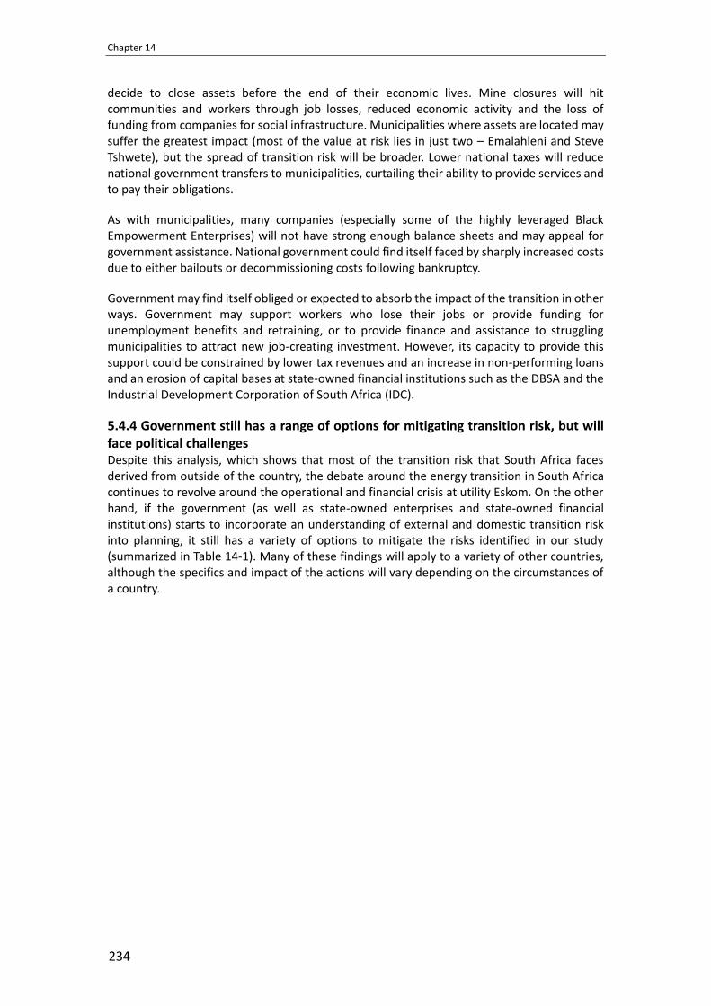
Chapter 14
234
decide to close assets before the end of their economic lives. Mine closures will hit communities and workers through job losses, reduced economic activity and the loss of funding from companies for social infrastructure. Municipalities where assets are located may suffer the greatest impact (most of the value at risk lies in just two – Emalahleni and Steve Tshwete), but the spread of transition risk will be broader. Lower national taxes will reduce national government transfers to municipalities, curtailing their ability to provide services and to pay their obligations.
As with municipalities, many companies (especially some of the highly leveraged Black Empowerment Enterprises) will not have strong enough balance sheets and may appeal for government assistance. National government could find itself faced by sharply increased costs due to either bailouts or decommissioning costs following bankruptcy.
Government may find itself obliged or expected to absorb the impact of the transition in other ways. Government may support workers who lose their jobs or provide funding for unemployment benefits and retraining, or to provide finance and assistance to struggling municipalities to attract new job-creating investment. However, its capacity to provide this support could be constrained by lower tax revenues and an increase in non-performing loans and an erosion of capital bases at state-owned financial institutions such as the DBSA and the Industrial Development Corporation of South Africa (IDC).
5.4.4 Government still has a range of options for mitigating transition risk, but will face political challenges Despite this analysis, which shows that most of the transition risk that South Africa faces derived from outside of the country, the debate around the energy transition in South Africa continues to revolve around the operational and financial crisis at utility Eskom. On the other hand, if the government (as well as state-owned enterprises and state-owned financial institutions) starts to incorporate an understanding of external and domestic transition risk into planning, it still has a variety of options to mitigate the risks identified in our study (summarized in Table 14-1). Many of these findings will apply to a variety of other countries, although the specifics and impact of the actions will vary depending on the circumstances of a country.
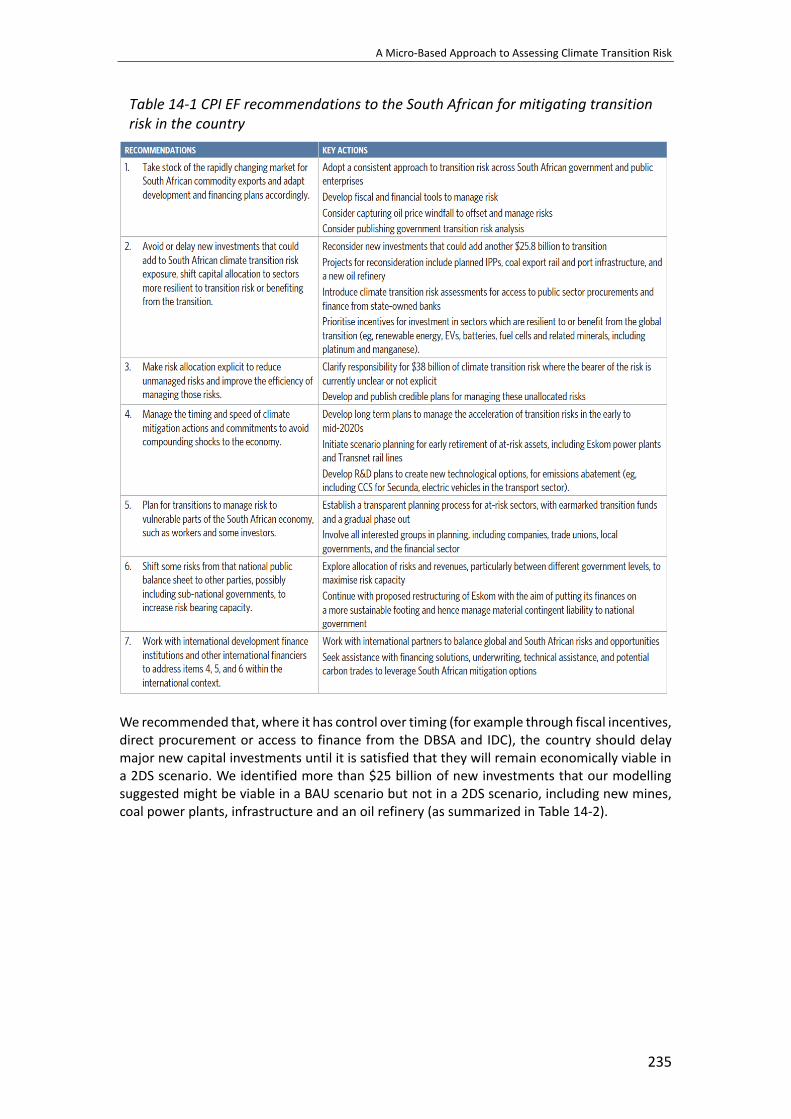
A Micro-Based Approach to Assessing Climate Transition Risk
235
Table 14-1 CPI EF recommendations to the South African for mitigating transition risk in the country
We recommended that, where it has control over timing (for example through fiscal incentives, direct procurement or access to finance from the DBSA and IDC), the country should delay major new capital investments until it is satisfied that they will remain economically viable in a 2DS scenario. We identified more than $25 billion of new investments that our modelling suggested might be viable in a BAU scenario but not in a 2DS scenario, including new mines, coal power plants, infrastructure and an oil refinery (as summarized in Table 14-2).

Chapter 14
236
Table 14-2 Pending infrastructure investments that could destroy value in a 2DS scenario
During a sustained period of weak economic growth, it may prove challenging politically for government to pull back support from new investments, especially if they attract capital into the country. If this sum was instead invested in industries or assets that are more resilient to transition risk, or benefit from a low carbon transition, it could spur a more sustainable source of jobs and economic growth.
Beyond the very short-term, the phasing of government action to mitigate transition risk will also be critical, especially given the country’s weakened public finances. Closing power plants and fuel production assets too fast and the cost of generating or procuring replacement power and fuel could limit the government’s ability to spend on social programs and have a significantly negative impact on the workers (our analysis shows job losses of 25,000-35,000 between now and 2035) and their communities. Act too slowly and the political barriers to future accelerated climate action will only rise. For example, if the government sought to introduce an accelerated ramp down of the coal mining industry in the mid-2020s in response to falling export demand, it would be challenging to ensure a process where all key stakeholders were able to provide input (including trade unions and local government) and the pressure for bailouts from coal companies falling into financial distress would become difficult to resist.
By contrast, a transition plan designed well in advance of the decline in export coal markets would enable state-owned financial institutions such as the DBSA to develop new sources of transition funding instruments, which could draw in international climate finance to support

A Micro-Based Approach to Assessing Climate Transition Risk
237
South Africa’s low carbon transition. A roadmap, which specified the least-cost means of supplying each power plant’s coal demand (and for what period) would also help the financial sector avoid stranded assets while also providing a justification for continuing some of its coal funding to keep the lights on for a specific period.
A government-wide acceptance of coal’s finite future might open up options for South Africa to be proactive in harnessing the potential benefits of the global low-carbon transition. This could include reallocating investment incentives within mining from coal to minerals that might benefit from a low-carbon transition (including manganese and vanadium) and planning to make the most of benefits of lower oil prices that our report identified.
Lower oil prices could dampen the effect of falling coal exports on the balance of payments. A more proactive policy could use the benefit of lower oil prices to offset risks from other sectors (see Figure 14-5 for an example). For example, national government might choose to increase taxes on oil products, diluting the benefit to consumers but reducing its own risk. Additional fuel tax revenues could be redistributed to parties struggling to bear the negative effects of the transition and/or retained to offset any pressure on the sovereign credit rating.
Figure 14-5 Using micro-level analysis to design targeted mitigation policy – using the benefits of a lower oil price
Source: CPI EF. Figures show transition risk in billions of US dollars
Lessons learned our South Africa case study We have explained some of the key findings from our work in South Africa, which illustrates the methodology set out earlier in this chapter. More detail can be found in the full report. Although the focus was on South Africa, we believe that versions of the above approach can be valuable to a wide variety of policymakers in countries with different characteristics. However, having access to the relevant data is an important prerequisite to a meaningful analysis. In South Africa, we benefited from the fact that most of the companies with exposed assets had publicly listed securities. Public institutions in South Africa are also subject to rigorous reporting requirements. The extensive disclosure from both sources provided a solid basis for drawing conclusions. In jurisdictions where assets are to a greater extent owned by private entities, or where there are weaker auditing and disclosure standards, analysis of this type will inevitably involve more educated guess work than in the South Africa example.

Chapter 14
238
6 Limitations of the current approach
Transition risk analysis using macroeconomic modelling tools only would not generate the level of insight as we have described here. Macroeconomic modelling provides policymakers, central bankers and regulators with only a partial understanding of transition risk. However, at the same time, CPI EF’s analysis on its own will not be sufficient to inform policymakers’ decisions as it does not provide a full picture of the second and third order effects such as impacts on inflation or economy-wide employment levels. We continue to work with partners to develop approaches to integrate the insights from both “micro” and “macro” analyses.
Similarly, the nature of CPI EF’s analysis necessarily points to policy responses that are most effective in targeted channels. Recent literature has proposed a wider range of potential central bank interventions including exclusion of fossil-related assets from central bank collateral frameworks and asset purchases; accounting for transition risks in setting microprudential capital requirements; introducing macroprudential capital buffers for coal exposure and including stranded asset risk in stress tests. An approach which combines CPI EF’s analysis with macroeconomic modelling would open up a wider range of potential risk mitigation solutions.
Inherent uncertainty Beyond the limitations discussed above and the need for more work on integrating the insights from micro- and macro-level modelling, CPI EF is currently working to understand many other inherent uncertainties about transition risk. As the global low carbon transition progresses, countries are likely to face transition risk to assets in sectors where there is no current emissions pricing or obvious transmission mechanism for that risk. Emissions relating to land use and deforestation are a clear example of a sector responsible for material emissions but with no current method for pricing those emissions. We think that applying a hypothetical carbon price is unlikely to provide a meaningful estimate of transition risk as it will not account for the multiple different dynamics that may affect land use emissions, including shifts in demand for agricultural products; technological and policy changes that improve the productivity of land use and new synthetic food production techniques. CPI EF is working to develop a conceptual framework for understanding the potential drivers of transition risk in land use.
Finally, the question of scenario-generation is a key methodological area for further research. Given the inherent uncertainty about the development timeframe of different low carbon technologies and their cost, there will be multiple potential pathways to 2DS. Our analysis currently uses static scenarios, but in practice, probabilistic scenarios will be required which account for a variety of potential transmission pathways. These will be critical not just for increasingly useful transition risk analysis, but much more broadly across policymaking, strategic and investment decisions.
Other climate-related financial risks Our analysis focused only on climate transition risk. However, countries and regions also face significant physical climate risk that would have material effects on economies and financial systems if not monitored and managed effectively. While we expect the majority of physical risk on a global basis to crystallise later than transition risk, physical risk shocks, such as Hurricane Idai, can negatively affect the capacity of countries to be proactive in managing
A Micro-Based Approach to Assessing Climate Transition Risk
239
transition risk. 16 Physical risk also interacts in important ways with the issues we have addressed in this work:
• Rising temperatures will affect the number of hours per day that South African mine workers are able to work; in water-stressed regions, the cost of water may rise significantly (either because of scarcity or because of the investment in expensive technologies such as desalination), further affecting the operating costs of all businesses including those exposed to transition risk.
• Some global warming may already be “locked in” as a result of historic greenhouse gas emissions. However, the incremental amount of warming (and hence, physical damage) resulting from future emissions may be higher or lower depending on the speed of global climate mitigation action. All else being equal, lower expected levels of physical damage may mean lower required spending on climate adaptation. However, the benefits of lower adaptation costs are likely to be in the longer term. Further work is needed to provide policymakers with a broader picture of climate-related financial risks.
7 Conclusion
Over the past decade, we have seen how the need for action on climate change has become more broadly accepted by governments, corporates and investors. But how urgently global action can be implemented over the coming decade is difficult to determine.
At COP26 parties to the Paris agreement will, in theory, be required to submit revised Nationally Determined Contributions which raise “ambition” for climate mitigation action. As pressure for more aggressive climate mitigation continues to grow, particularly in light of the IPCC’s special report on 1.5C warming, we can only anticipate further demand for detailed analytical work such as that set out earlier in this chapter.
We believe that financial shocks triggered by climate transition risk are not inevitable but will be much more likely to pose risk to financial stability if they are not managed in an effective way. We think that the analytical approach outlined in this chapter will help regulators and policymakers do this.
If climate-related financial risks are managed more effectively, economies can become more resilient, companies can continue to grow, new industries can emerge that are aligned with a low carbon economy, and the transition of workers from carbon intensive industries can be managed more smoothly.
16 Other shocks to economic capacity or the strength of financial systems, such the crisis precipitated by the COVID-19
pandemic, also sap the capacity of governments to undertake climate mitigation action where it requires up-front
investment or fiscal support.

Chapter 14
240
Bibliography
Bank for International Settlements. (2020). The green swan. Huxham, M., Anwar, M., & Nelson, D. (2019). Understanding the impact of a low carbon
transition on South Africa. Climate Policy Initiative Energy Finance.

A Macroeconomic Approach to Assessing Economy-Wide Transition Risks
241
A Macroeconomic Approach to Assessing Economy-Wide Transition Risks: The Case of South Africa
By
Agence Française de Developpement (AFD)1
Abstract
Using a simple macroeconomic approach, this chapter highlights the interconnected nature of the production network and shows why this is relevant when assessing transition risks. We consider two simplified transition shocks on the coal and automotive exports of South Africa, analyze how these propagate in the economy due to reduced demand of these sectors, and assess the indirect loss of production, gross operating surplus and employment ensuing the original shocks. We then use financial data and a simple econometric model to quantify the evolution of financial fragility within all sectors, and determine which sectors are the most exposed and most sensitive to transition risks emerging out of our two scenarios.
Keywords: macroeconomics, input-output, transition risks, financial fragility, production network, sectorial interconnection
1 Introduction
Given the ambition of the Paris Agreement to maintain global warming below 2C, a low-carbon transition will have to take place, impacting most, if not all, sectors of the economy and creating dynamics similar to Schumpeter’s creative destruction. To study ways in which decarbonisation is prone to hamper the economic and financial system, the notion of stranded assets and transition risks has emerged in the literature, demonstrating possible roots for financial instability (Carney, 2015; Rozenberg et al., 2018). Campiglio et al. (2017), among others, argue that stranded assets could generate broader macroeconomic negative consequences through financial repercussions. For financial regulators, central banks, finance ministries, and other financial institutions it is thus of the utmost importance to understand to what extent their portfolio and the financial system in general is exposed to these risks.
As a financial institution exposed to these risks, and more importantly as a development bank keen to contribute to the acceleration of smooth low carbon transitions,2 AFD is engaged in research programs and studies in this field. AFD is working on a macroeconomic modelling effort called GEMMES 3 (Generalized Multisecorial and Monetary Macrodynamics for the Ecological Shift), currently developed in several countries and of high relevance for transition
1 This chapter is written by Antoine Godin (corresponding author), head of the GEMMES macro-modelling team Agence
Francaise de Developpement and research associate at Centre d’Economie de l’Université de Paris Nord, email:
[email protected]; Paul Hadji-Lazaro, Ph.D. student at Université Sorbonne Paris Nord, and Laurent Bergadaa, Research Officer,
Agence Française de Développement. 2 As financial institutions and corporates analyze transition risks they are more likely to hedge themselves against these
risks by greening their portfolios. This is also true at a sovereign and sub-sovereign level. In addition, transition risk analyses
allow to identify potential “losers” of the transition (companies, sectors, municipalities, communities) and to provide support
to them in order to maximize social and financial stability, and lessen resistance to policies favorable to the transition. 3 https://www.afd.fr/en/page-programme-de-recherche/gemmes-new-modelling-tool-incorporates-energy-transition

Chapter 15
242
risk analysis. AFD has also partnered with Climate Policy Initiative to develop microeconomic analyses of transition risks, the first of which was done on South Africa. The work presented in this chapter is a variation of the macroeconomic approach using simple modelling of the production structure on the economy.
All these studies show that it is useful to perceive the low carbon transition as a transformation of the production structure whereby carbon-intensive activities will disappear and be replaced by low-carbon-intensive activities, and where all sectors in the economy will be impacted, in one way or the other. The reason behind this is that our economies comprise highly interconnected and specialized production processes where the production of one sector is used by other sectors to produce their own goods and services. These value chains require to look at more sectors than the usual suspects (carbon-intensive sectors) when trying to asses transition risks.
When assessing transition risks, whether at the level of a single company, financial institution, or of a financial system, analysts will typically define a scenario associated with a low carbon transition (such as a new carbon tax, or reduced demand for carbon intensive products) and apply that scenario through the use of models to the object of analysis. As the Climate Policy Institute (CPI) study of low carbon transition risks in South Africa shows quite clearly, looking at the direct impact of a particular low carbon shock or scenario is not enough to have a sense of the overall consequences of such a scenario (Huxham et al., 2019). It is also crucial to assess how the initial impact is spread throughout the whole economy, by looking at commercial, financial and capitalistic relationships. This can be done effectively from a microeconomic approach by building heuristic models and analyzing contracts where appropriate, as CPI have done. However, this approach lacks the macroeconomic dimension and thus underestimates economy-wide 2nd round effects. On the other hand, the complete dynamic macroeconomic transition risk stress tests, such as those being developed by a number of NGFS members, could be seen by some central banks or finance ministries wanting to start with a bird’s eye view of the issue, as highly technical, labor and data intensive.
We present in this paper what could be considered as a simplified macroeconomic approach to the issue of transition risk analysis. Using a static Input-Output model of the South African economy, we assess the impact on various economic sectors’ output of a theoretical negative shock on South Africa’s coal and automotive exports. We then use jobs and financial data to look at the total impact on employment, and to identify the sectors most at risk of representing a burden to financial system through increased default probabilities.
Although we mainly intend to provide an illustration of an interesting and readily usable methodological approach to transition risks, the choice of South Africa as a case study is pertinent. The country is particularly exposed to transition risks, in particular through its export sector. We were also able to build on the work done by CPI in this regard, by using the low-carbon scenario on coal that was developed. Last but not least, South Africa’s statistical office, Statistics South Africa, provides detailed Input-Output (IO) tables as well as financial data at the sectorial level, allowing for a connection between impacts at the production level and impacts at the financial level.
Carley et al. (2018) develop a conceptual framework where they decompose vulnerability as the combination of exposure, sensitivity and adaptive capacity, in the context of the energy transition. The higher the exposure and the sensitivity and the lower the adaptive capacity, the more vulnerable is a sector. We apply this framework to our results and highlight how certain sectors are exposed and sensitive to financial risks emerging out of simplified transition scenarios (under the form of two exports shocks to the coal or automotive sectors). More

A Macroeconomic Approach to Assessing Economy-Wide Transition Risks
243
precisely, we indicate how indirectly affected sectors see a loss of production and employment as well as a worsening of two financial fragility indicators: the net debt to EBITDA ratio and the Z-score. We further quantify the magnitude of these worsening and highlight that the transport, and electricity, gas and water (and auxiliary financial services4 to a lesser extent) sectors are particularly exposed to the coal shock, while the metal ores, basic iron and steel, glass, auxiliary financial services and again the electricity, gas and water sectors are exposed to the automotive shock.
The data sources and technicalities to assess the impact of a specific transition shock are described in Section 2. Section 3 illustrates the methodology with a case study of transition shocks and stranding implications in South Africa. Section 4 concludes.
2 Methodological overview
Transition shock The low-carbon transition can generate shocks to the production and consumption structure by many ways. For example, firms may decide to stop using a specific technology because of a carbon tax or due to more stringent regulation. In some cases, this might affect downstream firms using these goods because the new technology has changed the characteristics of the produced goods. This is what we call a supply shock. A demand shock on the other hand would take place where specific policies, technological change or consumer behavior change induce a change in consumption behavior, either in the final demand, i.e., households’ consumption patterns, or in intermediate consumption, i.e., firms’ decision on their usage of inputs. A reduction in demand for a specific sector will also propagate into the rest of the economy, as the firms in that sector are very likely to produce their goods and services using goods and services produced in other sectors. A demand shock can have a domestic origin, i.e., firms and households within the country changing their behaviors, or a foreign origin.
In a liberal market economy, the vast majority of transition shocks will materialize in the form of demand shocks. It should also be stated that these shocks will materialize in various ways, will not be limited to a single event (hence the use of scenarios) and will come in the form of both negative and positive impacts. In this study, we have aimed mainly at exposing a particular methodology, and have chosen to concentrate on a specific type of shock, that is an external negative demand shocks taking the form of a marked reduction in the exports (specifically: coal and automotive).
This choice of a simplified external shock impacting negatively only one sector is made for illustrative purposes only. The methodology can accommodate shocks of any nature: domestic or external, demand loss or demand increase, and one or many impacted sectors.
Input-Output model An IO table is a matrix, see Table 15-1, representing all the transactions of goods and services taking place in the economy, specifying the buying (columns) and selling sectors (rows). The transactions are grouped into two categories: intermediate consumption and final demand. The top left quadrant in Table 15-1 represents intermediate consumption taking place between two productive sectors in the production process (e.g. corn supplied by farmers and used by restaurants to produce meals). The top right quadrant of Table 15-1 represents final
4 The Activities auxiliary to financial intermediation sector combines activities such as administration of financial markets,
security dealing activities or activities auxiliary to insurance and pension funds. They are considered as auxiliary because
these activities do not involve taking the ownership of the financial assets and liabilities being transacted.
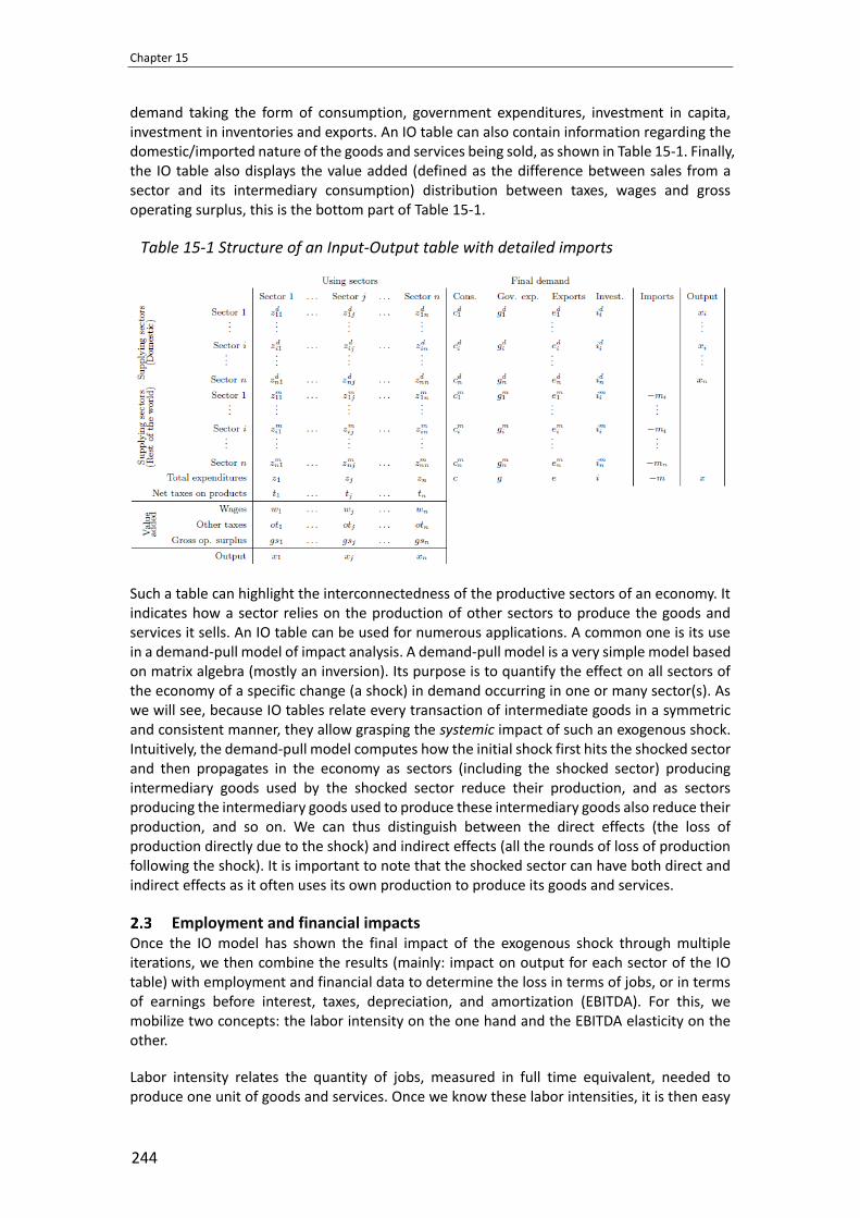
Chapter 15
244
demand taking the form of consumption, government expenditures, investment in capita, investment in inventories and exports. An IO table can also contain information regarding the domestic/imported nature of the goods and services being sold, as shown in Table 15-1. Finally, the IO table also displays the value added (defined as the difference between sales from a sector and its intermediary consumption) distribution between taxes, wages and gross operating surplus, this is the bottom part of Table 15-1.
Table 15-1 Structure of an Input-Output table with detailed imports
Such a table can highlight the interconnectedness of the productive sectors of an economy. It indicates how a sector relies on the production of other sectors to produce the goods and services it sells. An IO table can be used for numerous applications. A common one is its use in a demand-pull model of impact analysis. A demand-pull model is a very simple model based on matrix algebra (mostly an inversion). Its purpose is to quantify the effect on all sectors of the economy of a specific change (a shock) in demand occurring in one or many sector(s). As we will see, because IO tables relate every transaction of intermediate goods in a symmetric and consistent manner, they allow grasping the systemic impact of such an exogenous shock. Intuitively, the demand-pull model computes how the initial shock first hits the shocked sector and then propagates in the economy as sectors (including the shocked sector) producing intermediary goods used by the shocked sector reduce their production, and as sectors producing the intermediary goods used to produce these intermediary goods also reduce their production, and so on. We can thus distinguish between the direct effects (the loss of production directly due to the shock) and indirect effects (all the rounds of loss of production following the shock). It is important to note that the shocked sector can have both direct and indirect effects as it often uses its own production to produce its goods and services.
Employment and financial impacts Once the IO model has shown the final impact of the exogenous shock through multiple iterations, we then combine the results (mainly: impact on output for each sector of the IO table) with employment and financial data to determine the loss in terms of jobs, or in terms of earnings before interest, taxes, depreciation, and amortization (EBITDA). For this, we mobilize two concepts: the labor intensity on the one hand and the EBITDA elasticity on the other.
Labor intensity relates the quantity of jobs, measured in full time equivalent, needed to produce one unit of goods and services. Once we know these labor intensities, it is then easy

A Macroeconomic Approach to Assessing Economy-Wide Transition Risks
245
to compute the total loss of jobs in the economy due to a demand shock by computing direct and indirect job losses across all the affected sectors.
While the relationship between production and labor is relatively straightforward, it is less so for EBITDA. There are indeed non-linearities between output and EBITDA due to the presence of fixed costs or non-production costs such as interests’ payments, marketing costs etc. This is why we posit an elasticity of transformation between output and EBITDA at the sectorial level. We estimate this elasticity via a log-log econometric regression, using 2006-2018 time series from the financial dataset. The combination of the demand-pull model and this simple econometric model allows us to compute the loss of EBITDA in all sectors of the economy due to a shock in demand.
We then use two different financial fragility indicators, namely the Net-Debt to EBITDA ratio and a version of Altman’s Z-score, at an aggregated sectoral level, to identify those sectors that are most likely to represent a challenge from a macroeconomic perspective, as well as for the financial system, or to individual financial institutions depending on their exposure to these sectors.
Assumptions and limitations The IO model and the further development we have described here rely on strong assumptions that could be framed as follows:
• The scenario is a one-time event, and firms do not adapt to the shock by changing their production processes (the technical coefficients of the IO matrix are static and there is no substitution between inputs).
• Producers face constant returns to scale (a change in the output level will induce a change in the same proportion in the needed inputs for a unitary production).
• Labor and capital are unlimited and available at fixed price (a change in the demand for productive factors will not induce a change in their cost).
• We assume a linear relationship between labor and output and a non-linear relationship (in the form of an elasticity) between output and EBITDA.
Data sources We use a 50 sectors IO table published in 2014 by Statistics South Africa. We construct employment data combining the 2014 Quarterly Labor Force Survey and the 2014 Quarterly Employment Statistics. We decomposed the mining sector into two Gold and Non-Gold sectors, using the 2015 report on the Mining Industry (StatSA, 2015).
We use the Annual Financial Statistics for 2014, published by Statistics South Africa. The
financial dataset does not cover four IO sectors: Agriculture, Financial intermediation,
Insurance and pensions, and Education. Their financial data are arbitrarily set to null.
3 Transition shocks and stranding implications in South Africa
In this chapter, we model transition dynamics as exports shocks. The main shock we simulate concerns the coal sector. With 9.9 billion tons of proven coal reserves at the end of 2017, South Africa has 1.0% of the world’s proven reserves and ranks 12th as such. The coal industry

Chapter 15
246
represented 1.52% in the GDP in 2014 (the year of our IO table). Over the period 2001-2017, around 28% of extracted tons of coal were exported, with South Africa being the 6th largest exporter in 2017. To quantify the shock we study, we follow scenarios by Huxham et al. (2019), who model a decrease of around 70% in South African exports value until 2025 under a scenario which would limit the rise in global temperature to 2°C (compared to the pre-industrial period). We model this shock as a single exogenous event, rather than as a times series.
In order to compare and contrast the transition risks emerging from a loss in coal exports, we also simulate an export loss in the motor vehicles sector. South Africa is indeed well inserted within the global value chain of the motor industry (Barnes and Morris 2008), and it is reasonable to assume that a global transition to a low carbon economy will lead to a reduction in demand for internal combustion engine vehicles. For illustrative purposes only, we use a shock of the same magnitude than in the coal sector (approx. 44bn Rand) to compare the results.
The propagation of an external transition shock Figure 15-1 represents the propagation of the coal shock. Each node is a sector and each vertex represent the fact that the upstream sectors demands less goods and services produced in the downstream sector. We kept only the most impacted sector, following the methodology described in Cahen-Fourot et al. (2019, 2020).
Figure 15-1 Network of output stranding due to a unitary loss in final demand in the coal and lignite sector
Source: StatSA, 2017 and authors’ computation
Figure 2-1 illustrates that there can be many different paths of different length by which a specific sector is impacted by the loss of final demand in the shocked sector, even if that sector seems quite far in the industrial network from the originating sector.
We can indeed observe different supply chains, such as the trade industry chain relying on telecommunication, real estate activities, and computer activities. Each sector in the chain produces output used by sectors higher in the chain as intermediary inputs for their own production. These chains are thus propagation cascades where the loss of production in sectors high in the chain leads to loss of production for sector lower in the chain.

A Macroeconomic Approach to Assessing Economy-Wide Transition Risks
247
From stranded output to stranded jobs and stranded profits Once we determine the quantity of output loss in each sector, it is possible to pursue the analysis and compute the quantity of profits, taxes or wages being lost. Importantly, this will depend on the nature of the production process in each sector, as different sectors have different levels of capital or labor intensity. These characteristics lead to different distributions of the added value between labor income (wages) and capital income (profits). The overall quantity of lost profits or lost wages in the economy thus depends on which sectors are impacted and on their added value distribution among the different factors.
Figure 15-2 shows the total relative losses in output, employment and gross operating surplus (GOS) in the case of a reduction of export demand in the coal and lignite sector, while Delving deeper on the sectoral impacts of a loss of motor vehicles exports, we can see that while the indirect impacts are more than 100% the direct impacts on output being stranded, the direct impacts corresponds to only 25% (resp. 5%) of the total impact for employment (resp. GOS). Sectors indirectly impacted, such as trade, other services or transports, even see a larger decrease in GOS than the directly impacted motor vehicles sector.
Figure 15-3 shows the same indicators for the motor vehicles shock. Each stacked element of the bar plot corresponds to the loss of output, employment or GOS in a specific sector. The bar plots have been normalized to one, for ease of reading but the aggregate loss is indicated under each bar plot, as a percentage of total output, employment or GOS in the South African economy. The direct effect, i.e., the loss due to the original shock, has been highlighted in blue.

Chapter 15
248
Figure 15-2 Sectorial stranding components, i.e., output, employment and GOS, due to a loss in demand in the coal sector
Source: StatSA (20175, 2019b6, 2019c7) and authors’ computation
We observe that, in the case of the coal export loss, the original shock (highlighted in blue) corresponds to 2/3 of the total impact in terms of total nominal output. This means that for every two Rands of lost output in the coal export sector, there will be another Rand of lost output distributed in the rest of the economy due to the lost purchases of goods and services of the coal sector to the rest of the economy, and to the knock-on effects. The sectors most impacted are transport and trade. The relative impacts change drastically when looking at the two other impacted variables. Coal and lignite being capital intensive, one sees that the indirect loss of GOS amounts to only 25% of the total loss8. On the other hand, as the coal sector is relatively less intensive in labor, the direct loss of employment represents roughly 1/3 of the total loss in employment. This means that for every job at risk in the coal export sector, there are actually two other jobs at risk in the rest of the economy. Naturally we find the same impacted sectors when looking at jobs and when looking at output (with transport and trade playing a key role), driven by the structure of the supply chain, as highlighted in Figure 1. However, the relative sectorial losses differ, reflecting varying sectorial capital or labor intensity. This indicates that both the structure and the sectorial characteristics of the economy are important when trying to evaluate an external transition shock.
The results are strikingly different in the case of a shock to the motor vehicles industry, as shown in Figure 3. We first see that while the original shock to the two sectors are identical in
5 StatSA (2017). Input-output tables for South Africa. Accessed: 2020-01-08. 6 StatSA (2019b). Quarterly employment statistics. Accessed: 2020-01-08. 7 StatSA (2019c). Quarterly labour force survey. Accessed: 2020-01-08. 8 All things being equal, a capital intensive company usually have a higher ratio of GOS to Value added.

A Macroeconomic Approach to Assessing Economy-Wide Transition Risks
249
magnitude (again - for illustrative purposes), they lead to different total stranding impacts in output (0.93% of domestic output in the case of coal vs. 1.33% in the case of motor vehicles), employment (0.42% vs. 0.79%) and GOS (1.57% vs. 0.65%). This illustrates again that the structure of the economy is not neutral in driving how different shocks spread through the economy and affect different indicators. The total impact on a specific indicator is the sum of sectorial impacts, which are themselves a multiplier of the original shock. The sectorial multiplier depends on the strength of the connection between the initial sector and the sector under scrutiny and on the nature of each sector: more or less labor intensive for employment, more or less capital intensive for GOS. The fact that the automotive sector is more integrated in the production structure of the South African economy explains why it generates a larger total loss of production than the coal sector. The economic characteristics of the directly and indirectly impacted sectors explains why the loss in coal exports leads to a larger impact on GOS and a smaller impact on employment.
Delving deeper on the sectoral impacts of a loss of motor vehicles exports, we can see that while the indirect impacts are more than 100% the direct impacts on output being stranded, the direct impacts corresponds to only 25% (resp. 5%) of the total impact for employment (resp. GOS). Sectors indirectly impacted, such as trade, other services9 or transports, even see a larger decrease in GOS than the directly impacted motor vehicles sector.
9 Other services correspond to a combination of services supplied to the household sectors, as well as any
service provider that does not enter in the otherwise classified service sectors. The diffuse nature of the sector
explains why it is strongly connected to the industry.

Chapter 15
250
Figure 15-3 Sectorial stranding components, i.e., output, employment and GOS, due to a loss in demand in the motor vehicles sector
Source: StatSA (201710, 2019b11, 2019c12) and authors' computation
Financial implications As interesting the outcome of the stranding analysis in terms of employment or GOS is, it fails to assess the impact of the export shock on financial stability. In order to do so, we combine the demand-pull model of output stranding with two financial fragility indicators: the net debt to EBITDA ratio and a version of Altman’s Z-score.
We use the non-linear relationship described in the methodology section to determine the loss of EBITDA due to the two exports shocks. Figure 4 shows the results we obtained. The size of the bubbles represent the total amount of debt (both short-term and long-term) per sector, while their color represents the shock: red for coal and blue for automotive. Their position on the x-axis indicates their initial financial fragility, using the net debt to EBITDA ratio, while their position on the y-axis indicates the increase in fragility following each shock. To facilitate reading, we do not display extreme case such as Furniture and Electronic valves sectors which have very high net debt to EBITDA ratio (above 20) and a relatively large increase fragility (around 2%) for either shock. The same is true for the Basic Iron and steel and leather and luggage sectors displaying a very high increase in their net debt to EBITDA (around 10%) in the case of the automotive shock, although having a low initial ratio (less than 2).
In the case of the coal shock (red bubbles), we observe that, on top of the the unseen electronic valves and furniture, the electricity, gas and water and transport (and auxiliary
10 StatSA (2017). Input-output tables for South Africa. Accessed: 2020-01-08. 11 StatSA (2019b). Quarterly employment statistics. Accessed: 2020-01-08. 12 StatSA (2019c). Quarterly labour force survey. Accessed: 2020-01-08.

A Macroeconomic Approach to Assessing Economy-Wide Transition Risks
251
financial services to a lesser extent) sectors combine a relatively higher net debt to EBITDA ratio and higher variation in the same ratio. In the case of the motor vehicles shock (blue bubbles), we see, on top of the electronic valves and furniture, electricity, gas and water and coal and lignite (and spinning and textiles, glass, nuclear fuel, metal ores
Figure 15-4 Stranding EBITDA, financial fragility, and liability sizes
Source: StatSA (2017, 2019a) and authors’ computation
We complement the previous results with an analysis of the evolution of the Z’’-score following the two exports shocks. The lower the score, the more likely the company is to face bankruptcy with a value of zero being equated to a default (D) rated bond. Figure 15-5 plots the same bubble representing total sectorial liabilities where their position on the x-axis represents the initial sectorial Z-score and their position on the y-axis represents the evolution of that indicator for the two shocks(red for coal and blue for automotive). In order to avoid clogging the figure, we only show sectors having a Z-score below six. While we find some of the previously mentioned sectors standing out again (Basic iron and steel, glass, metal ores, electricity, gas and water, transport), the others however display a relatively high Z-score.

Chapter 15
252
Figure 15-5 Z-scores and variation in Z-score
Source: StatSA (2017, 2019a) and authors' computation
4 Discussion and conclusion
Using the South African coal export sector as a case study, we have illustrated how using a simple static Input-Output model can yield interesting insights on the importance of indirect effects of exogenous low carbon shocks, both on loss of output and job losses. The approach can also combined with financial statistical data to help identify those sectors that are most likely to contribute to potential financial instability.
Our main results highlight that while carbon intensive sectors are more likely to be directly affected by transition risks, other less carbon intensive sectors might indirectly be impacted through the network of supply and use of intermediate inputs. This is highlighted through the use of a static Input-Output model of the economy. In a sense, this approach illustrates the importance of looking at scope 3 carbon footprints when analyzing transition risks. Indeed, the often-used approach of using scope 1 carbon footprints for transition risk mapping misses how value chains are a vector of carbon relationships and carbon-related risk. The Input-Output models can be considered a way to address the near impossibility of mobilizing scope 3 carbon footprints at scale.
With regards to financial vulnerability in the face of climate related risks, it is useful to distinguish between exposure, sensitivity and adaptive capacity. We thus use these concepts to discuss our results. In the case of the coal export loss, we thus observe that sectors such as transport, and electricity, gas and water (and auxiliary financial to a lesser extent) are combining exposure (due to their position in the cascade of production loss) and sensitivity (due to their relative financial fragility). In order to determine financial vulnerability, one would need to determine the adaptive capacity of each sector, which is beyond the scope of this

A Macroeconomic Approach to Assessing Economy-Wide Transition Risks
253
exercise. We nonetheless can assume that the adaptive capacity of the utilities sector is quite high, given its strategic position in an economy and its public nature. This however could imply a transfer of fragility to the public sector, which would have to recapitalize the sector.
In the case of the cars export loss, we first observe that the South African economy is more exposed in general to production loss. This is because of the stronger integration of the automotive in the production network. We thus find more sectors combining exposure and sensitivity: metal ores, basic iron and steel, glass, auxiliary financial services and again the electricity, gas and water.
From a case study point of view, the approach developed here shows that scenario building is a contextual exercise, which needs to be thought both in terms of reduction in Green House Gas emissions and in terms of the production structure of the economy at hand. Concentrating only on carbon intensive sector would be an error as financial vulnerabilities might develop in other sectors as well. Of course, the case study developed here only considers negative shocks while the transition to a low carbon economy is also a source of opportunities. This does not change the nature of our results: grasping the systemic impacts of a transition to a low carbon economy is fundamental.
The advantage of this approach is its ease of implementation, only requiring a few matrix calculus operations, its relative frugality in terms of data (we combined an IO table with sectorial employment and financial data) implying that it can easily be implemented in data-poor countries. The main limitations of the approach are the fact that input-output data are sometimes outdated and of irregular quality 13 , the static economy assumption, and the absence of an economy-wide multi-sector low-carbon transition scenario.
While the proposed approach allows us to capture direct and indirect effects of transition shocks, highlighting the systemic nature of the low carbon economy, the analysis done here should not be considered as approaching a full macroeconomic model and there are many ways in which it could be improved to strengthen the results.
13 In the case of South Africa, we had to use input-output data from 2014. And although we have no reason to doubt the
quality of the data, this is however not always the case.

Chapter 15
254
Bibliography
Barnes, J., & Morris, M. (2008). Staying alive in the global automotive industry: what can developing economies learn from South Africa about linking into global automotive value chains? The European journal of development research 20 (1), 31-55.
Cahen-Fourot, L., Campiglio, E., Dawkins, E., Godin, A., & Kemp-Benedict, E. (2019). Capital stranding cascades: The impact of decarbonisation on productive asset utilisation.
Cahen-Fourot, L., Campiglio, E., Dawkins, E., Godin, A., & Kemp-Benedict, E. (2020). Looking for the inverted pyramid: An application using input-output networks. Ecological Economics, 169, 106554.
Campiglio, E., Godin, A., Kemp-Benedict, E., & Matikainen, S. (2017). The tightening links between financial systems and the low-carbon transition. In Economic policies since the global financial crisis (pp. 313-356): Springer.
Carley, S., Evans, T. P., Graff, M., & Konisky, D. M. (2018). A framework for evaluating geographic disparities in energy transition vulnerability. Nature Energy, 3(8), 621-627.
Carney, M. (2015). Breaking the Tragedy of the Horizon–climate change and financial stability. Speech given at Lloyd’s of London, 29, 220-230.
Huxham, M., Anwar, M., & Nelson, D. (2019). Understanding the impact of a low carbon transition on South Africa. Climate Policy Initiative Energy Finance.
Rozenberg, J., Vogt-Schilb, A., & Hallegatte, S. (2018). Instrument choice and stranded assets in the transition to clean capital. Journal of Environmental Economics and Management, 102183.
StatSA. (2015). Mining industry. StatSA. (2017). Input-output tables for South Africa. StatSA. (2019a). Annual financial statistics. StatSA. (2019b). Quarterly employment statistics. StatSA. (2019c). Quarterly labour force survey.

Environmental Stress Testing for Equity Portfolios
255
Environmental Stress Testing for Equity Portfolios
By
Yao Wang and Yi-Chen Shi1
Abstract
China has come under greater environmental and resource pressure at a time when increasingly severe global warming brings climate risks into focus. Assessing the impact of climate risks on financial performance, this research conducts climate stress testing on equity portfolios. First, it employs the asset-pricing model to analyze whether the investment portfolio of an asset management company is impacted by climatic factors through sensitivity analysis. It then simulates changes of share values in the asset portfolio under several climate stress scenarios. Lastly, it calculates the possible maximum value at risk (VaR) of the equity portfolio under an extreme climatic risk scenario. The empirical results show that carbon risk constitutes a significant impact on the returns and market values of the stocks making up the CSI 300 Index, and an extreme carbon risk event can cause the market value of the index portfolio to drop as much as 10%. Further, this research finds that carbon risk can have a positive effect on the returns of green stocks and a significant negative impact on brown stocks.
Keywords: environmental stress testing, climate risk, equity portfolio, VaR, scenario and sensitivity analysis, carbon asset pricing
1 Introduction
The G20 Green Finance Synthesis Report 2016 points out that a major barrier to the development of green finance is the absence of environmental risk analysis tools and capacity. Therefore, stakeholders should develop and promote environmental risk analysis tools and apply them to the financial industry. In April 2019, the NGFS released A call for action Climate change as a source of financial risk, and pointed to the need to integrate climate-related risks into financial-stability monitoring and regulation.
The academic community has studied environmental stress testing of the financial sectors, mostly focused on banks (Batten et al., 2016; Battiston et al., 2017; Monasterolo et al., 2017; Zhang et al., 2016), but little on the asset management industry. Amongst them, Alessi et al., 2019 performed a carbon stress test on the actual equity holdings of various institutional sectors and presented a tool to assess a portfolio’s exposure to climate risks. They found that even in a benign scenario, losses could be reduced by 30% by halving the exposure to carbon-intensive sectors.
In China, seven ministry-level bodies, including the People’s Bank of China (PBC), jointly launched the Guidelines for Establishing Green Finance System on August 31, 2016. Article 10
1 Prof. Yao Wang is the Director General of International Institute of Green Finance (IIGF) at Central University of Finance
and Economics (CUFE), email: [email protected]. Dr. Yi-Chen Shi is a Deputy Director General, chair professor and
head of Green Finance Innovation Laboratory of IIGF, [email protected].
Chapter 16
256
and Article 18 of the guidelines explicitly specify financial institutions’ implementation of environmental-risk stress testing. The document encourages banks and other financial institutions to assess loans and asset risk exposures in the areas with high environmental risks, as well as perform quantitative analysis of potential credit risks and market risks from exposures under different scenarios. Furthermore, the Guidelines require institutional investors to enhance the ability to assess environmental risks and carbon emissions involved in their assets and demand institutional investors (particularly insurance companies) to conduct stress tests on the impact of environmental and climate factors.
Based on this, environmental stress testing for the financial sectors has been studied since 2016 in China. For instance, Industrial and Commercial Bank of China (ICBC) analyzed the impact of climate change on the credit risks of commercial banks and conducted environmental cost stress tests on thermal power and cement industries (Zhang et al., 2016). The International Institute of Green Finance, CUFE (IIGF), launched the first research conducting environmental stress tests for asset-management companies in China. In its report, the IIGF describes the methodology and tests on the impact of climate and environmental risks on stock returns and market values (Wang & Shi, 2017). This paper introduces the findings published by IIGF in 2017 and discusses their potential applications.
IIGF’s research does not limit the methodology to only employing the normal discounted cash flow (DCF) to explore how risk factors affect a company’s operating profit. Instead, based on the characteristics of the asset management companies, this research uses asset-pricing to measure market risks and includes environmental factors in the model, thereby reflecting the risk factor with market prices and influences on the unexpected return of the asset. At the same time, this research employs the VaR model to derive quantitative environmental risks, namely VaR monetization. On this basis, it provides a decision-making basis for industry and companies and provides a quantitative reference for the government to establish policies on environmental information disclosure and environmental stress-testing.
This research combines sensitivity and scenario analyses to explore the impacts of climate risk on firms’ financial performance. Previous researches on environmental stress testing mostly adopted scenario analysis methods with few sensitivity analyses performed. This is because the DCF method only needs to assume discount cash flows under certain future scenarios, while the sensitivity analysis incorporates historical data. Few researchers have taken this approach, let alone combining sensitivity analysis and scenario analysis.
The implementation of environmental stress testing helps prompt financial institutions to recognize the significance of environmental and climatic risks and further push their corporate customers to disclose environmental information. Research and development of related methods will also gradually refine the methodology for the environmental stress testing of the financial industry, creating a set of public environmental stress testing models for the industry.
2 Research methodology for climate Stress Testing of Equity
Portfolios
Climate stress testing architecture The first step of a climate stress test is to identify concrete climate risks, including physical and transition risks. After identifying the climate risks, we can perform scenario analysis and sensitivity analysis pertaining to bonds, equities, real estate and other assets held by an asset management company based on these predefined risks. Since carbon pricing is an important

Environmental Stress Testing for Equity Portfolios
257
tool to mitigate climate change with market mechanisms, and carbon price can reflect some of the climate risks, we add it to our model as a climate risk factor. This approach is based on an efficient carbon-emissions market.
Figure 16-1 Climate stress testing architecture for equity portfolios
Sensitivity analysis and scenario analysis This research methodology changes from the previous empirical approach of using mainly scenario analysis by combining scenario and sensitivity analyses. The sensitivity analysis aims to build the model based on historical data, thus informing us of the adjustment of the discount rate and the probability of scenario occurrence for the scenario analysis.
2.2.1 Sensitivity analysis A sensitivity analysis uses data to identify the relationship between the climate risk and the return, meaning the extent to which the rise of the climate risk by one unit affects the return. For example, the percentage decrease in return on an asset as the carbon price rises by 1% will be the value of the carbon risk coefficient.
For stocks, we can use a series of models to find their corresponding values of the risk coefficient and measure their liquidity risk and market risk in terms of liquidity indicator and investment income respectively. Specifically, we add the climate risk factors into the CAPM model to get the Beta of climate risk, using the following:
𝐸(𝑟𝑖) = 𝑟𝑓 + 𝛽𝑖𝑚(𝐸(𝑟𝑚) − 𝑟𝑓) + 𝛽𝑖𝐶𝑅𝑅𝐶𝑅
where 𝐸(𝑟𝑖) is the expected return of investment, 𝑟𝑓 is the risk-free rate, 𝛽𝑖𝑚 is the beta of
investment, 𝐸(𝑟𝑚) − 𝑟𝑓 represents market risk premium, 𝑅𝐶𝑅 is climate risk, and 𝛽𝑖𝐶𝑅 is the
beta of climate risk.
The analysis concept for bonds only differs by having the values of risk coefficient computed with the models (KMV model and Creditportfolio view model) measure the interest rate risk and credit risk of bonds, and these risk indicators and the market risk indicators for stocks jointly constitute the investment income risk of the asset management company. (see Figure 16-2)

Chapter 16
258
2.2.2 Scenario analysis
A scenario analysis simulates the possible losses under hypothetical scenarios. For example, we can set carbon prices high, medium and low to calculate the subsequent investment loss, then obtain the maximum VaR of the investment income and further measure the impact of the environmental risk on the investment portfolio.
Figure 16-2 Analysis methodology for climate stress testing for equity portfolio
Asset pricing models and VaR Another innovation of this methodology is that prior stress tests generally used the DCF method, exploring how risk factors affected the unexpected operating profit of a company. This research instead uses the asset pricing model to measure the market risk based on the conditions of the asset management companies. We seek to reflect the risk factor with the market price and influence the unexpected return of the asset. Also, this research employs the VaR model to estimate quantitative environmental risk known as VaR monetization. Our study’s goal is to provide a decision-making basis for the asset managers.
2.3.1 Asset-pricing models integrating environmental risk factors This research uses the asset-pricing model to measure the expected returns of individual stocks and integrate climate risk factors into the model. We first use the model to identify the impact of climate factors on the portfolio of an asset management company, then we simulate value changes of the portfolio’s components under future environment, climate and other environmental stress scenarios. Finally, we quantitatively measure the impact of these risks on the ROI of the portfolio.
2.3.2 VaR model After computing the expected return and standard deviation of the investment portfolio, we use the VaR model to calculate the VaR of the portfolio and discuss the maximum VaR of the portfolio under extreme scenarios with the probability of 10%, 5%, and 1% respectively.
Transmission from carbon price changes to market risks For example, if carbon standard gets stricter, carbon prices will rise, forcing an enterprise to pay more for the right of carbon emissions, which reduces its profit as it faces higher carbon risks. The bigger the carbon risk factor, the higher the carbon price, the higher the risk premium on the emission right, which may result in declining share prices and returns. In this research, we calculate returns and carbon risk factors of individual stocks, work out the

Environmental Stress Testing for Equity Portfolios
259
average return, standard deviation and carbon risk factor of the investment portfolio as well as the loss in the value of the portfolio due to the risks of rising carbon prices.
Figure 16-3 Analysis flow for carbon price risk
3 Empirical analysis of climate stress testing of equity portfolio – CSI
300 Index
This research simulates the climate risk of the equity portfolio resulting from the investment in the stocks making up the CSI 300 Index, which consists of the 300 largest and most liquid A-share stocks and gauges the overall performance of China A-share market. This research conducts climate stress testing over the carbon-price risks of listed companies given the availability of data, limiting the scope to the sample shares within the CSI 300 Index. It uses data on monthly returns from the Wind database, and data on carbon prices from seven local carbon trade pilots in China.

Chapter 16
260
Table 16-1 Descriptive statistics of carbon price risk of CSI 300 Index in August 2013 to June 2016
Carbon price Rate of Change Carbon risk factor
Average value 33.18 0.0529 -0.002
Median 29.62 -0.0040 -0.0059
Standard deviation 16.98 0.3978 0.0535
Minimum 9.33 -0.7099 -0.1403
Maximum 78.46 1.3675 0.4243
Number 35 34 281
Table 16-2 The impact of rising carbon prices on CSI 300
Change of average return of CSI 300 index
Carbon price doubled, 5% VaR, loss in market value of CSI 300 (100 million yuan) and percentage in total market capitalization
Carbon price tripled, 5% VaR, loss in market value of CSI 300 (100 million yuan) and percentage in total market capitalization
Carbon price quadrupled, 5% VaR, loss in market value of CSI 300 (100 million yuan) and percentage in total market capitalization
change in average return when carbon price doubled
change in average return when carbon price tripled
change in average return when carbon price quadrupled
-0.88% -1.76% -2.53% 26381
(10.8%) 28540
(16.0%) 30700
(24.8%)
Table 16-3 Impact of a 10-fold rise in carbon price on CSI 300
A 10-fold rise in carbon price and 20% VaR, loss in market value of CSI 300 (100 million yuan)
A 10-fold rise in carbon price and 30% VaR, loss in market value of CSI 300 (100 million yuan)
A 10-fold rise in carbon price and 40% VaR, loss in market value of CSI 300 (100 million yuan)
A 10-fold rise in the carbon price and 20% VaR, Percentage decline in CSI 300
A 10-fold rise in the carbon price and 30% VaR, Percentage decline in CSI 300
A 10-fold rise in the carbon price and 40% VaR, Percentage decline in CSI 300
31228 25467 20544 12.70% 10.35% 8.35%
Using the Fama-MacBeth regression methodology, the research produced empirical results (see Table 16-2) showing that an increase in carbon price will reduce the investment return on CSI 300 index. If the carbon price doubles, triples and quadruples, the return falls 0.9%, 1.8% and 2.5%, respectively. In compliance with the Basel Agreement, we opt for the extreme risk scenario of 5% value at risk (VaR). If carbon price doubles, the market value of the CSI 300

Environmental Stress Testing for Equity Portfolios
261
index declines by 2.6 trillion yuan (about 10.8% of the current total market value 25 trillion yuan). If carbon price triples and quadruples, the market value of the CSI 300 index may drop by 2.9 trillion yuan and 3.1 trillion yuan, respectively. However, even a fourfold rise in carbon price may not be enough to meet the Paris Agreement. According to the World Bank, a price at USD 80-120 (approximately 560-850 Yuan) a tonne in 2030 is needed to meet the Paris Agreement targets. Based on this prediction, if the carbon price rises from 20 yuan to 200 yuan (approximately USD28), the market value of CSI 300 index has a 40% chance of dropping 8.4%, a 30% chance of losing 10.4%, and a 20% chance of falling 12.7%. In short, the carbon price risk can deliver a significant shock on the returns and market values of the CSI 300 Index components.
Furthermore, we compare the impact of carbon price risk on green and carbon-intensive (brown) sectors. Based on the industry classification standard set by China’s securities regulator (2012 edition), we take the companies in the industries of health, agriculture, ecological protection and environmental management, and water production and distribution as green stocks, and select the companies in air transport industry, and electricity and heat production and distribution as brown stocks. All portfolios are constructed with equal weightings. As shown in Table 16-4, an increase in carbon price will reduce the investment return on brown assets, while increasing the return on green assets. Also, under the scenario of 5% VaR, the decline in the market value of green assets is much smaller than that of brown assets. The empirical results indicate that carbon risk mainly influences the carbon-intensive sectors.
Table 16-4 The impact of rising carbon prices on green and brown assets
Type Industry
Average return change carbon price rises once, VaR at 5% (100 million RMB)
carbon price rises twice, VaR at 5% (100 million RMB)
carbon price rises three times, VaR at 5% (100 million RMB)
carbon price rises once
carbon price rises twice
carbon price rises three times
Green assets
Health 0.02 0.04 0.06 13
(3.52%) 6
(1.57%) 1
(0.38%)
Agriculture 0.15 0.29 0.44 3
(1.45%) 29
(13.06%) 61
(27.57%)
Ecological protection and environmental management
0.00 0.01 0.01 47
(13.98%) 49
(14.62%) 51
(15.26%)
water production and distribution
0.01 0.02 0.03 32 (17.05%) 30 (16.08%) 28
(15.11%)
Brown assets
Electricity and heat production and supply
-0.02 -0.04 -0.06 89
(23.08%) 108
(28.14%) 128
(33.20%)
Air transport -0.05 -0.10 -0.15 133
(21.81%) 169
(27.77%) 206
(33.73%)

Chapter 16
262
4 Conclusion
This research has built a carbon risk model to explore the relationship between investment returns and carbon risk factors. It measures the maximum VaR of the investment portfolio and prices the carbon risks based on the market pricing mechanism. The empirical results show that:
Carbon risk does deliver a significant impact on the returns and market values of the CSI 300 Index components, causing the portfolio to lose as much as 10% of its market value under an extreme scenario. Further, this research finds that carbon risk can have a positive effect on the returns of green stocks and a significant negative impact on brown stocks.
Our research reveals that the market price mechanism can genuinely internalize climate cost. This is because climate risk factors will affect returns on assets, boosting returns on green stocks while reducing those on brown stocks.

Environmental Stress Testing for Equity Portfolios
263
Bibliography
Alessi, L., Ossola, E., & Panzica, R. (2019). The Greenium Matters: Evidence on the Pricing of Climate Risk. University of Milan Bicocca Department of Economics. Management and Statistics Working Paper,(418).
Batten, S., Sowerbutts, R., & Tanaka, M. (2016). Let's talk about the weather: the impact of climate change on central banks.
Battiston, S., Mandel, A., Monasterolo, I., Schütze, F., & Visentin, G. (2017). A Climate stress-test of the financial system. Nature Climate Change, 7(4), 283–288.
Monasterolo, I., Battiston, S., Janetos, A. C., & Zheng, Z. (2017). Vulnerable yet relevant: the two dimensions of climate-related financial disclosure. Climatic Change, 145(3-4), 495-507.
Wang, Y., & Shi, Y.-C. (2017). Analysis and management of environmental risk in asset management: China Financial Publishing House.
Zhang, H., Zhou, Y., Ma, J., Yin, H., Yang, X., Le, Y., & Qiu, M. (2016). Impact of Environmental Factors on Credit Risk of Commercial Banks – Based on Stress Testing Research and Application of Industrial and Commercial Bank of China. Finance Forum, 2016(02), 3-16.

Chapter 17
264
Climate Change “Physical Risk” Assessment on Investment Portfolios
By
Carbone41
Abstract
The CRIS methodology was created in 2017 to provide climate-related risk metrics at the asset and portfolio levels. It enables asset managers and lenders to better report and manage climate-related risks, and more effectively engage with stakeholders. It is based on a comprehensive, robust and transparent assessment framework covering acute and chronic climate hazards, for different climate scenarios and future time horizons. The method was developed to be applied to listed equities and bonds, including green bonds, sovereign bonds, and real assets (infrastructure, real estate and natural resources). Anticipating data availability constraints, CRIS applies a pragmatic tier-based approach in conducting individual analyses. The challenges ahead are the lack of asset-specific data and the reliability of damage functions.
Keywords: climate risk, physical risks, TCFD, risk assessment, risk metrics, mainstreaming climate risks, portfolio assessment
1 Purpose of the study/methodology
CRIS – Climate Risk Impact Screening2 - is an innovative method developed to assess the exposure of investment portfolios to physical risks3 posed by climate change. The method was developed by Carbone 44 in 2017 with the support of major financial actors (i.e., AFD, Caisse des Depots et Consignation, FRR, Mirova-Natixis, CCR, ERAFP, BNP, CDG Capital and EDF) and with the help and advice from a scientific council gathering financial and scientific experts.
CRIS provides risk metrics at the asset and portfolio levels. It enables asset managers and lenders to report, manage risk and engage with stakeholders. It is based on a comprehensive, robust and transparent assessment framework covering acute and chronic hazards, for different climate scenarios and future time horizons. The method was developed so as to be applied to listed equities and bonds, including green bonds, sovereign bonds, and real assets (infrastructure, real estate and natural resources). Figure 17-1 shows the Exposure Map of mineral deposits to droughts around the world; this preliminary CRIS analysis aims at screening a portfolio to climate hazards only based on asset location. A complete CRIS analysis also includes vulnerability information on each asset to create asset-specific risk scoring (see following sections). For listed companies, CRIS can be applied to a large universe, based on
1 This chapter is written by Violaine Lepousez, Manager and Climate Risk Expert at Carbone 4, email:
[email protected]. 2 See crisforfinance.com for more information. 3 Physical risk relates to risks coming from the impacts of a changing climate (increased heat waves or storms for instance),
as opposed to transition risk that relates to risks coming from the increased needs and pressure to reduce the impacts of
our economy to climate change (see TCFD). 4 Carbone 4 is a French leading independent consulting firm specialized in low carbon strategy and climate change
adaptation. Created 12 years ago, Carbone 4 develops methods, tools and data and support economic actors to help them
integrate climate into their decisions.

Climate Change “Physical Risk” Assessment on Investment Portfolios
265
public financial data. For sovereigns, all countries have already been assessed. For real assets, CRIS can be applied to several specific portfolios.
Figure 17-1 Exposure of mineral deposits to climate change physical risks, run with CRIS exposure datasets (multi hazard on left, droughts on right; both based on future increases in climate hazards’ intensity and frequency due to climate change)
Source: Carbone4
CRIS scorings on physical risks at the portfolio level allow users to understand how much of their portfolio is at high risk due to climate change, for three IPCC scenarios. CRIS scorings can be incorporated into risk management systems to enhance long-term return at the portfolio and asset level. Best-in-class and benchmark analysis makes it possible to identify the riskiest assets across a portfolio. More detailed information enhances dialogue with the underlying assets’ owners.
CRIS risk metrics are useful to various financial actors:
- to (re)insurance companies to appreciate the risks on their market (sovereign analysis) or on their clients (companies or buildings) for instance;
- to commercial banks to appreciate the risks on their clients and markets, integrate the risks on their analytics and to feed their sustainability risk ratings;
- to asset owners and managers to measure and manage the risks on their portfolio and assets and to engage with the underlying components.
Figure 17-2 shows a real estate portfolio’s credit risks to heat waves. This information was created for several hazards and for several regions. It was used by a bank to understand the risks on its current portfolio. Next steps will be to create a tool to assess this risk at an earlier stage in their risk assessment procedures.
Assets risk scores
Scoring scale
0 100
Assets exposure to droughts
Scoring scale
0 100
Score finalAlé
a 1
Alé
a 2
Alé
a 3
Alé
a 4
Alé
a 5
Gorj
Mahaica-Berbice
Illinois
Jambi
Tennessee
Tennessee
Tennessee
Tennessee
Tennessee
Tennessee
Sipaliwini
Arkansas
Mekes - Tafilalet
Hilmand
Eskisehir
Score finalAlé
a 1
Alé
a 2
Alé
a 3
Alé
a 4
Alé
a 5
66 53 92 86 10 3
58 38 73 62 71 32
58 49 89 63 6 32
57 35 75 51 65 47
57 43 89 62 4 33
57 43 89 62 4 33
57 43 89 62 4 33
57 43 89 62 4 33
57 43 89 62 4 33
57 43 89 62 4 33
56 37 71 58 68 31
56 45 87 65 2,2 33
55 49,6 78,4 32,1 72,4 4,9
54 54,9 73,9 17,8 68,5 35,7
54 50,1 69,2 42,8 69,2 26,6
© 2
01
9 C
arb
on
e 4

Chapter 17
266
Figure 17-2 Exposure of a real estate portfolio’s credit risks to heat waves, faced with current climate and with 2050 BAU high emission scenario’s climate
Source: Carbone4
2 Methodology
The climate-related risk of an asset, such as a corporate stock or bond, infrastructure project, or sovereign bond, can be studied with varying degrees of detail and at various scales. An extensive literature and market review revealed in 2017 a lack of comprehensive methodology to assess the physical risk exposure of large, multi-asset portfolios spanning the entire globe. Most studies carried out by asset owners and managers have centered on a few individual assets at the project evaluation or pre-investment stages (i.e., for project finance), or have focused on a specific sector, specific geographic region, or on a handful of extreme climate events. However, there is a clear need to measure the risk level of entire portfolios, both to guide investment strategy and to meet reporting requirements. The high number of assets requires an efficient and comprehensive approach to risk analysis, all while maintaining a high level of accuracy regarding asset-specific characteristics and location.
CRIS responded to the need for global coverage, all with a bottom-up, asset-by-asset approach. Its main objective is to enable users to assess the exposure of multi-asset portfolios to all main physical climate change hazards in all geographical regions. CRIS offers a multi-hazard risk screening, based on a multi-scenario climate projections analysis and a value-chain sectoral vulnerability assessment.
CRIS methodological framework is based on the IPCC definition of physical risk: i.e., the combination of climate hazard, exposure and vulnerability (see Figure 17-3). CRIS quantifies climate exposure and provides risks metrics.

Climate Change “Physical Risk” Assessment on Investment Portfolios
267
Figure 17-3 CRIS simplified methodological framework for physical risk assessment
Source: Carbone 4
CRIS’s bottom-up approach combines the analysis of geographical exposure and sectoral and sovereign vulnerability to seven climate hazards (both acute and chronic), see Figure 17-4. Nine indirect climate hazards are also factored in (such as water scarcity, coastal erosion wildfires, etc.). Climate data is derived from climate models used by IPCC, for three IPCC scenarios and three time horizons. CRIS databases cover all countries, with a 25km average resolution (up to 8km in France), and all sectors.
CRIS main methodological framework for climate physical risk assessment
© 2019 Carbone 4
Adaptability
(territorial and/or asset-
specific)
Vulnerability
The vulnerability
depends on the
object studied
and its location
Climate hazard
Climate
projectionsEx : extreme
rainfalls
The climate hazard
depends on the
location of the
object studied
OPEX
CAPEX
Sales
Climate Risk
Sensitivity profiles
by asset typology
Aggravating
contextEx : flood prone
zone
Exposure

Chapter 17
268
Figure 17-4 CRIS comprehensive scope of analysis
Source: Carbone4
Climate vulnerability is based on sectoral vulnerability literature covering 15 factors across value chains, and sovereign vulnerability on 24 thematic indicators covering both environmental and socio-economic issues. These vulnerability profiles gather maximum loss damage intensity for each sector and each hazard. The vulnerability profiles are then consolidated for each hazard, before being aggregated to climate hazards and exposure.
• For companies and infrastructure, 15 factors of vulnerability (such as needs for cold chain, outdoor workers, etc.) that cover impacts on the entire value chain were used to assess vulnerability on CAPEX, OPEX and sales.
• For real assets, 12 technical blocks (such as roof, AC, etc.) that cover materiality, equipment, and comfort were used to assess risks on buildings.
• For governments, 24 socio-economical and geophysical indicators were assessed to cover all impacts (such as freshwater withdrawal/resources, %GDP Agriculture, etc.).
CRIS classifications are compatible with classic reporting ones: ICB, GICS and NAICS. To date, CRIS sectoral/asset classification are:
• For companies: a 60-type classification covering all sectors (industries, farming, financial, utilities etc.);
• For real estate: a 20-type classification covering residential and tertiary buildings;
Acute hazards
Chronic hazards
Direct climate hazards Indirect climate hazards
Changes in the intensity or frequency of storms
Changes in drought extremes Wildfire risks
Water scarcity risks
Changes in rainfall patterns
Flood risks (river & groundwater flood)
Increase in average temperature
Biodiversity migration and loss risks
Air quality risks
Changes in the intensity or frequency of
heatwaves
Urban heat island risks
Sea level rise
Coastal erosion risks
Landslide and mass movement risks
Changes in rainfall extremes
Coastal flood risks
© 2019 Carbone 4

Climate Change “Physical Risk” Assessment on Investment Portfolios
269
• For infrastructure: a 60-type classification covering all sectors (energy, transportation, water, telecom, farming, etc.).
Exposure is based on asset-level data or financial business data for each of the issuer. It captures the sectoral and geographical breakdown of markets and operations. For instance, for a listed equity, for sectoral breakdown, CRIS always uses revenue as the major proxy. For geographical breakdown, it depends on the sector and data availability. For capital intensive sectors, ideally, « tangible assets » or PPE are used to capture geographical breakdown. For low capital-intensive sector, revenue is used to capture both sectoral and geographical breakdown.
When creating the risk metrics, CRIS’s model is based on geometric functions used to over-weight high risk profiles and capture non-linear risk profiles. For instance, CRIS overall multi-hazard risk score is based on hazard-specific risk score. This aggregation step is based on the inversed geometric mean with a weighting system that gives more weight to acute hazard compared to chronic ones (Other information can be detailed on request).
In terms of climate projections, CRIS covers 7 direct climate hazards and 9 indirect hazards. The dataset captures future changes in climate compared to the current reference period. For each hazard, a selection of climate models was used (from CMIP3 or CMIP5) to create a median signal and information on uncertainty. For sea level rise and storm hazard, aggregated projections from IPCC were used. CRIS is based on multi-model ensemble, and multiple IPCC scenarios experiences. Most studies include:
• climate scenarios from the IPCC: RCP4.5 and RCP8.5. These scenarios cover respectively optimistic and business-as-usual visions of the evolution of GHG emissions worldwide.
• For each of these scenarios, several climate models (3 to 10) are used to capture uncertainty and minimize the dispersion of values related to the models.
Climate data are available for several future time horizons. Most studies include:
• 1 historic reference period;
• future time horizons: 2035, 2050 and 2100.
Climate signal captures the future anomalies compared to the historical reference period (+2°C in 2035 for instance), see Figure 17-5 for mean temperature maps. CRIS thus captures the risks coming from a changing climate, and not the absolute weather-related risks.
For acute hazards such as heat waves, climate scores are created based on 2 climate indicators: one that describes the intensity (e.g. max temperature), and another one that describes the frequency (e.g. number of hots days).
CRIS methodology can be applied to assess physical risks for all countries. Climate projections are at a resolution of 25x25km to 100x100km, depending on the region and/or the hazard studied (up to 8km in France). Environmental aggravating factors (such as flood prone areas) are site-specific for real assets.

Chapter 17
270
Figure 17-5 Example of hazard exposure scores for the reference period and 2 future time horizons, used in CRIS assessments run at infra-national spatial resolution
Source: Carbone4
3 Input and output metrics/data
For one particular asset with very few specific information available, risk depends mostly on its location and on its sectoral activity. Climate risk is a function of location-specific climate hazards and industry-specific vulnerability. It is a combination of climate projections for specific geographic locations (such as higher temperatures, more intense heat waves, etc.) and an issuer's sector-based vulnerability.
Therefore, CRIS combines for each issuer (i.e., company, infrastructure etc.), see Figure 17-6:
1. Descriptive financial data on the issuer's activity that are issuer-specific, to capture the geographic and sectoral breakdown of its activities (fixed assets or revenues depending on the sectoral capital intensity);
2. Scientific data on climate hazards and sectoral and sovereign vulnerability, that are respectively location-specific and sectoral specific, to assess the climate evolutions and the gross vulnerability of each sector to each hazard.
These scientific databases have been built usinga rigorous and transparent approach. For instance, climate data was extracted and statistically processed from multi-model ensemble and scenarios used by IPCC for each hazard. Median signal and uncertainties coming from the models are captured, for each scenario and time horizon. Original data are sourced and all processing steps are described.
§ 207 countries covered
§ The hazard rating is
based on relative
changes of one climate
variable: Mean of
annual temperatures
Key characteristics
Projected changes in 2046-2065 relative to 1961-1990 under the medium scenario
FutureProjected changes in 2080-2100 relative to 1961-1990 under the high-emission scenario
Future
Historical mean temperature (historical averages 1961-1990)
Past
In the past: 0 is reached for -16°C in Greeland, 99 is reached for +29°C in UAE
In the future: 1 is reached for +0,76°C in Tonga, 99 is reached for +6,42°C in Canada
0 99

Climate Change “Physical Risk” Assessment on Investment Portfolios
271
Figure 17-6 CRIS functioning principles
Source: Carbone4
CRIS combines thematic proprietary or public databases (climate, sector vulnerability, environmental of other related issues) with asset-level information to calculate risk metrics. Furthermore, CRIS methodology follows a bottom-up approach. Anticipating data availability constraints, CRIS applies a pragmatic tier-based approach in conducting individual analyses: the most precise and relevant data are used where available, with progressively less precise data, even averages, being used if necessary. In this way, CRIS is operational even in the absence of the most precise data, and easily accommodates updated and higher quality data as they are published.
For instance, at the company level, for each climate hazard, risk is a combination of the risks of each country-sector coupling composing its business, weighted by the breakdown of its activity in each of these couples. The indicator used to understand the geographic breakdown depends on the capital intensity of the sector (CAPEX to revenue ratio): fixed assets for high capital intensity sectors, and revenue for low capital intensity sectors.
For real assets, more detailed asset-specific information is used as the location is known.
CRIS provides various output indicators that may be used for reporting, risk management or engagement. For instance, at the portfolio level, aggregated indicators such as global multi-hazard scores are useful for reporting or risk management, whereas hazard-specific scores are more useful for engagement. A non-exhaustive list of useful indicators would be:
- At the portfolio level: Global, hazard specific physical risk scoring for various IPCC scenarios; Sectoral and global best and worst in class; Sectoral averages, part of the portfolio exposed to high risk, distribution of scorings across portfolio, exposure to vulnerable sectors, benchmark comparison.
- At the issuer level: Global, hazard specific physical risk scoring for various IPCC scenarios; Hazard-specific scoring for each business unit (sector/country based); Benchmark comparison; Qualitative comments and recommendations on adaptation.
5
41
51
44
56
45
64 M e d ium risk rat ing o f 44
Increase in
average
temperature
Increase in
heatwaves
Increase in
droughts
Changes in
ra infal l patterns
Increase in
heavy rainfa ll
Increase in sea
level rise
Increase in
storms
29 40 46 22 43 55 49
M id -t e rm (2050)
L o n g -t e rm (2100)
L o w -e m i ss io n sc e n a r io
M e d iu m -e m i s s io n s c e n a rio
H ig h -e m i ss io n sc e n a r io
Risk ratings by climate hazard for the asset for mid-term horizon and medium-emission scenario Ratings fo r each hazard are expressed on a scale fr om 0 to 99 across all sce narios, time horizons, and countries.
Aggreg ated risk ra ting for mid -term a nd med ium-emission scena rio, a nd sensitivity a nalysis for
various scenarios and time horizons
Ratings are expressed on a scale from 0 to 99 across all scenarios, time horizons, and countries.
Score Key
Lower Risk Moderate Risk Medium Risk High Ri sk Very Hi gh Risk
CRIS Prop. datasets
Information on risk-aggravating context
Vulnerability profiles for all sectors
Sovereign resilience profiles for all
countries
IPCC projections for climate hazards, run for 2 time horizons
and scenarios
CRIS model and analysis
Asset-specific information
Location, sector, site-specific aggravating
factors
Risk scores and information
© 2019 Carbone 4

Chapter 17
272
Figure 17-7 ENGIE’s physical risk assessment to climate change, based on public financial information and CRIS model
Source: Carbone4
4 Case study
N°1: corporate portfolio’s analysis For corporates, CRIS was applied to 1 765 companies - covering most of the MSCI World’s constituents, see Figure 17-8). Results show a strong inter-sector and intra-sector disparity in risk levels, allowing for an active management of the risks (stock-picking, benchmarking, etc.). Sectors most at risk are on average chemicals & pharmaceutical, food & beverages, utilities, industrial and mining & materials. Strong disparity appears in the utility sector as it comprises companies from very different countries (more diverse than in other sectors). The
Notes de risque par aléa pour la société (horizon moyen-terme et scénario d’émissions moyen)Les notes pour chaque aléa sont construites sur une échelle de 0 à 99 pour tous les scénarios, tous les horizons de temps et tous les pays.
Moyen-terme
(2050)
Long-terme
(2100)
Notes de risque agrégées pour différents horizons de temps et scénarios (échelle 0-99)
TempératureVagues de
chaleurSécheresse
Régime de précipitations
Précipitations intenses
Hausse du niveau marin
Tempêtes
30 41 33 26 39 51 29
35
4237
4738
52
La note de risque d’ENGIE est de 37/100 en 2050
42 Moyenne sectorielle
34 Meilleure note du secteur
© 2
01
9 C
arb
on
e 4
Description des principaux risques pour les aléas climatiques les plus importants (horizon moyen-terme
et scénario d’émissions moyen)
Les activités d’Engie sont très sensibles à l’élévation du niveau de la mer et présentent unrisque au vu des géographies d’implantation. Les activités de production d’électricité sont
sensibles du fait de leur dépendance aux infrastructures portuaires pour l’approvisionnement
en ressources fossiles. De plus les actifs sont difficilement relocalisables. Par conséquent, Engieest exposé à une dépréciation possible de certains actifs, à une augmentation des frais de
maintenance et des frais d’assurance et à des baisses de production possibles. Parmi lesopérations principales d’Engie, ce sont les activités de production au Qatar et aux Emirats
Arabes Unis qui seraient exposées (note de 57 et 58). Parmi toutes ses business units, les
opérations à Singapour présentent le niveau de risque le plus élevé (88).
Hausse du niveau marin
Les opérations de services
intégrés de production et distribution d’électricité à
Singapour sont très
exposées(88).
Point d’attention
Risque faible Risque modéré Risque moyen Risque fort Risque très fort
Les activités d’Engie sont très sensibles à l’augmentation de l’intensité et de la fréquence desvagues de chaleur, du fait de la forte sensibilité de la demande d’électricité à la chaleur et
du besoin en refroidissement de ces opérations pour maintenir un bon niveau de production.
Des baisses de production sont donc possibles (mais opportunités de demande croissante,non étudiée ici).
Ses activités au Qatar sont les plus exposées (notes de 74).
Les opérations de services
intégrés de production et distribution d’électricité
au Qatar sont très
exposées (74).
Point d’attention
51
41
88
74
Vagues de chaleur
ENGIE 37/100Secteur majoritaire: Production d’électricité conventionnelle Note de risque en 2050
Scénario
optimiste
Scénario
moyen
Scénario
tendanciel
Commentaire général
Engie présente un profil de risque modéré (note agrégée de 37), et inférieur à la moyenne du
secteur. Les aléas les plus importants pour le groupe sont, dans l’ordre décroissant de risque,
la hausse du niveau marin, les vagues de chaleur et les précipitations intenses. Ces aléaspeuvent causer des dommages importants sur les actifs et avoir des implications fortes sur les
coûts de maintenance et de réparation. Des ruptures dans le niveau de production sont àprévoir. L’étude n’étudie pas les opportunités liées à la demande croissante en électricité.
Les notes de risque associées à ces aléas sont très variées au sein des nombreuses
géographies d’intervention du groupe : le Qatar, les Emirats Arabes Unis et Singapourapparaissent comme des géographiques particulièrement exposées.

Climate Change “Physical Risk” Assessment on Investment Portfolios
273
company most at risk is an electric utility (several power plant) based in Asia, very much exposed and potentially vulnerable to storms, sea level rise and floods.
Figure 17-8 Physical risk assessment of a global portfolio of listed companies, based on CRIS model
Source: Carbone4
N°2: sovereign portfolio’s analysis For sovereign analysis, CRIS was applied to all countries in 2018. Detailed results are thus available. For instance, Figure 17-9 is the report for Vietnam that comprises synthetic risk metrics but also detailed information on the vulnerability and exposure of the country to physical risks coming from climate change. The results displayed were run with the optimistic climate scenario and with a focus on 2050 time horizon. The country is particularly at risk to heavy rainfall and sea level rise. Indeed, the country is very vulnerable to floods because most of its population and GDP is located in flood prone areas and areas prone to landslides because of mountainous context. Vietnam is also vulnerable to other hazards (droughts, change in rainfall patterns), but risks are lower because climate trends are less dramatic.
Distribution of the levels of future cliamte-related for a sample of
companies Multi-criteria CRIS risk scores according to the high-emissions scenario to 2100.
0 10 20 30 40 50 60 70 80 90
BU
ILD
ING
S
CH
EM
ICA
LS &
P
HA
RM
AC
EU
TIC
AL
FO
OD
& B
EV
ER
AG
ES
FO
RE
ST
& W
OO
D
HEA
VY
C
ON
STR
UC
TIO
N
IND
USTR
IAL
MIN
ING
& M
ATE
RIA
LS
NO
N M
ATE
RIA
L
SER
VIC
ES
PU
BLIC
EQ
UIP
MEN
TS
RE
TAIL
TELEC
OM
TOU
RIS
M
TRA
NSP
OR
TATI
ON
UTI
LIT
IES
Average Risk Rating
The 6 sectors at highest risk © 2019 Carbone 4
Distribution of the levels of future cliamte-related for a sample of
companies Multi-criteria CRIS risk scores according to the high-emissions scenario to 2100.
0 10 20 30 40 50 60 70 80 90
BU
ILD
ING
S
CH
EM
ICA
LS &
P
HA
RM
AC
EU
TIC
AL
FOO
D &
BEV
ER
AG
ES
FOR
EST
& W
OO
D
HEA
VY
C
ON
STR
UC
TIO
N
IND
UST
RIA
L
MIN
ING
& M
ATE
RIA
LS
NO
N M
ATE
RIA
L SE
RV
ICE
S
PU
BLI
C E
QU
IPM
EN
TS
RE
TAIL
TELE
CO
M
TOU
RIS
M
TRA
NSP
OR
TATI
ON
UTI
LITI
ES
Average Risk Rating
The 6 sectors at highest risk © 2019 Carbone 4

Chapter 17
274
Figure 17-9 Vietnam climate risk profiles based on CRIS model
Source: Carbone 4

Climate Change “Physical Risk” Assessment on Investment Portfolios
275
5 Limitations, outlook and future development
CRIS’ objective to provide a comprehensive assessment of physical risks at the asset level and at the portfolio level has been achieved. CRIS risk metrics encompass risks coming from a large panel of hazards and are available for all sectors and geographies. However, CRIS do not provide a quantified estimation of future financial risks in monetary terms (except exposure), which is one of the major challenges in this research field. We know rigorous damage functions does not exist for all sectors, geographies, and hazards; therefore we only provide quantified estimations of future financial risks only for some sectors and some impacts (for instance, energy or agriculture), or through detailed asset-specific assessments. To enrich damage modeling on portfolios, more details on past damages should be requested or consolidated at the sector level (for each hazard) with the help of (re)insurance actors.
Another gap is the lack of robust asset-specific data at the company level (listed or not). Spatially specific information on the value chain is key in this assessment as it determines the climate exposure of the supply chain, production facility and markets. This is particularly true for some vulnerable sectors. More detailed disclosure should be requested to enrich these assessments.
The main challenge today is to demystify the damage functions and climate impact modelling and to explain that most black boxes providing financial estimation of future physical risks on large portfolios of universe also cause higher levels of uncertainty. The appetite for financial output indicators should not impede the level of scientific rigor needed in the risk assessment, nor the use of other risk metrics that already enable mainstreaming climate physical risk in risk analysis, management and reporting.
Carbone 4 has been developing other specific methods for infrastructures and real assets that provides more accurate risk metrics based on more specific damage functions and asset-specific information. More information on the 2InfraChallenge can be found from the following link: http://www.carbone4.com/2-infrachallenge/.

Chapter 18
276
Scenario Analysis for Systemic Climate Risk
By
Ortec Finance1
Abstract
This chapter by Ortec Finance focuses on climate scenario analysis from a top-down, systemic risk perspective. It describes how transition and physical climate risks have macroeconomic consequences (i.e., networked effects) based on indicators such as GDP growth, interest rates, inflation, investment and international trade flows and other considerations. These climate-adjusted macro-economic risk drivers in turn affect risk-return expectations across all asset classes, regions and sectors. Insights gained from climate scenario analysis allow financial institutions (pension funds, asset managers, banks and insurance companies) to make better informed strategic investment decisions, including Asset Liability Management (ALM) and Strategic Asset Allocation (SAA) approaches with the aim to achieving more climate resilient investment portfolios and loan books.
Keywords: climate, scenario-analysis, systemic risk, asset-liability management, strategic asset allocation
1 Introduction
This chapter is written by Ortec Finance, an independent provider of technology and solutions for risk and return management headquartered in The Netherlands. Ortec Finance is innovating the modelling of systemic climate-related risks and opportunities for use in, inter alia, strategic asset allocation and asset-liability management. The chapter focusses on explaining key concepts around climate change as a systemic risk and climate change informed scenario analysis for investors. This chapter also presents a case study in the form of a representative diversified investment portfolio analyzed through the systemic climate risk lens using the ClimateMAPS methodology. The chapter concludes with a discussion on what practical steps investors can take in order to act on the outcomes of the analysis and options for further modelling sophistication.
2 Climate-informed scenario analysis in the context of SAA & ALM
Why scenario analysis? Scenario analysis is an important tool for managing uncertainty in both business and financial modelling, as well as in the climate science world. In general, “a scenario is a possible evolution of the future consistent with a clear set of assumptions” (Bunn and Solo, 1993). Scenario
1 The authors of this chapter are Willemijn Verdegaal and Lisa Eichler, both of whom are Co-Heads of Climate & ESG
Solutions at Ortec Finance. Emails: [email protected]; [email protected].
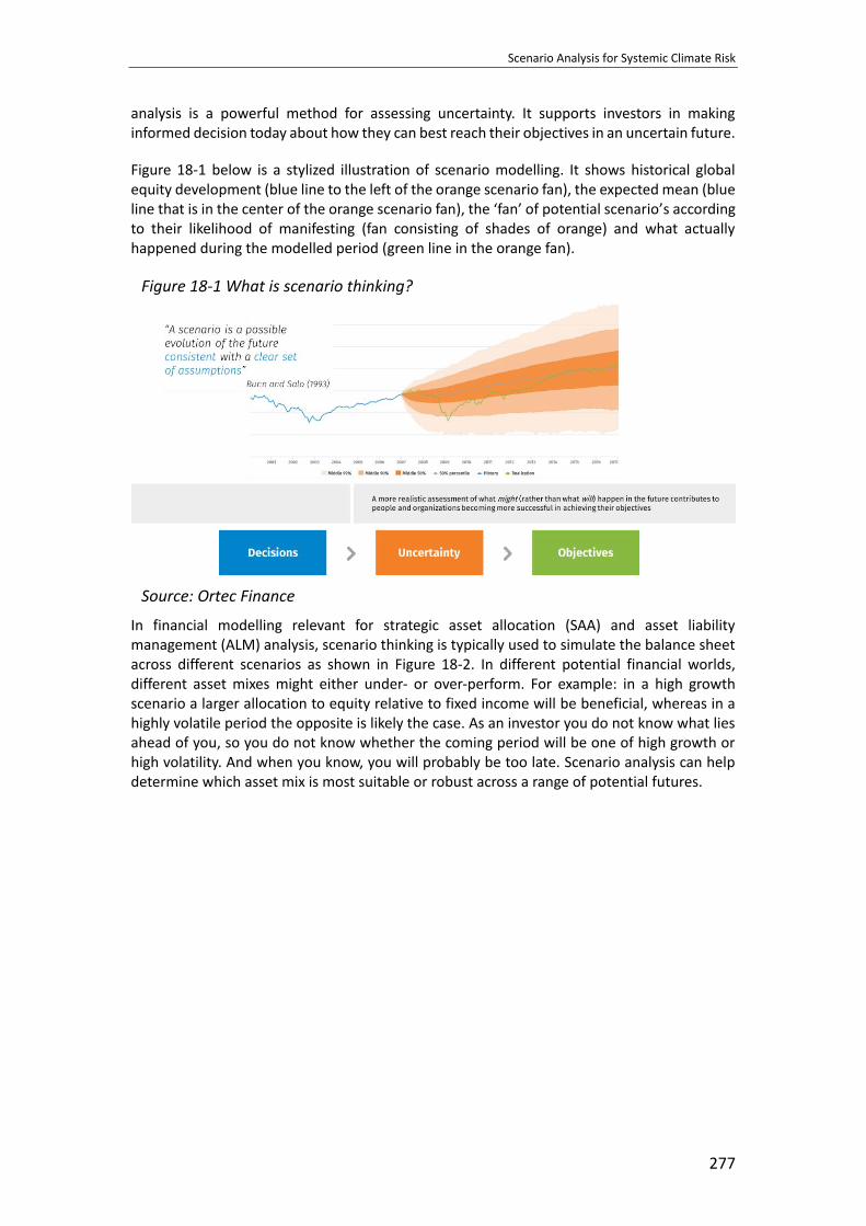
Scenario Analysis for Systemic Climate Risk
277
analysis is a powerful method for assessing uncertainty. It supports investors in making informed decision today about how they can best reach their objectives in an uncertain future.
Figure 18-1 below is a stylized illustration of scenario modelling. It shows historical global equity development (blue line to the left of the orange scenario fan), the expected mean (blue line that is in the center of the orange scenario fan), the ‘fan’ of potential scenario’s according to their likelihood of manifesting (fan consisting of shades of orange) and what actually happened during the modelled period (green line in the orange fan).
Figure 18-1 What is scenario thinking?
Source: Ortec Finance
In financial modelling relevant for strategic asset allocation (SAA) and asset liability management (ALM) analysis, scenario thinking is typically used to simulate the balance sheet across different scenarios as shown in Figure 18-2. In different potential financial worlds, different asset mixes might either under- or over-perform. For example: in a high growth scenario a larger allocation to equity relative to fixed income will be beneficial, whereas in a highly volatile period the opposite is likely the case. As an investor you do not know what lies ahead of you, so you do not know whether the coming period will be one of high growth or high volatility. And when you know, you will probably be too late. Scenario analysis can help determine which asset mix is most suitable or robust across a range of potential futures.

Chapter 18
278
Figure 18-2 Scenario modelling applied to balance sheet simulations for SAA/ALM analysis
Source: Ortec Finance
Thinking critically about assumptions As explained in the previous section, scenario modelling requires the development of one or more scenarios based on a consistent set of well-motivated assumptions. These assumptions determine how key variables or ‘risk drivers’ develop across possible futures. In the case of financial scenario sets the key risk drivers are GDP, inflation and interest rates. They are the building blocks of the financial scenario sets and drive the changes in risk-return profiles of asset classes across the different scenarios.
So if assumptions drive the development of key risk drivers (GDP, inflation and interest rates), and risk drivers determine the investment performance of the portfolio in a given scenario – then what are these assumptions based on? This is the key question.
Traditionally, assumptions on how GDP, interest rates and inflation develop, and how they influence financial performance, are based on historical relationships and historical averages. It is a ‘backward-looking’ methodology. For many applications this is an effective and appropriate methodology, but not when it comes to modelling the potential impacts of climate change. By definition historical data only includes information on past events. As there have not been significant periods of climate change in the period on which there is economic and financial data available, it is barely reflected in the historical data. Therefore, climate risk is not captured by most traditional assumption building methodologies.
Considering how material both physical and transitional climate-related financial risks are, the fact that they are not captured by traditional methodologies used for SAA/ALM processes is highly problematic. Investors are taking crucial decisions about portfolio construction based on methodologies that do not capture climate-related financial risks. This becomes even more problematic in the realization that climate-related financial risk is a systemic risk that influences all sectors, geographies and asset classes. The next paragraph considers climate as a systemic risk in more detail.

Scenario Analysis for Systemic Climate Risk
279
Climate change as a systemic risk Figure 18-3 sets out the concept of systemic risk in the context of climate change.
Figure 18-3 Climate change as a systemic risk
Source: Ortec Finance
Climate change can affect macro-economic variables (the risk drivers) such as economic growth, interest rates and inflation. Therefore, climate change impacts may significantly influence the resulting performance of asset classes and industry sectors. Take, for example, the impact of average temperature rise on the productivity of labor and land. It is well established in the literature2 that when temperatures rise above a certain point, productivity declines. The relationship is non-linear and so productivity rapidly declines in the face of rising temperatures. This has knock-on effects across the economy. Another example is the potential collapse of certain high-carbon sectors. This event impacts all other sectors it is networked with, even if they are not particularly high carbon. Retail, banking, real-estate and even government budgets and expenditures can be impacted. Via these routes of contagion, climate-related risks (and opportunities) spread through the economy. Figure 18-4 and Figure 18-5 illustrate this principle. Figure 18-4 illustrates how a policy intervention (in this case a carbon tax) works its way through the real economy. Figure 18-5 shows how policies aligning the world economy with Paris climate goals can impact particular countries economies – in this example Canada – very differently vis-à-vis the global average.
2 See for instance Burke & Tanutama (2019).

Chapter 18
280
Figure 18-4 Modelling the impact of a carbon tax
Source: Cambridge Econometrics, stylized example from the E3ME model
Figure 18-5 Impact on output per sector of Canada vs. the global average in a Paris aligned pathway
Source: Ortec Finance, based on outputs from E3ME
Note: Results are merely for illustrative purposes and should not be used to inform investment decision making.
The above examples illustrate the systemic nature of climate risk. These risks (and opportunities) are associated with each potential global warming pathway – ranging from an ambitious transition to no further action. Therefore, the assessment of climate change as a systemic risk driver in strategic investment decision-making is an increasingly necessary activity.
Bottom-up versus top-down approaches In order to understand how systemic climate risks are captured in various scenario-analysis methodologies it is useful to distinguish between the two main approaches currently used by investors in the market: bottom-up and top-down.
Scenario Analysis for Systemic Climate Risk
281
• Bottom-up approaches: these approaches look at company level data such as carbon foot printing, emission intensity, costs associated with reducing a company’s carbon footprint, management quality, etc. The risks per company are added up in order to have an understanding of the total amount of risk in – for example an equity portfolio. Advantages of this approach is that it allows for a very granular, company level view. The draw-back is that it does not capture networked effects. It is highly questionable if adding up the risks of all the individual companies equals the total level of risk. Due to networked effects the total level of risk is likely to be many order of magnitudes higher.
• Top-down approaches: these approaches use macro-economic models to understand how the economy functions as a whole. Variables like consumer spending, government spending, taxation, international trade, and production are considered. These approaches build up from the sector and region levels and are fit-for-purpose in capturing systemic risks (the networked effects) and therefore the total level of risk. The drawback is that they are restricted in the level of granularity they can achieve as they cannot look beyond the country and sector level of granularity.
Top-down approaches are required to capture climate as a systemic risk. Top-down approaches allow for better informed forward-looking assumptions about how GDP, inflation, and interest rates may develop in climate-informed scenarios, and how this in turn affects portfolio performance across all asset classes, countries and sectors. Therefore, using a top-down approach is crucial when performing climate-informed SAA/ALM analysis.
Integrating climate risk consistently throughout the investment process Unquestionably, the investment process goes beyond SAA/ALM. Ideally, therefore, when integrating climate-related financial risks, these risks should be integrated consistently throughout the entire investment process: from the strategic to the implementation (holding selection) level. For example: if the asset owner optimizes the asset allocation for a 2°C warming pathway (increasing exposures to sectors and regions likely to be least affected by systemic climate risk and even stand to benefit from it) then the asset manager should select companies that are more likely to perform well under this Paris-aligned pathway as well. Too often asset managers seem to not take the systemic nature of climate-related risks and opportunities sufficiently into account. For example, a certain low-carbon technology company may seem to perform well in a 2°C warming pathway – however if that company is likely to face severe macro-economic headwinds because the rest of the economy it operates in is exposed to negative impacts, then the company is not likely to do well in that pathway (networked effects), then perhaps the asset manager should be cautious to invest.
In order to design this consistent climate-informed portfolio it is important that asset owners and asset managers cooperate closely in order to achieve this consistency. Also, in such a setting, top-down and bottom-up data may play a complementary role.
The section below describes the process of designing a consistent climate-informed portfolio and highlights the respective roles of asset owners, asset managers as well as top-down and bottom-up datasets.

Chapter 18
282
Figure 18-6 Towards a fully consistent climate resilient investment strategy
Source: Ortec Finance
What investors should be asking themselves When integrating climate-related risks and opportunities into SAA/ALM, investors may want to ask themselves the following questions:
• Does my organization recognize climate as systemic risk?
• Are the datasets that I am using to measure climate risk able to capture the networked impacts of both physical (including extreme weather events) and transition climate-related risks and opportunities or are they assuming companies operate in isolation?
• Are the assumptions used in the scenario methodology for ALM/SAA climate-informed or are they only based on historical, backward-looking information?
• Are my projected return estimates reasonable under different global warming pathways?
• What risks and opportunities are relevant for me on which time horizon?
• How will climate-related risks impact my funding or solvency ratios?
• Is the management of climate-related financial risks implemented consistent across the different steps of the investment process: from asset allocation, to manager selection and portfolio implementation?
In conclusion of the first section of this chapter we would like to reiterate the importance of investors challenging whether key assumptions used for modelling risk and return projections remain valid under different global warming pathways. A scenario approach considering different plausible climate futures may be more appropriate than taking a traditional climate uninformed approach. Taking this climate informed approach is increasingly being recognized by central banks and regulators as part of the fiduciary duty of institutional investors.3
3 UN PRI, “Embedding ESG issues into strategic asset allocation frameworks: Discussion paper”, September 2019

Scenario Analysis for Systemic Climate Risk
283
Taking an approach that is ‘systemically climate risk-informed’ can therefore contribute to taking better investment decisions for allocations to asset classes, regions, and sectors; and consequently, can construct a more climate resilient investment portfolio given a certain global warming pathway. If the systemic climate risk-informed approach is implemented both at the strategic and implementation level then the entire investment strategy is consistently addressing climate-related risks at every level of decision-making.
3 Case study: Applying a systemic climate risk-informed approach to
SAA & ALM
Applying a systemic-climate risk informed approach to a diversified institutional investment portfolio enables a comprehensive analysis of total portfolio performance and attribution by asset classes per country and per sector. In this section of the chapter, we provide a high-level overview of the modelling methodology used by Ortec Finance in order to achieve a systemic-climate risk informed approach (ClimateMAPS). We then provide indicative quantified results for an illustrative portfolio. The chapter concludes with pointing out current model limitations and areas in which the model can be further developed.
Methodology The climate risk integration logic applied by Ortec Finance in order to ‘tie together’ climate science, macro-econometric modelling, and financial modelling can be explained as follows:
Figure 18-7 ClimateMAPS – climate risk integration logic
Source: Ortec Finance. ClimateMAPS
The climate change impact per global warming pathway and the policy and technological changes necessary to reach the different temperature targets are based on robust climate science. These assumptions inform the macro-econometric model of Cambridge Econometrics, which considers worldwide macro-economic interactions. The Cambridge Econometrics E3ME model is a non-equilibrium global macro econometric model with linkages between the economy, energy sector, and environment. It can fully assess both short and long-term impacts and is not limited by many of the restrictive assumptions common to Computable General Equilibrium (CGE) models. The model facilitates the integrated treatment of the world’s economies, energy systems, emissions and material demands. This enables it to capture two-way linkages and feedbacks between these components.

Chapter 18
284
The outputs from the macro econometric model are deltas (differences) in annual growth rates per country, from a macro-economic baseline outlook that does not use the climate specific inputs, i.e., that is climate-uninformed.
These “climate-adjusted GDP shocks” per country/sector and per year are then put into the Ortec Finance stochastic financial model. This model translates the impacts of the climate-adjusted GDP shocks onto a wide range of financial and economic variables (including interest rate, inflation, impacts on different asset classes) via stylized facts based on historic data and economic rationale.
The resulting systemic climate risk-aware scenarios set delivers quantified climate-adjusted consistent global economic and financial outlooks up to 2060 differentiated per country/sector and per global warming pathway, which then can be used for climate-informed portfolio analysis. It should be noted that the pathway assumption narratives extend to the end of the century as this aligns with climate science time horizons. Financial modelling is not extended beyond 2060 as, under the Failed Transition pathway, changes might become so dramatic that stability of the entire financial system is at risk. This is uncharted territory and would render quantified modelling results very uncertain.
We consider two broad options for the future: either the world continues on the current path or we transition to a low-carbon economy. To represent these two alternative pathways, Ortec Finance has developed economic scenario sets to reflect these two variants: the Paris Transition pathway and the Failed Transition pathway. These two pathways inform the underlying transition and physical climate risk parameters. Furthermore, the Paris Transition pathway is then broken down into two possible market reactions: orderly versus disorderly. In the latter case, the transition risks are supplemented by a confidence shock representing an aggressive market correction of carbon-intensive and related assets.
Each main pathway is built on key policy and technological assumptions across countries and sectors to represent transition risks and opportunities, which are summarized in Figure 18-8. Physical risks are composed of, on the one hand, gradual physical risks, such as sea level rise and temperature effects on worker and agricultural productivity. On the other hand, physical risk also derives from increasing frequency and loss impacts of extreme weather events, such as floods, storms, wildfires, that are attributable to climate change.
A continuation of current policies and technological trends will lead to increasing global CO2 emissions (Failed Transition pathway) and in turn continuously increasing average global temperature reaching up to 4°C by the end of this century. However, in a pathway that limits warming to below 2°C, CO2 emissions peak in 2020 and decrease sharply to reach net zero before 2066 (in both Paris pathways).

Scenario Analysis for Systemic Climate Risk
285
Figure 18-8 Key assumptions per global warming pathway
Source: Ortec Finance. ClimateMAPS
Pricing-in the future impact of transition and physical risks The main driver of differences in investment returns in the coming decade between the different pathways is a potential price correction (“pricing-in”) in financial markets, particularly equity markets. That is, at a certain point in time, financial markets will realize what the longer-term impacts will be of the transition to a low-carbon world and what the impact will be of gradual physical risks (such as reduced agricultural productivity) and extreme weather events (whether the transition succeeds or not). By translating this impact to changes in future expected output, earnings and dividend growth, the modelling estimates the expected price correction on financial markets. This price correction differs per climate pathway and per country and sector. Therefore, the overall impact on investment return will depend on the composition of the investment portfolio.
In the Paris Orderly Transition pathway, we assume that pricing-in will take place in the coming five years, i.e., 2020 - 2024. In the Paris Disorderly Transition pathway, we assume that pricing-in starts later, in 2024, and that the full price correction materializes within one year. This large price correction leads to negative market sentiment, and consequently to a sentiment shock in 2025, followed by (positive) price corrections in consecutive years to compensate for the overshooting in previous years. Market volatility is high in this 2024 - 2026 period.
In the Failed Transition pathway, in the second half of this decade investors will start to realize that the transition to a low-carbon economy will fail. Therefore, they will price in the resulting impact of increasing physical risks and extreme weather events on expected future output, earnings and dividend growth in the period 2025 - 2029. We assume that this first pricing-in shock reflects only the impact of physical risks and extreme weather events on growth prospects up to 2050. However, in the Failed Transition pathway, physical risks will increase

Chapter 18
286
significantly in the second half of this century. At some point in the future, financial markets will start to also price in these very substantial post-2050 physical risks. We assume that this second pricing-in shock occurs in 2035 - 2039.
Modelling climate-related extreme weather event frequency & associated losses While most climate scenario models are already well advanced in the modelling of transition risks and opportunities, the modelling of physical risks is still rather underdeveloped. In particular, most academic climate models currently do not capture the effects of climate-related extreme weather events and how these would influence climate scenarios. To overcome the current lack of inclusion in scientific models, we apply the PALgamma model, which forecasts the increase in frequency as well as the financial impact of climate-related extreme weather risk and, uniquely, identifies the extent to which urbanization and climate change contribute to risk, year by year and across over 120 countries worldwide.
Figure 18-9 PALgamma (climate change-related) Extreme Weather Risk & Impact Model
Source: Ortec Finance. ClimatePREDICT
This quantification of year-on-year and region-by-region exposure to risk from extreme weather attributable to climate change is integrated in the systemic climate risk scenarios, but when disaggregated into the individual climate risk drivers, insights help inform other aspects of improved investment decision-making such as assessing climate related physical risks of real assets, real estate and mortgage portfolios, or enhance insurance companies’ in-house P&C catastrophe models.
Case study portfolio description The case study in this chapter provides an illustrative example - based on a UK diversified investment portfolio – of the type of forward-looking, quantified analysis that can be done by using a systemic-climate risk informed approach. The scope covered provides a perspective of climate-related risk (and opportunities) for institutional investors under the three different global warming temperature pathways: Paris Orderly Transition, Paris Disorderly Transition and Failed Transition pathways compared to a climate-uninformed baseline.

Scenario Analysis for Systemic Climate Risk
287
Due to the nature of climate risks, the time horizon is longer than typical periods utilized by pension funds. The analysis covers forecasts up to 40 years ahead and results are expressed relative to the baseline (climate-uninformed) pathway. It should be noted that all climate-adjusted economies used in this case study are built on the December 2019 market situation.4
The example pension scheme that we use in our case study has been chosen to be fairly typical of the current situation of DB schemes in the UK. It has a relatively high initial allocation to growth assets which results in higher exposure to climate risks than a more mature scheme with a low allocation to growth assets. The liabilities and investments modelled give a starting funding ratio of 75% on the Long-Term Funding Objective. To help to eliminate the deficit, a recovery plan has been agreed such that company contributions are paid annually over the first 10 years.
We assume that the pension fund invests according to a fixed, static asset allocation with the following characteristics:
Table 18-1 UK pension scheme asset allocation table
Insights: Impacts on financial risk drivers The physical and transition risks and opportunities narratives that are informed by the climate and macro-econometric modelling influence the behavior of key financial risk drivers such as growth and inflation.
Impacts on GDP growth The figures below illustrate the dynamics of the growth risk driver for three countries: The US, Canada and Europe.
4 Ortec Finance, December 2019 Quarterly Outlook (https://www.ortecfinance.com/en/insights/whitepaper-and-
report/quarterly-outlook)
Asset Class Duration (Years) Weight
Fixed Income 22 50%
UK GILTS 31 12.5%
UK Index-Linked GILTS 40 12.5%
UK Corporate Credits (Investment Grade) 9 25%
Equity 40%
Equity World (USD) 35%
Equity Emerging Markets (USD) 2.5%
Equity UK 2.5%
Property 5%
UK Retail 2.5%
UK Offices 2.5%
High Yield 4 5%
US Corporate Credits (High Yield) 4 5%

Chapter 18
288
Figure 18-10 Cumulative real GDP growth across all climate-informed pathways (percentage difference to climate-uninformed baseline pathway in the level of GDP)
Source: Ortec Finance. ClimateMAPS
Note: Results are merely for illustrative purposes and should not be used to inform investment decision making.
There is considerable variation in the impacts across geographic regions. These differences are mainly caused by the level of transition risks over the short term and physical risks over the longer term. Higher temperatures exacerbate damage intensity and the frequency of natural disasters.
Impact on interest rates Transition and physical risk impact economic variables and asset prices. An example is given in Figure 18-11 with the changes in interest rates across four different regions under the Paris Disorderly Transition pathway.
Figure 18-11 Paris Disorderly Transition-adjusted interest rate growth (annual difference to climate-uninformed baseline pathway)
Source: Ortec Finance. ClimateMAPS
Note: Results are merely for illustrative purposes and should not be used to inform investment decision making.

Scenario Analysis for Systemic Climate Risk
289
The impact of ‘pricing-in’ across equity sectors and regions Different sectors and regions will be impacted differently by a transition towards a low-carbon economy and by materializing physical risks and extreme weather events. In a successful transition, the low-carbon energy sector will probably benefit, whereas fossil fuel producers and other carbon-intensive sectors will suffer losses. Likewise, countries with economies that are highly dependent on fossil fuel extraction and exploration will suffer, whereas net importers of fossil fuels will be hit less. Finally, how severely economies will be impacted by physical risks and extreme weather events depends on their geographical location. These differences in sensitivities to transition risk and opportunities, and physical risks and extreme weather events, are also visible in the size and direction of the pricing-in shocks. These differences can also be seen in Figure 18-12 and Figure 18-13. In these figures, you can see that the low carbon electricity sector will benefit greatly in a successful transition to a low-carbon economy, where other (i.e., brown) utilities will be hit severely. When the transition fails, India is expected to suffer significantly from increasing physical risks (lower labor and agricultural productivity due to increasing temperatures), where countries closer to the North Pole, like Canada, are much less sensitive to increasing temperatures. On the other hand, the Canadian economy is hit severely in a transition pathway, as the Canadian economy is heavily dependent on tar sand, and this sector will be entirely wiped out when we transition to a low-carbon world.
Figure 18-12 Global equity pricing-in shocks for a selection of sectors (expressed as a difference to climate-uninformed baseline)
Source: Ortec Finance. ClimateMAPS
Note: Results are merely for illustrative purposes and should not be used to inform investment decision making.

Chapter 18
290
Figure 18-13 Equity pricing-in shocks for a selection of regions (expressed as a difference to climate-uninformed baseline)
Source: Ortec Finance. ClimateMAPS
Note: Results are merely for illustrative purposes and should not be used to inform investment decision making.
Portfolio performance results This section provides model results on the performance of the case study portfolio (as described in section 3.2 above). The illustrative analysis focuses on risk-return impact on total fund level, impact attribution across asset classes and regions, as well as insights of contributing financial impacts to the underlying climate risk factors.
Risk-return impact at the total fund level The results on a total fund level for the hypothetical portfolio are summarized in the table below. The table highlights results separately for each of the analyzed global warming pathways by time horizon. The results are shown at the ‘total portfolio’ level of aggregation.

Scenario Analysis for Systemic Climate Risk
291
Table 18-2 Quantified Cumulative Return Impact for Total Fund Value, shown as climate pathways relative to climate-uninformed baseline
Source: Ortec Finance. ClimateMAPS
Note: Case study results are merely for illustrative purposes and should not be used to inform investment decision making.
Figure 18-14 shows the mean annual investment return and the 5% Value-at-Risk for two time periods. Figure 18-15 shows the result in an ALM context, focusing on the mean and 5% VaR of the funding ratio in year 10 and year 20 respectively. A key insight from this stage of the analysis is that the climate-uninformed baseline overestimates the expected returns and underestimates the risks. Furthermore, an orderly transition pathway to meet the Paris agreement has positive implications on the fund performance compared to a disorderly or failed transition. The more disorderly the transition, the more value is destroyed in the short term. In the longer term, even a disorderly transition shows lower negative impacts in terms of risk-return than a Failed Transition pathway.
Figure 18-14 SAA insights: from climate-uninformed to climate risk-aware thinking about risk-return measures
Source: Ortec Finance. ClimateMAPS
Note: Case study results are merely for illustrative purposes and should not be used to inform investment decision making.
Median Median Median Median Median Median
Paris orderly transition
pathway-3% 0% -1% -2% -3% -8%
Paris disorderly transition
pathway-4% -4% -1% -2% -3% -12%
Failed transition pathway 0% -5% -13% -3% -7% -25%
2020-2024 2025-2029
Cumulative return relative to climate-uninformed baseline
Quantified Return Impact for Total Fund Value
Investment portfolio 2030-2039 2040-2049 2020-20592050-2059

Chapter 18
292
Figure 18-15 ALM context: from climate-uninformed to climate risk-aware thinking about funding ratios
Source: Ortec Finance. ClimateMAPS
Note: Case study results are merely for illustrative purposes and should not be used to inform investment decision making.
Impact attribution across asset classes and regions For the three climate informed pathways, Table 18-3 below shows the cumulative return impact relative to the climate-uninformed baseline of the assets that the example pension fund is invested in. It can be seen that, in this example, especially equities and real estate are significantly impacted by transition and physical risks, leading to substantially lower returns than in the climate-uninformed baseline. In the Failed Transition pathway, over a 40-year horizon, the cumulative return on equity is around 50% lower than in the climate-uninformed baseline. This lower return is purely due to the increasing and devastating impact of gradual physical risks and extreme weather events caused by increasing temperatures.

Scenario Analysis for Systemic Climate Risk
293
Table 18-3 Cumulative return differences to baseline for several asset classes
Source: Ortec Finance. ClimateMAPS
Note: Results are merely for illustrative purposes and should not be used to inform investment decision making. Conditional formatting is applied per column per period to highlight the differences per (sub) asset class. Returns are calculated using the geometric mean methodology.
Cumulative measures
Paris orderly transition pathway
(ratio to climate-uninformed baseline)
Fixed Income
FI Government Bonds
Index-Linked Gilts UK 0% 0% 0% 0% -1% -1% -6% -6%
Gilts UK 0% 0% 0% 0% 0% 0% 1% -1%
Credits
Credits GB 0% 0% 1% 1% 0% 0% -2% -2%
Equity
Equity Developed Markets -6% -6% -1% -2% -2% -2% -14% -16%
Equity Emerging Markets -8% -8% -1% -1% -3% -3% -19% -19%
Equity United Kingdom -6% -6% -1% -1% -2% -2% -16% -16%
Property
Direct Real Estate UK -6% -6% -1% -1% -3% -3% -17% -17%
Direct Real Estate Residential UK -4% -4% -1% -1% -2% -2% -13% -13%
Direct Real Estate Offices UK -6% -7% -1% -1% -3% -3% -18% -18%
High Yield
Corporate Credits HY US 0% 0% 2% 2% 0% 0% -1% -1%
5
%
V
a
Median 5% VaR
2025-2029 2030-20392020-20242
02020-2059
Median 5% VaR Median 5% VaR Median 5% VaR
Cumulative measures
Paris disorderly transition pathway
(ratio to climate-uninformed baseline)
Fixed Income
FI Government Bonds
Index-Linked Gilts UK -1% -1% 1% 1% -1% -1% -6% -6%
Gilts UK 0% 0% 1% 0% 0% 0% 1% -1%
Credits
Credits GB -1% -1% 2% 2% 0% 0% -1% -1%
Equity
Equity Developed Markets -7% -9% -12% -17% -2% -3% -25% -31%
Equity Emerging Markets -9% -9% -13% -16% -3% -3% -30% -30%
Equity United Kingdom -8% -17% -10% -29% -2% -2% -26% -35%
Property
Direct Real Estate UK -7% -7% -7% -7% -4% -3% -24% -24%
Direct Real Estate Residential UK -5% -5% -4% -3% -2% -2% -16% -17%
Direct Real Estate Offices UK -8% -9% -7% -6% -4% -4% -25% -26%
High Yield
Corporate Credits HY US -3% -4% 8% 7% 0% 0% 2% 1%
Median 5% VaR Median 5% VaR
2030-2039 2020-20592020-2024 2025-2029
Median 5% VaR Median 5% VaR
Cumulative measures
Failed transition pathway
(ratio to climate-uninformed baseline)
Fixed Income
FI Government Bonds
Index-Linked Gilts UK 0% 0% 0% 0% -1% -1% -10% -10%
Gilts UK 0% 0% 0% 0% 0% 0% 3% -1%
Credits
Credits GB 0% 0% 0% 0% 1% 1% -2% -2%
Equity
Equity Developed Markets 0% 0% -10% -10% -28% -28% -48% -48%
Equity Emerging Markets -1% -1% -14% -14% -32% -32% -56% -56%
Equity United Kingdom -1% -1% -9% -9% -18% -18% -40% -40%
Property
Direct Real Estate UK -2% -2% -10% -11% -15% -16% -41% -41%
Direct Real Estate Residential UK -1% -1% -6% -6% -23% -23% -42% -42%
Direct Real Estate Offices UK -2% -2% -11% -12% -16% -16% -43% -43%
High Yield
Corporate Credits HY US 0% 0% 1% 1% 6% 6% 16% 15%
Median
2030-20392020-2024 2025-2029
5% VaR Median 5% VaR Median 5% VaR
2020-2059
Median 5% VaR

Chapter 18
294
Depending on the level of granularity of the fund hierarchy, a deeper assessment of climate risks is possible. Within emerging markets equities, for example, one can assess which countries are the most impacted by climate factors in the region.
Contributing financial impacts to the underlying climate risk factors Asset owners are also interested in gaining a better understanding about the underlying drivers for the differences in return with the climate-uninformed baseline. In Figure 18-16, for global equities, we can see that in the Failed Transition pathway, the underperformance is largely driven by the second pricing-in shock that is expected in the late 2030s. This pricing-in shock takes into account the expected negative impact of the increasing physical risks beyond 2050. Furthermore, in case of a Paris Disorderly Transition pathway to a low-carbon economy, the expected sentiment shock is actually larger than the impact of transition and physical risks in the real economy. On a global level, the real world transition impact is actually very small. That is, risks and opportunities level out more or less.
Figure 18-16 Cumulative return differences to baseline for several asset classes
Source: Ortec Finance. ClimateMAPS
Note: The vertical axis shows the annualized difference in return between the climate uninformed baseline and the climate-informed pathway.
The following textbox provides a zoom-in to the potential future impacts of extreme weather events and how these may affect the portfolio’s exposure to assets located in London. These zoomed-in insights aim to illustrate and underline the importance to take into account not only gradual physical risks, such as the effects of sea level rise, but to also consider the consequences of more frequent and more severe extreme weather events and how much of them can be attributed to climate change.
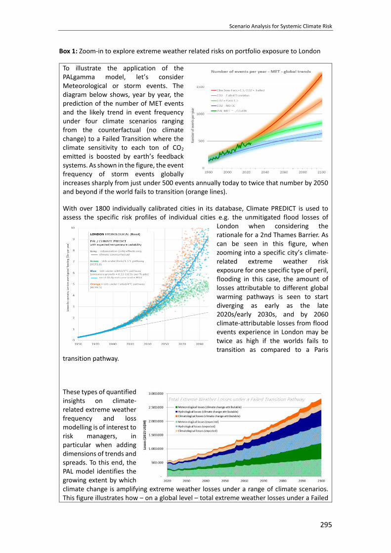
Scenario Analysis for Systemic Climate Risk
295
Box 1: Zoom-in to explore extreme weather related risks on portfolio exposure to London
To illustrate the application of the PALgamma model, let’s consider Meteorological or storm events. The diagram below shows, year by year, the prediction of the number of MET events and the likely trend in event frequency under four climate scenarios ranging from the counterfactual (no climate change) to a Failed Transition where the climate sensitivity to each ton of CO2 emitted is boosted by earth’s feedback systems. As shown in the figure, the event frequency of storm events globally increases sharply from just under 500 events annually today to twice that number by 2050 and beyond if the world fails to transition (orange lines).
With over 1800 individually calibrated cities in its database, Climate PREDICT is used to assess the specific risk profiles of individual cities e.g. the unmitigated flood losses of
London when considering the rationale for a 2nd Thames Barrier. As can be seen in this figure, when zooming into a specific city’s climate-related extreme weather risk exposure for one specific type of peril, flooding in this case, the amount of losses attributable to different global warming pathways is seen to start diverging as early as the late 2020s/early 2030s, and by 2060 climate-attributable losses from flood events experience in London may be twice as high if the worlds fails to transition as compared to a Paris
transition pathway.
These types of quantified insights on climate-related extreme weather frequency and loss modelling is of interest to risk managers, in particular when adding dimensions of trends and spreads. To this end, the PAL model identifies the growing extent by which climate change is amplifying extreme weather losses under a range of climate scenarios. This figure illustrates how – on a global level – total extreme weather losses under a Failed

Chapter 18
296
Transition pathway can be split into expected trends under a climate-uninformed baseline (i.e., expected losses per type of peril) and a proportion that is attributable to the specific climate scenario (in this case a Failed Transition) the world would find itself in. Under this scenario, whilst the frequency of extreme weather events is expected to almost triple between now and 2100, overall direct losses are expected to increase almost fivefold (in 2015 US$ terms).
Source: Ortec Finance. ClimatePREDICT
From insight to action Central banks, pension funds, insurers and banks increasingly use scenario analysis to better understand and analyze their potential exposure to climate-related risks (and opportunities). Climate-informed decision making has become a fundamental consideration for institutional investors as part of their fiduciary duties, to support in strategic investment decisions, for better holistic risk management and in developing more resilience in their portfolios.
This chapter has illustrated one possible approach to carry out such forward-looking climate scenario analysis: a top-down model to explore the financial impacts of three plausible climate pathways on the performance and funding position of an example UK diversified portfolio. It is important to note that the scenarios illustrated are not intended to be extreme. The climate impacts for the example portfolio under “worst case” scenarios could be much larger than those illustrated.
However, as the case study results in this chapter have shown, these impacts alone are quite dramatic particularly under a Failed Transition pathway:
• GDP: drops 60% for the UK by 2100 with similar impacts globally. Indeed in the longer term the physical damage caused by climate change is expected to outweigh the economy’s ability to grow resulting in real GDP declining from the 2060’s and future generations being worse off than their parents.
• Financial market impact will also be significant with permanent declines in median cumulative returns of 50% relative to a climate-uninformed baseline by 2050 and an accelerating downward trend thereafter.
There are also significant short-term risks for financial markets especially from a disorderly transition: In the Paris Disorderly Transition pathway, equity markets fall by almost 50% within the next 5 years relative to the climate-uninformed baseline, although then recover about half of those losses by 2035. A smoother Paris Orderly Transition pathway, on the other hand, would reduce the severity of these impacts. With equity markets declining by ca. 20% over the next five years relative to the climate-uninformed baseline and recovering about half by 2035.
In the longer term, from 2035 to 2060 both Paris Transition Aligned pathways slightly underperform the climate-uninformed baseline pathway due to lower GDP growth expectations from physical risks and the repayment of transition investment. This lower GDP also leads to lower long-term interest rates by 2060 but this decline in yields is roughly half that than the Failed Transition pathway.
These modelling insights represent significant market risks and therefore have significant implications for financial planning within financial intuitions over both short and longer-term

Scenario Analysis for Systemic Climate Risk
297
horizons. The implications for markets and GDP are relevant for turning ‘insights into action’ not only by financial institutions but also by regulators and policymakers.
Once implemented, the results of a top-down climate scenario analysis, such as the one provided in this chapter’s case study, can be ‘turned into action’ via several routes. Most directly, the quantified insights can support financial institutions in:
• Enabling climate-risk integrated modelling of macro-economic outlooks and macro-economic risk drivers used by financial institutions;
• Identifying and quantifying impact of systemic climate risk (networked effects) on a portfolio;
• Increasing resilience of a portfolio’s top-down risk budget under different global warming pathways via sector-, region-, or asset class re-allocation.
Furthermore, top-down, systemic climate risk insights enable more informed decision-making throughout other aspects of the investment process:
• Better informed portfolio management via risk-return insights per asset class, sector, and region across different possible global warming pathways that should be used in conjunction with bottom-up climate risk analysis on the individual securities level;
• Climate scenario analysis helps prepare for and fulfil climate-related disclosure and regulatory requirements (e.g., TCFD);
• Delivers complementary information to enable effective engagement (regulatory & corporate).
4 Limitations and outlook
Given that the future is uncertain, the random variation in future economic variables and investment returns over the short-term may result in experience that is significantly different to the expected long‑term average experience. This is true of all stochastic financial models but is particularly important here because there is material uncertainty in all aspects of climate scenario modelling. The use of judgment is required at all stages in both the formulation and application of climate scenario models.
The modelling is intended to illustrate possible plausible impacts. Rather than focusing on the absolute results under each scenario, we encourage readers to focus on the relative results of the climate-aware scenarios compared with the climate-uninformed baseline.
The scenarios we have modelled do not cover the full range of possibilities. For example, our Paris Disorderly Transition pathway assumes a late realization only on the part of the financial markets of the physical and transition risks of climate change. Other possible drivers of disorder include a late realization of the risks by policy makers leading to abrupt policy action, unexpected technological breakthroughs, or a sudden shift in consumer sentiment. These would all result in disorderly impacts that would differ in impact and timing from what we have modelled. Moreover, the actual outcome is likely to be different from any of our scenarios. However, the scenarios do give some idea of the types of impacts that may be seen, and of their potential relative significance.

Chapter 18
298
The model we have used relies on Cambridge Econometrics’ macro-econometric model E3ME to integrate transition and physical risk drivers and calculate their impact on macro-economic outputs. E3ME considers only CO2 emissions from the energy sector and does not model land use and emissions from land use change. In order to capture the effects of other greenhouse gas emissions, the model uses a climate sensitivity coefficient that implicitly includes these other emissions. Another assumption in E3ME is that natural resources are unlimited, i.e., only the demand side is modelled, not supply.
The modelling translates the impacts of climate-adjusted GDP shocks onto a wide range of financial and economic variables. To do this, GDP is the only translation mechanism from the macro econometric model to the stochastic financial scenario model. Other potential translation mechanisms (such as carbon-price impact on inflation and interest rates) are out of scope and follow purely from the estimated relationships with GDP in the financial model. The results of the modelling are highly dependent on the assumptions used to translate the GDP shocks onto the other variables.
There is particular uncertainty about how climate change might affect interest rates and inflation since there has not yet been much research in this area, and the evidence that is available is mixed. Historically, inflation and interest rates have generally been lower when economic growth is low. In this model, inflation and interest rates fall broadly together in the central case which means that the real interest rate, which is the most important driver of pension scheme liabilities, does not change that much. However, plausible narratives can be constructed in which interest rates fall but inflation is stable or even rises.
Existing research on how climate change affects financial market volatility is limited and inconclusive. Volatility might increase as the physical and transition impacts of climate change unfold, particularly if this happens in an unpredictable manner. Due to the inconclusiveness of the research, the modelling does not make any allowance for this, except in the Paris Disorderly Transition pathway during the period 2024-2026 while pricing in of climate-related risks takes place.
Furthermore, it should be noted that the modelling does not consider broader environmental tipping points and knock-on effects, such as climate change related migration and conflicts. Nor does it consider the potential for food or other resource shortages which may lead to both lower GDP and higher inflation. In the aggregate, it is quite likely that the modelling is biased to under-estimate the potential impacts of climate related risks, especially for the Failed Transition pathway.
Finally, the modelling is based on market conditions at 31 December 2019 and makes no allowance for subsequent events, notably the Covid-19 pandemic.

Scenario Analysis for Systemic Climate Risk
299
Bibliography
Burke, M., & Tanutama, V. (2019). “Climatic Constraints on Aggregate Economic Output,” NBER Working Paper No. 25779, April.

Chapter 19
300
Factoring Transition Risk into Regulatory Stress-Tests for “Late & Sudden” Transition
By
2°Investing Initiative1,2
Abstract
A debate has recently emerged as to whether climate risks may be material for financial stability. This is driven by a solid body of evidence that climate risks may strand assets across key sectors that are prominently represented in financial markets. As a result, financial supervisory authorities are starting to explore how these risks can be integrated into existing stress-testing frameworks. This study proposes a methodology that financial supervisors could follow to build “late & sudden” transition scenarios that could be used to input into either traditional or climate-specific stress-tests of regulated entities. It also proses that supervisors run multiple simulations of these scenarios across regulated entities to inform on system and idiosyncratic ‘impact tolerance’ and enable the setting of minimum recovery standards. An illustrative application of the process is shown, focusing on listed equity and corporate bonds tied to climate sensitive sectors (fossil fuels, power, steel, cement, automotive and aviation).
Keywords: climate stress-test, climate transition risks, scenario analysis
1 Introduction
In order for global temperatures to stay below 1.5° above the pre-industrial era by the end of the century, estimates suggest that $2.4 trillion would have to be invested annually until 2035 for the transition of the industrial, energy, agricultural, residential and transport sectors (IPCC, 2018). Similarly, a significant amount of capital will need to be moved out of current high-carbon investments in a range of sectors, including fossil-fuel mining, utilities, certain types of high-carbon manufacturing, and transport infrastructure. These necessary shifts in global financing flows will give rise to a new set of financial risks associated with the transition to a low-carbon economy. Failing to anticipate these so called “energy transition” risks might lead to large-scale mispricing of carbon-intensive assets (Delis et al., 2018), inevitably followed by sudden repricing when the market finally realizes the depth of the transition to come.
In the speech that he gave to the European Commission on 21st March 2019, Mark Carney, the then Governor of the Bank of England, highlighted the need for financial supervisors to conduct climate stress-tests to assess the resilience of their regulated entities to such risks, and specifically to consider the eventuality of a “Climate Minsky moment”, i.e., a sudden materialization of climate risks. Similarly, the European Systemic Risk Board (ESRB) recommended exploring how transition risks could be integrated into mainstream banking stress-testing frameworks, and described in its scientific advisory board’s report “Too late, too
1 This chapter is written by Michael Hayne, Senior Analyst at the 2° Investing Initiative, email: michael@2degrees-
investing.org; Soline Ralite, Analyst at the 2° Investing Initiative; Jakob Thomä, Managing Director of the 2° Investing
Initiative, email: [email protected]; Daan Koopman, Data Scientist at 2° Investing Initiative. 2 This report was supported by the International Climate Initiative (IKI) through project grant18_I_351_Global_A_Paris and
financial markets.

Factoring Transition Risk into Regulatory Stress-Tests for “Late & Sudden” Transition
301
sudden?” how a “late & sudden” transition scenario could impact overall financial stability (ESRB, 2016).
The aim of this chapter is to outline why current stress tests do not capture the nature of true “late & sudden” economic decarbonization and calls for a new approach. It then provides financial supervisors with a methodology that could help build a range of late & sudden transition scenarios to input into either traditional or climate-specific stress-tests of regulated entities. The methodology specifically focuses on equity and corporate bonds tied to climate sensitive sectors (fossil fuels, power, steel, cement, automotive and aviation). Section 1 of this chapter describes the scope of traditional regulatory stress-tests and reviews past climate stress-testing initiatives. Section 2 provides discussion on why current stress test may not be appropriate and why there is a need for abrupt late & sudden transition scenarios. Section 3 details the methodology that financial regulators could follow to estimate the impact of a late & sudden scenario on equity & bonds in climate-sensitive sectors to provide ‘impact tolerance’ indicators for markets, portfolios or firms. Finally, Section 4 presents illustrative results obtained by applying this methodology.
2 Background
The scope of traditional regulatory stress-tests According to Bank of England, “Stress testing involves putting a severe amount of pressure on an object or system, to test how resilient it is under extreme conditions. When applied to banks, stress testing involves analyzing how these institutions would cope with hypothetical adverse scenarios, such as severe recessions or financial crises” (Bank of England, 2016). Stress-tests are conducted internally by financial institutions as part of their risk management strategy, by regulators as part of the macroprudential policy framework, or by outside actors providing external analysis.
Stress-tests usually consist of three main parts: (i) a qualitative description of several disruptive economic scenarios and how they could propagate to the financial sector, (ii) a list of macroeconomic and sectoral parameters, as well as the values that they would take under each above-mentioned scenario, and (iii) impact indicators reflecting how each scenario impacts the financial sector. The time horizon of the scenarios is usually three years, and the scenario parameters and impact indicators displayed are often limited to a dozen. Table 19-1 displays the main characteristics of the stress-test conducted yearly by the Fed reserve in the United States, and by the ESRB in Europe.

Chapter 19
302
Table 19-1 Main characteristics of US & EU regulatory stress-tests
Fed reserve stress-test (USA) ESRB stress-test (EU)
Risk scenarios considered
• Severe global recession accompanied by a global aversion for long-term fixed income assets, leading to a broad-based and deep correction in asset prices
• Weakening economic activities across all sectors, accompanied by rapid declines in long-term rates and flattening yield curves
• Abrupt and sizeable repricing of risk premia in global financial markets – triggered e.g. by a policy expectation shock
• Adverse feedback loop between weak bank profitability and low nominal growth
• Public and private debt sustainability concerns;
• Liquidity risks in the non-bank financial sector
Time horizon 3 years 3 years
Macroeconomic & sectoral indicators displayed
GDP growth rate, unemployment rate, National House Price Index
GDP growth rate, unemployment, HICP, Real estate prices
Impact indicators displayed
Value of the Dow Jones Stock Market Index, U.S. BBB corporate yield, Projected loan/revenues/net income losses & capital ratios for participating institutions
Stock prices, Long-term rates, Exchange rates, Foreign demand & commodity prices, SWAP rates, Credit spread indices
Sources: Authors, based on ESRB (2018) & FED reserve (2018)
A growing interest from regulators for climate stress-testing There is a growing debate as to whether climate risks may be material for financial stability. The claim is driven by a solid body of evidence that climate risks may create value destruction for key industrial sectors that are prominently represented in financial markets (e.g. energy, utilities). Indeed, according to Moody’s analysis, $9 trillion of their rated debt may be at immediate or elevated risk of downgrade in response to environmental risks (Thomä & Dupre, 2017). Around $15-20 trillion of market capitalization in stock markets is tied up with companies that are covered in the decarbonization scenarios of the International Energy Agency (Thomä & Dupre, 2017).
As a result, financial supervisory authorities are starting to explore how climate risks – and especially transition risks – can be integrated into existing stress-testing frameworks. Associated recommendations around integrating such risks have been put forward by the UNEP Inquiry (Dupre et al., 2015), as well as a number of leading think tanks3. The European Systemic Risk Board (ESRB) also recommended exploring how transition risks could be integrated into mainstream banking stress-testing frameworks (ESRB, 2016). Research initiatives along these lines have been launched by the financial supervisory authorities in Sweden, the Netherlands, United Kingdom, and France (Chenet et al., 2015). We detail hereafter some of the most notable initiatives.
3 See for example the report from Bruegel, Schoenmaker & van Tilburg (2016).

Factoring Transition Risk into Regulatory Stress-Tests for “Late & Sudden” Transition
303
In 2017, Battiston et al., assessed the exposure of European financial institutions to fossil fuel production sectors and energy intensive sectors and analyzed the losses that these institutions would bear assuming an arbitrary 100% shock in the market capitalization of the fossil fuel sector. They concluded that such a shock to the equity value of the fossil fuel sector wouldn’t threaten European financial stability, although specific banks could be significantly impacted.
In the same year, the Dutch Central Bank assessed the potential impact of floods on credit losses and quantified the exposure of Dutch financial institutions to transition risks (Regelink et al., 2017). This report was followed by another, more in-depth analysis of transition risks and their impact on financial institutions’ expected losses (Vermeulen et al., 2018). This latter analysis was conducted using a Computable General Equilibrium model (CGE), whose production functions were modified to reflect the consequences of several transition scenarios, and the macroeconomic impact was then distributed across sectors based on their relative emission intensities.
In 2018, the California Insurance Commissioner’s Office conducted, in partnership with the 2° Investing Initiative (2°II), a climate scenario analysis of insurance companies operating in California, aiming at quantifying the current and future exposure of these institutions to transitions risks, and physical risks on the asset-side of their balance sheets. However, the impact of these risks, were they to materialize, wasn’t quantified. The Bank of England also included the impact of climate change and of a delayed transition in its UK insurers stress tests in 2019, partly based on the methodology presented in this study. Finally, building on Battiston’s (2017) paper, Battiston & Monasterolo, published in 2019 a stress-testing methodology aiming at pricing transition risks in today’s value of equity and corporate bonds in the energy & power sector, as well as in sovereign bonds’ value.
The choice of the transition scenario Many uncertainties remain as to the form that a low-carbon transition would take. The ESRB scientific advisory board’s report “Too late, too sudden?” (ESRB, 2016) identified two types of scenario outcomes, a “gradual”, smooth ambitious scenario and a late & sudden one. This concept has been further developed by the UN PRI in 2018 operating under the premise of an “Inevitable Policy Response” (PRI, 2018). In addition to the two more ambitious scenarios, transition outcomes could also involve a “do nothing” approach or a limited climate transition ambition but are of little interest to assess the materiality of transition risks.
Considering that the purpose of a stress-testing exercise is to assess the impact of a worst-case scenario on the financial system, a late & sudden scenario is more suited than one that describes a smooth transition. Such a late & sudden scenario assumes that limited climate action is taken for several years but is then followed by ambitious action to stay below the 2°C threshold by the end of the century. This approach also includes a “sentiment” shock at the moment climate action is taken, leading to a sudden repricing of financial assets.
However, these types of scenarios are yet to be fully explored by macroeconomic or energy-economy models, and little information is available to quantify their economic implications. A project aiming at bridging this gap and commissioned by the PRI is currently underway (PRI, 2019), however this project focuses on establishing alternative baseline scenarios and not ‘stress-tests’-type results representing tail risks.
The choice of methodological approaches Before estimating the impact of the energy transition on the value of tradable financial assets, the first step is to understand how the profits of companies issuing these securities would be

Chapter 19
304
affected by an energy transition, and in particular by a “too late, too sudden” transition. Generally speaking, this can either in top down or bottom up fashion as per Table 19-2.
Table 19-2 Main approaches used by studies to estimate the impact of transition risks on share prices
Source: CISL (2015), Vermeulen et al. (2018), Ecofys (2018)
3 The case for of a standardized framework for climate stress testing
and abrupt late & sudden scenarios
As highlighted above, methodologies already exist to quantify the exposure of financial institutions’ portfolios to climate risks, and first steps have been taken to assess the potential losses that these institutions would incur, were these risks to materialize. The purpose of this chapter is to propose ‘upgrades’ on two fronts. The first is on how climate stress tests are designed and the coordination between the designers and financial supervisors. The second is on the need for abrupt late and sudden scenarios, as current stress tests scenarios do not capture the potential effects between macroeconomic indicators, firm specific microeconomic indicators and financial asset evaluation.
To address how stress tests are created, a guiding framework is required to enable cross comparison of scenarios and stress test results. The need for a unified framework arises from the lack of capacity across supervisors to develop consistent scenarios using consistent and disclosed inputs as well as methodologies. For example, the information on the activity in the real economy (e.g., the future production and capital expenditure plans of non-financial companies), the relationships of macroeconomic and sectorial indicators (currently based on historical relationships, e.g. oil price and GDP), as well as the relationship between economic and financial indicators (e.g., GDP and non-financial firms’ individual revenues) should all be considered.
Trying to predict how the markets might behave in an abrupt late & sudden low-carbon transition is a daunting task given the lack of precedence and knowledge of the relationship between economic and financial indicators under such circumstances. An approach to address this uncertainty could be by evolving the current research question of “which institutions or markets fail in specific scenarios” to, “how many different scenarios does a financial institution or market show significant stability to solvency concerns”. For this to be possible there needs to be a common framework for creating scenarios. This would both help mitigate the error and uncertainty that arises from the speculative nature of how the markets might behave in

Factoring Transition Risk into Regulatory Stress-Tests for “Late & Sudden” Transition
305
abrupt late & sudden low-carbon transition, give an estimation of resilience of financial markets, as well as reduce transaction cost of conducting such assessments.
Abrupt late & sudden scenarios
Current scenarios and the assessments that apply them do not capture the anticipated nature of an abrupt late & sudden decarbonization of global economies on several fronts. Explicitly current assessments do not cover one or more of the follow attributes:
• The change in sectorial production from non-financial firms (or value) would be non-linear, and the magnitude will accumulate with inaction.
• There will be strong differentiation in the evaluation of financial assets issued by different non-financial firms in sectors undergoing the transition.
• The change in sectorial production and/or revenues would not be cyclic.
• The change in demand would likely be too sudden to allow market forces act to induce cost minimized deployment of future supply and it is uncertain how this would be reflected in terms of market sentiment.
Current scenarios that apply a linear shock to a sector or demand from a specific technology fail to capture the true dynamic of an absolute carbon budget that is being continually exhausted and the action that would be required to reduce greenhouse gas concentration. An ‘inevitable policy response’ would trigger a tipping point in sectoral and/or technological demand, which will manifest itself some point in the future. Consequently, the required magnitude of change accumulates over time as the carbon budget is consumed, and thus greater action is required sooner. As the dependent variable in stress tests is the evaluation of financial assets, which is always a function of future cash flows, when the tipping point occurs will also impact the results independent of the magnitude of shock. Consequently, the time in which the policy response is enacted will have a strong impact on the size of the required response, and testing should be carried out across both size of the shock and when it occurs.
The future capacity for non-financial companies to meet demand and estimations of their future production is available at market intelligence agencies, who track capacity and production at the asset level (Weber at al., 2017). These databases track the purchases of land, permits, and supply chains to be the first to identify corporate activity and sell that to respective industries constituents, as market intelligence. Such data has already been used extensively by financial institutions and supervisory authorities to track the alignment of capital expenditure plans with climate change mitigation commitments (Thomä et al., 2017). This forward-looking information can be used in conjunction with demand-side production shocks and discounted cashflow modelling to estimate the impact of these shocks on the financial asset prices of each non-financial firm in a bottom-up fashion. The benefits of this approach are threefold. It incorporates granular firm specific data at the physical asset level, it is informed by future expectations and not just past performance, and lastly the methodology of formulating/accounting of these expectations is in a consistent manor across each firm in each sector. In theory this should in turn provide more accurate assessment of non-financial firm solvency and be able to be translated into asset prices and inform financial firms solvency.
The nature of decarbonization of some sectors will not manifest in a cyclical nature as there will be no rebounding for some sectors or some technologies. Traditional stress tests have a

Chapter 19
306
time horizon of three years, assuming cyclicality would imply that companies in transitioning sectors generally have an adaptive capacity to rebound within this time horizon. This does not seem likely for non-financial firms that operate solely in fossil-fuel extraction and production for example. An outcome of a stress test should be the degree in which these companies can remain solvent indefinitely given that there is no rebound in sectoral value.
The change in the evaluation of equity and bonds (the sentiment shock) will not be the direct evaluation of the demand side change currently theorized and represented by traditional integrated assessment models, such as those created by the IEA and members of the Integrated Assessment Modelling Consortium. This is because without any early warning system, the tipping point would likely be too sudden to allow market forces act to induce cost minimized deployment of future supply. This especially true within the time frame of traditional stress tests of three years.
4 A framework for climate stress testing and developing late &
sudden scenarios
To the authors’ knowledge, there are currently no energy-economy models assessing the consequences of a truly “late & sudden” scenario on sectoral value-added. The following section outlines an illustrative framework and methodology to build these scenarios using a bottom up approach. First it outlines the framework below in point form, it then illustrates our first attempt in completing such an exercise. Finally, it shows illustrative results of the application of such a framework on two theoretical equity and bonds portfolios whose sectoral investments are aligned with the IEA’s NPS scenario.
In this chapter we have only run one scenario, but the key message of the chapter is that many can be run, and that solvency over different scenarios will provide useful insight into market stability and resilience. In addition, although we focus on changes in aggregated sectoral and technological profits for selected indices in this study, a bottom-up approach also allows total market-level analysis, firm-level analysis as well portfolio level analysis. Consequently, it can inform on both idiosyncratic and systemic sensitivities to late and abrupt decarbonization.
The application framework consisting of the following elements:
• Identification of relevant financial indicators that that drive relationship between industrial GHG emissions and firm profits
• Identification of the appropriate granularity of the above indicators and sourcing the corresponding business as usual data for each
• The formulation of a wide range of plausible abrupt late & sudden scenarios
• Identification of an appropriate evaluation methodology to suit each financial asset class
• Benchmarking each firm/portfolio or market BAU evaluation against the range of scenarios developed through step iii
Inputs and Indicators under a business as usual scenario The first steps in building the model is to define the relevant data inputs and indicators that drive financial asset evaluation and identify the appropriate granularity and consistent sources for this data under a business-as-usual scenario. The independent variables calculating the net

Factoring Transition Risk into Regulatory Stress-Tests for “Late & Sudden” Transition
307
profit, in simplified terms, are production, prices, and the fixed and variable costs. Table 19-3 below illustrates how transition risks, and particularly those stemming from a “too late, too sudden” transition, would impact carbon-intensive industries’ profits across the entire “profit value chain”, and details the indicators needed to quantify each of these impacts.

Chapter 19
308
Table 19-3 Impact of transition on sectoral profits & indicators needed to quantify the impact
How could transition risks impact sectoral profits? Net profits = (Production volume * Prices) – Costs of Goods Sold
– OPex – (Taxes + Interests)
Indicators needed to quantify the impact
Increased cost of emitting CO2: Under a transition scenario, the implementation of a carbon tax will cut the margin of carbon intensive industries proportionally to their emissions. Under a “too late, too sudden” scenario, carbon prices would need to be higher than under a “smooth” transition scenario, in order to foster a quick decrease in emissions.
- Production
- Carbon intensity of production
- Carbon tax
Increased cost of production inputs: During a low carbon transition, carbon intensive goods will increase in prices due to pass-through of direct emissions costs. Industries using such carbon intensive goods as production inputs will thus be impacted.
- Prices of production inputs
Additional depreciation costs and R&D expenditures: Under a transition scenario, significant capital expenditures in low-carbon technologies will increase companies’ annual depreciation costs (included in Operating Expenses). R&D expenditures will also likely increase in the short-term as deployment of new technologies will have to be expedited to meet the unanticipated demand.
- CAPEX
- R&D expenditures
- All other OPEX
Changes in revenues: Companies’ revenues will be affected through a change in prices and consumer demand: As they become increasingly costly to produce, prices of carbon intensive goods will likely increase, and consumers will, in turn, decrease their demand for such goods. A delayed transition, as it would increase the costs bared by carbon-intensive industries, would likely deepen this effect.
- Production
- Prices
A range of initiatives have already sought to quantify the sectoral impacts of a “smooth” energy transition, and provide some indicators allowing to quantify its impact on the profits’ determinants detailed in Table 19-3. Two relevant initiatives in this regard are the EU H2020-funded ET Risk project and UNEP FI’s working group on transition risks (UNEP FI & Mercer, 2018). To the knowledge of the authors, no research has however yet been conducted to understand the impact on sectoral profits of a delayed transition scenario, although initiatives looking at this issue are under way (notably led by UN Principles for Responsible Investment as part of their “Inevitable Policy Response” work) (PRI, 2019).
Building on this formulation, Table 19-4 below details the indicators and their data sources that were used to build the “too late, too sudden” scenarios used here.
1
2
3
4

Factoring Transition Risk into Regulatory Stress-Tests for “Late & Sudden” Transition
309
Table 19-4 Sectors included in the analysis and indicators used for profits calculation
Sector Target companies
Geography Indicators used for profits calculation
Source of the data for the BaU & smooth transition scenarios
Oil Upstream oil Europe, North America, South & Central America, Middle East, Africa, Asia Pacific, Eurasia
Production, Prices
-Production data taken from Asset Resolution4, IEA WEO2018 SDS & NPS - Prices data taken from ETP2017 B2DS & RTS
Coal Coal mining
Natural gas Upstream natural gas
Power
Power generators (Coal, Gas, Solar, Wind)
Europe, USA, Latin America
Production, Prices, Levelized Cost of Electricity, Subsidies
- Production data taken from Asset Resolution, WEO2018 SDS & NPS - Electricity prices, LCOE & Subsidies taken from ET Risk
Steel Crude steel producers
Brazil, USA, Mexico, France, Germany, Italy
Production, Prices, Carbon prices, Carbon intensity
Production data taken from Asset Resolution, Prices, carbon prices & carbon intensity taken from ET Risk
Cement Cement producers
Automotive Car producers
World average
Production, Net margin by powertrain type
Production data taken from Asset Resolution, Production data & net margin derived from ETP2017 & BNEF
Aviation Airlines (international)
Demand, Fuel efficiency, Fuel prices
Fleet data taken from Asset Resolution, Demand taken from ETP2017 B2DS & RTS, fuel prices & fuel efficiency taken from ET Risk
4 Asset resolution is a market intelligence data aggregator, that links real economy production data form various high
carbon sectors to financial securities (https://asset-resolution.com/).

Chapter 19
310
Estimating prices and production under an abrupt transition Once the baseline values for each of the indicators are defined, the next step is to develop a framework for producing late and sudden scenarios expressed in the terms of the required identified indicators listed above in Table 19-2.
There many different approaches to estimating future production profiles as well as a plenitude of different outcomes from these models. For instance, the are dozens of integrated assessment models used to inform on the probability of global warming, in part by estimating future production profiles, and thousands of outcomes. Thus, it is anything but certain what the exact production profiles representing global markets undergoing a climate Minsky moment may look like and how they should be formulated. However, for measuring the tolerance of financial markets to these different outcomes, the exact method for producing the production profiles may not need to be so sophisticated. Here we present two simple approaches to estimating the future production profiles representing global markets undergoing a climate Minsky moment.
The first method defines the year in which a production shock occurs, and the duration of this shock. After which the production trajectory resumes the profile of current IAM estimations of future demand. The intent of this style of approach, would be purely understanding how financial asset prices may react under modification of parameters independent on what the consequences may be for emissions, as well as the impact of those emissions on future demand.
The second approach attempts to use a global carbon budget accounting approach that approximates keeping GHG emissions within roughly within 450 ppm, albeit in a very simplified manner (further detailed in Annex A). The intent of this approach is to simulate the outcome of a policy response that manages to maintain a likely probability of limiting global warming to within 2 degrees by the turn of the century, i.e., stylizing an attempt to meet the Paris Agreement, assuming the policy action occurs somewhere between 2025-2035.
Using the first model to understand a market, firm or portfolios’ sensitivity to a climate Minsky moment in general, requires that the production profiles for each region and technology to be iterated over the parameter for size of the shock, when the shock occurs, and its duration. The evaluation of the impact of this production/demand side shock then informs financial asset pricing through DCF modeling and bond default probability and pricing models. Similarly, for the second model, the year of the shock and the assumed ‘climate lag’, the residence time for emitted CO2 in the atmosphere, would be iterated over suitable range of values. The results could be representing in simple matrices that illustrate the tolerance of a market, firm or portfolio to the combinations of shock magnitude and climate Minsky year for each technology or sector.
Although both approaches described above represents a valuable first step in the development of “too late, too sudden” transition scenarios, there are several caveats to bear in mind. First, the approaches overlook possible interactions between sectors (in reality, emissions may decrease less than needed in an industry and more than needed in another) – although it takes into account risk propagation across industries (e.g., an increase in oil prices impacts airlines expenses). Second, in the absence of alternative solutions, it features a very simplistic price dynamic. Finally, in the absence of alternative solutions, it neglects changes in net margins for some sectors. In both methods however, all other indicators within Table 3 could be also be varied to help understand if the uncertainty in their estimations flow through to impact evaluation at the market, portfolio, or firm level.

Factoring Transition Risk into Regulatory Stress-Tests for “Late & Sudden” Transition
311
Estimating equity value under a “too late, too sudden” transition scenario As explained above, the energy transition will impact companies’ revenues and expenses, with the amplitude of the effect varying depending on the sector they operate in, which market they operate in, and when the shock occurs. These changes in the companies’ profits will subsequently impact their market value, as the demand for shares issued by weakened companies will decrease. We rely on standard evaluation approaches to capture these changes.
To estimate changes in share prices under a “too late, too sudden” scenario, we rely on Gordon’s formulation of future dividends’ flows (Gordon, 1959). The equity market price 𝑉𝐸 at time 𝑡0 is given by:
𝑉𝐸,𝑡0=
𝐷1𝑟−𝑔
with 𝐷1 being the expected dividends for the next year, r being the cost risk of capital
for the company, and g being the dividend’s growth rate.
Assuming dividends for a given year are proportional to the net profits of the company for this year, and explicitly modeling the future evolution of profits, we derive the following formula:
𝑉𝐸,𝑡0=𝛼 ∑
𝑃𝑡
(1+𝑟)𝑡𝑡𝑏𝑡=𝑡0
∗(1+𝑥)
With Pt being the profits made by the company in year t (modelled as explained in Section 2.1), tb the date until which we explicitly model cash-flows, x the percentage of modelled value in the terminal value, and α the proportionality coefficient between net profits and dividends.
In simple words, the value of equity for a given company is assumed to equate the Net Present Value of its future cash-flows. The difference between VE,t0 under the BAU and the “too late, too sudden” scenarios is the equity value put at risk by the transition.
Estimating corporate bonds’ value under a “too late, too sudden” transition scenario
The most influential factors that affect a bond's market value are its yield, prevailing interest rates (as they affect the discount rate of the bond’s cash flows) and the bond's probability of default. For simplicity, we don’t hypothesis how a “late & sudden” transition would affect inflation and thus long-term interest rates. Therefore, in our application we focus on default-risk as the sole driver of bond value changes under a transition scenario. Discount rates are kept constant across all scenarios.
1) Estimating the probability of default under a transition scenario There are many methods used calculate in credit risk, each require different assumptions and data, and ultimately have various forecasting accuracies (Tanthanongsakkun et al., 2009). Commercial credit rating typically employs derivates of the Merton distance-to-default model (e.g. Moody’s KVM and Bloomberg’s credit risks models). Nonetheless it is clear that bonds’ probabilities of default are heavily correlated with the main financial ratios of their issuers (Tang & Yan, 2010).
For sake of computational convenience, we employ Zmijewski’s bankruptcy model to calculate the change in probability of default at time t under a business as usual scenario and then over the range of “late & too sudden” scenarios. We then apply this change in default probability to commercially published default probabilities at the security level. This helps to calibrate the results based on exogenous risks not captured within our framework and is assumed to compensate for some of our simplifications.
(1)

Chapter 19
312
To apply Zmijewski’s model we assume that a change of a 𝑥% in net income translates into an 𝑥% change in NI/TA. In addition, we simplify to assume that both the total liabilities and current assets are assumed constant over time, and thus in accordance to Zmijewski, the bond defaulting at a certain time 𝑡 can be expressed as:
𝑃𝐷𝑡 = φ(−4.336 − 4.513𝑁𝐼𝑡
𝑇𝐴+ 5.679
𝑇𝐿
𝑇𝐴+ 0.004
𝐶𝐴
𝐶𝐿) (2)
Where PD is the 1-year probability of default, φ the standard normal cumulative distribution function, NI/TA net income over total assets, TL/TA total liabilities over total assets, and CA/CL current assets over current liabilities.
Taking the limitations of Zmijewski’s model into account, the changes in NI/TA over time are used to calculate the changes in PD over time:
∆𝑃𝐷𝑡 = 𝑃𝐷𝑡 − 𝑃𝐷𝑡−1 (3)
The probability of default for each bond in the market or index is then the product of ∆𝑃𝐷𝑡 and the bonds current probability of default in time t.
2) Estimating the value of a bond under a transition scenario The value of a bond is then given by probability weighted discounted cash flow represented by:
𝑉𝑗 = ∑ 𝑋𝑡𝑃𝐷𝑡(∏ (1 − 𝑃𝐷𝑘))𝑡−1𝑘=0
𝑇𝑡=1 (4)
With Vj being the value of bond j, T being the maturity date of the bond, X represent the net present value of a bond’s cash flow (defined below), and PDt being the probability of default computed in Section 2.4.1.
Where the net present value of the bonds future cash flows is given by:
𝑋𝑇 = ∑𝐶𝑗𝐹𝑗
(1+𝑟𝑗)𝑡 +𝐹𝑗
(1+𝑟𝑗)𝑇𝑇𝑡=1 (5)
Where Fj is the face value of the bond j, Cj is the coupon rate of the bond j, R is the recovery rate in case of default, rj is the discount rate for the cash flows.
For a bond expected to mature in T time periods, with coupons paid every period, the present value of its cash flow stream, assuming no default, can be written as:
𝑉𝑗 = ∑𝐶𝑗𝐹𝑗
(1+𝑟)𝑡 (∏ (1 − 𝑃𝐷𝑘)) + 𝑅𝑗𝐹𝑗 ∑𝑃𝐷𝑡
(1+𝑟)𝑡 (∏ (1 − 𝑃𝐷𝑘)) +𝐹𝑗
(1+𝑟)𝑇𝑡−1𝑘=0
𝑇𝑡=1
𝑡𝑘=1
𝑇𝑡=1 ∏ (1 −𝑇
𝑘=1
𝑃𝐷𝑘) (6)
In the example displayed in Section 3 below, we set Rj = 38%5, Fj = 1000, Cj = 5%, r = 5%.
5 Illustrative results
In this section, we display some results obtained using the GHG concentration driven stylized late & sudden scenarios developed in Annex A. Changes in the mean equity value of companies in key sectors under a “late & sudden” transition scenario, assuming a sudden repricing due
5 Historical recovery rate of senior bonds (Moody’s, 2017)

Factoring Transition Risk into Regulatory Stress-Tests for “Late & Sudden” Transition
313
to a market sentiment shock when the transition starts, are displayed in Table 19-4 (World average). As for corporate bonds, Table 19-5 illustrates the increase in the mean 1-year probability of default of bonds tied to sensitive sectors, 1 year and 10 years after the beginning of a “late & sudden” transition (World average). Table 19-6 displays the change in the value of an illustrative bond with a face value of 1000$, a 5% coupon rate, and a 38% recovery rate, depending on the sector it is tied to, and depending on its remaining time to maturity after the “late & sudden” transition starts (in 2025).
We set 𝑟 = 5% ; 𝑡0 = 2025 (i.e., we assume a sudden repricing of equity in 2025, date at which the TLTS transition starts, due to a market sentiment shock), 𝑡𝑏 = 2040, 𝑥 = 10% and α = 1 for all scenarios.
Table 19-5 Mean change in equity value compared to a BAU scenario under a “too late, too sudden” transition scenario for key sectors, assuming a sudden repricing in 2025 (%)
Change in equity value (%)
Upstream Oil -53.3%
Coal mining -57.0%
Upstream gas -30.8%
Coal electricity -80.1%
Gas electricity -20.3%
Solar PV 19.2%
Wind electricity 12.8%
Nuclear 19.9%
Crude steel -52.0%
Cement -27.0%
Automotive -9.5%
Aviation -21.0%
As expected, upstream fossil fuel industrials and fossil-based power producers, in particular coal electricity producers, are the most strongly hit by the transition, while listed renewable energy producers enjoy a significant revaluation of their shares.
It is worth noting that these results are sectoral averages, and thus do not consider the adaptive capacities of individual companies that the proposed model can and should produce. This aggregated impact on sectoral equity value might hide significant disparities between companies of a given sector. As, in the context of regulatory stress-testing, changes in the value of entire asset classes are of more interest than changes in individual asset values, this isn’t much of a concern. Our flexible bottom-up approach to estimating changes in sectoral profits, detailed in Section 2.1, could however be adapted to uncover these disparities. Global production trends taken from the IEA could be broken down to company level using a fair-share approach, while indicators related to energy efficiency and operating margin could be estimated on a case-by-case basis, based on the CAPEX and R&D expenditures already engaged by the company. Such an approach would enable the assessment of the consequences of the transition on companies with mixed revenue streams (e.g. revenues from carbon intensive and renewable power production at the same time) (Röttmer et al., 2018).

Chapter 19
314
Table 19-6 Mean 1-yr probabilities of default of bonds issued by climate-sensitive sectors under a “too late, too sudden” transition scenario (%)
2018 (Baseline6) 2026 2035
Steel 0.03 0.03 0.06
Cement 0.02 0.02 0.05
Oil 0.01 0.03 0.06
Coal 0.03 0.04 0.09
Gas 0.02 0.02 0.05
Coal power
0.027
0.04 0.09
Gas power 0.02 0.04
Nuclear 0.02 0.00
Solar PV 0.02 0.00
Wind 0.01 0.00
Airlines 0.03 0.04 0.06
Automotive 0.01 0.01 0.02
Table 19-7 Mean change in bond values compared to baseline under a “too late, too sudden” transition scenario, depending on their remaining time to maturity, and assuming a sudden repricing in 2025 (%)
1 2 3 4 5 6 7 8 9 10
Steel -0.2% -0.7% -1.2% -1.9% -2.6% -3.3% -4.1% -4.9% -5.7% -6.5%
Cement -0.2% -0.5% -1.0% -1.5% -2.2% -2.9% -3.8% -4.7% -5.6% -6.6%
Oil -1.4% -2.9% -4.6% -6.4% -8.3% -10.0% -11.7% -13.3% -14.8% -16.2%
Coal -0.8% -1.9% -3.2% -4.6% -6.2% -7.7% -9.2% -10.6% -12.0% -13.1%
Gas -0.5% -1.1% -1.9% -2.9% -3.9% -5.0% -6.1% -7.2% -8.2% -9.3%
Coal power -1.1% -2.5% -4.2% -6.2% -8.4% -10.2% -12.1% -13.8% -15.5% -17.1%
Gas power -0.4% -0.8% -1.2% -1.6% -2.1% -2.8% -3.5% -4.2% -5.0% -5.7%
Nuclear 0.1% 0.3% 0.6% 0.9% 1.4% 1.8% 2.4% 3.0% 3.7% 4.4%
Solar PV 0.4% 1.1% 2.2% 3.5% 4.6% 5.6% 6.6% 7.6% 8.5% 9.3%
Wind 0.3% 0.9% 1.7% 2.8% 4.0% 5.1% 6.1% 7.0% 7.9% 8.8%
Airlines -0.2% -0.6% -1.2% -1.9% -2.6% -3.4% -4.2% -5.1% -5.9% -6.7%
Automotive -0.2% -0.5% -0.8% -1.1% -1.3% -1.5% -1.8% -2.1% -2.4% -2.7%
As illustrated by Table 19-6 and Table 19-7, the bond value that is put at risk by a “late & sudden” transition increases as a function of the time to maturity of the bonds, driven by a rise in their 1-year probability of default as the transition progresses. As highlighted above for equity, Coal & Oil producers, as well as Coal power producers are the most strongly affected by a late & sudden transition.
6 Bloomberg data, Q4 2018. 7 Mean 1yr probability of default of power producers worldwide in Q4 2018 (Source: Bloomberg)

Factoring Transition Risk into Regulatory Stress-Tests for “Late & Sudden” Transition
315
6 Caveats
Although the approach developed above represents a valuable first step in the development of a “too late, too sudden” transition scenario that could be used by financial supervisors as an input into climate stress-tests of regulated entities, there are several caveats to bear in mind.
First, the methodology that we developed in Section 2.2 to estimate the impact of a late & sudden transition on sectoral profits suffers some limitations – as detailed in Section 2.2.: it overlooks some possible interactions between sectors, it considers a simplistic price dynamic, and it neglects changes in net margins for some sectors. The approach developed in this study fills a gap – the absence of a proper late & sudden transition ‘stress-test’ scenario including the indicators needed to estimate the changes in sectoral profits, but it shouldn’t be considered sufficient. A proper “late & sudden” scenario developed by the energy-economy modelling community, granular both at geography and sectoral levels, would to take climate stress-testing a step further. The Inevitable Policy Response project, led by the PRI, will likely fill this gap. Multiple scenarios covering different potential outcomes and tools that enable easy assessment of both markets and portfolios should be developed further.
Second, the methodology that we developed to assess the changes in bond and equity value for companies in carbon-intensive sectors doesn’t consider potential mixed revenue streams, they apply to theoretical companies with all their revenues coming from only one carbon-intensive sector. When applying the equity and bond shocks estimated above to investment portfolios, a solution would thus be to compute an average shock for each company in the portfolio, weighed by the share of their revenues coming from each carbon-intensive sector. Alternatively, as mentioned pg. 12, our methodology could also be applied at company-level and directly factor mixed revenue streams into future profits calculations.
Third, this study doesn’t cover sovereign bonds. This is because contrary to Battiston et al. (2017), we do not consider that a correlation between short-term GDP changes and sovereign interest rates is clearly established in the literature, either in developed or emerging economies (Poghosyan, 2014; Min, 1999). let alone did we find a value to use for the sensitivity factor. Fiscal indicators, in turn, are designated by the literature as key drivers of sovereign bonds’ interest rates, but the methodology developed in this study doesn’t yet allow us to quantify the changes in a country’s indebtedness under a late & sudden transition scenario. A next step would thus be to investigate the relationships between profits of carbon-intensive sectors and fiscal revenues and understand how shocks to the value-added of these sectors would impact a country’s dept-to-GDP ratio.
7 Conclusion
To respond to the growing demand for supervisors to be able to answer questions on the materiality of transitions risks posed to financial markets in a late and sudden decarbonization of economies, this study first highlights the inadequacy of current approaches. The shortfalls of applying traditional stress testing for assessing systemic risk, to assessing risk associated with sudden economic decarbonization, lie in the lack of use of available information on the future capital expenditure plans of non-financial companies, the inadequacy of the time horizon of traditional tests leading to implicit assumptions about the rebounding of sectoral value, and the lack of abrupt late & sudden scenarios to test against.

Chapter 19
316
To combat this, the study proposes that risk assessment should be carried out via sensitivity analysis producing ‘impact tolerance’ indicators. Assessing a range of possible futures could mitigate uncertainty around how market sentiment may respond to an inevitable policy response. Given that this sort of test does not exist, nor the scenarios, we demonstrate how this could be done by: (1) building “late & sudden” transition scenarios including all the indicators needed to estimate future changes in profits of carbon-intensive sectors, that can also be calibrated to reflect the current climate trajectory of any investment portfolio, (2) demonstrating how a to price the risks associated with a late & sudden transition into equity and corporate bonds’ value, and (3) and finally by empirically demonstrating the need, by estimating and showing the risk associated with a late & sudden transition might have a significant impact on equity and bond value of companies in carbon-intensive sectors, fossil fuels extraction and coal-based power production being the most threatened activities.
Combining the methodology developed above with an analysis of the exposure of financial institutions to carbon intensive sectors would allow financial supervisors to assess the potential impact of a “late & sudden” transition on financial stability. Such a combination of top-down stress-tests and exposure analysis through asset-level data has been pioneered in the Bank of England’s 2019 insurance stress-test, which was informed in part by the results presented above. This methodology will also be applied by the 2°Investing Initiative in their partnership with the European Insurance and Occupational Pension Authority (EIOPA) in 2019.

Factoring Transition Risk into Regulatory Stress-Tests for “Late & Sudden” Transition
317
ANNEX A: Detailed methodology for GHG concentration driven stylized
late & sudden production curves
This annex outlines the assumptions used to derive an approximated production curves used to illustrate the general methodology of stress testing late & sudden scenarios.
Production & efficiency: • For each sector, the additional emissions occurring before the start of the transition under
a delayed action scenario compared to a smooth transition scenario (date at which the transition starts) need to be offset if the Minsky moment is intended to capture a market sentiment of actualize the Paris Agreement (i.e., limiting global warming by 2 degrees or less by the turn of the century). Thus, the timing of the Minsky moment is a key independent variable, and markets and portfolio should be tested across a range of time horizons. In our simulation, we chose to model production out to by 2040, and assumed a climate lag of 60 years (the temperature of 2100 is determined by the GHG emitted 60 years before).
• How these emissions are offset is dependent on the sector. Generally speaking offsetting can be achieved through either reducing production, increasing efficiency, or offsetting by carbon removal activities will impact the relationship between production and profit. Which route emission reduction take is based on the function of each sector the global economy. For example, cement being an essential material to build the infrastructures needed for the 10 billion humans expected by 2050, assuming a major drop in production would seem unlikely (as illustrative in IAM e.g. the IEA in ETP 2017), a surge in energy efficiency due to sudden R&D efforts seems more realistic (or the development of a substitution product, but we didn’t consider this possibility in the study).
• The offsetting can either be done at economy level, i.e., considering the emissions occurring in each sector before 2025 in the IEA New Policy Scenario (or any other global Business as Usual scenario of this kind) or done at the portfolio level, using tools such as
the Paris Agreement Capital Transition Assessment (PACTA) Transition Monitor.8 The tool
quantifies the current exposure of investment portfolios to “climate-relevant” sectors and technologies (Fossil fuels – Oil, coal, natural gas; Power – Coal, gas, renewables; and Automotive – Electric vehicles, hybrid vehicles, ICE vehicles) and provides a forward-looking assessment of its alignment with 2°C scenarios (based on the production and investment plans of the companies financed by the portfolio). The emissions occurring before the start of the transition, which must be offset afterwards, will thus reflect the production that is currently funded by the portfolio, and its expected evolutions in the next 5 years. That way, the shocks applied to the portfolio are calibrated to its current trajectory.
• The results displayed in this study are based on the “global market” approach (i.e., the production in each sector before the start of the transition follows the NPS scenario).
Figure 19-1 below illustrate these principles for the coal mining sector:
8 See https://www.transitionmonitor.com/ for more details.
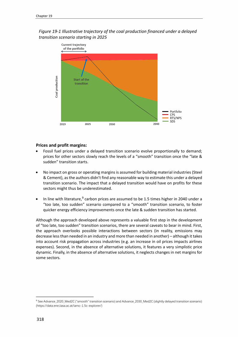
Chapter 19
318
Figure 19-1 Illustrative trajectory of the coal production financed under a delayed transition scenario starting in 2025
Prices and profit margins: • Fossil fuel prices under a delayed transition scenario evolve proportionally to demand;
prices for other sectors slowly reach the levels of a “smooth” transition once the “late & sudden” transition starts.
• No impact on gross or operating margins is assumed for building material industries (Steel & Cement), as the authors didn’t find any reasonable way to estimate this under a delayed transition scenario. The impact that a delayed transition would have on profits for these sectors might thus be underestimated.
• In line with literature,9 carbon prices are assumed to be 1.5 times higher in 2040 under a
“too late, too sudden” scenario compared to a “smooth” transition scenario, to foster quicker energy efficiency improvements once the late & sudden transition has started.
Although the approach developed above represents a valuable first step in the development of “too late, too sudden” transition scenarios, there are several caveats to bear in mind. First, the approach overlooks possible interactions between sectors (in reality, emissions may decrease less than needed in an industry and more than needed in another) – although it takes into account risk propagation across industries (e.g. an increase in oil prices impacts airlines expenses). Second, in the absence of alternative solutions, it features a very simplistic price dynamic. Finally, in the absence of alternative solutions, it neglects changes in net margins for some sectors.
9 See Advance_2020_Med2C (“smooth” transition scenario) and Advance_2030_Med2C (slightly delayed transition scenario)
(https://data.ene.iiasa.ac.at/iamc-1.5c-explorer/)

Factoring Transition Risk into Regulatory Stress-Tests for “Late & Sudden” Transition
319
Bibliography
Bank of England. (2016). Stress testing of banks: an introduction. Retrieved from https://www.bankofengland.co.uk/-/media/boe/files/quarterly-bulletin/2016/stress-testing-of-banks-an-introduction.pdf
Battiston, S., Mandel, A., Monasterolo, I., Schütze, F., & Visentin, G. (2017). A climate stress-test of the financial system. Nature Climate Change, 7(4), 283-288.
Battiston, S., & Monasterolo, I. (2019). A climate risk assessment of sovereign bonds’ portfolio. University of Milan Bicocca Department of Economics, Management and Statistics Working Paper(420).
Chenet, H., Thomä, J., Janci, D., Dupre, S., Hubert, R., Robins, N., & Cruickshank, P. (2015). Financial risk and the transition to a low-carbon economy. Towards a carbon stress testing framework.
CISL. (2015). Unhedgeable risk. Delis, M., Greiff, K., & Ongena, S. (2018). Being Stranded on the Carbon Bubble? Climate
Policy Risk and the Pricing of Bank Loans. SSRN Electronic Journal. Dupré, S., Thomä, J., Dejonckheere, S., Fischer, R., Weber, C., Cummis, C., & Srivastava, A.
(2015). Climate Strategies and Metrics: Exploring Options for Institutional Investors. A Joint Report from UNEP-Fi, GHG Protocol, and the, 2.
Ecofys. (2018). Climate risks of 3 funds of Actiam. ESRB. (2016). Too Late, Too Sudden: Transition to a Low-carbon Economy and Systemic Risk:
ESRB. ESRB. (2018). Adverse macro-financial scenario for the 2018 EU-wide banking sector stress
test. FED reserve. (2018). Dodd-Frank Act Stress Test 2018: Supervisory Stress Test Methodology
and Results. Gordon, M. J. (1959). Dividends, earnings, and stock prices. The Review of Economics and
Statistics, 41(2), 99-105. IPCC. (2018). Summary for Policymakers. In: Global Warming of 1.5°C. Min, H. G. (1999). Determinants of emerging market bond spread: do economic
fundamentals matter? : The World Bank. Poghosyan, T. (2014). Long-run and short-run determinants of sovereign bond yields in
advanced economies. Economic Systems, 38(1), 100-114. PRI. (2018). The inevitable policy response: Act now. PRI. (2019). Inevitable Policy Response: Policy Forecasts. Regelink, M., Reinders, H. J., & van de Wiel, M. V. e. I. (2017). An exploration of climate-
related risks for the Dutch financial sector. Röttmer, N., Brunke, J.-C., & Mintenig, J. (2018). Climate scenario analysis: cement’s financial
performance under 2°c and 2.7°c. Schoenmaker, D., & van Tilburg, R. (2016). Financial risks and opportunities in the time of
climate change. Bruegel Policy Brief 2016(02): 1-8. Tang, D. Y., & Yan, H. (2010). Market conditions, default risk and credit spreads. Journal of
Banking & Finance, 34(4), 743-753. Tanthanongsakkun, S., Pitt, D., & Treepongkaruna, S. (2009). A Comparison of Corporate
Bankruptcy Models in Australia: The Merton vs. Accounting-based Models. Asia-Pacific journal of risk and insurance, 3(2).
Thomä, J., & Dupre, S. (2017). Right Direction, Wrong Equipment: Why Transition Risks do not Fit into Regulatory Stress Tests.
Thomä, J., Murray, C., Hayne, M., & Hagedorn, K. (2017). Out of the fog: quantifying the alignment of Swiss pension funds and insurances with the Paris Agreement. In: Berlin.

Chapter 19
320
UNEP FI, & Mercer. (2018). Extending Our Horizons: Assessing credit risk and opportunity in a changing climate: Outputs of a working group of 16 banks piloting the TCFD Recommendations.
Vermeulen, R., Schets, E., Lohuis, M., Kolbl, B., Jansen, D.-J., & Heeringa, W. (2018). An energy transition risk stress test for the financial system of the Netherlands.
Weber, C., Hayne, M., Dupré, S., Thomä, J., & Braschi, T. (2017). “Asset-level data and climate-related financial analysis: A market survey” available at: https://2degrees-investing.org/wp-content/uploads/2017/02/Asset-Level-Data-Market-Report.pdf (accessed 15 January 2018).
Zmijewski, M. E. (1984). Methodological issues related to the estimation of financial distress prediction models. Journal of Accounting research, 59-82.

ClimateWise Physical Risk Framework
321
ClimateWise Physical Risk Framework
by
Cambridge Institute for Sustainability Leadership1
Abstract
Physical risks – such as rising temperatures, flooding, drought, sea level rise and water scarcity – are already being felt globally, and the associated financial losses (both insured and uninsured) have significantly increased in recent years. The ClimateWise Insurance Advisory Council has developed the ClimateWise Physical risk framework (CISL, 2019), which demonstrates how the risk analysis tools of the insurance industry can inform other parts of the financial sector and demonstrate the role of adaptation in mitigating these risks. The framework offers real estate investors and lenders a means of understanding the potential physical risks of climate change on their portfolios.
Physical risk exposure is likely to vary geographically both within and between portfolios but the impacts are significant across the board. For example, a 4°C warming scenario could see average annual losses caused by floods to UK mortgages more than double. While insurance will play an important role in managing the impact of climate change, the increase in risk could, in the most severe cases, make premiums unaffordable.
Keywords: climate change, physical risk, infrastructure, scenario analysis, catastrophe modelling, risk management, insurance industry, financial sector
1 Introduction
The changing climate poses new risks and challenges to investors and lenders. While much attention has focused on transition risks – the risks posed by rapid decarbonization of the world economy – at present, political agreements to cut emissions have not been matched by equivalent action on the ground. Instead, the world is currently on track to see substantial climate change throughout the 21st century. The definition of physical risks applied here follows CISL (2016), where physical risks arise from the impact of climatic (i.e., extremes of weather) or geologic (i.e., seismic) events or widespread changes in ecosystem equilibria, such as soil quality or marine ecology, and can be event-driven (‘acute’) or longer-term in nature (‘chronic’).
Climate change will influence the likelihood and intensity of extreme weather events, which threaten the interests of investors and lenders in real estate and infrastructure assets in particular. The Intergovernmental Panel on Climate Change (IPCC) reports that climate change
1 The authors of the chapter are Dr Bronwyn Claire and Dr Nina Seega from the Cambridge Institute for Sustainability
Leadership. The Chapter is based on a report authored by the Cambridge Institute for Sustainability Leadership. The authors
would like to thank Kajetan Czyz and Rachel Austin of CISL, Vivid Economics, Sayers and Partners, ETH Zurich, as well as
the ClimateWise Insurance Advisory Council and the Advisory Panel which was established for the project. All queries are
to be directed to [email protected].

Chapter 20
322
will result, for example, in increased frequency and intensity of heatwaves; more heavy precipitation events, leading to a greater risk of flooding at the regional scale; and an increased frequency and intensity of extreme high sea levels, such as those caused by storm surges (IPCC, 2018)2. The large year-to-year natural climate variability means that, even with further climate change, such events will not take place every year, even in more extreme scenarios. However, early signs of these risks materializing can be seen in more frequent heatwaves in most regions, a global increase in the frequency and intensity of heavy rainfall events and an increased risk of drought (IPCC, 2018). These changes pose particular threats to both infrastructure assets – for which global investment needs may exceed US$90 trillion by 2030 – and residential and commercial building stock – which is expected to grow by 13 percent between 2017 and 2026 (Navigant Research, 2018). For financial institutions lending against real estate and infrastructure assets, increases in the frequency and intensity of extreme weather events might increase the likelihood of defaults due to the increased financial losses borrowers face. For investors in real estate and infrastructure assets, such changes might lead to asset devaluation and reduced yields.
Insurance will likely play an important role in helping investors and lenders manage these increased risks, but insurance should not be used as a reason to ignore them. Insurance can play a key role in helping to manage physical risks, especially of the most extreme events. But growing physical risks will also influence the future affordability and availability of insurance protection. In their first-ever report on climate change, the UK’s Bank of England (2015, p. 37) noted that “increasing levels of physical risks could present challenges, both to market-based risk transfer mechanisms and to the underlying assumptions behind general insurance business models”. As such, investors and lenders need to be directly empowered to understand how these risks might influence them.
2 Overview of the ClimateWise transition risk framework
ClimateWise This unique framework was developed through the ClimateWise Insurance Advisory Council and builds on existing work on physical climate change risks to the financial sector. ClimateWise is a global network of leading insurers, reinsurers, brokers and industry service providers who share a commitment to reduce the impact of climate change on the insurance industry and society. In 2016, the ClimateWise Insurance Advisory Council was established to lead research into ways the insurance industry can support the transition to a low carbon economy. The Council is formed of a group of C-suite executives from across the ClimateWise membership. The development of the ClimateWise Transition risk framework was guided by an Advisory panel of representatives of policy and the market.
Background of the ClimateWise Physical risk framework The purpose of the ClimateWise Physical risk framework is to show how investors and lenders can make use of insurance industry catastrophe modelling tools and metrics to improve their management of the physical risks of climate change, especially by encouraging adaptation measures in targeted areas (CISL, 2019). The ClimateWise Physical risk framework shows how investors and lenders can use catastrophe modelling tools and associated metrics, refined by the insurance industry over decades, to better assess, manage, report, and reduce their exposure to physical risks, particularly those from extreme weather events. Catastrophe models have long been used by the insurance industry to assess and price extreme weather event risk, and hence help them and their clients manage these risks. Recently, the Geneva
2 (IPCC) Intergovernmental Panel on Climate Change. (2018). Global Warming of 1.5°C.

ClimateWise Physical Risk Framework
323
Association (2018), a leading international insurance think tank, recommended that climate science projections should be used within natural catastrophe models to provide more forward-looking forecasts. The framework shows how, in practice, outputs from climate models and climate scientists can be used in combination with natural catastrophe models to assess risk under future climate scenarios. Used in this way, the insurance industry’s catastrophe models are powerful tools that can be used by investors and lenders within their scenario analysis to help quantify the physical risks of climate change, while recognizing the inherent uncertainty surrounding the future incidence of climate events.
The framework outlines a four-step process that investors and lenders can follow to use these tools, as set out in Figure 20-1:
• First, investors and lenders need to collect data on the physical assets (‘exposure’) they are concerned about. As a minimum, this should include their geographic locations and some information on asset class, such as whether they are residential or non-residential property. The more detailed that property-level information can be – in terms of construction type and year, roof type, number of floors, occupancy and square footage – the more robust the associated results will be.
• Second, they need to decide which natural catastrophe model(s) to use for their analysis. Several factors will play into this choice. A critical one will be whether the modelling will be undertaken in-house or sub-contracted to a commercial model vendor. The former would require use of an open source model. This may allow for more bespoke analysis to be undertaken and provide greater understanding of what drives any results, but these models may not have received as much investment and will also require reasonable technical skills to be confident that the work is being undertaken accurately. The advantages and disadvantages are reversed for vendor models. For models supplied by vendors, the extent and transparency of model documentation is another important factor, since this will enable investors and lenders to understand and review the assumptions that have been made in the modelling.
• The third stage involves choosing the climate scenarios to model and defining how those climate scenarios might influence the probability and severity of extreme weather events. In order to account for uncertainty about the extent of global action on reducing emissions, scenarios chosen should cover a wide range of plausible futures. The scope of potential ranges in temperature increases, typically expressed in terms of temperature increases by 2100 above a preindustrial baseline, might range from 1.5°C, the temperature target ‘aimed for’ in the Paris Agreement, to 4°C or more, which broadly reflects the temperature increases that would be expected given the current trajectory of emissions. The relationship between these temperature changes and the severity and frequency of disaster events within a region should incorporate the latest peer-reviewed developments in climate science and acknowledge/account for the uncertainty around these relationships. Some models already include effects of climate change on the frequency and intensity of the perils within their models. Otherwise, collaborations with academics or specialist climate change impact modelers may need to be sought out in consultation with the model developer. As climate models continue to develop, for example in their geographic fidelity, these developments can be incorporated into this stage of the analysis.
• The final stage is model execution and interpretation of the associated results. Catastrophe models can provide a wide range of different results of interest. Two of the most common outputs are Average Annual Loss (AAL) – the average losses from

Chapter 20
324
property damage experienced by a portfolio per year – and annual probability of occurrence – the probability that, over the period of one year, a given asset experiences an event of a given magnitude. Any results should be compared against a ‘present day’ climate scenario baseline and, where possible, these baseline results should be compared with and scrutinized against historical loss data. Forward-looking results should also be benchmarked against those from comparable studies, where available. When there is confidence that these results are robust, investors and lenders then have the option to convert the changes in expected losses into potential changes in asset values. They can also use the natural catastrophe model(s) to analyze how adaptation measures might reduce losses and asset value impacts.
Figure 20-1 Key steps for investors and lenders to follow in modelling the physical risks of climate change
Source: CISL (2019)
3 Applying catastrophe models to infrastructure
Catastrophe models estimate risks from extreme weather events. Catastrophe models are sophisticated computer models used to estimate the risk of physical damage and the financial costs of such damage (‘losses’) to a geographically specified portfolio of physical assets, typically buildings, caused by extreme weather events including tropical cyclones (hurricanes/typhoons), earthquakes, hail, winter wind storms, floods, and wild fires. Typically, the key output of a natural catastrophe model will be the distribution of possible losses, expressed in financial terms, to the portfolio.
Catastrophe models vary in detail but typically share the same key hazard, vulnerability and financial modules that are applied to a set of physical assets, referred to as exposures. As shown in Figure 20-2, these components work in combination to estimate the risk of financial losses to a portfolio of exposures. Where information is available, most models can also incorporate attributes about building type (modifiers) in relation to the exposures, and details on insurance arrangements for the purposes of calculating financial losses.
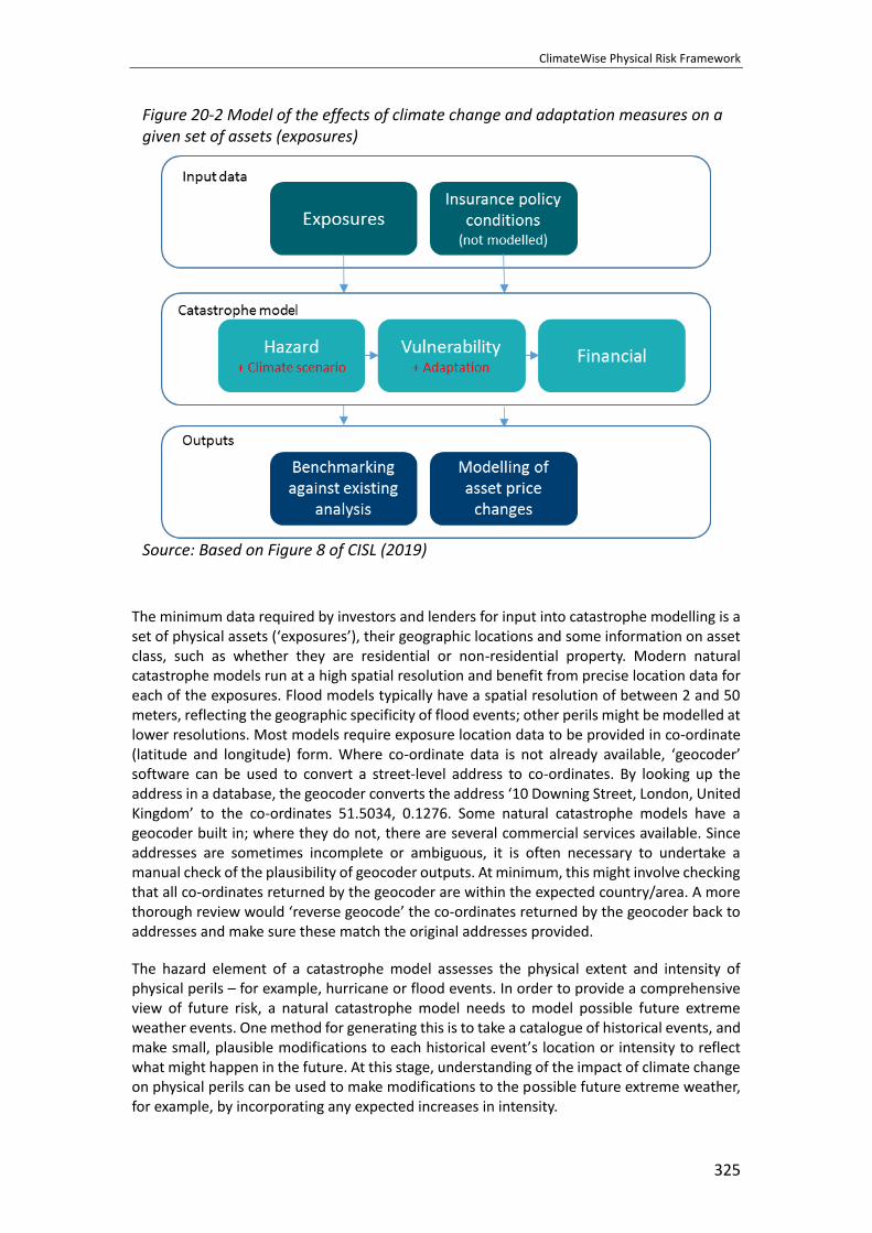
ClimateWise Physical Risk Framework
325
Figure 20-2 Model of the effects of climate change and adaptation measures on a given set of assets (exposures)
Source: Based on Figure 8 of CISL (2019)
The minimum data required by investors and lenders for input into catastrophe modelling is a set of physical assets (‘exposures’), their geographic locations and some information on asset class, such as whether they are residential or non-residential property. Modern natural catastrophe models run at a high spatial resolution and benefit from precise location data for each of the exposures. Flood models typically have a spatial resolution of between 2 and 50 meters, reflecting the geographic specificity of flood events; other perils might be modelled at lower resolutions. Most models require exposure location data to be provided in co-ordinate (latitude and longitude) form. Where co-ordinate data is not already available, ‘geocoder’ software can be used to convert a street-level address to co-ordinates. By looking up the address in a database, the geocoder converts the address ‘10 Downing Street, London, United Kingdom’ to the co-ordinates 51.5034, 0.1276. Some natural catastrophe models have a geocoder built in; where they do not, there are several commercial services available. Since addresses are sometimes incomplete or ambiguous, it is often necessary to undertake a manual check of the plausibility of geocoder outputs. At minimum, this might involve checking that all co-ordinates returned by the geocoder are within the expected country/area. A more thorough review would ‘reverse geocode’ the co-ordinates returned by the geocoder back to addresses and make sure these match the original addresses provided.
The hazard element of a catastrophe model assesses the physical extent and intensity of physical perils – for example, hurricane or flood events. In order to provide a comprehensive view of future risk, a natural catastrophe model needs to model possible future extreme weather events. One method for generating this is to take a catalogue of historical events, and make small, plausible modifications to each historical event’s location or intensity to reflect what might happen in the future. At this stage, understanding of the impact of climate change on physical perils can be used to make modifications to the possible future extreme weather, for example, by incorporating any expected increases in intensity.

Chapter 20
326
Climate models can be used to predict how climate change will influence the likelihood and severity of extreme weather events, although modelling some perils still represents a challenge. Drawing on evidence from the IPCC’s Fifth Assessment Report, Table 20-1 shows how the scientific understanding of the physical relationship between climate change and perils varies. In general, extreme events related to temperature, such as extreme cold or heat, are better understood than complex meteorological phenomena such as storms and cyclones.
Table 20-1 The impact of climate change is better understood for some perils than for others.
Likelihood of further changes by late 21st
century Region
Warmer and/or more frequent hot days and nights over most land areas
Virtually certain (99–100%) Over most land areas
Increase in precipitation Very likely (90–100%) Arctic, Northern Europe, North America and Southern Hemisphere
Increases in intensity and/or duration of drought
Likely (66–100%) On a global scale
Increase in intense tropical cyclone activity
More likely than not (50–100%)
In the western North Pacific (affecting e.g. China, Hong Kong, Macau, Japan, Korea, Philippines, Taiwan and Vietnam) and North Atlantic Ocean basins (affecting for example the Atlantic coast of the United States and Central America)
Increased incidence and/or magnitude of extreme high sea level
Very likely (90–100%) Global
Small increases in winter wind speed extremes (European winter wind storms)
Likelihood not provided “Medium confidence” in change
Central and Northern Europe
Source: IPCC (2013)
The vulnerability element estimates the physical damage caused by an extreme weather event. This normally uses damage curves, which relate the intensity of a hazard at a particular location to damage caused to assets at that location. For example, a damage curve for flood events describes the damage which would occur to assets at various flood depths. Damage is normally expressed in terms of a damage ratio, with a damage ratio of 100 percent indicating total destruction of an asset. Damage curves are generated either using observed data from historical events, or using analytic or experimental estimates. In the latter case, detailed characteristics such as building age, structural characteristics, and building occupancy can be used to select an appropriate damage curve for a given exposure. Uncertainty around damage curves is a major source of uncertainty in natural catastrophe models.

ClimateWise Physical Risk Framework
327
The vulnerability element can be used to model impacts of adaptation. Many adaptation measures involve physical changes to real estate assets so as to reduce the damage done to assets by hazards of given intensities. This, in turn, reduces expected financial losses. Inside natural catastrophe models, the effects of this type of adaptation measure can be modelled by selecting a damage curve with a lower damage ratio at given intensities. A comparison of losses with a ‘baseline’ and ‘adaptation’ damage curve provides an estimate of the effect of adaptation.
The financial element transforms physical damage to economic loss. By combining distribution of damage ratios with input data on replacement costs and any possible insurance contracts, the financial implications of the physical damage done by the event can be calculated. In many modelling approaches, this process is then repeated many thousands of times to help understand different scenarios of future losses.
Although natural catastrophe models vary in their implementations, they typically produce a common set of outputs, including the following:
• Average Annual Loss (AAL): This expresses the average losses from property damage experienced by a portfolio per year. If insurance is available and priced commensurate with risk, the AAL provides a lower-bound estimate of the premium required to insure against the risk. For illustration, Table 20-2 shows the calculation of AAL over a ten-year period for two scenarios. In both scenarios, total losses over ten years amount to £620 million, yielding an AAL of £62 million. However, the AAL metric provides no indication of whether losses are expected to be concentrated in a small number of years (as per Scenario 2) or spread more evenly through time (as per Scenario 1).
• Annual probability of occurrence: This measures the probability that, over the period of one year, a given asset (exposure) experiences an event of a given magnitude. For example, an asset might be at a 1 percent chance of flooding at a depth of one meter or more in any given year.
• Annual exceedance probability curve: This shows the probability that any given threshold of losses will be exceeded in any given year. For example, the hypothetical exceedance probability curve in Figure 20-3 shows there is a 1 percent chance of the portfolio experiencing a loss of £100 million or higher in any given year. AAL can be derived from an exceedance probability curve.
• Return periods: These are ways of describing the magnitude of an event. A flood with a 100-year return period has a 1 percent chance of being exceeded by a higher-magnitude event in any year. Such a flood is expected to occur approximately, but not exactly, every 100 years. Table 20-3 shows the relationship between return period and probability of exceedance at some frequently used values.

Chapter 20
328
Table 20-2 Comparison of two scenarios where in both scenarios, the Average Annual Loss is £62 million but the pattern of losses in the two scenarios is very different
Year Scenario 1 loss
(£ million) Scenario 2 loss
(£ million)
2001 7 0
2002 0 0
2003 194 620
2004 125 0
2005 9 0
2006 21 0
2007 0 0
2008 14 0
2009 250 0
2010 0 0
Source: CISL (2019)
Table 20-3 Probability losses and return periods
Probability losses are exceeded
Approximate return period
0.5% 200
1% 100
1.3% 75
2% 50
5% 20
10% 10
20% 5
Source: CISL (2019)

ClimateWise Physical Risk Framework
329
Figure 20-3 Annual exceedance probability
Source: CISL (2019)
4 Illustrative results
The following provides an illustrative analysis of 12 real estate asset portfolios, consisting of assets in the UK, Europe, North America, South America and Asia. Seven of these portfolios consist of UK residential mortgage assets held by large UK retail banks and building societies, whilst five are real estate investment portfolios held by ClimateWise members. The latter portfolios mostly comprise offices and shopping centers, with assets across Europe, North America, South America and Asia. The analysis compares present day losses of the portfolios from extreme weather events to their expected losses in the 2050s. Financial institutions with long-term investments, including banks and building societies providing new 35-year mortgages today, will have exposure to risks in this time period.
The results derive from two natural catastrophe models that are characteristic of those used in the insurance industry. The application uses CLIMADA (Aznar Siguan & Bresch, 2019), an open source model developed by ETH Zurich, to explore European winter wind storm and tropical cyclone risks. A strong attraction of CLIMADA is that it is an open source model, which means that all assumptions behind the model are visible and, with modifications to the source code, can be adapted by advanced users. However, the sophistication of the modelling does not match that of the commercial vendors. The application also uses Future Flood Explorer (FFE), developed by an international team of academics and experts, to explore UK flood risk. The FFE was previously used as part of the 2017 Climate Change Risk Assessment for the UK government’s Committee on Climate Change (Sayers and Partners, 2015).
The application explores expected losses in the 2050s in two climate change scenarios (acknowledging that this is just a sample of possible future climate change scenarios):
• The first scenario is consistent with 4°C of global warming by the end of the century, an outcome in line with the warming implied by current trajectories of climate action.
• The second scenario reflects the possibility that aggressive mitigation action and technological innovation leads to rapidly decreasing emissions levels and the global temperature rise being limited to 2°C by the end of the century.

Chapter 20
330
The illustrative analysis uses results from climate models to map these changes in global average temperature increases into expected changes in the frequency and severity of floods and storms. It is recognized that this is an area subject to ongoing scientific enquiry, with the effects of climate change better understood for some extreme weather events such as UK floods, those for others such as European wind storms. Furthermore, the changes in these events represent just a subset of future climate impacts.
The results show that, for these particular portfolios, climate change could have large impacts on the losses that investors and lenders face from floods in the UK and tropical cyclones in North America and the Pacific Rim, but that their increases in losses from European winter wind storms are likely to be lower. Under a 4°C warming scenario, the modelling suggests the AAL caused by UK floods to residential mortgage assets could increase by 130 percent. It also suggests a 40 percent increase in the number of residential properties exposed to significant flood risk (defined as a 1.3 percent or 1 in 75 annual probability of flooding or above), equivalent to 180,000 properties within the portfolios examined. These results are for large, geographically well-diversified portfolios; more regionally concentrated lenders may see larger increases. For investment portfolios, in a 4°C warming scenario, the increase in AAL from flood risk across four UK portfolios is modelled to be 70 percent higher in the 2050s than today. Across the two portfolios with assets in North America and the Pacific Rim, the analysis based on best evidence suggests that the equivalent expected increase from tropical cyclone risk is 80 percent. The portfolios examined face much smaller increases in risk from European winter wind storms.
The analysis also suggests that losses faced by investors and lenders are lower, but still substantial, if global efforts to reduce emissions are successful. For the UK residential portfolios, AAL from floods would increase by only half the amount of a 4°C scenario, while the modelling suggests that the number of properties within the portfolios at risk of significant flooding (1.3 percent or 1 in 75 annual probability or above) might only increase by 25 percent. For investment portfolios in the UK, the increase in AAL is 40 percent, which is similar to the potential increase in AAL from tropical cyclone risk (Table 20-4). These results reinforce that it is paramount for governments, business and society to try and keep warming as low as possible, as underlined by the most recent IPCC analysis.
Table 20-4 Expected losses for two scenarios
Peril Asset type Risk metric 2°C warming
by end of century
4°C warming by end of century
UK flood risk Residential mortgages
% increase in AAL by 2050s
61% 130%
UK flood risk Investment portfolios
% increase in AAL by 2050s
40% 70%
North America and Pacific Rim tropical
cyclones
Investment portfolios
% increase in AAL by 2050s
43% 80%
European winter wind storms
Investment portfolios
% increase in AAL by 2050s
6.3% 3.6%
Source: CISL (2019)

ClimateWise Physical Risk Framework
331
These findings align with those from earlier studies, including those from the insurance sector. For instance, JBA Risk (2018) found a 25–30 percent increase in AAL for UK residential properties in the 2040s, while the UK’s Climate Change Risk Assessment (Sayers and Partners, 2015), also using the Future Flood Explorer as in this analysis, found a 30–62 percent increase in AAL in the 2050s for UK residential properties. The smaller increases in AAL found in these previous analyses are likely to reflect differences in assumptions around community-based adaptation and in the portfolios examined, while in the case of the JBA analysis, also differences in model set-up and time horizon. Similarly, the relatively modest increases in AAL from wind storms match the findings of research carried out on behalf of the Association of British Insurers regarding the effect of climate change on wind storm losses to UK assets (Association of British Insurers, 2013). The ABI modelling exercise found the AAL from UK wind storms was expected to increase 11 percent by the end of the century under a 1.5°C scenario and 25 percent by the end of the century under a 4.5°C scenario. It is likely that differences to our analysis are largely attributable to the different time horizon and scenarios considered, as well as some differences in the model set-up and the underlying climate models used to drive the results.
The potential increases in risk, especially in a 4°C scenario, raise important questions for investors, lenders, insurers, and policymakers as to how they can be managed in the most cost-effective manner. In cases where commercially provided insurance policies are held in relation to these perils, policyholders might expect to see, on average, increases in premiums and insurance companies would need to purchase substantially more reinsurance to ensure solvency and in line with any increases in modelled uncertainty. For assets that have no insurance cover (such as some commercial properties), all of any increase in risk will be faced by investors and/or lenders. This also has important implications for the strategy of organizations set up to help address the insurance protection gap. In the specific case of the UK residential mortgage market, this applies particularly to Flood Re, whose role is to provide an affordable market for home insurance for properties built before 2009 that are at risk of flooding (Flood Re, 2018). Flood Re achieves this by offering fixed premiums according to council tax banding, with the funding gap between the premiums it charges and the risk-based price for insurance met through a levy imposed on the insurance industry (and, ultimately, its policyholders). This analysis suggests its funding gap could increase, reinforcing previous concerns about the sustainability of these arrangements. For example, although a formal assessment of when insurance availability for residential properties through normal market arrangements may become challenging has not been undertaken, a typical rule of thumb is that it can be challenging to provide affordable insurance in cases where the annual probability of flooding is 1.3 percent or above. The modelling shows that, in a 4°C warming scenario, by the 2050s, the number of residential properties falling into this category could increase by 40 percent to 180,000 properties across the portfolios examined. Scaled to the UK mortgage portfolio as a whole this could amount to an additional 250,000 properties, and compares with approximately 150,000 who were benefiting from the Flood Re scheme during the most recently reported financial year (Flood Re, 2018). Moreover, Flood Re is, by statute, to transition the UK residential market back to risk-reflective pricing, meaning that after 2039 premiums and excesses should, as well as being risk-reflective, remain affordable without the benefit of the levy: careful investigation will be required of whether and how Flood Re can achieve this in light of the projected increased risks arising from climate change.
In the absence of Flood Re or for UK residential properties excluded from Flood Re (those built after 2009), the implications for both homeowners and mortgage providers could be more profound. It is possible that, in some cases, this increase in risk will mean that buildings insurance for residential properties may no longer be available for some homes at an affordable price (recognizing that what is seen as an affordable premium can vary by

Chapter 20
332
household). A lack of access to affordable insurance would have adverse implications for homeowners living in those properties who may find that their properties suffer significant decreases in value, potentially leaving them in negative equity and either unable to sell their homes and/or unable to re-mortgage. This could have significant personal costs, as well as disrupting the liquidity and efficiency of the housing and mortgage markets. In turn, lenders may need to consider the increased risk of mortgage default, which is likely to be geographically concentrated, and ensure that their business strategies are robust to this risk.
A crucial next step from this work should be for national regulators to explore in more detail the interlinkages between flood risk, insurance availability and the residential property market – with a particular focus on how these interlinkages could evolve over time. In the UK, this would build on the concern expressed by the Bank of England regarding the possible crystallization of financial risks from greater flood risk to the UK residential mortgage market if flood insurance would become unaffordable (Bank of England, 2018).
While a substantial overall elevation in physical risks is expected in a 4°C scenario, not all lenders and investors are likely to be equally exposed. Especially in a 4°C warming scenario, the modelling finds significant differences in the risk of different portfolios of mortgage and investor assets. Under a 4°C warming scenario, the range of increase in expected losses across the seven UK residential mortgage portfolios varies between 108 percent and 132 percent. For the two portfolios of assets at risk of tropical cyclones in North America and the Pacific Rim, the range in the increase in losses is 17 percentage points, with much of this difference driven by the location of just a small number of assets. The modelling suggests that the spread in risk across different portfolios is substantially smaller if emission reductions are successful in moving the world onto a 2°C warming trajectory.
Property-level adaptation measures can materially reduce climate change induced losses, and this is most effective when combined with global efforts to reduce emissions. The increase in losses identified above assumes relatively limited efforts to adapt to the impacts of climate change. In the UK, the modelling suggests that, under a 2°C scenario, around two thirds of the additional losses might be offset if half of at-risk households install flood protection measures. This includes measures to prevent flood ingress and measures to reduce damage if flood water does ingress, such as resilient flooring. Further reductions in losses, and a reduction in the number of properties at significant risk of floods (annual probability of flooding above 1.3 percent), could be secured by increased community-level flood adaptation measures. The analysis of tropical cyclone risk suggests that, in a 2°C temperature scenario, roof upgrades to properties at risk of tropical cyclones might offset around half of the increase in AAL. However, adaptation measures offset a smaller proportion of the increases in losses in higher temperature scenarios, when extreme weather events are expected to be more severe. In other words, rather than considering adaptation as an alternative to efforts to reduce emissions, it is best thought as a complement to these efforts.
There are several reasons why the estimates of losses by the current framework might underestimate the true increase in physical risks faced by investors and lenders. The analysis focuses on future changes in the likelihood and intensity of extreme weather events, overlooking other chronic changes or multiple acute events. Also, climate models which drive predictions of extreme weather events may also not be capable of capturing tipping points in the climate system. The modelled portfolios are large and diverse, while smaller or regionally concentrated lenders might have higher risk than these. As well, increased urbanization and demand for new housing might result in new buildings in high-risk locations. Indirect impacts from extreme weather events and the financial losses associated with that damage are excluded. Physical damage to assets is also likely to cause business interruption and supply

ClimateWise Physical Risk Framework
333
chain interruptions, as well as potentially increase rates for labor and materials required to repair damage to assets.
5 Conclusions and outlook
The potential increases in risk, especially in a 4°C scenario, raise important questions for investors, lenders, insurers and policymakers as to how they can be managed in the most cost-effective manner. In cases where commercially provided insurance policies are held in relation to these perils, policyholders might expect to see, on average, increases in premiums and insurance companies would need to purchase substantially more reinsurance to ensure solvency in line with any increases in modelled uncertainty. For assets that have no insurance cover (such as some commercial properties), all of any increase in risk will be faced by investors and/or lenders. This also has important implications for the strategy of organizations set up to help address the insurance protection gap.
A crucial next step from this work should be for national regulators to explore in more detail the interlinkages between flood risk, insurance availability and the residential property market – with a particular focus on how these interlinkages could evolve over time. While a substantial overall elevation in physical risks is expected in a 4°C scenario, not all lenders and investors are likely to be equally exposed. The modelling suggests that the spread in risk across different portfolios is substantially smaller if emission reductions are successful in moving the world onto a 2°C warming trajectory. Property-level adaptation measures can materially reduce climate change induced losses, and this is most effective when combined with global efforts to reduce emissions.
There is a powerful opportunity for investors, lenders, the insurance industry and policymakers to target the uptake of adaptation measures in the most beneficial areas. Although it allows for rapid repricing of risk, the short time horizons created by the insurance industry’s practice of one-year insurance contracts limits the ability for insurers to incentivize adaptation measures. However, investors and lenders, combined with policymakers, may find it easier to take a longer-term perspective. They could work in concert with insurers to encourage the uptake of adaptation measures, for instance, by making both loans and insurance contingent on the installation of relevant adaptation measures. These efforts could help overcome ‘first-mover risks’ whereby households may be unwilling to introduce adaptation measures that similar households do not have, for fear that their abnormality, and the signal that the property may be exposed to physical risks, might reduce the value of the property. A further area to explore is the role of adaptation at the municipal level to demonstrate the potential value of municipal adaptation measures and the implications for the availability and design of insurance products.

Chapter 20
334
Bibliography
Association of British Insurers. (2013). Revised Statement of Principles on the Provision of Flood Insurance. 55-60.
Aznar Siguan, G., & Bresch, D. N. (2019). CLIMADA v1: a global weather and climate risk assessment platform. Geoscientific Model Development, 12, 3085-3097.
Bank of England. (2015). The impact of climate change on the UK insurance sector – A Climate Change Adaptation Report by the Prudential Regulation Authority. Prudential Regulation Authority.
Bank of England. (2018). Transition in thinking: The impact of climate change on the UK banking sectors
CISL. (2016). Environmental risk analysis by financial institutions: a review of global practice. Cambridge, UK: Cambridge Institute for Sustainability Leadership.
CISL. (2019). Physical risk framework: Understanding the impacts of climate change on real estate lending and investment portfolios. the Cambridge Institute for Sustainability Leadership.
Flood Re. (2018). Annual Report and Financial Statements. Geneva Association. (2018). Managing Physical Climate Risk: Leveraging Innovations in
Catastrophe Risk Modelling: Research Brief. IPCC. (2013). Climate change 2013: The physical science basis. Contribution of working group
I to the fifth assessment report of the intergovernmental panel on climate change, 1535.
IPCC. (2018). Global Warming of 1.5◦C - Summary for Policymakers. . Technical Report Intergovernmental Panel on Climate Change.
JBA Risk. (2018). New UK Climate Change Model. Retrieved from https://www.jbarisk.com/news-blogs/new-uk-climate-change-flood-model/
Navigant Research. (2018). Global Building Stock Database. Sayers and Partners. (2015). Climate Change Risk Assessment 2017: Projections of future
flood risk in the UK. Pages 125. Sayers and Partners LLP report for the Committee on Climate Change.

ClimateWise Transition Risk Framework
335
ClimateWise Transition Risk Framework
By
Cambridge Institute for Sustainability Leadership1
Abstract
Global efforts to tackle climate change by reducing carbon emissions will result in a transition to a low carbon economy. This transition, already underway, presents both risks and opportunities for the financial sector. The ClimateWise Insurance Advisory Council has developed the ClimateWise Transition risk framework (CISL, 2019), an open-source model which explores how to quantify these risks and opportunities within infrastructure investment portfolios.
The framework is set out in three steps, which can be used independently or combined to explore transition risks and opportunities. Specifically, the framework is designed to help investors 1) to assess the breadth of asset types exposed to transition risk at portfolio level (across different subsectors, regions, and timeframes; 2) to define the potential financial impact of the low carbon transition down to asset level; and 3) to incorporate transition impacts into asset financial models.
Each of the three steps highlights practical actions investors might take in order to manage risks and capture opportunities. The framework applies this analysis to an array of global infrastructure asset types.
Keywords: climate change, transition risk, infrastructure, scenario analysis, catastrophe modelling, risk management, insurance industry, financial sector
1 Introduction
The commitment to hold the increase in the global average temperature to well below 2°C above pre-industrial levels lies at the heart of Paris Agreement (United Nations, 2016). Achieving that objective will require a significant change in global energy consumption across all sectors. This brings material financial implications for companies, governments, and the wider global economy.
In particular, markets are required to reallocate global capital in line with a pathway of low greenhouse gas emissions and climate-resilient development (United Nations, 2016). In order to limit global warming to below 2°C, the remaining global carbon budget must remain below 1,000 GtCO2 (World Resources Institute, 2014). However, the carbon potential of the earth’s known fossil fuel reserves is more than 2,860 Gt CO2. Consequently, if global action on climate policy accelerates, or the target of 2°C is enforced, many carbon intensive reserves will become unburnable, with implications for the infrastructure that serves them. Under current estimates,
1 The authors of the chapter are Dr Bronwyn Claire and Dr Nina Seega from the Cambridge Institute for Sustainability
Leadership. The Chapter is based on a report authored by the Cambridge Institute for Sustainability Leadership. The authors
would like to thank Kajetan Czyz and Rachel Austin of CISL, ERM, as well as the ClimateWise Insurance Advisory Council
and the Advisory Panel which was established for the project. All queries are to be directed to [email protected].

Chapter 21
336
this could cut the revenues of upstream oil and gas companies by US$20 trillion, and coal companies’ revenues by US$5 trillion (The CO-Firm & Kepler Cheuvreux, 2014). This will result in a considerable knock-on impact along the value chain, ranging from transportation to manufacturing and chemicals to power.
2 Overview of the ClimateWise transition risk framework
ClimateWise ClimateWise is a global network of leading insurers, reinsurers, brokers and industry service providers who share a commitment to reduce the impact of climate change on the insurance industry and society. In 2016, the ClimateWise Insurance Advisory Council was established to lead research on transition risk management in insurance industry. The Advisory Council is formed of a group of C-suite executives from across the ClimateWise membership. The development of the ClimateWise Transition risk framework was guided by an Advisory panel of representatives of policy and the market.
Background of the framework The ClimateWise Transition risk framework aligns with recommendations from the Task Force on Climate-related Financial Disclosures (TCFD, 2017). The ClimateWise Transition risk framework (CISL, 2019) provides an open-source, step-by-step guide that captures risks and opportunities emerging from the low carbon transition to infrastructure investments (Figure 21-1). The definition of transition risks applied here follows CISL (2016), where transition risks arise from efforts to address climate change, including but not limited to abrupt or disorderly introduction of public policies, technological changes, investor sentiment and disruptive business model innovation. The framework is intended to provide real and practical value for chief investment officers (CIOs), asset managers, regulators and the wider financial community.
The objectives of the framework are to:
1. provide a structural framework to understand and measure financial implications of transition risks with the focus on infrastructure assets;
2. identify scenarios and time horizons in which exposure to low carbon transition risks will materialized;
3. demonstrate a transparent, adaptable and robust methodology for assessing transition risks.
Investors can use the framework in multiple ways. The framework can serve as a basis for a high-level assessment of risk exposure across their portfolios. Alternatively, investors can use the framework to complete a deep-dive into a particular sector. Finally, investors can incorporate the quantifiable impacts of transition risks into their own financial models.

ClimateWise Transition Risk Framework
337
Figure 21-1 ClimateWise Transition risk framework
Source: CISL (2019)
Assessing risk exposure of infrastructure investments Across the global investment community, investors hold a wide variety of infrastructure portfolios. This results in a range of diverse needs to manage the exposure of portfolios to the risks and opportunities presented by a low carbon transition. This framework is adaptable and therefore accommodates the diversity of investors’ needs.
Financial driver analysis
At the core of the framework is the analysis of the financial drivers of transition risks. It allows users to assess financial impacts from different transition scenarios and across a range of time horizons. For each asset type, the financial cost and revenue drivers (e.g. typical inputs for the financial model of that asset type) are identified and assessed for any potential impact from transition risks. The framework can also be used as a starting point for building customised scenarios by allowing users to sense check the underpinning financial drivers within the low carbon scenarios and tailor these in line with in-house views on the direction and speed of the transition.
Each step of the framework can be used independently to inform various stages of risk mitigation and investment strategy. If all three steps are completed, the framework can provide a more thorough assessment and measurement of financial exposure to transition risk:
Step 1 – Portfolio risk and opportunity exposure
Step 1 of the framework enables investors and regulators to quickly identify where there could be exposure to material financial risks or opportunities, across a large portfolio of assets. This consists of applying the Infrastructure Risk Exposure Matrix, a tool developed to quantify the

Chapter 21
338
transition impact on asset financial drivers. The matrix is also used as a starting point for Steps 2 and 3 of the framework to define the potential transition impact at an asset specific level and to incorporate asset-specific financial drivers into a financial model.2
The process followed to leverage and adapt the matrix is summarised as follows:
• Set the scope and select scenarios: scenarios provide plausible alternative views of how the future could evolve – in this instance, the transition to a low carbon economy. The scenarios are not a ‘what if’ exercise for one uncertainty, and neither do they assess outcome probability. But rather, they provide a holistic view of potential risk impacts on future investments in infrastructure. A variety of transition risk factors (as defined by TCFD (2017)) are considered, including market and technology shifts, regulatory and policy changes, reputational impacts and investor sentiment. Scenarios can be developed either in-house or in leveraging publicly referenced scenarios. The latter provides greater transparency to investor stakeholders and potential for shareholder disclosure, and is therefore recommended in the TCFD guidelines.
• Identify financial drivers: the next stage is to identify which revenue and cost drivers could be materially impacted by TCFD-defined transition risks. For each asset type, financial cost and revenue drivers are first identified based on typical inputs for a financial model of that asset type; and where transition risks could significantly impact future asset revenues and costs. Transition risks have been defined in line with the TCFD transition risk categories: market and technology shifts, emerging policy and legal requirements, mounting reputational pressures and investor sentiment. The impacts on the financial drivers are assessed by comparing the trajectory of a business-as-usual baseline to the transition scenarios.
• Assess financial drivers: for the identified financial drivers, next analyse the change in trajectory between business-as-usual baseline and a low carbon transition scenario. Then assess the potential impact on each asset type’s financial driver (e.g. one revenue driver for a coal-fired power plant is plant utilisation) by calculating the difference in the trajectory between a business-as-usual baseline and the low carbon transition scenarios using the scenario indicators and data sets. The potential impact is then defined against the scale of positive/negative impact on each financial driver, based on changes to the scenario indicator, and assigned a risk weighting on the estimated relative contribution of each financial driver to the financial performance of each asset type.
• Estimate impact on asset type: finally, the potential impact of each financial driver on asset financial performance is weighted. This means classifying the overall exposure from transition risks and opportunities on the asset financial performance, based on cumulative net impact of the drivers associated with each asset type, for each region, scenario, and timeline.
Finally use the Infrastructure Risk Exposure Matrix to determine which asset types within the investor portfolio are likely to be exposed to the highest degree of transition risk and/or opportunity, and identify the assets from the portfolio that are highlighted as having high financial risk or opportunity accounting for transition risks and material value in the portfolio. The results can be used to: (1) inform future portfolio investment strategy – including
2 See the www.cisl.cam.ac.uk/transition-risk, provided with open-source access to all investor practitioners.

ClimateWise Transition Risk Framework
339
allocation of funds or divestments, and (2) select assets for more granular assessment in Steps 2 and 3 of the framework.
Step 2 – Asset impact identification
Transition risks vary within asset types, down to an asset-specific level due to an asset’s specific location, competitive positioning, carbon intensity and exposure to low carbon technologies. The Asset Impact Identification Methodology provides asset managers and owners with an approach to define financial impact on an asset and to identify options to improve asset resilience. This step requires additional resources for the more granular analysis but is particularly useful for highly exposed assets or for direct application to a smaller, less-diversified investment portfolio. Risks vary considerably between assets of the same type, depending on their geography, carbon intensity, technology (e.g. solar versus wind), and competitive positioning in the local market. Therefore, investors gain significant benefit in conducting asset-level specific analysis.
Firstly, identify the specific assets from the portfolio for assessment based on having high risk or opportunity, and/or making up a significant part of the portfolio in terms of financial value. The methodology outlined in Step 1 is reapplied to assess the impact on financial drivers for the specific asset, taking into account particularly the:
• local geography (e.g. country, or state/province)
• asset carbon intensity (particularly for asset types where the matrix highlights carbon reduction as a key factor)
• technological factors that may come into play (e.g. solar versus wind in the renewable sector)
• competitive positioning in the market (e.g. lowest cost provider, government-regulated asset)
Where available for the specific assets, consider publicly referenced scenarios that can provide more asset-specific insights to analyses potential impact on the financial drivers. For instance, if the asset is in the UK power sector, the UK National Grid and UK Fifth Carbon Budget scenarios could be applied – considering technology-driven and specific government policy scenarios. Once this is complete, the user can identify which financial cost and revenue drivers for the asset could be most financially impacted. Referencing the key underlying factors from the selected scenario data sets, the user can use this insight to inform investment options to improve asset resilience or improve portfolio management processes to monitor for emerging risks and opportunities.
Step 3 – Financial modelling analysis
In Step 3, the asset impact assessment is used to build risk and contingency scenarios within in-house asset financial models. This will enable stress testing and opportunity identification through quantifying the potential financial impact from transition risks directly within financial models. Investors are then able to assess transition risk drivers on asset financial performance, helping to identify investment options for improving asset resilience or for an exit strategy, as well as supporting delivery of the TCFD recommendations. The portfolio or lending manager can then use the matrix to update their valuation models (e.g. net present value or discounted cashflow models) by inputting the estimated scale of the transition risk driver into their models.

Chapter 21
340
For example, they could increase the expected revenues from their gas distribution network by X percent by 2030 in a low carbon scenario where a swifter shift to gas as a bridge fuel is likely to occur.
The potential risk impact on each financial driver in a low carbon transition scenario can be estimated on an annual basis, referring to the methodology provided in the Infrastructure Risk Exposure Matrix and refined where possible to an asset-specific level based on the Asset Impact Identification Methodology. Leveraging the methodology provided and scenario data sets, investor practitioners can incorporate the financial drivers most materially impacted by the transition scenarios directly into their own financial models.
Once the financial drivers are incorporated into the model, a key output is the ability to assess the financial materiality of transition risks (and opportunities) for a specific asset. Asset managers and owners could then assess how the low carbon transition could impact a variety of the asset’s financial metrics; and leverage the work to consider exit strategies where risk is high or develop investment options to improve asset resilience.
Baselines and sources Low carbon transition scenarios: the key enabler The framework leverages a scenario-based approach, as introduced by the TCFD. This helps to assess the potential financial impacts transition risk may have for an asset’s financial drivers and future financial performance. Companies typically use scenarios to test a variety of alternative views of the market. This ensures a robust future investment strategy. These scenarios provide plausible alternative views on how the transition to a lower carbon economy could evolve over time, including a more rapid, disorderly transition.
Aligned with the TCFD recommendations, the framework relies on scenario data sets to assess potential impacts from the low carbon transition. While the framework is adaptable to a variety of scenarios being applied, the approach is demonstrated with scenarios from the International Energy Agency (IEA). This is due to their transparency as a publicly referenced source, as well as a potential emerging benchmark for investors and the TCFD. Further, the IEA scenarios provide a holistic view on global market demand, supply, prices and technology shifts across the broad range of energy-intensive sectors.
While a variety of transition scenarios could be applied to the framework to assess financial impacts, the Infrastructure Risk Exposure Matrix tool uses the Nationally Determined Contributions (NDCs) submitted at COP 21 in 2015 (which currently falls short of the Paris Agreement’s ambition) and the 2°C consistent scenarios from the IEA’s World Energy Model. This provides a range of plausible climate outcomes aligned with the signatory country governments’ current NDCs submitted at COP21, as well as the Paris Agreement’s ultimate target.
Where required, any gaps in the scenario data sets have been supplemented with other publicly referenced sources. This includes the World Bank and government policy-driven scenarios.
Some investors may also choose to stress test against a 1.5°C scenario to ensure the robustness of their portfolios. They may also consider alternative pathways to a 2°C scenario which focus on specific technological advances (e.g. energy storage, carbon capture and storage) rather than policy changes or carbon taxes.

ClimateWise Transition Risk Framework
341
Time frames Investment time frames typically vary: 5 years for banks, 10 to 15 years for infrastructure investment companies, 20 years or more for governments, depending on asset life. While the framework can be adapted to cover any year (as scenario data sets typically cover a year-by-year basis), the Infrastructure Risk Exposure Matrix focuses on 2020, 2030 and 2040 to cover as broad a range of investment horizons as possible.
Infrastructure asset types A variety of asset types were selected to demonstrate the breadth of potential transition risks. Selected sectors were chosen based on primary and secondary research on key infrastructure investments across Organisation for Economic Co-operation and Development (OECD) and non-OECD economies. Asset types were split into subcategories, to untangle all sector-specific transition risk issues. For instance, power assets were divided into sub-categories from coal to renewable power generation:
• Power Assets – Coal power plants, Gas power plants, Nuclear power plants, Renewables (utility scale)
• Fuel Infrastructure – Oil pipelines & midstream infrastructure, Gas pipelines & midstream infrastructure
• Transport – Rail networks, Airports, Toll roads, Ports
• Social – Public buildings
• Water – Water utilities
• Telecommunications – Telecommunications infrastructure
Geographies: The US, EU and India Geographies were chosen to illustrate how transition risks could vary in different parts of the world. This ensures relevancy for all investment portfolios. The geographies chosen focused on: (1) governments with an interest in infrastructure aimed at supporting economic growth; (2) countries that are amenable to foreign investment and (3) countries offering substantial investment potential. Two OECD markets and one non-OECD market were selected: the US, EU and India. These geographies cover three of the largest markets in the world. Each varies greatly from the other in how the low carbon transition will take hold (e.g. US shale gas displacing coal-fired generation, the broad uptake of renewables in the EU and India’s conundrum of coal versus solar).
3 Illustrative results
The practicality and robustness of the framework has been validated by applying it to three separate case studies based on investors’ real-life portfolios – including two of the world’s largest insurance companies and one of the global top five investors in infrastructure. Examples for Step 1 portfolio risks and opportunities exposure results, Step 2 asset impact identification results for a UK airport and Step 3 financial modelling analysis results for a German gas distribution pipeline are presented in the following.

Chapter 21
342
Step 1: Portfolio risk and opportunity exposure Step 1 allows investors to quickly identify the material financial impacts from transition risks across a large portfolio, by applying the Infrastructure Risk Exposure Matrix (Figure 21-2). This tool helps to assess potential exposure to transition risks across a breadth of asset types, geographies, climate scenarios and time frames. The Infrastructure Risk Exposure Matrix provides insights on the infrastructure asset types most exposed to the low carbon transition:
• The most significant risk is coal-fired power generation globally and oil & gas infrastructure in the US and EU. These risks are more pronounced in the 2°C scenario compared to the Paris Agreement (NDC) scenario.
• There is minimal risk associated with gas-fired power generation in India, as well as globally in telecommunications, ports and water utilities (excluding physical climate change risk).
• The greatest opportunities exist in the renewables sector globally, and to a lesser extent in mass transit.

ClimateWise Transition Risk Framework
343
Figure 21-2 Summary of the Infrastructure Risk Exposure Matrix for the infrastructure asset types considered
Source: CISL (2019)
An investor would use the Infrastructure Risk Exposure Matrix to determine which asset types within the investor portfolio are likely to be exposed to the highest degree of transition risk and/or opportunity. Overlaying the matrix with a company’s portfolio of assets (risk level and asset value) shows how the potential risk and/or opportunity exposures could significantly increase through time and with the pace of change in a low carbon transition scenario (as seen in Figure 21-3 below).

Chapter 21
344
Figure 21-3 Example of an investment portfolio facilitating analysis of exposure to transition risks and opportunities across infrastructure asset types
Source: CISL (2019)
Identifying the assets in the portfolio that are highlighted as facing high financial risk or opportunity due to transition risks, the results can be used to: (1) inform a future portfolio investment strategy – including allocation of funds or divestments – and (2) select assets for more granular assessment in Steps 2 and 3 of the framework.
Step 2: Asset impact identification Step 2 allows investors to assess the financial impact from the low carbon transition at an asset-by-asset level, which provides insights on ways to improve asset resilience. Risks vary considerably between assets of the same type, depending on their geography, carbon intensity, technology and competitive positioning in the local market. Therefore, investors gain significant benefit in conducting an asset-level specific analysis.
Depending on an investor’s portfolio size and risk appetite, the Asset Impact Identification Methodology can be re-applied asset-by-asset to an entire portfolio, or to the most exposed assets identified by overlaying the Infrastructure Risk Exposure Matrix. Additionally, stress testing of the portfolio under different time frames and scenarios will produce a more holistic understanding of transition risk and opportunity. For example, using asset-specific data, a gas distribution business in Germany was found to have a medium financial risk in 2030 and low risk in 2040 under the Paris Agreement (NDC) scenario, but a low risk in 2030 and medium risk in 2040 under the 2°C scenario – these were driven by shifts in the local market from coal to renewables.
Leveraging the Infrastructure Risk Exposure Matrix and the Asset Impact Identification Methodology, investors can identify how a specific asset, and its cost and revenue drivers, could be impacted by transition risk (or opportunity). While an asset may be identified as having high exposure due to the sector or geography it operates in, it could be impacted in different ways due to the asset’s specific location.
Take for example an airport in Europe (Table 21-1 and Table 21-2). If the generic scenario shows a fall in aviation demand in the EU driven by an uptake in high-speed electric rail infrastructure, then an airport could diversify more into long-haul versus short-haul flights (with the latter

ClimateWise Transition Risk Framework
345
more risk exposed). Alternatively, an airport’s competitive positioning could drive a gain in demand, as other airports more focused on short-haul flights are potentially driven to closure.
Table 21-1 Example of impact assessment of financial drivers for a specific airport in the UK compared to generic EU airport
Source: CISL (2019)
Table 21-2 Example of investment strategy implications from impact assessment for a specific airport in the UK compared to generic EU airport
Source: CISL (2019)

Chapter 21
346
Step 3: Financial modelling analysis Step 3 allows investors to incorporate the potential impacts of transition risk directly into their own financial models. Using such a granular approach to defining asset impact enables investors to develop an in-house view based on their opinion of the probabilities linked to the key transition drivers outlined in the framework. This is done by integrating the financial drivers identified in Steps 1 and 2 into investors’ in-house financial models. Referring to the relevant scenario data sets, the potential impact on asset revenue and costs can be quantified. Leveraging this analysis, asset managers and owners can:
• evaluate investment profiles required under different scenarios;
• determine impacts on key revenue and cost drivers under different scenarios, with the resulting impact on cash flow, valuation, return on equity and other metrics as required;
• explore investment options to improve asset resilience or exit strategies.
In this instance, a gas distribution company in Germany is less impacted by the low carbon transition than the rest of the EU, thus altering the risk profile for the asset. The Infrastructure Risk Exposure Matrix (Table 21-3) indicates a risk to gas demand in the EU, with a potential decline of more than 25 percent by the early 2030s compared with the base case, according to the IEA’s 2°C scenario. Assuming a direct relationship between demand and asset utilisation, this suggests declining asset revenues. However, German gas demand will fall at a slower pace than the rest of the EU, as a substantial coal market is still being phased out in the near term. Thus, the impact in Germany is lower than in the rest of the EU, due to local market conditions and government policies on specific assets.
Table 21-3 Example of an impact assessment of financial drivers for a gas distribution pipeline in Germany
An asset manager or owner investing in this gas distribution company, could quantify the potential financial impact at an asset level by incorporating the outputs of the Infrastructure Risk Exposure Matrix or Asset Impact Identification Methodology in their own financial models.

ClimateWise Transition Risk Framework
347
The financial drivers affected by the low carbon transition, specific to the gas distribution company, are listed in the Infrastructure Risk Exposure Matrix (Table 21-4).
Table 21-4 Example of the impact on asset financial drivers is determined using scenarios
Taking the approach outlined above, the outputs and the suggested scenario data sets, asset managers can interpolate potential changes in revenue and cost (Table 21-4), incorporate them into an asset financial model and quantify the potential impact on the value or returns of the asset (Table 21-5). Accounting for potential increases in costs and a decline in asset utilisation, financial modelling indicates that earnings before interest and tax (EBIT) for the specific asset could fall by more than 70 percent against the base case, under a 2°C scenario (Figure 21-4 and Figure 21-5).
Table 21-5 Interpolation of financial drivers into the asset financial model

Chapter 21
348
Figure 21-4 Example of transition risk effects on asset returns and costs
Figure 21-5 Example of transition risk effects on asset net present values
Inform investment strategy and risk management
The framework has been developed to empower investors to take practical actions to mitigate their exposure to transition risks, capture opportunities and disclose their exposure to key stakeholders. Across the three case studies, each step of the framework was applied to inform investment strategy and risk management. Insights were provided on how the framework could inform investment decisions and guide strategic responses to transition risks.
Take for instance the EU gas distribution company case study:
• Step 1 identified this asset as one of the more exposed assets in the investor’s portfolio in 2040 – highlighting options for specific risk monitoring as part of the portfolio investment strategy.
• Step 2 defined the impact of transition risk on the asset’s key revenue and cost drivers. This included a fall in pipeline utilisation, and a rise in capital and operation expenditure due to emission reduction and carbon pricing – and options for asset managers and owners to improve the asset’s resilience to transition risk.
• Step 3 integrated the analysis through a financial model to determine the impact on the asset’s financial performance in line with the Paris Agreement (NDCs) and 2°C scenario – and explored investment options to improve asset resilience.

ClimateWise Transition Risk Framework
349
4 Conclusion and outlook
The ClimateWise Transition Risk Framework can support investors and regulators to assess the financial impact of transition risks. It enables a quantification of potential impacts, as called for by the TCFD. It enhances investors’ and regulators’ ability to manage risk and capture opportunity. Transition risk could increase significantly by 2030. The framework demonstrates that the low carbon transition could financially impact a variety of infrastructure asset types. However, it also unpacks transition risk according to sector, geography, and time horizon.
Investors and regulators can enhance their understanding of how the financial performance of their infrastructure portfolios and assets could be affected. The framework provides them with the ability to:
• assess portfolios for risk and opportunity exposure;
• define potential financial impact down to an asset-specific level;
• incorporate transition risk directly into asset managers’ and owners’ own financial models.
Across the global investment community, investors hold a variety of infrastructure portfolios, and therefore, have a range of diverse needs to manage exposure to transition risk. The framework has been designed to allow for this variation in investors’ needs, by providing an open-source and adaptable methodology. CIOs, asset managers and owners, and the wider financial community can take practical actions to mitigate transition risks, capture transition opportunities and communicate their strategic response plans to key stakeholders. Each step of the framework provides opportunities to inform investment strategies from a large portfolio down to asset-specific levels. Likewise, this methodology can be leveraged by regulators to inform future risk mitigation approaches and policies. The framework has been developed to empower investors and deliver real value.
Further pilot testing of the framework is being undertaken to gather insights as to how it could be improved. Feedback from this process will be pooled and used to produce a second version of the framework. While the scope of the initial project was constrained, the aim was to demonstrate the robustness of the framework’s approach and its potential wider application using infrastructure assets worldwide as a case study. As part of a next phase of work, it would be beneficial to expand coverage to more geographies and asset types. Significant differences can exist within asset types, and across national boundaries, for example for renewable power in different European countries. Asset types not yet covered include district heating systems and electricity transmission infrastructure.
In terms of future development, the framework application in this report focuses on infrastructure, but could equally be adapted to any type of asset and serve as a tool for a broad range of investors. The approach could also be expanded to wider applications across the financial community, incorporating physical risks and a variety of low carbon transition scenarios. In line with TCFD recommendations, investors may wish to adapt this framework and embed it in the organisation’s risk management processes, metrics and targets, and governance framework.

Chapter 21
350
Bibliography
CISL. (2016). Environmental risk analysis by financial institutions: a review of global practice. CISL. (2019). Transition risk framework: Managing the impacts of the low carbon transition
on infrastructure investments. TCFD. (2017). Recommendations of the Task Force on Climate-related Financial Disclosures. The CO-Firm, & Kepler Cheuvreux. (2014). Stranded assets, fossilized revenues. United Nations. (2016). Paris Agreement: Article 2. World Resources Institute. (2014). The Carbon Budget [Infographic].

MSCI Climate Value-at-Risk
351
MSCI Climate Value-at-Risk
By
MSCI ESG Research LLC1
Abstract
The Climate Value-at-Risk (Climate VaR) metric offered by MSCI ESG Research provides a forward-looking and returns-based measure of climate-related risks for financial institutions. The methodology is designed to closely align with the Task Force on Climate-related Financial Disclosures (TCFD) recommendations for conducting scenario analysis on investment portfolios. Climate VaR includes both low-carbon transition and physical climate-modelling methodologies. Both methodologies use top-down and bottom-up modelling techniques. All Climate VaR metrics are quantitative, forward-looking and focused on either the risks or opportunities that climate change may pose to a company’s securities due to low-carbon transition or physical effects of climate change. The primary applications of Climate VaR include engagement, investment decision-making, risk analysis, monitoring and compliance, and TCFD reporting.
Keywords: climate VaR, low-carbon transition, physical climate risks, Task Force on Climate-related Financial Disclosures (TCFD), engagement, investment decision-making, risk analysis, monitoring and compliance
1 Introduction
MSCI ESG Research firmly believes that climate change presents clear and pressing risks and opportunities to financial markets. 2 In addition to risks to livelihood from increasing temperatures and rising oceans, climate change also highlights the economic and investment risks and opportunities associated with the world’s transition to a low-carbon economy. An extensive body of scientific evidence has established that man-made factors are driving climate change on our planet. Citizens are demanding action from governments, companies and investors, because humans face a catastrophic future unless remedial actions are taken swiftly. Investors everywhere need to incorporate this new reality into their investment practices.
To address these needs, our Climate Value-at-Risk (Climate VaR) metric provides a forward-looking and returns-based impact metric for financial institutions. This metric was developed using an integrated approach, incorporating the latest academic findings from climate science as well as input from the financial services industry.3 Climate VaR can be used to inform
1 This chapter is written by Josip Spec, email: [email protected]; Bruno Rauis, email: [email protected]; and David
Lunsford, email: [email protected]. 2 For more information, see The MSCI Principles of Sustainable Investing, www.msci.com/esg-investing 3 In 2019, Carbon Delta (an MSCI company) together with twenty institutional investors and UNEP FI piloted a metric for
determining the value at risk for equity, bond, and real estate portfolios. https://www.unepfi.org/investment/tcfd/

Chapter 22
352
investors on appropriate action with regards to climate related investment risks, e.g., whether to diversify, divest, or engage.
As extreme weather events manifest themselves more frequently and intensely, we have seen the investment industry undergo a sea change.4 Policy makers around the world have also begun to forge robust and decisive climate-change regulations.5 Evaluating companies’ climate change resilience has become a preeminent investment issue.
Broadly speaking, there is growing evidence that tangible actions are being taken. More companies have disclosed the carbon-intensities of their operations, 6 more shareholder resolutions have urged company management to address climate change-related issues and investor pledges, 7 and widely publicized divestments have redirected money to more environmentally benign assets.8
We believe that readying a business model for a decarbonized future goes beyond reporting and marketing in response to green initiatives; it requires a fundamental transition. Against this background, identifying business models with resilience to the low-carbon transition and physical climate risks associated with climate change has emerged as a financial need. By providing financial institutions with a climate finance metric that helps distinguish assets based on how much climate risk they are exposed to, we seek to support the transition to a low-carbon economy. A portfolio that is effectively resilient to climate change should not see its value fluctuate significantly from either the physical changes associated with climate change or when action is taken to prevent damaging climate change from occurring.
2 Purpose
Climate Value-at-Risk is designed to provide a forward-looking and return-based valuation assessment to measure climate-related risks and opportunities in an investment portfolio. The overall methodology of Climate VaR is designed to be closely aligned with the Task Force on Climate-related Financial Disclosures (TCFD) 9 recommendations scenario analysis on investment portfolio Key features of the modeling approach are summarized within the box below:
4 TCFD. “Second TCFD Status Report Shows Steady Increase in TCFD Adoption,” June 2019. https://www.fsb-tcfd.org/wp-
content/uploads/2019/06/Press-Release-2019-TCFD-Status-Report_FINAL.pdf 5 For a list of climate change pledges by country, see MSCI ESG Research, “Who will lead the race to cut carbon?” February
2019. https://www.msci.com/who-will-lead-the-race-to-cut-carbon 6 In 2019, over 8,400 companies disclosed through CDP – a 20% increase on the previous year. Reporting companies now
represent over 50% of global market capitalization according to CDP: https://www.cdp.net/en/companies/companies-
scores 7 WSJ. “Show Us Your Climate Risks, Investors Tell Companies,” February 2019. https://www.wsj.com/articles/show-us-
your-climate-risks-investors-tell-companies-11551349800 8 In 2018, nearly 1,000 institutional investors with USD 6.24 trillion in assets have committed to divest from fossil fuels, up
from USD 52 billion four years ago: Arabella Advisors, “The Global Fossil Fuel Divestment and Clean Energy Investment
Movement,” September 2019. https://www.arabellaadvisors.com/wp-content/uploads/2018/09/Global-Divestment-
Report-2018.pdf 9 TCFD, https://www.tcfdhub.org/scenario-analysis/
MSCI Climate Value-at-Risk
353
The fully quantitative model offers deep insights into how climate change could affect company valuations. Our software-based and modular modeling approach enables a fast and flexible adaptation fit to the needs of institutional investors. The Climate VaR methodology integrates the following elements:
Computations of policy- and technology-related transition risks under 1.5°C, 2°C and 3°C scenarios.
Computations of physical risks due to numerous extreme weather events, such as extreme heat, cold, wind, precipitation, snowfall, coastal flooding and tropical cyclones.
Scope 1 GHG footprints for all companies in the database along with intra- and inter- portfolio analysis.
Warming potential of individual securities and guidance on a 2°C alignment at the portfolio level.
Low carbon patent analysis articulating potential future technology opportunities on a company enterprise and portfolio level.
A performance-based methodology of computing costs resulting from climate change, providing a simple mechanism to integrate risks directly into standard financial reporting frameworks.
Typical use cases We have seen a wide range of applications from financial institutions using our analysis and data. The main themes we observed are below.
• Engagement: clients such as pension funds have used the Climate VaR metric in their discussions with portfolio companies to make them aware of the risks of climate change to their business operations, e.g., transition risk from regulations, physical damage to assets, and business interruptions. Such clients often take the view that divestment is the last course of action and engagement is preferable. The quantification of costs under different scenarios can be used during company engagements to communicate the potential operational risks posed by climate change.
• Investment decision-making: clients such as asset managers have used the technology opportunity component of Climate VaR to identify companies that may have been overlooked by the market. The ‘green’ patent analysis provides extra-financial information that can be integrated into investment decision-making processes. Product development is another avenue that has been actively explored by clients, utilizing the Climate VaR metric in dedicated ESG products as a quantitative model input in universe selection or screening processes.
• Risk analysis: Climate VaR metrics can be aggregated across portfolios, so that investment managers can understand portfolio-wide climate risk levels. Some risk departments have set Climate VaR targets or risk tolerance levels for portfolio managers.
• Monitoring & compliance: some jurisdictions such as France have introduced mandatory reporting requirements for investors. Notably, France’s Article 173 requires investors in the country to comply or explain their portfolio’s alignment with

Chapter 22
354
the 2°C warming target set out in the Paris Agreement in the United Nations Framework Convention on Climate Change.10
• TCFD reporting: our analysis is closely aligned with the TCFD 11. We support clients with their reporting disclosure requirements and our analysis can be used to communicate the risks of assets and portfolios.
3 Methodology
Policy risk Methodological approach We employ a top-down and bottom-up hybrid methodology to calculate potential risks from future climate change policies. The modelling begins with the quantification of country-level greenhouse gas (GHG) emission-reduction targets within policies proposed under the Nationally Determined Contributions (NDCs)12 of the Paris Agreement. Country-level emission reduction targets are then broken down into sector-level targets based on details within the NDCs as well as recently proposed climate regulations at the national level. With our production facilities database (further described in section 3.3 below), sector-specific emission-reduction targets are then assigned to each company’s production facilities, based on each facility’s emission level, which gives us insights into the emission-reduction requirements for facilities owned and operated by companies globally. Using Integrated Assessment Models (IAMs) 13 and estimates of future carbon prices under specific policy scenarios, it is then possible to estimate the potential costs associated with such emission-reduction targets and compute “Policy Climate Value-at-Risk” metrics for approximately 9,000 companies and their securities.
10 https://www.unpri.org/climate-change/french-energy-transition-law-global-investor-briefing-on-article-
173/295.article 11 https://www.fsb-tcfd.org, see https://www.msci.com/tcfd for more information. 12 All NDCs are public, and can be found in a public registry maintained by the UNFCCC Secretariat at
https://www4.unfccc.int/sites/NDCStaging/Pages/All.aspx 13 Integrated Assessment Models (IAMs) are used to evaluate the technological and economic feasibility of climate goals
such as the Paris Agreement’s long-term temperature goal to hold global warming well below 2˚C and pursue efforts to
limit this warming to 1.5˚C above pre-industrial level.

MSCI Climate Value-at-Risk
355
Figure 22-1 Overview of the policy risk methodology
Source: MSCI ESG Research LLC.
The modelling steps to compute the Policy Climate Value-at-Risk are:
• Quantifying forward-looking company-level GHG emissions reductions;
• Quantifying the company-level costs associated with those reductions;
• Quantifying the impact on the valuation of the companies and their securities.
Quantifying company-level GHG reduction requirements 189 countries have prepared and submitted NDCs to the United Nations Framework Convention on Climate Change (UNFCCC) Secretariat each pledging a contribution to the Agreement’s goal of limiting global warming to below 2°C by 2100, as of the time of writing. Together, the 189 NDCs represent the largest body of international climate policies to be assembled under any single agreement to date. NDCs are required to be updated and resubmitted to the UNFCCC Secretariat every five years, with the next round due in late 2020. NDCs reflect countries’ individual circumstances in terms of (among others) climate mitigation and adaptation objectives, climate vulnerability, level of development, resource availability and institutional framework.
As the NDCs differ based on each country’s individual reduction requirement, their direct comparison can be difficult. 14 However, they typically contain some common elements relevant for our modelling activities, including:
• A baseline “business-as-usual” emissions pathway that underpins the NDC;
• A commitment to reduce GHG emissions by a certain amount;
• Details about the pathway to achieve this commitment, such as specific policies to be implemented, technology needs, financing needs and sometimes explicit sectoral breakdowns of the emission reductions.
14 For a tool that makes all the NDCs comparable, see: https://www.msci.com/who-will-lead-the-race-to-cut-carbon

Chapter 22
356
We use the information in the NDCs to estimate the sectoral “burden sharing” of the national targets. In some cases, the NDCs include an explicit sectoral breakdown of the emissions reductions; in other cases, the sectoral burden-sharing must be inferred from the details of the policy initiatives included in the NDC.
Once in-country sectoral GHG emission reduction targets are established, the Climate VaR model allocates these targets to companies active in those sectors. Each company in the database has a GHG emission reduction target based on the countries and sectors in which it is active.
The NDCs as currently set are insufficient to achieve the stated goal of the Paris Agreement of limiting global warming to below 2°C by 2100, as the emission cuts they represent are not ambitious enough. In order to compute company-level GHG emission reduction requirements for 2°C and 1.5°C scenarios, we increase the scale of emission reductions, in line with carbon budgets for those temperature targets.
Quantifying company-level policy costs To calculate a company’s costs associated with reaching emission-reduction targets, we use carbon price estimates from global IAMs. The carbon price estimates are consistent with different scenarios, each represented by different technology and policy pathways. The model computes the GHG emissions reduction requirements per company on an annual basis and then multiplies the reduction amount by scenario-specific yearly estimates of emission reduction prices. The formula for calculating the costs associated with reaching an emission reduction requirement is:
Total Cost = Required GHG Emissions Reduction Amount * Price per tCO2e
We run many different scenarios – some of which are characterised by smoother or more disruptive transition narratives, and each with its own “trajectory”. In general, as we move from less ambitious to more ambitious scenarios, the annual costs of inaction increase for two reasons: the emission reduction targets increase, and so do the carbon prices (reflecting increasing marginal cost of abatement).
Quantifying company- and security-level valuation impacts In this last step, the forward-looking timeseries of policy costs are processed through financial models. Specifically, we use discounted cash-flow and Merton-inspired models of capital structure in order to compute the valuation impact of the future costs on companies and their issued securities. This valuation impact is the Policy Climate Value-at-Risk.
For each scenario, the model computes a Policy Climate Value-at-Risk at the level of the company as well as at the level of its issued securities. The security-level Policy Climate Value-at-Risk distinguishes between equity and bond securities – and among bond securities, differentiates by bond maturities.
Technology opportunity Methodological approach The transition to a low-carbon economy can also present opportunities, including growth potential for investors. The solar industry is one of many areas that had vastly underestimated growth potential over the past decade. Looking into the future, one may wonder which companies will emerge as the innovators of tomorrow and take advantage of these high-growth opportunities through the successful development and deployment of key low-carbon technologies.

MSCI Climate Value-at-Risk
357
Our low-carbon technology opportunity assessment is based on a combination of a company’s current green revenues and its specific patent data. Recently published patent databases allow an evidence-based view into the strategic research and development investment of companies, which suitably complements the policy risk analysis on GHG reduction requirements. Our model currently covers 95 million unique patents granted by 40 patent authorities worldwide. Using granted patents as a proxy for low-carbon innovative capacity, our model provides an indication of which companies will be the likely beneficiaries if/when 3°C, 2°C or 1.5°C climate policies are implemented on a global level.
The modelling steps to compute Technology Opportunities are as follows:
• Quantifying the company’s current low-carbon revenue;
• Quantifying company-level low-carbon patent scores;
• Quantifying the company’s future low-carbon revenue and profits;
• Quantifying the impact on the valuation of the company and its issued securities.
Quantifying company-level current low-carbon revenue The first step is to understand a company’s exposure to clean technology products and services through their current green revenues. We provide estimates for the following categories:
• Alternative Energy: products, services or infrastructure projects supporting the development or delivery of renewable energy and alternative fuels;
• Energy Efficiency: products, services, infrastructure or technologies that proactively address the growing global demand for energy while minimizing effects on the environment;
• Green Building: design, construction, redevelopment, retrofitting and management of ‘green’ certified properties;
• Sustainable Water: products, services and projects that attempt to address water scarcity and water quality issues, including minimizing and monitoring current water use and demand increases, improving water supply quality and improving the availability and reliability of water;
• Pollution Prevention: products, services or projects that support pollution prevention, waste minimization or recycling as a means of alleviating the burden of brown waste generation.
Quantifying company-level low-carbon patent score This process starts with a careful matching of the information contained in the patent databases with the legal entities of companies that are part of the MSCI Climate VaR universe. The next step is separating patents pertaining to low-carbon technologies. The patent databases operate a classification system defined by the European Patent Office (EPO), the International Centre for Trade and Sustainable Development (ICTSD) and the UNFCCC: The Cooperative Patent Classification (CPC) system. Introduced in 2013, the system is based on the International Patent Classification (IPC) system and divided into nine sections, A through H and Y, with Section Y categorizing new emerging technologies, including more than 400 groups of low-carbon technologies.

Chapter 22
358
With this process, we can determine for any given company, on a yearly basis, how many patents it filed, how many were granted, and how many of those pertained to low-carbon technologies, from the late 1990s to today.
Since not all patents are equally valuable, a mere count of low-carbon patents can be a poor
predictor of a company’s innovative potential or the market potential of the technologies such patents pertain to. To improve on this analysis, we perform a quality scoring of the patents on four statistical measures well accepted by academic literature and practitioners:
Figure 22-2 Summary of patent score methodology
Source: MSCI ESG Research LLC
Forward citations When a patent is cited by other patents this is known as a forward citation. The number of forward citations received by a patent is often used as a measure of a patent's significance. New patents rarely earn many forward citations because it takes time for a patent to be recognized and cited by newer patent documents. In other words, forward citations build up over time and a strict citation analysis will favour older patents.
Backward citations Backward citations are the opposite of forward citations, i.e., when the patent is citing other patents pertaining to established older patent technologies. A higher number of backward citations decreases the overall patent score.
Market coverage Market coverage refers to the size of the market in which a patent was granted protection. We calculate this by looking at the cumulative GDP of all countries covered by a granted patent filing. The higher the cumulative GDP, the higher the patent score.
The Cooperative Patent Classification (CPC) system This classification system is based on the IPC system, as mentioned above. It is divided into nine sections, A through H and Y. The sections are further sub-divided into classes, sub-classes, groups and sub-groups. The Y codes classify new emerging technologies, such as low carbon. Overall, there are approximately 250,000 classification entries in the database15. The more CPC codes a patent is classified in, the higher the patent score.
These four measures are normalized and aggregated into a unique score for each patent.
Figure 22-3 below illustrates the methodological steps for calculating a company’s low-carbon patent score:
15 For more information, see www.epo.org

MSCI Climate Value-at-Risk
359
Figure 22-3 Patent matching and scoring process
Source: MSCI ESG Research LLC
Quantifying company-level future low-carbon revenue and profits At the company level, to go from current green-revenue share and low-carbon patent share to future low-carbon profits, we follow the following six steps:
1. Calculate the total future low-carbon revenue in each sector. We assume that within a sector, the total future low-carbon revenue equals the total future policy costs, given that low-carbon revenues are in essence a transfer of the emission reduction costs by some companies to others that license or produce low-carbon technologies. As a result, the ambition of the transition scenario considered impacts the low-carbon revenue afforded to a sector – i.e., more ambitious temperature targets result in higher policy costs and therefore also higher low-carbon revenue.
2. Calculate the company’s share of the total current green revenues in each sector. The company’s share is simply the ratio of its current green revenues in that sector to the cumulative current green revenues (of all companies in the universe) in that sector.
3. Calculate the company’s share of the total score of granted low-carbon patents in each sector, derived from calculating the ratio of its cumulative granted patent score in that sector as a percentage of the sector overall.
4. Step 1 above yields scenario-specific projections of future low-carbon revenue in different sectors, while the next two steps provide an indication of how much of these sector low-carbon revenues a company might be expected to claim based on its share of the sector’s current low-carbon revenues (step 2) and low-carbon patents (step 3). In step 4, we combine the two shares found in steps 2 and 3 in a single overall “share” applicable to future low-carbon revenue.16 We use this combined share to calculate the company-level low-carbon revenue by multiplying it by the total future low-carbon revenue in the sector.
16 The combination function gives more weight to the share of current low-carbon revenue in earlier years and more weight
to the share of low-carbon patents in later years.
95 MillionPatents
400+
Low Carbon
Patent
Categories
Patent
QualityScore
Forwardcitations
Backwardcitations
Market coverage
CPC & IPC coverage

Chapter 22
360
5. Calculate the company-level low-carbon profits in each sector by multiplying the company’s low-carbon revenue by a profit margin (profit margins assumptions vary by sector).
6. Calculate the total future low-carbon profits for any given company in any given scenario by summing the low-carbon profits across the sectors to which their technologies relate.
Quantifying company- and security-level valuation impacts This last step is very similar to the last step applied to policy risks: the forward-looking timeseries of low-carbon profits are processed through discounted cash flow and capital structure modelling in order to calculate the valuation impact of these future profits, yielding the Technology Opportunities Climate Value-at-Risk metrics at the levels of both the company as a whole and the securities they issue.
Physical risks & opportunities Methodological approach Physical climate risk scenarios define possible climatic consequences resulting from increased levels of GHG emissions, and the ensuing financial burden (or opportunity) shouldered by businesses and their investors. With the observed weather patterns over the past 40 years set as a historical baseline, we bring both acute and chronic climate developments into perspective. As with the transition risk/opportunity analysis, costs/profits and risk/opportunity can be aggregated at regional, sectoral, or company levels, meaning that we can assign portions of risks or opportunities to several asset classes that have been integrated into our model. The physical climate risk model is hybrid in nature, meaning that it has both top-down and bottom-up elements within the calculations.
MSCI ESG Research actively collaborates with climate scientists at scientific institutes, such as the Potsdam Institute for Climate Impact Research (PIK) and ETH Zürich, and has acquired a wealth of physical climate change data. Developed through a close collaboration with these groups, MSCI ESG Research’s physical risk framework is highly modular, meaning that new hazards can be added easily into the model. All physical risk modelling has global coverage and is based on our proprietary database of approximately 370,000 company locations and 23,500 publicly traded companies. The typical model resolution is that of a global 0.5° grid or finer, depending on the physical hazard assessed.
Forecasted costs can be integrated into standard investment metrics. As is custom practice in the insurance industry, most risk models follow this mathematical modeling approach:

MSCI Climate Value-at-Risk
361
Figure 22-4 A high-level overview of MSCI ESG Research’s physical risk calculation
Source: MSCI ESG Research LLC
“Exposure” (also Assets or Inventory) is to be understood as the presence of people, livelihoods, resources, and other assets in places and settings that could be adversely affected by an extreme weather event.
“Vulnerability” (also Sensitivity or Susceptibility) means the propensity or predisposition of an asset to be affected by an extreme weather event, including vulnerability to financial harm (or opportunity) and the capacity to cope and adapt. An example is the reduction of labor productivity in the construction sector due to high temperatures, or the impact of heavy snowfall on transport companies.
And “Hazard” (also Risk or Impact) defines present and future climatology, including the probability of occurrence and intensity of extreme weather events. Examples are the increase of extremely hot days or the measure of water stress in a certain region.
Asset level assessment It is essential to understand the geographical and structural characteristics of an asset in order to model the effects of an extreme weather event. Accordingly, our proprietary Asset Location Database (ALD) is at the heart of the physical risk assessment. The database covered approximately 370,000 asset locations for around 23,500 companies as of April 30, 2020, ranging typically between 1 and 100 worldwide locations per company. For each covered company, this location data is combined with fundamental financial data, for example sector activity and sectoral revenue breakdown by country, to generate a location specific analysis of possible facility risk. This combined data constitutes our exposure data for physical risk modelling.
Illustrated below is a graphic example of the asset-level data for a specific company, Renault SA. The blue squares denote locations of infrastructure assets for the company. The database contains detailed and high-resolution coordinates that allow for a comprehensive understanding of the risks associated with the location of an asset.
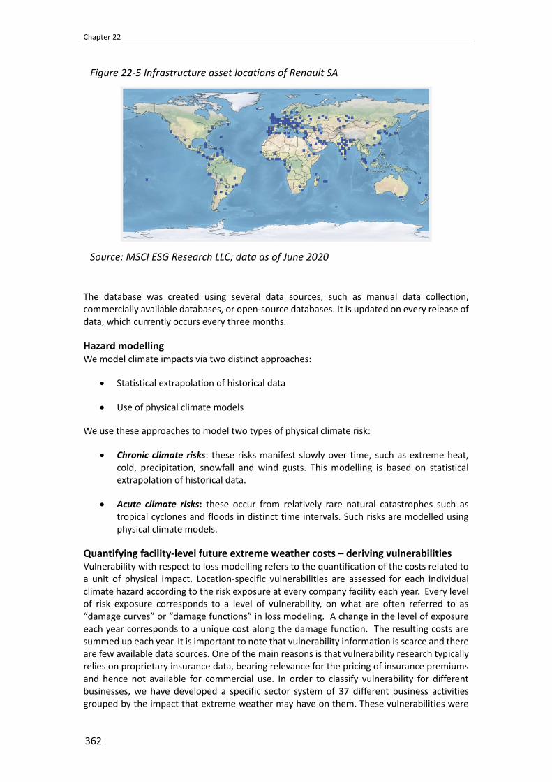
Chapter 22
362
Figure 22-5 Infrastructure asset locations of Renault SA
Source: MSCI ESG Research LLC; data as of June 2020
The database was created using several data sources, such as manual data collection, commercially available databases, or open-source databases. It is updated on every release of data, which currently occurs every three months.
Hazard modelling We model climate impacts via two distinct approaches:
• Statistical extrapolation of historical data
• Use of physical climate models
We use these approaches to model two types of physical climate risk:
• Chronic climate risks: these risks manifest slowly over time, such as extreme heat, cold, precipitation, snowfall and wind gusts. This modelling is based on statistical extrapolation of historical data.
• Acute climate risks: these occur from relatively rare natural catastrophes such as tropical cyclones and floods in distinct time intervals. Such risks are modelled using physical climate models.
Quantifying facility-level future extreme weather costs – deriving vulnerabilities Vulnerability with respect to loss modelling refers to the quantification of the costs related to a unit of physical impact. Location-specific vulnerabilities are assessed for each individual climate hazard according to the risk exposure at every company facility each year. Every level of risk exposure corresponds to a level of vulnerability, on what are often referred to as “damage curves” or “damage functions” in loss modeling. A change in the level of exposure each year corresponds to a unique cost along the damage function. The resulting costs are summed up each year. It is important to note that vulnerability information is scarce and there are few available data sources. One of the main reasons is that vulnerability research typically relies on proprietary insurance data, bearing relevance for the pricing of insurance premiums and hence not available for commercial use. In order to classify vulnerability for different businesses, we have developed a specific sector system of 37 different business activities grouped by the impact that extreme weather may have on them. These vulnerabilities were

MSCI Climate Value-at-Risk
363
derived from scientific publications and augmented by media reports for each hazard and extreme weather.
Quantifying company- and security-level valuation impacts Finally, the last step is again very similar to the last step for transition Climate Value-at-Risk metrics, i.e., the forward-looking timeseries of extreme weather costs are discounted and fed into a capital structure model in order to calculate the Physical Risks and Opportunities Climate Value-at-Risk metrics.
4 Case study: Managing climate risks in investment portfolios
Introduction In this case study, we selected a sample portfolio representative of a global actively-managed fund in terms of risk-return characteristics and used the MSCI Climate Value-at-Risk (“Climate VaR”) model to examine the different dimensions of climate-related risks. We show how Climate VaR can be used to measure climate risks for the portfolio as a whole, as well as further explore which sectors, countries and securities were driving these risks in the portfolio.
We also considered some approaches which a portfolio manager might follow in order to manage these risks. Specifically, we tested four simple exclusion strategies based on the worst-performing decile of the portfolio on the following measures:
• Aggregated Climate VaR
• Transition Risks and Opportunities Climate VaR
• Physical Risks and Opportunities Climate VaR
• Carbon intensity
For each exclusion strategy, we investigated the impact on climate risks as well as on the risk and return characteristics of the sample portfolio, including sector, country and style exposures. We show that while these exclusion strategies had substantial impacts on the measures of climate risks for the sample portfolio, they had minimal impact on the sample portfolio’s conventional risk, return and market exposures. We conclude that, in the case of the sample portfolio chosen, it was possible to substantially reduce the portfolio’s climate risk exposures without significantly altering the portfolio’s conventional risk and return characteristics or its market exposures, such as to sectors, countries and styles.
Portfolio climate risk assessment Sample portfolio We selected a sample portfolio from the Lipper database of mutual funds focusing on the peer group of global developed market funds.17 The goal of the selection process was to have a “typical” fund in the sense that it has a 5-year active performance relative to the fund’s own benchmark which is close to the median fund active performance in that peer group. We also aimed for a fund that has more than 50 holdings to reduce concentration. The “typical” fund
17 We started with all global funds available in the Lipper database and selected all the funds that have at least 75% invested
in equity and filtered out funds with assets under management below US$1mm or above US$500bln. We also filtered out
funds with larger than 15% exposure to emerging markets and then excluded 5% of funds with largest and smallest tracking
error and funds with reference to index tracking in their name.

Chapter 22
364
selected was representative of a global actively-managed fund in terms of risk-return characteristics: its 5-year return (10.71%) and volatility (12.76%) were in line with the median of global actively-managed funds in the database, as of December 2019.
Figure 22-6 shows the country and Global Industry Classification Standard (GICS®) Industry Group18 breakdowns of the sample portfolio.
Figure 22-6 Sample portfolio country and GICS Industry Group breakdowns
Source: MSCI ESG Research LLC
Portfolio-level Climate VaR Figure 22-7 displays a Climate VaR report snapshot for the sample portfolio.
Figure 22-7 Climate VaR portfolio report snapshot
Source: MSCI ESG Research LLC
18 GICS is a global industry classification standard jointly developed by MSCI and Standard & Poor’s.

MSCI Climate Value-at-Risk
365
The Aggregated Climate VaR is -7.75%, resulting in a US$7.75m monetary risk contribution for a US$100m investment.19 This means that, under the scenarios considered, climate risk and opportunities were estimated to represent a downside valuation impact of 7.75% of the portfolio.
This risk can be further broken between Transition Risks and Opportunities and Physical Risks and Opportunities:
• Under the 2°C scenario considered, Transition Risks and Opportunities amounted to a downside valuation impact of -0.59%. This number is in fact comprised of two effects: -4.43% downside coming from Policy Risks, and +3.84% upside stemming from Technology Opportunities.
• On Physical Risks and Opportunities, the overall risk of -7.16% was largely driven by Coastal Flooding (-6.15%) and Extreme Heat (-1.44%). We also observe that some of the Physical Risks and Opportunities Climate VaRs were positive – i.e., representing an upside. This was the case for Extreme Cold (+0.22%) and in this case stems from the fact that, in the scenario considered, in many locations around the globe the number of days with temperatures reaching below 0°C are likely to decrease, resulting in fewer business interruptions.
For a more robust climate risk assessment, it is useful to look beyond the portfolio risk measures and into what drives them – be it at the level of sectors, countries or individual securities.
Sectors The three GICS Industry Groups in the sample portfolio with the highest Transition Risks are Real Estate, Materials and Food & Staples Retailing (Figure 22-8) – activities with substantial carbon footprints and, in the case of the companies in this portfolio, also operating in jurisdictions with substantial regulatory oversight (we also note that the risk in the Real Estate GICS Industry Group was somewhat inflated by the fact that one company classified in this group owns an airline).
Looking at Transition Opportunities, we found that the upside of the low-carbon transition came from the stocks in the sample portfolio in Technology Hardware & Equipment and Capital Goods – activities with comparatively lower direct GHG-emissions or with a focus on developing new technologies.
19 This case study is based on a hypothetical USD 100 million investment. The monetary contribution is calculated as the
product of the Climate VaR contribution and the portfolio value.

Chapter 22
366
Figure 22-8 Climate VaR by GICS Industry Group – Transition Risks and Opportunities
Source: MSCI ESG Research LLC
Turning to Physical Risks and Opportunities (Figure 22-9), the three highest risk sectors were Real Estate, Materials, and Consumer Durables & Apparel. This mostly reflected the location of the facilities of the companies classified in these sectors as well as how their facilities were subject to different hazards. In the case of the companies in this portfolio, coastal flooding and extreme heat were the main drivers of the physical risks.

MSCI Climate Value-at-Risk
367
Figure 22-9 Climate VaR by GICS Industry Group – Physical Risks and Opportunities
Source: MSCI ESG Research LLC
Countries We then investigated the countries showing the highest level of climate risks in the sample portfolio. For this analysis, the Climate VaR model looks through to a company’s activities, identifying the different countries in which companies operate. Doing so is necessary, as transition and physical risks (e.g. climate policy, extreme weather events) are likely to have local impacts on companies’ international operations.
The country with the highest downside in Transition Risks and Opportunities was Canada (Figure 22-10), accounting for over a third of the sample portfolio’s Policy Risks (-1.49% out of -4.43%). The United States and China were also among the highest contributors to Policy Risks, an intuitive result given the large portfolio weights the two countries represent (70% and 11%, respectively) and the importance of those markets in the global economy, meaning that many companies incorporated elsewhere also tend to have operations there.

Chapter 22
368
Figure 22-10 Countries representing the most Policy Risks
Source: MSCI ESG Research LLC
China and the United States also contributed substantially to the portfolio’s Physical Risks and Opportunities (Figure 22-11), with the two countries representing by far the largest contributions. They were followed by the Netherlands, Japan, and India.
Figure 22-11 Countries representing the most Physical Risks
Source: MSCI ESG Research LLC
Portfolio climate risk management Having used Climate VaR to review the climate risks of the sample portfolio, we then considered the approaches which a portfolio manager might follow to manage these risks and we investigated the impact that such approaches would have on the risk and return characteristics of the sample portfolio.
One approach to managing climate risks is to exclude the portfolio constituents that contribute the most to the risks. In this section, we adopted this approach and, starting with the holdings of the sample portfolio, excluded the “worst” decile (8 stocks) of the sample portfolio. We performed this exercise four times, each time excluding the “worst” decile on the following criteria:20
20 For Climate VaR, the “worst” performers were those with the lowest Climate VaR (which in many cases means the most

MSCI Climate Value-at-Risk
369
• Aggregated Climate VaR
• Transition Risks and Opportunities Climate VaR
• Physical Risks and Opportunities Climate VaR
• Carbon intensity
Doing so, we obtained four new portfolios (A through D), which we could compare with the original sample portfolio (“Original”).
Impacts on climate risks Figure 22-12 displays the impact that the four exclusion strategies had on climate risks.
Figure 22-12 Climate risk impacts of the different exclusion strategies
Source: MSCI ESG Research LLC
All exclusions tended to improved Climate VaR and reduce the portfolio’s carbon intensity, albeit to varying degrees: exclusion strategies A through C improved Climate VaR the most, and exclusion strategy D reduced the carbon intensity the most. This is, of course, by design – but it is worth noting that the reductions achieved by the exclusions were substantial: strategy A reduced the Aggregated Climate VaR by 74% (from -7.75% to -2.04%); strategy B changed the sign of Transition Risks and Opportunities Climate VaR (from -0.59% to +2.03%); strategy C reduced the Physical Risks and Opportunities Climate VaR by 65% (from -7.16% to -2.48%); and strategy D reduced the Weighted Average Carbon Intensity (“WACI”) of Scopes 1 and 2 (“S12”) by 89% (from 185.87 to 20.67 tCO2e/US$m sales).
The four strategies had different impacts:
• Strategy A improved not just the Aggregated Climate VaR but also both the sub-components of Climate VaR and the carbon intensity;
• On the other hand, excluding on the basis of a single component of Climate VaR seemed to exacerbate the other component of Climate VaR in this sample portfolio: strategy B improved Transition Risks and Opportunities Climate VaR, but did not have much impact on the Physical Risks and Opportunities Climate VaR, (a small improvement from -7.16% to -6.34%). The opposite was true for strategy C;
• In strategy D, exclusions on the basis of carbon intensity not only reduced the WACI but also improved the Transition Risks and Opportunities Climate VaR. This result is intuitive, considering that the transition is likely to compel companies to reduce their
negative Climate VaR). For carbon intensity “worst” performers were those with the highest carbon intensity. carbon
intensity was defined in this analysis as the amount of Scope 1 and 2 GHG-emissions, in tons of CO2 equivalent (tCO2e)
per US$ of sales.

Chapter 22
370
carbon emissions – hence, companies with higher carbon intensities would, on average, face more transition risks. For the same reason we can also see that strategies A and B, which substantially improved the Transition Risks and Opportunities Climate VaR, also substantially reduced the carbon intensity. However, these results also highlight that carbon intensity and transition risks are not one and the same, as the exclusions in strategies A, B and D were not identical; for example, Northland Power Inc. was excluded in strategy D on account of its carbon intensity (1,294 tCO2e/US$m sales), but it was not excluded from strategy A or B because it had a relatively small Transition Risks and Opportunities Climate VaR, thanks to having 59.1% of its total revenue generated in alternative energy.
Impacts on traditional risk / return profile The above analysis showed that it was possible to reduce the climate risks in the sample portfolio, as measured by four different criteria. Of course, this is only one part of the story, as a portfolio manager would also want to know the impact each exclusion approach might have on the sample portfolio’s risk/return characteristics.
We investigated this question and show the results in Figure 22-13, which compared the 5-year simulated performance of the five strategies. 21 Interestingly, although exclusion strategies A through D substantially improved the various measures of climate risks, the traditional risk/return characteristics of the five strategies remained largely similar to the original strategy: all strategies had 5-year simulated returns in the mid to high 10% range (compared to 10.71% in the original strategy), and volatilities in the mid 12% range (compared to 12.76% in the original strategy). All exclusion strategies showed tracking errors to the original strategy of approximately 1%.
Figure 22-13 Risk/return impacts of the different exclusion strategies
Source: MSCI ESG Research LLC
We also investigated the impact that these exclusions had on the sector, country, style and other exposures of the strategy using MSCI’s Global Total Equity Market Factor model. The high-level contributions from the factor groups are shown in Figure 22-14. In general, the factor profile of the original strategy was only slightly modified by the exclusion strategies. Industry factors and stock-specific returns tended to have a higher impact than styles,
21 We use a 5-year simulation period based on the availability of historical data.
This report may contain analysis of historical data, which may include hypothetical, backtested or simulated performance
results. There are frequently material differences between backtested or simulated performance results and actual results
subsequently achieved by any investment strategy.
The analysis and observations in this report are limited solely to the period of the relevant historical data, backtest or
simulation. Past performance — whether actual, backtested or simulated — is no indication or guarantee of future
performance. None of the information or analysis herein is intended to constitute investment advice or a recommendation
to make (or refrain from making) any kind of investment decision or asset allocation and should not be relied on as such.

MSCI Climate Value-at-Risk
371
countries and currencies, but overall the contributions of all five sources of return remained very small when compared to the overall simulated returns of these strategies.
Figure 22-14 High-level contributions from factor groups
Source: MSCI ESG Research LLC
5 Conclusion and outlook
Globally there is an increased drive to encourage the widespread adoption of climate scenario analysis among companies and financial institutions. Most leading climate change frameworks – TCFD, HLEG, TEG, etc. – base their recommendations and policy advice on a range of accepted scenarios developed by climate change scientists. Scenarios provide a forward-looking assessment of climate change risks, giving insights into the order of magnitude for which assets and investments are threatened and how their return prospects are affected. Crucially, they also indicate which assets and investments might stand to profit from a low-carbon transition – insights that can be leveraged into both building up portfolio-level resilience vis-à-vis climate change and signaling to the wider community that climate change risks are actively managed. In analyzing the risks and the costs of climate change in a proactive and forward-looking way, the management of companies can mitigate and avoid a plethora of possible threats ranging from class-action lawsuits, significant remediation costs, and irreversible damages to the reputations of corporations and their executives.
The merits of scenarios are that they provide organizations with a method of forward-looking assessment to understand the strategic implications of climate-related risks, while at the same time informing investors, lenders, insurance providers and other stakeholders of how a particular organization might perform under different transition and physical risk pathways. Hence, scenario analysis provides an invaluable lens through which to assess a company’s targets, strategy and governance of sustainability issues and take a view on whether they are fit for purpose in a changing world.
For all its benefits, scenario analysis also has certain drawbacks, the most obvious being that it is inherently unclear which scenario will eventually occur. Also, most climate reference targets delivered by scenario analysis come in the form of optimal energy mixes, a format ill-suited for conducting company- or asset-level analysis, complicating the integration into portfolio-construction procedures which focus on individual holdings.
To compute the Climate VaR metric, we evaluate data underpinning a particular climate scenario and then quantifies the potential future cost for the scenario and company in question. A calculation is then made to understand by how much a company’s financial valuation is poised to decrease or increase in the face of those climate related costs. To achieve this, the methodology relies on a discounted cash flow model that calculates the present-day value of future climate-related cost. By basing the financial impact calculation on traditional valuation techniques used in the financial industry, we attempt to bridge the disparate fields

Chapter 22
372
of academic climate science and the day-to-day tools used by financial practitioners to create resonance with the finance industry. As a result of this process, climate risks become embedded into an output in a format that can be processed and integrated into further financial analysis, so that climate risks can become a part of the fundamental analysis.
We have seen numerous applications of Climate VaR in investment management practices. Most often, investors use Climate VaR for:
• Engagement;
• Investment decision-making;
• Risk analysis;
• Monitoring & compliance;
• TCFD reporting.
A portfolio’s Climate VaR can vary greatly depending on the detailed holdings contained therein. Investors need to understand security and portfolio level climate risks in order to start incorporating these risks into their investment practices. This is a first step for portfolios, companies, assets, governments, benchmarks, etc., to become resilient to the impacts that climate change may cause. Understanding, quantifying and managing these risks should become normal practices in financial management in years to come. Climate VaR is one of the new and innovative metrics that investors can use to help them establish the climate change resilience needed within investment portfolios.
While Climate VaR is quickly becoming a recognized metric for assessing climate risks within and across portfolios, it is also time to take important steps forward to deliver deeper and more wide-ranging assessments of climate risks. For example, the Climate VaR methodologies outlined above can currently be used to assess direct impacts from climate change, but new methodologies are being explored to include indirect impacts as well. Climate VaR is also currently applied to equities and corporate bonds, but soon will be offered for additional asset classes, such as private equity and loans. This will allow for users to cover a larger portion of their portfolio(s) with Climate VaR analysis and also evaluate additional forms of risk via the assessment approach. We believe the use of Climate VaR will expand as climate risk analysis becomes more embedded within general risk management and reporting practices.

Aviva’s Analysis of Climate Value at Risk for Asset Owner and Managers
373
Aviva’s Analysis of Climate Value at Risk for Asset Owner and Managers
By
Aviva1
Abstract
Aviva’s Climate Value at Risk measure enables the potential business impacts of climate-related risks and opportunities to be assessed taking into consideration different scenarios and assumptions regarding policies, technologies, demand, and various other macroeconomic factors, as well as extreme weather. This measure looks at the evolution of climate-related risks and opportunities over the next 15 years, but with the ability to consider shorter time periods (3 to 5 years) where appropriate. Aviva was awarded the Climate Risk Initiative of the Year 2020 by InsuranceERM, because the “Climate value-at-risk (VaR) initiative shows the practical benefits that can be achieved when insurers focus resources, time and expertise on climate risk management, as well as collaborating with other knowledge partners”.2
Keywords: Climate Value at Risk, climate-related risks and opportunities, transition risks, physical risks, climate risk management
1 Introduction
Aviva included the results of scenario analysis in its 2018 and 2019 Climate-related Financial Disclosures. The scenario analysis is based on the Climate Value at Risk or “Climate VaR” measure3 we have developed in conjunction with the United Nations Environment Programme Finance Initiative (UNEP FI) Investor pilot and Carbon Delta, an environmental FinTech (See UNEP FI Changing Course report for further details).4 This scenario analysis provides a forward-looking view of climate-related transition and physical risks and opportunities. Transition risks and opportunities include the projected costs of policy action related to limiting greenhouse gas emissions as well as projected profits from green revenues arising from developing new technologies and patents. Physical risks cover the financial impact of acute weather events as well as chronic impacts.
Aviva has extended this Climate VaR approach with Elseware, a risk management and quantification expert consultancy, to enable it to be applied to its whole balance sheet. In order to support this initiative, an inter-disciplinary team has been created with representation from across the business and an expert panel has been set-up to review and
1 This chapter is written by Ben Carr, RCAM Director at Aviva, email: [email protected]. The authors would like to thank
Finn Clawon, Loubna Benkirane, Tom Tayler and Paddy Arber. 2 https://www.insuranceerm.com/content/galleries/insuranceerm-annual-awards-2020-uk-and-europe-
winners/climate-risk-initiative-of-the-year-aviva.html 3 For further details on Aviva’s Climate VaR methodology, please see Aviva’s Climate-related Financial Disclosure at
http://www.aviva.com/TCFD 4 https://www.unepfi.org/publications/investment-publications/changing-course-a-comprehensive-investor-guide-to-
scenario-based-methods-for-climate-risk-assessment-in-response-to-the-tcfd/

Chapter 23
374
challenge the main assumptions made in the selection, development and modelling of the scenarios. The panel includes internal experts as well as external experts5.
Aviva’s use of the Climate VaR approach described in this case study demonstrates the value of innovation and scenario analysis in climate risk modelling. It also shows the importance of collaboration and sharing of best practice with peers. Outputs and evaluations of this methodology are intended as a first step in incorporating the TCFD recommendations on scenario-based risk assessment in financial disclosures. We will continue to work internally and with external partners to develop best practice in this area.
2 Methodology description – Climate VaR modelling approach
Aviva developed a Climate VaR measure that enables the potential business impacts of future climate-related risks and opportunities to be assessed in each of the Intergovernmental Panel on Climate Change (IPCC) scenarios and in aggregate.
Climate scenarios considered The IPCC scenarios aim to measure the effect on the energy balance of the global climate system due to changes in the composition of the atmosphere from sources like greenhouse gas emissions, other air pollutants (Vallero, 2014) and changes in land use. The four IPCC scenarios represent different Representative Concentration Pathways (RCPs) which describe the composition of the atmosphere at the end of the 21st century. Table 23-1 summarises the link between the RCPs, potential temperature rises by 2100 and the level of mitigation required, which we will use to describe the scenarios in this chapter.
Table 23-1 Mapping for RCPs, potential temperature rises and levels of mitigations
RCP Temperature rise Description
RCP2.6 1.5°C Aggressive mitigation
RCP4.5 2°C Strong mitigation
RCP6.0 3°C Some mitigation
RCP8.5 4°C Business as usual (BAU)
Source: TCFD
The TCFD graphic “The choice we face now” (see case study below) sets out implications for greenhouse gas emissions and potential temperature rise by 2100 for each scenario. The aggressive mitigation scenario is the only one where it is more likely than not that the temperature change in 2100 will be less than 2°C. Aviva developed this Climate VaR measure in conjunction with the UNEP FI investor pilot project, which developed models and scenario analysis tools to assess the potential impact on corporate assets and real estate of the four IPCC scenarios in conjunction with MSCI (Carbon Delta).
MSCI (Carbon Delta) is using the AIM/CGE model6 from the Japanese National Institute for Environmental Studies (NIES).7 Whilst these scenarios reflect current scientific research and
5 Dr Simon Dietz, Dr Nick Robins & Dr Swenja Surminski from the Grantham Research Institute on Climate Change and the
Environment at the London School of Economics, Dr Paul Pritchard – an independent sustainability advisor – and Dr
Katharina Dittrich from Warwick Business School. 6 The AIM/CGE model is a multi-regional, multi-sectoral, computable general equilibrium (CGE) model. 7 NIES is a Japanese research institute that undertakes a broad range of environmental research in an interdisciplinary and
comprehensive manner.

Aviva’s Analysis of Climate Value at Risk for Asset Owner and Managers
375
the Paris agreement, there clearly remains significant uncertainty regarding future climate trajectories as well as political risk with respect to implementation of the Paris agreement and Nationally Determined Contributions (NDCs).8 It is important to note that the four scenarios all assume a gradual path, in which temperatures slowly rise but climate policy is ramped up at varying speeds with a fairly high degree of global coordination. They do not consider the transition risk in a more chaotic policy environment, where there is lack of global coordination and policy action is taken too late and too suddenly. This may result in an understatement of transition risk. The MSCI (Carbon Delta) model and scenario analysis tools also allow consideration of the five Shared Socioeconomic Pathways (SSPs). These consider socio-economic characteristics including things such as population, economic growth, education, urbanisation and the rate of technological development. Within SSPs, scenarios can also be selected that represent early policy action or late policy action. The timing of climate action can represent orderly and disorderly transition pathways.
Time horizon considered for each scenario In conjunction with the UNEP FI investor pilot project, it was agreed to use a single 15-year time horizon for the Climate VaR measure to analyse the impact of the different scenarios on our business but with the capability to consider transition effects over shorter time horizons depending on the business decision being considered. Consideration was given as to whether a longer time horizon was needed to capture the worst physical impacts of climate change, as these are not likely to manifest themselves until the second half of the century (Figure 23-1). To address this point in a decision-useful way and ensure consistency with the 15-year time horizon for transition risk, it was agreed to look at a higher, 95th percentile of physical risks as well as the expected outcome in the BAU scenario over the 15-year horizon. Figure 23-2 shows large dispersion around the mean from the impact of climate change on coastal flooding over the next 15 years.
Figure 23-1 Global average surface temperature change
Source: IPCC
8 Intended NDCs is a term used under the UN Framework Convention on Climate Change for reductions in greenhouse
gas emissions that all countries that signed the UNFCCC were asked to publish in the lead-up to COP21.

Chapter 23
376
Figure 23-2 Example of coastal flooding
Source: MSCI (Carbon Delta)
Risks and opportunities covered The modelling of transition and physical risks and opportunities specifically covers the projected costs of policy action related to limiting greenhouse gas emissions as well as projected profits from green revenues arising from developing new technologies and patents. In addition, it captures acute weather impacts such as coastal flooding and tropical cyclones as well as chronic impacts from gradual changes in extreme heat and cold, heavy precipitation and snowfall, or wind gusts. Regional sea level rise is an important input to the risk model and constitutes a key driver of coastal flooding impacts. It is important to note that the changes in acute and chronic impacts can also have a positive as well as negative effect on individual companies or instruments (Figure 23-3).
Figure 23-3 Risks and opportunities covered
Source: MSCI (Carbon Delta)
Building Block Approach To assess these risks and opportunities, a building block approach has been adopted (Figure 23-4).

Aviva’s Analysis of Climate Value at Risk for Asset Owner and Managers
377
Figure 23-4 Building Block Approach
Source: MSCI (Carbon Delta)
When assessing the impact of climate-related risks and opportunities associated with each scenario, different financial indicators need to be used and assumptions made. To assess the impact on market value of investments and the impact on reserves or premiums, for example, the following assumptions need to be considered:
1. The extent to which asset valuations, reserves and premiums already take account of the climate-related risks and opportunities in each scenario;
2. The likely timing of future changes to asset valuations, where not all these climate-related risks and opportunities are currently considered;
3. Changes in our asset portfolio over time and the timing of such changes relative to the timing of any future market corrections to take account of these climate-related risks and opportunities;
4. The extent to which changes in costs over the next 15 years will be passed on to policyholders and/or sales volumes could reduce or increase for specific lines of business; and
5. The impact on reinsurance market capacity and pricing, as well as the creditworthiness of reinsurers, and the implications for our reinsurance strategy.
Finally, to assess the overall impact of climate-related risks and opportunities across all scenarios, the relative likelihoods or probabilities of each scenario need to be assigned. To do this Aviva considered amongst other things the current scientific analysis of the likely trajectory of emissions as well as policy commitments made by countries to reduce emissions (Figure 23-5).
Figure 23-5 Most Likely outcome based on where we are
Source: Aviva

Chapter 23
378
Transition risks and opportunities The financial impact of transition risks and opportunities are calculated relative to the BAU scenario (i.e., there are assumed to be no transition costs or opportunities in the BAU scenario, where current emissions are presumed to continue to rise at the current rate). The calculation covers both emission reduction prices and revenues from new technologies.
Figure 23-6 Emission Reduction Prices (2010 US$/tCO2e)
Source: MSCI (Carbon Delta)
2.5.1 Investments The following high-level methodology is used to assess the potential downside risk from different transition scenarios on our investments (Figure 23-7). For both corporate bonds and equity securities the difference between the market value and the adjusted value after factoring in future climate change costs and/or revenues is measured (i.e., the impact relative to current climate conditions and emissions trajectory). To estimate the impact in a consistent way when a company has issued both shares and bonds, the Merton model is used.9 This model enables the impact on a business as a whole to be translated into a change in value of its corporate bonds and equity securities. As both costs and opportunities are covered, the Climate VaR can be either negative or positive depending on the balance of future anticipated carbon-related costs and revenues for individual companies or instruments.
9 Analysts and investors utilise the Merton model to understand how capable a company is at meeting financial obligations,
servicing its debt, and weighing the general possibility that it will go into credit default.

Aviva’s Analysis of Climate Value at Risk for Asset Owner and Managers
379
Figure 23-7 High level methodology overview
Source: MSCI (Carbon Delta)
Carbon Delta has also developed a methodology for estimating the transition exposure of property assets which we have used for both direct real estate and real-estate-linked debt holdings. For infrastructure assets, Aviva plans to use the ClimateWise Transition Risk Framework to identify the key risk exposures across our portfolio of assets, taking into account how transition risk and opportunities vary by geography, sector and sub-sector to assess the potential impact in different climate scenarios. For example, a recent review of transport infrastructure highlighted strong potential opportunities.
2.5.2 Insurance liabilities Aviva has assessed the impact on life insurance reserves from the potential reduction in mortality rates resulting from less air pollution in the aggressive and strong mitigation scenarios. This reflects an anticipated reduction in carbon emissions and an increase in electric vehicles replacing vehicles with internal combustion engines. For each transition scenario, there is potential for fewer deaths relating to air pollution, although we note that this is very much dependent on the fuel mix generating electrical power for the grid. Whilst waste-to-energy plants have similar particulate outputs to gas-fired power stations, biomass plants such as wood pellet fired facilities, for their many positives, produce significantly more particulates than gas-fired power stations for example (Hajat et al., 2014).
On the general insurance side, transition risks and opportunities may also arise. For example, the wider adoption of electric vehicles and the rise of car-sharing and automated cars might decrease the pool of vehicles to be insured leading to a decrease in claims frequencies but also premiums. However, these affects have not been included to date. We plan to extend our modelling to cover general insurance transition risks and opportunities over time.
Physical risks and opportunities The financial impact of physical risks and opportunities is based on an assessment of both the expected costs in the BAU scenario and the costs at a higher 95th percentile arising from hazards such as: extreme heat and cold, heavy precipitation and snow, coastal flooding, wind gusts and tropical cyclones. We use the expected costs and the costs at a higher percentile to define a distribution of physical risk outcomes for each scenario and thus capture some of the more extreme potential physical effects of climate change whilst using a consistent 15-year time horizon as that used for transition risk.

Chapter 23
380
2.6.1 Investments The physical risks on investments are generally going to be driven by the exposure of the facilities (buildings, plant, infrastructure) owned or used by the company who has issued the financial instrument, their “facilities”, and the supply chain they rely on for producing their end product. We use the following high-level methodology to assess the potential physical risk from different scenarios on our investments in this regard. The cost in Figure 23-8 is built up by mapping the facilities onto a world map, with measures that define the facility’s exposure to different extreme weather hazards, and then combining this with a vulnerability function that converts the exposure and an assessment of the physical hazard impact in each scenario into an estimated monetary cost, per facility.
Figure 23-8 Impact modelling and expected cost estimate
Source: MSCI (Carbon Delta)
For both corporate bonds and equity shares, the difference between the market value and the adjusted value after factoring in aggregated facility costs and/or revenues is measured. The costs and/or revenues to a business are measured relative to an assessment of physical risks under current conditions as these are assumed to be already factored into the market value. This business impact is then translated into a change in the value of its corporate bonds and equity securities using the Merton model.
Aviva recognises that the current approach does not capture the impact on companies’ supply chains nor necessarily demand for its products and services or potential mitigating impact of insurance. For example, in the case of a major car manufacturer their real assets will mainly include their factories and machinery and possibly their dealerships. Their supply chain will be broad, complex and potentially geographically diverse and if disrupted it could adversely impact companies’ costs and/or revenues. We will continue to work internally and with external partners to develop best practice in this area. For directly held real estate assets, real estate loans and infrastructure assets, we use the same approach described above. For directly held real estate the impact is carried directly against the property valuation. For real estate loans, we assess the physical climate change risk impact by running the stressed property value through our debt valuation models.
For sovereign bonds, the impact on the market value of a security is measured by assessing how a sovereign’s rating could change as a result of the occurrence of different extreme weather hazards in each scenario. The following climate-related factors may impact sovereign debt: exposure and vulnerability to climate change; readiness and adaptation; ability to raise money for mitigation and post-disaster repair; ability to raise money via taxation and debt;

Aviva’s Analysis of Climate Value at Risk for Asset Owner and Managers
381
reliance on foreign aid and support of the International Monetary Fund and other supra-national bodies. To assess a sovereign’s vulnerability to climate change and readiness, the Notre-Dame University’s Notre Dame-Global Adaptation Index (ND-GAIN) measure for country climate change risk has been used. We note that the assessment of sovereign debt is difficult because sovereigns are exposed to climate change via several vectors: government buildings and government owned infrastructure, cost of emergency relief to areas effected by climate-related disasters, aid and rebuilding costs and the cost of acting as insurer of last resort. So, the ND-GAIN data has been used to help support expert judgements about the appropriate stresses to apply to different sovereign bonds in our modelling at this stage. We will continue to work internally and with external partners to develop best practice in this area.
2.6.2 Insurance liabilities The Climate VaR for life insurance risks calculates the impact on reserves of a change in mortality rates as a result of the occurrence of different extreme weather hazards in each scenario based on a review of academic literature linking climate change to potential changes in mortality rates (Gasparrini et al., 2017). For higher temperature scenarios, where climate change has dramatically taken hold, the picture is complicated. For example, it is possible that both summers and winters will be warmer or that seasons will in fact be more extreme. The latter is more likely to have an adverse impact and for the UK could plausibly result from the Gulf Stream changing its path and missing the UK.
On the general insurance side, the Climate VaR calculates the impact on premiums as a result of the occurrence of different extreme weather hazards in each scenario. The impact on premiums is then used to determine the impact on our business, considering the impact on pricing, sales volumes and our reinsurance strategy. During 2019 we have extended the scope of physical risks covered to different regions (UK, Canada and France) and various perils (flood, freeze, subsidence, wildfire, winter storm, hail and severe convective storm) noting that the precise list of perils is region dependent. We have worked with internal and external experts to consider how climate change could change the frequency and severity of UK Flood and leveraged our existing catastrophe modelling capability to assess the impact of this on premiums.
Aggregation of climate-related risks and opportunities In conjunction with Elseware, a risk management and quantification expert consultancy, we have used a Bayesian Network10 methodology to aggregate all the component parts of our exposure to derive an aggregate view of the impact of climate-related risks and opportunities. The attraction of this approach is that we can combine a set of beliefs, expert judgements, internal data and external data to assess the potential impact of these risks, on an aggregated basis. We can then determine an overall Climate VaR for each scenario (Figure 23-9).
The impact distributions of each climate scenario are then combined to give a fully aggregated result across all four scenarios. This final step of aggregation uses the assigned likelihood given to each scenario taking into consideration amongst other things the current scientific analysis of the likely trajectory of emissions as well as policy commitments made by countries to reduce emissions (Figure 23-10).
10 A Bayesian Network is a probabilistic graphical model that represents a set of variables and their conditional
dependencies via a directed acyclic graph.

Chapter 23
382
Figure 23-9 Aviva’s aggregation process for each scenario
Source: Aviva
Figure 23-10 Overall assessed climate change impact
Source: Aviva
3 Case study
Data inputs Data inputs for the Climate VaR can be broadly split into data to derive exposure and data to support assessing the impact of climate change. The model takes a holistic view of Aviva’s balance sheet and as such requires internal exposures for our assets and liabilities. Asset and liability data have been sourced from regulatory reporting systems (or the systems that feed into those). For assets the exposure is based on shareholder exposure (rather than

Aviva’s Analysis of Climate Value at Risk for Asset Owner and Managers
383
policyholder exposure), for life insurance exposure is based on reserves and for general insurance exposure is based on premiums.
For assets (equity, credit and property) the physical and transitional impact of the different climate scenarios are provided by MSCI (Carbon Delta). This model incorporates various datasets (some of which we have discussed above) including but not limited to output from an Integrated Assessment Model. For sovereign bond exposures a key input is the ND-GAIN, which measures a countries potential vulnerability to climate change and readiness to adapt. The impact for both life and general insurance has been driven by expert judgement based on input from internal and external experts.
Scenario analysis The Climate VaR measure allows four potential future scenarios with respect to climate change developed by the IPCC to be analysed (Figure 23-11)(IPCC, 2013). Each scenario describes a potential trajectory for future levels of greenhouse gases and other air pollutants and can be mapped to potential temperature rises and levels of mitigation required: 1.5°C (aggressive mitigation), 2°C (strong mitigation), 3°C (some mitigation) and 4°C (Business as usual). It is important to note that the four scenarios all assume a gradual path, in which temperatures rise slowly but climate policy is ramped up at varying speeds with a fairly high degree of global coordination. They do not consider the transition risk in a more chaotic policy environment, where there is lack of global coordination and policy action is taken too late and too suddenly. This may result in an understatement of climate-related risks.
Figure 23-11 The choice we face now
Source: TCFD
The initial results from Aviva’s Climate VaR analysis compare a plausible range of outcomes (5th to 95th Percentile) from the different scenarios considered. Aviva is most exposed to the business-as-usual 4°C scenario where physical risk dominates, negatively impacting long-term investment returns on equities, corporate bonds, real estate, real estate loans and sovereign

Chapter 23
384
exposures. The aggressive mitigation 1.5°C and 2°C scenarios are the only scenarios with potential upside. Physical risk impacts are more limited but there is still downside risk on long-term investment returns from carbon intensive sectors (for example utilities) as a result of transition policy actions. This is offset partially by revenues on new technologies from some sectors (for example automotive).
Figure 23-12 Aviva’s Climate VaR output by scenario for shareholder funds as at 30/11/2019
Source: Aviva
Note: The grey bars represent the range of outputs between the 5th percentile and the central estimate for each scenario and the orange bars represent the range between the central estimate and the 95th percentile.
When aggregated together to determine an overall impact of climate-related risks and opportunities across all scenarios, the plausible range is dominated by the results of the 3°C and 4°C scenarios, reflecting that neither existing nor planned policy actions are sufficiently ambitious to meet the 1.5°C Paris Agreement target. In the 1.5°C scenario, transition risk is larger than physical risk even after considering mitigating technology opportunities (Figure 23-3). In the 2°C scenario, transition and physical risks are somewhat balanced, whereas in the 3°C and 4°C scenarios physical risk dominates.
Figure 23-13 Physical versus transition risks by scenario for Aviva’s shareholder funds as at 30/11/2019
Source: Aviva

Aviva’s Analysis of Climate Value at Risk for Asset Owner and Managers
385
In all scenarios the impact on insurance liabilities is more limited than on investment returns. However, there is potential for some impact on life and pensions business as a result of changes in mortality rates in different scenarios either from physical effects such as more extreme hot and cold weather or transition effects related to changes in pollution levels. The impact on general insurance liabilities is relatively limited because of the short-term nature of the business and the ability to re-price annually and mitigation provided by our reinsurance programme. However, the physical effects of climate change will result in more risks and perils becoming either uninsurable or unaffordable over the longer term.
4 Limitations and outlook
Aviva will continue to develop and incorporate Climate VaR into its overall strategy, risk management and reporting frameworks. In particular, it will refine and improve the Climate VaR approach in the light of new research and data as well as emerging best practice including using output from the UNEP FI Insurance TCFD pilot. In addition, litigation risk could be explicitly modelled as could transition risk for sovereign bonds or physical risk modelling extended to cover wider factors such the supply chain, demand for products or services and access to capital. We could also consider how adaptation measures could be incorporated.

Chapter 23
386
Bibliography
Gasparrini, A., Guo, Y., Sera, F., Vicedo-Cabrera, A. M., Huber, V., Tong, S., . . . Correa, P. M. (2017). Projections of temperature-related excess mortality under climate change scenarios. The Lancet Planetary Health, 1(9), e360-e367.
Hajat, S., Vardoulakis, S., Heaviside, C., & Eggen, B. (2014). Climate change effects on human health: projections of temperature-related mortality for the UK during the 2020s, 2050s and 2080s. J Epidemiol Community Health, 68(7), 641-648.
IPCC, I. (2013). Fifth assessment report (AR5). IPCC: Geneva, Switzerland, 10-12. Vallero, D. A. (2014). Fundamentals of air pollution: Academic press.

Using Catastrophe Risk Modeling to Help Understand Physical Climate Change Risk
387
Using Catastrophe Risk Modeling to Help Understand Physical Climate Change Risk
By
Risk Management Solutions (RMS)1
Abstract
Catastrophe risk models are widely used by the insurance industry to quantify risk from climate-related events. They can also be used to quantify physical climate risk impacts beyond insurance – as companies, investors, governments, and regulators look for answers. This chapter discusses how catastrophe risk models work, what the key components are that make up a risk model, and how different organizations are using these models to assess physical climate change risk.
Keywords: catastrophe risk models, physical climate change risk
1 Introduction
The impact of physical climate change risk on our world is the source of many questions. What could be the possible extent of the exacerbated damage caused to communities around the globe in 10, 20 or 50 years’ time or more due to climate change? What will be the financial cost of the buildings and infrastructure made unusable by continual flooding? How will asset prices be affected, or for interconnected, global supply chains, what will the cost of recovery be?
For future development, we need to build to mitigate what climate change could have in store, through directly tackling carbon emissions to put us on a different path, to transition to cleaner industries for instance, or adaptation – adjusting construction methods and standards to cope with new extremes.
There is an urgent need to quantify physical climate change risk, as warning after warning comes from the scientific community about how climate change is already impacting the earth, and what the future has in store unless radical action to curb carbon emissions is taken very soon. Recent catastrophes such as Hurricane Harvey in 2017, wildfires in California during 2017-18 and the 2019-20 Australian bushfires have been attributed to some extent to climate change by climate scientists. Sea level rise, changes to sea ice formation, retreating glaciers, warming and acidifying oceans, rising temperatures and record levels of carbon dioxide and other greenhouse gases in the atmosphere, are all measurable aspects of climate change.
The speed of the change is causing concern. Central banks and regulators such as the Bank of England Prudential Regulation Authority have issued new stress tests, with consultations starting for new tests in 2021. New climate change reporting standards for businesses such as the Financial Stability Board Task Force on Climate-related Financial Disclosures (TCFD) are
1 This chapter is written by Ben Brookes, managing director – Capital and Resilience Solutions of RMS, email:
Chapter 24
388
rolling in – TCFD has more than 1,000 members – asking businesses, governments to start to quantify physical, liability and transition risks associated with climate change, and to start drawing up action plans to manage them.
The climate models themselves represent a fast-evolving science, scenarios such as the Intergovernmental Panel on Climate Change (IPCC)’s Representative Concentration Pathways (RCPs) shape trajectories of greenhouse gas emissions reflecting various actions taken by society to either reduce or even ignore climate warnings. With all this, how can the probability of different scenarios be calculated, how can the dollar value of action or inaction be assessed, and in terms of the losses incurred as a result of future climate change events, what is in store for us all?
This confluence of science, risk distribution, on-the-ground reality, and financial loss has been tackled before. Many of these questions have been grasped by catastrophe risk modeling, and physical climate change risk represents another risk to analyze and manage.
Models for measuring catastrophe loss have been developed since the late 1980s; as growing computer power helped link previously disparate areas such as scientific studies of natural hazards, historical event datasets and geographic information systems (GIS) together. Historical, actuarial-based risk modeling approaches, reliant on an empirical data set of actual events, which might only reliably go back less than 100 years, do provide a rich, vital foundation for a risk model, and a means of validation.
But these historical-based approaches were found wanting in the early 1990’s. Hurricane Andrew, a Category 5 storm that hit Florida in 1992 stood out as a turning point for more sophisticated risk modeling techniques. As we face a similar turning point with physical climate change risk, it is interesting to examine what happened to the risk community before and after Andrew, as the community learned how to better manage the risk and move forward.
Hurricane Andrew Florida had never experienced a Cat 5 strength hurricane before and for an event of this strength, the potential level of losses had been underestimated. Before Hurricane Andrew, a projected loss estimate for an event of this size was US$4 to 5 billion (1992 values). In the end the economic losses reached US$26.5 billion with insured losses of US$15.5 billion. It was the costliest natural disaster to ever hit the United States. Eight insurance companies became insolvent, and a number of insurers left the state resulting in the setting up of an involuntary insurance market (state pools).
Similar to financial institutions now, faced with quantifying the cost of physical climate change risk, the insurance industry recognized that its approach to risk modeling and management had to change. Catastrophe risk modeling companies, such as RMS which was founded in 1989, began to pioneer this new approach of probabilistic risk modeling. At their core, catastrophe models have helped insurance companies ensure they have the capital needed to pay the anticipated losses and support the fundamentals of the business. These models have helped to create a standardized “currency of risk” that allow risk data to be transferred and understood from one party to another.
As the 1990s progressed and through to the present day, risk modeling has expanded to more perils and regions, and introduced new forms of capital into the market, such as insurance-linked securities (ILS), and catastrophe bonds to assist nation states with rebuilding after a disaster. Models continue to grow in their scope and sophistication, covering “human-made” perils such as terrorism and cyber, and their usage outside of the insurance industry has grown.

Using Catastrophe Risk Modeling to Help Understand Physical Climate Change Risk
389
Catastrophe risk models have also acted as a catalyst for action. The ability to calculate the potential financial loss from perils for a country, region, through to a single structure is helping all stakeholders who plan, build or finance these assets. Through this understanding of a risk, it is possible to start to manage it – whether it is through actions such as mitigation, risk transfer, or effective capital management for those who hold an asset or a risk.
Risk models have been used to begin to assess the financial impact of climate change, such as sea level rise. Examples from RMS include studies with the OECD in 2007 looking at the risk of sea level rise to port cities around the world; in 2014, RMS partnered with the Risky Business initiative to examine the effect of sea level rise along the East Coast of the U.S., projected through to 2100. These projects and others looked to establish the economic cost of the effects of climate change. Through modification of catastrophe risk models to attempt to reflect future events influenced by climate change, it is possible to make the breakthrough and equate the costs and impacts from a micro local level to nation states, and to examine the potential of mitigation.
How do the modular components within a risk model work? Looking at the basics and the original principles of catastrophe risk modeling, models, by definition, attempt to provide a representation of complex physical phenomena and their impact on portfolios of assets, whether they are owned or insured. This probabilistic approach lies at the heart of modeling the complexity inherent in catastrophes, but the approach is complex itself. Probabilistic modeling requires simulating thousands of these representative, or stochastic, catastrophic events in time and space; compiling detailed databases of building inventories and estimating physical damage to various types of structures and their contents. The physical damage then needs to be translated to monetary loss; and, finally, totaling this for a portfolio – from a single building to millions of structures in a country as big as the U.S.
It would be impossible to include or replicate absolutely every aspect required to deliver a completely precise result. So, from the modeler’s perspective, the task is to simulate, realistically and adequately, the most important aspects of this very complex system and the associated uncertainty. Risk managers who use a model need to familiarize themselves with the underlying assumptions of the models and understand the implications and limitations of their output in order to utilize the results effectively.
Catastrophe models require substantial amounts of data for model construction and validation. Over time, the volume of data has increased dramatically, as more data sources have been introduced to give more rich, granular detail from millions of data points in a wind-field or storm surge hitting a shore through to finite descriptions of an individual structure.
Collaboration across many disciplines is required, as the reliability of a risk models depends heavily on an understanding of the underlying physical mechanisms that control the occurrence and behavior of natural hazards. While no single individual would claim to have a complete understanding of all the intricacies of these physical systems, scientists and engineers, aided by increasingly sophisticated instrumentation and computing capabilities, have accumulated vast amounts of information and knowledge in these areas. By incorporating this information, the sophisticated theoretical and empirical models currently being developed can reasonably simulate these complex phenomena.
The basic framework for modeling the impacts of natural hazards on exposures can be broken down into the following four modules (Figure 24-1):

Chapter 24
390
• Stochastic Event Module
• Hazard Module
• Vulnerability Module
• Financial Analysis Module
Figure 24-1 Main modules used with catastrophe risk models
Stochastic Event Module: Defining the Hazard Phenomena
The first stage of catastrophe modeling begins with the generation of a stochastic event set, which is a database of scenario events. Each event is defined by a specific strength or size, location or path, and probability of occurring or event rate. Thousands of possible event scenarios are simulated based on realistic parameters and historical data to probabilistically model what could happen over time.
Hazard Module: Assessing the Level of Hazard
The hazard component of catastrophe models assesses the level of physical hazard across a geographical area at risk. For hurricanes for instance, a model calculates the strength of the winds around a storm, considering the region’s terrain and built environment (Figure 24-2).
Figure 24-2 Typical framework for catastrophe modeling
Vulnerability Module: Quantifying the Physical Impact of Hazard on Properties at Risk
The vulnerability component calculates the amount of expected damage to the properties at risk. Vulnerability functions are region-specific and vary by a property’s susceptibility to damage from earthquake ground shaking or hurricane winds, for example. Parameters defining this susceptibility include a building’s construction material, its occupancy type, its year of construction, and its height.

Using Catastrophe Risk Modeling to Help Understand Physical Climate Change Risk
391
In catastrophe models, different vulnerability curves are used to estimate damage for a structure, its contents, and time element coverages such as business interruption loss or relocation expenses. Damage is quantified as a mean damage ratio, which is the ratio of the average anticipated loss to the replacement value of the building. This module also includes critical estimates of uncertainty around expected damage (i.e., standard deviations).
Together, the stochastic event, hazard and vulnerability modules comprise what is traditionally known as a probabilistic risk analysis.
Financial Module: Measuring the Monetary Loss from Various Financial Perspectives
Catastrophe loss models can be thought of as one application of probabilistic risk analysis, characterized by their refinement of the financial analysis module. This module translates physical damage into total monetary loss. For insurers, estimates of insured losses are then computed by applying policy conditions (e.g. deductibles, limits) to the total loss estimates.
Losses from a catastrophe run much deeper than just the immediate physical damage, and modeling will also examine the longer-term losses due to the need to restore both social and physical infrastructure. Power, water, sanitation, healthcare, education – through to transport, supply chains, law and order, each factor is interlinked to each other in terms of restoration after a disaster. Business interruption, common in many business insurance policies, looks to help as a business suffers a loss of trade – whether it is without power, supplies or customers. Pressure on both construction labor and materials pushes up prices and slows down recovery. These factors can be as detrimental as the initial losses.
Business interruption is calculated by estimating downtime based on the physical damage to a building itself, as well as to critical lifelines required to support use of the building (e.g. water and power) for its operational purpose. Economic factors inflating losses following an event are captured within our post-event loss amplification model which adjusts losses upwards depending upon the level of demand surge, claims inflation and other secondary effects, such as containment failures or long-term evacuation anticipated from a particular event.
Modeled output The main output of a probabilistic catastrophe model is the Exceedance Probability (EP) curve, which illustrates the annual probability of exceeding a certain level of loss. Typically, EP curves are displayed graphically, but they can also be summarized by key return period loss levels. For example, a 0.4 percent annual probability of exceedance corresponds to a 250-year return period loss (i.e., 1/250 = 0.4 percent). The data for this is derived from the Event or Period Loss Table, which contains a database of all possible independent events for a given peril, and a calculation of the frequency and severity of individual events – all these events are used to total up the average annual loss (AAL).

Chapter 24
392
Figure 24-3 Exceedance Probability (EP) curve
The AAL is a key risk metric – an estimate of the annual excepted losses from the modeled peril(s) over time, assuming that the exposure remains constant. AAL is used in EP curves (see Figure 24-3), calculated as the area under the EP curve or as the sum product of the mean loss and the annual likelihood of occurrence (i.e., the event rate) for each event in the event set, and can be used to evaluate the catastrophe load portion of an insurance rating function.
Using modeled losses Modeled loss results provide valuable insight into the potential severity and frequency of catastrophic losses, and into the volatility of the analyzed risks. The quantification of these components can then be used to assist risk managers with critical decisions around key issues such as portfolio management, individual risk assessment, and – for insurers in particular – pricing. By using AAL, commonly used by insurers to understand the changes in loss drivers, an asset manager, for instance, can understand how losses could grow over time, make judgments on the potential effects on asset prices, ensure diversification and take decisions on whether to add or divest to a portfolio.
2 Using catastrophe risk models to assess physical climate change
risk
As mentioned previously, many organizations are using catastrophe risk models to get an understanding of the impact of physical climate change risk for regions that they cover or a portfolio of liabilities or assets, for example. Developed based on physical principles to reflect the current risk, catastrophe models can be modified to capture forward looking projections. Hazard model components can be adjusted to reflect future climate change scenarios, vulnerability adjusted to account for population, exposure and construction changes, making catastrophe models a valuable tool in examining physical climate change risk.
While catastrophe models use historical data for calibration during development, the stochastic events contained within them are not confined to history, representing the

Using Catastrophe Risk Modeling to Help Understand Physical Climate Change Risk
393
complete range of physically possible events under the current climate. These include currently rare events which may become much more frequent under future climate change scenarios. As a result, many of the effects of future climate change can be captured through an adjustment to the frequency of existing events within the model. Changes to severity such as sea level rise may not so easily be captured via frequency adjustments, but can be represented through changes to the hazard of existing events within the model, for instance increasing the inundation extent and depth of a storm surge event to represent the greater hazard that would occur under higher sea levels. In this section, we examine three recent applications of catastrophe risk models to help assess physical climate change risk.
Sea level rise action plan for San Francisco In 2013, the City of San Francisco appointed a Sea Level Rise (SLR) Technical Committee to address the SLR vulnerability with a focus on the city-owned assets contained in its 10-year capital plan. In the twentieth century, sea levels had risen by eight inches around the San Francisco Bay and Pacific Coast, and by the end of the twenty-first century, sea levels were most likely to rise by an additional 36 inches. Tidal activity – King Tides or extreme tides caused by storms or El Niño, for instance, can reach up to 42 inches (100-year extreme tide) above the average daily tide.
In a groundbreaking study started in 2015, coordinated across several San Francisco departments and asset owners from the public and private sector, the then Major Ed Lee, set about to produce a Sea Level Rise Action Plan. The plan would use the latest climate science and would help set an aggressive agenda for further analysis, adaptation, planning and implementation. Given the current understanding of SLR potential, San Francisco needed to identify the best course of action to prepare for the future. The decision-making process required balancing risks and costs, to be able to answer the question: If no special actions are taken to prepare for SLR, what would be the financial impact on public and private property? Taking an upper-end projection of SLR of 66 inches by the year 2100, RMS completed an analysis to quantify the economic risk to San Francisco property from future sea level rise.
When discussing flooding in this context, it was important to distinguish between permanent flooding that will occur due to SLR and temporary flooding that will occur as a result of extreme tide events. The permanent inundation of a building will render its entire value completely unusable, while temporary flooding will cause damage that can potentially be repaired and will likely be far lower than the full value of the building. For this study, it was assumed that property located within the upper-range, 66-inch scenario will be permanently lost if nothing is done to protect against SLR; property within the 108-inch scenario includes these properties plus those that will be at risk to some level of flooding under a 100-year extreme tide.
2.2.1 Data Requirements RMS used a proprietary, industry-standard valuation model and property data to create a building-by-building exposure dataset for privately owned properties (i.e., private property) within the SLR Vulnerability Zone, which was then overlaid onto the inundation footprints. This dataset is used as the basis of an analysis of the value of the exposed private property.
In addition to the replacement cost, the private property data contained information used for catastrophe risk modeling, such as the occupancy type, number of stories, construction type, and year built, to give a more granular view of the type of properties in San Francisco that will be affected by SLR. Viewing total exposure in each scenario broken down by the property’s primary use, for example, reveals that the majority of vulnerable buildings currently contain commercial or industrial uses. Further, when the 100-year extreme tide is added to permanent

Chapter 24
394
SLR flooding conditions, a significant amount of additional property will be at risk, almost doubling the exposure value.
For public building data, this was derived by combining building information from the RMS exposure dataset with value information provided by San Francisco. Information about impacted infrastructure, certain Port of San Francisco facilities, and the San Francisco Airport was provided based on independent asset analyses carried out by San Francisco, and exposure estimates were provided for each asset, as well as each asset category and each scenario.
Figure 24-4 Sea-level Projections for San Francisco Relative to the Year 2000
Source: San Francisco Sea Level Rise Action Plan – National Research Council (NRC) statistics
RMS found that US$55 billion of private and public sector property in the low-lying coastal areas around San Francisco would be permanently inundated by the end of the century – within a SLR vulnerability zone (Table 24-1 and Table 24-2). The calculation assumes that no measures are put in place to increase the city’s resilience and reflects present day costs to rebuild the affected buildings and infrastructure, rather than the market values in 2100.
Table 24-1 Total property value at risk by 2100 in San Francisco by category. Value expressed in 2016 US Dollar value of property replacement value and does not take into account any planned or anticipated adaptation efforts
Source: San Francisco Sea Level Rise Action Plan/RMS

Using Catastrophe Risk Modeling to Help Understand Physical Climate Change Risk
395
Table 24-2 Total value of private property at risk by 2100 in San Francisco by category. Value expressed in 2016 US Dollar value of property replacement value and does not take into account any planned or anticipated adaptation efforts
Source: San Francisco Sea Level Rise Action Plan/RMS
RMS also calculated the property loss estimates for a 1-in-100-year extreme storm surge temporarily pushing up sea levels further to 108 inches. In this scenario, an additional US$22 billion of property assets would be at risk, bringing the total exposure to US$77 billion. Public assets including San Francisco International Airport were in the vulnerability zone.
Regulators look to assess climate change risk There is a great deal of interest from financial regulators across the globe to include climate change risk factors into their regulatory regimes. One example of this is the U.K. Prudential Regulation Authority (PRA). In 2013, the Bank of England was given new duties in respect of insurers and is responsible for the prudential supervision of all authorized insurers in the U.K. In 2017, the Bank published an article in its Quarterly Bulletin recognizing that climate change, and society’s responses to it, present financial risks which impact upon the Bank’s objectives.
It identified that these risks arise through two primary channels: the physical effects of climate change and the impact of changes associated with the transition to a lower carbon economy, and it set out its response which had two core elements. First, to engage with firms which face current climate-related risks, such as segments of the insurance industry. Second, enhancing the resilience of the U.K. financial system by supporting an orderly market transition.
The Bank believes that forming a strategic response to the financial risks from climate change will help ensure it can fulfil its mission to maintain monetary and financial stability, both now and for the long term. The Bank has acted on many fronts, including a close interest in the Financial Stability Board’s TCFD and co-chairing the G20 Green Finance Study Group on behalf of the United Kingdom.
The PRA is a member of the Sustainable Insurance Forum with other like-minded regulators looking to strengthen the understanding and response to sustainability challenges in regulation. One of the first major actions by the U.K. PRA was the introduction of Climate Change Scenarios into its biennial General Insurance Stress Test (GIST). As part of the GIST, the PRA asked the largest U.K. regulated general insurers and Lloyd’s syndicates to respond to a set of climate change scenarios. An exploratory exercise, it was designed to provide additional market impetus in this area.
The exercise comprised three climate change scenarios, some based on IPCC scenarios, looking at the potential impact of climate change:
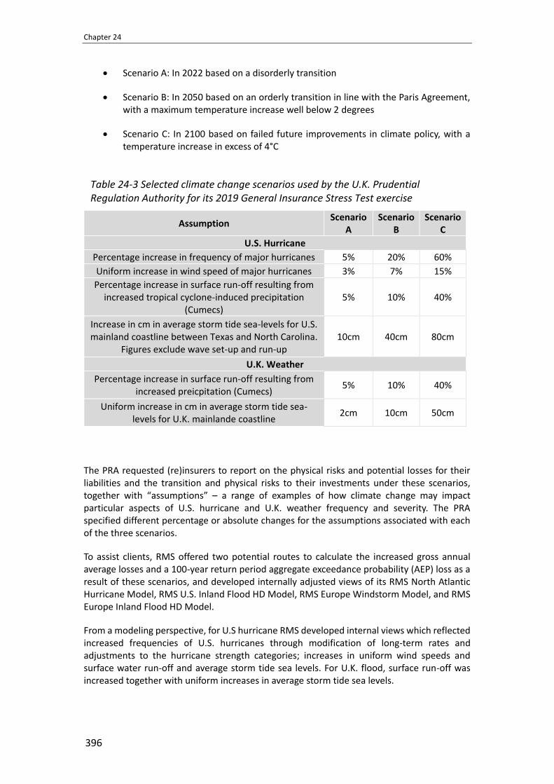
Chapter 24
396
• Scenario A: In 2022 based on a disorderly transition
• Scenario B: In 2050 based on an orderly transition in line with the Paris Agreement, with a maximum temperature increase well below 2 degrees
• Scenario C: In 2100 based on failed future improvements in climate policy, with a temperature increase in excess of 4°C
Table 24-3 Selected climate change scenarios used by the U.K. Prudential Regulation Authority for its 2019 General Insurance Stress Test exercise
Assumption Scenario
A Scenario
B Scenario
C
U.S. Hurricane
Percentage increase in frequency of major hurricanes 5% 20% 60%
Uniform increase in wind speed of major hurricanes 3% 7% 15%
Percentage increase in surface run-off resulting from increased tropical cyclone-induced precipitation
(Cumecs) 5% 10% 40%
Increase in cm in average storm tide sea-levels for U.S. mainland coastline between Texas and North Carolina.
Figures exclude wave set-up and run-up 10cm 40cm 80cm
U.K. Weather
Percentage increase in surface run-off resulting from increased preicpitation (Cumecs)
5% 10% 40%
Uniform increase in cm in average storm tide sea-levels for U.K. mainlande coastline
2cm 10cm 50cm
The PRA requested (re)insurers to report on the physical risks and potential losses for their liabilities and the transition and physical risks to their investments under these scenarios, together with “assumptions” – a range of examples of how climate change may impact particular aspects of U.S. hurricane and U.K. weather frequency and severity. The PRA specified different percentage or absolute changes for the assumptions associated with each of the three scenarios.
To assist clients, RMS offered two potential routes to calculate the increased gross annual average losses and a 100-year return period aggregate exceedance probability (AEP) loss as a result of these scenarios, and developed internally adjusted views of its RMS North Atlantic Hurricane Model, RMS U.S. Inland Flood HD Model, RMS Europe Windstorm Model, and RMS Europe Inland Flood HD Model.
From a modeling perspective, for U.S hurricane RMS developed internal views which reflected increased frequencies of U.S. hurricanes through modification of long-term rates and adjustments to the hurricane strength categories; increases in uniform wind speeds and surface water run-off and average storm tide sea levels. For U.K. flood, surface run-off was increased together with uniform increases in average storm tide sea levels.

Using Catastrophe Risk Modeling to Help Understand Physical Climate Change Risk
397
Clients could multiply their own AAL and 100-year return period AEP by predetermined “industry factors” calculated by RMS which reflect the percentage loss changes for an overall view of the change, or use a bespoke service where RMS would run the adjusted models for a client’s specific portfolio. The latter approach gave a more tailored assessment that better reflects a client’s book of business.
The exercise provided useful insight into where the direction of travel could be in terms of increased losses, with significant differences between the three scenarios. It provides awareness about the potential future risk and has acted as kick-start for insurers to include climate change risk assessment into their strategy. Other regulators across financial services and insurance are looking to follow suit.
Modeling the impact of severe drought for corporate lenders Drought is often overlooked when examining the physical risk of climate change, even though it is a significant potential source of shock to the global financial system. There is also a common misconception that sustained lack of water is primarily a problem for agriculture and food production. But, in Europe alone, it is estimated that around 40 percent of total water extraction is used for industry and energy production (cooling in power plants) and 15 percent for public water supply. Globally, the main water consumption sectors are irrigation, utilities and manufacturing.
In essence, practically every industry in the world has some reliance on water availability in some shape or form, and in this increasingly interconnected world it means that the impact of drought on one industry sector or one geographic region can have a material impact on adjacent industries or regions, regardless of whether they themselves are impacted by that phenomenon or not. Corporate lenders need to be able to quantify the default losses they would expect if severe drought events were to occur.
In 2016, the Natural Capital Finance Alliance, which is made up of the Global Canopy Program and the United Nations Environment Programme Finance Initiative, teamed up with Deutsche Gesellschaft für Internationale Zusammenarbeit GmbH Emerging Markets Dialogue on Finance (EMDF) and several leading financial institutions to launch a project to pilot scenario modeling for drought. Funded by the German Federal Ministry for Economic Cooperation and Development, RMS was appointed to develop a first-of-its-kind drought model. The aim was to help financial institutions and wider economies become more resilient to extreme droughts.
RMS adapted its risk modeling frameworks frequently used by insurers with help from a consortium complemented by the Universities of Cambridge and Oxford – to build a tool for banks to stress test the impact of drought. As part of this work, RMS investigated the likelihood of having a severe drought event, and the extent to which climate change has modified this likelihood. Although in this project, scenarios were devised, it would be possible to adapt the modeling further to make it fully probabilistic
Some of the findings show that extreme droughts could increase loan defaults ten-fold for institutions with specific portfolios that are most exposed to drought risks. Even when exposed to drought scenarios of medium severity, most companies see their credit ratings downgraded. The most affected sectors are water supply, agriculture and power generation, particularly in countries that are heavily reliant upon hydroelectric power. Significant impacts are also found in water-dependent sectors such as food and beverages.
Some of the largest losses seen in some of the scenarios were not necessarily a result of an industry sector not having access to water, but because other industry sectors didn’t have

Chapter 24
398
access to water, so demand dropped significantly and those companies were therefore not able to sell their wares. This was particularly true for petrochemical businesses that are heavily reliant on the health of the broader economy, with the model providing a broad framework that incorporates domestic interconnectivity and trade, as well as global macroeconomic effects.
There is significant scope to apply this approach to modeling other major threats and potential sources of global economic shock, including natural, manmade and emerging perils, as drought is just one environmental risk facing the financial services industry. This approach can be replicated to measure the potential impact of other systemic risks on macro and micro economic scales.
The banking sector is starting to see the relevance of stress testing portfolios on a geographic basis, and especially for mortgage books the required level of geographic information is emerging, making this type of modeling more readily implementable to the sector.
Global (re)insurer builds climate change action plan A global top 20 insurer and reinsurer wanted to analyze the potential impact of climate change on modeled losses for its portfolio. As part of the business’s climate change action plan, it wanted to better understand the uncertainty around climate-change driven changes in future losses to produce metrics and targets for how it manages climate change risk and opportunities across its business.
Through identifying the drivers of changes in risk within its portfolio, it could then target areas and priorities for further analyses, which can then inform its internal discussions and ultimately its business strategy. Two perils and regions came under the spotlight; U.S. hurricane and Australia cyclone. RMS was asked to help establish modeled losses for three different timeframes, through to 2030, 2050 and as far out as 2100.
The IPCC, founded in 1988, is an intergovernmental body of the United Nations with a stated aim to “provide the world with objective, scientific information relevant to understanding the scientific basis of the risk of human-induced climate change, its natural, political, and economic impacts and risks, and possible response options.”2 The IPCC publishes regular Assessment Reports, the first was published in 1990, and since 2000, it has included projections of greenhouse gas emissions, and from 2014, it includes RCPs which describe different climate futures. These RCPs are all considered possible depending on the volume of greenhouse gases (GHG) emitted in the years to come. The different pathways also reflect how collective mitigation efforts will affect emissions.
2 Please see IPCC (2013). Principles governing IPCC work, IPCC Batumi, Ga. Link: https://archive.ipcc.ch/pdf/ipcc-
principles/ipcc-principles.pdf.

Using Catastrophe Risk Modeling to Help Understand Physical Climate Change Risk
399
Figure 24-5 Representative Concentration Pathways (RCPs) featured in the IPCC Fifth Assessment Report
–RCP2.6: Most stringent mitigation is put into place. Emissions reach a peak by 2020
–RCP4.5: Emissions continue to rise until 2040 after which they begin to decline
–RCP6.0: Emissions continue to rise until 2080 after which they begin to decline
–RCP8.5: Extremely high levels of emission occur unchecked
Emissions levels and the effect of mitigation efforts are all very uncertain. But, by selecting an RCP it provides a basis for the analysis to assess the impact on key global climate variables, such as air/sea temperature and sea levels – and onward to assessing the impact on specific perils.
RCP4.5 was selected as a default view for the project; it is a well-established and frequently quoted scenario, but also the lower RCP2.6 and extreme RCP8.5 were considered. When examining the impact of climate change on local and global climate variables, the most well-respected and commonly used modeling framework is the Coupled Model Intercomparison Project (CMIP) model ensemble.
When examining the resulting changes in tropical cyclone activity, RMS used the latest scientific reference papers to estimate future changes along the U.S. and Australia coastlines, and for storm surge risk in the U.S. In order to assess resulting impacts on modeled losses to our clients’ portfolio, RMS modified the rate assumptions underlying the latest RMS North Atlantic Hurricane and Australia Cyclone Models to reflect the tropical cyclone frequency changes projected in the two selected reference papers for each region. The RMS long-term view of North Atlantic hurricane risk was used as the baseline for the U.S. RMS assessed modeled losses across the RMS Industry Exposure Database for wind and storm surge losses for each timeframe and also for the client’s specific portfolio. Risk from hurricane storm surge saw losses increase significantly, with annual average losses more than doubling by the end of the century.
Accounting for exposure changes To account for possible future changes to exposure in Australia and the U.S., RMS developed a series of county-level factors, which reflected how the exposure for each county is projected to change by 2050. These factors were then applied on both the industry-wide and the client’s portfolio loss results, to provide view of how exposure changes might be expected to impact tropical cyclone risk in the future.

Chapter 24
400
Typically, exposure projection exercises are used to forecast existing data (census housing counts, for example) into the very near future, usually in the order of 3-5 years. In order to project current exposure to 2050, a different approach needed to be developed. Population growth was selected as a proxy for longer-term exposure trends and used to develop a time series of exposure projections to 2050 based on established research and projection benchmarks. The key driver of the change in exposure across both countries is population growth. Population is expected to grow by 19 percent in the U.S. and 31 percent in Australia by 2050, with a trend of particularly high growth rates in urban areas.
In addition, the redistribution of the population due to climate change (specifically, rising sea levels) was incorporated in the analysis. For this aspect of the analysis, the population map was overlaid with sea level rise inundation maps and a relationship linking time to/since inundation with relocation was developed to consider coastal retreat caused by rising sea levels.
To determine the speed at which a population moves from an area prone to inundation, a distribution is applied on when residents are expected to relocate relative to when they are inundated (e.g. x percent will have left by the time they are inundated etc.). In terms of relocation location, assumptions are made on how far residents would move, such as 20 percent staying within the same ZIP code.
The resulting changes in population due to both growth and coastal retreat were aggregated into adjustment factors for each U.S. and Australian county and applied to the present-day industry and client portfolio. Combining the peril analysis with the exposure changes, RMS could then show by overall losses or at state/county level, the changes in annual average loss, with some areas showing greater levels of losses than the country average.
Using this analysis as a baseline, the client can then build on this and examine other potential scenarios, such as a different RCP or modifications in factors such as tropical cyclone tracks, and precipitation.
3 Conclusion
The physical risk of climate change must be quantified in terms of the potential financial impact on businesses to help them and their stakeholders and regulators to adapt effectively to this emerging threat. Catastrophe risk models are well placed to do this and have previously been instrumental in driving change at similar times of uncertainty, such as after Hurricane Andrew. Probabilistic modeling is proven to capture the potential wide spread of events and allows for the models to reflect new possible climate change scenarios. Catastrophe risk models are now frequently being used by a wide range of organizations as a vital tool to help quantify, understand and plan for the increasing threat of climate change.
Modelling Climate Change Risk for the Insurance Industry
401
Modelling Climate Change Risk for the Insurance Industry
by
Swiss Re Institute 1
Abstract
Modelling the insurance impact from climate change is complicated by uncertainties at two levels. First, there is a range of possible outcomes for underlying biophysical processes, and second, there are several confounding steps in the causal chain from emissions to temperature to global and regional climate variations to materialization of extreme weather events to the physical damages from catastrophes to insurance claims. Hence, the processes of how a changing climate impacts the frequency and severity of natural catastrophes are not fully understood. There is a higher confidence about the impacts on secondary perils. However, many secondary perils are more difficult to model, enhancing uncertainties around modelling the impact of climate change. This chapter outlines various influencing factors, time horizons, modelling challenges and levels of confidence for a range of natural catastrophe perils. It is increasingly important to regularly re-assess trends in input variables and model assumptions for current underwriting models. Incorporating the latest findings from climate science into catastrophe risk modelling is necessary for increasing the sustainability of the insurance industry and building socio-economic resilience.
Keywords: climate physical risks, insurance, catastrophe risk modelling, impact of climate change, underwriting models
1 Introduction
One of the main challenges in understanding insurance risks arising from climate change lies in the range of uncertainties involved. Risks arise along a complex causal chain. Emissions influence both global climate and regional climate variations, which in turn influence the risk of specific natural hazards (such as storm surge, floods, droughts and wildfires), which then influence the risk of physical damage (such as property damages, crop shortfalls and business interruption), which finally translate into insurance claims. There is considerable uncertainty involved in quantifying the parameters of the underlying biophysical processes and determining what their probability distributions look like. Modelling efforts rely on assumptions made along the causal chain: about emission paths and adaptation schemes, global and regional climate models, physical damage functions, and knock-on effects. The further one goes along the chain, the greater the intrinsic model uncertainty (McKinsey Global Institute, 2020), adding another layer on top of already uncertain parameters and processes.
1 This chapter is written by Thomas Holzheu, chief economist Americas, Swiss Re Institute, Swiss Reinsurance Americas,
Armonk, NY, USA, email: [email protected]; Michael Gloor, senior Nat Cat Specialist, Swiss Re Institute, Swiss
Reinsurance, Zurich, Switzerland, email: [email protected]; Kulli Tamm, senior Economist, Swiss Re Institute,
Swiss Reinsurance Americas, Armonk, NY, USA, email: [email protected].

Chapter 25
402
Climate change is a systemic risk, affecting all parts of the economy. In terms of the impact on the insurance industry, climate change not only affects short-tail business lines such as property insurance, but it can also change the risk landscape for life & health or casualty insurance, thus requiring a holistic, long-term analysis of climate risks. Additionally, the risks arising from a changing climate do not stop on the liability side of an insurance company’s balance sheet but also affect the asset side if insurers’ investment portfolios include assets that are exposed to the effects of a transition to a low-carbon economy. This chapter primarily focuses on physical risks to property re/insurance. The re/insurance industry traditionally deploys probabilistic catastrophe models for the purposes of risk underwriting and capital steering. Incorporating the latest findings in climate science into catastrophe risk modelling is necessary to increase its usefulness to the insurance industry and society. Integrating climate change scenarios will allow for a more forward-looking assessment of extreme weather risk.
2 Uncertainty about the magnitude of global warming
The temperature of the atmosphere and the oceans has a direct or indirect impact on most physical processes in the Earth’s system that define our climate and its extremes. The global average temperature itself is influenced by the concentration (and thus the emissions) of greenhouse gases (GHG) in the atmosphere. Any change in GHG concentrations and global temperatures, whether man-made or natural, will alter the risk exposure of humans, their assets, and the natural environment. The scientific community takes human influence on the Earth’s climate as a fact, but the implications of that fact are clouded in multiple layers of uncertainty.
A lot of the analysis and reporting on climate change is focused on the expected averages (means) of GHG concentration and temperature changes. For example, in a recent report, the Intergovernmental Panel on Climate Change (IPCC) concluded: “Human activities are estimated to have caused approximately 1.0°C of global warming above pre-industrial levels, with a likely range of 0.8°C to 1.2°C. Global warming is likely to reach 1.5°C between 2030 and 2052 if it continues to increase at the current rate”(IPCC, 2018). By the end of the 21st century, the IPCC projects a temperature increase of more than 4°C in a business-as-usual scenario2. But the uncertainty around those mid- and end-of century estimates is exceptionally wide, a facet that is lost in the discussion by only focusing on the means and likely outcomes. As noted by a number of climate change researchers, focusing on the “most likely” outcomes, even including some 1-2 standard deviation bands around the mean, lulls policymakers and the society to a false sense of security (Heal, 2017; Kunreuther et al., 2013; Wagner & Weitzman, 2015).
A key parameter in climate change modelling is equilibrium climate sensitivity (ECS), which is defined as the “global average surface warming following a doubling of carbon dioxide concentrations.”(IPCC, 2007) This is the metric that underpins all the estimates of future global temperatures, and any further impacts of those temperatures. In the IPCCs assessment, the ECS is “likely” (that is, with probability above 66%) to be in the range 1.5 to 4.5°C (IPCC, 2013). However, this means that there is up to a 17% probability that climate sensitivity is greater than 4.5°C even with a normal distribution. Averaging more recent estimates of 14 leading climate scientists puts that probability even higher, at 23% (Weitzman, 2012). Distributional assumptions around the fatness of the tails of the ECS matter greatly for this assessment – the probability of ECS being 6°C, though low in absolute terms, is twice as large
2 Refers to projections for RCP-8.5 scenario, IPCC (2014).

Modelling Climate Change Risk for the Insurance Industry
403
if the distribution function is lognormal rather than normal, and more than triple if the distribution is Pareto.3 Yet the actual distribution appears unknowable4
– the distributions in a number of published papers look quite different from one another and decidedly non-normal (see Figure 25-1). Some highly-reputed climate models give a chance of at least 15% that ECS is no less than 6°C (Heal, 2017).
Figure 25-1 Estimated probability density functions for the ECS from a variety of published studies
Source: Millner et al. (2013). Modified from Meinshausen et al. (2009).
Taking the analysis from an uncertain ECS to estimates of GHG concentrations by end-of-century and the resultant temperature increases, to the changes in the risk exposure profile for natural catastrophes, to economic and social impacts compounds the levels of scientific and modelling uncertainty. Uncertainty on the far-reaching implementation of climate-mitigation and adaptation policies as well as on other macro-risk trends, such as social and economic development, will require the insurance industry to think in different qualitative and quantitative scenarios when attempting to assess the future impact of climate change. Uncertainty around the primary driver for change, namely increasing global average temperatures, will lead to even larger uncertainty on local effects of natural catastrophes.
This uncertainty, however, should not lead to inaction: first, several changes to local risk factors are already observable today and need to be incorporated into risk assessment and modelling for an appropriate view of today’s risk landscape. Second, different projections are in sufficient agreement when limiting the time horizon to the next few decades. In the face of climate change, the focus for the re/insurance industry and for financial regulators should be on an accurate representation of today’s risk landscape and expected changes in the near future.
3 Physical climate risks and their impact on the insurance industry
The following sections will highlight how globally increasing temperatures and other macro-risk trends change natural catastrophe risks. While the industry often focuses on key insurance
3 See Table 1, Ibid. 4 See for example Pindyck (2011).

Chapter 25
404
risks such as tropical cyclones, we show the importance of also recognizing climate-induced changes to secondary perils that have traditionally received less attention.
Some effects of climate change and global warming are already evident and shaking up our risk landscape: warmer average temperatures, rising sea levels, melting ice caps, longer and more frequent heatwaves, erratic rainfall patterns and more weather extremes. There are increasing concerns on how societies and companies manage the short- and long-term risks posed by climate impacts. Risks associated with climate change include losses from both chronic (e.g. slow temperature increase and sea level rise) and acute physical risks (e.g. extreme weather events) and a repricing of financial assets in the transition to a low carbon economy (transition risks) (see Figure 2). While physical risks can cause actual damage to people, assets or the environment, transition risks primarily affect the value of assets or result in additional costs. The scope of this analysis focuses on modelling physical risks. A comprehensive risk assessment for insurance companies will require the integration of both.
Figure 25-2 Classification of climate change risks
Source: Swiss Re Institute
The (re)insurance industry traditionally thinks about natural-catastrophe risks in two dimensions: frequency and severity. Climate change affects these two dimensions, but it also introduces two new complexities to the risk equation: time horizon and level of confidence. It is important to understand the time scale as this enables us to learn what changes have already happened and to make predictions about potential future changes. Slow but steady changes leave time for adaptation and measures to increase resilience. On the other hand, climatic changes of severe and rare events are difficult to observe because of their rare occurrence. Thus, many decades might be necessary to statistically prove changing trends, ultimately limiting (political) will to mitigate climate change and to invest in measures that increase resilience.
Weather is an individual observation at a given point in space and time. Climate is the distribution of observations over an extended period and geography. With climate change, there can be a shift in the means, a change in variability or change in skew where extremes become more extreme and more frequent (see Figure 25-3).

Modelling Climate Change Risk for the Insurance Industry
405
Figure 25-3 Possible range of impact of climate change on climate variables (e.g. temperature)
Source: IPCC (2013)
Climate change, in combination with economic growth and rising urbanisation, is increasing the number of small-to-medium sized losses stemming from secondary perils and can impact the profitability of certain lines of business if not priced accurately. Absent a formal definition, industry practice has been to consider secondary perils as high-frequency, low-to-medium severity events as opposed to losses resulting from primary perils, which are low-frequency-high-severity events such as earthquakes and hurricanes. Secondary perils can happen on an independent basis – this would include river floods, flash floods, hailstorms, tornadoes, snow and ice storms, drought and wildfire outbreaks. However, often the events appear as secondary effects of primary perils, such as the flooding of Houston after hurricane Harvey in 2017. For the last two decades, secondary perils accounted for more than half of the insured losses globally. The single biggest natural catastrophe insurance loss-event of 2018 was Camp Fire in California (USD 12 billion), a “secondary” peril. There are areas of relatively high confidence in the impacts of climate change on natural hazards based on an alignment of empirical observations, quantitative models and unambiguous scientific theory. Many of these relate to the so-called secondary perils. Sea level rise, for example, caused by thermal expansion of water and the melting of glaciers and icecaps will directly increase the magnitude of storm surges and pose a material long-term risk for low-lying coastal regions. Increased temperature variability can lead to longer and/or more frequent heat waves, droughts, water scarcity and wildfires. Confidence for these trends is high and heat waves not only affect agriculture, productivity, water resources, health and mortality but also increase the risk of conflicts in certain regions. Increasingly hot and dry conditions also exacerbate wildfire risk, with severe consequences for exposure in the wildland-urban interface. Furthermore, increasing temperatures enable the atmosphere to hold more water vapor, leading (on average) to an increased risk of extreme rainfall and subsequent flooding. While this effect can occur in many regions, the effect is especially impactful for torrential rainfall associated with tropical cyclones.
Currently, confidence in climate trends is considerably lower for atmospheric and oceanographic circulation changes, which affect natural phenomena like the frequency and intensity of severe tropical cyclones, European windstorms or tornado and hail storms. Confidence levels are partially lower due to the above-mentioned lower frequency of occurrence and because of the complex interplay of the climate system (IPCC, 2018). While warmer sea-surface temperatures will increase the probability of tropical cyclone formation and intensification, higher wind shear can be a counter-force. Uncertainty about the influence of climate change on jet streams, for example, will influence extratropical cyclones and impact the occurrence of anomalously stationary weather patterns (Coumou et al., 2018). These complex interactions introduce a “confidence barrier” (see Figure 4) that renders any
Pro
bab
ility
Increase in mean
Extremes shift with mean
Pro
bab
ility
Increase in variability
Extremes become more extreme and more frequent
Mean remains
the same
Pro
bab
ility
Becomes skewed
Mean remains the same
Extreme highs become more extreme and more frequent
Extreme lows remain nearly the same

Chapter 25
406
insurance-related quantification of climate-change effects on certain high severity perils (such as hurricanes) as highly uncertain. Because of their material impact, insurers need to lower this barrier by increasing confidence through additional research or by quantifying modelling uncertainties if confidence remains low.
Figure 25-4 Classification of climate change effects by drivers, perils and confidence levels.
Source: Swiss Re Institute
4 Confounding impacts of other exposure drivers: urbanisation,
economic development and demographics
As climate changes, so too are populations and economies around the world. Many loss trends observed today still largely originate from shifts in growing asset values and concentrations, as well as from changing patterns in land use. During the last six decades, the world population has grown by a factor of approximately 2.5 (United Nations Department of Economic Social Affairs, 2019), while world real gross domestic product (GDP) has grown by more than sevenfold. In the 1950s, approximately 30% of the global population lived in urban areas. That figure has increased to over 50% today. These trends are expected to continue, and by 2050 almost 70% of the global population will live in urban centres (United Nations Department of Economic Social Affairs, 2018). Rapid urbanisation, especially in coastal cities, amplifies existing and future climate risks. B. Neumann et al. (2015) estimate that the number of people living in the low-elevation coastal zone, as well as the number of people exposed to storm surge events worldwide grow by about 1.3% annually or 0.8% faster than the overall population, especially in Asia and Africa. This implies that overall GDP growth for these

Modelling Climate Change Risk for the Insurance Industry
407
countries underestimates the pace of development exposed to flood risk. Sealing of surfaces in cities and building activities in flood-prone or coastal areas increase the risk of water-related damage. As green areas disappear, heat and air-pollution islands intensify and pose severe risks to human health. Climate change often amplifies the negative impacts of human activities that remove natural absorption or buffer zones.
Furthermore, increasing development in the wildland-urban interface (WUI) raises the risk of damaging wildfire. For example, between 1990 and 2010, the number of houses in the wildland-urban interface grew 41% in the West of the US (Radeloff et al., 2018). Having more structures in the WUI increases not only the damage wildfires inflict (because they are harder to fight) but also the risk that they will break out in the first place. Population growth and development are also a contributing factor for exposures to tornado risk. Population in the more at-risk regions in the US grew by an annual average rate of 3.0% between 1950 and 2010 compared to 1.8% for the country overall (Ashley & Strader, 2016).
Beyond these demographic and urbanization factors, there are other economic drivers of exposure growth. Value of assets grow faster than GDP. For example, the value of tangible commercial assets and residential buildings in the US grew by 5% to 6% per year between 1980 and 2003 compared to a nominal GDP growth of 4.7%5. Average US construction costs for new residential homes grew by an average real 1.1% per year between 1998 and 2017 because of higher standards of building due to insulation, air conditioning, plumbing etc. (Ford, 2017). The inclusion of socioeconomic factors in forward-looking climate change models for natural hazard losses show similar patterns. Several studies that use projected increases in the value of exposed assets project the contribution from socio-economic growth to be about equal or larger than the contribution from climate change (Bouwer, 2013; Pielke Jr, 2007; Schmidt et al., 2009). Studies that only use population growth estimates or similar quantities such as land-use change project the signal from climate change to be somewhat larger than the signal from exposure change (Dorland et al., 1999).
Example of modeling historic events with current exposure data To illustrate the impact of socio-economic contributions to exposure growth, we modeled the thought experiment what would happen if Hurricane Andrew were to hit South Florida in 2017, taking an identical track and at the same intensity. Swiss Re Institute ran Andrew’s 1992 footprint on a market portfolio for the state of Florida, in Swiss Re’s proprietary tropical cyclone model. The tropical cyclone model contains every historical event in the National Oceanic and Atmospheric Administration’s HURDAT database along with probabilistic tropical cyclones for each historical tropical cyclone, resulting in more than 220,000 realizations of possible Atlantic tropical cyclones. The market portfolio is a representation of all insured property values (residential, commercial and automotive), along with coverage terms. Compared to an original insured loss of USD 27 bn in 2017 dollars, the 2017 insured losses would have increased to between 80bn to USD 100bn, assuming a similar coverage percentage (take-up rate, deductibles etc.) by the insurance industry, due to a combination of increased development and asset values. Adjusted for inflation, this translates into 4 to 5% annual growth in exposures (Linkin & Schwartz, 2017).
5 Source: U.S. Bureau of Economic Analysis, Survey of Current Business, April 2005.

Chapter 25
408
5 Impact of climate change on specific perils
Wildfires In the case of wildfires, warming and drying are the primary causes. Pre-historical evidence stored in tree rings and charcoal buried in lakes tell us that for thousands of years, periods of warming have coincided with periods of increased wildfire activity (Parisien et al., 2020). While fire is very complex and affected by much more than just climate, the data from recent decades indicate that the hot years are the years with the most wildfire, and as temperatures have increased, burned areas have increased in step.
Some risk solutions providers such as AIR, CoreLogic, RMS, and RiskFrontier have started to develop full-scale probabilistic wildfire models for regions with comparatively high exposure, such as California, Australia, and Canada (Swiss Re Institute, 2017). These probabilistic models aim to provide assessment scores for wildfire risks that are based on a variety of region/location specific characteristics. Some of the factors that are considered include natural and man-made sources of ignition, long- and short-term weather and climatological conditions at the location of ignition that could impact how a fire spreads, prior suppression efforts in the area that could have an influence on the amount of existing fuel loads, as well as current suppression access and capabilities.
In comparison to other modelled natural catastrophe risks, wildfire is a complex paradigm with many elements (Johnston, 2018). There is only a limited amount of historical data from which vulnerability curves can be developed to link hazard with actual damage to properties. Meanwhile, the number of inputs a probabilistic wildfire model needs to consider is enormous (Parisien et al., 2020). In addition, physical characteristics of the surrounding interface locations are critical – such as construction and roof type, clearance distance, surrounding vegetation, and more – as lofted embers often create exposure in secondary locations. Meanwhile, the built environment and mitigation work in the interface area is rapidly changing. A key factor is a change in underlying exposures, marked by growth in populations and properties in the WUI. With rising urbanization of wildland as well as increasing industrial activity across the boreal forest areas, a full mapping of the Canadian WUI was only completed recently (Johnston & Flannigan, 2018).
Drought The IPCC expects higher temperatures to likely lead to greater magnitudes of agricultural droughts in continental area of US (IPCC, 2018), in accordance to what is projected by EEA (European Environment Agency) regarding the frequency of meteorological and hydrological droughts in most of Europe over the 21st century (European Environment Agency, 2020). Recent reports from IPCC state with high confidence that heatwaves will increase in intensity and duration into the 21st century in most regions around the globe (IPCC, 2018, 2019).
Technological advancements through different innovations are expected to be able to partly offset the potential increased severity of climate events in the medium time horizon (Aggarwal et al., 2019). These include advances in precision farming, land monitoring, irrigation efficiency, as well as adoption of new farm practices to mitigate and adapt to climate changes (resistant varieties of crops, diversification, changes in cropping patterns, etc.). This impact is expected to vary among regions also based on socio-economic conditions and policy support.
Inland flooding Inland flood risk, including river flood and pluvial flood risk (flooding caused by extreme rainfall), is expected to experience substantial changes in many regions, due to changing extreme precipitation patterns. As the atmosphere warms, it can hold more water vapour. In

Modelling Climate Change Risk for the Insurance Industry
409
addition to this effect, changes in dynamical processes (e.g. hurricanes, extratropical cyclones) affect extreme precipitation. Large increases in flood risk associated with hurricane rainfall are projected, due to a slowdown of the speed hurricanes move along their track (Kossin, 2018), as well as increasing rainfall rates (Liu et al., 2019).
Observations of precipitation in the United States generally suggest an increase of heavy precipitation, particularly in the eastern and central parts of the country, both in terms of intensity and frequency (Donat et al., 2013). However, these trends vary regionally, with decreases in parts of the southern United States (Hoerling et al., 2016). Changes in precipitation may not be translated into similar changes in flooding, due to complex interactions between climate, catchments, rivers, and water management practices. Indeed, there are few sites with significant observed changes in moderate or major floods (Slater & Villarini, 2016). However, whilst much of the United States has shown little or no change, flood magnitudes have decreased in the Southwest, and increased in parts of the Midwest, and from the northern Appalachian Mountains to New England (Peterson et al., 2013). The trends are not unequivocally due to climate change, with land management practices and long-term cycles also potential contributors to the observed patterns (Shapley et al., 2005; Villarini et al., 2011; Y.-K. Zhang & Schilling, 2006).
Projections, however, show a clear impact of climate change on flood risk in the US. An increase in flood frequency is projected, with the annual number of 100-year flood events expected to increase by 50% by 2100 under RCP 4.5, and by 150% under RCP 8.5 (Wobus et al., 2017). Regionally, the largest fractional changes in flood frequency are expected to occur in the southern Appalachians and Ohio River valley, the northern and central Rocky Mountains, and the Northwest, with historical 1% AEP events becoming 2-5 times more frequent by 2100 in these regions. In terms of magnitude, there is a lack of a spatially coherent trend for the US (Arnell & Gosling, 2016). However, regionally, increases are expected in the central US (Naz et al., 2016) and Pacific Northwest (Salathe Jr et al., 2014).
Climate change impacts on flood risk may be further exacerbated by other trends, including urbanization. Rapid urbanisation reduces avenues for water discharge and can lead to heavy flooding, as highlighted by attribution studies for Hurricane Harvey flooding (Van Oldenborgh et al., 2017; W. Zhang et al., 2018) Another example is Mumbai (2005), when flooding after heavy rains resulted in one of the largest insurance loss events ever experienced in India (USD 0.9 billion, according to sigma data).
Coastal flooding Climate change also impacts coastal flood risk, principally via two mechanisms: global warming-induced sea-level rise and changes to the activity of storms associated with surge (e.g. hurricane frequency and intensity changes). It is recognized that substantial but gradual changes in the probability of extreme storm surge events may take a long time to detect in observational records (Ceres et al., 2017). However, observations of coastal flooding have already noted an increase in risk during the past century along the US East Coast (Grinsted et al., 2012). Increased coastal flood risk may also compound river flood risk, with evidence of a significant increase in the number of compound flood events over the past century at many of the major coastal cities of the United States (Wahl et al., 2015). One such city is New York, which has experienced an increase in coastal flooding during the past century, with a large contribution from rising sea levels (Talke et al., 2014), but also from an increase in the number of storm surge weather patterns that are associated with high precipitation (Wahl et al., 2015).
Projections show substantial increases in coastal flood risk for the US, with the greatest storm surge increases on the East and Gulf coasts (J. E. Neumann et al., 2015). For the US Florida and

Chapter 25
410
Gulf coasts, research suggests a median increase in storm surge risk of 25-47% comparing the last two decades of the 20th and 21st centuries under the RCP 4.5 scenario (Balaguru et al., 2016). Under RCP 8.5, the historical 100-year flood level is projected to occur every 1-30 years along the southeast Atlantic and Gulf coasts of the US, and annually in the New England and mid-Atlantic regions by the end of the century (Marsooli et al., 2019). The relative contribution of TC climatology changes to coastal flood hazard varies along the coast, with the largest contributions in the Gulf of Mexico, where the effect of TC climatology is larger than that of sea-level rise for more than 40% of coastal counties. Yet regional differences in changes in coastal flood risk may vary depending on which return period is examined (Buchanan et al., 2017). For example, considering a 50 cm sea-level rise, the increased frequency of historically 1-in-10-year floods is lower in Seattle, WA than Charleston, SC, whereas for 1-in-500 year floods the pattern is reversed. While sea-level rise this century is expected to be lower than that (Bamber et al., 2019), it will nevertheless severely alter coastal flood risk (Marsooli et al., 2019).
6 Modelling challenges
Cat models and increased parameter uncertainty The insurance industry uses catastrophe models to assess the risks from extreme weather events. These models are designed to solve the analytical problem that most disaster losses come from a few large events. The most extreme events are rare and therefore only represented with few actual observations in the historic data. Cat models generate large numbers of synthetic events that are designed to be realistic and fill gaps in the loss history. These synthetic hazard events get combined with data on the physical characteristics of assets (such as buildings and infrastructure) to provide information about vulnerabilities to the modeled hazards. As a final step, modeled vulnerabilities get combined with data about insurance coverage to provide information about individual insurers’ or the industry’s financial exposures (see Figure 25-5). Catastrophe models vary in many aspects and can result in different probability distributions for the same insurers’ portfolios (Weinkle & Pielke Jr, 2017).
Figure 25-5 Layers of a typical catastrophe model
Source: Swiss Re Institute
Such catastrophe models have served the insurance industry well until now for underwriting and risk-management purposes. Standard short-tail property insurance typically gets renewed

Modelling Climate Change Risk for the Insurance Industry
411
on an annual basis and thus allows for continuous adjustments to underlying slow trends in hazard, vulnerability, exposure and insurance policies. However, these models have limitations when trying to assess the future medium- and long-term impact of changing climatic and socio-economic conditions.
Historical bias and uncertain socio-economic and exposure trends Catastrophe models have been developed based on historical hazard, vulnerability and insurance-loss data sets and embedded theories and interpretations, which implicitly assume that the present and near future will be comparable to the past. One important modelling and underwriting risk in the context of climate change, and all other macro-risk trends, is a potential underestimation of risk premiums by relying on historical loss data or incomplete / outdated models to assess the current risk. Especially for low-frequency perils, this can lead to risk assessments that lag decades behind the current risk landscape. This is illustrated conceptually in Figure 25-6: if a risk assessment is based on a long-term historical average of e.g. a physical hazard, a historical bias can create a gap between actual risk and modelled risk.
Figure 25-6 Illustration of historical bias
Source: Swiss Re Institute
Model builders have developed techniques to debias and correct the models for (multi-) decadal variability of the underlying natural hazard, for changing building codes and protection measures that affect the vulnerability and to adjust for a growing insurance exposure with the goal to best assess the current risk landscape. However, the models are, per se, not designed to analyse the sensitivity of financial losses in a future and potentially rapidly changing climate, while also incorporating future socio-economic trends as well as climate-mitigation and adaptation measures that eventually affect the ultimate impact on the re/insurance industry (see Figure 25-7). Therefore, all layers of a natural-catastrophe re/insurance model potentially need to be analysed and likely changed for an adequate representation of insurance risk in a future climate, leading to a vast number of model parameters that are often highly uncertain for medium- to long-term projections. While a gradual debiasing of models remains possible to assess today’s property-insurance risk, even in a changing climate, the models are, by design, often not adequate to efficiently study the sensitivity of many highly uncertain and time-dependent parameters.

Chapter 25
412
Figure 25-7 Influence of macro trends on model components for weather-related risks
Source: Swiss Re Institute
Currently, many efforts focus on incorporating potential future hazard trends for long-term scenarios (e.g. 2050 and beyond) for key natural-catastrophe risks (such as North-Atlantic Hurricanes) while keeping other model components constant (such as the underlying portfolio and vulnerabilities). While such exercises can be interesting, they provide little decision-useful information because today’s insurance exposure is inserted into a possible future climate state without considering the complex interaction of insurance with other (socio-economic) macro trends, ultimately leading to an unrealistic future representation of the insurance environment.
An additional challenge for the re/insurance industry is that the most influential and widely used models are proprietary, meaning the details of their construction and output are not subject to open scientific debate and peer review. Finally, they are designed to be used in places and for assets where the insurance industry has significant exposure but tend to be less accurate or non-existent for countries where current risks are low and/or insurance cover is low (Sobel, 2019).
Lack of robust models for secondary perils Fully-probabilistic insurance models are currently well established for key perils such as tropical cyclone risks while secondary perils that are most affected by climate change in the near- and mid-term have received less attention from the modelling community. By only focusing on peak perils, there is therefore a considerable risk of significantly underestimating the overall impact of climate change by neglecting perils such as local flooding, wildfire or droughts. With a few exceptions (e.g. flood risk models in US), the discipline of secondary peril risk modelling has not been afforded the same priority as the primary peak loss-generating perils such as hurricanes in the North Atlantic. Also, secondary perils modelling is more complex.
• The areas vulnerable to primary perils are generally well-defined (e.g. near seismic fault lines (earthquakes) and coastal areas (tropical cyclones)). Many secondary perils,

Modelling Climate Change Risk for the Insurance Industry
413
on the other hand, can happen anywhere (e.g. heavy precipitation in large urban centres far inland or away from river plains). Swiss Re for example developed global flood maps based on LiDAR data for a consistent elevation data set on a 30-meter resolution. For certain markets in North America, Europe and Asia Pacific, this is complemented with modelled events for a full probabilistic model.
• While primary perils typically affect large areas in a relatively homogeneous way, many secondary perils are highly localized (e.g. hailstorms or tornados) and driven by complex thermodynamics. A large amount of data and computational power is required to model these perils. Data history is short and biased towards human observation. Today’s weather models still cannot reliably simulate severe convective storms that produce tornadoes. Thus, it is difficult for researchers to evaluate the impact of climate change based on current computer models because the counterfactual scenarios, by definition, did not actually happen (Ornes, 2018).
• Some secondary perils are strongly influenced by unpredictable human intervention. The scale of wildfires for example, are impacted by human prevention, ignition (e.g. the mechanical failure of a vehicle that set off the Carr Fire in California in 2018), containment and suppression activities. Pluvial flood risks are more dependent on urbanization, man-made surface modifications and soil conditions than for example storm surge risks.
With more than 50% of insured losses over the last decade coming from secondary perils, this is an obvious challenge for the insurance industry. Unlike primary perils, the regional footprint of secondary perils is more ubiquitous and therefore of growing relevance for many smaller regional and super-regional insurers outside of the traditional peak cat scenarios which did not need to worry too much about modelling cat risk exposures in the past. Currently, this is more a profitability topic, however, with the possibility of accelerating climate-driven claims trends, secondary perils can morph into a financial-stability risk for insurance companies and therefore for regulators and rating agencies.
Scenario analysis as the way forward Complexity and uncertainty should not stop the re/insurance industry from evaluating the impact of climate change on both today’s insurance risks and the expected future risk landscape. Improving our understanding and modelling capabilities on the impact of climate change help to a) ensure today’s risk premiums and capital requirements reflect the current risk landscape, b) create transparency and ultimately improve stability of financial markets by publicly disclosing climate-related risks to investors, and c) create a framework for decision makers to steer a company’s exposure to climate risks. If companies, or the industry overall, fail to provide meaningful answers, ambiguity will be the result. Ambiguity (also referred to as parameter risk) about risk distributions increases capital cost and challenges the insurability of perils. Cabantous et al. (2011) show that insurers charge higher premiums when faced with ambiguity than when the probability of a loss is well specified (risk). Furthermore, they tend to charge more for conflict ambiguity (different models produce diverging probability distributions) than imprecise ambiguity (a model produces a loss distribution with low confidence) for flood and hurricane hazards.
Normally, not all model parameters can be investigated with the same level of depth. However, meaningful scenario analyses that can be both qualitative and quantitative can help to address above-mentioned key purposes. The Financial Stability Board (FSB) Task Force for Climate-related Financial Disclosures (TCFD), which is a widely supported and accepted industry body, has developed recommendations on how to best analyse and disclose climate-related risks.

Chapter 25
414
For scenario analysis, TCFD has published an extensive report (TCFD, 2017). These recommendations should be used as a baseline for the industry. Individual regulatory jurisdictions have also developed and published frameworks for the financial industry to address physical and transition risk originating from climate change. For physical risks, see for instance Bank of England (2019).
It should also be mentioned that the insurance industry can and should play an important role in communicating risks to clients and governments in areas that are exposed to climate-related risks. Climate-scenario analysis is one of the tools that can be used for such purposes. For example, Swiss Re has performed an analysis for New York City to not only better understand the risk drivers related to a change in frequency and intensity of hurricanes and resulting storm surges but also to assess the economics of climate-adaptation measures (ECA, 2009). For example, Figure 25-8 shows that expected annual losses from sea-level rise and an increase in frequency and intensity of hurricanes could more than double by 2050. The cost/benefit ratios of different resiliency measures are shown on the right, providing an economic framework for decision makers. This case study also highlights again that climate-risk scenarios should not only focus on changes in hazard but should also incorporate potential risk adaptation measures. Extensive coastal flood protection measures are currently under consideration or development to protect many urban areas around the globe.
Figure 25-8 Case study on changing hurricane risk in 2050 for New York City to analyse drivers of loss (left) and Cost/Benefit ratios of adaptation measures (right)
Source: Swiss Re Institute
Limited scope of modelling for long-term time horizon Besides above-discussed scenario-analysis frameworks, (re)insurance firms apply a forward-looking approach through active monitoring/research, e.g. by using emerging risk and Own Risk and Solvency Assessment (ORSA) processes. The ORSA time-horizon is typically shorter than the timespan over which climate risks will evolve. However, firms could also assess their longer-term strategy as part of their ORSA, i.e., the impact of climate change for certain (re)insurance products. Emerging risk tools support the review of early signals. Emerging risks are defined as newly developing or changing risks that are difficult to quantify and could have a major impact on society and industry. It involves external and internal sources, e.g. databases and literature, and subject matter experts from different business areas. Figure 25-9 illustrates the complex interactions of climate change that are in scope of Swiss Re’s “SONAR” early warning tool, an internal crowdsourcing platform that collects input and feedback from underwriters, client managers, risk experts and others across the company (Swiss Re Institute, 2019). The graph lists the natural catastrophe perils that are subject to explicit modelling

Modelling Climate Change Risk for the Insurance Industry
415
efforts – at various stages – as described above. The graph also shows other areas that have not yet been afforded the same degree of investigation such as the impact of climate change on human life and health. Furthermore, there are knock-on effects on migration, urbanisation, food security, water scarcity, etc. These areas are observed in a more qualitative manner which can morph into quantitative modelling as scientific evidence and data become available.
Figure 25-9 Climate change in the framework of Swiss Re’s emerging risk tool “SONAR”
Source: Swiss Re Institute
Feedback loops and tipping points From a broader risk management perspective, traditional approaches generally extrapolate from historical data and assume a normal distribution for shocks. As noted above, however, historical data can create a downward bias and most of the climate-related risks appear to have fat tails, necessitating an "epistemological break" with regard to risk management (Bank for International Settlements, 2020). Forward-looking scenario-based analysis has started to develop to fill a part of this void. Nevertheless, several further modelling limitations remain to be addressed, including that of the timing and impact of feedback loops and tipping points.
A major long-term risk of unmitigated climate change is posed by irreversible tipping points. The Earth’s climate system comprises many dynamic oceanic and atmospheric processes, which are strongly interlinked and thus not necessarily self-stabilising. This means that even relatively small perturbations can “tip” the climate into a new state or initiate positive feedback loops, which can significantly alter the climate for centuries to come. An example of a positive feedback loop is the thawing of permafrost in arctic regions, releasing immense quantities of carbon dioxide and methane currently stored in the frozen soil (Schuur et al., 2015)..The release of these greenhouse gases will cause even more warming and more permafrost thawing. Another feedback loop is around temperature changes and ice sheet disintegration. However, the parameter values that determine the strength (and even the sign) of those feedback loops are largely unknown or possibly unknowable (Pindyck, 2013). Such feedback loops are often projected to act only over the very long term (centuries and millennia) and therefore omitted from most general circulation models (Weitzman, 2011). For example,

Chapter 25
416
none of the IPCC’s climate models though the Fifth Assessment Report include the warming tundra feedback loop (Romm, 2018). Yet more recent analysis shows that some of the feedbacks are not as slow as previously believed (Dixon, 2019). For instance, a recent paper for the feedback loops from temperature to sea level rise suggests that due to non-linear ice sheet dynamics, it only takes decades rather than centuries or millennia for the lag between the two (Hansen et al., 2015). Thus, current analysis potentially significantly underestimates future warming. This would have follow-on implications to the risk and exposure profile on which catastrophe modelling depends, and the uncertainty about the changes to the risk landscape adds another layer of challenges to the modelling.
7 Summary and conclusions
The effects of climate change are already evident: warmer average temperatures, rising sea levels, melting ice caps, longer and more frequent heatwaves, erratic rainfall patterns and more weather extremes. The effects contribute most notably to growing losses from secondary perils. Most of the past increase in economic and insured losses from natural hazards has come from greater exposure to hazards rather than increases in their mean and tail intensity. Yet quantifying the relative contributions of socio-economic vs climate related divers is challenging given the data limitations and short time periods with consistent exposure data. In the future, hazard intensification will likely assume a greater role.
Modelling the insurance impact from climate change is complicated by the uncertainties surrounding the estimated magnitude of the underlying biophysical processes, and further confounded by the several steps in the causal chain from emissions to temperature to global and regional climate variations to materialization of extreme weather events to the physical damages from catastrophes to insurance claims. Hence, the processes of how a changing climate impacts the frequency and severity of natural catastrophes are not fully understood.
There is a higher confidence about the impacts on secondary perils. However, many secondary perils are more difficult to model and have received less attention by the modelling community in the past, enhancing the current uncertainties in modelling the impact of climate change. Today, the effects of climate change on property risks are still manageable for re/insurers. The short-term nature of most property re/insurance business allows for continuous adjustments of risk view and risk to reflect observed climate, exposure and vulnerability changes. However, it is increasingly important to regularly reassess the inherent trends in input variables and model assumptions for current underwriting models.
Insurers need to keep abreast of the latest scientific findings and incorporate them into their natural-catastrophe models, in order to remain sustainable in the era of climate change. Substantial effort is needed to translate scientific results into valuable and workable risk-assessment know-how and tools. More sophisticated modelling approaches are needed to account for (the growing loss impacts of) secondary perils that have been inadequately modelled in the past.
Climate change is a systemic risk. Important questions for the insurance industry relate to the possibility of increasing tail risks and/or more correlations of risk factors. If left unmitigated, it will have severe consequences for the global risk landscape. Complexity and uncertainty should not stop the re/insurance industry from evaluating the impact of climate change on both today’s insurance risks and the expected future risk landscape. Scenario analysis provides one way forward. Qualitative emerging risks tools further support the review of early signals.

Modelling Climate Change Risk for the Insurance Industry
417
Transitioning to a more sustainable economy will bring transition risks, with significant relevance for insurers investment portfolios, but also provide opportunities for the insurance industry both on the asset and liability side of the balance sheet. A rapid transition will moreover allow for the reduction of the worst tail risks on the physical risks side.
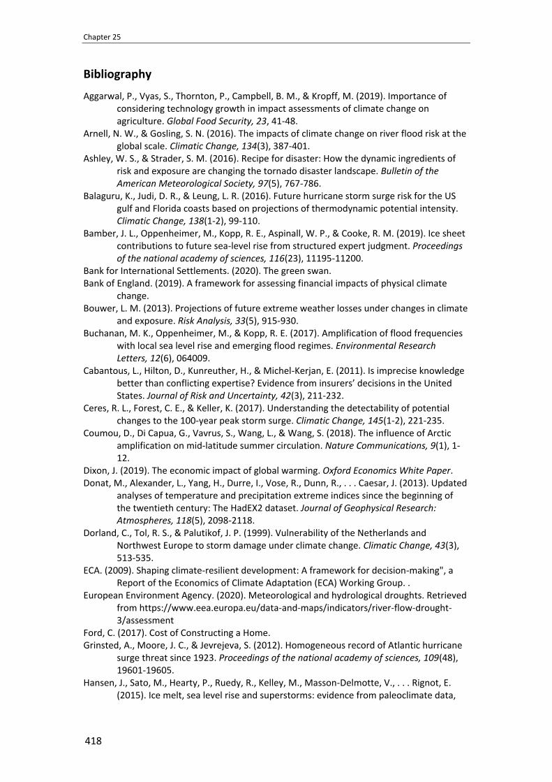
Chapter 25
418
Bibliography
Aggarwal, P., Vyas, S., Thornton, P., Campbell, B. M., & Kropff, M. (2019). Importance of considering technology growth in impact assessments of climate change on agriculture. Global Food Security, 23, 41-48.
Arnell, N. W., & Gosling, S. N. (2016). The impacts of climate change on river flood risk at the global scale. Climatic Change, 134(3), 387-401.
Ashley, W. S., & Strader, S. M. (2016). Recipe for disaster: How the dynamic ingredients of risk and exposure are changing the tornado disaster landscape. Bulletin of the American Meteorological Society, 97(5), 767-786.
Balaguru, K., Judi, D. R., & Leung, L. R. (2016). Future hurricane storm surge risk for the US gulf and Florida coasts based on projections of thermodynamic potential intensity. Climatic Change, 138(1-2), 99-110.
Bamber, J. L., Oppenheimer, M., Kopp, R. E., Aspinall, W. P., & Cooke, R. M. (2019). Ice sheet contributions to future sea-level rise from structured expert judgment. Proceedings of the national academy of sciences, 116(23), 11195-11200.
Bank for International Settlements. (2020). The green swan. Bank of England. (2019). A framework for assessing financial impacts of physical climate
change. Bouwer, L. M. (2013). Projections of future extreme weather losses under changes in climate
and exposure. Risk Analysis, 33(5), 915-930. Buchanan, M. K., Oppenheimer, M., & Kopp, R. E. (2017). Amplification of flood frequencies
with local sea level rise and emerging flood regimes. Environmental Research Letters, 12(6), 064009.
Cabantous, L., Hilton, D., Kunreuther, H., & Michel-Kerjan, E. (2011). Is imprecise knowledge better than conflicting expertise? Evidence from insurers’ decisions in the United States. Journal of Risk and Uncertainty, 42(3), 211-232.
Ceres, R. L., Forest, C. E., & Keller, K. (2017). Understanding the detectability of potential changes to the 100-year peak storm surge. Climatic Change, 145(1-2), 221-235.
Coumou, D., Di Capua, G., Vavrus, S., Wang, L., & Wang, S. (2018). The influence of Arctic amplification on mid-latitude summer circulation. Nature Communications, 9(1), 1-12.
Dixon, J. (2019). The economic impact of global warming. Oxford Economics White Paper. Donat, M., Alexander, L., Yang, H., Durre, I., Vose, R., Dunn, R., . . . Caesar, J. (2013). Updated
analyses of temperature and precipitation extreme indices since the beginning of the twentieth century: The HadEX2 dataset. Journal of Geophysical Research: Atmospheres, 118(5), 2098-2118.
Dorland, C., Tol, R. S., & Palutikof, J. P. (1999). Vulnerability of the Netherlands and Northwest Europe to storm damage under climate change. Climatic Change, 43(3), 513-535.
ECA. (2009). Shaping climate-resilient development: A framework for decision-making", a Report of the Economics of Climate Adaptation (ECA) Working Group. .
European Environment Agency. (2020). Meteorological and hydrological droughts. Retrieved from https://www.eea.europa.eu/data-and-maps/indicators/river-flow-drought-3/assessment
Ford, C. (2017). Cost of Constructing a Home. Grinsted, A., Moore, J. C., & Jevrejeva, S. (2012). Homogeneous record of Atlantic hurricane
surge threat since 1923. Proceedings of the national academy of sciences, 109(48), 19601-19605.
Hansen, J., Sato, M., Hearty, P., Ruedy, R., Kelley, M., Masson-Delmotte, V., . . . Rignot, E. (2015). Ice melt, sea level rise and superstorms: evidence from paleoclimate data,

Modelling Climate Change Risk for the Insurance Industry
419
climate modeling, and modern observations that 2° C global warming is highly dangerous. Atmospheric Chemistry & Physics Discussions, 15(14).
Heal, G. (2017). The economics of the climate. Journal of Economic Literature, 55(3), 1046-1063.
Hoerling, M., Eischeid, J., Perlwitz, J., Quan, X.-W., Wolter, K., & Cheng, L. (2016). Characterizing recent trends in US heavy precipitation. Journal of Climate, 29(7), 2313-2332.
IPCC. (2007). Climate change 2007-the physical science basis. IPCC. (2013). Summary for policymakers. Climate change 2013 - the physical science basis IPCC. (2014). Climate Change 2014: Synthesis Report. IPCC. (2018). Summary for Policymakers. Global Warming of 1.5 C. An IPCC Special Report on
the Impacts of Global Warming of 1.5 C Above pre-Industrial Levels., Global Warming of 1.5 C. An IPCC Special Report on the Impacts of Global Warming of 1.5 C Above Pre-Industrial Levels and Related Global Greenhouse gas Emission Pathways, in the Context of Strengthening the Global Response to the Threat of Climate Change. In.
IPCC. (2019). Climate Change and Land: an IPCC special report on climate change, desertification, land degradation, sustainable land management, food security, and greenhouse gas fluxes in terrestrial ecosystems.
Johnston, L. M. (2018). Current research on Canada’s interface areas. Canadian Wildland Fire and Smoke Newsletter, Spring 2018.
Johnston, L. M., & Flannigan, M. D. (2018). Mapping Canadian wildland fire interface areas. International journal of wildland fire, 27(1), 1-14.
Kossin, J. P. (2018). A global slowdown of tropical-cyclone translation speed. Nature, 558(7708), 104-107.
Kunreuther, H., Heal, G., Allen, M., Edenhofer, O., Field, C. B., & Yohe, G. (2013). Risk management and climate change. Nature Climate Change, 3(5), 447-450.
Linkin, M., & Schwartz, M. (2017). Hurricane Andrew: The 20 miles that saved Miami, Swiss Re.
Liu, M., Vecchi, G. A., Smith, J. A., & Knutson, T. R. (2019). Causes of large projected increases in hurricane precipitation rates with global warming. npj Climate and Atmospheric Science, 2(1), 1-5.
Marsooli, R., Lin, N., Emanuel, K., & Feng, K. (2019). Climate change exacerbates hurricane flood hazards along US Atlantic and Gulf Coasts in spatially varying patterns. Nature Communications, 10(1), 1-9.
McKinsey Global Institute. (2020). Climate risk and response: Physical hazards and socioeconomic impacts.
Meinshausen, M., Meinshausen, N., Hare, W., Raper, S. C., Frieler, K., Knutti, R., . . . Allen, M. R. (2009). Greenhouse-gas emission targets for limiting global warming to 2 C. Nature, 458(7242), 1158-1162.
Millner, A., Dietz, S., & Heal, G. (2013). Scientific ambiguity and climate policy. Environmental and Resource Economics, 55(1), 21-46.
Naz, B. S., Kao, S.-C., Ashfaq, M., Rastogi, D., Mei, R., & Bowling, L. C. (2016). Regional hydrologic response to climate change in the conterminous United States using high-resolution hydroclimate simulations. Global and Planetary Change, 143, 100-117.
Neumann, B., Vafeidis, A. T., Zimmermann, J., & Nicholls, R. J. (2015). Future coastal population growth and exposure to sea-level rise and coastal flooding-a global assessment. PloS one, 10(3), e0118571.
Neumann, J. E., Emanuel, K., Ravela, S., Ludwig, L., Kirshen, P., Bosma, K., & Martinich, J. (2015). Joint effects of storm surge and sea-level rise on US Coasts: new economic

Chapter 25
420
estimates of impacts, adaptation, and benefits of mitigation policy. Climatic Change, 129(1-2), 337-349.
Ornes, S. (2018). Core Concept: How does climate change influence extreme weather? Impact attribution research seeks answers. Proceedings of the national academy of sciences, 115(33), 8232-8235.
Parisien, M.-A., Dawe, D. A., Miller, C., Stockdale, C. A., & Armitage, O. B. (2020). Applications of simulation-based burn probability modelling: a review. International journal of wildland fire, 28(12), 913-926.
Peterson, T. C., Heim Jr, R. R., Hirsch, R., Kaiser, D. P., Brooks, H., Diffenbaugh, N. S., . . . Karl, T. R. (2013). Monitoring and understanding changes in heat waves, cold waves, floods, and droughts in the United States: state of knowledge. Bulletin of the American Meteorological Society, 94(6), 821-834.
Pielke Jr, R. A. (2007). Future economic damage from tropical cyclones: sensitivities to societal and climate changes. Philosophical Transactions of the Royal Society A: Mathematical, Physical and Engineering Sciences, 365(1860), 2717-2729.
Pindyck, R. S. (2011). Fat tails, thin tails, and climate change policy. Review of Environmental Economics and Policy, 5(2), 258-274.
Pindyck, R. S. (2013). Climate change policy: What do the models tell us? Journal of Economic Literature, 51(3), 860-872.
Radeloff, V. C., Helmers, D. P., Kramer, H. A., Mockrin, M. H., Alexandre, P. M., Bar-Massada, A., . . . Syphard, A. D. (2018). Rapid growth of the US wildland-urban interface raises wildfire risk. Proceedings of the national academy of sciences, 115(13), 3314-3319.
Romm, J. (2018). Climate Change: What Everyone Needs to Know®: Oxford University Press. Salathé Jr, E. P., Hamlet, A. F., Mass, C. F., Lee, S.-Y., Stumbaugh, M., & Steed, R. (2014).
Estimates of twenty-first-century flood risk in the Pacific Northwest based on regional climate model simulations. Journal of Hydrometeorology, 15(5), 1881-1899.
Schmidt, S., Kemfert, C., & Faust, E. (2009). Simulation of economic losses from tropical cyclones in the years 2015 and 2050: the effects of anthropogenic climate change and growing wealth.
Schuur, E. A., McGuire, A. D., Schädel, C., Grosse, G., Harden, J., Hayes, D. J., . . . Lawrence, D. M. (2015). Climate change and the permafrost carbon feedback. Nature, 520(7546), 171-179.
Shapley, M. D., Johnson, W., Engstrom, D., & Osterkamp, W. (2005). Late-Holocene flooding and drought in the Northern Great Plains, USA, reconstructed from tree rings, lake sediments and ancient shorelines. The Holocene, 15(1), 29-41.
Slater, L. J., & Villarini, G. (2016). Recent trends in US flood risk. Geophysical Research Letters, 43(24), 12,428-412,436.
Sobel, A. (2019). Testimony before the House, Science, Space, and Technology Committee of the House of Representatives. Washington, DC, 26 September 2019.
Swiss Re Institute. (2017). Wildfire in Canada: Fostering resilience through advances in modelling, Swiss Re.
Swiss Re Institute. (2019). Swiss Re SONAR: New emerging risk insights, Swiss Re. Talke, S. A., Orton, P., & Jay, D. A. (2014). Increasing storm tides in new york harbor, 1844–
2013. Geophysical Research Letters, 41(9), 3149-3155. TCFD. (2017). Technical Supplement: The Use of Scenario Analysis in Disclosure of Climate-
Related Risks and Opportunities. In: Task Force on Climate-Related Financial Disclosures.
United Nations Department of Economic Social Affairs. (2018). 2018 revision of world urbanization prospects.
United Nations Department of Economic Social Affairs. (2019). World Population Prospects: The 2019 Revision, Department of Economic and Social Affairs.

Modelling Climate Change Risk for the Insurance Industry
421
Van Oldenborgh, G. J., Van Der Wiel, K., Sebastian, A., Singh, R., Arrighi, J., Otto, F., . . . Cullen, H. (2017). Attribution of extreme rainfall from Hurricane Harvey, August 2017. Environmental Research Letters, 12(12), 124009.
Villarini, G., Smith, J. A., Baeck, M. L., & Krajewski, W. F. (2011). Examining flood frequency distributions in the Midwest US 1. JAWRA Journal of the American Water Resources Association, 47(3), 447-463.
Wagner, G., & Weitzman, M. L. (2015). Climate shock: the economic consequences of a hotter planet: Princeton University Press.
Wahl, T., Jain, S., Bender, J., Meyers, S. D., & Luther, M. E. (2015). Increasing risk of compound flooding from storm surge and rainfall for major US cities. Nature Climate Change, 5(12), 1093-1097.
Weinkle, J., & Pielke Jr, R. (2017). The Truthiness about hurricane catastrophe models. Science, Technology, & Human Values, 42(4), 547-576.
Weitzman, M. L. (2011). Fat-tailed uncertainty in the economics of catastrophic climate change. Review of Environmental Economics and Policy, 5(2), 275-292.
Weitzman, M. L. (2012). GHG targets as insurance against catastrophic climate damages. Journal of Public Economic Theory, 14(2), 221-244.
Wobus, C., Gutmann, E., Jones, R., Rissing, M., Mizukami, N., Lorie, M., . . . Martinich, J. (2017). Climate change impacts on flood risk and asset damages within mapped 100-year floodplains of the contiguous United States. Natural Hazards and Earth System Sciences, 17(12), 2199.
Zhang, W., Villarini, G., Vecchi, G. A., & Smith, J. A. (2018). Urbanization exacerbated the rainfall and flooding caused by hurricane Harvey in Houston. Nature, 563(7731), 384-388.
Zhang, Y.-K., & Schilling, K. (2006). Increasing streamflow and baseflow in Mississippi River since the 1940 s: Effect of land use change. Journal of Hydrology, 324(1-4), 412-422.

Chapter 25
422
Disclaimer
© 2020 Swiss Re. All rights reserved.
The entire content of this chapter is subject to copyright with all rights reserved. The information may be used for private or internal purposes, provided that any copyright or other proprietary notices are not removed. Electronic reuse of the data published in this report is prohibited.
Reproduction in whole or in part or use for any public purpose is permitted only with the prior written approval of Swiss Re Institute. Courtesy copies are appreciated.
Although all the information used in this study was taken from reliable sources, Swiss Re does not accept any responsibility for the accuracy or comprehensiveness of the information given or forward looking statements made. The information provided and forward-looking statements made are for informational purposes only and in no way constitute or should be taken to reflect Swiss Re’s position, in particular in relation to any ongoing or future dispute. In no event shall Swiss Re be liable for any loss or damage arising in connection with the use of this information and readers are cautioned not to place undue reliance on forward-looking statements. Swiss Re undertakes no obligation to publicly revise or update any forward-looking statements, whether as a result of new information, future events or otherwise.

423
Part III ESG Index and Rating Methodologies

Chapter 26
424
MSCI Tools for ESG Risk Management
By
MSCI ESG Research LLC1,2
Abstract
This chapter introduces three tools developed by MSCI to support ESG integration: ESG Ratings, ESG Indexes, and ESG Analytics3. ESG Ratings aims to help investors to identify and quantify the ESG risks and opportunities. ESG Indexes provide institutional investors with indexes that can be used manage and report on ESG mandates or as benchmarks to measure ESG investment performance. ESG Analytics can help investors integrate ESG Ratings and Indexes into their security selection and portfolio construction processes, stress testing, and risk and performance attribution analysis. We also discussed several transmission channels linking companies’ ESG performance with their financial performance.
Keywords: ESG ratings, ESG indexes, ESG and financial returns
1 Introduction
In recent years, institutional investor adoption of environmental, social and governance (ESG) investing and the subsequent growth in ESG assets under management has accelerated. While many factors have contributed to this growth, we focus here on three primary drivers of increased ESG investment: sustainability challenges, shifts in investor preferences, and improvement in data and analytics.
The world itself is changing: As companies face rising complexity on a global scale, modern investors are reevaluating traditional investment approaches global sustainability challenges such as flood risk and sea level rise, privacy and data security, demographic shifts, and regulatory pressures, are introducing new risk factors for investors that may not have been previously seen.
Investor preferences are changing: A growing body of studies suggest that millennials - as well as women - are asking more of their investments. Over the next two to three decades, the millennial generation could shift between $15 trillion and $20 trillion into U.S.-domiciled ESG investments, roughly doubling the size of the U.S. equity market (Bank of America Corporation, 2018).
1 This chapter is written by Emma Wu, MSCI ESG Research LLC, email: [email protected]; and Xiaoshu Wang, MSCI ESG
Research LLC, email: [email protected], based on publications by MSCI on ESG methodologies and related
research topics. 2 Certain information © 2020 and reproduced by permission of MSCI ESG Research LLC; all rights reserved. The ESG data
contained herein is the property of MSCI ESG Research LLC, its affiliates and/or information providers (“MSCI ESG”). MSCI
ESG makes no warranties with respect to any such ESG data. The ESG data contained herein is used under license and may
not be further used, distributed or disseminated without the express written consent of MSCI ESG. 3 MSCI ESG Ratings are produced by MSCI ESG Research LLC. MSCI ESG Indexes and Analytics utilize information from,
but are not provided by, MSCI ESG Research LLC. MSCI Indexes and Analytics are products of MSCI Inc. MSCI Indexes are
administered by MSCI Limited (UK).

MSCI Tools for ESG Risk Management
425
Investment data and analytics are evolving: Better data and analytics have paved the way for numerous studies that explore ESG investing. Better data from companies, combined with better ESG research and analytics capabilities, have resulted in more systematic, quantitative, objective and financially relevant approaches to ESG key issues.
Since its founding in 2006, the United Nations Principles for Responsible Investing (PRI) has attracted support from more than 1,800 signatories, representing over USD $68 trillion in assets under management as of April 2017. Signatories commit to six voluntary principles, the first of which is the incorporation of ESG issues into investment analysis and decision-making. More than $270 billion in assets have been allocated to investments tracking / benchmarked to MSCI ESG equity & fixed income indexes since 2014.4
2 MSCI Tools for ESG analysis and integration
In this section, we introduce three sets of MSCI tools for ESG analysis: ESG ratings, indexes, and analytics. ESG ratings aims to help investors to identify and quantify the ESG risks and opportunities. MSCI’s ESG Indexes provide institutional investors with indexes that can be used manage and report on ESG mandates or as benchmarks to measure ESG investment performance. ESG analytics can help investors integrate ESG ratings and indexes into their security selection and portfolio construction processes, stress testing, and risk and performance attribution analysis.
MSCI ESG Ratings MSCI ESG Ratings help investors identify ESG risks and opportunities within their portfolio. We research and rate companies on a ‘CCC’ (worst) to ‘AAA’ (best) scale according to their exposure to industry specific ESG risks and their ability to manage those risks relative to peers (Figure 26-1). Currently, MSCI ESG Ratings cover approximately 7,500 companies (13,500 total issuers, including subsidiaries) and more than 650,000 equity and fixed income securities globally.
Figure 26-1 MSCI ESG Rating scale
Issues addressed by ESG ratings The overall objective of MSCI ESG Ratings is to assess how well, relative to industry peers, a given company manages most relevant environmental, social and governance risks and
4 Based on publicly available information or press releases published by MSCI from 2014 to date.

Chapter 26
426
opportunities to ensure sustainable business growth. The MSCI ESG Rating model does so by addressing four key questions:
• What are the most significant ESG risks and opportunities facing a company and its industry?
• How exposed is the company to those key risks and/or opportunities?
• How well is the company managing key risks and opportunities?
• Based on its level of exposure and management of relevant risks and opportunities, how does the company compare to its global industry peers?
Environmental, social, and governance risks and opportunities are posed by large scale trends (e.g. climate change, resource scarcity, demographic shifts) as well as by the nature of the company’s operations. Companies in the same industry generally face the same major risks and opportunities, though individual exposure can vary.
A risk is considered financially relevant to an industry when it is likely that companies in a given industry will incur substantial costs in connection with it (for example: regulatory ban on a key chemical input requiring reformulation). An industry could see growth opportunity when it is likely that companies in a given industry could capitalize on social or environmental trends (for example: opportunities in clean technology for the LED lighting industry). The MSCI ESG Ratings model focuses only on issues that are determined to be most relevant for each industry.
We identify relevant risks and opportunities for each industry through a quantitative model that looks at ranges and average values for each industry for externalized impacts such as carbon intensity, water intensity, and injury rates. Companies with unusual business models for their industry may face fewer or additional key risks and opportunities. Company-specific exceptions are allowed for companies with diversified business models, facing controversies, or based on industry rules. Once identified, these key Issues are assigned to each industry and company. Three examples of these key issues are provided below.
Carbon Emissions: this issue evaluates the extent to which companies may face increased costs linked to carbon pricing or regulatory caps. Scores are based on exposure to GHG-intensive businesses and emerging regulations; carbon reduction targets and mitigation programs; and carbon intensity over time and vs. peers.
Labor Management: this issue evaluates the extent to which companies may face workflow disruptions due to labor unrest or reduced productivity due to poor job satisfaction. Scores are based on exposure to regions facing labor unrest, size of workforce, and corporate restructuring/layoffs; workforce policies, benefits, training, and employee engagement; and labor-related controversies.
Corporate Governance – Board: this issue is scored primarily on the basis of the board’s independence from management, and on various measures of board experience and effectiveness. Metrics included in this component evaluate basic board structures such as overall board independence; individual director qualifications and experience, including industry and financial expertise, cases of executive misconduct, as well as areas of concern such as attendance and overboarding; and negative governance-related events.

MSCI Tools for ESG Risk Management
427
Setting Key Issue weights Once the key issues have been selected, we set the weights that determine each key issue’s contribution to the overall rating. Each key issue typically comprises 5-30% of the total ESG Rating. The weightings take into account both the contribution of the industry, relative to all other industries, to the negative or positive impact on the environment or society; and the timeline within which we expect that risk or opportunity for companies in the industry to materialize.
Key Issue assessment Our ESG ratings assess both ESG related risks and opportunities. To understand whether a company is adequately managing a key ESG risk, it is essential to understand both the management strategies it has employed and how exposed it is to the risk. The MSCI ESG Ratings model measures both of these: risk exposure and risk management. To score well on a key issue, management needs to be commensurate with the level of exposure: a company with high exposure must also have very strong management, whereas a company with limited exposure can have a more modest approach. Conversely, a highly exposed company with poor management will score worse than a company with the same management practices but lower exposure to the risk.
Assessment of opportunities works similarly to risks, but the model for combining exposure and management differs. Exposure indicates the relevance of the opportunity to a given company based on its current business and geographic segments. Management indicates the company’s capacity to take advantage of the opportunity. Where exposure is limited, the key issue score is constrained toward the middle of the 0-10 range, while high exposure allows for both higher and lower scores.
Constructing the rating The ESG Ratings model is industry relative and uses a weighted average approach. Key Issue weights are set at the GICS®5 Sub-Industry level (8-digit) based on each industry’s relative external impact and the time horizon associated with each risk. Key Issues and weights undergo a formal review and feedback process at the end of each calendar year.
Corporate governance is equally relevant for all industries and therefore always weighted and analyzed for all companies. Where there are company-specific exceptions, weights depart from the industry standard weights but remain in proportion. For each company a Weighted Average Key Issue Score is calculated based on the underlying Key Issue scores and weights.
To arrive at a final letter rating, the Weighted Average Key Issue Score is normalized by industry. The range of scores for each industry is established annually by taking a rolling three-year average of the top and bottom scores among the MSCI ACWI Index constituents; the values are set at the 97.5th and 2.5th percentile. Using these ranges, the Weighted Average Key Issue Score is converted to an Industry Adjusted Score from 0-10, where zero is worst and 10 is best. The Industry Adjusted Score corresponds to a rating between worst (CCC) and best (AAA). These assessments of company performance are not absolute but are explicitly intended to be relative to the standards and performance of a company’s industry peers.
Data sources To assess companies’ exposure to and management of ESG risks and opportunities, we collect data from the following sources:
5 GICS, the global industry classification standard jointly developed by MSCI Inc. and S&P Global.

Chapter 26
428
• Macro data at segment or geographic level from academic, government, NGO datasets (e.g. Transparency International, US EPA, World Bank)
• Company disclosure (10-K, sustainability report, proxy report, AGM results, etc.)
• Government databases, 1600+ media, NGO, other stakeholder sources regarding specific companies
Issuer communications Companies are invited to participate in a formal data verification process prior to publication of their ESG Rating report. At that time, companies have the opportunity to review and comment on the facts contained in their existing MSCI ESG Rating report, as well as to provide MSCI ESG Research any additional ESG information if they wish. This process is also in accordance with the objective of frequently updating company reports with the latest available information as provided by companies. Issuers may request to see their reports and/or to provide updates or corrections at any time.
Monitoring and updates Companies are monitored on a systematic and ongoing basis, including daily monitoring of controversies and governance events. New information is reflected in reports on a weekly basis and significant score changes trigger analyst review and re-rating. Companies receive an in-depth review at least annually.
Quality review Formal in-depth quality review processes take place at each stage of analysis, including automated and quality checks of data and rating publication; industry and market lead oversight of ratings and reports; Methodology Committee approval of any exceptions, truncations, or major (two or more ratings level) rating changes; and an ESG Methodology Committee to review contentious cases.
Annual consultation In November of each year, MSCI ESG Research reviews the Key Issues assigned to each industry as well as their weights. This process also identifies emerging issues and those that have become less significant. As part of this process, MSCI ESG Research consults with clients about proposed changes to Key Issue selections for each industry as well as any proposed new Key Issues.
MSCI ESG Indexes MSCI ESG Indexes are designed to support common approaches to ESG investing, and help institutional investors more effectively benchmark to ESG investment performance as well as manage, measure and report on ESG mandates. MSCI ESG Indexes also provide institutional investors with transparency into ESG sustainability and values alignment, together with the ability to compare holdings.
The ESG integration indexes aim to maintain the key characteristics of the parent free float market capitalization indexes, either through an explicit tracking error constraint or by targeting sector weights that reflect the underlying parent indexes, designed to limit the systematic risk introduced by the ESG selection process.
Other indexes focus on single themes or issues, such as the MSCI Low Carbon Target Indexes, which are designed to achieve a target level of tracking error while minimizing carbon exposure. Indexes in the integration category are designed to help investors efficiently

MSCI Tools for ESG Risk Management
429
integrate ESG considerations into their core asset allocation without deviating from broad market characteristics.
Our indexes can be grouped into the value category and impact category. The value category aims to help investors to align their personal or ethical values, or faith, with their investment processes. These include the MSCI SRI Index, MSCI KLD 400 Index and the MSCI ex Controversial Weapons Index. The impact category indexes, such as the MSCI Sustainable Impact Index, include companies whose core business addresses at least one of the world’s social and environmental challenges, as defined by the United Nations Sustainable Development Goals. A few examples of these indexes are presented in the following boxes.

Chapter 26
430
Box 1:MSCI ESG Leaders Indexes
The MSCI ESG Leaders Indexes target companies that have the highest ESG Rating in each sector of the parent index. MSCI provides investors globally with ESG indexes designed to facilitate clients’ integration of ESG considerations into their investment process.
The indexes use a best-in-class approach by selecting companies that have the highest MSCI ESG Ratings. They are free float-adjusted market capitalization weighted indexes designed to represent the performance of companies that have favorable ESG profiles compared to industry peers. Overall the indexes target a 50% sector representation vs. the parent index.
The indexes are designed for institutional investors seeking exposure to companies with a strong sustainability profile and relatively low tracking error to the underlying equity market. The indexes aim to help investors seeking to:
• Mitigate short- and long-term ESG risk
• Meet their fiduciary obligations
• Mitigate reputational risk
• Maintain broad market exposure
• Have sector diversification
• Avoid taking active country or sector bets
Key features of MSCI ESG Leaders Indexes
• Leverages MSCI’s award winning MSCI ESG Research and ESG Ratings to identify companies that have demonstrated an ability to manage their ESG risks and opportunities
• Best-in-class approach – the indexes select the highest rated companies in each sector
• Designed to exclude companies involved in severe controversies
• Based on industry leading MSCI Indexes and are designed to enable seamless integration
• Parent index construction rules designed to achieve replicability
The indexes can be used as follows:
• As part of the portfolio creation process: Consistent market representation designed to represent a broad spectrum of the global equity opportunity set without home bias

MSCI Tools for ESG Risk Management
431
• Performance benchmarks for ESG funds for global mandates, with regional, country, sector and other subsets available for more targeted investment mandates
• May be licensed for use as the basis for structured products and other index-linked investment vehicles, such as exchange-traded funds (ETFs) and exchange-traded notes (ETNs)
• A source of research to aid ESG investment strategies
• To define a universe of securities that have a strong ESG profile
Figure 26-2 Cumulative index performance of MSCI World ESG Leaders Index— USD gross returns (September 2007 - February 2020)6
Table 26-1 Annual performance of MSCI World ESG Leaders Index
Source: MSCI as of Feb 28, 2020
6 All index performance data is historical and for informational purposes only. Past performance is not indicative of future
returns, which may differ materially.

Chapter 26
432
Figure 26-3 Cumulative Index Performance of MSCI Emerging Markets ESG Leaders Index — USD gross returns (September 2007 – February 2020)
Table 26-2 Annual performance of MSCI Emerging Markets ESG Leaders Index
Source: MSCI as of Feb 28, 2020

MSCI Tools for ESG Risk Management
433
Box 2: MSCI Low Carbon Indexes MSCI offers indexes designed to represent the performance of divestment and re-weighting strategies to reduce carbon exposure. These approaches are summarized below:
• Divestment strategies aim to enable institutions to have simple and clear communications with stakeholders but ignore short-term portfolio risks. For example, a portfolio replicating the MSCI Global ex Fossil Fuels Indexes aims to eliminate 100% of the policy benchmark’s carbon reserves exposure by excluding companies that own oil, gas and coal reserves.
• Re-weighting strategies, such as those applied to portfolios that track the MSCI Global Low Carbon Target Indexes, seek to increase exposure to more carbon-efficient companies while reducing short-term risk against the benchmark.
• Combining selection and re-weighting strategies may offer a clear message in communicating with stakeholders while taking into account short-term tracking error and long-term risk exposure to carbon-intensive companies. A portfolio replicating the MSCI Global Low Carbon Leaders Index would include companies with low carbon exposure while seeking to minimize ex-ante tracking error.
The MSCI Low Carbon Indexes are intended to help identify potential risks associated with the transition to a low carbon economy while representing the performance of the broad equity market. Launched in 2014 the index series are designed to address two dimensions of carbon exposure: carbon emissions and fossil fuel reserves.
MSCI Low Carbon Indexes can be split into two index suites:
• The MSCI Global Low Carbon Target Indexes re-weight stocks based on their carbon exposure in the form of carbon emissions and fossil fuel reserves. The indexes are designed to achieve maximum carbon exposure reduction and achieve 0.3% (30 basis points) ex ante tracking error target while minimizing carbon exposure relative to their parent indexes.
• The MSCI Global Low Carbon Leader Indexes aim to achieve at least 50% reduction in the carbon footprint of the parent index by excluding companies with the highest carbon emissions intensity and the largest owners of carbon reserves (per dollar of market capitalization). They also aim to minimize the tracking error relative to their parent index.
MSCI ESG Analytics Asset owners and their investment consultants increasingly demand systematic integration of ESG factors into their investment processes. Institutional investors often require regular reporting on the ESG exposures and characteristics of their investments. To meet these demands, user-friendly analytical tools are being developed by vendors. MSCI’s ESG research, data and indexes are available on its analytics systems, including the MSCI Beon platform. Investors can integrate MSCI ESG Ratings and MSCI Indexes into their security selection and portfolio construction processes, stress testing, and risk and performance attribution analysis.

Chapter 26
434
3 Has ESG historically compromised financial returns?
A common debate with ESG investing revolves around the idea that incorporating ESG factors into the investment process will hurt performance. However, many studies suggest that companies with robust ESG practices displayed a lower cost of capital, lower volatility, and fewer instances of bribery, corruption and fraud over certain time periods. And some studies have also shown that companies with poorer ESG performance have had a higher cost of capital, higher volatility due to controversies and other incidences such as spills, labor strikes and fraud, and accounting and other governance irregularities.7
Figure 26-4 Gross profitability of ESG quintiles
Note: Gross profitability (z-score) of size-adjusted ESG quintiles is computed as most recently reported sales less cost of goods sold, divided by most recently reported company total assets. Data from January 2007 to May 2017. Average value over the period is represented by blue dots; current exposure by red dots. The vertical bars represent the 5% to 95% range of observed values. Historical data for informational purposes only. Past performance is not indicative of future results, which may differ materially.
In a recent study (Melas et al., 2018), MSCI researchers focused on understanding how ESG characteristics have led to financially significant effects. The study examined how ESG information embedded within stocks is transmitted to the equity market. Borrowing from central banks, we created three “transmission channels” within a standard discounted cash flow (DCF) model. We call these the cash-flow channel, the idiosyncratic risk channel and the valuation channel. The former two channels are transmitted through corporations’ idiosyncratic risk profiles, whereas the latter transmission channel is linked to companies’ systematic risk profiles. Our research showed that ESG had an effect on valuation and performance of many of the companies in the study.
7 Sources: Chava, 2011; 20+ studies, both academic and industry; Lansilahti, 2012; Credit Suisse; Deutsche Bank; MSCI ESG
Research, et al.; Huang, 2010; Bhagat and Bolton, 2008; Cremers et al., 2005; Deutsche Bank, 2012; ISS, 2011; et al.

MSCI Tools for ESG Risk Management
435
Cash-flow channel: High ESG-rated companies were more competitive and generated abnormal returns, often leading to higher profitability and dividend payments, especially when compared to low ESG-rated companies.
Idiosyncratic risk channel: High ESG-rated companies experienced a lower frequency of idiosyncratic risk incidents such as major drawdowns. Conversely, companies with low ESG ratings were more likely to experience major incidents.
We saw that companies in the bottom fifth of the MSCI World Index experienced large drawdowns (above 95%) three times higher than those in the top fifth, as can be seen in the exhibit below, supporting the assertion that ESG has provided insight into incident risks throughout the 10-year period we studied.
Figure 26-5 Large drawdown frequency of top vs. bottom ESG quintile
Note: MSCI World Index, January 2007 to May 2017. We use a full three-year look-ahead window in reporting results. For each month, we report the number of stocks that realized a more than 95% cumulative loss over the next three years, taking the price at month end as the reference point for the return calculation. Thus, the last data point is from May Historical data for informational purposes only. Past performance is not indicative of future results, which may differ materially.
Valuation channel: High ESG-rated companies have shown lower systematic risk exposure, evidenced by less volatile earnings and less systematic volatility. Compared to low ESG-rated companies, they also experienced lower betas and lower costs of capital. In a DCF model framework, the systematic risk exposure affects the denominator of the DCF model, and a company with lower cost of capital would have a higher valuation.

Chapter 26
436
Figure 26-6 Systematic volatility of ESG quintiles
Note: Systematic volatility (or common factor risk) is calculated as the volatility predicted by all the factors of the GEMLT model. Data from January 2007 to May 2017. Average value over the period is represented by blue dots; current exposure by red dots. The vertical bars represent the 5% to 95% range of observed values. Historical data for informational purposes only. Past performance is not indicative of future results, which may differ materially.
4 Conclusion
The prominence of environmental, social, and governance issues on policy makers and the public agenda continues to fuel and shape the ESG investing landscape. MSCI delivers ESG indexes and analytics, and MSCI ESG Research delivers ratings, research and metrics, to help investors navigate this challenging landscape. As a pioneer in ESG Research and analytical tools, MSCI ESG Research offers an extensive history of data, scores, and ratings that enable more informed analysis of ESG risks and opportunities across all aspects of the investment process – from defining investment policy and selecting benchmarks to research, portfolio construction and risk management, engagement and reporting.

MSCI Tools for ESG Risk Management
437
Bibliography
Bank of America Corporation. (2018). 2016 Environmental Social & Governance Report. Melas, D., Nagy., Z., Nishikawa, L., Lee, L.-E., & Giese, G., (2019). Foundations of ESG Part 1:
How ESG Affects Equity Valuation, Risk and Performance, MSCI.

Chapter 27
438
Moody’s Approach to Incorporating ESG Risks into Credit Analysis
By
Moody’s Investors Service1,2
Abstract
This chapter provides an overview of Moody’s approach to incorporating ESG risks into credit analysis. It starts with a discussion of the general principles for assessing Environmental, Social and Governance (ESG) risks, followed by some key findings from Moody’s Environmental Risks Global Heat Map, a framework to assess carbon transition risk for corporate sectors, and the ESG impact analysis on the bank ratings.
Keywords: ratings, credit impact, ESG considerations, environmental risk, social risk, governance risk, heat map, climate change
1 General principles for assessing Environmental, Social and
Governance risks
Introduction In our credit analysis, Moody’s seeks to be comprehensive, incorporating the broadest possible view into the material considerations that can affect the credit quality of an issuer or sector.3 Our objective is to capture all considerations that have a material impact on credit quality.4 We are focused on the material credit considerations that may influence the relative risk of default and expected financial loss in the event of default for issuers and debt obligations over all time horizons, regardless of whether or not they are classified as ESG risks. However, a precise and widely accepted classification of ESG risks would be useful for more transparently describing when ESG risks are credit drivers behind our ratings.
In our analysis, we identify and assess credit implications arising from all material ESG considerations that we can discern, whether they have a current impact or a potential future impact. Material risks could include the impact that a prolonged drought has on a municipality’s tax revenue and capital spending on water infrastructure, or the likely credit
1 This Chapter is compiled by Moody’s Investors Service. For further details, please contact Brian Cahill, Managing Director
– Global Head ESG, email: [email protected]; Li Ma, Managing Director – Corporate Finance, email:
[email protected]; Jessie Tung, VP – Senior Credit Officer, Corporate Finance, email: [email protected]. 2 Contents of this chapter draw from various Moody ’ s publications, including: "General Principles for Assessing
Environmental, Social and Governance Risks", January 2019; "Environmental Risk - Global: Heat map: 11 sectors with $2.2
trillion debt have elevated environmental risk exposure", September 2018 ; “ Non-financial companies – Global:
Framework to assess carbon transition risk for corporate sectors”, September 2019;and "Banking - Global: The impact of
environmental, social and governance risks on bank ratings", July 2019. 3 See “Cross-Sector Rating Methodology: General Principles for Assessing Environmental, Social and Governance Risks”,
Moody’s Investors Service, January 2019. 4 Considerations that are material to credit quality may not include all investment parameters that some market participants
would regard as green, sustainable or ethical.

Moody’s Approach to Incorporating ESG Risks into Credit Analysis
439
impacts that regulatory frameworks and ESG-related laws, policies and regulations will have on rated issuers and sectors as a whole.5 We also assess any mitigating or adaptive behavior that issuers undertake. In some instances, we may identify ESG trends that are positive for an issuer’s credit profile.
In order to be meaningful for ratings, ESG considerations must be material with regard to the likelihood of default and credit loss. Issuers encounter a multitude of ESG risks and opportunities, many of which have little tangible impact on operating or financial performance. For example, a company’s volunteer work, charitable activities and other such initiatives are important to the extent that they produce social value, but their potential positive impact on the company’s financial health or credit standing is unlikely to be material.
The materiality of a particular aspect of ESG is typically specific to a sector or even an issuer or a transaction. For example, air pollution emissions standards may be an important credit issue for the auto manufacturing sector but may not be meaningful for the credit quality of media companies. The strategies issuers within a given sector follow to address an ESG risk that is common to them all may result in improvements in credit strength for some issuers and deterioration in credit strength for others.
Our approach to ESG considerations is similar to our approach for other material credit considerations in that it includes an assessment of the impact on an issuer’s cash flows and the value of its assets over time; the sufficiency of cash flows and assets in relation to the issuer’s debt burden and other financial obligations; and liquidity and the ability to access capital. Typically, for two issuers at the same rating level, the issuer with greater stability of cash flows can carry higher levels of leverage than the issuer that has less stable cash flows. Visibility into future cash flows is also an important consideration.
For example, for a non-financial corporate, we seek to assess how ESG issues such as reputation for product safety and carbon transition risks influence credit drivers such as demand for its products, the cost of production and the need for financing to make capital expenditures, as well as the potential that these drivers could change meaningfully over time (Figure 27-1). For structured finance transactions, we typically assess how ESG considerations may affect underlying asset values, in addition to considering how the special purpose vehicle’s governance affects creditors. For sovereigns, meanwhile, we seek to assess how ESG considerations such as the economic effects of environmental issues, including climate change, or social and governance-related issues, such as control of corruption and the rule of law, could affect GDP, the trajectory and stability of the government’s revenues and expenditures as well as the government’s ability to withstand shocks, among other drivers of government creditworthiness (Figure 27-2).
5 Ratings and rating actions, even those in response to policy decisions or changes, do not express judgments on the
appropriateness of any policy; rather, they reflect our view of how those policies affect the ability of an issuer to repay its
financial obligations.

Chapter 27
440
Figure 27-1 An Illustration of How ESG Considerations Are Captured in Corporate Credit Ratings
Source: Moody’s Investors Service
Note: The information in this exhibit is not exhaustive.
Figure 27-2 An Illustration of How ESG Considerations Are Captured in Sovereign Credit Ratings
Source: Moody’s Investors Service
Note: The information in this exhibit is not exhaustive.
General principles for assessing environmental risk Environmental risks are a significant consideration for a large number of issuers in the public and private sectors. We view environmental risk as falling broadly into two categories: (i) the consequences of regulatory or policy initiatives that seek to reduce or prevent environmental trends or hazards or perceived trends or hazards; and (ii) the adverse effects of direct environmental trends and hazards, such as pollution, drought, severe natural and human-

Moody’s Approach to Incorporating ESG Risks into Credit Analysis
441
caused disasters, and climate change. Some environmental considerations straddle these categories, such as carbon transition risk, where we consider the regulatory risk and the potential direct effect of the hazards that may result.
Among environmental risks, we see three tiers related to timing, certainty and severity:
• Regulations that have been implemented or those that are likely to be introduced (given, for example, proposals by regulators or legislators or binding agreements under an international accord) have the clearest impact on the credit profiles of issuers and sectors.
• Longer-term regulatory initiatives where implementation is unclear or subject to delays or meaningful regional variations (given, for example, very general agreements under an international accord with no enforcement mechanisms) provide less visibility into the likely impacts on the relative risk of default and credit loss for issuers. Lack of clarity may also diminish issuers' ability to adapt to regulations, adding a further layer of uncertainty regarding the credit implications.
• Direct environmental trends such as the those arising from climate change (for example, rising temperatures) are typically incremental, developing over very long time frames, with diffuse consequences and limited immediate impact on ratings. High impact environmental hazards such as hurricanes or cyclones, wildfires or floods are episodic; they can be severe, concentrated in their impact and can sometimes have an immediate impact on ratings. The credit impact of long-term environmental trends or future hazards may be curbed or offset by other influences. These could include the implementation of regulations or technological changes that mitigate the effects of the trend, adaptation strategies such as improvements in physical and institutional infrastructure, or rising income levels that increase a government’s tax base, allowing it to finance needed improvements.
The impact of these risks may affect factor or sub-factor scoring in methodology scorecards; for example, these risks could affect our forward-looking assessment of business profile, leverage and coverage, economic strength or GDP, or they may be considered outside of the scorecard. We also consider environmental risks in tandem with other issuer or sector characteristics that may mitigate or exacerbate their impact.
For example, factors such as scale, high barriers to entry, the ability to recover rising costs from customers or taxpayers, financial flexibility, and expertise in handling operational and regulatory issues are important to the ability of issuers in most sectors to handle environmental exposures and implement adaptation strategies while maintaining their credit profiles. Conversely, small scale, geographic concentration, low income levels and deteriorating demographic trends make some issuers much more susceptible to environmental hazards or less likely to be able to implement adaptation strategies.
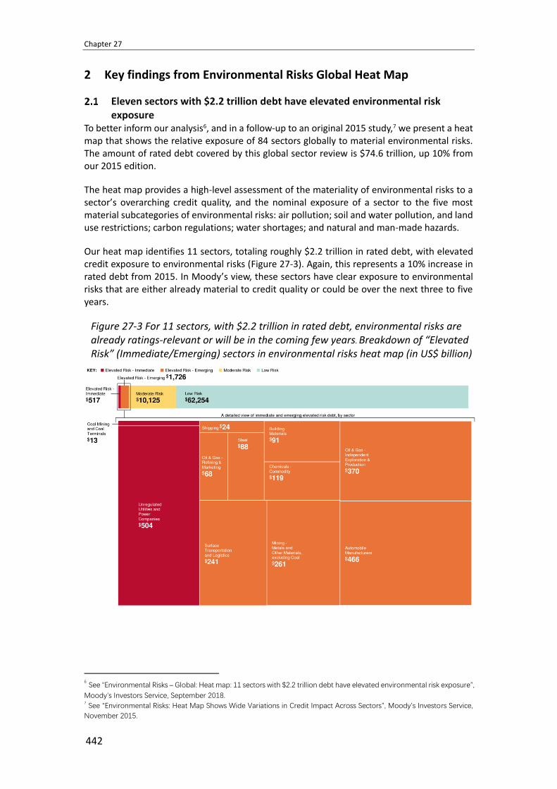
Chapter 27
442
2 Key findings from Environmental Risks Global Heat Map
Eleven sectors with $2.2 trillion debt have elevated environmental risk exposure
To better inform our analysis6, and in a follow-up to an original 2015 study,7 we present a heat map that shows the relative exposure of 84 sectors globally to material environmental risks. The amount of rated debt covered by this global sector review is $74.6 trillion, up 10% from our 2015 edition.
The heat map provides a high-level assessment of the materiality of environmental risks to a sector’s overarching credit quality, and the nominal exposure of a sector to the five most material subcategories of environmental risks: air pollution; soil and water pollution, and land use restrictions; carbon regulations; water shortages; and natural and man-made hazards.
Our heat map identifies 11 sectors, totaling roughly $2.2 trillion in rated debt, with elevated credit exposure to environmental risks (Figure 27-3). Again, this represents a 10% increase in rated debt from 2015. In Moody’s view, these sectors have clear exposure to environmental risks that are either already material to credit quality or could be over the next three to five years.
Figure 27-3 For 11 sectors, with $2.2 trillion in rated debt, environmental risks are already ratings-relevant or will be in the coming few years. Breakdown of “Elevated Risk” (Immediate/Emerging) sectors in environmental risks heat map (in US$ billion)
6 See “Environmental Risks – Global: Heat map: 11 sectors with $2.2 trillion debt have elevated environmental risk exposure”,
Moody’s Investors Service, September 2018. 7 See “Environmental Risks: Heat Map Shows Wide Variations in Credit Impact Across Sectors”, Moody’s Investors Service,
November 2015.

Moody’s Approach to Incorporating ESG Risks into Credit Analysis
443
Source: Moody’s Investors Service
Note: Boxes are sized relative to the value of rated debt (in US$ billion) and color indicated for overall credit exposure.
The relative scoring in our 2018 environmental risks heat map remains largely stable since our 2015 edition. However, there have been a number of changes in overall scoring, as illustrated in Figure 27-4. Shipping, and surface transportation and logistics are now scored as “Elevated Risk - Emerging,” compared with “Moderate Risk” previously, reflecting a gradual tightening of environmental regulations and emissions standards. Six sectors accounting for $1.8 trillion in rated debt move to “Moderate Risk” from “Low Risk.” While the specific rationale for these changes is sector-specific, the change to scores generally reflects our view that the potential for environmental risks to become material for these sectors over five or more years has increased. Meanwhile, power generation projects move down to “Moderate Risk” from “Elevated Risk - Emerging,” as a result of a shift in our rated portfolio toward renewable generation. Finally, two new sectors – pension funds and asset managers – have been added, both scoring “Low Risk.”
Figure 27-4 Changes in overall sector environmental risk scores since 2015. Heat map score and rated debt, US$ billion.
Source: Moody’s Investors Service
Note: For 2015 heat map, see “Environmental Risks: Heat Map Shows Wide Variations in Credit Impact Across Sectors”, November 2015.
Two sectors – coal mining and terminals, and unregulated utilities and power companies – are scored as “Elevated Risk – Immediate”
Coal mining and coal terminals, and unregulated utilities and power companies (with total outstanding rated debt of $517 billion) have already experienced material credit pressure as a result of environmental risks.
Indeed, environmental considerations have constrained credit quality and contributed to downward pressure on the ratings of coal companies, primarily through reducing demand for the commodity. Such pressures are incorporated into our present and future view of coal producers’ revenues and margins, although the degree of impact varies by region and type of coal. For example, metallurgical coal producers are not facing the same demand pressures as thermal coal producers. Notably, the US coal industry has undergone a significant ratings

Chapter 27
444
migration due, in part, to the impact of rising environmental concerns related to the use of coal and eroding cost competitiveness compared with gas and renewables.
Unregulated utilities and power companies, meanwhile, are directly exposed to the policy pressure to cut emissions, which continues to disrupt business models and pressure margins in mature economies. The overall credit impact for a particular issuer is a function of a number of variables, notably the share of generation in the company’s total business, generation technology, and geographic location. For instance, the impact on generators is more pronounced in Europe than in Asia, because power demand is still growing significantly in the latter and emission reduction policies are less stringent in many countries there.
Nine sectors are categorized as “Elevated Risk – Emerging" meaning that the credit impact of environmental exposures is likely to crystallize over the next few years
Nine sectors are categorized as “Elevated Risk - Emerging," accounting for $1.7 trillion in rated debt. They include automotive manufacturers, building materials, commodity chemicals, independent oil and gas exploration and production, oil and gas refining and marketing, mining, steel, shipping, and surface transportation and logistics. The latter two represent new additions to the “Elevated Risk - Emerging” category, as they were scored as “Moderate Risk” in our 2015 report.
In Moody’s view, all of these sectors exhibit clear exposure to environmental risks that could be material to credit quality within the next three to five years. Issuers in these sectors tend to have greater flexibility than those in the “Elevated Risk - Immediate” category in responding to regulations, in the timing of required capital spending to remediate or prevent environmental hazards, or in passing on expected cost increases to customers or taxpayers.
For example, for the global oil and gas refining and marketing industry, we expect the trend toward stricter requirements to continue for air, water and carbon emissions, as well as product specifications (for example, lower sulfur content). Furthermore, carbon regulations may dampen demand for refined products over the longer term. Refiners face the choice of incurring mandatory expenditures or closing refineries that do not meet more stringent requirements. Overall, we expect refiners that have better geographic or asset diversification, larger crude distillation capacity and stronger margins to be better positioned to cope with changing requirements, and environmental and disaster risks in the sector.
A further 22 sectors with $10.1 trillion in rated debt face moderate credit exposure to environmental risks
For 22 sectors with $10.1 trillion in rated debt, we identify some exposure to environmental risks. However, there is less certainty that these risks will develop in a way that is material to ratings for most issuers in the sector, or there is a longer runway for issuers to adjust business models and balance sheets to substantially mitigate the overall credit impact. Developing economy sovereigns ($5.2 trillion), manufacturing ($1.2 trillion), integrated oil and gas companies ($714 billion), and regulated electric and gas utilities with generation ($673 billion) are the four largest sectors that face moderate risks (Figure 27-5).
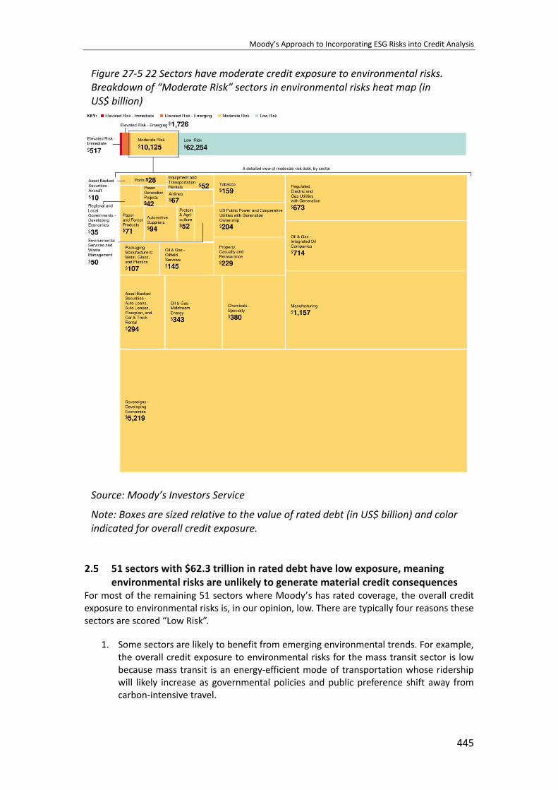
Moody’s Approach to Incorporating ESG Risks into Credit Analysis
445
Figure 27-5 22 Sectors have moderate credit exposure to environmental risks. Breakdown of “Moderate Risk” sectors in environmental risks heat map (in US$ billion)
Source: Moody’s Investors Service
Note: Boxes are sized relative to the value of rated debt (in US$ billion) and color indicated for overall credit exposure.
51 sectors with $62.3 trillion in rated debt have low exposure, meaning environmental risks are unlikely to generate material credit consequences
For most of the remaining 51 sectors where Moody’s has rated coverage, the overall credit exposure to environmental risks is, in our opinion, low. There are typically four reasons these sectors are scored “Low Risk”.
1. Some sectors are likely to benefit from emerging environmental trends. For example, the overall credit exposure to environmental risks for the mass transit sector is low because mass transit is an energy-efficient mode of transportation whose ridership will likely increase as governmental policies and public preference shift away from carbon-intensive travel.

Chapter 27
446
2. There are other sectors with fundamentally low business exposure to environmental risks. For example, the media and broadcasting sector has very low emissions of pollutants and carbon, and major publishing and printing companies have transitioned to digital offerings, resulting in a decline in exposure to environmental risks related to paper products.
3. Many sectors have business diversity and flexibility that mitigate the environmental risks they may face. For example, environmental risks to banks and finance companies are indirect, undertaken through financing clients' operations. Such risk exposure is unlikely to translate into a meaningful credit impact because banks and finance companies typically benefit from portfolio diversification, and lending is typically short to medium term. This provides these entities with flexibility to shift portfolio composition away from clients highly exposed to environmental risks.
4. Finally, some sectors have the economic, policy or financial flexibility to adapt to the environmental risks they cannot avoid. For example, while climate change is a global phenomenon, developed economy sovereigns and regional and local governments typically have much greater financial resources, economic resilience and institutional capacity to assist in climate adaptation.
Descriptions of the five environmental risk subcategories Air Pollution Along with soil and water pollution, air pollution is one of the traditional areas of environmental risk and regulation. Air pollutants, which may stay in the atmosphere or eventually pollute land and waterways, have the potential to harm the health of humans, other organisms and habitats. This category excludes carbon dioxide emissions, but includes those greenhouse gases that have been regulated as pollutants outside of concerns about their contribution to global warming, for instance nitrous oxides, sulfur oxides, and particulate matters.
Soil and Water Pollution and Land Use Restrictions Soil and water pollution most typically occurs from industrial, human and agricultural waste, as well as surface water run-off. More acute examples include the presence of toxic and nuclear wastes that can render land uninhabitable or poison drinking water, but more typically these pollutants increase risks for humans or harm wildlife. They may also render land infertile. An emerging area of concern is antibiotics. Environmental land restrictions may relate to preserving habitats, watersheds, green space or arable land, protecting species, or preventing certain activities due to general environmental concerns.
Carbon Regulation Our focus in this category is the impact of current and future policy initiatives that seek to reduce the amount of carbon dioxide and other greenhouse gases being emitted at a national and global level. In this category, we do not seek to anticipate the likelihood of climate change or the natural consequences of climate change and its impact on rated entities (those direct hazards are included in the following two categories). We score carbon emission regulation separately from air pollution because regulatory implications are potentially very wide-ranging and more difficult to predict than for traditional pollutants, given the scope of activities that produce carbon dioxide. For these reasons, we focus on the existing and likely future policy responses and their potential impact on credit quality. Please see Moody’s Approach to Assessing the Credit Impacts of Environmental Risks, November 2015, and Environmental Risks: Moody's To Analyse Carbon Transition Risk Based On Emissions Reduction Scenario Consistent with Paris Agreement, June 2016.

Moody’s Approach to Incorporating ESG Risks into Credit Analysis
447
Water Shortages Water shortages may be caused by a decrease in available water supplies or an increase in demand. Water supplies may decrease due to drought (including from climate change), the pollution or diversion of waterways, over-pumping of aquifers, or real estate development in watersheds. Water demand may increase due to population growth, urbanization, general economic development, or changes in economic activities (e.g. irrigation farming, shale-gas fracking).
Natural and Man-made Hazards Natural and mad-made hazards include changing trends in the global climate that are typically chronic in nature. They include the trend of warming, as illustrated by rising mean temperatures globally, and other slow-moving trends such as rising sea levels. This category also covers low probability, high-severity events arising from a variety of sources, including (without limitation) weather events such as hurricanes, earthquakes or floods (including coastal flooding), regulations on activities that may cause them, industrial disasters, and nuclear incidents. While the occurrence of a singular, isolated event may not be the direct result of climate change, the Intergovernmental Panel on Climate Change (IPCC) notes that the probability and frequency of such shocks (e.g. damaging cyclones) will increase at higher temperatures and/or greater extremes in temperatures and precipitation.
Our heat map points to 16 sectors with “very high” or “high” nominal exposure to carbon regulation
Our heat map points to 16 sectors with “very high” or “high” nominal exposure to carbon regulation, accounting for $3.7 trillion in rated debt (Figure 27-6). These sectors tend to be among the most carbon-intensive industries globally, such as utilities and power companies, and/or where regulations governing emissions are tightening rapidly, such as airlines.8 Of the 16 sectors with “very high” or “high” nominal exposure to carbon regulation, 10 have immediate or emerging “Elevated Risk” overall credit exposure. The remaining six score “Moderate Risk” for a variety of reasons, including diversification of business model or ability to pass on costs.
8 See Unregulated utilities and power companies – Global: Carbon transition brings risks and opportunities, June 2018, and
Passenger Airlines – Global: Pricing power, route mix to determine credit implications of carbon transition, April 2018.

Chapter 27
448
Figure 27-6 Carbon regulation will have a tangible impact on the most exposed sectors. Sectors with “very high” or “high” exposure to carbon regulation (in US$ billion)
Source: Moody’s Investors Service
Alongside market (for example, demand substitution) and technology risks, we consider regulatory risks as one of the key determinants in assessing the credit effects of carbon transition at an entity level for the most exposed sectors globally (Figure 27-7).9 In the absence of substantial counterbalancing initiatives, the transition to a lower carbon future will likely result in increasing pressure on the affected companies’ credit profiles.
Figure 27-7 Regulation is a key determinant in assessing the credit impact of carbon transition on companies
Source: Moody’s Investors Service
9 We seek to incorporate all material credit considerations, including those related to environmental, social and governance
elements, into our credit rating analysis.

Moody’s Approach to Incorporating ESG Risks into Credit Analysis
449
Thirteen sectors have “very high” or “high” nominal exposure to air pollution
Thirteen sectors ($3.5 trillion in rated debt) are scored as having “very high” or “high” nominal exposure to air pollution, which we define as including greenhouse gases that have been regulated as pollutants outside of concerns about their contribution to global warming. They include nitrous oxides, sulfur oxides, chlorofluorocarbons and particulate matter.
As Figure 27-8 illustrates, a similar cross-section of industrial sectors is exposed to both air pollution and carbon regulation. These sectors are typically susceptible to more stringent environmental enforcement of particulate emissions and air pollution. Environmental policies focused on air pollution often result in forcing an industry to move toward low-carbon products, even in the absence of any actual carbon regulations. For example, automobile fuel efficiency standards and smog regulations are moving the industry toward alternative fuel vehicles that also reduce carbon intensity. And policies to reduce mercury and acid gas emissions from power generation have resulted in the shutdown of coal-fired generation, which has also reduced carbon emissions.
Figure 27-8 Industrial sectors tend to have significant exposure to both air pollution and carbon regulation. Selected sector exposure to air pollution and carbon regulation (bubble size in US$ billion)
Source: Moody’s Investors Service
Fourteen sectors, including central and local governments in developing economies, score “high” for natural and man-made hazards; four score “high” for water shortages
Natural and man-made hazards, and water shortages constitute physical environmental risks, potentially as a result of climate change. Hazards can relate to changing trends in the global

Chapter 27
450
climate that are typically chronic in nature. They include the trend of warming, as illustrated by rising mean temperatures globally, and other slow-moving trends, such as rising sea levels. Hazards also encapsulate the occurrence of episodic events, including natural disasters or extreme weather events (such as storms, floods, wildfires, drought and cyclones).
Physical risks can affect an issuer’s operations and capital spending directly, or have indirect effects such as supply chain disruptions or market volatility.10 While most sectors – particularly those reliant on large tangible assets and extensive supply chains – tend to have some degree of vulnerability to such risks, geographical footprint clearly matters. Indeed, where an issuer operates (or where its main markets are located), coupled with the location of its main suppliers, will significantly affect its exposure to natural and man-made hazards.
Figure 27-9 Majority of sectors have “moderate” or “high” exposure to natural and man-made hazards. Selected sector exposure to natural and man-made hazards (in US$ billion)
Source: Moody’s Investors Service
10 Moody’s contributed to a report titled Advancing TCFD Guidance on Physical Climate Risks and Opportunities produced
on behalf of the European Bank for Reconstruction and Development and Global Centre of Excellence on Climate
Adaptation in May 2018. Among other issues, the report outlines how physical climate risks and opportunities can influence
an issuer’s creditworthiness.

Moody’s Approach to Incorporating ESG Risks into Credit Analysis
451
Figure 27-10 25 sectors with “moderate” or “high” exposure to water shortages. Selected sector exposure to water shortages (in US$ billion)
Source: Moody’s Investors Service
Six sectors have “very high” or “high” exposure to soil and water pollution, and land use restrictions
As illustrated in Figure 27-11, we identify six sectors with “very high” or “high” exposure to this category, including mining, commodity and specialty chemicals, and shipping – with the latter specifically exposed to water pollution.
Figure 27-11 Mining, commodity and specialty chemicals, and shipping are among the most exposed. Sectors with “high” or “very high” exposure to soil/water pollution and land use restrictions (in US$ billion)
Source: Moody's Investors Service
3 Framework to assess carbon transition risk for corporate sectors
We published our report “Non-financial companies – Global: Framework to assess carbon transition risk for corporate sectors” in September 2019, which outlines our approach to
Chapter 27
452
creating a scoring tool that provides a standalone assessment of one specific ESG risk, namely carbon transition risk.11
Moody’s carbon transition assessment (CTA) tool provides a consistent, transparent and verifiable means to analyse carbon transition risk for rated non-financial companies. This report explains the framework, scoring system and data that informs the scoring of our CTAs. We will initially apply the framework to our analysis of sectors that we identify as having “very high” or “high” exposure to carbon transition risk12.
In September 2018, we published an update to our environmental heat map (first published in November 2015) identifying sectors with significant exposure to carbon transition risk. As discussed further above, our heat map points to 16 sectors with “very high” or “high” nominal exposure to carbon regulation, accounting for $3.7 trillion in rated debt. These sectors tend to be among the most carbon-intensive industries globally, such as utilities and power companies, and/or where regulations governing emissions are tightening rapidly, such as airlines.
4 The impact of environmental, social and governance risks on bank
ratings
ESG risks are becoming more significant Some ESG risks are well-established drivers of bank creditworthiness. Governance quality, for instance, has long been a key contributor to bank credit strength. Nevertheless, ESG risks have become more significant for the banking sector in recent years. This is principally due to evolving regulations, policy measures, market developments, and underlying changes in social attitudes as a result of which banking sector activities previously considered acceptable are now increasingly challenged.
Social risks, for instance, have become more pronounced for banks after the global financial crisis contributed to a negative shift in popular attitudes towards banks. This has made customer backlashes against business practices deemed to be socially unacceptable, a social risk, more likely. Similarly, the transition to a low carbon economy, accelerated by the 2015 Paris Agreement, is gradually increasing environmental risk for banks. These include risks associated with investments in technologies which may become obsolete as less carbon-intensive alternatives emerge. Overall, we believe that growing awareness of climate change and its consequences has played a key role in increasing the relevance of ESG risks.
ESG risks typically affect banks’ creditworthiness through the same channels as conventional risks. For instance, an increase in customer defaults can result from an environmental hazard such as drought, just as it can from an increase in interest rates or unemployment. Similarly, an inadequate commercial strategy and socially unacceptable business practices can both result in a loss of customers, hitting profitability.
Banks are exposed to ESG risks directly, but also indirectly through their balance sheets, given their role as lenders and investors. Governance-related risks have historically had the most direct impact on bank creditworthiness. Environmental risks primarily affect banks indirectly
11 See “Non-financial companies – Global: Framework to assess carbon transition risk for corporate sectors”,
Moody’s Investors Service, September 2019. 12 See “Automotive manufacturing – Global: Substantial variation exists in automakers' carbon transition risk
profiles”, Moody’s Investors Service, November 2019.

Moody’s Approach to Incorporating ESG Risks into Credit Analysis
453
through their investment and lending decisions. Social risks can also arise indirectly, for example when the credit quality of a borrower weakens because of social considerations.
Environmental risks may also influence bank capital in the future, as regulators may incorporate environmental considerations into banks' prudential requirements. The quality of a bank’s governance can itself influence its exposure to environmental and social risks, with better-governed banks likely to face fewer such risks.
Sustainable finance is influencing banks' behaviour
Sustainable finance has become a key theme globally in recent years, driven by international agreements aimed at promoting investments that take account of ESG considerations. The most important of these include the Paris Climate Agreement (December 2015), the UN 2030 Agenda for Sustainable Development (September 2015) and the European Commission Action Plan on Sustainable Finance (March 2018).
The rise of sustainable finance has put banks under particular pressure for two reasons. Firstly, banks are the backbone of the global financial system, and consequently play a key role in financing the projects required to establish a sustainable economy. Secondly, banks’ expertise in credit risk management makes them uniquely qualified to ensure that increased funding for sustainable assets and activities does not come at the expense of financial stability.
Regulators and policymakers are one of the main driving forces in the shift towards sustainable finance. Although banks are exposed to regulatory and policy risks as they affect their investment decisions, the level of environmental regulation directly aimed at banks is currently low. However, we expect this to change as a result of a gradual increase in regulation designed to: (1) ensure that the financial system is resilient to climate-related risks; and (2) support the implementation of environmental policies. For example, the UK's Prudential Regulation Authority has already proposed to incorporate environmental considerations into banks’ prudential frameworks.
Sustainable finance is not driven solely by regulation. Bank stakeholders are becoming increasingly aware of ESG issues, and are demanding improved ESG management. This is illustrated by investors’ rapid integration of ESG factors into their asset allocation decisions. Signatories to the Principles for Responsible Investment (PRI), which take ESG considerations into account in their investment policies, had combined assets under management of USD82 trillion in 2018, an increase of 19% from the previous year. Pressure to meet ESG targets also arises from bank shareholders exercising their voting rights according to ESG criteria, as well as from bank customers.
In this context, banks are increasingly under pressure to re-focus their strategy and business models on sustainability, and to integrate ESG considerations into their investment decisions. The rise of sustainable finance offers banks opportunities to unlock new lending markets, and to reinforce their relationship with clients, for instance by advising them on the impact of ESG factors on their businesses. Banks can also reinforce their franchise value through strong management of ESG factors.
However, it also potentially exposes banks to increased capital constraints, asset stranding, and fines or litigation in the event of noncompliance with new regulations. New regulation will also add compliance costs, and banks may forgo currently profitable businesses because of the way they might develop over the long-term. At the same time, engaging in or facilitating activities with a significant negative environmental impact may inflict reputational damage on

Chapter 27
454
banks, tarnishing their brands. Increased credit risk can also arise from regulatory incentives to promote sustainable finance as they have the potential to distort risk measurement.
Bank exposure to reputational damage largely depends on how aware their stakeholders are of ESG issues, but we believe that the risk is more material for larger banks. This is because any negative externalities they create will affect a larger number of people, given their large size and broader geographic footprint.
ESG risks are captured in our bank credit analysis Our assessment of a bank’s baseline credit assessment (BCA), a measure of its standalone credit strength,13 is based on five key financial ratios and three qualitative factors. These are in our view the key indicators of how likely the bank is to default in the absence of external support. Any positive or negative impact from ESG considerations would influence our assessment of these eight indicators, affecting our overall view of the risk of bank failure in turn.
Strong corporate governance is at the core of a bank’s financial health. Our qualitative adjustment for corporate behaviour measures governance risk directly. However, the absence of an explicit corporate behaviour adjustment for most banks does not indicate a lack of governance strengths or weaknesses, rather that their governance quality is already reflected in other rating factors. The impact of governance risk is typically greatest in our assessment of asset risk, as a poor risk governance framework can lead to severe deterioration in asset quality. Governance risk can also materially affect profitability via fines or regulatory sanctions because of governance breaches.
Environmental and social risks have historically had a low impact on banks' credit profiles, but their influence can still be material. Environmental factors can increase risk in banks’ investment portfolios, and therefore lead to a deterioration in asset risk. If they cause financial losses, or if banks forgo profitable businesses on environmental grounds, they can also weigh on profitability.
Social risks are less likely to affect asset quality, but they can have a material impact on profitability, for example through litigation, regulatory fines, or regulatory measures that constrain earnings. Social factors can also have a positive impact on profitability, as in the case of banks which grow thanks to financial inclusion initiatives.
The potential inclusion of ESG considerations in banks’ prudential frameworks may also affect our assessment of their capital adequacy. A number of recent regulatory proposals would incorporate environmental considerations into bank capital requirements. Regulators may also incorporate ESG risks into their supervisory work, for instance by taking account of banks' resilience to climate change when conducting stress tests.
Reputational damage because of poor ESG performance can affect banks’ profitability and liquidity. The loss of customers whose ESG expectations have not been met may affect a bank's business volumes and therefore its earnings capacity. Customers may also withdraw their funds, and the banks’ issuances may attract less market interest, as investors increasingly integrate ESG considerations into their investment decisions.
13 Moody’s rating approach for banks builds around four components, of which the baseline credit assessment (BCA) is the
most sensitive to the impact of ESG factors. For further details, see “Rating Methodology: Banks Methodology”, Moody’s
Investors Service, November 2019.

Moody’s Approach to Incorporating ESG Risks into Credit Analysis
455
Figure 27-12 shows the rating factors that make up Moody’s baseline credit assessment (BCA) methodology, with a brief description of how our assessment captures ESG risks, directly or indirectly.
Figure 27-12 ESG risks relate to rating factors. Moody's bank rating methodology
Source: Moody’s Investors Service
ESG factors can also influence bank ratings through the Macro Profile, an assessment of banks’ operating and economic environment. The Macro Profile draws heavily on three of the rating factors used in the sovereign rating methodology14, and ESG considerations are included in the assessment of each of these factors. One of them, institutional strength, is directly and closely linked to governance risk, while environmental and social risks are indirectly related to all sovereign rating factors.
Governance is the main ESG risk for banks Governance quality is particularly important for banks because they operate with higher leverage and are generally more confidence-sensitive than corporates, particularly regarding their funding arrangements. The consequences of a governance breach can go beyond the immediate impact, such as a financial penalty or asset quality deterioration. In some cases, there can also be reputational damage leading to franchise erosion, resulting in a loss of business, or customers withdrawing funds.
14 See “Rating Methodology: Sovereign Ratings Methodology”, Moody’s Investors Service, November 2019.
Chapter 27
456
We do not assign a score for quality of risk governance when determining a bank’s financial profile, which reflects our view of its solvency and liquidity. Rather, our assessment of governance quality influences the scores that we assign to the different solvency and liquidity scorecard factors.
In some cases, however, credit considerations related to corporate governance are not fully captured in any of the solvency or liquidity factors on our scorecard. To determine such banks' BCAs, we apply a qualitative adjustment to their financial profile. This adjustment typically reflects idiosyncratic corporate governance issues captured through behavioural aspects of a bank, which we assess under a broad qualitative framework which we term “corporate behaviour”.
We assess corporate behaviour around six factors: key person risk, insider and related-party risk, strategy and management, dividend policy, compensation policy and accounting policy.
Social risk includes a wide range of potential hazards Social risks arise from a bank’s interaction with its stakeholders and society at large. This is the broadest of the three ESG risks, and typically affects credit quality through litigation, as well as reputational, operational, and regulatory channels. Social risks generally have a moderate impact on bank credit quality. Although social risks in some cases are high, banks' financial and operational flexibility, and their long track record of adjusting to emerging social issues, act as mitigants.
Banks are exposed to social risks directly through their dealings with customers, employees, and other stakeholders. Examples include the possibility of regulatory penalties or reputational damage for failing to treat customers fairly. Social risks can also stem from external factors such as legislative changes prompted by underlying changes in social attitudes. Regulations requiring banks to prioritize lending to particular sectors of the economy are an example.
Banks are also exposed to social risk indirectly through their lending and investment decisions. The most significant social risks for banks are those they are directly exposed to, as their portfolio flexibility and diversification help mitigate risks from their indirect exposure.
The social risks that private sector issuers generally are exposed to fall into five categories: customer relations, human capital, health and safety, responsible production and demographic and societal trends.
Environmental risk exposure is generally low but increasing Environmental risks take a number of different forms. Our global environmental risks heat map identifies the five categories of environmental risk that are most material to an issuer's credit quality.
Banks' current balance sheet exposure to environmental risk is generally low. Their own environmental footprint does not typically raise credit concerns, and their main exposure to environmental risks is indirect, through their investment and lending decisions. This indirect exposure is less significant for banks that are well diversified both by industry and geography. Moreover, the relatively short duration of bank loans provides lenders with some ability to rebalance their portfolios as stranded assets and other environmental risks emerge over time.
However, we expect environmental risks to become more significant for banks in the future, particularly as the transition to a low carbon economy accelerates, the physical effects of

Moody’s Approach to Incorporating ESG Risks into Credit Analysis
457
climate change increase, and climate policy changes the regulatory environment. The impact of these developments on bank credit strength will depend on how quickly they take place, with longer time frames giving banks greater opportunity to adapt to changed circumstances. It will also depend on the level of engagement that policymakers and regulators seek from banks to meet their environmental objectives.

Chapter 28
458
ISS ESG Corporate Rating and Applications
By
ISS1
Abstract
Many companies today operate in a world characterized by enormous environmental challenges including climate change, biodiversity losses, overexploitation of natural resources, and pollution. The ISS ESG Corporate Rating is a highly granular, sector-specific and risk-oriented methodology that provides investors with a way to ascertain the degree to which companies are exposed to and manage such risks and to assess whether companies contribute to or obstruct sustainable development goals. The ESG Corporate Rating can also serve to identify particularly progressive companies, for instance in relation to mitigating climate-change, and the development of indices.
Keywords: ESG, sustainability ratings, environmental ratings, sustainability performance, environmental performance, climate change
1 Introduction
The ISS ESG Corporate Rating originated from Frankfurt-Hohenheimer Leitfaden, a comprehensive set of indicators conceived at the Goethe University in Frankfurt am Main in the late 1990s to assess companies’ sustainability performance. Over the years, the ISS ESG has continuously refined and calibrated the sector-specific methodology to incorporate industry standards and best practices, regulatory developments, social debates, and the latest trends in science and technology. Global norms and conventions such as the UN Global Compact, the UN Universal Declaration on Human Rights, the ILO Core Labor Standards, and the Voluntary Principles on Security and Human Rights are the foundation of ISS ESG’s philosophy. The rating methodology has thus evolved into a holistic, forward-looking approach capturing the most pertinent social and environmental challenges of the 21st century. It helps align investments with global norms and responds to new standards and regulations. It also highlights critical company-specific ESG risks typically not considered by traditional credit ratings.
2 Methodology
The corporate rating methodology rests on a two-pronged approach. The positive criteria, the backbone of the methodology, assesses the sustainability performance of companies’ management systems and operations along the entire value chain, and the impacts of their product/service portfolios. The ratings draw on a pool of more than 800 indicators, the majority of which sector-specific. Each sector is analyzed based on a selection of approximately 100 social, environmental and governance-related indicators. The total number
1 This chapter was written by Alexander Hellwig, Senior Associate at ISS, email: [email protected]. The author
would like to thank Kristina Rüter and Karsten Greye for their continued support and inputs.

ISS ESG Corporate Rating and Applications
459
and their weightings depend on a company’s inherent ESG impact profile and concomitant risks. ISS ESG employs particularly stringent performance requirements for business activities considered to entail elevated risks and negative impacts on the society and the environment. This holds true for companies from sectors such as oil & gas, petrochemicals, and metals & mining.
Each indicator typically comprises a content element (either one or several sub-indicators) and a coverage. The latter examines to what extent the relevant operations of a company are covered by the policy, strategy or management measures under scrutiny. The basic rationale is that isolated company initiatives alone may not lead to satisfying results. Conversely, an underlying downgrading mechanism ensures that poor or average content is not upgraded simply because it was implemented at the corporate level. Content and coverage are graded separately and add up to the total indicator performance score (see Table 28-1 for an example).
Table 28-1 Indicator example – design and operation of wind power plants
Performance requirements Weight
1.Responsible site selection
Company commitment to refrain from sites in protected areas and areas of high biodiversity value. Prioritization of brownfield sites over greenfields.
Ind
ivid
ual
sco
re
25%
Tota
l in
dic
ato
r sc
ore
Coverage Percentage of relevant operations covered
2.Environmental impact assessments
The company conducts comprehensive environmental impact assessments prior to construction that cover relevant biodiversity aspects.
Ind
ivid
ual
sco
re
25%
Coverage Percentage of relevant operations covered
3.Onshore wind power plants
The company carries out adequate measures to protect birds and/or bats, and engages in continuous monitoring of environmental impacts.
Ind
ivid
ual
sco
re
50% 4.Offshore wind power plants
The company carries out adequate measures to protect marine life, including noise reduction and the mitigation of impacts from lines. Continuous monitoring of environmental impacts.
Coverage Percentage of relevant operations covered
The scoring mechanism can be illustrated by these aforementioned indicators. If a company systematically excludes wind farms in protected areas or areas of high biodiversity and prioritizes brown fields, all the (content-related) requirements are met by responsible site selection. However, the coverage of this approach ultimately determines the indicator grade. If less than 20% of the relevant operations are covered, the company is assigned a D+ (based on a twelve-point rating scale ranging from A+ (excellent performance) to D- (poor

Chapter 28
460
performance)). In case coverages exceeding 20%, 50% or 80%, the indicator scores a B+, A and A+, respectively.
The indicators are either qualitative or quantitative and address management aspects, operational performance and corporate transparency. In addition, trend analyses and strategy-related assessments help identify corporations with particularly progressive and future-proof business models. For each sector, four to five key topic areas are defined, reflecting the most material sustainability issues (see also breakout 2 for the importance of capturing sector-specific risks). They are assigned a weighting of at least 50%. All the indicators are individually weighted, evaluated, and aggregated to yield an overall score.
The positive criteria previously mentioned are complemented by an assessment of controversial business practices. ISS ESG’s norm-based research monitors corporate compliance with recognized international norms and guidelines on human rights, labor standards, environmental protection and business malpractice as a critical gauge of ESG performance. Each controversy is examined along several dimensions, including the degree to which a company’s misconduct has been corroborated by an authoritative source (verification), the severity of impacts, company involvement and accountability for the transgression (severity), and the prevalence of relevant countermeasures (remediation). The continuum of controversy classifications ranges from potential to moderate, severe and very severe assessments. By causing a downgrade – 20% for moderate, 50% for severe, and 80% for very severe cases – in the affected topic sections of the corporate rating, controversies exert a direct bearing on a company’s ESG performance. As such, the score of the topic area ‘climate change strategy’ is, for instance, downgraded in case of a climate-related misconduct. In order to paint a sufficiently accurate and objective picture of a controversy, information is gleaned from independent sources and from the company in question as a part of a comprehensive feedback process.
The final ESG performance, an aggregation of the analysis of both the positive evaluation criteria and controversies, is reflected in a twelve-point rating scale from A+ (excellent performance) to D- (poor performance). The performance assessment at an indicator- and topic-level makes use of the same grading scale. In 2019, ISS ESG also introduced a decile ranking of a company’s overall performance against those of its industry peers. A rank of 1 indicates a high relative performance, whereas 10 points to a low relative performance.
The ISS ESG Corporate Rating assesses companies’ sustainability performance on an absolute best-in-class basis. The so-called ISS ESG Prime status takes account of prevailing risks and impacts in each sector and denotes companies that meet ISS ESG’s ambitious sustainability performance requirements. Companies in high-risk sectors such as oil & gas, for instance, have to meet more demanding standards than those in low-risk sectors to obtain the ISS ESG Prime status.
The ratings are updated on an annual basis to ensure that companies reporting such as newly published annual and sustainability reports are continuously integrated into the assessments. Event-driven updates in relation to major controversies, mergers or significant company transactions are equally conducted on a rolling basis. Lastly, a comprehensive dialogue process with the rated issuers is carried out once every two to three years.
2 https://www.theguardian.com/us-news/2019/oct/08/california-pge-power-shutdown-wildfire

ISS ESG Corporate Rating and Applications
461
The corporate rating methodology is reviewed regularly to meet the latest developments in science, technology, society and the regulatory landscape.
3 Environmental aspects of ISS ESG ratings
The ISS ESG Corporate Rating has two main components: social responsibility and governance as well as the environment. These two elements are weighted in accordance with the underlying risk and impact classification of each sector. We will focus particularly on environmental aspects and explain how the rating and its underlying data can be used by investors.
By default, the environmental rating has three integral parts (see Table 28-2 for a high-level overview). The section on environmental management (standard set of indicators) includes several topics relevant for all sectors from a risk perspective.
Table 28-2 Components of the environmental rating
1 Environmental management (standard set of indicators)
Environmental management systems
Energy management systems, energy use reduction targets, energy use by fuel type
Climate change strategy: inventories, reduction targets and action plans, disclosure of risks and mitigation/adaptation strategies
Water risk and impact management
Management of environmental risks in the supply chain
2 Environmental management (sector-specific indicators)
Assessment of environmental impacts of the product/service portfolio in relation to the achievement of the United Nations Sustainable Development Goals (SDGs)
Indicators specific to industry risks and impacts
3 Eco-efficiency
Time-series analyses of relevant resource use efficiencies (e.g. energy, freshwater) and output efficiencies (e.g. greenhouse gas emissions, waste, pollutants)
The standard set of environmental topics is complemented by a range of indicators for the specific risk profiles of the various industries covered by ISS ESG (section also includes the product portfolio assessment) and an analysis of resource use as well as output efficiencies. Each indicator is characterized by specific performance requirements often based on international standards and frameworks. The indicator ‘Greenhouse gas emission reduction targets and action plans’, for instance, requires companies to set science-based targets in line with the 2°C scenario adopted by the Paris Agreement to achieve the best possible grade. In doing so, ISS ESG draws on the work of the Science-Based Target Initiative. The targets need to be underpinned by comprehensive action plans with a clear set of measures, subgoals and progress reports.
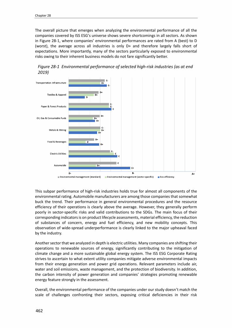
Chapter 28
462
The overall picture that emerges when analyzing the environmental performance of all the companies covered by ISS ESG’s universe shows severe shortcomings in all sectors. As shown in Figure 28-1, where companies’ environmental performances are rated from A (best) to D (worst), the average across all industries is only D+ and therefore largely falls short of expectations. More importantly, many of the sectors particularly exposed to environmental risks owing to their inherent business models do not fare significantly better.
Figure 28-1 Environmental performance of selected high-risk industries (as at end 2019)
This subpar performance of high-risk industries holds true for almost all components of the environmental rating. Automobile manufacturers are among those companies that somewhat buck the trend. Their performance in general environmental procedures and the resource efficiency of their operations is clearly above the average. However, they generally perform poorly in sector-specific risks and valid contributions to the SDGs. The main focus of their corresponding indicators is on product lifecycle assessments, material efficiency, the reduction of substances of concern, energy and fuel efficiency, and new mobility concepts. This observation of wide-spread underperformance is clearly linked to the major upheaval faced by the industry.
Another sector that we analyzed in depth is electric utilities. Many companies are shifting their operations to renewable sources of energy, significantly contributing to the mitigation of climate change and a more sustainable global energy system. The ISS ESG Corporate Rating strives to ascertain to what extent utility companies mitigate adverse environmental impacts from their energy generation and power grid operations. Relevant parameters include air, water and soil emissions, waste management, and the protection of biodiversity. In addition, the carbon intensity of power generation and companies’ strategies promoting renewable energy feature strongly in the assessment.
Overall, the environmental performance of the companies under our study doesn’t match the scale of challenges confronting their sectors, exposing critical deficiencies in their risk

ISS ESG Corporate Rating and Applications
463
management frameworks. Nevertheless, progressive companies that are particularly mindful of environmental risks do exist in most industries. The following Table 28-3 illustrates some positive examples.
Table 28-3 Environmental strengths and weaknesses of selected industry leaders (as at end 2019)
Environmental strengths and weaknesses (non-exhaustive) Ø rsted AS (Electric Utilities) + Comprehensive climate change mitigation strategy (including science-based targets) + Sound supplier environmental standards + High-and=increasing share of using renewables + Ambitious strategies to promote renewables + Comprehensive measures addressing adverse environmental impacts from renewable
power generation and power grid operations - Limited evidence of taking measures to reduce environmental impacts from fossil fuel-fired
power plants (air emissions, solid waste and wastewater) - Insufficient evidence of monitoring and mitigating impacts on freshwater sources Kellogg Company (Food & Beverages) + Convincing climate change mitigation strategy, including science-based targets and
comprehensive measures aimed at reducing the negative carbon impact of crop farming along the value chain + Sound supplier environmental standards
+ Reasonable measures to promote sustainable soil and biodiversity management in agricultural production
+ Using comparatively high share of certified palm oil
+ Sound measures to ensure water conservation in agricultural production along the value chain
+ Strategy and/or measures in place designed to reduce food waste in the supply chain and in company operations
- No clear evidence of monitoring and mitigating impacts on freshwater sources
- Low shares of raw materials/products from certified organic farming sources
- Limited measures in place to reduce environmental impacts of packaging
Outokumpu (Metals & Mining)
+ Comprehensive climate change mitigation strategy (including science-based targets)
+ Reasonable supplier environmental standards
+ Comprehensive measures to ensure safe handling of hazardous materials in mining and ore processing
+ A higher share of recycled materials in steel production
+ Sound measures to promote recycling of scrap metal
+ Sound procedures managing waste water, hazardous waste and air emissions
+ Sound measures to ensure facility safety and emergency management
- A significant share of energy comes from nuclear power and coal
- Limited evidence of measures to monitor and mitigate impacts on freshwater sources
- Only some indications suggesting adequate tailings and waste rock management
In recent years, ESG discussions have mostly revolved around climate change, eclipsing other major environmental challenges. A topic drawing more attention today is biodiversity conservation, in part due to the publication of the Global Assessment Report by the Intergovernmental Science-Policy Platform on Biodiversity and Ecosystem Services (IPBES) in May 2019 and other news reports highlighting distressing levels of global biodiversity decline. These developments have also piqued the interest of the investment community. The critical

Chapter 28
464
issue of biodiversity loss will be brought into global focus by the 15th meeting of the Conference of the Parties (COP 15) to the Convention on Biological Diversity (CBD), which will give new impetus to protection initiatives. The conference was originally set to take place in China in 2020 but is likely to be postponed until 2021.
Companies’ biodiversity impacts are closely linked to their business models and activities. ISS ESG has therefore developed a range of indicators for the specific impacts of each sector. Industries in the spotlight include construction, chemicals, food & beverages, household & personal care products, metals & mining, oil & gas, paper & forest products, pharmaceuticals & biotechnology, and utilities. A total of 30 biodiversity-related indicators are applied across different sectors, typically focusing on corporate policies, conservation strategies and management measures designed to curb negative effects. Two of the most commonly used metrics look at the extent to which operational biodiversity risks and impacts are addressed and whether companies address the sensitivity of protected areas. Some sectors are also particularly subject to supply chain-related risks, underscoring the pivotal importance of sustainable procurement practices and corresponding compliance measures.
4 Applications of ISS ESG corporate rating
The ISS ESG Corporate Rating can be used in many ways. With a granular, sector-specific and risk-oriented methodology, it can be used in a wide range of applications, giving rise to a variety of ESG products, some of which are presented below.
SDG solutions assessment A key element and impact component of the ISS ESG Corporate Rating is the SDG Solutions Assessment (SDGA), a tool that lets investors align their investment decisions with the achievement of the United Nations Sustainable Development Goals (SDGs). The SDGA identifies to what extent a company’s products and services contribute to or obstruct the 15 overriding sustainability objectives, eight of which pertain to environmental matters. These eight objectives include global challenges such as the mitigation of climate change, sustainable energy use, sustainable agriculture and forestry, the conservation of water, the optimized use of materials, the promotion of sustainable buildings, and the preservation of both marine and terrestrial ecosystems.
The assessment takes account of companies’ unique and distinctive business impacts with regard to each of the objectives, which are evaluated along a continuum from significant obstruction (-10), limited obstruction (-5), and no net impact (0), to limited contribution (+5), and significant contribution (+10). An exemplary overview of product impacts on climate change mitigation is depicted in Figure 28-2:
Figure 28-2 Illustration of product impacts on “Mitigation of climate change”
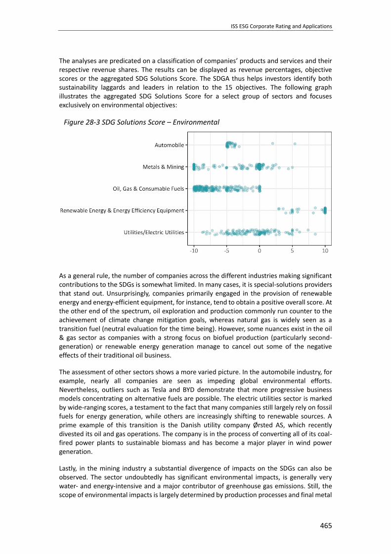
ISS ESG Corporate Rating and Applications
465
The analyses are predicated on a classification of companies’ products and services and their respective revenue shares. The results can be displayed as revenue percentages, objective scores or the aggregated SDG Solutions Score. The SDGA thus helps investors identify both sustainability laggards and leaders in relation to the 15 objectives. The following graph illustrates the aggregated SDG Solutions Score for a select group of sectors and focuses exclusively on environmental objectives:
Figure 28-3 SDG Solutions Score – Environmental
As a general rule, the number of companies across the different industries making significant contributions to the SDGs is somewhat limited. In many cases, it is special-solutions providers that stand out. Unsurprisingly, companies primarily engaged in the provision of renewable energy and energy-efficient equipment, for instance, tend to obtain a positive overall score. At the other end of the spectrum, oil exploration and production commonly run counter to the achievement of climate change mitigation goals, whereas natural gas is widely seen as a transition fuel (neutral evaluation for the time being). However, some nuances exist in the oil & gas sector as companies with a strong focus on biofuel production (particularly second-generation) or renewable energy generation manage to cancel out some of the negative effects of their traditional oil business.
The assessment of other sectors shows a more varied picture. In the automobile industry, for example, nearly all companies are seen as impeding global environmental efforts. Nevertheless, outliers such as Tesla and BYD demonstrate that more progressive business models concentrating on alternative fuels are possible. The electric utilities sector is marked by wide-ranging scores, a testament to the fact that many companies still largely rely on fossil fuels for energy generation, while others are increasingly shifting to renewable sources. A prime example of this transition is the Danish utility company Ørsted AS, which recently divested its oil and gas operations. The company is in the process of converting all of its coal-fired power plants to sustainable biomass and has become a major player in wind power generation.
Lastly, in the mining industry a substantial divergence of impacts on the SDGs can also be observed. The sector undoubtedly has significant environmental impacts, is generally very water- and energy-intensive and a major contributor of greenhouse gas emissions. Still, the scope of environmental impacts is largely determined by production processes and final metal

Chapter 28
466
utilization. The multitude contexts of applications and possible uses of the products make it difficult to clearly attribute the impacts on the individual SDGs. However, many corporations solely engage in the extraction of highly sensitive materials with enormous ecological footprints (e.g. gold, diamonds) or operate in highly sensitive ecosystems. On a positive note, some companies have geared their business models towards metals recycling (particularly aluminium), thus making valuable contributions to the circular economy. A few other players are involved in the manufacturing of lightweight metals that promote fuel efficiency in the automobile and aviation industry.
Index development The highly granular ISS ESG Corporate Rating and its comprehensive underlying data can also be used for the development of (thematic) indices. Asset managers acquire index licenses for the development of various financial products. They can, for instance, track indices via exchange traded funds (ETFs) or use indices to design their own benchmarks. ISS ESG collaborates with index providers to develop solutions based on high quality, reliable, and relevant ESG data.
In 2007, the Hanover Stock Exchange and ISS ESG (then oekom research AG) jointly developed the Global Challenges Index (GCX). Since its inception, the GCX has had a 174-percent rate of return of, outperforming several other leading indices.3 The GCX comprises the shares of 50 companies that help tackle the following seven global challenges:
▪ mitigating climate change
▪ ensuring the adequate provision of drinking water
▪ stopping deforestation and promoting sustainable forestry
▪ protecting biodiversity
▪ dealing with population growth
▪ alleviating poverty
▪ supporting responsible governance structures
Multi-level safeguards are in place to ensure a consistent sustainability performance by all the companies listed in the GCX. They are premised on the application of performance standards, exclusion criteria (covering both controversial business areas and practices) and meaningful contributions to the above-mentioned fields of action. The approach is bolstered by continuous monitoring efforts, entailing a six-monthly rebalancing of the index coupled with a review by an independent expert panel. In doing so, the GCX singles out companies with outstanding sustainability credentials and allows investors to benefit from these companies’ competitive advantage in light of global transformation and the concomitant risks and opportunities.
Another practical application of the ISS ESG Corporate Rating targeting a distinct impact area is illustrated by the newly developed Solactive ISS ESG Beyond Plastic Waste Index. The index was devised by Solactive and ISS ESG and only covers companies that tackle the growing plastic waste and contribute to the shift to a more circular economy. More specifically, these companies offer solutions for reducing plastic pollution, efficient plastic recycling, enhanced
3 https://www.dasinvestment.com/vermoegensverwalter-mark-uwe-falkenhain-nachhaltige-investments-rechnen-sich

ISS ESG Corporate Rating and Applications
467
plastics reusability and the development of viable substitutes for plastic-based products. Current index constituents include Brambles Ltd., a supplier of reusable pallets, crates, and containers, and BillerudKorsnäs AB, which specializes in pulp and paper manufacturing and renewable packaging materials4. The index is available for licensing and may be used as a basis for ETFs and structured products, benchmarking purposes or as a starting point for customized index strategies.
Climate solutions Climate change has undoubtedly become one of the most prominent issues in the investment community in recent years, not least because of mounting regulatory pressures and discussions related to financial risks. The ISS ESG Corporate Rating lays the foundation for holistic data insights helping investors gain a better understanding of their exposures to climate-related risks. The Carbon Risk Rating (CRR) is an exemplary case assessing a company’s climate management performance. The CRR has two components: Carbon Performance Score (CPS) and Carbon Risk Classification (CRC). The former draws on more than a hundred indicators of a company’s ability to manage climate-related risks through its value chain (see Table 28-4). For each company, a certain subset of indicators is applicable (typically 15 to 30 parameters). The assessment of these indicators is compiled into the Corporate Rating. The grades are added up according to their relative weightings in deriving the Corporate Rating, thus yielding a CPS from 1.0 (poor performance) to 4.0 (excellent performance).
The CRC measures a company’s exposure to carbon-related risks from its main business activities. It is derived from a proprietary classification system predicated on the GHG emission and energy intensity of production (including outsourced services and the transportation of products), and the GHG emission and energy intensity of the use of products and services. The resulting CRC classifies the climate risk exposure of an industry on a scale from 1.0 (very high exposure) to 4.0 (very low risk exposure or positive opportunities outweighing risks).
A company’s Carbon Risk Rating (CRR) is calculated as the weighted sum of the company’s CPS and its CRC (w represents the weighting of the CRC, which is automatically assigned depending on the value of the CRC):
CRR = w * CRC + (1 – w) * CPS
More than a status quo assessment, the Carbon Risk Rating delivers a comprehensive climate and carbon performance analysis giving due consideration to forward-looking targets and strategic transformation processes.
4 https://www.solactive.com/wp-content/uploads/2019/08/Press-Release-Solactive-and-ISS-ESG-create-new-Solactive-
ISS-Beyond-Plastic-Waste-Index.pdf

Chapter 28
468
Table 28-4 Corporate Rating indicators feeding into the Carbon Risk Rating
Exemplary cross-sectoral indicators
Position on climate change
Greenhouse gas emission inventory
Emission reduction targets and action plans
Disclosure of climate change risks and mitigation strategy
Greenhouse gas emission and energy intensity
Energy management
Business travel and transport
Impacts of the product portfolio: ‘Mitigating climate change’ and ‘Sustainable energy use’
Strategy shift towards a more environmentally beneficial product portfolio
Exemplary industry-specific indicators – Electric Utilities
Share of renewables in electricity generation and trend
Carbon intensity of energy generation and trend
Strategy to promote renewable energy
Thermal efficiency of a company’s fossil-fired power plants
Other climate-related data and the state of general climate disclosures are discussed in more detail in Chapter 33 of this NGFS Occasional Paper.
5 Conclusion
The ISS ESG Corporate Rating, its underlying data and derived products provide investors with diverse options to realize specific investment strategies. Investors can also assess companies’ sustainability performances on an indicator, a topic or overall and ascertain how the selected players measure against their peers and industry leaders.
More specifically, the applications include the targeted selection of stocks and bonds, portfolio and index construction, and reporting. Positive criteria screening, ESG integration, exclusions, best-in-class approaches and the alignment with global norms and standards are some of the widely used methods. Other popular applications include impact investing strategies, which intend to generate measurable social or environmental impacts alongside financial returns, and efforts to engage directly with companies (engagement and voting). The ISS ESG Corporate Rating can be instrumental in supporting all of the aforementioned sustainable investment strategies and applications.
ESG ratings are embedded in a dynamic and fast-paced environment with regulatory developments, societal trends and shifts in customer expectations. Sustainable finance initiatives are emerging in many parts of the world. At the forefront of this development, the EU is devising a classification system, referred to as taxonomy, for economic activities that can be considered green or sustainable investments. Financial market participants are expected to use the taxonomy to disclose the sustainability of financial products, providing investors with transparent and clear information. These disclosures are expected to indicate to what extent a product contains taxonomy-compliant green economic activities (as a percentage, calculated based on revenue). Economic activities are deemed environmentally sustainable or green if

ISS ESG Corporate Rating and Applications
469
they contribute to one of the six environmental objectives without harming other objectives while adhering to minimum social safeguards.
Outside the EU, several other markets are also devising their own sustainable finance standards. ESG ratings must evolve to account for the latest developments and ensure that investors are able to respond to multitude regulatory requirements or expectations.

Chapter 28
470
Bibliography
CICERO. (2017). Shades of Climate Risk: Categorizing Climate Risk for Investors. CICERO. (2018). Climate scenarios demystified: A climate scenario guide for investors. CICERO. (2019). Physical climate risk: Investor needs and information gaps. Clapp, C., & Sillmann, J. (2019). Facilitating Climate-Smart Investments. One Earth, 1(1), 57-
61. Huppmann, D., Rogelj, J., Kriegler, E., Krey, V., & Riahi, K. (2018). A new scenario resource for
integrated 1.5 °C research. Nature Climate Change, 8(12), 1027-1030. IEA. (2018). World Energy Outlook 2018. Riahi, K., van Vuuren, D. P., Kriegler, E., Edmonds, J., O'Neill, B. C., Fujimori, S., Tavoni, M.
(2017). The Shared Socioeconomic Pathways and their energy, land use, and greenhouse gas emissions implications: An overview. Global Environmental Change, 42, 153-168.
Rogelj, J., Popp, A., Calvin, K. V., Luderer, G., Emmerling, J., Gernaat, D., Tavoni, M. (2018). Scenarios towards limiting global mean temperature increase below 1.5 °c. Nature Climate Change, 8(4), 325-332.
Sutton, R. T. (2019). Climate science needs to take risk assessment much more seriously. Bulletin of the American Meteorological Society, 100(9), 1637-1642.
TCFD. (2017). The Use of Scenario Analysis in Disclosure of Climate-Related Risks and Opportunities
UNEP FI. (2018). EXTENDING OUR HORIZONS -- Assessing credit risk and opportunity in a changing climate: Outputs of a working group of 16 banks -- piloting the TCFD Recommendations PART 1: Transition-related risks & opportunities.
Wagner, G. (2015). Climate shock the economic consequences of a hotter planet. Princeton: Princeton : Princeton University Press.
Weber, C., McCollum, D., Edmonds, J., Faria, P., Pyanet, A., Rogelj, J., Kriegler, E. (2018). Mitigation scenarios must cater to new users. Nature Climate Change, 8(10), 845-848.

Statistical and AI Tools for ESG Assessment in Sustainable Lending and Investing
471
Statistical and AI Tools for ESG Assessment in Sustainable Lending and Investing
By
Olaf Weber1
University of Waterloo
Abstract
This paper discusses the use of complex statistical methods as well as AI methods for ESG assessment in lending and investing. Until to date, AI has not been used commercially to conduct integrate ESG criteria into lending and decision making. Lending approaches mostly use discriminant and regression functions, including logistic regression that is able to process categorical data. In investing, analyses are mostly based on regression models, such as those based on Carhart’s and French and Fama’s studies. In contrast to financial data, however, ESG data is qualitative and has to be gathered from reports. In these cases, AI could be able to improve the integration of ESG into financial decision making through the use of data gathering and analysis tools.
Keywords: lending, investment, artificial intelligence, ESG
1 Introduction
Statistical and AI based tools have a long tradition in credit risk assessment and in other risk assessment fields in finance and banking (Weber, 1997). In credit risk assessment, multivariate statistical algorithms have been used since the 1960s (Altman & Saunders, 1997). Particularly, the discriminant analysis approach by Altman (1968) revolutionized credit risks assessment. Later, in the 1990, banks and other lenders started to implement decision support systems that also have been called expert systems to support credit risk assessment (Weber, 1997). Also, AI tools, such as rule-based systems (Puppe, 2012), fuzzy systems (Yager & Zadeh, 2012), and neural networks (West, 2000) have been researched and used since the 1990s and complemented complex statistical approaches of credit risk assessment.
In addition, investment decisions and financial market analyses used statistical approaches such as regressions (Carhart, 1997) to analyze the financial market performance of stocks. Also in this field, AI methods, such as artificial neural networks, expert systems and hybrid intelligence systems have been used successfully (Bahrammirzaee, 2010).
Later, these methods have also been used to integrate environmental, social, and governance criteria into commercial credit risk assessment (Weber et al., 2015), portfolio risk analyses (Battiston et al., 2017), and ESG ratings of companies (Weber et al., 2008). The use of AI tools in ESG assessment, however, is still in a nascent phase, and to the best knowledge of the author,
1 Author: Olaf Weber is a Professor at the School of Environment, Enterprise and Development, email:
[email protected]. In addition, he holds the position as the University of Waterloo Research Chair in Sustainable
Finance and is Senior Fellow of CIGI.

Chapter 29
472
no applications have been reported. While ESG assessment in credit risk management mainly relies on statistical methods, such as regression analyses, ESG assessment in investment decisions mainly relies on the calculation of alpha based on Carhart’s model and the application of regression analyses and time series models.
This Chapter will introduce complex quantitative methods that have been used to integrate ESG factors into credit risk assessment and investment decision making. Examples are taken from commercial credit risk assessment, ESG analyses of companies, and low-carbon investment decisions. Furthermore, we will present some conclusions on why and how AI could and should be used in ESG assessment.
2 Intended users of the study
This study is intended for lenders, investors, and financial regulators. Lenders and investors will gain insights about how complex statistical approaches as well as AI are able to increase the validity of their risk assessment procedures through the integration of ESG criteria. Furthermore, regulators might integrate ESG criteria into the risk assessment of the banks and investors they regulate. To date, with the exception of China and the Bank of England, no financial regulators has addressed climate and environmental challenges in their risk assessment and risk evaluation of chartered banks and other financial institutions. The presented methods and results might help them to introduce ESG risks into their risk assessment procedures and practices because they are based on quantitative analyses.
3 Credit risk assessment approaches
The lending business has been one of the first financial services to try to integrate ESG criteria into business decisions because they have been affected by the introduction of environmental laws and regulations that address the trade of contaminated sites and the liabilities of polluters for environmental impacts (Weber & Remer, 2011). The first credit defaults influenced by environmental risks occurred in 1990s (Scholz et al., 1995). Since then, environmental risks have usually been integrated into commercial credit risk and project finance assessments. Consequently, the lending business has been the first field of banking to introduce systematic assessment procedures for environmental, social and governance impacts.
Most models to integrate ESG risks into credit risk assessment are based on discriminant analytic and regression models used for conventional credit risk assessment. The conventional models and their use are described in Altman and Saunders (1997) and in Caouette et al. (1998). The quality of the prediction of the models is often evaluated by calculating the Area under the Receiver Operating Characteristic (AUROC) (Zhou et al., 2009).
An example for a function for the conventional discriminant analysis used for credit risk prediction is
Z = β1x1 + β2x2 + ⋯ + βnxn
where β1, β2,…, βn,= discriminant coefficients
x1, x2,…, xn,= explanatory variables

Statistical and AI Tools for ESG Assessment in Sustainable Lending and Investing
473
For conventional systems, independent variables might be financial variables, such as working capital / total assets, retained earnings / total assets, etc. (Altman, 1968).
Similar to discriminant analysis, logistic regression strives to predict the probability that a credit belongs to the group of defaults or non-defaults (Laitinen, 1999). The function for the logistic regression looks as follows:
Π =exp[B0 + ∑ BiXi
ni=1 ]
1 + exp[B0 + BiXi]
Where
Π = conditional probability that the company is risky
X1, Xn, … Xn= explanatory variables
B1, Bn, … Bn= parameters of the logistic regression model
Again, financial or management indicators have been used as explanatory variables to predict the default probability.
The third statistical approach to predicting credit risks is the linear regression approach that assumes that the dependent variable is not categorized in two groups but is continuous. The function can be described as follows:
Y = B0 + ∑ BiXi
n
i=1
+ e
Where
Y = credit risk rating
X1, Xn, … Xn= explanatory variables
B1, Bn, … Bn= parameters of the linear regression model
4 Integration of ESG risks into commercial credit risk assessment and
credit portfolio management
Based on these models ESG indicators have been integrated into credit risk assessment systems to understand the contribution of ESG indicators to credit risks and to improve the predictive validity of the credit risk assessment through the addition of indicators. If ESG indicators are correlated with the credit risk they should be able to increase the explanation of variance r2 of the discriminant or regression functions.
Hence, one study used discriminant analysis to analyze whether adding ESG criteria increases the validity of the credit rating in commercial lending (Weber et al., 2010). The original function used 33 criteria that are used in a conventional credit risk assessment system. Furthermore, 31 economic sustainability criteria, 15 environmental, and 6 social criteria have been added (Weber, 1997). The results indicated a significant increase in correct default predictions of the function that includes the ESG criteria compared to the function without
Chapter 29
474
ESG criteria. The ratio of correct predictions without ESG criteria has been 78.9 percent while the ratio of correct predictions with added SESG criteria has been 86.6 percent which is significantly higher.
A similar approach based on logistic regression has been used by Weber et al. (2015) to analyze the effect of adding ESG criteria to the credit risk rating systems in Bangladesh banks. The advantage of logistic regression models is that the independent variables can be categorical or continuous. Furthermore, the model does not assume normal distribution of the variables. In this study, 31 economic sustainability indicators, 16 environmental, and 7 social criteria have been added to the conventional assessment system used by Bangladesh banks that is based on 20 indicators addressing financial risks, business risk, management risk, and relationship risk. Again, adding ESG criteria through a multivariate regression analysis increased the predictive validity of the credit risk assessment system. While the indicator for variance explanation R2 = 0.21 for the conventional credit risk assessment system it increases to R2 = 0.472 if ESG criteria are added to the function. In this case even the use of ESG criteria alone increased the predictive validity of the system to R2= 0.398.
A third example of the use of complex statistical approaches is the analysis of the connection between green lending and non-performing loans in Chinese banks. Based on studies that found a positive connection between having a high ESG performance and financial performance (Friede et al., 2015), a study used a two-stage least-square regression analysis to analyze the connection between the green credit ratio of a bank on their non-performing loans ratio.
The two-stage model looks as follows:
First stage: X = γ0 + γ1Z + γ2W + u
Second stage: Y = β0 + β1X + β2W + u
Where
X == predicted management’s decision on the proportion of green credit in terms of total loans,
Y = NPL ratio,
Z = instrumental variable (type of bank),
W = exogenous variables (credit quality, Return on Assets (ROA), cost efficiency, solvency, size of bank).
The results of the two-stage least-square regression can explain 39 percent of the variance of the non-performing loan ratio. Hence, again, multivariate statistical algorithms are able to explain the influence of ESG performance on financial performance.
5 Using ESG indicators to analyze corporate financial risks
In addition to commercial lending, multivariate approaches have been used to analyze the connection between the corporate sustainability performance and the financial performance of firms. Often regression models are used. Some studies use regression models to calculate abnormal returns based on Carhart’s (1997) or Fama and French’s (2004) models, while other

Statistical and AI Tools for ESG Assessment in Sustainable Lending and Investing
475
studies use statistical methods to predict corporate financial performance based on corporate sustainability performance.
One example that uses logistic regression (Anderson, 1984) is a study by Weber et al. (2008) that employs ESG criteria to predict accounting indicators, such as EBITDA margin (EBITDA margin), Return on Assets (ROA), and Return on Equity (ROE) as well as financial market indicators, such as Total Returns (TR). Independent variables ESG drivers and outcomes have been used in this analysis. To calculate ESG performance the following regression function has been used:
Environment = β1 * materials + β2 * energy + β3 * water + β4 * biodiversity + β5 * emissions + β6 * products and services + β7 * compliance and expenditures + c
Social = β1 * employment + β2 * labour management relations + β3 * health and safety + β4 * training and education + β5 * diversity and opportunity + β6 * human rights + β7 * society + β8 * product responsibility + c
Governance = β1 * stakeholder profile and engagement + β2 * governance structure, management systems and overarching policies + c.
The results indicate that the statistical approach is useful to show that ESG performance can explain corporate financial performance with regard to EBITDA margin, ROA, and ROE. However, it cannot predict TR, because there might be too many other important influences on TR (Cerin & Dobers, 2001) or that the shareholders do not integrate sustainability performance into the price of the company shares, as suggested by Schaltegger and Figge (2000).
Another study with a similar goal that addresses the connection between ESG performance and financial performance of Chinese banks used panel regression to analyze the impact of ESG performance on financial performance over time (Weber, 2017). To analyze Granger causality (Granger, 1969) a time-lagged approach has been used to analyze cause-and-effect between ESG and financial performance. Compared to the methods above, time-lagged panel regression delivered better information about cause-and-effect. It was possible to explain 46 percent of the variance in total assets and 52 percent of the variance in net-profits using a time-lag approach with one- and two-year delays for a sample that offered data for 5 years.
6 The use of AI to improve ESG assessment
There is no doubt that the integration of ESG data is useful for financial decision makers (Monk et al., 2019). However, though statistical analyses help to integrate ESG into lending and investment decision making, AI might be able to contribute to a better integration.
Until to date the discussion about whether and how ESG should be integrated into financial decision making is ongoing. While particularly early studies suggested a trade-off between the ESG and financial performance (Bauer et al., 2005), more recent studies found that ESG and financial performance go hand in hand (Cui et al., 2018; Friede et al., 2015). One reason for these mixed results might be the heterogeneity of ESG ratings (Berg et al., 2019) caused by differences in measurement and because of subjectivity.
AI may improve the collection and data as well as its analysis (In et al., 2019). New technologies are able to find and code information automatically. For instance, tools such as Twarc are able

Chapter 29
476
to analyze Twitter with regard to ESG related tweets. These tweets, including responses, can be analyzed to assess the ESG performance of a company.
Furthermore, AI provides methods to analyze mixed data. In contrast to financial data, ESG data can be text data, categorical data, and quantitative. Many statistical methods are not able to process different types of data. AI methods, such as machine learning or neural networks, however, are able to process different types of data. Furthermore, these methods are able to recognize patterns without assuming a certain distribution of the data, such as normal distribution. Since, ESG evaluation usually does not follow statistical distributions, AI methods might be better suited to simulate human decision making that statistical methods.
7 Potential applications and outlook
Although the use of statistical methods is great progress in analyzing the impact of ESG data, AI methods might be useful to achieve more detailed insights about the connection between ESG and financial performance. The following sections present a number of potential applications of AI that can help enhance the performance of ESG analysis.
• Mixing of quantitative and qualitative data. A number of AI methods are able to process a mix of quantitative and qualitative data. Often ESG performance can be analyzed using qualitative data. One example is the analysis of ESG and CSR reports. Currently, most analyses are conducted by researchers that analyze reports through keyword searches or text analyses. Though these tasks are supported through software-based text analysis tools, they are often a long-term and error-prone task. AI methods that are able to analyze texts and extract performance indicators might be a next step in using AI for ESG analysis. For instance, the company RepRisk (www.reprisk.com) uses machine learning to extract information about the ESG performance of companies from information available on the internet, including reports. This information can be extracted and analyzed through machine learning to monitor firms with regard to their ESG performance.
• Integrate both quantitative and qualitative data. Furthermore, AI methods are often able to integrate both, quantitative and qualitative data into their analyses. Since, ESG data is often qualitative, methods, such as neural networks, rule-based systems, and tools based on fuzzy logic might be helpful to analyze the connection between ESG and financial risks. Neural networks, for instance, have been used to analyze corporate credit risks. The systems cluster balance sheet information and qualitative management evaluation to calculate commercial credit risks (Baetge et al., 1996).
• Conducting non-linear analyses. AI tools are also able to conduct non-linear analyses in contrast to many statistical approaches used in the literature. Some studies found non-linear relations between ESG and financial performance (Wagner & Blom, 2011). Analyzing non-linear or fuzzy relationships, however, are not strengths of statistical methods. Therefore, we propose to analyze the usefulness of AI methods to analyze ESG. Non-parametric nearest neighbor classification, for instance, is able to classify commercial borrowers with regard to their credit risk based on the similarity of their balance sheets (Weber, 1997).
• Creation of high frequency data. AI methods might also be helpful to create more frequent ESG data. Often financial analysts and researchers complain about the frequency of ESG data because the data is gathered annually based on corporate ESG

Statistical and AI Tools for ESG Assessment in Sustainable Lending and Investing
477
reporting or ESG databases, while financial data is much more frequently available. Hence, AI might be able to analyze media and stakeholder feedbacks on the ESG performance of firms to create real-time ESG performance data. This data can be integrated in standard models that analyze financial data. In China, high frequency data on environmental performance of companies (such as penalties imposed by environmental regulators, media coverage of negative news, and emission data) have been used by Tsinghua University to create ESG indicators.
• Working with small databases. Multivariate statistical algorithms need relatively big databases to produce robust results. However, rule-based systems, an AI application, might be able to analyze the ESG performance of firms without a high number of data points. Furthermore, it might be able to create rules for cause-and-effect based on heterogeneous data instead of correlations that often cannot be explained. Fuzzy rule-based credit scoring systems, for instance, are able to develop rules than can classify commercial loans with regard to their risk (Gorzałczany & Rudziński, 2016). The advantage of such systems is that the results can be better interpreted because they are based on rules and not on statistical classification.

Chapter 29
478
Bibliography
Altman, E. I. (1968). Financial ratios, discriminant analysis and the prediction of corporate bankruptcy. The Journal of Finance, 23(4), 589-609.
Altman, E. I., & Saunders, A. (1997). Credit risk measurement: Developments over the last 20 years. Journal of Banking & Finance, 21(11-12), 1721-1742.
Anderson, T. W. (1984). An introduction to multivariate statistical analysis, John Wiley & Sons. New York.
Baetge, J., Kruse, A., & Uthoff, C. (1996). Bonitätsklassifikationen von Unternehmen mit Neuronalen Netzen. Wirtschaftsinformatik, 38(3), 273-281.
Bahrammirzaee, A. (2010). A comparative survey of artificial intelligence applications in finance: artificial neural networks, expert system and hybrid intelligent systems. Neural Computing and Applications, 19(8), 1165-1195.
Battiston, S., Mandel, A., Monasterolo, I., Schütze, F., & Visentin, G. (2017). A climate stress-test of the financial system. Nature Climate Change, 7(4), 283-288.
Bauer, R., Koedijk, K., & Otten, R. (2005). International evidence on ethical mutual fund performance and investment style. Journal of Banking & Finance, 29(7), 1751-1767.
Berg, F., Koelbel, J. F., & Rigobon, R. (2019). Aggregate Confusion: The Divergence of ESG Ratings.
Caouette, J. B., Caouette, J. B., Altman, E. I., & Narayanan, P. (1998). Managing credit risk: the next great financial challenge (Vol. 2): John Wiley & Sons.
Carhart, M. M. (1997). On persistence in mutual fund performance. The journal of finance, 52(1), 57-82.
Cerin, P., & Dobers, P. (2001). What does the performance of the Dow Jones Sustainability Group Index tell us? Eco-Management and Auditing: The Journal of Corporate Environmental Management, 8(3), 123-133.
Cui, Y., Geobey, S., Weber, O., & Lin, H. (2018). The impact of green lending on credit risk in China. Sustainability, 10(6), 2008.
Fama, E. F., & French, K. R. (2004). The capital asset pricing model: Theory and evidence. Journal of economic perspectives, 18(3), 25-46.
Friede, G., Busch, T., & Bassen, A. (2015). ESG and financial performance: aggregated evidence from more than 2000 empirical studies. Journal of Sustainable Finance & Investment, 5(4), 210-233.
Gorzałczany, M. B., & Rudziński, F. (2016). A multi-objective genetic optimization for fast, fuzzy rule-based credit classification with balanced accuracy and interpretability. Applied Soft Computing, 40, 206-220.
Granger, C. W. (1969). Investigating causal relations by econometric models and cross-spectral methods. Econometrica: journal of the Econometric Society, 424-438.
In, S. Y., Rook, D., & Monk, A. (2019). Integrating Alternative Data (Also Known as ESG Data) in Investment Decision Making. Global Economic Review, 48(3), 237-260.
Laitinen, E. K. (1999). Predicting a corporate credit analyst's risk estimate by logistic and linear models. International review of financial analysis, 8(2), 97-121.
Monk, A., Prins, M., & Rook, D. (2019). Rethinking Alternative Data in Institutional Investment. The Journal of Financial Data Science, 1(1), 14-31.
Puppe, F. (2012). Systematic introduction to expert systems: Knowledge representations and problem-solving methods: Springer Science & Business Media.
Schaltegger, S., & Figge, F. (2000). Environmental shareholder value: economic success with corporate environmental management. Eco-Management and Auditing: The Journal of Corporate Environmental Management, 7(1), 29-42.
Scholz, R. W., Weber, O., & Michalik, G. (1995). Ö kologische Risiken im Firmenkreditgeschäft. Kreditrisiken aus Umweltrisiken. Economica und Deutscher Sparkassenverlag, Bonn, 1-49.

Statistical and AI Tools for ESG Assessment in Sustainable Lending and Investing
479
Wagner, M., & Blom, J. (2011). The reciprocal and non-linear relationship of sustainability and financial performance. Business Ethics: A European Review, 20(4), 418-432.
Weber, O. (1997). Integration von Wissensmodulen bei der Kreditvergabe [Integration of Knowledge Modules into the Credit Decision Process](Vol. 7). Lang: Frankfurt aM.
Weber, O. (2017). Corporate sustainability and financial performance of Chinese banks. Sustainability Accounting, Management and Policy Journal.
Weber, O., Hoque, A., & Ayub Islam, M. (2015). Incorporating environmental criteria into credit risk management in Bangladeshi banks. Journal of Sustainable Finance & Investment, 5(1-2), 1-15.
Weber, O., Koellner, T., Habegger, D., Steffensen, H., & Ohnemus, P. (2008). The relation between the GRI indicators and the financial performance of firms. Progress in Industrial Ecology, an International Journal, 5(3), 236-254.
Weber, O., & Remer, S. (2011). Social banks and the future of sustainable finance (Vol. 64): Taylor & Francis.
Weber, O., Scholz, R. W., & Michalik, G. (2010). Incorporating sustainability criteria into credit risk management. Business Strategy and the Environment, 19(1), 39-50.
West, D. (2000). Neural network credit scoring models. Computers & Operations Research, 27(11-12), 1131-1152.
Yager, R. R., & Zadeh, L. A. (2012). An introduction to fuzzy logic applications in intelligent systems (Vol. 165): Springer Science & Business Media.
Zhou, L., Lai, K. K., & Yen, J. (2009). Credit scoring models with AUC maximization based on weighted SVM. International journal of information technology & decision making, 8(04), 677-696.

Chapter 30
480
Overview of ESG Rating, Data Providers and Applications
By
RepRisk 1
Abstract
Many financial institutions and corporations are turning to ESG rating agencies and ESG data providers to help them identify ESG factors in their investment portfolios as well as in their own operations. ESG rating agencies and data providers offer a wide range of products. However, each agency has developed its own research scope, scoring methodology, and sources of raw data to assess a company’s corporate sustainability and ESG factors. This chapter gives an overview of ESG rating and data providers and their scoring approaches. It further outlines ESG-related investment products and investment strategies.
Keywords: rating agencies, ESG, SRI, CSR, impact investing, due diligence, AI, SRI indices
1 Background to ESG investing
The last decade has seen a surging interest in environmental, social, and governance (ESG) issues, amid recognition that non-financial risks, often referred to as ESG risks, can have an impact on the future financial performance of companies. As a result, institutional and retail investors are increasingly incorporating ESG factors, as well as traditional financial analysis, into their investment decision-making processes.
Various reports and academic studies have shown that portfolios that integrate ESG factors into financial analysis have outperformed over the medium to long term.2 In 2016, a study produced by Barclays found “that a positive ESG tilt resulted in a small but steady performance advantage” and that “no evidence of a negative performance impact was found.”3
There are also clear signs that investors are embracing sustainable investing. According to the 2018 Global Sustainable Investment Review, sustainable investing assets were just over USD 30 trillion at the beginning of 2018, a 34 percent increase from 2016.4
As of October 2019, the United Nations Principles for Responsible Investing (PRI) had more than 2,500 signatories, representing over USD 80 trillion in assets under management. 5
1 This chapter is written by Stella Kenway, Senior ESG Research Analyst, email: stella.kenway@repriskcom (Author),
Alessandra Oglino, Senior ESG Advisor, [email protected] (Editor), Gina Walser, Head of Marketing and
Communications, email: [email protected] (Editor). 2 https://papers.ssrn.com/sol3/papers.cfm?abstract_id=3004689; https://www.bcg.com/publications/2019/asset-
managers-seize-lead-sustainable-investing.aspx; https://us.allianzgi.com/en-us/institutional/sustainability/sustainable-
ideas/how-do-esg-factors-impact-portfolio-performance 3 https://www.investmentbank.barclays.com/content/dam/barclaysmicrosites/ibpublic/documents/our-
insights/esg/barclays-sustainable-investing-and-bond-returns-3.6mb.pdf 4 http://www.gsi-alliance.org/wp-content/uploads/2019/03/GSIR_Review2018.3.28.pdf
5 https://www.lazardassetmanagement.com/research-insights/lazard-insights/green-bonds-growing-role-in-esg-

Overview of ESG Rating, Data Providers and Applications
481
Signatories of the PRI agree to implement six voluntary Principles, including three that relate to ESG issues:6
• We will incorporate ESG issues into investment analysis and decision-making processes.
• We will be active owners and incorporate ESG issues into our ownership policies and practices.
• We will seek appropriate disclosure on ESG issues by the entities in which we invest.
Islamic finance, sometimes known as Sharia investing, which excludes investments in sectors that do not fit with the principles of the Muslim religion, such as the production and sale of alcohol, pork, pornography, gambling, and military equipment, has also grown considerably. The Malaysia Islamic International Financial Center estimated that the global Islamic assets under management totaled USD 70.8 billion in March 2017, up from USD 47 billion in 2008.7
2 History of ESG investing
In Europe, ESG investing, known originally as socially responsible investing (SRI), can trace its roots back 200 years to when faith-based movements, such as the Christian Methodists and the Quakers, called on their followers to avoid investing in entities that made a profit from certain products and activities, such as alcohol, tobacco, weapons, or gambling, that harmed the community. Sharia investing dates back to the beginning of Islam in the seventh century. In the late nineteenth and early twentieth centuries some philanthropic investors used their wealth to support socially beneficial ventures.
It was in the 1960s, however, that investors began deselecting companies, such as weapons manufacturers, that were accused of fueling the conflict in Vietnam. A decade later, investors also began excluding companies operating in South Africa due to concerns over the country’s Apartheid regime. The 1980s saw a growth in social concerns related to investment decisions, and by the 1990s 400 US corporations agreed to join the Domini Social Index, which measured their social and environmental performance. In recent years, concerns about climate change have been driving sustainable investing. The UN-backed 2015 Paris Climate Accord has triggered calls for companies to disclose and reduce their greenhouse gas emissions and provided momentum for investors to consider climate and environmental factors in their portfolio selection.
At the beginning of the new millennium, the prevailing assumption was that companies would have to accept lower profits in order to maintain ethical principles. This concept changed, however, due to a growing recognition that non-financial factors can affect a company’s financial performance. Therefore, investment managers that take such ESG factors into consideration could potentially reduce risk and even improve the performance of their portfolios. A 2009 report published by the UN Environment Programme Finance Initiative (UNEP FI) entitled, “Fiduciary Duty,” concluded that: “we believe that the global economy has now reached the point where ESG issues are a critical consideration for all institutional
investing
6 https://www.unpri.org/pri/an-introduction-to-responsible-investment/what-are-the-principles-for-responsible-
investment 7 https://www.investopedia.com/terms/s/shariah-compliant-funds.asp

Chapter 30
482
investors and their agents.” 8 In 2017, InvestmentNews reported that the new generation of investors, which includes millennials as well as women, also favor socially responsible investing.
Early names for responsible investing included such terms as “green investing”, “eco-investing”, “socially responsible investing (SRI)”, “sustainable investing”, and “ethical investing”. However, in the financial services sector, “ESG investing” and “impact investing” seem to have now become the most widely accepted terms.
3 ESG rating agencies
The measurement of non-financial risks can be difficult, and asset managers and financial institutions are increasingly turning to ESG rating agencies and ESG data providers to help them identify ESG risks and opportunities in their portfolios. Unlike financial rating agencies, whose services are paid for by the entity that is seeking a rating for itself, the services of ESG ratings agencies are paid for by investors.
Each ESG rating agency has developed its own methodology to research and assess a company’s corporate sustainability or social impact. Some ESG rating agencies combine both financial and non-financial data, while others provide only non-financial information. This data helps investors analyze ESG risks and identify trends.
There has been considerable consolidation of ESG rating agencies over the past few years. Some agencies have merged or have been taken over, and there are some new players in the market. Examples include: In July 2017, the US financial services firm Morningstar acquired a 40 percent stake in Sustainalytics, an ESG ratings agency headquartered in the Netherlands.9 In April 2019, Moody’s Corporation acquired a majority stake in Paris-based Vigeo Eiris10 (itself a merger of Paris-based Vigeo and UK-based EIRIS which took place in 2015), and in August 2019, the London Stock Exchange Group proposed an all share acquisition of Refinitiv, an ESG data provider jointly owned by the Blackstone Group and Thomson Reuters.11 Some major agencies have entered into research partnerships with local agencies or opened regional offices in order to enhance their geographic coverage, while others have partnered with specialist agencies to enable them to provide specific data on issues such as greenhouse gas emissions. For example, in March 2018, the proxy advisory firm Institutional Shareholder Services bought the German-based rating agency Oekom Research. In the same month Sustainalytics acquired certain assets from the Indian-based research company Solaron Sustainability Services to boost its coverage of Asia.
4 ESG-related products and services
The major ESG rating agencies and data providers offer a wide range of products:
Norm-based analysis Companies are assessed according to their compliance with international standards and conventions such as the Universal Declaration of Human Rights (UNDR), the conventions of the International Labor Organization (ILO), and the 10 Principles of the United National Global
8https://www.unepfi.org/fileadmin/events/2009/roundtable/WS14McQuillen.pdf 9 https://www.sustainalytics.com/esg-investing-news/morningstar-acquire-stake-sustainalytics/ 10 https://ir.moodys.com/news-and-financials/press-releases/press-release-details/2019/Moodys-Acquires-Majority-
Stake-in-Vigeo-Eiris-a-Global-Leader-in-ESG-Assessments/default.aspx 11 https://www.lseg.com/resources/media-centre/press-releases/proposed-all-share-acquisition-refinitiv-create-
financial-markets-infrastructure-leader-future
Overview of ESG Rating, Data Providers and Applications
483
Compact (UNGC). Any incidents that conflict with these standards are then categorized according to severity as well as the quality of the company’s response.
ESG analysis of companies ESG rating agencies use their own proprietary methodology to analyze a company’s ESG performance and compare it with the company’s own policies. Most agencies use international standards such as the World Bank Group Environmental, Health, and Safety Guidelines, the IFC Performance Standards, the Equator Principles, the OECD Guidelines for Multinational Enterprises, and the ILO Conventions as a benchmark for their analysis and to provide an overall rating for the company.
Evaluation of portfolios Many ESG rating agencies offer investors an ESG risk assessment at the portfolio level, which allows investors to compare their exposure to ESG risks across different portfolios.
SRI indices Some ESG rating agencies analyze selected issuers included in traditional indices (e.g., Dow Jones Sustainability Index, FTSE4Good) to create an SRI index. Companies are eager to be included in such indices as it highlights their commitment to sustainability.
Analysis of countries Some ESG ratings agencies have developed methodologies that allow them to give an ESG rating to countries. Such analysis is usually based on major international conventions as well as from data from such entities as the World Bank and Transparency International.
Controversy alerts These alert services warn investors of new ESG violations and controversies associated with companies in their portfolio.
Corporate engagement Most major ESG rating agencies offer engagement services whereby the agency has direct contact with the company concerned – often in the form of sending questionnaires – to assess the company’s response to an ESG risk incident or allegation.
Governance and proxy voting Shareholder voting allows shareholders to influence a company’s corporate governance and social responsibility commitments. Specialized agencies deliver the required documentation to shareholders to allow them to vote for, or against, the resolutions presented.
Green bonds verification Green bonds, also sometimes known as climate bonds or SDG-linked bonds, are fixed-income financial instruments linked to climate change solutions and other environmental projects. Some ESG rating agencies provide verification services to check whether the bonds align with Green and Social Bond Principles.
5 Methodologies used by ESG rating agencies
Most ESG rating agencies and data providers measure a company’s ESG performance by analyzing data points across different categories of sustainability criteria (e.g. emissions, waste management, transparency, executive compensation, etc.). This analysis is used to create sustainability scores, which are used by asset owners and managers in their investment strategies, for CSR and sustainability reporting, and supply chain monitoring.

Chapter 30
484
However, each ESG rating agency has developed its own research scope, incorporating different categories of sustainability, different measurements, and different weightings in the overall ESG score. There is also a divergence in the types of raw data sources used by ESG rating agencies and ESG data providers.
ESG rating agencies Most traditional ESG ratings agencies analyze the performance of a finite selection of listed companies by basing their analysis on information obtained from the companies themselves; for example, performing a content analysis of corporate communications, such as the company’s Corporate Responsibility Report and website, to flag certain keywords related to ESG issues. Some agencies collect data about ESG performance by sending questionnaires to the companies that are being assessed, and engage with stakeholders such as NGOs, government bodies, or trade unions. Most agencies use international standards, such as the ILO Conventions, the UN Global Compact, and the Declaration of Human Rights, as a benchmark for their analysis. They then use their own methodologies to analyze the data and determine a rating for each company. The ratings and analysis are usually updated two or three times a year.
ESG data providers The increasing demand for reliable and timely ESG data has given rise to ESG data providers that use technology – such as artificial intelligence and machine learning algorithms – to screen vast quantities of unstructured data from sources external to a company, such as news articles, NGO reports, social media and other sources. Automated search tools using pre-defined keywords linked to specific ESG issues (e.g., climate change, water scarcity, labor relations, corporate governance, etc.) can scan vast quantities of data to identify risk incidents and controversies related to a company’s ESG performance and sustainability. This data can then be used to compile ESG scores and metrics, which are used by clients such as banks, institutional investors and investment managers for due diligence and risk management.
Specialist ESG data providers Specialist ESG data providers have developed expertise in niche markets. Some providers assign ratings to countries by using publicly available data from sources such as the World Bank, Eurostat, and Transparency International, while others focus on single issues such as climate change, water scarcity, plastic pollution, or CO2 emissions. There are also a growing number of alternative data providers that rely on non-traditional sources; for example, satellite images can be used to monitor risk incidents such as oil spills or natural disasters such as forest fires.
However, these AI systems and machine learning algorithms are only as powerful as the quality of the data upon which they are built. To solve for this challenge, leading ESG data providers combine artificial intelligence with human intelligence by training analysts how to use a rules-based methodology to evaluate raw data. This system of quality control ensures that the final research and analytics are relevant and actionable. These annotated or curated data points can also be used to train machine learning algorithms, ultimately making them faster and more accurate over time. By combining the best of both the machine and human worlds, these AI-driven data providers can show whether a company’s policies actually translate into performance on the ground – in effect, providing a “reality check” on whether a company walks the walk instead of just talking the talk.
The timeliness, granularity and availability of such data – and the scope and scale of the underlying databases – makes these datasets ideal as inputs into quantitative investing strategies. The longer the dataset, the better it can be used to back-test trading strategies or conduct research. This is an important differentiator among AI-driven ESG data providers,

Overview of ESG Rating, Data Providers and Applications
485
since some firms have an unbroken time series of high-quality data that dates back more than 10 years, while other firms may only have a few years of data or rely on back-filled data, which tends to be less reliable.
Scoring methods ESG rating agencies and ESG data providers have developed their own scoring methodology to assess a company’s corporate sustainability performance. The scores of many ESG rating agencies follow the methodology of credit rating agencies, and are expressed as a letter grade, usually ranging from A+ – D-, with an A grade denoting a high level of corporate sustainability. ESG data providers more frequently use numeric values. Other ESG scoring systems include percentages, heat maps, Boolean logic (true/false statements), and “traffic light” classifications.
6 Categories of sustainable investment
Institutional investors take different approaches when it comes to sustainable investing. Some rely on ESG integration strategies, while others primarily employ exclusionary or negative screening strategies. There is also thematic investing, which focuses on investing in a specific theme such as those defined by the UN’s Sustainable Development Goals (SDGs), and impact investing, which seeks to generate a measurable positive social or environment impact. The Global Sustainable Investment Alliance (GSIA) has defined seven categories of sustainable investment: 12
Negative/exclusionary screening: the exclusion from a fund or portfolio of certain sectors, companies, or practices based on specific ESG criteria
Positive/Best in class screening: investment in sectors, companies or projects selected for positive ESG performance relative to industry peers
Norms-based screening: screening of investments against minimum standards of business practice based on international norms, such as those issued by the International Labour Organization, the Universal Declaration of Human Rights, and the United Nations Global Compact Principles
ESG integration: the systematic and explicit inclusion by investment managers of environmental, social and governance factors into financial analysis
Sustainability themed investing: investment in themes or assets specifically related to sustainability such as clean energy, green technology, or sustainable agriculture
Impact/community investing: targeted investments aimed at solving social or environmental problems and including community investing, where capital is specifically directed to traditionally underserved individuals or communities, as well as financing that is provided to businesses with a clear social or environmental purpose
Corporate engagement and shareholder action: the use of shareholder power to influence corporate behavior, including through direct corporate engagement, filing or co-filing shareholder proposals, and proxy voting that is guided by comprehensive ESG guidelines
12 http://www.gsi-alliance.org/wp-content/uploads/2019/03/GSIR_Review2018.3.28.pdf

Chapter 30
486
According to the GSIA, although most global investors, particularly those in Europe, rely on negative or exclusionary screening, ESG integration has been widely adopted by US, Canadian, Australian, and New Zealand-based investors, and grew by 69 percent between 2016 and 2018. Japanese investors reportedly rely more on corporate engagement and shareholder action.
In addition to the above-mentioned approaches to sustainable investing, many investors also invest via CSR or ESG index products. CSR or ESG indices were developed at both national and international levels to establish a benchmark for companies involved in sustainable activities, and provide the basis for many ETF products. Many companies dedicate considerable resources to maximize their chances of being included in one of the major CSR Indices.
7 Challenges facing ESG rating agencies and ESG data providers
ESG ratings agencies have been the subject of recent criticism, with some investors skeptical about the reliability of such data. The controversy mainly revolves around inconsistencies in the ESG scores provided by different rating agencies for the same company. A 2018 report published by the Asian investment bank CLSA and the Asian Corporate Governance Association warns: “the quality and comparability of ESG data remains hotly contested and we would caution against over-reliance on simple ESG scores.”13 A graph from the report was published in an FT article in December 2018 highlighted the lack of consistency among company ratings by different providers.14
Such inconsistencies may arise because each ESG rating agency uses its own methodology and those methodologies have often changed over time. Agencies may base their analysis on different definitions of ESG performance and may adopt different approaches to measuring such performance, especially by giving different weights to certain ESG factors in the final score. For example, one agency might include tax optimization as one of its criteria, while another may not, leading to differences in the final rating.
Agencies may also use different indicators to measure the same ESG issue. For example, a firm’s gender equality could be evaluated on the basis of the number of female staff in management positions, or by comparing the salaries of male and female staff, or both. A study published in the Journal of Applied Corporate Finance confirmed that inconsistencies lead to significantly different results for the same group of companies, and cited as an example over 20 different ways companies report their employee health and safety data. Similarly, a study published by MIT and University of Zurich researchers entitled, “Aggregate Confusion: The Divergence of ESG Ratings,” found that “measurement divergence” (i.e., the different ways ESG criteria are measured) explains more than 50 percent of the inconsistencies across ESG ratings (Berg et al., 2019).
Most ESG rating agencies primarily measure the self-reported sustainability of a company’s operations and do not take into account the ethical impact of the business activities. This may lead them to rate a weapons manufacturer as high as a manufacturer of solar panels. When it comes to adverse impacts and risks, self-reported information may not be reliable and sources from third-parties are needed to help assess whether a company’s policies and processes are translating into actual performance on the ground.
ESG rating agencies that rely on questionnaires may also find that socially responsible companies are more likely to respond than companies that are less concerned about corporate
13 https://corporate-citizenship.com/2019/03/26/message-to-the-sceptics-sustainability-is-the-future-of-investing/ 14 https://ftalphaville.ft.com/2018/12/06/1544076001000/Lies--damned-lies-and-ESG-rating-methodologies/

Overview of ESG Rating, Data Providers and Applications
487
responsibility. This bias could of course be solved by mandatory and standardized disclosures of information. While many government and regulatory agencies (particularly those in Europe) are actively working towards instituting mandated disclosures, it may be several years before the current patchwork of different frameworks evolves into a single universal standard (or standards).
Another shortcoming among some ESG rating agencies and data providers is their limited coverage of private companies, emerging markets companies, and infrastructure projects, all of which tend to have less available data about them than large, listed companies in developed countries. While some data providers focus only on those companies where data is relatively easily accessible, other data providers take a broader approach that allows them to cover a larger section of the market.
Data providers that exclusively use artificial intelligence also face the challenges of sorting the vast quantities of data obtained from automated searches into relevant and actionable insights that can be used to make better-informed investment and business decisions. These AI-driven data providers have also been criticized for focusing on the speed rather than the relevance of the information, resulting in a lot of data “noise.”15
8 How do companies use ESG ratings and ESG data?
Different types of companies have different uses for ESG ratings and ESG data. For a large corporation, an ESG rating or data point may provide senior managers with a better understanding of their business risks and potential areas of improvement. For example, a food or beverage company may discover that it uses significantly more water and energy resources than any of its competitors, a sign of operational inefficiencies that may have a material impact on that company’s share price and future financial prospects.
For banks and insurance companies, ESG data could be used as an input into due diligence and risk management. Both banking and insurance professionals are often responsible for deciding whether to extend a loan (or an insurance policy) to a particular business, and at what interest rate (or insurance premium). These professionals rely on ESG data to evaluate the relevant ESG risks for a business, which can then be used to estimate the chances of a default or a coverage trigger and thereby determine an appropriate risk-return trade-off.
By far the biggest consumers of ESG ratings and data to-date are institutional investors and investment management firms. This should come as no surprise given that ESG factors are well understood to affect a company’s performance, and therefore have the potential to affect an investor’s portfolio and financial returns. But there is a wide disparity in how the investment community incorporates ESG data into their research and investment processes, which is reflected in the earlier section on “Categories of sustainable investment.”
In general, ESG data is used as one of many inputs to guide investment decision-making. For some investors, a low ESG rating or a high frequency of ESG risk incidents is reason enough to exclude a company from a portfolio (i.e., negative screening). Likewise, some investors may prefer to only invest in companies that score above a certain ESG rating threshold or have minimal controversies (i.e., positive screening). Other investors may take a more nuanced approach that considers the overall risk-return profile for a particular investment based on that company’s financial and non-financial performance. The most sophisticated investors will
15 https://www.ipe.com/investment/asset-class-reports/small-and-mid-caps/esg-awareness-grows/10033571.article

Chapter 30
488
use ESG data to measure and report on a company’s performance on certain ESG issues, and also use shareholder engagement tactics to pressure a company to improve.
As the quality and quantity of ESG data have improved, so too has the range of approaches aiming at mining the data for investment risks and opportunities. Some investment firms are using a number of external ESG data and research sources to complement their own in-house research and investment processes, thereby allowing them to get a more complete picture of a company’s behavior and intentions. A growing number of firms are also looking at ways to incorporate ESG data into their quantitative investing strategies, which rely on AI and machine learning algorithms to parse through large datasets at hyper speeds looking for material signals.
These different approaches and use cases all come with their respective advantages and disadvantages. But there is a broad consensus in the marketplace that ESG ratings and ESG data can, at the very least, be used to better inform business and investment decisions.
9 Outlook for ESG ratings
The ESG Ratings sector is changing fast, and there is a growing call for open and transparent disclosure standards and transparency in ESG reporting and scoring. Traditionally, sustainability reporting has been primarily driven by voluntary initiatives such as the UN Global Compact and the Global Reporting Initiative (GRI). However, legislation such as the UK Bribery Act, the US Foreign Corrupt Practices Act, the UK Modern Slavery Act, the Dodd-Frank Conflict Mineral Disclosure Provision, and the EU Directive for Multinational Enterprises are now forcing companies to tighten up their due diligence processes.
There are also calls for clear legislation on responsible investing and ESG disclosure. In March 2019, the EU Parliament agreed on new rules governing disclosure on sustainable investments and sustainability risks.16 In July 2019, the US held its first congressional hearing on ESG issues and the chair of the committee urged the US Securities and Exchange Commission to establish ESG disclosure standards.17 The UN-supported Principles for Responsible Investment (PRI) has launched the ESG in Credit Risk and Ratings Initiative, which aims to ensure that ESG factors are considered in credit risk analysis. As of January 2019, 146 investors had signed up to the initiative. 18
As investors increasingly embrace the concept that ESG criteria can affect a company’s financial performance, credit rating agencies are beginning to analyze ESG data when assessing corporate bond issuers. In January 2019, Fitch Ratings announced the launch of ESG Relevance Scores to show the impact of ESG on credit rating decisions. 19 John Berisford, President of S&P Global Ratings, has also confirmed that: “At S&P Global Ratings, our analysts work to ensure that we provide essential insights into ESG factors as they relate to the financial markets.” 20 Moody’s has also confirmed that it considers ESG issues when making credit decisions.21
16 https://europa.eu/rapid/press-release_IP-19-1571_en.htm 17 https://www.greenbiz.com/article/us-congress-just-held-its-first-hearing-esg-issues-whats-next 18 https://www.unpri.org/credit-ratings/esg-credit-risk-and-ratings-part-3-from-disconnects-to-action-areas-
/3996.article 19 https://www.fitchratings.com/site/pr/10058528 20 https://www.spglobal.com/ratings/en/products-benefits/products/esg-in-credit-ratings 21 https://www.ft.com/content/c1f29e0c-6012-3ac5-9a05-13444b89c5ec

Overview of ESG Rating, Data Providers and Applications
489
Banks, investors and other organizations are increasingly demanding quality ESG data as they realize the materiality of ESG risk incidents, which can lead to compliance, reputational, and financial risks. As State Street points out: “Quality data is the lifeblood of investment analysis. While “quality” can be defined in several ways, most investors agree that consistency and comparability in the availability of data across companies are essential elements of an effective data set.”22
22 https://www.ssga.com/investment-topics/environmental-social-governance/2019/03/esg-data-challenge.pdf

Chapter 30
490
Bibliography
Berg, F., Kölbel, J., & Rigobon, R. (2019). Aggregate Confusion: The Divergence of ESG Ratings. MIT Sloan Research Paper No. 5822-19. https://papers.ssrn.com/sol3/papers.cfm?abstract_id=3438533

Overview of ESG Rating, Data Providers and Applications
491
Appendix
List of Major ESG Rating Agencies (information as of November 2019)
Name HQ
Bloomberg Headquartered in New York City, and with 167 locations around the world, Bloomberg provides financial software tools, data services, and news via its Bloomberg Terminal. The company also provides ESG data on publicly listed companies.
US
EcoVadis Headquartered in Paris, EcoVadis provides a collaborative platform to monitor the sustainability performance of supply chains.
France
ISS-Ethix -Oekom Institutional Shareholder Services Inc. (ISS) provides corporate governance and responsible investment solutions including governance research and recommendations; RI data, analytics, and research; end-to-end proxy voting and distribution solutions; turnkey securities class-action claims management; as well as global governance data and modeling tools.
US
MSCI ESG Research Headquartered in New York, MSCI ESG Research provides research, ratings, and analysis of the environmental, social and governance-related business practices of companies both in developed and emerging markets. MSCI ESG Research data and ratings are used in the construction of the MSCI ESG Indexes.
US
Sustainalytics (Morningstar owns 40% as of 2017) Based in Amsterdam, and with offices in 17 cities around the world, Sustainalytics rates the sustainability of listed companies based on their ESG performance. In January 2019 Sustainalytics acquired GES International, a provider of engagement, screening, and fiduciary voting services to institutional investors.
The Netherlands
Refinitiv (acquisition by LSEG underway) With headquarters in London and New York, Thomson Reuters Refinitiv is a provider of financial markets data and infrastructure. The company, founded in 2018, is jointly owned by Blackstone Group LP and Thomson Reuters. In August 2019, the London Stock Exchange Group agreed to buy the company in an all-share transaction valuing Refinitiv at USD 27 billion.
US
TruCost (acquired by S&P in 2017) Based in London, TruCost estimates the hidden costs of the brown use of natural resources by companies. S&P Dow Jones Indices acquired a controlling stake in Trucost in October 2016.
UK
Vigeo EIRIS (acquired by Moody’s in 2019) The Vigeo Eiris group, headquartered in Paris and London, evaluates organizations’ integration of social environmental and governance factors into their strategies, operations and management – with a focus on promoting economic performance, responsible investment and sustainable value creation. Since April 2019, Vigeo Eiris is a subsidiary of Moody's.
France

Chapter 30
492
Main ESG Data Providers (Information as at January 2019)
Name HQ
Arabesque
Founded in 2013 and headquartered in London, Arabesque is a global asset management firm that integrates ESG big data with quantitative investment strategies.
UK
RavenPack
Headquartered in Marbella, RavenPack is a big data analytics provider for financial services.
Spain
RepRisk
Headquartered in Zurich, RepRisk is the only provider to combine AI and human intelligence to screen publicly-available information and identify material ESG and business conduct risks related to companies and infrastructure projects around the world.
Switzerland
SenseFolio
Based in Chicago, SenseFolio tracks and assesses a company’s ESG involvement by using artificial intelligence and machine learning algorithms.
US
TruValue Labs
Headquartered in San Francisco, TruValueLabs uses machine learning and natural language processing for artificial intelligence powered engines to analyze unstructured data in real time, extract relevant metrics, and turn them into material insights.
US

Overview of ESG Rating, Data Providers and Applications
493
Specialist ESG Data Providers
Name HQ
CDP (formerly Carbon Disclosure Project)
CDP is a not-for-profit organization that runs the global disclosure system for investors, companies, cities, states and regions to manage their environmental impacts.
UK
Maplecroft
Maplecroft analyzes key political, economic, social, and environmental risks related to countries, regions, and local sites.
UK
South Pole Group
South Pole is a Swiss carbon finance consultancy founded in 2006 in Zurich. Switzerland
SigWatch
SigWatch tracks and analyzes NGO concerns and campaigns. UK

494
Part IV Cross-Cutting Issues

Carbon Impact Analytics - an Approach to Measuring the Climate Performance of Investments
495
Carbon Impact Analytics - an Approach to Measuring the Climate Performance of Investments
by
Carbone41
Abstract
Carbon Impact Analytics (CIA) is a methodology developed by Carbone 4, leveraging its 13 years’ experience advising corporates in all sectors on their carbon footprint assessment and decarbonization strategies. It enables an in-depth analysis of the carbon performance of assets, including: carbon footprint of the whole value chain (including indirect emissions), the emissions savings from the contribution to the low-carbon transition and a forward-looking analysis capturing decarbonization ambition. It aims to both measure the (negative and positive) impact of assets on climate and the climate transition risk of financial portfolios. Used by asset managers, asset owners, index providers and banks, the database built by Carbon4 Finance based on the CIA methodology enables 1) all financial actors to report on their climate performance and understand the carbon dependency of their portfolios; 2) financial institutions to develop active and passive investment strategies regarding climate transition (impact and/or risk related); 3) banks to implement a green weighting factor.
Keywords: carbon footprint, scenario alignment, climate performance, transition risk, impact assessment
1 Purpose of the study/methodology
Carbon Impact Analytics (‘CIA’) is an innovative suite of methodologies to measure financial assets’ climate impact and identify their contributors to the low-carbon transition.
CIA is based on a bottom-up assessment of corporate, institutional, asset or sovereign climate impacts and can measure the climate performance of any kind of portfolio (loans, bonds, stocks etc.). It assesses the key carbon metrics (induced emissions scope 1, 2 and 3 and emissions savings) of the underlying activities financed by the lender or investor.
The approach was developed to be applied to listed equities and bonds, green bonds, sovereign bonds, private equity and debt, loans and real assets (infrastructure, real estate and natural resources). For listed securities, Carbone 4 develops a dataset of metrics covering 10,000 companies based on public financial data. For sovereign, all countries have been assessed. For real assets and infrastructure, we applied the method on several specific portfolios.
The risk metrics can be useful to various financial actors:
1 This chapter is written by Clémence Lacharme, senior consultant at Carbone 4, email: [email protected];
Jean-Yves Wilmotte, manager at Carbone 4, email: [email protected].

Chapter 31
496
- to asset managers or institutional investors to measure and manage the risks on their portfolio and assets and to engage with the underlying components (TCFD or the French article 173 reporting);
- to commercial banks to appreciate the risks on their clients and markets, integrate the transition risks on their analytics and to feed their sustainability risk ratings (ex: integration of green supporting factor in credit risk ratings);
- to regulators and financial actors in stress test approaches. Indeed, CIA metrics capture the vulnerability of issuers, enabling a bottom-up approach in stress-test models.
The full methodology is available online (CIA & Carbon4, 2018).
2 Fundamental components
The fundamental concept of CIA relies on the fact that transition risk comes from misalignment of real carbon emissions of companies and how the emissions should be reduced to achieve climate outcomes. For example, for two competitors, the one with the best climate impact (the less emissions for the same service) will be less at risk than the other, he will pay a smaller carbon tax, he will need less CAPEX to be on track, whatever the type of financial impact, it will be smaller. The main challenge is then to calculate properly this climate impact, and this is made possible with the following components.
- Bottom-up approach for more information, data precision, comparability, and qualitative analysis.
- Value chain assessment including scope 1, 2 and 3 emissions, to shed light on the “real” carbon dependency of assets.
- Assessment of emissions savings: going beyond carbon footprinting to measure contribution and steer investments towards assets best positioned for the low-carbon transition.
- Forward-looking analysis: where are your assets headed? Rating system comparing company strategy, targets, and investments to 2-degree scenarios and sectoral benchmarks.
3 Detailed methodology
Focus on high-stakes sectors The stakes for the low-carbon transition vary by economic sector. Roughly 80% of worldwide GHG emissions are generated by some sectors, on which transition efforts must be focused. A similar conclusion can be made about levers to reduce emissions and provide low-carbon innovations; some sectors have more to contribute than others. Therefore, the CIA methodology distinguishes high-stakes sectors from low-stakes sectors and carries out a very detailed analysis for high-stakes sectors in order to focus the analysis effort on assets that have a material impact on the carbon performance of the portfolio. Carbon4 Finance develops sector-specific indicators and calculation modules to factor in the specificities of each sector. This in-depth assessment of portfolio constituents covers all operating segments and is based on several operational and company-specific data: production volumes (tons of steel, MWh

Carbon Impact Analytics - an Approach to Measuring the Climate Performance of Investments
497
per source, etc.), production or sales locations, energy efficiency of the process, sources of supply, etc. This operational data is collected from various reports made publicly available by the company (annual, CSR and ESG reports). For low-stakes companies, Scope 1 and 2 data is provided, based on the emissions reported by the companies, after a consistency check. When and only when Scope 1 and 2 data has not been published by the company, the analysis is based on the company’s revenue and its sector. An average ratio (emissions/M€) is calculated per sector on a representative sample of companies. This statistical ratio is then applied to the company’s revenue to estimate its GHG emissions.
The bottom-up advantage CIA measures the carbon footprint of companies through a detailed bottom-up approach. Each issuer is analyzed individually and in a discriminating manner before consolidation of results at the portfolio level. CIA therefore delivers results at both the portfolio level and at the level of each analyzed company. This methodological choice allows for the comparison of the carbon performance of companies within the same sector, contrary to statistical methodologies, which calculate the carbon footprint based on sectorial ratios. This method is ideal for distinguishing best in class and laggards within sectors. In designing a streamlined methodology for portfolio and portfolio carbon analysis, Carbon4 Finance made the explicit choice to privilege a bottom-up method, as opposed to a statistics-based approach, such as an input-output (I/O) model. Here stands the comparison between a bottom-up approach and an Input-Output model.
Table 31-1 Comparison between CIA’s bottom-up approach and an Input-Output model
Bottom-up Carbon4Finance
Input-Output model
Use of physical emissions factors (rather than monetary EFs)
Yes No
Data precision and certainty level High Low
Estimation of emissions savings (focus on opportunity not just risks)
Yes No
Ability to capture forward-looking trend (alignment of investments and targets with 2-degree goals)
Yes No
Enables intra-sector comparison (best in class) and stock-picking
Yes No
Enables dialogue with companies on what and how they can improve
Yes No
Adapts to level of information reported by the company (e.g. fuel efficiency of vehicles produced when available vs. average)
Yes No

Chapter 31
498
CIA was designed by engineers, specialized by sector, and is the result of Carbone 4’s 10 years of experience in performing life-cycle GHG assessments in all economic sectors. Carbone 4 cofounder Jean-Marc Jancovici developed the Bilan Carbone® method for the ADEME, reference accounting methodology in France which went on to influence international standards. Carbone 4 strongly contributed to the working group for the ISO 14069 and associated guide which specifies rules for GHG emissions accounting. Carbone 4 was also involved in the Finance for Tomorrow working group to support the construction of the 50 ClimActs launched on the One Planet Summit in December 2017. Last but not least, Carbone 4 is represented among the TEG (Technical Expert Group) on sustainable fi of the European Commission that is establishing EU-wide standards on green taxonomy.
CIA relies on physical emissions factors (i.e., tCO2e per tonne of oil combusted) derived from real emissions measurements, not from statistical averages based on revenue. Emissions factors used by Carbone4 are sourced by independent regulatory authorities:
- IEA (International Energy Agency)
- ADEME (French Energy and Environment Agency)
- FAOSTAT (Food and Agriculture Organization of the United Nations)
- UNCTAD (United Nations Conference on Trade and Development)
- FCBA (Institut Technologique Forêt Cellulose Bois-construction Ameublement), etc.
The bottom-up approach is a useful way to underline the strong link between economic activity and climate impact. The revenues breakdown by activity is done for each company analyzed. For a diversified group such as Bouygues, the GICS sector does not reflect the diversity of the company activities. Therefore, the CIA methodology differentiates itself from the Output/Input approach by giving a comprehensive vision of the economic activity in the results.
The precision of this approach also limits the uncertainty on the output results as illustrated in Figure 31-1below. It gives a clear vision of the real impact of high-stakes company within a portfolio. Uncertainty is a major factor in the decision process, as conclusions can be easily reversed depending on the degree of uncertainty. For example, a company with a low carbon impact and high uncertainty vs high carbon impact but certainty on the data provided.

Carbon Impact Analytics - an Approach to Measuring the Climate Performance of Investments
499
Figure 31-1 Comparison of the order of magnitude of the uncertainties depending on the methodology
Calculation of induced emissions Carbon4’s experience in carbon footprinting dates back to 2007. Indirect emissions (categorized in Scope 3) are predominant for many sectors of activity. The only way to gauge systemic transition risk is to apply a full value chain approach, which includes Scope 3 emissions.
The inclusion of all emission scopes is necessary in order to capture climate challenges in an exhaustive way. Carbon4 Finance recognizes the imperative to examine Scope 1, 2, and 3 emissions, both induced and saved by corporate entities. This need is illustrated in Figure 31-2 below.
Figure 31-2 Example of the importance to include scope 3 emissions in GHG assessments
In the above comparison of two listed companies, we see that analyzing only Scope 1 & 2 emissions leads to the wrong conclusion. When only Scope 1 & 2 emissions are considered, windows manufacturer Saint-Gobain appears more emissions intensive. However, once Scope 3 emissions are considered, oil and gas company Total becomes more emissions intensive.

Chapter 31
500
Total is economically dependent on the downstream combustion of its fossil fuels, and thus on its Scope 3 emissions, that depends on the type and volumes of fuel traded. Scopes 1 and 2 are recalculated, and if the result is consistent with the issuer’s reported emissions, we retain the issuer’s reported emissions. Scope 3 is always calculated, which ensures a consistent approach within a sector.
Calculation of emissions savings In order to evaluate the alignment of a portfolio with the low-carbon transition, it is necessary to look beyond the carbon footprint and evaluate a company’s capacity to contribute to the low-carbon transition: reduce its emissions, decarbonize its customers, etc. CIA measures emissions savings (scopes 1, 2 and 3) to steer investments towards solutions for the low-carbon transition. Induced and saved emissions (scopes 1, 2 and 3) are calculated over the same scope of activity and the same period. Inclusion of emissions savings is important in order to help understand how disruptive an underlying firm is, either through more efficient processes or carbon-efficient products or services. A firm in a highly carbon intensive sector could contribute significantly to decreasing emissions by creating a disruptive product or process.
The assessment of the emissions savings is based on the comparison of the induced emissions of the company with a reference scenario. This reference scenario is sector-specific. Emissions savings are always calculated to ensure a consistent approach within a sector, even when internationally recognized reference scenarios are unavailable for a sector. The principles of the reference scenario are described in Figure 31-3.
Figure 31-3 How the reference scenarios are designed in CIA
In addition to the absolute figure of induced or avoided emissions, the extent to which a firm reduces GHG emissions relative to its total emissions is a key performance indicator.
Note: emissions savings cannot be subtracted from the induced emissions. Emissions savings are not a physical indicator but represent the difference between the emissions induced by the company and a baseline scenario. They provide information on the company's

Carbon Impact Analytics - an Approach to Measuring the Climate Performance of Investments
501
contribution to global emissions reduction. On the contrary, induced emissions represent the amount of CO2e physically emitted by the company and therefore cannot be added to emissions savings. To calculate an overall performance indicator, we divide the emissions savings by the induced emissions. This ratio is called the CIR: Carbon Impact Ratio, which is an indicator of the climate performance of a company.
Figure 31-4 Example of the added value of the emissions saving in the assessment of the climate performance
In the above example (Figure 31-4), when only Scope 1, 2 & 3 emissions are considered, Saint-Gobain and Rockwool Int, insulation manufacturer, have a similar carbon impact. Once emissions savings are considered, Rockwool Int has the strongest contribution in terms of emissions savings and consequently a better Carbon Impact Ratio (CIR)3 than Saint-Gobain: CIRSaint-Gobain = 0.23 < CIRRockwool Int = 0.44.
Calculation methods vary by sector and include reduced emissions (based on changes in carbon intensity over the past 5 years) and avoided emissions (i.e., against an IEA 2°C scenario).
Forward looking rating In order to evaluate the company's long-term strategy, we examine four criteria:
- the company’s long-term strategy and the evolution of its business model regarding the low-carbon transition;
- the investments in R&D and projects related to low carbon activities;
- the reduction target of scope 1&2 emissions intensity;
- the reduction target of scope 3 emissions intensity.
The rating of each criterion is adapted to each sector, based on sectoral benchmarks and on IEA’s ETP scenarios.
For example, in the power sector, the decarbonization strategy, investment and target will be positioned toward IEA’s scenarios for the power sector.
Figure 31-5 illustrates the forward-looking analysis principles.

Chapter 31
502
Figure 31-5 Principles of the forward-looking analysis
The overall rating: how do we calculate it? An overall rating is provided for each activity, and then consolidated at company level. This rating seeks to assess the company’s impact on climate change and its contribution to reducing GHG emissions, while taking into account induced emissions, emissions savings, and the forward-looking analysis (indicators detailed in the following). It means that this overall rating aggregates the current and the future climate performance of the company. Principles are summarized in the following figure.
Figure 31-6 Principles of the overall rating
This rating is sector-based, which allows benchmarking within sectors and between sectors. We believe that this overall rating, due to its comprehensiveness (quantitative and qualitative

Carbon Impact Analytics - an Approach to Measuring the Climate Performance of Investments
503
indicators, current and future performance) is especially adapted for use by Central Banks as a Green Weighting Factor.
Companies with a high contribution to the low-carbon transition (CIA rating of A) would be considered “green” and be rewarded with more advantageous risk-weighted factor, whereas companies with a rating of E would be considered brown and receive less favorable risk-weighted factor.
It provides a synthetic view of the climate performance, positive or negative, of the corporate analyzed. It takes into account quantitative as well as qualitative information specific to the underlying corporate. It points out the most carbon intensive companies among a given sector. Plus, the consistency in the methodology allows the comparison of overall rating across sectors, in order to identify best and worst in universe and drive capital allocation.
4 Input and output metrics/data
CIA is a sector-specific approach to measure corporate energy and climate performance. The overall rating detailed above is calculated based on the aggregation of individually calculated Key Climate Indicators at issuer level. Then they are consolidated at portfolio level.
These indicators are summarized in the following table.
Figure 31-7 Indicators provided by Carbon Impact Analytics
5 Case study: analysis of a company with CIA methodology
Let’s take an example of the analysis of a company in the Energy sector, such as ENI. The following chapter presents an example of the analysis and data we can use and generate for ENI.
The first step will be to identity all the activities of the company and the associated breakdown of the revenues. ENI will have activities in the oil value chain, natural gas value chain, electricity production and chemicals.
The second step is to identify the “activity data” that quantifies the physical flows of the different activities. For the oil and gas activities, these activity data are the fossil fuels reserves and volumes treated on the value chain: exploration and production, trading, transportation, refining, supply. For the electricity production, the produced volume by energy source is
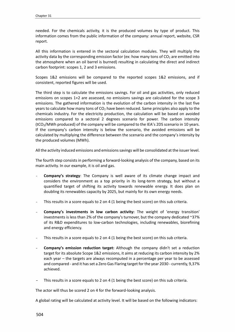
Chapter 31
504
needed. For the chemicals activity, it is the produced volumes by type of product. This information comes from the public information of the company: annual report, website, CSR report.
All this information is entered in the sectoral calculation modules. They will multiply the activity data by the corresponding emission factor (ex: how many tons of CO2 are emitted into the atmosphere when an oil barrel is burned) resulting in calculating the direct and indirect carbon footprint: scopes 1, 2 and 3 emissions.
Scopes 1&2 emissions will be compared to the reported scopes 1&2 emissions, and if consistent, reported figures will be used.
The third step is to calculate the emissions savings. For oil and gas activities, only reduced emissions on scopes 1+2 are assessed, no emissions savings are calculated for the scope 3 emissions. The gathered information is the evolution of the carbon intensity in the last five years to calculate how many tons of CO2 have been reduced. Same principles also apply to the chemicals industry. For the electricity production, the calculation will be based on avoided emissions compared to a sectoral 2 degrees scenario for power. The carbon intensity (tCO2/MWh produced) of the company will be compared to the IEA’s 2DS scenario in 10 years. If the company’s carbon intensity is below the scenario, the avoided emissions will be calculated by multiplying the difference between the scenario and the company’s intensity by the produced volumes (MWh).
All the activity induced emissions and emissions savings will be consolidated at the issuer level.
The fourth step consists in performing a forward-looking analysis of the company, based on its main activity. In our example, it is oil and gas.
- Company’s strategy: The Company is well aware of its climate change impact and considers the environment as a top priority in its long-term strategy, but without a quantified target of shifting its activity towards renewable energy. It does plan on doubling its renewables capacity by 2025, but mainly for its own energy needs.
- This results in a score equals to 2 on 4 (1 being the best score) on this sub criteria.
- Company’s investments in low carbon activity: The weight of 'energy transition' investments is less than 2% of the company's turnover, but the company dedicated ~37% of its R&D expenditures to low-carbon technologies, including renewables, biorefining and energy efficiency.
- This results in a score equals to 2 on 4 (1 being the best score) on this sub criteria.
- Company’s emission reduction target: Although the company didn't set a reduction target for its absolute Scope 1&2 emissions, it aims at reducing its carbon intensity by 2% each year – the targets are always recomputed in a percentage per year to be assessed and compared - and it has set a Zero Gas Flaring target for the year 2030 - currently, 9,37% achieved.
- This results in a score equals to 2 on 4 (1 being the best score) on this sub criteria.
The actor will thus be scored 2 on 4 for the forward-looking analysis.
A global rating will be calculated at activity level. It will be based on the following indicators:

Carbon Impact Analytics - an Approach to Measuring the Climate Performance of Investments
505
- Oil&gas: Carbon intensity of scope 3 fossil fuel emissions
- Electricity: Carbon intensity of electricity mix
- Chemicals: Carbon Impact Ratio = reduced emissions / induced emissions
- + forward looking analysis
This global rating will be calculated at issuer level based on an average weighted by the revenues.
Figure 31-8 Overall rating calculating for our example
6 Case study: analysis of a portfolio with CIA methodology
The portfolio analysis will be performed by the users/clients of the database on the dedicated platform. To do so, the portfolio needs to be imported through a csv file describing it with to columns:
- ISIN code to identify the issuer,
- Amount invested in the selected currency.
In a few second, all the indicators will then automatically be consolidated at portfolio level (including double accounting retreatments). The typical output of this analysis in presented in the following figure.
Current performance
(Reference indicators)
Future performance
(Forward-looking rating)
CIA Overall Rating
2Carbon intensity of the energy produced
Carbon Impact Ratio
Carbon intensity of electricity mix
A B C D E
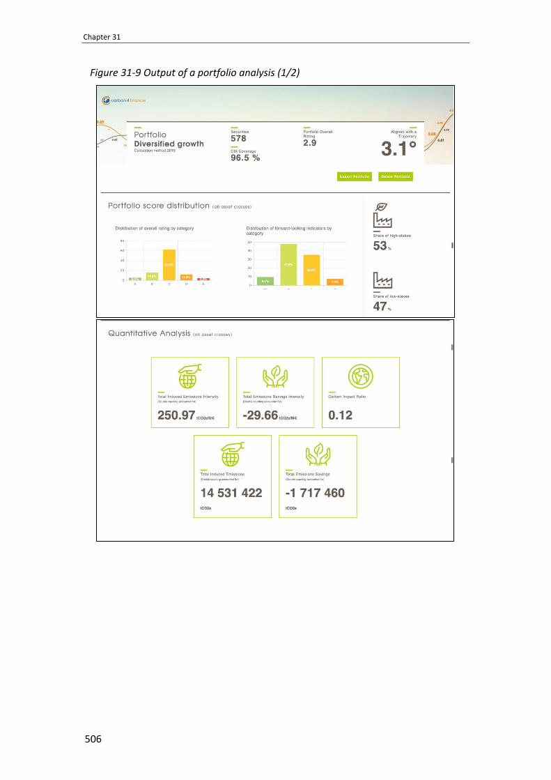
Chapter 31
506
Figure 31-9 Output of a portfolio analysis (1/2)

Carbon Impact Analytics - an Approach to Measuring the Climate Performance of Investments
507
Figure 31-10 Output of a portfolio analysis (2/2)
Then top 5 and worst 5 by indicators are disclosed.

Chapter 31
508
7 Limitations of the current approach future development
For listed institutions, we cover all the major listed corporates of the developed countries, especially those listed within the Stoxx 600, SBF 120, S&P 500, and MSCI World. For institutions which are bond issuers (corporates and sovereigns), we initiated in June the coverage of the largest EURO Investment Grade issuers, including the main listed in the Bloomberg Barclays EURO Aggregate index. We extend the scope of our data base in bottom-up on demand to cover all strategic exposure or investment in a portfolio.
A statistical approach derived from the core bottom-up approach enables to cover the largest portfolios, as soon as sector and revenues can be identified.
The planned future developments are:
- an update of the methodology for summer 2020 with an integration of the 2°C or 1.5°C alignment of companies that have defined a scientific and realistic target. In CIA methodology, Energy sectors already have this approach, but we want to take advantage of the methodological efforts put in place by companies.
- Integration of the pathway to carbon neutrality assessment. A reflection is underway with the Net Zero initiative that Carbon 4 has implemented, which aims to define what a scientific and robust carbon neutrality for companies means.
- The alignment of CIA’s green share with the EU taxonomy.
8 Conclusion
The CIA approach enables to provide relevant climate data in a world where reported data is clearly incomplete and inconsistent. The inclusion of GHG scope 3 emissions remains a “must have” when addressing climate change challenges, and CIA constitutes a solution to address it. Looking at the opportunity side with the emission savings is also important to bring a proper vision of a company’s climate performance.
If CIA enables reporting at portfolio level, its strength is the ability to rank companies within a sector. This can be the source of several active and passive strategies, from impact investing to transition risk management, for financial markets as for bank loanbooks.
This methodology had also been transposed to other asset classes like sovereign, green bonds or real assets, constituting a very polyvalent and complete methodology.

Carbon Impact Analytics - an Approach to Measuring the Climate Performance of Investments
509
Bibliography
CIA, & Carbon4. (2018). Carbon Impact Analytics: How to measure the contribution of a portfolio to the energy and climate transition.

Chapter 32
510
Carbon Accounting Methods for Assessing Carbon Footprint and Intensity of Underlying Assets
By
ISS1
Abstract
Potential climate change implications pose risks to established investment positions. A key to understanding those risks is by measuring the carbon footprint and emissions that companies and facilities produce. Increased regulatory pressure has increased the visibility of these data collection efforts, which has brought increased participation, but also a need for common practices. Organizations like the TCFD seek to bring commonality to climate reporting in-line with current financial disclosure practices. The Greenhouse Gas Protocol gives guidance on standardized reporting practices, however, wide variation of actual data persists. Different methods to turn reported data into usable data exist, including carbon footprinting and carbon intensity comparisons. Despite social and regulatory backing, an overwhelming minority of companies effectively report their emissions, creating a challenge for analysts. Analysts are faced with data challenges such as incompleteness, source discrepancy, time lag, or timeframe creep. Scenario analysis is a useful tool for investors to conduct forward-looking assessments, to analyse multiple pathways of action for the companies long-term sustainability. The 2°C scenario is a common example offering multiple degrees to which the earth will warm over a given time frame, allowing investors to limit emission in order to stay aligned with a certain pathway. Being able to measure company environmental impacts are the first step to setting them on a path of change.
Keywords: TCFD, carbon footprint, GHG protocol, exposure, carbon intensity, data quality, point-in-time analysis, sustainable, scenario analysis
1 Measurement of investors’ carbon footprint
Carbon footprint measures the absolute current emissions exposure that investors have through their investments. An investment portfolio’s carbon footprint is the sum of each portfolio company’s most recently reported emissions, proportional to the amount of stocks (or bonds) held in the portfolio.
ISS ESG helped pioneer this type of assessment for equity portfolios 10 years ago. Since then, diversified approaches for several asset classes have emerged. This section examines the key considerations and the primary approaches for calculating the most commonly used metrics for equity and fixed income portfolios as outlined by the TCFD.
The three key steps to evaluate the carbon footprint of an investment portfolio are:
1This chapter is written by Fredrik Fogde, Vice President, Head of Data Research of ISS, email: [email protected];
Dr. Guido Lorenzi, Data Research Associate, email: [email protected]; and Graeme Wilson, Data Research
Associate, email: [email protected].

Carbon Accounting Methods for Assessing Carbon Footprint and Intensity of Underlying Assets
511
1) Determination of the annual emissions for the underlying entity;
2) Determination of investors’ ownership or exposure to the emissions of the investee;
3) Aggregation of entities’ emissions present in the portfolio, according to the chosen measure for ownership and intensity metrics.
The key challenge for investors related to point 1) concerns the reliability and the availability of emissions for underlying securities. Despite the increased regulatory pressure on companies to report emissions, in 2019, only ca. 3700 companies reported emissions worldwide. Moreover, there are several discrepancies and methodological inaccuracies with regard to reported numbers (see Challenges for additional details).
The emissions aggregation on the portfolio level also present its challenges. The implementation of the TCFD recommendations gave a strong impulse to the development of methodologies to assess portfolios’ carbon footprints. As a result of this process, three main portfolio metrics have gained a diffusion level that makes them widely accepted by investors. These are emission exposure, relative carbon footprint, and weighted average carbon intensity. A detailed description of the above methods is given in the next sections.
Emission exposure The greenhouse gas emissions exposure that an investor is attributed as a result of its investments is the main outcome of a carbon footprint assessment. It essentially determines a portion of the indirect emissions of an investor. In particular, this emissions category (category 15 of Scope 3) is specified in the Greenhouse Gas Protocol 2 (see the section Reporting under the Greenhouse Gas Protocol), which is one of the most commonly adopted frameworks that companies use as an accounting methodology to estimate their emissions.
In order to implement a carbon footprint analysis of an investment portfolio, the first step is to determine the part of an underlying companies’ carbon footprint can be attributed to the investor. This most often done by determining the “ownership” of the investor of an investee. The ownership is defined as the portion of the security held by the investor. The ownership calculation is influenced by the type of the portfolio (pure equity, mixed or pure fixed-income) and by the investors’ preferences. For equity portfolios, 3 the investor ownership has traditionally been calculated by dividing the value invested in a certain holding by the corresponding market capitalization. However, the need to analyze portfolios including fixed-income securities requires an alternative measure of the company value. Although there is no standard, outstanding debt or enterprise value4 are the most common proxies to estimate the ownership for each entity in the portfolio. The current trend in the market shows that an increasing number of investors are using enterprise value as the denominator for both pure equity, pure fixed income, and mixed portfolios. This choice reduces complexity and double counting, and favors comparability among portfolios containing different types of holdings. Moreover, this approach is recommended by the Partnership for Carbon Accounting Financials
2 “GHG Protocol establishes comprehensive global standardized frameworks to measure and manage greenhouse gas
(GHG) emissions from private and public sectors operations, value chains and mitigation actions” (http://ghgprotocol.org/) 3 Equity methodologies are mainly used to assess pure-equity portfolios. In these cases, the company value is represented
by her market capitalization (i.e., the value of a company traded on the stock market). 4 Outstanding debt is the debt that has not yet been repaid in full, while enterprise value is the sum of market capitalization
and outstanding debt.

Chapter 32
512
(PCAF), that includes several banks and asset managers from all over the world5, as well as being a key metric for performance measurement in EU Climate Benchmarks.
Absolute carbon footprint The calculation of the emission exposure of a portfolio containing n securities, also called absolute carbon footprint, is reported in Equation 1, where enterprise value is used as denominator.
∑𝐼𝑛𝑣𝑒𝑠𝑡𝑚𝑒𝑛𝑡 𝑖𝑛𝑡𝑜 𝐶𝑜𝑚𝑝𝑎𝑛𝑦𝑖
𝐸𝑛𝑡𝑒𝑟𝑝𝑟𝑖𝑠𝑒 𝑉𝑎𝑙𝑢𝑒 𝑜𝑓 𝐶𝑜𝑚𝑝𝑎𝑛𝑦𝑖×
𝑛
𝑖
𝑇𝑜𝑡𝑎𝑙 𝐸𝑚𝑖𝑠𝑠𝑖𝑜𝑛𝑠 𝑜𝑓 𝐶𝑜𝑚𝑝𝑎𝑛𝑦𝑖 [tCO2e] Equation 1
The absolute carbon footprint is dependent on the size of the portfolio and this limits the comparison with other portfolios or with a benchmark. Therefore, larger portfolios including fewer polluting companies might have absolute carbon footprints lower than smaller portfolios with more polluting companies. Moreover, this approach is sensitive to market capitalization and currency fluctuations, but it is historically the first metric used to estimate investments’ carbon footprints, especially because it is easy to communicate and clearly shows the investment strategy through the concept of ownership. This metric also gives a representation of the absolute impact on the climate by the investor. The absolute number can subsequently be compared with more relatable metrics, such as the number of cars taken off the road in terms of CO2.
Challenges often faced with this metric includes issues of double counting and lack of applicability when looking at other asset classes then fixed income or equity. For derivatives for example, the link between investor ownership and the underlying asset are not as straight forward.
Relative carbon footprint The comparability of portfolios improves when the emissions are normalized on the size of the portfolio. This can be achieved by referring the total emissions exposure to the total capital invested in the portfolio (Equation 2). Essentially, the below calculation equates to the Weighted Average Carbon Intensity but using enterprise value rather than revenue. This calculation is the metric used in the newly launched EU Climate Benchmarks to track the year on year decarbonization requirement. A key discussion point of this metric is the impact that a change in company valuation can have on results, where a drop in valuation of a company can have a significant impact on the intensity of a company. This makes alignment of date of holdings and enterprise value used an important part of the calculation. Alternatively, as suggested in the EU Climate Benchmark Regulations, yearly average valuations can be applied.
∑𝐼𝑛𝑣𝑒𝑠𝑡𝑚𝑒𝑛𝑡 𝑖𝑛𝑡𝑜 𝐶𝑜𝑚𝑝𝑎𝑛𝑦𝑖
𝐸𝑛𝑡𝑒𝑟𝑝𝑟𝑖𝑠𝑒 𝑉𝑎𝑙𝑢𝑒 𝑜𝑓 𝐶𝑜𝑚𝑝𝑎𝑛𝑦𝑖×𝑛
𝑖 𝑇𝑜𝑡𝑎𝑙 𝐸𝑚𝑖𝑠𝑠𝑖𝑜𝑛𝑠 𝑜𝑓 𝐶𝑜𝑚𝑝𝑎𝑛𝑦𝑖
𝑇𝑜𝑡𝑎𝑙 𝐼𝑛𝑣𝑒𝑠𝑡𝑚𝑒𝑛𝑡 (𝑃𝑜𝑟𝑡𝑓𝑜𝑙𝑖𝑜) [
tCO2e
M$invested
] Equation 2
Carbon intensity There are currently two widely used metrics that incorporate total sales of a company as a normalizer. In these cases, the emission intensity (expressed in terms of emissions per sales
5 https://carbonaccountingfinancials.com/

Carbon Accounting Methods for Assessing Carbon Footprint and Intensity of Underlying Assets
513
volume), is used to give an indication of the revenues that a company produces per unit of emissions. This metric is a good indication of the type of the entities that are included in a portfolio. For instance, a portfolio containing a high share of financial companies is more likely to have a lower carbon intensity than one which is predominantly composed of energy and heavy-industry companies.
The emissions normalized by portfolio claim on sales measure the efficiency of a portfolio in terms of emissions per unit of revenue (Equation 3).
∑𝐼𝑛𝑣𝑒𝑠𝑡𝑚𝑒𝑛𝑡 𝑖𝑛𝑡𝑜 𝐶𝑜𝑚𝑝𝑎𝑛𝑦𝑖
𝐸𝑛𝑡𝑒𝑟𝑝𝑟𝑖𝑠𝑒 𝑉𝑎𝑙𝑢𝑒 𝑜𝑓 𝐶𝑜𝑚𝑝𝑎𝑛𝑦𝑖×𝑛
𝑖 𝑇𝑜𝑡𝑎𝑙 𝐸𝑚𝑖𝑠𝑠𝑖𝑜𝑛𝑠 𝑜𝑓 𝐶𝑜𝑚𝑝𝑎𝑛𝑦𝑖
∑𝐼𝑛𝑣𝑒𝑠𝑡𝑚𝑒𝑛𝑡 𝑖𝑛𝑡𝑜 𝐶𝑜𝑚𝑝𝑎𝑛𝑦𝑖
𝐸𝑛𝑡𝑒𝑟𝑝𝑟𝑖𝑠𝑒 𝑉𝑎𝑙𝑢𝑒 𝑜𝑓 𝐶𝑜𝑚𝑝𝑎𝑛𝑦𝑖×𝑛
𝑖 𝑅𝑒𝑣𝑒𝑛𝑢𝑒 𝑜𝑓 𝐶𝑜𝑚𝑝𝑎𝑛𝑦𝑖
[tCO2e
M$] Equation 3
Comparisons with other portfolios and benchmarks are possible with this approach and the ownership of a security influences the final result. However, companies selling premium products (e.g. Porsche) have a lower intensity than companies selling lower-price products (e.g. Tata Motors). This suggests that sales volumes are not a perfect proxy to evaluate companies’ climate impact. Furthermore, as the emissions and revenue are first summed up separately, the effects of the largest contributors and of the outliers can be watered down by companies with low emissions and high revenues.
Weighted average carbon intensity The weighted average carbon intensity (WACI) is the key metric recommended in the ‘Metrics and Targets’ pillar section of the Final TCFD Recommendation Report (TCFD, 2017). However, this approach does not produce a carbon footprint estimation or an indication of absolute impact, since a measure of the investor ownership of the entities in the portfolio is not included, and cannot be applies in a similar way as the relative carbon footprint. In other words, the result is not affected by the share of a company that an investor owns, but rather the weight that the company has within the assessed portfolio. On the other hand, this metric is useful to establish a comparison with other portfolios or benchmarks.
∑𝐼𝑛𝑣𝑒𝑠𝑡𝑚𝑒𝑛𝑡 𝑖𝑛𝑡𝑜 𝐶𝑜𝑚𝑝𝑎𝑛𝑦𝑖
𝑇𝑜𝑡𝑎𝑙 𝑃𝑜𝑟𝑡𝑓𝑜𝑙𝑖𝑜 𝐼𝑛𝑣𝑒𝑠𝑡𝑚𝑒𝑛𝑡×
𝑛
𝑖
𝑇𝑜𝑡𝑎𝑙 𝐸𝑚𝑖𝑠𝑠𝑖𝑜𝑛𝑠 𝑜𝑓 𝐶𝑜𝑚𝑝𝑎𝑛𝑦 𝑖𝑇𝑜𝑡𝑎𝑙 𝑅𝑒𝑣𝑒𝑛𝑢𝑒 𝑜𝑓 𝐶𝑜𝑚𝑝𝑎𝑛𝑦𝑖
Equation 4
The intention of the metric, and the reason for using revenue, is to create a proxy for efficiency that can be applied across sectors. Using industry specific indicators as the denominator in these calculations would lead to a more accurate indication of efficiency but would be difficult to apply on a portfolio with companies with different types of output. Using revenue as proxy for output can be a stretch in many service sectors, and can to a certain extent favor companies with a high degree of potential stranded assets. Oil & Gas companies with high earnings is an example of this.
2 Challenges
As the field of carbon footprinting of investment portfolios is relatively new compared to GHG accounting of corporates, as well as the fact that methodology development has been driven by investor demand rather than regulation, investors are faced with a few key challenges when conducting such an analysis.

Chapter 32
514
State of reporting Despite the increasing focus on reporting, ISS ESG found that from a universe of 25,000 global companies, only 15% reported emissions, and out of these, 6% were assessed to be reporting incomplete or unreliable numbers and were, thus, discarded. Although the focus on transparency and corporate reporting has increased, basing assessments on disclosed information only would present incomplete pictures of many investment portfolios. For instance, among the equity portfolios analyzed by ISS ESG, the percentage of disclosing companies generally lies between 65-70%. This section gives an overview of the current state of climate data reported by companies and highlights some common issues of data quality that investors should be aware of.
Reporting under the Greenhouse Gas Protocol Under ideal circumstances, a company would catalog and disclose its full GHG inventory, thus making it very simple for analysts to sift through and utilize the data. In practice, it is much more difficult to measure and collect this data. Without a common, widely accepted mandatory standard, the problem is compounded. However, the Greenhouse Gas Protocol has developed one of the most widely accepted standards for disclosing GHG emissions.
Figure 32-1 Representation of the standard for emissions accounting according to the GHG Protocol.
Data discrepancies between sources The widespread application of the above framework does not guarantee that investors will not find inconsistencies when looking at corporate emissions data. As an example, companies choose through which channels they wish to publish their GHG inventories. Considering the companies for which emissions were collected in 2018, 21% reported only through sustainability or annual reports, 38% reported only through the CDP, and 42% reported via both channels. Often, the numbers do not perfectly match between sources.
One frequent data issue is that emissions reported to different sources can differ. Common reasons for this include:
- Stricter frameworks from CDP on what types of reduction activities can be subtracted from scope 2 emissions. In CSR reports, companies will for example often subtract offsets from scope 2 emissions, something which the CDP framework does not allow.

Carbon Accounting Methods for Assessing Carbon Footprint and Intensity of Underlying Assets
515
- Selective inclusion/exclusion of facilities. The facilities and operations that companies include emissions for in their reporting can differ between sustainability and CDP reports.
- Control approach used. The GHG protocol provides three key approaches for how to set the boundaries within which to include emissions: financial control, operational control, or equity share. These are sometimes applied differently when disclosing to different sources.
Incomplete reporting While many companies have felt the groundswell social pressure to increase the level and quality of their environmental disclosure through CSR and sustainability reports, the good intentions are often met with misguided understanding of how to effectively disclose the environmental effects of company activities. Many companies rush into including what turns out to be an incomplete accounting of their emissions. While they deserve credit for getting the ball moving in the right direction, this often leads to them missing the mark. The three most common forms of incomplete public emissions disclosures are loosely termed “no-number graphs,” “intensity only,” and “total only”.
Often, companies will proclaim that their emissions have gone down year over year, perhaps also meeting a goal, perhaps also mentioning a percentage with which they have declined relative to a base year goal or target. However, when these claims are presented in “no-number graphs” without specific absolute inventories, the reliability decreases. The level of certainty and completeness that analysts attribute to such disclosures is thus limited. On the other hand, some companies do not report absolute emissions but just an intensity metric, i.e., a relative value of emissions per unit of production or revenue. This approach is referred to as “intensity only”. When a company discloses an emissions intensity number this is viewed as more valid, as the value requires that the company performed an inventory of emissions in order to place it into relation to production. However, the failure to disclose a specific inventory devalues the company’s disclosure. Doing a backwards calculation of the intensity to arrive at an emissions value is possible, but this is an unreliable method and is not as credible as best practice would require the company to disclose the emissions inventory in the first place. Similarly, while intensity is a useful measure, it is not an ideal metric for the quality of emissions disclosure. A third type of ineffective reporting is when companies give a single total (“total only”) for the emissions of the entire organization, without breaking it out by operations or by scopes. These instances are ambiguous and must be qualitatively assessed by analysts. Divisions between direct and indirect emissions, business travel, and third-party services must be searched for and identified, if possible.
Data lagging A common issue encountered in emissions collection is untimely data disclosure and the mismatches in reporting periods that can arise from solely using the latest available emissions from each company. Since companies and regions have their own fiscal year periods, which can vary widely across the full calendar year, it can therefore be difficult to accurately compare companies against each other. What is labeled as 2018 data in one platform may cover the fiscal year ending March 31 for company A and September 30 for Company B. Likewise, it can be difficult for analysts to correctly time the data collection process for the most current data for the coverage universe. If a company publishes its annual report or sustainability report after the cutoff date for a data collector’s cycle, this could lead to a one or even two-year data lag, depending on the timing. Some companies only disclose their GHG emissions in a sustainability report that is not connected to their annual report and is published arbitrarily within the year, thus lagging behind their mandatory financial disclosures. In both cases,

Chapter 32
516
investors trying to make informed decisions in the present year would be operating with outdated data.
Point-in-time analysis While a carbon footprint assessment of a portfolio provides several comparable metrics, these metrics serve only as the starting point towards understanding the climate risks or opportunities associated with an investment portfolio. A carbon footprint assessment is a point-in-time analysis and, while it measures current performance and impact, it does not take into account forward-looking indicators on how well a company is placed to deal with aforementioned physical or transitional risks. For a holistic climate analysis, forward-looking indicators.
Dealing with non-disclosing companies With only roughly 15% of listed corporates reporting their emissions worldwide, relying only on reported emissions for portfolio level analysis would not suffice. Excluding companies that do not report could in many cases lead to ignoring the companies most exposed to climate related risks, i.e., those companies with high emissions that are not managing this impact at all.
Several approaches towards estimating emissions exist currently in the market the methodologies of which can be categorized into overarching methodologies (Kepler Cheuvreux, 2015).
- Industry averages and regression models. Companies that report emissions are grouped together and regression models run using financial indicators of the companies to create coefficients per sector.
- Environmentally-extended input-output models (EEIO). This approach looks extends traditional input-output models to include emissions created from various parts of the supply chain for each unit of economic output.
- Life cycle analysis (LCA). Life cycle databases such as EcoInvent provide emission factors for all raw materials that go into a product.
The most common approach currently available is one of regression models and certain types of EEIOs. ISS ESG use a combination of all three models, where regression models are used for Scope 1 & 2 emissions, and a combination of EEIO and LCA for Scope 3.
For the Scope 1 & 2 emissions database, ISS ESG applies an approach in five steps.
1) Self-reported emissions are collected from a range of various sources, and aligned in terms of fiscal years, ensuring that numbers provided for several companies are in line, and so that different fiscal years’ worth of data is not provided in the same dataset
2) Self-reported numbers are thoroughly quality-checked for consistency and completeness, and the extent to which the reporting methodology aligns with the GHG protocol. Several of the issues discussed earlier in this report are discovered in this step.
3) For any regression model, it is important that these are run on groups that have very similar carbon emissions profiles. This is something that traditional financial classification systems fail to capture. Here ISS ESG has developed a proprietary Climate Industry

Carbon Accounting Methods for Assessing Carbon Footprint and Intensity of Underlying Assets
517
Classification System (CICS). In this step analysts take great care to classify companies into the correct industry from a carbon footprint point of view.
4) Regression models are then run on the verified data. In most regression approaches currently used, revenue is used as the only factor against which to compare emissions with. However, for many sectors, ISS ESG research finds very little correlation between scope 1 & 2 emissions per revenue. The regression models are thus run on a range of financial indicators, where different combinations are used for each industry.
5) The resulting regression models and accompanying financials required are then applied to non-reporting companies. For transparency reasons, the adjusted R-Squared for each underlying model is also provided to clients.
This approach was developed in collaboration with ETH Zurich and has been used by investors for over a decade.
3 Discussion & outlook
This chapter has highlighted some of the challenges that investors may face when looking for reliable data on which to base carbon metric calculations. Many of these issues are dampened by data providers, who aggregate reported data in a comparable manner, and offer estimations for companies that do not report. In addition, the use of different portfolio level carbon metrics for reporting on the emissions of the portfolio, can often lead to conflicting messages from a report. For example, while the WACI may show outperformance against a benchmark, the relative carbon footprint could be outperforming to a lower extent, or in certain cases actually underperform against the benchmark. The convergence of estimation methodologies, the use cases for pure carbon footprint reports, and the use of different metrics are thus likely to dominate the discussion around carbon footprinting for the foreseeable future. The following section provides some concluding thoughts on these topics.
Diverging methodologies & use cases for carbon footprinting As discussed, approaches for filling the gaps in company reporting differs, and subsequently have an impact on the metrics discussed. This is particularly true when revenue numbers are both used as the primary input source for estimation, and then subsequently as the normalization factor to calculate the WACI. A similar argument can be made for companies that are yet to generate much revenue, but are none-the-less emitting a significant amount of emissions (see Oil & Gas Exploration or Mining companies). Using revenue numbers to estimate emissions for these companies can often lead to gross underestimations. Conversely, while using fixed assets or amount of employees (or other estimations based not only on revenue) may lead to a more accurate estimation of the absolute emissions, but using the low revenue numbers as a basis for efficiency will cause the company to be an outlier in terms of emissions/revenue and significantly impact the WACI.
However, despite the differences in approaches described above, and despite some of the limitations of looking at backward looking performance, there are still several useful outcomes for the investor from a pure carbon footprint analysis:
1) The fact that there is a need to create estimations for one of the most basic forms of climate risk management by companies is an indictment of how far we still need to go in terms of putting climate risk on the agenda of companies. Few indexes or funds, unless climate themed, are likely to have 100% coverage in terms of reported emissions.

Chapter 32
518
Highlighting these companies, and those in transition-exposed sectors or with high estimated emissions, is still a powerful and useful starting point for any type of engagement activities.
2) While several types of scenario analyses that focus on transition risk look at a company’s alignments with certain types of scenarios, potential changes in carbon pricing is a form of transition risk that will have a direct impact on absolute emission numbers. Looking at a company’s emissions exposure, and subsequently the aggregated absolute number on a portfolio level, can be directly compared to certain carbon pricing scenarios.
3) A carbon footprint report of a portfolio also serves as a heat map to identify the potential hot spots of a portfolio and serve as a starting point from which to start looking at sector specific, forward looking indicators. By analyzing aspects such as sector contribution to portfolio results, top 10 lists and % of disclosed emissions by sectors and regions, investors can focus further research on areas most exposed to carbon emissions.
4) Lastly, continuing to apply and calculate metrics based on an ownership approach, paves the way for more accurate scope 3 emission reporting by financial institutions, in particular the carbon footprint from investments.
While the above use cases are valuable in their own right, a holistic climate risk analysis should include a scenario analysis element, whether that be looking at transition risks, physical risks or scenario 1.5 degree alignment of the portfolio.
The metrics debate While four key carbon footprint metrics were presented in previous chapters, we see an increasing preference and use of two in particular.
- The Weighted Average Carbon Intensity – The growing application by investors of the TCFD recommendations, has led to many investors focusing on this metric for reporting and comparison. Several climate-themed indexes have also been launched where carbon performance is tracked with this metric.
- Relative Carbon Footprint – This metric was one of the first metrics to measure carbon footprint performance of a portfolio and has been used by investors for over a decade. The link to ownership and potential to calculate an absolute number, which in turn can be compared to more relatable, still makes it a very applicable number to communicate to stakeholders, particularly for asset owners. As stated earlier, this metric has also been adopted as the metric with which to track year on year reduction progress for EU Climate Benchmarks.
The launch of the EU climate benchmarks and the inclusion of the relative carbon footprint in tracking progress has sparked a debate surrounding which of the two above mention metrics are most applicable for tracking performance. Proponents of the relative carbon footprint argues that several big polluters (particularly Oil & Gas companies), benefit in such an analysis due to high recent earnings (Azizuddin, 2020). In addition, the metric is sensitive to outliers in cases where revenue numbers are low but emissions significant, and as mentioned earlier, the question remains on how suitable revenue is as a proxy for efficiency. One the other hand, the relative carbon footprint is sensitive to changes in valuation, as a company increases in value, the intensity of the company decreases. Conversely, in economic downturns, intensity can decrease if latest valuations and historic emissions data. This effect can be counteracted by using yearly average valuations. Another argument against the use of relative carbon footprint

Carbon Accounting Methods for Assessing Carbon Footprint and Intensity of Underlying Assets
519
is that discourages from investments in growth companies, where valuation might still be low, and thus potentially resulting in a high intensity, despite relatively low absolute emissions.
As more and more non-financial companies continue to set quantifiable, science-based reduction targets, there will continue to be a wish from financial industry players to have a meaningful emissions reduction methodology of their own. What is becoming increasingly clear however, is that carbon metrics alone are unlikely to be the answer, and that meaningful climate risk reduction strategies needs to take forward-looking indicators into account. How to combine these factors into an agreed upon, meaningful metric, will be a key challenge for sustainable finance in the years to come.

Chapter 32
520
Bibliography
Azizuddin, K. (2020). EU Climate Benchmarks: The row over carbon intensity metrics explained. https://www.responsible-investor.com/articles/eu-climate-benchmarks-the-row-over-carbon-intensity-metrics-explained. Retrieved from
Kepler Cheuvreux. (2015). Carbon compass: Investor guide to carbon footprinting. https://www.iigcc.org/download/carbon-compass-investor-guide-to-carbon-footprinting/?wpdmdl=1512&refresh=5e7b5fc6bb36b1585143750.
TCFD. (2017). Final Report: Recommendations of the Task Force on Climate-related Financial Disclosures. Retrieved from https://www.fsb-tcfd.org/publications/final-recommendations-report/.

ClimFIT: A Portfolio Carbon & Climate Accounting Tool
521
ClimFIT: A Portfolio Carbon & Climate Accounting Tool
By
EcoAct1
Abstract
ClimFIT (Climate Financial Institutions Tool) is a tool designed to address multi–asset portfolio challenges related to climate performance measurement and management. It collects and analyses issuers’ financial and climate data to equip users with an optimal combination of Portfolio Climate Key Performance Indicators (Climate KPIs). The Climate KPIs consist of main ESG-Climate indicators such as financed emissions, capital carbon intensity, operational carbon efficiency, and portfolio exposure to high and low carbon assets. Users benefit from insightful information assessed at portfolio, asset class, sector, geography, issuer, and asset or project level. ClimFIT considers multi-level challenges related to the latest changes in regulatory and voluntary frameworks and uses recent data. While it is constructed around recommended sets of KPIs, it also allows customized settings and bespoke analysis.
Keywords: portfolio, issuer, assets, indicator, metric, KPI, assessment, climate, carbon, impact, performance
1 Purpose of the methodology
Financial sector challenges In order to accelerate the economic transition, the financial sector should transform itself through the integration of a climate-aligned investment strategy combining both climate and financial efficiency. Evolving regulations, standards and initiatives around climate issues hasten the process of reformation.
Facing this rapid evolution, Financial Institutions need to grasp, evaluate and manage two main interconnected impacts: “impact of '' and “impact on” investments.
• The first one is “impact on”: impact of climate change and energy transition on portfolio performance. This impact determines possible risks and opportunities tied to underlying assets and to a portfolio.
• The second one, named “impact of,” is the impact of investments on climate change and sustainable development. This impact defines an investor’s contribution to the transition towards a carbon-neutral economy or to the 1.5°C-2°C trajectory.
1 This chapter is written by Ekaterina Reshetnikova, Finance & Climate Expert of Research & Innovation Department, EcoAct.
Ekaterina, email: [email protected]. The author would like to thank Emilie Alberola, Arnaud Doré, Gauthier Faure,
Kai Larson, Paul Stephenson, Martin Sedgwick, Laurence Guimard, Coraline Barré, Aubin Roy, Fanny Guezennec.
Chapter 33
522
The impacts are not distributed uniformly across sectors, geographies, issuers, and assets which results in different implications for different investments and affects overall portfolio risks and returns.
Therefore, asset managers and owners need methods, models, and tools that ensure consistency with regulation, recommendations, and standards, that combine growing cross-sectional data while remaining operational for users and suitable for diversified portfolios. These challenges lie at the core of the ClimFIT concept (Figure 33-1), the method and tool developed to tackle climate-related impact assessments of investments. The tool provides actors with key indicators helping to identify, measure and manage associated performance, risk and opportunities. Thus, ClimFIT facilitates investment decision-making, as well as fits the specific needs and interests of various capital market actors.
Purpose of ClimFIT and ClimFIT framework The purpose of ClimFIT is to address challenges associated with portfolio climate performance and risk assessment, management and disclosure. The tool is designed to:
• Identify operational efficiency.
Measure climate performance at portfolio, asset class, sector, issuer, and asset level;
• Manage risk and opportunities.
Choose the manageable level of exposure to sensitive to changes in policy and market assets;
• Drive actionable insights.
Track progress, operationalize target setting and enhance climate-aligned capital allocation;
• Ensure regulatory compliance.
Meet mandatory and voluntary reporting requirements and recommendations.
Thus, ClimFIT helps financial institutions to respond to stakeholders’ demands, enlarge engagement and facilitate disclosure, as well as to ease the integration of climate change issues into investment process and strategy.
Aiming at providing all-inclusive and up-to-date solutions, ClimFIT is in continuous evolution and broadening of scope. In this regard it is important to distinguish the ClimFIT tool from the ClimFIT Framework. The tool development is backed by constant research projects – i.e., Framework. While the ClimFIT tool is designed to meet the operational needs of capital market agents, the ClimFiT Framework brings wider expertise to bear on the establishment of ESG and ESG-Climate “impact of” and “impact on” accounting at the portfolio level. Furthermore, the research component fosters proactive integration of ongoing market and policy changes and allows the tool to meet the demanding requirements of advanced actors.

ClimFIT: A Portfolio Carbon & Climate Accounting Tool
523
Figure 33-1 ClimFIT framework
Source: EcoAct
The ClimFIT Framework intends to contribute to overall methodology and data improvement, and harmonization across the market. The aim of the framework is to enhance:
• Development of advanced approaches, accounting rules and data;
• Harmonization of methodologies, terminologies, indicators and metrics;
• Transparency and disclosure, robustness and comparability of assessed results.
Thereby, the Framework supports the development of advanced climate-related accounting methodologies, impact measurement and attribution, benchmarking, proper risk assessment, and science-based targets setting.
2 Intended users and application
Range of users ClimFIT responds to needs of a wide range of financial market actors that can be divided into two groups.
• The first one consists of institutional investors, banks, asset and fund managers, corporates as investors and issuers, investment advisors, rating agencies, and index makers. For banks, insurance companies, pensions and other funds the ClimFIT model is a step forward towards better understanding and management of climate-related drivers for asset price corrections, portfolio composition and rebalancing, inflow and outflow management, factor-based strategies development.
• The ClimFIT framework could also provide insightful information for the second group of actors: policymakers, supervisors, professional initiatives and associations, standard developers, and R&D departments of financial institutions. Namely, the Framework analyses the evolving context and implements various assessment

Chapter 33
524
approaches. It can serve as a basis for (i) identification of best practices, (ii) establishment of common rules for climate accountancy at the financial instruments and portfolio levels, (iii) improvement of reported and estimated data at issuers’ level; (iii) better disclosure at portfolio and fund level.
Scope of assets Regarding a coverage, ClimFIT is applicable to multi-asset portfolios and products composed of a broad variety of holdings. All industries and geographies (countries and regions) are included into assessment. Concerning asset classes, the perimeter includes listed equity, corporate bonds, notes, loans, commercial real estate, mortgage; sovereign, municipal, multilateral bonds; alternatives including private equities, real estate, infrastructure, lands, forests. Listed and unlisted, linked and not linked to physical assets and projects instruments are also covered. As regards issuer’s type, the tool covers corporate, sovereign, supranational, sub-sovereign and agency issuers.
Climate decision-support system Based on Climate KPIs, the tool provides actors with ‘navigating’ information allowing for robust, practical, and dynamic steering of capital allocation in terms of climate performance and alignment with the 1.5°C-2°C trajectory.
ClimFIT provides asset managers and owners with a tailored climate decision-support system. The tool collects and analyses data to equip users with a combination of Portfolio Climate KPIs. The design of the Climate KPIs considers multi-level challenges related to indicators and metrics construction principles that are organized into several recommended sets. The synthetization of quantified results serves to produce comprehensive reports and actionable information. The tool also contains advanced settings options allowing bespoke configurations and customized reports and dashboards (Figure 33-2).
Figure 33-2 ClimFIT Settings
Source: EcoAct
Thus, ClimFIT supports Investors and Managers: financial analysts may use KPIs to anticipate the impact of the low carbon transition on a portfolio or an asset in order to:
• determine the key elements to assess for each type of portfolio and asset class;

ClimFIT: A Portfolio Carbon & Climate Accounting Tool
525
• accompany the decarbonization of issuers and the economy;
• address issues of when and how to rebuild capital allocation;
• define a benchmark to ensure portfolio alignment at different stages of the transition.
Concerning the extended application, while being relevant to the process – portfolio or investor relation management, ClimFIT also provides assessments suitable for financial product structuring and design, such as thematic funds and indices. Fund structuring and product development specialists may rely on the tools’ functionality to design climate-aligned financial products and services.
Regarding Corporates, the tool helps with providing answers regarding the adjustment of investment plans and the facilitation of proactive dialogue with investors. Company executives might use ClimFiT to assess the firm’s climate-related attractiveness from investors’ perspective and ensure future financial inflows.
3 Fundamental components
Multi-level challenges of climate KPIs design ClimFIT is constructed around a concept composed of several market-, science- and management-related elements.
The design of Climate KPIs is based on six fundamental components (Figure 33-3):
• Mandatory and voluntary context alignment;
• Applicability to portfolios diversified across different sectors, geographies, asset classes;
• Climate and transition scenarios integration;
• Science-based approaches;
• Finance-smart climate impact attribution;
• Operationality for a wide range of users.

Chapter 33
526
Figure 33-3 Challenges of portfolio climate KPIs design
Source: EcoAct
Alignment with context Concerning the context alignment, the tool offers settings enabling the production of indicators relevant to a targeted regulation or an initiative. Today, to meet mandatory and voluntary assessment, reporting requirements and recommendations, financial institutions should consider several levels of the framework:
• World. The Paris Agreement and financial flows consistency with a resilient development;
• G-20. TCFD recommendations, Financial Stability Board (FSB);
• European Union. EU Regulation 2019/2088 on Sustainability-Related Disclosures in the Financial Services Sector, EU Regulation 2019/2089 on Climate Transition and EU Paris-Aligned Benchmarks, on sustainability-related disclosures in the financial services sector, EU Directive 2014/95/EU on non-financial disclosure, etc.;
• National level. French Energy Transition for Green Growth Act, art. 173-VI, 2015, UK Companies Act 2006. Regional and National frameworks on low carbon transition and sustainable finance;
• Assessment and Reporting initiatives and standards. PRI ESG and Climate reporting, CDP Climate Change, CDP Financial Services, GHG Protocol Scope 3 Category 15 Investments, Bilan Carbone®2, ISO/CD 14097 Framework and principles for assessing and reporting investments and financing activities related to climate change3, guides developed by professional associations and initiatives - PCAF, FFA, Climate Action 100+, Portfolio Decarbonization Coalition, Science-Based Target (SBT), SBT-Financial Institutions (SBT-FI)4 etc.
2 French standard on GHG Accounting 3 Currently the standard is under elaboration, expected to be published in February 2021. 4 Currently methods are under development, expected to be published in Autumn 2020.

ClimFIT: A Portfolio Carbon & Climate Accounting Tool
527
From complex and heterogeneous to essential and harmonised In this context, asset owners and managers face growing challenges in terms of climate-related financial evaluation, management, and disclosure. Financial sector needs indicators and metrics with enhanced relevance for policy and investment decision making, methods capable of addressing multi-asset portfolio challenges, and tools processing various sets of historical, instant and forecasted data. The ambition behind ClimFIT is to face complex multi-factor problems within the financial sector and to pare them down to the essentials – metrics and indicators. Therefore, the challenge for context aligned KPIs assessment includes a variety of existing approaches. Different methodologies use diverse terminologies and definitions, while also being constructed around different indicators, metrics, impact attribution rules and data. Lack of uniformity causes difficulty related to the necessity of conducting several different analyses associated with various requirements. The ClimFIT model helps tackle this challenge by proposing various settings and serving as universal tool for multi-purpose assessments. KPIs can be calibrated according to any of the above-mentioned requirements and recommendations. To enable this functionality, the tool moved through several phases:
• examination of existing methodologies and recommendations,
• harmonization of terminology and introduction of common language,
• decryption of quantification approaches using common terms and language,
• classification and description of indicators, metrics, variables, and data.
These steps helped to systematize and integrate all existing calculation rules into the ClimFIT’s algorithm and settings. The approach fosters results comparability, comprehensive benchmarking and progress tracking.
4 Detailed methodology
Range of KPIs and methodological steps The portfolio performance assessment method contains two main sets of indicators: Portfolio Climate KPIs and Portfolio Advanced Climate KPIs. The indicators are computed by compiling numerous climate, financial and operational data at sectoral and issuer levels using a portfolio composition information.
• The first set of KPIs measures carbon footprint, capital carbon intensity, operational climate efficiency, and portfolio exposure to high and low carbon assets.
• The second set of KPIs provides further information regarding the portfolio alignment with the 1.5°C -2°C trajectory: SBT- and TCFD-committed and aligned assets, portfolio temperature, market-related transition risks & carbon price, green and brown assets, contribution to the energy transition, climate performance score among issuers and sectors, carbon neutrality & net zero GHG emissions committed assets, the 2°C and below 2°C trajectories aligned investments.
As illustrated in Figure 33-4, the tool’s workflow is composed of four parts:
1. Definition and setting. The workflow starts with a formulation of specific problems and the determination of perimeter. This step helps to proceed with right settings and deliver the targeted results;

Chapter 33
528
2. Data collection and preparation. At this stage the tool gathers issuers’ climate and financial reported data using information related to portfolio composition. Further collected data are processed in order to ensure accuracy and test availability, followed by the addition of estimated data if the threshold for reported data is not reached;
3. Assessment. The model relies on an algorithm that simultaneously and contextually assesses different indicators. The algorithm within the tool relates the different metrics and variables at asset, issuer, sector, and geography levels in order to attribute the impact generated by underlying assets to an investment and aggregate it at a portfolio level;
4. Results and graphics. This stage enables better understanding and communication of obtained results. Quantified information can be visualized using a comparison of Portfolio Climate KPIs with those of a chosen benchmark.
Figure 33-4 ClimFIT workflow
Source: EcoAct
Quantitative and bottom-up methodology The computation starts with a compilation of climate and financial attributes of underlying assets. It begins at issuer, asset or project level and continues by analysis across and within asset classes, industries and geographies. In order to quantify attributed impact, asset specific variables are combined with portfolio variables. All variables are divided into three groups: portfolio variables, issuer’s financial and operational variables and issuer’s GHG emissions variables. Table 33-1 lists all inputs used by the model. The main inputs are:
• Ii - market value of an investment;
• mPV -market value of a portfolio;
• Oi- financial variable of an issuer;

ClimFIT: A Portfolio Carbon & Climate Accounting Tool
529
• Ei- GHG emissions of an issuer;
• Si - sales or production of an issuer.
Where Oi is presented with such variables as: Market Capitalization, Enterprise Value, Debt Outstanding, Liabilities, Sum of Market Capitalization and Debt Outstanding, Assets; Ei takes values as GHG emissions according to a recommended Scope; and Si equals Sales, Assets, or Production.
Table 33-1 ClimFIT inputs
Variable Acronym Variables Explanatory notes
Portfolio variables Ii, mPV
Investment Im 𝐼𝑖 Amount of investments in market or nominal value
Market value of Portfolio
mPV 𝑚𝑃𝑉 Sum of values of assets composing a portfolio
Corporate financial and operational variables Oi, Si
Market capitalisation
mCap Oi Equity value, market value
Debt outstanding
Do Oi Financial debt, market value
Enterprise Value EV Oi Market Cap + Market Value of Debt – Cash and Equivalents
Liabilities L Oi Liabilities of an issuer
Sales S Si Sales of an issuer
Assets A Oi, Si Assets of an issuer
Production P Si Production of an issuer
Country financial and operational variables Oi, Si
Debt outstanding
Do Oi Financial debt of a country
GDP GDP Si Gross domestic product of a countru country
GHG Emissions variables Ei
Scope 1 E1 Ei Scope 1 of GHG emissions of an issuer
Scope 2 E2 Ei Scope 2 of GHG emissions of an issuer
Scope 3 E3 Ei Scope 3 of GHG emissions of an issuer
Emissions E Ei GHG emissions of a country
Source: EcoAct

Chapter 33
530
Data sources and key indicators The ClimFIT methodology links investees’ characteristics with investments using information about portfolio composition. It associates GHG emissions and economic outputs generated by financed activities with securities held by an investor (Figure 33-5). As a primary data source of information, the tool uses Corporate Reporting, the FactSet, OECD, Eurostat, and EcoAct databases.
The quantification provides such indicators as:
• Carbon Footprint or Absolute Carbon Emissions (ACE), expressed in tons of CO2 equivalent (tCO2e). The indicator gives an estimation of an investor’s contribution to an issuer’s absolute carbon emissions. This indicator is known as the concept of “financed emissions”;
• Capital Carbon Intensity or Weighted Carbon Emissions (WCE), expressed in tons of CO2 equivalent per unit of currency invested (tCO2e / $M invested). It provides an estimation of the carbon footprint of a unit of currency invested. Computing issuer’s, sector’s, country’s, and portfolio’s capital carbon intensity, the indicator provides information on the carbon-related efficiency of invested capital;
• Operational Carbon Efficiency or Carbon Intensity (CI), expressed in tons of CO2 equivalent per unit of currency generated by an investee (tCO2e / $M issuer’s sales/assets/product). It evaluates the contribution of an investor to an underlying company’s GHG emissions per unit of revenue or assets generated by the firm;
• Portfolio Exposure or Weighted Average Carbon Intensity (WACI), expressed in tons of CO2 equivalent per unit of currency generated by an investee tCO2e / $M issuer’s sales/assets/product. It is derived from the carbon intensity of each individual investee and their weight in the entire portfolio. It measures a portfolio’s exposure to high and low carbon intensive companies.

ClimFIT: A Portfolio Carbon & Climate Accounting Tool
531
Figure 33-5 ClimFIT process: input, model, output
Source: EcoAct
While the approach mainly focuses on providing an overall portfolio assessment it also provides users with more granular and actionable insights at asset class, sector, geography (countries, regions), issuer, and asset/project levels. Table 33-2 summarizes core information about Climate KPIs.
Table 33-2 ClimFIT outputs
Indicator ClimFIT name Variables Units Level 5
CARBON FOOTPRINT
Absolute Carbon
Emissions
ACE Ii , Oi , Ei tCO2e P, A, S, G, I, AP
CAPITAL CARBON INTENSITY
Weighted Carbon
Emissions
WCE Ii , Oi , Ei , mPV tCO2e / $M invested P, A, S, G, I, AP
OPERATIONAL CARBON EFFICIENCY
Carbon Intensity
CI Ii , Oi , Ei , Si tCO2e / $M issuer’s sales/assets/product
P, A, S, G, I, AP
PORTFOLIO EXPOSURE Weighted Average Carbon
Intensity
WACI Ii , Ei , mPV, Si tCO2e / $M issuer’s sales/assets/product
P, A, S, G
Source: EcoAct
The use of the combination of indicators enables a better understanding of the climate performance of a portfolio and assets, allows for the identification of the best and worst
5 Levels: P - Portfolio, A - Asset Class, S - Sector, G - Geography, I - Issuer, AP - Asset/Project

Chapter 33
532
performers within a portfolio, and consequently enhances carbon-related risk and opportunity management.
5 Sample
A case study of the ClimFIT tool is discussed below with example outputs. Depending on the requirements, these outputs are tailored according to recommendations on next steps.
Portfolio climate KPIs Portfolio Climate KPIs are constructed around carbon footprint or attributed GHG emissions (ACE), capital carbon intensity (WCE), operational climate efficiency (CI), and portfolio exposure to high and low carbon assets (WACI) measured at portfolio, asset class, sector, and issuer level.
Figure 33-6 Portfolio Climate KPIs
Source: EcoAct
5.1.1. Portfolio overview
Portfolio type
Data coverage Scope Benchmarking Levels
Equity Bonds
100% Reported - 96% Estimated - 4%
Scope 1 & 2 Scope 1, 2 & 3
Mainstream index Low Carbon index Scope 1 & 2
Portfolio Asset class Sector Issuer
An initial breakdown of absolute GHG emissions in Scope 1, 2 & 3 is created to highlight the key areas of focus, it also further shows the detail of where the emissions occur between the types of assets in the portfolio. Table 33-3 above shows the emissions associated with Bonds and Equities.

ClimFIT: A Portfolio Carbon & Climate Accounting Tool
533
Table 33-3 Breakdown of portfolio carbon footprint for Scope 1, 2 and 3
Source: EcoAct
In this case, the Scope 1 & 2 footprint is small in comparison to that of the Scope 3 emissions. Equities for both Scope 1 & 2 and Scope 3 contain the highest absolute emissions and is therefore the asset type that will receive the most attention in terms of further analysis. Figure 33-7 below shows the breakdown as percentages of this portfolio.
Figure 33-7 Breakdown of absolute emissions by asset type and associated scope
Source: EcoAct
5.1.2. Portfolio level The absolute and relative indicators of the portfolio’s GHG emissions are analyzed to identify and rank the companies within the equities portfolio that emit the most, and least carbon emissions: the top 10 and bottom 10 performers. Table 33-4 and Table 33-5 below are ranked by absolute emissions from Scope 1 & 2 due to the mandatory requirements on these emissions; weighted Carbon Emissions (WCE) and the investment share % are also shown for reference. Scope 3 emissions are shown separately as percentages of ACE and WCE, which reflects the larger emissions exposure of Scope 3 emissions within the portfolio. This type of analysis identifies the best and worst contributors to a portfolio’s climate performance, a ranking that varies depending on which Scopes of GHG emissions are considered. For instance, as demonstrated in Table 33-4 below: while Company A has the greatest share of Scope 1 & 2 emissions, it is Company D that has the highest share of Scope 3 emissions. However, as the boundaries of scope 3 differ across each business and sector, this data can be misleading without further analysis.
6% 5% 49% 41%
0 500 1,000 1,500 2,000 2,500 3,000 3,500 4,000 4,500
tCO2eACE Equities scope1&2 ACE Bonds scope1&2 ACE Equities scope3 ACE Bonds scope3

Chapter 33
534
Figure 33-8 Analysis of portfolio carbon intensity
Source: EcoAct
5.1.3. Issuer level Figure 33-8 shows that regarding the portfolio’s capital and operational carbon intensity, there are three main issuers that bring the results down. More detailed analysis of Table 33-2 shows that the bottom ten performers represent 16% of investments while accounting for 87% of Scope 1 & 2 GHG emissions, or 53% if Scope 3 is included. Regarding the bottom three, Companies A, B, C, they account for 41.9%, 20.0%, and 9.5% of GHG emissions, and only for 3.0%, 4.3%, and 3.7 % of investments respectively. Thus, the portfolio’s high carbon impact is concentrated into a limited number of issuers. The situation is different when Scope 3 is considered, because the associated intensity is distributed among all issuers in a less concentrated manner.
Table 33-4 Top ten high carbon intensive companies
Source: EcoAct
As Table 33-5 demonstrates the top ten performers represent 15% of the total investment, 2% of Scope 1 & 2 emissions and 20% of emissions when Scope 3 is included in the analysis. The Scope 3 performance is deteriorated mainly because of only one issuer - Company W from the banking sector that is considered as low carbon when Scope 1 & 2 are included and high carbon when Category 15 Investments Scope 3 enters the equation.

ClimFIT: A Portfolio Carbon & Climate Accounting Tool
535
Table 33-5 Top ten low carbon intensive companies, contributing positively to portfolio climate KPIs
Source: EcoAct
5.1.4. Sector level Sector level analysis shows that portfolio carbon footprint is driven mainly by such sectors as non-energy materials and industrials if scope 1 & 2 are considered. Figure 33-9 shows that these two sectors account for 76% of the emissions, followed by consumer cyclicals and non-cyclicals presenting each 7% of overall financed emissions.
It is important to also review the data including the Scope 3 emissions to identify any further trends in sectoral carbon emissions. Figure 33-9 shows the difference between Scope 1 & 2 only versus Scope 1, 2 & 3 sectoral contribution. Regarding the full scope of emissions there are three sectors impacting the most a portfolio footprint and accounting for 69% of overall emissions. Among them consumer cyclicals 31%, Industrials 19% and Finance 19%.
Figure 33-9 Breakdown of sectoral contribution to portfolio emissions, Scope 1 & 2, Scope 1, 2 & 3
Source: EcoAct
5.1.5. Benchmarking Benchmarking portfolio’s Climate KPIs provides information on the portfolio’s overall performance. The analysis on portfolio carbon intensity, when benchmarked against both mainstream and low carbon indices' intensity provides more insights on portfolio efficiency.

Chapter 33
536
Figure 33-10 Benchmarking portfolio climate KPIs, Scope 1 & 2
Source: EcoAct
A comparison of capital carbon intensity (WCE) shows that the portfolio performs better compared to both low carbon and mainstream benchmarks. Each unit of currency invested thus contributes to a smaller carbon impact. One million euros within the portfolio contributes 37 tCO2e which is 2.6 and 3.3 times less compared to low carbon and mainstream indicators respectively.
From operational carbon intensity (CI) perspective, after adjusting attributed emissions (ACE) by issuers’ sales, portfolio holdings look more efficient since they emit 63tCO2e for each million euros of sales generated by underling assets. The portfolio is 1.4 and 2 times more efficient compared to low carbon and mainstream indices' performance.
Concerning portfolio exposure to high carbon assets or weighted average carbon intensity (WACI), the portfolio’s performance is positioned between indices, being 1.2 times more exposed than the low carbon benchmark and twice less exposed compared to the mainstream index.
It Is interesting to notice that in terms of weighted average carbon intensity the portfolio performs worse compared to the low carbon index despite it performs better for the previous two KPIs. Due to its design WACI excludes ownership metrics such as market capitalization or enterprise value, thus, it does not contain related to enterprise market valuation biases. Being constructed around weight of an issuer into a portfolio and its operational carbon intensity WACI shows where portfolio risks are concentrated. Despite good carbon-related capital and operational efficiency of the portfolio, a comparison across all indicators at once reveals the pattern that we see in the mainstream index – accumulation of negative exposure to carbon intensive assets while the low carbon index decreases exposure.

ClimFIT: A Portfolio Carbon & Climate Accounting Tool
537
Such accumulation requires a deeper analysis at issuer level identifying those companies bringing negative exposure to the portfolio. Figure 33-11 demonstrates assets taking into account their individual operational carbon intensity, attributed to the portfolio emissions as well as amount invested. Such analysis reveals that the portfolio exposure is driven by three issuers: companies A, B, and C.
Figure 33-11 Detailed analysis on portfolio carbon exposure, Scope 1 & 2, Scope 1, 2 & 3
Source: EcoAct
Portfolio Climate KPIs provide information related to basic understanding of performance management of portfolios and underlying assets, whereas additional indicators – including SDG, TCFD and SBT-aligned assets – provide a deeper assessment of climate risks and opportunities.
Advanced portfolio climate KPIs Advanced Portfolio Climate KPIs provide further information regarding the portfolio alignment with the 1.5°C-2°C trajectory: SBT- and TCFD-committed and aligned assets, portfolio temperature, market-related transition risks & carbon price, green and brown assets, contribution to the energy transition, climate performance score among issuers and sectors, carbon neutrality & net zero GHG emissions committed assets, the 2°C and below 2°C trajectory aligned investments.

Chapter 33
538
Figure 33-12 Dashboard: TCFD and SBT-aligned assets
Source: EcoAct
Figure 33-13 Dashboard SDG-engagement, CDP scoring, carbon reduction and neutrality of assets
Source: EcoAct

ClimFIT: A Portfolio Carbon & Climate Accounting Tool
539
6 Future development
There is an already urgent and growing need for advanced impact accounting rules and impact assessment solutions. The current context requires more data and climate and increased transition scenario application. Therefore, the roadmap of ClimFIT’s future development is based on three main axes.
Broadening of forward-looking and science-based indicators. The current and ongoing medium- and long-term considerations regarding alignment with climate scenarios and trajectories provide fertile soil for the development of forward-looking indicators. Development of qualitative and quantitative approaches will be a major concern for future development.
Inclusion of EU Benchmarks and EU Taxonomy indicators. EU regulation of financial markets motivates the development of data and solutions. Adaptive and contextualized models supported by better data will be vital in helping address the portfolio climate-related assessment and management challenges. ClimFiT will implement recommended indicators, enabling their quantification for large portfolios and indexes.
Solutions for linking technical issuers with final borrowers. Another obstacle to retrieve appropriate data is the absence of a direct link between corporates - borrowers and their technical issuers, the later are used as a legal entity to raise funds for corporates. Related mostly to fixed-income instruments as bonds, loans, notes, legal and financial structuring - the usage of SPV (special purpose vehicles) - impedes the direct link between an investment and a financed activity and impact. One of the main focuses of the tool’s development will be an investigation of possible solutions to tackle this issue.

Chapter 34
540
CARIMA – A Capital Market-Based Approach to Quantifying and Managing Transition Risks
By
University of Augsburg and VfU1,2
Abstract
The impact of uncertainty associated with the ongoing transition towards a green and in particular low-carbon economy affects virtually all financial market participants. If the transition process accelerates compared to current expectations, the values of carbon-based firms are likely to decline, while the values of low-carbon firms will tend to benefit from this development. On the other hand, if the transition process decelerates unexpectedly, the reverse could happen.
The central goal of CARIMA is to quantify exactly those types of risks as well as opportunities for firm values via a capital-market based approach. Using a factor model, carbon risks are simply “extracted” from the historical returns of global stock prices using the Carbon Risk Factor BMG (Brown-Minus-Green) return time-series.
The CARIMA concept is essentially directed towards key players in the financial industry, such as portfolio managers, who want to take carbon risks in their asset management process into account. CARIMA also addresses further stakeholder groups, such as firms, regulatory authorities, politicians, and finally scientists.
Keywords: carbon risk, carbon beta, climate finance, economic transition, asset pricing, factor models, carbon risk management
1 Introduction
The research project Carbon Risk Management (CARIMA), funded by the German Federal Ministry of Education and Research (BMBF), aims to quantify the existing risks and opportunities for the values of financial assets and respective portfolios in light of climate change and the transition towards a green economy, since values of firms, in many cases, also depend on the expected developments of this transition process. If the transition process accelerates compared to current expectations, the values of carbon-based (“brown”) firms are likely to decline, while the values of low-carbon (“green”) firms will tend to benefit from this development. On the other hand, if the transition process decelerates unexpectedly, the reverse could happen.
1 This chapter is written by Maximilian Görgen, Research Assistant, Chair of Finance and Banking, Faculty of Business
Administration and Economics, University of Augsburg, email: [email protected]; Marco Wilkens,
Professor/ Chair holder, Chair of Finance and Banking, Faculty of Business Administration and Economics, University of
Augsburg, email: [email protected]; Henrik Ohlsen, Managing Director, Verein für
Umweltmanagement und Nachhaltigkeit in Finanzinstituten e.V. (VfU), email: [email protected]. 2 The project Carbon Risk Management (CARIMA; funding code: 01LA1601) is sponsored by the German Federal Ministry
of Education and Research.
CARIMA – A Capital Market-Based Approach to Quantifying and Managing Transition Risks
541
A key challenge for policy is to plan and shape the transition process of the economy in such a way that it results in the lowest possible uncertainties for firm values and thus avoids unnecessary welfare losses that will affect not only the firms, but also society as a whole. An unstructured transition towards a green and low-carbon economy that does not consider such losses would have unforeseen consequences. It is therefore vital that the risks arising from the uncertainty associated with the transition process be as transparent, quantifiable, and manageable as possible.
The impact of uncertainty associated with the transition process affects virtually all financial market participants, as the risks for firm values are directly reflected in the risks for all financial assets issued by firms, such as stocks, corporate bonds, loans, and hybrid financial assets. Since all these financial assets are in turn an integral part of a vast array of portfolios including investment funds, pension funds, pensions offices, life insurances, and portfolios by private investors, such portfolios are exposed to these risks as well.
It is therefore a key challenge for investors and financial intermediaries to assess how well firms can or cannot adapt to the transition process and to take this into account in their investment decisions. An important challenge for central banks and supervisors is to understand the impact of the transition process on the financial institutions they monitor and the overall stability of financial markets.
Risks threatening the existence of firms are particularly worrisome. These ultimately affect not only shareholders or lenders, but also employees, suppliers, and consumers. The transition process of the economy must not lead to unnecessary frictions due to an inappropriate handling of the associated risks of the transition process, as these risks ultimately determine the welfare of all people.
The central goal of CARIMA is to quantify exactly those types of risks as well as opportunities for firm values − the so-called “carbon risks”, also often referred to as “transition risks”. A rational handling of these carbon risks is necessary to achieve the Paris Agreement’s target to keep global warming well below 2°C while avoiding unnecessary socioeconomic losses.
As far as we are aware, CARIMA is currently the only concept to derive such a risk measure based on a capital market-based approach. Compared to other approaches, a crucial advantage of CARIMA is that when applying the CARIMA approach using the freely available Carbon Risk Factor BMG (Brown-Minus-Green), there is no need for detailed fundamental climate change-relevant information about firms, which is often difficult and expensive to obtain or, in the case of many small caps, may not even be available.
The two-year project carried out by the two peer project partners, the University of Augsburg and the Verein für Umweltmanagement und Nachhaltigkeit in Finanzinstituten e.V. (VfU), ended in August 2019. The CARIMA concept was presented to financial practitioners at a rollout-conference and many other workshops and conferences. The CARIMA handbook as well as its related Excel tool and the Working Paper “Carbon Risk” (Görgen et al., 2019) describe the general approach and contain the key results of the project. The corresponding files can be accessed and downloaded free of charge from the project website.3
The CARIMA concept is essentially directed towards key players in the financial industry, such as professional portfolio managers, who want to take carbon risks in their asset management
3 See https://carima-project.de/en/

Chapter 34
542
process into account. In addition, CARIMA also addresses further stakeholder groups, such as firms, regulatory authorities, politicians, and finally scientists.
2 CARIMA – a capital market-based approach
The core idea of CARIMA is to use fluctuations in stock prices to determine the risks and opportunities for single stocks and portfolios. The CARIMA concept thus derives the carbon risks directly from historical stock prices on the capital market, where new information about the expectations of market participants concerning the transition towards a green economy is constantly processed and priced.
Thus, the CARIMA concept presents a capital market-based approach where carbon risks and opportunities of the economy's transition process can be quantified comparatively easy, since they are simply “extracted” from the historical returns of global stock prices using a Carbon Risk Factor BMG (Brown-Minus-Green) in a factor model.
3 Methodology introduction of the CARIMA concept
This section briefly outlines the different modules of the development and application of the CARIMA concept. Figure 34-1 shows an overview of the CARIMA concept with its five modules A to E.

CARIMA – A Capital Market-Based Approach to Quantifying and Managing Transition Risks
543
Figure 34-1 The five modules of the CARIMA concept
Module A: Master dataset
The construction and calculation of a Carbon Risk Factor BMG with a high degree of discriminatory power requires a huge amount of fundamental information from firms. It is crucial that the data allow a sufficiently accurate assessment of a firm’s change in value in the event of unexpected changes in the transition process of the economy. The better firms can be divided into highly selective portfolios in this respect, the more efficient the carbon risk factor calculated will be. Therefore, data from different databases, namely Thomson Reuters ESG, MSCI ESG-Stats and IVA-Ratings, Sustainalytics ESG Ratings, and CDP is used. This data is

Chapter 34
544
carefully prepared, processed, and combined with capital market data (e.g., return data) from Thomson Reuters Datastream.
The individual ESG databases used have different strengths and weaknesses. By combining the databases, some weaknesses in the individual databases are compensated for. For example, the dataset contains information on firms that was collected using various approaches, such as audited annual reports, external scorings, and ratings, (ESG) analyst assessments and self-disclosures. By combining the databases, database-specific distortions can be reduced and various estimation methods from analysts can be integrated. This gives us an extensive selection of firms from which to calculate a meaningful Carbon Risk Factor BMG.
Module B: Scoring concept
Module B describes the 55 Carbon Risk Proxy Variables, which are selected to support a fundamental assessment of whether firm values (and thus their stock prices) are influenced positively or negatively by unexpected changes in the ongoing transition process. These 55 variables are assigned to one of the three group indicators “Value Chain”, “Adaptability”, and “Public Perception”, which represent three impact channels of carbon risk.
The first group indicator “Value Chain” contains Carbon Risk Proxy Variables that reflect the impact of carbon risk across a firm‘s value chain. This group indicator therefore contains variables that deal with all components of a firm’s value chain – such as its production, processes, products, technologies, and supply chain.
The second group indicator “Public Perception” consists of Carbon Risk Proxy Variables that map the influence of carbon risks through another impact channel, so-called public perception. For example, a firm with low-emission production may still be affected by carbon risks if the public believes that the firm is particularly affected by unexpected changes in the transition process to a green economy.
The third group indicator “Adaptability” mainly comprises Carbon Risk Proxy variables that deal with the strategies, guidelines, and management of a firm. A firm can be prepared for unexpected changes in the transition process so that it can respond to these changes efficiently. The effect of the carbon risk on a firm is therefore reduced by a high degree of adaptability.
As part of the development of the CARIMA concept, the selection and allocation of variables were discussed and finalized in two specially organized workshop with climate and financial experts from NGOs, universities, and consulting firms to ensures the variables’ ability to accurately assess a firm’s change in value in the event of unexpected changes in the transition process of the economy as this is a prerequisite for the construction of highly selective portfolios and thus the efficiency of the Carbon Risk Factor BMG formed based on this information.
In a next step, the information from these 55 variables is condensed into the three group indicators via a simple scoring concept in order to calculate the so-called Brown-Green-Score BGS for each firm. A detailed documentation of this scoring concept and the aggregation of the three subscores to the final BGS can be found in the CARIMA manual. This measure ultimately provides a fundamental assessment of the direction and strength of the changes in – or in other words risks to − firm values. BGS is determined annually for each firm. It is important to note that this scoring concept is only the prerequisite for deriving the

CARIMA – A Capital Market-Based Approach to Quantifying and Managing Transition Risks
545
Carbon Risk Factor, which is described in the next paragraph. It is not an assessment measure on its own.
Figure 34-2 Assignment of the 55 Carbon Risk Proxy Variables to group indicators
Module C: Carbon risk factor BMG
Next, appropriate firms for the factor construction are selected. First, all non-listed firms are excluded. In addition, firms in the financial sector are not included, as their carbon risk differs significantly from firms in other sectors. For example, banks have almost no direct emissions of their own, but they finance firms with high emissions that can be particularly affected by carbon risks. Banks may therefore be indirectly affected by carbon risks through their loan portfolio, but this may not be reflected in the fundamental data. An in-depth analysis of the financial sector’s carbon risk can be found in the CARIMA manual.
In addition, only firms that are represented in all four databases and for which data is available for at least five Carbon Risk Proxy Variables are used for factor construction. These conditions are necessary to minimize distortions in the database-specific data collection methodology.
In total, these criteria lead to a sample of 1,637 listed global firms from 50 countries. Table 34-1 shows the geographical and sectoral distribution of the 1,637 firms selected. Most of these firms are based in the USA, followed by Japan and the United Kingdom.

Chapter 34
546
Table 34-1 Geographical and sectoral distribution of the 1,637 firms selected for the construction of the Carbon Risk Factor BMG
Country N % Sector N %
USA 418 25.53
Industry 368 22.48
Japan 227 13.87
Consumer Cyclical 277 16.92
UK 193 11.79
Basic Materials 239 14.60
Canada 97 5.93
Technology 191 11.67
Australia 75 4.58
Consumer Defensive 167 10.20
France 66 4.03
Energy 118 7.21
South Africa 59 3.60
Utilities 104 6.35
Germany 53 3.24
Healthcare 109 6.66
Taiwan 48 2.93
Communication Services 64 3.91
South Korea 36 2.20
Other Europe 237 14.48
Other Asia 78 4.76
Other Americas 37 2.26
Other Oceania 13 0.79
Total 1,637 100.00 Total 1,637 100.00
Looking at the sectoral breakdown of the dataset, most firms are active in the sectors “Industry”, “Consumer Cyclical” and “Basic Materials”. The Carbon Risk Factor BMG is constructed using firms from numerous countries and various sectors. This ensures that the factor contains global information from all sectors of the economy.
Based on their average Brown-Green-Score BGS, those 1,108 firms (624 “brown” and 484 “green” firms) are then assigned to one of two mimicking stock portfolios: the first portfolio consists of stocks of “brown” firms and the other of stocks of “green” firms. Breakpoints for this classification are the terciles of the average Brown-Green-Score BGS.
However, the Carbon Risk Factor BMG should also be as independent as possible from the size of a firm. Each firm is therefore assigned the characteristic “small” or “large” based on its market capitalization, independently of its BGS. This classification is based on the median.
Subsequently, the Carbon Risk Factor “Brown-Minus-Green” (BMG) can be formed from the historical returns of the four value-weighted portfolios described (brown/small (BS), brown/big (BB), green/small (GS) and green/big (GB) following formula 1:
𝐵𝑀𝐺𝑡 = 0.5 (𝐵𝑆𝑡 + 𝐵𝐵𝑡) − 0.5 (𝐺𝑆𝑡 + 𝐺𝐵𝑡) (5)
The Carbon Risk Factor BMG reflects a hypothetical portfolio that is invested long in “brown” and short in “green” stocks, thus reflecting the return difference between fundamentally “brown” and “green” firms.
Of course, it is also possible to consider other ways of constructing the Carbon Risk Factor BMG. For example, the threshold value of a characteristic that serves as the basis for the sorting into the different portfolios can be varied. Country-specific or sector-specific factors are also conceivable, depending on requirements. More information on such modifications can be found in the CARIMA manual.
We check the correlation between BMG and other risk factors and test an orthogonalized variant of the factor to ensure that BMG is not already covered by other common risk factors.

CARIMA – A Capital Market-Based Approach to Quantifying and Managing Transition Risks
547
We also test the scoring concept for robustness by varying the weights for the subscores and breakpoints. More details can be found in the CARIMA manual.
Module D: Factor model
Module D describes how the carbon risk of practically all stocks and other financial assets, as well as the portfolios containing them, can be estimated relatively easily based on the Carbon Risk Factor BMG.
Since stock market prices at any time reflect the speed of the transition process that market participants currently assume is occurring and thus which transition path is expected by society, the return time series of the Carbon Risk Factor BMG, constructed as a mimicking portfolio for carbon risk, contains such information in a condensed form. This information can be extracted by breaking down the firm's (or generally speaking a financial asset’s) return time series into its individual components using a simple regression analysis. One of these components, besides other known risk components, such as a firm’s exposure to common risk factors like SMB or HML, is a firm’s carbon risk exposure, which is assessed by the Carbon Beta through the Carbon Risk Factor BMG. Thus, the Carbon Beta reflects the capital market’s assessment of the carbon risk of the respective financial asset or portfolio.
So, who determines the Carbon Beta in the end? The answer is simple: all market participants, i.e., all buyers and sellers of the stocks and portfolios under consideration, i.e., all equity analysts and other capital market participants worldwide, because they determine the changes in stock prices worldwide, from which the Carbon Risk Factor BMG is calculated. It can also be said that the Carbon Beta is in principle the aggregated assessment of the carbon risk (of all participants) on the capital market.
Only the historical returns of the financial assets or portfolios are required as the dependent variable in the regression. The return time series of the explaining variables, such as the Carbon Risk Factor BMG and the other factors, are available on the project website and further publicly accessible websites, respectively.
Economic intuition and interpretation of the Carbon Beta The Carbon Beta estimates the impacts or effects on firms, and their values or stock prices, of possible changes in expectations that may occur as the present economy moves towards a green economy. Sudden changes in expectations regarding the transition process of the economy are reflected in the Carbon Beta. The higher the absolute Carbon Beta value, the greater the impact (either upward or downward) on the stock price.
Estimation of the market’s carbon risk However, there may also be unexpected changes in the transition process that affect all firms (“brown”, “neutral”, and “green”) to the same or at least a very similar extent. This “general market carbon risk” is not captured with the individual Carbon Betas of the stocks, as it is part of the total market risk. In general, the Carbon Beta is used to estimate the individual risk of a stock in relation to the overall market. It thus determines how the value of a stock is likely to change in relation to the market as a whole if expectations about the transition process of the economy change. The “general market carbon risk” can be estimated through the correlation between the market factor and the Carbon Risk Factor BMG. Our empirical research shows a (slightly) positive and constant correlation between the (global) market index and the Carbon Risk Factor BMG. This suggests that an acceleration of the transition process of the economy towards a green economy will tend to reduce the value of all stocks in the overall market.

Chapter 34
548
In this context, as already described above, the CARIMA manual offers details on the use of an orthogonalized variant of risk factors in the regression model. Here, the correlation between BMG and the other factors in the factor model is set to zero without changing its variance structure. This ensures that the factor continues to explain only those risks that are specific to it and does not capture any other systematic effects.
Carbon Betas quantify risks and opportunities The CARIMA concept does not only quantify the risk of losses, but also the chance of profits. When talking about risks in the following, not only negative events (i.e., risks in conventional language), but also positive events (i.e., opportunities in conventional language) are considered. In this respect, the Carbon Beta is comparable to the volatility (standard deviation) of equity returns, which is widely used in financial practice. This indicator also subsumes opportunities and risks.
Module E: Applications
A variety of potential applications for the Carbon Beta is included in Module E. The Carbon Beta can be determined for different asset classes such as stocks, corporate bonds, loans, portfolios, and funds. Furthermore, various country and sector aggregations and corresponding analyses are possible. Scenarios for stress testing the values of financial assets and portfolios can be generated based on the Carbon Beta. In portfolio management, the Carbon Beta can be integrated into investment strategies, such as Factor Investing and Best-in-class approaches and can be used for hedging carbon risks. The potential applications mentioned here are explained in more detail in the CARIMA manual and supported by exemplary Excel applications.
The CARIMA concept for different user groups The CARIMA concept is applicable for both, users who “only” want to estimate carbon risk exposure, and for advanced users, who want to construct and validate the Carbon Risk Factor BMG by themselves. By making the Carbon Risk Factor BMG publicly available, any user can start directly with determining the carbon risk of financial assets and portfolios easily and quickly by themselves, since only the historical return time series of the respective financial assets or portfolios are needed.
More detailed explanations of modules A to D are given in the CARIMA manual, which is available on the project website. These explanations address advanced users in particular, who would like to adapt and further develop the CARIMA concept to their individual needs and have the appropriate resources to do so.
4 Determination of Carbon Beta with the Carbon Risk Factor BMG
As already described, the CARIMA concept offers a market-based approach to quantify carbon risks by using factor models. The relevance of factor models is reflected not only in their acceptance as study content at practically all universities, but also in their broad recognition in academia and in a wide range of applications in financial practice.
Factor models as the starting point for the calculation of Carbon Betas A typical factor model that is widely used in both financial practice and science is the Carhart (1997) four-factor model, which is a further development of the very well-known Fama and French (1993) three-factor model, which is again a further development of the Nobel Prize-winning Capital Asset Pricing Model (CAPM) of Sharpe (1964), Lintner (1965), and Mossin

CARIMA – A Capital Market-Based Approach to Quantifying and Managing Transition Risks
549
(1966). However, the Carbon Risk Factor BMG can in principle be added to any factor model as long as no other factor is too highly correlated with the Carbon Risk Factor BMG.
In the following applications, the Carbon Risk Factor “Brown-Minus-Green” (BMG) extends the Carhart model so that it has the following form:
eri,t = αi + 𝛽imkterM,t + 𝛽i
smb SMBt + 𝛽ihml HMLt + 𝛽i
wml WMLt + 𝛽ibmg
BMGt + εi,t (6)
With:
• eri,t = return on an asset i minus return on a risk-free investment in period t (excess return)
• erM,t = excess return of the market in period t
• SMBt = return of the global size factor in period t
• HMLt = return of the global value factor in period t
• WMLt = return of the global momentum factor in period t
• BMGt = return on the global Carbon Risk Factor BMG in period t
• αi, 𝛽imkt, 𝛽i
smb, 𝛽ihml und 𝛽i
wml = parameters αi and 𝛽ix of the Carhart Model
• 𝛽ibmg
= Carbon Beta of the asset i. This key figure serves as the central carbon risk measure. It is estimated via a simple multiple linear regression according to this factor model
The central idea of factor models is that the returns on assets and thus the overall risks of those assets can be broken down into various components (“factors”). One of these components is the sensitivity of an asset’s value towards unexpected changes in the transition process of the economy. Assets can be equities, funds or portfolios. In addition, the CARIMA concept is also suitable in principle for determining the carbon risk of corporate bonds and loans. For this, however, some additional considerations and modifications are necessary.
For example, the carbon risk of corporate bonds can be determined using different factor models that are specifically designed to explain the returns of corporate bonds, such as the models by Fama and French (1993) or Elton et al. (1995). However, determining Carbon Betas for loans is somewhat more demanding, because unlike, e.g., stocks or bonds, there are typically no market prices and thus no historical time series of returns for loans. Without these time series returns, no direct estimation of the Carbon Beta using a factor model is possible. Under certain circumstances, the Carbon Betas of firms’ stocks and corporate bonds can be used to estimate the Carbon Betas of loans more or less accurately (see Table 34-2). More information can be found in the CARIMA manual.

Chapter 34
550
Table 34-2 Using Carbon Betas from stocks and corporate bonds to determine Carbon Betas of loans
Carbon Beta of the stock of the same firm is known
Carbon Beta of the stock of the same firm is unknown
Carbon Beta of a corporate bond of the firm is known
Using the Carbon Beta of the stock or a corporate bond to
determine the Carbon Beta of the loan
Using the Carbon Beta of a corporate bond to determine the Carbon Beta of the loan
Carbon Beta of a corporate bond of the firm is unknown
Using the Carbon Beta of the stock to determine the Carbon
Beta of the loan
Using the Carbon Beta of comparable firms to
determine the Carbon Beta of the loan
General interpretation of the Carbon Beta
The Carbon Beta 𝛽ibmg
of an asset can be interpreted as follows: if the Carbon Beta is greater
than zero, it can be expected that the value of this asset will fall compared to the market, if the transition process of the economy towards a green economy accelerates unexpectedly. If, on the other hand, the Carbon Beta is less than zero, the value of this asset will rise compared to an average asset in expectation, if the transition process of the economy towards a green economy decelerates unexpectedly. The value of an asset with a Carbon Beta close to zero is influenced to a market-average extent by the transition process.
Input for calculating Carbon Betas: Historical returns of the Carbon Risk Factor BMG and other risk factors One of the explanatory variables on the right side of Equation (6) is the Carbon Risk Factor BMG. BMG is simply a time series of historical returns on a specific hypothetical stock portfolio; more precisely, it is the difference between the historical returns from “brown” firms and those from “green” firms. This time series is illustrated in Figure 34-3 on a monthly basis from January 2010 to December 2018.
Figure 34-3 Monthly returns of the Carbon Risk Factor BMG (2010-2018)

CARIMA – A Capital Market-Based Approach to Quantifying and Managing Transition Risks
551
Figure 34-4 shows the historical cumulative returns of the “brown” portfolio and the “green” portfolio as well as the historical returns of the Carbon Risk Factor BMG. The cumulative return on the Carbon Risk Factor BMG is slightly positive in the first years of the reviewed period but falls back to zero by the end of 2012. From 2013 to the end of 2015, the cumulative return on the factor fell almost steadily to almost –30% overall. During this period, “brown” firms thus had a much lower return than “green” firms. In the last years of the reviewed period, however, there was a slight increase again, so that the Carbon Risk Factor BMG shows a cumulative return of –20% overall.
Figure 34-4 Cumulative returns of the Carbon Risk Factor BMG and the two portfolios “green” and “brown”
Table 34-3 shows descriptive statistics of the monthly Carbon Risk Factor BMG and its correlations with other global risk factors of the reference model. The average monthly return on the Carbon Risk Factor BMG is negative at −0.25%, the standard deviation is 1.95%. The correlations between the Carbon Risk Factor BMG and the market, size, value, and momentum factors are all relatively low. As mentioned above, a low correlation with other risk factors of the Carhart model is a good first indication for the factor model.
Table 34-3 Descriptive statistics and correlations of the Carbon Risk Factor BMG
Factor Ø Return
(%) Standard-
deviation (%) t-
stat.
Correlations
BMG erM SMB HML WML
BMG −0.25 1.95 −1.17 1.00
erM 0.76 4.02 1.74 0.09 1.00
SMB 0.06 1.39 0.37 0.20 −0.02 1.00
HML −0.00 1.68 −0.02 0.27 0.19 −0.06 1.00
WML 0.57 2.53 2.06 −0.24 −0.20 0.00 −0.41 1.00

Chapter 34
552
Input for calculating Carbon Betas: Historical returns of other risk factors
Other key explanatory variables include the excess returns of the entire stock market erM,t, SMBt, a global size factor, HMLt, a global value factor, and WMLt, a global momentum factor at the time of t. These factors are available free of charge on the Internet. They can for example be downloaded from the Kenneth R. French Data Library 4 or the AQR Data Library 5 . All common factors based on the published literature can also be reproduced individually.
Output: Carbon Betas for stocks
Figure 34-5 Carbon Betas of some example stocks
Figure 34-5 shows the calculated Carbon Betas for some well-known example firms. It is clear that in particular those firms have a high Carbon Beta, which are usually classified as “brown”. On the other hand, especially "green" firms show low Carbon Betas. Similarly, some firms have Carbon Betas close to zero, i.e., apart from the general market carbon risk mentioned above, they are not exposed to carbon risk.
It is not surprising that the Carbon Betas of “brown” stocks are usually more or less positive, and the Carbon Betas of “green” stocks are more or less negative. However, at this point it is worth mentioning that it may also be the case that a firm that, e.g., does not burn fossil fuels itself and is therefore commonly seen as “clean”, also has a positive Carbon Beta and belongs by CARIMA-definition to the “brown” firms.
This could be the case if the firm relies heavily on “brown” inputs or is a supplier to “brown” firms. In this case, an unexpected acceleration in the transition process of the economy could be expected to lead to a decline in profits for this “clean” firm as well, since this firm depends
4 See http://mba.tuck.dartmouth.edu/pages/faculty/ken.french/data_library.html 5 See https://www.aqr.com/Insights/Datasets/

CARIMA – A Capital Market-Based Approach to Quantifying and Managing Transition Risks
553
in turn on firms whose value and business models are negatively affected by the unexpected acceleration. The same, of course, applies vice versa.
The level of the estimated Carbon Betas can be used very easily to compare the carbon risk exposures of different firms.
Output: Carbon Beta for portfolios
In a similar way as for stocks, carbon risk can also be determined for portfolios. When assessing the current carbon risk in portfolios for today or future periods, respectively, two approaches, in particular the top-down and bottom-up approach, are conceivable. In both cases, historical return time series serve to estimate a portfolio’s current carbon risk. The composition of the portfolio, or more precisely its change over time, is a key factor in choosing the appropriate approach.
For the top-down approach, only the portfolio’s historical time series of returns must be known, while the bottom-up approach requires the current portfolio weights of the individual assets and their return time series.
To determine a portfolio’s Carbon Beta using the top-down approach, the user only needs to have the portfolio’s historical time series of the excess returns. This corresponds to the weighted excess returns of the individual stocks in the portfolio. These excess returns are used as a dependent variable in the regression, as previously described for stocks. Thus, the Carbon Beta can be determined directly from the regression Equation (6). This once again illustrates the great advantage of the CARIMA concept. For portfolios with any number of different types of financial securities, the carbon risk can be estimated with just one regression.
However, to ensure that this approach does not lead to wrong results in the estimation of current Carbon Betas, the composition of the portfolio must, strictly speaking, have remained the same over the entire historical period under consideration. Note that the weights of the stocks in the portfolio can change automatically over time depending on the performance of stocks in the portfolio.
If the assumption of a constant portfolio composition over time is (severely) violated, it is more reasonable to determine the portfolio’s Carbon Beta using the bottom-up approach. However, for this approach, the historical time series of (excess) returns of the individual stocks and their weighting in the portfolio are required. Subsequently, the Carbon Betas of each stock in the portfolio can be determined using Formula (6). The Carbon Beta of the portfolio is then calculated as the weighted sum of the Carbon Betas of the stocks held in the portfolio.
Output: Carbon Beta of funds
The following section describes how to determine the Carbon Beta of funds, in particular, equity funds. Equity funds are investment funds that invest their assets primarily or exclusively in (individual) stocks.
Determining the Carbon Beta at fund level is basically analogous to the procedure for portfolios, since funds are basically special forms of portfolios that also consist of various individual securities. The carbon risk of a fund can thus also be determined bottom-up or top-down. Nevertheless, some differences between funds and portfolios must be considered.
Certainly, the main difference is the fact that, unlike a private portfolio, funds are managed externally. This typically leads to different degrees of knowledge about the composition and

Chapter 34
554
the historical time series of returns of the portfolio and fund. In many cases, the historical time series of returns is unknown for a private portfolio, while the composition of the portfolio is known. In contrast, the historical time series of returns is often available for funds, but the (historical) composition of a fund is often unknown. Therefore, the top-down approach is particularly relevant for funds.
Figure 34-6 Carbon Betas of various example funds
As an example, the Carbon Betas for some funds were determined above. Based on a Carhart four-factor model extended by the Carbon Risk Factor BMG, a (constant) Carbon Beta for the period from January 2010 to December 2018 is estimated using monthly return data. The results are visualized in Figure 34-6. The US GI World Precious Minerals fund has a high carbon risk with a Carbon Beta of 2.59. This suggests that in the event of an unexpected change in the transition towards a green economy, the fund would be severely adversely affected. However, it is also possible to find funds with a negative Carbon Beta that would develop positively in the event of an unexpected change in the transition process towards a green economy. This applies to ProShares UltraShort Oil & Gas (Carbon Beta –1.92) and to a lesser extent to Triodos Sustainable Equity (Carbon Beta –0.20) and UniNachhaltig Aktien Global (Carbon Beta –0.17). This is offset by funds such as RobecoSam Sustainable EE and iShares Global Clean Energy ETF, for which no Carbon Beta significantly different from zero can be measured. A possible explanation for the relatively low (negative) Carbon Betas of these funds is the fact that the Carbon Beta estimates the individual carbon risk of a stock (or an asset in general) in relation to the market. It thus determines how the value of a stock is likely to change in relation to the market as a whole if expectations about the transition process of the economy change. However, since funds are mostly very broadly invested, i.e., their returns depend more on the movements of the market, the funds’ return time series primarily load on the market factor. In other words, these funds are only affected by the average carbon risk of the market.
5 Further applications of the CARIMA concept
This chapter presents some more practical applications of the CARIMA concept from a perspective of a portfolio manager. In the CARIMA manual, the applications shown in the

CARIMA – A Capital Market-Based Approach to Quantifying and Managing Transition Risks
555
following as well as further applications are described in detail. Many of these applications can also be reproduced with the corresponding Excel tool.
Management and hedging of carbon risks The Carbon Beta enables portfolio managers and investors to manage the carbon risk of their portfolios. For example, they can steer the exposure to carbon risks of a certain portfolio to the desired level. Portfolio managers can construct “green” and “brown” portfolios in a targeted manner and speculate on developments that may occur in the economy’s transition process (unexpected by the market). Furthermore, portfolio managers can use the Carbon Beta to create portfolios that are neutral to carbon risks, in other words, portfolios hedged against this risk. In this way, not only hedging strategies can be implemented into existing portfolio strategies, but also new portfolios and products with a certain carbon risk exposure can be generated.
Example application: hedging carbon risk It is assumed that a portfolio manager has various investment opportunities, in this example the US Global Investors Precious Minerals Fund, the iShares MSCI World Exchange Traded Fund (ETF), and the stock of Vestas. Initially, the portfolio manager is invested solely in the US Global Investors Precious Minerals Fund. This fund shows a relatively high Carbon Beta of 2.59 and can thus be classified as “brown”. The portfolio manager is now urged by his investors to actively reduce the carbon risk of this portfolio. If he includes the stock of Vestas in his portfolio with a Carbon Beta of –2.13, the carbon risk can be reduced. For example, if the portfolio manager opts for an equal weighting of the fund and the stock in the portfolio, the Carbon Beta is 0.23. Thus, this portfolio formation enables the manager to reduce the carbon risk of his portfolio. The returns and values of the Carbon Beta of the hedged portfolio and its respective underlyings are shown in Figure 34-7.
Figure 34-7 Returns and Carbon Betas of the hedged portfolio and its respective underlyings
Of course, due to the additivity of the betas, it is also possible to achieve other degrees of exposure to carbon risks. This example makes clear that portfolio managers and investors can use the Carbon Beta to hedge their portfolios easily. In addition, Carbon Betas can be realized at almost any magnitude, i.e., any investment strategy can be pursued through the composition of “green”, “neutral”, and “brown” portfolios.

Chapter 34
556
Portfolio allocation strategies: “Best-in-class” approach based on the Carbon Beta The idea of a best-in-class approach is to select the stocks with the lowest Carbon Beta in a particular group of firms, in this example from each sector. This group of stocks is referred to as the “Best-in-class” portfolio. The other way around, stocks with the highest Carbon Beta within their sector are grouped into the “Worst-in-class” portfolio, i.e., the “brown” portfolio. For these two portfolios, different thresholds for the classification into “green” or “brown” are conceivable. Such best-in-class approaches are often used for the construction of (sustainability) indices. For example, the Dow Jones Sustainability World Index is constructed in such a way that the selected firms are among the top ten percent of sustainable firms in terms of the defined sustainability characteristics. Such indices serve as benchmarks and thus as a basis for other financial products.
Example application: “Best-in-class” approach Figure 34-8 Best-in-class approach across eleven sectors
Figure 34-8 shows an example for this approach and the respective results. The threshold value in this example is defined as the median of the Carbon Beta within each sector. Stocks below the median of a particular sector are included in the Best-in-class portfolio, while stocks with a Carbon Beta above the median enter into the Worst-in-class portfolio for that sector. The average values across eleven sectors per portfolio are shown. In this example, a global investment universe is assumed. The global investment universe shows a Carbon Beta of 0.01 and a Sharpe Ratio of 0.41, whereas the Best(Worst)-in-class Portfolio shows a Carbon Beta of –0.50 (0.52) and a Sharpe Ratio of 0.44 (0.39).
Thus, the difference between the Carbon Betas of the Best-in-class and Worst-in-class portfolios amounts to –1.02, whereas the Sharpe Ratios do not show any major differences. In this scenario, portfolio managers and investors can maintain the sector allocation of their portfolios with a corresponding Sharpe Ratio while simultaneously managing carbon risk via the Best-in-class approach.
Factor Investing taking carbon risks into account In Factor Investing, stocks are selected based on certain factors, such as firm size or book-to-market ratio. The ultimate objective is to generate a stock portfolio that shows certain characteristics (exposures) with respect to these factors across all stocks.

CARIMA – A Capital Market-Based Approach to Quantifying and Managing Transition Risks
557
According to Invesco's Global Factor Investing Study (Invesco, 2018), risk reduction and better control over the risk exposure of a portfolio are key reasons to implement Factor Investing strategies. In addition, factor strategies can be used to easily map thematic focuses, e.g., regarding ESG risks in the portfolio.
It can be assumed that the integration of ESG issues into Factor Investing will gain in importance in upcoming years. It is therefore obvious that carbon risks will also find their way into new factor strategies. By taking the Carbon Beta into account, portfolio managers and investors can incorporate carbon risk into the composition of their portfolios. The Carbon Beta, for example, can be used to develop a multi-factor strategy aimed at specifying a specific carbon risk without deviating from the original investment strategy. This allows portfolio managers to consider investors’ preferences for carbon risks in conventional factor strategies.
Example application: “Factor Investing” approach In the following scenario, a portfolio manager wants to achieve a certain level of carbon risk for his portfolio while maintaining the sensitivity (betas) to the risk factors market, SMB, and HML. The portfolio manager’s investment universe consists of global stocks. He determines all factor sensitivities for each of these stocks, in other words he uses a multi-factor strategy. The sensitivities with regard to the factors market, SMB, and HML are crucial, whereby two portfolios with similar sensitivities should exist while being “brown” or “green” depending on investors’ preferences. In a three-step procedure, the portfolio manager sorts all stocks into portfolios according to their sensitivities with regard to the factors market, SMB, and HML. For portfolio formation, a quintile classification is carried out. First, all firms are divided into quintile portfolios based on their market beta. The companies in each of these five portfolios are then sequentially divided into further portfolios based on their SMB-beta and finally their HML-beta. This results in a total of 125 (5x5x5) portfolios which each show a certain sensitivity, i.e., beta, to the factors market, SMB, and HML. Each of these portfolios is then categorized as either a “green” or “brown” Carbon Beta portfolio based on the median of the Carbon Betas of the stocks in that specific portfolio. Investments can now be made into these portfolios according to the multi-factor strategy selected.
Figure 34-9 Carbon Betas in Factor Investing
Figure 34-9 shows four potential portfolios. If the portfolio manager adopts a multi-factor strategy based on the entire investment universe without taking the Carbon Beta into account, he obtains a portfolio with a Carbon Beta of –0.02, which is almost neutral to carbon risks.
Chapter 34
558
From this investment universe, portfolios are constructed with a Carbon Beta below the median (“Green” Portfolio) and above the median (“Brown” Portfolio). These two portfolios represent the extreme cases, with a Carbon Beta of –0.44 for the “Green Portfolio” and 0.47 for the “Brown Portfolio”, respectively. The other factor loadings, i.e., Beta MKT, Beta SMB, and Beta HML, on the other hand, hardly differ at all.
Generally, a portfolio manager will set a bandwidth for the carbon risk of his portfolio. In this case, one could imagine that the portfolio manager prefers a slightly positive Carbon Beta between 0.15 and 0.25. He can easily implement this by composing his portfolio accordingly, for example by combining the “Brown” and “Green” Portfolios with different weightings. This is demonstrated by the Investor Portfolio with a Carbon Beta of 0.20. The portfolio manager can thus realize any level of the Carbon Beta. Again, the betas of the factors market, SMB, and HML differ only marginally, while the Carbon Beta can be steered towards any desired level.
6 Conclusion
CARIMA provides a new measure for financial market actors to assess risks and opportunities in stocks and portfolios arising from climate change and the transition process of the economy towards a green and in particular low-carbon economy, based on capital market information. In other words, CARIMA supports the financial sector in the transition process of the economy towards a green economy and can thus contribute to the overall societal goal of preventing welfare losses.
Nevertheless, a number of related topics in research and practice are relevant for the future. Examples include the integrative consideration of carbon risks in asset management, the evaluation of carbon risks in derivative financial instruments, and the question how carbon risks influence expected returns of stocks and other financial assets. Subsequent work will not only fill gaps in scientific and applied research, but will also support the financing of the transition process of the economy towards the 2°C target and, where appropriate, the fulfillment of further sustainable development goals.

CARIMA – A Capital Market-Based Approach to Quantifying and Managing Transition Risks
559
Bibliography
Carhart, M. M. (1997). On Persistence in Mutual Fund Performance. Journal of Finance. Elton, E. J., Gruber, M. J., & Blake, C. R. (1995). Fundamental Economic Variables, Expected
Returns, and Bond Fund Performance. The Journal of Finance, 50(4), 1229-1256. Fama, E. F., & French, K. R. (1993). Common risk factors in the returns on stocks and bonds.
Journal of financial economics, 33(1), 3-56. Görgen, M., Jacob, A., Nerlinger, M., Riordan, R., Rohleder, M., & Wilkens, M. (2019). Carbon
Risk. SSRN 2930897. Invesco. (2018). Invesco Global Factor Investing Study 2018. Lintner, J. (1965). Security Prices, Risk, and Maximal Gains From Diversification. The Journal
of Finance, 20(4), 587-615. Mossin, J. (1966). Equilibrium in a Capital Asset Market. Econometrica, 34(4), 768-783. Sharpe, W. F. (1964). Capital Asset Prices: A Theory of Market Equilibrium under Conditions of Risk. The Journal of Finance, 19(3), 425-442.

Chapter 35
560
A Review of Methodologies Analyzing Physical Climate Risks
By
Institute for Climate Economics (I4CE)1
Abstract
This chapter reviews and compares the approaches developed by several service providers to inform financial institutions on their exposures to physical climate risks. We introduce common concepts and terminology defining these approaches as “physical climate risks analysis in finance,” and present several available approaches developed by service providers to analyze these risks. We also review further details on the underlying methodologies, and discuss the limitations of these methodologies.
Keywords: financial sector, physical climate risk, climate services, review
1 Introduction
In January 2019, the California utility giant PG&E filed for bankruptcy protection with billions of dollars in potential liabilities resulted from damages to its equipment during the 2017 and 2018 major wildfires. 2 This demonstrated that climate change had already caused major financial losses to a major economy. While climate change is materializing and expected to continue for decades, financial institutions need to understand how their portfolios are vulnerable to potential impacts of climate change, known as “physical climate risks”.
In 2018, only a few financial institutions reportedly conducted analyses on physical climate risks, most of which done jointly with external service providers with developed methodologies to analyze such risks (Hubert & Cardona, 2018).
This chapter compares the approaches developed by several service providers to inform financial institutions on their exposures to physical climate risks. Section two introduces common concepts and terminology defining these approaches as “physical climate risks analysis in finance,” Section three introduces the background of available approaches developed by service providers to analyze these risks, and Section four provides further details on the underlying methodologies, while the final conclusion discusses the limitations of the methodologies.
1 This chapter is written by Romain Hubert, Project Manager, I4CE – Institute for Climate Economics, email:
[email protected]; and Michel Cardona, Senior Advisor, I4CE – Institute for Climate Economics, email:
[email protected]. This chapter is based on I4CE’s contribution to ClimINVEST. Project ClimINVEST is a part of
ERA4CS, an ERA-NET initiated by JPI Climate, with funding from RCN (NO), ANR (FR), NWO (NL) and the European Union
(Grant 690462). 2 More detail at: https://fr.reuters.com/article/bankingfinancial-SP/idUKL3N27N41U.

A Review of Methodologies Analyzing Physical Climate Risks
561
The approaches described in this chapter were those accessible to the authors in 2018 when they undertook the ClimINVEST research project.3 The methodologies were not described in full detail.
2 Common framework for reviewing the approaches
The methodologies reviewed in this chapter were developed to inform financial institutions about their exposures to potential impacts of climate change. This section presents a common framework of physical climate risk analysis in finance.
Analyzing impact chains: from climate hazards to financial activities 2.1.1 Climate hazards are the drivers of physical climate risks As shown on Figure 35-1, physical climate risks in finance arise from a set of risk drivers called “climate hazards”. The approaches generally define them as persistent or acute changes in weather conditions.4 In reference to the TCFD’s language, the approaches can focus on “acute climate hazards” defined as changes in frequency, intensity, duration and geographical spread of extreme events (e.g., typhoons; heatwaves). They can also cover “chronic climate hazards” defined as the gradual changes in the broader climate-related conditions (e.g., gradual air and ocean warming, changing rain patterns including seasonality, intensity, changing wind patterns).
Climate hazards in available approaches also include both the gradual and acute consequences of climate change for the natural environment where human activities take place in, including consequences on the natural physical environment (e.g., sea-level rise, drier soils or floods) and consequences on animals, plants and ecosystems (e.g., species proliferation, extinction or migration).5
These different categories of climate hazards can compound each other. For instance, a gradual sea-level rise can exacerbate coastal flooding, as two types of hazards can occur at the same time with compounded impact.
2.1.2 Climate hazards impact financial activities through the real economy The available approaches analyzing physical climate risks in finance aim to study how climate hazards translate into potential impacts on financial institutions. These methods recognize that the potential impacts manifest through the economic entities that institutions finance in their portfolios. These entities can be physical assets (e.g., plants and buildings), governments, individuals or companies. Therefore, physical climate risk analysis in finance consists in analyzing the chain of impact from climate hazards to the financed entities and ultimately the financial institutions.
Exploring the complete chains of impacts step by step, the approaches analyze how a specific climate hazard triggers physical impacts on an entity in the real economy, how it leads to financial impacts at the scale of the entity, and ultimately how this affects the main categories of financial risks, namely underwriting, credit or market risks, that a financial institution is exposed to. Indeed, climate hazards can cause an entity to be liable for insurance claims,
3 The complete information validated by the service providers is available online in annex to I4CE’s 2018 report “Getting
started on physical climate risk analysis in finance”. 4 In a few instances, the approaches developed by the service providers define “climate hazards” in reference to past or
current climate conditions. 5 In IPCC reports the consequences of climate change on natural physical systems are called “physical impacts of climate
change”.

Chapter 35
562
jeopardize its ability to repay loans and generate financial returns for investors. Climate hazards may also create macroeconomic impacts with broader implications for financial activities.
The implementation of this general “impact chain” framework has different implications depending on the financed entity.
Relevance of the characteristics of the financed entity 2.2.1 The general setting of impact chains depends on the type of financed entity Different types of physical and financial impacts can be analyzed according to the nature of the entity (e.g., a company, a project or a government). Figure 35-1 synthesizes the categories of physical and financial impacts that can be analyzed when the financed entity is a company. Climate hazards can impact the operation sites (e.g., damages to physical installations, losses of workforce productivity and natural resources available for industrial production). As importantly, the company is exposed to climate hazards across its value chain and broader business environment. The approaches reviewed in this chapter address different aspects of this analytical framework and provide various levels of details on specific impacts. For example, some approaches present separately the impacts on the suppliers or upstream value chain, the market or downstream value chain, and the logistics.
Figure 35-1 Propagation channels of climate risks to a company in the real economy
Source: Authors, after Hubert et al. 2018. Getting started on Physical climate risk analysis in finance
2.2.2 The appropriate level of data granularity depends on the type of financed entity The developers of the approaches reviewed in this chapter seek to use the appropriate level of data according to the type of entity in the portfolio.
Sectoral and regional information may be appropriate for analyzing physical climate risks at the scale of governments. For most entities in the portfolios such as corporates, this information may be useful6 but insufficient. The climate impacts on these entities propagate along complex channels that may vary with the specific activities of the company. The
6 For example, floods in a region may lead to general increase in insurance premia, while the company itself may not be
actually be impacted.

A Review of Methodologies Analyzing Physical Climate Risks
563
magnitude of impacts may also vary widely with specific characteristics of the entity and its environment.
Two companies operating in the same activity and geographic area may sustain different impacts depending on their characteristics. For instance, flood damages to operation sites may depend on the elevation of the machines or the resilience of the building materials to water. Impacts on the value chain may also depend on the location of the specific network of key suppliers and markets, and on a company’s bargaining power. Other elements can influence the vulnerability and adaptability of the company when facing climate hazards, like its financial capacity or insurance coverage.
Relevance of different time horizons and accounting for future uncertainties 2.3.1 Uncertain climate impacts can be analyzed from near- to long-term horizons The approaches reviewed in this chapter look at the potential impact of climate hazards in different timeframes from the current moment to 2100. The potential impact at these different horizons depends on the specific types of uncertainties.
Physical climate risk analysis is relevant for the near term. The trends in climate hazards are already set for the coming decades, no matter how much we limit GHG emissions 7 . The resulting impacts from climate change will depend on short-term decisions that humans make to change their systems to adapt.
Physical climate risk analysis is also relevant for longer-term horizons, when potential impacts may be more severe. The evolution of climate hazards in longer-term horizons depends heavily on short-term actions to reduce GHG emissions, and the resulting impacts also depend on the decisions that humans make on adaptation. In a pessimistic-case scenario where GHG emissions continue at the same pace, every region in the world will be exposed to intensified climate hazards by the end of the century as analyzed by Mora et al. (2018). 8 Conversely, the most optimistic perspective is that drastic limitations of GHG emissions are implemented to successfully limit global warming below 1.5°C. The global scientific community reckons that some significant climate impacts will remain even in this best-case scenario (IPCC, 2018) 9.
The explanation above on time horizons introduces the broader topic of uncertainties about future climate impacts. For instance, the uncertain evolution of climate hazards depends not only on uncertain GHG emission trajectories, but also on the potential tipping points in the response of the climate system to GHG emissions, or on the unpredictable evolution of natural phenomena affecting the climate. In addition, climate models do not fully agree on the representation of climate evolutions. The relative importance of these uncertainties varies across climate hazards and time horizons.
2.3.2 Some uncertainties can be addressed with scenario analysis Available approaches can use specific tools to account for major uncertainties when analyzing potential climate impacts.
7 The impact of humans on the climate in the near term is already done, given GHG emissions accumulated in the
atmosphere and that response of the climate system may be delayed. 8 Mora et al (2018) in Nature Climate Change concluded that a joint evolution of 10 selected types of climate hazards (e.g.
drought; heatwaves) may result in overall increased exposure to intensified climate hazards worldwide by 2095 compared
to 1955. 9 Global scientific community also believes that each half degree of global warming goes with large differences in terms of
impacts.

Chapter 35
564
Many uncertainties over climate hazards and resulting impacts arise from unpredictable future societal choices. Therefore, physical climate risk analyses cannot rely exclusively on historical information. For long-term horizons, climate scenario analyses can be useful for exploring plausible climate trajectories depending on the future GHG emissions from human activities. For short- and long-term horizons, climate impact and adaptation scenarios can also be used to explore how societal choices may affect ‘humans’ exposure and vulnerability to changing climate conditions (Colin et al., 2019).
Other tools can be used to account for diverse types of uncertainties. For instance, in order to account for the divergence of results across climate models, some scientists generate climate data from multiple climate models instead of a single model. This generates a consolidated result accounting for the divergence of the results across models.
3 Main aspects of available approaches
All available approaches seek to inform financial institutions on their exposures to physical climate risks. However, they target different audiences at financial institutions and provide them with different types of information outputs as shown in this section.
A limited number of approaches with diverse targets There are only a limited number of approaches on physical climate risk analysis tailored for financial institutions. The specialized institutions that developed these approaches include Acclimatise (Asian Development Bank, 2016), WRI (Gassert et al., 2014; Luck et al., 2015), Four Twenty Seven (Four Twenty Seven & Deutsche Asset Management, 2017), Carbone 4 (Carbone 4, 2017), Carbon Delta (Carbon Delta, 2019), Mercer (Mercer, 2015; Mercer & CALStrs, 2016), and Trucost (Ecolab, 2017). Moody’s (MOODY, 2016) also developed research to study how its rating system correlates with climate risk exposures. Figure 35-2 below details the name of approaches under in-depth studies in the context of the ClimINVEST project during 2018.
The UNEP FI also gathered financial institutions and service providers to pilot methodologies on scenario-based climate risk assessment, in response to the TCFD. In this context, 16 leading banks and Acclimatise piloted methodological guidelines on physical climate risk analysis that were released in July 2018 (UNEP FI & Acclimatise, 2018). These are summarized in Box 1 below and differ significantly from the Acclimatise’s Aware for Project platform used in the ClimINVEST project and detailed in this chapter. In 2018-2019, 20 institutional investors and Carbon Delta also tested available methodologies and built their work upon Carbon Delta’s Climate Value at Risk methodology used in the ClimINVEST project and detailed further in this chapter (UNEP FI & Carbon Delta, 2019).

A Review of Methodologies Analyzing Physical Climate Risks
565
Box 1: The UNEP FI’s pilot exercise on physical climate risk analysis for banks
In July 2018, 16 leading banks gathered by the UNEP FI and supported by the consultancy Acclimatise released methodological frameworks on physical climate risk analysis (UNEP FI & Acclimatise, 2018). They sought to help banks make in-house estimates of the financial physical climate risks in their loan portfolios, expressed as key credit risk metrics: probability of default (PD) and loan-to-value ratio (LTV). The methodological framework was piloted specifically for agriculture10, energy11 and real estate portfolios12.
The methodology on agriculture and energy
This methodology provides guidance for recalculating the default probability of borrowers under climate impacts. The output can be generated per time period (2020s and 2040s) and climate scenario (2°C and 4°C) on sectoral borrowers or portfolios. The output builds on:
- Estimated impacts from incremental climate change (temperatures and precipitations) on production (agriculture and energy) and prices (agriculture) per sub-sector and region/country, sourced from peer-reviewed impact studies. These impacts are translated into equivalent percentages of annual revenue losses for all borrowers in a sub-sector and region/country.
- Estimated impacts from extreme events (tropical cyclones, flood, wildfire, drought and extreme heat) in terms of production losses (proportion of crops lost in agriculture sector; electricity production downtime or reduction in energy production). They are estimated from empirical evidence on observed losses and projected into the future with high-level assumptions of future changing frequency of each type of extreme event. These impacts are translated into equivalent percentages of annual revenue losses. Through Risk Management Solutions (RMS) models, the variations in annual revenue can also estimate changes in cost of goods sold.
The methodology stresses directly the variables in PD modelling with revenue and cost components. The authors acknowledge that other PD modelling factors may be modified, but are left unchanged for practical reasons. In order to assess PD variations in a bank’s specific portfolio, the methodology assesses a sample of borrowers in terms of PD, range of debt and geographic distribution. This requires data from the bank on the borrower: annual revenue, cost of goods sold, key operating assets and their location and output. The methodology extrapolates results of this representative sample to the sectoral portfolio. To improve the overall quality of the assessment, the UNEP FI partners flag the need for understanding better the historic relationships between extreme climate-related events and PDs.
The methodology on real estate
This approach provides some guidance for revising LTV ratios per climate scenario (2°C or 4°C) and time period (2020s and 2040s). The output builds on high-level estimates of impacts of extreme climate-related events on property value, sourced from high-level observed losses and projected into the future (see the agriculture and energy methodology above). The UNEP FI partners recommend that the banks carry out historical analyses on their portfolios to specify how extreme events impact specific property markets.
The estimated sectoral impact on property values is used as a basis for calculating impact on the LTV for the bank’s portfolio. The bank calculates the average remaining mortgage
Chapter 35
566
term for its portfolio, multiplies it by the probability of hazards occur in this period. This is combined with the high-level estimated change in property value to provide a “risk to property value” factor. Then the bank combines it with the original property value and locations in its portfolio as well as outstanding loan amounts to arrive at revised LTV ratios.
Limitations of the methodologies as described in the UNEP FI and Acclimatise report
The UNEP FI partners explain that macroeconomic impacts are not included in the pilot project methodologies. They highlight the need for research on the macroeconomic impacts of climate change, for instance in terms of interest rates or inflation. The partners also flag that most macroeconomic modeling approaches focus on GDP and provide a very wide range of estimates. In addition, the pilot project focuses on publicly available data which preclude the integration of value chain considerations. Insurance is excluded due to uncertainties on present-day coverage and future changes in insurance availability and pricing. The methodologies do not account for adaptation actions that borrowers may undertake.
Source: UNEP FI and Acclimatise (2018)
All these approaches try to answer the same question: how climate change affects the entities receiving funding from a financial institution. However, they have different targets as detailed in Figure 35-2 below. They seek to inform different users at financial institutions, at different stages of decision making, and can apply to different portfolios depending on the types of entities funded by this financial institution. The WRI’s Aqueduct - Water Risk Atlas is included in this review as a salient example of an online tool that financial institutions can use as a part of their physical climate risk analysis. More specifically, this tool maps some physical climate-related hazards. As such, the WRI’s tool does not focus on one particular entity.
10 With 3 sub-sectors: crop production, livestock farming, timber production 11 With 5 sub-sectors: thermal power production, hydropower production, power transmission, oil and gas upstream
(exploration and production), oil and gas midstream and downstream (liquefied natural gas, gas-to-liquids, refining,
petrochemicals 12 Applicable to retail mortgages, income-producing real estate

A Review of Methodologies Analyzing Physical Climate Risks
567
Figure 35-2 Selected approaches and targets
Source: Authors, after Hubert et al. 2018. Getting started on Physical climate risk analysis in finance
Approaches providing two main types of output information The selected approaches provide two broad types of information to the targeted audience in financial institutions. On the one hand, some service providers choose to generate risk indicators in terms of normalized scores. Except for WRI, the construction of such scores considers at some point how climate hazards may generate financial impacts on the entity in a portfolio. On the other hand, some approaches provide quantitative estimates of financial impacts. Trucost explains the financial impacts at the scale of the financed entity with revenue at risk and total cost of water while Carbon Delta and Mercer explain impacts in terms of financial returns.
In both cases, the output metrics can provide different levels of aggregation and details, as illustrated in Figure 35-3, and provide diverse insights to decision making. For instance, Mercer provides financial return impact depending on the type of impact at the scale of the company (i.e., climate sensitive resources or physical damaged) while Four Twenty Seven provides scores on different aspects of a company’s value chain (i.e., supply, operations and markets).
1 Moody’s approach is exploratory in the sense that it does not constitute a new product to investors and it is based on illustrative data.
Service provider
AcclimatiseMoody’s Investors
ServiceWRI
Four TwentySeven
Carbone 4 Carbon Delta Mercer Ecolab, Trucost and
Microsoft
Approach
Aware for Projects
Physical Effects of Climate Change on
Sovereign
Aqueduct –Water Risk
Atlas
427 ClimateRisk Scores
CRIS Climate VaR TRIP frameworkWater Risk Monetizer
Target use
Pre-screening before financing
Exploratory approach1
Analysis of a portfolio exposure to climate hazards
Analysis of physical climate risk
Target user
Project officer and risk manager – development bank
Risk managers –All financial institutions
Not defined –All financial institutions
Entity in portfolio
Government
Corporate
Project
Service Paid Paid Paid Paid Paid Paid FreeFree

Chapter 35
568
Figure 35-3 Selected approaches and output information
Source: Authors, after Hubert et al. 2018. Getting started on Physical climate risk analysis in finance
4 Key aspects of the methodologies underpinning the available
approaches
The approaches under review apply the general analytical framework presented in section two on different perimeters, with specific data and tools as shown in this section.
A common analytical framework To analyze the physical climate risks of a financial institution, the approaches usually focus first on the “risk exposure”, i.e., scale at which climate hazards generate physical and financial impacts on the financed entity. Financial institutions can then use the information to compute impacts on their portfolios.
This requires setting the perimeter of analysis on several aspects: the set of hazards considered, the types of physical and financial impacts, the perimeter of the entity being studied (e.g., the entire company, one business unit doing a specific activity or in one particular country, key operation sites, the whole value chain and the evolution of its broader business environment), the time horizon of the analysis, and the range of uncertainties about the future (e.g., one or several climate scenarios).
Service provider
AcclimatiseMoody’s Investors
ServiceWRI
Four TwentySeven
Carbone 4 Carbon Delta Mercer Ecolab, Trucost and
Microsoft
Approach
Aware for Projects
Physical Effects of Climate Change on
Sovereign
Aqueduct –Water Risk
Atlas
427 ClimateRisk Scores
CRIS Climate VaR TRIP frameworkWater Risk Monetizer
Quantification
Qualitative scoring
Financial estimate
On financed entities
Portfolio
On time horizon
Detail and aggregation per horizon
Restricted to one horizon
On hazard
Financed entity (or sub level, e.g. business unit)
Asset class
Detail and aggregation per:
Element of value chain
Sector
Geography
Type of impact
On scenario
Specific hazard addressed
All hazards combined
Output for different scenarios

A Review of Methodologies Analyzing Physical Climate Risks
569
To implement the analysis of physical and financial impacts on the financed entity in the chosen perimeter, the approaches may combine information on four broad aspects: climate hazards, exposure to these hazards; the sensitivity of the entity to this exposure, and its capacity to address these potential impacts (also called adaptive capacity). The term vulnerability is also frequently used to describe concepts such as sensitivity and adaptive capacity.
As illustrated in Figure 35-4 with the case of a corporate entity, the assessment relies on “indicators,” with each describing one or several aspects of the risk to the entity (i.e., hazard, exposure, sensitivity, adaptive capacity), which combine to produce an output describing a type of impact. These indicators are chosen according to the available data and tools calculating them. Thus, some indicators provide a very precise picture of a specific variable while others are proxies of a more complex reality.
Figure 35-4 Implementing physical climate risk analysis on a corporate entity13
Source: ClimINVEST project, 2019
The service providers implement this analytical framework with variations in terms of perimeter of hazards and impacts on the entity, time horizons and uncertainties, but also different data and modeling approaches. The subsections below summarize these methodological aspects of the approaches. More complete information can be found about the methodology of each approach in I4CE’s 2018 report “Getting started on physical climate risk analysis in finance” written for the ClimINVEST project (Hubert et al., 2018).
Different perimeters of hazards, impacts and adaptive capacity
4.2.1 Hazards “Climate hazards” are defined either in absolute terms – as climate conditions at a point in time – or in relative terms – as the delta in climate conditions between a future period and a reference period.
The scope of climate-related phenomena differs across the methodologies. Most of the approaches cover disruptive and extreme events (e.g., hurricanes, heat waves, drought and floods) while the overage of gradual changes in the broader climate-related conditions is only emerging (e.g., the WRI and Trucost focus specifically on water availability).
Some methodologies show differences in the indicators that describe a given hazard (e.g., water stress can be studied through mean yearly water supply or intra-year variability of water supply). However, the choice of indicators is not fully transparent in several approaches.
13 An exemplar -- financial impacts of physical climate risks on Company A. One material risk analyzed here is potential
impacts from floods on the buildings that Company A uses for its operations. “Indicators” can be the output information
or intermediary building blocks.
Number of days whenrainfall exceeds 50mm
Financial value and location of the building
Data
Indicator
Selectedasset and impact chain
EXPOSURE OF BUILDING ON OPERATION SITE
SENSITIVITY OF BUILDING ON OPERATION SITE
ADAPTIVE CAPACITY
FINANCIAL IMPACT TO COMPANY FROM FLOODS ON OPERATION BUILDINGS
Climate dataEconomicalasset-level data
Incline of landsAge of the building, etc.
Technical and environmental data
Asset specific data and contextual data
Early warning system InsuranceTechnical measures
Variation of OPEX over next 5 years
FLOOD (HAZARD)

Chapter 35
570
Figure 35-5 Selected approaches and perimeter of climate hazards
Source: Authors, after Hubert et al. 2018. Getting started on Physical climate risk analysis in finance
4.2.2 Impacts Available methodologies recognize that climate hazards may lead to an array of physical impacts on the entity, translating into financial impacts on this entity and ultimately impacts on financial institutions providing capital and services. However, the methodologies concentrate efforts on analyzing diverse subsets of impacts, as shown with the example below on corporate entities.
The scope of physical impacts on the companies The available methodologies apply different scopes of analysis to characterize physical impacts to companies. Depending on the data and analytical tools, the scope of impacts can be explicit or not.
The methodologies can target different segments of the company’s value chain (i.e., supply chain, logistics, operations, markets). The methodologies can also cover different types of vulnerabilities on each segment of the value chain (e.g., vulnerability of labor in terms of productivity; vulnerability of infrastructure in terms of damage; vulnerability of natural resources in terms of availability or quality). Some approaches directly target the consequences of climate hazards on production (e.g., in terms of downtime or quantity) or sales.
For instance, Carbon Delta focuses on damages and disruption of activities arising on operation sites and the downstream value chain. Four Twenty Seven and Carbone 4 focus qualitatively on operations and markets but also on the supply chain. Depending on the segment of value chain, they can cover for instance physical damage, labor productivity, availability of natural resources and climate-sensitivity of market preferences. Mercer provides implicit coverage of the value chain through aggregate physical impacts on the built environment and on business interruptions on the one side and through the investment
Service provider
AcclimatiseMoody’s Investors
ServiceWRI
Four TwentySeven
Carbone 4 Carbon Delta Mercer Ecolab, Trucost and
Microsoft
Approach
Aware for Projects
Physical Effects of Climate Change on
Sovereign
Aqueduct –Water Risk
Atlas
427 ClimateRisk Scores
CRIS Climate VaR TRIP frameworkWater Risk Monetizer
Extremes
Chronic changes
LandslidesFloods
Fires
Storms
Temperature
Drought
Precipitation
Temperature
Precipitation
Water scarcity
Sea level rise
Ice and snow

A Review of Methodologies Analyzing Physical Climate Risks
571
impact of climate change on natural and material resource distribution/availability on the other.14
When analyzing climate impacts on corporates, the available approaches usually do not integrate the consequences of climate hazards on the broader business environment of the company. As an exception, Four Twenty Seven includes some indicators about the climate resilience of countries as a part of the general business environment, with the perspective that such context may influence the resilience of the company.
It is worth noting that in some instances the methodologies are not hazard-centric as in the case of Mercer. Such methodologies identify impacts from a set of climate hazards instead of individual hazards.
The scope of financial impacts on the companies The methodologies that provide qualitative indicators on climate impacts consider financial impacts to some extent even though it is not reflected transparently in the output information. Such considerations can guide the choice of indicators that help characterize the level of physical climate risks on an entity in a portfolio.
Some methodologies quantify financial impacts on the entity, on a non-exhaustive set of financial parameters (e.g. impacts on production costs; on sales; on asset value). Carbon Delta provides cost estimates from asset damages and disruptions in the value chain. Mercer starts with estimates of GDP loss from various climate-related hazards and allocates it to different sectors, thus producing an indicator of the impact on the company’s production.
In all cases, the current methodologies are not integrating complex mechanisms including dynamics within the financial system and feedback loops between the real economy and the financial system.
4.2.3 Adaptive capacity Adaptive capacity is defined here as the resources that an entity can use to deal with the consequences of climate hazards and keep working. Adaptive capacity can take the form of early warning systems; contingency plans; financial capacity of the company to absorb shocks; insurance policies; etc. The adaptive capacity is often addressed for sovereign entities but less covered for corporates. This is due largely to the lack of data for analysis.
Modelling techniques for generating output indicators on impacts
4.3.1 Quantitative modelling techniques to estimate financial impacts Quantitative estimates of financial impacts at the scale of the entity usually rely on vulnerability functions. Carbon Delta provides cost estimates from disruptions in the value chain, arising from a sectoral cost function. Based on scientific publications in combination with information from media reports, Carbon Delta specifies further the vulnerability factors at the subsector level. They also provide cost estimates from asset damage with regionally calibrated damage functions as detailed by UNEP FI and Carbon Delta (2019). Mercer uses essentially a top-down strategy. The methodology starts from GDP losses simulated with damage functions of the FUND IAM. This model calculates impacts in different domains that are not necessarily economic sectors. Thus, these impacts are spread across economic sectors based on expert judgment in order to generate sectoral sensitivities.
14 Detailed information on the scope of impacts addressed by each methodology is available in section 2.6 of Hubert et
el.2018. Getting started on Physical climate risk analysis in finance.
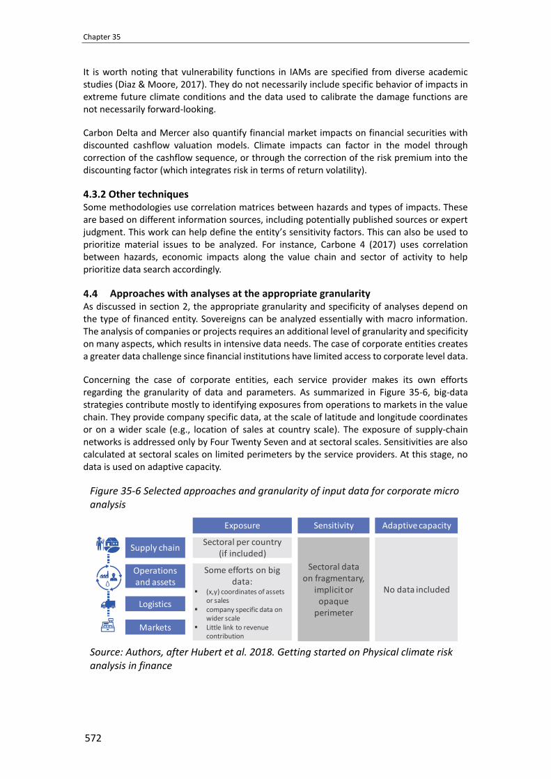
Chapter 35
572
It is worth noting that vulnerability functions in IAMs are specified from diverse academic studies (Diaz & Moore, 2017). They do not necessarily include specific behavior of impacts in extreme future climate conditions and the data used to calibrate the damage functions are not necessarily forward-looking.
Carbon Delta and Mercer also quantify financial market impacts on financial securities with discounted cashflow valuation models. Climate impacts can factor in the model through correction of the cashflow sequence, or through the correction of the risk premium into the discounting factor (which integrates risk in terms of return volatility).
4.3.2 Other techniques Some methodologies use correlation matrices between hazards and types of impacts. These are based on different information sources, including potentially published sources or expert judgment. This work can help define the entity’s sensitivity factors. This can also be used to prioritize material issues to be analyzed. For instance, Carbone 4 (2017) uses correlation between hazards, economic impacts along the value chain and sector of activity to help prioritize data search accordingly.
Approaches with analyses at the appropriate granularity As discussed in section 2, the appropriate granularity and specificity of analyses depend on the type of financed entity. Sovereigns can be analyzed essentially with macro information. The analysis of companies or projects requires an additional level of granularity and specificity on many aspects, which results in intensive data needs. The case of corporate entities creates a greater data challenge since financial institutions have limited access to corporate level data.
Concerning the case of corporate entities, each service provider makes its own efforts regarding the granularity of data and parameters. As summarized in Figure 35-6, big-data strategies contribute mostly to identifying exposures from operations to markets in the value chain. They provide company specific data, at the scale of latitude and longitude coordinates or on a wider scale (e.g., location of sales at country scale). The exposure of supply-chain networks is addressed only by Four Twenty Seven and at sectoral scales. Sensitivities are also calculated at sectoral scales on limited perimeters by the service providers. At this stage, no data is used on adaptive capacity.
Figure 35-6 Selected approaches and granularity of input data for corporate micro analysis
Source: Authors, after Hubert et al. 2018. Getting started on Physical climate risk analysis in finance
Supply chain
Operations and assets
Logistics
Markets
Exposure Sensitivity Adaptive capacity
Sectoral per country (if included)
Some efforts on big data:
▪ (x,y) coordinates of assets or sales
▪ company specific data on wider scale
▪ Little link to revenue contribution
Sectoral dataon fragmentary,
implicit or opaque
perimeter
No data included

A Review of Methodologies Analyzing Physical Climate Risks
573
While Mercer’s approach to corporate analysis is essentially top-down, service providers generally provide hybrid scale analyses. For instance, Four Twenty Seven’s corporate analysis integrates the macro climate resilience of the country where the company sells its products, in addition to the other micro and sectoral qualitative indicators (However no public information is available on how these indicators combine).15
Forward-looking analysis on climate hazards and the evolution of human systems
Most approaches analyze physical climate risks over future horizons. This would require accounting for the uncertainties on how climate conditions and socio-economic behaviors will evolve. While this usually comes down to the evolution of climate conditions with appropriate use of scenario analysis, this is not the case for the evolution of socio-economic behaviors.
Figure 35-7 Selected approaches and forward-looking analysis
Source: Authors, after Hubert et al. 2018. Getting started on Physical climate risk analysis in finance
4.5.1 Exploring the evolution of climate hazards Except for Moody’s Investors Service, the approaches analyze future hazards with climate scenario analysis on variable time horizons ranging from the next 15 years to 2100.
Most approaches focusing on the longer term analyze several up-to-date IPCC climate scenarios. They take as input different trajectories of future GHG emissions broadly used in academic research. This is recommended since future GHG emissions can make a large difference on climate conditions in distant horizons.
One approach produces climate scenarios as a part of a broader simulation from an Integrated Assessment Model (IAM). As opposed to the climate models used for IPCC’s scenarios, the
15 For more examples see the synthesis in section 2.8.4 and detailed analysis in annex to Hubert et al. 2018. Getting started on Physical climate risk analysis in finance.

Chapter 35
574
IAM generates climate data through simplified equation that translates a GHG trajectory into a climate hazard. The GHG trajectory is also a hypothetical construct by the service provider.
One approach focusing on the short term also makes use of “trend scenarios” that extrapolate past weather events onto a 15-year horizon. However, this methodology does not account for potentially unprecedented combinations of hazards possibly in concentrated timeline and on different key locations affecting a financed entity. It does not account either for fluctuations arising from natural variability in the climate system.
4.5.2 Exploring the evolution of socio-economic behaviors Beside the influence of human-caused GHG emissions on climate hazards, socio-economic systems may be more or less affected by the resulting impacts depending on their future development choices that modify their own exposure, vulnerability and adaptability. Societies may even undergo structural changes in the future, for instance in relation to climate impacts or the transition towards a low-carbon economy. Such evolutions may also deserve scenario-based analyses, for instance using a range of impact scenarios or adaptation scenarios. However, the current methodologies adopt essentially a historical perspective on the behavior of socio-economic systems.
Conclusion: limitations in current approaches The approaches analyzed in this chapter are pioneering efforts to provide financial institutions with decision-useful information on their exposures to physical climate risks. However, these approaches also faced significant limitations as they stood in 2018 when the authors reviewed them for the ClimINVEST project.
1. Limited scope of analysis. The approaches are insufficiently addressing network effects of climate impacts in both the real economy and the financial sector as well as potential systemic risks. Most approaches analyzing climate impacts on companies insufficiently address the macro-economic consequences of climate hazards. The scope of impacts on company’s value chains is also patchy on certain approaches while the others cover a broader scope but this comes at the expense of the separability of information per specific types of impacts.
2. Limited consideration of entities’ specific characteristics due to heavy data requirements. Approaches analyzing impacts on companies require a large amount of company-specific data. The approaches still face difficulties obtaining the data on locations of production sites and partners that are key contributors to the benefits of the company. Adaptive capacity is not accounted for due to the lack of data. Sensitivities are still approached at sectoral level and there is a need for empirical evidence to make them more precise. Forward-looking approach could also be enhanced to anticipate how counterparties’ behaviors will evolve and change their adaptation to climate hazards.
3. Limited transparency. Most approaches still lack transparency on core aspects of the methodology such as the characteristics of some databases and the sensitivity of entities that are exposed to climate hazards. This is partly because the approaches are provided by commercial vendors. Hence, the quality of information is not totally ensured. Financial actors consider that transparency is a key requirement for them to use this information for their decisions (Bruin et al., 2019).
4. Limited compatibility with decision-making at financial institutions. There are discrepancies between some characteristics of physical climate risk information and decision-making processes at financial institutions. Some approaches provide information on long-term impacts that is not relevant for day-to-day operations at financial institutions. They also

A Review of Methodologies Analyzing Physical Climate Risks
575
explore the uncertainties on future climate conditions and socio-economic behaviors as well as secular changes that financial models do not properly integrate. In addition, data intensity combined with little data availability make these approaches difficult to replicate on an array of large portfolios. Further research is needed so that financial institutions can make a better use of physical climate risk information (Depoues et al., 2019).

Chapter 35
576
Bibliography
Asian Development Bank. (2016). Project climate risk assessment and management - Guangxi Regional Cooperation and Integration Promotion Investment Program.
Bruin, K. d., Romain, H., Evain, J., Clapp, C., Dahl, M. S., & Bolt, J. (2019). Physical climate risk: Investor needs and information gaps. CICERO Report.
Carbon Delta. (2019). Climate Value-at-Risk (VaR). Carbone 4. (2017). CRIS - Climate Risk Impact Screening. Colin, A., Vailles, C., & Hubert, R. (2019). Understanding transition scenarios – Eight steps for
reading and interpreting these scenarios. Dépoues, V., Bouchet, V., Cardon, M., & Nicol, M. (2019). Pour une autre approche du risque
climatique en finance – Tenir pleinement compte des incertitudes. Diaz, D., & Moore, F. (2017). Quantifying the economic risks of climate change. Nature
Climate Change, 7(11), 774-782. Ecolab. (2017). Water Risk Monetizer - Smart water management for business growth:
Integrating water risk into business decision making. Four Twenty Seven, & Deutsche Asset Management. (2017). Measuring Physical Climate Risk
in Equity Portfolio. Gassert, F., Luck, M., Landis, M., Reig, P., & Shiao, T. (2014). Aqueduct global maps 2.1:
Constructing decision-relevant global water risk indicators. World Resources Institute, 31.
Hubert, R., & Cardona, M. (2018). La finance n’a pas encore pris la mesure des impacts climatiques.
Hubert, R., Evain, J., & Nicol, M. (2018). Getting started on physical climate risk analysis in finance – Available approaches and the way forward.
IPCC. (2018). Global Warming of 1.5◦C - Summary for Policymakers. . Technical Report Intergovernmental Panel on Climate Change.
Luck, M., Landis, M., & Gassert, F. (2015). Aqueduct water stress projections: decadal projections of water supply and demand using CMIP5 GCMs. World Resources Institute.
Mercer. (2015). Investing in a time of climate change. London, UK: Mercer International Finance Corporation and the UK Department for International Development.
Mercer, & CALStrs. (2016). CALStrs Portfolio Climate Change Risk Assessment. MOODY, S. (2016). Environmental Risks--Sovereigns: How Moody’s Assesses the Physical
Effects of Climate Change on Sovereign Issuers. Moody’s Investors Service. Mora, C., Spirandelli, D., Franklin, E. C., Lynham, J., Kantar, M. B., Miles, W., . . . Hunter, C. L.
(2018). Broad threat to humanity from cumulative climate hazards intensified by greenhouse gas emissions. Nature Climate Change, 8(12), 1062-1071.
UNEP FI, & Acclimatise. (2018). Navigating a new climate. UNEP FI, & Carbon Delta. (2019). Changing Course: A Comprehensive Investor Guide to
Scenario-based Methods for Climate Risk Assessment, in Response to the TCFD.

Transition Risk Assessment Methodologies
577
Transition Risk Assessment Methodologies
By
Carbon Trust1
Abstract
Currently, multiple methodologies are available to asses transition risks for financial institutions. In this paper we discuss the key characteristics of existing approaches and develop a criteria framework to help financial institutions select the most suitable methodologies. The criteria are separated into three broad groups: i) General applicability, based on the types of transition risks covered, scenarios and outputs; ii) Coverage considerations, based on geographies, asset classes, sectors and levels of analysis; iii) Practicality and implementation, based on data requirements, integration challenges, costs and development stage of the methodologies. We also identify overarching methodological limitations to inform end-users, supervisors and methodology developers.
Keywords: transition risk assessment methodology, climate risk for financial institutions, methodology selection, methodology review
1 Introduction and purpose of the chapter
The aim of transition risk assessment is to understand climate-related transition risks in relation to other mainstream risks. It also serves to identify, disclose and manage the impact of these risks on the underlying business, strategy, and financial planning of a company (TCFD, 2017a). Climate-related transition risks, as well as their potential impacts, differ significantly across sectors, regions and time horizons. Various transition risk assessment methodologies have been developed in response to the challenge of pricing and addressing increasingly material transition risks that drive demand from end users and regulators. It is crucial for end users to identify their objectives for risk assessment, and prioritise their requirements, given the diversity of methodological approaches.
This chapter presents a discussion of the characteristics of available transition risk assessment methodologies as applicable to a variety of financial institutions. Originally based on a comprehensive assessment of a sample of methodologies carried out by the Carbon Trust, the chapter outlines the key, high-level criteria for different financial institutions to consider when selecting an appropriate methodology. The chapter also helps supervisors to take account of the constraints and limitations of transition risk assessment tools material for financial institutions. This can then inform the expectations put in place in supervising financial
1 This chapter is written by Nick Harris, Senior Manager, Green Finance, [email protected]; Ben Peel, Consultant,
email: [email protected]; Tianyue Wu, Analyst, email: [email protected]; Alp Katalan, Analyst, email:
[email protected]; Vitaliy Komar, Analyst, email: [email protected]; Lijian Zhao, China Country
Manager, email: [email protected]; Gina Hall, Global Head of Sustainable Finance, email:

Chapter 36
578
institutions, helping to build systemic resilience within the constraints of existing methodologies. A conceptual framework of the criteria is summarised in Figure 36-1 below:
Figure 36-1 Summary of the key criteria to consider when selecting a transition risk methodology
Note: The order of criteria above does not reflect their relative importance or stages of analysis. Readers can refer to individual sections independent of order.
The structure of this chapter reflects the above high-level criteria groupings:
• General considerations are the key factors that financial institutions should consider when determining their objectives for a risk assessment exercise.
• Coverage considerations refer to the applicability of different methodologies based on a financial institution’s needs and portfolios.
• Practicality and implementation refer to the ease of implementation (cost, time and effort, systems requirements etc.) of a given methodology.
This chapter also outlines several key limitations of the current methodological field, and suggests avenues for overcoming them. These include incomplete risk coverage, neglecting transition risks beyond of the direct operations of counterparties, and inadequate integration of risk assessment into internal processes.
Our conceptual mapping of methodologies and selection criteria are simplified and can be further refined. Notably, UNEP FI has previously produced a detailed review of the field, categorising a range of existing methodology providers and presenting findings of their own pilot (UNEP FI & Carbon Delta, 2019). Our simplified approach has been informed by this and other similar publications, empirical methodology reviews, and sectoral expertise of the authors.
2 General considerations and alignment with needs
As outlined in the conceptual framework in Figure 36-1, the high level characteristics of any given methodology include three main criteria: a) types of transition risks covered; b) types of

Transition Risk Assessment Methodologies
579
scenarios used; c) types of outputs produced. While these characteristics might not always be the primary considerations for all financial institutions when considering risk assessment implementation, they tackle some of the main aspects of the exercise. Specifically, these criteria help the reader to navigate the general landscape of transition risks, better understand available climate scenarios, and types of assessment outcomes.
Figure 36-2 Criteria for general consideration
Key takeaways of the section: • Transition risks, as defined by the TCFD, include technology, market, reputation, and
policy and legal risks. The ease of risk assessment can vary according to type of risk, for example, policy and technology risks are easier to assess than market, legal and reputation risks. Not all methodologies cover all types of transition risks.
• The type of scenario used will depend on whether the financial institution is trying to understand its vulnerability to gradual policy and market shifts caused by climate change (temperature-based), or whether it is trying to understand the impact from a single occurrence (event-based). The number of scenarios available in the risk assessment vary by methodology.
• The outputs produced by existing tools can be quantitative, qualitative, or a combination of both. This will be largely dependent on the types of transition risks assessed, and can be adjusted to cater to specific needs of a financial institution.
Types of transition risks The TCFD has identified four overarching categories for transition risk that all companies, including financial institutions, should consider. However, not all methodologies cover all types of transition risks. The most common transition risks assessed are policy risk (often via an assumed carbon price) and technology risk (often via assumed technology cost trajectories). Impacts from legal risk and reputation risk are likely omitted from methodologies because they are harder to quantify (UNEP FI & Carbon Delta, 2019), however this is not to say they cannot and will not be integrated into future iterations of risk assessments. Figure 36-3 lists the types of transition risks, as defined by the TCFD, which methodologies may assess.

Chapter 36
580
Figure 36-3 Types of climate-related transition risks
Source: adapted from TCFD (2017a)
Financial institutions should select methodologies that best cover the risks that are most material to their counterparties and portfolios, as well as meet their objectives for undertaking the transition risk assessment in the first place (e.g. whether it is for reporting their transition risks to regulators, or simply understanding which of their counterparties are most exposed to transition risks).
The TCFD also provides supplemental guidance for the financial sector in considering transition risks (TCFD, 2017a). For example, the TCFD recommends banks to consider characterising their climate-related risks in the context of traditional banking industry risk categories such as credit risk, market risk, liquidity risk, and operational risk. Similarly, they recommend insurance companies to assess transition risks resulting from a reduction in insurable interest due to a decline in value, changing energy costs, implementation of carbon regulation, and liability risks from a possible increase in litigation.

Transition Risk Assessment Methodologies
581
Types of scenarios used
Box 2: Low-carbon transition scenarios
A scenario describes a path of development leading to a particular outcome. They are intended to highlight core elements of a possible future and to draw attention to the key factors that will drive future developments (TCFD, 2017c). Different scenarios allow financial institutions to conduct ‘what-if’ analyses of how different transition pathways could affect their assets and/or portfolios, and to explore the resilience and vulnerabilities of a firm’s business model to a range of outcomes.
Two types of scenarios that financial institutions could consider when selecting an appropriate methodology, as identified by Oliver Wyman (2019), are:
• Temperature-based scenarios: these often describe a smooth and orderly transition to a low carbon economy, and have a long-term view. However, they can also describe a disorderly transition where stringent policies kick off at a later date to meet climate commitments. Temperature-based scenarios are comprehensive and holistic scenarios analysing how the world might develop, and the corresponding impacts that these pathways have on average global temperatures and climate change.
• Event-based scenarios: these are often used to illustrate aspects of an abrupt or a disorderly transition to a low-carbon economy, and take a short-term outlook when compared to temperature-based scenarios. Event-based scenarios focus on the potential impacts of one triggering event, such as a sudden change in government policy or the introduction of a disruptive energy technology.
Currently, industry at large is increasingly looking into longer-term, orderly, temperature-based scenarios. This is in-line with the TCFD’s recommendation that organisations use a 2°C or lower scenario in addition to two or three other scenarios most relevant to their circumstances (TCFD, 2017b). Though event-based scenarios are not common in transition risk assessment methodologies at the moment, they may be relevant to consider as supervisors are interested in abrupt and disorderly transition scenarios, which are likely to result in higher stress for financial entities as they do not provide the time horizon for a planned movement out of exposed sectors to lower carbon assets.
Multiple methodologies look at a range of temperature-based scenarios – from a smooth and orderly transition keeping global temperature rise to 1.5°C, to overshooting 2-3°C warming through the implementation of current national pledges and objectives, or even ‘no-additional policy’ scenarios exceeding 4°C of warming. In addition, some methodologies can also compute implied temperature alignment of portfolios according to the collated total emissions and/or future decarbonisation plans.
Temperature-based scenarios are underpinned by models which translate underlying assumptions around the climate, the economy, and societies into scenario outputs. For transition risk assessments, the most relevant types of underlying models used in scenarios are:
Chapter 36
582
• Sector-specific models: energy system models (e.g. looking at interlinked energy and transport systems) and land-use models (e.g. looking at agriculture and forestry) explore how different economic sectors evolve based on changing policy, technology and market conditions. Popular developers of scenarios using these models are the International Energy Agency (IEA) and the International Institute for Applied Systems Analysis (IIASA) respectively.
• Macroeconomic models: these are often computable general equilibrium (CGE) models and cover various macroeconomic variables, including an economy’s resources (e.g. capital and labour), sectoral composition, and international trade. They look at how changes in one part of the economy affect the whole system. Examples of developers of macroeconomic models for transition risk assessments are Vivid Economics and E3ME.
• Integrated Assessment Models (IAMs): consider the socioeconomic factors that affect the earth systems to determine how these then affect human welfare. These are based on the best available science and underpin policymaking and the Intergovernmental Panel on Climate Change (IPCC)’s assessments, particularly, IAMs aligned to the use of Shared Socioeconomic Pathways (SSPs) will be used for the upcoming IPCC assessment. Scenarios using IAMs are developed by IIASA, the Potsdam Institute for Climate Research (PIK), and the Joint Global Change Research Institute (JGCRI), among others.
Sector-specific models produce scenarios that can be used for transition risk assessments, whereas IAMs are often used when assessing both transition and physical climate risk (UNEP FI & Carbon Delta, 2019). Other types of scenario models include climate models (to simulate the response of the climate to GHG emissions) and hazard models (to determine the risk of hazards like droughts, floods, and hurricanes based on different climatic conditions). These are relevant for assessing physical climate risk rather than transition risk.
Some methodologies allow the user to run any chosen scenario, while others offer a pre-determined set. Using multiple scenarios allows for an assessment of the portfolio against various possible temperature goals, technological trajectories and national contributions. Therefore, methodologies allowing for multiple scenarios can help financial institutions to develop a better understanding of their exposure to transition risks. However, using varying scenarios can also make the comparability of climate related disclosures across institutions challenging.

Transition Risk Assessment Methodologies
583
Box 3. The difference between scenario alignment and risk assessment
It is important to note that the assessment of climate-related transition risk is a separate task to aligning operational and financial activities to mitigation and climate resilience goals, such as the Paris Agreement goals, which have the objective of “holding the increase in the global average temperature to well below 2°C above pre-industrial levels and pursuing efforts to limit the temperature increase to 1.5°C above pre-industrial levels” (UNFCCC, 2015). A portfolio that is aligned to a 2° pathway is one in which the counterparties, collectively, are developing in a way that is consistent with a 2° transition. As such they are likely to avoid being caught out by policies, are bringing low carbon technologies to market, and responding to climate change driven market signals, which are the hallmarks of transition risk exposure. There is still some divergence though as a 2° alignment focuses only on one transition scenario and does not quantify the potential downside risk of the transition, instead only identifying whether counterparties are on the right path.
There is strong correlation between those companies that are not aligned to the 2° transition and those who are most exposed to transition risks, due to their lack or readiness for a low carbon transition. An aligned portfolio is, on balance, investing in counterparties who are already in the process of low carbon transition, and therefore have a likely lower level of transition risk exposure – there is not perfect correlation though, as some sectors ultimately will carry greater financial risk on an absolute basis. Therefore, even financial institutions aligned with a 1.5°C scenario need to undertake further transition risk assessments.
Output of assessments The types of outputs produced by existing transition risk assessment tools can vary considerably. In the broadest sense, risk assessment outputs can be separated into:
• Quantitative outputs: these include metrics such as projected changes in EBITDA, VaR, as well as CapEx and OpEx impacts.
• Qualitative outputs: these can be graphical, such as risk prioritisation heat-maps, as well as descriptive or numerical, such as discrete scale risk scores.
• Combined outputs: some methodology providers can use a combination of the two formats, e.g. producing an initial qualitative screening with a subsequent quantitative deep dive.
As highlighted previously, transition risk is not affecting portfolios and counterparties in a uniform way. A commercial bank, for instance, might be primarily interested in quantifying medium-term risks to its utility sector loans, and would therefore look for a methodology that produces a climate-related Probability of Default, or Expected Shortfall metric. On the other hand, a pension fund in the initial stages of risk assessment might favour a qualitative mapping of their total portfolio by asset class, in order to identify potential risk hotspots for subsequent quantitative analysis, or identify sectors for direct investee engagement. In line with these various user demands, risk assessment tools by design produce various outcomes: some can act as screening tools whereas others quantify the financial impacts of transition risks. Per TCFD guidance, effective disclosures on implications of transition risk can be both quantitative and qualitative, depending on the institution and economic sector in question.

Chapter 36
584
3 Coverage considerations
Despite the existence of more than 40 methodologies on assessing climate-related transition risks, many of them are designed for specific target portfolios and users. No one methodology covers all regions, all types of financial instruments, and all industry sectors exhaustively. These considerations are summarised in Figure 36-4 below:
Figure 36-4 Criteria for coverage considerations
Key takeaways of the section:
• Geographic location of counterparties2 and their supply chains is a major source of transition risk, and users should conceptually determine its potential portfolio significance before choosing the appropriate methodology.
• The breadth of asset class coverage has been a clear differentiator between methodologies, and further asset classes are being added on an ongoing basis.
• Sector-specific transition risks can be addressed by single-sector focused methodologies as well as cross-sectoral methodologies. A suitable methodology usually covers the majority of a financial institution’s sector exposure.
• Effects of transition risks manifest on different levels: from individual physical assets to whole economic sectors of counterparties. Thus, tools provide various level of analysis, using bottom-up or top-down or both approaches to capture various aspects of transition risk. Choosing the right level of output is essential for effective implementation of the results of the risk assessment. The choice of analysis level depends on objective of the assessment and requires different input data granularity, which will be further elaborated in the next section Practicality and Implementation.
Geographic coverage Location matters to transition risk analysis because each location has unique policy requirements, technology development level, market traits and trends, as well as specific consumer and investor behaviours. For example, certain technology that is still regarded as “clean” in South-east Asia region might not be acceptable or bankable in the European Union region (“EU”). Therefore, for financial institutions with international asset exposure, choosing a tool developed for the right geography is fundamental.
2 This chapter used the definition of UNEP FI on the term counterparty. It refers to “entities that investors, through their
portfolios, have exposure to and that are more directly affected by climate-related risk. These range from countries to
companies and individual facilities/projects”.

Transition Risk Assessment Methodologies
585
Different tools’ geographic risk coverage provides various levels of granularity and generally varies in three ways: risks at global level, regional level (e.g. EU) or country-specific level. Often, a methodology will offer a mix of two levels, and some methodologies provide analysis on all three. When a financial institution selects a methodology, it is critical to answer the following four questions:
• Where are your counterparties’ activities predominantly located?
• Where will their future activities be located?
• Are key sectors driven by global trends or local trends?
• Does it matter for your portfolio to differentiate risks at a country-specific level?
The hypothetical example below showcases the differences in geographic coverage:
Tool A provides regional-level data and limited country-level data. This framework covers broader regions like EU, and some country-level analysis for Germany and India. Tool B can assess data over 58 different countries globally and greater country specification is offered in sectors which require further differentiation.
If a financial institution is exposed to EU-based equity assets and also has significant holdings in real assets in India, both methodologies above could be a good fit, as EU countries share a similar climate-related policy framework, and any more granular coverage at European country-level would be less necessary in this case.
Asset class coverage Given the wide range of financial instruments across financial institutions’ portfolios, asset class applicability is an important practical consideration for selecting an appropriate methodology. Some methodologies were designed specifically for certain end user portfolios, e.g. bank loan portfolios focusing on credit risk, or project finance, focusing on market risk. Others offer a broader range of instrument coverage. As such, financial institutions need to be mindful of each methodology’s asset class coverage in relation to their specific needs.
Figure 36-5 Examples for asset class coverage

Chapter 36
586
As shown in Figure 36-5, if Asset Management Firm B mostly invests in equity and fixed income, Tool I could be a suitable option. On the other hand, this tool may not be suitable for Commercial Bank A, which holds more assets in cash and real asset debt.
Lastly, it is worth pointing out that instrument coverage is generally an evolving variable as many methodologies are increasingly adding to the number of instruments they cover.
Sectoral coverage This assessment reflects the coverage provided by methodologies for a financial institution’s sectoral exposure. Climate-related transition risks vary across economic sectors. For example, high risk energy and resource intensive sectors, such as power, transport and industry (cement, iron and steel in particular) have traditionally received the most attention from tool developers. Other sectors widely covered include, but are not limited to, real estate and other infrastructure. Some tools can be adapted to almost all sectors after bespoke collaboration with tool developers.
It is also noteworthy that different methodologies cover sectors at different levels of granularity. For example, while two methodologies might both cover transport, one might analyse at the whole transport sector level, while the other breaks the sector down into automotive, aviation and shipping sub-sectors.
Some of the reasons for this variation are suggested below:
• Underlying scenarios used
• Expertise of a developer (e.g. developers having existing intellectual property in infrastructure)
• Intrinsic variable significance of transition risk across sectors (e.g. tool developers tend to prioritise analysis on those with higher perceived risks)
• Reference materials (e.g. some tools define sectors according to various taxonomies but others take a practical approach in defining sectors according to the target audience’s internal segmentation)

Transition Risk Assessment Methodologies
587
Level of analysis Transition risk exposure can manifest at various levels, from total portfolio, through to the individual physical assets of a counterparty (as shown in Figure 36-6). The UNEP FI’s Investor Guide in response to TCFD recommendations (UNEP FI & Carbon Delta, 2019), notes that risks tend to materialise at the physical asset level, subsequently translating to a counterparty and later portfolio impact. Nevertheless, aggregating risk exposure on a portfolio level can be a desired output for financial institutions, allowing informed strategic decision making and disclosure.
Existing tool providers often offer a combined approach, for example informing portfolio level analysis with asset level data, or executing asset level quantitative analysis after portfolio level risk hotspot identification. The results of different scopes of analysis vary in their applicability among financial institutions. For instance, identifying drivers of transition risks at a physical asset level could help active asset owners inform their engagement strategies with investee companies, while portfolio level insights would enable
shareholder disclosure. Assessment granularity also has practical implications, such as data requirements and costs, further addressed in section 1.3.
While the level of analysis relates to the type of outputs produced, it should be noted that the underlying methodologies can take different analytical approaches:
4 Practicality and implementation
This section deals with the practicality and ease of implementation of risk assessment methodologies. These criteria are important primarily at the implementation stage of the risk
Box 4. Top-down and bottom-up approaches
Tool providers currently can take either one of these approaches, or a combination of both:
• A top-down assessment typically looks at portfolio impacts as a result of either country-specific or sector-specific variables.
• A bottom-up approach will individually assess each counterparty or asset in a portfolio, before integrating the results to provide a portfolio-wide viewpoint.
Some tools will, for example, only provide a top-down view on listed companies, while others will have a capability to deliver a bottom-up view on physical assets of all listed portfolio companies. On the other hand, methodologies might factor in firms’ adaptative capacity in bottom-up assessment, but then find it challenging to apply the conclusions at the sector or the portfolio level.
Figure 36-6 Investor risk exposure

Chapter 36
588
assessment process and have direct implications for the exercise’s feasibility. Figure 36-7 below summarises the criteria:
Figure 36-7 Practicality and implementation criteria
Key takeaways of the section: • For certain asset classes, e.g. listed equity, it is possible to carry out insightful
transition risk assessment with minimum data inputs. However, there is a trade-off between input data granularity and level of bespoke insights on risk.
• Important trade-offs exist between simplicity and applicability of risk assessment, and the level of time and internal integration effort needed.
• Other practical considerations include the cost structure (ranging from open-source to bespoke consulting pricing) of tool offerings, as well as their development stage, given the dynamic nature of the space.
Input data requirements The level of input data required depends on the depth of analysis and would normally include financial asset level or portfolio level data. There is a trade-off between the amount of input data and the level of insights gleaned from the analysis. The less data financial institutions input into the tool (either due to the lack of internal data system consolidation, or simply because of lack of reporting from the counterparty), the more generic the output analysis will be. Therefore, financial institutions can opt to provide less data if they simply want a snapshot view of portfolio transition risks, or alternatively, provide granular data for bespoke in-depth analysis.
Typically, general data requirements include portfolio breakdown, such as security names, International Securities Identification Number (ISIN), total asset value, and currency. However, the data required will vary by asset class. For example, in addition to the above inputs, equity portfolios may require portfolio weights.
More granular data (such as asset geography, carbon emissions data, and technology data) may be required for a project finance portfolio, or in the case of a deep-dive analysis of transition risks. This could also include detailed balance sheet data, as well as profit and loss data at the individual counterparty or asset level. When granular data is not available, top-down, rather than bottom-up, approaches can be applied (see Box 4 for further reference).
Some methodologies may use proprietary asset-level datasets, significantly reducing data requirements from the end user. However, these datasets are often applicable only to large listed entities, and therefore may not be appropriate for alternative asset classes. Also, in this

Transition Risk Assessment Methodologies
589
case the quality of transition-risk assessment will be dependent on the accuracy of the third-party dataset, rather than the internally collected data.
Internal integration The ideal tool, besides meeting all relevant requirements, would be easily incorporated into end users’ risk management practices and general decision-making procedures. This is a challenging task, given the diverse levels of internal process complexity across financial institutions. Below this chapter outlines two common trade-offs to consider in terms of implementation complexity:
Trade-off 1: time efficiency vs. depth of analysis
The time frame of an assessment process will depend on portfolio composition, data availability and complexity of results expected. Some tools are available online, which makes it possible to assess portfolios relatively quickly. However, this type of general tool likely offers less flexibility for users to include tailored variables. Some tools, on the other hand, might take up to six months to analyse an institution’s portfolio in detail, but once the screening session is completed, the assessment is less time intensive and the result is more detailed.
Trade-off 2: tool feasibility vs. applicability to internal stakeholders
A specific tool may not produce easy to use outcomes for a range of internal divisions within an institution. For example, certain tools are explicitly targeted at commercial banking risk management, while others cater to the needs of equity portfolio managers. This may make results less helpful for another type of financial institution, or even different internal divisions, requiring additional work for refining data and output types. It is critical to ensure the outputs are ‘translatable’ and can be used broadly across an organisation. In general, climate risk assessment data can be used for strategic asset allocation, stock selection, sector risk identification, due diligence, internal buy-in, external engagement, monitoring and compliance, disclosure and reporting, and more, depending on end users’ needs.
In the selection of tools, having a clear objective is at the essence of making the right trade-off. The objective might vary from targeting specific types of risks to particular level of analysis to be achieved. External factors such as pressure from investors and regulatory disclosure requirements, or internal incentives such as group’s long-term strategy and risk appetite will lead end users to make different trade-offs.
In summary, it is in the interest of the end user to select a tool that aligns the best to their goal, while also requiring relatively less additional effort in implementation (e.g., a tool that can produce the most flexible output, which can be used across a financial institution’s various business units and with a range of stakeholders).
Other considerations Cost structure Costs of transition risk assessment tools on the market can vary widely depending on types of outcome and general methodological approach. Tool developers may also provide tiered access to their product, e.g. ‘basic’ or ‘premium’ services at different prices. In general, their cost structure falls into the following categories:
• Free: some tools are free to use and may be hosted online or may be available as open-source spreadsheet models. However, it is important to note that these are often in a pilot phase, or when a provider is looking to attract initial customers.

Chapter 36
590
Therefore, the cost of the tool during this development stage may not be representative of its full cost when it is eventually rolled out to a wider client base.
• Licensing fee: licensing a tool will scale in price depending on the assessment undertaken. The cost of licensing depends on a variety of factors such as: number and size of assets/portfolios, number of sectors, frequency of analysis, granularity of the financial risk, and number of metrics used. Moreover, there may be additional costs related to the level of customisation required, quality assurance, and data updates.
• Consulting services: some bespoke tools cannot be licensed and the cost will be structured as a consulting fee for implementation, with a scaling cost similar to that of licensing models.
Development stage The current market for transition risk assessment methodologies is still quite young, but nevertheless a rapidly growing one. Tools and methods will have various maturity levels, from research and pilot stage to established commercial offering. The development stage is therefore important for practical implementation of a given methodology in the context of immediate applicability for financial institutions’ portfolios. End users are also advised to monitor the space and contribute to tool and method development through pilot participation. Similarly, the use of climate scenarios by the private sector and financial institutions is a relatively new phenomenon. Scenarios are continuously adjusted and developed to adjust to the needs of the sector, given that their initial audience has historically been scientists and policymakers.
5 General limitations
In a relatively short period of time the market for transition risk assessment methodologies has grown rapidly, catering to the needs of a wide range of financial institutions. The space is very dynamic, and several tools and methodologies are still in early stage development. Transition risk assessment is intrinsically a complex process, and some key limitations can be identified. These limitations do not relate to any one specific tool or its methodology, but rather highlight some of the systemic considerations for effective implementation of transition risk assessment.
Key limitations and suggested avenues for addressing them are given below:
• Scenario analysis rarely addresses whether the counterparty can pass the cost of the transition to consumers. The adaptive ability of the counterparty is one the direct determinants of risk, and should therefore be explored. Counterparties’ strategies developed to transform and adapt themselves to the transition pathways are examples of adaptive capacity indicators that should be addressed. Increased TCFD-aligned disclosures by counterparties, as well as upskilling of financial institution analyst teams are examples of positive developments to tackle the issue.
• Drivers of transition risk currently covered across methodologies are often limited to policy, quantified through a carbon price variable. There is still low coverage of legal and reputational risk drivers, and policy risk coverage is yet to expand beyond just a carbon price to include wider climate policy landscape factors such as minimum standards, energy regulations, emissions caps and technology phase outs.

Transition Risk Assessment Methodologies
591
• Integration of risk assessment results into a financial institution’s actual risk management process requires strategic commitment from end users, not only output adjustment from the tool provider.
• The risk assessment approach might focus on specific financial risk categories or sectors, preventing a systemic approach to the exercise. For instance, scope 2 and 3 emissions are often excluded from counterparty analysis, making conclusions less coherent for several sectors, such for example, retail. Leveraging financial research capabilities and expanding beyond simple carbon metrics is imperative.
• Standardised counterparty reporting at high levels of granularity is essential as an input for risk assessment. Forward looking and TCFD compliant disclosures have only recently started to pick up, and consistent coverage across sectors will be an important facilitator of effective risk assessments. Multiple national and international level policy programmes to support this are currently being rolled out, such as the Bank of England stress testing, Article 173 in France, and the EU Non-financial Reporting Directive.
• Quantitative methodologies may still face some fundamental challenges such as extending the conventional modelling time horizon from short to medium and long term. Similarly, building forward looking climate change transition risk models based on historical data can be challenging. This time horizon misalignment is also one of the key barriers to wider integration of transition risk to general financial risk management frameworks.

Chapter 36
592
Bibliography
TCFD. (2017a). Implementing the Recommendations of the Task Force on Climate-related Financial Disclosures.
TCFD. (2017b). Recommendations of the Task Force on Climate-related Financial Disclosures. TCFD. (2017c). Technical Supplement: The Use of Scenario Analysis in Disclosure of Climate-
Related Risks and Opportunities. UNEP FI, & Carbon Delta. (2019). Changing Course: A Comprehensive Investor Guide to
Scenario-based Methods for Climate Risk Assessment, in Response to the TCFD. Paris Agreement, (2015). Wyman, O. (2019). Climate Change: Managing a New Financial Risk.

Framing Scenarios for Transition and Physical Risks
593
Framing Scenarios for Transition and Physical Risks
By
CICERO1
Abstract
Climate and energy scenarios are being used in new ways to assess financial risks. While current policies seem to point towards 3°C warming by the end of the century, higher and lower temperature scenarios need to be considered for their potential impact on physical and transition risk. However, improvements need to be made in the availability of near-term risk-based scenario information for financial decision makers, and in the comparability of reported scenario information from companies.
Keywords: scenarios, climate risk, physical risk, transition risk, finance
1 Introduction
The Paris Agreement was a call to action for policy makers, businesses, and financial actors. The role of the financial sector is critical to accelerating a transition to a low carbon society. First, the financial sector must play an important role by redirecting capital towards low carbon and climate-resilient infrastructure in support of the Paris Agreement. Second, the financial sector must manage risk in a dynamic climate policy landscape and with the intensification of physical climate impacts.
Climate change can affect firms’ profitability and investment portfolio returns via regulations that imply carbon prices and climate-related damages from flooding or other physical impacts (Figure 37-1). Investment funds, pension funds, and bank loans can all be exposed to climate risks. Clear messaging from financial authorities have shifted attention to the financial risk that can result from climate risks. The framing of climate change in terms of potential impact on financial bottom lines brought climate change onto the radar screen of many financial actors. Two different types of climate risk that can have financial impact have been delineated by the Task Force on Climate-Related Financial Disclosures (TCFD, 2017):
Transition risks associated to the transition to a low carbon economy, which are dependent on scenario analysis and the speed of political, societal and technological changes as well as the associated legal risks; and
Physical risks associated with physical impacts of the changing climate, some of which are already occurring and resulting in significant costs, such as extreme precipitation. In the short-
1 This chapter is written by Christa Clapp, Research Director on climate finance at CICERO, email:
[email protected]; Glen Peters Research Director on climate mitigation at CICERO; and Alexander Berg, Senior
Advisor on climate finance at CICERO.

Chapter 37
594
term, physical risks are largely independent of the climate scenario, and other ongoing projects address physical risk (CICERO, 2019).
Figure 37-1 Scope of climate risk and financial impacts
Source: (CICERO, 2018)
Climate scenario stress-testing features strongly in recommendations from financial and regulatory authorities to financial institutions and companies. The TCFD recommends disclosure for all financial institutions and companies on “the resilience of an organization’s strategy, taking into consideration different climate-related scenarios, including a 2° Celsius or lower scenario” (TCFD, 2017). Regulatory developments in France and at the European Union (EU) level echo the focus on climate risk disclosure and climate scenario stress-testing. France became the first country to mandate climate risk disclosure for financial institutions in 2015 via Article 173. The current draft of the EU Sustainable Finance Action Plan proposes mandatory disclosure of a similar nature.
This chapter provides an overview of the landscape of scenarios for assessing transition and physical risks. We highlight that with today’s policy ambitions, an average global warming of approximately 3°C is the most likely future scenario but note that a range of scenarios is necessary to stress-test against the transition to possible futures. To analyze physical risk in the next decade, other tools are required given that we have locked-in greenhouse gas (GHG) emissions in the atmosphere already that will have consequences for near term impacts. Going forward, financial decision-makers could benefit from more consistent near-term risk-based information from scenarios.
2 Scenarios in transition risk assessment Scenarios are coherent futures, each with advantages and disadvantages. They are used to explore key uncertainties, not to predict the future. There is no one ‘correct’ scenario.

Framing Scenarios for Transition and Physical Risks
595
There are many ways to get to an emissions or temperature target depending on socioeconomic and modelling assumptions. To reach the target in the Paris Agreement of 2°C or lower, there are many different pathways, however, all 2°C scenarios require rapid decarbonization in the short term, net-zero emissions between 2050 and 2100, and net-negative emissions thereafter – such as with afforestation or by using bioenergy with carbon capture and storage (CCS).
What are the different types of climate and energy scenarios used in stress-testing?
In practice, climate scenario stress-testing may involve using scenarios from very different types of models. The choice of modelling platform and the underlying technological and socio-economic assumptions can have significant impact on the scenario outcomes. Two commonly used model types are:
Integrated Assessment Models (IAMs) link various aspects of the economic, energy, land, and climate system to assess future emissions pathways under various types of climate policy. Some models may focus on specific aspects of the system (e.g., energy), while others may broadly cover all activities leading to emissions IAMs are useful to examine potential transition impacts, and it is possible to explore hundreds of alternate futures.
Climate models have a detailed representation of the climate system, translating emissions or concentrations into climate variables such as temperature and precipitation. These models are useful for physical impacts, and it is possible to explore only a few representative scenarios due to the computational time.
Transition impacts can be examined using scenarios of socioeconomic and technical systems, with emission pathways changing with policy choices. It is possible to focus on specific aspects of society (e.g., the energy system) or to consider the interlinkages between systems (e.g., energy and land). The International Energy Agency (IEA)’s World Energy Outlook (WEO) is perhaps the most known and publicized energy-system model with detailed annual releases. There are a range of other IAMs, often run by research groups, that generate scenarios across socioeconomic systems (energy, land, and agriculture). These research groups often cooperate to develop model inter-comparison projects, where many IAMs are used to address the same research question to assess uncertainties. These IAMs, either individually or in inter-comparison projects, generate thousands of scenarios that are often compiled into databases that are assessed by the Intergovernmental Panel on Climate Change. These scenarios are developed continuously, but major assessments are released every 5-7 years.
Physical impacts can be examined using the output of climate system models. Because of computational constraints, these climate models generally take a few selected scenarios from IAMs and translate the emissions or concentrations into climate variables (e.g. temperature, precipitation and wind). The Representative Concentration Pathways (RCPs) are four well known pathways used by these climate models, but these are being replaced by a selection of the Shared Socioeconomic Pathways (SSPs). These pathways allow the exploration of different temperature outcomes. The outputs of these climate models are generally quite coarse (greater than 100’s of kilometers), but can be downscaled using either models or empirical approaches to give more detailed regional information.
In combination, IAMs and climate system models enable us to link models of the energy and other societal systems to temperature increases in coherent scenarios. Scenarios from the IEA and assessed by the IPCC are independently produced and well-known (Table 37-1

Chapter 37
596
Table 37-1 Commonly used scenario families
). In addition, business organizations (e.g. World Business Council for Sustainable Development) and companies (e.g. Equinor, BP) produce their own scenarios. Scenarios vary in how often they are updated and the end year that they model.
Table 37-1 Commonly used scenario families
Scenario Purpose Update
frequency Number
scenarios End year
Key focus
IPCC community: Marker Scenarios (RCPs)
Physical and transition risk
5-7 years 4-6 2100 Focus on the climate system and impacts
IPCC community: Scenario databases
Physical and transition risk
5-7 years ~1000 2100
Comprehensive exploration of socioeconomic pathways using a range of models and model intercomparisons
IEA WEO Transition risk
Annual 3 2040 Focus on markets
IEA Energy Technology Perspectives (ETP)
Transition risk
Annual 3 2060 Focus on energy technology
Source: CICERO (2018)
Approximate alignment of commonly used scenarios with various temperature targets is mapped out in Figure 37-2. The IPCC’s Representative Concentration Pathway (RCP) RCP1.9 and RCP2.6 roughly map to 1.5°C and well below 2°C warming at the end of the century, and the WEO Sustainable Development Scenario (IEA, 2018) describes a pathway that stretches to 2050 and with around 1.8°C at the end of the century, assuming net-zero emissions from the year 2070.

Framing Scenarios for Transition and Physical Risks
597
Figure 37-2 Mapping a range of emission scenarios to temperature levels
Source: Rogelj et al. (2018); Riahi et al. (2017)
Which range of scenarios is useful for stress-testing? The global average temperature is likely to be approximately 1.5°C higher pre-industrial levels in the next 10-20 years, regardless of the emissions scenario. Historical emissions accumulate in the atmosphere and there is a time lag before they result in temperature impacts. Towards the end of the century, temperatures could span from approximately 2°C to 4°C, across a range of average emission scenarios.
Reaching approximately 3°C degrees in 2100 is more likely than 2°C, given today’s policy ambition. Still, 2°C is considered to be somewhat more likely than 4-5°C, given the possibility of tightening ambition under the Paris Agreement design, and the rapid progress made with low-carbon technologies like solar, wind, and electric vehicles. Reaching approximately 4-5°C would mean that current climate policies would be rescinded or relaxed.
Political, social, or technological events can influence the temperature increase, pushing it up to 4-5°C or pulling it lower towards 2°C. Examples of push factors towards a higher temperature outcome include key emitting countries (i.e., China, EU, India, US – which are jointly responsible for 60% of global emissions) failing to implement their climate targets (Nationally Determined Contributions, NDCs), or CCS deployment is delayed due to cost and public opposition. Examples of pull factors towards a lower temperature outcome include rapid deployment of clean technologies, CCS being deployed more rapidly (CCS plants are built at the historical pace of coal plants in China or nuclear plants in Europe), or key emitting countries ambitiously tighten their climate targets every 5 years under the Paris agreement.
Stress testing against a range of scenarios can help prepare for transition risk, across all periods. Given today’s policy ambition, approximately 3°C global warming by 2100 is the most likely scenario, but we don’t know enough to quantify the probability of reaching that temperature outcome (Figure 37-3). We also do not know much about the distribution curve at higher emission levels, which could be a fat-tail risk with a lower probability of occurrence but with

Chapter 37
598
higher potential financial impacts from systemic climate disruptions (Wagner, 2015). Thus, a range of scenarios should be examined to understand the range of transition and physical risks, including 2°C, 3°C, and even 4°C scenarios.
Figure 37-3 Probability distribution of scenarios based on expert judgement
Source: (CICERO, 2018)
3 Scenarios in physical risk assessments Physical impacts are observed in all regions today and can have abrupt consequences across all sectors (CICERO, 2017). Physical impacts manifest themselves mainly by rare events becoming more variable, (sometimes much) more frequent and intense. Observed impacts today include:
• Extreme weather such as stronger hurricanes and flooding,
• Flooding in already wet areas is increasing,
• Drought is observed in all regions, and
• Sea level rise is accelerating faster than expected.
While physical impacts are highly location-specific, they can have wide-reaching financial impacts across all sectors. Physical climate change can be felt both directly (via infrastructure damage) and indirectly (via supply chain and transportation disruptions). Physical impacts can be chronic or abrupt, which may require different stress testing for companies.
We do not need elaborate scenario testing to prepare for physical climate change for the next 10-20 years. We are already locked in for 1.5°C global warming, because of historical emissions. Changes such as extreme events and flooding are impacting all sectors and regions already. These impacts will become clearer over the next 10-20 years.
There is a trade-off between mitigation and adaptation, and policy decisions now can impact physical risk in the future. Using a higher temperature scenario e.g. 4°C can be useful for examining a possible worst-case scenario of potential physical impacts in the long run.

Framing Scenarios for Transition and Physical Risks
599
However, commonly used climate models for IPCC scenario analysis may be underestimating the recent non-linear increase in extreme weather trends related to climate change (Sutton, 2019). Furthermore, the accumulated impacts of compounded extreme weather events have the possibility to lead to systemic disruption of the climate. The potential for financial instability from this fat-tail risk is not well explored.
The risk of physical climate change is a factor of the probability of the event occurring, the vulnerability of the asset or infrastructure to the event, and the exposure of a portfolio or company to the event. Regional assessments of specific hazards, many of which are available from government sources e.g. on flooding, can provide information to help assess the probability of a hazard occurring.
A global overview of the potential for physical hazards occurring across different scenarios can be distilled from the IPCC 5th Assessment Report, however some of the information is patchy depending on literature focused on particular hazards or regions. Using a color-coding indication of when a hazard was observed or projected to occur in a region across different time frames and scenarios, the Shades of Climate Risk study from CICERO shows high risk coding for some hazards in each region of the world (Figure 37-4)(CICERO, 2017). Regional studies and information from meteorological institutes can provide additional data at a much more granular level.
Figure 37-4 Physical climate hazard overview from IPCC AR5
Source: (CICERO, 2017)
There are several service providers of physical risk assessment tools with diverse scope of coverage and methodologies that offer tailored risk assessment. Since most of these approaches use proprietary methods, it is difficult to assess the indicators, data, scenarios and

Chapter 37
600
methodology they incorporate (CICERO, 2019). Publicly available data is available for water scarcity only.
4 Challenges in adapting climate scenarios to assess financial risk The regulatory push on climate risk stress-testing and disclosure has created a whole new customer base for scenarios, with financial actors struggling to respond to assess risk across a range of future scenarios (Clapp & Sillmann, 2019). Climate and energy scenarios were largely designed for policy makers to examine emission pathways towards a global or national emissions targets decades in the future. Existing climate scenarios are ill-adapted to the short term and risk-based “stress-testing” needs of financial actors. Challenges in using existing scenario information include:
• Time scale. Many emission scenarios only present data in decade time steps, and are updated only every 5-7 years, well outside the timescales for financial decision making (CICERO, 2018).
• Risk framing. Available scenario outputs focus on emissions rather than forward-looking investment considerations. Further, focusing on outcomes from a single model and for a limited number of economic sectors greatly limits the ability to assess climate risk.
• Granularity. Scenarios that are updated annually, such as those from the IEA (IEA, 2018), provide more detail and regularity, but only cover the energy sector. Further, some users may need regional or sectoral detail, which is not available in many scenarios.
Several recent initiatives have focused on improving limited aspects of scenario information. CICERO has developed a manual to help build capacity within the financial sector on climate scenarios (CICERO, 2018), and has used this as a platform to discuss user needs with similar findings to other initiatives. The International Institute for Applied Systems Analysis (IIASA) has a 1.5°C Scenario Explorer that presents comparable data from scenarios used in the recent IPCC 1.5°C (Huppmann et al., 2018). The World Resources Institute has an Emissions Scenario Portal that compiles data from various scenarios. The 2 Degrees Investing Initiative and KPMG have developed independent tools to test if a portfolio is aligned with 2°C. Other approaches such as the Climate Risk Impact Screening (CRIS) by Carbone4 is focused only on physical risk. Another initiative to pull investment decision information from transition scenarios is convened by the United Nations Environment Programme Finance Initiative (UNEP FI) for a group of banks (UNEP FI, 2018).
However, the financial sector generally needs metrics not commonly included in scenario databases and relevant on short timescales, greater granularity, and importantly, flexibility to meet their specific activities. Scenario information for the financial sector is not yet reflected in the scientific literature (Weber et al., 2018). While the academic scenario community is becoming more transparent, existing scenario data and tools do not yet meet the needs of the financial sector. Some tools are purely descriptive, which help build capacity but do not help users perform analysis. Other tools are proprietary, or not transparent, making it difficult to assess their robustness. None of the initiatives provide the data that users need to perform their own in-house analysis, nor do they provide guidance on how to report and respond to climate-related risks.

Framing Scenarios for Transition and Physical Risks
601
5 How can we move towards more consistent scenario stress-
testing? Portfolio managers and bankers face a challenge in comparing the application of climate risk stress-testing across companies. Implementing scenario stress testing requires information that is tailored to sector and company characteristics. However, a common understanding, and transparency on a consistent set of assumptions for climate scenarios can support investors in doing due diligence on companies or portfolios (CICERO, 2018). To this end, the macro-financial work stream of NGFS (Workstream 2) is, in joint effort with the climate science community, in the process of developing a consistent and comparable set of data-driven scenarios encompassing a range of different plausible future states of the world.
Looking across the strategic risk planning needs of companies and financial decision makers, principles for the implementation of scenario stress testing that support investor due diligence could include:
• Coherency of the storyline assumptions embedded within a scenario,
• Consistency of key driver assumptions across scenarios,
• Flexibility for companies to adapt scenarios to what they know about their sector/business, and
• Compatibility with common reporting metrics on scenarios.
While one-size-fits-all scenarios are not suited to capture the range of climate risk, benchmarking against commonly used scenarios such as WEO and IPCC for 2°C could be used to illustrate scenario due diligence.
Chapter 37
602
Bibliography
CICERO. (2017). Shades of Climate Risk: Categorizing Climate Risk for Investors. CICERO. (2018). Climate scenarios demystified: A climate scenario guide for investors. CICERO. (2019). Physical climate risk: Investor needs and information gaps. Clapp, C., & Sillmann, J. (2019). Facilitating Climate-Smart Investments. One Earth, 1(1), 57-
61. Huppmann, D., Rogelj, J., Kriegler, E., Krey, V., & Riahi, K. (2018). A new scenario resource for
integrated 1.5 °C research. Nature Climate Change, 8(12), 1027-1030. IEA. (2018). World Energy Outlook 2018. Riahi, K., van Vuuren, D. P., Kriegler, E., Edmonds, J., O'Neill, B. C., Fujimori, S., . . . Tavoni, M.
(2017). The Shared Socioeconomic Pathways and their energy, land use, and greenhouse gas emissions implications: An overview. Global environmental change, 42, 153-168.
Rogelj, J., Popp, A., Calvin, K. V., Luderer, G., Emmerling, J., Gernaat, D., . . . Tavoni, M. (2018). Scenarios towards limiting global mean temperature increase below 1.5 °c. Nature Climate Change, 8(4), 325-332.
Sutton, R. T. (2019). Climate science needs to take risk assessment much more seriously. Bulletin of the American Meteorological Society, 100(9), 1637-1642.
TCFD. (2017). The Use of Scenario Analysis in Disclosure of Climate-Related Risks and Opportunities
UNEP FI. (2018). EXTENDING OUR HORIZONS -- Assessing credit risk and opportunity in a changing climate: Outputs of a working group of 16 banks -- piloting the TCFD Recommendations PART 1: Transition-related risks & opportunities.
Wagner, G. (2015). Climate shock the economic consequences of a hotter planet. Princeton, NJ: Princeton University Press.
Weber, C., McCollum, D., Edmonds, J., Faria, P., Pyanet, A., Rogelj, J., . . . Kriegler, E. (2018). Mitigation scenarios must cater to new users. Nature Climate Change, 8(10), 845-848.

Acknowledgments
603
Acknowledgments
This NGFS Occasional Paper, Case Studies of Environmental Risk Analysis Methodologies, is a collaborative effort of many financial institutions, third-party service providers, research institutions, NGOs and distinguished members of the NGFS. It was jointly edited by Dr. Ma Jun, the Chair of NGFS supervision workstream and Special Advisor to the Governor of the People’s Bank of China (PBC), Dr. Ben Caldecott of University of Oxford, and Dr. Ulrich Volz of SOAS University of London.
The editors of this Occasional Paper would like to thank the authors of the 37 chapters and the research team led by Dr. Ma, including Dr. Sun Tianyin, Dr. Li Jing, Zhu Yun, Meng Tingyi and Cheng Lin at the PBC School of Finance of Tsinghua University, for the excellent content and organization, as well as the NGFS Secretariat (in particular Bertille Delaveau, Emilie Fialon and Lea Grisey) at the Banque de France for lending its enthusiastic support.
The editors would like to express their gratitude to ClimateWorks Foundation for generously funding this critical project.
The editors are also grateful for the valuable comments and suggestions provided by: Judson Berkey (UBS), Christa Clapp (CICERO), Emanuele Campiglio (Wien University of Economics and Business), Michel Cardona (I4CE), Benjamin Guin (Bank of England), Sonja Gibbs (IIF), Soh Young In (Stanford University), Xianfu Lu (Acclimatise), Maxine Nelson (GARP), Jo Paisley (GARP), Bernhard Schießl (CICERO), Edo Schets (Bank of England), Julien Wallen (Blackrock) and many others. Our thanks also go to William Bi, the copy editor for most of this Occasional Paper.
Copyright © 2022 FDOKUMEN