Can’t Buy Mommy’s Love? Universal Childcare and Children’s Long-Term Cognitive Development

ORIGINAL PAPER

Can’t buy mommy’s love? Universal childcareand children’s long-term cognitive development

Christina Felfe & Natalia Nollenberger &

Núria Rodríguez-Planas

Received: 8 August 2013 /Accepted: 2 August 2014# Springer-Verlag Berlin Heidelberg 2014

Abstract What happens to children’s long-run cognitive development when introduc-ing universal high-quality childcare for 3-year-olds mainly crowds out family care? Toanswer this question, we take advantage of a sizeable expansion of publicly subsidizedfull-time high-quality childcare for 3-year-olds in Spain in the early 1990s. Identifica-tion relies on variation in the initial speed of the expansion of childcare slots acrossstates. Using a difference-in-difference approach, we find strong evidence for sizeableimprovements in children’s reading skills at age 15 (0.15 standard deviation) and weakevidence for a reduction in grade retentions during primary school (2.5 percentagepoints). The effects are driven by girls and disadvantaged children.

Keywords Universal high-quality childcare . Long-termconsequences .Cognitive skills

JEL Classification J13 . I28

J Popul EconDOI 10.1007/s00148-014-0532-x

Responsible Editor: Erdal Tekin

C. Felfe (*)Universität St. Gallen, Varnbüel str. 14, 9000 St. Gallen, Switzerlande-mail: [email protected]

C. FelfeCESifo, Munich, Germany

N. NollenbergerSchool of Business and Management, Queen Mary University of London, Mile End Road,E1 4NS London, UKe-mail: [email protected]

N. Rodríguez-PlanasQueens College, CUNY, 65-30 Kissena Blvd, Queens, NY 11367-1597, USAe-mail: [email protected]

N. Rodríguez-PlanasIZA, Bonn, Germany

1 Introduction

Governments on both sides of the Atlantic are currently discussing rolling out publicchildcare. For instance, in his last presidential address, Barack Obama proposed “tomake high-quality preschool available to every child in America” (Economist 2013). InGermany, the recently introduced legal right for parents to have a place in a publicchildcare center once their child is a year old represented one of the most contestedissues ahead of the general election in 2013 (Economist 2013). Yet, what are theconsequences of high-quality public childcare for children’s development?

When judging the effects of publicly provided childcare on child outcomes, it isimportant to consider the quality of both the publicly provided care and the existingcare. In addition, there are (at least) two further important dimensions to childoutcomes in this literature: short- or medium-run versus long-run outcomes andcognitive versus non-cognitive outcomes. This paper aims to understand the effectsof introducing high-quality public childcare on children’s long-run cognitive devel-opment when it crowds out care provided by the nuclear family. More specifically, weuse a natural experiment framework to analyze whether expanding high-quality publicchildcare for 3-year-olds influences children’s cognitive performance by the end ofmandatory schooling in a context in which the counterfactual care mode is familycare. Analyzing the impact of a substitution between family care and public care onchildren’s development is interesting from at least two points of view. First, itimproves our understanding of the role of alternative care modes on skill acquisitionearly in life and thus contributes to the literature examining the determinants ofchildren’s human capital formation. Second, family care, particularly motherly care,is still perceived to be best for children in many countries. This perception is one, ifnot even the main, factor hampering the equality of men and women on the labormarket. Thus, analyzing the role of public care in comparison to family care, which ismostly provided by the mother, might help to change role models and thus fomentwomen’s status in the labor market.

Our focus lies on an early 1990s reform in Spain, which led to a sizeable expansionof publicly subsidized full-time high-quality childcare for 3-year-olds. This reformimplied universal access to high-quality public childcare for all 3-year-olds, indepen-dent of their family background. Following the reform, overall enrollment in publicchildcare among 3-year-olds increased from 8.5 % in 1990 to 29.1 % in 1993, 42.9 %in 1997, and 67.1 % in 2002. Importantly, this reform had a modest effect on maternalemployment, did not affect fertility, and did not lead to a crowding out of privatechildcare (see a significantly revised version of Nollenberger and Rodríguez-Planas2011). Moreover, a crowding out of informal care was unlikely, given that most 3-year-olds whose mothers worked prior to the reform were already enrolled in either public orprivate childcare. As a result, our effects should be mainly interpreted as the effects ofsubstituting family care by high-quality public care. In addition, the income effect—dueto either a reduction in childcare costs (by crowding out private childcare) or an increasein maternal earnings (by increasing maternal employment)—is rather negligible.1

1 In this aspect, our paper contrasts with that of Black et al. (2012) in which the authors are able to isolate theeffects of childcare subsidies on both parental and student outcomes.

C. Felfe et al.

The Spanish reform also included a federal provision of several quality aspects(such as curriculum, group size, and staff skill composition). While the qualityimprovements are applied to preschool in general (to childcare for 3-, 4-, and 5-year-olds) and thus were not exclusive to the children who were directly affected bythe expansion of public childcare at age 3, it is important to bear in mind that ourfindings have to be interpreted as the consequences of introducing regulated high-quality care.

Although the reform was national, the responsibility for implementing its pre-school component was transferred to the states. The timing of such implementationexpanded over 10 years and varied considerably across states. We exploit the initialvariation in the speed of the implementation of public childcare slots to isolate theimpact of providing high-quality public care on children’s educational achievementsin the long run. Our main empirical strategy is thus a difference-in-difference(henceforth, DiD) design, which is structured as follows: we compare the educationaloutcomes of children (at age 15) who were 3 years old before and after the reform instates where public childcare expanded substantially (from a coverage rate of 9.9 %in 1990/1991 to 44.0 % in 1993/1994 and 57.1 % in 1996/1997) and states with aless pronounced increase in public childcare (from a coverage rate of 7.4 % in1990/1991 to 15.3 % in 1993/1994 and 29.4 % in 1996/1997) in the years imme-diately after the reform.

The data used in this study stem from the 2000, 2003, 2006, and 2009 Programmefor International Student Assessment (PISA). Children from PISA 2000 and 2003 wereborn in 1984 and 1987, respectively, and hence, they were 7 and 4 years old when thereform was first implemented in 1991. Consequently, they were unaffected by theexpansion of publicly subsidized childcare for 3-year-olds. Children from PISA 2006and 2009 were born in 1990 and 1993, respectively, and thus they were affected by theexpansion of childcare at age 3.

We find that the introduction of universal high-quality public childcare for 3-year-olds led to a sizable increase in reading test scores. More specifically, we findimproved reading test scores at age 15 by 0.15 standard deviations. Moreover, wefind some weak evidence of the reduced likelihood of falling behind a grade. Inparticular, the prevalence of grade retention in primary school declined by 2.5percentage points. Our results are robust to the use of alternative specifications andalternative identification strategies. In addition, placebo estimates pretending that thereform took place in the pre-reform period support the hypothesis that our findings arenot spurious.

Subgroup analysis with respect to gender reveals that the achievement effectsare mainly present among girls. This gender heterogeneity is in line withexisting research reporting larger benefits of public childcare for girls thanboys (Gathmann and Saß 2012; Havnes and Mogstad 2011). Subgroup analysiswith respect to parental education also supports the findings from previousstudies that public childcare is particularly beneficial for children from disad-vantaged backgrounds (Datta Gupta and Simonsen 2010; Havnes and Mogstad2011; Fitzpatrick 2008). Finally, subgroup analysis by PISA cohorts and thusby earlier and later periods after the reform reveals stronger consequences interms of the development of children being 3 years old in the early years afterthe reform.

Can’t buy mommy’s love?

Our paper builds on the existing research concerning the effects of public childcareon children’s development.2 This research can be classified according to the type ofcare being crowded out by the expansion of public care: crowding out of paid (private)care, crowding out of targeted care, crowding out of informal care, or crowding out offamily care. The seminal study by Baker et al. (2008) focuses on a setting in whichpublic childcare replaced mainly private (paid) childcare arrangements. Exploiting theintroduction of highly subsidized childcare in Québec, they find negative effects onchildren’s short-run health and well-being. Cascio (2009) documents reductions in highschool dropouts and institutionalization after the introduction of public childcare in theUSA in the 1960s and 1970s. However, the positive effects are only found amongwhites but not among other groups of the population that are likely to enjoy targeted(and thus higher quality) care. Fitzpatrick (2008) and Havnes and Mogstad (2011)analyze the consequences of crowding out informal care (that is, nannies orchildminders). Both studies document the positive effects of moving children frominformal care to public care on children’s educational outcomes. Havnes and Mogstad(2011) also report positive effects on children’s labor force participation when theyreach adulthood. Our study falls into the category of papers that focus on settings inwhich public childcare crowds out mainly family care. Most of the existing studiesanalyzing the consequences of public childcare crowding out family care focus onshort-run effects on children’s outcomes (Datta Gupta and Simonsen 2010; Felfe andLalive 2012). The only exception is Drange et al. (2012) who analyze the consequencesof a reform in Norway in 1997 that lowered the mandatory school starting age from 7 to6 in terms of children’s cognitive outcomes at the end of mandatory schooling. Incontrast to our paper, their paper finds no significant effects, although the followingdifferences between the two studies might explain the conflicting evidence. First, thetwo studies analyze childcare targeted to different age groups, with our study focusingon childcare for 3-year-olds, whereas their study focuses on childcare for 6-year-olds. Aprogram that (like ours) focuses on learning through play is likely to matter more foryounger children. Second, in contrast to Spain, access to childcare in Norway wasalready substantial prior to the reform; in other words, the two studies analyze theconsequences of expanding public childcare at different levels of supply. At a higherlevel of initial supply, such as in Norway, parents might have sorted relatively effi-ciently into the existing programs, so that children who are not in such programs mightin fact opt out, partly because they will benefit little from them. Finally, the two studiesconsider very different geographical and thus also potentially cultural areas, one in themost northern part of Europe and the other in the most southern part.

The reminder of the paper is organized as follows. The next section provides anoverview of the institutional background. Sections 3 and 4 present the empirical

2 Please refer to Appendix Table A.1 for an overview of the research on the impact of public childcare onchildren’s development. In addition, several recent studies evaluate the other side of the coin: the impact ofmaternal care on children’s development. Exploiting parental leave expansions, most studies do not find anysignificant effect on children’s long-run development (Baker and Milligan 2011; Dustmann and Schöenberg2012; Liu and Oskar 2010; Rasmussen 2010). The exception is Carneiro et al. (2011) who find improvementsin children’s long-run educational outcomes following a parental leave expansion in Norway. Likewise, arecent paper by Bettinger et al. (2013) exploits the introduction of an allowance paid to parents who do notutilize public care as an exogenous shock to maternal time devoted to their children in Norway. They also findpositive effects on elderly siblings’ long-run educational outcomes.

C. Felfe et al.

strategy and the data. Sections 5, 6, and 7 present the main results, the sensitivityanalysis, and the heterogeneity analysis, respectively, before Section 8 concludes.

2 Background information

2.1 Institutional background prior to the reform

Female labor force participation rates in Spain are among the lowest in the OECD. In1990, before the reform under analysis came into force, the Spanish female labor forceparticipation rate was 43 %. In addition, Spanish mothers experienced a large drop inpost-birth employment, as explained in Gutierrez-Domenech (2005): first-timemothers’ employment drops from 70 % 2 years prior to having a child to 34 % 10 yearsafterwards. The reasons for such a scenario are manifold. In the late 1980s and early1990s, Spain was not a family-friendly country for working parents (and especiallyworking mothers), as reflected by its low levels of social assistance to families (Adserà2004), one of the shortest maternity leaves in Europe with 14 to 16 weeks of paid leave(Gutierrez-Domenech 2005), an extremely low incidence of part-time work with only8 % of all jobs in 1990 (Fernández-Kranz and Rodríguez-Planas 2011), as well as arigid labor market with many jobs in the service sector having a split shift from 9 a.m.to 2 p.m. and from 5 to 8 p.m. (Amuedo-Dorantes and de la Rica 2009). Moreover,Spain was a traditional country with low male participation in household production(Bettio and Villa 1998).

While mandatory schooling in Spain began at age 6, preschool for 4- and 5-year-olds was also offered at the premises of primary schools from 9 a.m. to 5 p.m.(regardless of school ownership status). Once a primary school offered places for 4-year-olds, parents who wished to enroll their children in that particular school did sowhen the child turned 4 years old, as the chance of being accepted by the school mightconsiderably decrease a year later (as priority for enrollment of 5- and 6-year-olds wasgiven to those children already enrolled in that particular school). Consequently,enrollment rates for 4- and 5-year-olds in the late 1980s were 94 and 100 %,respectively.

Primary and secondary schooling was either public or private.3 Public schools werefree of charge, except for school lunch, which cost about 100 euros per child per month.Private school costs were higher—between 250 and 350 euros per child per month(including lunch).

At the beginning of the 1990s, childcare for children 0 to 3 years old was ratherscarce, predominantly private, and also relatively expensive (on average, costingbetween 300 and 400 euros per child per month, including lunch). Family day care,whereby a reduced number of children is under the care of a certified person in herhouse, was practically non-existent. In Spain, children under 4 years old were thuseither in formal (public or private) childcare—which was true for 28.7 % of all 3-year-olds—or with their mother or grandmother. Unfortunately, information on grandmothercare is unavailable; in other words, we cannot distinguish between care provided by the

3 About one third of children in primary school in Spain are enrolled in private schools. In this paper, privateschools refer to escuelas concertadas for which the government subsidizes the staff costs (including teachers).


mother and care provided by the grandmother and thus analyze the substitution of careprovided by the nuclear family.

2.2 The reform

In 1990, Spain underwent a major national education reform (named Ley Orgánica deOrdenación General del Sistema Educativo), which affected preschool, primary school,and high school. The focus of our study is on the preschool component of this reform,which consisted of regulating the supply and quality of preschool. Its implementationbegan in the 1991/1992 school year. The primary and secondary school component ofthe reform increased mandatory schooling by 2 years (from age 14 to age 16) startingfrom the 1996/1997 school year. In addition, it established that primary school wouldend at age 12 (instead of age 14). Our analysis isolates the effect of the preschoolcomponent by focusing on children born between 1984 and 1993 who were all affectedby the primary and secondary school component but not necessarily by the preschoolcomponent. 4

The LOGSE divided preschool into two levels: the first level included children up to3 years old, while the second level included children 3 to 5 years old. While notintroducing mandatory attendance, the government began regulating the supply of slotsfor 3-year-olds. Prior to the LOGSE, free universal preschool education had only beenoffered to children aged 4 to 5 years old. After the LOGSE, preschool slots for 3-year-olds were offered within the premises of primary schools and were run by the sameteam of teachers. This implied that childcare for 3-year-olds was free of charge,operated on a full-day basis during the five working days, and followed a homogeneousand well-designed program.

With the introduction of the LOGSE, schools had to accept children in September ofthe year in which the child turned 3 whenever parents asked for admission, if placeswere available. Importantly, there were no eligibility criteria, but available preschoolplaces were allocated among those who had requested admission by lottery (regardlessof parents’ employment, marital status, or income). In other words, acceptance did notdepend on children’s family background, thus implying that the reform made preschoolde facto universal. As previously explained, although enrollment was not mandatory, itwas necessary to ensure a place in the parents’ preferred school choice. Consequently,childcare enrollment among 3-year-old children went from meager to universal in amatter of a decade, with most of the increase occurring in public schools.5 Between theacademic years of 1990/1991 and 2002/2003, the number of 3-year-old childrenenrolled in public preschool centers increased extraordinarily from 33,128 to238,709. This represented an increase in public enrollment of 3-year-olds by morethan 58.6 percentage points, from 8.5 to 67.1 %. Federal funding for preschool andprimary education increased from an average expenditure of 1,769 euros per child in1990/1991 to 2,405 euros in 1996/1997 (both measured in 1997 constant euros),implying a 35.9 % increase in education expenditure per child. 6

4 See Felgueroso et al. (2014) for an analysis of the effects of the primary and secondary school component ofthe reform on high school dropout rates.5 Unfortunately, we only have information on enrollment rates and not on actual supply rates. In the context ofrationed supply, enrollment rates should, however, resemble coverage rates quite closely.6 Unfortunately, data disaggregated at the preschool level or at a lower regional level is not available.

C. Felfe et al.

Apart from regulating the supply of public childcare, LOGSE also provided federalprovisions for the first time in Spain regarding educational content, group size, and staffskill composition for children 3 to 5 years old, regardless of ownership status. Psycho-educational theories such as constructivism (put forward by Jean Piaget and Lev Vygotski)and progressive education (based on Célestin Freinet and Ovide Decroly) served asguidelines for the design of the curriculum. There was a strong emphasis on play-basededucation, group play, and learning through experiencing the environment.7 The particularobjectives of preschool education focused on (1) personal development, in which the childmasters its own body and understands its own movement possibilities; (2) emotionaldevelopment, in which the child interacts with others in a variety of context and commu-nication modes; (3) social development, in which the child forms good relationships withadults and peers and understands that people have different needs, views, cultures, andbeliefs; and (4) personal autonomy in the child’s usual activities (LOGSE, Ley Organica 1,1990). Notice that the targeted competencies—emotional and social competencies—con-stitute the basis for children’s literacy development (Lenneberg 1964). In addition, the first3 years of life correspond to the critical phase of language acquisition, while analytical andmath skills are developed slightly later at age 4–6 (Montessori 1963). Thus, we can expectthat childrenmostly benefit from high-quality childcare at age 3 in terms of language skills.

In addition, the LOGSE established the maximum number of students per class to be20 for 3-year-olds and 25 for 4- and 5-year-olds. It is important to point out that classesare grouped based on the year in which children were born and thus are not mixed inages. Finally, the LOGSE required preschool teachers to have a college degree inpedagogy, which was previously only enforced for teachers of 4- and 5-year-olds.Recent findings by Bauchmüller et al. (2014), highlighting that a lower staff/child-ratioand a higher share of staff with a pedagogic education lead to significant improvementsin children’s language test results at age 15/16, might further prompt us to expect apositive impact of the LOGSE on children’s language development.

Despite being a national law and financed nationwide, the responsibility forimplementing the expansion of public preschool slots was transferred to the states.The timing of this implementation expanded over 10 years and varied considerablyacross states. Implementation lags arose largely due to a scarcity of qualified teachersand constraints on classroom space in existing primary schools (El País 2005). In fact,in 1990, the number of children per classroom (in public and private childcare centersfor children age 0 to 5 years old) was 24.1 among states that expanded childcare fasterversus 27.2 among those that did so more slowly. In addition, an initially higher level ofprivate childcare facilities in fast-expanding states in comparison to slower-expandingstates might have provided the necessary know-how to implement childcare facilities ata faster speed (see Section 3 for more details).

Our empirical strategy exploits the differences in the initial speed of implementationacross states, which is likely to occur due to a slackening of financial constraints. It isimportant to bear in mind that the implementation of new slots in public childcare waslargely paid by the federal government and thus would have been unlikely to occur (at thesame speed) in the absence of the reform. This is further discussed in the next section.

7 While the pedagogical movements behind the LOGSE are close to those in Scandinavian countries, theyhave been viewed as an alternative to the test-oriented instruction legislated by the No Child Left Behindeducational funding act in the USA or the reception class in the UK.


3 Empirical specification

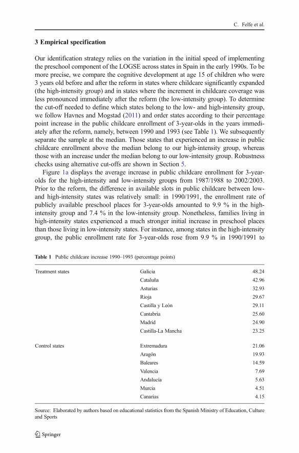
Our identification strategy relies on the variation in the initial speed of implementingthe preschool component of the LOGSE across states in Spain in the early 1990s. To bemore precise, we compare the cognitive development at age 15 of children who were3 years old before and after the reform in states where childcare significantly expanded(the high-intensity group) and in states where the increment in childcare coverage wasless pronounced immediately after the reform (the low-intensity group). To determinethe cut-off needed to define which states belong to the low- and high-intensity group,we follow Havnes and Mogstad (2011) and order states according to their percentagepoint increase in the public childcare enrollment of 3-year-olds in the years immedi-ately after the reform, namely, between 1990 and 1993 (see Table 1). We subsequentlyseparate the sample at the median. Those states that experienced an increase in publicchildcare enrollment above the median belong to our high-intensity group, whereasthose with an increase under the median belong to our low-intensity group. Robustnesschecks using alternative cut-offs are shown in Section 5.

Figure 1a displays the average increase in public childcare enrollment for 3-year-olds for the high-intensity and low-intensity groups from 1987/1988 to 2002/2003.Prior to the reform, the difference in available slots in public childcare between low-and high-intensity states was relatively small: in 1990/1991, the enrollment rate ofpublicly available preschool places for 3-year-olds amounted to 9.9 % in the high-intensity group and 7.4 % in the low-intensity group. Nonetheless, families living inhigh-intensity states experienced a much stronger initial increase in preschool placesthan those living in low-intensity states. For instance, among states in the high-intensitygroup, the public enrollment rate for 3-year-olds rose from 9.9 % in 1990/1991 to

Table 1 Public childcare increase 1990–1993 (percentage points)

Treatment states Galicia 48.24

Cataluña 42.96

Asturias 32.93

Rioja 29.67

Castilla y León 29.11

Cantabria 25.60

Madrid 24.90

Castilla-La Mancha 23.25

Control states Extremadura 21.06

Aragón 19.93

Baleares 14.59

Valencia 7.69

Andalucía 5.63

Murcia 4.51

Canarias 4.15

Source: Elaborated by authors based on educational statistics from the Spanish Ministry of Education, Cultureand Sports

C. Felfe et al.

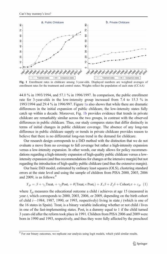
44.0 % in 1993/1994, and 57.1 % in 1996/1997. In comparison, the public enrollmentrate for 3-year-olds in the low-intensity group increased from 7.4 to 15.3 % in1993/1994 and 29.4 % in 1996/997. Figure 1a also shows that while there are dramaticdifferences in the initial expansion of public childcare, the low-intensity states fullycatch up within a decade. Moreover, Fig. 1b provides evidence that trends in privatechildcare are remarkably similar across the two groups, in contrast with the observeddifferences in public childcare. Thus, our study compares states that differ distinctly interms of initial changes in public childcare coverage. The absence of any long-rundifference in public childcare supply or trends in private childcare provides reason tobelieve that there is no differential long-run trend in the demand for childcare.

Our research design corresponds to a DiD method with the distinction that we do notevaluate a move from no coverage to full coverage but rather a high-intensity expansionversus a low-intensity expansion. In other words, our study allows for policy recommen-dations regarding a high-intensity expansion of high-quality public childcare versus a low-intensity expansion (and thus recommendations for changes at the intensivemargin) but notregarding the introduction of high-quality public childcare (and thus the extensive margin).

Our basic DiD model, estimated by ordinary least squares (OLS), clustering standarderrors at the state level and using the sample of children from PISA 2000, 2003, 2006and 2009, is as follows:8

Y ijt ¼ β þ γ1Treati þ γ2Postt þ θ Treati�Posttð Þ þ X iβ þ Z jδ þ Cohorttπþ εijt ð1Þwhere Yijt measures the educational outcome a child i achieves at age 15 (measured inyear t, which corresponds to 2000, 2003, 2006, or 2009, depending on the birth cohortof child i—1984, 1987, 1990, or 1993, respectively) living in state j (which is one ofthe 16 states in Spain). Treati is a binary variable indicating whether or not child i livesin one of the fast-implementing states. Postt is a dummy equal to 1 if the child turned3 years old after the reform took place in 1991. Children from PISA 2006 and 2009 wereborn in 1990 and 1993, respectively, and thus they were fully affected by the preschool

010

2030

4050

6070

80

1987

1988

1989

1990

1991

1992

1993

1994

1995

1996

1997

1998

1999

2000

2001

2002

Treatment states Comparison states

a. Public Childcare

010

2030

4050

6070

80

1987

1988

1989

1990

1991

1992

1993

1994

1995

1996

1997

1998

1999

2000

2001

2002


b. Private Childcare

Fig. 1 Enrollment rates in childcare among 3-year-olds. Displayed numbers are weighted averages ofenrollment rates for the treatment and control states. Weights reflect the population of each state (CCAA)

8 For our binary outcomes, we replicate our analysis using logit models, which yield similar results.


component of the LOGSE at age 3 if they lived in a state that rapidly expanded thesupply of public childcare slots. Children from PISA 2000 and 2003 were born in 1984and 1987, respectively. They were 7 and 4 years old when the LOGSE was firstimplemented, and thus they were unaffected by the expansion of publicly subsidizedchildcare. Therefore, Postt takes on the value 1 for children belonging to the PISAcohorts 2006 and 2009, and zero for children belonging to the PISA cohorts 2000 and2003. To allow for any underlying trend in the PISA test scores, we control for a set ofcohort fixed effects (in other words, a set of dummies for the PISA cohort 2000, 2003,2006, and 2009).9,10 The vector Xi includes only time-invariant individual features thatare expected to be correlated with educational achievement: gender and immigrantstatus. Since all additional socio-demographic characteristics that we observe at age15 are time variant and thus potentially endogenous to our treatment, we decided not toinclude them in our main specification. However, our results are robust to sensitivityanalysis, where we sequentially add these additional variables to Eq. 1, as shown inAppendix Table A.2. Finally, the vector Zj includes pre-reform state-specific featuressuch as gross domestic product (GDP) per capita, unemployment rate, female employ-ment rate, average educational level, and population density (measured as the average forthe years 1987 to 1990). Controlling for such prereform-specific features shall accountfor the fact that some states are better equipped to expand childcare rapidly than others. Ina separate specification, we allow for pre-reform heterogeneity within the group oftreatment states by including state-specific fixed effects instead. As the coefficients varylittle across these two specifications, we use the former as our main specification.

The coefficient θ belonging to the interaction term between the Treati dummy andthe Postt dummy measures the average effect of the increase in high-quality childcareslots for 3-year-olds in high-intensity states versus the increase in low-intensity states.For this estimate to be causal, the assumption of common trends needs to be fulfilled. Inother words, in the absence of the reform, the outcomes for treated and comparisonchildren should have evolved in parallel. Is this assumption credible or are there reasonsto believe that there are further differences between high- and low-intensity states thatcould have sent children on different outcome paths in the absence of the reform?

By choosing the initial years after the reform, we aim at capturing variation in thespeed of the expansion in high-quality public childcare due to a slackening of initialconstraints and not due to differences in underlying preferences or demand. In otherwords, we believe that an expansion of public childcare of comparable magnitudewould have been unlikely in any Spanish state without the federal subsidies provideddue to the LOGSE, at least in the short run. Unfortunately, we lack a longer time seriesfor the outcome variables to provide some evidence for parallel trends prior to thereform. Nonetheless, given two data points prior to treatment, we can estimate aplacebo test assuming that the reform would have taken place in the late 1980s andthus affected the PISA 2003 cohort, yet not the PISA 2000 cohort (see Section 6 for

9 Due to perfect collinearity between the constant and the Postt dummy on the one hand and the PISA cohortson the other hand, we omit two cohort dummies (2000 and 2009). Alternatively, we could omit the Posttdummy and include dummies for both “post reform” cohorts (see Section 7).10 While we have administrative data on preschool enrollment at the lower level, we lack that information inPISA (in fact, gaining access to PISA data disaggregated at the state level is already quite hard). As such, ouranalysis relies on variation between states but ignores potential variation within states.

C. Felfe et al.

results on this placebo estimation). In addition, we discuss supplementary evidence forthe assumption of common trends.

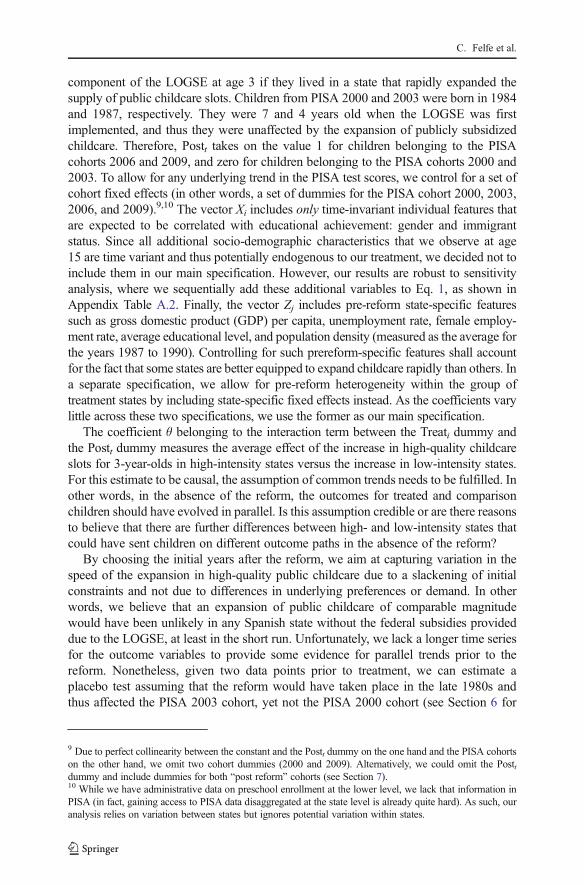
Why were some states better equipped to implement the reform immediately, whileothers could do so only with a certain time lag? As discussed in Section 2, a lack of know-how due to a lower level of private childcare, the scarcity of qualified teachers, andclassroom space represented important barriers for a fast expansion. Nonetheless, whilethere were initial differences regarding such barriers across states, Fig. 2 shows that therewas no differential improvement in available proxies for these barriers (such as the children/staff ratio in public and private primary schools) after the implementation of the reform.

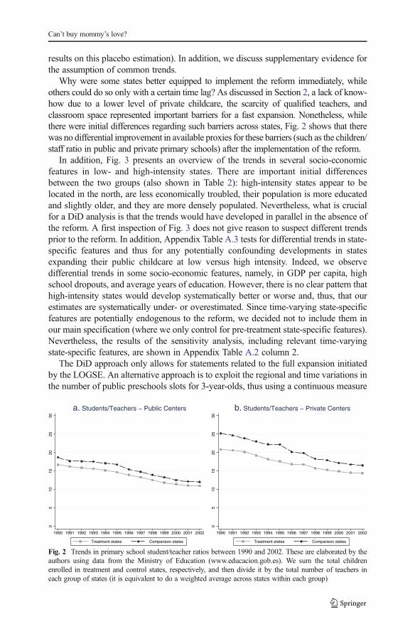
In addition, Fig. 3 presents an overview of the trends in several socio-economicfeatures in low- and high-intensity states. There are important initial differencesbetween the two groups (also shown in Table 2): high-intensity states appear to belocated in the north, are less economically troubled, their population is more educatedand slightly older, and they are more densely populated. Nevertheless, what is crucialfor a DiD analysis is that the trends would have developed in parallel in the absence ofthe reform. A first inspection of Fig. 3 does not give reason to suspect different trendsprior to the reform. In addition, Appendix Table A.3 tests for differential trends in state-specific features and thus for any potentially confounding developments in statesexpanding their public childcare at low versus high intensity. Indeed, we observedifferential trends in some socio-economic features, namely, in GDP per capita, highschool dropouts, and average years of education. However, there is no clear pattern thathigh-intensity states would develop systematically better or worse and, thus, that ourestimates are systematically under- or overestimated. Since time-varying state-specificfeatures are potentially endogenous to the reform, we decided not to include them inour main specification (where we only control for pre-treatment state-specific features).Nevertheless, the results of the sensitivity analysis, including relevant time-varyingstate-specific features, are shown in Appendix Table A.2 column 2.

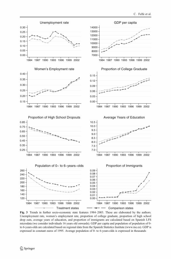
The DiD approach only allows for statements related to the full expansion initiatedby the LOGSE. An alternative approach is to exploit the regional and time variations inthe number of public preschools slots for 3-year-olds, thus using a continuous measure

05

1015

2025

30

1990 1991 1992 1993 1994 1995 1996 1997 1998 1999 2000 2001 2002


a. Students/Teachers − Public Centers

05

1015

2025

30

1990 1991 1992 1993 1994 1995 1996 1997 1998 1999 2000 2001 2002


b. Students/Teachers − Private Centers

Fig. 2 Trends in primary school student/teacher ratios between 1990 and 2002. These are elaborated by theauthors using data from the Ministry of Education (www.educacion.gob.es). We sum the total childrenenrolled in treatment and control states, respectively, and then divide it by the total number of teachers ineach group of states (it is equivalent to do a weighted average across states within each group)


0.00

0.05

0.10

0.15

0.20

0.25

0.30

1984 1987 1990 1993 1996 1999 2002

Unemployment rate

7000

8000

9000

10000

11000

12000

13000

14000

1984 1987 1990 1993 1996 1999 2002

GDP per capita

0.15

0.20

0.25

0.30

0.35

0.40

1984 1987 1990 1993 1996 1999 2002

Women’s Employment rate

0.00

0.03

0.06

0.09

0.12

0.15

1984 1987 1990 1993 1996 1999 2002

Proportion of College Graduate

0.25

0.35

0.45

0.55

0.65

0.75

0.85

1984 1987 1990 1993 1996 1999 2002

Proportion of High School Dropouts

7.0

7.5

8.0

8.5

9.0

9.5

10.0

10.5

1984 1987 1990 1993 1996 1999 2002

Average Years of Education

120

140

160

180

200

220

240

260

1984 1987 1990 1993 1996 1999 2002

Population of 0− to 6−years−olds

0.000.010.020.030.040.050.060.070.080.09

1984 1987 1990 1993 1996 1999 2002

Proportion of Immigrants

Treatment states Comparison statesFig. 3 Trends in further socio-economic state features 1984–2003. These are elaborated by the authors.Unemployment rate, women’s employment rate, proportion of college graduate, proportion of high schooldrop outs, average years of education, and proportion of immigrants are calculated based on Spanish LFSmicrodata (we consider individuals 16 years old onwards). GDP per capita and population of population of 0-to 6-years-olds are calculated based on regional data from the Spanish Statistics Institute (www.ine.es). GDP isexpressed in constant euros of 1995. Average population of 0- to 6-years-olds is expressed in thousands

C. Felfe et al.

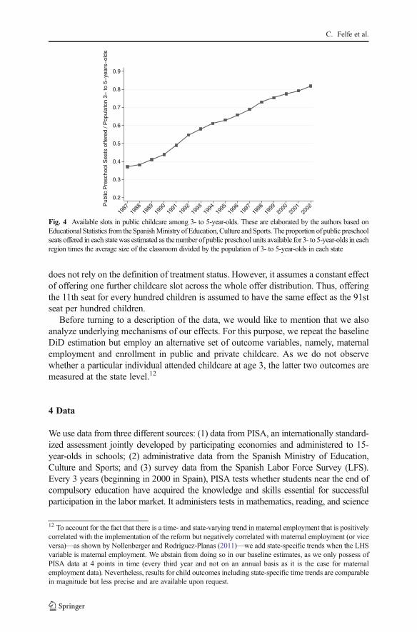
of the expansion in public childcare. As numbers of slots available in public preschoolare not available for detailed age groups, we employ a proxy: the number of publicpreschool units available for 3- to 5-year-olds.11 Figure 4 displays the overall increasein available slots for 3- to 5-year-olds from 1987/1988 to 2002/2003. To estimate thisrelationship, we follow Berlinski and Galiani (2007) and estimate the effect of offeringone additional seat in public childcare, estimating the following equation by OLS:

Y ij tþ12ð Þ ¼ θSeatsjt þX

s¼1987

1993

αsl s ¼ tð Þ þ X iβ þ Z jδ þ εij tþ12ð Þ ð2Þ

where t=1987, 1990, 1993, and 1996, and Yij (t + 12) is a measure of the educationaloutcome that child i achieves at age 15 measured in year (t+12), which corresponds to2000, 2003, 2006, or 2009, depending on the birth cohort of child i—1984, 1987, 1990,or 1993, respectively, living in state j (which is one of the 16 states in Spain). Seatsjt isthe number of public preschool seats per 100 for children aged 3 to 5 years old in state jin the year t. The vector Xi includes time-invariant individual characteristics (genderand immigration status). As in the baseline specification, we include state (Zj) and

cohort fixed effects ( ∑s¼1987

1993

αsl s ¼ tð Þ ). This specification has the advantage that it

11 Following Berlinski and Galiani (2007), we estimate the proportion of public preschool seats offered in eachstate as the number of public preschool units available for 3- to 5-year-olds in each region times the averagesize of the classroom divided by the population of 3- to 5-year-olds in each state.

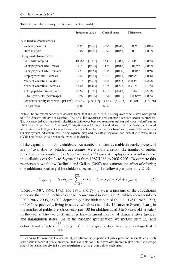
Table 2 Pre-reform descriptive statistics—control variables

Treatment states Control states Differences

A Individual characteristics

Gender (male=1) 0.485 [0.500] 0.494 [0.500] −0.009 (0.015)

Born in Spain 0.996 [0.062] 0.997 [0.053] −0.001 (0.002)

B Regional characteristics

GDP (euros/capita) 10,687 [2,136] 8,543 [1,481] 2,144* (1,085)

Unemployment rate—males 0.114 [0.024] 0.186 [0.068] −0.072** (0.032)

Unemployment rate—females 0.227 [0.054] 0.315 [0.070] −0.088** (0.039)

Employment rate—females 0.262 [0.044] 0.209 [0.043] 0.053* (0.026)

Years of education—males 8.919 [0.573] 8.456 [0.233] 0.464* (0.252)

Years of education—females 8.400 [0.419] 8.028 [0.227] 0.371* (0.185)

Total population (in millions) 4.022 [1.816] 4.368 [2.502] −0.346 (1.502)

0- to 6-years-old (percentage) 0.076 [0.007] 0.094 [0.011] −0.018*** (0.005)

Population density (inhabitants per km2) 247.637 [228.343] 103.633 [51.718] 144.004 (113.176)

Sample sizes 6,846 4,650

Notes: The pre-reform period includes data from 2000 and 2003 PISA. The displayed sample sizes correspondto PISA datasets and are not weighted. The table displays means and standard deviations shown in brackets.The asterisks indicate statistically significant differences between treatment and control states: *significant at10 % level; **significant at 5 % level; ***significant at 1 % level. Standard errors in parenthesis are clusteredat the state level. Regional characteristics are calculated by the authors based on Spanish LFS microdata(unemployment, education, female employment rate) and on data at regional level available in www.ine.es(GDP, population, 0- to 6-years-old, population density)


does not rely on the definition of treatment status. However, it assumes a constant effectof offering one further childcare slot across the whole offer distribution. Thus, offeringthe 11th seat for every hundred children is assumed to have the same effect as the 91stseat per hundred children.

Before turning to a description of the data, we would like to mention that we alsoanalyze underlying mechanisms of our effects. For this purpose, we repeat the baselineDiD estimation but employ an alternative set of outcome variables, namely, maternalemployment and enrollment in public and private childcare. As we do not observewhether a particular individual attended childcare at age 3, the latter two outcomes aremeasured at the state level.12

4 Data

We use data from three different sources: (1) data from PISA, an internationally standard-ized assessment jointly developed by participating economies and administered to 15-year-olds in schools; (2) administrative data from the Spanish Ministry of Education,Culture and Sports; and (3) survey data from the Spanish Labor Force Survey (LFS).Every 3 years (beginning in 2000 in Spain), PISA tests whether students near the end ofcompulsory education have acquired the knowledge and skills essential for successfulparticipation in the labor market. It administers tests in mathematics, reading, and science

12 To account for the fact that there is a time- and state-varying trend in maternal employment that is positivelycorrelated with the implementation of the reform but negatively correlated with maternal employment (or viceversa)—as shown by Nollenberger and Rodríguez-Planas (2011)—we add state-specific trends when the LHSvariable is maternal employment. We abstain from doing so in our baseline estimates, as we only possess ofPISA data at 4 points in time (every third year and not on an annual basis as it is the case for maternalemployment data). Nevertheless, results for child outcomes including state-specific time trends are comparablein magnitude but less precise and are available upon request.

0.2

0.3

0.4

0.5

0.6

0.7

0.8

0.9

Pub

lic P

resc

hool

Sea

ts o

ffere

d / P

opul

aton

3−

to 5

−ye

ars−

olds

1987

1988

1989

1990

1991

1992

1993

1994

1995

1996

1997

1998

1999

2000

2001

2002

Fig. 4 Available slots in public childcare among 3- to 5-year-olds. These are elaborated by the authors based onEducational Statistics from the SpanishMinistry of Education, Culture andSports. The proportion of public preschoolseats offered in each statewas estimated as the number of public preschool units available for 3- to 5-year-olds in eachregion times the average size of the classroom divided by the population of 3- to 5-year-olds in each state

C. Felfe et al.

to assess whether students can analyze, reason, and communicate effectively. Backgroundquestionnaires are completed by students and school principals, which help to providedetailed information on children, family, and school characteristics. Our analysis focuseson reading and mathematics as performance in these two domains are fully comparableacross PISA cycles from 2000 onwards. Questions entering the scientific scores are notcomparable before and after 2006 and thus are not included in our analysis (OECD 2006).The PISA sample is stratified at two stages: first, schools are randomly selected; andsecond, students at each school are randomly assigned to carry out the test in all threesubjects. Participation in PISA is voluntary for schools and students, although a minimumparticipation rate of 65% (80%) of schools (students) from the original sample is requiredfor a country to be included in the international database. We check the robustness of ourresults to this double stratification sampling design by re-estimating the effects of thereform using Fay’s balanced repeated replicated (BRR) methodology in Section 6. Thetest scores are standardized, implying that the estimated coefficient represents the percent-age increase (or decrease) in standard deviations (henceforth SD). We also estimate theeffect of the reform on two additional variables that are only available in the 2003 and2009 PISA waves: falling behind a grade during primary school or secondary school.Unfortunately, PISA does not provide information on preschool attendance at specificages and thus, similar to related studies in this field (Baker et al. 2008; Fitzpatrick 2008;Havnes and Mogstad 2011), our estimates are intention-to-treat (ITT) estimates only.

Administrative data include enrollment rates by age, state and type of school (public orprivate), as well as the number of preschool units (classrooms) by state, and type of schoolfrom the 1986/1987 school year onwards. Enrollment rates from the 1992/1993 school yearonwards are available from the web page of the Ministry of Education, Culture andSports. 13 Data before 1992/1993 were taken from the Education Statistics yearbookspublished by the Ministry of Education, Culture and Sports.14 The number of preschoolunits (classrooms) by state and type of school is also available from the web page of theMinistry from the 1986/1987 school year onwards; however, this information is not availableby age. As explained in Section 3 (see footnote 11), we use the total number of preschoolunits to estimate a measure of the proportion of total preschool slots offered (to children from3 to 5 years old).

We obtain information on maternal employment from 1987 to 1997 from the SpanishLFS, a quarterly cross-sectional dataset that gathers information on socio-demographiccharacteristics (such as, age, years of education, marital status, and state of residence),employment, and fertility (number of children living in the household and their birth year).15

We exclude immigrant children who arrived to Spain after their third birthday, as wellas children residing in the Basque Country, Navarra, and Ceuta and Melilla. The reason

13 See http://www.mecd.gob.es/servicios-al-ciudadano-mecd/estadisticas/educacion/no-universitaria/alumnado/matriculado/series.html.14 As the Ministry did not publish the enrollment rates at state level in the yearbooks, they were calculated bythe authors as the ratio between the number of children enrolled in public and private schools (available at statelevel in the Education Statistics yearbooks) and the population of the corresponding age group and state fromthe Spanish Statistics Institute. (http://www.ine.es/jaxi/menu.do?type=pcaxis&path=/t20/p263/pob_91/&file=pcaxis). We check the consistency of our calculations comparing overlapping data for the school years1992/1993 and 1993/1994.15 Again, we do not observe children’s day care enrollment, thus precluding us from analyzing a “first-stage”model, as in Cascio (2009) and Berlinski and Galiani (2007) with a dummy for public day care enrollment ofthe mother’s youngest child as dependent variable.


for doing so is that the Basque Country and Navarra have had greater fiscal and politicalautonomy since the mid 1970s and consequently their educational policy has differedfrom that of Spain as a whole. In particular, practically all 3-year-olds have been inchildcare in the Basque Country and Navarra since the early 1990s.16 Data on childrenliving in Ceuta and Melilla are only available in the PISA data from 2006 onwards.

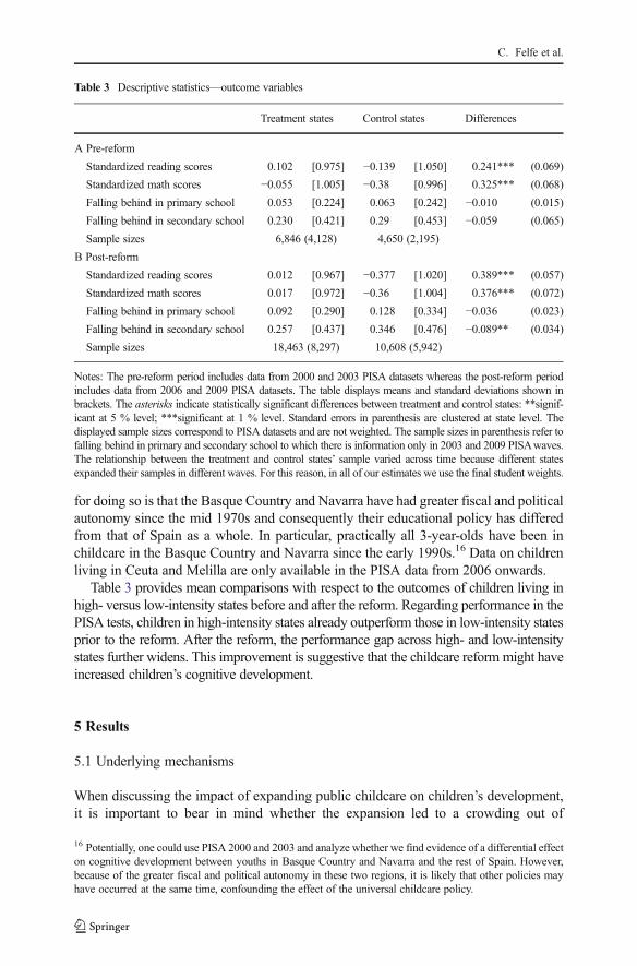
Table 3 provides mean comparisons with respect to the outcomes of children living inhigh- versus low-intensity states before and after the reform. Regarding performance in thePISA tests, children in high-intensity states already outperform those in low-intensity statesprior to the reform. After the reform, the performance gap across high- and low-intensitystates further widens. This improvement is suggestive that the childcare reform might haveincreased children’s cognitive development.

5 Results

5.1 Underlying mechanisms

When discussing the impact of expanding public childcare on children’s development,it is important to bear in mind whether the expansion led to a crowding out of

Table 3 Descriptive statistics—outcome variables

Treatment states Control states Differences

A Pre-reform

Standardized reading scores 0.102 [0.975] −0.139 [1.050] 0.241*** (0.069)

Standardized math scores −0.055 [1.005] −0.38 [0.996] 0.325*** (0.068)

Falling behind in primary school 0.053 [0.224] 0.063 [0.242] −0.010 (0.015)

Falling behind in secondary school 0.230 [0.421] 0.29 [0.453] −0.059 (0.065)

Sample sizes 6,846 (4,128) 4,650 (2,195)

B Post-reform

Standardized reading scores 0.012 [0.967] −0.377 [1.020] 0.389*** (0.057)

Standardized math scores 0.017 [0.972] −0.36 [1.004] 0.376*** (0.072)

Falling behind in primary school 0.092 [0.290] 0.128 [0.334] −0.036 (0.023)

Falling behind in secondary school 0.257 [0.437] 0.346 [0.476] −0.089** (0.034)

Sample sizes 18,463 (8,297) 10,608 (5,942)

Notes: The pre-reform period includes data from 2000 and 2003 PISA datasets whereas the post-reform periodincludes data from 2006 and 2009 PISA datasets. The table displays means and standard deviations shown inbrackets. The asterisks indicate statistically significant differences between treatment and control states: **signif-icant at 5 % level; ***significant at 1 % level. Standard errors in parenthesis are clustered at state level. Thedisplayed sample sizes correspond to PISA datasets and are not weighted. The sample sizes in parenthesis refer tofalling behind in primary and secondary school to which there is information only in 2003 and 2009 PISAwaves.The relationship between the treatment and control states’ sample varied across time because different statesexpanded their samples in different waves. For this reason, in all of our estimates we use the final student weights.

16 Potentially, one could use PISA 2000 and 2003 and analyze whether we find evidence of a differential effecton cognitive development between youths in Basque Country and Navarra and the rest of Spain. However,because of the greater fiscal and political autonomy in these two regions, it is likely that other policies mayhave occurred at the same time, confounding the effect of the universal childcare policy.

C. Felfe et al.

alternative care modes. Therefore, we first discuss the changes in public and privatechildcare as well as maternal employment that arose after the introduction of theLOGSE. For the purpose of the latter, we re-estimate the results by Nollenberger andRodríguez-Planas (2011).17

Panel A in Table 4 shows that children residing in high-intensity states were offeredsubstantially more public childcare than those residing in low-intensity states: thisdifferential increase amounted to 25.8 percentage points.18 Nonetheless, the reformdid not lead to a crowding out of private childcare enrollment. While this result mightcome as a surprise, it is important to highlight that preschool for 3-year-olds wasimplemented within primary schools regardless of school ownership. Consequently,parents who wished to enroll their children in private school would now enroll their 3-year-old in the private school as soon as preschool for that age group was offered (toguarantee a space thereafter). Panel A in Table 4 also shows that the effect of universalchildcare on maternal employment is not only much smaller than the increase in theenrollment in childcare but also less precise. Despite not being statistically significantlydifferent from zero, the economic interpretation of the estimate is that after thelegislation was passed, mothers of 3-year-olds from fast-implementing states were2.4 percentage points (or 6.7 %) more likely to work than their counterparts in slow-implementing states.19 While this finding might seem puzzling at first, it makes sense inthe light of Spain being characterized by the male breadwinner model (as described inSection 2), especially since the reform was implemented during a period of low labordemand in a country well known for its rigid labor market.

Finally, it is important to note that the expansion in public childcare was unlikely tolead to a crowding out of informal care arrangements. Prior to the reform, 35.7 % ofmothers of 3-year-olds worked in treated states, while 32.5 % of 3-year-olds wereenrolled in formal care (9.9 % in public childcare and 22.6 % in private childcare).Thus, most mothers of 3-year-olds who worked prior to the reform were likely to havetheir child already enrolled in either public or private childcare. The Spanish reformtherefore mainly implied that mothers took their children to full-time childcare, eventhough they continued not to work.

Overall, our findings should be interpreted as the effects of an expansion inhigh-quality public childcare, which mainly led to a crowding out of familycare, but not to a crowding out of private or informal care arrangements. Thisimplies that our estimates mainly measure the effects of offering universal high-quality childcare, as the reform under analysis did not imply a major incomeshock due to a shift from private to public childcare. Moreover, any potentialincome effect from an increase in maternal employment caused by the reform ismodest at most.

17 As explained at the end of Section 3, we adjust the identification strategy to be comparable to the baselinestrategy of the current paper.18 We estimate the separate effect on the 1993/1994 and 1996/1997 cohorts and find similar coefficients(0.261 versus 0.256). As a consequence, we decided to pool both post-reform cohorts into one. Results whenestimating our specification using the two cohorts separately are shown in Table 8 panel C and are discussed inSection 7.19 Prior to the reform, the average employment rate of mothers of 3-year-olds was 35.7 % in fast-implementing states.


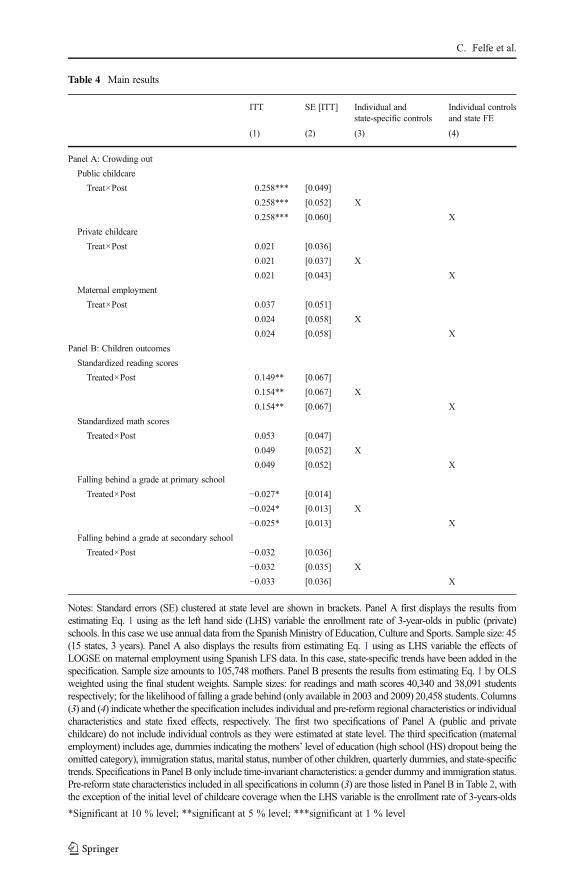
Table 4 Main results

ITT SE [ITT] Individual andstate-specific controls

Individual controlsand state FE

(1) (2) (3) (4)

Panel A: Crowding out

Public childcare

Treat×Post 0.258*** [0.049]

0.258*** [0.052] X

0.258*** [0.060] X

Private childcare

Treat×Post 0.021 [0.036]

0.021 [0.037] X

0.021 [0.043] X

Maternal employment

Treat×Post 0.037 [0.051]

0.024 [0.058] X

0.024 [0.058] X

Panel B: Children outcomes

Standardized reading scores

Treated×Post 0.149** [0.067]

0.154** [0.067] X

0.154** [0.067] X

Standardized math scores

Treated×Post 0.053 [0.047]

0.049 [0.052] X

0.049 [0.052] X

Falling behind a grade at primary school

Treated×Post −0.027* [0.014]

−0.024* [0.013] X

−0.025* [0.013] X

Falling behind a grade at secondary school

Treated×Post −0.032 [0.036]

−0.032 [0.035] X

−0.033 [0.036] X

Notes: Standard errors (SE) clustered at state level are shown in brackets. Panel A first displays the results fromestimating Eq. 1 using as the left hand side (LHS) variable the enrollment rate of 3-year-olds in public (private)schools. In this case we use annual data from the SpanishMinistry of Education, Culture and Sports. Sample size: 45(15 states, 3 years). Panel A also displays the results from estimating Eq. 1 using as LHS variable the effects ofLOGSE on maternal employment using Spanish LFS data. In this case, state-specific trends have been added in thespecification. Sample size amounts to 105,748 mothers. Panel B presents the results from estimating Eq. 1 by OLSweighted using the final student weights. Sample sizes: for readings and math scores 40,340 and 38,091 studentsrespectively; for the likelihood of falling a grade behind (only available in 2003 and 2009) 20,458 students. Columns(3) and (4) indicate whether the specification includes individual and pre-reform regional characteristics or individualcharacteristics and state fixed effects, respectively. The first two specifications of Panel A (public and privatechildcare) do not include individual controls as they were estimated at state level. The third specification (maternalemployment) includes age, dummies indicating the mothers’ level of education (high school (HS) dropout being theomitted category), immigration status, marital status, number of other children, quarterly dummies, and state-specifictrends. Specifications in Panel B only include time-invariant characteristics: a gender dummy and immigration status.Pre-reform state characteristics included in all specifications in column (3) are those listed in Panel B in Table 2, withthe exception of the initial level of childcare coverage when the LHS variable is the enrollment rate of 3-years-olds

*Significant at 10 % level; **significant at 5 % level; ***significant at 1 % level

C. Felfe et al.

5.2 Children’s cognitive long-term outcomes

Panel B in Table 4 shows the impact of expanding public childcare on all childrenliving in the high-intensity states—the so-called intention-to-treat effect—for fouralternative outcome variables: test scores in reading and math, as well as the likelihoodof falling behind one grade in primary and secondary school. All regressions areestimated using OLS and clustering standard errors at the state level, first not control-ling for any further control variables and then controlling for pre-reform individual andstate characteristics. Comparing the estimates with and without time-invariant individ-ual and pre-reform regional controls in Panel B in Table 4 reveals no significantdifferences. We therefore focus our discussion on the latter specification.

Focusing first on the effects of the reform on children’s standardized reading testscores at age 15, the effect of the expansion in public childcare for 3-year-olds ispositive and statistically significant at any conventional significance level. The expan-sion of public childcare places leads to an increase in reading test scores by 0.15 SD.We cannot find a significant effect of the reform on children’s math performance. Thus,our results are in line with the expectations that the activities undertaken in publicchildcare stimulate children’s social and emotional competencies and thus their lan-guage and reading skills but not necessarily their math skills.

How do these effects compare to the established evidence? The existing studiesevaluating the impact of universal childcare provision find effects of similar directionand size, despite being measured at an earlier age. In the case of an Argentinean reform,Berlinski et al. (2009) find a substantial improvement of cognitive skills (by 0.23 SD)among children in the third grade. Analyzing the consequences of the introduction ofuniversal childcare in Georgia (USA) on the reading and math skills among children infourth grade, Fitzpatrick (2008) finds slightly lower effects and only for the populationof disadvantaged children, defined as those living in rural areas. More specifically, shefinds significant gains, ranging between 0.07 and 0.12 SD for reading scores, andbetween 0.06 and 0.09 SD for math scores.

Moving to the effects of the reform on the likelihood of falling behind a grade, we alsofind beneficial effects of the reform.More specifically, we observe that the reform reducedthe incidence of falling behind a grade by 2.4 percentage points in primary school. Giventhe initial likelihood of falling behind a grade among children in the treated states of 5% inprimary school, the effect of the reform represents a substantial decrease in the incidenceof retention (almost 50 %). While the estimations also indicate a reduction of fallingbehind in secondary school, the estimated coefficient is not significant at any conventionalsignificance level. In other words, while initial gains in cognitive skills might be strongenough to help children master the requirements to pass a grade during primary school,they might not necessarily be sufficient to make a difference in secondary school.

The two existing studies considering the consequences of universal childcare pro-vision on this outcome are US studies by Fitzpatrick (2008) and Cascio (2009). Ourresults are similar to those found by Fitzpatrick (2008) for disadvantaged children. Infact, analyzing universal pre-kindergarten in Georgia, she finds that the probability ofbeing on-grade for their age (fourth graders and thus in primary school) increases by 7percentage points (about 10 %) among black children. By contrast, analyzing the long-term effects of public childcare provision, Cascio (2009) did not find any significantimprovements in grade retention. One possible reason behind the differences between


our results and those of Cascio (2009) is that she analyzes the effects of introducinglow-intensity kindergarten for 5-year-olds, while we analyze the effects of high-qualityfull-time childcare for 3-year-olds.

6 Sensitivity analysis

In this section, we address several potential sources of bias. In particular, we discussissues such as selective migration and common trend assumption, as well as addingfurther specification checks.

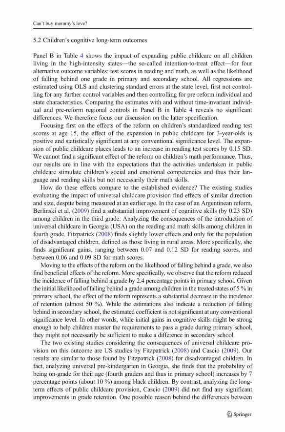
Selective migration: One potential source of bias might be selective migration, wherebyfamilies might have moved from slow-implementing states to fast-implementing states.Since PISA only provides information on the state of residence at age 15 (but not at age 3),we rely on the LFS (for 2000, 2003, 2006 and 2009) to assess the concern of selectivemigration.We first assess the likelihood of living at age 15 in a state different from the stateof birth. However, this probability is small (4.0 % in 2000, 4.6 % in 2003, 5.2 % in 2006,and 4.9 % in 2009). Second, we estimate the likelihood of having migrated from a low- toa high-implementing state (and vice versa). The results do not indicate an increasedmigration into high-implementing states (shown in Table 5, Panel A). Thus, selectivemigration should not be a major threat for the internal validity of the study.20

Common trend assumption: The strongest assumption underlying any DiD estimation isthe absence of any differential time trend in high- and low-implementing states. Besidesinspecting pre-existing trends, the most commonly used test to shed some light on thisassumption is to estimate the effect of a placebo reform, pretending that the reform tookplace at an earlier moment in time. Given the time horizon of PISA data, we can onlypursue a placebo test assuming that the reform took place in the late 1980s and thusaffected the cohort born in 1987 (the PISA cohort 2003) but not the cohort born in 1984(the PISA cohort 2000). Re-estimating Eq. 1 but using only PISA 2000 and 2003 data andtreating the PISA 2003 cohort as the post-reform cohort do not reveal any significantimpact of the imaginary policy change on children’s reading and math test scores (seePanel B in Table 5). Note that we do not lose precision in this specification, but instead thesize of the coefficients is cut in half and are no longer significant.

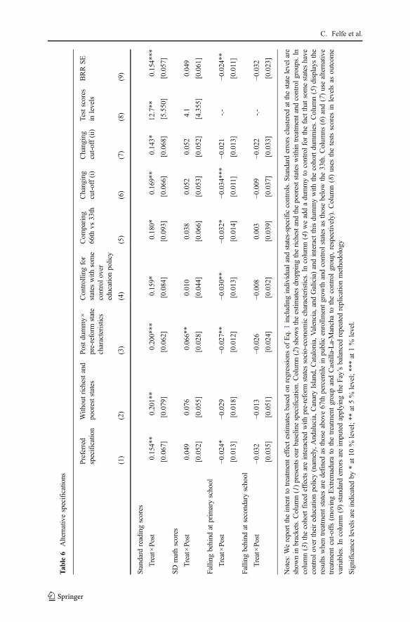
In addition, we estimate a specification where we use a more homogenous sample ofstates and exclude the poorest and richest states from our sample. In doing so, we wantto address the fact that Spanish regions strongly differ in their economic developmentand thus might potentially follow differential trends. The results are fairly robust to thissample restriction. Three of the four coefficients increase in size in this specification,although only the effect on reading is statistically significant (see Table 6, column 2).Finally, we estimate a specification in which we interact the Post dummy with all pre-reform regional characteristics shown in Table 2 (Duflo 2001). In doing so, we checkwhether regional pre-reform characteristics are correlated with the development ofchildren’s cognitive skills over time. The results shown in column 3 of Table 6 are

20 In addition, the migration flow by skill level is similar to the ones presented in the table and does notindicate any migration flows that would threaten our identification strategy.

C. Felfe et al.

robust and provide supportive evidence for the underlying assumption of common timetrends (at least in terms of observables).

Further robustness checks: Finally, we carry out the following additional sensitivitychecks. First, some states (Andalucía, Canary Island, Catalonia, Valencia, and Galicia)traditionally had more control over their education policy. Since this may affect our results,we have re-estimated a specification, adding a dummy for these five states and interacting itwith the post-reform dummy (shown in Table 6, column 4). Second, as in Havnes andMogstad (2011), we experiment with a different definition of the treatment and the controlgroups, whereby high-implementing states are defined as those with growth in publicenrollment above the 67th percentile, and low-implementing states are those with growth inpublic enrollment below the 33th percentile (shown in Table 6, column 5). In addition, weuse alternative cut-offs for the definition of treatment and control states and include the statewith the lowest increase of public childcare among the high-implementing states into the

Table 5 Robustness checks

ITT SE [ITT] Individualand state-specificcontrols

Individualcontrolsand state FE

Panel A Effect on probability of having migrated across states by age 16 using LFS

A.1 From control to treatment states

Treated×Post −0.006 [0.009]

−0.006 [0.009] X

−0.006 [0.009] X

A.2 From treatment to control states

Treated×Post 0.009 [0.006]

0.009 [0.006] X

0.009 [0.006] X

Panel B Placebo test: pre-reform data


Treated×Cohort90 0.082 [0.061]

0.085 [0.060] X

0.086 [0.060] X


Treated×Cohort90 0.000 [0.060]

0.025 [0.063] X

0.025 [0.062] X

Notes: The table displays the results from estimating Eq. 1 using different outcomes as LHS variable. In eachcase, we present the raw estimate and also one that includes individual controls (invariant characteristics) andeither the pre-regional characteristics listed in the Panel B of Table 2 or state fixed effects. In Panel A.1, the LHSvariable is a dummy equal to one if the individual has migrated from a control to a treatment state (and vice versain Panel A.2). We use all quarters of 2000, 2003, 2006, and 2009 LFS and restrict the sample to natives. The totalsample size is of 27,602 observations. In Panel B, we estimate Eq. 1 using only 2000 and 2003 PISA datasets,assuming that the reform took place in between 1988 and 1990. Sample size, 11,400 and 9,151 students forreadings and math scores, respectively. Standard errors clustered at state level are shown in brackets.


Tab

le6

Alternativespecifications

Preferred

specification

With

outrichestand

pooreststates

Postdummy×

pre-reform

state

characteristics

Controllingfor

states

with

some

controlover

educationpolicy

Com

paring

66th

vs33th

Changing

cut-off(i)

Changing

cut-off(ii)

Testscores

inlevels

BRRSE

(1)

(2)

(3)

(4)

(5)

(6)

(7)

(8)

(9)

Standard

readingscores

Treat×Po

st0.154**

0.201**

0.200***

0.159*

0.180*

0.169**

0.143*

12.7**

0.154***

[0.067]

[0.079]

[0.062]

[0.084]

[0.093]

[0.066]

[0.068]

[5.550]

[0.057]

SDmathscores

Treat×Po

st0.049

0.076

0.066**

0.010

0.038

0.052

0.052

4.1

0.049

[0.052]

[0.055]

[0.028]

[0.044]

[0.066]

[0.053]

[0.052]

[4.355]

[0.061]

Falling

behind

atprim

aryschool

Treat×Po

st−0

.024*

−0.029

−0.027**

−0.030**

−0.032*

−0.034***

−0.021

-.-−0

.024**

[0.013]

[0.018]

[0.012]

[0.013]

[0.014]

[0.011]

[0.013]

[0.011]

Falling

behind

atsecondaryschool

Treat×Po

st−0

.032

−0.013

−0.026

−0.008

0.003

−0.009

−0.022

-.-−0

.032

[0.035]

[0.051]

[0.024]

[0.032]

[0.039]

[0.037]

[0.033]

[0.023]

Notes:Wereporttheintent

totreatm

enteffectestim

ates

basedon

regressionsof

Eq.

1includingindividualandstates-specificcontrols.S

tandarderrorsclusteredatthestatelevelare

show

nin

brackets.C

olum

n(1)presentsourbaselin

especification.Colum

n(2)show

stheestim

ates

dropping

therichestand

thepooreststateswith

intreatm

entand

controlg

roups.In

column(3)thecohortfixedeffectsareinteracted

with

pre-reform

states

socio-econom

iccharacteristics.In

column(4)weaddadummyto

controlforthefactthatsomestates

have

controlover

theireducationpolicy(nam

ely,Andalucia,C

anaryIsland,Catalonia,V

alencia,andGalicia)andinteractthisdummywith

thecohortdummies.Colum

n(5)displays

the

results

whentreatm

entstates

aredefinedas

thoseabove67th

percentilein

publicenrollm

entgrow

thandcontrolstates

asthosebelow

the33th.Colum

ns(6)and(7)usealternative

treatm

entcut-offs

(movingExtremadurato

thetreatm

entgroupandCastilla-La-Manchato

thecontrolgroup,

respectiv

ely).Colum

n(8)uses

thetestsscores

inlevelsas

outcom

evariables.In

column(9)standard

errorsareim

putedapplying

theFay’sbalanced

repeated

replicationmethodology

Significance

levelsareindicatedby

*at10

%level;**

at5%

level;***at1%

level.

C. Felfe et al.

low-implementing states in one alternative specification, as well as the state with the highestincrease of public childcare among the low-implementing states into the high-implementing states in another alternative specification (shown in Table 6, columns 6and 7, respectively). In addition, we repeat our estimations using the levels of the outcomevariables rather than the standardized test scores (shown in column 8). Finally, column 9shows a specification that takes into account the double stratification nature of the samplingdesign employed by PISA, whereby we run our regression applying the Fay’s BRRmethodology. Notice that this method implies clustering at the school level. Overall, theresults regarding reading scores are robust to all of these sensitivity checks, while the resultsregarding falling behind a grade in primary school are robust to six out of eight robustnesschecks (see Table 6).21

Alternative identification: Estimates from Eq. 2 are shown in Table 7. Offering one moreslot per hundred children leads on average to a statistically significant improvement inchildren’s reading test scores (0.01 SD) and a statistically significant reduction in thelikelihood of falling behind a grade while in primary school of 0.2 percentage points. Giventhe average increase in public enrollment by 25.8 percentage points after the introduction ofLOGSE, this implies an improvement of 0.26 SD in reading test scores and a reduction ofabout 5.2 percentage points in the likelihood of falling behind a grade in primary school.Analogous to the baseline specification, there does not seem to be a statistically significanteffect on math test scores and falling behind a grade during high school. 22

7 Heterogeneity analysis

Table 8 displays estimates by children’s gender, children’s birth cohort, and parents’educational level. Such analysis might reveal policy relevant effect heterogeneity.

Gender: Estimates from Panel A in Table 8 reveal that universal preschool provisionhad large, positive, and significant effects on girls’ cognitive development. We observea significant improvement in reading skills by 0.19 SD, while math test scores alsoincrease by 0.11 SD, yet they are not significant at any conventional level. We also findpositive and significant effects (at the 90 % level) on grade retention among girls,whereby those in the high-intensity states are 2.4 percentage points (50 %) less likely to

21 Appendix Table A.2 explores additionally the sensitivity of our results to sequentially adding other(potentially endogenous) regional characteristics, individual characteristics, such as family characteristics(parents’ level of education and home possessions), type of school, and population density of the area ofresidence. While the effect on reading is robust across all specifications, the estimate on falling behind a gradebecomes practically zero when regional characteristics are included. In this specification (column 2), thereform has a significant and beneficial effect on grade retention during secondary school. Yet, it is important tokeep in mind that these additional control variables are likely to be affected by the reform and thus theestimated coefficients represent only net (off potential channels) effects of the reform on children’s cognitivelong-run development.22 While additional analysis adding a second-order polynomial of the number of available seats does notindicate any nonlinear impact of public childcare slots on children’s long-run cognitive development, using astep function instead does indicate that the effect is the effect of adding slots when the supply is still low (e.g.,below the median and even in the lower tercile) is stronger than when the supply is rising. This evidence goesin line with the subgroup analysis by cohort which indicates stronger effects for the cohort 1990 when thesupply of slots was still low than for the cohort 1993 when the supply of slots had already risen.


fall behind a grade during primary school and 4.5 percentage points (23.7 %) duringsecondary school (although only the former coefficient is significant at the 90 %significance level). For boys, the point estimate for reading skills is 0.12 and for fallingbehind a grade during primary school is 2.4 percentage points. However, the standarderrors render the boys’ results uninformative.

Other authors have also found that public childcare improves girls’ cognitive skills. Forinstance, Gathmann and Saß (2012) find that attending public childcare improves girls’ earlydevelopment of socio-motor skills. In a study by Havnes and Mogstad (2011), improvedlabor market outcomes due to an expansion of public childcare are also only present amongwomen (although the authors find that both men and women benefit similarly in terms ofeducational outcomes, such as secondary school completion or college attendance).

Parental education: Panel B in Table 8 presents results by parents’ educational level.Gains in cognitive performance due to universal childcare are more pronounced amongchildren of low-skilled parents, defined as children for whom neither parent has asecondary school degree. To be more precise, we observe a significant improvement inreading skills among low-skilled families by 0.17 SD. In addition, we also find positiveeffects on grade retention during primary school, whereby children in the high-intensitystates are 4 percentage points (59.7 %) less likely to fall behind a grade in primaryschool. However, the effect is not significant at any conventional level.

These results are again consistent with those found by others. For instance,Fitzpatrick (2008) only finds substantial effects of the introduction of universal pre-kindergarten on disadvantaged children residing in small towns and rural areas.Similarly, Havnes and Mogstad (2011) show that universal childcare provision haspositive long-run effects on income equality.

Cohort: Finally, we test whether the effect of expanding childcare was consistent overtime. For this purpose, we split our post-reform cohort into the birth cohort 1990 (PISA

Table 7 Alternative identification strategy

ITT Se [ITT]


Seats 0.010** [0.003]


Seats 0.002 [0.003]

Falling behind at primary school

Seats −0.002*** [0.000]

Falling behind at secondary school

Seats 0.001 [0.002]

Notes: The table displays the results from estimating the Eq. 2—see main text for details. Standard errorsclustered at state level are shown in brackets. The specification includes state fixed effects and time-invariantindividual characteristics (a gender dummy and immigration status). Sample sizes: for readings and mathscores 40,340 and 38,091 students, respectively; for the likelihood of falling a grade behind (only available in2003 and 2009) 20,458 students

** Significant at 5 % level; *** significant at 1 % level.

C. Felfe et al.

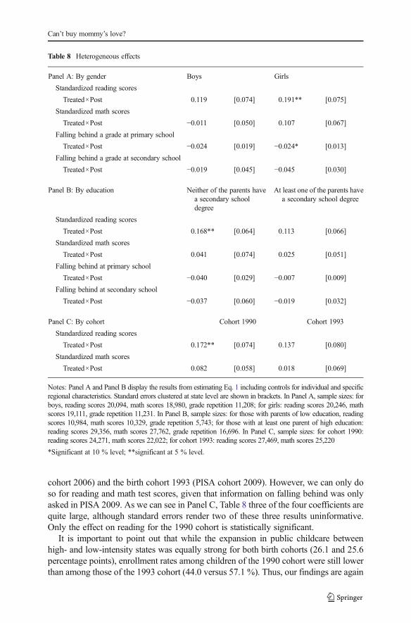
cohort 2006) and the birth cohort 1993 (PISA cohort 2009). However, we can only doso for reading and math test scores, given that information on falling behind was onlyasked in PISA 2009. As we can see in Panel C, Table 8 three of the four coefficients arequite large, although standard errors render two of these three results uninformative.Only the effect on reading for the 1990 cohort is statistically significant.

It is important to point out that while the expansion in public childcare betweenhigh- and low-intensity states was equally strong for both birth cohorts (26.1 and 25.6percentage points), enrollment rates among children of the 1990 cohort were still lowerthan among those of the 1993 cohort (44.0 versus 57.1 %). Thus, our findings are again

Table 8 Heterogeneous effects

Panel A: By gender Boys Girls


Treated×Post 0.119 [0.074] 0.191** [0.075]


Treated×Post −0.011 [0.050] 0.107 [0.067]


Treated×Post −0.024 [0.019] −0.024* [0.013]


Treated×Post −0.019 [0.045] −0.045 [0.030]

Panel B: By education Neither of the parents havea secondary schooldegree

At least one of the parents havea secondary school degree


Treated×Post 0.168** [0.064] 0.113 [0.066]


Treated×Post 0.041 [0.074] 0.025 [0.051]

Falling behind at primary school

Treated×Post −0.040 [0.029] −0.007 [0.009]

Falling behind at secondary school

Treated×Post −0.037 [0.060] −0.019 [0.032]

Panel C: By cohort Cohort 1990 Cohort 1993


Treated×Post 0.172** [0.074] 0.137 [0.080]


Treated×Post 0.082 [0.058] 0.018 [0.069]

Notes: Panel A and Panel B display the results from estimating Eq. 1 including controls for individual and specificregional characteristics. Standard errors clustered at state level are shown in brackets. In Panel A, sample sizes: forboys, reading scores 20,094, math scores 18,980, grade repetition 11,208; for girls: reading scores 20,246, mathscores 19,111, grade repetition 11,231. In Panel B, sample sizes: for those with parents of low education, readingscores 10,984, math scores 10,329, grade repetition 5,743; for those with at least one parent of high education:reading scores 29,356, math scores 27,762, grade repetition 16,696. In Panel C, sample sizes: for cohort 1990:reading scores 24,271, math scores 22,022; for cohort 1993: reading scores 27,469, math scores 25,220

*Significant at 10 % level; **significant at 5 % level.


in line with the previous findings indicating differential effects of public childcaredepending on the level of supply (Felfe and Lalive 2012).

To conclude, it remains to say that although the results seem to be driven by theearlier cohort, girls and children from a lower socio-economic background, differencesbetween the respective subgroups are not statistically significant.

8 Conclusions

There is fervent current political debate concerning the extent to which the Governmentmust provide sufficient, affordable childcare. For instance, on June 6, 2012 the GermanGovernment approved a bill to give parents of toddlers an allowance for keeping theirchildren out of state-run day care, instead of investing in the expansion of childcare centers(New York Times 2012). At the same time, in countries hard hit by the Great Recession,such as Spain, many governments are rolling back subsidized childcare (New York Times2012). A major concern among opponents of public childcare is its high costs for a non-mandatory service for which the short- and long-term gains on the children’s developmentrelative to other forms of early childcare (such as parental, informal, or private care)remain uncertain. Indeed, there is still limited consensus in the literature about the effect ofchildcare on child development, partly as the effects of universalizing childcare depend onthe quality of both public childcare and the counterfactual care mode.

This paper contributes to closing this gap in the literature by providingquasi-experimental evidence of the impact of shifting hours of care providedby mothers to hours of care provided by high-quality public preschools. Wefind that high-quality public childcare not only neutralizes potentially negativeeffects of maternal employment but even has positive effects on children’scognitive development, at least among children with less educated parents andfor girls. Hence, these early childhood investments might well pay off them-selves in the long run.

One crucial feature of the childcare expansion under study, however, is the guaranteeof maintaining high-quality care. In the absence of quality regulations, a rapid expan-sion of universal care might well have negative consequences on children’s develop-ment. Hence, sending children to public childcare might indeed be one way to “buymommy’s love”, albeit only if the quality of care provided in the childcare centersmeets that provided by the mother.

Acknowledgments We would like to thank the editor, Erdal Tekin, and three anonymous referees for helpfulcomments that greatly improved the paper. The authors are also grateful to Manuel Bagues, Paul Devereux, SusanDinarsky, Maria Fitzpatrick, Libertad González, Lídia Farré, Michael Lechner, Oskar Nordström Skans, BjörnÖckert, Xavi Ramos, Antonio Cabrales, Ismael Sanz Labrador, Uta Schönberg, Anna Sjögren, Anna Vignoles,ConnyWunsch, Natalia Zinovyeva, as well as participants from the V INSIDE-MOVE, NORFACE, and CReAMWorkshop onMigration andLabor Economics, the IIIWorkshop onEconomics of Education “ImprovingQuality inEducation,” the CESifo Area Conference on the Economics of Education, the RES Annual Meeting, the SOLEAnnual Meeting, the ESPE Annual Meeting the EALE Annual Meeting as well as seminars at DIW, IFAU,University College Dublin, Ludwigs-Maximilians Universität, and University of St Gallen. The authors also wouldlike to thank the Spanish InstitutoNacional de Evaluación Educativa (INEE) delMinisterio de Educación, Cultura yDeporte for facilitating access to the geo-codes for PISA 2000 and Brindusa Anghel from FEDEA for her supportwith the Spanish Labor Force Survey.

C. Felfe et al.

Tab

leA.1

Literature

overview

Existingcare

Privateform

alcare/targeted

care

Inform

alcare

Maternalcare

Publiccare

reform

Short-run

Long-run

Short-run

Long-run

Short-run

Long-run

Withoutexplicit

quality

regulatio

nsBaker

etal.(2008):

Deteriorationof

health,and

motor

andsocialskills—

Québec,Canada

Cascio(2009):Reductio

nin

high

school

dropout

andinstitu

tionalization

(onlyforwhites)—US

Fitzpatrick(2008):

Improvem

entof

reading

andmathscores

(only

fordisadvantaged

children)—Georgia,U

S

Berlin

skietal.(2008):

Improvem

entin

school

completion—

Uruguay

Berlin

skietal.(2009):

Improvem

entof

reading,

mathandbehavior—

Argentina

With

explicitquality

regulatio

nsHavnesandMogstad

(2011):Im

provem

ent

inschool

completion

andearnings—

Norway

DattaGuptaandSimonsen

(2010):Neutralresults—

Denmark

FelfeandLalive(2012):

Improvem

entof

language,

socialandmotor

skills

(heterogeneity

across

child

ren)—Germany

Drangeetal.

(2012):No

effects—

Norway

Notes:Fu

rtherstudiesinvestigatingtheim

pactof

publicchild

care

onchildren’sshort-runoutcom

esareGormleyandGayer

(2005),L

oebetal.(2007),andMagnusonetal.(2007).

How

ever,thesestudiesdo

notclarifywhich

type

ofcare

theintroductio

nof

publiccare

issubstituted

for.In

addition,

thisliteraturecomplem

entssubstantialexperimentalor

quasi-

experimentalresearch

ontheeffectsof

childhood

educationalprogramstargeted

explicitlyatdisadvantagedchild

ren(for

anoverview

please

referto

BlauandCurrie(2006))

App

endix


Table A.3 Difference-in-difference estimates for regional features

Baseline specification

Unemployment rate 0.011

[0.011]

GDP per capita 509.552*

[275.751]

Women employment rate −0.027[0.017]

College graduate 0.002

[0.005]

HS dropouts 0.022***

[0.007]

Years of education −0.127***[0.036]

Population 0–6 −4.402[20.313]

Immigrants −0.01[0.008]

Notes: Standard errors clustered at state level are shown in brackets. Results from estimating Eq. 1 using as theLHS variable those in Fig. 3 and controlling for state and year fixed effects. Sample size, 300

HS high school

*Significant at 10 % level; ***significant at 1 % level

Table A.2 Sensitivity analysis of covariates included

Unconditional + Regionalcharacteristics

+ Individualcharacteristics

+ Familycharacteristics

+ Typeof school

(1) (2) (3) (4) (5)

Standardized reading score

Treat×Post 0.149** 0.122** 0.154** 0.118* 0.119*

[0.067] [0.047] [0.067] [0.065] [0.066]


Treat×Post 0.053 0.056 0.049 0.017 0.025

[0.047] [0.065] [0.052] [0.036] [0.038]


Treat×Post −0.027* −0.007 −0.024* −0.023* −0.029**

[0.014] [0.016] [0.013] [0.012] [0.013]


Treat×Post −0.032 −0.068** −0.032 −0.026 −0.034

[0.036] [0.031] [0.035] [0.034] [0.036]

Notes: Above results are estimated using Eq. 1 and including as additional control variables (2) the GDP percapita, the proportion of HS dropouts and the average years of education by state for the years when the cohortsassessed in each PISAwave were 3 years old, that is, 1987, 1990, 1993, and 1996—these three variables are thosefor which we could not reject the tests of parallel trends between the treated and comparison states (see AppendixTable A.3); (3) individual characteristics: male, immigrants; (4) family characteristics: home possession score (anindex derived from students’ responses to the following items: Do you have: a desk for study, a room of your own,a computer, internet, classic literature, books, works of art, dishwasher, among others), mother’s and father’seducation; (5) type of school: public-omitted, private. Standard errors clustered at state level are shown in brackets

*Significant at 10 % level; **significant at 5 % level

C. Felfe et al.

References

Adserà A (2004) Changing fertility rates in developed countries. The impact of labor market institutions. JPopul Econ 17(1):17–43

Amuedo-Dorantes C, de la Rica S (2009) The timing of work and work-family conflicts in Spain: who has asplit work schedule and why? IZA discussion paper 4542

Baker M, Milligan K (2011) Maternity leave and children’s cognitive and behavioral development. NBERworking paper 17105.

Baker M, Gruber J, Milligan K (2008) Universal child care, maternal labor supply, and family well-being. JPolit Econ 116(4):709–745

Bauchmüller R, Gørtz M, Würtz-Rasmussen A (2014) Long-run benefits from universal high-qualitypreschooling. Early Child Res Q 29(4):457–470.

Berlinski S, Galiani S (2007) The effect of a large expansion in pre-primary school facilities on preschoolattendance and maternal employment. Labour Econ 14(3):665–680

Berlinski S, Galiani S, Manacorda M (2008) Giving children a better start: preschool attendance and school-age profiles. J Public Econ 92(5):1416–1440

Berlinski S, Galiani S, Gertler P (2009) The effect of pre-primary education on primary school performance. JPublic Econ 93(1–2):219–234

Bettinger E, Haegeland T, Rege M (2013) Home with mom: the effects of stay-at-home parents on children’slong-run educational outcomes. CESifo working papers 4274

Bettio F, Villa P (1998) A Mediterranean perspective on the breakdown of the relationship betweenparticipation and fertility. Cambridge J Econ 22(2):137–171

Black S, Devereux P, Loken K, Salvanes K (2012) Care or cash? The effect of child care subsidies on studentperformance. NBER working paper 18086

BlauD, Currie J (2006) Preschool, day care, and after school care: who'sminding the kids? In: Hanushek E,WelshF (eds) Handbook of economics of education vol 2. Amsterdam, North Holland Press, pp. 1163–278

Carneiro P, Løken K, Salvanes K (2011) A flying start? Maternity leave benefits and long run outcomes ofchildren. IZA discussion paper 5793

Cascio E (2009) Do investments in universal early education pay off? Long-term effects of introducing intopublic schools. NBER working paper 14951

Datta Gupta N, Simonsen M (2010) Non-cognitive child outcomes and universal high quality child care. JPublic Econ 94(1–2):30–42

Drange N, Havnes T, Sandsør A (2012) Kindergarten for all: long run effects of a universal intervention. StatNorway DP 695

Duflo E (2001) Schooling and labor market consequences of school construction in Indonesia: evidence froman unusual policy experiment. Am Econ Rev 91(4):795–813

Dustmann C, Schöenberg U (2012) Expansions in maternity leave coverage on children long-term outcomes.Am Econ J Appl Econ 4(3):190–224

Economist. Does subsidized preschool pay-off? 13 February 2013Economist, Fighting over the kinder. 17 August 2013El País, La LOGSE, 15 años después (by Elena Martín Ortega). 3 October 2005Felfe C, Lalive R (2012) Early child care and child development: for whom it works and why. IZA Discussion

Papers 7100.Felgueroso F, Gutiérrez M, Jimenez S (2014) Why school dropout remained so high in the last two decades?

The role of the educational law (LOGSE). IZA J Labor Policy 3:9, 9 May 2014Fernández-Kranz D, Rodríguez-Planas N (2011) The part-time penalty in a segmented labor market. Labour

Econ 18(5):591–606Fitzpatrick M (2008) Starting school at four: the effect of universal pre-kindergarten on children’s academic

achievement. BE J Econ Anal Poli 8(1):1–38Gathmann C, Saß B (2012) Taxing childcare: effects on family labor supply and children. IZA discussion

paper 6640Gormley W Jr, Gayer T (2005) Promoting school readiness in Oklahoma. An evaluation of Tulsa’s pre-k

program. J Hum Resour 3:533–558Gutierrez-Domenech M (2005) Employment transitions after motherhood in Spain. Labour 19:123–148Havnes T, Mogstad M (2011) No child left behind: subsidized child care and children’s long-run outcomes.

Am Econ J Econ Policy 3:97–129Lenneberg, E (1964) The capacity of language acquisition. In: J Fodor and J Katz (eds) The structure of

language. Englewood Cliffs, NJ: Prentice Hall, pp 579–603


Liu Q, Oskar S (2010) The duration of paid parental leave and children’s scholastic performance. BE J EconAnal Poli 10(1):1935–1682

Loeb S, Bridges M, Bassok D, Fuller B, Rumberger R (2007) How much is too much? The influence ofpreschool centers on children’s social and cognitive development. Econ Educ Rev 26:52–66

LOGSE, Ley Orgánica 1, 1990 de Ordenación General del Sistema Educativo, 03.10.2013, BOE No. 238,28927–28942

Magnuson K, Ruhm C, Waldfogel J (2007) Does prekindergarten improve school preparation and perfor-mance? Econ Educ Rev 26(1):33–51

Montessori M (1963) The secret of childhood. Ballentine Books, New YorkNew York Times. German Lawmakers Spar Over Child Care Subsidy, by Melissa Eddy. 6 Jun 2012Nollenberger N, Rodríguez-Planas, N (2011) Child care, maternal employment and persistence: a natural

experiment from Spain. IZA discussion paper 5888OECD (2006). PISA 2006 science competencies for tomorrow’s worldRasmussen A (2010) Increasing the length of parents’ birth-related leave: the effect on children’s long-term

educational outcomes. Labour Econ 17(1):91–100

C. Felfe et al.

Can’t Buy Mommy’s Love? Universal Childcare and Children’s Long-Term Cognitive Development

Documents

Transcript of Can’t Buy Mommy’s Love? Universal Childcare and Children’s Long-Term Cognitive Development