canada's grain handling and transportation system - CiteSeerX

CANADA’S GRAIN HANDLING AND TRANSPORTATION SYSTEM:

A GIS-BASED EVALUATION OF POLICY CHANGES

A Thesis Submitted to the College of Graduate Studies and Research

In Partial Fulfillment of the Requirements For the Degree of Masters of Science

In the Department of Bioresource Policy, Business, & Economics

University of Saskatchewan Saskatoon

By

Savannah W. Gleim

Copyright Savannah W. Gleim, October, 2014. All rights reserved

i

PERMISSION TO USE

In presenting this thesis in partial fulfillment of the requirements for a Postgraduate degree from the

University of Saskatchewan, I agree that the Libraries of this University may make it freely available for

inspection. I further agree that permission for copying of this thesis in any manner, in whole or in part,

for scholarly purposes may be granted by the professor or professors who supervised my thesis work or,

in their absence, by the Head of the Department or the Dean of the College in which my thesis work was

done. It is understood that any copying or publication or use of this thesis or parts thereof for financial

gain shall not be allowed without my written permission. It is also understood that due recognition shall

be given to me and to the University of Saskatchewan in any scholarly use which may be made of any

material in my thesis.

Requests for permission to copy or to make other uses of materials in this thesis in whole or part should

be addressed to:

Head of the Department of Bioresource Policy, Business & Economics

University of Saskatchewan

Saskatoon, Saskatchewan, S7N 5A8

ii

ABSTRACT

Gleim, Savannah W. M.Sc. University of Saskatchewan, Saskatoon, October 2014. Canada’s Grain

Handling and Transportation System: A GIS-based Evaluation of Policy Changes.

Supervisors James F. Nolan,

Committee Members: Richard A. Schoney and William A. Kerr.

Keywords: grain handling, logistics, optimization, transportation problem, GIS, and VRP

Western Canada is in a post Canadian Wheat Board single-desk market, in which grain handlers face

policy, allocation, and logistical changes to the transportation of grains. This research looks at the rails

transportation problem for allocating wheat from Prairie to port position, offering a new allocation

system that fits the evolving environment of Western Canada’s grain market. Optimization and analysis

of the transport of wheat by railroads is performed using geographic information system software as

well as spatial and historical data. The studied transportation problem searches to minimize the costs of

time rather than look purely at locational costs or closest proximity to port. Through optimization three

major bottlenecks are found to constrain the transportation problem; 1) an allocation preference

towards Thunder Bay and Vancouver ports, 2) small capacity train inefficiency, and 3) a mismatched

distribution of supply and demand between the Class 1 railway firms. Through analysis of counterfactual

policies and a scaled sensitivity analysis of the transportation problem, the grains transport system of

railroads is found to be dynamic and time efficient; specifically when utilizing larger train capacities,

offering open access to rail, and under times of increased availability of supplies. Even under the current

circumstances of reduced grain movement and inefficiencies, there are policies and logistics that can be

implemented to offer grain handlers in Western Canada with the transportation needed to fulfill their

export demands.

iii

ACKNOWLEDGEMENTS

Looking back at my time spent in this program, I have many thanks to give to those who have provided

me with support and inspiration, pushed me to challenge myself, and patiently listened to me, thank you!

Thanks to AFBI for providing me with a scholarship to pursue the opportunities of the master’s program.

I cannot extend enough thanks and gratitude to my supervisor, Dr. James Nolan. Not only has James

offered guidance and support, he has kindly shared his interest in transportation and logistics with me,

which has sparked an interest to pursue a future in transportation and spatial analysis. To my committee

members Dr. Richard Schoney and Dr. William Kerr, many thanks are owed to these two individuals for

their patience, time, and advice. Finally thanks to my external Mr. Ed Knopf, Senior Policy Advisor from

the Saskatchewan Ministry of Highways and Infrastructure.

I would like to thank the Department of Bioresource Policy, Business and Economics (BPBE), the members

of this department that have become an extended family and given me many fond memories. To my BPBE

peers, classmates, faculty and staff, it has been a pleasure to meet you all and gain new friends and

memories. A special thanks must be given to the ladies of the office who have been of great help and

support throughout this process, thank you Heather Baerg, Barb Burton, Melissa Zink, Deborah Rousson,

and Lori Hagan.

Of all those in the industry who I have reached out to for help and information, thank you! One person of

boundless help has been Anh Phan, Chief Statistician of the Canadian Grain Commission, thank you Anh.

To my family, thank you for the continuous love and support. Thanks to my parents, sister and extended

family for being my cheering squad and for showing me that my goals were achievable and worth

reaching. To my friends, like my family, you have supported me, listened to me gripe, and offered an

outlet to momentarily forget the stresses of grad life, thank you.

I am grateful to my loving boyfriend Warren, throughout this process I have turned on you in times on

frustration and in time of success. I cannot express enough gratitude for your love, support and friendship.

Finally, I would like to dedicate this work to two women who have shown me the importance of following

your passions and the strength needed to succeed – my grandmothers’ Edith Gleim and Ida Scandrett.

iv

TABLE OF CONTENTS

Permission to Use .................................................................................................................................................. i

Abstract ................................................................................................................................................................. ii

Acknowledgements ............................................................................................................................................. iii

Table of Contents ................................................................................................................................................. iv

List of Tables ....................................................................................................................................................... vii

List of Figures ..................................................................................................................................................... viii

List of Charts ...................................................................................................................................................... viii

Important Abbreviations ..................................................................................................................................... ix

Chapter 1 Introduction ......................................................................................................................................... 1

1.0 Introduction .............................................................................................................................................. 1

1.1 Problem Statement .................................................................................................................................. 2

1.2 Objectives ................................................................................................................................................. 2

1.3 Problem Characteristics ........................................................................................................................... 3

1.4 Outline of Thesis ....................................................................................................................................... 5

Chapter 2 Western Canadian Grain Logistics ........................................................................................................ 6

2.0 Introduction .............................................................................................................................................. 6

2.1 Grain Logistics in Western Canada ........................................................................................................... 6

2.1.1 Grain on the Prairies ............................................................................................................................ 6

2.1.2 CWB ...................................................................................................................................................... 8

2.1.2.1 History .......................................................................................................................................... 8

2.1.2.2 CWB Operations......................................................................................................................... 10

2.1.2.3 CWB Payments ........................................................................................................................... 10

2.1.2.4 CWB 2.0 ..................................................................................................................................... 11

2.1.3 Railways and Elevation ....................................................................................................................... 11

2.1.3.1 Rail Transportation .................................................................................................................... 12

2.1.3.2 Trains vs. Trucks ......................................................................................................................... 12

2.1.3.3 Regulation and Freight Rates ..................................................................................................... 14

2.1.3.4 Grain Companies ........................................................................................................................ 15

2.1.4 Exports ............................................................................................................................................... 17

2.1.4.1 Ports ........................................................................................................................................... 17

2.1.4.2 FAF and Grain Allocation under the CWB .................................................................................. 18

2.1.4.3 CWB Export Basis Costs ............................................................................................................. 21

2.1.4.3.1 Demurrage Costs ............................................................................................................... 23

2.2 Logistics .................................................................................................................................................. 25

2.2.1 Organization ....................................................................................................................................... 26

2.2.1.1 Inventory Logistics - Just in time ................................................................................................ 27

2.2.1.2 Transportation Logistics ............................................................................................................. 28

2.2.2 Transportation Problem ..................................................................................................................... 29

2.2.2.1 Linear Programming Problem .................................................................................................... 30

2.2.2.2 General Transportation Problem ............................................................................................... 30

v

2.2.2.2.1 Combinatorial Optimization .............................................................................................. 31

2.3 Summary ................................................................................................................................................ 32

Chapter 3 Solving a Transportation Problem Using Geographic Information Systems ...................................... 34

3.0 Introduction ............................................................................................................................................ 34

3.1 GIS .......................................................................................................................................................... 34

3.1.1 How GIS Works ................................................................................................................................... 36

3.2 ESRI and Network Analyst ...................................................................................................................... 38

3.2.1 Network Analyst ................................................................................................................................. 38

3.2.2 Vehicle Routing Problem .................................................................................................................... 39

3.2.2.1 VRP Layer ................................................................................................................................... 39

3.2.2.1.1 VRP Classes ........................................................................................................................ 40

3.2.2.1.1.1 Orders .......................................................................................................................... 40

3.2.2.1.1.2 Depots .......................................................................................................................... 41

3.2.2.1.1.3 Routes .......................................................................................................................... 41

3.2.2.1.1.4 Route Zones ................................................................................................................. 42

3.2.2.1.1.5 Outputs ........................................................................................................................ 43

3.2.2.1.2 VRP Parameters ................................................................................................................. 43

3.2.2.2 VRP Solver .................................................................................................................................. 45

3.2.2.2.1 VRP Algorithm ................................................................................................................... 45

3.2.2.2.1.1 Capacitated Vehicle Routing Problem (CVRP) .............................................................. 46

3.2.2.2.1.2 Dijkstra ......................................................................................................................... 47

3.2.2.2.1.3 Tabu Search .................................................................................................................. 49

3.2.2.2.2 VRP Objective Function ..................................................................................................... 52

3.3 Summary ................................................................................................................................................ 52

Chapter 4 Optimized Export Grain Logistics for Western Canada – Base Case .................................................. 53

4.0 Introduction ............................................................................................................................................ 53

4.1 Model Overview ..................................................................................................................................... 53

4.1.1 Crop Years 2009/10 and 2010/11 ...................................................................................................... 54

4.1.2 Model Constraints .............................................................................................................................. 54

4.1.2.1 Orders and Supplies ................................................................................................................... 55

4.1.2.2 Depots and Demands ................................................................................................................. 56

4.1.2.3 Network Datasets ...................................................................................................................... 57

4.1.3 Assumptions ....................................................................................................................................... 59

4.2 Model Application - August 2009 to July 2011 ....................................................................................... 67

4.2.1 Spatial Allocations .............................................................................................................................. 68

4.2.2 Port Route Performance .................................................................................................................... 69

4.2.3 Critical Time Periods........................................................................................................................... 71

4.2.3.1 West Dominant .......................................................................................................................... 72

4.2.3.2 East Dominant ............................................................................................................................ 73

4.2.3.3 Underperforming Ports .............................................................................................................. 74

4.2.3.4 Optimal Port Performance ......................................................................................................... 75

4.3 Summary ................................................................................................................................................ 77

vi

Chapter 5 Alternative Model Scenarios .............................................................................................................. 78

5.0 Introduction ............................................................................................................................................ 78

5.1 Counterfactual Scenarios ....................................................................................................................... 78

5.1.1 Counterfactual Analysis ..................................................................................................................... 80

5.1.1.1 Optimizing Route Transport Times ............................................................................................ 80

5.1.1.2 Supply meeting Export Demands ............................................................................................... 84

5.1.1.2.1 Monthly Delivery ............................................................................................................... 85

5.1.1.2.2 Deliveries by Port............................................................................................................... 86

5.1.1.3 Utilizing Potential of Routes ...................................................................................................... 89

5.1.1.4 Freight rate costs incurred ......................................................................................................... 94

5.1.2 Counterfactual Conclusions ............................................................................................................... 95

5.2 Hypothetical Optimization Scenarios ..................................................................................................... 96

5.2.1 Open Access Railway .......................................................................................................................... 97

5.2.1.1 Open Access Inputs .................................................................................................................... 98

5.2.1.2 Open Access Results .................................................................................................................. 99

5.2.2 Sensitivity Analysis ........................................................................................................................... 101

5.2.2.1 High Volume Parameterization ................................................................................................ 102

5.2.2.2 High Volumes on Open Access Rail (HVOA) ............................................................................. 103

5.2.2.3 Basic High Volume Results ....................................................................................................... 103

5.3 Summary .............................................................................................................................................. 107

Chapter 6 Summary and Conclusions ............................................................................................................... 109

6.0 Introduction .......................................................................................................................................... 109

6.1 Summary of Results .............................................................................................................................. 110

6.2 Western Canadian Outlook .................................................................................................................. 111

6.3 Potential Improvements ....................................................................................................................... 113

6.4 Future Studies and Applications ........................................................................................................... 114

References ........................................................................................................................................................ 117

APPENDIX .......................................................................................................................................................... 128

A-1 Computer Code .................................................................................................................................... 128

A-2 Dijkstra and Tabu Search Process Explained ........................................................................................ 129

A-2.1 VAM .................................................................................................................................................. 129

A-2.2 MODI ................................................................................................................................................ 131

A-2.3 Unbalanced TP ................................................................................................................................. 133

A-3 2009/11 Base Model Deliveries ........................................................................................................... 139

A-4 Critical Time Period Maps .................................................................................................................... 140

A-5 Scenario Maps ...................................................................................................................................... 142

A-6 Results of Scenarios .............................................................................................................................. 143

A-7 Hypothetical Scenario Maps................................................................................................................. 144

A-7.1 Open Access Maps ........................................................................................................................... 144

A-7.2 Sensitivity Analysis Maps ................................................................................................................. 145

vii

LIST OF TABLES

Table 1 Range of Fuel Efficiency (tonne-km/gallon) ........................................................................................... 13

Table 2 Changes in FCR allocation with varying FAF ........................................................................................... 20

Table 3 Unconstrained labelled vertices ............................................................................................................. 48

Table 4 Constrained labelled vertices ................................................................................................................. 49

Table 5 Tender contract distribution .................................................................................................................. 63

Table 6 Distribution of Modular Train capacities ............................................................................................... 63

Table 7 Reallocation of 900 CN car demand by Vancouver in August 2009 into full capacity routes ................ 64

Table 8 Overall route durations .......................................................................................................................... 81

Table 9 Average distance traveled by routes (km) ............................................................................................. 82

Table 10 Average travelled time by routes used (hours) .................................................................................... 83

Table 11 Average time (minutes) between single car pick-ups a ........................................................................ 83

Table 12 Model demand deliveries routed ......................................................................................................... 85

Table 13 Route deliverance performance of total demands .............................................................................. 85

Table 14 Delivery performances of port demands ............................................................................................. 87

Table 15 Routes not used, by month and model (% of total demanded) routes) .............................................. 90

Table 16 Route capacity utilization by simulated policy and month .................................................................. 92

Table 17 Average freight rate charged per tonne transported, without FAF ..................................................... 95

Table 18 Total demands met by open access policy ........................................................................................... 99

Table 19 Efficiency to utilize route capacities ................................................................................................... 100

Table 20 May 2010 overall performances ........................................................................................................ 104

Table 21 Average freight rate per delivered tonne .......................................................................................... 107

Table 22 Simple Dijkstra code ........................................................................................................................... 128

Table 23 Tabu Search Code ............................................................................................................................... 128

Table 24 Cost Matrix ......................................................................................................................................... 130

Table 25 VAM penalties .................................................................................................................................... 131

Table 26 VAM first allocation ............................................................................................................................ 131

Table 27 VAM solution ...................................................................................................................................... 131

Table 28 MODI allocations cij = ui +vj ................................................................................................................ 132

Table 29 MODI cij – ( ui +vj ) ............................................................................................................................... 133

Table 30 MODI solution .................................................................................................................................... 133

Table 31 Unbalanced VAM initial solution using neighbours ........................................................................... 134

Table 32 First allocation of unbalanced VAM ................................................................................................... 135

Table 33 Unbalanced VAM Solution ................................................................................................................. 135

Table 34 MODI process of unbalanced VAM .................................................................................................... 136

Table 35 Final iteration solution ....................................................................................................................... 137

Table 36 Model demand deliveries, by Class 1 railway providers .................................................................... 143

Table 37 Utilization of used route capacities .................................................................................................... 143

viii

LIST OF FIGURES

Figure 1 GIS Data Layers ..................................................................................................................................... 37

Figure 2 Dijkstra unconstrained example ........................................................................................................... 48

Figure 3 Dijkstra constrained example ............................................................................................................... 49

Figure 4 Tabu Search Visual ................................................................................................................................ 50

Figure 5 Model Classes and Scale ....................................................................................................................... 55

Figure 6 Simulated Closest Delivery Points to Port............................................................................................. 68

Figure 7 February 2011 ..................................................................................................................................... 140

Figure 8 June 2011 ............................................................................................................................................ 140

Figure 9 September 2009 .................................................................................................................................. 141

Figure 10 May 2010 .......................................................................................................................................... 141

Figure 11 May 2010 catchment managed policy routes .................................................................................. 142

Figure 12 May 2010 larger train policy routes .................................................................................................. 142

Figure 13 Open access rail for the base model, OAB, May 2010 ...................................................................... 144

Figure 14 Open access for larger trains, OALT, May 2010 ................................................................................ 144

Figure 15 Open access for larger trains, OALT, September 2009 ..................................................................... 145

Figure 16 High volume on the base model, HVB, May 2010 ............................................................................ 145

Figure 17 High volume on open access rail of base model, HVOAB, May 2010 ............................................... 146

Figure 18 High volume on open access rail using larger trains, HVOALT, May 2010 ........................................ 146

LIST OF CHARTS

Chart 1 Car Deliveries to Port ............................................................................................................................. 70

Chart 2 West Coast Allocations ......................................................................................................................... 139

Chart 3 East Coast Allocations .......................................................................................................................... 139

file:///C:/Users/Savannah/Desktop/Thesis%20Chapters/Thesis_Oct14_Defense%20Draft.docx%23_Toc399999322

file:///C:/Users/Savannah/Desktop/Thesis%20Chapters/Thesis_Oct14_Defense%20Draft.docx%23_Toc399999325

ix

IMPORTANT ABBREVIATIONS

FIRST MENTIONED:

B

BFS: Basic Feasible Solution, 31

C

CGC: Canadian Grain Commission, 14

CH: Churchill, 16

CN: Canadian National Railway, 11

CP: Canadian Pacific Railway, 11

CTA: Canadian Transportation Act, 14

CVRP: Capacitated Vehicle Routing Problem, 39

CWB: Canadian Wheat Board, 1

CWRS: Canadian Western Red Spring Wheat, 21

D

DBLUNCT: Double Unlimited Customized Model, 105

F

FAF: Freight Adjustment Factor, 3

FCR: Freight Consideration Rate, 18

FOB: Free on Board, 4

G

GIS: Geographic Information System, 2

H

HVB: High volumes of base model, 102

HVLR: high volumes of larger trains policy, 102

HVOA: High volume using Open Access rail policy, 103

HVOAB: High volume and open access policy of base

model, 103

HVOALT: High volume using open access and larger trains

policies, 103

J

JIT: Just in Time, 27

L

LP: Linear Programming, 30

LT: Larger trains policy, 79

M

MMT: Million Metric Tonnes, 1

N

NA: Network Analyst, 38

NTA: National Transportation Act, 14

O

OAB: Open access policy of base model, 98

OALT: Open access and larger trains policy, 98

OD: Origin-Destination, 38

ORNL: Oak Ridge National Labratories, 58

P

PR: Prince Rupert, 16

T

TB: Thunder Bay, 16

TP: Transportation Problem, 29

TS: Tabu Search, 45

TSP: Traveling Salesman Problem, 31

V

VAM: Vogel's Approximation Method, 31

VC: Vancouver, 16

VRP: Vehicle Routing Problem, 4

W

WGTA: Western Grain Transportation Act, 14

1

Chapter 1

INTRODUCTION

1.0 Introduction While rooted in the history of this country, the transportation of Prairie wheat from grain elevators

across Western Canada continues to be an issue of contention for agriculture. Recent changes in the

sector have only deepened this concern. As of August, 2012 the Canadian Wheat Board (CWB), formerly

the primary marketer for Canadian wheat, barley and durum since 1935, was stripped of this

responsibility. Effectively, the CWB had its mandate to market so-called “board” grains removed,

transferring the logistics of moving Canadian grain to multiple grain handling firms (Veeman and

Veeman 2006). Since Western Canada is a significant producer of export grain, its grain handling system

continues to rely on good grain logistics to move landlocked grain to ocean port in order to meet export

demands. Now that the CWB no longer controls the allocation and marketing of these grains, it is

expected that significant changes will occur within the future logistics and allocation system for

Western Canadian grain.

Up until the Federal government’s decision to remove the marketing function of the CWB, it was the

largest marketer of wheat and barley in the world (Canadian Wheat Board 2011b). Marketing grain to

over 70 countries meant that the CWB had a major role in the Canadian grain sector. For example, In

the 2011/12 crop year the CWB exported approximately 21.3 million metric tonnes (MMT of grain,

representing approximately 60% of Western Canada’s grain exports (Canadian Grain Commission

2012c). Of those exports, wheat was the largest export grain, with 15.4 MMT moved across Western

Canada. With the policy change, the export of Canadian grain will necessitate an updated and possibly

quite different logistics system. The very enormity of the grain sector means that this transition will not

likely be smooth. In effect, Canada’s private grain companies will now be greatly increasing the volume

of grain over which they have responsibility for transportation, while at the same time working on

honing their logistics systems to move these grains.

As Western Canada’s grain handlers absorb the remaining 60% of Western grains, their individual and

collective transportation problems will grow. Novel logistics and transportation solutions will need to

be found by each of them in order to move primary export grains over the three Prairie provinces, using

the two national railways to connect to four major ports for export (Vancouver, Prince Rupert, Thunder

Bay, and Churchill). Unlike the collectivist goals of the CWB, the grain transportation solution that will

2

be found shifts focus away from producers’ overall benefit over to the profitability of the individual

grain handling firms. It is not well understood how this change in the Canadian grain logistics system

will affect overall grain allocations and movement, or participant revenues and costs. To this end, a

spatially based analysis has been developed in this thesis to literally map out the evolution of the

agricultural transportation issue in Western Canada. This analysis will help to determine how changes in

grain transportation, particularly for wheat, will affect system participants. Finally, the analysis will also

help to evaluate the relative benefits of potential alternative grain allocation and logistics systems.

1.1 Problem Statement This thesis will develop a GIS model to evaluate the relative efficiency of transportation systems for

Western Canadian grain. One primary contribution is that the model will also allow us to simulate the

new grain handling logistics environment whereby multiple grain companies have the responsibility to

transport grain. The current situation will also be briefly contrasted with the previous grain handling

system, whereby a single state trading enterprise (the CWB) controlled allocation and the logistics of

Western Canadian grain exports. The research will address the following questions in varying levels of

detail:

I. What effect does an alternative grain logistics system and costing mechanism (i.e. time of

transport vs. distance moved) have on the grain supply chain and grain movement?

II. How will a potential new logistics system differ from the previous CWB system?

III. What will be the challenges and difficulties of implementing the new logistics system?

1.2 Objectives The focus and objective of this research is to examine alternative grain logistics systems (in lieu of the

CWB) that will satisfy projected export demands. Compared to the grain allocation system used by the

CWB, the actual grain transportation problem is now more heavily constrained because of multiple

players trying to optimize transportation allocations within the system. This analysis of the problem will

be developed using Geographic Information System (GIS) software, using industry data and the

software programmed to optimize large scale grain transportation allocations. In turn, the model will

also help to identify other potential problems in the new system, including potential mismatch of

supply and demand, or the continued presence of various cost based inefficiencies. The results of the

analysis will be monthly optimized allocations for grain transportation by multiple grain shippers, with

3

solutions generated by minimizing the system wide cost of transport time in allocating diffuse grain

supplies to meet varying export demands.

1.3 Problem Characteristics To begin this research, it is necessary to understand how grain logistics were conducted under the

CWB. In fact, the formal logistics algorithm used by the CWB is still proprietary and not readily

accessible beyond a few broad descriptions by consultants and academics. One major distinction worth

highlighting is that the CWB allocations were based on minimizing system transportation costs in the

form of rail rates paid by each farmer. As a collectivist solution imposed by a monopolist, their

optimization objectives stand in contrast with the new operational environment for grain movement.

Due to this, the model is designed to more closely align with the optimization problem of individual

grain firms as they seek to maximize profit in the new grain transportation system. In this light, the

model instead optimizes the time (as an opportunity cost) spent moving grain within the system.

The description of CWB logistics draws upon the limited literature outlining the process at a restricted

level of detail. The overview focus will be a description and explanation of the so-called Freight

Adjustment Factor (FAF) used by the CWB, which acted as a basis (i.e. local price) adjustment designed

to remove any inherent locational advantages for grain producers. As a result, FAF directly affected the

flow of export grain and also the transportation costs borne by producers. Understanding basic

elements of CWB logistics like FAF will help to understand the changes that will likely occur with the use

of alternative post-CWB grain allocation systems based on modern logistics metrics and methods.

The CWB was created by the Federal Government as a means to maximize returns to grain producers

through single-desk marketing of grain purchases, sales, and exports (Schmitz and Furtan 2000). In 1995,

the CWB updated its grain logistics system to better reflect the value of grain at each grain delivery

location using FAF. As a cost adjustment mechanism, the system wide FAF was generated to reflect not

only the cost of transportation (in particular) to the St. Lawrence Seaway, but also the flow of grain

trade in a given year, as well as export capacity constraints (Gray 1996). Thus, the CWB’s grain allocation

system through FAF was designed to minimize collective costs of freight for all producers by removing

any inherent locational advantages of certain producers, particularly those located along the boundary

of a catchment region.1 Since the CWB had complete logistical control over Western Canadian board

1 The CWB divided Prairie producers into West and East catchments which were created by the lesser cost of FAF plus freight to Thunder Bay or the rate to Vancouver.

4

grains, the CWB also had the power to allocate grain movement as it saw fit using FAF, which minimized

collective freight rates for producers and reduced the costs incurred to pooled grains.

With the removal of CWB single-desk marketing power, some have argued that grain handlers will have

to shift their focus towards reducing risks in grain flows rather than on overall freight costs (Wilson,

Carlson and Dahl 2004). Under the CWB, Free on Board (FOB) contracts were used for which grain

handlers were responsible for the costs to transport grain to the vessel, while grain producers then

covered the cost of transportation to port (Wilson, Dahl and Carlson, Logistical Strategies And Risks In

Canadian Grain Marketing 2000). Thus for CWB logistics, their objective was to reduce the overall cost of

grain transportation while meeting the demands of each port, so as to benefit the producer collective.

Critically, their cost minimization did not account for late fees or demurrage incurred if time parameters

of both railway and ocean vessel contracts were not met.

To further motivate this research, a description of the basic transportation problem in logistics and

operations research is necessary. Knowledge of both demand and supply of the product being

transported are fundamental to solving the transportation problem. The data to solve the problem

must contain the supplies at various origins, the volume supplied and the timing of deliveries, while the

volumes demanded at each port (destination) are also needed. It is these demands and supplies which

support the final optimized allocation, along with space availability on transport routes, costs and

timing.

In contrast to the optimization method used by the CWB for grain allocation, the transportation

problem for grain movement in this new era of multiple competing grain marketers is best examined

using spatial analysis. The scale of the Canadian grain transportation problem is enormous, spanning

four provinces with numerous delivery points (elevators) and a few distant port locations. GIS software

can be programmed to solve as well as illustrate these complex spatial transportation solutions. In this

thesis, ArcGIS software is programmed to implement a vehicle routing problem (VRP) toolkit that

identifies the least costly (based on time) set of grain transportation routes that allocate (monthly)

wheat supplies from across the Prairie elevator system to meet particular (monthly) export demands at

each port.

In a competitive grain transportation market, grain handlers incur both the benefits and costs associated

with delivering grain to port destination within a particular time frame. For instance, if a grain handler

can deliver grain to port before a set date, they receive what is known as a dispatch payment. However,

5

if grain is not delivered within the time frame of the contract, a demurrage fee (on FOB contracts) is

charged to the grain handling firm (Wilson, Carlson and Dahl 2004). In order to get a better sense of the

importance of delivery reliability, for the 2009/10 crop year, grain handling firms netted $6.0M in

dispatch, whereas in contrast for 2010/11, they incurred a net of $40.6M in demurrage fees (Quorum

Corportation 2011). It is for these reasons that the movement of grain across the Prairies in the post

CWB era will need to focus on reducing the risks of incurring additional delivery costs and maintaining

reliability, rather than simply focusing on reducing the collective producer costs of grain transportation.

Since the profit maximizing grain handling firm’s objective is to get grain to the right port at the right

time (Ballou 1992), for this research, the GIS toolkit, vehicle routing problem (VRP), will be used to

generate a solution that minimizes the cost of travel time, rather than distance or freight rates. The use

of the VRP in this regard also offers an opportunity to examine the effects of varying inputs, including

demand, supply, routings, and catchments. Solving for system grain allocations relevant to the new era

in Canadian grain transportation using the VRP also allows some comparisons to be made between

these solutions against the former CWB FAF system allocations. Given the system transportation

problems that have arisen this year (2014), these comparisons promise to be both interesting and

relevant to future policy in the sector.

1.4 Outline of Thesis This thesis consists of six chapters. The first provides a broad overview of the research, while the

remaining chapters summarize and examine the issues described in Chapter 1. To start, Chapter 2 gives

a broad literature review of grain logistics for Western Canadian board grains, as well as describing the

grain logistics problem. Chapter 3 explains the use of GIS in this research, along with describing its

capabilities using programmed toolkits such as ArcGIS’s Network Analyst, and more specifically, the

implementation of the Vehicle Routing Problem (VRP) for grain transportation. The methods and data

needed to construct a new and modern grain logistics model are explored in Chapter 4, and model

results will be generated, reviewed, assessed, and compared to determine grain allocations and the

effects on the overall the grain supply chain. Subsequently, four alternative policy scenarios will be

simulated and examined in Chapter 5 in search of gain of efficiencies and optimization. These scenarios

will build upon the base model results and also help to clarify certain ambiguities within the base model.

Finally, Chapter 6 contains an overview discussion of the thesis and brings the research to a conclusion.

6

Chapter 2

WESTERN CANADIAN GRAIN LOGISTICS

2.0 Introduction Like all supply chains, grain handing requires supporting logistics to help organize the flow of material

from production to consumer. In this context, logistics is defined as the “organization and

implementation of a complex operation” (Oxford Dictionary of English 2010). This section will examine

the logistics process that serves the industry from the Prairie elevator to the exporting vessel,

highlighting how each component of the supply chain works together to move grain one step closer to

the end consumer. To start, it will be necessary to clarify the scope of modern logistics and how supply

chains are created using logistics. Within this thesis, logistics will refer to the allocation, delivery, and

timing of so-called board grains, meaning it will also be necessary to briefly examine both the

construction and solutions to transportation and related problems in the logistics and operations

research literature.

2.1 Grain Logistics in Western Canada In Western Canada, the collection and delivery of grains for export has always been important to

farmers livelihood and in fact this market helped in the process of settling the Prairie provinces.

Historically, it has been the cost efficient allocation of grain that has determined when and to which port

Western Canadian grain flows, and subsequently, the freight rate (or transportation cost) that is borne

by the farmer. To this end, we next examine historical grain logistics in Western Canada in order to

motivate some of the changes that are likely to occur under a modern grain allocation system.

2.1.1 Grain on the Prairies

The grain handling process in Canada, although complex and involving multiple handlers, is still

fundamentally a relatively simple supply chain. Farmers grow their grain, and in most cases, move their

grain to a proximate grain elevator. At the elevator, it is blended, cleaned and stored until it can be

loaded onto railcars and moved to port for export. Considering the distances between Canadian port

facilities and Prairie elevators, railways are still by far the least expensive means of transporting grains

over land at these distances, especially when compared to trucking grains to port (Park and Koo 2001).

Once at port, the grain is moved to the appropriate ocean vessel and loaded. Ultimately, the ocean

vessel delivers to a grain importer at a foreign port, and from there it moves to the next (often final)

location for import. This delivery cycle occurs all year round, so the system experiences fluctuations in

7

volumes based on availability and the particular type of grain being demanded. As described, the

process does not seem particularly complex, yet it can be difficult to generate optimized solutions all the

time. This is due to a number of dynamic factors, including the time component and transaction cost

involved in shuttling the grain through the supply chain. The organization of these movements takes

time and cooperation to maintain and sustain grain movement from the landlocked Prairies to the

exporting port facilities.

Canada’s grain producers are centered in the Prairies: Alberta, Saskatchewan and Manitoba, and the

Peace River area of British Columbia. The Canadian Census of Agriculture in 2011 reported the three

Prairie provinces and BC represented 136.6M acres of farm land, representing 85% of Canadian farm

acres (Statistics Canada 2012). With the majority of farmland coming from Western Canada, Canada is

dependent on western grain production to supply both domestic and international markets. For

instance in the 2011/12 crop year, total deliveries of grains from Western Canada equalled 33.5 MMT:

of which 15 MMT was wheat, 9 MMT canola, 5.5 MMT durum, with the remaining deliveries being

barley, oats, peas, corn, flax, and rye (Canadian Grain Commission 2013). Western Canada’s grain

production is far greater than domestic demand, so producers rely on grain companies to help move

these grains for export.

Elevators in Western Canada are facilities that essentially store and/or blend grain before it is moved to

port. Prairie elevators normally receive grain directly for storage and/or forwarding to another facility,

with some facilities also processing or transferring grain after inspection (Canadian Grain Commission

2009). In 2012, there were 395 elevators across Western Canada, with a total capacity of 8.0 MMT.2

These facilities are, for the most part are owned by large agricultural corporations such as Viterra,

Richardson Pioneer, Paterson Grain, Cargill Limited, and Parrish and Heimbecker (P&H) (Canadian Grain

Commission 2009). In addition to storage, a grain elevator offers cleaning, grain grading, and railcar

loading services that are of great convenience for the producer. Elevators also offer contracts for selling

grain. Depending on the grain, elevators are able to offer their own contracts or those of other

institutions, including the CWB. These contracts pull in grain to elevators for export at specific times in

order to fill exports and other demands in a timely manner. With respect to handling grain cars, in

Western Canada the length of railway siding owned by many small and medium elevators is inadequate

to hold larger unit grain trains (which obtain lower rates) so many elevators are limited as to how many

2 In 2002, CGC reported 425 elevator facilities over the four western provinces with a capacity of 5.3 MMT. Facility numbers have declined by 7%, while capacity has grown by 51%.

8

railcars they can load. Thus, in a profit driven grain handling system, the siding capacity of a given

elevator also influences the logistics and movement of grain within the system.

2.1.2 CWB

Historically, the Canadian Wheat Board served as a broker between elevators and importers for wheat,

durum and barley. Since 1935, the CWB has played a significant role for Western Canadian grain

producers as a public agency offering marketing and exporting services for wheat, durum, and barley. In

fact, the CWB was designated by the Canadian Government to be the single-desk seller of board grains

domestically and internationally (Schmitz and Furtan 2000). Since its inception, producers have both

supported and resisted the services offered by the CWB. On one side, the single-desk power for Western

Canadian grain marketing offered producers the ability to produce their crops without the worries of

marketing their product internationally. The CWB developed an international quality reputation that

was an asset to board grain producers, since traditionally it meant a higher premium for their grain.

Aside from these operating advantages of a single-desk, the CWB also used so-called “pools” in order to

better benefit producers as a collective.3 Pooling and single-desk power, however, generated

controversy among many producers. Fundamentally, these functions meant that as a producer of board

grains, an individual farmer had no say as to who sold their crop or the value received for it. Many

Western Canadian producers felt that the CWB, as a mandatory marketer, was in fact a legalized price

discriminator, allowing eastern producers the right to sell their own grain while Western producers

faced the pooled rate of the CWB (Resource News International 2006). In August of 2012, producers

were finally given the choice to make a voluntarily decision as to the marketing and exporting of grains.

In the new era, they can opt to stick with the CWB (as a grain company) or instead rely upon grain

companies and their supply chains in the newly competitive grain market.

2.1.2.1 History

The CWB was formed before WWI as a centralized grain selling agency for Canada under the name

Board of Grain Supervisors (McCalla and Schmitz 1979). The CWB offered an initial payment and price-

pooling basis for the 1919/20 crop year, when world grain markets were still uncertain due to the

aftermath of the war. Initially, this situation was supposed to last just one year, as the government at

3 A pool is the collection of revenues from sales across a region, western Canada, for a specific grain over a set period of time. These pools than pay out an average of the total revenues minus pool operation costs over total grain tonnes delivered. Producers than receive a pool payment based on the volume of tonnes they delivered in that time frame (Alberta Government 2007).

9

that time did not wish to be in the grain business (McCalla and Schmitz 1979). However by 1929,

western grain producers relied upon large grain handling cooperatives that were created in each

province. Eventually, these cooperative grain pools together established the so-called Central Selling

Agency. The Agency offered initial payments that were higher than actual grain prices in order to ensure

the Agency had grain for marketing. This strategy, however, put the Agency at risk for bankruptcy, and

provincial governments stepped in as guarantors. In 1930, the federal government became the sole

backer of loans and operations. In fact, the federal government kept trying to pull away from investing

in grain operations, but political pressure from the farming community kept them involved in the second

iteration of the voluntary CWB (Schmitz and Furtan 2000).

In 1935, the Canadian Wheat Board Act was passed by legislation, making it a Crown Corporation. This

Act gave the CWB monopoly power over specific grain marketing. The Act also ensured the federal

government would back any loans made by the CWB, as well as offering the Board a favourable interest

rate for those loans (Parkinson 2007). In 1943 (during WWII), enrolment in the CWB became mandatory

for Prairie wheat producers, giving the CWB monopoly power for marketing Prairie wheat. The CWB was

endowed with similar powers over barley and oats as well in 1949 (Schmitz and Furtan 2000).

In 1967, the CWB Act’s five-year renewal clause was amended, removing the evaluation process of the

federal government’s involvement with the CWB and grain handling. This meant the CWB was now a

permanent crown corporation with single-desk selling rights over all board grains in Western Canada

(Parkinson 2007). This also implied there would be no future opportunity for private grain companies to

gain marketing and selling powers for the export of western grain. The amendment affected

competition for grain handling services across the Prairies.

In 1997 another amendment was passed through the CWB Act. This ended its status as a Crown

Corporation and moved it over to a shared governance structure. A Board of Directors was created

representing both the public and the government. The Directors consisted of ten farmer-elected

members from the ten CWB districts, four members appointed by the order of council, while the final

member was appointed by the Minister for the Canadian Wheat Board as the CEO (Schmitz and Furtan

2000). This structure was intended to allow farmers a major voice and role in the operations of grain

handling and marketing of their product.

As a single-desk marketing entity, the CWB, in fact, did not retain any physical assets (like elevators) to

the corporations’ name other than grain hopper cars. Even though the CWB retained considerable

10

market power in the grain handling system, it still wanted competitors to play a role in the grain

handling process, including cleaning and storage facilities, rail transportation, and port terminal

operations. In effect, the CWB relied on the logistics and cooperation of private agricultural and

transportation companies in order to market and export the grains that they oversaw.

2.1.2.2 CWB Operations

Until August 2012, all board grains grown in Western Canada were sold by the CWB both domestically

and internationally. This monopoly-monopsony system was effectively a single-desk seller to market

Canadian board grain (Clark 2005). The position of the CWB always raised questions about quality and

pricing of grain. Through their mandated marketing power, the CWB did gain a strong reputation for

quality and high standards for their grains. On the pricing side, without competition from grain handling

firms for board grains, the price of board grains was not heavily influenced by market forces.

2.1.2.3 CWB Payments

Under the CWB’s single-desk operation, grains were pooled and their profits were equally distributed

from pool accounts to producers. The objective of pooling grains was to provide producers an average

market value of that crop for a given year (Alberta Government 2007). This pool pricing began with an

initial payment to a producer for the delivery of their grain based on the quality and quantity of the

grain. The initial payment was fixed throughout the year for each of the four pool accounts: wheat,

durum, feed barley, and designated barley (Schmitz and Furtan 2000). An initial payment was set prior

to the beginning of the crop year and was below the expected price of the grain. By setting the payment

low, if grain prices fell, producers had a safeguard with respect to the lower price. If board prices fell

below the initial payment, the federal government acted as a guarantor to ensure CWB prices remained

where they were (Parkinson 2007). Initial payments were often set between 70 and 75 percent of the

estimated pool return, or the total pooled payments expected from sales. The final value collected by

producers was the initial payment plus any surplus in the pool, minus the freight rate and costs of

cleaning and grain handling by elevators (Schmitz and Furtan 2000).

During the crop year, the CWB continued to buy grain in order to fill domestic and international sale

demands. Sales were met through the collection of delivery contracts and calls to producers, which were

promises that producers would deliver grain to meet a set quantity, quality, and delivery timing of sales

(Clark 2005). At the end of a crop year, the sales were pooled for each grain account and costs of

operation, marketing and expenses such as storage, insurance, and interest deducted (Schmitz and

Furtan 2000). Schmitz and Furtan highlight that the remaining pooled money was divided among

11

producers as a final payout, while the payment was made based on the quantity producers sold in

contracts that crop year.

2.1.2.4 CWB 2.0

In 2011, the Minister of Agriculture and Agri-Food and the Canadian Wheat Board announced that the

CWB’s single-desk marketing power would be rescinded as of August 1, 2012 (Government of Canada

2014). The removal of single-desk selling power left the CWB to make operational changes and opened

Prairie grain handling to a competitive market. Now producers could voluntary choose to conduct

business with the CWB or any other grain handling firm for the sale and marketing of their grains. With

the loss of sole marketing power over board grains, the current CWB expanded their offered contracts

to include canola, which was not a former board grain (Canadian Wheat Board 2013).

Now that former board grains are marketed competitively, the CWB has had to make changes to its

contracts to stay competitive. These changes include offering early delivery pools, futures choices pools,

annual pools, winter pools, as well as cash contracts. Although the CWB does not currently have

elevator capacity of their own, they offer CWB contracts through their competitors and locally owned

elevators. Under CWB contracts, producers are allowed to choose which grain handling facility they will

deliver to after purchasing the contract, based on the recommendations and information given to the

producer by the CWB. In this light, CWB 2.0 offers producers a wider variety of choices for managing

risk. The new system has forced the CWB to offer contracts which will fundamentally alter grain logistics

as compared to the prior single desk logistics system. With multiple grain handlers and contracts offered

for the former board grains, the collection of grain has become more complicated, as has the gathering

of relevant information.

2.1.3 Railways and Elevation

Railways transport the majority of grain from Canada’s landlocked Prairies to sea-port facilities. Serving

Western Canada are two national Class 1 railway firms: Canadian National Railway (CN) and Canadian

Pacific Railway (CP). Smaller privately owned short line firms also contribute to the transportation of

grains by moving grain on to the large railway networks. As of 2012, respectively 164 and 203 elevator

facilities were reported along the CN and CP lines in Western Canada (Canadian Grain Commission

2012b).4 Over time, the number of private elevators and short line railways have declined across the

Prairies. While elevator numbers have fallen precipitously over the years, their importance and necessity

4 These facilities include primary, processing, and terminal elevators.

12

in transporting grain to port has not diminished. Growing export demands could simply not be met

without the network of elevators to collect and tranship grain to export position.

2.1.3.1 Rail Transportation

Railways have always been an integral part of the lifestyle of Canadians from settlement to globalization.

Canada’s railway industry played an important role in the movement of immigrants and the

development of farming in Western Canada. In 1881, CP was founded as a railway intended to link

Eastern Canada to the West Coast, and in fact it accomplished this by 1885 (Canadian Pacific 2012). To

ensure future markets for itself, CP promoted land settlement in Western Canada. Since the inception of

CP, it had grown to play a central role in the Western Canadian lifestyle. Today, CP covers 23,600 km of

railway tracks and operates across six provinces and 13 US states.

Through the early part of the 20th century, CN emerged as a government operated railway having been

created out of a number of other railways facing bankruptcy. Like CP, CN took the role of promoting

Western Canadian living and settlement of the west. Today CN operates over 32,200 km of track in

North America. In Western Canada, CN runs approximately 13,500 km of track, running from the Pacific

Ocean, across the mountains, to Diamond, Manitoba,5 in addition offering exclusive access to the port of

Prince Rupert, BC while partnering with Hudson Bay Railway (HBRY) for access to the port of Churchill,

MB (Canadian National Railway Company 2013). Together the two national railways have and will

continue to play a very important role in the Western Canadian economy, moving bulk commodities

such as grain.

Today, there are a few privately or cooperatively owned short line railways that provide services for

Prairie delivery points located away from the tracks of the Class 1 railways. In fact, these railways are in

direct competition with the trucking industry since they often operate over shorter distances than a

trunk railway. Trucking can offer similarly priced services over these reduced distances. In 2011 that

Western Canada had 14 registered short line providers (Railway Association of Canada 2011). Many of

these short lines rely on partnerships with the Class 1 railways to provide services to and from the trunk

lines, servicing more remote locations far from CN and CP lines.

2.1.3.2 Trains vs. Trucks

In Western Canada, due to the vast distances from grain elevators to ports, railways are often the lowest

cost means of transportation for Prairie grains. Sometimes, however, a farmer can opt to truck grain to a

5 CN’s rail line extends from Diamond, MB (12 km West of Winnipeg) to Thunder Bay in its Eastern region.

13

delivery point in order to gain from rates that may be more favorable. However, trucking has a relatively

high cost structure compared to a short line railway, if the latter is available. While trains can move

multiple railcars full of grain at a time, trucks are often limited to pulling just one to three trailers. For

instance, for grain transported within Saskatchewan, the maximum weight a B train double trailer can

transport at one time is 62.5 tonnes, whereas just a single covered hopper car can hold as much as 90

tonnes of wheat (Council of Ministers of Transportation and Highway Safety 2011). With rail, more grain

can be moved at one time, thus saving costs of multiple drivers, fuel, and time needed for trucking. By

comparison, 1994 estimates of the average operating costs for a 14.80 ton truckload were 8.42₵ (USD)

per ton-mile, whereas a train pulling 100 cars of 105 tons each over 1000 miles cost an average of 1.19₵

(Forkenbrock 2001). Over longer hauls, railways can exploit their large economies of scale to reduce

operational costs whereas trucking does not possess this same cost structure.

In fact, railways offer the most cost-efficient long-distance transportation today, other than moving

goods over water. Railways also offer farmers the ability to reduce their proportion of operational costs

while trucking effectively forces all operational costs onto fewer (often just one) producers. One major

operational input which helps increase the cost of movement is fuel, so that the more fuel efficient the

mode of transportation, the lower the operating costs borne by the producer.

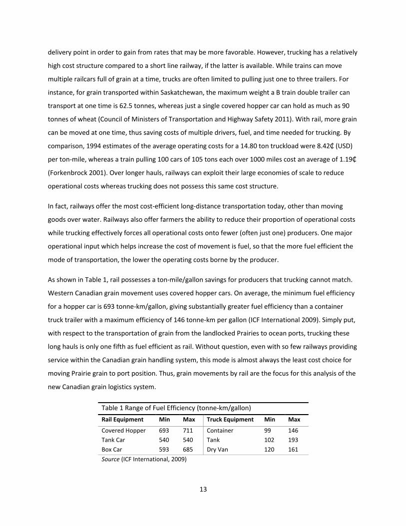
As shown in Table 1, rail possesses a ton-mile/gallon savings for producers that trucking cannot match.

Western Canadian grain movement uses covered hopper cars. On average, the minimum fuel efficiency

for a hopper car is 693 tonne-km/gallon, giving substantially greater fuel efficiency than a container

truck trailer with a maximum efficiency of 146 tonne-km per gallon (ICF International 2009). Simply put,

with respect to the transportation of grain from the landlocked Prairies to ocean ports, trucking these

long hauls is only one fifth as fuel efficient as rail. Without question, even with so few railways providing

service within the Canadian grain handling system, this mode is almost always the least cost choice for

moving Prairie grain to port position. Thus, grain movements by rail are the focus for this analysis of the

new Canadian grain logistics system.

Table 1 Range of Fuel Efficiency (tonne-km/gallon)

Rail Equipment Min Max Truck Equipment Min Max

Covered Hopper 693 711 Container 99 146

Tank Car 540 540 Tank 102 193

Box Car 593 685 Dry Van 120 161

Source (ICF International, 2009)

14

2.1.3.3 Regulation and Freight Rates

For 2011, the Canadian Grain Commission (CGC) reported a total of 305,363 loaded railcars, carrying 13

different types of grain from Prairie elevators to port terminals. The two major crops moved were wheat

and canola, representing 42.5% and 32.4% of grain cars, moving 12.1 MMT and 7.8 MMT to ports

respectively (Canadian Grain Commission 2012b). Since there are only two major railways serving the

system and they play such an important role in the movement and allocation of Prairie grain, regulation

still exists to oversee grain transportation. Regulation and the subsequent freight rates set by the

railways affect the movement and flow of grain across Western Canada.

Canada’s Federal Government has been involved in the transportation of grains for over a century. In

1897, the Canadian Government put in place a grain transportation regulation known as the Crow’s Nest

Pass Agreement (Klein and Kerr 1996). This agreement on regulated transportation prices, later called

the Crow Rate, locked in wheat transportation rates in order to maintain exports at an affordable rate

for farmers. With the expansion of CP through the Crows Nest Pass from the Prairies into the mining

areas of southern British Columbia, the Crow Rate eventually expanded to include other grains and the

other major railway, CN. Over time, it was found that these rates covered an ever smaller amount of the

actual railway costs to move grain.

After years of dispute in the sector and the virtual deregulation of all other Canadian transportation

sectors, in 1984 the Western Grain Transportation Act (WGTA) was introduced to regulate freight rates

for farmers and railways in a fashion that was referred to as ‘fair’. The WGTA did not remove the fixed

crow rates but provided subsidies to compensate the railway’s budgetary shortfalls associated with

moving grain under the so-called Crow Benefit (Vercammen, Fulton and Gray 1996). The Federal

Government’s implementation of this system set the freight rate on a cost recovery basis. An appointed

board distributed the increased cost of rail transportation amongst Western Canadian grain producers

and railways. Effectively, this program subsidized about half of the producers’ freight rate, while setting

rates to cover variable and some fixed costs of the railways. By 1990, the Crow Benefit program had

distorted Western Canada’s agricultural economy through the subsidy of 70% of board grain movement,

costing approximately $720M (Doan, Paddock and Dyer 2003).

On August 1, 1995, the WGTA was dissolved and was replaced by the National Transportation Act (NTA)

(Doan, Paddock and Dyer 2003). With the removal of WGTA, the NTA set rates so that grain producers

would pay actual rail cost. However, this change immediately doubled the cost of railway transportation

for farmers. The shock to producers eventually drove the implementation of a freight rate cap policy,

15

based on distance from port. This policy also restricted rate increases to the rate of inflation (Fulton, et

al. 1998). The freight rate caps set a maximum rate that could be charged but the actual rate could fall

under the cap, and the cap was applied to all crops.

The most recent regulatory change occurred in 2000 after a major service problem that precipitated a

set of hearings on the state of the grain transportation system, a process known as the Estey Review.

From this and at the request of one of the major railways, the Canadian Government changed the

regulatory regime from the rate cap to a revenue cap on grain movements (Estey 1998). The revenue

cap allows the Canadian Class 1 railways to freely set rates for western grain while ensuring that total

yearly revenues from grain movement fall under a calculated cap or ceiling. The maximum revenue

ceiling is set yearly by the Canadian Transportation Agency (CTA), and depends, among other factors, on

an inflationary adjustment factor and the average length of grain haul in a given year.

After considerably controversy on both sides over rates and service under the rate cap regime, the

revenue cap was designed to lower average grain rates while giving the railways some pricing flexibility.

Starting with the 2000/01 crop year, rates were set on average at 18% less (roughly $6 per tonne) than

they would have been under the rate cap regime (Canadian Pacific 2008). The revenue cap offers

railways the opportunity to set rates based on a number of cost factors, including origin, type of grain,

and the volume transported (Schmitz, Furtan and Baylis 2002). At year end, if total earnings from grain

movements for a railway are greater than the pre-set cap, the railways pay a fine based on the excess

revenue earned (Park and Koo 2001). While the intent of the revenue cap is to protect grain shippers by

restricting the market power of the railways, some shippers feel the railways have circumvented the

spirit of the cap in several ways. This includes the gradual shifting of some transport related costs to

grain companies, as well as the creation of new service charges that fall outside the cap regime but

effectively raise the transacted rate for moving grain (Library of Parliment 2007).

2.1.3.4 Grain Companies

Western Canada’s grain companies are the brokers within the grain export supply chain and are relied

on by both farmers and consumers to collect and market grains. Today, there are five major competitors

in the Prairies. They are Viterra, Richardson Pioneer, Paterson Grain, Cargill, and Parrish & Heimbecker.

During the 2010/11 crop year, Western Canada had 323 licensed primary elevators,6 318 which were

operational. Of these operational elevators, the five major grain firms operated about 75 % of them with

6 Primary elevators principal function is to receive grain from producers for the storage and/or forwarding of grain to a terminal or processing elevator (Canadian Grain Commission, 2010).

16

the others operated by small independent companies (Canadian Grain Commission 2010). In total, the

current licensed elevator total capacity at any moment is 5.7 MMT, for which Saskatchewan’s 160

primary elevators make up half of that total, or 2.9 MMT (Canadian Grain Commission 2010).

Considering catchment areas for grain, Saskatchewan producers are the farthest away from the coast

port position, which exports the majority of Prairie grains. However, Saskatchewan has the largest

percentage of total grain production, so Saskatchewan grain producers are heavily reliant on elevator

facilities to store, blend and forward their grains.

Grain handling firms in turn are reliant on railways for transportation. Elevator locations are most often

found directly along a rail track connecting to railway siding, facilitating pickup and drop off of grain

cars. Of the primary elevators operating during the 2010/11 crop year, just 10 facilities were not located

directly on working rail lines. The elevators on rail lines are divided amongst the Class 1 railways and

short lines, with 170 serviced by CP, 132 by CN, and 6 receiving initial service by a short line before

handing loads off to a Class 1 railway (Canadian Grain Commission 2010).

The final handling before grain is loaded onto a vessel at port is done at a port terminal elevator. During

the 2010/11 crop year, Western Canadian grains were handled by 15 terminals between the ports of

Vancouver (VC), Prince Rupert (PR), Churchill (CH), and Thunder Bay (TB) (Canadian Grain Commission

2010). The overall grain capacity of these terminals was 2.5 MMT, a point to be further explored in the

next section. Grain moving through Thunder Bay moves though the Great Lakes/St. Lawrence Seaway

and is often unloaded to a so-called transfer elevator, where the previously inspected grain is held until

transferred to an ocean-going vessel for its final export. During the 2010/11 crop year, there were 12

operational transfer elevators in Eastern Canada, with a capacity of just under 2.2 MMT of grain. Since

much of the grain going through Thunder Bay is simply transferred from smaller lakers to larger ocean

going vessels, three of these transfer elevators do not possess any rail connections (capacity of 0.8

MMT). Of the remaining nine elevators, six are located along CN tracks (with a 1.1 MMT capacity), two

along CP tracks (with just under 0.2 MMT of capacity), while the final transfer elevator is located on a

short line and has a capacity of just over 0.1 MMT.

In effect, western grain producers are equally as reliant on grain handlers as they are on railways to

move their grain to export. Now that grain companies are part of the marketing chain of former ‘board’

grains, their services have expanded from simply holding wheat, durum, and barley, to increased

responsibilities for logistics and allocation of grains to export position.

17

2.1.4 Exports

Canada is known for its production of cash crops for export to the world markets. Canada exported 30.3

MMT of grain in the 2011/12 crop year, in which wheat and canola exports equalled 13.8 MMT and 8.7

MMT, totalling 74% of grain exports (Statistics Canada 2013). The majority of those export supplies

came from Canada’s western provinces. In 2011, roughly 87% and 99% of wheat (excluding durum) and

canola production came from Western Canada (Statistics Canada 2014). Western producers rely on grain

exports to remain in the agricultural industry. During 2010 and 2011, oilseed and grain farmers exported

$13.2 and $15.6 billion ($CDN) in sales (Industry Canada 2013). These grain exports move to over 200

countries, which helps to drive and maintain grain production on the Prairies. If international oilseed

and grain demands were to decline, in the short term at least, Western Canadian producers would face

the challenge of lower prices and excess grain production.

2.1.4.1 Ports

Canada has dozens of ports along its vast coastline. Western Canadian grains rely most heavily on the

ports of Vancouver, Prince Rupert, Churchill and Thunder Bay, along with some Eastern ports like

Montreal and Halifax. The largest of these ports by grain handling capacity is Thunder Bay, ON, whose

seven facilities have a grain capacity of 1.2 MMT. These facilities receive grain from both CN and CP rail

(Canadian Grain Commission 2012b). Thunder Bay’s facilities ship grain generally from mid-March

through till January, until it is no longer safe to travel the icy Great Lakes and St. Lawrence Seaway (Port

of Thunder Bay 2014). Vancouver, BC, has six facilities with a total capacity just under 1 MMT, again

accessible by both Class 1 railways. Vancouver and Thunder Bay move grain collected by firms such as

Cargill, Richardson, and Viterra, as well as a handful of other facility operators. Prince Rupert, BC,

currently has only one terminal which holds just over 200,000 MT of grain. Churchill, MB, also has only

one facility, with a capacity of 140,000 tonnes. In addition, Churchill’s facility is operational at the end of

summer for three to four months when the sea ice has been broken and has melted away, allowing

transportation through Hudson Bay and part of the Arctic Ocean. It is worth noting that CN has sole

access to the port facilities of Prince Rupert and Churchill, primarily because CN lines are generally

located across the upper half of Western Canada.

As an export focused economy, Canada’s ports are responsible for handling more than grain. They also

handle forestry products, chemicals, iron and steel, food products, and natural resources (coal, sulphur,

and potash) (Association of Canadian Port Authorities 2013). As a result, ports possess their own

logistics systems for organizing and timing movements in and out of the port and associated facilities.

18

During the 2009/10 crop year, the grain export sector relied upon 823 ships to export grain from

Canadian ports (Quorum Corportation 2011).7 Quorum reports on average, these ships waited three

days before they could move the facility docks for an actual loading. At the docks and berths, these ships

waited on average an additional 3.2 days to complete loading. The port logistics system also stores

grains at terminal facilities, and Canadian grain typically spent 16.2 days at the terminals before being

loaded onto a ship. With respect to this thesis, since ports rely on their own logistics system and are

separate from the land-based grain handling logistics system in Canada, they will not be explicitly

considered in this research.

2.1.4.2 FAF and Grain Allocation under the CWB

The mechanics of the CWB’s grain exports becomes complex when port allocation protocol is examined.

While the CWB had developed various means over time to allocate grain across the Praires, to ensure

port grain demands were met by expected grain production, through the 1990’s the CWB began to

implement a grain allocation mechanism known as the Freight Consideration Rate or FCR. The computed

FCR was the final rate a producer paid to ship grain to port. The FCR paid equalled the lowest rate at

each delivery point for moving grain either east or west. By using FCR, Prairie elevators were effectively

split into two catchment areas, whereby each catchment moved grain to the least costly port from the

perspective of all producers (Gray 1995). Although four ports process export grain in Western Canada,

effectively only two catchments were created: Vancouver (including Prince Rupert) and Thunder Bay.

Not only were catchments set to generate the lowest collective transportation cost, the catchments

were also set so that producers located along the edges of the two catchments were rendered

indifferent about sending their grain east or west. This was designed to remove any incentives on the

part of producers to truck grain across the catchment line in order to receive a lower FCR (Gray 1995).

In 1995, the policy of FCR was introduced by the CWB when their price pooling system was updated,

allowing for an unequal pool distribution between Vancouver and Thunder Bay. Prior to 1995, based on

historical demands around the globe, the two ports were considered to be in an equal position for

export from delivery locations (Gray 1995). Under FCR, upon delivery of grain to an elevator, the

producer would pay the freight rate to the “closest” port regardless of whether the grain would actually

be transported to that port (Parliment of Canada 1995). The CWB recognized that the value for export

grain should be set using the St. Lawrence Seaway (instead of Thunder Bay) and Vancouver, both better

representing whatever final Canadian port handled grain before being exported. In this manner, the

7Grain vessels: 445 Vancouver, 260 Thunder Bay, 100 Prince Rupert, and 18 Churchill (Quorum Corportation 2011).

19

freight rates would need to be set to reflect the cost to transport grains to these final Canadian export

positions. The shift of grain basis pricing from Thunder Bay to the St. Lawrence Seaway meant that grain

moving east possessed higher transportation costs with the inclusion of St. Lawrence Seaway fees

(Tyrchniewicz, et al. 1998). The need to include Seaway fees on east-bound grain (where this charge

now fell within the pooling system) led the way to the development of the FCR system and effectively

set spatially asymmetric catchment areas for Prairie grain transport allocations.

As stated above, the computed FCR was the final rate a producer paid on railway freight, and was the

calculated minimum cost direction for moving grain (east or west) to port position. However, it is worth

noting that FCR was not just the lowest posted freight rate to Vancouver or Thunder Bay within each

catchment, it was actually the minimum posted freight rate between Vancouver and Thunder Bay for a

catchment, plus the Freight Adjustment Factor (FAF). For Western Canada, FAF was only added onto the

Thunder Bay rates in order to help lower the (pooled) higher costs in using the St. Lawrence Seaway

(Tyrchniewicz, et al. 1998). Its inclusion increased the overall transport rate to Thunder Bay, thus shifting

the historical catchment split further east. Unfortunately, this shift resulted in some producers paying a

higher than previously freight rate to move grain east. For example, during the 2010/11 crop year, the

freight rates per tonne from Moose Jaw, SK, to Vancouver and Thunder Bay were $41.93, and $35.42

respectively. Without FAF, Thunder Bay had the lower freight rate for producers. But that year, CWB set

wheat’s FAF at $7.24/tonne, which meant the effective Thunder Bay rate increased to $42.66, rendering

Vancouver the lowest available freight rate for Moose Jaw producers by $0.73 (Canadian Wheat Board

2011a). In this example, with the incorporation of FAF charges Moose Jaw no longer fell within the

Thunder Bay catchment area and was moved over to the Vancouver catchment.

It is also worth noting that one stated objective of FAF was to create a basis deduction system for each

board grain to best reflect the value of grain at each delivery point (Gray, 1995). In effect, the

implementation of FAF allowed the CWB to adjust rates to create two catchments designed to just meet

port grain demands, minimize producers transport cost, and maximize pool accounts. FAF also

accounted for the change in rates from Thunder Bay to the St. Lawrence Seaway, along with deliveries

to Churchill and the USA (Quorum Corportation 2012a).

As mentioned, while the FAF computation is still proprietary, we do know something about other factors

that went into its calculation. For instance, in order to compute FAF, the CWB must have first known

what markets through which it would be moving grain as well as the least costly ports for transporting

grain to each grain customer. Forecasts of output from Prairie delivery points were required in order to

20

determine grain allocations to each port while minimizing overall transportation costs. Essentially, the

CWB attempted to minimize the costs of transportation to each port by allocating the closest delivery

points and volumes to the port that would meet forecasted demands, thus avoiding the cost of cross

hauling between ports (Gray 1996).

In any given year, the use of FAF and FCR by the CWB shifted the division of least cost freight allocation

and also changed the average freight rate paid by producers. Some of the effect of FAF on delivery

allocation is demonstrated in Table 2, where FAF rates are varied to simulate the effects they have on

producers. During the 2010/11 crop year, without FAF rates, 191 of the 311 wheat delivery points would

have identified Thunder Bay as the lowest rail freight rate (Canadian Wheat Board, 2011). In this crop

year, 33.5% of the Thunder Bay catchment border delivery points were reassigned to Vancouver’s

catchment because of the $7.24 FAF rate. In fact, in that year FAF allocated freight costs of over 1.1

million tonnes of wheat to Vancouver rather than Thunder Bay (having a lower posted freight rate

without FAF), a shift representing 10.6% of Canada’s wheat delivered in the western provinces in that

crop year (Canadian Grain Commission 2012a). Ultimately, the use of FAF and the FCR had a profound

impact on wheat freight rates paid by producers as well as the producer pools.

Table 2 Changes in FCR allocation with varying FAF

No FAF FAF = $5 FAF = $5 FAF = $10

Vancouver (VC) 120 162 184 205

Thunder Bay (TB) 191 149 127 106

TB change from Non-FAF (%) -21.99% 33.51% 44.50%

Average FCR Rate $33.70 $36.47 $37.44 $38.50

TB change in FCR from Non-FAF (%) 8.22% 10.10% 12.24%

Source (Canadian Wheat Board, 2011)

What is also known is that FAF was computed using a relatively simple linear programming algorithm

that minimized a system cost function containing items such as freight rates for each delivery point,

level of deliveries, sales by individual port, constrained by grain capacity at each port. The resulting

output (the FAF rate) effectively generated a logistics plan for grain shipments and, in turn, created port

catchment areas (Froystad 2012). Recall that FAF set boundaries of the catchment to create just

indifferent transportation decisions between east and west ports. In effect, FAF was designed to

eliminate location premiums and thus the policy enforced a localized law of one price (Gray 1996).

21

As it developed, the CWB FAF calculation was performed before the start of a given crop year, and in

most cases, the rate remained fixed throughout that crop year (Gray 1995). The CWB use of FAF for

generating transportation catchments required a wealth of knowledge and industry information. In fact,

the CWB often had this available as a result of their marketing mandate. With the removal of the single-

desk mandate, FAF is now truly history and under the current competitive multi-firm handling system, it

would be impossible for any individual grain handler to implement a similar centrally planned grain

allocation system and get it to work as well. Therefore, there exists a need to examine possible logistics

solutions and directions for future grain allocations in a more competitive Canadian market.

2.1.4.3 CWB Export Basis Costs

The movement of grain from diffuse producer bins to port vessels relies on logistics to get the grain to

the appropriate port at the right time and with the correct volume. The costs of this are passed onto the

producer for the export of their grain. Export costs are a result of logistics and include direct costs,

administrative expenses, grain handling fees, and net interest rates (Quorum Corportation 2002).

Expenses incurred from direct costs include elevation and terminal fees, trucking, freight, cleaning,

inspection, and when they operated, CWB costs (CWB hopper cars and demurrage). It is these costs that

affected the net payment a producer received for their grain deliveries. In 1999 under the CWB, on

average Canadian Western Red Spring wheat (CWRS) logistic costs were $54.58/tonne, representing

roughly 38% of the finalized real price, leaving producers an average of $143.25/tonne as payment from

the CWB pool accounts (Quorum Corportation 2012b). Clearly, the greater the costs of logistics, the less

payment a producer receives for their delivered grains. Therefore, grain sellers and producers want an

allocation system that minimizes the cost of logistics.

The CWB allocation system was designed to manage the direct costs incurred by producers through the

use of FCR and FAF rates. An individual FAF rate was assigned to each board grain to reflect the value of

that grain at each individual delivery point, while accounting for changes in transportation costs, supply

and demand, and to reflect other locational advantages (Gray 1996). As previously explained, producers

paid the lesser of either the Thunder Bay freight rate plus FAF or the freight rate to Vancouver, and it is

through this process that the CWB minimized the freight cost to all producers. However, the

minimization of freight rates is conditional with the incorporation of FAF, as FAF does not reflect the

true minimum freight cost for a given location.8 Recall that the freight adjustment factor was used to

8 The freight rates paid by producers are conditional on location and the value of FAF. If FAF is set below the full costs of the seaway, and the rate to Thunder Bay plus FAF is less than the rate to Vancouver, then the producer

22

account for some of the additional costs of grain using the St. Lawrence Seaway, but FAF was not set to

fully cover the costs of the seaway. In other words, even under FAF, the CWB claimed that farmers

whose grain flowed east did not bear the full costs of Seaway transportation and in fact received a

conditional minimum rate (Tyrchniewicz, et al. 1998).

As an example, from 1996, the CWB estimated the cost of using the St. Lawrence Seaway to be roughly

$20 per tonne of grain (Tyrchniewicz, et al. 1998). Assuming this rate had not increased by the 2009/10

crop year, and also that FAF was set to equal to the full $20, it turns out that only 104 of 541 delivery

points in that year would have fallen into the eastern catchment (Canadian Wheat Board 2011a). The

CWB did not set FAF to cover the full Seaway cost, as a freight cost minimizing grain handling system

would not have been able to move enough grain east to meet demands.9 At the same time, the net

payment of an eastern catchment producer would be significantly lower than one located in the western

catchment (Canadian Wheat Board 2011a).

In order for the CWB to cover Seaway costs and not set FAF so high that east-bound grain demands

cannot be met, the remainder of the Seaway costs were subtracted from the pool accounts. By

subtracting the remaining costs of the Seaway in this manner, freight costs are dispersed equally

amongst all pool account deliveries, as a form of cross-subsidy. For example in 1998, wheat FAF was set

to cover $11.55 of Seaway cost, while the remaining $8.45/tonne was subtracted from pool accounts,

reducing net payouts of each delivery by approximately $4.00/ tonne. As a result, the FAF allocation

system helped maintain costs at a manageable level for producers in the eastern catchment, while

dispersing the remaining costs equally amongst producers through the pool account (Tyrchniewicz, et al.

1998). The system helped to minimize costs within the constraints of the model (FAF and port demands)

and dispersed the pool revenues more evenly. In the example, producers who sent their wheat west lost

$4.00/tonne of pool revenues in order to help subsidize the costs of the Seaway. While the producers

who sent their grain east also lost $4.00/tonne, this was $4.45 less than they would have paid for the full

cost of shipping wheat east (Schmitz and Furtan 2000). In sum, the cost minimizing logistics system used

by the CWB was established to help lower the freight costs of eastern catchment grain exporters. By

pays a minimum lower than the total cost to transport grain to an Eastern port. Therefore the minimization is conditional to the rate at which the FAF is set. 9 The FAF for wheat’s 2009/10 crop year was set to $8.12/tonne, this made 224 of the 541 locations have a conditional minimum cost to move grain east.

23

minimizing only across freight costs with the inclusion of FAF, the CWB reduced locational advantages

and dispersed producer returns more evenly across the Prairies.

2.1.4.3.1 Demurrage Costs

Under FAF, the distribution of the remaining St. Lawrence Seaway costs resulted in a cost allocation

solution to benefit the overall producer pool account, and therefore the average benefit for all

producers. With the removal of the CWB single-desk marketing power, this cost allocation designed for

the overall good of a producer pool account is no longer feasible. The core focus in the grain handling

system will now shift from reducing overall freight costs for producers to optimizing handling costs and

profits of the grain handling firms.

The CWB focus for the grain logistics problem was on minimizing producer freight costs rather than CWB

costs. As an example, in the 1996/97 crop year, logistical costs from Saskatoon to export wheat through

Vancouver were estimated to be around $53.11/tonne: $35.37 for freight, $11.89 in elevation and

dockage, and $5.85 for CWB costs (Fulton, et al. 1998). Grain companies do not set railway freight rates

and they do not incur these costs, so minimizing the latter for the allocation of grain is not their primary

objective.

Today, the costs of elevation at a primary elevator are still paid by producers and are profitable to the

grain handler meaning that grain handlers are not concerned with minimizing these costs. This left grain

handlers concerned only with the minimization of the ‘CWB’ costs. These CWB costs were paid by all

producers and comprised of rates for the use of a number of services, including country elevators,

terminal storage, additional freight, drying, CWB railcars, administrative expenses, and net demurrage

fees. In fact, the CWB did not seek to minimize these costs, as they were rates set for the use of other

grain companies’ supply chains (Quorum Corportation 2002). With the transition to a competitive grain

handling market, the ‘CWB costs’ fees which grain handlers can now change are demurrage fees, while

other costs are internal fees to the grain handling firms. Referring to the example for Saskatoon wheat

from 1996/97, logistics fees equal $0.95, while $2.07 accounts for the demurrage and additional freight

fees as part of the listed $5.85/tonne CWB costs (Quorum Corportation 2002). In fact, these latter two

cost sources can be minimized by grain handling logistics to benefit company profits as well as

producers, since they are costs incurred as a result of export contracts not being met.

How can demurrage costs and additional freight fees be minimized, and why was the CWB not explicitly

accounting for these costs in their optimization? These elements are assimilated into overall costs as a

24

result of transportation contract obligations not being met. Demurrage in this situation can be incurred

by a seller for not delivering grain to a port vessel within the time period stipulated in a buyer contract

(Schlecht, Wilson and Dahl 2004) or not meeting the contract return time of a railcar (Canadian Pacific,

2013). In essence, the CWB worked under Free on Board (FOB) contracts where the CWB covered the

logistical costs of transportation until the delivery was made to the port, while grain buyers were

responsible for chartering the vessel to and from port. With an FOB contract, a grain seller tries to

coordinate deliveries to port to meet the vessel in a timely manner, yet has no real control over the ship.

Conversely, if a seller delivers within a set window of time stipulated in the contract, an incentive

payment known as dispatch can be paid to the grain seller (Wilson, Dahl and Carlson, Logistical

Strategies And Risks In Canadian Grain Marketing 2000).

If delivery is not made within the stipulated time, demurrage costs are charged to the seller of grain for

the time period the ship is late for departure. Demurrage is charged to offset the losses incurred by the

vessel itself (sitting in port and not sailing) and for slow loading by the seller. In 2007, daily demurrage

costs for a vessel at the port of Prince Rupert were between $125,000-175,000 (USD), as compared to

between $135,000-180,000 (USD) at ports in Vancouver (Klassen 2007). Of course these various fees and

charges can be a negative or a plus on the ledger. For example, during the 2009/10 crop year, $17.2M

(CDN) was collected in dispatch payments for Western Canada, and this more than offset the $11.2M

collected in demurrage. However in the next crop year, net demurrage fees were $40.6M (Quorum

Corportation 2011). At that time, the CWB paid these demurrage costs as they likely did not want to

reduce the quality and grade of the contracted grain with possibly other grains sourced closer to port.

The new allocation system for grain will likely strive to reduce the costs of demurrage by minimizing the

travel time of grain shipments. This will help ensure that deliveries are made reliably, in order to avoid

demurrage or even to collect dispatch incentives. If a vessel is not loaded within the contracted

timeframe, often congested ports will need scarce berth positions to load other vessels, so ships are

often moved out of port to await their turn again to be loaded. Each time a vessel is re-berthed in this

manner, the incurred cost of re-using the berth and facilities reduces the profits from the grain (Park

and Koo 2001). Demurrage fees are also incurred for use of railway and privately owned cars. Producers

often pay a demurrage fee for each additional day that cars are not released back to the railway or the

owner of the car for the time frame of the contract (Canadian Pacific 2013). If railcar contents are not

accepted at port for some reason, the car and its contents may be held by customs and inspected, which

could lead to a late return of the railcar. There are also instances when cars are not ready for timely pick

25

up, and in this case a grain handler can be charged for car demurrage, again reducing the revenues for

grain. In total, if demurrage fees are incurred by a grain handler or producers, they are unfavourable

costs resulting from untimely or unreliable logistics. To resolve this problem, logistics of travel time and

allocation need to be better optimized to reduce the chance of demurrage.

The reason the CWB could not optimize their logistics system through the minimization of demurrage

costs was a result of their not owning port assets and relying on other firms logistical systems to the

ports, including availability at port berths and for terminal storage. With the shift towards a competitive

market, grain handlers now own assets along the supply chain, and therefore they should be able to

allocate grain to meet time windows much better than did the CWB, who actually had less physical

control within the overall supply chain. Under the CWB, demurrage fees were dispersed equally

amongst deliveries. In contrast, a non-pooling grain allocation system will likely result in some producers

incurring greater demurrage costs. Structurally, the new grain supply chain will generate the need to

shift away from a focus on minimizing freight costs to instead minimizing the chance or risk of

demurrage through the optimization of delivery timing.

2.2 Logistics Logistics are the processes used which join production to consumption through coordination within a

supply chain. A logistical problem requires planning and organization of services/production for a time

and place. Logistics is used to find solutions in operations such as managing products, people, and

information. In the case of managing goods, logistics are used within the production, transportation, and

sales of the goods produced. The implementation of logistics allows for multiple variables to be assessed

within a problem. In turn, these problems can be solved by minimizing or optimizing a desired set of

constraints (Kasilingam 1998). Logistics leads to organization and efficiency, and when proper logistics

are implemented, it should reduce chaos through organization and planning that minimizes waste and

costs to an industry or process.

Many firms rely on logistics to maintain the flow and success of their business or operation. Industries

which regularly use logistics are manufacturing, health care, resource management, and transportation.

Industry logistics may represent a small segment of the supply chain, but over multiple components of

the chain. Often times in logistics, implementation is based on minimum cost, however, it can also be

based on other attributes such as time, safety, or a combination of cost and time (Kasilingam 1998). For

26

this research, a logistics program will be used to optimize grain allocation by minimizing the costs of

travel time for grain to get to port position.

2.2.1 Organization

For a logistics systems to add value, there needs to be supply, demand, and a network to link the two

ends of the transaction to create a market. The organization of a supply chain leads to a coordination of

a logistics system (Sadler 2007). A supply chain can be constructed either upstream or downstream, in

which supplies and demands are needed to anchor the chain. A supply chain also requires a plan of flow

for the commodity or service to move along the chain to the end user. As products and services move

along the supply chain so, too, does information and management.

Supply chains can be complex or simple, and can exist within other supply chains. For this research, the

scope of the grain supply chain examined will be from grain elevators to port terminal position. The

scope of the supply chain examined in this thesis exists within a broader supply chain that can be

mapped back to seed companies and forward to the final foreign consumer of grains. The researched

supply chain begins with grain elevators, a point where producers have already delivered grain for their

specified contracts. These grain contracts act as a flow of information, signaling a need to produce a

particular grain, and also informing the grain contractor where, when, and how much grain will be

available for export. The contract also informs the contractor how many railcars will be required to

transport the needed volume of grain. Logistics have to help move that grain to the appropriate port

within a set timeframe, and help create a grain supply chain. The supply chain emerges as a result of the

implementation of a logistics system which maintains a flow of grain and information, while optimizing

the routes and minimizing costs.

The arrangement and management of logistics is a difficult task to orchestrate, as there are multiple

factors that need to be accounted for simultaneously. The scale of a supply chain and the number of

points along the chain influence the organizational structure and management of its logistics. Supply

chain logistics are often said to be complex due to several factors, including the existence of multiple

suppliers, buyers, inputs, outputs, and locations; also outsourcing, third party distribution, and external

inputs (policies, regulations, trade issues, and market power) (Sadler 2007). The former CWB’s logistics

system was a good example of the management of complexity in order to transport and allocate

enormous volumes of grain from diffuse Prairie locations to distant port facilities for eventual trade.

27

Logistics are not a modern invention and such management systems have been used historically for such

diverse activities as the construction of the pyramids or the organization of tea trade by the British

Empire, and they still play important roles in our daily lives (DHL 2005). The systems used today can be a

novel system created to fit a new problem, but more likely, the logistics are similar to a previous system,

but now adapted and improved to fit the particular problem. Today, globalization has required formal

logistics to be implemented in almost every industry, and as a result many industries use a known

logistics framework and adapt it to fit their needs. Changes made can include fitting the system to their

needs regarding supply, demand, costs, policies, and information (Kasilingam 1998). The logistics

process often occurs unnoticed by the consumer, so below are listed a few different types of logistics

systems that affect life around us.

2.2.1.1 Inventory Logistics - Just in time

Inventory logistics are used in the vendor industrial supply chain, ensuring that appropriate quantities

are available for a stochastic demand environment. Balance between minimizing inventory costs and

maximizing service levels is critical (Kasilingam 1998). Each point along a supply chain requires an

appropriate level of inventory be maintained to sustain the supply chain. In other words, inventory

logistics require a specific balance between the volume and timing of inventory at each point along the

chain. Such a system sets these inventories by accounting for plausible uncertainties such as delivery

delays, change in demands, and damaged goods. An industry accounting for uncertainties to forecast

and ensure that inventory is available where it needs to be, allows the supply chain to function without

interruption or delay.

The grain industry of Western Canada relies on inventory systems to handle, transport, and export

grains. The purpose of an inventory model within grain movement is to maximize service levels while

minimizing total inventory costs (including transportation, handling, and processing). To balance the

level of product along the supply chain and minimize costs, many firms use the so-called ‘just-in-time’

(JIT) model. A JIT model does not require production to occur in proximity to demand, but rather it relies

on physical and information networks to connect the supply chain so as to deliver product at the

approximate time it is demanded (Black 2003a). A JIT system is effectively designed to move a product

to the next point along its supply chain, while the product at the next point in the chain also moves to

the next point along the chain, and so on. This process ensures that no location has more inventory than

it can process at a given time, and ensures goods delivery does not occur until the last portion of

inventory is being processed. When JIT runs smoothly, a firm can reduce its costs of holding inventory

28

and can increase productivity. This system first emerged from the auto manufacturer Toyota, by timing

manufacturing to meet demands of their customers (Özalp, Suvaci and Tonus 2010). This concept may

well prove influential to the Canadian grain supply chain, as the capacity of our ports is fixed, yet the

flow of grain to fill export orders fluctuates significantly over the year.

2.2.1.2 Transportation Logistics

Only infrequently is an entire supply chain located in one place. Globalization has resulted in a growing

dependence on efficient transportation of goods or services between nodes along a supply chain.

Transportation is an essential component of logistics. In transportation logistics, the typical objective of

the firm is to locate the most efficient transport link between supply chain points in order to minimize

‘costs' or maximize profits. Transport links are often chosen to meet lowest total system cost, based on

the mode of transportation and the volume demanded for transport (Kasilingam 1998). Transportation

logistics can cover several modes of transportation, including trucking, rail, ship, air, pipeline or even

personal courier. Within each mode of transportation, there are different types of equipment that may

be used and this may influence the choice of logistical system (Sadler 2007). For each mode of transport,

the logistics system chosen will be constrained by the product or service being transported, policies and

procedures, frequency of use, capacity, and costs. The importance of transportation logistics has grown

with globalization. Goods trade and trade in services are no longer limited by their proximity to

consumers. Globalization has had an influence on the development of transportation networks as

production of numerous goods has been gradually moved to farther away consumers into lower cost

regions that have lower costs (Black 2003d). More so than ever, transportation logistics is a vital

component of a modern supply chain. This aspect of logistics is the focus of this research to analyze the

transportation of Western Canada’s grain exports.

Transportation logistics can be designed to meet different objectives. These include providing improved

safety or offering conveniences to consumers. In many cases, however, reducing product costs at point

of sale is the objective motivating transport logistics. By way of example, in Canada many agricultural

products are not domestically grown and need to be imported from elsewhere, including the United

States. In turn, the price of these products in Canada is affected by the cost of their transportation,

meaning that sellers of these goods will try to minimize transportation costs in order to keep larger

profit margins for themselves. Before consumers can purchase such goods in Canada, they are shipped,

either by rail, boat and ultimately truck from growing regions to supermarkets. Of course, ships and rail

allow a larger quantity of goods to be moved at once from production areas, as opposed to sending

29

goods by truck from these areas. From a cost perspective, the use of a ship or train versus a truck for a

very long haul reduces overall cost, keeping the goods price lower while producers still profit (Black

2003b, ICF International 2009).

The growth of formal transportation logistics not only helps to keep the prices of goods lower, it has also

led to the provision of services that have become increasingly necessary and convenient to our current

lifestyles. These transportation services include waste removal, school bus transportation, dairy tankers,

fresh produce deliveries, fuel transportation, and the system of traffic lights (Black 2003d). Without

these logistical systems, the current lifestyles we live would not be as comfortable, safe or convenient.

Logistics in transportation is influential to the way we live our lives. Without growth and acceptance of

this aspect of transportation, individual communities would need to be much more self-reliant. In the

context of this thesis, this could lead to a situation where Western Canada’s excess production of grains

for export could instead become a problem. The next section will describe the formalization of the basic

transportation analytical problem. This particular formulation is used almost ubiquitously with

modifications to help optimize various modern logistic needs.

2.2.2 Transportation Problem The transportation problem (TP) is a mathematical programming problem which solves to optimally

transport goods or services from n origins to m destinations (Black 2003c). A TP is essentially a logistics

problem that often solves for the optima10 or minimum total cost of system transportation (Kaiser and

Messer 2011). The objective of the program is to transport supplies to meet demands, while minimizing

the cost to perform this transportation. Without the mathematical formalization, this is often a very

complicated and non-intuitive task. For this research, the TP developed and solved is designed to move

grain from diffuse Prairie elevators using various ‘cost’ minimizing rail routes in an attempt to meet port

demands for grain.

Since the research problem here is focused on both the movement of grain between supply chain points

as well as the economic objective of minimizing of costs, the TP is effectively the “logistics” chosen to

solve the problem. Most often, TP’s rely upon linear programming to search for solutions that optimize

costs subject to a set of physical or institutional constraints (Luderer, Nollau and Vetters 2005). A TP can

be solved to identify the minimum costs of transportation, but it can also be used to analyze welfare

10 An optimal solution is the best solution for the feasible solutions of the problem. A feasible solution is a solution that meets all the constraints of a problem (Hillier and Lieberman 1986b). In 2.2.2.2 General Transportation Problem, the criteria of an initial basic feasible solution within a TP is given.

30

aspects for producers or consumers in the market (Foster 1963). The TP performed in this research

generates an economic analysis of grain allocations that minimize system ‘costs’.

2.2.2.1 Linear Programming Problem

The transportation problem is a particular type of linear optimization program (LP), and so the concept

of a mathematical linear program must be clarified. Linear programs are optimization problems that

solve an objective function that is built to represent a set of activities. An LP uses a linear function on

input variables as an objective, with the goal of minimizing or maximizing the objective subject to a set

of linear constraints (Dorfman, Samuelson and Solow 1958). The most basic LP will have m constraints

and n activities to solve for as part of the objective function (which minimizes/maximizes a choice

variable, often called z). For this thesis the objective function is based on equation 1 below, and is solved

to minimize the total (linear) costs of grain transportation. The LP objective is solved subject to m + 1

constraint sets, shown here in the general equation 2 (Kaiser and Messer 2011). The solution to the

objective that falls within all the constraints becomes the optimal solution. Since the TP is a stylized type

of LP problem, this thesis will expand upon the basic LP foundation in order to illustrate how the GIS

software solves the spatial transportation cost problem for grain movement.

nnxcxcxcZ ...Min 2211 1

n

j

jjij bxa1

2

0 where jx

2.2.2.2 General Transportation Problem

Like an LP, the typical TP is a balanced optimization (minimization) problem characterized by a set of

variables but with additional assumptions. Within the research conducted here, there are m points of

demand, d; with n points of supply, s; for the wheat, x, in elevator storage. In a balanced TP, the sum of

supplies are equal to the sum of demands for x. As well, demand and supply locations cannot have the

same location. In turn, the unit transportation cost, c, or rate from each point of supply to each point of

demand is known (these are fixed coefficients in the problem), and based on this formulation, the

program solves for a minimum sum of transportation costs, 𝑀𝑖𝑛 ∑ ∑ 𝐶𝑖𝑗𝑋𝑖𝑗 (Kaiser and Messer 2011). If

the problem meets the above description, than the problem is considered a linear basic transportation

problem. The following conditions must hold for a linear basic transportation problem:

I. ∑ 𝐱𝐢𝐣 = 𝐬𝐢 ∀𝐢 & ∑ 𝐱𝐢𝐣 = 𝐝𝐣 ∀𝐣

II. 𝑥𝑖𝑗 ≥ 0

31

III. ∑ 𝑠𝑖 = ∑ 𝑑𝑗

IV. 𝑐𝑖𝑗 ≥ 0

In order to solve a TP, an initial basic feasible solution (BFS) must be identified to move towards final

optimality. An initial BSF is any solution to an LP where the solution values are nonnegative, the solution

fits within the constraints, but in fact it is not the best or optimal solution (Bazaraa and Jarvis 1977). For

practical purposes, the initial BSF in complicated multivariate problems can be found a number of ways

(algorithms). These include the so-called north-west corner rule, the lowest/minimum cost entry

method (column, row, or matrix minima), or Vogel’s Approximation method (VAM; also known as the

penalty cost method) (Pearson Education 2002). In addition, the following conditions should also hold

for the BFS of a TP:

I. ∑ 𝐬𝐢 = ∑ 𝐝𝐣

II. Non-negativity 𝐱𝐢𝐣 ≥ 𝟎

III. Allocations are independent and do not form a loop11

IV. Total allocations = m + n - 1

As mentioned, an initial BFS is used to help find the global lowest cost solution. In turn, the least cost

solutions are found by searching the transportation matrix12 and re-allocating supply to demand based

on the BFS (Black 2003c). The closer the BFS is to the optimal solution, the fewer iterations of search will

be needed to locate an optimal (global) solution.

2.2.2.2.1 Combinatorial Optimization

The optimization of a TP can be performed through different processes but some problems reach a

certain threshold of size and constraints where they can be better solved through combinatorial

optimization. Combinatorial optimization is designed to search more efficiently for an optimal solution

for large and complex optimization problems (Schrijver 2003). Combinatorial optimization problems

often require a specific set of TP (or LP) algorithms to identify an optimal solution. The scope of the TP

solved in this thesis is too large to be solved by hand, so dedicated TP algorithms in the GIS software will

be used. The famous problem that introduced the notion of combinatorial optimization for solving TP’s

was the Traveling Salesman Problem (TSP). The TSP is also the foundation on which the optimization

11 A loop means a solution process where one moves through the allocation matrix via a series of vertical and horizontal movements along the extant allocations (through a minimum of four allocations in this case) back to the original allocation where you started. 12 The transportation matrix is a table which are the dimensions of supplier and demanders (depots). For each possible movement between a supplier and demander, a cell of the matrix is assigned. Each cell lists the ‘cost’ (per unit of supply) to move one unit of supply from the supplier to the demanding port.

32

software used in this research was designed (Pillac, et al. 2013). The objective of the TSP was to solve a

TP for a hypothetical salesman who travels to numerous destinations and collects revenues, all the while

trying to minimize travel costs while passing through each destination only once in the circuit (Fiellet,

Dejax and Gendreau 2005). The TSP solution will have a set number of locations for the salesman to

travel, n, as well as known distances between each location, dij, thus creating a matrix of distances. The

trick to the solution is that it permits each location to be visited only once under a minimum sum of

distance travelled (Arthur and Frendewey 1988).

The combinatorial problem with the TSP is that as you increase the number of locations, the problem

becomes much more complex to solve and optimize. The objective function of TSP is to minimize

distance travelled, yet when a large sample of locations are required, the binary search becomes

restricted by the Hamilton circuit. A Hamilton circuit requires the hypothetical salesman to travel only

once to each location, thereby forming a closed loop. However, the optimization of a large scale

problem is a complex binary search. Therefore this assumption of only one visit or route to each location

is removed and replaced by a non-negativity constraint, the problem can than handle larger scaled

problems and search using mulitple paths rather than a binary path (Arthur and Frendewey 1988). These

changes lead to more forms of combinatorial optimization problems, such as the more modern vehicle

routing problem (VRP). The latter is the problem and set of algorithms that this thesis will rely upon to

solve the large scale TP for grain exports across Western Canada. Since TSP cannot optimize within the

scope of the research problem, a VRP heuristic13 process will be implemented that can readily identify

near-optimal solutions to the problem.

2.3 Summary While a very mature industry, the on-going export of Western Canadian grains will continue to rely on

logistics to help market and transport producer grains. The logistics of the problem is intricate since the

system consists of thousands of grain producers, hundreds of delivery locations, a handful of grain

handlers, and a few private railway firms and ports. Together, these parties along with the CWB

identified solutions to the transportation problem of collecting and delivering grain from diffuse Prairie

elevators to ships in port. Recent changes in the basic logistics of grain transportation mean that moving

forward, all the remaining industry players must cope with the removal of the CWB’s single-desk market

13 Heuristics is the process of solving a problem through trial and error or loosely structured rules when there is an absence of a practical algorithm (Dictionary.com Unabridged 2013). It is a programs allowance to take shortcuts within a problems algorithm, which does not guarantee a best solution.

33

power and essential logistics function. Western Canadian grains now require a change in logistical

strategy, and as the grain supply chain changes a modern grain allocation system with differing

objectives will be necessary to continue transporting grains for export in a cost efficient manner.

34

Chapter 3

SOLVING A TRANSPORTATION PROBLEM USING GEOGRAPHIC INFORMATION SYSTEMS

3.0 Introduction The scale of the problem to be solved is large and will be accomplished using appropriate computational

software. The use of software reduces the time and complexity in searching for an optimum solution.

Since the optimization occurs over a large geographical region, a spatial interface is used, known as a

Geographic Information Systems (GIS) is used to set up and solve the problem. Essentially, GIS builds an

interactive map that allows the researcher to create both a visual and numerical solution for the

programmed TP.

Geographic Information Systems consist of software and hardware used for the collection,

management, analysis, and display of information in terms of geographic references (ESRI 2013e). In

today’s world, GIS plays an important role in multiple fields such as computer science, geography,

economics, zoology, and mathematics. GIS software has contributed to policy development in diverse

areas such as environmental protection, military intelligence, property taxation, and urban planning

(Coppock and Rhind 1991). For this research, GIS software will be used to investigate optimal and

dynamic supply chain allocations for Prairie grains. By solving the grain TP through GIS, optimum

allocations by the railways in a post CWB market can be visually and numerically represented. These

visualizations help to offer insight as to whether there exist undeveloped locational advantages or grain

catchments within the system. This chapter will also explain how GIS can be used to solve a large TP, as

well as explore the ArcGIS toolset (known as Network Analyst) that is used in this research.

3.1 GIS The term geographic information systems has been used to broadly define geographically associated

computer software since the 1960s. There is no single definition of GIS, but for the purpose of this

thesis, GIS will refer to computer software consisting of toolsets and systems that allow for analysis and

querying of databases and associated maps (Maguire 1991). Maguire’s GIS definition includes four

critical components: computer hardware, computer software, data, and liveware.14 There are currently a

variety of GIS software programs available, all offering different toolsets and capability: these include

GRASS,15 MapGuide Open Source, GeoBase, ESRI, and Mapinfo (Wikipedia 2013). None of this software

14 Liveware is “the person responsible for designing, implementing and using GIS” (Maguire 1991). 15 GRASS GIS developed by the U.S. Army Corps of Engineers.

35

can function without spatial data. However, the necessary data can be expensive and difficult to collect,

and at times it can also be difficult to transform into the appropriate format (Maguire 1991). When GIS

was first developed it had comparatively primitive software capabilities, and data was expensive and

undeveloped with few individuals or institutions able to create either. Today’s GIS software and data has

evolved to run very detailed and timely analysis of expansive and detailed spatial problems. GIS has

gradually evolved into a system accessible to both the general public for everyday use and by industry

and government. The U.S. Federal government uses GIS for defense and intelligence capabilities (ESRI

2013b). Geographic information systems are an accessible tool as a result of innovative geography

researchers looking for new sources and formats for collecting, retaining, and analysing information.

One individual who sparked the movement towards GIS in the early 1960s was D. P. Bickmore. Bickmore

wanted to produce maps through the use of computers and output data which could later be edited.

The result of his vision was the Atlas of Great Britain and North Ireland, published in 1963 (Coppock and

Rhind 1991). Roger Tomlinson of Canadian Federal Department of Forestry and Rural Development also

helped lead early GIS development. In 1965 Tomlinson recognized the potential for investing into

computer resources to create maps and collect data on a more detailed scale. This was done to avoid

relying on the existing manual survey process that was labour and time intensive, even for the creation

of a single map. He projected that a 1:50,000 scale map of Canada’s land inventory would take 556

surveyors three years to complete at a cost of $8.0M (in 1965 dollars). Ultimately, he felt these

resources were better invested in technology development to process and store this enormous amount

of spatial data. Professionals like Bickmore and Tomlinson saw the potential for investing in the

development of software to process data and create detailed maps, which has encouraged the use of

computers in the simulation of spatial data (Coppock and Rhind 1991). The world of mapping and

geospatial data collection changed the focus from a micro outlook at one area or trait to compiling data

at a macro level which could be later reviewed and manipulated to analyze areas of interest.

The role of GIS software has developed over the years as digital computing improved and costs

decreased over time. Although there was no one single contributor responsible for the progress of GIS

used today, Tomlinson has been referred to as the ‘father of GIS’ (Coppock and Rhind 1991). Tomlinson

teamed up with the Canadian Federal Department of Agriculture working with Canada Land Inventory

(CLI), along with IBM, to create one of the first GIS programs, the Canadian Geographic Information

System (CGIS). Since the first GIS program, universities and corporate adoption has played an important

role in GIS dissemination, researching and contributing to efforts to design software for projects such as

36

automation cartography. In order for the software to evolve to where it is a household tool as well as a

system used by governments, it has been driven by several factors. These include updated hardware

evolving with computers used today, the actions of individuals motivated to solve spatial problems

through new GIS capabilities, the development of software that is continually evolving, and finally, the

availability of compatible and detailed data sources.

3.1.1 How GIS Works

The evolution of GIS has moved from non-graphic computer punch card cartography technology to

sophisticated visual systems with thousands of data sources and hundreds of toolsets for analysis.

Modern GIS interfaces are able to translate digital data into visual representations through linking data

to spatial references. A GIS program first requires a visual representation to create a map. Visual

representations can be satellite images, aerial imagining, digital maps, or Tabular data that translates

into an image (U.S. Geological Survey 2007). These visual representations are referred to as raster data.

Raster data stores pixels and cells of images into matrix datasets, within which each cell contains a

proportion of the image and information (ESRI 2013f).

Geographic information systems also require other datasets containing information for regional

features, variables, and characteristics. This data is known as vector data. Vector datasets require spatial

references through a coordinate system to link datasets to each other and also to any associated raster

data. Data is spatially linked through coordinates of longitude, latitude, and at times elevation. This

process endows data with true spatial representation. Coordinates are than geo-referenced onto a map

projected coordinate system for analysis. This allows data to be transferred onto the surface of the

Earth at precise positions as a so-called layer or attribute. The projected information is transformed

visually into a point, a line, or a polygon, or else the raster image can be referenced. These attribute

layers can then be combined with other data to form detailed multi-level maps for spatial analysis

(Scurry 1998).

Spatial analysis can be performed in a number of ways. For our purposes, it begins with the GIS software

interpreting the relationships between spatial data layers. Layers of points, lines, or polygons which all

share the same physical coordinates are literally stacked on top of one another and then linked together

through their coordinates. Figure 1 demonstrates that as information is overlaid with one another, the

map begins to take shape, and relationships form between the different elements or properties of the

layers (Scurry 1998). Each layer represents a different set of attributes that are saved as either vector or

raster data. Vector data is represented as either polygons, lines, or points. Polygons are large designated

37

areas that require boundaries, while lines are arcs and line segments representing a path in which

relationships (like movement) can occur, and points represent single locations and objects. Data that is

not as clean, distinct, or concise visually as vector data, yet has measurable values of data is represented

as raster data.

Linked layers of raster and vector data create maps of both spatial and empirical information which can

be used for analysis. Each layer of GIS represents a different function, yet together they combine to

generate results. For example, the city map in Figure 1 shows how and where each layer contributes to

the function of the overall map. For instance, the

orthophoto layer is an aerial photo of raster data, in

which each pixel of the image represents an equal

measurement of distance and elevation. The

remaining layers in this example are vector data.

Land ownership and parcel layers use polygons

which contain data of property ownership, values of

land, taxes, and land area. Line data is used in the

administrative layer to represent roads and walking

paths, containing data attributes covering factors

such as speeds, length, bike accessible, and capacity. Figure 1 does not have point data however, the

map could have been used to demonstrate the location of bus stops and parks in the area. Point data

could also represent scaled values, such as the size of cities on a world map (Ormsby, et al. 2010).

Together, these layers generate a map whose purpose is only limited by the information contained

within each layer.

The use of digital computation enables GIS software to compile layer and attribute data into usable

information packages. These packages of data can be examined and additionally transformed through

GIS tools. GIS tools are computational software packages which provide analytical convenience to the

user. Whether GIS is transforming rainfall data into a visual representation or is used to find the best

location for a supermarket, GIS software performs these tasks through computational coding and

algorithms designed to convert the solutions into a visual representation (ESRI 2013a). The tools of GIS

software are assigned data by the user and analysis is performed through a set of queries, spatial

analysis, and various other interfaces used to compute relevant results for the problem under analysis.

In most cases, GIS software uses standard algorithms that a user would need to perform analysis. For

Figure 1 GIS Data Layers Source (ESRI 2009)

38

example, if analysis requires mapping rainfall in a region, in GIS a query for yearly total rainfalls can be

performed and the software assigns the results amongst quintiles, shown through topographic colour

ranges of rainfall along the map. Other tasks, such as finding the best location for a business or school,

use so-called proximity analysis to infer the best location for a school based on set constraints. Such a

task can only be performed by GIS if appropriate properties are available within the datasets. To extract

the best performance from GIS software, quality data covering various aspects of the problem set are

needed, along with users who can code and understand the algorithms contained in the software.

3.2 ESRI and Network Analyst One of the most widely used GIS software packages in North America is called ArcGIS. It is maintained by

Esri - Environmental Systems Research Institute. In 1969, Esri was founded as a small research group for

land use planning, which led to research that improved the digital mapping process. During the 1970s,

Esri developed a polygon information overlay system (PIOS), which became their first effort to develop

their own GIS software. However it wasn’t until 1982 that they released software known as ARC/INFO,

the first commercially available GIS program. Since then Esri has expanded its research and software to

include many popular and useful interfaces such as ArcView, ArcGIS, and ArcGIS Explorer (ESRI 2012b).

Since its inception, Esri has become a key player in GIS software. The company foresaw the industrial

needs of GIS and developed various applications to meet them, with the result that Esri software now

contains hundreds of application tools for a vast number of industrial uses (Coppock and Rhind 1991).

The transportation research on grain routings conducted in this thesis is performed using one of the

ArcGIS tools.

3.2.1 Network Analyst Of the many toolkits offered by Esri in ArcGIS, this thesis will use what is called the Network Analyst (NA)

toolkit. Network analyst provides spatial transportation and routing analysis of line network data. The

network-based analyses are performed through six toolset applications. These are known as; routing,

closest facility, service areas, OD (origin-destination) cost matrix, vehicle routing problem (VRP), and

location-allocation (ESRI 2012e). To use any one of these toolsets, spatial networks of data are required.

These networks of data will represent an interconnected system of lines and points representing actual

movement and routing that occur over the surface of the region. Networks are either geometric or

network datasets. A geometric network allows travel to occur in only one direction, and is often used for

the study and mapping of utilities and waterways. A network dataset connects a system of edges and

junctions (which are lines and points) to capture bidirectional flow. Network datasets also allow turns to

39

occur at joints and do not restrict movement to a particular direction of flow (ESRI 2012c). Since this

research will solve transportation optimization problems for the Canadian grain transportation system,

network datasets are used here and effectively represent rail tracks.

The NA set of tools are useful and important when it comes to understanding the nature of

transportation costs, time, and the area serviced by the movement of goods. For those reasons, the NA

toolsets will be used to help optimize rail routings and grain catchments across a post single-desk grain

market in Western Canada.

3.2.2 Vehicle Routing Problem

Network Analyst helps solve network data problems comprising the fastest, shortest, closest, best

routes or locations within a specified region. Examples include routing to a nearest facility, identifying a

particular service area, and routing a set of vehicles for the delivery of goods. The TP conducted in this

research required a tool to optimize routings and minimize transportation costs, both of which are the

functions of the vehicle routing problem (VRP) tool in NA. The application of a VRP for this research to

solve a grain TP accounts for constraints consisting of both capacity and costs (time). Before exploring

how the ArcGIS VRP tool works and its application to this research, the VRP will be examined in more

detail below.

3.2.2.1 VRP Layer

Vehicle routing problems are used in operations research to identify the minimum cost route(s) for a set

of vehicles moving from various origin(s) to destination(s). There are a variety of VRP’s which originate

from the standard or capacitated VRP (CVRP), which is a TP with vehicles of identical capacities. The

CVRP has evolved to satisfy a number of constraints, including capacity, time, and time windows, each of

which limit the ability of algorithms to minimize the objective function (Laporte and Osman 1995).

To perform a VRP within ArcGIS or any other program, data describing the transportation network and

its associated constraints are required. In ArcGIS this data is represented via four attributes: cost,

descriptors, hierarchy, and restrictions (ESRI 2012a). Cost attribute data are values associated with the

edges and lines of the network dataset. The VRP requires a minimum of one cost attribute to solve the

problem. Descriptors are information attributes that do not contain actual measurements, but in fact

other classes and properties use this information to select data for calculations. Descriptor examples are

the number of lanes within a segment of highway, direction of traffic, or whether a transportation path

permits a certain mode. ArcGIS data hierarchies use classification scales for data points and network

40

lines in which preferences can be set to favour specific classifications and orders. In fact, hierarchies are

not used in the research, but it is mentioned because future research could implement hierarchies for

key locations such as ports, grain elevators or railway lines if a preference exists to use a specific port,

elevator or railway segment. Finally, restriction data is used to prohibit movements along a network. For

example there could be restrictions for movements around a construction site, restrictions on left turns,

limits for one-way streets, etc. (ESRI 2012c). These four data attributes are available for VRP classes and

parameters which structure the VRP in the software.

3.2.2.1.1 VRP Classes

Within all GIS programs, input data layers are required and output data layers are created. In ArcGIS, the

VRP can use up to 13 classes of data layers. In no particular order, these are; orders, depots, routes,

depot visits, breaks, route zones, route seed points, route renewals, specialities, order pairs, point

barriers, line barriers, and polygon barriers (ESRI 2012d).16 The following section focuses only on the

classes relevant to the thesis.

3.2.2.1.1.1 Orders

Within VRPs, orders are vector point data that represent the locations where collection or distribution of

goods and services are required (ESRI 2012d). A layer of order points represent cost, descriptor, and

restriction data. The order layer is essential to the VRP and a minimum of a single order is required, but

there are no upper limits as to how many can be used. As with the TSP, when the number of order

points increase, the VRP can have a difficult time finding an optimal solution (Arthur and Frendewey

1988). Orders are required within the VRP to list data for each order point, including descriptor

attributes of name, location, and good quantity for movement. Location and quantities are important

for the VRP to calculate and balance its routes. Based on the location of the order point, distances will

be calculated and minimized based on routes. Quantities of orders available are used to assign a route

to an order and fill route capacities. Cost data can be allocated to order data, and assigned revenue or

cost can be accounted for within the VRP when routes stop at an order point (in fact, this research does

not include order costs, as routes cannot distinguish the correct cost to assign from an order to the

depot where it will be moved). Order points can also be restricted to time windows, which are the

effective hours of operation in which orders are available for routes (ESRI 2012d). Time windows are

used here, but they are set as 24 hour access so not to limit the railways ability to pick up cars when

16 Polygons can be added into a VRP to create a barrier over a spatial area to restrict the entry or exit to and from a polygon. In ArcGIS, these barriers are used as route zones, which can then be used to limit transportation to a polygons area or at an additional cost to transport outside of the polygon (ESRI 2012d).

41

needed. For this research, orders are represented as delivery point locations along with the deliveries of

wheat in each month by producers in the region.

3.2.2.1.1.2 Depots

In the VRP, depots are required to collect and dispense routes. Like order data, depots are points along a

particular network, with a required minimum of one depot point (with no maximum) needed to solve a

VRP. The data within the depot layer is limited to descriptor and restrictive attributes, as depots merely

serve as a hub for routes. A depot’s data contains its name, location, and time windows (ESRI 2012d).

Unlike an order, a depot in ArcGIS 10.1 cannot set the capacity of its facility. If a depot has capacity, it

must be set through the use of routes. For the VRP used within the research, port facilities are

designated as depots and are the final destination of the scaled supply chain.

3.2.2.1.1.3 Routes

To run a VRP conceptually, vehicles are required to transport goods or services over a network. In

ArcGIS, the use of a vehicle is a route. Route input data has no visual representation or physical

existence because routes are output data created from the optimization of the VRP. So for routes to be

generated in the problem, descriptive attributes are required to set up the problem, including a name

and a start and/or end depot. Here, a route is not required to have the same start and end depot (ESRI

2012d). Since this research is concerned only with moving Western Canadian grain to port, only the

routes end depots are set, so that the VRP effectively also forces the route to begin from this depot.

Routes offer multiple opportunities to constrain the problem through constraint or restriction

properties, but many of these options do not pertain to the objective of this research and thus will not

be examined further. Attributes of restrictions that are important to this TP, however, are the route

capacities and the maximum number of orders which can be visited per route. Route capacities are set

to account for volume, weight, quantity, or a combination of these units within a route. The capacity of

a route limits how much a route can pick-up from or deliver to an order data point. So when an order

finds a pick-up is greater than route capacity, the route will not stop at this order point. Later in Chapter

4, how this researches order pick-ups are set to meet route capacities is examined. Like route capacities,

maximum order counts are used to limit the number of stops a route can make to order point data (ESRI

2012d).

The route layers are also restricted by the size of the fleet. Increasing the size of the fleet increases the

number of possible route combinations, which either restricts or enhances the best sum of vehicles

42

routed (Baldacci, Toth and Vigo 2010). By way of example, when a fleet and their capacities are less than

the available supply, not all order points are visited, and only those which serve to minimize the

objective function of the problem are chosen. In the converse situation, however, where fleet size and

capacities are greater than supplied, the VRP solution has one of two options. First either all routes are

mandated to run, in which routes do not utilize their capacities optimally, or routes are not mandated to

run, and in this case only absolutely necessary routes are used to minimize costs and find the optimal

solution (ESRI 2012d). Thus, fleet size and capacity of routes are constraints on the operations of a VRP.

Finally, routes require cost attribute data to solve the TP. Costs exist as monetary values, as rates of time

and/or distances that are fixed or variable. Fixed and variable costs comprise the total cost of the route,

where a minimum of a single cost unit is required to optimize the VRP. Rates are set per unit of time

and/or distance, but if this is not possible, then the default value is unity. Costs associated with distance

are not necessary to solve the problem, but time costs are mandatory. The VRP solution equals the

least-cost sum of routing costs of time and distance. When costs of unity are assigned to both units of

time and distance, then the VRP solution necessarily weights time and distance equally within the

solution (ESRI 2012d). In fact, time costs are often more influential on the VRP as time travelled depends

on the speed and distance of a route. However if the unit cost of time is set lower than that for distance,

distance will be more influential to the final solution. In essence, routes are the connections between

order and depot properties, so how routes are set up will result in different least-cost solutions of the

VRP.

3.2.2.1.1.4 Route Zones

A restrictive attribute input data layer known as route zones can be used to limit the boundaries of a

route. Route zones are polygons that surround specific areas and data points serving to limit the VRP to

solve routes only within the zones. Only routes within these designated zones can move goods and

services between the order and depot points of that zone. A route zone can be set to permit travel

outside of zone for a set cost. If the problem is set to allow travel outside the zone, typically this cost is

based on straight Euclidean distance, meaning that the further the distance, the greater the cost

increases (ESRI 2012d). This formulation forces the VRP to try to solve for locations closest to the zone.

Route zones are not used in the base research model, but in the latter part of Chapter 5 they are used to

try to simulate routings within a scenario so-called catchments managed. The use of route zones

emulates FCR catchment areas, which force the VRP to allocate routes only within the catchments

created by the FAF system and FCR. The VRP results generated in this manner are not expected to

43

generate exact CWB grain transportation allocations. Rather these allocations are intended to

demonstrate how effective grain routings were by comparison if they were made by zone and time costs

as opposed to strictly focusing on distance based transportation costs.

3.2.2.1.1.5 Outputs

From each VRP comes a number of key outputs. These are added to the order, depot, and route layers.

These solution outputs are descriptive results, including items like the route name to which an order

point is assigned along with the sequence in which orders were picked up. Cost data is also recorded,

such as the time and distance travelled between order points and the total costs of routings. By virtue of

the software, these VRP results are readily converted into new visual or mapping representations to

display the set of optimized solutions (ESRI 2012d).

3.2.2.1.2 VRP Parameters

All NA tools in ArcInfo require parameters to define the behaviour as well as the objective of a problem

(ESRI 2013d). The parameters which determine the VRP objective function in this research are units of

time and distance, turn policies, and network restrictions. Parameters require that there be data to

support them within the network dataset or routes in order for the VRP to function properly.

The objective of this research is to minimize the total cost for a fleet of routes, where costs are defined

by travel time. The network dataset and routes need to account for a unit of time and distance in order

to calculate travel time. The railway dataset contains the distance, d, of a chosen unit of measurement,

using geometry and database coordinate projection. The edges of the rail network also contain data on

the maximum speed, s, of rail travel for a unit of time, t. The railway network dataset has set distance

and time to kilometers and hours. Travel times are calculated and added to the network dataset by

computing the distance of the line edge divided by the railway speed limit, then multiplied by the unit of

time,hr

km

km ts

d*

. The use of time and distance units to compute the network dataset’s edge distance

and travel time data are then input as costs (or impedance) in order to minimize the VRP (ESRI 2012c).

Traffic rules are included in the VRP to improve TP accuracy. Directional data on edges and

connectivity/turn rules for junctions and lines are imposed on the network as traffic parameters.

Network edges can contain directional data to determine the direction in which vehicles can move

across a given edge. Edge connectivity is another option that can improve traffic flow. The connectivity

of an edge determines whether the ends of the edge allow movement to occur from one edge to

44

another or at junctions (ESRI 2013c). In networks, the edges (lines) might overlap and intersect one

another, but not in all cases are edges physically connected allowing access to one another. A common

example is the intersection of overpasses and underpasses, which overlap on the road network but are

not connected, while the ends of the overpass do not connect to the underpass (Fischer 2004). Without

network dataset traffic parameters, traffic can flow in either direction and this permits connectivity of all

neighbouring edges. Without loss of generality, in this research bidirectional traffic is allowed on all

railway edges which are connected. However, the CN and CP networks will be split into two separate

networks to restrict the connectivity of CN and CP edges, and therefore removing the opportunity for

routes to inter-switch between Class 1 railways.

Since many applications are road based, vehicle routing problems in ArcGIS also require that a U-turn

rule be set, and this particular parameter influences accessibility and selection of routes. The U-turn

parameter controls the restriction of reverse movement along an edge and turn, but not its connectivity

of lines (ESRI 2010). For this research and for continuity, the VRP permits U-turns at track dead ends and

intersections since a route is still required to return to a depot (i.e. port facility). Given the topography

of the Canadian rail network, U-turns are highly unlikely in any event. But even though U-turns are

allowed at rail intersections, their implementation on a route is not mandatory and a U-turn can only

occur when it is part of a least cost solution. The occurrence of the U-turn is likely to occur at the point

where the route has travelled its furthest distance from the port depot, and is required to journey back

with its load of railcars.

Lastly, a VRP can have restriction parameters that set other rules and limitations along the network

dataset (ESRI 2013d). Restrictions, as previously explained, are put in place to limit movements, access,

times, distances, costs, and capacities. Such restrictions are saved within the network dataset as

attributes. These may include such diverse items as a limited volume that can be transported over a

specific edge segment, a situation where passing is allowed over a single lane of traffic, or restricting the

height of rail cars passing through tunnels. Multiple restrictions are allowed, but it is the discretion of

the researcher as to which restrictions to use to correctly model the VRP. One such restriction

implemented is that only one route can travel across a segment of rail network at a time. The rail

network is capacitated by the number of available tracks at a given time. Therefore the VRP restricts the

model from routing two modular trains over the same segment of rail at any single moment in time.

Together, both classes and parameters create the VRP. The network dataset forms the virtual

infrastructure, and its associated parameters help generate the restrictions as well as to formulate the

45

objective of the problem. To solve a VRP, classes are used as inputs and also modified to save the

outputs. Without question, the solution of a VRP depends on the quality, quantity, and scale of the data,

along with the network and its associated parameters.

3.2.2.2 VRP Solver

Once the network dataset, classes, and parameters have been input into the problem, the objective

function of the VRP can be solved. Unfortunately, the ArcGIS VRP algorithm is proprietary, and its exact

workings remain somewhat vague. In lieu of a description of the algorithm, Esri explains that a VRP that

observes time windows uses a modified TSP to fit the constraints of the set VRP. Thus, the VRP solver

works in two sections. First the origin-destination (OD) matrix shortest path for cost is solved (ESRI

2013a). In ArcGIS, these paths are identified using Dijkstra’s algorithm. After, a well-known heuristic

called a Tabu Search (TS) searches again for an improved sequence of routes. Thus, the VRP algorithm

within ArcGIS uses a combination of Dijsktra’s algorithm to generate an initial low cost feasible solution,

which is subsequently checked and improved upon through iterations of TS to further minimize costs

and optimize the solution of the VRP. The Dijkstra algorithm and process of Tabu search are reviewed

later in this chapter, after the basic VRP algorithm is reviewed.

3.2.2.2.1 VRP Algorithm

The first mention of using algorithms to solve the VRP came from Dantzig and Ramser (1959) as a

formulation to solve a generalized TSP (Pillac, et al. 2013). The first VRP algorithms, known as CVRP (i.e.

capacitated) graphically solved across homogeneous fleets of vehicles, all holding the same capacity or

costs. The basic VRP in this light consists of vertices, arcs, and costs. Notationally, G = (V, Ɛ, C), where

𝑣 = {𝑣0, … . 𝑣𝑛} are vertices, and often v0 is the depot, while the remaining v’s are orders or customers.

Network lengths or arcs, 𝜀 = {(𝑣𝑖 , 𝑣𝑗)|(𝑣𝑖 , 𝑣𝑗) ∈ 𝑣2, 𝑖 ≠ 𝑗} are observed between vertices and each arc Ɛ

has associated cost 𝐶 = (𝑐𝑖𝑗)(𝑣𝑖,𝑣𝑗)∈𝜀

, accounting for distances, travel times, and monetary costs. The

basic CVRP searches for a set of routes, k, for the homogeneous fleet, between v0 and the remaining v,

allowing a visit to each vertex only once while minimizing the set of K’s routing costs (Pillac, et al. 2013).

From this basic problem, variations have been made to account for different policies or scenarios. The

most common of these is the heterogeneous VRP (HVRP), where there are a fixed number of routes with

heterogeneous capacities and cost (Baldacci, Toth and Vigo 2010). Other well-known variations of the

VRP include time windows, split deliveries, fixed and free fleet sizes, among others.

As discussed above, the VRP within NA for ArcGIS operates using its own proprietary variation on the

VRP. Even though the algorithm is proprietary, it relies on the combined efforts of Dijkstra’s algorithm

46

and a Tabu search (TS), so that these two methods form the building blocks of their VRP procedure (ESRI

2013a). For expository purposes the remainder of this chapter examines the generalized VRP algorithm,

along with the process of optimization using Dijkstra’s algorithm and Tabu search.

3.2.2.2.1.1 Capacitated Vehicle Routing Problem (CVRP)

As previously highlighted, the CVRP solves for a fleet of homogeneous but constrained capacity vehicles,

m, moving a commodity to a single depot. The objective is to minimize the total cost to serve all vertices

(customers) demands, as shown below in equation 3 (Christofides, Mingozzi and Toth 1981). The

problem is constrained so that each customer is visited only once, where route k visits customer xj after

visiting xi, satisfying linearity in the network, 𝜉𝑖𝑗𝑘=1 or else 𝜉𝑖𝑗𝑘 = 0. This linear solution requires a route

to depart from the last customer visited, as shown in equation 5. Constraints or restrictions are also

given in equations 6 and 7, whereby each route is limited by its capacity, Q, as well as the cost, T, of the

route. The cost of the route is based on units of time or distance. In this problem, routes are used only

once, using only one vehicle of the fleet of the CVRP. Finally, the sub-tour elimination17 condition

(equation 9) associated with the TSP requires routes to be completed only when they return to the

depot. If a route fails to meet any of the six constraints, the CVRP will not generate a least-cost routing

solution between customers (demand) and depots (supply).

𝑚𝑖𝑛 𝑧 = ∑ ∑ (𝑐𝑖𝑗 ∑ 𝜉𝑖𝑗𝑘𝑀𝑘=1 )𝑁

𝑗=0𝑁𝑖=0 , 3

𝑠. 𝑡 ∑ ∑ 𝜉𝑖𝑗𝑘 = 1, 𝑗 = 1, … , 𝑁𝑀𝑗=0

𝑁𝑖=0 , 4

∑ 𝜉𝑖𝑝𝑘𝑁𝑖=0 − ∑ 𝜉𝑝𝑗𝑘

𝑀𝑗=0 = 0, 𝑘 = 1, … , 𝑀, 𝑝 = 0, … , 𝑁, 5

∑ (𝑞𝑖 ∑ 𝜉𝑖𝑗𝑘𝑁𝑗=0 ) ≤ 𝑄, 𝑘 = 1, … 𝑀,𝑁

𝑖=𝑜 6

∑ ∑ 𝑐𝑖𝑗𝜉𝑖𝑗𝑘𝑁𝑗=0 + ∑ (𝑐𝑖 ∑ 𝜉𝑖𝑗𝑘

𝑁𝑗−0 ) ≤ 𝑇, 𝑘 = 1, … 𝑀,𝑁

𝑖=1 𝑁𝑖=0 7

∑ 𝜉0𝑗𝑘𝑁𝑗=1 = 1, 𝑘 = 1, … , 𝑀, 8

𝑦𝑖 − 𝑦𝑗 + 𝑁 ∑ 𝜉𝑖𝑗𝑘 ≤ 𝑁 − 1, 𝑖 ≠ 𝑗 = 1, … , 𝑁, 𝑀𝑘=1 9

𝜉𝑖𝑗𝑘 ∈ {0,1} 𝑓𝑜𝑟 𝑎𝑙𝑙 𝑖, 𝑗, 𝑘, ∎ 10

𝑦𝑖 𝑖𝑠 𝑎𝑟𝑏𝑖𝑡𝑟𝑎𝑟𝑦

The VRP process of solving the function to meet model constraints is not a simple task. The VRP treats

each route as its own sub problem within the larger problem, searching for each possible solution for

each route simultaneously. As a result, computational systems have built in route optimization models

17 Sub-tour eliminations are constraints that ensure all vertices are visited exactly once. A sub-tour is when a route or arc leaves a depot and later returns to it (Lan 2009).

47

to ease the process of solving the TP. The NA toolkit in ArcGIS does just that, offering different models to

meet the demands of different problems. With the basic VRP algorithm description, the two processes

which make up the ArcGIS VRP, the Dijkstra algorithm and Tabu search, are examined next.

3.2.2.2.1.2 Dijkstra

Within ArcGIS’ VRP tool, the Dijkstra algorithm is used to solve an OD matrix before a better solution can

be identified by Tabu search. The Dijkstra algorithm was formulated in 1956 by computer scientist

Edsger Dijkstra, and first published in 1959 as a graphical solver to a shortest path problem. Since then,

the algorithm has become a popular tool for finding shortest distance paths and least-cost routes

between vertices on a graph (Deng, et al. 2012).

The Dijkstra algorithm uses OD data, similar to the pseudocode found in Table 22 Simple Dijkstra code of

the Appendix. The pseudocode solves for the shortest path within a weighted graph, where G = (V, E),

vertices and the associated arc between each vertex. As vertices are ‘visited’ during the Dijkstra solution

process, they move from a subset of ‘unlabelled’ to a ‘labelled’ category, signifying that the vertex has

been visited. Once all vertices are ‘labelled’, a solution is found. To start the problem only the initial

vertex point, the start depot, is ‘labelled’, therefore the distance from the origin to the ‘labelled’ vertex

is zero. The algorithm searches for the least cost path using iterations, or loops, until all vertex points

have been so ‘labelled’. Note that only a single vertex becomes ‘labelled’ over a single iteration. To

begin the initial ‘labelled’ vertex searches, only the neighbouring ‘unlabelled’ vertices to the initial

vertex are searched, and the closest one will then become a part of the ‘labelled’ path, called S. From

the newly ‘labelled’ vertex, this process is repeated until there are no vertices left ‘unlabelled’, meaning

all vertices have become part of the path S. The algorithm then searches the ‘labelled’ path to identify

the sequence with the shortest total distance from the initial vertex to the final (Fredman and Tarjan

1987).

To better understand this process, a small example with eight vertices is used. In Figure 2 the objective

is to move along the shortest path from A to H. Vertex A is the start depot ‘labelled’ s1, the remaining

seven vertices start off as ‘unlabelled’. The closest ‘unlabeled’ neighbour from vertex A is vertex B, a

distance of 3 units away. Vertex B then becomes ‘labelled’ as s2 and the search of neighbouring

‘unlabelled’ vertices continues. Within Dijkstra, unlike the CVRP (equation 5), the path of ‘labelled’

vertices does not need to be linear, the neighbours of all ‘labelled’ vertices of S are searched (Yan,

2002). The neighbour with the smallest sum of distance gains ‘labelled’ status. For example, the search

of ‘unlabelled’ neighbours from B finds D and C to be the closest neighbours of S. Although D is only 7

48

units away from vertex A, vertex C is just 4 units away from vertex A. Vertex C costs 4 units as it does not

need to travel to B first. Thus, the shortest distance from A to vertex C is 4 as opposed to 11 units.

Vertex C then becomes the newest subset of S, s3. The neighbouring ‘unlabelled’ vertices to the S subset

are now E, F, and D, whose shortest arc sum equals 7 units to D, s4. The process repeats until all vertices

have been ‘labelled’, shown in Table 3, the shortest path solution will be the linear path from A to H. In

this case it is the path of visiting ACEFH comprising of 18 units of distance.

Table 3 Unconstrained labelled vertices

Sequence S1 S2 S3 S4 S5 S6 S7 S8

Vertex A B C D E F G H

u

(Min Distance)

A

0

A + 3

3

A + 4

4

B + 4

7

C + 4

8

E + 2

10

F + 5

15

F+ 8

18

Other constraints or restrictions can be applied to a VRP. In the above example, there were no traffic

flow rules. So if a restriction is placed between vertices C and E, meaning that traffic can only be routed

from E to C while the C to E direction is restricted, the solution found for the Figure 3 Dijkstra

constrained example will be changed. In the first solution (ACEFH), traffic now cannot flow from C to E.

The routing sequence changes causing the minimum cost to E to increase from 8 to 13 units. A restricted

one-way flow between C and E results in a new shortest visited path of ACFH, at a total cost of 19 units.

Depending on the problem, the Dijkstra algorithm will not necessarily generate the best solution, but it

is simple to implement and does provide a good feasible solution based on constraints.

Figure 2 Dijkstra unconstrained example

49

Figure 3 Dijkstra constrained example

Table 4 Constrained labelled vertices

Sequence S1 S2 S3 S4 S5 S6 S7 S8

Vertex A B C D E F H g

u

(Min Distance)

A

0

A + 3

3

A + 4

4

B + 4

7

D + 10

17

C + 7

11

F + 8

19

F + 5

16

3.2.2.2.1.3 Tabu Search

The terms Tabu Search (TS) was first introduced by Glover (1986). The solution processes of Dijkstra and

TS are very similar, the major difference being that TS contains a search memory process, improving its

search efforts. Tabu search looks for an ‘optimized’ solution among neighbours via iterations (Glover

and Taillard 1993). These iterations also rely on a memory restriction to limit new solutions from

searching over previously used solutions or unfavourable attributes. The process of TS is

computationally intensive. By hand, such calculations would be extremely labour intensive. This means

local searching algorithms are implemented to help solve TS as a combinatorial optimization problem.18

Tabu searches are used for multiple applications including scheduling, routing, telecommunications, as

well as applications of design and production (Glover, Laguna and Marti 2007).

The search for an optimal solution with Tabu begins by calculating the opportunities of movement

between the neighbouring vertices from an initial vertex location (Glover, Laguna and Marti 2007).

Within ArcGIS, optimization software uses Dijkstra’s least cost solution as a feasible solution for TS,

which in turn searches for improvements to the initial solution. Memory in TS is utilized to explore

alternative route improvements that Dijkstra may not have been able to process in efforts to find an

18 Combinatorial optimization finds an ‘optimal’ solution or object from a finite sample, but the objective is to find the best solution when a true optimization may not be feasible (Ólafsson 2006). Some examples of this are computational formats for the travelling salesman, vehicle routing, and linear programming problems.

50

even better solution. By design, Tabu searches are capable of evaluating large complex optimization

problems in relatively short time intervals which could not be done easily or quickly by hand.

Tabu searches perform combinatorial optimization by searching the neighbouring vertices of the

feasible solution (in this case, Dijkstra’s solution) through multiple iterations in an effort to improve the

initial solution. Each iteration tries to identify a neighbouring vertex of the previous optimal vertex that

better fits the objective function. The vertex found to be optimal during this iteration is selected. To be

an improvement, the vertex cannot have been previously used, meaning it is accessible and not listed as

Tabu. Tabu lists have limited access, and their significance will be explained later. The optimal vertex of

an iteration is then used in the next iteration to seek the next optimal neighbour (Tahir and Smith 2008).

This process is demonstrated in Figure 4, and

continues through n iterations, whereby an

optimal or close to optimal solution will result.

Tabu searches are effective optimization tools

and result from adaptive memory structures and

so-called aspiration level criteria. Adaptive

memory allows data to be searched in an

efficient and objective improving manner.

Aspirational levels in the algorithm permit

exceptions to be made to adaptive memory

within a set of attribute criteria. To better

understand these aspiration level criteria, the implementation of adaptive memory through a

combination of short and long term memories in the algorithm needs clarification (Glover, Laguna and

Marti 2007). Essentially, through each iteration TS stores data in short term or long term computer

memory. One form of short term memory used is a called Tabu list, and this list contains data about

recently visited vertices. A Tabu list has limited capacity and retains only the memory of the most recent

visited vertices. This particular memory list restricts the current iteration from selecting a vertex visited

previously, reducing the likelihood of the algorithm falling into a cycle or loop.

However, the use of short-term memory is not sufficient to ensure that the TS solution finds an

optimum solution. Long-term memory structures are also used to retain search results about former

neighbours. These long-term memories on neighbouring vertices allow TS to potentially select a path

from former neighbours if the path is favourable over current neighbourhood paths (Glover, Laguna and

Figure 4 Tabu Search Visual

Source (Fang 2012)

51

Marti 2007). For example in Figure 2, during the third iteration neighbours E and F were available from

vertex C, however, a neighbour from a previous iteration identified a lower cost path to D, making D the

newest vertex in the solution. Search memory allows TS to select the best path of vertices from a

current vertex of neighbours as well as previous neighbourhoods (Glover, Laguna and Marti 2007).

From this perspective, aspirational criteria are criteria set to allow Tabu list restrictions to be broken. It

is not always the case that routing to a Tabu listed vertex will result in improvements, so in some cases

internal parameters are introduced to allow movement to a Tabu listed vertex if the movement

generates a better objective value than the current solution (Gendreau and Potvin 2006). Tabu status is

only overruled if a location improves the objective function more than the current solution (Glover and

Taillard 1993).19 Thus, it is the combination of adaptive memory and aspiration criteria that allow the TS

algorithm to efficiently search for an optimal solution.

Tabu searches are used to find optima through multiple local searches within large and complex

datasets (Glover and Taillard 1993). This process replies on coding (see Table 23 in the Appendix) to

generate the computational framework as well as the restrictions to optimize the search on the data.

Before TS can be performed, three mandatory conditions must hold. These are: 1) the optimization

problem must start from the current solution (start position), S, of a known feasible solution, Ω; 2)

parameters must be set to limit the length of the Tabu list memory as well as the aspiration levels over

which the Tabu list can be violated; and 3) there must be a set number of iterations, Dn, used to

determine the optimum or best fit solution, S* (Tahir and Smith 2008). Within each iteration, the

objective value of a neighbouring vertex is calculated, and the vertex with a best fit towards the

objective function, S*, is accepted as the solution. This vertex becomes a part of S* for the next iteration

if it is not listed in the Tabu list, T (Glover and Taillard 1993). If a movement from S to S* is already listed

with the tracked Tabu list, it can only be accepted if its costs are less than the aspiration level. However,

if an S* is listed in T, and its cost of movement is greater than the aspiration level, then the algorithm

within the iteration must choose the second best vertex. After all such iterations are complete, the TS

will have found the global optimum or something very close to the global optimum. In order for the TS

to optimize the solution, the VRP must set objectives of an LP subject to constraints.

19 An example of an aspiration criteria level being met is if the current solution cost was 11, however movement to a Tabu vertex C can be performed at a cost of 10, then C’s Tabu status is overruled and the movement is allowed.

52

3.2.2.2.2 VRP Objective Function

To create a TP addressing the logistics and transportation of grain handling, this research will use a VRP

to solve or optimize the problem. In ArcGIS, a VRP is solved through the process of Dijkstra and TS, as

explained previously. The objective criteria of the VRP for this research is to minimize the total travel of

train routes subject to the constraints of supplies, demands, routes, network access, speeds, and space.

The VRP for this research minimizes the sum of routes travel times while maximizing the throughputs of

demand. In the form of an algorithm, this function would take on the form of equation 1 from Chapter

2, where z is the travel time, and x represents the constraints. In the next chapter, the data which used

as the VRP’s variable classes as constraints to the problem will be explained. Afterwards the optimized

results of minimized travel times will be reviewed to determine which are the critical bottlenecks to the

grain TP in Western Canada.

3.3 Summary Solutions of VRP’s are dependent on the structure of the problem. The algorithms developed to solve

these complex problems rely on several criteria for optimization, including search memory and

specialized coding to improve their ability to locate an optimal solution. This chapter described how

modern VRPs are designed to identify optimal solutions. For this research the data management and

optimization software in ArcGIS. It will be used to optimize the travel time of Canadian grain TP. For the

interested reader, the Appendix to this thesis provides a detailed descriptions of both the Dijkstra and

TS, as well as an example solved without a computer, demonstrating the process and difficulty in solving

a large TP without computing power. While a technical overview, this chapter provides a foundation to

the transportation problem solved for in Chapter 4.

53

Chapter 4

OPTIMIZED EXPORT GRAIN LOGISTICS FOR WESTERN CANADA – BASE CASE

4.0 Introduction Given a post CWB managed grain logistics market, this chapter focuses on developing a modern

transportation solution process which will identify optimal grain movement in the current market driven

grain handling system. It hopes to readily identify an alternative allocation system for grain that can

effectively replace the former CWB allocation system. Given the recent changes in the Canadian grain

handling system and market, the research model will generate grain routings or allocations that no

longer minimize freight rates, but instead will optimize freight route timing in order to reduce the risk of

unreliable delivery and subsequent charges for port demurrage. Given existing institutions and

relationships among the players in the supply chain, this switch in focus for the system optimization

problem is more compatible with the objectives of profit-seeking grain companies, but also represents a

move away from the collectivist perspective of the CWB optimization formulation. In addition, wheat is

generally a lower value commodity, so greater benefits will likely be found improving system capacity

utilization rather than reducing inventory costs for grain handlers and railways (Quorum Corportation

2001). The most valuable test of an efficient supply chain is whether it can provide timely delivery as

needed.

The base model will be generated using GIS and historical industry data in order to optimize routings

and travel times for grain movement. This model will investigate the set of allocation methods that may

potentially replace what has been done in the past as well as possibly improve overall grain movement

in the system. This will be done by generating and examining the base model results in order to

determine what factors affect the grain handling optimization problem as well as identifying constraints

leading to bottlenecks. This in turn will lead to the analysis in Chapter 5 where some of these constraints

are relaxed in order to re-optimize the system.

4.1 Model Overview The vehicle routing problem used here represents a full scale transportation problem for wheat

movements from the grain handling facilities of the Prairies to the four major grain ports of Western

Canada. To construct a VRP in ArcGIS, industry data was needed to generate supplies from Prairie

elevators and port demands. In addition, information on the railway network and its topology was

required. Since this research focuses on optimizing route times, it is important to note that certain

54

speed restrictions within the rail network will affect the results. With this information, routes can also

be added and the VRP will use all of these inputs to optimize the total time it takes to route grain

supplies to meet concentrated port demands. In the following section, the choice of time period for the

research is motivated, followed by a description of the data used and the set of assumptions made to

develop the base model.

4.1.1 Crop Years 2009/10 and 2010/11

To construct an accurate spatial VRP of western grain transportation, data representing demands,

supplies, and networks serving grain movement are needed. Timing considerations dictated that data

used within this thesis was to be collected prior to the August, 2012 removal of the CWB’s primary

marketing position, so the base model uses recent data from the crop years 2009/10 and 2010/11. Data

from the last year of CWB single desk function (2011/2012) was not collected for two reasons. When

data was first collected by the author, that crop year had not yet ended, meaning that a full dataset was

unavailable. Secondly, the announcement of cancellation of the CWB mandate was released to the

public early in the fall of 2011, giving a lot of time after the announcement for producers and grain

buyers to significantly modify how they bought and sold their grains in the time leading up to the actual

transition date (Barney 2011). By choosing the two most recent consecutive crop years with full data,

the model should adequately capture recent patterns of supply and demand in the grain handling

market. Overall, for these years approximately 12-13 MMT tonnes of wheat were exported from

Western Canada, a level close to average for the last decade (Canadian Grain Commission 2012a).

4.1.2 Model Constraints Since the scale of this research problem is very large and the relevant data covers 24 consecutive

months, only the essential classes and their properties are used in order to reduce the degree of

difficulty in model estimation. Thus, the model is constructed over four key classes: order points

(elevator delivery points), depots (port facilities), the network dataset (railway network), and routes

(which are examined in assumptions). It is assumed that there are multiple order points for each month

that represent primary producer deliveries across Western Canada, while four port locations receive

goods over the two Class 1 railway networks. This configuration is shown in Figure 5.

55

Figure 5 Model Classes and Scale Maps are created using data from the following sources (Canadian Grain Commission 2012b, Oak Ridge National Laboratory 2012, DMTI Spatial 2012, Canadian Wheat Board 2011a)

4.1.2.1 Orders and Supplies

As highlighted in Chapter 2, as of 2011 Western Canada had 318 operational primary elevators which

stored grain to load hopper cars. However grain cars can be loaded and picked up from producer

delivery spots as well (Canadian Grain Commission 2010). Within the time frame of the research, the

railways set freight rates and the CWB set FCR’s for roughly 550 delivery point locations (because 200+

are producer loading sites) across Western Canada (Canadian Wheat Board 2011a). In effect, the

locations reported by the CWB become the order locations for the VRP, supplying railcars for movement

along the network. For each of the delivery points, the CWB reported data in tables covering both CWB

and railway station numbers, train runs, zones, and area number. All of these also indicate which railway

line had access to that particular location. In fact, there are a handful of locations that have access to

both Class 1 railways. In these cases, the locations were given a station number for each railway

provider. This is important because as order locations will be split between CN and CP, depending on the

station number, the order point will only have access to a single railway.

Included in the FCR data are also rates to each of the four major Western Canadian ports (VC, PR, TB,

and CH). These rates are assigned to each board grain, in which both the freight rate and FCR are listed,

0 400 800200 Kilometers

Legend

Ports

Churchill

Prince Rupert

Thunder Bay

Vancouver

Delivery Points

Rail lines

56

and this allows catchments to be constructed. Note that the CWB FCR information was reported

monthly, but changes to the monthly data in the sample were minimal as freight rates did not change

very often, and neither did the FCR generated catchments. Also it is worth recalling at this point that

because of the way this model has been designed to align with concerns over timing, freight rates were

not used to solve the model. However, they will be used post-optimization to calculate the cost of a

computed allocation.

Not all data points listed by the CWB are used each month, and sometimes not at all during the crop

year. During the two crop years under analysis, of the 550 delivery points reported by CWB, only 351

and 310 locations respectively actually reported wheat for delivery for export. Subsequently, only

locations that processed wheat deliveries in the data are included in the optimization model. The

locational deliveries are known, through the use of CGC datasets that report the monthly net delivery

tonnage made to terminal elevators by railcar from elevator origins. Thus, the volume of grain reported

by the CGC in this dataset reflects only the quantity of grain moved by railway to port from each location

for export (Canadian Grain Commission 2012a).

The delivery data supplied by the CGC are reported by origin to final port destination. For this research

the data is aggregated into a total available supply of deliveries per location. The total monthly supplies

of wheat (in tonnes) for each order location account for all the wheat reported by the CGC moved by rail

to the ports of Vancouver, Prince Rupert, Churchill, and Thunder Bay plus other eastern ports. Together

the CWB FCR tables and total tonnes reported by the CGC are combined to form the order supply

location list for the VRP. To incorporate the deliveries of grain producers from order points, map

coordinates are used to represent the deliveries physical proximity to the railway network and distance

from port. As constructed, the final order point data can then be used by the ArcGIS VRP to solve

routings for the 12.6 (2009/2010) and 10.9 (2010/2011) MMT’s of wheat actually delivered in the grain

handling system.

4.1.2.2 Depots and Demands

Export demands drive Western Canadian cash crop production. These demands are required in the VRP

by the depot locations. For this research, port facilities demand wheat to fill their monthly export

orders, so the ports are represented in the VRP as depots. Recall from Chapter 2 that in Western

Canada, the port facilities of Vancouver, Prince Rupert, Thunder Bay, and Churchill service the majority

of grain export demand. However, even though each port has its own grain handling firms and terminals

that load vessels, this research does not incorporate these factors into the optimization problem.

57

Instead ports are represented as the aggregated volume demanded by each port over each railway

network.

In total, the Vancouver port authority has six facilities, with a handling capacity of 954,290 tonnes. Four

are serviced by CN, one by CP, and the remaining facility is serviced by both CN and CP. North of

Vancouver along the pacific coast is Prince Rupert’s port whose single facility can hold 209,510 tonnes of

grain and is accessible only by CN’s railway. Thunder Bay’s port handles the majority of the Eastern port

demands with its seven facilities (three serviced by CN and four by CP) moving under 1.2 MMT of grain.

Thunder Bay’s ports act as a hub for transfer of grain either south to the USA or further east out through

the St. Lawrence Seaway (Canadian Grain Commission 2010). Prairie exports are also transported by CN

and the Hudson Bay railway to the single 140,000 tonne facility at the Port of Churchill. Both Thunder

Bay and Churchill are restricted in their access by winter cold, and both have seasonal access for just a

few months each year.

To account for the port export demands in the VRP in ArcGIS, the same monthly CGC data reporting the

volume of wheat moved from Prairie origins to port for export is used. For example, for August of 2009,

CGC reported 283,384 tonnes of wheat transported by railway from Prairie locations to Vancouver.

Therefore, in the research the export demand of Vancouver in August of 2009 is set at 283,384 tonnes

(Canadian Grain Commission 2012a).

Supplies are also set to be greater than demand since the order data accounts for the volume of grain

moved by railway to the four major ports (and Eastern ports), but the VRP depot demands account for

just the four major ports. In fact, Eastern port demands are not included in the model for a couple of

reasons. First, they are listed as one single East port in the data, and not as individual ports. In addition,

East Coast demands would require the inclusion of water transport along the St. Lawrence Seaway,

requiring extensive VRP coding beyond the scope of this analysis. Ultimately, wheat movement to

eastern Ports from Prairie origins reported by the CGC, are not accounted for within the export demand

side of the VRP.

4.1.2.3 Network Datasets

To connect port demand with supply from Prairie delivery points, transportation network datasets are

needed in the model. This research uses Canada’s Class 1 railroads, along with a few short line providers

58

to create the appropriate network dataset. The railway data used here combines the ORNL20 North

American railway network and CanMap’s railway data to build an accurate geospatial representation of

the Western Canadian railway system serving grain movement. The ORNL railway network has multiple

link attributes for each segment of railway, including distance, track ownership, access, main line class,

access control,21 and track type (Oak Ridge National Laboratory 2012). The data from CanMAP is added

to fill any gaps within the ORNL railway network (DMTI Spatial 2012). Together, the two railway data

sources generate over 27,291 km of track operated in the region by the Class 1 railways and 3,440 km by

short line firms.

Railway access is broken into two networks. The VRP tool in ArcGIS allows only one transportation

network dataset to be used per problem, meaning that generated routes are initially separated and

must remain either on CN or CP tracks, with no switching. Based on the railway network datasets, routes

are created to transport supply from diffuse Prairie points of origin to the ports. Without appropriate

mapped networks and data, the ArcGIS VRP cannot “move” goods and the problem could not be solved

in the software.

To resolve this problem, the railway network had to be divided into ownership and access by CN and CP.

The majority of track was split easily between the railways. Tracks can be owned by one railway, yet

offer some access to its competitor. This situation is quite common in the rail sector. In fact, the network

dataset of this research possessed 632 km of track listed as being owned by one company, but offering

access to competitors (Oak Ridge National Laboratory 2012). Of the 632 km of this shared railway

access, only 25 km of track were accessible by both CN and CP. The shared access to track CN and CP

occurs in two cases, both owned by the US based BNSF railway. These occurred in the area south of

Vancouver Ports, and also for a segment of railway near the city of Winnipeg, Manitoba. In these cases,

the track was added to both the CN and CP network datasets.

The network dataset is also set to constrain the access to the track. Since the VRP utilizes time, the

program is set to allow only one train to travel over a segment of rail network at a time (ESRI 2013d).

The rail network dataset is somewhat like a road at one moment in time where a single lane can only

20 ORNL is the Oak Ridge National Laboratory which is a founder science and technology research facility funded by the USA’s DOE. 21 Each segment of rail states the level of access offered which refers to the type of track which is based on its surrounding. Most rail is deemed “at grade”, meaning that it’s a line of track over an open level area. Other access controls are bridges, tunnels, in a street, underground, uncontrolled or controlled access, and snowshed (Peterson 2003).

59

have one vehicle in the right lane at a specific location. The network dataset is the same, constraining

the access to a segment of rail track to only one train at a time.

Given this preparation, an alternative set of allocations for the transport of grain in Western Canada can

be solved using the software building block classes comprising orders, depots, and networks. The

optimization is developed using additional assumptions to constrain the grain transportation problem.

Together, these will generate a solvable system wide VRP for allocating wheat to port position for export

across Western Canada.

4.1.3 Assumptions

To construct the appropriate VRP, several assumptions were required to formulate a model which best

reflects the real world, as not all the desired data were available to the author. This section outlines

these assumptions, justifying the use of each. These help to constrain the grain TP to more accurately

represent the real world situation in the industry. Changes are made in Chapter 5 to some assumptions

about certain classes in order to generate comparative scenarios. These scenarios will help demonstrate

the influence that various parameters have on the VRP solutions.

The first assumption is that monthly exports are an effective timeline for modeling the system grain TP.

Exports occur daily in the world of grain logistics, but 365 (or more) days of grain transportation

optimization would be both time consuming and difficult. Instead, grain movements in this thesis are

evaluated on a monthly basis, as data is available for this timeframe. Monthly deliveries, as reported by

the CGC, are assumed to be exported in the same month with no delays outside the month. In the real

world, farmer deliveries made to an elevator one month may not necessarily be moved to port position

in the same month; for tractability this possibility is not considered. The demands used here are based

on this same CGC data, meaning that by design in the base model, supplies will are always be sufficient

to meet demands. Thus, the VRP examines only the deliveries that have left each origin by rail for a

given month, and not do not consider the time when producers actually delivered to the elevator or

origin point.

The limitations of the base VRP required that the TP be split into two VRP problems for each month

analyzed in the research, with only one VRP for each of the Class 1 railways (i.e. no inter-switching). The

CN and CP railway access data were divided into separate networks and a VRP must be run for each of

the rail networks. In fact, the optimization of two separate railway networks is likely to be a reasonable

representation of actual Western Canadian grain movement by rail. In any case, very little information is

60

publicly available about the actual amount of inter-switching between the two Class 1 railways with

respect to grain movement (Nolan and Skotheim 2008). The use of two separate VRP’s running each

month does not allow ports or railways to coordinate movements, but we know that only 25 km of track

are shared between the two railway networks (Oak Ridge National Laboratory 2012). Thus, it is assumed

that routes generated by each VRP do not disrupt the others’ VRP. Although the use of two individual

VRP’s does not account for precise timing between the VRP’s, it still results in the best available solution

within the constraints imposed upon the models. In the next chapter, a variation of this model is run

using a single rail network, emulating the permission of unlimited inter-switching or rail access across

both CN and CP networks. This counterfactual optimization will highlight changes that could occur if

policy were enacted to force the railways to cooperate in order to allocate grain in a TP.

Since the overall grain TP must be solved through two VRP’s, the order data for grain deliveries are also

split into CN and CP deliveries. Recall that the CWB FCR data noted whether a delivery location was

served by CN, CP, or both, while only such 20 locations were serviced by both railways (Canadian Wheat

Board 2011a). The CGC data does not specify the tonnage moved by each railway from these 20

locations, but rather lists the total tonnage moved by both railways. Therefore to perform the VRP’s,

another assumption must be made to divide the order delivery tonnage between the CN and CP

networks at these delivery points. For simplicity, it is assumed that if an order point has direct access to

both CN and CP, the deliveries are split equally between the two railways. Since there is no way to know

the exact distribution of wheat at each of the 20 locations between the two Class 1 railways, setting the

volumes to be equal seems a reasonable solution.

The use of two VRP’s required export demands of ports to be split between railways. For the ports of

Prince Rupert and Churchill, CN has exclusive access to these ports, so 100% of these ports demands are

allocated to CN. However, Vancouver and Thunder Bay ports are serviced by both rail networks, so their

port demands must be divided between two VRP problems moving grain to port. The exact quantity

moved by each railway to these ports is unknown. The CGC data does not state the railway provider, but

rather the total tonnes moved by both railways to each port. Even though the delivery point data for

this research is divided into CN and CP locations, the supplied grain listed for each delivery points are

the total quantities moved and not quantities moved to each port. For example, if for Saskatoon, SK,

assuming CGC data stated 10 tonnes moved to Vancouver and four tonnes to Thunder Bay, meaning

that Saskatoon’s supply equalled 14 tonnes. Since Saskatoon is located on both railway networks, we

can assume it supplies the CN and CP networks each with seven tonnes. Of the four tonnes allocated to

61

Thunder Bay and 10 tonnes to Vancouver, from the CGC data we cannot know which railway(s)

delivered particular port demands. Therefore, for this research, distribution of Vancouver and Thunder

Bay’s demands among the railway is assumed to be based on the distribution of total tonnes of all grains

moved by each railway. This suggests that wheat movements for these southern ports is equally

proportionate to the rail distributions of all grains moved. If such implication is not true, CN and CP

demands and supplies may become unbalanced.

To set port demands for CN and CP, it was assumed that railway allocation of wheat to port matched the

distribution reported by the Canadian Transportation Agency (CTA) in their yearly Western Grain

Revenue Caps reports. Since 2001, railways have had to declare to the CTA their total revenue and

tonnage for grain moved to each port. In 2009/10, CN moved 42.8% and 23.6% of all grain tonnes to

Vancouver and Thunder Bay ports respectively, while the remaining 57.2% and 76.7% were moved by CP

(Canadian Transportation Agency 2010a). For the 2010/11 crop year, CN increased its total grain

deliveries to Vancouver and Thunder Bay, meeting 48.0% and 25.5% of grain demands at those ports

(Canadian Transportation Agency 2011). By setting the distribution of wheat moved by railway to match

the known distribution of grain revenue data, route demands will reflect the actual dispersal of railway

demands for the given year. The availability of the revenue cap data offers the best available fit to

reflect each railway’s role in moving grain to the ports of Vancouver and Thunder Bay.

Other manipulations to the basic problem were done to accommodate both the data and the software.

For instance, the assumption to divide port demands into railway distributions requires routes be

created to move the supplies to port position within the VRPs. In ArcGIS, however, when orders for

available quantities are greater than the capacity of the route, pickups will not occur. A route needs to

pick up all of the supplies at an order point, or none at all. So within the software, for pickup to occur

route capacity must be greater or equal to the available supply of the order point. Unfortunately, this is

not often a realistic situation for monthly data as total deliveries of an order point in a month at times

can be greater than what one route (as defined) can carry.

Since monthly supplies can be greater than route capacity, the order data (rather than being processed

in tonnage) needs to be divided into sub-units. Fortunately, there is a logical way to divide the volume

so that the problem becomes tractable for the software. The notion of loaded 90 tonne covered grain

62

hopper cars is employed (Alberta Government 2011).22 These cars or units can then be packaged into

manageable 25 car blocks, just like an actual grain train. Subsequently, each block of railcars for a given

location are saved as their own order point within the VRP. For example, Saskatoon’s wheat supplies on

CP in August 2010 equaled 15,284.6 tonnes. This total was then divided into 169.8 cars holding 90

tonnes each, which subsequently became 6 blocks of 25 90 tonne cars, plus one remaining block of 19.8

railcars (Canadian Grain Commission 2012b). Each block of railcars are added to the CP VRP orders with

a name and a number, all with the same location and station number. Therefore, Saskatoon’s August,

2010 wheat supplies moved by CP are represented by seven order points for the CP VRP, recorded as

Saskatoon 1,…, Saskatoon 6 all with a capacity of 25 railcars, and Saskatoon 7 with a capacity of 19.8

cars.23

The railcars are assumed to be a standard 90 tonnes in weight to reflect the actual capacity used by

railways for determining average freight rates (in fact CP uses a 91 tonne car) (Alberta Government

2011). While in 2005, the Saskatchewan Provincial Government released an intent to invest in new grain

hopper cars with a 100 tonne capacity, this research assumes the use of 90 tonne hopper cars since not

all hopper cars used through 2009/11 would fall under the new 100 tonne standard (Government of

Saskatchewan 2005). Delivery point supplies are further placed into 25 car blocks, as moving single 90

tonne cars is not only unrealistic, but would be time consuming to both create and run for each month’s

VRP. As described, car block orders are set to 25 cars to reduce the total number of orders needed and

they are the most commonly used block for all route sizes in this research. In Chapter 5, a reference is

made to a model that uses a 5 car block. This was time consuming to create and run in ArcGIS, but it

generated results that improved upon the comparative 25 car block model. For this research, the blocks

of 25 car orders are assumed to be an acceptable train size as this size does not exclude any routes for

pick-ups.

Setting order supplies into 25 car blocks of 90 tonne cars leads to certain assumptions and limitations

regarding route size as solved in the VRP. While routes are required for solving the VRP, there is no

readily available data listing the exact size (capacities) of real grain routes or even what proportion of

the available railcar and locomotive fleets are designated for wheat movement. In the absence of such

22 Covered hopper grain cars are used to transport bulk grain. Wheat is exported as a bulk grain not a bagged grain, therefore, the hopper grain car is the best car available. A hopper grain car is fully enclosed during transportation to protect grains from the weather and elements from damaging the product. As well a covered hopper is easily loaded at the top into one to multiple individual bays or the car, and is unloaded from bottom chutes. 23 19.8 rail cars is equal to 19 cars of 90 tonnes and a 20th car of 73.8 tonnes.

63

data, this research sets route sizes and their distribution based on volumes of tendered grain contracts

as reported by Quorum Corporation. As the grain system monitor, Quorum reports on the logistical

efficiency of the grain handling and transportation system. Quorum’s reports do not list the average

actual grain train sizes used per year, but rather the distribution of tendered contracts. During the

2009/10 and 2010/11 crop years, 311 and 216 tendered contracts were reported over six contract

distribution sizes (see Table 5). These numbers were adjusted to reflect the route sizes generated in this

research (Quorum Corportation 2011). Note that Class 1 railways may offer reduced freight rates as

incentives for varied contract sizes, ranging from 25-49, 50-99, 100, or 112 cars. There are reduced

incentives for larger modular train, so this research focuses on the mid-size ranges. In addition,

Quorum’s data reported the weighted average tender train sizes to be 64.8 and 59.8 cars during the two

crop years of this research, it appears that routes for the majority of movement should be less than 100

cars in size, mostly falling between 50-99 cars.

Table 5 Tender contract distribution

# of Cars in a Contract # of Contracts in 2009/10 # of Contracts in 2010/11

<25 26 19

25-49 58 29

50-99 159 91

100-199 66 68

200-299 2 4

300+ 0 5

Source (Quorum Corportation 2011)

Table 6 Distribution of Modular Train capacities

Cars in a Modular Train 2009/10 2010/11

# of routes % of total cars # of routes % of total cars

25 26 8.4% 19 8.8% 50 58 18.7% 29 13.4%

100 159 51.1% 91 42.1% 125 39.6 12.7% 40.8 18.9% 150 26.4 8.5% 27.2 12.6% 200 2 0.6% 9 4.2%

Source (Quorum Corportation 2011)

When setting route size for the research problem, route capacity should be technically efficient. This

implies that routes should solve in 50 car units as often as possible, since that is the capacity of loaded

grain cars which can be moved by single locomotive (Quorum Corportation 2005). The distributions in

Table 5 are adjusted so that routes capture both 25 and 50 car modular trains, while routes are

64

distributed as 25, 50, 100, 125, 150, and 200 car routes. Where routes of 125 and 150 cars are

represented by 60% and 40% of the 100-199 contracts from Table 5, the 200 car routes represent

contracts of 200-299 and 300+ cars. The distributions used in this research (Table 6) show the

percentage of port car demands which are to be represented though different route sizes in a given

month. Note that the route size distribution used in this research only differs for the three largest

contract sizes. These distributions also contain minor adjustments to the Quorum tender data so as to

create a more normal distribution of route sizes.

From a rail perspective, it is not cost efficient to send out two locomotives and not utilize their full

pulling capacity. In this case, it would be inefficient not to fill up the route with 100 cars. Routes in the

solutions are set so capacities are well utilized. To construct routes based on the distribution in Table 6,

when demands on a route do not meet 50% of the maximum route capacity, those cars are distributed

to the next route size or to another route that is not receiving full capacity. For example, in Table 7,

Vancouver’s CN VRP demands 900 90 tonne cars during August 2009, while the distribution of route

sizes would allocate these 900 cars into 16 routes. Of these 16 routes, 10 routes demand full capacity,

while an additional routing is required by each route size, but the latter does not demand 100% of its

capacity. Three of the underutilized routes demand less than 50% of their potential capacity, so the

extra cars comprising route sizes of 25, 50, and 200 cars are redistributed to fill the demand capacities of

the these three underutilized routes. So when cars are redistributed in this fashion to fill available car

capacities of other routes, Vancouver better utilizes its locomotives by running a total of 13 routes, over

which now only three are not operating at full capacity, compared to six before re-allocation.

Table 7 Reallocation of 900 CN car demand by Vancouver in August 2009 into full capacity routes

MT a Capacity

Distribution Cars

allocated to MT

Routes per MT

Full Routes Filled

Extra Cars

Redistributed Full Routes

Cars in Extra

Route

# of Routes

25 8.4% 75.2 4 3 0.2 3 18.0 4

50 18.6% 167.8 4 3 17.8 3 0 3

100 51.1% 460.1 5 4 60.1 4 0 4

125 12.7% 114.6 1 0 114.6 0 120.3 1

150 8.5% 76.4 1 0 76.4 0 136. 1

200 0.6% 5.8 1 0 5.8 0 0 0

a MT stands for Modular Train.

To minimize travel times in a VRP solution, distance and travel speeds are required as input data. The

ORNL and CanMAP railway data used for the research list the distances of railway segments, but do not

65

list a maximum travel speed for the segment. Rated velocity data for Canadian railways are not readily

available. Once again certain assumptions need to be made based on available railway speed data (from

Transport Canada) as well as available CP employee timetables, in order to develop realistic travel times

throughout the network. Travel times are first created by setting railway velocity based on track class,

and then these are improved upon by adjusting the set speeds using employee timetable data. Once

these speeds are determined, travel times can be calculated for each segment of track within the

networks. It is this calculated travel time on track that is used by the VRP to optimize the grain routes.

To start, Transport Canada’s list of maximum allowable speed for long trains (i.e. 100 cars) are imposed

on the network. Transport Canada breaks the Canadian rail network into five track classes, where each

class is assigned a maximum speed ranging from 10-80 mph (16.1-128.8 kph) (Transport Canada 2012).

These speeds are then adjusted to match the limitations of track class, the number of tracks and their

types, as well as the capacity (in tonnes) of the railway (Peterson 2003). Railways with multiple lines of

track are given higher maximum speeds than railways with single tracks, and railways with higher track

classifications, such as most of CN and CP track, are permitted to operate at higher speeds than short-

lines.

Once railway speeds are assigned to the rail networks based on their track classification, they are again

adjusted to reflect speeds as indicated by available CP employee timetables. This data was limited to CP

as they were the only railway with readily available data. Their timetables list the maximum freight

speeds for track mileage of specific subdivisions (including Saskatchewan, regions of Alberta, and East

British Columbia). Employee timetable speed records are compared to the previously set speeds. Similar

areas and situations for CN are then adjusted to resemble CP attributes.

One issue with setting speeds based on the timetables are that speeds are recorded for specific sets of

mileage. In this research, however, our networks are not split into the same length of line segments as

found in the CP time tables. For example, between Field and Revelstoke, BC, the CP timetable split the

202.3 km of track into 25 segments, with speeds ranging between 32 to 80 kph (Canadian Pacific 2008).

The network dataset used for this research split the same stretch of railway into just nine segments.

Ultimately, not all speed variations listed by CP could be incorporated. The solution was to set the

railway speed close to the average speed of that track segment. This process was performed for the CP

network first, than the CN velocities were adjusted for similar cases where CP speeds were found to be

applicable. Without CN time tables, speeds through difficult terrain like mountain ranges and tight

curves are set to resemble CP segments under similar conditions. Overall the railway speeds as

66

determined represent expected maximum freight speeds under ideal conditions, and they help to solve

for favourable route paths for wheat moving to port.

Another assumption made about the routes is that a train does not need to be broken down into smaller

routes when travelling through the Rocky Mountains, and that the same distribution of route sizes exist

all year round. This means that the distribution of route sizes are identical for each month and season. In

times of unfavourable weather or when extra-long trains are moved through the mountains (e.g.

Roger’s and Kicking Horse Passes), sometimes actual trains need to be split into smaller ones to more

safely move the cargo. However, this particular situation is not accounted for in this model, as it would

require significant adjustments to the existing optimization code in GIS and would not significantly

change the generated solutions of the VRP.

Most importantly, it is assumed that grain hopper cars are readily available at delivery points to carry all

available wheat. In fact, this is a significant assumption as competition of available grain cars are not

accounted for. Rather, it is assumed that car allocations are not a constraint and thus set no restrictions

on available cars. Even though it is understood that at some times and places the availability of

functional hopper cars in the system can be limited (as seemed to be the case in the early part of 2014),

this model does not address the shortcomings of railcar allocation. It is worth noting that the CWB was

actively involved with the allocation of hopper cars and due to its position in the system, it was relatively

effective at maintaining a consistent car supply for so-called ‘board’ grains. However, in the post CWB

market, the former ‘board’ grains now compete with all grains for hopper car allocation (Alberta

Government 2012).

At the beginning of the 2009/10 crop year, there were approximately 9,911 government owned hopper

cars available, but by the end of the 2010/11 crop year the fleet had shrunk to 9800 cars (Transport

Canada 2011). Further, at this time, privately owned producer cars were used for only about 4% of grain

shipments (Alberta Government 2012). In sum, at times during the sample period there were just over

10,000 hopper cars available across Western Canada for grain movement, so it is assumed that car

availability is not a constraint in the network at most places and times. As this research focuses on

timely delivery of grain, constraining the VRP by the availability and allocation of grain cars was judged

to be beyond the scope of the research.

Finally, this research looks exclusively at wheat and no other commodities. The inclusion of commodities

such as other grains, natural resources, or box cars of mechanised that rely on rail transportation are not

67

considered. Due to the complexity of adding competition, this research looks solely at wheat rail

transportation, as a closed VRP system to rail commodity competition. This means the VRP’s do not

account for any traffic or hold up problems of other commodities, and thus is not able to simulate a real

world solution. This assumption is one that future studies could relax.

All assumptions within the model are made with the intent of providing full data requirements as well as

minimizing excessive limitations on the model, so as to mirror reality as closely as possible. Only the

necessary assumptions have been made to complete the class and parameter data needed to conduct

the research. Given the data and assumptions that have been made, the objective of this research is to

identify a viable grain allocation system that is likely to replace the former CWB allocation system. Other

issues arising in the system, including those involving freight rates, can be examined through VRP

simulations of time management over routings to check for efficiencies and reduce the risk of incurring

demurrage.

4.2 Model Application - August 2009 to July 2011 This research looks at wheat allocations from August 2009 until July 2011, in which over 23.5 MMT of

wheat was available at Prairie delivery points, of which 22.2 MMT were delivered to the four Canadian

ports included in this research (Canadian Grain Commission 2012a). As previously explained, the

supplies of the monthly VRP’s represent the quantities of wheat delivered to the elevators. The port

demands are set to equal the tonnes of wheat moved by rail from the Prairie supplies to each port

position. Once the TP is solved through the model VRP, these results show that not every month is able

to fulfill 100% of the port demands. Even though the months examined do not result in perfect port

allocations, the results show how well a market whose objective is to optimize travel time can meet

specified port demands.

This section reviews the simulation results of the grain handling TP for Western Canada’s wheat by rail.

The optimized TP results will be reviewed using; 1) a visual trend of allocations and proximity to port, 2)

port route performances and 3) categorizing months studied into critical time periods based on the

performances of the coastal demands. Through this examination, constraints which create system

bottlenecks can also be determined. The bottleneck issues will be examined in Chapter 5, with four

simulated scenarios run during critical time periods to uncover whether any bottlenecks can be resolved

or improved upon.

68

4.2.1 Spatial Allocations

Over the two recent crop years examined in this thesis, an individual VRP is performed for each Class 1

railway firm every month, resulting in 48 VRP’s which optimize allocations travel times. In effect each

month’s allocations resulted in the spatial overlapping of routes to ports. The occurrence of overlapping

routes results from the limited number or railway lines available and the clustering of delivery points

along the Prairies. All four ports location relative to supply is distant, and as a result once routes reach

Prairie supplies, in order to optimize route efficiencies in terms of time and capacity, the supply areas

have limited paths resulting in overlapping route paths for ports. Finally, there appears to be no real

spatial allocation trend that is consistent from one month to the next, suggesting that each monthly VRP

is unique. In addition, the CWB’s FCR catchments do not result from this model.

Figure 6 Simulated Closest Delivery Points to Port

The route allocations are all different and no route is bound to allocate supply to its closest port in

proximity. Figure 6 demonstrates for each segment of rail and delivery point of the Prairies, which is the

nearest port by distance of rail. Saskatchewan’s rail network is generally nearest to the eastern ports, in

which the northern producers are generally closer to the port of Churchill along the CN network and

southern Saskatchewan is closest to Thunder Bay facilities by CN and CP. To no surprise, Albertan rail is

-.-.

-.

-.

-.-.

-.-.

-.-.

-.

-.

-.-.

-.-.

-.-.

-.

-.

-.-.

-.-.

-.-.

-.

-.

-.-.

-.

-.-.

-.

-.

-.-.

-.-.

-.

-.

-.-.

-.-.

-.

-.

-.-.

-.-.-.-.

-.-.-.

-.

-.

-.-.

-.-.

-.

-.

-.

-.-.

-.

-.

-.

-.-.

-.

-.

-.

-.-.

-.

-.

-.

-.-.

-.

-.

-.

-.-.

-.

-.

-.

-.-.

-.

-.

-.

-.-.

-.

-.

-.

-.-.

-.

-.

-.-.

-. -.

-.-.

-.-.

-.

-.

-.-.

-.-.

-.

-.

-.-.

-.-.

-.

-.

-.

-.-.

-.

-.

-.

-.-.

-.

-.

-.-.

-.-.

-.

-.

-.-.

-.-.

-.

-.

-.-.

-.-.

-.

-.

-.-.

-.

-.

-.-.

-.-.

-.

-.

-.

-.-.

-.

-.

-.

-.-.

-.

-.

-.-.

-.-.

-.-.

-.

-.-.

-.

-.

-.-.

-.

-.

-.-.

-.-.

-.-.

-.

-.

-.-.

-. -.

-.-.

-.-.

-.-.

-.

-.

-.-.

-.

-.

-.

-.

-.

-.

-.

-.

-.

-.

-.

-.

-.

-.

-.

-.

-.-.-.

-.-.

-.-.

-.

-.

-.

-.

-.

-.

-.

-.

-.

-.

-.

-.

-.

-.

-.-.-.

-.

-.

-.-.

-. -.

-.

-.-.

-.

-.

-.-.

-.

-.-.-.

-.

-.

-.-. -.

-.-.

-.

-.

-.

-.

-.-.

-.

-.

-.-. -.

-.-.

-.

-.

-.-.

-. -.

-.

-.

-.

-.

-.

-.

-.

-.

-.

-.

-.

-.

-.

-.

-.

-.

-.

-.

-.

-.

-.

-.

-.

-.-.

-.-.

-.

-.-.

-. -.

-.

-.

-.-.

-.-.

-.

-.

-.-.

-.

-.

-.-.

-.

-.-.-.

-.

-.

-.

-.-.

-.

-.

-.

-.-.

-.

-.

-.

-.-.

-.

-.

-.

-.-.

-.

-.

-.

-.-.

-.

-.

-.

-.-.

-.

-.

-.

-.-.

-.

-.

-.

-.-.

-.

-.

-.-.

-.

-.

-.

-.-.

-.

-.-.

-.

-.

-.-.

-.

-.

-.

-.-.

-.

-.-.-.

-.

-.

-.

-.-.

-.

-.-.-.

-.

-.

-.

-.-.

-.

-.-.-.

-.

-.

-.

-.-.

-.

-.

-.

-.-.

-.

-.-.

-. -.-.

-.

-.

-.

-.

-.-.

-.

-.

-.

-.

-.-.

-.

-.

-.

-.

-.-.

-.

-.-.-.

-. -.

-.

-.

-.-.

-.

-.-.

-. -.-.

-.

-.

-.

-.

-.-.

-.

-.

-.

-.

-.-.

-.

-.-.

-. -.-.

-.

-.

-.

-.

-.-.

-.

-.-.

-. -.-.

-.

-.

-.

-.

-.-.

-.

-.-.

-.

-.

-.-.

-.

-.-.

-.

-.

-.-.

-.

-.-.

-. -.-.

-.

-.

-.

-.

-.-.

-.

-.-.

-.

-.

-.-.

-.

-.-.

-.

-.

-.

-.

-.

-.-.

-.

-.-.

-. -.-.

-.

-.-.

-.

-.

-.

-.-.

-.

-.-.

-. -.-.

-.

-.

-.

-.-.

-.

-.-.

-.

-.

-.-.

-.

-.-.

-. -.-.

-.

-.-.

-.-.

-.

-.

-.-.

-.

-.-.

-. -.-.

-.

-.

-.

-.-.

-.

-.-.

-.

-.

-.

-.

-.

-.-.

-.

-.-.

-. -.-.

-.

-.

-.

-.-.

-.

-.-.

-.

-.

-.

-.

-.

-.-.

-.

-.-.

-.

-.

-.-.

-.

-.-.

-.

-.

-.-.

-.

-.-.

-.

-.

-.-.

-.

-.-.

-.

-.

-.

-.

-.

-.-.

-.

-.-.

-. -.-.

-.

-.-.

-.-.

-.

-.

-.

-.-.

-.

-.-.

-.

-.

-.

-.

-.

-.-.

-.

-.-.

-. -.-.

-.

-.

-.-.

-.

-.-.

-.

-.

-.

-.

-.-.

-.

-.-.

-.

-.

-.-.

-.

-.-.

-.

-.-.

-.

-.

-.

-.-.

-.

-.-.

-.

-.

-.-.

-.

-.-.

-.

-.-.

-.

-.

-.

-.-.

-.

-.-.

-.

-.-.

-.

-.

-.-.

-.

-.-.

-.

-.

-.

-.-.

-.

-.-.

-.

-.-.

-.

-.

-.-.

-.

-.-.

-.

-.-.

-.

-.

-.-.

-.

-.-.

-. -.-.

-.

-.

-.-.

-.

-.-.

-.

-.

-.

-.-.

-.

-.-.

-.

-.

-.

-.-.

-.

-.-.

-.

-.

-.

-.-.

-.

-.-.

-. -.

-.

-.

-.-.

-.

-.-.

-.

-.

-.

-.

-.-.

-.

-.-.

-.

-.

-.

-.

-.-.

-.

-.-.

-.

-.-.

-.

-.

-.-.

-.

-.-.

-. -.

-.

-.

-.

-.-.

-.

-.-.

-. -.-.

-.

-.

-.-.

-.

-.-.

-.

-.-.

-.

-.

-.

-.-.

-.

-.-.

-.

-.-.

-.

-.

-.

-.-.

-.

-.-.

-.

-.-.

-.

-.

-.

-.-.

-.

-.-.

-.

-.-.

-.

-.

-.

-.-.

-.

-.-.

-.

-.-.

-.

-.

-.

-.-.

-.

-.-.

-.

-.-.

-.

-.

-.

-.-.

-.

-.-.

-.

-.-.

-.

-.

-.

-.-.

-.

-.-.

-.

-.-.

-.

-.

-.

-.-.

-.

-.-.

-.

-.

-.

-.-.

-.

-.-.

-. -.

-.

-.

-.-.

-.

-.-.

-. -.

-.

-.

-.-.

-.

-.-.

-.

-.-.

-.

-.

-.-.

-.

-.-.

-.

-.-.

-.

-.

-.-.

-.

-.-.

-.

-.-.

-.

-.

-.-.

-.

-.-.

-.

-.

-.

-.-.

-.

-.-.

-.

-.-.

-.

-.

-.

-.-.

-.

-.-.

-.

-.

-.

-.-.

-.

-.-.

-.

-.-.

-.

-.

-.

-.-.

-.

-.-.

-.

-.

-.

-.-.

-.

-.-.

-.

-.

-.

-.-.

-.

-.-.

-. -.

-.

-.

-.-.

-.

-.-.

-.

-.

-.

-.-.

-.

-.-.

-.

-.-.

-.

-.

-.-.

-.

-.-.

-.

-.-.

-.

-.

-.-.

-.

-.-.

-.

-.

-.

-.-.

-.

-.-.

-.

-.

-.

-.-.

-.

-.-.

-.

-.-.

-.

-.

-.-.

-.

-.-.

-.

-.

-.

-.-.

-.

-.-.

-.

-.-.

-.

-.

-.-.

-.

-.-.

-.

-.

-.

-.-.

-.

-.-.

-.

-.

-.

-.-.

-.

-.-.

-.

-.

-.

-.-.

-.

-.-.

-.

-.

-.

-.-.

-.

-.-.

-.

-.

-.

-.-.

-.

-.-.

-.

-.

-.

-.-.

-.

-.-.

-.

-.

-.

-.-.

-.

-.-.

-.

-.

-.

-.-.

-.

-.-.

-.

-.

-.

-.-.

-.

-.-.

-.

-.

-.

-.-.

-.

-.-.

-.

-.

-.

-.-.

-.

-.-.

-.

-.

-.

-.-.

-.

-.-.

-.

-.

-.

-.-.

-.

-.-.

-.

-.

-.

-.-.

-.

-.-.

-.

-.-.

-.

-.

-.-.

-.

-.-.

-.

-.

-.

-.-.

-.

-.-.

-.

-.

-.

-.-.

-.

-.-.

-.

-.-.

-.

-.

-.

-.-.

-.

-.-.

-.

-.

-.

-.-.

-.

-.-.

-.

-.

-.

-.

-.-.

-.

-.-.

-.

-.-.

-.

-.

-.-.

-.

-.-.

-.

-.

-.

-.

-.-.

-.

-.-.

-.

-.

-.

-.-.

-.

-.-.

-.

-.

-.

-.

-.-.

-.

-.-.

-.

-.-.

-.

-.

-.

-.-.

-.

-.-.

-. -.

-.

-.

-.-.

-.

-.-.

-.

-.

-.

-.

-.-.

-.

-.-.

-.

-.

-.

-.-.

-.

-.-.

-. -.

-.

-.

-.-.

-.

-.-.

-. -.

-.

-.

-.-.

-.

-.-.

-.

-.

-.

-.

-.-.

-.

-.-.

-.

-.

-.

-.

-.-.

-.

-.-.

-. -.

-.

-.

-.-.

-.

-.-.

-.

-.

-.

-.

-.-.

-.

-.-.

-. -.

-.

-.

-.-.

-.

-.-.

-. -.

-.

-.

-.-.

-.

-.-.

-.

-.

-.

-.

-.-.

-.

-.-.

-.

-.

-.

-.

-.-.

-.

-.-.

-.

-.

-.

-.

-.-.

-.

-.-.

-. -.

-.

-.

-.-.

-.

-.-.

-.

-.

-.

-.

-.-.

-.

-.-.

-.

-.

-.

-.

-.-.

-.

-.-.

-.

-.-.

-.

-.-.

-.

-.-.

-.

-.-.

-.

-.-.

-.

-.-.

-.

-.-.

-.

-.-.

-.

-.-.

-.

-.-.

-.

-.-.

-.

-.-.

-.

-.-.

-.

-.-.

-.

-.-.

-.

-.-.

-.

-.-.

-.

-.-.

-.

-.-.

-.

-.-.

-.

-.-.

-.

-.-.

-.

-.-.

-.

-.-.

-. -.

-.

-.

-.-.

-.

-.-.

-.

-.-.

-.

-.-.

-.

-.-.

-.

-.-.

-. -.

-.

-.

-.-.

-.

-.-.

-. -.

-.

-.

-.-.

-.

-.-.

-. -.

-.

-.

-.-.

-.

-.-.

-. -.-.

-.

-.

-.-.

-.

-.-.

-.

-.

-.

-.

-.-.

-.

-.-.

-. -.

-.

-.

-.-.

-.

-.-.

-. -.

-.

-.

-.-.

-.

-.-.

-. -.-.

-.

-.

-.

-.-.

-.

-.-.

-. -.-.

-.

-.

-.

-.-.

-.

-.-.

-. -.-.

-.

-.

-.-.

-.

-.-.

-. -.-.

-.

-.

-.

-.-.

-.

-.-.

-. -.

-.

-.

-.

-.-.

-.

-.-.

-. -.-.

-.

-.

-.-.

-.

-.-.

-. -.-.

-.

-.

-.-.

-.

-.-.

-. -.-.

-.

-.

-.-.

-.

-.-.

-. -.-.

-.

-.

-.-.

-.

-.-.

-. -.

-.

-.

-.

-.-.

-.

-.-.

-. -.-.

-.

-.

-.-.

-.

-.-.

-. -.

-.

!(!(!(!(!(!(

!(

!(!(!(

!(

!(

!(

!(!(!(!(!(!(

!(

!(!(!(

!(

!(

!(

!(!(!(!(!(!(

!(

!(!(!(

!(

!(

!(

!(!(!(!(!(!(

!(

!(!(!(!(

!(

!(

!(!(!(!(!(!(

!(

!(!(!(!(

!(

!(

!(!(!(!(!(!(

!(

!(!(!(!(

!(

!(

!(!(!(!(!(!(

!(

!(!(!(!(

!(

!(

!(!(!(!(!(!(

!(

!(!(!(!(

!(

!(

!(!(!(!(!(!(

!(

!(!(!(!(

!(

!(

!(!(!(!(!(!(

!(

!(!(!(!(

!(

!(

!(!(!(!(!(!(

!(

!(!(!(

!(

!(

!(

!(!(!(!(!(!(

!(

!(!(!(

!(

!(

!(!(

!(!(!(!(!(!(

!(

!(!(!(

!(

!(

!(!(

!(!(!(!(!(!(

!(

!(!(!(!(

!(

!(

!(!(!(!(!(!(

!(

!(!(!(!(

!(

!(

!(!(!(!(!(!(

!(

!(!(!(

!(

!(

!(

!(!(!(!(!(!(

!(

!(!(!(!(

!(

!(

!(!(!(!(!(!(

!(

!(!(!(!(

!(

!(!(!(!(!(!(

!(

!(!(!(!(

!(

!(

!(!(!(!(!(!(

!(

!(!(!(!(

!(

!(!(!(!(!(!(

!(

!(!(!(!(

!(

!(!(!(!(!(!(

!(

!(!(!(!(

!(

!(!(!(!(!(!(

!(

!(!(!(!(

!(

!(!(!(!(!(!(

!(

!(!(!(!(

!(

!(!(!(!(!(!(

!(

!(!(!(!(

!(

!(!(!(!(!(!(

!(

!(!(!(!(

!(

!(!(!(!(!(!(

!(

!(!(!(!(

!(

!(!(!(!(!(!(

!(

!(!(!(!(

!(

!(!(!(!(!(!(

!(

!(!(!(!(

!(

!(!(!(!(!(!(

!(

!(!(!(!(

!(

!(!(!(!(!(!(

!(

!(!(!(!(

!(

!(!(!(!(!(!(

!(

!(!(!(!(

!(

!(!(!(!(!(!(

!(

!(!(!(!(

!(

!(!(!(!(!(!(

!(

!(!(!(!(

!(

!(!(!(!(!(!(

!(

!(!(!(

!(

!(

!(!(!(!(!(!(

!(

!(!(!(!(

!(

!(!(!(!(!(!(

!(

!(!(!(!(

!(

!(!(!(!(!(!(

!(

!(!(!(!(

!(

!(!(!(!(!(!(

!(

!(!(!(

!(!(

!(!(!(!(!(!(

!(

!(!(!(

!(

!(

!(!(!(!(!(!(

!(

!(!(!(

!(!(

!(!(!(!(!(!(

!(

!(!(!(!(!(

!(!(!(!(!(!(

!(

!(!(!(

!(!(

!(!(!(!(!(!(

!(

!(!(!(!(

!(

!(!(!(!(!(!(

!(

!(!(!(!(!(

!(!(!(!(!(!(

!(

!(!(!(!(

!(!(!(!(!(!(

!(

!(!(!(!(

!(

!(!(!(!(!(!(

!(

!(!(!(!(

!(

!(!(!(!(!(!(

!(

!(!(!(!(

!(!(!(!(!(!(

!(

!(!(!(

!(

!(!(!(!(!(!(

!(

!(!(!(!(

!(!(!(!(!(!(

!(

!(!(!(

!(

!(!(!(!(!(!(

!(

!(!(!(!(

!(!(!(!(!(!(

!(

!(!(!(!(

!(!(!(!(!(!(

!(

!(!(!(!(

!(!(!(!(!(!(

!(

!(!(!(

!(

!(!(!(!(!(!(

!(

!(!(!(!(

!(!(!(!(!(!(

!(

!(!(!(!(

!(!(!(!(!(!(

!(

!(!(!(!(

!(!(!(!(!(!(

!(

!(!(!(

!(

!(!(!(!(!(!(

!(

!(!(!(

!(!(!(!(!(!(

!(

!(!(!(

!(!(!(!(!(!(

!(

!(

!(

!(!(

!(!(!(!(!(!(

!(

!(

!(

!(!(

!(!(!(!(!(!(

!(

!(!(!(

!(!(!(!(!(!(

!(

!(!(!(

!(!(!(!(!(!(

!(

!(!(!(

!(!(!(!(!(!(

!(

!(!(!(

!(!(!(!(!(!(

!(

!(!(!(

!(!(!(!(!(!(

!(

!(!(!(

!(!(!(!(!(!(

!(

!(

!(

!(!(

!(!(!(!(!(!(

!(

!(

!(

!(

!(!(

!(!(!(!(!(!(

!(

!(

!(

!(

!(!(!(!(!(!(

!(

!(

!(

!(

!(

!(!(!(!(!(!(

!(

!(

!(

!(

!(

!(!(!(!(!(!(

!(

!(

!(

!(

!(!(!(!(!(!(

!(

!(

!(

!(

!(!(

!(!(!(!(!(!(

!(

!(

!(

!(

!(

!(!(!(!(!(!(

!(

!(!(!(

!(!(!(!(!(!(

!(

!(!(!(

!(!(!(!(!(!(

!(

!(

!(

!(

!(

!(!(!(!(!(!(

!(

!(

!(

!(

!(!(!(!(!(!(

!(

!(

!(

!(

!(!(!(!(!(!(

!(

!(!(

!(!(!(!(!(!(

!(

!(!(

!(!(!(!(!(!(

!(

!(

!(

!(

!(!(!(!(!(!(

!(

!(

!(

!(

!(!(!(!(!(!(

!(

!(

!(

!(

!(!(!(!(!(!(

!(

!(

!(

!(

!(!(!(!(!(!(

!(

!(

!(

!(

!(!(!(!(!(!(

!(

!(

!(

!(

!(!(!(!(!(!(

!(

!(

!(

!(

!(!(!(!(!(!(

!(

!(!(

!(!(!(!(!(!(

!(

!(!(

!(!(!(!(!(!(

!(

!(

!(

!(!(!(!(!(!(

!(

!(!(

!(!(!(!(!(!(

!(

!(!(

!(!(!(!(!(!(

!(

!(!(

!(!(!(!(!(!(

!(

!(!(

!(!(!(!(!(!(

!(

!(!(

!(!(!(!(!(!(

!(

!(

!(

!(!(!(!(!(!(

!(

!(

!(

!(!(!(!(!(!(

!(

!(

!(

!(!(!(!(!(!(

!(

!(

!(

!(!(!(!(!(!(

!(

!(!(

!(!(!(!(!(!(

!(

!(!(

!(!(!(!(!(!(

!(

!(!(

!(!(!(!(!(!(

!(

!(

!(!(!(!(!(!(

!(

!(

!(!(!(!(!(!(

!(

!(

!(!(!(!(!(!(

!(

!(!(

!(!(!(!(!(!(

!(

!(!(

!(!(!(!(!(!(

!(

!(!(

!(!(!(!(!(!(

!(

!(!(

!(!(!(!(!(!(

!(

!(

!(!(!(!(!(!(

!(

!(

!(!(!(!(!(!(

!(

!(

!(!(!(!(!(!(

!(

!(

!(!(!(!(!(!(

!(!(

!(!(!(!(!(!(

!(

!(

!(!(!(!(!(!(

!(

!(

!(!(!(!(!(!(

!(!(

!(!(!(!(!(!(

!(

!(

!(!(!(!(!(!(

!(!(

!(!(!(!(!(!(

!(

!(

!(!(!(!(!(!(

!(

!(!(!(!(!(!(

!(

!(!(!(!(!(!(

!(

!(!(!(!(!(!(

!(!(

!(!(!(!(!(!(

!(!(

!(!(!(!(!(!(

!(

!(!(!(!(!(!(

!(

!(!(!(!(!(!(

!(!(

!(!(!(!(!(!(

!(

!(!(!(!(!(!(

!(

!(!(!(!(!(!(

!(!(

!(!(!(!(!(!(

!(!(

!(!(!(!(!(!(

!(!(

!(!(!(!(!(!(

!(!(

!(!(!(!(!(!(

!(

!(!(!(!(!(!(

!(!(

!(!(!(!(!(!(

!(

!(!(!(!(!(!(

!(

!(!(!(!(!(!(

!(

!(!(!(!(!(!(

!(

!(!(!(!(!(!(

!(

!(!(!(!(!(!(

!(

!(!(!(!(!(!(

!(

!(!(!(!(!(!(

!(

!(!(!(!(!(!(

!(

!(!(!(!(!(!(

!(

!(!(!(!(!(!(

!(

!(!(!(!(!(!(

!(

!(!(!(!(!(!(

!(

!(!(!(!(!(!(

!(

!(!(!(!(!(!(

!(

!(!(!(!(!(!(

!(

!(!(!(!(!(!(

!(

!(!(!(!(!(!(

!(

!(!(!(!(!(!(

!(

!(!(!(!(!(!(

!(

!(!(!(!(!(!(

!(

!(!(!(!(!(!(

!(

!(!(!(!(!(!(

!(

!(!(!(!(!(!(

!(

!(!(!(!(!(!(

!(

!(!(!(!(!(!(

!(

!(!(!(!(!(!(

!(

!(!(!(!(!(!(

!(

!(!(!(!(!(!(

!(!(

!(!(!(!(!(!(

!(!(

!(!(!(!(!(!(

!(!(!(!(!(!(

!(!(!(!(!( !(!(!(!(!( !(!(!(!(!( !(!(!(!(!( !(!(!(!(!(!(

!(!(

!(!(!(!(!(!(

!(!(

!(!(!(!(!( !(!(!(!(!( !(!(!(!(!( !(!(!(!(!( !(!(!(!(!(!(

!(!(!(

!(!(!(!( !(!(!(!( !(!(!(!( !(!(!(!( !(!(!(!( !(!(!(!( !(!(!(!( !(!(!(!( !(!(!(!( !(!(!(!( !(!(!(

!(!(!(

!(!( !(!( !(!(!(!(!(!(!(

!(!(!(!(!(!(!(!(!(!(!(

!(!(

-.-.-.-.-.

-.

-. -.-.-.-.-.

-.

-. -.-.-.-.-.

-.

-. -.-.-.-.-.

-.

-. -.-.-.-.-.

-.

-. -.-.-.-.-.

-.

-. -.-.-.-.-.

-.

-. -.-.-.-.-.

-.

-. -.-.-.-.-.

-.

-. -.-.-.-.-.

-.

-. -.-.-.-.-.

-.

-. -.-.-.-.-.

-.

-. -.-.-.-.-.

-.

-. -.-.-.-.-.

-.

-. -.-.-.-.-.

-.

-. -.-.-.-.-.

-.

-. -.-.-.-.-.

-.

-. -.-.-.-.-.

-.

-. -.-.-.-.-.

-.

-. -.-.-.-.-.

-.

-. -.-.-.-.-.

-.

-. -.-.-.-.-.

-.

-. -.-.-.-.-.

-.

-. -.-.-.-.-.

-.

-. -.-.-.-.-.

-.

-. -.-.-.-.-.

-.

-. -.-.-.-.-.

-.

-. -.-.-.-.-.

-.

-. -.-.-.-.-.

-.

-. -.-.-.-.-.

-.

-. -.-.-.-.-.

-.

-. -.-.-.-.-.

-.

-. -.-.-.-.-.

-.

-. -.-.-.-.-.

-.

-. -.-.-.-.-.

-.

-. -.-.-.-.-.

-.

-. -.-.-.-.-.

-.

-. -.-.-.-.-.

-.

-. -.-.-.-.-.

-.

-. -.-.-.-.-.

-.

-. -.-.-.-.-.

-.

-. -.-.-.-.-.

-.

-. -.-.-.-.-.

-.

-. -.-.-.-.-.

-.

-. -.-.-.-.-.

-.

-. -.-.-.-.-.

-.

-. -.-.-.-.-.

-.

-. -.-.-.-.-.

-.

-. -.-.-.-.-.

-.

-. -.-.-.-.-.

-.

-. -.-.-.-.-.

-.

-. -.-.-.-.-.

-.

-. -.-.-.-.-.

-.

-. -.-.-.-.-.

-.

-. -.-.-.-.-.

-.

-. -.-.-.-.-.

-.

-. -.-.-.-.-.

-.

-. -.-.-.-.-.

-.

-. -.-.-.-.-.

-.

-. -.-.-.-.-.

-.

-. -.-.-.-.-.

-.

-. -.-.-.-.-.

-.

-. -.-.-.-.-.

-.

-. -.-.-.-.-.

-.

-. -.-.-.-.-.

-. -.-.-.-.-.

-. -.-.-.-.-.

-. -.-.-.-.-.

-.-.-.-.-.

-.-.-.-.-.

-.-.-.-.-.

-.-.-.-.-.

-.-.-.-.-.

-. -.-.-.-.-.

-.-.-.-.-.

-. -.-.-.-.-.

-. -.-.-.-.-.

-. -.-.-.-.-.

-.-.-.-.-.

-.-.-.-.-.

-.-.-.-.-.

-.-.-.-.-.

-.-.-.-.-.

-.-.-.-.

-.-.-.-.

-.-.-.-.

-.-.-.-.

-.-.-.-.

-.-.-.-.

-.-.-.-.

-.-.-.-.

-.-.-.-.

-.-.-.-.

-.-.-.-.

-.-.-.-.

-.-.-.-.

-.-.-.

-.-.-.-.

-.-.-.

-.

-.-.

-.-.

-.-.-.

-.

-.-.

-.-.

-.

-.-.

-.-.-.

-.

-.-.

-.-.

-.

-.-.

-.-.

-.-.

-.

-.-.

-.-.

-.

-.-.

-.-.

-.-.

-.-.

-.-.

-.-.

-.-.

-.

-.-.

-.

-.-.

-.-. -.-.

-.

-.-.

-.

-.

-.-.

-.

-.

-.-.

-.

-.

-.-.

-.

-.-.

-.

-.

-.-.-.

-.

-.

-.-.

-.

-.

-.-.

-.

-.-.

-.

-.

-.-.

-.

-.

-.-.

-.

-.

-.-.

-.

-.-.

-.

-.-.

-.

-.-.

-.

-.-.

-.

-.

-.

-.

-.

-.

-.

-.-.

-.

-.

-.

-.

-.

-.

-.

-.-.

-.-.

-.-.-.-.

-.

-.

-.

-.

-.

-.-.-.

-.

-.

-.

-.

-.

-.

-.-.

-.

-.

-.

-.-.

-.

-.

-.

-.

-.

-.

-.

-.

-.

-.

-.

-.

-.

-.

-.

-.

-.

-.

-.

-.

-.

-.

-.

-.

-.

-.

-.

-.

-.

-.

-.

-.

-.

-.

-.

-.

-.-.-.-.

-.

-.

-.

-.

-.

-.

-.

-.

-.-.-.-.-.-.

-.

-.

-.

-.

-.

-.-.

-.-.

-.-.-.

-.

-.-.-.-.

-.-.

-.

-.

-.

!(!(

!(

!(

!(

!(!(

!(!(

-.

-.

-.-.

-.

-.

-.

-.

-.!(!(

!(

-.

-.

-.

-.

-.

-.

-.

-.

-. -.

-.-.

-.

-. -.

-.-.

-.

-.

-.

-. -.

-.

!(!(

!(

!(

!(!(

!(

!(

-.

-.

-.

-.

-. -.

-.

!(!(

!(

!(!(

!(

!(

!(!(

!(

!(

!(!(

!(

!(!(

!(

-.

-.

-. -.

-.

!(!(

!(

-.

-.

-. -.

-.-.

-.

-.

-.

-.

!(!(!(

!(

!(

!(

!(

!(!(!(

-.

-.

-. -.

!(!(!(!(!(!(

-.

-.

-.

!(

!(

!(

!(

!(!(!(

!(!( !(!( !(!( !(!(!(!(!(!(!(!(!(

-.

-.

-.

!(!( !(!(!(!(!(!(!(!(!(!(!( !(!( !(!( !(!(

-.

-.

-. -.

-.

-.

-.

!(

!(

!(

!(

!(!(!(

!(

!(

!(

!(

!(!(!(

!(

-.

-.

-. -.

-.

-.

-. -.

!(!(

-.

-.

-. -.

!(!(!(

!(

!(!(!(

!(

!(

-.

-.

-.

!(!(!(

!(-.

-.

-. -.

-.

-.

-. -.

-.

-.

-. -.

-.

-.

-. -.

-.

-.

-. -.

!(

!(

!(

!(

!(!(

!(

!(

!(

!(

!(!(!(

!(

!(

-.

-.

-. -.

-.

-.

-. -.

!(

!(

!(

!(!(

!(

-.

-.

-. -.

!(!(!(

!(

!(!(!(

!(

!(!(

!(

!(

!(

!(

!(

!(

!(

!(

!(

!(

!(!(!(

!(

!(

!(

!(!(

!(

!(

!(

!(

!(!(

!(

!(

!(!(

!(

!(

!(

!(

!(

!(!(!(!(

!(

!(

!(

!(

!(!(!(

!(

!(

!(!(

!(

!(

!(

!(

!(

!(

!(

!(

!(

!(

!(!(!(

!(

!(

!(

!(!(

!(

!(

!(

!(

!(!(

!(

!(

!(

!(!(

!(

!(

!(

!(!(

!(

!(

!(

!(!(

!(

!(

!(

!(

!(

!(

!(

!(

!(

!(

!(

!(

!(

!(

!(

!(!(

!(

!(

!(

!(!(!(!(!(

!(

!(

!(

!(

!(!(

!(

!(

!(

!(

!(

!(

!(

!(

!(

!(

!(

!(

!(

!(

!(

!(

!(

!(

!(

!(

!(

!(

!(

!(

!(

!(

!(

!(

!(

!(

!(

!(

!(

!(

!(

!(

!(

!(

!(

!(

!(

!(

!(

!(

!(

!(

!(

!(

!(

!(

!(

!(!(

!(!(

!(

!(

!(

!(

!(

!(

!(

!(

!(

!(!(

!(

!(

!(

!(

!(

!(

!(

!(

!(

!(!(

!(

!(

!(

!(

!(

!(

!(

!(

!(

!(

!(

!(

!(

!(

!(

!(

!(

!(

!(

!(

!(

!(

!(

!(

!(

!(

!(

!(

!(

!(

!(

!(

!(

!(

!(

!(

!(

!(

!(

!(

!(

!(

!(

!(

!(

!(

!(

!(

!(

!(

!(

!(

!(

!(

!(

!(

!(

!(

!(

!(

!(

!(

!(

!(

!(

!(

!(

!(!(!(

!(

!(

!(

!(

!(

!(

!(

!(

!(

!(

!(

!(

!(

!(

!(

!(

!(

!(

!(

!(

!(

!(

!(

!(

!(

!(

!(

!(

!(

!(

!(

!(

!(

!(

!(

!(

!(

!(

!(

!(

!(!(!(

!(

!(

!(!(

!(!(

!(!(

!(!(

!(!(

!(!(

!(

!(

!(

!(

!(

!(

!(

!(

!(

!(

!(

!(

!(

!(

!(

!(

!(

!(

!(

!(

!(

!(

!(

!(

!(

!(

!(

!(

!(

!(

!(

!(

!(

!(

!(

!(

!(

!(

!(

!(

!(

!(

!(

!(

!(

!(!(

!(

!(!(

!(

!(

!(

!(

!(

!(

!(

!(

!(

!(

!(

!(!(

!(

!(

!(

!(

!(!(

!(

!(!(

!(

!(

!(

!(

!(

!(

!(

!(

!(

!(

!(

!(

!(

!(!(

!(

!(!(

!(

!(

!(

!(

!(

!(

!(

!(

!(

!(

!(

!(

!(

!(

!(

!(

!(

!(

!(

!(

!(

!(

!(

!(

!(

!(

!(

!(

!(

!(

!(

!(

!(

!(

!(

!(

!(

!(

!(

!(

!(

!(

!(

!(

!(

!(

!(

!(

!(

!(

!(

!(

!(

!(

!(

!(

!(

!(

!(

!(!(

!(

!(

!(

!(

!(

!(!(

!(

!(!(

!(

!(!(

!(

!(!(

!(

!(

!(

!(

!(

!(

!(

!(

!(

!(

!(

!(

!(

!(!(

!(

!(

!(

!(!(

!( !(!(!(

!(

!(

!(

!(

!(

!(

!(!(

!(

!(

!(

!(

!(

!(

!(!(

!(

!(

!(!(

!(

!(

!(!(

!(

!(

!(

!(

!(

!(

!(

!(

!(

!(

!(

!(!(

!(

!(

!(

!(!(

!(

!(

!(

!(

!(!(

!( !(!(!(

!(

!(

!(!(

!(

!(

!(

!(

!(

!(

!(

!(

!(

!(

!(!(

!(

!(!(

!(

!(

!(

!(

!(!(

!(

!(

!(

!(

!(

!(

!(

!(

!(

!(

!(

!(!(

!(

!(

!(

!(!(

!( !(!(

!(

!(

!(

!(

!(

!(

!(

!(!(

!(

!(

!(!(

!(

!(

!(

!(!(

!(

!(

!(

!(

!(

!(

!(

!(

!(

!(

!(

!(

!(!(

!(

!(

!(!(

!(

!(

!(

!(

!(

!(

!(

!(

!(

!(

!(

!(

!(!(

!( !(!(

!(

!(

!(!(

!(

!(

!(!(

!(

!(

!(

!(

!(

!(!(

!( !(!(

!(

!(

!(!(

!( !(

!(

!(

!(

!(

!(!(

!( !(!(

!(

!(

!(!(

!( !(!(

!(

!(

!(!(

!( !(!(

!(!(

!(

!(

!(

!(

!(

!(!(

!( !(!(

!(

!(

!(!(

!( !(!(

!(

!(

!(!(

!(

!(

!(

!(

!(!(

!( !(!(

!(

!(

!(!(

!( !(

!(

!(

!(

!(!(

!(

!(

!(

!(

!(!(

!(

!(

!(

!(

!(!(

!( !(

!(

!(

!(

!(

!(!(

!(

!(

!(

!(

!(!(

!(

!(

!(

!(

!(!(

!(

!(

!(

!(

!(!(

!(

!(

!(

!(

!(!(

!(

!(

!(

!(

!(!(

!(!(

!(

!(!(

!(

!(

!(

!(

!(

!(

!(!(

!(

!(

!(

!(

!(

!(!(

!( !(

!(

!(

!(!(

!(

!(

!(

!(

!(

!(

!(!(

!(!(

!(

!(

!(

!(!(

!(

!(

!(

!(

!(

!(!(

!(!(

!(

!(!(

!(

!(

!(

!(

!(

!(

!(!(

!( !(

!(

!(

!(

!(

!(!(

!(

!(

!(

!(!(

!(

!(

!( !(

!(

!(

!(

!(!(

!( !(

!( !(

!(

!(

!(

!(!(

!( !(

!( !(

!(

!(!(

!(

!(

!( !(

!(

!(!(

!(

!(

!( !(

!(

!(!(

!(

!(

!( !(

!(

!(!(

!(

!(

!( !(

!(

!(!(

!(

!(

!( !(

!(

!(!(

!(

!(

!( !(

!(

!(!(

!(

!(

!( !(

!(

!(!(

!(

!(

!( !( !(!(

!(!(

!(

!(

!( !(

!(

!(!(

!(

!(

!( !( !(

!(

!(

!(!(

!(

!(

!( !(

!(

!(!(

!(

!(

!( !( !(

!(

!(!(

!(

!(

!( !( !(

!(

!(!(

!(

!(

!( !( !(!(

!(!(

!(

!(

!( !( !(

!(

!(!(

!(

!(

!( !(

!(

!(

!(!(

!(

!(

!( !(

!(

!(!(

!(

!(

!( !(

!(!(

!(

!(!(

!(

!(

!( !(

!(

!(

!(!(

!(

!(

!( !( !(

!(

!(!(

!(

!(

!( !(

!(

!(

!(

!(!(

!(

!(

!( !(

!(

!(

!(

!(!(

!(

!(

!( !(

!(

!(

!(

!(!(

!(

!(

!( !(

!(

!(

!(

!(!(

!(

!(

!( !(

!(

!(

!(

!(!(

!(

!(

!( !(

!(

!(

!(

!(!(

!(

!(

!( !( !(

!(

!(!(

!(

!(

!( !(

!(

!(

!(!(

!(

!(

!( !( !(

!(

!(!(

!(

!(

!( !( !(

!(

!(!(

!(

!(

!( !( !(

!(

!(!(

!(

!(

!( !(

!(

!(

!(!(

!(

!(

!( !(

!(

!(

!(!(

!(

!(

!( !(

!(

!(

!(!(

!(

!(

!( !(

!(

!(

!(!(

!(

!(

!( !(

!(

!(

!(!(

!(

!(

!( !(

!(

!(

!(!(

!(

!(

!( !(

!(

!(

!(!(

!(

!(

!( !(

!(

!(

!(!(

!(

!(

!( !(

!(

!(

!(!(

!(

!(

!( !(

!(

!(

!(!(

!(

!(

!( !(

!(

!(

!(!(

!(

!(

!( !(

!(

!(

!(!(

!(

!(

!( !(

!(

!(

!(!(

!(

!(

!( !(

!(

!(

!(!(

!(

!(

!( !(

!(

!(

!(!(

!(

!(

!( !(

!(

!(

!(!(

!(

!(

!( !(

!(

!(

!(!(

!(

!(

!( !(

!(

!(

!(!(

!(

!(

!( !(

!(

!(

!(!(

!(

!(

!( !(

!(

!(

!(!(

!(

!(

!( !(

!(

!(

!(!(

!(

!(

!( !(

!(

!(

!(!(

!(

!(

!( !(

!(

!(

!(!(

!(

!(

!( !(

!(

!(

!(!(

!(

!(

!( !(

!(

!(

!(!(

!(

!(

!( !(

!(

!(

!(!(

!(

!(

!( !(

!(

!(

!(!(

!(

!(

!( !(

!(

!(

!(!(

!(

!(

!( !(

!(

!(

!(!(

!(

!(

!( !(

!(

!(

!(

!(!(

!(

!(

!( !(

!(

!(

!(!(

!(

!(

!( !(

!( !(

!(

!(!(

!(

!(

!( !(

!( !(

!(

!(!(

!(

!(

!( !(

!( !(

!(

!(!(

!(

!(

!( !(

!( !(

!(

!(!(

!(

!(

!( !(

!( !(

!(

!(!(

!(

!(

!( !(

!( !(!(

!(

!(!(

!(

!(

!( !(

!( !(!(

!(

!(!(

!(

!(

!( !(

!( !(!( !(

!(

!(!(

!(

!(

!( !(

!( !(!( !(

!(

!(!(

!(

!(

!( !(

!( !(!( !(

!(

!(

!(!(

!(

!(

!( !(

!( !(!( !(

!(

!(

!(!(

!(

!(

!( !(

!( !(!( !(

!(

!(

!(

!(!(

!(

!(

!( !(

!( !(!( !(

!(

!(

!(

!(!(

!(

!(

!( !(

!( !(!( !(

!(

!(

!(

!(!(

!(

!(

!( !(

!( !(!( !(

!(

!(

!(

!(!(

!(

!(

!( !(

!( !(!( !(

!(

!(

!(

!(!(

!(

!(

!( !(

!( !(!( !(

!(

!(

!(

!(!(

!(

!(

!( !(

!( !(!( !(

!(

!(

!(

!(

!(!(

!(

!(

!( !(

!( !(!( !(

!(

!(

!(

!(

!(!(

!(

!(

!( !(

!( !(!( !(

!(

!(

!(

!(

!(!(

!(

!(

!( !(

!( !(!( !(

!(

!(

!(

!(

!(!(

!(

!(

!( !(

!( !(!( !(

!(

!(

!(

!(

!(!(

!(

!(

!( !(

!( !(!( !(

!(

!(

!(

!(

!(!(

!(

!(

!( !(

!( !(!( !(

!(

!(

!(

!(

!(!(

!(

!(

!( !(

!( !(!( !(

!(

!(

!(

!(

!(!(

!(

!(

!( !(

!( !(!( !(

!(

!(

!(

!(

!(!(

!(

!(

!( !(

!( !(!( !(

!(

!(

!(

!(

!(!(

!(

!(

!( !(

!( !(!( !(

!(

!(

!(

!(

!(!(

!(

!(

!( !(

!( !(!( !(

!(

!(

!(!(

!(

!(!(

!(

!(

!( !(

!( !(!( !(

!(

!(

!(!(

!(

!(!(

!(

!(

!( !(

!( !(!( !(

!(

!(

!(!( !(


Legend

Route to Closest Port

Churchill

Prince Rupert

-. Vancouver

!( Thunder Bay

Ports

Churchill

Prince Rupert

Thunder Bay

Vancouver

69

closest in proximity to the western ports, however only a small section of rail is closest to Prince Rupert,

in which none of the delivery points of this research have a closest proximity to Prince Rupert. In

comparison to the allocations of the period study where port routes are not limited by their proximity to

supplies. Figure 7 to Figure 10 in the Appendix demonstrate the array of spatial allocation, and that the

optimization of time travelled allocations differ greatly from the closest proximity of rail lines and that

designating spatial areas of allocation is not the best means of optimizing the grain TP.

4.2.2 Port Route Performance

Even though the allocations did not show any visually discernible trends on the maps, this does not

imply that the model did not generate good overall allocations. For instance, over the studied months

the total volume of cars allocated to port, met 92.7% of all ports wheat export demands. During the

2009/10 crop year, the model generated monthly variation of fulfilling the port demands ranged from

61.9% to 99.0%, whereas, the 2010/11 crop year narrowed this variance to between 81.3% to 99.0%,

indicating greater success in allocating wheat overall. Over the studied period, 18 out of 24 months had

90% delivery of port demand or greater. In fact in 2009/10 and 2010/11, the ports demands were met

on average by 92.3% and 94.0%. This is a complicated and large optimization problem, and at the rate

observed, there appears to be some room for improvement but at the expense of additional complexity.

However, the model is generally able to allocate grain to port demands with a high success rate in

refernece to the actual data.

Under further examination, six months yielded performance below 90% allocation of port demand,

shown in Chart 1. The chart also shows that seven months delivered between 90-95%, with the

remaining 11 months meeting demands by over 95%. A closer look at the performance of demand

deliveries through the monthly distribution of hopper cars to port for the west coast and eastern port

demands is found in Chart 2 and Chart 3 of the Appendix. The demand for wheat is lower in the Fall and

tends to increase over the winter into early spring until summer, as international demand falls. The

eastern port demands emulate this pattern while west coast demands are less consistent, which is likely

why the results do not yield strong allocation trends. Canadian grain exports experience these demand

variations through the winter to summer, as importers of grain are short of grain supply while they

await the harvest of their fall crops. Although the demands for wheat from eastern ports is lower than

west coast demands, the model is slightly better able to meet eastern rather than western demands,

delivering only 92.1% of west coast demands (compared to of 94.8% east coast).

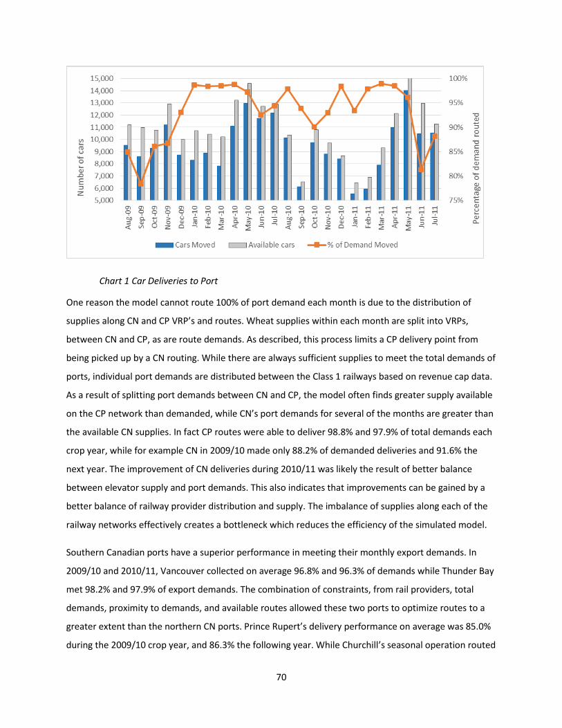
70

Chart 1 Car Deliveries to Port

One reason the model cannot route 100% of port demand each month is due to the distribution of

supplies along CN and CP VRP’s and routes. Wheat supplies within each month are split into VRPs,

between CN and CP, as are route demands. As described, this process limits a CP delivery point from

being picked up by a CN routing. While there are always sufficient supplies to meet the total demands of

ports, individual port demands are distributed between the Class 1 railways based on revenue cap data.

As a result of splitting port demands between CN and CP, the model often finds greater supply available

on the CP network than demanded, while CN’s port demands for several of the months are greater than

the available CN supplies. In fact CP routes were able to deliver 98.8% and 97.9% of total demands each

crop year, while for example CN in 2009/10 made only 88.2% of demanded deliveries and 91.6% the

next year. The improvement of CN deliveries during 2010/11 was likely the result of better balance

between elevator supply and port demands. This also indicates that improvements can be gained by a

better balance of railway provider distribution and supply. The imbalance of supplies along each of the

railway networks effectively creates a bottleneck which reduces the efficiency of the simulated model.

Southern Canadian ports have a superior performance in meeting their monthly export demands. In

2009/10 and 2010/11, Vancouver collected on average 96.8% and 96.3% of demands while Thunder Bay

met 98.2% and 97.9% of export demands. The combination of constraints, from rail providers, total

demands, proximity to demands, and available routes allowed these two ports to optimize routes to a

greater extent than the northern CN ports. Prince Rupert’s delivery performance on average was 85.0%

during the 2009/10 crop year, and 86.3% the following year. While Churchill’s seasonal operation routed

71

a low 58.4% for 2009/10’s exports and 88.3% during 2010/11. From the results of the base model, the

VRP results often have a higher preference to route to Vancouver and Thunder Bay over the ports of

Prince Rupert and Churchill. If there is a high demand for these northern CN access ports, the preference

to route to Thunder Bay and Vancouver creates a bottleneck in the optimization problem.

4.2.3 Critical Time Periods

For ease of illustration, monthly data will be broken down into categorized time periods based on

performance for wheat allocations. Rather than look at overall performance, however, critical time

periods will be broken down into the performance of coastal deliveries, west and east. The coastal

deliveries for each month are evaluated as either successful or unsuccessful in filling port demands

according to the following criterion. When demands are met by 95% or greater, the port or coast is

deemed to have successfully achieved its allocations. Conversely, when the ports of a coast do not

obtain greater than 95% of demanded deliveries, the coastal ports allocation is deemed to be

unsuccessful. In this light, the relative success of port deliveries are shown in Chart 2 and Chart 3 in the

Appendix.

With the division of successful and unsuccessful coastal deliveries performances, there are four critical

time periods for this research. First there is a west dominant time period, where west coast demands

are met successfully however east coast demands are not. The opposite of this is the east dominant

time period, where eastern port demands are met by 95% or greater, whereas the demands of the west

coast are not successful. Then there is the time period where neither demands of the east or west coast

are met successfully, which will be referred to as underperforming ports time period. Finally, the

preferred time period is when both west and east coasts achieve a minimum of 95% of demands or

higher, this is referred to as the optimal port performance time period. The distribution of months

across each time period is not ever, there are two months of west dominant, nine east dominant, four

instances of underperforming ports, and nine occurrences of optimal port performance.

With the division of the studies period into four critical time periods, a month from each critical time

period is chosen to represent the performance for the period. Each critical time period is examined for:

1) the importance of reviewing this period, 2) why a particular month is chosen to represent the time

period, 3) the performance of port deliveries, and 4) the optimization of travel time.

72

4.2.3.1 West Dominant

Over the last few decades an increase in wheat exports to Asia and other Pacific Rim countries has

solidified the west coast’s importance in exporting Western Canada’s wheat. Over the studied period on

average, the two west coast ports demanded 77.0% of all wheat exports (Canadian Grain Commission

2012a). During this time period 11 months were found to have successful total deliveries, which all

experienced high export demands being met by the west coast. The large demands for west-bound

exports do not always accommodate the east-bound demands. With the higher premium for wheat on

the west coast, grain handlers have a preference for filling Pacific Ocean demands before Atlantic

destination exports. If west-bound demands continue to grow, east-bound demands may become of less

importance, and solving a VRP to meet west coast demands could be more important than meeting the

demand of both east-bound and west-bound requirements. This time period is represented by only two

months, February 2010 and 2011. February of 2011 is chosen to represent this critical time period of

west dominant deliveries, as it offered the lowest performance of east coast deliveries. This month will

be examined to determine why west coast demands are favoured and how this will influence allocations

if this becomes a future trend.

During February 2011, west coast demands were 47.5 cars greater than the 5,948 car Prairie supply

(Canadian Grain Commission 2012b). As shown in Figure 7 of the Appendix, 98.0% of the west-bound

demand was met while the 70 cars routed to Thunder Bay filled only 86.5% of port demands. All west-

bound routes were used, with the exception of one 25 car shipment to Prince Rupert, routing in

relatively straight and direct paths to port from as far east as Winnipeg, MB. There is little crossover of

west-bound and east-bound routes, while Vancouver and Prince Rupert routes experienced minimal

overlap of routes along CN’s railway.

Within this critical time period the west-bound routes were better able to utilize their time and

distances travelled. On average, west-bound routes picked up a car every 26.1 minutes, while Thunder

Bay’s three routes averaged a car every 32.7 minutes. This measurement gauges how well a route is able

to source its wheat supplies in comparison to the route travels time, the shorter the time between each

car shows that the model is able to minimize route costs by time. Although Thunder Bay sourced wheat

within a close proximity to port, its smaller routes prevented demands from being as efficient or fast to

source wheat as western routes. Overall, the VRPs routed demands over 2,688 hours, in which west-

bound routes travelled longer routes to fill their port demands. If demands continue to follow this trend,

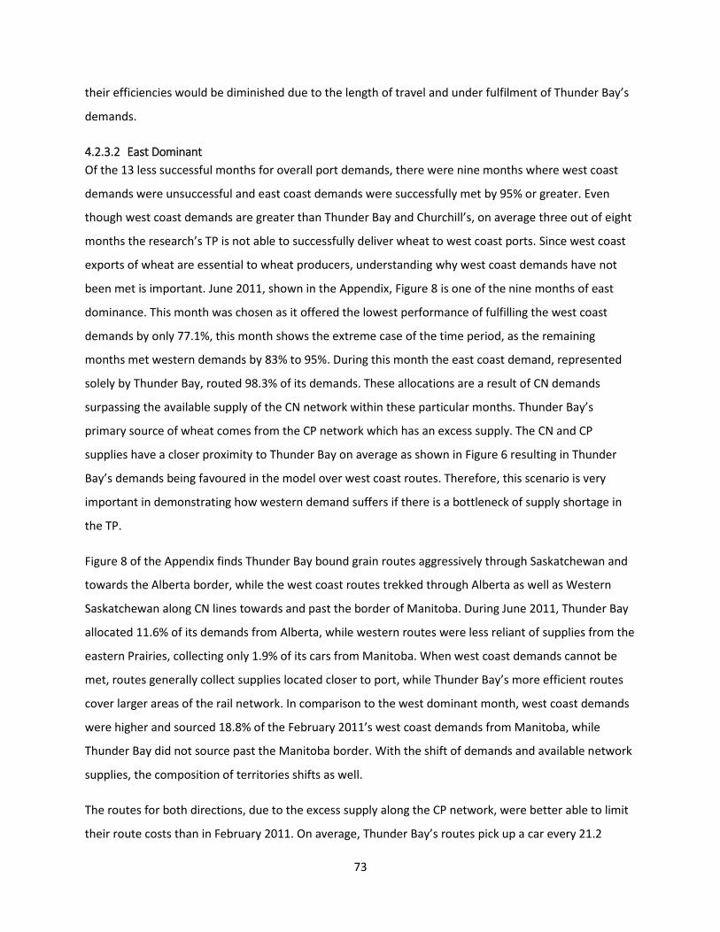
73

their efficiencies would be diminished due to the length of travel and under fulfilment of Thunder Bay’s

demands.

4.2.3.2 East Dominant

Of the 13 less successful months for overall port demands, there were nine months where west coast

demands were unsuccessful and east coast demands were successfully met by 95% or greater. Even

though west coast demands are greater than Thunder Bay and Churchill’s, on average three out of eight

months the research’s TP is not able to successfully deliver wheat to west coast ports. Since west coast

exports of wheat are essential to wheat producers, understanding why west coast demands have not

been met is important. June 2011, shown in the Appendix, Figure 8 is one of the nine months of east

dominance. This month was chosen as it offered the lowest performance of fulfilling the west coast

demands by only 77.1%, this month shows the extreme case of the time period, as the remaining

months met western demands by 83% to 95%. During this month the east coast demand, represented

solely by Thunder Bay, routed 98.3% of its demands. These allocations are a result of CN demands

surpassing the available supply of the CN network within these particular months. Thunder Bay’s

primary source of wheat comes from the CP network which has an excess supply. The CN and CP

supplies have a closer proximity to Thunder Bay on average as shown in Figure 6 resulting in Thunder

Bay’s demands being favoured in the model over west coast routes. Therefore, this scenario is very

important in demonstrating how western demand suffers if there is a bottleneck of supply shortage in

the TP.

Figure 8 of the Appendix finds Thunder Bay bound grain routes aggressively through Saskatchewan and

towards the Alberta border, while the west coast routes trekked through Alberta as well as Western

Saskatchewan along CN lines towards and past the border of Manitoba. During June 2011, Thunder Bay

allocated 11.6% of its demands from Alberta, while western routes were less reliant of supplies from the

eastern Prairies, collecting only 1.9% of its cars from Manitoba. When west coast demands cannot be

met, routes generally collect supplies located closer to port, while Thunder Bay’s more efficient routes

cover larger areas of the rail network. In comparison to the west dominant month, west coast demands

were higher and sourced 18.8% of the February 2011’s west coast demands from Manitoba, while

Thunder Bay did not source past the Manitoba border. With the shift of demands and available network

supplies, the composition of territories shifts as well.

The routes for both directions, due to the excess supply along the CP network, were better able to limit

their route costs than in February 2011. On average, Thunder Bay’s routes pick up a car every 21.2

74

minutes, while the west coast averages a car pick up every 18.4 minutes. Thunder Bay is able to source

wheat on the fastest routes along the CP, while the west coast demands are greater than CN supplies,

which allows the VRP to select the best routes to optimize the costs of picking up the limited supplies. As

a result, CN does not use the smaller routes of 25 cars for Vancouver or Prince Rupert. As shown in

Figure 6, Prince Rupert is not the closest port to any delivery points, and as a result, the port is the least

favourable when optimizing routes. As a result in June 2011, Prince Rupert also does not use 25 or 50

car routes and only half of the available 100 car routes. With the supply shortage, CN being the only

source to Prince Rupert results in few export demands being met for this port. In the absence of supply

along the CN network, west coast demands suffer, as CP continues to supply Thunder Bay’s optimal

demands, resulting in fewer overlaps of supply and extra supplies left on the Prairies along the CP

network.

4.2.3.3 Underperforming Ports

During the sample period, the base model found that neither east nor west coast ports were able to

successfully reach as high as 95% of their export demands in a given month. Although significant

shortfalls were not a frequent occurrence within the model solutions, these are undesirable and their

occurrences need to be investigated. September 2009 is chosen to represent these underperforming

solution time periods as performance in that month was the worst, routing only 78.4% of all demands.

Examining Figure 9 in the Appendix, the solution for this month routed only 84.4% of west-bound

demands and 58.7% of east-bound demands. Although September 2009 and June 2011 are categorized

in different critical time periods, both are similar in that they exhibit low total deliveries, in which June

2011’s total demands was met only by 81.3%. Therefore in future analysis, there may be more

similarties between route performances of September and June, than the other studied months.

Breaking this down, this occurred because CN based grain supplies were 2,239 cars short of CN port

demands, while CP had actually an excess of 2,335 cars on its network. Although the east coast is

primarily serviced by CP’s railway network, during the early fall months, CN also has eastern access to

the port of Churchill. The inclusion of Churchill in the model results in Thunder Bay having to effectively

share its closest proximity supplies. For September 2009, Churchill obtained only 19.1% of its demands,

which further reduced east-bound demand deliveries. As well, the overall CN supply shortage resulted in

only 64.6% of Prince Rupert’s demands being met. In the case of both CN served ports, they are farther

away from supplies than the competitive coastal ports so the model routes a lower percentage of CN

based export demands and optimizes routes with the use of available larger capacities. In detail, Prince

75

Rupert used no routes smaller than 125 cars, while Churchill used one routing of 25 cars and just eight

100 car routes. Vancouver also optimized capacities and routes while not using any 25 car routes. In

general within the VRP, we find that smaller routes do not generate the same supply over a similar time

frame as larger routes.

During this studied month the routes generated, although they do not always meet port demands, they

seem to perform relatively well. Regarding the duration of the average routes solved, in September

2009 Vancouver’s routes pick up a car every 21.1 minutes, whereas, Prince Rupert’s longer routes bring

more cars at one time and improve its overall timing, picking up a railcar every 19.7 minutes. Thunder

Bay’s routes, on average, collect a railcar every 17.6 minutes. Churchill is unable to match these

efficiencies as the slower (done for safety purposes) speeds on the rail line to Churchill result in a car

pick up, on average, every 32.1 minutes. What is interesting to see is that even though Churchill is closer

in proximity to its supply than Prince Rupert, because of speed constraints its routes are less efficient in

this model at meeting the percentage of total demands as well average car obtained compared to Prince

Rupert.

Given these findings in the base model, there would seem to be improvements available particularly for

grain distribution on the CN network. The research speculates that a policy of improved access to these

lines could help to resolve the inefficiencies of the northern ports serving Western Canadian grain.

Overall a system optimization preference towards larger capacity modular trains was also revealed. Yet

conversely, the CP rail network often used all available routes, small and large, clearly due to its location

and excess grain supplies. With a clear VRP preference for larger capacity routes to solve this vast

transportation problem, continued use of smaller grain routings may lead to future inefficiency with

respect to route timing in the grain supply chain if smaller routings are encouraged. This potential

bottleneck will be examined in Chapter 5 through simulations of even larger grain trains to determine if

these smaller trains are generating system inefficiencies.

4.2.3.4 Optimal Port Performance

The most desirable outcome of the TP is optimized port performance, where both the east and west

coast port demands are met to a minimum of 95% efficiency. Simply put, when the base model

generates movements to the west and east corridors that meet actual demands as near to 100% as

possible, the solution is working with a high level of success and is certainly a condition that would

please grain handlers. There were nine months (out of 24) where very near to optimal port performance

was achieved. To illustrate, May 2010 is chosen as an example because it represents the lowest of the

76

nine months of good model port performance at 96.2%. By investigating the lower end of the optimal

port performance spectrum, what makes this month so successful can be highlighted. The next chapter

examines whether improvements can be made on these near perfect solutions to the system TP.24

During this month, CN’s solved network was short only 250 cars of grain demanded, translating to a

simulated routing of 94.2% of total actual CN demands.25 In fact for that month in the entire system,

13,337 cars were demanded, of which 12,971 cars were moved to ports. This solution would be an ideal

case for grain producers, because demands were high and a very high percentage of supplies were

successfully routed to their designated ports.

One downfall of meeting demands in this case is that the VRP cannot optimize the route by selecting a

better fit for route capacity. Even though the VRP optimizes the routes, by design all routes need to be

used and therefore any efficiencies gained from selecting large routes as can be done in some other

poorer performing months is not an option in this instance. When there are underperforming port time

periods, the VRP in fact chooses larger capacity routes to improve efficiency. During optimal port

performance months, selecting different and larger route sizes is not an option. Again it appears that the

smaller capacity routes could be generating bottlenecks to even further improve this particular grain TP.

Since all routes were utilized in this month, the VRP fills each route to capacity. This generates

numerous overlapping routes, as shown in Figure 10 of the Appendix. Even though some routes cross

over one another and some of the allocations are intermingled, it appears that the routes generated by

the base model, on average, performed very well when considered against reality. For example, the

average grain haul of all solved routes is 1,604 km, an amount close to the average length of grain haul

reported by Quorum over the sample period.26

One way to evaluate the relative performance of each port is by examining the average time it took the

optimized system to generate a car destined to deliver to a particular port. Since a high concentration of

Thunder Bay supply is provided by the eastern half of Saskatchewan’s CP network, TB’s routes on

average, obtained a car pickup once every 17.3 minutes. Prince Rupert did not obtain such a successful

24 May 2010 was chosen as it offered for future room of improvement, however, if a month such as March 2011 was chosen at 99.0% of total demand performance, there is little to no room for measurable improvements if they are achievable. 25 Of the nine months to route >95% of demand, five months did not experience an imbalance of supply on CN or CP, three months were short supply on CN, and one month was short supply on the CP network. 26 Quorum reported the average annual haul of grain reported by the CTA in Revenue cap as 1,573 km in 2009/10 and 1,551 km in 2010/11 (Quorum Corportation 2011).

77

route utilization, so PR was only able to obtain a grain car once every 30.5 minutes. The latter poor

performance is the result of both Vancouver and Thunder Bay relying on shorter routes to fill demand,

while Prince Rupert had to find a balance between the smaller routings as used by the other efficient

ports and its remaining demand. Vancouver relied on all its assigned routes and therefore, the results

could not find routes to improve its minimized transportation time. For VC, a grain car was generated

every 22.5 minutes. Comparing these results by month, grain handler were found to prefer more

months like May 2010. In May 2010 Churchill’s port is not operational and does not demand wheat

exports. This results in the base models wheat supplies needing to be only split three ways rather than

four, making routing and allocation easier for the VRP. This month in particular had high port demands

smoothly met by the timely supply of Prairie wheat.

4.3 Summary Reviewing the transportation problem used in this research, between August 2009 and July 2011 unique

optimized allocations using monthly grain flow data which varied over grain supplies, port demands, and

route size distributions were obtained. Over the studied period, when supplies are limited along the CN

network, Vancouver and Thunder Bay port demands are more efficiently readily solved than for Prince

Rupert. This due to the distance that needs to be covered for most Prairie grain to get to Prince Rupert.

When CP’s network faces excess supply, Thunder Bay’s port finds grain from suppliers farther west, as in

many cases they still offer convenient proximity. Finally, the results generated by the base model also

show when the VRP generates routes to port to optimize the allocation of limited supplies, routes with

less grain capacity are not used, in other words the smaller capacity modular trains of 25 and 50 car

blocks are often unused by the ports. Given these observations on the nature of bottlenecks in the

model, scenarios or extensions of the base model are constructed to examine policies that might

improve optimization by improving the travel time for optimal routings as well as utilization of route

capacities.

78

Chapter 5

ALTERNATIVE MODEL SCENARIOS

5.0 Introduction This chapter develops four scenarios constructed using the base optimization model detailed in Chapter

4. These scenarios will be compared with each other and the base model to determine how

improvements can be made to the grain handling optimization process used in this research. The

contents of this chapter is divided into two sections. The first section looks at two counterfactual

scenarios dealing with catchment areas and route size capacities, while the second section examines

two more hypothetical scenarios. Given the current policy environment in the grain transportation

sector, the hypothetical scenarios include a potential regulated access rail policy with a single track and

operator. As well, a sensitivity analysis is performed, parameterizing the base model of greater grain

volumes to mimic the situation caused by a grain transportation bottleneck, similar to the one

experienced in the spring of 2014. The overall intent of this chapter is to review policies that could

potentially reduce the effects of bottlenecks in grain movement as well as to investigate the railways’

ability to continue to provide common carrier service to the grain industry of Western Canada.

5.1 Counterfactual Scenarios The simulated base model of Western Canadian grain transport yielded a relatively good solution at

matching diffuse elevator supplies to port demands, yet the month by month performance of the

optimization simulation against the real data showed that there is still room for modification and

improvement. Therefore, this section explores two counterfactual scenarios using the base model to

search for possible improvements. Each scenario examines the transportation optimization that solves

when polices are implemented to resolve bottlenecks (port preference and smaller capacity

inefficiencies). The two scenarios are simulated for the same four months of data, chosen to represent

critical time periods of the base transportation problem. Originally four alternate scenarios were

constructed to test the two kinds of bottleneck, but two of these were decidedly inferior to the results

generated by the base model and therefore are not included in this discussion.27

27 Of the two scenarios not examined in this chapter, the results were inferior to the base TP. The first looked only at allocations to Vancouver and Thunder Bay, however this represented only 61.3% of total Western Canadian demands, and showed no means of improvements. The second scenario reduced the number of route sizes from the base TP, while retaining the distribution similar to the tendered contracts reported by Quorum Corporation. The results of this simulation were often found be marginally less than the performance of the larger train policy simulation, and therefore it did not provide any new means of improving the TP efficiencies and performances.

79

The first counterfactual scenario to be shown here will be referred to as catchment managed. This

simulated optimization restricts route movements from occurring outside an area matching the

catchments implicitly created by the CWB’s FCR shadow price methodology. In fact, the catchment

managed scenario is simulated for two reasons - 1) to determine if the CWB’s catchments in those years

were large enough to fill each port demand (Gray 1995); and 2) to determine if a similar catchment

policy is imposed on the new competitive system, could performance be improved for Prince Rupert and

Churchill without affecting the allocations of Vancouver and Thunder Bay.

Although the CWB did not strictly enforce their policy of grain needing to be sourced from a particular

port catchment, this counterfactual scenario does restrict routes from sourcing wheat outside of the

catchment route zones. The port of Prince Rupert will also be confined to the Vancouver catchment area

(as was done in reality) while Thunder Bay is presumed to share its catchment with Churchill. The goal of

this exercise is to demonstrate how well port demands could be met in the VRP had the grain allocation

been limited to those CWB catchments. The comparison of this simulation to the base model will also

help to determine the importance of Prince Rupert and Churchill to Western Canadian wheat exports

and can also show if there are advantages to creating catchments for wheat routes in the new system. If

catchment managed policy can efficiently optimize the TP, the constraint of port preference would no

longer have influence over wheat allocations.

The second counterfactual policy simulated from the base model in this section will be called larger

trains (LT). This is conducted to address bottleneck inefficiencies potentially created by smaller modular

train capacities. This scenario alters the base model routes to use fewer sizes of modular trains, and

allows us to examine whether policies to increase average modular train capacities could also improve

efficiencies in the grain transportation problem.

To test the performance and preference of routes, the base models’ six modular train capacities are

reduced to three. The three modular train capacities imposed here are for 50, 100, and 150 car trains.

Routes are thus set into a 50 car denomination, as this is corresponds to the maximum number of

hopper cars a single locomotive can pull on average. In fact, 50 car trains are the most efficient scale per

route to best utilize locomotive capacity (Quorum Corportation 2005). Routes larger than 150 cars are

not used, as Saskatchewan railway siding data does not show any elevators that had the capacity to

handle a larger train spot (Informa Economics 2012). Table 5, from Chapter 4, shows the railways do not

often route larger volumes than 200+ car routings, while a 100 car routing represents a significant

80

volume of routes used in each year. Hence the use of 50, 100, and 150 car modular trains may become a

more accurate representation of train routes used.

Canadian Pacific Railways announced in 2008 that their average grain train is 114 cars long, a level they

intend to increase to 168 cars in the future (Vantuono 2011). Taking into consideration this information

this scenario simulates a policy to increase the average capacity of the routes, so 90% of routings are set

to be greater than 50 car modular trains. This policy of larger trains sets 50% of modular train capacities

to carry 100 cars, 40% to carry 150 cars, and 10% are set as 50 car trains. In this case, the average

modular train capacity is 115 cars, compared to the base model that carried 93 cars on average in

2009/10 and 102 cars on average during the 2010/11 simulation. This policy will produce similar results

to the base, but should improve the overall time of transport.

5.1.1 Counterfactual Analysis

As wheat in Western Canada is now open to market oriented grain handling, this requires a logistics and

allocation system to move or route wheat to port in a timely manner, efficiently utilizing the capacities

of the routes chosen. The two counterfactual scenarios described above are examined against the

results of the base model to determine if any improvements, trends, port preferences, or enhanced

efficiency of deliveries to port can be gained. These results are evaluated based on their; 1) optimization

of travel times, 2) ability to move supply to meet export demands, and 3) utilization of route capacities.

The intent is to distinguish those policies which best improve the base grain TP, and whether any

improvements can be found for more than a single time period or port. After, the average cost of freight

(using rates) will be evaluated to show how changing inputs from the base TP can influence average

freight costs. For tractability, the maps generated by these scenarios are not included in this section.

However, a few of them are included in the Appendix for examination by the reader (Figure 11 and

Figure 12).

5.1.1.1 Optimizing Route Transport Times

Benjamin Franklin once said “time is money”. This is particularly true in the world of modern

transportation where faster delivery results in increased product turnover, providing more services in

the same amount of time and generating increased revenues. This thesis assumes that grain handling

firms in the new operating environment will want to improve their product turnover and speed up

transportation to avoid the risk of demurrage or delay costs. Grain handling firms also want to keep the

flow of grain moving within their large supply chains. Delay receiving grain at port creates a delay for the

entire chain as grain handlers need hopper cars to be back hauled as quickly as possible to Prairie

81

elevators to repeat the process. By routing grain in a more time efficient manner, the grain companies

avoid holding up ocean vessels at berth, and avoid the risk of delaying future deliveries and exports. This

logistics idea was discussed in Chapter 2 (just-in-time logistics), and major international firms like Toyota

and Walmart rely on JIT to reduce potential risks of delay costs, which lead to profit reductions (Sadler

2007).

The route durations and paths of the base model and the two counterfactual scenarios are examined in

this section to determine which version offers the best time saving allocations. Specifically, the scenarios

will be evaluated based on 1) total distance (in kilometers) and hours travelled; 2) average route

duration, by kilometer and hours; and 3) the average time it takes to pick up a grain car per route. These

measures will determine which scenario is superior at routing in a timely matter. Note that comparisons

done throughout this chapter will only examine the months highlighted in Chapter 4, the four chosen

critical months within the two year sample used for this research. As expected, no two simulation

results were the same. It seems that each input set influences the VRP solutions. Table 8 shows the

sums and averages of routes in the critical months for the base plus the two simulated scenarios.

The catchment managed simulation performs exceptionally well, while the results are dependent on the

quantity of cars that the model could allocate to ports in the zones. If in fact the zones or catchments

were able to sufficiently supply port demands, then the CWB catchment method would necessarily

generate the most efficient (least distance travelled) solution. However, if catchments cannot meet

demands, even though the restricted zones use shorter and faster routes they would not optimize their

port demands.

Note that the total distance covered by the solved routes does not actually determine whether they are

good allocations or not, but rather shows which models need to generate longer trips to optimize model

demands. For these simulations which maintain complete access to grain supplies for all ports, the use

of larger train policies route the shortest times and move grain in fewer km than the base model. The

Table 8 Overall route durations

Base Catchment Managed Larger Trains

Total distance travelled (km) 777,848 612,607 644,712

Average distance per route 1,583 1,472 1,789

Total hours travelled 14,118 11,819 11,356

Average hours per route 28.5 28.1 31.4

Average car pick-up (minutes) 22.5 20.8 18.1

82

results suggest that larger trains scale of routes allow for better collection and delivery of clustered

orders.

Again the volume of routes used within each simulation varied, so that the total distances and hours

travelled are not a fair means of relative evaluation. Instead, the average kilometers travelled and hours

used per route are reviewed in Table 8, where we see that catchment managed routes (CWB type

solution) offer the shortest and fastest average routes. This results was expected due to route

confinement within the catchment zones which limited route distances and trip durations.

The average distances travelled are reviewed by month in Table 9. Overall the results are quite spread

out, but the catchment managed simulation is the only one to offer reasonably consistent average

distance travelled because of the limited catchment zones. The average kilometers travelled per route is

what was expected. Larger trains are required to travel greater distances to collect grain. Note that by

this metric, the base falls in the midst of these simulations, while the catchment managed policy yields a

consistent route distance quite close to the more flexible base results.

Table 9 Average distance traveled by routes (km)


11-Feb 1,706 1,585 1,831

11-Jun 1,411 1,438 1.642

09-Sep 1,611 1,401 1,882

10-May 1,604 1,463 1,799

Given the nature of the optimization problem developed here, the travel duration results are similar

with respect to the distribution of kilometers travelled. Looking at Table 8, the average travel time per

route over the four months of the simulations ranged between 28 - 31 ½ hours of travel. A slightly more

detailed review (Table 10) shows that in fact, the results are on average quite close to one another.

These results are pretty much what was expected in that larger train capacities generate longer routes,

catchments limit the duration that solved routes will travel, and the base model reliance on smaller

capacity routes finds itself routing over a slightly shorter average time. What is somewhat unexpected is

how similar the results are, and that larger trains in a scenario do not route drastically longer hours

compared to the other scenarios. This implies that larger capacity trains, at least in terms of time, face

no time disadvantage associated with their larger hauling capacity.

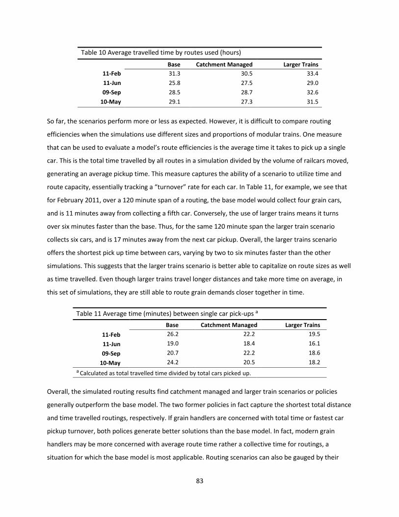
83

Table 10 Average travelled time by routes used (hours)


11-Feb 31.3 30.5 33.4

11-Jun 25.8 27.5 29.0

09-Sep 28.5 28.7 32.6

10-May 29.1 27.3 31.5

So far, the scenarios perform more or less as expected. However, it is difficult to compare routing

efficiencies when the simulations use different sizes and proportions of modular trains. One measure

that can be used to evaluate a model’s route efficiencies is the average time it takes to pick up a single

car. This is the total time travelled by all routes in a simulation divided by the volume of railcars moved,

generating an average pickup time. This measure captures the ability of a scenario to utilize time and

route capacity, essentially tracking a “turnover” rate for each car. In Table 11, for example, we see that

for February 2011, over a 120 minute span of a routing, the base model would collect four grain cars,

and is 11 minutes away from collecting a fifth car. Conversely, the use of larger trains means it turns

over six minutes faster than the base. Thus, for the same 120 minute span the larger train scenario

collects six cars, and is 17 minutes away from the next car pickup. Overall, the larger trains scenario

offers the shortest pick up time between cars, varying by two to six minutes faster than the other

simulations. This suggests that the larger trains scenario is better able to capitalize on route sizes as well

as time travelled. Even though larger trains travel longer distances and take more time on average, in

this set of simulations, they are still able to route grain demands closer together in time.

Table 11 Average time (minutes) between single car pick-ups a


11-Feb 26.2 22.2 19.5

11-Jun 19.0 18.4 16.1

09-Sep 20.7 22.2 18.6

10-May 24.2 20.5 18.2

a Calculated as total travelled time divided by total cars picked up.

Overall, the simulated routing results find catchment managed and larger train scenarios or policies

generally outperform the base model. The two former policies in fact capture the shortest total distance

and time travelled routings, respectively. If grain handlers are concerned with total time or fastest car

pickup turnover, both polices generate better solutions than the base model. In fact, modern grain

handlers may be more concerned with average route time rather a collective time for routings, a

situation for which the base model is most applicable. Routing scenarios can also be gauged by their

84

efficiency in minimizing the time taken between hopper car pickups, for which the larger trains scenario

utilizes routes capacities to source grain closer together in time on average. While the comparative

simulations take longer to collect cars as the number of routes increase and average capacities

decrease.

The catchment managed policy is the best scenario for routing durations of time and distance most

efficiently. However, its advantages hinge on its ability to meet port demands in a given time period. If a

situation can be found that meets port demands in a manner comparable to the base model, then the

catchments scenario is the most efficient among these comparable simulations. However, if the

catchments allocations cannot meet the level of demands contained in the base scenario, this allocation

policy would no longer be an attractive model for system logistics. In sum, if it is assumed that the

catchment managed and larger train polices can attain the same level of deliveries as the base model,

the latter would be superior to the base using the metrics considered here.

5.1.1.2 Supply meeting Export Demands

To fulfill the objective of evaluating reasonable alternate logistics policies for the new Canadian grain

handling system, meeting port demands in a given time frame is essential. In the base model, an

imbalance of supplies and demands along CN and CP networks resulted in months where actual

demands could not be met.28 The simulations contained in this section use the same distribution of

railway services for each port, meaning that the inherent deficit of cars described earlier for most of the

CN network remains. Therefore demands are not expected to be met fully or even grow by significant

volumes. However, the comparative policies run in the simulations illustrate whether marginal

improvements to demand are gained through the use of parameter restrictions or route sizes and

distributions.

Overall, the policy results are mixed, see Table 12. The policy of managed catchments reduces deliveries

by 8%, suggesting that the routing preference to Vancouver and Thunder Bay creates bottlenecks that

are not resolved. It appears for all four months under analysis, the base scenario can only be improved

by less than 0.5% using the larger trains scenario. However, the parameters of the grain logistics system

are somewhat unique to each month, and the performance of a particular policy may be dependent on

the time period or port. The next section evaluates the performance of each of the scenarios based on:

1) monthly total deliveries and 2) port deliveries.

28 Of the 24 months, two months experienced a CP network supply shortage and 16 months on the CN network.

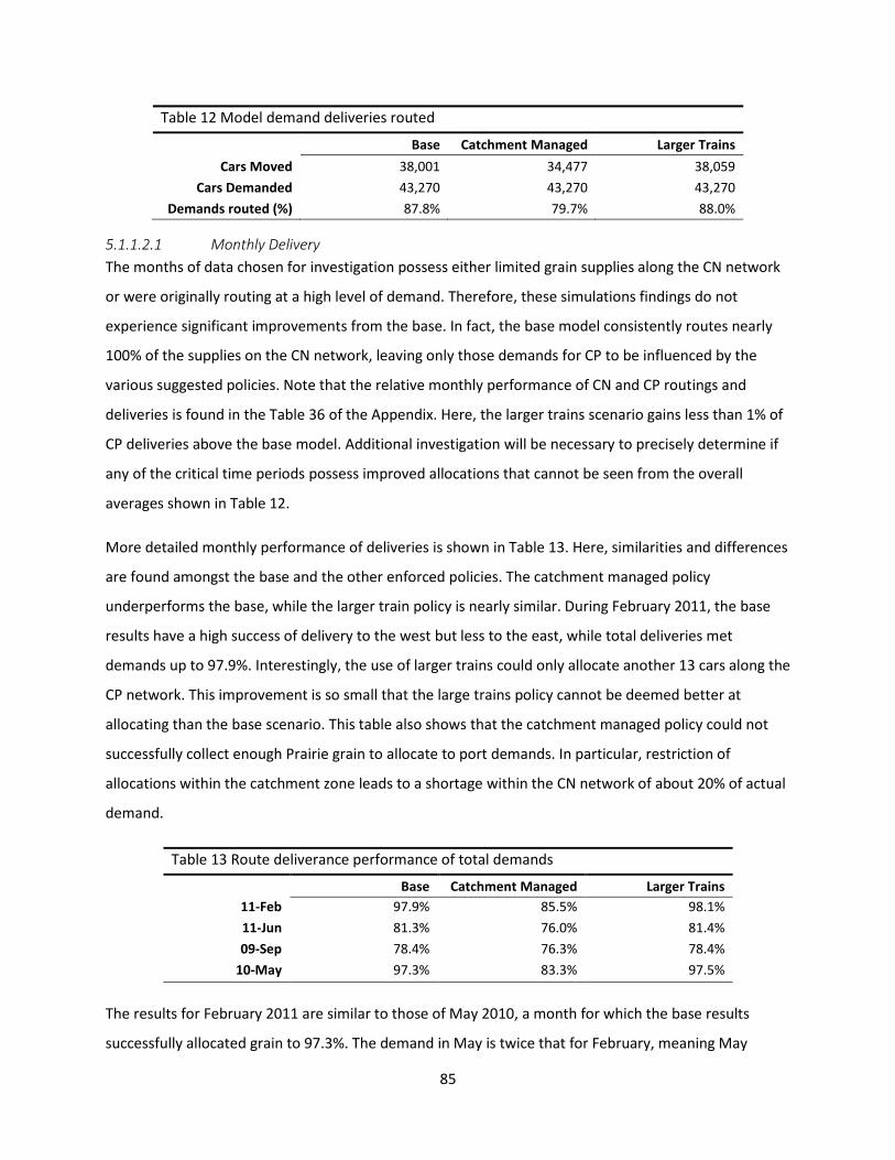
85

Table 12 Model demand deliveries routed Base Catchment Managed Larger Trains

Cars Moved 38,001 34,477 38,059

Cars Demanded 43,270 43,270 43,270

Demands routed (%) 87.8% 79.7% 88.0%

5.1.1.2.1 Monthly Delivery

The months of data chosen for investigation possess either limited grain supplies along the CN network

or were originally routing at a high level of demand. Therefore, these simulations findings do not

experience significant improvements from the base. In fact, the base model consistently routes nearly

100% of the supplies on the CN network, leaving only those demands for CP to be influenced by the

various suggested policies. Note that the relative monthly performance of CN and CP routings and

deliveries is found in the Table 36 of the Appendix. Here, the larger trains scenario gains less than 1% of

CP deliveries above the base model. Additional investigation will be necessary to precisely determine if

any of the critical time periods possess improved allocations that cannot be seen from the overall

averages shown in Table 12.

More detailed monthly performance of deliveries is shown in Table 13. Here, similarities and differences

are found amongst the base and the other enforced policies. The catchment managed policy

underperforms the base, while the larger train policy is nearly similar. During February 2011, the base

results have a high success of delivery to the west but less to the east, while total deliveries met

demands up to 97.9%. Interestingly, the use of larger trains could only allocate another 13 cars along the

CP network. This improvement is so small that the large trains policy cannot be deemed better at

allocating than the base scenario. This table also shows that the catchment managed policy could not

successfully collect enough Prairie grain to allocate to port demands. In particular, restriction of

allocations within the catchment zone leads to a shortage within the CN network of about 20% of actual

demand.

Table 13 Route deliverance performance of total demands


11-Feb 97.9% 85.5% 98.1%

11-Jun 81.3% 76.0% 81.4%

09-Sep 78.4% 76.3% 78.4%

10-May 97.3% 83.3% 97.5%

The results for February 2011 are similar to those of May 2010, a month for which the base results

successfully allocated grain to 97.3%. The demand in May is twice that for February, meaning May

86

requires more routes, a situation offering the larger trains scenario an opportunity to improve route

allocations over base with fewer but larger capacity routes. In fact, the scenario collects an additional 31

cars over the base, but again these improvements are not enough to conclude that it would have been a

superior method for delivering grain in that month.

In review of the eastern ports dominant time period (June 2011), and the underperforming port time

period, September 2009, the results are relatively similar. The changes observed between catchment

managed and base scenarios are not that different in comparison to the other scenario months. It

appears that during these relatively unsuccessful months, the imbalance of grain supply between CN

and CP offers little room for improvement amongst the various policies of catchment or larger trains.

Overall, for each month the base model provides a successful delivery service, and the larger train policy

offers a slight improvement over base by just a few additional cars.

5.1.1.2.2 Deliveries by Port

The counterfactual scenarios tested so far did not make significant gains to overall deliveries compared

to the base as a result of the imbalance of supplies and demands along the networks. These scenarios,

however, could be changing the allocation to port. In Table 14, port deliveries by scenario and month

are presented to determine if port performance improves from the base. If ports have preferred

scenarios, it could be of interest to adopt a policy to favour a port which might benefit grain logistics.

However, the use of different policies for each port will not yield in the same system results. Since the

TP is effectively a closed system, if one port get its deliveries improved than there will be less grain

available for the other ports and their deliveries will decline as a result. This section will investigate

whether one particular policy would best allocate deliveries for all ports or all months.

The port of Vancouver possesses the greatest wheat demand over the four months under analysis. Over

the two year span of this research, Vancouver demanded 46.5% of all Canadian wheat exports (Canadian

Grain Commission 2012a). During the 2009/10 and 2010/11 crop years, the railways reported in revenue

cap data that Vancouver accounted for 56.1% and 57.2% of all grains moved to port from Western

Canada (Canadian Transportation Agency 2011). Short of moving grain through the U.S. system,

Vancouver’s continued ability to source wheat from the Prairies would seem to be essential in the new

grain transportation system in Canada. Table 14 suggests that Vancouver’s demands are best met

through the use of the larger train policy, since the latter delivered over 2.5% more of demands than the

base model. From the months studied, the larger trains policy allocated between 41 and 254 cars more

87

than the base, collecting 98.8% of demands. Alternatively, the catchment managed policy was not able

to improve Vancouver’s allocations from the base case.

Table 14 Delivery performances of port demands

Port Base Catchment

Managed Larger Trains

Cars = 0.5% Demand

VC

11-Feb 97.9% 95.2% 99.1% 17.2

11-Jun 94.0% 93.7% 98.8% 26.5

09-Sep 94.7% 87.0% 98.3% 27.4

10-May 98.1% 94.5% 99.3% 28.2

Total 96.1% 92.4% 98.8% 99.4

PR

11-Feb 98.2% 72.0% 96.9% 12.8

11-Jun 58.9% 59.8% 53.9% 24.9

09-Sep 68.7% 38.1% 61.0% 14.9

10-May 95.6% 61.3% 94.4% 24.1

Total 78.1% 58.1% 75.1% 76.7

TB

11-Feb 86.5% 99.7% 93.5% 0.4

11-Jun 98.3% 71.0% 98.8% 13.0

09-Sep 99.1% 98.8% 98.7% 5.5

10-May 98.4% 98.3% 99.3% 14.4

Total 98.3% 87.7% 98.9% 33.3

CH 09-Sep 19.1% 98.2% 21.5% 7.0

Vancouver has had trouble handling the growing demands of grain exports to Pacific Rim importers. In

response, Prince Rupert’s grain terminal updated its facility in order to help with increased demands

(Everitt and Gill 2005-2006). Over the two crop years researched, rail revenue cap data reported nearly

15% of all Western grain tonnage moved through Prince Rupert’s port (Canadian Transportation Agency

2010b), while the CGC reported that wheat accounts for one third of the grains exports through Prince

Rupert (Canadian Grain Commission 2012a). Prince Rupert plays a minor role in western grain exports,

as its more remote location and single railway access render its allocation process difficult. Nether the

catchment management nor the larger train policies were able to improve from the base model

performance of 78.1% of deliveries at Prince Rupert. The only improvement to the base case occurred in

June 2011 when catchment managed policies collected an additional 42 cars more than the base.

However, the catchment policy reduced the ports performance in the other three critical time period.

Although the larger train policy performed well for Vancouver, the longer routes it generated were not

as effective in meeting demands at Prince Rupert.

88

If grain handlers are concerned about routing to the west coast as a whole rather than individual ports,

in total over the four studied months the base allocation as well as the larger train policy scenario

generate the highest throughput for the transportation problem, delivering 88.3% and 88.5% of western

wheat export demands. Although the monthly results vary in comparison to the scenarios under

individual ports, the larger trains option offers better service over the base, filling 90.2% of western

demands over the four studied months. Here, the catchment policy does not substantially improve

west-bound deliveries (filling only 80.0%), concluding that the catchment policy is an ineffective means

for resolving this bottleneck of port preference.

Thunder Bay’s role overall in the Canadian grain export market is relatively small in comparison to the

west coast. Thunder Bay accounted for only 18.5% of all wheat exports over the two crop years

(Canadian Grain Commission 2012b). Thunder Bay, however, does accept 73% of east coast destined

exports, and for half of the year it is the sole exporter of east-bound grain in the system. Therefore, it is

important that Thunder Bay’s demands are met to maintain east bound grain exports. Thunder Bay’s

optimized results from Table 14 are relatively good with little difference between the base model and

larger trains. This is likely due to the closer proximity of the port to supplies, along with the major

railway provider to TB (CP) supplying 76.4% and 74.5% of deliveries over the two crop years. As

mentioned, CP’s network is well supplied with grain, and excess grain supply in these models guarantees

good delivery performance. Overall, Thunder Bay is marginally best serviced through the larger train

policy, which obtains 98.9% of actual deliveries.

Over this sample, the grain handling system called on Churchill as well for east-bound grain. However,

Churchill is relatively small as a port and active only four months out of year due to climate conditions.

In fact, it accounted for just 9.1% of total export demands over the two crop years of this research

(Canadian Grain Commission 2012a). In this research, only one of the four scenarios included Churchill

movements, so no definitive conclusions can be made as to which simulated scenario best serves this

port. However, looking at Churchill can give insight to which policy performs best for their east-bound

deliveries. For September 2009, the catchment managed policy generated the greatest deliveries to

Churchill. When this is added to the total east-bound performance for the same month, the formerly

best policy (larger trains) drops to the bottom as it delivered only 55.7% of the grain demanded in that

month. It seems the policy best suited for Thunder Bay and Churchill movement in the months studied is

the use of managed catchments, which delivers at 98.4% efficiency. During Churchill’s operational

89

months, the restricted catchments are best at filling east-bound demands overall, but the larger train

policy give marginally better service for the remainder of the months under study.

In sum, the larger train policy performs best for both Vancouver and Thunder Bay, while the base model

is best for Prince Rupert. Looking at west-bound and east-bound allocations, the larger train policy

generates the best performance for west-bound traffic. Alternatively, during September 2009 when the

two east-bound ports demand considerable volumes of wheat, the catchment managed policy yields the

greatest allocations. Although the east-bound demand performance is somewhat unexpected, for the

most part, larger trains and the base scenario are the optimal choices for grain allocations in this system.

In addition, the results confirm that catchment managed policy does not resolve the preferences or

performance of ports in the sample. This indicates that claims the CWB’s FAF created catchments could

meet the changing demands of its respective ports (Gray 1995) are not valid, and that the policy should

not be considered for future allocations in the new grain transportation system.

However, a grain handler cannot assume that total deliveries are the only metric for evaluation in the

new grain handling system. In the next section, the ability of each simulated alternative policy to utilize

the rail network capacities as well as the distribution of routes will be evaluated to help determine if

they generate improvements over the base transportation model solutions.

5.1.1.3 Utilizing Potential of Routes

A new system solution for grain transportation logistics in Western Canada not only needs to provide

timely routes that meet demand, but it will also require routes that most efficiently utilize capacity and

distribution. An efficient route in this model framework is one that optimally fills route capacities, where

capacity not filled a lost profit opportunity for that route. Each route chosen ultimately costs the grain

handler in terms of time, locomotives, and crew. By filling a route to its optimal capacity, the grain

handler will lower their costs. Simply put, when a route’s capacity is filled to only 90% (i.e. 90 out of a

possible 100 hopper cars moving on a route), grain handlers must spread their costs over 90 cars rather

than 100. By way of example, if Cargill requires 1,000 cars at Vancouver, and if railway fixed costs are

$2,000 for a 100 car train at 100% route capacity, for the 10 trains or routes needed to fill demand the

grain handler would pay $20,000 or $20 per car moved. But if the routes operate on average at only 90%

of train capacity, 1.1 extra routes would be required to fill demand, increasing average cost to $24.00

per car. As a result, the grain transportation problem solution that is more attractive to the grain

handler is one that maximizes the utilization of route capacities. The following section looks at what

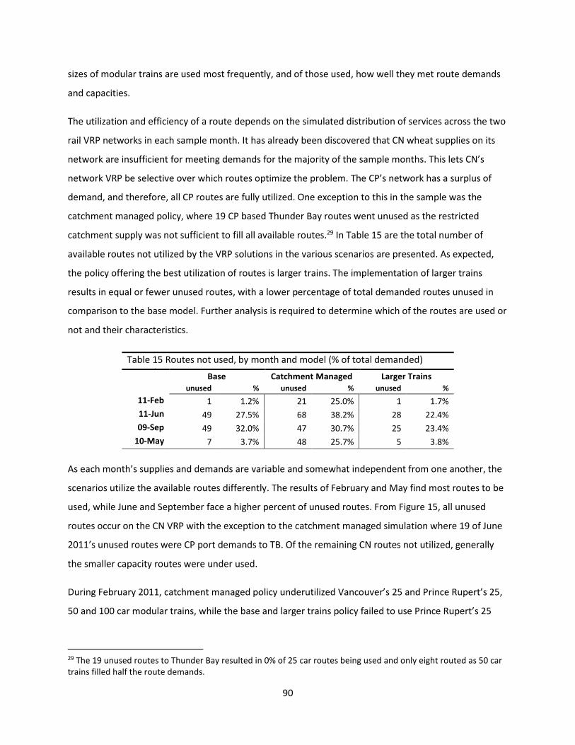
90

sizes of modular trains are used most frequently, and of those used, how well they met route demands

and capacities.

The utilization and efficiency of a route depends on the simulated distribution of services across the two

rail VRP networks in each sample month. It has already been discovered that CN wheat supplies on its

network are insufficient for meeting demands for the majority of the sample months. This lets CN’s

network VRP be selective over which routes optimize the problem. The CP’s network has a surplus of

demand, and therefore, all CP routes are fully utilized. One exception to this in the sample was the

catchment managed policy, where 19 CP based Thunder Bay routes went unused as the restricted

catchment supply was not sufficient to fill all available routes.29 In Table 15 are the total number of

available routes not utilized by the VRP solutions in the various scenarios are presented. As expected,

the policy offering the best utilization of routes is larger trains. The implementation of larger trains

results in equal or fewer unused routes, with a lower percentage of total demanded routes unused in

comparison to the base model. Further analysis is required to determine which of the routes are used or

not and their characteristics.

Table 15 Routes not used, by month and model (% of total demanded) routes)


unused % unused % unused %

11-Feb 1 1.2% 21 25.0% 1 1.7%

11-Jun 49 27.5% 68 38.2% 28 22.4%

09-Sep 49 32.0% 47 30.7% 25 23.4%

10-May 7 3.7% 48 25.7% 5 3.8%

As each month’s supplies and demands are variable and somewhat independent from one another, the

scenarios utilize the available routes differently. The results of February and May find most routes to be

used, while June and September face a higher percent of unused routes. From Figure 15, all unused

routes occur on the CN VRP with the exception to the catchment managed simulation where 19 of June

2011’s unused routes were CP port demands to TB. Of the remaining CN routes not utilized, generally

the smaller capacity routes were under used.

During February 2011, catchment managed policy underutilized Vancouver’s 25 and Prince Rupert’s 25,

50 and 100 car modular trains, while the base and larger trains policy failed to use Prince Rupert’s 25

29 The 19 unused routes to Thunder Bay resulted in 0% of 25 car routes being used and only eight routed as 50 car trains filled half the route demands.

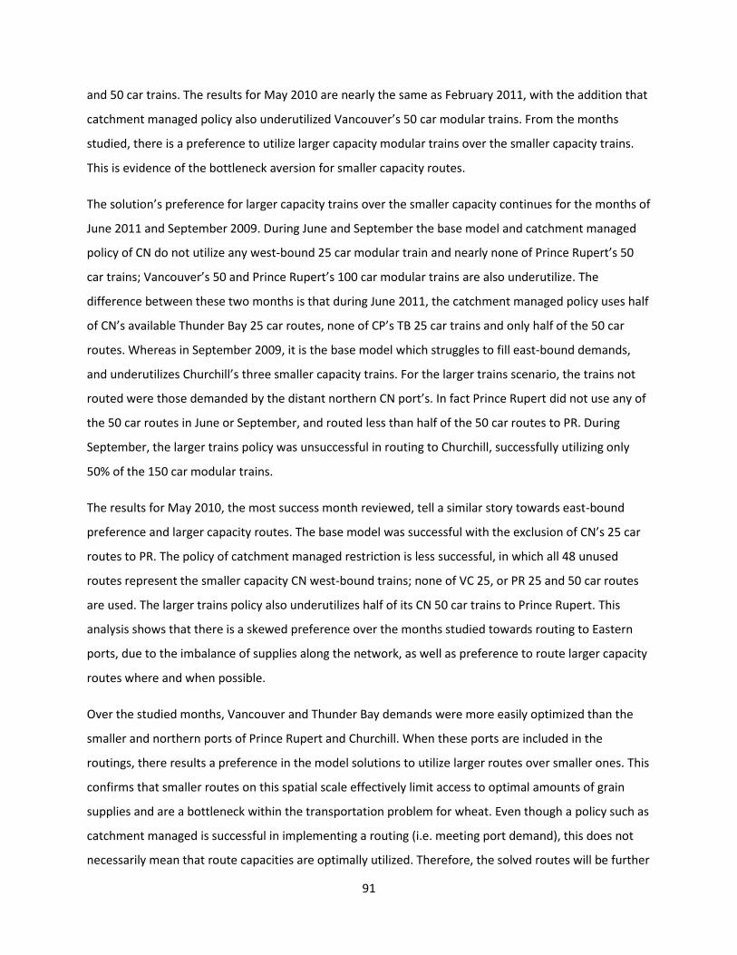
91

and 50 car trains. The results for May 2010 are nearly the same as February 2011, with the addition that

catchment managed policy also underutilized Vancouver’s 50 car modular trains. From the months

studied, there is a preference to utilize larger capacity modular trains over the smaller capacity trains.

This is evidence of the bottleneck aversion for smaller capacity routes.

The solution’s preference for larger capacity trains over the smaller capacity continues for the months of

June 2011 and September 2009. During June and September the base model and catchment managed

policy of CN do not utilize any west-bound 25 car modular train and nearly none of Prince Rupert’s 50

car trains; Vancouver’s 50 and Prince Rupert’s 100 car modular trains are also underutilize. The

difference between these two months is that during June 2011, the catchment managed policy uses half

of CN’s available Thunder Bay 25 car routes, none of CP’s TB 25 car trains and only half of the 50 car

routes. Whereas in September 2009, it is the base model which struggles to fill east-bound demands,

and underutilizes Churchill’s three smaller capacity trains. For the larger trains scenario, the trains not

routed were those demanded by the distant northern CN port’s. In fact Prince Rupert did not use any of

the 50 car routes in June or September, and routed less than half of the 50 car routes to PR. During

September, the larger trains policy was unsuccessful in routing to Churchill, successfully utilizing only

50% of the 150 car modular trains.

The results for May 2010, the most success month reviewed, tell a similar story towards east-bound

preference and larger capacity routes. The base model was successful with the exclusion of CN’s 25 car

routes to PR. The policy of catchment managed restriction is less successful, in which all 48 unused

routes represent the smaller capacity CN west-bound trains; none of VC 25, or PR 25 and 50 car routes

are used. The larger trains policy also underutilizes half of its CN 50 car trains to Prince Rupert. This

analysis shows that there is a skewed preference over the months studied towards routing to Eastern

ports, due to the imbalance of supplies along the network, as well as preference to route larger capacity

routes where and when possible.

Over the studied months, Vancouver and Thunder Bay demands were more easily optimized than the

smaller and northern ports of Prince Rupert and Churchill. When these ports are included in the

routings, there results a preference in the model solutions to utilize larger routes over smaller ones. This

confirms that smaller routes on this spatial scale effectively limit access to optimal amounts of grain

supplies and are a bottleneck within the transportation problem for wheat. Even though a policy such as

catchment managed is successful in implementing a routing (i.e. meeting port demand), this does not

necessarily mean that route capacities are optimally utilized. Therefore, the solved routes will be further

92

analysed to assess how efficient the policies are at filling route capacities while minimizing overall travel

times.

The objective of the VRP as used in this research was explained in Chapter 3. The VRP minimizes system

travel time, in effect maximizing commodity throughput. The VRP optimally matches the available

supplies to fill the capacities of the routes. When the routes are not filled to 100% capacity, this

situation generates increased costs for grain handlers and railways. Grain and railways want to maximize

utilization of the route capacities. In Table 37 (Appendix) and Table 16 below, the ability of the VRP to

utilize the available route capacities are listed by railway and port to assess if a particular policy

increases routed capacity. The base model is effective in meeting route capacities (Table 37) and the

possible gains to route capacity efficiency is small. Also noteworthy is that during most months, use of

larger train policy improves both CN and CP routes capacities by approximately 1% over the base. Table

16 confirms that over the sample period, larger trains do best at filling route capacities. A larger trains

policy is better able to fit the available supplies into routes in comparison to the base model.

Table 16 Route capacity utilization by simulated policy and month Port Base Catchment Managed Larger Trains

VC

11-Feb 97.9% 98.0% 99.1%

11-Jun 99.0% 98.7% 98.8%

09-Sep 99.2% 97.4% 98.3%

10-May 98.1% 98.8% 99.3%

Total 98.6% 98.2% 98.8%

PR

11-Feb 99.2% 96.7% 98.8%

11-Jun 95.0% 94.5% 97.9%

09-Sep 94.7% 92.0% 96.5%

10-May 99.2% 96.6% 99.3%

Total 97.4% 95.4% 98.4%

TB

11-Feb 86.5% 99.7% 93.5%

11-Jun 98.3% 97.1% 98.8%

09-Sep 99.1% 98.8% 98.7%

10-May 98.4% 98.3% 99.3%

Total 98.3% 98.0% 98.9%

CH 09-Sep 99.2% 98.2% 100%

Total route capacity efficiency

98.2% 97.5% 98.7%

93

Under further analysis of the different sizes of modular trains used for each port, it is found that the

majority of routes utilized 98-100% of their capacities.30 With respect to the base model, over the four

months only seven instances occurred where modular trains moving to a port averaged less than 95% of

capacity, and five of these happened serving Thunder Bay routes. Of the two remaining to fall short of

95% capacity, there was Churchill 150 car destined routing at 94.2% and a Prince Rupert 200 car routing

in June that achieved only 42.9% of capacity. The base model utilizes route capacities very well for the

most part. The only routing of major concern was the aforementioned 200 car train routing to Prince

Rupert, which could have been better served if this particular train size was eliminated and redistributed

to another routing.

The simulated catchment managed policy generated 12 instances where route capacity was not met at a

level of 95% or greater. Six of these occurrences represented Thunder Bay modular trains and four for

Prince Rupert. They covered a range of train sizes, and were not focused singularly on smaller routes as

was the case in the base model. In any case, the catchment policy does not meet the port demands at

the same level as the base model and has a lower route capacity efficiency, as listed in Table 16.

Finally, the larger trains policy generated only four routes utilizing modular train capacities below 95%.

Of the four cases, the only one performing below capacity that might be improved upon a set of CN

September 50 car routings to Vancouver at 83.2%. During this month, five routes of 50 cars were

demanded (247 cars demanded), and which carried 41 cars on average, for 205 cars in total. The existing

model provides no means for adjusting this allocation. It is easy to see, however, that had the simulation

actually utilized only four routings, efficiency would have improved while the five remaining cars could

have been routed elsewhere in the CN transportation problem. However the VRP finds the use of the

five 50 car routes using an average of 83.2% to be the optimal solution over allocating only four routes

carrying a total of 200 cars to Vancouver. The three remaining instances falling below 95% efficiency are

a CN Prince Rupert 100 car train, a Thunder Bay 50 car train, and a CP Thunder Bay 100 car train. Policy

for larger capacity trains requires fewer routes across the system, resulting in an average greater

utilization of capacities.

The simulation of the larger capacity routing policy helps to improve efficiencies of Thunder Bay route

capacities over the base model. The route capacities which could use improvements are the smaller

30 Over the two VRP’s and four months, there were a total of 90 allocation’s based on ports and their modular train sizes, and the months studied; from these allocations 59 route size allocations met their capacities on average between 98% ≤ x < 100%, while 21 allocations were made between 95% ≤ x < 98%, and three =100%.

94

routings for each Thunder Bay simulation, with the exception of the large train policy. Although no

simulation generated bad utilizations of route capacities, the larger train policy provided the best

optimization for capacity utilization. This was due to having fewer smaller capacity routes to fill and that

modular train capacities need to be greater than 25 car blocks for most Prairie pick up points.

Alternatively, a modular train with a capacity of 25 cars requires additional effort and time to pick up

grain from multiple locations that happen to have less than 25 cars of grain each. Smaller capacity

routes have troubles finding supplies that add up to the 25 and 50 car capacity and still remain close

enough to fit into the optimal solution. Whereas the use of larger trains are able to better optimize their

capacities to fill demands.

5.1.1.4 Freight rate costs incurred

Given the new operating environment faced by the Canadian grain handling system, the objective of the

optimization problem modeled in this thesis does not seek to minimize transportation rates paid by

farmers but rather optimizes system time travelled from diffuse origins to port destinations. In fact, post

optimization, freight costs incurred by producers applicable to rates on the solved routings can be

tabulated. To this end, Table 17 lists the computed average producer rate paid in each simulation to

transport one tonne of wheat. This calculated freight rate is the weighted average of total cost to move

all routed tonnes (at 90 tonnes/car) to each respective port in a given month, divided by the total

tonnes of grain moved in the month. Note that the difference between average freight rates across the

scenarios are anywhere from a few cents to nearly seven dollars, a reasonably significant variation. The

difference between the computed freight rates in a given month shows similar fluctuations.

Generally, the large train policy generates the highest freight rates, a situation likely due to the larger

average capacities and therefore longer distances travelled on average to both collect and move grain.

These longer optimized routes result in ports sourcing grain from farther distances, driving up the

freight rate. Not surprisingly, the catchment managed policy (with the exception of June 2011)

generated the lowest average freight rates, resulting from the limited distance restrictions of the

catchments. This shows that under this policy, although the catchments are unable to fill demands of

the deliveries made, producers do pay a lower cost than the other scenarios. It should be noted that if

the other scenarios were to route the same (reduced) volume as the catchment managed scenarios,

their average rates could fall due to reduced travel (less supply needed) on routes. The next generation

of grain logistics system for Western Canadian grains will be chosen by the grain companies and will not

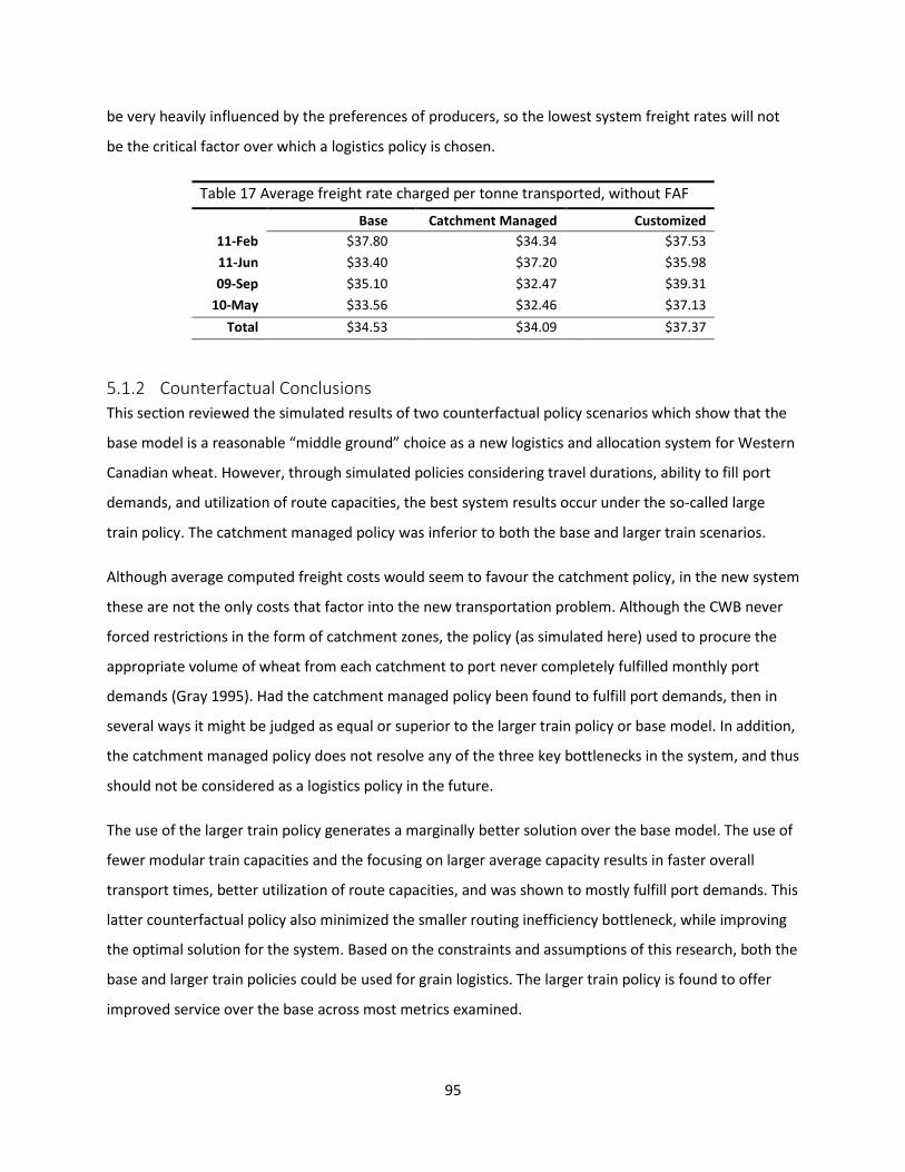
95

be very heavily influenced by the preferences of producers, so the lowest system freight rates will not

be the critical factor over which a logistics policy is chosen.

Table 17 Average freight rate charged per tonne transported, without FAF

Base Catchment Managed Customized

11-Feb $37.80 $34.34 $37.53

11-Jun $33.40 $37.20 $35.98

09-Sep $35.10 $32.47 $39.31

10-May $33.56 $32.46 $37.13

Total $34.53 $34.09 $37.37

5.1.2 Counterfactual Conclusions This section reviewed the simulated results of two counterfactual policy scenarios which show that the

base model is a reasonable “middle ground” choice as a new logistics and allocation system for Western

Canadian wheat. However, through simulated policies considering travel durations, ability to fill port

demands, and utilization of route capacities, the best system results occur under the so-called large

train policy. The catchment managed policy was inferior to both the base and larger train scenarios.

Although average computed freight costs would seem to favour the catchment policy, in the new system

these are not the only costs that factor into the new transportation problem. Although the CWB never

forced restrictions in the form of catchment zones, the policy (as simulated here) used to procure the

appropriate volume of wheat from each catchment to port never completely fulfilled monthly port

demands (Gray 1995). Had the catchment managed policy been found to fulfill port demands, then in

several ways it might be judged as equal or superior to the larger train policy or base model. In addition,

the catchment managed policy does not resolve any of the three key bottlenecks in the system, and thus

should not be considered as a logistics policy in the future.

The use of the larger train policy generates a marginally better solution over the base model. The use of

fewer modular train capacities and the focusing on larger average capacity results in faster overall

transport times, better utilization of route capacities, and was shown to mostly fulfill port demands. This

latter counterfactual policy also minimized the smaller routing inefficiency bottleneck, while improving

the optimal solution for the system. Based on the constraints and assumptions of this research, both the

base and larger train policies could be used for grain logistics. The larger train policy is found to offer

improved service over the base across most metrics examined.

96

5.2 Hypothetical Optimization Scenarios The analysis conducted up to this point has optimized the transport of what are considered to be more

or less typical grain supplies and demands through two separate transportation (railway) networks.

Building upon the previous section, the remainder of the chapter will use the same transportation

problem, but alternately solve for two hypothetical situations of topical interest. The first is a

counterfactual scenario where current policy is changed so that the two separate railway networks

instead must function as a single co-ordinated transportation network. The second scenario is a re-

parameterization of the base model to mimic the bumper crop harvested in 2013 and examine the

ability of the new optimized system to handle this increased volume. In fact, higher volumes moving

through the Canadian grain transportation system may end up being the future norm for a variety of

reasons, including climate change and growing global food demand.

As of early 2014, grain transportation policy in Canada is at a crossroads. Next possible consequences of

this uncertainty by conducting applicable “what if” scenarios using the base simulation model are

examined. Given current uncertainty in the supply chain, it is entirely possible that a very different

Canadian grain transportation system could be seen, including a system that could either lack economic

regulation entirely or alternately, a system that moves to more extreme forms of regulation in the

interest of protecting vulnerable grain shippers. Given that this model more easily conducted the latter

investigation, a counterfactual scenario of extreme railway regulation is developed characterized by the

complete integration of the two Class 1 railway networks through reciprocal access. In this scenario,

which is referred to as open access, Western Canada’s railway networks are treated as mutual access

infrastructure whereby the railways now coordinate transportation across the centralized network in

order to move grain. This scenario is also functionally equivalent to a fully vertically integrated rail

network with a single operator, as only the current Canadian railways are considered in the simulation

and it does not consider the potential effects of new rail operators in the network. This particular

scenario is used to test whether the bottleneck of distributed supply along rail networks can be resolved

under a single network, and allows examination of to what extent efficiencies and optimized network

solutions could be improved.

The second scenario to be evaluated estimates any efficiencies that might be found under increased

system supply and demands, and is based on actual data for grain movement. In this scenario, referred

to as high volume, supply and demand are increased (up to double compared to the base model) and a

sensitivity analysis is conducted to assess the ability of the grain transportation system to operate under

97

the simulated stress of a bumper type crop year. This situation is especially relevant as the 2013 harvest

yielded nearly 20.1 MMT more grain than the 2011 harvest, of which 12.2 MMT are gains to wheat

production (Statistics Canada 2014).31 This drastic increase has resulted in heavily delayed grain

deliveries to port, and potential solutions to the situation are still being considered.

Ultimately, both scenarios will help develop some perspective on the issue of food security. With

expected 50% world population growth from 2000 and 2050 to 9 billion people, can appropriate

changes in grain transportation policies further help Canada feed the world through to the foreseeable

future (United Nations 2013)? Projected population growth is likely to increase pressure to intensify the

production of grain on the Prairies, and it is worth noting that the OECD projects that Canada’s wheat,

coarse grain, and oilseed production will increase 8.7% between 2013 and 2022 to 78.9 MMT due to

population and greater consumption of grains per capita (OECD 2014). In fact, the 2013 bumper crop

may simply reflect future levels of production, and therefore being able to transport it efficiently for

export will likely be an important component of food security from Canada’s perspective. Moving

forward, food security will require producers and industries to invest in infrastructure and logistics that

can adequately support the growing demands of food production. Thus, the intent of this section is to

shed some light on the ability of the current rail system to readily accommodate drastic increases in

grain movement.

5.2.1 Open Access Railway

For the 2010/11 crop year, Canadian Class 1 railways moved nearly 10.5 MMT of wheat from Prairie

elevators to the four ports considered in this research (Canadian Grain Commission 2012a). As they have

done historically and based on geography and the port locations, the two Class 1 railways typically work

independently in grain movement. When they do collaborate and use the track of their competitor

through formal inter-switching, this often incurs additional costs, removing some incentive to

collaborate (Canadian Transportation Agency 2010b). If the government enforced singular rail

ownership or for the two major railways to cooperate more often with one another under an open

access railway system, could this situation improve the logistics of grain handling?

As part of the Estey Review initiated in the late 1990’s, the Canadian government explored options for

increasing competition in the grain transportation system. One option that was heavily favoured in the

31 In 2013, 71.0 MMT of grains were producer in Western Canada (barley, canary seed, canola, chick peas, corn for grain, lentils, mustard seed, oats, soybeans, sunflower seeds, and all wheat). In 2012, the reported production for Western Canada totalled only 52.5 MMT for the same grains (Statistics Canada 2014).

98

provinces of Manitoba and Saskatchewan (as well as the CWB) was to apply a policy of open access for

grain movement within the rail network. However, Transport Canada opposed the implementation of

this policy as they felt the already ‘well-functioning’ industry would then be at risk of various

inefficiencies. Transport Canada and others opposed also believed that open access would remove

incentives to invest in rail infrastructure, while requiring new complex regulations as well as increased

monitoring costs for the industry and government. One interesting argument made by the railways was

that they felt open access would require more trains to move the same volume of freight as the current

system, resulting in decreased efficiencies (Library of Parliment 2007). If these latter arguments are true

and open access reduces rail efficiencies, then it should be found that the simulated policy, especially

with no new competitors under consideration, will do little or nothing to improve grain movements over

the current model.

If railways operated under co-ordinated or open access for grain movements, the operations of the track

would likely require a greater level of logistical planning and exchange of information between the

railways, which could initially come at a higher planning cost. Yet because of potential scale efficiencies,

the open access system might also open up the opportunity to improve rail allocations, even though the

Class 1 railways have argued otherwise. The question is whether or not simulated open access will

improve the optimized solution, or instead result in reduced efficiency in meeting port demands along

with route utilization.

5.2.1.1 Open Access Inputs

An open access policy requires a unified rail network to allow trains to access all track across Western

Canada. To simulate this, the two Class 1 railway networks used in the base model are merged into one

network dataset, and duplication of tracks are removed. This allows the VRP to route along any line of

track and route travel across any and all places where rail lines cross. For instance, the CN and CP order

class supplies for the base model of May 2010 are input into a single VRP as the order class. In this

manner, the simulated open access rail network is similar to a situation where Class 1 railways permit

unlimited track inter-switching.

The open access policy is simulated on the data for the same the four months examined in Chapter 4 to

represent those critical time periods in the sample. Since the larger train policy from the previous

section was found to offer the best performance for meeting port demands, filling route capacities, and

optimizing times, the open access scenario will also be simulated using the modular trains from the

larger train policy (OALT). As well, May 2010’s base model is to examine as open access (OAB) what

99

improvements are possible. The open access scenario tests whether the policy applied to grain

movements in Western Canada can in fact improve grain allocations, or alternatively if the railways were

correct in their supposition that open access is an inefficient solution to the issue of grain logistics.

5.2.1.2 Open Access Results

The simulated open access policy shows that a single co-ordinated railway can overcome the bottleneck

issue of unmet demands within the CN network, identified in Chapter 4. Using the combined railway

networks, open access with larger trains policy, OALT, results in delivery improvements of 11% (to 99.2%

efficiency) over the four months under study. If fact, demands are not filled to 100% efficiency as a

result of routes being set into minimum 25 car blocks in the VRP. Interestingly, if routes or supplies were

set as individual cars, open access could likely increase monthly deliveries even closer to 100%

efficiency.32 All simulated VRP’s on open access registered improvements to their deliveries, as shown in

Table 18. As a result of OALT policies, Prince Rupert and Churchill increased average deliveries from

75.1% and 21.5% (see Table 14) to 99%. Overall, the open access policy increases each ports’ ability to

meet timely demands.

Table 18 Total demands met by open access policy

Base

Open Access Base (OAB)

Larger Trains (LT)

Open Access Larger Trains (OALT)

11-Feb - - 98.1% 99.1%

11-Jun - - 81.4% 99.1%

09-Sep - - 78.4% 99.1%

10-May 97.3% 99.2% 97.5% 99.3%

The simulated open access policy is not found to diminish efficiencies. The implementation of open

access uses more routes, but only to move more cars. Looking at the average size of routes used, LT on

its own collected 105.1 cars on average, while OALT rail moved 101.9 cars on average. The OALT

simulation used all available routes, in contrast to the LT on its own which did not utilize some 50 car

routes for Prince Rupert or Churchill. Open access as considered here permits all routes to be filled, for

which the inclusion of 50 car routes in fact lowers the average number of cars collected per route when

using both the OALT policies.

32 In May 2010 an OALT policies simulation was run using orders in 5 car blocks rather than 25 car block orders. The smaller sized blocks allowed for the VRP to better route another 65 grain cars, increasing route efficiency and delivery of demands from 99.2% to 99.8%.

100

Implementation of open access improves route efficiencies. Simulations of open access were able to

better match supplies along the network to fit the route demands (see Table 19), resulting in improved

delivery efficiencies with little room for improvement. Routes generated using the OALT filled 99% of

their capacities, a result contrary to stated railway concerns about reduced efficiencies under the policy

of open access. Using the objectives relevant to the new grain transportation system, there would

appear to be potential efficiencies to be had with the use of an open access policy.33

Table 19 Efficiency to utilize route capacities

Port Larger Trains (LT) Open Access Larger

Trains (OALT)

VC 98.8% 99.1%

PR 98.4% 99.3%

TB 98.9% 99.1%

Total route capacity efficiency 98.7% 99.2%

Transport related efficiencies can include more than deliveries and utilizing capacities, and also include

total distance moved and travelled time. The OALT simulations moved longer distances in total, since it

generated 59 more routes. The average routing of OALT travelled only 30 km further than the LT policy

under separate rail networks, yet did so in 2.7% less the time. In comparison to LT policy, the

implementation of open access with the larger train policy finds relatively comparable efficiencies of

travel time and distance based the number of routes used. The bottleneck of unmet demands, however,

is resolved under the open access policy. The latter is better at optimizing the grain transportation

problem while maximizing throughput.

Although the open access policy does permit all port demands to be optimized in the sample, the

simulations do not seem to identify any specific spatial allocation tied to any specific region or port. As

shown in Appendix Figure 13 and Figure 15, under this policy west coast ports continue to rely on

supplies from Saskatchewan’s eastern producers, up to Manitoba’s Winnipeg district. Interestingly, in

Figure 14 in the Appendix, Churchill uses routes into eastern Alberta, instead of producers in Manitoba.

These results seem to confirm that in the future grain transportation system, routes will not be based

purely on locational costs and proximity but rather, on the broader allocation to meet system demands.

33 During May 2010 the OAB model also increased its overall route capacity efficiencies 1.0% to 99.2%.

101

5.2.2 Sensitivity Analysis

Western Canada’s grain production also reacts to signals from international markets, innovation in seed

genetics, and new agricultural practices. The combination of increased knowledge and practice, along

with environmental factors has led to improved harvests over time. The grain industry has worked to

improve harvest yields, and there have been years when harvest surpasses expectations. As mentioned,

the harvested 2013 bumper crop generated a 41.2% larger crop than 2011 (Statistics Canada 2014).

While there have been years when yields do not meet the expectations of producers, it is those bumper

crop years which cause the most turbulence in the grain transportation system.34 In addition, as a result

of changing demands and continued pressures from other commodities for their services, railways also

experience times when their planning is better aligned to meet demands of grain movement than other

years. This raises the question - when supply and demands vary from the expected norm, can the

logistics and allocation process in the grain transportation still be effective? If production continues to

grow considering the demands of food production, can the Canadian rail system continue to provide the

necessary capacity to move Canadian grain for export?

Currently, the 2013 harvest of 71 MMT of grain has led to a major logistics problem in the system.

Without the CWB to help mitigate the logistics backlog, elevators are holding near maximum capacity

and are turning away deliveries as they wait for rail car deliveries. This situation has left some asking

whether or not the current rail system support increased demands for grain transportation (Statistics

Canada 2014). To date, the railways blame their inability to move grain in a timely manner on unusually

cold weather along with increased volume of grain that needs to be moved. Others have argued that

another reason is that the railways are increasing crude oil movements from the region at the expense

of the grain movements.

Grain producers have more harvested grain to store for which they will incur costs until the railways can

catch up with their grain movements. The grain companies are also incurring demurrage fees; as of early

March 2014, about 50 vessels were sitting at West Coast ports waiting for grain to arrive at the nearly

empty port facilities (Cross, Clogged: slow rail service causes port delays 2014). Combined with relatively

strong world grain prices at the start of the season, Canadian producers expected to do well financially

from this bumper crop. Full grain elevators and a long wait to turnover hopper cars, however, has

resulted in reduced cash flows for farmers as well as lower grain prices (Atkins 2014). Disregarding who

34 In 2010 the prairies faced above average precipitation which led to a poor harvest of only 46.3 MMT of grain, which was a 9.7% drop from 2009 (Statistics Canada 2014).

102

or what is to blame for the current shortfall in grain movements by the railways, costs for delayed

shipments and contracts will be borne by the grain handling companies and the producers, reducing

profits from this particular bountiful harvest.

The situation was so untenable that on March 7, 2014 the federal government announced the

implementation of a short term fix for the grain transportation system. The government mandated that

both CN and CP move a weekly minimum volume of grain, or face fines. For 90 days over the spring and

summer of 2014, each week the combined volume of grain moved by rail must be 1 MMT or over. If not,

railways would be charged a daily $100,000 fine until the minimum weekly volume is met (Atkins 2014).

Even with this mandate, estimates are that the system will still have over 25 MMT of stored grain to

move by the time of the fall 2014 harvest. Clearly, this is a short term solution for what may be a longer

term problem with grain transportation. What can be done? It is the topical issue of the use of rail

capacity to move potential future grain harvests for which this research can shed some light on using the

GIS based simulation model developed for this thesis.

5.2.2.1 High Volume Parameterization

This section parameterizes the grain transportation problem to analyze these concerns about increased

grain movements in the system. To this end a very basic grain transportation scenario is developed and

optimized consisting of higher supplies and demands than are contained in the existing data. For the

hypothetical scenario, the system demands and supplies are doubled as this simple re-parameterization

generates a simulated monthly volume approaching the average level that currently needs to be moved.

For illustration, this exercise is performed solely for the month of May, 2010 using the base model and

the larger train policy. May 2010 is used because the VRP optimization worked well for this month in

moving the greatest volumes and highest efficiencies among the four months reviewed in Chapter 4 and

in the earlier part of this chapter. Higher volumes will be evaluated for May 2010 using both the base

model (HVB) and the larger trains policy (HVLR). In addition to increasing the volumes of wheat supplies

and demands, this parameterization like the base model does not account for any form of rail access

competition of other commodities such as canola or oil. Therefore the results of this hypothetical higher

volume simulation does not account for any changes that increased supplies or demands of other

commodities have on the wheat transportation problem. The exercise of higher volumes of wheat in a

closed competition system will demonstrate whether there is enough room for expansion and continued

efficiencies in the system in the face of increased demand.

103

5.2.2.2 High Volumes on Open Access Rail (HVOA)

In addition, this section will again simulate a scenario of high volume optimization, but also includes the

policy of open access for the rail system. In this model, open access was shown to improve the

performance of the system with typical monthly demands, so it will be of interest to see if the policy can

improve system performance under doubled grain volumes as well. This scenario will be referred to as

high volume using open access rail simulation or HVOA. As done previously, the performance of the high

volume and HVOA simulations will be evaluated using the metrics of; 1) total deliveries, 2) transport

efficiencies, including time, distance, and car turnover, and 3) overall system freight costs. The use of

higher volume and open access policy will be again tested on May 2010’s base model (HVOAB) and

larger trains policy (HVOALT).

To reiterate, one key assumption made in Chapter 4 still holds - there are no restrictions on railcar

availability. In essence, the model assumes that every elevator has available the necessary number of

cars to transport their monthly supply of wheat. Therefore, these particular simulations test whether

the railways can handle such movements within a busy month if sufficient cars were available, and these

results will also indicate how routes would be changed relative to the previous optimization results.

5.2.2.3 Basic High Volume Results

Using increased volumes of grain moving in the system relative to the May 2010 data, one finds that

port demands and efficiencies are, in fact, improved. Table 20 compares the results from the high

volume as well as the HVOA simulation to the base May 2010 TP results from Chapter 4. Generally,

higher volumes increased meeting total deliveries by less than a full percent, while the HVOA simulation

increased port deliveries by almost 2%. Under both the high volume and HVOA simulations, route

capacity also improved marginally to reach nearly 100% utilization. The simulations also show that the

solved for route efficiencies increase, and the average time to pick up a hopper car decreased.

Looking at the differences between the base model and HVB, we observe overall improved efficiencies.

The HVB simulation increased transported distances by 106% over the base, but this solution was able

to improve the time travelled in the system to 95.5% relative to the base. In effect, the time it took the

high volume optimization to route double the cars was less than doubled, meaning that route durations

are less than the base TP, and as well the time between car pick-ups was reduced. The new solved

routing allocations are shown in Figure 16 in the Appendix. Note that these require Vancouver’s routings

to stretch even further east, while Prince Rupert generates routes within a smaller radius in comparison

to the base TP (Figure 10 in Appendix).

104

Table 20 May 2010 overall performances

Base

High Volume Base (HVB)

HVOAB c Larger Trains (LT)

High Volume Larger Trains (HVLT)

HVOALT d

Cars routed 12,971 26,116 26,535 13,002 26,106 26,572

Cars demanded 13,337 26,674 26,674 13,337 26,674 26,674

Demands routed (%) 97.3% 97.9% 99.5% 97.5% 97.9% 99.6%

Efficiency of routed capacity

98.6% 99.5% 99.5% 99.3% 99.4% 99.6%

Total KM 228,673 594,633 392,297 224,900 447,460 290,030

Change (%) a - 106% 35.9% - 99.0% 29.0%

Total hours 5,231 10,228 6,364 3,939 7,688 4,664

Change (%) b - 95.5% 21.7% - 95.2% 18.4%

Average car pick up (min)

24.2 23.5 14.4 18.2 17.7 10.5

a, b c, d

Measures the increased totals as a percentage from the original simulation (base or larger trains). HVOA stands for high volumes moved along open access rails.

Under the HVOA, there are other gains over the base model. The use of open access with high volumes,

HVOAB, led to an increase in total deliveries by 2% over the base results. Compared to the results of

HVB, HVOAB created travel time efficiencies, and routed higher volumes, using only 66.0% more over

the distance and just 61.7% more of the time generated by the HVB simulation. Even though HVOAB

offers a nearly ideal system of deliveries and efficiencies, the VRP solves for a greater overlap of routes

shown, as shown in Figure 17 of the Appendix. Again, these simulated optimization results show that the

VRP as used here focuses on the best fit of supply to route demands while minimizing both time and

distance travelled for all routes.

Results for the high volumes simulation using the larger train policy, HVLT, finds that increasing grain

volumes does not restrict the efficiencies generated by the transportation problem, and in fact certain

gains are made when the volume is increased. An overview of these results are shown in Table 20. When

demand, supply and routes are doubled, the simulation generated shorter faster routes. The solution

also picked up a car on average every 17.7 minutes, a 30 second improvement over the average of the

LT policy scenario. The allocations generated by HVLT policy although not shown in this thesis are very

similar to Figure 16 in the Appendix, but note that in this case the increased volumes cause Prince

Rupert routes to extend to just west of the Winnipeg area.

In what was already a relatively efficiently solved month of data for grain deliveries, the VRP enhanced

its performance for collecting larger volumes, a finding suggesting there are still economies of scale to

105

be captured in the system. In fact, it is not clear at what level the system would hit its minimum efficient

scale, which for this commodity may occur at surprisingly large volumes. These identified potential scale

economies almost certainly result from bulk nature of grain movements, for which larger levels of

supply and demands offer extended opportunities to better utilize time and route capacity (Bonsor

1984).35

Ultimately the greatest optimized efficiencies occur for the HVOA simulation using the longer train

policy, HBOALT, where 99.6% of demands are fulfilled. And not only does the open access policy allow

for demands to be better filled, it also improves the efficiency of route capacities. As shown in Table 20

(and also through Figure 18 of the Appendix) HVOALT routes are quite different from those of its

simulated predecessor from Chapter 4. Policies of open access and larger trains for the high volumes

problem reveals evidence of performance improvements in optimizing the grain handling problem. Not

only do the routes create near perfect deliveries, the increased input also condenses routes in terms of

time and distances travelled. In this case, an average route travels for 18 hours and six minutes over just

1,124 km, levels 12.5 hours faster and 666 km shorter than the average of the HVLT scenario routes. The

routes shown in Figure 18 of the Appendix does not clearly demonstrate visually the sufficient saving of

time and distance are made to the transportation problem using HVOALT in comparison to the other

reviewed scenarios.

Table 20 shows that the increased volumes resulted in VRP on average optimizing routes in shorter

times, and this was paired by with a 1% increase in deliveries, lowered the turnover time of between

pickups. The optimization of HVB and HVLT from the original demanded volume of Chapter 4 found that

the average travel time to pick up a single tonnes reduced by 3 to 4 seconds.36 If this metric is changed

to look at the average travel time between routed railcars (90 tonnes), the effects of higher volumes

remain constant, but can be more easily understood. The base model picks up a car every 24.2 minutes

while the HVB model is 2.9% faster, picking up a car every 23.5 minutes. Larger trains policy experience

similar improvements under high volume inputs, reducing the travel time between car pickups from the

base model by 2.8% to 17.7 minutes for HVLT.

35 In May 2010’s HVLT policy, multiple simulations were performed increasing the demands and supplies of the TP by 10% at a time. Between 1.1 to 2.0 times the original volumes of LT, the results costs declined in time travelled. All incremental increases found May 2010’s average single car pick up time to be less than the results of the normal input levels of supply and demand, which occurred every 18.2 minutes. 36 The average cost of time per moved tonne reduced from 16.0 to 12.1 seconds for the HVB model. The larger train policy picks up a tonne every 15.8 seconds, and under HVLT every 11.8 seconds.

106

Although there appear to be economies of scale to be capitalized on within these simulations, these will

not come without trade-offs within the system. The simulated policies described in this section improve

overall route performance, but they also increase the average freight rate per tonne. As listed in Table

21 with respect to the base model and the larger train policy which solved to allocate May 2010’s

historical demands, on average the freight cost per transported tonne was $33.56 and $37.13. However

under higher volume simulation the average freight rate to producers equalled $37.12 for HVB and

$38.37 for HVLT. Thus, the base average rate per tonne increases by 10.6%, while the cost per tonne of

LT increases by only 3.3%. So of the two high volume simulations studied, it appears as if producers will

lose with respect to freight rates.37

Unfortunately, complete open access costs cannot be calculated due to allocations made from Prairie

elevators to Prince Rupert, in which the CWB freight rate data does not list the freight rates for all

delivery points to PR port. These solved freight rates also do not account for additional costs of the St.

Lawrence Seaway for eastbound grain. Producers in the new system without the CWB will still likely

have to bear additional fees to move grain through Thunder Bay. Using Tyrchniewicz’s (1998) Seaway

fee of 1996 of $20 per tonne, when this fee is added to all wheat allocated to Thunder Bay, the average

freight rate increases from roughly 9% to 13% per tonne for all models. The HVB model yielded the

lowest average rate, but due to its solved routings, it experiences the greatest change with the inclusion

of a $20/tonne fee for lake movement from Thunder Bay to the St. Lawrence Seaway.

In both simulations of high volumes, as expected the increase of inputs increases the average freight

rate. It is expected that the larger trains policy under high volumes, HVLT, would be better able to

collect railcars in closer clusters and proximity to the port, and therefore the freight rates would be

marginally greater on average. Even though HVLT yields the highest freight rate, the change in rates of

the hypothetical high volume simulations from its original inputs is 3.3% while the base models average

freight rates increases by 10.6% under high volume simulation.

The higher freight rates found in Table 21 also could be beneficial to railway firms’ profits. Depending on

the additional costs of railway operations under each simulation, and without a revenue cap, not

surprisingly the railways are found to have an opportunity to generate greater profits from the larger

37 The increase in costs for larger train policy from “normal” to high volume inputs is quite small. For the railways to accommodate double “normal” demand and still deliver at a high efficiency a 3.34% cost increase is assumed to be not excessive. However, the measured 10.61% cost increase with the base model is significant, yet this increase could potentially be less than the costs to the system to store grain over the foreseeable future.

107

train policy and higher volume grain movements. Despite that under hypothetical high volume

simulation, the average freight rate for producers’ increased, in the new grain handling allocation

system the cost to producers will not be as important as the delivery and reliability of rapid grain routes

to port.

Table 21 Average freight rate per delivered tonne

Simulations Avg. Freight Rate

($/tonne) Average Freight Rate with St.

Lawrence $20 ($/tonne) Difference

(%)

Base $33.56 $37.91 13.0%

High volume base (HVB) $37.12 $41.50 11.8%

Larger Trains (LT) $37.13 $41.52 11.8%

High volume larger trains (HVLT) $38.37 $41.81 9.0%

5.3 Summary This chapter developed and motivated four alternative scenarios building on the base model of Chapter

4. These were done to determine if improvements could be made to resolve identified bottlenecks in

the base solution. In effect, three policies were constructed and tested how or if catchments, route

sizes, and rail accessibility improved the TP optimization, which the latter two policies were found to

improve the TP solution. These policies were evaluated by their performance in delivering supply to

meet port demands, total time travelled, and efficiencies of the route capacities. The results show there

are gains to be had for grain transportation with the use of larger capacity modular train routes as well

as an open access rail network.

The final two scenarios using high volumes were essentially a sensitivity analysis of the parameterized

base model, but a case where grain volumes (supplies and demands) were doubled. This scenario was

done to analyze present and future concerns regarding the grain transportation system in the presence

of increasing yields and the need to feed a growing population. The VRP solutions generated for these

scenarios showed that the system without accounting for competition of other commodities should be

able to support increased grain volumes. Under high volume inputs, with or without the use of larger

trains policy, it is found that the railway network can adapt to these changes and can sustain or improve

system performance under the circumstances. The improvement in railway efficiency under these

scenarios indicates there is available capacity in the system for moving current or future grain surpluses,

all else equal. Improvements in travel time with increased demands were also found, but due to the

nature of the VRP objective and the optimized solutions, freight rates would also increase under higher

volumes. As suggested by Bonsor (1984) and others, the results also indicated there are potential

108

economies of scale available with respect to grain movement, as simulated per unit costs were relatively

stable over the large growth in output. The latter does suggest the lack of current grain movement to

transport the bumper 2013 harvest is likely due to weather conditions along with hopper car availability.

While the transportation of oil may be an issue as well, measuring the system or congestive effects of

increased oil transportation on the Prairie rail network falls outside of the scope of this model.

It is important to remember that grain not only competes against other agricultural products for railway

service and capacity, but also with other commodities. Currently, the relatively low price for grain in

comparison to crude oil as well as the restrictions of the revenue cap make grains a relatively less

attractive commodity for rail to transport. As a result, railways have incentives to give the higher profit

commodity routing priority in their networks. The high volume simulations of this chapter suggest that

under greater availability and demand for grains (with no revenue cap), the average freight rate for grain

in the system will necessarily increase (as shown in Table 21). The results also suggest that railways

would have incentives to move grain in a reliable manner in times of increased grain supply and

demand, since this situation would represent an opportunity to generate additional profits. However, if

the revenue cap is still in place in that case, there would be no greater incentive to move grain when

there is more grain to move. Even though the railways would likely improve their overall efficiencies in a

situation of increased grain volumes, without changes to the revenue cap policy there is just too little

incentive for them to offer additional movements and routings under the revenue cap.

109

Chapter 6

SUMMARY AND CONCLUSIONS

6.0 Introduction The August 2012 removal of the Canadian Wheat Board as Western Canada’s sole marketer of wheat

and grain gave handling companies full responsibility for marketing as well as logistics. Although grain

handling companies have performed non-CWB grain logistics for years, the complexity of organizing

their supply chains has grown with the addition of the former board grains. Those board grains

represent a significant amount of Western Canadian grain exports (nearly 60%) which now must be

absorbed into the everyday business of the remaining grain companies (Canadian Grain Commission

2012d). This has led to a transition of the former board grains to a handling and transportation system

now focused on grain company profit rather than the collective good of Canadian farmers.

Being a relatively low value commodity and moving long distances on what has often been characterized

as a natural monopoly (railways), grain has always had very little leverage in obtaining competitive

freight rates. However, the current Canadian revenue cap policy on grain movement ensures railways

cannot always exploit their market power over grain movement. And as highlighted, the former CWB

FCR logistics policy optimized on freight rates and thus treated the former CWB pool accounts equally

amongst all farmers in the region. Today, without the CWB to generate grain logistics allocations based

on minimized freight rates, the new grain transportation market will likely use very different approaches

to optimize grain logistics. For example, some have argued that grain handling and logistics in a post

CWB era will likely be characterized by more efficient utilization of available grain transportation

capacity (Quorum Corportation 2001). Given the uncertainty that has characterized the grain handling

and transportation system transition to a post-CWB era, it is instructive to identify workable grain

logistics solutions that both support on-going efficient grain movements while continuing to fulfill

foreseeable grain export demands.

The remainder of this chapter will provide an overview of my results about the future of grain handling

and transportation for wheat in Western Canada. This is followed by a discussion of possible extensions

and improvements applicable to the current research.

110

6.1 Summary of Results The use of GIS based methods to model and solve a large transportation optimization problem has the

added benefit of allowing scenario simulations to also be conducted. Using more realistic assumptions

about current industry objectives and historical monthly data (CWB, CGC, and Quorum Corporation) on

wheat supplies and demands from the 2009/10 and 2010/11 crop years, effectively transportation

allocations of wheat across Western Canada for these years were re-optimized. Over the two years

covered in the analysis, the base transportation allocation using the alternative assumptions routed

92.7% of total historical demands. This base outcome was quite efficient, especially given certain

bottleneck constraints in the grain transportation system that emerged as the research progressed.

The base transportation model simulated alternate rail transportation allocations over 24 months.

Foremost, it represents a possible perspective on how alternative grain logistics solutions could be made

in the post CWB era. Subsequently, a deeper investigation of what were considered to be four critical

months from the full data set was conducted. This investigation exposed three potentially key system

bottlenecks: 1) preferences for port delivery, 2) small capacity route inefficiencies, and 3) unmet

demands along the Canadian National Railway network.

Using these identified bottlenecks, three different scenarios or policies were created and simulated as

variations on the base transportation model. Effectively, these were done to try to resolve the system

bottlenecks and potentially improve solutions generated by the base transportation scenario. The

policies simulated in this manner were: 1) catchment managed zones, which are similar to the FCR

catchments created and managed by the CWB; 2) an enforced larger train size policy, thus increasing the

average capacity of train routes; and 3) a reciprocal open access rail policy. These simulations showed

that while the base model did a good job finding a feasible solution for grain logistics, in particular the

larger trains (LT) and open access (OA) policies improved system logistics allocations over the base

results and reduced the effects of the bottlenecks. In effect, these policies resulted in greater hopper car

turnover, small increases in deliveries, as well as enhanced route capacity efficiencies. Within the

current and evolving grain transportation system in Canada, it seems that larger capacity unit trains

and/or reciprocal rail access between Class 1 rail networks have the potential to improve overall grain

logistics.

The simulated catchment managed policy relied on similar catchment basins to those formulated by

CWB’s FAF grain allocation policy. However for the months analyzed, these catchments did not generate

111

sufficient volumes of wheat to meet the historical port demands associated with each (CWB) catchment.

Interestingly, this outcome stands in contrast with the CWB’s stated intent for the catchment design,

which was to generate grain volumes just sufficient for the catchment demands (Gray 1995).

The efficiency gains and rebalancing of the base transportation problem revealed that the rail network

solution solved for the base model was underperforming, and furthermore that relatively simple

improvements were available. This observation highlighted the issue as to whether these policies would

also best optimize grain logistics in conditions when both demand and supply increased significantly.

Using sensitivity analysis, significantly higher volumes of grain (e.g. doubled over base levels) were

found to actually improve the base rail system allocation. One interpretation of this result is that both

railways must still possess some economies of scale in grain movement, noting that the solved

transportation model lacks any consideration for the movement of other commodities on rail, including

oil. In any case, the results indicate that typical grain volumes moved in the system during these years

were not close to levels that would achieve minimum efficient scale. In contrast to some of the public

comments made by the railways about capacity concerns, this research concludes that even with

current volumes being transported, rail system capacity is not a concern for the movement of grain.

While the research was fundamentally about grain transportation, the policy implications of the results

could be far-reaching. Elements of this work touch upon historically controversial issues fundamental to

both the Prairie economy and the development of the nation as a whole. The next section

contextualizes my work in this context and raises philosophical issues about the interactions between

industry, a region and its population.

6.2 Western Canadian Outlook With the removal of CWB influence on grain logistics, the future of agriculture in Western Canada faces

changes reaching beyond varying freight rates and route turnover. If grain industry objectives shift

towards a focus on time optimization for grain movement in a manner similar to that assumed in this

research, this fact coupled with a more open grain market will likely have a lasting influence on the

Canadian West. This influence will touch upon broader policy issues including the future of regional

agriculture as well as rural development.

Using the assumption that grain companies will minimize transport time rather than the cost to

transport grains, this research showed that efficient grain routes on rail will generally become larger in

capacity and move increasing distances. Longer routes will occur on faster segments of track and

112

between locations which offer faster loading or handling services for a grain train. Ultimately, I expect

the preference of the Class 1 railroads will be to move grain almost exclusively along their main

corridors, forming their so-called “pipeline” model for commodity movement. This situation has already

been observed in my maps (see Appendix) and during the transport of the most recent 2013 harvest,

where the limited routes run with grain moved mostly along the mainline tracks of either CN or CP

(Cross, Dyck, et al. 2014, Franz-Warkentin 2014).

Over time, if continued preference is given to those delivery points or elevators with proximity to

primary rail corridors, I expect in particular that short line railways, elevators and farms not located near

to these primary corridors will be at risk. Without a reason for Class 1 railways to connect to more

distant locations, many distant grain elevators may not be able to sustain operations. Thus, proximity to

fast and efficient rail routes will become more influential to agriculture and will transform grain farming

and agriculture in Western Canada. Without policies to protect less proximate regional grain farms,

grain production throughout the Prairies will be transformed from the current diffuse patchwork of

regional grain farms to one where proximity to Class 1 rail and loading facilities will be crucial factors in

regional farm success.

My work shows that the removal of the CWB and the shift towards timely optimization of grain

transportation will result in the Canadian Prairies facing a radical shift towards more transportation

focused grain farm location and production. I conclude that the deregulation of grain marketing in this

manner will eventually result in many fewer grain elevators and farms across the Prairies. In this

scenario, the province of Saskatchewan will be most affected. Within Canada, Saskatchewan grain

producers are located farthest away on average from ports and export markets. As a current large grain

producing province, these changes mean Saskatchewan will very likely see a shift in agricultural

production away from cash crop exports.

Should policies be put in place to postpone or re-direct this process? Historically, Canadian governments

made a series of deliberate decisions to support Prairie economic development and in particular grain

production over the vast interior of the country. It seems to have been understood at that time that

without deliberate protection from the rail sector and its natural market power over grain movement,

agriculture and indeed population settlement in the region would have been very different. Now that

essentially all of these historical regulatory protections to Prairie grain farming have been removed, it

remains to be seen not so much what will happen to Prairie grain farming, but how quickly it will

happen.

113

6.3 Potential Thesis Improvements The reliability and predictive power of the simulated grain movements in the thesis were limited due to

several issues. These include data availability, the use of assumption based parameters, as well as the

scale of the problem being analyzed. As described at various points, certain assumptions were required

to complete the analysis and several of these might be modified in the future to help improve the

optimized grain transportation solutions.

In my assessment, the assumption that had the greatest effect on the model was the use of the revenue

cap data on the distribution of rail services to each port. Using this data led to fewer port deliveries

being made, compared to those actually observed. In fact, several months (including those studied in

greater detail) generated network supplies that did not match demands, in particular for the Canadian

National Railway. Either the listed port distributions in the revenue cap data were incorrect or

alternatively, in those months where CN car supplies were below demands, the two railways may have

done some reciprocal switching in order to transfer CP based grain over to CN’s network to meet CN

port demands. Hinting at the latter possibility is that during the 2010/11 crop year, revenue cap data

reported that CP moved 40,239 tonnes of grain to Prince Rupert, yet CP does not own track connecting

to Prince Rupert. As a result, 0.91% of CP’s 2010/11 rail service was not formally accounted for in the

grain data used here (Canadian Transportation Agency 2011).

If more accurate CN and CP car distribution data had been available, monthly, rather than yearly,

distributions would have been preferred. Grain on the respective rail networks moves in different

quantities each month. It would be more precise to assume that the railways match demands with

available supplies in each (monthly) planning time period rather than referencing a (longer term) yearly

average. Without question, the greatest improvement would come if weekly grain movement data was

available. It is highly likely that the grain transportation problem could be improved by solving it more

frequently so as to generate a more refined allocation of grain throughout the network. In fact, this

would better mirror reality since grain cars are actually ordered weekly by elevators, not monthly,

meaning that temporal variances in car demands could be better accommodated.

Finally, while the use of 25 car blocks made solving the problem feasible, this assumption also created

its own problems. The large scale of the chosen block size made a more precise solution of the larger

network problem more difficult identify. If I could have added each available hopper car individually as

supply, the optimization of route capacities would have been improved. To check this, a simple test

114

using 5 car blocks for the May 2010 data was performed, using both the larger trains and open access

policy (OALT). By doing this, improvements in the VRP solution were generated. In effect, the VRP was

able to better fit the smaller pieces together for a more precise solution. However, I found that the

solution improvements were marginal when considering the time it took the software to solve the latter

more detailed problem.

6.4 Future Studies and Applications In many economic analyses of industrial efficiency or regulatory transition, equilibrium models are

created to examine the effects of parameter changes on system performance. In a similar but spatially

explicit fashion, this research represents some initial steps towards understanding the market for future

logistics applicable to the movement of Western Canadian grain in a new competitive grain marketing

environment. This research has broadened the scope of grain handling logistics in Canada by

investigating the implementation of the basic transportation problem from the perspective of system

participants - farmers, grain companies and railways. Using standard VRP methods within modern GIS

software, a feasible logistics solution is developed that might be used by industry participants in the new

grain marketing era.

To this end, a basic spatial grain logistics network was solved in order to minimize overall travel times

(not distances) for grain train routes. Of interest is that the VRP solutions generated are distinct as

compared to the solutions generated by the CWB under their FAF allocation system, where the latter

possessed a very different objective function and effectively treated grain transportation as but one

facet of grain marketing. Looking to the future without the CWB influence on grain transportation and

the growing importance of transactions costs such as demurrage to the system, a spatially oriented

temporal optimization model such as this will likely become the foundation for generating grain

handling system logistics solutions. Further research should adapt this particular model to increase the

number of goods moved on the network, while removing some regulatory constraints on the movement

of grain.

Any future modelling should incorporate as much as possible rail infrastructure details such as railway

sidings and inland terminal capacities. Applying such data in GIS will allow more accurate modelling of

routes to delivery points across the landscape. The use of precise capacities and sidings would help

determine the size of modular trains that could be serviced at each delivery point. In turn, this will also

allow for interesting restrictions to be imposed on the problem. For example, one such restriction could

115

be to charge a fee to any assembled train sizes that that exceed an elevator’s siding capacity. In turn,

elevator capacity information and maximum length of siding could affect preferences for filling route

demands. Using such information will certainly generate very different routings and volumes from those

generated under the historical CWB FAF grain allocation system.

A GIS transportation optimization framework could also account for details like individual grain

companies as well as the inclusion of delivery point ownership and port terminal data. Grain companies

require their own logistics solutions to best meet their own needs, based on their available storage on

the Prairies and port. While the latter is more complicated because it would require assumptions about

competition in elevation, such an exercise would transition the current framework from an analysis of

what works if all grain companies are treated equally (similar to the situation in the CWB logistics era) to

instead uncover how competition among grain companies might affect system-wide grain allocation

through individualized routings.

Another interesting extension would be to perform VRP analysis using costs of freight rates, time, fuel,

wages, demurrage, and movement restrictions. This research did not incorporate such costs and, hence,

minimized the problem based on time due to the difficulty of structuring the problem using monetary

costs. Although the software was not able to process and accurately account for multiple port freight

rates from one delivery point, its inclusion would allow for an investigation into economic welfare

implications. Such analysis would allow for comparisons to be made between, for example, farmer costs

and the benefits to the rail sector. There are obvious locational advantages for some producers with

respect to each port, so that under other assumptions one could also examine if the former CWB FAF

system did optimize overall welfare under the pooled accounts system.

Finally, the grain allocation system could also be examined more directly from the perspective of the

Canadian railways. Canada’s Class 1 railways provide transportation to many other industries. Aligning

grain routes within the overall railway logistical system allows for examination of potential congestion

issues, as well as optimization of the use of rail infrastructure.

With common carrier laws and remaining regulations on grain transportation, the movement of grain is

still a service which the railways must provide. With the recent oil boom in the region and changes in rail

priorities and allocations, revenues associated with grain movement may not be as enticing to the

railways as in the past. Using this set of models, a study of how railways might move grain under various

regulatory and commodity scenarios can help determine how CN and CP will conduct grain

116

transportation in the future. This includes understanding how they will allocate grain cars and help

identify those Prairie delivery points that will face increased risk from reduced grain transportation

services. Such a study will rely upon a detailed rail network configuration to generate an optimization

model that can closely emulate what real routings would look like, while accounting for grain movement

in the broader rail system. This type of study would be useful for grain companies in that it would

provide them with information about where and what to invest in to maintain or grow rail services while

maximizing revenues and reliability.

This research has developed a transportation optimization model of the current grain handling and

transportation system in Canada that is applicable to the post-CWB era. In particular, I found that a

larger train scenario (as developed in the thesis) has the greatest potential to be a working solution for

Western Canadian grain movement. Additional simulations founded upon the base model were run to

address other topical issues in the sector, including possible open access in the rail industry as well as

the doubling of the amount of grain in the system to study future capacity utilization. In addition, the

modelling framework is sufficiently flexible that modifications can be made to it in order to address

other issues facing the industry such as the level of rail rates, the effect of elevator competition or even

the movement of more and multiple grains. In the post CWB world, the movement of grain in Canada

must transition to a modern and flexible logistics framework more compatible with a fully market

oriented grain handling system. Within this new paradigm, there is clearly scope for the players to

implement innovative logistics solutions that take into account value added as well as overall system

welfare.

117

REFERENCES

Alberta Government. 2011. 2004-2009 Western Canadian Rail Rates & CWB Deductions. Agriculture and

Rural Development. June 24. http://www1.agric.gov.ab.ca/$department/deptdocs.nsf/all/econ1523.

—. 2007. How Price Pooling Works. Agriculture and Rural Development. October 25. Accessed October 2012.

http://www1.agric.gov.ab.ca/$department/deptdocs.nsf/all/sis11760.

—. 2012. The Grain Handling and Transportation System. Agriculture and Rural Development. May 31.

http://www1.agric.gov.ab.ca/$department/deptdocs.nsf/all/sis14046.

Arthur, Jeffery L., and James O. Frendewey. 1988. "Generating Travelling-Salesman Problems with Known

Optimal Tours." Journal of Opernational Research Society 39 (2): 153-159. doi:10.2307/2582378.

Association of Canadian Port Authorities. 2013. Industry Information- CPA Facts. http://www.acpa-

ports.net/industry/cpafacts.html.

Atkins, Eric. 2014. "Ottawa gives railways grain-moving quota." The Globe and Mail, March 7.

http://www.theglobeandmail.com/report-on-business/ottawa-takes-aim-at-grain-backlog-with-

tough-new-transport-rules/article17367492/.

Baldacci, Roberto, Paolo Toth, and Daniele Vigo. 2010. "Exact algorithms for routing problems under vehicle

capacity constraints." Annals of Operations Research 175 (1): 213-245. doi:10.1007/s10479-009-

0650-0.

Ballou, Ronald H. 1992. Business logistics management. 3rd. Englewood Cliffs, NJ: Prentice Hall.

Barney, Darin. 2011. "The End of the Canadian Wheat Board: What's at Stake?" Montréal, Quebec: The

Huffington Post, August 22. www.huffingtonpost.ca/darin-barney/canadian-wheat-

board_b_933200.html.

Bazaraa, Mokhtar S., and John J. Jarvis. 1977. Linear Programming and Network Flows. 1st. New York, NY:

John Wiley and Sons.

Black, William A. 2003a. "A History of Transportation." In Transportation: A Geograpgic Analysis, by William A

Black, 12-37. New York, NY: Guilford Press.

Black, William A. 2003b. "Basic Elements of Transport Networks." In Transportation: A Geograpgic Analysis,

by William A Black, 57-71. New York, NY: Guildford Press.

Black, William A. 2003c. "Methods of Flow Analysis." In Transportation: A Geographical Analysis, by William A

Black, 128-150. New York: Guilford Press.

Black, William A. 2003d. "Societal Trends and Their Impact on Transport." In Transportation: A Geographical

Analysis, by William A Black, 289-302. New York: Guilford Press.

Bonsor, Norman C. 1984. Theory and Canadian Policy. Toronto, ON: Butterworths.

118

Canadian Grain Commission. 2012a. "Canadian Grain Unloaded (net tonnes) at Terminal Elevators by Railcar

Origin." Wheat unloads by month origin tonnes: 2009-11. Microsoft Excel. Comp. Anh Phan.

Winnipeg, Manitoba, May 10.

—. 2009. Classes of licences and definitions. September 15. Accessed February 9, 2012.

http://www.grainscanada.gc.ca/licensee-licence/cld-cld-eng.htm.

—. 2010. "Grain Elevators In Canada Crop year 2010 - 2011." Grain elevators in Canada statistics by crop year.

August 1. http://www.grainscanada.gc.ca/statistics-statistiques/geic-sgc/archive/2010-08-01.pdf.

Canadian Grain Commission. 2012b. Grain elevators in Canada statistics by crop year, 2009-2010 to 2010-

2011. Microsoft Excel. Winnipeg, Manitoba, July 23. https://www.grainscanada.gc.ca/wa-aw/geic-

sgc/search-recherche-eng.asp.

Canadian Grain Commission. 2012c. Grain Statistics Weekly- 2011-12 crop year- Week 52, July 31, 2012.

Winnipeg, Manitoba, August 7. Accessed January 21, 2013.

http://www.grainscanada.gc.ca/statistics-statistiques/gsw-shg/2011-12/week-semaine-52/gsw-shg-

05-eng.htm.

Canadian Grain Commission. 2012d. Licensed Exports (tonnes) of Canadian Wheat (not including Amber

Durum) by Crop Year, Month, Clearance Sector & Destination. Excel File. Comp. Anh Phan. Winnipeg,

Manitoba, September.

Canadian Grain Commission. 2013. "Terminal Unloads (tonnes) by Grain." CGC Statistics: Unloads Warehouse

queried 04FEB13. Comp. Anh Phan. Winnipeg, Manitoba: Canadian Grain Commission, February 5.

Canadian National Railway Company. 2013. Regions. Accessed January 22, 2013.

http://www.cn.ca/en/company-snapshot-profile-regions.htm.

Canadian Pacific. 2012. Our History. Accessed January 22, 2013. http://www.cpr.ca/en/about-cp/our-past-

present-and-future/Pages/our-history.aspx.

—. 2013. "Railcar Supplemental Services Tariff 2." Supplemental services. July 29.

http://www.cpr.ca/en/customer-centre/tariffs/supplemental-services/Documents/Tariff-2-railcar-

supplemental-services-Jul-29.pdf.

Canadian Pacific. 2008. "Time Table." Employee Time Tables.

http://www.tcrc322.ca/files/operating_rules/timetable60.pdf.

Canadian Transportation Agency. 2011. Decision No. 443-R-2011. December 22. http://www.otc-

cta.gc.ca/eng/ruling/443-r-2011.

—. 2010a. Decision No. 512-R-2010. December 21. https://www.otc-cta.gc.ca/eng/ruling/512-r-2010.

—. 2010b. Decision No. LET-R-66-2010 - Review of the Railway Interswitching Regulations. April 21.

https://www.otc-cta.gc.ca/eng/decision-no-let-r-66-2010-review-railway-interswitching-regulations.

119

Canadian Wheat Board. 2011a. 2009-2011 FCR Table with CH and PR. Microsoft Excel. Winnipeg, Manitoba,

April.

—. 2011b. About Us. Accessed April 14, 2011. https://www.cwb.ca/public/en/.

—. 2013. Cash Contracts. April. Accessed May 14, 2013. http://www.cwb.ca/cash-contracts.

Christofides, N., A. Mingozzi, and P. Toth. 1981. "Exact algorithms for the vehicle routing problem, based on

spanning tree and shortest path relaxations." Mathematic Programming (Springer) 20 (1): 255-282.

doi:10.1007/BF01589353.

Clark, J. Stephen. 2005. "Single Desk Selling by the Canadian Wheat Board: Does It Have an Impact?"

Canadian Journal of Agricultural Economics 43 (2): 225-236. doi:10.1111/j.1744-

7976.1995.tb00120.x.

Coppock, John T., and David W. Rhind. 1991. History of GIS. Vol. 1, chap. 2 in Geographical Information

Systems: Principles and Applications, edited by D.J. Maguire, M. F. Goodchild and D.W. Rhind, 21-43.

London: Longman. http://www.grossmont.edu/judd.curran/History_of_GIS.pdf.

Cormen, Thomas H. 2001. "Single-Source Shortest Path." Chap. 24 in Introduction to Algorithms, 580-619.

Cambridge: MIT Press.

Council of Ministers of Transportation and Highway Safety. 2011. "Heavy Truck Weight and Dimension Limits

for Interprovincial Operations in Canada ." Task Force on Vehicle Weights and Dimensions Policy.

http://www.comt.ca/english/programs/trucking/MOU%202011.pdf.

Cross, Brian. 2014. "Clogged: slow rail service causes port delays." The Western Producer, February 28.

http://www.producer.com/2014/02/clogged-slow-rail-service-causes-port-delays/.

Cross, Brian, Bruce Dyck, Terry Fries, Barb Glen, Brian MacLeod, and D'Acre McMillian. 2014. "Short-line

railways get shunted by ramp-up on main lines." The Western Producer, October 30.

http://www.producer.com/2014/10/short-line-railways-get-shunted-by-ramp-up-on-main-lines/.

Dantzig, George B., and J.H. Ramser. 1959. "The Truck Dispatching Problem." Management Science 6 (1): 80-

91. http://www.jstor.org/stable/2627477.

Deng, Yong, Yuxin Chen, Yajuan Zhang, and Sankaran Mahadevan. 2012. "Fuzzy Dijkstra algorithm for

shortest path problem under uncertain environment." Applied Soft Computing 12 (3): 1231-1237.

doi: http://dx.doi.org/10.1016/j.asoc.2011.11.011.

DHL. 2005. "Historical development of logistics." DHL logistics. http://www.dhl-

discoverlogistics.com/cms/en/course/origin/historical_development.jsp.

Dictionary.com Unabridged. 2013. "Heuristic." Random House, Inc. Accessed June 21, 2012.

http://dictionary.reference.com/browse/heuristic.

DMTI Spatial. 2012. CanMap Rail. Shapefile. DMTI Spatial Mapping Academic Research Tools. Markham, ON:

Retrieved through Equinox (equinox2.uwo.ca).

120

Doan, Darcie, Brian Paddock, and Jan Dyer. 2003. "Grain Transportation Policy and Transformation in

Western Canadian Agriculture." Policy Reform and Adjustment Workshop. Kent, UK: Agriculture and

Agri-food Canada. 1-10. http://purl.umn.edu/15748.

Dorfman, Robert, Paul A. Samuelson, and Robert M. Solow. 1958. Linear Programming and Economic

Analysis. New York, NY: McGraw-Hill Book Company.

ESRI. 2013a. Algorithms used by the ArcGIS Network Analyst extension. March 20.

http://resources.arcgis.com/en/help/main/10.1/index.html#//004700000053000000.

—. 2009. An overview of geodatabase design.

http://webhelp.esri.com/arcgisserver/9.3/java/index.htm#geodatabases/an_over-776141322.htm.

—. 2012a. Essiential Network Analyst vocabulary. February 2.

http://help.arcgis.com/en/arcgisdesktop/10.0/help/index.html#/Essential_Network_Analyst_vocabu

lary/004700000003000000/.

—. 2013b. GIS for Defence and Intelligence. www.esri.com/industries/defense.

—. 2012b. "History Up Close." Esri. May 9. www.esri.com/about-esri/history/history-more.

—. 2010. "Network Analyst Tutorial." ArcGIS Help 10.0.

http://help.arcgis.com/en/arcgisdesktop/10.0/pdf/network-analyst-tutorial.pdf.

—. 2013c. Understanding connectivity. July 19.

http://resources.arcgis.com/en/help/main/10.1/index.html#//004700000009000000.

—. 2012c. Understanding the network attributes. February 2.

http://help.arcgis.com/en/arcgisdesktop/10.0/help/index.html#/Understanding_the_network_attrib

ute/00470000000m000000/.

—. 2013d. Using parameters with network attributes. July 19.

http://resources.arcgis.com/en/help/main/10.1/index.html#/Using_parameters_with_network_attri

butes/00470000000s000000/.

—. 2012d. Vehicle routing problem analysis. February 2.

http://help.arcgis.com/en/arcgisdesktop/10.0/help/index.html#/Vehicle_routing_problem_analysis/

00470000004v000000/.

—. 2013e. What is GIS? www.esri.com/what-is-gis/overview#overview_panel.

—. 2012e. What is Network Analyst? February 2.

http://help.arcgis.com/en/arcgisdesktop/10.0/help/index.html#//004700000001000000.

—. 2013f. What is raster data? March 8.

http://resources.arcgis.com/en/help/main/10.1/index.html#//009t00000002000000.

121

Estey, Willard Z. 1998. Grain Handling and Transportation Review: Final Report. Ottawa: Minister of

Transport.

Everitt, John, and Warren Gill. 2005-2006. "The Early Development of Terminal Grain Elevators on Canada’s

Pacific Coast." Western Geography 15-16: 28-52. http://www.geog.uvic.ca/dept/wcag/everitt06.pdf.

Fang, Shu-Cherng. 2012. "Overview of Tabu Search Lecture." Edward P. Fitts Department of Industrial and

Systems Engineering. Edited by North Carolina State University. Course Page: IE789 Soft Computing.

http://www.ise.ncsu.edu/fangroup/ie789.dir/IE789F_tabu.pdf.

Fiellet, Dominique, Pierre Dejax, and Michel Gendreau. 2005. "Traveling Salesman Problems with Profits."

Transportation Science 39 (2): 188-205. doi:10.1287/trsc.1030.0079.

Fischer, Manfred M. 2004. GIS and Network Analysis. Vol. 5, chap. 22 in Handbook of Transportation

Geography and Spatial Systems, edited by D.A Hensher, K.J. Button, K.E. Heynes and P.R. Stopher,

391-407. Elsevier.

Forkenbrock, David. 2001. "Comparison of external costs of rail and truck freight transportation."

Transportation Research Part A: Policy and Practice (Elsevier) 35 (4): 321-337.

Foster, C.D. 1963. The Transport Problem. London: Blackie and Son.

Franz-Warkentin, Phil. 2014. "Shortlines shortchanged in Western Canada." AGCanada. October 17.

http://www.agcanada.com/daily/shortlines-shortchanged-in-western-canada.

Fredman, Michael L., and Robert E. Tarjan. 1987. "Fibonacci heaps and their uses in improved network

optimization algorithms." Journal of ACM 34 (3): 596-615. doi:10.1145/28869.28874.

Froystad, Eric. 2012. Canadian Wheat Board. Personal e-mail communication, September 4.

Fulton, Murray, Baylis K., H. Brooks, and R. Gray. 1998. "The Impact of Deregulation of the Export Basis in the

Canadian Grain Handling and Transportation System." Research Report, Saskatchewan Agriculture

and Food, Regina, SK.

Gendreau, Michel, and Jean-Yves Potvin. 2006. "Tabu Search." Chap. 6 in Search Methodologies: Introductory

Tutorials in Optimization and Decision Support Techniques, edited by Edmund K. Burke and Graham

Kendall, 165-186. New York, NY: Springer.

http://www.inf.ufpr.br/aurora/disciplinas/topicosia2/livros/search/TS.pdf.

Glover, Fred. 1986. "Future Paths for Integer Programming and Links to Artificial Intelligence." Computers and

Operations Research (Elsevier Ltd.) 13 (5): 553-539.

Glover, Fred, and Eric Taillard. 1993. "A user's guide to tabu search." Annals of Operations Research 41 (1): 1-

28. doi:10.1007/BF02078647.

Glover, Fred, Manuel Laguna, and Rafael Marti. 2007. "Principles of Tabu Search." Chap. 23 in Handbook of

Approximation Algorithms and Metaheuristics, edited by Teofilo F. Gonzalez, 23(1-12). Santa

Barbara, CA: CRC Press.

122

Government of Canada. 2014. Canadian Wheat Board Transition. February 5.

http://www.agr.gc.ca/eng/industry-markets-and-trade/statistics-and-market-information/by-

product-sector/crops/initiatives-supporting-producers/marketing-freedom-for-grain-

farmers/canadian-wheat-board-transition/?id=1323987970940.

Government of Saskatchewan. 2005. Upgrades to Provincial Hopper Car Fleet Announced. Edited by Tim

Shoulak. Saskatchewan Grain car Corporation. July 12.

http://www.gov.sk.ca/news?newsId=e40886c4-b0e1-4313-b352-a5f8c70cde96.

Gray, Richard. 1995. Basis Deductions for CWB Deliveries in Western Canada: A Proposal for Basis

Calculations. Consultant, Saskatoon: Department of Agricultural Economics, University of

Saskatchewan, 79.

Gray, Richard. 1996. Preliminary Basis Deduction Calculations for CWB Deliveries in Western Canada: Basis

Calculations for 1996-97. Consultant Report, Saskatoon: University of Saskatchewan, pages 23.

Hay, Alan M. 1977. "Linear Programming: Elementary Geographical Applications of the Transportation

Problem." Edited by Quantitative Methods Study Group the Institute of British Geographers.

Concepts and Techniques in Modern Geography (Issue 11): 3-28.

Hillier, Frederick S., and Gerald J. Lieberman. 1986a. "Introduction to Linear Programming." Chap. 3 in

Introduction to Operations Research, edited by Frederick S. Hillier and Gerald J. Lieberman, 29-51.

New York, NY: McGraw-Hill Inc.

Hillier, Frederick S., and Gerald J. Lieberman. 1986b. "Special Types of Linear Programming Problems." Chap.

7 in Introduction to Operations Research, edited by Frederick S. Hillier and Gerald J. Lieberman, 184-

224. New York, NY: McGraw-Hill Inc.

ICF International. 2009. Comparative Evaluation of Rail and Truck Fuel Efficincy on Competitive Corridors.

Final Report, Fairfax, VA: Federal Railroad Administration, 156.

http://www.ontrackamerica.org/files/Comparative_Evaluation_Rail_Truck_Fuel_Efficiency.pd.

Industry Canada. 2013. "NAICS 1111 - Oilseed and Grain Farming." Canadian Total Exports. June 19.

https://www.ic.gc.ca/app/scr/tdst/tdo/crtr.html?naArea=9999&searchType=BL&hSelectedCodes=%

7C1111&productType=NAICS&timePeriod=5%7CComplete+Years&reportType=TE&toFromCountry=C

DN&currency=CDN&countryList=ALL&grouped=GROUPED&runReport=true.

Informa Economics. 2012. "Review of the Proposed Glencore Acquisition of Viterra and Related

Transactions." Consultant Report, Prepared for the Saskatchewan Ministry of Agriculture, Memphis.

Accessed January 9, 2014.

http://www.gov.sk.ca/adx/aspx/adxGetMedia.aspx?mediaId=1698&PN=Shared.

Kaiser, Harry M., and Kent D. Messer. 2011. "Transportation and Assignment Models for Food and

Agricultural Markets." Chap. 5 in Mathematical Programming for Agricultural, Environmental, and

Resource Economics, 173-210. New York, NY: Wiley.

Kasilingam, Raja G. 1998. Logistics and Transportation: Design and Planning. 1st. Springer US.

123

Klassen, Dwayne. 2007. "Demurrage Charges Hurting Canadian Farmers." Resource News International,

February 14. Accessed December 5, 2013.

http://bi.galegroup.com.cyber.usask.ca/essentials/article/GALE%7CA159343869/314160cd3f4b34c1f

f9b18334cf3ef7e?u=usaskmain.

Klein, Kurt K., and William A. Kerr. 1996. "The Crow Rate Issue: A Retrospective on the Contributions of the

Agricultural Economics Profession in Canada." Canadian Journal of Agricultural Economics (Blackwell

Publishing Ltd) 44 (1): 1-18. doi:10.1111/j.1744-7976.1996.tb00139.x.

Lan, Yingjie. 2009. Case: Subtour Elimination. http://pymprog.sourceforge.net/subtour.html.

Laporte, Gilbert, and Ilbrahim H. Osman. 1995. "Routing problems: A bibliography." Annals of Operations

Research 61 (1): 227-262. doi:10.1007/BF02098290.

Library of Parliment. 2007. "Rail Shipper Protection Under the Canada Transportation Act." Parliament of

Canada. Economics Division. July 16.

http://www.parl.gc.ca/content/lop/researchpublications/prb0573-e.htm#access.

Luderer, Bernd, Volker Nollau, and Klaus Vetters. 2005. "Linear Programming. Transportation Problem."

Chap. 14 in Mathematical Formulas for Economists, 129-138. Berlin: Springer.

Maguire, David J. 1991. "An overview and definition of GIS." Chap. 1 in Geographical Information Systems:

Principles and Applications, edited by D.J. Maguire, M.F. Goodchild and D.W. Rhind, 9-20. London:

Longman. http://www.wiley.com/legacy/wileychi/gis/Volume1/BB1v1_ch1.pdf.

McCalla, Alex F., and Andrew Schmitz. 1979. "Grain Marketing Systems: The Case of the United States versus

Canada." American Journal of Agricultureal Economics 61 (2): 199-212. doi:10.2307/1239725.

Nolan, James, and Jason Skotheim. 2008. "Spatial competition and regulatory change in the grain handling

and transportation system in western Canada." Annals of Regional Science 42: 929-944.

doi:10.1007/s00168-007-0193-8.

Oak Ridge National Laboratory. 2012. "Current operational network QC28." CTA Railroad Network. Shapefile

format. Oak Ridge, TN, August. http://cta.ornl.gov/transnet/RailRoads.html.

OECD. 2014. Database - OECD-FAO Agricultural Outlook. Database. Accessed April 24, 2014.

http://www.oecd.org/site/oecd-faoagriculturaloutlook/database-oecd-faoagriculturaloutlook.htm.

Ólafsson, Sigurdur. 2006. Metaheuristics. Vol. 13, chap. 21 in Handbooks in Operations Research and

Management Science, edited by Shane G. Henderson and Barry L. Nelson, 633-654. Elsevier.

doi:10.1016/S0927-0507(06)13021-2.

Ormsby, Napoleon, Burke, Groessl, and Bowden. 2010. "Introducing GIS." Chap. 1 in Getting to know ArcGIS:

Desktop, 1-12. Redlands, CA: ESRI Incorporated.

Oxford Dictionary of English. 2010. "logistics." Edited by Angus Stevenson. Oxford University Press. Accessed

April 2013. http://oxforddictionaries.com/definition/english/logistics?q=logistics.

124

Özalp, İnan, Bahar Suvaci, and H. Zümrüt Tonus. 2010. "A New Approach in Logistics Management: Just in

Time-Logistics (JIT-L)." International Journal of Business and Management Studies 2 (1): 37-45.

Park, Joon J., and Won W. Koo. 2001. U.S./Canada Grain Handling and Transportation SYstems. Agribusiness

& Applied Economics Report, Department of Agribusiness and Applied Economics, North Dakota

State University, Fargo: Northern Plains Trade Research Center. Accessed September 2012.

http://ageconsearch.umn.edu/bitstream/23576/1/aer451.pdf.

Parkinson, Rhonda. 2007. "The Canadian Wheat Board." Maple Leaf Web. Edited by Department of Political

Science of the University . June 1. http://www.mapleleafweb.com/features/canadian-wheat-board.

Parliment of Canada. 1995. "Parlimentary Business." Parliment of Canada. May 3. Accessed October 17, 2013.

http://www.parl.gc.ca/content/hoc/archives/committee/351/sgrt/evidence/11_95-05-

03/sgrt11_blk-e.html.

Pearson Education. 2002. "THE MODI AND VAM METHODS OF SOLVING TRANSPORTATION PROBLEMS."

Online Tutorial. November 15. Accessed 2012.

http://wps.prenhall.com/wps/media/objects/9434/9660836/online_tutorials/heizer10e_tut4.pdf.

Peterson, Bruce. 2003. "Description of the CTA Railroad Network." CTA Railroad Network. Oak Ridge National

Laboratory. January 6. Accessed June 2012. http://cta.ornl.gov/transnet/rrdescr.txt.

Pillac, Victor, Michel Gendreau, Christelle Gueret, and Andres L. Medaglis. 2013. "A review of dynamic vehicle

routing problems." European Journal of Operational Research 225 (1): 1-11.

doi:10.1016/j.ejor.2012.08.015.

Port of Thunder Bay. 2014. Port of Thunder Bay Cargo Statistics. Accessed April 26, 2014.

http://www.portofthunderbay.com/article/port-of-thunder-bay-cargo-statistics-267.asp.

Quorum Corportation. 2011. Annual Report 2010-2011 Data Tables. Microsoft Excel. Edmonton, Alberta,

May.

Quorum Corportation. 2012a. "Annual Report of the Monitor – Canadian Grain Handling and Transportation

System." Annual Report, Edmonton, 90.

http://www.quorumcorp.net/Downloads/AnnualReports/AnnualReport201011English.pdf.

Quorum Corportation. 2001. "Annual Report of the Monitor – Canadian Grain Handling and Transportation

System 2000- 2001 Crop Year." Annual Report, Edmonton, 172.

http://www.quorumcorp.net/Downloads/AnnualReports/AnnualReport200001English.pdf.

Quorum Corportation. 2002. Grain Monitoring Program Base Measurement Program. Report, Edmonton:

Transport Canada & Agriculture and Agri-Food Canada, 31.

http://www.quorumcorp.net/Downloads/SupplementalReports/ProducerNetback.pdf.

Quorum Corportation. 2012b. "Grain Monitoring Program: The GHTS at a Glance." Annual Report, Edmonton.

http://www.quorumcorp.net/Downloads/AnnualReports/GHTS_Glance20112012.pdf.

125

Quorum Corportation. 2005. "Railway Capacity Background & Overview." Quorum Corportation Reports,

Edmonton. http://www.quorumcorp.net/Downloads/Papers/RailwayCapacityOverview.pdf.

Railway Association of Canada. 2011. Freight - Short Line/Regional Members. Accessed January 22, 2013.

http://www.railcan.ca/rac/member_railways?type=Freight+-+Short+Line%2FRegional.

Resource News International. 2006. "Manitoba and Saskatchewan Call For Immediate Plebiscite on CWB."

November 10. Accessed December 5, 2013.

http://bi.galegroup.com.cyber.usask.ca/essentials/article/GALE%7CA154272824/6d486545473080f7

d57e1cb27be6b1aa?u=usaskmain.

Sadler, Ian. 2007. "Logistics in Manufacturing Organisations." Chap. 2 in Logistics and Supply Chain

Integration, 31-79. Los Angeles: Sage Publications.

Schlecht, Shannon, William W. Wilson, and Bruce L. Dahl. 2004. "Logistical Costs and Strategies for Wheat

Segregation." Agribusiness & Applied Economics Report, Department of Agribusiness and Applied

Economics, North Dakota State University, Fargo, ND, 41. http://purl.umn.edu/23507.

Schmitz, Andrew, and W. Hartley Furtan. 2000. The Canadian Wheat Board: Marketing in the New

Millennium. Vol. 38. Regina, Saskatchewan: Canadian Plains Research Center.

Schmitz, Andrew, W. Hartley Furtan, and Katherine Baylis. 2002. "Marketing and Market Regulation." In

Agricultural Policy, Agribusiness, and Rent-Seeking Behaviour, by Andrew Schmitz, Hartley Furtan and

Katherine Baylis, 154-177. Toronto, ON: University of Toronto Press.

Schrijver, Alexander. 2003. Introduction. Vol. 1, chap. 83 in Combinatorial Optimization: Polyhedra and

Efficiency, by A. Schrijver, 1-8. Berlin: Springer.

Scurry, Jim. 1998. What is GIS? Edited by National Estuarine Research Reserve System. Water and

Conservation Division SCDNR Land. December 17. Accessed April 2012.

http://www.nerrs.noaa.gov/doc/siteprofile/acebasin/html/gis_data/gisint2.htm.

Srinivasan, G. 2009a. Lecture 13- Transportation Problem. Video Lecture. Prod. Department of Managment

Studies. Youtube, August 30. Accessed June 4, 2012.

http://www.youtube.com/watch?v=Q31jKiEXxdc.

Srinivasan, G. 2009b. Lecture 14- Transportation Problem- Optimal Solution. Video Lecture. Prod. Department

of Management Studies. Youtube, September 22. Accessed June 4, 2012.

http://www.youtube.com/watch?v=RnZnIIksdwU.

Statistics Canada. 2012. Farm and Farm Operator Data, 2011 Census of Agriculture (95-640-X). Catalogue no.

95-640-X, Ottawa: Minister of Industry. http://www.statcan.gc.ca/pub/95-640-x/2012002/01-

eng.htm.

Statistics Canada. 2014. Table 001-0010 - Estimated areas, yield, production and average farm price of

principal field crops, in metric units, annual. Statistics Canada.

126

http://www5.statcan.gc.ca/cansim/a26?lang=eng&retrLang=eng&id=0010010&paSer=&pattern=&st

ByVal=1&p1=1&p2=-1&tabMode=dataTable&csid=.

Statistics Canada. 2013. "Table 001-0015 - Exports of grains, by final destination, monthly (tonnes)."

Tahir, Muhammad A., and James E. Smith. 2008. "Feature Selection for Heterogeneous Ensembles of

Nearest-neighbour Classifiers Using Hybrid Tabu Search." In Advances in Metaheuristics for Hard

Optimization, edited by Patrick Siarry and Zbigniew Michalewics, 69-85. Berlin: Springer.

doi:10.1007/978-3-540-72960-0_4.

Transport Canada. 2011. "Government of Canada Hopper Car Fleet 2011 Annual Report." Ministry of

Transport, Government of Canada. https://www.tc.gc.ca/eng/policy/acg-acgb-grain-annual-

report2011-3026.htm.

—. 2012. Subpart A- Classes of Track. June 8. Accessed June 2012. http://www.tc.gc.ca/eng/railsafety/rules-

tce54-832.htm.

Tyrchniewicz, Edward, Richard Gray, Daryl Kraft, Cameron Dahl, and Brenda Chomey. 1998. A Study of The

Canadian Wheat Board's Role in Grain Transportation. Report, Department of Agricultural Economics

and Farm Management, University of Manitoba, Winnipeg: Agriculture and Agri-Food Canada and

Transport Canada, 254.

U.S. Geological Survey. 2007. Geographic Information Systems. February 22.

http://egsc.usgs.gov/isb//pubs/gis_poster/.

United Nations. 2013. "World Population Prospects: The 2012 Revision." Press Release. Department of

Economic and Social Affairs, Population Division, June 13. 4.

http://esa.un.org/wpp/Documentation/pdf/WPP2012_Press_Release.pdf.

Vantuono, William C. 2011. "Canadian Pacific charts a comeback course." Railway Age. September 30.

Accessed November 20, 2013. http://www.railwayage.com/index.php/operations/canadian-pacific-

charts-a-comeback-course.html.

Veeman, Michele M., and Terrence.S. Veeman. 2006. "Canadian Wheat Board." The Canadian Encyclopedia.

February 06. Accessed January 2012. http://www.thecanadianencyclopedia.com/articles/canadian-

wheat-board.

Vercammen, James, Murray Fulton, and Richard Gray. 1996. The Economics of Western Grain Transportation

and Handling. 1996 Van LIet Publication Series, Saskatoon, SK: Department of Agricultural

Economics, University of Saskatchewan.

Wikipedia. 2013. List of geographic information systems software. May 24.

http://en.wikipedia.org/wiki/List_of_geographic_information_systems_software#Desktop_GIS.

Wilson, William W., Bruce L. Dahl, and Donald C.E. Carlson. 2000. "Logistical Strategies And Risks In Canadian

Grain Marketing." Canadian Journal of Agricultural Economics 48: 141-160. doi:10.1111/j.1744-

7976.2000.tb00271.x.

127

Wilson, William W., Donald C.E. Carlson, and Bruce L. Dahl. 2004. "Logistics and Supply Chain Strategies in

Grain Exporting." Agribusiness 20 (4): 449-464. doi:10.1002/agr.20026.

Yan, Melissa. 2002. "Dijkstra's Algorithm." MIT Mathematics. August 6.

http://math.mit.edu/~rothvoss/18.304.3PM/Presentations/1-Melissa.pdf.

128

APPENDIX

A-1 Computer Code

Table 22 Simple Dijkstra code

1 𝐝𝐢𝐬𝐭[𝐬] ← 𝟎 ∗∗ 𝑡ℎ𝑒 𝑑𝑖𝑠𝑡𝑎𝑛𝑐𝑒 𝑓𝑟𝑜𝑚 𝑡ℎ𝑒 𝑜𝑟𝑖𝑔𝑖𝑎𝑛𝑙 𝑠𝑜𝑢𝑟𝑐𝑒 𝑡𝑜 𝑣𝑒𝑟𝑡𝑒𝑥 𝑖𝑠 𝑒𝑞𝑢𝑎𝑙 𝑡𝑜 0 ∗∗ 2 𝐟𝐨𝐫 𝐚𝐥𝐥 𝐯 ∈ 𝐕– {𝐬} 3 all other 𝐝𝐢𝐬𝐭[𝐯] ← ∞ ∗∗ 𝑠𝑒𝑡 𝑎𝑙𝑙 𝑜𝑡ℎ𝑒𝑟 𝑑𝑖𝑠𝑡𝑎𝑛𝑐𝑒𝑠 𝑒𝑞𝑢𝑎𝑙 𝑡𝑜 𝑖𝑛𝑓𝑖𝑛𝑖𝑡𝑦 ∗∗

4 𝐒 ← ∅ 𝑆 ∗∗ 𝑖𝑠 𝑡ℎ𝑒 𝑠𝑒𝑡 𝑜𝑓 𝑣𝑖𝑠𝑖𝑡𝑒𝑑 𝑣𝑒𝑟𝑡𝑖𝑐𝑒𝑠 𝑜𝑓 𝑡ℎ𝑒 𝑔𝑟𝑎𝑝ℎ, 𝑎𝑛𝑑 𝑎𝑟𝑒 𝑖𝑛𝑖𝑡𝑖𝑎𝑙𝑙𝑦 𝑒𝑚𝑝𝑡𝑦 ∗∗

5 𝐐 ← 𝐕 ∗∗ 𝑄 𝑖𝑠 𝑡ℎ𝑒 𝑞𝑢𝑒𝑢𝑒 𝑤ℎ𝑖𝑐ℎ 𝑖𝑛𝑖𝑡𝑖𝑎𝑙𝑙𝑦 𝑐𝑜𝑛𝑡𝑎𝑖𝑛𝑠 𝑎𝑙𝑙 𝑣𝑒𝑟𝑡𝑖𝑐𝑒𝑠 ∗∗

6 𝐐 ≠ ∅ ∗∗ 𝑡ℎ𝑒𝑟𝑒 𝑚𝑢𝑠𝑡 𝑏𝑒 𝑎 𝑠𝑢𝑏𝑠𝑒𝑡 𝑜𝑓 𝑢𝑛𝑙𝑎𝑏𝑒𝑙𝑒𝑑 𝑣𝑒𝑟𝑡𝑖𝑐𝑒𝑠 𝑓𝑜𝑟 𝑡ℎ𝑒 𝑝𝑟𝑜𝑏𝑙𝑒𝑚 𝑡𝑜 𝑠𝑒𝑎𝑟𝑐ℎ ∗∗

7 𝐝𝐨 𝐮 ← 𝐦𝐢𝐧𝐝𝐢𝐬𝐭𝐚𝐧𝐜𝐞(𝐐, 𝐝𝐢𝐬𝐭) ∗∗ 𝑢 𝑒𝑞𝑢𝑎𝑙𝑠 𝑡ℎ𝑒 𝑚𝑖𝑛. 𝑑𝑖𝑠𝑡𝑎𝑛𝑐𝑒 𝑓𝑟𝑜𝑚 𝑡ℎ𝑒 𝑖𝑛𝑖𝑡𝑖𝑎𝑙 𝑆 𝑡𝑜 𝑄 ∗∗

8 𝐟𝐨𝐫 𝐚𝐥𝐥 𝐯 ∈ 𝐧𝐞𝐢𝐠𝐡𝐛𝐨𝐫𝐬[𝐮]

9 𝐝𝐨 𝐢𝐟 𝐝𝐢𝐬𝐭[𝐯] > 𝐝𝐢𝐬𝐭[𝐮] + 𝐰(𝐮, 𝐯) ∗∗ 𝑖𝑓 𝑡ℎ𝑒 𝑛𝑒𝑤 𝑝𝑟𝑒𝑑𝑒𝑐𝑒𝑠𝑠𝑜𝑟 𝑣𝑒𝑟𝑡𝑖𝑐𝑒′𝑠 𝑑𝑖𝑠𝑡𝑎𝑛𝑐𝑒 𝑖𝑠 𝑙𝑒𝑠𝑠

𝑡ℎ𝑎𝑛 𝑓𝑜𝑟𝑚𝑒𝑟 𝑣𝑒𝑟𝑡𝑒𝑥 𝑑𝑖𝑠𝑡𝑎𝑛𝑐𝑒, 𝑖𝑡 𝑏𝑒𝑐𝑜𝑚𝑒𝑠 𝑡ℎ𝑒 𝑛𝑒𝑤 𝑠ℎ𝑜𝑟𝑡𝑒𝑠𝑡 𝑝𝑎𝑡ℎ 𝑓𝑜𝑢𝑛𝑑**

10 𝐭𝐡𝐞𝐧 𝐝[𝐯] ← 𝐝[𝐮] + 𝐰(𝐮, 𝐯)

∗∗ 𝑠𝑒𝑡 𝑡ℎ𝑒 𝑣𝑎𝑙𝑢𝑒 𝑜𝑓 𝑡ℎ𝑒 𝑛𝑒𝑤 𝑠ℎ𝑜𝑟𝑡𝑒𝑠𝑡 𝑝𝑎𝑡ℎ 𝑡𝑜 𝑡ℎ𝑒 𝑣𝑎𝑙𝑢𝑒 𝑜𝑓 𝑣 ∗∗

11 𝐫𝐞𝐭𝐮𝐫𝐧 𝐝𝐢𝐬𝐭 ∎

Source (Yan 2002)

Table 23 Tabu Search Code

1 Begin with initial feasible solution 𝐒 ∈ 𝛀 ,

2 𝐈𝐧𝐭𝐢𝐚𝐥𝐢𝐳𝐞 𝐭𝐚𝐛𝐮 𝐥𝐢𝐬𝐭 𝐚𝐧𝐝 𝐚𝐬𝐩𝐢𝐫𝐚𝐭𝐢𝐨𝐧 𝐥𝐞𝐯𝐞𝐥,

3 For fixed number of iterations 𝑫𝒏,

4 Generate neighbour solution ∗ ⊂ 𝑵(𝑺),

5 Find best 𝑺∗ ∈ 𝑽∗,

6 If move S to S* is not in T then,

7 Accept move and update best solution

8 Update Tabu list and aspiration level

9 Increment iteration number

10 Else

11 If Cost (𝑺∗) < 𝐴𝐿 Then,

12 Accept move and update best solution

13 Update Tabu list and aspiration level

14 Increment iteration number

15 End If

16 End ∎

Source (Tahir and Smith 2008)

129

A-2 Dijkstra and Tabu Search Process Explained Both Dijkstra’s algorithm and TS are computer programs that rely heavily on a computer’s memory and

processing power. Within the ArcGIS software, these programs or algorithms make up the VRP, and are

able to efficiently perform analysis on large complex datasets. However, the exact procedures used by

these programs may not be fully clear from Chapter 3. To better understand how the two programs

search for an optimal solution, two comparable programs will be examined to demonstrate the process

on a scaled problem that can be solved by hand. These comparable programs are the Vogel

Approximation Method (VAM) and the so-called Modified Distribution Method (MODI). Together VAM

and MODI can be combined and solved iteratively and help depict the steps required to solve a VRP

using Dijkstra and TS. The processes of VAM, MODI, Dijkstra, and TS are not all that different, but rather

vary by the scale of their problems,38 and users/industries who use them. Vogel’s approximation

method, like the Dijkstra algorithm, searches a dataset for a least cost solution, resulting in an initial

feasible solution. This solution is then inputted into MODI to search for an optimal solution. MODI can

be set up to run in multiple iterations to account for the neighbours of the initial solution, which is

comparable to the TS search process. This section will explore the process of VAM and MODI, and will be

applied to a small transportation problem example in this thesis.

A-2.1 VAM

As discussed in Chapter 2, the TP optimizes a balanced problem within a set of variables and constraints.

Goods or services, x, need to be routed between m points of demand and n points of supply. The routes

are selected to minimize the sum of transportation costs (Kaiser and Messer 2011). Cost minimization

can only be performed after an initial basic feasible solution (BFS) has been found. Afterwards, this

solution will be used to search for improvements of movements between m and n. In Chapter 2, four

conditions were required for an initial BFS, so the problem must be balanced and the solution must have

m + n – 1 non-negative allocations, which do not form a loop. An initial BFS is found by searching a

matrix of penalties, constraints, and seeking out a low sum of costs for allocating supply to demand. The

lower the cost and the closer the solution to the optimal, the better. This could mean fewer iterations or

less time is required to find the optimal solution (Srinivasan 2009a). The solution of an initial BFS is also

not required to be an optimal, although processes such as VAM and Dijkstra search for the closest

solution to optimal that it can.

38 VAM and MODI solve LP whereas Dijkstra and TS can be used for linear, nonlinear, stochastic, and combinatorial problems (Glover, Laguna and Marti 2007).

130

The Vogel Approximation method (also called the Penalty Cost method) is a BFS process that uses costs

and assigned “penalties” to determine BFS allocations. Using VAM to find an initial BFS begins by

calculating the penalties of each row and column, which is equal to the cost difference between the two

smallest transportation costs of each row and column. The first allocation will be made to the row or

column with the largest penalty, which will allocate to its lowest cost cell. This allocation will ultimately

represent the greatest value of supply equal to demand available (Hillier and Lieberman 1986b). After

each allocation, penalties are recalculated and the process is repeated until all allocations are made. The

solution is not based on matrix location or purely the minimum cost, instead the VAM solution allocates

penalty rates for each matrix position and allocates based on these rates in order to find the least costly

penalty of allocating supply to demand (Srinivasan 2009a).

A sample TP demonstrates how VAM creates an initial BFS which will later be used by MODI to find an

optimal solution. Assume a situation where there are three suppliers of goods, m = 3, supplying s1 = 35,

s2 = 15, and s3 = 40 ∴ ∑ s = 90. The demand side of the market has four buyers, n = 4, with demands

d1 = 20, d2 = 25, d3 = 5, and d4 = 40 ∴ ∑ d = 90. The TP is balanced and the costs of travel between

suppliers i to demanders’ j locations are shown in the Table 24 Cost Matrix, and penalty calculation of

each row and column are shown in Table 25 . The largest penalty occurs at row s1 (8 – 5 = 3), this allows

s1 to allocate supply to its lowest cost cell, s1 d1. Supplier 1 is able to deliver 20 units to depot 1, filling its

demands, and leaving supplier 1 with a remaining 15 units. Once an allocation is complete, penalties are

calculated again, this time between only the available supplier and depots, since the demand of d1 has

been exhausted, the costs to d1 will no longer be used on penalty calculations. In the case of maximum

penalties being equal, such as in the Table 26 VAM first allocation, any row or column tied for max

penalty can be used for the next attempt to allocate supply to demand. The process of calculating

penalties and allocating supplies is repeated until all supply is allocated to depots.

Table 24 Cost Matrix

5 8 9 9 s1=35

4 8 6 9 s2=15

8 6 6 7 s3=40

d1=20 d2=25 d3=5 d4=40 90

131

Table 25 VAM penalties Penalty 5 8 9 9 s1=35 3

4 8 6 9 s2=15 2

8 6 6 7 s3=40 1

d1=20 d2=25 d3=5 d4=40 90

Penalty 1 2 0 2

Table 26 VAM first allocation Remaining

supply Penalty 5 20 8 9 9 s1=35 15 3

4 8 6 9 s2=15 15 2

8 6 6 7 s3=40 40 1

d1=20 d2=25 d3=5 d4=40 90

Remaining demand

0 25 5 40

Penalty - 2 0 2

After all allocations have been made, the VAM solution has found the initial BFS, if all four BFS

conditions hold. The results shown in the Table 27 VAM solution demonstrate an initial BFS solution. The

problem is balanced and there are m + n -1 (4 + 3 – 1 = 6 allocations) made, which are all non-negative

allocations. The total cost of this VAM solution is $610 and can now be solved using MODI to determine

if it is an optimal solution, or whether additional improvements can be made to the allocations to

reduce costs (Srinivasan 2009a).

Table 27 VAM solution

5 20 8 9 9 15 s1=35

4 8 6 5 9 10 s2=15

8 6 25 6 7 15 s3=40

d1=20 d2=25 d3=5 d4=40 90

A-2.2 MODI After an initial BFS was found, the TP searched for optimal solution(s). The method of optimizing a

feasible solution can be performed through linear or non-linear methods (Hillier and Lieberman 1986a).

Since TP are most often linear problems (as is the research problem in this thesis), the optimization can

be performed by either the stepping stone or modified distribution method (MODI) (Srinivasan 2009b).

132

Below is a continuation of the previous example in which VAM’s BFS will be optimized using MODI’s

stepping stone process.

For an optimal solution(s) to be found using MODI, the costs associated with each allocation, xij, must

equal the summed value of the row and column, 𝐶𝑖𝑗 = 𝑢𝑖 + 𝑣𝑗. To find the values of the rows and

columns (known as index values), the first row, u1, or the row or column with the largest number of

allocations is set to equal zero. This allows for the remaining columns and rows values to be calculated

using the Cij of allocated cells. Using the initial BSF solution from VAM, row and column values are found

by first setting u1=0, and solving for column’s v1 and v4 using 𝐶𝑖𝑗 − (𝑢𝑖) = 𝑣𝑗 , v1 = C11 =5 and v4 = C14 =9.

With v4’s cost now know, u2 and u3 can be calculated as they share an allocation with column d4. This

process is continued until all ui and vj costs are known, shown in Table 28.

Table 28 MODI allocations cij = ui +vj

Index v1= 5 v2= 8 v3= 6 v4= 9

u1= 0 5 20 8 9 9 15 s1=35

u2= 0 4 8 6 5 9 10 s2=15

u3= -2 8 6 25 6 7 15 s3=40

d1=20 d2=25 d3=5 d4=40 90

After ui and vj values have been identified, the same equation, 𝐶𝑖𝑗 − (𝑢𝑖 + 𝑣𝑗), is used to calculate the

index values of the non-allocated positions. Index values of non-allocated xij reflect whether there exists

an improvement to the solution. If the value is positive, then that cell does not require an allocation. If it

equals zero then there is an alternate allocation available. And when the index is negative, the solution

is not an optimum. When a non-allocated cell is negative, 𝐶𝑖𝑗 − (𝑢𝑖 + 𝑣𝑗) < 0, there is a net decrease of

cost that can be realized if supplies are shifted through a “loop”.39 If there is more than one negative

index value, the largest negative index cell will perform the loop (Pearson Education 2002). In the VAM

example, only one cell has a negative index, u1v3 = -1, demonstrated in Table 29. A loop can then be

used to shift supply to this location, x12; the only loop that can be formed is between cells x11, x12, x21,

and x22. The loop will redistribute 𝜃, from the allocated cell - 𝜃, to the non-allocated cells 𝜃. The value of

𝜃 will equal the smallest allocation of the two –𝜃 positions. Cell x22 of the loop has the lowest – 𝜃, at 10

units of supply. By redistributing 10 units of supply from x11, and x21 to, x12 and x22, a net decrease in cost

39 Within the loop, two alternate corners must contain an allocation which can be moved to the next corner of the loop in a clockwise motion. One of the non-allocated corners must have a negative index.

133

has resulted it is equal to $10. The MODI than recalculates costs of rows and columns once more and

the index of the non-allocated cells. If there are no negative values, then an optimal solution has been

found. This is shown in Table 30 MODI , with an optimum solution at Min ∑ ∑ CijXij = 600. Since there

exists an index equal to zero in the optimum solution, there exists an alternate optimum. This optimum

is found by creating a loop x11, x12, x31, and x32, with redistribution 𝜃 = 10, for which the solution also

equals $600.

Table 29 MODI cij – ( ui +vj )

Index v1= 5 v2= 8 v3= 6 v4= 9

u1= 0 5 20 8 0

9 3

9 15 s1=35 - θ θ

u2= 0 4

-1 8

0 6 5 9

10 s2=15 θ - θ

u3= -2 8

5 6

25 6

2 7

15 s3=40

d1=20 d2=25 d3=5 d4=40 90

Table 30 MODI solution

Index v1= 5 v2= 8 v3= 7 v4= 9

u1= 0 5

10 8

0 9

2 9

15 s1=35 - θ θ

u2= -1 4

10 8

1 6 5 9

1 s2=15 θ - θ

u3= -2 8

5 6

25 6

1 7

15 s3=40

d1=20 d2=25 d3=5 d4=40 90

A-2.3 Unbalanced TP

In order to perform optimization of a TP, the problem needs to be balanced with respect to supply and

demand. Unfortunately in real world cases, supply and demand are not always perfectly balanced.

When supply and demand are not balanced, dummy variables are introduced to resolve the imbalance.

In an unbalanced TP, either a depot or origin variable vertex is added to regain balance. This dummy is

an invisible input used to balance the problem, yet not physical goods are exchanged with the dummy

variable. As a result, there are no costs assigned for the use of the dummy variable (Hay 1977).

Dummy variables are required in this research since in every month, the supply and demands are

dynamic and unbalanced. Dummy variables are important components within the TP solver, as for each

iteration searching the neighbourhood problem, dummy values will vary to retain a balance. For

example, an iteration may find supply to equal 140 units, but demand is 90 units, therefore a 50 unit

depot demand dummy is required. And then in the next iteration, say the neighbourhoods supply equals

134

180 units while demand remains at 90, so to balance the TP a demand dummy now must equal 90 units.

This process in ArcGIS’ VRP solver requires a TS to continually balance the problem within each iteration.

Again, the use of VAM and MODI can help demonstrate this balancing procedure within a TS format. The

modified distribution method will evaluate a balanced VAM initial BFS in the first iteration, followed by

another iteration of VAM and MODI that requires a dummy variable to balance the previous solution,

plus neighbours. This process of balancing iterations to account for the changing supplies of neighbours

will result in an optimized solution.

To illustrate the process of balancing a TP with VRP, the previous example is used but this time to

account for a larger problem and a larger neighbourhood. The TS/MODI process begins with an initial

solution (found in Table 27) costing $610 to deliver 90 units. When MODI is performed, the iteration

finds the same $600 solution as Table 30. The suppliers in the solution move to the next iteration, where

their neighbouring suppliers are also included. With the inclusion of additional neighbours, ∑ 𝑠𝑖 = ∑ 𝑑𝑗 to

be unsatisfied, there will be excess supply, so a demand dummy is needed to find a new BFS using VAM.

In many real world cases, there is no perfect balance of supply and demand. The dummy satisfies the

basic feasible problem and allows the problem to find a pseudo optimal equilibrium (Hillier and

Lieberman 1986a). Continuing from the previous MODI solution, there are three neighbouring suppliers

to the former solution, equalling 50 units of extra supply in excess of our TP demands. This results in a

dummy column of 50 units at no cost being added to demand in order to regain a balanced problem, as

shown in Table 31. Once balance is restored, VAM can search for a new BFS.

Table 31 Unbalanced VAM initial solution using neighbours

Demand dummy

5 8 9 9 0 s1=35 Initial solution



10 8 4 8 0 s4=5 Neighbour



d1=20 d2=25 d3=5 d4=40 d5=50 140

The next step is then to allocate supply to demand, with the objective of finding a solution with a cost

less than the initial solution using MODI. If a solution is found to cost less than the initial solution, it will

135

then move onto another round of iteration and account for the neighbours around that solution in a TS

problem.

The process of implementing VAM and MODI are exactly the same as before. For VAM to find a BFS,

calculated penalties are required to calculate for each row and column, and allocations are made to the

lowest cost cell of the highest penalty row or column. For this problem, Table 32 shows that s3 has the

highest penalty of 6, and allocates 40 units to the dummy variable d5, as its cost is the lowest (non-

existent). In the first iteration s3 allocated to both d2 & d4, but this iteration of VAM suggests that a

better solution can be found without allocating the supplies of s3. The final VAM allocation solution is

shown in Table 33, yielding a lower cost BFS than the previous iterations solution at $475, or $135 less

than the previous MODI solution. With an improved BFS, the solution is examined in MODI to determine

if there are any improvements available within the neighbourhood’s solution.

Table 32 First allocation of unbalanced VAM

Demand dummy

Penalty

5 8 9 9 0 s1=35 5

4 8 6 9 0 s2=15 4

8 6 6 7 0 40 s3=40 6

10 8 4 7 0 s4=5 4

7 5 7 4 0 s5=25 4

3 4 8 8 0 s6=20 3

d1=20 d2=25 d3=5 d4=40 d5=50 140

Penalty 1 1 2 4 0

Table 33 Unbalanced VAM Solution

Demand dummy

5

20 8

5 9

9

0

10 s1=35

4

8

6

9 15

0 s2=15

8

6

6

7

0 40 s3=40

10

8

4 5

7

0 s4=5

7

5

7

4

0 s5=25

3

4 20

8

8

0 s6=20

d1=20 d2=25 d3=5 d4=40 d5=50 140

136

Since VAM’s solution meets the requirements of a BFS, the solution is evaluated by MODI for

modifications to improve the solution. Within the MODI process, there are several non-allocated cells

with a negative index 𝐶𝑖𝑗 − (𝑢𝑖 + 𝑣𝑗), suggesting that the BFS is not the optimal solution. With negative

indexes, the cell with the largest negative value is used to perform redistribution of supply within a loop.

After each loop, new costs per row and columns as well as indexes, are calculated. This example

required several distribution loops to be performed until a non-negative 𝐶𝑖𝑗 − (𝑢𝑖 + 𝑣𝑗) ≥ 0 solution

was found. The MODI solution after the second iteration is shown in Table 34, costing $420, or $55 less

than the previous MODI solution. There are also other possible alternative solutions, since there are

cells where 𝐶𝑖𝑗 − (𝑢𝑖 + 𝑣𝑗) = 0. And had this iteration not found a MODI solution where all indexes

were 𝐶𝑖𝑗 − (𝑢𝑖 + 𝑣𝑗) ≥ 0, then MODI would have chosen a distribution of resources representing a

least costly solution that also has minimum negative indexes. The MODI solution within each iteration

does not require the neighbourhood solution to be optimum, but as close to optimum as possible (Hay

1977).

Table 34 MODI process of unbalanced VAM

Demand dummy

5 5

8

9

9

0 30 s1=35

4 15

8

6

9

0 s2=15

8

6 5

6

7 15

0 20 s3=40

10

8

4 5

7

0 s4=5

7

5

7

4 25

0 s5=25

3

4 20

8

8

0 s6=20

d1=20 d2=25 d3=5 d4=40 d5=50 140

If the TP required three iterations, the next iteration would need to find the optimal or closest solution

to the optimum as possible. The suppliers who delivered to actual depots in the last MODI solution will

be used in VAM solution along with its neighbouring suppliers. In this case, all six suppliers made

deliveries to one or more of the demanding depots, therefore they all advance into the VAM problem.

Unlike TS, VAM and MODI do not possess computational memory that allows access to former

neighbours, therefore VAM and MODI cannot “look back” in the way TS can. This gives TS an advantage

of accessing preferable allocations from its Tabu list if it meets an aspiration level. For VAM and MODI to

have access to these previously visited neighbours, each iteration would need to retain all explored

137

vertex neighbours. In the example, the neighbours introduced have all been visited, therefore they all

advance to the level of iteration. In the final iteration of VAM, the six formerly visited suppliers and two

new neighbours have a supply of 180 units, requiring a demand dummy of 90 units to be used.

The same procedure of VAM and MODI is applied to the third iteration. This results in an optimal

solution of $356, shown in Table 35 where six of the suppliers deliver to the four depots. As a result of

exploring a neighbourhood solution, a dummy variable was introduced to balance the solution in the

search for an optimal allocation. The dummy variable is assigned allocations from three ports, two of the

ports assign their full supply to the dummy and one supplier, s1, allocated 32 units to the dummy and

makes an actual delivery of three units to d1. This final solution is quite different from the first VAM or

MODI solutions, making large improvements from a cost of $610 to $475, to $420, and finally to $356.

The solution however is optimal, it that it meets all four of the BFS criteria of a balanced equation with

non-negative xij in m + n − 1 allocations without forming loops.

Table 35 Final iteration solution

Demand dummy

5 3

8

9

9

0 32 s1=35

4 15

8

6

9

0 s2=15

8

6

6 5

7

0 35 s3=40

10

8

4

7

0 5 s4=5

7

5 7

7

4 18

0 s5=25

3 2

4 18

8

8

0 s6=20

8

6

7

9

0 18 s7=18

4

7

8

3 22

0 s8=22

d1=20 d2=25 d3=5 d4=40 d5=90 180

Through VAM and MODI, the iteration process can search the vertex neighbours of a problem to find an

optimal or close to optimal solution. The use of VAM and MODI in larger models of multiple iterations

will find the best solution within its capacity. However it may not match the optimal solution of TS as a

result of reduced ability to search through memory. The reason behind this is TS’ adaptive and

aspiration level gives a problem the ability to reference previous solutions not currently within the

searched neighbours. Whereas with VAM and MODI, after exploring the space of the problem, only the

current solution advances along with unused neighbours. In other words VAM and MODI can only

search in the present moment and forward, whereas TS can use its memory to search previous solutions

138

while looking for future possibilities of the problem space to find a better solution (Glover, Laguna and

Marti 2007). The unused and unfavourable search results of VAM and MODI move to their own type of

Tabu list. This list, however, only restricts future use, whereas TS allows Tabu status to be broken as a

result of its memory to access this data plus aspiration data which allows the use of Tabu if it meets

specific criteria. If the example used were to have a fourth iteration and several other neighbours to be

examined, in a VAM and MODI iteration, supplier’s s4 and s7 would not be used within the problem.

However within the TS, these two suppliers move to the Tabu list. They can only be used if they can be

routed into the problem for less than the previous solution cost and if this cost is less lost than any

current feasible solutions within the neighbouring vertices. The results of a VAM and MODI and a TS

fourth iteration can have very different results, it all depends on the costs of the neighbours included in

the fourth iteration.

The iteration of a TS is more likely to result in an optimum or near to optimal solution than VAM and

MODI due to its memory search capacity. Although VAM and MODI are successful processes at finding

optimums, they are limited by their ability to only handle smaller problems. These processes can find

close to optimum solutions, however as the scale of problems grow, the ability to find an optimal

solution is limited by its lack of memory and access to former results. This is why tool interfaces such as

ArcGIS’ VRP uses a combination of Dijkstra and Tabu search. These programs are able to compute

optimal solutions to larger more complex problems more accurately and in a time-efficient manner.

139

A-3 2009/11 Base Model Deliveries

Chart 2 West Coast Allocations

Chart 3 East Coast Allocations

140

A-4 Critical Time Period Maps

Figure 7 February 2011

Figure 8 June 2011


Legend

Port Routes

Prince Rupert

Vancouver

Thunder Bay


Legend

Port Routes

Prince Rupert

Vancouver

Thunder Bay

141

Figure 9 September 2009

Figure 10 May 2010


Legend

Port Routes

Churchill

Prince Rupert

Vancouver

Thunder Bay


Legend

Port Routes

Prince Rupert

Vancouver

Thunder Bay

142

A-5 Scenario Maps

Figure 11 May 2010 catchment managed policy routes

Figure 12 May 2010 larger train policy routes


Legend

Port Routes

Churchill

Prince Rupert

Vancouver

Thunder Bay

Legend

Port Routes

Churchill

Prince Rupert

Vancouver

Thunder Bay 0 400 800200 Kilometers

143

A-6 Results of Scenarios

Table 36 Model demand deliveries, by Class 1 railway providers


CN

11-Feb 97.8% 80.0% 97.8%

11-Jun 71.1% 71.1% 71.1%

09-Sep 66.5% 63.7% 66.5%

10-May 96.3% 72.9% 96.3%

CP

11-Feb 98.1% 98.0% 98.8%

11-Jun 99.2% 84.6% 99.5%

09-Sep 99.3% 98.5% 99.3%

10-May 98.7% 98.6% 99.2%

Table 37 Utilization of used route capacities

CN CP Total

Base

11-Feb 98.4% 98.1% 98.3%

11-Jun 96.5% 99.2% 97.7%

09-Sep 97.1% 99.3% 98.1%

10-May 98.5% 98.7% 98.6%

Catchment Managed

11-Feb 97.4% 98.0% 97.6%

11-Jun 96.1% 98.8% 97.2%

09-Sep 95.6% 98.5% 96.9%

10-May 97.6% 98.6% 98.1%

Larger Trains

11-Feb 99.0% 98.8% 98.9%

11-Jun 97.9% 99.5% 98.6%

09-Sep 97.0% 99.3% 98.0%

10-May 99.3% 99.2% 99.3%

Open Access

11-Feb 99.0% 99.4% 99.1%

11-Jun 99.2% 98.8% 99.1%

09-Sep 99.1% 99.2% 99.1%

10-May 99.3% 99.3% 99.3%

144

A-7 Hypothetical Scenario Maps

A-7.1 Open Access Maps

Figure 13 Open access rail for the base model, OAB, May 2010

Figure 14 Open access for larger trains, OALT, May 2010

Legend

Port Routes

Churchill

Prince Rupert

Vancouver


Legend

Port Routes

Churchill

Prince Rupert

Vancouver


145

Figure 15 Open access for larger trains, OALT, September 2009

A-7.2 Sensitivity Analysis Maps

Figure 16 High volume on the base model, HVB, May 2010

Legend

Port Routes

Churchill

Prince Rupert

Vancouver


Legend

Port Routes

Churchill

Prince Rupert

Vancouver


146

Figure 17 High volume on open access rail of base model, HVOAB, May 2010

Figure 18 High volume on open access rail using larger trains, HVOALT, May 2010

Legend

Port Routes

Churchill

Prince Rupert

Vancouver


Legend

Port Routes

Churchill

Prince Rupert

Vancouver


canada's grain handling and transportation system - CiteSeerX

Documents

Transcript of canada's grain handling and transportation system - CiteSeerX