P A U L S C H E R R E R I N S T I T U T

C H 0 7 0 0 0 0 3

PSI Bericht Nr. 07-01March, 2007

ISSN 1019-0643

Department LogisticsDivision for Radiation Safety and Security

Calibration and Verification of SurfaceContamination Meters - Procedures andTechniques

Christoph Schuler, Gernot Butterweck, Christian Wernli,Francois Bochud, Jean-Franc,ois Valley

P A U L S C H E R R E R I N S T I T U T

1 - — PSI Bericht Nr. 07-01March, 2007

ISSN 1019-0643

Department LogisticsDivision for Radiation Safety and Security

Calibration and Verification of SurfaceContamination Meters - Procedures andTechniques

Christoph Schuler1, Gernot Butterweck1, Christian Wernli',Francois Bochud2, Jean-Francois Valley2

1 Paul Scherrer Institut, 5232 Villigen PSI, Switzerland2 Institut Universitaire de Radiophysique Appliquee,

Grand-Pre 1, 1007 Lausanne, Switzerland

Paul Scherrer Institut5232 Villigen PSISwitzerlandTel. +41 (0)56 310 21 11Fax +41 (0)56 310 21 99www.psi.ch

Abstract

A standardised measurement procedure for surface contamination meters (SCM) ispresented. The procedure aims at rendering surface contamination measurements tobe simply and safely interpretable. Essential for the approach is the introduction andcommon use of the radionuclide specific quantity "guideline value" specified in theSwiss Radiation Protection Ordinance as unit for the measurement of surface activity.The according radionuclide specific "guideline value count rate" can be summarizedas verification reference value for a group of radionuclides ("basis guideline valuecount rate"). The concept can be generalized for SCM of the same type or for SCM ofdifferent types using the same principle of detection.

A SCM multisource calibration technique is applied for the determination of the in-strument efficiency. Four different electron radiation energy regions, four differentphoton radiation energy regions and an alpha radiation energy region are repre-sented by a set of calibration sources built according to ISO standard 8769-2. A gui-deline value count rate representing the activity per unit area of a surface contami-nation of one guideline value can be calculated for any radionuclide using instrumentefficiency, radionuclide decay data, contamination source efficiency, guideline valueaveraging area (100 cm2), and radionuclide specific guideline value. In this way, in-strument responses for the evaluation of surface contaminations are obtained forradionuclides without available calibration sources as well as for short-lived radio-nuclides, for which the continuous replacement of certified calibration sources canlead to unreasonable costs.

SCM verification is based on surface emission rates of reference sources with anactive area of 100 cm2. The verification for a given list of radionuclides is based onthe radionuclide specific quantity guideline value count rate. Guideline value countrates for groups of radionuclides can be represented within the maximum permissibleerrors of verification of ± 50% by an average basis guideline value count rate as veri-fication reference.

The SCM calibration and verification procedures are illustrated by means of calibra-tion and verification of 17 different products of SCM sensitive for a, ß/y, or a/ß/y ra-diation. In addition, realistic verification scenarios demonstrate the SCM verificationprocedure.

Zusammenfassung

Resultate von Oberflächen-Kontaminationsmessungen müssen einfach und sicherinterpretierbar sein. Diese Forderung kann mit einer Standardisierung der Messpro-zedur für Oberflächen-Kontaminationsmessungen erfüllt werden. Grundlage dieserStrategie ist die Verwendung der radionuklidspezifischen Grosse „Richtwert" als Ein-heit für die Messung der Oberflächen-Aktivität. Diese von Dosisfaktoren und Beur-teilungsgrössen abgeleiteten Richtwerte sind in der schweizerischen Strahlenschutz-verordnung aufgeführt. Die Antwort eines Oberflächen-Kontaminationsmonitors aufeine Grossflächen-Kalibrierquelle mit 100 cm2 aktiver Fläche und einer Aktivität voneinem Richtwert, die „Richtwertzählrate", kann zusammengefasst in Form einer „Ba-sis-Richtwertzäh Irate" als Referenzwert für die Eichung eines Oberflächen-Kontami-nationsmonitors für eine Gruppe von Radionukliden herangezogen werden. GeeichteMonitore des gleichen Typs können mit einer einheitlichen Basis-Richtwertzählrateals Beurteilungsgrösse von Oberflächen-Kontaminationen eingesetzt werden. DiesesKonzept kann verallgemeinert werden für Monitore unterschiedlichen Typs, aber glei-cher Detektorbauart.

Für die Bestimmung der Instrument-Empfindlichkeit bzw. des Wirkungsgrades wirdeine spezielle Kalibriermethodik verwendet. Je vier Energiebereiche für Elektronen-bzw. Photonenstrahlung und ein Energiebereich für Alphastrahlung werden durchoberflächenemissionszertifizierte Kalibrierquellen repräsentiert, welche nach der ISO-Norm 8769-2 gefertigt sind. Die für die Bestimmung der Aktivität einer Oberflächen-Kontamination relevante Richtwertzählrate für ein Radionuklid wird mit Instrument-Empfindlichkeit, Radionuklid-Zerfallswahrscheinlichkeit, Emissionsanteil der Oberflä-chen-Kontamination, Mittelungsfläche für den Richtwert (100 cm2) und radionuklid-spezifischem Richtwert berechnet. Auf diese Weise können Instrumente rechnerischkalibriert werden für die Beurteilung von Oberflächen-Kontaminationen bestehendaus Radionukliden, für die keine Kalibrierquellen erhältlich sind oder bestehend ausRadionukliden, deren Kurzlebigkeit die periodische Anschaffung neuer Kalibrierquel-len notwendig machen würde.

Die Basis der Eichung von Messgeräten für die Beurteilung von Oberflächen-Kon-taminationen bilden die Oberflächen-Emissionsraten von radioaktiven Referenzquel-len. Die Eichung wird auf die aktive Fläche der Referenzquellen von 100 cm2 bezo-gen. Referenzgrösse ist die radionuklidspezifische Richtwertzäh Irate. Richtwertzähl-raten für eine Gruppe von Radionukliden können innerhalb der zugelassenen Eich-fehlergrenzen von ± 50% durch eine Basis-Richtwertzählrate als Referenz für dieEichung repräsentiert werden.

Die beschriebene Kalibrier- und Eichmethodik wird durch die Ergebnisse der Kalibrie-rung und Eichung von 17 unterschiedlichen, für Alpha-, für Beta- und Photonen- oderfür Alpha-, Beta- und Photonenstrahlung empfindlichen Oberflächen-Kontaminations-monitoren veranschaulicht. Die Vorteile einer Eichung dieser Messgeräte werden an-hand von realistischen Szenarien aus der Praxis hervorgehoben.

Table of Contents

1 Introduction 1

1.1 SCM measurement procedure standardisation 1

1.1.1 Requirements on the SCM calibration procedure 1

1.1.2 Requirements on the SCM verification procedure 1

1.2 Legal SCM verification basis 2

1.3 Purpose of the study on hand 2

2 SCM calibration procedure 3

2.1 SCM requirements 3

2.1.1 SCM sample for calibration 3

2.1.2 Measurement result reading methodology 5

2.2 Determination of the instrument efficiency 5

2.2.1 Calibration sources 5

2.2.2 Calibration distance , 8

2.2.3 Calibration proceeding 11

2.2.4 Calculation of the instrument efficiency .12

2.2.5 Calculation of the efficiency for the > 400 keV ß energy region 12

2.2.6 Calculation of the efficiency for the > 300 keV photon energy region 13

2.2.7 Determination of the instrument efficiency for single radionuclides 14

2.3 Results of instrument efficiency determinations 14

2.3.1 Discussion of instrument efficiency for ß radiation 29

2.3.1.1 SCM with Xe-filled sealed proportional detector 29

2.3.1.2 SCM with gas-flow proportional detector 29

2.3.1.3 SCM with plastic/Zn(Ag)S scintillator detector 30

2.3.2 Discussion of instrument efficiency for photon radiation 30

2.3.2.1 SCM with Xe-filled sealed proportional detector 30

2.3.2.2 SCM with gas-flow proportional detector 31

2.3.2.3 SCM with plastic/Zn(Ag)S scintillator detector .31

2.3.3 Discussion of instrument efficiency for a radiation 31

2.3.4 Instrument efficiency decrease as function of distance from source 32

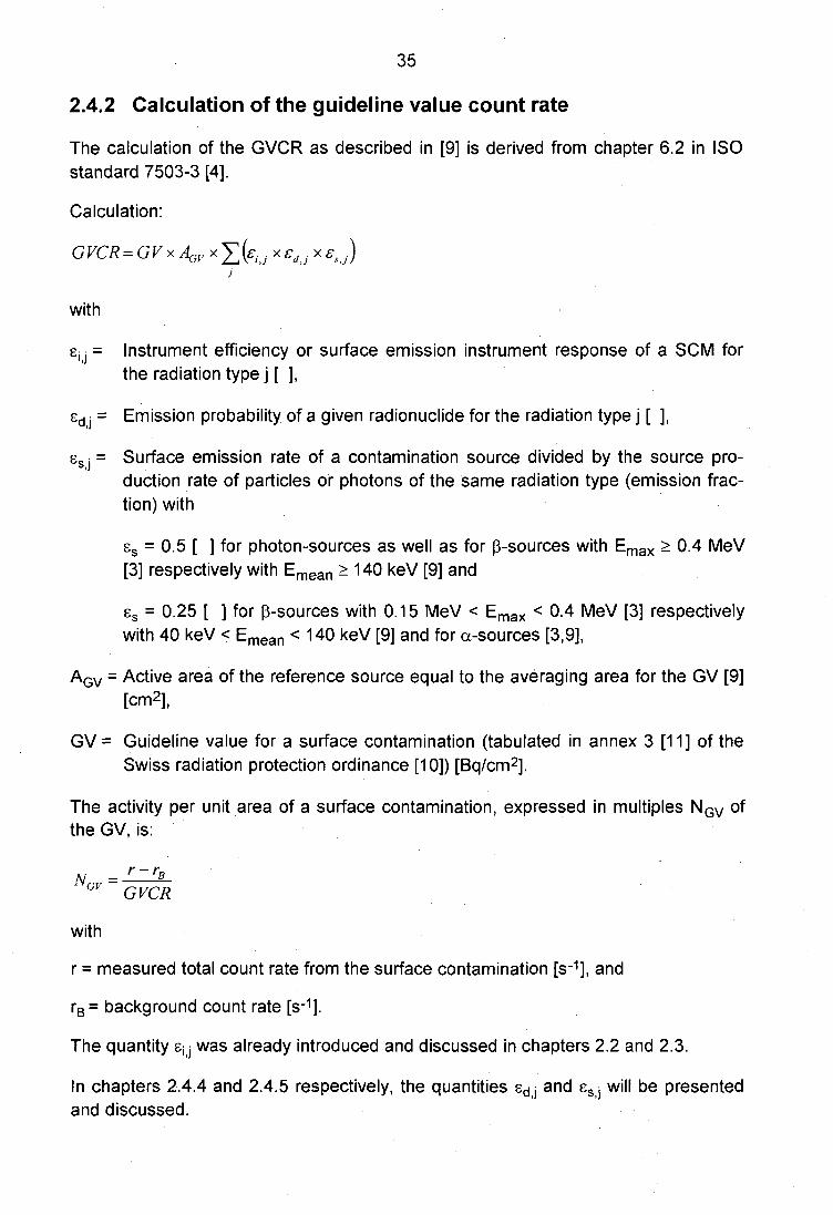
2.4 Determination of the guideline value count rate as relation to surface activity34

2.4.1 Definition of the guideline value count rate 34

2.4.2 Calculation of the guideline value count rate 35

2.4.3 Calculation of the guideline value count rate for a radionuclide mixture ....36

II

2.4.3.1 Calculation of the guideline value count rate for a radionuclide vector36

2.4.3.2 Calculation of the guideline value count rate for radionuclide pairs 37

2.4.3.2.1 Principal consideration 37

2.4.3.2.2 Radionuclide pairs with a single GV 38

2.4.3.2.3 Radionuclide pairs with individual GV 39

2.4.3.2.4 Calculation of parent and progeny weighting factors 39

2.4.3.2.5 Calculation of the guideline value count rate for radionuclidepairs with known mixture composition 41

2.4.4 Emission probability sdj of a radionuclide for the radiation type j 42

2.4.4.1 a, ß and photon emission probabilities sda , sdß and sdy 42

2.4.4.2 Treatment of positron decay data 43

2.4.4.3 Comparison of radionuclide decay data 45

2.4.5 Emission fraction ssj for the radiation type j 45

2.4.6 Consequences of summation effect on the instrument detectionefficiency 49

2.4.7 Example of a guideline value count rate determination 52

2.4.7.1 Sorting of 1-131 intensity data 52

2.4.7.2 Calculation of the summation term 52

2.4.7.3 Calculation of the guideline value count rate for 1-131 53

2.4.8 Uncertainty of guideline value count rates 53

2.4.9 Variation of guideline value count rates for instruments of the same type .54

2.5 Assessment of a guideline value count rate 56

3 SCM verification procedure 57

3.1 SCM verification requirements 57

3.2 Principal verification proceeding 57

3.2.1 Uncertainty of the maximum permissible errors 57

3.3 SCM verification examples 57

3.3.1 SCM sample for verification 58

3.3.2 Verification examples for groups of SCM with identical detector system ...58

3.3.3 Verification examples with a single BGVCR for selected radionuclides 58

3.3.4 Verification examples with several BGVCR 61

3.3.5 Variation of BGVCR number as function of SCM type 63

4 Discussion 65

4.1 Introductory remarks 65

4.2 Calibration discussion points 65

Ill

4.2.1 Calibration area relation 65

4.2.2 Calibration distance 66

4.2.3 Guideline value definition 66

4.2.4 Radionuclide emission data edj 66

4.2.5 Emission fraction ss j 67

4.2.6 Uncertainty of GVCR values 67

4.3 Verification discussion points 67

4.3.1 Conceptual use of the BGVCR 67

4.3.2 Verification of SCM with a single BGVCR for a radionuclide group 68

4.3.3 Verification of SCM with several BGVCR 68

5 Acknowledgements 69

6 References 70

IV

List of Tables

Table 1: List of calibrated SCM 4

Table 2: Selected technical SCM data 4

Table 3: SCM measurement result reading methodology to apply 5

Table 4: Basis radionuclides for the determination of the instrument efficiency 7

Table 5: Distances between construction and protective elements and foil ofdetectors 10

Table 6: Comparison of the calibration distance of this study with measuring

distances of surface contaminations 11

Table 7: Radionuclide pairs with only a single GV 38

Table 8: Examples of radionuclide pairs with individual GV 39

Table 9: Examples of parent and progeny radionuclide weighting factors 41

Table 10: Nuclear data as presented by software NuChart (example Cs-137/Ba) 42Table 11: Intensities summarized for ß and photon emission energy regions for

Cs-137/Ba 44

Table 12: Comparison of ENSDF, ICRP 38 and NEA edj data 46

Table 13: Example of summation effect for SCM CoMo170 ..' 51

Table 14: Example of summation effect for SCM DP6AD 51

Table 15: Added up intensities for beta and photon emission energy regions for

1-131 * : 52

Table 16: Calculation scheme for the summation term 53

Table 17: Uncertainty of GVCR 53

Table 18: Statistical data for GVCR determinations... 55Table 19: edj data of selected radionuclides intended for SCM verification 59

Table 20: BGVCR for a verification for the radionuclides Co-60, Cs-137/Ba,

Cs-134, Mn-54, Zn-65 und Sr-90/Y-90 60

Table 21: Example of a verification for a complex radionuclide composition 62

Table 22: Individual GVCR (in cps) variation for five SCM of the same type 63

Table 23: Variation of BGVCR as function of SCM type 64

V

List of Figures

Figure 1: Construction of the detector probe of SCM H1359C 8

Figure 2: Construction of the detector of SCM Senso 8

Figure 3: Construction of the detector of SCM LB122 9

Figure 4: Instrument efficiency profile for ß and photon emissions (upper part;chapter 2.3) and BGVCR (lower part; chapter 3.3.3) for SCM6150AD4-6150AD-k 15

Figure 5: Instrument efficiency profile for ß and photon emissions (upper part;chapter 2.3) and BGVCR (lower part; chapter 3.3.3) for SCMLB1210B-BZ100 16

Figure 6: Instrument efficiency profile for ß and photon emissions (upper part;chapter 2.3) and BGVCR (lower part; chapter 3.3.3) for SCMLB122-LB6357F..... 17

Figure 7: Instrument efficiency profile for ß and photon emissions (upper part;chapter 2.3) and BGVCR (lower part; chapter 3.3.3) for SCM LB124. 18

Figure 8: Instrument efficiency profile for ß and photon emissions (upper part;chapter 2.3) and BGVCR (lower part; chapter 3.3.3) for SCMContamat FHT 111 G 19

Figure 9: Instrument efficiency profile for ß and photon emissions (upper part;chapter 2.3) and BGVCR (lower part; chapter 3.3.3) for SCMMicrocontH13422/HXE260-10 20

Figure 10: Instrument efficiency profile for ß and photon emissions (upper part;chapter 2.3) and BGVCR (lower part; chapter 3.3.3) for SCMLB122-LB6358G 21

Figure 11: Instrument efficiency profile for ß and photon emissions (upper part;chapter 2.3) and BGVCR (lower part; chapter 3.3.3) for SCMH1359A-HGZI 22

Figure 12: Instrument efficiency profile for ß and photon emissions (upper part;chapter 2.3) and BGVCR (lower part; chapter 3.3.3) for SCMH1359C-HGZ200T 23

Figure 13: Instrument efficiency profile for ß and photon emissions (upper part;chapter 2.3) and BGVCR (lower part; chapter 3.3.3) for SCMContamat FHT 111 M 24

Figure 14: Instrument efficiency profile for ß and photon emissions (upper part;chapter 2.3) and BGVCR (lower part; chapter 3.3.3) for SCMLB124SCINT 25

Figure 15: Instrument efficiency profile for ß and photon emissions (upper part;chapter 2.3) and BGVCR (lower part; chapter 3.3.3) for SCMelectra 1A-DP6AD 26

Figure 16: Instrument efficiency profile for ß and photon emissions (upper part;chapter 2.3) and BGVCR (lower part; chapter 3.3.3) for SCM CoMo 17027

VI

Figure 17: Instrument efficiency profile for ß and photon emissions (upper part;chapter 2.3) and BGVCR (lower part; chapter 3.3.3) for SCM SE 3200 ..28

Figure 18: Comparison of ß radiation instrument efficiency 29

Figure 19: Comparison of photon radiation instrument efficiency 30

Figure 20: Comparison of a radiation instrument efficiency 32

Figure 21: Instrument efficiency decrease as function of distance from source forSCM electra 1A-DP6AD •... 33

Figure 22: Instrument efficiency decrease as function of distance from source forSCMCoMo170 33

VII

Definitions and Abbreviations

AD-kAP5ACoMo170DP6ADFHT111FHT111MH13422H1359AH1359CLB1210BLB122LB122GLB124LB124SRM5AP3RM6AP3Senso

BGVCR

SCM abbreviations —• table 1 in chapter 2.1.1 forexact device identification and serial number(s)

Calibration

Efficiency of a source, es

(emission fraction)

Emission probability, sd

(decay efficiency)

GV

Basis GVCR. GVCR reference value for verifica- [8]tion, defined in a way that the radionuclide speci-fic GVCR do not deviate more than the ±50%MPEV from the BGVCR

Set of operations that establish, under specified [26]conditions, the relationship between values ofquantities indicated by a measuring instrument ormeasuring system, or values represented by amaterial measure or a reference material, and thecorresponding values realised by standards

Ratio between the number of particles of a given [3]type above a given energy [or of photons] emerg-ing from the front face of a source or its windowper unit time (surface emission rate) and thenumber of particles of the same type [or of pho-tons] created or released within the source (for athin source) or its saturation layer thickness (for athick source) per unit time

Ratio of the number of particles or photons of a [4]given energy created per unit time by a given ra-dionuclide to the number of decays of this radio-nuclide per unit time

Guideline value in Bq/cm2 for the surface conta-mination. Valid as the average value of 100 cm2

contaminated surface

[11]

VIII

GVCR

Instrument efficiency,

METAS

MPEV

SCM

Source production rate

Surface emissioninstrument response

Guideline value count rate: Net count rate of a [8]SCM which is generated by a wide area source of100 cm2 area having the surface activity of oneGV

Ratio of the instrument net reading to the surface [4]emission rate of a source for particles or photonsof a given energy under given geometric condi-tions

Swiss Federal Office of Metrology

Maximum permissible errors of verification

Surface contamination meter

Traceability

Verification

[26]

Number of particles produced by the decay pro- [4]cess(es) in the source, or the number of photonsof given energy(ies) produced by decay in thesource, per unit time

—• Instrument efficiency

Surface emission rate, q2TT Number of particles above a certain energy, or [4]number of photons whose origin is as describedfor production rate, emerging from the surface ofthe source per unit time

Property of the result of a measurement or the [26]value of a standard whereby it can be related tostated references, usually national or internationalstandards, through an unbroken chain of compa-risons all having stated uncertainties

Sequence of operations carried out by an empow- [1]ered authority or organisation to test and confirmthat a measuring device satisfies legal regulations

1 Introduction

1.1 SCM measurement procedure standardisation

In Switzerland, the demand that surface contamination meter (SCM) measurementresults should be in a simple manner and safely interpretable has a long tradition. Anessential step towards the fulfillment of this demand was the introduction andcommon use of the radionuclide specific quantity "guideline value" (GV; chapter2.4.1) as unit for surface contamination activities (Example: 1 GV Co-60 correspondsto a surface contamination Co-60 activity per unit area of 3 Bq/cm2 averaged over100 cm2 area). The according instrument response is defined as "guideline valuecount rate" (GVCR).

The next step towards a simplification of measurement procedures combines ra-dionuclide specific GVCR, as result of SCM calibration, to a "basis guideline valuecount rate" (BGVCR; chapter 3.2) as verification reference value for a group ofradionuclides. This concept can, where possible, be extended to all SCM of the sametype or to SCM of different producers with the same principle of detection.

1.1.1 Requirements on the SCM calibration procedure

The calibration procedure has to be standardised and traceable to internationallyacknowledged standards.

A multisource calibration technique is applied to determine the instrument efficiencyfor four different ß radiation energy regions, for four different photon radiation energyregions and for an a radiation energy region (chapter 2.2.1). Thus, the instrumentsensitivity refers to selected energy regions instead to the specific radionuclides usedfor calibration. The a, ß or photon surface emission rate of the calibration sources iscertified.

The relation to the activity per unit area of a surface contamination in units of theguideline value count rate is calculated using instrument efficiency, radionuclidedecay data, emission fraction, averaging area, and guideline value (chapter 2.4.2). Inthis way the evaluation of surface contaminations is possible for any radionuclide.

1.1.2 Requirements on the SCM verification procedure

The bundling of radionuclide specific calibration results to one or several reasonablychosen reference values is limited by the maximum permissible errors of verification(MPEV) (chapter 3.2).

Consistent BGVCR (chapter 3.2) as reference values for defined radionuclide groupsare chosen by adequately using the space given by the MPEV.

1.2 Legal SCM verification basis

A verification obligation exists in Switzerland for SCM which are used for specificlegally binding measurement tasks. First respective verification directives have beenpublished by the Swiss Federal Office of Metrology (METAS) [2]. Implemented inthese directives, based on ISO standards [3,4,5], is a SCM verification procedureincluding calibration requirements.

Usually, the result of a verification is in general a pure yes/no answer about themeasurement result lying within the MPEV for a specific measuring instrument class.Verification therefore demands an existing calibration of the instrument. If such a cali-bration is not available, a calibration can be included into the verification task.

1.3 Purpose of the study on hand

SCM calibration and verification procedures and first experiences have been de-scribed in [6,7,8]. Based on [8], the METAS directives have been revised in 2002 [9].

In this study, SCM calibration and verification procedures and techniques followingthe revised METAS verification directives [9] are presented and discussed. The aimof the study, however, is not a pure theoretical treatment of principles but a de-scribtion of the practical aspects of calibration and verification procedures. Criticalparameters for the calibration of SCM are presented and discussed.

Representative samples of the PSI a, ß/y and oc/ß/y SCM stock have been used toprovide information on both procedures by means of practical results.

2 SCM calibration procedure

Calibration of SCM according to [9] is a two step procedure. The first step consists ofthe determination of the instrument efficiency or surface emission instrument re-sponse (chapter 2.2). The relation between instrument response, the surface activityper unit area of a contamination and guideline value yields the instrument specificguideline value count rate (chapter 2.4).

2.1 SCM requirements

Construction as well as measuring technique properties of an SCM have to beadequate to the provided measuring task and represent state of the art to renderthem eligible for calibration and verification according to [9].

Furthermore, an SCM has to indicate a count rate or a multiple of the radionuclidespecific guideline value for the surface contamination listed in annex 3 [11] of theSwiss radiation protection ordinance [10]. Additional to an indication of the multiple ofthe radionuclide specific guideline value, the instrument indication must also beswitchable to countrate indication.

2.1.1 SCM sample for calibration

Table 1 lists the SCM calibrated at PSI according to [9]. The meters are groupedaccording to their detection principle. The bulk of these instruments is used at PSIand at Swiss nuclear power plants. Since these instruments do not in every case re-present the actual state of SCM technology, the SCM sample was completed withSCM supplied by their Swiss distributors (LB124, LB124 SCINT, ContamatFHT111M, SE 3200) or by other SCM users (H1359C-HGZ 200T, MicrocontH13422-HXE 260-10).

Each of the instruments listed in table 1 has a sensitive window area of the detectorequal to or larger than 100 cm2 (table 2).

Table 1: List of calibrated SCM

Device group(Detector type)

Xe-filled sealedproportional detector

Gas-flowproportional detector

Plastic/Zn(Ag)Sscintillator detector

Zn(Ag)S scintillatordetector

Manufacturer

AutomessBertholdBertholdBertholdFAGHerfurth

BertholdHerfurthHerfurthThermo Eberline ESM

BertholdNE TechnologyS.E.A.Sensomess

NE TechnologyNE TechnologyNE Technology

Device identification

6150AD4-6150AD-kLB1210B-BZ100LB122-LB6357FLB124ContamatFHT 111 GMicrocont H13422-HXE260-10

LB122-LB6358GH1359A-HGZIH1359C-HGZ200TContamat FHT 111 M

LB124SCINTelectra 1A-DP6ADCoMo 170*SE 3200

electra 1A-AP5ARM5-AP3RM6-AP3

Serial number(s)

72140-723505570-38133970-403236515-10131085-2142358-919

5202-2765360-565486-4693928-591

10-60784041-225103551012

1454-3231598-34760-3239

Abbreviation

AD-kLB1210BLB122LB124FHT111H13422

LB122GH1359AH1359CFHT111M

LB124SDP6ADCoMo170Senso

AP5ARM5AP3RM6AP3

* model development considered by the end of 2005

Table 2: Selected technical SCM data

Instrument

AD-kLB1210BLB122LB124FHT111H13422

FHT111MLB122GH1359AH1359C

LB124SCoMo170DP6ADSenso

AP5ARM5AP3RM6AP3

Detector type

Xe-filled sealedproportional detector

Gas-flowproportional detector

Plastic/Zn(Ag)Sscintillator detector

Zn(Ag)S scintillatordetector

Detector window area(manufacturer specification)

[cm x cm]

10.0x17.010.0x10.011.8x 19.011.8x19.010.0x15.611.2x22.6

10.0x16.611.8x19.011.7 x 18.911.7x18.9

11.8x14.510.0x17.06.7x15.010.0x12.0

6.7x15.010.0x10.010.0x10.0

Radiationsensitivity

a,ß,yß,Yß,Yß,Yß,Yß,Y

a,ß,ya, ß,ya, ß,ya, ß,Y

a, ß,Ya, ß,ya, ß,Ya,ß,y

aaa

Countrate

indication

digitalanalogue

digitaldigital

analoguedigital

digitaldigital

analogueanalogue

digitaldigitaldigitaldigital

digitalanalogueanalogue

2.1.2 Measurement result reading methodology

Not all the instruments listed in table 2 indicate the count rate as a digital value.Whereas most digital indicating SCM perform an integration over a given time in-terval, SCM with analogue display delegate the averaging of readings ambitious es-pecially at low count rates to the user. Standardized procedures have therefore beendeveloped (table 3) which compensate for the missing integrating measurement mo-de of analogue instruments. Such standardised procedures are necessary for the de-rivation of detection limits according to ISO standards [12] for integrating instruments.

Measurement times used in the calibration procedure exceed 20 s for the instrumentbackground determination and 60 s for the measurement of the calibration source.

Table 3: SCM measurement result reading methodology to apply

Indication Procedure Device

Analogue - During the chosen measurement period, take a reading each second or in LB1210Ba frequency as high as possible and calculate average of all readings. FHT111Alternatively: Observe continuously minimum and maximum readings du- H1359Aring the chosen measurement period and calculate average of largest and H1359Clowest reading (pay attention if scale is logarithmic).1) RM5AP3

RM6AP3

Digital - Read measurement value after termination of chosen measurement pe- LB122riod (Accuracy of measurement value is increasing with increasing mea- LB122Gsurement time). H13422

Senso

Adjust integration time and start measurement. CoMo170FHT111MLB124LB124S

Use measurement modus "Indication of mean" and read measurement AD-kvalue after termination of chosen measurement period.

Read measurement value after termination of chosen measurement pe- AP5Ariod (A floating mean is indicated for measurement times exceeding eight DP6ADseconds duration).

1) Note: Because maximum and minimum count rates are low probability events, the observation period shouldbe chosen as long as possible and maintainable in order to avoid the risk of producing wrong readings.

2.2 Determination of the instrument efficiency

2.2.1 Calibration sources

Calibration has to be performed by a prescribed [8,9] set of basis radionuclide refe-rence sources with 10 cm x 10 cm active area and certified a, ß or photon surfaceemission rate q2TT (table 4). These reference sources are consistent with international

ISO standards [3,4,5]. Use of such calibration sources guarantees traceability to in-ternational standards. Respective uncertainties between 1.5% and 6% (coverage fac-tor k = 1; 68% confidence level) of the surface emission rate q2TT as stated in therespective certificates are given in table 4. These calibration reference sources areused as emitters of alpha particles, electrons or photons of a particular energy range.They are not perceived as sources of particular radionuclides.

The calibration sources for the photon energy regions are where necessary coveredwith filters according to [5] for the suppression of the ß radiation (table 4).

Table 4: Basis radionuclides for the determination of the instrument efficiency

Radionuclide Emission type Relative emission Uncertainty ofprobability surface emission rate q2TT

[%, coverage factor k = 2]

Emission energy [keV]

Am-241 alpha 1.0

C-14

Tc-99

CI-36

Sr-90/Y-90

beta

beta

beta

beta

1.0

1.0

0.98

1.0 each

3.3

3.0

3.0

3.0

Fe-55

1-129

Co-57

Cs-137

Co-60

photon

photon*

photon*

photon*

photon*

0.28

0.78

0.96

0.85

2.0

9

9

7

10

12

Energy region for all alpha emitters

5390 - 5490

Energy regions for beta emitters (average energy)

40-70

50

5-15

70-140 140-400 >400

85

250

190 940

Energy regions for photon emitters

15-90 90 - 300 >300

32

124

660

1200

*Supression of electron emission by means of filters according to [5].

8

2.2.2 Calibration distance

In article 7.6, the METAS directives [9] require a distance between reference sourceand detector window of 5 mm.

However, the term "detector window" is rather a general notation. The detector foil ofSCM is covered by a variety of constructive and protective elements. Very differentdetector construction and protection principles can be observed for the instrumentslisted in table 1. In table 5, distances between the various detector elements aregiven.

An example of an elementary construction is given by the detector probe of SCMH1359C (figure 1). The detector foil is covered by a grid constituting also the frame ofthe detector. A detector protective grille is missing and the distance from the foil tothe frame under edge is small. Similar construction principles have been realised forthe detectors of SCM AP5A, DP6AD, H13422, H1359A, LB1210B, LB124, LB124S,RM5AP3 and RM6AP3.

Figure 1: Construction of the detector probe of SCM H1359C

An additional frame is mounted on the grid of the detectors of SCM FHT111,FHT111M, LB124, LB124S and Senso (example Senso in figure 2). This additionalframe can be identical with the SCM housing (e.g. SCM LB124, LB124S and Senso).

Figure 2: Construction of the detector of SCM Senso

SCM AD-k, CoMo170, FHT111, FHT111M, LB122, and LB122G are equipped wihdetectors of a more complex design having a protective grille which is significantlyfiner in comparison to the grid (example LB122 in figure 3).

Figure 3: Construction of the detector of SCM LB122

One of the main goals of the SCM calibration performed for this study was to obtaincomparable surface emission instrument responses. For this reason, the foil of thedetector instead of a constructive or protective detector element was taken as pointof reference for the calibration distance. In order to obtain a small distance betweendetector foil and surface of reference source, distance holders of 5 mm thicknesswere mounted either on the grid or on the protective grille of the detector. The co-lumn "Calibration distance source - foil" on the right hand side of table 5 shows that inthis way the resulting distances between detector foil and reference source surfacevary between 6 mm and 7.5 mm. The mean distance is 6.6 mm with a variation co-efficient of 9%.

These calibration distances can now be compared to distances between foil and con-tamination surface for a SCM in a measurement position "support" (i.e. the SCMstands on the surface) and in a measurement position allowing 5 mm distance bet-ween contamination surface and detector frame. Respective distances contaminationsurface - detector foil are given in table 6.

Positioning the instrument on the surface (mid column in table 6) raises the variationcoefficient for the distance contamination surface - detector foil up to 50%. With5 mm distance between contamination surface and detector frame, the variation co-efficient would be lowered to 18%. Note that the values given in the right column oftable 6 are in seven cases equal to the distances reference source - detector foilobtained for the calibration geometry (left column in table 6).

10

Table 5: Distances between construction and protective elements and foil of detectors

SCM

AD-k

LB1210B

LB122

LB124

FHT111

H13422

LB122G

H1359A

H1359C

FHT111M

LB124S

DP6AD

CoMo170

Senso

AP5A

RM5AP3

RM6AP3

Foot-frame

1.5

2.0

1.0

1.5

1.0

2.0

4.0

1.5

1.5

Frame -protective grille

1.4

2.0

3.2

2.5

3.3

1.5

Protective grille -grid

1.6

1.5

0.5

1.2

1.0

Distances [mm]

Frame -grid

3.5

3.8

0.3

4.3

3.3

4.2

Grid-foil

0.5

0.5

1.0

0.5

1.0

1.0

2.0

2.0

0.5

2.2

2.5

3.5

1.0

2.5

1.0

1.0

Frame -foil

3.5

1.0

4.0

4.5

4.0

1.3

4.7

2.0

2.0

4.8

5.5

2.5

3.5

5.2

2.5

1.0

1.0

Protective grille -foil

2.1

2.0

1.0

2.2

1.5

2.0

Calibration distancesource - foil

7.1

6.0

7.0

6.0

6.0

6.0

7.2

7.0

7.0

65

7.2

7.5

7.0

6.0

7.5

6.0

6.0

11

Table 6: Comparison of the calibration distance of this study with measuringdistances of surface contaminations

SCM Calibration distance [mm] Distance surface contamination - foil [mm]

source - foil at support on surface at 5 mm distance from frame

3.5 8.5

2.5 6.0

6.0 9.0

4.5 9.5

4.0 9.0

2.3 7.3

6.2 9.7

2.0 7.0

2.0 7.0

5.8 9.8

5.5 10.5

2.5 7.5

5.5 8.5

9.2 10.2

2.5 7.5

2.5 6.0

2.5 6.0

In consequence of the results shown in table 6, SCM calibrated with a distance of5 mm between grid or protective grille and reference source with one exception over-estimate contaminations in the measuring geometry "support". A correct evaluation oran underestimation of the contamination can be observed for a measurement dis-tance of 5 mm between detector frame and contamination surface.

The comparability of instrument efficiencies determined with a calibration distance asdescribed above is conform with the requirements posed in chapter 1.1. An other ap-proach would be to ask each SCM owner demanding calibration for the measuringdistance of a surface contamination and to calibrate using this distance. However,surface contaminations are usually measured by placing the instrument on thesurface or holding it at a minimal distance to the surface. The calibration distanceintroduced in this chapter is therefore considered to be an adequate approximationfor this practice.

2.2.3 Calibration proceeding

Each calibration source is positioned in a center position below the detector windowarea. Multiple measurements of the calibration source over the whole detector areaas recommended in ISO standard 7503-1 [3] and calculation of a mean surface

AD-k

LB1210B

LB122

LB124

FHT111

H13422

LB122G

H1359A

H1359C

FHT111M

LB124S

DP6AD

CoMo170

Senso

AP5A

RM5AP3

RM6AP3

7.1

6.0

7.0

6.0

6.0

6.0

7.2

7.0

7.0

6.5

7.2

7.5

7.0

6.0

7.5

6.0

6.0

12

emission instrument response for the entire sensitive detector window are omitted.As an alternative method, the homogeneity Of the detector efficiency is checked bymeans of measurements with point sources positioned in center and corners of thedetector window.

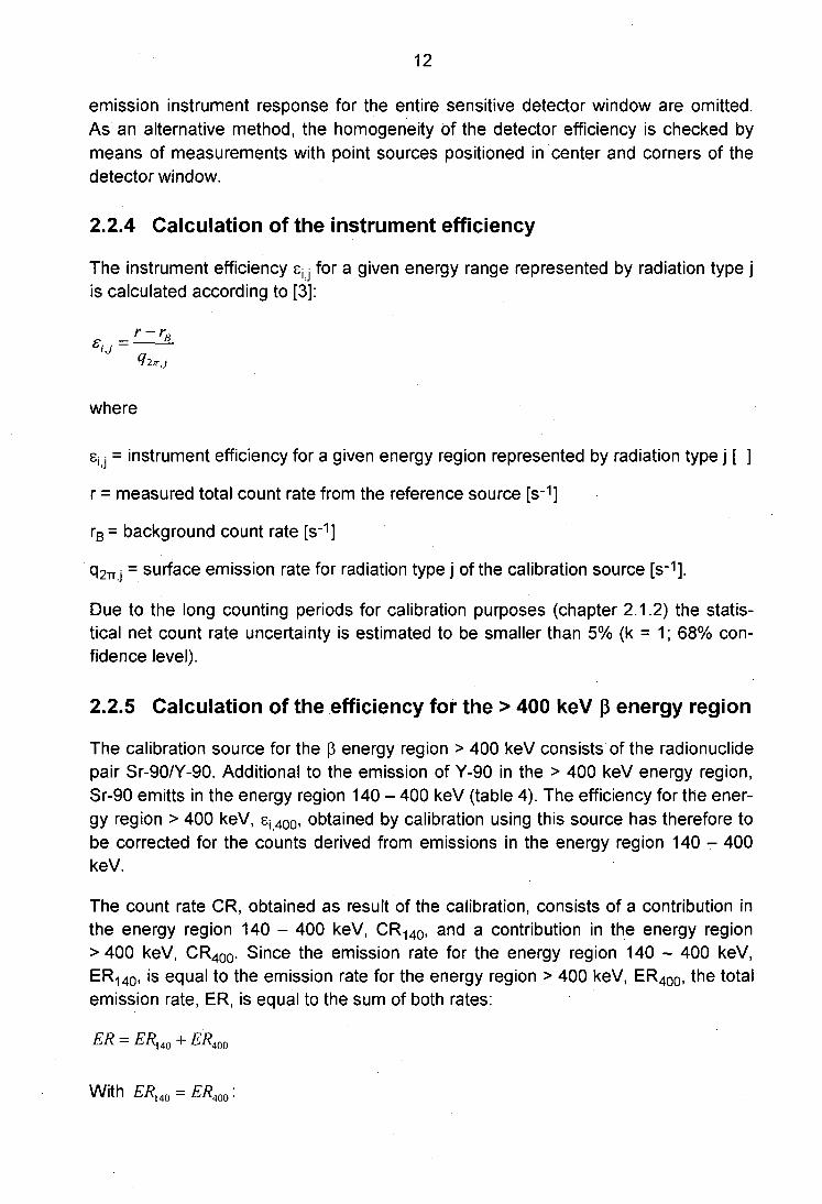
2.2.4 Calculation of the instrument efficiency

The instrument efficiency e^ for a given energy range represented by radiation type jis calculated according to [3]:

r - rR

where

Sjj = instrument efficiency for a given energy region represented by radiation type j [ ]

r = measured total count rate from the reference source [s"1]

rB = background count rate [s"1]

q2TT j = surface emission rate for radiation type j of the calibration source [s"1].

Due to the long counting periods for calibration purposes (chapter 2.1.2) the statis-tical net count rate uncertainty is estimated to be smaller than 5% (k = 1; 68% con-fidence level).

2.2.5 Calculation of the efficiency for the > 400 keV ß energy region

The calibration source for the ß energy region > 400 keV consists of the radionuclidepair Sr-90/Y-90. Additional to the emission of Y-90 in the > 400 keV energy region,Sr-90 emitts in the energy region 140 - 400 keV (table 4). The efficiency for the ener-gy region > 400 keV, 8Ji400, obtained by calibration using this source has therefore tobe corrected for the counts derived from emissions in the energy region 140 - 400keV.

The count rate CR, obtained as result of the calibration, consists of a contribution inthe energy region 140 - 400 keV, CR140, and a contribution in the energy region> 400 keV, CR400. Since the emission rate for the energy region 140 - 400 keV,ER140, is equal to the emission rate for the energy region > 400 keV, ER400, the totalemission rate, ER, is equal to the sum of both rates:

ER = ERl40 + ER400

With ERl40 = ER400:

13

ER - 2ERH0 - 2ER400.

From a measurement of the 140 - 400 keV energy region calibration source (CI-36),the efficiency for this region, e,iCh is known:

_'Cl ~ ER, 40

The total efficiency for the energy regions 140 - 400 keV and > 400 keV, e, SrY, isderived from a measurement of the > 400 keV energy region Sr-90/Y-90 calibrationsource.

The total efficiency, 8iiSrY, can be calculated as:

e _ Ci? _ (C7?,40 + CR400) _ C7?,40 | CR4Q0

''Sr¥ ER ER ER ER

, ^400 _ ! C^40 , !

2ER 2 ER 22ER]40 2ER400 2 ER^^ 2 ER400

J~ ~ Si,Cl + ~ ^(,400

So it follows that:

Rearranged:

£i,400 = A'Si,SrV ~ ~^ei,Cl •

To summarize the formula given above: The efficiencies determined by means of the140 - 400 keV energy region calibration source (CI-36) and by means of the140 - 400 keV plus > 400 keV energy region calibration source (Sr-90/Y-90) are usedto calculate a corrected efficiency for the > 400 keV energy region.

2.2.6 Calculation of the efficiency for the > 300 keV photon energyregion

Two different basis radionuclide reference sources (Cs-137 and Co-60) are availablefor the > 300 keV photon energy region. The instrument efficiency in this energyrange is chosen as average of the calibration results obtained with both prescribedreference sources (table 4). Would a SCM be calibrated with the Co-60 calibration

14

reference source only, the efficiency for the > 300 keV photon energy region wouldbe higher.

2.2.7 Determination of the instrument efficiency for singleradionuclides

If a calibration for a particular radionuclide has to be performed, calibration sourcescan be selected according to the ß and photon radiation emission characteristics ofthe radionuclide (article 7.4 in [9]). This can be illustrated by the radionuclide exam-ple Co-60, which has emissions in the ß energy region 70 -140 keV and in the pho-ton energy region > 300 keV or by the radionuclide example Tc-99m, which emitselectrons in the beta energy region 7 0 - 1 4 0 keV and photons in the energy regions1 5 - 9 0 keV and 90 - 300 keV. The sources to be used for calibration in these casesare the sources designated for the respective energy regions (table 4).

2.3 Results of instrument efficiency determinations

Calibration results for the ß and photon radiation sensitive SCM listed in tables 1 and2 are summarised in surface emission instrument response profiles or instrumentefficiency profiles for ß and photon emissions (upper part of figures 4 -17 ) . Figure 20allows a comparison of the a radiation surface emission instrument response for thea radiation sensitive SCM.

The probes of instrument DP6AD and AP5A with 100 cm2 area (table 2) are smallerthan 10 cm and the calibration reference sources. To account for this, the efficienciesfor these two SCM obtained by calibration with the quadratic reference sources aremultiplied by a factor of 10 cm/6.7 cm = 1.5.

The instrument efficiency profiles for ß and photon emissions appearing in the upperpart of figures 4 - 1 7 are discussed in chapters 2.3.1 and 2.3.2, respectively. Alpharadiation instrument efficiencies are compared in chapter 2.3.3.

15

6150AD4-6150AD-k 72140-72350

O

LJJ

iI

Electrons Photons

1 1

a:ao

6150AD4-6150AD-k 72140-72350 - BGVCR 83 cps

Co-60 Cs-137/Ba Cs-134 Mn-54 Zn-65 Sr-90A'

Radionuclide

Figure 4: Instrument efficiency profile for ß and photon emissions (upper part;chapter 2.3) and BGVCR (lower part; chapter 3.3.3) for SCM 6150AD4-6150AD-k

16

LB1210B-BZ100 5570-3813

„ 0 8

i 07

f 0.6vc

0.5

0.4

8. 0.3

I 0.20

si 0.1

0.0i

Electrons Photons

a>

o

LB1210B-BZ100 5570-3813 - BGVCR 53 cps

Co-60 Cs-137/Ba Cs-134 Mn-54

Radionuclide

Zn-65 Sr-90/Y

Figure 5: Instrument efficiency profile for ß and photon emissions (upper part;chapter 2.3) and BGVCR (lower part; chapter 3.3.3) for SCM LB1210B-BZ100

17

LB122-LB6357F 3970-4032

LB122-LB6357F 3970-4032 - BGVCR 51 cps

toQ.

croo

100

90

80

70

60

50

40

30

20

10

0

m

MF3EV +

/

-50% |-

- -H

-Co-60 Cs-137/Ba Cs-134 Mn-54

Radionuclide

Zn-65 Sr-90/Y

Figure 6: Instrument efficiency profile for ß and photon emissions (upper part;chapter 2.3) and BGVCR (lower part; chapter 3.3.3) for SCM LB122-LB6357F

18

0.8

o•g» 0.6

>

CÜ

0.5

0.4

S. 0.3 HÜC 0.2

g 0.1LU

0.0

I1

LB124 36515-1013

Electrons Photons

<D <D

O

ooo

LB124 36515-1013 - BGVCR 55 cps

Co-60 Cs-137/Ba Cs-134 Mn-54

Radionuclide

Zn-65

Figure 7: Instrument efficiency profile for ß and photon emissions (upper part;chapter 2.3) and BGVCR (lower part; chapter 3.3.3) for SCM LB124

19

Contamat FHT 111 G 1085-2142

g

CD

CU

<DQ .

O

CDO

£LJJ

0.8

0.7

0.6

0.5

0.4

0.3

0.2

0.1

0.0

Electrons Photons

I I _ H

1 1 is2

ID to a>

o

in

ooCOoO5

oocoA

Contamat FHT 111 G 1085-2142 - BGVCR 57 cps

110

100

90

MPEV +- 50%

80

To 70Q.

Ä 60

Ü 50

CD 4030

20

10

0Co-60 Cs-137/Ba Cs-134 Mn-54

Radionuclide

Zn-65 Sr-90/Y

Figure 8: Instrument efficiency profile for ß and photon emissions (upper part;chapter 2.3) and BGVCR (lower part; chapter 3.3.3) for SCM ContamatFHT 111G

0.8

£ °7

• | 0 .6

§ 0.5

§ 0.4

IIUJ

0.2

0.0

20

Microcont H13422-HXE260-10 358-919

Electrons Photons

^m • _•o

mQ

70-1

Q

1a>ooA

<V

mi n

a>o

15-

•oQ

90-3

<D

OOCOA

Microcont H13422-HXE260-10 358-919 - BGVCR 61 cps

110

100

90

80

In 70a.Ä 60

O 50>CD 40

30

20

10

0

1

J

MPEV +-

/50%

mi _

= =Co-60 Cs-137/Ba Cs-134 Mn-54

Radionuclide

Zn-65 Sr-90/Y

Figure 9: Instrument efficiency profile for ß and photon emissions (upper part;chapter 2.3) and BGVCR (lower part; chapter 3.3.3) for SCM Microcont H13422/HXE260-10

21

LB122-LB6358G 5202-2765

—

gion

- ene

rgy

rey

pe

Efn

cien

c

VJ.V

0.7 -

0.6 -

0.5

0.4

0.3

0.2 -

0.1 -

0.0

Electrons40

-70

keV

70-1

40 k

eV

40-4

00 k

eV

> 400

keV

5-15

keV

1

Photons

15-9

0 ke

V

90-3

00 k

eV

> 30

0 k

eV

80

70

60

[cps

GV

CR

50

40

30

20

10

LB122-LB6358G 5202-2765 - BGVCR 46 cps

f MPEV+-50% |S

• • I

Co-60 Cs-137/Ba Cs-134 Mn-54

Radionuclide

Zn-65 Sr-90/Y

Figure 10: Instrument efficiency profile for ß and photon emissions (upper part;chapter 2.3) and BGVCR (lower part; chapter 3.3.3) for SCM LB122-LB6358G

22

0.8

i °7

I 0.6

CDQ.

CCDO

111

ra 0.5 ^CDCCD 0.4

0.3

0.2 -

0.1 -

0.0

H1359A-HGZ I 360-565

Electrons Photons

1 o 8o

<a

ocpin

8co

8

ID

8COA

H1359A-HGZ I 360-565 - BGVCR 58 cps

a:oo

uu

90 -

80

70 -

50

40

20

10 -

0 -

MPEV +- 50%4

—

pi

-

•

Co-60 Cs-137/Ba Cs-134 Mn-54

Radionuclide

Zn-65

Figure 11: Instrument efficiency profile for ß and photon emissions (upper part;chapter 2.3) and BGVCR (lower part; chapter 3.3.3) for SCM H1359A-HGZ I

23

H1359C-HGZ 200T 486-469

0.8

r 0.7if

ILU

0.6

0.5

0.4

0.3

0.2

0.1

0.0

Electrons Photons

i3

i 1

5-90 30

0 o

sA

H1359C-HGZ 200T 486-469 - BGVCR 49 cps

80 -i

70 -

60

•gso-_oa: 40oO 30

20 -

10

0

" MPEV+-50% !

Co-60 Cs-137/Ba Cs-134 Mn-54

Radionuclide

Zn-65 Sr-90/Y

Figure 12: Instrument efficiency profile for ß and photon emissions (upper part;chapter 2.3) and BGVCR (lower part; chapter 3.3.3) for SCM H1359C-HGZ 200T

24

Contamat FHT 111 M 3928-591

0.7

0.6

0.5 ̂

0.4

0.3 ̂

0.2

o.i ̂

0.0

Electrons

1I

Photons

o•«t

<uooo

ioo

>ocpin

>

58°?oCO

Contamat FHT 111 M 3928-591 - BGVCR 55 cps

ex

a:o

ID

an

80

7f1

60

50

40

30 -

20

10

n - wnrm

Co-60

•1

Cs-137/Ba (

MPEV +- 50% -

:s-134 Mn-54

Radionuclide

Zn-65 c3r-90r<

Figure 13: Instrument efficiency profile for ß and photon emissions (upper part;chapter 2.3) and BGVCR (lower part; chapter 3.3.3) for SCM ContamatFHT 111M

25

LB124SCINT 10-6078

Q)

IHI

0.8

0.7

0.6

0.5

0.4

0.3

0.2 ^

0.1

0.0

Electrons Photons

l1

£

LB124 SCINT 10-6078 - BGVCR 73 cps

130 i120 -1 in -

iftfi

90 -

2. so— 70

g 60-CD 5 0

4030

2010 -n -

MPEV +- 50%I 1 /

Co-60

-•1

i i > i

Cs-137/Ba Cs-134 Mn-54 Zn-65 Sr-90/Y

Radionuclide

Figure 14: Instrument efficiency profile for ß and photon emissions (upper part;chapter 2.3) and BGVCR (lower part; chapter 3.3.3) for SCM LB124 SCINT

0.8

— 0.7

f 0-6§> 0.5

I 0.42. 0.3

0)

LU

0.2

0.1

0.0

26

electra 1A-DP6AD 4041-2251

Electrons Photons

o

40-

d>

o

o

d)

oo

0-4

0)

ooA

d>

in

in

d)

oCD

15-

ooCO

1

oen

>

A

90

80

70

_ 60Q.

Ü 50a:o 400 30

20

10

electra 1A-DP6AD 4041-2251 - BGVCR 44 cps

•MPEV ± 50%/

Co-60 Cs-137/Ba Cs-134 Mn-54

Radionuclide

Zn-65 Sr-90/Y

Figure 15: Instrument efficiency profile for ß and photon emissions (upper part;chapter 2.3) and BGVCR (lower part; chapter 3.3.3) for SCM electra 1A-DP6AD

27

CoMo 170 0355

o

8.

o

LU

0.8

0.7

0.6

0.5

0.4

0.3

0.2

0.1

0.0

Electrons Photons

8 8•<*•

A

190180170160150140

„ 130£ 120Ü 110a: iooo 90

80Ü 70

605040 -I3020 -I100

CoMo 170 0355 - BGVCR 110 cps

Co-60 Cs-137/Ba Cs-134 Mn-54 Zn-65

Radionuclide

Figure 16: Instrument efficiency profile for ß and photon emissions (upper part;chapter 2.3) and BGVCR (lower part; chapter 3.3.3) for SCM CoMo 170

28

SE 3200 1012

0.8

- 0.7 H

£ 0.6

p 0.5cug 0.4cu

oc(Po

LU

0.3

0.2

0.1

0.0

Electrons Photons

I I

O

70-1

5ooo•<!•

<D

OO

A

<D

l O

m

0)

OCt)

ooCO

SE 3200 1012 - BGVCR 41 cps

CD

70

60

50

40

30

20

10

0

_•r

MPEV +- 50%

F\

Co-60 Cs-137/Ba Cs-134 Mn-54

Radionuclide

Zn-65

Figure 17: Instrument efficiency profile for ß and photon emissions (upper part;chapter 2.3) and BGVCR (lower part; chapter 3.3.3) for SCM SE 3200

29

2.3.1 Discussion of instrument efficiency for ß radiation

The individual SCM efficiency data given in figures 4 - 1 7 are summarized in figure

18 for a comparison of the ß radiation surface emission instrument response.

Comparison of beta radiation instrument efficiency

Efficiencyper energy region

•40 - 70 keV• 70-140keVD140-400keVD>400keV

Figure 18: Comparison of ß radiation instrument efficiency

2.3.1.1 SCM with Xe-filled sealed proportional detector

In figure 18, the data for the SCM with Xe-filled sealed proportional detector areindicated in the left hand side data block. Efficiencies for the 40 - 70 keV energyregion and for the 70 -140 keV energy region differ only slightly. Greater differencesare observed for the efficiencies of the 140 - 400 keV and the > 400 keV energyregion. Slightly enhanced efficiencies for the 70 - 140 keV and > 400 keV energyregions show SCM LB124 and H13422.

2.3.1.2 SCM with gas-flow proportional detector

The data for the SCM with gas-flow proportional detector are indicated in the mid da-ta block of figure 18. Remarkable is the overall higher efficiency for all energy regionsof this SCM group relative to the SCM group with Xe-filled sealed proportionaldetector. In comparison to the other Herfurth instrument H1359C the data for SCMH1359A are outstanding. The reason for these efficiency differences may be theenhanced usage of the SCM H1359C leading to an efficiency decrease. The greatestrelative variation of efficiency data in this instrument group is shown in the > 400 keVenergy region.

30

2.3.1.3 SCM with plastic/Zn(Ag)S scintillator detector

The efficiency data for this SCM group indicated in the right hand side data block offigure 18 are very inconsistent. Whereas two instruments show low ß radiation sur-face emission instrument responses, the other two reveal data exceeding the data forthe remaining SCM of this group. Factoring out the data for these high instrumentefficiency SCM it can be stated that the efficiency data for the energy regions140 -400 keV and > 400 keV are comparable to the data for the SCM group withgas-flow proportional counter detector.

2.3.2 Discussion of instrument efficiency for photon radiation

Figure 19 shows the summarized photon radiation surface emission instrument res-ponses. For better visibility, the appearance sequence of the energy regions is re-versed so that the efficiency data for the > 300 keV energy region appear in thefrontside data row of the diagram.

Comparison of photon radiation instrument efficiency

0.14

0.12

0.10

Efficiency 0.08per energy region

[ ] 0.06

0.04

0.02

0.00• >300keV• 90D15• 5-

- 300 keV- 90 keV15keV

Figure 19: Comparison of photon radiation instrument efficiency (note that thefront data row represents data for the > 300 keV energy region)

2.3.2.1 SCM with Xe-filled sealed proportional detector

Factoring out the SCM AD-k, the efficiency data of SCM with Xe-filled sealedproportional detector are more or less uniform for the energy regions 5 - 1 5 keV and90 - 300 keV (data block at the left hand side of figure 19). The data for the energyregion 1 5 - 9 0 keV are very variable with a factor of 2 between lowest and highestefficiency. The SCM AD-k is distinguished by an extraordinary high efficiency for the

31

5 - 1 5 keV energy region and a very low efficiency for the 90 - 300 keV energyregion.

2.3.2.2 SCM with gas-flow proportional detector

The distribution of the photon radiation surface emission instrument responses ofSCM with gas-flow proportional detector is remarkably homogeneous, as shown bythe mid data block in figure 19. Exceptions are only the efficiencies of SCM LB122Gfor the 15 - 90 keV and 90 - 300 keV energy regions. Overall, the photon radiationsurface emission instrument responses of SCM with gas-flow proportional detectorare significantly lower than the respective efficiencies for SCM with Xe-filled sealedproportional counter detector.

2.3.2.3 SCM with plastic/Zn(Ag)S scintillator detector

A very heterogeneous distribution of efficiencies show SCM with plastic/Zn(Ag)Sscintillator detector (figure 19; right hand side data block). Only the efficiency for the> 300 keV energy region is of the same order for all four SCM. Two SCM reveal anextraordinary high efficiency for the energy region 1 5 - 9 0 keV and one SCM for the5 - 1 5 keV energy region.

2.3.3 Discussion of instrument efficiency for a radiation

A summary of instrument efficiencies for a radiation is given in figure 20. Only a mo-derate efficiency variation exists with values between 0.25 and 0.40; the SCM withXe-filled sealed proportional detector, however, shows a lower instrument efficiencyfor a radiation than the other instruments.

32

Comparison of alpha radiation instrument efficiency

0

0

0

Z o

cT °•S oUJ 0

0

0

0

.45

.40

35

.30

.25

20

15

10

05

00

111III6<

Xe-1sea

iropodete

illedledrtionactor

LB12

2G

Gas

8I

-flow uropc § H

1359

C

I dete a ° FH

T111

M

LB12

4S

Elastic

Q$Q.O

7Zn(Ag)Ss

oou

cintillE tordc

oencV

03

itector

AP

5A

n(Agd

CO

1S seietectc

itillatc>r

RM

6AP

3

Figure 20: Comparison of a radiation instrument efficiency

2.3.4 Instrument efficiency decrease as function of distance fromsource

The instrument efficiency determinations presented in this chapter 2.3 are based ona standardised calibration distance (chapter 2.2.2). To get an impression about thedecrease of efficiency with increasing distance from a calibration source, mea-surements were conducted with two SCM with plastic/Zn(Ag)S scintillator detectorhaving different surface emission instrument responses. Efficiency variations as func-tion of distance from source for the ß energy region 140 - 400 keV and the a energyregion 5390 - 5490 keV are illustrated in figure 21 for a low efficiency instrument(DP6AD) and in figure 22 for a SCM with high efficiency (CoMo170).

For SCM DP6AD (figure 21), the distance is measured from the grid (see DP6ADdetector measuring data in table 5). Therefore, at distance 0 mm the detector probeis in contact with the calibration source surface.

In case of SCM CoMo170 (figure 22), the distance is measured from the protectivegrille mounted below the grid (see CoMo170 detector measuring data in table 5). Dueto the instrument housing feet, the nearest adjustable distance protective grille -calibration source surface is 3 mm with the SCM positioned on the calibration sourcesurface. The distance scale in figure 22 was adjusted accordingly.

33

electra 1A-DP6AD: Efficiency decrease as function of distance from source

1

5"53

0.450

0.400

0.350

0.300

0.250

0.200

0.150

0.100

0.050

0.000

y = -0.018 x +0.398R2 = 0.995

• Efficiency 140-400 keV• Efficiency 5390-5490 keV

Linear (Efficiency 140-400 keV)Linear (Efficiency 5390-5490 keV)

10

Distance [mm]

15 20

Figure 21: Instrument efficiency decrease as function of distance from sourcefor SCM electra 1A-DP6AD

CoMo 170: Efficiency decrease as function of distance from source

0.800

0.700

^ 0.600

o

CD

(D

I

0.500

0.400

0.300

0.200

0.100

0.000

y = -0.012 x + 0.675R2 = 0.992

* « • •

• Efficiency 140-400 keV• Efficiency 5390-5490 keV

Linear (Efficiency 140-400 keV)Linear (Efficiency 5390-5490 keV)

y =-0.019 x +0.409R2 = 0.986

10 15Distance [mm]

20 25

Figure 22: Instrument efficiency decrease as function of distance from sourceforSCMCoMo170

34

Relative decreases in instrument efficiency for the 140 - 400 keV ß energy region fora 10 mm distance increase are 13% and 19% for the insensitive and the sensitiveSCM, respectively.

The non-linear behaviour of the attenuation curve [29] observed for the instrumentefficiency for the ß energy region 40 - 70 keV can be empirically approximated by thefunctions

y = 0.007e-°044x and y = 0.4382e^044*

for the insensitive and the sensitive SCM, respectively (not shown in figures 21 and22), leading to a relative instrument efficiency decrease of 36% per 10 mm distanceincrease for both instruments.

The a radiation instrument efficiency decreases 45% and 54% per 10 mm distanceincrease for the insensitive and the sensitive SCM, respectively.

Note that the above indicated relative instrument efficiency decreases for the energyregions 40 - 70 keV, 140 - 400 keV and 5390 - 5490 keV are interpretations of mea-surements from a distance range of 0 - 20 mm as indicated in figures 21 and 22. Ex-trapolation outside this distance range will lead to faulty values.

2.4 Determination of the guideline value count rate asrelation to surface activity

2.4.1 Definition of the guideline value count rate

In annex 3 [11] of the Swiss radiation protection ordinance [10], radionuclide specificevaluation quantities in the form of guideline values (GV) in Bq/cm2 for the surfacecontamination are given (column 12; the term "CS" is derived from the french ex-pression "contamination surface").

The GV represent the average value of 100 cm2 contaminated surface.

A guideline value count rate (GVCR) in cps (counts per second) is defined as the netcount rate of a SCM which is generated by a wide area source of 100 cm2 area ha-ving the surface activity per unit area of one GV.

35

2.4.2 Calculation of the guideline value count rate

The calculation of the GVCR as described in [9] is derived from chapter 6.2 in ISOstandard 7503-3 [4].

Calculation:

GVCR = GVx AGV x £ ( s u x edj x eMj)j

with

Sjj = Instrument efficiency or surface emission instrument response of a SCM forthe radiation type j [ ],

sdj = Emission probability of a given radionuclide for the radiation type j [ ],

8Sj = Surface emission rate of a contamination source divided by the source pro-duction rate of particles or photons of the Same radiation type (emission frac-tion) with

ss = 0.5 [ ] for photon-sources as well as for ß-sources with Emax > 0.4 MeV[3] respectively with Emean > 140 keV [9] and

8S = 0.25 [ ] for ß-sources with 0.15 MeV < Emax < 0.4 MeV [3] respectivelywith 40 keV < Emean < 140 keV [9] and for a-sources [3,9],

AGV = Active area of the reference source equal to the averaging area for the GV [9][cm2],

GV = Guideline value for a surface contamination (tabulated in annex 3 [11] of theSwiss radiation protection ordinance [10]) [Bq/cm2].

The activity per unit area of a surface contamination, expressed in multiples NGV ofthe GV, is:

N - r~rBcv GVCR

with

r = measured total count rate from the surface contamination [s-1], and

rB= background count rate [s-1].

The quantity eKi was already introduced and discussed in chapters 2.2 and 2.3.

In chapters 2.4.4 and 2.4.5 respectively, the quantities sdj and ssj will be presentedand discussed.

36

2.4.3 Calculation of the guideline value count rate for aradionuclide mixture

2.4.3.1 Calculation of the guideline value count rate for a radionuclide vector

In this chapter, a formula for the calculation of the guideline value count rate for a ra-dionuclide vector, i.e. a mixture of radionuclides with known radionuclide contributionto the mixture, is derived. Abbreviations used are:

A = Surface activity,CR = Count rate,GVCR = Guideline value count rate,GV = Guideline value for a surface contamination (tabulated in annex 3 [11 ] of the

radiation protection ordinance [10]),f = Relative radionuclide vector fraction,j = Value for radionuclide i,

NV = Total radionuclide vector value.

The total surface activity, ANV, is the sum of each individual contribution, A,, of the ra-dionuclide mixture:

The count rate of the total mixture, CRNV, is the sum of the individual count rates,CRj, related to the separate measurement of the individual contributions, A^

(1)

The number of guideline value multiples can be expressed either related to the sur-face activity or related to the count rate:

A CR

GVNV GVCRm,

Rearranged:

_GVCRM

The count rate for a single radionuclide can be calculated accordingly, which yieldsusing 4 = / 4 W :

CR = - ^S GVGVC

GVi S GV,

Inserted in (1) yields:

37

GVCR^. t

QV t-1 GV

Rearranged:

GVCRm = 4m

where the total guideline value for the radionuclide vector, GVNV, is calculated ac-cording to the definition of the "additive rule" for mixtures of radionuclides in the an-nex 1 of the radiation protection ordinance [10]:

1 _ ^ /GVm

The activity per unit area of a surface contamination of a radionuclide vector, ex-pressed in multiples NGV of the GVNV, is:

GVCRNV

with

r = measured total count rate from the surface contamination [s-1], andrB = background count rate [s-1].

2.4.3.2 Calculation of the guideline value count rate for radionuclide pairs

2.4.3.2.1 Principal consideration

For the following discussion, it is assumed that no radionuclide pair relevant infor-mation is given by the owner of a SCM who is demanding a calibration, i.e. the pa-rent-progeny mixture composition or the parent-progeny radionuclide vector is un-known.

Consider a contamination of the radionuclide pair Sr-90/Y-90 where Y-90 is in tran-sient equilibrium with its parent radionuclide Sr-90. Both radionuclides emit with aprobability of 1. In the radiation protection ordinance annex 3 [11], a GV of 3 Bq/cm2

is given for both Sr-90 and Y-90. According to the treatment of radionuclide mixturesdescribed in chapter 2.4.3.1, the GVCRSr_9O/Y_9o can be calculated with

GVCRSr_90/T_90 = YfGVs'^r9° GVCR> = ° 4 G F C ^ + 0.5^UV 5 5

Thus, the individual GVCR of the single radionuclides of the radionuclide pair areweighted with a factor of 0.5 to render the GVCR for the pair.

38

Radionuclide pairs are either indicated in the radiation protection ordinance annex 3[11] with a single GV or the pairs can be formed if both parent and progeny half-livesindicate a transient equilibrium of the parent-progeny radionuclide pair.

2.4.3.2.2 Radionuclide pairs with a single GV

The radiation protection ordinance annex 3 [11] contains radionuclide mixtures withonly a single GV (table 7). The criterium given for this radionuclide pair formation is aprogeny half-life of less than 10 minutes. Indicated in the annex is the parent half-life.In case of these radionuclide pairs, the emission probability data of parent andprogeny radionuclide are summarized as described in chapter 2.4.4.1.

Table 7: Radionuclide pairs with only a single GV

Radionuclide pair

Mg-28 / AI-28

Zn-62 / Cu-62

Ni-66 / Cu-66

Sr-80 / Rb-80

Sr-82 / Rb-82

Ru-106/Rh-106

Ag-108m/Ag-108

Ag-110m/Ag-110

ln-114m/ln-114

ln-119m/ln-119

Ba-126/Cs-126

Ba-128/Cs-128

Ce-134/La-134

Cs-137/Ba-137m

Ce-144/Pr-144m

Nd-138/Pr-138

Sm-142/Pm-142

W-178/Ta-178(1)

Os-180/Re-180

Pb-211 / Bi-211

Bi-212/Po-212, TI-208

Bi-213/Po-213, TI-209

Th-234 / Pa-234m

Half-life

20.91 h

9.26 h

54.6 h

100 m

25.0 d

368.2 d

127 y

249.9 d

49.51 d

18.0 m

96.5 m

2.43 d

72.0 h

30.0 y

284.3 d

5.04 h

72.49 m

21.7d

22 m

36.1 m

60.55 m

45.65 m

24.10 d

Type ofdecay/radiation

ß".y

e,ß+,Y

ß",y

e,ß+,y.

£,ß+,Y

ß'.Y

B,ß+,ß-,Y

s.ß",y

e,ß+,ß-,r

ß",y

e,ß+,Y

e,ß+,Y

e,ß+,Y

ß'.y

ß",y

e,ß+,Y

e,ß+,Y

e.y

e,ß+,Y

a, ß", y

a, ß", Y

a, ß", y

ß",y

Guideline value[Bq/cm2]

3

3

3

3

3

3

30

10

3

3

3

3

10

3

10

3

3

30

10

3

3

3

3

(1)T1/2 = 9.31 min

39

2.4.3.2.3 Radionuclide pairs with individual GV

In its column 13, annex 3 [11] of the radiation protection ordinance lists one or seve-ral so called "unstable radionuclide daughter(s)".

As a first step, the half-life of this progeny has to be examined. If it is significantlyshorter than the parent radionuclide half-life, radionuclide pairs can be formed asshown for the examples in table 8. If the half-life of the progeny listed in column 13,annex 3 [11], is significantly greater than the parent radionuclide half-life, the radio-nuclide pair formation is omitted. Table 8 contains also the parent and progeny GV.

Table 8: Examples of radionuclide pairs with individual GV

Radionuclide

Ba-131/Cs

Ca-47/Sc

Ce-144/Pr

Fe-52/Mn

Ge-68/Ga

Hf-172/Lu

Lu-177m/Lu

Mo-99/Tc

Pd-103/Rh

Re-189/Os

Sb-125/Te

Sc-44m/Sc

Sn-113/ln

Sr-90/Y

Sr-91/Y

Te-132/l

Ti-44/Sc

Zr-95/Nb

Parenthalf-life

11.8 d

4.53 d

284.3 d

8.275 h

288 d

1.87 y

160.9 d

66.0 h

16.96 d

24.3 h

2.77 y

58.6 h

115.1 d

29.12 y

9.5 h

78.2 h

47.3 y

63.98 d

Type ofdecay/radiation

e, ß+, y

ß-,y

ß",y

B,ß+,y

s

e,y

ß~,Y

ß",7

e.y

ß-.y

ß",y

e.y

e.y

ß~ß",Y

ß",y

ß~,Y

ParentGV

[Bq/cm2]

10

3

10

3

3.

100

3

3

300

3

10

3

100

3

3

10

30

3

In stableProgeny

Cs-131

Sc-47

Pr-144

Mn-52m

Ga-68

Lu-172

Lu-177

Tc-99m

Rh-103m

Os-189m

Te-125m

Sc-44

ln-113m

Y-90

Y-91m

1-132

Sc-44

Nb-95

Progenyhalf-life

9.69 d

3.351 d

17.28 m

21.1 m

68.0 m

6.70 d

6.71 d

6.02 h

56.12 m

6.0 h

58 d

3.927 h

1.658 h

64.0 h

49.71 m

2.30 h

3.927 h

35.15 d

ProgenyGV

[Bq/cm2]

1000

3

3

3

3

10

3

30

1000

1000

3

3

10

3

30

3

3

30

2.4.3.2.4 Calculation of parent and progeny weighting factors

If the progeny half-life is significantly shorter than the parent radionuclide half-life, atransient equilibrium exists under the requirement that the observation time of a pa-rent-progeny radionuclide pair is large compared to both parent and progeny radio-nuclide lifetime (i.e. tobs > TP > xDP) [17]. This transient equilibrium under the assump-tion of a branching ratio R can be described as:

RT P

'•DP T —T = const.\/2,DP

40

with

AP = parent radionuclide activity,

ADP = progeny radionuclide activity,

ip = mean parent radionuclide lifetime,

xDP = mean progeny radionuclide lifetime,

i (T1/2 = half-life).

The total activity of the radionuclide mixture is AMIX = Ap + ADP . Thus, the fractions ofparent and progeny radionuclide can be determined to:

y /jip Ap 1 1

— AMLX Ap+ADP { + ^ML { ,AA T —T

P l\l2,P ll/2,DP

T -T•M/2.P 1M2,DPR)TU2P-Tx \/2,DP

T -T1\l2,P 1M2,DP

f - DP - DP - LJDP - ~. - A A- A ~~ A

"•MIX "-p """ "DP P_+1

ADP K1XI1P

A/2.P 1\I2,DP +^-L\/2,P (1 + R)TU2 p —

The guideline value of the radionuclide mixture can be calculated according to:

j (]!+/• ( ] 1- w - w f i v (I G V J (l + ̂ W W H G V J 0 + /GV

MLX

If the individual guideline value count rates for parent, GVRCP, and decay productradionuclide, GVCRDP, are determined separately, the guideline value count rate forthe radionuclide mixture in transient equilibrium can be calculated by:

DP

RTu2j> GVP

DP

With

41

\M/2,/> *-\l2,L-GVCRDP.

RTl/2P GVP

+ 1

VM/2.P

Mm, GVP *p

—p i

= FP andV\l2,p-T\l2,Dp)GVDp | ^

RT GV

GVCRUIX = FDPGVCRDP.

Results of calculations of parent and progeny weighting factors FP and FDP, respec-tively, for the radionuclide pairs indicated in table 8 are shown in table 9.

Table 9: Examples of parent and progeny radionuclide weighting factors

Radio-nuclide

Ba-131/Cs

Ca-47/Sc

Ce-144/Pr

Fe-52/Mn

Ge-68/Ga

Hf-172/Lu

Lu-177m/Lu

Mo-99/Tc

Pd-103/Rh

Re-189/Os

Sb-125/Te

Sc-44 m/Sc

Sn-113/ln

Sr-90/Y

Sr-91/Y

Te-132/1

Ti-44/Sc

Zr-95/Nb

Parenthalf-life

11.8 d

4.53 d

284.3 d

8.275 h

288 d

1.87 y

160.9 d

66.0 h

16.96 d

24.3 h

2.77 y

58.6 h

115.1 d

29.12 y

9.5 h

78.2 h

47.3 y

63.98 d

Type ofdecay/radiation

e,ß+,Y

ß".y

ß".Y

e,ß+,Y

8

e,Y

ß",Y

ß",y

e,Y

ß",Y

ß",y

e.Y

e,Y

ß"ß'.y

ß",Y

e,Y

ß",Y

ParentGV

[Bq/cm2]

10

3

10

3

3

100

3

3

300

3

10

3

100

3

3

10

30

3

In stableProgeny

Cs-131

Sc-47

Pr-144

Mn-52m

Ga-68

Lu-172

Lu-177

Tc-99m

Rh-103m

Os-189m

Te-125m

Sc-44

ln-113m

Y-90

Y-91m

1-132

Sc-44

Nb-95

Progenyhalf-life

9.69 d

3.351 d

17.28 m

21.1 m

68.0 m

6.70 d

6.71 d

6.02 h

56.12 m

6.0 h

58 d

3.927 h

1.658 h

64.0 h

49.71 m

2.30 h

3.927 h

35.15 d

ProgenyGV

[Bq/cm2]

1000

3

3

3

3

10

3

30

1000

1000

3

3

10

3

30

3

3

30

Fp

0.947

0.207

0.231

0.489

0.500

0.090

0.815

0.912

0.769

0.996

0.542

0.483

0.091

0.500

0.901

0.226

0.091

0.818

F DP

0.053

0.793

0.769

0.511

0.500

0.910

0.185

0.088

0.231

0.004

0.458

0.517

0.909

0.500

0.099

0.774

0.909

0.182

2.4.3.2.5 Calculation of the guideline value count rate for radionuclide pairswith known mixture composition

The sdj data base (chapter 2.4.4) contains the individual parent and progeny sdj data.If an exact parent-progeny radionuclide vector is provided with the SCM calibration

42

order, the GVCR for the radionuclide pair is calculated according to chapter 2.4.3.1.

2.4.4 Emission probability sdj of a radionuclide for the radiationtype j

2.4.4.1 a, ß and photon emission probabilities eda,ed>pand edy

The Institut Universitaire de Radiophysique Appliquee used emission probability ordecay data taken from the Joint Evaluated File (JEF) version 2.2 managed by theOECD/NEA Data Bank [18].

At Paul Scherrer Institut, decay data were taken from the software NuChart byCanberra Industries [13]. NuChart nuclear data files as of October, 1997, were ex-tracted from the NuDat data files [14]. NuDat contains among others information onlevel and adopted gamma rays, derived from ENSDF (Evaluated Nuclear StructureData File [14]), nuclear and metastable state properties extracted from "Nuclearwallet cards and its updates" [14], and decay radiations from ENSDF decay data pro-cessed by RADLIST [15].

Decay data were edited by deleting emission probabilities or intensities less than0.1 % (example Cs-137/Ba in table 10).

Table 10: Nuclear data as presented by software NuChart (example Cs-137/Ba)

Radionuclide

Cs-137

Cs-137

Cs-137

Cs-137

Ba-137m

Ba-137m

Ba-137m

Ba-137m

Ba-137m

Ba-137m

Ba-137m

HalfLife

30.04

30.04

30.04

30.04

30.04

30.04

30.04

30.04

30.04

30.04

30.04

Unit

y

y

y

y

y

y

y

y

y

y

y

Rad. Type

beta particles

beta particles

ECEK

ECEL

EAU K

EAUL

gamma

XKA1

XKA2

XKB

XL

Energy

174.32

416.26

624.216

655.668

26.4

3.67

661.657

32.1936

31.8171

36.4

4.47

DE

0.07

0.08

0.003

0.003

0

0

0.003

0

0

0

0

Intensity

94.4

5.6

8

1.4

0.8

7

85.1

3.6

2

1.3

1

Dl

0.2

0.2

6

0.6

0.6

5

0.2

2.5

1.4

0.9

0.7

Dose End Point

0.351 513.97

0.05 1175.62

0.102

0.019

4E-04

6E-04

1.2

0.003

0.001

0.001

0

In a next step, intensity data were sorted according to radiation type and emissionenergy into energy regions and the intensity data per energy region were added up

43

(table 11). The sums marked bold in table 11 represent the radionuclide and radiationtype specific edj values. The thus derived data set was expanded with the radionu-clide specific GV taken from [11] (table 11).Radionuclide name, GV and the summarized intensities per emission energy region(bottom line in table 11) constitute a data base delivering the quantity GV and radio-nuclide specific sdj values necessary for the calculation of the GVCR (chapter 2.4.2).

2.4.4.2 Treatment of positron decay data

Various radionuclides decay by emitting positron (ß+) particles. These anti-particles ofthe electron annihilate when interacting with electrons. Nevertheless, a sufficient lossof kinetic energy is a prerequisite for ß+ annihilation [16]. Thus, prior to the fatalenergy loss, positrons perform similar reactions with matter as ß particles. Positronemission data for respective radionuclides are therefore included in the edj databasis.

44

Table 11: Intensities summarized for ß and photon emission energy regions for Cs-137/Ba

Radionuclide GV HalfLife Unit Rad. Type Energy DE . Intensity Dl Dose End Point 40-70 70-140 140-400 > 400 5-15 15-90 90-300 > 300keV keV keV keV keV keV keV keV

Cs-137

Cs-137

Cs-137

Cs-137

Ba-137m

Ba-137m

Ba-137m

Ba-137m

Ba-137m

Ba-137m

Ba-137m

Cs-137/Ba

3 30.04 y beta particles 174.32 0.07 94.4 0.2 0.351 513.97

3 30.04 y beta particles 416.26 0.08 5.6 0.2 0.05 1175.62

3 30.04 y E CE K

3 30.04 y E CE L

3 30.04 y E AU K

3 30.04 y E AU L

3 30.04 y gamma

3 30.04 y XKA1

3 30.04 y XKA2

3 30.04 y XKB

3 30.04 y XL

3

624.2160.003 8 6 0.102

655.6680.003 1.4 0.6 0.019

26.4 0 0.8 0.6 4E-04

3.67 0 7 5 6E-04

661.6570.003 85.1 0.2 1.2

32.1936 0 3.6 2.5 0.003

31.8171 0 2 1.4 0.001

36.4 0 1.3 0.9 0.001

4.47 0 1 0.7 0

0

0

0

0

0

0

0

0

0

0

0

0

94.4

0

0

0

0

0

0

5.6

8

1.4

0

0

0

0

0

0

0

0

3.6

2

1.3

0

0

0

0

0

0

85.1

0

0

0

0

0.0000 0.0000 0.9440 0.1500 0.0000 0.0690 0.0000 0.8510

45

2.4.4.3 Comparison of radionuclide decay data

Summarized intensities edj per emission energy region of a total of 107 radionuclidesderived from ENSDF [14] were compared to data of the same type derived from theJoint Evaluated File (JEF) version 2.2 [18]. Only data differences greater than 0.02were considered. The result of this comparison showed a total of 32 radionuclideswith differences exceeding 2%.

A second comparison of these specific data with data excerpted from ICRP Pub-lication 38 [19] was performed. Radionuclide specific edj data from ENSDF, ICRP 38and NEA data bases showing differences are summarized in table 12 with boldENSDF data indication.

It is difficult to evaluate the reason for these differences in the data of the threesources. If the closeness of the ENSDF data to the NEA or ICRP 38 data is taken ascriterium and the cases of closeness per energy region are summarized, then theENSDF data in 39 cases is closer to the ICRP 38 data and in 19 cases is closer tothe NEA data (table 12).

However, the data of 75 radionuclides did not show differences greater than 2% inthe comparison ENSDF - NEA. Taken into account that there may be greater diffe-rences as shown by the examples in table 12, an assumed uncertainty of 5% (k = 1;68% confidence level) may be attributed to the energy region specific edj data de-rived from ENSDF and NEA.

2.4.5 Emission fraction esj for the radiation type j

The quantity ssj is defined as the surface emission rate of a contamination sourcedivided by the source production rate of particles or photons of the same radiationtype (emission fraction) [3,9]. Note that this definition clearly relates to a contami-nation source and not to a calibration source.

For low energy ß and for a emissions, an amount of 50% absorption in a realisticcontamination is assumed by the ISO standards [3,4]. For all radiation types, 271 geo-metry yields a reduction of the detectable emissions by a factor of 2. Thus, ss = 0.25for ß contamination sources with 0.15 MeV < Emax < 0.4 MeV [3] respectively with40 keV< Emean < 140 keV [9] and for a contamination sources [3,9] (see chapter2.4.2). These es values are a best estimate in the absence of data measured directlyat the contamination under test [3].

Arguments for a 50% absorption for contaminations consisting of low energy ß emit-ters or a emitters are given in chapter A.4.2 in the ISO standard 7503-1 [3].

46

Table 12: Comparison of ENSDF, ICRP 38 and NEA edJ data

Radio- Databasenuclide

for electrons per energyregion in [keV]

for photons per energyregion in [keV]

t ]

ENSDF Datacloser to data

of:[cases]

40-70 70 - 140 140-400 > 400 5-15 15 - 9090 - 300 > 300 NEA ICRP 38

Ca-47

Co-56

Cu-64

Ga-67

Se-75

Zr-88

Zr-97

Mo-99

Ru-103

Cd-109

Cd-115

45d

Cd-115

53h

NEA

ENSDF

ICRP 38

NEA

ENSDF

ICRP 38

NEA

ENSDF

ICRP 38

NEA

ENSDF

ICRP 38

NEA

ENSDF

ICRP 38

NEA

ENSDF

ICRP 38

NEA

ENSDF

ICRP 38

NEA

ENSDF

ICRP 38

NEA

ENSDF

ICRP 38

NEA

ENSDF

NEA

ENSDF

ICRP 38

NEA

ENSDF

ICRP 38

0.00

0.42

0.28

0.34

0.31

0.00

0.55

0.40

0.39

0.37

0.10

0.07

0.08

0.04

0.01

0.07

0.38

0.02

0.01

0.01

1.00

1.00

0.58

0.80

0.53

0.01

0.05

0.04

0.01

0.09

0.05

0.98 0.00 0.00

0.00 0.38 0.03

0.00 0.35 0.03

0.89

0.84

0.89

2.54

2.87

2.88

0.39

0.35

0.36

0.62

0.66

0.65

1.00

0.97

1.00

0.24

1.14

0.22

0.02

0.81

0.43

1

1

1

1

1

1

2

1

1

1

1

5

47

Table 12 continued: Comparison of ENSDF, ICRP 38 and NEA ed j data

Radio- Databasenuclide

for electrons per energy ed for photons per energy ENSDF Dataregion in [keV] region in [keV] closer to data

of:[ ] [ ] [cases]

Sb-125

Te-132

1-124

1-129

1-132

1-135

Cs-136

Ba-133

La-140

Ce-143

Ce-144

Eu-152

NEA

ENSDF

ICRP 38

NEA

ENSDF

ICRP 38

NEA

ENSDF

ICRP 38

NEA

ENSDF

ICRP 38

NEA

ENSDF

ICRP 38

NEA

ENSDF

ICRP 38

NEA

ENSDF

ICRP 38

NEA

ENSDF

ICRP 38

NEA

ENSDF

ICRP 38

NEA

ENSDF

ICRP 38

NEA

ENSDF

ICRP 38

NEA

ENSDF

ICRP 38

40-70

0.24

0.02

0.02

0.55

0.50

0.54

0.15

0.12

0.10

0.20

0.24

0.25

70-140

0.42

0.48

0.47

0.04

0.16

0.08

0.77

0.87

0.93

0.87

0.83

0.78

0.00

0.36

0.07

140-400

0.22

0.15

0.14

0.32

0.35

0.32

0.54

0.50

0.42

0.34

0.24

0.05

>400

0.42

0.34

0.42

1.00

0.97

1.00

0.38

0.35

0.35

5-15

0.00

0.15

0.00

15-9090

0.83

0.88

0.79

0.73

0.78

0.71

0.13

0.21

0.19

1.62

1.58

1.48

0.00

0.75

0.74

- 300> 300

1.40

1.44

1.41

2.93

2.88

2.24

NEA

1

1

1

1

1

1

1

ICRP 38

3

1

1

2

1

2

1

2

48

Table 12 continued: Comparison of ENSDF, ICRP 38 and NEA sdj data

Radio-nuclide

Database ed for electrons per energyregion in [keV]

for photons per energyregion in [keV]

ENSDF Datacloser to data

of:[cases]

Gd-153

Yb-169

Hf-175

Os-185

Au-198

Hg-197

Bi-207

Np-239

NEA

ENSDF

ICRP 38

NEA

ENSDF

ICRP 38

NEA

ENSDF

ICRP 38

NEA

ENSDF

ICRP 38

NEA

ENSDF

ICRP 38

NEA

ENSDF

ICRP 38

NEA

ENSDF

ICRP 38

NEA

ENSDF

ICRP 38

40-70

0.40

0.00

0.51

0.51

0.56

0.42

0.00

0.64

0.34

70-140

0.08

0.00

0.07

0.00

0.20

0.19

1.42

1.35

0.64

140-400>400

0.99

1.03

1.02

0.00

0.12

0.11

5-15

0.25

0.15

0.10

0.31

0.51

0.20

0.00

0.65

0.20

0.00

0.36

0.15

0.51

0.63

0.24

15-9090-

1.26

0.78

1.33

1.49

2.32

2.07

0.91

0.95

0.83

0.73

0.70

0.65

0.00

0.03

0.02

0.18

1.30

0.81

0.00

0.75

0.66

300> 300

0.17

0.96

0.99

NEA

2

2

1

1

2

ICRP 38

2

1

1

2

4

3

49

2.4.6 Consequences of summation effect on the instrumentdetection efficiency

Radioactive decay typically yields nearly simultaneous emissions of particles andphotons. For example is a nucleus after beta decay usually in an excited energylevel, which is reduced to ground state by the emission of photon energy in one orseveral steps. Another example are conversion electrons in combination with photonemissions.

These combined emissions cannot be counted separately, if the detector responsetime is larger than the time difference between emissions (summation effect).

For an approximation of the maximum impact of the summation effect it is assumed,that all detected combined emissions of particles and photons are summed. Thesummation effect is correlated to the instrument efficiency per decay instead to theinstrument efficiency per surface emission. The probability Pd for a SCM to detect acascade of n steps can be expressed in terms of the decay based detection effi-ciency {s,jX£s /.xsd f) for the radiation type j as:

For a cascade consisting of one ß decay followed by one photon decay with sdj = 1:

pd = l ~ I 1 " (ei,ß x es,ß Ä 1 " isij x ss,y)) = (£i,ß x £s,ß)+ (£i,r x £s,r)~ (si,ß x ss,ß fai,y x £s,r) •

Thus Pd is not exactly the sum of ß and photon detection efficiency but the sum re-duced by the product of the respective detection efficiencies.

For the calculation of the GVCR (chapter 2.4.2), instrument efficiencies for ß andphoton radiation multiplied by the respective radionuclide decay efficiencies areadded up. Therefore, the summation effect consequences have to be assessed.

For this assessment is assumed, that summation of different photon emissions canbe neglected. The detection efficiencies derived above are added up ("Sum" in table13 and table 14). An analogue summation is separately made for the the ß and pho-ton radiation energy regions and the product of the two sums is calculated ("Product"in table 13 and table 14). By comparison of "sum" and "product", the relative extent ofthe summation effect for a given radionuclide can be derived.

The above described analysis was performed for a total of 158 radionuclides from thedecay efficiency data base (chapter 2.4.4) for a high instrument efficiency SCM(CoMo170) and for a total of 105 radionuclides for a low instrument efficiency SCM(DP6AD).

50

The analysis of the extent of the summation effect on the detection efficiency shows,that this effect does not exceed 7% (table 13 and table 14). For the SCM having highinstrument efficiencies, the mean summation effect amounts to (1.5 ±0.1)% (stan-dard uncertainty; k = 1; 68% confidence level) and for the SCM having low instrumentefficiencies to (0.8 ± 0.1)% (standard uncertainty; k = 1; 68% confidence level).

51

Table 13: Example of summation effect for SCM CoMo170

Electrons Photons Sum

40-70 70-140 140-400 > 400 5-15 15-90 90-300 > 300 II \ \keV keV keV keV keV keV keV keV M r ' , ; *es,j)X£dj)

Product Product

as percentof sum

{£iJx£s,j) 0.085 0.151 0.331 0.329 0.035 0.048 0.005 0.008

0.560 0.470 0.060 0.000 0.510 2.320 0.930 0.100

0.047 0.071 0.019 0.000 0.018 0.110 0.004 0.001 0.272 0.018 6.8%

Table 14: Example of summation effect for SCM DP6AD

Electrons Photons

40-70keV

70-140keV

140-400keV

>400keV

5-15keV

15-90keV

90-300keV

•300; X£

Sum

:.j)X£dj)

Product

x£sj)x£d,ß)*Z.{{£i,yx£s!y)x£d,y)

Productas percentof sum

{£iJX£S,j}

^.yV/-i34

0.

0.

001

000

0.026

0.010

0

0

.183

.050

0.229

0.960

0.000

0.000

0.

0.

000

020

0.000

0.090

0.

2.

008

920

{£ijX£s,j)X£dj 0.000 0.000 0.010 0.220 0.000 0.000 0.000 0.022 0.253 0.005 2.0%

52

2.4.7 Example of a guideline value count rate determination

2.4.7.1 Sorting of 1-131 intensity data

As example, the guideline value count rate for the radionuclide 1-131, GVCRM31, isdetermined. Table 15 shows the intensity data sorted and added up according tochapter 2.4.4.1. The summarized data marked bold in table 15 form the sdj values forthe radionuclide 1-131.

Table 15: Added up intensities for beta and photon emission energy regions for1-131

Radio- Half-life Unit Radiation Energy uE Intensity ul 40-70 70-140140-400 > 400 5-15 15-90 90-300 > 300nuclide type keV keV keV keV keV keV keV keV

-131 8.0207 d beta part. 69.36 0.19 2.1 0.03

1-131 8.0207 d beta part. 86.94 0.2 0.651 0.023

1-131 8.0207 d beta part. 96.62 0.2 7.27 0.1

-131 8.0207 d beta part. 191.58 0.23 89.9 0.8

-131 8.0207 d beta part. 283.24 0.23 0.48 0.01

-131 8.0207 d EAUK 24.6 0 0.6 0.04

-131 8.0207 d EAUL 3.43 0 5.1 0.4

-131 8.0207 d ECEK 45.6236 0 3.5 0.3

1-131 8.0207 d E CE K 249.7440.005 0.252 0.017

1-131 8.0207 d E CE K 329.9280.005 1.55 0.2

-131 8.0207 d ECEL 74.7322 0 0.46 0.04

-131 8.0207 d E CE L 359.0360.005 0.246 0.022

-131 8.0207 d gamma 80.185 0 2.62 0.04

-131 8.0207 d gamma 177.214 0 0.27 0.004

-131 8.0207 d gamma 284.3050.005 6.14 0.07

-131 8.0207 d gamma 325.7890.004 0.274 0.022

-131 8.0207 d gamma 364.4890.005 81.7 0.8

-131 8.0207 d gamma 503.0040.004 0.36 0.004

-131 8.0207 d gamma 636.9890.004 7.17 0.1

-131 8.0207 d gamma 642.7190.005 0.217 0.005

-131 8.0207 d gamma 722.9110.005 1.77 0.03

-131 8.0207 d XKA1 29.779 0 2.56 0.16

-131 8.0207 d XKA2 29.458

-131 8.0207 d XKB 33.6

1-131 8.0207 d X L 4.11

-131 0.0560|0.0838|0.9243[0.0000}0.0000|0.0747J0.0641|0.9149

2.4.7.2 Calculation of the summation term

For illustration, the data necessary for the calculation are represented in a 8 x 4 ma-trix (table 16).

00

0

1.380.91

0.57

0.090.06

0.18

2.1

0

0

0

0

0

0

3.5

0

0

0

0

0

0.651

7.27

0

0

0

0

0

0

0

0.46

0

0

0

0

89.9

0.5

0

0

0

0.3

1.6

0

0.2

0

0

0

0

0

0

0

0

0

0

0

0

0

0

0

0

0

0

0

0

0

0

0

0

0

2.62

0

0

0

0

0

0

0

0

2.56

1.38

0.91

0

0

0.27

6.14

0

0

0

0

0

0

0

0

0

0

0

0

0

0.274

81.7

0.36

7.17

0.217

1.77

0

0

0

0

53

Table 16: Calculation scheme for the summation term

Instrumentefficiency e{]

Emissionprobability edj

Contaminationsource eff. esj

Product ofindiv. columns

The products formed for the individual columns are added up to give the summationterm:

= 0.241.

40-70keV

0.275

0.0560

0.25

0.0039

70-140keV

0.416

0.0838

0.25

0.0087

140-400keV

0.485

0.9243

0.5

0.2241

>400keV

0.553

0.0000

0.5

0.0000

5-15keV

0.019

0.0000

0.5

0.0000

15-90keV

0.003

0.0747

0.5

0.0001

90-300keV

0.003

0.0641

0.5

0.0001

>300keV

0.009

0.9149

0.5

0.0041

2.4.7.3 Calculation of the guideline value count rate for 1-131

With the surface contamination guideline value GV1-131 of 3 Bq/cm2 and the ave-raging area of 100 cm2 for the surface contamination guideline value the GVCR1-131calculates to:

GVCR,_l3i =3Bqcm'2 x 100cm2 x0.241 = 72s~[.

2.4.8 Uncertainty of guideline value count rates

An uncertainty budget [21] for GVCR values containing the main uncertainty sourcesis outlined in table 17.

Table 17: Uncertainty of GVCR

Source of uncertainty

q2lT of calibration sources

net count rate

8d j data

summation effect

total combined uncertainty uc

total expanded uncertainty ue

Uncertainty[%]

3(1.5-6)

5

5

1.5

8

16

Coverage factor k[ ]

1

1

1

1

1

2

Uncertainty discussedin chapter:

2.2.1

2.2.4

2.4.4.3

2.4.6

54

2.4.9 Variation of guideline value count rates for instruments of thesame type

Everyday radiation protection measurements should be as simple as reasonablyachievable to reduce sources of measurement or interpretation errors. It is of prac-tical advantage to group individual GVCR into the same or few BGVCR, as describedin chapter 1.1. If several instruments of the same type or of different producers withthe same principle of detection can be characterised by a single BGVCR value, us-age of an instrument pool would be facilitated.

A prerequisite of this simplification approach is a small variation of the calibration re-sults between individual instruments of the same type.

Statistical data have been collected for a number of instruments (table 18). The sta-tistical data are based on an instrument specific number of independent calibrationsperformed up to 1997, i.e. prior to this study, with activity certified instead of surfaceemission certified calibration sources ("Number of calibrated instruments" in table18).

The variation of the GVCR is described by the variation coefficient (marked bold intable 18). The table shows that this statistical quantity is dependent from instrumenttype, instrument efficiency and detector design, and that it is radionuclide specific. Incase of SCM H1359C, a proper handling of the SCM and its detector during cali-bration is necessary. This instrument equipped with gas-flow proportional detectorneeds a careful evaluation of the maximum efficiency by a sufficient gas flushing andsubsequent measurement of a test source. Therefore, table 18 includes besides theinstrument specific differences also additional differences in calibration results whichare strictly operator based.

The smallest GVCR variation coefficient is found for the instrument LB122 (radio-nuclide Cs-137/Ba) and the largest for radionuclide C-14 and SCM DP6AD, an instru-ment which due to its low efficiency for the 40 - 70 keV ß energy region (figure 15) isnot appropriate for the evaluation of contaminations containing low energy ß emitters.Neglecting the low energy ß emitters C-14 and 1-129, a mean GVCR variation co-efficient of (8 ± 1)% is observed for the radionuclides Co-60, Cs-137/Ba and Sr-90/Y-90 with a maximum of 21% and a minimum of 1.5%. For Am-241, it is (11 ± 2)%,16% and 4.5%, respectively. The standard uncertainties of the mean variation coef-ficients stated above are related to the 68% confidence level (k = 1).

55

Table 18: Statistical data for GVCR determinations

AD-k

Number of calibrated instruments

Mean GVCR [cps]Variance [cps2]

Standard deviation

Variation coefficient [%]

LB1210B

Number of calibrated instruments

Mean GVCR [cps]

Variance [cps2]

Standard deviation [cps]Variation coefficient [%]

LB 122

Number of calibrated instruments

Mean GVCR [cps]

Variance [cps2]

Standard deviation [cps]Variation coefficient [%]

FHT111

Number of calibrated instruments

Mean GVCR [cps]Variance [cps2]Standard deviation [cps]Variation coefficient [%]

H1359C

Number of calibrated instruments

Mean GVCR [cps]Variance [cps2]Standard deviation [cps]Variation coefficient [%]

DP6AD

Number of calibrated instruments

Mean GVCR [cps]Variance [cps2]Standard deviation [cps]Variation coefficient [%]

C-14

12

192

617.8

4.1

C-14

20

127

57324

19

C-14

1691

31

6

6.6

C-14

19127

886

3024

C-14

C-14

819

678.2

43

Co-60

12383.31.84.7

Co-60

2038174.211

Co-60

16302.01.44.7

Co-601936557.421

Co-606

70143.75.3

Co-60

825133.614

Cs-137/Ba

1271

204.4

6.2

Cs-137/Ba

2072

487.0

10

Cs-137/Ba

5600.80.91.5

Cs-137/Ba

Cs-137/Ba

6106143.73.5

Cs-137/Ba

868174.16.0

Sr-90/Y

1287164.0

4.6

Sr-90/Y

2087969.8

11

Sr-90/Y

16717.92.83.9

Sr-90/Y

1988189

1416

Sr-90/Y

6103164.03.9

Sr-90/Y

891194.44.8

1-129

1-129

2031

123.511

1-129

16232.0

1.46.1

1-129

194194

1024

1-129

1-129

Am-241

121.9

0.05

0.211

Am-241

Am-241

Am-241

Am-241

64.40.040.24.5

Am-241

84.20.20.49.5

56

Table 18 continued: Statistical data for GVCR determinations

CoMo170

Number of calibrated instruments

Mean GVCR [cps]

Variance [cps2]

Standard deviation [cps]

Variation coefficient [%]

AP5A

Number of calibrated instruments

Mean GVCR [cps]

Variance [cps2]

Standard deviation [cps]

Variation coefficient [%]

C-14

13

638

2886

54

8.5

C-14

Co-60

13

83

32

5.7

6.9

Co-60

Cs-137/Ba

13

141

93

10

7.1

Cs-137/Ba

Sr-90/Y 1-129

13

144

100

10

6.9

Sr-90/Y 1-129

Am-241

13

50.3

0.612

Am-241

9

4.30.5

0.7

16

2.5 Assessment of a guideline value count rate

When applying the GVCR for the evaluation of a surface contamination, the statisticalsignificance of this value is important. The GVCR is amongst others a function of theinstrument efficiency e,j. If an instrument with a too low instrument efficiency is used,the detection limit for a calibrated GVCR, a chosen measurement procedure andchosen statistical parameters can exceed the guideline value.

The examination of statistical significance is done as follows:

1. Values for the background and sample measurement time t0 and ts, re-spectively, are set with t0 » ts. The statistical parameters kiKX and k^ß arechosen according to [12]

2. The detection limit p* in [s-1] is calculated according to [12]

3. The guideline value count rate detection limit DLGVCR in [Bq/cm2] iscalculated according to:

VCR — p xGV

GVCR

4. The relation DLGVCR < GV is checked. If DLGVCR ^ GV then the samplemeasurement time ts is increased. When this action is ineffective for a de-crease of the DLGVCR, a more sensitive instrument has to be used for thesurface contamination evaluation.

57

3 SCM verification procedure

3.1 SCM verification requirements

The technical instrument prerequisites for verification according to the METAS direc-tives [9] have already been presented in chapter 2.1. A SCM count rate indication isdemanded for verification.

Preceeding the verification, the SCM owner supplies the verification laboratory withinformation on the specific radionuclides the SCM should be be verified for [9].

3.2 Principal verification proceeding

SCM verification is based on the reference source surface emission rates [9]. It isrelated to an active area of the reference sources of 100 cm2. Reference quantity isthe GVCR calculated according to the equation given in chapter 2.4.2 for the ra-dionuclides to be included in the verification. The MPEV are ±50% [9].

After calculation of the radionuclide specific GVCR, one or several BGVCR (i.e.reference values) are defined in a way that the radionuclide specific GVCR do notdeviate more than the MPEV from the BGVCR. Following [9], the BGVCR data areclearly indicated on the SCM.

BGVCR selection is done either by calculating the value(s) using the radionuclidespecific GVCR data or by following the SCM owners suggestion for one or severaluser specific BGVCR where appropriate.

3.2.1 Uncertainty of the maximum permissible errors

A combined uncertainty of ±16% (k = 2; 95% confidence level; see chapter 2.4.8 foruncertainty derivation) has to be attributed to the MPEV. In a strict statistical sense,measurement deviations lying within an MPEV uncertainty region included in the±50% interval are unacceptable. However, following [28] the region of acceptablemeasurement deviation of ±50% defined by the MPEV is not reduced by the MPEVuncertainty.

3.3 SCM verification examples

This chapter serves to illustrate the SCM measurement procedure strategy outlinedin chapter 1.1 by means of adequate scenarios.

58

3.3.1 SCM sample for verification

The SCM sample for verification is identical with the SCM sample for calibration pre-sented in chapter 2.1.1.

3.3.2 Verification examples for groups of SCM with identicaldetector system

Suppose a laboratory, where the SCM FHT111, LB122, and LB1210B with Xe-filledsealed proportional detector are in use. Calibration results of SCM individual GVCRfor the radionuclide Co-60 are 17 cps, 15 cps, and 14 cps, respectively. Verificationof these three instruments of two different manufacturers could be performed with asingle BGVCR of 15 cps for Co-60. This easily remembered BGVCR is marked oneach SCM.

A second example is given by the a radiation sensitive SCM AP5A, RM5AP3, andRM6AP3 with SCM individual GVCR for the radionuclide Am-241 of 2.4 cps, 2.0 cps,and 2.8 cps, respectively. In this case a verification of the three instruments with aBGVCR of 2 cps for Am-241 is useful for the reasons outlined in chapter 1.1.

3.3.3 Verification examples with a single BGVCR for selectedradionuclides

To illustrate the effect of the SCM specific instrument efficiencies for ß and photonradiation on verification, it is assumed that a SCM owner wants to evaluate contami-nations consisting of the radionuclides Co-60, Cs-137/Ba, Cs-134, Mn-54, Zn-65 andSr-90/Y, whereby the specific contribution of individual radionuclides to the radio-nuclide mixture is not known. Such a rather complex radionuclide mixture may befound for example in a nuclear power plant environment. The energy region specificemission data sdj of the radionuclides presented above are summarized in table 19.

As is obvious from table 19, the main ß emission of the radionuclides occurs in theenergy regions 140 - 400 keV and > 400 keV. The main photon emission energyregion is the > 300 keV region, but the radionuclides Mn-54 and Zn-65 show alsosignificant emissions in the low energy photon region 5 - 1 5 keV. Note that these tworadionuclides have guideline values of 100 Bq/cm2 and 30 Bq/cm2, respectively.

The hypothetical SCM owner mentioned above would consider a verification with asingle BGVCR advantageous. The SCM sample for verification (chapter 3.3.1) is the-refore tested by verification for the above listed radionuclides.

59

Table 19: edj data of selected radionuclides intended for SCM verification

Radio-nuclide

Co-60

Cs-137/Ba

Cs-134

Mn-54

Zn-65

Sr-90/Y1)

GV[Bq/cm2]

3

3

3

100

30

3

edfor

40-70

0.00

0.00

0.00

0.00

0.00

0.00

electrons per energyinkeV[ ]

70-140

1.00

0.00

0.03

0.00

0.00

0.00

140-400

0.00

0.94

0.70

0.00

0.01

0.50

region

>400

0.00

0.15

0.01

0.00

0.00

0.50

edfor

5-15

0.00

0.00

0.00

0.25

0.39

0.00

photons perin keV |

15-90 !

0.00

0.07

0.01

0.00

0.00

0.00

energy[ ]

30-300

0.00

0.00

0.00

0.00

0.00

0.00

region

>300

2.00

0.85

2.23

1.00

0.53

0.00

1) see chapter 2.4.3.2.4

A BGVCR or reference value for the verification is determined as follows:

1. Calculation of the individual GVCR for the particular radionuclides percalibrated SCM.

2. Determination of minimum GVCR, GVCRmjn, and maximum GVCR, GVCRmax.

3. Calculation of the BGVCR: BGVCR = (GVCRmin + GVCRmax)/2.

4. Calculation of the range of dispersion (RD):RD in % = ((GVCRmax - GVCRmin)/BGVCR) • 100.

5. Assessment of the MPEV:0.5 • BGVCR and 1.5 • BGVCR, respectively.

Results of BGVCR and range of dispersion determinations for the ß and photon ra-diation sensitive SCM listed in table 1 are presented in table 20. SCM individualGVCR values, BGVCR as well as MPEV are shown in figures 4 - 1 7 . The intention ofthe applied placement of verification diagram figures below efficiency diagram figuresis to visualize the relation between SCM efficiency for ß and photon radiation and thedispersion of individual radionuclide specific GVCR data around the BGVCR.

Given the MPEV, the range of dispersion must be lower than 100% for any SCM tobe verified with a single BGVCR. Table 20 shows this condition to be true only for theSCM group with gas-flow proportional detector (figures 10-13) .

If the ß emission data of the radionuclides (table 19) and the ß radiation instrumentefficiency data of the four SCM with a single BGVCR (figures 10 - 13) are viewedtogether, it becomes obvious that the Cs-137/Ba GVCR has to be larger than the

60

Co-60 GVCR since the surface emission instrument response for the 140 - 400 keVenergy region is in all cases larger than the instrument efficiency for the 70-140 keVenergy region.

On the other hand, the Co-60 GVCR is the smaller the more the 70-140 keV energyregion efficiency is approaching the efficiency for the energy region 140 - 400 keV.The efficiency for the > 400 keV energy region should be approaching the efficiencyfor the 140 - 400 keV energy region (figure 10). If this does not hold true, the Sr-90/YGVCR may become equal to or larger than the Cs-137/Ba GVCR (see exampleH1359A in figure 11 with equal Cs-137 and Sr-90/Y GVCR).

Table 20: BGVCR for a verification for the radionuclides Co-60, Cs-137/Ba,Cs-134, Mn-54, Zn-65 und Sr-90/Y

Device group

(Detector type)

Xe-filled sealedproportional detector

Gas-flowproportional detector

Plastic/Zn(Ag)S scintillatordetector

Device

AD-kLB1210BLB122LB124FHT111H13422

LB122GH1359AH1359CFHT111M

LB124SDP6ADCoMo170Senso

BGVCR

[cps]

835351555761

46584955

734411041

Range of dispersion

[%]

156146140128139132

93979698

115145109118

Comparing the photon emission data given in table 19 and the photon radiationefficiency data of the SCM group with gas-flow proportional detector (figures 10 -13 ;figure 19), it can be stated that the GVCR for the radionuclides Mn-54 and Zn-65emitting in the 5 - 1 5 keV and > 300 keV energy regions (table 19) depends on theinstrument efficiency for the energy region 5 - 1 5 keV.

However, the conditions found in the above discussion to be essential for a SCMverification with a single BGVCR are applicable only for the specific radionuclidecomposition considered in this verification example and cannot be assigned to otherradionuclide compositions. The fact that only four of a total of 14 SCM can be verifiedwith a single BGVCR shows, that each individual radionuclide composition togetherwith the instrument efficiency data have to be examined carefully prior to a verifi-cation with a single BGVCR.

Figures 1 0 - 1 3 and table 20 indicate a nearly complete spread of the GVCR datawithin the allowed 100% range of dispersion. Taking the GVCR variation coefficient

61

(chapter 2.4.9) into account, it seems improbably that a larger number of SCM of thesame type can be verified with a single BGVCR. Some instruments will show a grea-ter variation in the radionuclide specific GVCR values than others and therefore willmake a verification with a single GVCR impossible for these instruments. In this case,these instruments have to be excluded from the customer's request for a singleBGVCR verification.

3.3.4 Verification examples with several BGVCR

A SCM can be verified for a group of radionuclides with several BGVCR.

Start point for the determination is a list L-, of radionuclides and their individualGVCR. Then the following operations are applied:

1. Calculate BGVCR, the average of all GVCR in L v

2. Search for GVCRmax, the largest GVCR of L1 which is greater than 1.5 timesBGVCR.

3. If GVCRmax exists, remove the according radionuclide from L., to a new list L2.

4. Repeat steps 1. -3 . until no further GVCRmax can be found.

5. Calculate BGVCR, the average of all GVCR in L1.

6. Search for GVCRmin, the smallest GVCR of L-, which is less than 0.5 timesBGVCR.

7. If GVCRmin exists, remove the according radionuclide from L1 to a new list L3.

8. Repeat steps 5. - 7. until no further GVCRmin can be found.

9. Repeat steps 1 . -8 . for each newly created list until no further lists are crea-ted or a predefined maximum number of lists has been reached.

An example of a verification of SCM CoMo170 for a total of 30 radionuclides accor-ding to the procedure described above is given in table 21. Application of the algo-rithm given above results in a total of three BGVCR. The individual GVCR are listedtogether with their deviation from the respective BGVCR. As can be seen in table 21,the majority of radionuclides is allocated to the BGVCR of 91 cps.

The verification shown in table 21 can now be applied to other SCM of the typeCoMo 170. The results of SCM individual GVCR determinations for four additionalinstruments are presented in table 22. The table shows the individual GVCR variationfor these five SCM of the same type to be small. The mean variation coefficient

62

amounts to (2.9 ±0.6)% (standard uncertainty; k = 1; 68% confidence level) with aminimum and maximum variation coefficient of 1.1% and 15%, respectively.

A verification with BGVCR 17 cps, 91 cps, and 225 cps (table 21) is therefore pos-sible for the instruments listed in table 22 combining all the five instruments under thesame three BGVCR.

This facilitates the work with this specific SCM type. Due to its size, the allocation ofthe radionuclides listed in table 21 to the respective BGVCR is listed only in the verifi-cation certificate and not placed on the instrument itself.

Table 21: Example of a verification for a complex radionuclide composition

Radionuclide

Cr-51

Be-7C-11N-130-15F-18Na-22Na-24P-32CI-36Fe-59Co-60Zn-65Cu-67Sr-90/YTc-99mAg-110m/Ag1-1231-1251-131Cs-134Cs-137/Balr-192

C-14Ca-45Mn-54Fe-55Co-58Cu-64Sr-85

Radionuclide specificGVCR[cps]

17

85103103104101961049998765068779972129737010077112114

254151169296207195305

AssignedBGVCR

[cps]

17

91919191919191919191919191919191919191919191

225225225225225225225

Deviation of GVCRfrom BGVCR

[%]

0

-71313131051387

-17-45-26-169

-2141-20-2310-152225

13-33-2531-8-1335

63

Table 22: Individual GVCR (in cps) variation for five SCM of the same type

Radionuclide

Ag-110m/AgC-111-1231-1251-131Cs-134Cs-137/BaN-13C-140-15F-18lr-192Na-22Na-24P-32CI-36Ca-45Cr-51Mn-54Fe-55Co-58Fe-59Co-60Cu-64Zn-65Cu-67Be-7Sr-85Sr-90/YTc-99m

337

12910371

6899

77111

103233

103100

11396103

989714316

160256204

754819363

758728099

70

338

131106

7063

103

79115

106237

106103

11798106

10210015216

158265208

785020064

7883282

102

71

SCM serial number352

13210470

65

102

79114

104243

104103116

98104

99100

15014

142198

202

775019855

7787

23810169

354

12910471

66101

78112

104256

104101

115

96104

1009815217

166284

207

765019666

7785297

10073

355

129103

7370100

77112103254

104101

114

96104

999815117

169296207

765019568

7785

30599

72

Variationcoefficient [%]

1.11.21.7

4.11.6

1.31.51.2

4.2

1.11.3

1.4

1.11.1

1.51.4

2.57.7

6.6151.2

1.51.81.47.9

1.42.0

9.21.3

2.2

3.3.5 Variation of BGVCR number as function of SCM type

The examples presented above in chapter 3.3.4 are verifications for a SCM with aplastic/Zn(Ag)S scintillator detector showing very high surface emission instrumentresponses both for ß and photon radiation (see figures 18 and 19). The same ex-ample procedure was applied to four SCM of the detector group "gas-flow propor-tional detector". The SCM of this detector group are selected because only for theseSCM a verification was feasible with a single BGVCR for the example described inchapter 3.3.3. Verification results are listed in table 23.

CoMo170

LB122G

H1359A

H1359C

FHT111M

1 6545

17

25312628

91

61816572

104158125139

64

Table 23: Variation of BGVCR as function of SCM type

SCM BGVCR [cps] Number of different BGVCR

225 3

181 6444

Whereas a verification of SCM CoMo170 is possible with three different BGVCR thenumber of BGVCR is increased to four BGVCR for three SCM of the gas-flowproportional detector group. For one instrument, however, it is increased to sixdifferent BGVCR. The reason for this BGVCR number difference lays in the differentsurface emission instrument responses both for ß and photon radiation. Figures 18and 19 reveal these differences in instrument efficiency. The instrument efficiency forSCM LB122G is lower for the 140 - 400 keV and > 400 keV energy region than theinstrument efficiency of the other members of this detector group (figure 18). As forphoton radiation instrument efficiency, the lowest instrument efficiencies for thesedetector group are also shown by the instrument LB122G for the energy regions15 - 90 keV and 90 - 300 keV (figure 19).

The conclusion which can be drawn from the verification examples presented in thischapter as well as in chapter 3.3.4 is that the number of BGVCR generated isstrongly correlated to the character of both the ß and photon radiation surface emis-sion instrument response profiles (upper half of figures 4 -17 ) .

65

4 Discussion

4.1 Introductory remarks

The complex verification procedures described in the previous text can lead to theimpression that these are more an academic exercise than a necessity for everydaycontamination measurements. A few examples may help to underline the relevanceof the verification procedure to routine measurement tasks.

If an empty package used for the transport of radioactive goods has to be clearedwithout releasing it from ADR ordinance scope (Ordinance on the Transportation ofDangerous Goods [22]), the requirements of the ADR ordinance have to be fulfilled.In this case, limits and not guideline values have to be fulfilled. These limits of4 Bq/cm2 for ß/y emitters and 0.4 Bq/cm2 for a emitters are small. Since the capabilityof a SCM type for this rather ambitious measurement task depends largely on thedetection limits, demands especially on the SCM calibration quality are tall.

The second example deals with the clearance measurement technique in Switzer-land. HSK guideline R-13 [23] states that SCM clearance measurements performedby the owner of goods and the authority have to agree better than a factor of 2. Thisseems to be a large margin, but without standardised calibration and verification pro-cedures for both instruments it is easily exceeded.

A further example stems from the contamination clearance measurement techniquein Germany. Due to the lack of standardised calibration procedures, measurementsin each individual clearance project have to be evaluated by independent expertswith according expenditure in cost and time.

4.2 Calibration discussion points

The main advantage of the calibration procedure described in this study is the fact,that instrument responses for the evaluation of surface contaminations are calculablefor radionuclides for which no calibration sources are available (i.e. Cs-134, Zn-65, orMn-54) or for radionuclides with short half-lifes making the use of calibration sourcestoo expensive.

4.2.1 Calibration area relation

The majority of the sensitive detector window areas of SCM presented in this study islarger than 100 cm2 (chapter 2.1.1). For the calculation of GVCR a relation is madeto an area of 100 cm2 (i.e. area of the 100 cm2 reference source) and not to the SCMsensitive detector window area as demanded from ISO standards [3,4]. The conse-

66

quence is that surface contaminations may be evaluated in a conservative mannerusing an SCM with a sensitive detector window area larger than 100 cm2.

4.2.2 Calibration distance

ISO standard 7503-1 [3] states that "Instrument efficiency shall be determined underknown geometrical conditions which shall be as close as practicable to the conditionsfor subsequent ... measurement". A reference distance is not given and it is notstated too, to what part of the detector this distance has to be related to. A furtherrecommendation is given by the IAEA Safety Report Series No. 16 [24]: "The calibra-tion distance, from the surface of the source to the detector window, is small andusually chosen to be equal to, or very close to, the distance that will be used for sub-sequent measurements of contaminated surfaces." The inaccurate term "detectorwindow" is also used by the METAS directives [9], as presented in chapter 2.2.2.

As already outlined in chapter 2.2.2, for standardisation purposes it is necessary todefine the relevant part of a detector (foil, grid, or protection grille) to which the cali-bration distance is referenced. A relation of the calibration distance to the detectorframe or even the instrument housing edge, however, would lead to incomparableSCM surface emission instrument responses. The same holds true if instrument spe-cific calibration distances would be used or if an SCM owner would be allowed to as-sess the calibration distance.

Relative decreases in instrument efficiency for the 140 - 400 keV ß energy region of13% to 19% for a 10 mm distance increase as shown in chapter 2.3.4 for two arbi-trarily chosen SCM examples confirm the above discussion.

4.2.3 Guideline value definition

The quantity "guideline value" (chapter 2.4.1) as unit for surface contaminations is anational definition given in the Swiss radiation protection ordinance. There is no fur-ther integration into national and international systems of measurement units.

4.2.4 Radionuclide emission data sd j

Comparison of radionuclide emission data is cumbersome, since the data of differentofficial data bases may give different decay and emission data for a radionuclide. Inaddition, standard reference works (for instance [25] and [26]) are focused on photondecay data since this data type is necessary for correct photon spectroscopic ana-lysis. Nevertheless, the described data basis created with the help of ENSDF andNEA data is assumed to be 95% correct (chapter 2.4.4.3), in particular becauseemission lines with emission probabilities < 0.1% are omitted (chapter 2.4.4.1).

67

The Swiss verification laboratories for radiation protection instruments at the InstitutUniversitaire de Radiophysique Appliquee and at the Paul Scherrer Institut havecompared (chapter 2.4.4.3) and consolidated the data bases for radionuclide dataused in each laboratory.

4.2.5 Emission fraction esj

The ISO standard 7503-1 [3] proposes a 50% absorption for low energy ß emitting aswell as a emitting surface contaminations (chapter 2.4.5). This seems a conservativeestimation of the quantity ssj, since experiments with real Co-60 contaminations in anuclear power plant radioanalytical laboratory gave ss ß results close to a value of 0.5.(pers. communication to the first author). Such experimental results, however, shouldbe regarded with caution. They often are related to very specific parameters likesurface state, surface roughness, and others. In view of radiation protection a con-servative element such as esj in the absence of any better knowledge is altogetheracceptable.

Results of experiments described in [20] with the aim to determine the efficiency ss ofa real contamination source lead to the conclusion that application of the ISO stan-dard recommended es values yields reasonable conservativity of contamination inter-pretation.

However, caution is demanded if e s a= 0.25 is applied for the evaluation of surfacecontaminations of a emitters covered with dust or other inactive material. This maylead to an underestimation of the activity per unit area as pointed out in [3].

4.2.6 Uncertainty of GVCR values

With 8% for the combined uncertainty (k = 1), the GVCR uncertainty derived fromcalibration uncertainties (chapter 2.4.8) is in the same order of magnitude as theGVCR variation coefficient of 8% for ß emitters (mean, derived from GVCR for Co-60,Cs-137/Ba and Sr-90/Y) and 11% for a emitters (mean, derived from Am-241 GVCR;chapter 2.4.9).

4.3 Verification discussion points

4.3.1 Conceptual use of the BGVCR

The possibility of introducing a common BGVCR for a group of radionuclides andoptionally a group of SCM depends strongly on radionuclide emission and instrumentefficiency characteristics (chapters 3.3.3 to 3.3.5).

68

4.3.2 Verification of SCM with a single BGVCR for a radionuclidegroup

In chapter 3.3.3 it was shown that SCM with gas-flow proportional detector could beverified for the radionuclides Co-60, Cs-137/Ba, Cs-134, Mn-54, Zn-65 and Sr-90/Ywith a single instrument type specific BGVCR. This instrument group represents SCMfrom three different manufacturers. However, the MPEV interval had to be strainedfor this purpose (lower halves of figures 10-13).

As already discussed in chapter 3.3.3, due to instrument GVCR variation (chapter2.4.9), only a limited number of instruments can be verified of an SCM type for whicha verification with a single BGVCR for the desired radionuclides is possible.

4.3.3 Verification of SCM with several BGVCR

SCM verification examples of the gas-flow proportional detector type group yieldeddifferent sets of BGVCR for a given list of 30 radionuclides (table 23 in chapter 3.3.5).The feasibility of a verification with several BGVCR has to be carefully examined inrespect to radionuclide list and surface emission instrument response (chapters 3.3.4and 3.3.5).

69

5 Acknowledgements

The authors of this study are much obliged to A. Klett (Berthold Technologies GmbH& Co. KG), J. Schär (Beznau Nuclear Power Plant), E. Goetz (Gotele AG), K. Linggi(Melit GmbH), A. Pfeiffer (Nuklearmedizin Universitätsspital Zürich) and U. Perini(Raditec AG) who made a number of surface contamination meters available.

H.P. Zimmerli (PSI) is thanked for calibration and verification work.

Thank is also due to R. Housseini (PSI) who did the precise detector measurementsnecessary for the calibration distance standardisation.

The question of the influence of summation effects on the detection efficiency of sur-face contamination meters was introduced by S. Judge (National Physical Labora-tory, UK). The authors are grateful for this valuable suggestion.

70

6 References

1. Swiss Federal Office of Metrology (METAS)Annual Report 2002http://www.metas.ch/en/print/ib2002/ib 02 en.pdf

2. Weisungen des Eidgenössischen Amtes für Messwesen über den Aufbau, diemesstechnischen Eigenschaften, die Eichung und Kontrolle vonStrahlenschutzmessgeräten für die Messung der Oberflächenkontamination vom20. Juni 1997

3. ISO 7503-1, First edition 1988-08-01Evaluation of surface contamination - Part 1: Beta-emitters (maximum betaenergy greater than 0.15 MeV) and alpha-emitters

4. ISO 7503-3, First edition 1996-11 -15Evaluation of surface contamination - Part 3: Isomeric transition and electroncapture emitters, low energy beta emitters (maximum beta energy less than0.15 MeV)

5. ISO 8769-2, First edition 1996-11 -15Reference sources for the calibration of surface contamination monitors -Electrons of energy less than 0.15 MeV and photons of energies less than1.5 MeV

6. M. Grecescu , J.-F. Valley, W. Munch, C. WernliVerification of Surface Contamination MetersFachverband für StrahlenschutzPublikationsreihe Fortschritte im Strahlenschutz FS-97-83-T; 1997:223-228

7. C. WernliEichung von Messgeräten für nuklidspezifischeOberflächenkontaminationsrichtwerte: Verfahren und Erfahrungen in derSchweizStrahlenschutzpraxis 2/99:20-23, 1999

8. Ch. Schuler, F. Bochud, R. Moning, W. Münch, J.-F. Valley, C. WernliKalibrierung und Eichung von OberflächenkontaminationsmonitorenFachverband für StrahlenschutzPublikationsreihe Fortschritte im Strahlenschutz FS-01-118-T; 2001:54-57

9. Weisungen des Bundesamtes für Metrologie und Akkreditierung über denAufbau, die messtechnischen Eigenschaften, die Eichung und Kontrolle vonOberflächenkontaminationsmonitoren vom 23. Mai 2002http://www.metas.ch/de/calib/dod/w5015 d.pdf

10. Schweizerische Strahlenschutzverordnung vom 22. Juni 1994http://www.admin.ch/ch/d/sr/814 501/index.html

11. Strahlenschutzverordnung Anhang 3Daten für den operationellen Strahlenschutz.http://www.admin.ch/ch/d/sr/814 501/app3.html

71

12. ISO 11929-1, First edition 2000-07-01Determination of the detection limit and decision threshold for ionizing radiationmeasurements - Part 1: Fundamentals and application to countingmeasurements without the influence of sample treatment

13. Canberra IndustriesModel S544 NuChart Nuclide Table Software, Version 4.0.0, July 1998http://www.canberra.com/products/842.asp

14. NuDat, by National Nuclear Data Center, Brookhaven National Laboratory.http://www.nndc.bnl.gov/

15. T. W. BurrowsThe Program RADLISTReport BNL-NCS-52142, 1988

16. G. R. Choppin, J.-O. Liljenzin, J. RydbergRadiochemistry and nuclear chemistryBoston: Butterworth-Heinemann, 2002

17. P. MarmierKernphysik IZürich: Verein Mathematiker Physiker ETH Zürich; 1963

18. NEA Data Bankhttp://www.nea.fr/html/dbdata/databases.htm

19. ICRP Publication 38Radionuclide TransformationsEnergy and Intensity of EmissionsAnnals of the ICRP Vol. 11-13,1983.

20. P. Hewing, R. SchwabVersuche zur Ermittlung des Wirkungsgrades einer wahrenKontaminationsquelleFachverband für StrahlenschutzPublikationsreihe Fortschritte im Strahlenschutz FS-02-119-T; 2002:25-30

21. BIPM/IEC/IFCC/ISO/IUPAC/IUPAP/OIMLGuide to the expression of uncertainty in measurementGeneva, 1995

22. ADROrdinance on the Transportation of Dangerous GoodsEuropäisches Übereinkommen über die internationale Beförderung gefährlicherGüter auf der Strasse (ADR); Stand 1.7.2001

23. Hauptabteilung für die Sicherheit von KernanlagenInaktivfreigabe von Materialien und Bereichen aus kontrollierten Zonen(Freimessrichtlinie)Villigen HSK: Hauptabteilung für die Sicherheit von KernanlagenGuideline HSK-R-13, Feb. 2002

72

24. IAEA Safety Report Series No. 16Calibration of radiation protection monitoring instrumentsVienna: Int. Atomic Energy Agency, 2000

25. W. WahlRadionuclide Handbook for Laboratory Workers in Spectrometry, RadiationProtection and Medicine. Version 3.7.1Schliersee, Germany: Institute for Spectrometry and Radiation Protection,Nov. 2001

26. U. Schötzig, H. SchraderHalbwertszeiten und Photonen-Emissionswahrscheinlichkeiten von häufigverwendeten RadionuklidenBraunschweig, Germany: Physikalisch-Technische BundesanstaltReport PTB-Ra-16/5; May 2000

27. ISO, Second edition, 1993International vocabulary of basic and general terms in metrology

28. K.-D. SommerEichen und Kalibrieren:Gleiche metrologische Basis, verschiedene Strategien, vergleichbare ErgebnisseBraunschweig, Germany: Physikalisch-Technische BundesanstaltPTB-Mitteilungen 111/1,2001

29. G. F. KnollRadiation Detection and Measurement 3rd ed.New York: John Wiley & Sons, 2000

PAUL SCHERRER INSTITUT

Paul Scherrer Institut, 5232 Vil l igen PSI, Switzerland

Tel. +41 (0)56 310 21 11, Fax +41 (0)56 310 21 99

www.psi.ch