Digital Signal Cross-Connect and Digital Signal Interconnect ...
Behavior Research Methods, Instruments, & Computers1999,3/ (I), /37-149
Calculation of signal detection theory measures
HAROLD STANISLAWCalifornia State University, Stanislaus, Turlock, California
and
NATASHA TODOROVMacquarie University, Sydney, New South Wales, Australia
Signal detection theory (SDT)may be applied to any area of psychology in which two different typesof stimuli must be discriminated. Wedescribe several of these areas and the advantages that can be realized through the application of SDT. Three of the most popular tasks used to study discriminabilityare then discussed, together with the measures that SDT prescribes for quantifying performance inthese tasks. Mathematical formulae for the measures are presented, as are methods for calculating themeasures with lookup tables, computer software specifically developed for SDTapplications, and general purpose computer software (including spreadsheets and statistical analysis software).
Signal detection theory (SOT) is widely accepted bypsychologists; the Social Sciences Citation Index citesover 2,000 references to an influential book by Green andSwets (1966) that describes SOT and its application topsychology. Even so, fewer than half ofthe studies to whichSOT isapplicable actually make use ofthe theory (Stanislaw& Todorov, 1992). One possible reason for this apparentunderutilization of SOT is that relevant textbooks rarelydescribe the methods needed to implement the theory. Atypical example is Goldstein's (1996) popular perceptiontextbook, which concludes a nine-page description of SOTwith the statement that measures prescribed by SOT "canbe calculated ... by means of a mathematical procedurewe will not discuss here" (p. 594).
The failure of many authors to describe SOT's methodsmay have been acceptable when lengthy, specialized tableswere required to implement the theory. Today, however,readily available computer software makes an SOT analysis no more difficult than a t test. The present paper attempts to demonstrate this and to render SOT available toa larger audience than currently seems to be the case.
We begin with a brief overview of SOT, including adescription of its performance measures. We then presentthe formulae needed to calculate these measures. Next, wedescribe different methods for calculating SOT measures.Finally, we provide sample calculations so that readerscan verify their understanding and implementation of thetechniques.
Weare indebted to James Thomas, Neil Macmillan, John Swets, Douglas Creelman, Scott Maxwell, Mark Frank, Helena Kadlec, and ananonymous reviewer for providing insightful comments on earlier versions of this manuscript. We also thank Mack Goldsmith for testingsome of our spreadsheet commands. Correspondence concerning thisarticle should be addressed to H. Stanislaw, Department of Psychology,California State University, Stanislaus, 801 West Monte Vista Avenue,Turlock, CA 95382 (e-mail: [email protected]).
OVERVIEW OF SIGNALDETECTION THEORY
Proper application of SOT requires an understanding ofthe theory and the measures it prescribes. We present anoverview of SOT here; for more extensive discussions, seeGreen and Swets (1966) or Macmillan and Creelman(1991). Readers who are already familiar with SDT maywish to skip this section.
SOT can be applied whenever two possible stimulustypes must be discriminated. Psychologists first applied thetheory in studies of perception, where subjects discriminated between signals (stimuli) and noise (no stimuli). Thesignal and noise labels remain, but SOT has since been applied in many other areas. Examples (and their corresponding signal and noise stimuli) include recognitionmemory (old and new items), lie detection (lies and truths),personnel selection (desirable and undesirable applicants),jury decision making (guilty and innocent defendants),medical diagnosis (diseased and well patients), industrialinspection (unacceptable and acceptable items), and information retrieval (relevant and irrelevant information;see also Hutchinson, 1981; Swets, 1973; and the extensivebibliographies compiled by Swets, 1988b, pp. 685-742).Performance in each of these areas may be studied with avariety of tasks. We deal here with three of the most popular: yes/no tasks, rating tasks, and forced-choice tasks.
YeslNo TasksA yes/no task involves signal trials, which present one
or more signals, and noise trials, which present one ormore noise stimuli. For example, yes/no tasks in auditoryperception may present a tone during signal trials andnothing at all during noise trials, whereas yes/no tasks formemory may present old (previously studied) words during signal trials and new (distractor) words during noisetrials. After each trial, the subjects indicate whether a sig-
137 Copyright 1999 Psychonomic Society, Inc.
138 STANISLAW AND TODOROV
d'
"0oo:£
~Q)en·0Z
432oCriterion
-1-2.O...fll=;...._-""III=~_~...,.................,;:i:IIIpo......~.....,.,
-3
.4Noise
distribution.3
>-.~
:.0m .2.00.....
0...
.1
Decision variable
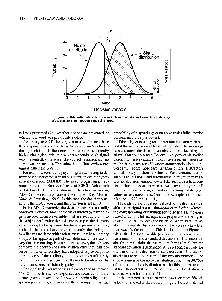
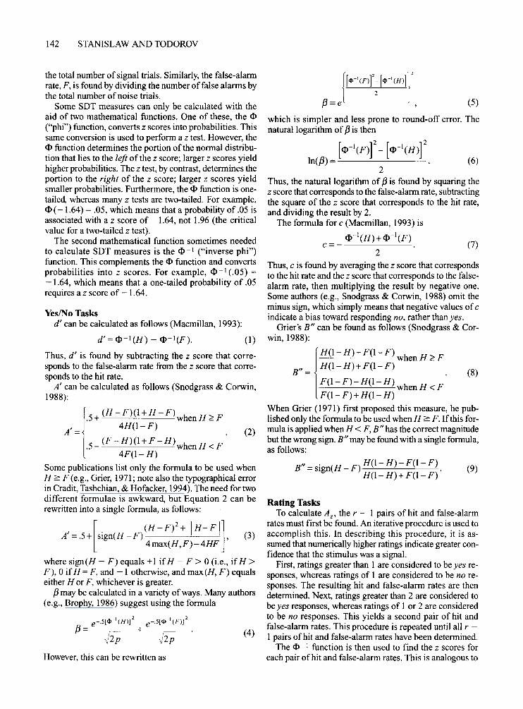
Figure 1. Distribution ofthe decision variable across noise and signal trials, showingd'; c, and the likelihoods on which f3 is based.
nal was presented (i.e., whether a tone was presented, orwhether the word was previously studied).
According to SDT, the subjects in a yes/no task basetheir response on the value that a decision variable achievesduring each trial. If the decision variable is sufficientlyhigh during a given trial, the subject responds yes (a signalwas presented); otherwise, the subject responds no (nosignal was presented). The value that defines sufficientlyhigh is called the criterion.
For example, consider a psychologist attempting to determine whether or not a child has attention deficit hyperactivity disorder (ADHD). The psychologist might administer the Child Behavior Checklist (CBCL; Achenbach& Edelbrock, 1983) and diagnose the child as havingADHD if the resulting score is 10 or higher (Rey, MorrisYates, & Stanislaw, 1992). In this case, the decision variable is the CBCL score, and the criterion is set at 10.
In the ADHD example, the decision variable is readilyobserved. However, most of the tasks studied by psychologists involve decision variables that are available only tothe subject performing the task. For example, the decisionvariable may be the apparent loudness experienced duringeach trial in an auditory perception study, the feeling offamiliarity associated with each stimulus item in a memorystudy, or the apparent guilt ofeach defendant in a study ofjury decision making. In each of these cases, the subjectscompare the decision variable (which only they can observe) to the criterion they have adopted. A yes responseis made only if the auditory stimulus seems sufficientlyloud, the stimulus item seems sufficiently familiar, or thedefendant seems sufficiently guilty.
On signal trials, yes responses are correct and are termedhits. On noise trials, yes responses are incorrect and aretermedfalse alarms. The hit rate (the probability ofrespondingyes on signal trials) and thefalse-alarm rate (the
probability of responding yes on noise trials) fully describeperformance on a yes/no task.
If the subject is using an appropriate decision variable,and ifthe subject is capable ofdistinguishing between signals and noise, the decision variable will be affected by thestimuli that are presented. For example, previously studiedwords in a memory study should, on average, seem more familiar than distractors. However, some previously studiedwords will seem more familiar than others. Distractorswill also vary in their familiarity. Furthermore, factorssuch as neural noise and fluctuations in attention may affect the decision variable, even if the stimulus is held constant. Thus, the decision variable will have a range of different values across signal trials and a range of differentvalues across noise trials. (For more examples of this, seeMcNicol, 1972, pp. 11-14.)
The distribution ofvalues realized by the decision variable across signal trials is the signal distribution, whereasthe corresponding distribution for noise trials is the noisedistribution. The hit rate equals the proportion ofthe signaldistribution that exceeds the criterion, whereas the falsealarm rate equals the proportion of the noise distributionthat exceeds the criterion. This is illustrated in Figure I,where the decision variable (measured in arbitrary units)has a mean of0 and a standard deviation of 1 on noise trials. On signal trials, the mean is higher (M = 2), but thestandard deviation is unchanged. Ayes response is made fortrials in which the decision variable exceeds 0.5; these trials lie in the shaded region of the two distributions. Theshaded region of the noise distribution constitutes 30.85%of the entire noise distribution, so the false-alarm rate is.3085. By contrast, 93.32% of the signal distribution isshaded, so the hit rate is .9332.
If the criterion is set to an even lower, or more liberal,value (i.e., moved to the far left in Figure I), it will almost
CALCULATION OF SIGNAL DETECTION THEORY MEASURES 139
always be exceeded on signal trials. This will producemostly yes responses and a high hit rate. However, the criterion will also be exceeded on most noise trials, resultingin a high proportion ofyes responses on noise trials (i.e., ahigh false-alarm rate). Thus, a liberal criterion biases thesubject toward responding yes, regardless of the stimulus.By contrast, a high, or conservative, value for the criterion biases the subject toward responding no, because thecriterion will rarely be exceeded on signal or noise trials.This will result in a low false-alarm rate, but also a low hitrate. The only way to increase the hit rate while reducingthe false-alarm rate is to reduce the overlap between thesignal and the noise distributions.
Clearly, the hit and false-alarm rates reflect two factors:response bias (the general tendency to respond yes or no,as determined by the location of the criterion) and the degree of overlap between the signal and the noise distributions. The latter factor is usually called sensitivity, reflecting the perceptual origins of SDT: When an auditorysignal is presented, the decision variable will have a greatervalue (the stimulus will sound louder) in listeners withmore sensitive hearing. The major contribution of SDT topsychology is the separation of response bias and sensitivity. This point is so critical that we illustrate it with fiveexamples from widely disparate areas of study.
Our first example is drawn from perception, wherehigher thresholds have been reported for swear words thanfor neutral stimuli (Naylor & Lawshe, 1958). A somewhatFreudian interpretation of this finding is that it reflectsa change in sensitivity that provides perceptual "protection" against negative stimuli (Erdelyi, 1974). However, afalse alarm is more embarrassing for swear words than forneutral stimuli. Furthermore, subjects do not expect to encounter swear words in a study and are, therefore, cautiousabout reporting them. Thus, different apparent thresholds for negative than for neutral stimuli may stem fromdifferent response biases, as well as from different levelsof sensitivity. In order to determine which explanation iscorrect, sensitivity and response bias must be measuredseparately.
A second example involves memory studies. Hypnosissometimes improves recall, but it also increases the number of intrusions (false alarms). It is important, therefore,to determine whether hypnosis actually improves memory, or whether demand characteristics cause hypnotizedsubjects to report more memories about which they are uncertain (Klatzky & Erdelyi, 1985). The former explanationimplies an increase in sensitivity, whereas the latter impliesthat hypnosis affects response bias. Again, it is importantto measure sensitivity and response bias separately.
Our third example involves a problem that sometimesarises when comparing the efficacy of two tests used todiagnose the same mental disorder. One test may have ahigher hit rate than the other, but a higher false-alarm rateas well. This problem typically arises because the tests usedifferent criteria for determining when the disorder is actually present. SDT can solve this problem by determin-
ing the sensitivity of each test in a metric that is independent of the criterion (Rey et aI., 1992).
A fourth example concerns jury decision making. SDTanalyses (Thomas & Hogue, 1976) have shown that juryinstructions regarding the definition of reasonable doubtaffect response bias (the willingness to convict) ratherthan sensitivity (the ability to distinguish guilty from innocent defendants). Response bias also varies with theseverity of the case: Civil cases and criminal cases withrelatively lenient sentences require less evidence to drawa conviction than criminal cases with severe penalties.
Our final example is drawn from industry, wherequality-control inspectors often detect fewer faulty itemsas their work shift progresses. This declining hit rate usuallyresults from a change in response bias (Davies & Parasuraman, 1982, pp. 60-99), which has led to remedies thatwould fail if declining sensitivity were to blame (Craig,1985). SDT also successfully predicts how repeated inspections improve performance (Stanislaw, 1995).
Medical diagnosis illustrates the problems that existedbefore SDT was developed. In his presidential address tothe Radiological Society ofNorth America, Garland (1949)noted that different radiologists sometimes classified thesame X ray differently. This problem was considered bothdisturbing and mysterious until it was discovered that different response biases were partly to blame. Subsequently,radiologists were instructed first to examine all images,using a liberal criterion, and then to reexamine positiveimages, using a conservative criterion.
Sensitivity and response bias are confounded by mostperformance measures, including the hit rate, the falsealarm rate, the hit rate "corrected" by subtracting the falsealarm rate, and the proportion of correct responses in ayes/no task. Thus, if (for example) the hit rate varies between two different conditions, it is not clear whether theconditions differ in sensitivity, response bias, or both.
One solution to this problem involves noting that sensitivity is related to the distance between the mean of thesignal distribution and the mean of the noise distribution(i.e., the distance between the peaks of the two distributions in Figure I). As this distance increases, the overlapbetween the two distributions decreases. Overlap also decreases ifthe means maintain a constant separation but thestandard deviations decrease. Thus, sensitivity can bequantified by using the hit and false-alarm rates to determine the distance between the means, relative to theirstandard deviations.
One measure that attempts to do this is d', which measures the distance between the signal and the noise meansin standard deviation units. The use of standard deviatesoften makes it difficult to interpret particular values of d',However, a value of 0 indicates an inability to distinguishsignals from noise, whereas larger values indicate a correspondingly greater ability to distinguish signals fromnoise. The maximum possible value ofd' is +X, which signifies perfect performance. Negative values ofd' can arisethrough sampling error or response confusion (responding
140 STANISLAW AND TODOROV
yes when intending to respond no, and vice versa); theminimum possible value is -00. d' has a value of 2.00 inFigure I, as the distance between the means is twice aslarge as the standard deviations of the two distributions.
SDT states that d' is unaffected by response bias (i.e.,is a pure measure of sensitivity) if two assumptions aremet regarding the decision variable: (1) The signal andnoise distributions are both normal, and (2) the signal andnoise distributions have the same standard deviation. Wecall these the d' assumptions. The assumptions cannot actually be tested in yes/no tasks; rating tasks are requiredfor this purpose. However, for some yes/no tasks, the d'assumptions may not be tenable; the assumption regardingthe equality of the signal and the noise standard deviationsis particularly suspect (Swets, 1986).
If either assumption is violated, d' will vary with response bias, even ifthe amount of overlap between the signal and the noise distributions remains constant. Becauseofthis, some researchers prefer to use nonparametric measures of sensitivity. These measures may also be usedwhen d' cannot be calculated. (This problem is discussedin more detail below.) Several nonparametric measures ofsensitivity have been proposed (e.g., Nelson, 1984, 1986;W D. Smith, 1995), but the most popular is A'. This measure was devised by Pollack and Norman (1964); a complete history is provided by Macmillan and Creelman(1996) and W D. Smith. A' typically ranges from .5, whichindicates that signals cannot be distinguished from noise,to 1, which corresponds to perfect performance. Valuesless than .5 may arise from sampling error or responseconfusion; the minimum possible value is O. In Figure 1,A' has a value of .89.
Response bias in a yes/no task is often quantified with{3. Use of this measure assumes that responses are basedon a likelihoodratio. Suppose the decision variable achievesa value ofx on a given trial. The numerator for the ratio isthe likelihood of obtaining x on a signal trial (i.e., theheight of the signal distribution at x), whereas the denominator for the ratio is the likelihood of obtaining x on anoise trial (i.e., the height of the noise distribution at x).Subjects respond yes ifz the likelihood ratio (or a variablemonotonically related to it) exceeds {3, and no otherwise.
When subjects favor neither the yes response nor the noresponse, {3 = 1. Values less than I signify a bias towardresponding yes, whereas values of{3 greater than 1 signifya bias toward the no response. In Figure 1, the signal likelihood is .1295 at the criterion, whereas the noise likelihood is .3521 at the criterion. Thus, {3 equals .1295 -:.3521, or .37. This implies that the subjects will respondyes on any trial in which the height of signal distributionat x, divided by the height ofthe noise distribution at x, exceeds 0.37.
Because {3 is based on a ratio, the natural logarithm of{3 is often analyzed in place of {3 itself (McNicol, 1972,pp. 62-63). Negative values ofln({3) signify bias in favorofyes responses, whereas positive values ofln({3) signifybias in favor of no responses. A value of 0 signifies that
no response bias exists. In Figure 1, the natural logarithmof {3 equals -1.00.
Historically, {3 has been the most popular measure ofresponse bias. However, many authors now recommendmeasuring response bias with c (Banks, 1970; Macmillan& Creelman, 1990; Snodgrass & Corwin, 1988). Thismeasure assumes that subjects respond yes when the decision variable exceeds the criterion and no otherwise; responses are based directly on the decision variable, whichsome researchers regard as more plausible than assumingthat responses are based on a likelihood ratio (Richardson,1994). Another advantage of c is that it is unaffected bychanges in d', whereas {3 is not (Ingham, 1970; Macmillan, 1993; McNicol, 1972, pp. 63--64).
c is defined as the distance between the criterion andthe neutral point, where neither response is favored. Theneutral point is located where the noise and signal distributions cross over (i.e., where {3 = 1). If the criterion is located at this point, c has a value ofO. Deviations from theneutral point are measured in standard deviation units.Negative values ofc signify a bias toward responding yes(the criterion lies to the left of the neutral point), whereaspositive values signify a bias toward the no response (thecriterion lies to the right of the neutral point). In Figure 1,the neutral point is located 1 standard deviation above thenoise mean. The criterion is located 0.50 standard deviations to the left of this point, so c has a value of -0.50.
A popular nonparametric measure of response bias isB". This measure was devised by Grier (1971) from a similar measure proposed by Hodos (1970). Unfortunately,some researchers have confused the two measures, usingthe formula for Grier's B" to compute what is claimed tobe Hodos's bias measure (e.g., Macmillan & Creelman,1996). Both nonparametric bias measures can range from- 1 (extreme bias in favor ofyes responses) to I (extremebias in favor ofno responses). A value of0 signifies no response bias. In Figure 1, Grier's B" has a value of -0.55.
Rating TasksRating tasks are like yes/no tasks, in that they present
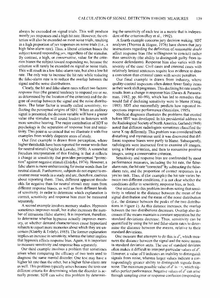
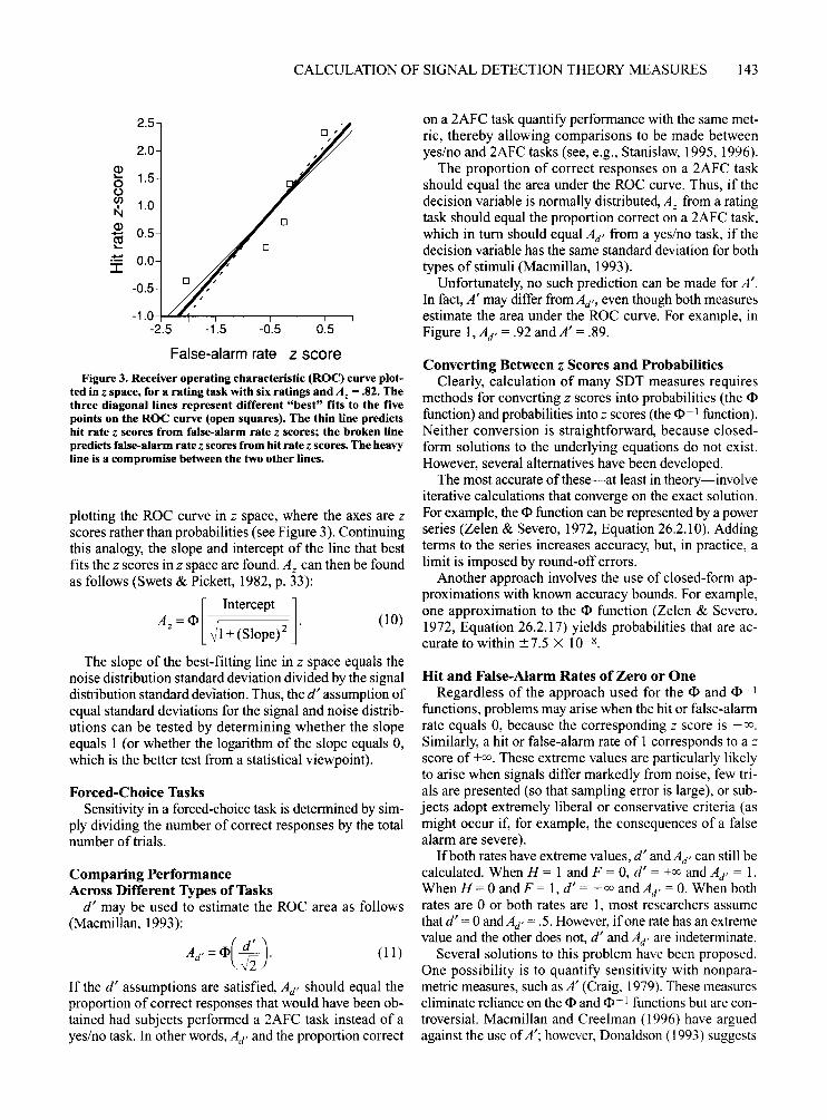
only one stimulus type during each trial. However, ratherthan requiring a dichotomous (yes or no) response, ratingtasks require graded responses. For example, subjects in astudy ofjury decision making may rate each defendant ona scale of 1 (most certainly guilty) to 6 (most certainly innocent). These ratings can be used to determine points ona receiver operating characteristic (ROC) curve, whichplots the hit rate as a function of the false-alarm rate forall possible values of the criterion. A typical ROC curveis illustrated in Figure 2.
A rating task with r ratings determines r - I points onthe ROC curve, each corresponding to a different criterion. For example, one criterion distinguishes ratings of" I"from ratings of "2." Another criterion distinguishes ratings of"2" from ratings of"3," and so on. The ROC curvein Figure 2 was generated from a rating task with four possible ratings, resulting in three points (the open squares).
CALCULATION OF SIGNAL DETECTION THEORY MEASURES 141
1.0
.8
Q) .6+-'ctl....+-' .4I
.2
.0
the standard deviation for signals equals that for noise. Infact, rating tasks may be used to determine the validity ofthe assumption regarding equal standard deviations .
The ROC area can be calculated from yes/no data, aswell as from rating data. One method involves using d' toestimate the ROC area; the resulting measure is called Ad"
This measure is valid only when the d' assumptions aremet. A' also estimates the ROC area, and does so withoutassuming that the decision variable has a particular (e.g.,normal) distribution. However, A' is problematic in otherrespects (Macmillan & Kaplan, 1985; W D. Smith, 1995).In general, A z (when it can be calculated) is the preferredmeasure of the ROC area and, thus, of sensitivity (Swets,1988a; Swets & Pickett, 1982, pp. 31-32).
Figure 2. Receiver operating characteristic (ROC) curve for arating task with four ratings and At = .90. Three points on theROC curve are shown (open squares). The area under the curve,as estimated by linear extrapolation, is indicated by shading; theactual area includes the gray regions.
The remainder of the ROC curve is determined by extrapolation, as will be described below.
Rating tasks are primarily used to measure sensitivity.According to SDT, the area under the ROC curve is a measure of sensitivity unaffected by response bias. The ROCarea typically ranges from .5 (signals cannot be distinguished from noise) to 1 (perfect performance). Areas lessthan .5 may arise from sampling error or response confusion; the minimum possible value is O. The area under theROC curve in Figure 2 equals .90; this includes both thelarge shaded region and the smaller gray regions.
The ROC area can be interpreted as the proportion oftimes subjects would correctly identify the signal, if signal and noise stimuli were presented simultaneously (Green& Moses, 1966; Green &: Swets, 1966, pp. 45-49). Thus,Figure 2 implies that signals would be correctly identifiedon 90% ofthe trials in which signal and noise stimuli werepresented together.
The ROC area can be estimated quite easily iflinear extrapolation is used to connect the points on the ROC curve(for details, see Centor, 1985, and Snodgrass, Levy-Berger,& Haydon, 1985, pp. 449-454). However, this approachgenerally underestimates sensitivity. For example, linearextrapolation measures only the shaded region in Figure 2;the gray regions are excluded. A common remedy is to assume that the decision variable is normally distributed andto use this information to fit a curvilinear function to theROC curve. The ROC area can then be estimated from parameters of the curvilinear function. When this procedureis used, the ROC area is called A z , where the z (whichrefers to z scores) indicates that the noise and signal distributions are assumed to be normal.
In calculating Az , no assumptions are made concerningthe decision variable's standard deviation. This differsfrom yes/no tasks, where one of the d' assumptions is that
Forced-Choice TasksIn a forced-choice task, each trial presents one signal
and one or more noise stimuli. The subjects indicatewhich stimulus was the signal. Tasks are labeled according to the total number of stimuli presented in each trial;an m-alternative forced-choice (mAFC) task presents onesignal and m - 1 noise stimuli. For example, a 3AFC taskfor the study ofrecognition memory presents one old itemand two distractors in each trial. The subjects indicatewhich of the three stimuli is the old item.
Each stimulus in an mAFC trial affects the decisionvariable. Thus, each mAFC trial yields m decision variablescores. Subjects presumably compare these m scores (ortheir corresponding likelihood ratios) with each other anddetermine which is the largest and, thus, the most likely tohave been generated by a signal. Because this comparisondoes not involve a criterion, mAFC tasks are only suitablefor measuring sensitivity.
SDT states that, if subjects donot favor any of the m alternatives a priori, the proportion of correct responses onan mAFC task is a measure of sensitivity unaffected by response bias (Green & Swets, 1966, pp. 45-49). This measure typically ranges from 11m (chance performance) to amaximum of 1 (perfect performance). Values less than 11mmay result from sampling error or response confusion; theminimum possible value is O.
FORMULAE FOR CALCULATINGSIGNAL DETECTION THEORY MEASURES
Few textbooks provide any information about SDT beyond that just presented. This section provides the mathematical details that textbooks generally omit. Readers whowould rather not concern themselves with formulae mayskip this section entirely; familiarity with the underlyingmathematical concepts is not required to calculate SDTmeasures. However, readers who dislike handwaving, orwho desire a deeper understanding ofSDT, are encouragedto read on.
In the discussion below, H is used to indicate the hitrate. This rate is found by dividing the number of hits by
142 STANISLAW AND TODOROV
Thus, d' is found by subtracting the z score that corresponds to the false-alarm rate from the z score that corresponds to the hit rate.
A' can be calculated as follows (Snodgrass & Corwin,1988):
(6)
(5)
(7)
(8)
(9)
!rO'(FJ]';ro ' (H>Ir{3 =e ,
which is simpler and less prone to round-off error. Thenatural logarithm of {3 is then
[<1>-1 (F)r - [<I>-I(H)rIn({3)= -=------=-------=------
2Thus, the natural logarithm of {3 is found by squaring thez score that corresponds to the false-alarm rate, subtractingthe square of the z score that corresponds to the hit rate,and dividing the result by 2.
The formula for c (Macmillan, 1993) is
<I>-l(H)+ <1>-] (F)c=-
2
Thus, c is found by averaging the z score that correspondsto the hit rate and the z score that corresponds to the falsealarm rate, then multiplying the result by negative one.Some authors (e.g., Snodgrass & Corwin, 1988) omit theminus sign, which simply means that negative values ofcindicate a bias toward responding no, rather than yes.
Grier's B" can be found as follows (Snodgrass & Corwin, 1988):
{
H (1 - H ) - F (I - F ) when H? F" H(1-H)+F(I-F)
B =F(1-F)-H(1-H) when H < FF(1-F)+H(1-H)
When Grier (1971) first proposed this measure, he published only the formula to be used when H 2:: F. Ifthis formula is applied when H < F, B" has the correct magnitudebut the wrong sign. B" may be found with a single formula,as follows:
B"= i n(H_F)H(1-H)-F(1-F).sg H(I-H)+F(I-F)
Rating TasksTo calculate Az ' the r - 1 pairs of hit and false-alarm
rates must first be found. An iterative procedure is used toaccomplish this. In describing this procedure, it is assumed that numerically higher ratings indicate greater confidence that the stimulus was a signal.
First, ratings greater than 1 are considered to be yes responses, whereas ratings of 1 are considered to be no responses. The resulting hit and false-alarm rates are thendetermined. Next, ratings greater than 2 are considered tobe yes responses, whereas ratings of 1 or 2 are consideredto be no responses. This yields a second pair of hit andfalse-alarm rates. This procedure is repeated until all r 1 pairs ofhit and false-alarm rates have been determined.
The <I> ~ 1 function is then used to find the z scores foreach pair ofhit and false-alarm rates. This is analogous to
(I)
(2)
(3)
(4)r';
<j2p
e-.5[4> - 1(H)] 2 e-.5[4>- 1(F)] 2
{3 = c' -r-
~2p
YeslNo Tasksd' can be calculated as follows (Macmillan, 1993):
d'=<I>-l(H) - <I>-l(F).
the total number of signal trials. Similarly, the false-alarmrate, F, is found by dividing the number of false alarms bythe total number of noise trials.
Some SDT measures can only be calculated with theaid of two mathematical functions. One of these, the <I>("phi") function, converts z scores into probabilities. Thissame conversion is used to perform a z test. However, the<I> function determines the portion of the normal distribution that lies to the left of the z score; larger z scores yieldhigher probabilities. The z test, by contrast, determines theportion to the right of the z score; larger z scores yieldsmaller probabilities. Furthermore, the <I> function is onetailed, whereas many z tests are two-tailed. For example,<I> (-1.64) = .05, which means that a probability of .05 isassociated with a z score of -1.64, not 1.96 (the criticalvalue for a two-tailed z test).
The second mathematical function sometimes neededto calculate SDT measures is the <I> -] ("inverse phi")function. This complements the <I> function and convertsprobabilities into z scores. For example, <I> -] (.05) =-1.64, which means that a one-tailed probability of .05requires a z score of -1.64.
{
.5 + (H -F)(l+H -F)whenH? F, 4H(1-F)
A =.5 - (F - H) (1+ F - H) when H < F
4F(1-H)
Some publications list only the formula to be used whenH 2:: F (e.g., Grier, 1971; note also the typographical errorin Cradit, Tashchian, & Hofacker, 1994). The need for twodifferent formulae is awkward, but Equation 2 can berewritten into a single formula, as follows:
r(H _F)2+ IH-F 11
A' = .5+ sign(H -F) ,4max(H,F)-4HF
where sign(H - F) equals +1 ifH - F> 0 (i.e., ifH >F), 0 ifH = F, and -1 otherwise, and max(H, F) equalseither H or F, whichever is greater.
{3 may be calculated in a variety ofways. Many authors(e.g., Brophy, 1986) suggest using the formula
However, this can be rewritten as
CALCULATION OF SIGNAL DETECTION THEORY MEASURES 143
2.5
2.0Q)
1.5...0o(/)
1.0K,Q)
0.5-co...."!:: 0.0I
-0.5
-1.0-2.5 -1.5 -0.5 0.5
False-alarm rate z score
Figure 3. Receiver operating characteristic (ROC) curve plotted in z space, for a rating task with six ratings and A z = .82. Thethree diagonal lines represent different "best" fits to the fivepoints on the ROC curve (open squares). The thin line predictshit rate z scores from false-alarm rate z scores; the broken linepredicts false-alarm rate z scores from hit rate z scores. The heavyline is a compromise between the two other lines.
plotting the ROC curve in z space, where the axes are zscores rather than probabilities (see Figure 3). Continuingthis analogy, the slope and intercept of the line that bestfits the z scores in z space are found. A z can then be foundas follows (Swets & Pickett, 1982, p. 33):
A <I> [ Intercept ] (10)z = ~1+(Slope)2·
The slope of the best-fitting line in z space equals thenoise distribution standard deviation divided by the signaldistribution standard deviation. Thus, the d' assumption ofequal standard deviations for the signal and noise distributions can be tested by determining whether the slopeequals 1 (or whether the logarithm of the slope equals 0,which is the better test from a statistical viewpoint).
Forced-Choice TasksSensitivity in a forced-choice task is determined by sim
ply dividing the number of correct responses by the totalnumber oftrials.
Comparing PerformanceAcross Different Types of Tasks
d' may be used to estimate the ROC area as follows(Macmillan, 1993):
Ad' =<1>( Ji). (II)
If the d' assumptions are satisfied, Ad' should equal theproportion of correct responses that would have been obtained had subjects performed a 2AFC task instead of ayes/no task. In other words, Ad' and the proportion correct
on a 2AFC task quantify performance with the same metric, thereby allowing comparisons to be made betweenyes/no and 2AFC tasks (see, e.g., Stanislaw, 1995, 1996).
The proportion of correct responses on a 2AFC taskshould equal the area under the ROC curve. Thus, if thedecision variable is normally distributed, Az from a ratingtask should equal the proportion correct on a 2AFC task,which in turn should equal Ad' from a yes/no task, if thedecision variable has the same standard deviation for bothtypes of stimuli (Macmillan, 1993).
Unfortunately, no such prediction can be made for A'.In fact, A' may differ from Ad" even though both measuresestimate the area under the ROC curve. For example, inFigure 1, Ad' = .92 and A' = .89.
Converting Between z Scores and ProbabilitiesClearly, calculation of many SDT measures requires
methods for converting z scores into probabilities (the <I>function) and probabilities into z scores (the <1>-1 function).Neither conversion is straightforward, because closedform solutions to the underlying equations do not exist.However, several alternatives have been developed.
The most accurate ofthese--at least in theory-involveiterative calculations that converge on the exact solution.For example, the <I> function can be represented by a powerseries (Zelen & Severo, 1972, Equation 26.2.10). Addingterms to the series increases accuracy, but, in practice, alimit is imposed by round-off errors.
Another approach involves the use of closed-form approximations with known accuracy bounds. For example,one approximation to the <I> function (Zelen & Severo,1972, Equation 26.2.17) yields probabilities that are accurate to within ±7.5 X ]0-8.
Hit and False-Alarm Rates of Zero or OneRegardless of the approach used for the <I> and <1>-1
functions, problems may arise when the hit or false-alarmrate equals 0, because the corresponding z score is -rx.
Similarly, a hit or false-alarm rate of 1 corresponds to a zscore of +00. These extreme values are particularly likelyto arise when signals differ markedly from noise, few trials are presented (so that sampling error is large), or subjects adopt extremely liberal or conservative criteria (asmight occur if, for example, the consequences of a falsealarm are severe).
Ifboth rates have extreme values, d' and Ad' can still becalculated. When H = 1 and F = 0, d' = +00 and Ad' = I.When H =°and F = 1, d' = -00 and Ad' = 0. When bothrates are °or both rates are I, most researchers assumethat d' =°and Ad' = .5. However, ifone rate has an extremevalue and the other does not, d' and Ad' are indeterminate.
Several solutions to this problem have been proposed.One possibility is to quantify sensitivity with nonparametric measures, such as A' (Craig, 1979). These measureseliminate reliance on the <I> and <1>-1 functions but are controversial. Macmillan and Creelman (1996) have arguedagainst the use ofA'; however, Donaldson (1993) suggests
144 STANISLAW AND TODOROV
that A' may estimate sensitivity better than d' when the signal and noise distributions are normal but have differentstandard deviations.
Another alternative is to combine the data from severalsubjects before calculating the hit and false-alarm rates(Macmillan & Kaplan, 1985). However, this approachcomplicates statistical testing and should only be appliedto subjects who have comparable response biases and levels of sensitivity.
A third approach, dubbed loglinear, involves adding 0.5to both the number of hits and the number offalse alarmsand adding 1 to both the number of signal trials and thenumber ofnoise trials, before calculating the hit and falsealarm rates. This seems to work reasonably well (Hautus,1995). Advocates of the loglinear approach recommendusing it regardless ofwhether or not extreme rates are obtained.
A fourth approach involves adjusting only the extremerates themselves. Rates of0 are replaced with 0.5 -;- n, andrates of 1 are replaced with (n - 0.5) -;- n, where n is thenumber of signal or noise trials (Macmillan & Kaplan,1985). This approach yields biased measures of sensitivity (Miller, 1996) and may be less satisfactory than theloglinear approach (Hautus, 1995). However, it is the mostcommon remedy for extreme values and is utilized in several computer programs that calculate SDT measures (see,e.g., Dorfman, 1982). Thus, it is the convention we adoptin our computational example below.
METHODS FORCALCULATING SDT MEASURES
In this section, we describe three general approachesthat can be used to calculate the measures prescribed bySDT: tabular methods, methods that use software specifically developed for SDT, and methods that rely on generalpurpose software.
Tabular MethodsElliott (1964) published one of the first and most pop
ular listings of d' values for particular pairs of hit andfalse-alarm rates. Similar tables followed. The most extensive of these is Freeman's (1973), which also lists valuesof 13. (See Gardner, Dalsing, Reyes, & Brake, 1984, for abriefer table of 13 values.)
Tables for d' are not restricted just to yes/no tasks. Elliott (1964) published an early d' table for forced-choicetasks; more recent versions that correct some errors havesince appeared (Hacker & Ratcliff, 1979; Macmillan &Creelman, 1991, pp. 319-322). Tables for other tasks havebeen published by Craven (1992), Hershman and Small(1968), Kaplan, Macmillan, and Creelman (1978), andMacmillan and Creelman (1991, pp. 323-354).
Tabular methods have relatively poor accuracy. Sometables contain incorrect entries, but even error-free tablescan be used only after the hit and false-alarm rates arerounded off (usually to two significant digits). Roundingintroduces errors; changing the fourth significant digit of
the hit or the false-alarm rate can often affect the secondsignificant digit ofd'. Interpolation between tabled valuescan minimize the impact ofrounding errors, but the properinterpolation method is nonlinear. Furthermore, even linear interpolation requires calculations that the tabularmethod is specifically designed to avoid.
When SDT was first developed, most researchers wereforced to rely on the tabular approach. However, this approach is difficult to justify today.Computers can quantifySDT performance far more quickly and accurately thancan tables. Computers also provide the only reasonablemeans of analyzing rating task data; tables can determineneither the slope nor the intercept of the best-fitting linein z space.
Some computer programs (e.g., Ahroon & Pastore,1977) calculate SDT measures by incorporating look-uptables, thus gaining a slight speed advantage over closedform approximations and iterative techniques. However,speed is likely to be of concern only in Monte Carlo simulations involving thousands of replications. Even here,tables are of questionable utility, because of their limitedaccuracy. Thus, the tabular approach should be used onlyas a last resort.
Signal Detection Theory SoftwareAhroon and Pastore (1977) were the first authors to
publish programs (written in FORTRAN and BASIC) fordetermining values ofd' and 13 for yes/no tasks. However,these programs should be used with caution, as they relyon look-up tables for the cI> -1 function. Furthermore, 13 iscalculated with Equation 4 rather than Equation 5. Thisimposes speed and accuracy penalties, thus offsetting whatever advantage might be gained from the tabular approach.
Better choices for analyzing yes/no data are Brophy's(1986) BASIC program and the Pascal program publishedby Macmillan and Creelman (1991, pp. 358-359). Otherpublished programs are written in APL (McGowan &Appel, 1977) and Applesoft (which is similar to BASIC;Gardner & Boice, 1986). Programmers who wish to writetheir own code can refer to algorithms for the cI>-1 function(see Brophy, 1985, for a review) and then apply the appropriate equation. Algorithms for calculating d' for forcedchoice tasks can be found in 1.E. K. Smith (1982).
More extensive programs are required to analyze datafrom rating tasks. Centor (1985) has published a spreadsheet macro for this purpose, but his program uses linearextrapolation and thus tends to underestimate A z . (SeeCentor & Schwartz, 1985, for a discussion of this problem.) A better choice is RSCORE, written by Donald Dorfman. Source code is availablein both FORTRAN (Dorfman,1982) and BASIC (Alf & Grossberg, 1987). The latestversion, RSCORE4, may be downloaded (from ftp:!/perception.radiology.uiowa.edu/public/rscore). A comparable program, Charles Metz's ROCFIT,may be downloaded(from ftp://random.bsd.uchicago.edu/roc). Both programsare available in source code (FORTRAN) and compiledform (PC-compatible for RSCORE4; PC-compatible,
CALCULATION OF SIGNAL DETECTION THEORY MEASURES 145
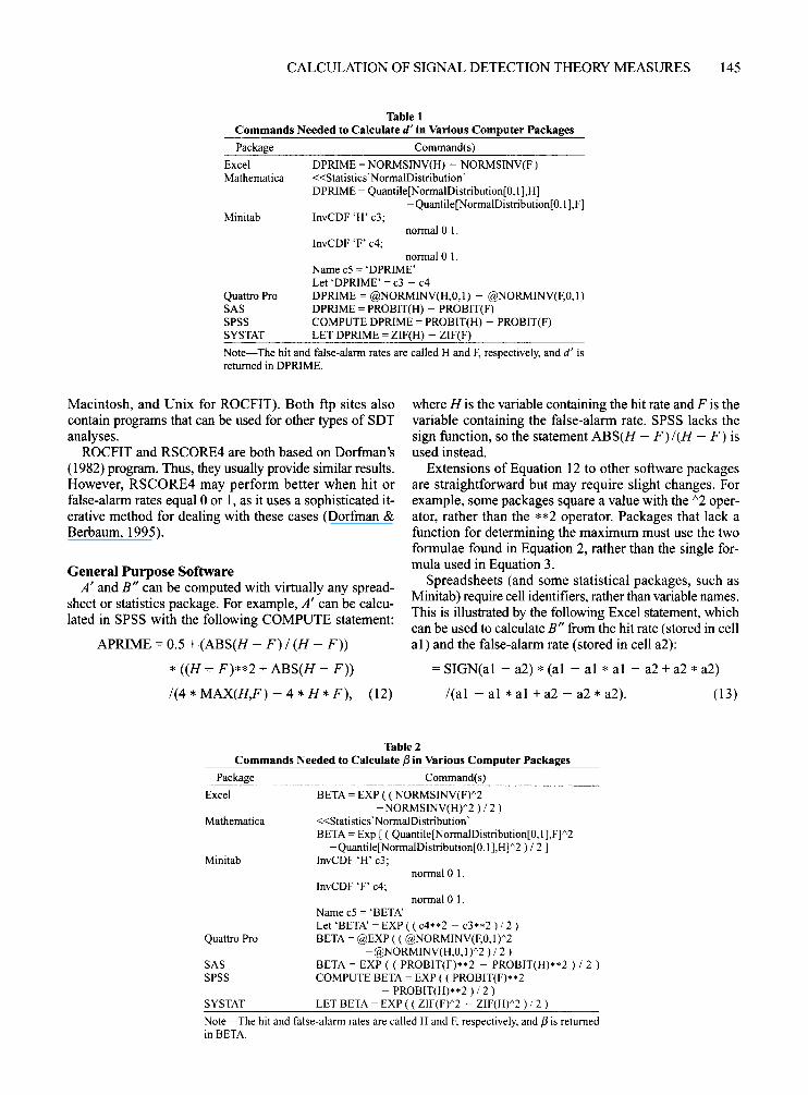
Table 1Commands Needed to Calculate d' in Various Computer Packages
Package Command(s)
Excel DPRIME = NORMSINV(H) - NORMSINV(F)Mathematica «Statistics'N ormalDistribution'
DPRIME = Quantile[NormalDistribution[O,I],H]-Quantile[NormalDistribution[O, I],F]
Minitab InvCDF 'H' c3;
InvCDF 'F' c4;normal °I.
normal °I.Name c5 = 'DPRIME'Let 'DPRIME' = c3 - c4
Quattro Pro DPRIME = @NORMINV(H,O,I) - @NORMINV(F,O,I)SAS DPRIME = PROBIT(H) - PROBIT(F)SPSS COMPUTE DPRIME = PROBIT(H) - PROBIT(F)SYSTAT LET DPRIME = ZIF(H) - ZIF(F)
Note-The hit and false-alarm rates are called Hand F, respectively, and d' isreturned in DPRIME,
Macintosh, and Unix for ROCFIT). Both ftp sites alsocontain programs that can be used for other types of SDTanalyses.
ROCFIT and RSCORE4 are both based on Dorfman's(1982) program. Thus, they usually provide similar results.However, RSCORE4 may perform better when hit orfalse-alarm rates equal 0 or 1, as it uses a sophisticated iterative method for dealing with these cases (Dorfman &Berbaum, 1995).
General Purpose SoftwareA' and B" can be computed with virtually any spread
sheet or statistics package. For example, A' can be calculated in SPSS with the following COMPUTE statement:
APRIME = 0.5 + (ABS(H - F) 1(H - F»
* ((H"", F)**2 + ABS(H - F»
1(4 * MAX(H,F) - 4 * H * F), (12)
where H is the variable containing the hit rate and F is thevariable containing the false-alarm rate. SPSS lacks thesign function, so the statement ABS(H - F)/(H - F) isused instead.
Extensions of Equation 12 to other software packagesare straightforward but may require slight changes. Forexample, some packages square a value with the 1\2 operator, rather than the **2 operator. Packages that lack afunction for determining the maximum must use the twoformulae found in Equation 2, rather than the single formula used in Equation 3.
Spreadsheets (and some statistical packages, such asMinitab) require cell identifiers, rather than variablenames.This is illustrated by the following Excel statement, whichcan be used to calculate B" from the hit rate (stored in cellal) and the false-alarm rate (stored in cell a2):
= SIGN(al - a2) * (al - al * al - a2 + a2 * a2)
I(al - al * al + a2 - a2 * a2). (13)
Table 2Commands Needed to Calculate f3in Various Computer Packages
Package Command(s)
Excel BETA = EXP ( ( NORMSINV(F)"2- NORMSINV(H)"2 ) / 2 )
Mathematica «Statistics'Normallristribution'BETA = Exp [ ( Quantile[NormalDistribution[O, I],F]"2
-Quantile[NormalDistribution[O,l],H]"2) / 2]Minitab InvCDF 'H' c3;
normal °I.InvCDF 'F' c4;
normal °I.Name c5 = 'BETA'Let 'BETA' = EXP ( ( c4**2 - c3**2 ) /2)
Quattro Pro BETA = @EXP ( ( @NORMINV(F,O,I)"2-@NORMINV(H,O,I)"2)/2 )
SAS BETA = EXP ( ( PROBIT(F)**2 - PROBIT(H)**2 ) / 2 )SPSS COMPUTE BETA = EXP ( ( PROBIT(F)**2
- PROBIT(H)**2 ) / 2 )SYSTAT LET BETA = EXP ( ( ZIF(F)"2 ~ ZIF(H)"2 ) / 2 )
Note-The hit and false-alarm rates are called Hand F, respectively, and f3 is returnedin BETA.
146 STANISLAW AND TODOROV
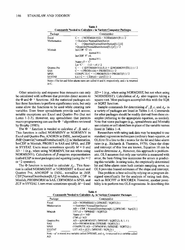
Table 3Commands Needed to Calculate c in Various Computer Packages
Package
ExcelMathematica
Minitab
Quattro ProSASSPSSSYSTAT
Command(s)
C = -( NORMSINV(H) + NORMSINV(F) ) / 2«Statistics' NormalDistributionC = -( Quantile[NormalDistribution[O,I],H]+Quantile[NormalDistribution[O, I],F] ) / 2InvCDF 'H' c3;
normal 0 I.InvCDF 'F' c4;
normal 0 I.Name c5 = 'C'Let 'C' = -( c3 +c4 )/2C = -( @NORMINV(H,O,I) + @NORMINV(F,O,I)) / 2C = -( PROBIT(H) + PROBIT(F) ) / 2COMPUTE C = -( PROBIT(H) + PROBIT(F) ) / 2LET C = -( ZIF(H) + ZIF(F) ) / 2
Note-The hit and false-alarm rates are called Hand F, respectively, and c is returnedin C.
Other sensitivity and response bias measures can onlybe calculated with software that provides direct access tothe cD and cD-I functions. All the statistical packages utilize these functions to perform significance tests, but onlysome allow the functions to be used while creating newvariables. Even fewer spreadsheets provide such access;notable exceptions are Excel and Quattro Pro (but notLotus 1-2-3). However, any spreadsheet that permitsmacro programming can use the cD -I algorithms reviewedby Brophy (1985).
The cD-I function is needed to calculate d', {3, and c.This function is called NORMSINV or NORMINV inExcel and Quattro Pro, ANORIN in IMSL, normQuant inJMp, Quantile[NormalDistribution[O,1]] in Mathematica,InvCDF in Minitab, PROBIT in SAS and SPSS, and ZIFin SYSTAT. Users must sometimes specify M = 0 andSD = 1 (e.g., when using NORMINY, but not when usingNORMSINV). Calculation of {3 requires exponentiation(called EXP in most packages) and squaring (using the **2or 1\2 operator).
The cD function is needed to calculate Ad" This function is called NORMSDIST or NORMDIST in Excel andQuattro Pro, ANORDF in IMSL, normDist in JMP,CDF[NormalDistribution[O, I]] in Mathematica, CDF inMinitab, PROBNORM in SAS, CDFNORM in SPSS, andZCF in SYSTAT. Users must sometimes specify M = 0 and
SD = I (e.g., when using NORMDIST, but not when usingNORMSDIST). Calculation ofAd' also requires taking asquare root. Most packages accomplish this with the SQRor SQRT function.
Sample commands for determining d', {3, c, and Ad' ina variety of packages are listed in Tables l~. Commandsfor other packages should be readily derived from these examples (referring to the appropriate equation, as needed).Note that some packages (e.g., spreadsheets and Minitab)use column or cell identifiers in place ofthe variable nameslisted in Tables l~.
Researchers with rating task data may be tempted to usestandard regression techniques (ordinary least-squares, orOLS) to fit a line to the z scores for the hit and false-alarmrates (e.g., Richards & Thornton, 1970). Once the slopeand intercept of this line are known, Equation 10 can beused to determine A z : However, this approach is problematic. OLS assumes that only one variable is measured witherror; the best-fitting line minimizes the errors in predicting this variable. In rating tasks, the empirically determinedhit and false-alarm rates both contain sampling error, soOLS provides biased estimates of the slope and intercept.
This problem is best solved by relying on a program designed specifically for the analysis of rating task data,such as ROCFIT or RSCORE4. However, another possibility is to perform two OLS regressions. In describing this
Table 4Commands Needed to Calculate Ad' in Various Computer Packages
Package Command(s)
Excel AD = NORMSDIST ( DPRIME / SQRT(2) )Mathematica «Statistics'Normallristribution'
AD = CDF [ NorrnalDistribution[O,I],DPRIME / Sqrt[2] ]Minitab LET c2 = 'DPRIME' / SQRT(2)
Name c3 = 'AD'CDFc2 'AD'
Quattro Pro AD = @NORMDlST ( DPRIME / SQRT(2), 0, I, I )SAS AD = PROBNORM ( DPRIME / SQRT(2) )SPSS COMPUTE AD = CDFNORM ( DPRIME / SQRT(2) )SYSTAT LET AD = ZCF ( DPRIME / SQR(2) )
Note-d' is stored in a variable called DPRIME, and Ad' is returned in a variable calledAD.
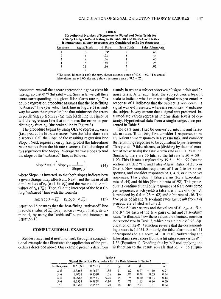
CALCULATION OF SIGNAL DETECTION THEORY MEASURES 147
TableSHypothetical Number of Responses in Signal and Noise Trials for
a Study Using a 6-Point Rating Scale, and Hit and False-Alarm Ratesif Numerically Higher Responses Are Considered to Be Yes Responses
Response Signal Trials Hit Rate Noise Trials False-Alarm Rate
I 0 .99* 8 .682 4 .92 6 .443 8 .76 I .404 8 .60 3 .285 12 .36 7 .02t6 18 0
*The actual hit rate is 1.00; the entry shown assumes a rate of 49.5 -7 50. "The actualfalse-alarm rate is 0.00; the entry shown assumes a rate of 0.5 -725.
procedure, we call the Z score corresponding to a given hitrate zH' so that <1>-] (hit rate) = ZH' Similarly, we call the Z
score corresponding to a given false-alarm rate ZF' Thedouble regression procedure assumes that the best-fitting"unbiased" line (the solid black line in Figure 3) is midway between the regression line that minimizes the errorsin predicting ZH from ZF (the thin black line in Figure 3)and the regression line that minimizes the errors in predicting ZF from ZH (the broken line in Figure 3).
The procedure begins by using OLS to regress zH on Z F
(i.e., predict the hit rate Z scores from the false-alarm rateZ scores). Call the slope of the resulting regression lineSlope]. Next, regress ZF on ZH (i.e., predict the false-alarmrate Z scores from the hit rate Z scores). Call the slope ofthis regression line Slope.. Average the two slopes to findthe slope of the "unbiased" line, as follows:
Slope*= 0.5 (SlOpe]+_1_), (14)Slope,
where Slope2 is inverted, so that both slopes indicate howa given change in zF affects zH' Next, find the mean ofallr - 1 values ofZ F (call this Z F) and the mean of all r - 1values of ZH (zH ). Then, find the intercept of the best fitting "unbiased" line with the formula
Intercept- =ZH - (Slope- X zF)' (15)
Equation 15 ensures that the best-fitting "unbiased" linepredicts a value of ZH for ZH when ZF = Z F' Finally, determine Az by using the "unbiased" slope and intercept inEquation 10.
COMPUTATIONAL EXAMPLES
Readers may find it useful to work through a computational example that illustrates the application of the procedures described above. Our example presents data from
a study in which a subject observes 50 signal trials and 25noise trials. After each trial, the subject uses a 6-pointscale to indicate whether or not a signal was presented. Aresponse of 1 indicates that the subject is very certain asignal was not presented, whereas a response of 6 indicatesthe subject is very certain that a signal was presented. Intermediate values represent intermediate levels of certainty. Hypothetical data from a single subject are presented in Table 5.
The data must first be converted into hit and falsealarm rates. To do this, first consider 1 responses to beequivalent to no responses in a yes/no task, and considerthe remaining responses to be equivalent to yes responses.This yields 17 false alarms, so (dividing by the total number of noise trials) the false-alarm rate is 17 -:- 25 = .68.Similarly, there are 50 hits, so the hit rate is 50 -:- 50 =1.00. This hit rate is replaced by 49.5 -i- 50 = .99 (see thesection entitled "Hit and False-Alarm Rates of Zero orOne"). Now consider responses of 1 or 2 to be no responses, and consider responses of 3, 4, 5, or 6 to be yesresponses. This yields 11 false alarms (for a false-alarmrate of .44) and 46 hits (for a hit rate of .92). This procedure is continued until only responses of 6 are consideredyes responses, which yields a false-alarm rate of a(whichis replaced by 0.5 -:- 25 = .02) and a hit rate of .36. Thefive pairs of hit and false-alarm rates that result from thisprocedure are listed in Table 5.
Table 6 lists Z scores and the values of d', Ad" A', [3, c,and B" for each of the five pairs of hit and false-alarmrates. To illustrate how these values are obtained, considerthe second row in Table 5, which has a hit rate of .92. Application of the <I> -] function reveals that the corresponding Z score is 104051. Similarly, the false-alarm rate of 044corresponds to a Z score of -0.1510. Subtracting thefalse-alarm rate Z score from the hit rate Z score yields d' =1.56 (Equation 1). Dividing this by v2 and applying the<I> function to the result reveals that Ad' = .86 (Equa-
Table 6Signal Detection Parameters for the Data Shown in Table S
Yes Response CP-I(H) CP-I(F) d' Ad' A' {3 c B U
2-6 2.3263 0.4677 1.86 .91 .82 0.07 -1.40 -0.913-6 1.4051 -0.1510 1.56 .86 .84 0.38 -0.63 -0.544-6 0.7063 -0.2533 0.96 .75 .75 0.80 -0.23 -0.145-6 0.2533 -0.5828 0.84 .72 .72 1.15 0.16 0.09
6 -0.3585 -2.0537 1.70 .88 .88 7.73 1.21 0.84
148 STANISLAW AND TODOROV
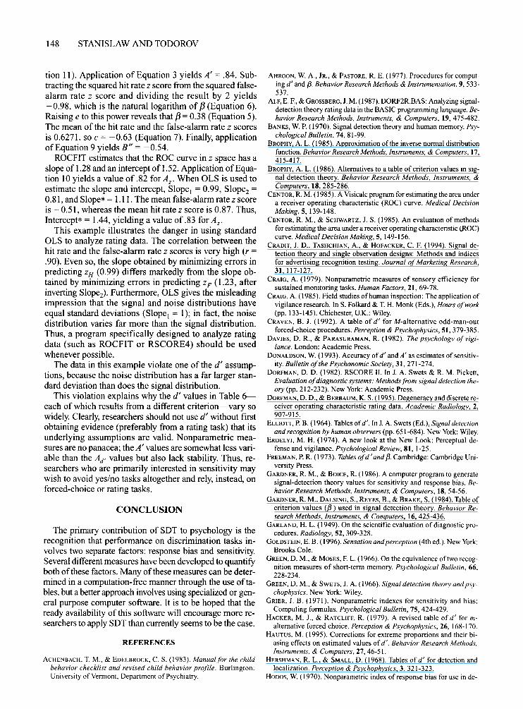
tion 11). Application of Equation 3 yields A' = .84. Subtracting the squared hit rate z score from the squared falsealarm rate z score and dividing the result by 2 yields-0.98, which is the natural logarithm of f3 (Equation 6).Raising e to this power reveals that f3 = 0.38 (Equation 5).The mean of the hit rate and the false-alarm rate z scoresis 0.6271, so c = -0.63 (Equation 7). Finally, applicationof Equation 9 yields B" = -0.54.
ROCFIT estimates that the ROC curve in z space has aslope of 1.28 and an intercept of 1.52. Application ofEquation 10 yields a value of .82 for Az . When OLS is used toestimate the slope and intercept, Slope) = 0.99, Slope, =0.81, and Slope» = 1.11. The mean false-alarm rate z scoreis -0.51, whereas the mean hit rate z score is 0.87. Thus,Intercept- = 1.44, yielding a value of .83 for Az .
This example illustrates the danger in using standardOLS to analyze rating data. The correlation between thehit rate and the false-alarm rate z scores is very high (r =.90). Even so, the slope obtained by minimizing errors inpredicting zH (0.99) differs markedly from the slope obtained by minimizing errors in predicting zF (1.23, afterinverting Slope-), Furthermore, OLS gives the misleadingimpression that the signal and noise distributions haveequal standard deviations (Slope) "" 1); in fact, the noisedistribution varies far more than the signal distribution.Thus, a program specifically designed to analyze ratingdata (such as ROCFIT or RSCORE4) should be usedwhenever possible.
The data in this example violate one of the d' assumptions, because the noise distribution has a far larger standard deviation than does the signal distribution.
This violation explains why the d' values in Table 6each of which results from a different criterion-vary sowidely. Clearly, researchers should not use d' without firstobtaining evidence (preferably from a rating task) that itsunderlying assumptions are valid. Nonparametric measures are no panacea; theA' values are somewhat less variable than the Ad' values but also lack stability. Thus, researchers who are primarily interested in sensitivity maywish to avoid yes/no tasks altogether and rely, instead, onforced-choice or rating tasks.
CONCLUSION
The primary contribution of SDT to psychology is therecognition that performance on discrimination tasks involves two separate factors: response bias and sensitivity.Several different measures have been developed to quantifyboth ofthese factors. Many ofthese measures can be determined in a computation-free manner through the use oftables, but a better approach involves using specialized or general purpose computer software. It is to be hoped that theready availability of this software will encourage more researchers to apply SDT than currently seems to be the case.
REFERENCES
ACHENBACH, T. M., & EDELBROCK, C. S. (1983). Manualfor the childbehavior checklist and revised child behavior profile. Burlington:University of Vermont, Department of Psychiatry.
AHROON, W. A., JR., & PASTORE, R. E. (1977). Procedures for computing d' and (3. Behavior Research Methods & Instrumentation, 9, 533537.
ALF,E. E, & GROSSBERG, 1. M. (1987). DORF2R.BAS: Analyzing signaldetection theory rating data in the BASIC programming language. Behavior Research Methods, Instruments, & Computers, 19,475-482.
BANKS, W. P. (1970). Signal detection theory and human memory. Psychological Bulletin, 74, 81-99.
BROPHY, A. L. (1985). Approximation of the inverse normal distributionfunction. Behavior Research Methods. Instruments, & Computers, 17,415-417.
BROPHY, A. L. (1986). Alternatives to a table of criterion values in signal detection theory. Behavior Research Methods, Instruments, &Computers, 18, 285-286.
CENTOR, R. M. (1985). A Visica1c program for estimating the area undera receiver operating characteristic (ROC) curve. Medical DecisionMaking.S, 139-148.
CENTOR, R. M., & SCHWARTZ, J. S. (1985). An evaluation of methodsfor estimating the area under a receiver operating characteristic (ROC)curve. Medical Decision Making.S, 149-156.
CRADIT, J. D., TASHCHIAN, A., & HOFACKER, C. E (1994). Signal detection theory and single observation designs: Methods and indicesfor advertising recognition testing. Journal ofMarketing Research,31, 117-127.
CRAIG, A. (1979). Nonparametric measures of sensory efficiency forsustained monitoring tasks. Human Factors, 21, 69-78.
CRAIG, A. (1985). Field studies ofhuman inspection: The application ofvigilance research. In S. Folkard & T. H. Monk (Eds.), Hours ofwork(pp. 133-145). Chichester, U.K.: Wiley.
CRAVEN, B. J. (1992). A table of d' for M-alternative odd-man-outforced-choice procedures. Perception & Psychophysics, 51, 379-385.
DAVIES, D. R., & PARASURAMAN, R. (1982). The psychology of vigilance. London: Academic Press.
DONALDSON, W. (1993). Accuracy ofd' and A' as estimates of sensitivity. Bulletin ofthe Psychonomic Society, 31, 271-274.
DORFMAN, D. D. (1982). RSCORE II. In 1. A. Swets & R. M. Pickett,Evaluation ofdiagnostic systems: Methods from signal detection theory (pp. 212-232). New York: Academic Press.
DoRFMAN, D. D., & BERBAUM, K. S. (1995). Degeneracy and discrete receiver operating characteristic rating data. Academic Radiology, 2,907-915.
ELLIOTT, P. B. (1964). Tables ofd', In 1.A. Swets (Ed.), Signal detectionand recognition by human observers (pp. 651-684). New York: Wiley.
ERDELYI, M. H. (1974). A new look at the New Look: Perceptual defense and vigilance. Psychological Review, 81, 1-25.
FREEMAN, P. R. (1973). Tablesofd ' and {3. Cambridge: Cambridge University Press.
GARDNER, R. M., & BOICE, R. (1986). A computer program to generatesignal-detection theory values for sensitivity and response bias. Behavior Research Methods, Instruments, & Computers, 18, 54-56.
GARDNER, R. M., DALSING, S., REYES, B., & BRAKE, S. (1984). Table ofcriterion values ({3) used in signal detection theory. Behavior Research Methods, Instruments, & Computers, 16,425-436.
GARLAND, H. L. (1949). On the scientific evaluation of diagnostic procedures. Radiology, 52, 309-328.
GOLDSTEIN, E. B. (1996). Sensation and perception (4th ed.). New York:Brooks Cole.
GREEN, D. M., & MOSES, E L. (1966). On the equivalence of two recognition measures of short-term memory. Psychological Bulletin, 66,228-234.
GREEN, D. M., & SWETS, J. A. (1966). Signal detection theory and psychophysics. New York: Wiley.
GRIER,J. B. (1971). Nonparametric indexes for sensitivity and bias:Computing formulas. Psychological Bulletin, 75, 424-429.
HACKER, M. J., & RATCLIFF, R. (1979). A revised table of d' for malternative forced choice. Perception & Psychophysics, 26, 168-170.
HAUTUS, M. (1995). Corrections for extreme proportions and their biasing effects on estimated values of d', Behavior Research Methods.Instruments. & Computers, 27, 46-51.
HERSHMAN, R. L., & SMALL, D. (1968). Tables of d' for detection andlocalization. Perception & Psychophysics, 3,321-323.
HODOS, W. (1970). Nonparametric index of response bias for use in de-
CALCULATION OF SIGNAL DETECTION THEORY MEASURES 149
tection and recognition experiments. Psychological Bulletin, 74, 351354.
HUTCHINSON, T. P. (1981). A review of some unusual applications ofsignal detection theory. Quality & Quantity, 15, 71-98.
INGHAM, J. G. (1970). Individual differences in signal detection. ActaPsychologica, 34, 39-50.
KAPLAN, H. L., MACMILLAN, N. A., & CREELMAN, C. D. (1978). Tablesof d' for variable-standard discrimination paradigms. Behavior Research Methods & Instrumentation, 10,796-813.
KLATZKY, R. L., & ERDELYI, M. H. (1985). The response criterion problem in tests of hypnosis and memory. International Journal ofClinical & Experimental Hypnosis, 33, 246-257.
MACMILLAN, N. A. (1993). Signal detection theory as data analysismethod and psychological decision model. In G. Keren & C. Lewis(Eds.), A handbookfor data analysis in the behavioral sciences:Methodological issues (pp. 21-57). Hillsdale, NJ: Erlbaum.
MACMILLAN, N. A., & CREELMAN, C. D. (1990). Response bias: Characteristics ofdetection theory, threshold theory, and "nonparametric"indexes. Psychological Bulletin, 107,401-413.
MACMILLAN, N. A., & CREELMAN, C. D. (1991). Detection theory: Auser's guide. Cambridge: Cambridge University Press.
MACMILLAN, N. A., & CREELMAN, C. D. (1996). Triangles in ROCspace: History and theory of"nonparametric" measures of sensitivityand bias. Psychonomic Bulletin & Review, 3, 164-170.
MACMILLAN, N. A., & KAPLAN, H. L. (1985). Detection theory analysisofgroup data: Estimating sensitivity from average hit and false-alarmrates. Psychological Bulletin, 98, 185-199.
MCGOWAN, W. T., III, & ApPEL,J. B. (1977). An APL program for calculating signal detection indices. Behavior Research Methods & Instrumentation, 9, 517-521.
McNICOL, D. (1972). A primer ofsignal detection theory. London: Allen& Unwin.
MILLER, J. (1996). The sampling distribution of d', Perception & Psychophysics, 58, 65-72.
NAYLOR, J. C; & LAWSHE, C. H. (1958). An analytical review of the experimental basis of subception. Journal of Psychology, 46, 75-96.
NELSON, T.O. (1984). A comparison ofcurrent measures ofthe accuracyof feeling-of-knowing predictions. Psychological Bulletin, 95, 109133.
NELSON, T. O. (1986). ROC curves and measures of discrimination accuracy: A reply to Swets. Psychological Bulletin, 100, 128-132.
POLLACK, 1., & NORMAN, D. A. (1964). A nonparametric analysis ofrecognition experiments. Psychonomic Science, 1,125-126.
REY,J. M., MORRIS-YATES, A., & STANISLAW, H. (1992). Measuring theaccuracy of diagnostic tests using receiver operating characteristic(ROC) analysis. International Journal ofMethods in Psychiatric Research, 2, 39-50.
RICHARDS, B. L., & THORNTON, C. L. (1970). Quantitative methods ofcalculating the d' of signal detection theory. Educational & Psychological Measurement, 30, 855-859.
RICHARDSON, J. T. E. (1994). Continuous recognition memory tests: Arethe assumptions of the theory of signal detection really met? JournalofClinical & Experimental Neuropsychology, 16,482-486.
SMITH, J. E. K. (1982). Simple algorithms for M-alternative forcedchoice calculations. Perception & Psychophysics, 31, 95-96.
SMITH,W. D. (1995). Clarification of sensitivity measure A'. Journal ofMathematical Psychology, 39, 82-89.
SNODGRASS, J. G., & CORWIN, J. (1988). Pragmatics of measuringrecognition memory: Applications to dementia and amnesia. JournalofExperimental Psychology: General, 117, 34-50.
SNODGRASS, 1. G., LEVY-BERGER, G., & HAYDON, M. (1985). Humanexperimental psychology. New York: Oxford University Press.
STANISLAW, H. (1995). Effect of type of task and number of inspectorson performance ofan industrial inspection-type task. Human Factors,37, 182-192.
STANISLAW, H. (1996). Relative versus absolute judgments, and the effect of batch composition on simulated industrial inspection. In R. 1.Koubek & W. Karwowski (Eds.), Manufacturing agility and hybridautomation: I (pp. 105-108). Louisville, KY: lEA Press.
STANISLAW, H., & TODOROV, N. (1992). Documenting the rise and fallofa psychological theory: Whatever happened to signal detection theory? (Abstract). Australian Journal ofPsychology, 44, 128.
SWETS, J. A. (1973). The relative operating characteristic in psychology.Science, 182,990-1000.
SWETS, J. A. (1986). Form of empirical ROCs in discrimination and diagnostic tasks: Implications for theory and measurement of performance. Psychological Bulletin, 99,181-198.
SWETS, J. A. (1988a). Measuring the accuracy of diagnostic systems.Science, 240, 1285-1293.
SWETS, J. A. (ED.) (l988b). Signal detection and recognition by humanobservers. New York: Wiley.
SWETS, J. A., & PICKETT, R. M. (1982). Evaluation ofdiagnostic systems:Methods from signal detection theory. New York: Academic Press.
THOMAS, E. A. C., & HOGUE, A. (1976). Apparent weight of evidence,decision criteria, and confidence ratings in juror decision making.Psychological Review, 83,442-465.
ZELEN, M., & SEVERO, N. C. (1972). Probability functions. InM. Abramowitz & 1. A. Stegun (Eds.), Handbook ofmathematicalfunctions with formulas, graphs, and mathematical tables (pp. 925973). Washington, DC: National Bureau of Standards.
(Manuscript received August 15, 1997;revision accepted for publication February 9, 1998.)
Copyright © 2022 FDOKUMEN