Calculation of linelists for Chromium Hydride (CrH ...
431
-
Upload
khangminh22 -
Category
Documents
-
view
0 -
download
0
Transcript of Calculation of linelists for Chromium Hydride (CrH ...

Calculation of linelists for
Chromium Hydride (CrH)
& Manganese Hydride (MnH)
Maire N. Gorman
Department of Physics & Astronomy
University College London
A thesis submitted for the degree of
Doctor of Philosophy
August 31, 2016
Supervisors: Dr Sergey N. Yurchenko
&
Professor Jonathan Tennyson

I, Maire N. Gorman certify that, unless otherwise stated the work contained within
this thesis is my own. I conrm that where information has been obtained from other
sources this has been indicated.

To Donal, Mum & Dad.
Acknowledgements
Throughout my time as a PhD student I have felt privileged to be part of the vibrant
and talented group that is ExoMol. I have always found the Department of Physics
at UCL very welcoming and supportive which I am grateful for. I would like to thank
my supervisors Sergey & Jonathan for giving me the challenging and unpredictable
molecule of Chromium Hydride. I am really grateful for the opportunities I have had
to present work at various conferences & scientic meetings throughout the UK and
Europe.
I would rstly like to pay tribute to Kirsty McCabe, a former student from my
school who inspired me to rstly study physics and also to apply to Oxford where I
spent an enjoyable and hugely challenging 4 years prior to coming to UCL. I would
like to thank my tutors at Oxford Dr Jo Ashbourn, Dr Je Tseng & Professor Philipp
Podsiadlowski who encouraged me to apply for a PhD and have since oered inspira-
tion me when I have visited.
I would like to thank Professor Jonathan Tennyson for oering me a place at UCL
in the ExoMol group having applied to study magnetospheric physics in the astronomy
department. During the lunch which the department put on for interviewees I guess
I was in the right place at the right time! I fully appreciate that there were many
strong candidates and thus am indebted to Jonathan for taking me on.
When I moved to London I was very fortunate to live in the Victoria League House
in Bayswater for two years and then for a further year as a study duty ocer. On
behalf of fellow students I would like to thank the charity for providing a safe, quiet,
convenient & aordable place for students to live. I thoroughly enjoyed my time as a
student duty ocer-thank you students for been very well behaved!
Outside of my PhD I have spent many a happy hour demonstrating in the under-
graduate laboratories. I would like to thank Dr Paul Bartlett with whom I shared
many helpful discussions with about research, teaching, academia and industry. Also
Kirsty Dunnett, a fellow PhD student whom I demonstrated with. I would also like
to thank the Brilliant Club for giving me the opportunity to teach mathematics in
two primary schools. To all the pupils I had the privilege of teaching: thank you for
been delightful in character and very insightful about the modern world.
Within the ExoMol group, there are several people within the group I would like to
thank in particular. Lorenzo Lodi for sharing his experience about diatomic hydrides
with me and also Laura McKemmish and Emma Barton for their encouragement
as well as practical support & advice during this last year. Also I would like to
acknowledge the support and friendliness I have received from the rest of the ExoMol
group: Christian Hill, Emil Zak, Phillip Coles, Oleg Polyansky, Andrey Yachmenev,
1

Katie Chubb, the late Anatoly Pavlyuchko, Ahmed Al-Refaie, Renia Diamantopoulou
& Clara Sousa Silva. I have thoroughly enjoyed our weekly ExoMol meetings where
we have shared journal papers & also each given 20 minute presentations on our
individual research on a rota basis: an invaluable exercise in itself.
I am very grateful to both Professor Andrew Evans and Professor Eleri Pryse
from Aberystwyth University who have been supporting me professionally and on a
personal level.
And nally I'd like to thank my rst supervisor Sergey for his patience, under-
standing and pragmatic advice.
2

Abstract
New linelists (list of wavelengths with associated frequencies) for the open-shell transi-
tion metal diatomics Chromium Hydride (CrH) and Manganese Hydride (MnH) have
been calculated. These linelists have been calculated from rst principles making use
of the Born-Oppenheimer approximation which decomposes the Schrödinger equation
for a molecule into an electronic equation and rovibronic equation.
To solve the electronic Schrödinger equation and thus produce Potential Energy
Curves (PECs), Dipole Moment Curves (DMCs) and all relevant couplings (transition
dipole, electronic angular momentum, spin-orbit) the MRCI (Multi-Reference Con-
guration Interaction) method as implemented in the ab initio MOLPRO package was
used. The electronic states considered were those up to 20 000 cm−1 as this region is
of most importance to astronomers to whom we are creating the linelists for within
the ExoMol project.
The construction of linelists for transition metal diatomics is very much at a de-
velopmental stage due to the myriad of low-lying electronic states of high multiplicity
which couple together. Hence during the calculation of ab initio curves a systematic
study of the CASSCF orbitals used for the proceeding MRCI calculations was under-
taken for both CrH and MnH. Also the eect of changing the conguration space of
electrons was found to have profound eects on the behaviour of the PECs obtained.
Additionally, the variation in properties obtained by changing the number of states
calculated within a single MRCI calculation was investigated.
A choice selection of these ab initio curves were then implemented into the in-
house programme Duo to produce linelists for CrH and MnH. These linelists were
rened using available experimental data.
At present, the existing linelist available for CrH in literature has 2 electronic
states. Our new linelist is composed from 8 low-lying electronic states of CrH. CrH
is used to classify L type dwarfs under the widely accepted classication scheme of
Kirkpatrick. Additionally it has been shown theoretically that CrH could be used as
a sensitive probe of magnetic elds of stars and also in the so-called deuterium test
to probe the evolutionary history of sub-stellar objects. Due to the limited coverage
of the existing linelist, a new linelist is sought after by astronomers.
At present MnH has not been discovered in outer space but due to the favourable
abundance of manganese it has been speculated that it could be present in the ISM.
Hence the creation of a linelist opens up the possibility of the rst astronomical
detection of this molecule.
Since January 2016 I have been working as a teaching fellow at Aberystwyth
University. Hence preliminary work has been done on creating projects for under-

graduate students for the molecules of BeH, MgH and CaH. A summary of literature
has also been created for FeH with a view to in future creating a new linelist for this
molecule which is of considerable interest both from an astronomical and theoretical
perspective.
4

Contents
1 Astronomical Context 40
1.1 Stellar Evolution . . . . . . . . . . . . . . . . . . . . . . . . . . . . . . 41
1.2 Stellar Classication . . . . . . . . . . . . . . . . . . . . . . . . . . . . 42
1.3 Brown Dwarfs . . . . . . . . . . . . . . . . . . . . . . . . . . . . . . . . 43
1.4 Detection of Exoplanets . . . . . . . . . . . . . . . . . . . . . . . . . . 45
1.4.1 Exoplanet transit Method (Photometric Method) . . . . . . . . 46
1.4.2 Radial Velocity Method . . . . . . . . . . . . . . . . . . . . . . 47
1.5 ExoMoons . . . . . . . . . . . . . . . . . . . . . . . . . . . . . . . . . . 48
1.6 Characterisation of Exoplanets . . . . . . . . . . . . . . . . . . . . . . 49
1.6.1 Super-Earth GJ 1214b . . . . . . . . . . . . . . . . . . . . . . . 52
1.6.2 Hot Jupiter HD 189733b . . . . . . . . . . . . . . . . . . . . . . 53
1.6.3 HAT-P-32b & HAT-P-33b . . . . . . . . . . . . . . . . . . . . 53
1.6.4 WASP-33b . . . . . . . . . . . . . . . . . . . . . . . . . . . . . 53
1.7 Astrobiology . . . . . . . . . . . . . . . . . . . . . . . . . . . . . . . . 54
1.8 Past, Present, Proposed and Future Satellites for Exoplanetary Study 54
1.8.1 TESS . . . . . . . . . . . . . . . . . . . . . . . . . . . . . . . . 54
1.8.2 JWST . . . . . . . . . . . . . . . . . . . . . . . . . . . . . . . . 55
1.8.3 The ECho Science Mission . . . . . . . . . . . . . . . . . . . . . 57
1.8.4 ARIEL . . . . . . . . . . . . . . . . . . . . . . . . . . . . . . . 58
1.8.5 TWINKLE . . . . . . . . . . . . . . . . . . . . . . . . . . . . . 58
1.9 Existing Molecular Databases . . . . . . . . . . . . . . . . . . . . . . . 60
1.9.1 HITRAN & HITEMP . . . . . . . . . . . . . . . . . . . . . . . 61
1.9.2 The Cologne Database for Molecular Spectroscopy (CDMS) . . 61
1.10 The ExoMol Database . . . . . . . . . . . . . . . . . . . . . . . . . . . 62
2 Theory and Methodology 64
2.1 Atomic Spectroscopy . . . . . . . . . . . . . . . . . . . . . . . . . . . 64
2.2 Molecular Spectroscopy . . . . . . . . . . . . . . . . . . . . . . . . . . 66
2.3 Selection Rules and Transition Strengths . . . . . . . . . . . . . . . . . 69
2.4 Producing a Linelist: Solving the Schrödinger Equation for a molecule 70
2.5 Producing a Linelist for Open-shell transition metal diatomic hydrides 73
2.6 Solving the Electronic Schrödinger equation . . . . . . . . . . . . . . . 73
2.6.1 Electronic Basis sets . . . . . . . . . . . . . . . . . . . . . . . . 74
2.6.2 Level of Theory . . . . . . . . . . . . . . . . . . . . . . . . . . . 75
2.7 Calculation of Ab initio Curves in MOLPRO . . . . . . . . . . . . . . . . 77
5

2.7.1 Grid of inter-nuclear points . . . . . . . . . . . . . . . . . . . . 78
2.7.2 Description of the C2v framework . . . . . . . . . . . . . . . . . 78
2.7.3 Deduction of Molecular states to be calculated for diatomic hy-
drides . . . . . . . . . . . . . . . . . . . . . . . . . . . . . . . . 80
2.7.4 Deduction of Molecular states to be calculated for CrH . . . . 80
2.7.5 Specifying the Electronic Conguration for CrH . . . . . . . . 81
2.7.6 Specication of wf card for CrH . . . . . . . . . . . . . . . . 82
2.7.7 Deduction of Molecular states to be calculated for MnH . . . . 84
2.7.8 Specifying the Electronic Conguration for MnH . . . . . . . . 84
2.7.9 Specication of wf card for MnH . . . . . . . . . . . . . . . . 85
2.8 Description of MRCI calculations . . . . . . . . . . . . . . . . . . . . . 86
2.8.1 CASSSCF orbital testing calculations . . . . . . . . . . . . . . 86
2.8.2 Calculation of PECs and DMCs at MRCI level . . . . . . . . . 87
2.8.3 Calculation of Couplings at MRCI level . . . . . . . . . . . . . 90
2.8.4 Behaviour of Spin-Orbit matrix elements at dissociation limits:
CrH . . . . . . . . . . . . . . . . . . . . . . . . . . . . . . . . . 97
2.8.5 Behaviour of Spin-Orbit matrix elements at dissociation limits:
MnH . . . . . . . . . . . . . . . . . . . . . . . . . . . . . . . . . 99
2.9 Duo program . . . . . . . . . . . . . . . . . . . . . . . . . . . . . . . . 100
2.9.1 Input structure of a Duo le . . . . . . . . . . . . . . . . . . . . 101
2.9.2 Using Duo interpolation to determine PEC properties . . . . . 101
2.9.3 Using Duo to renement PECs . . . . . . . . . . . . . . . . . . 102
2.9.4 Fitting Experimental Data in Duo . . . . . . . . . . . . . . . . 104
2.9.5 Solving the Rovibronic Schrödinger equation . . . . . . . . . . 106
2.9.6 Einstein A-coecients . . . . . . . . . . . . . . . . . . . . . . . 108
2.10 The ExoCross Program . . . . . . . . . . . . . . . . . . . . . . . . . . 111
2.10.1 Partition Function . . . . . . . . . . . . . . . . . . . . . . . . . 111
2.11 Broadening of Spectral Lines . . . . . . . . . . . . . . . . . . . . . . . 111
2.11.1 Natural broadening . . . . . . . . . . . . . . . . . . . . . . . . . 112
2.11.2 Doppler Broadening . . . . . . . . . . . . . . . . . . . . . . . . 112
2.11.3 Collisional broadening . . . . . . . . . . . . . . . . . . . . . . . 113
3 Introduction to Chromium Hydride 114
3.1 Review of previous theoretical studies . . . . . . . . . . . . . . . . . . 114
3.2 Review of previous experimental studies . . . . . . . . . . . . . . . . . 117
3.3 Existing CrH linelist . . . . . . . . . . . . . . . . . . . . . . . . . . . . 120
3.4 CrH in astrophysics . . . . . . . . . . . . . . . . . . . . . . . . . . . . 120
4 Ab initio calculations for CrH 130
4.1 Dai & Balasubramanian (1993) study . . . . . . . . . . . . . . . . . . 130
4.2 Testing at CASSCF level of theory . . . . . . . . . . . . . . . . . . . . 134
4.3 Results of CASSCF testing . . . . . . . . . . . . . . . . . . . . . . . . 136
4.4 MRCI calculations . . . . . . . . . . . . . . . . . . . . . . . . . . . . . 138
4.4.1 Basis Set Investigation . . . . . . . . . . . . . . . . . . . . . . . 138
4.5 Eect of CASSCF state-combination upon MRCI calculations . . . . . 144
4.6 Choice of Method for calculation of DMCs . . . . . . . . . . . . . . . . 147
6

4.7 PECs, DMCs and diagonal TDMs for the 6Σ+ and 6∆ states . . . . . 148
4.7.1 PECs for the X6Σ+ and A6Σ+ states . . . . . . . . . . . . . . 158
4.7.2 Equilibrium Dipole Moments for the X6Σ+ and A6Σ+ states . 162
4.7.3 PECs and DMCs for the 6∆ state . . . . . . . . . . . . . . . . 165
4.7.4 PECs and DMCs for the 6Σ+(III) state . . . . . . . . . . . . . 168
4.7.5 TDMs between the three 6Σ+ states . . . . . . . . . . . . . . . 168
4.8 PEC and DMC for the 6Π state . . . . . . . . . . . . . . . . . . . . . . 171
4.9 PECs and DMCs for the a4Σ+ and 4∆ states . . . . . . . . . . . . . . 173
4.9.1 Higher-lying Quartet states . . . . . . . . . . . . . . . . . . . . 177
4.10 PEC and DMC for the 4Π state . . . . . . . . . . . . . . . . . . . . . . 178
4.11 8Σ+ state . . . . . . . . . . . . . . . . . . . . . . . . . . . . . . . . . . 179
4.12 O-diagonal Transition Dipoles . . . . . . . . . . . . . . . . . . . . . . 181
4.13 Angular-Momenta coupling . . . . . . . . . . . . . . . . . . . . . . . . 182
4.14 Spin-Orbit coupling . . . . . . . . . . . . . . . . . . . . . . . . . . . . 183
4.15 Concluding Remarks . . . . . . . . . . . . . . . . . . . . . . . . . . . . 189
5 Chromium Hydride Linelist 192
5.1 Ab initio curves input into linelist . . . . . . . . . . . . . . . . . . . . 192
5.2 Fitting to experiment . . . . . . . . . . . . . . . . . . . . . . . . . . . 193
5.3 Spectra simulated from CrH linelist . . . . . . . . . . . . . . . . . . . . 197
6 Introduction to Manganese Hydride 204
6.1 Previous theoretical studies of MnH . . . . . . . . . . . . . . . . . . . 204
6.2 Previous experimental studies of MnH . . . . . . . . . . . . . . . . . . 206
6.3 Experimental and Observational work undertaken by Ziury's Group . 212
6.3.1 Manganese bearing diatomics studied by the Ziurys' Group . . 213
6.4 Concluding Remarks . . . . . . . . . . . . . . . . . . . . . . . . . . . . 214
7 Ab initio Calculations for MnH 216
7.1 CASSCF testing . . . . . . . . . . . . . . . . . . . . . . . . . . . . . . 216
7.2 MRCI results of MnH . . . . . . . . . . . . . . . . . . . . . . . . . . . 220
7.2.1 Potential Energy Curves . . . . . . . . . . . . . . . . . . . . . . 220
7.2.2 Dipole Moment Curves . . . . . . . . . . . . . . . . . . . . . . 234
7.2.3 DMCs for the quintet states . . . . . . . . . . . . . . . . . . . . 234
7.2.4 Transition Dipole Moments (TDMs) . . . . . . . . . . . . . . . 243
7.2.5 Angular Momenta coupling . . . . . . . . . . . . . . . . . . . . 248
7.2.6 Spin-Orbit coupling . . . . . . . . . . . . . . . . . . . . . . . . 249
7.3 Concluding Remarks . . . . . . . . . . . . . . . . . . . . . . . . . . . . 250
8 Manganese Hydride Linelist 255
8.1 Ab initio calculations used in the linelist . . . . . . . . . . . . . . . . . 255
8.2 Processing Experimental data for MnH . . . . . . . . . . . . . . . . . . 255
8.2.1 Processing experimental data for the A7Π − X7Σ+ system of
MnH . . . . . . . . . . . . . . . . . . . . . . . . . . . . . . . . . 256
8.2.2 Processing experimental data for the quintet states of MnH . . 258
8.3 Linelist Spectra . . . . . . . . . . . . . . . . . . . . . . . . . . . . . . . 261
7

9 Further Research Directions and Conclusions 267
9.1 Experimental work . . . . . . . . . . . . . . . . . . . . . . . . . . . . . 267
9.2 Theoretical Work . . . . . . . . . . . . . . . . . . . . . . . . . . . . . . 268
9.3 Astronomical work . . . . . . . . . . . . . . . . . . . . . . . . . . . . . 269
9.4 Creation of a new linelist for FeH . . . . . . . . . . . . . . . . . . . . . 269
9.4.1 Astrophysical importance of FeH . . . . . . . . . . . . . . . . . 270
9.4.2 Existing linelist of FeH of Dulick et al. (2003) . . . . . . . . . . 271
9.4.3 Potential collaboration with Uppsala University . . . . . . . . . 271
9.4.4 Experimental studies of FeH . . . . . . . . . . . . . . . . . . . 272
9.4.5 Review of previous theoretical studies of FeH . . . . . . . . . . 278
9.4.6 Calculating ab initio curves for FeH . . . . . . . . . . . . . . . 278
9.4.7 Concluding Remarks . . . . . . . . . . . . . . . . . . . . . . . . 281
9.5 Creation of new linelists for the Group II diatomic hydrides . . . . . . 281
9.5.1 Astrophysical importance of Group II diatomic Hydrides . . . . 282
9.5.2 Summary of previous theoretical studies . . . . . . . . . . . . . 285
9.5.3 Summary of experimental studies . . . . . . . . . . . . . . . . . 286
9.5.4 Royal Astronomical Partnership Grant Proposal . . . . . . . . 286
9.5.5 Preliminary calculations . . . . . . . . . . . . . . . . . . . . . . 292
9.5.6 Concluding remarks . . . . . . . . . . . . . . . . . . . . . . . . 292
9.6 Conclusions for PhD . . . . . . . . . . . . . . . . . . . . . . . . . . . . 292
A CASSCF testing for CrH: elimination of possibilities 299
B CrH CASSCF Calculations: Results 306
C MnH CASSCF Testing Results 326
D Preliminary Calculations for Group II diatomic Hydrides 348
D.1 Preliminary MRCI calculations . . . . . . . . . . . . . . . . . . . . . . 351
D.2 CASSCF state-combination testing . . . . . . . . . . . . . . . . . . . . 352
D.2.1 BeH . . . . . . . . . . . . . . . . . . . . . . . . . . . . . . . . . 355
D.2.2 MgH . . . . . . . . . . . . . . . . . . . . . . . . . . . . . . . . . 360
D.2.3 CaH . . . . . . . . . . . . . . . . . . . . . . . . . . . . . . . . . 364
D.3 Convergence at CI level as a function of CASSCF orbitals . . . . . . . 369
Bibliography 379
8

List of Tables
1.1 Summary of the Harvard Spectral Classication Scheme developed by
Annie Jump Cannon between 1918 and 1924 as part of a team led by
Edward Pickering (Cannon & Pickering 1924). . . . . . . . . . . . . . 42
1.2 The Yerkes spectral classication developed by Morgan, Keenan and
Kellman (known as MKK) for distinguishing stars of the same eective
temperature but dierent immensities rst published in 1943. . . . . . 42
1.3 Transition of Brown Dwarfs across the L/T boundary. . . . . . . . . . 45
1.4 Summary of studies undertaken by the HEK project . . . . . . . . . . 48
1.5 Summary of Exoplanet & Brown dwarf atmospheric characterisation
review papers . . . . . . . . . . . . . . . . . . . . . . . . . . . . . . . . 51
1.6 Parameters of the Super-Earth GJ 1214b and its' host star, GJ 1214
estimated by Charbonneau et al. (2009) assuming a solid core of water 52
1.7 Planetary objects considered by Barstow et al. (2013) considered for
study by JWST. . . . . . . . . . . . . . . . . . . . . . . . . . . . . . . 56
1.8 Molecular data used in the simulations of Barstow et al. (2013). . . . 56
1.9 Minimum concentration required for trace elements in order for there to
be a detection for a typical Hot Jupiter and Hot Neptune as determined
by Barstow et al. (2013) . . . . . . . . . . . . . . . . . . . . . . . . . . 56
1.10 Summary of deductions made about data required to successfully char-
acterise dierent exoplanets by Barstow et al. (2013, 2014). Here D is
the distance in pc to the system . . . . . . . . . . . . . . . . . . . . . . 57
1.11 Diatomic hyrides contained with the CDMS database as of November
2015. . . . . . . . . . . . . . . . . . . . . . . . . . . . . . . . . . . . . 62
1.12 Diatomic molecules in the CDMS database which are commonly found
in the Interstellar medium of Circumstellar Shells . . . . . . . . . . . . 62
1.13 Extragalactic diatomic molecules in the CDMS database . . . . . . . . 62
2.1 Summary and Description of Angular Momentum Quantum numbers
used to describe the state of a diatomic molecule. . . . . . . . . . . . 68
2.2 Summary of matrix of inter-nuclear distances used in calculations through-
out the project. . . . . . . . . . . . . . . . . . . . . . . . . . . . . . . 78
2.3 Denition of C2v symmetry (Willock 2009). . . . . . . . . . . . . . . 79
2.4 Assignment of atomic electron conguration orbitals to symmetries 1,
2, 3 & 4 within the C2v framework . . . . . . . . . . . . . . . . . . . . 79
2.5 Atomic s, p, d electron conguration orbitals symmetry assignments
within the C2v symmetry framework . . . . . . . . . . . . . . . . . . . 79
9

2.6 MOLPRO C2v framework: electronic state classication . . . . . . . . . . 79
2.7 H atom dissociation energy limits . . . . . . . . . . . . . . . . . . . . . 80
2.8 Chromium atom dissociation energy limits and list of respective elec-
tronic molecular states expected for CrH up to approximately 20 000 cm−1.
81
2.9 Deduction of closed and occupied orbitals for CrH . . . . . . . . . . . 82
2.10 Specication of wf cards required to calculate the various molecular
states of interest for CrH. . . . . . . . . . . . . . . . . . . . . . . . . . 83
2.11 Manganese atom dissociation energy limits and list of molecular states
for MnH which dissociate to these. . . . . . . . . . . . . . . . . . . . 84
2.12 Electronic congurations for low-lying states of diatomic molecule MnH
(a) Closed and Occupied orbitals for the molecular states arising from
the a6S and a6D atomic terms
(b) Closed and Occupied orbitals for the molecular states arising from
the z8P 0 atomic terms . . . . . . . . . . . . . . . . . . . . . . . . . . . 85
2.13 Specication of wf cards required to calculate the various molecular
states of interest for MnH. . . . . . . . . . . . . . . . . . . . . . . . . 85
2.14 Summary of CI PROCs tested for CrH . . . . . . . . . . . . . . . . . . . 90
2.15 Summary of CI PROCs tested for MnH . . . . . . . . . . . . . . . . . . 90
2.16 Overview of TDM deduction for 6Σ+ states for CrH . . . . . . . . . . 91
2.17 Symmetry states of Spin-Orbit operators ˆSOx, ˆSOy, ˆSOz . . . . . . . 94
2.18 C2v symmetry operators multiplication table . . . . . . . . . . . . . . 95
2.19 List of non-zero matrix elements for spin-orbit coupling in C2v symme-
try for CrH . . . . . . . . . . . . . . . . . . . . . . . . . . . . . . . . . 95
2.20 List of non-zero matrix elements for spin-orbit coupling in C2v symme-
try for MnH. . . . . . . . . . . . . . . . . . . . . . . . . . . . . . . . . 96
2.21 Summary of ξ values determined for the various atomic dissociation
limits of the Manganese atom. . . . . . . . . . . . . . . . . . . . . . . 99
3.1 Percentage abundances of the top twenty elements in the universe and
their abundances in the sun . . . . . . . . . . . . . . . . . . . . . . . . 121
3.2 Values of Spectroscopic Ratios used by Kirkpatrick et al. (1999) to
classify various objects into L subclasses. Table reproduced from
Kirkpatrick et al. (1999) . . . . . . . . . . . . . . . . . . . . . . . . . . 124
4.1 Summary of molecular states (highlighted in green, blue and magneta)
calculated by Dai & Balasubramanian (1993). The atomic experimen-
tal dissociation limits data available at the time which these authors
used in their study is indicated as well as the dissociation limits they
obtained for the various molecular electronic states using various levels
of theory. States marked * are shown in the plots of Dai & Balasubra-
manian (1993) to dissociate to another limit from that indicated. . . 131
4.2 List of atomic dissocation limits for the Cr atom up to 24 000 cm−1
with the corresponding molecular states of CrH which are expected to
dissociate to these various limits. . . . . . . . . . . . . . . . . . . . . . 132
10

4.3 List of wf blocks tested at CASSCF level of theory. It should be noted
that this notation of using letters to denote single or combinations of
wf cards is not standard-it was simply devised for the purposes of this
project. It should not be confused with the standard spectroscopic
notation for electronic states used for molecules where "X" denotes
the ground state and electronic states of the same multiplicity to the
ground state labelled A, B, C, D, E etc in order of increasing
energy: those states with a dierent multiplicity to the ground state
are simply labelled a, b, c etc. . . . . . . . . . . . . . . . . . . . . 134
4.4 Summary of state-combinations which produced promising results within
CASSCF calculations which were then used for subsequent CI calcula-
tions. . . . . . . . . . . . . . . . . . . . . . . . . . . . . . . . . . . . . 137
4.5 Comparison of CPU times and Disk memory used for various basis sets
for an MRCI calculation at R = 1.35 Å for the PECs and DMCs of
X6Σ+, A6Σ+(II), 6∆, 6Σ+(III) and 6Π and the spin-orbit coupling
between these states. The basis sets tested are Dunning types. For
a fair and consistent comparison, the state-combination used in the
CASSCF calculations which these MRCI calculations built upon was
ABF (see table 4.3). . . . . . . . . . . . . . . . . . . . . . . . . . . . 139
4.6 Comparison of number of points converged using the various basis sets
tested for MRCI calculations of PECs and DMCs of electronic states
of CrH. The basis sets tested are Dunning types. Basis set(f) indi-
cates that the core orbitals of (5, 2, 2, 0) of the C2v framework in the
CASSCF calculation were frozen. For a fair and consistent compar-
ison, the state-combination used in the CASSCF calculations which
these MRCI calculations built upon was ABF (see table 4.3). . . . . 140
4.7 Map of convergence across various basis sets tested for an MRCI cal-
culation of the a4Σ+ and 4∆ states. A • indicates that convergence wasobtained for this calculation at the respective inter-nuclear distance(s)
and basis set. A • indicates that convergence was not obtained. In
this table four families of basis sets are presented(Dunning type Ba-
sis sets). The size of the basis set(n) for each family is indicated by the
letters D, T and Q which denote double, triple and quadruple'.
Here (f) indicates that the core orbitals of (5, 2, 2, 0) of the C2v frame-
work in the CASSCF calculation were frozen. For a fair and consistent
comparison, the state-combination used in the CASSCF calculations
which these MRCI calculations built upon was ABF(see table 4.3). . 141
11

4.8 Map of convergence across various basis sets tested for an MRCI
calculation of the a4Σ+, 4∆ and 4Σ+(II) states(compare with table
4.7 which is for two quartet states only). A • indicates that conver-gence was obtained for this calculation at the respective inter-nuclear
distance(s) and basis set. A • indicates that convergence was not ob-tained. In this table four families of basis sets are presented(Dunning
type Basis sets). The size of the basis set(n) for each family is indi-
cated by the letters D, T and Q which denote double, triple
and quadruple'. Here (f) indicates that the core orbitals of (5, 2, 2,
0) of the C2v framework in the CASSCF calculation were frozen. For
a fair and consistent comparison, the state-combination used in the
CASSCF calculations which these MRCI calculations built upon was
ABF (see table 4.3). . . . . . . . . . . . . . . . . . . . . . . . . . . . 142
4.9 Map of convergence across various basis sets tested for an MRCI cal-
culation of the X6Σ+, A6Σ+, 6∆ and 6Σ+(II) states. A • indicatesthat convergence was obtained for this calculation at the respective
inter-nuclear distance(s) and basis set. A • indicates that convergencewas not obtained. In this table four families of basis sets are pre-
sented(Dunning type Basis sets). The size of the basis set(n) for each
family is indicated by the letters D, T and Q which denote dou-
ble, triple and quadruple'. Here (f) indicates that the core orbitals
of (5, 2, 2, 0) of the C2v framework in the CASSCF calculation were
frozen. For a fair and consistent comparison, the state-combination
used in the CASSCF calculations which these MRCI calculations built
upon was ABF (see table 4.3). . . . . . . . . . . . . . . . . . . . . . 143
4.10 Re values obtained for the various PECs calculated at MRCI level of
theory using an initial CASSCF calculation with the state-combination
of ABF for various basis sets. Here the number in the brackets indicates
the error on the minima obtained by using the interpolation function-
ality of Duo, see section 2.9.2. In this table the Re values calculated
by Dai & Balasubramanian (1993) have been shown for reference. . . . 144
4.11 De values obtained for the various PECs calculated at MRCI level of
theory using an initial CASSCF calculation with the state-combination
of ABF for various basis sets. For a bound PEC, a De value is simply
the dierence in energy between the minima of the of PEC and the
value at dissociaiton. . . . . . . . . . . . . . . . . . . . . . . . . . . . 145
4.12 Energy levels of the ν = 1 vibronic states of the various PECs cal-
culated at MRCI level of theory using an initial CASSCF calculation
with the state-combination of ABF for various basis sets. . . . . . . . 145
12

4.13 Relative Te values for each electronic state where the minima (0) for
each is taken from the basis-set which produces the lowest-lying PEC
for the particular state. Note this table is not showing where the var-
ious states lies with respect to each other: it is showing how for each
state the eect of basis-set is to move the calculated PEC of this state
up/down the energy scale. These dierences in energy were taken at
the equilibrium point for each of the dierent states. The PECs were
calculated at MRCI level of theory using an initial CASSCF calculation
with the state-combination of ABF for various basis sets. . . . . . . . 146
4.14 Schematic showing how PEC-Gs were constructed using a nite dier-
ence method. Here the original PEC has N points withe inter-nuclear
values of R1, R2,...RN with corresponding energy values E1, E2,...,
EN . The constructed PEC-G graph has N − 1 data points. DMC-Gs
were constructed in a similar manner by taking the dierence of dipole
moment values instead of energies. . . . . . . . . . . . . . . . . . . . . 147
4.15 Summary of MRCI calculations carried out for the 6Σ+ and 6∆ states.
In the results the notation for the CI PROC s dened here will be
used throughout. The notation 3+1 signies that three sextet states of
symmetry 1 and one sextet state of symmetry 4 were calculated in an
MRCI calculation. This table indicates the number of points(out of a
possible 88) which converged for the various MRCI calculations which
were performed for the various proceeding CASSCF state-combination
calculations (as indicated by AB, AF etc). . . . . . . . . . . . . . . . 149
4.16 Summary of colour scheme used throughout gures 4.8 to 4.14. . . . 150
4.17 Summary of distinguishing features of the various MRCI calculations
performed of the X6Σ+, A6Σ+, 6∆ and 6Σ+(III) electronic states of
CrH for dierent CASSCF state-combinations tested. All calculations
were performed with a cc-pVQZ basis set. The relevant gures which
this table refers to are gure 4.9 to 4.14. . . . . . . . . . . . . . . . . 158
4.18 Summary of properties determined for various PECs of the X6Σ+
which were judged to be of good quality. . . . . . . . . . . . . . . . . 159
4.19 Summary of PEC properties of the X6Σ+ state of CrH obtained by
Bauschlicher et al. (2001). . . . . . . . . . . . . . . . . . . . . . . . . 159
4.20 Summary ofRe values of theX6Σ+ state of CrH determined in previous
theoretical studies with the experimental comparison available at the
time. . . . . . . . . . . . . . . . . . . . . . . . . . . . . . . . . . . . . 160
4.21 Summary of gaps in energy between various electronic states of CrH
at dissociation calculated at MRCI level of theory for various CASSCF
state-combinations. . . . . . . . . . . . . . . . . . . . . . . . . . . . . . 161
4.22 Summary of properties of PECs calculated for the A6Σ+ state of CrH. 161
4.23 Summary of Re and ωe values determined for the A6Σ+ state of CrH
by Bauschlicher et al. (2001) for various methods and basis sets. . . . 161
13

4.26 Summary statistics for the dipole moments calculated for the A6Σ+
state at R = 1.672 Å. See table 4.24 for details of these calculations.
Here EXP and FFD refer to the two methods which can be used to
calculate dipole moments namely, expecation value method and nite-
eld method. . . . . . . . . . . . . . . . . . . . . . . . . . . . . . . . . 162
4.24 Calculation of equilibrium dipole moment for the X6Σ+ state(in De-
bye) at R = 1.672 Å using a cc-pVQZ basis set. The values shown here
are the magnitudes. This table shows the values obtained when vary-
ing the state-combinations used in the CASSCF calculation(horizontal)
and the number of sextet states calculated in symmetry 1 for the pro-
ceeding MRCI calculations which built upon the orbitals generated in
the preliminary CASSCF calculations. Finally, EXP and FFD re-
fer to the method used at MRCI level to calculate the dipole moment
namely the expectation method(EXP) and nite-eld method(FFD). . 163
4.25 Calculation of equilibrium dipole moment for the A6Σ+ state (in De-
bye) at 1.781 Å using a cc-pVQZ basis set. The values shown here are
the magnitudes. This table shows the values obtained when varying
the state-combinations used in the CASSCF calculation (horizontal)
and the number of sextet states calculated in symmetry 1 for the pro-
ceeding MRCI calculations which built upon the orbitals generated in
the preliminary CASSCF calculations. Finally, EXP and FFD re-
fer to the method used at MRCI level to calculate the dipole moment
namely the expectation method (EXP) and nite-eld method (FFD). 164
4.27 Summary statistics for the dipole moments calculated for the X6Σ+
state at R = 1.781 Å. See table 4.25 for details of these calculations.
Here EXP and FFD refer to the two methods which can be used to
calculate dipole moments namely, expecation value method and nite-
eld method. . . . . . . . . . . . . . . . . . . . . . . . . . . . . . . . . 164
4.28 Summary of equilibrium dipole moment of the X6Σ+ state obtained in
previous studies. . . . . . . . . . . . . . . . . . . . . . . . . . . . . . . 165
4.29 Analytical comparison of the stationary points of the 〈A6Σ+(II)|µz |X6Σ+〉coupling curves obtained in this study and by Bauschlicher et al. (2001).Here
the units are Å for the inter-nuclear distance and Debye for the TDM. 171
4.30 Comparison of minima values obtained in this study (table 4.30a) and
the previous theoretical studies of Roos(2003) and Dai & Balasabara-
nium(1993), table 4.30b. . . . . . . . . . . . . . . . . . . . . . . . . . 172
4.31 Summary of points converged (out of a possible 88) for the various
MRCI calculations performed for quartet states of symmetry 1 and 4
which built upon the various CASSCF state-combinations. In this table
the notation 3+1 indicates that three quartet states of symmetry 1
and one quartet state of symmetry 4 were calculated at MRCI level
of theory. All calculations used a cc-pVQZ basis set. The symbols
indicated are then used througout the following plots. . . . . . . . . . 173
4.32 Overview of legend colour scheme used to distinguish the various quar-
tet electronic states calcualated at MRCI level of theory. . . . . . . . 173
14

4.33 Comparison of asymptotic spin-orbit coupling values obtained using the
Breit-Pauli (BP) and mean-eld (MF) methods for various basis sets.184
4.34 Summary of non-zero asymptotic spin-orbit coupling values obtained
using the Breit-Pauli (BP) method at MRCI level of theory for the
various couplings involving the SOx operator . . . . . . . . . . . . . . 190
5.1 Summary of ab initio PECs and DMCs used in the calculation of the
nal linelists with references to the relevant gures. In this table the
notation 2+1 means two states calculated in symmetry 1 and one state
calculated in symmetry 4 for the given multiplicity (i.e. either sextet
or quartet) at MRCI level of theory. . . . . . . . . . . . . . . . . . . . 193
5.2 Summary of ab initio coupling curves used in the calculation of the
nal linelists. All of these curves were calculated at MRCI level of
theory using a cc-pVQZ basis set and a CASSCF state-combination
calculation of ABF (see table 4.3). In this table the notation 2+1
means two states calculated in symmetry 1 and one state calculated
in symmetry 4 for the given multiplicity (i.e. either sextet or quartet)
at MRCI level of theory. In this table for the SOz couplings, (q)
indicates the MRCI calculation for the quartet states and (s) indicates
the MRCI calculation for the sextet states. . . . . . . . . . . . . . . . 194
5.3 Summary of experimental frequencies available for the A6Σ+ −X6Σ+
transition of CrH. In this table N is the rotational number for a system
been modelled as a Hund's case (b). For details see section 2.2. . . . 194
5.4 Mapping between J and N as a function of the spin-component num-
ber (1-6) and also assignment of parity depending on J and the spin-
component number. N is the rotational number in Hund's case (b) and
J is the rotational number in Hund's case (a). . . . . . . . . . . . . . 195
5.5 Representative sample of renement accuracy obtained for the A6Σ+−X6Σ+ system of CrH. In this table obs is an experimentally measured
frequency, calc is the frequency calculated using our rened model
and Obs-Calc is simply the dierence of the two. State 2 refers to
the A6Σ+ state and state 1 refers to the X6Σ+ state. The quantum
numbers shown take on their usual meanings as explained in section
2.2. For simplicities sake, given that the two states of interest are both
Σ+ states, the Λ′ and Λ′′ columns have been omitted as they are simply
both zero and also the Ω′ and Ω′′ columns as they are simply the same
value as Σ′ and Σ′′ respectively. . . . . . . . . . . . . . . . . . . . . . . 197
5.6 Partition Function Coecients calculated by Sauval & Tatum 1984 . . 202
6.1 Band heads of A7Π−X7Σ+ system of MnH observed and tentatively
assigned by Pearse & Gaydon in 1937. . . . . . . . . . . . . . . . . . . 206
6.2 New measurements of band heads recorded by Pearse & Gaydon in 1938.207
6.3 Vibrational frequencies for a selection of diatomic metal hydrides as
recorded experimentally and hence calculated by Pearse & Gaydon. . . 207
6.4 Summary of branches recorded of X7Σ+ of MnH by Urban & Jones in
1989. . . . . . . . . . . . . . . . . . . . . . . . . . . . . . . . . . . . . . 208
15

6.5 Branches of the X7Σ+ state for MnD recorded by Urban & Jones in
1991. . . . . . . . . . . . . . . . . . . . . . . . . . . . . . . . . . . . . . 209
6.6 Branches recorded by Gordon et al. 2005 using a Fourier-Transform
emission experimental set-up for the X7Σ+ state of MnH. . . . . . . . 210
6.7 Comparison of equilibrium parameters for the X7Σ+ state of MnH
obtained by various experimentalists. In this table, a indicates a value
calculated using ε01 × 103 = −2.234(22) and ε02 × 104 = 1.3(18)
given by Urban & Jones (1989), b indicates a value taken from Hayes,
McCarvill & Nevin 1957 and c indicates a value taken from Pacher 1974.
Numbers in parentheses represent one standard deviation in units of
the last digit. . . . . . . . . . . . . . . . . . . . . . . . . . . . . . . . . 210
6.8 Comparison of equilibrium parameters for the X7Σ+ state of MnD
obtained by various experimentalists. In this table, a indicates that
the value in question was calculated from the values of α0,1 and α1,1
listed by Urban & Jones 1991. Numbers in parentheses represent one
standard deviation in units of the last digit. . . . . . . . . . . . . . . . 211
6.9 Summary of metal Hydrides, ions, halides and cyanides which have
been studied experimentally by the Ziurys group for the purposes of
astronomical detections. . . . . . . . . . . . . . . . . . . . . . . . . . 212
6.10 Hyperne parametes for Manganese-bearing diatomic molecules . . . . 214
7.1 Table summarising the list of states used in combination to test out
CASSCF orbitals for MnH. . . . . . . . . . . . . . . . . . . . . . . . . 217
7.2 Summary of results for CASSCF orbital testing for MnH for the case of
adding a single component dened in table 7.1 with the ground a5Σ+
and X7Σ+ states. For the graphs showing these PECs and DMCs,
and for all other combinations of states tested at CASSCF level, see
appendix C. . . . . . . . . . . . . . . . . . . . . . . . . . . . . . . . . . 218
7.3 Summary of the CASSCF orbitals tested formed by combinations of
the components (i.e. states) dened in table 7.1. . . . . . . . . . . . . 219
7.4 Summary of wf cards with corresponding states used for proceeding
CI calculations for MnH. . . . . . . . . . . . . . . . . . . . . . . . . . 219
7.5 Summary of properties determined for PECs of quintet states calcu-
lated using various number of states at MRCI level of theory using a
choice of two basis sets and two CASSCF state-combinations. The two
basis sets tested were cc-pVQZ and aug-cc-pVQZ. In this table, 8
refers to the CASSCF state-combination of ABC-DEF and 7 refers to
the CASSCF state-combination of BC-DEF. These PEC properties
have been determined using the procedure described in section 2.9.2. 223
7.6 Summary of spectroscopic properties determined in previous experi-
mental and theoretical studies for the a5Σ+ state. . . . . . . . . . . . 224
7.7 Range in De values calculated for individual quintet states. . . . . . . 225
7.8 Range in E(ν = 1) energy levels for individual quintet states calculated. 225
16

7.9 Summary of properties determined for PECs of septuplet states calcu-
lated using various number of states at MRCI level of theory using a
choice of two basis sets and two CASSCF state-combinations. The two
basis sets tested were cc-pVQZ and aug-cc-pVQZ. In this table, 8
refers to the CASSCF state-combination of ABC-DEF and 7 refers to
the CASSCF state-combination of BC-DEF. These PEC properties
have been determined using the procedure described in section 2.9.2. 229
7.10 Summary of spectroscopic properties determined in previous experi-
mental and theoretical studies for the X7Σ+ state. . . . . . . . . . . . 230
7.11 Eect of changing the CASSCF state-combination upon the PECs cal-
cualted at MRCI level of theory for the 7Σ+ states of MnH using a
cc-pVQZ basis set. These PEC properties have been determined using
the procedure described in section 2.9.2. In this table X refers to the
X7Σ+ state, B refers to the B7Σ+(II) state and D refers to the7Σ+(III) state. . . . . . . . . . . . . . . . . . . . . . . . . . . . . . . 231
7.12 Eect of changing the CASSCF state-combination upon the PECs cal-
culated at MRCI level of theory for the A7Π and E7Π(II) states of
MnH (2-state calculation) using a cc-pVQZ basis set. These PEC
properties have been determined using the procedure described in sec-
tion 2.9.2. . . . . . . . . . . . . . . . . . . . . . . . . . . . . . . . . . 232
7.13 Summary of spectroscopic properties determined in previous experi-
mental and theoretical studies for the A7Π state. . . . . . . . . . . . . 233
7.14 PEC properties of the nonuplet states calculated at MRCI level of
theory using a cc-pVQZ basis set and a CASSCF state-combination of
ABC-DEF. . . . . . . . . . . . . . . . . . . . . . . . . . . . . . . . . . 233
7.15 Positions and values of minima for calculated DMCs of the a5Σ+ state
at MRCI level of theory using a cc-pVQZ basis set. These values pre-
sented are from the purely ab initio curves. . . . . . . . . . . . . . . . 235
7.16 Comparison of DMCs obtained for low-lying quintet states of MnH in
this present with that of the theoretical study undertaken by Langho
et al. (1989). In this study the DMCs have been calculated using a
cc-pVQZ basis set at MRCI level of theory. . . . . . . . . . . . . . . . 236
7.17 Mapping between raw MOLPRO output and the true identity of DMCs
and couplings for the A7Π and E7Π(II) states. . . . . . . . . . . . . 240
7.18 Position and value of peaks of DMCs calculated at CASSCF level of
theory for a single 7Π state. Unless otherwise stated, the basis set
used was cc-pVQZ. See table 7.1 for a guide to the various CASSCF
state-combinations presented. . . . . . . . . . . . . . . . . . . . . . . 241
7.19 Comparison of DMC peak values obtained for dierent MRCI calcu-
lations. For the two-state calculations the mapping outlined in table
7.17 has been applied to assign the untangled DMC to the correct 7Π
state. Unless otherwise indicated the basis set used was cc-pVQZ. . . 242
17

7.20 Comparison of TDMs calculated for the c5Σ+(II) − a5Σ+ and b5Π −a5Σ+ transitions with that of Langho et al. (1989). The units of
the TDMs are in Debye. The TDMs calculated in this study were
calculated at MRCI level of theory using a cc-pVQZ basis set, the
UPPER active space, a CASSCF state-combination of ABC-DEF.
At MRCI level of theory there were three states of symmetry 1 and one
state of symmetry 4 calculated. . . . . . . . . . . . . . . . . . . . . . 245
7.21 Non-zero dissociation spin-orbit coupling values obtained for MnH at
MRCI level of theory using a cc-pVQZ basis set and a CASSCF state-
combination of ABC-DEF. . . . . . . . . . . . . . . . . . . . . . . . . 253
8.1 Input format of reference experimental energies for a Duo input le. . 256
8.2 pectroscopic constants (in cm−1) for the X7Σ+ ground state of MnH
presented by Gordon et al. (2005). These constants were used to
generate a list of experimental energies for this X7Σ+ state to t the
ab initio curves to. . . . . . . . . . . . . . . . . . . . . . . . . . . . . 256
8.3 Spectroscopic parameters determined for the A7Π, ν = 0 state of MnH
by Gengler et al. (2007) using an N2 t and an R2 t and by Varberg
et al. (1991, 1992) using an R2 t. . . . . . . . . . . . . . . . . . . . . 257
8.4 Representative example of renement accuracy obtained for the ν = 0
and ν = 1 bands of the X7Π state of MnH. In this table and in table
8.5 and 8.6, the quantum numbers shown take on their usual meanings
as explained in section 2.2. State refers to the electronic state: state
1 refers to the X7Σ+ electronic states and state 2 refers to the A7Π
state. Obs is an experimentally derived energy level and Calc is
one calculated using the rened parameters. Hence Obs-Calc gives
an indication of the accuracy of renement obtained. . . . . . . . . . 258
8.5 Representative example of renement accuracy obtained for the ν = 2
and ν = 3 bands of the X7Π state of MnH. In this table the units
of the calculated rovibronic states are in cm−1. Refer to table 8.4 for
details of the notation. . . . . . . . . . . . . . . . . . . . . . . . . . . 259
8.6 Representative example of renement accuracy obtained for the A7Π
state of MnH. In this table the units of the calculated rovibronic states
are in cm−1. Refer to table 8.4 for details of the notation. . . . . . . 259
8.7 Summary of FTS experimental measurements on the quintet states of
MnH and MnD undertaken by Balfour and co-workers. . . . . . . . . 260
8.8 Summary of deductions concerning the assignment of Parity, Σ and
Ω for constant J and ν for 5Σ+ states using the c5Σ+(I) and a5Σ+
term values presented in Balfour (1990) and also the term values pre-
sented for the e5Σ+(II) and a5Σ+ electronic states presented in Balfour
(1992). For each values of J there are 5 components labelled F1, F2,
F3, F4 and F5 which are presented in increasing order of energy. . . . 260
18

8.9 Summary of deductions concerning the assignment of Parity, Λ, Σ and
Ω for constant J and ν for 5Π states. These deductions were made
by reference to the term values for the b5Π state presented in Balfour
(1990) and the term values for the d5Π(II) state presented in Balfour
(1992). For each J and parity pair, there are 5 components labelled in
order of increasing energy as indicated in this table. This is in contrast
to the 5Σ+ states in which there are 5 components for each value of J
as compared to 10 for these Π states. . . . . . . . . . . . . . . . . . . 261
9.1 Periodic table for the rst 36 elements with the alkaline earth metals
of Be, Ca & Mg highlighted as well as the transition metals Mn & Cr 269
9.2 Tentative vibronic assignment made by Carroll, McCormack, O'Connor
(1976) of the near infra-red band they observed. . . . . . . . . . . . . 273
9.3 Summary of vibrational absorption bands measured using an Argon-
matrix trapping experiment for FeH & FeD by Dendramis, Van Zee &
Weltner(1979). . . . . . . . . . . . . . . . . . . . . . . . . . . . . . . . 273
9.4 Vibronic band assignments made by Phillips, Davis, Lindgren, Balfour,
1987 for the 4∆−4 ∆ system of FeH. . . . . . . . . . . . . . . . . . . . 274
9.5 Summary of range of experimental wavenumbers measures by Phillips,
Davis, Lindgren & Balfour (1987) for the 4∆−4 ∆ system of FeH. . . 274
9.6 Sub band origins for the 4∆−4 ∆ system of FeH measured by Phillips,
Davis, Lindgren & Balfour(1987). . . . . . . . . . . . . . . . . . . . . 274
9.7 Bands of the 4∆−4∆ system of FeH for which Phillips, Davis, Lindgren
& Balfour (1987) calculated wavenumbers up to J = 17.5 for during
their rotational analysis. . . . . . . . . . . . . . . . . . . . . . . . . . 275
9.8 Summary of experimental frequencies values measured within the John
Brown group. . . . . . . . . . . . . . . . . . . . . . . . . . . . . . . . . 276
9.9 Summary of term values derived by the John Brown group. . . . . . . 277
9.10 The rst 8 atomic dissociation limits of the element iron, Fe and the
various molecular electronic states of FeH expecting to dissociate to
them. . . . . . . . . . . . . . . . . . . . . . . . . . . . . . . . . . . . . 279
9.11 Deduction of closed space for FeH within the C2v framework. . . . . . 280
9.12 Deduction of the closed and occupied orbitals within the C2v framework
required for the various low-lying atomic dissociation limits for which
various molecular states of FeH would dissociate to. . . . . . . . . . . 280
9.13 Experimental sources used by Shanmugavel et al. (2008) to search for
BeH, BeD and BeT in the sunspot data of Wallace et al. (2000) for
the A2Π−X2Σ+ transtion. . . . . . . . . . . . . . . . . . . . . . . . . 283
9.14 Summary of systems for which Shanmugavel, Bagare & Rajamanickam
(2006) calculated Franck-Condon factors. . . . . . . . . . . . . . . . . 283
9.15 Summary of Theoretical work studies undertaken developing method-
ology and examining trends in Group II metal hydrides. . . . . . . . 286
9.16 Summary of Theoretical work done on calculating the electronic struc-
ture of the BeH molecule . . . . . . . . . . . . . . . . . . . . . . . . . 287
19

9.17 Summary of Theoretical work done on calculating the electronic struc-
ture of the MgH molecule . . . . . . . . . . . . . . . . . . . . . . . . . 288
9.18 Summary of Theoretical work done on calculating the electronic struc-
ture of the CaH molecule . . . . . . . . . . . . . . . . . . . . . . . . . 288
9.19 Summary of experimentally measured rovibronic transitions measured
for BeH which could be used in constraining ab initio curves. . . . . . 289
9.20 Summary of experimentally measured rovibronic transitions measured
for BeT which could be used in constraining ab initio curves. . . . . . 289
9.21 Summary of experimentally measured rovibronic transitions measured
for BeD which could be used in constraining ab initio curves. . . . . . 290
9.22 Summary of experimentally measured rovibronic transitions measured
for MgD which could be used in constraining ab initio curves. . . . . 290
9.23 Summary of experimentally measured rovibronic transitions measured
for MgH which could be used in constraining ab initio curves. . . . . . 295
9.24 Summary of experimentally measured rovibronic transitions measured
for CaH which could be used in constraining ab initio curves. . . . . . 297
9.25 Summary of experimentally measured rovibronic transitions measured
for CaD which could be used in constraining ab initio curves. . . . . 298
A.1 Table showing various state-combinations in which there are two com-
ponents combined as dened in table 4.3. However, as is explained in
section 4.2 not all of these state-combinations are physically sensible
due to how the wf blocks were dened. Such state-combinations are
highlighted in red to thus give the visual impression of how many are
eliminated by this realisation. . . . . . . . . . . . . . . . . . . . . . . . 299
A.2 Table showing various state-combinations in which there are seven com-
ponents combined as dened in table 4.3. However, as is explained in
section 4.2 not all of these state-combinations are physically sensible
due to how the wf blocks were dened. Such state-combinations are
highlighted in red to thus give the visual impression of how many are
eliminated by this realisation. The only way in which seven wf blocks
can be combined is by using BFGIJ and one of A, D, H and one of C
and E. All these combinations possible are shown in this table. Hence it
is non sensical to combine more than seven of the wf blocks together
to make a state combination. . . . . . . . . . . . . . . . . . . . . . . . 299
A.3 Table showing various state-combinations in which there are three com-
ponents combined as dened in table 4.3. However, as is explained in
section 4.2 not all of these state-combinations are physically sensible
due to how the wf blocks were dened. Such state-combinations are
highlighted in red to thus give the visual impression of how many are
eliminated by this realisation. . . . . . . . . . . . . . . . . . . . . . . . 300
20

A.4 Table showing various state-combinations in which there are four com-
ponents combined as dened in table 4.3. However, as is explained in
section 4.2 not all of these state-combinations are physically sensible
due to how the wf blocks were dened. Such state-combinations are
highlighted in red to thus give the visual impression of how many are
eliminated by this realisation. . . . . . . . . . . . . . . . . . . . . . . . 301
A.5 Table showing various state-combinations in which there are ve com-
ponents combined as dened in table 4.3. However, as is explained in
section 4.2 not all of these state-combinations are physically sensible
due to how the wf blocks were dened. Such state-combinations are
highlighted in red to thus give the visual impression of how many are
eliminated by this realisation. . . . . . . . . . . . . . . . . . . . . . . . 302
A.6 Table showing various state-combinations in which there are six com-
ponents combined as dened in table 4.3. However, as is explained in
section 4.2 not all of these state-combinations are physically sensible
due to how the wf blocks were dened. Such state-combinations are
highlighted in red to thus give the visual impression of how many are
eliminated by this realisation. . . . . . . . . . . . . . . . . . . . . . . . 304
D.1 H atom dissociation energy limits up to approximately 92 000 cm−1. 348
D.2 Be atom dissociation energy limits up to approximately 42 000 cm−1. 348
D.3 Mg atom dissociation energy limits up to approximately 35 000 cm−1. 348
D.4 Ca atom dissociation energy limits up to approximately 32 000 cm−1. 349
D.5 Molecular states expected for alkaline metal hydrides. . . . . . . . . . 349
D.6 Electronic congurations for low-lying states of diatomic molecule BeH
(a) Closed and Occupied orbitals for the 1s22s2 ground state congu-
ration
(b) Closed and Occupied orbitals for the 1s22s12p1 electronic congu-
ration . . . . . . . . . . . . . . . . . . . . . . . . . . . . . . . . . . . . 350
D.7 Electronic congurations for low-lying states of diatomic molecule MgH
(a) Closed and Occupied orbitals for the 3s2 ground state conguration
(b) Closed and Occupied orbitals for the 3s13p1 electronic conguration 350
D.8 Electronic congurations for low-lying states of diatomic molecule CaH
(a) Closed and Occupied orbitals for the 3p64s2 ground state congu-
ration
(b) Closed and Occupied orbitals for the 3p64s14p1 electronic congu-
ration . . . . . . . . . . . . . . . . . . . . . . . . . . . . . . . . . . . . 350
D.9 Summary of active spaces required for calculation of electronic states
for BeH, MgH and CaH. . . . . . . . . . . . . . . . . . . . . . . . . . 351
D.10 Summary of PROCS used in MOLPRO to calculate at CI level of theory
the various low-lying electronic states of BeH, MgH and CaH. . . . . . 351
D.11 Summary of letters ( `components) assigned to the various low-lying
states for testing at CASSCF level for the group 2 hydrides. . . . . . 354
21

D.12 Summary of all the CASSCF test calculations performed for each of
BeH, MgH and CaH. In this table the letters A, B, C and D have been
dened in terms of what molecular electronic states they represent in
table D.11. . . . . . . . . . . . . . . . . . . . . . . . . . . . . . . . . . 355
D.13 Summary of convergence for BeH for CI calculations of the X2Σ+ and2Σ+ for a range of inter-nuclear distances R. For inter-nuclear distances
greated than R = 3.8 Å, all CI calculations converged. The grid of
inter-nuclear points is dened in section 2.7.1. The CI calculations were
based on the orbitals produced by proceeding CASSCF calculations
which were performed for dierent combinations of the various low-
lying electronic states indicated by the letters A, B, C, and D: this
lettering scheme is dened in table D.11. . . . . . . . . . . . . . . . . . 370
D.14 Summary of convergence for BeH for CI calculations of the 2Π state for
a range of inter-nuclear distances R. For inter-nuclear distances greated
than R = 1.8 Å, all CI calculations converged. The grid of inter-nuclear
points is dened in section 2.7.1. The CI calculations were based on
the orbitals produced by proceeding CASSCF calculations which were
performed for dierent combinations of the various low-lying electronic
states indicated by the letters A, B, C, and D: this lettering scheme is
dened in table D.11. . . . . . . . . . . . . . . . . . . . . . . . . . . . 371
D.15 Summary of convergence for BeH for CI calculations of the 4Σ+ state
for a range of inter-nuclear distances R. For inter-nuclear distances
greated than R = 1.7 Å, all CI calculations converged. The grid of
inter-nuclear points is dened in section 2.7.1. The CI calculations were
based on the orbitals produced by proceeding CASSCF calculations
which were performed for dierent combinations of the various low-
lying electronic states indicated by the letters A, B, C, and D: this
lettering scheme is dened in table D.11. . . . . . . . . . . . . . . . . . 371
D.16 Summary of convergence for MgH for CI calculations of the X2Σ+ and2Σ+ state for a range of inter-nuclear distances R. For inter-nuclear
distances greated than R = 4.4 Å, all CI calculations converged. The
grid of inter-nuclear points is dened in section 2.7.1. The CI calcu-
lations were based on the orbitals produced by proceeding CASSCF
calculations which were performed for dierent combinations of the
various low-lying electronic states indicated by the letters A, B, C, and
D: this lettering scheme is dened in table D.11. . . . . . . . . . . . . 372
D.17 Summary of convergence for MgH for CI calculations of the 2Π state for
a range of inter-nuclear distances R. For inter-nuclear distances greated
than R = 2.1 Å, all CI calculations converged. The grid of inter-nuclear
points is dened in section 2.7.1. The CI calculations were based on
the orbitals produced by proceeding CASSCF calculations which were
performed for dierent combinations of the various low-lying electronic
states indicated by the letters A, B, C, and D: this lettering scheme is
dened in table D.11. . . . . . . . . . . . . . . . . . . . . . . . . . . . 373
22

D.18 Summary of convergence for MgH for CI calculations of the 4Π state for
a range of inter-nuclear distances R. For inter-nuclear distances greated
than R = 2.1 Å, all CI calculations converged. The grid of inter-nuclear
points is dened in section 2.7.1. The CI calculations were based on
the orbitals produced by proceeding CASSCF calculations which were
performed for dierent combinations of the various low-lying electronic
states indicated by the letters A, B, C, and D: this lettering scheme is
dened in table D.11. . . . . . . . . . . . . . . . . . . . . . . . . . . . 374
D.19 Summary of convergence for CaH for CI calculations of the X2Σ+ and2Σ+ states for a range of inter-nuclear distances R. The grid of inter-
nuclear points is dened in section 2.7.1. The CI calculations were
based on the orbitals produced by proceeding CASSCF calculations
which were performed for dierent combinations of the various low-
lying electronic states indicated by the letters A, B, C, and D: this
lettering scheme is dened in table D.11. . . . . . . . . . . . . . . . . . 375
D.20 Summary of convergence for CaH for CI calculations of the X2Σ+ and2Σ+ states for a range of inter-nuclear distances R. For inter-nuclear
distances greated than R = 5.6 Å, all CI calculations converged. The
grid of inter-nuclear points is dened in section 2.7.1. The CI calcu-
lations were based on the orbitals produced by proceeding CASSCF
calculations which were performed for dierent combinations of the
various low-lying electronic states indicated by the letters A, B, C, and
D: this lettering scheme is dened in table D.11. . . . . . . . . . . . . 376
D.21 Summary of convergence for CaH for CI calculations of the 2Π states for
a range of inter-nuclear distances R. For inter-nuclear distances greated
than R = 3.0 Å, all CI calculations converged. The grid of inter-nuclear
points is dened in section 2.7.1. The CI calculations were based on
the orbitals produced by proceeding CASSCF calculations which were
performed for dierent combinations of the various low-lying electronic
states indicated by the letters A, B, C, and D: this lettering scheme is
dened in table D.11. . . . . . . . . . . . . . . . . . . . . . . . . . . . 377
D.22 Summary of convergence for CaH for CI calculations of the 4Σ+ states
for a range of inter-nuclear distances R. For inter-nuclear distances
greated than R = 3.0 Å, all CI calculations converged. The grid of
inter-nuclear points is dened in section 2.7.1. The CI calculations were
based on the orbitals produced by proceeding CASSCF calculations
which were performed for dierent combinations of the various low-
lying electronic states indicated by the letters A, B, C, and D: this
lettering scheme is dened in table D.11. . . . . . . . . . . . . . . . . . 378
23

D.23 Summary of convergence for CaH for CI calculations of the 4Π states for
a range of inter-nuclear distances R. For inter-nuclear distances greated
than R = 3.0 Å, all CI calculations converged. The grid of inter-nuclear
points is dened in section 2.7.1. The CI calculations were based on
the orbitals produced by proceeding CASSCF calculations which were
performed for dierent combinations of the various low-lying electronic
states indicated by the letters A, B, C, and D: this lettering scheme is
dened in table D.11. . . . . . . . . . . . . . . . . . . . . . . . . . . . 379
24

List of Figures
1.1 Hertzsprung-Russell diagram showing the classication and evolution
of stars. Image retrieved from Australian Telescope National Facility
(ATNF) webpages. For approximately 90% of a main-sequence star's
lifetime, stellar evolution is driven by burning of Hydrogen in the core.
The fate of any protostar is dependent upon its' initial mass. Several
methods can be used to determine the distance a star is away, d such as
the method of parallax and using Cepheid Variables. With this distance
known and by measuring the ux, F of the star reaching Earth, the
intrinsic luminosity, L of the star can be determined using L = 4πd2F .
The mass-luminosity relationship, LL
=(MM
)acan then be applied
in order to determine the mass of the star: for main-sequence stars
the index a is commonly taken to be 3.5. If the spectrum emitted
by the star is of the form of a Blackbody, Wein's Displacement Law,
λmaxT = b ≈ 2900µmK, can then be applied in order to determine the
surface temperature T of the star. Finally, the radius of the star, R
can be determined using the Luminosity and Temperature of the star,
L = 4πR2σT 4 where σ is Stefan's constant. . . . . . . . . . . . . . . . 44
1.2 A summary of methods by which exoplanets can be detected, Perryman
(2000). . . . . . . . . . . . . . . . . . . . . . . . . . . . . . . . . . . . . 46
1.3 Radial Velocity Phase curve for 51 Pegasi which was used to discern the
presence of 51 Pegasi b which has been widely accepted to be the rst
exoplanet discovered orbiting a main-sequence star. Image retrieved
from exoplanets.org webpages. . . . . . . . . . . . . . . . . . . . . . . 47
1.4 Present and Future Exoplanet Missions . . . . . . . . . . . . . . . . . 55
1.5 Concept view of the ARIEL spacecraft, credit ESA (gure 1.5a) and a
computer generated image of the Twinkle spacecraft (gure 1.5b) been
built by Surrey Satellite Technology Ltd. Images retrieved from the
website for the centre of planetary sciences(cps) based at UCL. . . . . 59
2.1 Pictorial representation of a diatomic molecule with nuclei A and nuclei
B separated by an internuclear distance, R. . . . . . . . . . . . . . . . 70
2.2 Overall process to produce a linelist. . . . . . . . . . . . . . . . . . . . 72
2.3 An example of a Pople Diagram the concept of which was introduced
by John A. Pople who was the joint recipient of the Nobel Prize for
Chemistry in 1998. . . . . . . . . . . . . . . . . . . . . . . . . . . . . 74
2.4 Sum of Squared residuals for varying ζ . . . . . . . . . . . . . . . . . . 99
25

2.5 Sum of Squared residuals for varying ξ for the three atomic dissociation
limits of relevance to this project on MnH. . . . . . . . . . . . . . . . 100
3.1 Percentage abundances of the top twenty elements in the universe and
their abundances in the sun . . . . . . . . . . . . . . . . . . . . . . . . 121
3.2 Percentage abundance of selected rst-row transition metals . . . . . . 122
3.3 Selected spectral ratios investigated by Kirkpatrick et al. (1999). As
can be seen from the top-left hand gure, the absorption feature, la-
belled CrH-a rises to a peak at L5 before decreasing. . . . . . . . . . 123
3.4 Spectral classication of L dwarfs according to Kirkpatrick et al. (1999).125
3.5 Fine structure splitting of the rotational levels due to the presence
of an external magnetic eld. Figure reproduced from Kuzmychov &
Berdyugina(2013a) . . . . . . . . . . . . . . . . . . . . . . . . . . . . . 126
3.6 Synthetic Spectra generated using COND model atmosphere at 1800K
with D/H=1 for MgH/MgD and CrH/CrD. Both gures show observed
spectra of two L dwarfs L dwarfs 2MASS1632+19 (Martìn et al. 1999)
and SDSS 0236+0048 (Leggett et al. 2001) for comparison. In both
gures the red lines indicate real observations with the purple and blue
lines indicating synthetic spectra generated in the study. . . . . . . . 128
4.1 Figure 2 from the study of Dai & Balasubramanian (1993) showing
the PECs of nine quartet and double states they calculated in their
theoretical study of low-lying states of CrH. . . . . . . . . . . . . . . . 133
4.2 Figure and table demonstrating how signicant majority of CASSCF
wf blocks can be eliminated using the four rules above . . . . . . . . 135
4.3 Calculation of PECs and DMCs using a cc-pVDZ basis set at CASSCF
level then CI level for the case where the states used in the CASSCF
calculation are those labelled by ABI as dened in table 4.3. . . . . . 137
4.4 Calculation of PECs and DMCs using a cc-pVDZ basis set at CASSCF
level then CI level for the case where the states used in the CASSCF
calculation are those labelled by ABJ as dened in table 4.3. . . . . 138
4.5 Calculation of DMCs at MRCI level of theory for various electronic
states using the nite-eld method. Each plot shows a comparison of
curves calculated using increasingngly larger basis sets within a Dun-
ning basis set family. In all of these MRCI calculations the CASSCF
state-combination used was ABF to allow for a fair comparison. . . 148
4.6 Comparison of PECs and DMCs calculated at MRCI level of theory
using a cc-pVQZ basis set for various CASSCF state-combinations for
the X6Σ+ state of CrH. . . . . . . . . . . . . . . . . . . . . . . . . . . 149
4.7 PECs and DMCs calculated at MRCI level of theory using a cc-pVQZ
basis set and CASSCF state-combination of AB for the X6Σ+ state of
CrH. . . . . . . . . . . . . . . . . . . . . . . . . . . . . . . . . . . . . 150
4.8 AB: PECs and DMCs calculated at MRCI level of theory using a cc-
pVQZ basis set and CASSCF state-combination of AB for the X6Σ+,
A6Σ+, 6∆ and 6Σ+(III) electronic states of CrH. . . . . . . . . . . . 151
26

4.9 MRCI calculations of PECs and DMCs of the X6Σ+, A6Σ+, 6∆ and6Σ+(III) electronic states of CrH using a cc-pVQZ basis set which are
built upon the CASSCF state-combination of AF. . . . . . . . . . . . 152
4.10 MRCI calculations of PECs and DMCs of the X6Σ+, A6Σ+, 6∆ and6Σ+(III) electronic states of CrH using a cc-pVQZ basis set which are
built upon the CASSCF state-combination of ABF. . . . . . . . . . . . 153
4.11 MRCI calculations of PECs and DMCs of the X6Σ+, A6Σ+, 6∆ and6Σ+(III) electronic states of CrH using a cc-pVQZ basis set which are
built upon the CASSCF state-combination of BF. . . . . . . . . . . . . 154
4.12 MRCI calculations of PECs and DMCs of the X6Σ+, A6Σ+, 6∆ and6Σ+(III) electronic states of CrH using a cc-pVQZ basis set which are
built upon the CASSCF state-combination of BFH. . . . . . . . . . . . 155
4.13 MRCI calculations of PECs and DMCs of the X6Σ+, A6Σ+, 6∆ and6Σ+(III) electronic states of CrH using a cc-pVQZ basis set which are
built upon the CASSCF state-combination of BJ. . . . . . . . . . . . . 156
4.14 MRCI calculations of PECs and DMCs of the X6Σ+, A6Σ+, 6∆ and6Σ+(III) electronic states of CrH using a cc-pVQZ basis set which are
built upon the CASSCF state-combination of BFJ. . . . . . . . . . . . 157
4.15 DMC of the X6Σ+ state calculated by Ghigo et al. (2004). Here the
units of the axis are atomic units. . . . . . . . . . . . . . . . . . . . . . 165
4.16 Comparison of PECs obtained at MRCI level of theory for sextet states
when the number of sextet states in symmetry 1 calculated is var-
ied. Each of these MRCI calculations builds on a CASSCF state-
combination of ABF and have been calculated using a cc-pVQZ basis
set. . . . . . . . . . . . . . . . . . . . . . . . . . . . . . . . . . . . . . 166
4.17 Comparison of DMCs obtained at MRCI level of theory for sextet
states when the number of sextet states in symmetry 1 calculated is
varied. Each of these MRCI calculations builds on a CASSCF state-
combination of ABF and have been calculated using a cc-pVQZ basis
set. . . . . . . . . . . . . . . . . . . . . . . . . . . . . . . . . . . . . . 167
4.18 Calculation of PEC and DMCs for the 6Σ+(III) state of CrH at MRCI
level of theory. . . . . . . . . . . . . . . . . . . . . . . . . . . . . . . . 168
4.19 Calculation of TDMs between the three 6Σ+ states at MRCI level of
theory using a cc-pVQZ basis set. The CASSCF state-combination is
indicated by the title of each plot. . . . . . . . . . . . . . . . . . . . . 169
4.20 Comparison of Transition dipole moment calculated for the 〈A6Σ+(II)|µz |X6Σ+〉transition in this study of CrH and by Bauschlicher et al. 2001 . . . . 170
4.21 TDMs calculated between the three low-lying 6Σ+ states of CrH by
Ghigo et al. (2004). . . . . . . . . . . . . . . . . . . . . . . . . . . . . 171
4.22 PECs and DMCs for the 6Π state of CrH calculated at MRCI level of
theory. . . . . . . . . . . . . . . . . . . . . . . . . . . . . . . . . . . . . 172
4.23 Analysis of PECs and DMCs calculated at CI level of theory using
VQZ basis set for quartet Σ+ and ∆ states using various CASSCF
state combinations as dened in table 4.3. . . . . . . . . . . . . . . . . 174
27

4.24 Analysis of PECs and DMCs calculated at CI level of theory using
VQZ basis set for quartet Σ+ and ∆ states using various CASSCF
state combinations as dened in table 4.3. . . . . . . . . . . . . . . . . 175
4.25 Comparison of calculation of PECs for a4Σ+ and 4∆ states at MRCI
level of theory (PROC S2) using a cc-pVQZ basis set using the CASSCF
state combinations of ABF and BJ. . . . . . . . . . . . . . . . . . . . . 176
4.26 Dierence in energy between calculated PECs at MRCI level of theory
for the CASSCF state-combinations of ABF and BJ. In gure 4.26a
the dierence in energy shown is that between an MRCI calculation in
which 2 quartet states of symmetry 1 are calculated (PROC S2 ) and
one in which only one quartet state of symmetry 1 is calculated (PROC
S1 ). In gure 4.26a the dierences in energy shown are those between
the symmetry 4 and symmetry 1 components for the case where two
quartet symmetry 1 state were calculated (PROC S2 ) and for the
case of three quartet symmetry 1 states were calculated (PROC S3 ). 177
4.27 Dierence in DMC calculated at MRCI level of theory for the a4Σ+
state. Here the dierence is between the DMC calculated when two
quartet states of symmetry 1 are calculates and when only one quartet
state of symmetry 1 is calculated at MRCI level of theory. The labels
ABF and BJ refer to which CASSCF state-combination the calculations
were based on. . . . . . . . . . . . . . . . . . . . . . . . . . . . . . . . 177
4.28 Calculation of PECs and DMCs for quartet states at MRCI level of
theory using a cc-pVQZ basis set and a CASSCF state-combination of
ABF. The MRCI calculations were for four quartet states of symmetry
1 and two quartet states of symmetry 4. . . . . . . . . . . . . . . . . 178
4.29 Calculation at MRCI level of theory of PECs and DMCs for the 4Π
state using a VQZ basis set and various CASSCF state-combinations. 179
4.30 Calculation at MRCI level of theory of PECs and DMCs for the 8Σ+
state using a VQZ basis set and various CASSCF state-combinations. 180
4.31 O-diagonal transition dipole moment coupling curves between the
quartet states calculated at MRCI level of theory using a cc-pVQZ
basis set and the CASSCF state-combination of ABF. . . . . . . . . . 181
4.32 O-diagonal transition dipole moment coupling curves between the sex-
tet states calculated at MRCI level of theory using a cc-pVQZ basis set
and the CASSCF state-combination of ABF. . . . . . . . . . . . . . . 182
4.33 Angular momenta coupling curves calculated at MRCI level of theory
using a cc-pVQZ basis set. The CASSCF state-combination used was
ABF. . . . . . . . . . . . . . . . . . . . . . . . . . . . . . . . . . . . . . 183
4.34 Spin-Orbit coupling within the individual 4Π and 6Π states calculated
at MRCI level of theory using a cc-pVQZ basis set. The dierent
CASSCF state-combinations tested are indicated in the legends of the
plots. . . . . . . . . . . . . . . . . . . . . . . . . . . . . . . . . . . . . 185
4.35 Spin-Orbit coupling of various calculated at MRCI level of theory using
a cc-pVQZ basis set. The CASSCF state-combination used is ABF. . . 186
28

4.36 Spin-orbit coupling calculated between the three 6Σ+ states and the4Π and 6Π states using MRCI level of theory and a cc-pVQZ basis set.
The CASSCF state-combination used is ABF. These gures show the
variation in coupling calculated when dierent number of sextet states
of symmetry 1 are calculated. . . . . . . . . . . . . . . . . . . . . . . 187
4.37 Spin-orbit coupling calculated involving the a4Σ+ with the 4Π and 6Π
states calculated at MRCI level of theory using a cc-pVQZ basis set.
The CASSCF state-combination used was ABF. . . . . . . . . . . . . 188
4.38 Spin-orbit coupling between the 8Σ+ state and the 6Π state calculated
at MRCI level of theory using a cc-pVQZ basis set. The dierent
CASSCF state-combinations tested are indicated in the legends of the
plots. . . . . . . . . . . . . . . . . . . . . . . . . . . . . . . . . . . . . . 189
5.1 PECs for 9 low-lying electronic states of CrH calculated using MRCI
level of theory and a cc-pVQZ basis set. In our nal linelist all of these
states were included with the exception of the anti-bonding 8Σ+ state. 193
5.2 Simulated absorption spectra for the 52CrH linelist calculated using a
Gaussian line prole with a half width at half maximum (HWHM) is
1 cm−1) at a temperature of 2000 K. . . . . . . . . . . . . . . . . . . . 198
5.3 Comparison of spectra simulated using purely ab initio data, the rened
linelist to that of the linelist of Burrows et al. (2002) as indicated by
the black spectra. . . . . . . . . . . . . . . . . . . . . . . . . . . . . . . 199
5.4 Comparison of our rened linelist to the experimental spectrum mea-
sured by Bauschlicher et al. (2001) for the (1, 0) band of the A6Σ+ −X6Σ+ system. . . . . . . . . . . . . . . . . . . . . . . . . . . . . . . . 199
5.5 Comparison to experimental absorption cross-sections (Chowdhury et
al. 2006) at 40 K using a Gaussian prole with a HWHM of 2 cm−1
for the (1, 0) band of the A6Σ+ −X6Σ+ system. The top panel is the
measured experimental spectra and the bottom panel the simulated
spectra using the linelist. . . . . . . . . . . . . . . . . . . . . . . . . . 200
5.6 Temperature dependence of the absorption spectra of CrH (Gaussian
prole, HWHM=5 cm−1). . . . . . . . . . . . . . . . . . . . . . . . . . 201
5.7 Comparison of spectra for the A6Σ+−X6Σ+ system of 52CrH and 52CrD201
5.8 Comparison of spectra from 2 L dwarfs and simulated spectra using
the CrH ExoMol linelist and the linelist for FeH of Dulick (2003). . . 202
5.9 Comparison of calculated partition functions of CrH as a function of
temperature to that of Sauval & Tatum (1984). . . . . . . . . . . . . . 203
6.1 SA-CASSCF potential curves for the lowest three 7Σ+ and 7Π states
of MnH. . . . . . . . . . . . . . . . . . . . . . . . . . . . . . . . . . . . 205
7.1 PECs curves for the lowest-lying 8 states of MnH calculated using a
cc-pVQZ basis set at CI level using the LOWER active space for the
CI calculations as dened in section 2.7.8. These CI calculations are
based on orbitals generated by combining states ABC-DEF as dened
in tabel 7.1. . . . . . . . . . . . . . . . . . . . . . . . . . . . . . . . . . 221
29

7.2 Calculation of PECs of quintet states at MRCI level of theory using a
cc-pVQZ basis set, the UPPER active space and a CASSCF state-
combination of ABC-DEF . The PECs shown here for the a5Σ+, c′5∆
and c5Σ+(II) states were calculated using a 3+1 calculation at MRCI
level of theory. The PECs for the e5Σ+(III) and f5∆ states were
calculated using a 5+2 calculation. Finally the PECs for the b5Π and
d5Π(II) states were calculated using one-state and two-state calcula-
tions respectively. . . . . . . . . . . . . . . . . . . . . . . . . . . . . . 222
7.3 Comparison of PECs calculated at CI level for low-lying septuplet
states using the two dierent active spaces as dened in section 2.7.8
using cc-pVQZ basis set. Figure 7.3a shows the case where a single7Π state is calculated and gure 7.3b shows where two 7Π states are
calculted: the need for calculating two such states for the case of us-
ing the UPPER active space is demonstrated in gure 7.4. For both
cases the CI calculations are based on orbitals generated by combining
states ABC-DEF as dened in tabel 7.1. . . . . . . . . . . . . . . . . . 226
7.4 Comparison of PECs calculated at CI level, using a cc-pVQZ basis set,
for 7Π states using the UPPER active space (see section 2.7.8) for
the cases when 1 7Π state is requested and when two 7Π states are
requested. These CI calculations are based on orbitals generated by
combining states ABC-DEF as dened in tabel 7.1. . . . . . . . . . . . 226
7.5 Comparison of PECs calculated at CI level, using the UPPER active
space (see section 2.7.8 and a cc-pVQZ basis set, for low-lying 7Σ+ and7∆ states. Figure 7.5a shows the case when three states of septuplet
multiplicity are calculated in symmetry 1 and gure 7.5b shows the
case when four such states are calculated. In both cases a single state
of septuplet multiplicity is calculated in symmetry 4. These CI calcu-
lations are based on orbitals generated by combining states ABC-DEF
as dened in tabel 7.1. . . . . . . . . . . . . . . . . . . . . . . . . . . . 227
7.6 Compilation of PECs for low-lying septuplet states calculated at CI
level, using the UPPER active space (see section 2.7.8 and a cc-
pVQZ basis set. The allowed crossing between the 7Σ+(III) state and7∆ can be seen where the 7Σ+(III) has been constructed by stitching
together energy values produced in MOLPRO calculations for dierent
states of symmetry 1 and septuplet multiplicity. The 7Σ+ and 7∆ states
shown here where calculated using a 4+1 calculation at CI level and the
two 7Π states were calculated by requesting two states of symmetries
2 and 3, septuplet multiplicity. These CI calculations are based on
orbitals generated by combining states ABC-DEF as dened in table 7.1.228
7.7 Compilation of PECs for the 9Σ+ and 9Π states at CI level, using
the UPPER active space(see section 2.7.8 and a cc-pVQZ basis set.
These PECs shown were calculated using a 3+1 calculation. These
CI calculations are based on orbitals generated by combining states
ABC-DEF as dened in tabel 7.1. . . . . . . . . . . . . . . . . . . . . . 233
30

7.8 PECs for 15 low-lying electronic states of MnH calculated at MRCI
level of theory using a cc-pVQZ basis set and a CASSCF state-combination
of ABC-DEF. . . . . . . . . . . . . . . . . . . . . . . . . . . . . . . . . 234
7.9 Comparison of DMCs calculated at CI level, using a cc-pVQZ basis
set, for the a5Σ+ state. The LOWER and UPPER active spaces
are dened in section 2.7.8. All of these CI calculations are based on
orbitals generated by combining states ABC-DEF as dened in tabel 7.1.235
7.10 Calculation of DMCs at CI level, using a cc-pVQZ basis set, for quintet
states using the UPPER active space(see section 2.7.8). These CI
calculations are based on orbitals generated by combining states ABC-
DEF as dened in tabel 7.1. . . . . . . . . . . . . . . . . . . . . . . . . 236
7.11 DMCs calculated at MRCI level of theory for higher-lying quintet elec-
tronic states. These DMCs have been calculated using the UPPER
active space as is necessary, a cc-pVQZ basis set and a CASSCF state-
combination of ABC-DEF. . . . . . . . . . . . . . . . . . . . . . . . . 237
7.12 Calculation of DMCs at CI level, using a cc-pVQZ basis set, for 7Σ+
and 7∆ states using the UPPER active space(see section 2.7.8). These
CI calculations are based on orbitals generated by combining states
ABC-DEF as dened in tabel 7.1. . . . . . . . . . . . . . . . . . . . . . 237
7.13 Calculation of Expectation Dipole Moments for 7Π states . . . . . . . 238
7.14 Lx coupling between the 7Π states and the B7Σ+(II) state calculated
at MRCI level of theory using a cc-pVQZ basis set, UPPER active
space and a CASSCF state-combination of ABC-DEF. The MRCI cal-
culation for the B7Σ+(II) was simply a 2+0 calculation for simplicity.
Figure 7.14a shows the raw MOLPRO output obtained: gure 7.14b
shows the resolved couplings where the coupling between the A7Π and
B7Σ+(II) state goes to a non-zero value in the dissociation limit and
the coupling between the E7Π(II) and B7Σ+(II) state tends to zero. 239
7.15 Spin-orbit couplings between the two 7Π states and the c′5Σ+ state
calculated at MRCI level of theory using a cc-pVQZ basis set, UP-
PER active space and a CASSCF state-combination of ABC-DEF.
The MRCI calculation for the c′5∆ was simply a 2+1 calculation for
simplicity. Figure 7.15a shows the raw MOLPRO output obtained:
gure 7.15b shows the resolved couplings where the coupling between
the A7Π and c′5∆ state goes to a non-zero value in the dissociation
limit and the coupling between the E7Π(II) and c′5∆ state tends to
zero. . . . . . . . . . . . . . . . . . . . . . . . . . . . . . . . . . . . . . 239
7.16 Calculation of DMCs for the 7Π states at MRCI level of theory us-
ing a cc-pVQZ basis set, the UPPER active space and a CASSCF
state-combination of ABC-DEF. Figure 7.16a shows the raw MOLPRO
output and gure 7.16b shows the resolved DMCs in which the mapping
detailed in table 7.17 has been applied. . . . . . . . . . . . . . . . . . 240
7.17 Calculation of DMC for the A7Π state at CASSCF level of theory. In
this gure the CASSCF state-combination and basis set for each of the
four calculations is indicated in the legend. . . . . . . . . . . . . . . . 241
31

7.18 Calculations of DMCs at CI level, using a cc-pVQZ basis set, for
the e9Π and f9Σ+ states using the UPPER active space(see sec-
tion 2.7.8). These CI calculations are based on orbitals generated by
combining states ABC-DEF as dened in table 7.1. . . . . . . . . . . . 243
7.19 TDMs between the three quintet states and two delta states calculated
at MRCI level of theory using a cc-pVQZ basis set and a CASSCF
combination of ABC-DEF. The 〈c5Σ+(II)|µz |a5Σ+〉 TDM shown is
using a 3+1 MRCI calculation: all other couplings shown are for a
5+2 MRCI calculation: i.e. ve quintet states of symmetry 1 and two
quintet states of symmetry 4 calculated. . . . . . . . . . . . . . . . . 244
7.20 TDMs to the b5Π state calculated at MRCI level of theory using a cc-
pVQZ basis set and a CASSCF state-combination of ABC-DEF and
the UPPER active space. For this gure, as an example, the curve
listed as a5Σ+ is the 〈a5Σ+|µz |b5Π〉. For the a5Σ+, c′5∆, c5Σ+(II)
and e5Σ+(III) states the MRCI calculation performed was of the form
5+2, i.e. ve quintet states of symmetry 1 and two quintet states of
symmetry 4 calculated. For all calculations shown in this gure, two5Π states were calculated within a single MRCI calculation. . . . . . 244
7.21 MRCI transition moment functions(a.u) for the c5Σ+ − a5Σ+, b5Σ+ −a5Σ+ and c5Σ+− b5Π band systems of MnH calculated by Langho et
al. (1989). . . . . . . . . . . . . . . . . . . . . . . . . . . . . . . . . . . 245
7.22 Calculation of the 〈B7Σ+(II)|µz |X7Σ+〉 coupling using a cc-pVQZ
basis set. The rst curve is for a CASSCF calculation and the others
are for MRCI calculations which built upon this CASSCF calculation
which has a state-combination of ABC-DEF. In this gure L and U
refer to calculations using the LOWER and UPPER active spaces
respectively. The notation 3+1 indicates that an MRCI calculation
of three septuplet states of symmetry 1 and one septuplet state of
symmetry 4 was used. . . . . . . . . . . . . . . . . . . . . . . . . . . . 246
7.23 TDMs coupling the D7Σ+(III) to the X7Σ+ and B7Σ+(II) states
calculated at MRCI level of theory using a cc-pVQZ basis set and a
CASSCF state-combination of ABC-DEF. The MRCI calculation is
for four septuplet states of symmetry 1 and one septuplet state of
symmetry 4 i.e. 4+1 calculation. . . . . . . . . . . . . . . . . . . . . . 246
7.24 TDMs coupling the A7Π and E7Π(II) and X7Σ+, B7Σ+(II) and C7∆
states calculated at MRCI level of theory using a cc-pVQZ basis set,
the UPPER active space and a CASSCF state-combinaiton of ABC-
DEF. At MRCI level of theory the X7Σ+, B7Σ+(II) and C7∆ states
have been calculated by calculating three septuplet states of symmetry
1 and one septuplet state of symmetry 4. . . . . . . . . . . . . . . . . 247
7.25 TDM between the E7Π(II) and A7Π(I) states calculated at MRCI
level of theory using a cc-pVQZ basis set and a CASSCF state-combination
of ABC-DEF. This calculation shown uses the UPPER active space
as is necessary for the calculation of the E7Π(II) state but also for
obtaining the correct bonding behaviour of the A7Π(I) state. . . . . . 248
32

7.26 TDM coupling the h9Σ+ and g9Π states calculated at MRCI level of
theory using a cc-pVQZ basis set and a CASSCF state-combination
of ABC-DEF. As is necessary for the calculation of these states the
UPPER active space was used. . . . . . . . . . . . . . . . . . . . . . 248
7.27 Lx coupling between low-lying 55Σ+ and the b5Π state calculated at
MRCI level of theory using a cc-pVQZ basis set and a CASSCF state-
combination of ABC-DEF. In this gure the notation 2+1 indicates
that two quintet states of symmetry 1 and one quintet state of sym-
metry 4 were calculated. All curves show the couplings using the UP-
PER active space. . . . . . . . . . . . . . . . . . . . . . . . . . . . . 249
7.28 Lx between low-lying 7Σ+ and 7∆ states and the two 7Π states calcu-
lated at MRCI level of theory using a cc-pVQZ basis set and a CASSCF
state-combination of ABC-DEF. This gure shows couplings in which
three septuplet states of symmetry 1 and one septuplet state of sym-
metry 4 have been calculated and coupled with the two 7Π states. All
curves show the couplings using the UPPER active space. . . . . . 250
7.29 Lx coupling between the nonuplet states calculated at MRCI level of
theory using a cc-pVQZ basis set and a CASSCF state-combination of
ABC-DEF. . . . . . . . . . . . . . . . . . . . . . . . . . . . . . . . . . 251
7.30 Spin-orbit matrix elements within individual Π and ∆ states. These
curves were calculated using MRCI level of theory with a cc-pVQZ basis
set and a CASSCF state combination of ABC-DEF. In these gures L
and U refer to calculations were the LOWER and UPPER active
spaces have been used respectively. . . . . . . . . . . . . . . . . . . . 251
7.31 Spin-orbit matrix elements between Π and ∆ states. These curves were
calculated using MRCI level of theory with a cc-pVQZ basis set and a
CASSCF state combination of ABC-DEF. In these gures L and U
refer to calculations were the LOWER and UPPER active spaces
have been used respectively. . . . . . . . . . . . . . . . . . . . . . . . 252
7.32 O-diagonal spin-orbit coupling curves. These curves were calculated
using a cc-pVQZ basis set at MRCI level of theory using a CASSCF
state-combination of ABC-DEF. In all these gure the UPPER active
space was used. . . . . . . . . . . . . . . . . . . . . . . . . . . . . . . 252
7.33 Spin-orbit coupling between the nonuplet states calculated at MRCI
level of theory using a cc-pVQZ basis set. In this calculation the
CASSCF state-combination used was ABC-DEF. . . . . . . . . . . . . 253
8.1 Ab initio PECs used in the construction of the linelist for MnH. These
PECs have been calculated using a cc-pVQZ basis set at MRCI level
of theory. See chapter 7 for details of these calculations. . . . . . . . 256
8.2 Cross-sectional absorption bands for the 55MnH isotopomer calculated
using a Gaussian prole with a half-width half-maximum of 1.0 at a
temperature of 1500 K. . . . . . . . . . . . . . . . . . . . . . . . . . . 262
33

8.3 Eect of temperature on the absorption cross section for the A7Π −X7Σ+ band of the 55MnH isotopomer calculated using a Gaussian pro-
le with a half-width half-maximum of 1.0 . . . . . . . . . . . . . . . . 263
8.4 Comparison of the absorption band for the A7Π − X7Σ+ band for55MnH and 55MnD calculated using a Stick prole at a temperature of
1500 K. . . . . . . . . . . . . . . . . . . . . . . . . . . . . . . . . . . . 263
8.5 Comparison of total partition function calculated as a function of Tem-
perature for the 55MnH linelist with that predicted by Sauval & Tatum
(1984). The partition function of Sauval and Tatum (1984) has been
multiplied by a factor of 12 to account for the eects of nuclear spin
statistics which they did not account for in their study. . . . . . . . . 264
8.6 Partition function as a function of J for dierent temperatures which
are applicable to the study of L and M dwarfs. . . . . . . . . . . . . . 265
8.7 Percentage dierence between the total partition function Q and the
partition function Q(E) in which only states up to the rst dissociation
limit of 12785 cm−1 are populated. . . . . . . . . . . . . . . . . . . . 265
B.1 CASSCF calculations using a cc-pVDZ basis set that combine a single6Σ+ state (A) with a single other component as dened in table 4.3 . 306
B.2 CASSCF calculations using a cc-pVDZ basis set that combine a single6Σ+ state (A) with a single other component as dened in table 4.3 . 307
B.3 CASSCF calculations using a cc-pVDZ basis set that combine a single6Σ+ state (A), a single 8Σ+ state (B) and a 4Σ+ state . . . . . . . . . 307
B.4 CASSCF calculations using a cc-pVDZ basis set that combine a single8Σ+ state (B) with a single other component as dened in table 4.3. . 308
B.5 CASSCF calculations using a cc-pVDZ basis set that combine a single8Σ+ state (B) with a single other component as dened in table 4.3.
Continued from previous page . . . . . . . . . . . . . . . . . . . . . . . 309
B.6 CASSCF calculations using a cc-pVDZ basis set that combine two 6Σ+
states (D) with a single other component as dened in table 4.3. . . . 310
B.7 CASSCF calculations using a cc-pVDZ basis set that combine a single4Π state (F) with a single other component as dened in table 4.3. . 311
B.8 Figures B.8a, B.8b, B.8c, B.8d show CASSCF calculations using a cc-
pVDZ basis set that combine three 6Σ+ states (H) with a single other
component as dened in table 4.3 Figures B.8e andB.8f show results
from a CASSCF calculations using a cc-pVDZ basis set that combine
a single 6Π (I) state with a single 6∆ (J) state as dened in table 4.3. 312
B.9 CASSCF calculations using a cc-pVDZ basis set that combine a single6Σ+ (A) state and a single 8Σ+ (B) state with one other component
as dened in table 4.3. . . . . . . . . . . . . . . . . . . . . . . . . . . . 313
B.10 CASSCF calculations using a cc-pVDZ basis set that combine a single6Σ+ state (A) and eihter a single 4Π state (F) or a single 6Π state (I)
along with one other component as dened in table 4.3. . . . . . . . . 314
34

B.11 CASSCF calculations using a cc-pVDZ basis set that combine a single8Σ+ state (B) and two 6Σ+ states (D) with one other component as
dened in table 4.3. . . . . . . . . . . . . . . . . . . . . . . . . . . . . 315
B.12 CASSCF calculations using a cc-pVDZ basis set that combine a single8Σ+ state (B) and two 6Σ+ states (D) with one other component as
dened in table 4.3. . . . . . . . . . . . . . . . . . . . . . . . . . . . . 316
B.13 CASSCF calculations using a cc-pVDZ basis set that combine a single8Σ+ state (B) and a single 6Π state (I) with one other component as
dened in table 4.3. . . . . . . . . . . . . . . . . . . . . . . . . . . . . 317
B.14 CASSCF calculations using a cc-pVDZ basis set that combine a two6Σ+ states (D) and a single 4Π state (F) with one other component as
dened in table 4.3. . . . . . . . . . . . . . . . . . . . . . . . . . . . . 318
B.15 CASSCF calculations using a cc-pVDZ basis set that combine a two6Σ+ states (D) and a single 6Π state (F) with one other component as
dened in table 4.3. . . . . . . . . . . . . . . . . . . . . . . . . . . . . 318
B.16 CASSCF calculations using a cc-pVDZ basis set that single 4Π state
(F) and three 6Σ+ states (H) with one other component as dened in
table 4.3. . . . . . . . . . . . . . . . . . . . . . . . . . . . . . . . . . . 319
B.17 CASSCF calculations using a cc-pVDZ basis set that single 4Π state
(F) and a single 6Π state with one other component as dened in table
4.3. . . . . . . . . . . . . . . . . . . . . . . . . . . . . . . . . . . . . . . 319
B.18 CASSCF calculations using a cc-pVDZ basis set that combine three6Σ+ states (H), a single 6Π state (I) and a single 6∆ state as dened
in table 4.3. . . . . . . . . . . . . . . . . . . . . . . . . . . . . . . . . . 320
B.19 CASSCF calculations using a cc-pVDZ basis set that combine a single6Σ+ state (A), a single 8Σ+ state (B) and two other componenets as
dened in table 4.3. . . . . . . . . . . . . . . . . . . . . . . . . . . . . 321
B.20 CASSCF calculations using a cc-pVDZ basis set that combine a single8Σ+ state (B), two 6Σ+ state (D), a single 8Σ+ state (B) and two other
componenets as dened in table 4.3. . . . . . . . . . . . . . . . . . . . 322
B.21 CASSCF calculations using a cc-pVDZ basis set that combine a single8Σ+ state (B), a single 4Π state and two other componenets as dened
in table 4.3. . . . . . . . . . . . . . . . . . . . . . . . . . . . . . . . . . 323
B.22 CASSCF calculations using a cc-pVDZ basis set that combine two 6Σ+
states (D), a single 4Π state (F) and two other componenets as dened
in table 4.3. . . . . . . . . . . . . . . . . . . . . . . . . . . . . . . . . . 324
B.23 CASSCF calculations using a cc-pVDZ basis set that combine a single4Π state (F), three 6Σ+ states (H), and two other componenets as
dened in table 4.3. . . . . . . . . . . . . . . . . . . . . . . . . . . . . 324
B.24 CASSCF calculations using a cc-pVDZ basis set that combine ve com-
ponents as dened in table 4.3. . . . . . . . . . . . . . . . . . . . . . . 325
C.1 CASSCF calculations using a cc-pVQZ basis set that combine a single7Σ+ and a single 5Σ+ state. See section 7.1 for guidance. . . . . . . . 326
35

C.2 CASSCF calculations using a cc-pVQZ basis set that combine a single7Σ+ state, a single 5Σ+ state and all six other components (i.e. A,
B, C, D, E and F) as dened in table 7.1. . . . . . . . . . . . . 326
C.3 CASSCF calculations using a cc-pVQZ basis set that combine a single7Σ+ and 5Σ+ state with a single other component as dened in table
7.1. . . . . . . . . . . . . . . . . . . . . . . . . . . . . . . . . . . . . . . 327
C.4 CASSCF calculations using a cc-pVQZ basis set that combine a single7Σ+, a single 5Σ+ state, a single 5Π state (i.e. B) with a single other
component as dened in table 7.1. . . . . . . . . . . . . . . . . . . . . 328
C.5 CASSCF calculations using a cc-pVQZ basis set that combine a single7Σ+, two 5Σ+ states (i.e. A) with a single other component as dened
in table 7.1. . . . . . . . . . . . . . . . . . . . . . . . . . . . . . . . . . 328
C.6 CASSCF calculations using a cc-pVQZ basis set that combine a single7Σ+ and 5Σ+ state with a single other component as dened in table
7.1. . . . . . . . . . . . . . . . . . . . . . . . . . . . . . . . . . . . . . . 329
C.7 CASSCF calculations using a cc-pVQZ basis set that combine a single7Σ+, two 5Σ+ states (i.e. A) with a single other component as dened
in table 7.1. . . . . . . . . . . . . . . . . . . . . . . . . . . . . . . . . . 330
C.8 CASSCF calculations using a cc-pVQZ basis set that combine a single7Σ+, a single 5Σ+ state, a single 5Π state (i.e. B) with a single other
component as dened in table 7.1. . . . . . . . . . . . . . . . . . . . . 331
C.9 CASSCF calculations using a cc-pVQZ basis set that combine a single7Σ+ state, two symmetry 1 components of quintet multiplicity, a single
symmetry 4 component of quintet multiplicity (i.e. C) and a single
other component as dened in table 7.1. . . . . . . . . . . . . . . . . . 332
C.10 CASSCF calculations using a cc-pVQZ basis set that combine a two7Σ+ states (i.e. D), a single 5Σ+ state and a single other component
as dened in table 7.1. . . . . . . . . . . . . . . . . . . . . . . . . . . . 333
C.11 CASSCF calculations using a cc-pVQZ basis set that combine a single5Σ+ state, two symmetry 1 components of septuplet multiplicity, a
single symmetry 4 component of septuplet multiplicity (i.e. F) and a7Π (i.e. E) as dened in table 7.1. . . . . . . . . . . . . . . . . . . . . 333
C.12 CASSCF calculations using a cc-pVQZ basis set that combine a single7Σ+ state, three 5Σ+ states, a 5Π state and a 5∆ state as dened in
table 7.1, two of which are A and B. . . . . . . . . . . . . . . . . . 334
C.13 CASSCF calculations using a cc-pVQZ basis set that combine a single7Σ+ state, a single 5Σ+ state and three other components dened in
table 7.1, two of which are B and D. . . . . . . . . . . . . . . . . . 334
C.14 CASSCF calculations using a cc-pVQZ basis set that combine a single7Σ+ state, two 5Σ+ states (A), a 5Π (B) and one other component
as dened in table 7.1, two of which are A and B. . . . . . . . . . . 335
C.15 CASSCF calculations using a cc-pVQZ basis set that combine a single7Σ+ state, a single 5Σ+ state and three other components dened in
table 7.1, two of which are A and C. . . . . . . . . . . . . . . . . . 336
36

C.16 CASSCF calculations using a cc-pVQZ basis set that combine a single7Σ+ state, a single 5Σ+ state and three other components dened in
table 7.1, one of which is A and the other two selected from D, E
and F. . . . . . . . . . . . . . . . . . . . . . . . . . . . . . . . . . . . 337
C.17 CASSCF calculations using a cc-pVQZ basis set that combine a single7Σ+ state, a single 5Σ+ state and three other components dened in
table 7.1, two of which are B and C. . . . . . . . . . . . . . . . . . 338
C.18 CASSCF calculations using a cc-pVQZ basis set that combine a single7Σ+ state, a single 5Σ+ state and three other components dened in
table 7.1, two of which are E and F. . . . . . . . . . . . . . . . . . 339
C.19 CASSCF calculations using a cc-pVQZ basis set that combine a single7Σ+ state, a single 5Σ+ state and three other components dened in
table 7.1, two of which are C and D. . . . . . . . . . . . . . . . . . 340
C.20 CASSCF calculations using a cc-pVQZ basis set that combine a single7Σ+ state, a single 5Σ+ state and the three other components of C,
D and E' as dened in table 7.1. . . . . . . . . . . . . . . . . . . . . 340
C.21 CASSCF calculations using a cc-pVQZ basis set that combine a single7Σ+ state, a single 5Σ+ state and four other components dened in
table 7.1, three of which are A, B and C. . . . . . . . . . . . . . . 341
C.22 CASSCF calculations using a cc-pVQZ basis set that combine a single7Σ+ state, a single 5Σ+ state and four other components dened in
table 7.1, two of which are A and B and the other two selected
from D, E and F. . . . . . . . . . . . . . . . . . . . . . . . . . . . 342
C.23 CASSCF calculations using a cc-pVQZ basis set that combine a single7Σ+ state, a single 5Σ+ state and four other components dened in
table 7.1, two of which are A and C and the other two selected
from D, E and F. . . . . . . . . . . . . . . . . . . . . . . . . . . . 343
C.24 CASSCF calculations using a cc-pVQZ basis set that combine a single7Σ+ state, a single 5Σ+ state and four other components dened in
table 7.1, two of which are B and C and the other two selected from
D, E and F. . . . . . . . . . . . . . . . . . . . . . . . . . . . . . . 344
C.25 CASSCF calculations using a cc-pVQZ basis set that combine a single7Σ+ state, a single 5Σ+ state and four other components dened in
table 7.1, three of which are D, E and F and the other selected
from A, B and C. . . . . . . . . . . . . . . . . . . . . . . . . . . . 345
C.26 CASSCF calculations using a cc-pVQZ basis set that combine a single7Σ+ state, a single 5Σ+ state and ve other components dened in table
7.1, three of which are A, B and C and the other two selected from
D, E and F. . . . . . . . . . . . . . . . . . . . . . . . . . . . . . . 346
C.27 CASSCF calculations using a cc-pVQZ basis set that combine a single7Σ+ state, a single 5Σ+ state and ve other components dened in table
7.1, three of which are D, E and F and the other two selected from
A, B and C. . . . . . . . . . . . . . . . . . . . . . . . . . . . . . . 347
37

D.1 PECs and DMCs calculated at CASSCF level of theory using a cc-
pVDZ basis set for the ground X2Σ+ states of BeH, MgH and CaH.
In all cases the CASSCF calculation was for this state only and used
the respective LOWER active space for each molecule as dened in
table D.9. . . . . . . . . . . . . . . . . . . . . . . . . . . . . . . . . . . 352
D.2 PEC and DMC curves calculated at CI level for BeH, CaH and MgH
using cc-pVDZ basis set and the UPPER active space as dened
in table D.9. The proceeding CASSCF calculation for which the CI
orbitals were built upon was for the ground X2Σ+ state using the
respective LOWER active space. . . . . . . . . . . . . . . . . . . . . 353
D.3 Transition Dipole, anglar momenta and Spin-Orbit Couplings for BeH
calculated at CI level of theory using a cc-pVDZ basis set and the UP-
PER active space as dened in table D.9. The proceeding CASSCF
calculation for which the CI orbitals were built upon was for the ground
X2Σ+ state using the LOWER active space for BeH. . . . . . . . . 354
D.4 CASSCF calculations of PECs and DMCs for BeH using a cc-pVQZ
basis set that combine the ground X2Σ+ state, the 2Σ+(II) state (A)
and other components as dened in table D.11. . . . . . . . . . . . . . 355
D.5 CASSCF calculations of PECs and DMCs for BeH using a cc-pVQZ
basis set that combine the ground X2Σ+ state and a single other com-
ponent as dened in table D.11. . . . . . . . . . . . . . . . . . . . . . . 356
D.6 CASSCF calculations of PECs and DMCs for BeH using a cc-pVQZ
basis set that combine the ground X2Σ+ state and 2Σ+(II) state (A)
with and a single other component as dened in table D.11. . . . . . . 357
D.7 CASSCF calculations of PECs and DMCs for BeH using a cc-pVQZ ba-
sis set that combine the ground X2Σ+ state and two other components
as dened in table D.11. . . . . . . . . . . . . . . . . . . . . . . . . . . 358
D.8 CASSCF calculations of PECs and DMCs for BeH using a cc-pVQZ
basis set that combine the ground X2Σ+ state, the 2Σ+(II) state (A)
and two other components as dened in table D.11. . . . . . . . . . . . 359
D.9 CASSCF calculations of PECs and DMCs for MgH using a cc-pVQZ
basis set that combine the ground X2Σ+ state and a single other com-
ponent as dened in table D.11. . . . . . . . . . . . . . . . . . . . . . . 360
D.10 CASSCF calculations of PECs and DMCs for MgH using a cc-pVQZ
basis set that combine the ground X2Σ+ state and 2Σ+(II) state (A)
with and a single other component as dened in table D.11. . . . . . . 361
D.11 CASSCF calculations of PECs and DMCs for MgH using a cc-pVQZ
basis set that combine the ground X2Σ+ state and two other compo-
nents as dened in table D.11. . . . . . . . . . . . . . . . . . . . . . . . 362
D.12 CASSCF calculations of PECs and DMCs for MgH using a cc-pVQZ
basis set that combine the ground X2Σ+ state, the 2Σ+(II) state (A)
and two other components as dened in table D.11. . . . . . . . . . . . 363
D.13 CASSCF calculations of PECs and DMCs for MgH using a cc-pVQZ
basis set that combine the ground X2Σ+ state, the 2Σ+(II) state (A)
and other components as dened in table D.11. . . . . . . . . . . . . 364
38

D.14 CASSCF calculations of PECs and DMCs for CaH using a cc-pVQZ
basis set that combine the ve lowest electronic states. . . . . . . . . . 364
D.15 CASSCF calculations of PECs and DMCs for CaH using a cc-pVQZ
basis set that combine the ground X2Σ+ state and a single other com-
ponent as dened in table D.11. . . . . . . . . . . . . . . . . . . . . . . 365
D.16 CASSCF calculations of PECs and DMCs for CaH using a cc-pVQZ
basis set that combine the ground X2Σ+ state and 2Σ+(II) state (A)
with and a single other component as dened in table D.11. . . . . . . 366
D.17 CASSCF calculations of PECs and DMCs for CaH using a cc-pVQZ ba-
sis set that combine the ground X2Σ+ state and two other components
as dened in table D.11. . . . . . . . . . . . . . . . . . . . . . . . . . . 367
D.18 CASSCF calculations of PECs and DMCs for CaH using a cc-pVQZ
basis set that combine the ground X2Σ+ state and three other compo-
nents as dened in table D.11. . . . . . . . . . . . . . . . . . . . . . . . 368
39

Chapter 1
Astronomical Context
In this chapter the astronomical motivation for the ExoMol project will be outlined.
Since the rst exoplanet was discovered orbiting a main-sequence star in 1995 (Mayor
& Queloz 1995, see section 1.4), a whole community of exoplanet observers has evolved
which is developing increasingly novel methods to detect these far-away worlds. With
the launch of the Kepler satellite in 2009, the eld has literally exploded with new
planetary candidates been identied every week, papers submitted to the arXiv and
intellectual debates ensuing as to whether candidates can be conrmed: or indeed
if what was once thought a planet is actually a planet or just an aberration in sig-
nal. Indeed, as of April 2016, there are over 200 exoplanets listed as unconrmed,
controversial or retracted in the Exoplanet.eu database. In detecting, and indeed
conrming the existence of an exoplanet, a detailed knowledge of the host star is of-
ten paramount as often sunspots can give the illusion of an exoplanet (see Barstow et
al. 2014). In this chapter, an overview of stellar evolution (section 1.1) and classica-
tion (section 1.2) is given as well as a brief introduction to the study of brown dwarf
objects: CrH is an important molecule in the study of brown dwarfs (see section 3.4).
With this ever-increasing population of conrmed exoplanets, statistical studies can
be undertaken of properties such as planetary and stellar radii, distance to host star,
eective temperature and surface gravity: these studies do indeed show the biases
inherent in the various detection methods which favour large Hot Jupiter planets
orbiting close to their host star (section 1.4). These population studies also act as
crucial feedback to the protoplanetary disk formation communities: indeed questions
have been now raised about the formation sequence of our very own solar system.
An overview of the highly sophisticated eld of exomoons is presented in section 1.5
which has in some cases, helped conrm or de-conrm exoplanetary candidates.
Now as well as actually nding exoplanets, an increasingly diverse and vibrant
community characterising the atmospheres of these planets has evolved. After all,
the million-dollar question is Are we alone in the Universe?. Certain exoplanets
have proved very popular with the exoplanet community (section 1.6) due to their
short orbits which has allowed repeat observations to made in realistic timescales.
With this increasing desire to understand the chemistry of exoplanets, the need for
developments in atmospheric modelling but also for higher quality, more complete
linelists applicable to higher temperatures commonly found on these exoplanets has
40

been invoked. It is this need for higher quality molecular data which has led to the
creation of the ExoMol project. At present the ExoMol project is feeding this research
community with molecular data which can be used in theoretical atmospheric models
which are aiming to reproduce observed spectra.
1.1 Stellar Evolution
This section was written with reference to Philips (1999). A star is formed when
a giant molecular cloud collapses under gravity: during this collapse, gravitational
potential energy is released in the form of heat. Provided the mass of this protostar
is greater than 0.08 M, once its' temperature reaches approximately 10 × 106 K
hydrogen-burning is ignited and thus the star 'joins' the main-sequence. Classically,
by equatingQ2p
4πε0r2to kBT it would be expected that in order for protons to overcome
their electrostatic repulsion and thus be 10−15 m apart (at which point the strong
force becomes dominant), a temperature of 1010 K would be required. However, due
to the phenomenon of quantum tunnelling this threshold temperature for Hydrogen
burning to occur is reduced. The timescale for which a star is on the main-sequence
and its' eventual fate is dependent on its mass: heavier stars have higher core tem-
peratures and greater inner gravitational forces acting which allows hydrogen to burn
(fuse) quicker. For solar-type stars, during the main-sequence part of a star's life,
there is equilibrium between the inward gravitational forces and the outward ther-
mal pressure produced by the nuclear fusion processes. For larger stars, the outward
pressure is due to radiation.
As a star begins to leave the main sequence, this balance oscillates as the star
goes through phases of internal contraction of the core and expansion of outer layers:
the exact sequence and whether or not there is a so-called Helium-ash depends on
the initial mass of the star. Once hydrogen in the core has been exhausted there is
hence then no outward pressure acting outwards to counteract the force of gravity
pulling inwards: thus gravitational collapse of the core occurs. This collapse releases
heat which thus allows an outer layer of hydrogen to be ignited. This outer 'shell'
then starts fusing hydrogen: the radiation pressure produced counteracts further
gravitational collapse until the hydrogen in this shell is exhausted. For a star of mass
between approximately 0.5-10 M these outer shells of hydrogen burning expand
thus causing the star to expand to become a red giant. As the core continues to
collapse, gravitational potential energy is released and the outer layers are expelled
as planetary nebula leaving behind a white dwarf. This will be the fate of our own
sun which is predicted to leave the main sequence in around 5 billion years.
For more massive stars, M > 10 M if the mass of the inert core exceeds the
Chandrasekhar limit, then the outward acting electron degeneracy pressure is not
sucient to withstand gravitational collapse: thus the cores collapse to become a
neutron star or black hole as the outer shells are blown o. A neutron star is formed
when electrons are captured by protons to create neutrons.
41

1.2 Stellar Classication
This section was written with reference to Gray & Corbally (2009). Stars are classied
using a letter, number & roman numeral based on the temperature and density of
their photosphere. For our own star, the sun, the photosphere is what we actually
see in the visible with the chromosphere radiating in the infrared. The temperature
of a star is classied by the under the Morgan-Keenan system as shown in table 1.1.
Spectral Class Te (K)Main sequence
FractionMass (M) Radius (R) Luminosity
(L)O > 30, 000 > 16 > 6.6 30, 000 0.00003%B 10,000-30,000 2.1-16 1.8-6.6 25-30, 000 0.13%A 7500-10,000 1.4-2.1 1.4-1.8 5-25 0.6%F 6000-7500 1.04-1.4 1.15-1.4 1.5-5 3.0%G 5200-6000 0.8-1.04 0.96-1.15 0.6-1.5 7.6%K 3700-5200 0.45-0.8 0.7-0.96 0.08-0.6 12.1%M 2400-3700 0.08-0.45 6 0.7 6 0.08 76.45%
Table 1.1: Summary of the Harvard Spectral Classication Scheme developed byAnnie Jump Cannon between 1918 and 1924 as part of a team led by Edward Pickering(Cannon & Pickering 1924).
In table 1.1 the fraction is the % fraction of all main sequence stars which fall under
the respective classication. Continuing on this classication after M stars there is
also L, T and Y dwarfs which have approximate temperatures Te of 1300-2400 K,
700-1300 K and < 700 K respectively. Here Te is the eective temperature which is
commonly dened by tting a Planck function to the stars atmosphere. Within each
spectral class, stars are further subdivided by their photosphere temperature using
the numbers 0 to 9 with 9 been the coolest within a spectral class and '0' being the
hottest.
To distinguish between stars with a similar temperature prole, a Roman numeral
is used to classify the stars based on absorption features within the photosphere which
are dependent on the density and surface gravity of the photosphere and hence the
mass of the star. The assigned Roman numerals are as follows which distinguish these
luminosity classes are shown in table 1.2.
Roman Numeral Classication0/Ia+ Hyper giantsIa Luminous super-giantsIab Intermediate luminous supergiantsIb Less luminous super-giantsII Bright giantsIII regular(normal) giantsIV sub giantsV main sequence starssd sub dwarfsD white dwarfs
Table 1.2: The Yerkes spectral classication developed by Morgan, Keenan and Kell-man (known as MKK) for distinguishing stars of the same eective temperature butdierent immensities rst published in 1943.
42

The Hertzsprung-Russell diagram shows the relation between the spectral & lu-
minosity classes of stars: during and after its' construction it was realised that it was
actually a convenient method to plot the evolution of stars. A Hertzsprung-Russell
diagram is shown for reference in gure 1.1.
1.3 Brown Dwarfs
This section was written with reference to Reid & Hawley (2005). Protostars which
have masses less than approximately 0.08 M will not obtain this required core
temperature to ignite hydrogen (10 × 106 K). However, if their mass is above 13
MJ (Jupiter Masses), deuterium burning can instead take place which requires a
temperature of 8 × 10⁵ K. By the IAU, a brown dwarf is dened as an object with
mass between 13 MJ and 65 MJ . For objects which have mass less than 13 MJ are
classied as sub brown-dwarfs.
Brown dwarfs are classied into M, L, T and Y dwarfs which is simply an extension
of the Harvard Spectral Classication Scheme (see table 1.1). Broadly speaking, M
dwarfs have atmospheres dominated by oxide species such as TiO, VO with L dwarfs
dominated by hydride species such as CrH, FeH, CaH and T and Y dwarfs dominated
by H20 and CH4. L dwarfs are taken to have 1400 K . Teff . 2000 K with T and
Y dwarfs been even cooler.
The detection of brown dwarfs has mostly occurred during wide-angle eld searches
such as 2MASS, DENNIS & the SLOAN digital sky survey. The rst L subdwarf to
be discovered was 2MASS 0532+82 and the rst T dwarf conrmed was T6 2MASS
0937+29. One of the rst missions to detect brown dwarfs was the Wide-eld Infrared
Survey Explorer (WISE): the rst 100 brown dwarfs discovered by this mission was
composed of 6 Y dwarfs, 89 T dwarfs, 8 L dwarfs and 1 M dwarfs: over 80 of these
dwarfs had an age of T6 or older (Kirkpatrick et al. 2011).
Professor Isabelle Barae, who is based at the University of Exeter has undertaken
extensive theoretical studies of the evolution of brown dwarfs (Barae et al. 2003,
Barae et al. 2002, Chabrier et al. 2000, Barae et al. 1998). The Met Oce, which
produces climate forecasts for the UK and worldwide is also based in Exeter and has
beneted from her studies as the brown dwarf atmosphere characterisation community
frequently pushes the boundaries of modelling. Baraes' work includes producing
theoretical colour-magnitude diagrams as well as metallicity, mass, temperature and
luminosity calibrations for objects between 0.075-1 M with solar type metallicities
[M/H]=0 to 0.5: these have been found to match the observations of brown dwarf
made by Henry and McCarthy (1993). Her work has mostly focused on modelling
the interiors of brown dwarfs alongside initially grey atmospheres using the NEXT
Gen atmospheric models of Allard and Hauschildt (1998). It was realised that there
were shortcomings in the grey atmosphere models: hence these atmospheric models
were then updated to become the so-called DUSTY and COND models which
considered the eects of wavelength dependent opacity sources and grain formation
in limiting cases. Furthermore it has been found that the magnitude of the surface
gravity is important in correctly modelling convection in the atmospheres of brown
dwarfs.
43

Figure 1.1: Hertzsprung-Russell diagram showing the classication and evolution ofstars. Image retrieved from Australian Telescope National Facility (ATNF) webpages.For approximately 90% of a main-sequence star's lifetime, stellar evolution is drivenby burning of Hydrogen in the core. The fate of any protostar is dependent uponits' initial mass. Several methods can be used to determine the distance a star isaway, d such as the method of parallax and using Cepheid Variables. With thisdistance known and by measuring the ux, F of the star reaching Earth, the intrinsicluminosity, L of the star can be determined using L = 4πd2F . The mass-luminosityrelationship, L
L=(MM
)acan then be applied in order to determine the mass of
the star: for main-sequence stars the index a is commonly taken to be 3.5. If thespectrum emitted by the star is of the form of a Blackbody, Wein's DisplacementLaw, λmaxT = b ≈ 2900µmK, can then be applied in order to determine the surfacetemperature T of the star. Finally, the radius of the star, R can be determinedusing the Luminosity and Temperature of the star, L = 4πR2σT 4 where σ is Stefan'sconstant.
44
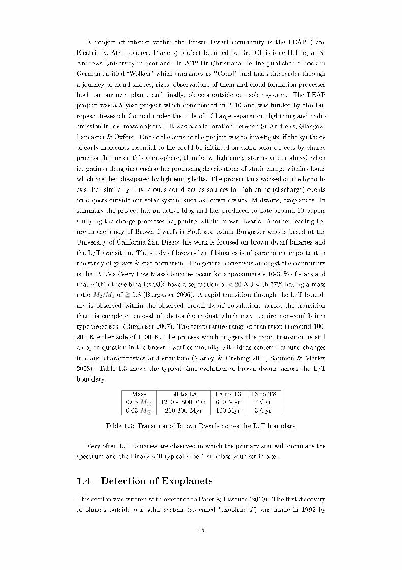
A project of interest within the Brown Dwarf community is the LEAP (Life,
Electricity, Atmospheres, Planets) project been led by Dr. Christiane Helling at St
Andrews University in Scotland. In 2012 Dr Christiana Helling published a book in
German entitled Wolken which translates as "Cloud" and takes the reader through
a journey of cloud shapes, sizes, observations of them and cloud formation processes
both on our own planet and nally, objects outside our solar system. The LEAP
project was a 5 year project which commenced in 2010 and was funded by the Eu-
ropean Research Council under the title of "Charge separation, lightning and radio
emission in low-mass objects". It was a collaboration between St Andrews, Glasgow,
Lancaster & Oxford. One of the aims of the project was to investigate if the synthesis
of early molecules essential to life could be initiated on extra-solar objects by charge
process. In our earth's atmosphere, thunder & lightening storms are produced when
ice grains rub against each other producing distributions of static charge within clouds
which are then dissipated by lightening bolts. The project thus worked on the hypoth-
esis that similarly, dust clouds could act as sources for lightening (discharge) events
on objects outside our solar system such as brown dwarfs, M-dwarfs, exoplanets. In
summary the project has an active blog and has produced to date around 60 papers
studying the charge processes happening within brown dwarfs. Another leading g-
ure in the study of Brown Dwarfs is Professor Adam Burgasser who is based at the
University of California San Diego: his work is focused on brown dwarf binaries and
the L/T transition. The study of brown-dwarf binaries is of paramount important in
the study of galaxy & star formation. The general consensus amongst the community
is that VLMs (Very Low Mass) binaries occur for approximately 10-30% of stars and
that within these binaries 93% have a separation of < 20 AU with 77% having a mass
ratio M2/M1 of = 0.8 (Burgasser 2006). A rapid transition through the L/T bound-
ary is observed within the observed brown dwarf population: across the transition
there is complete removal of photospheric dust which may require non-equilibrium
type processes. (Burgasser 2007). The temperature range of transition is around 100-
200 K either side of 1200 K. The process which triggers this rapid transition is still
an open question in the brown dwarf community with ideas centered around changes
in cloud characteristics and structure (Marley & Cushing 2010, Saumon & Marley
2008). Table 1.3 shows the typical time evolution of brown dwarfs across the L/T
boundary.
Mass L0 to L8 L8 to T3 T3 to T80.05 M 1200 -1800 Myr 600 Myr 7 Gyr0.03 M 200-300 Myr 100 Myr 3 Gyr
Table 1.3: Transition of Brown Dwarfs across the L/T boundary.
Very often L, T binaries are observed in which the primary star will dominate the
spectrum and the binary will typically be 1 subclass younger in age.
1.4 Detection of Exoplanets
This section was written with reference to Pater & Lissauer (2010). The rst discovery
of planets outside our solar system (so called exoplanets) was made in 1992 by
45

Aleksander Wolszczan who deduced that the pulsar PSR 1257 had two planets orbiting
around it. The rst exoplanet to be discovered orbiting around a main-sequence star
was 51 Pegasi b (Mayor & Queloz 1995) which is widely regarded as a prototype
for Hot Jupiters and orbits its host star at a distance of approximately 0.53 AU
(Mercury's orbit around our sun is 0.39 AU and that of Venus is 0.72 AU).
There are various methods by which exoplanets can be detected both directly and
by indirect means. A summary of existing and possible proposed methods is shown
in gure 1.2.
Figure 1.2: A summary of methods by which exoplanets can be detected, Perryman(2000).
As of August 2016, the Exoplanet.eu website lists a total of 2670 exoplanets con-
rmed using the transit method (section 1.4.1), 678 using the radial velocity method
(section 1.4.2), 70 conrmed using direct imaging, 50 by microlensing and 23 using
timing variations.
1.4.1 Exoplanet transit Method (Photometric Method)
The exoplanet transit method is a technique which uses photometry to study the ux
output from a star-planet system over a period of time. As a planet passes in front
of a star, the observed ux will decrease (primary transit). The transit technique can
only detect planets which have orbits aligned edge on to the direction of viewing-thus
around 98% of planets cannot be detected by this method as their orbits are not
parallel to the line of sight of a telescope. The change in ux, ∆F is related to the
radius of the eclipsing planet and its parent star by:
∆FF
=(Rplanet
Rstar
)2
(1.1)
where F is the ux when the planet it not transiting in front of the star. This relation
is derived by comparing the ux observed when the planet is away from the star and
when it transits in front: the power of 2 is simply a result of ux, by denition been
inversely proportional to surface area of the emitting body. The radius of Jupiter is
46

∼ 0.1R. The dip in brightness of Jupiter passing front of our own star as observed byan observer outside of Jupiter's solar orbit will be ∼ 1%. For the earth passing in front
of the sun the dip in brightness observed by an observer outside of the earths' solar
orbit will be ∼ 0.01% . Hence the transit technique is only suited to planets which
are orbiting close in to their parent star have planetary radii which are comparable to
the radii of their parent star. Additionally the transit method is only suited to cases
where the transit of the planet is near the line-of sight of the satellite or telescope
aiming to observe it (Borucki & Summers, 1984).
1.4.2 Radial Velocity Method
51 Pegasi b was discovered using the Doppler radial velocity method using the ELODIE
spectrograph on the Observatoire de Haute-Provence telescope based in south-east
France. The radial velocity phase curve for 51 Pegasi is shown in gure 1.3.
Figure 1.3: Radial Velocity Phase curve for 51 Pegasi which was used to discern thepresence of 51 Pegasi b which has been widely accepted to be the rst exoplanetdiscovered orbiting a main-sequence star. Image retrieved from exoplanets.org web-pages.
As a planet orbits around a star, the colloquially held belief is that the star
is stationary-or for the purposes of calculations (particularly at school)- the star is
assumed to be stationary. However, in practice both the star and planet orbit around
the centre of mass of the planet-star system they form. Hence the star actually
moves, aka "wobbles" as the planet orbits around. This "wobble" can be detected
using the so-called "Doppler method" where the star's spectral lines are observed to
be red shifted (as the star moves away from the observer) and blue-shifted (as the
star moves towards the observer) in a periodic trend as the planet orbits.
For this method, in order to observe a measurable eect in the line position of spectral
lines from a star the Doppler shift must be suciently large-this method favours large
planets that have small orbits around their host stars.
Our very own sun wobbles by around 12.6 ms−1 For a Hydrogen α line, λ0 = 6563
Å. The change in wavelength, ∆λ is given by:
δλ = λ0vc ∼ 2.8 × 10⁻⁴ Å where c is the speed of light.
A problem with this method is that very often wavelength of the star's spectral lines
47

are observed to oscillate without the presence of an exoplanet due to eects such as
stellar oscillation. Hence the concept of the PLATO mission (Rauer et al. 2014)
mentioned in section 1.8.3.
1.5 ExoMoons
Another interesting eld of study which has developed from the search for exoplanets
is the search for exomoons. This eld has been pushing the boundaries of exoplanet
detection by creating algorithms to thoroughly account for the systematic noise in-
herent in the Kepler satellite. David Kipping was a PhD student at UCL (2007-2011)
who, under the direction of Professor Giovanna Tinetti developed techniques for de-
tecting exomoons: this pioneering work won him several awards including the Royal
Astronomical Society Keith Runcorn Prize (2012 and the Springer Thesis Prize for
Outstanding PhD Research (2011). Since then he has worked at Harvard Univer-
sity, Smithsonian Institution and now Columbia University in the City of New York
where he is leading the HEK (Hunt for Exomoons with Kepler) project which uses
computer algorithms to search for bodies (moons) orbiting exoplanets. HEK is in-
dependently funded and has recently been able to purchase a new supercomputer
(Michael Dodds Computing Facility) from donations through the science crowd fund-
ing website Petridish.org. The HEK project searches for exomoons by automatically
selecting from KOIs (Kepler Objects of Interest) targets which could possibly host
exomoons and then comparing their observed lightcurves to simulated lightcurves of a
planet-only system and a a planet & moon system lightcurve. All of the comparisons
are done within a Bayesian framework. In principle the project can detect planet bi-
naries as well as distinct planet-moon systems (this denition is more of a continuum
and can be dened in terms of position of the centre of mass of the two objects). Early
pioneering work by Elser et al. (2011) of simulations of planet formation predicted
that ExoMoons should form: hence with this in mind, the HEK project was created.
A summary of the studies published to date by the HEK project are shown in table
1.4.
Reference Title YearHEK-I Description of a New Observational project 2012HEK-II Analysis of Seven Viable Satellite-hosting Planet Candidates 2013HEK-III The First Search for an Exomoon around a Habitable-zone Planet 2013HEK-IV A Search for Moons around Eight M Dwarfs 2014HEK-V A Survey of 41 Planetary Candidates for Exomoons 2015
Table 1.4: Summary of studies undertaken by the HEK project
Before the project started, Kipping et al. (2009) had done a test study of the
Kepler data and demonstrated that moons of mass ≥ 0.2 M⊕ should be detectable.
In contrast, the largest known moon in our solar system is Ganymede (which orbits
Jupiter) which has a mass of 0.025 M⊕. Thus the project is searching for moons that
are at least an order of magnitude larger in mass than any known in our own solar
system.
HEK I discusses the TSA (Target Selection Algorithm) and TSP(Target Selec-
48

tion Prioritisation) algorithms developed to automatically search through the Kepler
catalogue.
HEK II investigates 7 targets which were selected from 35 targets determined by
the TSA from 2321 objects. The LUNA algorithm (Kipping et al. 2011a) was used
to simulate model planet lightcurves: for each target 9 models were simulated using
various parameters and constraints and a prioris with planet-only system, planet and
moon system: additionally non-physical models were simulated. A Bayesian model
selection was then undertaken and conrmation was obtained that this model selection
was not favouring non-physical models (i.e. radius of moon set to zero). This model
selection was looking for so-called TTVs: Transit Timing Variations which would be
indicative of another mass perturbing the planet transiting in front of its' host star.
HEK III described the work undertaken in searching for an exomoon around Kepler
22b which is a planet in the so-called Habitable zone. This target is advantageous as
had previously been studied by astro-seismologists due to the low photometric noise
in its' transit curve and multiple radial velocity measurements. This study utilised the
CoFiAM algorithm(Cosine Filtering with Autocorrelation Minimization) to lter out
various systematic eects and sources of noise as described in Kipping et al. (2013a).
In summary no evidence was found for a moon larger than 0.2M⊕ and furthermore,
with the current availability and quality of lightcurve data only moons with mass
greater than 1M⊕ would theoretically be detectable.
HEK IV searched for planetary systems around 8 M dwarfs. A result of HEK IV
was the discovery of the lowest mass exoplanet to date which highlights why this work
is still important. It has been determined that this planet, KOI-314c has a mass of
1.0+4−3 earth masses and a radius of 1.61+0.16
−0.15 earth radii.
HEK V found no evidence for exomoons in a study of 41 planetary KOIs. The
authors do however note that when photodynamics is not used and instead only
photometric transits alone are used, it could be incorrectly discerned that around
1 out of 4 of the KOIs could harbour exomoons due to the eects of signal noise
inherent in the Kepler instruments. An ancillary result of this study is that 13 out of
41 KOIs have masquerading planet signals which are actually due to stellar variation
and various systematics of the detection equipment. Hence this result helps justify the
existence of the HEK project: even if no exomoons are detected, at the very least the
algorithms generated have helped tease apart true planetary transit signals from false
positives. In order to characterise exoplanets accurately using the transit method it
is vitally important that all systematics aecting the transit curves are considered.
1.6 Characterisation of Exoplanets
Since the discovery of 51 Pegasi b in 1995 (Mayor & Queloz 1995) the eld of exo-
planetary science has blossomed with over 2000 exoplanets conrmed(as of February
2016) with a further 201 candidates which are classed as controversial as dened on
the Exoplanets.eu website. Over 60% of these conrmed planets are transiting exo-
planets and around 30% have been detected by the indirect radial velocity technique.
This website can be used to generate histograms and scatter plots of data showing
the inherent bias in the detection methods for nding large planets orbiting close-in
49

to their host stars. An analysis of the exoplanets detected to date can also potentially
provide information on how planetary systems form and evolve in general.
However, an obvious next step for the eld is to ask the question: What do
these exoplanets contain?. Is there life on other planets? In order to characterise
the atmospheres of exoplanets, spectroscopy is needed as well as developments in
modelling of atmospheres.
A modern description of spectroscopy is that it is the interaction between matter
and radiation. However traditionally spectroscopy was thought of as the process by
which visible light is split by prisms: for example the experiments on optics done by
Newton. Joseph von Fraunhofer was a key player in the development of spectroscopy
becoming a precise science with his development of disperse spectrometers. Today
spectroscopy can be used in all areas of science to identify both atoms and molecules
in samples by precise knowledge of the wavelengths that they emit or absorb.
Spectroscopy can be applied to the transit method of detection: by observing a
planet orbiting its' host star changes in the transit depth at dierent wavelengths
can be used to help deduce which molecules are in the planets' atmosphere using
knowledge of which molecules absorb at particular wavelengths.
In exoplanetary modelling very often the process called forward modelling is
used: by this we mean that a synthetic spectrum is generated using a computer
programme for a whole range of model atmospheres which sample a huge range of pa-
rameters such as temperature, pressure and molecular composition. These synthetic
models are then compared to real observations with the aim of hence placing con-
straints on what the atmosphere of the planet observed in question contains and its
Temperature & pressure proles. At present due to the lack of data covering multi-
ple wavelength regions very often there are huge degeneracy's in the models selected.
The opposite of this approach is to use inverse modelling in which a programme
tries to work backwards to solve what the atmospheric prole is of an observed
exoplanet. The geosciences literature contains many reviews explaining the dierence
between forward and inverse modelling applied to modelling scenarios such as along
tectonic fault lines (Allmendinger, 1998), helioseismic modelling (Ritzwoller & Lavely,
1991) and also in understanding how light propagates through materials (Arridge &
Schotland 2009).
NEMESIS (Irwin 2008), which is an acronym for Non-linear optimal Estimator
for MultivariateE spectral analysis, is an example of a program developed to create
synthetic spectra for model atmospheres. It was originally developed by Professor
Patrick Irwin for analysing data from the NASA Cassini spacecraft of Saturn and
Titan. Since then it has been used for making predictions of exoplanetary atmospheres
in the near Infra red to microwave regions.
UCL are developing a program called Tau-REx (Tau Retrieval of Exoplanets)
which uses a Bayesian framework in order to select in an unbiased manner a model
atmospheric composition from sampling a large sample space of input composition
(Waldmann et al. 2015, 2016). Tau-REx will use all molecular data provided and
make no assumptions about molecular composition or temperature thus sidestepping
human bias. In order to model the (T, p) prole of a planet, Tau-Rex will combine
the two commonly used approaches of writing an analytic equation for prole and
50

a layer by layer approach thus gaining the unique benets of both methods. This
programme will use linelists from the ExoMol project and is designed to make use
of parallel computing so that it is fully scale-able for use in cluster computing sites.
This work is described in Waldmann et al. 2015 in which the functionality of the
programme is demonstrated for the cases of the Hot Jupiter WASP-76b and the
SuperEarth 55 Cnc e.
To date several exoplanets have been studied intensively by astronomers wishing
to characterise their atmospheres, for example, GJ 1214b, HD 189733b, HAT-P-32b
& HAT-P-33b and WASP 33b. These are discussed in proceeding sections. Table 1.5
gives a summary of notable review papers in the eld of the exoplanetary atmosphere
characterisation.
Author(s) Year Title Journal/BookG. Laughlin, Gregory,J. J. Lissauer
2015 Exoplanetary Geophysics- An Emerging Discipline
Review chapter to appear in Treatise onGeophysics, 2nd Edition
K. Heng, A. P. Show-man
2015 Atmospheric Dynamics ofHot Exoplanets
Annual Review of Earth and PlanetarySciences
K. Poppenhaeger 2014 Stellar magnetic activityand Star-Planet Interac-tions
Invited review for the CoRoT Sympo-sium 3 / Kepler KASC-7 joint meeting,Toulouse, July 2014.
A. S. Burrows 2014 Spectra as windows intoexoplanet atmospheres
Proceedings of the National Academyof Sciences
N. Madhusudhan, H.Knutson, J. J. Fortney& T. Barman
2014 Exoplanetary Atmo-spheres
Protostars and Planets VI
J. Bailey 2014 The Dawes Review 3: TheAtmospheres of Extraso-lar Planets and BrownDwarfs
Publications of the Astronomical Soci-ety of Australia
A. S. Burrows 2014 Highlights in the study ofexoplanet atmospheres
Nature
M. S. Marley, A. S.Ackerman, J. N. Cuzzi,D. Kitzmann
2013 Clouds and Hazes in Exo-planet Atmospheres
Comparative Climatology of TerrestrialPlanets
G. Tinetti, T. Encre-naz, A. Coustenis
2013 Spectroscopy of plane-tary atmospheres in ourGalaxy
The Astronomy and Astrophysics Re-view
F. Allard, D. Homeier,B. Freytag W. Schaf-fenberger, A. S. Ra-jpurohit
2013 Progress in modeling verylow mass stars, browndwarfs, and planetarymass objects.
Memorie della Societa AstronomicaItaliana Supplement
F. Allard, D. Homeier,B, Freytag C. M. Sharp
2012 Atmospheres From VeryLow-Mass Stars to Extra-solar Planets
EAS Publications Series
A. P. Showman, J.Y.K. Cho, K. Menou
2010 Atmospheric Circulationof Exoplanets
Exoplanets, edited by S. Seager
G. Chabrier, I. Barae,F. Allard & P. H.Hauschildt
2005 Review on low-mass starsand brown dwarfs
Invited review, "Resolved Stellar Pop-ulations", Cancun, april 2005
Table 1.5: Summary of Exoplanet & Brown dwarf atmospheric characterisation reviewpapers
51

1.6.1 Super-Earth GJ 1214b
The Super-Earth GJ 1214b, originally nicknamed The Water World is a particular
favourite of exoplanet scientists. Super-earths are commonly dened as planets with
mass between 1.9 and 10 M⊕. GJ 1214b was found by Charbonneau et al. (2009)
orbiting its host star GJ 1214 using the MEarth project which uses the technique
of planetary transits to detect planets. Table 1.6 shows a sample of parameters for
the planet and its' host star estimated by the authors in their original Nature paper
assuming a thin outer envelope of hydrogen and helium with the remaining 95% of
the mass of the planet been water.
Property Estimate
Planetary
Mass 6.55 ± 0.98 M⊕Radius 2.678 ± 0.13 R⊕
Gravitational Acceleration 8.93 ± 1.3 ms−2
Hydrodynamical Escape Rate 9 × 10⁵ kg s−1
Orbital Period 1.5803925 ± 0.0000117 days
Planetary equilibrium temperatureAssuming a Bond albedo of 0 555 K
Assuming a Bond albedo of 0.75 393 K
StellarMass 0.157 ± 0.019 MRadius 0.2110 ± 0.0097 R
Eective Temperature 3,026 ± 130 K
Table 1.6: Parameters of the Super-Earth GJ 1214b and its' host star, GJ 1214estimated by Charbonneau et al. (2009) assuming a solid core of water
Since this planet-star system is only 13 parsecs away it is accessible to be studied by
spectroscopic analysis and has since been with over 130 papers as of December in the
SAO/NASA Astrophysics Data System (ADS) referring to GJ 1214b. Of particular
controversy is the the at spectrum of GJ 1214b (Bean et al. 2010) which has
sparked debate within the exoplanet community as very often any atmospheric model
put forward is loaded with assumptions and at present it is dicult, if not impossible
to break the degeneracies of parameters between model atmospheres.
To briey summarise a choice selection of papers:
Bean et al. (2010) performed a ground-bases transmission spectrum analysis
between 780 and 1000 nm and concluded that, to a signicance level of 4.9
σ, that the spectrum was featureless and hence must contain clouds that are
obscuring any underlying features at the measured wavelengths. Furthermore a
dense atmosphere of water vapour is consistent with the at spectrum observed.
Bean et al. (2011) put forward evidence for a metal-rich atmosphere by ex-
amining the transmission spectrum at optical and near infra-red wavelengths.
They conclude from their cross-analysis of data that either GJ 1214b has an
atmosphere composed of 70% H2O(by mass) or contains optically thick clouds
or haze at high altitude.
Morley et al. (2013) have performed simulations of model atmospheres for GJ
1214b using two types of cloud cover which are physically motivated: a) clouds
that are present in chemical equilibrium and b) clouds due to photochemical
kinetic models. They conclude that the former type of clouds if present in the
52

upper-atmosphere and of enhanced metallicity can match the observations of
GJ 1214b.
1.6.2 Hot Jupiter HD 189733b
The Hot Jupiter planet of HD 189733b was discovered by Bouchy et al. (2005)
who were undertaking a joint photometric (transit) and radial-velocity search for
exoplanets orbiting stars of high metallicity: they estimated its' mass and radius to
be 1.15 ± 0.04 MJ and a radius of 1.26 ± 0.03 RJ respectively. It was the rst planet
to be found with visible scattered polarised light (Berdyugina et al. 2008). Since it is
one of the closest transiting Hot Jupiter to earth known, and coupled with its short
planetary transit of 2.219 days making it tidally locked it has thus been vigorously
studied from an orbital dynamics and spectroscopic (atmospheric characterisation)
perspective.
Again, to briey summarise a choice selection of papers: Knutson et al. (2007)
have constructed a map of the temperature and thermal transport on HD 189733b:
they concluded that heat energy is eectively transported from the dayside to the
nightside with a dayside temperature range between 973 ± 33 K and 1212 ± 11
K. In 2007, Tinetti et al. put forward the hypothesis that water vapour absorption
in the atmosphere of HD 189733b was responsible for changes in eective radius
when observed at infrared wavelengths of 3.6 µm, 5.8 µm and 8 µm. They also
demonstrate in their paper that a so-called non-detection of water is the likely result
of assuming an isothermal atmospheric temperature prole. In 2007, Swain et al.
(also based at UCL) backed this claim of water detection with a resolved water band
at 1.9 µm and also claimed the presence of methane in a near infra-red transmission
spectrum taken of HD 189733b. The authors also note that models of Hot Jupiters
predict also the presence of carbon monoxide that they were unable to observe hence
potentially implying the need for new models including potentially photochemical
reactions and/or horizontal chemical gradients.
1.6.3 HAT-P-32b & HAT-P-33b
The discoveries of HAT-P-32b and HAT-P-33b were reported by Hartman et al. (2011)
and both orbit so called high-jitter stars which made their detection troublesome
and hence required detailed photometric modelling of light curves. The authors noted
that "both planets are among the largest radii transiting planets discovered to date".
Their orbital periods were estimated by the authors to be 2.150008 ± 0.000001 days
and 3.474474 ± 0.000001 days respectively. Indeed, the discovery of large Hot Jupiter
planets orbiting close in to their host stars has sparked fresh debate and questioning
as to the formation of our own solar system.
1.6.4 WASP-33b
Guenther et al. (2011) reported the detection of WASP-33b (also known as HD
15082b) using SuperWasp project which searches for exoplanetary transits. It orbits
the A5 star of HD15082 with an estimated orbital period of 1.22 days and thus, to
date is the hottest known exoplanet detected with an the initial estimated of eective
53

surface temperature being 2700 K. Since its' discovery, studies have been undertaken
of heat distribution within its atmosphere. Ground based transit observation of Smith
et al. (2011) in the 0.91 µm region of its luminosity prole indicated that it has a
corresponding brightness temperature of 3620200250 K which is consistent with a model
in which there is very inecient, if any at all distribution of heat from the tidally
locked dayside to nightside of the planet. Furthermore, Haynes et al. (2015) presented
spectroscopic evidence for a temperature inversion in this tidally-locked dayside which
they hypothesis is due to the presence of TiO: if this is conrmed it would be the rst
hot Jupiter to have a thermal inversion due to this molecule.
1.7 Astrobiology
Due to the extensive eorts that have been made to characterise exoplanets a eld of
study which has developed is that of Astrobiology. To quote Professor Peter Read
(Oxford University) at a RAS(Royal Astronomical Society) meeting in London during
March 2013 Astrobiology can be viewed as an interesting new subject or an annoying
distraction (!).
A very notable paper uploaded to the Archive was that by Jacob Haqq-Misra(2013)
who proposed a funding mechanism for searching for extra terrestrial intelligence
(SETI) using a lottery bond for which maturity would occur when ETI was con-
rmed. In his paper he discusses ethical considerations and puts forward mathemat-
ical models of the funding structure. He concludes by noting that In the best case,
SETI succeeds; but even in the worst case, if SETI nds nothing, then it will at least
have taught us how to think more seriously about our nancial future. On a more
serious note, a prominent gure in the emerging discipline of astrobiology is Professor
Sara Seager who is based at MIT. Her work focuses on studying transiting exoplanets
with a particular focus on modelling the photochemistry of atmospheres containing
so-called biosignatures which are dened as gases such as methane whose simulta-
neous presence could possibly indicate the presence of life(Seager 2013, Seager, Bains
& Hu 2013, Seager, Turner, Seager & Deming 2010, Schafer & Ford 2005).
1.8 Past, Present, Proposed and Future Satellites for
Exoplanetary Study
Figure 1.4 shows a summary of present and future missions which will be used to
study exoplanets. The future missions of TESS and the JWST are described below
as well as the proposed missions of ARIEL and Twinkle.
1.8.1 TESS
TESS, Transiting Exoplanet Survey Satellite, selected by NASA in 2013 as an Ex-
plorer (EX) Mission, is due to launch between August 2017 and June 2018 and will
be delivered into orbit by the Falcoln 9 rocket which has a track record of launching
NASA and commercial satellites. TESS will be a two year survey which will mon-
itor 50, 000 stars in the solar neighbourhood for transiting exoplanets. It is led by
54

Figure 1.4: Present and Future Exoplanet Missions
Dr. George Ricker and MIT and has the principle goal of detecting small plan-
ets with bright host stars in the solar neighbourhood. Since the stars surveyed will
be 30-100 times brighter than those surveyed by Kepler, follow-on characterisation
of atmospheres and determination of parameters such as planetary masses & radii
should be enhanced. By statistical arguments, it is expected that from the 50, 000
stars surveyed, approximately 3000 transiting exoplanet candidates should be ob-
served by TESS: in amongst these candidates it is reasonable to expect around 500
Super-Earth planets. The instruments onboard TESS will include 4 wide eld CCS
cameras which have been designed for photometric stability.
1.8.2 JWST
The James Webb Space Telescope (JWST) is, at present expected to launch in Oc-
tober 2018 and is a joint international eort between NAA, ESA and CAS(Canadian
Space Agency). It is named after James Webb who is a former administrator of NASA.
It will be a telescope operating in the infra-red (0.6 to 28.5 µm) with 4 instruments
which will study over a 5-10 year lifetime a range of astrophysical environments. It is
designed to be a follow-on to the Hubble space telescope(which operates in the visible
and UV) with mission goals including searching for primordial galaxies formed closely
after the Big Bang, tracking the evolution of galaxies and stars and also searching for
life on other planets by the chemical and physical properties of exoplanetary systems.
Upon been placed in an L2 orbit at approximately 1.5 million km from earth its'
primary 6.5 m mirror will unfold from 18 dierent segments and will be protected
from the damaging eects of our sun by a 5-layer sunshield the size of a tennis court.
A notable tweet on twitter about the JWST is that of Dr Jo Barstow: "It'll be 15
55

DAYS after JWST arrives at L2 b4 telescope fully unfolded. 15 DAYS of TERROR.
Every1 will be on blood pressure meds. "
Dr Jo Barstow, has undertaken work on constraining what quality of exoplanet
atmosphere retrievals would theoretically be possible with the JWST: Transit spec-
troscopy with JWST: Systematics, starspots and stitching, Barstow et al. (2015).
This study investigates how data from the NIRSpec and MIRI-LRS instruments could
be stitched together to help degeneracy's inherent within models of exoplanetary
atmospheres provided that individual instrument noise as well as the eects of taking
measurements at dierent times is considered. These instruments will operate at 0.6-5
µm and 5-12 µm respectively. Using the NEMESIS programme Barstow et al. (2013)
created synthetic single-slab model atmosphere spectra for primary and secondary
transits for dierent planetary objects shown in table 1.7 using the molecular data
shown in table 1.8. For the Earth like planet they used a bulk composition of N2−O2
and for the other planets used a bulk H2−He composition: for each of these planets
they varied the concentration of the trace elements of CO2, CO and CH4. They then
applied the expected noise levels expected from the instrument systematic on-board
JWST before nally using NEMESIS to retrieve the input model atmosphere. The
team then established the minimum concentrations of trace elements, as shown in ta-
ble 1.9 for the various exoplanets required so that a single observation would correctly
constrain the input model atmosphere within a statistical uncertainty of 2σ.
Planet Mass(1024kg) Radius (km)Hot Jupiter 1800 75000Hot Neptune 180 30000GJ 1214b 37 15355Earth 6 6378
Table 1.7: Planetary objects considered by Barstow et al. (2013) considered for studyby JWST.
Molecule Source Reference paperH2O HITEMP2010 Rothman et al. (2010)CO2 CDSD-1000 Tashkun et al. (2003)CO HITRAN1995 Rothman et al. (1995)CH4 STDS (Wenger & Champion
(1998)
H2/HeBorysow & Frommhold 1989; Borysow et al. 1989;
Borysow & Frommhold 1990; Borysow et al. 1997; Borysow 2002
Table 1.8: Molecular data used in the simulations of Barstow et al. (2013).
GasHot Jupiter Hot Neptune
Precision factor concentration (ppmv) Precision factor concentration (ppmv)H2O 3 0.1 1.5 1CO2 2 0.5 3 10CO 10 10 5 10CH4 3 0.1 2 0.1
Table 1.9: Minimum concentration required for trace elements in order for there tobe a detection for a typical Hot Jupiter and Hot Neptune as determined by Barstowet al. (2013)
56

Barstow et al. have also studied how the presence of star spots observed in the
primary transit may eect the orbital radius of the planet determined which is depen-
dent on the wavelength observed. For M dwarfs with sunspots it is not appropriate
to model the stellar spectrum using a Boltzmann distribution. Barstow also points
out that as star spots may vary between the time of observations taken by the two
instruments there is a need for a study of the time variability of individual star spots.
The team also establish that the JWST could be used to distinguish between cloudy
and cloud free atmospheres and the authors point out that, with the increasing char-
acterisation work been undertaken within the research eld, using cloud-free models
is no longer a physically accurate interpretation. In summary the team highlight the
need for planning on behalf of the exoplanet community in order that suitable targets
are selected which would really make ecient use of the capabilities of the JWST.
Since the JWST is not dedicated solely to exoplanetary science the community will
be competing for observation time with astronomers working in competing elds.
1.8.3 The ECho Science Mission
Prior to studying the capabilities of the JWST, Barstow et al. (2013, 2014) studied
what the capabilities for atmospheric retrieval of ECho would have been. ECho was
a short-listed candidate mission for the M3 launch of the ESA's cosmic vision pro-
gramme, PI'd by Professor Giovanna Tinetti. Again, using the technique of simulating
synthetic spectra using NEMESIS, integrating in system noise (using the specially de-
veloped EChoSim programme) and then carrying out a retrieval Barstow et al. found
that for planets with bulk H2−He composition it would be possible using ECho to
correctly detect the trace molecules of H20, CO2, CO and CH4 within a certainty of
2σ and also retrieve the temperature prole within 200 K given the necessary data
shown in table 1.10. For GJ 1214b no CO or NH3 was included. Planets with a
bulk H2−He composition are those that lie close to their host star and thus have a
composition which reects the centre of the protoplanetary disc which they emerged
from.
PlanetHost star D Data required
type Mass (MJ) Radius (RJ) Teff (K)Hot Jupiter 0.95 1.07 1500 G2(sun like) 35 single transit or eclipseWarm Jupiter 0.95 1.07 650 G2 35 20 transits or eclipsesHot Neptune 0.095 0.43 800 M dwarf 6 10 transits of eclipsesGJ 1214b 0.02 0.22 450 GJ 1214 13 30 transits
Table 1.10: Summary of deductions made about data required to successfully char-acterise dierent exoplanets by Barstow et al. (2013, 2014). Here D is the distancein pc to the system
Unfortunately ECho was not selected but instead PLATO, The PLAnetary Tran-
sits and Oscillations of stars was instead selected and is expected to launch in 2024.
PLATO will search for planets orbiting in the so-called Habitable zone of their host
stars as part of a survey searching for extrasolar planetary systems. PLATO will also
be used to study seismic activity of stars: a very important consideration when trying
to characterise exoplanets as at present it is very dicult to distinguish between host
57

star variability and variability in transit curves which is genuinely due to a planet
passing in front of the star.
Following on from all the substantial scientic research which had been invested
into ECho by the exoplanet community, two proposed missions, ARIEL and Twinkle
have been created and are both been led by Prof. Tinetti.
1.8.4 ARIEL
ARIEL (Atmospheric Remote-sensing Infra-red Exoplanet Large-survey) is a proposed
European Space Agency M4 mission which has been selected for further study along
with THOR (Turbulence Heating ObserveR) and XIPE (X-ray Imaging Polarimetry
Explorer) from 27 original proposals. From these three proposed missions, one will be
selected and scheduled for launch in 2024 into the L2 orbit with a budget of around
450 million Euros. If ARIEL is selected it will study the atmospheres of around 500
planets which are orbiting close in to their parent stars within our galaxy using a 90
cm infra-red telescope. This telescope will cover the wavelength range from around
1.95 to 7.8 µm: additionally to aid the detection and characterisation of clouds there
will be photometric bands in both the visible and near-IR which will also assist with
the monitoring of stellar activity. Figure 1.5a shows a concept view of what ARIEL
will look like if it is selected for ight.
1.8.5 TWINKLE
"Twinkle: A British Space Mission to Explore Faraway Worlds" is a proposed satel-
lite which aims to investigate the atmospheres of target exoplanets by studying the
wavelength region of approximately 0.5 to 5 µm (subject to renement). This is
a region in which molecules of signicant importance to life (e.g. methane, ethane
and precursors to amino acids such as ammonia and HCN) have important distin-
guishable features. Twinkle will observe around 100 nearby known exoplanets: by
building up repeat measurements over multiple wavelengths over time of the plane-
tary transits unprecedented information will be obtained about the atmospheres of
these planets. It is been built by Surrey Satellites-a company which has a proven
track record of delivering small scale, small cost missions on time and on budget.
Since the satellite will be using o the shelf components the budget for research &
development of detection technology is reduced. It will be placed in a a low-earth po-
lar orbit 700 km above the earth's surface with a launch date been targeted within the
next 4 years. Universities and Research Institutions throughout the UK are involved
in the development of the payload study and science case including UCL Depart-
ment of Physics and Astronomy & UCL Mullard Space Science Laboratory, Surrey
Satellite Technology Ltd, Selex ES, STFC Rutherford Appleton Laboratory, STFC
UK Astronomy Technology Centre, Cardi University, Imperial College, Queen Mary
University London, Royal Holloway, Open University, Oxford University, University
of Hertfordshire, University of Leicester, University of East Anglia, Keele University,
University of Manchester and Royal Observatory Edinburgh. Figure 1.5b shows a
computer generated image of what Twinkle is designed to look like upon been built
and launched into space. In terms of funding, the project has a budge of around 50
58

million pounds: at present the ongoing payload study is been funded by grants from
various UK Universites and the European Research council. The Twinkle team is
actively seeking funding from both private and public sources e.g. schemes such as
crowdfunding which was a highly ecient means of raising capita for the case of the
Lunar One module.
(a) (b)
Figure 1.5: Concept view of the ARIEL spacecraft, credit ESA (gure 1.5a) anda computer generated image of the Twinkle spacecraft (gure 1.5b) been built bySurrey Satellite Technology Ltd. Images retrieved from the website for the centre ofplanetary sciences(cps) based at UCL.
EduTwinkle
Alongside the scientic research work and money-raising eorts been undertaken to
ensure that TWINKLE ies, a concerted eort is been put into developing an accom-
panying educational program, EduTwinkle which is been led by Dr Clara Sousa-Silva,
a former PhD student of the ExoMol group. EduTwinkle covers all Key Stages with
an emphasis on encouraging more girls to enter STEM careers. The IOP (Institute
of Physics) undertakes a lot of research investigating why fewer girls choose to study
A-Level physics (It's dierent for Girls) and eventually university. EduTwinkle ac-
tivities include:
CPD (Continuing Professional Development) sessions run for Primary School
teachers demonstrating how they can use the science in Twinkle to inspire their
pupils.
Twinkle's Little Stars (KS2/KS3)
The Twinkle Challenge (KS4)-A challenge in which school pupils work as teams
on activities that showcase how scientic missions are multi-disciplinary and
thus how a science degree can lead to many career opportunities
Exoplanet Explorers-AS level(KS5)-module aimed at getting pupils to under-
stand the ethics of scientic work
59

Work with the Brilliant Club which is an award-winning charity which places
PhD and postdocs in state schools all over England with the aim of raising
attainment
ORBYTS (Original Research By Young Twinkle Students)-an initiative in which
Year 12 and Year 13 students work with a PhD student within the ExoMol group
on analyses experimental data which can then be used in the construction of
new linelists
Engaging school pupils as well as the public in scientic missions is a worthwhile
cause. The so-called public can also be potentially a substantial help in undertaking
research: for example the Galaxy Zoo project. An example of a citizen science project
in the eld of exoplanets is that of the Disk detectives which asks users to examine
images taken by the WISE spacecraft and determine if young stars contain dusty
disks which could potentially harbour planets.
1.9 Existing Molecular Databases
Before the ExoMol project was created (Tennyson & Yurchenko 2012), there were and
still are several other groups working in molecular spectroscopy on creating databases
of molecular data that can be used by astronomers for characterisation purposes.
The HITRAM, HITEMP and CDMS databases are discussed below. Other sources
of molecular and atomic data include:
SPECTRA, based in Tomsk
GEISA Database
NIST: Quantitative Infrared Database (Version 1.10), Chu, Rhoderick, Guen-
ther & Laerty)
Pacic Northwest National Laboratory, Vapor phase infrared spectral library
CHIANTI: An Atomic Database for Spectroscopic Diagnostics of Astrophysical
Plasmas (Version 6)
The University of Denver Atlas of High-Resolution IR Stratospheric Spectra
SMPO (Spectroscopy and Molecular Properties of Ozone), Universitè de Reims,
Reims, FRANCE, Institute of Atmospheric Optics, Tomsk, RUSSIA
SpectralCalc.com, GATS, Inc.
The Virtual Atomic and Molecular Database Consortium (VAMDC)
Jet Propulsion Laboratory , Molecular Spectroscopy Catalog,
Database of Bernard Plez
The Kurucz databases
The Submilimtetre IR experimental data recorded by the Ziury's Group based
in Arizona
60

With all these databases available the obvious question to ask is: why is the
ExoMol project needed? Put very simply these databases are typically only valid for
molecules(and atoms) existing at room temperatures. As the temperature increases
electrons within the molecules reach higher electronic states and molecules rotate &
vibrate faster: hence new and more transitions occur between molecular states(which
are a combination of electronic conguration, rotational state and vibrational state)
as higher energy states are accessed. Also, often these databases only cover specic
regions: in order to model the opacity of molecules within an atmosphere accurately
all transitions between possible molecular states need to be known. And nally one
of the key aims of the ExoMol project is high accuracy.
Prior to the creation of the ExoMol project in 2011, two of the most commonly used
databases by astronomers for molecular data were the HITRAN and CDMS databases
which are described in sections 1.9.1 and 1.9.2 respectively. These databases both
aim to create self-consistent parameters for molecules using hybrids of all available
experimental and theoretical data for each particular species.
1.9.1 HITRAN & HITEMP
The HITRAN (HIgh-resolution TRANsmission molecular absorption database) and
HITEMP (HIgh-TEMPerature spectroscopic absorption parameters) projects are based
at the Harvard-Smithsonian Centre for Astrophysics and led by Dr L. Rothman and
Dr I. Gordon. The aim of the HITRAN projects is to produce spectroscopic parame-
ters for molecules of interest to modelling the earths' atmosphere (180 to 300K) which
are self consistent with all available experimental data. HITRAN is essentially a cen-
tral database for wavelength data (measured in the vacuum) for molecules. HITEMP
is the high temperature analogue and is in development: the aim of this project is to
gather and compile data which can be used for exoplanets with higher atmospheric
temperatures than the Earth. At present the HITRAN database (HITRAN 2012)
contains data for 47 molecules(covering 120 isotopologues): a new version is due in
2016. These molecules are: H2O, CO2, O3, N2O, CO, CH4, O2, NO, SO2, NO2,
NH3, HNO3, OH, HF, HCl, HBr, HI, ClO, OCS, H2CO, HOCl, N2, HCN, CH3Cl,
HOBr, C2H2, C2H6, PH3, COF2, SF6, H2S, HCOOH, HO2, ClONO2, NO+, HOBr,
C2H4, CH3OH, CH3Br, CH3CN, CF4, C4H2, HC3N, H2, CS and SO3. Addition-
ally the HITRAN project also contains cross sectional absorption data for around 38
molecules.
1.9.2 The Cologne Database for Molecular Spectroscopy (CDMS)
The CDMS database is a database of theoretical predictions of wavenumbers for both
atoms and molecules which are of interest to astronomers and atmospheric scien-
tists. As of November 2015 the database contains 788 entries. The diatomic hydride
molecules and diatomic molecules found in the ISM and extragalactically contained
in this database are shown in tables 1.11, 1.12 and 1.13 respectively.
61

Group Molecules1 NaH, KH2 MgH11 CuH, 65CuH12 66ZnH, ZnH, 68ZnH13 BH, AlH14 CH, CH+, 13CH+, CD+, 13CD+, CT+, SiH15 NH, ND, PH16 OH+, 18OH+, OD+, OH−, 18OH−, OD−, SH, SH+, SH−
18 NeH+, 22NeH+, NeD+, 36ArH+, 40ArH+
Table 1.11: Diatomic hyrides contained with the CDMS database as of November2015.
Diatomic Hydrides Other diatomicsH2, HD AlF, AlCl, KCl, NaCl
CH, CH+, SiH? C2**, CN, CO, CO+, CP, SiC, CF+, CNNH PN, SiN
OH, OH+,SH, SH+ SiS, CS, NSHF, HCl, HCl+ NO, NO+, SO, SO+, SiO, O2, PO, AlO
ArH+ TiO, FeO?
Table 1.12: Diatomic molecules in the CDMS database which are commonly found inthe Interstellar medium of Circumstellar Shells
Diatomic Hydrides Other diatomicsArH+(2015) CO, CO+
H2 CSCH, CH+ CN
NH SO, SO+
OH, OH+ SiOHF NO
NS
Table 1.13: Extragalactic diatomic molecules in the CDMS database
1.10 The ExoMol Database
The ExoMol project was created in May 2011 at UCL and is funded by a 5 year ERC
Advanced Investigator fund awarded to Professor Jonathan Tennyson. The outline
aims of the project are to provide linelists for molecules of astronomical importance
which are of high accuracy and more complete than existing experimentally based
databases (Tennyson & Yurchenko 2012). As the temperature of a molecule is in-
creased, higher states can be reached and thus more transitions (i.e. lines) are
created.
Experimentally it is often very dicult, if not too dangerous to measure the spectra
of molecules at temperatures exceeding 5000 K. As an example BeH and PH3 are
both toxic species but are of interest astronomically (Tennyson et al. 2016).
Hence why there is a need to use state-of-the are ab initio methods to solve the
Schrödinger equation and hence produce a list of wavelengths and frequencies. Nev-
ertheless, experimental data acts as a valuable sanity check and is indeed used to
62

rene theoretical predictions. The methane linelist, which is aptly named 10to10 as
it contains 9.8 billion lines has proved very popular with the exoplanetary community
due to its completeness. For example, Yurchenko et al. (2014) have applied this
methane linelist to atmospheric models the T4.5 brown dwarf 2MASS 0559-14 and
found that the opacities matched observations in places where previously they had
either under or over-estimated the opacity. Since 2011 the expertise of the group has
increased for both diatomic and triatomic and tetratomic molecules. Molecules for
which linelists have been created, or are indeed in the process include: BeH, MgH,
CaH, ScH, CaO, AlO, SiO, VO, TiO CS, NaCl, KCl, PH3, H2O2, H2S, SO2, SO3, CH4,
NH3, HCN, HNC, nitric acid (HNO3) and formaldehyde (H2CO). With each confer-
ence, new molecules have been added to the to do list as the exoplanet community
becomes more ambitious in their characterisation of far-away atmospheres. Collab-
orations with industry have been formed such as that with Alexander Fateev based
at the Technical University of Denmark who wishes to make in-situ measurements of
gases such as SO2 and SO3 which are a by-product of coal-based power plants. Due
to the size of the linelists generated, the need to make our linelists accessible and of
an appropriate format to be put into atmospheric models has been recognised and
addressed with the creation of cross-sections (Hill, Yurchenko & Tennyson 2013) and
also the creation of the ExoMol Database paper, Tennyson et al. (2015).
63

Chapter 2
Theory and Methodology
In this chapter important concepts in molecular spectroscopy will be summarised
and then hence used to explain how linelists for diatomic molecules are constructed.
Before studying molecules, it is useful to understand atomic spectroscopy which is
detailed in section 2.1. Molecular spectroscopy is then explained in section 2.2 with
the selection rules which determine allowed transitions detailed in section 2.3. The
Born-Oppenheimer approximation is outlined in section 2.4: this approximation al-
lows the construction of linelists to be done in several distinct parts as it decouples
the Schrödinger equation into an electronic Schrödinger equation and a rovibronic
Schrödinger equation. These sections have been written in reference to Haken &
Wolf(2004), Brown (1998) and Bransden & Joachain (2000). The challenges of con-
structing linelists for transition-metal bearing diatomics is discussed in section 2.5.
Moving onto methodology, section 2.6 explains how the electronic Schrödinger equa-
tion was solved using the ab initio program MOLPRO and section 2.9 explains how the
rovibronic Schrödinger equation was solved using the in-house program Duo.
2.1 Atomic Spectroscopy
Starting with the case of the Hydrogen atom, in the classical picture, electrons orbit
around the nucleus (composed of a single proton) in atomic shells which can be
thought of as regions of probability in which an electron can be found at any one
time. These shells are labelled by their principle quantum number n = 1, 2, 3, 4 which
describes how far away it is from the nucleus. The famous Rydberg formula describing
the so-called gross structure of the Hydrogen atom is as follows:
Enhc
= −R 1n2
(2.1)
where R = 1 × 10⁷ m−1 the Rydberg constant, h is the Planck constant, c is the
speed of light and En is the energy of the shell with principle quantum number n.
When an electron falls from a higher shell (ni) into a shell lower in energy (nf ), a
photon is emitted which is of energy equal to the energy gap between these two energy
shells:∆Ehc
= −R( 1n2i
− 1n2f
). (2.2)
64

Within each shell labelled by n there are subshells which are labelled by l, the angular
momentum quantum number which describes the shape of the subshell. The value
of the angular momentum quantum number l can take on any integer value from
0 to n − 1. By historic conventions, the subshells dened by l for each shell are
labelled as s, p, d, f etc with s subshells having a spherical shape and p orbitals been
dumb-bell shaped: there are three of them, px, py and pz which can be thought of
as three dumb-bell shaped regions of space aligned along the x, y and z directions
respectively.
For the case of the Hydrogen atom the subshells within a shell have the same
energy. For the case of atoms larger than Hydrogen, the subshells have dierent
energies. The idea of electron conguration refers to how electrons are arranged in
these subshells within an atom. Since electrons are fermions they have to obey the
Pauli Exclusion Principle which means that no two electrons can be in the same spin-
subshell (refereed to as spin-orbital from herein) at the same time: i.e. two electrons
both with spin up cannot occupy the same s orbital. An electron can have a spin of
either spin-up or spin-down. To overcome this constraint of quantum mechanics,
electrons therefore pair up in subshells. The number of electrons which can ll a
subshell is 2(2l + 1). Hence s subshells can house two electrons, p orbitals can house
6 electrons and d orbitals can house 10 electrons etc. When lling the subshells,
electrons obey the Aufbau Principle which states that they will ll subshells in order
of increasing energy. For the case when electrons ll the p orbitals (and d, f orbitals
etc) the electrons will typically ll each of the px, py and pz orbitals each with spin
up rst as this is energetically favourable as electrons will repel each other due to
both having a negative charge. As an example of describing electronic conguration,
for an Argon atom the electron conguration can be given as:
1s22s22p63s23p6 (2.3)
where
1s2 indicates that there are 2 electrons occupying the s subshell of the n = 1
shell.
2s2 indicates that there are 2 electrons occupying the s subshell of the n = 2
shell.
2p6 indicates that there are 6 electrons occupying the three p subshells of the
n = 2 shell.
3s2 indicates that there are 2 electrons occupying the s subshell of the n = 3
shell.
3p6 indicates that there are 6 electrons occupying the three p subshells of the
n = 3 shell.
This electronic conguration stated in terms of the Principle Quantum Number n and
the angular momentum quantum number l is referred to as the central eld approx-
imation with corresponding Hamiltonian H0. The atomic term value is determined
65

by the so-called valence electrons of the atom: these are the electrons which occupy
unlled shells. The notation for an atomic Term value is
2S+1L (2.4)
where S is the total spin and L is the total orbital momentum of the electrons for
the respective atomic state. In standard notation, the value of L is represented by
the letters S, P , D etc corresponding to L = 0, 1, 2 respectively. J is the total
angular momentum, L+ S which takes integer or half-integer values from − |L+ S|,− |L+ S| + 1, ... |L+ S| − 1, |L+ S|
The vector model is a graphical method to illustrate how the various angular
momenta within an atom or molecule couple together. It can be used to show the vec-
tors representing various angular momenta couple together and thus precess around
an axis dened through the centre of the atom or molecule. In terms of perturbation
to the gross structure, residual electrostatic interactions lead to splitting of atomic
terms dened by L (total angular momenta of all the electrons) and S (total spin mo-
menta of all the electrons). As a further perturbation, spin-orbit coupling in which
L and S couple together leads to energy levels dened by the quantum number J.
Finally, an external magnetic eld can split these energy levels into states dened by
the quantum number MJ which can take the values MJ = −J,−J + 1, .., J − 1, J
provided it is weaker than the internal spin-orbit interaction (Zeeman Eect). The
Paschen-Back eect occurs when the External magnetic eld is strong enough that it
breaks the coupling between L and S.
2.2 Molecular Spectroscopy
As two atoms join together to form a diatomic molecule, electrons which are in closed
atomic shells will typically remain in these shells. The valence electrons will, however
become distributed throughout the molecule and form molecular orbitals. As is the
case of atoms, when an electron redistributes itself to another orbital a photon will be
emitted when the new orbital energy is lower than the rst. For a molecule, its state is
not only an indication of its electron conguration: it also indicates how it is rotating
and vibrating. Hence in molecules, as well as changes in electronic energy state, there
are additionally two other forms of transitions of state which can occur: vibrational
and rotational. For the case of a diatomic molecules, the vibrational motions can be
described in terms of the vibrational quantum number ν and the rotational motion
in terms of J . By conservation of energy, when a diatomic either starts vibrating
slower of rotating at a slower rate, there must be energy emitted: i.e a photon. We
can approximate the relative sizes of these transitions.
If we assume that the valence electrons are conned within an area of length a
we can approximate that, via the Heisenberg Uncertainty Principle, the momentum
of these electrons is ≈ ~a . Hence the electronic energy of these electrons will be of
the order Ee ≈ p2
2me= ~2
2mea2 which, if we assume a = 2a0 is ≈ 30 000 cm−1. To
approximate the order of magnitude of the vibronic energy of a molecule, if we assume
that the vibrations follow simple harmonic motion then the vibrational energy is of
66

order for an inter-nuclear separation of x is U(x) = 12µω
2νx
2 where µ is the reduced
mass of the two nuclei and ων is the harmonic angular frequency. It can be assumed
that when a molecule dissociates (i.e. x = a), the vibronic energy will be of the same
order as the electronic energy i.e. U(a) ≈ Ee. Hence by simple algebra it can thus be
shown that the virbonic energy of a molecule is Eν = ~ων =√
mµ Ee. Finally for the
rotational energy of a molecule, if we assume that the angular momentum L = Iωr
where ωr is the angular rotational frequency and I is the moment of inertia given by
I = µa2, is of the order ~ then it can be shown that the typical rotational energy of
a molecule is of the order Er ≈ mµ Ee.
Hence in summary it can be expected that the separate electronic, vibrational
and rotational energy level transitions occur in dierent regions of the electromag-
netic spectrum. It should however be noted that often the vibrational and rotational
transitions are coupled and hence called rovibronic transitions.
Moving onto notation, the notation for molecular electronic states is analogous to
atomic term values and is given by:
2S+1Λ+. (2.5)
Here S is the electronic spin of the molecule in a given electronic molecular state-for
reference its projection onto the inter-nuclear axis is Σ. Λ is the projection of the
total orbital angular momentum along the inter-nuclear axis: for Σ, Π and ∆ states
its value is 0, 1 and 2 respectively. In the case of atoms, spherical symmetry can be
assumed. However, for the case of diatomic molecules this symmetry is broken by
the inter-nuclear axis. Hence states with Λ > 0 are doubly-degenerate. Classically
this can be explained by the fact that electrons spinning either clockwise or anti-
clockwise around the axis will have the same energy hence the states been doubly
degenerate. For the case of Λ = 0, Σ+ and Σ− states are distinct in energy. In the
molecular term, (+) refers only to Σ states and describes the reection properties
of the molecular orbitals through a plane containing the inter-nuclear axis. As an
example of this notation, a 6Σ+ state has Λ = 0 and total electronic spin of 52 , with
projections of (−5/2,−3/2,−1/2, 1/2, 3/2, 5/2) along the inter-nuclear axis. For the
case of homonuclear molecules, subscripts gerade (g) and ungerade (u) which indicate
if the total wavefunction of the molecule is symmetric or anti-symmetric respectively
under reection through the centre of mass of the molecule.
As is the case in an atom, molecular terms can be split by couplings of angular
momenta (such as spin-orbit) and also by the presence of external magnetic and
electric elds. The work that is been undertaken in understanding the splitting of
molecular energy levels by external magnetic elds for astrophysics applications by the
HotMol is described in sections 3.4 and 9.2. Also hyperne splitting can occur which
is the result of the interaction of the nuclear spin acting on the various electronic
momenta. For the MnH molecule hyperne splitting can be pretty signicant: this
was investigated experimentally by Varberg for his PhD thesis (see section 6.2). A
summary of quantum numbers which are frequently used to describe the various
momenta within a diatomic molecule are shown in table 2.1.
67
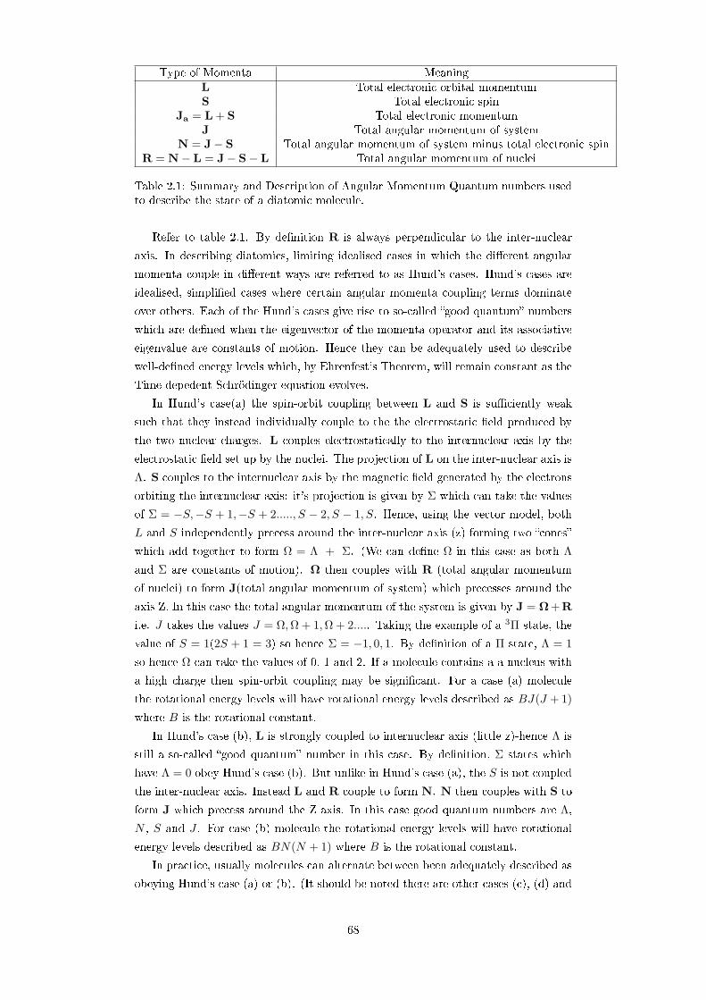
Type of Momenta MeaningL Total electronic orbital momentumS Total electronic spin
Ja = L + S Total electronic momentumJ Total angular momentum of system
N = J− S Total angular momentum of system minus total electronic spinR = N− L = J− S− L Total angular momentum of nuclei
Table 2.1: Summary and Description of Angular Momentum Quantum numbers usedto describe the state of a diatomic molecule.
Refer to table 2.1. By denition R is always perpendicular to the inter-nuclear
axis. In describing diatomics, limiting idealised cases in which the dierent angular
momenta couple in dierent ways are referred to as Hund's cases. Hund's cases are
idealised, simplied cases where certain angular momenta coupling terms dominate
over others. Each of the Hund's cases give rise to so-called good quantum numbers
which are dened when the eigenvector of the momenta operator and its associative
eigenvalue are constants of motion. Hence they can be adequately used to describe
well-dened energy levels which, by Ehrenfest's Theorem, will remain constant as the
Time-depedent Schrödinger equation evolves.
In Hund's case(a) the spin-orbit coupling between L and S is suciently weak
such that they instead individually couple to the the electrostatic eld produced by
the two nuclear charges. L couples electrostatically to the internuclear axis by the
electrostatic eld set up by the nuclei. The projection of L on the inter-nuclear axis is
Λ. S couples to the internuclear axis by the magnetic eld generated by the electrons
orbiting the internuclear axis: it's projection is given by Σ which can take the values
of Σ = −S,−S + 1,−S + 2....., S − 2, S − 1, S. Hence, using the vector model, both
L and S independently precess around the inter-nuclear axis (z) forming two cones
which add together to form Ω = Λ + Σ. (We can dene Ω in this case as both Λ
and Σ are constants of motion). Ω then couples with R (total angular momentum
of nuclei) to form J(total angular momentum of system) which precesses around the
axis Z. In this case the total angular momentum of the system is given by J = Ω + R
i.e. J takes the values J = Ω,Ω + 1,Ω + 2..... Taking the example of a 3Π state, the
value of S = 1(2S + 1 = 3) so hence Σ = −1, 0, 1. By denition of a Π state, Λ = 1
so hence Ω can take the values of 0, 1 and 2. If a molecule contains a a nucleus with
a high charge then spin-orbit coupling may be signicant. For a case (a) molecule
the rotational energy levels will have rotational energy levels described as BJ(J + 1)
where B is the rotational constant.
In Hund's case (b), L is strongly coupled to internuclear axis (little z)-hence Λ is
still a so-called good quantum number in this case. By denition, Σ states which
have Λ = 0 obey Hund's case (b). But unlike in Hund's case (a), the S is not coupled
the inter-nuclear axis. Instead L and R couple to form N. N then couples with S to
form J which precess around the Z axis. In this case good quantum numbers are Λ,
N , S and J . For case (b) molecule the rotational energy levels will have rotational
energy levels described as BN(N + 1) where B is the rotational constant.
In practice, usually molecules can alternate between been adequately described as
obeying Hund's case (a) or (b). (It should be noted there are other cases (c), (d) and
68

(e) but these are less common. In general molecules that are rotating slowing are best
described as Hund's case (a) and those that are rotating at a greater rate as Hund's
case(b)).
2.3 Selection Rules and Transition Strengths
The probability of a transition between two molecular states is related to the tran-
sition dipole moment operator acting between them. It can be shown that when
applying this operator between the wavefunctions of the two respective states, that
the probability of a transition occuring can be decomposed into three parts, namely:
1. The Electronic transitional probability.
2. The Franck-Condon Factor describing the vibrational probability.
3. The Hönl-London factor which describes the probability of transitions within
individual P, Q and R branches (see below).
To carry out this decomposition, it is assumed that the wavefunction describing the
state of the molecule can be approximated as being decomposed into three wavefunc-
tions describing the electronic motion, vibrational motion and rotation motion. It
is assumed that both the electronic and vibrational wavefunctions only depend on
the inter-nuclear distance R only with the rotational wavefunctions depending on the
angular co-ordinates θ and φ. The key result from carrying out these integrals over
the wavefunctions and transition dipole moment operator is the derivation of selection
rules which govern which transitions are actually allowed to take place. The selection
rules can be derived by use of Ladder Operators and known identities. For a di-
atomic molecule, it can be shown that the selection rules are as follows for transitions
between dierent molecular states:
∆Λ = 0,±1 (2.6)
∆S = 0 (2.7)
∆J = 0, ±1, with J = 0→ 0 forbidden (2.8)
The selection rules on J , gives rise to P, Q and R branches which are dened as:
R : J ′ − J ′′ = +1 (2.9)
Q : J ′ − J ′′ = 0 (2.10)
P : J ′ − J ′′ = −1 (2.11)
where J ′ refers to the upper state and J ′′ refers to the lower state. It should be noted
that selection rule, Eq. 2.7 can break down if the nuclear charge is signicant leading
to so-called forbidden transitions e.g. singlet-triplet transitions. The Franck-Condon
Factor is simply the integral over the inter-nuclear distances of the two vibrational
wavefunctions of the two states in question. The Franck-Condon Principle states that
69

the intensity of a transition between two states will be largest where the wavefunctions
overlap at the same inter-nuclear distance.
2.4 Producing a Linelist: Solving the Schrödinger
Equation for a molecule
Refer to gure 2.2 which outlines the generic process employed within the ExoMol
project to produce a linelist for a molecule of interest whereby the Born-Oppenheimer
approximation is implicitly employed. The state of a molecule is described using the
formalism of quantum mechanics by use of the Schrödinger equation,
HΨ = EΨ (2.12)
where H is the Hamiltonian describing the molecule and Ψ and E are the energy
eigenvectors and eigenvalues respectively with Ψ describing the wavefunction of the
molecule (Lodi & Tennyson 2012). For the case of a diatomic molecule with nuclei A
and B the non-relativistic Hamiltonian is:
H = VAe + VBe + Vee + VAB + TA + TB + Te (2.13)
where V terms represent the potential energy between nuclei and electrons (Ae and
Be), between electrons (ee) and between the two nuclei (AB). The T terms represents
the kinetic energy of nuclei A, B and electrons e. Figure 2.1 shows a schematic of
a diatomic molecule in which the inter-nuclear distance, R is represented: it is the
distance between the two nuclei which varies as the molecule vibrates and, in the case
of higher-order rotation may also increase (centrifugal distortion).
A B
Inter-nuclear distance, R
Figure 2.1: Pictorial representation of a diatomic molecule with nuclei A and nucleiB separated by an internuclear distance, R.
70
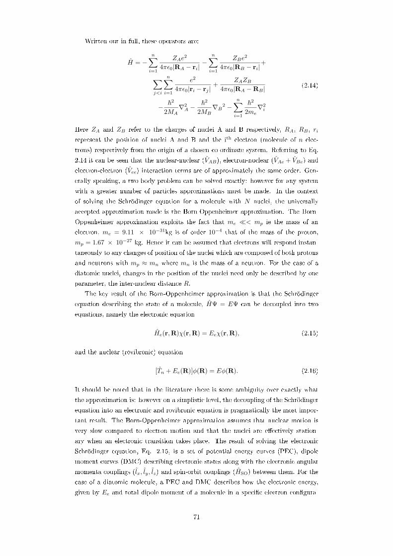
Written out in full, these operators are:
H = −n∑i=1
ZAe2
4πε0|RA − ri|−
n∑i=1
ZBe2
4πε0|RB − ri|+
∑j<i
n∑i=1
e2
4πε0|ri − rj |+
ZAZB4πε0|RA −RB |
− ~2
2MA∇2A −
~2
2MB∇B2 −
n∑i=1
~2
2me∇2i
(2.14)
Here ZA and ZB refer to the charges of nuclei A and B respectively, RA, RB , rirepresent the position of nuclei A and B and the ith electron (molecule of n elec-
trons) respectively from the origin of a chosen co-ordinate system. Referring to Eq.
2.14 it can be seen that the nuclear-nuclear (VAB), electron-nuclear (VAe + VBe) and
electron-electron (Vee) interaction terms are of approximately the same order. Gen-
erally speaking, a two-body problem can be solved exactly: however for any system
with a greater number of particles approximations must be made. In the context
of solving the Schrödinger equation for a molecule with N nuclei, the universally
accepted approximation made is the Born-Oppenheimer approximation. The Born-
Oppenheimer approximation exploits the fact that me < mp ie the mass of an
electron, me = 9.11 × 10⁻³¹kg is of order 10−4 that of the mass of the proton,
mp = 1.67 × 10⁻²⁷ kg. Hence it can be assumed that electrons will respond instan-
taneously to any changes of position of the nuclei which are composed of both protons
and neutrons with mp ≈ mn where mn is the mass of a neutron. For the case of a
diatomic nuclei, changes in the position of the nuclei need only be described by one
parameter, the inter-nuclear distance R.
The key result of the Born-Oppenheimer approximation is that the Schrödinger
equation describing the state of a molecule, HΨ = EΨ can be decoupled into two
equations, namely the electronic equation
He(r,R)χ(r,R) = Eeχ(r,R), (2.15)
and the nuclear (rovibronic) equation
[Tn + Ee(R)]φ(R) = Eφ(R). (2.16)
It should be noted that in the literature there is some ambiguity over exactly what
the approximation is: however on a simplistic level, the decoupling of the Schrödinger
equation into an electronic and rovibronic equation is pragmatically the most impor-
tant result. The Born-Oppenheimer approximation assumes that nuclear motion is
very slow compared to electron motion and that the nuclei are eectively station-
ary when an electronic transition takes place. The result of solving the electronic
Schrödinger equation, Eq. 2.15, is a set of potential energy curves (PEC), dipole
moment curves (DMC) describing electronic states along with the electronic angular
momenta couplings (lx, ly, lz) and spin-orbit couplings (HSO) between them. For the
case of a diatomic molecule, a PEC and DMC describes how the electronic energy,
given by Ee and total dipole moment of a molecule in a specic electron congura-
71

tion (state) changes with inter-nuclear distance R. In the electronic Schrödinger, Eq.
2.15, χ(r,R) represents the electronic wavefunctions which are a function of both the
inter-nuclear distance R and the position of the electrons represented by the quantity
r. More generally for triatomic or larger molecules, these functions are replaced by a
surface which is simply the energy or dipole moment plotted against two co-ordinates
describing the position of nuclei using a convenient co-ordinate framework. Within
the Born-Oppenheimer framework, for each PEC (i.e. list of Ee values for range of
inter-nuclear distances R) generated by solving the electronic Schrödinger, 2.15, the
nuclear Schrödinger equation, Eq. 2.16 is then solved.
Applying the Born-Oppenheimer framework to the case of CrH, the electronic
Schrödinger equation, given by Eq. 2.15 is solved by use of ab initio methods imple-
mented in the quantum chemistry package MOLPRO (Werner and Knowles 2012) and
the nuclear Schrödinger equation, Eq. 2.16 is solved by use of the in-house programme
Duo (Yurchenko et al. (2016). The programme Duo has been developed specically
for solving the nuclear equation for transition-metal diatomics using the programme
TROVE (Yurchenko, Thiel, Jensen 2007) as guidance.
For CrH (or indeed any transition metal hydride) it would not be appropriate to
use the nuclear programme LEVEL (Le Roy 2007) due to the high spin (multiplicity
6) of the ground state 6Σ+ and also due to the nature of electronic structure i.e.
manifolds of low-lying coupled electronic states.
Using the PECs calculated in MOLPRO, Duo calculates rovibronic energy levels.
These are then matched to experimental data and thus the PECs are then semi-
empirically rened. Typically, experimental data is in the form of a list of transition
frequencies with assigned quantum numbers-Duo can t to this or alternatively, to
a set of energies generated from the experimental frequencies using the programme
MARVEL (Furtenbacher, Csàszàr, and Tennyson 2007).
Duo performs a variational calculation whereby the sum of squares residual for
the ab initio data to the experimental data and to a functional form is minimised.
Using these tted functional forms (e.g. Morse potential) for each PEC along with
the respective dipole moment curves, Duo then calculates rovibronic wavefunctions
and intensities for transitions in the form of Einstein A coecients. Hence combining
the list of rovibronic energy levels with the respective Einstein A-coecients, a list of
transition energies and frequencies, ie a linelist is thus produced.
Ab initio calculations: motion of electrons
Dipole Moment
Potential Energy
Solving for (vibration-rotational)
motion of nuclei
Rovibrational wavefunctions
Rovibrational energies
Intensities (Aif)
Line list
Ref
inem
ent
MOLPRO MOLPRO
DUO
Billions of transitions
Bor
n-O
ppen
heim
er
Figure 2.2: Overall process to produce a linelist.
72

2.5 Producing a Linelist for Open-shell transition metal
diatomic hydrides
It should be noted that the production of linelists for transition-metal bearing di-
atomics is still very much at the developmental stage compared to that of triatomic
and tetratomic molecules. At present there are no routine procedures for solving both
the electronic Schrödinger equation and rovibronic Schrödinger equation for transi-
tion metal containing molecules. In larger molecules containing elements such as
H, O, N, C, S, P very often there is typically one low-lying electronic ground state
with many excited states high up in energy and non-interacting. Solving the elec-
tronic Schrödinger equation for these molecules for the ground state PEC is thus
usually reasonably straightforward: the tricky and computationally challenging part
is solving the rovibronic Schrödinger equation which typically involves undertaking a
transformation of co-ordinates, expanding a kinetic energy operator within a basis set
and diagonalising matrices of the order 106. For transition-metal bearing diatomics,
the situation is the reverse. Due to the myriad of low-lying electronic states within
these molecules which couple together via angular momenta and spin-orbit coupling,
solving the electronic Schrödinger equation is often the most challenging part. Indeed
studies talk about transition metals been an interesting theoretical playground. In
terms of solving the rovibronic Schrödinger equation, the in-house program Duo (sec-
tion 2.9) had to be created as there was no such program which could deal with
coupled electronic states of high multiplicity.
2.6 Solving the Electronic Schrödinger equation
For any electronic calculation, in general there are two factors which aect the accu-
racy of the result namely the level of theory (e.g. HF, MP2, CCSD (T), MRCI) used
and the size of the basis set used. The basis set used act as the building blocks for
constructing the electronic wavefunctions: as the size of the basis set is expanded the
answer obtained will converge to what is called the complete basis set limit (CBSL).
These two factors can be conveniently plotted on a so-called `Pople' diagram. In the
limit of innte basis set and higher-order theory, the solution obtained should converge
to the exact solution. John A. Pople was a recipient of the Nobel Prize for Chemistry
in 1998 for his work on computational methods in quantum chemistry: he shared
the prize with Walter John who was awarded it for his work on developing density
functional theory, DFT. Figure 2.3 shows a typical Pople diagram for reference.
73

Figure 2.3: An example of a Pople Diagram the concept of which was introduced byJohn A. Pople who was the joint recipient of the Nobel Prize for Chemistry in 1998.
The Pople diagram can be used to extrapolate results in 2 dimensions: if the
eect of changing a basis set at one level of theory is known and the eect of changing
method for a single basis set is known then a prediction can be made about upgrading
both a basis set and level of theory simultaneously without the need to run expensive
calculations.
2.6.1 Electronic Basis sets
For a given ab initio method, the level of accuracy obtained is dependent on the size
of the basis set employed. The basis set is simply a series of basis functions which
are used to generate wavefunctions i.e. act as building blocks. Gaussian functions are
typically used as basis functions owing to their desirable integral qualities which is
paramount in determining the speed of ab initio calculations as most ab initio methods
make frequent use of Gaussian integrals. The most simplest type of Gaussian Basis
sets used is the STO− nG family where n is an integer. The most popular Gaussian
basis sets which are used are:
Pople basis sets such as 6-31G
Dunning family of basis sets, cc-pVNZ which are optimized for MP2 calculations
Jensen Basis sets of the form pc-n which are optimized for DFT calculations
In this work a correlation-consistent basis sets of the form cc-pVNZ developed by
Dunning et al. was used where N denotes the size of the basis set. Here the cc-p
is an abbreviation for correlation-consistent polarized. These are also valence-only
basis functions which is signied by the V. The progressive series of basis sets within
this family are denoted cc-pVDZ, cc-pVTZ, cc-pVQZ, cc-PV5Z, etc where D, T,
Q and 5 represent double, triple, quadruple and 5 respectively. These dene
the number of separate functions used for describing the valence region of electrons.
These basis sets are designed such that as the size of the set is increased, the CBSL is
74

converged to. However, it should be noted that when moving up a basis set within a
family towards towards the CBSL, more exibility is introduced in the orbitals hence
there is more likely to be problems with convergence. Typically these basis functions
are used to solve problems involving organic chemistry which is typically concerned
with the study of large molecules: for these molecules there is typically a low-lying
ground state with any excited states relatively high up in energy such that they are of
less signicance for the study. Hence these basis functions have thus been optimised
for use in studying low-lying ground states of large molecules. For the application of
diatomic transition metal hydrides which have many low-lying excited states, these
basis functions can be augmented by adding so-called diuse' functions to thus
create the family of aug-cc-pVNZ basis functions.
2.6.2 Level of Theory
There is a myriad of quantum chemistry ab initio methods which can be used to
solve the electronic Schrödinger equation. As was stated in section 2.4 to solve any
problem with more than two particles, approximations must be used. Generally
speaking, for the case of solving the electronic Schrödinger equation for a molecule,
various ab initio methods are available. Discretion is needed as to which method is
most appropriate for the given molecule of interest and the level of accuracy desired
or, more prudently which is feasible given the computational resources available. The
various ab initio quantum chemistry methods have been implemented into various
quantum chemistry packages such as Gaussian, QChem, GAMESS, TURBOMOLE,
MOLPRO, MOLCAS, NWChem, Dalton and CFOUR. It should be noted that this
is by no means an exhaustive list. Each quantum chemistry package available, either
commercially or through open source has its own speciality/(ies). Throughout this
project MOLPRO (H.J. Werner and P. J. Knowles, 2012) was used as the MRCI method
has been developed signicantly within this package.
It should be noted that whichever method or package is used to solve a problem,
the Variational Principle will always apply:
Eground state ≤ Eguess from method. (2.17)
Hence, as a consequence of the Variational Principle, a calculation will never compute
an energy which is lower than the true value. When the size of the basis set used
is increased, the energy calculated will get lower and approach the true value as you
reach the CBSL. The derivation of the Variational Theorem can be found in any
standard quantum physics textbooks: the derivation involves taking derivative of
wavefunctions to nd a minimum by varying the coecients of the functions used to
describe the total wavefunction.
Slater Determinants, Hartree-Fock, CASSCF and MRCI theory
One of the most simplest type of calculation which can be performed is the variational
method of Hartree-Fock. However, this method is only applicable to the ground state
of molecules and as we are interested in the ground but also excited states for CrH
& MnH, Hartree-Fock is not adequate. Hence higher-order methods are required:
75

in this project Multi-Reference Conguration Interaction (MRCI) calculations were
undertaken.
The Hartree-Fock method is one, if not the simplest method which can be used to
solve for the motion of electrons orbiting within atoms or molecules. The key features
of the Hartree-Fock method are:
It is a Variational method using the Self-Consistent Field (SCF) method.
A single Slater Determinant is used.
No relativistic eects are included.
No electron correlation (as dened within the chemistry community) is incor-
porated.
For the case of a molecule which has n electrons with positions denoted by r1, r2,....rneach occupying an orbital denoted φi, a wavefunction, Ψ of the simplest form which
can be used to describe them is:
Ψ(r1, r2, ....rn) = φ1(r1)φ2(r2).....φn(rn) (2.18)
Here electrons are each positioned in a unique spin orbital. Note each space
orbital can occupy two electrons. Since electrons are classied as indistinguishable
particles, the total electronic wavefunction must obey the Pauli Exclusion Principle.
As a consequence, the total wavefunction must be anti-symmetric with respect to the
swapping of two electrons, i.e. the sign of the total wavefunction must change upon
exchanging two electrons. In the above notation, placing electron 1 in orbital 2 is
denoted by φ2(r1).
For the example of a two electron system, a very simple way to make the total
wavefunction antisymmetric with respect to exchange of electrons is to expand simple
wavefunction as follows:
Ψ(r1, r2, ....rn) = φ1(r1)φ2(r2)− φ1(r2)φ2(r1) (2.19)
For the case of a larger system, the Pauli Exclusion Principle can be satised by
introducing the antisymmetric operator such that the total wavefunction becomes:
Ψ = A[φ1(r1)φ2(r2)......φn(rn)] (2.20)
This is known as a Slater Determinant. A determinant matrix has the essential
required property for this application that if you swap a pair of rows or columns,
the determinant is left unchanged. The Hartree-Fock method uses a single Slater
Determinant. The starting Ansatz (guess) for a Hartree-Fock solution is:
φi =N∑k
cikχk (2.21)
where χk = is a basis function and cik are the coecients of the Basis functions to
be used in the orbital i. Thus cik is a matrix of coecients. It should be noted that
the basis functions within a basis set are not always ortho-normal. If basis functions
76

are orthogonal then the inner product of any two dierent basis functions is zero i.e.
〈χiχk〉 = 0 for all i, k where i 6= k. If the basis functions are ortho-normal then there
exists no linear dependence between between basis functions i.e. it is not possible to
write one basis function as linear sum of the others and the inner product of a single
basis function is unity. As an example of non-orthogonal basis functions, diuse basis
functions will often have some inherent linear dependence between them as they are
describing the physics of dissociation.
Molecular orbitals, φi on the other hand are always dened to be ortho-normal.
In Hartree-Fock theory the total wavefunction Ψtotal is simply one single Slater
Determinant which is a product of molecular orbitals φi. In Hartree-Fock theory these
molecular orbitals are varied by varying the coecients cik. In MCSCF and MRCI
theory, the total wavefunction Ψtotal is a linear sum of Slater Determinants each
denoted by Ψj . The total wavefunction is thus given by Ψtotal =∑j CjΨj(φ(k)). In
MCSCF theory both the coecient Cj and cik are varied. In CI theory, the molecular
orbitals φi are kept constant (i.e. cik are not varied) but the coecients of each Slater
Determinant Cj is varied.
For further reading on the MCSCF method the following resources should be con-
sulted:
H. J. Werner and W. Meyer, J. Chem. Phys. 73, 2342 (1980)
H. J. Werner and W. Meyer, J. Chem. Phys. 74, 5794 (1981)
H. J. Werner and P. J. Knowles, J. Chem. Phys. 82, 5053 (1985)
P. J. Knowles and H. J. Werner, Chem. Phys. Lett. 115, 259 (1985)
and for the MRCI method:
H. J. Werner and E.A. Reinsch, J. Chem. Phys. 76, 3144 (1982)
H. J. Werner and P.J. Knowles, J. Chem. Phys. 89, 5803 (1988)
P. J. Knowles and H. J. Werner, Chem. Phys. Lett. 145, 514 (1988)
2.7 Calculation of Ab initio Curves in MOLPRO
Ab initio calculations for the electronic Schrödinger equation, given by Eq. (2.15)
were performed using the quantum chemistry package MOLPRO for the diatomics of
CrH and MnH. The result of these calculations are potential energy curves, dipole
moment curves and coupling curves for the various interactions. These curves are
calculated by calculating the relevant parameter (i.e. energy for the case of PEC,
dipole moment for the case of DMC) at a set inter-nuclear point R. The matrix of
inter-nuclear points used in this project is outlined in section 2.7.1. For any calcula-
tion of molecular states, knowledge of atomic and molecular term values is required:
this is presented in sections 2.1 and 2.2 respectively. The C2v symmetry point group
framework that is utilised in MOLPRO is then described, along with its ramications
in section 2.7.2. In order to deduce what molecular states are of interest below a
pre-dened energy level, knowledge of atomic dissociation limits for the hydrogen and
relevant transition metal atom are needed. The process for deducing which molecular
states are to be calculated for each molecule is described in section 2.7.3. Sections
2.7.4 and 2.7.7 then outline the molecular states of interest for CrH and MnH respec-
77

tively along with full description of their implementation into a MOLPRO calculation.
2.7.1 Grid of inter-nuclear points
For each calculation run during the project a matrix of inter-nuclear distances, R,
consisting of 88 points ranging from 0.70 to 10.0 Å was used. A summary of this
matrix is shown in table 2.2 which shows how the points were distributed from R =
0.7 Å to R= 6.20 Å. The remaining points were 6.50, 6.70, 7.00, 7.20, 7.40, 7.50, 7.70,
8.00, 8.50, 9.00 and 10.00 Å.
Range (Å) Spacing (Å)0.70 ≤ R ≥ 1.20 0.101.20 ≤ R ≥ 1.65 0.05intermediate point 1.661.68 ≤ R ≥ 1.76 0.01intermediate point 1.781.80 ≤ R ≥ 3.00 0.053.0 ≤ R ≥ 5.00 0.105.0 ≤ R ≥ 6.20 0.20
Table 2.2: Summary of matrix of inter-nuclear distances used in calculations through-out the project.
Table 2.2 shows how the R values were distributed such that more points were
calculated between 1.65 and 1.80 Å as this is the region of the minima for the majority
of PECs for both CrH and MnH. Indeed for both molecules it was found that most
of the PECs important behaviour was between approximately 0.90 and 4.00 Å with
most PECs reaching their respective dissociation limits by R=5.00 Å.
2.7.2 Description of the C2v framework
To aid eciency of calculations, MOLPRO makes use of symmetry point groups: for our
case of diatomic metal hydrides, the relevant point group is C2v symmetry which has
4 symmetry components namely A1, B1, B2 and A2. Hereafter, in line with MOLPRO
notation these will be referred to as symmetries 1,2,3, and 4 respectively. Naturally,
the point group which a diatomic molecule belongs to is C2∞. However, for the
purposes of computation this is a non-Albelian group (i.e. rules of commutation do
not apply) so hence for this reason the makers of MOLPRO set up the code using the
reduced C2v point group.
Mathematically speaking, a symmetry point group is simply a collection of symmetry
components which together as a group obey the axioms required to be a point group.
Each symmetry component is dened to have certain properties relating to reections,
denoted by σ and rotations about the principle axis, X, Y , Z. For the C2v symmetry
point group these properties are shown in table 2.3.
78

SYM SYM σν(xy) σν(yz) Linear functions (Rotations) Quadratic functions Cubic functionsA1 1 +1 +1 z x2, y2, z2 z3, x2y, y2xB1 2 +1 -1 X,Ry xz xz2, x3, xy2
B2 3 -1 +1 Y , Rx yz yz2,y3,x2yA2 4 -1 -1 Rz xy xyz
Table 2.3: Denition of C2v symmetry (Willock 2009).
For practical purposes, the consequences of working within the MOLPRO C2v sym-
metry framework is that atomic orbital (e.g. s, p, d orbitals) and molecular states
(e.g. Σ+, Σ−, Π and ∆) belong to the four symmetry components, irrespective of
their spin(multiplicity). Table 2.4 demonstrates how s, p and d atomic orbitals are
assigned to the 4 symmetries within the C2v framework and hence table 2.5 then
summarises how the dierent components of the p and d orbitals add. Table 2.6 lists
out which molecular states have components in the 4 symmetries.
Atomic Orbital E C2(z) σν(xz) σν(yz) Symmetrys +1 +1 +1 +1 1px +1 -1 +1 -1 2py +1 -1 -1 +1 3pz +1 +1 +1 +1 1dxy +1 +1 -1 -1 4dxz +1 -1 +1 -1 2dyz +1 -1 -1 +1 3
dx2−y2 +1 +1 +1 +1 1dz2 +1 +1 +1 +1 1
Table 2.4: Assignment of atomic electron conguration orbitals to symmetries 1, 2, 3& 4 within the C2v framework
orbital sym1 sym2 sym3 sym4s 1 0 0 0p 1 1 1 0d 2 1 1 1
Table 2.5: Atomic s, p, d electron conguration orbitals symmetry assignments withinthe C2v symmetry framework
Symmetry Molecular states1 Σ+, ∆, Γ, . . .2 Π, Φ, . . .3 Π, Φ, . . .4 Σ−, ∆, Γ, . . .
Table 2.6: MOLPRO C2v framework: electronic state classication
Hence the main consequence of using this framework is that, as an example for a
Π molecular state, a calculation for both a symmetry 2 state and a state of symmetry
3 need to be performed. Theoretically the values of properties such as energy and
dipole moment produced by these calculations should be numerically the same within
79

the convergence thresholds selected. Also for a ∆ molecular state a calculation for
both symmetry 1 and symmetry 4 needs to be undertaken.
2.7.3 Deduction of Molecular states to be calculated for di-
atomic hydrides
Before any ab initio calculations can be undertaken, we rst need to establish which
molecular electronic states are expected to be of greatest interest and important ie
determine a list of electronic states which are theoretically expected to be present
up to a pre-dened energy limit. For the purpose of this project, it was agreed
that we focus on molecular states that converge to atomic dissociation limits below
approximately 20 000 cm−1 were of primary concern. This limit was chosen as it
corresponds to an astronomical range beginning at 0.5 µm heading into the infrared
which is most concern to astromers studying L type dwards in which CrH has been
detected (see section 3.4). Also, it can be shown that energy levels of 20 000 cm−1
have a corresponding Boltzmann factor of 2× 10⁻⁷ at a typical L dwarf temperature
of 2000 K so hence are unlikely to be populated. Table 2.7 shows the lowest lying
atomic term values for the hydrogen atom.
Conguration Term J Energy (cm−1)1s 2S 1/2 0.00000 00000
2p 2P 0 1/2 82 259.91911333/2 92 259.2850014
Table 2.7: H atom dissociation energy limits
Hence referring to table 2.7, it can be assumed that for the diatomic metal hydride
molecules studied, the electron associated with the Hydrogen nucleus will have a
conguration of 1s.
2.7.4 Deduction of Molecular states to be calculated for CrH
Using data from the NIST website, the lowest lying atomic-dissociation limits with
respective atomic term values and atomic electronic congurations for the Hydrogen
and Chromium atom are presented in tables 2.7 and 2.8 respectively.
80

Conguration Term J EJ (cm−1) E0 (cm−1) Molecular States[Ar]3d5(6S)4s a7S 3 0.0000 0.0000 X6Σ+ 8Σ+
[Ar]3d5(6S)4s a5S 2 7 593.1484 7 593.1484 A6Σ+ 4Σ+
[Ar]3d44s2 a5D
0 7 750.7465
8 090.1903
6Σ+(III) 4Σ+(II)1 7 810.7795 6Π 4Π2 7 927.4410 6∆ 4∆3 8 095.18424 8 307.5753
[Ar]3d5(4G)4s a5G
2 20 517.4222
20521.4036
6Σ+(IV ) 4Σ+(III)6 20 519.5515 6Π(II) 4Π(II)3 20 520.9029 6∆(II) 4∆(II)4 20 523.6290 6Φ 4Φ5 20 523.8999 6Γ 4Γ
Table 2.8: Chromium atom dissociation energy limits and list of respective electronicmolecular states expected for CrH up to approximately 20 000 cm−1.
In tables 2.7 and 2.8, conguration refers to the atomic electron conguration of
the respective neutral atoms where the Aufbau principle is used to ll the electron
orbitals. An explanation of the notation used is given in section 2.1. For the case of
the Chromium atom, which has 24 electrons, the rst 18 electrons ll the 1s, 2s, 2p,
3s and 3p atomic orbitals forming an Argon inner-shell denoted by [Ar] which has
conguration 1s22s22p63s23p6 in standard atomic notation. In table 2.8 the values of
EJ can be averaged in a weighted average sum to obtain a value of E0 by Eq. 2.22:
E0 =∑J(2J + 1)EJ∑J 2J + 1
. (2.22)
For the a7S and a5S term values the value of E0 is simply 0.000 cm−1 and 7 593.1484
cm−1 respectively as there is only a single value of J . For the case of the a5D the
value of E0 is 8090.1903 cm−1.
For a set of two atomic dissociation terms, the molecular states which are expected
to arise from them can be deduced by applicaiton of the Wigner-Witmer or correla-
tions rules (Zare 2007). Hence, we have a list of electronic states of which the aim
is to calculate ab inito potential energy curves, dipole moment curves and couplings
for.
2.7.5 Specifying the Electronic Conguration for CrH
In the MOLPRO package, the electronic conguration of each of the desired electronic
states needs to be specied. This is done by specifying the number of closed and oc-
cupied, occ orbitals which can simply be thought of as the core orbitals and the sum
of the core and valence orbitals respectively. The syntax is closed,sym1, sym2,
sym3, sym4 where sym1, sym2, sym3, sym4 denotes the number of orbitals within
each of the four symmetries respectively. Similarly for occupied (occ) orbitals. The
desired orbitals are deduced by considering the electron conguration within the C2v
framework.
Referring to table 2.8 the relevant electron conguration for the outer orbitals of the
molecule CrH correspond to the Cr atom been in the congurations 3d54s1 and 3d44s2
81

and as discussed the single electron associated with the hydrogen nuclear having con-
guration 1s. It is assumed that the inner electrons within the CrH molecule form a
conguration of that of the argon atom namely 1s22s22p63s23p6.
Hence for the molecule CrH, the electron conguration ie closed and occupied or-
bitals for the molecular electronic states we are interested in is simply 5220− 9331 as
demonstrated in table 2.9.
Conguration Atomic OrbitalsC2v Symmetry1 2 3 4
Argon conguration
1s2 1 0 0 02s2 1 0 0 02p6 1 1 1 03s2 1 0 0 03p6 1 1 1 0
TOTAL INNER ELECTRONS 5 2 2 0
Valence conguration4s1 or 2 1 0 0 03d5 or 1 2 1 1 1
1s(from H nucleus) 1 0 0 0TOTAL VALENCE ELECTRONS 4 1 1 1TOTAL OCCUPIED ELECTRONS 9 3 3 1
Table 2.9: Deduction of closed and occupied orbitals for CrH
2.7.6 Specication of wf card for CrH
Owing to the C2v symmetry framework employed by MOLPRO, electronic states are
calculated by specifying a wf card. Put simply, a wf card is a description of the
multipliicty and symmetry of a desired electronic state. The form of the wf card is
as follows:
wf, number of electrons, symmetry, 2S
For the CrH molecule, the number of electrons is simply 25 where 24 electrons are
associated with the Chromium nucleus and the 1 electron from the Hydrogen nucleus.
The symmetry is either 1, 2, 3, 4 as dened in section 2.6. Referring to table 2.6,
the ramication of using C2v framework is that, as an example for a Π state, two
wf cards need to be specied-one with symmetry 2 and the other with symmetry 3.
Theoretically the values of properties such as energy, dipole moment produced by
these two wf cards should be numerically the same within the convergence thresholds
selected. Ditto for ∆ states with the symmetries required been symmetry 1 and
symmetry 4. Finally, within the wf card, 2S is simply the multiplicity minus 1. So
for a state of multiplicity 6, 2S is 5, for multiplicity 4, 2S is 3 etc. To fully clarify
table 2.10 shows the dierent wf cards required for the various types of molecular
states calculated for CrH.
82

Molecular state wf card(s) required4Σ+ 25, 1, 34Π 25, 2, 3 and 25, 3, 34∆ 25, 1, 3 and 25, 4, 3
6Σ+ 25, 1, 56Π 25, 2, 5 and 25, 3, 56∆ 25, 1, 5 and 25, 4, 5
8Σ+ 25, 1, 7
Table 2.10: Specication of wf cards required to calculate the various molecularstates of interest for CrH.
For the case of multiple states requiring the same wf card the option state,
value is inserted. As an example for the simultaneous calculation involving a single6Σ+ and single 6∆ state the relevant wf cards required are:
wf,25, 1, 5; state,2
wf,25, 4, 5; state,1
where the ∆ state will have components in both symmetry 1 and symmetry 4 and
the Σ+ state is simply within symmetry 1.
For a 6Σ+ state the only wf card required is simply wf, 25, 1, 5. As a further
example for clarity for the calculation of three 6Σ+ states and a single 6∆ state, the
required wf cards are:
wf,25, 1, 5; state,4
wf,25, 4, 5; state,1.
In this case, one of the energy values produced by the wf,25, 1, 5;state,4 card will
theoretically be numerically the same as that produced by the wf,25, 4, 5;state,1
card-this corresponds to the ∆ state. The other states within the wf,25,1,5;state,4
will simply be the Σ+ states. It should be noted that the ordering of states, which is
done by MOLPRO based on energy can change due to crossing particularly as the inter-
nuclear distance, R approaches zero and hence the potential energy of that particular
state goes asymptotically to innity.To dene some important notation for proceeding results, hereafter a multiplicity-
symmetry block will simply refer to wf card which has multiple states eg the
`multiplicity-symmetry block for a wf card of:
wf,25, 1, 5; state,2
is simply 6, symmetry 1 (remembering that in the wf notation 5 here refers to 2S:
the multiplicity of a state is given by 2S + 1 which for this case is 6 ie sextet state.
In a plot of PECs (or any other curves) produced from using this wf card the curves
will be labelled as:
6, symmetry 1, state 1 and
6, symmetry 1, state 2
respectively.There is an option within MOLPRO, lqaunt, which can be used within the CASSCF
calculation, but not CI calculation to specify the λ value desired which is 0,1 and 2
for Σ, Π and ∆ states respectively. Based on previous experience, it was decided not
to use this option but as further investigative work this option could be explored.
83

2.7.7 Deduction of Molecular states to be calculated for MnH
In a similar manner for CrH, the molecular states for MnH which are expected to dis-
sociate to the various atomic dissociation limits below approximately 20 000 cm−1(see
section 2.7.3 for discussion) can be deduced by inspection of the atomic dissociation
limits for the Mn atom and also the H atom. As discussed in section 2.7.3 for the
electron associated with the hydrogen nuclei within a diatomic metal hydride it can
be assumed that it will occupy a 1s atomic orbital. Table 2.11 shows the rst four
low-lying dissociation limits for the Manganese atom.
Conguration Term J EJ (cm−1) E0 (cm−1) Molecular States3d54s2 a6S 2.5 0.000 0.000 5Σ+ 7Σ+
3d6(5D)4s a6D
4.5 17 052.29
17 301.21
5Σ+(II) 7Σ+(II)3.5 17 282.00 5Π 7Π2.5 17 451.52 5∆ 7∆1.5 17 568.480.5 17 637.15
3d5(6S)4s4p(3P o) z8P o2.5 18 402.46
18 571.73
7Σ+(III) 9Σ+
3.5 18 531.64 7Π(II) 9Π4.5 18 705.37
3d6(5D)4s a4D
3.5 23 296.67
23 509.22
5Σ+(III) 7Σ+(II)2.5 23 549.20 5Π(II) 7Π(III)1.5 23 719.52 5∆(II) 7∆(II)0.5 23 818.87
Table 2.11: Manganese atom dissociation energy limits and list of molecular statesfor MnH which dissociate to these.
As for the case of the Chromium atom, a value of E0 as given by Eq. 2.22 can
be calculated for the each term value for the Manganese atom: these values are
shown in table 2.11 along with the molecular states for MnH which are expected to
dissociate to them. The decision was made to initially calculate the molecular states
that dissociate to the rst three atomic limits of the Manganese atom. However upon
later discovery of experimental data for higher lying 5Σ+ and 5Π states dissociating
to the a4D term, calculations were done for these states as well as the 5∆ molecular
state of MnH dissociating to this particular atomic dissociation limit.
2.7.8 Specifying the Electronic Conguration for MnH
As can be seen from table 2.11, the rst two dissociation limits and the fourth (ordered
in terms of increasing energy) for the Manganese atom have electrons in the 3d and
4s orbitals: the third dissociation limit has electrons occupying the 3d, 4s and 4p
atomic orbitals. Deduction of the closed and active space for these two dierent
congurations within the C2v framework imposed within MOLPRO is shown in table
2.12.
84

OrbitalsC2V Symmetry
A1 B1 B2 A2
closed
1s2 1 0 0 02s2 1 0 0 02p6 1 1 1 03s6 1 0 0 03p6 1 1 1 0
Total closed 5 2 2 0
Active4s2 1 0 0 03d5 2 1 1 1
1s1 (H) 1 0 0 0Total active 4 1 1 1
Total occupied 9 3 3 1(a)
OrbitalsC2V Symmetry
A1 B1 B2 A2
closed
1s2 1 0 0 02s2 1 0 0 02p6 1 1 1 03s6 1 0 0 03p6 1 1 1 0
Total closed 5 2 2 0
Active
4s1 1 0 0 03d5 2 1 1 14p1 1 1 1 0
1s1(H) 1 0 0 0Total active 5 2 2 1
Total occupied 10 4 4 1(b)
Table 2.12: Electronic congurations for low-lying states of diatomic molecule MnH(a) Closed and Occupied orbitals for the molecular states arising from the a6S anda6D atomic terms(b) Closed and Occupied orbitals for the molecular states arising from the z8P 0 atomicterms
Hence in summary the closed and active spaces for the two dierent cases are (5,
2, 2, 0)/(9, 3, 3, 1) and (5, 2, 2, 0)/(10, 4, 4, 1). It was later found that the subtle
change in adding an extra atomic p orbital to the active space had a profound and
physically signicant eect upon the results of calculations.
For future reference these active spaces will be refereed to as LOWER and UPPER respectively
2.7.9 Specication of wf card for MnH
As a reminder the form of the wf card within MOLPRO (see section 2.7.6) is of the
form: wf, number of electrons, symmetry, 2S
The number of electrons within the MnH atom is 26. Hence, referring to sections 2.7.6
and 2.7.2 the wf card required for the calculation of the various molecular states for
MnH are shown in table 2.13 as examples.
Molecular state wf card(s) required5Σ+ 26, 1, 45Π 26, 2, 4 and 26, 3, 45∆ 26, 1, 4 and 26, 4, 4
7Σ+ 26, 1, 67Π 26, 2, 6 and 26, 3, 67∆ 26, 1, 6 and 26, 4, 6
9Σ+ 26, 1, 89Π 26, 2, 8 and 26, 3, 8
Table 2.13: Specication of wf cards required to calculate the various molecularstates of interest for MnH.
Again, as is the case of CrH there are several wf cards which have multiple
occurrences. For example by referring to table 2.11 there are three low-lying 5Σ+
85

states and two low-lying 5∆ molecular states for the MnH molecule. To calculate
all ve simultaneously, bearing in mind that the 5∆ states have components in both
symmetry 1 and symmetry 4, two wf cards need to be specied namely:
wf, 26, 1, 4; state 5; ! This is the symmetry 1 components
wf, 26, 4, 4; state 5; ! This is the symmetry 4 components
The order (in energy) of these quintet states is generally not known until calculations
are done: in order to deduce which of the energy values calculated in symmetry 1 are
the ∆ states (as opposed to the Σ+ states) a comparison needs to be done with the
energies produced by the symmetry 4 calculation. For the ∆ states the energy values
produced in symmetry 1 and symmetry 4 should be numerically equal. Similarly to
check the assignment of states within the symmetry 1 calculation a comparison of
the expectation dipole moment calculations can be done: again this is a method to
determine what order the various Σ+ and ∆ states lie in.
2.8 Description of MRCI calculations
In this project, MRCI calculations were performed to obtain potential energy curves,
dipole moment curves, spin-orbit & angular momentum coupling curves. These cal-
culations follow three distinct steps namely:
1. Complete Active Space Self-Consistent Field (CASSCF) calculation in which
energies and dipole moments are calculated.
2. Conguration Interaction (CI) calculation, where the orbitals generated in the
CASSCF calculations are used for CI calculations of energy and dipole moments.
3. CI calculations of couplings (dipole, angular momentum, spin-orbit) between
states which use the CI orbitals generated in the CI part of the calculation.
Hence it is imperative that care is taken in generating the highest quality orbitals
possible in the CASSCF in order to obtain convergence but also continuity in the
CI calculations. It should be noted that continuity of curves, be it potential energy
curves, dipole moment curves, spin-orbit coupling curves is not always guaranteed
from obtaining convergence. Each input le for a MOLPRO calculation was divided
into procedures, labelled as PROCSs. A loop was then run over the matrix of
inter-nuclear distance values of R (see section 2.7.1) and each PROC calculated as
necessary. It should be noted that a CASSCF (and indeed CI) calculation for each
point is independent of calculations for all other points: thus the order in which
calculations were run for dierent points has no consequences for the end result.
2.8.1 CASSSCF orbital testing calculations
The result of the initial CASSCF calculations are PECs and DMCs. For both CrH
and MnH extensive testing of CASSCF orbitals was undertaken: these orbitals were
varied by doing CASSCF calculations where dierent combinations of molecular states
were requested. Practically, each dierent CASSCF orbital set to be tested was
inputted into MOLPRO as a PROC within a single input le. The process of testing
86

was automated such that a run le was used in which the PROC to be tested was
specied in the command line and thus calculations run over the matrix of inter-
nuclear distances, R for this PROC.
An example of such a CASSCF orbital PROC is shown for CrH below: PROC
MULTIRUN-A
multi;maxiter,40;occ,9,3,3,1;closed,5,2,2,0;frozen,0,0,0,0;
wf,25,1,5;state 1;
wf,25,1,7;state 1;
wf,25,2,3;state 1;
wf,25,3,3;state 1;
orbital,2352.1
enermulti1=energy(1)
enermulti2=energy(2)
enermulti3=energy(3)
enermulti4=energy(4)
dipz_multi1=dmz(1)
dipz_multi2=dmz(2)
dipz_multi3=dmz(3)
dipz_multi4=dmz(4)
XY = 'AAA'
table, XY,rpl,enermulti1, enermulti2,enermulti3,enermulti4,dipz_multi1,
dipz_multi2, dipz_multi3, dipz_multi4
DIGITS, 0, 4, 12, 12, 12, 12, 12, 12, 12, 12, 12, 12, 12, 12
ENDPROC
Here the
PROC is called MULTIRUN-A,
The occupied and closed orbitals within the C2v symmetry framework as (9, 3,
3, 1) and (5, 2, 2, 0) respectively as discussed in section 2.7.5.
A 6Σ+, 6Σ+ and a 4Π state are calculated within this CASSCF calculation-see
section 2.7.6 for explanation of wf cards.
The orbital, 2352.1 refers to how MOLPRO saves this CASSCF orbital: this
can then be called upon in proceeding CI calculations.
The enermulti and dipz_multi are simply labels used and formatted in a
table to assist with the extraction of data from the output les.
Once a CASSCF calculation has been done proceeding CI calculations can be done:
for each value of the inter-nuclear distance R the starting orbital used is the orbital
calculated in a proceeding CASSCF calculation.
2.8.2 Calculation of PECs and DMCs at MRCI level
Using the orbitals calculated in the PROC MULTIRUN-A in sectionn 2.8.1 as start-
ing points, CI calculations can then be performed. An exmaple of a CI calculation
for a 4Σ+ state for CrH. PROC CIRUN-S1
87

!4 SIGMA + In FORTRAN notation upon which MOLPRO based, a ! is a comment
to help the reader of the code.
ci;occ,9,3,3,1;core,5,2,2,0;wf,25,1,3;state 1;orbital,2352.1; save,3051.2;
thresh,energy=1.d-9,coeff=1.d-8,thrint=1.d-8,zero=1.d-8;maxiter,4000;maxit,4000;
enerci1_1 = energy(1);
dipzci1_1 = dmz(1);
XY = 'xxyyS1'
table, XY,rpl,enerci1_1,dipzci1_1
DIGITS, 0, 4, 12, 12
ENDPROC
Here the
PROC is called S1
The occupied and closed orbitals within the C2v symmetry framework as (9, 3,
3, 1) and (5, 2, 2, 0) respectively as discussed in section 2.7.5.
A quartet state within symmetry 1 is requested
The orbital 2352.1 is used as a starting point: see proceeding section.
The orbital calculated from this CI calculation is then saved as 3051.2
Some convergence thresholds are given
The enerci1_1 and dipzici1_1 labels are simply ways of assisting with the
extraction of values of energy and expectation dipole moment respectively from
the calculation
The calculation is done on the assumption that the rst molecular state within the
multiplicity-symmetry block of quartet-symmetry 1 is indeed a Σ+ state and not a ∆
state(which would require also the calculation of a quartet state with symmetry 4).
An example of a calculation for a 6Π state for CrH.
PROC CIRUN-S8
!6 PI
ci;occ,9,3,3,1;core,5,2,2,0;wf,25,2,5;state 1; orbital,2352.1;save,3065.2;
thresh,energy=1.d-9,coeff=1.d-8,thrint=1.d-8,zero=1.d-8;maxiter,8000;maxit,8000;
enerci4_1 = energy(1);
dipzci4_1 = dmz(1);
ci;occ,9,3,3,1;core,5,2,2,0;wf,25,3,5;state 1; orbital,2352.1; save,3066.2;
thresh,energy=1.d-9,coeff=1.d-8,thrint=1.d-8,zero=1.d-8;maxiter,8000;maxit,8000;
enerci4_2 = energy(1);
dipzci4_2 = dmz(1);
XY = 'xxyyS6'
table, XY,rpl,enerci4_1,enerci4_2,dipzci4_1, dipzci4_2
DIGITS, 0, 4, 12, 12, 12, 12
ENDPROC
PROC is called S8
88

The occupied and closed orbitals within the C2v symmetry framework as (9, 3,
3, 1) and (5, 2, 2, 0) respectively as discussed in section 2.7.5.
A sextet state within symmetry 2 is requested
The orbital 2352.1 is used as a starting point: see proceeding section.
The orbital calculated from this CI calculation is then saved as 3056.2
Some convergence thresholds are given
A sextet state within symmetry 3 is requested
The orbital 2352.1 is used as a starting point: see proceeding section.
The orbital calculated from this CI calculation is then saved as 3057.2
Some convergence thresholds are given
The enerci and dipzici labels are simply ways of assisting with the extrac-
tion of values of energy and expectation dipole moment respectively from the
calculation
In this calculation of energy and dipole moment, both the symmetry 2 and symmetry
3 components of a 6Π state for CrH are calculated. For both components the starting
orbitals used, saved as 2352.1 are those calculated from a proceeding CASSCF orbital
calculation (as in the example shown in section 2.8.1) and the orbitals produced
are saved as 3056.2 and 3057.2 respectively. These can then be used in proceeding
calculations of coupling terms between the various components of various states.
As an example of CI calculation for multiple states within a multiplicity-symmetry
block the PROC for the calculation of the three 6Σ+ and one 6∆ state is shown below:
PROC CIRUN-S8
!3 6 SIGMA+ states, 6 DELTA
ci;occ,9,3,3,1;core,5,2,2,0;wf,25,1,5;state 4; orbital,2352.1; save,3063.2;thresh,energy=1.d-9,coeff=1.d-8,thrint=1.d-8,zero=1.d-8;maxiter,8000;maxit,8000;
enerci8_1 = energy(1)
etc
dipzci8_1 = dmz(1);
etc
ci;occ,9,3,3,1;core,5,2,2,0;wf,25,4,5;state 1; orbital,2352.1;save,3064.2;
thresh,energy=1.d-9,coeff=1.d-8,thrint=1.d-8,zero=1.d-8;maxiter,8000;maxit,8000;
enerci8_5 = energy(1)
dipzci8_5 = dmz(1);
XY = 'xxyyS8' table, XY,rpl,enerci8_1,enerci8_2,enerci8_3,enerci8_4,enerci8_5,
dipzci8_1, dipzci8_2, dipzci8_3, dipzci8_4, dipzci8_5
DIGITS, 0, 4, 12, 12, 12, 12, 12, 12, 12, 12
ENDPROC
Table 2.14 gives a summary for CrH of the dierent CI PROCs tested out along with
the relevant save cards upon which the orbitals were saved.
89

PROC wf card(s) save card Molecular states corresponding toS1 25, 1, 3; state 1 3051.2 a4Σ+
S2 25, 1, 3; state 2 3052.2 a4Σ+, 4∆(sym 1)25, 4, 3 3053.2 4∆(sym 4)
S3 25, 1, 3; state 3 3054.2 a4Σ+, 4∆(sym 1), 4Σ+(II)25, 4, 3 3055.2 4∆(sym 4)
S4 25, 2, 3 3056.2 4Π(sym 2)25, 3, 3 3057.2 4Π(sym 3)
S5 25, 1, 5 3058.2 X6Σ+
S6 25, 1, 5; state 2 3059.2 X6Σ+, A6Σ+(II)S7 25, 1, 5; state 3 3061.2 X6Σ+, A6Σ+(II), 6∆(sym 1)
25, 4, 5 3062.2 6∆(sym 4)S8 25, 1, 5; state 4 3063.2 X6Σ+, A6Σ+(II), 6∆(sym 1), 6Σ+(III)
25, 4, 5 3064.2 6∆(sym 4)S9 25, 2, 5 3065.2 6Π(sym 2)
25, 3, 5 3066.2 6Π(sym 3)S10 25, 1, 7 3067.2 8Σ+
Table 2.14: Summary of CI PROCs tested for CrH
A similar table for MnH is shown below in table 2.15 where the LOWER and
UPPER phrases refer to the two dierent active spaces deduced in section 2.7.8.
lower PROC wf card States card number
Lower
S1 wf,26,1,4;state,1; a5Σ+ 3051.2
S2wf,26,1,4;state,2; a5Σ+, 5∆(sym 1) 3052.2wf,26,4,4;state,1; 5∆(sym 4) 3053.2
S3wf,26,1,4;state,3; a5Σ+, 5Σ+, 5∆(sym 1) 3054.2wf,26,4,4;state,1; 5∆(sym 4) 3055.2
S4wf,26,2,4;state,1; 5Π(sym 2) 3056.2wf,26,3,4;state,1; 5Π(sym 3) 3057.2
S5 wf,26,1,6;state,1; X7Σ+ 3058.2
S6wf,26,1,6;state,2; X7Σ+, 7∆(sym 1) 3059.2wf,26,4,6;state,1; 7∆(sym 4) 3060.2
S7wf,26,1,6;state,3; X7Σ+, 7Σ+(II), 7∆(sym 1) 3061.2wf,26,4,6;state,1; 7∆(sym 4) 3062.2
S8wf,26,2,6;state,1; A7Π(sym 2) 3063.2wf,26,3,6;state,1; A7Π(sym 3) 3064.2
Upper
S9wf,26,1,6;state,4; X7Σ+, 7Σ+(II),7Σ+(III), 7∆(sym 1) 3065.2wf,26,4,6;state,1; 7∆(sym 4) 3066.2
S10wf,26,2,6;state,2; A7Π(sym 2), E7Π(sym 2) 3067.2wf,26,3,6;state,2; A7Π(sym 3), E7Π(sym 3) 3068.2
S11 wf,26,1,8;state,1; 9Σ+ 3069.2
S12wf,26,2,8;state,1; 9Π(sym 2) 3070.2wf,26,4,8;state,1; 9Π(sym 3) 3071.2
Table 2.15: Summary of CI PROCs tested for MnH
Table 2.15 summarises the initial states that were targeted for MnH: see the pro-
ceeding sections for how this then increased to include upper 5Σ+, 5Π and 5∆ states.
2.8.3 Calculation of Couplings at MRCI level
In this project three types of coupling between electronic molecular states were calcu-
lated namely transition dipole, angular moment and spin-orbit: these are described
90

in sections 2.8.3, 2.8.3 and 2.8.3 respectively. To calculate these couplings, coupling
PROCs were used.
Transition Dipole Moment Calculations
The µz operator links states of the same multiplicity and Λ value e.g. the three
low-lying 6Σ+ molecular states for CrH and the two 7Π states for MnH. These are
calculated automatically by MOLPRO within the CI calculations for PECs and dipole
moments.
As an example of the results of this calculation for the TDMs between the three
low-lying 6Σ+ molecular states for CrH, using the S8 PROC described in table 2.14
there are 6 values at each inter-nuclear distance calculated. These are 〈2.1|DMZ|1.1〉,〈3.1|DMZ|1.1〉, 〈4.1|DMZ|1.1〉, 〈3.1|DMZ|2.1〉, 〈4.1|DMZ|2.1〉 and 〈4.1|DMZ|3.1〉.In this notation which MOLPRO uses to output data, 4.1 signies the fourth state
calculated in symmetry 1. Unfortunately MOLPRO does not include the multiplicity-
hence this created the need to run separate calculation for quartet and sextet states
for the case of CrH and quintet, septuplet and nonuplet states for the case of MnH.
As an example the term <4.1|DMZ|1.1> signies the µz operator acting between
the 4th and 1st state within symmetry 1. Since the order of the electronic states
frequently changes, upon grepping out (standard UNIX command) this data, the
three transition dipole moments would then be constructed over the range of inter-
nuclear distance R.
R(Å) 〈2.1|DMZ |1.1〉 〈3.1|DMZ |1.1〉 〈4.1|DMZ |1.1〉 〈3.1|DMZ |2.1〉 〈4.1|DMZ |2.1〉 〈4.1|DMZ |3.1〉
0.70 • • •0.80 • • •0.90 • • •1.00 • • •1.10 • • •
1.20-2.50 • • •2.55 • • •2.60 • • •2.65 • • •2.70 • • •2.75 • • •2.80 • • •2.85 • • •
2.90-7.00 • • •
Table 2.16: Overview of TDM deduction for 6Σ+ states for CrH
Table 2.16 gives an overview of the raw data produced by a MOLPRO calculation
for the TDMs between 6Σ+ states which have been calculated by requesting 4 states
within a sextet symmetry 1 calculation. Four states are required as there is also a 6∆
state which has a component in symmetry 1(as well as symmetry 4). In table 2.16,
the rgeom values are shown down the vertical axis-these represent the internuclear
distances. The horizontal axis is the list of TDMs calculated by MOLPRO. The coloured
bullets i.e. •, • and • indicate the values of rgeom for which MOLPRO produced a value
for the given TDM such as 〈3.1|DMZ |1.1〉 in MOLPRO notation. Out of this table
of values the goal is to determine the three transition dipole moments concerning the
91

6Σ+ states i.e. 〈A6Σ+|µz |X6Σ+〉, 〈6Σ+(III)|µz |X6Σ+〉 and 〈6Σ+(III)|µz |A6Σ+〉from the 6 dierent TDMs produced by MOLPRO e.g. 〈2.1|DMZ |1.1〉, 〈3.1|DMZ |1.1〉etc. By inspection of the values, continuous curves can be formed which is indicated
using the three dierent colours for the •s. The change in ordering of the electronic
states(three 6Σ+ states and the 6∆ state) is apparent but, looking at the limits when
the internuclear distance is around 10 Å, we can see from 2.16 that the 6∆ state is
highest in energy within this sextet, symmetry 1 calculation in the limit of atomic
dissociation.
Calculation of µx and µy couplings
The selection rules for the µx, µy coupling are ∆Λ=±1, ∆Σ=0 and ∆S=0. Hence
applying these to the ten electronic states of interest, the expected non-zero matrix
elements are those between Σ+ and Π states and also between Π and ∆ states which
have the same spin (multiplicity) e.g. between 6Π and 6∆ for the case of CrH and5Σ+ and 5Π for the case of MnH.
Again using the example of CrH and referring to table 2.14 to calculate the µxmatrix elements acting between the symmetry 1 components of the 6Σ+ and 6∆ states
with the 6Π state, the following command is needed:
ci;trans,3063.2,3065.2,dm; (2.23)
Here the 3063.2 and 3065.2 are the save cards that are dened in table 2.14: the
MOLPRO program records these CI orbitals when the PECs and DMCs are calculated
at CI level (see section 2.8.2) and then here is using them to calculate the coupling
requested. 3063.2 is the symmetry 1 orbitals of the sextet-symmetry 1 calculation
(for 4 states) and 3065.2 is for the symmetry 2 component of the 6Π state. This line
of code will produce the following matrix elements in MOLPRO notation:
< 1.1|DMX|1.2 > (2.24)
< 2.1|DMX|1.2 > (2.25)
< 3.1|DMX|1.2 > (2.26)
< 4.1|DMX|1.2 > (2.27)
Here the bra vector refers to the symmetry 1 calculation(4 states) and the ket
vector is the symmetry 2 component of the 6Π state. In order to obtain the µy matrix
element between these states, the symmetry 3 component of the 6Π state would be
requested i.e. use the command ci;trans,3063.2,3066.2,dm; where 3066.2 is
the save card for the third symmetry component of the 6Π state.
In practice only µx matrix elements were calculated as these were implemented
into the Duo program: in practice the µx and µy components simply have the opposite
sign.
To calulate the µx coupling between the symmetry 4 component of the 6∆ state
and the 6Π state, the following command was required:
92

ci;trans,3064.2,3066.2,dm; (2.28)
Again referring to table 2.14, 3064.2 refers to the save card of the symmetry 4
component of the 6∆ state and 3066.2 refers to the symmetry three component of
the 6Π state. This command (Eq. 2.28 produces the following output:
<1.4|DMX|1.3> (2.29)
In practice the value of output 2.29 will be numerically equal to one of the outputs
2.24, 2.25 and 2.26 (which will change for dierent values of the inter-nuclear distance).
As is the case for the TDM calculations involving the 6Σ+ states a certain element of
de-tangling is required (see section 2.8.3). Once continuous curves have been formed
from the raw MOLPRO output, these curves need to be assigned i.e. deduce which
of the 6Σ+ states they are associated with. This was usually reasonably obvious.
Nevertheless, one technique to assign the correct curve was to inspect coupling
calculations in which fewer states were requested in the of sextet multiplicity and
symmetry 1.
Angular Momentum coupling Calculations
The selection rules for the electronic angular momentum operators, Lx and Ly are the
same as those for the dipole moment operators µx and µy namely: ∆Λ=±1, ∆Σ=0,
∆S = 0. Thus as was the case for the µx and µy operators, Lx and Ly connect Σ+
with Π states and Π states with ∆ states that are of the same multiplicity.
However, in terms of MOLPRO implementation to obtain the desired Lx couplings
(to calculate the Ly couplings would be degenerate and unnecessary) the symmetries
of the Π states is reversed in comparison to the µx couplings. As an example of
calculating the Lx coupling between the three 6Σ+ states and 6∆ state with the 6Π
state, the following commands were required:
ci;trans,3063.2,3066.2,lop; (2.30)
ci;trans,3064.2,3065.2,lop;. (2.31)
Here the values of 3063.2, 3064.2 etc refer to the save les in table 2.14. These two
input thus produced the following outputs in MOLPRO notation:
< 1.1|LX|1.3 > (2.32)
< 2.1|LX|1.3 > (2.33)
< 3.1|LX|1.3 > (2.34)
< 4.1|LX|1.3 > (2.35)
< 1.4|LX|1.2 > (2.36)
By comparing the values of 2.36 command with 2.32, 2.33, 2.34 and 2.35 the coupling
between the 6∆ and 6Π state could be deduced. Then, as was explained in sections
93

2.8.3 and 2.8.3, a detangling process was undertaken.
For Lz couplings the selection rules are the same as for µz coupling namely ∆Λ=0,
∆Σ=0 and ∆S=0 with the additional rule that Λ 6= 0. Hence Lz coupling occurs
between the dierent symmetry components of Π and ∆ states. The calculated values
of these matrix elements were found to be imaginary and numerically constant with a
magnitude of 1 for Π states and 2 for ∆ states. To calculate the Lz coupling between
the two components of the single 4Π state in CrH, the following command was used:
ci;trans,3056.2,3057.2,lop; (2.37)
In command 2.37, 3056.2 and 3057.2 refer to the save les (see table 2.14) used
by MOLPRO to save the orbitals of the symmetry 2 and symmetry 3 components re-
spectively.
To calculate the Lz coupling with the 4∆ state for the case where 3 states with
quartet multiplicity and symmetry 1 (refer to table 2.14, PROC S3) the following
command was inputted:
ci;trans,3054.2,3055.2,lop;. (2.38)
This command produced the following output values:
< 1.1|LZ|1.4 > (2.39)
< 2.1|LZ|1.4 > (2.40)
< 3.1|LZ|1.4 > (2.41)
Since there is no LZ coupling within Σ+ states, over the range of calculated inter-
nuclear distances, the majority of the output values of 2.39, 2.40 and 2.41 will be zero.
The non-zero values which are numerically equal to ±2 represent the Lz coupling
between the symmetry 1 and symmetry 4 components of the 4∆ state in question. In
practice, calculating an Lz coupling was a useful way of deciphering if a state was a
Σ+ or ∆ or Γ state for the dierent values of inter-nuclear distance as the order of
states did change for the cases of allowed crossings.
Spin-Orbit calculations
Spin-orbit matrix elements formed between electronic states using the ˆSOx, ˆSOyand ˆSOz operators were calculated using the Breit-Pauli method. For spin-orbit
coupling, the expected couplings can be deduced by consideration of the symmetry
of the operators ˆSOx, ˆSOy, ˆSOz as shown in table 2.17 and by the product table for
C2v symmetry shown in table 2.18.
OPERATOR SYMMETRYˆSOx 3ˆSOy 2ˆSOz 4
Table 2.17: Symmetry states of Spin-Orbit operators ˆSOx, ˆSOy, ˆSOz
94

For there to be non-zero spin-orbit coupling, the overall product of the matrix
element
〈state 1 symmetry| operator symmetry |state 2 symmetry〉must be symmetry 1.
X 1 2 3 41 1 2 3 42 2 1 4 33 3 4 1 24 4 3 2 1
Table 2.18: C2v symmetry operators multiplication table
Thus by by reference to tables 2.17 and 2.18, it can be shown that the matrix
elements presented in the rst column of table 2.19 will be non-zero for any system
obeying C2v symmetry. It is is irrelevant which state is the bra wave-function and
which is the ket wave-function as the C2v symmetry product table is commutative.
Additionally, for a spin-orbit coupling to be non-zero, the following rules concerning
spin, S and Λ apply: ∆S = 0,±1 and ∆Λ = 0,±1. Hence spin-orbit coupling between
Σ+ states (symmetry 1) and the symmetry 4 component of ∆ states is forbidden.
Hence by application of these rules, the non-zero spin-orbit matrix elements expected
for CrH are tabulated in the second column of table 2.19. See table 2.8 for a summary
of the electronic molecular states of interest in this project for CrH. As was the case
for µz, µx, Lx and Lz coupling calculations, only the x and z coupling matrices
were calculated for spin-orbit coupling (calculating the SOy in addition to the SOxcoupling would be a degenerate operation).
Matrix Element Application to CrH
〈Σ+| ˆSOx |Π(sym 3)〉
〈X6Σ+| ˆSOx |6Π〉〈A6Σ+| ˆSOx |6Π〉〈6Σ+(III)| ˆSOx |6Π〉〈X6Σ+| ˆSOx |4Π〉〈A6Σ+| ˆSOx |4Π〉〈6Σ+(III)| ˆSOx |4Π〉〈a4Σ+| ˆSOx |4Π〉〈4Σ+(II)| ˆSOx |4Π〉〈a4Σ+| ˆSOx |6Π〉〈4Σ+(II)| ˆSOx |6Π〉
〈Π(sym 2)| ˆSOx |∆(sym 4)〉
〈6Π| ˆSOx |6∆〉〈6Π| ˆSOx |4∆〉〈4Π| ˆSOx |6∆〉〈4Π| ˆSOx |4∆〉
〈Π(sym 2)| ˆSOz |Π(sym 3)〉〈4Π| ˆSOz |4Π〉〈6Π| ˆSOz |6Π〉〈4Π| ˆSOz |6Π〉
〈∆(sym 1)| ˆSOz |∆(sym 4)〉〈4∆| ˆSOz |4∆〉〈6∆| ˆSOz |6∆〉〈4∆| ˆSOz |6∆〉
Table 2.19: List of non-zero matrix elements for spin-orbit coupling in C2v symmetryfor CrH
95

Table 2.19 shows all the spin-orbit couplings between the various molecular states
of interest for CrH. Similarly, table 2.20 lists out the spin-orbit coupling curves for
MnH acting between the dierent molecular states of interest.
Matrix Element Application to MnH
〈Σ+| ˆSOx |Π(sym 3)〉
〈X7Σ+| ˆSOx |A7Π(I)〉〈7Σ+(II)| ˆSOx |A7Π(I)〉〈7Σ+(III)| ˆSOx |A7Π(I)〉〈X7Σ+| ˆSOx |E7Π(II)〉〈7Σ+(II)| ˆSOx |E7Π(II)〉〈7Σ+(III)| ˆSOx |E7Π(II)〉
〈X7Σ+| ˆSOx |5Π〉〈7Σ+(II)| ˆSOx |5Π〉〈7Σ+(III)| ˆSOx |5Π〉〈X7Σ+| ˆSOx |9Π〉〈7Σ+(II)| ˆSOx |9Π〉〈7Σ+(III)| ˆSOx |9Π〉〈a5Σ+| ˆSOx |5Π〉〈5Σ+(II)| ˆSOx |5Π〉〈a5Σ+| ˆSOx |A7Π(I)〉〈5Σ+(II)| ˆSOx |A7Π(I)〉〈a5Σ+| ˆSOx |E7Π(II)〉〈5Σ+(II)| ˆSOx |E7Π(II)〉
〈Π(sym 2)| ˆSOx |∆(sym 4)〉
〈5Π| ˆSOx |5∆〉〈5Π| ˆSOx |7∆〉
〈A7Π(I)| ˆSOx |5∆〉〈E7Π(II)| ˆSOx |5∆〉〈A7Π(I)| ˆSOx |7∆〉〈E7Π(II)| ˆSOx |7∆〉
〈Π(sym 2)| ˆSOz |Π(sym 3)〉
〈5Π| ˆSOz |5Π〉〈7Π(I)| ˆSOz |A7Π(I)〉〈7Π(II)| ˆSOz |E7Π(II)〉
〈9Π| ˆSOz |9Π〉
〈∆(sym 1)| ˆSOz |∆(sym 4)〉〈5∆| ˆSOz |5∆〉〈7∆| ˆSOz |7∆〉〈5∆| ˆSOz |7∆〉
Table 2.20: List of non-zero matrix elements for spin-orbit coupling in C2v symmetryfor MnH.
Spin-Orbit calculations: Practical Implication
To calculate spin-orbit couplings using the MOLPRO package, the procedure is very
similar to calculating the dipole moment and angular momenta couplings. As an
example for CrH to calculate the SOx coupling between the 6Σ+ states and 6∆ with
the 4Π state, the commands used were as follows:
mrci;hlsmat,ls,3063.2,3057.2;options,matel=1;print (2.42)
mrci;hlsmat,ls,3064.2,3056.2;options,matel=1;print (2.43)
Refer to table 2.15. Statement 2.42 calculates the matrix element formed using the
SOx operator between states of sextet multiplicity and symmetry 1 and the symmetry
96

3 component of the 4Π state. Statement 2.43 calculates the matrix element formed
using the SOx operator between the symmetry 4 component of the 6∆ state and
the symmetry 2 component of the 4Π state. Again, a process of de-tangling was
required to ascertain which matrix values for dierent values of inter-nuclear distance
corresponded to the desired couplings sought. As an example of calculating the spin-
orbit coupling between the symmetry 2 and symmetry 3 components of a Π state, for
the case of the 6Π state of CrH the following command was used:
mrci;hlsmat,ls,3065.2,3066.2;options,matel=1;print. (2.44)
And nally to calculate the spin-orbit coupling between the symmetry 1 and symmetry
4 component of, as an example the 4∆ state of CrH,
mrci;hlsmat,ls,3054.2,355.2;options,matel=1;print. (2.45)
(Again refer to table 2.15-this is for the case of PROC S3 where three states are re-
quested of quartet multiplcity and symmetry 1). The result of command 2.45 were
the following matrix values:
< 1.1|LZ|1.4 > (2.46)
< 2.1|LZ|1.4 > (2.47)
< 3.1|LZ|1.4 > (2.48)
Again, as for the case of Lz couplings, from these matrix elements spanning the range
of inter-nuclear distances, a single curve was constructed. For the case of Lz coupling
this had constant numerical value of ±2. For the case of spin-orbit coupling, since
there is no spin-orbit coupling within Σ states, the majority of printed values would
be zero. The remaining values (typically of order around 200 cm−1) would thus form
the SOz coupling curve between the symmetry 1 and symmetry 4 components of the
∆ state.
2.8.4 Behaviour of Spin-Orbit matrix elements at dissociation
limits: CrH
The atomic dissociation limits can also be used to give an estimate of the atomic
spin-orbit constant in the dissociation limit. We expect that in the limit of R tending
to innity (dissociation limit) spin-orbit coupling between molecular electronic states
which converge to dierent asymptotes will tend to zero.
Since there is only one value of J for the a7S and a5S atomic terms we therefore
expect in the limit of large R for the spin-orbit coupling to be zero between molecular
states which converge to these respective limits. To elaborate, for the case of a7S
limit, to which the X6Σ+ and 8Σ+ states converge, it is expected anyway from the
selection rules that for all R the spin-orbit coupling will be zero between them which
was indeed the case. Similarly there is only one value of J for the a5S limit to which
the A6Σ+ and X4Σ+ converge and again, as per selection rules at all R spin-orbit
coupling is forbidden as was calculated.
97

For the molecular states which converge to the a5D atomic dissociation limit which
are namely 6Σ+(III), 6Π, 6∆, a4Σ+, 4Π, 4∆. We expect there to be non-zero spin-
orbit coupling in the atomic dissociation limit as there are several J values associated
with the a5D dissociation limit(see table 2.8).
The energy levels, EJ corresponding to J = 0, 1, 2, 3, 4 are then theoretically linked
to E0 (given by Eq. 2.22) by:
EJ = E0 + ξ[J(J + 1)− L(L+ 1)− S(S + 1)]
2(2.49)
where ξ is the atomic spin-orbit parameter, L is the atomic orbital angular momentum
and S is the atomic spin orbital angular momentum. In this case L = 2 (hence the D
letter) and S = 2 where the 5 in the term value a5D represents the multiplicity of
the spin, 2S + 1. Re-arranging Eq. 2.49, it can be shown that:
EJ+1 − EJ = ξ(J + 1) (2.50)
using the fact that L and S are constant for an atomic dissociation limit. Thus, Eq.
2.50 can be used to ascertain value of ξ using dierent pair of EJ values.
In practice, the parameter ξ was tted by applying the values of EJ with their
respective J values as listed in table 2.8 to Eq. 2.49. For each EJ value the residual
is dened as the dierence between the known EJ value shown in table 2.8 and that
calculated for a given trial ξ using Eq. 2.49. The sum of the squared residuals is
simply the sum of the ve squared residual values. Using this data, ξ was tted and
found to be 55.72 cm−1 as is shown in gure 2.4. The Wigner-Eckart theorem can
then be used to calculate the scaling factor which should be applied to this atomic
spin-orbit coupling parameter to obtain a theoretical value of the spin-orbit coupling
between two states (which both converge to this atomic dissociation limit a5D) in the
dissociation limit.
98

Figure 2.4: Sum of Squared residuals for varying ζ
2.8.5 Behaviour of Spin-Orbit matrix elements at dissociation
limits: MnH
Again, as was the case for CrH, for MnH the atomic dissociation limits of the Man-
ganese atom can be used to give an estimation of the spin-orbit coupling constant at
dissociation. Refer back to table 2.11 and equations 2.22 and 2.49.
For the case of MnH, the rst dissociation limit, the a5S term has no dependence
on J . The values of ξ are tabulated for the next three dissociation limits in table 2.21
with respective plots demonstrating the tting of ξ shown in gure 2.5.
Dissociation Limit Term Magnitude of ξ (cm−1)a6D 48.69Z8P 0 37.90a4D 69.67
Table 2.21: Summary of ξ values determined for the various atomic dissociation limitsof the Manganese atom.
99

(a) (b) (c)
Figure 2.5: Sum of Squared residuals for varying ξ for the three atomic dissociationlimits of relevance to this project on MnH.
2.9 Duo program
Once the ab initio calculations had been run and hence PECs, DMCs, TDMs and spin-
orbit and angular momentum couplings obtained, the rovibronic Schrödinger equation
(see section 2.4) was then solved using the in-house program Duo. Duo is a program
that has been built by members of the ExoMol group along with Andrey Stolyarov
from Moscow State University. Duo is now freely available to download via the website
GitHub (https://github.com/Trovemaster/Duo) and can also be accessed through the
CCCPForge website under the project Diatomics. The motivation for creating Duo
was that there was not a known program available which could solve the rovibronic
Schrödinger equation for open-shell diatomics with couplings. The accompanying
paper describing the Duo program and Manual have both been published (Yurchenko,
Lodi, Tennyson & Stolyarov 2016). To create a linelist using Duo from the ab initio
data, two steps are required:
1. The PECs need to be rened to any available experimental data in order for the
nal linelist to be of an accuracy desired by the exoplanet and brown dwarf com-
munity for characterisation purposes. Also historically, detections of molecules
in space have been made by using experimental measurements thus our linelists
need to at least match this level of accuracy where experimental measurements
of transition wavelengths are available.
2. Once these curves are then tted, Duo can then be used to calculate a tted
linelist by solving the coupled rovibronic Schrödinger equation.
It is possible to calculate a purely ab initio linelist using Duo but it is always prefer-
able to use available experimental data to constrain any theoretical inputs as best as
possible. Calculating a purely ab initio linelist can however help give useful insight of
which electronic transition bands could potentially be of greatest relative intensity:
an important note to consider when there are potentially a myriad of electronic tran-
sitions, some of which are more important ultimately from an astronomy perspective
than others.
100

2.9.1 Input structure of a Duo le
At the start of any Duo input le the masses of the two nuclei are dened, the
number of electronic states to be taken into consideration and the reference range in
J required. The number of electronic states to be taken into account is simply the
number of bound states which will thus produce physically bound energy levels. The
categorisation of states into bound and unbound states is not a simple black and
white story: very shallow curves can still give rise to bound transitions. The grid
of points in then dened which is simply the range in inter-nuclear distance and also
the spacing between successive points on this grid. The vibronic contraction is then
dened which is dened by the user specifying the maximum number of vibrational
basis functions the program to use to construct rovibronic basis functions (see section
2.9.5). Finally the parameters for the input diagonaliser are then dened which are
simply the number of roots which the user wishes to calculate (related to the accuracy
of the resulting calculation) and the maximum energy cut-o.
The remaining structure of a Duo input le is as follows:
Fitted PECs presented in an empirical form.
Experimental data inputted in theDuo format along with corresponding in-
struction for Duo of what to t during the process of tting
Ab initio curves which are labelled as state 1, 2, 3 etc
An set of instructions for the intensity where the user species the energy ranges
desired in the linelist calculation.
The tting process is described in detail in section 2.9.3 and the calculation of linelist
(list of energy levels and intensities) in section 2.9.5.
2.9.2 Using Duo interpolation to determine PEC properties
One functionality within Duo is that of interpolation. This functionality was used to
determine properties of the ab initio curves calculated.
Each ab initio PEC (up to 88 points) was put into a Duo le and a new inter-
nuclear distance grid set from 0.700 to 10.000 Åin steps 0.001 Å. The interpola-
tion functionality within Duo was used to ll this new grid using the ab initio
points.
For each PEC, the minima on the interpolated grid of points was determined.
The range in each of the Re values indicates what R values covered had this
same minima to an accuracy of 1 cm−1.
The dissociation energy of each interpolated grid was then determined by simply
subtracting the minimum value from the dissociation value.
For each PEC, a Duo calculation has been run using a basis of 20 vibronic
basis functions. The value of the rst vibronic energy level has been recorded
and compared to literature available. For future values these term values are
denoted by E(ν = 1).
101

The values in Te presented show the dierence in energy in minima between all
the equilibrium points of the PECs under study.
2.9.3 Using Duo to renement PECs
In any tting process, the aim is to minimise the functional SSQ: the sum of the
squared errors which quanties deviations between the raw data points and any curve
tted to this data. Dierentiation is the method typically used to minimise (or indeed
maximise) any function as, on a fundamental level dierentiation is about nding
the gradient of any function with stationary points (minima, maxima or points of
inection) occurring when the gradient is zero. An example of using this process for
the case of tting a straight line through a set of points is described below for the
purposes of demonstration. It should be noted that in Duo the process of tting is
actually a multi-D process where D is the number of parameters tted.
Linear regression
The process of linear regression is where a straight line of the form y = ax + b is
tted through a set of data points (Xi, Yi) which, when plotted appear to be linked
by a linear relation. The assumptions made in linear regression are that the data
points and errors are independent with the errors following a Gaussian distribution.
If Yf is used to denote the tted value of Y given a data point Xi from a set of N
data points, the SSQ to be minimised, Q can be expressed as:
Q =N∑i
(Yf − Yi)2 =N∑i
(a+ bXi − Yi)2 (2.51)
To minimise the quantity Q, partial derivatives of Q with respect to the gradient, a
and slope intercerpt, b of the tted line can be taken:
∂Q
∂a=
N∑i=1
(2(a+ bXi − Yi)1 = 0. (2.52)
Take out the factor of 2 to hence obtain:
aN + b
N∑i=1
Xi −N∑i=1
Yi = 0. (2.53)
Hence by re-arranging:
a =1N
(N∑i=1
Yi − bN∑i=1
Xi
)= Yi − bXi (2.54)
where Yi and Xi denotes the respective averages of the data points to which a linear
curve is been tted.
Now taking the partial derivative of Q with respect to b.
∂Q
∂b=
N∑i=1
2(a+ bXi − Yi)Xi = 0. (2.55)
102

Divding through by 2:N∑i=1
(a+ bXi − Yi)Xi = 0 (2.56)
Substitute in the expression for a given by Eq. 2.54 into Eq. 2.56 to thus obtain:
N∑i=1
(Y Xi − bXXi + bX2i − YiXi) = 0 (2.57)
Hence separating out into two terms and re-arraning for b
N∑i=1
(Y Xi − YiXi
)+ b
N∑i=1
(X2i −XiX
)= 0 (2.58)
b =∑Ni=1XiYi − Y Xi∑Ni=1X
2i −XiX
(2.59)
we thus obtain that:
b =∑Ni=1XiYi − nXY∑Ni=1 x
2i − nX2
(2.60)
Hence overall the process of minimising Q by taking partial derivatives of it with
respect to a and b thus yields formulae for these desired quantites. Thus a straight
line can be tted through a set of data points (Xi, Yi) of the form Y = aX + b under
the knowledge that a and b are formulated such that the squared sum of the deviations
between the initial data points and tted data points is minimised.
Morse Potential
A common function used to model the PEC of an electronic state is the Morse Po-
tential which takes the form shown in Eq. 2.61.
V (r) = De
(1− e−α(R−Re)
)2
(2.61)
In Eq. 2.61, De is the dissociation limit, Re is the equilibrium point and R is the inter-
nuclear distance. α is a quantity determined below. It can be seen from equatiion
2.61 that in the limit that R→∞, V (R)→ De as expected. Equations 2.62 and 2.63
below show the deduction of the rst and second derivatives of the Morse function.
dV (R)dR
= 2Deα[e−α(R−Re)][1−e−α(R−Re)]dV (R)
dR|R=Re = 2Deα(1)(1−0) = 0 (2.62)
d2V (R)dR2
= 2Deα2e−α(R−Re)[−1 + 2e−α(R−Re)]
d2V (R)dR2
|R=Re = 2Deα2 (2.63)
As Eq. 2.62 shows, dV (R)dR |R=Re = 0 for a Morse Potential as expected. If we model
the vibration of a diatomic molecule (or for a polyatomic a single vibronic mode) as
spring obeying Hooke's Law, Force = −keR where ke is the spring constant then,
from standard formulae linking V to F we know that d2V (R)dR2 = ke. Hence the spring-
constant of a vibrating diatomic molecule can hence be approximated as ke = 2Deα2.
103

Thus re-arranging α can be expressed in terms of ke by Eq. 2.64
α =√
ke2De
. (2.64)
By Hookes' Law, F = −kr = md2Rdt2 when an Ansatz of R = R0cos(ωt + φ) is used
the solution for ω is that ω =√
km . Hence substituting this into Eq. 2.64 we thus
obtain an expression for α given by Eq. 2.65
α = ωe
√m
2De(2.65)
with ν0 given by:
ν0 =α
2π
√2De
m. (2.66)
The solutions of the Schrödinger equation with Morse potential are given by Eq. 2.67,
E(ν) = hν0(ν +12
)−[hν0(ν + 1
2 )]2
4De(2.67)
where the spacing of Energy levels in Morse Potential is:
E(ν + 1) − E(ν) = hν0 −(hν0)2
2De(ν + 1) (2.68)
i.e. anharmonic spacing.
2.9.4 Fitting Experimental Data in Duo
The experimental data which is useful for the tting of PECs can be classied as
following:
1. Experimental measurements of the dissociation energy of a molecule. This mea-
surement can then be linked to the dissociation energy of the ground state by
application of knowledge of the atomic dissociation limits.
2. Experimentally measured spectroscopic parameters such as ωe (e.g. Argon ma-
trix experiments)
3. Experimental measurements of wavenumbers.
Duo can be used to t an empirical curve to describe the behaviour of a PEC using
experimental data either in the form of transitional frequencies or energy levels (term
values) to theoretically calculated PECs. In practice, it is easier to t to term values
rst before tting to frequencies to increase the accuracy of the t. In tting an
empirical curve, Duo tries to minimise the sum of squared energy dierenced between
the tted curve and the experimental data as well as the ab initio data. The relative
weight (preference) given to the experimental data or ab initio PECs can be adjusted
based on knowledge of the accuracy obtained by the experimentalists and the relative
degree of trust of experimental versus theoretical work.
The form of the empirical PEC can be implemented in several forms: Dunham vari-
ables, Taylor polynomial expansion, Simons-Parr-Finlan expansion, Murrell-Sorbie
104

(MS), Chebyshev polynomial expansion, Perturbed Morse Oscillator, Extended Morse
Oscillator (EMO), Morse Long-Range (MLR) function, Surkus-polynomial expansion
and Surkus-polynomial expansion with a damping function. For full mathematical
details see the Duo reference paper (Yurchenko et al. 2016). The form used in this
project for the tted PECs was the extended Morse Oscillator.
Spin-orbit, Spin-spin, spin-rotation and Born-Oppenheimer breakdown potentials
can also be added to improve the accuracy of the t.
Where no experimental frequencies or term values are available, the program PGO-
pher can be used to calculate a list of term values using experimental (or theoretical)
molecular constants. PGopher is a program developed within Colin Western's laser
group at Bristol University which is the amalgamation of several programs developed
within this group to simulate and t molecular experimental data. It can be used to
model diatomic, linear, symmetric and antisymmetric top molecules. It is an open
source program available to download onto mac, windows and Linux platforms. The
simulation aspect of PGopher allows a user to input in molecular constants and ob-
tain a list of rovibronic energy levels. The tting functionality (the reverse of the
simulation functionality) of PGopher can be used to t constants to band contours,
intensities or line positions.
For the case of only experimental frequencies been available, the program MAR-
VEL (T. Furtenbacher, A. G. Csàszàr, and J. Tennyson 2007) can be used to calculate
a set of self-consistent energy levels. This process of building up a network of energy
levels can be done manually using a spreadsheet where quantum numbers of the lower
and upper states are matched in a zig-zag ladder-like manner.
Any list of rovibronic energy values rst needs to be converted into Duo format
before any tting can take place. This format is of the following form:
J , parity, Running number, Energy, ν, Λ, Σ, Ω and weight.
The quantum numbers of J , ν, Λ, Σ and Ω take on the standard denitions described
in section 2.2. The parity of the state can either be described in terms of e/f parity
or rotationless parity of +/-. The Running number is simply an internal label used
by Duo-each rovibronic state has a unique label. Finally the weight is simply a
measure of the emphasis the user wants Duo to put on the particular energy level in
tting i.e. use a lower weight for energy levels that have been obtained by a form of
extrapolation in comparison to energy levels which are known with greater certainty.
Now that the reference data is in Duo format, the user can then t an empirical curve
to this data and also the ab initio data.
In practice, the process of tting, starting for low J and then increasing to higher
J , can be described as an oscillation between the following steps:
running a Duo calculation of energy values and correcting the assignment of
quantum numbers to that which Duo is calculating.
An iteration run in which parameters in the empirical PEC and associated em-
pirical functions(such as spin-spin etc) are systematically varied in order to re-
duce the overall dierences between experimental energies and those calculated
by Duo using the empirical functions been tted to (obs-calc).
105

The choice of parameters to be varied is motivated by observing any systematic in-
creases in the obs-calc values which depend on vibrational or rotational eects. For
the case of vibrational dependence the most appropriate parameters to vary in the
Extended Morse Oscillator potential are B0, B1 and B2. For rotational eects Reand De should be adjusted in the rst instance to obtain a reasonable quality of t
at lower J . At higher J the eects of Born-Oppenheimer breakdown may become
signicant. Initial parameters of any spin-spin and spin-rotation functions added can
often be obtained by searching through experimental papers in which such eects
have been considered. Once a t has been obtained to energy values, experimental
frequencies can then be used to constrain the t. The input structure for inputting in
experimental frequencies for tting into Duo is similar to that for energies and takes
the following form: J , parity, Running number of the lower state followed by
J , parity, Running number of the upper state followed by
the experimental frequency of the transition between the two states
(ν, Λ, Σ and Ω of the lower state) followed by (ν, Λ, Σ and Ω) of the upper state.
2.9.5 Solving the Rovibronic Schrödinger equation
To create a linelist, the non-relativistic Hamiltonian to be solved is of the following
form:
HTotal = He + Hµ + Hvib + Hrot (2.69)
In Eq. 2.69,
He is the electronic Hamiltonian (i.e. the Hamiltonian describing the electronic
structure of the molecule)
Hµ is the mass polarisation term which qualitatively is a result of treating the
nuclei of having nite mass when a transformation of co-ordinate system is
undertaken. It is given by Hµ = ~2
2mN
∑Nei=1
∑Nej=1 δi.δj where mN is the total
mass of the two nuclei, Ne is the total number of electrons and co-ordinates i
and j describe their position.
The vibronic kinetic energy operator is given by Hvib = − ~2
2µd2
dr2 where r is the
inter-nuclear distance and µ is the reduced mass of the system.
Hrot is the Hamiltonian describing the rotational motion of the molecule, given
by
Hrot = ~2
2µr2 R2where R = J − L − S. Here J is the total angular momentum
of the system and L and S represent the electronic orbital and spin momentum
respectively.
Duo uses a body-xed axis system (axis along the inter-nuclear axis of the diatomic
molecule) to describe co-ordinates. The Hrot term can be re-written by use of the
Ladder Operators:
J± = J+ ± iJy (2.70)
L± = L+ ± iLy (2.71)
S± = S+ ± iSy. (2.72)
106

The use of ladder operators is a standard operation within undergraduate level quan-
tum mechanics textbooks. Hence using these ladder operators, the rotational Hamil-
tonian, Hrot can hence be written as:
Hr = [(J2−J2z )+(L2−L2
z)+(S2−S2z )+(J+S−+J−S+)−(J+L−+J−L+)+(S+L−+S−L+)]
(2.73)
Duo uses the expression in Eq. 2.73 to solve the rovibronic Schrödinger equation
within the framework of Hund's case (a).
Thus Duo can be used to solve the rovibronic equation for a given set of PECs for
a diatomic molecule. These PECs, indicated by Vstate(r) are assumed to obey the
following:
He |state,Λ, S,Σ〉 = Vstate(r) |state,Λ, S,Σ〉 . (2.74)
In Eq. 2.74, state is simply a number given to each PEC e.g. if 6 PECs were
calculated for a diatomic these would be labelled 1, 2, 3, 4, 5, and 6 in Duo. Λ, S
and Σ have the usual denitions in molecular spectroscopy (see section 2.2).
For reference, the 1-dimensional Schrödinger Eq. is given by:
− ~2
2µd2
dr2ψνJ(r) + Vstate(r) +
J(J + 1)2µr2
]ψνJ(r) = EνJψνJ(r) (2.75)
The procedure that Duo uses to solve the rovibronic Schrödinger equation is as follows:
For each PEC inputted, the 1-dimensional Schrödinger equation is solved (see
Eq. 2.75) for the case of J = 0 to give, for each PEC a set of vibronic wave-
functions, 〈state, ν| with eigenvalues, Eν . Here ν is the vibrational quantum
number given by 0, 1, 2, etc. Eν are ordered in terms of energy.
A basis set of rovibronic wavefunctions is then formed by selecting a set of size
Nν of these vibronic wavefunctions. These rovibronic wavefunctions have the
form:
|state, J,Ω,Λ, S,Σ, ν〉 = |state,Λ, S,Σ〉 |state, ν〉 〈J,Ω,M | (2.76)
Eq. 2.76 clearly shows the Born-Oppenheimer approximation: i.e. the total ba-
sis functions been split into electronic basis functions, |state,Λ, S,Σ〉, vibronic basisfunctions, |state, ν〉 and rotational basis functions |J,Ω,M〉. In Eq. 2.76, Ω = Λ + Σ
and M is the projection of the total angular momentum J on the inter-nuclear axis.
The complete rovibonic Hamiltonian expressed by Eq. 2.69 is then solved using this
dened rovibronic basis set composed of the vibronic basis functions for the individual
PECs. Hund's case (a) is used. Within the framework of Hund's case (a), several
identities are used to solve the total rovibronic Schrödinger equation. In the case of
Hund's case (a), L and S both independently precess around the inter-nuclear axis,
little z hence their indivual projections are constant so hence sum is constant. For the
rigid rotor functions describing the rotational motion given by |J,Ω,M〉 these are:
〈J,Ω,M | Jz |J,Ω,M〉 = Ω
〈J,Ω,M | J2 |J,Ω,M〉 = J(J + 1)
107

〈J,Ω∓ 1,M | Jpm |J,Ω,M〉 =√J(J + 1)− Ω(Ω∓ 1).
For the electronic wavefunctions given by |state,Λ, S,Σ〉 the identities of practical useare:
〈state,Λ, S,Σ| S2 |state,Λ, S,Σ〉 = S(S + 1)
〈state,Λ, S,Σ| Sz |state,Λ, S,Σ〉 = Σ
〈state,Λ, S,Σ± 1| S± |state,Λ, S,Σ〉 =√S(S + 1)− Σ(Σ± 1)
One of the unique features about Duo is that it takes into account the coupling
between electronic states. For full technical details see the Duo reference paper
(Yurchenko, Lodi, Tennyson & Stolyarov 2016).
The output of solving the rovibronic equation in Duo is a set of energies and
wavefunctions. These can be used to produce a linelist. When Duo is used to create
a linelist, the following les are the outputs:
1. A states le which gives a list of states with energy values and identifying
quantum numbers. Each energy level is given a unique identifying number.
2. A trans le which gives a list of transitional wavenumbers with calculated
Einstein A-coecients. For each transition the two energy states that give rise
to it are referenced by their unique identifying number.
The Einstein A-coecient, Afi gives the probability of spontaneous emission between
state i and f. Together with the Einstein A coecients and partition function, Q(T )
the associated line intensity between these two states can be calculated. Background
information of what the Einstein A-coecient and partition function physically rep-
resent are given in sections 2.9.6 and 2.10.1 respectively. The line intensity of a line
emitted as a result of a transition between state i and f is given by:
I(f ← i) =gns(2Jf + 1)Afi
8πhcν2
e− EikBT (1− −hc ˜νif
kBT)
Q(T )(2.77)
In Eq. 2.77, ν is the vibrational frequency in units of s−1 and Jf is the total angular
momentum quantum number for the nal state. For full details of how Duo calculates
the Einstein A-coecient (measured in s−1) for a given transition, refer to Yurchenko
et al. (2016). Put very simply the Einstein A-coecient is proportional to the expec-
tation value of the transition dipole moment between two states acted upon by the
two wavefunctions of the two states concerned.
2.9.6 Einstein A-coecients
The Einstein A-coecient can best be described by considering the emission and
absorption processes(in the absence of broadening) that occur within a two state
system e.g. a molecule which has two bound states with energies such that E2 > E1.
In an emission process, for the case of an atom, an electron in state 2 drops down
to state 1 and in doing so, by the conservation of energy a photon of energy corre-
sponding to E2 − E1 is emitted. In the process of an absorption a photon of energy
E2 − E1 is absorbed and thus excites an electron in state 1 to state 2. Continuum
108
radiation is emitted when the state E2 is not bound and thus an electron in a lower
energy level that is excited by a photon is thus ejected if the energy imparted onto
it by the photon is sucient. There are three processes which allow molecules to
change whether they are in state 1 or 2 namely spontaneous emission, absorption and
induced emission.
A21 is the Einstein A coecient for spontaneous emission from state 2 to state
1
B12 is the Einstein absorption coecient for a transition from the lower state
of energy E1 to the upper state of energy E2.
B21 is the Einstein coecient for induced emission from the upper state 2 to
the lower state, state 1.
Note that the units of the Einstein A coecient are s−1 and the units of the Einstein
B coecients are J−1m3s−1. The number densities n2 and n1 refer to how many
molecules in a gas are in state 2 and in state 1 respectively. In thermodynamic
equilibrium, the rates of emission and absorption can be determined using the Einstein
A & B coecients, n1, n2 and the spectral energy density given by ρ(ν). The result
of spontaneous emission is that the number density of the upper state, 2 will decrease
as the number density of the lower state 1, is increased by the process.(dn2
dt
)spontaneous emission
= −A21n2 (2.78)
(dn1
dt
)spontaneous emission
= +A21n2 (2.79)
Stimulated emission occurs when an electron in state 2 decays down to state 1-this
process is induced when an electromagnetic eld which has a frequency at or near
the frequency corresponding to the dierence in the energy between the two states is
present. This electromagnetic eld which causes this process of simulated emission is
assumed to be isotropic with a spectral energy density of frequency ν of ρ(ν).
Thus the occupations of molecules in state 1 and 2 will thus be changed by the process
of stimulated emission according to:(dn2
dt
)stimulated emission
= −B21n2ρ(ν) (2.80)
(dn1
dt
)stimulated emission
= B21n2ρ(ν) (2.81)
Another manner in which the matter(molecules) can interact with the radiation is by
the process of absorption whereby an electron from the lower state 1 absorbs a photon
from the electromagnetic radiation eld and is thus excited to the upper state, state
2. Thus the populations are altered by(dn2
dt
)photon absorption
= B12n1ρ(ν) (2.82)
109

(dn1
dt
)photon absorption
= −B12n1ρ(ν) (2.83)
where B12 is the Einstein B coecient describing the probability of an electron in
state 1 absorbing a photon of the correct energy to be excited to the upper state 2.
Hence putting these three processes together, the populations of molecules in state
1 and state 2 will change with time by interaction with a radiation eld as well spon-
taneous emission by the following:(dn2
dt
)spontaneous emission
= −A21n2 − B21n2ρ(ν) + B12n1ρ(ν) (2.84)
(dn1
dt
)spontaneous emission
= A21n2 + B21n2ρ(ν) − B12n1ρ(ν) (2.85)
The phrase "detailed balance" is used to describe when the rate of molecules changing
from state 1 to state 2 balances the rate that molecules go from state 2 to state 1. i.e.(dn2
dt
)spontaneous emission
= −A21n2 − B21n2ρ(ν) + B12n1ρ(ν) = 0 (2.86)
Or equivalently,(dn1
dt
)spontaneous emission
= A21n2 + B21n2ρ(ν) − B12n1ρ(ν) = 0 (2.87)
From statistical mechanics we know that:
n1
n=g1 exp (−βE1)
Z(2.88)
n2
n=g2 exp (−βE2)
Z(2.89)
where n is the total number density of all the molecules, g1 and g2 are the degenera-
cies of states 1 and 2 respectively and Z is the partition function.
The spectral energy distribution of the electromagnetic radiation eld can be de-
scribed by:
ρ(ν) =8πν3
c31
expβhν − 1= C(ν)
1expβhν − 1
(2.90)
where C(ν) is simply introduced for convenience. Hence by substituting Eq. 2.90 in
to equations 2.86 and 2.87 we thus obtain:
A21g2 exp (−βE2) + B21g2 exp (−βE2)ρ(ν) = B12g1 exp (−βE1)ρ(ν). (2.91)
Eq. 2.91 can be re-arranged and by equating like-terms it can be shown that:
A21g2 = B12g1C(ν) (2.92)
Hence the Einstein B coecient are related to each other by B12g1 = B21g2 and the
Einstein A-coecient can be expressed as:
A21 = B12g1
g2C(ν) = B21C(ν) = B21
8πν3
c3(2.93)
110

using the denition of C(ν) dened in Eq. 2.90.
2.10 The ExoCross Program
The output linelist of energy levels, transitional energy wavelengths and Einstein A
coecients can then be used directly by astronomers for input into models. For a
comprehensive summary describing the format of the ExoMol database please see the
ExoMol database paper (Tennyson et al. 2016).
Within the ExoMol group, the linelists produced by Duo for open-shell diatomics
can be used to simulate spectra for dierent temperatures using dierent line broad-
ening proles using the in-house program ExoCross. The following sections describe
the underlining physics of the dierent processes which can contribute to line broad-
ening and are hence are critical in any simulations of atmospheres of planetary and
stellar objects.
The ExoCross program can also be used to calculate the partition function and
cooling functions for dierent temperatures as a function of J .
2.10.1 Partition Function
The partition function, Z is a thermodynamic function which physically speaking is
the sum of the Boltzmann factors of individual quantum mechanical states weighted
by their degeneracy. The symbol Z is chosen for the partition function from the
German word Zustandsumme. The partition function is given by:
Q(T ) = gns∑i
(2Ji + 1)e−EikBT (2.94)
where gns is the nuclear statistical weight factor which depends on the nuclear spin
of each of the two nuclei, Ia and Ib and is given by: gns = (2Ib + 1)(2Ia + 1). For the
special case when Ia = Ib one needs to consider if the nuclei are ferminons (odd I)
or bosons (even I). The sum is over the rovibronic energy levels Ei with the factor
of (2Ji + 1) to take into account the rotational degeneracy of the states. Finally,
kB is the Boltzmann constant and T is the temperature in Kelvin. The Boltzmann
factor, e− EikBT
Q(T ) gives a measure of probability that a molecule will be in a particular
state of energy Ei at temperature T . By denition of the Partition function these
probabilities add to unity. Physically, as the temperature increases, more energy levels
are accessible to a molecule as the higher temperature allows electrons to occupy
higher orbitals and for the nuclei to vibrate and rotate faster. The partition function
can be used to determine thermodynamic properties such as the total energy of a
system and its variation by taking partial derivatives of the Eq. 2.94.
2.11 Broadening of Spectral Lines
Atomic and molecular spectral lines can be broadened by three main mechanisms
thus making individual spectral lines not perfectly monochromatic. Spectral lines are
broadened by various processes, the main processes been:
111

Natural broadening as a ramication of the Heisenberg Uncertainty principle
Doppler broadening due to the random thermal motion of molecules in a sample
following a Maxwellian distribution
Collisional broadening due to collisions between molecules
These three processes are described in detail in sections 2.11.1, 2.11.2 and 2.11.3 re-
spectively. Spectral lines are broadened by various processes which can be divided into
two categories-homogeneous (Natural & Collisional) and inhomogeneous (Doppler)
broadening in which dierent molecules are aected in dierent ways. A Voigt prole
is formed when a Lorentzian and Gaussian prole are convoluted together: a Voigt
prole is necessary to accurately describe the broadening of molecular lines as often
populations of molecules are subject to all three broadening mechanisms simultane-
ously.
2.11.1 Natural broadening
In quantum mechanics, the Heisenberg uncertainty principle places a constraint on
the accuracy that the position and momentum of a particle can simultaneously be
determined, ∆x∆p ≥ ~2 . This is a result of the quantum mechanical description
of wave-particle duality. Similarly there is a constraint on the minimum that the
product of uncertainty in energy and uncertainty in time can be for a simultane-
ous measurement:∆E∆t ≥ ~2 . Natural, or so called "lifetime" broadening is a di-
rect consequence of the Uncertainty principle. Replacing ∆E with ~∆ω, we obtain:
∆ω ∼ 1∆ ∼
1τ where we assume that the uncertainty in the lifetime of the excited
state, δt is the statistically weighted natural lifetime of this state. Hence a natural
spread in frequencies of emitted radiation, ∆ω is observed. If it is assumed that the
population of the upper state decays exponentially, then the distribution of this spead
in frequency is a Lorentzian prole of the following form:
I(ω) ∼ 1(ω − ω0)2 + (1/τ)2
. (2.95)
In equation 2.95, ω0 is the true frequency, ω − ω0 is the change in frequency due to
natural broadening and τ is the time that the molecule survives in a particular state.
2.11.2 Doppler Broadening
Within a gas of emitting molecules, dierent molecules will be moving at dierent
speed and in dierent direction with respect to the line of sight through the sample.
As molecules move towards or away from an observer, the wavelengths they emit
will be shifted in frequency. This is known as the Doppler eect. When an atom
or molecules moves away from the line of sight, a frequency emitted by it will be
observed as:
ν = ν0(1 +vrc
) (2.96)
where ν0 is the rest frequency of emission, ν is the observed frequency, vr is the
relative velocity of the emitting species with respect to the observer amd c is the
112

speed of light. Hence the change in frequency is given by:
∆ν = ν − ν0 = ν0vrc. (2.97)
Assuming that the atoms or molecules are in local thermodynamic equilibrium (LTE)
with a Maxwellian distribution of speeds, it can be shown that:
dn(vr)ntotal
=√
m
2πkbTexp(− mv
2r
2kbT)dvr (2.98)
Using Eq. 2.97 to replace vr in Eq. 2.98 as vr = c(ν−ν0)ν0
, it can be shown that:
dn(vr)ntotal
=1√
π∆νDexp(−(
ν − ν0
νD)2)dν (2.99)
where the Doppler width has been dened as
∆νD =ν0
c
√2kbTm
(2.100)
This Doppler distribution of observed frequencies is of the form of a Gaussian distri-
bution. The above derivation is for the case of random thermal motion of atoms and
molecules within a gas which is obeying LTE. For this distribution, the Full-width
Half-Maximum (FWHM) can be shown to be:
FWHM = 2∆νD√In(2) (2.101)
2.11.3 Collisional broadening
When molecules collide with each other their inherent energy levels are distorted by
the collision leading to a change in phase of their oscillation. The frequency at which
collisions occur is given by:
νcollision = vthermalnσcollision (2.102)
where vthermal =√
2kTm , n is the number density of emitting molecules and σcollision is
collisional cross-sectional which is a measure of the probability for collision. Collisional
broadening results in a Lorentzian prole of linewidths.
113

Chapter 3
Introduction to Chromium
Hydride
In this chapter the astronomical importance of CrH will be put into context (section
3.4) with a summary of the existing linelist available in the literature to date (section
3.3). Experimentally CrH has been studied in the past-however theses studies con-
centrate only on the A6Σ+ −X6Σ+ transition (section 3.2). Due to the manifold of
low-lying interacting electronic states of high spin, in keeping with neighbouring tran-
sition metal diatomics, CrH has found itself to be of considerable theoretical interest
both as an individual molecule in itself but also as part of larger studies examining
trends in properties such as bonding in these molecules (section 3.1).
3.1 Review of previous theoretical studies
Diatomic transition metal hydrides are of theoretical interest due to the presence of
several low-lying atomic congurations, 4s23dn, 4s13dn+1, 4s14p13dn of the metal
atom which can be utilised in bonding with the hydrogen atom and thus give rise to
several low-lying molecular electronic states. Since diatomic transition metal hydrides
are open-shell molecules, single-conguration methods such as Hartree-Fock are not
applicable but instead multi-conguration methods are required.
For these molecules, ab initio calculations are of particular importance as they can
be used to predict electronic states which are yet to be observed in the laboratory and
facilitate understanding of perturbation states. For the case of CrH this is a pertinent
point as the only available experimental data is for theX6Σ+ and A6Σ+ states though
it was recognised as early as 1959 by Kleman & Uhler that the upper A6Σ+ state is
perturbed by interactions with other electronic states. When a PEC is perturbed it
simply means that an otherwise regularly spaced pattern of its associated rovibronic
energy levels is disrupted. Theses interactions between electronic states can take
the form of spin-spin, spin-rotation or spin-orbit coupling to name a few. Following
further work by Ram et al. (1993) it has been substantiated that the perturbation
originates from the presence of a low-lying a4Σ+ state near 11 186 cm−1.
Previous ab initio calculations have been performed for the rst row transition
metals by several authors. Bagus & Schaefer (1973) followed by Scott & Richards
114

(1974, 1975) performed Hartree-Fock calculations. Henderson, Das & Wahl (1975)
and Das (1981) carried out preliminary Multi Conguration Self-Consistent Field
(MCSCF) calculations. Das (1981) did a preliminary study of the bonding in these
metal hydrides using the Phillips-Kleinman pseudo-potential method. Gropen et al.
(1982) investigated the suitability of pseudo-potential methods for studying diatomic
oxides and hydrides of scandium, titanium, chromium, nickel and zinc, and concluded
that for all the operators they tested smaller core potentials would potentially be
required to obtain more reliable results. Anglada et al. (1990a, 1990b) performed
calculations on the low-lying states of both CoH+ and TiH. More recently, Barone
& Adamo (1997) investigated the properties of both neutral and cationic hydrides
of the rst-row transition metals using a self-consistent hybrid Hartree Fock/density
functional method. Generally speaking, transition metals and their ions are of interest
due to their established as well as further possible applications in catalytic converters,
an area of research which is of global concern in industrialised countries(Blomberg &
Siegbahn 1982, Walch 1984).
The early theoretical calculations from the 1970s largely neglected the eects of
atomic correlation which, for several cases such as for vanadium hydride, VH seemed
to be acceptable but later work by Bauschlicher & Walch (1982) disproved this as
they showed that for nickel hydride, NiH and scandium hydride, ScH all atomic
conguration terms needed to be implemented into calculations in a balanced manner.
Walch & Bauschlicher (1983) performed CASSCF/CI calculations ie Complete Ac-
tive Space Self-Consistent Field/Conguration Interaction and predicted the ground
states of serveral species to be TiH (4Φ), VH (5∆), CrH (6Σ+), MnH (7Σ+) by consid-
eration of atomic coupling arguments. Their work allows for electron correlation by
correlating the 3d electrons at CI level and includes a detailed discussion of bonding
inherent within diatomic transition metal hydrides arising from the various atomic
conguration terms. In summary, for the case of molecular states arising from bonding
involving a transition metal with atomic conguration of [Ar]4s13dn+1 the bonding
is simply of the form [Sc](4s)-H(1s) bond polarised towards hydrogen.
For chromium hydride this is the case as chromium atom contains twenty-four
electrons so due to the stability of having ve electrons occupying the 3d orbitals,
hence the bonding within chromium hydride arises predominantly from [Ar]4s13d5
chromium atom conguration and similarly for MnH the bonding arises primarily
from a 4s23d5 Manganese atomic conguration with stability gained from half-lled
3d shell. However, for nickel hydride the 4s23dn and 4s13dn+1 congurations are
almost degenerate leading to a complex manifold of electronic molecular states. For
the case of both CrH and MnH little mixing occurs between these two atomic cong-
urations (Mn forms 4s23d5 states). For reference the atomic conguration of Argon,
[Ar] is 1s22s22p63s23p6 i. e. eighteen electrons. Walch & Bauschlicher (1983) have
calculated the spectroscopic constants Re, ωe, De for their calculated ground poten-
tial energy curves-for the case of CrH they are found to be in reasonable agreement
with the experimental work available at the time documented in Huber & Herzberg
(1979) and with the theoretical MCSCF work of Das (1981).
Following on from Walch & Bauschlicher's work on transition metal bonding,
Chong et al. (1986) calculated theoretical dipole moments with tted parameters
115

De, re, µ for rst row transition metal hydrides using modied coupled pair func-
tional (MCPF) theory and better than DZP basis sets. Since the dipole moments
are dependent on the bonding mechanism involved, Chong et al. (1986) demonstrated
how the magnitude of the dipole moment of a molecular electronic state would be a
sensitive test of the bonding involved. For the case of CrH, their calculated values
of re, µ for the ground 6Σ+ state were found to be in good agreement with the ex-
perimental literature available at the time but, their value of De diered signicantly
from that of Gaydon (1968).
The most comprehensive study of electronic states beyond the ground state for
CrH, X6Σ+ has been done by Dai & Balasubramanian (1993) who calculated PECs
& DMCs along with tted spectroscopic parameters (Re, ωe, Te, De (eV)) for twenty-
one low lying states by using all-electron complete active space multiconguration
self-consistent eld (CASMCSCF) followed by rst-order conguration interaction
(FOCI) and full second-order CI (SOCI) and multireference CI including Rydberg
state calculations. They have found that their spectroscopic constants for the A6Σ+
and X6Σ+ states was in close agreement with experimental work done by Ram et al.
(1993) and supportive of their prediction that the A6Σ+ state is heavily perturbed
by an a4Σ+ state-indeed it was the experimental work of Ram et al. (1993) which
prompted Dai & Balasubramanian to carry out ab initio calculations.
However, as their work does not contain couplings or values of De for all states it
is insucient to create a linelist. Hence the need to do ab initio calculations.
Roos (2003) has performed ab initio multiconguration second-order perturbation
theory in the multi-state formalism(MS-CASPT2) calculations using the Molcas-5
software for the X6Σ+, A6Σ+ and 6∆ states of CrH and presents in addition to
spectroscopic constants radiative lifetimes for the ν = 0, 1, 2, 3 levels of the A6Σ+
state.
Finally, Ghigo et al. (2004) performed a theoretical study of the X6Σ+, A6Σ+,6Σ+(III), 6Π, 6Π(II), 6Π(III) and 6∆ states of CrH and have presented PECs,
DMCs and radiative lifetimes for these states. Their work is in good agreement with
the available experimental data for the X6Σ+ and A6Σ+ states which are the only
states for CrH which have been characterised experimentally.
Bauschlicher at al. (2001) performed a joint experimental and theoretical study
of the A6Σ+−X6Σ+ transition of CrH. Experimentally, they used the Fourier Trans-
form Spectrometer at the National Solar Observatory to re-investigate the 9000 −15 000 cm−1 region and thus measured the 1 − 0 and 1 − 1 bands. Using these ex-
perimental measurements they then calculated improved spectroscopic constants and
additionally predicted the 2 − 0 band origin to be at 14 468.6 cm−1 using the band
head of 14 510 cm−1 reported by Kleman & Uhler (1959) as guidance. Theoretically
they performed multireference conguration interaction (MRCI) calculations with the
inclusion of both scalar relativistic corrections and 3s3p correlation. They report ab
initio Einstein A coecients and radiative lifetimes for the A6Σ+ state and conclude
that as these values do not vary substantially with the level of theory employed they
must be of reasonable accuracy. Of particular interest is their calculation of the
transition dipole moment (TDM) between the A6Σ+ and X6Σ+ states.
116

3.2 Review of previous experimental studies
The diatomic molecule Chromium Hydride, hereafter referred to as CrH has been
studied using a range of various experimental set-ups and techniques such as with
a King Furnace, Fourier Transform Spectrometry, Laser Magnetic resonance (LMR).
Descriptions and explanations of these techniques can be found in Corney (1977),
Bernath (2000) and Evenson & Saykally (1980) respectively.
CrH was rst studied in 1937 by Gaydon & Pearse who observed a band in the
UV region spanning approximately 3600 − 3700 Å region using a ame of hydrogen
placed between a high-tension arc and chromium electrodes. This study formed part
of a larger study of diatomics which came about from the need to identify impurities
which were commonly observed in the laboratory. Gaydon & Pearse then went on to
publish listings of molecular band heads for diatomic molecules in the 10 000 Å to
2000 Å range as at the time these were not available: instead users of spectroscopy
had to manually calculate band head positions from spectroscopic constants, a process
that would rely on the user having considerable knowledge and experience. In their
work, Gaydon & Pearse placed an emphasis on molecules containing elements which
were known or suspected to be cosmically abundant and hence helped precipitate the
eld of astrophysical spectroscopy.
Following on from this rst observation of a UV band, a handful of experimental
studies have been performed on CrH.
Kleman & Liljeqvist (1955) observed this UV band using a high temperature
furnace: in addition, they observed a weaker UV band near 3290 Å and an infrared
band centred at 8611 Å in the range 689 − 1065 nm for which they undertook a
rotational analysis. Thereafter Kleman & Uhler (1959) extended this analysis of the
IR system at 8611 Å and showed that it arose from a 6Σ+ −6 Σ+ transition.
Thereafter, O'Connor (1967) photographed this infrared system in emission using
a high current discharge tube and re-analysed the 1− 0 and 1− 1 vibrational bands
of this A6Σ+−X6Σ+ transition of CrH and also did a rotational analysis of the 0− 0
vibrational band of chromium deuteride, CrD. The vibrational quantum number is ν
and in this notation 1 − 0 signies that the upper state has vibrational quantum of
ν′ = 1 and the lower state has ν′′ = 0.
In 1973, Smith published a study on the absorption spectra of diatomic hydrides
and deuterides of the second row transition metals between 290 nm and 700 nm
using a shock tube experimental set-up with temperatures up to ≈ 3000 to 4000 K.
Of particular interest was analysis of new bands which were found during the work
undertaken on NiH and CoD. Using this experimental set-up, Smith observed the two
ultraviolet systems noted by Gaydon & Pearse (1937), Kleman & Liljeqvist (1955) and
O'Connor (1969).The advantages of using a shock tube set up is the high temperatures
which can be reached in comparison with using King Furnaces. Smith found that for
CrH & CrD, using gas inset gas mixtures of 50% hydrogen/deuterium to 50% Argon,
the optimal reected shock temperature is around 3000 K and powdered particle size
between 5 and 30 µm.
Independent conrmation of the ground state of CrH to be 6Σ+ was provided
by Van Zee et al. (1985) who measured ne structure and hyperne splittings by
117

trapping CrH and CrD in an argon matrix. It is interesting to note Jacox (1987)'s
study which compares the results obtained of around 230 electronic transitions for
diatomic molecules in the gas phase and inert solid matrices.
Ram et al. (1993) have studied the emission spectra of the 52Cr isotopologue of
CrH in the infra-red region spanning 10 000 − 17 500 cm−1 at the National Solar
Observatory at Kitt Peak via use of a hollow cathode discharge lamp alongside the
Fourier Transform spectrometer associated with the McMath Solar Telescope. CrH
has four naturally occurring isotopologues, namely 50CrH, 52CrH, 53CrH and 54CrH
with abundances of 4.8, 83.8, 9.5 and 2.4% respectively. Isotopologues are simply
molecules consisting of atoms with the same number of protons but diering number
of neutrons. The observed wavelengths published for the 0 − 0 vibrational band
of the A6Σ+ − X6Σ+ transition of CrH is in the range from approximately N =
0 to N = 31 in the structure of six P branches (∆J = −1) and six R branches
(∆ J = +1) which is consistent with the A6Σ+−X6Σ+ assignment for CrH. Using
standard spectroscopic notation, N here refers to the total angular momentum of the
molecule excluding contributions from the nuclear and electron spins and J refers to
the total angular momentum of the molecule excluding nuclear spin. Their work is
of great interest from a theoretical respect for their observation and analysis of the
perturbation of the A6Σ+ state-an observation originally noted by Kleman & Uhler.
Kleman & Uhler observed that all six spin components, F1, F2, F3, F4, F5 and F6
of the A6Σ+ state were perturbed between N = 20 and N = 21 and thus reasoned
that the perturbing state was the dissociative 8Σ+ state which converges at the same
asymptote as the X6Σ+ state. Here F refers to the total angular momentum of
the molecule. In contrast, Ram et al.'s observations showed that only the F1, F2
and F3 spin components were perturbed between N = 9 and N = 10 with severe
non-local perturbation to the F2, F3, F4 and F5 components between N = 20 and
N = 21. Given that the perturbation was found to aect four dierent J values at
constant N , via use of selection rules, Ram et al. thus concluded that a a4Σ+ state
was responsible for the perturbations which will interact with the 6Σ+ states via the
spin-spin operator.This conclusion is supported by O'Connor's study of CrD which
showed that the F1, F2 and F3 spin components of the A6Σ+ state were perturbed
at N = 18. By tting to a N2 Hamiltonian provided by Brown & Milton (1978)
and thus performing a rotational analysis of the 0 − 0 band, Ram et al.(1993) thus
obtained improved rotational constants for the X6Σ+,A6Σ+ and a4Σ+ states of CrH.
The rst reported study undertaken on the pure rotational spectrum of CrH in
its ground electronic state, X6Σ+ was done by Corkery et al. (1991) who used a
far-infrared laser magnetic resonance technique (LMR). This work was undertaken
as part of a larger study of rst row transition metal hydrides by LMR technique
(Beaton et al. 1988, Nelis et al. 1991). Corkery et al. (1991) assigned spectra for
the rst ve rotational transitions for the predominant isotopomer, namely 52CrH
for the ν = 0 label of the X6Σ+ state and thus tted rotational, spin and hyperne
spectroscopic constants.
As a compliment to this work, Lipus et al. (1991) undertook a study of rovibra-
tional spectrum for the 1− 0 and 2− 1 vibrational bands of the CrH molecule in its
X6Σ+ ground state by use of Faraday laser Magnetic resonance (LMR) technique.
118

In addition, Brown et al. (1993) measured the frequencies of the lowest rotational
transitions in ground electronic state by using an LMR technique. As elucidated in
their paper in the early 1990s the eld of far infra-red astronomy was burgeoning
due to the development of spectrometer technology. Hence a study measuring the
rotational lines of diatomic molecules to aid astrophysical detection was initiated.
More recently Halfen & Ziurys (2004) have measured the N = 0 to N = 1 (pure-
rotational) transitions of the A6Σ+ and X6Σ+ states in CrH directly using sub-
millimetre absorption spectroscopy. In addition,the N = 1 to N = 2 transition of
CrD have been measured. In both cases, experimentally the relevant species was
produced via reaction of vaporised Chromium metal with D2 and H2 respectively.
By tting to a Hund's case (b) Hamiltonian, Halfen & Ziurys have produced rened
rotational, spin and hyperne constants for the CrH molecule and also established for
the rst time spectroscopic constants for the CrD molecule.
The bond dissociation energy of CrH has been studied by Chen et al. (1993) using
gas phase thermochemistry reactions of Cr+ with mono-, di- and tri-methylamine.
This study was motivated by the disagreement between previous experimental work
(Sallans et al. 1985, Kant & Moon 1979, Gaydon 1968) and the available theoretical
work (Walch & Bauschlicher 1983, Ziegler et al. 1987). Chen et al. (1993) obtained
D0(Cr+ −H−) = 7.95 ± 0.07eV and the 0K value D0(Cr-H) to be 1.93 ± 0.07 eV.
The photoelectric spectrum of the CrH− ion has been measured by Miller et
al.(1987) and has been shown to be in excellent agreement with the theoretical cal-
culations performed by Lin & Ortiz (1990).
The dipole moment of both the A6Σ+(ν = 0) and X6Σ+(ν = 0) states has been
measured via use of the Stark eect by Chen et al. (2007) who have compared and
contrasted the µe andµeRe
values obtained with previous theoretical and experimental
work for rst row transition metal hydrides. Here µe refers to the dipole moments of
these states at the equilibrium bond length denoted Re.
The radiative lifetime of the ν=0, 1 levels of the A6Σ+ state for the lesser isotopo-
logue 50CrH has been studied by Shin et al. (2005) using a time-delayed resonant two
photon ionisation method. Using this technique, Shin et al.(2005) found the measured
lifetime to dier by ≈ 16− 45% than those published in the theoretical literature and
that calculated by Burrows et al. (2002) for use in a study of L type dwarfs. The life-
times they measured are ν = 0 : 0.939 ± 0.019 µs and for ν = 1 : 1.027 ± 0.066 µs.
This observation has ramications for opacity functions used by astronomers in de-
termining the column density and abundance of CrH. Theoretically, both Ram et
al.(1993) and also Bauschlicher et al. (2001) attributed the perturbation of the ν = 1
level of the A6Σ+ state due to a a4Σ+ state. Thus it can be concluded that any
perturbation of this ν = 1 state of the upper A6Σ+ state by this state is likely to
increase its uorescence lifetime so that it is greater than the ν = 0 lifetime owing to
varying levels of mixing by the a4Σ+ state with the A6Σ+ state.
As a result of this perturbation it is thus non-trivial to extrapolate an opacity
function from these lifetimes. Furthermore, Shin et al. (2005) have also found during
their rotational analysis of the A6Σ+−X6Σ+ 0−0 vibrational band of CrH departures
from Hund's case (b) allowed transitions ie forbidden lines implying that either or both
of the X6Σ+ and A6Σ+ states do not fully obey Hund's case (b).
119

As noted by Shin et al.(2005), to date there are no published experimental mea-
surements of the intensity of the A6Σ+−X6Σ+ system and thus astronomers have to
thus rely on theoretical estimates. Included in Shin's study are line positions for the
0 − 0 band of the A6Σ+ − X6Σ+ system of the 50CrH isotopomer which have been
tted to the standard matrix Hamiltonian via a least-squares tting procedure.
In summary the A6Σ+ − X6Σ+ system of CrH has been extensively studied by
several experimental groups since the 1930s. What is striking is that it appears that
no other electronic systems are observable. This may be due to either constraints of
experimental set-ups (i.e. if other electronic systems appeared in regions which are
hard to be measure experimentally) or that the spectra of CrH is dominated purely by
the A6Σ+−X6Σ+ system. Our new linelist for CrH does shed light on this observation
(see chapter 5). From our linelist is can be concluded that the A6Σ+−X6Σ+ system
is dominant in the spectra of CrH but there is the possibility that some bands of
the B6Π −X6Σ+ system could be observed. This demonstrates the interplay which
should occur over time between experimental and theoretical studies.
3.3 Existing CrH linelist
Using the work of Bauschlicher et al. (2001), Burrows et al. (2002) then generated the
only published linelist available at present for CrH. This linelist contains transition
frequencies and ground state energies with associated quantum numbers of the 12
bands of the A6Σ+−X6Σ+ electronic system of CrH for ν′ = 0, 1, 2 and ν′′ = 0, 1, 2, 3
up to J = 39.5. The twelve bands consist of 6 P (∆J = −1) branches and 6 R
(∆J = +1) branches corresponding to Σ = −5/2,−3/2,−1/2, 1/2, 3/2, 5/2 where Σ
represents the projection of the total electron spin S on the inter-nuclear axis.
This linelist was constructed by using the spectroscopic constants reported by
Bauschlicher et al. (2001) to determine ground state term values with the upper
state term values determined by these constants for the cases where there was no ex-
perimental transition wavenumbers available. Line strengths were evaluated by using
the Einstein A coecients reported by Bauschlicher at al. (2001) along with calcu-
lated Hönl-London factors calculated by M. Dulick of the National Solar Observatory
(private communication).
As an application of their created linelist, Burrows et al. (2002) created three
synthetic models of the atmosphere of the L5 dwarf 2MASS1507038-151648: by com-
paring these to observations of this L5 dwarf they concluded that the the abundance
of CrH relative to H2 was around (2− 4 × 10⁻⁹) which is in broad agreement with
what can be expected from chemical equilibrium models.
3.4 CrH in astrophysics
It has been speculated that CrH is present in several astrophysical settings and in
particular, has found itself of considerable interest in the emerging eld of brown
dwarfs which are dened as sub-stellar objects which do not reach the required mass
to ignite hydrogen but instead ignite deuterium.
120

It has been estimated by Grevesse & Sauval (1998) that the transition metal
chromium is a cosmically abundant metal with Cr/H ≈ 2 × 10⁻⁵. Table 3.1 shows
the percentage abundances of the top twenty elements in the universe and in the sun
which is the ramication of big bang and solar nuclear synthesis. This data is then
represented pictorially in gure 3.1 which show the percentage abundance of elements
in the Universe and Sun with the exception of Hydrogen and Helium.
Rank ElementPercentage abundance(%)
Rank ElementPercentage abundance(%)
Universe Solar Universe Solar1 Hydrogen 75.00 75.00 11 Argon 0.0200 0.00702 Helium 23.00 23.00 12 Calcium 0.0070 0.00703 Oxygen 1.00 0.90 13 Nickel 0.0060 0.00804 Carbon 0.50 0.30 14 Aluminium 0.0050 0.00605 Neon 0.13 0.10 15 Sodium 0.0020 0.00406 Iron 0.11 0.10 16 Chromium 0.0015 0.00207 Nitrogen 0.10 0.10 17 Manganese 0.0008 0.00108 Silicon 0.07 0.09 0.0008 (Chlorine)9 Magnesium 0.06 0.07 18 Phosphorus 0.0007 0.000710 Sulphur 0.05 0.04 19 Potassium 0.0003 0.0004
20 Titanium 0.0003 0.0004
Table 3.1: Percentage abundances of the top twenty elements in the universe andtheir abundances in the sun
Figure 3.1: Percentage abundances of the top twenty elements in the universe andtheir abundances in the sun
In terms of rst row transition metals, after Iron and Nickel, Chromium is the
most abundant in the universe as shown by gure 3.2a which excludes Iron and Nickel
which have abundances that dwarf those of the other metals. In the Sun, Chromium
is the fth most abundance rst row transition metal after Iron, Titanium, Nickel and
Vanadium as shown in gure 3.2b which excludes Iron and Titanium which are the
predominant rst-row transition metals in the sun.
121

(a) Percentage abundance of selected rst-rowtransition metals in the Universe
(b) Percentage abundance of selected rst-rowtransition metals in the Sun
Figure 3.2: Percentage abundance of selected rst-row transition metals
In 1980, Engvold et al. speculated that CrH was present in high resolution visible
spectral observations of the large sunspot (diameter of around 27 arcsec) observed
on March 31, 1976, Roma number 6751 using the results of the rotational transitions
in the A6Σ+ −X6Σ+ 0 − 0 spectrum, band head at 8611 Å recorded by Kleman &
Uhler (1959). Using a statistical analysis designed to eliminate chance coincidences,
169 such transitions were identied. These observations of the sunspot were taken
using the Fourier Transform Spectrometer housed in the McMath Solar Telescope at
the Kitt Peak National Observatory. Data was taken during dry days to limit eects
of terrestrial absorption lines and was predominantly recorded in the region 6 000 Å
to 10 000 Å as this corresponds to where best quality data was available-the FTS was
capable of resolution up to 0.005 cm−1.
Also in 1980, Lindgren & Olofsson investigated the origin of rst three of the
so-called "Keenan Bands" named after Keenan (1950, 1957) who discovered 4 red-
degraded strong bonds in S stars in the region of 8000 − 9000Å namely at 8271 Å
8464 Å 8611 Å and 8820 Å. Previously, Dubois (1977) suggested that BaF, BaCl
were responsible for the three bands-however this was put into doubt by Wycko and
Clegg (1978) who analysed a medium-resolution spectrograph of the S star R Cyg.
To clarify the situation, Lindgren & Olofsson measured in the lab absorption spectra
of BaF and BaCl in the region 7000 to 8800 Å using a King Furnace and compared
results of this experimental work to spectra of the S star R Cyg and two cool M stars,
T Cep and M6 dwarf HD 1326 B in the red and infrared spectral region obtained
using a Boller and Chivens spectrograph attached to the 1 m reector at Stockholm
University. Their conclusion was that BaF and BaCl were not responsible for the
bands but instead the bandhead of the A6Σ+−X6Σ+ transition of CrH with bandhead
at 8611 Å was responsible for the Keenan band at 8611 Å. However they note that a
higher resolution spectrograph would be required for line-by-line identication. For
references, a single spectral line is formed by the wavelength of light emitted when a
molecule changes from one state to another. When several spectral lines within an
interval overlap, the overall intensity of the resulting spectra is simply the sum of the
individual intensities. Rovibronic spectra from molecules typically takes on a regular
pattern of bands in which the intensity rises as the wavelength increases due to this
122

superposition eect-when the intensity drops down again to begin the next band, a
bandhead is formed.
Using data from the 2-Micron All-Sky Survey (2MASS) Kirkpatrick et al. (1999)
identied twenty stellar objects with spectral types later than M9.5. At the time only
6 such objects had been found. By analysing spectroscopically these objects using
the Low Resolution Imaging Spectrograph (LRIS) at the W. M. Keck Observatory,
Kirkpatrick et al.(1999) dened a new spectral class "L" which is characterised by the
disappearance of TiO and VO bands which dominateM objects and the appearance
of metal hydrides CrH, FeH, CaH as well as neutral alkali metals. One of the objects
of selection, GI-229B was classed as a methane-dominated object which Kirkpatrick
proposed to be called a T dwarf. Since these objects were found to contain the
lithium doublet at 6708 Å it was conrmed that they were sub-stellar. In order for
Lithium to be burned the mass of the star needs to be greater than > 75MJ (Pavlenko
et al. 2008). Previously Kirkpatrick, Beichman & Skrutskie (1997) as well as Delfosse
et al. (1997) had dened the M-dwarf classication scheme.
To dene subclasses within this L classication scheme (e.g. L0, L1, L2 etc),
Kirkpatrick et al.(1999) investigated suitability of spectral ratios which had been
previously devised by Kirkpatrick, Henry & McCarthy(1991) and are dened as a
measure of the summed ux in a region containing a line or band of interest divided
by the summed ux in a nearby region approximating the local pseudo-continuum.
For CrH they investigated the suitability of two such ratios which they labelled CrH-a
and CrH-b corresponding to the 0−0 bandhead at 8611 Å and the 0−1 bandhead at
9969 Å of the A6Σ+ −X6Σ+ electronic transition system. They found that the later
was unsuitable as a spectral diagnostic due to poor sensitivity of CCD at this region.
However, the CrH-a ratio was found to follow a well-dened trajectory whereby the
ratio increased in strength from late M dwarfs to early L dwarfs with a peak at L5 V
before decaying to later L dwarfs. This is shown in gure 3.3 which is taken from the
paper.
Figure 3.3: Selected spectral ratios investigated by Kirkpatrick et al. (1999). As canbe seen from the top-left hand gure, the absorption feature, labelled CrH-a rises to
a peak at L5 before decreasing.
123

Thus Kirkpatrick et al. (1999) dened a recipe for classifying L type dwarfs using
the following criteria:
metal hydride ratio
Oxide ratio
alkaline metal ratio
redness (colour) ratio
broadening of Potassium doublet lines
where the metal hydride ratio selected was CrH-a. Ratios involving FeH were dis-
missed. This CrH ratio is dened as the ux in the 8580.0− 8600.0 Å region divided
by the ux in the 8621.0 − 8041.0 region which thus gives a quantitative measure
of the 8611 Å feature of CrH. Having dened spectral-diagnostics, Kirkpatrick et al.
(1999) then classied the twenty-ve objects using a least-squares minimisation tech-
nique described in Kirkpatrick, Henry & McCarthy (1991) within their new dened
L classication scheme which has been widely accepted. Figure 3.4 is taken from
Kirkpatrick et al.'s 1999 paper and shows enlarged spectra of M9, L3 and L8 classi-
ed objects (taken from the 2MASS catalogue) with prominent features marked such
as the disappearance of oxides going from M9 to L3 along the with the subsequent
increase in metal hydride bands and alkaline metal bands. Table 3.2 demonstrates
quantitatively how the spectroscopic ratios devised were used to classify objects into
L subclasses.
Object Type CrH-a Rb-b/TiO-b Cs-a/VO-b Color-d2MASSW J1214063 + 202702 M7 V 0.996 0.649 0.867 2.7932MASSW J1434264 + 194050 M8 V 1.034 0.588 0.795 3.7252MASSW J1239194 + 202952 M9 V 1.043 0.576 0.736 5.3452MASP J0345432 + 254023 L0 V 1.161 0.662 0.781 6.6542MASSW J1439284 + 192915 L1 V 1.371 0.812 0.856 7.333
Kelu-1 L2 V 1.537 1.048 1.029 6.72MASSW J1146345 + 223053 L3 V 1.636 1.155 1.125 7.212MASSW J1155009 + 230706 L4 V 1.909 1.323 1.258 9.713DENIS-P J1228.2− 1547 L5 V 2.203 1.658 1.488 14.406
2MASSS J0850359 + 105716 L6 V 1.786 1.703 1.561 15.549DENIS-P J0205.4− 1159 L7 V 1.551 2.189 1.604 22.027
2MASSW J1632291 + 190441 L8 V 1.289 2.564 1.626 30.015
Table 3.2: Values of Spectroscopic Ratios used by Kirkpatrick et al. (1999) to classifyvarious objects into L subclasses. Table reproduced from Kirkpatrick et al. (1999)
As well as been used to classify L-type objects, CrH has been the subject of
studies to determine if it could be used as a sensitive detector of magnetic elds in
brown dwarfs.
The Zeeman-eect in atoms is commonly used to measure the magnetic eld of
stellar objects (Robinson Jr 1980; Saar 1988; Valenti & Johns-Krull 2001a). However,
for temperatures less than approximately 3000 K, atomic lines become too weak to be
observed hence with the discovery of brown-dwarfs and sub-stellar objects with lower
temperatures, investigations into using molecules began as summarised by Bernath
124

Figure 3.4: Spectral classication of L dwarfs according to Kirkpatrick et al. (1999).
(2009). Following on from the suggestions of Valenti et al. (2001b) and Berdyugina
et al. (2001), Berdyugina & Solanki (2002) and Berdyugina et al. (2003) investigated
the use of FeH as a magnetic eld strength diagnostic in such objects as part of the
HotMol project.
Kuzmychov & Berdyugina (2013a, 2013b) investigated if the Paschen-Back (case of
strong magnetic eld that breaks coupling between orbital and spin angular momenta
of electrons) could be exploited in the 0 − 0 band of the A6Σ+ − X6Σ+ electronic
transition of CrH to measure magnetic elds. They performed quantum mechan-
ical calculations to determine the vibrational-rotational energy structure with and
without the presence of an external magnetic eld and also the associated transition
wavenumbers and Hönl-London factors. Using these results and by solving analyti-
cally under the Milne-Eddington approximation the transport equation for polarised
125

radiative transfer in a stellar atmosphere, the four Stokes parameters were calculated.
The Stoke's parameters (I/Ic, Q/Ic, U/Ic, V/Ic) are a formalism universally used in
astrophysics for describing analytically the intensity and polarisation of electromag-
netic radiation. Thus the eect of the strength & orientation of the magnetic eld on
the polarisation signal was calculated.
The key results are shown in gure 3.5 which shows the calculated ne-structure
splitting induced by an external magnetic eld for N = 3 and N = 4 in standard
spectroscopic notation. Each of the six ne structure levels J splits into 2J + 1
magnetic levels M, which are perturbed by nearby levels with the same M number.
In summary, Kuzmychov & Berdyugina (2013a, 2013b) demonstrated theoretically
that in Paschen-Back regime (strong-eld limit) a net polarisation can be detected
due to the asymmetry induced into the Stokes parameters for the CrH molecule.
(a) N = 3 (b) N = 4
Figure 3.5: Fine structure splitting of the rotational levels due to the presence of anexternal magnetic eld. Figure reproduced from Kuzmychov & Berdyugina(2013a)
These results were then utilised by Kuzmychov et al. (2013) who modelled the
spectra of two observed radio pulsating brown dwarfs and predict that they have
magnetic elds of order kG which is in agreement with previous determinations using
simultaneous ratio, Hα and X-Ray observations of a similar dwarf by Hallinan et
al.(2006, 2007).
Since the publication of the linelist for CrH of Burrows et al. (2002), several au-
thors have used this to study astronomical objects of interest: however, it is apparent
that the incompleteness of this linelist presents a limit to the progress of their work.
The construction of the linelist is described in section 3.1.
For example, Pavlenko et al. (2006) have computed a spectral energy distribution
for the M dwarf GJ406 in the spectral region (0.35 − 5)µm and by comparing with
observational data have determined Teff = (2800 ± 100)K and also Mbol = (12.13 ±0.10). These parameters indicate that GJ406 has an age of approximately 0.1 - 3.5
Gyr and is thus in a state of high evolutionary activity which is supported by the
evolutionary models of Barae et al. (2003). However, Pavlenko et al. (2006) note
that their work is limited by the incompleteness of molecular lines in particular those
for both FeH and CrH.
The spectral energy distribution they generated for GJ406 was created by use of
the NextGen Dusty and Cloud Model atmospheres(Hauschildt et al. 1999) assuming
Voigt proles with linelists taken from various sources for H2O, TiO, FeH, CO, MgH
126

and CrH (Burrows et al. 2002) and the atomic VALD linelists for input. GJ406,
which is referred to by many names is described as an archetype dwarf of spectral
type M6V(Mohanty et al. 2004) and it has been determined by Henry et al. (2004)
that GJ406 sits at a distance of 2.39 pc from our sun.
M type dwarfs have been found to form a signicant fraction of observable stars:
indeed it has been estimated that approximately 70% of the stars within 10 parsecs of
our own sun are indeed M dwarfs: it is likely that this density is prevalent throughout
our galaxy.
In a similar fashion to Pavlenko et al. (2006), Lyubchik et al. (2007) have com-
puted synthetic spectra for comparison with observed high resolution spectra of ve
ultra cool dwarfs at the peak of their energy distribution, located in the J band from
M6 to L0. Their calculations are done using the approximations of Local Thermo-
dynamic Equilibrium(LTE), hydrostatic equilibrium, in the absence of sources and
sinks of energy by use of the WITA6 programme (Pavlenko et al. 2000) alongside the
NextGen model structures again with various sources of molecular linelists. One of
their key ndings is that several features predicted by the existing linelists for CrH
and FeH predict features which are not apparent in the observed spectra. The au-
thors have hence concluded that the incompleteness of these linelists are the "main
limiting factor" in their study. For the wavelength region (12800−13010 Å, Lyubchik
et al. (2007) have computed the eect of individual molecular and atomic species
upon the calculated spectral energy distribution and found that the total opacity is
dominated by contributions from FeH and CrH as Teff drops below around 2500 K.
Owing to the high multiplicity of both the A and X states, Lyubchik et al. (2007)
have found tting computed synthetic spectra containing CrH to observational data
very problematic-indeed in all ve cases, the t improved by omitting the CrH linelist
of Burrows et al. (2002) from their synthetic spectra generation calculation. Indeed,
Lyubchik et al.(2007) have made persistent reference to the incompleteness of the
existing CrH and FeH linelists (Dulick et al. 2003) as explanation for the poor t
they obtained between observed and synthetic spectra calculated.
Pavlenko et al. (2008) investigated the potential use of both MgH/MgD and
CrH/CrD as diagnostics for the so-called deuterium test. For objects with M <
13MJ where MJ is mass of Jupiter, deuterium burning does not occur as the core
does not reach a temperature of around 8 × 10⁵ K which is required for deuterium to
ignite and fuse to form 3He. A brown dwarf is dened as an object than has sucient
mass to burn deuterium but insucient mass to burn 1H to 4He. In larger stars,
deuterium burning happens within the rst several million years after formation hence
by measuring the abundance of deuterium, the evolutionary history of a stellar object
can be determined. Also, since the deuterium abundance of objects with M < 13MJ
is unchanged from when they formed, brown dwarfs can thus be distinguished from
these objects. Previously, Chabrier et al. (2000) and Pavlenko (2002) had investigated
if H2O and HDO could be used as a probe of the abundance of deuterium. However
despite the HDO vibrational bands are shifted suciently with respect to the H2O
bands they are hard to observe as their intensity is dwarfed by that of strong H2O
lines.
By using the Burrows et al. (2002) linelist of energies and extrapolating energy
127

states using spectroscopic constants determined by Bauschlicher et al. (2001) for the
dominant isotopomer of CrH namely 52CrH, Pavlenko et al.(2008) generated Just
Overlapping Line Approximation(JOLA) synthetic band spectra for A6Σ+ −X6Σ+
electronic transition between 1200-1800 K using the COND grid of Allard et al. (2001)
implemented into the WITA6 program (Pavlenko 2000). The WITA6 program models
a one dimensional stellar atmosphere with no sources or sinks of energy under the
assumptions of Local Thermodynamic Equilibrium (LTE) and hydrostatic equilibrium
using solar metallicity determined by Anders & Grevesse 1989. The energy levels for
CrD were calculated by adjusting those for CrH by multiplying the relevant rotational-
vibrational spectroscopic parameters by orders of the reduced mass ratio of the two
species as formulated by Craybeal 1988. Similarly JOLA band spectra was generated
for the dominant species of MgH, 24MgH for the electronic transition A2Π −X2Σ+
and MgD by use of the spectroscopic parameters determined by Balfour & Cartwright
(1976) and Lemoine et al. (1988). Frank-Condon factors were used to calculate
vibrational frequencies. All models used log g = 5.0 as is commonly determined for
brown dwarfs where g is the gravitational constant. The results are shown in gures
3.6 for CrH/CrD and MgH/MgD.
(a) Computed Molecular Bands of theA6Σ+ −X6Σ+ systems of CrH and CrD
(b) Computed Molecular Bands of theA2 −X2Σ+ systems of MgH and MgD
Figure 3.6: Synthetic Spectra generated using COND model atmosphere at 1800Kwith D/H=1 for MgH/MgD and CrH/CrD. Both gures show observed spectra oftwo L dwarfs L dwarfs 2MASS1632+19 (Martìn et al. 1999) and SDSS 0236+0048(Leggett et al. 2001) for comparison. In both gures the red lines indicate real
observations with the purple and blue lines indicating synthetic spectra generated inthe study.
Referring to gure 3.6 which are taken from Pavlenko et al. (2008), it can be seen
that the MgH/MgD bands are almost coincident. However, the CrH and CrD bands
are reasonably distinct for ∆ν = +1 at 0.795 µm and ∆ν = −1 at 0.968 µm with the
∆ν = 0 bands coincident.Pavlenko et al. (2008) note that the ∆ν = −1 band could
potentially be especially useful for use in the deuterium test as the near infra-red
band in this location is relatively devoid of strong absorption lines from other species
with the exception of the 0 − 0 Wing-Ford bands of FeH located at 0.99 µm and
potentially certain water bands. Pavlenko et al. (2008) note that more accurate and
detailed linelists required to investigate this possibility and explicitly mention that
there are perturbations in spectra from electronic states which need to be quantied.
Combining all these previous astronomical studies, it is clear that there is a need
for a new linelist of CrH which is more complete in wavelength coverage. CrH is
128

obviously an important molecule astronomically as even with the various problems in
modelling its abundance, it has nonetheless been found to potentially be useful for
several applications (i.e magnetic eld studies, Deuterium test).
129

Chapter 4
Ab initio calculations for CrH
In this chapter ab initio results will be presented for CrH. As was mentioned in section
2.5, the calculation of excited states for transition metal diatomics is in the devel-
opment stage with no standardised methods available as yet to obtain good quality
ab initio curves. In published papers in which MRCI calculations have been per-
formed, the states used in the proceeding CASSCF calculations are rarely mentioned.
Hence for CrH, a full investigation of how combining dierent states in a CASSCF
calculation produces a huge variation in quality of ab initio curves has been under-
taken. These calculations are summarised in section 4.2 with Appendix B showing
the results. Following on from these CASSCF test calculations, 7 dierent CASSCF
state-combinations were selected. These were then tested out by performing MRCI
calculations using the orbitals that they generated. At MRCI level of theory, the
number of states of a particular symmetry and multiplicity calculated was also found
to have an eect (e.g number of sextet states of symmetry 1). The notation which
will be used to describe this is as follows: 2+1 indicates that two states of symmetry
1 and one state of symmetry 4 of a particular multiplicity (i.e either quartet or sex-
tet) was calculated at MRCI level of theory. Referring back to table 2.3, Σ+ states
are calculated within symmetry 1 and ∆ states have components in symmetry 1 and
4. The aim of all of this testing was to nd the best feasible ab initio curves to
input into creating a linelist. In section 4.4 the process for choosing these ab initio
curves is presented for each curve with justication given. In summary this was a
process of calculating MRCI calculations using each of the chosen seven CASSCF
state-combinations and comparing which starting orbitals produced the best quality
results.
4.1 Dai & Balasubramanian (1993) study
As was explained in section 2.4, the rst step in calculating a linelist is to calculate
ab initio curves for the molecular electronic states of interest. Previously, Dai &
Balasubramanian (1993) had calculated the PECs and DMCs for the lowest lying 21
states of CrH using high level MRCI theory. However, their work is now dated as
the atomic dissociation limit data for the Chromium atom has since been updated.
In their study they had assumed the dissociation limit data shown in table 4.1. This
130

table lists out the molecular electronic states which are expected to converge for these
respective atomic dissociation limits for which they presented results for 21 of the
molecular states. Table 4.1 highlights the molecular electronic states for which Dai &
Atomic State Term AtomicTerm
Molecular EnergyCr + H States FOCI SOCI SOCI+Q Exp(a)
(3d54s1)a7Sg +2 Sg a7S 8Σ+ 6Σ+ 0 0 0 0(3d54s1)a5Sg +2 Sg a5S 4Σ+ 6Σ+(II) 8416 7803 7344 7593
(3d44s2)a5Dg +2 Sg a5D
4Σ+(II) 6Σ+(III)8244 8275 7997 80904Π 6Π
4∆ 6∆
(3d44s2)b5Dg +2 Sg b5D
4Σ+(III) 6Σ+(IV )22 672 26 938 22 612 24 2924Π(II) 6Π(II)
4∆(II)* 6∆(II)
(3d44s2)a3Fg +2 Sg a3F
2Σ− 4Σ−
24 863 27 478 26 619 25 0972Π 4Π(III)2∆ 4∆(III)2Φ 4Φ
(3d44s2)b3Gg +2 Sg b3G
2Σ+ 4Σ+(IV)
26 215 28 217 27 468 27 7222Π(II) 4Π(IV)2∆(II) 4∆(IV)2Φ(II) 4Φ(II)
2Γ 4Γ
Table 4.1: Summary of molecular states (highlighted in green, blue and magneta)calculated by Dai & Balasubramanian (1993). The atomic experimental dissociationlimits data available at the time which these authors used in their study is indicatedas well as the dissociation limits they obtained for the various molecular electronicstates using various levels of theory. States marked * are shown in the plots of Dai &Balasubramanian (1993) to dissociate to another limit from that indicated.
Balasubramanian (1993) obtained PECs and DMCs. Table 4.2 is an extended version
of table 2.8 which has the most up to date data from the NIST atomic database. As
was done for table 2.8, the molecular states which are expected to dissociate to the
various atomic limits have been deduced by use of the correlation rules and the values
of E0 calculated using equation 2.22. Hence comparing the atomic dissociation limits
presented in tables 4.1 and 4.2 it can be seen that:
the rst three atomic limits of the Cr atom (i.e. a7S, a5S and a5D terms) are
unchanged from the older data set which Dai & Balasubramanian (1993) had
used. Hence their results for molecular states dissociating to these limits are still
very valid and hence act as a valuable source of comparison for new theoretical
calculations. These states appear in green in table 4.2.
However, with advances in experimentation, new knowledge of the low-lying
atomic limits of the Chromium atom has been gained in the last 20 years. Thus
a dierent set of low-lying molecular states are expected as shown in table 4.2.
Hence this lays question about the validity of Dai & Balasubramanian (1993)
work.
In Dai & Balasubramanian's (1993) study, they calculated the PECs of a 4Π,4Σ+
and a 6Π state dissociating to the same dissociation limit which they label at
a5D. In table 4.2 it is assumed that these states are those that actually dissociate
131

Cr atom conguration Term E0 (cm−1) Molecular States3d5(6S)4s a7S 0.0000 8Σ+ X6Σ+
3d5(6S)4s a5S 7 593.1484 4Σ+ A6Σ+
3d44s2 a5D 8 090.1903
4Σ+(II) 6Σ+(III)4Π 6Π4∆ 6∆
3d5(4G)4s a5G 20521.4036
4Σ+(III) 6Σ+(IV )4Π(II) 6Π(II)4∆(II) 6∆(II)
4Φ 6Φ4Γ 6Γ
3d5(4P )4s a5P 21846.37524Σ− 6Σ−
4Π(III) 6Π(III)
3d44s2 a3P 23796.081452Σ− 4Σ−(II)2Π 4Π(IV )
3d5(6S)4p Z7P 0 23415.17848Σ+ 6Σ+(V )8Π 6Π(IV )
3d44s2 a3H 24079.5068
2Σ−(II) 4Σ−(III)2Π(II) 4Π(V )
2∆ 4∆(III)2Φ 4Φ(II)2Γ 4Γ(II)2H 4H
Table 4.2: List of atomic dissocation limits for the Cr atom up to 24 000 cm−1 withthe corresponding molecular states of CrH which are expected to dissociate to thesevarious limits.
to the a5G state. These states are highlighted in blue in table 4.2.
In gure 2 of their study, Dai & Balasubramanian (1993) show nine PECs of
doublet and quartet states dissociating to two limits which are separated by
around 0.1 Hartree i.e. about 2.19 × 104 cm−1 apart. These nine states are
highlighted in magneta in table 4.2 with the assumption that the 2∆(II) and4∆(II) states are actually 2Σ− and 4Σ− states. This gure is reproduced in
gure 4.1 below. Without a colour copy of this plot available it is visually
challenging to untangle the states and thus determine which PECs dissociate
to the two limits shown.
By inspection of table 4.2, it can be seen that it appears that Dai & Bala-
subramanian have been able to calculate 4Σ− and 4∆ states (which appear in
symmetry 4 under C2v construct which they used) without calculating lower
lying states which dissociate to a lower atomic dissociation limit. This should
not be possible. For example they appear to have been able to calculate a PEC
for the 4Σ−(II) state without calculating the 4∆(II) & 4Γ states which theo-
retically dissociate to the lower lying a5G atomic term and also the 4Σ− term
which theoretically dissociates to the lower lying a5P atomic term.
Dai & & Balasubramanian (1993) were using high-level MRCI theory to obtain
their results. Thus it is a cause for concern that molecular states can be cal-
culated which may not physically exist, or may appear to dissociate along with
other electronic states to a particular atomic dissociation limit.
132

Figure 4.1: Figure 2 from the study of Dai & Balasubramanian (1993) showing thePECs of nine quartet and double states they calculated in their theoretical study oflow-lying states of CrH.
With this knowledge, it was decided to proceed with caution in the calculation of
new ab initio curves for CrH. For the creation of a linelist, transition dipole moment
curves are required as well as spin-orbit and angular momenta coupling curves. Un-
fortunately in Dai & Balasubramanian's study they did not calculate these couplings:
for transition metal bearing molecules spin-orbit couplings are expected to be large
and indeed were found to be of order several hundred wavenumbers.
Also, the states used in the initial CASSCF calculations which proceed any CI
calculations are rarely, if ever stated. An obvious exception is the FeH linelist paper
of Dulick et al. (2003) where the authors explicitly say how many 4∆ states they used
in these initial calculations.
Previous small-scale preliminary work done within the ExoMol group by Dr Lodi
indicated that obtaining convergence and continuity of curves for CrH would be chal-
lenging: thus it was decided to undertake a study in which dierent combinations of
states were varied within a CASSCF calculation to test which combination produced
subsequent CI curves which showed physical behaviour.
133

4.2 Testing at CASSCF level of theory
In order to obtain high-quality CI results, extensive CASSCF calculations were under-
taken in order to generate the best quality molecular orbitals which are then used as
a starting approximation in proceeding CI calculations. The ten molecular electronic
states of interest as shown in table 2.8 in section 2.7.4 were implemented into MOL-
PRO: the result of this implementation was 10 wf blocks which is a consequence of
how multiple states with the same multiplicity and belonging to the same symmetry
are calculated. These 10 wf blocks are as shown in table 4.3.
Molecular States wf cards LabelX6Σ+ wf,25,1,5;state,1; A
8Σ+ wf,25,1,7;state,1; Ba4Σ+ wf,25,1,3;state,1; C
X6Σ+, A6Σ+(II) wf,25,1,5;state,2 Da4Σ+, 4Σ+(II) wf,25,1,3;state,2 E
4Π wf,25,2,3;state,1;F
wf,25,3,3;state,1;
4∆ wf,25,1,3;state,1;G
wf,25,4,2;state,1;
X6Σ+, A6Σ+(II), 6Σ+(III) wf,25,1,5;state,3; H6Π wf,25,2,5;state,1;
Iwf,25,3,5;state,1;
6∆ wf,25,1,5;state,1J
wf,25,4,5;state,1;
Table 4.3: List of wf blocks tested at CASSCF level of theory. It should be notedthat this notation of using letters to denote single or combinations of wf cards is notstandard-it was simply devised for the purposes of this project. It should not be con-fused with the standard spectroscopic notation for electronic states used for moleculeswhere "X" denotes the ground state and electronic states of the same multiplicity tothe ground state labelled A, B, C, D, E etc in order of increasing energy:those states with a dierent multiplicity to the ground state are simply labelled a,b, c etc.
All possible combinations of these wf blocks (letters A, B, C...J) were then tested
out in MOLPRO in a CASSCF calculation where energy and expectation dipole values
were calculated. These combinations of wf blocks will subsequently be referred by
the phrase state-combinations which gives a more physical meaning to the process.
Naively, the total number of combinations is
Total number of possible combinations =i=10∑i=2
10Ci (4.1)
where 10Ci is the number of combinations of making groups of size i from 10 objects
which is given by10Ci =
10!(10− i)!i!
(4.2)
where ! is the standard mathematics notation for factorial e.g. 4! = 4 × 3 × 2 × 1.
Thus explicitly carrying out this sum shown in equation ,
=10 C2 +10 C3 +10 C4 +10 C5 +10 C6 +10 C7 +10 C8 +10 C9 +10 C10 (4.3)
134

= 45 + 120 + 210 + 252 + 210 + 120 + 45 + 10 + 1 = 1013. (4.4)
Hence, naively the total sample space to test is 813 ie 813 possible calculations.
However, on closer inspection of table 4.3, it can be seen that the following combina-
tions would be nonsensical: A with D, A with H, D with H and C with E. Appendix A
demonstrate how these simple rules eliminate the vast majority of combinations with
those forbidden highlighted in red. Figure 4.2 demonstrates visually how the number
of combinations to investigate is reduced drastically from the naive guess with the
values summarised in the adjoining table.
Naive guess Eliminated RemainingPairs 45 4 41
Triplets 120 30 90Quads 210 95 115Fives 252 170 82Sixes 210 180 30Sevens 120 114 6Eights 45 45 0Nines 10 10 0Ten(s) 1 1 0Total 1013 649 364
Figure 4.2: Figure and table demonstrating how signicant majority of CASSCF wfblocks can be eliminated using the four rules above
Thus, the total number of state-combinations to test out was thus reduced from
1013 to 364. The testing procedure for each of these 364 state-combinations was as
follows:
1. A CASSCF calculation was performed for several dierent inter-nuclear dis-
tances (points) around equilibrium, which for states in the CrH atom is typ-
ically between 1.6 − 1.8 Å. The result of a CASSCF calculation is energy and
dipole for each state at that point.
2. If these points did not converge, based on previous experience it was unlikely
there would be convergence elsewhere. Hence no further CASSCF calculations
done for this particular combination of states.
3. If however these points did converge, then more CASSCF calculations were per-
formed for dierent points outside this range, and if again, convergence was
135

reached, more points were calculated out from equilibrium and thus produce
PECs and DMCs in the range from approximately 0.7− 10.0 Å were produced
if convergence was systematically reached. The method used to calculate DMCs
was by calculating the expectation value of the dipole operator with the elec-
tronic wavefunctions.
It should be noted that:
1. A CASSCF (and indeed CI) calculation for each point is independent of calcu-
lations for all other points: thus the order in which calculations were run for
dierent points has no consequences for the end result.
2. As noted previously, convergence does not guarantee that curves will be contin-
uous.
These plots of PECs and DMCs are shown in appendix B.
4.3 Results of CASSCF testing
Having undertaken the CASSCF testing for the state-combinations described in sec-
tion 4.2, all plots of Potential Energy Curves and Dipole Moment curves from combi-
nations that produced convergence were visually inspected-those combinations which
showed the best continuity where then used as starting point for trial CI calculations.
If CASSCF calculation of PECs and DMCs has an obvious visible discontinuity
then all PECs and DMCs calculated at CI level will have discontunity in that same
region. To demonstrate this refer to gures
Referring to gures 4.3 and 4.4 it can be seen that the discontinuities visible from
the PECs and DMCs calculated from the CASSCF calculations propagate into the
subsequent respective CI calculations. From experience it was realised that increasing
the size of the basis set(e.g. to cc-pVQZ) or augmenting it would not alleviate these
issues. Also at CI level of calculation adding more states would not alleviate the
fundamental discontinuities. Hence Hence for the purposes of testing which CASSCF
calculations produced the best quality orbitals for use in nal CI calculations used
cc-pVDZ basis sets to maximise the eciency of computer time used.
With this knowledge the plots of PECs and DMCs shown in appendix 4.3 were
inspected and from these 7 state-combinations were then selected. These state-
combinations are listed in table 4.4 which outlines for clarity the wf cards that
they are composed of for a more physical understanding. Table 4.4 also outlines the
consistent colour scheme which is used in the following graphs and text.
136

(a) (b)
(c) (d)
Figure 4.3: Calculation of PECs and DMCs using a cc-pVDZ basis set at CASSCFlevel then CI level for the case where the states used in the CASSCF calculation arethose labelled by ABI as dened in table 4.3.
State-combination wf cards used Physical interpretation
AB25, 1, 5 6, SYM 125, 1, 7 8, SYM 1
AF25, 1, 5 6, SYM 125, 2, 3 4, SYM 225, 3, 3 4, SYM 3
ABF
25, 1, 5 6, SYM 125, 1, 7 8, SYM 125, 2, 3 4, SYM 225, 3, 3 4, SYM 3
BF25, 1, 7 8, SYM 125, 2, 3 4, SYM 225, 3, 3 4, SYM 3
BFH
25, 1, 7 8, SYM 125, 2, 3 4, SYM 225, 3, 3 4, SYM 3
25, 1, 5, STATE 3 3 states of 6, SYM 1
BJ25, 1, 7 8, SYM 125, 1, 5 6, SYM 125, 4, 5 6, SYM 4
BFJ
25, 1, 7 8, SYM 125, 2, 3 6, SYM 225, 3, 3 6, SYM 3
25, 1, 5, STATE 3 3 states of 6, SYM 1
Table 4.4: Summary of state-combinations which produced promising results withinCASSCF calculations which were then used for subsequent CI calculations.137

(a) (b)
(c) (d)
Figure 4.4: Calculation of PECs and DMCs using a cc-pVDZ basis set at CASSCFlevel then CI level for the case where the states used in the CASSCF calculation arethose labelled by ABJ as dened in table 4.3.
4.4 MRCI calculations
In the following section MRCI calculations of PECs, DMCs, TDMS, o-diagonal
TDMs, angular momentum and spin-orbit couplings will be presented for the low-lying
states of CrH. For these calculations a basis set of cc-pVQZ was used throughout-the
justication for using a quadruple basis set is outlined in section 4.4.1. For each of
these curves, MRCI calculations were performed for each of the 7 CASSCF state-
combinations chosen in table 4.4 and the results compared. It should be noted that
since the 8Σ+ was found to be anti-bonding in nature, for the purposes of the linelist
it was not included as at present, Duo is only designed for bound states. However,
for completeness an analysis of MRCI calculations of this state has been undertaken
(see section 4.15).
4.4.1 Basis Set Investigation
An investigation of the eects of basis set for the various PECs, DMCs and dissociation
values of spin-orbits couplings calculated at MRCI level for CrH was carried out.
To allow a fair comparison and for consistency, the state-combination used in the
proceeding CASSCF calculations was that of ABF (see table 4.3). The basis sets
138

tested out were from the Dunning family and were as follows: cc-pVDZ, cc-pVTZ,
cc-pVQZ along with the corresponding augmented basis sets of aug-cc-pVDZ, aug-cc-
pVTZ, aug-cc-pVQZ. Additionally, as part of this investigation the eect of freezing
core orbitals in the CASSCF calculation was investigated: by this we mean that the
core orbitals of 5, 2, 2, 0 (see section 2.7.5) were doubly occupied in all congurations
and not optimized i.e. only the valence orbitals of 4, 1, 1, 0 were allowed to vary.
These calculations are referred to in the following sections as frozen. A comparison
of the CPU time and disk space required for a sample MRCI calculation is shown
in table 4.5. For the case of the frozen calculations, the relative scaling between
calculations involving a progression in basis set was similar: the absolute values were
around a factor of 2 greater.
Basis set CPU times (s) Disk used (Mb)cc-pVDZ 16.88 36.35cc-pVTZ 95.89 138.92cc-pVQZ 355.4 792.43
aug-cc-pVDZ 80.71 65.25aug-cc-pVTZ 167.99 453.79aug-cc-pVQZ 1301.46 2870
Table 4.5: Comparison of CPU times and Disk memory used for various basis sets foran MRCI calculation at R = 1.35 Å for the PECs and DMCs of X6Σ+, A6Σ+(II),6∆, 6Σ+(III) and 6Π and the spin-orbit coupling between these states. The basis setstested are Dunning types. For a fair and consistent comparison, the state-combinationused in the CASSCF calculations which these MRCI calculations built upon wasABF (see table 4.3).
Referring to table 4.5, it can be seen that both the memory and CPU time re-
quired increases non-linearly for both the augmented and non-augmented basis sets.
Going from a double to triple basis set the memory required increases by a factor
of approximately 6 and 2 respectively for the non-augmented and augmented basis
sets and, going from triple to quadruple the factors are around 4 and 8. CPU in-
creases as well by factors of approximately 4 and 7 going from double to triple and
by around 6 going from triple to quadruple. Theoretically, as the size of a basis set
increases, the complete basis limit is approached. An obvious question to ponder,
is why was ve-zeta, six-zeta etc not investigated? Pragmatically, the computing
power required increases in terms of both CPU and memory. As will be shown in
proceeding sections, generally speaking the greatest dierence in properties of PECs
was found when changing from a double basis set to a triple basis set. Hence it
was decided that performing 5-zeta calculations would be irrelevant when all factors
aecting the accuracy of ab initio calculations are considered. Test calculations for
all inter-nuclear distances dened in the regom matrix (see section 2.7.1) at CASSCF
level for the state combination of ABF was performed using a cc-pV5Z basis set and
the CPU and disk space required compared to the same calculations performed using
a cc-pVQZ basis set. In summary the CPU time increased by a factor between 3.12
and 6.88 and the disk space required by a factor between 3.87 and 5.11.
Also, it was found that as the size of the basis set increased, the number of points
which converged decreased. More pertinently, the regions of non-convergence tended
to be around equilibrium which is crucial in determining the rovibronic structure of
139
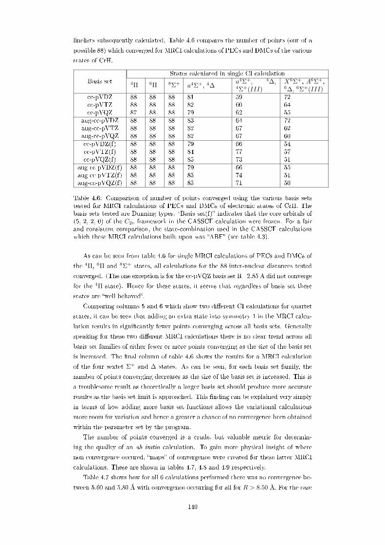
linelists subsequently calculated. Table 4.6 compares the number of points (out of a
possible 88) which converged for MRCI calculations of PECs and DMCs of the various
states of CrH.
Basis setStates calculated in single CI calculation
4Π 6Π 8Σ+ a4Σ+, 4∆a4Σ+, 4∆,4Σ+(III)
X6Σ+, A6Σ+,6∆, 6Σ+(III)
cc-pVDZ 88 88 88 81 59 72cc-pVTZ 88 88 88 82 60 64cc-pVQZ 87 88 88 79 62 55
aug-cc-pVDZ 88 88 88 83 64 72aug-cc-pVTZ 88 88 88 82 67 62aug-cc-pVQZ 88 88 88 82 67 60cc-pVDZ(f) 88 88 88 79 66 54cc-pVTZ(f) 88 88 88 84 77 57cc-pVQZ(f) 88 88 88 85 73 51
aug-cc-pVDZ(f) 88 88 88 79 66 55aug-cc-pVTZ(f) 88 88 88 85 74 51aug-cc-pVQZ(f) 88 88 88 85 71 50
Table 4.6: Comparison of number of points converged using the various basis setstested for MRCI calculations of PECs and DMCs of electronic states of CrH. Thebasis sets tested are Dunning types. Basis set(f) indicates that the core orbitals of(5, 2, 2, 0) of the C2v framework in the CASSCF calculation were frozen. For a fairand consistent comparison, the state-combination used in the CASSCF calculationswhich these MRCI calculations built upon was ABF (see table 4.3).
As can be seen from table 4.6 for single MRCI calculations of PECs and DMCs of
the 4Π, 6Π and 8Σ+ states, all calculations for the 88 inter-nuclear distances tested
converged. (The one exception is for the cc-pVQZ basis set R=2.85 Å did not converge
for the 4Π state). Hence for these states, it seems that regardless of basis set these
states are well behaved.
Comparing columns 5 and 6 which show two dierent CI calculations for quartet
states, it can be seen that adding an extra state into symmetry 1 in the MRCI calcu-
lation results in signicantly fewer points converging across all basis sets. Generally
speaking for these two dierent MRCI calculations there is no clear trend across all
basis set families of either fewer or more points converging as the size of the basis set
is increased. The nal column of table 4.6 shows the results for a MRCI calculation
of the four sextet Σ+ and ∆ states. As can be seen, for each basis set family, the
number of points converging decreases as the size of the basis set is increased. This is
a troublesome result as theoretically a larger basis set should produce more accurate
results as the basis set limit is approached. This nding can be explained very simply
in terms of how adding more basis set functions allows the variational calculations
more room for variation and hence a greater a chance of no convergence been obtained
within the parameter set by the program.
The number of points converged is a crude, but valuable metric for determin-
ing the quality of an ab initio calculation. To gain more physical insight of where
non-convergence occured, maps of convergence were created for these latter MRCI
calculations. These are shown in tables 4.7, 4.8 and 4.9 respectively.
Table 4.7 shows how for all 6 calculations performed there was no convergence be-
tween 5.60 and 5.80 Å with convergence occurring for all for R > 8.50 Å. For the case
140

Basis set family cc-pVnZ | aug-cc-pVnZ cc-pVnZ(f) aug-cc-pVnZ(f)R(Å)/Basis set size D T Q D T Q D T Q D T Q
0.70 • • • • • • • • • • • •0.80-1.55 • • • • • • • • • • • •1.60 • • • • • • • • • • • •
1.65-4.60 • • • • • • • • • • • •4.70 • • • • • • • • • • • •4.80 • • • • • • • • • • • •4.90 • • • • • • • • • • • •5.00 • • • • • • • • • • •5.20 • • • • • • • • • • •5.40 • • • • • • • • • • •5.60 • • • • • • • • • • •5.80 • • • • • • • • • • •6.00 • • • • • • • • • • •6.20 • • • • • • • • • • • •
6.50-7.50 • • • • • • • • • • • •7.70 • • • • • • • • • • • •8.00 • • • • • • • • • • • •8.50 • • • • • • • • • • • •9.00 • • • • • • • • • • • •10.00 • • • • • • • • • • • •
Table 4.7: Map of convergence across various basis sets tested for an MRCI calcu-lation of the a4Σ+ and 4∆ states. A • indicates that convergence was obtained forthis calculation at the respective inter-nuclear distance(s) and basis set. A • indi-cates that convergence was not obtained. In this table four families of basis sets arepresented(Dunning type Basis sets). The size of the basis set(n) for each family isindicated by the letters D, T and Q which denote double, triple and quadru-ple'. Here (f) indicates that the core orbitals of (5, 2, 2, 0) of the C2v frameworkin the CASSCF calculation were frozen. For a fair and consistent comparison, thestate-combination used in the CASSCF calculations which these MRCI calculationsbuilt upon was ABF(see table 4.3).
of the frozen calculations, the regions of non-convergence decrease when going up
the basis set. Table 4.8 clearly shows the large regions of non-convergence. Compare
this to table 4.7 in which one less quartet state of symmetry 1 has been calculated.
For all basis sets tested and for non-frozen and frozen all MRCI calculations of the
a4Σ+, 4∆ 4Σ+(II) (table 4.8) did however converge between 2.75 Å and 3.40 Å t.
Table 4.9 shows the map of convergence for MRCI calculations using cc-pVQZ basis
set of X6Σ+, , A6Σ+, 6∆ and 6Σ+(III) for the case of a proceeding CASSCF calcu-
lation using the state-combination of ABF. This table shows two important features:
the frozen calculations result in less points converging in the crucial region around
equilibrium (around 1.70 Å) and, the regions of non-convergence increase with in-
creasing basis set. This is a very unfortunate result as the reverse would normally be
expected: i.e. the number of points converging to increase with the size of the basis
set.
Tables 4.10, 4.11, 4.12 and 4.13 show the properties of the PECs obtained from
these calculations described in this section. For all tables the MRCI calculations of
the a4Σ+ and 4∆ states only are shown. The process for determining these properties
is described in section 2.9.2.
Table 4.10 shows that the eect of increasing the size of a basis set is to reduce
the value of Re by up to 0.1 Å. Augmenting a basis set or applying the frozen
option generally have the same eect of increasing Re by 0.10 Å when compared to
the respective cc-pVnZ calculation. The highest values of Re are obtained where an
augmented basis set has been used and the core orbitals frozen.
141

Basis set family cc-pVnZ | aug-cc-pVnZ cc-pVnZ(f) aug-cc-pVnZ(f)R(Å)/Basis set size D T Q D T Q D T Q D T Q
0.70-1.70 • • • • • • • • • • • •1.71 • • • • • • • • • • • •
1.72-2.20 • • • • • • • • • • • •2.25 • • • • • • • • • • • •2.30 • • • • • • • • • • • •2.35 • • • • • • • • • • • •2.40 • • • • • • • • • • • •2.45 • • • • • • • • • • • •2.50 • • • • • • • • • • • •2.55 • • • • • • • • • • • •2.60 • • • • • • • • • • • •2.65 • • • • • • • • • • • •2.70 • • • • • • • • • • • •
2.75-3.40 • • • • • • • • • • • •3.50 • • • • • • • • • • • •3.60 • • • • • • • • • • • •3.70 • • • • • • • • • • • •3.80 • • • • • • • • • • • •3.90 • • • • • • • • • • • •4.00 • • • • • • • • • • • •4.10 • • • • • • • • • • • •4.20 • • • • • • • • • • • •4.30 • • • • • • • • • • • •4.40 • • • • • • • • • • • •4.50 • • • • • • • • • • • •4.60 • • • • • • • • • • • •4.70 • • • • • • • • • • • •4.80 • • • • • • • • • • • •4.90 • • • • • • • • • • • •5.00 • • • • • • • • • • • •5.20 • • • • • • • • • • • •5.40 • • • • • • • • • • • •5.60 • • • • • • • • • • • •5.80 • • • • • • • • • • • •6.00 • • • • • • • • • • • •6.20 • • • • • • • • • • • •6.50 • • • • • • • • • • • •6.70 • • • • • • • • • • • •7.00 • • • • • • • • • • • •7.20 • • • • • • • • • • • •
7.40-10.00 • • • • • • • • • • • •
Table 4.8: Map of convergence across various basis sets tested for an MRCI calcula-tion of the a4Σ+, 4∆ and 4Σ+(II) states(compare with table 4.7 which is for two quar-tet states only). A • indicates that convergence was obtained for this calculation atthe respective inter-nuclear distance(s) and basis set. A • indicates that convergencewas not obtained. In this table four families of basis sets are presented(Dunningtype Basis sets). The size of the basis set(n) for each family is indicated by the lettersD, T and Q which denote double, triple and quadruple'. Here (f) indicatesthat the core orbitals of (5, 2, 2, 0) of the C2v framework in the CASSCF calculationwere frozen. For a fair and consistent comparison, the state-combination used in theCASSCF calculations which these MRCI calculations built upon was ABF (see table4.3).
Table 4.11 shows the shocking variation is dissociation energy for the various electronic
states as a function of basis set. As the size of the basis set increases, the size of
the dissociation energy increases. For each state, the lowest dissociation energy was
obtained when using a cc-pVDZ basis set and the highest when the core orbitals were
frozen and a cc-pVQZ basis set used. The dierence between these two values varies
between 3928 cm−1 for the A6Σ+ state and 1387 for the 4Π state. The variation in
De (cm−1) for the other electronic states is as follows: 6Π (1501), a4Σ+ (3758), 4∆
(1404), X6Σ+ (1918), 6∆ (3600).
142

Basis set family cc-pVnZ | aug-cc-pVnZ cc-pVnZ(f) aug-cc-pVnZ(f)R(Å)/Basis set size D T Q D T Q D T Q D T Q
0.70-1.30 • • • • • • • • • • • •1.35 • • • • • • • • • • • •1.40 • • • • • • • • • • • •1.45 • • • • • • • • • • • •1.50 • • • • • • • • • • • •1.55 • • • • • • • • • • • •1.60 • • • • • • • • • • • •1.65 • • • • • • • • • • • •1.66 • • • • • • • • • • • •1.68 • • • • • • • • • • • •1.69 • • • • • • • • • • • •1.70 • • • • • • • • • • • •1.71 • • • • • • • • • • • •1.72 • • • • • • • • • • • •1.73 • • • • • • • • • • • •1.74 • • • • • • • • • • • •1.75 • • • • • • • • • • • •1.76 • • • • • • • • • • • •1.78 • • • • • • • • • • • •1.80 • • • • • • • • • • • •1.85 • • • • • • • • • • • •1.90 • • • • • • • • • • • •1.95 • • • • • • • • • • • •2.00 • • • • • • • • • • • •2.05 • • • • • • • • • • • •2.10 • • • • • • • • • • • •2.15 • • • • • • • • • • • •2.20 • • • • • • • • • • • •2.25 • • • • • • • • • • • •
2.30-2.75 • • • • • • • • • • • •2.80 • • • • • • • • • • • •
2.85-4.70 • • • • • • • • • • • •4.80 • • • • • • • • • • • •4.90 • • • • • • • • • • • •5.00 • • • • • • • • • • • •5.20 • • • • • • • • • • • •5.40 • • • • • • • • • • • •5.60 • • • • • • • • • • • •5.80 • • • • • • • • • • • •6.00 • • • • • • • • • • • •6.20 • • • • • • • • • • • •6.50 • • • • • • • • • • • •6.70 • • • • • • • • • • • •7.00 • • • • • • • • • • • •7.20 • • • • • • • • • • • •7.40 • • • • • • • • • • • •7.50 • • • • • • • • • • • •7.70 • • • • • • • • • • • •8.00 • • • • • • • • • • • •8.50 • • • • • • • • • • • •9.00 • • • • • • • • • • • •10.00 • • • • • • • • • • • •
Table 4.9: Map of convergence across various basis sets tested for an MRCI calcu-lation of the X6Σ+, A6Σ+, 6∆ and 6Σ+(II) states. A • indicates that convergencewas obtained for this calculation at the respective inter-nuclear distance(s) and basisset. A • indicates that convergence was not obtained. In this table four familiesof basis sets are presented(Dunning type Basis sets). The size of the basis set(n) foreach family is indicated by the letters D, T and Q which denote double, tripleand quadruple'. Here (f) indicates that the core orbitals of (5, 2, 2, 0) of the C2v
framework in the CASSCF calculation were frozen. For a fair and consistent com-parison, the state-combination used in the CASSCF calculations which these MRCIcalculations built upon was ABF (see table 4.3).
Table 4.12 shows the variation in the calculated value of the ν = 1 energy state for
each electronic state as a function of basis set. Thankfully the variation is much less
143

Basis setElectronic state
X6Σ+ A6Σ+ 6Π 6∆ a4Σ+ 4Π 4∆cc-pVDZ 1.680(4) 1.780(2) 1.786(2) 1.777(4) 1.664(3) 1.705(5) 1.672(4)cc-pVTZ 1.672(3) 1.780(4) 1.784(3) 1.774(3) 1.663(4) 1.703(3) 1.668(1)cc-pVQZ 1.672(4) 1.783(1) 1.784(4) 1.779(2) 1.661(3) 1.702(2) 1.667(4)
aug-cc-pVDZ 1.687(4) 1.786(4) 1.793(4) 1.784(1) 1.670(2) 1.712(3) 1.679(2)aug-cc-pVTZ 1.676(2) 1.784(2) 1.788(4) 1.778(3) 1.665(4) 1.707(4) 1.672(5)aug-cc-pVQZ 1.673(5) 1.783(2) 1.787(4) 1.777(1) 1.663(2) 1.703(3) 1.669(2)cc-pVDZ(f) 1.690(4) 1.921(3) 1.791(5) 1.932(3) 1.669(5) 1.711(3) 1.677(1)cc-pVTZ(f) 1.584(3) 1.789(1) 1.790(5) 1.786(2) 1.671(5) 1.709(4) 1.671(5)cc-pVQZ(f) 1.580(2) 1.789(2) 1.790(5) 1.787(1) 1.670(2) 1.708(2) 1.671(4)
aug-cc-pVDZ(f) 1.697(5) 1.908(1) 1.798(4) 1.914(3) 1.676(4) 1.719(5) 1.684(3)aug-cc-pVTZ(f) 1.585(3) 1.789(2) 1.795(2) 1.788(2) 1.674(2) 1.712(5) 1.676(2)aug-cc-pVQZ(f) 1.667(2) 1.788(2) 1.792(3) 1.783(2) 1.671(3) 1.710(2) 1.672(4)
Ref. 1.690 1.772 1.803 1.824 1.693 1.714 1.717
Table 4.10: Re values obtained for the various PECs calculated at MRCI level oftheory using an initial CASSCF calculation with the state-combination of ABF forvarious basis sets. Here the number in the brackets indicates the error on the minimaobtained by using the interpolation functionality of Duo, see section 2.9.2. In thistable the Re values calculated by Dai & Balasubramanian (1993) have been shownfor reference.
than for the De values hence indicating that the range in De values will only aect
the number of higher-order vibronic states obtained for each PEC as opposed to the
actual energy of these individual vibronic states. By examination of table 4.12 there
is no clear trends as for some electronic states the highest value is for the case of a
cc-pVDZ basis set and for others the highest value is for a cc-pVQZ basis set where
the core orbitals have been frozen.
Finally, table 4.13 how the absolute position on the energy scale of PECs of each
electronic state varies as a function of basis set. As can be seen a PEC of any particular
state can appear up to 13 000 cm−1 higher or lower in energy depending on the basis
set used. For all states, it can be seen that the lowest PECs obtained are for the cases
of quadruple basis sets used: this is consistent with the Variational Theorem and the
idea of the Basis Set Limit. In practice, all PECs were moved up/down the energy
scale according to where they should lie as determined by the atomic dissociation
limits of the Chromium atom for the calculation of the nal linelist. In our study,
relativistic basis sets and those for core-correlation were not investigated as it was
know from previous work that their eects tend to cancel, see Lodi et al. (2008).
4.5 Eect of CASSCF state-combination uponMRCI
calculations
Using the seven chosen state-combinations for CASSCF calculations shown in table
4.4, CI calculations were perfomed. The results produced by these CI calculations
which each used one of these state-combinations in the proceeding CASSCF calcu-
lations were then compared. To reiterate for the construction of a linelist several ab
initio curves are necessary:
PECs: the parameters of these PECs for each of the molecular states determine
144

Basis setElectronic state
X6Σ+ A6Σ+ 6Π 6∆ a4Σ+ 4Π 4∆cc-pVDZ 15700 12129 13104 11621 12130 11210 10744cc-pVTZ 16734 13320 14278 12826 13623 12471 12003cc-pVQZ 16988 13258 14520 13073 13758 12866 12405
aug-cc-pVDZ 16242 12433 13817 12334 12433 11928 11451aug-cc-pVTZ 16924 13180 14452 13023 13596 12760 12296aug-cc-pVQZ 17069 13216 14575 13144 13747 12966 12508cc-pVDZ(f) 16286 12451 13136 10862 13130 10949 10460cc-pVTZ(f) 16043 21565 14320 20535 15336 12120 11660cc-pVQZ(f) 16245 21545 14561 20639 15769 12499 12046
aug-cc-pVDZ(f) 16801 12867 13857 11697 13417 11660 11139aug-cc-pVTZ(f) 16163 21323 14490 20555 15667 12400 11949aug-cc-pVQZ(f) 17618 16057 14614 15221 15888 12597 12148
Table 4.11: De values obtained for the various PECs calculated at MRCI level oftheory using an initial CASSCF calculation with the state-combination of ABF forvarious basis sets. For a bound PEC, a De value is simply the dierence in energybetween the minima of the of PEC and the value at dissociaiton.
Basis setElectronic state
X6Σ+ A6Σ+ 6Π 6∆ a4Σ+ 4Π 4∆cc-pVDZ 1483 1714 1757 1722.082366 1685 1573 1522cc-pVTZ 1509 1715 1757 1718.655687 1687 1576 1532cc-pVQZ 1511 1711 1756 1717.432249 1686 1574 1533
aug-cc-pVDZ 1465 1699 1748 1713.447707 1669 1566 1516aug-cc-pVTZ 1497 1710 1755 1717.661735 1678 1569 1526aug-cc-pVQZ 1501 1712 1754 1716.275966 1682 1570 1529cc-pVDZ(f) 1642 1378 1673 1322.517761 1655 1529 1479cc-pVTZ(f) 1339 3041 1617 3192.160096 1645 1523 1490cc-pVQZ(f) 1337 3038 1618 3164.201293 1646 1524 1492
aug-cc-pVDZ(f) 1637 1426 1658 1393.747181 1637 1520 1471aug-cc-pVTZ(f) 1291 3019 1614 3162.938876 1637 1516 1482aug-cc-pVQZ(f) 1499 1974 1615 2151.46828 1642 1520 1487
Table 4.12: Energy levels of the ν = 1 vibronic states of the various PECs calculated atMRCI level of theory using an initial CASSCF calculation with the state-combinationof ABF for various basis sets.
the energy levels
DMCs and TDMs: these curves determine the relative intensities of transitions
between rovirbonic energy levels
Angular-momentum coupling (i.e. Lx, Lz operators) which acts as a perturba-
tion on the PECs
Spin-orbit coupling (i.e. SOx, SOz operators) which acts as a perturbation on
the PECs.
Hence, to a rst order it is important to strive to obtain the best quality PECs,
DMCs and TDMs as possible. The quality of the curves was selected in terms of
the following criteria:
Convergence of the curves-are the regions where convergence has not occurred
(i.e. no numbers produced hence gaps) of physical importance? Generally
145

Basis setElectronic state
X6Σ+ A6Σ+ 6Π 6∆ a4Σ+ 4Π 4∆cc-pVDZ 5890 11390 6158 13677 6398 6443 6404cc-pVTZ 2011 7436 1882 9401 2144 2080 2074cc-pVQZ 240 5766 212 7742 277 257 260
aug-cc-pVDZ 4735 10261 4951 12480 5271 5231 5214aug-cc-pVTZ 1282 6756 1248 8749 1352 1331 1326aug-cc-pVQZ 0 5520 0 7514 0 0 0cc-pVDZ(f) 6528 12342 6052 14098 6682 6630 6350cc-pVTZ(f) 5010 1637 1926 1495 2881 2517 2220cc-pVQZ(f) 3318 0 288 0 1054 741 443
aug-cc-pVDZ(f) 5389 11094 4829 12768 5566 5417 5176aug-cc-pVTZ(f) 4303 1046 1268 993 2065 1749 1449aug-cc-pVQZ(f) 1768 5176 68 5252 768 476 175
Table 4.13: Relative Te values for each electronic state where the minima (0) for eachis taken from the basis-set which produces the lowest-lying PEC for the particularstate. Note this table is not showing where the various states lies with respect to eachother: it is showing how for each state the eect of basis-set is to move the calculatedPEC of this state up/down the energy scale. These dierences in energy were takenat the equilibrium point for each of the dierent states. The PECs were calculated atMRCI level of theory using an initial CASSCF calculation with the state-combinationof ABF for various basis sets.
speaking, the well' of a PEC is more crucial than any missing asymptotic
points provided there are plenty others to act as reference.
Continuity of the curves. This was checked by visual inspection of the various
plots but also by taking the gradient of the curves as a means to determine
discontinuities. An explanation of this process is given below.
Another check of quality was considering the behaviour of these various curves
when dierent numbers of states of the same symmetry and multiplicity were
calcualted at CI level. As an example comparing the case of 1+0, 2+1 and 3+1
calculations for 4Σ+ and 4∆.
For the case of X6Σ+ and A6Σ+, comparisons were made to experimental data.
For the other electronic states it is interested to compare to previous theoretical
work however in these cases it can be hard to ascertain either way which study
is more accurate without experimentally derived reference values.
To help determine how continuous the various ab initio curves where, gradients of the
curves were calculated and plotted. This was done using a nite dierence method
to produce PEC-G and DMC-G plots. To generate a PEC-G plot, the set of inter-
nuclear points R∗1, ...R∗N for the respective PEC was rstly used to construct a new
set of inter-nuclear distances, size N − 1 denoted R∗ where N is the number of inter-
nuclear points in the respective PEC using the formula, R∗a = 12 (Ra +Ra+1) where a
goes from 1 to N − 1. The corresponding gradient of energy, denoted E′for each of
these new R∗ valus was calculated by E′
a = Ea+1−EaRa+1−Ra where a runs from 1 to N − 1.
Hence the PEC-G curve contained N −1 data points where N is the number of inter-
nuclear points, R for the original PEC. For clarity, table 4.14 demonstrates the use
of these formula in constructing PEC-G curves.
146

PEC Gradient of PEC
R1, E1
R∗1 = 12 (R1 +R2), E
′
1 = E2−E1R2−R1
R2, E2
R∗2 = 12 (R2 +R3), E
′
2 = E3−E2R2−R1
R3, E3
R∗3 = 12 (R3 +R4), E
′
3 = E4−E3R4−R3
R4, E4
RN−2, EN−2
RN−2 +RN−1), E′
N−2 = EN−1−EN−2RN−1−RN−2
RN−1, EN−1
R∗N−1 = 12 (RN−1 +RN ), E
′
N−1 = EN−EN−1RN−RN−1
RN , EN
Table 4.14: Schematic showing how PEC-Gs were constructed using a nite dierencemethod. Here the original PEC has N points withe inter-nuclear values of R1,R2,...RN with corresponding energy values E1, E2,..., EN . The constructed PEC-Ggraph has N−1 data points. DMC-Gs were constructed in a similar manner by takingthe dierence of dipole moment values instead of energies.
In a similar fashion, DMC-G curves were calculated using this nite dierence
method.
In the following sections, the PECs, DMCs & TDMS calculated at CI level of
theory using the seven dierent CASSCF state-combinations in table 4.4 are compared
and discussion presented for each decision made. For the angular momentum and spin-
orbit couplings calculated at CI level it was found that these are generally speaking
independent to within several percent of the state-combinations used in the proceeding
CASSCF calculation. A summary of the ab initio curves hence used in the nal linelist
for CrH is given in section 5.1.
4.6 Choice of Method for calculation of DMCs
With respect to the DMCs, there are two methods (Tennyson 2014) in which to cal-
culate the dipole moment namely the expectation method and the nite eld method
where the former calculates the matrix element formed by acting the dipole moment
operators µx, µy, µz on the electronic wave-functions and the latter makes use of the
Stark Eect. In this work all DMCs were calculated using the expectation method.
In order to obtain accurate intensity values, it is paramount that we obtain accurate
DMCs.
In sections 4.11 4.8 and 4.10 the DMCs presented are those that have been calcu-
lated using expectation method. Figure 4.5 shows DMCs calculated using the nite-
dierence method for the 8Σ+, 6Π and 4Π states. Each plot shows DMCs calculates
using a dierent family of basis. For each calculation the state-combination used in
147

the proceeding CASSCF calculation was ABF.
(a) (b)
(c)
Figure 4.5: Calculation of DMCs at MRCI level of theory for various electronic statesusing the nite-eld method. Each plot shows a comparison of curves calculatedusing increasingngly larger basis sets within a Dunning basis set family. In all ofthese MRCI calculations the CASSCF state-combination used was ABF to allowfor a fair comparison.
Figure 4.5 demonstrates that increasing the size of the basis set generally does not
alleviate discontinuities. For all plots, clear discontinuities can be seen and appear
more signicant than those for the ABF curves presented in sections 4.11, 4.8 and
4.10 where the expectation value method was used. Hence on this comparison it was
decided to continue to use the expectation method to calculate the full DMCs of
electronic states. For the case of the X6Σ+ and A6Σ+ states a comparison between
the two methods has been made: see section 4.7.2.
4.7 PECs, DMCs and diagonal TDMs for the 6Σ+
and 6∆ states
As a reminder, ∆ states have components in both symmetry 1 and 4 within the c2v
framework, hence 6Σ+ and 6∆ states need to be calculated together. It was established
from the CASSCF testing that the relative order of these states in terms of potential
energy is X6Σ+, A6Σ+(II), 6∆ and 6Σ+(III). Thus when calculating curves at CI
148

level it makes sense to perform calculations which reect this. Thus for each dierent
CASSCF state-combination, 4 CI calculations of PEC, DMC and TDMs were carried
out as summarised in table 4.15. This testing was done to investigate how CI results
for a particular proceeding CASSCF state-calculation are aected by the number of
states requested at CI levels in the various symmetries. As a reminder, the notation
4+1 indicates a CI calculation in which four sextet states within symmetry 1 and one
state of symmetry 4 are calculated. Table 4.15 also shows the number of inter-nuclear
distance points, R out of a total of 88 tested (see section 2.7.1 which denes the grid
used) which converged. It should be noted that as well as the raw number of points
that converge, the regions where non-convergence takes place is also important i.e. if
there is gaps deep in the well of potentials compared to at dissociation.
CI PROC Meaning AB AF ABF BF BFH BJ BFJS5 1+0 88 88 88 88 88 88 88S6 2+0 57 62 81 61 88 71 68S7 3+1 53 72 81 73 62 69 84S8 4+1 42 25 55 48 40 68 31
Table 4.15: Summary of MRCI calculations carried out for the 6Σ+ and 6∆ states.In the results the notation for the CI PROC s dened here will be used throughout.The notation 3+1 signies that three sextet states of symmetry 1 and one sextetstate of symmetry 4 were calculated in an MRCI calculation. This table indicates thenumber of points(out of a possible 88) which converged for the various MRCI calcu-lations which were performed for the various proceeding CASSCF state-combinationcalculations (as indicated by AB, AF etc).
As can be seen from table 4.15, for PROC S5, all 88 PECs and DMCs converged for
the seven CASSCF state-combinations tested. As was mentioned previously, having
a series of calculations converge does not guarantee that all these points will form a
continuous curve. Figure 4.6 shows plots of PECs, PEC-Gs and DMCs calculated at
CI level produced by PROC S5 for the seven CASSCF state-combinations under test.
(a) (b)
Figure 4.6: Comparison of PECs and DMCs calculated at MRCI level of theory usinga cc-pVQZ basis set for various CASSCF state-combinations for the X6Σ+ state ofCrH.
Figure 4.6 shows the PECs calculated of the X6Σ+ state: as can be seen the AF,
BF and BFH curves all jump at between 2.3 and 2.5 Å Figure 4.6 shows the DMCs:
149

it is clear that the AB curve is the only continuous curve. A plot of the PEC and
DMC calculated at CI level for the X6Σ+ state using the PROC S5 (i.e. a 1+0
calculation) is shown in gure 4.7.
Figure 4.7: PECs and DMCs calculated at MRCI level of theory using a cc-pVQZbasis set and CASSCF state-combination of AB for the X6Σ+ state of CrH.
Figure 4.7 show that the PEC and DMC produced by a 1+0 CI calculation using
the CASSCF state-combination of AB are both appear to be continuous. Unfortu-
nately, refering to table 4.15 for CI calculations using PROC s S6, S7 and S8 for AB
drops. But what is not revealed by this table that the region of non-convergence is a
crucial region: it is between approximately 1.90 and 3.60 Åfor PROC s S2, S3 and S4
which is the region in which the shape of the PECs is paramount to the calculation
of accurate vibronic energy levels.
Throughout the following analysis of these CI PROC s the colouring scheme shown
in table 4.16 is used in plots which show PECs and DMCs for the 6Σ+ and 6∆ states
calculated using the PROCS S5, S6, S7 and S8 as dened in table 4.15.
Colour StateBlack X6Σ+
Red A6Σ+
Green 6∆(sym 1)Magneta 6Σ+(III)Blue 6∆(sym 4)
Table 4.16: Summary of colour scheme used throughout gures 4.8 to 4.14.
Figure 4.8 shows this colour scheme in action for the case of a CASSCF state-
combination of AB been used in a CI calculation of four sextet states in symmetry 1
and one sextet state in symmetry 4(i.e. 4+1 calculation, PROC S4 ).
150

Figure 4.8: AB: PECs and DMCs calculated at MRCI level of theory using a cc-pVQZ basis set and CASSCF state-combination of AB for the X6Σ+, A6Σ+, 6∆ and6Σ+(III) electronic states of CrH.
As gure 4.8 shows, CASSCF state-combination of AB produces PECs and DMCs
at CI level which have gaps in the crucial region.
In the following pages, the colour scheme described in table 4.16 is employed to
show the results of CI calculations of PROC s S5, S6, S7 and S8 dened in table 4.15
of PECs and DMCs produced using the six remaining CASSCF state-combinations as
respective proceeding calculations. Table 4.17 provides a summary of the key distin-
guishing features of Figures 4.9 to 4.14. In summary, all CASSCF state-combinations
produce their best CI results when the S7 PROC is used.
151

(a) (b)
(c) (d)
(e) (f)
(g) (h)
Figure 4.9: MRCI calculations of PECs and DMCs of the X6Σ+, A6Σ+, 6∆ and6Σ+(III) electronic states of CrH using a cc-pVQZ basis set which are built upon theCASSCF state-combination of AF.
152

(a) (b)
(c) (d)
(e) (f)
(g) (h)
Figure 4.10: MRCI calculations of PECs and DMCs of the X6Σ+, A6Σ+, 6∆ and6Σ+(III) electronic states of CrH using a cc-pVQZ basis set which are built upon theCASSCF state-combination of ABF.
153

(a) (b)
(c) (d)
(e) (f)
(g) (h)
Figure 4.11: MRCI calculations of PECs and DMCs of the X6Σ+, A6Σ+, 6∆ and6Σ+(III) electronic states of CrH using a cc-pVQZ basis set which are built upon theCASSCF state-combination of BF.
154

(a) (b)
(c) (d)
(e) (f)
(g) (h)
Figure 4.12: MRCI calculations of PECs and DMCs of the X6Σ+, A6Σ+, 6∆ and6Σ+(III) electronic states of CrH using a cc-pVQZ basis set which are built upon theCASSCF state-combination of BFH.
155

(a) (b)
(c) (d)
(e) (f)
(g) (h)
Figure 4.13: MRCI calculations of PECs and DMCs of the X6Σ+, A6Σ+, 6∆ and6Σ+(III) electronic states of CrH using a cc-pVQZ basis set which are built upon theCASSCF state-combination of BJ.
156

(a) (b)
(c) (d)
(e) (f)
(g) (h)
Figure 4.14: MRCI calculations of PECs and DMCs of the X6Σ+, A6Σ+, 6∆ and6Σ+(III) electronic states of CrH using a cc-pVQZ basis set which are built upon theCASSCF state-combination of BFJ.
157

CASSF PROC Notes
AF
S5PEC: Minor discontinuity at 2.2Å and between 7.00 and 8.00 Åjump up to another asymptote
Three stray points between1.30 and 1.50 Å and a sharpchange in behaviour at 2.5 Å.
S6Discontinuity at 1.5 Å in bothPECs: gaps between 2.1 and 2.5Å
S7 Very obvious discontinuity at 2.5 ÅS8 Gap in convergence between 1.5 and 2.5 Å
ABF
S5 PEC: Small hump around 2.10Å
DMC(s) appears of good quality
S6 PEC: Discontinuity of A6Σ+
state around 2.10 Å.S7 All curves continuous and of good quality
S8 Gap in convergence between 1.55 Å and 1.80 Å(aects PECs morethan DMCs)
BF
S5Continuous curves: PEC does have a bump around 2.2 Å com-parable in size to the S5 calculation of ABF
S6Gap in convergence between 2.50 Å and 3.00 Å and also between3.60 Å and 6.7 Å: the former is not as signicant as there aresucient points either side in which to reconstruct curve.
S7 PEC: Jump between 2.30 and2.40 Åfor the upper states and agap in convergence between 2.40Å and 2.80 Å.
DMC: Sharp cusp around 2.1 Åfor all DMC
S8 DMC & PEC: gap in conver-gence between 2.4 Å and 2.8 Å
BFH
S5PECs: Discontinuity at 2.30 Å. DMCs: sharp change in be-
haviour at 2.4 Å.S6S7 PECs: gap and an apparent
jump between 2.40 Å and 2.60Å for the upper states
S8 No convergence in the crucial region between 2.40 Å and 8.40 Å.
BJ
S5 PEC: continuous and well-behaved
DMC: shows a slightly steepchange in character at 2.1 Å butnevertheless of good quality.
S6 Gap in convergence between 2.10and 2.60 Å but appear of goodquality.
DMC of several upper states ap-pears to have an abrupt change-exception is 6∆ state
S7S8
BFJ
S5PEC: Discontinuity at 2.40 Å.
DMC: Sharp change in be-haviour at 2.4 Å.
S6 DMC of ground state moresmooth than S5 but A6Σ+ statehas a change in behaviour in thisregion.
S7 DMC of third sextet state ofsymmetry 1 abruplty changes be-tween 2.10 Å and 2.50 Å.
S8 No convergence in the crucial region between 1.2 and 2.3 Å.
Table 4.17: Summary of distinguishing features of the various MRCI calculationsperformed of theX6Σ+, A6Σ+, 6∆ and 6Σ+(III) electronic states of CrH for dierentCASSCF state-combinations tested. All calculations were performed with a cc-pVQZbasis set. The relevant gures which this table refers to are gure 4.9 to 4.14.
4.7.1 PECs for the X6Σ+ and A6Σ+ states
Gathering together all the good quality PECs and DMCs for the X6Σ+ state, Re,
De and ωe were calculated. These values are shown in table 4.18.
158

CASSCFstate-combination
CIPROC
Re(Å)Dissociationenergy(cm−1)
ν = 1 energy(cm−1)
Te relative(cm−1)
ABF S5 1.675(2) 16229 1507.05 553ABF S5 1.660(1) 16120 1434.18 979ABF S7 1.673(2) 16949 1508.81 150BFH S7 1.673(3) 17235 1565.19 285
BF
S5 1.662(4) 16042.00 1527.36 1508S6 1.666(3) 16363 1530.32 1187S7 1.675(4) 16995 1535.95 555S8 1.673(3) 17053 1537.55 509
BJ
S5 1.694(2) 16305.00 1452.89 589S6 1.682(4) 16837 1522.70 57S7 1.682(4) 16870 1522.32 27S8 1.682(4) 16897 1520.43 0
Table 4.18: Summary of properties determined for various PECs of the X6Σ+ whichwere judged to be of good quality.
The PEC properties shown in table 4.18 were determined by using the procedure
described in section 2.9.2. As table 4.18 shows, the values of Re for these chosen PECs
vary between 1.660 and 1.694. Within the BF calculations the trend is an increase in
Re as more states are added at CI level up to 3+1. For the BJ calculations, the value
of Re is constant for the S6, S7 and S8 values. These values of Re can be compared to
the theoretical values calculated by Dai & Balasubramanian(1993) which are shown
in table 4.19. Additionally, table 4.20 shows previous theoretical determination of Reobtained in other studies.
Method Basis Re (Å) ωe (cm−1) D0 (cm−1)MCSCF ANO 1.721 1525 11211.40IC-MRCI ANO 1.684 1581 16615.45
IC-MRCI+Q ANO 1.685 1577 17422.02IC-MRCI ANO+ 1.681 1586 16857.42
IC-MRCI+Q ANO+ 1.682 1584 17583.34IC-MRCI+dd' ANO 1.679 1593 16776.76
IC-MRCI+Q+dd' ANO 1.679 1596 17180.05IC-MRCI+pp ANO 1.683 1586 16615.45
IC-MRCI+Q+pp ANO 1.683 1582 17422.02IC-MRCI GEN 1.683 1581 16454.13
IC-MRCI+Q GEN 1.684 1577 17422.02IC-MRCI+3s3p GEN 1.673 1595 15970.19
IC-MRCI+Q+3s3p GEN 1.670 1601 17422.02MRCI GEN 1.681 1585 16696.11
MRCI+Q GEN 1.682 1581 17502.68DK-MRCI GEN 1.669 1631 17341.37
DK-MRCI+Q GEN 1.669 1628 17502.68Experiment work(within paper) 1.655 1656 15566.90(564.60)
Table 4.19: Summary of PEC properties of the X6Σ+ state of CrH obtained byBauschlicher et al. (2001).
By comparing table 4.18 to tables 4.19 and 4.20 it can be seen that the range of
Re for the X6Σ+ state of CrH calculated within this study is consistent with previous
theoretical work.
The estimates for ν = 1 vibronic state can be compared against the joint experimental
159

Study Method Re (Å)
Barone & Adamo (1997)
CISDa 1.691CPFa 1.694MCPFa 1.694
BLYP/DZP 1.652B3LYP/DZP 1.654Experiment 1.662
Roos(2003)CASPT2 1.642MSPT2 1.641
Experiment 1.655Koseki Matsushita & Gordon (2006) ECP 1.676
Table 4.20: Summary of Re values of the X6Σ+ state of CrH determined in previoustheoretical studies with the experimental comparison available at the time.
and theoretical study of Bauschlicher et al. (2001) who obtained an experimental value
of 1595.068 70(14) cm−1. As can be seen all estimates presented in table 4.18 are
too low. As table 4.18, there is a variation between 1434.18 and 1527.36 cm−1 for
the values determined. However, this variation in both ν = 1 energy level and indeed
also the dissociation energy is a result in itself. It is hence reasonable to suppose that
there will be a variation in ωe. Bauschlicher et al. (2001) obtained an experimental
value of ωe of 1656.05115(54) cm−1 which they commented was remarkably similar
to their theoretical prediction of 1653.6 cm−1.The values calculated are around 150
cm−1 lower than the experimental value. Finally the relative energy spacing of the
minima of these PECs is given in table 4.18: this demonstrates how the energy scale
for dierent CASSCF calculations leading into CI calculations can vary by potentially
1000 s of wavenumbers. Table 4.19 is taken from the study of Bauschlicher et al.
(2001) and shows the PEC properties they calculated using various basis sets and
also methods. This table indicates how sensitive calculated PECs are to both basis
set and method. In this study of CrH both of these have been validated.
Moving onto the A6Σ+, a similar analysis as was carried out for the X6Σ+ state
has been carried out for the good quality PECs identied in table 4.17. Referring to
table 4.15, an unusual feature of AF, BF and BFJ is that more points converge for
PROC S7 then they do PROC S6. This dees the trend of fewer points converging
as more states are added at CI level. Table 4.21 quanties the gap at dissociation
between the various sextet states for the dierent calculations. For ABF and BJ the
gap between the A6Σ+ state and X6Σ+ state stays constant at around 7700 cm−1
and around 11 000 cm−1 irrespective of the CI PROC used. However, for PROC
S6 for AF, BF, BFH and BFJ the A6Σ+ state is clearly dissociating to the wrong
dissociation limit: referring back to table 2.8, the A6Σ+(II) state should dissociate to
a lower asymptote than the 6∆ and 6Σ+(III) states. Hence this is evidence that these
CASSCF state-combinations give inaccurate results when a proceeding CI calculation
with 2+0(i.e. S6 ) states is used.
160

Gap at dissociation between (cm−1) CI PROC AF ABF BF BFH BJ BFJA6Σ+(II) and X6Σ+ S6 9815 7717 9815 9469 7814 9965A6Σ+(II) and X6Σ+
S79688 7706 9688 9335 7803 9939
6∆ and X6Σ+ 9782 10667 9782 9439 11671 10022A6Σ+(II) and X6Σ+
S87607 7694 7607 7574 7792 7625
6∆ and X6Σ+ 9652 10603 9652 9301 11470 99016Σ+(III) and X6Σ+ 9752 10721 9752 9408 11650 9984
Table 4.21: Summary of gaps in energy between various electronic states of CrH at dis-sociation calculated at MRCI level of theory for various CASSCF state-combinations.
Table 4.22 gives a summary of the parameters obtained for the A6Σ+ PECs of
interest: these were calculated in the same manner as they were for the X6Σ+ state.
CASSCFstate-combination
CI PROC Re(Å)Dissociationenergy(cm−1)
Vibronic(cm−1)
Te relative(cm−1)
ABF S7 1.782(3) 13224 1737 506ABF S8 1.781(4) 13261 1714 458BF S7 1.785(4) 15604 1556 559BF S8 1.783(3) 13584 1547 505BJ S7 1.756(2) 13582 1624 43BJ S8 1.757(3) 13614 1611 0
Table 4.22: Summary of properties of PECs calculated for the A6Σ+ state of CrH.
As can be seen from table 4.22, Re varies between 1.757 Å and 1.782 Å This can
be compared to the theoretical value obtained by Dai & Balasubramanian (1993) of
1.772 Å which lies just about middle of the values presented in table 4.22. Again,
as was the case for the X6Σ+ state, these can be compared to those obtained by
Bauschlicher et al. (2001) whose results are shown in table 4.23.
Method Basis Re ωe (cm−1)MCSCF ANO 1.876 1337IC-MRCI ANO 1.782 1516
IC-MRCI+Q ANO 1.774 1537IC-MRCI ANO+ 1.779 1521
IC-MRCI+Q ANO+ 1.771 1542IC-MRCI+dd' ANO 1.776 1525
IC-MRCI+Q+dd' ANO 1.774 1531IC-MRCI+pp ANO 1.781 1520IC-MRCI1Q1pp ANO 1.773 1538IC-MRCI+ppdd' ANO
IC-MRCI GEN 1.78 1519IC-MRCI+Q GEN 1.772 1539
IC-MRCI+3s3p GEN 1.778 1506IC-MRCI+Q+3s3p GEN 1.764 1514
MRCI GEN 1.779 1515MRCI+Q GEN 1.771 1535DK-MRCI GEN 1.783 1494
DK-MRCI+Q GEN 1.775 1517Experiment work(within paper) 1.786 1525
Table 4.23: Summary of Re and ωe values determined for the A6Σ+ state of CrH byBauschlicher et al. (2001) for various methods and basis sets.
161

As table 4.23 shows, Bauschlicher et al. (2001) obtained a spread in Re values
between 1.764 Å and 1.876 Å. With the exception of the BJ values this present study
is consistent with the calculations of Bauschlicher et al. (2001). A very obvious outlier
in dissociation energy is that of the BF, S7 calculation producing a result of 15 604
cm−1: the other ve values determined vary between 13224 cm−1 and 13614 cm−1.
The estimates of ωe obtained show huge variation with the lowest estimate of 1547
and the highest of 1737. Bauschlicher et al. (2001) obtained an experimental value
of 1524.80(5) cm−1 and a theoretical value of 1525.2 cm−1.
Table 4.23 also shows the variation in ωe which Bauschlicher et al. (2001) obtained:
the range is from 1337 to 1535 with the experimental value measured been 1525. This
is consistent with the variation of the ν = 1 energy level presented in table 4.22.In summary for both the X6Σ+ and A6Σ+ states of CrH, there is signicant variation
in the PEC properties calculated as both a function of the CASSCF state-combination
used and number of sextet states of symmetry 1 calculated at MRCI level. Pragmat-
ically for the linelist experimental data was obtained of these two states and two
empirical PECs tted to this data. Hence ab initio PECs for these two states were
simply used as a guide in starting o the process of tting to experimental data.
Hence, for the nal linelist the nal PEC chosen for each of these states is largely
irrelevant.
4.7.2 Equilibrium Dipole Moments for the X6Σ+ and A6Σ+
states
To test out the stability of the equilibrium dipole moments obtained for both the
X6Σ+ and A6Σ+ states, calculations at MRCI level theory were performed using
dierent state-combinations in the initial CASSCF calculation. These values were
calculated for a single point, namely for the case of an inter-nuclear distance of 1.672
Åfor the X6Σ+ state and 1.781 Åfor the A6Σ+ state respectively. Additionally, the
eect of the number of states calculated at MRCI level was tested. For each CASSCF
state-combination, four MRCI calculations were performed each with a dierent num-
ber of sextet states calculated within symmetry 1. Each of these MRCI calculations
was performed using a nite-eld method(FFD) and expectation method(EXP) For
all calculations, a cc-pVQZ basis set was used. Tables 4.24 and 4.25 show these results.
EXP FFD EXP FFD EXP FFD EXP FFDNo. values 56 55 55 54 54 54 21 16Mean 2.581 3.723 2.958 3.840 3.670 3.936 3.473 3.696Median 2.465 3.692 2.836 3.729 3.528 3.732 3.441 3.674Minimum 2.031 2.259 2.489 2.341 3.318 2.364 3.308 3.506Maximum 4.082 4.599 3.877 4.879 4.717 5.093 3.721 3.884
Table 4.26: Summary statistics for the dipole moments calculated for the A6Σ+ stateat R = 1.672 Å. See table 4.24 for details of these calculations. Here EXP andFFD refer to the two methods which can be used to calculate dipole momentsnamely, expecation value method and nite-eld method.
162
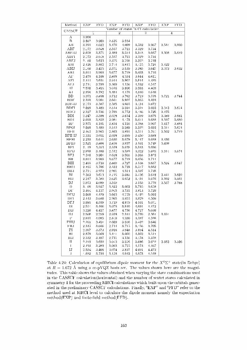
Method EXP FFD EXP FFD EXP FFD EXP FFD
CASSCFNumber of states in CI calculation
1 2 3 4A 3.900B 3.882 3.900 2.835 3.934AB 3.391 4.022 3.476 4.009 3.502 3.967 3.584 3.930ABF 2.172 3.648 2.557 3.711 3.329 3.734
ABF-IJ 2.059 3.375 2.489 3.514 3.318 3.667 3.308 3.649ABFI 2.172 3.648 2.557 3.711 3.329 3.734ABFJ 2.180 3.633 2.575 3.708 3.352 3.748ABI 2.426 3.862 2.744 3.845 3.425 3.724 3.422ABIJ 2.160 3.425 2.571 3.539 3.385 3.647 3.373 3.632ABJ 3.011 3.908 3.677 3.719 3.663 3.716AF 2.479 4.108 2.898 4.334 3.644 4.611AFI 2.411 3.631 2.914 3.967 3.844 4.485AFJ 2.734 3.799 3.309 4.156 4.102 4.547AI 2.520 3.455 3.016 3.806 3.993 4.409AJ 2.896 3.792 3.484 4.178 4.340 4.640BD 3.371 3.858 3.712 3.762 3.719 3.755 3.721 3.744BDF 2.310 3.901 2.661 3.907 3.365 3.823
BDF-IJ 2.173 3.507 2.595 3.605 3.434 3.672BDFI 2.099 3.480 2.514 3.591 3.321 3.693 3.313 3.674BDFJ 2.327 3.736 2.708 3.772 3.486 3.725 3.475BDI 2.247 3.588 2.628 3.654 3.399 3.675 3.389 3.661BDJ 2.693 3.850 2.981 4.473 3.611 3.688 3.597 3.680BF 2.571 4.191 2.834 4.116 3.388 3.907 3.417 3.884
BFGI 2.099 3.480 2.512 3.589 3.322 3.693 3.314 3.674BFH 2.465 3.905 2.803 3.891 3.511 3.761 3.502 3.749
BFH-IJ 2.331 3.651 2.698 3.699 3.450 3.688BFHI 2.233 3.611 2.636 3.679 3.447 3.689 3.436BFHJ 2.521 3.866 2.836 3.857 3.501 3.748 3.498BFI 2.119 3.553 2.528 3.638 3.343 3.696BFIJ 2.099 3.480 2.512 3.589 3.322 3.693 3.314 3.674BFJ 2.310 3.901 2.658 3.905 3.368 3.823BH 3.011 3.908 3.677 3.719 3.656 3.714BHI 2.465 3.710 2.809 3.727 3.538 3.657 3.524 3.647BHIJ 2.495 3.706 2.822 3.723 3.517 3.662BHJ 2.714 3.974 2.991 4.514 3.597 3.735BI 2.383 3.673 2.715 3.685 3.436 3.618 3.441 3.602BIJ 2.247 3.588 2.625 3.652 3.401 3.676 3.392 3.661BJ 2.973 4.089 3.559 3.555 3.779 3.557 3.768D 3.100 3.927 3.822 3.662 3.795 3.659DF 2.464 4.127 2.945 3.731 3.813 3.729DFIJ 3.009 4.429 3.663 4.779 4.492 5.093DFI 2.443 3.600 2.965 3.955 3.929 4.509DFJ 3.095 4.599 3.719 4.879 4.501 5.071DI 2.554 3.466 3.078 3.840 4.091 4.472DIJ 3.220 4.417 3.877 4.756 4.717 5.030DJ 2.508 2.259 2.928 2.341 3.709 2.364 3.694F 2.031 4.085 2.840 4.330 3.587 4.596
FHIJ 2.205 3.451 2.609 3.556 3.402 3.646FHJ 2.345 3.666 2.714 3.715 3.456 3.705FI 2.367 3.573 2.916 3.948 3.894 4.514HI 2.879 3.069 3.441 3.660 4.362 3.514HIJ 2.332 3.497 2.711 3.156 3.478 3.358H 2.219 3.692 3.043 3.576 3.686 3.622 3.663 3.506I 2.493 3.289 3.063 3.725 4.173 4.467IJ 2.554 3.466 3.074 3.837 4.091 4.473J 4.082 3.738 3.158 4.042 4.073 4.549
Table 4.24: Calculation of equilibrium dipole moment for the X6Σ+ state(in Debye)at R = 1.672 Å using a cc-pVQZ basis set. The values shown here are the magni-tudes. This table shows the values obtained when varying the state-combinations usedin the CASSCF calculation(horizontal) and the number of sextet states calculated insymmetry 1 for the proceeding MRCI calculations which built upon the orbitals gener-ated in the preliminary CASSCF calculations. Finally, EXP and FFD refer to themethod used at MRCI level to calculate the dipole moment namely the expectationmethod(EXP) and nite-eld method(FFD).
163

Method EXP FFD EXP FFD EXP Method EXP FFD EXP FFD EXP
CASSCFNumber of states in CI calculation
CASSCFNumber of states in CI calculation
2 3 4 2 3 4B 0.803 1.693 0.997 1.319 ABF 1.724 1.372 1.716BD 1.310 1.312 1.219 1.315 1.210 ABF-IJ 1.762 1.493 1.486BDF 1.697 1.257 ABFI 1.724 1.372 1.716
BDF-IJ 1.641 1.421 ABFJ 1.725 1.396 1.715BDFI 1.747 1.449 1.738 1.443 ABI 1.666 1.306 1.659BDFJ 1.579 1.343 1.565 ABIJ 1.745 1.483 1.733 1.477BDI 1.718 1.428 1.707 1.423 ABJ 1.435 1.437 1.247BDJ 1.516 1.307 1.500 AF 1.795 1.796B 0.788 1.748 AFI 1.877 2.105BF 1.556 0.925 1.574 0.916 AFJ 1.573 1.696
BFGI 1.747 1.449 1.737 1.443 AI 2.100 2.230BFH 1.533 1.275 1.521 1.271 AJ 1.752 1.837
BFH-IJ 1.629 1.352 D 1.266 1.266 1.180BFHI 1.612 1.384 1.598 DF 1.794 1.309BFHJ 1.558 1.253 1.550 DFIJ 1.483 2.043BFI 1.666 1.380 DFI 1.855 2.110BFIJ 1.747 1.449 1.737 1.443 DFJ 1.430 1.809BFJ 1.697 1.257 DI 2.014 2.177BH 1.435 1.438 1.246 DIJ 1.570 1.884BHI 1.570 1.360 1.555 1.355 DJ 1.547 1.290BHIJ 1.586 1.336 HI 1.553 1.112BHJ 1.978 1.556 1.280 HIJ 1.674 1.781BI 1.594 1.320 1.588 1.316 H 1.492 1.421 1.480 1.101BIJ 1.717 1.428 1.706 1.423 I 1.938 2.151BJ 1.527 1.530 1.541 0.986 IJ 2.014 2.177F 1.499 1.597 J 2.058
FHIJ 1.714 1.432FHJ 1.648 1.340FI 1.750 2.077
Table 4.25: Calculation of equilibrium dipole moment for the A6Σ+ state (in Debye)at 1.781 Å using a cc-pVQZ basis set. The values shown here are the magnitudes.This table shows the values obtained when varying the state-combinations used inthe CASSCF calculation (horizontal) and the number of sextet states calculated insymmetry 1 for the proceeding MRCI calculations which built upon the orbitals gener-ated in the preliminary CASSCF calculations. Finally, EXP and FFD refer to themethod used at MRCI level to calculate the dipole moment namely the expectationmethod (EXP) and nite-eld method (FFD).
Method EXP FFD EXP FFD EXPno.values 55 54 27 14 1Mean 1.639 1.540 1.529 1.302 1.210Median 1.666 1.430 1.565 1.337 1.210Minimum 0.788 0.925 0.997 0.916 1.210Maximum 2.100 2.230 1.738 1.477 1.210
Table 4.27: Summary statistics for the dipole moments calculated for the X6Σ+
state at R = 1.781 Å. See table 4.25 for details of these calculations. Here EXPand FFD refer to the two methods which can be used to calculate dipole momentsnamely, expecation value method and nite-eld method.
For comparison, the minima shown by the calculation of Ghigo et al. (2004) is
around (2.38 Å, -5.210 Debye). Using this plot it can be shown that at approximately
1.672 Å, the value calculated by Ghigo et al. (2004) has a magnitude of around 3.6
Debye.
For the A6Σ+ state of CrH, Chen, Steimle & Merer (2007) experimentally deter-
mined an equilibrium dipole moment of 1.15(3) D.
164

Study Method µe (D)
Chong et al. (1986)SDCI 4.250CPF 3.779MCPF 3.807
Dai & Balasubramanian (1993) SOCI 3.864Koseki, Matsushita & Gordon (2006) ECP-FOCI 4.190
Chen, Steimle & Merer (2007) Experimental 3.510(33) (CrD)
Table 4.28: Summary of equilibrium dipole moment of the X6Σ+ state obtained inprevious studies.
Figure 4.15: DMC of the X6Σ+ state calculated by Ghigo et al. (2004). Here theunits of the axis are atomic units.
4.7.3 PECs and DMCs for the 6∆ state
For CrH, unfortunately experimental data is only available on the X6Σ+ and A6Σ+
states. Hence for the higher-lying electronic states, the only constraining factor is
knowing the relative energy (with respect to the X6Σ+ state) which they should
dissociate to. As was shown in tables 4.17 and 4.22, PECs for a single state can move
up and down the energy scale depending on what state-combinations are used in the
inital CASSCF calculation and then also how many states are calculated within a
particular symmetry for a given multiplicity at CI level. Figure 4.16 demonstrates
the latter eect for the case of using the state-combination of ABF at CASSCF level
and then calculating dierent number of states at CI level.
For the 6∆ state it was decided to use the PEC calculated using the CASSCF
state-combination of ABF for the case where the proceeding CI calculation of S7 (i.e.
3+1). Table 4.15 shows that for the S7 calculation, ABF had the greatest number
of points converged. For all CASSCF state-combinations the number of points which
converge dramatically drops o when going from an S7 calculation to an S8 calcula-
165

(a) (b)
(c) (d)
(e) (f)
(g)
Figure 4.16: Comparison of PECs obtained at MRCI level of theory for sextet stateswhen the number of sextet states in symmetry 1 calculated is varied. Each of theseMRCI calculations builds on a CASSCF state-combination of ABF and have beencalculated using a cc-pVQZ basis set.
tion with the exception of BJ for which an almost identical number of points converge.
Inspection of gure 4.9e, 4.12e and 4.14e show obvious discontinuities around 2.5 Å.
166

(a) (b)
(c) (d)
(e)
Figure 4.17: Comparison of DMCs obtained at MRCI level of theory for sextet stateswhen the number of sextet states in symmetry 1 calculated is varied. Each of theseMRCI calculations builds on a CASSCF state-combination of ABF and have beencalculated using a cc-pVQZ basis set.
Hence the AF, BFH and BFJ are not suitable for the 6∆ state. Comparing gures
4.10e, 4.11e and 4.13e for the S7 calculations of ABF, BF and BJ respectively it can
be seen that all three are of good quality. On the basis of number of points converged
it was decided to use the PEC calculated using the CASSCF state-combination of
ABF as this had the greatest number of inter-nuclear points converged(see table 4.15).The S7 MRCI calculation using the CASSCF state combination of ABF was used
for the 6∆ state in the nal linelist.
167

4.7.4 PECs and DMCs for the 6Σ+(III) state
Figure 4.7.4 shows all the PECs calculated at CI level using the S8 PROC for each
of the seven dierent proceeding CASSCF state-combinations. Figure 4.18a clearly
(a) (b)
Figure 4.18: Calculation of PEC and DMCs for the 6Σ+(III) state of CrH at MRCIlevel of theory.
shows that the 6Σ+(III) state, appears to be anti-bonding. However the ABF cal-
culation produces a bound state. The Variational Theorem states that, the energy
obtained from a quantum-mechanical calculation will be greater than or equal to the
true value. Hence with this in mind, ABF seems the best choice. This gure is clearly
highlighting the how using dierent state-combinations in CASSCF calculations can
have a signicant eect on any subsequent CI calculations which use these CASSCF
generated orbitals. Figure 4.18a also shows how the AF calculation appears to jump
to a higher state between 1.60 Å and 2.60 Å.The S8 MRCI calculation using the CASSCF state combination of ABF was used
for the 6Σ+(III) state in the nal linelist.
4.7.5 TDMs between the three 6Σ+ states
The transition dipole moments between the three 6Σ+ states were calculated at CI
level for each of the seven CASSCF state-combinations listed in table 4.4. These plots
are shown in gure 4.19. The legend of each plot is summarised as follows:
Black for the TDM of the 〈A6Σ+(II)|µz |X6Σ+〉 transition.
Red for the TDM of the 〈6Σ+(III)|µz |X6Σ+〉 transition
Green for the TDM of the 〈6Σ+(III)|µz |A6Σ+〉 transition
square signifying a two-state calculation, i.e. two sextet states of symmetry 1
calculated.
circle signifying a three-state calculation.
+ sign signifying a four-state calculation.
168

(a) (b)
(c) (d)
(e) (f)
(g)
Figure 4.19: Calculation of TDMs between the three 6Σ+ states at MRCI level oftheory using a cc-pVQZ basis set. The CASSCF state-combination is indicated bythe title of each plot.
169

As can be seen from gure 4.19 the various CASSCF state-combinations produce
TDMs with various degrees of discontinuity and also gaps in convergence. By in-
spection, it can be seen that the ABF calculation produces the most complete and
continuous TDMs at MRCI level of theory. One noticeable feature however is the vari-
ation between the four-state calculation and the two- and three-state calculations for
the 〈A6Σ+(II)|µz |X6Σ+〉 transition: this is shown more clearly in gure 4.20a. For
all CASSCF state-combinations, in order to obtain the 6Σ+(III) state, and hence
any TDM involving it, a four-state calculation is required. This is because within
the sextet states which are calculated within symmetry 1 the ordering is as follows:
X6Σ+, A6Σ+, 6∆ and 6Σ+(III).
The TDMs shown in gure 4.19 for the 〈A6Σ+(II)|µz |X6Σ+〉 transition can be
compared to the coupling curve calculated by Bauschlicher et al. (2001) as shown in
gure 4.20. Figure 4.20 shows a comparison between the TDM for the A6Σ+−X6Σ+
(a) (b)
Figure 4.20: Comparison of Transition dipole moment calculated for the〈A6Σ+(II)|µz |X6Σ+〉 transition in this study of CrH and by Bauschlicher et al.2001
calculated in this study and that calculated by Bauschlicher et al. (2001). Figure
4.20a shows the variation in the TDM produced when three or four sextet states of
symmetry 1 are calculated at MRCI level using a cc-pVQZ basis set built upon a
CASSCF calculation using the state-combination of ABF. Figure 4.20b shows the
various curves obtained by Bauschlicher et al. (2001) in their joint theoretical and
experimental study using various basis sets and levels of theory. On a very crude
visual inspection, the curves appear to have similar shape. Table 4.29 shows a more
analytical comparison of the curves where the curves presented by Bauschlicher et
al. (2001) have been converted into units of Å and Debye. As table 4.29 shows,
the absolute values of the local minima and maxima obtained by Bauschlicher et
al. (2001) in their theoretical calculations is lower by around 0.14 Debye and 0.54
Debye respectively. Also the local maxima is shifted more than the minima. Without
experimental constraints of intensity, the exact shape of this TDM is open to question.
As a closing note, Ghigo et al. (2004) calculated this TDM using various levels of
theory: these are shown in gure 4.21. These curves highlight the diculties which
170

Stationary PointPresent study Bauschlicher et al. (2001)
3-state calculation 4-state calculation DK-MRCI curveMinima (2.15-2.20, 1.13) (2.40-2.45, 1.08) (2.50 0.99)Maxima (2.80-2.85, 1.70) (2.90, 1.64) (3.25, 1.16)
Table 4.29: Analytical comparison of the stationary points of the〈A6Σ+(II)|µz |X6Σ+〉 coupling curves obtained in this study and by Bauschlicheret al. (2001).Here the units are Å for the inter-nuclear distance and Debye for theTDM.
in producing continuous curves and also open up the possibility that the TDM has
an entirely dierent shape.
Figure 4.21: TDMs calculated between the three low-lying 6Σ+ states of CrH byGhigo et al. (2004).
4.8 PEC and DMC for the 6Π state
For the case of the electronic state of 6Π, there are no nearby Π (or Φ etc) states of
sextet multiplicity nearby in energy to this low-lying state for CrH. Hence as was the
case for 8Σ+ the choice of PECs and DMCs to use was hence relatively straightfor-
ward. Figure 4.22 shows plots of PECs, PEC-Gs, DMCs, DMC-Gs calculate for this6Π state at CI level using the seven proceeding CASSCF state-combinations detailed
in table 4.4. Figure 4.22a shows the PECs: this gure clearly shows that all curves
with the exceptions of of AB, ABF and BJ have clear discontinuities in the region
2.3 - 2.5 Å. This is further shown by gure 4.22c which shows the gradients of these
PECs: this plot also indicates that both ABF and BJ have discontinuities. Hence
on the basis of these two gures, AB seems like the best choice. This decision can
also be reached by inspection of gures 4.22b and 4.22d which show the DMCs and
DMC-Gs respectively of these CI curves: as can be seen AB is the only CASSCF
state-combination from the choice of seven summarised in table 4.4 which does not
171

appear to produce discontinuities in CI calculations of the PEC and DMC for the6Π state when used as a starting point. The minima values of these various PECs
(a) (b)
(c) (d)
Figure 4.22: PECs and DMCs for the 6Π state of CrH calculated at MRCI level oftheory.
calculated for the 6Π state can be compared to the theoretical study of Roos(2003)
and also Dai & Balasabaranium(1993). Table 4.30 shows this comparison. As can be
CASSCF state combination Re (Å)AB 1.72AF 1.85ABF 1.78BF 1.78BFH 1.78BJ 1.76BFJ 1.80
(a)
Study Method Re (Å)
Roos(2003)CASPT2
1.749MSPT2
Dai & Balasabaranium(1993) MRCI 1.803(b)
Table 4.30: Comparison of minima values obtained in this study (table 4.30a) andthe previous theoretical studies of Roos(2003) and Dai & Balasabaranium(1993), table4.30b.
seen from table 4.30 the minima of the ab initio curves calculated in this study at
MRCI level of theory compare favourably to the two previous theoretical studies: the
values obtained here lie between the previously predicted values of 1.749 Åand 1.803
172

Åwith the exception of the AB and AF calculations which still nevertheless lie close
by.
For both PEC & DMC of 6Π choice is AB
4.9 PECs and DMCs for the a4Σ+ and 4∆ states
In a similar fashion for the 6Σ+ and 6∆ states, the PECs, DMCs and TDMs concerning
the 4Σ+ and 4∆ states were calculated at CI level using various PROC s for the
seven dierent CASSCF state-combinations listed in table 4.4. A summary of these
PROC s is given in table 4.31 which also shows how many points for each of these
PROC s converged when the various CASSCF state-combinations were used. As table
CI PROC Symbol Meaning AB AF ABF BF BFH BJ BFJS1 Square 1+0 88 88 87 88 88 88 88S2 Circle 2+1 88 80 82 81 88 86 78S3 + 3+1 85 74 63 74 83 87 71
Table 4.31: Summary of points converged (out of a possible 88) for the various MRCIcalculations performed for quartet states of symmetry 1 and 4 which built uponthe various CASSCF state-combinations. In this table the notation 3+1 indicatesthat three quartet states of symmetry 1 and one quartet state of symmetry 4 werecalculated at MRCI level of theory. All calculations used a cc-pVQZ basis set. Thesymbols indicated are then used througout the following plots.
4.31 shows, generally speaking all of the CASSCF state-combinations resulted in CI
calculations using PROC S1 and S2 which converged for over 80 of the 88 inter-
nuclear distance points. For PROC S3 there was a wider variation. As has been
mentioned previously, obtaining convergence over a series of points does not always
guarantee that all those points will form a continuous curve. This is demonstrated
by gures 4.23 and 4.24. These gures show plots of the PECs and DMCs obtained
for the CI calculations run: each plot shows either a PEC or DMC in which dierent
CI calculations(i.e. PROC s S1, S2, S3 ) have been performed for one of the CASSCF
state-combinations. The legend colour scheme for each of these plots is set out in
table 4.32: table 4.31 also indicates the symbols used to distinguish the dierent
MRCI calculations summarised in table 4.31.
Colour StateBlack a4Σ+
Red 4∆(sym 1)Green 4∆(sym 4)Blue 3rd quartet state of symmetry 1
Table 4.32: Overview of legend colour scheme used to distinguish the various quartetelectronic states calcualated at MRCI level of theory.
173

(a) (b)
(c) (d)
(e) (f)
(g) (h)
Figure 4.23: Analysis of PECs and DMCs calculated at CI level of theory using VQZbasis set for quartet Σ+ and ∆ states using various CASSCF state combinations asdened in table 4.3. 174

(a) (b)
(c) (d)
(e) (f)
Figure 4.24: Analysis of PECs and DMCs calculated at CI level of theory using VQZbasis set for quartet Σ+ and ∆ states using various CASSCF state combinations asdened in table 4.3.
Referring to gure 4.23a, as was the case for the 4Π state, the AB calculation
shows an unphysical hump in the PEC of the upper states (see gure 4.23c). The
DMCs of the a4Σ+ state calculated for AF also show variation between that calculated
using S1, S2 and S3 (see gure 4.23d). As was discussed in section 4.10 this particular
state-combination at CASSCF level is totally unsuitable for the calculation of quartet
states as AB refers to the combination of a 6Σ+ state and a 8Σ+ state.
Referring to gures 4.23c and 4.23d, all PECs and DMCs have acute changes at
around 2.4 Å which is indicative of an allowed crossing. This section hence concen-
175

trates on the a4Σ+ and 4∆ states.
In gures 4.24 and 4.24, generally speaking all of the plots show, at rst sight
good quality PECs for the a4Σ+ state with the exception of this AF calculation.
However upon closer inspection, gures 4.23g, 4.24a and 4.24c for BF, BFH and BJ
show that the dissociation limit of this a4Σ+ state changes depending on how many
quartet states of symmetry 1 are calculated at CI level(i.e. PROC s S1, S2, S3 ).
From table 2.8, we know that the a4Σ+ state must converge to a lower asymptote
than the 4∆ and 4Σ+(II) states. Given that these CASSCF state-combinations are
capable of producing CI results in which the ground state converges to the wrong
asymptote, it would be unwise to use them. Both gures 4.23e and 4.24e for ABF
and BJ respectively show slight variations in the shape of the a4Σ+ curve does vary
depending on how many states at CI level are calculated but crucially all of the curves
have converged to the correct dissociation limits. Thus this hence leaves ABF and
also BJ as possible choices.
ABF was chosen over BJ for the calculation of quartet states for several reasons.
Firstly, on closer inspection of the PECs calculated using PROC S2, BJ it can be
seen that the PEC of the 4∆ state has a discontinuity around 2.50 Å where the
PEC jumps from (2.45 Å, 13796.83 cm−1) to (2.50 Å, 17052.50 cm−1). This is
clearly shown in gure 4.25. Figure 4.25 compares the MRCI calculations of the
(a) (b)
Figure 4.25: Comparison of calculation of PECs for a4Σ+ and 4∆ states at MRCI levelof theory (PROC S2) using a cc-pVQZ basis set using the CASSCF state combinationsof ABF and BJ.
PECs of a4Σ+ and 4∆ states performed using the CASSCF state-combinations of
ABF and BJ. The energy dierence between the PEC calculated using the S2 and S1
PROCS for ABF and BJ is shown in gure 4.26a. The energy dierence between
the symmetry 1 and symmetry 4 components of the 4∆ state calculated using PROC
S2 for ABF and B is shown in gure 4.26b. As is clearly shown in gure 4.26, the
CASSCF state-combination of ABF produces less variation in magnitude subsequent
CI calculations of the PECs of the a4Σ+ and 4∆ states. Also gure 4.26b again
indicates the discontinuity in the BJ, S2 calculation. Finally, to put forward another
case for choosing ABF over BJ for quartet states, gure 4.27 shows the variation
in the DMC of the a4Σ+ obtained at MRCI level of theory for the CASSCF state-
combinations of ABF and BJ. As is shown in gure 4.27 the BJ CASSCF state-
combination results in MRCI calculations which are less consistent with each other
176

(a) (b)
Figure 4.26: Dierence in energy between calculated PECs at MRCI level of theoryfor the CASSCF state-combinations of ABF and BJ. In gure 4.26a the dierencein energy shown is that between an MRCI calculation in which 2 quartet states ofsymmetry 1 are calculated (PROC S2 ) and one in which only one quartet stateof symmetry 1 is calculated (PROC S1 ). In gure 4.26a the dierences in energyshown are those between the symmetry 4 and symmetry 1 components for the casewhere two quartet symmetry 1 state were calculated (PROC S2 ) and for the caseof three quartet symmetry 1 states were calculated (PROC S3 ).
Figure 4.27: Dierence in DMC calculated at MRCI level of theory for the a4Σ+
state. Here the dierence is between the DMC calculated when two quartet statesof symmetry 1 are calculates and when only one quartet state of symmetry 1 iscalculated at MRCI level of theory. The labels ABF and BJ refer to which CASSCFstate-combination the calculations were based on.
compared with those based on a CASSCF state-combination of ABF.
Hence to summarise: for quartet states of symmetry 1 and 4, there is a clear
avoided crossing between two states at around 2.4 Å This behaviour is shown for all
MRCI calculations based on the seven dierent CASSCF state-combinations under
test. Examining the behaviour of the lower-lying a4Σ+ and 4∆ states it can be
argued that the CASSCF state-combination of ABF produces the most reliable results
in terms of consistency between MRCI calculations with varying number of quartet
states of symmetry 1.
4.9.1 Higher-lying Quartet states
As was mentioned previously, there is clearly a crossing occuring between quartet
states lying about the a4Σ+ and 4∆ states. Further calculations were performed in
177

an eort to decipher the identity of the states involved. Figure 4.28 shows such a
calculation for the PEC and DMCs. As can be seen from gure 4.28 the order of
Figure 4.28: Calculation of PECs and DMCs for quartet states at MRCI level oftheory using a cc-pVQZ basis set and a CASSCF state-combination of ABF. TheMRCI calculations were for four quartet states of symmetry 1 and two quartet statesof symmetry 4.
quartet states with symmetry 1 and 4 components is as follows: a4Σ+ followed by
a 4∆ and then a crossing between two states: one which has a component only in
symmetry 1 and another which goes to a higher asymptote that has a component in
symmetry 1 and symmetry 4. By consideration of Lz coupling terms the idendity
of these two later states was identied as the 4Σ+(II) state and a 4Γ state. The
ab inito data for the PEC of the 4Σ+(II) state can be extrapolated to produce a
continuous curve with its dipole remaining as shown in gure 4.28 which shows the
classic crossing picture. The DMC for the 4Γ state is simply assumed to be that
shown in gure 4.28 (sym 1, state 4 and sym 4, state 2 curves) with the exception of
the few stray points in the region between 2.00 Å and 2.50 Å. By considering data
from the NIST atomic database, we know that this 4Γ state must dissociate to an Cr
term value of a5G which lies ≈ 12 500 cm−1 above the a5D atomic term to which the4Π, 4∆ and 4Σ+(II) terms dissociate to. This interpretation is consistent with the
PECs shown in gure 4.28. For the purposes of the linelist, these PECs and DMCs
of these two crossing states were not included.
4.10 PEC and DMC for the 4Π state
Repeating the process of analysing PECs, PEC-Gs, DMCs and DMC-Gs for CI cal-
culation of the 4Π state, some interesting and quite shocking results are observed as
shown in gure 4.29. Figure 4.29a shows the PECs calculated at CI level for the 4Π
state: as can be seen the AB curve has a hump not seen in the other PECs with
one stray point around 2.90 Å. Otherwise the PEC appears continuous. Examining
gure 4.29b which shows the DMC this stray point is again observed. It should
be noted that, referring back to table 4.3, AB corresponds to combining a 6Σ+ state
and 8Σ+ state in a CASSCF calculation to produce orbitals to use for the following
CI calculation. Since neither of these are of quartet multiplicity or of symmetry 2
or 3(required to calculate a 4Π state, it raises the question of why can this seem-
ingly unsuitable state-combination CASSCF calculation thus help produce even any
178

(a) (b)
(c) (d)
Figure 4.29: Calculation at MRCI level of theory of PECs and DMCs for the 4Π stateusing a VQZ basis set and various CASSCF state-combinations.
convergence at CI level? With this in mind it was decided to discard this AB. Also
from gures 4.29a and 4.29b it can be seen that AF has a clear discontinuity around
2.5 Å. Hence both AB and AF were discarded. The Re values for each PEC can
be compared to that calculated of Dai & Balasubramanian (1993) who calculated a
value of 1.714 Å The Re values are as follows: AB (1.65), AF (1.76), ABF (1.70),
BF (1.70), BFH (1.71), BJ (1.69) and BFJ(1.71). Hence generally speaking with the
exception of AB and AF the values obtained match those of Dai & Balasubramanian
(1993) within 0.2 Å. Figures 4.29c and 4.29d show the PEC-Gs and DMC-Gs of
the ve remaining choices respectively. As can be seen from both of these gures,
all ve remaining choices of state-combinations at CASSCF produce CI curves which
are discontinuous. In practice, all kind of arguments could be put forward but for
the sake of consistency with the quartet Σ+ and ∆ states, the ABF option was chosen.
For both PEC & DMC of 4Π choice is ABF.
4.11 8Σ+ state
For the anti-bonding 8Σ+ state, gure 4.30 shows the PECs, PEC-Gs, DMCs and
DMC-Gs calculated at CI level for the dierent CASSCF state-combinations presented
179

in table 4.4. Obtaining good quality, unambiguous results for the 8Σ+ state was
relatively straightforward as there are no other octuplet states of CrH in the energy
region which are more pertinently have a symmetry 1 component(i.e. Σ+ states, Σ−
or ∆ states). Figure 4.30a shows a clear anomaly for the AF calculation in which
(a) (b)
(c) (d)
(e) (f)
Figure 4.30: Calculation at MRCI level of theory of PECs and DMCs for the 8Σ+
state using a VQZ basis set and various CASSCF state-combinations.
the calculated PEC jumps to a higher PEC at around 1.5 Åbefore returning to the
lower PEC of interest at 2.5 Å. Figure 4.30b is thus a zoomed in graph of the PECs
with the exception of the AF PEC. As can be seen from this plot, BFH and BFJ
have clear visible discontinuities at 2.4 Å. Figure 4.30d shows the calculated DMCs:
180

again as for the PECs, the AF calculation clearly alternates between two states.
Similarly to gure 4.30b, gure 4.30d shows the calculated DMCs for the other 6
CI calculations: It can be seen that with the exception of the AB calculation, all
of the curves have a jump' around 2.5 Å. Thus it would seem that the AB state-
combination produces the most continuous orbitals for calculation of the 8Σ+ state
at CI level. To further corroborate this argument, gures 4.30e and 4.30f show the
calculated gradients of the PECs and DMCs (with the exception of AF for clarity)
constructed using the procedure summarised in table 4.14. These gures both show
that, all curves with the exception of AB have visible discontinuities. A conclusion
from this work is that the 8Σ+ state is almost certainly anti-bonding in nature, which
is in line with the previous theoretical study of Dai & Balasubramanian (1993). Hence
it was not included in our nal linelist for CrH.
4.12 O-diagonal Transition Dipoles
The o-diagonal transition dipoles formed by acting the µx operator on states of the
same multiplicity were calculated at MRCI level of theory using a cc-pVQZ basis set
with the CASSCF state-combination of ABF used. Figure 4.32 shows these coupling
curves for the quartet states and Figure 4.31 for the sextet states.
(a) (b)
Figure 4.31: O-diagonal transition dipole moment coupling curves between the quar-tet states calculated at MRCI level of theory using a cc-pVQZ basis set and theCASSCF state-combination of ABF.
Figures 4.31a and 4.31b show the transition dipole coupling between the 4Π state
and the a4Σ+ and 4∆ states respectively. Both gures show the variation obtained
in the coupling curves when dierent numbers of quartet states of symmetry 1 are
calculated. For the case of the ∆ state the variation between the symmetry 1 and
symmetry 4 calculations is shown as well. In summary the transition dipole moment
of both is under 0.20 Debye which is signicantly smaller than the transition dipole
moments calculated between the three 6Σ+ states.
Similarly, gure 4.32 shows the o-diagonal transition dipole couplings between the
sextet states as a function of the number of sextet states of symmetry 1 calculated for
the relevant Σ+ and ∆ states. It is worth noting that the relative scale of the plots:
gure 4.32c which involves the 6∆ state is signicantly smaller than the couplings
181

(a) (b)
(c) (d)
Figure 4.32: O-diagonal transition dipole moment coupling curves between the sextetstates calculated at MRCI level of theory using a cc-pVQZ basis set and the CASSCFstate-combination of ABF.
involving the 6Σ+ states with the 6Π state.
4.13 Angular-Momenta coupling
As was explained in section 2.8.3, the angular momenta operator of Lx couples Σ+ and
∆ states to Π states of the same multiplicity. Figure 4.33 shows the calculated angular
momenta coupling curves created using the Lx operator for low-lying electronic states
of CrH. Figure 4.33 shows the calculated angular-momenta couplings between Σ+ and
Π states calculated using MRCI level of theory with a cc-pVQZ basis set. For all
gures the CASSCF state-combination used was ABF. Figures 4.33a and 4.33b show
the Lx coupling between the 6Π state and the X6Σ+ and A6Σ+ states respectively.
In both gures the eect of changing the number of sextet states of symmetry 1 used
to calculate the respective 6Σ+ state is shown. For the X6Σ+ state the size of the
hump decreases by 0.2 going from a one-state to a four-state calculation. For the
A6Σ+ state, it can be seem that the two-state calculation produces a stark change
in behaviour of the coupling obtained at around 2.00 Å. It can be seen that the
four-state calculation produces a more continuous coupling curve than the three-state
calculation which has a sharp peak around 2.00 Å. Figure 4.33c shows the coupling
between the 6Σ+(III) state and the 6Π state as starting from zero and increasing in
an approximately linear fashion up to√
3 at 2.6 Å. Finally, gure 4.33d shows the
182

(a) (b)
(c) (d)
Figure 4.33: Angular momenta coupling curves calculated at MRCI level of theoryusing a cc-pVQZ basis set. The CASSCF state-combination used was ABF.
coupling between the a4Σ+ and 4Π state as a function of the number of quartet states
of symmetry 1 calculated at MRCI level of theory. As can be seen from this gure,
the variation between the four-state calculation and the other three has a maximum
of 0.05. The coupling between the ∆ and Π states for both quartet and sextet
multiplicity was found to be -1 with a variation of around 0.02.
The angular momentum operator of Lz operates within individual Π and ∆ states
and produces a constant value. These values were found to be +1i for the 4Π and 6Π
states and +2i and -2i for the 4∆ and 6∆ states respectively.
4.14 Spin-Orbit coupling
The spin-orbit couplings between the various low-lying electronic states of CrH were
calculates using MRCI level of theory. Plots of these couplings are shown in this
section which demonstrate the variation obtained for a single coupling curve by vary-
ing both the CASSCF state combination and also the number of states calculated at
MRCI level of theory of a particular multiplicity and symmetry, e.g. sextet states of
symmetry 1. For spin-orbit coupling there are two methods, namely the mean-eld
and Breit-Pauli. The asymptotic values obtained of spin-orbit couplings between var-
ious states using these two methods are shown in table 4.33 which also shows the
eect of basis set. As can be seen from table 4.33 the variation dierence between
183

Basis Set/Method〈4Π| ˆSOz |4Π〉 〈6Π| ˆSOz |6Π〉 〈4Π| ˆSOz |6Π〉BP MF BP MF BP MF
cc-pVTZ 102.41 108.51 113.79 120.57 -22.76 -5.06cc-pVQZ 102.48 108.59 113.86 120.65 -22.77 -5.02
aug-cc-pVDZ 102.30 108.40 113.66 120.44 -22.73 -5.10aug-cc-pVTZ 102.26 108.36 113.62 120.40 -22.72 -5.02aug-cc-pVQZ 102.43 108.54 113.81 120.60 -22.76 -5.00
(a)
Basis Set/Method〈4∆|SOz |4∆〉 〈6∆| ˆSOz |6∆〉 〈4∆| ˆSOz |6∆〉BP MF BP MF BP MF
cc-pVTZ -207.42 -220.11 -230.51 -245.07 46.16 7.99cc-pVQZ -207.68 -220.38 -230.79 -245.38 46.22 7.90
aug-cc-pVDZ -207.32 -220.00 -230.39 -244.95 46.13 7.92aug-cc-pVTZ -207.15 -219.85 -230.21 -244.79 46.10 7.90aug-cc-pVQZ -207.60 -220.31 -230.70 -245.29 46.20 7.86
(b)
Table 4.33: Comparison of asymptotic spin-orbit coupling values obtained using theBreit-Pauli (BP) and mean-eld (MF) methods for various basis sets.
the Breit-Pauli and Mean-eld for spin-orbit coupling within an indivual state is be-
tween 6 cm−1 and 15 cm−1 with the mean-eld always having a greater magnitude.
For the cases of spin-orbit coupling between the two Π and ∆ states, the dierence is
more signicant. Indeed, plots of these couplings show the mean-eld to produce non-
continuous couplings. For this reason, it was decided to use the Breit-Pauli method
which is shown for all proceeding gures. Table 4.33 also shows that the variation
due to basis set alone is of order < 0.3 cm−1.
The spin-orbit coupling within the individual 4Π and 6Π states is shown in gure
4.34 which shows analysis of these two curves. Figure 4.34a shows the spin-orbit
coupling within the 4Π state calculated at MRCI level of theory using a cc-pVQZ
basis set for the various CASSCF state-combinations tested out. As can be seen from
this plot, the AB calculation is signicantly dierent in character and magnitude from
the other six. This is consistent with what was found for calculations of the PEC and
DMC of this 4Π state. As was discussed in section 4.10 this is an inappropriate
CASSCF state-combination to use for the calculation of any properties of the 4Π
state. Figure 4.34b is simply a repeat of gure 4.34a with the AB calculation taken
out so that the dierences between the other calculations can be more clearly seen.
As this gure shows, the BJ calculation is approximately up to 10 cm−1 dierent in
magnitude for certain inter-nuclear distances.
Figure 4.34c shows the spin-orbit coupling within the 6Π state calculated at MRCI
level of theory using a cc-pVQZ basis set for the various CASSCF state-combinations
tested out. This gure shows the variation in the calculated values depending on
the CASSCF state-combination used previously. As can be seen, the AF calculation
produces a non-continuous coupling curve. Figure 4.34d then shows the dierence
between the AB calculation and the remaining ve calculations. As this plot shows,
the variation is typically up to 3 cm−1.
In summary, the variation between coupling curves calculated using dierent
184

(a) (b)
(c) (d)
Figure 4.34: Spin-Orbit coupling within the individual 4Π and 6Π states calculatedat MRCI level of theory using a cc-pVQZ basis set. The dierent CASSCF state-combinations tested are indicated in the legends of the plots.
CASSCF state-combinations was found to vary up to around 10 cm−1. This may
seem signicant: however, compared to the variation in the De and Te values found
for the PECs this is reasonably insignicant. With this in mind, it was decided to
calculate the remaining spin-orbit couplings using the CASSCF state-combination of
ABF for consistency.
Figure 4.35 shows the calculated spin-orbit coupling involving the 4∆ and 6∆
states and also the spin-orbit coupling between these states and the two Π states.
Refer to gure 4.35. In all cases the CASSCF state-combination used is ABF. Figure
4.35a shows the spin-orbit coupling calculated within the 4∆ state at MRCI level
of theory. The three calculations shown are those where two, three and four quartet
states of symmetry 1 have been calculated respectively. This gure shows the variation
between these dierent MRCI calculations of been of order 1 cm−1. Similarly, gure
4.35b shows the calculated spin-orbit coupling within the 6∆ state for the cases where
three and four sextet states of symmetry 1 have been calculated. For the sextet states
the third state of symmetry 1 is the 6∆ state hence a two-state calculation would not
produce the desired coupling curve. Again this gure shows the variation between
dierent MRCI calculations of spin-orbit coupling to be of order 1 cm−1. Figure
4.35c shows the spin-orbit coupling between the 4∆ and 6∆ states. In this gure a
four-state calculation has been used for the 6∆ state: the legend refers to the number
of states used to calculate the 4∆ state. Finally, gure 4.35d shows the spin-orbit
185

(a) (b)
(c) (d)
Figure 4.35: Spin-Orbit coupling of various calculated at MRCI level of theory usinga cc-pVQZ basis set. The CASSCF state-combination used is ABF.
coupling between the 4Π and 6Π states calculated at MRCI level of theory using a
cc-pVQZ basis set.
As well as these been spin-orbit coupling acting between and within states which
involves the z-component of the spin-orbit operator, SOz, there is also spin-orbit
coupling involving the SOx operator. Refer to section 2.8.3 which presents the relevant
theory. In summary the SOx operator links Σ+ and ∆ states to Π states.
Figure 4.36 shows the calculated spin-orbit coupling between the three 6Σ+ states
and the 4Π and 6Π states.
186

(a) (b)
(c) (d)
(e) (f)
Figure 4.36: Spin-orbit coupling calculated between the three 6Σ+ states and the 4Πand 6Π states using MRCI level of theory and a cc-pVQZ basis set. The CASSCFstate-combination used is ABF. These gures show the variation in coupling calculatedwhen dierent number of sextet states of symmetry 1 are calculated.
Refer to gure 4.36. Figures 4.36a and 4.36b show the spin-orbit coupling between
the X6Σ+ and 4Π state with the latter plot been a blown-up version of the former.
These plots show the variation to be up to approximately 3 cm−1. Figure 4.36c shows
the spin-orbit coupling between the X6Σ+ state and 6Π state. As can be seen the
size of the hump for the one-, two- and three-state calculations varies by around 10
cm−1. The four-state calculation shows a signicant departure in behaviour from the
previous three calculations: the hump is wider (around 1 Å) and for R > 2 Å the
calculated spin-orbit coupling is up to around 30 cm−1 higher in value. Figure 4.36e
and 4.36e shows the spin-orbit coupling between the A6Σ+ state and the 4Π and 6Π
187

states respectively. Each gure shows the variation between two-, three- and four-
state calculations of been of order of several cm−1. Again, the four-state calculation
results in coupling curves that are visibly dierent in behaviour from the two- and
three-state calculations. The coupling between the 6∆ and Π states is not shown
simply as it is approximately a constant of 25 cm−1 and 51 cm−1 for the 6Π and4Π states respectively. Finally, gure 4.36d shows the spin-orbit coupling between
the 6Σ+(III) state the two Π states. As 6Σ+(III) is the fourth sextet state of
symmetry 1, only a four-state calculation will produce the desired coupling. (Higher
order calculations would but this would be outside the realm of study).
Finally, gure 4.37 shows the spin-orbit couplings calculated between the a4Σ+
state and 4Π and 6Π states. Refer to gure 4.37. Figures 4.37a and 4.37b show the
(a) (b)
Figure 4.37: Spin-orbit coupling calculated involving the a4Σ+ with the 4Π and 6Πstates calculated at MRCI level of theory using a cc-pVQZ basis set. The CASSCFstate-combination used was ABF.
spin-orbit coupling between the a4Σ+ state the 4Π and 6Π states respectively. For
each gure, the variation in the coupling calculated when a one-, two- three- and four-
state calculation has been used for the a4Σ+ state is shown. Here this terminology
refers to quartet states of symmetry 1. The spin-orbit coupling between the 4∆ state
and the 4Π and 6Π state was approximately 59 cm−1 and 25 cm−1 respectively.
For completeness of this ab initio study, the spin orbit matrix elements at MRCI
level between the repulsive 8Σ+ state and the 6Π state was calculated using the
seven dierent state-combinations for the preliminary CASSCF calculations. Figure
4.38 shows this spin-orbit coupling between these two states and the variation found
between the MRCI calculations that were built upon dierent state-combinations at
CASSCF level. Refer to gure 4.38. Figure 4.38a shows the spin-orbit coupling
between 8Σ+ and 6Π calculated at MRCI level of theory using a cc-pVQZ basis set
for dierent CASSCF state-combinations. By inspection of this plot it appears that,
with the exception of the AF calculation, the remaining six calculations produce a
continuous curve representing this coupling. Figure 4.38b shows the gradient of these
remaining six coupling curves. The gradient has been calculated for each curve as
per the procedure dened in section 4.5. This gure shows that BFH and BFJ have
a discontinuity around 2.3 Å and BF and BJ around 2.1 Å. Figures 4.38c and 4.38d
quantify the dierence in value between the AF and ABF calculations respectively
188

(a) (b)
(c) (d)
Figure 4.38: Spin-orbit coupling between the 8Σ+ state and the 6Π state calculatedat MRCI level of theory using a cc-pVQZ basis set. The dierent CASSCF state-combinations tested are indicated in the legends of the plots.
and the ve other calculations. As these gures show, the dierence in magnitude
between the dierent calculations of the the spin-orbit coupling varies between 1 and
10 cm−1.
Hence, in summary the gures shown in this section for the calculates spin-orbit
couplings between the various low-lying states of CrH demonstrate the eect of chang-
ing both the CASSCF state-combination used and also the number of states of a
particular multiplicity and symmetry at MRCI level.
Finally, tables 4.33 and 4.34 show the non-zero asymptotic values of spin-orbit
coupling obtained using the SOz and SOx operators respectively. As was calculated
in section 2.8.4, the atomic spin-orbit parameter ξ for CrH is 55.72 cm−1 based on
measured atomic dissociation values of the Chromium atom. In tables 4.33 and 4.34,
the factor refers to the scaling factor applied to this value for the relevant spin-orbit
coupling. This factor can be computed by using the Wigner-Eckart theorem. As these
tables show the calculated asymptotic values are up to 10 cm−1 dierent from the
theoretical values.
4.15 Concluding Remarks
In this chapter, a systematic study of how changing the states used in a CASSCF
calculation aects the quality of the PECs and DMCs calculated has been presented.
This type of study has never been done for CrH. By inspection of these results (shown
189

Coupling Value Theory Factor〈6∆| ˆSOx |6Π〉 25.63 27.86 0.5〈6∆| ˆSOx |4Π〉 51.19 55.72 1.0
〈6Σ+(III)| ˆSOx |6Π〉 89.02 78.80√
2〈6Σ+(III)| ˆSOx |4Π〉 44.51 48.25
√3
2
〈4∆| ˆSOx |6Π〉 44.50 48.25√
32
〈4∆| ˆSOx |4Π〉 103.43 111.44 2.0〈4Σ+(II)| ˆSOx |6Π〉 25.62 27.86 0.5〈4Σ+(II)| ˆSOx |4Π〉 59.45 55.72 1.0
Table 4.34: Summary of non-zero asymptotic spin-orbit coupling values obtainedusing the Breit-Pauli (BP) method at MRCI level of theory for the various couplingsinvolving the SOx operator
in Appendix B), 7 CASSCF state-combinations were chosen. It was found that even
if a calculation converges it does not always follow that the resulting curves will
be continuous. These 7 CASSCF state-combinations were then used to tested out by
calculating MRCI calculations which used these CASSCF calculations as their starting
orbitals for 11 low-lying electronic states of CrH. Previously, Dai & Balasubramanian
(1993) had calculated PECs and DMCs for 21 low-lying electronic states. It was shown
in section 4.1 that their results for the higher-lying 11 electronic states raised questions
about the state-of the art methods they had used. The only other theoretical study
in which electronic states beyond the X6Σ+ and A6Σ+ states had been calculated is
that of Roos (2003), see section 3.1.
This ab initio study presented in this chapter was done with the goal of selecting
the best quality ab initio curves which could be calculated for input into our nal CrH
linelist. The size of the basis set used for these calculations was justied in section
4.4.1 in which it was shown that increasing the size of the basis set can actually
decrease the number of inter-nuclear distances for which a calculation will converge
(see table 4.15).
For each PEC and DMC, MRCI calculations which used the 7 dierent CASSCF
state-combinations were inspected and analysed. Ab initio curves were selected by
the following criteria: the number of points converging, judgement of if regions of non-
convergence were important, inspection of plots of these curves (and their gradients,
see section 4.5 for obvious discontinuities, comparison of MRCI results in which the
number of states of a particular symmetry and multiplicity had been varied and nally
also by using a knowledge of which electronic states should converge to which atomic
dissociation limits. Thus a set of criteria for selection of ab initio curves has been
developed within this study. Previously there has not been a study in which dierent
MRCI calculations produced using dierent CASSCF state-combinations have been
compared.
For the DMCs, a choice was made to use the expectation value method rather than
the nite-eld method (see section 4.6). For the X6Σ+ and A6Σ+ states calculations
were run to test the stability of these DMCs around equilibrium. For these tests
performed at MRCI level of theory, the CASSCF state-combination was varied as well
as the number of sextet states of symmetry 1 varied in each MRCI calculation. The
dierence between using the expectation value method and the nite-eld method
190

at equilibrium was also investigated, see tables 4.24 and 4.25. Again, this type of
study has never been undertaken and it demonstrates clearly that both the CASSCF
state-combination used and the number of states calculated at MRCI level of theory
are two factors which should always be specied when quoting any MRCI results.
These results were compared to previous theoretical and experimental studies and
found to be in broad agreement. The TMDs acting between the three 6Σ+ states has
been calculated at MRCI level of theory. The TDM between the A6Σ+ −X6Σ+ has
been compared to that calculated by Bauschlicher et al. (2001). At present, without
experimental measurements of intensity for this system it is dicult to ascertain which
result is more correct. However, it is encouraging that we have calculated a TDM
with a similar functional form of Bauschlicher et al. (2001). We have also shown that
the exact shape does depend signicantly on whether 3 sextet states of symmetry
1 or 4 sextet states of symmetry 1 are used in the calculation. The TDMs for the
D6Σ+(III) − X6Σ+ and D6Σ+(III) − A6Σ+ transitions have been calculated and
have been found to be around a factor of 4 smaller around equilibrium compared to
the A6Σ+ −X6Σ+ transition (see gure 4.19c). The consequences for the linelist is
that these two electronic systems are then expected to give rise to transitions which
are at least an order of magnitude smaller than those arising from the A6Σ+−X6Σ+
system.
Moving onto the quartet states, the calculations presented in this chapter indicate
that the c4Σ+(II) state undergoes a crossing with a higher-lying quartet state: by
consideration of Lz coupling calculations this state was identied as been a 4Γ state.
Finally, for the rst time for CrH, electronic angular momenta and spin-orbit cou-
plings have been calculated. For the electronic angular momenta couplings calculated
it was found that the number of states used in the MRCI calculation had a bearing
on the shape of the coupling curve produced, e.g. see gures 4.33a and 4.33b. The
spin-orbit calculations were found to vary by up to, at most 10 cm−1 depending on
the CASSCF state-combination used for the MRCI calculation. Typically these spin-
orbit couplings between 25.63 and 103.42 cm−1 at dissociation (see table 4.34). In
the context of producing an accurate linelist this is important as it demonstrates that
for transition-metal bearing compounds, spin-orbit coupling should not be ignored.
In summary, from this forest of data presented in this chapter, PECs, DMCs,
TDMs, electronic angular momenta and spin-orbit coupling curves were selected to the
form the basis of our linelist for CrH. During this journey through testing out CASSCF
state-combinations and varying the number of states in a given MRCI calculation,
signicant variations were found which demonstrate the need for published MRCI
calculations to specify these parameters which at present is not commonly done.
191

Chapter 5
Chromium Hydride Linelist
In this chapter a summary of the ab initio curves used in the construction of the
nal linelist for CrH will be summarised in section 5.1. The rening of the ab initio
PECs for the X6Σ+ and A6Σ+ electronic states using available experimental data is
discussed in section 5.2. In this section the calculation using these rened potentials
is summarised. Finally section 5.3 presents the linelist computed for the various
isotopologues of CrH.
5.1 Ab initio curves input into linelist
In section 4.4, PECs and DMCs of 11 low-lying electronic states of CrH were pre-
sented. In our nal linelist we included 8 of them, namely X6Σ+, A6Σ+, B6Π, C6∆,
D6Σ+(III), a4Σ+, b4Π and c4∆. These ab initio PECs are shown in gure 5.1. Table
5.1 summarises all PEC and DMC ab initio curves, calculated at MRCI level of the-
ory, inputted into the nal linelist for CrH with table 5.2 summarising the couplings.
In table 5.1 the CASSCF refers to the combination of states used in the proceeding
CASSCF calculation. In both tables 5.1 and 5.2, the notation 2+1 indicates that
two states of symmetry 1 and one state of symmetry 4 have been used for a particular
multiplicity (i.e. either quartet or sextet) within the MRCI calculation. The term
N/A simply means non-applicable which is for the cases of the B6Π and b4Π states
as there no other states which have components in symmetry 2 and 3 to consider e.g.
Π, Φ states (see table 2.6).
192

Figure 5.1: PECs for 9 low-lying electronic states of CrH calculated using MRCI levelof theory and a cc-pVQZ basis set. In our nal linelist all of these states were includedwith the exception of the anti-bonding 8Σ+ state.
State CASSCFPEC DMC
MRCI Figure MRCI FigureX6Σ+ ABF 3+1 4.16b 4+1 4.17bA6Σ+ ABF 3+1 4.16d 4+1 4.17cB6Π AB N/A 4.22 N/A 4.22C6∆ ABF 3+1 4.16f 4+1 4.17d
D6Σ+(III) ABF 4+1 4.18a 4+1 4.18ba4Σ+ ABF 2+1 4.25a 2+1 4.23fb4Π ABF N/A 4.29 N/A 4.29c4∆ ABF 4+1 4.28 2+1 4.23f
Table 5.1: Summary of ab initio PECs and DMCs used in the calculation of the nallinelists with references to the relevant gures. In this table the notation 2+1 meanstwo states calculated in symmetry 1 and one state calculated in symmetry 4 for thegiven multiplicity (i.e. either sextet or quartet) at MRCI level of theory.
5.2 Fitting to experiment
As was mentioned in section 3.2, experimental data was used to rene the ab initio
potentials of the X6Σ+ and A6Σ+ states of CrH. Unfortunately for CrH there is only
experimental data available for these two electronic states. Table 5.3 gives a summary
of this data which is available.
193

Coupling MRCI Figure
TDM
〈A6Σ+|µz |X6Σ+〉 4+1 4.19c〈D6Σ+(III)|µz |X6Σ+〉 4+1 4.19c〈D6Σ+(III)|µz |A6Σ+〉 4+1 4.19c〈X6Σ+|µx |B6Π〉 3+1 4.32a〈A6Σ+|µx |B6Π〉 3+1 4.32b〈D6∆|µx |B6Π〉 4+1 4.32c〈D6Σ+(III)|µx |B6Π〉 4+1 4.32d〈a4Σ+|µx |b4Π〉 3+1 4.31a〈c4∆|µx |b4Π〉 2+1 4.31b
Lx
〈X6Σ+| Lx |B6Π〉 3+1 4.33a〈A6Σ+| Lx |B6Π〉 4+1 4.33b〈C6∆| Lx |B6Π〉 4+1 4.33b〈D6Σ+(III)| Lx |B6Π〉 4+1 4.33c〈a4Σ+| Lx |b4Π〉 3+1 4.33d〈c4∆| Lx |b4Π〉 3+1 4.33d
ˆSOx
〈X6Σ+| ˆSOx |B6Π〉 3+1 4.36c〈A6Σ+| ˆSOx |B6Π〉 4+1 4.36f〈C6∆| ˆSOx |B6Π〉 3+1 4.36f〈D6Σ+(III)| ˆSOx |B6Π〉 4+1 4.36d〈X6Σ+| ˆSOx |b4Π〉 4+1 4.36b〈A6Σ+| ˆSOx |b4Π〉 3+1 4.36e〈C6∆| ˆSOx |b4Π〉 3+1 4.36e〈D6Σ+(III)| ˆSOx |b4Π〉 4+1 4.36d〈a4Σ+| ˆSOx |b4Π〉 4+1 4.37a〈c4∆| ˆSOx |b4Π〉 2+1 4.37a〈a4Σ+| ˆSOx |6Π〉 2+1 4.37b〈c4∆| ˆSOx |B6Π〉 2+1 4.37b
ˆSOz
〈B6Π| ˆSOz |B6Π〉 N/A 4.34d〈b4Π| ˆSOz |b4Π〉 N/A 4.34b〈b4Π| ˆSOz |B6Π〉 N/A 4.35d〈C6∆| ˆSOz |C6∆〉 3+1 4.35b〈c4∆| ˆSOz |c4∆〉 4+1 4.35a〈c4∆| ˆSOz |C6∆〉 3+1 (q),
4+1) (s)4.35c
Table 5.2: Summary of ab initio coupling curves used in the calculation of the nallinelists. All of these curves were calculated at MRCI level of theory using a cc-pVQZbasis set and a CASSCF state-combination calculation of ABF (see table 4.3). Inthis table the notation 2+1 means two states calculated in symmetry 1 and one statecalculated in symmetry 4 for the given multiplicity (i.e. either sextet or quartet) atMRCI level of theory. In this table for the SOz couplings, (q) indicates the MRCIcalculation for the quartet states and (s) indicates the MRCI calculation for thesextet states.
Study Isotopologue Band Branches Range in N
O'Connor(1967)CrH (1, 1)
R1, R2, R3, R4, R5, R6,P1, P2, P3, P4, P5, P6
0-24CrH (1, 0) 0-27CrD (0, 0) 0-31
Ram et al. (1993) CrH (0, 0) 0-30
Ram et al. (1995) CrD
(0, 0) 0-48(0, 1) 0-25(1, 0) 0-35(1, 2) 0-24
Bauschlicher et al. (2001) CrH(1, 0) 1-27(1, 1) 2-24
Shin et al. (2005) 50CrH (0, 0)R1, R2, R3, R4, R5
0-7Q21, Q32, Q43, Q54, Q65
P42, P53, P64
Table 5.3: Summary of experimental frequencies available for the A6Σ+ − X6Σ+
transition of CrH. In this table N is the rotational number for a system been modelledas a Hund's case (b). For details see section 2.2.
194

As well as these pure measured experimental frequencies summarised in table 5.3,
there is also the existing linelist of Burrows et al. (2001). This data is in the form
of energies and intensities for 12 vibrational bands ((0, 0), (0, 1), (0, 2), (0, 3), (1,
0), (1, 1), (1, 2), (1, 3), (2, 0), (2, 1), (2, 2) and (2, 3)). All of this data was
processed into Duo format. Experimental frequencies were typically labelled with
the quantum numbers of N , ν′, ν′′ and a transition label of P1−6, Q1−6 or R1−6. As
a reminder of the information presented in section 2.2, ν′ is the vibrational number of
the upper state and ν′′ is the vibrational number of the lower state. A P transition
corresponds to ∆N = −1 (or ∆J), a Q transition is for ∆N = 0 and a R transition
for ∆N = +1 where ∆N = N ′ − N ′′. The subscripts 1 to 6 (e.g P1, P2, P3, P4, P5
and P6) are the spin-components numbers which are used to describe the frequencies
in increasing order for each P branch, Q or R branch. It was assumed that the N
presented corresponded to the lower state (as is convention) so hence from knowing if
the transition was P, Q or R the N value of the upper state was easily deduced.
To link N to J the rules shown in table 5.4a where deducted from the data of Shin
et al. (2005) whom had listed both J and N for the transitions.
Spin-component Rule1 J = N + 2.52 J = N + 1.53 J = N + 0.54 J = N − 0.55 J = N − 1.56 J = N − 2.5
(a)
J − 0.5 Branch nunber ParityEven Even -Even Odd +Odd Even +Odd Odd -
(b)
Table 5.4: Mapping between J and N as a function of the spin-component number(1-6) and also assignment of parity depending on J and the spin-component number.N is the rotational number in Hund's case (b) and J is the rotational number inHund's case (a).
The relations shown in table 5.4a were also independently veried by doing a cross-
check between the Burrows et al. (2001) linelist and the experimental frequencies of
Ram et al. (1993). The e/f parities presented in the linelist of Burrows et al. (2002)
were converted into rotationless parity by using the Kurucz parity conversion (Brown
& Carrington 2003):
e: Parity= (−1)J−0.5
f: Parity= (−1)J+0.5.
Hence the relation between parity, J and spin-component number was obtained as
shown in table 5.4b was deduced and then applied to the experimental frequency data.
For the upper state the parity is simply opposite in sign to the lower state. Hence
the quantum numbers of the upper and lower states were converted into Duo format
which were then used to rene the ab initio potentials.
For the renement process and indeed the calculation of the nal linelist, the
program Duo was used (see section 2.9). The generic process of the line list pro-
duction employed within the ExoMol project is explained in detail by Tennyson &
Yurchenko (2012) and involves a solution of a nuclear motion problem using PECs
within the Born-Oppenheimer framework which are coupled by spin-orbit and elec-
195

tronic angular momenta (Yurchenko, Lodi,Tennyson & Stolyarov 2016). For CrH (or
indeed any transition metal hydride) a more sophisticated method for solving the nu-
clear Schrödinger equation is required than the commonly used nuclear programme
LEVEL (Le Roy 2007), due to the high spin (multiplicity 6) of the ground state 6Σ+
and also due to the nature of electronic structure (manifolds of low-lying coupled
electronic states).
Duo has previously been used within the group for building accurate, empirical
line lists for diatomic molecules including AlO (Patrascu et el. 2014 & 2015), ScH
(Lodi, Yurchenko & Tennyson 2015) and CaO (Yurchenko et al. 2016).
In order to facilitate the renement procedure, which was done for the X6Σ+ and
A6Σ+ states only, we excluded all other states from the Duo calculations. This was
also the method of choice of Burrows et al. (2002). The CrH PECs of the X6Σ+
and A6Σ+ states were represented as analytical functions using the Morse Oscillator
(MO):
V (r) = Te + (Ae − Te) (1 − exp −a(R−Re))2, (5.1)
where Ae is the corresponding asymptotic limit relative to the minimum of the X6Σ+
state. Due to the lack of the vibrational coverage in the experimental data (v′ ≤ 1
and v′′ ≤ 2), Te, De, Re, and a were the only parameters we could vary, and only for
the two states X6Σ+ and A6Σ+. In order to improve the t, we have also introduced
the following two empirical Hamiltonian terms: spin-spin and spin-rotation couplings,
which were represented using a urkus-polynomial expansion (urkus et al. 1984):
F (r) = (1− yp)∑i≥0
aiyip + ypainf , (5.2)
where
yp =Rp −RpeRp +Rpe
with p = 2. During the rening process, initially the linelist of Burrows was used
before switching to use experimental frequencies for the nal t. In this nal t
the various experimental sources were weighted accordingly to their accuracy and
the vibrational energies within the linelist of Burrows et al. (2002) which had been
generated by extrapolation put to a lower weighting.
Table 5.5 gives a representative summary of the accuracy of renement obtained.
As can be seen from table 5.5, for the (0, 0) band we typically achieved an accuracy of
between 0.04 cm−1 and 1.52 cm−1. For the (1,0) band the accuracy of our t was less
satisfying. However in this wavelength region, an accuracy of 2.0 cm−1 corresponds
to a required resolution of 6467.
For the calculation of this nal rened linelist, we used a grid of 501 points in
conjunction with the a grid-based Sinc method with R ranging from 0.72 to 8.0 Å to
solve the un-coupled vibrational eigenvalue problems for each state separately. The
lowest 40 vibrational eigenfunctions were then used as the vibrational basis functions
for the ro-vibronic, fully coupled problem in a Hund's case (a) representation, which
was then solved variationally for each total angular momentum quantum number, J ,
and parity by explicit diagonalisation of the coupled-states Hamiltonian matrix.
The chromium atom has 4 stable isotopes namely 50Cr, 52Cr, 53Cr, 54Cr with 52Cr
196

J' P' J P Obs Calc Obs-Calc state ν′ σ′ state ν′′ σ′′
1.5 + 2.5 + 36.094 36.2251 -0.1311 1 0 1.5 1 0 0.52.5 + 2.5 + 121.592 121.7525 -0.1605 1 0 1.5 1 0 0.52.5 - 3.5 + 11530.215 11530.3074 -0.0924 2 0 -2.5 1 0 2.53.5 + 4.5 - 11468.068 11468.1719 -0.1039 2 0 2.5 1 0 -2.54.5 - 3.5 + 11584.601 11584.6938 -0.0928 2 0 -1.5 1 0 2.55.5 - 6.5 + 11455.821 11455.8596 -0.0386 2 0 -2.5 1 0 2.56.5 + 7.5 - 11361.653 11361.7392 -0.0862 2 0 1.5 1 0 -1.57.5 + 6.5 - 11580.873 11580.9465 -0.0735 2 0 2.5 1 0 -2.58.5 + 9.5 - 11446.171 11446.2453 -0.0743 2 0 0.5 1 0 -0.59.5 + 10.5 - 11395.508 11395.4364 0.0716 2 0 1.5 1 0 -1.510.5 - 11.5 + 11286.612 11286.5576 0.0544 2 0 -2.5 1 0 2.512.5 + 11.5 - 11607.067 11607.5784 -0.5114 2 0 0.5 1 0 -0.514.5 + 15.5 - 11297.066 11297.3514 -0.2854 2 0 0.5 1 0 -0.516.5 - 15.5 + 11399.62 11399.5023 0.1177 2 0 -0.5 1 0 0.518.5 + 19.5 - 11055.639 11054.1227 1.5163 2 0 2.5 1 0 -2.520.5 - 21.5 + 11037.646 11036.1805 1.4655 2 0 -1.5 1 0 1.523.5 + 24.5 - 10609.034 10608.8773 0.1567 2 0 0.5 1 0 -0.526.5 + 27.5 - 10537.798 10537.9552 -0.1572 2 0 1.5 1 0 -1.529.5 + 28.5 - 11271.729 11271.1692 0.5598 2 0 1.5 1 0 -1.51.5 + 2.5 + 13052.85 13054.3744 -1.5244 2 1 1.5 1 0 0.54.5 + 5.5 - 12957.323 12953.911 3.412 2 1 2.5 1 0 -2.55.5 - 6.5 + 12934.593 12932.5252 2.0678 2 1 -2.5 1 0 2.56.5 - 5.5 + 11482.081 11481.9318 0.1492 2 1 -1.5 1 1 2.58.5 + 9.5 - 12766.919 12769.8779 -2.9589 2 1 1.5 1 0 -1.510.5 + 9.5 - 13081.765 13081.2057 0.5593 2 1 0.5 1 0 -0.512.5 - 13.5 + 12778.776 12778.4819 0.2941 2 1 -1.5 1 0 1.514.5 + 13.5 - 13059.986 13059.5309 0.4551 2 1 0.5 1 0 -0.516.5 + 15.5 - 13037.58 13037.1626 0.4174 2 1 0.5 1 0 -0.518.5 + 19.5 - 11075.42 11075.128 0.292 2 1 0.5 1 1 -0.5
Table 5.5: Representative sample of renement accuracy obtained for the A6Σ+ −X6Σ+ system of CrH. In this table obs is an experimentally measured frequency,calc is the frequency calculated using our rened model and Obs-Calc is simplythe dierence of the two. State 2 refers to the A6Σ+ state and state 1 refers to theX6Σ+ state. The quantum numbers shown take on their usual meanings as explainedin section 2.2. For simplicities sake, given that the two states of interest are both Σ+
states, the Λ′ and Λ′′ columns have been omitted as they are simply both zero and alsothe Ω′ and Ω′′ columns as they are simply the same value as Σ′ and Σ′′ respectively.
been naturally the most abundant (84%). Hence 8 linelists have been computed for50CrH, 52CrH, 53CrH, 54CrH and their deuterated counterparts. In total the linelist
for 52CrH has 89, 121 states and 11, 595, 704 transitions with a coverage from
J = 0.5 to J = 82.5.
5.3 Spectra simulated from CrH linelist
Using the rened linelist created for CrH, spectra have been simulated using the
ExoCross program (see section 2.10). In the following gures, HWHF is an ab-
breviation for Half-width-half-maximum. Figure 5.2 shows the absorption spectra
simulated using the 52CrH linelist for a Gaussian line prole.
Figure 5.2 shows that the X6Σ+−X6Σ+ and A6Σ+(II)−X6Σ+ electronic tran-
sitions dominate the spectra. The contribution from the other electronic transition
systems is labelled as minus A-X. This model in which the X−X and A−X transi-
197

Figure 5.2: Simulated absorption spectra for the 52CrH linelist calculated using aGaussian line prole with a half width at half maximum (HWHM) is 1 cm−1) at atemperature of 2000 K.
tions dominate the spectra is consistent with previous experimental studies in which
to date here are no experimentally recorded transitions which have been positively
identied as belonging to the B6Π−X6Σ+ system (see section 3.2). As can be seen
from gure 5.2 there is a possibility that with a favourable shift in Te, bands from
the B −X system could be observed. With the uncertainties in Te values of higher
excited states for transition-metal diatomics, the question of whether the B −X sys-
tem can actually be observed is now an experimental one. Indeed Professor Dennis
Tokaryk from the University of New Brunswick in Canada has expressed an interest
searching experimentally for the B−X system of CrH. Figure 5.3 shows a comparison
of simulated spectra for a purely ab initio linelist (no renement of PECs) and the
nal tted linelist.
As can be seen from gure 5.3 the eect of renement is to make the band heads
more pronounced and the spectra more structured. Thus this gure demonstrates that
for open-shell diatomics it is imperative to t ab initio curves to any experimental
data which is available. As can be seen from the top panel of gure 5.3 the positions
of our rened linelist agree extremely well to those of the existing linelist of Burrows
et al. (2002). This is not surprising given that we tted our ab initio linelist to the
experimental data set used by Burrows et al. (2002) as well as earlier experimental
data sets. Figure 5.4 shows a zoomed in comparison of our rened linelist to the
experimental measurements made by Bauschlicher et al. (2001) for the (1, 0) band
of the A6Σ+ − X6Σ+ system. Figure 5.5 shows a comparison with the (1, 0) band
198

Figure 5.3: Comparison of spectra simulated using purely ab initio data, the renedlinelist to that of the linelist of Burrows et al. (2002) as indicated by the black spectra.
measured by Chowdhury et al. (2006).
Figure 5.4: Comparison of our rened linelist to the experimental spectrum measuredby Bauschlicher et al. (2001) for the (1, 0) band of the A6Σ+ −X6Σ+ system.
As can be seen from gure 5.4 our line positions agree well with those of experiment
and also demonstrates that our linelist is more complete than what can be feasibly
measured by experiment.
199

Figure 5.5: Comparison to experimental absorption cross-sections (Chowdhury et al.2006) at 40 K using a Gaussian prole with a HWHM of 2 cm−1 for the (1, 0) bandof the A6Σ+ − X6Σ+ system. The top panel is the measured experimental spectraand the bottom panel the simulated spectra using the linelist.
In terms of astronomical applications, any signicant temperature eect in simu-
lated spectra can potentially be used as a temperature diagnostic. Figure 5.6 shows
absorption spectra calculated using the linelist for dierent temperatures using a
Gaussian prole with a HWHM of 5 cm−1.
As can be seen from gure 5.6 between 1000 K and 2000 K the intensity of the
spectra can dier by up to two orders of magnitude for each band. Pavlenko et al.
(2008) have suggested that the shift in line positions seen between CrH and CrD
bands could be used in the so-called deuterium test (see section 3.4). Figure 5.7
shows the comparison of bands for the A6Σ+−X6Σ+ system for two most abundant
isotopologues of CrH, 52CrH and 52CrD. Figure 5.7 shows that the bandhead of (0,
1) band is shifted by 0.04 µm. In order to observe this shift a resolution of 25 would
be required.
Figure 5.8 shows the spectra of 2 L dwarfs observed by Rayner et al. (2009). In
the bottom panel of gure 5.8 the CrH linelist presented in this thesis and the linelist
for FeH of Dulick et al. (2004) have been used to generate absorption cross-sections
at T = 2200 K. As can be seen from this gure there is a good agreement with
observations with CrH dominating around 0.86 µm before the FeH spectra dominates
at 1 µm.
200

Figure 5.6: Temperature dependence of the absorption spectra of CrH (Gaussianprole, HWHM=5 cm−1).
Figure 5.7: Comparison of spectra for the A6Σ+−X6Σ+ system of 52CrH and 52CrD
The partition function, Q, is a measure of the completeness of a linelist. Sauval
& Tatum (1984) have calculated for CrH polynomial coecients for the partition
function using the spectroscopic constants presented in Huber & Herzberg (1979) for
the temperature range 1000 − 9000 K. These constants are presented in table 5.6.
This was done as part of a larger study of around 300 molecules by these authors.
The equation used to calculate the partition function, Q as a function of temper-
201

Figure 5.8: Comparison of spectra from 2 L dwarfs and simulated spectra using theCrH ExoMol linelist and the linelist for FeH of Dulick (2003).
Coecient Valuea0 4.0929a1 -22491a2 0.8923a3 -0.1787
Table 5.6: Partition Function Coecients calculated by Sauval & Tatum 1984
ature T using these coecients is
log Q =n=3∑n=0
an(log θ)n (5.3)
where θ = 5040/T is a dimensionless parameter with T given in Kelvin, valid for
the range 1000 − 9000 K. Using these coecients presented by Sauval & Tatum the
resultant theoretical partition function was calculated which is valid for the A6Σ+ and
X6Σ+ states only. Figure 5.9 gives a comparison between our calculated partition
function and that of Sauval & Tatum (1984).
Figure 5.9 shows that our work is in agreement with that of Sauval & Tatum
(1984) up to temperatures of 3000 K after which we are predicting a greater partition
function which could indicate our model is more complete. CrH is of interest in L
dwarfs which have temperatures up to 2200 K.
In summary a new linelist for CrH has been created for the 8 major isotopo-
logues. The existing linelist of Burrows et al. (2002), see section 3.3 only covers the
A6Σ+ −X6Σ+ system up to ν = 3. Our model includes not only this system but the
contribution from 6 other electronic states with vibrational coverage up to ν = 40 and
J coverage up to 82.5. These contributions could this prove to be important in cor-
202

Figure 5.9: Comparison of calculated partition functions of CrH as a function oftemperature to that of Sauval & Tatum (1984).
rectly modelling the opacity of L type dwarfs which to date has proved troublesome
(see section 3.2).
203

Chapter 6
Introduction to Manganese
Hydride
Following on from the the work done on Chromium Hydride (CrH), the diatomic metal
hydride Manganese Hydride (MnH) was studied. As is is the case for CrH, the MnH
molecule has a complex manifold of low-lying electronic states with high multiplicity
which makes it another interesting molecule to investigate theoretically. Additionally
the Manganese nucleus has a high nuclear spin (I = 5/2) which gives rise to complex
hyperne structure which has been studied extensively by experimentalists. Previous
theoretical studies and experimental are outlined in sections 6.1 and 6.2 respectively.
At present there are no astrophysical detections of Manganese hydride to date.
However, as is pointed out by Halfen & Ziurys (2008, 2006), the cosmic Manganese
abundance is of similar order of magnitude to Chromium (see table 3.1). The diatomic
molecule Chromium Hydride (CrH) has been found to be important in various astro-
physical settings (see section 4.15). Furthermore the abundance of both chlorine &
uorine is less than that of Manganese yet HCl and HF have been detected in molec-
ular clouds. Given that diatomic hydrides such as CH and OH are widely observed
in the inter-stellar medium it seems possible that MnH could yet to be observed in
space. The joint experimental observational work undertaken by the Ziruys group is
reviewed in section 6.3.
At present there is no existing linelist of MnH available in the literature. In this
study I have a calculated a linelist for the 10 low-lying electronic states of MnH
where the X7Σ+ and A7Π) states have been rened to experimental data. In a
similar fashion to CrH, this linelist was constructed by rst calculating the potential
energy curves (PECs), dipole moments, angular momenta couplings and spin-orbit
couplings for the various electronic states and then implementing these into the in-
house programme Duo (Yurchenko et al. 2015). Chapter 7 outlines the ab initio
calculations undertaken on MnH and chapter 8 presents the linelist calculated.
6.1 Previous theoretical studies of MnH
The diatomic molecule MnH has previously been studied theoretically by several
authors as a single molecule but also as part of larger studies of diatomic transition
204

metal hydrides such as those by Das (1981), Walch & Bauschlicher (1983) and Chong
et al. (1986). Balabanova and Peterson (2005) have generated, for each of the rst
row transition metals, two families of basis sets that converge systematically: these
families are non-relativistic and Douglas-Kroll-Hess.
Langho, Bauschlicher & Rendell (1989) used a state-averaged CASSCF/MRCI
method to calculate low-lying quintet and septuplet states up to 30 000 cm−1 of MnH
with a particular focus on the A7Π−X7Σ+, b5Π− a5Σ+ and c5Σ+ − a5Σ+ systems.
In their study, SA-CASSCF curves were presented for the lowest-lying 7Σ+ and 7Π
states as shown in gure 6.1.
Figure 6.1: SA-CASSCF potential curves for the lowest three 7Σ+ and 7Π states ofMnH.
At MRCI level, the authors calculated PECs and DMCs for the X7Σ+, A7Π,
a5Σ+, b5Π and c5Σ+ states and also the TMDs for the A7Π−X7Σ+, b5Π−a5Σ+ and
c5Σ+ − a5Σ+ transitions. Radiative lifetimes of the A7Π, b5Π and c5Σ+ for ν′ = 0
were calculated as 96.6 ns, 3.2 µs and 0.39 µs.
More recently, Wang & Andrews (2003) have undertaken a joint experimental
and theoretical study of Manganese and Rhenium Hydrides. Experimentally, they
205

reacted laser-ablated Mn atoms with H2 gas and thus made measurements of the
MnH formed in neon and argon matrices. On the theoretical side they used DFT
(density functional theorem) to calculate Re and ωe for the X7Σ+ and a5Σ+ state
using various DFT methods and basis sets.
Tomonari, Nagashima & Hirano (2009) then re-calculated the ab inito curves
of the X7Σ+, A7Π and low-lying quintet states using Slater-type basis sets in a
Cinf v construction using multireference single and double excitation conguration
interaction (MR-SDCI) with Davidson's correction (+Q).
6.2 Previous experimental studies of MnH
The rst observation of the A7Π−X7Σ+ band system of MnH was made by Heimer
in 1936 using optical spectroscopy. Soon after Pearse & Gaydon in 1937 and 1938
observed and tentaviely assigned 4 bands within this system using a discharge tube
source in a high temperature ark. These 4 bands with the tentative assignments
proposed by Pearse & Gaydon in 1937 are shown in table 6.1.
Colour Band head(s) (Å) Tentative Assignment
green5172
(0, 0)5205
Yellow/green degraded to violet5678 (strong)
(1, 0)5722 (weaker)
red 6204 (0, 1)blue degraded to red around 4500 no assignment made
Table 6.1: Band heads of A7Π − X7Σ+ system of MnH observed and tentativelyassigned by Pearse & Gaydon in 1937.
Pearse & Gaydon concluded at the time that, due to the complexity of the vi-
brational bands they observed, the electronic transition concerned was most likely
a Π − Σ transition. They believed this had multiplicity of 5 (i.e. quintet states)
as, by following the rule of Heitler and London only the 5Σ+ state going to the rst
atomic dissociation of Manganese atom, namely 6S would be stable. We now know
that the ground state of MnH is actually X7Σ+ and is a bound stable state. Both
the a5Σ+ and X7Σ+ states of Manganese hydride go to the rst dissociation limit of
the Manganese atom in the atomic dissociation limit.
Heimer had at the time already recorded the rst three bands and concluded the
same vibrtional band assignment. Heimer had recorded a band structure in the region
4 700 − 4 850 Å which Pearse & Gaydon had also observed upon closer observation
of their plates. However the band structure recorded by Heimer was dierent to the
band structure observed by Pearse & Gaydon at 4500 Å. The bands were however
observed to overlap suggesting that they could arise from two dierent, but related
electronic or vibrational transitions. In 1938, Pearse & Gaydon re-measured the
rst three bands using a new design for the discharge tube which allowed tham to
photograph spectrum under higger dispersion as shown in table 6.2. They note that
as the rotational structure is complex, the band heads are tricky to locate exactly
hence the updated band head locations assigned for the yellow-green and red bands.
206

Band λ (Å) ν (cm−1)Blue-green 5172 19 330Yellow-green 5677 17 610
Red 6237 16 030
Table 6.2: New measurements of band heads recorded by Pearse & Gaydon in 1938.
From these band-head values Pearse & Gaydon calculated the ω′
0 and ω”0 , for the
initial and nal electronic states as 1720 and 1580 cm−1. Table 6.3 shows the compar-
ison they made with other diatomic metal hydrides using their own measurements.
Species ω′
0 ω”0
CaH 1333 1299MnH 1720 1580NiH 1493 (1900)CuH 1611 1866ZnH 1824 1552ZnH+ 1337 1832
Table 6.3: Vibrational frequencies for a selection of diatomic metal hydrides asrecorded experimentally and hence calculated by Pearse & Gaydon.
Pearse & Gaydon also comment further on the blue band which they observed
to degrade to red with band heads at 4741 Å and 4794 Å. They concluded that due
to the rotational structure it must be the (0, 0) band of a dierent system from the
3 other bands. Since they observed 5 branches of type P structure they concluded
that this blue band must be transitions involving quintet states namely a 5Π−5 Σ+.
Previously they had postulated that the rst three bands arised from quintet states-in
their 1938 paper, with this new deduction, they simply state that "It is fairly certain
that the blue and blue-violet bands show a multiplicity of ve, and the multiplicity of
the yellow-green band also appears to be very high; we are thus led to expect many
branches of unusual form in addition to the strong P, Q, and R branches."
Following on from this early work on MnH, the group led by Nevin and co-workers
published six papers on MnH and MnD between 1942 and 1957 in which they mea-
sured rovibronic transitions in emission using a 21 foot grating spectrometer. Nevin
(1942 and 1945) measured the rovibronic transition of the (0, 0) and (0, 1) bands of
the A7Π−X7Σ+ system of MnH which lie around 568 nm and 624 nm respectively.
Hence with this data the authors undertook a rotational analysis and hence deter-
mined molecular parameters (ωe, ωeχe, Be, αe, De, βe, He, γe, γDe, ε) as well as
spin-rotation and spin-spin for the X7Σ+ electronic state of MnH. To obtain these pa-
rameters, the authors assumed that the ground state followed a case (b) Hamiltonian.
Nevin & Doyle (1948) then measured the (1, 0) band.
The (0, 0) and (0, 1) transitions of MnD were then photographed by Nevin, Con-
way & Cranley (1952): here the band heads lie at 5703.7 Å and 6073.3 Å respectively.
By their rotational analysis the authors deduced that the spectra has considerable
ne structure due to coupling between rotation and spin: crucially they also found
that the 7Π state appears to be perturbed with showing Hund's case (a) behaviour at
low J before transitioning to Hund's case(b) for higher J . Neven & Stephens (1953)
then calculated Dunham coecients for the X7Σ+ state of MnD which hence allowed
207

them to compare MnH and MnD. Improved constants for the X7Σ+ state of both
MnH and MnD were obtained by Hayes, McCarvill & Nevin 1957 who measured the
(0, 2) vibrational band of the A7Π −X7Σ+ transition of MnH and MnD. The early
work on MnH by Nevin and co-workers, which is regarded as been pioneering for the
time based on the complexity of the spectra, established that the ground state was
X7Σ+.
Pacher (1974) and Kovacs & Pacher (1975) then re-derived from a theoretical
perspective the molecular constants for the ν = 0 and ν = 1 states for the X7Σ+
state by taking into account the interaction with the A7Π state and thus synthesising
a new ne structure interpretation. Their work on MnH was part of a larger more
general study of 7Σ+ and 7Π electronic states of diatomic molecules.
Van Zee et al. (1978) performed ESR (electron spin-resonance) experiments in the
visible and infra-red on the X7Σ+ state of MnH and MnD in matrix trapping exper-
iments using both Argon and Neon at a temperature of 4 K. These matrix-trapping
experiments helped to conrm experimentally that the ground state of MnH is indeed
X7Σ+. As a side-note, these experimentalists also studied MnH2 and MnD2 molecules
which until then was unknown and also observed evidence for MnH3 molecules. The
results of their studies on MnH and MnD are magnetic parameters such as the Hy-
perne (A) tensor parameters and also a published series of experimentally measured
hyperne line positions.
Van Zee et al. (1986) then followed up this preliminary work by carrying out
ENDOR (Electron nuclear double resonance) experiments on MnH in solid argon.
At the time the technique of ENDOR had recently been applied to triatomic and
tetratomic molecules. The motivation for their new study was to use the technique of
ENDOR for studying the high-spin state of MnH. The results of this new analysis was
the determination of the hyperne constant and also the nuclear quadrupole coupling
constant. Hence the authors then made predictions of the Zeeman energy levels for
the X7Σ+ state of MnH for the case of MS = 0.
The ground X7Σ+ state of 55MnH was then further studied by Urban & Jones
(1989) using diode laser spectroscopy in the infrared region. At the time of publication
Urban & Jones's lab had recorded spectra on other diatomic molecules including NaH,
RbH, CsH , SrH, BaH, GaH, InH, TiH, ZnH, AgH, CdH. A summary of the branches
they recorded for MnH, with an accuracy of around 0.001 cm−1 is shown in table 6.4.
Vibrational band Branchesν = 1← 0 P(2), P(3), P(4), P(5), P(6), P(7), P(8), P(9), P(10), P(11), P(17)ν = 2← 1 P(7), P(14), P(15), R(2), R(11), R(14)ν = 3← 2 P(7), P(8), P(10), P(11), R(4), R(5), R(18)(S= 0 only)
Table 6.4: Summary of branches recorded of X7Σ+ of MnH by Urban & Jones in1989.
Using their recorded transitions Urban & Jones then produced ground state pa-
rameters by tting to a Hund's case (b) Hamiltonian-briey this means that the
energy of a state is given by:
E = EV R + ESR + ESS
where EV R is rovibronic energy, ESR is spin-rotation contribution and ESS is spin-
208

spin contribution. In this coupling scheme, for each value of N , the quantum number
J takes one of seven values namely N − 3, N − 2, N − 1, N , N + 1, N + 2, N + 3 as
S = 3 for the X7Σ+ state.
Following on from their work on MnH, in 1991 Urban & Jones recorded infra-
red transitions in the X7Σ+ state of MnD. The motivation behind this study was to
determine mass-independent parameters and also Watson's mass-scaling coecients
by comparing their new results with their work on MnH. This was part of a larger
study exploring diatomic metal hydrides and their corresponding diatomic deuterides.
Table 6.5 summarises the branches for MnD recorded by Urban & Jones in 1991.
Vibrational band Branches
ν = 1← 0P(4), P(5), P(7), P(8), P(9), P(10), P(12), P(13), P(16),
R(2), R(3), R(4), R(5), R(8), R(10),R(12), R(13), R(14), R(16), R(17), R(19), R(20)
ν = 2← 1 P(6), P(7), P(9), P(10),R(5), R(8), R(9), R(11), R(13), R(14), R(15), R(16), R(17), R(20)
ν = 3← 2 P(3), P(5), P(6), P(7),R(6), R(7), R(8), R(9), R(10), R(14), R(15), R(17), R(18)
Table 6.5: Branches of the X7Σ+ state for MnD recorded by Urban & Jones in 1991.
Urban & Jones then combined their two studies on MnH and MnD to generate
mass-independent Dunham coecients and mass-scaling factors.
The nuclear hyperne interaction within MnH was then studied by Varberg (1990,
1991 1992) for his PhD: his measurements were obtained by laser uorescence exci-
tation spectroscopy with sub-Doppler resolution using a discharge tube to generate
MnH. Varberg built on the work on Nevin et al. by measuring the missing spin com-
ponents in the low J values and corrected any misassignments as necessary for the (0,
0) band of the A7Π−X7Σ+ electronic transition. Varberg speculated the misassign-
ments he found in Nevin's work were due to rapid spin-uncoupling of the A7Π state.
From his rotational analysis of the A7Π−X7Σ+ system of MnH he was able to obtain
improved rotational and ne structure constants for the X7Σ+ state and also for the
A7Π state. Varberg found that certain transitions at low J obeyed the rule ∆J = ±2
which is normally forbidden: he speculated that these transitions were due to hy-
perne interactions of the Manganese nucleus mixing the electron spin components
in the ground state. Using a least-squares tting procedure, A7Π−X7Σ+ hyperne
splitting were tted to a hyperne Hamiltonian and hence 14 hyperne parameters
were determined. Varberg (1990) found that the Fermi-contact interaction, bF was
11 % lower when measured in the gas phase compared to when measured in an Argon
matrix and hence put forward an explanation in terms of bonding and polarization
eect of the argon matrix.
More recently, Gordon et al. (2005) have extended the work of Urban & Jones by
using a Fourier Transform emission method to measure a much more extensive list
of branches for several vibronic transitions for the X7Σ+ state of MnH & MnD and
have thus produced improved spectroscopic constants for this state. A summary of
the transitions they recorded is shown in table 6.6.
209

Species Vibrational transition Branches
MnH
ν = 1→ 0P(1), P(2), P(3),....P(26), P(27)
Q(0), Q(1), Q(2), Q(3)R(1), R(2), R(3),.....R(24), R(25)
ν = 1→ 0P(2), P(3), P(4),.....P(23), P(24)R(1), R(2), R(3),.....R(23), R(24)
ν = 3→ 2 P(4), P(5), P(6),.....P(17), P(18)R(3), R(4), R(5),.....R(20), R(21)
MnD
ν = 1→ 0P(0), P(1), P(2),.....P(24), P(25)
Q(0), Q(2)R(0), R(1), R(2),......R(36), R(37)
ν = 2→ 1 P(1), P(2), P(3),......P(21), P(22)R(1), R(2), R(3),......R(35), R(36)
ν = 3→ 2 P(4), P(5), P(6),......P(16), P(17)R(4), R(5), R(6),......R(32), R(33)
ν = 4→ 3 R(10), R(11), R(12),...R(28), R(29)
Table 6.6: Branches recorded by Gordon et al. 2005 using a Fourier-Transform emis-sion experimental set-up for the X7Σ+ state of MnH.
Comparisons of the ground state equilibrium parameters obtained for the X7Σ+
state obtained by Nevin, Urban & Jones and Gordon et al. (2005) for MnH and for
MnD are shown in tables 6.7 and 6.8 respectively.
Parameter Gordon 2005 Urban & Jones 1989 Nevin(1945)Y1,0 1546.84518(65) 1546.8536(15) ωe 1548.0b
Y2,0 -27.59744(39) -27.6028(91) ωeχe 28.8b
Y3,0 -0.309037(67) -0.30822(15)Y0,1 5.6856789(103) 5.685795(37) Be 5.68548Y1,1 -0.1602038(70) -0.160488(22) α2 × 10 1.6079
104Y2,1 -1.2(40) 0.405(91)104Y3,1 -3.0252(72) -3.255(13)104Y0,2 -3.05384(58) -3.063(30) De × 104 3.0315106Y1,2 1.397(22) 2.983(68) βe × 106 1.46107Y2,2 -2.823(83) -12.01(16)107Y3,2 -1.225(16)109Y0,3 9.467(128) 8.68(60) Ee × 109 9.10109Y1,3 -1.551(48)1012Y0,4 1.36(89)1013Y1,4 9.16(39)102γ0,1 3.1749(35) 3.2055(83) γe 3.13104γ1,1 -7.698(54) -8.32(13)105γ2,1 -4.1(101) -3.4(33)106γ0,2 -6.763(53) -7.54(21) γDe × 106 -65(4)c
107γ1,2 -2.554(98)103λ0,0 -3.758(92) -3.35(12)a ε × 103 -4.0104λ1,0 -2.623(117)106λ0,1 -5.39(43) -0.0195(27)a
Table 6.7: Comparison of equilibrium parameters for theX7Σ+ state of MnH obtainedby various experimentalists. In this table, a indicates a value calculated using ε01 ×103 = −2.234(22) and ε02 × 104 = 1.3(18) given by Urban & Jones (1989), b indicatesa value taken from Hayes, McCarvill & Nevin 1957 and c indicates a value taken fromPacher 1974. Numbers in parentheses represent one standard deviation in units ofthe last digit.
210

Parameter Gordon 2005 Urban & Jones 1991 Nevin, Conway & Cranley (1952)Y1,0 1104.65312(51) 1104.65225(93) 1102.0Y2,0 -14.22657(31) -14.22656(54) -13.9Y3,0 -0.085848(52) -0.085813(90)Y0,1 2.8987214(57) 2.898685(12) 2.89725Y1,1 -0.0581028(33) -0.0580972(79) -0.05532
104Y2,1 -1.065(20) -0.943(31) -0.2698104Y3,1 -0.45(35) -0.4784(44)104Y0,2 -0.796939(190) -0.79584(54) -0.795106Y1,2 0.2543(41) 0.201(21)107Y2,2 -0.521(22) -0.897(40)107Y3,2 -0.087(38)109Y0,3 1.5713(197) 1.58(12) 1.03109Y1,3 -0.0957(30)102γ0,1 1.6234(30) 1.6388(67)104γ1,1 -3.026(37) -2.954(76)105γ2,1 -0.831(99) -1.03(18)106γ0,2 -1.968(39) -2.19(13)103λ0,0 -1.823(55) -1.44(21)a
104λ1,0 -1.17(11) -1.33(19)a
α01 × 104 -9.6(14)α11 × 105 -8.9(13)
Table 6.8: Comparison of equilibrium parameters for theX7Σ+ state of MnD obtainedby various experimentalists. In this table, a indicates that the value in question wascalculated from the values of α0,1 and α1,1 listed by Urban & Jones 1991. Numbersin parentheses represent one standard deviation in units of the last digit.
Additionally, Gordon et al.(2005) estimated the Born-Oppenheimer breakdown
constants, δHl,m using the Le Roy formalism. Using their recorded transitions, Gordon
et al. (2005) obtained equilibrium parameters for MnH and MnD using a Dunham-
type t using the program SPFIT for MnH and MnD. For MnD they did not include
the data for the ν = 4→ 3 transitions as most of these were heavily blended and thus
distorted the t.
The most recent experimental study of the A7Π−X7Σ+ system is that of Gengler
et al. (2007) who have measured and rotationally analysed the (0, 0) band using a
laser-induced uorescence (LIR) technique to an accuracy of ±0.003 cm−1.
As well as the A7Π − X7Σ+ transition of MnH lying around 568 nm been of
interest, there is also quintet manifolds which have been studied by Balfour and co-
workers (1988, 1990, 1992) using the technique of Fourier-Transform Spectroscopy.
Balfour (1988) studied both MnH and MnD in emission from a King furnace at 1850
K in the region of 11 250 − 12 250 cm−1 with an estimated Doppler linewidth of
0.04 cm−1. Their spectra showed 10 distinct P and R branches which they deduced
to be from a 5Σ+ −5 Σ+ transition and hence for ν = 0 they determined B, D and
re constants for these two electronic states. Balfour et al. (1990) then analysed
the systems around 846 nm and 1060 nm in both MnH and MnD: they concluded
that both of these systems have a common lower ground state. They assigned these
two systems as corresponding to c5Σ+ − a5Σ+ and b5Π− a5Σ+ respectively. Finally
Balfour et al. (1992) undertook a study of the 450 nm (e5Σ+ − a5Σ+) and 480 nm
(d5Π−a5Σ+) of MnH and and also the 480 nm system of MnD. Table 8.7 summarises
the quintet bands studied by Balfour and co-workers.
211

Theoretically, in the absence of coupling, transitions between quintet and sep-
tuplet states are spin-forbidden transitions. However, experimental work has been
undertaken to determine the energy gap between the X7Σ+ and a5Σ+ electronic
states. Stevens et al. (1983) undertook a laser photoelectric spectroscopy study of
both MnH−, MnD−, FeH− and FeD− as part of a larger experimental study of elec-
tronic structure of metal hydrides. Their motivation for studying MnH− and MnD−
was as a stepping stone to shedding light on the electronic structure of FeH which
they describe as been a formidable challenge. The key result of their work is their
determination that the a5Σ+ state lies 1725± 50 cm−1 above the X7Σ+ state.
6.3 Experimental and Observational work undertaken
by Ziury's Group
Lucy Ziurys leads a group of experimentalists at the University of Arizona. Over the
years from the mid-ninties this group has studied experimentally the rotational struc-
ture of many diatomic molecules and ions and thus provided data in the millimeter
and submillimeter regions which can be used for detection. These diatomic molecules
include hydrides, halides, nitrides, oxides and sulphides. Table 6.9 shows a sample of
molecules and ions studied by the Ziury's group.
Group Species Electronic stateMetal Hydrides AlH X1Σ+
CrH X6Σ+
MnH X7Σ+
MgH X2Σ+
CaH X2Σ+
KH X1Σ+
Metal ions VCl+ X4Σ−
TiCl+ X3ΦrTiF+ X4ΦrFeCO+ X4Σ−
SH+ X3Σ−
Metal halides MnCl X7Σ+
ZnF X2Σ+
ZnCl X2Σ+
TiCl+ XΦr)VCl+ X4Σ−
Cyanides 52Cr12C14NX6Σ+53Cr12C14N
52Cr13C14NHZnCN X1Σ+
ZnCN X2Σ+
AlNC X1Σ+
CoCN X3Φi
Table 6.9: Summary of metal Hydrides, ions, halides and cyanides which have beenstudied experimentally by the Ziurys group for the purposes of astronomical detec-tions.
As well as provide data for astronomers, the group has also actively made searches
for molecules using the IRAM 30 m telescope based at the Arizona Radio Observatory.
212

Halfen et al. (2005) note that in the Inter-stellar medium (ISM) both neutral and
ionic forms of diatomic hydrides are basic building blocks of the interstellar chemistry
and comment that refractory elements in dense gas may be "carried" by ionic forms of
diatomic hydrides. Before 2005 there was scant high resolution data available for metal
hydride species hence their motivation to study them. The authors note that this data
is essential for the long-term success of missions such as SOFIA and HERSCHEL.
SOFIA, which is a collaboration between NASA and the German Aerospce Centre
(DLR) is a specially modied Boeing 747-SP aeroplane which has on board a 2.5
m diameter reecting telescope. SOFIA is at present studying many astrophysical
settings including regions of star birth & death, nebulae, dust in galaxies, planets,
comets and is been used to identify complex molecules in space. SOFIA operates
in the near, mid and far infrared. The Herschel spacecraft (2009-2013) studied the
sub-millimetre and far infra-red regions: regions in which diatomic hydride molecules
tend to produce spectra.
As a side note, well as diatomic molecules, the Ziurys group has also searched
for organic molecules including Glycolaldehyde (HOCH2-CH=0) which, along with
Formeldehyde (CH2O) is an important molecule in the formation of life on earth.
Their search for Glycolaldehyde was conducted using the ARO 12m telescope operat-
ing 2/3 mm aimed at the molecular cloud Sgr B2(N) positioned in the galactic centre
of the Milky Way (Halfen, Apponi & Ziurys 2005). The conclusion of their work was
that Formaldehyde may be a precursor to Glycolaledhyde.
6.3.1 Manganese bearing diatomics studied by the Ziurys' Group
The Ziurys group has extensively studied Manganese-bearing diatomics. Sheridan
& Ziurys (2003) have studied the diatomic molecule of Manganese Fluoride (MnF)
using millimeter/sub-miliitmeter absorption methods they measured the pure rota-
tional spectrum of its' X7Σ+ ground state and thus determined rotational, spin-
rotational, spin-spin and hyperne parameters. They comment that "some of the
most complicated spectra of molecules containing 3d transition metals are those with
Manganese" and go on to explain how the nuclear spin of I1 = 5/2 for 55Mn re-
quires that a hyperne analysis is usually required to resolve and assign any spectra
of molecules containing Manganese. The nuclear spin of 19F is I2 = 1/2 hence,
to a rst approximation, every rotational transition in MnF (X7Σ+) is split into
(2S + 1)(2I1 + 1)(2I2 + 1) = 7(6)(2) = 84 separate ne/hyperne components. They
found that as the spin-interactions are small the spacing between them becomes in-
signicant so hence the resultant spectrum is almost continuous and hard to resolve.
Similarly for MnO, MnS and MnCl a full hyperne analysis was needed to resolve
transitions when their rotational spectra were measured by Namiki & Saito (1997),
Thompsen, Brewster & Ziurys (2002) and Launila (1992) respectively. This is con-
sistent with the nding of Varberg (1992) who found the hyperne interactions to
be substantial in MnH. By examining the Fermi contact term, bF and the dipole c
constant for various Manganese-bearing compounds as shown in table 6.10, Sheridan
& Ziurys have tentatively concluded that there is a decrease in ionic character going
down a column in the periodic table (i.e. Mn0/MnS, MnF/MnCl). From the diatomic
213

compounds presented in table 6.10, it can be seen that MnH and MnS are the most
covalent in character and MnO the most ionic in character.
Molecule Ground State bF (MHz) c (MHz) ReferenceMnH
X7Σ+279(1) 36.0(2.4) Varberg, Field & Merer (1991)
MnF 431.615(30) 35.584(3) Sheridan & Ziurys (2003)MnCl 376(11) -102(30) Baumann, Van Zee & Weltner (1982)MnO
X6Σ+ 479.861(100) -48.199(178) Namiki & Saito (1997)MnS 206.51(79) -27.8(1.6) Thompsen, Brewster & Ziurys (2002)
Table 6.10: Hyperne parametes for Manganese-bearing diatomic molecules
To date, no ab initio calculations have been done on MnF. However, experimen-
tally, A7Π−X7Σ+, b5∆− a5Σ+, c5Σ+ − a5Σ+ and d5Π− a5Σ+ have been recorded
by Launila, Simard and collaborators.
In 2008, Halfen & Ziurys measured the sub-millimeter spectrum of both MnH and
MnD for the ground X7Σ+ state. They created the respective species for study by
reacting Manganese vapour with H2 and D2 using a DC discharge. The authors
measured the N = 0 → 1 transition of MnH near 339 GHz and the N = 2 → 3
transition of MnD near 517 GHz with a precision of ±100 kHz. Experimentally, up to
70 scans needed to be averaged for the authors to obtain a signal-to-noise ratio which
they deemed to be adequate. From their analysis they produced rened hyperne
structure and rotational constants.
Hence in summary, Manganese bearing diatomics have been extensively studied
by the Ziury's group in anticipation that they are indeed to be discovered in space
and could inform important constituents of ISM chemistry.
6.4 Concluding Remarks
Theoretically, MnH has been studied by several authors who have calculated PECs,
DMCs and TDMs for low-lying electronic states. As for CrH, it acts as a playground
in which to test out dierent theoretical approaches. From an experimental perspec-
tive, MnH is clearly a molecule of fascination due to its inherent and complicated ne,
rotational and hyperne structures which have been found to perturb each other. The
A7Π−X7Σ+ system has been studied by several experimental groups since the 1930s
and molecular parameters for these states progressively rened for both MnH and
MnD. Balfour and co-workers have recorded measured transition frequencies for the
e5Σ+(II)−a5Σ+, d5Π−a5Σ+, c5Σ+(I)−a5Σ+ and b5Π−a5Σ+ systems of MnH and
MnD. As will be explained in chapter 8 these experimental measurements were used
in our linelist for MnH along with ab initio calculations which are presented in chap-
ter 7. As validation for making the eort to produce a linelist for MnH (at present
there is not a linelist available in the literature), it should be noted that Manganese
bearing diatomics have been studied by the Ziurys experiemental group with the aim
of detecting these species in space. Also, the universal abundance of Manganese is
approximately half that of Chromium, (see table 3.1). The universal abundance of
Iron is around 75 times that of Chromium. Given these pieces of information, it seems
plausible that Manganese bearing compounds could, and should indeed be detected
214

in space. If MnH was to be detected in space, there are possibilities for work to be
done in nding applications such as measuring the stellar magnetic elds or to play a
role in the deuterium test for which CrH has been shown to potentially of use (see
section 3.4).
215

Chapter 7
Ab initio Calculations for MnH
In this chapter the ab initio calculations performed for MnH will be presented. Section
7.1 gives an overview of the CASSCF state-combination testing which was undertaken.
In these CASSCF calculations dierent combinations of states were taken; a CASSCF
calculation was performed for the corresponding PECs and DMCs. The results of
these calculations are shown in appendix C. In contrast to the case for CrH, it was
found that increasing the number of states in a CASSCF calculation improved the
quality of the PECs and DMCs obtained. Hence it was decided for the proceeding
MRCI calculations to use a CASSCF state-combination which combined the 8 lowest-
electronic states of MnH: this is referred to throughout the chapter as ABC-DEF
where the components A, B, C, D, E and F are described in table 7.1. In section 7.2
the ab initio calculations performed using this proceeding CASSCF state-combination
are presented. For reference MRCI calculations which built upon dierent CASSCF
state-combinations are presented to demonstrate again that the details of CASSCF
calculations (which feed into MRCI calculations) cannot be swept under the carpet.
For MnH, the active space used was found to be crucial in determining the properties
of PECs: two active spaces are dened, LOWER and UPPER (see section 2.7.8).
Indeed the behaviour of the A7Π state changed dramatically when using the UPPER
active space. Additionally, as was the case for CrH, the number of states calculated
with a particular multiplicity and symmetry at MRCI level of theory had an eect on
the behaviour of ab initio curves.
7.1 CASSCF testing
As was stated in section 4.3, before running any calculations at MRCI level, it is
imperative to obtain good quality CASSCF orbitals to use as input for proceeding CI
calculations. As was the case for CrH, extensive testing at CASSCF level of theory
was undertaken.
Refer back to table 2.11 in section 2.7.7 which lists out the molecular states of
interest for MnH. It was decided to run CASSCF test calculations which included the
lowest lying 7Σ+ and 5Σ+ states as it was known from the experimental literature
that both the quintet and septuplet manifolds of MnH are of sucient intensity for
observation. The variations in CASSCF orbitals were then obtained by taking combi-
216

nations of the 6 states which dissociate to the a6D dissociation limit, E0 = 17 301.21
cm−1, i.e. 5Σ+, 5Π, 5∆, 7Σ+, 7Π and 7∆. Table 7.1 lists out these states and sum-
marises the colour scheme and letter assigned to each one which is used in the results
section in appendix C. Referring back to section 2.7.8, the active space hence used
for these CASSCF calculations was 9331/5220 i.e. an occupied space of 9331 and
a closed space of 5220 as dened within the C2v symmetry framework. All of these
CASSCF orbital testing calculations were carried out using a cc-pVQZ basis.
State Colour in plots Letter used in CASSCF calculations wf cardX7Σ+ RED
Included in all CASSCF test calculations26, 1, 6
a5Σ+ BLACK 26, 1, 45Σ+ GREEN A 26, 1, 45Π BLUE B
26, 2, 426, 3, 4
5∆ CYANC
26, 1, 4DARK GREEN 26, 4, 4
7Σ+ MAGNETA D 26, 1, 67Π ORANGE E
26, 2, 626, 3, 6
7∆ INDIGOF
26, 1, 6MAROON 26, 4, 6
Table 7.1: Table summarising the list of states used in combination to test outCASSCF orbitals for MnH.
It should be noted that the relevant wf cards are additive as was explained in
section 2.7.6.
It should be noted that before any CASSCF orbital testing calculations were
carried out, it was unknown what order the various Σ and ∆ states for a given
multiplicity (i.e. for MnH these are quintet, septuplet and nonuplet) lay in. All
possible combinations of the letters A, B, C, D, E and F were tested out. A summary
of these combinations with references to relevant plots is given in table 7.3 with the
number of converged points (out of the possible 88 as dened in the inter-nuclear
distance grid, see section 2.7.1) given. A brief comment about quality of the orbitals
as indicated by the continuity of the PECs and DMCs calculated at CASSCF level of
theory is given in table 7.2 for cases where the ground a5Σ+ and X7Σ+ states were
combined with a single component dened in table 7.1.
217

Combination Ref P.C(/88)
Notes
GROUND C.1a,C.1b
84 Gap in DMCs at 2.5 Å of 3.5 Debye for the X7Σ+ stateand 3.0 Debye for the a5Σ+ state.
AC.3a,
80There is an obvious gap in convergence between 2.3 and 2.4Å, spurious points at 2.5 and 2.7 Å and between 2.5 and2.6 Å there is also a jump.
C.3b
B C.3c 87 In the PEC at 2.5 Å there is a jump of around 1000 cm−1
for the X7Σ+ state.C.3d In the DMC there is a jump at 2.5 Å for the a5Σ+ of around
4.0 Debye, 2.75 Debye for the X7Σ+ state and 1 Debye forthe 5Π state.
C C.3e 85 In the PEC at 2.4 Å there is an obvious jump of around1000 cm−1.
C.3f In the DMC there is a jump at 2.5 Å for the a5Σ+ of around3.5 Debye and 1.5 Debye for the X7Σ+ state.
D C.6a,C.6b
88 For the PEC of the second septuplet state of symmetry 1there is jump of around 1000 cm−1 at 3.5 Å.For the DMC of the second septuplet state of symmetry 1there is jump between -12 Debye and 0 Debye at 3.5 Å.
E C.6c,C.6d
89 Both PEC and DMC are continuous.
F C.6e,C.6f
88 For the PEC between 3.1 Å and 3.2 Å there is an obviousjump in all PECs.For the DMC of the second septuplet state of symmetry 1there is jump between -12 Debye and 0 Debye at 3.2 Å.
Table 7.2: Summary of results for CASSCF orbital testing for MnH for the caseof adding a single component dened in table 7.1 with the ground a5Σ+ and X7Σ+
states. For the graphs showing these PECs and DMCs, and for all other combinationsof states tested at CASSCF level, see appendix C.
In summary, as can be seen from table 7.2, combining a single component as de-
ned in table 7.1 with the a5Σ+ and X7Σ+ states produces poor quality discontinuous
PECs and DMCs at CASSCF level of theory. Looking through the results in section
C it can be seen that there is a general trend in improvement of the continuity of the
PECs and DMCs as more states are added: hence this indicates that the CASSCF
orbitals are of higher quality and thus more likely to produce continuous CI curves.
218

AB C.7a, C.7b 82 ABC C.12a, C.12b 86 ABCD C.21a, C.21b 88AC C.7c, C.7d 84 ABD C.14a, C.14b 87 ABCE C.21c, C.21d 88AD C.7e, C.7f 86 ABE C.14c, C.14d 88 ABCF C.21e, C.21f 88AE C.5a, C.5b 88 ABF C.14e, C.14f 80 ABDE C.22a, C.22b 88AF C.5c, C.5d 86 ACD C.15a, C.15b 84 ABDF C.22c, C.22d 88
ACE C.15c, C.15d 88 ABEF C.22e, C.22d 87ACF C.15e, C.15f 87 ACDE C.23a, C.22f 88ADE C.16a, C.16b 88 ACDF C.23c, C.23d 87ADF C.16c, C.16d 88 ACEF C.23e, C.23f 88AEF C.16e, C.16f 84 ADEF C.25a, C.25b 88
BC C.4a, C.4b 80 BCD C.17a, C.17b 88 BCDE C.24a, C.24b 88BD C.8a, C.8b 88 BCE C.17c, C.17d 87 BCDF C.24c, C.24d 88BE C.8c, C.8d 88 BCF C.17e, C.17f 87 BCEF C.24e, C.24f 88BF C.8e, C.8f 88 BDE C.13a, C.13b 88 BDEF C.25c, C.25d 88
BDF C.13c, C.13d 88 CDEF C.25e, C.25f 87BEF C.18a, C.18b 86 ABC-DE C.26a, C.26b 88
CD C.9a, C.9b 73 CDE C.20a, C.20b 88 ABC-DF C.26c, C.26d 88CE C.9c, C.9d 88 CDF C.19c, C.19d 88 ABC-EF C.26e, C.26f 88CF C.9e, C.9f 88 CEF C.18c, C.18d 88 ABD-EF C.27a, C.27b 88DE C.10a, C.10b 88 DEF C.18e, C.18f 88 ACD-EF C.27c, C.27d 88DF C.10c, C.10d 88 BCD-EF C.27e, C.27f 88EF C.11a, C.11b 88 ABC-DEF C.2a, C.2b 88
Table 7.3: Summary of the CASSCF orbitals tested formed by combinations of thecomponents (i.e. states) dened in table 7.1.
In summary, it was decided to use CASSCF orbitals that combined all the lower
8 electronic states (see table 2.11 in section 2.7.7): this corresponds to using all
6 components dened in table 7.1. Generally speaking, the quality of a CASSCF
calculation should improve as more states are added which was indeed what was
found for MnH. Physically, it makes sense to include all the electronic states which
are desired within any CASSCF calculations which are used to generate orbitals for
proceeding MRCI calculations. In summary the wf cards used during the CASSCF
part of the calculations for MnH (refer back to section 2.8 which explains how there
are two parts to a CI calculation: CASSCF part following by the CI part) are as
shown in table 7.4.
wf card Electonic States26, 1, 6; state 3 X7Σ+, 7Σ+(II), 7∆ (symmetry 1)
26, 2, 6 7Π26, 3, 626, 4, 6 Symmetry 4 component of 7∆ state
26, 1, 4; state 3 a5Σ+, 5Σ+(II), 5∆ (symmetry 1)26, 2, 4 5Π26, 3, 426, 4, 4 Symmetry 4 component of 5∆ state
Table 7.4: Summary of wf cards with corresponding states used for proceeding CIcalculations for MnH.
As can be seen from Appendix C, there are several other state-combinations which
produce continuous curves. For reference these have been used in the proceeding
section which discusses the CI results for the purposes of comparison of how dierent
state-combinations within CASSCF calculations aects the results of proceeding CI
219

calculations.
7.2 MRCI results of MnH
As for the case of CrH, CI calculations were performed using the orbitals generating
in proceeding CASSCF calculations. Before discussing results, it is important to
reiterate and dene some notation which will be used throughout the proceeding
section:
The CASSCF orbitals used will be referred to as the components dened in
table 7.1, i.e. AB, ABC etc.
Refering back to section 7.1, the occupied and closed orbitals for the CASSCF
calculations used was 9331/5220.
For the CI calculations there was a choice in which closed and occupied orbitals
to use: referring back to section 2.7.8 the two choices were 9331/5220 (hereafter
denoted as LOWER active space) and 10441/5220 (hereafter denoted UPPER
active space.
For the calculation of Σ+ and ∆ states within a given multiplicity (e.g. quintet,
septuplet), a 3+1 calculation signies that three states were calculated within
symmetry 1 and one state calculated within symmetry 4. The curves are then
labelled accordingly on the graph legends as, for example for septuplet states:
7, symmetry 1, state 1; 7, symmetry 1, state 2; 7, symmetry 1, state 3 and
7 symmetry 4.
For the nal linelist it was decided to use MRCI calculations which were built upon
CASSCF state-combination calculation of ABC-DEF (i.e. the rst 8 low-lying elec-
tronic states). The gures presented in the remainder of this chapter show these g-
ures. Comparison has however been made with MRCI calculations built upon other
CASSCF state-combinations to demonstrate and emphasize that the CASSCF state-
combination used is of signicant importance: it cannot be ignored as is commonly
done in published MRCI calculations.
7.2.1 Potential Energy Curves
Initially, PECs and DMCs were calculated for both available active spaces in order
to determine the relative order of the states within each multiplicity. As was the
case for CrH, all potential energies have been converted from Hartrees to cm−1 with
the PECs normalised to the lowest lying electronic state to allow relative comparison
of the energies. Initially the LOWER active space was used for CI calculations of
the 8 lowest electronic states (i.e. the electronic states that dissociate to the a6S
and a6D atomic dissociation limits of manganese as dened in table 2.11 in section
2.7.7). However, it was realised that this active space produced an anti-bonding (i.e.
dissociative) curve for the 7Π(I) state: since there have been experimental studies
in which bound transitions have been measured for the 7Π − X7Σ+ transition, it
was concluded that this LOWER active space was not sucient for calculating the
220

correct behaviour of the various electronic states. Using the UPPER active space
this problem was remedied and this also allowed calculation of electronic states higher
up in energy (i.e. the nonuplet states, see table 2.11). Figure 7.1 shows the PECs
calculated using the LOWER active space for the lowest lying eight electronic states
of MnH.
Figure 7.1: PECs curves for the lowest-lying 8 states of MnH calculated using a cc-pVQZ basis set at CI level using the LOWER active space for the CI calculationsas dened in section 2.7.8. These CI calculations are based on orbitals generated bycombining states ABC-DEF as dened in tabel 7.1.
PECs for quintet states
For the calculation of quintet Σ+ and ∆ states, a 3+1 calculation was performed at
CI level, i.e. 3 states were calculated in symmetry 1 and one state in symmetry 4.
As can be seen, the relative order of the quintet states appears to be a5Σ, 5Π, 5∆
followed by 5Σ+(II) state. The identity of the 5∆ state was deduced by comparing
the energies calculated in symmetry 1 with that calculated in symmetry 4; the energy
corresponding to the second state of symmetry 1 was numerically similar to that
calculated in symmetry 4. As can be seen, fewer points converged for the 5Σ+(II)
state. For clarity, gure 7.1 shows the results of a 2+1 calculation for the a5Σ, 5Π and5∆ states and the results of the 3+1 calculation for 5Σ+(II). The variation between
the results of the 2+1 and 3+1 calculations for these low-lying states is minimal and
does not aect the relative energy order. The lower-lying quintet states were assigned
in gure 7.1 as a5Σ+, b5Π, c′5∆ and c5Σ+ (to keep in line with previously discovered
experimentally-named electronic states). It should be noted that this relative ordering
of quintet states did not change when using the UPPER active space: what did
change was that the number of points converging for the c5Σ+ state did increase.
This is shown in gure 7.2.
221

Figure 7.2: Calculation of PECs of quintet states at MRCI level of theory using a cc-pVQZ basis set, the UPPER active space and a CASSCF state-combination of ABC-DEF . The PECs shown here for the a5Σ+, c′5∆ and c5Σ+(II) states were calculatedusing a 3+1 calculation at MRCI level of theory. The PECs for the e5Σ+(III) andf5∆ states were calculated using a 5+2 calculation. Finally the PECs for the b5Π andd5Π(II) states were calculated using one-state and two-state calculations respectively.
Refer back to table 2.11. Since there is experimental data available for the d5Π
and e5Σ+ states, it was decided to calculate the PECs, DMCs of these states and
the relevant TDMs linking them to the lower quintet states. These curves were also
calculated for the f5∆ state which dissociates to the same atomic limit as the d5Π
and e5Σ+ states. Figure 7.2 shows the calculation of the PECs of these upper quintet
states. Table 7.5 gives a summary of PEC properties determined for the various
quintet states when the basis set, the CASSCF state-combination and number of
states at MRCI level of theory is varied.
222

State
MRCI
87
87
87
87
87
87
cc-pVQZ
aug-cc-pVQZ
cc-pVQZ
aug-cc-pVQZ
cc-pVQZ
aug-cc-pVQZ
Re(Å
)De(cm−
1)
E(ν
=1)
(cm−
1)
a5Σ
+1+
01.624(4)
1.624(5)
1.624(4)
1.624(2)
11103
10776
11619
11286
1693
1661
1717
1689
a5Σ
+2+
11.624(3)
1.625(3)
1.625
1.624(2)
11121
10801
11653
11327
1691
1660
1711
1684
a5Σ
+3+
11.633(3)
1.635(5)
1.633
1.634(1)
11371
11111
11893
11620
1641
1622
1662
1644
a5Σ
+4+
01.648(2)
1.630(1)
1.633
1.633(3)
11383
11162
11915
11646
1627
1613
1640
1619
a5Σ
+5+
21.639(2)
1.631(4)
1.620(2)
1.664(2)
11454
11210
12030
11664
1629
1618
1663
1626
c′5∆(sym
4)2+
11.692(4)
1.687(4)
1.694
1.688(5)
15788
15817
15828
15842
1484
1481
1493
1488
c′5∆(sym
4)5+
21.683(1)
1.681(2)
1.684(1)
1.680(5)
15989
16009
16086
16070
1514
1507
1528
1523
c′5∆(sym
1)2+
11.690(3)
1.685(2)
1.692
1.687(3)
15889
15876
15926
15902
1486
1483
1494
1491
c′5∆(sym
1)3+
11.690(5)
1.685(4)
1.692
1.686(4)
15910
15899
15954
15932
1485
1483
1492
1490
c′5∆(sym
1)4+
01.673(1)
1.658(1)
1.684(5)
1.680(5)
16083
16011
16110
16091
1499
1486
1534
1526
c′5∆(sym
1)5+
21.682(5)
1.680(5)
1.676(3)
1.678(7)
16058
16038
16165
16095
1494
1486
1490
1489
c5Σ
+(II)
3+1
1.688(5)
1.689(5)
1.691(1)
1.692(5)
14459
14208
13941
13583
1486
1461
1517
1484
c5Σ
+(II)
4+0
1.694(1)
1.683(1)
1.688(5)
1.753(1)
14685
14424
14019
13716
1516
1501
1512
1487
c5Σ
+(II)
5+2
1.674(5)
1.676(2)
1.620(1)
1.682(1)
14721
14461
14340
13919
1513
1500
1565
1518
e5Σ
+(III)
4+0
1.694(1)
1.683(1)
1.785(1)
1.754(1)
9855
9443
8960
8769
1746
1700
1672
1592
e5Σ
+(III)
5+2
1.656(2)
1.665(2)
1.615(1)
1.682(1)
9820
9437
9894
8969
1600
1606
1680
1602
f5∆
(sym
1)5+
21.678(1)
1.672(3)
1.615(1)
1.682(1)
9088
8808
10218
8496
1982
1932
1875
1862
f5∆
(sym
4)5+
21.677(3)
1.677(3)
1.669(2)
1.662(2)
8953
8579
8721
8287
1988
1972
2027
2066
b5Π
1SC
1.637(3)
1.631(4)
1.639(4)
1.633(3)
17096
17094
17123
17118
1559
1563
1556
1560
b5Π
2SC
1.635(4)
1.630(3)
1.637
1.648(1)
17300
17292
17230
17209
1565
1568
1522
1534
d5Π
(II)
2SC
1.653(2)
1.657(5)
1.754(1)
1.714(1)
11841
11628
8712
8399
1644
1646
1669
1850
Table
7.5:
Summaryof
properties
determ
ined
forPECsof
quintetstates
calculated
usingvariousnumberof
states
atMRCIlevelof
theory
usingachoice
oftwobasissets
andtwoCASS
CFstate-combinations.
The
twobasissets
tested
werecc-pV
QZandaug-cc-pV
QZ.In
thistable,
8refers
totheCASS
CF
state-combination
ofABC-DEFand7refersto
theCASS
CFstate-combination
ofBC-DEF.These
PECproperties
have
been
determ
ined
usingtheprocedure
describedin
section2.9.2.
223

For the case of the a5Σ+ state, table 7.5 can be compared to table 7.6 which
gives a summary of previously determined spectroscopic properties for this state from
both experimental and theoretical studies. For the Re value of the a5Σ+ state the
Study Method Re (Å) ωe (cm−1)Stevens et al. (1983)
Experiment
1.605(20) 1720± 55Balfour 1988 1.638(r0)Balfour et al. (1990) 1.624 631(51)Huber & Herzberg (1979) 1.628 1623Varberg et al. (1992) 1.6383(r0)Gengler et al. (2007) 1.8381(r0)Langho et al. (1989) MR-SDCI+Q 1549.9
Wang & Andrews (2003)
BPW91/6-311++G (d,p) 1.590 1739.1 (20)BPW91/6-311++G (3df,3pd) 1.588 1727.5 (17)B3LYP/6-311++G (d,p) 1.590 1612.4
(195)B3LYP/6-311++G (3df,3pd) 1.644 1604.5
(189)
Tomonari, Nagashima &Hirano(2009)
13-ref CI+Q 1.6527 155915-ref CI+Q 1.6505 156017-ref CI+Q 1.6501 1559
Table 7.6: Summary of spectroscopic properties determined in previous experimentaland theoretical studies for the a5Σ+ state.
experimental studies cumulatively predicted it to be in the range 1.605 and 1.628 Å.
The past theoretical predictions varying in the range from 1.588 and 1.6527 Å: By
inspection of table 7.5 it can be seen that the Re values obtained in this study generally
lie in this upper range. It can also be seen that for the 1+0, 2+1 and 3+1 calculations,
the variation between the two basis sets and CASSCF state-combinations is of order
0.02 Å: going to higher-order MRCI calculations produces more erratic predictions.
There are no published De values to compare against (bear in the mind the ground
state of MnH is X7Σ+) for this a5Σ+ state. Table 7.6 shows that the PECs in this
study had De values in the range from 10776 to 12030 cm−1. Theoretically, the a5Σ+
and the X7Σ+ states dissociate to the same dissociation limit. Taking the value of the
gap between the a5Σ+ state and the X7Σ+ state determined by Stevens et al. (1983)
of 1725 ± 50 cm−1 and adding this to the De values of the a5Σ+ state determined
gives a prediction of De of the X7Σ+ state of been between 12 451 and 13 805 cm−1.
Referring to table 7.10 this value can be compared to previous theoretical predictions
of 8669, 13470, 13550, 13792, 13873 and 15325 cm−1. This is obviously a huge range
in De but it seems that we are consistent with several of the studies. From table 7.9
it can be seen that our predications for De of the X7Σ+ state lie in the range 13267
to 14613 cm−1. Given Steven's value the lower half of this range is consistent with
the range predicted for De of the a5Σ+ state. Table 7.6 presents previously predicted
ωe values for the a5Σ+ state which have a range of 170 cm−1. This is consistent with
the variability found in the energy values of the ν = 1 state as shown in table 7.5
which range between 1626 and 1717 cm−1.
For the other quintet states, an examination of table 7.5 reveals the following
features:
For the b5Π and c′5∆ states the Re values obtained using the CASSCF state
224

combination of BC-DEF is generally lower than when using the ABC-DEF state-
combination: the eect of augmentation of the basis set is to increase the pre-
dicted Re.
The De values for the individual states are in ranges shown in table 7.7:
State Range in De (cm−1) Variability (cm−1)a5Σ+ 10776 - 12030 1254b5Π 17096 - 17300 204
c5Σ+(II) 13583 - 14721 1138c′5∆ 15788 - 16165 377
d5Π(II) 8399 - 11841 3442e5Σ+(III) 8769 - 9894 1125
f5∆ 8287 - 10218 1931
Table 7.7: Range in De values calculated for individual quintet states.
It is striking that the b5Π and c′5∆ states seem the most tightly constrained
compared to the 5Σ+ states which have a large variation depending on how
many of them are calculated at MRCI level of theory.
The corresponding ranges in the ν = 1 energy vibronic energy levels for each
electronic state are shown in table 7.8.
State Range in E(ν = 1) (cm−1) Variability (cm−1)a5Σ+ 1613 - 1717 104b5Π 1522 - 1568 46
c5Σ+(II) 1461 - 1518 57c′5∆ 1481 - 1534 53
d5Π(II) 1644 - 1850 206e5Σ+(III) 1592 - 1700 108
f5∆ 1862 - 2066 204
Table 7.8: Range in E(ν = 1) energy levels for individual quintet states calcu-lated.
As was the case for the De values, the range for the ν = 1 vibronic energy level
is largest for the excited states: additionally the a5Σ+ state is very dependent
on how many states are calculated at MRCI level of theory.
In summary, in order to constrain the properties shown in table 7.6, experimental
studies of these quintet states is required as it appears that MRCI theoretical pred-
ications are very sensitive to both the basis set and the CASSCF state-combination
used.
PECs for Septuplet states
As can be seen from gure 7.1, it appears that the order of the septuplet states is as
follows: X7Σ+, A7Σ+(II), B7Π, C7∆. These septuplet states are the result of a 3+1
calculation. Now refer to gure 7.3 which compares the order of the septuplet states
when the LOWER and UPPER active spaces are used. Both plots show the result
of performing a 3+1 calculation for the 7Σ+ and 7∆ states with only the X7Σ+ and7Σ+(II) states shown simply for clarity of the plots.
225
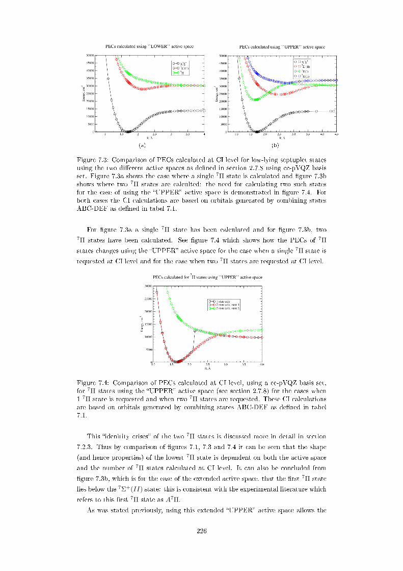
(a) (b)
Figure 7.3: Comparison of PECs calculated at CI level for low-lying septuplet statesusing the two dierent active spaces as dened in section 2.7.8 using cc-pVQZ basisset. Figure 7.3a shows the case where a single 7Π state is calculated and gure 7.3bshows where two 7Π states are calculted: the need for calculating two such statesfor the case of using the UPPER active space is demonstrated in gure 7.4. Forboth cases the CI calculations are based on orbitals generated by combining statesABC-DEF as dened in tabel 7.1.
For gure 7.3a a single 7Π state has been calculated and for gure 7.3b, two7Π states have been calculated. See gure 7.4 which shows how the PECs of 7Π
states changes using the UPPER active space for the case when a single 7Π state is
requested at CI level and for the case when two 7Π states are requested at CI level.
Figure 7.4: Comparison of PECs calculated at CI level, using a cc-pVQZ basis set,for 7Π states using the UPPER active space (see section 2.7.8) for the cases when1 7Π state is requested and when two 7Π states are requested. These CI calculationsare based on orbitals generated by combining states ABC-DEF as dened in tabel7.1.
This idenitity crises of the two 7Π states is discussed more in detail in section
7.2.3. Thus by comparison of gures 7.1, 7.3 and 7.4 it can be seen that the shape
(and hence properties) of the lowest 7Π state is dependent on both the active space
and the number of 7Π states calculated at CI level. It can also be concluded from
gure 7.3b, which is for the case of the extended active space, that the rst 7Π state
lies below the 7Σ+(II) state: this is consistent with the experimental literature which
refers to this rst 7Π state as A7Π.
As was stated previously, using this extended UPPER active space allows the
226

calculation of electronic states that dissociate to the z8P o atomic dissociation limit
of Mn: referring back to table 2.11 these states are 7Σ+(III), 7Π(II), 9Σ+ and 9Π.
Remembering that there are lower-lying X7Σ+, 7∆ and 7Σ+(II) states, to calculate
this 7Σ+(III) state, it is thus necessary to perform a 4+1 calculation. Figures 7.5a
and 7.5b show the PECs obtained when a 3+1 and 4+1 calculation is performed at
CI level. From both gures it can be concluded that the rst two states in symmetry
1 are 7Σ+ states.
(a) (b)
Figure 7.5: Comparison of PECs calculated at CI level, using the UPPER activespace (see section 2.7.8 and a cc-pVQZ basis set, for low-lying 7Σ+ and 7∆ states.Figure 7.5a shows the case when three states of septuplet multiplicity are calculatedin symmetry 1 and gure 7.5b shows the case when four such states are calculated. Inboth cases a single state of septuplet multiplicity is calculated in symmetry 4. TheseCI calculations are based on orbitals generated by combining states ABC-DEF asdened in tabel 7.1.
Referring to gure 7.5a at around 1.6 Å, the third state within symmetry 1
switches from been a distinctive PEC to becoming numerically the same as the
PEC calculated in symmetry 4. Thus it would seem that until 1.5 Å this PEC is a7Σ+ state and then switches to been a 7∆ state. Figure 7.5b resolves this ambiguity.
Using the rule that Σ+ and ∆ states are allowed to cross each other, it can thus be
deduced that it is possible to construct the 7Σ+(III) state from stitching together
the part of the third state of symmetry 1 from R=0.7 to 1.5 Å with that of the fourth
state of symmetry 1 from 1.5Å onwards. The PEC of 7∆ state is simply the PEC
calculated in symmetry 4. Thus, in order to calculate the X7Σ+, 7Σ+(II), 7Σ+(III)
and 7∆ states, a 4+1 calculation is required at CI level using the UPPER active
space with the necessary stitching together of energies done by examining plots of
the raw energies produced by the MOLPRO calculations.
Thus putting together all the PECs of septuplet states onto one gure, the order
of the relative upper states can be determined. Figure 7.6 shows PECs calculated
using the UPPER active space with two 7Π states calculated and a 4+1 calculation
done for the 7Σ+ and 7∆ states.
227

Figure 7.6: Compilation of PECs for low-lying septuplet states calculated at CI level,using the UPPER active space (see section 2.7.8 and a cc-pVQZ basis set. Theallowed crossing between the 7Σ+(III) state and 7∆ can be seen where the 7Σ+(III)has been constructed by stitching together energy values produced in MOLPROcalculations for dierent states of symmetry 1 and septuplet multiplicity. The 7Σ+ and7∆ states shown here where calculated using a 4+1 calculation at CI level and the two7Π states were calculated by requesting two states of symmetries 2 and 3, septupletmultiplicity. These CI calculations are based on orbitals generated by combiningstates ABC-DEF as dened in table 7.1.
In gure 7.6, the 7Σ+(III) state has been constructed as described previously
with the allowed crossing over the 7∆ state clearly shown. Moving onto the analysis
of these calculated PECs, table 7.9 shows the variation between MRCI calculations
for a xed CASSCF state-combination of ABC-DEF.
228

State
MRCI
87
87
87
87
87
87
cc-pVQZ
aug-cc-pVQZ
cc-pVQZ
aug-cc-pVQZ
cc-pVQZ
aug-cc-pVQZ
Re(Å
)De(cm−
1)
E(ν
=1)
(cm−
1)
X7Σ
+1+
01.703(3)
1.708(2)
1.699(2)
1.703(3)
13499
13102
13888
13436
1656
1620
1697
1660
X7Σ
+2+
01.704(4)
1.710(2)
1.701(3)
1.706(4)
13605
13234
14006
13578
1630
1594
1671
1634
X7Σ
+3+
11.706(1)
1.711(2)
1.702(4)
1.707(4)
13618
13257
14035
13621
1623
1589
1660
1623
X7Σ
+4+
11.707(3)
1.713(2)
1.703(4)
1.708(4)
13659
13307
14047
13634
1608
1573
1649
1611
B7Σ
+(II)
2+0
2.342(3)
2.371(8)
2.372(10)
4611
4664
3689
1733
1763
1598
B7Σ
+(II)
3+1
2.339(4)
2.368(8)
2.302(8)
2.334(7)
4788
4851
3892
3968
868
864
838
764
B7Σ
+(II)
4+1
2.511(8)
2.522(5)
2.29(4)
2.413(7)
6093
6158
4318
4742
764
780
799
845
C7∆(sym
1)3+
15.412(134)
5.398(107)
5.516(95)
55
72
3231
3231
C7∆(sym
1)4+
15.428(17)
5.309(57)
5.413(28)
5.517(380)
1218
78
3334
3031
C7∆(sym
4)3+
15.734(314)
5.757(425)
5.684(175)
44
933
3232
D7Σ
+(III)
4+1
3.537(10)
3.573(5)
2.970(8)
2.995(7)
2307
2232
5475
5394
423
415
907
759
A7Π(I)
2SC
1.643(4)
1.647(5)
1.654(4)
1.657(2)
9616
9428
2589
2419
1588
1579
1548
1545
E7Π(II)
2SC
2.793(1)
2.795(3)
2.222(2)
2.211(3)
1990
1960
6168
6104
710
705
1376
1372
Table
7.9:
Summaryof
properties
determ
ined
forPECsof
septup
letstates
calculated
usingvariousnumberof
states
atMRCIlevelof
theory
usingachoice
oftwobasissets
andtwoCASS
CFstate-combinations.
The
twobasissets
tested
werecc-pV
QZandaug-cc-pV
QZ.In
thistable,
8refers
totheCASS
CF
state-combination
ofABC-DEFand7refersto
theCASS
CFstate-combination
ofBC-DEF.These
PECproperties
have
been
determ
ined
usingtheprocedure
describedin
section2.9.2.
229

By examination of table 7.9 it can be seen that the predicted values of Re for
the X7Σ+ state generally decrease when augmented values basis functions are used
and increases when the CASSCF state-combination is decreased from that of ABC-
DEF to BC-DEF. Both the X7Σ+ and A7Π states have been studied previously
theoretically and experimentally so hence there are studies to compare with. Hence
table 7.9 is providing new theoretical predictions of the properties of the PECs for
the B7Σ+(II), C7∆, D7Σ+(III) and E7Π(II) states. Starting with the X7Σ+ state,
table 7.10 gives a summary of previous experimental and theoretical predictions for
this state. Table 7.11 shows the variation in spectroscopic parameters determined
for the X7Σ+ state at MRCI level of theory as a function of the CASSCF state-
combination used.
Study Method Re (Å) ωe (cm−1) De (cm−1)Huber & Herzberg (1979)
Experiment
1.7311 1548Nevin (1945) 1.73089Urban & Jones (1989) 1.730842(5) 1547Varberg et al. (1992) 1.7432Gordon et al. (2005) 1.7432(r0) 1547Gengler et al. (2007) 1.7398601(47)Halfen & Ziurys (2008) 1.7310Das (1981) MCSCF 1432 15325Walch & Bauschlicher(1983)
CAS/CISD 1639 13792
Chong et al. (1986)CISD 1553 13873CPF 1530 13550MCPF 1530 13470
Langho et al. (1989) MR-SDCI+Q 1517.6Barone & Adamo (1997) B3LYP 1586 8669
Wang & Andrews (2003)W91/6-311++G(d,p) 1.710 1548.3(540)BPW91/6-311++G(3df,3pd) 1.711 1522.0(528)B3LYP/6-311++G(3df,3pd) 1.735 1507.0(496)
Tomonari, Nagashima &Hirano (2009)
9-ref CI+Q 1.7372 154213-ref CI+Q 1.7359 154014-ref CI+Q 1.7356 154415-ref CI+Q 1.7343 154216-ref CI+Q 1.7344 1542
Table 7.10: Summary of spectroscopic properties determined in previous experimentaland theoretical studies for the X7Σ+ state.
230

CASS
CF
Re(Å
)De(cm−
1)
Te(cm−
1)
Eν
=1(cm−
1)
XB
DX
BD
XB
DX
BD
ABE
1.701(2)
2.520(4)
3.704(17)
13764
1444
1814
679
984
293
1613
771
371
AEF
1.726(2)
2.511(4)
3.525(8)
13516
2255
2069
927
490
01522
807
422
AE
1.721(2)
2.516(5)
4.001(9)
13719
1539
1411
223
346
215
1605
801
309
BCE
1.697(5)
2.527(5)
3.656(10)
13592
1379
1938
1019
1247
311
1619
765
386
BDE
1.726(4)
2.466(12)
3.645(19)
14043
1664
1954
400
541
167
1596
773
385
BDF
1.735(1)
2.468(12)
3.652(11)
14236
1654
1968
207
522
121
1609
767
382
BEF
1.720(4)
998
1131
4277
BE
1.715(4)
2.514(2)
3.771(22)
13835
1511
1661
402
690
301
1663
784
341
CDE
1.718(3)
2.477(8)
3.653(14)
13986
1627
1948
457
567
122
1564
768
388
CDF
1.722(5)
2.390(10)
3.684(17)
13906
1684
1903
537
537
191
1578
787
373
CEF
1.720(4)
2.509(6)
3.682(17)
13499
2233
1912
1114
740
304
1520
789
372
CE
1.706(4)
2.517(8)
3.778(17)
13692
1481
1646
539
702
236
1584
783
338
DEF
1.730(2)
2.546(2)
3.652(9)
13215
2180
1989
1227
485
981544
807
EF
1.733(4)
2.507(10)
3.696(8)
13433
1627
1829
798
198
531530
818
364
E1.734(2)
2.531(4)
13408
2273
142
01570
847
ABC-EF
1.702(2)
2.506(4)
3.548(10)
13890
6081
2268
1053
1269
251
1626
75426
ABD-EF
1.715(2)
2.521(4)
3.583(17)
13344
6347
2191
1506
1019
258
1575
791
410
ABDF
1.719(2)
2.492(9)
3.627(15)
14184
6473
2038
424
839
189
16528
748
396
ACD-EF
1.714(4)
2.513(3)
3.566(13)
13625
6339
2242
1227
992
202
1600
786
416
ACDF
1.727(4)
2.479(4)
3.611(17)
14613
6488
2084
0829
156
1748
749
399
ADEF
1.724(4)
2.532(8)
3.626(5)
13267
6636
2064
1341
675
164
1555
808
393
BCDF
1.705(3)
2.504(10)
3.610(17)
13993
6212
2108
747
1105
249
1632
743
403
BCEF
1.711(4)
2.516(6)
13493
6181
1360
1153
1579
767
BDEF
1.718(3)
2.524(8)
3.594(16)
13364
6588
2155
1379
844
212
1574
802
404
CDEF
1.720(4)
2.524(4)
3.608(10)
13274
6436
2117
1470
862
223
1560
801
400
Table7.11:Eect
ofchanging
theCASS
CFstate-combination
upon
thePECscalcualted
atMRCIlevelof
theory
forthe
7Σ
+states
ofMnH
usingacc-pVQZ
basisset.
These
PECproperties
have
been
determ
ined
usingtheproceduredescribedin
section2.9.2.
InthistableXrefers
totheX
7Σ
+state,Brefers
totheB
7Σ
+(II)stateandDrefers
tothe
7Σ
+(III)state.
231

Refer to tables 7.9 7.11 and 7.10. Experimentally, previous studies for the X7Σ+
state predict Re to be in the range from 1.730842 and 1.7432 Å with previous theoret-
ical studies predicting Re to be between 1.710 and 1.7372 Å. In this study it has been
shown that MRCI calculations can predict Re to be in the range from 1.697 to 1.734 Å
depending on which CASSCF state-combination is used. The upper part of this range
overlaps with the experimental range. The De values were discussed in conjunction
with the a5Σ+ state in section 7.2.1. For ωe, previous theoretical studies predict val-
ues between 1432 and 1586 cm−1 and experimental studies a value of 1548± 1 cm−1.
From table 7.11 it can be seen that MRCI calculations predict a range in the ν = 1
vibronic energy state to vary between 1521 and 1632 cm−1 (there is a clear outlier
at 1131 cm−1). Table 7.11 also shows how the position of PECs calculated for the
X7Σ+ state can vary up and down the absolute energy scale (values of Te). Moving
onto the A7Π state, table 7.12 shows the variation in spectroscopic parameters de-
termined for the X7Σ+ state at MRCI level of theory as a function of the CASSCF
state-combination used. Table 7.13 gives a summary of previous experimental and
theoretical predictions for this state.
CASSCF Re (Å) De (cm−1) Te (cm−1) E(ν = 1) (cm−1
ABE 1.645(1) 10193 621 1619AE 1.654(2) 10672 404 1595AEF 1.656(3) 10102 881 1551BCE 1.625(3) 10018 836 1591BDE 1.658(4) 10671 180 1614BDF 1.664(3) 10845 119 1603BE 1.650(2) 10413 468 1630BEF 1.653(4) 9996 857 1592CDE 1.654(1) 10781 234 1613CDF 1.653(3) 10862 385 1616CE 1.646(2) 11265 586 1601CEF 1.652(3) 10036 989 1556DEF 1.660(3) 10353 1395 1544E 1.659(5) 10846 407 1557EF 1.662(2) 10175 838 1547
ABC-DE 1.637(4) 10010 893 1625ABD-EF 1.649(2) 9478 1399 1579ABDF 1.657(4) 10726 253 1664ACD-EF 1.648(4) 9707 1287 1578ACDF 1.663(3) 11214 0 1724ACEF 1.645(2) 10185 810 1614ADEF 1.656(4) 9558 1409 1556BCDF 1.644(3) 10542 454 1671BCEF 1.644(1) 9823 1082 1597BDEF 1.652(5) 9509 1343 1577CDEF 1.653(3) 9542 1454 1562
Table 7.12: Eect of changing the CASSCF state-combination upon the PECs cal-culated at MRCI level of theory for the A7Π and E7Π(II) states of MnH (2-statecalculation) using a cc-pVQZ basis set. These PEC properties have been determinedusing the procedure described in section 2.9.2.
232

Study Method Re(Å) ωe(cm−1)Langho et al. (1989) MR-SDCI+Q 1639
Tomonari, Nagashima & Hirano (2009)3-ref CI+Q 1.6415 16536-ref CI+Q 1.6407 16597-ref CI+Q 1.6403 1659
Table 7.13: Summary of spectroscopic properties determined in previous experimentaland theoretical studies for the A7Π state.
Refer to tables 7.12 and 7.13. In the previous theoretical study of the A7Π state,
Tomonari, Nagashima & Hirano (2009) have predicted Re to be 1.64 Å. Table 7.12
shows our predictions to lie in the range from 1.625 and 1.664 Å depending on which
CASSCF state-combinations are used.
PECs for nonuplet states
Figure 7.7 shows the calculation of the two nonuplet states, 9Σ+ and 9Π.
Figure 7.7: Compilation of PECs for the 9Σ+ and 9Π states at CI level, using theUPPER active space(see section 2.7.8 and a cc-pVQZ basis set. These PECs shownwere calculated using a 3+1 calculation. These CI calculations are based on orbitalsgenerated by combining states ABC-DEF as dened in tabel 7.1.
Figure 7.7 shows that both nonuplet states appear to be anti-bonding in nature
with the 9Π state lying below the 9Σ+ state. These have been labelled g and h
using the convention of lower-case letters for electronic states that are of dierent
multiplicity from the ground state. Analysis of these curves does however reveal the
that they are both very shallow potentials with the properties shown in table 7.14.
State Re (Å) De (cm−1) E(ν = 1) (cm−1)g9Π 4.057(126) 32 24h9Σ+ 5.461(47) 124 81
Table 7.14: PEC properties of the nonuplet states calculated at MRCI level of theoryusing a cc-pVQZ basis set and a CASSCF state-combination of ABC-DEF.
233

PECs of 15 low-lying electronic states of MnH
Finally, putting together all quintet, septuplet and nonuplet PECs into one plot, gure
7.8 shows a plot all 15 of the PECs calculated using the UPPER active space.
Figure 7.8: PECs for 15 low-lying electronic states of MnH calculated at MRCI levelof theory using a cc-pVQZ basis set and a CASSCF state-combination of ABC-DEF.
In gure 7.8, continuous lines have been used to show the quintet and nonuplet
states with circles used to indicate the septuplet states.
7.2.2 Dipole Moment Curves
In the calculation of dipole moments at CI level, the expectation dipole moment was
calculated in all cases. The results of using the LOWER active space were used as
a method in order to identify the DMCs produced using the UPPER active space.
7.2.3 DMCs for the quintet states
Starting with the quintet states, gure 7.10 shows DMCs calculated at MRCI level
for the a5Σ+ state.
234

Figure 7.9: Comparison of DMCs calculated at CI level, using a cc-pVQZ basis set,for the a5Σ+ state. The LOWER and UPPER active spaces are dened in section2.7.8. All of these CI calculations are based on orbitals generated by combining statesABC-DEF as dened in tabel 7.1.
As gure 7.10 shows, the shape (and hence minima) of the DMC calculated for
the a5Σ+ vary as shown in table 7.15.
MRCI calculation Position of minima (Å) Value (Debye)1+0 1.95 -1.9642+1 1.95 -1.9553+1 1.85 -1.655
Table 7.15: Positions and values of minima for calculated DMCs of the a5Σ+ stateat MRCI level of theory using a cc-pVQZ basis set. These values presented are fromthe purely ab initio curves.
Table 7.16 shows a comparison of calculated DMC quintets with the study of
Langho et al. (1989). The DMCs calculated for the b5Π, c′5∆, and c5Σ+(II) states
is shown in gure 7.10.
235

Langho et al. (1989) Present Study
R(Å) a5Σ+ b5Π c5Σ+ R(Å)a5Σ+
b5Π c5Σ+(II)c1+0 2+1 3+1 5+2 3+1 5+2
1.32 1.21 2.74 0.941.30 1.15 1.15 1.18 1.18 1.95 0.86 1.271.35 1.19 1.20 1.21 1.21 2.12 1.10 1.48
1.43 1.191.38 1.40 1.25 1.25 1.25 1.24 2.30 1.32 1.68
1.45 1.32 1.32 1.29 1.28 2.48 1.53 1.87
1.53 1.20 3.27 1.761.50 1.40 1.40 1.35 1.33 .66 1.73 2.041.55 1.48 1.48 1.40 1.40 2.84 1.92 1.95
1.59 1.23 3.37 1.93 1.60 1.58 1.57 1.46 1.46 3.01 2.09 2.131.64 1.26 3.47 2.09 1.65 1.67 1.66 1.52 1.50 3.17 2.26 2.461.69 1.31 3.57 2.24 1.69 1.74 1.73 1.56 1.55 3.29 2.38 2.551.75 1.36 3.65 2.39 1.75 1.83 1.82 1.61 1.61 3.44 2.54 2.661.85 1.48 3.81 2.65 1.85 1.94 1.93 1.65 1.70 3.63 2.74 2.811.96 1.60 3.93 2.87 1.95 1.96 1.96 1.64 1.73 3.76 2.86 2.922.06 1.70 4.02 3.06 2.05 1.89 1.88 1.54 1.69 3.82 2.93 2.98
2.17 1.77 4.08 3.212.15 1.72 1.72 1.39 1.56 3.80 2.95 3.012.20 1.61 1.61 1.30 1.47 3.76 2.96 3.02
2.28 1.80 4.09 3.30 2.30 1.35 1.36 1.10 1.26 3.64 2.95 3.04
Table 7.16: Comparison of DMCs obtained for low-lying quintet states of MnH in thispresent with that of the theoretical study undertaken by Langho et al. (1989). Inthis study the DMCs have been calculated using a cc-pVQZ basis set at MRCI levelof theory.
Figure 7.10: Calculation of DMCs at CI level, using a cc-pVQZ basis set, for quintetstates using the UPPER active space(see section 2.7.8). These CI calculations arebased on orbitals generated by combining states ABC-DEF as dened in tabel 7.1.
As can be seen from table 7.16 for the a5Σ+ state there is a change in character
for the DMC dependent on the MRCI calculation used. These calculations dier to
those of Langho et al. (1989) by up to 0.4 Debye for this a5Σ+ state and by up to
0.2 Debye for the b5Π and c5Σ+ state calculations. Without experimental data it is
an unknown question what the true values are for these DMCs.
To complete this section on the DMCs of the quintet states, gure 7.11 shows the
calculated DMCs of the d5Π(II), e5Σ+ and f5∆ states.
236

Figure 7.11: DMCs calculated at MRCI level of theory for higher-lying quintet elec-tronic states. These DMCs have been calculated using the UPPER active space asis necessary, a cc-pVQZ basis set and a CASSCF state-combination of ABC-DEF.
DMCs for the 7Σ+ and 7∆ states
Moving onto the septuplets, again variation was found between calculations which
used either the LOWER or UPPER active space and also the number of septuplet
states of a given symmetry calculated at CI level. Figure 7.12 shows a comparison of
the DMCs produced at CI level using the UPPER active space for the various 7Σ+
and 7∆ states. Figure 7.12a shows the case when a 3+1 calculation is done and gure
7.12b shows the case of a 4+1 calculation.
(a) (b)
Figure 7.12: Calculation of DMCs at CI level, using a cc-pVQZ basis set, for 7Σ+ and7∆ states using the UPPER active space(see section 2.7.8). These CI calculationsare based on orbitals generated by combining states ABC-DEF as dened in tabel7.1.
As was the case of the PECs, the identity of the third state of symmetry 1 is
remedied when changing from a 3+1 calculation to a 4+1 calculation. The third state
of symmetry 1 is initially 7Σ+(III) for low inter-nuclear distances before changing to7∆.
237

DMCs for the A7Π and E7Π states
When calculations were undertaken at MRCI level of theory for the DMCs and asso-
ciated TDMs, angular momenta couplings and spin-orbit couplings for the A7Π and
E7Π(II) states, it was found that there was an identity crises involving these two
states. Figure 7.13 shows the DMCs obtained for these states for the case of one 7Π
state been calculated at MRCI level of theory and for the case of two states been cal-
culated at MRCI level of theory. Figure 7.13 shows the expectation dipole moments
Figure 7.13: Calculation of Expectation Dipole Moments for 7Π states
obtained for 7Π states using a cc-pVQZ basis set and ABC-DEF CASSCF space. As
the plot shows, for the 1 state calculation, the dipole moment calculated ips from
-0.58 Debye at R=2.10 Å to 0.43 Debye at R=2.15. The result of a 2 state calculation
shows the possibility of two distinct continuous curves-one with positive values and
one with negative values. As can be seen from the gure 7.13, the identity of the
states (i.e. which one is state 1 and which is state 2) ips between 2.80 Å and 2.90
Å. It is not clear which curve belongs to which state. Figure 7.16 shows these two
DMCs untangled for the 2 state calculation in CI: one has a maximum magnitude of
around 3 Å and the other a maximum magnitude of around 2 Å. Thus the question is,
when the states are untangled, which curve belongs to the rst 7Π state and which
one belongs to the second 7Π state?. To solve this puzzle, various calculations were
inspected.
A similar story with couplings involving these two 7Π states was found. Figures
7.14 and 7.15 show this story for a sample of angular momenta and spin-orbit couplings
respectively. For these couplings we know that since the A7Π state dissociates to the
238

same dissociation limit as the B7Σ+(II) and c′5∆ states any couplings between it and
these states must be non-zero in the dissociation limit. Also, and more crucially that
any couplings involving the E7Π(II) state and the B7Σ+(II) and c′5∆ states must
tend to zero in the dissociation limit as the E7Π(II) state dissociates to a higher
dissociation limit. Hence with this knowledge, gures 7.14a and 7.15a have been
de-tangled and the identity of the coupling 7Π state revealed as indicated by gures
7.14b and 7.15a respectively.
(a) (b)
Figure 7.14: Lx coupling between the 7Π states and the B7Σ+(II) state calculated atMRCI level of theory using a cc-pVQZ basis set, UPPER active space and a CASSCFstate-combination of ABC-DEF. The MRCI calculation for the B7Σ+(II) was simplya 2+0 calculation for simplicity. Figure 7.14a shows the raw MOLPRO outputobtained: gure 7.14b shows the resolved couplings where the coupling between theA7Π and B7Σ+(II) state goes to a non-zero value in the dissociation limit and thecoupling between the E7Π(II) and B7Σ+(II) state tends to zero.
(a) (b)
Figure 7.15: Spin-orbit couplings between the two 7Π states and the c′5Σ+ state cal-culated at MRCI level of theory using a cc-pVQZ basis set, UPPER active spaceand a CASSCF state-combination of ABC-DEF. The MRCI calculation for the c′5∆was simply a 2+1 calculation for simplicity. Figure 7.15a shows the raw MOLPROoutput obtained: gure 7.15b shows the resolved couplings where the coupling be-tween the A7Π and c′5∆ state goes to a non-zero value in the dissociation limit andthe coupling between the E7Π(II) and c′5∆ state tends to zero.
By examination of gures 7.14 and 7.15, it can be seen that the mapping between
the raw MOLPRO output (i.e. state 1, state 2) and the actual physical states is as
shown in table 7.17.
239

R (Å) State 1 State 20.70 - 2.80 E7Π(II) A7Π> 2.80 A7Π E7Π(II)
Table 7.17: Mapping between raw MOLPRO output and the true identity of DMCsand couplings for the A7Π and E7Π(II) states.
Hence, applying this mapping to gure 7.13 we can thus resolve the identity of
the DMCs for the two 7Π states. This mapping was found to be consistent for all
couplings involving the 7Π states using the arguments presented above for knowing
which couplings should tend to zero in the atomic dissociation limit.
(a) (b)
Figure 7.16: Calculation of DMCs for the 7Π states at MRCI level of theory using acc-pVQZ basis set, the UPPER active space and a CASSCF state-combination ofABC-DEF. Figure 7.16a shows the raw MOLPRO output and gure 7.16b shows theresolved DMCs in which the mapping detailed in table 7.17 has been applied.
To demonstrate the variability in the peak of the DMCs for these two 7Π states,
several calculations can be inspected. Firstly, the peak values of pure CASSCF calcu-
lations in which only one 7Π state is calculated. Referring back to table 7.1, these are
the CASSCF state-combinations which include the component E. Table 7.18 shows
these peaks. Figure 7.17 shows the CASSCF calculation of a DMC in which a single7Π state is calculated for the state-combinations of ABC-DEF, BC-DEF and the
basis sets of cc-pVQZ and aug-cc-pVQZ.
240

Figure 7.17: Calculation of DMC for the A7Π state at CASSCF level of theory. In thisgure the CASSCF state-combination and basis set for each of the four calculationsis indicated in the legend.
CASSCF Rmax (Å) Dmax (Debye)ABC-DEF 1.35 4.015ABC-DEF (aug-cc-pVQZ) 1.35 4.000BC-DEF 1.10 3.781BC-DEF (aug-cc-pVQZ) 1.10 3.766ABE 1.50 4.552AE 1.50 4.689AEF 1.30 4.203BDE 1.35 3.846BEF 1.30 3.856BE 1.50 4.286CDE 1.30 4.235EF 1.30 3.967E 1.50 4.534
Table 7.18: Position and value of peaks of DMCs calculated at CASSCF level oftheory for a single 7Π state. Unless otherwise stated, the basis set used was cc-pVQZ.See table 7.1 for a guide to the various CASSCF state-combinations presented.
Moving onto MRCI results, the variation in the peak of the DMCs can be com-
pared for MRCI calculations which use the LOWER active space (calculation of
one state) and for those which use the UPPER active space (calculation of either
one or two states) and build upon dierent CASSCF state-combinations. Table 7.19
shows these values. The picture shown in gure 7.16a whereby a 2 state calculation
has the identity of states 1 & 2 ipping around 2.80 Å was found to be common for
all CASSCF variations tested at CI level.
241

CASSCFA7Π(I) E7Π(II)
Rmax (Å) Dmax (Debye) Rmin (Å) Dmin (Debye)1 state calculations, LOWER active space
ABC-DEF 1.35 3.247ABC-DEF (aug-cc-pVQZ) 1.30 3.190BC-DEF 1.30 3.165BC-DEF (aug-cc-pVQZ) 1.30 3.107
1 state calculations, UPPER active spaceABC-DEF 1.50 -2.334ABC-DEF (aug-cc-pVQZ) 1.35 -2.446BC-DEF 1.50 -2.314BC-DEF (aug-cc-pVQZ) 1.40 -2.446
2 state calculations-UPPER active spaceABC-DEF 1.25 3.042 1.55 -2.313ABC-DEF(aug-cc-pVQZ) 1.30 3.097 1.40 -2.378BC-DEF 1.10 2.983 1.55 -2.295BC-DEF(aug-cc-pVQZ) 1.30 3.018 1.40 -2.376E 1.25 3.143 1.55 -2.509AE 1.20 3.181 1.55 -2.483BE 1.30 3.034 1.55 -2.352CE 1.25 3.162 1.55 -2.427EF 1.20 3.044 1.55 -2.476ABE 1.25 3.106 1.55 -2.373AEF 1.20 3.099 1.55 -2.474BCE 1.30 3.082 1.50 -2.316BDE 1.20 2.921 1.55 -2.361BDF 1.20 2.926 1.55 -2.388BEF 1.25 2.979 1.55 -2.369CDE 1.20 3.046 1.55 -2.424CDF 1.20 3.021 1.55 -2.366CEF 1.20 3.085 1.55 -2.417DEF 1.25 3.079 1.50 -2.481ABDF 1.20 3.005 1.55 -2.333ACDF 1.20 3.014 1.60 -2.392ACEF 1.25 3.072 1.55 -2.368ADEF 1.25 3.126 1.50 -2.421BCDF 1.25 2.984 1.55 -2.283BCEF 1.25 3.034 1.55 -2.273BDEF 1.25 3.016 1.55 -2.383CDEF 1.25 3.111 1.55 -2.368ABC-EF 1.25 3.019 1.55 -2.299ABD-EF 1.25 3.075 1.55 -2.336ACD-EF 1.25 3.094 1.55 -2.379
Table 7.19: Comparison of DMC peak values obtained for dierent MRCI calculations.For the two-state calculations the mapping outlined in table 7.17 has been applied toassign the untangled DMC to the correct 7Π state. Unless otherwise indicated thebasis set used was cc-pVQZ.
Refer to table 7.19. For the one state-calculations (1SC) performed at MRCI level
of theory using the LOWER active space the output shape of the DMC calculation
was that of gure 7.17 but with a lower peak value. For the one state-calculations
performed using the UPPER active space, the shape of the curve for each CASSCF
state-combination was that indicated in gure 7.13 i.e. the DMC of the E7Π(II) state
up to 2.80 Å is calculated before the calculation switches to calculating the DMC
of the A7Π state. As can be seen for a 2-state calculation (2SC) using the UPPER
242

active space, the peak of the DMC for the A7Π state calculated using MRCI level of
theory varies between 2.921 and 3.181 Debye with a position between 1.20 and 1.30
Å depending on the CASSCF state-combination used. For these calculations, the
minima of the DMC for the E7Π state is located between 1.40 Å and 1.60 Å and varies
between -2.295 and -2.505 Debye depending on which CASSCF state-combination is
used.
DMCs for the nonuplet states
Finally, the DMCs of the e9Π and f9Σ+ state were calculated at CI level as shown in
gure 7.18: for these states it is only possible to use the UPPER active space.
Figure 7.18: Calculations of DMCs at CI level, using a cc-pVQZ basis set, for thee9Π and f9Σ+ states using the UPPER active space(see section 2.7.8). These CIcalculations are based on orbitals generated by combining states ABC-DEF as denedin table 7.1.
Even though the DMC of the f9Σ+ state is comparitively large, it should be
remember that this state(as well as the e9Π state) is an antibonding curve as shown
in gure 7.7. Comparing gures 7.10, 7.11, 7.16, 7.12 and 7.18 it can be seen that, in
terms of magntidue around equilibrium ( 1.7 Å), D7Σ+(III) is the largest by about
a factor of two compared to other DMCs.
7.2.4 Transition Dipole Moments (TDMs)
The TDMS between electronic states were calculated and are shown in the following
gures: TDMs couple states of the sane multiplicity. Starting with the quintet states,
the TDMs between the various 5Σ+ and 5∆ states are shown in gure 7.19 and the
TDMs to the b5Π state is shown in gure 7.20.
243

Figure 7.19: TDMs between the three quintet states and two delta states calculatedat MRCI level of theory using a cc-pVQZ basis set and a CASSCF combination ofABC-DEF. The 〈c5Σ+(II)|µz |a5Σ+〉 TDM shown is using a 3+1 MRCI calculation:all other couplings shown are for a 5+2 MRCI calculation: i.e. ve quintet states ofsymmetry 1 and two quintet states of symmetry 4 calculated.
Figure 7.20: TDMs to the b5Π state calculated at MRCI level of theory using acc-pVQZ basis set and a CASSCF state-combination of ABC-DEF and the UP-PER active space. For this gure, as an example, the curve listed as a5Σ+ is the〈a5Σ+|µz |b5Π〉. For the a5Σ+, c′5∆, c5Σ+(II) and e5Σ+(III) states the MRCI cal-culation performed was of the form 5+2, i.e. ve quintet states of symmetry 1 andtwo quintet states of symmetry 4 calculated. For all calculations shown in this gure,two 5Π states were calculated within a single MRCI calculation.
These TDMs calculated can for these quintet states can be compared to those
calculated by Langho et al. (1989) whose calculations are shown in gure 7.21. As
can be seen from gure 7.21, Langho et al. (1989) have unfortunately mislabelled
one of their coupling curves (one of them should be for the c5Σ+ − b5Π transition).
However, the authors did provide a table of values which are shown in table 7.20 in
244

Figure 7.21: MRCI transition moment functions(a.u) for the c5Σ+ − a5Σ+, b5Σ+ −a5Σ+ and c5Σ+ − b5Π band systems of MnH calculated by Langho et al. (1989).
which a comparison is done with the results obtained in this study.
Langho et al. (1989) Present StudyR (Å) c5Σ+(II)− a5Σ+ b5Π− a5Σ+ R (Å) c5Σ+(II)− a5Σ+ b5Π− a5Σ+
1.32 2.53 0.451.30 2.18 0.501.35 2.13 0.57
1.43 2.46 0.611.40 2.08 0.641.45 2.03 0.70
1.53 2.37 0.771.50 1.99 0.761.55 1.79 0.81
1.59 2.32 0.84 1.60 1.78 0.861.64 2.27 0.91 1.65 1.89 0.891.69 2.22 0.97 1.69 1.87 0.911.75 2.18 1.02 1.75 1.84 0.931.85 2.08 1.10 1.85 1.81 0.941.96 1.98 1.14 1.95 1.80 0.922.06 1.87 1.16 2.05 1.81 0.90
2.17 1.76 1.152.15 1.85 0.822.20 1.85 0.76
2.28 1.64 1.122.25 1.84 0.722.30 1.82 0.68
Table 7.20: Comparison of TDMs calculated for the c5Σ+(II)−a5Σ+ and b5Π−a5Σ+
transitions with that of Langho et al. (1989). The units of the TDMs are in Debye.The TDMs calculated in this study were calculated at MRCI level of theory usinga cc-pVQZ basis set, the UPPER active space, a CASSCF state-combination ofABC-DEF. At MRCI level of theory there were three states of symmetry 1 and onestate of symmetry 4 calculated.
As can be seen from table 7.20 for the b5Π− a5Σ+ we do compare favourably but
for the c5Σ+(II)− a5Σ+ TDM our values dier from those of Langho et al. (1989)
245
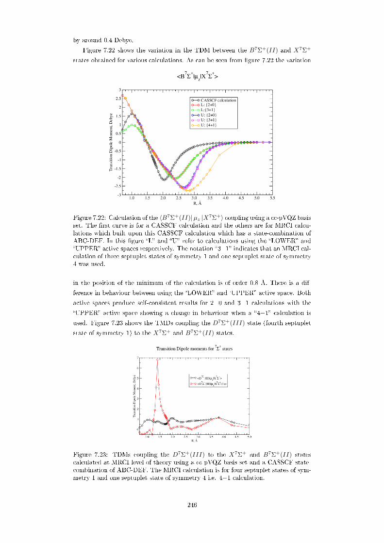
by around 0.4 Debye.
Figure 7.22 shows the variation in the TDM between the B7Σ+(II) and X7Σ+
states obtained for various calculations. As can be seen from gure 7.22 the variation
Figure 7.22: Calculation of the 〈B7Σ+(II)|µz |X7Σ+〉 coupling using a cc-pVQZ basisset. The rst curve is for a CASSCF calculation and the others are for MRCI calcu-lations which built upon this CASSCF calculation which has a state-combination ofABC-DEF. In this gure L and U refer to calculations using the LOWER andUPPER active spaces respectively. The notation 3+1 indicates that an MRCI cal-culation of three septuplet states of symmetry 1 and one septuplet state of symmetry4 was used.
in the position of the minimum of the calculation is of order 0.8 Å. There is a dif-
ference in behaviour between using the LOWER and `UPPER active space. Both
active spaces produce self-consistent results for 2+0 and 3+1 calculations with the
UPPER active space showing a change in behaviour when a 4+1 calculation is
used. Figure 7.23 shows the TMDs coupling the D7Σ+(III) state (fourth septuplet
state of symmetry 1) to the X7Σ+ and B7Σ+(II) states.
Figure 7.23: TDMs coupling the D7Σ+(III) to the X7Σ+ and B7Σ+(II) statescalculated at MRCI level of theory using a cc-pVQZ basis set and a CASSCF state-combination of ABC-DEF. The MRCI calculation is for four septuplet states of sym-metry 1 and one septuplet state of symmetry 4 i.e. 4+1 calculation.
246

As can be seen from gure 7.23, more work is clearly required to produce contin-
uous coupling curves involving the D7Σ+(II) states. Given that there are at least
eight electronic states lying below the D7Σ+(III) state, the D7Σ+(III)−B7Σ+(II)
is of overall lower priority given that to date there is no published linelist for MnH.
Hence producing a linelist for MnH involving even just the eight low-lying electronic
states is a contribution to knowledge in itself. Figure 7.24 shows the transition dipole
moments coupling the A7Π and E7Π(II) states to the X7Σ+, B7Σ+(II) and C7∆
states.
Figure 7.24: TDMs coupling the A7Π and E7Π(II) and X7Σ+, B7Σ+(II) and C7∆states calculated at MRCI level of theory using a cc-pVQZ basis set, the UPPERactive space and a CASSCF state-combinaiton of ABC-DEF. At MRCI level oftheory the X7Σ+, B7Σ+(II) and C7∆ states have been calculated by calculatingthree septuplet states of symmetry 1 and one septuplet state of symmetry 4.
In gure 7.24 it can be seen that the strongest transition dipole moment is that
between the E7Π(II) and X7Σ+ state. This may seem a surprising result. However
the magnitude of the TDM between the A7Π and X7Σ+ state was veried by com-
paring against CASSCF calculations of this coupling and also MRCI calculations in
which there are fewer septuplet states of symmetry 1 calculated.
Figure 7.25 shows the TDM between the two 7Π states.
247

Figure 7.25: TDM between the E7Π(II) and A7Π(I) states calculated at MRCIlevel of theory using a cc-pVQZ basis set and a CASSCF state-combination of ABC-DEF. This calculation shown uses the UPPER active space as is necessary for thecalculation of the E7Π(II) state but also for obtaining the correct bonding behaviourof the A7Π(I) state.
As can be seen from gure 7.25 the transition dipole coupling between the two 7Π
states is comparable to that between the A7Π and X7Σ+ state.
Finally, moving onto the nonuplet states, gure 7.26 shows the TDM calculated
between the h9Σ+ and g9Π states.
Figure 7.26: TDM coupling the h9Σ+ and g9Π states calculated at MRCI level oftheory using a cc-pVQZ basis set and a CASSCF state-combination of ABC-DEF. Asis necessary for the calculation of these states the UPPER active space was used.
7.2.5 Angular Momenta coupling
The angular momenta coupling linking Σ+ and ∆ states to Π states of the same multi-
plicity was calculated. Figures 7.27, 7.28 and 7.29 show this coupling for the low-lying
quintet, septuplet and nonuplet states respectively. Figure 7.27 shows the variation
between the 〈a5Σ+| Lx |b5Π〉 couplings calculated when the number of quintet states
of symmetry 1 calculated is varied. As can be seen having three states instead of one
or two of symmetry 1 within the MRCI calculation makes a dierence of the order
0.2 (angular momenta coupling is a dimensionless quantity). The asymptotic value
of the 〈c5Σ+(II)| Lx |b5Π〉 coupling is√
3. As expected the 〈a5Σ+| Lx |b5Π〉 couplingtends to zero in the atomic dissociation limit as the a5Σ+ and b5Π states dissociate to
dierent Mn atom terms. As can be seen in gure 7.28, the 〈B7Σ+(II)|Lx |A7Π(II)〉
248

Figure 7.27: Lx coupling between low-lying 55Σ+ and the b5Π state calculated atMRCI level of theory using a cc-pVQZ basis set and a CASSCF state-combinationof ABC-DEF. In this gure the notation 2+1 indicates that two quintet states ofsymmetry 1 and one quintet state of symmetry 4 were calculated. All curves showthe couplings using the UPPER active space.
coupling tend to a non-zero value of√
3 in the dissociation limit: this is expected
as these two states involved dissociate to the same atomic dissociation limit. As ex-
pected, the other couplings tend to zero as they couple molecular electronic states
which dissociate to dierent atomic dissociation limits. The 〈C7∆|Lx |A7Π〉 couplinghas a constant of value of 0.99 ± 0.02 and the 〈C7∆|Lx |E7Π(II)〉 coupling is nu-
merically zero as expected. Figure 7.29 shows the Lx coupling between the h9Σ+
and g9Π states which tends to a constant value of +1 in the dissociation limit. The
angular momentum coupling within individual Π and ∆ states was calculated and
can be summarised as follows: for the b5Π, d5Π, A7Π, E7Π(II) and g9Π this had a
magnitude of +1, for the C7∆ a value of +2 and for both the c′5∆ and f5∆ states a
value of -2.
7.2.6 Spin-Orbit coupling
The diagonal spin-orbit coupling elements were calculated within individual Π states
and individual ∆ states. Figure 7.30 shows these couplings. Figure 7.30a shows the
results for when one 7Π state is calculated using the LOWER active space and two
states were calculated using the UPPER active space. In gure 7.30b the quintet
state calculations were calculated using a 3+1 calculation: i.e. three quintet states
of symmetry 1 and one quintet state of symmetry 4. For the septuplet states, it
was found that results gained using 3+1 and 4+1 calculations showed the same
behaviour with a variation between them of a few cm−1. The curves shown in gure
7.30b are for the 3+1 calculations. As can be seen from gure 7.30 the variation
between curves calculated using the LOWER and UPPER active spaces is of order
< 1 cm−1. Figure 7.31 shows the calculated spin-orbit couplings between Π and ∆
states. In gure 7.31a the 〈c′5∆|SOz |C7∆〉 coupling has been calculated using a 3+1
249

Figure 7.28: Lx between low-lying 7Σ+ and 7∆ states and the two 7Π states calculatedat MRCI level of theory using a cc-pVQZ basis set and a CASSCF state-combinationof ABC-DEF. This gure shows couplings in which three septuplet states of symmetry1 and one septuplet state of symmetry 4 have been calculated and coupled with thetwo 7Π states. All curves show the couplings using the UPPER active space.
calculation for both the quintet and septuplet states. In gures 7.31b and 7.31c for
the calculations using the UPPER active space, two 7Π states were calculated and
for the LOWER active space, one 7Π state was calculated.
Moving onto the o-diagonal spin-orbit couplings, the ˆSOx operator couples Σ+
and ∆ states to Π states provided they have the same multiplicity or it diers by
two. Figure 7.32 shows such couplings for quintet and septuplet states. Figure 7.32a
shows the couplings between low-lying quintet states in the case where one 5Π state
has been calculated. In this gure the notation 2+1 indicates that two quintet
states of symmetry 1 and one quintet state of symmetry 4 have been calculated at
MRCI level of theory. As can be seen from gure 7.32a the variation between the
〈a5Σ+|SOz |b5Π〉 coupling curves calculated is of the order several cm−1 when the
number of quintet states of symmetry 1 is varied. Figure 7.32b shows the spin-orbit
coupling between the a5Σ+, c′5∆, c5Σ+(II) states with the A7Π and E7Π states.
In these calculations the 5Σ+ and 5∆ states have been calculated at MRCI level of
theory using a 3+1 calculation, i.e. three quintet states of symmetry 1 and one
state of symmetry 4. For all curves shown the 7Π states were calculated using a
two-state calculation. Finally, gure 7.33 shows the spin-orbit coupling between the
g9Π and h9Σ+ states. As is the case for CrH, to date in the literature there are no
recorded spin-orbit couplings. Table 7.21 lists out the non-zero dissociation values of
the spin-orbit couplings obtained in this study.
7.3 Concluding Remarks
In this chapter, ab initio calculations have been performed for MnH. A systematic
study of CASSCF state-combinations has been carried out with results shown in
250

Figure 7.29: Lx coupling between the nonuplet states calculated at MRCI level oftheory using a cc-pVQZ basis set and a CASSCF state-combination of ABC-DEF.
bgImg
(a) (b)
Figure 7.30: Spin-orbit matrix elements within individual Π and ∆ states. Thesecurves were calculated using MRCI level of theory with a cc-pVQZ basis set and aCASSCF state combination of ABC-DEF. In these gures L and U refer to calcu-lations were the LOWER and UPPER active spaces have been used respectively.
appendix C. To our knowledge, this type of study has never been undertaken for
MnH. By examining the PECs and DMCs computed for these CASSCF calculations,
a CASSCF state-combination of ABC-DEF (see table 7.1) was then used to generate
starting orbitals for MRCI calculations. This CASSCF state-combination combines
all the 8 lowest electronic states of MnH (see table 2.11). In contrast to the case
of CrH, it was found that generally speaking the quality of the CASSCF PECs and
DMCs obtained improved as more states were added to the CASSCF calculation.
For the MRCI calculations, PECs and DMCs were calculated for 15 low-lying
electronic states of MnH including, for the rst time the nonuplet states of g9Π
and h9Σ+. Were applicable, these PECs and DMCs calculated were compared to
the previous theoretical study of Langho et al. (1989) in which PECs had been
calculated for 8 low-lying electronic states. Some dierences were found. However, in
our new study for each PEC, several calculations were performed. Again, as was the
case for CrH, it was found that varying both the CASSCF state-combination used
and the basis set had an aect on the properties of the PECs and also the DMCs.
The eect of changing the CASSCF state-combination in MRCI calculations of
251

(a) (b)
(c)
Figure 7.31: Spin-orbit matrix elements between Π and ∆ states. These curves werecalculated using MRCI level of theory with a cc-pVQZ basis set and a CASSCF statecombination of ABC-DEF. In these gures L and U refer to calculations were theLOWER and UPPER active spaces have been used respectively.
(a) (b)
(c) (d)
Figure 7.32: O-diagonal spin-orbit coupling curves. These curves were calculatedusing a cc-pVQZ basis set at MRCI level of theory using a CASSCF state-combinationof ABC-DEF. In all these gure the UPPER active space was used.
PECs was investigated for the X7Σ+, B7Σ+(II), D7Σ+(III), A7Π and E7Π(II)
states and found to be signicant in varying parameters such as re, De, Te and
E(ν = 1). Again this is a new and signicant result as published MRCI results
seldom mention the states used in the CASSCF calculation proceeding any MRCI
252

Figure 7.33: Spin-orbit coupling between the nonuplet states calculated at MRCIlevel of theory using a cc-pVQZ basis set. In this calculation the CASSCF state-combination used was ABC-DEF.
Mn Atom dissociation term Coupling Magnitude (cm−1)
a6D
〈B7Σ+(II)|SOx |A7Π〉 95.46〈C7∆|SOx |A7Π〉 55.19
〈B7Σ+(II)|SOx |b5Π〉 42.72〈C7∆|SOx |b5Π〉 24.68
〈c5Σ+(II)|SOx |b5Π〉 109.65〈c′5∆|SOx |b5Π〉 62.09
〈c5Σ+(II)|SOx |A7Π〉 42.68〈c′5∆|SOx |A7Π〉 24.67〈b5Π|SOz |b5Π〉 126.16〈A7Π|SOz |A7Π〉 135.21〈b5Π|SOz |A7Π〉 20.15
Z8P 0
〈h9Σ+|SOx |g9Π〉 31.16〈h9Σ+|SOx |E7Π(II)〉 11.77〈g9Π|SOz |g9Π〉 88.15
〈E7Π(II)|SOz |E7Π(II)〉 84.96〈E7Π(II)|SOz |g9Π〉 8.33
Table 7.21: Non-zero dissociation spin-orbit coupling values obtained for MnH atMRCI level of theory using a cc-pVQZ basis set and a CASSCF state-combination ofABC-DEF.
calculations. The re values of both the a5Σ+ and X7Σ+ have been found to be
consistent with previous experimental studies. The TDMs acting between these 15
low-lying electronic states have been calculated. Previously Langho et al. (1989)
has calculated the TDMs between the TDMs for the c5Σ+ − a5Σ+, c5Σ+ − b5Π and
b5Π− a5Σ+ transitions.
For the 7Π states, it was found that for the A7Π state, the PEC underwent a
dramatic change in character from been anti-bonding to bonding in nature when
an increased active space was used. This is very important as naively, one could
undertake MRCI calculations using a lower active space for one 7Π state and obtain
a PEC which seems continuous and reasonable in character. Also the DMCs and
couplings of the A7Π and E7Π(II) states needed to be de-tangled.
Finally, for the rst time, electronic angular momenta and spin-orbit couplings
have been calculated for MnH for couplings acting between the 15 low-lying electronic
states acting. The spin-orbit couplings within individual Π states and ∆ states were
253

found to be between 85-135 cm−1 and 255-275 cm−1 respectively: the spin-orbit
couplings connecting dierent electronic states were found to be up to 40 cm−1. These
spin-orbit couplings have been plotted and non-zero dissociation values tabulated.
These results are important in the context of creating accurate linelists and go to
show that couplings between electronic states for transition metal diatomics should
not be ignored when aiming for spectroscopic accuracy.
254

Chapter 8
Manganese Hydride Linelist
In this chapter the linelist calculated for MnH will be presented. Section 8.1 briey
summarises the ab initio calculations used in the construction of the linelist. In
order to improve this ab initio model, experimental data was gathered and processed
into Duo format (see section 8.2) and used to produce rened potentials for the
X7Σ+ and A7Π states. This processing for the A7Π −X7Σ+ system is described in
section 8.2.1 and that for the quintet systems described in section 8.2.2. Section 8.3
presents spectra generated using ExoCross for this linelist with a discussion of possible
astronomical applications. The spectra simulated ties in with previous experimental
observations and helps shed light on why certain electronic transitions have been
observed previously but not others.
8.1 Ab initio calculations used in the linelist
Using the ab initio results presented in chapter 7.2, a 10 state linelist for MnH was
calculated. Since the D7Σ+(III), E7Π(II), g9Π and h9Σ+ states are anti-bonding
in nature (see section 7.2.1), these were not included in the nal linelist. Figure 8.1
shows the ab initio PECs of the 10 electronic states included in the nal linelist.
In this linelist the A7Π and X7Σ+ were tted to the available experimental data as
described in section 8.2.1. For the quintet states, the experimental data available was
used to replace rovibronic states calculated hence making the linelist of experimental
accuracy. The electronic states included were the X7Σ+, A7Π, B7Σ+(II), a5Σ+, b5Π,
c′5∆, c5Σ+(II), d5Π, e5Σ+(III) and f5∆ states with all TDMs included coupling the
X7Σ+, a5Σ+ and b5Π electronic states to the upper electronic states.
8.2 Processing Experimental data for MnH
This section describes how experimental data for both the septuplet (section 8.2.1)
and quintet states (section 8.2.2) which is available in literature was processed into
Duo format. Once the data was in Duo format it was then used to rene the respective
PECs of the electronic states it was for. The process of tting experimental data is
described in section 2.9.3. For a Duo input le, the required format is as shown in
table 8.1.
255

Figure 8.1: Ab initio PECs used in the construction of the linelist for MnH. ThesePECs have been calculated using a cc-pVQZ basis set at MRCI level of theory. Seechapter 7 for details of these calculations.
J Parity Running # Energy E-state ν Λ Σ Ω
Table 8.1: Input format of reference experimental energies for a Duo input le.
8.2.1 Processing experimental data for the A7Π−X7Σ+ system
of MnH
As was summarised in section 6.2, there has been several studies of the A7Π−X7Σ+
system and X7Σ+ state of MnH.
Starting with the X7Σ+ ground state only, the programme PGopher (Western,
2010 & 2015) was used to generate a list of experimental energies to t to. For an
overview of the PGopher program see section 2.9.4. Using the experimental constants
presented by Gordon et al. (2005) for the X7Σ+ state, ν = 0, 1, 2, PGopher was used
to generate the list of experimental energies. These constants are shown in table 8.2.
The molecular constants presented by Gordon et al. (2005) were used instead of those
presented by Varberg (1992), Gengler et al. (2007) and Halfen & Ziurys as these later
three studies only focussed on ν = 0 for low values of J .
Constant ν = 0 ν = 1 ν = 2 ν = 3Tν 1490.644889 2923.31542(34) 4296.15620(55)Bν 5.6055050(96) 5.4441092(96) 5.2797006(106) 5.1104876(160)
104Dν 3.04743(57) 3.04512(62) 3.05665(76) 3.08943(128)109Hν 8.639(131) 7.532(152) 5.926(196) 3.38(39)1012Lν 1.861(96) 2.473(122) 3.324(174) 5.12(39)γν 0.031349(36) 0.030497(37) 0.029559(38) 0.028548(38)
106γDν -6.902(58) -7.159(64) -7.399(71) -7.681(80)λν -0.004020(92) -0.004230(92) -0.004462(95) -0.004778(103)
106λDν -5.20(46) -5.22(49) -5.40(55) -5.32(60)
Table 8.2: pectroscopic constants (in cm−1) for the X7Σ+ ground state of MnHpresented by Gordon et al. (2005). These constants were used to generate a list ofexperimental energies for this X7Σ+ state to t the ab initio curves to.
256

Gordon et al. (2005) derived these spectroscopic constants by doing a Dunham-
type t to their measured experimental data for transitions within this ground state,
X7Σ+ for N ′ = 0 to 26 and N ′′ = 0 to 27. The accuracy of this list of energies, each
denoted E(PG) generated using PGopher was checked using the vibrational frequen-
cies recorded by Gordon. Using the quantum numbers given in this list of energies
generated and the frequencies given by Gordon et al. 2005 an upper energy, E' was
constructed as follows:
E'(check)=E”(PG) + ν(Gordon)
This energy, E′(check) was then compared to E′(PG) and the average absolute value
of the dierence between these two energies were found to be 0.0027 cm−1 thus sug-
gested that the list of energies constructed using PGopher was consistent with ob-
served experimental frequencies.
In a similar fashion for the X7Σ+ state, PGopher was used to construct a list of
energies for the A7Π state. For this state, the spectroscopic parameters produced by
Gengler et al. (2007) for the ν = 0 state were used (constants for higher ν are not at
present available for this electronic state). These constants are shown in table 8.3.
Study Gengler et al. (2007) Varberg(1991, 1992)Constant N2 t R2 t R2 t
A 40.52859(45) 40.51621(25) 40.51878(93)AD 0.00512(16) 0.00471(25) 0.00223(71)η 9.75(33) × 10−4 0.001011(50) 0.00166(27)B 6.34829(11) 6.34784(17) 6.346098(91)D 4.025(24) × 10−4 4.099(36) × 10−4 3.7204(82) × 10−4
γ −0.01703(38) −0.01801(58) −0.0231(16)λ 0.30164(30) 0.30239(45) 0.3050(12)λD −2.66(62) × 10−5 −2.20(86) × 10−5 −5.70(54) × 10−5
o+ p+ q −0.065425(66) −0.065405(96) −0.06566(39)p+ 2q 0.062687(79) 0.06257(12) 0.06218(23)q 0.005826(39) 0.005753(59) 0.005430(63)
(o+ p+ q)D 1.72(39) × 10−5 1.71(58) × 10−5 1.53(78) × 10−5
(p+ 2q)D −2.12(37) × 10−5 −1.56(55) × 10−5 −1.93(28) × 10−5
T00(A−X) 17660.4723(49) 17666.8067(75) 17666.791(19)Standard dev 0.0021 0.0021
Table 8.3: Spectroscopic parameters determined for the A7Π, ν = 0 state of MnH byGengler et al. (2007) using an N2 t and an R2 t and by Varberg et al. (1991, 1992)using an R2 t.
Table 8.3 compares the parameters derived for this state with those obtained by
Varberg et al. (1991, 1992). As a reminder both the studies of Gordon et al. (2005)
and Halfen & Ziurys (2008) were on the X7Σ+ state only. It was decided to use the
parameters for the N2 t performed by Gengler et al. (2007) as these are more recent
and from a study which covered a larger range in the N quantum number.
Hence for both the X7Σ+ and A7Π states we thus had a list of energies generated
from PGopher using molecular parameters tted by experimentalists to their mea-
sured results. By default this energy list produced by PGopher gave all the quantum
numbers required by Duo: hence the process of putting these lists of energies into
Duo format (see table 8.1) was relatively straightforward.
Finally using these two lists of experimental energies for the X7Π and A7Π states,
257
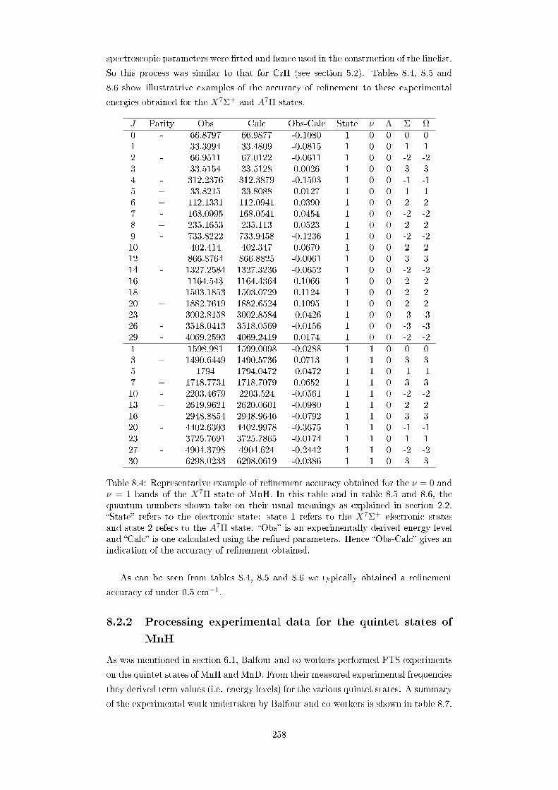
spectroscopic parameters were tted and hence used in the construction of the linelist.
So this process was similar to that for CrH (see section 5.2). Tables 8.4, 8.5 and
8.6 show illustratrive examples of the accuracy of renement to these experimental
energies obtained for the X7Σ+ and A7Π states.
J Parity Obs Calc Obs-Calc State ν Λ Σ Ω0 - 66.8797 66.9877 -0.1080 1 0 0 0 01 + 33.3994 33.4809 -0.0815 1 0 0 1 12 - 66.9511 67.0122 -0.0611 1 0 0 -2 -23 + 33.5154 33.5128 0.0026 1 0 0 3 34 - 312.2376 312.3879 -0.1503 1 0 0 -1 -15 + 33.8215 33.8088 0.0127 1 0 0 1 16 + 112.1331 112.0941 0.0390 1 0 0 2 27 - 168.0995 168.0541 0.0454 1 0 0 -2 -28 + 235.1653 235.113 0.0523 1 0 0 2 29 - 733.8222 733.9458 -0.1236 1 0 0 -2 -210 + 402.414 402.347 0.0670 1 0 0 2 212 + 866.8764 866.8825 -0.0061 1 0 0 3 314 - 1327.2584 1327.3236 -0.0652 1 0 0 -2 -216 + 1164.543 1164.4364 0.1066 1 0 0 2 218 + 1503.1853 1503.0729 0.1124 1 0 0 2 220 + 1882.7619 1882.6524 0.1095 1 0 0 2 223 - 3002.8158 3002.8584 -0.0426 1 0 0 -3 -326 - 3518.0413 3518.0569 -0.0156 1 0 0 -3 -329 - 4069.2593 4069.2419 0.0174 1 0 0 -2 -21 + 1598.981 1599.0098 -0.0288 1 1 0 0 03 + 1490.6449 1490.5736 0.0713 1 1 0 3 35 - 1794 1794.0472 -0.0472 1 1 0 -1 -17 + 1718.7731 1718.7079 0.0652 1 1 0 3 310 - 2203.4679 2203.524 -0.0561 1 1 0 -2 -213 + 2619.9621 2620.0601 -0.0980 1 1 0 2 216 + 2948.8854 2948.9646 -0.0792 1 1 0 3 320 - 4402.6303 4402.9978 -0.3675 1 1 0 -1 -123 + 3725.7691 3725.7865 -0.0174 1 1 0 1 127 - 4904.3798 4904.624 -0.2442 1 1 0 -2 -230 + 6298.0233 6298.0619 -0.0386 1 1 0 3 3
Table 8.4: Representative example of renement accuracy obtained for the ν = 0 andν = 1 bands of the X7Π state of MnH. In this table and in table 8.5 and 8.6, thequantum numbers shown take on their usual meanings as explained in section 2.2.State refers to the electronic state: state 1 refers to the X7Σ+ electronic statesand state 2 refers to the A7Π state. Obs is an experimentally derived energy leveland Calc is one calculated using the rened parameters. Hence Obs-Calc gives anindication of the accuracy of renement obtained.
As can be seen from tables 8.4, 8.5 and 8.6 we typically obtained a renement
accuracy of under 0.5 cm−1.
8.2.2 Processing experimental data for the quintet states of
MnH
As was mentioned in section 6.1, Balfour and co-workers performed FTS experiments
on the quintet states of MnH and MnD. From their measured experimental frequencies
they derived term values (i.e. energy levels) for the various quintet states. A summary
of the experimental work undertaken by Balfour and co-workers is shown in table 8.7.
258

J Parity Obs Calc Obs-Calc State ν Λ Σ Ω3 - 3081.0069 3081.1046 -0.0977 1 2 0 -1 -15 - 3081.2417 3081.2896 -0.0479 1 2 0 -3 -37 + 3301.4585 3301.5275 -0.0690 1 2 0 2 210 + 3738.7177 3738.8151 -0.0974 1 2 0 2 214 + 3740.1251 3740.043 0.0821 1 2 0 2 217 + 4337.1991 4337.1531 0.0460 1 2 0 3 321 + 4694.9924 4694.8533 0.1391 1 2 0 1 124 + 6480.5057 6480.5468 -0.0411 1 2 0 2 227 + 7012.688 7012.5697 0.1183 1 2 0 3 330 + 7014.7554 7014.6558 0.0996 1 2 0 2 22 - 4448.7161 4448.8642 -0.1481 1 3 0 0 04 + 4326.8159 4326.9048 -0.0889 1 3 0 3 36 - 4357.7098 4357.7677 -0.0579 1 3 0 -1 -18 + 4510.496 4510.5215 -0.0255 1 3 0 2 211 + 4663.2048 4663.1543 0.0505 1 3 0 1 114 + 5662.4751 5662.5341 -0.0590 1 3 0 2 217 - 6192.7258 6192.8293 -0.1035 1 3 0 -2 -220 - 6194.1575 6194.1675 -0.0100 1 3 0 -3 -322 + 7251.3592 7251.633 -0.2738 1 3 0 2 225 + 7253.0508 7253.3067 -0.2559 1 3 0 3 328 - 7986.7165 7987.0446 -0.3281 1 3 0 -3 -330 + 7576.1468 7575.6855 0.4613 1 3 0 3 3
Table 8.5: Representative example of renement accuracy obtained for the ν = 2and ν = 3 bands of the X7Π state of MnH. In this table the units of the calculatedrovibronic states are in cm−1. Refer to table 8.4 for details of the notation.
J Parity Obs Calc Obs-Calc State ν Λ Σ Ω0 - 17694.055 17694.0611 -0.0061 2 0 -1 1 01 + 17765.62 17765.5195 0.1005 2 0 1 0 12 + 17712.536 17712.4007 0.1353 2 0 1 0 13 - 17850.081 17849.8203 0.2607 2 0 -1 -2 -34 + 17695.333 17695.1433 0.1897 2 0 1 -1 05 + 17734.252 17734.047 0.2050 2 0 1 -3 -27 - 17934.733 17934.4701 0.2629 2 0 -1 -2 -39 + 18119.272 18119.3278 -0.0558 2 0 1 -3 -210 + 18232.7 18232.8153 -0.1153 2 0 1 -3 -213 - 18342.884 18343.1803 -0.2963 2 0 -1 1 014 + 18481.458 18481.8011 -0.3431 2 0 1 -1 015 + 18629.549 18629.2057 0.3433 2 0 1 -1 0
Table 8.6: Representative example of renement accuracy obtained for the A7Π stateof MnH. In this table the units of the calculated rovibronic states are in cm−1. Referto table 8.4 for details of the notation.
Referring to table 8.7, term values for the a5Σ+, b5Π and c5Σ+ states were obtained
from the 1990 study and term values for the a5Σ+, d5Π and e5Σ+ states obtained
from the 1992 study. A check was done to compare the two sets of term values for
the a5Σ+ state from the 1990 and 1992 studies: they were found to be self-consistent
within experimental error. Hence the term values for the a5Σ+ state from the 1992
study were used as these contained energy levels for ν = 2 which the 1990 study did
not.
For each of the 5Σ+ states, the term values presented by Balfour and co-workers
were labelled by quantum numbers J and ν and label Fi where i = 1, 2, 3, 4, 5 i.e. 5
259

Study Region(cm−1) System (nm) Electronic TransitionBands
MnH MnD1990 9 000− 10 380 1060 b5Π− a5Σ+ (0, 0) (0, 0)1990 11 200− 12 500 846 c5Σ+ − a5Σ+ (0, 0), (1, 1) (0, 0)1992 20 200− 21 200 480 d5Π− a5Σ+ (0, 0), (1, 1), (2, 2) (0, 0)1992 21 400− 22 400 450 e5Σ+ − a5Σ+ (0, 0), (1, 1)
Table 8.7: Summary of FTS experimental measurements on the quintet states of MnHand MnD undertaken by Balfour and co-workers.
spin-state components. For each value of J and ν there were ve of them: these spin-
components were simply labelled in order of increasing energy, F1, F2, F3, F4, F5.
Refer to table 8.1 which gives the required Duo input format for reference experimental
data. For these 5Σ+ states, J , ν were taken as given and, by denition of a Σ+ state,
Λ = 0. To deduce the parity, Σ and Ω, a single Duo input le containing an ab
initio PEC of the a5Σ+ state was created: this Duo le was then compiled hence
producing a calculation of rovibronic energies and transitions for this unrened PEC.
The output energy le of this calculation was then examined. For each value of J
and ν there were ve energies calculated (i.e. the 5 spin components). By examining
various blocks of output data of constant J and ν, the deductions about the ordering
of Parity and the quantum numbers of Σ and Ω for the spin-components as shown in
table 8.8 were made. This process was repeated for sample ab initio calculations of
c5Σ+ and e5Σ+ states and the same deductions made. For the b5Π and d5Π states,
J Spin-Component Parity Σ Ω
EVEN
F1 + 1 1F2 - -2 -2F3 + 2 2F4 - -1 -1F5 + 1 1
(a)
J Spin-Component Parity Σ Ω
ODD
F1 - -2 -2F2 + 2 2F3 - -2 -2F4 + 1 1F5 - -1 -1
(b)
Table 8.8: Summary of deductions concerning the assignment of Parity, Σ and Ω forconstant J and ν for 5Σ+ states using the c5Σ+(I) and a5Σ+ term values presentedin Balfour (1990) and also the term values presented for the e5Σ+(II) and a5Σ+ elec-tronic states presented in Balfour (1992). For each values of J there are 5 componentslabelled F1, F2, F3, F4 and F5 which are presented in increasing order of energy.
a similar process of running a Duo calculation of rovibronic transitions and energies
and examining the energy le to assign quantum numbers was performed to process
the term values presented for these states into Duo format. For these 5Π states, the
term values presented were again labelled by J and ν: for each value of J and ν
there were 10 components: contrast this to the case of the 5Σ+ states which had 5
such components for each J and ν. These 10 components were labelled with parity
as either e or f and an integer number from the selection 3, 2, 1, 0, -1: for each
J , ν and parity these components were presented in increasing order of energy. This
e/f parity which is commonly used was converted into the rotationless parity used
by Duo using the rules:
e: Parity = (−1)J
f: Parity = (−1)J+1.
260

Hence running seperate Duo input les with ab initio PECs of the b5Π state and d5Π
state respectively, the deductions concerning Λ, Σ and Ω shown in table 8.9 for these5Π states were made. Hence with the deductions made by running these sample Duo
J Parity Component Λ Σ Ω
ODD -
3e -1 -1 -22e -1 -2 -31e -1 -1 -20e -1 2 1-1e -1 1 0
(a)
J Parity Component Λ Σ Ω
ODD +
3f 1 2 32f 1 2 31f 1 1 20f 1 2 3-1f 1 -1 0
(b)
J Parity Component Λ Σ Ω
EVEN -
3f -1 -2 -32f -1 0 -11f -1 1 00f -1 2 1-1f -1 1 0
(c)
J Parity Component Λ Σ Ω
EVEN +
3e 1 2 32e 1 0 11e 1 -1 00e 1 -2 -1-1e 1 -1 0
(d)
Table 8.9: Summary of deductions concerning the assignment of Parity, Λ, Σ and Ωfor constant J and ν for 5Π states. These deductions were made by reference to theterm values for the b5Π state presented in Balfour (1990) and the term values for thed5Π(II) state presented in Balfour (1992). For each J and parity pair, there are 5components labelled in order of increasing energy as indicated in this table. This isin contrast to the 5Σ+ states in which there are 5 components for each value of J ascompared to 10 for these Π states.
input les, it was then possible to put the term values generated by Balfour for both
the 5Σ+ states (see table 8.8) and the 5Π state (see table 8.9) into the required Duo
input format presented in table 8.1. In table 8.1, the E-state label is simply a label
which references each electronic state (1 for the a5Σ+, 2 for b5Π, 3 for c5Σ+, 4 for
d5Π and 5 for e5Σ+). The Running # is simply an internal Duo integer referencing
label: all of the term values for all 5 states were put in increasing order and hence the
terms labelled 1, 2, 3 etc. This list of experimentally derived term values was used in
the nal linelist.
8.3 Linelist Spectra
The Manganese atom has 1 stable isotope of atomic mass 55: additionally, there are
over 25 radioisotopes with half-lives varying between 105 ns (44Mn) and 3.7 × 10⁶
years (53Mn). In terms of astronomical importance, the 55Mn isotope is of interest
in supernova explosions (Iwamoto et al. 2009). Lugmair & Shukolyukov (1998) have
investigated if the 53Mn and 53Cr isotopes can be used to determine timescales for
solar system objects such as chondrites and meteorites. Also, since the possibility of
using CrH and CrD spectra to infer the age of brown dwarfs has been postulated (see
section 3.4) it was hence decided to generate linelists for the 55MnH, 55MnD, 53MnH
and 53MnH isotopologues.
The number of rovibronic states in this linelist is 47 573 and the number of transi-
tions is 5 408 337. All transitions up to J = 50 are included with the vibrational range
261

for each electronic state as follows: X7Σ+ (ν = 12), A7Π (10), B7Σ+(II) (14), a5Σ+
(9), b5Π (23), c′5∆ (23), c5Σ+(II) (22), d5Π(II) (10), e5Σ+(III) (10) and f5∆(II)
(10).
As was done for the calculated linelist of CrH, the program ExoCross (see section
2.10) was used to simulate spectra using the calculated linelist of MnH as input. Figure
8.2 shows the calculated absorption spectra at 1500 K for the 55MnH isotopologue
for the electronic transitions to the X7Σ+ and a5Σ+ electronic states. Figure 8.2
Figure 8.2: Cross-sectional absorption bands for the 55MnH isotopomer calculatedusing a Gaussian prole with a half-width half-maximum of 1.0 at a temperature of1500 K.
shows clear band structure for the various electronic transitions. As can be seen the
various bands spans the the mid infrared to the near UV regions. As can be seen from
gure 8.2 the X−X rovibronic transitions dwarf those of the a−a and also the spin-
forbidden transitions of X − a. Thus this could explain why pure rovibronic spectra
within the a5Σ+ has not been observed by experimentalists which seems surprising
given that Balfour and co-workers have been able to measure the b − a, c − a, d − aand e− a transitions. Figure 8.2 clearly shows why they were able to measure these
transitions as the band heads are clearly visible and each isolated. Also it can be seen
that the c′ − a transitions are dwarfed by those of the b− a transitions and similarly
the f − a transitions are dwarfed by the e − a transitions. This is expected as both
the and c′ and f states are ∆ states so hence not normally expected to couple to Σ+
states. A band head of the A − X transition is also clearly shown. Finally gure
8.2 raises the possibility that the B − X transition could potentially be measured
at wavelengths greater than approximately 27 000 cm−1 given a suciently sensitive
experimental set-up given that there does not appear to be any other electronic bands
obscuring it in this region.
Figure 8.3 shows the eect of temperature on the simulated spectra for all of the
bands shown in gure 8.2. As can be seen from gure 8.3 between 500 K and 1500 K
the dierence in intensity generated is around 4 orders of magnitude. This temper-
ature range is applicable to exoplanets and also T dwarfs. For L dwarfs in which
diatomic hydrides such as FeH, CrH and CaH have been discovered the temperature
262
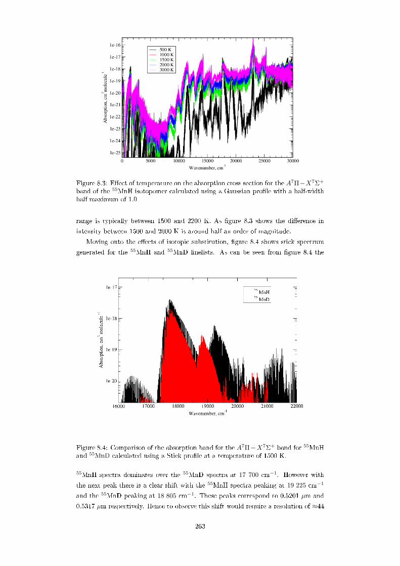
Figure 8.3: Eect of temperature on the absorption cross section for the A7Π−X7Σ+
band of the 55MnH isotopomer calculated using a Gaussian prole with a half-widthhalf-maximum of 1.0
range is typically between 1500 and 2200 K. As gure 8.3 shows the dierence in
intensity between 1500 and 2000 K is around half an order of magnitude.
Moving onto the eects of isotopic substitution, gure 8.4 shows stick spectrum
generated for the 55MnH and 55MnD linelists. As can be seen from gure 8.4 the
Figure 8.4: Comparison of the absorption band for the A7Π−X7Σ+ band for 55MnHand 55MnD calculated using a Stick prole at a temperature of 1500 K.
55MnH spectra dominates over the 55MnD spectra at 17 700 cm−1. However with
the next peak there is a clear shift with the 55MnH spectra peaking at 19 225 cm−1
and the 55MnD peaking at 18 805 cm−1. These peaks correspond to 0.5201 µm and
0.5317 µm respectively. Hence to observe this shift would require a resolution of ≈44
263

in the visible region.
Moving onto the partition function, gure 8.5 shows a comparison between the
partition function calculated for the linelist and that of Sauval & Tatum (1984). The
coecients for the partition function which Sauval & Tatum (1984) derived using
experimental data were a0 = 4.1860, a1 = −2.1839, a2 = 0.8747, a3 = −0.2513 which
were inserted into equation 5.3 to generate the partition function shown in gure 8.5.
As can be seen from gure 8.5 our partition function is larger which suggests hence
Figure 8.5: Comparison of total partition function calculated as a function of Tem-perature for the 55MnH linelist with that predicted by Sauval & Tatum (1984). Thepartition function of Sauval and Tatum (1984) has been multiplied by a factor of 12to account for the eects of nuclear spin statistics which they did not account for intheir study.
our model of MnH more complete. Figure 8.6 shows the total partition function as
a function of the quantum number J for dierent temperatures. Our linelist goes
up to J = 50 as it was determined from initial Duo calculations that this would be
sucient. Figure 8.5 demonstrates this as it can be seen that for temperatures up
to 3000 K the partition function is converging well before J = 50. To gain an idea
of the completeness of the total partition function Q, a partition function Q(E) can
be calculated in which only states up to the rst dissociation limit are populated.
A comparison can be made between these two partition functions by plotting the
percentage dierence between them calculated as 100 × (Q − Q(E))/Q. This is
shown in gure 8.7 as a function of temperature.
264

Figure 8.6: Partition function as a function of J for dierent temperatures which areapplicable to the study of L and M dwarfs.
Figure 8.7: Percentage dierence between the total partition function Q and thepartition function Q(E) in which only states up to the rst dissociation limit of 12785cm−1 are populated.
Since both the Partition function and intensity both have the same Boltzmann
factor, an error in the partition function (i.e error in completeness) can be related to
an error in intensities and hence opacities. As can be seen from gure 8.7 if an accuracy
of 10% is judged to be acceptable then up to temperatures of 4500 K a linelist in which
only states up to the rst dissociation limit are populated is suciently complete.
In summary a linelist for MnH has been created by calculating ab initio curves
and tting to the available experimental data sets. At present there is no linelist in
the literature for this molecule. Hence this creates the opportunity for a potential
detection of this molecule in space. Given that the cosmic abundance of Chromium
and Manganese are relatively similar (see table 3.1) it does beg the question of why
it has not been observed to date. Given the problems astronomers have experienced
265

using the existing linelists for CrH and FeH to successfully model observed L dwarf
spectra (see section 3.4) the possibility that MnH is accountable for at least some of
the discrepancies in opacity can now be investigated.
266

Chapter 9
Further Research Directions
and Conclusions
The calculation of linelists for CrH and MnH has opened up many possible future
directions for research from theoretical, experimental and astronomical viewpoints.
Also, having studied the molecules of CrH and MnH there is potential for linelists to
be created for other diatomic metal hydrides.
9.1 Experimental work
The construction of the linelist for CrH highlighted how imperative it is to rene
ab initio PECs to experimental data. As was shown in table 5.3 for CrH there
is only experimental data available for the A6Σ+ − X6Σ+ system and only for a
handful of vibrational bands. In order to better constrain the PECs of the X6Σ+
and A6Σ+ states experimental data of vibrational bands with ν > 2 would be of
signicant assistance. The experimental group led by Amanda Ross in Universite
Lyon 1 is planing to measure the intensities of CrH spectra: this would provide
valuable assistance in constraining the transition dipole coupling the A6Σ+ andX6Σ+
electronic states.
For MnH, luckily there was experimental data available for 5 electronic transition
systems (X−A, b−a, c−a, d−a and e−a) but again this was limited to ν = 0, 1, 2. Any
new measurements going beyond ν > 2 would be particularly useful in the context of
brown dwarfs as the temperatures reached mean that these higher vibrational states
are likely to be occupied.
Longer term, as has been the case for the water molecule, for the open-shell di-
atomics a productive and instructive way forward would be a bouncing back and forth
pattern between theoretical calculations making predictions which are then tested by
experimentalists whose data is then used by theorists to generate new models which
are tested by experimentalists and so on and so forth.
267

9.2 Theoretical Work
There are several possible avenues in terms of basis set optimisation which could be
explored. Throughout this study, relativistic and core-correlation eects have not
been incorporated due to the demands they place on computing power: however it
was known from previous studies within the group that for similar diatomic molecules
that these tend to cancel each other out. A computational project could be to design
algorithms to decrease the RAM required for such calculations.
When deciding what basis sets to use it is desirable to choose a basis set which
best describes the behaviour of the valence electrons. Dr Laura K. McKemmish, a
Research Associate within the ExoMol group worked on replacing the primitive core
basis-functions within basis sets with a single RAMP function for her PhD. Using the
analogy of a model of the Earth made out of Lego, if you are only interested in the
surface (i.e. valence electrons) then you don't care what Lego blocks are used in the
centre i.e. you are only interested in Lego blocks on and near to the surface. Hence
in this case (which is the standard within quantum chemistry) it is allowable to use
bigger Lego bricks to model the centre of the earth and then for the surface layers (i.
e the valence electrons), use smaller bricks for the desired accuracy.
Taking the example of a carbon atom, the number of Gaussians used in a basis set
typically is:
6 primitive functions to describe the 1s atomic orbitals
3 functions to describe the for 2s atomic orbitals
1 function to describe the 2p atomic orbitals
1 Gaussian function to describe harmonic behaviour.
The idea behind RAMPS basis functions is to replace the 6 primitive Gaussians with
1 Gaussian & 1 ramp to describe the core region. Since the functions describing the
valence electrons are left the same, the behaviour of these electrons (which ultimately
determine the chemistry of the species under consideration) remains unchanged. The
advantage of replacing the core with this simplied pair of functions is that the speed
of computational calculations can be signicantly improved.
Taking the case of CrH and MnH both molecules have core electrons which form
a core Argon electron conguration around the respective transition metal nucleus:
the remaining electrons, 7 for the case of CrH and 8 for the case of MnH, act as valence
electrons. A possible area of future research is thus to replace the core basis functions
with a hybrid function of a primitive Gaussian and a RAMP into the basis sets used
in order to increase the speed of calculations. This would hence allow more focus to
be directed to improving the accuracy of results obtained. Since the valence electrons
are dominant (as they determine the molecular orbitals) it would be wise for future
research to investigate the eects of adding more primitive Gaussian functions to the
basis sets used to hence more accurately describe the behaviour of these electrons.
268

9.3 Astronomical work
An educational school student project could be to undertake a search of literature for
diatomic hydrides, chlorides, iodides, uorides and oxides going through the periodic
table up to the 2nd row of transition metals. For reference this section of the periodic
table is shown in table 9.1. The aim of this search would be to ascertain if there are
any such molecules not already covered by the ExoMol project which are of astronom-
ical interest not just for stars and planets but also in settings such as the ISM. An
understanding of the chemistry of the ISM is an active research area. For any such
molecules identied, a search could be undertaken to ascertain the scope and accuracy
of experimental and theoretical data available for detection and characterisation.
H He1 2Li Be B C N O F Ne3 4 5 6 7 8 9 10Na Mg Al Si P S Cl Ar11 12 13 14 15 16 17 18K Ca Sc Ti V Cr Mn Fe Co Ni Cu Zn Ga Ge As Se Br Kr19 20 21 22 23 24 25 26 27 28 29 30 31 32 33 34 35 36Rb Sr Y Zr Nb Mo Tc Ru Rh Pd Ag Cd In Sn Sb Te I Xe37 38 39 40 41 42 43 44 45 46 47 48 49 50 51 52 53 54
Table 9.1: Periodic table for the rst 36 elements with the alkaline earth metals ofBe, Ca & Mg highlighted as well as the transition metals Mn & Cr
A potentially exciting project to undertake is a search for MnH in the sunspot
spectra of Wallace et al. (2006) and also in spectra of brown dwarfs published such as
those on the DwarfArchives webpage. The former could be a coding based project in
which computer code is written which systematically searches for matches within an
accuracy level which can be adjusted and then, for any matches found a statistical
study undertaken to ascertain the probability of each match been a coincidence.
In terms of stellar astronomy, HotMol is an ERC funded project based in Freiberg
led by Professor Svetlana Berdyugina (see section 3.4). One of the aims of Svetlana's
work is to investigate if the Paschen-Back eect in molecules can be exploited as a
method to determine the magnetic eld strength of dierent classes of stars and brown
dwarfs. Dierent molecules, and indeed dierent electronic states within molecules
will be sensitive to various magnetic eld strengths-the hope is that a set of molecules
can be determined which can be used to determine the magnetic eld strengths of
various astrophysical objects which can cover a huge range of magnitudes. Oleksii
Kuzmychov investigated CrH as a probe of magnetic eld strengths for his PhD. If
MnH was to be found within stellar objects, a similar quantum mechanical study for
MnH could be undertaken now that PECs have been calculated within this PhD.
9.4 Creation of a new linelist for FeH
A diatomic hydride molecule which is an obvious candidate for further work is di-
atomic Iron Hydride, FeH. The atomic element Iron sits along the rst row of the
269

transition metals in the periodic table after Chromium and Manganese. The molecule
FeH has 27 electrons in total. FeH is of interest from an astronomical perspective as
summarised in section 9.4.1. The existing linelist of the F 4∆i − X4∆i transition
available to astronomers for characterisation is summarised in section 9.4.2. Section
9.4.3 then discusses a possible collaboration and source of funding which could be
used to begin the process of constructing a new and more extensive linelist of FeH.
Section 9.4.4 then gives a summary of the experimental work that has been done on
FeH and could thus be used in tting any calculated PECs. In summary there are a
range of small student projects in working with the experimental data which would
greatly assist with the renement of any calculated ab initio curves. The theoretical
work which has previously been undertaken on FeH is summarised in section 9.4.5.
Finally, section 9.4.6 then discusses the theoretical diculties that would be involved
in calculating new ab initio data for use in the construction of a new linelist.
9.4.1 Astrophysical importance of FeH
Iron Hydride (FeH) is a molecule of signicant interest in astronomy: the element
Iron has one of the most stable nuclei in existence in the universe. In terms of
transition metals, the abundance of iron dwarfs those of other metals (see section 3.4).
The interest in FeH in space started back in 1972 when Carroll & McCormack rst
identied FeH in the solar spectrum. Wing, Cohen & Brault (1977) then conrmed
this detection of the two bands at 9896 Å and 8691 Å. Mould & Wycko (1978)
also modelled the FeH column densities of late-type stellar atmospheres and noted
how sensitive the FeH Wing-Ford bands are to surface gravity. Additionally, Nordt,
Lindgren & Wing (1977) made a tentative identication of a band of FeH near 9900
Å in M dwarfs and S stars using experimental data from Klymming & Lindgren. This
identication in S stars was then conrmed by Clegg & Lambert in 1978: additionally
Hirai & Chinami (1992) detected FeH in M, S and C stars. Since these early studies,
numerous studies of FeH in the solar spectrum, cool stars and brown dwarfs have
been undertaken including:
The Wing-Ford band (9900 Å) detected and modelled in M dwarfs by several
authors: Schiavon, Barbuy & Singh (1997); Reiners (2007); Wende, Reiners
& Ludwig (2009); Wende, Reiners, Seifahrt & Bernath (2010); Shulyak et al.
(2010);
FeH is an important molecule in brown dwarfs in particular L type dwarfs.
The presence and variability of FeH in dwarfs spanning dierent ages has been
studied by numerous authors including Cushing et al. (2003), Knapp et al.
(2004), McLean et al. (2007), Bailer-Jones (2008), Goldman et al. (2008),
Burgo et al. (2009), Martìn et al. (2010), Hargreaves et al. (2010).
Mulchaey (1989) measured the sunspot spectra and searched for the 7 dierent
bands of FeH as measured by Phillips et al. (1987) and identied 3 of them.
He then calculated an average eective rotational temperature of 1740 ± 100
K. This temperature he noted is signicantly lower than previous rotational
temperatures obtained using other molecules such as TiO.
270

Fawzy, Youssef & Engvold (1998) have identied FeH in the sunspot using the
(2, 0) and (2, 1) bands of the 4∆ −4 ∆ system using the FTS spectrometer at
the Kitt Peak Observatory.
Wallace & Hinkle (2001) have identied the E4Π−A4Π system of FeH near 1.6
µm in sunspot and cool star spectra.
Ramos, Bueno and Collados (2004) have identied both linear and circular
polarisation induced from the Zeeman eect from the E4Π − A4Π system of
FeH in sunspot spectra around 1.6 µm.
Fawzy (2009) has used equivalent widths for the (0-0), (1-0), (2-0), and (2-1)
band of the 4∆ −4 ∆ system of FeH to derive a rotational temperature of the
large sunspot San Fernando 535 of Trot = 2900 ± 300 K which Fawzy notes is
in agreement with rotational temperatures for this sunspot derived using other
molecules.
Reiners, Schmitt & Liefke (2007) have undertaken a study of the magnetic ux
variability of Wing-Ford band near 1 µm in the nearby are star of CN Leonis.
Bar-Nun, Pasternack & Barrett (1980) have proposed the existence of FeH and
FeH2 in interstellar clouds on the basis of previous Argon matrix trapping ex-
periments
In summary, FeH is a molecule of signicant interest to the solar, cool star and
brown dwarf communities: the electronic system of E4Π − A4Π has been identied
as well as the 4∆−4 ∆ for which the current linelist for FeH contains.
9.4.2 Existing linelist of FeH of Dulick et al. (2003)
The existing linelist of FeH commonly in use is that of Dulick et al. (2003). This
linelist is a list of the rovibronic wavelengths associated with the F 4∆i −X4∆i tran-
sition for 25 vibrational bands up to J = 50.5. The authors used existing term values
for the ν = 0, ν = 1 and ν = 2 levels of of the X4∆ electronic state and then
extrapolated to ν = 3 and ν = 4. For this linelist, the transition dipole moment
function was calculated using ab initio theory and then used to calculate Einstin
A-coecients. The level of theory used was a SA-CASSCF calculations followed by
MRCI with an active space of (6, 1, 1, 1) within the framework of C2v symmetry.
The SA-CASSCF orbitals were constructed using the three lowest 4∆ states and in
the proceeding MRCI calculation, 4 states in symmetry 4 were requested which thus
yielded the three lowest lying 4∆ states and one 4Σ− state. Using this data the au-
thors calculated spectroscopic constants. The authors did not however, shift their
theoretical potentials to be in line with their experimental potentials.
9.4.3 Potential collaboration with Uppsala University
Sara Lindgren is a fellow PhD student based at Uppsala University in Sweden who
studies the metalicity of M type dwarfs. By constraining the metallicity of host stars,
271

the metallicity of the orbiting exoplanets can thus be deduced under the approxi-
mation that they were formed from the protoplanetary disc of their host star. To
determine metalicity of a population of M type stars she is using the CRIRES spec-
trograph onboard on the VLT. Sara has made observations in the J band(1100-1400
nm) of around 30-40 M dwarfs and analysed the data using the SME (Spectroscopy
Made Easy) programme. She has used the following inputs:
MARCS model atmospheres
Atomic linelists for Potassium and Sodium from the VALD database, with some
additional atomic data from Melendez & Barbuy (1999)
Linelist for CrH calculated by Burrow et al. (2002)
Linelist of H2O calculated by Barber et al. (2006)
Line data calculated for FeH by Bertrand Plez, (unpublished)
In particular she has looked at FeH lines and constructed contour plots to investigate
if there are degeneracy's between eective temperatures and metallicity. By com-
paring of accepted values of metalicities, she has concluded that metallicities can be
determined accurately using the above technique. The lines of FeH from Bernard Plez
are unpublished.
The Royal Society of Chemistry have a Researcher Mobility Grant scheme which
is open to Masters, PhD students and early career researchers to apply to spend up
to three months as an institution to carry out work which would benet both their
home and visiting institution. This is a possible source of funding which could be
used to do preliminary work on the calculation of a new linelist of FeH: a new linelist
for FeH would be of benet for the ExoMol project based at UCL and also for Sara's
work.
9.4.4 Experimental studies of FeH
FeH has been extensively studied experimentally: thus there is a large volume of data
available on this radical. Of most pragmatic interest are measurements of experimen-
tal frequencies of transitions which can be used to t ab initio data.
The spectrum of FeH has been measured by as far back as the experiments of
Kleman & Kerland who used a King-like Furnace to observe a red degraded band at
9896 Å. This work was unpublished: however, Klynning & Lindgren (1973) did then
later measure and publish the wavelengths witin this band.
FeH & FeD were then studied in the region of 2360 - 8900 Å by Carroll, McCor-
mack, O'Connor (1976) who found two regions of complex structure in the:
Blue: 4920 Å (2 regions of absorption)
Green: 5320 Å (3 regions of absorption)
For the green they found no signicant isotope shift for FeD so speculated that could
be due to a (0, 0) band: similarly for one of the regions in the blue with the other
could possibly be a (1, 0) band. They also measured another band with a band head
272

in the near infrared peaked at 8690.82 Å which degraded at longer wavelengths and
made the tentative vibronic assignment to this system as shown in table 9.2.
Band Band Head measurement (Å)(0, 0) 9896.22(1, 0) 8690.82(2, 0) 7818.54
Table 9.2: Tentative vibronic assignment made by Carroll, McCormack, O'Connor(1976) of the near infra-red band they observed.
Carroll, McCormack, O'Connor(1976) also calculated vibronic constants for this
band. Their work is of paramount important from an astrophysical perspective as they
concluded that FeH could be in sunspots by comparing their measured experimental
frequencies with the sunspot spectra of Moore, Monnaert, Houtgast 1966.
McCormack & O'Connor then went on in 1976 to measure these blue and green
regions in detail and publish around 1700 rovibronic lines to aid the detection of FeH
in space: they decided that, at the time the rotational analysis was too complex.
Dendramis, Van Zee & Weltner (1979) performed experiments in which both FeH
& FeD were trapped in solid argon at 4 K and values of ωe and ωeχe determined using
a vibrational analysis. They observed 5 weak electronic transitions in visible region:
a summary of the vibrational absorption bands observed is shown in table 9.3.
Band DesignationFeH FeD
λ (Å) ν (cm−1) ∆ν (cm−1) λ (Å) ν (cm−1) ∆ν (cm−1)E 3996(10) 25 018(70) 4007(10) 24 949(70)
1130 929D 4185(5) 23 888(30) 4162(5) 24 020(30)
1301 1101C 4426(20) 22 587(100) 4362(20) 22 919(100)
1143 1383B 4662(20) 21 444(100) 4642(20) 21 536(100)
1401 1518A 4988(30) 20 043(120) 4994(30) 20 018(120)
Table 9.3: Summary of vibrational absorption bands measured using an Argon-matrixtrapping experiment for FeH & FeD by Dendramis, Van Zee & Weltner(1979).
Table 9.3 gives a summary of the vibrational bands measured by Dendramis, Van
Zee & Weltner (1979) for FeH and FeD and also the vibronic constants determined by
their rotational analysis. Their uncertainty is indicated for each value by the numbers
in brackets. These values could be used as comparison to any theoretical ab initio
curves.
Following on from this work, Phillips, Davis, Lindgren & Balfour (1987) used the
FTS onboard the McMath telescope bases at Kitt Peak (National Solar Observatory)
to undertake a rotational analysis of the 4∆ −4 ∆ system of FeH. A summary of
their vibronic band assignments with respective band heads and origins is shown in
table 9.4. Table 9.5 shows a more in-depth summary of the range of J and ω values
measured for the bands shown in table 9.4: the sub-band heads are also shown in
table 9.6. The authors also calculated the wavelengths for the bands shown in table
9.7.
273

Band Band head(Å) Band Origin (Å)(2, 0) 7786 12 769.46(1, 0) 8692 11 419.44(2, 1) 9020 11 006.53(0, 0) 9896 9995.14(1, 1) 10 253 9656.68(0, 1) 11 939 8232.20(1, 2) 12 389 7957.48
Table 9.4: Vibronic band assignments made by Phillips, Davis, Lindgren, Balfour,1987 for the 4∆−4 ∆ system of FeH.
Band Ω′ Ω′′ J ′′ range(1, 1) 7/2 7/2 5.5 to 19.5
5/2 5/2 5.5 to 19.53/2 3/2 4.5 to 18.51/2 1/2 2.5 to 13.5
(1, 0) 7/2 7/2 3.5 to 28.55/2 5/2 2.5 to 22.53/2 3/2 2.5 to 22.51/2 1/2 1.5 to 19.57/2 5/2 5.5 to 24.53/2 1/2 8.5 to 18.55/2 7/2 5.5 to 18.53/2 5/2 5.5 to 20.5
(2, 1) 7/2 7/2 4.5 to 21.55/2 5/2 5.5 to 17.53/2 3/2 4.5 to 19.51/2 1/2 5.5 to 17.5
(2, 0) 7/2 7/2 3.5 to 22.55/2 5/2 4.5 to 19.53/2 3/2 4.5 to 18.51/2 1/2 3.5 to 17.5
(0, 1) 7/2 7/2 3.5 to 21.55/2 5/2 4.5 to 19.53/2 3/2 4.5 to 19.51/2 1/2 2.5 to 21.5
(1, 2) 7/2 7/2 5.5 to 15.55/2 5/2 5.5 to 19.53/2 3/2 5.5 to 18.51/2 1/2 6.5 to 17.5
Table 9.5: Summary of range of experimental wavenumbers measures by Phillips,Davis, Lindgren & Balfour (1987) for the 4∆−4 ∆ system of FeH.
Sub-band 7/2-7/2 5/2-5/2 3/2-3/2 1/2-1/2(0, 0) 9 928.71 10 026.03 10 038.75 9 983.78(1, 0) 11 352.87 11 455.81 11 453.69 11 410.09(2, 0) 12 697.22 12 806.58 12 795.52 12 754.81(0, 1) 8 171.06 8 624.25 8 277.01 8 223.66(1, 1) 9 595.44 9 694.00 9 691.94 9 649.86(2, 1) 10 989.81 11 044.87 11 033.55 10 995.45(1, 2) 7 895.74 8 000.46 8 005.95 7 936.05
Table 9.6: Sub band origins for the 4∆ −4 ∆ system of FeH measured by Phillips,Davis, Lindgren & Balfour(1987).
274

Band Band head(Å)(2, 2) 10 639(0, 2) 14 927
Table 9.7: Bands of the 4∆ −4 ∆ system of FeH for which Phillips, Davis, Lindgren& Balfour (1987) calculated wavenumbers up to J = 17.5 for during their rotationalanalysis.
Phillips, Davis, Lindgren & Balfour (1987) used their experimental data sum-
marised in tables 9.4, 9.5, 9.6 and 9.7 to calculate molecular constants (B, D, H for
ν = 0, 1, 2 and ωe & ωeχe for both electronic states), term values, spin-splitting and
λ doubling values. Later on, it was shown by Balfour & Klynning (1994) that the
700 nm region observed by Phillips, Davis, Lindgren, Balfour (1987) is actually due
to CaH and CaD. They explain that the CaH data from Berg & Klynning for the
A2Π − X2Σ+ transition of CaH can be matched in the data recorded by Phillips.
Previously Phillips & Davies 1993 had speculated that this anomalous band could
be due to the presence of triatomic molecule, HFeH: in their paper they put forward
arguments for and against this assignment. They conclude that the assignment of
HFeH to the 700 nm region observed as unconrmed.
The most recent sets of experimental frequencies which could be used for tting
ab initio curves comes from the group led by the late Professor John Brown at Ox-
ford University who have undertaken many measurements of electronic transitions
involving the X4∆, A4Π, E4Π, a6∆, b6Π, c6Σ+ and e6Π, states using dispersed &
undispersed laser-induced uorescence. A summary of the experimental frequencies
measured within this group is shown in table 9.8. Table 9.8 gives a summary of the
experimental frequencies measured by the John Brown group which would be avail-
able for rening ab initio curves. The table shows the electronic transitions measured
with the associated range measured in terms of the quantum numbers ω and J . As
can be seen from table 9.8 there are several electronic bands which have repeatedly
measured. Of particular note are the measurements of the inter-combination system
of g6Φ − X4∆ which could be used to help constrain the energy shift between the
quartet and sextet state systems. Additionally, the John Brown group has also cal-
culated term values for each of the electronic transitions measured. Another project
could be is to use the experimental frequencies with the program MARVEL (Furten-
bacher, Császár & Tennyson 2007) to produce term values and compare with those
presented in the respective papers. A summary of the experimentally derived term
values are shown in table 9.9.
Table 9.9 summarises the range of term values calculated by the John Brown
group using the respective experimental frequencies that they measured. In terms of
tting ab initio in practice it would be easier to rst initially t to the term values
presented to get a rst guess at molecular state curve parameters and then use the
actual measured experimental frequencies to rene further aiming for higher accuracy.
Other experimental work done by this group which would assist in the construction of
a new linelist is the measurement of lifetimes of states of the g6Φ electronic state by
Carter & Brown (1994). This would assist in checking the intensities calculated using
theoretical dipoles. For astronomers, the intensity of transitions is very important
275

Electronic transition Band Ω′ Ω′′ J ′′ range Source
E4Π−X4∆ (0, 0)
5/2 7/2 3.5 to 34.5
Balfour, Brown & Wallace (2004)
3/2 5/2 3.5 to 29.51/2 3/2 3.5 to 24.55/2 5/2 1.5 to 23.53/2 3/2 1.5 to 26.51/2 1/2 1.5 to 22.5
E4Π−A4Π (0, 0)5/2 5/2 2.5 to 21.53/2 3/2 2.5 to 19.51/2 1/2 3.5 to 19.5
e6Π−X4∆ (0, 2) 7/2 7/2 4.5 to 10.5 Hullah, Barrow & Brown (1999)
g6Φ−X4∆ (0, 0)9/2 7/2 2.5 to 11.5
Carter, Steimle & Brown (1993)7/2 5/2 2.5 to 7.5
g6Φ−X4∆ (0, 0)11/2 7/2 4.5 to 9.5
Carter & Brown (1994b)11/2 7/2 4.5 to 9.5
e6Π− a6∆
(0, 0)7/2 9/2 4.5 to 10.5
Goodridge, Carter & Brown (1997)
5/2 7/2 3.5 to 8.53/2 5/2 2.5 to 5.5
(0, 1)7/2 9/2 4.5 to 9.55/2 7/2 3.5 to 6.53/2 5/2 2.5 to 4.5
(0, 0)1/2 3/2 1.5 to 4.5
Hullah, Wilson, Barrow & Brown (1998)7/2 9/2 9.5 to 12.5
(1, 1)
7/2 9/2 4.5 to 9.5
Wilson & Brown (1999)5/2 7/2 3.5 to 7.53/2 5/2 2.5 to 6.51/2 3/2 1.5 to 3.5
(0, 0)
7/2 7/2 3.5 to 13.5
Wilson, Cook & Brown (2001)
5/2 5/2 2.5 to 10.53/2 3/2 1.5 to 7.51/2 1/2 0.5 to 4.5-1/2 -1/2 0.5 to 4.5
(0, 0)
7/2 9/2 11.5 to 12.55/2 7/2 7.5 to 10.53/2 5/2 4.5 to 7.5-1/2 1/2 0.5 to 5.5
g6Φ− a6∆
(0, 1)
11/2 9/2 4.5 to 10.5
Wilson & Brown (1999)9/2 7/2 3.5 to 10.57/2 5/2 2.5 to 7.55/2 3/2 1.5 to 7.51/2 3/2 1.5 to 4.5
(0, 0)11/2 9/2 4.5 to 10.5
Carter & Brown (1994a)9/2 7/2 3.5 to 9.57/2 5/2 2.5 to 6.5
e6Π− b6Π
(0, 0)
7/2 7/2 3.5 to 11.5
Hullah, Barrow & Brown (1999)5/2 7/2 3.5 to 6.57/2 5/2 2.5 to 6.55/2 5/2 2.5 to 6.53/2 5/2 2.5 to 5.5
(0, 0)7/2 5/2 2.5 to 8.5
Goodridge, Hullah & Brown (1997)5/2 3/2 1.5 to 5.53/2 1/2 0.5 to 4.5
e6Π− c6Σ+ (0, 0) 1/2 -1/2 0.5 to 4.5 Hullah, Wilson, Barrow & Brown (1998)
Table 9.8: Summary of experimental frequencies values measured within the JohnBrown group.
276

Electronic transition ν Ω J SourceX4∆ 2 7/2 4.5 to 10.5 Hullah, Barrow & Brown (1999)
A4Π 05/2 2.5 to 21.5
Balfour, Brown & Wallace (2004)3/2 3.5 to 20.51/2 3.5 to 19.5
E4Π 05/2 2.5 to 29.5
Balfour, Brown & Wallace (2004)3/2 2.5 to 29.51/2 1.5 to 21.5
a6∆
0
9/2 4.5 to 10.5Carter & Brown (1994a)7/2 3.5 to 9.5
5/2 2.5 to 6.59/2 4.5 to 9.5
Goodridge, Carter & Brown (1997)7/2 4.5 to 6.55/2 2.5 to 4.53/2 1.5 to 4.5
Hullah, Wilson, Barrow & Brown (1998)9/2 11.5 to 12.59/2 12.5
Wilson, Cook & Brown (2001)
7/2 10.5 to 13.55/2 7.5 to 10.53/2 5.5 to 7.51/2 0.5 to 4.5-1/2 0.5 to 4.5
1
9/2 4.5 to 9.5Goodridge, Carter & Brown, 19979/2 3.5 to 6.5
9/2 2.5 to 4.59/2 4.5 to 10.5
Wilson & Brown (1999)7/2 3.5 to 10.55/2 2.5 to 7.53/2 1.5 to 7.5
b6Π 03/2 1.5 to 7.5
Hullah, Barrow & Brown (1999)5/2 2.5 to 6.57/2 3.5 to 11.5
c6Σ+ 05/2 2.5 to 8.5
Goodridge, Hullah & Brown (1997)3/2 1.5 to 5.51/2 0.5 to 4.5
e6Π
0
7/2 12.5
Wilson, Cook & Brown (2001)5/2 8.5 to 9.53/2 5.51/2 6.5-1/2 0.5 to 4.57/2 3.5 to 9.5
Goodridge, Carter & Brown (1997)5/2 2.5 to 7.53/2 1.5 to 4.51/2 0.5 to 3.5
Hullah, Wilson, Barrow & Brown (1998)7/2 10.5 to 12.5
17/2 3.5 to 8.5
Wilson & Brown (1999)5/2 2.5 to 6.53/2 1.5 to 5.5
g6Φ 0 9/2 4.5 to 10.5Carter, Steimle & Brown (1993)
g6Φ 0 7/2 3.5 to 7.5g6Φ 0 5/2 2.5 to 7.5 Wilson & Brown (1999)
Table 9.9: Summary of term values derived by the John Brown group.
in determining the opacity produced by dierent molecules. Additionally, Brown,
Körsgen, Beaton, Evenson (2006) have used LMR (laser magnetic resonance) in the
far infra-red to measure ν = 0 rotational states of the ground X4∆ of the FeH
277

molecule. Similarly, Jackson, Zink, Towle, Riley & Brown (2009) have performed a
similar experiment for the FeD molecule.
In summary, there is a large amount of experimental frequency data available for
multiple electronic systems of FeH and also molecular constants determined using
experimental data which could be used to assist in the construction of a new linelist
for FeH.
9.4.5 Review of previous theoretical studies of FeH
Theoretically, FeH has an extremely complex electronic structure of low-lying elec-
tronic states which dissociate to closely-spaced dissociation limits which have dierent
electronic congurations. It is noteable that Sauval & Tatum (1984) have not calcu-
lated empirical coecients for a partition function for this molecule. In their extensive
paper, in terms of the periodic table using the standardised dened rows & columns
for groups 1, 2, 13, 14, 15, 16, 17, rows 2 to 5 have all the diatomic hydrides listed. For
the rst row of transition metals (row 4) have CrH, MnH, CoH, NiH, CuH, ZnH listed
and for the second row of transition metals (row 5) have PdH, AgH & CdH listed and
row for 6 have PtH, AuH, HgH listed (groups 10, 11, 12). Also from LaH, YbH &
LuH which are hydrides formed from elements of the rst row of the lanthanides.
Theoretically, the low-lying electronic states of FeH have been studied by:
Scott & Richards (1974) who performed calculations of the low-lying 6∆, 6Σ+,6Π, 4∆ and 4Π states using a matrix Hartree-Fock approximation.
Langho & Bauschlicher (1990) have used the SA-CASSCF/MRCI method to
calculate the PECs of 10 sextet and 9 quartet low-lying states below 25 000
cm−1.
Sodupe, Lluch & Oliva (1990) have performed Hartree-Fock and CI calculations
using nonempirical pseudopotentials for the low-lying 4Σ+, 4Π, 4∆ and 6Σ+,6Π, ∆ states.
Tanaka & Sekiya (2001) have used the Multireference coupled pair approxima-
tion [MRCPA4] technique for the X4∆, A4Π, C4Φ, F 4∆ and a6∆, b6Π, c6Σ+,
e6Π states.
9.4.6 Calculating ab initio curves for FeH
Shown in table 9.10 are the rst 10 atomic dissociation limits of the Iron atom which
the FeH molecule will dissociate to (along with the H atom) in the range of large
internuclear distance R. As table 9.10 shows there are many atomic dissociation
limits up to around 20 000 cm−1. Even more pertinently these limits have competing
atomic congurations namely 3d64s2, 3d74s1 and 3d64s4p which are highlighted in
colour for clarity.
The a5F limit at 7459.752 cm−1 is close enough to the a5D term that there could
be interaction between the molecular states dissociating to these limits which have
dierent atomic conguration. The next limit up from the a5D term which also has
278

a 3d64s2 atomic conguration is a3P 2 at approximately 18 000 cm−1. This limit
is close to the z7D0 which is the lowest (rst) appearance of the entirely dierent
conguration namely 3d64s4p.
Thus for any ab initio calculations to be done it would be prudent to start with
only the states that dissociate to the lowest atomic term namely a5D with atomic
conguration 3d64s2. To calculate any molecular states higher would consequently
mean calculating molecular states that dissociate to a dierent atomic conguration
namely 3d7(4F )4s1 to which corresponds to the a5F , a3F , a3F terms. However the
upper molecular states of these are likely also inuenced by states dissociating to the
a3P 2 term (atomic conguration 3d64s2) which in turn will be perturbed by states
dissociating to the z7D0 term with atomic conguration of 3d6(5D)4s4p(3P 0).
Conrguation Term J Level (cm−1) EJ (cm−1) Molecular states
3d64s2 a5D
4 0.000
402.961
4Σ+ 6Σ+
3 415.933 4Π 6Π2 704.007 4∆ 6∆1 888.1320 978.074
3d7(4F )4s1 a5F
5 6 928.268
7459.752
4Σ+ 6Σ+
4 7 376.764 4Π 6Π3 7 728.060 4∆ 6∆2 7 985.785 4Φ 6Φ1 8 154.714
3d7(4F )4s1 a3F
4 11 976.239
12407.403
4Σ+ 2Σ+
3 12 560.934 4Π 2Π2 12 968.554 4∆ 2∆
4Φ 2Φ
3d7(4P )4s1 a5P3 17 550.181
17 684.5570
4Σ+ 4Σ+
2 17 726.988 4Π 6Π1 17 927.382
3d64s2 a3P 22 18 378.186
18 954.0200
4Σ+ 2Σ+
1 19 552.478 4Π 2Π0 20 037.816
3d6(5D)4s4p(3P 0) z7D0
5 19 350.891
19 624.0671
8Σ+ 6Σ+
4 19 562.439 8Π 6Π3 19 757.032 8∆ 6∆2 19 912.495 8Φ 6Φ1 20 019.635
3d64s2 a3H
6 19 390.168
19 575.6821
4Σ− 2Σ−4Π 2Π
5 19 621.006 4∆ 2∆4Φ 2Φ
4 19 788.251 4Γ 2Γ4H 2H
3d64s2 b3F 2
4 20 641.110
20813.6333
4Σ− 2Σ−
3 20 874.482 4Π 2Π2 21 038.987 4∆ 2∆
4Φ 2Φ
Table 9.10: The rst 8 atomic dissociation limits of the element iron, Fe and thevarious molecular electronic states of FeH expecting to dissociate to them.
Table 9.10 shows the molecular states expected to dissociate to the rst 8 atomic
terms of the Iron atom. In this table the E0 values are are obtained by applying
279

equation (9.1):
E0 =∑J(2J + 1)EJ∑J(2J + 1)
(9.1)
where the values of J and EJ (Levels") are presented in table 9.10.
Moving onto deducing what the closed and active space required would be, for all
three atomic congurations namely 3d64s2, 3d74s1, 3d64s14p1, they all have the same
closed space, namely that of an argon inner shell with 18 electrons. In the framework
of C2v symmetry this is represented in table 9.11.
OrbitalsC2V Symmetry
A1 B1 B2 A2
closed
1s2 1 0 0 02s2 1 0 0 02p6 1 1 1 03s2 1 0 0 03p6 1 1 1 0
Total closed 5 2 2 0
Table 9.11: Deduction of closed space for FeH within the C2v framework.
Tables 9.12a 9.12b and 9.12c show the active space required for the 3d64s2, 3d74s1,
3d64s14p1 congurations respectively.
OrbitalsC2V Symmetry
A1 B1 B2 A2
Active3d6 2 1 1 14s2 1 0 0 0
1s1(H) 1 0 0 0Total active 4 1 1 1
Total occupied 9 3 3 1(a)
OrbitalsC2V Symmetry
A1 B1 B2 A2
Active3d7 2 1 1 14s1 1 0 0 0
1s1(H) 1 0 0 0Total active 4 1 1 1
Total occupied 9 3 3 1(b)
OrbitalsC2V Symmetry
A1 B1 B2 A2
Active
3d6 2 1 1 14s1 1 0 0 04p1 1 1 1 0
1s1(H) 1 0 0 0Total active 5 2 2 1
Total occupied 10 4 4 1(c)
Table 9.12: Deduction of the closed and occupied orbitals within the C2v frameworkrequired for the various low-lying atomic dissociation limits for which various molec-ular states of FeH would dissociate to.
As can be seen from tables 9.12a and 9.12b, the congurations of 3d64s2, 3d74s1
require identical active space. Thus, as is a similar case with CrH, two of the low-lying
dissociation limits require the same active space which arise from dierent atomic
congurations.
For the case of MnH (even number of electrons), there is an energy gap of around
17 000 cm−1 between the rst two lowest-lying dissociation limits (see table 2.11).
280

For CrH (odd number of electrons) this gap is around 7 000 cm−1. Hence, for the
case of FeH (odd number of electrons), it is likely that the CASSCF orbitals which
would be of highest quality would be those involving fewer states.
Ideally, preliminary ab initio work would concentrate on calculating the 6 PECs
that converge to the a5D dissociation term. However, astronomers are now also
interested in transitions involving the E4Π state (see section 9.4.1) so in practice it
would be more useful, and also probably necessary from an MRCI prospective to
consider the 8 molecular states dissociating to the a5F term as shown in table 9.10.
Indeed, there is also ample experimental data available on these states (most notably
the e6Π and g6Φ) as summarised in section 9.4.4.
9.4.7 Concluding Remarks
Hence in summary:
There is a signicant astronomical interest in FeH.
The existing linelist of Dulick et al. (2003) has been shown to be incomplete
and lead to inaccurate modelling of stellar objects such as brown dwarfs.
Ample experimental measurements have been made of several electronic transi-
tions for FeH which could be used in rening calculated ab initio curves.
Previous theoretical studies of the electronic structure of FeH have been under-
taken and demonstrated that it has a complex structure.
The calculation of new ab initio curves would be challenging: however the
experience of doing so for CrH & MnH would assist in formulating a strategy.
9.5 Creation of new linelists for the Group II di-
atomic hydrides
Within the ExoMol group, the diatomic metal hydrides of group II of BeH, MgH and
CaH were the rst molecules for which linelists were calculated using the ExoMol
methodology of calculating ab initio curves and then rening to experiment. This
work was undertaken by a group of summer students in the summer of 2011. There
results are published in the paper The rovibrational spectrum of BeH, MgH and
CaH at high temperatures in the X2Σ+ state: a theoretical summary". In summary,
the students created rovibronic linelists for the ground state (X2Σ+) of each of these
molecules which are applicable up to 2000 K using the programs of LEVEL and
DPotFit. The isotopologues were: 9BeH, 24MgH, 25MgH, 26MgH and 40CaH. In this
study for both BeH and MgH, PECs were taken from the literature: a new PEC was
calculated for CaH using MRCI level of theory and aug-cc-pwCV5Z basis set. For all
three molecules, new ab initio DMCs were calculated using the nite eld method.
For BeH the level of theory used was MRCI and for MgH and CaH RCCSD(T):
all were calculated using a aug-cc-pwCV5Z basis set. The dipole moments selected
for the nal linelists were those which agreed best with experimentally determined
values at equilibrium. In terms of renement, for BeH no renement was made to
281

the spectroscopic parameters produced previously by Le Roy for an extended Morse
Oscillator. The accuracy obtained of tting the MgH and CaH curves to the available
experimental data was less than 0.01 cm−1. Thus, high-accurate rovibronic linelists
covering the ground state were obtained. The number of rovibronic transitions in each
of the linelists were 16 400, 10 354 and 15 278 for BeH, MgH and CaH respectively.
An obvious way to extend these linelists would be to include electronic transitions
from excited electronic curves. Indeed, in astronomy, for all three molecules electronic
transitions involving the A2Π−X2Σ+ have been observed. This is further work which
has the potential to create several small undergraduate projects and also, an activity
for A-Level students to learn about Spectra. An outline of a Royal Society Partnership
Grant application which I submitted is given in section 9.5.4. Within my PhD I have
made a start on analysing the electronic structure of these molecules and for each of
them undertaken a test of CASSCF orbitals involving the lowest 5 electronic states
as was done in a similar manner for the lowest-lying states of CrH & MnH. This
work is summarised in section 9.5.5. The astronomical interest in these molecules
is reviewed in section 9.5.1 and summaries of previous theoretical and experimental
work undertaken given in sections 9.5.2 and 9.5.3 respectively.
For the case of MgH, a linelist involving the A2Π − X2Σ+ and B′2Σ+ − X2Σ+
transitions has been calculated by Nezhad, Shayesteh and Bernath (2013) who have
used high accuracy ab initio dipole moment curves and along with am analytic poten-
tial curve for X2Σ+ and Rydberg-Klein-Rees curves for the A2Π and B′2Σ+ states.
Previously published term values which were obtained from experimentally measured
frequencies were used to constrain the rovibronic transitions. The authors used the
program LEVEL to calculate the Einstein A-coecients and Hönl-London factors for
around 30, 000 rovibronic transitions. The range in ν is ν = 0 − 11 for the X2Σ+
state, ν = 0, 1, 2 and 3 for the A2Π state and ν = 0− 9 for the B′2Σ+. The authors
did note the eect of perturbations: a possible project could be to quantify the eects
of implementing spin-orbit and angular momenta coupling within a Duo calculation.
Also, the program LEVEL can only account for singlet states: the authors did ac-
tually purposely cheat by introducing the X, A and B′ states as singlet states to
obtain rovibonic intensities. There is also a linelist for MgH computed previously by
Kurucz (1992).
For the case of CaH a new linelist has been calculated by Li et al. (2012) for the
E2Π−X2Σ+ up to J = 50.5 using a similar methodology to that of Nezhad, Shayesteh
and Bernath (2013) for MgH. The Frank-Condon factors of the E2Π−X2Σ+ transition
of CaH have also been calculated by Ureña. (2000).
9.5.1 Astrophysical importance of Group II diatomic Hydrides
The astronomical interest of the three diatomic molecules of BeH, MgH and CaH
molecules is outlined in the following sections. In summary all three are of interest
to the solar community in the study of sunspots: hence the potential for small-scale
student projects in identifying these molecules within more recent sunspots than the
original detections.
282

Astronomical Interest in BeH
BeH is of interest to astronomers for its conrmed presence in sunspots as far back
as 1971 (Wohl). More recently,an over-abundance of Be has been detected in Hg-Mn
stars.
Wöhl (1971) made a study of molecules in sunspots in the region 4000 − 8000
cm−1 and re-identied several thousand molecules. He searched for 80 lines of the
A2Π−X2Σ+ (0, 0) band of BeH in the region 4825-5100 Å and found 45 lines which
he classied as coincidences.
Shanmugavel et al. (2008) then did a higher resolution study searching for BeH,
BeD and BeT in sunspot data of Wallace et al. (2010) in the region 15 000 to 20 500
cm−1 using various experimental sources shown in table 9.14.
Isotopologue Vibronic bands Rotational Temperature estimated (K) Experimental Source
BeH(0, 0)
Olsson(1932)(1, 1) 4228(2, 2) 4057
BeD
(0, 0)
Fosca et al. (1998)(1, 1) 3941(2, 2)(3, 3)
BeT(0, 0)
DeGreef and Colin (1974)(1, 1)(2, 2) 3243
Table 9.13: Experimental sources used by Shanmugavel et al. (2008) to search forBeH, BeD and BeT in the sunspot data of Wallace et al. (2000) for the A2Π−X2Σ+
transtion.
Shanmugavel et al. (2008) found that all the bands they searched for as shown
in table 9.14 were present in the sunspot data with the addition of the (4, 4) band
of BeD. Using these identications, the authors then calculated eective rotational
temperatures for various bands as shown in table 9.14.
Previously, calculations of Franck-Condon (FC) factors had been performed by
Shanmugavel, Bagare & Rajamanickam (2006) for the systems of isotopologues of
BeH presented in table 9.14.
Isotopologue Electronic Transition studiedBeH C2Σ+ −X2Σ+
BeDA2Π−X2Σ+
C2Σ+ −X2Σ+
BeT A2Π−X2Σ+
Table 9.14: Summary of systems for which Shanmugavel, Bagare & Rajamanickam(2006) calculated Franck-Condon factors.
The motivation behind the study of Shanmugavel, Bagare & Rajamanickam (2006)
was that the element beryllium has been observed to have an enhanced abundance in
Hg-Mn stars of approximately 200 compared to the solar abundance of beryllium.
In summary, BeH is of established astronomical interest: a study of beryllium
compounds in Hg-Mn stars is another potential eld of research.
283

Astronomical Interest in MgH
The diatomic molecule MgH has been used by astronomers in a range of astrophysical
settings for many novel applications. These can be summarised as follows:
Visscher, Lodders & Fegley (2010) have undertaken a thermochemical study of
how Fe, Mg and Si gases behave in the atmospheres of a range of astronomical
objects including giant planets and brown dwarfs.
Bell, Edvardsson & Gustafsson have used MgH features to determine a surface
gravity of Arcturus star (brightest star in northern celestial hemisphere) of
log g= 1.8 by rst determining the abundance of Magnesium using Mg I lines.
Additionally, Bonnell & Bell (1993) have used MgH features to constrain surface
gravity of 5 cool giant stars.
MgH has been tested as potential indicator of surface gravity for red giants
(Berdyugina & Savanov 1992).
Rao & Rangarajan (1999) have observed linear polarisation of the MgH molecule
in sunspot spectra which they propose is due to coherent scattering processes
Berdyugina et al. (2000) have calculated Zeeman Stokes' proles of the A2Π−X2Σ+ system: they found that there simulations did not completely reproduce
observations. Ramos & Bueno (2005) have observed depolariztion in the rota-
tional levels of MgH which they believe is due to collisional eects: this has
consequences for understanding the spatial distribution of the sun's magnetic
eld. This has been analysed further by Bommier, DeglâInnocenti, Feautrier
& Molodi (2006).
Tomkin & Lambert (1980) observed lines of the A2Π − X2Σ+(0, 0) band of
MgH in 5 dierent 5 G & K dwarfs for the dierent isotopologues of 24MgH,25MgH and 26MgH. For four of these dwarfs they found that the relative abun-
dance of the isotopes of MgH to be the same as on earth(within error bars)
of 24MgH:25MgH:26MgH=79.88: 10.00: 11.01 (de Bièvre & Barnes 1985). One
dwarf, Gmb 1830 was found to have a dierent abundance prole which poten-
tially has consequences for modelling of galaxy evolution. This result was then
corroborated by Lambert & McWilliam(1986) who found a similar prole for
another metal-rich subgiant of ν Indi.
Gay & Lambert (2000) have also used this transition to constrain the isotopic
abundances in 20 dwarf stars and found that the abundance of 25MgH and26MgH to decrease with metallicity which is in agreement with galaxy evolution
studies. Additionally, Yound, Lambert & Ivans (2003) have determined the
abundance of 61 cool dwarfs and giants.
Wallace, Hinkle, Li & Bernath(1999) have proposed that the B2Σ+ − X2Σ+
transition could also be used for isotope abundance elements with the principle
advantage been that lines from this system are much less blended than those
from the more intense A2Π−X2Σ+ system. In their study they identied lines
in the vibrational bands of (0, 3), (0, 4), (0, 5), (0, 6), (1, 3), (1, 7) and (1, 8)
284

of 24MgH and also the (0, 7) bands of the 25MgH and 26MgH isotopologues and
hence constrained the relative abundance of the isotopes.
MgH lines of the A2Π−X2Σ+(0, 0) band have been observed in the sun's pho-
tosphere by Moore, Minnaert & Houtgast(1966) and Lambert, Mallia, Pertford
(1971). Kulaczcewski, Degenhardt & Kneer (1989) proposed that a spectral line
of MgH near 5175 Å could be used as indicator of solar pressure and temperature
in the photospheric region between z = 0 and z = 30 km.
Astronomical Interest in CaH
The rst detection of CaH in outerspace was made by Fowler in 1907 who detected
CaH in the spectra of M dwarfs. The next year in 1908 Olmsted established the
presence of CaH in sunspot spectra. Later on, Öhman (1934) proposed that it could
be used to classify M stars. Barbury et al. (2003) have modelled CaH lines in the
photosphere and cool dwarfs to establish if CaH lines can be used as indicators of
temperature and/or gravity. In T Tauri stars, CaH lines are used as indicators of
surface gravity. McGovern et al. (2004) found that, as part of the Brown Dwarf
Spectroscopic Survey Gravity Project, CaH lines are sensitive to surface gravity as
well as lines of K I, Na I, Cs I, Rb I, TiO, VO, FeH and CaH. Burgasser, Kirkpatrick,
Liebert & and Burrows (2003) have identied weak CaH lines in the spectra of T
dwarfs in the red optical (6750 - 7150 Å) region. These lines identied are from the
A2Π−X2Σ+ (0, 0) band of CaH measured by Berg & Klynning 1974. The authors note
that the precense of these lines could potentially indicate non-equilibrium chemistry
as it would be expected that the element Calcium would be locked up in in minerals.
Along with CrH and FeH, CaH is an imprtant species in the optical spectra of L
dwarfs (Reiners et al. 2007). The possibility of using CaH as a probe of magnetic eld
strengths for astrophysical objects has been investigated by the HotMol group (see
sections 9.3 and 3.4). Sakamoto et al. (1998) undertook a seach for absorption lines
of both MgH and CaH in nearby molecular clouds for the N = 0→ 1 transition: they
found no trace. However, their study is important for the purposes of understanding
grain formation. In 1993, Barclay, Anderson & Ziurys, measured the submilimeter
spectrum of CaH & CaD using direct absorption spectroscopy and resolved the 6
hyperne components of the N = 0 → 1 transiton of CaH near 254 GHz and the
main hyperne components for CaD in the N = 0 → 1, N = 1 → 2, N = 2 → 3
rotational transitions. A summary of the work the Ziury's group has done with
particular regard to Manganese bearing species is presented in section 6.3.
9.5.2 Summary of previous theoretical studies
There have been several studies done on how propeties such as transition dipole
moments vary within the group II diatomic hydrides. There has also been development
work undertaken on electronic structure methodology for these molecules. A summary
of studies of such studies is shown in table 9.15.
There are numerous theoretical studies of the individual molecules of BeH, MgH
and CaH in the literature. From this vast literature, the studies which are most appli-
cable and would act as reference checks during the construction of new ab initio curves
285

Category of Work done Year AuthorsElectronic Structure
Hartree-Fock-Heitler-London Method applied to rstand second row diatomic hydrides
2006 Corongiu
Restricted Hartree-Fock calculations on open shelldiatomics
1988 Laaksonen, Müller-Plathe &, Diercksen
MP2 method 1997 Kokayashi, Sasagane & YamaguchiPseudopotential approaches 1991 Kaupp, Schleyer, Stoll & PreussSystematic DFT approach 2010 Kulika & MarzariApplication of DFT methods to open shell molecules 2000 Guan, Casida & SalahubCoupled cluster approach 1995 Li & PaldusBorn-Oppenheimer Breakdown 1998 UeharaStudy of electron correlation eects in group I andII Hydrides
1975 Meyer & Rosmus
Basis set optimization for hyrides 2006 Klein & ZottolaBonding and Dipole Moments
Ground state propeties 1987 Fuentealba, Reyes, Stoll & PreussHydride Anities for group I and group II hydrides 2000 WentholdIonic Bonding 1979 Klynning & MartinCovalent Bonding 2003 Magnusson & PetrieTransition dipole moments for the A-X transition 1999 Heerlin & KuznetsovaVariation of dipole moment for XH+ ions 2010 Abe, Kajita, Hada & MoriwakiElectronic Transition Probability (A2Π−X2Σ+) forBeH & MgH
1971 Popkie
Fundamental Physicsme/mp variation 2008 Kajita
Hyperne Structure CalculationsHyperne splitting constants for the X2Σ+ state ofBeH and MgH
1987 Richman, Shi and McCullough
Hyperne coupling constants (hfcc), electron-sping-factors, excitation energies (DE) and oscillatorstrengths (f-values) for the X2Σ+ states of BeH,MgH, CaH as well as other radicals
2003 Bruna & and Friedrich Grein
Table 9.15: Summary of Theoretical work studies undertaken developing methodologyand examining trends in Group II metal hydrides.
are summarised in tables 9.16, 9.17 and 9.18 for BeH, MgH and CaH respectively.
9.5.3 Summary of experimental studies
9.5.4 Royal Astronomical Partnership Grant Proposal
In July 2015, me and Edward Simmons, Deputy Headteacher for STEM subjects
from Graveney School in Tooting, made an application for a Royal Society Partner-
ship Grant. These grants are available up to the value of 3000 pounds: the aim of
the scheme is to help facilitate schools in helping their pupils carry out science inves-
tigations and thus gain experience of scientic research. Our proposed project was
called 'Sixth form introduction To Astronomical Research (STAR)' which would be
delivered to a select group of around twelve 6th former's. The project idea was as
follows:
I would teach GCSE astronomy for two hours a week: the students would
then be given homework and encouraged to undertake signicant independent
286

study thus helping with transition from school-based teaching to university style
teaching. Additionally I would help train the teachers at the school so that in
future years they would be able to teach this course thus making the project
sustainable.
Students would be introduced to Citizen Science projects such as Galaxy Zoo.
Galaxy Zoo was set up by was set up by Professor Kevin Schawinski & Professor
Chris Lintott (host of BBC Sky at night) who realised that they could (and
needed to) use the shared brain power of many users to help classify galaxy
images obtained from over 900,000 images from the Sloan Digital Sky Survey
(SDSS). Computer algorithms to distinguish elliptical and spiral galaxies often
fail hence images need to be visually inspected by humans. The project is set
up so that each image is classied by 10 users who are given guidance on how
to clasify: if 8 or more classify it as an elliptical object then it is recorded as
elliptical: otherwise further users are requested to inspect it. The team can
track the contributions of individual users. These classications are then used
by researchers working on understanding the formation of galaxies and the early
universe. In 2007 a Dutch school teacher called Hanny van Arkel observed an
object in an image which has now been renamed as Hanny's Voorwerp. The
object has since been identied as a quasar ionization echo.
Have a session using the free online resource of Observing with NASA. This
resource, based at the Harvard-Smithsonian Center for Astrophysics, allows
users to pick a target from a list and request that the robotic telescope takes an
image within 24 hours using a eld of view, exposure time and lter chosen by
Category of Work done Year AuthorsInvestigation of a possible potential barrier in theground state
1984 Larsson
Ab initio study of the ground state using Multi-Reference averaged couple-pair approach(MR-ACPF)
2011 Koput
Ab initio studies of the low-lying states of BeH
1968 Chan & Davidson1972 Bagus, Moser, Goethals & Verhaegen1979 Tino, Kilmo, Claxton & Burton1982 Claxton, Tinot & Burton1983 Coopers1984 Coopers1984 Henriet & Vekhaegen1984 Bird & Claxton1992 Petsalakis, Theodorakopoulos & Nico-
laides2000 Szalay & Gauss2001 Martinazzo, Famulari & Raimondi2008 Pitarch-Ruiz, Sánchez-Marin, Velasco
& MartinDirac-Hartree-Fock Calculations of BeH 2004 Quiney, Gluchkov & WilsonBasis set optimisation 2004 Glushkov & Wilson
Table 9.16: Summary of Theoretical work done on calculating the electronic structureof the BeH molecule
287

Category of Work done Year Authors
Ab initio studies of the low-lying states of MgH
1976 Sink, Bandrauk, Henneker,Lefebvre-Brion & Raseev
1978 & 1983 Saxon, Kirby & Liu1985 Jen & Brandt2009 Abdallah, Najar, Jaidane,
Lakhdar, Feautrier, Spieledel& Lique
2009 Mestdagh, Pujo, Soep, Spiegel-man
2010 Guitou, Spieledel, FeautrierStudy of MgH+ ion 2009 Aymar, Gùerout, Sahlaoui &
Dulieu
Spin-Splitting eects1982 Cooper2008 Gui-Xia, Tao & Yun-Guang
Partion function & Dissociation constants 1979 Tripathi & Gaur
Table 9.17: Summary of Theoretical work done on calculating the electronic structureof the MgH molecule
the user (with guidance from the programme). Objects which can be observed
(depending on the time of year) include Jupiter's Moons, our moon,Venus, Crab
Nebula, Messier 15, the Andromeda Galaxy and the Whirlpool Galaxy. The
images obtained are then emailed to the user whom can then download them
and use the online software and/or their own to analyse the images obtained:
these images can be stacked from multiple observations.
A virtual science proposals bidding contest. In this session the students would be
allocated in teams one of the proposed M4 Missions currently being considered
by the Europen Space Agency: their task would be to create a poster and
give a presentation outlining why the mission should be chosen. This would
thus allow the students opportunity to carry out individual research within a
group setting and help develop their organisational and communication skills.
The three shortlisted M4 missions are: Atmospheric Remote-Sensing Infrared
Category of Work done Year Authors
Ab initio studies of the low-lying states of CaH
1980 Honjou, Noro, Takagi, Ohno, Makita1981 Honjou, Noro, Takagi, Ohno, Makita1981 Klynning & Martin1983 Jeung, Daudey & Malrieu1983 Rao1987 Shida, Tanaka & Ohno1988 Martin1989 Chambaud & Levy1992 Boutalib & Daudey1995 Leininger & Jeunga2007 Kerkines & Mavridis
Theoretical dipole moment studies 2006 Holka & UrbanCore vallence correlation eects 1983 Pettersson & SiegbahnSpin-doublng eects 1980 Cooper & Richards 1980
Table 9.18: Summary of Theoretical work done on calculating the electronic structureof the CaH molecule
288

Electronictransition
Vibrationalband
range inJ/N
Source
A2Π−X2Σ+
(0, 0) 2.5 to 50.5
Focsa, Firth, Bernath, Colin (1998)
(0, 1) 4.5 to 30. 5(1, 1) 1.5 to 44.5(1, 2) 4.5 to 28.5(2, 2) 1.5 to 37.5(2, 3) 4.5 to 25.5(3, 3) 4.5 to 29.5(3, 4) 8.5 to 22.5(4, 4) 1.5 to 30.5(4, 5) 4.5 to 27.5(5, 5) 1.5 to 27.5(5, 6) 5.5 to 17.5(6, 6) 5.5 to 25.5(6, 7) 1.5 to 19.5
X2Σ+ −X2Σ+
(0, 0) 1.5 to 49. 5
Focsa, Firth, Bernath, Colin (1998)
(1, 1) 1.5 to 45.5(2, 2) 1.5 to 37.5(3, 3) 1.5 to 36.5(4, 4) 1.5 to 33.5(5, 5) 2.5 to 24.5(6, 6) 5.5 to 25.5(7, 7) 2.5 to 26.5(8, 7) 3.5 to 24.5(8, 8) 1.5 to 22.5(9, 7) 3.5 to 19.5(9, 8) 2.5 to 19.5(9, 9) 2.5 to 15.5(10, 9) 3.5 to 11.5(10, 10) 1.5 to 9.5
A2Π−X2Σ+(0, 0) 0 - 41
De Greef & Colin (1974)(1, 1) 0 - 42(2, 2) 0 - 27
A2Π−X2Σ+ (4, 4) 6 - 24Colin, Dreeze & Steinhauer (1983)
(5, 5) 7 - 21
C2Σ+ −X2Σ+
(0, 6) 21 -32
Colin, Dreeze & Steinhauer (1983)
(0, 7) 2 - 28(0, 8) 1 - 24(0, 9) 2 - 19(1, 9) 2 - 17(2, 9) 1 - 12(1, 10) 1 - 11
Table 9.19: Summary of experimentally measured rovibronic transitions measured forBeH which could be used in constraining ab initio curves.
A2Π−X2Σ+
(0, 0) 0 - 41
De Greef & Colin (1974)(1, 1) 0 - 42(2, 2) 0 - 34(3, 3) 0 - 27
Table 9.20: Summary of experimentally measured rovibronic transitions measured forBeT which could be used in constraining ab initio curves.
Exoplanet Large-survey (Ariel), the Turbulence Heating ObserveR (Thor) and
the X-ray Imaging Polarimetry Explorer (Xipe). The PI of AERIAL is Professor
289

Electronictransition
Vibrationalband
range in N Source
C2Σ+ −X2Σ+
(0, 8) 19 - 42
Colin, Dreeze & Steinhauer (1983)(0, 9) 20 - 41(0, 10) 5 - 37(0, 11) 7 - 28(0, 12) 5 - 19
A2Π−X2Σ+
(0, 0) 0 - 56
Focsa, Bernath, Mitzer, Colin (1998)
(1, 1) 0 - 53(2, 2) 3 - 43(3, 3) 4 - 41(4, 4) 5 - 39(5, 5) 6 - 35(6, 6) 6 - 25(0, 1) 9 - 30(1, 2) 4 - 32(2, 3) 5 - 31(3, 4) 7 - 38(4, 5) 8 - 29(5, 6) 4 - 28
Table 9.21: Summary of experimentally measured rovibronic transitions measured forBeD which could be used in constraining ab initio curves.
Electronic Transition Band Range inN/J
TermValues
Source
X2Σ+ −X2Σ+ (24MgD)
(0, 0) 0 - 4
YesShayesteh, Appadoo, Gordon, Le Roy,Bernath (2004)
(1, 0) 0 - 26(2, 1) 0 - 21(3, 2) 0 - 15(4, 3) 3 - 24(5, 4) 9 - 20
X2Σ+ −X2Σ+ (25MgD)
(1, 0) 0 - 29(2, 1) 2 - 28(3, 2) 3 - 28(4, 3) 14,18,21
X2Σ+ −X2Σ+ (26MgD)
(1, 0) 0 - 19(2, 1) 2 - 28(3, 2) 3 - 21(4, 3) 13 - 21
A2Π−X2Σ+ (0, 0) 1 - 41 No Balfour (1970b)2Π − X2Σ+(232.9 nmsystem)
5 - 26 No Balfour (1980)
C2Π−X2Σ+(0, 0) 1- 28
No Balfour (1970b)(1, 0) 4 -22(1, 1) 6 -25
Table 9.22: Summary of experimentally measured rovibronic transitions measured forMgD which could be used in constraining ab initio curves.
Giovanna Tinetti who is also PI of the TWINKLE mission.
A practical session in using scale analysis and dimensional analysis to help solve
physics problems and also a brief talk about the Mars Climate Observer.
Visit to the Dark Skies festival in Hay on Wye in the Breacon Beacons in Wales.
The festival is due to be held on the weekend of 1 to 3 April 2016 and will
290

encompass public lectures, activities, planetarium experiences.
Visit to the Mill Hill Observatory in North London where Dr Steve Fossey and
Dr Francisco Diego are based. Dr Steve Fossey was awarded the UCL Commu-
nication & Culture Award in 2014 after he, along with third year undergraduate
students famously discovered the SN 2014J Supernova in the so called Cigar
Galaxy (Messier 82) on January 21st 2014. I previously had demonstrated on
this very same course. Dr Francisco Diego has appeared in several TV pro-
grammes and is the founding organiser of Your Universe which is an annual
festival of astronomy put on for schools and the public featuring exhibitions and
invited lectures. The observatory regularly hosts public tours and also school
visits: the observatory has two classrooms fo teaching, and is home to the The
Radclie 18/24-inch Double Refractor, The Allen 24-inch Reector, The Fry 8-
inch Refractor and Two Celestron C14 14-inch Reectors which can be remotely
controlled and are now connected to a system where users can request images
to be taken from them which are prioritised and scheduled by the system.
The students would undertake a project (outlined below) which would allow
them to gain experience of working in teams, running calculations on cluster
machines, plotting & analysing spectra, reading scientic papers and presenting
their work both individually as a group.
Adopt Isotopologues, create & analyse spectra, test for applications
I am a PhD student working in the ExoMol project at UCL. My task is to create
linelists (list of transitional energies between energy states with associated intensities
in molecules) for diatomic metal hydrides-I do this by solving the Schrödinger equa-
tion using quantum chemistry packages to create 'ab initio' data (step 1). With this
data I then run a programme called DUO to create a linelist (step 2) and then nally
analyse the spectra simulated using these linelists (step 3).
For the diatomic molecules of Beryylium Hydride (BeH), Magnesium Hydride
(MgH) & Calcium Hydride (CaH) I have completed step 1-the students can now do
steps 2 & 3 thus helping me with my research.
The students would rstly be asked to research which stable isotopes of the atoms
Hydrogen (H), Berrylium (Be), Magnesium (Mg) and Calcium(Ca) exist quoting all
references. In total there are 20 possible stable isotopologues for BeH, MgH & CaH-
the students will adopt 2 or 3 each.
Using my data from step 1, the students will adapt a DUO input le by changing
the nuclear masses for each of their isotopologues respectively. They will then set o
running these input les on the UCL clusters via internet connection on my laptop
thus creating linelists (step 2 complete).
Using their calculated linelists (several days to calculate), for each isotopologues
they will then simulate and plot spectra (step 3) for various input parameters which
291

they can change.
The students will then share their spectra and thus investigate if dierent isotopo-
logues have spectra which can be distinguished (e.g. BeH, BeD). This is an important
result as by tracking tracking dierent isotopes of elements astronomers can place con-
straints on formation of exoplanets and stars.
Finally, the students will then write reports with the help of relevant astronomical
papers I will provide.
9.5.5 Preliminary calculations
Preliminary ab initio MRCI results have been obtained for the ve lowest-lying elec-
tronic states which are X2Σ+, 2Σ+(II), 2Π, 4Σ+ and 4Π states for BeH, MgH
and CaH. Also a CASSCF state-combination study has been undertaken for these
molecules. These calculations are shown in appendix D. This work could act as a
basis for further study examining the trends in these hydrides and also shedding light
on convergence issues encountered during CI calculations.
9.5.6 Concluding remarks
There is a comprehensive range of experimental data available for these molecules
which can be a source of student projects which would teach basic skills in ExCel.
There is certainly a well-established interest in these molecules from an astrophysical
perspective, in particular for MgH. The experimental data available on higher elec-
tronic states which create UV transitions could hence be used to create even more
extensive linelists than those already available in the literature. Hence preliminary
ab initio calculations have been done for this purpose.
9.6 Conclusions for PhD
In summary this PhD has generated work which is of interest to both quantum chem-
istry and astronomical communities.
For CrH, a set of 11 PECs, DMCs and all TDMs, angular momenta and spin-orbit
couplings curves have been calculated at MRCI level of theory using a cc-pVQZ basis
set. The eect of changing the size of the basis set was investigated by studying how
many inter-nuclear distances certain calculations converged for and also considering
the regions in R space in which they did not. It was demonstrated for CrH, that
the expectation value method generally produces more continuous DMCs than the
nite-dipole method. Nonetheless, these two methods were compared at equilibrium
for the X6Σ+ and A6Σ+ states.
For CrH, a comprehensive analysis was undertaken for MRCI calculations of each
PEC and DMC in order to obtain the best quality ab initio curves for input into our
linelist. At present, there are no well-established methodologies for the calculation of
higher-excited states for transition-metal bearing compounds or procedures for which
to select high quality curves devoid of discontinuities. It was shown that the quality
292

of the PECs and DMCs for excited states of CrH varied considerably as the CASSCF
state-combination used was varied.
Using the experience gained by analysing ab initio calculations for CrH, MnH
was studied. For MnH, the PECs and DMCs for 7 low-lying quintet states, 6 low-
lying septuplet states and two nonuplet states with all TDMs calculated connecting
the X7Σ+ and a5Σ+ states to the upper electronic states were calculated. For this
molecule it was found that the eect of increasing the active space had a signicant
eect on the behaviour of the A7Π state. This is signicant as naively it is not obvious
that the increased active space would be necessary.
The eect on PECs, DMCs and TDMs of changing the states used in CASSCF
calculations has been systematically investigated for both CrH and MnH in MRCI
calculations. Also the consequences of changing the number of states with a given
multiplicity and symmetry within the MRCI calculation has been investigated. Ad-
ditionally for MnH the eect of changing the active space used was found to be sig-
nicant in determining the behaviour (i.e. bonding or anti-bonding) of PECs. This
PhD shows that these variables should always be specied in any publication detailing
MRCI calculations.
For both CrH and MnH, spin-orbit couplings and angular momenta couplings
have been calculated for the rst time. For both molecules the size of the spin-orbit
couplings have been found to be of magnitude up to 240 cm−1. This is important for
the calculation of accurate linelists for these molecules.
Moving onto the astronomy side of this PhD, a comprehensive literature review of
the astronomical importance of CrH has been undertaken. Also, reviews have been
produced for the previous theoretical and experimental studies of this molecule. The
available experimental data for the A6Σ+ −X6Σ+ system of CrH has been gathered
from various resources and processed into Duo format. This processed data was then
used to rene the ab initio PECs for the the X6Σ+ and A6Σ+ electronic states.
A new linelist for CrH has been created for the 8 main isotopologues of 50CrH,52CrH, 53CrH and 54CrH and their deuterated counterparts. This linelist contains
the contributions from 8 low-lying electronic states of CrH with all electronic angular
momenta and spin-orbit couplings included. In this linelist the PECs for the X6Σ+
and A6Σ+ states have been rened to the available experimentally measured frequen-
cies to an accuracy of between 0.04−1 and 1.52 cm−1 for the (0, 0) band and 2 cm−1
for the (1, 0) band. Our calculated linelist raises the question of whether any bands
of the B6Π−X6Σ+ system could be observed with a favourable shift in the Te value
of the B6Π state. Our linelist however shows that broadly speaking the spectra of
CrH is dominated by the X6Σ+−X6Σ+ and A6Σ+−X6Σ+ systems. We have shown
that our linelist predicts a partition function which is in agreement with Sauval &
Tatum (1984) up to 3000 K before been greater which indicates our model is more
complete. Our linelist has a wavelength covered from zero to ≈ 18 000 cm−1 which
corresponds in astronomical units to 0.56 µm to ≈ 10 µm, i.e the infra-red region.
Our vibrational and J coverage supersedes that of the linelist of Burrows et al. (2001)
which is for only the A6Σ+ − X6Σ+ system. Hence this more complete linelist can
now be used by astronomers to search for CrH in astrophysical objects and also assist
with modelling of CrH in atmospheres of brown dwarfs for which it is an important
293

constituent. A creation of a new linelist for CrH was clearly required by the brown
dwarf community due to the problems with correctly modelling the opacity of these
objects (see section 3.4).
At present there is no linelist available in the literature for MnH. However, given
that it has been speculated that MnH could exist in the ISM and the favourable
abundance of manganese (see chapter 6), a linelist was thus created. Hence this
opens up the possibility of a detection of MnH. This linelist created for MnH consists
of 10 low-lying electronic states and the couplings acting between them. Using the
available experimental data for the A7Π−X7Σ+ system, the PECs of the X7Σ+ and
A7Π states were rened to an accuracy of around 0.5 cm−1. For the quintet states, the
experimentally derived term values presented by Balfour (1990, 1992) for the a5Σ+,
b5Π, c5Σ+(II), d5Π(II) and e5Σ+ states were processed into Duo format and used
in the nal linelist. Spectra simulated using our linelist is in line with the electronic
systems which have been observed for MnH namely the A7Π −X7Σ+, b5Π − a5Σ+,
c5Σ+(II)−a5Σ+, d5Π(II)−a5Σ+ and e5Σ+(III)−a5Σ+ systems. Our linelist has a
coverage in J up to 50 which we showed to be more than adequate for temperatures
up to 3000 K and a wavelength range up to 32 000 cm−1 i.e. from 0.31 µm (visible
region) onwards into the infra-red region.
Finally, preliminary work for the group II metal hydrides of BeH, MgH and CaH
has been undertaken for the purposes of creating undergraduate and school student
based projects. All of these molecules, in particular MgH are important astronom-
ically. A literature search for experimental studies and previous theoretical studies
for Iron Hydride, FeH has been undertaken with a view to creating a new linelist
for this molecule in future. FeH is of considerable interest to astronomers: indeed
in L dwarfs the spectra it produced tends to be intertwinned with that of CrH. At
present there is a linelist for the F 4∆i − X4∆i (Dulick et al. 2003). However, as
has been shown by the literature search undertaken there is vast sets of experimental
data available for the sextet states of FeH. Also, as is the case of CrH, modelling of
FeH in brown dwarf spectra has proved to be challenging with most authors pointing
to the incompleteness of the existing linelist for FeH.
In summary this PhD has created a new linelist for CrH which was sought after
and a linelist for MnH for which at present there is no linelist available for. During
the process of calculating these linelists, the MRCI method has been investigated with
a focus on the eects of changing the states in the preliminary CASSCF calculation.
This is, to our knowledge, a new line of research in itself.
294

Electronic Transition Band Range inN/J
TermValues
Source
X2Σ+ −X2Σ+ (24MgH)
(0, 0) 0 - 5
YesShayesteh, Appadoo, Gordon,Le Roy, Bernath (2004)
(1, 0) 0 - 28(2, 1) 0 - 23(3, 2) 0 - 23(4, 3) 0 - 17
X2Σ+ −X2Σ+ (25MgH)(1, 0) 0 - 24(2, 1) 1 - 21(3, 2) 4 - 16
X2Σ+ −X2Σ+ (26MgH)(1, 0) 0 - 24(2, 1) 0 - 21(3, 2) 2 - 16
A2Π−X2Σ+ (24MgH)(0, 0) 0 - 49
No Balfour (1970a)
(0, 1) 2 - 36
A2Π−X2Σ+ (25MgH)(0, 0) 15 - 42(0, 1) 4 - 27
A2Π−X2Σ+ (26MgH)(0, 0) 14 - 42(0, 1) 2 - 22
A2Π−X2Σ+ (0, 0) 3 - 14 No Balfour(1970b)2Π − X2Σ+ (234.8 nmsystem)
(0, 0) Q (1-21)No Balfour (1980)
(1, 1) Q (1-21)
A2Π−X2Σ+
(0, 0) 0 - 45
Yes Balfour & Cartwright (1976b)
(0, 1) 0 - 38(0, 2) 0 - 33(1, 0) 0 - 38(1, 1) 0 - 39(1, 2) 0 - 33(1, 3) 0 - 39(2, 1) 2 - 29(2, 2) 3 - 29(2, 3) 4 - 27(2, 4) 2 - 29(3, 2) 3 - 16(3, 5) 5 - 15
A2Π−X2Σ+ (24MgH)
(0, 0) 0 - 43
Yes Shayesteh & Bernath (2011)
(0, 1) 0 - 41(0, 2) 0 - 33(0, 3) 0 - 28(1, 0) 0 - 35(1, 1) 0 - 36(1, 2) 0 - 36(1, 3) 0 - 33(1, 4) 0 - 30
A2Π−X2Σ+ (24MgH)
(2, 1) 0 - 30
Yes Shayesteh & Bernath (2011)
(3, 2) 0 - 31(2, 3) 0 - 31(2, 4) 0 - 30(2, 5) 0 - 26(3, 2) 0 - 24(3, 3) 0 - 24(3, 4) 0 - 24(3, 5) 0 - 24(3, 6) 0 - 20(3, 7) 0 - 4(3, 8) 0 - 4(3, 9) 0 - 5
Table 9.23: Summary of experimentally measured rovibronic transitions measured forMgH which could be used in constraining ab initio curves.
295

Electronic Transition Band Range inN/J
TermValues
Source
B′2Σ+ −X2Σ+ (24MgH)
(0, 2) 0 - 49
Yes Shayesteh & Bernath (2011)
(0, 3) 0 - 45(0, 4) 0 - 41(0, 5) 0 - 36(0, 6) 0 - 32(0, 7) 0 - 26(0, 8) 0 - 20(0, 9) 7 - 15
B′2Σ+ −X2Σ+ (25MgH)
(1, 2) 0 - 48
Yes Shayesteh & Bernath (2011)
(1, 3) 0 - 44(1, 4) 0 - 39(1, 5) 0 - 29(1, 6) 0 - 32(1, 7) 0 - 27(1, 8) 0 - 21(1, 9) 0 - 13(1, 10) 0 - 8
B′2Σ+ −X2Σ+ (24MgH)
(2, 1) 8 - 36
Yes Shayesteh & Bernath (2011)
(2, 2) 0 - 39(2, 3) 0 - 41(2, 4) 0 - 36(2, 5) 21 - 35(2, 6) 0 - 30(2, 7) 0 - 26(2, 8) 0 - 21(2, 9) 0 - 15(2, 10) 0 - 9
Summary of experimentally measured rovibronic transitions measured for MgH whichcould be used in constraining ab initio curves (continued).
Electronic Transition Band Range inN/J
TermValues
Source
B′2Σ+ −X2Σ+ (24MgH)
(3, 1) 16 - 33
Yes Shayesteh & Bernath (2011)
(3, 2) 0 - 33(3, 3) 0 - 33(3, 4) 0 - 19(3, 5) 1 - 34(3, 6) 0 - 27(3, 7) 3 - 25(3, 8) 0 - 21(3, 9) 0 - 15(3, 10) 0 - 9(3, 11) 0 - 4
B′2Σ+ −X2Σ+ (24MgH)(4, 2) 4 - 21
Yes Shayesteh & Bernath (2011)(4, 10) 0 -9(4, 11) 0 -4
C2Π−X2Σ+ (0, 0) 1- 34No Balfour (1970b)
(1, 1) 3 -20
Summary of experimentally measured rovibronic transitions measured for MgH whichcould be used in constraining ab initio curves (continued).
296

Electronic Transition Band Range inN/J
TermValues
Source
X2Σ+ −X2Σ+
(0, 1) 5 - 30
NoPetitprez, Lemoine, Demuynck,Destombes & Macke (1989)
(1, 2) 1 - 25(2, 3) 1 - 23(3, 4) 10,15,19(1, 0) 1 - 20
No Frum & Pickett (1993)(2, 1) 8 - 19
X2Σ+ −X2Σ+ (40CaH)(1, 0) 0 - 32
NoShayesteh, Walker, Gordon, Appadoo& Bernath (2004)
(2, 1) 7 - 29(3, 2) 0 - 25(4, 3) 3 - 20
A2Π−X2Σ+
(0, 0) 0.5 - 42.5Yes Berg & Klynning (1974)(0, 1) 3.5 - 40. 5
(0, 2) 0.5 - 28.5(1, 1) 2.5 - 30.5
No Martin 1984
(1, 0) 1.5 - 27.5(2, 2) 3.5 - 36.5(2, 1) 2.5 - 26.5(3, 3) 7.5 - 26.5(3, 2) 2.5 - 27.5(0, 0) 0 - 7
NoPereira, Skowronek, Urena,Pardo, Poy-ato & Pardo (2002)(1, 0) 0 - 7
B2Π−X2Σ+ (0, 1) 0.5 - 42.5Yes Berg & Klynning (1974)
(0, 2) 0.5 - 41.5
B2Σ+ −X2Σ+ (1, 0) 0.5 - 26.5No Berg, Klynning & Martin (1976)
(2, 1) 0.5 - 18.5
C2Σ+ −X2Σ+(1, 0) 5 - 20
Yes Kaving & Lindgren (1981)(1, 1) 6 - 20(2, 1) 3 - 10
D2Σ+ −X2Σ+
(4, 0) 0 - 10
Yes Bell, Herman, Johns & Peck (1979)
(5, 0) 0 - 15(6, 0) 0 - 20(7, 0) 0 - 16(8, 0) 0 - 21(9, 0) 0 - 14(10, 0) 0 - 19(11, 0) 8 - 20(12, 0) 2 - 17(12, 1) 3 - 9
D2Σ+ −X2Σ+ (13, 0) 2 -11 Yes Kaving & Lindgren (1981)E2Π−X2Σ+ (0, 0) 0.5 - 28.5 No Ram, Tereszchuk, Gordon, Walker,
Bernath (2011)G2Σ+ −X2Σ+ (0, 0) 0.5 - 18.5
Yes Kavin & Lindgren (1974)
J2Π−X2Σ+ (0, 0) 0.5 - 22.5(0, 1) 1.5 - 19.5
K2Σ+ −X2Σ+ (0, 0) 1.5 - 32.5(0, 1) 1.5 - 18.5
L2Π−X2Σ+
(0, 0) 1.5 - 35.5(1, 0) 2.5 - 23.5(0, 1) 2.5 - 20.5(1, 1) 0.5 - 23.5
M2∆−X2Σ+ (0, 0) 2.5 - 7.5
Table 9.24: Summary of experimentally measured rovibronic transitions measured forCaH which could be used in constraining ab initio curves.
297

Electronic Tran-sition
Band Range inN/J
TermValues
Source
D2Σ+ −X2Σ+
(0, 1-5)
J = 0.5to 25.5
YesGustavsson, Klynning & Lindgren(1985)
(1, 6)(2, 1-3 and 6)(3, 1 and 2)(4, 1-2 and 7(5, 0 and 1(6, 0 and 1)(7, 0)(8, 0)(9, 0)(10, 0)(11, 0)(12, 0)(13, 0 and 1)(14, 0 and 1)(15, 0 and 1)(16, 0 and 1)(17, 0 and 1)
Summary of experimentally measured rovibronic transitions measured for CaH whichcould be used in constraining ab initio curves.
Electronic Transition Band Range inN/J
TermValues
Source
X2Σ+ −X2Σ+
(0, 1) 1 - 43
NoPetitprez, Lemoine, Demuynck,Destombes & Macke (1989)
(1, 2) 4 - 16(2, 3) 4 - 17(3, 4) 5 - 15
X2Σ+ −X2Σ+ (40CaD)
(1, 0) 1 - 26
YesShayesteh, Walker, Gordon, Appadoo& Bernath (2004)
(2, 1) 3 - 16(3, 2) 4 - 17(4, 3) 5 - 15
G2Σ+ −X2Σ+ (0, 0) 7.5-29.5
Yes Kaving & Lindgren (1976)
J2Π−X2Σ+ (0, 0) 0.5-33.5
K2Σ+ −X2Σ+ (0, 0) 1.5-11.5(0, 1) 4.5-10.5
L2Π−X2Σ+
(0, 0) 1.5 - 49.5(0, 1) 4.5 - 33.5(1, 0) 1.5 - 23.5(1, 1) 3.5 - 41.5(2, 1) 5.5 - 29.5(2, 0) 5.5 - 29.5
Table 9.25: Summary of experimentally measured rovibronic transitions measured forCaD which could be used in constraining ab initio curves.
298

Appendix A
CASSCF testing for CrH:
elimination of possibilities
Red signies that the combination is nonsensical as outlined in section 4.2.
ABAC BCAD BD CDAE BE CE DEAF BF CF DF EFAG BG CG DG EG FGAH BH CH DH EH FH GHAI BI CI DI EI FI GI HIAJ BJ CJ DJ EJ FJ GJ HJ IJ
Table A.1: Table showing various state-combinations in which there are two com-ponents combined as dened in table 4.3. However, as is explained in section 4.2not all of these state-combinations are physically sensible due to how the wf blockswere dened. Such state-combinations are highlighted in red to thus give the visualimpression of how many are eliminated by this realisation.
BFGIJ-AC BFGIJ-AEBFGIJ-DC BFGIJ-DEBFGIJ-HC BFGIJ-HE
Table A.2: Table showing various state-combinations in which there are seven com-ponents combined as dened in table 4.3. However, as is explained in section 4.2 notall of these state-combinations are physically sensible due to how the wf blocks weredened. Such state-combinations are highlighted in red to thus give the visual im-pression of how many are eliminated by this realisation. The only way in which sevenwf blocks can be combined is by using BFGIJ and one of A, D, H and one of C andE. All these combinations possible are shown in this table. Hence it is non sensicalto combine more than seven of the wf blocks together to make a state combination.
299
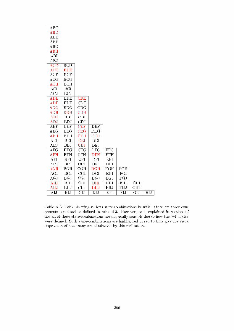
ABCABDABEABFABGABHABIABJACD BCDACE BCEACF BCFACG BCGACH BCHACI BCIACJ BCJADE BDE CDEADF BDF CDFADG BDG CDGADH BDH CDHADI BDI CDIADJ BDJ CDJAEF BEF CEF DEFAEG BEG CEG DEGAEH BEH CEH DEHAEI BEI CEI DEIAEJ BEJ CEJ DEJAFG BFG CFG DFG EFGAFH BFH CFH DFH EFHAFI BFI CFI DFI EFIAFJ BFJ CFJ DFJ EFJAGH BGH CGH DGH EGH FGHAGI BGI CGI DGI EGI FGIAGJ BGJ CGJ DGJ EGJ FGJAHI BHI CHI DHI EHI FHI GHIAHJ BHJ CHJ DHJ EHJ FHJ GHJAIJ BIJ CIJ DIJ EIJ FIJ GIJ HIJ
Table A.3: Table showing various state-combinations in which there are three com-ponents combined as dened in table 4.3. However, as is explained in section 4.2not all of these state-combinations are physically sensible due to how the wf blockswere dened. Such state-combinations are highlighted in red to thus give the visualimpression of how many are eliminated by this realisation.
300

ABCDABCEABCFABCGABCHABCIABCJABDEABDFABDGABDHABDIABDJABEFABEGABEHABEIABEJABFGABFHABFIABFJABGHABGIABGJABHIABHJABIJ
a
ACDE BCDEACDF BCDFACDG BCDGACDH BCDHACDI BCDIACDJ BCDJACEF BCEFACEG BCEGACEH BCEHACEI BCEIACEJ BCEJACFG BCFGACFH BCFHACFI BCFIACFJ BCFJACGH BCGHACGI BCGIACGJ BCGJACHI BCHIACHJ BCHJACIJ BCIJ
b
ADEF BDEF CDEFADEG BDEG CDEGADEH BDEH CDEHADEI BDEI CDEIADEJ BDEJ CDEJADFG BDFG CDFGADFH BDFH CDFHADFI BDFI CDFIADFJ BDFJ CDFJADGH BDGH CDGHADGI BDGI CDGIADGJ BDGJ CDGJADHI BDHI CDHIADHJ BDHJ CDHJADIJ BDIJ CDIJ
c
AEFG BEFG CEFG DEFGAEFH BEFH CEFH DEFHAEFI BEFI CEFI DEFIAEFJ BEFJ CEFJ DEFJAEGH BEGH CEGH DEGHAEGI BEGI CEGI DEGIAEGJ BEGJ CEGJ DEGJAEHI BEHI CEHI DEHIAEHJ BEHJ CEHJ DEHJAEIJ BEIJ CEIJ DEIJ
d
AFGH BFGH CFGH DFGH EFGHAFGI BFGI CFGI DFGI EFGIAFGJ BFGJ CFGJ DFGJ EFGJAFHI BFHI CFHI DFHI EFHIAFHJ BFHJ CFHJ DFHJ EFHJAFIJ BFIJ CFIJ DFIJ EFIJ
e
AGHI BGHI CGHI DGHI EGHI FGHIAGHJ BGHJ CGHJ DGHJ EGHJ FGHJAGIJ BGIJ CGIJ DGIJ EGIJ FGIJ
f
AHIJ BHIJ CHIJ DHIJ EHIJ FHIJ GHIJg
Table A.4: Table showing various state-combinations in which there are four com-ponents combined as dened in table 4.3. However, as is explained in section 4.2not all of these state-combinations are physically sensible due to how the wf blockswere dened. Such state-combinations are highlighted in red to thus give the visualimpression of how many are eliminated by this realisation.
301

ABC-DEABC-DFABC-DGABC-DHABC-DIABC-DJABC-EF ABD-EFABC-EG ABD-EGABC-EH ABD-EHABC-EI ABD-EIABC-EJ ABD-EJABC-FG ABD-FG ABE-FGABC-FH ABD-FH ABE-FHABC-FI ABD-FI ABE-FIABC-FJ ABD-FJ ABE-FJABC-GH ABD-GH ABE-GH ABF-GHABC-GI ABD-GI ABE-GI ABF-GIABC-GJ ABD-GJ ABE-GJ ABF-GJABC-HI ABD-HI ABE-HI ABF-HI ABG-HIABC-HJ ABD-HJ ABE-HJ ABF-HJ ABG-HJABC-IJ ABD-IJ ABE-IJ ABF-IJ ABG-IJ ABH-IJ
a
ACD-EFACD-EGACD-EHACD-EIACD-EJACD-FG ACE-FGACD-FH ACE-FHACD-FI ACE-FIACD-FJ ACE-FJACD-GH ACE-GH ACF-GHACD-GI ACE-GI ACF-GIACD-GJ ACE-GJ ACF-GJACD-HI ACE-HI ACF-HIACD-HJ ACE-HJ ACF-HJACD-IJ ACE-IJ ACF-IJ
ACG-HIACG-HJACG-IJACH-IJ
b
BCD-EFBCD-EGBCD-EHBCD-EIBCD-EJBCD-FG BCE-FGBCD-FH BCE-FHBCD-FI BCE-FIBCD-FJ BCE-FJBCD-GH BCE-GH BCF-GHBCD-GI BCE-GI BCF-GIBCD-GJ BCE-GJ BCF-GJBCD-HI BCE-HI BCF-HIBCD-IJ BCE-HJ BCF-HJBCD-HJ BCE-IJ BCF-IJ
BCG-HIBCG-HJBCG-IJBCH-IJ
c
Table A.5: Table showing various state-combinations in which there are ve com-ponents combined as dened in table 4.3. However, as is explained in section 4.2not all of these state-combinations are physically sensible due to how the wf blockswere dened. Such state-combinations are highlighted in red to thus give the visualimpression of how many are eliminated by this realisation.
302

ADE-FGADE-FHADE-FIADE-FJADE-GH ADF-GHADE-GI ADF-GIADE-GJ ADF-GJADE-HI ADF-HI ADG-HIADE-HJ ADF-HJ ADG-HJADE-IJ ADF-IJ ADG-IJ ADH-IJ
d
BDE-FGBDE-FHBDE-FIBDE-FJBDE-GH BDF-GHBDE-GI BDF-GIBDE-GJ BDF-GJBDE-HI BDF-HI BDG-HIBDE-HJ BDF-HJ BDG-HJBDE-IJ BDF-IJ BDG-IJ
BDH-IJe
CDE-FGCDE-FHCDE-FICDE-FJCDE-GH CDF-GHCDE-GI CDF-GICDE-GJ CDF-GJCDE-HI CDF-HI CDG-HICDE-HJ CDF-HJ CDG-HJCDE-IJ CDF-IJ CDG-IJ CDH-IJ
f
AEF-GHAEF-GIAEF-GJAEF-HI AEG-HIAEF-HJ AEG-HJAEF-IJ AEG-IJ AEH-IJ
g
BEF-GHBEF-GIBEF-GJBEF-HI BEG-HIBEF-HJ BEG-HJBEF-IJ BEG-IJ BEH-IJ
h
CEF-GHCEF-GICEF-GJCEF-HI CEG-HICEF-HJ CEG-HJCEF-IJ CEG-IJ CEH-IJ
i
DEF-GHDEF-GIDEF-GJDEF-HI DEG-HIDEF-HJ DEG-HJDEF-IJ DEG-IJ DEH-IJ
j
AFG-HIAFG-HJAFG-IJ AFH-IJ
k
BFG-HIBFG-HJBFG-IJ BFH-IJ
l
CFG-HICFG-HJCFG-IJ CFH-IJ
m
DFG-HIDFG-HJDFG-IJ DFH-IJ
n
EFG-HIEFG-HJEFG-IJ EFH-IJ
o
AGH-IJ BGH-IJ CGH-IJ DGH-IJ EGH-IJ FGH-IJp
Table A.5 continued: This table shows various state-combinations in which there areve components combined as dened in table 4.3. However, as is explained in section4.2 not all of these state-combinations are physically sensible due to how the wfblocks were dened. Such state-combinations are highlighted in red to thus give thevisual impression of how many are eliminated by this realisation.
303

ABC-DEFABC-DEGABC-DEHABC-DEIABC-DEJABC-DFGABC-DFHABC-DFIABC-DFJABC-DGHABC-DGIABC-DGJABC-DHIABC-DHJABC-DIJABC-EFG ABD-EFGABC-EFH ABD-EFHABC-EFI ABD-EFIABC-EFJ ABD-EFJABC-EGH ABD-EGHABC-EGI ABD-EGIABC-EGJ ABD-EGJABC-EHI ABD-EHIABC-EHJ ABD-EHJABC-EIJ ABD-EIJABC-FGH ABD-FGH ABE-FGHABC-FGI ABD-FGI ABE-FGIABC-FGJ ABD-FGJ ABE-FGJABC-FHI ABD-FHI ABE-FHIABC-FHJ ABD-FHJ ABE-FHJABC-FIJ ABD-FIJ ABE-FIJABC-GHI ABD-GHI ABE-GHI ABF-GHIABC-GHJ ABD-GHJ ABE-GHJ ABF-GHJABC-GIJ ABD-GIJ ABE-GIJ ABF-GIJABC-HIJ ABD-HIJ ABE-HIJ ABF-HIJ ABG-HIJ
a
AEF-GHIAEF-GHJAEF-GIJAEF-HIJ AEG-HIJ
b
BEF-GHIBEF-GHJBEF-GIJBEF-HIJ BEG-HIJ
c
CEF-GHICEF-GHJCEF-GIJCEF-HIJ CEG-HIJ
d
DEF-GHIDEF-GHJDEF-GIJDEF-HIJ DEG-HIJ
e
AFG-HIJ DFG-HIJBFG-HIJ EFG-HIJCFG-HIJ
f
Table A.6: Table showing various state-combinations in which there are six compo-nents combined as dened in table 4.3. However, as is explained in section 4.2 notall of these state-combinations are physically sensible due to how the wf blockswere dened. Such state-combinations are highlighted in red to thus give the visualimpression of how many are eliminated by this realisation.
304

ACD-EFGACD-EFHACD-EFIACD-EFJACD-EGHACD-EGIACD-EGJACD-EHIACD-EHJACD-EIJACD-FGH ACE-FGHACD-FGI ACE-FGIACD-FGJ ACE-FGJACD-FHI ACE-FHIACD-FHJ ACE-FHJACD-FIJ ACE-FIJACD-GHI ACE-GHI ACF-GHIACD-GHJ ACE-GHJ ACF-GHJACD-GIJ ACE-GIJ ACF-GIJACD-HIJ ACE-HIJ ACF-HIJ
ACG-HIJg
BCD-EFGBCD-EFHBCD-EFIBCD-EFJBCD-EGHBCD-EGIBCD-EGJBCD-EHIBCD-EHJBCD-EIJBCD-FGH BCE-FGHBCD-FGI BCE-FGIBCD-FGJ BCE-FGJBCD-FHI BCE-FHIBCD-FHJ BCE-FHJBCD-FIJ BCE-FIJBCD-GHI BCE-GHI BCF-GHIBCD-GHJ BCE-GHJ BCF-GHJBCD-GIJ BCE-GIJ BCF-GIJBCD-HIJ BCE-HIJ BCF-HIJ
BCG-HIJh
ADE-FGHADE-FGIADE-FGJADE-FHIADE-FHJADE-FIJADE-GHI ADF-GHIADE-GHJ ADF-GHJADE-GIJ ADF-GIJADE-HIJ ADF-HIJ ADG-HIJ
i
BDE-FGHBDE-FGIBDE-FGJBDE-FHIBDE-FHJBDE-FIJBDE-GHI BDF-GHIBDE-GHJ BDF-GHJBDE-GIJ BDF-GIJBDE-HIJ BDF-HIJ BDG-HIJ
j
CDE-FGHCDE-FGICDE-FGJCDE-FHICDE-FHJCDE-FIJCDE-GHI CDF-GHICDE-GHJ CDF-GHJCDE-GIJ CDF-GIJCDE-HIJ CDF-HIJ CDG-HIJ
k
Table A.6 continued: This table shows various state-combinations in which there aresix components combined as dened in table 4.3. However, as is explained in section4.2 not all of these state-combinations are physically sensible due to how the wfblocks were dened. Such state-combinations are highlighted in red to thus give thevisual impression of how many are eliminated by this realisation.
305

Appendix B
CrH CASSCF Calculations:
Results
(a) PEC, AB (b) DMZ, AB
(c) PEC, AF (d) DMZ, AF
Figure B.1: CASSCF calculations using a cc-pVDZ basis set that combine a single6Σ+ state (A) with a single other component as dened in table 4.3
306

CASSCF results (continued)
(a) PEC, AI (b) DMZ, AI
(c) PEC, AJ (d) DMZ, AJ
Figure B.2: CASSCF calculations using a cc-pVDZ basis set that combine a single6Σ+ state (A) with a single other component as dened in table 4.3
(a) PEC, ABC (b) DMZ, ABC
Figure B.3: CASSCF calculations using a cc-pVDZ basis set that combine a single6Σ+ state (A), a single 8Σ+ state (B) and a 4Σ+ state
307

CASSCF results (continued)
(a) PEC, BC (b) DMZ, BC
(c) PEC, BD (d) DMZ, BD
(e) PEC, BF (f) DMZ, BF
Figure B.4: CASSCF calculations using a cc-pVDZ basis set that combine a single8Σ+ state (B) with a single other component as dened in table 4.3.
308

CASSCF results (continued)
(a) PEC, BH (b) DMZ, BH
(c) PEC, BI (d) DMZ, BI
(e) PEC, BJ (f) DMZ, BJ
Figure B.5: CASSCF calculations using a cc-pVDZ basis set that combine a single8Σ+ state (B) with a single other component as dened in table 4.3. Continued
from previous page
309

CASSCF results (continued)
(a) PEC, DF (b) DMZ, DF
(c) PEC, DI (d) DMZ, DI
(e) PEC, DJ (f) DMZ, DJ
Figure B.6: CASSCF calculations using a cc-pVDZ basis set that combine two 6Σ+
states (D) with a single other component as dened in table 4.3.
310

CASSCF results (continued)
(a) PEC, FH (b) DMZ, FH
(c) PEC, FI (d) DMZ, FI
(e) PEC, FJ (f) DMZ, FJ
Figure B.7: CASSCF calculations using a cc-pVDZ basis set that combine a single4Π state (F) with a single other component as dened in table 4.3.
311
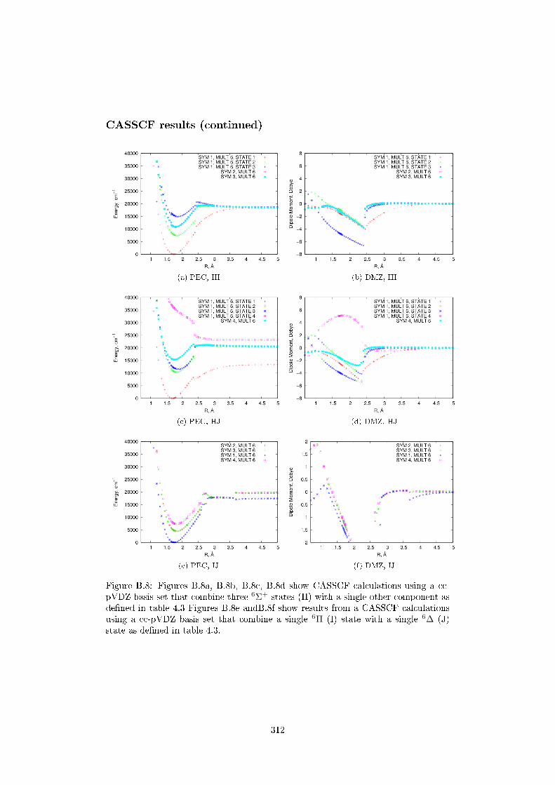
CASSCF results (continued)
(a) PEC, HI (b) DMZ, HI
(c) PEC, HJ (d) DMZ, HJ
(e) PEC, IJ (f) DMZ, IJ
Figure B.8: Figures B.8a, B.8b, B.8c, B.8d show CASSCF calculations using a cc-pVDZ basis set that combine three 6Σ+ states (H) with a single other component asdened in table 4.3 Figures B.8e andB.8f show results from a CASSCF calculationsusing a cc-pVDZ basis set that combine a single 6Π (I) state with a single 6∆ (J)state as dened in table 4.3.
312

CASSCF results (continued)
(a) PEC, ABF (b) DMZ, ABF
(c) PEC, ABI (d) DMZ, ABI
(e) PEC, ABJ (f) DMZ, ABJ
Figure B.9: CASSCF calculations using a cc-pVDZ basis set that combine a single6Σ+ (A) state and a single 8Σ+ (B) state with one other component as dened intable 4.3.
313

CASSCF results (continued)
(a) PEC, AFI (b) DMZ, AFI
(c) PEC, AF (d) DMZ, AFJ
(e) PEC, AIJ (f) DMZ, AIJ
Figure B.10: CASSCF calculations using a cc-pVDZ basis set that combine a single6Σ+ state (A) and eihter a single 4Π state (F) or a single 6Π state (I) along with oneother component as dened in table 4.3.
314

CASSCF results (continued)
(a) PEC, BDF (b) DMZ, BDF
(c) PEC, BDI (d) DMZ, BDI
(e) PEC, BDJ (f) DMZ, BDJ
Figure B.11: CASSCF calculations using a cc-pVDZ basis set that combine a single8Σ+ state (B) and two 6Σ+ states (D) with one other component as dened in table4.3.
315

CASSCF results (continued)
(a) PEC, BFH (b) DMZ, BFH
(c) PEC, BFI (d) DMZ, BFI
(e) PEC, BFJ (f) DMZ, BFJ
Figure B.12: CASSCF calculations using a cc-pVDZ basis set that combine a single8Σ+ state (B) and two 6Σ+ states (D) with one other component as dened in table4.3.
316

CASSCF results (continued)
(a) PEC, BHI (b) DMZ, BHI
(c) PEC, BHJ (d) DMZ, BHJ
(e) PEC, BIJ (f) DMZ, BIJ
Figure B.13: CASSCF calculations using a cc-pVDZ basis set that combine a single8Σ+ state (B) and a single 6Π state (I) with one other component as dened in table4.3.
317

CASSCF results (continued)
(a) PEC, DFI (b) DMZ, DFI
(c) PEC, DFJ (d) DMZ, DFJ
Figure B.14: CASSCF calculations using a cc-pVDZ basis set that combine a two6Σ+ states (D) and a single 4Π state (F) with one other component as dened intable 4.3.
(a) PEC, DIJ (b) DMZ, DIJ
Figure B.15: CASSCF calculations using a cc-pVDZ basis set that combine a two6Σ+ states (D) and a single 6Π state (F) with one other component as dened intable 4.3.
318

CASSCF results (continued)
(a) PEC, FHI (b) DMZ, FHI
(c) PEC, FHJ (d) DMZ, FHJ
Figure B.16: CASSCF calculations using a cc-pVDZ basis set that single 4Π state (F)and three 6Σ+ states (H) with one other component as dened in table 4.3.
(a) PEC, FIJ (b) DMZ, FIJ
Figure B.17: CASSCF calculations using a cc-pVDZ basis set that single 4Π state (F)and a single 6Π state with one other component as dened in table 4.3.
319

CASSCF results (continued)
(a) PEC, HIJ (b) DMZ, HIJ
Figure B.18: CASSCF calculations using a cc-pVDZ basis set that combine three 6Σ+
states (H), a single 6Π state (I) and a single 6∆ state as dened in table 4.3.
(a) PEC, AFIJ (b) DMZ, AFIJ
320

(a) PEC, ABFI (b) DMZ, ABFI
(c) PEC, ABFJ (d) DMZ, ABFJ
(e) PEC, ABIJ (f) DMZ, ABIJ
Figure B.19: CASSCF calculations using a cc-pVDZ basis set that combine a single6Σ+ state (A), a single 8Σ+ state (B) and two other componenets as dened in table4.3.
321

CASSCF results (continued)
(a) PEC, BDFI (b) DMZ, BDFI
(c) PEC, BDFJ (d) DMZ, BDFJ
Figure B.20: CASSCF calculations using a cc-pVDZ basis set that combine a single8Σ+ state (B), two 6Σ+ state (D), a single 8Σ+ state (B) and two other componenetsas dened in table 4.3.
322

CASSCF results (continued)
(a) PEC, BFHI (b) DMZ, BFHI
(c) PEC, BFHJ (d) DMZ, BFHJ
(e) PEC, BFIJ (f) DMZ, BFIJ
Figure B.21: CASSCF calculations using a cc-pVDZ basis set that combine a single8Σ+ state (B), a single 4Π state and two other componenets as dened in table 4.3.
323

CASSCF results (continued)
(a) PEC, BHIJ (b) DMZ, BHIJ
(c) PEC, DFIJ (d) DMZ, DFIJ
Figure B.22: CASSCF calculations using a cc-pVDZ basis set that combine two 6Σ+
states (D), a single 4Π state (F) and two other componenets as dened in table 4.3.
(a) PEC, FHIJ (b) DMZ, FHIJ
Figure B.23: CASSCF calculations using a cc-pVDZ basis set that combine a single4Π state (F), three 6Σ+ states (H), and two other componenets as dened in table4.3.
324

(a) PEC, ABF-IJ (b) DMZ, ABF-IJ
(c) PEC, BDF-IJ (d) DMZ, BDF-IJ
(e) PEC, BFH-IJ (f) DMZ, BFH-IJ
Figure B.24: CASSCF calculations using a cc-pVDZ basis set that combine ve com-ponents as dened in table 4.3.
325

Appendix C
MnH CASSCF Testing Results
(a) (b)
Figure C.1: CASSCF calculations using a cc-pVQZ basis set that combine a single7Σ+ and a single 5Σ+ state. See section 7.1 for guidance.
(a) (b)
Figure C.2: CASSCF calculations using a cc-pVQZ basis set that combine a single7Σ+ state, a single 5Σ+ state and all six other components (i.e. A, B, C, D,
E and F) as dened in table 7.1.
326

(a) (b)
(c) (d)
(e) (f)
Figure C.3: CASSCF calculations using a cc-pVQZ basis set that combine a single7Σ+ and 5Σ+ state with a single other component as dened in table 7.1.
327

(a) (b)
Figure C.4: CASSCF calculations using a cc-pVQZ basis set that combine a single7Σ+, a single 5Σ+ state, a single 5Π state (i.e. B) with a single other component as
dened in table 7.1.
(a) (b)
(c) (d)
Figure C.5: CASSCF calculations using a cc-pVQZ basis set that combine a single7Σ+, two 5Σ+ states (i.e. A) with a single other component as dened in table 7.1.
328

(a) (b)
(c) (d)
(e) (f)
Figure C.6: CASSCF calculations using a cc-pVQZ basis set that combine a single7Σ+ and 5Σ+ state with a single other component as dened in table 7.1.
329

(a) (b)
(c) (d)
(e) (f)
Figure C.7: CASSCF calculations using a cc-pVQZ basis set that combine a single7Σ+, two 5Σ+ states (i.e. A) with a single other component as dened in table 7.1.
330

(a) (b)
(c) (d)
(e) (f)
Figure C.8: CASSCF calculations using a cc-pVQZ basis set that combine a single7Σ+, a single 5Σ+ state, a single 5Π state (i.e. B) with a single other component as
dened in table 7.1.
331

(a) (b)
(c) (d)
(e) (f)
Figure C.9: CASSCF calculations using a cc-pVQZ basis set that combine a single7Σ+ state, two symmetry 1 components of quintet multiplicity, a single symmetry 4component of quintet multiplicity (i.e. C) and a single other component as dened
in table 7.1.
332

(a) (b)
(c) (d)
Figure C.10: CASSCF calculations using a cc-pVQZ basis set that combine a two7Σ+ states (i.e. D), a single 5Σ+ state and a single other component as dened in
table 7.1.
(a) (b)
Figure C.11: CASSCF calculations using a cc-pVQZ basis set that combine a single5Σ+ state, two symmetry 1 components of septuplet multiplicity, a single symmetry4 component of septuplet multiplicity (i.e. F) and a 7Π (i.e. E) as dened in
table 7.1.
333

(a) (b)
Figure C.12: CASSCF calculations using a cc-pVQZ basis set that combine a single7Σ+ state, three 5Σ+ states, a 5Π state and a 5∆ state as dened in table 7.1, two of
which are A and B.
(a) (b)
(c) (d)
Figure C.13: CASSCF calculations using a cc-pVQZ basis set that combine a single7Σ+ state, a single 5Σ+ state and three other components dened in table 7.1, two
of which are B and D.
334

(a) (b)
(c) (d)
(e) (f)
Figure C.14: CASSCF calculations using a cc-pVQZ basis set that combine a single7Σ+ state, two 5Σ+ states (A), a 5Π (B) and one other component as dened in
table 7.1, two of which are A and B.
335
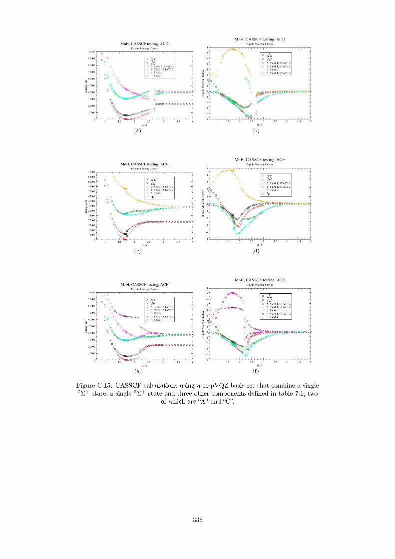
(a) (b)
(c) (d)
(e) (f)
Figure C.15: CASSCF calculations using a cc-pVQZ basis set that combine a single7Σ+ state, a single 5Σ+ state and three other components dened in table 7.1, two
of which are A and C.
336

(a) (b)
(c) (d)
(e) (f)
Figure C.16: CASSCF calculations using a cc-pVQZ basis set that combine a single7Σ+ state, a single 5Σ+ state and three other components dened in table 7.1, one
of which is A and the other two selected from D, E and F.
337

(a) (b)
(c) (d)
(e) (f)
Figure C.17: CASSCF calculations using a cc-pVQZ basis set that combine a single7Σ+ state, a single 5Σ+ state and three other components dened in table 7.1, two
of which are B and C.
338

(a) (b)
(c) (d)
(e) (f)
Figure C.18: CASSCF calculations using a cc-pVQZ basis set that combine a single7Σ+ state, a single 5Σ+ state and three other components dened in table 7.1, two
of which are E and F.
339
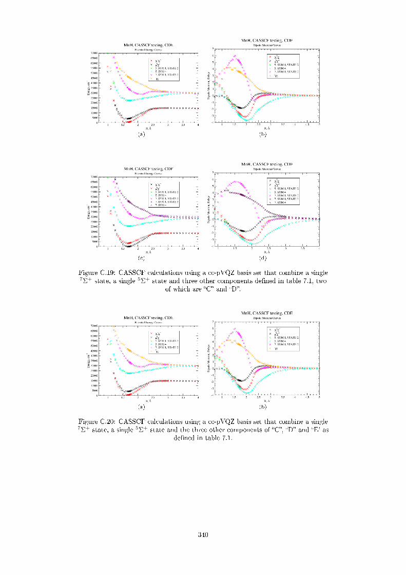
(a) (b)
(c) (d)
Figure C.19: CASSCF calculations using a cc-pVQZ basis set that combine a single7Σ+ state, a single 5Σ+ state and three other components dened in table 7.1, two
of which are C and D.
(a) (b)
Figure C.20: CASSCF calculations using a cc-pVQZ basis set that combine a single7Σ+ state, a single 5Σ+ state and the three other components of C, D and E' as
dened in table 7.1.
340

(a) (b)
(c) (d)
(e) (f)
Figure C.21: CASSCF calculations using a cc-pVQZ basis set that combine a single7Σ+ state, a single 5Σ+ state and four other components dened in table 7.1, three
of which are A, B and C.
341

(a) (b)
(c) (d)
(e) (f)
Figure C.22: CASSCF calculations using a cc-pVQZ basis set that combine a single7Σ+ state, a single 5Σ+ state and four other components dened in table 7.1, two of
which are A and B and the other two selected from D, E and F.
342

(a) (b)
(c) (d)
(e) (f)
Figure C.23: CASSCF calculations using a cc-pVQZ basis set that combine a single7Σ+ state, a single 5Σ+ state and four other components dened in table 7.1, two of
which are A and C and the other two selected from D, E and F.
343

(a) (b)
(c) (d)
(e) (f)
Figure C.24: CASSCF calculations using a cc-pVQZ basis set that combine a single7Σ+ state, a single 5Σ+ state and four other components dened in table 7.1, two of
which are B and C and the other two selected from D, E and F.
344

(a) (b)
(c) (d)
(e) (f)
Figure C.25: CASSCF calculations using a cc-pVQZ basis set that combine a single7Σ+ state, a single 5Σ+ state and four other components dened in table 7.1, three
of which are D, E and F and the other selected from A, B and C.
345

(a) (b)
(c) (d)
(e) (f)
Figure C.26: CASSCF calculations using a cc-pVQZ basis set that combine a single7Σ+ state, a single 5Σ+ state and ve other components dened in table 7.1, threeof which are A, B and C and the other two selected from D, E and F.
346

(a) (b)
(c) (d)
(e) (f)
Figure C.27: CASSCF calculations using a cc-pVQZ basis set that combine a single7Σ+ state, a single 5Σ+ state and ve other components dened in table 7.1, threeof which are D, E and F and the other two selected from A, B and C.
347

Appendix D
Preliminary Calculations for
Group II diatomic Hydrides
As was the case for CrH and MnH, before any ab initio calculations were undertaken,
the lowest lying electronic states needed to be determined by consideration of the
atomic dissociation limits for the H, Be, Mg and Ca atoms. These are shown in tables
D.1, D.2, D.3 and D.4 respectively.
Cong Term J Level(cm−1)1s 2S 1/2 0.00000 00000
2p 2P 0 1/2 82 259.91911333/2 92 259.2850014
Table D.1: H atom dissociation energy limits up to approximately 92 000 cm−1.
Conguration Term J Level(cm−1)1s22s2 1S 0 0.000
1s22s2p 3P o0 21 978.281 21 978.9252 21 981.27
1s22s2p 1P o 1 42 565.35
Table D.2: Be atom dissociation energy limits up to approximately 42 000 cm−1.
Conrguation Term J Level(cm−1)2p63s2 1S 0 0.000
3s3p 3P o0 21 850.4051 21 870.4642 21 911.178
3s3p 1P o 1 35 051.264
Table D.3: Mg atom dissociation energy limits up to approximately 35 000 cm−1.
348

Conguration Term J Level(cm−1)3p64s2 1S 0 0.000
3p64s4p 3P o0 15 157.9011 15 210.0632 15 315.943
3p63d4s 3D1 20 335.3602 20 349.2603 20 371.000
3p63d4s 1D 2 21 849.6343p64s4p 1P o 1 23 652.3043p64s5s 3S 1 31 539.495
Table D.4: Ca atom dissociation energy limits up to approximately 32 000 cm−1.
To summarise, referring to tables D.2, D.3 and D.4 for BeH, CaH, MgH respec-
tively, it can be seen that molecular states arising from the 1S and 3P 0 atomic terms
are of greatest interest. For both Be and Mg, the 1P 0 terms are signicantly higher in
energy so thus we can tentatively assume that that interactions with molecular states
arising from these atomic dissociation limits with the lower molecular states will be
negligible. Table D.5 summarises the molecular states of interest arising from the
various atomic dissociation limits for BeH, MgH and CaH. Finally, tables D.6, D.7
and D.8 show the deduction of the closed and active space required for the molecules
of BeH, MgH and CaH respectively with a summary of results shown in table D.9.
Atomic TermEnergy (cm−1)
Molecular StatesBeH MgH CaH
1S 0.000 0.000 0.000 2Σ+
3P o 21 980.156 21 980.854 15 263.0892Σ+ 4Σ+
2Π 4Π
3D 20 356.625
2Σ+ 4Σ+
2Π 4Π2∆ 4∆
1D 21 849.634
2Σ+
2Π2∆
1P o 42 565.350 35 051.264 23 652.3042Σ+
2Π3S 31 539.495 2Σ+ 4Σ+
Table D.5: Molecular states expected for alkaline metal hydrides.
349

OrbitalsC2V Symmetry
A1 B1 B2 A2closed 1s2 1 0 0 0Total closed 1 0 0 0
Active2s2 1 0 0 0
1s1(H) 1 0 0 0Total active 2 0 0 0
Total occupied 3 0 0 0(a)
OrbitalsC2V Symmetry
A1 B1 B2 A2closed 1s2 1 0 0 0Total closed 1 0 0 0
Active2s1 1 0 0 02p1 1 1 1 0
1s1(H) 1 0 0 0Total active 3 1 1 0
Total occupied 4 1 1 0(b)
Table D.6: Electronic congurations for low-lying states of diatomic molecule BeH(a) Closed and Occupied orbitals for the 1s22s2 ground state conguration(b) Closed and Occupied orbitals for the 1s22s12p1 electronic conguration
OrbitalsC2V Symmetry
A1 B1 B2 A2
closed1s2 1 0 0 02s2 1 0 0 02p6 1 1 1 0
Total closed 3 1 1 0
Active3s2 1 0 0 0
1s1(H) 1 0 0 0Total active 2 0 0 0
Total occupied 5 1 1 0(a)
OrbitalsC2V Symmetry
A1 B1 B2 A2
closed1s2 1 0 0 02s2 1 0 0 02p6 1 1 1 0
Total closed 3 1 1 0
Active3s1 1 0 0 03p1 1 1 1 0
1s1(H) 1 0 0 0Total active 3 1 1 0
Total occupied 6 2 2 0(b)
Table D.7: Electronic congurations for low-lying states of diatomic molecule MgH(a) Closed and Occupied orbitals for the 3s2 ground state conguration(b) Closed and Occupied orbitals for the 3s13p1 electronic conguration
OrbitalsC2V Symmetry
A1 B1 B2 A2
closed
1s2 1 0 0 02s2 1 0 0 02p6 1 1 1 03s2 1 0 0 03p6 1 1 1 0
Total closed 5 2 2 0
Active4s2 1 0 0 0
1s1(H) 1 0 0 0Total active 2 0 0 0
Total occupied 7 2 2 0(a)
OrbitalsC2V Symmetry
A1 B1 B2 A2
closed
1s2 1 0 0 02s2 1 0 0 02p6 1 1 1 03s2 1 0 0 03p6 1 1 1 0
Total closed 5 2 2 0
Active4s1 1 0 0 04p1 1 1 1 0
1s1(H) 1 0 0 0Total active 3 1 1 0
Total occupied 8 3 3 0
Table D.8: Electronic congurations for low-lying states of diatomic molecule CaH(a) Closed and Occupied orbitals for the 3p64s2 ground state conguration(b) Closed and Occupied orbitals for the 3p64s14p1 electronic conguration
As was the case for MnH, for each of the three Group II diatomic hydrides, there is
a LOWER and UPPER active space: the UPPER active space is required for the
350

calculation of molecular states which do not converge to the lowest lying asymptote
of the group II metal atom. Table D.9 summaries these various active spaces using
the information determined from tables D.6, D.7 and D.8.
MoleculeActive space
ClosedOccupied
Lower UpperBeH 1000 3000 4110MgH 3110 5110 6220CaH 5220 7220 8330
Table D.9: Summary of active spaces required for calculation of electronic states forBeH, MgH and CaH.
D.1 Preliminary MRCI calculations
Preliminary MRCI calculations were performed for the Group II diatomic hydrides
of BeH, MgH and CaH. The basis set used was cc-pVDZ. For each molecule, the
proceeding CASSCF calculation done before the CI calculations was that for the sin-
gle X2Σ+ ground state using the relevant LOWER active space for each molecule
as summarised in table D.9. Figure D.1 shows for BeH, MgH and CaH the PECs
and DMCs obtained for these CASSCF calculations which generated the starting
orbitals used in the subsequent CI calculations. As for CrH and MnH, the CI calcula-
tions of PECs and DMCs for the various electronic states were performed by dening
PROCS . These are outlines in table D.10 which also states the required active
space to obtain the particular electronic states. Simply put, for all three molecules
the X2Σ+ state only requires the LOWER active space: the four other electronic
states require the use of the UPPER active space. As was a similar case for MnH,
PROC wf cards STATE Occupied orbitalsS1
doublet, symmetry 1, 1 state X2Σ+ LOWERS2 UPPERS6 doublet, symmetry 1, 2 states X2Σ+, A2Σ+ UPPERS3 doublet, symmetries 2 & 3, 1 state each 2Π UPPERS4 quartet, symmetry 1, 1 state 4Σ+ UPPERS5 quartet, symmetries 2 & 3, 1 state each 4Π UPPER
Table D.10: Summary of PROCS used in MOLPRO to calculate at CI level of theorythe various low-lying electronic states of BeH, MgH and CaH.
it was found that better (i.e. lower in energy) PEC for the X2Σ+ state was obtained
by using PROC S6 in which two 2Σ+ states are requested and the UPPER active
space is used. The results of calculations for the PECs and DMCs of the states listed
in table D.10 are shown in gure D.2.
As was the case for CrH & MnH, the expected couplings between the various elec-
tronic states can be deduced by consideration of the various selection rules governing
changes in spin (S), orbital angular momenta (L) and total angular momenta J . A
sample of couplings calculated is shown in gure D.3 which is for BeH.
351

(a) (b)
(c) (d)
(e) (f)
Figure D.1: PECs and DMCs calculated at CASSCF level of theory using acc-pVDZ basis set for the ground X2Σ+ states of BeH, MgH and CaH. In all casesthe CASSCF calculation was for this state only and used the respective LOWER
active space for each molecule as dened in table D.9.
D.2 CASSCF state-combination testing
In addition to these preliminary calculations of PECs, DMCs and couplings, the eect
of dierent combination of states used in the initial CASSCF has been tested out as
was done in a a similar vein for CrH and MnH. More specically the number of inter-
nuclear points (as dened on the rgeom grid, see section 2.7.1) for which a calculation
converged has been summarised from this preliminary work. For all these dierent
CASSCF combinations the ground X2Σ+ state was included. These test calcula-
tions were done using a cc-pVQZ basis set and, in contrast to the results presented
in section D.1, all of these CASSCF calculations used the respective UPPER active
352

(a) (b)
(c) (d)
(e) (f)
Figure D.2: PEC and DMC curves calculated at CI level for BeH, CaH and MgHusing cc-pVDZ basis set and the UPPER active space as dened in table D.9. Theproceeding CASSCF calculation for which the CI orbitals were built upon was for
the ground X2Σ+ state using the respective LOWER active space.
space as dened in table D.9. As this table shows, for all three molecules, all electronic
states above the X2Σ+ state require this. Table D.11 sets out the naming scheme (i.e.
A, B, C, D) used. Referring to table D.11, combinations of these components (i.e. A,
B, C, D) were then tested out by running CASSCF calculations. A summary of all
the possible combinations of these components is shown in table D.12. Table D.12
thus shows that there are 15 possible CASSCF combinations to test out i.e.∑4i=1
4Ci =4 C1 + 4C2 + 4C3 + 4C4 = 4 + 6 + 4 + 1 = 15. The PECs and DMCs
produced by these dierent combinations of states within a CASSCF calculation are
shown in sections D.2.1, D.2.2 and D.2.3 for BeH, MgH and CaH respectively.
353

(a) (b)
(c) (d)
(e) (f)
Figure D.3: Transition Dipole, anglar momenta and Spin-Orbit Couplings for BeHcalculated at CI level of theory using a cc-pVDZ basis set and the UPPER activespace as dened in table D.9. The proceeding CASSCF calculation for which the CIorbitals were built upon was for the ground X2Σ+ state using the LOWER active
space for BeH.
Component State(s) Colour used in subsequnent guresX X2Σ+ RedA 2Σ+(II) BlackB 2Π CyanC 4Σ+ MagnetaD 4Π Orange
Table D.11: Summary of letters ( `components) assigned to the various low-lyingstates for testing at CASSCF level for the group 2 hydrides.
354

Singles Pairs Triplets QuadsA AB ABC ABCDB AC ABDC AD ACDD BC BCD
BDCD
Table D.12: Summary of all the CASSCF test calculations performed for each of BeH,MgH and CaH. In this table the letters A, B, C and D have been dened in terms ofwhat molecular electronic states they represent in table D.11.
D.2.1 BeH
(a) (b)
(c) (d)
Figure D.4: CASSCF calculations of PECs and DMCs for BeH using a cc-pVQZbasis set that combine the ground X2Σ+ state, the 2Σ+(II) state (A) and other
components as dened in table D.11.
355

(a) (b)
(c) (d)
(e) (f)
(g) (h)
Figure D.5: CASSCF calculations of PECs and DMCs for BeH using a cc-pVQZbasis set that combine the ground X2Σ+ state and a single other component as
dened in table D.11.
356

(a) (b)
(c) (d)
(e) (f)
Figure D.6: CASSCF calculations of PECs and DMCs for BeH using a cc-pVQZbasis set that combine the ground X2Σ+ state and 2Σ+(II) state (A) with and a
single other component as dened in table D.11.
357

(a) (b)
(c) (d)
(e) (f)
Figure D.7: CASSCF calculations of PECs and DMCs for BeH using a cc-pVQZbasis set that combine the ground X2Σ+ state and two other components as dened
in table D.11.
358

(a) (b)
(c) (d)
(e) (f)
Figure D.8: CASSCF calculations of PECs and DMCs for BeH using a cc-pVQZbasis set that combine the ground X2Σ+ state, the 2Σ+(II) state (A) and two
other components as dened in table D.11.
359

D.2.2 MgH
(a) (b)
(c) (d)
(e) (f)
(g) (h)
Figure D.9: CASSCF calculations of PECs and DMCs for MgH using a cc-pVQZbasis set that combine the ground X2Σ+ state and a single other component as
dened in table D.11.
360

(a) (b)
(c) (d)
(e) (f)
Figure D.10: CASSCF calculations of PECs and DMCs for MgH using a cc-pVQZbasis set that combine the ground X2Σ+ state and 2Σ+(II) state (A) with and a
single other component as dened in table D.11.
361

(a) (b)
(c) (d)
(e) (f)
Figure D.11: CASSCF calculations of PECs and DMCs for MgH using a cc-pVQZbasis set that combine the ground X2Σ+ state and two other components as dened
in table D.11.
362

(a) (b)
(c) (d)
(e) (f)
Figure D.12: CASSCF calculations of PECs and DMCs for MgH using a cc-pVQZbasis set that combine the ground X2Σ+ state, the 2Σ+(II) state (A) and two
other components as dened in table D.11.
363

(a) (b)
(c) (d)
Figure D.13: CASSCF calculations of PECs and DMCs for MgH using a cc-pVQZbasis set that combine the ground X2Σ+ state, the 2Σ+(II) state (A) and other
components as dened in table D.11.
D.2.3 CaH
(a) (b)
Figure D.14: CASSCF calculations of PECs and DMCs for CaH using a cc-pVQZbasis set that combine the ve lowest electronic states.
364

(a) (b)
(c) (d)
(e) (f)
(g) (h)
Figure D.15: CASSCF calculations of PECs and DMCs for CaH using a cc-pVQZbasis set that combine the ground X2Σ+ state and a single other component as
dened in table D.11.
365

(a) (b)
(c) (d)
(e) (f)
Figure D.16: CASSCF calculations of PECs and DMCs for CaH using a cc-pVQZbasis set that combine the ground X2Σ+ state and 2Σ+(II) state (A) with and a
single other component as dened in table D.11.
366

(a) (b)
(c) (d)
(e) (f)
Figure D.17: CASSCF calculations of PECs and DMCs for CaH using a cc-pVQZbasis set that combine the ground X2Σ+ state and two other components as dened
in table D.11.
367

(a) (b)
(c) (d)
(e) (f)
(g) (h)
Figure D.18: CASSCF calculations of PECs and DMCs for CaH using a cc-pVQZbasis set that combine the ground X2Σ+ state and three other components as
dened in table D.11.
These preliminary CASSCF orbital testing results can thus act as a guide to what
combinations of states will give favourable convergence properties at CI level. For each
set of CASSCF orbitals generated, PECs and DMCs for the ve lowest-lying states
368

of BeH, MgH and CaH have been calculated at CI level. Maps of the inter-nuclear
distances which converge for these various states at CI level for the dierent CASSCF
calculations (i.e. dierent combinations of states put in a CASSCF calculation) are
shown in section D.3.
D.3 Convergence at CI level as a function of CASSCF
orbitals
In the following tables, a • symbol indicates that the CI calculation converged for this
inter-nuclear distance using the CASSCF orbitals generated from combining various
states (e.g. A, BC, ABCD etc) converged. A • symbol indicates that, according to
MOLPRO there was insucient overlap between the various orbitals and a • symbolindicates that there was a Catastrophic failure in diagonalization (hsdel). The CI
calculations run are the PROCs S6, S3, S4 and S5 as dened in table D.10. In the fol-
lowing tables the inter-nuclear distances are those of the rgeom matrix summarised
in section 2.7.1. The letters going along the horizontal are dened in table D.11; the
letter X refers to the CASSCF calculation described in section D. As a reminder,
it should be noted when interpreting these tables that convergence does not always
guarantee that the curves plotted from these converged points will be devoid of dis-
continuities. For BeH, for the case of calculating the PEC and DMC of the 4Π state,
all points for all inter-nuclear distances and various CASSCF calculations converged.
For the case of calculating the PEC and DMC of the 4Σ+ state of MgH, all points for
all inter-nuclear distances and various CASSCF calculations converged.
369

R() X A B C D AB AC AD BC BD CD ABC ABD ACD BCD ABCD0.70 • • • • • • • • • • •0.80 • • • • • • • • • • • •0.90 • • • • • • • • • • •1.00 • • • • • • • • • • •1.10 • • • • • • • • •1.20 • • • • • • • • • • • • • • • •1.25 • • • • • • • • • • • • • • • •1.30 • • • • • • • • • • • • • • •1.35 • • • • • • • • • • • • • • •1.40 • • • • • • • • • • • • • • •1.45 • • • • • • • • • • • • • • • •1.50 • • • • • • • • • • • • • • • •1.55 • • • • • • • • • • • • • • • •1.60 • • • • • • • • • • • • • • • •1.65 • • • • • • • • • • • • • • • •1.66 • • • • • • • • • • • • • • • •1.68 • • • • • • • • • • • • • • • •1.69 • • • • • • • • • • • • • • • •1.70 • • • • • • • • • • • • • • • •1.71 • • • • • • • • • • • • • • • •1.72 • • • • • • • • • • • • • • • •1.73 • • • • • • • • • • • • • • • •1.74 • • • • • • • • • • • • • • • •1.75 • • • • • • • • • • • • • • • •1.76 • • • • • • • • • • • • • • • •1.78 • • • • • • • • • • • • • • • •1.80 • • • • • • • • • • • • • • • •1.85 • • • • • • • • • • • • • • • •1.90 • • • • • • • • • • • • • • • •1.95 • • • • • • • • • • • • • • • •2.00 • • • • • • • • • • • • • • • •2.05 • • • • • • • • • • • • • • • •2.10 • • • • • • • • • • • • • • • •2.15 • • • • • • • • • • • • • • • •2.20 • • • • • • • • • • • • • • • •2.25 • • • • • • • • • • • • • • •2.30 • • • • • • • • • • • • • • • •2.35 • • • • • • • • • • • • •2.40 • • • • • • • • • • •2.45 • • • • • • • • •2.50 • • • •2.55 • • • •2.60 • • • •2.65 • • • •2.70 • • • •2.75 • • • •2.80 • • • • • •2.85 • • • • • •2.90 • • • • • •2.95 • • • • • • •3.00 • • • • • • • • • •3.10 • • • • • • • • • •3.20 • • • • • • • • • •3.30 • • • • • • • • • • • •3.40 • • • • • • • • • • • •3.50 • • • • • • • • • • • •3.60 • • • • • • • • • • • • • • • •3.70 • • • • • • • • • • • • • • • •3.80 • • • • • • • • • • • • • • • •
Table D.13: Summary of convergence for BeH for CI calculations of the X2Σ+ and2Σ+ for a range of inter-nuclear distances R. For inter-nuclear distances greatedthan R = 3.8 Å, all CI calculations converged. The grid of inter-nuclear points isdened in section 2.7.1. The CI calculations were based on the orbitals produced byproceeding CASSCF calculations which were performed for dierent combinations ofthe various low-lying electronic states indicated by the letters A, B, C, and D: thislettering scheme is dened in table D.11.
370

R() X A B C D AB AC AD BC BD CD ABC ABD ACD BCD ABCD0.70 • • • • • • • • • • • •0.80 • • • • • • • • • • • •0.90 • • • • • • • • • • • •1.00 • • • • • • • • • • • •1.10 • • • • • • • • • • • •1.20 • • • • • • • • • • • • • •1.25 • • • • • • • • • • • • • •1.30 • • • • • • • • • • • • • •1.35 • • • • • • • • • • • • • •1.40 • • • • • • • • • • • • • •1.45 • • • • • • • • • • • • • •1.50 • • • • • • • • • • • • • •1.55 • • • • • • • • • • • • • •1.60 • • • • • • • • • • • • • •1.65 • • • • • • • • • • • • • •1.66 • • • • • • • • • • • • • •1.68 • • • • • • • • • • • • • •1.69 • • • • • • • • • • • • • •1.70 • • • • • • • • • • • • • •1.71 • • • • • • • • • • • • • •1.72 • • • • • • • • • • • • • • •1.73 • • • • • • • • • • • • • • •1.74 • • • • • • • • • • • • • • •1.75 • • • • • • • • • • • • • • • •1.76 • • • • • • • • • • • • • • • •1.78 • • • • • • • • • • • • • • • •1.80 • • • • • • • • • • • • • • • •
Table D.14: Summary of convergence for BeH for CI calculations of the 2Π statefor a range of inter-nuclear distances R. For inter-nuclear distances greated thanR = 1.8 Å, all CI calculations converged. The grid of inter-nuclear points is dened insection 2.7.1. The CI calculations were based on the orbitals produced by proceedingCASSCF calculations which were performed for dierent combinations of the variouslow-lying electronic states indicated by the letters A, B, C, and D: this letteringscheme is dened in table D.11.
R (Å) X A B C D AB AC AD BC BD CD ABC ABD ACD BCD ABCD0.70 • • • • • • • • • • • •0.80 • • • • • • • • • • • •0.90 • • • • • • • • • • •1.00 • • • • • • • • • • •1.10 • • • • • • • • •1.20 • • • • • • • •1.25 • • • • • • • •1.30 • • • • • • • •1.35 • • • • • • • •1.40 • • •1.45 •1.50 • • • • • •1.55 • • • • • • • • • • • • • • •1.60 • • • • • • • • • • • • • • • •1.65 • • • • • • • • • • • • • • • •1.66 • • • • • • • • • • • • • • • •1.68 • • • • • • • • • • • • • • • •1.69 • • • • • • • • • • • • • • • •1.70 • • • • • • • • • • • • • • • •
Table D.15: Summary of convergence for BeH for CI calculations of the 4Σ+ statefor a range of inter-nuclear distances R. For inter-nuclear distances greated thanR = 1.7 Å, all CI calculations converged. The grid of inter-nuclear points is dened insection 2.7.1. The CI calculations were based on the orbitals produced by proceedingCASSCF calculations which were performed for dierent combinations of the variouslow-lying electronic states indicated by the letters A, B, C, and D: this letteringscheme is dened in table D.11.
371

R() X A B C D AB AC AD BC BD CD ABC ABD ACD BCD ABCD0.70 • • • • • • • • • • • • • • • •0.80 • • • • • • • • • • • • • • • •0.90 • • • • • • • • • • • • • • • •1.00 • • • • • • • • • • • • • • • •1.10 • • • • • • • • • • • • • • • •1.20 • • • • • • • • • • • • • • • •1.25 • • • • • • • • • • • • • • • •1.30 • • • • • • • • • • • • • • • •1.35 • • • • • • • • • • • • • • • •1.40 • • • • • • • • • • • • • • • •1.45 • • • • • • • • • • • • • • • •1.50 • • • • • • • • • • • • • • • •1.55 • • • • • • • • • • • • • • • •1.60 • • • • • • • • • • • • • • • •1.65 • • • • • • • • • • • • • • • •1.66 • • • • • • • • • • • • • • • •1.68 • • • • • • • • • • • • • • • •1.69 • • • • • • • • • • • • • • • •1.70 • • • • • • • • • • • • • • • •1.71 • • • • • • • • • • • • • • • •1.72 • • • • • • • • • • • • • • • •1.73 • • • • • • • • • • • • • • • •1.74 • • • • • • • • • • • • • • • •1.75 • • • • • • • • • • • • • • • •1.76 • • • • • • • • • • • • • • • •1.78 • • • • • • • • • • • • • • • •1.80 • • • • • • • • • • • • • • • •1.85 • • • • • • • • • • • • • • • •1.90 • • • • • • • • • • • • • • • •1.95 • • • • • • • • • • • • • • • •2.00 • • • • • • • • • • • • • • • •2.05 • • • • • • • • • • • • • • • •2.10 • • • • • • • • • • • • • • • •2.15 • • • • • • • • • • • • • • • •2.20 • • • • • • • • • • • • • • • •2.25 • • • • • • • • • • • • • • • •2.30 • • • • • • • • • • • • • • • •2.35 • • • • • • • • • • • • • • • •2.40 • • • • • • • • • • • • • • • •2.45 • • • • • • • • • • • • • • • •2.50 • • • • • • • • • • • • • • • •2.55 • • • • • • • • • • • • • • • •2.60 • • • • • • • • • • • • • • • •2.65 • • • • • • • • • • • • • • • •2.70 • • • • • • • • • • • • • • • •2.75 • • • • • • • • • • • • • • • •2.80 • • • • • • • • • • • • • • • •2.85 • • • • • • • • • • • • • • • •2.90 • • • • • • • • • • • • • • • •2.95 • • • • • • • • • • • • • • • •3.00 • • • • • • • • • • • • • • • •3.10 • • • • • • • • • • • • • • • •3.20 • • • • • • • • • • • • • • • •3.30 • • • • • • • • • • • • • • • •3.40 • • • • • • • • • • • • • • • •3.50 • • • • • • • • • • • • • • • •3.60 • • • • • • • • • • • • • • • •3.70 • • • • • • • • • • • • • • • •3.80 • • • • • • • • • • • • • • • •3.90 • • • • • • • • • • • • • • • •4.00 • • • • • • • • • • • • • • • •4.10 • • • • • • • • • • • • • • • •4.20 • • • • • • • • • • • • • • • •4.30 • • • • • • • • • • • • • • • •4.40 • • • • • • • • • • • • • • • •
Table D.16: Summary of convergence for MgH for CI calculations of the X2Σ+ and2Σ+ state for a range of inter-nuclear distances R. For inter-nuclear distances greatedthan R = 4.4 Å, all CI calculations converged. The grid of inter-nuclear points isdened in section 2.7.1. The CI calculations were based on the orbitals produced byproceeding CASSCF calculations which were performed for dierent combinations ofthe various low-lying electronic states indicated by the letters A, B, C, and D: thislettering scheme is dened in table D.11.
372
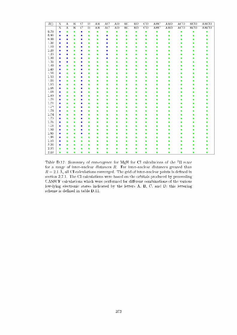
R() X A B C D AB AC AD BC BD CD ABC ABD ACD BCD ABCDX A B C D AB AC AD BC BD CD ABC ABD ACD BCD ABCD
0.70 • • • • • • • • • • • • • • • •0.80 • • • • • • • • • • • • • • • •0.90 • • • • • • • • • • • • • • • •1.00 • • • • • • • • • • • • • • • •1.10 • • • • • • • • • • • • • • • •1.20 • • • • • • • • • • • • • • • •1.25 • • • • • • • • • • • • • • • •1.30 • • • • • • • • • • • • • • • •1.35 • • • • • • • • • • • • • • • •1.40 • • • • • • • • • • • • • • • •1.45 • • • • • • • • • • • • • • • •1.50 • • • • • • • • • • • • • • • •1.55 • • • • • • • • • • • • • • • •1.60 • • • • • • • • • • • • • • • •1.65 • • • • • • • • • • • • • • • •1.66 • • • • • • • • • • • • • • • •1.68 • • • • • • • • • • • • • • • •1.69 • • • • • • • • • • • • • • • •1.70 • • • • • • • • • • • • • • • •1.71 • • • • • • • • • • • • • • • •1.72 • • • • • • • • • • • • • • • •1.73 • • • • • • • • • • • • • • • •1.74 • • • • • • • • • • • • • • • •1.75 • • • • • • • • • • • • • • • •1.76 • • • • • • • • • • • • • • • •1.78 • • • • • • • • • • • • • • • •1.80 • • • • • • • • • • • • • • • •1.85 • • • • • • • • • • • • • • • •1.90 • • • • • • • • • • • • • • • •1.95 • • • • • • • • • • • • • • • •2.00 • • • • • • • • • • • • • • • •2.05 • • • • • • • • • • • • • • • •2.10 • • • • • • • • • • • • • • • •
Table D.17: Summary of convergence for MgH for CI calculations of the 2Π statefor a range of inter-nuclear distances R. For inter-nuclear distances greated thanR = 2.1 Å, all CI calculations converged. The grid of inter-nuclear points is dened insection 2.7.1. The CI calculations were based on the orbitals produced by proceedingCASSCF calculations which were performed for dierent combinations of the variouslow-lying electronic states indicated by the letters A, B, C, and D: this letteringscheme is dened in table D.11.
373

R() X A B C D AB AC AD BC BD CD ABC ABD ACD BCD ABCDX A B C D AB AC AD BC BD CD ABC ABD ACD BCD ABCD
0.70 • • • • • • • • • • • • • • • •0.80 • • • • • • • • • • • • • • • •0.90 • • • • • • • • • • • • • • • •1.00 • • • • • • • • • • • • • • • •1.10 • • • • • • • • • • • • • • • •1.20 • • • • • • • • • • • • • • • •1.25 • • • • • • • • • • • • • • • •1.30 • • • • • • • • • • • • • • • •1.35 • • • • • • • • • • • • • • • •1.40 • • • • • • • • • • • • • • • •1.45 • • • • • • • • • • • • • • • •1.50 • • • • • • • • • • • • • • • •1.55 • • • • • • • • • • • • • • • •1.60 • • • • • • • • • • • • • • • •1.65 • • • • • • • • • • • • • • • •1.66 • • • • • • • • • • • • • • • •1.68 • • • • • • • • • • • • • • • •1.69 • • • • • • • • • • • • • • • •1.70 • • • • • • • • • • • • • • • •1.71 • • • • • • • • • • • • • • • •1.72 • • • • • • • • • • • • • • • •1.73 • • • • • • • • • • • • • • • •1.74 • • • • • • • • • • • • • • • •1.75 • • • • • • • • • • • • • • • •1.76 • • • • • • • • • • • • • • • •1.78 • • • • • • • • • • • • • • • •1.80 • • • • • • • • • • • • • • • •1.85 • • • • • • • • • • • • • • • •1.90 • • • • • • • • • • • • • • • •1.95 • • • • • • • • • • • • • • • •2.00 • • • • • • • • • • • • • • • •2.05 • • • • • • • • • • • • • • • •2.10 • • • • • • • • • • • • • • • •
Table D.18: Summary of convergence for MgH for CI calculations of the 4Π statefor a range of inter-nuclear distances R. For inter-nuclear distances greated thanR = 2.1 Å, all CI calculations converged. The grid of inter-nuclear points is dened insection 2.7.1. The CI calculations were based on the orbitals produced by proceedingCASSCF calculations which were performed for dierent combinations of the variouslow-lying electronic states indicated by the letters A, B, C, and D: this letteringscheme is dened in table D.11.
374

R() X A B C D AB AC AD BC BD CD ABC ABD ACD BCD ABCD0.70 • • • • • • • • • • • • • • • •0.80 • • • • • • • • • • • • • • • •0.90 • • • • • • • • • • • • • • • •1.00 • • • • • • • • • • • • • • • •1.10 • • • • • • • • • • • • • • • •1.20 • • • • • • • • • • • • • • • •1.25 • • • • • • • • • • • • • • • •1.30 • • • • • • • • • • • • • • • •1.35 • • • • • • • • • • • • • • • •1.40 • • • • • • • • • • • • • • • •1.45 • • • • • • • • • • • • • • • •1.50 • • • • • • • • • • • • • • • •1.55 • • • • • • • • • • • • • • • •1.60 • • • • • • • • • • • • • • • •1.65 • • • • • • • • • • • • • • • •1.66 • • • • • • • • • • • • • • • •1.68 • • • • • • • • • • • • • • • •1.69 • • • • • • • • • • • • • • • •1.70 • • • • • • • • • • • • • • • •1.71 • • • • • • • • • • • • • • • •1.72 • • • • • • • • • • • • • • • •1.73 • • • • • • • • • • • • • • • •1.74 • • • • • • • • • • • • • • • •1.75 • • • • • • • • • • • • • • • •1.76 • • • • • • • • • • • • • • • •1.78 • • • • • • • • • • • • • • • •1.80 • • • • • • • • • • • • • • • •1.85 • • • • • • • • • • • • • • • •1.90 • • • • • • • • • • • • • • • •1.95 • • • • • • • • • • • • • • • •2.00 • • • • • • • • • • • • • • • •2.05 • • • • • • • • • • • • • • • •2.10 • • • • • • • • • • • • • • • •2.15 • • • • • • • • • • • • • • • •2.20 • • • • • • • • • • • • • • • •2.25 • • • • • • • • • • • • • • • •2.30 • • • • • • • • • • • • • • • •2.35 • • • • • • • • • • • • • • • •2.40 • • • • • • • • • • • • • • • •2.45 • • • • • • • • • • • • • • • •2.50 • • • • • • • • • • • • • • • •2.55 • • • • • • • • • • • • • • • •2.60 • • • • • • • • • • • • • • • •2.65 • • • • • • • • • • • • • • • •2.70 • • • • • • • • • • • • • • • •2.75 • • • • • • • • • • • • • • • •2.80 • • • • • • • • • • • • • • • •2.85 • • • • • • • • • • • • • • • •2.90 • • • • • • • • • • • • • • • •2.95 • • • • • • • • • • • • • • • •3.00 • • • • • • • • • • • • • • • •3.10 • • • • • • • • • • • • • • • •
Table D.19: Summary of convergence for CaH for CI calculations of the X2Σ+ and2Σ+ states for a range of inter-nuclear distances R. The grid of inter-nuclear pointsis dened in section 2.7.1. The CI calculations were based on the orbitals producedby proceeding CASSCF calculations which were performed for dierent combinationsof the various low-lying electronic states indicated by the letters A, B, C, and D: thislettering scheme is dened in table D.11.
375

R() X A B C D AB AC AD BC BD CD ABC ABD ACD BCD ABCD3.20 • • • • • • • • • • • • • • • •3.30 • • • • • • • • • • • • • • • •3.40 • • • • • • • • • • • • • • • •3.50 • • • • • • • • • • • • • • • •3.60 • • • • • • • • • • • • • • • •3.70 • • • • • • • • • • • • • • • •3.80 • • • • • • • • • • • • • • • •3.90 • • • • • • • • • • • • • • • •4.00 • • • • • • • • • • • • • • • •4.10 • • • • • • • • • • • • • • • •4.20 • • • • • • • • • • • • • • • •4.30 • • • • • • • • • • • • • • • •4.40 • • • • • • • • • • • • • • • •4.50 • • • • • • • • • • • • • • • •4.60 • • • • • • • • • • • • • • • •4.70 • • • • • • • • • • • • • • • •4.80 • • • • • • • • • • • • • • • •4.90 • • • • • • • • • • • • • • • •5.00 • • • • • • • • • • • • • • • •5.20 • • • • • • • • • • • • • • • •5.40 • • • • • • • • • • • • • • • •5.60 • • • • • • • • • • • • • • • •
Table D.20: Summary of convergence for CaH for CI calculations of the X2Σ+ and2Σ+ states for a range of inter-nuclear distances R. For inter-nuclear distances greatedthan R = 5.6 Å, all CI calculations converged. The grid of inter-nuclear points isdened in section 2.7.1. The CI calculations were based on the orbitals produced byproceeding CASSCF calculations which were performed for dierent combinations ofthe various low-lying electronic states indicated by the letters A, B, C, and D: thislettering scheme is dened in table D.11.
376
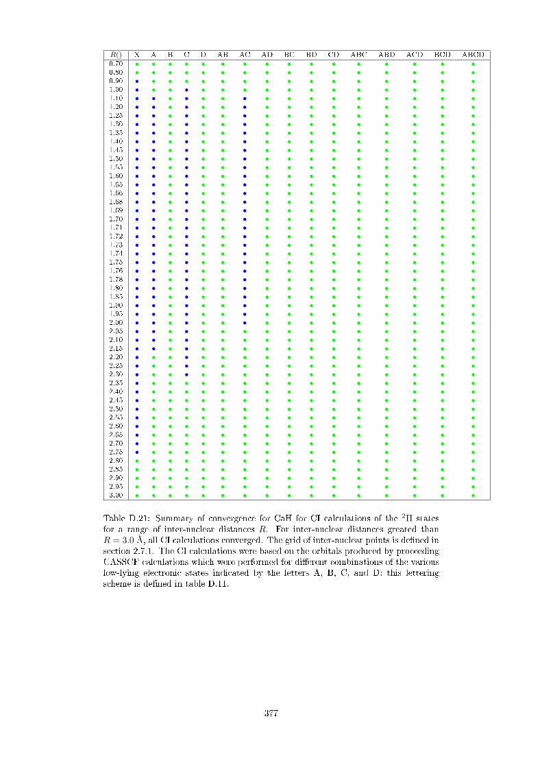
R() X A B C D AB AC AD BC BD CD ABC ABD ACD BCD ABCD0.70 • • • • • • • • • • • • • • • •0.80 • • • • • • • • • • • • • • • •0.90 • • • • • • • • • • • • • • • •1.00 • • • • • • • • • • • • • • • •1.10 • • • • • • • • • • • • • • • •1.20 • • • • • • • • • • • • • • • •1.25 • • • • • • • • • • • • • • • •1.30 • • • • • • • • • • • • • • • •1.35 • • • • • • • • • • • • • • • •1.40 • • • • • • • • • • • • • • • •1.45 • • • • • • • • • • • • • • • •1.50 • • • • • • • • • • • • • • • •1.55 • • • • • • • • • • • • • • • •1.60 • • • • • • • • • • • • • • • •1.65 • • • • • • • • • • • • • • • •1.66 • • • • • • • • • • • • • • • •1.68 • • • • • • • • • • • • • • • •1.69 • • • • • • • • • • • • • • • •1.70 • • • • • • • • • • • • • • • •1.71 • • • • • • • • • • • • • • • •1.72 • • • • • • • • • • • • • • • •1.73 • • • • • • • • • • • • • • • •1.74 • • • • • • • • • • • • • • • •1.75 • • • • • • • • • • • • • • • •1.76 • • • • • • • • • • • • • • • •1.78 • • • • • • • • • • • • • • • •1.80 • • • • • • • • • • • • • • • •1.85 • • • • • • • • • • • • • • • •1.90 • • • • • • • • • • • • • • • •1.95 • • • • • • • • • • • • • • • •2.00 • • • • • • • • • • • • • • • •2.05 • • • • • • • • • • • • • • • •2.10 • • • • • • • • • • • • • • • •2.15 • • • • • • • • • • • • • • • •2.20 • • • • • • • • • • • • • • • •2.25 • • • • • • • • • • • • • • • •2.30 • • • • • • • • • • • • • • • •2.35 • • • • • • • • • • • • • • • •2.40 • • • • • • • • • • • • • • • •2.45 • • • • • • • • • • • • • • • •2.50 • • • • • • • • • • • • • • • •2.55 • • • • • • • • • • • • • • • •2.60 • • • • • • • • • • • • • • • •2.65 • • • • • • • • • • • • • • • •2.70 • • • • • • • • • • • • • • • •2.75 • • • • • • • • • • • • • • • •2.80 • • • • • • • • • • • • • • • •2.85 • • • • • • • • • • • • • • • •2.90 • • • • • • • • • • • • • • • •2.95 • • • • • • • • • • • • • • • •3.00 • • • • • • • • • • • • • • • •
Table D.21: Summary of convergence for CaH for CI calculations of the 2Π statesfor a range of inter-nuclear distances R. For inter-nuclear distances greated thanR = 3.0 Å, all CI calculations converged. The grid of inter-nuclear points is dened insection 2.7.1. The CI calculations were based on the orbitals produced by proceedingCASSCF calculations which were performed for dierent combinations of the variouslow-lying electronic states indicated by the letters A, B, C, and D: this letteringscheme is dened in table D.11.
377

R() X A B C D AB AC AD BC BD CD ABC ABD ACD BCD ABCDX A B C D AB AC AD BC BD CD ABC ABD ACD BCD ABCD
0.70 • • • • • • • • • • • • • • • •0.80 • • • • • • • • • • • • • • • •0.90 • • • • • • • • • • • • • • • •1.00 • • • • • • • • • • • • • • • •1.10 • • • • • • • • • • • • • • • •1.20 • • • • • • • • • • • • • • • •1.25 • • • • • • • • • • • • • • • •1.30 • • • • • • • • • • • • • • • •1.35 • • • • • • • • • • • • • • • •1.40 • • • • • • • • • • • • • • • •1.45 • • • • • • • • • • • • • • • •1.50 • • • • • • • • • • • • • • • •1.55 • • • • • • • • • • • • • • • •1.60 • • • • • • • • • • • • • • • •1.65 • • • • • • • • • • • • • • • •1.66 • • • • • • • • • • • • • • • •1.68 • • • • • • • • • • • • • • • •1.69 • • • • • • • • • • • • • • • •1.70 • • • • • • • • • • • • • • • •1.71 • • • • • • • • • • • • • • • •1.72 • • • • • • • • • • • • • • • •1.73 • • • • • • • • • • • • • • • •1.74 • • • • • • • • • • • • • • • •1.75 • • • • • • • • • • • • • • • •1.76 • • • • • • • • • • • • • • • •1.78 • • • • • • • • • • • • • • • •1.80 • • • • • • • • • • • • • • • •1.85 • • • • • • • • • • • • • • • •1.90 • • • • • • • • • • • • • • • •1.95 • • • • • • • • • • • • • • • •2.00 • • • • • • • • • • • • • • • •2.05 • • • • • • • • • • • • • • • •2.10 • • • • • • • • • • • • • • • •2.15 • • • • • • • • • • • • • • • •2.20 • • • • • • • • • • • • • • • •2.25 • • • • • • • • • • • • • • • •2.30 • • • • • • • • • • • • • • • •2.35 • • • • • • • • • • • • • • • •2.40 • • • • • • • • • • • • • • • •2.45 • • • • • • • • • • • • • • • •2.50 • • • • • • • • • • • • • • • •2.55 • • • • • • • • • • • • • • • •2.60 • • • • • • • • • • • • • • • •2.65 • • • • • • • • • • • • • • • •2.70 • • • • • • • • • • • • • • • •2.75 • • • • • • • • • • • • • • • •2.80 • • • • • • • • • • • • • • • •2.85 • • • • • • • • • • • • • • • •2.90 • • • • • • • • • • • • • • • •2.95 • • • • • • • • • • • • • • • •3.00 • • • • • • • • • • • • • • • •
Table D.22: Summary of convergence for CaH for CI calculations of the 4Σ+ statesfor a range of inter-nuclear distances R. For inter-nuclear distances greated thanR = 3.0 Å, all CI calculations converged. The grid of inter-nuclear points is dened insection 2.7.1. The CI calculations were based on the orbitals produced by proceedingCASSCF calculations which were performed for dierent combinations of the variouslow-lying electronic states indicated by the letters A, B, C, and D: this letteringscheme is dened in table D.11.
378

R() X A B C D AB AC AD BC BD CD ABC ABD ACD BCD ABCD0.70 • • • • • • • • • • • • • • • •0.80 • • • • • • • • • • • • • • • •0.90 • • • • • • • • • • • • • • • •1.00 • • • • • • • • • • • • • • • •1.10 • • • • • • • • • • • • • • • •1.20 • • • • • • • • • • • • • • • •1.25 • • • • • • • • • • • • • • • •1.30 • • • • • • • • • • • • • • • •1.35 • • • • • • • • • • • • • • • •1.40 • • • • • • • • • • • • • • • •1.45 • • • • • • • • • • • • • • • •1.50 • • • • • • • • • • • • • • • •1.55 • • • • • • • • • • • • • • • •1.60 • • • • • • • • • • • • • • • •1.65 • • • • • • • • • • • • • • • •1.66 • • • • • • • • • • • • • • • •1.68 • • • • • • • • • • • • • • • •1.69 • • • • • • • • • • • • • • • •1.70 • • • • • • • • • • • • • • • •1.71 • • • • • • • • • • • • • • • •1.72 • • • • • • • • • • • • • • • •1.73 • • • • • • • • • • • • • • • •1.74 • • • • • • • • • • • • • • • •1.75 • • • • • • • • • • • • • • • •1.76 • • • • • • • • • • • • • • • •1.78 • • • • • • • • • • • • • • • •1.80 • • • • • • • • • • • • • • • •1.85 • • • • • • • • • • • • • • • •1.90 • • • • • • • • • • • • • • • •1.95 • • • • • • • • • • • • • • • •2.00 • • • • • • • • • • • • • • • •2.05 • • • • • • • • • • • • • • • •2.10 • • • • • • • • • • • • • • • •2.15 • • • • • • • • • • • • • • • •2.20 • • • • • • • • • • • • • • • •2.25 • • • • • • • • • • • • • • • •2.30 • • • • • • • • • • • • • • • •2.35 • • • • • • • • • • • • • • • •2.40 • • • • • • • • • • • • • • • •2.45 • • • • • • • • • • • • • • • •2.50 • • • • • • • • • • • • • • • •2.55 • • • • • • • • • • • • • • • •2.60 • • • • • • • • • • • • • • • •2.65 • • • • • • • • • • • • • • • •2.70 • • • • • • • • • • • • • • • •2.75 • • • • • • • • • • • • • • • •2.80 • • • • • • • • • • • • • • • •2.85 • • • • • • • • • • • • • • • •2.90 • • • • • • • • • • • • • • • •2.95 • • • • • • • • • • • • • • • •3.00 • • • • • • • • • • • • • • • •
Table D.23: Summary of convergence for CaH for CI calculations of the 4Π statesfor a range of inter-nuclear distances R. For inter-nuclear distances greated thanR = 3.0 Å, all CI calculations converged. The grid of inter-nuclear points is dened insection 2.7.1. The CI calculations were based on the orbitals produced by proceedingCASSCF calculations which were performed for dierent combinations of the variouslow-lying electronic states indicated by the letters A, B, C, and D: this letteringscheme is dened in table D.11.
379

Bibliography
[1] M. Abe, M. Kajita, M. Hada, and Y. Moriwaki. Ab initio study on vibrational
dipole moments of XH+ molecular ions: X=24Mg, 40Ca, 64Zn, 88Sr, 114Cd,138Ba, 174Yb and 202Hg. Journal of Physics B, 43(24), DEC 28 2010.
[2] E. Abrahamsson, T. V. Tscherbul, and R. V. Krems. Inelastic collisions of cold
polar molecules in nonparallel electric and magnetic elds. Journal of Chemical
Physics, 127(4), JUL 28 2007.
[3] S. Aldridge and A. J. Downs. Hydrides of the main-group metals: New varia-
tions on an old theme. Chemical Reviews, 101(11):33053365, NOV 2001.
[4] F. Allard, D. R. Alexander, and P. H. Hauschildt. Model Atmospheres of Very
Low Mass Stars and Brown Dwarfs. In R. A. Donahue and J. A. Bookbinder,
editors, Cool Stars, Stellar Systems, and the Sun, volume 154 of Astronomical
Society of the Pacic Conference Series, page 63, 1998.
[5] F. Allard, P. H. Hauschildt, D. R. Alexander, and S. Starreld. Model Atmo-
spheres of Very Low Mass Stars and Brown Dwarfs. Annual Review of Astron-
omy and Astrophysics, 35:137177, 1997.
[6] F. Allard, P. H. Hauschildt, D. R. Alexander, A. Tamanai, and A. Schweitzer.
The limiting eects of dust in brown dwarf model atmospheres. Astrophysical
Journal, 556(1, Part 1):357372, JUL 20 2001.
[7] F. Allard, D. Homeier, B. Freytag, Schaenberger, W. , and A. S. Rajpurohit.
Progress in modeling very low mass stars, brown dwarfs, and planetary mass
objects. Memorie della Societa Astronomica Italiana Supplementi, 24:128, 2013.
[8] F. Allard, D. Homeier, B. Freytag, and C. M. Sharp. Atmospheres From
Very Low-Mass Stars to Extrasolar Planets. In C. Reylé, C. Charbonnel, and
M. Schultheis, editors, EAS Publications Series, volume 57 of EAS Publications
Series, pages 343, 2012.
[9] R. W. Allmendinger. Inverse and forward numerical modeling of trishear fault-
propagation folds. Tectonics, 17:640656, August 1998.
[10] S. V. Alyabyshev, T. V. Tscherbul, and R. V. Krems. Microwave-laser-eld
modication of molecular collisions at low temperatures. Physics Review A,
79(6), JUN 2009.
380

[11] E. Anders and N. Grevesse. Abundances of the elements - Meteoritic and
solar. Geochimica et Cosmochimica Acta, 53:197, 1989. doi:10.1016/0016-
7037(89)90286-X.
[12] J. Anglada, P. J. Bruna, and F. Grein. Theoretical study of low-lying electronic
states of CoH+. The Journal of Chemical Physics, 92(11):67326741, 1990.
doi:10.1063/1.458258.
[13] J. Anglada, P. J. Bruna, and S. D. Peyerimho. Theoretical investigation of the
low-lying electronic states of TiH. Molecular Physics, 69:281303, 1990.
[14] S. R. Arridge and J. C. Schotland. TOPICAL REVIEW: Optical tomography:
forward and inverse problems. Inverse Problems, 25(12):123010, December 2009.
[15] L. W. Avery, M. B. Bell, C. T. Cunningham, P. A. Feldman, R. H. Hayward,
J. M. Macleod, H. E. Matthews, and J. D. Wade. Submillimeter molecular
line observations of IRC +10216: Searches for MgH, SiH2, and hco(+), and
detection of hot HCN. Astrophysical Journal, 426(2, Part 1):737741, MAY 10
1994.
[16] M. Aymar, R. Guerout, M. Sahlaoui, and O. Dulieu. Electronic structure of the
magnesium hydride molecular ion. Journal of Physics B, 42(15), AUG 14 2009.
[17] M. C. Bacchus-Montabonel and D. Talbi. A theoretical treatment of the LiH and
BeH formation through radiative association. Journal of Molecular Structure,
463(1-2):9197, APR 23 1999. 2nd European Conference on Computational
Chemistry (EUCO-CC2), LISBON, PORTUGAL, SEP 02-06, 1997.
[18] P. S. Bagus and H. F. Schaefer III. 7Σ+ and 7Πstates of manganese hydride.
Journal of Chemical Physics, 58(5):1844, 1973.
[19] P. S. Bagus, C. M. Moser, P. Goethals, and G. Verhaege. Accurate ab initio
calculation of BeH. 1. X2Σ+ and A2Π states. Journal of Chemical Physics,
58(5), 1973.
[20] P. S. Bagus and H. F. Schaefer, III. 7Σ+ and 7Π states of manganese
hydride. Journal of Chemical Physics, 58:18441848, March 1973. doi:
10.1063/1.1679441.
[21] C. A. L. Bailer-Jones. Correlated spectral variability in brown dwarfs. Monthly
Notices of the Royal Astronomical Society, 384(3):11451157, MAR 1 2008.
[22] J. Bailey. The Dawes Review 3: The Atmospheres of Extrasolar Planets and
Brown Dwarfs. Publications of the Astronomical Society of Australia, 31:e043,
2014.
[23] N. B. Balabanov and K. A. Peterson. Systematically convergent basis sets
for transition metals. I. All-electron correlation consistent basis sets for the 3d
elements Sc-Zn. Journal of Chemical Physics, 123(6):064107, August 2005. doi:
10.1063/1.1998907.
381

[24] N. Balakrishnan, G. C. Groenenboom, R. V. Krems, and A. Dalgarno. The he-
cah(2Σ+) interaction. ii. collisions at cold and ultracold temperatures. Journal
of Chemical Physics, 118(16):73867393, APR 22 2003.
[25] W. J. BALFOUR. The electronic spectrum of magnesium hydride and magne-
sium deuteride. Journal of Physics B, 3(12):1749, 1970.
[26] W. J. Balfour. The A2Π −X2Σ+ systems of 24MgH, 25MgH and 26MgH. As-
trophysical Journal, 162:1031, December 1970.
[27] W. J Balfour. MgH and MgD spectra in the 230 - 235 nm region. Journal of
Molecular Spectroscopy, 79(2):507511, 1980.
[28] W. J. Balfour. The electronic spectrum of manganese hydride. Journal of
Chemical Physics, 88:52425243, April 1988.
[29] W. J. Balfour and H. M. Cartwright. The 2Π−X2Σ+system and dissociation
energy of magnesium hydride. Astronomy & Astrophysics Supplement Series,
26:389, 1976.
[30] W. J. Balfour and H. M. Cartwright. The A2Π−X2Σ+ system and dissociation
energy of magnesium hydride. Astronomy and Astrophysics Supplement Series,
26:389397, December 1976.
[31] W. J. Balfour and L. Klynning. On the carrier of the band at 700 nanometers
in the iron hydride spectrum of phillips and davis: Evidence favoring calcium
hydride. The Astrophysical Journal, 424(2, Part 1):10491053, APR 1 1994.
[32] W. J. Balfour, O. Launila, and L. Klynning. Fourier transform spectroscopy of
MnH and MnD. Molecular Physics, 69:443461, 1990.
[33] W. J. Balfour, B. Lindgren, O. Launila, S. O'Connor, and E. J. Cusack. The
visible spectrum of manganese hydride: Rotational analyses of the 480- and
450-nm systems. Journal of Molecular Spectroscopy, 154:177200, July 1992.
[34] W. J. Balfour, B. Lindgren, and S. O'Connor. On the 1 µm system of iron
hydride. Chemical Physics Letters, 96(2):251252, 1983.
[35] WJ Balfour, JM Brown, and L Wallace. Electronic spectra of iron monohy-
dride in the infrared near 1.35 and 1.58 mu m. Journal of Chemical Physics,
121(16):77357742, OCT 22 2004.
[36] A. Bar-Nun, M. Pasternak, and P. H. Barrett. Iron hydrides formation in
interstellar clouds. Astronomy & Astrophysics, 87(3):328329, 1980.
[37] I. Barae, G. Chabrier, F. Allard, and P. H. Hauschildt. Evolutionary models
for solar metallicity low-mass stars: mass-magnitude relationships and color-
magnitude diagrams. Astronomy and Astrophysics, 337:403412, September
1998.
[38] I. Barae, G. Chabrier, F. Allard, and P. H. Hauschildt. Evolutionary models
for low-mass stars and brown dwarfs: Uncertainties and limits at very young
ages. Astronomy and Astrophysics, 382:563572, February 2002.
382

[39] I. Barae, G. Chabrier, T. S. Barman, F. Allard, and P. Hauschildt. Evolu-
tionary models for cool brown dwarfs and extrasolar giant planets. The case
of HD 209458. Astronomy & Astrophysics, 402:701, 2003. doi:10.1051/0004-
6361:20030252.
[40] I. Barae, G. Chabrier, T. S. Barman, F. Allard, and P. H. Hauschildt. Evolu-
tionary models for cool brown dwarfs and extrasolar giant planets. The case of
HD 209458. Astronomy and Astrophysics, 402:701712, May 2003.
[41] B. Barbuy, R. P. Schiavon, J. Gregoriohetem, P. D. Singh, and C Batalha.
Intensity of caH Lines in Cool Dwarfs. Astronomy and Astrophysics Supplement,
101(2):409413, OCT 1993.
[42] W. L. Barclay, M. A. Anderson, and M. Ziurys, L. The millimeter-wave spec-
trum of CaH(X2Σ+). The Astrophysical Journal, 408(1, Part 2):L65L67, MAY
1 1993.
[43] V. Barone and C. Adamo. First-row transition-metal hydrides: A challenging
playground for new theoretical approaches. International Journal of Quantum
Chemistry, 61(3):443451, JAN 20 1997.
[44] V. Barone and C. Adamo. First-row transition-metal hydrides: A challenging
playground for new theoretical approaches. International Journal Of Quantum
Chemistry, 61:443451, 1997.
[45] J. K. Barstow, S. Aigrain, P. Irwin, S. Kendrew, and L. N. Fletcher.
Transit spectroscopy with JWST: Systematics, starspots and stitching.
In AAS/Division for Planetary Sciences Meeting Abstracts, volume 46 of
AAS/Division for Planetary Sciences Meeting Abstracts, 2014.
[46] J. K. Barstow, S. Aigrain, P. G. J. Irwin, N. Bowles, L. N. Fletcher, and J.-M.
Lee. On the potential of the EChO mission to characterize gas giant atmo-
spheres. Monthly Notices of the Royal Astronomical Society, 430:11881207,
April 2013.
[47] J. K. Barstow, N. E. Bowles, S. Aigrain, L. N. Fletcher, P. G. J. Irwin, R. Varley,
and E. Pascale. Exoplanet atmospheres with EChO: spectral retrievals using
EChOSim. Experimental Astronomy, June 2014.
[48] C. A. Baumann, R. J. Van Zee, and W. Jr. J. Weltner. High-spin molecules:
electron spin resonance of manganese halides and sulde at 4 K. Journal of
Physical Chemistry, 86:5084, 1982.
[49] C. W. Bauschlicher and S. R Langho. Theoretical conrmation of a4∆ ground
state for FeH. Chemical Physics Letters, 145(3):205210, APR 1 1988.
[50] C. W. Bauschlicher, R. S. Ram, P. F. Bernath, C. G. Parsons, and D. Galehouse.
The A 6Σ+-X 6Σ+ transition of CrH, Einstein coecients, and an improved
description of the A state. Journal Of Chemical Physics, 115:13121318, July
2001. doi:10.1063/1.1377892.
383

[51] C. W. Bauschlicher and S. P. Walch. On the d bond in ScH. Journal of Chemical
Physics, 76(9):4560, 1982.
[52] J. L. Bean, J.-M. Désert, P. Kabath, B. Stalder, S. Seager, E. Miller-Ricci
Kempton, Z. K. Berta, D. Homeier, S. Walsh, and A. Seifahrt. The Optical and
Near-infrared Transmission Spectrum of the Super-Earth GJ 1214b: Further
Evidence for a Metal-rich Atmosphere. Astrophysical Journal, 743:92, December
2011.
[53] J. L. Bean, E. Miller-Ricci Kempton, and D. Homeier. A ground-based trans-
mission spectrum of the super-Earth exoplanet GJ 1214b. Nature, 468:669672,
December 2010.
[54] S. P. Beaton, K. M. Evenson, T. Nelis, and J. M. Brown. Detection of the free
radicals FeH, CoH, and NiH by far infrared laser magnetic resonance. Journal
of Chemical Physics, 89(7):44464448, OCT 1 1988.
[55] S. P. Beaton, K. M. Evenson, T. Nelis, and J. M. Brown. Detection of the
free radicals FeH, CoH, and NiH by far infrared laser magnetic resonance. The
Journal of Chemical Physics, 89(7):44464448, 1988. doi:10.1063/1.454781.
[56] F. Beitia, F. Castano, M. N. S. Rayo, R. Martinez, L. Santos, and D. Hu-
sain. Kinetic investigation of the collisional quenching of ca(43pJ) by c4h10
at elevated temperatures (750â923 k). time-resolved atomic emission and
electronic energy transfer between c(43pJ) and cah(X2Σ+) observed by molec-
ular chemiluminescence. Journal of the Chemical Society-Faraday Trancactions,
87(10):15031508, MAY 21 1991.
[57] G. D. Bell, M. Herman, J. W. C. Johns, and E. R. Peck. The D2Σ+ −X2Σ+
Band System of CaH. Physica Scripta, 20(5-6):609616, 1979.
[58] R. A. Bell, B. Edvardsson, and B. Gustafsson. The surface gravity of Arc-
turus from MgH lines, strong metal lines and the ionization equilibrium of iron.
Monthly Notices of the Royal Astronomical Society, 212(3):497515, 1985.
[59] R. A. Bell and M. J. Tripicco. Molecular equilibria and the luminosity classi-
cation of G and K stars. Astronomical Journal, 102(2):777786, AUG 1991.
[60] D. Ben Abdallah, F. Najar, N. Jaidane, Z. Ben Lakhdar, N. Feautrier,
A. Spieledel, and F. Lique. Ab initio potential energy surfaces for the 1a′
and 3a′ states of the MgH(x2σ+) + h(2s) system. Chemical Physics Letters,
473(1-3):3942, APR 29 2009.
[61] S. V. Berdyugina, A. V. Berdyugin, D. M. Fluri, and V. Piirola. First Detection
of Polarized Scattered Light from an Exoplanetary Atmosphere. Astrophysical
Journal Letters, 673:L83L86, January 2008.
[62] S. V. Berdyugina, D. M. Fluri, R. Ramelli, M. Bianda, D. Gisler, and J. O.
Steno. First polarimetric measurements and modeling of the Paschen-Back
eect in CaH transitions. The Astrophysical Journal, 649(1, Part 2):L49L52,
SEP 20 2006.
384

[63] S. V. Berdyugina, C. Frutiger, S. K. Solanki, and W. Livingstone. Successful
spectral synthesis of Zeeman-split molecular bands in sunspot spectra. Astron-
omy and Astrophysics, 364(2):L101L104, DEC 2000.
[64] S. V. Berdyugina and I. S. Savanov. Determination of the parameters of red
giants' atmospheres - MgH as a luminosity criterion. Astronomicheskii Zhurnal,
69(4):829841, JUL-AUG 1992.
[65] S. V. Berdyugina and S. K. Solanki. The molecular Zeeman eect and di-
agnostics of solar and stellar magnetic elds. I. Theoretical spectral pat-
terns in the Zeeman regime. Astronomy & Astrophysics, 385:701715, 2002.
doi:10.1051/0004-6361:20020130.
[66] S. V. Berdyugina, S. K. Solanki, and C. Frutiger. Solar and Stellar Magnetic
Fields: the Molecular Zeeman Eect as a Probe. In ASP Conference Proceed-
ings, volume 248, page 99, 2001.
[67] S. V. Berdyugina, S. K. Solanki, and C. Frutiger. The molecular Zeeman ef-
fect and diagnostics of solar and stellar magnetic elds. II. Synthetic Stokes
proles in the Zeeman regime. Astronomy & Astrophysics, 412:513527, 2003.
doi:10.1051/0004-6361:20031473.
[68] L. E. Berg, K. Ekvall, and S. Kelly. Radiative lifetime measurement of vibronic
levels of the B2Σ+ state of CaH by laser excitation spectroscopy. Chemical
Physics Letters, 257(3-4):351355, JUL 26 1996.
[69] L. E. Berg and L. Klynning. Rotational analysis of A−X and B −X band
systems of CaH. Physica Scripta, 10(6):331336, 1974.
[70] L. E. Berg, L. Klynning, and H. Martin. Laser excitation spectroscopy of the
B2Σ−X2 transition of the CaH molecule. Optics Communications, 17(3):320
324, 1976.
[71] P. F. Bernath. 6 infrared emission spectroscopy. Annu. Rep. Prog. Chem., Sect.
C: Phys. Chem., 96:177224, 2000.
[72] P. F. Bernath. Molecular astronomy of cool stars and sub-stellar objects. In-
ternational Reviews in Physical Chemistry, 28(4):681709, 2009.
[73] P. F. Bernath. Molecular astronomy of cool stars and sub-stellar ob-
jects. International Reviews in Physical Chemistry, 28(4):681709, 2009.
doi:10.1080/01442350903292442.
[74] P. F. Bernath, J. H. Black, and J. W. Brault. The spectrum of magnesium
hydride. Astrophysical Journal, 298(1):375381, 1985.
[75] S. S. Bhattacjaryya and D. Basu. Shape resonances and the photodissociation
cross sectionof mgh near threshold. Chemical Physics, 79(1):129135, 1983.
[76] S. Bird and T. A. Claxton. Orbitally ordered conguration-interaction calcula-
tions on small radicals. NH2 and BeH. Journal of the Chemical Society, Faraday
Transactions II, 80(Part 7):851860, 1984.
385

[77] D. M. Bishop, J. Pipin, and B. Lam. Field and eld-gradient polarizabilities of
BeH, BH and CH+. Chemical Physics Letters, 127(4):377380, JUN 20 1986.
[78] M. R. A. Blomberg and P. E. M. Siegbahn. A theoretical study of NiH Optical
spectrum and potential curves. Molecular Physics, 47:127, 1982.
[79] V. Bommier, E. Landi Degl'Innocenti, N. Feautrier, and G. Molodij. Collisional
inuence on the dierential Hanle eect method applied to the second solar
spectrum of the a2π − x2σ+(0, 0) band of MgH. Astronomy & Astrophysics,
458(2):625633, NOV 2006.
[80] J. T. Bonnell and R. A. Bell. Further determinations of the gravities of cool giant
stars using Mg I and MgH features. Monthly Notices of the Royal Astronomical
Society, 264(2):334344, SEP 15 1993.
[81] W. J. Borucki and A. L. Summers. The photometric method of detecting other
planetary systems. ICARUS, 58:121134, April 1984.
[82] F. Bouchy, S. Udry, M. Mayor, C. Moutou, F. Pont, N. Iribarne, R. da Silva,
S. Ilovaisky, D. Queloz, N. C. Santos, D. Ségransan, and S. Zucker. ELODIE
metallicity-biased search for transiting Hot Jupiters. II. A very hot Jupiter
transiting the bright K star HD 189733. Astronomy and Astrophysics, 444:L15
L19, December 2005.
[83] A. Boutalib, J. P. Daudey, and M. Elmouhtadi. Theoretical study of the lowest
electronic states of CaH and CaH+ molecules. Chemical Physics, 167(1-2):111
120, NOV 1 1992.
[84] B.H. Bransden and C.J. Joachain. Physics of Atoms and Molecules. Prentice
Hall, 2000.
[85] W. H. Breckenridge and H. Umemoto. Bimodal rotational quantum state distri-
bution of MgH (x2σ+, ν = 0) in the reaction of mg(3s3p1p1) with H2: Evidence
for microscopic branching. Journal of Chemical Physics, 75(8):41534155, 1981.
[86] W. H. Breckenridge and H. Umemoto. Nascent internal energy distributions
of mgh produced in the reaction of Mg(3s3p 1p1) with a variety of polyatomic
molecules. Journal of Chemical Physics, 81(9):38523865, 1984.
[87] W. H. Breckenridge and H. Umemoto. Nascent internal energy distributions of
mgh(mgd) produced in the reaction of Mg(3s3p 1p1) with h2(d2). Journal of
Chemical Physics, 80(9):41684176, 1984.
[88] W. H. Breckenridge and J. H Wang. Dynamics of the reactions of mg(3s3p1p1)
with h2, hd, and d2: Rotational quantum state distributions of MgH (MgD)
products. Chemical Physics Letters, 137(3):195200, JUN 12 1987.
[89] WH BRECKENRIDGE and H UMEMOTO. Reaction of mg(3s3p1p1) with a
variety of alkyl câh bonds: Identical initial MgH(x2σ+, ν = 0) rotational
quantum state distributions. Journal of Chemical Physics, 77(9):44644468,
1982.
386

[90] J. M. Brown. Molecular Spectroscopy. Oxford University Press, 1998.
[91] J. M. Brown, S. P. Beaton, and K. M. Evenson. Rotational frequencies of transi-
tion metal hydrides for astrophysical searches in the far-infrared. Astrophysical
Journal, 414(2, Part 2):L125L127, SEP 10 1993.
[92] J. M. Brown, S. P. Beaton, and K. M. Evenson. Rotational frequencies of transi-
tion metal hydrides for astrophysical searches in the far-infrared. Astrophysical
Journal, Letters, 414:L125L127, September 1993. doi:10.1086/187012.
[93] J. M. Brown, H. Korsgen, S. P. Beaton, and K. M. Evenson. The rotational and
ne-structure spectrum of FeH, studied by far-infrared laser magnetic resonance.
Journal of Chemical Physics, 124(23), JUN 21 2006.
[94] P. J. Bruna and F. Grein. Hyperne coupling constants, electron-spin g-factors
and vertical spectra of the x2σ+ radicals BeH, MgH, CaH and BZ+(+) AlZ+,
GaZ+ (Z = H, Li, Na, K). A theoretical study. Physical Chemistry Chemical
Physics, 5(15):31403153, 2003.
[95] P. J. Bruna and F. Grein. Hyperne coupling constants, electron-spin g-factors
and vertical spectra of the X2Σ+ radicals BeH, MgH, CaH and BZ+, AlZ+,
GaZ+ (Z = H, Li, Na, K). a theoretical study. PCCP, 5(15):31403153, 2003.
[96] PJ Bruna and F Grein. Hyperne coupling constants, electron-spin g-factors
and vertical spectra of the X2Σ+ radicals BeH, MgH, CaH and BZ+, AlZ+,
GaZ+ (Z = H, Li, Na, K). a theoretical study. Physical Chemistry Chemical
Physics, 5(15):31403153, 2003.
[97] Sergiy Bubin and Ludwik Adamowicz. Calculations of the ground states of BeH
and BeH+ without the Born-Oppenheimer approximation. Journal of Chemical
Physics, 126(21), JUN 7 2007.
[98] A. J. Burgasser. Binaries and the L Dwarf/T Dwarf Transition. Astrophysical
Journal, 659:655674, April 2007.
[99] A. J. Burgasser. The L dwarf/T dwarf transition: Multiplicity, magnetic activity
and mineral meteorology across the hydrogen burning limit. Astronomische
Nachrichten, 334:32, February 2013.
[100] A. J. Burgasser, J. D. Kirkpatrick, and S. Lépine. Ultracool subdwarfs: metal-
poor stars and brown dwarfs extending into the late-type M, L and T dwarf
regimes. In F. Favata, G. A. J. Hussain, and B. Battrick, editors, 13th Cam-
bridge Workshop on Cool Stars, Stellar Systems and the Sun, volume 560 of
ESA Special Publication, page 237, March 2005.
[101] A. J. Burgasser, J. D. Kirkpatrick, J. Liebert, and A. Burrows. The spectra of T
dwarfs. II. Red optical data. The Astrophysical Journal, 594(1, Part 1):510524,
SEP 1 2003.
[102] A. J. Burgasser, I. N. Reid, N. Siegler, L. Close, P. Allen, P. Lowrance, and
J. Gizis. Not Alone: Tracing the Origins of Very-Low-Mass Stars and Brown
387

Dwarfs Through Multiplicity Studies. Protostars and Planets V, pages 427441,
2007.
[103] A. Burrows, M. Marley, W. B. Hubbard, J. I. Lunine, T. Guillot, D. Saumon,
R. Freedman, D. Sudarsky, and C. Sharp. A Nongray Theory of Extrasolar Gi-
ant Planets and Brown Dwarfs. Astrophysical Journal, 491:856875, December
1997.
[104] A. Burrows, R. S. Ram, P. Bernath, C. M. Sharp, and J. A. Milsom. New
CrH Opacities for the Study of L and Brown Dwarf Atmospheres. Astrophysical
Journal, 577:986992, October 2002. doi:10.1086/342242.
[105] A. S. Burrows. Highlights in the study of exoplanet atmospheres. Nature,
513:345352, September 2014.
[106] A. S. Burrows. Spectra as windows into exoplanet atmospheres. Proceedings of
the National Academy of Science, 111:1260112609, September 2014.
[107] A. J. Cannon and E. C. Pickering. The Henry Draper catalogue : 21h, 22h, and
23h. Annals of Harvard College Observatory, 99, 1924.
[108] E. Cantarella, F. Culot, and J. Lievin. Ab initio calculation of vibrational dipole
moment matrix elements. I. methods of calculation and diatomic test systems.
Physica Scripta, 46(6):489501, DEC 1992.
[109] C. Carlsund-Levin, N. Elander, A. Nunez, and A. Scrinzi. An exterior complex
rotated coupled channel description of predissociation in diatomic molecules
applied to a model of the four lowest 2Σ+ states in CaH. Physica Scripta,
65(4):306322, APR 2002.
[110] PK CARROLL, P MCCORMACK, and S OCONNOR. IRON HYDRIDE -
LABORATORY STUDIES AND SOLAR IDENTIFICATION. Astrophysical
Journal, 208(3):903&, 1976.
[111] R. T. Carter and J. M. Brown. Observation and identication of the g6∆−a6∆
transition in the blue system of FeH at 493 nm. Journal of Chemical Physics,
101(4):26992709, AUG 15 1994.
[112] R. T. Carter and J. M. Brown. Observation of the g6Φ11/12 − X4∆7/2,∆ω=2
Subband in FeH. Journal of Molecular Spectroscopy, 166(1):249250, JUL 1994.
[113] R. T. Carter, T. C. Steimle, and J. M. Brown. The identication of a 6Φ−X4∆
intercombination system in the FeH radical at 448 nm. Journal of Chemical
Physics, 99(5):31663173, SEP 1993.
[114] G. Chabrier and I. Barae. Structure and evolution of low-mass stars. Astron-
omy and Astrophysics, 327:10391053, 1997.
[115] G. Chabrier, I. Barae, F. Allard, and P. Hauschildt. Deuterium Burning
in Substellar Objects. The Astrophysical Journal, 542(2):L119L122, 2000.
doi:10.1086/312941.
388

[116] G. Chabrier, I. Barae, F. Allard, and P. Hauschildt. Evolutionary Models for
Very Low-Mass Stars and Brown Dwarfs with Dusty Atmospheres. Astrophysical
Journal, 542:464472, October 2000.
[117] G. Chabrier, I. Barae, F. Allard, and P. H. Hauschildt. Review on low-mass
stars and brown dwarfs. ArXiv Astrophysics e-prints, September 2005.
[118] G. Chambaud and B Levy. CaH∗ potential curves: a simple theoretical treat-
ment of intershell eects. Journal of Physics B, 22(20):31553165, OCT 28
1989.
[119] A. C. H. Chan and E. R. Davidson. Theoretical Study of the BeH Molecule.
Journal of Chemical Physics, 49, 1968.
[120] W. T. Chan and I. P. Hamilton. Geometries and vibrational frequencies for
calcium and strontium radical salts of H, F, Cl, Br, I, OH, SH, CN, NC, CCH,
NNN, NCO, NCS, NH2, CH3, OCH3, SCH3, HCOO, CH3COO, HCONH and
HCONCH3. Chemical Physics Letters, 297(3-4):217224, NOV 27 1998.
[121] T. C. Chang. Pauli repulsion in the open shell species BeH and Co+. Journal
of Computational Chemistry, 13(3):268274, APR 1992.
[122] Y. L. Chang, L Chen, M. K. Hsiao, J. J. Chen, and K. C. Lin. Reaction pathway
for the nonadiabatic reaction of ca(4s3d1D) + H2 → CaH(X2Σ+) + H. Journal
of Chemical Physics, 122(8), FEB 22 2005.
[123] Y. W. Chang and H. Sun. Spin-orbit splittings in the valence states of XH
(X = K, Ca, Ga, Ge, As, Se, and Br) by the eective Hamiltonian approach.
Chemical Physics Letters, 493(4-6):371375, JUN 25 2010.
[124] D. Charbonneau, Z. K. Berta, J. Irwin, C. J. Burke, P. Nutzman, L. A. Buch-
have, C. Lovis, X. Bonls, D. W. Latham, S. Udry, R. A. Murray-Clay, M. J.
Holman, E. E. Falco, J. N. Winn, D. Queloz, F. Pepe, M. Mayor, X. Delfosse,
and T. Forveille. A super-Earth transiting a nearby low-mass star. Nature,
462:891894, December 2009.
[125] J. Chen, T. C. Steimle, and A. J. Merer. The permanent electric dipole
moment of chromium monodeuteride, CrD. Journal Of Chemical Physics,
127(20):204307, 2007.
[126] J. H. Chen, J. Gengler, T. C. Steimle, and J. M. Brown. Optical Zeeman
spectroscopy of calcium monohydride. Physics Review A, 73(1), JAN 2006.
[127] J. J. Chen, Y. W. Song, K. C. Lin, and Y. M. Hung. Reaction pathway and
energy disposal of the cah product in the reaction of ca(4s4p1P1)+CH4 →CaH(X2Σ+) + CH3. Journal of Chemical Physics, 118(11):49384944, MAR
15 2003.
[128] Jinhai Chen and T.C. Steimle. The permanent electric dipole moment of calcium
monodeuteride. Journal of Chemical Physics, 128(14), APR 14 2008.
389

[129] L. Chen, M. K. Hsiao, Y. L. Chang, and K. C. Lin. Reaction dynamics of
ca(4s3d1D(2)+ CH4 → CaH(X2Σ+) + CH3: Reaction pathway and energy
disposal for the CaH product. Journal of Chemical Physics, 124(2), JAN 14
2006.
[130] Y. M. Chen, D. E. Clemmer, and P. B. Armentrout. Gas-phase thermochemistry
of VH and CrH. Journal Of Chemical Physics, 98:49294936, March 1993.
doi:10.1063/1.464948.
[131] G. V. Chertihin and L. Andrews. Infrared Spectra of FeH, FeH2, and FeH3 in
Solid Argon. Journal of Physical Chemistry, 99(32):1213112134, AUG 1995.
[132] A. Chiavassa, R. Collet, L. Casagrande, and M. Asplund. Three-dimensional hy-
drodynamical simulations of red giant stars: semi-global models for interpreting
interferometric observations. Astronomy & Astrophysics, 524, DEC 2010.
[133] D. P. Chong, S. R. Langho, C. W. Bauschlicher, and S. P. Walch. Theoretical
dipole moments for the rst-row transition metal hydrides. Journal of Chemical
Physics, 85(5):28502860, SEP 1 1986.
[134] D. P. Chong, S. R. Langho, C. W. Bauschlicher, S. P. Walch, and H. Partridge.
Theoretical dipole moments for the rst-row transition metal hydrides. Journal
Of Chemical Physics, 85:28502860, September 1986. doi:10.1063/1.451044.
[135] P. K. Chowdhury, A. J. Merer, S. J. Rixon, P. F. Bernath, and R. S. Ram. Low-
N lines of the A6Σ+ X6Σ+ (1,0) band of CrH. Physical Chemistry Chemical
Physics (Incorporating Faraday Transactions), 8:822, 2006.
[136] T. A. Claxton, J. Tino, B. Burtons, and V. Klimo. Further study of the BeH
radical by UHF-type and conguration interaction methods. Journal of the
Chemical Society, Faraday Transactions II, 76(Part 12):16551663, 1980.
[137] R. E. S. Clegg and D. L. Lembert. On the identication of FeH and CeO in S
stars. Astrophysical Journal, 226(3):931936, 1978.
[138] C. Clerbaux and R. Colin. The 3d Rydberg state of the beh molecule. Molecular
Physics, 72(2):471486, FEB 10 1991.
[139] P. Coelho, B. Barbuy, J. Melendez, R. P. Schiavon, and B. V. Castilho. A library
of high resolution synthetic stellar spectra from 300 nm to 1.8 µm with solar
and alpha-enhanced composition. Astronomy & Astrophysics, 443(2):735U183,
NOV 2005.
[140] R. Colin, D. Degreef, P. Goethals, and Verhaege G. The ionization-potential of
the BeH molecule. Chemical Physics Letters, 25(1):7073, 1974.
[141] R. Colin and M. Steinhauer. The 3d − 4s Molecular Complex of Beryllium
Monohydride. Bulletin Des Societes Chimiques Belges, 92(6-7):507, 1983.
[142] D. L Cooper. Spin splitting in the x2σ+ state of MgH. Journal of Chemical
Physics, 76(7):36923693, 1982.
390

[143] D. L. Cooper. Theoretical investigation of the X2Σ+ and C2Σ+ states of BeH.
Journal of Chemical Physics, 80(5):19611963, 1984.
[144] D. L. Cooper, R. Ponec, T. Thorsteinsson, and G. Raos. Pair populations and
eective valencies from ab initio scf and spin-coupled wave functions. Interna-
tional Journal of Quantum Chemistry, 57(3):501518, FEB 5 1996. 8th Interna-
tional Congress of Quantum Chemistry, PRAGUE, CZECH REPUBLIC, JUN
19-23, 1994.
[145] D. L. Cooper and W. G. Richards. Spin doubling in CaH. Journal of Chemical
Physics, 73(2):991992, 1980.
[146] S. M. Corkery, J. M. Brown, S. P. Beaton, and K. M. Evenson. Molecular param-
eters of chromium hydride in its X6Σ + state determined by far-infrared laser
magnetic resonance spectroscopy. Journal of Molecular Spectroscopy, 149:257
273, September 1991. doi:10.1016/0022-2852(91)90158-7.
[147] A. Corney. Atomic and laser spectroscopy. Oxford: Clarendon Press, 1977.
[148] Giorgina Corongiu. Hartree-Fock-Heitler-London method. 2. First and second
row diatomic hydrides. Journal of Physical Chemistry A, 110(40):1158411598,
OCT 12 2006.
[149] P. L Cottrell. Extreme subdwarfs. I - Molecular band strengths - A theoretical
approach. Astrophysical Journal, 223(2):544551, 1978.
[150] MC Cushing, JT Rayner, SP Davis, and WD Vacca. FeH absorption in the
near-infrared spectra of late M and L dwarfs. Astrophysical Journal, 582(2,
Part 1):10661072, JAN 10 2003.
[151] J. Czarny, P. Felenbok, and E. Roue. A search for interstellar NaH and MgH
in diuse clouds. Astronomy and Astrophysics, 188(1):155158, DEC 1987.
[152] D. G. Dai and K. Balasubramanian. Spectroscopic Properties and Potential En-
ergy Curves for 21 Electronic States of CrH. Journal of Molecular Spectroscopy,
161(2):455465, October 1993. doi:10.1006/jmsp.1993.1251.
[153] G DAS. A pseudopotential study of the iron-series transition metal hydrides.
Journal of Chemical Physics, 74(10):57665774, 1981.
[154] G. Das. A pseudopotential study of the ironseries transition
metal hydrides. Journal of Chemical Physics, 74:5766, 1981.
http://dx.doi.org/10.1063/1.440888.
[155] K. K. Datta, D. Basu, S. Saha, and A. K. Barua. Photodissociation of mgh in
the solar atmosphere. Journal of Physics B, 16(13):23772384, 1983.
[156] P. de Bievre and I. L. Barnes. Table of the isotopic composition of the elements
as determined by mass spectrometry. International Journal of Mass Spectrom-
etry and Ion Processes, 65(1-2):211230, 1985.
[157] D. Degreef and R. Colin. The electronic isotope-shift in A2Σ+X2Σ+ bands of
BeH, BeD and BeT. Journal of Molecular Structure, 53(3):455465, 1974.
391
[158] C. del Burgo, E. L. Martin, M. R. Zapatero Osorio, and P. H. Hauschildt. Phys-
ical parameters of T dwarfs derived from high-resolution near-infrared spectra.
Astronomy & Astrophysics, 501(3):10591071, JUL 2009.
[159] X. Delfosse, C. G. Tinney, T. Forveille, N. Epchtein, E. Bertin, J. Borsenberger,
E. Copet, B. de Batz, P. Fouque, S. Kimeswenger, T. Le Bertre, F. Lacombe,
D. Rouan, and D. Tiphene. Field brown dwarfs found by DENIS. Astronomy
& Astrophysics, 327:L25L28, 1997.
[160] A. Dendramis, R. J. van Zee, and W. Weltner, Jr. The feh molecule at 4 k.
Astronomy & Astrophysics, 231:632636, July 1979.
[161] A. Dendramis, RJ VANZEE, and W WELTNER. The FeH molecule at 4 .
Astrophysical Journal, 231(2):632636, 1979.
[162] M. D. Di Rosa. Laser-cooling molecules - concept, candidates, and supporting
hyperne-resolved measurements of rotational lines in the a − x(0, 0) band of
CaH. European Physical Journal D, 31(2):395402, NOV 2004.
[163] M. Dolg, U. Wedig, H. Stoll, and H. Preuss. A b i n i t i o pseudopotential study
of the rst row transition metal monoxides and iron monohydride. Journal of
Chemical Physics, 86(4):21232131, FEB 15 1987.
[164] M. Dulick, C. W. Bauschlicher, A. Burrows, C. M. Sharp, R. S. Ram,
and P. Bernath. Line Intensities and Molecular Opacities of the FeH
F 4∆ − X4∆ Transition. The Astrophysical Journal, 594(1):651663, 2003.
doi:10.1086/376791.
[165] M. Dulick, C. W. Bauschlicher, A. Burrows, C. M. Sharp, R. S. Ram, and
P. Bernath. Line intensities and molecular opacities of the FeH F 4∆i −X4∆i
transition. Astrophysical Journal, 594(1, Part 1):651663, SEP 1 2003.
[166] C. M. Dutta, C. Oubre, P. Nordlander, M. Kimura, and A. Dalgarno. Charge-
transfer cross sections in collisions of ground-state Ca and H+. Physics Review
A, 73(3), MAR 2006.
[167] G. Duxbury, M. F. Stamp, and H. P. Summers. Observations and modelling of
diatomic molecular spectra from JET. Plasma Physics AND Controlled Fusion,
40(3):361370, MAR 1998.
[168] J. L Elkind and P. B. Armentrout. Transition-metal hydride bond energies:
rst and second row. Inorganic Chemistry, 25(8):10781080, APR 9 1986.
[169] F. O. Ellison and C. Chen. Generalization of atoms in molecules theory to
include independent scaling of inner and outer shells. Journal of Chemical
Physics, 81(12):58555863, 1984.
[170] S. Elser, B. Moore, J. Stadel, and R. Morishima. How common are Earth-Moon
planetary systems? Icarus, 214:357365, August 2011.
392

[171] O. Engvold, H. Woehl, and J. W. Brault. Identication of the CrH molecule in
a sunspot spectrum. Astronomy & Astrophysics Supplement Series, 42:209213,
1980.
[172] K. M. Evenson and R. J. Saykally. Far Infrared Laser Magnetic Resonance
Spectroscopy. Interstellar Molecules, Proceedings of the IAU Symposium No.
87 held 6-10 August 1979 in Mont Tremblant, Quebec, Canada. Edited by B.H.
Andrews. Dordrecht: D. Reidel Publishing Co, 1980.
[173] G. Fabre, M. Elajli, R. Stringat, C. Eantin, J. Dincan, and A. Bernard. Cah
emission from Ca excited in its metastable state 4s4p 3p. Chemical Physics
Letters, 259(1-2):237240, AUG 30 1996.
[174] P. L. Fast, M. L. Sanchez, J. C. Corchado, and D. G. Truhlar. The Gaussian-2
method with proper dissociation, improved accuracy, and less cost. Journal of
Chemical Physics, 110(24):1167911681, JUN 22 1999.
[175] D. Fawzy. The rotational temperature of the FeH molecules in a large sunspot.
NEW ASTRONOMY, 14(8):708710, NOV 2009.
[176] D. E. Fawzy, N. H. Youssef, and O. Engvold. Identication of FeH molecular
lines in the spectrum of a sunspot umbra. Astronomy & Astrophysics Supple-
ment Series, 129(3):435443, MAY 1998.
[177] B Fernandez and P Jorgensen. Evaluation of hyperne coupling tensors of the
BeH and BeF radicals. Chemical Physics Letters, 232(5-6):463471, JAN 27
1995.
[178] J. Fiser and J. Vojtik. Nuclear quadrupole coupling constants of BeH, BeH+
and BeH: Ab initio study of their rovibrational dependence. Chemical Physics,
205(3):351358, MAY 1 1996.
[179] D. A. Fletcher, R. T. Carter, J. M. Brown, and T. C. Steimle. The green
system of FeH recorded at ambient temperatures. Journal of Chemical Physics,
93(12):91929193, DEC 15 1990.
[180] C Focsa, PF Bernath, R Mitzner, and R Colin. Fourier transform emission
spectroscopy of the A2Π − X2Σ+ transition of BeD. Journal of Molecular
Structure, 192(2):348358, DEC 1998.
[181] C. Focsa, S. Firth, P. F. Bernath, and R. Colin. Fourier transform emission
spectroscopy of the A2Π−X2Σ+ system of BeH. Journal of Chemical Physics,
109(14):57955802, OCT 8 1998.
[182] A. Frank, R. Lemus, and F. Iachello. Algebraic approach to molecular electronic
spectra. I. Energy levels. Journal of Chemical Physics, 91(1):2941, JUL 1 1989.
[183] B. Friedrich, J. D. Weinstein, R. Decarvalho, and J. M. Doyle. Zeeman spec-
troscopy of CaH molecules in a magnetic trap. Journal of Chemical Physics,
110(5):23762383, FEB 1 1999.
393

[184] C. I. Frum, J. J. Oh, E. A. Cohen, and H. M. Pickett. Rotational spectra of
the X2Σ+ states of CaH and CaD. The Astrophysical Journal, 408(1):L61L64,
MAY 1 1993.
[185] C. I. Frum and H. M. Pickett. High-Resolution Infrared Fourier Transform
Emission Spectroscopy of Metal Hydrides: X2Σ+ state of CaH. Journal of
Molecular Spectroscopy, 159(2):329336, JUN 1993.
[186] P. Fuentealba, O. Reyes, H. Stoll, and H. Preuss. Ground state properties of
alkali and alkalineâearth hydrides. Journal of Chemical Physics, 87(9):5338
5345, NOV 1 1987.
[187] P. Fuentealba, O. Reyes, H. Stoll, and H. Preuss. Ground state properties of
alkali and alkalineâearth hydrides. Journal of Chemical Physics, 87(9):5338
5345, NOV 1 1987.
[188] P. Fuentealba, O. Reyes, H. Stoll, and H. Preuss. Ground state properties of
alkali and alkalineâearth hydrides. Journal of Chemical Physics, 87(9):5338
5345, NOV 1 1987.
[189] MP Fulscher and L Serrano-Andres. Quasi diabatic CASSCF state functions.
Molecular Physics, 100(6):903909, MAR 2002.
[190] T. Furtenbacher, A. G. Császár, and J. Tennyson. MARVEL: measured ac-
tive rotational vibrational energy levels. Journal of Molecular Spectroscopy,
245(2):115125, 2007. doi:10.1016/j.jms.2007.07.005.
[191] F. X. Gadea and A. V. Zaitsevskii. Variational Ansatz for eective Hamilto-
nians: solution of convergence problem via the intermediate Hamiltonian ap-
proach. Chemical Physics Letters, 191(1-2):7781, MAR 27 1992.
[192] K. Gasmi, R. M. Al-Tuwirqi, S. Skowronek, H. H. Telle, and A. G. Urena. Rota-
tionally resolved (1+1‘) resonance-enhanced multiphoton ionization (REMPI) of
CaR (r = H, D) in supersonic beams: CaR X2Σ+(ν′′ = 0)→ CaR∗B2Σ+(ν′ =
0, 1) → CaR+X1Σ+. Journal of Physical Chemistry A, 107(50):1096010968,
DEC 18 2003.
[193] P. L. Gay and D. L. Lambert. The isotopic abundances of magnesium in stars.
Astrophysical Journal, 533(1, Part 1):260270, APR 10 2000.
[194] P. L. Gay and D. L. Lambert. The isotopic abundances of magnesium in stars.
Astrophysical Journal, 533(1, Part 1):260270, APR 10 2000.
[195] A. G. Gaydon. Dissociation Energies and Spectra of Diatomic Molecules. Chap-
man and Hall, Ltd., London, 3 edition, 1968.
[196] A. G. Gaydon and R. W. B. Pearse. Band Spectrum of Chromium Hydride,
CrH. Nature(London), 140:110, 1937. doi:10.1038/140110a0.
[197] J. J. Gengler, T. C. Steimle, J. J. Harrison, and J. M. Brown. An analysis of
the rotational, ne and hyperne eects in the (0, 0) band of the A7Π- X7Σ +
transition of manganese monohydride, MnH. Journal of Molecular Spectroscopy,
241:192199, February 2007. doi: 10.1016/j.jms.2006.12.010.
394

[198] J. Gerratt and M. Raimondi. The Spin-Coupled Valence Bond Theory of Molec-
ular Electronic Structure. i. Basic Theory and Application to the 2Σ+ States of
BeH. Proceedings of the Royal Society of London Series A, 371(1747):525552,
1980.
[199] G. Ghigo, B. O. Roos, P. C. Stancil, and P. F. Weck. A theoretical
study of the excited states of CrH: Potential energies, transition moments,
and lifetimes. Journal Of Chemical Physics, 121:81948200, November 2004.
doi:10.1063/1.1794631.
[200] V. N. Glushkov. On a choice of multireference space in many-body perturbation
theory. Chemical Physics Letters, 244(1-2):19, SEP 29 1995.
[201] V. N. Glushkov. Asymptotic method of building restricted open-shell wavefunc-
tions satisfying the generalized Brillouin's theorem. Chemical Physics Letters,
273(3-4):122128, JUL 18 1997.
[202] VN Glushkov and S Wilson. Distributed gaussian basis sets: Variationally
optimized s-type sets for the open-shell systems HeH and BeH. International
Journal of Quantum Chemistry, 99(6, SI):903913, SEP 20 2004. 7th Euro-
pean Workshop on Quantum Systems in Chemistry and Physics (QSCP 7),
Bratislava, SLOVAKIA, SEP 10-15, 2002.
[203] S. Goel and A. E. Masunov. Potential energy curves and electronic structure
of 3d transition metal hydrides and their cations. Journal of Chemical Physics,
129(21), DEC 7 2008.
[204] B. Goldman, M. C. Cushing, M. S. Marley, E. Artigau, K. S. Baliyan, V. J. S.
Bejar, J. A. Caballero, N. Chanover, M. Connelley, R. Doyon, T. Forveille,
S. Ganesh, C. R. Gelino, H. B. Hammel, J. Holtzman, S. Joshi, U. C. Joshi,
S. K. Leggett, M. C. Liu, E. L. Martin, V. Mohan, D. Nadeau, R. Sagar, and
D. Stephens. CLOUDS search for variability in brown dwarf atmospheres -
Infrared spectroscopic time series of L/T transition brown dwarfs. Astronomy
& Astrophysics, 487(1):277292, AUG 2008.
[205] L. Gonzalez-Sanchez, E. Bodo, E. Yurtsever, and F. A. Gianturco. Quench-
ing eciency of hot polar molecules by He buer gas at ultralow energies:
quantum results for MgH and LiH rotations. European Physical Journal D,
48(1):7582, JUN 2008.
[206] D. M. Goodridge, R. T. Carter, J. M. Brown, and T. C. Steimle. Rotational
analysis and assignment of the green band system of FeH to the e6Π − a6∆
transition. Journal of Chemical Physics, 106(12):48234831, MAR 22 1997.
[207] D. M. Goodridge, D. F. Hullah, and J. M. Brown. Rotational analysis and
assignment of the 630 nm band system of FeH to the e6Π − c6Σ+ transition.
Journal of Chemical Physics, 108(2):428435, JAN 1998.
[208] I. E. Gordon, D. R. T. Appadoo, A. Shayesteh, K. A. Walker, and P. F. Bernath.
Fourier transform infrared emission spectra of MnH and MnD. Journal of Molec-
ular Spectroscopy, 229:145149, January 2005. doi: 10.1016/j.jms.2004.08.010.
395
[209] R. O. Gray and C. J. Corbally. Stellar Spectral Classication. Princeton Uni-
versity Press, 2009.
[210] N. Grevesse and A. J. Sauval. Standard Solar Composition. Space Science
Reviews, 85:161174, May 1998.
[211] G. C. Groenenboom and N. Balakrishnan. The He-CaH (2Σ+) interaction.
I. Three-dimensional ab initio potential energy surface. Journal of Chemical
Physics, 118(16):73807385, APR 22 2003.
[212] O. Gropen, U. Wahlgren, and L. Pettersson. Eective core potential calcula-
tions on small molecules containing transition metal atoms. Chemical Physics,
66:459464, April 1982. doi:10.1016/0301-0104(82)88047-6.
[213] J. Guan, M. E. Casida, and D. R. Salahub. Time-dependent density-functional
theory investigation of excitation spectra of open-shell molecules. Journal of
Molecular Structure, 527(SI):229244, AUG 4 2000.
[214] M. Guitou, A. Spieledel, and N. Feautrier. Accurate potential energy functions
and non-adiabatic couplings in th Mg + H system. Chemical Physics Letters,
488(4-6):145152, MAR 22 2010.
[215] T. R. Gull, G. V. Kober, and K. E. Nielsen. Eta Carinae across the 2003.5
Minimum: The Character and Variability of the Ejecta Absorption in the Near-
Ultraviolet. The Astrophysical Journal Supplement Series, 163:173183, March
2006. doi: 10.1086/500113.
[216] T. Gustavsson, L. Klynning, and B. Lindgren. Absorption and Emission Spec-
trum of the D2Σ−X2Σ Transition of the CaD Molecule. Physica Scripta,
31(4):269274, 1985.
[217] H. C. Wolf H. Haken. Molecular Physics and Elements of Quantum Chemistry.
Springer-Verlag Berlin Heidelberg, 2004.
[218] E. A. Reinsch H. J. Werner. The self-consistent electron pairs method for mul-
ticonguration reference state functions. Journal of Chemical Physics, 76:3144,
1982.
[219] P. J. Knowles H. J. Werner. A second order multiconguration SCF procedure
with optimum convergence. Journal of Chemical Physics, 82:5053, 1985.
[220] W. Meyer H. J. Werner. A quadratically convergent multiconguration-self-
consistent eld method with simultaneous optimization of orbitals and CI coef-
cients. Journal of Chemical Physics, 73:2342, 1980.
[221] W. Meyer H. J. Werner. A quadratically convergent MCSCF method for the si-
multaneous optimization of several states. Journal of Chemical Physics, 74:5794,
1981.
[222] D. Halfen and L. Ziurys. Laboratory Rotational Spectroscopy of Astrophysi-
cal Interesting Diatomic Hydrides. In American Astronomical Society Meeting
Abstracts #212, volume 40 of Bulletin of the American Astronomical Society,
page 189, May 2008.
396

[223] D. T. Halfen, A. J. Apponi, and L. M. Ziurys. Astronomical Searches for Organic
Molecules. In IAU Symposium, volume 235 of IAU Symposium, page 269P, 2005.
[224] D. T. Halfen, C. S. Savage, A. J. Apponi, and L. M. Ziurys. Sub-millimeter
Spectroscopy of Diatomic Hydrides of Astrophysical Interest. In American As-
tronomical Society Meeting Abstracts #206, volume 37 of Bulletin of the Amer-
ican Astronomical Society, page 482, May 2005.
[225] D. T. Halfen and L. M. Ziurys. The Submillimeter Spectrum of CrH and CrD
(X6Σ+). The Astrophysical Journal, 611(1):L65L68, 2004. doi:10.1086/423426.
[226] D. T. Halfen and L. M. Ziurys. The Submillimeter Spectrum of MnH
and MnD (X7Σ+). The Astrophysical Journal, 672:L77L80, January 2008.
doi:10.1086/526399.
[227] G. Hallinan, A. Antonova, J. G. Doyle, S. Bourke, W. F. Brisken, and A. Golden.
Rotational Modulation of the Radio Emission from the M9 Dwarf TVLM 513-
46546: Broadband Coherent Emission at the Substellar Boundary? The Astro-
physical Journal, Volume, 653:690, 2006. doi:10.1086/508678.
[228] G. Hallinan, S. Bourke, C. Lane, A. Antonova, R. T. Zavala, W. F. Brisken,
R. P. Boyle, F. J. Vrba, J. G. Doyle, and A. Golden. Periodic Bursts of Co-
herent Radio Emission from an Ultracool Dwarf. The Astrophysical Journal,
663(1):L25L28, 2007. doi:10.1086/519790.
[229] K. Hammami, N. Jaidane, N. Feautrier, A. Spieledel, and F. Lique. Tensor
cross sections and collisional depolarization of MgH by He atoms. Chemical
Physics Letters, 484(4-6):148153, JAN 7 2010.
[230] J. Haqq-Misra. Funding the Search for Extraterrestrial Intelligence with a Lot-
tery Bond. ArXiv e-prints, 2013.
[231] R. J. Hargreaves, K. H. Hinkle, C. W. Bauschlicher, Jr., S. Wende, A. Seifahrt,
and P. F. Bernath. High-resolution 1.6 µm Spectra of FeH in M and L Dwarfs.
Astronomical Journal, 140(4):919924, OCT 2010.
[232] J. F. Harrison. Electronic structure of diatomic molecules composed of a
rst-row transition metal and main-group element (H-F). Chemical Reviews,
100(2):679716, FEB 2000.
[233] J. J. Harrison and J. M. Brown. Measurement of the Magnetic Properties of
FeH in its X4∆ and F 4∆ States from Sunspot Spectra. Astrophysical Journal,
686(2):14261431, OCT 20 2008.
[234] J. D. Hartman, G. Á. Bakos, G. Torres, D. W. Latham, G. Kovács, B. Béky,
S. N. Quinn, T. Mazeh, A. Shporer, G. W. Marcy, A. W. Howard, D. A. Fischer,
J. A. Johnson, G. A. Esquerdo, R. W. Noyes, D. D. Sasselov, R. P. Stefanik,
J. M. Fernandez, T. Szklenár, J. Lázár, I. Papp, and P. Sári. HAT-P-32b
and HAT-P-33b: Two Highly Inated Hot Jupiters Transiting High-jitter Stars.
Astrophysical Journal, 742:59, 2011.
397

[235] P. H. Hauschildt, F. Allard, and E. Baron. The NextGen Model Atmosphere
Grid for 3000<=Te<=10,000 K. The Astrophysical Journal, 512:377, 1999.
doi:10.1086/306745.
[236] N. L. Haworth, M. B. Sullivan, A. K. Wilson, J. M. L. Martin, and L. Radom.
Structures and thermochemistry of calcium-containing molecules. Journal of
Physical Chemistry A, 109(40):91569168, OCT 13 2005.
[237] W. Hayes, P. D. McCarvill, and T. E. Nevin. RESEARCH NOTES: The Struc-
ture of the X7Σ State of MnH and MnD. Proceedings of the Physical Society
A, 70:904905, December 1957. doi: 10.1088/0370-1298/70/12/409.
[238] K. Haynes, A. M. Mandell, N. Madhusudhan, D. Deming, and H. Knutson.
Spectroscopic Evidence for a Temperature Inversion in the Dayside Atmosphere
of Hot Jupiter WASP-33b. Astrophysical Journal, 806:146, June 2015.
[239] R. Heerlin and L. A. Kuznetsova. Systematics of diatomic molecular tran-
sition moments. Journal of Quantitative Spectroscopy & Radiative Transfer,
62(6):765774, AUG 1999.
[240] T. Heimer. Das Bandenspektrum von MnH. Naturwissenschaften, 24:521522,
August 1936. doi: 10.1007/BF01473820.
[241] A. Henderson, G. Das, and A. C. Wahl. Multiconguration studies of some
low lying bound states of VH. Journal of Chemical Physics, 63(7):2805, 1975.
http://dx.doi.org/10.1063/1.431712.
[242] K. Heng and A. P. Showman. Atmospheric Dynamics of Hot Exoplanets. Annual
Review of Earth and Planetary Sciences, 43:509540, May 2015.
[243] C. Henriet and G. Verhaegen. Valence and Rydberg states of the BeH molecule.
Journal of Molecular Structure, 16(FEB):6373, 1984.
[244] C. Henriet and G. Verhaegen. Accurate Calculation of the Excited States of the
Molecule BeH. Physica Scripta, 33(4):299309, APR 1986.
[245] T. J. Henry and D. W. McCarthy, Jr. The mass-luminosity relation for stars of
mass 1.0 to 0.08 solar mass. Astronomical Journal, 106:773789, August 1993.
[246] T. J. Henry, J. P. Subasavage, M. A. Brown, T. D. Beaulieu, W. Jao, and N. C.
Hambly. The Solar Neighborhood. X. New Nearby Stars in the Southern Sky and
Accurate Photometric Distance Estimates for Red Dwarfs. The Astronomical
Journal, 128(5):24602473, 2004. doi:10.1086/425052.
[247] C. Hill, S. N. Yurchenko, and J. Tennyson. Temperature-dependent molec-
ular absorption cross sections for exoplanets and other atmospheres. Icarus,
226:16731677, 2013.
[248] M. Hirai and K. Chinami. Identication of FeH Lines in M, S and C Stars.
Proceedings of the Japan Academy, Series B, 68(1):48, JAN 1992.
398

[249] S. Hirata and M. Head-Gordon. Time-dependent density functional theory for
radicals - an improved description of excited states with substantial double
excitation character. Chemical Physics Letters, 302(5-6):375382, MAR 26 1999.
[250] F. Holka and M. Urban. The dipole moment and molecular properties of CaH:
A theoretical study. Chemical Physics Letters, 426(4-6):252256, AUG 4 2006.
[251] N. Honjou, T. Noro, M. Takagi, K. Ohno, and M. Makita. Ab Initio Con-
guration Interaction Calculation of the Low-Lying Electronic States of CaH
Molecule. Journal of the Physical Society of Japan, 48(2):586590, 1980.
[252] N. Honjou, M. Takagi, M. Makita, and K. Ohno. Theoretical Study of the
Low-Lying Electronic States of CaH. Journal of the Physical Society of Japan,
50(6):20952100, 1981.
[253] J. Horner, J. B. Gilmore, and D. Waltham. The role of Jupiter in driving Earth's
orbital evolution: an update. ArXiv e-prints, November 2015.
[254] H. P. Huber and G. Herzberg. Molecular Spectra and Molecular Structure. IV.
Constants of Diatomic Molecules. Van Nostrand Reinhold Company, New York,
1979.
[255] D. F. Hullah, R. F. Barrow, and J. M. Brown. Low-lying energy levels of the
FeH molecule. Molecular Physics, 97(1-2):93103, JUL 10 1999.
[256] D. F. Hullah, C. Wilson, R. F. Barrow, and J. M. Brown. New assignments
in the green and red band systems of the FeH radical. Journal of Molecular
Spectroscopy, 192(1):191197, NOV 1998.
[257] Y. M. Hung and K. C. Lin. Quasiclassical Trajectory Calculations of
Mg(3s3p1p1) + h2 (ν = 0, n = 1) → MgH (ν, n) + h: Trajectory and An-
gular Momentum Analysis on Improved ab Initio Potential Energy Surfaces.
Journal of Physical Chemistry A, 105(1):4147, JAN 11 2001.
[258] Karl K. Irikura. Experimental vibrational zero-point energies: Diatomic
molecules. Journal of Physical and Chemical Reference Data, 36(2):389397,
JUN 2007.
[259] P. G. J. Irwin, N. A. Teanby, R. de Kok, L. N. Fletcher, C. J. A. Howett,
C. C. C. Tsang, C. F. Wilson, S. B. Calcutt, C. A. Nixon, and P. D. Parrish. The
NEMESIS planetary atmosphere radiative transfer and retrieval tool. Journal
of Quantitative Spectroscopy & Radiative Transfer, 109:11361150, April 2008.
[260] K. Ishida. Spin and charge densities from the Hiller-Sucher-Feinberg identity:
H2 and BeH. Chemical Physics Letters, 158(3-4):217221, JUN 9 1989.
[261] K. Ishida. Spin and charge densities from the Hiller-Sucher-Feinberg identity:
double-perturbation calculations for BeH. Chemical Physics Letters, 175(1-
2):133137, NOV 30 1990.
399

[262] K. Iwamoto, F. Brachwitz, K. Nomoto, N. Kishimoto, H. Umeda, W. R. Hix,
and F.-K. Thielemann. Nucleosynthesis in Chandrasekhar Mass Models for
Type IA Supernovae and Constraints on Progenitor Systems and Burning-Front
Propagation. The Astrophysical Journal Supplement Series, 125:439462, De-
cember 1999.
[263] J. M. Brown and A. Carrington. Rotational Spectroscopy of Diatomic Molecules.
Cambridge University Press, 2003.
[264] M. Jackson, L. R. Zink, J. P. Towle, N. Riley, and J. M. Brown. The rotational
spectrum of the FeD radical in its X4∆ state measured by far-infrared laser
magnetic resonance. Journal of Chemical Physics, 130(15), APR 21 2009.
[265] Michael Jackson, Lyndon R. Zink, Jonathan P. Towle, Neil Riley, and John M.
Brown. The rotational spectrum of the FeD radical in its X (4)Delta state,
measured by far-infrared laser magnetic resonance. Journal of Chemical Physics,
130(15), APR 21 2009.
[266] M. E. Jacok. Comparison of the electronic energy levels of diatomic molecules
in the gas phase and in inert solid matrices. Journal Of Molecular Structure,
157:4359, 1987. doi:10.1016/0022-2860(87)87081-3.
[267] T. Jayasekharan and Tapan K. Ghanty. Signicant increase in the stability of
rare gas hydrides on insertion of beryllium atom. Journal of Chemical Physics,
127:114314, 2007.
[268] F. Jenc and B. A. Brandt. The ground state reduced potential curves (RPC) of
the metal hydrides CuH and MgH. Spectrochimica Acta Part A, 41(10):1211
1214, 1985.
[269] G. Jeung, J. P. Daudey, and J. P. Malrieu. Theoretical study of the electronic
states of calcium and calcium hydride. Chemical Physics Letters, 98(5):433438,
1983.
[270] Masatoshi Kajita. Prospects of detecting me/mp variance using vibrational
transition frequencies of 2Σ state molecules. Physics Review A, 77(1), JAN
2008.
[271] Masatoshi Kajita. Sensitive measurement of mp/me variance using vibrational
transition frequencies of cold molecules. New Journal of Physics, 11, MAY 14
2009.
[272] M. Kaupp, P. V. Schleyer, H. Stoll, and H. Preuss. Pseudopotential approaches
to Ca, Sr, and Ba hydrides. why are some alkaline earth mx2 compounds bent?
Journal of Chemical Physics, 94(2):13601366, JAN 15 1991.
[273] B. Kaving and B. Lindgren. Ultraviolet Absorption Spectrum of the CaH
Molecule II. the structure of the d-complex around 2 850 å. Physica Scripta,
10(1-2):8185, 1974.
400

[274] B. Kaving and B. Lindgren. Ultraviolet Absorption Spectrum of the CaH
Molecule III. A comparison between CaH and CaD spectra in the region
2800− 3200 å. Physica Scripta, 13(1):3946, 1976.
[275] B. Kaving and B. Lindgren. Ultraviolet Absorption Spectrum of the CaH
Molecule. IV. on the c− x System. Physica Scripta, 24(4):752754, 1981.
[276] B. Kaving, B. Lindgren, and D. A. Ramsay. Ultraviolet Absorption Spectrum
of the CaH Molecule I. Rotational analysis of the 3 060 åband system. Physica
Scripta, 10(1-2):7379, 1974.
[277] P. C. Keenan. Bands in the photographic infra-red spectra of S-type stars.
Astronomical Journal, 55:74, 1950. doi:10.1086/106346.
[278] P. C. Keenan. Stellar Spectra in the Red and Near Infrared. Publications of the
Astronomical Society of the Pacic, 69(406):5, 1957. doi:10.1086/127007.
[279] B. Kerkeni. Depolarization rates of resonance lines of Mg, Ca, Sr and Na atoms
by collisions with neutral hydrogen. Astronomy & Astrophysics, 390(2):783791,
AUG 2002.
[280] B. Kerkeni, P. S. Barklem, A. Spieledel, and N. Feautrier. Collisional broad-
ening of Mg, Sr, Ca and Na resonance lines by atomic hydrogen. Journal of
Physics B, 37(3):677688, FEB 14 2004.
[281] I. S. K. Kerkines and A. Mavridis. A theoretical study of calcium monohydride,
CaH: Low-lying states and their permanent electric dipole moments. Journal
of Physical Chemistry A, 111(2):371374, JAN 18 2007.
[282] I. A. Khan, S. J. A. Hussainee, M. Ra, and M. A. Khan. Studies of CaH
spectra around 2535 å. Il Nuovo Cimento B, 49(2):298306, 1979.
[283] K. H. Kim, H. S. Lee, Y. S. Lee, and G. H. Jeung. Potential energy surfaces
for the photochemical reactions ca∗ + h2 → CaH + h. Journal of Chemical
Physics, 116(2):589593, JAN 8 2002.
[284] D. M. Kipping. LUNA: an algorithm for generating dynamic planet-moon tran-
sits. Monthly Notices of the Royal Astronomical Society, 416:689709, Septem-
ber 2011.
[285] D. M. Kipping, G. Á. Bakos, L. Buchhave, D. Nesvorný, and A. Schmitt. The
Hunt for Exomoons with Kepler (HEK). I. Description of a New Observational
project. Astrophysical Journal, 750:115, May 2012.
[286] D. M. Kipping, D. Forgan, J. Hartman, D. Nesvorný, G. Á. Bakos, A. Schmitt,
and L. Buchhave. The Hunt for Exomoons with Kepler (HEK). III. The First
Search for an Exomoon around a Habitable-zone Planet. Astrophysical Journal,
777:134, 2013.
[287] D. M. Kipping, S. J. Fossey, and G. Campanella. On the detectability of hab-
itable exomoons with Kepler-class photometry. Monthly Notices of the Royal
Astronomical Society, 400:398405, November 2009.
401

[288] D. M. Kipping, J. Hartman, L. A. Buchhave, A. R. Schmitt, G. Á. Bakos,
and D. Nesvorný. The Hunt for Exomoons with Kepler (HEK). II. Analysis
of Seven Viable Satellite-hosting Planet Candidates. Astrophysical Journal,
770:101, June 2013.
[289] D. M. Kipping, D. Nesvorný, L. A. Buchhave, J. Hartman, G. Á. Bakos, and
A. R. Schmitt. The Hunt for Exomoons with Kepler (HEK). IV. A Search for
Moons around Eight M Dwarfs. Astrophysical Journal, 784:28, March 2014.
[290] D. M. Kipping, A. R. Schmitt, X. Huang, G. Torres, D. Nesvorný, L. A. Buch-
have, J. Hartman, and G. Á. Bakos. The Hunt for Exomoons with Kepler
(HEK): V. A Survey of 41 Planetary Candidates for Exomoons. Astrophysical
Journal, 813:14, 2015.
[291] K KIRBY, RP SAXON, and B LIU. Oscillator Strengths and Photodissociation
Cross Sections in the x→a and x→b' Band Systems in MgH. Astrophysical
Journal, 231(2):637641, 1979.
[292] J. D. Kirkpatrick, C. A. Beichman, and M. F. Skrutskie. The Coolest Isolated M
Dwarf and Other 2MASS Discoveries. The Astrophysical Journal, 476(1):311
318, 1997.
[293] J. D. Kirkpatrick, M. C. Cushing, C. R. Gelino, R. L. Grith, M. F. Skrut-
skie, K. A. Marsh, E. L. Wright, A. Mainzer, P. R. Eisenhardt, I. S. McLean,
M. A. Thompson, J. M. Bauer, D. J. Benford, C. R. Bridge, S. E. Lake, S. M.
Petty, S. A. Stanford, C.-W. Tsai, V. Bailey, C. A. Beichman, J. S. Bloom,
J. J. Bochanski, A. J. Burgasser, P. L. Capak, K. L. Cruz, P. M. Hinz, J. S.
Kartaltepe, R. P. Knox, S. Manohar, D. Masters, M. Morales-Calderón, L. A.
Prato, T. J. Rodigas, M. Salvato, S. D. Schurr, N. Z. Scoville, R. A. Simcoe,
K. R. Stapelfeldt, D. Stern, N. D. Stock, and W. D. Vacca. The First Hundred
Brown Dwarfs Discovered by the Wide-eld Infrared Survey Explorer (WISE).
Astrophysical Journal, 197:19, December 2011.
[294] J. D. Kirkpatrick, T. J. Henry, and D. W.Jr. McCarthy. A standard stellar
spectral sequence in the red/near-infrared - Classes K5 to M9. Astrophysical
Journal Supplement Series, 77:417400, 1991. doi:10.1086/191611.
[295] J. D. Kirkpatrick, I. N. Reid, J. Liebert, R. M. Cutri, B. Nelson, C. A. Beichman,
C. C. Dahn, D. G. Monet, J. E. Gizis, and M. F. Skrutskie. Dwarfs Cooler than
M: The Denition of Spectral Type L Using Discoveries from the 2 Micron
All-Sky Survey (2MASS). The Astrophysical Journal, 519(2):802833, 1999.
doi:10.1086/307414.
[296] R. A. Klein and M. A Zottola. Corrigendum and Addendum to Pople versus
dunning basis-sets for group IA metal hydrides and some other second row
hydrides. BeH and BeH2. Chemical Physics Letters, 421(4-6):595596, APR 15
2006.
402

[297] RA Klein and MA Zottola. Pople versus Dunning basis-sets for group IA metal
hydrides and some other second row hydrides: The case against a de Facto
standard. Chemical Physics Letters, 419:254258, 2006.
[298] B. Kleman and B. Liljeqvist. On the band spectrum of CrH. Arkiv foer Physik,
9:345, 1955.
[299] B. Kleman and U. Uhler. A 6Σ −6 Σ transition in CrH. Canadian Journal of
Physics, 37:537, 1959. doi:10.1139/p59-061.
[300] L Klynning and H. Martin. Ionic Bonds in the Group-IIA Hydrides. Physia
Scripta, 20(5-6):594598, 1979.
[301] L. Klynning and H. Martin. Ionic Bonds in the Group IIA Hydrides. Physica
Scripta, 20(5-6):594598, 1979.
[302] L. Klynning and H. Martin. A doublet state perturbing the a state of CaH.
Journal of Physics B, 14(11):L365L366, 1981.
[303] L. Klynning, H. Martin, P. Nylen, and P. Royen. Radiative Lifetime Mea-
surements of the Low Lying Electronic B2Σ State of CaH. Physica Scripta,
25(2):362364, 1982.
[304] G. R. Knapp, S. K Leggett, X Fan, MS Marley, TR Geballe, D. A. Golimowski,
D. Finkbeiner, J. E. Gunn, J. Hennawi, Z. Ivezic, R. H. Lupton, D. J. Schlegel,
M. A. Strauss, Z. I. Tsvetanov, K. Chiu, E. A. Hoversten, K. Glazebrook,
W. Zheng, M. Hendrickson, C. C. Williams, A. Uomoto, F. J. Vrba, A. A. Hen-
den, C. B. Luginbuhl, H. H. Guetter, J. A. Munn, B. Canzian, D. P. Schneider,
and J. Brinkmann. Near-infrared photometry and spectroscopy of L and T
dwarfs: The eects of temperature, clouds, and gravity. Astronomical Journal,
127(6):35533578, JUN 2004.
[305] P. J. Knowles and H.-J. Werner. An ecient method for the evaluation
of coupling coecients in conguration interaction calculations. Chemical
Physics Letters, Volume 145, Issue 6, p. 514-522., 145(6):514552, April 1988.
doi:10.1016/0009-2614(88)87412-8.
[306] H. A. Knutson, D. Charbonneau, L. E. Allen, J. J. Fortney, E. Agol, N. B.
Cowan, A. P. Showman, C. S. Cooper, and S. T. Megeath. A map of the day-
night contrast of the extrasolar planet HD 189733b. Nature, 447:183186, May
2007.
[307] T Kobayashi, K Sasagane, and K Yamaguchi. Calculation of frequency-
dependent polarizabilities for open-shell systems at the second-order Moller-
Plesset perturbation theory level based on the quasi-energy derivative method.
International Journal of Quantum Chemistry, 65(5):665677, DEC 5 1997.
[308] T. Kobayashi, K. Sasagane, and K. Yamaguchi. Calculation of frequency-
dependent polarizabilities for open-shell systems at the second-order Moller-
Plesset perturbation theory level based on the quasi-energy derivative method.
International Journal of Quantum Chemistry, 65(5):665677, DEC 5 1997.
403

37th Annual Sanibel Symposium, UNIV FLORIDA, PONCE DE LEON CONF
CTR, ST AUGUSTINE, FL, MAR 01-07, 1997.
[309] T. Kobayashi, K. Sasagane, and K. Yamaguchi. Calculation of frequency-
dependent polarizabilities for open-shell systems at the second-order Mollerâ-
Plesset perturbation theory level based on the quasi-energy derivative method.
International Journal of Quantum Chemistry, 65(5):665677, DEC 5 1997.
37th Annual Sanibel Symposium, UNIV FLORIDA, PONCE DE LEON CONF
CTR, ST AUGUSTINE, FL, MAR 01-07, 1997.
[310] Jacek Koput. The ab initio ground-state potential energy function of beryllium
monohydride, BeH. Journal of Chemical Physics, 135(24, Part 2011), DEC 28
2011.
[311] S. Koseki, T. Matsushita, and M. S. Gordon. Dissociation Potential Curves
of Low-Lying States in Transition Metal Hydrides. 3. Hydrides of Groups
6 and 7. Journal of Physical Chemistry A, 110:25602570, February 2006.
doi:10.1021/jp056258z.
[312] I. Kovacs. Rotational structure in the spectra of diatomic molecules. Cambridge
University Press, 1969.
[313] I. Kovacs and P. Pacher. Fine structure of 7Π and 7Σ states in diatomic
molecules. Journal of Physics B Atomic Molecular Physics, 8:796803, April
1975. doi: 10.1088/0022-3700/8/5/014.
[314] A. Kramida, Y. Ralchenko, J. Reader, and NIST ASD team. NIST Atomic
Spectra Database (version 5.0), 2014.
[315] A. E. Kramida. A Critical Compilation of Experimental Data on Spec-
tral Lines and Energy Levels of Hydrogen, Deuterium, and Tritium.
Atomic Data and Nuclear Data Tables, 96(6):586644, November 2010.
doi:10.1016/j.adt.2010.05.001.
[316] L. Kreidberg. BATMAN: BAsic Transit Model cAlculatioN in Python. Pub-
lications of the Astronomical Society of the Pacic, 127:11611165, December
2015.
[317] R. V. Krems and A. Dalgarno. Quantum-mechanical theory of atom-molecule
and molecular collisions in a magnetic eld: Spin depolarization. Journal of
Chemical Physics, 120(5):22962307, FEB 1 2004.
[318] R. V. Krems, A. Dalgarno, N. Balakrishnan, and G. C. Groenenboom. Spin-
ipping transitions in 2Σ molecules induced by collisions with structureless
atoms. Physics Review A, 67(6), JUN 2003.
[319] N. Krstulovi¢, I. Labazan, and S. Milo²evi¢. Study of Mn laser ablation in
methane atmosphere. European Physical Journal D, 37:209215, February 2006.
doi: 10.1140/epjd/e2005-00285-3.
404

[320] J. Kulaczewski, D. Degenhardt, and F. Kneer. MgH as a diagnostic tool for
uctuations in the solar photosphere. Astronomy and Astrophysics, 234:530
534, August 1990.
[321] H. J. Kulik and N. Marzari. Systematic study of rst-row transition-metal
diatomic molecules: A self-consistent DFT + U approach. Journal of Chemical
Physics, 133(11), SEP 21 2010.
[322] H. J. Kulik and N. Marzari. Systematic study of rst-row transition-metal
diatomic molecules: A self-consistent DFT + U approach. Journal of Chemical
Physics, 133(11), SEP 21 2010.
[323] R. L. Kurucz. Atomic and molecular data for opacity calculations. Revista
Mexicana de Astronomia y Astrosica, 23(SI):4548, MAR 1992.
[324] O. Kuzmychov and S. V. Berdyugina. CrH molecule: New diagnos-
tic tool for measuring magnetic elds of cool dwarfs. In Proceedings of
the International Astronomical Union, volume 294, pages 477478, 2013.
doi:10.1017/S1743921313002949.
[325] O. Kuzmychov and S. V. Berdyugina. Paschen-Back eect in the CrH molecule
and its application for magnetic eld measurements on stars, brown dwarfs,
and hot exoplanets. Astronomy & Astrophysics, 558, 2013. doi:10.1051/0004-
6361/201220041.
[326] O. Kuzmychov, S. V. Berdyugina, D. Harrington, and J. Kuhn. Investigating
the magnetism of brown dwarfs. Memorie della Societa Astronomica Italiana,
84(4):1127, 2013.
[327] L. Laaksonen, F. Mullerplathe, and G. H. F. Diercksen. Fully numerical re-
stricted hartree-fock calculations on openâshell hydrides: On the basis-set
truncation error. Journal of Chemical Physics, 89(8):49034908, OCT 15 1988.
[328] L. Laaksonen, F. Mullerplathe, and Diercksenm G. H. F. Fully numerical re-
stricted Hartree-Fock calculations on open-shell hydrides: On the basis-set trun-
cation error. Journal of Chemical Physics, 89(8):49034908, OCT 15 1988.
[329] D. L. Lambert, E. A. Mallia, and A. D. Petford. Magnesium hydride in the sun.
Monthly Notices of the Royal Astronomical Society, 154(3):265, 1971.
[330] D. L Lambert and A. McWilliam. Isotopic abundances of magnesium in the
metal-poor subgiant V INDI. Astrophysical Journal, 304(1, Part 1):436442,
MAY 1 1986.
[331] S. R. Langho and C. W. Bauschlicher. Theoretical study of the spectroscopy
of FeH. Journal of Molecular Spectroscopy, 141(2):243257, JUN 1990.
[332] S. R. Langho, C. W. Bauschlicher, and A. P. Rendell. The spectroscopy of
MnH. Journal of Molecular Spectroscopy, 138:108122, November 1989. doi:
10.1016/0022-2852(89)90104-5.
405

[333] M. Larsson. On the possibility of a potential barrier in the ground state of BeH.
Journal of Chemical Physics, 81(12):64096410, 1984.
[334] M. Larsson. Ab-initio Calculated Infrared Transition Probabilities, Dipole Mo-
ments and Spectroscopic constants for the X2Σ+ State of BeH. Physica Scripta,
32(2):97102, 1985.
[335] G. Laughlin and J. J. Lissauer. Exoplanetary Geophysics An Emerging Dis-
cipline. ArXiv e-prints, January 2015.
[336] O. Launila. Spectroscopy of MnCl: vibrational analysis of a band system near
877 nm and observation of a new band system near 1001 nm. Molecular Physics,
76:319325, June 1992. doi: 10.1080/00268979200101351.
[337] B. J. Laurenzi and C. Litto. Isoelectronic molecules: The 13 and 22 electron
sequences of diatomics. Journal of Chemical Physics, 78(11):68086823, 1983.
[338] R. J. Le Roy, D. R. T. Appadoo, R. Colin, and P. F. Bernath. On the X2Σ+,
A2Π and C2Σ+ states of BeH, BeD, and BeT. Journal of Molecular Structure,
236(2):178188, APR 2006.
[339] H. Lefebvrebrion and R. Colin. Anomalous isotope eects in indirect predisso-
ciations: An example in the spectrum of beh. Journal of Molecular Structure,
65(1):3345, 1977.
[340] T. Leininger and G. H. Jeung. Ab initio calculation of rovibronic transition
spectra of CaH. Journal of Chemical Physics, 103(10):39423949, SEP 8 1995.
[341] M. Lemeshko and B. Friedrich. Collisions of paramagnetic molecules in magnetic
elds: An analytic model based on Fraunhofer diraction of matter waves.
Physics Review A, 79(1), JAN 2009.
[342] B. Lemine, C. Demuynck, J. L Destombes, and P. B. Davies. Infrared diode laser
spectra of MgH and MgD (x2σ+). Journal of Chemical Physics, 89(2):673677,
JUL 15 1988.
[343] B. Lemoine, C. Demuynck, J. L. Destombes, and P. B. Davies. Infrared diode
laser spectra of MgH and MgD (X2Σ+). Journal of Chemical Physics, 89:673
677, July 1988. doi:10.1063/1.455188.
[344] K. R. Leopold, L. R. Zink, K. M. Evenson, D. A Jennings, and M. Mizushima.
The far infrared spectrum of magnesium hydride. Journal of Chemical Physics,
84(3):19351937, FEB 1 1986.
[345] G. Li, J. J. Harrison, R. S. Ram, C. M. Western, and P. F. Bernath. Einstein A
coecients and absolute line intensities for the E2Π−X2Σ+ transition of CaH.
Journal of quantitative spectroscopy & radiative transfer, 113:6774, January
2012.
[346] X. Z. Li and J. Paldus. Spin-adapted open-shell stateâselective coupled
cluster approach and doublet stability of its HartreeâFock reference. Journal
of Chemical Physics, 102(5):20132023, FEB 1 1995.
406

[347] J. S. Lin and J. V. Ortiz. Electron propagator calculations on the ionization
energies of CrH−, MnH− and FeH−. Chemical Physics Letters, 171(3):197200,
1990. doi:10.1016/0009-2614(90)85226-3.
[348] B. Lindgren and G. Olofsson. On the identication problem of the infrared
'Keenan bands' in S stars. Astronomy & Astrophysics, 84:300303, April 1980.
[349] K. Lipus, E. Bachem, and W. Urban. Vibration-rotation spectroscopy of the
CrH radical in its X6Σ ground state by CO-Faraday laser magnetic resonance.
Molecular Physics, 73:10411050, 1991. doi:10.1080/00268979100101751.
[350] D. K. Liu, J. J. Chen, C. F. Nien, and K. C. Lin. Nascent rotational distribution
and energy disposal of the cah product in the reaction of Ca(4s4p1P1) + H2 →CaH(X2Σ+) + H. Journal of Chemical Physics, 111(11):52775278, SEP 15
1999.
[351] D. K. Liu, T. L. Chin, and K. C. Lin. Vibrational and rotational population
distributions of MgH(ν′′
= 0 and 1) produced in the reaction of Mg(3s3p1p1)
with h2. Physical Review A, 50(6, Part a):48914898, DEC 1994.
[352] M. Liu, T. Pauchard, M. Sjodin, O. Launila, P. Van Der Meulen, and L. E. Berg.
Time-resolved study of the A2Π state of CaH by laser spectroscopy. Journal of
Molecular Spectroscopy, 257(1):105107, SEP 2009.
[353] L. Lodi and J. Tennyson. PhD TUTORIAL: Theoretical methods for small-
molecule ro-vibrational spectroscopy. Journal of Physics B: Atomic, Molecular,
and Optical Physics, 43(13), jul 2010. doi:10.1088/0953-4075/43/13/133001.
[354] L. Lodi, R. N. Tolchenov, J. Tennyson, A. E. Lynas-Gray, S. V. Shirin, N. F.
Zobov, O. L. Polyansky, A. G. Császár, J. N. P. van Stralen, and L. Visscher.
A new ab initio ground-state dipole moment surface for the water molecule.
Journal of Chemical Physics, 128(4):044304044304, January 2008.
[355] L. Lodi, S.N. Yurchenko, and J. Tennyson. The calculated rovibronic spectrum
of scandium hydride, ScH. Journal of Molecular Physics, 113:19982011, 2015.
[356] A. Luchow and J. B. Anderson. First-row hydrides: Dissociation and ground
state energies using quantum Monte Carlo. Journal of Chemical Physics,
105(17):75737578, NOV 1 1996.
[357] G. W. Lugmair and A. Shukolyukov. Early solar system timescales according
to 53Mn- 53Cr systematics. Geochimica et Cosmochimica Acta, 62:28632886,
August 1998.
[358] G. H. Lushington, P. J. Bruna, and F. Grein. Ab initio calculations of electron-
spin magnetic moments for Li, Be and B hydrides in X2Σ+ states. Zeitschrift
für Physik D Atoms, Molecules and Clusters, 36(3-4):301309, 1996.
[359] Y. Lyubchik, H. R. A. Jones, Y. V. Pavlenko, E. Martin, I. S. McLean, L. Prato,
R. J. Barber, and J. Tennyson. Spectral analysis of high resolution near-infrared
spectra of ultra cool dwarfs. Astronomy & Astrophysics, 473(1):257264, OCT
2007.
407

[360] Y. Lyubchik, H. R. A. Jones, Ya. V. Pavlenko, E. Martin, I. S. McLean, L. Prato,
R. J. Barber, and J. Tennyson. Spectral analysis of high resolution near-infrared
spectra of ultra cool dwarfs. Astronomy & Astrophysics, 473(1):257264, 2007.
doi:10.1051/0004-6361:20065386.
[361] Pettersson L. G. M., U. Wahlgreen, and O. Gropen. Eective core potential
calculations using frozen orbitals. Applications to transition metals. Chemical
Physics, 80(1-2):716, 1983.
[362] M. Pasternak and M. Van Der Heyden and G. Langouche. The characteriza-
tion of FeH molecules by mössbauer spectroscopy. Chemical Physics Letters,
104(4):398 400, 1984.
[363] A. Maatouk, A. Ben Houria, O. Yazidi, N. Jaidane, and M. Hochlaf.
Electronic states of MgO: Spectroscopy, predissociation, and cold atomic
Mg and O production. Journal of Chemical Physics, 133:144302, 2010.
http://dx.doi.org/10.1063/1.3498900.
[364] F. B. C. Machado, O. Roberto-Neto, and F. R. Ornellas. On the assignment of
transitions involving some 2Π Rydberg states of the BeH molecule. Chemical
Physics Letters, 284(3-4):293299, FEB 27 1998.
[365] F. B. C. Machado, O. Roberto-Neto, and F. R. Ornellas. Radiative transition
probabilities and lifetimes for the band systems A2Π−X2Σ+ and C2Σ+−X2Σ+
of the BeH molecule. Chemical Physics Letters, 305(1-2):156162, MAY 14 1999.
[366] W. J Maciel and P. D Singh. The 24MgH Molecule in the Atmospheres of Late
Type Stars - Transition Probabilities, Oscillator Strengths and Fine Structures
of Rotation-vibration bands. Astronomy and Astrophysics, 54(2):417424, 1977.
[367] N. Madhusudhan, H. Knutson, J. J. Fortney, and T. Barman. Exoplanetary
Atmospheres. Protostars and Planets VI, pages 739762, 2014.
[368] L. Magnani, S. Lugo, and T. M. Dame. CH 3 GHz Observations of Molecular
Clouds along the Galactic Plane. The Astronomical Journal, 130:27252731,
December 2005. doi: 10.1086/497538.
[369] E. Magnusson and S. Petrie. Classical versus nonclassical covalent bonding
between the metal hydride radicals MH and M'Hj (MH = HBe, HMg, HCa;
M'Hj = Li, BeH, BH2, Na, MgH, AlH2, K, CaH, GaH2). Journal of Physical
Chemistry A, 107(35):68826890, SEP 4 2003.
[370] M. S. Marley, A. S. Ackerman, J. N. Cuzzi, and D. Kitzmann. Clouds and
Hazes in Exoplanet Atmospheres, pages 367391. University of Arizona Press,
2013.
[371] M. S. Marley, M. C. Cushing, and D. Saumon. The L to T dwarf transition. In
F. Favata, G. A. J. Hussain, and B. Battrick, editors, 13th Cambridge Work-
shop on Cool Stars, Stellar Systems and the Sun, volume 560 of ESA Special
Publication, page 791, March 2005.
408
[372] E. L. Martin, N. Phan-Bao, M. Bessell, X. Delfosse, T. Forveille, A. Magazzu,
C. Reyle, H. Bouy, and R. Tata. Spectroscopic characterization of 78 DENIS
ultracool dwarf candidates in the solar neighborhood and the Upper Scorpii OB
association. Astronomy & Astrophysics, 517, JUL 2010.
[373] H. Martin. Laser spectroscopic investigations of the red band systems of CaH.
Journal of Molecular Spectroscopy, 108(1):6681, 1984.
[374] H. MARTIN. Empirically tting the potential energy curves for the x, b, and b
double minimum and the D2Σ+ states in CaH using united knowledge of CaH
and CaD. Journal of Chemical Physics, 88(3):17971806, FEB 1 1988.
[375] J. M. L. Martin. Benchmark ab initio calculations of the total atomization
energies of the rst-row hydrides AH(n) (A=Li-F). Chemical Physics Letters,
273(1-2):98106, JUL 11 1997.
[376] J. M. L. Martin. Benchmark ab initio potential curves for the light diatomic
hydrides. Unusually large nonadiabatic eects in BeH and BH. Chemical Physics
Letters, 283(5-6):283293, FEB 13 1998.
[377] J. M. L. Martin, J. P. Francois, and R. Gijbels. Accurate ab initio predictions
of the dissociation energy and heat of formation of rst-row hydrides. Chemical
Physics Letters, 163(4-5):387391, NOV 17 1989.
[378] R. Martinazzo, A. Famulari, M. Raimondi, E. Bodo, and F. A. Gianturco. A
multireference valence bond approach to electronic excited states. Journal of
Chemical Physics, 115(7):29172925, AUG 15 2001.
[379] M. Mayor and D. Queloz. A Jupiter-mass companion to a solar-type star.
Nature, 378:355359, November 1995.
[380] P. McCormack and S. Oconnor. Wavelengths and line intensities for the 4920 å,
5320 åand 8690 åbands of feh. Astronomy & Astrophysics Supplement Series,
26:373380, December 1976.
[381] A. McDougall and M. D. Albrow. Microlensing observations rapid search for
exoplanets: MORSE code for GPUs. Monthly Notices of the Royal Astronomical
Society, 456:565570, February 2016.
[382] R. H. McFarland, A. S. Schlachter, J. W. Stearns, B. Liu, and R. E. Olson. D−
production by charge transfer of (0.3 -3) keV D+ in thick alkaline-earth vapor
targets: Interaction energies for CaH+, CaH, and CaH−. Physics Review A,
26(2):775785, 1982.
[383] M. R. McGovern, J. D. Kirkpatrick, I. S. McLean, A. J. Burgasser, L. Prato,
and P. J. Lowrance. Identifying young brown dwarfs using gravity-sensitive
spectral features. The Astrophysical Journal, 600(2, Part 1):10201024, JAN 10
2004.
[384] I. S. McLean, L. Prato, M. R. McGovern, A. J. Burgasser, J. D. Kirkpatrick,
E. L. Rice, and S. S. Kim. The nirspec brown dwarf spectroscopic survey. II.
409

High-resolution J-band spectra of M, L, and T dwarfs. Astrophysical Journal,
658(2, Part 1):12171235, APR 1 2007.
[385] H. Meissner and J. Paldus. Direct iterative solution of the generalized bloch
equation. iv. Application to h2, LiH, BeH, and CH2. Journal of Chemical
Physics, 113(7):26222637, AUG 15 2000.
[386] A. J. Merer. Spectroscopy of the Diatomic 3d Transition Metal Oxides. Annual
Review of Physical Chemistry, 40:407438, October 1989. doi: 10.1146/an-
nurev.pc.40.100189.002203.
[387] J. M. Mestdagh, P. de Pujo, B. Soep, and F. Spiegelman. Ab-initio calculation
of the ground and excited states of MgH using a pseudopotential approach.
CHEMICAL PHYSICS LETTERS, 471(1-3):2228, MAR 16 2009.
[388] W. Meyer and P. Rosmus. Pnoâci and cepa studies of electron correlation
eects. iii. spectroscopic constants and dipole moment functions for the ground
states of the rst-row and second-row diatomic hydrides. Journal of Chemical
Physics, 63(6):23562375, 1975.
[389] W. Meyer and P. Rosmus. Pnoâci and CEPA studies of electron correlation
eects. III. Spectroscopic constants and dipole moment functions for the ground
states of the rst-row and second-row diatomic hydrides. Journal of Chemical
Physics, 63(6):23562375, 1975.
[390] A. E. S. Miller, C. S. Feigerle, and W. C. Lineberger. Laser photoelectron spec-
troscopy of CrH−, CoH−, and NiH−: Periodic trends in the electronic structure
of the transition-metal hydrides. Journal Of Chemical Physics, 87:15491556,
August 1987. doi:10.1063/1.453214.
[391] J. Mitroy and J. Y. Zhang. Long range dispersion interactions of the low lying
states of mg with H, He, Ne, Ar, Kr and Xe. Molecular Physics, 106(1):127132,
2008.
[392] J. Mitroya and J. Y. Zhang. Properties and long range interactions of the
calcium atom. Journal of Chemical Physics, 128(13), APR 7 2008.
[393] S. Mohanty, G. Basri, Allard. F Javardhana, R., P. Hauschildt, and D. Ardila.
Measuring Fundamental Parameters of Substellar Objects. I. Surface Gravities.
The Astrophysical Journal, 609(2):854, 2004. doi:10.1086/420923.
[394] R. Mohlenkamp and H. J. Korsch. Semiclassical complex-energy quantization for
coupled equations: Feshbach resonances and predissociation. Physical Review
A, 34(6):47164721, DEC 1986.
[395] W. W. Morgan, P. C. Keenan, and E. Kellman. An atlas of stellar spectra, with
an outline of spectral classication. The University of Chicago press, 1943.
[396] C. V. Morley, J. J. Fortney, E. M.-R. Kempton, M. S. Marley, C. Visscher, and
K. Zahnle. Quantitatively Assessing the Role of Clouds in the Transmission
Spectrum of GJ 1214b. Astrophysical Journal, 775:33, September 2013.
410

[397] J. R. Mould and S. Wycjo. Iron hydride in stellar atmospheres. Monthly
Notices of the Royal Astronomical Society, 182(1):63&, 1978.
[398] J. S. Mulchaey. The rotational temperature of the FeH molecule in a sunspot.
Publications of the Astronomical Society of the Pacic, 101(636):211214, FEB
1989.
[399] M. Munzarová and M. Kaupp. A Critical Validation of Density Functional and
Coupled-Cluster Approaches for the Calculation of EPR Hyperne Coupling
Constants in Transition Metal Complexes. Journal of Physical Chemistry A,
103:99669983, December 1999. doi: 10.1021/jp992303p.
[400] M. L. Munzarová, P. Kubá£ek, and M. Kaupp. Mechanisms of EPR Hyperne
Coupling in Transition Metal Complexes. Journal of the American Chemical
Society, 122:1190011913, 2000.
[401] T. Nakajima and H. Nakatsuji. Energy gradient method for the ground, ex-
cited, ionized, and electron-attached states calculated by the SAC (symmetry-
adapted cluster)/SAC-CI (conguration interaction) method. Chemical Physics,
242(2):177193, APR 1 1999.
[402] T. Nakajima and H. Nakatsuji. Second-order perturbative approximation to the
SAC/SAC-CI method. Chemical Physics Letters, 300(1-2):18, JAN 29 1999.
[403] K.-i. Namiki and S. Saito. Microwave spectrum of the MnO radical in the
X6Σ+ state. Journal of Chemical Physics, 107:88488853, December 1997. doi:
10.1063/1.475176.
[404] O. Nedelec and Dufayard J. Lifetimes of the mgh (mgd) and hgh (hgd) a 2π
states excited by a pulsed dye laser. Journal of Chemical Physics, 69(5):1833
1835, 1978.
[405] T. Nelis, S. P. Beaton, K. M. Evenson, and J. M. Brown. A determination
of the molecular parameters for NiH in its 2∆ ground state by laser mag-
netic resonance. Journal of Molecular Spectroscopy, 148(2):462478, 1991.
doi:10.1016/0022-2852(91)90402-V.
[406] D. A. Neufeld, J. Zmuidzinas, P. Schilke, and T. G. Phillips. Discovery of In-
terstellar Hydrogen Fluoride 1. Astrophysical Journal, 488:L141L144, October
1997. doi: 10.1086/310942.
[407] T. E. Nevin. Proceedings of the Royal Irish Academy, 1, 1942.
[408] T. E. Nevin. Proceedings of the Royal Irish Academy, 50:123, 1945.
[409] T. E. Nevin and D. V. Stephens.
[410] T. E. Nevin and P. G. Doyle. The band spectrum of manganese hydride, mn h.
iii - the structure of the a 5207 band. Proceedings of the Royal Irish Academy,
52:123, 1948.
411

[411] T.E. Nevin, M. Conway, and M. Cranley. The Rotational Analysis of the (0,O)
and (0,1) Bands of the 7Π −7 Σ System of Manganese Deuteride. Proceedings
of the Physical Society, 65:115124, 1952.
[412] H. L. Nordh, B. Lindgren, and R. F. Wing. A proposed identication of FeH in
the spectra of M dwarfs and S stars. Astronomy & Astrophysics, 56(1-2):16,
1977.
[413] .S O'Connor. The Infrared Spectrum of CrH and CrD. Proceedings of the
Royal Irish Academy. Section A: Mathematical and Physical Sciences, 65:95
111, 1966/1967. ISSN:00358975.
[414] S. O'Connor. A predissociation in the chromium hydride molecule. Journal of
Physics B: Atomic and Molecular Physics, 2(5):541, 1969. doi:10.1088/0022-
3700/2/5/306.
[415] B. R. Oppenheimer, S. R. Kulkarni, K. Matthews, and T. Nakajima. Infrared
Spectrum of the Cool Brown Dwarf Gl 229B. Science, 270:14781479, December
1995.
[416] Y. R. Ou, Y. H. Hung, and K. C. Lin. Quasiclassical Trajectory Study of
Mg(3s3p1p1) + h2 Reaction on Fitted ab Initio Surfaces. Journal of Physical
Chemistry A, 103(40):79387948, OCT 7 1999.
[417] H. J. Werner P. J. Knowles. An ecient second-order MCSCF method for long
conguration expansions. Chemical Physics Letters, page 259, 115 1985.
[418] H. J. Werner P. J. Knowles. An ecient method for the evaluation of coupling
coecients in conguration interaction calculations. Chemical Physics Letters,
145:514, 1988.
[419] P. Pacher. Fine structure of septet states in diatomic molecules, the X7Σ+ state
of MnH. Acta Physica Academiae Scientiarum Hungaricae, 35:7378, March
1974.
[420] S. Patchkovskii, R. T. Strong, C. J. Pickard, and S. Un. Gauge invariance
of the spin-other-orbit contribution to the g-tensors of electron paramagnetic
resonance. Journal of Chemical Physics, 122(21):214101, June 2005. doi:
10.1063/1.1917840.
[421] S. Patchkovskii and T. Ziegler. Calculation of the EPR g-Tensors of High-Spin
Radicals with Density Functional Theory. Journal of Physical Chemistry A,
105:54905497, June 2001. doi: 10.1021/jp010457a.
[422] I. Pater and J. J. Lissauer. Planetary Sciences 3rd Edition. Cambridge Univer-
sity Press, 2010.
[423] A. T. Patrascu, C. Hill, J. Tennyson, and S. N. Yurchenko. Study of the elec-
tronic and rovibronic structure of the X2Σ+, A2Π and B2Σ+ states of AlO.
The Journal of Chemical Physics, 141(14), 2014.
412

[424] A.T. Patrascu, S. N. Yurchenko, and J. Tennyson. The spectrum of AlO.
Monthly Notices of the Royal Astronomical Society, 449:36133619, 2015.
[425] Ya. V. Pavlenko. Lithium Lines in the Spectra of M Dwarfs: UX Tau C.
Astronomy Reports, 44(4):219226, 2000. doi:10.1134/1.163844.
[426] Ya. V. Pavlenko. H2O and HDO Bands in the Spectra of Late-Type Dwarfs.
Astronomy Reports, 46(7):567578, 2002. doi:10.1134/1.1495033.
[427] Ya. V. Pavlenko, G. J. Harris, J. Tennyson, H. R. A. Jones, J. M. Brown,
C. Hill, and L. A. Yakovina. The electronic bands of CrD, CrH, MgD and MgH:
application to the `deuterium test'. Monthly Notices of the Royal Astronomical
Society, 386(3):13381346, 2008. doi:10.1111/j.1365-2966.2008.12522.x.
[428] Ya. V. Pavlenko, H. R. A. Jones, Yu. Lyubchik, J. Tennyson, and D. J. Pineld.
Spectral energy distribution for GJ406. Astronomy & Astrophysics, 447(2):709
717, 2006. doi:10.1051/0004-6361:20052979.
[429] Ya. V. Pavlenko, M. R. Zapatero Osorio, and R. Rebolo. On the interpretation
of the optical spectra of L-type dwarfs. Astronomy & Astrophysics, 355:245255,
2000.
[430] R. W. B. Pearse and A. G. Gaydon. Band Spectrum of Manganese Hydride,
MnH. Nature, 139:590, April 1937. doi: 10.1038/139590a0.
[431] R. W. B. Pearse and A. G. Gaydon. The spectrum of manganese hydride, MnH.
Proceedings of the Physical Society, 50:201206, March 1938. doi: 10.1088/0959-
5309/50/2/305.
[432] R. Pereira, S. Skowronek, A. G. Urena, A. Pardo, J. M. L. Poyato, and A. H.
Pardo. Rotationally resolved REMPI spectra of CaH in a molecular beam.
Journal of Molecular Spectroscopy, 212(1):1721, MAR 2002.
[433] M. A. C. Perryman. Extra-solar planets. Reports on Progress in Physics,
63:12091272, August 2000.
[434] D. Petitprez, B. Lemoine, C. Demuynck, J. L. Destombes, and B. Macke. In-
frared diode laser spectroscopy of CaH and CaD(X2Σ+). Determination of
mass-independent parameters. Journal of Chemical Physics, 91(8):44624467,
OCT 15 1989.
[435] I. D. Petsalakis, R. J. Buenker, G. Hirsch, and G. Theodorakopoulos. Predisso-
ciation widths and lifetimes of the n = 32Σ+ states of BeH and BeD. Journal
of Physics B, 30(21):49354941, NOV 14 1997.
[436] I. D. Petsalakis, D. Papadopoulos, G. Theodorakopoulos, and R. J. Buenker.
Theoretical calculations on the linewidths of rovibrational levels of the 3d Ryd-
berg states of BeH and BeD. Journal of Physics B, 32(13):32253237, JUL 14
1999.
413

[437] I. D. Petsalakis, G. Theodorakopoulos, and C. A. Nicolaides. Adiabatic and
quasidiabatic 2Σ+ States of BeH. Journal of Chemical Physics, 97(10):7623
7628, NOV 15 1992.
[438] L. G. M Pettersson, P. E. M. Siegbahn, and S. Ismail. Core-valence correlation
eects in calcium hydride. Chemical Physics, 82(3):355368, 1983.
[439] A. C. Philips. The Physics of Stars. John Wiley and Sons Ltd, England, 1999.
[440] J. G. Phillips and S. P. Davis. On the rotation and vibration-rotation spectrum
of FeH. Astrophysical Journal Supplement Series, 66(2):227232, FEB 1988.
[441] J. G. Phillips and S. P. Davis. On the carrier of the band at 700 nanometers in
the iron hydride spectrum. Astrophysical Journal, 409(2, Part 1):860868, JUN
1 1993.
[442] J. G. Phillips, S. P. Davis, B. Lindgren, and W. J. Balfour. The near-
infrared spectrum of the FeH molecule. Astrophysical Journal Supplement Se-
ries, 65(4):721778, DEC 1987.
[443] J. Pitarch-Ruiz, J. Sanchez-Marin, A. M. Velasco, and I. Martin. Full cong-
uration interaction calculation of BeH adiabatic states. Journal of Chemical
Physics, 129(5), AUG 7 2008.
[444] M. Polasek and R. Zahradnik. A quantum chemical study of small beryllium
hydrides and their radical anions. International Journal of Quantum Chemistry,
54(2):9398, APR 15 1995.
[445] R. Pollet, A. Savin, T. Leininger, and H. Stoll. Combining multideterminantal
wave functions with density functionals to handle near-degeneracy in atoms and
molecules. Journal of Chemical Physics, 116(4):12501258, JAN 22 2002.
[446] HE Popkie. Theoretical Electronic Transition Probabilities in Diatomic
Molecules. III BeH and MgH (a2π − x2σ+) systems. Journal of Chemical
Physics, 54(11):4597, 1971.
[447] K. Poppenhaeger. Stellar magnetic activity and Star-Planet Interactions (in-
vited review). ArXiv e-prints, 2014.
[448] W. Qin, D. G. McCoy, L. Torop, and A. J. Blake. Intermediate coupling strength
pre-dissociation of diatomic molecules: transition from diabatic to adiabatic
case. Chemical Physics, 221(1-2):7784, AUG 15 1997.
[449] Li Qui-Xia, Gao Tao, and Zhang Yun-Guang. The splitting of low-lying or low
excited states for hydride molecules(cations) of the third period under spin-orbit
coupling. CHINESE PHYSICS B, 17(6):20402047, JUN 2008.
[450] H. M. Quiney, V. N. Glushkov, and S. Wilson. The dirac equation in the al-
gebraic approximation. IX. Matrix Dirac-Hartree-Fock calculations for the Heh
and Beh ground states using distributed Gaussian basis sets. International
Journal of Quantum Chemistry, 99(6, SI):950962, SEP 20 2004. 7th Euro-
pean Workshop on Quantum Systems in Chemistry and Physics (QSCP 7)*,
Bratislava, SLOVAKIA, SEP 10-15, 2002.
414

[451] P. Raghavan. Table of Nuclear Moments. Atomic Data and Nuclear Data Tables,
42:189, 1989. doi: 10.1016/0092-640X(89)90008-9.
[452] R. S. Ram, C. N. Jarman, and P. F. Bernath. Fourier Transform Emission
Spectroscopy of the A6Σ − X6Σ System of CrH: Evidence for a 4Σ+ Lowest
Excited State. Journal of Molecular Spectroscopy, 161:445454, October 1993.
doi:10.1006/jmsp.1993.1250.
[453] R. S. Ram, K. Tereszchuk, I. E. Gordon, K. A. Walker, and P. F. Bernath.
Fourier transform emission spectroscopy of the E2Π−X2Σ+ transition of CaH
and CaD. Journal of Molecular Spectroscopy, 266(2):8691, APR 2011.
[454] A. A. Ramos and J. T. Bueno. Evidence for collisional depolarization in the
mgh lines of the second solar spectrum. Astrophysical Journal, 635(1, Part
2):L109L112, DEC 10 2005.
[455] A. A. Ramos, J. T. Bueno, and M. Collados. Detection of polarization from
the E4Π − A4Π system of FeH in sunspot spectra. Astrophysical Journal,
603(2):L125L128, MAR 10 2004.
[456] D. M. Rao and K. E. Rangarajan. Molecular line polarization in the solar
atmosphere: MgH lines. Astrophysical Journal, 524(2, Part 2):L139L142, OCT
20 1999.
[457] T. V. R. Rao, R. R. Reddy, and A. S. Reddy. Potential energy curves and
bond dissociation energies of CaF, CaCl, CaI and CaH. Journal of Molecular
Structure, 14(3-4):249257, 1983.
[458] H. Rauer, C. Catala, C. Aerts, T. Appourchaux, W. Benz, A. Brandeker,
J. Christensen-Dalsgaard, M. Deleuil, L. Gizon, M.-J. Goupil, M. Güdel,
E. Janot-Pacheco, M. Mas-Hesse, I. Pagano, G. Piotto, D. Pollacco, C. Santos,
A. Smith, J.-C. Suárez, R. Szabó, S. Udry, V. Adibekyan, Y. Alibert, J.-M. Al-
menara, P. Amaro-Seoane, M. A.-v. Ei, M. Asplund, E. Antonello, S. Barnes,
F. Baudin, K. Belkacem, M. Bergemann, G. Bihain, A. C. Birch, X. Bon-
ls, I. Boisse, A. S. Bonomo, F. Borsa, I. M. Brandão, E. Brocato, S. Brun,
M. Burleigh, R. Burston, J. Cabrera, S. Cassisi, W. Chaplin, S. Charpinet,
C. Chiappini, R. P. Church, S. Csizmadia, M. Cunha, M. Damasso, M. B.
Davies, H. J. Deeg, R. F. Díaz, S. Dreizler, C. Dreyer, P. Eggenberger, D. Ehren-
reich, P. Eigmüller, A. Erikson, R. Farmer, S. Feltzing, F. de Oliveira Fialho,
P. Figueira, T. Forveille, M. Fridlund, R. A. García, P. Giommi, G. Giurida,
M. Godolt, J. Gomes da Silva, T. Granzer, J. L. Grenfell, A. Grotsch-Noels,
E. Günther, C. A. Haswell, A. P. Hatzes, G. Hébrard, S. Hekker, R. Helled,
K. Heng, J. M. Jenkins, A. Johansen, M. L. Khodachenko, K. G. Kislyakova,
W. Kley, U. Kolb, N. Krivova, F. Kupka, H. Lammer, A. F. Lanza, Y. Le-
breton, D. Magrin, P. Marcos-Arenal, P. M. Marrese, J. P. Marques, J. Mar-
tins, S. Mathis, S. Mathur, S. Messina, A. Miglio, J. Montalban, M. Montalto,
M. J. P. F. G. Monteiro, H. Moradi, E. Moravveji, C. Mordasini, T. Morel,
A. Mortier, V. Nascimbeni, R. P. Nelson, M. B. Nielsen, L. Noack, A. J. Nor-
ton, A. Or, M. Oshagh, R.-M. Ouazzani, P. Pápics, V. C. Parro, P. Petit,
415

B. Plez, E. Poretti, A. Quirrenbach, R. Ragazzoni, G. Raimondo, M. Rainer,
D. R. Reese, R. Redmer, S. Reert, B. Rojas-Ayala, I. W. Roxburgh, S. Salmon,
A. Santerne, J. Schneider, J. Schou, S. Schuh, H. Schunker, A. Silva-Valio, R. Sil-
votti, I. Skillen, I. Snellen, F. Sohl, S. G. Sousa, A. Sozzetti, D. Stello, K. G.
Strassmeier, M. vanda, G. M. Szabó, A. Tkachenko, D. Valencia, V. Van Groo-
tel, S. D. Vauclair, P. Ventura, F. W. Wagner, N. A. Walton, J. Weingrill, S. C.
Werner, P. J. Wheatley, and K. Zwintz. The PLATO 2.0 mission. Experimental
Astronomy, 38:249330, November 2014.
[459] J. T. Rayner, M. C. Cushing, and W. D. Vacca. The Infrared Telescope Facility
(IRTF) Spectral Library: Cool Stars. Astrophysical Journal Supplement Series,
185(2):289432, DEC 2009.
[460] John T. Rayner, Michael C. Cushing, and William D. Vacca. The infrared
telescope facility (IRTF) spectral library: Cool stars. Astrophysical Journal,
185(2):289432, DEC 2009.
[461] I. N. Reid, J. E. Gizis, J. G. Cohen, M. A. Pahre, D. W. Hogg, L. Cowie,
E. Hu, and A. Songaila. Faint M dwarfs and the structure of the galactic disk.
Publications Of The Astronomical Society Of The Pacic, 109(735):559565,
MAY 1997.
[462] I. N. Reid and S. L. Hawley. New Light on Dark Stars. Praxis Publishing Ltd,
2005.
[463] A. Reiners. The narrowest M-dwarf line proles and the rotation-activity con-
nection at very slow rotation. Astronomy & Astrophysics, 467(1):259268, MAY
2007.
[464] A. Reiners and G. Basri. Measuring magnetic elds in ultracool stars and brown
dwarfs. Astrophysical Journal, 644(1, Part 1):497509, JUN 10 2006.
[465] A. Reiners, D. Homeier, P. H. Hauschildt, and F. Allard. A high resolution
spectral atlas of brown dwarfs. Astronomy & Astrophysics, 473(1):245255,
OCT 2007.
[466] A. Reiners, J. H. M. M. Schmitt, and C. Liefke. Rapid magnetic ux variability
on the are star CN Leonis. Astronomy & Astrophysics, 466(2):L13L16, MAY
2007.
[467] K. W. Richman, Z. G. Shi, and E. A. McCullough. Calculation of the hyper-
ne splitting constants for diatomic molecules using numerical wave-functions.
Chemical Physics Letters, 141(3):186192, NOV 6 1987.
[468] K. W. Richman, Z. G. Shi, and E. A. McCullough. Calculation of the hyper-
ne splitting constants for diatomic molecules using numerical wavefunctions.
Chemical Physics Letters, 141(3):186192, NOV 6 1987.
[469] Z. Rinkevicius, L. Telyatnyk, O. Vahtras, and H. Ågren. Density functional the-
ory for hyperne coupling constants with the restricted-unrestricted approach.
The Journal of Chemical Physics, 121:7614, 2004. doi: 10.1063/1.1799013.
416

[470] M. H. Ritzwoller and E. M. Lavely. A unied approach to the helioseismic
forward and inverse problems of dierential rotation. Astrophysical Journal,
369:557566, March 1991.
[471] R.D. Robinson Jr. Magnetic eld measurements on stellar sources - A new
method. Astrophysical Journal, 239:961, 1980. doi:10.1086/158184.
[472] B. 0. Roos. A theoretical study of the X6Σ+, A6Σ+, and 6∆ states of CrH.
Molecular Physics, 101:8791, 2003. doi:10.1080/00268970210158731.
[473] P. Rosmus and H. J. Werner. Einstein transition-probability coecients in
the electronic ground states of the diatomic hydrides. Journal of Molecular
Structure, 60(JAN):405408, 1980.
[474] P. Rosmus and H. J Werner. Einstein transition-probability coecients in the
electronic ground states of the diatomic hydrides. Journal of Molecular Struc-
ture, 60(JAN):405408, 1980.
[475] R. J. Le Roy. LEVEL 8.0: A Computer Program for Solving the Radial
Schróodinger Equation for Bound and Quasibound Levels. Guelph-Waterloo
Centre for Graduate Work in Chemistry University of Waterloo, Waterloo, On-
tario N2L 3G1, Canada, 2007. see http://leroy.uwaterloo.ca/programs/.
[476] S. N. Yurchenko and A. Blissett and U. Asari and M. Vasilios and C. Hill and J.
Tennyson. ExoMol molecular line lists - XIII: The spectrum of CaO. Monthly
Notices of the Royal Astronomical Society, 456:4524, 2016.
[477] S.H. Saar. Improved methods for the measurement and analysis of stellar mag-
netic elds. Astrophysical Journal, 324:441, 1988. doi:10.1086/165907.
[478] S. Sakamoto, G. J. White, K. Kawaguchi, M. Ohishi, K. S. Usuda, and
T. Hasegawa. A search for absorption of Mg and Ca compounds in molecu-
lar clouds towards galactic continuum sources. Monthly Notices of the Royal
Astronomical Society, 301(3):872880, DEC 11 1998.
[479] C. J. Sansonetti and G. Nave. Extended Analysis of the Spectrum of Singly
Ionized Chromium (Cr II). The Astrophysical Journal Supplement, 213, August
2014. doi:10.1088/0067-0049/213/2/28.
[480] D. Saumon and M. S. Marley. The Evolution of L and T Dwarfs in Color-
Magnitude Diagrams. Astrophysical Journal, 689:13271344, December 2008.
[481] A. J. Sauval and J. B. Tatum. A set of partition functions and equilibrium
constants for 300 diatomic molecules of astrophysical interest. Astrophysical
Journal Supplement Series, 56(2):193209, 1984.
[482] R. P. Saxon, K. Kirby, and B. Liu. Erratum: Ab initio conguration interaction
study of the low-lying electronic states of mgh [j. chem. phys. [bold 69], 5301
(1978)]. The Journal of Chemical Physics, 78(12):75077507, 1983.
417

[483] R. P. Saxon, K. Kirkby, and B. Liu. Ab initio conguration interaction
study of the low-lying electronic states of MgH. Journal of Chemical Physics,
69(12):53015309, 1978.
[484] R. P. Schiavon, B. Barbuy, and P. D. Singh. The FeHWing-Ford band in spectra
of M stars. Astrophysical Journal, 484(1, Part 1):499510, JUL 20 1997.
[485] A. B. Schultz, F. Allard, M. Clampin, M. McGrath, F. C. Bruhweiler, J. A.
Valenti, P. Plait, S. Hulbert, S. Baum, B. E. Woodgate, C. W. Bowers, R. A.
Kimble, S. P. Maran, H. W. Moos, and F. Roesler. First results from the Space
Telescope Imaging Spectrograph: Optical spectra of Gliese 229B. Astrophysical
Journal, 492(2, Part 2):L181L184, JAN 10 1998.
[486] R. H. Schultz and P. B. Armentrout. The gas-phase thermochemistry of FeH.
Journal of Chemical Physics, 94(3):22622268, FEB 1 1991.
[487] P. R. Scott and W. G. Richards. On the low-lying electronic states of ScH.
Journal of Physics B, 7:1679, 1974.
[488] P. R. Scott and W. G. Richards. On the low-lying electronic states of TiH.
Journal of Physics B, 7:500, 1974.
[489] P. R. Scott and W. G. Richards. Electronic structure of FeH. Journal of
Chemical Physics, 63(4):16901691, 1975.
[490] P. R. Scott and W. G. Richards. Electronic structure of FeH. Journal of
Chemical Physics, 83(4):1690, 1975.
[491] S. Seager. Exoplanet Habitability. Science, 340:577581, May 2013.
[492] S. Seager, W. Bains, and R. Hu. A Biomass-based Model to Estimate the
Plausibility of Exoplanet Biosignature Gases. Astrophysical Journal, 775:104,
October 2013.
[493] S. Seager and D. Deming. Exoplanet Atmospheres. Annual Review of Astron-
omy and Astrophysics, 48:631672, September 2010.
[494] S. Seager, M. Kuchner, C. A. Hier-Majumder, and B. Militzer. Mass-Radius Re-
lationships for Solid Exoplanets. Astrophysical Journal, 669:12791297, Novem-
ber 2007.
[495] S. Seager, E. L. Turner, J. Schafer, and E. B. Ford. Vegetation's Red Edge:
A Possible Spectroscopic Biosignature of Extraterrestrial Plants. Astrobiology,
5:372390, June 2005.
[496] H. Sekino and R. J. Bartlett. Spin density of radicals by nite eld manybody
methods. Journal of Chemical Physics, 82(9):42254229, 1985.
[497] A. Serrano and S. Canuto. Calculated polarizabilities and gradients: Rayleigh
and Raman scattering activities for the MgH molecule. Journal of Molecular
Structure, 432(1):6974, MAY 2 1998.
418

[498] K. R. Shamasundar, G. Knizia, and H.-J. Werner. A new internally contracted
multi-reference conguration interaction method. Journal of Chemical Physics,
135(5):05410105410117, August 2011. doi;10.1063/1.3609809.
[499] R. Shanmugavel, S. P. Bagare, and N. Rajamanickam. Astrophysically Useful
Parameters for Certain Band Systems of BeH, BeD and BeT Molecules. Serbian
Astronomical Journal, 173:83, December 2006.
[500] R. Shanmugavel, S. P. Bagare, N. Rajamanickam, and K. Balachandra Ku-
mar. Identication of Beryllium Hydride Isotopomer Lines in Sunspot Umbral
Spectra. Serbian Astronomical Journal, 176:5158, June 2008.
[501] A. Shayesteh, D. R. T. Appadoo, I. Gordon, R. J. Le Roy, and P. F. Bernath.
Fourier transform infrared emission spectra of MgH and MgD. Journal of Chem-
ical Physics, 120(21):1000210008, JUN 1 2004.
[502] A. Shayesteh and Peter F. Bernath. Rotational analysis and deperturbation
of the a2π → x2σ+ and b′2σ+ → x2σ+ emission spectra of MgH. Journal OF
Chemical Physics, 135(9), SEP 7 2011.
[503] A. Shayesteh, K. Tereszchuk, P. F. Bernath, and R. Colin. Infrared emission
spectra of BeH and BeD. Journal of Chemical Physics, 118(3):11581161, JAN
15 2003.
[504] A. Shayesteh, K. A. Walker, I. Gordon, D. R. T. Appadoo, and P. F. Bernath.
New fourier transform infrared emission spectra of CaH and SrH: combined
isotopomer analyses with CaD and SrD. Journal of Molecular Structure,
695(SI):2337, JUN 30 2004.
[505] P. M. Sheridan and L. M. Ziurys. Molecules in high spin states II: the pure
rotational spectrum of MnF (X 7Σ +). Chemical Physics Letters, 380:632646,
October 2003. doi: 10.1016/j.cplett.2003.08.106.
[506] N. Shida, K. Tanaka, and K. Ohno. A theoretical study of rotational-vibrational
levels of the lower two 2Σ+ states of the CaH molecule. Journal of Molecular
Spectroscopy, 121(2):283293, FEB 1987.
[507] S. Shin, D. J. Brugh, and M. D. Morse. Radiative Lifetime of the v=0, 1 Levels
of the A6Σ+ State of CrH. Astrophysical Journal, 619:407411, January 2005.
doi:10.1086/426468.
[508] A. P. Showman, J. Y.-K. Cho, and K. Menou. Atmospheric Circulation of
Exoplanets, pages 471516. University of Arizona Press", December 2010.
[509] D. Shulyak, A. Reiners, S. Wende, O. Kochukhov, N. Piskunov, and A. Seifahrt.
Modelling the molecular Zeeman-eect in M-dwarfs: methods and rst results.
Astronomy & Astrophysics, 523, NOV-DEC 2010.
[510] M. Singh and J. P. Chaturvedi. One hundred and fty-three diatomic molecules,
molecular ions, and radicals of astrophysical interest. Astrophysics & Space
Science, 135(1):174, JUL 1987.
419

[511] M. L. Sink, A. D. Bandraux, W. H. Henneker, H. Lefbvrebriton, and G. Raseev.
Theoretical study of the low-lying electronic states of MgH. Chemical Physics
Letters, 39(3):505510, 1976.
[512] S. Skory, P. F. Weck, P. C. Stancil, and K. Kirby. New Theoretical Line List for
the b′2σ+ ← x2σ+ System of 24MgH. Astrophysical Journal Supplement Series,
148(2):599606, OCT 2003.
[513] A. M. S. Smith, D. R. Anderson, I. Skillen, A. Collier Cameron, and B. Smalley.
Thermal emission from WASP-33b, the hottest known planet. Monthly Notices
of the Royal Astronomical Society, 416:20962101, September 2011.
[514] R. E. Smith. Diatomic Hydride and Deuteride Spectra of the Second Row
Transition Metals. Proceedings of the Royal Society of London. Series A, Math-
ematical and Physical Sciences, 332(1588):113127, February 1973.
[515] M Sodupe, J. M. Lluch, A. Oliva, F. Illas, and J. Rubio. Abinitio study of the
ground and low-lying states of FeH. Journal of Chemical Physics, 92(4):2478
2480, FEB 15 1990.
[516] Y. W. Song, J. J. Chen, M. K. Hsiao, K. C. Lin, and Y. M. Hung. Reaction path-
way and potential barrier for the cah product in the reaction of ca(4s4p1P1)+
H2 → CaH(X2Σ+) + H. Journal of Chemical Physics, 120(6):27742779, FEB
8 2004.
[517] H. Spinrad and D. B. Wood. Magnesium hydride in cool stars and galaxies.
Astrophysical Journal, 141(1):109&, 1965.
[518] J. M. Standard and P. R. Certain. Bounds to two- and three-body longârange
interaction coecients for s-state atoms. Journal of Chemical Physics, 83:3002,
1985.
[519] T. C. Steimle, T. P. Meyer, Y. Alramadin, and P. Bernath. Excited state mag-
netic hyperne interactions in gas phase strontium and calcium monohydrides.
Journal of Molecular Spectroscopy, 125(1):225232, SEP 1987.
[520] TC Steimle, JH Chen, and J Gengler. The permanent electric dipole moments
of calcium monohydride, CaH. Journal of Chemical Physics, 121(2):829834,
JUL 8 2004.
[521] Steimle, T. C. and Chen, J. H. and Harrison, J. J. and Brown, J. M. A molecular-
beam optical Stark study of lines in the (1,0) band of the F 4∆7/2 − X4∆7/2
transition of iron monohydride, FeH. Journal of Chemical Physics, 124(18),
MAY 2006.
[522] A. E. Stevens, C. S. Feigerle, and W. C. Lineberger. Laser photoelectron spec-
troscopy of MnH− and FeH−: Electronic structures of the metal hydrides, iden-
tication of a low-spin excited state of MnH, and evidence for a low-spin ground
state of FeH. Journal of Chemical Physics, 78:54205431, May 1983. doi:
10.1063/1.445470.
420
[523] A. E. Stevens, C. S. Feigerle, and W. C. Lineberger. Laser photoelectron spec-
troscopy of mnh− and feh−: Electronic structures of the metal hydrides, identi-
cation of a low-spin excited state of mnh, and evidence for a low-spin ground
state of feh. Journal of Chemical Physics, 78, 1983.
[524] A. E. Stevens Miller, C. S. Feigerle, and W. C. Lineberger. Laser photoelec-
tron spectroscopy of CrH−, CoH−, and NiH−: Periodic trends in the elec-
tronic structure of the transition-metal hydrides. Journal of Chemical Physics,
87:15491556, August 1987. doi:10.1063/1.453214.
[525] J. Sugar and C. Corliss. Atomic energy levels of the iron-period elements:
Potassium through Nickel. Washington: American Chemical Society, 1985.
http://adsabs.harvard.edu/abs/1985aeli.book.....S.
[526] M. R. Swain, G. Vasisht, and G. Tinetti. The presence of methane in the
atmosphere of an extrasolar planet. Nature, 452:329331, March 2008.
[527] P. G. Szalay and J. Gauss. Spin-restricted open-shell coupled-cluster theory for
excited states. Journal of Chemical Physics, 112(9):40274036, MAR 1 2000.
[528] M. Tacconi, F. A. Gianturco, E. Yurtsever, and D. Caruso. Cooling and quench-
ing of 24MgH(x1σ+) by 4He(1s) in a Coulomb trap: A quantum study of the
dynamics. Physical Review A, 84(1), JUL 13 2011.
[529] T. J. Tague and L. Andrews. Pulsed Laser Evaporated Magnesium Atom Reac-
tions with Hydrogen: Infrared Spectra of Five Magnesium Hydride Molecules.
Journal of Physical Chemistry, 98(35):86118616, SEP 1 1994.
[530] TJ Tague and L Andrews. Reactions of beryllium atoms with hydrogen. Matrix
infrared spectra of novel product molecules. Journal of the American Chemical
Society, 115(25):1211112116, DEC 15 1993.
[531] K. Tanaka, M. Sekiya, and M Yoshimine. Ab initio study of the lower few states
of FeH: Application of the multireference coupled pair approximation. Journal
of Chemical Physics, 115(10):45584564, SEP 8 2001.
[532] J. Tennyson. Vibration-rotation transition dipoles from rst principles. Journal
of Molecular Spectroscopy, 298:16, April 2014. doi:10.1016/j.jms.2014.01.012.
[533] J. Tennyson, C. Hill, and S. N. Yurchenko. Data structures for ExoMol: Molec-
ular line lists for exoplanet and other atmospheres. AIP Conference Proceedings,
1545:186, 2013.
[534] J. Tennyson and S. N. Yurchenko. ExoMol: molecular line lists for exoplanet
and other atmospheres. Monthly Notices of the Royal Astronomical Society,
425(1):2133, September 2012. doi:10.1111/j.1365-2966.2012.21440.x.
[535] J. Tennyson and S. N. Yurchenko. ExoMol: molecular line lists for exoplanet
and other atmospheres. Monthly Notices of the Royal Astronomical Society,
425:2133, 2012.
421

[536] J. Tennyson, S. N. Yurchenko, A. F. Al-Refaie, E. J. Barton, K. L. Chubb,
P. A. Coles, S. Diamantopoulou, M. N. Gorman, C. Hill, A. Z. Lam, L. Lodi,
L. K. McKemmish, Y. Na, A. Owens, O. L. Polyansky, C. Sousa-Silva, D. S.
Underwood, A. Yachmenev, and E. Zak. The ExoMol database: molecular line
lists for exoplanet and other hot atmospheres. ArXiv e-prints, March 2016.
[537] J. M. Thompsen, M. A. Brewster, and L. M. Ziurys. Molecules in high
spin states: The millimeter and submillimeter spectrum of the MnS radi-
cal (X6Σ+). Journal of Chemical Physics, 116:1021210220, June 2002. doi:
10.1063/1.1476931.
[538] C. Thomson. Ab initio calculations on small molecules, and potential energy
surfaces . Annual Reports on the Progress of Chemistry, Section A, 71:528,
1974.
[539] G. Tinetti, T. Encrenaz, and A. Coustenis. Spectroscopy of planetary atmo-
spheres in our Galaxy. The Astronomy and Astrophysics Review, 21:63, October
2013.
[540] G. Tinetti, A. Vidal-Madjar, M.-C. Liang, J.-P. Beaulieu, Y. Yung, S. Carey,
R. J. Barber, J. Tennyson, I. Ribas, N. Allard, G. E. Ballester, D. K. Sing, and
F. Selsis. Water vapour in the atmosphere of a transiting extrasolar planet.
Nature, 448:169171, July 2007.
[541] J. Tino, V. Klimo, T. A. Claxton, and B. Burton. Study of the BeH radical
by UHF-type and complete conguration interaction methods. Journal of the
Chemical Society, Faraday Transactions II, 75(Part 9):13071312, 1979.
[542] J. Tomkin and D. L Lambert. Isotopic abundances of magnesium in ve G and
K dwarfs. Astrophysical Journal, 235(3):925938, 1980.
[543] M. Tomonari, U. Nagashima, and T. Hirano. Ab initio calculation of the
electronic structures of the 7Σ+ ground and A 7Π and a 5Σ+ excited states
of MnH. Journal of Chemical Physics, 130(15):154105, April 2009. doi:
10.1063/1.3098917.
[544] J. P. Towle, J. M. Brown, K. Lipus, E. Bachem, and W. Urban. The infrared
spectrum of the FeH radical by laser magnetic resonance. Molecular Physics,
79(4):835845, JUL 1993.
[545] B. M. Tripahi and V. P. Gaur. Partition functions and dissociation constants for
MgH. Journal of Quantitative Spectroscopy & Radiative Transfer, 22(4):407
409, 1979.
[546] H. Uehara. Dunham treatment including eects of the Born-Oppenheimer
breakdown for open-shell diatomic molecules in 2Σ states. Journal of Molecular
Spectroscopy, 192(2):417423, DEC 1998.
[547] R.-D. Urban and H. Jones. The ground state infrared spectrum of the MnH
radical (7Σ) from diode laser spectroscopy. Chemical Physics Letters, 163:3440,
November 1989. doi: 10.1016/0009-2614(89)80007-7.
422

[548] R.-D. Urban and H. Jones. Diode laser spectroscopy of the MnD radical (7Σ)
and the determination of mass-independent parameters. Chemical Physics Let-
ters, 178:295300, March 1991. doi: 10.1016/0009-2614(91)87072-J.
[549] F. P. Urena, M. F. Gomez, J. J. L. Gonzalez, and N. Rajamanickam. Astrophys-
ical molecules AlD and CaH: Transition probabilities and dissociation energy.
Astrophysics and Space Science, 272(4):345352, 2000.
[550] J.A. Valenti and C.M. Johns-Krull. Magnetic Field Measurements for Cool
Stars. In ASP Conference Proceedings, volume 248, page 179, 2001.
[551] J.A. Valenti, C.M. Johns-Krull, and N. E. Piskunov. Using FeH to Measure
Magnetic Fields on Cool Stars and Brown Dwarfs. In ASP Conference Proceed-
ings, volume 223, page 1579, 2001.
[552] R. Vallon, S. H. Ashworth, P. Crozet, R. W. Field, D. Forthomme, H. Harker,
C. Richard, and A. J. Ross. Room-Temperature Metal-Hydride Discharge
Source, with Observations on NiH and FeH. Journal of Physical Chemistry
A, 113(47):1315913166, NOV 26 2009.
[553] R. J. van Zee, C. A. Baumann, and W. Weltner, Jr. HCr, LiCr, and
NaCr molecules: ESR and ground state properties. Chemical Physics Letters,
113:524529, February 1985. doi:10.1016/0009-2614(85)85025-9.
[554] R. J. van Zee, T. C. Devore, J. L. Wilkerson, and W. Weltner, Jr. High
spin molecules: ESR and optical spectroscopy of MnH (7Σ) and MnH2 (6A1)
at 4 K. Journal of Chemical Physics, 69:18691875, September 1978. doi:
10.1063/1.436823.
[555] R. J. van Zee, D. A. Garland, and W. Weltner, Jr. ENDOR of the MnH
molecule. Journal of Chemical Physics, 84:59685970, May 1986. doi:
10.1063/1.450784.
[556] R. J. van Zee, D. A. Garland, and W. Weltner, Jr. ENDOR/ESR of Mn atoms
and MnH molecules in solid argon. Journal of Chemical Physics, 85:32373242,
September 1986. doi: 10.1063/1.450993.
[557] T. D. Varberg, R. W. Field, and A. J. Merer. Hyperne structure of the MnH
X7Sigma+ state: A large gas-to-matrix shift in the Fermi contact interaction.
Journal of Chemical Physics, 92:71237127, June 1990. doi: 10.1063/1.458252.
[558] T. D. Varberg, R. W. Field, and A. J. Merer. Elucidation of electronic struc-
ture by the analysis of hyperne interactions: The MnH A7Π−X7Sigma+
(0, 0) band. Journal of Chemical Physics, 95:15631576, August 1991. doi:
10.1063/1.461071.
[559] T. D. Varberg, J. A. Gray, R. W. Field, and A. J. Merer. Reanalysis and
extension of the MnH A7Π−X7Σ+ (0, 0) band: Fine structure and hyperne-
induced rotational branches. Journal of Molecular Spectroscopy, 156:296318,
December 1992. doi: 10.1016/0022-2852(92)90233-E.
423

[560] A. M. Velasco, C. Lavin, I. Martin, J. Pitarch-Ruiz, and J. Sanchez-Marin.
Theoretical study of the discrete and continuum spectrum of BeH. Chemical
Physics Letters, 462(4-6):344347, SEP 10 2008.
[561] C. Visscher, K. Lodders, and B. Fegley, Jr. Atmospheric Chemistry in Giant
Planets, Brown Dwarfs, and Low-Mass Dwarf Stars III. Iron, Magnesium, and
Silicon. Astrophysical Journal, 716(2):10601075, JUN 20 2010.
[562] A. A. urkus, R.J. Rakauskas, and A.B. Bolotin. The generalized potential
energy function for diatomic molecules. Chemical Physics Letters, 105:291,
1984.
[563] S. P. Walch, , and C. W. Bauschlicher. CASSCF/CI Calculations for First
Row Transition Metal Hydrides - the TiH(4Φ), VH(5∆), CrH(6Σ+), MnH(7Σ+),
FeH(4∆, 6∆) and NiH(2∆) States. Journal Of Chemical Physics, 78:45974605,
April 1983. doi:10.1063/1.445301.
[564] S. P. Walch. Model studies of the interaction of h atoms with bcc iron. Surface
Science, 143:188, 1984.
[565] S. P. Walch. Theoretical evidence supporting the 4∆ ground-state assignment
for FeH. Chemical Physics Letters, 105(1):5457, 1984.
[566] S. P. Walch and C. W. Bauschlicher. CASSCF/CI calculations for rst row
transition metal hydrides: The TiH (4Φ), VH (5∆), CrH (6Σ+), MnH (7Σ+),
FeH (4,6∆), and NiH (2∆) states. Journal of Chemical Physics, 78(7):4597
4605, 1983.
[567] I. P. Waldmann, M. Rocchetto, G. Tinetti, E. J. Barton, S. N. Yurchenko, and
J. Tennyson. Tau-REx II: Retrieval of Emission Spectra. Astrophysical Journal,
813:13, 2015.
[568] I. P. Waldmann, G. Tinetti, M. Rocchetto, E. J. Barton, S. N. Yurchenko, and
J. Tennyson. Tau-REx I: A Next Generation Retrieval Code for Exoplanetary
Atmospheres. Astrophysical Journal, 802:107, April 2015.
[569] L. Wallace and K. Hinkle. Detection of the 1.6 µm E4Π−A4Π FeH system in
sunspot and cool star spectra. Astrophysical Journal, 559(1, Part 1):424427,
SEP 20 2001.
[570] L. Wallace, K. Hinkle, G. Li, and P. Bernath. The MgH b‘2σ+−x2σ+ transition:
A new tool for studying magnesium isotope abundances. Astrophysical Journal,
524(1, Part 1):454461, OCT 10 1999.
[571] X. Wang and L. Andrews. Matrix Infrared Spectra and Density Functional
Theory Calculations of Manganese and Rhenium Hydrides. Journal of Physical
Chemistry A, 107:40814091, May 2003. doi: 10.1021/jp034392i.
[572] X. Wang and L. Andrews. Infrared Spectra and Theoretical Calculations for Fe,
Ru, and Os Metal Hydrides and Dihydrogen Complexes. Journal of Physical
Chemistry A, 113(3):551563, JAN 2009.
424

[573] X. F. Wang and L. Andrews. Infrared spectra of magnesium hydride molecules,
complexes, and solid magnesium dihydride. Journal of Physical Chemistry A,
108(52):1151111520, DEC 30 2004.
[574] P. F. Weck, A. Schweitzer, P. C. Stancil, P. H. Hauschildt, and K. Kirby. The
molecular continuum opacity of 24MgH in cool stellar atmospheres. Astrophys-
ical Journal, 584(1, Part 1):459464, FEB 10 2003.
[575] P. F. Weck, A. Schweitzer, P. C. Stancil, P. H. Hauschildt, and K. Kirby. The
molecular line opacity of MgH in cool stellar atmospheres. ASTROPHYSICAL
JOURNAL, 582(2, Part 1):10591065, JAN 10 2003.
[576] P. F. Weck, P. C. Stancil, and K. Kirby. B‘ ← X rovibrationally resolved
photodissociation of 24(MgH). ASTROPHYSICAL JOURNAL, 582(2, Part
1):12631268, JAN 10 2003.
[577] P. F. Weck, P. C. Stancil, and K. Kirby. Theoretical study of the rovibrationally
resolved transitions of CaH. Journal of Chemical Physics, 118(22):999710005,
JUN 8 2003.
[578] J. D. Weinstein, R. Decarvalho, T. Guillet, B. Friedrich, and J. M. Doyle. Mag-
netic trapping of calcium monohydride molecules at millikelvin temperatures.
Nature, 395(6698):148150, SEP 10 1998.
[579] S. Wende, A. Reiners, and H-G. Ludwig. 3D simulations of M star atmosphere
velocities and their inuence on molecular FeH lines. Astronomy & Astrophysics,
508(3):14291442, DEC 2009.
[580] S. Wende, A. Reiners, A. Seifahrt, and P. F. Bernath. CRIRES spectroscopy
and empirical line-by-line identication of FeH molecular absorption in an M
dwarf. Astronomy & Astrophysics, 523, NOV-DEC 2010.
[581] PG Wenthold. A computational study of the hydride anities of group I and
group II metals. International Journal of Mass Spectrometry, 195(SI):319325,
JAN 21 2000.
[582] PG Wenthold. A computational study of the hydride anities of group I and
group II metals. International Journal of Mass Spectrometry, 195(SI):319325,
JAN 21 2000.
[583] H.-J. Werner. Ab Initio Methods in Quantum Chemistry. Advances in Chemical
Physics, (LXIX,1), 1987.
[584] H.-J. Werner and P. J. Knowles. An ecient internally contracted
multiconguration-reference conguration interaction method. Journal of
Chemical Physics, 89(9):5803, November 1988. doi:10.1063/1.455556.
[585] H. J. Werner and P. J. Knowles. An ecient internally contracted multicon-
gurationâreference conguration interaction method. Journal of Chemical
Physics, 89:5803, 1988.
425

[586] H.-J. Werner, P. J. Knowles, G. Knizia, F. R. Manby, and M. Schütz. MOLPRO:
a general purpose quantum chemistry program package. Wiley Interdisciplinary
Reviews: Computational Molecular Science, 2012.
[587] H.-J. Werner, P. J. Knowles, G. Knizia, F. R. Manby, M. Schütz, P. Celani,
T. Korona, R. Lindh, A. Mitrushenkov, G. Rauhut, K. R. Shamasundar, T. B.
Adler, R. D. Amos, A. Bernhardsson, A. Berning, D. L. Cooper, M. J. O. Dee-
gan, A. J. Dobbyn, F. Eckert, E. Goll, C. Hampel, A. Hesselmann, G. Hetzer,
T. Hrenar, G. Jansen, C. Köppl, Y. Liu, A. W. Lloyd, R. A. Mata, A. J.
May, S. J. McNicholas, W. Meyer, M. E. Mura, A. Nicklass, D. P. O'Neill,
P. Palmieri, D. Peng, K. Püger, R. Pitzer, M. Reiher, T. Shiozaki, H. Stoll,
A. J. Stone, R. Tarroni, T. Thorsteinsson, and M. Wang. MOLPRO, version
2012.1, a package of ab initio programs, 2012. see http://www.molpro.net.
[588] H.-J. Werner and E. A. Reinsch. The self-consistent electron pairs method
for multiconguration reference state functions. Journal of Chemical Physics,
76(6):31443156, mar 1982. doi:10.1063/1.443357.
[589] C. Western. Recent Changes in Pgopher: a General Purpose Program for Sim-
ulating Rotational Structure. In 65th International Symposium On Molecular
Spectroscopy, June 2010.
[590] C. Western. PGOPHER in the Classroom and the Laboratory. In 70th Inter-
national Symposium on Molecular Spectroscopy, June 2015.
[591] D. M. Williams, J. F. Kasting, and R. A. Wade. Habitable moons around
extrasolar giant planets. Nature, 385:234236, January 1997.
[592] D. Willock. Molecular Symmetry. Wiley & Sons, 2009.
[593] C. Wilson and J. M. Brown. Identication of new hot bands in the blue and
green band systems of FeH. Journal of Molecular Spectroscopy, 197(2):188198,
OCT 1999.
[594] C. Wilson and J. M. Brown. The FeH radical: rotational assignment of the
a6∆(ν = 2) and b6Π(ν = 1) levels. Molecular Physics, 99(18):15491561, SEP
2001.
[595] C Wilson, HM Cook, and JM Brown. Complete characterization of the a6∆
state of the FeH radical. Journal of Chemical Physics, 115(13):59435956, OCT
1 2001.
[596] R. F. Wing, J. Cohen, and J. W. Brault. Conrmation of the presence of iron
hydride in sunspots and cool stars. Astrophysical Journal, 216(2):659664, 1977.
[597] H. Wöhl. On Molecules in Sunspots. Solar Physics, 16(2):362372, 1971.
[598] A. A. Wyller. Rotational temperatures of C2, CH, AlH, MgH and SiH in Beta
Pegasi. Astrophysical Journal, 134(3):805808, 1961.
426

[599] B. Yadin, T. Veness, P. Conti, C. Hill, S. N. Yurchenko, and J. Tennyson.
ExoMol line lists I. The rovibrational spectrum of BeH, MgH and CaH in the
X2Σ+ state. Monthly Notices of the Royal Astronomical Society, 425:3443,
Sep 2012.
[600] B. Yadin, T. Veness, P. Conti, C. Hill, S. N. Yurchenko, and J. Tennyson.
ExoMol line lists â I. The rovibrational spectrum of BeH, MgH and CaH in
the X2Σ+ state. Monthly Notices of the Royal Astronomical Society, 425:3443,
September 2012.
[601] D. Yong, D. L. Lambert, and I. I. Ivans. Magnesium isotopic abundance ratios
in cool stars. Astrophysical Journal, 599(2, Part 1):13571371, DEC 20 2003.
[602] S. N. Yurchenko, L. Lodi, J. Tennyson, and A. V. Stolyarov. DUO: A gen-
eral program for calculating spectra of diatomic molecules. Computer Physics
Communications, 202:262275, May 2016.
[603] S. N. Yurchenko, L. Lodi, J. Tennyson, and A. V. Stolyarov. Duo: A gen-
eral program for calculating spectra of diatomic molecules. Computer Physics
Communications, 2016.
[604] S. N. Yurchenko, J. Tennyson, J. Bailey, M. D. J. Hollis, and G. Tinetti. Spec-
trum of hot methane in astronomical objects using a comprehensive computed
line list. Proceedings of the National Academy of Science, 111:93799383, July
2014.
[605] S. N. Yurchenko, W. Thiel, and P. Jensen. Theoretical ROVibrational Energies
(TROVE): A robust numerical approach to the calculation of rovibrational en-
ergies for polyatomic molecules. Journal of Molecular Spectroscopy, 245(2):126
140, October 2007. doi:10.1016/j.jms.2007.07.009.
[606] R.N. Zare. Angular Momentum: Understanding Spatial Aspects in Chemistry
and Physics. Dover Publications, Incorporated, 2007.
[607] L. R. Zink, D. A. Jennings, K. M. Evenson, and K. R. Leopold. Laboratory mea-
surements for the astrophysical identication of MgH. Astrophysical Journal,
359(2, Part 2):L65L66, AUG 20 1990.
[608] L. Ziurys. Millimeter/Sub-millimeter Spectroscopy: Revealing the Building
Blocks of Complex Molecules in Space. In APS Division of Atomic, Molecular
and Optical Physics Meeting Abstracts, page C2001, May 2006.
[609] L. M. Ziurys. Interstellar Chemistry Special Feature: The chemistry in circum-
stellar envelopes of evolved stars: Following the origin of the elements to the
origin of life. Proceedings of the National Academy of Science, 103:1227412279,
August 2006.
[610] L. M. Ziurys. Millimeter-Wave Spectroscopy of Metal-Bearing Molecules in the
ISM. In R. I. Kaiser, P. Bernath, Y. Osamura, S. Petrie, and A. M. Mebel, ed-
itors, Astrochemistry - From Laboratory Studies to Astronomical Observations,
427

volume 855 of American Institute of Physics Conference Series, pages 231242,
September 2006.
[611] L. M Ziurys, W. L. Barclay, and M. A. Anderson. The millimeter-wave spectrum
of the MgH and MgD radicals. Astrophysical Journal, 402(1, Part 2):L21L24,
JAN 1 1993.
[612] L. M. Ziurys, W. L. Barclay, Jr., M. A. Anderson, D. A. Fletcher, and J. W.
Lamb. A millimeter/submillimeter spectrometer for high resolution studies of
transient molecules. Review of Scientic Instruments, 65:15171522, May 1994.
doi: 10.1063/1.1144885.
[613] L. M. Ziurys, M. A. Flory, and D. T. Halfen. Sub-millimeter Spectroscopy of
Astrophysically Important Molecules and Ions: Metal Hydrides, Halides, and
Cyanides. In P. F. Weck, V. H. S. Kwong, and F. Salama, editors, NASA LAW
2006, page 292, 2006.
428