The use of complementary and alternative medicine by patients with cancer: In Turkey
Upload
khangminh22Category
view
6download
0
A SELF-MOBILE SKELETON IN THE PRESENCE OF
EXTERNAL LOADS
by
Turkey Alsalkini
Submitted for the degree of
Doctor of Philosophy
Department of Computer Science
School of Mathematical and Computer Sciences
Heriot-Watt University
October 2017
The copyright in this thesis is owned by the author. Any quotation from the report or
use of any of the information contained in it must acknowledge this report as the source
of the quotation or information.
Abstract
Multicore clusters provide cost-effective platforms for running CPU-intensive anddata-intensive parallel applications. To effectively utilise these platforms, sharingtheir resources is needed amongst the applications rather than dedicated environ-ments. When such computational platforms are shared, user applications mustcompete at runtime for the same resource so the demand is irregular and hence theload is changeable and unpredictable.This thesis explores a mechanism to exploit shared multicore clusters taking intoaccount the external load. This mechanism seeks to reduce runtime by finding thebest computing locations to serve the running computations. We propose a genericalgorithmic data-parallel skeleton which is aware of its computations and the loadstate of the computing environment. This skeleton is structured using the Mas-ter/Worker pattern where the master and workers are distributed on the nodes ofthe cluster. This skeleton divides the problem into computations where all thesecomputations are initiated by the master and coordinated by the distributed work-ers. Moreover, the skeleton has built-in mobility to implicitly move the parallelcomputations between two workers. This mobility is data mobility controlled bythe application, the skeleton. This skeleton is not problem-specific and therefore itis able to execute different kinds of problems. Our experiments suggest that thisskeleton is able to efficiently compensate for unpredictable load variations.We also propose a performance cost model that estimates the continuation time ofthe running computations locally and remotely. This model also takes the networkdelay, data size and the load state as inputs to estimate the transfer time of thepotential movement. Our experiments demonstrate that this model takes accuratedecisions based on estimates in different load patterns to reduce the total executiontime. This model is problem-independent because it considers the progress of allcurrent computations. Moreover, this model is based on measurements so it is notdependent on the programming language. Furthermore, this model takes into ac-count the load state of the nodes on which the computation run. This state includesthe characteristics of the nodes and hence this model is architecture-independent.Because the scheduling has direct impact on system performance, we support theskeleton with a cost-informed scheduler that uses a hybrid scheduling policy to im-prove the dynamicity and adaptivity of the skeleton. This scheduler has agentsdistributed over the participating workers to keep the load information up to date,trigger the estimations, and facilitate the mobility operations. On runtime, the skele-ton co-schedules its computations over computational resources without interferingwith the native operating system scheduler. We demonstrate that using a hybrid ap-proach the system makes mobility decisions which lead to improved performance andscalability over large number of computational resources. Our experiments suggestthat the adaptivity of our skeleton in shared environment improves the performanceand reduces resource contention on nodes that are heavily loaded. Therefore, thisadaptivity allows other applications to acquire more resources. Finally, our exper-iments show that the load scheduler has a low incurred overhead, not exceeding0.6%, compared to the total execution time.

In the name of Allah, Most Gracious, Most Merciful,<< Taught man what he did not know >> (Qur’an, 95:5)
<< My Lord, enable me to be grateful for Your favour which You havebestowed upon me and upon my parents and to do righteousness ofwhich You approve. And admit me by Your Mercy into [the ranks of]Your righteous servants. >> (Qur’an, 27:19)
i

Acknowledgements
All praises are due to Allah for His boundless and, in particular, for giving me goodhealth, the strength of determination and support to perform this work.
I am forever indebted to my supervisor, Greg Michaelson, for his support andencouragement to accomplish this research. He was not only a supervisor, but also,he was the best friend who offered his continuous advice and encouragement duringmy PhD study. Weekly meetings have given me the power to proceed when I wasdown.
A special thank to Prof Phil Trinder for his help with HiPEAC in granting mean internship in Samsung.
I am very grateful to the people in the department of computing at Heriot-WattUniversity for providing valuable assistance. I am very thankful to my examiners JonKerridge and in particular Hans-Wolfgang Loidl for his time and useful comments.
I acknowledge my gratitude to the people I have been in contact with in Ed-inburgh and the UK. I am also grateful to many others, all of whom cannot benamed.
Many thanks for the Ministry of Higher Education in Syria for offering me thisscholarship. Also I would like to thank the British Council (HECBP) for theirfinancial support.
And now it is time to register my profound gratitude to my grandmother whotrained me, taught me and encouraged me to face the life challenges. To my mumfor her love, help, and belief in me. To my beautiful angel, Nouha, who I met andbewitched me with her eyes and smile. She has been a constant source of strengthand inspiration. She gave me the happiness and deep joys of sharing in Love. Tomy grandfather who passed away. To my aunt for her constant encouragement andsupport. To my uncles, brother, sisters for all their emotional support and limitlesslove. Also I would like to take this opportunity to express my gratitude to my friendand graduate class mate, Bassel, who has been detained and killed in the prison inSyria. To all my friends who I met during my life.
To my country Syria and people who suffered from long years of displacementand suffering. To the martyrs, detainees and all innocent people who are sufferingthroughout these years.
This thesis is therefore dedicated to them.
ii

Contents
1 Introduction 1
1.1 Context . . . . . . . . . . . . . . . . . . . . . . . . . . . . . . . . . . 1
1.2 Contribution . . . . . . . . . . . . . . . . . . . . . . . . . . . . . . . . 3
1.3 Thesis Structure . . . . . . . . . . . . . . . . . . . . . . . . . . . . . . 5
1.4 Publications . . . . . . . . . . . . . . . . . . . . . . . . . . . . . . . . 6
2 Literature Review 7
2.1 Parallel Computing . . . . . . . . . . . . . . . . . . . . . . . . . . . . 8
2.1.1 Parallel Architectures . . . . . . . . . . . . . . . . . . . . . . . 8
2.1.1.1 Distributed Memory Architectures . . . . . . . . . . 9
2.1.1.2 Shared Memory Architecture . . . . . . . . . . . . . 10
2.1.1.3 Multi/Many-core Architectures . . . . . . . . . . . . 11
2.1.2 Parallel Programming Patterns . . . . . . . . . . . . . . . . . 12
2.1.3 Parallel Programming Models . . . . . . . . . . . . . . . . . . 13
2.1.3.1 Distributed Memory Systems . . . . . . . . . . . . . 14
2.1.3.2 Shared Memory Systems . . . . . . . . . . . . . . . . 15
2.2 Skeletons for Parallel Computing . . . . . . . . . . . . . . . . . . . . 16
2.2.1 Skeleton Types . . . . . . . . . . . . . . . . . . . . . . . . . . 17
2.2.2 Advantage of Using Skeletons . . . . . . . . . . . . . . . . . . 18
2.2.3 Skeletons in Parallel Environments . . . . . . . . . . . . . . . 19
2.3 Parallel Cost models . . . . . . . . . . . . . . . . . . . . . . . . . . . 26
2.3.1 Constrained Parallel Programming Paradigms . . . . . . . . . 28
2.3.2 Cost Models . . . . . . . . . . . . . . . . . . . . . . . . . . . . 29
2.3.2.1 PRAM Cost Models . . . . . . . . . . . . . . . . . . 30
iii
2.3.2.2 LogP Cost Models . . . . . . . . . . . . . . . . . . . 30
2.3.2.3 BSP Cost Models . . . . . . . . . . . . . . . . . . . . 31
2.3.2.4 DRUM Cost Models . . . . . . . . . . . . . . . . . . 33
2.3.2.5 System-Oriented Cost Models . . . . . . . . . . . . . 33
2.3.2.6 Skeleton Cost Models . . . . . . . . . . . . . . . . . 34
2.4 Scheduling . . . . . . . . . . . . . . . . . . . . . . . . . . . . . . . . . 37
2.4.1 Scheduling Model . . . . . . . . . . . . . . . . . . . . . . . . . 38
2.4.2 Challenges of Application Scheduling . . . . . . . . . . . . . . 39
2.4.3 Load Management . . . . . . . . . . . . . . . . . . . . . . . . 40
2.4.3.1 Static and Dynamic Load Management . . . . . . . . 40
2.4.3.2 Strategies of Dynamic Load Management . . . . . . 42
2.5 Mobility . . . . . . . . . . . . . . . . . . . . . . . . . . . . . . . . . . 43
2.5.1 Mobility Models . . . . . . . . . . . . . . . . . . . . . . . . . . 44
2.5.2 Properties of Mobile Systems . . . . . . . . . . . . . . . . . . 45
2.5.3 Advantages of Mobility . . . . . . . . . . . . . . . . . . . . . . 46
2.5.4 Code Mobility . . . . . . . . . . . . . . . . . . . . . . . . . . . 47
2.5.5 Agent-based Systems . . . . . . . . . . . . . . . . . . . . . . . 48
2.5.6 Autonomic Systems . . . . . . . . . . . . . . . . . . . . . . . . 49
2.6 Summary . . . . . . . . . . . . . . . . . . . . . . . . . . . . . . . . . 50
3 Self-Mobile Skeleton 53
3.1 Pragmatic Manifesto . . . . . . . . . . . . . . . . . . . . . . . . . . . 53
3.2 HWFarm Skeleton . . . . . . . . . . . . . . . . . . . . . . . . . . . . 55
3.2.1 Motivation . . . . . . . . . . . . . . . . . . . . . . . . . . . . . 55
3.2.2 Skeleton Design . . . . . . . . . . . . . . . . . . . . . . . . . . 57
3.2.2.1 Static Skeleton . . . . . . . . . . . . . . . . . . . . . 58
3.2.2.2 Mobility Support . . . . . . . . . . . . . . . . . . . . 61
3.2.3 Host Language . . . . . . . . . . . . . . . . . . . . . . . . . . 62
3.2.4 Skeleton Implementation . . . . . . . . . . . . . . . . . . . . . 63
3.2.4.1 Dealing with Data . . . . . . . . . . . . . . . . . . . 63
3.2.4.2 Allocating Model . . . . . . . . . . . . . . . . . . . . 69
iv

3.2.4.3 Implementation Summary . . . . . . . . . . . . . . . 69
3.2.4.4 Mobility . . . . . . . . . . . . . . . . . . . . . . . . . 78
3.2.4.5 Prototype . . . . . . . . . . . . . . . . . . . . . . . . 81
3.2.4.6 Skeleton Initialisation and Finalization . . . . . . . . 83
3.2.5 Using the HWFarm Skeleton . . . . . . . . . . . . . . . . . . . 83
3.2.6 Skeleton Assessment . . . . . . . . . . . . . . . . . . . . . . . 89
3.3 Experiments . . . . . . . . . . . . . . . . . . . . . . . . . . . . . . . . 90
3.3.1 Platform . . . . . . . . . . . . . . . . . . . . . . . . . . . . . . 90
3.3.2 Skeletal Experiments . . . . . . . . . . . . . . . . . . . . . . . 90
3.4 Summary . . . . . . . . . . . . . . . . . . . . . . . . . . . . . . . . . 92
4 Measurement-based Performance Cost Model 94
4.1 Performance Cost Model . . . . . . . . . . . . . . . . . . . . . . . . . 94
4.1.1 Cost Model Design . . . . . . . . . . . . . . . . . . . . . . . . 95
4.1.2 The HWFarm Cost Model . . . . . . . . . . . . . . . . . . . . 99
4.1.2.1 Mobility Cost . . . . . . . . . . . . . . . . . . . . . . 102
4.1.3 Changes to the HWFarm skeleton . . . . . . . . . . . . . . . . 111
4.2 Cost Model Validation . . . . . . . . . . . . . . . . . . . . . . . . . . 111
4.2.1 Execution Time Validation . . . . . . . . . . . . . . . . . . . . 111
4.2.1.1 Regular Computations . . . . . . . . . . . . . . . . . 112
4.2.1.2 Irregular Computations . . . . . . . . . . . . . . . . 115
4.2.2 Mobility Decision Validation . . . . . . . . . . . . . . . . . . . 118
4.2.3 Mobility Cost Validation . . . . . . . . . . . . . . . . . . . . . 120
4.3 Summary . . . . . . . . . . . . . . . . . . . . . . . . . . . . . . . . . 122
5 Optimising HWFarm Scheduling 125
5.1 HWFarm Scheduler . . . . . . . . . . . . . . . . . . . . . . . . . . . . 125
5.1.1 HWFarm Scheduler Components . . . . . . . . . . . . . . . . 127
5.1.2 HWFarm Scheduler Properties . . . . . . . . . . . . . . . . . . 127
5.1.3 Scheduling Policies . . . . . . . . . . . . . . . . . . . . . . . . 128
5.1.3.1 Load Information Exchange . . . . . . . . . . . . . . 129
v

5.1.3.2 Transfer Policy . . . . . . . . . . . . . . . . . . . . . 133
5.1.3.3 Mobility Policy . . . . . . . . . . . . . . . . . . . . . 135
5.2 HWFarm Scheduling Optimisation . . . . . . . . . . . . . . . . . . . 141
5.2.1 Accurate Relative Processing Power . . . . . . . . . . . . . . . 141
5.2.2 Movement Confirmation . . . . . . . . . . . . . . . . . . . . . 142
5.3 Overhead . . . . . . . . . . . . . . . . . . . . . . . . . . . . . . . . . 142
5.3.1 Allocation Overhead . . . . . . . . . . . . . . . . . . . . . . . 143
5.3.2 Load Diffusion Overhead . . . . . . . . . . . . . . . . . . . . . 144
5.3.2.1 Overhead at the Load Agent . . . . . . . . . . . . . 145
5.3.2.2 Overhead at the Workers . . . . . . . . . . . . . . . 146
5.3.2.3 Overhead at the Master . . . . . . . . . . . . . . . . 147
5.3.3 Mobility Overhead . . . . . . . . . . . . . . . . . . . . . . . . 147
5.3.4 Overhead Summary . . . . . . . . . . . . . . . . . . . . . . . . 149
5.4 Scheduling Evaluation . . . . . . . . . . . . . . . . . . . . . . . . . . 151
5.4.1 Mobility Behaviour Validation . . . . . . . . . . . . . . . . . . 151
5.4.2 Mobility Performance Validation . . . . . . . . . . . . . . . . 153
5.5 Summary . . . . . . . . . . . . . . . . . . . . . . . . . . . . . . . . . 155
6 Generating Load Patterns 157
6.1 Introduction . . . . . . . . . . . . . . . . . . . . . . . . . . . . . . . . 158
6.2 Design and Implementation . . . . . . . . . . . . . . . . . . . . . . . 159
6.2.1 Load and Scheduling . . . . . . . . . . . . . . . . . . . . . . . 159
6.2.2 Load Function Design . . . . . . . . . . . . . . . . . . . . . . 160
6.2.3 The Implementation . . . . . . . . . . . . . . . . . . . . . . . 162
6.3 Load Function Evaluation . . . . . . . . . . . . . . . . . . . . . . . . 163
6.3.1 The Load Function Impact . . . . . . . . . . . . . . . . . . . . 165
6.3.2 Load Balancing . . . . . . . . . . . . . . . . . . . . . . . . . . 166
6.3.3 Work Stealing . . . . . . . . . . . . . . . . . . . . . . . . . . . 168
6.3.4 Mobility . . . . . . . . . . . . . . . . . . . . . . . . . . . . . . 169
6.4 Summary . . . . . . . . . . . . . . . . . . . . . . . . . . . . . . . . . 169
vi

7 Evaluation 171
7.1 Introduction . . . . . . . . . . . . . . . . . . . . . . . . . . . . . . . . 171
7.2 Parallel Pipeline . . . . . . . . . . . . . . . . . . . . . . . . . . . . . . 173
7.3 Scalability . . . . . . . . . . . . . . . . . . . . . . . . . . . . . . . . . 177
7.4 Adaptivity . . . . . . . . . . . . . . . . . . . . . . . . . . . . . . . . . 179
7.5 Summary . . . . . . . . . . . . . . . . . . . . . . . . . . . . . . . . . 185
8 Conclusion and Future Work 186
8.1 Summary . . . . . . . . . . . . . . . . . . . . . . . . . . . . . . . . . 186
8.2 Limitations . . . . . . . . . . . . . . . . . . . . . . . . . . . . . . . . 190
8.2.1 MPI Compatible Platforms . . . . . . . . . . . . . . . . . . . 190
8.2.2 Program Pattern . . . . . . . . . . . . . . . . . . . . . . . . . 190
8.2.3 Granularity . . . . . . . . . . . . . . . . . . . . . . . . . . . . 190
8.2.4 GPU Architectures . . . . . . . . . . . . . . . . . . . . . . . . 191
8.3 Future Work . . . . . . . . . . . . . . . . . . . . . . . . . . . . . . . . 191
8.3.1 Data Locality and Mobility . . . . . . . . . . . . . . . . . . . 191
8.3.2 Fault Tolerance . . . . . . . . . . . . . . . . . . . . . . . . . . 192
8.3.3 Memory and Cache . . . . . . . . . . . . . . . . . . . . . . . . 192
8.3.4 New Skeletons . . . . . . . . . . . . . . . . . . . . . . . . . . . 192
8.3.5 Dynamic Allocation Model . . . . . . . . . . . . . . . . . . . . 192
A Applications Source Code 194
A.1 Square Numbers Application . . . . . . . . . . . . . . . . . . . . . . . 194
A.2 Matrix Multiplication Application . . . . . . . . . . . . . . . . . . . . 195
A.3 Raytracer Application . . . . . . . . . . . . . . . . . . . . . . . . . . 197
A.4 Molecular Dynamics Application . . . . . . . . . . . . . . . . . . . . 209
A.5 BLAST Application . . . . . . . . . . . . . . . . . . . . . . . . . . . . 212
A.6 findWord Application . . . . . . . . . . . . . . . . . . . . . . . . . . . 214
B The HWFarm Skeleton Source Code 223
B.1 The HWFarm Function Header File . . . . . . . . . . . . . . . . . . . 223
B.2 The HWFarm Function Source Code . . . . . . . . . . . . . . . . . . 224
vii

Bibliography 260
viii

List of Tables
2.1 Skeletons summary. . . . . . . . . . . . . . . . . . . . . . . . . . . . . 27
4.1 Parameters of the HWFarm cost model. . . . . . . . . . . . . . . . . 102
4.2 Summary of the results of mobility decision validation in Matrix Mul-
tiplication. . . . . . . . . . . . . . . . . . . . . . . . . . . . . . . . . . 119
4.3 Summary of the results of mobility decision validation in Raytracer. . 120
4.4 Mobility cost validation with Matrix Multiplication. . . . . . . . . . . 123
4.5 Mobility cost validation with Raytracer. . . . . . . . . . . . . . . . . 124
5.1 The local estimated times of all tasks at worker 3. . . . . . . . . . . . 138
5.2 Estimated move costs to the remote workers. . . . . . . . . . . . . . . 138
5.3 The final move report of the estimation algorithm. . . . . . . . . . . . 141
5.4 The characteristics of the architectures used in the overhead investi-
gation. . . . . . . . . . . . . . . . . . . . . . . . . . . . . . . . . . . . 144
5.5 The measured times of the allocation overhead. . . . . . . . . . . . . 145
5.6 The measured overhead for collecting the load information. . . . . . . 145
5.7 The measured overhead at one worker process. . . . . . . . . . . . . . 146
5.8 The measured overhead at the master. . . . . . . . . . . . . . . . . . 147
5.9 Measurements of the sub-operations of the mobility overhead. . . . . 148
5.10 The measured times to execute the Matrix Multiplication application
and its overhead. . . . . . . . . . . . . . . . . . . . . . . . . . . . . . 150
5.11 The measured times to execute the Raytracer application and its
overhead. . . . . . . . . . . . . . . . . . . . . . . . . . . . . . . . . . 150
5.12 The improvement in the performance in the presence of external
load(Matrix) . . . . . . . . . . . . . . . . . . . . . . . . . . . . . . . . 154
ix

5.13 The improvement in the performance in the presence of external
load(Raytracer) . . . . . . . . . . . . . . . . . . . . . . . . . . . . . . 155
6.1 The precision of load generation by the load function. . . . . . . . . . 166
6.2 The impact of the load function on the system. . . . . . . . . . . . . 166
6.3 Work Stealing with the number of tasks processed on each core (bold
number refers to the number of tasks processed on a loaded core) . . 168
7.1 The sizes and number of tasks of some applications. . . . . . . . . . . 180
7.2 The cases of running the HWFarm problems. . . . . . . . . . . . . . . 181
7.3 Summary of the execution times and the improvements for all appli-
cations. . . . . . . . . . . . . . . . . . . . . . . . . . . . . . . . . . . 181
x

List of Figures
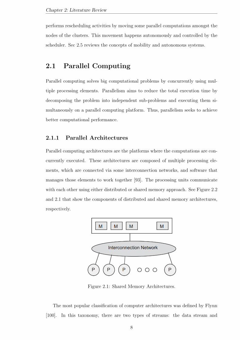
2.1 Shared Memory Architectures. . . . . . . . . . . . . . . . . . . . . . . 8
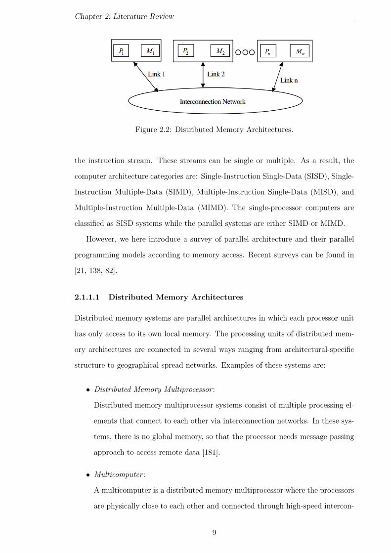
2.2 Distributed Memory Architectures. . . . . . . . . . . . . . . . . . . . 9
3.1 The effect of running multiple applications on the same processor. . . 56
3.2 The HWFarm structure. . . . . . . . . . . . . . . . . . . . . . . . . . 58
3.3 The HWFarm structure with mobility. . . . . . . . . . . . . . . . . . 62
3.4 Sequential and parallel programs. . . . . . . . . . . . . . . . . . . . . 64
3.5 Task structure in the HWFarm skeleton. . . . . . . . . . . . . . . . . 64
3.6 The distribution of data in the HWFarm skeleton.(I: Input, O: Out-
put, S: State, P: Program). . . . . . . . . . . . . . . . . . . . . . . . . 67
3.7 The distribution of tasks based on the allocation model. 8: 8-core
node; 24: 24-core node; 64: 64-core node. . . . . . . . . . . . . . . . . 70
3.8 Allocating MPI processes into cluster nodes. . . . . . . . . . . . . . . 71
3.9 Master/Worker cooperation. . . . . . . . . . . . . . . . . . . . . . . . 71
3.10 Tasks table at one worker. . . . . . . . . . . . . . . . . . . . . . . . . 76
3.11 An overview of the mobility operation in the HWFarm skeleton. . . . 78
3.12 Step a of the mobility operation in the HWFarm skeleton. . . . . . . 80
3.13 Step b of the mobility operation in the HWFarm skeleton. . . . . . . 80
3.14 Step c of the mobility operation in the HWFarm skeleton. . . . . . . 80
3.15 Step d of the mobility operation in the HWFarm skeleton. . . . . . . 81
3.16 The main loop of the user function. . . . . . . . . . . . . . . . . . . . 87
3.17 The execution time and the speedup when using the HWFarm skele-
ton to solve 2000*2000 Matrix Multiplication problem. . . . . . . . . 91
xi

3.18 The execution time and the speedup when using the HWFarm skele-
ton to solve Raytracer problem with 100 rays. . . . . . . . . . . . . . 92
4.1 Deng’s cost model . . . . . . . . . . . . . . . . . . . . . . . . . . . . . 100
4.2 The HWFarm cost model . . . . . . . . . . . . . . . . . . . . . . . . . 101
4.3 The HWFarm cost model with its parameters. . . . . . . . . . . . . . 103
4.4 The scaled transfer times compared to the scaled data-sizes. . . . . . 105
4.5 The scaled transfer times compared to the scaled relative processing
power. . . . . . . . . . . . . . . . . . . . . . . . . . . . . . . . . . . . 107
4.6 The relationship between the transfer time and the network latency. . 108
4.7 The scaled transfer times compared to the scaled network latency. . . 109
4.8 Execution time validation of Matrix Multiplication with one task. . . 112
4.9 Execution time validation of Matrix Multiplication with two tasks. . . 113
4.10 Execution time validation of Matrix Multiplication with four tasks. . 113
4.11 Execution time validation of Matrix Multiplication with eight tasks. . 114
4.12 Summary of the estimation accuracy in validating the execution time
in Matrix Multiplication. . . . . . . . . . . . . . . . . . . . . . . . . . 114
4.13 Example of 2D Raytracer problem with 3 objects in the scene. . . . . 115
4.14 Execution time validation of Raytracer with one task. . . . . . . . . . 116
4.15 Execution time validation of Raytracer with two tasks. . . . . . . . . 116
4.16 Execution time validation of Raytracer with four tasks. . . . . . . . . 117
4.17 Execution time validation of Raytracer with eight tasks (100 rays). . 117
4.18 Summary of the estimation accuracy in validation the execution time
in Raytracer. . . . . . . . . . . . . . . . . . . . . . . . . . . . . . . . 118
4.19 Execution times for a Matrix Multiplication task (2000*2000) on 2
locations . . . . . . . . . . . . . . . . . . . . . . . . . . . . . . . . . . 119
4.20 Execution times for a task (raytracer with 40 rays) on 2 locations . . 120
5.1 The circulating approach used to diffuse the load information in HW-
Farm. . . . . . . . . . . . . . . . . . . . . . . . . . . . . . . . . . . . 133
5.2 Load state of a normal loaded node. . . . . . . . . . . . . . . . . . . . 134
5.3 Load state of a highly loaded node. . . . . . . . . . . . . . . . . . . . 134
xii
5.4 An example showing how the HWFarm scheduler reschedules the
tasks when worker 3 becomes highly loaded. . . . . . . . . . . . . . . 137
5.5 Stage A of the estimation operation at worker 3. . . . . . . . . . . . . 139
5.6 Stage B of the estimation operation at worker 3. . . . . . . . . . . . . 139
5.7 Stage C of the estimation operation at worker 3. . . . . . . . . . . . . 140
5.8 Stage D of the estimation operation at worker 3. . . . . . . . . . . . . 140
5.9 Stage E of the estimation operation at worker 3. . . . . . . . . . . . . 141
5.10 The mobility behaviour of 10 tasks on 3 workers(Matrix Multiplication)152
5.11 The mobility behaviour of 8 tasks on 3 workers(Raytracer) . . . . . . 153
6.1 The load function design. . . . . . . . . . . . . . . . . . . . . . . . . . 161
6.2 The load function structure. . . . . . . . . . . . . . . . . . . . . . . . 163
6.3 The required and actual load in node 4. . . . . . . . . . . . . . . . . . 164
6.4 The required and actual load in the node with other changes in the
load (adaptive mode). . . . . . . . . . . . . . . . . . . . . . . . . . . 165
6.5 Load balancing (static/dynamic) under load changes. . . . . . . . . . 167
6.6 The load pattern applied to Raytracer and its impact on moving tasks
between workers. . . . . . . . . . . . . . . . . . . . . . . . . . . . . . 169
7.1 The pipeline approach. . . . . . . . . . . . . . . . . . . . . . . . . . . 173
7.2 Parallel pipeline with skeletons. . . . . . . . . . . . . . . . . . . . . . 174
7.3 The structure of the HWFarm skeleton to solve a findWord example. 174
7.4 The load pattern and the mobility behaviour of tasks at at Worker 1. 175
7.5 The load pattern and the mobility behaviour of tasks at at Worker 2. 175
7.6 The load pattern and the mobility behaviour of tasks at at Worker 3. 176
7.7 The load pattern and the mobility behaviour of tasks at at Worker 4. 176
7.8 Task 1 and its locations in the findWord problem. . . . . . . . . . . . 177
7.9 Task 7 and its locations in the findWord problem. . . . . . . . . . . . 177
7.10 The execution times of running the findWord problem using the HW-
farm skeleton. . . . . . . . . . . . . . . . . . . . . . . . . . . . . . . . 178
7.11 The execution times of running the N-body problem using the HW-
farm skeleton. . . . . . . . . . . . . . . . . . . . . . . . . . . . . . . . 179
xiii

7.12 Mapping the tasks on worker 1 for case AllOff. . . . . . . . . . . . . . 182
7.13 Mapping the tasks on worker 1 and worker 2 for case POn. . . . . . . 183
7.14 Mapping the tasks on worker 1 and worker 2 for case MOn. . . . . . . 184
7.15 Mapping the tasks on worker 1 and worker 2 for case BOn. . . . . . . 185
xiv
Chapter 1
Introduction
1.1 Context
In recent years, there has been a dramatic increase in the amount of available com-
pute and storage resources. Emerging multicore clusters offer popular high per-
formance computing platforms for commercial and scientific applications. These
clusters are either dedicated or non-dedicated. Dedicated clusters are expensive
and rare resources while non-dedicated clusters provide sharing resources amongst
multiple applications.
The increasing availability of shared resources on parallel platforms associated
with the growing demand for parallel applications leads to load variations and re-
source contention. Resource contention occurs when multiple processes or threads
are sharing and competing to acquire processing units. Such contention has a major
impact on the performance of the running applications. Hence, resource contention
implicitly leads to poor performance, high energy consumption, and application slow
down and high latency.
In this thesis, we address the problem of exploiting non-dedicated multicore clus-
ters taking into consideration resource contention under unpredictable workloads.
To achieve a desired performance, a framework has been proposed to solve prob-
lems and run algorithms in the shortest time in the presence of external load. This
framework is designed using skeletal programming approach. This approach is able
to manage the complexity of developing parallel computational applications and ex-
1

Chapter 1: Introduction
ploit easily a parallel computing platform. In this context, our skeleton/framework
works as a user-space parallel application that maintains to divide the problem into
sub-problems, computations, and run them on the nodes of the cluster concurrently
where the skeleton has distributed components hosted on these nodes to harness the
computing power of the multicore cluster.
To be adaptive to the variations of the competitive workload, a scheduling policy
has been provided. As a result, this scheduler is load-aware, performance-oriented
where it takes into consideration the external load and performs pre-emptive schedul-
ing of the parallel computations to meet the performance goal, reducing the total
execution time.
Because the variations of workload are changeable and unpredictable, gathering
system information to perform better rescheduling decisions is needed along with
a dynamic mechanism that takes appropriate decisions. Accordingly, the scheduler
uses a measurement-based performance cost model to predict the behaviour of the
parallel computations on a running architecture by deriving a mathematical formula
that expresses the completion time of the given computations. In this model, we
address architecture specific metrics such as resource usage and availability. Fur-
thermore, the behaviour of the parallel computations and network status are also
considered.
The rescheduling behaviour of our skeleton is implemented using a pre-emptive
approach. This approach requires moving the live computations amongst the nodes
of the clusters looking for better computational power to serve these computations
faster. The skeleton is enhanced with a built-in mobility support implemented im-
plicitly in the skeleton. The mobility of the skeleton computations is driven by the
CPU load of the nodes where those computations run. So once a node becomes
highly loaded, a move will be produced for better utilisation of computational re-
sources of that node and to meet the application performance goal. Mobility is an
appropriate solution when resource contention happens.
Thus, our research question is how can we enable parallel programs to adapt to
a dynamically changing environment, to minimise effects on run-times? To sum-
2
Chapter 1: Introduction
marise our answer, this thesis proposes a data-parallel generic skeleton that is able
to harness the computational power of non-dedicated multicore clusters taking into
account resource contention in the presence of external loads. This skeleton seeks
to find the best computational power to execute its computations faster. Hence
the performance goal of the skeleton is application-specific. This makes our skele-
ton selfish in meeting its performance metric which is sometimes bad in terms of
shared computing platforms. But, our experiments show that the skeleton somehow
improves the global load balancing and application throughput of the whole sys-
tem. Moreover, the experiments suggest that the skeleton is scalable and produces
speed-up when running different problems. Also, the experiments show significant
improvement of the performance and how the skeletons compensate for the load
variations. Our skeleton can be used by programmers to solve problems in parallel.
1.2 Contribution
The contributions of this research are as follow:
• We present a data-parallel skeleton called HWFarm for multicore clusters.
Multicore clusters provide standard general purpose platforms in terms of
computing. This skeleton is designed using Master/Worker pattern and im-
plemented using the C programming language and MPI as a communication
library for distributed memory architectures. Therefore, this skeleton works
best in parallel platforms compatible with MPI. For local collaboration on
the nodes, the PThreads library has been used. This skeleton reallocates its
computations/tasks amongst the involved nodes using a built-in mobility ap-
proach. This approach uses strong mobility with data mobility where the
skeleton saves the execution state of its computations, transfers them, and
resumes their execution. Experiments showing the mobility behaviour of the
skeleton tasks suggest that the skeleton is able to improve the performance
when running problems over shared parallel environments under high loaded
conditions. Our experiments show that the HWFarm skeleton is able to miti-
gate the resource contention by dynamically moving its tasks across the nodes
3

Chapter 1: Introduction
of the cluster.
• To manage the mobility behaviour of the skeleton, we provide the HWFarm
skeleton with a load scheduler which is autonomously responsible for taking
mobility decisions and managing load information. The mobility decision is
taken using a performance cost model that uses dynamic measures obtained
from the environment, the running program, and the load state of the system.
The cost model is dynamic where the external load changeable and unpre-
dictable at run-time. The environment measures are the characteristics of the
nodes where the skeleton runs. Moreover, the information of the running pro-
gram includes the progress of the program. Finally, the load state reflects the
current internal and external load. The load state is crucial in taking move-
ment decisions. Consequently, this model is dynamic, problem-independent,
language-independent, and architecture-independent. This enhances the adap-
tivity of the HWFarm skeleton.
• We explore a mechanism to generate artificial CPU loads to degrade system
performance on multicore architectures and control the resource usage. This
leads to a novel load function which may be instantiated to generate pre-
dictable patterns of load in a dedicated system to simulate different control-
lable load scenarios that may occur in a shared distributed non-dedicated
system. The generated load is dynamic, precise and adaptive. We present
a new tool which helps in evaluating experiments that depend on changes in
the load in multi-processor and multi-core environments. Examples of exper-
iments that can be evaluated using the load function are the static/dynamic
load balancing, work stealing and mobility experiments. This tool might be
used in a homogeneous setting to simulate a heterogeneous environment by
giving differential constant loads to the processing elements with the same
characteristics. It might also be used to simulate different patterns of system
component failure by giving processing elements infeasibly large loads.
4

Chapter 1: Introduction
1.3 Thesis Structure
The structure of this thesis is as follow:
Chapter 2 introduces concepts of parallel computing, skeletal programming,
mobility, scheduling, and cost modelling. Furthermore, this chapter provides a sur-
vey of skeletons and parallel programming languages that support the skeletal-based
approach.
Chapter 3 gives an overview about designing skeletal-based systems. Then we
propose the design of the HWFarm skeleton and the implementation of our skeleton.
Furthermore, we explore how we support our skeleton with a mobility mechanism
that enables it to move its live computations amongst nodes. Moreover, we discuss
the usability of this skeleton and provide guides about how to run different types of
problems with some assumptions/restrictions.
Chapter 4 introduces the performance cost model used in the HWFarm skele-
ton. This chapter describes how the cost model is aware to the environment load
state and the computation behaviour. Furthermore, experiments are performed to
evaluate the decisions taken by this cost model. These experiments show the accu-
racy of these decisions in terms of completion times, mobility decisions and mobility
costs. Furthermore, this chapter shows that these decisions lead to improve of the
performance of the skeleton and meet the performance goal.
Chapter 5 proposes the load scheduler used in the HWFarm skeleton. This
scheduler uses a circulating approach to diffuse the load information in order to
provide the most recent load information to all participated nodes. Moreover, this
chapter discusses in depth how this scheduler uses a measurement-based cost model
to take movement decisions that can be used to produce a new schedule. Evalu-
ation experiments have been carried out to demonstrate the improvement of the
performance and the mobility behaviour. This chapter also demonstrates that the
scheduling and cost operations incur low overhead compared to the total execution
time.
Chapter 6 presents a tool implemented as a load function that generates dy-
namic, adaptive load patterns across multiple processors. This load function is
5
Chapter 1: Introduction
highly effective in a shared dedicated system for simulating patterns of load changes.
Moreover, this chapter shows that this function has minimal impact in an experi-
mental setting.
Chapter 7 explores the evaluation of HWFarm on a range of applications with
different characteristics. It also demonstrates the usability of the skeleton over large
scale applications. Furthermore, this chapter evaluates the adaptivity feature of the
HWFarm skeleton that has a large positive impact on all applications running on
shared nodes.
Chapter 8 gives a summary of the thesis, outlines the research direction for
future work, and discusses the limitations of this work.
1.4 Publications
This work has led to three publications. The first paper explains the HWFarm
skeleton design and implementation with its mobility behaviour. The second paper
presents the load function structure and its usability. The third paper propose the
dynamic cost model and the load scheduler to improve the performance eof the
HWFarm skeleton. These published papers are:
• Alsalkini T. and Michaelson G., 2012. Dynamic Farm Skeleton Task Allocation
through Task Mobility. In: 18th International Conference on Parallel and
Distributed Processing Techniques and Applications. Las Vegas, USA, pp.
232-238.
• Alsalkini T. and Michaelson G., 2014. Generating Artificial Load Patterns
on Multi-Processor Platforms. In: 11th International Conference on Applied
Computing. Porto, Portugal, pp. 77-84.
• Alsalkini T. and Michaelson G., 2015. Optimising Data-Parallel Performance
with a Cost Model in The Presence of External Load. In: 12th International
Conference on Applied Computing. Greater Dublin, Ireland, pp. 89-96.
6

Chapter 2
Literature Review
Hardware development has been progressing in the recent years. However, the rise
of multi-core processors has affected the ability of the software developers to har-
ness the resources of these architectures to match their requirements. Designing
parallel and distributed software models to manage the scientific problems is needed
to fully exploit such platforms. These models should offer abstractions of low-level
details to free the developers from this burden. In this thesis, we propose a parallel
framework that aims to harness the compute power of multi-core clusters. In Sec
2.1 we review the development of the architectures and parallel computing as well
as computing platforms used to run parallel applications. Furthermore, the paral-
lel programming models needed to fully exploit such platforms are discussed. This
framework is proposed as a skeleton that encapsulates all coordination and low level
issues. This helps the programmers to focus on their problem rather than spending
too much time dealing with parallel programming details. Algorithmic skeletons are
high-level parallel programming constructs that embed parallel coordination over
sets of locations. A background of algorithmic skeletons and a survey of skeletal-
based libraries/languages have been shown in Sec 2.2. Our skeleton addresses the
resource contention issue in shared platforms. This requires a scheduling policy that
deals with the changeable load conditions in the system and takes appropriate deci-
sions. Dynamic cost modelling and performance models used in the skeletal based
frameworks and structured parallel models are introduced in Sec 2.3. The notions
of scheduling and their techniques are discussed in Sec 2.4. Finally, the skeleton
7
Chapter 2: Literature Review
performs rescheduling activities by moving some parallel computations amongst the
nodes of the clusters. This movement happens autonomously and controlled by the
scheduler. Sec 2.5 reviews the concepts of mobility and autonomous systems.
2.1 Parallel Computing
Parallel computing solves big computational problems by concurrently using mul-
tiple processing elements. Parallelism aims to reduce the total execution time by
decomposing the problem into independent sub-problems and executing them si-
multaneously on a parallel computing platform. Thus, parallelism seeks to achieve
better computational performance.
2.1.1 Parallel Architectures
Parallel computing architectures are the platforms where the computations are con-
currently executed. These architectures are composed of multiple processing ele-
ments, which are connected via some interconnection networks, and software that
manages those elements to work together [93]. The processing units communicate
with each other using either distributed or shared memory approach. See Figure 2.2
and 2.1 that show the components of distributed and shared memory architectures,
respectively.
Figure 2.1: Shared Memory Architectures.
The most popular classification of computer architectures was defined by Flynn
[100]. In this taxonomy, there are two types of streams: the data stream and
8
Chapter 2: Literature Review
Figure 2.2: Distributed Memory Architectures.
the instruction stream. These streams can be single or multiple. As a result, the
computer architecture categories are: Single-Instruction Single-Data (SISD), Single-
Instruction Multiple-Data (SIMD), Multiple-Instruction Single-Data (MISD), and
Multiple-Instruction Multiple-Data (MIMD). The single-processor computers are
classified as SISD systems while the parallel systems are either SIMD or MIMD.
However, we here introduce a survey of parallel architecture and their parallel
programming models according to memory access. Recent surveys can be found in
[21, 138, 82].
2.1.1.1 Distributed Memory Architectures
Distributed memory systems are parallel architectures in which each processor unit
has only access to its own local memory. The processing units of distributed mem-
ory architectures are connected in several ways ranging from architectural-specific
structure to geographical spread networks. Examples of these systems are:
• Distributed Memory Multiprocessor :
Distributed memory multiprocessor systems consist of multiple processing el-
ements that connect to each other via interconnection networks. In these sys-
tems, there is no global memory, so that the processor needs message passing
approach to access remote data [181].
• Multicomputer :
A multicomputer is a distributed memory multiprocessor where the processors
are physically close to each other and connected through high-speed intercon-
9
Chapter 2: Literature Review
nection network [19].
• Clusters :
A cluster is a parallel computing system that consists of a set of computers
interconnected with each other by a network to comprise a computing system
[49]. Each computer in a cluster may have a single processor or multiple pro-
cessors and connects to other computers via a LAN (Local Area Network).
The nodes, the computers in the cluster, can work together as an integrated
computing resource or they can operate individually. Hence, clusters provide
cost-effective environments that offer computing services for solving high per-
formance problems. An example of a cluster is a Beowulf system which is a
scalable cluster hosted by open source software [209]. A Beowulf system is
composed of group of nodes incorporated in personal computers and based on
a private system network. In this thesis, we are studying this architecture as
one of parallel computing platforms.
• Grid :
A Grid is a system for sharing the computational resources, such as data
storage, I/O capacity, or computing power, over the Internet [102, 103]. A
computational Grid is a mechanism to access shared computational resources
in a scalable, secure, high-performance manner. Those who use a Grid are
able to share and use computational resources in geographically distributed
locations.
2.1.1.2 Shared Memory Architecture
A shared memory system is a category of parallel architectures where each pro-
cessing unit has access to a global memory. Through this memory, the processes
communicate, coordinate, and synchronise with other processes in the system [93].
In such systems, there are independent processors connected with memory modules
via an interconnection network. In terms of memory access, shared memory systems
can be categorised in three categories:
• Uniform Memory Access (UMA): In UMA, the shared memory locations are
10
Chapter 2: Literature Review
accessible by all processors with the same access time. These systems are also
known as Symmetric Multiprocessor (SMP). An Example of this architecture
is PMC-Sierra RM9000x2 [192].
• Non-uniform Memory Access (NUMA): NUMA is a memory organisation
where each processor has part of the shared memory. In these systems, the
access times are not equal due to the distance between the processor and the
memory module. For an example, see the Intel Single-chip Cloud Computer
(SCC) [164].
• Cache-Only Memory Access (COMA): In COMA, the shared memory com-
prises cache memory and the address space is made of all the caches. In this
case, part of the shared memory and a cache directory are attached to each
processor. The Swedish Institute of Computer Sciences Data Diffusion Ma-
chine (DDM) [113] is an example of this architecture. Another example is
KiloCore [39] which is a chip that has 1000 cores and 12 memory modules.
This chip is developed by the VLSI Computation Laboratory (VCL) at UC
Davis.
2.1.1.3 Multi/Many-core Architectures
Computer manufacturers initially made chips with one processor. Producing faster
processors requires increasing the number of transistors and raising the clock speed.
Due to the limit on the scaling of clock speeds, which is known as the power wall,
manufacturers turned to multicore architectures to overcome the space and over-
heating issues. In this architecture, the chips have two or more processors (cores)
and share hardware caches [120]. Multicore architecture is an effective example of
a shared memory architecture where the communication amongst cores is fast and
the bandwidth is high.
Another core-based approach has been introduced in parallel programming. This
approach, which is known as many-core, uses a large number of small cores. An
example of a many-core architecture is the Graphical Processing Unit (GPUs) [125]
where a GPU is a special-purpose SIMD processor initially designed for a particular
11

Chapter 2: Literature Review
class of applications [178]. Recently, GPUs have been employed to perform general
purpose applications GPGPU [232].
2.1.2 Parallel Programming Patterns
Effective use of parallel architectures involves dividing a problem into computations
that can be of executed on available processing units. Parallelising a problem can
be several kinds: data, task, or pipeline parallelism [163, 119].
In terms of parallel programming design, Mattson el al [163] introduced a pat-
tern language that provides patterns to help users in developing parallel programs.
This language has 19 patterns organised into four design phases: Finding Con-
currency, Algorithm Structure, Supporting Structures, and Implementation Mecha-
nisms. However, the patterns that support structure design and correspond to the
parallel programming models are: SPMD (Single Program Multiple Data), Master/-
Worker (task pool), Loop Parallelism (independent iterations), and the Fork/Join
pattern.
• SPMD : In this pattern, each process or thread, performs the same operations
but with different set of data. SPMD can be used either in distributed or
shared memory systems. This pattern provides processes that are easy to
manage, achieves high scalability, and shows close to parallel environment.
• Master/Worker : This pattern involves two kinds of processes: Master pro-
cesses and worker processes. A master process initiates a bag of tasks and sets
a pool of workers. Whilst, a worker process obtains a task from the master
and executes it. All workers run concurrently until the bag becomes empty.
This pattern is typically used in problems that require the workload to be bal-
anced amongst the workers. The Master/Worker pattern has good scalability
and fault tolerance support. A disadvantage of this pattern is the bottleneck
between master and workers but this problem can be avoided if the algorithm
is well implemented.
12
Chapter 2: Literature Review
• Loop Parallelism: In this pattern, the runtime will split up the intensive iter-
ations amongst the processes or threads if they are nearly independent. Loop
parallelism is mainly suitable for shared memory systems. But it also can be
used in a distributed fashion if each loop iteration is really big.
• Fork/Join: This pattern has a main process that creates new processes to
execute some concrete operations. The main process will wait for all forked
processes to join. The Fork/Join pattern is suitable for problems that create
tasks dynamically and good for shared systems. The overhead in this pattern
is related to the cost of creating and destroying the processes.
2.1.3 Parallel Programming Models
Developing parallel applications in a wide range of parallel systems is a complicated
task [49]. Developers are challenged by a variety of issues related to the system
and the programming style. To solve these issues, there are two main approaches:
automatic parallelization and parallel programming [138].
The first approach relies on parallelizing compilers that are used for parallelizing
a sequential program into a version able to execute on a parallel system. Such
compilers are limited to problems that have regular computations and commonly do
not provide useful speedup on distributed memory machines [49]. An alternative to
parallelizing compilers is parallel programming languages which are used to relieve
programmers from the complexity of parallelism. However, these languages are
designed from principles that help to produce a parallel programming language to
deal with the difficulties of parallelism.
The second approach is parallel programming which is based on developer efforts
to exploit parallel architectures. In this approach, developers use a traditional high-
level programing language, like C or Fortran, augmented with a library, such as
PThreads [48], or extended with parallelism support, like CILK [37].
Other ways of parallel programming are providing programming skeletons that
support some parallelization. Skeletal programming will be explained in further
details later.
13
Chapter 2: Literature Review
As mention above, parallel architectures are categorised into shared memory and
distributed memory [207]. Here, we discuss the parallel programming models used
to develop across parallel systems.
2.1.3.1 Distributed Memory Systems
The message passing model is commonly used in distributed memory systems to
move data between processing elements without the need for a global memory. Pro-
gramming using the message passing model has the advantages [85]: portability of
parallel programs as they do not require any hardware support, and the ability to
explicitly control the placement of data on the memory by the programmer. This
model also has disadvantages [49, 85]. The first one is that the programmers have to
manage the tasks of parallelisation, such as: communication, synchronisation, data
distribution, and load balancing. The second disadvantage is that these models may
incur communication overhead due to the time needed for processes to communicate.
Message passing model suits the SPMD parallel programming pattern in addition
to the Master/Worker pattern [163].
Examples of message-passing models:
• MPI : Message Passing Interface is a library of routines to connect processes
that are located across the distributed memory system [112]. This library
can be bound to C, C++, Fortran, Java, etc. MPI operations are classi-
fied as point-to-point and collective routines. Point-to-point routines, such
as send/receive, provide communication between two processes. Collective
routines ease communication amongst groups of two or more processes.
• PVM : Parallel Virtual Machine is a software environment that uses the mes-
sage passing model to exploit heterogeneous distributed processing elements.
PVM makes a set of computing units appear as a virtual computing system
[27].
14
Chapter 2: Literature Review
2.1.3.2 Shared Memory Systems
In shared memory systems, processes or threads, which execute tasks concurrently,
have access to a global shared memory [93, 19]. The communication amongst pro-
cesses can be accomplished through shared variables or shared communication chan-
nels. Shared memory architectures have low latency and high bandwidth. However,
this raises two issues: consistency and coherency [85]. The consistency issue is raised
when multiple processors try to access or update shared memory locations. There-
fore, a proper memory coherence model should be chosen in designing distributed
memory systems.
Examples include:
• POSIX Threads (Portable Operating System Interface Threads): In this model,
there are several threads, running simultaneously on a shared memory plat-
form [19]. PThreads [48] is introduced as a low level, flexible library of routines
to manage the threads explicitly. This library is used with the C programming
language. Using PThreads, programmers have full control to create, manage,
and destroy threads. Parallelism using this model needs much effort from de-
velopers to avoid race conditions and deadlock. The most appropriate parallel
programming pattern when using this library is the Fork/Join model [163].
• Intel TBB (Intel Threading Building Blocks): Intel TBB is a multithreaded
model in shared memory systems [191]. It is presented as a C++ template
library that manages and schedules threads to run concurrently in order to
execute tasks in parallel. This library also contains various generic algorithms
and supports dependency and data flow graphs as well as offering synchroni-
sation and collective primitives.
• OpenMP (Open Multi Processing): OpenMP is a shared memory based parallel
programming model; it is also known as a multithreaded model [57]. OpenMP
is implemented as an API to provide a set of compiler primitives and runtime
library routines. This API can be used with Fortran, C, and C++. The
parallel program patterns that are suited to OpenMP are loop parallelization,
15
Chapter 2: Literature Review
SPMD, and join/fork pattern.
To combine the ease of writing parallel programs in shared memory systems
with the scalability of the distributed memory environments, the DSM (Distributed
Shared Memory) model has been proposed [185]. In this model, the system is
implemented as shared memory in a distributed memory environment. An example
of a model that uses the DSM approach is PGAS (Partitioned Global Address Space)
[63]. An example of a PGAS language is Chapel [56]. Moreover, UPC (Unified
Parallel C) is a parallel programming language that supports the PGAS model.
UPC is an extension of the programing language C and can be used in shared or
distributed memory environments [220].
For GPU architectures, the SPMD programming model is used as each element is
independent from other elements [178]. To develop applications over GPUs, NVIDIA
proposed CUDA (Compute Unified Device Architecture) as a parallel programming
model [176]. Moreover, OpenCL (Open Computing Language) provides a standard
interface to implement data and task parallelism over heterogeneous platforms [212].
2.2 Skeletons for Parallel Computing
The algorithmic skeleton, according to Cole [65], is an approach in parallel program-
ming to abstract the complexities that exist in the parallel implementations. The
skeleton concept is closely related to functional languages, so higher order functional
structures can be produced by using skeletons [187].
A parallel program can be composed of simple skeletons. These skeletons are
referred to as elementary skeletons. These skeletons abstract the basic operations
of the data parallel model [159]. Furthermore, elementary skeletons may use per-
formance cost measures to achieve effective implementations. Using elementary
skeletons, it is difficult to adapt the architectural characteristics of the wide range
of parallel computing systems. Moreover, acquiring the best performance when com-
posing several elementary skeletons is a very tough job. To solve these issues, exact
skeletons can be used to define complex patterns.
16

Chapter 2: Literature Review
Each skeleton has an implicit parallel implementation hidden from the user; thus,
the main advantage is that the communication and parallelism details are embedded
in the skeleton. The skeletons are equivalent to polymorphic higher order functions
so that there are various kinds of skeletons covering different programs over different
data types [99]. In contrast, skeletons that support particular data structures are
known as homomorphic skeletons. Homomorphic skeletons may deal with lists,
arrays, trees or graphs. Thus, some authors may name skeletons depending on
the data structure that the skeletons support, for example list skeletons, matrix
skeletons, or tree skeletons.
2.2.1 Skeleton Types
In terms of functionality, parallel skeletons can be classified into three types: task-
parallel, data-parallel and resolution skeletons [187, 111]:
• Task-parallel skeletons : In this kind of skeleton, the parallelism will be based
on the task, so there are many function calls in parallel. Examples of task-
parallel skeleton are: the pipe skeleton where computations that are relevant
to different stages can run simultaneously, and the farm skeleton which can
schedule independent tasks across several processing units. This is also known
as Master/Slave. The pipe skeleton can be found in different frameworks such
as SKELib [74] and Muskel [9] while examples of libraries that support the
farm skeleton are JaSkel [98] and Eden [152].
• Data-parallel skeletons : These skeletons apply parallelism by partitioning the
data amongst processors and performing the computation on different parts
concurrently. For examples: the map skeleton applies a function or operation
concurrently over items in a list. The map skeleton is an example of SIMD
parallel programming pattern. The reduce skeleton executes a function or
operation on each pair of elements to form the final result. It is also referred as
scan. The fork skeleton applies different operations on various data elements.
The fork skeleton is an example of a MIMD parallel programming pattern.
Most of the libraries support data-parallel skeletons. For examples P3L [73]
17
Chapter 2: Literature Review
offers the map, reduce and scan skeletons while Calcium [51] library support
the fork skeleton.
• Resolution skeletons : these skeletons are designed as the solution of a family of
problems. An example of a resolution-parallel skeleton is Divide and Conquer
(D&C) which divides the list of elements recursively into two lists until a
condition is met. Then, the D&C skeleton applies a function to the list and
afterwards merges the results back to produce the final result. The D&C
skeleton is provided in many libraries such as Skandium [149] and Calcium
[51]. Another example of resolution-parallel skeletons is Branch and Bound
(B&B) which also branches recursively across the search space. Then, it uses
an objective function to bound the resulting data. An example of libraries
that supports the B&B skeleton is Muesli [62].
2.2.2 Advantage of Using Skeletons
The main target of skeletons in parallel programming is to separate the application
from the implementation [99]. By using skeletons, users can specify the parallel
parts and leave the parallelism complexities to the skeletons.
Skeletons are modelled as higher-order functions able to be customised to specific
applications. However, optimised skeleton implementations, which fit specific lan-
guages and parallel architectures, should be generated to achieve high performance
and portability over various machines.
The main advantages of using algorithmic skeletons in parallel programming are
[49]:
• Programmability : Skeletons hide the low-level details, such as communications
and coordination, from the programmers. Therefore, such solutions help the
programmers to spend more time in optimising the problem. Hence, using
skeletons improves the programmability of the parallel programming systems
and increases the productivity of users.
• Reusability : Skeletons have been built to form generic patterns for developing
18
Chapter 2: Literature Review
the problems that have the same parallel structure. This will increase the
reusability and avoid the repetition of efforts in programming and optimising
the programs that belong to particular parallel template.
• Portability : Portability has considerable importance in parallel applications.
So, skeletons should adapt to the parallel systems and the hardware archi-
tecture. Thus, parallel applications that are developed using skeletons have
ability to run on various platforms.
• Efficiency : Developing parallel applications requires a balance between effi-
ciency and portability. Skeletal-based parallel programming using cost models
can achieve improvement in the performance.
2.2.3 Skeletons in Parallel Environments
Skeletal programming is used to overcome the problems of coordination in parallel
programming by exploiting generic program structures. Much work has been carried
out on skeletal programming for different data types for various parallel architec-
tures. Skeleton implementations may support either a specific parallel architec-
ture or heterogeneous architectures, including shared memory, distributed memory,
multi-core, or many-core architectures. Such skeletons are provided as libraries on
top of a parallelisation mechanism, such as MPI, or a high level parallel language
that supports skeletal constructs. Each skeleton may be associated with a compiler
that translates the high-level functions into source code able to run over the target
hardware. Some implementations may support a list of skeleton patterns: map,
reduce, farm, etc. Others may support one or more types of skeletal programming.
In this section, we are going to review some examples of available skeletons and
parallel programming languages that support the skeletal approach. Other surveys
can be found in [21, 111].
• P3L, SkIE & SkELib
P3L (Pisa Parallel Programming Language), 1992, [73] is a skeleton-based
parallel programming language that provides skeleton constructs. These con-
19

Chapter 2: Literature Review
structs abstract the common patterns of task and data parallelism. P3L is
associated to a template-based compiler that is used to optimise the imple-
mentation of templates to a specific architecture. Moreover, the P3L compiler
can use a performance cost model to help in allocating resources corresponding
to parallel systems.
SkIE (Skeleton-based Integrated Environment), 1999, [24] is a coordination
language similar to P3L. This language enables the user to interact with graph-
ical tools to compose skeletal parallel modules. Furthermore, this language
provides advanced tools such as visualisation, performance analysis and de-
bugging tools.
SkELib, 2000, [74], which is a C library, inherits from P3L and SkIE and uses
a template-based system.
• SCL
SCL (Structured Coordination Language), 1995, [77] is a skeletal program-
ming language that supports various commonly used data structures through
configuration skeletons. Furthermore, SCL offers data-parallel skeletons, like
map, and task-parallel skeletons, like farm, using elementary skeletons and
computation skeletons, respectively.
• Skil
Skil, 1996, [43] is an imperative language supported with higher-order func-
tions and a polymorphic type system. Skil offers data and task parallelism over
parallel distributed architectures. Skeletons in Skil language are not nestable.
• HDC
HDC (Higher-order Divide and Conquer), 2000, [121] is a sub set of Haskell
that uses a higher-order functional style. It has many implementations of
the Divide and Concur paradigm starting from the general model to concrete
cases such as multiple block recursion and elementwise operations. Therefore,
it supports resolution parallelism over distributed platforms.
• Muskel & nmc
20

Chapter 2: Literature Review
Muskel, 2001, [9], provides nestable skeletons for data and task parallelism
and exploits a macro data flow model to achieve parallelism. Muskel gives
users a skeletal-based parallel programming system by targeting parallel dis-
tributed architectures. Furthermore, Muskel has features that optimise the
performance such as load balancing and resource usage. Much work has been
done on skeletal extensibility [9] and combining structured with unstructured
programming [72].
Nmc, 2010, [10] is the multicore version of the Muskel library. This version
provides some skeletons to run on multicore clusters.
• ASSIST
ASSIST, 2002, [223] is a structured programming language that uses a module-
described graph to express parallel applications. It has performance optimisa-
tion through controlling resource usage and supporting load balancing.
• SkiPPER
SkiPPER, 2002, [198] is a library of skeletons for vision applications in Caml
with type safety. Skeletons in SkiPPER are either declarative or operational.
• Mallba
Mallba, 2002, [8] is a skeletal-based library for combinational optimisation.
Mallba provides three generic resolution methods: exact, heuristic, and hybrid
with three different implementations: sequential, parallel in local area, and
parallel in wide area.
• Llc language
Llc, 2003, [87] is a high-level parallel programming language that offers sup-
port for four skeletons: forall, parallel sections, task farms and pipelines [8].
Skeletons with Llc can be executed on multicore or distributed systems. Llc
uses a compiler that generates MPI code based on OpenMP like directives. A
new approach to generate a hybrid MPI/OpenMP code has been developed to
control the communication on the node itself and amongst the nodes [194].
• Alt & HOC-SA
21

Chapter 2: Literature Review
Alt, 2003, [16, 15] a Java-based Grid programming system composed of a set
of skeletons. These skeletons are provided as services to the clients on parallel
distributed systems. It supports a data-parallelism approach over shared dis-
tributed memory architectures.
HOC-SA (Higher-Order Components-Service Architecture), 2004, [91] encap-
sulates the Alt approach to support parallelism. In HOC-SA, clients send the
code and the data to be executed to servers with a skeleton description flow.
Once the execution completes, the result is delivered to the users.
• Lithium
Lithium, 2003, [12] is a Java library that provides nestable skeletons to support
data and task parallelism. Lithium is implemented with a macro data flow
implementation model. In this model, the nodes in the data flow graph host a
piece of code to be executed on the computational units. Extensions of Lithium
have been proposed for performance optimisation such as load balancing.
• Eden
Eden, 2005, [152] is an extension of Haskel. It supports task and data par-
allelism over distributed memory environments. It also supports automatic
communication between processes. Many extensions have been proposed for
Eden such as a flexible distributed work pool skeleton [83] in 2010 and a skele-
ton iteration framework [84] in 2012.
• eSkel
eSkel (Edinburgh Skeleton Library), 2005, [29] is a C library that offers a set of
skeletons over the MPI model. This library supports data and task parallelism
on parallel distributed systems. eSkel provides two skeleton modes, nesting
and interaction. In terms of performance, eSkel uses empirical methods and
the Amoget process algebra for resource allocation and scheduling.
The Edinburgh group has done much work on the adaptive approach through
presenting a parallel pipeline pattern [110].
• JaSkel
22
Chapter 2: Literature Review
JaSkel, 2006, [98] is a skeleton based framework in Java. It provides nestable
skeletons that can run on different platforms. JaSkel skeletons execute sequen-
tially, concurrently on shared memory systems, or in parallel on clusters.
• QUAFF
QUAFF, 2006, [97] is a C++ and MPI based skeleton library that uses a
template-based meta-programming approach to reduce overhead and enable
compile time optimisation. QUAFF provides a set of nested skeletons on
parallel distributed environments. Moreover, QUAFF uses type checking and
C++ templates to generate new C/MPI code at compile time.
• SkeTo
SkeTo, 2006, is a C++ library that provides a set of operations on parallel
data structures, such as list, on distributed memory systems [162]. This li-
brary provides parallel skeletons based on the BMF programming model [32].
SkeTo supports nestable skeletons for data and resolution parallelism. To op-
timise SkeTo, a fusion transformation approach has been provided in order to
reduce the overhead. A new version of SkeTo has been proposed in 2009 to
work on multicore architectures [136]. In the multicore version, SkeTo offers
a number of skeletons that manage the dynamic scheduling using the size of
cache. Recently, a new version with list support has been released [160] in
2010. In this version, the skeletons are equipped with fusion optimisation that
is implemented based on an expression templates programming technique.
• AMSs
AMSs (Autonomous Mobility Skeletons), 2007, [80] are higher order functions
that support autonomous mobility. These skeletons are guided by a cost model
which makes them aware of the load changes on the network.
• Calcium
Calcium, 2007, [51] is a library of skeletons in Java. This library supports
nestable data and task parallel skeletons on parallel distributed architectures.
Moreover, Calcium provides additional features that help in improving the
23

Chapter 2: Literature Review
performance such as a performance tuning model.
• TBB
TBB (Threading Block Building), 2007, [191] is a pattern-based library, de-
veloped by Intel, for parallel applications on multicore architectures. TBB
provides a wide range of parallel patterns such as, for, reduce, sort, in addi-
tion to some patterns. TBB offers concurrent data structures and gives the
programmer ability to control other threads, task scheduling, and granularity.
Major industry powerhouses have developed similar frameworks, TPL, 2009,
[147] from Microsoft, MapReduce, 2008, [79] from Google, Hadoop, 2012, [228]
and Phoenix, 2007, [189] from Apache, and BlockLib, 2008 [14] from IBM.
• Muesli
Muesli, 2009, [62] is a skeleton library that offers skeletons through C++
methods. This library provides nestable skeletons for data and task parallelism
and supports parallel distributed architectures. Muesli was extended in 2010
to support multicore parallel programming [61].
• Skandium
Skandium, 2010, [149], like Calcium, is also a Java library that supports skele-
tal programming on shared memory systems. This library is a reimplemen-
tation of the Calcium library on multicore architectures. Skandium offers
nestable skeletons for both data and task parallelism.
• STAPL
STAPL (Standard Template Adaptive Parallel Library), 2010, [47] is a skele-
ton framework that gives the user the ability to compose a parallel program
from a set of elementary skeletons. Using a parametric data flow graph, this
framework is a representation of a parallel implementation of STL (Standard
Template Library). STAPL can work in both shared and distributed mem-
ory platforms. Furthermore, this framework supports nested composition for
multi-level parallelism.
• FastFlow
24

Chapter 2: Literature Review
FastFlow, 2011, [11] is a parallel programming framework written in C++.
This framework supports pattern-based programming on parallel shared/dis-
tributed memory systems in addition to GPU architectures. FastFlow is struc-
tured into three layers to provide different levels of abstractions to the ap-
plication developer. These layers give the programmer a high level parallel
programming, flexibility, and portability to different platforms. In 2014, a
ParallelFor skeleton [75] was added to the framework that supports many-core
architecture. This skeleton filled the gap between the conventional data struc-
tures and loop parallelisation facilities provided by low-level frameworks, such
as OpenMP.
• OSL
OSL (Orlans Skeleton Librray), 2011, [128] is a C++ library of data-parallel
skeletons that follow the BSP parallel model [36] of parallel computations. It
is built over MPI and uses expression templates to optimise the efficiency in a
functional programming style. Skeletons in the OSL library perform operations
on distributed arrays where the data is distributed amongst the processors. In
an update of this library, in 2013, a skeleton has been implemented to support
list homomorphism. This skeleton is called BH [146] (BSP homomorphism).
Like SkeTo, OSL also uses expression templates for fusion optimisation.
• HWSkel
HWSkel, 2013, [21] is a skeletal based parallel programming library for hetero-
geneous multicore cluster and GPUs. HWSkel provides a number of skeletons
optimised through a static performance model.
• Skel
Skel, 2014, [46] is a domain specific language implemented in Erlang. This
library supports map, farm, pipe and seq skeletons as well as providing a
high-level cost model related to each skeleton. This cost model predicts the
performance of the parallel program. Skeletons of Skel can be nestable where
they run over shared memory platforms.
25
Chapter 2: Literature Review
• SkelCL
SkelCL, 2015, [210] is skeleton library for GPUs to ease GPU programming.
Other examples of skeleton-based GPU programming frameworks are PSkel,
2015, [183], SkePU, 2010, [94], Marrow, 2013, [158], and Lapedo, 2016, [127].
Much work has been done to compose the memory affinity approach with skeletal
programming. Such skeletons seek to enhance the memory affinity by locating the
threads and the data for increasing the performance. Recent work can be found
in [109].
Some skeletons libraries have been developed for embedded real-time systems [208].
Another approach to skeletal programming is developing an implementation of
an existing library. Example of these approach are DatTel [35] and MCSTL [203],
which are parallel implementation of the standard library STL in C++.
Several researchers developed skeletons with various programming languages.
Surveys of work on skeletal programming can be found in [111, 21, 197, 190, 35,
161, 170, 68].
See Table 2.1 that summarises all skeleton mentioned in our survey.
2.3 Parallel Cost models
A cost model is a performance model [166] used to estimate the costs of program
performance metrics, such as time [193]. Cost models have two levels [80]:
• Computation Cost Model: to estimate the cost of a sequential computation.
• Coordination Cost Model: to estimate the cost of coordinating of parallel,
distributed and mobile programs.
Computation Cost Model
The estimation of execution time for a program running on a specific computer and
manipulating some data can be done in two ways [64]:
26

Chapter 2: Literature Review
Year Type ofSupport
Nesting Skeleton Set
P3L, SkIE &SkELib
1992-2000
language/ li-brary(SkELib)
limited map, reduce, scan, comp,pipe, farm, seq & loop
SCL 1995 language limited map, scan, fold & farm
Skil 1996 library no pardata, map & fold
HDC 2000 Haskell subset no map, red, scan, filter & dc
Muskel & nmc 2001 library yes farm, pipe & seq
ASSIST 2002 language no seq & parmod
SkiPPER 2002 library limited scm, df & tf
Mallba 2002 library no exact, heuristic & hybrid
Llc language 2003 language yes forall, parsection, farm &pipeline
Alt & HOC-SA
2003-2004
library no map, reduction, scan, dh,apply & sort
Lithium 2003 library yes map, farm, reduce & pipe
Eden 2005 Haskellextension
yes map, farm, dc, pipe &ring
eSkel 2005 library yes pipe, farm, deal, butterfly& hallowSwap
JaSkel 2006 library yes farm, pipeline &heartbeat
QUAFF 2006 library yes seq, pipe, farm & pardo
SkeTo 2006 library yes list, matrix & tree
AMSs 2007 library no automap, autofold &autoIterator
Calcium 2007 library yes seq, pipe, farm, for, while,map, dc & fork
TBB 2007 library yes for, reduce, scan, do, sort& pipeline
Muesli 2009 library yes array, matrix, farm, pipe& parallel comp
Skandium 2009 library yes seq, pipe, farm, for, while,map, dc & fork
STAPL 2010 library yes map, map-reduce, scan,butterfly, allreduce &
alltoall
FastFlow 2011 library yes pipeline, farm, parallelFor& mapReduce
OSL 2011-2013
library no map, zip, reduce, scan,permute, shift,
redistribute & flatten
HWSkel 2013 library no hMap, hMapAll,hReduce, hMapReduce &
hMapReduceAll
Skel 2014 language yes map, farm, pipe & seq
Table 2.1: Skeletons summary.
27

Chapter 2: Literature Review
• Static Analysis : The measurement is done by using mathematical reasoning on
the code of the program and the data to determine the time to execute the pro-
gram. The performance model of the program may be machine-independent.
These models are also called static cost models or analytical formula.
• Dynamic Analysis : The execution time of a program is measured on given data
and on a particular machine. The measurement is done by using an internal
clock and benchmarking the execution of the program where the benchmark
is machine-specific. These models are also called dynamic cost models.
Coordination Cost Models
Parallel programming is a complex activity that includes many decisions, such as
task allocation, scheduling and communication. The parallel programming model
can exploit the coordination cost models for parallel programming. Coordination
models may use the computation cost models for enhancing coordination decisions.
To simplify using a cost model with parallel programs, developers use constrained
parallel programming paradigms to simplify modelling the coordination in a parallel
application.
2.3.1 Constrained Parallel Programming Paradigms
To make a parallel programming solution efficient, the programmer should take care
of the coordination amongst the resources. However, programmers may typically
use constrained coordination patterns to ease the challenges of developing parallel
applications [219]. By using these coordination models, resource analysis will be
more flexible.
Bulk Synchronous Parallel
The BSP model uses a coordination pattern where the computations are composed
of a series of supersteps [123]. In a BSP computation, each superstep includes three
stages: independent computations, communication, and barrier synchronisation. In
28
Chapter 2: Literature Review
the first stage, independent computations run on each processor where each compu-
tation concurrently performs some operations on local data. In the communication
stage, data from each processor will be exchanged with other processors. The barrier
synchronisation stage blocks all processes and waits for other processes until they
finish their computations and communication.
The Bird-Meertens Formalism
Programmers in BMF [32] are constrained to use a set of higher-order functions,
HOFs. BMF is a calculus that uses bulk operations over data structures, such as
lists, to derive a functional program form specification. Rangaswami [188] proposed
the HOPP model ( Higher-order Parallel Programming ) which is a methodology
based on BMF.
Workflow Language
Using workflow languages [227], such as Pegasus [145], programmers are able to
manage the execution of computations on available resources. Such a language maps
an abstract workflow written by the user or constructed using Chimera [104] which
is a system that describe the logical input, the transformation, and the output.
Skeletons
As discussed above, common coordination models are encapsulated in constrained
patterns with associated cost models to be used by the programmers. These patterns
can be proposed as a library or language constructs.
2.3.2 Cost Models
Parallel cost models are used to predict the behaviour of a parallel application on a
running architecture by deriving a mathematical formula that depicts the execution
time of the given application. This formula is parameterised with a set of parameters
that reflect the characteristics that affect the program execution. These metrics can
be provided by the programmer or by the environment.
29

Chapter 2: Literature Review
Cost models are usually employed by structured frameworks, such as skeletons, to
enhance the performance or by schedulers to increase the accuracy of their decisions.
In the following, we will show some parallel performance models for parallel
systems. Other surveys can be found in [219, 21, 155, 115, 133, 179].
2.3.2.1 PRAM Cost Models
The PRAM, Parallel Random Access Machine, model [101] is an abstraction of
parallel computation by assuming that PRAM operations run synchronously on a
set of processors with global shared memory. The PRAM model is based on a
sequential model RAM [70].
Computations in the PRAM model are composed of synchronous steps; each
costs a unit of time regardless of the operation and wherever the location of shared
memory is. This helps in design-time analysis of the parallel algorithm where the
communications and the memory hierarchy are not needed to be addressed at this
phase of design to expose application-specific parallelism.
In real machines, the cost of a parallel algorithm may be affected by a number of
parallel activities, such as memory access and network latency. Thus, several vari-
ants of PRAM model have been proposed. Block PRAM (BPRAM) [5], Local mem-
ory PRAM (LPRAM) [6], and Hierarchical PRAM (H-PRAM) [122] are PRAM-
based variants for addressing the remote memory and data locality. Asynchronous
PRAM (APRAM) [69] is another PRAM variant that introduces the asynchrony
concept to the basic PRAM model. Concurrent shared memory access is addressed
through the variants [168]: Queue-Read Queue-Write PRAM (QRQW PRAM),
Exclusive-Read Exclusive-Write PRAM (EREW PRAM) , and Concurrent-Read
Concurrent-Write PRAM (CRCW PRAM).
2.3.2.2 LogP Cost Models
The LogP model [71] is a parallel computation model for distributed memory sys-
tems. In this model, a parallel machine is composed of a number of processors
that have access to local memory and communicate with other processors via mes-
sage passing. The communication costs are described in the LogP model using four
30
Chapter 2: Literature Review
parameters: L(latency), o(overhead), g(gap), and P (processors).
• Latency, L, is the maximum communication time needed to send a message
between two processors. It may depend on the hierarchy of the architecture.
• Overhead, o, is the amount of time required by a processor to receive and send
a message. Within this period, the processor cannot perform other activities.
• Gap, g, describes the minimal amount of time between receiving or sending
two messages. The inverse of gap is the communication bandwidth which is
the amount of data that can be exchanged within a period of time.
• Processors, P , is the number of processors in the system. Furthermore, P
indicates the degree of parallelism.
The LogP model supports only short messages and ignores long messages. To
overcome this shortcoming, an extension of the basic LogP model, LogGP model,
has been proposed by Alexandrov [13]. In this model, a new parameter G reflects
the bandwidth with regard to long messages.
Supporting long messages in LogGP raised an issue related to the increased
overhead incurred by the synchronisation cost between the sender and the receiver.
These costs have been described by the LogGP extension, LogGPS [126].
Memory access in the LogP model is also characterised where the costs of access
are the same for all memory locations. That may be true in homogeneous architec-
tures, such as clusters. But the costs may be different for heterogeneous systems.
To model these costs, HLogGP [42], an extension of LogGP, has been developed.
The LogP model offers a compromise between abstraction and simple models,
such as PRAM. However, LogP characterises the communication and coordination
costs to give a more realistic view of the performance implementation for algorithms
that need likely communications.
2.3.2.3 BSP Cost Models
The BSP cost model [205, 221] uses restricted BSP programming to fairly predict
the performance of computations. The BSP model provides a bridge that links the
31
Chapter 2: Literature Review
software and hardware. Moreover, this model offers a simple way to derive the values
of model parameters for a specific machine for realistic prediction on several parallel
architectures.
Due to the simplicity of the BSP programming model which consists of a se-
quence of supersteps, the cost of a BSP program equals the sum of the costs of each
superstep.
The BSP cost model estimates the cost of each superstep using this formula:
Tsuperstep = w + h.g + l
Where:
w: the cost of the longest superstep ( running local computation ).
h: number of messages between two processors.
g: an estimated value that depends on the communication network.
l: the constant cost of the barrier synchronisation.
In real parallel architectures, the cost of a superstep is the sum of three parts:
the cost of the longest parallel sub-superstep, the maximum time to deliver a mes-
sage between two processers, and the cost of synchronisation [179]. Then, BSP
uses the estimated cost of a superstep to estimate the cost of a program by sum-
ming the sub-costs of the remaining supersteps. Several updates have been made to
the BSP cost model for different aspects. D-BSP [78], Decomposable-BSP, model
is a variant that supports submachine synchronisation. Another variant is E-BSP
[132], Extended BSP, which models that targets data locality and different pat-
terns of communications. Recently, an updated BSP model, MultiBSP model, has
been introduced by Valiant [222]. This model takes into account the memory/cache
hierarchies and the memory/cache sizes on multi-core architectures.
In general, LogP and BSP models deal with communication bandwidth and net-
work latency via their parameters [31]. In addition, both assume that processors
can work asynchronously. But, the LogP model is capable of modelling the commu-
nication overhead and therefore makes LogP more realistic than BSP.
32
Chapter 2: Literature Review
2.3.2.4 DRUM Cost Models
DRUM [96], Dynamic Resource Utilisation Model, is a resource-aware model that
provides dynamic load balancing on parallel clusters with heterogeneous resources.
This model contains information about the underling hardware resources and the
interconnection network. Also, DRUM facilitates monitoring the capabilities of
processing, memory, and communications for evaluation purposes.
Heterogeneity and scalability are the most important features covered in DRUM.
Heterogeneous clusters are cost-effective platforms where their computational powers
are able to be expanded through incorporating new additional nodes. In DRUM,
each node n is assigned with a value, power, that represents the total load that can
be given based on its processing and communication capabilities. Thus, the power
of node is the weighted sum of processing power and communication power.
powern = wcommn cn + wcpu
n pn, wcommn + wcpu
n = 1
Where:
powern: the power of node n.
pn: the processing power pn.
cn: the communication power cn.
wcpun : weight factor of processing capabilities of node n.
wcommn : weight factor of communications capabilities of node n.
2.3.2.5 System-Oriented Cost Models
Software-oriented cost models can be used to capture characteristics of parallel hard-
ware through providing information about the cost of running concrete operations
on specific machines [219], for example the cost of creating a thread. These sorts of
models are often used in hardware design analysis of algorithms in order to provide
further information during runtime. This provides significant information that may
help in taking accurate decisions in dynamic resource mechanisms: load balancing,
data locality, or scheduling.
33
Chapter 2: Literature Review
2.3.2.6 Skeleton Cost Models
Algorithmic skeletons involve the parallel process, communication and synchronisa-
tion, and cost complexity [50]. Cost models are used to calculate the skeleton’s cost
complexity. The cost models of algorithmic skeletons measure the computation cost
and communication cost for skeletons.
Darlington
There are many parallel implementations of skeletons, such as FARM, PIPE and
(DC) Divide and Conquer. The cost model for each one according to Darlington is
[76]:
• DC Skeleton: The implementation of a DC skeleton assumes that there are
processors organised as a balanced binary tree, and all processors will work as
leaf. The execution time can be estimated using the formula:
tsolx =∑log(p)−1
i=0 (tdivx/2i + tsetupx/2i+tcombx/2i
+ tcommx/2i) + tseq
x/2logp
Where
tsolx : The time to solve a problem of size x.
tdivx : The time to divide a problem of size x.
tcombx : The time to combine two results.
tsetupx & tcommx : The setup and transmission time for communication.
tseqx : The time to solve problem of size x sequentially.
• FARM Skeleton: The implementation of a Farm skeleton has two major parts:
the master processor and worker processors. The execution time can be esti-
mated using the formula:
tfarm = ts +R(te + 2tc)
Where:
ts: The start-up time.
R: The number of tasks.
34
Chapter 2: Literature Review
te: The time to solve one task.
tc: The communication time.
• PIPE Skeleton: The execution time can be estimated using the formula:
tPipe = ts + (tev + tc)(p+ n− 1)
where:
ts: The start-up time.
p: The number of stages.
n: The number of elements in the list.
te: The execution time of one stage for one element.
tc: The communication time between stages.
v: The number of virtual stages allocated to a real stage.
BSP
The restricted parallel programming model, BSP, is associated with algorithmic
skeletal programming where the BSP approach eases optimising the performance
of skeletal-based programs. Zavanella [237] has proposed a BSP-based methodol-
ogy, Skel-BSP, that supports performance adaptivity for skeletons. Skel-BSP, which
is a subset of P3L [73], uses an extension of the D-BSP cost model called EdD-
BSP model. Enhancing portability in Skel-BSP is performed through adapting the
structure of the program to the target machine using EdD-BSP parameters and im-
plementation templates. Another example of a BSP-based approach is BSML [106],
Bulk-Synchronous Parallel ML. BSML, which is an extension of ML, a functional
parallel language designed for implementing BSP algorithms. Using BSML, efficient
hardware can be chosen based on the prediction of performance of a BSP program
on a given architecture. BSML is produced as a library [153] in the OCaml language
[148].
35
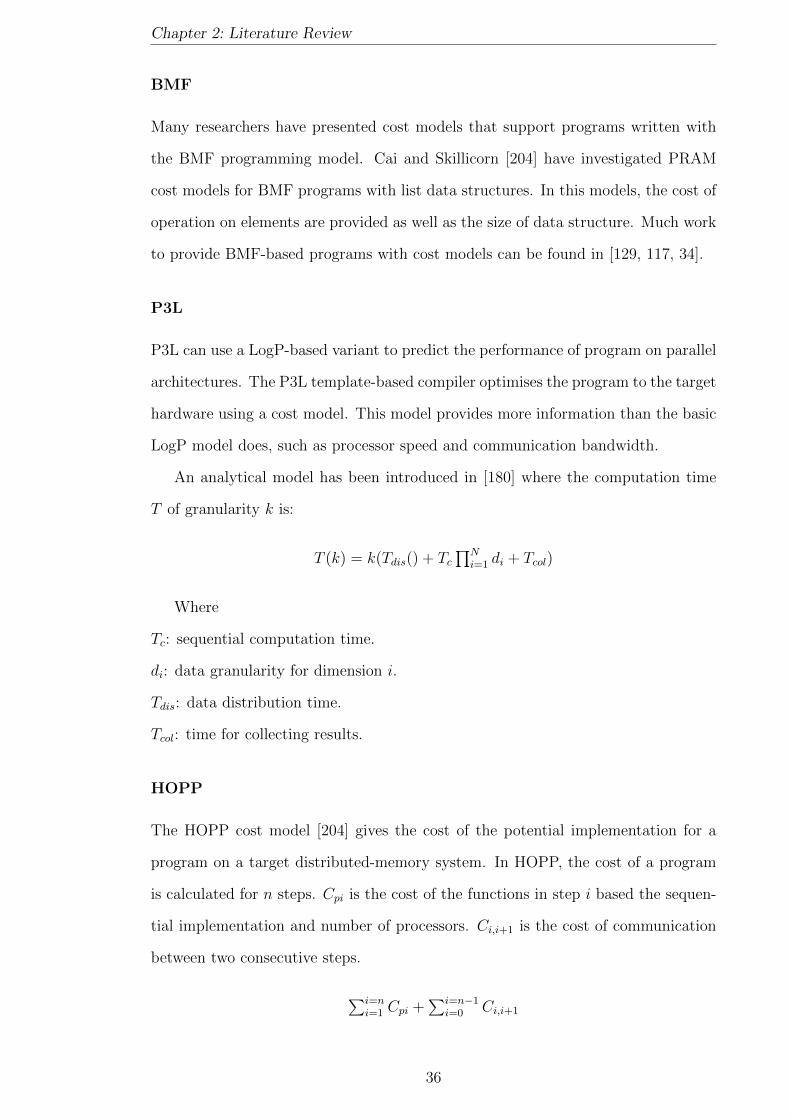
Chapter 2: Literature Review
BMF
Many researchers have presented cost models that support programs written with
the BMF programming model. Cai and Skillicorn [204] have investigated PRAM
cost models for BMF programs with list data structures. In this models, the cost of
operation on elements are provided as well as the size of data structure. Much work
to provide BMF-based programs with cost models can be found in [129, 117, 34].
P3L
P3L can use a LogP-based variant to predict the performance of program on parallel
architectures. The P3L template-based compiler optimises the program to the target
hardware using a cost model. This model provides more information than the basic
LogP model does, such as processor speed and communication bandwidth.
An analytical model has been introduced in [180] where the computation time
T of granularity k is:
T (k) = k(Tdis() + Tc∏N
i=1 di + Tcol)
Where
Tc: sequential computation time.
di: data granularity for dimension i.
Tdis: data distribution time.
Tcol: time for collecting results.
HOPP
The HOPP cost model [204] gives the cost of the potential implementation for a
program on a target distributed-memory system. In HOPP, the cost of a program
is calculated for n steps. Cpi is the cost of the functions in step i based the sequen-
tial implementation and number of processors. Ci,i+1 is the cost of communication
between two consecutive steps.
∑i=ni=1 Cpi +
∑i=n−1i=0 Ci,i+1
36

Chapter 2: Literature Review
SkelML
SkelML [44] provides performance cost models for several skeleton, such as farm and
pipeline. The SkelML compiler uses performance models to decide the efficient par-
allelism based on the predicted computational time and the network communication
overhead.
Other
Other performance cost models have been developed for several languages. Ham-
mond et al. [114] built a variety of cost formulas for a library of skeleton implemen-
tations in Eden, a parallel functional language. Thus, the proper implementation
will be chosen at compile time through instantiating parameters of a given platform.
Yaikhom et al.[234] presented a set of skeletons where each is associated with a cost
model. These models use a process algebra approach and have some parameters
that can be deduced from running of benchmarks.
2.4 Scheduling
One of the biggest issues in parallel and distributed systems is developing techniques
for scheduling the tasks on multiple locations [54]. The problem is how to distribute
the computations amongst all available processing elements to minimise the total
execution time and increase the performance.
Within a parallel computing environment, computation, data, and network re-
sources are shared amongst both system and application components. Consequently,
a scheduler is needed to achieve better performance [102]. Schedulers are classified
into three classes based on their performance goals. These are: job schedulers that
enhance the system performance by optimising throughput, resource schedulers that
control the resource usage in order to utilise resources or fair scheduling, and applica-
tion schedulers that improve the performance of an application through optimising
specific performance measures, like total execution time. Both job schedulers and
resource schedulers promote system performance while application schedulers target
37
Chapter 2: Literature Review
individual applications. Application schedulers are also referred as high-performance
schedulers.
In this thesis, our target is reducing the total execution time for a parallel appli-
cation so we will only review the developing of application schedulers, while resource
and job scheduler are beyond the scope of thesis.
2.4.1 Scheduling Model
Parallel applications are composed of one or more tasks that need to be executed
over different resources [103]. These tasks may communicate with each other to
solve a particular problem. Scheduling these tasks on participating resources in-
cludes a set of operations to produce a schedule and a cost model for evaluating the
performance measures. Scheduling involves the following activities: resource dis-
covery, task placement, data mapping, and task/communications ordering. Hence,
scheduling is assigning tasks and data into resources with some order in time.
High-performance schedulers use scheduling models to evaluate the performance,
define a schedule, and perform actions to produce the resulting schedule. Using
parameters from the application and the environment, high-performance schedulers
perform the best schedule based on the schedule policy.
Developing an effective high-performance scheduler is challenging because of the
heterogeneity of the hardware/software resources and the competition amongst users
to acquire resources in a shared environment. However, the scheduling model used
by a high-performance scheduler should represent the characteristics of the dynamic
environment and the application performance. Hence, a scheduling model can: pro-
duce time frame-specific predictions because the performance varies over time; uti-
lize dynamic information, which is needed to reflect the system state to develop
resource-aware schedules; and adapt to chosen execution platforms for deriving ac-
curate predictions.
A scheduling model comprises a scheduling policy, a program model, and a per-
formance model.
A program model is an abstraction of a program using a data-flow-style program
38
Chapter 2: Literature Review
graph or a set of characteristics. An example of systems that represent the program
using a data-flow-style program graph is MARS [107]. In contrast, AppLeS [30]
represents a program using a set of its characteristics.
A performance model evaluates the behaviour of the schedule. High-performance
schedulers employ performance models to make an optimal schedule. A performance
model is commonly parametrized with both static and dynamic information which
can be provided by the programmer, system, or a combination. SPP(X) [23] is an
example of a system that use performance models.
A scheduling policy is a set of rules that achieves a schedule to optimize the
performance goal of the application. Applications may have different performance
goals, where the common performance goal is minimising the execution time. As an
example, Dome [20] focuses on minimising the execution time using load balancing
as a scheduling policy. Much effort is on heuristic-based that are static schedulers
and take decision based on assumptions from prior knowledge of benchmark execu-
tion [45].
2.4.2 Challenges of Application Scheduling
There are number of challenges that need to be considered for High-performance
scheduling [103]:
• Portability and Performance: The main goal of scheduling is to improve the
performance. But, having better performance depends on leveraging environ-
ment features. However, a scheduling strategy should balance the performance
gain and the heterogeneity of the architecture resources.
• Scalability : it is important for a high-performance scheduler to use a dynamic,
scalable mechanism to select the resources.
• Efficiency : a high-performance scheduler is predicting the behaviour and mak-
ing a decision to redistribute the load. These decisions need to be accurate
and the schedule to be efficient with low overhead.
39

Chapter 2: Literature Review
• Multi-scheduling : resource schedulers, job schedulers and application sched-
ulers are all working for their performance goals. Coordinating multiple sched-
ulers is difficult and presents a challenge to the developers of schedulers. One
common problem that may occur is thrashing which cause unstable load bal-
ancing. However, multi-scheduling strategies must consider the stability of the
system for meeting their objectives.
• Locality : data locality may be affected when the tasks that process these data
are moved. Scheduler developers should find a compromise between commu-
nication overhead and the desired performance goal [225].
2.4.3 Load Management
Load management is one branch of a family of global scheduling polices, for man-
ageing the load of all locations in a network, cluster or Grid. The main goal of load
management is to improve the performance of an application by evenly assigning
tasks to each processing unit [177]. Load management is categorised into two types:
static and dynamic.
2.4.3.1 Static and Dynamic Load Management
The aim of static load management is to minimize the execution time of an appli-
cation [201]. Static load management predicts the run-time behaviour of a program
at compile time by estimating the task’s execution time and communication delays.
The main advantage of predicting the behaviour of the application is that the over-
head of the scheduling process takes place at compile time. However, the run-time of
the application may have unpredictable conditions such as network delays or reliance
on inputs, so that predicting the behaviour at compile time will be inaccurate and
may not be equal to real values at run-time. As a result, static load management
may make inappropriate decisions.
Dynamic load management depends on information collected at run-time to
reschedule tasks from heavily loaded machines to lightly loaded machines. The aim
of dynamic load management is to maximise the utilisation of processing power.
40

Chapter 2: Literature Review
The advantage of dynamic load management over static load management is that
the system does not need to be aware of the run-time behaviour of the applications
before execution. Dynamic load management incurs a run-time overhead resulting
from the communication cost of load information, the processing cost of decision
making and the communication cost for task transfer.
There are four policies, which also can be polices for dynamic scheduling, for
dynamic load management algorithms [92, 80, 172]. These policies are:
• Information Policy determines the information needed for predicting the be-
haviour in order to make a decision to redistribute the load. An information
policy also specifies the mechanism to collect and diffuse the information that
reflects the system state amongst locations. Triggering the collection of infor-
mation can occur via many approaches. A location can ask for the state of
other locations when it becomes a sender or receiver; this is called a Demand-
driven approach. Or a location may share its state when it is changed; this is
called a State-changed driven approach. Another approach is Periodic where
collecting the information happens periodically.
• Transfer Policy indicates the condition to transfer the load from a heavily
loaded location to lightly loaded locations. This policy may be a threshold-
based approach, a relative-load approach, or a hybrid approach.
• Selection Policy decides the tasks that should be moved. There are two ap-
proaches in selecting the tasks: non-pre-emptive and pre-emptive. A non-
pre-emptive approach assigns the tasks to the selected location before the
execution of the tasks. By contrast, a pre-emptive approach relocates tasks to
the selected location during the run-time. A pre-emptive policy can migrate
running tasks and therefore it is yielding significant performance benefits. A
pre-emptive policy is more costly than a non-pre-emptive policy, but it is more
flexible.
• Placement Policy identifies the locations to which a task should be transferred.
The commonly used approach is polling, by asking the destination location to
41

Chapter 2: Literature Review
accept transferring the task. Selecting a location can be: random, which
selects a random location to move the task; shortest, which determines the
lightly loaded location as a destination; or threshold, where the selected node
will be checked before moving the task.
In a dynamic load management system, the selection and placement policies are
combined together to produce an optimised schedule or to balance the system load
[151]. This combination can be either a push policy or a pull policy.
• Pull Policy : This is sometimes called a receiver-initiated policy, passive load
distribution policy, or work stealing. In this policy, when nodes become idle,
they request or steal work from other nodes.
• Push Policy : This is sometimes called sender-initiated policy, active load dis-
tribution policy, or work distribution. In this policy, the loaded nodes look for
lightly loaded nodes to give them some work.
For a low system load, the push policy works well and minimises the overhead
but this may cause unstable load in the system. On the other hand, a pull policy is
better for high system load.
Examples of dynamic load management systems are Load Sharing Facility (LSF)
[2] and GrapevineLB [165].
2.4.3.2 Strategies of Dynamic Load Management
Dynamic load management strategies are classified according to entities that hold
the information and share the load amongst the resources. Thus, a dynamic load
management strategy can be centralised, decentralised, or hierarchical [240, 186].
In a centralised management system, there is a central node which collects in-
formation about the system state and builds an estimate of the system state. The
central node may hold a shared file which records updates from all nodes. The
advantage of centralised load management is that the overhead is low during the
estimation process. The disadvantages are poor scalability and failure-proneness.
42

Chapter 2: Literature Review
In a decentralised management system, each node is responsible for collecting
state information and constructing an estimate of the system state. This organiza-
tion is not easy to scale to large system because it can incur large overheads to gain
accurate and consistent state information.
In hierarchical management systems, both centralised and decentralised load
management strategies are combined to inherit the properties and extract the ad-
vantages of both. A hybrid strategy can be implemented when nodes are divided
into clusters and the data are exchanged amongst them.
2.5 Mobility
The term mobility refers to a change of location achieved by system entities [37]. In
mobile computing, computations are moved amongst network locations and hence
enable a better use of resources in a network [176, 187]. A mobile program is able
to move its code and state from one location to another in a network and resume
its execution [143]. Mobility has different forms: hardware and software mobility.
Hardware mobility means the mobility of devices, such as laptops and PDAs.
Therefore, software mobility refers to moving computations from one location to
another [80, 40]. Some classifications of software mobility are process migration
and mobile languages. In process migration, the system decides when and where
to move, while in mobile languages, the system gives the programmer the ability
to decide the placement of computations on anew network location. MOSIX [25] is
an example of a distributed operating system that supports process migration. An
example of a mobile programming language is Java Voyager [3].
Check-pointing is a snapshot of the state of application; it is the main operation
in mobile systems to move the computations amongst processors in a network or
cluster [116]. Check-pointing is performed at a source location, sent and resumed at
the destination location. Check-pointing can be performed on an individual process
or on a whole operating system process. Check-pointing may be relevant to other
states, such as opened files or shared memory so that the check-pointing at process
level will often fail while the check-pointing at system-level will be able to get all
43
Chapter 2: Literature Review
local states.
2.5.1 Mobility Models
Mobility can be performed at different levels of granularity [116]. These models are:
• Data Mobility : A simple approach to mobility is that the application can save
its state and resume work from the saved point. Data mobility happens by
moving the saved state between locations on a network.
• Object Mobility : An object is a single unit that includes code and data. Object
mobility is serializing objects between machines where the program may con-
tain several objects roaming between machines. For example, RMI (Remote
Method Invocation) [184] will forward the calls transparently to the remote
object when method invocations happen for that object. RMI has a global
registry to save locations of a remote object during its life. Object mobility
is more complex because the remote object has one or more threads running
and these threads keep parts of the state of the object in the stack and CPU
registers. Some object mobility systems allow mobility when the invocation
reaches a specific execution safe point. For example, Emerald [131] supports
object mobility at several levels of granularity [105].
• Process Migration: process migration is moving the state of a program and
its data. The process is independent of the implementation language. Process
migration faces a problem when a process leaves an open file or similar unre-
solved state in the originating host; this is known as residual dependency. One
solution is to create a proxy process on the operating system on the originating
host, and that process handles the access to the local process. This solution
will require access to the resources over the network, so performance may be
reduced, and the process may fail if one of the two hosts crashes, which may
weaken the stability. Two examples of operating systems that support process
migration are Sprite [88] and MOSIX [25].
44

Chapter 2: Literature Review
• Virtual Machine Migration: A common problem with virtual machines is in-
creasing hardware utilization [26]. This problem can be solved by relocating
the workloads from an original host to another host before server downtime.
This process is called Virtual Machine Migration and happens when the down-
time of the server is planned or predicted. Sometimes VM migration happens
with migrating disk state. All applications running in the VM of the original
host will move to the new host. The shared memory and file system problems
are solved in this type of migration. An example of virtual machine migration
platforms is VMotion [1] which is included in VMware vSphere. This platform
seamlessly enables moving live VMs between physical machines.
Data mobility is an example of a fine-grained technique. On the other hand, pro-
cess migration and object migration are course-grained techniques. Virtual machine
migration is the most coarse-grained type of mobility.
2.5.2 Properties of Mobile Systems
Mobile systems should have mechanisms to effectively use the available resources.
The properties of mobile system include [80, 40, 105]:
• Mobility Control : A mobile system should have a mechanism to make the
programmer able to decide on the mobile operation.
• Weak or Strong Mobility : Mobility has two forms defined by Fuggutta et el
[105]: weak mobility and strong mobility. Weak mobility is moving the code
from one location to another. Whilst, strong mobility moves the code and
state information from one location to another and resumes the execution from
the stop state [81]. Strong mobility is also known as transparent migration.
Mobility systems may support weak mobility such as Java Voyager [3] or weak
and strong mobility like JavaGoX [196].
• Implicit or explicit mobility : Implicit mobile systems move the active compu-
tations, like a thread, from one location to another in the network. Implicit
mobile systems usually operate on a small scale, e.g. LAN or cluster [169].
45

Chapter 2: Literature Review
However, in explicit mobile systems, the moving of active computations is con-
trolled by the programmer. Explicit mobile systems usually operate on open
systems and in large-scale settings [40].
• Awareness of Location: after execution, the program may need to access re-
sources not located in the same location. In this case, the mobile operation
will happen under programmer control and be related to the resources [52].
• Safety and Security : Mobile systems have been developed to work in a network
where the resources are shared amongst entities of the network. Safety means
preventing undesired behaviour of programs. Security means the integrity of
the information and protection from malicious attacks [142].
• Architecture Independent : The main idea for mobile systems is to move the live
computations between locations on large distributed systems. These locations
may have different architectures and operating systems. Thus, it is necessary
to compile the program into architecture-independent code that is able to work
on heterogeneous networks [229].
2.5.3 Advantages of Mobility
Some of the main advantages of mobile computations are [211, 131]:
• Load Sharing : Moving the computations amongst processors on a network or
system can lead to a better use of resources and lighten the load on slowly-used
processors, and it gives a faster performance.
• Communications Performance: Moving the active objects that interact inten-
sively to the same node can reduce the communication costs of their interac-
tions.
• Availability : Moving objects to different nodes can improve service and protect
against broken or lost connection.
• Resource Utilisation: An object visiting a node can take advantage of services
or capabilities at that location.
46

Chapter 2: Literature Review
2.5.4 Code Mobility
In traditional computing, each computation is linked to a single machine [105].
Thus, the code of the computations belongs to the local machine. This is not true
for mobile systems. In mobile systems, the code, the execution state and the data
of computation, can be moved to a different machine.
Mobile systems provide mechanisms that support weak or strong mobility. There
are two mechanisms that support strong mobility: migration and remote cloning
[216]. The migration mechanism pauses the computation, moves it to the destina-
tion machine, and resumes execution. When the destination machine and the time
for migration are determined by the migrating machine, such migration is called
proactive. In contrast, when the movement is determined by a different computa-
tion that has some relationship with the computation to be migrated, this is called
reactive. For example, the MoviLog [242] platform supports migrating its computa-
tions either proactively or reactively.
The remote cloning mechanism will create a copy of a computation at a destination
machine without detaching it from the current machine. Remote cloning can also
be proactive and reactive [28].
Weak mobility is supported by a mechanism that is able to move the code
amongst machines and either links it to a running computation or uses it as a code
segment for a new computation [105]. The migration can be stand-alone code or a
code fragment. The stand-alone code will create a new computation on the destina-
tion machine, whereas a code fragment will be linked and executed in the context
of running code. The mechanism supporting weak mobility can be synchronous or
asynchronous depending on the computation suspension relative to when the code
is executed on the destination machine. The asynchronous mechanism can be in im-
mediate or deferred mode depending on the execution of the code on the destination
machine.
47
Chapter 2: Literature Review
2.5.5 Agent-based Systems
An agent is computer software hosted in an environment [217]. Agents are designed
to solve a specific problem in the system where they are located. The state and
the behaviour of agents may change due to interactions with the environment either
responding to external events or initiating actions in order to achieve particular
objectives. Thus, agents have to be both proactive and reactive [130]. Systems that
rely on agents as the key abstraction are called agent-based systems. Such systems
may use a single agent or multiple agents that cooperate with each other to achieve
a general objective. These systems are also known as multi-agent systems [231].
Properties that characterise agents are [231, 214]:
• Autonomy : each agent has control over its internal state without any external
intervention. This state can be used to make the decision to perform some ac-
tions. Because of the autonomy property, agents are referred to as autonomous
agents.
• Reactivity : agents situated in an environment respond with an action that
may change the environment.
• Pro-activeness : agents learn from the environment and interaction with others
to initiate goal-directed actions when necessary.
• Sociability : agents are capable of communicating with other agents or the
environment to achieve a certain goal.
Much work on agents can be found in [230, 231, 195].
Agents also may have a mobility property that enables them to change their
environment and move to another one [143]. Those agents are called mobile agents.
Agents that do not have the mobility property are called stationary agents. To gain
information from remote systems, a special communication mechanism is supported
in stationary agents. However, mobile agents are free to move amongst systems as
they are not bound to a particular system. Indeed, mobile agents keep their state
and code while moving which enables them to resume execution on other systems.
48

Chapter 2: Literature Review
Furthermore, mobility gives the agents the facilities needed to be in the same host
with the resources they request and the objects with which they interact. System
performance can be improved by agent mobility through reducing the network load
and overcoming network latency.
Mobile agents provide the flexibility and abstraction needed for building dis-
tributed systems.
2.5.6 Autonomic Systems
Autonomic systems are capable of managing themselves to achieve high-level ob-
jectives given from an administrator [139, 171]. Autonomous systems are also
referred to as autonomic systems. In this context, autonomic systems are self-
management systems that can maintain and manage their operations in the case of
system changes, such as workload, demand, or components, and software/hardware
failures. Self-management autonomic computing systems may have one or more of
these aspects [171]:
• Self-configuration: an autonomic system is able to automatically configure, ad-
just, setup, and install components. All system configurations will be adapted
in accordance with administrator objectives.
• Self-optimisation: autonomic systems attempt to improve their efficiency by
endeavouring to perform operations with high throughput and achieve goals
at optimum levels. Self-optimisation systems monitor their state and take
decisions, such as resource allocation, to improve the performance.
• Self-healing : autonomic systems are able to adjust, diagnose, and repair lo-
calised problems and failure in the software and hardware.
• Self-protection: the system can protect itself from malicious attacks. Also, the
system can use early reports to expect and prevent problems by taking actions
to avoid failure.
An example of an autonomous system is ASP [4] (Autonomic Job Scheduling Pol-
icy) for Grid that supports three of the self-management aspects: self-optimisation,
49

Chapter 2: Literature Review
self-healing, and self-protection. Liu et el [150] have presented a component-based
programming framework which is an example of a self-configuration system. More-
over, Deng [80] has developed resource-aware programs with a self-optimisation abil-
ity. These programs are called AMPs (Autonomous Mobility Programs).
2.6 Summary
A cluster is a distributed memory system that uses message passing approach for
communication. Emerging the latest multi-core technologies in the cluster systems
offered many benefits. System developers are forced to deal with parallelism across
nodes, cores and other processing units. It becomes necessary to make the appli-
cation scalable and automatically adaptable to different number of nodes/cores. In
this thesis, we target multi-core cluster with diverse number of nodes and quantity
of processing elements. To match our objectives, we need to design a distributed
programming framework which is able to exploit multicore clusters. We use MPI
as a message passing library in the distributed memory architecture to secure the
communications amongst those components. Our framework is designed as Master/-
Worker model to maintain the cooperation in the framework. At the node level, we
use Fork/Join pattern to manage the coordination inside the workers. Accordingly,
we use the PThread library to flexibly manage the threads within the multicore
nodes. At the level of the problem, or most specifically, the task, each task uses
SPMD model. The GPU programming is beyond the scope of our thesis where we
concentrate on the compute power of the CPU cores of the node.
This framework is implemented using skeletal approach and hence it offers a
high level data-parallel skeleton. This skeleton separates the computation from
the coordination. Hence, this skeleton helps in optimising the problems through
improving the productivity of programmers by focusing on the domain-specific issues
while parallel and communication details are implicitly maintained.
The skeleton implementation mainly supports executing farm pattern problems
but it also can be used to solve problems such as pipe pattern or map-reduce pattern
problems. Other patterns such as divide and conquer and scan patterns are not
50
Chapter 2: Literature Review
implemented in our framework. Skeletons usually provided as a language extension,
library or parallel programming language. A survey of skeletons has been proposed
in the literature. This work proposes a skeleton as a library in the C programming
language.
To enhance the dynamicity and adaptivity of our skeleton, we develop a high
performance dynamic application scheduler to optimise the performance of the skele-
ton. The main goal of the scheduler is minimising the total execution time under
loaded conditions. This scheduler uses real time observations and performs a set
of event-based operations to enhance the skeleton performance goal. Moreover, the
skeleton scheduler is triggered by the loaded nodes. Hence, push policy has been
used to implement the selection and placement policies. Our scheduler follows a
hybrid centralised/decentralised approach to exploit advantages of both strategies.
The operations of the skeleton scheduler depend on local coordination without in-
terfering with other scheduling systems or the native operating system scheduler.
There is a wide range of scheduling policies that has been proposed in the literature.
However, schedulers target potential execution environments, language representa-
tions, and problem domains. As a result, schedulers are difficult to compare [141].
The skeleton scheduler takes decisions based on a dynamic performance cost
model. This cost model helps the scheduler to decide if the current tasks can run
faster on remote locations taking into consideration the changeable load, the run-
ning architecture and the progress of the executing problem. Therefore, this cost
model depends on measurements at run-time. This cost model is based on the model
developed by Deng [81, 80] where our new version supports multicore architectures
and takes into account the external load of the application in the executing environ-
ment. Skeletons that are guided by performance model are also proposed in many
works. Examples of these skeletons can be found in [80, 51, 223, 9, 29].
This scheduler uses mobility in transferring live computations from node to node
using a pre-emptive approach. This mobility is implemented at the application
level, the skeleton, where strong mobility with data mobility has been used. In our
skeleton, mobility operations occur transparently where mobility operation includes
51

Chapter 2: Literature Review
saving the execution state, transferring, and resuming the execution of live com-
putations. Some programming language supports mobility like JavaGoX [196] and
Java Voyager [3] where some skeletons can get benefits of this feature like mobility
skeletons [81, 89]. In such skeletons, common patterns of mobile computations are
encapsulated. Other mobility support can be provided by the system like MOSIX
[25] where MOSIX is cluster management system that manages resources, allocates,
and migrates processes amongst nodes.
52
Chapter 3
Self-Mobile Skeleton
Skeletal programming has given significant benefits to developers to relieve them
from the difficulties of parallelism and keep them focusing on solving problems.
Such an approach has put forward solutions to exploit parallel systems without
going into low-level details, such as communications and coordination. This work
proposes a generic data-parallel skeleton, HWFarm, which can exploit multicore
clusters. This skeleton is self-mobile where all mobility operations are implemented
inside the skeleton. In this chapter, we start with the concepts of designing skeletal-
based systems in Section 3.1. Then, we propose the design and the implementation
of our skeleton with further details about its usability in Section 3.2. Next, we
show experiments for evaluating the performance in Section 3.3. Cost modelling
and scheduling will be discussed in the next chapters.
3.1 Pragmatic Manifesto
A wide range of skeletons are provided through either a library or language con-
structs. To effectively design skeletal-based systems, Cole [67] presented a manifesto.
These principles are:
1. Propagate the concept with minimal conceptual disruption: this principle re-
quires that the skeleton should be provided as a simple concept in an existing
programming language. This is necessary to ease the difficulties in learning
new programming languages with new constructs.
53
Chapter 3: Self-Mobile Skeleton
2. Integrate ad-hoc parallelism: the construction of skeletons must be integrated
with structured parallelism. Hence, skeletal systems should be developed in
order to implement a parallel pattern that has not been supported by available
skeletons.
3. Accommodate diversity : the specification of a skeleton offers a level of flexibil-
ity that provides variations in implementation of the real algorithms. Beside
flexibility, a straightforward abstraction of skeletons must be constructed. As
a result, a balance is needed between simplicity of abstraction and realistic
flexibility.
4. Show the pay-back : results and benefits of developing skeletal systems must
be presented. We must also show the improvements offered by the adoption
of skeletal systems.
Danelutto et al [72] extended Cole’s principles by adding three related to reusabil-
ity and modern heterogeneous platforms. These principles are:
5. Support code reuse: this allows the skeletons to be reused with very little
change to the sequential code.
6. Handle heterogeneity : with various kinds of parallel architectures, the skeleton
must be able to run on different platforms. This means that the implementa-
tion should be adapted to execute on heterogeneous resources such as clusters
or Grids.
7. Handle dynamicity : skeletons may run on environments, such as non-dedicated
clusters, that have changeable available resources. Hence, skeletons must be
supported with mechanisms to handle such situations.
Now, we will explore our skeleton that meets these principles to be able to
integrate with the mainstream of parallel programming.
54
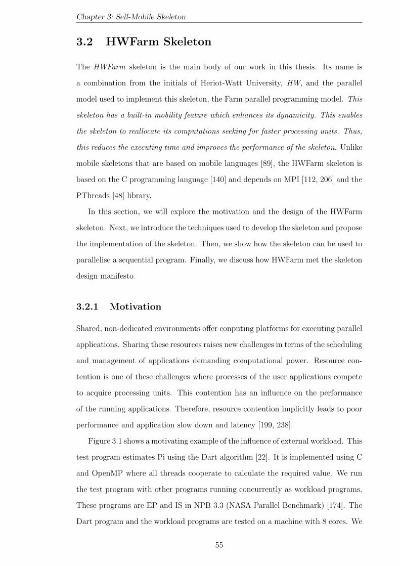
Chapter 3: Self-Mobile Skeleton
3.2 HWFarm Skeleton
The HWFarm skeleton is the main body of our work in this thesis. Its name is
a combination from the initials of Heriot-Watt University, HW, and the parallel
model used to implement this skeleton, the Farm parallel programming model. This
skeleton has a built-in mobility feature which enhances its dynamicity. This enables
the skeleton to reallocate its computations seeking for faster processing units. Thus,
this reduces the executing time and improves the performance of the skeleton. Unlike
mobile skeletons that are based on mobile languages [89], the HWFarm skeleton is
based on the C programming language [140] and depends on MPI [112, 206] and the
PThreads [48] library.
In this section, we will explore the motivation and the design of the HWFarm
skeleton. Next, we introduce the techniques used to develop the skeleton and propose
the implementation of the skeleton. Then, we show how the skeleton can be used to
parallelise a sequential program. Finally, we discuss how HWFarm met the skeleton
design manifesto.
3.2.1 Motivation
Shared, non-dedicated environments offer conputing platforms for executing parallel
applications. Sharing these resources raises new challenges in terms of the scheduling
and management of applications demanding computational power. Resource con-
tention is one of these challenges where processes of the user applications compete
to acquire processing units. This contention has an influence on the performance
of the running applications. Therefore, resource contention implicitly leads to poor
performance and application slow down and latency [199, 238].
Figure 3.1 shows a motivating example of the influence of external workload. This
test program estimates Pi using the Dart algorithm [22]. It is implemented using C
and OpenMP where all threads cooperate to calculate the required value. We run
the test program with other programs running concurrently as workload programs.
These programs are EP and IS in NPB 3.3 (NASA Parallel Benchmark) [174]. The
Dart program and the workload programs are tested on a machine with 8 cores. We
55

Chapter 3: Self-Mobile Skeleton
Figure 3.1: The effect of running multiple applications on the same processor.
56
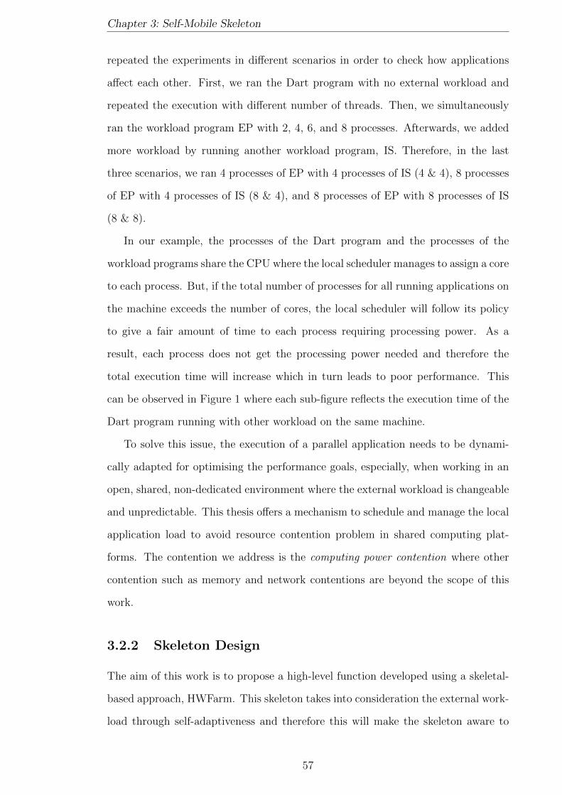
Chapter 3: Self-Mobile Skeleton
repeated the experiments in different scenarios in order to check how applications
affect each other. First, we ran the Dart program with no external workload and
repeated the execution with different number of threads. Then, we simultaneously
ran the workload program EP with 2, 4, 6, and 8 processes. Afterwards, we added
more workload by running another workload program, IS. Therefore, in the last
three scenarios, we ran 4 processes of EP with 4 processes of IS (4 & 4), 8 processes
of EP with 4 processes of IS (8 & 4), and 8 processes of EP with 8 processes of IS
(8 & 8).
In our example, the processes of the Dart program and the processes of the
workload programs share the CPU where the local scheduler manages to assign a core
to each process. But, if the total number of processes for all running applications on
the machine exceeds the number of cores, the local scheduler will follow its policy
to give a fair amount of time to each process requiring processing power. As a
result, each process does not get the processing power needed and therefore the
total execution time will increase which in turn leads to poor performance. This
can be observed in Figure 1 where each sub-figure reflects the execution time of the
Dart program running with other workload on the same machine.
To solve this issue, the execution of a parallel application needs to be dynami-
cally adapted for optimising the performance goals, especially, when working in an
open, shared, non-dedicated environment where the external workload is changeable
and unpredictable. This thesis offers a mechanism to schedule and manage the local
application load to avoid resource contention problem in shared computing plat-
forms. The contention we address is the computing power contention where other
contention such as memory and network contentions are beyond the scope of this
work.
3.2.2 Skeleton Design
The aim of this work is to propose a high-level function developed using a skeletal-
based approach, HWFarm. This skeleton takes into consideration the external work-
load through self-adaptiveness and therefore this will make the skeleton aware to
57
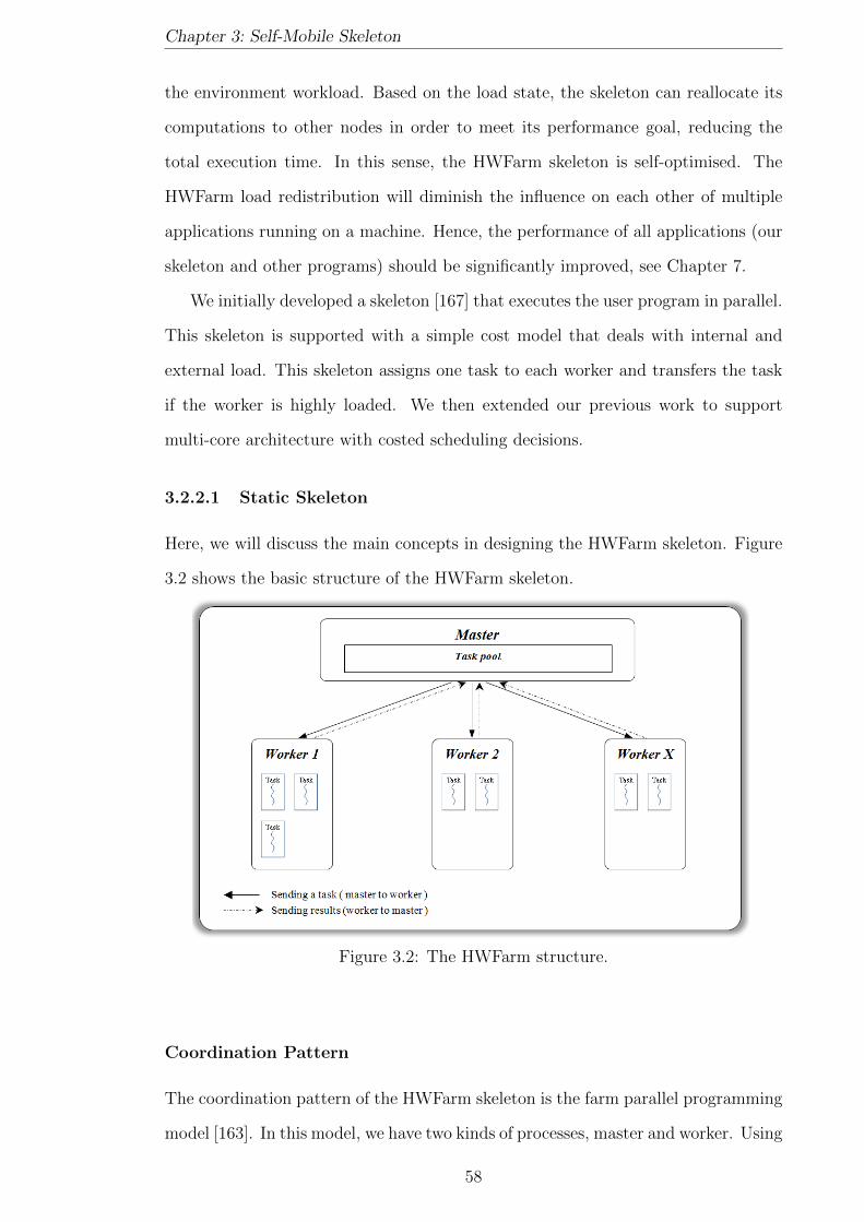
Chapter 3: Self-Mobile Skeleton
the environment workload. Based on the load state, the skeleton can reallocate its
computations to other nodes in order to meet its performance goal, reducing the
total execution time. In this sense, the HWFarm skeleton is self-optimised. The
HWFarm load redistribution will diminish the influence on each other of multiple
applications running on a machine. Hence, the performance of all applications (our
skeleton and other programs) should be significantly improved, see Chapter 7.
We initially developed a skeleton [167] that executes the user program in parallel.
This skeleton is supported with a simple cost model that deals with internal and
external load. This skeleton assigns one task to each worker and transfers the task
if the worker is highly loaded. We then extended our previous work to support
multi-core architecture with costed scheduling decisions.
3.2.2.1 Static Skeleton
Here, we will discuss the main concepts in designing the HWFarm skeleton. Figure
3.2 shows the basic structure of the HWFarm skeleton.
Figure 3.2: The HWFarm structure.
Coordination Pattern
The coordination pattern of the HWFarm skeleton is the farm parallel programming
model [163]. In this model, we have two kinds of processes, master and worker. Using
58

Chapter 3: Self-Mobile Skeleton
the farm model, the running computations on remote workers can be monitored.
Furthermore, this model helps in diffusing load information amongst the workers
which is helpful to make accurate decisions. In our skeleton, we assume that the
task pool is static and all tasks are assigned to workers and hence there are no new
tasks waiting in the pool. One of the disadvantages of the Master/Worker model is
a bottleneck due to the centralised master serving all workers. A bottleneck occurs
when a worker must wait until other workers finish communicating with the master.
This can be avoided through reducing the master-worker activities and devolving
the critical making decisions to remote workers. Details of this hybrid mechanism
are discussed in Chapter 5.
Master
The master is responsible for the whole coordination in the skeleton via: creating
the tasks, computations; dividing the data; assigning the tasks to workers; and
collecting the results of execution.
Worker
The worker executes the received tasks from the master and exchanges the load
information with other workers and with the master. The model used in the work-
ers is Fork/Join programming [163] where the worker maintains local threads and
manages the communications with the master.
Task Model
Tasks in the HWFarm skeleton are intensive computations that process data and
run concurrently in parallel. These tasks are initialised in the master process where
each task is linked with a function and an evenly divided chunk of data. In workers,
the function of the task will be executed to manipulate the input data to produce
the output data. An important assumption in this model is that the lengths of all
tasks are equal. In addition, another assumption is that there is no dependency
or communication amongst the tasks so that they are fully independent equal-sized
59

Chapter 3: Self-Mobile Skeleton
tasks. The chunk size is set by the user and hence the length of the task and the
number of tasks are not controlled by the skeleton.
Task Allocation
Assigning tasks to workers is based on the total number of cores and the number of
tasks. The tasks will be distributed amongst workers based on a static allocation
model used by the master. This distribution will achieve an initial balanced load
in proportion to the number of cores on each worker. Details of this model are in
Section 3.2.4.2.
Program Model
The class of problem that the skeleton executes is similar to the loop parallelism
model [163]. In the HWFarm model, the program has a number of iterations to
process a chunk of data. Hence, the program will perform the same operations
on different data segments. Thus, the skeleton can be classified as a data-parallel
skeleton.
Communication
Based on the coordination pattern, the communications inside the skeleton are only
between the master and the workers. Therefore, the connections are a master-
worker connection when the master assigns a task to the worker and a worker-master
connection when the worker returns the results to the master.
Platform
One of our design principles is to tackle homogeneous clusters. As a result, the
parallel computing architecture we target in the HWFarm skeleton is a multi-core
architecture, in particular a multi-core cluster. Cluster nodes may have different
number of cores with varied characteristics. In this thesis, GPU architectures and
CPU accelerators are not addressed.
60

Chapter 3: Self-Mobile Skeleton
Result Collection
Once a worker completes the execution of its tasks, it will send the results to the
master. Then, the master gathers the sub-results into a global array and delivers it
to the user program. The user program can now deal with the processed data, like
flushing to an external file or a disk.
3.2.2.2 Mobility Support
We provide our skeleton with ability to move running tasks amongst nodes in order
to have an improved schedule in the system. We use data mobility granularity where
the application itself is responsible for transferring the code, the data, and the state.
The HWFarm skeleton is built as an abstraction between the coordination and
the program. But, to make the skeleton able to move running tasks, there is a need
to access the user computations to monitor and manage their execution state. To
achieve this goal, the skeleton needs to keep a reference to all data processed in
the task as well as the running state. This requires that the user has the burden
to separate the state of execution from other internal iterations. In the HWFarm
program model, loop parallelism, if the variables that hold data are globalised out
of the main loop, this will save the state of the execution. As an example, during
running a loop, the progress of the execution can be indicated by the main counter.
Thus, whenever this counter is checked, the progress will be known.
Execution state includes the main loop counter that increases while the func-
tion is running. Also, the state can include any variables that are needed for the
computation.
Besides moving the state, mobility includes moving the results of the processed
data. Thus, when the program resumes, the sub-results will be available, and the
program will continue to produce the remaining results.
Mobility is triggered in the skeleton if it is better to execute selected tasks on
faster locations. When the scheduler decides to move a task, the mobility operation
will be triggered. First, the source worker requests permission to move a task to
the destination worker. Once permission is received, the source worker implicitly
61
Chapter 3: Self-Mobile Skeleton
performs check-pointing which is an operation to pack the task data and its state
before transferring the whole computation. Then, the selected task moves to the
destination worker. As a result, we have a new connection between workers involved
in the mobility operation. Accordingly, the connections in the skeletons are master-
worker for allocating tasks, worker-master for sending results and worker-worker for
mobility.
Figure 3.3 shows the structure of the HWFarm skeleton and how the master and
the workers communicate with each other to execute the problem in parallel.
Sending a task ( master to worker )
Sending results (worker to master )
Mobility operation (worker to worker)
Worker 1 Worker 2 Worker X
Master
Task pool
Task Task
Task
TaskTask Task Task Task
Figure 3.3: The HWFarm structure with mobility.
3.2.3 Host Language
Providing a high-level skeleton in a common existing language is much preferable
to the programmer than learning a new programming language. The HWFarm
skeleton is implemented in the C programming language, one of the most pervasive,
dominant programming languages in software engineering. It has many features
that are helpful in implementing our skeleton [140, 18]; some of them are:
• It is widely used in the software development domain.
62
Chapter 3: Self-Mobile Skeleton
• C uses memory through pointers which helps also in polymorphic programming
( void pointers ). This pointer capability has a significant use in supporting
function pointers. This has many benefits for high-level programming such as
abstraction.
• C gives access to the hardware and it is closely related to low-level languages
such as Assembly.
• C is portable and not linked to any operating system or processor type. This
enables our skeleton to run on a wide range of architectures.
To support parallel communications amongst the participating processes, we used
the MPI model [206]. This model is widely used in multi-processor architectures.
Thus, all aspects related to creating the processes and other issues are in MPI where
process management is implicitly handled in the MPI communication library. The
MPI library used in this work is MPICH.
To employ the shared memory platform, we used the PThreads library [48] that
provides full control of creating, managing, starting, and killing running threads.
OpenMP offers a mechanism to program shared memory but PThreads has full
control in order to maintain multi-threaded programming.
3.2.4 Skeleton Implementation
HWFarm is a skeleton provided as a function call that hides low-level details from
the user. In this section, we will explore how the skeleton deals with data. Then, we
show the allocation model used by the HWFarm skeleton. Finally, we give a further
look inside the structure of the skeleton.
3.2.4.1 Dealing with Data
In sequential programs, the program processes the input data to produce output
data, but, in concurrent execution, the program may have multiple instances where
each processes local data while all instances can access shared data. All instances
work to produce the output data; see Figure 3.4.
63

Chapter 3: Self-Mobile Skeleton
Sequential Program
Input Program Output
Parallel Program
Shared Input
Input1 Program1
Program2Input2Output
Figure 3.4: Sequential and parallel programs.
In the HWFarm skeleton, all tasks are running together. These tasks are dis-
tributed over the machines where some tasks may share the same node. To improve
the flexibility of dealing with local and shared data in a node, the HWFarm skeleton
classifies the data into three classes: input data, state data, and output data. All
these data buffers are identified by the user. Input data is both shared and will
be broadcast to all workers and local data will be equally divided into tasks. State
data is configured and set by the user and based on the user-program to save the
execution state of each task. Output data holds the results of the processed data;
see Figure 3.5.
Figure 3.5: Task structure in the HWFarm skeleton.
64
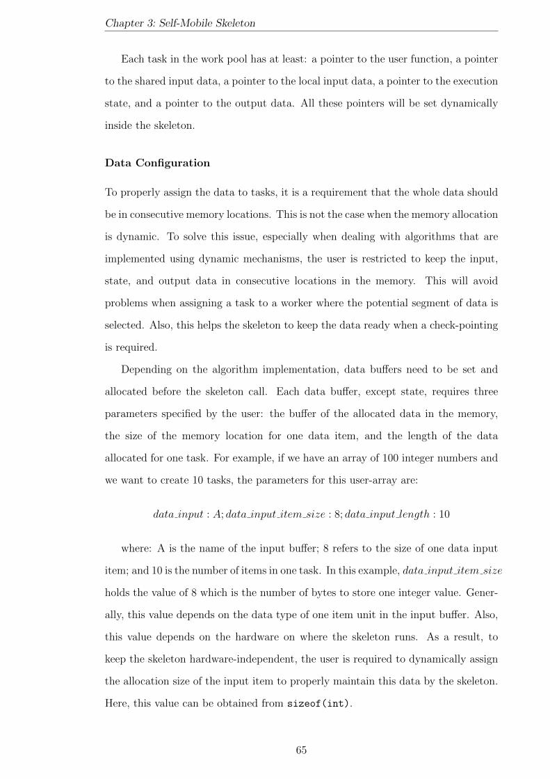
Chapter 3: Self-Mobile Skeleton
Each task in the work pool has at least: a pointer to the user function, a pointer
to the shared input data, a pointer to the local input data, a pointer to the execution
state, and a pointer to the output data. All these pointers will be set dynamically
inside the skeleton.
Data Configuration
To properly assign the data to tasks, it is a requirement that the whole data should
be in consecutive memory locations. This is not the case when the memory allocation
is dynamic. To solve this issue, especially when dealing with algorithms that are
implemented using dynamic mechanisms, the user is restricted to keep the input,
state, and output data in consecutive locations in the memory. This will avoid
problems when assigning a task to a worker where the potential segment of data is
selected. Also, this helps the skeleton to keep the data ready when a check-pointing
is required.
Depending on the algorithm implementation, data buffers need to be set and
allocated before the skeleton call. Each data buffer, except state, requires three
parameters specified by the user: the buffer of the allocated data in the memory,
the size of the memory location for one data item, and the length of the data
allocated for one task. For example, if we have an array of 100 integer numbers and
we want to create 10 tasks, the parameters for this user-array are:
data input : A; data input item size : 8; data input length : 10
where: A is the name of the input buffer; 8 refers to the size of one data input
item; and 10 is the number of items in one task. In this example, data input item size
holds the value of 8 which is the number of bytes to store one integer value. Gener-
ally, this value depends on the data type of one item unit in the input buffer. Also,
this value depends on the hardware on where the skeleton runs. As a result, to
keep the skeleton hardware-independent, the user is required to dynamically assign
the allocation size of the input item to properly maintain this data by the skeleton.
Here, this value can be obtained from sizeof(int).
65

Chapter 3: Self-Mobile Skeleton
The data type of the input buffer is not restricted to simple data types. The skele-
ton gives the user ability to define custom data types. But, the user is also required
to provide the same details for the relevant structures. Then, data input item size
refers to the size of the data structure defined by the user. Yet, they have to make
sure that all structures in the memory are consecutive.
State data is the main part of the data that saves the execution state. The state
in HWFarm is defined in the hwfarm state struct as follow:
typedef struct hwfarm_state{
int counter;
int max_counter;
void* state_data;
int state_len;
} hwfarm_state;
hwfarm state struct has four elements: two for the counter/index of the main
loop, a buffer for user defined state data, and the length of that buffer.
The user program must have a main index-based loop with a counter and the
maximum iterations of this loop. This counter should be used to iterate through
the data. These values will be set by the user before the skeleton call and then used
by the user function as an input. state data buffer is any data that the user may
need before or during the task execution where state len is the size of this buffer
in bytes. The counter will be used later by the scheduler for the estimation and
mobility operations. Hence, it is very important to configure the counter properly
before the function call and inside the main loop of the user program. This may
require minor re-factoring of the loop to be usable in the skeleton.
Figure 3.6 illustrates the work of the HWFarm skeleton from the perspective of
data. In this example, the problem will be divided into 4 tasks so that the input data
is divided into 4 chunks with a chunk per a task, see Figure 3.6.A. There are two
workers and hence two tasks are allocated to each worker. Then, the master sends
the shared data and the allocated tasks to the participating workers. Workers receive
the tasks and start executing, see Figure 3.6.B. On each worker, tasks execute the
66
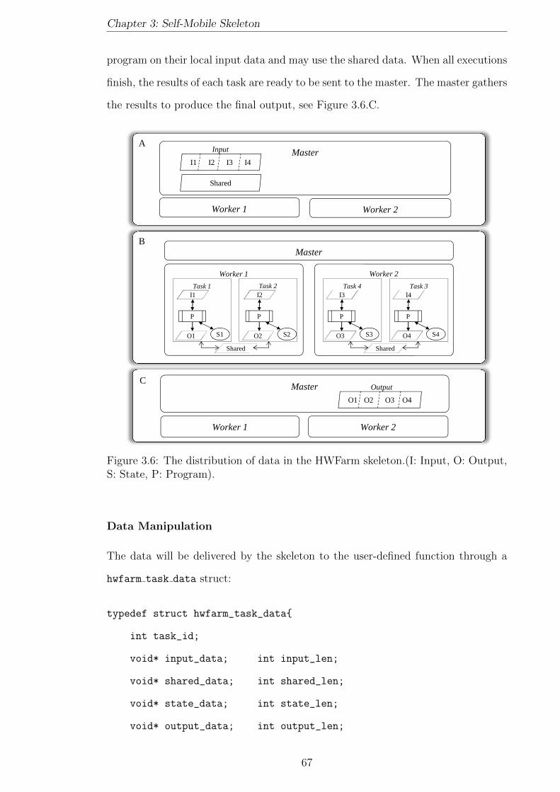
Chapter 3: Self-Mobile Skeleton
program on their local input data and may use the shared data. When all executions
finish, the results of each task are ready to be sent to the master. The master gathers
the results to produce the final output, see Figure 3.6.C.
Master
Worker 1
Task 1I1
P
S1O1
Shared
Task 2I2
P
S2O2
Worker 2
Task 3I3
P
S3O3
Shared
Task 4I4
P
S4O4
B
AMaster
Shared
Worker 1 Worker 2
I1 I2 I3 I4
Input
CMaster
O1 O2 O3 O4
Worker 1 Worker 2
Output
Figure 3.6: The distribution of data in the HWFarm skeleton.(I: Input, O: Output,S: State, P: Program).
Data Manipulation
The data will be delivered by the skeleton to the user-defined function through a
hwfarm task data struct:
typedef struct hwfarm_task_data{
int task_id;
void* input_data; int input_len;
void* shared_data; int shared_len;
void* state_data; int state_len;
void* output_data; int output_len;
67
Chapter 3: Self-Mobile Skeleton
int* counter; int* counter_max;
} hwfarm_task_data;
The fields of this structure are as follow:
• task id: The id of the current task.
• input data: The reference of the input buffer(chunk).
• input len: The length of the input buffer.
• shared data: The reference of the shared buffer.
• shared len: The length of the shared buffer.
• state data: The reference of the state buffer(chunk).
• state len: The length of the state buffer.
• output data: The reference of the output buffer.
• output len: The length of the output buffer.
• counter: The reference of the main counter.
• counter max: The reference of the maximum number of iterations in the main
loop.
When the user function is called, all data related to the task will be available in
this struct. The user has to follow the reference style in writing the code especially
the counter. This will keep all changes accessed and controlled by the skeleton for
enabling mobility and scheduling.
Inside the iterations of the main loop in the user program, the user can define
any data type and use any allocation method. But, before reaching the end of
the iteration, they have to save the result to output data and update the state.
Updating the state includes updating the index value, shared values and any other
data needed between iterations.
See the example in Section 3.3.2 that explains using the skeleton with its state.
68
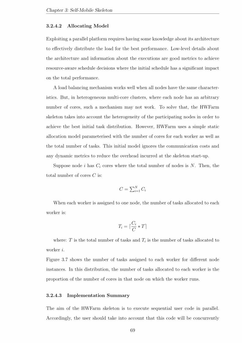
Chapter 3: Self-Mobile Skeleton
3.2.4.2 Allocating Model
Exploiting a parallel platform requires having some knowledge about its architecture
to effectively distribute the load for the best performance. Low-level details about
the architecture and information about the executions are good metrics to achieve
resource-aware schedule decisions where the initial schedule has a significant impact
on the total performance.
A load balancing mechanism works well when all nodes have the same character-
istics. But, in heterogeneous multi-core clusters, where each node has an arbitrary
number of cores, such a mechanism may not work. To solve that, the HWFarm
skeleton takes into account the heterogeneity of the participating nodes in order to
achieve the best initial task distribution. However, HWFarm uses a simple static
allocation model parameterised with the number of cores for each worker as well as
the total number of tasks. This initial model ignores the communication costs and
any dynamic metrics to reduce the overhead incurred at the skeleton start-up.
Suppose node i has Ci cores where the total number of nodes is N . Then, the
total number of cores C is:
C =∑N
i=1Ci
When each worker is assigned to one node, the number of tasks allocated to each
worker is:
Ti = dCi
C∗ T e
where: T is the total number of tasks and Ti is the number of tasks allocated to
worker i.
Figure 3.7 shows the number of tasks assigned to each worker for different node
instances. In this distribution, the number of tasks allocated to each worker is the
proportion of the number of cores in that node on which the worker runs.
3.2.4.3 Implementation Summary
The aim of the HWFarm skeleton is to execute sequential user code in parallel.
Accordingly, the user should take into account that this code will be concurrently
69
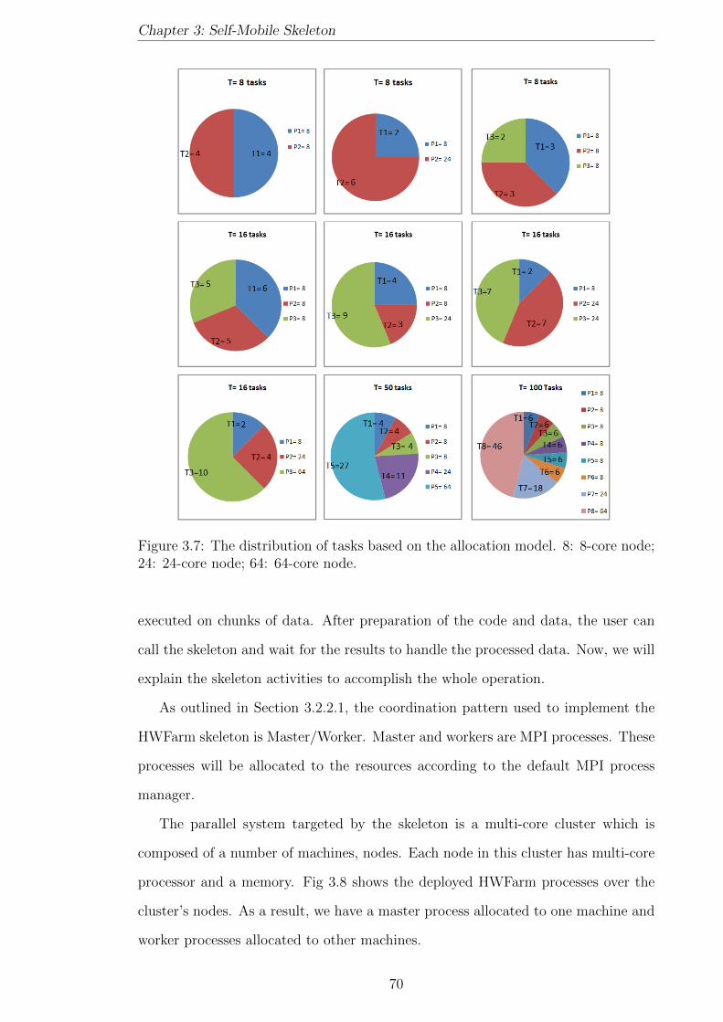
Chapter 3: Self-Mobile Skeleton
Figure 3.7: The distribution of tasks based on the allocation model. 8: 8-core node;24: 24-core node; 64: 64-core node.
executed on chunks of data. After preparation of the code and data, the user can
call the skeleton and wait for the results to handle the processed data. Now, we will
explain the skeleton activities to accomplish the whole operation.
As outlined in Section 3.2.2.1, the coordination pattern used to implement the
HWFarm skeleton is Master/Worker. Master and workers are MPI processes. These
processes will be allocated to the resources according to the default MPI process
manager.
The parallel system targeted by the skeleton is a multi-core cluster which is
composed of a number of machines, nodes. Each node in this cluster has multi-core
processor and a memory. Fig 3.8 shows the deployed HWFarm processes over the
cluster’s nodes. As a result, we have a master process allocated to one machine and
worker processes allocated to other machines.
70
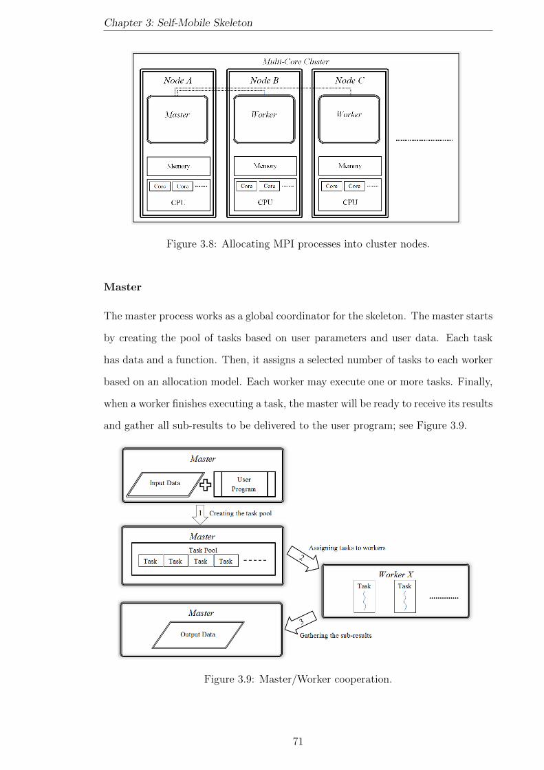
Chapter 3: Self-Mobile Skeleton
Figure 3.8: Allocating MPI processes into cluster nodes.
Master
The master process works as a global coordinator for the skeleton. The master starts
by creating the pool of tasks based on user parameters and user data. Each task
has data and a function. Then, it assigns a selected number of tasks to each worker
based on an allocation model. Each worker may execute one or more tasks. Finally,
when a worker finishes executing a task, the master will be ready to receive its results
and gather all sub-results to be delivered to the user program; see Figure 3.9.
Figure 3.9: Master/Worker cooperation.
71
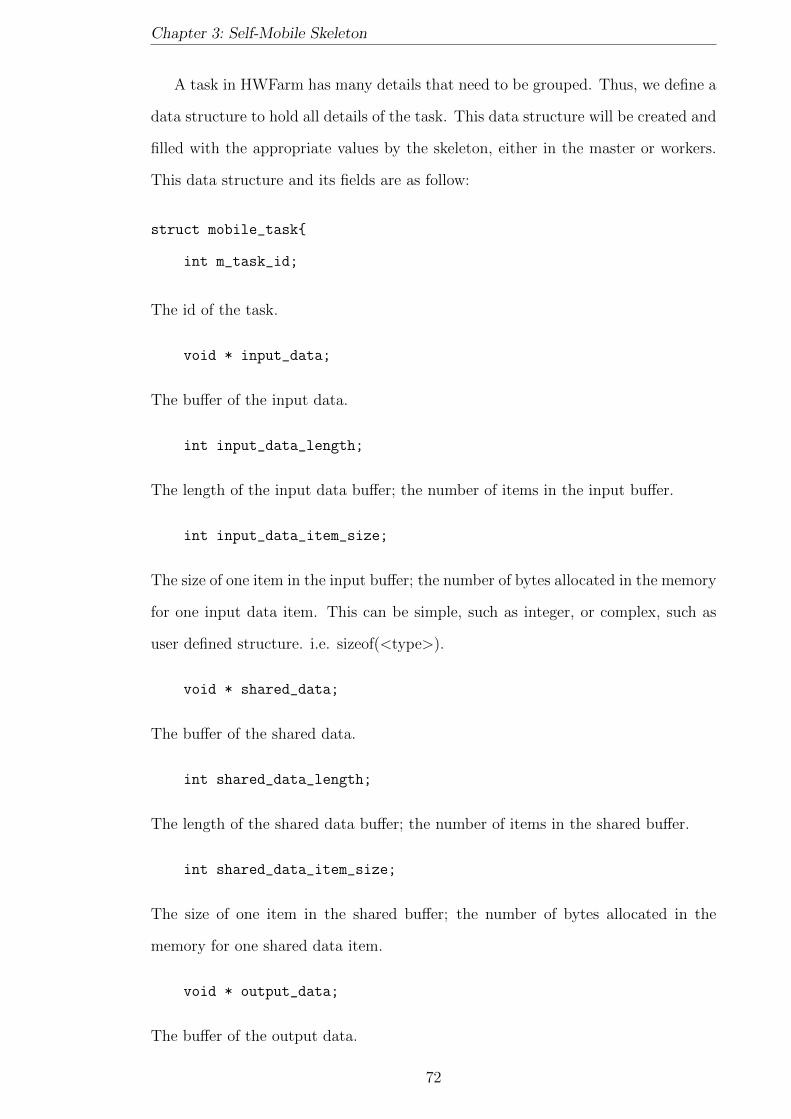
Chapter 3: Self-Mobile Skeleton
A task in HWFarm has many details that need to be grouped. Thus, we define a
data structure to hold all details of the task. This data structure will be created and
filled with the appropriate values by the skeleton, either in the master or workers.
This data structure and its fields are as follow:
struct mobile_task{
int m_task_id;
The id of the task.
void * input_data;
The buffer of the input data.
int input_data_length;
The length of the input data buffer; the number of items in the input buffer.
int input_data_item_size;
The size of one item in the input buffer; the number of bytes allocated in the memory
for one input data item. This can be simple, such as integer, or complex, such as
user defined structure. i.e. sizeof(<type>).
void * shared_data;
The buffer of the shared data.
int shared_data_length;
The length of the shared data buffer; the number of items in the shared buffer.
int shared_data_item_size;
The size of one item in the shared buffer; the number of bytes allocated in the
memory for one shared data item.
void * output_data;
The buffer of the output data.
72
Chapter 3: Self-Mobile Skeleton
int output_data_length;
The length of the output data buffer; the number of items in the output buffer.
int output_data_item_size;
The size of one item in the output buffer; the number of bytes allocated in the
memory for one output data item.
int counter;
This is a state field and refers to the value of the counter of the main loop.
int counter_max;
This is a state field and refers to the maximum number of iterations in the main
loop.
void * state_data;
The buffer of the state data; this is also a state field. This field can be used for
passing values or saving constants.
int state_data_size;
The size of the state buffer; the total number of bytes allocated for the whole state
buffer.
long shift;
This value points to the location of input data in the memory in the main input
buffer; this value is calculated for each task and it is very important when gathering
the sub-results of the executed tasks.
int moves;
The total number of movements of this task. Each task may encounter different
number of movements during its lifetime. This field also can be synchronously used
with the next four fields to store/obtain some useful information while this task is
visiting a concrete worker.
73
Chapter 3: Self-Mobile Skeleton
int m_dest[MAX_MOVES];
An array to store the ids of the workers that hosted this task as a result of mobility.
double m_start_time[MAX_MOVES];
An array to store the arrival times of this task.
double m_end_time[MAX_MOVES];
An array to store the leaving times of this task.
float m_avg_power[MAX_MOVES];
An array to store the average values of the relative computational power throughout
the execution of this task on that worker. Each value is calculated based on the CPU
MHz of the host node, the number of cores, and the number of active processes.
float m_work_start[MAX_MOVES];
An array to store the work done before the task arrives at this worker.
int done;
A Boolean field to check if the task is completed or not.
double task_move_time;
The total amount of time needed to move the task; this can be calculated once when
the master sends this task to a worker.
fp *task_fun;
};
A reference to the function on the worker. This value will be set by the worker when
it arrives.
Most of these fields are set by the master while the timing and moving fields will
be set by the workers.
During executing tasks on remote workers, the master keeps a log of all details
of the tasks. To implement this, the master has a table of task reports for profiling
all activities of each task. This task report is defined as follow:
74

Chapter 3: Self-Mobile Skeleton
struct mobile_task_report{
int task_id;
int task_status;
double task_start;
double task_end;
int task_worker;
int mobilities;
double m_dep_time[MAX_MOVES];
double m_arr_time[MAX_MOVES];
struct mobile_task * m_task;
};
The description of fields of a task report structure is:
• task id: The id of the task.
• task status: The status of this task(0: waiting for running; 1: running; 2:
completed; 3: moving).
• task start: When the task is allocated to a worker.
• task end: When the task is completed.
• task worker: The id of the worker that runs this task.
• moves: The number of movements of this task.
• m dep time[]: An array to store the times of movements(leaving source worker);
depends on moves.
• m arr time[]: An array to store the times(arriving destination worker); de-
pends on moves.
• m task: A reference to the details of the task in the master.
Some fields are set by the master at the beginning or at the end of the execution.
Others are set when a notification is received from a worker about an update on a
status of this task.
75

Chapter 3: Self-Mobile Skeleton
Worker
A worker process manages the local executions and all activities in the node so it
can be called as a local coordinator. First, a worker expects to receive tasks from
the master. But, within the execution, other workers may ask the current worker to
accept some tasks.
To keep monitoring all running tasks in one worker, the worker needs a table
of all local tasks running on this worker. Each record in this table refers to a task
running locally as well as some timing information and threads relevant to that task.
This table helps the worker control all hosted tasks for estimation and mobility. So
When estimation is triggered, the worker will iterate through this table to estimate
the total execution time of each task based on the local/global load information.
Figure 3.10 shows the table structure in one worker.
Figure 3.10: Tasks table at one worker.
This table is dynamically created and a record will be added to this table once
a task arrives. A record in this table is implemented in the HWFarm skeleton as
follow:
struct worker_task{
int task_no;
double w_task_start;
double w_task_end;
pthread_t task_pth;
pthread_t moving_pth;
struct mobile_task * m_task;
int move;
int go_move;
76

Chapter 3: Self-Mobile Skeleton
int go_to;
int move_status;
struct worker_local_load * w_l_load;
struct estimation * estimating_move;
struct worker_task * next;
};
The fields of worker task structure point to:
• task no: The id of the task.
• w task start: The time of execution here.
• w task end: The time of completion here.
• task pth: The thread that executes this task here.
• moving pth: The thread that is responsible for mobility.
• m task: A reference to the details of the mobile task.
• move, to, go move, move status: These four fields are used between task pth
thread and moving pth thread for synchronising the mobility operation.
• w l load: A pointer to the history of the local load; more details about this
struct are in Chapter 5.
• estimation move: A pointer to a structure used by the skeleton scheduler;
more details about this struct are in Chapter 5.
After creating a record for the arrived task, the worker creates a thread to run
the attached function over the input data. If the arrived task was already running
in another worker, a confirmation to the source worker and a notification to the
master will be sent.
When the task completes, the worker updates the fields and sends the results to
the master.
77
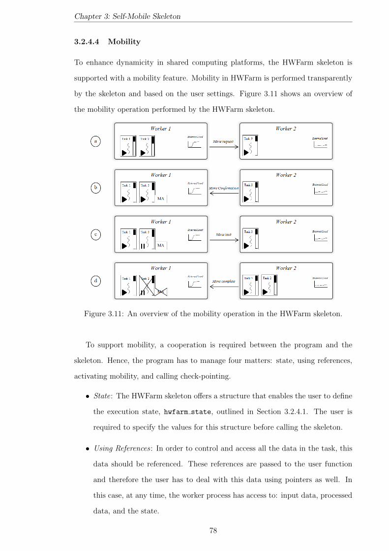
Chapter 3: Self-Mobile Skeleton
3.2.4.4 Mobility
To enhance dynamicity in shared computing platforms, the HWFarm skeleton is
supported with a mobility feature. Mobility in HWFarm is performed transparently
by the skeleton and based on the user settings. Figure 3.11 shows an overview of
the mobility operation performed by the HWFarm skeleton.
Figure 3.11: An overview of the mobility operation in the HWFarm skeleton.
To support mobility, a cooperation is required between the program and the
skeleton. Hence, the program has to manage four matters: state, using references,
activating mobility, and calling check-pointing.
• State: The HWFarm skeleton offers a structure that enables the user to define
the execution state, hwfarm state, outlined in Section 3.2.4.1. The user is
required to specify the values for this structure before calling the skeleton.
• Using References : In order to control and access all the data in the task, this
data should be referenced. These references are passed to the user function
and therefore the user has to deal with this data using pointers as well. In
this case, at any time, the worker process has access to: input data, processed
data, and the state.
78

Chapter 3: Self-Mobile Skeleton
• Activating Mobility : This is accomplished when calling the skeleton. The skele-
ton function has an argument that specifies the status of mobility, switched
on or off.
• Check-pointing : This operation is performed by the skeleton but under pro-
gram control. To avoid blocking the task execution during intensive com-
putation and critical memory access, it is preferred to check if there is need
for mobility between two iterations. Therefore, the HWFarm skeleton offers
a function which the program has to call at the end of each iteration. This
function is called checkForMobility() and it is also a parameter in the user
function. This function only checks a flag for this task and hence there is no
blocking for the executing thread.
To properly move a running computation to another location, we need to move
its code, its data, and the execution state to another location and then resume the
computation from its stop point. The code of the computation is already available on
all processes because HWFarm is based on top of MPI which has an SPMD model.
Thus, the user function is defined in the memory name space of all participating
processes.
The data including input, shared, output, and state is structured in the task data
structures mobile task and worker task. These data structures will keep access
to the data while the user function is running. Therefore, whenever the task stops
executing, the updated data is available and ready to be transferred.
The skeleton needs a decision maker to determine when and where mobility will
occur. This is performed by the skeleton scheduler guided by a performance cost
model. We will explore in Chapter 4 and Chapter 5 how the skeleton scheduler takes
move decisions based on the load state.
The mobility operation is a set of activities occurring in the workers involved
in this operation to move selected tasks from the source worker to the destination
worker. To illustrate this operation, we have worker 1 and worker 2 executing 2
tasks and one task, respectively. During the execution, the node that hosts worker
1 becomes highly loaded. In this case, when the skeleton scheduler triggers mobility
79
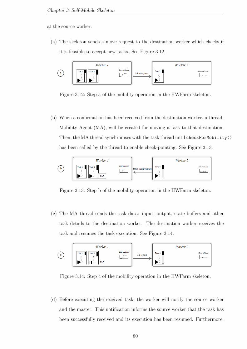
Chapter 3: Self-Mobile Skeleton
at the source worker:
(a) The skeleton sends a move request to the destination worker which checks if
it is feasible to accept new tasks. See Figure 3.12.
Figure 3.12: Step a of the mobility operation in the HWFarm skeleton.
(b) When a confirmation has been received from the destination worker, a thread,
Mobility Agent (MA), will be created for moving a task to that destination.
Then, the MA thread synchronises with the task thread until checkForMobility()
has been called by the thread to enable check-pointing. See Figure 3.13.
Figure 3.13: Step b of the mobility operation in the HWFarm skeleton.
(c) The MA thread sends the task data: input, output, state buffers and other
task details to the destination worker. The destination worker receives the
task and resumes the task execution. See Figure 3.14.
Figure 3.14: Step c of the mobility operation in the HWFarm skeleton.
(d) Before executing the received task, the worker will notify the source worker
and the master. This notification informs the source worker that the task has
been successfully received and its execution has been resumed. Furthermore,
80

Chapter 3: Self-Mobile Skeleton
the destination worker notifies the master that a task has been moved to a new
location and hence the mapping of the tasks needs to be updated. However,
the local task table will be updated at the destination worker. Once the
source worker receives a move complete, the source worker kills the thread of
the current moved task and frees the relevant resources. See Figure 3.15.
Figure 3.15: Step d of the mobility operation in the HWFarm skeleton.
Finally, the skeleton continues its activities and repeats mobility operations when
needed.
3.2.4.5 Prototype
in this section, we explore the usability of the HWFarm skeleton. All code fragments
presented in this section are in the C programming language, the programming
language we use to develop the HWFarm skeleton. We present the prototype of the
HWFarm function call as follow:
void hwfarm(fp user_function, int tasks,
void *input_data, int input_data_item_size, int input_data_length,
void*shared_data, int shared_data_item_size, int shared_data_length,
void *output_data, int output_data_item_size, int output_data_length,
hwfarm_state main_state, int mobility)
{. . .}
This prototype shows the parameters needed to call the skeleton function. The
parameters are:
• user function: The function written by the user to be called by workers to
manipulate the scattered data for one task.
81
Chapter 3: Self-Mobile Skeleton
• tasks: The total number of tasks.
• input data, input data item size, input data length: Input data de-
tails; outlined in Section 3.2.4.1.
• shared data, shared data item size, shared data length: Shared data
details; outlined in Section 3.2.4.1.
• output data, output data item size, output data length: Output data
details; outlined in Section 3.2.4.1.
• main state: A data structure that holds state of the execution. This param-
eter is essential in optimising the execution via the HWFarm scheduler; also
outlined in Section 3.2.4.1.
• mobility: A Boolean value to activate the mobility operations. If 0, the
skeleton will work as a static skeleton.
The prototype of the user function is as follow:
void user_function ( hwfarm_task_data* t_data,
chFM checkForMobility){ }
This function has two parameters: t data is an input parameter that holds all
data. Details about this structure are outlined in Section 3.2.4.1. checkForMobility
is a function to be called to check the mobility. Programs have to retrieve the data
from the input pointer hwfarm task data and update the execution state before
check-pointing. The implementation of the user function should follow the pattern:
void <function_name>(
hwfarm_task_data* t_data,
chFM checkForMobility){
int *i = t_data->counter;
int *i_max = t_data->counter_max;
//retrieve the input, the output, and the state.
while(*i < *i_max){
82

Chapter 3: Self-Mobile Skeleton
//Perform the computing over the input data
//Save the results of this iteration to the output data
//Increment the counter
checkForMobility();
}
}
3.2.4.6 Skeleton Initialisation and Finalization
Because the HWFarm skeleton is based on MPI, the environment needs to be
initialised and terminated when all executions are complete. This is done via
initHWFarm()and finalizeHWFarm().
initHWFarm() initializes the MPI environment to establish the communicator
and create the processes. We use MPI THREAD MULTIPLE to create MPI processes
with multithreaded support where we are creating many PThreads inside MPI pro-
cesses.
void initHWFarm(int argc, char ** argv){
int provided;
MPI_Init_thread(&argc, &argv, MPI_THREAD_MULTIPLE, &provided);
MPI_Comm_size(MPI_COMM_WORLD, &numprocs);
MPI_Comm_rank(MPI_COMM_WORLD, &rank);
}
finalizeHWFarm() terminates the MPI processes:
void finalizeHWFarm(){
MPI_Finalize();
}
3.2.5 Using the HWFarm Skeleton
Now, we will start with a simple sequential example and explain how this code can
be parallelised using HWFarm.
83
Chapter 3: Self-Mobile Skeleton
Suppose we have the sequential C code to square numbers in a list.
int num_array[ARRAY_SIZE];
while( i < ARRAY_SIZE ){
num_array[i] = num_array[i] * num_array[i];
i++;
}
To use the HWFarm skeleton to parallelise this code, we have to configure the
number of tasks and the chunk size. In this example, we set the number of tasks
to 10 tasks where the value of ARRAY SIZE is multiple of 10 and therefore all tasks
have an equal chunk of data. The code for configuring the initial values is:
int problem_size = ARRAY_SIZE;
int tasks = 10;
int chunk = problem_size / tasks;
Also, we need to set the input buffer and the input parameters. Here, we initialise
the input buffer with NULL because this buffer should be set at all processes. The
variable input data size is set to the number of bytes to store one integer number
in the host node. Finally, the variable input data len is set to the chunk size where
each task will processes this number of items. The fragment of code for configuring
the input is:
int * input_data = NULL;
int input_data_size = sizeof(int);
int input_data_len = chunk;
We will repeat the initialisation for the output buffer and its parameters. In
this example, the number of items in the output is equal to the number of items in
the input. This is not the case for all problems. The number of items in the input
and in the output can be flexibly set by the user depending on the problem. This
gives the HWFarm flexibility to manipulate a wide range of problems. The code for
configuring the output is:
84

Chapter 3: Self-Mobile Skeleton
int * output_data = NULL;
int output_data_size = sizeof(int);
int output_data_len = chunk;
Then, the state of the execution needs to be set. The values of the state depend
on the implementation of the problem as well as the number of items to be processed.
At the beginning, each task processes a chunk of data and therefore the main counter
is initialised to 0 and the maximum number of items is set to the chunk size. In
this example, the state is set to NULL where in this implementation the state is not
required. The code for specifying the values of the data structure hwfarm state is
as follows:
hwfarm_state main_state;
main_state.counter = 0;
main_state.max_counter = chunk;
main_state.state_data = NULL;
main_state.state_len = 0;
To activate mobility, the variable should have the value 1; otherwise it should
have the value 0.
int mobility = 1;
Before calling the skeleton, the master should allocate the input buffer and the
output buffer where the input data need to be initialised. The code is as follow:
if(rank == 0)
{
//Prepare the input data
//Prepare the output buffer
}
Then, the skeleton will be called with the parametrised values.
85
Chapter 3: Self-Mobile Skeleton
hwfarm( hwfarm_square, tasks,
input_data, input_data_size, input_data_len,
NULL, 0, 0,
output_data, output_data_size, output_data_len,
main_state, mobility);
When the skeleton function returns, the master can deal with the output data.
hwfarm square is the function that will be called for each task to process a
particular chunk of data. This function has the prototype outlined in the previous
section. First, the user obtains the values of the counter for the main loop. The
main counter values should be obtained using pointers as follow:
int *i = t_data->counter;
int *i_max = t_data->counter_max;
Then, the input and the output references will be obtained as follow:
int *input_p = (int*)t_data->input_data;
int *output_p = (int*)t_data->output_data;
Observe that all assignments in the user function should be performed through
pointers to reflect the updates on the passed arrays and to keep all data, such as
input, output, and counter, up to date during the execution of the task.
The main loop looks like:
while(*i < *i_max){
*(output_p + (*i)) = *(input_p + (*i)) * *(input_p + (*i));
(*i)++;
checkForMobility();
}
In comparison with the sequential code, we can see that parallel code is somehow
similar to serial code except using pointers and calling the check-point function,
checkForMobility(). A call to this function is needed to complete the check-
pointing and accomplish transferring the current task if necessary. Following this
86
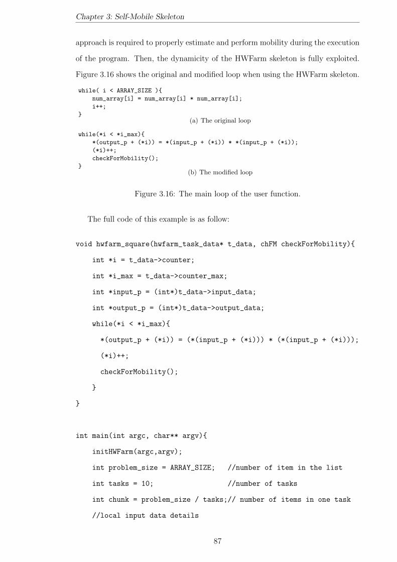
Chapter 3: Self-Mobile Skeleton
approach is required to properly estimate and perform mobility during the execution
of the program. Then, the dynamicity of the HWFarm skeleton is fully exploited.
Figure 3.16 shows the original and modified loop when using the HWFarm skeleton.
while( i < ARRAY_SIZE ){
num_array[i] = num_array[i] * num_array[i];
i++;
}(a) The original loop
while(*i < *i_max){
*(output_p + (*i)) = *(input_p + (*i)) * *(input_p + (*i));
(*i)++;
checkForMobility();
}(b) The modified loop
Figure 3.16: The main loop of the user function.
The full code of this example is as follow:
void hwfarm_square(hwfarm_task_data* t_data, chFM checkForMobility){
int *i = t_data->counter;
int *i_max = t_data->counter_max;
int *input_p = (int*)t_data->input_data;
int *output_p = (int*)t_data->output_data;
while(*i < *i_max){
*(output_p + (*i)) = (*(input_p + (*i))) * (*(input_p + (*i)));
(*i)++;
checkForMobility();
}
}
int main(int argc, char** argv){
initHWFarm(argc,argv);
int problem_size = ARRAY_SIZE; //number of item in the list
int tasks = 10; //number of tasks
int chunk = problem_size / tasks;// number of items in one task
//local input data details
87
Chapter 3: Self-Mobile Skeleton
int * input_data = NULL;
int input_data_size = sizeof(int);
int input_data_len = chunk;
//output data details
int * output_data = NULL;
int output_data_size = sizeof(int);
int output_data_len = chunk;
//details of the main counter
hwfarm_state main_state;
main_state.counter = 0;
main_state.max_counter = chunk;
main_state.state_data = NULL;
main_state.state_len = 0;
int mobility = 1;
if(rank == 0)
{
//Prepare the input data
//Prepare the output buffer
}
hwfarm( hwfarm_square, tasks,
input_data, input_data_size, input_data_len,
NULL, 0, 0,
output_data, output_data_size, output_data_len,
main_state, mobility);
if(rank == 0){
//Do something with the output
}
finalizeHWFarm();
}
88
Chapter 3: Self-Mobile Skeleton
3.2.6 Skeleton Assessment
The design of the HWFarm skeleton has addressed a pragmatic manifesto [67] and its
extension in [72]. Here, we discuss how the HWFarm skeleton met these principles:
1. Propagate the concept with minimal conceptual disruption: HWFarm is pre-
sented as a library or a function call in the C programming language. This
avoids learning new syntax and gets benefits from C features, such as porta-
bility. Nevertheless, rewriting of the code to obtain parallel code is required.
Moreover, HWFarm depends on the MPI and PThreads libraries to support
communications in distributed and shared memory platforms, respectively.
2. Integrate ad-hoc parallelism: because the HWFarm skeleton is built on top
of the most popular message passing libraries, this integrates with ad-hoc
parallelism.
3. Accommodate diversity : The program pattern supported by the HWFarm
skeleton is the loop parallelism pattern. Moreover, it is straight forward to
compose multiple HWFarm function calls to solve problems in a pipeline style.
However, the HWFarm skeleton is not nestable and the Divide and Conquer
pattern is not supported.
4. Show the pay-back : To illustrate the payback, we present a skeleton that is
straight forward to use and responsive to the load changes and where distri-
bution is based on machine characteristics.
5. Support code reuse: In the HWFarm skeleton, the sequential code can be
reused with some modifications where the structure of the code is unmodified.
But there is more effort when the implementation has special behaviour, such
as dynamic allocation.
6. Handle heterogeneity : The HWFarm skeleton supports multi-core clusters
that provide heterogeneous resources without addressing GPU architectures
or CPU accelerators. In addition, the HWFarm skeleton works in MPI com-
patible platforms with Linux based operation systems.
89
Chapter 3: Self-Mobile Skeleton
7. Handle dynamicity : The HWFarm skeleton is designed to be dynamic through
raising its awareness to the external load and supporting a mobility approach
to enable the skeleton to reallocate its computations amongst the nodes of
non-dedicated clusters. This enhances the skeleton to handle dynamicity and
adaptivity to the load state of the system.
3.3 Experiments
In this section, we present some experiments in order to show the improvement in
the performance from the perspective of speed up.
3.3.1 Platform
The HWFarm skeleton is tested on a Beowulf cluster located at Heriot-Watt Univer-
sity. The cluster consists of 32 eight-core machines: 8 quad-core Intel(R) Xeon(R)
CPU E5504, running GNU/Linux at 2.00GHz with 4096 kb L2 cache and using
12GB RAM.
3.3.2 Skeletal Experiments
In these experiments, we show the speed up when running our skeleton with different
chunk sizes for the same problem. We use two applications Matrix Multiplication
and Raytracer. For simplicity, we used two nodes of the Beowulf cluster to run our
skeleton, one for the master and one for the worker.
The Matrix Multiplication problem is based on:
for(i=0;i<n;i++) //n:row count in M1
for(j=0;j<m;j++) //m:col count in M2
for(k=0;k<c;k++) //c:col count in M1 = row count in M2
M3[i][j]=mul(M1[i][k],M2[k][j]);
In the first experiment, we run a 2000*2000 Matrix Multiplication problem with
different number of tasks to investigate that the skeleton achieves a speedup. The
90
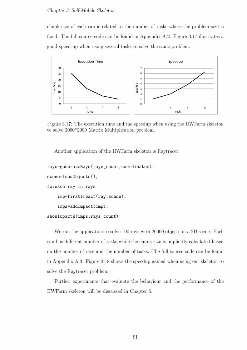
Chapter 3: Self-Mobile Skeleton
chunk size of each run is related to the number of tasks where the problem size is
fixed. The full source code can be found in Appendix A.2. Figure 3.17 illustrates a
good speed-up when using several tasks to solve the same problem.
Figure 3.17: The execution time and the speedup when using the HWFarm skeletonto solve 2000*2000 Matrix Multiplication problem.
Another application of the HWFarm skeleton is Raytracer.
rays=generateRays(rays_count,coordinates);
scene=loadObjects();
foreach ray in rays
imp=firstImpact(ray,scene);
imps=addImpact(imp);
showImpacts(imps,rays_count);
We run the application to solve 100 rays with 20000 objects in a 2D scene. Each
run has different number of tasks while the chunk size is implicitly calculated based
on the number of rays and the number of tasks. The full source code can be found
in Appendix A.3. Figure 3.18 shows the speedup gained when using our skeleton to
solve the Raytracer problem.
Further experiments that evaluate the behaviour and the performance of the
HWFarm skeleton will be discussed in Chapter 5.
91

Chapter 3: Self-Mobile Skeleton
Figure 3.18: The execution time and the speedup when using the HWFarm skeletonto solve Raytracer problem with 100 rays.
3.4 Summary
In this chapter, we presented the design and the structure of the HWFarm skele-
ton. The HWFarm skeleton is provided as a function or a library, hosted by the
C programming language, and dependent on the MPI and PThreads libraries. We
followed the skeletal principles provided by Cole [67] and Danelutto et al [72] to
implement this skeleton. We also showed how our skeleton fulfilled these design
concepts.
The HWFarm skeleton offers an efficient tool to exploit the processing power of
shared computing architectures, such as multi-core clusters. This skeleton can run
as a static skeleton or mobile skeleton. The requirements of running our skeleton in
static mode are as follows:
• The skeleton runs on platforms that are MPI compatible with Linux operating
system.
• The skeleton can be used to execute user programs in parallel. The user
program should follow the pattern outlined in Sec 3.2.4.5 where refactoring of
the sequential code is needed.
• The data that will be processed by the program should also be allocated by the
user. Therefore, the data buffers (input, shared and output), the unit sizes,
and buffer lengths are defined based on the executing platform.
• The data in each buffer should be allocated in consecutive memory locations.
92

Chapter 3: Self-Mobile Skeleton
• The program has to use pointers and references in updating the output buffer.
In the mobile version, the skeleton needs more requirements to take advantage
of its dynamicity. The requirements are as follows:
• The state of the program execution is defined with the state data structure,
hwfarm state. This structure is outlined in Sec 3.2.4.1. This structure has to
be modified, especially the counter field, at the end of each iteration by the
corresponding values to reflect the execution state of the program.
• At the end of each iteration, the checkForMobility() function should be
called.
• To activate mobility, calling the skeleton with mobility switched on is required.
Either running in static or mobile mode, the skeleton runs with assumptions. In
this thesis, we assume that:
• the sizes of tasks are fixed;
• the size of the task pool is static;
• the skeleton does not accept adding/removing nodes at run-time;
• and there is no dependency amongst tasks.
The experiments in this chapter show that the HWFarm skeleton gives good
speed-up when running in static mode. In the next chapters, we will explore how to
run the skeleton in mobile mode.
In the next chapter, we explore how HWFarm uses a performance cost model to
take the decisions needed to improve the performance.
93

Chapter 4
Measurement-based Performance
Cost Model
In the previous chapter, we presented our skeleton with a mobility approach to
enable the skeleton to reschedule its computations. Here, we discuss a performance
cost model used by the scheduler to produce costed decisions about the running
tasks. Such a model helps the scheduler to decide the computation location on
which a selected task can run faster. Therefore, this improves the performance and
reduces the total execution time. We discuss the cost model used by the HWFarm
skeleton in Section 4.1. Next, we show the evaluation of this cost model in Section
4.2.
4.1 Performance Cost Model
The presence of multiple applications in a shared environment may cause resource
contention by the running processes. Mobility is a good solution to lighten the
load and enhance the efficiency. But, mobility must be controlled and driven by
concerns related to the performance goals. Hence, a cost model is needed to take
accurate decisions. Accuracy of such decisions requires that the cost models should
be dynamic to reflect the environment load. Nonetheless, dynamic cost models incur
more overhead at run-time than static cost models.
In this thesis, we propose a dynamic performance cost model, the HWFarm cost
94
Chapter 4: Measurement-based Performance Cost Model
model. This model uses a measurement-based approach at run-time to estimate the
continuation time of the running computations. This model is parametrised with
dynamic parameters such as environment workload and the progress of the running
computations. Our experiments show that this cost model supports the adaptivity
of the HWFarm skeleton through taking accurate decisions. In this section, we
explore the HWFarm cost model design and its dynamic metrics.
4.1.1 Cost Model Design
The mobility decision in the HWFarm cost model is taken when the time to complete
executing a task at the current location is greater than the time to execute the same
task on a remote location aggregated with the transfer cost of that task. The
condition of the mobility decision is:
T i > Tmobility + T j; where i! = j
where: T i and T j are the estimated times for a task at location i and at location
j, respectively. Tmobility is the predicted cost of moving a task from the source
location to the destination location where transfer costs between all nodes are the
same.
To develop an adequate scheduling mechanism for the HWFarm skeleton, this
requires taking decisions based on the current behaviour. Therefore, we employ
a performance cost model to solve this issue. Nonetheless, evolving such a model
needs to take into consideration these challenges: architecture characteristics, ap-
plication parameters, system load, and network delays. All these challenges need to
be addressed in order to acquire the performance goals.
Architecture characteristics
To optimise the performance of HWFarm, the cost model should address the charac-
teristics of target architectures. These architectures are usually composed of various
kinds of processing units and hierarchical interconnections. To fully exploit these
rapidly evolving heterogeneous resources in the shared environments, HWFarm has
95
Chapter 4: Measurement-based Performance Cost Model
to be adaptive to the platforms where it is running. This also achieves performance
portability. However, due to the big influence of the architecture characteristics on
performance, these characteristics need to be integrated with the cost model. Con-
sequently, the HWFarm cost model should be architecture-independent and be able
to predict the performance on the target architectures.
The architecture parameters that affect the running computations and used in
architecture-independent cost models are: the speed of CPU, number of processing
units, number of cores, memory, and cache. Deng [80] presented a cost model
parameterised with the CPU speed. The number of processing units is also used
with many cost models such as LogP [71]. L2 cache is also addressed in the cost
model proposed by Khari [21].
In the HWFarm cost model, we use two static architecture parameters: the speed
of the CPU and number of cores on that CPU. We assume that all cores in a node
have the same clock speed. In this work, we do not address the memory and the
cache.
The static information used by the HWFarm cost model can be obtained once at
the start-up from the /proc virtual file system. These values reflect the maximum
potential computational power of the current machine.
Application
Conventionally, to estimate the cost of running an implementation, cost analysis of
the algorithm should be carried out. This requires knowledge of the application and
the executing platform. Furthermore, this may take much effort that transcends the
benefits of analysis.
In skeletal-based systems, the skeleton is adopted as a parallel subroutine to
execute a parametrised user code. This generic subroutine is referred to as a black-
box component [55]. Hence, there is no prior knowledge about the programs they
execute. In HWFarm, the skeleton executes its tasks with awareness about their
progress of execution. This is implemented with assistance from the user. This was
detailed further in Chapter 3.
96

Chapter 4: Measurement-based Performance Cost Model
Parallel applications are generally computationally intensive. Such applications
are typically implemented using constrained programming models. Constrained
programming models or concrete coordination patterns simplify the cost modelling
of these applications. Because the program model used in the HWFarm skeleton is
loop parallelism, this gives the running tasks a repetitive nature.
In iteration-based applications, each iteration that manipulates the specific amount
of data has an executing cost somehow similar to the cost of other iterations that
process the same amount of data [235]. That is correct if the execution continues
on the same platform with the same load state. But, this is not the case if the com-
putations are irregular. We will discuss the accuracy of the estimations in irregular
computations in Section 4.2.1.2. In some references, the iterations are referred to as
super-steps like the BSP parallel model [123].
Therefore, in the HWFarm cost model, we used a partial execution approach to
estimate the continuation times based on the past execution on the current node.
This approach is also based on monitoring and measuring of the behaviour of the
running computations. This approach was previously used by Yang et al [235]
where they showed that this mechanism is portable and cost-effective to predict the
performance. The metrics used in the model are: the elapsed time for a specific task
and how much work was completed in this location. These metrics are classified as
dynamic parameters that reflect the behaviour of the execution of the running tasks.
The first metric can be measured dynamically while the second is obtained from the
data structure of the relevant task. All details about this structure are outlined in
Section 3.2.4.1. These two metrics are also used in the cost model developed by
Deng [80].
System load
Selecting load metrics that characterize the system workload is crucial to the move-
ment decisions. The information about the system load reflects the environment’s
state. However, we need to employ the metrics that are useful to estimate the
continuation execution time from the past local load.
97

Chapter 4: Measurement-based Performance Cost Model
We identify the dynamic metrics that represent the workload of the systems:
• The load average represents the average system load over a period of time. It
appears in the form of three numbers which represent the system load during
the last one-, five-, and fifteen-minute period.
• The CPU utilisation refers to the percentage of usage of the CPU on all cores.
• The number of running processes refers to the number of processes and threads
currently assigned to the CPU.
In HWFarm, we use the CPU utilisation and the number of running processes as
dynamic input parameters of the HWFarm cost model. We exclude the load average
because it depends on the number of running and runnable tasks over a past period,
and its values are only updated in 3 second intervals in a typical Linux Kernel.
However, these values will be obtained periodically to measure the load state of the
host node. Like architecture characteristics, these values are also obtained from the
/proc virtual file system.
Network
The performance of parallel applications may be affected by the network contention
due to communication delay and latency. In order to produce accurate decisions,
the network characteristics should be considered in estimating the costs.
In the HWFarm cost model, the estimated times are calculated depending on
the local state on the current node and on other nodes. Because there are no inter-
communications amongst the tasks, the network latency has to be considered only
in mobility decisions. Therefore, to get accurate decisions for either moving a task
or not, that depends also on the cost of moving a task, Tmobility. Initially, we assume
that the communications are uniform within the cluster environment. Nonetheless,
for more accurate decisions, we need to observe the real network properties.
Network overhead, network contention, network bandwidth, and network latency
are metrics that have been used in cost modelling. An example of cost models that
use network characteristics is the LogP model [71].
98

Chapter 4: Measurement-based Performance Cost Model
In HWFarm, for simplicity, we use only the network latency as an indication of
whether the node is in a remote cluster or a local cluster.
As a conclusion, developing a highly accurate absolute cost model perfected
for a single implementation, a specific target language, and a concrete architec-
ture needs much effort. To overcome these challenges, the HWFarm cost model
might be used for a wide range of implementations written to solve different prob-
lems with various programming languages. Consequently, we propose a dynamic,
generic, architecture-independent, problem-independent and language-independent
cost model. This model supports the HWFarm skeleton to enhance its adaptivity
through predicting its own performance and hence the skeleton will be self-optimised.
However, the HWFarm cost model uses dynamic experimental measurements to
estimate the behaviour of the computations. This dynamicity incurs an overhead
that may influence the performance. We will explore further the overhead later in
Chapter 5.
4.1.2 The HWFarm Cost Model
The HWFarm cost model is based on a generic cost model [80] developed by Deng,
see Figure 4.1. Deng’s model combines the abstract static generated model with dy-
namic parameters. Furthermore, this model predicts the continuation times on the
current location and on other locations. This model also uses Formula 4.5 to deter-
mine mobility. Deng’s cost model is used in AMPs (Autonomous Mobile Programs)
and in AMSs (Autonomous Mobile Skeletons) such as automap, autofold, AutoIter-
ator implemented in Jocaml, and Java Voyager, and JavaGo over LANs. However,
Deng’s model addresses the processing power of the CPU but it does not take into
account the cores of that CPU. Moreover, this model takes into consideration only
the local load.
We use Deng’s model as a basis of our model and add more parameters that
optimise the performance. This model is implemented in C and accepts any program
able to run in parallel with some restrictions. Furthermore, it takes into account the
heterogeneity of the resources as well as the overall system workload in the shared
99

Chapter 4: Measurement-based Performance Cost Model
Ttotal = TComp + TComm + TCoord
Th > Tcomm + TnTComm = mTcomm
TCoord = npTcoordTCoord < OTstatic
n <OTstaticpTcoord
Te =Wd
Sh
Th =Wl
Sh
Tn =Wl
Sn
O : Overhead e.g. 5%Ttotal : total timeTstatic : time for static program running on the current locationTComm : total time for communicationTcomm : time for a single communicationTCoord : total time for coordinationTcoord : time for coordination with a single processor(location)TComp : time for computationTe : time has elapsed at current locationTh : time will take hereTn : time will take in the next locationWd : the work has been done at current locationWl : the work leftSh : the current CPU speedSn : the next location CPU speedm : number of communicationn : number of coordinationp : number of processor
Figure 4.1: Deng’s cost model
environment. This awareness guides the skeleton to be more adaptive and elastic.
The HWFarm cost model, see Figure 4.2, starts with calculating the total pro-
cessing power for the location where the task is running, P , Formula 4.1.
Next, the relative processing power will be calculated for the location on which
the worker is allocated, Ri, see Formula 4.2.
Then, after obtaining the dynamic parameters needed for estimation: architec-
ture characteristics, application parameters, and system load, the estimated time
to complete the task at the current location can be calculated, Ti, see Formula 4.3.
The previous steps will be repeated for the all participating workers in order to:
calculate the total processing power, Pj, calculate the relative processing power,
100
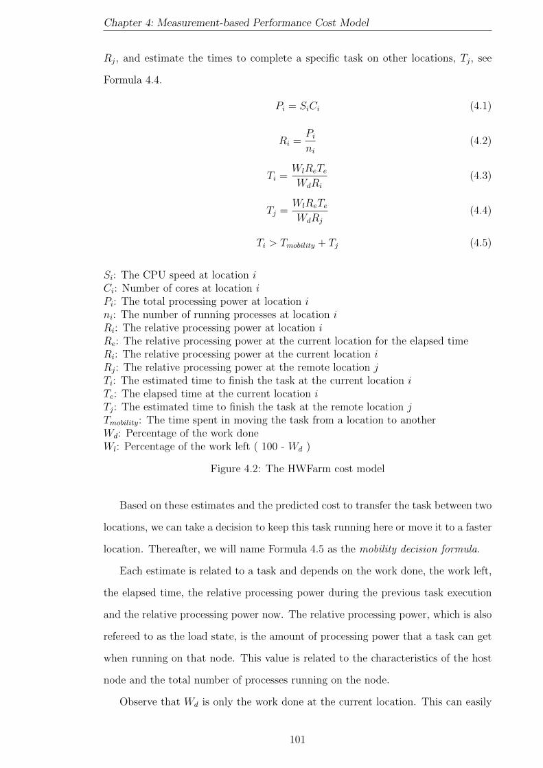
Chapter 4: Measurement-based Performance Cost Model
Rj, and estimate the times to complete a specific task on other locations, Tj, see
Formula 4.4.
Pi = SiCi (4.1)
Ri =Pi
ni
(4.2)
Ti =WlReTeWdRi
(4.3)
Tj =WlReTeWdRj
(4.4)
Ti > Tmobility + Tj (4.5)
Si: The CPU speed at location iCi: Number of cores at location iPi: The total processing power at location ini: The number of running processes at location iRi: The relative processing power at location iRe: The relative processing power at the current location for the elapsed timeRi: The relative processing power at the current location iRj: The relative processing power at the remote location jTi: The estimated time to finish the task at the current location iTe: The elapsed time at the current location iTj: The estimated time to finish the task at the remote location jTmobility: The time spent in moving the task from a location to anotherWd: Percentage of the work doneWl: Percentage of the work left ( 100 - Wd )
Figure 4.2: The HWFarm cost model
Based on these estimates and the predicted cost to transfer the task between two
locations, we can take a decision to keep this task running here or move it to a faster
location. Thereafter, we will name Formula 4.5 as the mobility decision formula.
Each estimate is related to a task and depends on the work done, the work left,
the elapsed time, the relative processing power during the previous task execution
and the relative processing power now. The relative processing power, which is also
refereed to as the load state, is the amount of processing power that a task can get
when running on that node. This value is related to the characteristics of the host
node and the total number of processes running on the node.
Observe that Wd is only the work done at the current location. This can easily
101

Chapter 4: Measurement-based Performance Cost Model
be measured but we need more details if the task previously has been moved in
order to calculate the work left. Each task has a field that holds the amount of work
processed when it leaves a location. Therefore, Wl will be the percentage of the work
left for processing the remaining data based on the work done at previous locations
and the work done here, at the current location. The work done is obtained from
the counter fields of the hwfarm state struct in the HWFarm skeleton. This struct
is discussed in details in Sec 3.2.4.1.
Table 4.1 summarizes the parameters used by the HWFarm cost model.
Parameter Description Type Static/Dynamic Source
Si Node CPU Speed Local/Remote Static ArchitectureCi Node Core Count Local/Remote Static Architectureni Number of processes Local/Remote Dynamic System LoadTe Elapsed Time Local Dynamic ApplicationWd Work done Local Dynamic ApplicationWl Work Left Local Dynamic ApplicationLi Network Latency Network Dynamic Network
Table 4.1: Parameters of the HWFarm cost model.
Figure 4.3 shows that the HWFarm cost model is divided into two stages: local
estimations and remote estimations. Local estimation, Stage 1, is parametrised
with the information about the node, the application and the load state. Then,
Stage 2 takes the local estimates as well as the information about the network, the
application, and the other nodes in order to produce the remote estimations and
finally concludes the final decision.
4.1.2.1 Mobility Cost
The mobility cost, Tmobility, is a significant component of the mobility decision for-
mula, see Formula 4.5 in Figure 4.2. This component represents the time predicted
to transfer the task to the destination node.
In HWFarm, there are three types of transfers: from the master to a worker,
assigning tasks; from a worker to the master, returning results; and from a worker
to a worker, task mobility. In this section, we focus on predicting the time needed
to transfer a selected task to a new location.
102
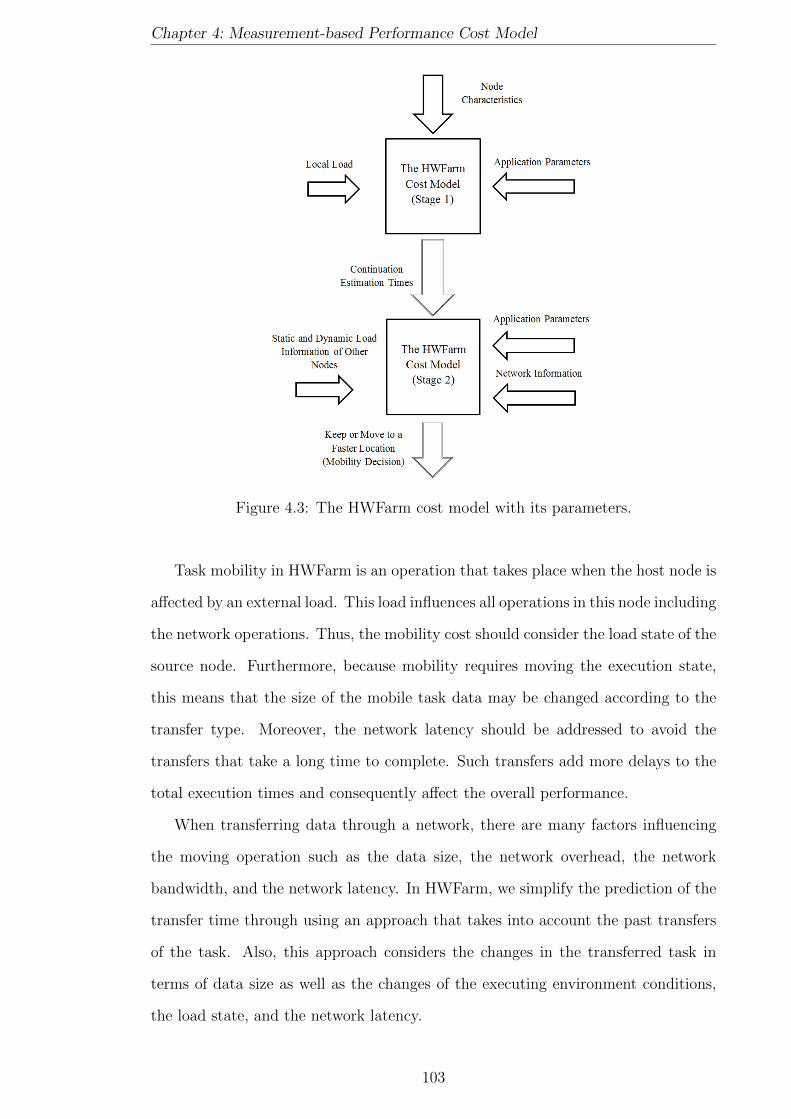
Chapter 4: Measurement-based Performance Cost Model
Figure 4.3: The HWFarm cost model with its parameters.
Task mobility in HWFarm is an operation that takes place when the host node is
affected by an external load. This load influences all operations in this node including
the network operations. Thus, the mobility cost should consider the load state of the
source node. Furthermore, because mobility requires moving the execution state,
this means that the size of the mobile task data may be changed according to the
transfer type. Moreover, the network latency should be addressed to avoid the
transfers that take a long time to complete. Such transfers add more delays to the
total execution times and consequently affect the overall performance.
When transferring data through a network, there are many factors influencing
the moving operation such as the data size, the network overhead, the network
bandwidth, and the network latency. In HWFarm, we simplify the prediction of the
transfer time through using an approach that takes into account the past transfers
of the task. Also, this approach considers the changes in the transferred task in
terms of data size as well as the changes of the executing environment conditions,
the load state, and the network latency.
103

Chapter 4: Measurement-based Performance Cost Model
Based on the previous approach, the prediction operation in HWFarm is application-
independent where it predicts the time of transferring data regardless of what the
task is. Also, the prediction is architecture-independent where the network structure
characteristics are featured in the times measured from the previous transfers.
Much work has been done to predict the cost of transferring data to another
location. For example, Vazhkudai et al [224] proposed a framework that predicts
the performance of data transfer in Grid platform based on past data transfer.
Next, we need to experiment with the impact of three factors: data size, load
state, and the network latency on the transfer time. Each one of these factors will be
individually investigated to find the relationship between this factor and the transfer
time. Here, we use the HWFarm skeleton with a simple program, a Square Numbers
application, that calculates the square of integer numbers in a one dimensional array.
Data Size
In HWFarm, the data size is the total amount of data attached to the task where
this amount might be changed according to the transfer type.
In this experiment, we will investigate the impact of data size on the transfer
times through measuring the times spent to transfer a task with various data sizes
between two nodes/workers. Here, we measure the transfer cost of sending a task
with a specific data size. Then, we compare the measured value with a new trans-
fer cost when sending a task with a different data size. Accordingly, the changes
of the transfer times are relevant to the changes of the data sizes. However, the
other factors, the load state and the network latency, are constant. We repeat this
experiment with various data sizes and then compare the changes of the transfer
times with the changes of the data sizes. Consequently, we have a relation between
the scaled transfer times and the the scaled data sizes. Figure 4.4 shows the scaled
transfer times compared to the scaled data sizes. The base unit of the times is
seconds while the base unit of the data size is byte.
Note that there is a dependency between the scaled data sizes and the scaled
transfer times. Therefore, from this relationship, a regression analysis [58] is needed
104

Chapter 4: Measurement-based Performance Cost Model
Figure 4.4: The scaled transfer times compared to the scaled data-sizes.
to predict the future transfer times based on changes of data size. We choose a power
regression, y = axb, to fit the given set of data. The reason behind this selection is
based on the assumption that if the data size of the task has not been changed, the
prediction of the future transfer time is similar to the previous transfer cost. As a
result, the power regression of the scaled transfer times compared to the scaled data
sizes yields: a = 1 and b = 1.023:
y = x1.023
Where: y refers the scaled transfer times while x points to the scaled data size.
As a conclusion:
y =T2T1, x =
DS2
DS1
=⇒ T2T1
= (DS2
DS1
)1.023 =⇒
T2 = (DS2
DS1
)1.023 ∗ T1 (4.6)
Where:
T1: The time of the previous transfer.
DS1: The data size at the previous transfer.
DS2: The data size at the next transfer
T2: The predicted time of the next transfer.
105
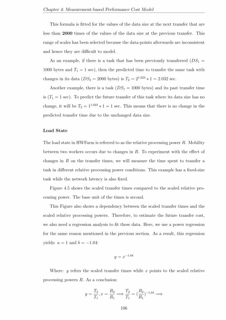
Chapter 4: Measurement-based Performance Cost Model
This formula is fitted for the values of the data size at the next transfer that are
less than 2000 times of the values of the data size at the previous transfer. This
range of scales has been selected because the data-points afterwards are inconsistent
and hence they are difficult to model.
As an example, if there is a task that has been previously transferred (DS1 =
1000 bytes and T1 = 1 sec), then the predicted time to transfer the same task with
changes in its data (DS2 = 2000 bytes) is T2 = 21.023 ∗ 1 = 2.032 sec.
Another example, there is a task (DS1 = 1000 bytes) and its past transfer time
is (T1 = 1 sec). To predict the future transfer of this task where its data size has no
change, it will be T2 = 11.023 ∗ 1 = 1 sec. This means that there is no change in the
predicted transfer time due to the unchanged data size.
Load State
The load state in HWFarm is referred to as the relative processing power R. Mobility
between two workers occurs due to changes in R. To experiment with the effect of
changes in R on the transfer times, we will measure the time spent to transfer a
task in different relative processing power conditions. This example has a fixed-size
task while the network latency is also fixed.
Figure 4.5 shows the scaled transfer times compared to the scaled relative pro-
cessing power. The base unit of the times is second.
This Figure also shows a dependency between the scaled transfer times and the
scaled relative processing powers. Therefore, to estimate the future transfer cost,
we also need a regression analysis to fit these data. Here, we use a power regression
for the same reason mentioned in the previous section. As a result, this regression
yields: a = 1 and b = −1.04:
y = x−1.04
Where: y refers the scaled transfer times while x points to the scaled relative
processing powers R. As a conclusion:
y =T2T1, x =
R2
R1
=⇒ T2T1
= (R2
R1
)−1.04 =⇒
106

Chapter 4: Measurement-based Performance Cost Model
Figure 4.5: The scaled transfer times compared to the scaled relative processingpower.
T2 = (R1
R2
)1.04 ∗ T1 (4.7)
where:
T1: The time of the previous transfer.
R1: The relative processing power at the previous transfer.
R2: The relative processing power at the next transfer.
T2: The predicted time of the next transfer.
This formula is fitted for the values of the load state that are less than 400%
where the scale of the relative processing power is ranging from 0.38 to 1. Like the
effect of the data size, the data set of this range reflects a consistent behaviour of the
scaled transfer time compared to the scaled relative processing power. However, the
computational efficiency of the extra loaded nodes, beyond 400%, degrades badly
and hence this model will produce movement decisions. Furthermore, this formula
says that the next transfer time equals to the previous transfer time if there is no
change on the relative processing power. This will not happen where the mobility
occurs only if the current worker is highly loaded.
107

Chapter 4: Measurement-based Performance Cost Model
Network Latency
Transferring tasks amongst locations occurs through a network which may have a
latency that affects the total time spent to accomplish this operation. Therefore,
we need to consider the network latency in estimating the transfer time. We control
the latency at a concrete location using the netem utility [118] that adds a specific
amount of delay to all outgoing packets.
Figure 4.6 shows that the time of transferring a task for different network delays.
These values depict that the times are equal if the latency is below a threshold value
point while they increase after that value. We assume that this value is a network
delay threshold where all network delays have a negligible influence on the transfer
time of a task. Based on these values, the threshold is L = 1.5ms.
Figure 4.6: The relationship between the transfer time and the network latency.
To investigate the effect of changes of the network latency on the transfer times,
we use the HWFarm skeleton with the Square program that has a fixed-size task
and unchanged relative processing power. We will measure the time spent to trans-
fer a task between two locations in different situations of network latency at the
destination location.
To find the scaled network latencies, the threshold L should be taken into ac-
count. This means that any delay value that is less than 1.5ms will be assumed as
L. This is true where all delays have the same effect on the transfer time.
108
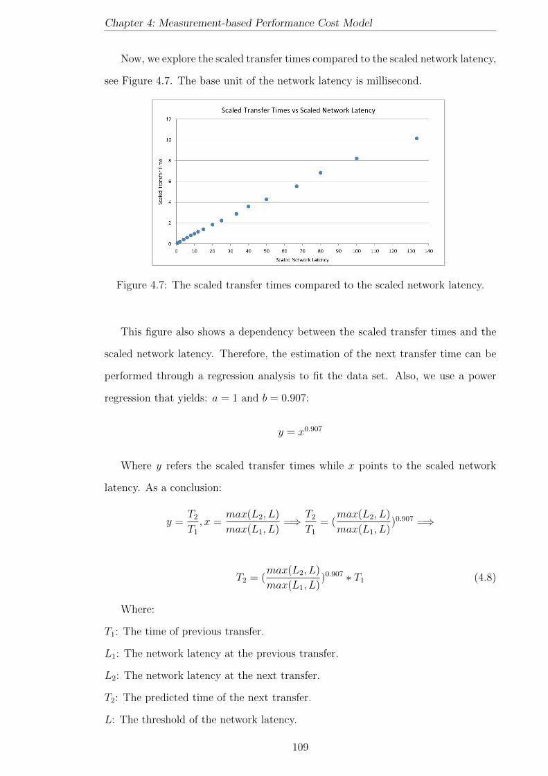
Chapter 4: Measurement-based Performance Cost Model
Now, we explore the scaled transfer times compared to the scaled network latency,
see Figure 4.7. The base unit of the network latency is millisecond.
Figure 4.7: The scaled transfer times compared to the scaled network latency.
This figure also shows a dependency between the scaled transfer times and the
scaled network latency. Therefore, the estimation of the next transfer time can be
performed through a regression analysis to fit the data set. Also, we use a power
regression that yields: a = 1 and b = 0.907:
y = x0.907
Where y refers the scaled transfer times while x points to the scaled network
latency. As a conclusion:
y =T2T1, x =
max(L2, L)
max(L1, L)=⇒ T2
T1= (
max(L2, L)
max(L1, L))0.907 =⇒
T2 = (max(L2, L)
max(L1, L))0.907 ∗ T1 (4.8)
Where:
T1: The time of previous transfer.
L1: The network latency at the previous transfer.
L2: The network latency at the next transfer.
T2: The predicted time of the next transfer.
L: The threshold of the network latency.
109

Chapter 4: Measurement-based Performance Cost Model
This formula is fitted for the scaled network latencies that are less than 13 times
where the maximum delay applied is 20 ms. Here, the network delays that are
greater than 20 ms are also difficult to model. As a result, if the network latency
at the previous transfer and at the next transfer are less than (L = 1.5 ms), the
network latency has no effect on the predicted cost. Then,
max(L2, L)
max(L1, L)=L
L= 1→ T2 = T1
Otherwise, if either L1 or L2 is greater than L, Formula 4.8 is applied where the
threshold L will be considered as a base to calculate the scaled latency.
Mobility Cost Summary
Now, we combine all three factors that affect the transfer times in one formula. Any
changes in the data size will change the transfer time. Then, if the load state is
changed, that will affect the whole operation. Moreover, if there is network latency,
this will affect the transfer.
We assume that the first transfer that occurs when the master assigns a task is
the baseline in predicting the mobility cost of this task. This time is referred to as
Tassignment or Ta.
The formula that predicts the transfer time of the task selected to move to a
destination worker is as follow:
Tmobility = (DSmobility
DSa
)1.023 ∗ (Ra
Rmobility
)1.04 ∗ (max(Lmobility, L)
max(La, L))0.907 ∗ Ta (4.9)
where:
DSa: The data size when this task is first assigned to the current worker.
DSmobility: The data size of this task that is supposed to be transferred to another
worker.
Ra: The relative processing power when this task is first assigned to a worker.
Rmobility: The relative processing power of the current node.
La: The network latency when this task is first assigned to the current worker.
110

Chapter 4: Measurement-based Performance Cost Model
Lmobility: The network latency at the destination node when this task is supposed
to be transferred to that node.
L: The threshold of the network latency.
Ta: The time spent when this task is first assigned to the current worker.
4.1.3 Changes to the HWFarm skeleton
To efficiently fulfil the objectives of building the HWFarm skeleton, the HWFarm
performance cost model is implemented in the skeleton. This is performed through
creating agents responsible for the estimating operations. These agents are called,
the Estimator Agents, EAs. This supports the distributed nature of the skeleton
where each worker runs an estimator agent when necessary. Details about triggering
decision making will be explained in Chapter 5.
4.2 Cost Model Validation
In this section, we present experiments with the HWFarm cost model to validate the
estimated execution times and the mobility decisions. We are exploring two types
of computations: regular and irregular. For regular problems, we use a Matrix
Multiplication application. In contrast, we experiment a Raytracer problem in a 2D
scene as an example of irregular computations.
For these experiments, we test the skeleton in a Beowulf cluster located at Heriot-
Watt University. This cluster consists of 32 eight-core machines (8 quad-core In-
tel(R) Xeon(R) CPU E5504, running GNU/Linux(2.6.32) at 2.00GHz with 4096 kb
L2 cache and using 12GB RAM).
4.2.1 Execution Time Validation
In this section, we validate the times estimated by the HWFarm cost model. These
times are crucial in taking decisions to remap the running tasks over the processing
units.
111
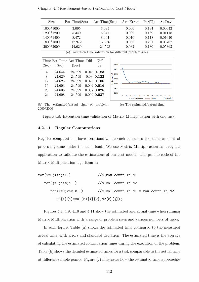
Chapter 4: Measurement-based Performance Cost Model
Size Est-Time(Sec) Act-Time(Sec) Ave-Error Per(%) St-Dev
1000*1000 3.095 3.095 0.006 0.194 0.000421200*1200 5.349 5.341 0.009 0.169 0.011181400*1400 8.472 8.464 0.010 0.118 0.010401800*1800 17.972 17.936 0.036 0.201 0.037072000*2000 24.629 24.598 0.032 0.130 0.05363
(a) Execution time validation for different problem sizes
Time Est-Time Act-Time Diff Diff(Sec) (Sec) (Sec) %
4 24.644 24.599 0.045 0.1838 24.629 24.599 0.03 0.12212 24.625 24.599 0.026 0.10616 24.603 24.599 0.004 0.01620 24.606 24.599 0.007 0.02824 24.608 24.599 0.009 0.037
(b) The estimated/actual time of problem2000*2000
(c) The estimated/actual time
Figure 4.8: Execution time validation of Matrix Multiplication with one task.
4.2.1.1 Regular Computations
Regular computations have iterations where each consumes the same amount of
processing time under the same load. We use Matrix Multiplication as a regular
application to validate the estimations of our cost model. The pseudo-code of the
Matrix Multiplication algorithm is:
for(i=0;i<n;i++) //n:row count in M1
for(j=0;j<m;j++) //m:col count in M2
for(k=0;k<c;k++) //c:col count in M1 = row count in M2
M3[i][j]=mul(M1[i][k],M2[k][j]);
Figures 4.8, 4.9, 4.10 and 4.11 show the estimated and actual time when running
Matrix Multiplication with a range of problem sizes and various numbers of tasks.
In each figure, Table (a) shows the estimated time compared to the measured
actual time, with errors and standard deviation. The estimated time is the average
of calculating the estimated continuation times during the execution of the problem.
Table (b) shows the detailed estimated times for a task comparable to the actual time
at different sample points. Figure (c) illustrates how the estimated time approaches
112
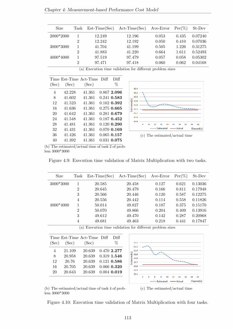
Chapter 4: Measurement-based Performance Cost Model
Size Task Est-Time(Sec) Act-Time(Sec) Ave-Error Per(%) St-Dev
2000*2000 1 12.249 12.196 0.053 0.435 0.072402 12.242 12.192 0.050 0.410 0.07036
3000*3000 1 41.704 41.199 0.505 1.226 0.312752 41.883 41.220 0.664 1.611 0.52493
4000*4000 1 97.519 97.479 0.057 0.058 0.053022 97.471 97.418 0.060 0.062 0.04168
(a) Execution time validation for different problem sizes
Time Est-Time Act-Time Diff Diff(Sec) (Sec) (Sec) %
4 42.228 41.361 0.867 2.0968 41.602 41.361 0.241 0.58312 41.523 41.361 0.162 0.39216 41.636 41.361 0.275 0.66520 41.642 41.361 0.281 0.67924 41.548 41.361 0.187 0.45228 41.481 41.361 0.120 0.29032 41.431 41.361 0.070 0.16936 41.426 41.361 0.065 0.15740 41.392 41.361 0.031 0.075
(b) The estimated/actual time of task 2 of prob-lem 3000*3000
(c) The estimated/actual time
Figure 4.9: Execution time validation of Matrix Multiplication with two tasks.
Size Task Est-Time(Sec) Act-Time(Sec) Ave-Error Per(%) St-Dev
3000*3000 1 20.585 20.458 0.127 0.621 0.130362 20.645 20.479 0.166 0.811 0.179483 20.566 20.446 0.120 0.587 0.122754 20.556 20.442 0.114 0.558 0.11826
4000*4000 1 50.014 49.827 0.187 0.375 0.151702 50.070 49.866 0.204 0.409 0.139163 49.612 49.470 0.142 0.287 0.209684 49.681 49.463 0.218 0.441 0.17847
(a) Execution time validation for different problem sizes
Time Est-Time Act-Time Diff Diff(Sec) (Sec) (Sec) %
4 21.109 20.639 0.470 2.2778 20.958 20.639 0.319 1.54612 20.76 20.639 0.121 0.58616 20.705 20.639 0.066 0.32020 20.643 20.639 0.004 0.019
(b) The estimated/actual time of task 4 of prob-lem 3000*3000
(c) The estimated/actual time
Figure 4.10: Execution time validation of Matrix Multiplication with four tasks.
113

Chapter 4: Measurement-based Performance Cost Model
Size Task Est-Time(Sec) Act-Time(Sec) Ave-Error Per(%) St-Dev
4000*4000 1 24.931 24.531 0.401 1.635 0.422242 24.935 24.537 0.403 1.642 0.430743 24.939 24.528 0.414 1.688 0.444594 24.944 24.526 0.422 1.721 0.457835 26.968 27.115 0.613 2.261 0.494696 26.933 27.128 0.725 2.673 0.521697 26.694 26.931 0.693 2.573 0.483568 30.248 30.480 0.529 1.736 0.27621
(a) Execution time validation for different problem sizes
Time Est-Time Act-Time Diff Diff(Sec) (Sec) (Sec) %
6 30.703 29.667 1.036 3.49212 29.48 29.667 0.187 0.63018 29.799 29.667 0.132 0.44524 29.993 29.667 0.326 1.09930 29.792 29.667 0.125 0.421
(b) The estimated/actual time of task 8 of prob-lem 4000*4000
(c) The estimated/actual time
Figure 4.11: Execution time validation of Matrix Multiplication with eight tasks.
the actual time where the solid line indicates the actual time projected backwards.
These results show how the estimated time are accurate with a maximum error of
3% when comparing those times to the actual times.
Figure 4.12 summaries the results presented above. This figure depicts that the
accuracy of the estimation is improved as the task progresses towards completion.
Figure 4.12: Summary of the estimation accuracy in validating the execution timein Matrix Multiplication.
114
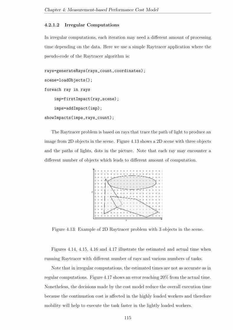
Chapter 4: Measurement-based Performance Cost Model
4.2.1.2 Irregular Computations
In irregular computations, each iteration may need a different amount of processing
time depending on the data. Here we use a simple Raytracer application where the
pseudo-code of the Raytracer algorithm is:
rays=generateRays(rays_count,coordinates);
scene=loadObjects();
foreach ray in rays
imp=firstImpact(ray,scene);
imps=addImpact(imp);
showImpacts(imps,rays_count);
The Raytracer problem is based on rays that trace the path of light to produce an
image from 2D objects in the scene. Figure 4.13 shows a 2D scene with three objects
and the paths of lights, dots in the picture. Note that each ray may encounter a
different number of objects which leads to different amount of computation.
Figure 4.13: Example of 2D Raytracer problem with 3 objects in the scene.
Figures 4.14, 4.15, 4.16 and 4.17 illustrate the estimated and actual time when
running Raytracer with different number of rays and various numbers of tasks.
Note that in irregular computations, the estimated times are not as accurate as in
regular computations. Figure 4.17 shows an error reaching 20% from the actual time.
Nonetheless, the decisions made by the cost model reduce the overall execution time
because the continuation cost is affected in the highly loaded workers and therefore
mobility will help to execute the task faster in the lightly loaded workers.
115
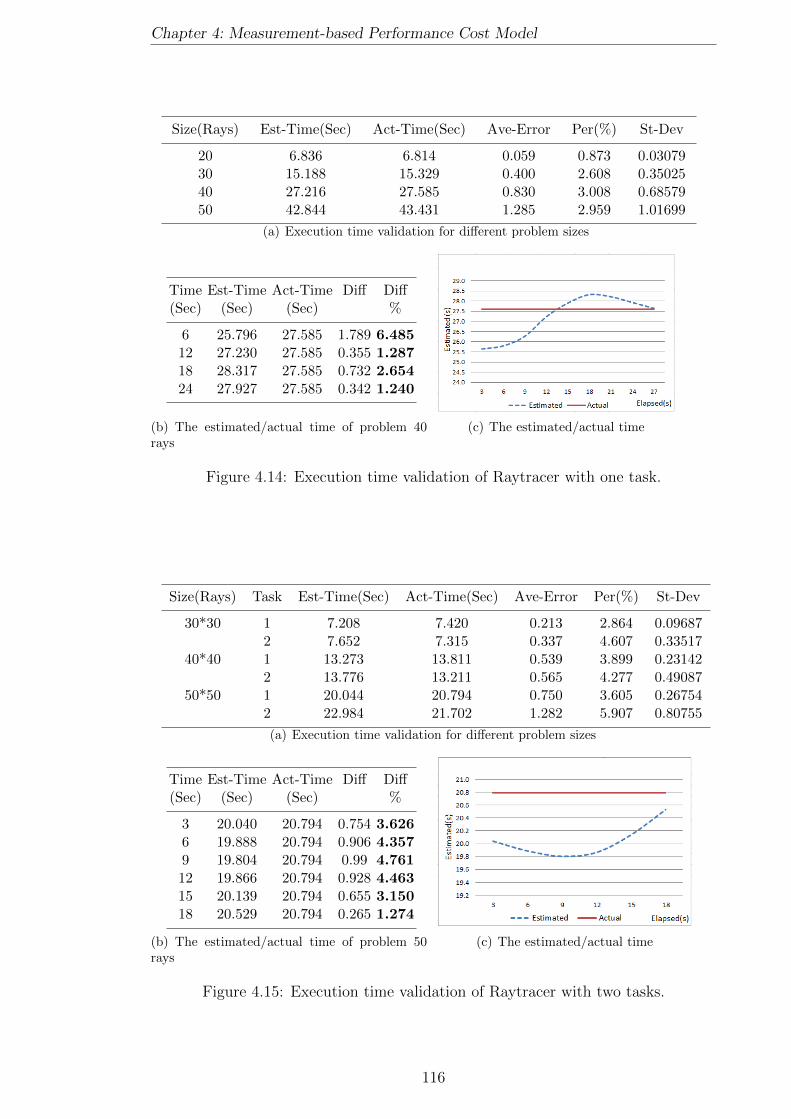
Chapter 4: Measurement-based Performance Cost Model
Size(Rays) Est-Time(Sec) Act-Time(Sec) Ave-Error Per(%) St-Dev
20 6.836 6.814 0.059 0.873 0.0307930 15.188 15.329 0.400 2.608 0.3502540 27.216 27.585 0.830 3.008 0.6857950 42.844 43.431 1.285 2.959 1.01699
(a) Execution time validation for different problem sizes
Time Est-Time Act-Time Diff Diff(Sec) (Sec) (Sec) %
6 25.796 27.585 1.789 6.48512 27.230 27.585 0.355 1.28718 28.317 27.585 0.732 2.65424 27.927 27.585 0.342 1.240
(b) The estimated/actual time of problem 40rays
(c) The estimated/actual time
Figure 4.14: Execution time validation of Raytracer with one task.
Size(Rays) Task Est-Time(Sec) Act-Time(Sec) Ave-Error Per(%) St-Dev
30*30 1 7.208 7.420 0.213 2.864 0.096872 7.652 7.315 0.337 4.607 0.33517
40*40 1 13.273 13.811 0.539 3.899 0.231422 13.776 13.211 0.565 4.277 0.49087
50*50 1 20.044 20.794 0.750 3.605 0.267542 22.984 21.702 1.282 5.907 0.80755
(a) Execution time validation for different problem sizes
Time Est-Time Act-Time Diff Diff(Sec) (Sec) (Sec) %
3 20.040 20.794 0.754 3.6266 19.888 20.794 0.906 4.3579 19.804 20.794 0.99 4.76112 19.866 20.794 0.928 4.46315 20.139 20.794 0.655 3.15018 20.529 20.794 0.265 1.274
(b) The estimated/actual time of problem 50rays
(c) The estimated/actual time
Figure 4.15: Execution time validation of Raytracer with two tasks.
116

Chapter 4: Measurement-based Performance Cost Model
Size(Rays) Task Est-Time(Sec) Act-Time(Sec) Ave-Error Per(%) St-Dev
50*50 1 10.307 10.365 0.058 0.560 0.042142 10.777 11.150 0.373 3.345 0.325853 11.940 11.563 0.377 3.258 0.143254 9.965 9.891 0.074 0.752 0.06602
100*100 1 39.158 39.296 0.138 0.352 0.101032 44.451 46.076 1.625 3.526 1.304303 46.500 44.573 1.927 4.324 0.832204 41.109 40.610 0.499 1.228 0.49682
(a) Execution time validation for different problem sizes
Time Est-Time Act-Time Diff Diff(Sec) (Sec) (Sec) %
5 42.624 46.076 3.452 7.49210 42.864 46.076 3.212 6.97115 43.342 46.076 2.734 5.93420 43.969 46.076 2.107 4.57325 44.638 46.076 1.438 3.12130 45.178 46.076 0.898 1.94935 45.524 46.076 0.552 1.19840 45.892 46.076 0.184 0.39945 46.032 46.076 0.044 0.095
(b) The estimated/actual time of problem 100rays
(c) The estimated/actual time
Figure 4.16: Execution time validation of Raytracer with four tasks.
Size(Rays) Task Est-Time(Sec) Act-Time(Sec) Ave-Error Per(%) St-Dev
100*100 1 20.418 20.717 0.328 1.585 0.345452 20.119 20.328 0.235 1.157 0.162343 26.109 26.172 0.789 3.015 1.042774 39.525 32.863 6.662 20.271 4.640255 38.298 32.471 5.827 17.945 4.076326 32.070 27.700 4.370 15.777 3.292347 22.355 21.277 1.078 5.069 1.248308 20.339 20.204 0.203 1.003 0.25247
(a) Execution time validation for different problem sizes
Time Est-Time Act-Time Diff Diff(Sec) (Sec) (Sec) %
5 19.870 20.328 0.458 2.25310 20.421 20.328 0.093 0.45715 20.181 20.328 0.147 0.72320 19.965 20.328 0.363 1.78625 19.944 20.328 0.384 1.88930 20.174 20.328 0.154 0.75835 20.281 20.328 0.047 0.231
(b) The estimated/actual time of problem 100rays
(c) The estimated/actual time
Figure 4.17: Execution time validation of Raytracer with eight tasks (100 rays).
117

Chapter 4: Measurement-based Performance Cost Model
Figure 4.18 summaries the results presented above. Also, this figure illustrates
that the estimation gives more accuracy while the elapsed time becomes longer.
Figure 4.18: Summary of the estimation accuracy in validation the execution timein Raytracer.
4.2.2 Mobility Decision Validation
As defined in the mobility decision formula, Formula 4.5, the mobility decision
should be taken when the current task may run faster at another location. We
need to validate that the decision is taken as expected. To investigate the accuracy
of the mobility decision, we run a Matrix Multiplication problem composed of one
task using our skeleton on two locations under three different execution modes: the
original mode (O) with mobility off and no load, the load mode (L) with mobility off
and load, and the mobility mode (M) with mobility on and load. Figure 4.19 shows
the estimated continuation times for one task calculated frequently in 3 seconds
period. In this figure, each table refers to a concert mode where the first column
in each table refers to the estimated times at Location 1 while the second column
refers to the estimated times at Location 2. Moreover, the bold numbers refer to
the estimated times of the task on that location. In mode O, the table shows that
the estimated times for both locations are the same because both locations have the
same relative processing power. In mode L, we apply an amount of load on the first
location after 3 seconds to make it highly loaded. The results show how the task is
affected by the load applied on Location 1 while the cost model gives an estimate
that the task can run faster on Location 2. When activating the mobility, in mode
118
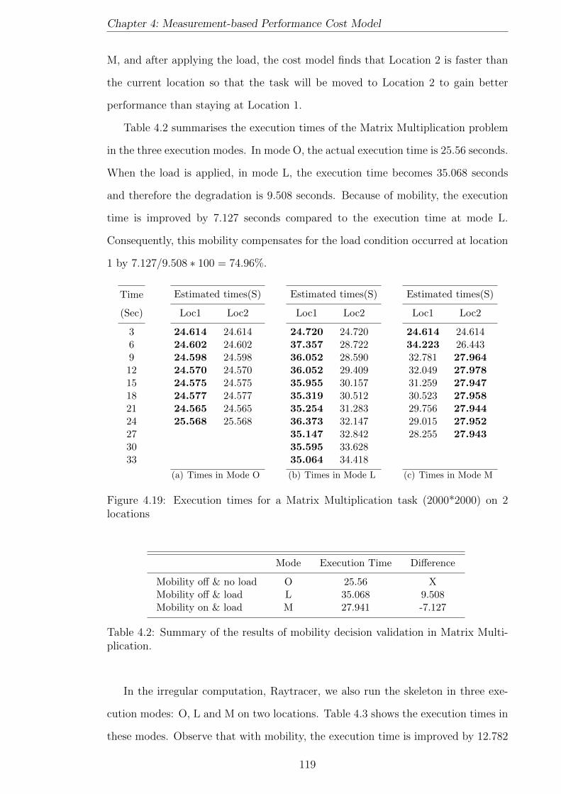
Chapter 4: Measurement-based Performance Cost Model
M, and after applying the load, the cost model finds that Location 2 is faster than
the current location so that the task will be moved to Location 2 to gain better
performance than staying at Location 1.
Table 4.2 summarises the execution times of the Matrix Multiplication problem
in the three execution modes. In mode O, the actual execution time is 25.56 seconds.
When the load is applied, in mode L, the execution time becomes 35.068 seconds
and therefore the degradation is 9.508 seconds. Because of mobility, the execution
time is improved by 7.127 seconds compared to the execution time at mode L.
Consequently, this mobility compensates for the load condition occurred at location
1 by 7.127/9.508 ∗ 100 = 74.96%.
Time
(Sec)
3691215182124273033
Estimated times(S)
Loc1 Loc2
24.614 24.61424.602 24.60224.598 24.59824.570 24.57024.575 24.57524.577 24.57724.565 24.56525.568 25.568
(a) Times in Mode O
Estimated times(S)
Loc1 Loc2
24.720 24.72037.357 28.72236.052 28.59036.052 29.40935.955 30.15735.319 30.51235.254 31.28336.373 32.14735.147 32.84235.595 33.62835.064 34.418
(b) Times in Mode L
Estimated times(S)
Loc1 Loc2
24.614 24.61434.223 26.44332.781 27.96432.049 27.97831.259 27.94730.523 27.95829.756 27.94429.015 27.95228.255 27.943
(c) Times in Mode M
Figure 4.19: Execution times for a Matrix Multiplication task (2000*2000) on 2locations
Mode Execution Time Difference
Mobility off & no load O 25.56 XMobility off & load L 35.068 9.508Mobility on & load M 27.941 -7.127
Table 4.2: Summary of the results of mobility decision validation in Matrix Multi-plication.
In the irregular computation, Raytracer, we also run the skeleton in three exe-
cution modes: O, L and M on two locations. Table 4.3 shows the execution times in
these modes. Observe that with mobility, the execution time is improved by 12.782
119
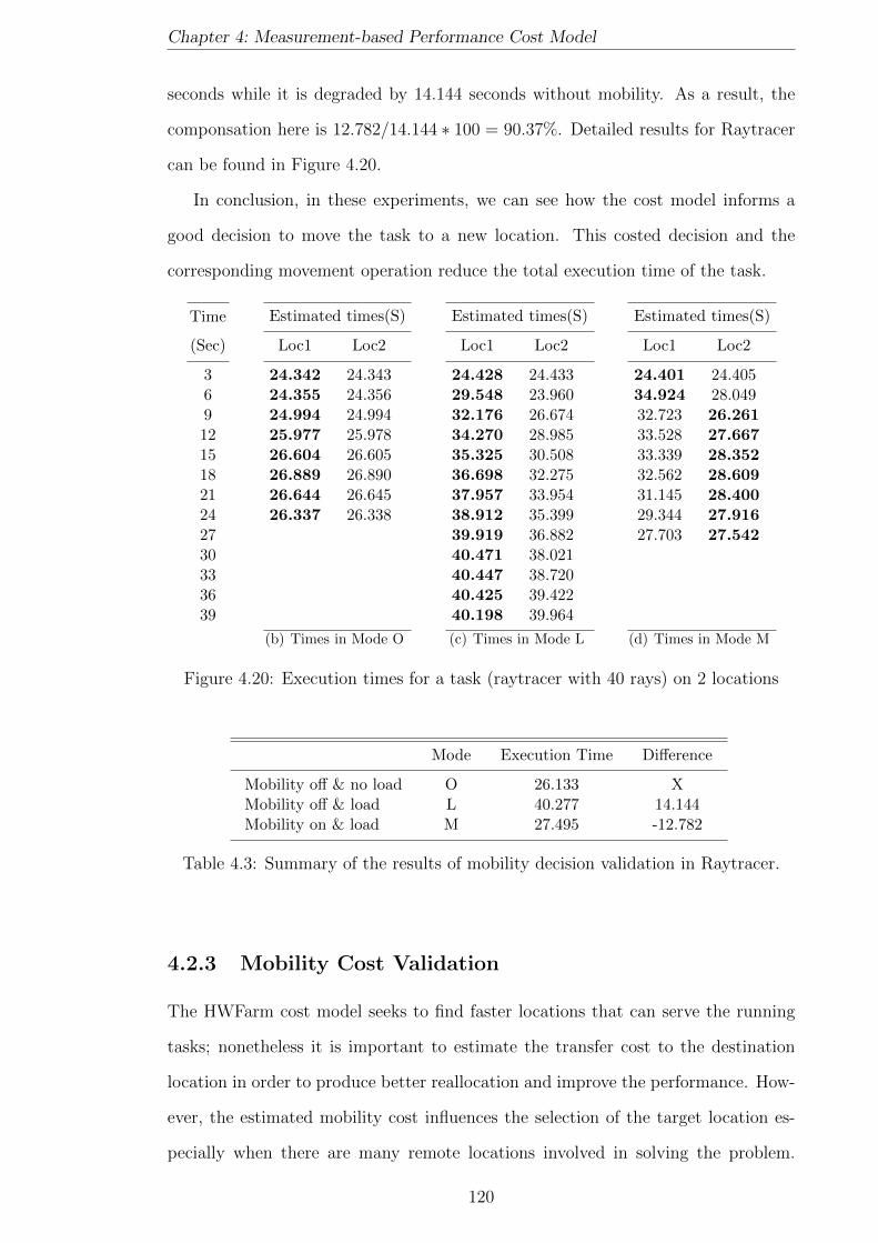
Chapter 4: Measurement-based Performance Cost Model
seconds while it is degraded by 14.144 seconds without mobility. As a result, the
componsation here is 12.782/14.144 ∗ 100 = 90.37%. Detailed results for Raytracer
can be found in Figure 4.20.
In conclusion, in these experiments, we can see how the cost model informs a
good decision to move the task to a new location. This costed decision and the
corresponding movement operation reduce the total execution time of the task.
Time
(Sec)
36912151821242730333639
Estimated times(S)
Loc1 Loc2
24.342 24.34324.355 24.35624.994 24.99425.977 25.97826.604 26.60526.889 26.89026.644 26.64526.337 26.338
(b) Times in Mode O
Estimated times(S)
Loc1 Loc2
24.428 24.43329.548 23.96032.176 26.67434.270 28.98535.325 30.50836.698 32.27537.957 33.95438.912 35.39939.919 36.88240.471 38.02140.447 38.72040.425 39.42240.198 39.964
(c) Times in Mode L
Estimated times(S)
Loc1 Loc2
24.401 24.40534.924 28.04932.723 26.26133.528 27.66733.339 28.35232.562 28.60931.145 28.40029.344 27.91627.703 27.542
(d) Times in Mode M
Figure 4.20: Execution times for a task (raytracer with 40 rays) on 2 locations
Mode Execution Time Difference
Mobility off & no load O 26.133 XMobility off & load L 40.277 14.144Mobility on & load M 27.495 -12.782
Table 4.3: Summary of the results of mobility decision validation in Raytracer.
4.2.3 Mobility Cost Validation
The HWFarm cost model seeks to find faster locations that can serve the running
tasks; nonetheless it is important to estimate the transfer cost to the destination
location in order to produce better reallocation and improve the performance. How-
ever, the estimated mobility cost influences the selection of the target location es-
pecially when there are many remote locations involved in solving the problem.
120

Chapter 4: Measurement-based Performance Cost Model
Therefore, the mobility cost has a considerable influence on the movement decision
taken by the cost model, see the mobility decision formula, Formula 4.5.
Here, we validate the mobility cost predicted by the HWFarm cost model, see
Formula 4.9. We again use the two applications: Matrix Multiplication and Ray-
tracer. For each benchmark, we run different sizes of tasks with different amount of
load on the host node. All measurement are collected by repeating the experiment
three times.
In Matrix Multiplication, we use a problem composed of one task. The im-
plementation we use in this experiment has matrix B as shared data amongst all
workers while matrix A will be divided amongst the tasks which will be allocated to
the workers. When mobility occurs, additional data will be packed with the initial
task data, the output, and state data. Then, the total transferred data may become
two times bigger, more or less. Table 4.4 shows the estimated mobility cost com-
pared to the actual cost. The relative error of the estimated mobility cost (actual
mobility cost) is ranging from 0.08% to 9.92%. The relative error of the estimated
mobility cost (total execution time) is not exceeding 0.6%.
In Raytracer, the problem is also composed of one task. Like the Matrix Multi-
plication implementation, the Raytracer implementation has the objects of the scene
as shared while the rays are divided amongst the workers. Each task processes a list
of rays to produce a list of impacts where processing one ray produces one impact.
When mobility occurs, the added data is the list of impacts produced by partially
processing the list of rays as well as the state data. Table 4.5 shows the estimated
mobility cost compared to the actual cost. The relative error of the estimated mo-
bility cost (actual mobility cost) ranges from 0.27% to 24.66%. The relative error
of the estimated mobility cost (total execution time) is not exceeding 0.03%.
Observe that if the initial transfer cost is too small, the error in estimating the
transfer cost is big, like the Raytracer results. But, the error is small when the
initial transfer cost is large, the Matrix Multiplication results. In both results, the
error is very small compared to the total execution time of the computation.
121
Chapter 4: Measurement-based Performance Cost Model
4.3 Summary
In this chapter, we presented the HWFarm cost model. This model is dynamic,
problem-independent, language-independent, and architecture-independent. This
model uses an approach that is based on real measurements of the computations
and the running environment.
This model estimates the continuation time of a task based on its progress and
some metrics obtained from the executing platform. We use the mobility decision
formula to take decisions about where this task can run faster, see Formula 4.5.
The progress of each task can be obtained from the HWFarm skeleton where
this model is embedded in the skeleton. As outlined in Chapter 3, the skeleton has
access to all running tasks and therefore it can acquire information regarding the
behaviour of running these tasks.
Regarding the executing platform metrics, the cost model uses static metrics
and dynamic metrics. The static metrics are the clock speed and the number of
cores where we assumed that the cores of each node have the same clock speed. The
dynamic metrics used in the cost mode are the CPU utilisation and the number of
running processes. These metrics reflect the relative processing power or the load
state of a concrete node.
We initially supposed that the communications within cluster environment are
uniform. Then, we proposed a model that predicts the future transfer cost of a task
based on the network latency, the task size and the load state of the system.
We validated the estimates produced by the HWFarm cost model where the
error in the estimated times is ranging from 3% to 20% for regular and irregular
computations. We also validated the mobility decisions where we found that this
model gives accurate decisions that help the HWFarm skeleton to find a faster node
to run each task. These decisions improve the total execution times where the
compensation reaches to 90%.
In this next chapter, we demonstrate how HWFarm uses the cost model to
reschedule the tasks in order to improve performance.
122
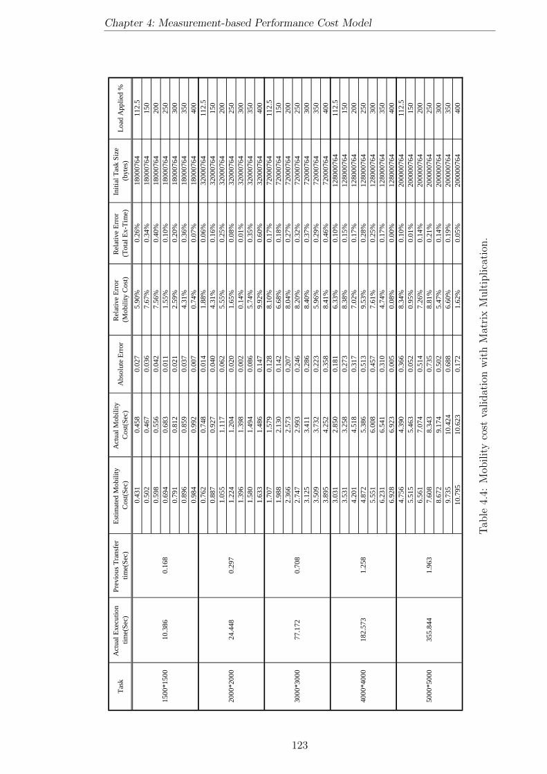
Chapter 4: Measurement-based Performance Cost Model
Tas
kA
ctua
l Exe
cuti
on
tim
e(S
ec)
Pre
viou
s T
rans
fer
tim
e(S
ec)
Est
imat
ed M
obil
ity
Cos
t(S
ec)
Act
ual M
obil
ity
Cos
t(S
ec)
Abs
olut
e E
rror
Rel
ativ
e E
rror
(M
obil
ity
Cos
t)R
elat
ive
Err
or
(Tot
al E
x-T
ime)
Init
ial T
ask
Siz
e (b
ytes
)L
oad
App
lied
%
0.43
10.
458
0.02
75.
90%
0.26
%18
0007
6411
2.5
0.50
20.
467
0.03
67.
67%
0.34
%18
0007
6415
00.
598
0.55
60.
042
7.56
%0.
40%
1800
0764
200
0.69
40.
683
0.01
11.
55%
0.10
%18
0007
6425
00.
791
0.81
20.
021
2.59
%0.
20%
1800
0764
300
0.89
60.
859
0.03
74.
31%
0.36
%18
0007
6435
00.
984
0.99
20.
007
0.74
%0.
07%
1800
0764
400
0.76
20.
748
0.01
41.
88%
0.06
%32
0007
6411
2.5
0.88
70.
927
0.04
04.
31%
0.16
%32
0007
6415
01.
055
1.11
70.
062
5.55
%0.
25%
3200
0764
200
1.22
41.
204
0.02
01.
65%
0.08
%32
0007
6425
01.
396
1.39
80.
002
0.14
%0.
01%
3200
0764
300
1.58
01.
494
0.08
65.
74%
0.35
%32
0007
6435
01.
633
1.48
60.
147
9.92
%0.
60%
3200
0764
400
1.70
71.
579
0.12
88.
10%
0.17
%72
0007
6411
2.5
1.98
82.
130
0.14
26.
68%
0.18
%72
0007
6415
02.
366
2.57
30.
207
8.04
%0.
27%
7200
0764
200
2.74
72.
993
0.24
68.
20%
0.32
%72
0007
6425
03.
125
3.41
10.
286
8.40
%0.
37%
7200
0764
300
3.50
93.
732
0.22
35.
96%
0.29
%72
0007
6435
03.
895
4.25
20.
358
8.41
%0.
46%
7200
0764
400
3.03
12.
850
0.18
16.
33%
0.10
%12
8000
764
112.
53.
531
3.25
80.
273
8.38
%0.
15%
1280
0076
415
04.
201
4.51
80.
317
7.02
%0.
17%
1280
0076
420
04.
872
5.38
60.
513
9.53
%0.
28%
1280
0076
425
05.
551
6.00
80.
457
7.61
%0.
25%
1280
0076
430
06.
231
6.54
10.
310
4.74
%0.
17%
1280
0076
435
06.
928
6.92
30.
005
0.08
%0.
00%
1280
0076
440
04.
756
4.39
00.
366
8.34
%0.
10%
2000
0076
411
2.5
5.51
55.
463
0.05
20.
95%
0.01
%20
0000
764
150
6.56
17.
074
0.51
47.
26%
0.14
%20
0000
764
200
7.60
88.
343
0.73
58.
81%
0.21
%20
0000
764
250
8.67
29.
174
0.50
25.
47%
0.14
%20
0000
764
300
9.73
510
.424
0.68
86.
60%
0.19
%20
0000
764
350
10.7
9510
.623
0.17
21.
62%
0.05
%20
0000
764
400
1.96
3
1.25
8
0.70
8
0.29
7
0.16
8
4000
*400
018
2.57
3
5000
*500
035
5.84
4
1500
*150
010
.386
2000
*200
024
.448
3000
*300
077
.172
Tab
le4.
4:M
obilit
yco
stva
lidat
ion
wit
hM
atri
xM
ult
iplica
tion
.
123

Chapter 4: Measurement-based Performance Cost Model
T
ask
(1
0000
Obj
ects
)A
ctua
l Exe
cutio
n tim
e(Se
c)Pr
evio
us T
rans
fer
time(
Sec)
Est
imat
ed M
obili
ty
Cos
t(Se
c)A
ctua
l Mob
ility
C
ost(
Sec)
Abs
olut
e E
rror
Rel
ativ
e E
rror
(M
obili
ty C
ost)
Rel
ativ
e E
rror
(T
otal
Ex-
Tim
e)In
itial
Tas
k Si
ze(b
ytes
)L
oad
App
lied
%
0.00
890.
0117
0.00
323
.668
%0.
019%
4807
6411
2.5
0.01
000.
0111
0.00
110
.378
%0.
008%
4807
6415
00.
0136
0.01
660.
003
18.2
59%
0.02
0%48
0764
200
0.01
340.
0165
0.00
318
.890
%0.
021%
4807
6425
00.
0155
0.01
990.
004
22.3
02%
0.03
0%48
0764
300
0.01
750.
0194
0.00
29.
942%
0.01
3%48
0764
350
0.01
90.
023
0.00
417
.125
%0.
026%
4807
6440
00.
0316
0.03
790.
006
16.6
31%
0.01
1%19
2076
411
2.5
0.03
630.
0398
0.00
38.
765%
0.00
6%19
2076
415
00.
0434
0.04
690.
003
7.39
2%0.
006%
1920
764
200
0.04
940.
0449
0.00
49.
966%
0.00
8%19
2076
425
00.
0574
0.05
210.
005
10.1
45%
0.00
9%19
2076
430
00.
0665
0.05
340.
013
24.6
56%
0.02
3%19
2076
435
00.
077
0.06
90.
008
12.3
16%
0.01
5%19
2076
440
00.
0724
0.07
260.
000
0.27
2%0.
000%
4320
764
112.
50.
0841
0.09
040.
006
6.94
2%0.
005%
4320
764
150
0.09
990.
1102
0.01
09.
361%
0.00
8%43
2076
420
00.
1158
0.13
710.
021
15.4
90%
0.01
6%43
2076
425
00.
1322
0.14
940.
017
11.4
73%
0.01
3%43
2076
430
00.
1444
0.16
830.
024
14.2
15%
0.01
8%43
2076
435
00.
159
0.15
30.
007
4.43
7%0.
005%
4320
764
400
300*
300
130.
580
0.00
6
0.02
1
0.04
5
100*
100
14.8
35
200*
200
57.9
46
Tab
le4.
5:M
obilit
yco
stva
lidat
ion
wit
hR
aytr
acer
.
124

Chapter 5
Optimising HWFarm Scheduling
The proposed skeleton supported with a mobility approach is guided by a cost model.
Effective cost modelling requires information from the system and the application.
The cooperation amongst the distributed components of HWFarm is controlled by a
hybrid scheduler. This scheduler is centralised in managing the global load informa-
tion and decentralised in taking appropriate mobility decisions through employing
a cost model. In this chapter, we demonstrate the scheduling in HWFarm and show
that this scheduler has a low overhead compared to the total execution time where
all its activities occur concurrently with the running computations. The rest of the
chapter is organized as follows: Section 5.1 discusses the policies of the HWFarm
scheduler in. Section 5.2 shows the optimisation of scheduling activities. Section 5.3
discusses the overhead introduced by HWFarm. Section 5.4 evaluates the scheduling
mechanism in behaviour and performance aspects.
5.1 HWFarm Scheduler
The HWFarm scheduler is a distributed scheduler that uses global information from
all nodes to perform a new schedule. Within the node scope, the HWFarm sched-
uler is an application-specific thread scheduler because it only manages its threads.
The HWFarm scheduler is classified as a pre-emptive scheduler because it suspends
running threads and reschedules them to run on different nodes.
Using an efficient scheduling algorithm is crucial to enhance the performance of
125
Chapter 5: Optimising HWFarm Scheduling
the cluster [60]. Batch scheduling is widely used in dedicated clusters to manage
non-interactive jobs. An example of a batch scheduler is IBM LoadLeveller [134].
For interactive systems, a wide range of algorithms can be used such as Round
Robin Scheduling and Priority Scheduling [215]. These are common in servers and
PCs. For more complex scheduling techniques, co-operative scheduling can be used
like gang scheduling [95]. In such scheduling, explicit global synchronisation is
used to simultaneously schedule a group of processes that belong to the same job.
On the other hand, communication-driven co-scheduling techniques, like SB(Spin
Block)[173], can be employed to schedule a parallel job through coordinating the
communicating processes.
Now, it is important to understand the scheduling technique used in the multi-
core cluster environment targeted by HWFarm. Linux is a popular operating system
that is widely used for multiprocessor environments. The default scheduler in Linux
is CFS (Completely Fair Scheduler) [239] which is available in Linux 2.6.23 and
above. This policy maintains providing a fair amount of the processor to the pro-
cesses. This policy considers the priority which ranges from 0 to 40.
Consequently, a simple scheduling technique, the local native scheduler, has been
chosen for the following reasons: 1) we want to keep the implementation simple and
minimise the overhead. 2) We assumed that the parallel job, the program executed
by the skeleton, has no internal dependencies and therefore there are no communica-
tions amongst the tasks. Therefore, complicated scheduling such as gang scheduling
or co-scheduling is not needed. 3) Due to working in a shared environment, it is not
desirable to change the scheduling policy of the operating system scheduler.
In summary, the HWFarm skeleton will run on a cluster as a user-space parallel
application whose processes are allocated to nodes. Each worker process and all
running threads have normal priority like any other process or thread running in
the system. Because there is no direct coordination between the worker and the local
scheduler, all processes or threads running on an individual node will be scheduled
to resources based on the local scheduling policy. However, the local scheduler will
take care of the assignment of resources to the running applications. When a worker
126

Chapter 5: Optimising HWFarm Scheduling
becomes overloaded, the HWFarm scheduler lightens the load of this node through
remapping its tasks to other nodes.
The HWFarm scheduling goal is reducing the total execution time and hence
improving the performance. It also can be referred to as cost driven scheduling
because it uses a performance cost model that suggests new faster locations. Fur-
thermore, the overall tasks in HWFarm are independent and hence there is no need
to take into consideration the communication amongst the tasks. The locality of the
running tasks also is not considered. Moreover, process or thread affinity is not ad-
dressed in this thesis where any thread migration or context switching is considered
as a local scheduler issue.
5.1.1 HWFarm Scheduler Components
As stated in Chapter 3, the HWFarm skeleton is composed of the master process
and worker processes allocated to machines/nodes. The master process works as a
global coordinator that maintains the global load information to any worker while
the worker process performs as a local scheduler that manages the running tasks.
The HWFarm scheduler is decomposed into three agents that cooperate with
each other in order to accomplish the scheduling:
• LA, the Load Agent, is a distributed agent responsible for locally collecting
the load information on workers and keeping the load information up to date
in the master.
• EA, the Estimator Agent, is responsible for taking decisions to suggest new
schedules based on cost model estimations.
• MA, the Mobility Agent, is responsible for performing the transfer of a task
to a destination worker.
5.1.2 HWFarm Scheduler Properties
The scheduler in HWFarm should have the following desirable properties:
127
Chapter 5: Optimising HWFarm Scheduling
• Efficient : the scheduler is efficient through rescheduling the tasks to enhance
the performance and balance the load. This happens with no interference with
the local policies.
• Dynamic: the scheduler is responsive and sensitive to the changes of workload
of the system.
• Transparent : the scheduler implicitly decides when and where to move the
tasks. Hence, the allocating and the reallocating of tasks occur autonomously
based on the skeleton behaviour and the load changes.
• Adaptive: the scheduler is able to exploit new architectures and new programs.
Furthermore, this gives the scheduler the ability to exploit a wide range of
computational architectures.
• Predictive: the scheduler can estimate the future performance depending on
the past behaviour within the constraints and assumptions made on the code.
• Asynchronous : the functionalities of the scheduler have been assigned to
agents that run concurrently on the workers where these agents work together
towards the global objective.
Now, we will explore the policies of the HWFarm scheduler to meet the perfor-
mance goal.
5.1.3 Scheduling Policies
Being a dynamic load management system, the load scheduler in HWFarm should
fulfil the following policies:
Information policy : determines the mechanism of collecting and exchanging the
load information amongst the processing elements. This policy will be discussed
further in Section 5.1.3.1.
Transfer policy : defines the conditions to move tasks. This is driven by the
workload status of workers. A sender-initiated or push policy has been chosen
because it is simple to implement. In addition, a loaded worker is able to decide
128

Chapter 5: Optimising HWFarm Scheduling
if it is better to move some tasks away from it. It is important to note that this
policy is decentralised because each worker triggers mobility and hence this supports
scalability. Deciding mobility is maintained by the worker and is not centralised in
the master. Further details about this policy will be explained in Section 5.1.3.2.
Selection policy : identifies what tasks should be moved. There are different
possible policies that help in selecting the tasks for movement. Some policies choose
the oldest tasks while others select the new ones. Yet other policies depend on the
estimation time, where the task that has the longest or the shortest estimation time
will be moved. We use the estimate of the local continuation time and compare
it to the estimate of the continuation time at remote locations. In this case, the
slower tasks that may run faster in remote locations will be selected. This means
that the most affected tasks will be selected for movement. Therefore, as much as
we minimize the influence of the external load, we will improve the performance of
our application.
Placement policy : specifies the location/node to which a task should be moved.
Depending on the cost model, the node that has plenty of resources to serve other
tasks and that is able to execute the slow tasks will be identified to receive those
tasks.
The selection and placement policies are combined in the mobility policy; see
Section 5.1.3.3, where the mobility decision is based on how the slow task will run
faster on the chosen target location.
5.1.3.1 Load Information Exchange
Seeking an optimal redistribution of the workload needs knowledge of the environ-
ment load states. When such information is available, the estimate will be most
accurate. In the HWFarm skeleton, we consider the overall workload in the system
because the dynamic load information is a significant factor in the estimations pro-
duced by the cost model. Consequently, we need an effective mechanism to make
this information available when needed.
Load information diffusion is a mechanism that can be used to share the load
129

Chapter 5: Optimising HWFarm Scheduling
information in the system. It is also referred to as information dissemination. Such
a mechanism is used by systems that need to take decisions during run-time, such
as dynamic/distributed load balancing, failure detection, database replication, and
aggregate computation. In dynamic load balancing, a load information diffusion
mechanism can be used to guide the workload redistribution. Examples of load
information policies used by dynamic load balancers are: direct neighbourhood [236],
average neighbourhood [241], dimension-exchange [233], and gossip-based protocol
[33]. A circulation approach has been used by Alzain [7] to update the dynamic load
information amongst processing elements.
Load Information Diffusion in HWFarm
In HWFarm, the master is dedicated to managing and controlling the global load
information. It collects the information from all workers and keeps this information
updated in order to provide it to a worker when needed.
To collect the information, the master uses a circulation approach where a mes-
sage circulates across all workers to gather their load information.
As outlined in Chapter 3, the pattern used in the HWFarm skeleton is Mas-
ter/Worker. We used a circulation approach in order to avoid the bottleneck when
collecting the information from all participating workers. The latest information
about the load is available at a concrete location so this mechanism is centralised
on the master. This is very useful for having accurate decisions because the most
recent global information will be available to the decision makers once they request
it. Experiments showed that this approach has a low overhead. More details about
the overhead will be discussed in Section 5.3.2.
At the start-up of the skeleton, the master creates a load agent which is re-
sponsible for triggering the collecting operation. After creating the load agent, a
logical table, WorkerLoad, of load information will be created. This table is dy-
namically maintained by the master and lists all details about the load states of the
participating workers/nodes. In this logical table, each record/row represents the
load information for a worker. This table is implemented in C via a linked list of
worker load data structure that has the definition:
130

Chapter 5: Optimising HWFarm Scheduling
struct worker_load{
int worker_id;
int m_id;
int current_tasks;
int total_tasks;
int status;
int w_cores; //Static metric
float w_cpu_speed; //Static metric
double w_cpu_uti; //Dynamic metric
int w_running_procs; //Dynamic metric
struct network_times net_times;
};
The fields of this structure refer to:
• worker id: The id of the worker.
• m id: The id of the message triggered by the load agent.
• current tasks: The number of tasks that are currently running at that
worker.
• total tasks: The total number of tasks processed at that worker.
• status: The status of the worker: 0: free; 1: busy; 2: requesting the latest
load details; 3: involved in mobility.
• w cores: A static value that refers to the number of cores.
• w cpu speed: A static value that refers to the processer speed.
• w cpu uti: A dynamic value that refers to the CPU utilisation.
• w running proc: A dynamic value that refers to the number of running pro-
cesses
• net times: A data structure that holds the network delay information.
131

Chapter 5: Optimising HWFarm Scheduling
The field net times stores the initial and current network delay of this node.
This network delay information will be used by the cost model to estimate the
mobility cost. The network times data structure has the definition:
struct network_times{
double init_net_time;
double cur_net_time;
};
Where:
• init net time: The initial network delay of this worker.
• cur net time: The current network delay of this worker.
The WorkerLoad table will be updated periodically in order to keep up to date
with the load state of the system. As discussed in Chapter 4, the cost model re-
quires the latest load information to accurately estimate the times and then makes
decisions. However, our experiments show that collecting the load information runs
concurrently and incurs low overhead. Accordingly, in HWFarm, we chose one sec-
ond as a refresh rate of the collection to keep the load updated globally with the
master. This rate has been chosen to make a trade-off between taking inaccurate
decisions and increasing the overhead of the collection. As previously mentioned,
taking inaccurate decisions is caused by using old load information where the refresh
rate is large. In contrast, decreasing the rate will increase the overhead incurred by
the load agents.
The collecting operation starts at the master where the load agent sends an empty
load message to a worker. Next, the receiving worker appends its load information
in the load message and circulates it to the next worker. When the load message
is full of information, the final worker sends the message to the master. Then, the
master updates the current load information with the latest information; see Figure
5.1.
At each worker, the load agent is responsible for obtaining the local load. Then
the load will be stored in a data structure that can be used later by other agents.
132
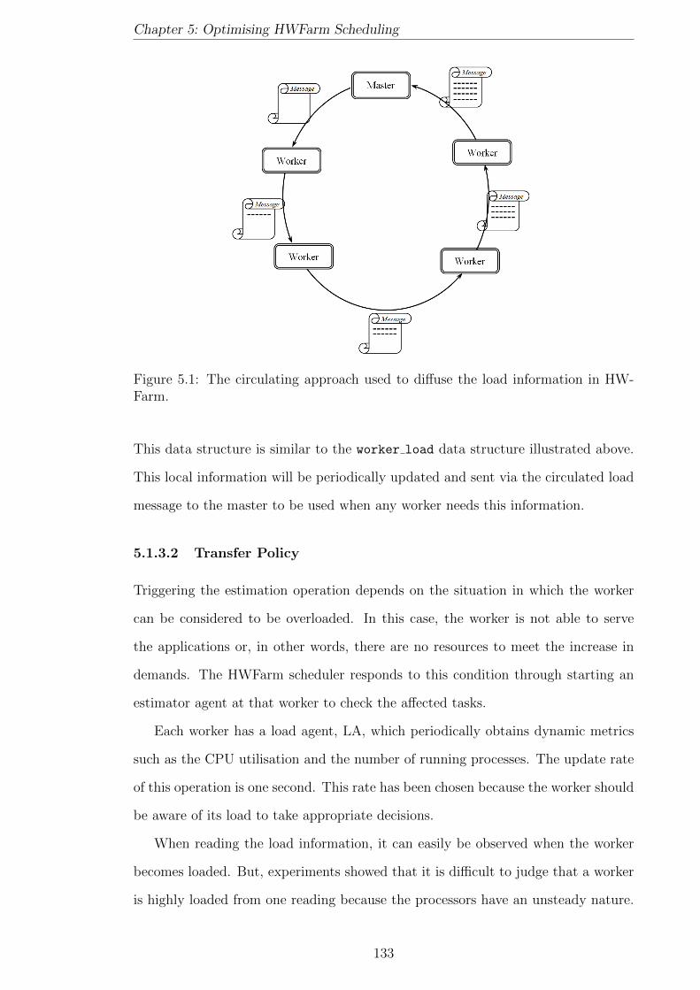
Chapter 5: Optimising HWFarm Scheduling
Figure 5.1: The circulating approach used to diffuse the load information in HW-Farm.
This data structure is similar to the worker load data structure illustrated above.
This local information will be periodically updated and sent via the circulated load
message to the master to be used when any worker needs this information.
5.1.3.2 Transfer Policy
Triggering the estimation operation depends on the situation in which the worker
can be considered to be overloaded. In this case, the worker is not able to serve
the applications or, in other words, there are no resources to meet the increase in
demands. The HWFarm scheduler responds to this condition through starting an
estimator agent at that worker to check the affected tasks.
Each worker has a load agent, LA, which periodically obtains dynamic metrics
such as the CPU utilisation and the number of running processes. The update rate
of this operation is one second. This rate has been chosen because the worker should
be aware of its load to take appropriate decisions.
When reading the load information, it can easily be observed when the worker
becomes loaded. But, experiments showed that it is difficult to judge that a worker
is highly loaded from one reading because the processors have an unsteady nature.
133

Chapter 5: Optimising HWFarm Scheduling
This unsteadiness in the load is because the processor supports a multitasking envi-
ronment where an arbitrary number of processes may use the resources for a short
period of time. Hence, it is not necessary to take an action if there are processes
that use the processor for a short period.
Figure 5.2: Load state of a normal loaded node.
Figure 5.3: Load state of a highly loaded node.
Figure 5.2 shows an example of the CPU utilisation of a node for one minute.
At second 11.5, the CPU utilisation is 100% and hence the node is loaded but
afterwards the workload becomes ordinary. Then, at second 52.4, the load becomes
100% and decreases again to be normal. In this scenario, there is no need to incur
the overheads in estimating and mobility where all tasks are running normally.
In contrast, Figure 5.3 shows an example of a node loaded with multiple appli-
cations where after second 12.4 many processes ask for resources and the CPU is
fully utilised.
134

Chapter 5: Optimising HWFarm Scheduling
Here, we propose a policy to trigger the estimation based on multiple readings.
This policy depends on checking if the following condition is true for three consec-
utive readings. The reason of choosing three readings is finding a balance between
the overhead of the estimation operation when the worker is not actually loaded
and the delay of triggering the estimation operation which affects the running tasks.
This to some extent implies that the load in the worker is not occasional and thus
the HWFarm tasks will be affected by this load.
Rh
Sh
< β (5.1)
where:
Rh: The relative processing power at the current location
Sh: The CPU speed at the current location
β : The load threshold
β is the threshold of the loading state at which it can be decided that this node
is loaded. Then, a delay will occur to the running processes on the future if the load
stayed steady or became worse. In this thesis, we use β = 0.95 as a threshold where
we empirically found this value.
This policy will avoid the redundancy of mobility amongst the workers because
it starts the estimation operation when the current worker is really loaded and takes
accurate decisions if needed.
5.1.3.3 Mobility Policy
To take decisions for scheduling the local running tasks, estimation operations for
the continuation and transfer times of the running computations are required. The
estimation of the continuation time compared to the continuation times on other
locations reflects the progress of running these computations on the current loca-
tion in loaded conditions. Then based on the estimation of the transfer times, the
mobility decision formula Ti > Tmobility + Tj will be applied to make a decision.
Making more accurate decisions requires the latest load information. Hence,
this load information of all nodes is prerequisite of these operation. Therefore, a
135

Chapter 5: Optimising HWFarm Scheduling
request for this information will be sent to the master. This invokes communication
overhead; whereas, per contra, this improves the accuracy of the taken decisions.
When this information is available, an estimator agent will be initialised to start
the estimation operations through applying the cost model. Next, for each task
running locally, estimated times to complete locally and remotely will be produced.
Then, the estimator agent will issue a mobility report that includes the suggested
movements of certain tasks to specific workers. The algorithm used by the estimator
agent to produce the mobility report is as follows:
EC_local = getEstimationCostHere(tasks);
//Get the continuation cost and the network cost (the cost model)
EC_remote = getEstimationCostOtherWorkers(tasks);
improvement = 1;
do{
longest_task = getTheSlowestTask(tasks, EC_local);
new_worker = getTheBestEstimate(EC_local, EC_remote);
if(new_worker != current_worker){
updateMobilityReport(longest_task, new_worker);
updateEstimations(EC_local, EC_remote);
}else
improvement = 0;
}while(improvement);
This algorithm seeks to find a task mapping that improves the total execution
time under the current load condition. In the estimation algorithm, first, the times
for running all local tasks on the current node and on remote nodes will be estimated
using the functions getEstimationCostHere and getEstimationCostOtherWorkers,
respectively. Then, the next step will be repeated until finding an provably opti-
mal mapping. In the loop, getTheSlowestTask function looks for the slowest task
based on the array of local estimated times, EC local. Then, getTheBestEstimate
function returns the worker where this longest task can run faster. If the task can
run faster on another worker, this task will be mapped to that worker and the es-
136

Chapter 5: Optimising HWFarm Scheduling
timated times will be updated based on the new mapping. Otherwise, there is no
improvement to run this task on any node and the loop will end. The output of
this algorithm is the mobility report or move report. This report contains the map-
ping of the selected tasks to the chosen workers. During the algorithm execution,
there is no actual mobility occurring for any task but there is only changes in the
tasks’ mapping. Once the tasks’ mapping has been changed the estimates should
be updated where the estimation should take into consideration the new mapping
because, when the tasks are rescheduled, this produces a change on the load state
of the local and remote nodes.
To illustrate how this algorithm works, we demonstrate it with an example, see
Figure 5.4. In this example, the skeleton has three workers involved in solving a
problem with 12 tasks. Each worker processes 4 tasks. From the estimation point of
view, each worker endeavours to reduce the execution time of its tasks. Hence, each
worker has no idea about the tasks of other workers and their execution progress
but it has knowledge of the load information of those workers. At some point,
worker 3 becomes highly loaded, so an estimator agent will be created to handle
the estimation operations. Then, a move report stating the affected tasks will be
produced and accordingly the HWFarm scheduler will reschedule these tasks.
Figure 5.4: An example showing how the HWFarm scheduler reschedules the taskswhen worker 3 becomes highly loaded.
Here, we are exploring the estimation operation at worker 3. Table 5.1 shows
the estimated completion times of the current tasks before worker 3 gets loaded.
Furthermore, the estimated move costs of all tasks to the participating workers are
illustrated in Table 5.2.
137
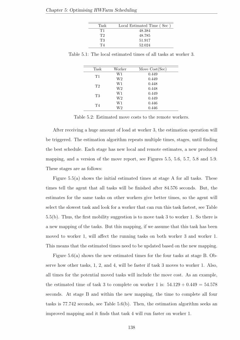
Chapter 5: Optimising HWFarm Scheduling
Task Local Estimated Time ( Sec )T1 48.384T2 48.785T3 51.917T4 52.024
Table 5.1: The local estimated times of all tasks at worker 3.
Task Worker Move Cost(Sec)
T1W1 0.449W2 0.449
T2W1 0.448W2 0.448
T3W1 0.449W2 0.449
T4W1 0.446W2 0.446
Table 5.2: Estimated move costs to the remote workers.
After receiving a huge amount of load at worker 3, the estimation operation will
be triggered. The estimation algorithm repeats multiple times, stages, until finding
the best schedule. Each stage has new local and remote estimates, a new produced
mapping, and a version of the move report, see Figures 5.5, 5.6, 5.7, 5.8 and 5.9.
These stages are as follows:
Figure 5.5(a) shows the initial estimated times at stage A for all tasks. These
times tell the agent that all tasks will be finished after 84.576 seconds. But, the
estimates for the same tasks on other workers give better times, so the agent will
select the slowest task and look for a worker that can run this task fastest, see Table
5.5(b). Thus, the first mobility suggestion is to move task 3 to worker 1. So there is
a new mapping of the tasks. But this mapping, if we assume that this task has been
moved to worker 1, will affect the running tasks on both worker 3 and worker 1.
This means that the estimated times need to be updated based on the new mapping.
Figure 5.6(a) shows the new estimated times for the four tasks at stage B. Ob-
serve how other tasks, 1, 2, and 4, will be faster if task 3 moves to worker 1. Also,
all times for the potential moved tasks will include the move cost. As an example,
the estimated time of task 3 to complete on worker 1 is: 54.129 + 0.449 = 54.578
seconds. At stage B and within the new mapping, the time to complete all four
tasks is 77.742 seconds, see Table 5.6(b). Then, the estimation algorithm seeks an
improved mapping and it finds that task 4 will run faster on worker 1.
138
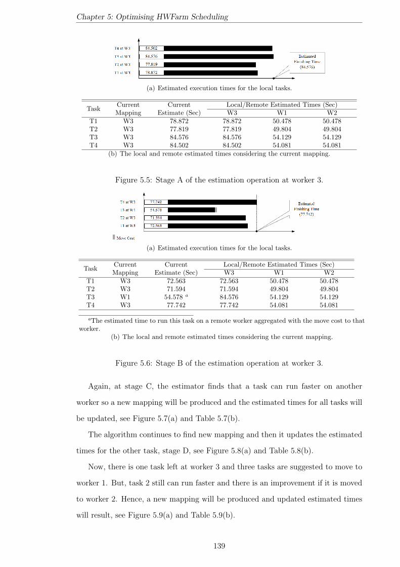
Chapter 5: Optimising HWFarm Scheduling
(a) Estimated execution times for the local tasks.
TaskCurrent Current Local/Remote Estimated Times (Sec)Mapping Estimate (Sec) W3 W1 W2
T1 W3 78.872 78.872 50.478 50.478T2 W3 77.819 77.819 49.804 49.804T3 W3 84.576 84.576 54.129 54.129T4 W3 84.502 84.502 54.081 54.081
(b) The local and remote estimated times considering the current mapping.
Figure 5.5: Stage A of the estimation operation at worker 3.
(a) Estimated execution times for the local tasks.
TaskCurrent Current Local/Remote Estimated Times (Sec)Mapping Estimate (Sec) W3 W1 W2
T1 W3 72.563 72.563 50.478 50.478T2 W3 71.594 71.594 49.804 49.804T3 W1 54.578 a 84.576 54.129 54.129T4 W3 77.742 77.742 54.081 54.081
aThe estimated time to run this task on a remote worker aggregated with the move cost to thatworker.
(b) The local and remote estimated times considering the current mapping.
Figure 5.6: Stage B of the estimation operation at worker 3.
Again, at stage C, the estimator finds that a task can run faster on another
worker so a new mapping will be produced and the estimated times for all tasks will
be updated, see Figure 5.7(a) and Table 5.7(b).
The algorithm continues to find new mapping and then it updates the estimated
times for the other task, stage D, see Figure 5.8(a) and Table 5.8(b).
Now, there is one task left at worker 3 and three tasks are suggested to move to
worker 1. But, task 2 still can run faster and there is an improvement if it is moved
to worker 2. Hence, a new mapping will be produced and updated estimated times
will result, see Figure 5.9(a) and Table 5.9(b).
139
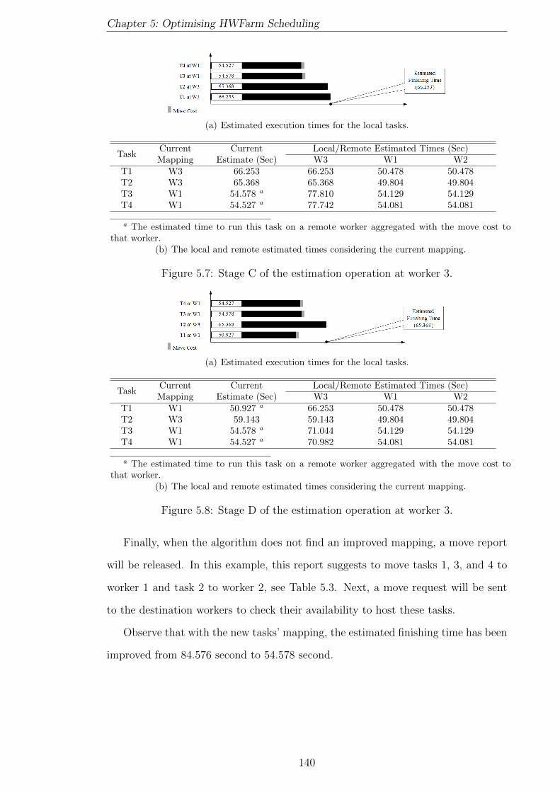
Chapter 5: Optimising HWFarm Scheduling
(a) Estimated execution times for the local tasks.
TaskCurrent Current Local/Remote Estimated Times (Sec)Mapping Estimate (Sec) W3 W1 W2
T1 W3 66.253 66.253 50.478 50.478T2 W3 65.368 65.368 49.804 49.804T3 W1 54.578 a 77.810 54.129 54.129T4 W1 54.527 a 77.742 54.081 54.081
a The estimated time to run this task on a remote worker aggregated with the move cost tothat worker.
(b) The local and remote estimated times considering the current mapping.
Figure 5.7: Stage C of the estimation operation at worker 3.
(a) Estimated execution times for the local tasks.
TaskCurrent Current Local/Remote Estimated Times (Sec)Mapping Estimate (Sec) W3 W1 W2
T1 W1 50.927 a 66.253 50.478 50.478T2 W3 59.143 59.143 49.804 49.804T3 W1 54.578 a 71.044 54.129 54.129T4 W1 54.527 a 70.982 54.081 54.081
a The estimated time to run this task on a remote worker aggregated with the move cost tothat worker.
(b) The local and remote estimated times considering the current mapping.
Figure 5.8: Stage D of the estimation operation at worker 3.
Finally, when the algorithm does not find an improved mapping, a move report
will be released. In this example, this report suggests to move tasks 1, 3, and 4 to
worker 1 and task 2 to worker 2, see Table 5.3. Next, a move request will be sent
to the destination workers to check their availability to host these tasks.
Observe that with the new tasks’ mapping, the estimated finishing time has been
improved from 84.576 second to 54.578 second.
140

Chapter 5: Optimising HWFarm Scheduling
(a) Estimated execution times for the local tasks.
TaskCurrent Current Local/Remote Estimated Times (Sec)Mapping Estimate (Sec) W3 W1 W2
T1 W1 50.927 a 59.943 50.478 50.478T2 W2 50.252 a 59.143 49.804 49.804T3 W1 54.578 a 64.278 54.129 54.129T4 W1 54.527 a 64.222 54.081 54.081
a The estimated time to run this task on a remote worker aggregated with the move cost tothat worker.
(b) The local and remote estimated times considering the current mapping.
Figure 5.9: Stage E of the estimation operation at worker 3.
# Selected Tasks Chosen Destination Worker
1 3, 4 & 1 12 2 2
Table 5.3: The final move report of the estimation algorithm.
5.2 HWFarm Scheduling Optimisation
The HWFarm scheduler depends on the mobility decisions to optimise the perfor-
mance. In this section, we discuss some additional procedures to guarantee that the
decisions taken are accurate.
5.2.1 Accurate Relative Processing Power
Decisions made using the HWFarm cost model are based on the behaviour of the
computations in the past as well as the load in the last period. During running
of a computation at a processing unit, it may experience different load situations
that influence its progress. Hence, measuring the elapsed time without considering
the slight changes in the system load may lead to inaccurate estimations of the
continuation times. To enhance the estimation locally, each worker monitors and
records the current system load for each running task. Therefore, each task will
keep the average of local load that indicates the load encountered while it is running
locally.
141

Chapter 5: Optimising HWFarm Scheduling
5.2.2 Movement Confirmation
After deciding which tasks to move to which workers, a request will be sent to those
workers to check their availability. This request ensures that the load states of the
destination workers have not changed during taking the decisions.
Mobility decisions may not be accurate in some situations in which the desti-
nation worker may receive an unexpected load. These new changes may invalidate
the decision produced by the cost model. To address this issue, the destination
worker needs to confirm task mobility. Therefore, before moving tasks to another
worker, each worker should receive permission from that destination worker to start
the mobility operation. This adds communication overhead which we will explore
in detail in the next section. But, this policy guarantees that the decision taken are
based on the updated load information.
In HWFarm, the destination worker agrees to receive tasks from any worker if it
is not already busy receiving tasks from other workers. This policy avoids moving
tasks at the same time from two workers to one destination workers. This is likely
to happen in a dynamic load management system where multiple workers have the
same load information. If the destination worker denies the move permission, no
action will be taken at the source worker. This tells the source worker that there is
reallocation of tasks happening in the skeleton. This reallocation will invalidate the
current load information and therefore the decisions are inaccurate. This policy can
be considered as a sort of negotiation between workers to avoid the location thrashing
which is one of the greedy effects that has been explored by Chechina [59].
5.3 Overhead
Dynamically managing the load in an environment requires further activities that
introduce overheads in the system. A balance is needed between the overhead and
the endeavour towards achieving the performance goals.
The overhead activities incurred in HWFarm are categorised into three cate-
gories:
142

Chapter 5: Optimising HWFarm Scheduling
• Allocation activities: This overhead is static and incurred only at the start-up.
• Load diffusion activities: These activities are carried out in the load agents
on the workers and on the master. This overhead is dynamic and runtime-
activated.
• Mobility activities: These activities are carried out by the estimator and the
mobility agents. This overhead is occasional and based on the load state.
Some procedures have been implemented to reduce the overhead in the HWFarm
scheduler:
• Using a sender-initiated mechanism: This mechanism will reduce overhead
because there is no need to estimate or perform any operation if the local load
is normal.
• Improving the sender-initiated policy: We optimised the sender-initiated pol-
icy through triggering the estimation operation only if the worker is actually
loaded; see Section 5.1.3.1.
• Asynchronous activities: Most of the HWFarm activities are performed con-
currently to avoid blocking the running computations.
To investigate these categories of overhead in HWFarm, we ran some experiments
on different architectures and with various numbers of nodes. These platforms are
located at Heriot-Watt University. Table 5.4 shows the characteristics of the nodes
used in these experiments.
In evaluating our measurements, we use the applications: Matrix multiplication,
Raytracer, and Square Numbers.
5.3.1 Allocation Overhead
This overhead is introduced at the start-up of the skeleton in order to collect the in-
formation needed to allocate the tasks to workers based on the node’s characteristics.
This overhead is only at the master.
143
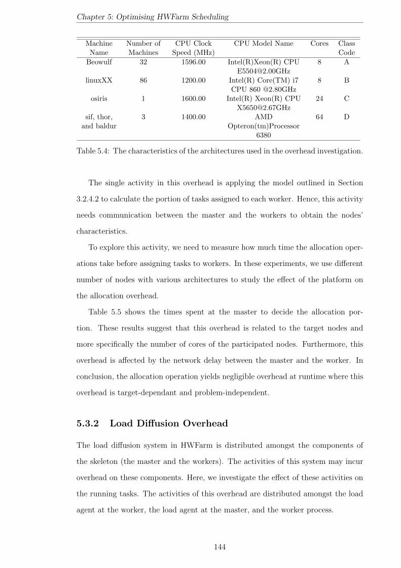
Chapter 5: Optimising HWFarm Scheduling
MachineName
Number ofMachines
CPU ClockSpeed (MHz)
CPU Model Name Cores ClassCode
Beowulf 32 1596.00 Intel(R)Xeon(R) [email protected]
8 A
linuxXX 86 1200.00 Intel(R) Core(TM) i7CPU 860 @2.80GHz
8 B
osiris 1 1600.00 Intel(R) Xeon(R) [email protected]
24 C
sif, thor,and baldur
3 1400.00 AMDOpteron(tm)Processor
6380
64 D
Table 5.4: The characteristics of the architectures used in the overhead investigation.
The single activity in this overhead is applying the model outlined in Section
3.2.4.2 to calculate the portion of tasks assigned to each worker. Hence, this activity
needs communication between the master and the workers to obtain the nodes’
characteristics.
To explore this activity, we need to measure how much time the allocation oper-
ations take before assigning tasks to workers. In these experiments, we use different
number of nodes with various architectures to study the effect of the platform on
the allocation overhead.
Table 5.5 shows the times spent at the master to decide the allocation por-
tion. These results suggest that this overhead is related to the target nodes and
more specifically the number of cores of the participated nodes. Furthermore, this
overhead is affected by the network delay between the master and the worker. In
conclusion, the allocation operation yields negligible overhead at runtime where this
overhead is target-dependant and problem-independent.
5.3.2 Load Diffusion Overhead
The load diffusion system in HWFarm is distributed amongst the components of
the skeleton (the master and the workers). The activities of this system may incur
overhead on these components. Here, we investigate the effect of these activities on
the running tasks. The activities of this overhead are distributed amongst the load
agent at the worker, the load agent at the master, and the worker process.
144

Chapter 5: Optimising HWFarm Scheduling
Nodes NodesTypes
Time for MatrixMultiplication (Sec)
Time forRaytracer (Sec)
Time for SquareNumbers(Sec)
1 1A 0.009 0.009 0.0092 2A 0.016 0.015 0.0154 4A 0.029 0.028 0.0288 8A 0.056 0.055 0.05516 16A 0.111 0.107 0.11124 24A 0.165 0.161 0.16432 32A 0.220 0.216 0.21950 32A+18B 0.346 0.341 0.349100 32A+68B 0.698 0.694 0.7025 4A+1C 0.036 0.036 0.0356 4A+1C+1D 0.042 0.041 0.0428 4A+1C+3D 0.057 0.056 0.056
Table 5.5: The measured times of the allocation overhead.
5.3.2.1 Overhead at the Load Agent
The activities performed by the local load agent at workers are:
Collecting the local load : This activity periodically collects the current load
states. Table 5.6 shows the measured overhead for obtaining the load details on
different architectures.
A B C DTLDO Collecting (Sec) 0.003972 0.00118 0.002315 0.010761
Table 5.6: The measured overhead for collecting the load information.
Recording R for all running tasks : Based on the optimisation procedure in Sec-
tion 5.2.1, this activity calculates R from the collected load details and then records
it to every local task. To investigate the time spent to perform this activity, we run
some experiments on the previous architectures. The measurements show that the
time does not exceed 1 nano second for each task. As a result, the total time of
collecting and recording the load on a worker is:
TLDO LLA = TLDO Collecting +N ∗ TLDO RecordingR (5.2)
where:
TLDO LLA: The load diffusion overhead at the local load agent
TLDO Collecting: The time spent to obtain the local load information
145

Chapter 5: Optimising HWFarm Scheduling
TLDO RecordingR: The time spent to record the current load state in one task
N : The total number of tasks on the current worker
As an example, if we run the skeleton on a local Beowulf cluster (architecture
A), then the overhead to collect the local load information on a worker that runs 8
tasks is:
TLDO LLA = 0.003972 + 8 ∗ (0.000001) = 0.00398sec
Another example, if we run the skeleton on an architecture where a node has 64
cores (architecture D), then the overhead to collect the local load information on
that worker that runs 64 tasks is:
TLDO LLA = 0.010761 + 64 ∗ (0.000001) = 0.010825sec
Observe that when running the skeleton on a worker with 8 cores, the overhead
is 0.004 second while it is 0.01 second on a 64-core machine.
5.3.2.2 Overhead at the Workers
Now, we need to investigate the overhead at the worker process. This overhead is
incurred when a worker receives the load message and then the worker has to append
its own load information. This overhead is based on communications amongst the
participating workers so the network delay has major influence on these measure-
ments.
Table 5.7 shows the time measured at a worker process that runs on different
platforms. This time includes the time to receive the load message, time to append
the local load, and the time to send the new load message to a new worker.
A B C DTLDO W (Sec) 0.000383 0.000444 0.000395 0.000352
Table 5.7: The measured overhead at one worker process.
146

Chapter 5: Optimising HWFarm Scheduling
5.3.2.3 Overhead at the Master
The master is dedicated to maintaining the global load information so the operations
at the master cannot be considered as an overhead.
Table 5.8 shows the times taken to circulate the load message and the time
spent to update the main worker load table, WorkerLoad. These operations are also
influenced by the network delay between the master and the workers.
A B C DTLDO Circulating (Sec) 0.000375 0.000429 0.000348 0.000356TLDO Updating (Sec) 0.000151 0.000160 0.000143 0.000090
Table 5.8: The measured overhead at the master.
5.3.3 Mobility Overhead
The mobility overhead is expected to be the main source of overhead. In HWFrm,
this overhead is concurrently introduced by the estimator agent that follows the
algorithm outlined in Section 5.1.3.3. Hence, it is related to the estimation pro-
cess and all mobility coordination before accomplishing the movement between the
workers. This overhead is difficult to calculate at the right time where the source
worker is loaded with different amount of load that causes various delays.
This overhead starts when the latest global load information is available at the
source worker and ends when the mobility report is sent to the destination worker.
The breakdown of this overhead is: initialising the arrays, finding the estimation
costs for each task, finding the best mapping, and sending the mobility report.
Based on the mobility algorithm, the time required to produce the new mapping
report in a skeleton with w workers executing N tasks is:
TMO = TMO init+t∑
i=1
T iMO findingEC∗N∗w+
t∑i=1
T iMO findingMapping+TMO Report (5.3)
where:
TMO: The mobility overhead.
147
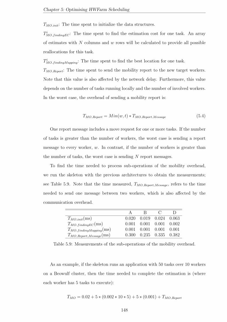
Chapter 5: Optimising HWFarm Scheduling
TMO init: The time spent to initialize the data structures.
T iMO findingEC : The time spent to find the estimation cost for one task. An array
of estimates with N columns and w rows will be calculated to provide all possible
reallocations for this task.
T iMO findingMapping: The time spent to find the best location for one task.
TMO Report: The time spent to send the mobility report to the new target workers.
Note that this value is also affected by the network delay. Furthermore, this value
depends on the number of tasks running locally and the number of involved workers.
In the worst case, the overhead of sending a mobility report is:
TMO Report = Min(w, t) ∗ TMO Report Message (5.4)
One report message includes a move request for one or more tasks. If the number
of tasks is greater than the number of workers, the worst case is sending a report
message to every worker, w. In contrast, if the number of workers is greater than
the number of tasks, the worst case is sending N report messages.
To find the time needed to process sub-operations of the mobility overhead,
we run the skeleton with the previous architectures to obtain the measurements;
see Table 5.9. Note that the time measured, TMO Report Message, refers to the time
needed to send one message between two workers, which is also affected by the
communication overhead.
A B C DTMO init(ms) 0.020 0.019 0.024 0.063TMO findingEC(ms) 0.001 0.001 0.001 0.002TMO findingMapping(ms) 0.001 0.001 0.001 0.001TMO Report Message(ms) 0.300 0.235 0.335 0.382
Table 5.9: Measurements of the sub-operations of the mobility overhead.
As an example, if the skeleton runs an application with 50 tasks over 10 workers
on a Beowulf cluster, then the time needed to complete the estimation is (where
each worker has 5 tasks to execute):
TMO = 0.02 + 5 ∗ (0.002 ∗ 10 ∗ 5) + 5 ∗ (0.001) + TMO Report
148
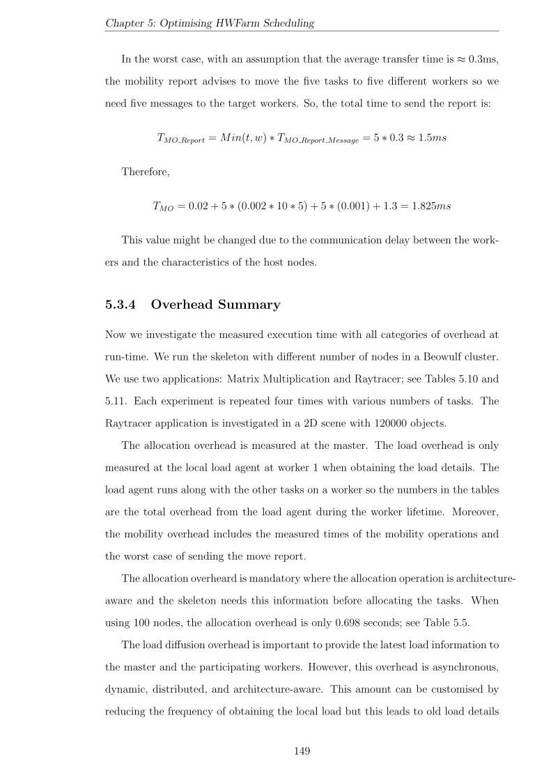
Chapter 5: Optimising HWFarm Scheduling
In the worst case, with an assumption that the average transfer time is ≈ 0.3ms,
the mobility report advises to move the five tasks to five different workers so we
need five messages to the target workers. So, the total time to send the report is:
TMO Report = Min(t, w) ∗ TMO Report Message = 5 ∗ 0.3 ≈ 1.5ms
Therefore,
TMO = 0.02 + 5 ∗ (0.002 ∗ 10 ∗ 5) + 5 ∗ (0.001) + 1.3 = 1.825ms
This value might be changed due to the communication delay between the work-
ers and the characteristics of the host nodes.
5.3.4 Overhead Summary
Now we investigate the measured execution time with all categories of overhead at
run-time. We run the skeleton with different number of nodes in a Beowulf cluster.
We use two applications: Matrix Multiplication and Raytracer; see Tables 5.10 and
5.11. Each experiment is repeated four times with various numbers of tasks. The
Raytracer application is investigated in a 2D scene with 120000 objects.
The allocation overhead is measured at the master. The load overhead is only
measured at the local load agent at worker 1 when obtaining the load details. The
load agent runs along with the other tasks on a worker so the numbers in the tables
are the total overhead from the load agent during the worker lifetime. Moreover,
the mobility overhead includes the measured times of the mobility operations and
the worst case of sending the move report.
The allocation overheard is mandatory where the allocation operation is architecture-
aware and the skeleton needs this information before allocating the tasks. When
using 100 nodes, the allocation overhead is only 0.698 seconds; see Table 5.5.
The load diffusion overhead is important to provide the latest load information to
the master and the participating workers. However, this overhead is asynchronous,
dynamic, distributed, and architecture-aware. This amount can be customised by
reducing the frequency of obtaining the local load but this leads to old load details
149
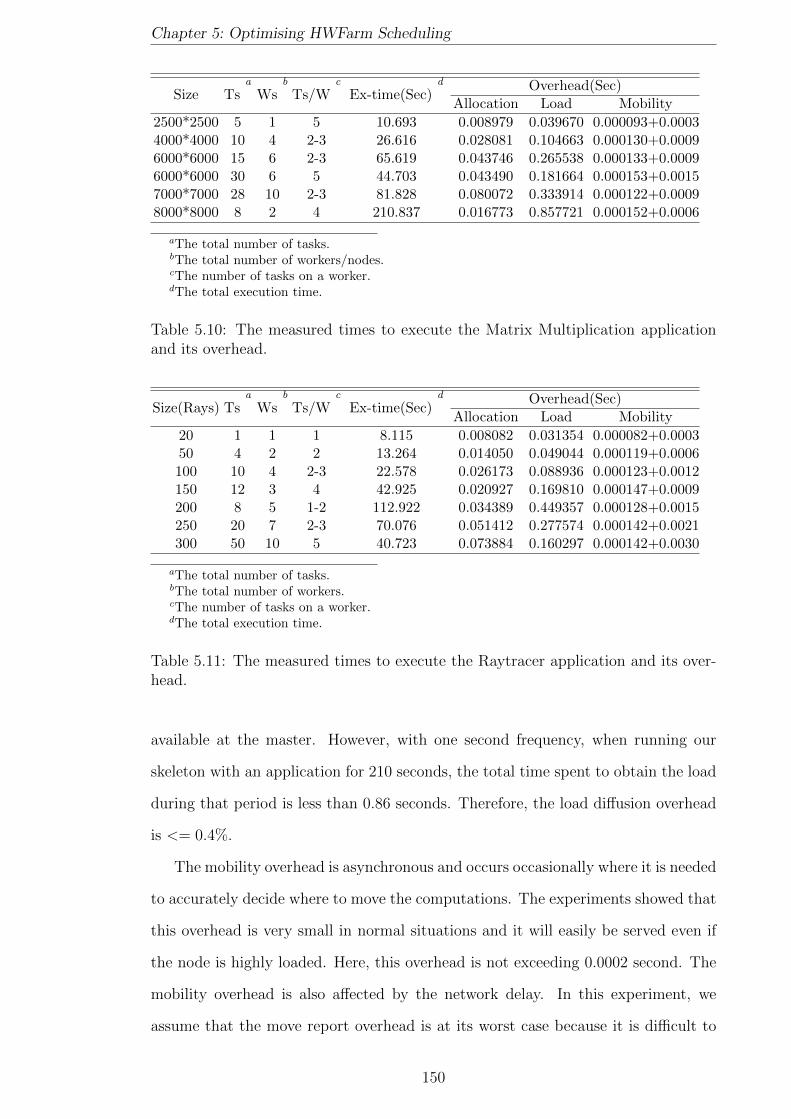
Chapter 5: Optimising HWFarm Scheduling
Size Tsa
Wsb
Ts/Wc
Ex-time(Sec)d Overhead(Sec)
Allocation Load Mobility
2500*2500 5 1 5 10.693 0.008979 0.039670 0.000093+0.00034000*4000 10 4 2-3 26.616 0.028081 0.104663 0.000130+0.00096000*6000 15 6 2-3 65.619 0.043746 0.265538 0.000133+0.00096000*6000 30 6 5 44.703 0.043490 0.181664 0.000153+0.00157000*7000 28 10 2-3 81.828 0.080072 0.333914 0.000122+0.00098000*8000 8 2 4 210.837 0.016773 0.857721 0.000152+0.0006
aThe total number of tasks.bThe total number of workers/nodes.cThe number of tasks on a worker.dThe total execution time.
Table 5.10: The measured times to execute the Matrix Multiplication applicationand its overhead.
Size(Rays) Tsa
Wsb
Ts/Wc
Ex-time(Sec)d Overhead(Sec)
Allocation Load Mobility
20 1 1 1 8.115 0.008082 0.031354 0.000082+0.000350 4 2 2 13.264 0.014050 0.049044 0.000119+0.0006100 10 4 2-3 22.578 0.026173 0.088936 0.000123+0.0012150 12 3 4 42.925 0.020927 0.169810 0.000147+0.0009200 8 5 1-2 112.922 0.034389 0.449357 0.000128+0.0015250 20 7 2-3 70.076 0.051412 0.277574 0.000142+0.0021300 50 10 5 40.723 0.073884 0.160297 0.000142+0.0030
aThe total number of tasks.bThe total number of workers.cThe number of tasks on a worker.dThe total execution time.
Table 5.11: The measured times to execute the Raytracer application and its over-head.
available at the master. However, with one second frequency, when running our
skeleton with an application for 210 seconds, the total time spent to obtain the load
during that period is less than 0.86 seconds. Therefore, the load diffusion overhead
is <= 0.4%.
The mobility overhead is asynchronous and occurs occasionally where it is needed
to accurately decide where to move the computations. The experiments showed that
this overhead is very small in normal situations and it will easily be served even if
the node is highly loaded. Here, this overhead is not exceeding 0.0002 second. The
mobility overhead is also affected by the network delay. In this experiment, we
assume that the move report overhead is at its worst case because it is difficult to
150
Chapter 5: Optimising HWFarm Scheduling
expect the move report in a load condition, as outlined in Sec 5.3.3. As an example,
when we have 50 tasks and 10 workers, the overhead of sending the move report is
0.003 sec.
Consequently, these experiments show that the overhead incurred from the ac-
tivities of HWFarm during the runtime is low when compared to the total execution
time, less than 0.58%. In the Matrix Multiplication application, the overall overhead
is ranging from 0.41% to 0.51%. Whilst in the Raytracer application the overhead
ranges from 0.43% to 0.58%.
5.4 Scheduling Evaluation
In this section, we demonstrate experiments to evaluate the HWFarm scheduling
in terms of the mobility behaviour and the optimised performance of the produced
schedule. We are exploring two types of computations: regular and irregular. For
regular problems, we use a simple Matrix Multiplication application. In contrast,
we are testing a simple Raytracer as an example of irregular computations.
The skeleton with its scheduler was tested in a Beowulf cluster located at Heriot-
Watt University. The cluster consists of 32 eight-core machines (8 quad-core Intel(R)
Xeon(R) CPU E5504, running GNU/Linux(2.6.32) at 2.00GHz with 4096 kb L2
cache and using 12GB RAM).
5.4.1 Mobility Behaviour Validation
To investigate that the mobility behaves as we expect, we run a Matrix Multi-
plication problem with 8 tasks running on 3 locations.
Figure 5.10(a) shows the changes on the load over these locations. We use our
load function that generates artificial load patterns on multi-core platforms. Further
details about this function will be discussed on Chapter 6. Figure 5.10(b) illustrates
the behaviour of the tasks during their executions. This behaviour is influenced by
the current load of the nodes. It can be seen that the HWFarm scheduler lightens
the loaded nodes whenever the worker becomes loaded. This figure shows that the
behaviour of the tasks is the inverse behaviour of the load.
151

Chapter 5: Optimising HWFarm Scheduling
(a) The load pattern applied to the skeleton
(b) The mobility behaviour
Figure 5.10: The mobility behaviour of 10 tasks on 3 workers(Matrix Multiplication)
For the Raytracer problem, we run with 8 tasks on 3 locations. The load is also
generated by the load function but with more delay amongst the nodes; see Figure
5.11(a). The HWFarm scheduler produces dynamic schedules according to the load
state of the nodes. Like the Matrix Multiplication example, the mobility of the tasks
is also behaving inversely to the load on the hosted nodes; see Figure 5.11(b).
Consequently, in both experiments, the skeleton responds quickly to load changes.
152

Chapter 5: Optimising HWFarm Scheduling
(a) The load pattern applied to the skeleton
(b) The mobility behaviour
Figure 5.11: The mobility behaviour of 8 tasks on 3 workers(Raytracer)
5.4.2 Mobility Performance Validation
After evaluating the mobility behaviour, we need to run our mobile skeleton to
explore how the skeleton improves the performance under loaded conditions. We
run each experiment in three execution modes: the original mode (O), the load
mode (L) and the mobility mode (M). In mode O, we measure the total execution
time of running the problem with no load applied and no mobility supported. For
mode L, we measure the times in the presence of the external load. In mode M, we
measure the total execution times for running each problem with the presence of
the external load while mobility is switched on.
To explore how mobility in HWFarm improves the execution time in the presence
of the external load, we compare the execution times before and after applying
mobility in modes L and M, respectively. Then we calculate the compensation by
comparing the improvement when mobility is applied compared to the degradation
of the execution time when the load is present, Compensation(%) = Diff(L&M)Diff(O&L)
.
Table 5.12 shows the results of Matrix Multiplication. We can see how the
153

Chapter 5: Optimising HWFarm Scheduling
execution time becomes longer due to the load applied. Then, after mobility, we
notice that the execution time is improved compared to the execution time without
mobility. Here, the compensation is ranging from 12.41% to 57.52%.
Matrix Ts/Ws a Mode Mode Mode Diffb Diffc ImprovementMulti O(S) L(S) M(S) (O&L) (L&M) (%)
3600*3600 6/3 26.65 40.35 32.47 13.7 7.78 57.524800*4800 12/3 31.08 47.28 42.15 16.2 5.13 31.665600*5600 14/3 42.74 61.46 57.83 18.72 3.63 19.416000*6000 6/3 120.95 164.91 159.55 43.96 5.36 12.196000*6000 10/3 73.81 104.08 94.42 30.27 9.66 31.926000*6000 12/3 60.98 86.83 81.69 25.85 5.14 19.917200*7200 12/3 102.52 143.58 138.12 41.06 5.46 13.317700*7700 14/3 108.9 165.09 149.35 56.19 15.74 28.01
aThe total number of tasks/workersbThe difference between mode O and mode LcThe difference between mode L and mode M
Table 5.12: The improvement in the performance in the presence of externalload(Matrix)
For the Raytracer problem, we also run different number of rays with various
numbers of tasks; see Table 5.13. Like Matrix Multiplication, we can see the im-
provement in the total execution time after applying mobility. The compensation
in Raytracer is ranging from 23.91% to 59.09%.
As a conclusion, in both experiments, either with regular or irregular compu-
tations, the HWFarm skeleton seeks to improve the performance of the problem it
runs when one or more of its nodes experience highly loaded conditions. Further-
more, these results show how our skeleton compensates for changes on the node’s
load. Our experiments suggest that the compensation can reach 59%. We should
mention that this improvement mostly depends on the amount of load on the loaded
nodes, when this load is applied, and how the local computations are affected by
this load. Note that in the irregular computations the estimation is less accurate
but the results show improvement in the performance when activating mobility.
154
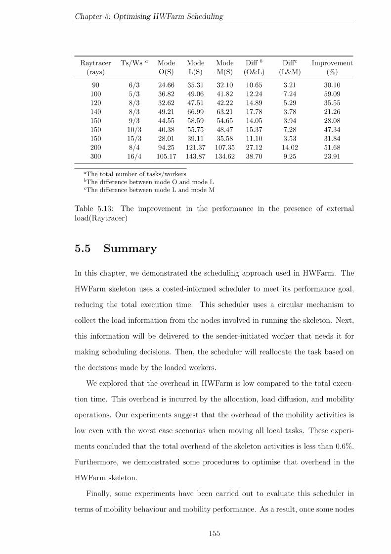
Chapter 5: Optimising HWFarm Scheduling
Raytracer Ts/Ws a Mode Mode Mode Diff b Diffc Improvement(rays) O(S) L(S) M(S) (O&L) (L&M) (%)
90 6/3 24.66 35.31 32.10 10.65 3.21 30.10100 5/3 36.82 49.06 41.82 12.24 7.24 59.09120 8/3 32.62 47.51 42.22 14.89 5.29 35.55140 8/3 49.21 66.99 63.21 17.78 3.78 21.26150 9/3 44.55 58.59 54.65 14.05 3.94 28.08150 10/3 40.38 55.75 48.47 15.37 7.28 47.34150 15/3 28.01 39.11 35.58 11.10 3.53 31.84200 8/4 94.25 121.37 107.35 27.12 14.02 51.68300 16/4 105.17 143.87 134.62 38.70 9.25 23.91
aThe total number of tasks/workersbThe difference between mode O and mode LcThe difference between mode L and mode M
Table 5.13: The improvement in the performance in the presence of externalload(Raytracer)
5.5 Summary
In this chapter, we demonstrated the scheduling approach used in HWFarm. The
HWFarm skeleton uses a costed-informed scheduler to meet its performance goal,
reducing the total execution time. This scheduler uses a circular mechanism to
collect the load information from the nodes involved in running the skeleton. Next,
this information will be delivered to the sender-initiated worker that needs it for
making scheduling decisions. Then, the scheduler will reallocate the task based on
the decisions made by the loaded workers.
We explored that the overhead in HWFarm is low compared to the total execu-
tion time. This overhead is incurred by the allocation, load diffusion, and mobility
operations. Our experiments suggest that the overhead of the mobility activities is
low even with the worst case scenarios when moving all local tasks. These experi-
ments concluded that the total overhead of the skeleton activities is less than 0.6%.
Furthermore, we demonstrated some procedures to optimise that overhead in the
HWFarm skeleton.
Finally, some experiments have been carried out to evaluate this scheduler in
terms of mobility behaviour and mobility performance. As a result, once some nodes
155

Chapter 5: Optimising HWFarm Scheduling
become loaded, this scheduler reduces the total execution time and compensates for
the load changes.
In the next chapter, we present our load generator tool that we used to apply
various patterns of load to the experimental nodes.
156

Chapter 6
Generating Load Patterns
In the previous chapters, we discussed the HWFarm skeleton and its dynamicity.
Nonetheless, it is necessary to evaluate the scheduling decisions and policies pro-
duced by this skeleton under repeatable conditions. Typically, such parallel systems
are evaluated on dedicated platforms with little or no external impact on load. For
dynamic systems, however, such as those that adapt to changing conditions, it is nec-
essary to generate both predictable and realistic patterns of load in order to mimic
a real loaded environment. We have developed a novel load function which may
be instantiated to generate dynamic, adaptive, predictable patterns of load across
multiple processors. Our function can both generate idealised load patterns, and
record and playback real load patterns. Furthermore, it can dynamically maintain
a required load pattern in the presence of external real-time load changes, which
makes it particularly suitable for experimentation on shared systems. In this chap-
ter, we start with an introduction in Section 6.1. Next, in Section 6.2, we discuss
the design of the load function and show that it can generate dynamic, adaptive and
precise load, with minimal impact on system load. We then illustrate its use in the
experimental evaluation of static/dynamic load balancing, load stealing and mobile
skeletons in Section 6.3.
157

Chapter 6: Generating Load Patterns
6.1 Introduction
In recent years, communication networks and computer environments have offered
resources which are distributed across a large number of systems and are shared by
a large number of users. The demand for resources in such computational environ-
ments is irregular, so the load may be unpredictable.
In real world systems, there is a fundamental difference in behaviour between
dedicated systems, like supercomputers, where the parallel system is dedicated to
execute the scheduled tasks, and non-dedicated systems, like servers, where multiple
tasks can share the resources, thus the system may have volatile loads.
Heterogeneous architecture software needs to be tested and validated, but re-
source usage depends on the computing demands from other user processes. Thus,
the experimental environment for such software needs to be adaptable to reflect
changing conditions. Some simulation tools, for example SimGrid [53], can be used
to explore varying loads. Nonetheless, simulating the interaction and behaviour of
distributed system nodes is very difficult and may be impossible in some situations
where it is very hard to obtain the influencing factors [41].
For better results, it is more efficient if these experiments run on real environ-
ments under controlled conditions. Thus, a load generator is needed to mimic such
conditions by producing a desired amount of load across the environment. Ideally,
the load generator would produce defined levels of load on CPU, memory, cache
and network. For example, KRASH [182] is a tool for reproducible generation of
system-level CPU load on many-core machines. It creates a dynamic and precise
load but only for multicore systems. Stress [226] is a workload generator for stressing
the CPU, memory, I/O and the disk. This tool spawns a fixed number of processes
with some calculations for stressing the CPU. The load generated using this tool is
non-dynamic where it is not changing at run-time. Another method presented by
Makineni et al to reduce the CPU performance is down-scaling the CPU frequency
which is used to reduce CPU power consumption [156]. Moreover, cpulimit [157] is a
tool to limit the CPU usage of a process. It controls the CPU time dynamically and
quickly without changing the scheduling settings but it does not handle multicore
158
Chapter 6: Generating Load Patterns
systems. Wrekavoc [90] is a tool for heterogeneity simulation which enables users
to limit the resources available to their application. Lublin et al [154] proposed
an approach to instrument workload models of the system. This approach analy-
ses and models the job-level workloads to substantially improve the experimental
procedures.
In this chapter, we are exploring a mechanism to generate loads to degrade
system performance on heterogeneous architectures and control the resource usage.
We discuss the implementation of a load function which may be instantiated to
apply dynamic, precise, adaptive patterns of load in a dedicated system to simulate
different load scenarios that may occur in a shared distributed non-dedicated system.
Our load function has been constructed to generate CPU load, as the CPU is a
significant element in high performance computing. This function is able to generate
a dynamic, precise and systematic load on shared/distributed memory architecture.
Hence, we can prepare and replicate real experimental conditions by applying various
patterns of loads. Moreover, the load function is able to measure and record the
load for the whole system, nodes and cores, where it can use the load pattern later
for mimicking the whole system. Generating loads for memory, cache and network
are beyond the scope of this work.
6.2 Design and Implementation
6.2.1 Load and Scheduling
In this section, we propose the design and implementation of the load function that
creates threads which are scheduled on a regular basis. The time slices assigned to
these threads depend on the amount of load in the load pattern.
Our function has been designed to meet the following requirements:
• Reproducibility : The load function is able to generate the desired load on the
system regardless of environmental conditions (number of machines, number
of cores, other user processes).
• Precise: It can generate a precise CPU load through matching the given load
159
Chapter 6: Generating Load Patterns
to the desired load.
• Dynamic: Under external real-time changes, a required load pattern can be
dynamically maintained, which makes the load function specifically appropri-
ate to be used in experimentations on shared systems.
• Adaptive: The load function is able to generate patterns of load consider-
ing the current load of the system. This also improves the precision of the
generated load where other user’s loads will be part of the given pattern of
load.
• Over-loading & Non Intervention: The load function can create any number
of loaders on a core, resulting in a highly loaded core. Furthermore, the load
function has minimal impact on the system because the scheduling policy is
not affected and the priorities of the current processes are not changed.
6.2.2 Load Function Design
The load function is designed using the Master/Worker model, see Figure 6.1. Here,
the master is responsible for managing and controlling the workers which are dis-
tributed over all the nodes in the system, as localised measurement entities and
load generators. The load function will run on multiprocessor systems where the
master will be hosted on a node as the global controller while worker processes are
distributed amongst the nodes. However, each worker process generates a thread,
the local controller, and the load generator threads, the loaders.
The load function operates in two modes: recording the current load and gen-
erating load patterns. Accordingly, the global controller will maintain the desired
operation through cooperating with the remote controllers. On other hand, the local
controller is responsible for either recording the node load or generating the desired
load on that node.
Generating load on a CPU means making it unavailable for processing other
work. In other words, generating the CPU load involves creating and running
threads/processes on the CPU cores. A loader is an intensive thread which runs
160

Chapter 6: Generating Load Patterns
on one CPU core and has to be controlled to adjust the amount of load, either by
the thread itself or by another thread, the local controller. This thread will run fre-
quently to monitor and manage the loader threads with no change in their priorities.
However, the frequency of running the local controller thread should be balanced to
avoid extra load on the CPU and to precisely control the load. Our function runs
with regular policy without changing any priorities.
Figure 6.1: The load function design.
Typical parallel applications are composed of many processes or threads [120].
These threads use the CPU cores which are the smallest computing elements in a
computing system. The operating system scheduler assigns a CPU core to threads.
These threads are competing for accessing the core at the same time. Then, the
scheduler has to choose which thread should run on the core using scheduling pol-
icy. The schedulers try to balance fairly resource usage amongst running threads.
Therefore, the scheduler will use time-slicing by assigning time intervals of the core
execution to all threads intend to run on the core where the time intervals assigned
to the threads depends on their priorities and the scheduler policy. We can conclude
that the core load is the ratio of unavailable time slices to the total time slices.
Applying a load on a core means making some time slices on the core unavailable.
Regarding the dynamic load, the local controller will change the number of unavail-
able time slices in the core depending on the load profile. In contrast, for adaptive
load, the local controller will take into account the current external real-time load
changes and generate the remaining amount of load to reach the desired load.
Variants of load injector use a supervisor model, for example KRASH [182] and
Wrekavoc [90].
161

Chapter 6: Generating Load Patterns
6.2.3 The Implementation
We implement our load function using C and MPI [206] while we use the PThreads
library to create and manage the threads [48]. In this implementation, we target
MPI compatible systems with Linux operating system (the Linux kernel is 2.6 or
later). Here, the function has two main tasks: recording the loads of the machines
and generating CPU loads.
To record the load, a monitor thread is created by the local controller to record all
information about the machine using the /proc virtual file system. The information
is collected every second by default, or according to input configurations. After that,
the information will be sent to the global controller to create the load pattern for
the current system.
To generate the CPU load, see Figure 6.2, the local controller will create a loader
thread for each core in the hosted node. Thereafter, it will assign a core to a thread
to guarantee that the thread is running only on one core. This is implemented using
cpuset, a Linux feature which can be used to restrict the thread execution on a
specific core or cores (in PThreads, this is implemented in thread affinity) [175].
Depending on the load pattern and for generating a precise load, the local controller
will check frequently each loader to make sure that it is loading the core with the
desired amount of load.
The loader thread is a simple infinite loop with conditions to keep the loader
monitored and controlled by the local controller so that it has minimal impact on
cache and memory. The local controller will run once per second by default, or
according to input configurations. Each time, the local controller will calculate the
amount of load for each loader depending on the load pattern and the actual load.
Then, it sets the sleep period of the loader threads. Hence, the generated load will
be precise and match the desired pattern of load. The local controller is not attached
to a specific core so that it does not matter where it runs. If the scheduling is fair,
the local controller will run on time.
162
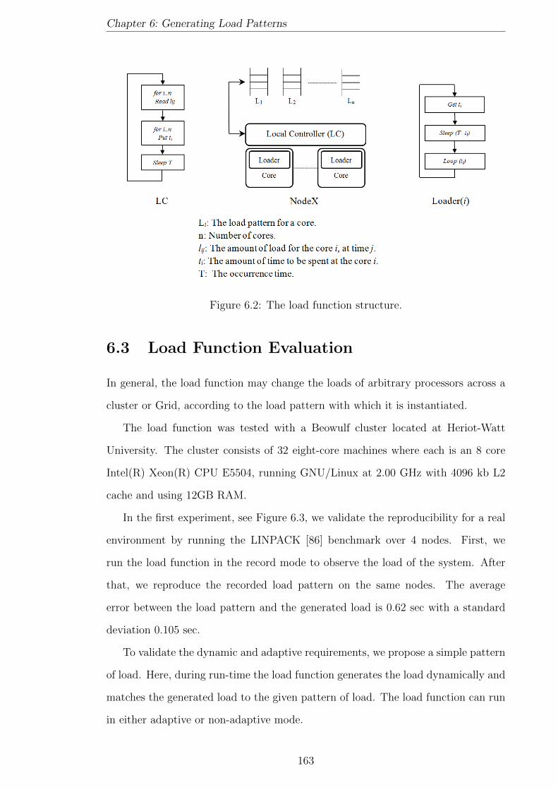
Chapter 6: Generating Load Patterns
Figure 6.2: The load function structure.
6.3 Load Function Evaluation
In general, the load function may change the loads of arbitrary processors across a
cluster or Grid, according to the load pattern with which it is instantiated.
The load function was tested with a Beowulf cluster located at Heriot-Watt
University. The cluster consists of 32 eight-core machines where each is an 8 core
Intel(R) Xeon(R) CPU E5504, running GNU/Linux at 2.00 GHz with 4096 kb L2
cache and using 12GB RAM.
In the first experiment, see Figure 6.3, we validate the reproducibility for a real
environment by running the LINPACK [86] benchmark over 4 nodes. First, we
run the load function in the record mode to observe the load of the system. After
that, we reproduce the recorded load pattern on the same nodes. The average
error between the load pattern and the generated load is 0.62 sec with a standard
deviation 0.105 sec.
To validate the dynamic and adaptive requirements, we propose a simple pattern
of load. Here, during run-time the load function generates the load dynamically and
matches the generated load to the given pattern of load. The load function can run
in either adaptive or non-adaptive mode.
163

Chapter 6: Generating Load Patterns
0
20
40
60
80
100
0 10 20 30 40 50 60 70 80 90 100
CP
U (
%)
Time(Sec)Node4(Required Load) Node4(Generated Load)
Figure 6.3: The required and actual load in node 4.
In adaptive mode the function will take into account the current system load
while in non-adaptive mode it will generate the load regardless of the current load.
In this experiment, we generate the load over 5 nodes with an adaptive mode.
Surprisingly, an external user monopolises the first node for some time, see the
green curve in Figure 6.4. In this case, the local controller in the first node will ask
the loaders to reduce the artificial load to make the total load equal to the required
load, see Figure 6.4. This will make the node loaded with the desired amount of
load apart from how many users are using the current node. The generated load will
be precise with a necessarily delay if the load of other users below the wanted load.
Note that there are many saliences in the generated load. This happens when there
are load changes on the system and the load function takes an action to adjust the
generated load to match the desired value.
The more precise a load is generated, the better a real system is simulated.
The local controller collects, generates and assigns the amount of load for a loader.
Therefore, it is very important to run the local controller thread on time to set
the required amount of load. See Table 6.1 which illustrates the average error
for generating varying amounts of load under 100%. We run the load function in
adaptive and non-adaptive modes. Here, we notice that the average error in the
adaptive mode is around 0.18 at the low loads while in the non-adaptive mode the
average error is around 0.2 at the high loads.
If the load is more than 100%, the local controllers will compete for acquiring
164

Chapter 6: Generating Load Patterns
Figure 6.4: The required and actual load in the node with other changes in the load(adaptive mode).
resource. An undesirable delay in executing the local controller will occur which
affects only the next time interval. This delay depends on the total number of
threads and the scheduling policy. The delay will not affect the generated load if
the required load is over 100% but if the load in the pattern decreases the load then
a slight error may appear.
6.3.1 The Load Function Impact
When conducting an experiment, the load function runs at the same time to apply
a load pattern for evaluating the solution. So it is important to ensure that running
the function itself will not have a significant impact on overall system performance.
To explore this, we use a Matrix Multiplication benchmark with the load function
doing nothing.
As Table 6.2 shows, we found that the effect on the system with a load function
doing nothing is from 0.05% to 0.87%. We conclude that the load function has an
insignificant impact on the overall performance of the system.
Because we are working across distributed memory architectures, it is also very
important to check the function’s impact on network performance. However, the
communications within the load function are performed only at the start-up and
165
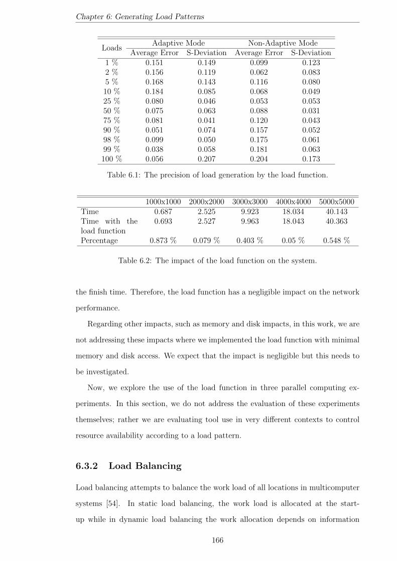
Chapter 6: Generating Load Patterns
LoadsAdaptive Mode Non-Adaptive Mode
Average Error S-Deviation Average Error S-Deviation1 % 0.151 0.149 0.099 0.1232 % 0.156 0.119 0.062 0.0835 % 0.168 0.143 0.116 0.08010 % 0.184 0.085 0.068 0.04925 % 0.080 0.046 0.053 0.05350 % 0.075 0.063 0.088 0.03175 % 0.081 0.041 0.120 0.04390 % 0.051 0.074 0.157 0.05298 % 0.099 0.050 0.175 0.06199 % 0.038 0.058 0.181 0.063100 % 0.056 0.207 0.204 0.173
Table 6.1: The precision of load generation by the load function.
1000x1000 2000x2000 3000x3000 4000x4000 5000x5000Time 0.687 2.525 9.923 18.034 40.143Time with theload function
0.693 2.527 9.963 18.043 40.363
Percentage 0.873 % 0.079 % 0.403 % 0.05 % 0.548 %
Table 6.2: The impact of the load function on the system.
the finish time. Therefore, the load function has a negligible impact on the network
performance.
Regarding other impacts, such as memory and disk impacts, in this work, we are
not addressing these impacts where we implemented the load function with minimal
memory and disk access. We expect that the impact is negligible but this needs to
be investigated.
Now, we explore the use of the load function in three parallel computing ex-
periments. In this section, we do not address the evaluation of these experiments
themselves; rather we are evaluating tool use in very different contexts to control
resource availability according to a load pattern.
6.3.2 Load Balancing
Load balancing attempts to balance the work load of all locations in multicomputer
systems [54]. In static load balancing, the work load is allocated at the start-
up while in dynamic load balancing the work allocation depends on information
166
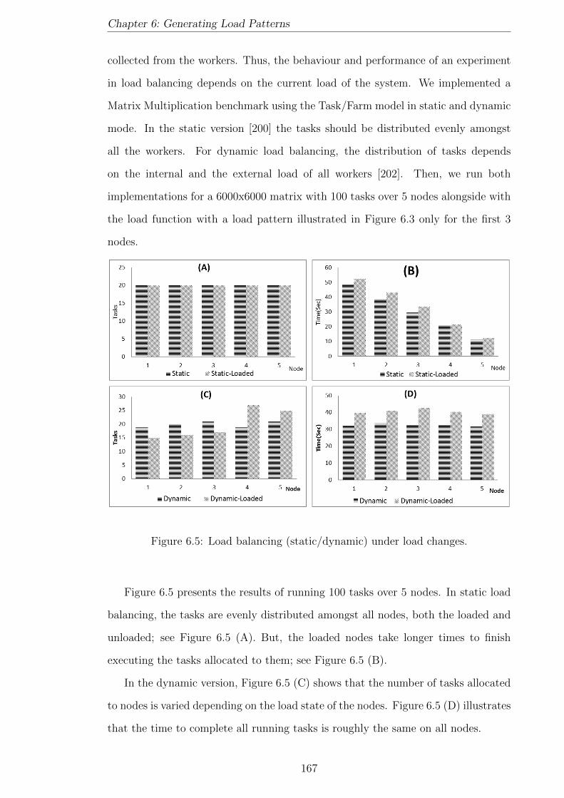
Chapter 6: Generating Load Patterns
collected from the workers. Thus, the behaviour and performance of an experiment
in load balancing depends on the current load of the system. We implemented a
Matrix Multiplication benchmark using the Task/Farm model in static and dynamic
mode. In the static version [200] the tasks should be distributed evenly amongst
all the workers. For dynamic load balancing, the distribution of tasks depends
on the internal and the external load of all workers [202]. Then, we run both
implementations for a 6000x6000 matrix with 100 tasks over 5 nodes alongside with
the load function with a load pattern illustrated in Figure 6.3 only for the first 3
nodes.
Figure 6.5: Load balancing (static/dynamic) under load changes.
Figure 6.5 presents the results of running 100 tasks over 5 nodes. In static load
balancing, the tasks are evenly distributed amongst all nodes, both the loaded and
unloaded; see Figure 6.5 (A). But, the loaded nodes take longer times to finish
executing the tasks allocated to them; see Figure 6.5 (B).
In the dynamic version, Figure 6.5 (C) shows that the number of tasks allocated
to nodes is varied depending on the load state of the nodes. Figure 6.5 (D) illustrates
that the time to complete all running tasks is roughly the same on all nodes.
167

Chapter 6: Generating Load Patterns
In the load balancing experiments, it can be observed that the generated load
has a direct impact on the behaviour of such experiments. Consequently, such a tool
can create a realistic loaded environment to help in evaluating these experiments.
6.3.3 Work Stealing
Work stealing is a thread scheduling technique for shared-memory multiprocessors
where a thread steals works from other threads [38]. For this experiment, we use
one node which has 8 cores. We run 8 threads over 8 cores where each thread has
a pool of tasks and these pools are shared amongst all threads. We repeated the
running 9 times with changing the number of loaded cores through assigning cores
to loaders.
Tasks onNumber of Loaded Cores
0 1 2 3 4 5 6 7 8Core 1 256 166 158 146 128 147 171 205 256Core 2 256 269 160 149 128 146 171 205 256Core 3 256 269 290 149 128 146 170 205 256Core 4 256 269 289 319 128 147 171 206 256Core 5 256 269 288 320 384 146 171 205 256Core 6 256 269 287 322 383 438 171 205 255Core 7 256 269 289 321 384 439 511 206 257Core 8 256 268 287 322 385 439 512 611 256
Table 6.3: Work Stealing with the number of tasks processed on each core (boldnumber refers to the number of tasks processed on a loaded core)
Table 6.3 illustrates the effect of changing the load on task distribution. Here,
the tasks should be evenly distributed amongst the cores if they have the same
amount of load. In the table, bold numbers refer to the number of tasks processed
on each loaded core. We can see that as more as cores are loaded, the tasks are
redistributed to maintain overall balance between loaded and unloaded cores. Note
that when the number of loaded cores is 7, this makes the 8th core execute more
tasks compared with the other loaded cores.
Like load balancing, the load function provides a mechanism to evaluate the work
stealing experiments.
168
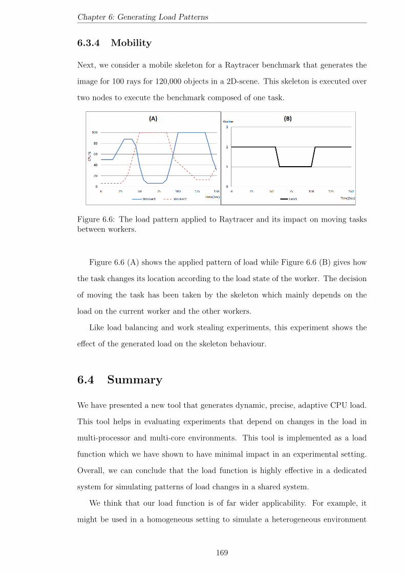
Chapter 6: Generating Load Patterns
6.3.4 Mobility
Next, we consider a mobile skeleton for a Raytracer benchmark that generates the
image for 100 rays for 120,000 objects in a 2D-scene. This skeleton is executed over
two nodes to execute the benchmark composed of one task.
Figure 6.6: The load pattern applied to Raytracer and its impact on moving tasksbetween workers.
Figure 6.6 (A) shows the applied pattern of load while Figure 6.6 (B) gives how
the task changes its location according to the load state of the worker. The decision
of moving the task has been taken by the skeleton which mainly depends on the
load on the current worker and the other workers.
Like load balancing and work stealing experiments, this experiment shows the
effect of the generated load on the skeleton behaviour.
6.4 Summary
We have presented a new tool that generates dynamic, precise, adaptive CPU load.
This tool helps in evaluating experiments that depend on changes in the load in
multi-processor and multi-core environments. This tool is implemented as a load
function which we have shown to have minimal impact in an experimental setting.
Overall, we can conclude that the load function is highly effective in a dedicated
system for simulating patterns of load changes in a shared system.
We think that our load function is of far wider applicability. For example, it
might be used in a homogeneous setting to simulate a heterogeneous environment
169

Chapter 6: Generating Load Patterns
by giving differential constant loads to the processing elements with the same char-
acteristics. It might also be used to simulate different patterns of system component
failure by giving processing elements infeasibly large loads.
170
Chapter 7
Evaluation
In this work, we propose a load-aware skeleton used to solve problems through ex-
ploiting shared parallel computing platforms. Here, we will discuss how our skeleton
can be used to solve different types of problems in many different areas as well as
running large scale problems. This enhances how our skeleton is capable of accom-
modating diversity, which is one of principles in designing skeletal-based systems.
Furthermore, we will explore one of the side effects of our skeleton behaviour through
investigating the effect of mobility on other applications running on shared nodes.
In this chapter, we start with an introduction in Section 7.1. Next, in Section 7.2,
we evaluate the usability of HWFarm by applying it to pipeline structures. Then,
we evaluate scalability by measuring runtime on large architectures in Section 7.3.
Most importantly, we evaluate adaptivity by measuring the runtimes of applications
competing for resources on a small cluster in Section 7.4.
7.1 Introduction
Parallelism with high performance computing has introduced techniques to solve
complex problems that were not manageable on single processors. These techniques
have been implemented in many different areas: finance and trading, climate re-
search, and biosciences. To put our skeleton in the right context, it should be able
to solve problems related to data science such as modelling and numerical simula-
tions. Here we will demonstrate three of the common problems in data sciences: the
171

Chapter 7: Evaluation
N-body simulation problem, the BLAST algorithm and the findWord problem.
The N-body problem is a numerical simulation for motion of N particles that
are interacting gravitationally [218]. N-body algorithms have a wide range of ap-
plications such as plasma physics and molecular dynamics. The simulation of the
movement of each particle is distributed over time-steps. Each step requires com-
puting all forces exerted on each particle and then updating the new locations and
the new velocities for all particles. At each time-step, O(N2) operations need to be
computed. The pseudo-code of the sequential version of this problem is:
Set initial positions for all particles
for each timestep do
for each particle j do
for each particle i do
calculate the force at particle j
update the velocity and the location of particle j
endfor
endfor
BLAST (Basic Local Alignment Search Tool) algorithm is used to search for
sequences in a database of DNA or proteins [17]. A parallel version of Blast has
been presented in [144]. This algorithm is used to compare a database of sequences
(biological sequences such as amino-acid sequences or DNA sequences) for detecting
sequences above a concrete threshold. The pseudo-code of the sequential version of
this algorithm is:
Set the query sequence
Make a k-letter query word list
Scan the database to find the list of matching words
Extend the exact match to High Scoring Pairs
Evaluate the score of High Scoring Pairs
Show the gapped local alignment
Report every match whose score is lower than a threshold
172
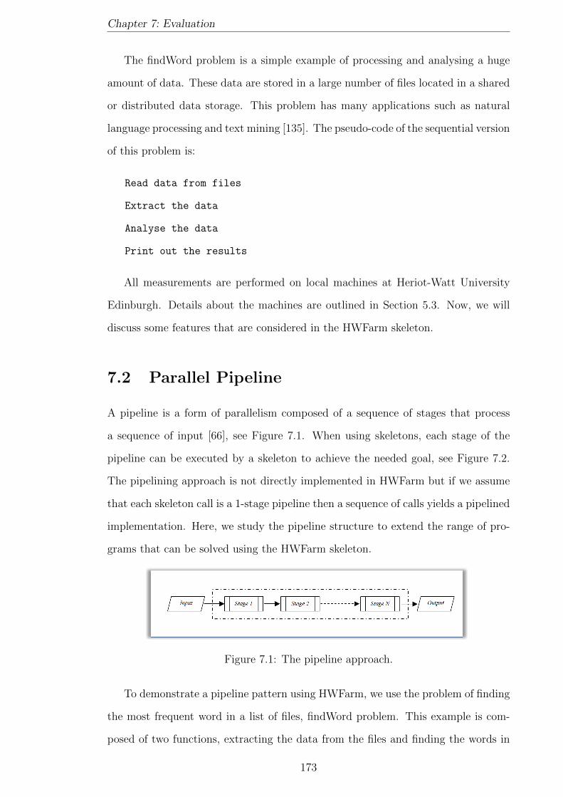
Chapter 7: Evaluation
The findWord problem is a simple example of processing and analysing a huge
amount of data. These data are stored in a large number of files located in a shared
or distributed data storage. This problem has many applications such as natural
language processing and text mining [135]. The pseudo-code of the sequential version
of this problem is:
Read data from files
Extract the data
Analyse the data
Print out the results
All measurements are performed on local machines at Heriot-Watt University
Edinburgh. Details about the machines are outlined in Section 5.3. Now, we will
discuss some features that are considered in the HWFarm skeleton.
7.2 Parallel Pipeline
A pipeline is a form of parallelism composed of a sequence of stages that process
a sequence of input [66], see Figure 7.1. When using skeletons, each stage of the
pipeline can be executed by a skeleton to achieve the needed goal, see Figure 7.2.
The pipelining approach is not directly implemented in HWFarm but if we assume
that each skeleton call is a 1-stage pipeline then a sequence of calls yields a pipelined
implementation. Here, we study the pipeline structure to extend the range of pro-
grams that can be solved using the HWFarm skeleton.
Figure 7.1: The pipeline approach.
To demonstrate a pipeline pattern using HWFarm, we use the problem of finding
the most frequent word in a list of files, findWord problem. This example is com-
posed of two functions, extracting the data from the files and finding the words in
173
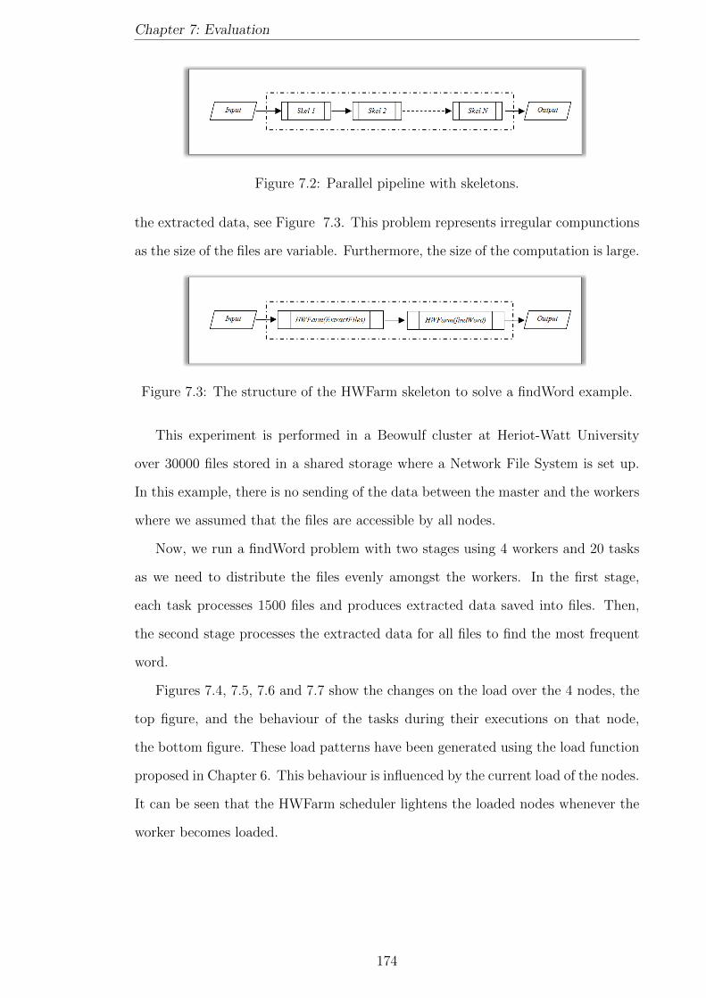
Chapter 7: Evaluation
Figure 7.2: Parallel pipeline with skeletons.
the extracted data, see Figure 7.3. This problem represents irregular compunctions
as the size of the files are variable. Furthermore, the size of the computation is large.
Figure 7.3: The structure of the HWFarm skeleton to solve a findWord example.
This experiment is performed in a Beowulf cluster at Heriot-Watt University
over 30000 files stored in a shared storage where a Network File System is set up.
In this example, there is no sending of the data between the master and the workers
where we assumed that the files are accessible by all nodes.
Now, we run a findWord problem with two stages using 4 workers and 20 tasks
as we need to distribute the files evenly amongst the workers. In the first stage,
each task processes 1500 files and produces extracted data saved into files. Then,
the second stage processes the extracted data for all files to find the most frequent
word.
Figures 7.4, 7.5, 7.6 and 7.7 show the changes on the load over the 4 nodes, the
top figure, and the behaviour of the tasks during their executions on that node,
the bottom figure. These load patterns have been generated using the load function
proposed in Chapter 6. This behaviour is influenced by the current load of the nodes.
It can be seen that the HWFarm scheduler lightens the loaded nodes whenever the
worker becomes loaded.
174

Chapter 7: Evaluation
Figure 7.4: The load pattern and the mobility behaviour of tasks at at Worker 1.
Figure 7.5: The load pattern and the mobility behaviour of tasks at at Worker 2.
175
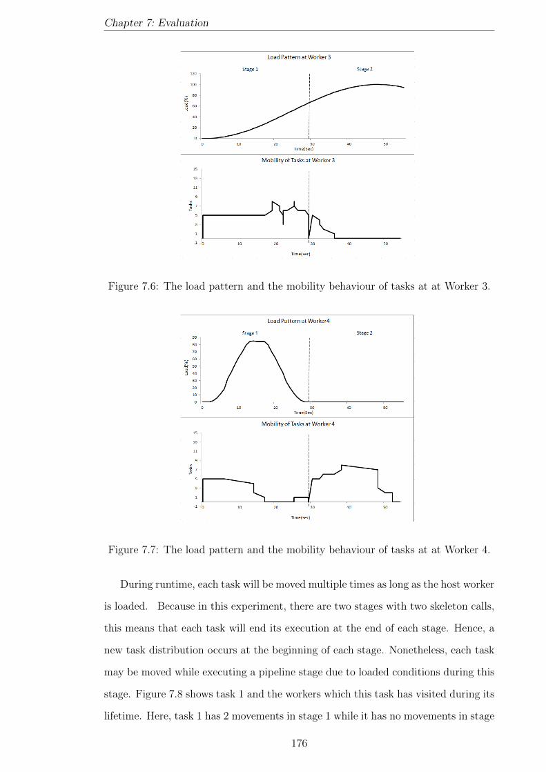
Chapter 7: Evaluation
Figure 7.6: The load pattern and the mobility behaviour of tasks at at Worker 3.
Figure 7.7: The load pattern and the mobility behaviour of tasks at at Worker 4.
During runtime, each task will be moved multiple times as long as the host worker
is loaded. Because in this experiment, there are two stages with two skeleton calls,
this means that each task will end its execution at the end of each stage. Hence, a
new task distribution occurs at the beginning of each stage. Nonetheless, each task
may be moved while executing a pipeline stage due to loaded conditions during this
stage. Figure 7.8 shows task 1 and the workers which this task has visited during its
lifetime. Here, task 1 has 2 movements in stage 1 while it has no movements in stage
176

Chapter 7: Evaluation
2. Furthermore, Figure 7.9 shows the execution of task 7 which has 1 movement in
stage 2 and 1 movement in stage 2.
Figure 7.8: Task 1 and its locations in the findWord problem.
Figure 7.9: Task 7 and its locations in the findWord problem.
7.3 Scalability
This section discusses the scalability of the HWFarm skeleton over parallel com-
puting architectures. We will measure the runtimes of running large-scale problems
using HWFarm over a big number of nodes. Here, speed-up evaluation is not ad-
dressed in this work.
During the design of HWFarm, several issues have been considered to support
scalability, such as:
• Making the mobility decision: The decision in HWFarm is taken through a
decentralised approach where each worker is responsible for the decisions to
move its tasks.
• Transfer policy : We used a sender-initiated mechanism where the loaded
worker only triggers for mobility.
177
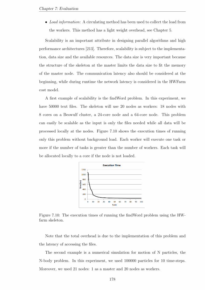
Chapter 7: Evaluation
• Load information: A circulating method has been used to collect the load from
the workers. This method has a light weight overhead, see Chapter 5.
Scalability is an important attribute in designing parallel algorithms and high
performance architectures [213]. Therefore, scalability is subject to the implementa-
tion, data size and the available resources. The data size is very important because
the structure of the skeleton at the master limits the data size to fit the memory
of the master node. The communication latency also should be considered at the
beginning, while during runtime the network latency is considered in the HWFarm
cost model.
A first example of scalability is the findWord problem. In this experiment, we
have 50000 text files. The skeleton will use 20 nodes as workers: 18 nodes with
8 cores on a Beowulf cluster, a 24-core node and a 64-core node. This problem
can easily be scalable as the input is only the files needed while all data will be
processed locally at the nodes. Figure 7.10 shows the execution times of running
only this problem without background load. Each worker will execute one task or
more if the number of tasks is greater than the number of workers. Each task will
be allocated locally to a core if the node is not loaded.
Figure 7.10: The execution times of running the findWord problem using the HW-farm skeleton.
Note that the total overhead is due to the implementation of this problem and
the latency of accessing the files.
The second example is a numerical simulation for motion of N particles, the
N-body problem. In this experiment, we used 100000 particles for 10 time-steps.
Moreover, we used 21 nodes: 1 as a master and 20 nodes as workers.
178
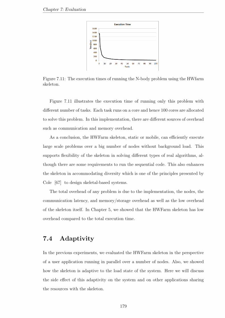
Chapter 7: Evaluation
Figure 7.11: The execution times of running the N-body problem using the HWfarmskeleton.
Figure 7.11 illustrates the execution time of running only this problem with
different number of tasks. Each task runs on a core and hence 100 cores are allocated
to solve this problem. In this implementation, there are different sources of overhead
such as communication and memory overhead.
As a conclusion, the HWFarm skeleton, static or mobile, can efficiently execute
large scale problems over a big number of nodes without background load. This
supports flexibility of the skeleton in solving different types of real algorithms, al-
though there are some requirements to run the sequential code. This also enhances
the skeleton in accommodating diversity which is one of the principles presented by
Cole [67] to design skeletal-based systems.
The total overhead of any problem is due to the implementation, the nodes, the
communication latency, and memory/storage overhead as well as the low overhead
of the skeleton itself. In Chapter 5, we showed that the HWFarm skeleton has low
overhead compared to the total execution time.
7.4 Adaptivity
In the previous experiments, we evaluated the HWFarm skeleton in the perspective
of a user application running in parallel over a number of nodes. Also, we showed
how the skeleton is adaptive to the load state of the system. Here we will discuss
the side effect of this adaptivity on the system and on other applications sharing
the resources with the skeleton.
179
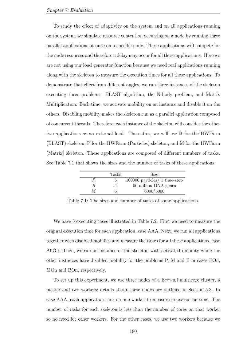
Chapter 7: Evaluation
To study the effect of adaptivity on the system and on all applications running
on the system, we simulate resource contention occurring on a node by running three
parallel applications at once on a specific node. These applications will compete for
the node resources and therefore a delay may occur for all these applications. Here we
are not using our load generator function because we need real applications running
along with the skeleton to measure the execution times for all these applications. To
demonstrate that effect from different angles, we run three instances of the skeleton
executing three problems: BLAST algorithm, the N-body problem, and Matrix
Multiplication. Each time, we activate mobility on an instance and disable it on the
others. Disabling mobility makes the skeleton run as a parallel application composed
of concurrent threads. Therefore, each instance of the skeleton will consider the other
two applications as an external load. Thereafter, we will use B for the HWFarm
(BLAST) skeleton, P for the HWFarm (Particles) skeleton, and M for the HWFarm
(Matrix) skeleton. These applications are composed of different numbers of tasks.
See Table 7.1 that shows the sizes and the number of tasks of these applications.
Tasks Size
P 5 100000 particles/ 1 time-stepB 4 50 million DNA genesM 6 6000*6000
Table 7.1: The sizes and number of tasks of some applications.
We have 5 executing cases illustrated in Table 7.2. First we need to measure the
original execution time for each application, case AAA. Next, we run all applications
together with disabled mobility and measure the times for all these applications, case
AllOff. Then, we run an instance of the skeleton with activated mobility while the
other instances have disabled mobility for the problems P, M and B in cases POn,
MOn and BOn, respectively.
To set up this experiment, we use three nodes of a Beowulf multicore cluster, a
master and two workers; details about these nodes are outlined in Section 5.3. In
case AAA, each application runs on one worker to measure its execution time. The
number of tasks for each skeleton is less than the number of cores on that worker
so no need for other workers. For the other cases, we use two workers because we
180

Chapter 7: Evaluation
need to keep one available worker in case there is a need to move tasks to a new
location when mobility is activated. We use only two workers because it is easier to
demonstrate the results and show the movement behaviour of the skeletons at the
run-time. Initially, all tasks of the three applications start at worker 1. Then, based
on the load state, mobility occurs for the tasks of the skeleton that has activated
mobility. In summary, our set-up shows that performance improvements are due to
mobility and not additional cores.
Case workers P M B
AAA 1 alone alone aloneAllOff 1 Mobility Off Mobility Off Mobility OffPOn 2 Mobility On Mobility Off Mobility OffMOn 2 Mobility Off Mobility On Mobility OffBOn 2 Mobility Off Mobility Off Mobility On
Table 7.2: The cases of running the HWFarm problems.
Table 7.3 summarises the results of all executing cases. In this table, each line
represents a case. In column Exec, each value represents the measured execution
time of running an application(col) in a case(line). The Diff columns in case AllOff
refers to the difference between the execution time in case AllOff and the execution
time in case AAA. This shows how each application is affected by other applications.
The Diff columns in cases POn, MOn and BOn, point to the difference between the
execution time in that case and the execution time in case AllOff. The compensa-
tions from mobility compared to the times with high background load are shown in
the Comp columns. Further details about those cases are as follows:
CaseP M B
Exec(S) Diff(S) Comp(%) Exec(S) Diff(S) Comp(%) Exec(S) Diff(S) Comp(%)AAA 108.711 119.388 60.538AllOff 187.977 +79.266 218.714 +99.326 142.287 +81.749POn 110.378 -77.599 97.90 158.732 -59.982 60.39 116.969 -25.318 30.97MOn 114.268 -73.709 92.99 122.188 -96.526 97.18 94.749 -47.538 58.15BOn 162.945 -25.032 31.58 181.539 -37.175 37.43 62.911 -79.376 97.10
Table 7.3: Summary of the execution times and the improvements for all applica-tions.
181

Chapter 7: Evaluation
Case AAA
In this case, each skeleton runs alone where its tasks are executed on one worker.
As a result, the measured total execution times are: 108.711 sec for P, 119.388 sec
for M, and 60.538 sec for B.
Case AllOff
We will run all skeletons together where all tasks will start executing on the same
worker, worker 1. In this experiment, all skeletons have disabled mobility and hence
worker 2 will be idle. Figure 7.12 shows the number of tasks running of worker 1
for each application.
0
1
2
3
4
5
6
7
0 10 20 30 40 50 60 70 80 90 100 110 120 130 140 150 160 170 180 190 200 210
Task
s
Time(sec)
Tasks at Worker 1
BPM
Figure 7.12: Mapping the tasks on worker 1 for case AllOff.
A delay will occur for all applications where worker 1 has only 8 cores while
the number of tasks at some points is 15 tasks. Consequently, P takes 187.977 sec,
M takes 218.714 sec, and B takes 142.287 sec. By comparing these times to the
times in case AAA, the execution times of these applications have been increased
by: 72.91%, 83.20%, and 135.04% for P, M and B respectively.
Case POn
In this case, we will turn mobility on for the HWFarm (P) skeleton to examine the
improvement of total execution time for this skeleton and other running applications.
Figure 7.13 shows that all tasks of the HWFarm (P) skeleton are moved to worker
2 as worker 1 experiences increased load from the other applications. Therefore, P
takes 110.378 sec, M takes 158.732 sec, and B takes 116.969 sec. By comparing
182
Chapter 7: Evaluation
0
1
2
3
4
5
6
7
0 10 20 30 40 50 60 70 80 90 100 110 120 130 140 150
Task
s
Time(sec)
Tasks on Worker 1
BPM
0
1
2
3
4
5
6
7
0 10 20 30 40 50 60 70 80 90 100 110 120 130 140 150
Task
s
Time(sec)
Tasks on Worker 2
BPM
Figure 7.13: Mapping the tasks on worker 1 and worker 2 for case POn.
these times to the times in case AllOff, we can observe that this mobility decreases
the delay due to the load where the execution time of the HWFarm (P) skeleton has
been improved by 77.599 sec. Therefore, the movement of the tasks of P produces a
large improvement and compensates for the loaded condition in worker 1 where the
compensation for P is : 77.599/79.266 ∗ 100 = 97.90%. Furthermore, this mobility
reduces the resource contention on worker 1 and hence other applications will acquire
more computing resources. As a result, the compensations for other applications,
M and B, are 60.39% and 30.97%, respectively.
Case MOn
In case MOn, the HWFarm (M) skeleton has mobility turned on while all applica-
tions run on worker 1. Like case POn, a large improvement has been gained due to
moving the 6 tasks of M to worker 2, see Figure 7.14. As a result, P takes 114.268
sec, M takes 122.188 sec, and B takes 94.749 sec. Here, the compensations are
97.18%, 92.99%, and 58.15% for M, P and B, respectively.
183
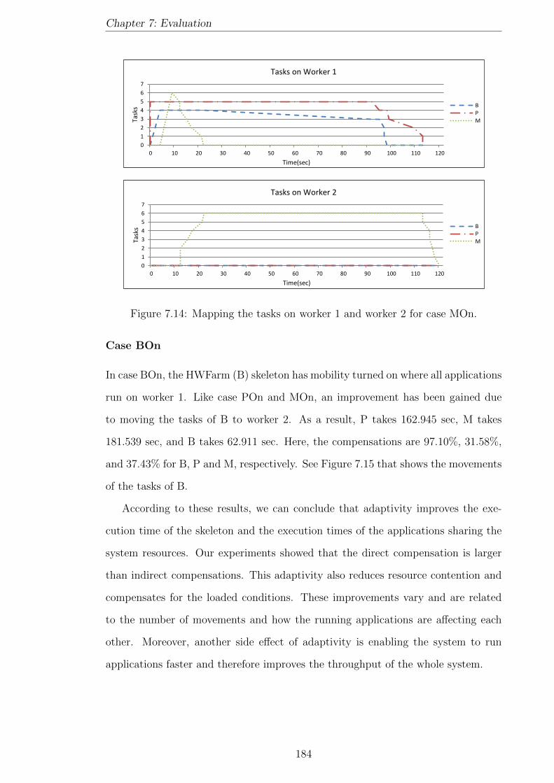
Chapter 7: Evaluation
0
1
2
3
4
5
6
7
0 10 20 30 40 50 60 70 80 90 100 110 120
Task
s
Time(sec)
Tasks on Worker 1
BP
M
0
1
2
3
4
5
6
7
0 10 20 30 40 50 60 70 80 90 100 110 120
Task
s
Time(sec)
Tasks on Worker 2
BPM
Figure 7.14: Mapping the tasks on worker 1 and worker 2 for case MOn.
Case BOn
In case BOn, the HWFarm (B) skeleton has mobility turned on where all applications
run on worker 1. Like case POn and MOn, an improvement has been gained due
to moving the tasks of B to worker 2. As a result, P takes 162.945 sec, M takes
181.539 sec, and B takes 62.911 sec. Here, the compensations are 97.10%, 31.58%,
and 37.43% for B, P and M, respectively. See Figure 7.15 that shows the movements
of the tasks of B.
According to these results, we can conclude that adaptivity improves the exe-
cution time of the skeleton and the execution times of the applications sharing the
system resources. Our experiments showed that the direct compensation is larger
than indirect compensations. This adaptivity also reduces resource contention and
compensates for the loaded conditions. These improvements vary and are related
to the number of movements and how the running applications are affecting each
other. Moreover, another side effect of adaptivity is enabling the system to run
applications faster and therefore improves the throughput of the whole system.
184
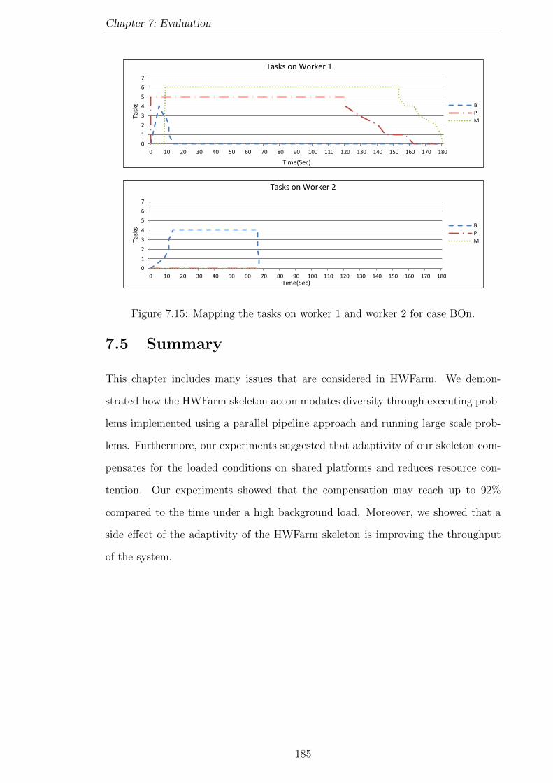
Chapter 7: Evaluation
0
1
2
3
4
5
6
7
0 10 20 30 40 50 60 70 80 90 100 110 120 130 140 150 160 170 180
Task
s
Time(Sec)
Tasks on Worker 1
B
P
M
0
1
2
3
4
5
6
7
0 10 20 30 40 50 60 70 80 90 100 110 120 130 140 150 160 170 180
Task
s
Time(Sec)
Tasks on Worker 2
B
P
M
Figure 7.15: Mapping the tasks on worker 1 and worker 2 for case BOn.
7.5 Summary
This chapter includes many issues that are considered in HWFarm. We demon-
strated how the HWFarm skeleton accommodates diversity through executing prob-
lems implemented using a parallel pipeline approach and running large scale prob-
lems. Furthermore, our experiments suggested that adaptivity of our skeleton com-
pensates for the loaded conditions on shared platforms and reduces resource con-
tention. Our experiments showed that the compensation may reach up to 92%
compared to the time under a high background load. Moreover, we showed that a
side effect of the adaptivity of the HWFarm skeleton is improving the throughput
of the system.
185

Chapter 8
Conclusion and Future Work
8.1 Summary
Multicore clusters have emerged providing high performance computing platforms
for running applications. Sharing the resources of parallel platforms amongst the ap-
plications demanding computing power leads to resource contention amongst these
applications. This thesis presents the design and implementation of a skeleton (pat-
tern) that seeks to find better locations for its computations taking into consideration
the load variation and resource contention in shared multicore clusters. This pattern
offers an efficient way to run algorithms and solve problems through exploiting par-
allel platforms when an external load is present. This pattern is implemented using
skeletal-based approach which hides parallel details to keep the developer focused
on the domain issues.
Chapter 2 provides the concepts related to parallel computing, cost modelling
and scheduling. Furthermore, a survey of skeletons and parallel programming lan-
guages that support the skeletal approach has been introduced.
Chapter 3 proposes the design and implementation of the HWFarm skeleton.
Moreover, this chapter gives a detailed description of the skeleton structure and how
it can be used to run algorithms. This skeleton is proposed in two modes: static,
where the skeleton allocates tasks to the nodes and waits until they finish their
execution, and mobile, where the skeleton can move tasks amongst locations. This
chapter explores how this mobility feature is implemented in the skeleton to enable it
186

Chapter 8: Conclusion and Future Work
to reallocate its tasks based on the system load state. This skeleton is implemented
in C and runs over distributed and shared memory architectures. To support these
architectures, we use the MPI and PThreads libraries. We also provide examples
about how to run problems using the skeleton with guidelines on how to refactor the
sequential code with following some restrictions. An example of these restrictions
is loop parallelism as the program pattern where this skeleton supports running
problems with index-based loops, outlined Sec 3.2.4.5. Moreover, the data defined
by the user should be configured and allocated in consecutive memory locations.
Also, pointers should be used in updating the output and state data. To support
mobility, there are some considerations outlined in Sec 3.2.4.4. Furthermore, we
assumed that the tasks are fixed length and the task pool is static. Also, the
skeleton does not support adding or removing resources during the runtime and the
tasks are independent with no communications. As a skeletal-based system, the
HWFarm skeleton is evaluated in meeting the principles proposed by Cole [67] and
Danelutto et al [72].
Chapter 4 introduces the dynamic, measurement-based cost model used in the
HWFarm skeleton. This cost model is embedded in the skeleton to take the costed
decisions needed for rescheduling the tasks. This model calculates the estimated
continuation times for the current tasks in the local/remote nodes. These estimates
help to find faster locations for the slow tasks. The concept used to estimate the
continuation time is based on the measurement of the partial execution of the cur-
rent tasks. Furthermore, this model calculates the mobility cost for moving a task
between two nodes. This cost considers the network delay, the task size, and the
load state of the system.
This chapter also describes in detail the parameters used by the HWFarm cost
model. There are static and dynamic parameters. The static parameters, the CPU
core clock speed and the number of cores, reflect the computing power of the nodes
that host the skeleton tasks. In this work, we assume that the cores of a node
have the same clock speed. The dynamic parameters used in the cost model are
the number of processes and the CPU utilisation. Dynamic parameters from the
187
Chapter 8: Conclusion and Future Work
running computations are also used. In the mobility cost estimation, network delay
is used as network metric.
Moreover, this chapter shows experiments on validating the decisions taken by
the HWFarm cost model. These experiments demonstrate that the cost model gives
accurate decisions under different load conditions for regular and irregular compu-
tations. In regular computations, our experiments show the accuracy of the cost
model decisions with maximum error 3%. For irregular computations, the estimates
are less accurate, as expected, with error reaching 20%. Regarding estimating the
mobility cost, the error in the estimation is ranging from 0.1% to 25% where the
actual mobility cost is relatively small.
This cost model uses these estimates to take mobility decisions. Therefore, val-
idating the mobility decisions is also investigated in this chapter. Our experiments
suggest that mobility decisions compensate for the loaded conditions by 75% and
90% for regular and irregular computations, respectively. These compensations de-
pend on the load pattern applied and the number of tasks affected by that load.
Chapter 5 proposes the load scheduler used in the HWFarm skeleton. Moreover,
this chapter explores the load information diffusion approach used in this scheduler.
In this approach, the HWFarm skeleton uses a centralised mechanism to collect the
load information of the nodes where the latest load information will be stored at the
master.
Moreover, this chapter explores the policies used to trigger the mobility oper-
ations based on estimations of remaining work. These operations are triggered by
the worker which is responsible for applying the cost model to calculate the required
estimates and to produce the move report accordingly. Then, upon confirmation,
mobility occurs for the selected tasks to the chosen workers. It is important to note
that in HWFarm, the decision making is decentralised at the workers.
Furthermore, this chapter shows experiments on validating the behaviour of the
tasks during the run-time when some nodes are highly loaded. In these experi-
ments, the current load of the nodes influences the behaviour of the tasks where the
HWFarm scheduler lightens the loaded nodes when they become loaded. Also, the
188
Chapter 8: Conclusion and Future Work
mobility performance is also validated where the compensations are ranging from
12.41% to 57.52% for regular computations and from 23.91% to 59.09% for irregular
computations. We observe that even if the accuracy of the estimates in the irregular
computations is less accurate, the mobility decisions improve the performance.
This chapter also provides an overhead analysis for all activities of the scheduler,
in the master and workers. We study the overhead of the allocation operations, load
information operations, and mobility operations. Mobility operations are expected
to be the major source of overhead but our experiments suggest that, with the worst
movement scenario, the overhead is low compared to the total execution times. As a
conclusion, the overhead of the HWFarm skeleton is not exceeding 0.58% compared
to the total execution time.
Chapter 6 presents a tool that is able to generate dynamic, precise, adaptive
pattern of load across multiple processors. This tool is implemented in C with
the MPI and PThread libraries. This tool is effective in dedicated systems for
simulating patterns of load changes. This chapter shows how this tool can be used
to help evaluating experiments that depend on changing the load on multi-processor
platforms.
Chapter 7 evaluates the HWFarm skeleton in terms of its usability, scalability
and adaptivity. In this thesis, we propose the HWFarm skeleton as a generic data-
parallel framework to run problems in parallel. In this chapter, we demonstrate how
this skeleton can run different types of problems as well as its ability to execute
algorithms implemented in the pipeline style. Moreover, large scale applications can
also be executed by the HWFarm skeleton. Furthermore, this chapter explores the
side effects of the adaptivity of the HWFarm skeleton. This adaptivity has three
side effects:
• It can produce a global load balancing where the workers try to lighten the
loaded nodes by moving tasks from the highly loaded nodes to the lightly
loaded nodes. This side effect is shown in the behaviour of the moved tasks in
Sec 5.4.1.
• For other applications running along with the skeleton, our experiments show
189

Chapter 8: Conclusion and Future Work
how the skeleton reduces resource contention in the loaded node and therefore
this enables other applications to acquire more processing power. In these
experiments, our skeleton adaptivity compensates for the loaded condition
where the compensation may reach to 92% for the other applications.
• In terms of the system, our experiments suggest that the adaptivity of our
skeleton may improve the throughput of the system.
8.2 Limitations
This section discusses the limitations of HWFarm.
8.2.1 MPI Compatible Platforms
The HWFarm skeleton works on platforms compatible with MPI. We used MPI to
facilitate mobility where all created processes have the program code. Furthermore,
this simplifies the implementation of the mobility operations between two nodes.
8.2.2 Program Pattern
The program pattern supported by the HWFarm skeleton is loop parallelism. This
pattern helps in estimating the remaining iterations when assuming that all it-
erations have similar execution time. This is somehow true when executing the
computation on the same platform with the same load state.
8.2.3 Granularity
The most effective way to exploit HWFarm is solving problems with coarse grain
granularity. This is because moving small computations that take few seconds of
execution is not efficient. Examples of these problems are: computational intensive
algorithms and big data analysis.
190

Chapter 8: Conclusion and Future Work
8.2.4 GPU Architectures
GPU architectures provide high efficient computational resources but in this work
we did not address these architectures for two reasons: the complexity of the im-
plementation; and the overhead of check-pointing and migrating data processed on
these architectures.
8.3 Future Work
8.3.1 Data Locality and Mobility
Accessing data efficiently is becoming a big challenge in managing the resources in
the parallel systems. In HWFarm, we assumed that the data is included in the task
and the task function will be executed over the local data. In some problems, the
data is too big and it is difficult to be mobilized amongst the nodes such as analysing
a huge database or extracting features from thousands of images. Mapping tasks
into computation resources over nodes is maintained by the HWFarm skeleton while
accessing the data is moved to the user’s responsibility. Then, the user has to manage
dealing with data. This issue can be solved when using distributed file system where
all nodes in the cluster can access the data transparently. But, other issues regarding
the replication and the location of the data will arise. Examples of distributed
file system are: HDFS (Hadoop Distributed File System) [124] and GFS (Google
File System) [108]. A significant future work can be developed through providing
awareness of the location of the replica that is executed by the current process. This
can be done by cooperation with the distributed data store or the distributed file
system to decide where to run the processes on the nodes where the data is located.
Then, in case of mobility, this will be considered to move only to nodes that have
the same replicas. Examples of frameworks that take into consideration the replicas
when allocating computations are Hadoop [228] and Apache Spark [137].
191
Chapter 8: Conclusion and Future Work
8.3.2 Fault Tolerance
In distributed systems, a partial failure might occur when a single machine fails
while other parts operate correctly. Fault tolerance enables the system to recover
from a failure. This is important future work for our HWFarm skeleton. The
Master/Worker model implemented in HWFarm helps to perform fault tolerance.
This can be done at the master that carries out health check operations to make
sure that all workers are running properly. If one worker fails, the master that keeps
a track of the running tasks assigns the tasks to other workers.
8.3.3 Memory and Cache
The cost model considers many parameters to be sensitive to the load state of the
hosting nodes. The memory and the cache of the host nodes are also important
metrics that can be considered to decide that the memory of the executing node is
not enough to process the task. In future work, these metrics can be addressed and
reflect the actual load state of the executing nodes.
8.3.4 New Skeletons
HWFarm offers a data-parallel skeleton on shared computing platforms with a mo-
bility feature. An important future work can be done to support other types of
skeletons: task-parallel and resolution skeletons. We showed how the HWFarm
skeleton can perform pipeline programming style but it is more efficient to embed
all low level coordination in a separate implementation. Also, a divide and conquer
skeleton is another future implementation. There are some problems that require
sharing the data in the middle of the execution. Providing a skeleton that addresses
this issue is also interesting future work.
8.3.5 Dynamic Allocation Model
In this work, we proposed a static allocation model that decides the number of
allocated tasks based on the number of cores. A future work can be developed
192

Chapter 8: Conclusion and Future Work
through making this model dynamic by taking into consideration the current load
of the nodes. Then, based on the load and the number of cores, the allocated tasks
for each worker can be identified.
193

Appendix A
Applications Source Code
This appendix presents the full C code of all applications mentioned in the thesis.
Each application calls the skeleton functions and uses the structures defined in
Section 3.2.4 to access the data in the worker nodes. The full source code can be
found in the link: https://github.com/talsalkini/hwfarm.
A.1 Square Numbers Application
1 #include <s t d i o . h>
2 #include <s t d l i b . h>
3 #include ”hwfarm . h”
4
5 void hwfarm square ( hwfarm task data∗ t data , chFM checkForMobi l i ty ){
6 int ∗ i = t data−>counter ;
7 int ∗ i max = t data−>counter max ;
8 int ∗ input p = ( int ∗) t data−>input data ;
9 int ∗output p = ( int ∗) t data−>output data ;
10 while (∗ i < ∗ i max ){
11 ∗( output p + (∗ i ) ) = (∗ ( input p + (∗ i ) ) ) ∗ (∗ ( input p + (∗ i ) ) ) ;
12 (∗ i )++;
13 checkForMobi l i ty ( ) ;
14 }
15 }
16
17 int main ( int argc , char∗∗ argv ){
18 initHWFarm( argc , argv ) ;
19 int prob l em s i z e = a to i ( argv [ 1 ] ) ;
20 int chunk = ato i ( argv [ 2 ] ) ; // number o f i t ems in one t a s k
21 int ta sks = prob l em s i z e / chunk ; //number o f t a s k s
22 int mobi l i ty = a to i ( argv [ 3 ] ) ;
23 // l o c a l i npu t data d e t a i l s
24 int ∗ input data = NULL;
25 int i n pu t da t a s i z e = s izeof ( int ) ;
26 int i npu t da ta l en = chunk ;
27 // ou tpu t data d e t a i l s
28 int ∗ output data = NULL;
29 int ou tpu t da ta s i z e = s izeof ( int ) ;
194

Appendix A. Applications Source Code
30 int output data l en = chunk ;
31 // d e t a i l s o f t h e main coun te r
32 hwfarm state main state ;
33 main state . counter = 0 ;
34 main state . max counter = chunk ;
35 main state . s t a t e da t a = NULL;
36 main state . s t a t e l e n = 0 ;
37 i f ( rank == 0){
38 // Prepare t h e inpu t data
39 input data = ( int ∗) mal loc ( s izeof ( int ) ∗( p rob l em s i z e ) ) ;
40 int j =0,k=0;
41 for ( j = 0 ; j < l en ; j++)
42 input data [ k++] = j +1;
43 // Prepare t h e ou tpu t b u f f e r
44 output data = ( int ∗) mal loc ( s izeof ( int ) ∗( l en ) ) ;
45 }
46
47 hwfarm( hwfarm square , tasks ,
48 input data , i npu t da ta s i z e , i nput data l en ,
49 NULL, 0 , 0 ,
50 output data , ou tput data s i z e , output data len ,
51 main state , mob i l i ty ) ;
52
53 i f ( rank == 0){
54 //Do someth ing w i th t h e ou tpu t
55 int i =0;
56 for ( i =0; i<prob l em s i z e ; i++)
57 p r i n t f ( ”%d\n” , ∗ ( ( int ∗) output data + ( i ) ) ) ;
58 }
59 finalizeHWFarm () ;
60 }
Listing A.1: The Square Numbers application C source code
A.2 Matrix Multiplication Application
1 #include <s t d i o . h>
2 #include <s t d l i b . h>
3 #include ”hwfarm . h”
4
5 void hwfarm mm( hwfarm task data∗ t data , chFM checkForMobi l i ty ){
6 void ∗ mat a = t data−>input data ;
7 void ∗ mat b = t data−>shared data ;
8 void ∗ r e s u l t = t data−>output data ;
9 int ∗ i = ( t data−>counter ) ;
10 int ∗ i max = ( t data−>counter max ) ;
11 int ∗ rows a = ( ( int ∗) t data−>s t a t e da t a ) ;
12 int ∗ c o l s b = ( ( int ∗) t data−>s t a t e da t a )+1;
13 int ∗mat s = ( ( int ∗) t data−>s t a t e da t a )+2;
14 int ∗ j = 0 ;
15 int ∗k = 0 ;
16 int ∗c = 0 ;
17
18 while ( (∗ i ) < (∗ i max ) ){
19 while ( (∗ j ) < (∗ c o l s b ) ){
20 ∗ ( ( (double∗) r e s u l t ) + ∗c ) = 0 ;
21 double mat res = 0 ;
22 while ( (∗ k ) < (∗mat s ) ){
195
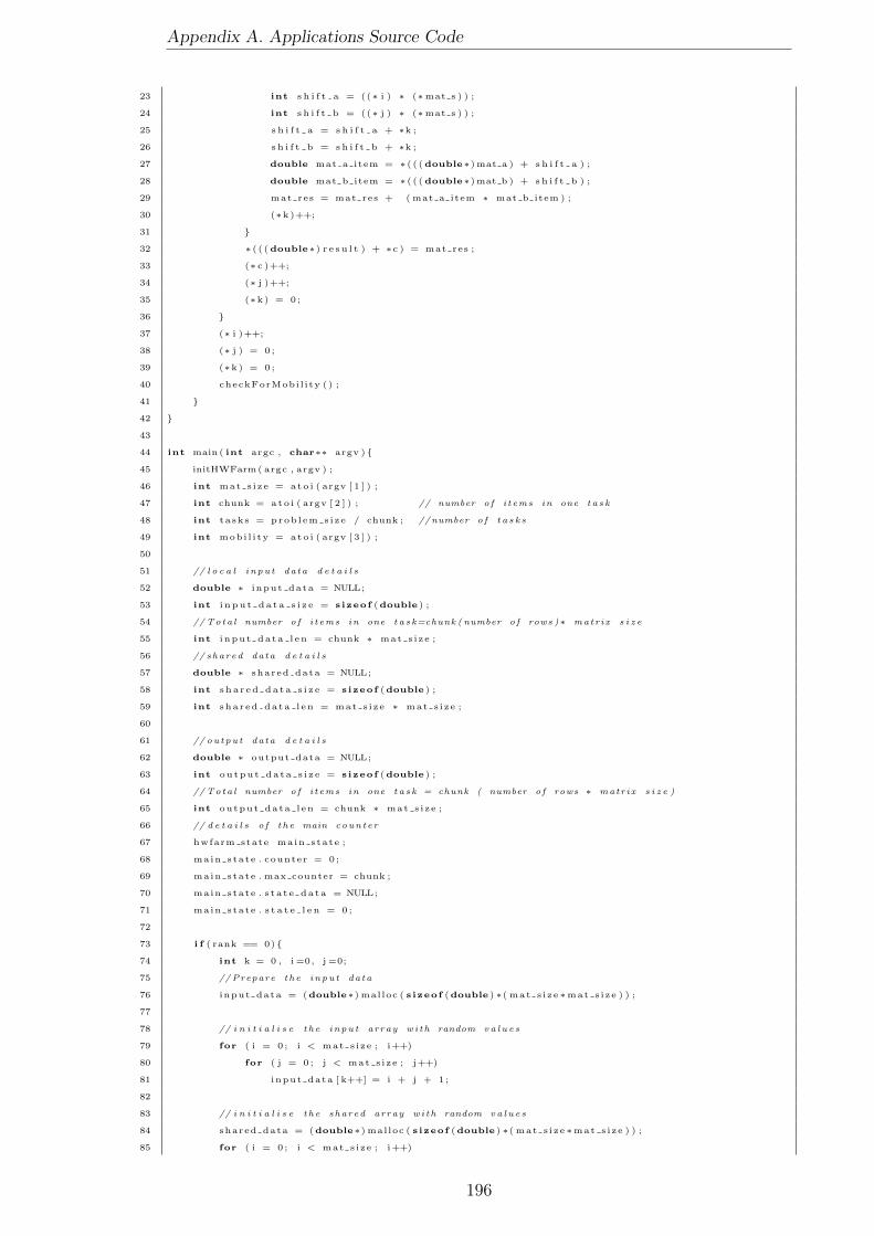
Appendix A. Applications Source Code
23 int s h i f t a = ((∗ i ) ∗ (∗mat s ) ) ;
24 int s h i f t b = ((∗ j ) ∗ (∗mat s ) ) ;
25 s h i f t a = s h i f t a + ∗k ;
26 s h i f t b = s h i f t b + ∗k ;
27 double mat a item = ∗ ( ( (double∗)mat a ) + s h i f t a ) ;
28 double mat b item = ∗ ( ( (double∗)mat b ) + s h i f t b ) ;
29 mat res = mat res + ( mat a item ∗ mat b item ) ;
30 (∗k )++;
31 }
32 ∗ ( ( (double∗) r e s u l t ) + ∗c ) = mat res ;
33 (∗ c )++;
34 (∗ j )++;
35 (∗k ) = 0 ;
36 }
37 (∗ i )++;
38 (∗ j ) = 0 ;
39 (∗k ) = 0 ;
40 checkForMobi l i ty ( ) ;
41 }
42 }
43
44 int main ( int argc , char∗∗ argv ){
45 initHWFarm( argc , argv ) ;
46 int mat s i ze = a to i ( argv [ 1 ] ) ;
47 int chunk = ato i ( argv [ 2 ] ) ; // number o f i t ems in one t a s k
48 int ta sks = prob l em s i z e / chunk ; //number o f t a s k s
49 int mobi l i ty = a to i ( argv [ 3 ] ) ;
50
51 // l o c a l i npu t data d e t a i l s
52 double ∗ input data = NULL;
53 int i n pu t da t a s i z e = s izeof (double ) ;
54 // Tota l number o f i t ems in one t a s k=chunk ( number o f rows )∗ matr ix s i z e
55 int i npu t da ta l en = chunk ∗ mat s i ze ;
56 // shared data d e t a i l s
57 double ∗ shared data = NULL;
58 int s h a r ed da t a s i z e = s izeof (double ) ;
59 int sha r ed da ta l en = mat s i ze ∗ mat s i ze ;
60
61 // ou tpu t data d e t a i l s
62 double ∗ output data = NULL;
63 int ou tpu t da ta s i z e = s izeof (double ) ;
64 // Tota l number o f i t ems in one t a s k = chunk ( number o f rows ∗ matr ix s i z e )
65 int output data l en = chunk ∗ mat s i ze ;
66 // d e t a i l s o f t h e main coun te r
67 hwfarm state main state ;
68 main state . counter = 0 ;
69 main state . max counter = chunk ;
70 main state . s t a t e da t a = NULL;
71 main state . s t a t e l e n = 0 ;
72
73 i f ( rank == 0){
74 int k = 0 , i =0, j =0;
75 // Prepare t h e inpu t data
76 input data = (double∗) mal loc ( s izeof (double ) ∗( mat s i ze ∗mat s i ze ) ) ;
77
78 // i n i t i a l i s e t h e i npu t array w i th random va l u e s
79 for ( i = 0 ; i < mat s i ze ; i++)
80 for ( j = 0 ; j < mat s i ze ; j++)
81 input data [ k++] = i + j + 1 ;
82
83 // i n i t i a l i s e t h e shared array w i th random va l u e s
84 shared data = (double∗) mal loc ( s izeof (double ) ∗( mat s i ze ∗mat s i ze ) ) ;
85 for ( i = 0 ; i < mat s i ze ; i++)
196
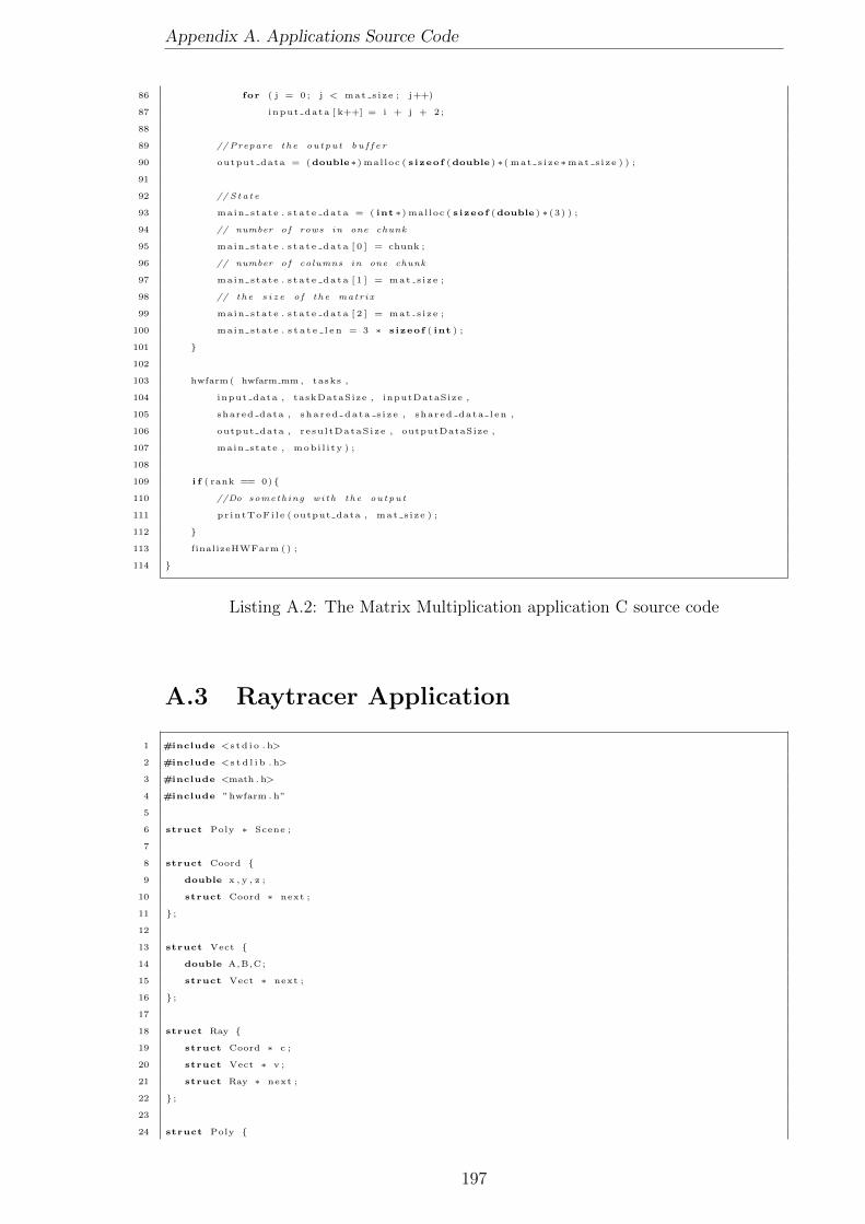
Appendix A. Applications Source Code
86 for ( j = 0 ; j < mat s i ze ; j++)
87 input data [ k++] = i + j + 2 ;
88
89 // Prepare t h e ou tpu t b u f f e r
90 output data = (double∗) mal loc ( s izeof (double ) ∗( mat s i ze ∗mat s i ze ) ) ;
91
92 // S t a t e
93 main state . s t a t e da t a = ( int ∗) mal loc ( s izeof (double ) ∗(3) ) ;
94 // number o f rows in one chunk
95 main state . s t a t e da t a [ 0 ] = chunk ;
96 // number o f columns in one chunk
97 main state . s t a t e da t a [ 1 ] = mat s i ze ;
98 // the s i z e o f t h e matr ix
99 main state . s t a t e da t a [ 2 ] = mat s i ze ;
100 main state . s t a t e l e n = 3 ∗ s izeof ( int ) ;
101 }
102
103 hwfarm( hwfarm mm , tasks ,
104 input data , taskDataSize , inputDataSize ,
105 shared data , sha r ed da ta s i z e , shared data l en ,
106 output data , r e su l tDataS i ze , outputDataSize ,
107 main state , mob i l i ty ) ;
108
109 i f ( rank == 0){
110 //Do someth ing w i th t h e ou tpu t
111 pr intToFi l e ( output data , mat s i ze ) ;
112 }
113 finalizeHWFarm () ;
114 }
Listing A.2: The Matrix Multiplication application C source code
A.3 Raytracer Application
1 #include <s t d i o . h>
2 #include <s t d l i b . h>
3 #include <math . h>
4 #include ”hwfarm . h”
5
6 struct Poly ∗ Scene ;
7
8 struct Coord {
9 double x , y , z ;
10 struct Coord ∗ next ;
11 } ;
12
13 struct Vect {
14 double A,B,C;
15 struct Vect ∗ next ;
16 } ;
17
18 struct Ray {
19 struct Coord ∗ c ;
20 struct Vect ∗ v ;
21 struct Ray ∗ next ;
22 } ;
23
24 struct Poly {
197
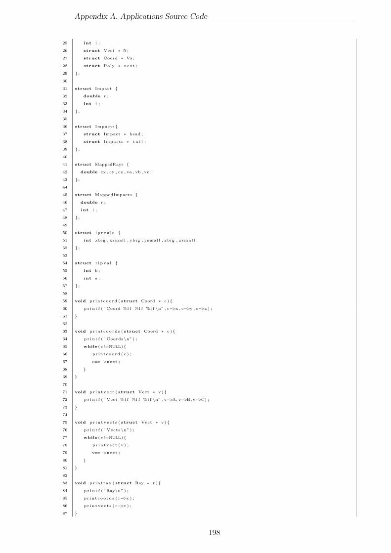
Appendix A. Applications Source Code
25 int i ;
26 struct Vect ∗ N;
27 struct Coord ∗ Vs ;
28 struct Poly ∗ next ;
29 } ;
30
31 struct Impact {
32 double r ;
33 int i ;
34 } ;
35
36 struct Impacts{
37 struct Impact ∗ head ;
38 struct Impacts ∗ t a i l ;
39 } ;
40
41 struct MappedRays {
42 double cx , cy , cz , va , vb , vc ;
43 } ;
44
45 struct MappedImpacts {
46 double r ;
47 int i ;
48 } ;
49
50 struct i p r v a l s {
51 int xbig , xsmall , ybig , ysmall , zbig , z smal l ;
52 } ;
53
54 struct r i p v a l {
55 int b ;
56 int s ;
57 } ;
58
59 void pr in tcoord ( struct Coord ∗ c ){
60 p r i n t f ( ”Coord %l f %l f %l f \n” , c−>x , c−>y , c−>z ) ;
61 }
62
63 void pr in t coo rd s ( struct Coord ∗ c ){
64 p r i n t f ( ”Coords\n” ) ;
65 while ( c !=NULL){
66 pr in tcoord ( c ) ;
67 c=c−>next ;
68 }
69 }
70
71 void pr i n tv e c t ( struct Vect ∗ v ){
72 p r i n t f ( ”Vect %l f %l f %l f \n” ,v−>A, v−>B, v−>C) ;
73 }
74
75 void p r i n t v e c t s ( struct Vect ∗ v ){
76 p r i n t f ( ”Vects\n” ) ;
77 while ( v!=NULL){
78 p r i n tv e c t (v ) ;
79 v=v−>next ;
80 }
81 }
82
83 void pr in t ray ( struct Ray ∗ r ){
84 p r i n t f ( ”Ray\n” ) ;
85 pr in t coo rd s ( r−>c ) ;
86 p r i n t v e c t s ( r−>v ) ;
87 }
198
Appendix A. Applications Source Code
88
89 void pr in t r ay s ( struct Ray ∗ r ){
90 int i =0;
91 while ( r !=NULL){
92 p r i n t f ( ” i :%d − ” , i++) ;
93 pr in t ray ( r ) ;
94 r=r−>next ;
95 }
96 }
97
98 void pr in tpo ly ( struct Poly ∗ p){
99 p r i n t f ( ”Poly %d\n” ,p−>i ) ;
100 pr in t coo rd s (p−>Vs) ;
101 p r i n t v e c t s (p−>N) ;
102 }
103
104 void pr i n tpo l y s ( struct Poly ∗ p){
105 p r i n t f ( ”Polys\n” ) ;
106 while (p!=NULL){
107 pr in tpo ly (p) ;
108 p=p−>next ;
109 }
110 }
111
112 void pr int impact ( struct Impact ∗ i ){
113 i f ( i==NULL)
114 p r i n t f ( ”No impact\n” ) ;
115 else
116 p r i n t f ( ” Impact %l f %d\n” , i−>r , i−>i ) ;
117 }
118
119 void pr int impacts ( struct Impacts ∗ i ){
120 p r i n t f ( ” Impacts\n” ) ;
121 while ( i !=NULL){
122 pr int impact ( i−>head ) ;
123 i=i−>t a i l ;
124 }
125 }
126
127 void p r i n t r i p v a l ( struct r i p v a l ∗ r ){
128 p r i n t f ( ”%d %d\n” , r−>b , r−>s ) ;
129 }
130
131 struct MappedRays ∗ mapRays( struct Ray ∗ rays , int raysCount ){
132 struct MappedRays ∗ m rays = ( struct MappedRays ∗) mal loc ( raysCount ∗ s izeof ( struct MappedRays
) ) ;
133 int i =0;
134 struct Ray ∗ r = rays ;
135 while ( r != NULL && i < raysCount ){
136 m rays [ i ] . cx = r−>c−>x ;
137 m rays [ i ] . cy = r−>c−>y ;
138 m rays [ i ] . cz = r−>c−>z ;
139 m rays [ i ] . va = r−>v−>A;
140 m rays [ i ] . vb = r−>v−>B;
141 m rays [ i ] . vc = r−>v−>C;
142 r=r−>next ;
143 i++;
144 }
145 return m rays ;
146 }
147
148 void mapImpactsItem ( struct MappedImpacts ∗ m imps , struct Impacts ∗ imp , int impsIndex ){
149 i f ( imp−>head != NULL){
199

Appendix A. Applications Source Code
150 m imps [ impsIndex ] . r = imp−>head−>r ;
151 m imps [ impsIndex ] . i = imp−>head−>i ;
152 } else {
153 m imps [ impsIndex ] . r = −1;
154 m imps [ impsIndex ] . i = −1;
155 }
156 }
157
158 void mapImpacts ( struct MappedImpacts ∗ m imps , struct Impacts ∗ imps , int impsCount ){
159 int j =0;
160 struct Impacts ∗ imp = imps ;
161 while ( imp != NULL && j < impsCount ){
162 mapImpactsItem (m imps , imp , j ) ;
163 imp = imp−>t a i l ;
164 j++;
165 }
166 }
167
168 struct Ray ∗ unmapRays ( struct MappedRays ∗ m rays , int raysCount ){
169 int i =0;
170 struct Ray ∗ rays = NULL;
171 struct Ray ∗ r = rays ;
172 while ( i < raysCount ){
173 i f ( r != NULL){
174 r−>next = ( struct Ray ∗) mal loc ( s izeof ( struct Ray) ) ;
175 r = r−>next ;
176 } else{
177 rays = ( struct Ray ∗) mal loc ( s izeof ( struct Ray) ) ;
178 r = rays ;
179 }
180
181 r−>c = ( struct Coord ∗) mal loc ( s izeof ( struct Coord ) ) ;
182 r−>c−>x = m rays [ i ] . cx ;
183 r−>c−>y = m rays [ i ] . cy ;
184 r−>c−>z = m rays [ i ] . cz ;
185 r−>c−>next = NULL;
186 r−>v = ( struct Vect ∗) mal loc ( s izeof ( struct Vect ) ) ;
187 r−>v−>A = m rays [ i ] . va ;
188 r−>v−>B = m rays [ i ] . vb ;
189 r−>v−>C = m rays [ i ] . vc ;
190 r−>v−>next = NULL;
191 r−>next = NULL;
192 i++;
193 }
194 return rays ;
195 }
196
197
198 struct Impacts ∗ unmapImpacts ( struct MappedImpacts ∗ m imps , int impsCount ){
199 int j =0;
200 struct Impacts ∗ imps = NULL;
201 struct Impacts ∗ imp = imps ;
202 while ( j < impsCount ){
203 i f ( imps != NULL){
204 imp−>t a i l = ( struct Impacts ∗) mal loc ( s izeof ( struct Impacts ) ) ;
205 imp = imp−>t a i l ;
206 } else{
207 imps = ( struct Impacts ∗) mal loc ( s izeof ( struct Impacts ) ) ;
208 imp = imps ;
209 }
210 i f (m imps [ j ] . r != −1 && m imps [ j ] . i != −1){
211 imp−>head = ( struct Impact ∗) mal loc ( s izeof ( struct Impact ) ) ;
212 imp−>head−>r = m imps [ j ] . r ;
200

Appendix A. Applications Source Code
213 imp−>head−>i = m imps [ j ] . i ;
214 } else
215 imp−>head = NULL;
216
217 imp−>t a i l = NULL;
218 j++;
219 }
220 return imps ;
221 }
222
223 void printMappedRays ( struct MappedRays ∗ m rays , int raysCount ){
224 int i =0;
225 while ( i < raysCount ){
226 p r i n t f ( ”Ray %d :\n” , ( i +1) ) ;
227 p r i n t f ( ”CX: %f , CY: %f . CZ: %f , VA: %f , VB: %f , VC: %f \n” ,
228 m rays [ i ] . cx , m rays [ i ] . cy , m rays [ i ] . cz , m rays [ i ] . va , m rays [ i ] . vb , m rays [ i ] . vc ) ;
229 i++;
230 }
231 }
232
233 struct Coord ∗ copyCoords ( struct Coord ∗ c ){
234 i f ( c == NULL)
235 return NULL;
236 struct Coord ∗ new c = NULL;
237 struct Coord ∗ new c h = new c ;
238 while ( c != NULL){
239 i f ( new c == NULL){
240 new c = ( struct Coord ∗) mal loc ( s izeof ( struct Coord ) ) ;
241 new c h = new c ;
242 } else{
243 new c h−>next = ( struct Coord ∗) mal loc ( s izeof ( struct Coord ) ) ;
244 new c h = new c h−>next ;
245 }
246 new c h−>x = c−>x ;
247 new c h−>y = c−>y ;
248 new c h−>z = c−>z ;
249 new c h−>next = NULL;
250 c=c−>next ;
251 }
252 return new c ;
253 }
254
255 struct Vect ∗ copyVects ( struct Vect ∗ v ){
256 i f ( v == NULL)
257 return NULL;
258 struct Vect ∗ new v = NULL;
259 struct Vect ∗ new v h = new v ;
260 while ( v != NULL){
261 i f ( new v == NULL){
262 new v = ( struct Vect ∗) mal loc ( s izeof ( struct Vect ) ) ;
263 new v h = new v ;
264 } else{
265 new v h−>next = ( struct Vect ∗) mal loc ( s izeof ( struct Vect ) ) ;
266 new v h = new v h−>next ;
267 }
268 new v h−>A = v−>A;
269 new v h−>B = v−>B;
270 new v h−>C = v−>C;
271 new v h−>next = NULL;
272 v=v−>next ;
273 }
274 return new v ;
275 }
201

Appendix A. Applications Source Code
276
277 struct Poly ∗ copyPolys ( struct Poly ∗ p){
278 i f (p == NULL)
279 return NULL;
280 struct Poly ∗ new p = NULL;
281 struct Poly ∗ new p h = NULL;
282
283 while (p != NULL){
284 i f ( new p == NULL){
285 new p = ( struct Poly ∗) mal loc ( s izeof ( struct Poly ) ) ;
286 new p h = new p ;
287 } else{
288 new p h−>next = ( struct Poly ∗) mal loc ( s izeof ( struct Poly ) ) ;
289 new p h = new p h−>next ;
290 }
291 new p h−>i = p−>i ;
292 new p h−>Vs = copyCoords (p−>Vs) ;
293 new p h−>N = copyVects (p−>N) ;
294 p=p−>next ;
295 }
296 return new p ;
297 }
298
299 void p r i n t i p r v a l s ( struct i p r v a l s ∗ i ){
300 p r i n t f ( ”%d %d %d %d %d %d\n” , i−>xbig , i−>xsmall , i−>ybig ,
301 i−>ysmall , i−>zbig , i−>zsmal l ) ;
302 }
303
304 struct i p r v a l s ∗ i n po l y r ange (double p , double q ,
305 double r , struct Coord ∗Vs){
306 struct i p r v a l s ∗ r e s u l t s ;
307 r e s u l t s =(struct i p r v a l s ∗) mal loc ( s izeof ( struct i p r v a l s ) ) ;
308 r e s u l t s−>xbig=1;
309 r e s u l t s−>xsmal l =1;
310 r e s u l t s−>ybig=1;
311 r e s u l t s−>ysmal l =1;
312 r e s u l t s−>zb ig =1;
313 r e s u l t s−>zsmal l =1;
314 while (Vs!=NULL){
315 r e s u l t s−>xbig=r e su l t s−>xbig && p>Vs−>x+1E−8;
316 r e s u l t s−>xsmal l=r e su l t s−>xsmal l && p<Vs−>x−1E−8;
317 r e s u l t s−>ybig=r e su l t s−>ybig && q>Vs−>y+1E−8;
318 r e s u l t s−>ysmal l=r e su l t s−>ysmal l && q<Vs−>y−1E−8;
319 r e s u l t s−>zb ig=r e su l t s−>zb ig && r>Vs−>z+1E−8;
320 r e s u l t s−>zsmal l=r e su l t s−>zsmal l && r<Vs−>z−1E−8;
321 Vs=Vs−>next ;
322 }
323 return r e s u l t s ;
324 }
325
326 int c r o s s d o t s i g n (double a , double b , double c , double d , double e ,
327 double f , double A, double B, double C){
328 double P,Q,R, cd ;
329 P=b∗ f−e∗c ;
330 Q=d∗c−a∗ f ;
331 R=a∗e−d∗b ;
332 cd=P∗A+Q∗B+R∗C;
333 i f ( cd<0.0)
334 return −1;
335 else
336 return 1 ;
337 }
338
202

Appendix A. Applications Source Code
339 struct r i p v a l ∗ r e a l l y i n p o l y (double p , double q , double r , double A,
340 double B, double C, struct Coord ∗ Vs){
341 struct r i p v a l ∗ r e s u l t s ;
342 int s1 ;
343 i f (Vs−>next−>next==NULL){
344 r e s u l t s =(struct r i p v a l ∗) mal loc ( s izeof ( struct r i p v a l ) ) ;
345 r e s u l t s−>b=1;
346 r e s u l t s−>s=c r o s s d o t s i g n (Vs−>next−>x−p ,Vs−>next−>y−q , Vs−>next−>z−r ,
347 Vs−>next−>x−Vs−>x , Vs−>next−>y−Vs−>y ,
348 Vs−>next−>z−Vs−>z ,A,B,C) ;
349 return r e s u l t s ;
350 }
351 r e s u l t s=r e a l l y i n p o l y (p , q , r ,A,B,C,Vs−>next ) ;
352 i f ( r e s u l t s−>b){
353 s1=c r o s s d o t s i g n (Vs−>next−>x−p ,Vs−>next−>y−q , Vs−>next−>z−r ,
354 Vs−>next−>x−Vs−>x , Vs−>next−>y−Vs−>y ,
355 Vs−>next−>z−Vs−>z ,A,B,C) ;
356 i f ( s1==re su l t s−>s ){
357 r e s u l t s−>b=1;
358 r e s u l t s−>s=s1 ;
359 } else{
360 r e s u l t s−>b=0;
361 r e s u l t s−>s=0;
362 }
363 }
364 return r e s u l t s ;
365 }
366
367 int i n p o l y t e s t (double p , double q , double r , double A,
368 double B, double C, struct Coord ∗ Vs){
369 struct i p r v a l s ∗ i p rcheck ;
370 struct r i p v a l ∗ r ipcheck ;
371 iprcheck = in po l y r ange (p , q , r , Vs) ;
372 i f ( iprcheck−>xbig | | iprcheck−>xsmal l | |
373 iprcheck−>ybig | | iprcheck−>ysmal l | |
374 iprcheck−>zb ig | | iprcheck−>zsmal l ){
375 f r e e ( ip rcheck ) ;
376 return 0 ;
377 }
378 r ipcheck=r e a l l y i n p o l y (p , q , r ,A,B,C, Vs) ;
379 int b = ripcheck−>b ;
380 f r e e ( r ipcheck ) ;
381 return b ;
382 }
383
384 void TestForImpact ( struct Ray ∗ ray , struct Poly ∗ poly , struct Impact ∗ imp){
385 double px , py , pz ;
386 double u , v ,w, l ,m, n ;
387 double d i s tance ;
388 double p , q , r ;
389 u=ray−>c−>x ;
390 v=ray−>c−>y ;
391 w=ray−>c−>z ;
392 l=ray−>v−>A;
393 m=ray−>v−>B;
394 n=ray−>v−>C;
395 px=poly−>Vs−>x ;
396 py=poly−>Vs−>y ;
397 pz=poly−>Vs−>z ;
398 d i s t ance=(poly−>N−>A∗(px−u)+poly−>N−>B∗(py−v )+poly−>N−>C∗( pz−w) ) /
399 ( poly−>N−>A∗ l+poly−>N−>B∗m+poly−>N−>C∗n) ;
400 p=u+d i s tance ∗ l ;
401 q=v+di s tance ∗m;
203

Appendix A. Applications Source Code
402 r=w+di s tance ∗n ;
403 i f ( ! i n p o l y t e s t (p , q , r , poly−>N−>A, poly−>N−>B, poly−>N−>C, poly−>Vs) ){
404 imp−>r = −1;
405 imp−>i = −1;
406 } else {
407 imp−>r=d i s t ance ;
408 imp−>i=poly−>i ;
409 }
410 }
411
412 void e a r l i e r ( struct Impact ∗ currentImpact , struct Impact ∗ newImpact ){
413 i f ( currentImpact−>r != −1 && newImpact−>r != −1){
414 i f ( currentImpact−>r > newImpact−>r ){
415 currentImpact−>r = newImpact−>r ;
416 currentImpact−>i = newImpact−>i ;
417 }
418 }
419 i f ( currentImpact−>r == −1 && newImpact−>r != −1){
420 currentImpact−>r = newImpact−>r ;
421 currentImpact−>i = newImpact−>i ;
422 }
423 }
424
425 struct Impact ∗ i n s e r t ( struct Impacts ∗ i ){
426 struct Impact ∗ e = NULL;
427 while ( i != NULL){
428 e a r l i e r ( i−>head , e ) ;
429 i = i−>t a i l ;
430 }
431 i f ( e == NULL)
432 return NULL;
433 else{
434 struct Impact ∗ i e ;
435 i e=(struct Impact ∗) mal loc ( s izeof ( struct Impact ) ) ;
436 ie−>r=e−>r ;
437 ie−>i=e−>i ;
438 return i e ;
439 }
440 }
441
442 struct Impact ∗ First Impact ( struct Poly ∗ os , struct Ray ∗ r ){
443 i f ( os==NULL)
444 return NULL;
445 struct Poly ∗ o = os ;
446 struct Impact∗ currentImpact = ( struct Impact ∗) mal loc ( s izeof ( struct Impact ) ) ;
447 struct Impact∗ newImpact = ( struct Impact ∗) mal loc ( s izeof ( struct Impact ) ) ;
448 TestForImpact ( r , o , currentImpact ) ;
449 o = o−>next ;
450
451 while ( o != NULL){
452 TestForImpact ( r , o , newImpact ) ;
453 e a r l i e r ( currentImpact , newImpact ) ;
454 o = o−>next ;
455 }
456 return currentImpact ;
457 }
458
459 double root (double x , double r ){
460 i f (x<0.00000001 && −0.00000001<x )
461 return 0 . 0 ;
462 while ( fabs ( ( r∗r−x ) /x ) >=0.0000001)
463 r=(r+x/ r ) / 2 . 0 ;
464 return r ;
204

Appendix A. Applications Source Code
465 }
466
467 struct Vect ∗ VAdd( struct Vect ∗ v1 , struct Vect ∗ v2 ){
468 struct Vect ∗ v ;
469 v=(struct Vect ∗) mal loc ( s izeof ( struct Vect ) ) ;
470 v−>A=v1−>A+v2−>A;
471 v−>B=v1−>B+v2−>B;
472 v−>C=v1−>C+v2−>C;
473 return v ;
474 }
475
476 struct Vect ∗ VMult (double n , struct Vect ∗ v1 ){
477 struct Vect ∗ v ;
478 v=(struct Vect ∗) mal loc ( s izeof ( struct Vect ) ) ;
479 v−>A=n∗v1−>A;
480 v−>B=n∗v1−>B;
481 v−>C=n∗v1−>C;
482 return v ;
483 }
484
485 struct Vect ∗ r ay po in t s ( int i , int j , int Detai l , struct Vect ∗ v ,
486 struct Vect ∗ Vx, struct Vect ∗ Vy){
487 struct Vect ∗ iVx ,∗ jVy ,∗ newv ;
488 i f ( j==Deta i l )
489 return NULL;
490 i f ( i==Deta i l )
491 return r ay po in t s (0 , j +1,Deta i l , v ,Vx ,Vy) ;
492 iVx=VMult ( ( ( double ) i ) / ( (double ) ( Deta i l −1) ) ,Vx) ;
493 jVy=VMult ( ( ( double ) j ) / ( (double ) ( Deta i l −1) ) ,Vy) ;
494 newv=VAdd(VAdd(v , iVx ) , jVy ) ;
495 newv−>next=ray po in t s ( i +1, j , Deta i l , v ,Vx ,Vy) ;
496 return newv ;
497 }
498
499 struct Ray ∗ GenerateRays ( int Det , double X, double Y, double Z){
500 double d ;
501 double Vza ,Vzb , Vzc ;
502 double ab ;
503 double ya , yb , yc ;
504 double y s i z e ;
505 struct Vect ∗ v ;
506 struct Vect ∗ rps ,∗ VX,∗ VY;
507 struct Ray ∗ newrays ,∗ t ;
508 d=root (X∗X+Y∗Y+Z∗Z , 1 . 0 ) ;
509 Vza=(−4.0∗X/d) ; Vzb=(−4.0∗Y/d) ; Vzc=(−4.0∗Z/d) ;
510 ab=root (Vza∗Vza+Vzb∗Vzb , 1 . 0 ) ;
511 VX=(struct Vect ∗) mal loc ( s izeof ( struct Vect ) ) ;
512 VX−>A=Vzb/ab ;VX−>B=(−Vza/ab ) ;VX−>C=0.0;
513 ya=Vzb∗VX−>C−VX−>B∗Vzc ;
514 yb=VX−>A∗Vzc−Vza∗VX−>C;
515 yc=Vza∗VX−>B−VX−>A∗Vzb ;
516 y s i z e=root ( ya∗ya+yb∗yb+yc∗yc , 1 . 0 ) ;
517 VY=(struct Vect ∗) mal loc ( s izeof ( struct Vect ) ) ;
518 VY−>A=ya/ y s i z e ;VY−>B=yb/ y s i z e ;VY−>C=yc/ y s i z e ;
519 i f (VY−>C>0.0){
520 VX−>A=(−VX−>A) ;VX−>B=(−VX−>B) ;VX−>C=(−VX−>C) ;
521 VY−>A=(−VY−>A) ;VY−>B=(−VY−>B) ;VY−>C=(−VY−>C) ;
522 }
523
524 v=(struct Vect ∗) mal loc ( s izeof ( struct Vect ) ) ;
525 v−>A=X+Vza−(VX−>A+VY−>A) /2 . 0 ;
526 v−>B=Y+Vzb−(VX−>B+VY−>B) / 2 . 0 ;
527 v−>C=Z+Vzc−(VX−>C+VY−>C) /2 . 0 ;
205

Appendix A. Applications Source Code
528 rps=ray po in t s (0 ,0 , Det , v ,VX,VY) ;
529
530 i f ( rps==NULL)
531 return NULL;
532 newrays=(struct Ray ∗) mal loc ( s izeof ( struct Ray) ) ;
533 newrays−>c=(struct Coord ∗) mal loc ( s izeof ( struct Coord ) ) ;
534 newrays−>c−>x=X;
535 newrays−>c−>y=Y;
536 newrays−>c−>z=Z ;
537 newrays−>v=(struct Vect ∗) mal loc ( s izeof ( struct Vect ) ) ;
538 newrays−>v−>A=rps−>A−X;
539 newrays−>v−>B=rps−>B−Y;
540 newrays−>v−>C=rps−>C−Z ;
541 t=newrays ;
542 rps=rps−>next ;
543
544 while ( rps !=NULL){
545 t−>next=(struct Ray ∗) mal loc ( s izeof ( struct Ray) ) ;
546 t=t−>next ;
547 t−>c=(struct Coord ∗) mal loc ( s izeof ( struct Coord ) ) ;
548 t−>c−>x=X;
549 t−>c−>y=Y;
550 t−>c−>z=Z ;
551 t−>v=(struct Vect ∗) mal loc ( s izeof ( struct Vect ) ) ;
552 t−>v−>A=rps−>A−X;
553 t−>v−>B=rps−>B−Y;
554 t−>v−>C=rps−>C−Z ;
555 rps=rps−>next ;
556 }
557 t−>next=NULL;
558 return newrays ;
559 }
560
561 void showimps ( int dv , int i , struct Impacts ∗ imps ){
562 FILE ∗ f r e s = fopen ( ” f i n a lR e s u l t . txt ” , ”w” ) ;
563 while ( imps != NULL){
564 i f ( i==0){
565 f p r i n t f ( f r e s , ”\n” ) ;
566 i=dv ;
567 }
568 i f ( imps−>head == NULL){
569 f p r i n t f ( f r e s , ”%2c” , ’ . ’ ) ;
570 } else{
571 f p r i n t f ( f r e s , ”%2d” , imps−>head−>i ) ;
572 }
573 f p r i n t f ( f r e s , ” ” ) ;
574 i=i −1;
575 imps=imps−>t a i l ;
576 }
577 f p r i n t f ( f r e s , ”\n” ) ;
578 f c l o s e ( f r e s ) ;
579 }
580
581 struct Poly ∗ getPoly (FILE ∗ s c e n e f i l e , int id ){
582 struct Poly ∗ p ;
583 struct Coord ∗ t ;
584 p=(struct Poly ∗) mal loc ( s izeof ( struct Poly ) ) ;
585 p−>i=id ;
586 p−>N=(struct Vect ∗) mal loc ( s izeof ( struct Vect ) ) ;
587 int numOfI = −1;
588 numOfI = f s c an f ( s c e n e f i l e , ”%l f %l f %l f ” ,&(p−>N−>A) ,&(p−>N−>B) ,&(p−>N−>C) ) ;
589 numOfI = f s c an f ( s c e n e f i l e , ”%d”,& id ) ;
590 p−>Vs=(struct Coord ∗) mal loc ( s izeof ( struct Coord ) ) ;
206

Appendix A. Applications Source Code
591 t=p−>Vs ;
592 numOfI = f s c an f ( s c e n e f i l e , ”%l f %l f %l f ” ,&( t−>x ) ,&( t−>y ) ,&( t−>z ) ) ;
593 t=p−>Vs ;
594 while(−− id ){
595 t−>next=(struct Coord ∗) mal loc ( s izeof ( struct Coord ) ) ;
596 t=t−>next ;
597 numOfI = f s c an f ( s c e n e f i l e , ”%l f %l f %l f ” ,&( t−>x ) ,&( t−>y ) ,&( t−>z ) ) ;
598 }
599 t−>next=NULL;
600 return p ;
601 }
602
603 struct Poly ∗ getScene ( char ∗ s c ene f i l e name , int l im i t ){
604 FILE ∗ s c e n e f i l e = fopen ( s c ene f i l e name , ” r ” ) ;
605 i f ( s c e n e f i l e == NULL){
606 p r i n t f ( ”can ’ t open %s\n” , s c en e f i l e n ame ) ;
607 e x i t (0 ) ;
608 }
609
610 struct Poly ∗ s ,∗ t ;
611 int id ;
612 i f ( f s c a n f ( s c e n e f i l e , ”%d”,& id ) == EOF){
613 f c l o s e ( s c e n e f i l e ) ;
614 return NULL;
615 }
616 s = getPoly ( s c e n e f i l e , id ) ;
617 t=s ;
618 int i =0;
619 while ( f s c a n f ( s c e n e f i l e , ”%d”,& id ) != EOF){
620 i f ( l im i t <= i++)
621 break ;
622 t−>next = getPoly ( s c e n e f i l e , id ) ;
623 t = t−>next ;
624 }
625 t−>next = NULL;
626 f c l o s e ( s c e n e f i l e ) ;
627 return s ;
628 }
629
630 void hwfarm rt ( hwfarm task data∗ t data , chFM checkForMobi l i ty ){
631 struct Ray ∗ rays = unmapRays( t data−>input data , t data−>i npu t l en ) ;
632 i f ( rays==NULL)
633 return ;
634 //Get t h e coun te r v a l u e
635 int ∗main index = ( t data−>counter ) ;
636 //The head o f t h e imapct array
637 struct Impacts ∗ imps = NULL;
638 // An a u x i l i a r y p o i n t e r
639 struct Impacts ∗ t = imps ;
640 int i =0;
641 // Nav i ga t e to t h e unproces sed ray ( to c on s i d e r t h e moved t a s k s )
642 while ( rays !=NULL && i < ∗main index ){
643 rays=rays−>next ;
644 i++;
645 }
646 while ( rays !=NULL){
647 i f ( imps == NULL){
648 imps = ( struct Impacts ∗) mal loc ( s izeof ( struct Impacts ) ) ;
649 t = imps ;
650 } else{
651 t−>t a i l =(struct Impacts ∗) mal loc ( s izeof ( struct Impacts ) ) ;
652 t=t−>t a i l ;
653 }
207

Appendix A. Applications Source Code
654 t−>head = First Impact ( Scene , rays ) ;
655 rays=rays−>next ;
656 mapImpactsItem ( t data−>output data , t , ∗main index ) ;
657 ∗main index = (∗main index ) + 1 ;
658 checkForMobi l i ty ( ) ;
659 }
660 t−>t a i l=NULL;
661 }
662
663 int main ( int argc , char∗∗ argv ){
664 initHWFarm( argc , argv ) ;
665
666 // De t a i l s r e f e r s to t h e number o f rays in one dimension
667 int Deta i l s = a to i ( argv [ 1 ] ) ;
668 int chunk = ato i ( argv [ 2 ] ) ;
669 char∗ s c e n e f i l e = ( argv [ 3 ] ) ;
670 int s c e n e l im i t = a to i ( argv [ 4 ] ) ;
671 int mobi l i ty = a to i ( argv [ 5 ] ) ;
672 int prob l em s i z e = Deta i l s ∗ Deta i l s ;
673 int ta sks = prob l em s i z e / chunk ;
674 f loat ViewX = 10 . 0 ;
675 f loat ViewY = 10 . 0 ;
676 f loat ViewZ = 10 . 0 ;
677 // inpu t
678 void ∗ input data = NULL;
679 int i n pu t da t a s i z e = s izeof ( struct MappedRays ) ;
680 int i npu t da ta l en = chunk ;
681 // ou tpu t
682 void ∗ output data = NULL;
683 int ou tpu t da ta s i z e = s izeof ( struct MappedImpacts ) ;
684 int output data l en = chunk ;
685 hwfarm state main state ;
686 main state . counter = 0 ;
687 main state . max counter = chunk ;
688 main state . s t a t e da t a = NULL;
689 main state . s t a t e l e n = 0 ;
690 i f ( rank == 0){
691 // Inpu t data
692 struct Ray ∗ rays ;
693 rays=GenerateRays ( Deta i l s , ViewX ,ViewY , ViewZ) ;
694 struct MappedRays ∗ mapped rays ;
695 mapped rays = mapRays( rays , De ta i l s ∗Deta i l s ) ;
696 input data = mapped rays ;
697 //Output Data
698 output data = malloc ( ou tpu t da ta s i z e ∗ prob l em s i z e ) ;
699 } else{
700 Scene = getScene ( s c e n e f i l e , s c e n e l im i t ) ;
701 }
702
703 hwfarm( hwfarm rt , tasks ,
704 input data , i npu t da ta s i z e , i nput data l en ,
705 NULL, 0 , 0 ,
706 output data , ou tput data s i z e , output data len ,
707 main state , mob i l i ty ) ;
708
709 i f ( rank == 0){
710 struct Impacts ∗ new imps = unmapImpacts ( output data , p rob l em s i z e ) ;
711 // Pr in t impact to a f i l e
712 showimps ( Deta i l s , Deta i l s , new imps ) ;
713 }
714
715 finalizeHWFarm () ;
716 return 1 ;
208

Appendix A. Applications Source Code
717 }
Listing A.3: The Raytracer application C source code
A.4 Molecular Dynamics Application
1 #include <s t d i o . h>
2 #include <s t d l i b . h>
3 #include <math . h>
4 #include ”hwfarm . h”
5
6 #define N 100000
7 #define G 6.673 e−11
8 #define TIMESTAMP 1e11
9
10 struct Pa r t i c l e {
11 double rx , ry ; // p o s i t i o n components
12 double vx , vy ; // v e l o c i t y components
13 double fx , fy ; // f o r c e components
14 double mass ; //mass o f t h e p a r t i c l e
15 } ;
16
17 struct Pa r t i c l e Update ( struct Pa r t i c l e p , double timestamp ){
18 p . vx += timestamp∗p . fx / p . mass ;
19 p . vy += timestamp∗p . fy / p . mass ;
20 p . rx += timestamp∗p . vx ;
21 p . ry += timestamp∗p . vy ;
22 return p ;
23 }
24
25 void Pr i n tPa r t i c l e ( struct Pa r t i c l e p){
26 p r i n t f ( ”[%d ] . %f \n%f \n%f \n%f \n%f \n%f \n%f \n\n” , rank , p . rx , p . ry , p . vx , p . vy , p . fx , p . fy , p . mass ) ;
27 }
28
29 struct Pa r t i c l e CopyPart ic le ( struct Pa r t i c l e p to , struct Pa r t i c l e p from ){
30 p to . fx = p from . fx ;
31 p to . fy = p from . fy ;
32 p to . rx = p from . rx ;
33 p to . ry = p from . ry ;
34 p to . vx = p from . vx ;
35 p to . vy = p from . vy ;
36 p to . mass = p from . mass ;
37 return p to ;
38 }
39
40 // Reset t h e f o r c e s on p a r t i c l e
41 struct Pa r t i c l e ResetForce ( struct Pa r t i c l e p){
42 p . fx = 0 . 0 ;
43 p . fy = 0 . 0 ;
44 return p ;
45 }
46
47 //Add f o r c e to p a r t i c l e a by p a r t i c l e b
48 struct Pa r t i c l e AddForce ( struct Pa r t i c l e a , struct Pa r t i c l e b){
49 //To avo id i n f i n i t i e s
50 double EPS = 3E4 ;
51 double dx = b . rx − a . rx ;
52 double dy = b . ry − a . ry ;
209

Appendix A. Applications Source Code
53 double d i s t = sq r t (dx∗dx + dy∗dy ) ;
54 double F = (G ∗ a . mass ∗ b . mass ) / ( d i s t ∗ d i s t + EPS∗EPS) ;
55 a . fx += F ∗ dx / d i s t ;
56 a . fy += F ∗ dy / d i s t ;
57 return a ;
58 }
59
60 void hwfarm nbody ( hwfarm task data∗ t data , chFM checkForMobi l i ty ){
61 int ∗ i = t data−>counter ;
62 int ∗ i max = t data−>counter max ;
63 int sha r ed l en = t data−>sha r ed l en ;
64 int c u r i = 0 , j = 0 ;
65 struct Pa r t i c l e ∗ shared p = ( struct Pa r t i c l e ∗) t data−>shared data ;
66 struct Pa r t i c l e ∗output p = ( struct Pa r t i c l e ∗) t data−>output data ;
67 while (∗ i < ∗ i max ){
68 c u r i = (∗ i ) + (∗ ( t data−>counter max ) ∗ t data−>t a s k i d ) ;
69 output p [∗ i ] = CopyPart ic le ( output p [∗ i ] , shared p [ c u r i ] ) ;
70 output p [∗ i ] = ResetForce ( output p [∗ i ] ) ;
71 for ( j = 0 ; j < sha r ed l en ; j++){
72 i f ( c u r i != j ){
73 output p [∗ i ] = AddForce ( output p [∗ i ] , shared p [ j ] ) ;
74 }
75 }
76 output p [∗ i ] = Update ( output p [∗ i ] , TIMESTAMP) ;
77 (∗ i )++;
78 checkForMobi l i ty ( ) ;
79 }
80 }
81
82 void r e adPa r t i c l e s ( struct Pa r t i c l e ∗ pa r t i c l e s , int n){
83 FILE∗ f ;
84 i f ( ( f=fopen ( ” t e s t da t a ” , ” r ” ) ) == NULL){
85 p r i n t f ( ”Cannot open f i l e .\n” ) ;
86 e x i t (0 ) ;
87 }
88 double d = 0 . 0 ;
89
90 int l = 0 ;
91 int i = 0 ;
92 while ( i<n){
93 l = f s c an f ( f , ”%l f \n” , &d) ;
94 p a r t i c l e s [ i ] . rx = d ;
95 l = f s c an f ( f , ”%l f \n” , &d) ;
96 p a r t i c l e s [ i ] . ry = d ;
97 l = f s c an f ( f , ”%l f \n” , &d) ;
98 p a r t i c l e s [ i ] . vx = d ;
99 l = f s c an f ( f , ”%l f \n” , &d) ;
100 p a r t i c l e s [ i ] . vy = d ;
101 l = f s c an f ( f , ”%l f \n” , &d) ;
102 p a r t i c l e s [ i ] . fx = d ;
103 l = f s c an f ( f , ”%l f \n” , &d) ;
104 p a r t i c l e s [ i ] . fx = d ;
105 l = f s c an f ( f , ”%l f \n” , &d) ;
106 p a r t i c l e s [ i ] . mass = d ;
107 i++;
108 }
109 f c l o s e ( f ) ;
110 }
111
112 int main ( int argc , char∗∗ argv ){
113 initHWFarm( argc , argv ) ;
114
115 int prob l em s i z e = N;
210
Appendix A. Applications Source Code
116 int chunk = ato i ( argv [ 1 ] ) ;
117 int ta sks = prob l em s i z e / chunk ;
118 int mobi l i ty = a to i ( argv [ 2 ] ) ;
119
120 // inpu t
121 void ∗ input data = NULL;
122 int i n pu t da t a s i z e = 0 ;
123 int i npu t da ta l en = 0 ;
124
125 // shared
126 struct Pa r t i c l e ∗ shared data = NULL;
127 int s h a r ed da t a s i z e = s izeof ( struct Pa r t i c l e ) ;
128 int sha r ed da ta l en = N;
129
130 // ou tpu t
131 struct Pa r t i c l e ∗ output data = NULL;
132 int ou tpu t da ta s i z e = s izeof ( struct Pa r t i c l e ) ;
133 int output data l en = chunk ;
134
135 hwfarm state main state ;
136 main state . counter = 0 ;
137 main state . max counter = chunk ;
138 main state . s t a t e da t a = NULL;
139 main state . s t a t e l e n = 0 ;
140
141 i f ( rank == 0){
142 struct Pa r t i c l e ∗ p a r t i c l e s = ( struct Pa r t i c l e ∗) mal loc ( s izeof ( struct Pa r t i c l e )∗N) ;
143
144 r e adPa r t i c l e s ( p a r t i c l e s , N) ;
145
146 // Shared data
147 shared data = p a r t i c l e s ;
148
149 //Output Data
150 output data = malloc ( prob l em s i z e ∗ ou tpu t da ta s i z e ) ;
151 }
152
153 int numbero f i t e ra t i ons = 10 ;
154 int count = 0 ;
155 while ( count < numbero f i t e ra t i ons ){
156 hwfarm( hwfarm nbody , tasks ,
157 input data , i npu t da ta s i z e , i nput data l en ,
158 shared data , sha r ed da ta s i z e , shared data l en ,
159 output data , ou tput data s i z e , output data len ,
160 main state , mob i l i ty ) ;
161
162 i f ( rank == 0){
163 shared data = output data ;
164 }
165 count++;
166 }
167 i f ( rank == 0){
168 // p r i n t t h e ou tpu t to a f i l e ( ou t pu t da t a , p r o b l em s i z e )
169 }
170
171 finalizeHWFarm () ;
172
173 return 1 ;
174 }
Listing A.4: The Molecular Dynamics application C source code
211
Appendix A. Applications Source Code
A.5 BLAST Application
1 #include <s t d i o . h>
2 #include <s t d l i b . h>
3 #include <s t r i n g . h>
4 #include <math . h>
5 #include ”hwfarm . h”
6
7 #define WORDLEN 3
8
9 struct word{
10 //3 f o r n e c l u t i d e s
11 char value [WORDLEN] ;
12 } ;
13
14 // f i n d t h e g i v en pa t t e r n in t he s earch s t r i n g
15 int f i nd ( char ∗ search , char ∗pattern , int s l en , int plen ) {
16 int i , j , k ;
17 int s co r e = 0 ;
18 int ∗ s c o r e s = ( int ∗) mal loc ( s izeof ( int ) ∗( s l e n − plen + 1) ) ;
19 for ( i = 0 ; i <= s l en − plen ; i++) {
20 s co r e = 0 ;
21 for ( j = 0 , k = i ; ( j < plen ) ; j++, k++){
22 i f ( search [ k ] == pattern [ j ] )
23 s co r e += 1 ;
24 else
25 s co r e += −3;
26 }
27 s c o r e s [ i ] = sco r e ;
28 i f ( j == plen )
29 s co r e = i ;
30 }
31
32 int max score = s co r e s [ 0 ] ;
33 int max sco r e l o ca t i on = 0 ;
34
35 for ( i =0; i<s l e n − plen + 1 ; i++){
36 i f ( max score <= sco r e s [ i ] ) {
37 max score = s co r e s [ i ] ;
38 max sco r e l o ca t i on = i ;
39 }
40 }
41
42 f r e e ( s c o r e s ) ;
43 return max score ;
44 }
45
46 int readGenes ( char ∗ search , int n){
47 FILE∗ f ;
48 i f ( ( f=fopen ( ”db/ chr . f s a ” , ” r ” ) ) == NULL){
49 p r i n t f ( ”Cannot open f i l e .\n” ) ;
50 e x i t (0 ) ;
51 }
52
53 char∗tmp = ( char∗) mal loc (100) ;
54
55 int i = 0 , tmp i = 0 , l = 0 ;
56 l = f s c an f ( f , ”%s\n” , tmp) ;
57 while ( l != −1){
58 while (tmp [ tmp i ] != ’ \0 ’ && tmp [ tmp i ] != ’\n ’ ){
59 search [ i ] = tmp [ tmp i ] ;
60 tmp i++; i++;
212
Appendix A. Applications Source Code
61 i f ( i >= n) break ;
62 }
63 i f ( i >= n) break ;
64 tmp i = 0 ;
65 l = f s c an f ( f , ”%s\n” , tmp) ;
66 }
67 f r e e (tmp) ;
68 f c l o s e ( f ) ;
69 return i ;
70 }
71
72 void printGenes ( char ∗ search , int n){
73 int i = 0 ;
74 while ( i < n){
75 p r i n t f ( ” i : %d − search : %c\n” , i , s earch [ i ] ) ;
76 i++;
77 }
78 }
79
80 void printWords ( struct word ∗ words , int l en ){
81 int i =0;
82 for ( i =0; i<l en ; i++){
83 p r i n t f ( ”word %d : %s\n” , i , words [ i ] . va lue ) ;
84 }
85 }
86
87 struct word ∗ getSubs ( char ∗pattern , int plen ){
88 int words len = plen − WORDLEN + 1 ;
89 struct word ∗ words = ( struct word ∗) mal loc ( s izeof ( struct word ) ∗( words len ) ) ;
90 int i = 0 ;
91 for ( i =0; i<words len ; i++){
92 words [ i ] . va lue [ 0 ] = pattern [ i ] ;
93 words [ i ] . va lue [ 1 ] = pattern [ i +1] ;
94 words [ i ] . va lue [ 2 ] = pattern [ i +2] ;
95 }
96 return words ;
97 }
98
99 void hwfarm blast ( hwfarm task data∗ t data , chFM checkForMobi l i ty ){
100 int ∗ i = t data−>counter ;
101 int ∗ i max = t data−>counter max ;
102 int ∗output p = ( int ∗) t data−>output data ;
103 struct word ∗ words = t data−>input data ;
104 char ∗ shared p = ( char ∗) t data−>shared data ;
105 int i npu t l en = t data−>i npu t l en ;
106
107 while (∗ i < ∗ i max ){
108 output p [∗ i ] = f i nd ( shared p , words [∗ i ] . value , input l en , WORDLEN) ;
109 (∗ i )++;
110 checkForMobi l i ty ( ) ;
111 }
112 }
113
114 int main ( int argc , char∗∗ argv ){
115 initHWFarm( argc , argv ) ;
116
117 int prob l em s i z e = a to i ( argv [ 1 ] ) ;
118 int ta sks = a to i ( argv [ 2 ] ) ;
119 int mobi l i ty = a to i ( argv [ 3 ] ) ;
120 // inpu t data
121 void ∗ input data = NULL;
122 int i n pu t da t a s i z e = s izeof ( struct word ) ;
123 int i npu t da ta l en = 0 ;
213
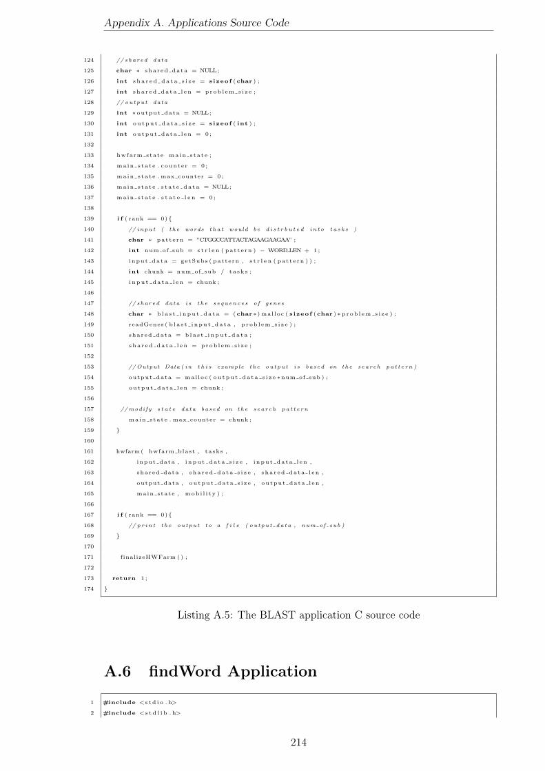
Appendix A. Applications Source Code
124 // shared data
125 char ∗ shared data = NULL;
126 int s h a r ed da t a s i z e = s izeof ( char ) ;
127 int sha r ed da ta l en = prob l em s i z e ;
128 // ou tpu t data
129 int ∗ output data = NULL;
130 int ou tpu t da ta s i z e = s izeof ( int ) ;
131 int output data l en = 0 ;
132
133 hwfarm state main state ;
134 main state . counter = 0 ;
135 main state . max counter = 0 ;
136 main state . s t a t e da t a = NULL;
137 main state . s t a t e l e n = 0 ;
138
139 i f ( rank == 0){
140 // inpu t ( t h e words t h a t would be d i s t r b u t e d i n t o t a s k s )
141 char ∗ pattern = ”CTGGCCATTACTAGAAGAAGAA” ;
142 int num of sub = s t r l e n ( pattern ) − WORDLEN + 1 ;
143 input data = getSubs ( pattern , s t r l e n ( pattern ) ) ;
144 int chunk = num of sub / tasks ;
145 inpu t da ta l en = chunk ;
146
147 // shared data i s t h e s e quence s o f genes
148 char ∗ b l a s t i npu t da t a = ( char∗) mal loc ( s izeof ( char )∗ prob l em s i z e ) ;
149 readGenes ( b l a s t i nput da ta , p rob l em s i z e ) ;
150 shared data = b l a s t i npu t da t a ;
151 sha r ed da ta l en = prob l em s i z e ;
152
153 //Output Data ( in t h i s example t h e ou tpu t i s based on the s earch pa t t e r n )
154 output data = malloc ( ou tpu t da ta s i z e ∗num of sub ) ;
155 output data l en = chunk ;
156
157 //modi fy s t a t e data based on the s earch pa t t e r n
158 main state . max counter = chunk ;
159 }
160
161 hwfarm( hwfarm blast , tasks ,
162 input data , i npu t da ta s i z e , i nput data l en ,
163 shared data , sha r ed da ta s i z e , shared data l en ,
164 output data , ou tput data s i z e , output data len ,
165 main state , mob i l i ty ) ;
166
167 i f ( rank == 0){
168 // p r i n t t h e ou tpu t to a f i l e ( ou t pu t da t a , num of sub )
169 }
170
171 finalizeHWFarm () ;
172
173 return 1 ;
174 }
Listing A.5: The BLAST application C source code
A.6 findWord Application
1 #include <s t d i o . h>
2 #include <s t d l i b . h>
214
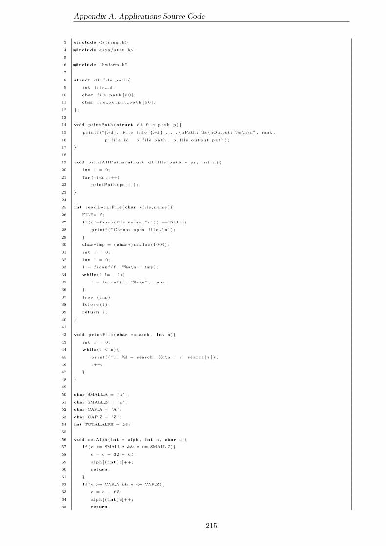
Appendix A. Applications Source Code
3 #include <s t r i n g . h>
4 #include <sys / s t a t . h>
5
6 #include ”hwfarm . h”
7
8 struct db f i l e p a t h {
9 int f i l e i d ;
10 char f i l e p a t h [ 5 0 ] ;
11 char f i l e o u t pu t p a t h [ 5 0 ] ;
12 } ;
13
14 void printPath ( struct db f i l e p a t h p){
15 p r i n t f ( ”[%d ] . F i l e i n f o {%d } . . . . . . \ nPath : %s\nOutput : %s\n\n” , rank ,
16 p . f i l e i d , p . f i l e p a t h , p . f i l e o u t pu t p a t h ) ;
17 }
18
19 void pr intAl lPaths ( struct db f i l e p a t h ∗ ps , int n){
20 int i = 0 ;
21 for ( ; i<n ; i++)
22 printPath ( ps [ i ] ) ;
23 }
24
25 int r eadLoca lF i l e ( char ∗ f i l e name ){
26 FILE∗ f ;
27 i f ( ( f=fopen ( f i l e name , ” r ” ) ) == NULL){
28 p r i n t f ( ”Cannot open f i l e .\n” ) ;
29 }
30 char∗tmp = ( char∗) mal loc (1000) ;
31 int i = 0 ;
32 int l = 0 ;
33 l = f s c an f ( f , ”%s\n” , tmp) ;
34 while ( l != −1){
35 l = f s c an f ( f , ”%s\n” , tmp) ;
36 }
37 f r e e (tmp) ;
38 f c l o s e ( f ) ;
39 return i ;
40 }
41
42 void p r i n tF i l e (char ∗ search , int n){
43 int i = 0 ;
44 while ( i < n){
45 p r i n t f ( ” i : %d − search : %c\n” , i , s earch [ i ] ) ;
46 i++;
47 }
48 }
49
50 char SMALL A = ’ a ’ ;
51 char SMALL Z = ’ z ’ ;
52 char CAP A = ’A ’ ;
53 char CAP Z = ’Z ’ ;
54 int TOTAL ALPH = 26 ;
55
56 void setAlph ( int ∗ alph , int n , char c ){
57 i f ( c >= SMALL A && c <= SMALL Z){
58 c = c − 32 − 65 ;
59 alph [ ( int ) c ]++;
60 return ;
61 }
62 i f ( c >= CAP A && c <= CAP Z){
63 c = c − 65 ;
64 alph [ ( int ) c ]++;
65 return ;
215
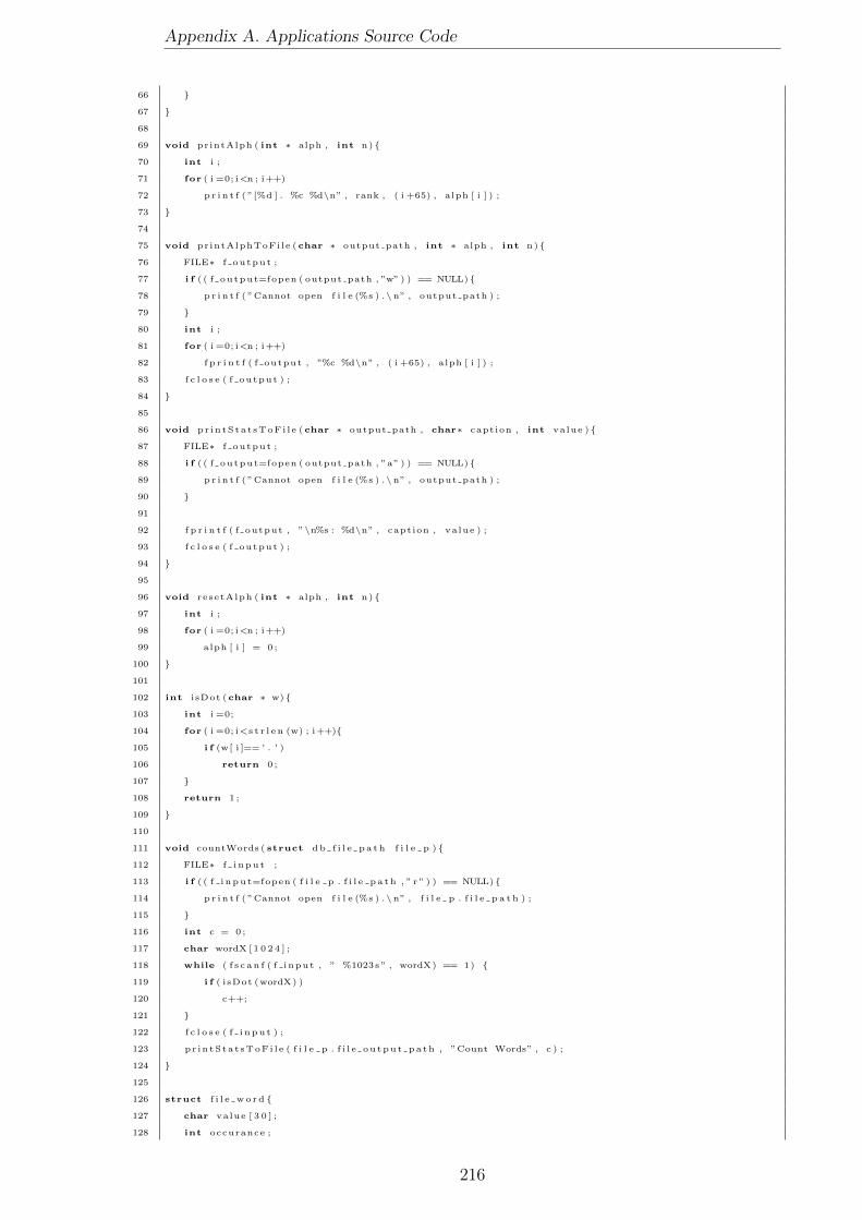
Appendix A. Applications Source Code
66 }
67 }
68
69 void printAlph ( int ∗ alph , int n){
70 int i ;
71 for ( i =0; i<n ; i++)
72 p r i n t f ( ”[%d ] . %c %d\n” , rank , ( i +65) , alph [ i ] ) ;
73 }
74
75 void printAlphToFi le ( char ∗ output path , int ∗ alph , int n){
76 FILE∗ f output ;
77 i f ( ( f output=fopen ( output path , ”w” ) ) == NULL){
78 p r i n t f ( ”Cannot open f i l e (%s ) .\n” , output path ) ;
79 }
80 int i ;
81 for ( i =0; i<n ; i++)
82 f p r i n t f ( f output , ”%c %d\n” , ( i +65) , alph [ i ] ) ;
83 f c l o s e ( f output ) ;
84 }
85
86 void pr in tS ta t sToF i l e ( char ∗ output path , char∗ caption , int value ){
87 FILE∗ f output ;
88 i f ( ( f output=fopen ( output path , ”a” ) ) == NULL){
89 p r i n t f ( ”Cannot open f i l e (%s ) .\n” , output path ) ;
90 }
91
92 f p r i n t f ( f output , ”\n%s : %d\n” , caption , value ) ;
93 f c l o s e ( f output ) ;
94 }
95
96 void resetAlph ( int ∗ alph , int n){
97 int i ;
98 for ( i =0; i<n ; i++)
99 alph [ i ] = 0 ;
100 }
101
102 int i sDot ( char ∗ w){
103 int i =0;
104 for ( i =0; i<s t r l e n (w) ; i++){
105 i f (w[ i ]== ’ . ’ )
106 return 0 ;
107 }
108 return 1 ;
109 }
110
111 void countWords ( struct db f i l e p a t h f i l e p ){
112 FILE∗ f i n pu t ;
113 i f ( ( f i npu t=fopen ( f i l e p . f i l e p a t h , ” r ” ) ) == NULL){
114 p r i n t f ( ”Cannot open f i l e (%s ) .\n” , f i l e p . f i l e p a t h ) ;
115 }
116 int c = 0 ;
117 char wordX [ 1 0 2 4 ] ;
118 while ( f s c a n f ( f i nput , ” %1023s ” , wordX) == 1) {
119 i f ( i sDot (wordX) )
120 c++;
121 }
122 f c l o s e ( f i npu t ) ;
123 pr in tS ta t sToF i l e ( f i l e p . f i l e ou tpu t pa th , ”Count Words” , c ) ;
124 }
125
126 struct f i l e wo r d {
127 char value [ 3 0 ] ;
128 int occurance ;
216
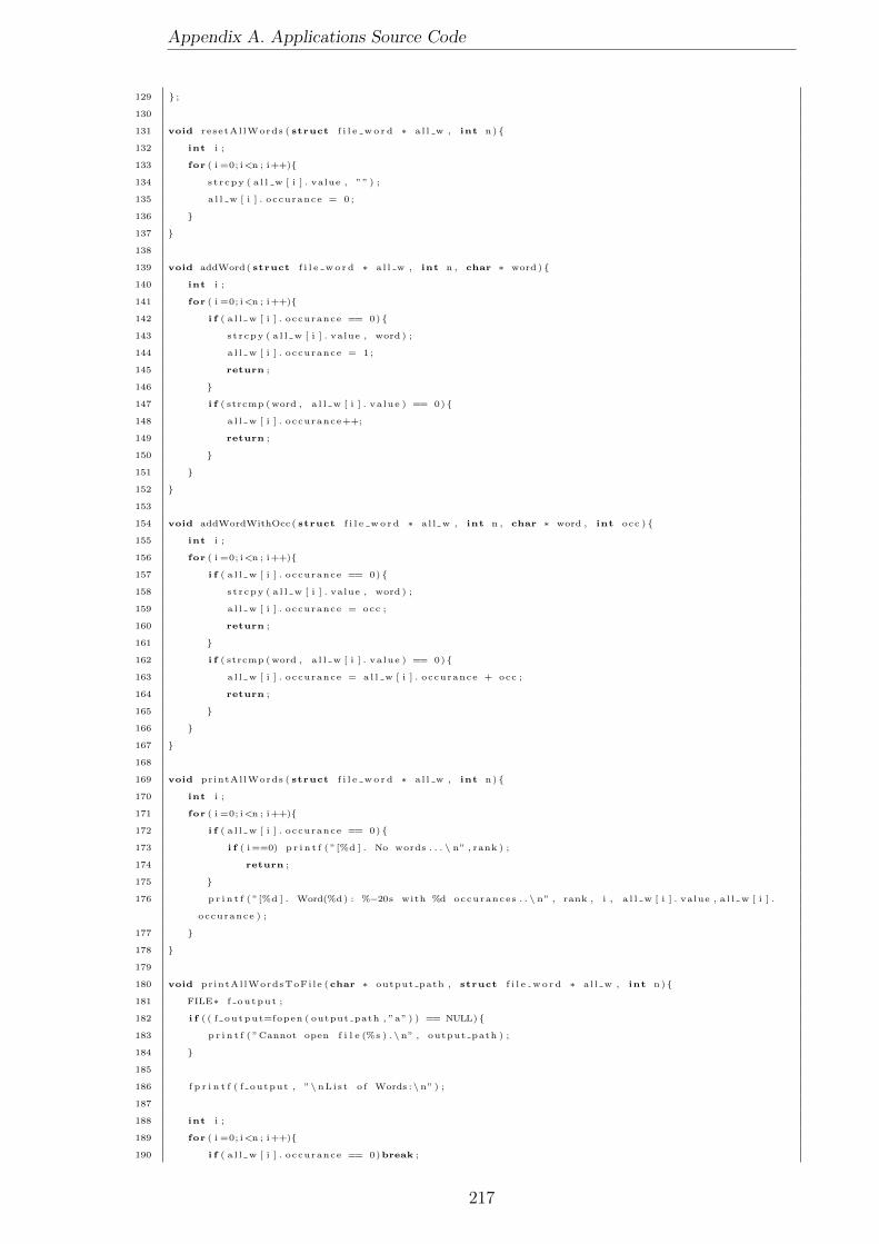
Appendix A. Applications Source Code
129 } ;
130
131 void resetAl lWords ( struct f i l e wo r d ∗ a l l w , int n){
132 int i ;
133 for ( i =0; i<n ; i++){
134 s t rcpy ( a l l w [ i ] . value , ”” ) ;
135 a l l w [ i ] . occurance = 0 ;
136 }
137 }
138
139 void addWord( struct f i l e wo r d ∗ a l l w , int n , char ∗ word ){
140 int i ;
141 for ( i =0; i<n ; i++){
142 i f ( a l l w [ i ] . occurance == 0){
143 s t rcpy ( a l l w [ i ] . value , word ) ;
144 a l l w [ i ] . occurance = 1 ;
145 return ;
146 }
147 i f ( strcmp (word , a l l w [ i ] . va lue ) == 0){
148 a l l w [ i ] . occurance++;
149 return ;
150 }
151 }
152 }
153
154 void addWordWithOcc ( struct f i l e wo r d ∗ a l l w , int n , char ∗ word , int occ ){
155 int i ;
156 for ( i =0; i<n ; i++){
157 i f ( a l l w [ i ] . occurance == 0){
158 s t rcpy ( a l l w [ i ] . value , word ) ;
159 a l l w [ i ] . occurance = occ ;
160 return ;
161 }
162 i f ( strcmp (word , a l l w [ i ] . va lue ) == 0){
163 a l l w [ i ] . occurance = a l l w [ i ] . occurance + occ ;
164 return ;
165 }
166 }
167 }
168
169 void printAllWords ( struct f i l e wo r d ∗ a l l w , int n){
170 int i ;
171 for ( i =0; i<n ; i++){
172 i f ( a l l w [ i ] . occurance == 0){
173 i f ( i==0) p r i n t f ( ”[%d ] . No words . . . \ n” , rank ) ;
174 return ;
175 }
176 p r i n t f ( ”[%d ] . Word(%d) : %−20s with %d occurances . . \ n” , rank , i , a l l w [ i ] . value , a l l w [ i ] .
occurance ) ;
177 }
178 }
179
180 void printAl lWordsToFi le ( char ∗ output path , struct f i l e wo r d ∗ a l l w , int n){
181 FILE∗ f output ;
182 i f ( ( f output=fopen ( output path , ”a” ) ) == NULL){
183 p r i n t f ( ”Cannot open f i l e (%s ) .\n” , output path ) ;
184 }
185
186 f p r i n t f ( f output , ”\nLis t o f Words :\n” ) ;
187
188 int i ;
189 for ( i =0; i<n ; i++){
190 i f ( a l l w [ i ] . occurance == 0)break ;
217

Appendix A. Applications Source Code
191 f p r i n t f ( f output , ”%s : %d\n” , a l l w [ i ] . value , a l l w [ i ] . occurance ) ;
192 }
193
194 f c l o s e ( f output ) ;
195 }
196
197 void printStage2WordsToFile ( char ∗ output path , struct f i l e wo r d ∗ a l l w , int n){
198 FILE∗ f output ;
199 i f ( ( f output=fopen ( output path , ”w” ) ) == NULL){
200 p r i n t f ( ”Cannot open f i l e (%s ) .\n” , output path ) ;
201 }
202
203 int i ;
204 for ( i =0; i<n ; i++){
205 i f ( a l l w [ i ] . occurance == 0)break ;
206 f p r i n t f ( f output , ”%s : %d\n” , a l l w [ i ] . value , a l l w [ i ] . occurance ) ;
207 }
208 f c l o s e ( f output ) ;
209 }
210
211 int va l i dS t a r t ( char ∗ w){
212 int c = w [ 0 ] ;
213 i f ( ( c <= SMALL Z && c >= SMALL A) | | ( c <= CAP Z && c >= CAP A) ){
214 return 1 ;
215 }
216 return 0 ;
217 }
218
219 int validWord ( char ∗ w){
220 int i = 0 ;
221 int c ;
222 i f ( s t r l e n (w)>25) return 0 ;
223 for ( i =0; i<s t r l e n (w) ; i++){
224 c = w[ i ] ;
225 i f ( ! ( ( c <= SMALL Z && c >= SMALL A)
226 | | ( c <= CAP Z && c >= CAP A)
227 | | ( c <= ’9 ’ && c >= ’0 ’ ) ) ){
228 return 0 ;
229 }
230 }
231 return 1 ;
232 }
233
234 void f i l t e rWord ( char ∗ w){
235 int c = w[ s t r l e n (w) −1];
236 i f ( ( c == ’ : ’ ) | | ( c == ’ ! ’ ) | | ( c == ’ , ’ ) | | ( c == ’ . ’ ) | | ( c == ’ ? ’ ) | | ( c == ’ ) ’ ) | | ( c == ’ ” ’ ) ){
237 w[ s t r l e n (w)−1] = ’ \0 ’ ;
238 }
239 }
240
241 void getWords ( struct db f i l e p a t h f i l e p ){
242 FILE∗ f i n pu t ;
243 i f ( ( f i npu t=fopen ( f i l e p . f i l e p a t h , ” r ” ) ) == NULL){
244 p r i n t f ( ”Cannot open f i l e (%s ) .\n” , f i l e p . f i l e p a t h ) ;
245 }
246 char wordX [ 1 0 2 4 ] ;
247 struct f i l e wo r d ∗ a l l wo rd s = ( struct f i l e wo r d ∗) mal loc ( s izeof ( struct f i l e wo r d ) ∗1000) ;
248 resetAl lWords ( a l l words , 1000) ;
249 while ( f s c a n f ( f i nput , ”%1023s ” , wordX) == 1) {
250 i f ( i sDot (wordX) ){
251 f i l t e rWord (wordX) ;
252 i f ( v a l i dS t a r t (wordX) && validWord (wordX) )
253 addWord( a l l words , 1000 , wordX) ;
218

Appendix A. Applications Source Code
254 }
255 }
256 f c l o s e ( f i npu t ) ;
257 printAl lWordsToFile ( f i l e p . f i l e ou tpu t pa th , a l l words , 1000) ;
258 f r e e ( a l l wo rd s ) ;
259 }
260
261 void calcLongestWord ( struct db f i l e p a t h f i l e p ){
262 FILE∗ f i n pu t ;
263 i f ( ( f i npu t=fopen ( f i l e p . f i l e p a t h , ” r ” ) ) == NULL){
264 p r i n t f ( ”Cannot open f i l e (%s ) .\n” , f i l e p . f i l e p a t h ) ;
265 }
266 char wordX [ 1 0 2 4 ] ;
267 int l onge s t = 0 ;
268 while ( f s c a n f ( f i nput , ”%1023s ” , wordX) == 1) {
269 i f ( i sDot (wordX) ){
270 i f ( l onge s t < s t r l e n (wordX) ){
271 l onge s t = s t r l e n (wordX) ;
272 }
273 }
274 }
275 f c l o s e ( f i npu t ) ;
276 pr in tS ta t sToF i l e ( f i l e p . f i l e ou tpu t pa th , ”Longest Words l ength ” , l onge s t ) ;
277 }
278
279 void calcAlph ( struct db f i l e p a t h f i l e p ){
280 FILE∗ f i n pu t ;
281 i f ( ( f i npu t=fopen ( f i l e p . f i l e p a t h , ” r ” ) ) == NULL){
282 p r i n t f ( ”Cannot open f i l e (%s ) .\n” , f i l e p . f i l e p a t h ) ;
283 }
284 int ∗ alph = ( int ∗) mal loc ( s izeof ( int )∗TOTAL ALPH) ;
285 int c ;
286 resetAlph ( alph , TOTAL ALPH) ;
287 while ( ( c = f g e t c ( f i npu t ) ) != EOF) {
288 setAlph ( alph , TOTAL ALPH, c ) ;
289 }
290 f c l o s e ( f i npu t ) ;
291 pr intAlphToFi le ( f i l e p . f i l e ou tpu t pa th , alph , TOTAL ALPH) ;
292 f r e e ( alph ) ;
293 }
294
295 void countLet te r s ( struct db f i l e p a t h f i l e p ){
296 FILE∗ f i n pu t ;
297 i f ( ( f i npu t=fopen ( f i l e p . f i l e p a t h , ” r ” ) ) == NULL){
298 p r i n t f ( ”Cannot open f i l e (%s ) .\n” , f i l e p . f i l e p a t h ) ;
299 }
300
301 int count = 0 ;
302 int c ;
303 while ( ( c = f g e t c ( f i npu t ) ) != EOF) {
304 count++;
305 }
306 f c l o s e ( f i npu t ) ;
307 pr in tS ta t sToF i l e ( f i l e p . f i l e ou tpu t pa th , ”Count Le t t e r s ” , count ) ;
308 }
309
310 void p r o c e s sF i l e ( struct db f i l e p a t h f i l e p ){
311 calcAlph ( f i l e p ) ;
312 countWords ( f i l e p ) ;
313 countLet te r s ( f i l e p ) ;
314 calcLongestWord ( f i l e p ) ;
315 getWords ( f i l e p ) ;
316 }
219
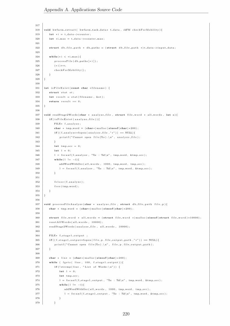
Appendix A. Applications Source Code
317
318 void hwfarm extract ( hwfarm task data∗ t data , chFM checkForMobi l i ty ){
319 int ∗ i = t data−>counter ;
320 int ∗ i max = t data−>counter max ;
321
322 struct db f i l e p a t h ∗ db paths = ( struct db f i l e p a t h ∗) t data−>input data ;
323
324 while (∗ i < ∗ i max ){
325 p r o c e s sF i l e ( db paths [∗ i ] ) ;
326 (∗ i )++;
327 checkForMobi l i ty ( ) ;
328 }
329 }
330
331 int i s F i l e E x i s t ( const char ∗ f i l ename ) {
332 struct s t a t s t ;
333 int r e s u l t = s t a t ( f i l ename , &s t ) ;
334 return r e s u l t == 0 ;
335 }
336
337 void readStage2Words ( char ∗ a n a l y z e f i l e , struct f i l e wo r d ∗ a l l words , int n){
338 i f ( i s F i l e E x i s t ( a n a l y z e f i l e ) ){
339 FILE∗ f a na l y z e ;
340 char ∗ tmp word = ( char∗) mal loc ( s izeof ( char ) ∗200) ;
341 i f ( ( f ana l y z e=fopen ( a n a l y z e f i l e , ” r ” ) ) == NULL){
342 p r i n t f ( ”Cannot open f i l e (%s ) .\n” , a n a l y z e f i l e ) ;
343 }
344 int tmp occ = 0 ;
345 int l = 0 ;
346 l = f s c an f ( f ana lyze , ”%s : %d\n” , tmp word , &tmp occ ) ;
347 while ( l != −1){
348 addWordWithOcc ( a l l words , 1000 , tmp word , tmp occ ) ;
349 l = f s c an f ( f ana lyze , ”%s : %d\n” , tmp word , &tmp occ ) ;
350 }
351
352 f c l o s e ( f ana l y z e ) ;
353 f r e e ( tmp word ) ;
354 }
355 }
356
357 void proce s sF i l eAna lyze ( char ∗ a n a l y z e f i l e , struct db f i l e p a t h f i l e p ){
358 char ∗ tmp word = ( char∗) mal loc ( s izeof ( char ) ∗200) ;
359
360 struct f i l e wo r d ∗ a l l wo rd s = ( struct f i l e wo r d ∗) mal loc ( s izeof ( struct f i l e wo r d ) ∗10000) ;
361 resetAl lWords ( a l l words , 10000) ;
362 readStage2Words ( a n a l y z e f i l e , a l l words , 10000) ;
363
364 FILE∗ f s t a g e1 ou tpu t ;
365 i f ( ( f s t a g e1 ou tpu t=fopen ( f i l e p . f i l e ou tpu t pa th , ” r ” ) ) == NULL){
366 p r i n t f ( ”Cannot open f i l e (%s ) .\n” , f i l e p . f i l e o u t pu t p a t h ) ;
367 }
368
369 char ∗ l i n e = ( char∗) mal loc ( s izeof ( char ) ∗200) ;
370 while ( f g e t s ( l i n e , 100 , f s t a g e1 ou tpu t ) ){
371 i f ( ! strcmp ( l i n e , ” L i s t o f Words :\n” ) ) {
372 int l = 0 ;
373 int tmp occ ;
374 l = f s c an f ( f s t age1 output , ”%s : %d\n” , tmp word , &tmp occ ) ;
375 while ( l != −1){
376 addWordWithOcc ( a l l words , 1000 , tmp word , tmp occ ) ;
377 l = f s c an f ( f s t age1 output , ”%s : %d\n” , tmp word , &tmp occ ) ;
378 }
379 }
220

Appendix A. Applications Source Code
380 }
381 f c l o s e ( f s t a g e1 ou tpu t ) ;
382 printStage2WordsToFile ( a n a l y z e f i l e , a l l words , 10000) ;
383
384 f r e e ( a l l wo rd s ) ;
385 f r e e ( tmp word ) ;
386 f r e e ( l i n e ) ;
387 }
388
389 void hwfarm analyze ( hwfarm task data∗ t data , chFM checkForMobi l i ty ){
390 int ∗ i = t data−>counter ;
391 int ∗ i max = t data−>counter max ;
392 int t i d = t data−>t a s k i d ;
393 char ∗ ana l y z e f i l e name = ( char∗) mal loc ( s izeof ( char ) ∗50) ;
394 s p r i n t f ( ana lyze f i l e name , ”db/ stage2 output/%d” , t i d ) ;
395 struct db f i l e p a t h ∗ db paths = ( struct db f i l e p a t h ∗) t data−>input data ;
396 while (∗ i < ∗ i max ){
397 proce s sF i l eAna lyze ( ana lyze f i l e name , db paths [∗ i ] ) ;
398 (∗ i )++;
399 checkForMobi l i ty ( ) ;
400 }
401 }
402
403 struct db f i l e p a t h ∗ a s s i gnF i l ePath s ( struct db f i l e p a t h ∗ ps , int n){
404 char ∗ o r i g pa th = ”db/ s tage1 input ” ;
405 char ∗ or i g output path = ”db/ stage1 output ” ;
406 char ∗ ls command = ( char∗) mal loc ( s izeof ( char ) ∗100) ;
407 s p r i n t f ( ls command , ” l s %s −1” , o r i g pa th ) ;
408
409 FILE ∗ fp1 ;
410 fp1 = popen ( ls command , ” r ” ) ;
411 i f ( fp1 == 0)
412 per ro r ( ls command ) ;
413
414 char ∗ l i n e = ( char∗) mal loc (35 ∗ s izeof ( char ) ) ;
415 int i = 0 ;
416 while ( f g e t s ( l i n e , 35 , fp1 ) ){
417 ps [ i ] . f i l e i d = i ;
418 s p r i n t f ( ps [ i ] . f i l e p a t h , ”%s/%s” , or ig path , l i n e ) ;
419 ps [ i ] . f i l e p a t h [ s t r l e n ( ps [ i ] . f i l e p a t h ) − 1 ] =’ \0 ’ ;
420 s p r i n t f ( ps [ i ] . f i l e ou tpu t pa th , ”%s/%s” , or ig output path , l i n e ) ;
421 ps [ i ] . f i l e o u t pu t p a t h [ s t r l e n ( ps [ i ] . f i l e o u t pu t p a t h ) − 1 ] =’ \0 ’ ;
422 i f (++i >= n) break ;
423 }
424 pc l o s e ( fp1 ) ;
425 f r e e ( l i n e ) ;
426 f r e e ( ls command ) ;
427 return ps ;
428 }
429
430 int main ( int argc , char∗∗ argv ){
431 initHWFarm( argc , argv ) ;
432
433 int prob l em s i z e = a to i ( argv [ 1 ] ) ;
434 int ta sks = a to i ( argv [ 2 ] ) ;
435 int mobi l i ty = a to i ( argv [ 3 ] ) ;
436 int chunk = prob l em s i z e / ta sks ;
437
438 // inpu t
439 struct db f i l e p a t h ∗ input data = NULL;
440 int i n pu t da t a s i z e = s izeof ( struct db f i l e p a t h ) ;
441 int i npu t da ta l en = chunk ;
442
221
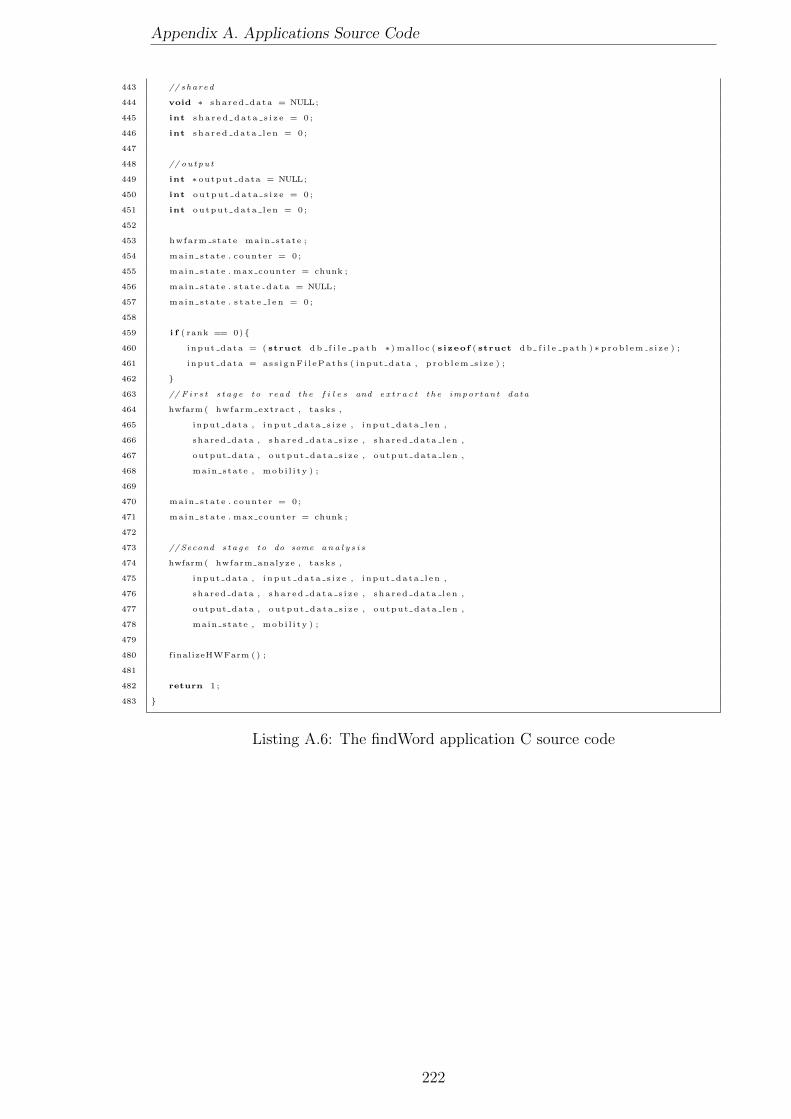
Appendix A. Applications Source Code
443 // shared
444 void ∗ shared data = NULL;
445 int s h a r ed da t a s i z e = 0 ;
446 int sha r ed da ta l en = 0 ;
447
448 // ou tpu t
449 int ∗ output data = NULL;
450 int ou tpu t da ta s i z e = 0 ;
451 int output data l en = 0 ;
452
453 hwfarm state main state ;
454 main state . counter = 0 ;
455 main state . max counter = chunk ;
456 main state . s t a t e da t a = NULL;
457 main state . s t a t e l e n = 0 ;
458
459 i f ( rank == 0){
460 input data = ( struct db f i l e p a t h ∗) mal loc ( s izeof ( struct db f i l e p a t h )∗ prob l em s i z e ) ;
461 input data = as s i gnF i l ePath s ( input data , p rob l em s i z e ) ;
462 }
463 // F i r s t s t a g e to read th e f i l e s and e x t r a c t t h e impor tan t data
464 hwfarm( hwfarm extract , tasks ,
465 input data , i npu t da ta s i z e , i nput data l en ,
466 shared data , sha r ed da ta s i z e , shared data l en ,
467 output data , ou tput data s i z e , output data len ,
468 main state , mob i l i ty ) ;
469
470 main state . counter = 0 ;
471 main state . max counter = chunk ;
472
473 // Second s t a g e to do some a n a l y s i s
474 hwfarm( hwfarm analyze , tasks ,
475 input data , i npu t da ta s i z e , i nput data l en ,
476 shared data , sha r ed da ta s i z e , shared data l en ,
477 output data , ou tput data s i z e , output data len ,
478 main state , mob i l i ty ) ;
479
480 finalizeHWFarm () ;
481
482 return 1 ;
483 }
Listing A.6: The findWord application C source code
222

Appendix B
The HWFarm Skeleton Source
Code
This appendix presents the full C code of the HWFarm skeleton. This code shows
all details related to mobility support, the cost model and the scheduler.
B.1 The HWFarm Function Header File
1 #include <mpi . h>
2 #include <pthread . h>
3
4 int numprocs ;
5 int namelen ;
6 char processor name [MPI MAX PROCESSOR NAME] ;
7 int rank ; // p ro c e s s rank
8
9 //For a l l p r o c e s s
10 double startTime ;
11 double startTaskTime ;
12 double s t a r t t ime ;
13
14 typedef struct hwfarm state{
15 int counter ;
16 int max counter ;
17 void∗ s t a t e da t a ;
18 int s t a t e s i z e ;
19 } hwfarm state ;
20
21 typedef struct hwfarm task data{
22 int t a s k i d ;
23 void∗ input data ;
24 int i npu t l en ;
25 void∗ shared data ;
26 int sha r ed l en ;
27 void∗ s t a t e da t a ;
28 int s t a t e l e n ;
29 void∗ output data ;
223

Appendix B. The HWFarm Skeleton Source Code
30 int output l en ;
31 int∗ counter ;
32 int∗ counter max ;
33 } hwfarm task data ;
34
35 typedef void (chFM) ( ) ;
36
37 typedef void ( fp ) ( hwfarm task data ∗ , void ( checkForMobi l i ty ) ( ) ) ;
38
39 void initHWFarm( int argc , char ∗∗ argv ) ;
40
41 void finalizeHWFarm () ;
42
43 void hwfarm( fp worker , int tasks ,
44 void ∗ input , int i nS i ze , int inLen ,
45 void ∗ shared data , int sha r ed da ta s i z e , int shared data l en ,
46 void ∗output , int outSize , int outLen , hwfarm state main state ,
47 int mobi l i ty ) ;
Listing B.1: The HWFarm Skeleton header file
B.2 The HWFarm Function Source Code
1 /∗∗∗∗∗∗∗∗∗∗∗∗∗∗∗∗∗∗∗∗∗∗∗∗∗∗∗∗∗∗∗∗∗∗∗∗∗∗∗∗∗∗∗∗∗∗∗∗∗∗∗∗∗∗∗∗∗∗∗∗∗∗∗∗∗∗∗∗∗∗∗
2 ∗ HWFarm Sk e l e t on us ing C, MPI and PThread .
3 ∗ Turkey A l s a l k i n i & Greg Michae l son
4 ∗ Heriot−Watt Un i v e r s i t y , Edinburgh , United Kingdom .
5 ∗∗∗∗∗∗∗∗∗∗∗∗∗∗∗∗∗∗∗∗∗∗∗∗∗∗∗∗∗∗∗∗∗∗∗∗∗∗∗∗∗∗∗∗∗∗∗∗∗∗∗∗∗∗∗∗∗∗∗∗∗∗∗∗∗∗∗∗∗∗∗/
6 #define GNU SOURCE
7 #ifde f WIN32
8 #define WIN32 LEAN AND MEAN
9 #include <windows . h>
10 #else
11 #include <unis td . h>
12 #endif
13
14 #include <errno . h>
15 #include <s t d i o . h>
16 #include <s t d l i b . h>
17 #include <math . h>
18 // He lpe r s
19 #include <s t r i n g . h>
20 #include <time . h>
21 #include <sys / timeb . h>
22 #include <s i g n a l . h>
23 //For RUSAGE
24 #include <sys / time . h>
25 #include <sys / r e sou r c e . h>
26
27 //Thread g e t t i d
28 #include <sys / types . h>
29 #include <unis td . h>
30 #include <sys / s y s c a l l . h>
31 //Top In f o
32 #include <sys / s y s i n f o . h>
33 #include <sys /un . h>
34 #include <unis td . h>
35 //MPI & PThread
224

Appendix B. The HWFarm Skeleton Source Code
36 #include <mpi . h>
37 #include <pthread . h>
38 //Header F i l e
39 #include ”hwfarm . h”
40 /∗∗∗∗∗∗∗∗∗∗∗∗∗∗∗∗∗∗∗∗ COMMUNICATION TAGS ∗∗∗∗∗∗∗∗∗∗∗∗∗∗∗∗∗∗∗∗∗∗∗∗∗∗∗∗∗∗∗/
41 //Master to workers Tags
42 #define INIT LOAD FROM WORKER 1
43 #define MOVEREPORTFROMWORKER 2
44 #define LATEST LOAD REQUEST 3
45 //#d e f i n e LOAD REPORT FROM WORKER 6
46 #define RESULTS FROM WORKER 7
47 #define MOBILITY CONFIRMATION FROM WORKER 9 // Shared w i th worker t a g s
48 #define MOBILITY NOTIFICATION FROM WORKER 10
49 //Worker t a g s
50 #define LOAD REQUEST FROM MASTER 1
51 #define TERMINATETHEWORKER 2
52 #define LOAD INFO FROM MASTER 3
53 #define SENDING CONFIRMATION FROM MASTER 4
54 #define MOBILITY ACCEPTANCE FROM WORKER 5
55 #define UPDATE LOAD REPORT REQUEST 6
56 #define TASK FROM MASTER 7
57 #define MOBILITY REQUEST FROM WORKER 8
58 #define TASKFROMWORKER 10
59 #define SHARED DATA FROM MASTER 11
60
61 /∗∗∗∗∗∗∗∗∗∗∗∗∗∗∗∗∗∗∗∗ SKELETON CONSTANTS ∗∗∗∗∗∗∗∗∗∗∗∗∗∗∗∗∗∗∗∗∗∗∗∗∗∗∗∗∗∗/
62 #define MSG LIMIT 400000000
63 #define ESTIMATOR BREAK TIME 3
64 #define NET LAT THRESHOLD 1.5
65 #define MAXMOVES 20 //MAX MOVES
66 typedef enum {M TO W, W TO W, W TO M} sendType ;
67 /∗∗∗∗∗∗∗∗∗∗∗∗∗∗∗∗∗∗∗∗ GLOBAL VARIABLES ∗∗∗∗∗∗∗∗∗∗∗∗∗∗∗∗∗∗∗∗∗∗∗∗∗∗∗∗∗∗∗∗/
68 double s t a r t t ime ; // ho l d s t h e s t a r t t ime
69 double end time ; // ho l d s t h e end t ime
70 int i s F i r s t C a l l = 1 ; //@Master to check i f h t e s k e l e t o n i s c a l l e d
71 f loat Master FREQ = 0 . 0 ; // Current Node Ch a r a c t e r s t i c s
72 int currentCores = 0 ; // Current Node Ch a r a c t e r s t i c s
73 int moving task = 0 ; //The worker i s s end ing a t a s k now
74 int worker sending = 0 ; //The worker i s moving a t a s k now
75 int ∗masterRece iv ing ; //To avo id c o l l i s i o n a t t h e master
76 int ∗masterSending ; //To avo id c o l l i s i o n a t t h e master
77 /∗∗∗∗∗∗∗∗∗∗∗∗∗∗∗∗∗∗ MPI GLOBAL VARIABLES ∗∗∗∗∗∗∗∗∗∗∗∗∗∗∗∗∗∗∗∗∗∗∗∗∗∗∗∗∗∗/
78 MPI Status s t a tu s ; // s t o r e s t a t u s o f a MPI Recv
79 MPI Request r eques t ; // cap tu r e r e q u e s t o f a MPI Isend
80
81 /∗∗∗∗∗∗∗∗∗∗∗∗∗∗∗∗∗ POSIX GLOBAL VARIABLES ∗∗∗∗∗∗∗∗∗∗∗∗∗∗∗∗∗∗∗∗∗∗∗∗∗∗∗∗∗/
82 //@Master
83 pthread t w load r epo r t th ;
84 pthread t w network latency th ;
85 //@Worker
86 //Thread to run the worker l oad agen t which c o l l e c t s t h e
87 // worker l oad and sends i t t o t h e master
88 pthread t w load pth ;
89 //Thread to run the worker e s t ima t o r which i s r e s p o n s i b l e
90 // f o r e s t ima t i n g t h e e s t ima t ed e x e cu t i on t ime f o r t h e t a s k s
91 // running on the t h i s worker . Then i t w i l l send th e
92 //move r e o r t to t h e s e r v e r to make t h e moving i f n e c e s s a r y .
93 pthread t w est imator pth ;
94 //To pr e v en t l o c k i n g
95 pthread mutex t mut ex l oad c i r cu l a t i ng = PTHREAD MUTEX INITIALIZER;
96 pthread mutex t mutex w sending = PTHREAD MUTEX INITIALIZER;
97
98 /∗∗∗∗∗∗∗∗∗∗∗∗∗∗∗∗∗∗ SKELETON DATA STRUCTURES ∗∗∗∗∗∗∗∗∗∗∗∗∗∗∗∗∗∗∗∗∗∗∗∗∗∗/
225
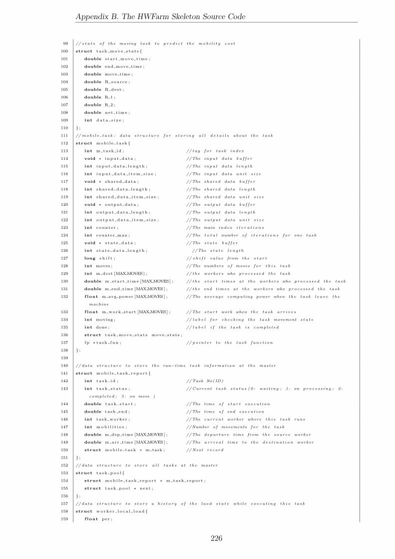
Appendix B. The HWFarm Skeleton Source Code
99 // s t a t s o f t h e moving t a s k to p r e d i c t t h e mo b i l i t y c o s t
100 struct ta sk move s ta t s {
101 double s tar t move t ime ;
102 double end move time ;
103 double move time ;
104 double R source ;
105 double R dest ;
106 double R 1 ;
107 double R 2 ;
108 double net t ime ;
109 int da t a s i z e ;
110 } ;
111 // mo b i l e t a s k : da ta s t r u c t u r e f o r s t o r i n g a l l d e t a i l s about t h e t a s k
112 struct mobi l e ta sk {
113 int m task id ; // tag f o r t a s k index
114 void ∗ input data ; //The inpu t data b u f f e r
115 int i nput da ta l eng th ; //The inpu t data l e n g t h
116 int i n pu t da t a i t em s i z e ; //The inpu t data un i t s i z e
117 void ∗ shared data ; //The shared data b u f f e r
118 int sha r ed data l eng th ; //The shared data l e n g t h
119 int s ha r ed da t a i t em s i z e ; //The shared data un i t s i z e
120 void ∗ output data ; //The ou tpu t data b u f f e r
121 int output data l ength ; //The ou tpu t data l e n g t h
122 int ou tpu t da ta i t em s i z e ; //The ou tpu t data un i t s i z e
123 int counter ; //The main index i t e r a t i o n s
124 int counter max ; //The t o t a l number o f i t e r a t i o n s f o r one t a s k
125 void ∗ s t a t e da t a ; //The s t a t e b u f f e r
126 int s t a t e da t a l e n g th ; //The s t a t e l e n g t h
127 long s h i f t ; // s h i f t v a l u e from the s t a r t
128 int moves ; //The numbers o f moves f o r t h i s t a s k
129 int m dest [MAXMOVES] ; // the workers who p ro c e s s ed t h e t a s k
130 double m start t ime [MAXMOVES] ; // the s t a r t t imes a t t h e workers who p roc e s s ed t h e t a s k
131 double m end time [MAXMOVES] ; // the end t imes a t t h e workers who p roc e s s ed t h e t a s k
132 f loat m avg power [MAXMOVES] ; //The average computing power when the t a s k l e a v e t h e
machine
133 f loat m work start [MAXMOVES] ; //The s t a r t work when the t a s k a r r i v e s
134 int moving ; // l a b e l f o r ch e c k i n g t h e t a s k movement s t a t e
135 int done ; // l a b e l i f t h e t a s k i s comp le ted
136 struct ta sk move s ta t s move stats ;
137 fp ∗ ta sk fun ; // p o i n t e r to t h e t a s k f u n c t i o n
138 } ;
139
140 // data s t r u c t u r e to s t o r e t h e run−t ime t a s k in f o rma t i on a t t h e master
141 struct mob i l e t a sk r epo r t {
142 int t a s k i d ; //Task No( ID)
143 int t a s k s t a t u s ; // Current t a s k s t a t u s ( 0 : wa i t i n g ; 1 : on p r o c e s s i n g ; 2 :
comp le ted ; 3 : on move )
144 double t a s k s t a r t ; //The t ime o f s t a r t e x e c u t i on
145 double task end ; //The t ime o f end e x e cu t i on
146 int task worker ; //The cu r r en t worker where t h i s t a s k runs
147 int mob i l i t i e s ; //Number o f movements f o r t h e t a s k
148 double m dep time [MAXMOVES] ; //The depa r t u r e t ime from the source worker
149 double m arr t ime [MAXMOVES] ; //The a r r i v a l t ime to t h e d e s t i n a t i o n worker
150 struct mobi l e ta sk ∗ m task ; //Next r ecord
151 } ;
152 // data s t r u c t u r e to s t o r e a l l t a s k s a t t h e master
153 struct t a sk poo l {
154 struct mob i l e t a sk r epo r t ∗ m task report ;
155 struct t a sk poo l ∗ next ;
156 } ;
157 // data s t r u c t u r e to s t o r e a h i s t o r y o f t h e l aod s t a t e wh i l e e x e c u t i n g t h i s t a s k
158 struct work e r l o c a l l o ad {
159 f loat per ;
226

Appendix B. The HWFarm Skeleton Source Code
160 f loat sec ;
161 f loat l oad avg ;
162 int e s t l o ad avg ;
163 long double w cpu ut i ;
164 int w running procs ;
165 struct work e r l o c a l l o ad ∗ next ;
166 } ;
167 // data s t r u c t u r e to s t o r e d e t a i l s o f t h i s t a s k on the worker
168 struct worker task {
169 int t a s k i d ;
170 double w ta sk s t a r t ;
171 double w task end ;
172 pthread t task pth ;
173 pthread t moving pth ;
174 struct mobi l e ta sk ∗ m task ;
175 f loat l o ca l R ;
176 int move ;
177 int go move ;
178 int go to ;
179 int move status ;
180 struct work e r l o c a l l o ad ∗ w l l oad ;
181 struct e s t imat ion ∗ est imating move ;
182 struct worker task ∗ next ;
183 } ;
184 // data s t r u c t u r e to s t o r e a t he network d e l a y s a t a l l o c a t i o n t ime and the cu r r en t t ime
185 struct network t imes{
186 double i n i t n e t t im e ;
187 double cu r ne t t ime ;
188 } ;
189 // data s t r u c t u r e to s t o r e t h e l oad s t a t e o f a l l workers
190 struct worker load {
191 int w rank ;
192 char w name [MPI MAX PROCESSOR NAME] ;
193 int m id ;
194 int cu r r en t t a s k s ;
195 int t o t a l t a s k ;
196 int s t a tu s ; // 0 : f r e e , 1 : working , 2 : Requs t ing , 3 : wa i t ing , 4 : envo l v ed in moving
197 int w cores ; // S t a t i c me t r i c
198 int w cache s i z e ; // S t a t i c me t r i c
199 f loat w cpu speed ; // S t a t i c me t r i c
200 f loat w load avg 1 ;
201 f loat w load avg 2 ;
202 int e s t imated load ;
203 long double w cpu ut i 1 ;
204 long double w cpu ut i 2 ;
205 int w running procs ;
206 int l ocked ;
207 struct network t imes net t imes ;
208 } ;
209 // data s t r u c t u r e to s t o r e t h e move r e p o r t i s s u e d by t he e s t ima t o r agen t
210 struct worker move report{
211 int w id ;
212 int num of tasks ;
213 int ∗ l i s t o f t a s k s ;
214 } ;
215 // data s t r u c t u r e to s t o r e d e t a i l s when a worker becomes busy in r e c e i v i n g a t a s k from a worker
216 struct worker hold{
217 int on hold ; // s e t t o i n d i c a t e t h a t t h i s worker i s on ho l d to comp le t e t h e move from
the source worker
218 int holded on ; //number o f t a s k s which t h e worker i s wa i t i n g f o r
219 int holded from ; // the worker who i am ho lded to
220 f loat hold t ime ; // the t ime o f ho l d . f o r c a n c e l a t i o n i f t h e r e q u e s t t imed out
221 } ;
227
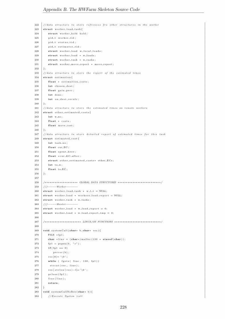
Appendix B. The HWFarm Skeleton Source Code
222 // data s t r u c t u r e to s t o r e r e f r e n c e s f r o o t h e r s t r u c t u r e s in t h e worker
223 struct worke r l oad ta sk {
224 struct worker hold hold ;
225 p id t worke r t id ;
226 p id t s t a t u s t i d ;
227 p id t e s t ima t o r t i d ;
228 struct worker load w l o c a l l o ad s ;
229 struct worker load ∗ w loads ;
230 struct worker task ∗ w tasks ;
231 struct worker move report ∗ move report ;
232 } ;
233 // data s t r u c t u r e to s t o r e t h e r e p o r t o f t h e e s t ima t e d t imes
234 struct e s t imat ion {
235 f loat ∗ e s t ima t i on c o s t s ;
236 int chosen des t ;
237 f loat ga in pe r c ;
238 int done ;
239 int on d e s t r e c a l c ;
240 } ;
241 // data s t r u c t u r e to s t o r e t h e e s t ima t ed t imes on remote workers
242 struct o th e r e s t ima t ed co s t s {
243 int w no ;
244 f loat ∗ c o s t s ;
245 f loat move cost ;
246 } ;
247 // data s t r u c t u r e to s t o r e d e t a i l e d r e p o r t o f e s t ima t ed t imes f o r t h i s t a s k
248 struct e s t imat ed co s t {
249 int task no ;
250 f loat cur EC ;
251 f loat spent he re ;
252 f loat ∗ cur EC af te r ;
253 struct o th e r e s t ima t ed co s t s ∗ other ECs ;
254 int to w ;
255 f loat to EC ;
256 } ;
257
258 /∗∗∗∗∗∗∗∗∗∗∗∗∗∗∗∗∗∗∗∗ GLOBAL DATA STRUCTURES ∗∗∗∗∗∗∗∗∗∗∗∗∗∗∗∗∗∗∗∗∗∗∗∗∗∗/
259 ///−−−−−Worker−−−−−−−
260 struct worke r l oad ta sk ∗ w l t = NULL;
261 struct worker load ∗ worke r s l o ad r epo r t = NULL;
262 struct worker task ∗ w tasks ;
263 ///−−−−−Master−−−−−−−
264 struct worker load ∗ w load repor t = 0 ;
265 struct worker load ∗ w load report tmp = 0 ;
266
267 /∗∗∗∗∗∗∗∗∗∗∗∗∗∗∗∗∗∗∗∗∗∗ LINUX/OS FUNCTIONS ∗∗∗∗∗∗∗∗∗∗∗∗∗∗∗∗∗∗∗∗∗∗∗∗∗∗∗∗/
268
269 void systemCal l ( char∗ b , char∗ r e s ){
270 FILE ∗ fp1 ;
271 char ∗ l i n e = ( char∗) mal loc (130 ∗ s izeof ( char ) ) ;
272 fp1 = popen (b , ” r ” ) ;
273 i f ( fp1 == 0)
274 per ro r (b) ;
275 r e s [0 ]= ’ \0 ’ ;
276 while ( f g e t s ( l i n e , 130 , fp1 ) )
277 s t r c a t ( res , l i n e ) ;
278 r e s [ s t r l e n ( r e s )−1]= ’ \0 ’ ;
279 pc l o s e ( fp1 ) ;
280 f r e e ( l i n e ) ;
281 return ;
282 }
283 void systemCallNoRes (char∗ b){
284 // Execute System c a l l
228

Appendix B. The HWFarm Skeleton Source Code
285 FILE ∗ fp ;
286 fp = popen (b , ” r ” ) ;
287 pc l o s e ( fp ) ;
288 }
289 // send p ing message to t h e s e l e c t e d worker
290 double sendPing (char ∗ node name ){
291 char ∗ pre ping command = ”ping %s −c 1 | grep \” r t t \” | awk ’{ s p l i t ( $0 , a ,\” \”) ; p r i n t a
[ 4 ] } ’ | awk ’{ s p l i t ( $0 , b ,\”/\”) ; p r i n t b [ 2 ] } ’ ” ;
292 char ∗ping command = ( char∗) mal loc ( s izeof ( char ) ∗200) ;
293 s p r i n t f ( ping command , pre ping command , node name ) ;
294 char ∗ r t t l a t e n c y s t r = ( char∗) mal loc ( s izeof ( char ) ∗20) ;
295 systemCal l ( ping command , r t t l a t e n c y s t r ) ;
296 double ne t l a t ency = ato f ( r t t l a t e n c y s t r ) ;
297 i f ( n e t l a t en cy != 0 . 0 ) {
298 f r e e ( ping command ) ;
299 f r e e ( r t t l a t e n c y s t r ) ;
300 return ne t l a t ency ;
301 } else {
302 f r e e ( ping command ) ;
303 f r e e ( r t t l a t e n c y s t r ) ;
304 return 0 . 0 ;
305 }
306 }
307
308 /∗∗∗∗∗∗∗∗∗∗∗∗∗∗∗∗∗∗∗∗ LOAD STATE FUNCTIONS ∗∗∗∗∗∗∗∗∗∗∗∗∗∗∗∗∗∗∗∗∗∗∗∗∗∗∗∗/
309
310 int conta ins (char t a r g e t [ ] , int m, char source [ ] , int n){
311 int i , j =0;
312 for ( i =0; i<n ; i++){
313 i f ( t a r g e t [ j ] == source [ i ] ) j++;
314 else j =0;
315 i f ( j == m) return 1 ;
316 }
317 return 0 ;
318 }
319
320 f loat getCoresFreq ( ) {
321 FILE ∗ f ;
322 int LINE MAX = 128;
323 char ∗ l i n e = ( char∗) mal loc (LINE MAX ∗ s izeof ( char ) ) ;
324 char ∗tmp = ( char∗) mal loc (10 ∗ s izeof ( char ) ) ;
325 f loat t o t a l c o r e s f r e q = 0 ;
326
327 f = fopen ( ”/proc / cpu in fo ” , ” r ” ) ;
328 i f ( f == 0){
329 per ro r ( ”Could open the f i l e : / proc / cpu in fo ” ) ;
330 return 0 ;
331 }
332
333 f loat c o r e f r e q = 0 , m in co r e f r eq = 0 ;
334 int c o r e s cn t = 0 ;
335 char c ;
336 while ( f g e t s ( l i n e , LINE MAX, f ) ){
337 i f ( conta in s ( ”cpu MHz” , 7 , l i n e , LINE MAX) ){
338 s s c an f ( l i n e , ”%s %s %c %f \n” , tmp , tmp , &c , &c o r e f r e q ) ;
339 i f ( c o r e s cn t == 0)
340 min co r e f r eq = c o r e f r e q ;
341 else i f ( m in co r e f r eq > c o r e f r e q )
342 min co r e f r eq = c o r e f r e q ;
343 t o t a l c o r e s f r e q += co r e f r e q ;
344 c o r e s cn t++;
345 }
346 }
229
Appendix B. The HWFarm Skeleton Source Code
347 f c l o s e ( f ) ;
348 f r e e (tmp) ;
349 f r e e ( l i n e ) ;
350 return min co r e f r eq ∗ c o r e s cn t ;
351 }
352
353 int getNumberOfCores ( ) {
354 long nprocs = −1;
355 long nprocs max = −1;
356 #i f d e f WIN32
357 #i f n d e f SC NPROCESSORS ONLN
358 SYSTEM INFO in f o ;
359 GetSystemInfo(& in f o ) ;
360 #de f i n e sy scon f ( a ) i n f o . dwNumberOfProcessors
361 #de f i n e SC NPROCESSORS ONLN
362 #end i f
363 #end i f
364 #i f d e f SC NPROCESSORS ONLN
365 nprocs = syscon f ( SC NPROCESSORS ONLN) ;
366 i f ( nprocs < 1){
367 f p r i n t f ( s tder r , ”Could not determine number o f CPUs on l i n e :\n%s\n” ,
368 s t r e r r o r ( errno ) ) ;
369 return nprocs ;
370 }
371 nprocs max = syscon f ( SC NPROCESSORS CONF) ;
372 i f ( nprocs max < 1){
373 f p r i n t f ( s tder r , ”Could not determine number o f CPUs con f i gured :\n%s\n” ,
374 s t r e r r o r ( errno ) ) ;
375 return nprocs ;
376 }
377 return nprocs ;
378 #else
379 f p r i n t f ( s tder r , ”Could not determine number o f CPUs” ) ;
380 return nprocs ;
381 #end i f
382 }
383
384 int ge tProce s sS ta t e ( int p id , int i s t a s k , int t i d ){
385 FILE ∗ f ;
386 char ∗ l i n e = ( char∗) mal loc (1000 ∗ s izeof ( char ) ) ;
387 char ∗ s t a t eF i l e = ( char∗) mal loc ( s izeof ( char ) ∗200) ;
388 i f ( i s t a s k == 1)
389 s p r i n t f ( s t a t eF i l e , ”/proc/%u/ task/%u/ s t a t ” , p id , t i d ) ;
390 else
391 s p r i n t f ( s t a t eF i l e , ”/proc/%u/ s t a t ” , p id ) ;
392 f = fopen ( s t a t eF i l e , ” r ” ) ;
393 i f ( f == 0)
394 return 0 ;
395 int s t a t e = 0 , i = 0 ;
396 do{
397 i f ( s t r l e n ( l i n e ) == 1){
398 char c = ∗ ( ( char ∗) l i n e ) ;
399 i f ( ( c == ’S ’ ) | | ( c == ’D’ ) | | ( c == ’T ’ ) | | ( c == ’W’ ) | | ( c == ’Z ’ ) ){
400 s t a t e = 0 ;
401 break ;
402 }
403 i f ( c == ’R ’ ){
404 s t a t e = 1 ;
405 break ;
406 }
407 }
408 }while ( i++ != 10) ;
409 f c l o s e ( f ) ;
230

Appendix B. The HWFarm Skeleton Source Code
410 f r e e ( l i n e ) ;
411 f r e e ( s t a t eF i l e ) ;
412 return s t a t e ;
413 }
414
415 int getRunningProc ( ) {
416 FILE ∗ f ;
417 char ∗ l i n e = ( char∗) mal loc (1000 ∗ s izeof ( char ) ) ;
418 int run proc = 0 ;
419
420 f = fopen ( ”/proc / s t a t ” , ” r ” ) ;
421 i f ( f == 0)
422 per ro r ( ”/proc / s t a t ” ) ;
423
424 int l = 0 , numOfI = 0 ;
425 do{
426 l = f s c an f ( f , ”%s\n” , l i n e ) ;
427 i f ( strcmp ( l i n e , ” procs runn ing ” ) == 0){
428 numOfI = f s c an f ( f , ”%d\n” , &run proc ) ;
429 break ;
430 }
431 }while ( l != 0) ;
432 f c l o s e ( f ) ;
433 f r e e ( l i n e ) ;
434 return run proc ;
435 }
436
437 void getCPUValues ( long double ∗ a ){
438 FILE ∗ f ;
439 f = fopen ( ”/proc / s t a t ” , ” r ” ) ;
440 int r = −1;
441 r = f s c an f ( f , ”%∗s %Lf %Lf %Lf %Lf %Lf” ,&a [0 ] ,& a [1 ] ,& a [2 ] ,& a [3 ] ,& a [ 4 ] ) ;
442 f c l o s e ( f ) ;
443 }
444
445 double calculateCPUUti ( long double ∗ a , long double ∗ b){
446 long double user = b [ 0 ] − a [ 0 ] ;
447 long double n i c e = b [ 1 ] − a [ 1 ] ;
448 long double system = b [ 2 ] − a [ 2 ] ;
449 long double i d l e = b [ 3 ] − a [ 3 ] ;
450 long double wa = b [ 4 ] − a [ 4 ] ;
451 long double t o t a l = user + n i c e + system + i d l e + wa ;
452 long double per = 0 . 0 ;
453 i f ( t o t a l != 0 . 0 )
454 per = ( ( user + n i ce + system ) ∗ 100) / t o t a l ;
455 return per ;
456 }
457
458 f loat getLoad ( ) {
459 struct s y s i n f o s y s i n f o ;
460 i f ( s y s i n f o (& s y s i n f o ) != 0)
461 per ro r ( ” s y s i n f o ” ) ;
462 return s y s i n f o . l oads [ 0 ] / 6 5 5 3 6 . 0 ;
463 }
464
465
466 void se tLoca lLoadIn fo ( long double ∗ a , long double ∗ b , long double ∗ per , int ∗rp , f loat ∗
l oad avg ){
467 double l oad overhead 1 = 0 . 0 ;
468 double l oad overhead 2 = 0 . 0 ;
469 double load overhead sum = 0 . 0 ;
470 long double tmp per = 0 ;
471 int tmp rp = 0 ;
231

Appendix B. The HWFarm Skeleton Source Code
472 int READCOUNT = 5 ;
473 int READ DELAY = 1000000 / READCOUNT;
474 int i =0;
475 for ( i = 0 ; i < READCOUNT; i++){
476 us l e ep (READ DELAY) ;
477 a [ 0 ] = b [ 0 ] ;
478 a [ 1 ] = b [ 1 ] ;
479 a [ 2 ] = b [ 2 ] ;
480 a [ 3 ] = b [ 3 ] ;
481 a [ 4 ] = b [ 4 ] ;
482 load overhead 1 = MPI Wtime ( ) ;
483 getCPUValues (b) ;
484 tmp per += calculateCPUUti ( a , b) ;
485 tmp rp += getRunningProc ( )−1;
486 load overhead 2 = MPI Wtime ( ) ;
487 load overhead sum += ( load overhead 2 − l oad overhead 1 ) ;
488 }
489
490 ∗per = tmp per / READCOUNT;
491 ∗ rp = tmp rp / READCOUNT;
492 load overhead 1 = MPI Wtime ( ) ;
493 ∗ l oad avg = getLoad ( ) ;
494 load overhead 2 = MPI Wtime ( ) ;
495 }
496
497 /∗∗∗∗∗∗∗∗∗∗∗∗∗∗∗∗∗∗∗∗∗∗ SKELETON FUNCTIONS ∗∗∗∗∗∗∗∗∗∗∗∗∗∗∗∗∗∗∗∗∗∗∗∗∗∗∗∗/
498 struct t a sk poo l ∗ addTasktoPool (
499 struct t a sk poo l ∗ pool , int task no , void ∗ input data , int i nput data l en ,
500 int i n pu t da t a un i t s i z e , void ∗ output data , int output data len ,
501 int ou tpu t da ta un i t s i z e , int tag , int s h i f t , void ∗ s tate ,
502 int s t a t e s i z e , int main index , int main index max ){
503
504 struct t a sk poo l ∗ pl = pool ;
505 i f ( pool == 0){
506 pool = ( struct t a sk poo l ∗) mal loc ( s izeof ( struct t a sk poo l ) ) ;
507 pool−>m task report = ( struct mob i l e t a sk r epo r t ∗) mal loc ( s izeof ( struct mob i l e t a sk r epo r t
) ) ;
508 pool−>m task report−>t a s k i d = task no ;
509 pool−>m task report−>t a s k s t a t u s = 0 ;
510 pool−>m task report−>t a s k s t a r t = 0 ;
511 pool−>m task report−>task end = 0 ;
512 pool−>m task report−>task worker = 0 ;
513 pool−>m task report−>mob i l i t i e s = 0 ;
514 pool−>m task report−>m task = ( struct mobi l e ta sk ∗) mal loc ( s izeof ( struct mobi l e ta sk ) ) ;
515 i f ( input data != NULL){
516 pool−>m task report−>m task−>input data = input data + s h i f t ;
517 pool−>m task report−>m task−>i nput da ta l eng th = input da ta l en ;
518 pool−>m task report−>m task−>i n pu t da t a i t em s i z e = i npu t d a t a un i t s i z e ;
519 }
520 pool−>m task report−>m task−>output data = output data ;
521 pool−>m task report−>m task−>output data l ength = output data l en ;
522 pool−>m task report−>m task−>ou tpu t da ta i t em s i z e = ou tpu t da t a un i t s i z e ;
523 pool−>m task report−>m task−>m task id = tag ;
524 pool−>m task report−>m task−>s h i f t = s h i f t ;
525 pool−>m task report−>m task−>s t a t e da t a = s t a t e ;
526 pool−>m task report−>m task−>s t a t e da t a l e n g th = s t a t e s i z e ;
527 pool−>m task report−>m task−>counter = main index ;
528 pool−>m task report−>m task−>counter max = main index max ;
529 pool−>m task report−>m task−>moves = 0 ;
530 pool−>m task report−>m task−>done = 0 ;
531 pool−>m task report−>m task−>moving = 0 ;
532 pool−>next = 0 ;
533 } else {
232
Appendix B. The HWFarm Skeleton Source Code
534 while ( pl−>next != 0)
535 pl = pl−>next ;
536
537 pl−>next = ( struct t a sk poo l ∗) mal loc ( s izeof ( struct t a sk poo l ) ) ;
538 pl = pl−>next ;
539 pl−>m task report = ( struct mob i l e t a sk r epo r t ∗) mal loc ( s izeof ( struct mob i l e t a sk r epo r t ) )
;
540 pl−>m task report−>t a s k i d = task no ;
541 pl−>m task report−>t a s k s t a t u s = 0 ;
542 pl−>m task report−>t a s k s t a r t = 0 ;
543 pl−>m task report−>task end = 0 ;
544 pl−>m task report−>task worker = 0 ;
545 pl−>m task report−>mob i l i t i e s = 0 ;
546 pl−>m task report−>m task = ( struct mobi l e ta sk ∗) mal loc ( s izeof ( struct mobi l e ta sk ) ) ;
547 i f ( input data != NULL){
548 pl−>m task report−>m task−>input data = input data + s h i f t ;
549 pl−>m task report−>m task−>i nput da ta l eng th = input da ta l en ;
550 pl−>m task report−>m task−>i n pu t da t a i t em s i z e = i npu t d a t a un i t s i z e ;
551 }
552 pl−>m task report−>m task−>output data = output data ;
553 pl−>m task report−>m task−>output data l ength = output data l en ;
554 pl−>m task report−>m task−>ou tpu t da ta i t em s i z e = ou tpu t da t a un i t s i z e ;
555 pl−>m task report−>m task−>m task id = tag ;
556 pl−>m task report−>m task−>s h i f t = s h i f t ;
557 pl−>m task report−>m task−>s t a t e da t a = s t a t e ;
558 pl−>m task report−>m task−>s t a t e da t a l e n g th = s t a t e s i z e ;
559 pl−>m task report−>m task−>counter = main index ;
560 pl−>m task report−>m task−>counter max = main index max ;
561 pl−>m task report−>m task−>moves = 0 ;
562 pl−>m task report−>m task−>done = 0 ;
563 ( pl−>m task report−>m task−>moving ) = 0 ;
564 pl−>next = 0 ;
565 }
566 return pool ;
567 }
568
569 struct t a sk poo l ∗ c r e a t e t a s k po o l (
570 int tasks , void∗ input , int i nput l en , int i npu t s i z e , void∗ output ,
571 int output len , int output s i z e , void∗ s tate , int s t a t e s i z e ,
572 int main index , int chunk s i z e ){
573
574 int t a s k i = 0 ;
575 int t a s k s h i f t = 0 ;
576 struct t a sk poo l ∗ pool = 0 ;
577 while ( t a s k i < ta sks ){
578 t a s k s h i f t = ( t a s k i ∗ i npu t l en ) ∗ i n p u t s i z e ;
579 pool = addTasktoPool ( pool , t a s k i , input , input l en , i npu t s i z e ,
580 output , output len , output s i z e , t a sk i , t a s k s h i f t ,
581 state , s t a t e s i z e , main index , chunk s i z e ) ;
582 t a s k i++;
583 }
584 return pool ;
585 }
586
587 ///This f u n c t i o n i s used to check t h e mo b i l i t y and perform a c h e c k p o i n t i n g
588 /// i f t h e r e i s a need to t r a n s f e r t h i s computat ion
589 void checkForMobi l i ty ( ) {
590 pthread t pth id = p th r e ad s e l f ( ) ;
591 i f ( w tasks == NULL) return ;
592 struct worker task ∗ wT = w tasks−>next ;
593 for ( ;wT!=0;wT=wT−>next ){
594 i f ( pth id == wT−>task pth )
595 i f ( (wT−>move == 1) && ( moving task == 0) ){
233

Appendix B. The HWFarm Skeleton Source Code
596 wT−>go move = 1 ;
597 while (wT−>move status == 0) us l e ep (1) ;
598 i f (wT−>move status == 1)
599 pth r ead ex i t (NULL) ;
600 }
601 }
602 }
603
604 void printMobileTask ( struct mobi l e ta sk ∗ mt){
605 p r i n t f ( ”Task id : %d @ %d\n−−−−−−−−−−−−−−−−−−−−−−−−−−−−−−−−−−−−−−−−−−−−−−−\n” , mt−>m task id ,
rank ) ;
606 p r i n t f ( ” Input : ( l en : %d) − ( u s i z e : %d)\n” , mt−>i nput data l ength , mt−>i n pu t da t a i t em s i z e )
;
607 p r i n t f ( ”Output : ( l en : %d) − ( u s i z e : %d)\n” , mt−>output data length , mt−>
ou tpu t da ta i t em s i z e ) ;
608 p r i n t f ( ” State : ( u s i z e : %d)\n” , mt−>s t a t e da t a l e n g th ) ;
609 p r i n t f ( ”Main Counter : ( i n i t : %d) − (max : %d)\n” , mt−>counter , mt−>counter max ) ;
610
611 double f i n a l e x t im e = 0 . 0 ;
612 int i ;
613 for ( i =0; i<mt−>moves ; i++){
614 f i n a l e x t im e += mt−>m end time [ i ] − mt−>m start t ime [ i ] ;
615 p r i n t f ( ”−−@ %d (F : %f − to : %f [% f ] ) \n” , mt−>m dest [ i ] , mt−>m start t ime [ i ] , mt−>
m end time [ i ] , mt−>m end time [ i ] − mt−>m start t ime [ i ] ) ;
616 }
617 p r i n t f ( ”−−@ X ( Total Ex Time : %f )\n” , f i n a l e x t im e ) ;
618 for ( i =0; i<mt−>moves ; i++)
619 p r i n t f ( ”%f \n%f \n” , mt−>m start t ime [ i ] , mt−>m end time [ i ] ) ;
620 p r i n t f ( ”\n−−−−−−−−−−−−−−−−−−−−−−−−−−−−−−−−−−−−−−−−−−−−−−−−−−−−−−\n” ) ;
621 }
622
623 void printTaskPool ( struct t a sk poo l ∗ pool ){
624 struct t a sk poo l ∗ p = pool ;
625 while (p != 0){
626 printMobileTask (p−>m task report−>m task ) ;
627 p = p−>next ;
628 }
629 }
630
631 void sendMobileMultiMsgs (void ∗ input , int dataLen , int l im i t , int proc , int tag ){
632 i f ( dataLen == 0) return ;
633 int msgCount = ( dataLen/ l im i t ) ;
634 i f ( ( dataLen % l im i t ) != 0) msgCount++;
635 int msgSize ;
636 int i =0;
637 MPI Ssend(&msgCount , 1 , MPI INT , proc , tag , MPICOMMWORLD) ;
638 for ( i = 0 ; i<msgCount ; i++){
639 i f ( dataLen < l im i t )
640 msgSize = dataLen ;
641 else
642 msgSize = l im i t ;
643 MPI Ssend ( input + ( i ∗ l im i t ) , msgSize , MPI CHAR, proc , tag + i + 1 , MPICOMMWORLD) ;
644 dataLen = dataLen − msgSize ;
645 }
646 }
647
648 void recvMobileMultiMsgs (void ∗ input , int dataLen , int l im i t , int source , int tag ){
649 i f ( dataLen == 0) return ;
650 int msgSize ;
651 int msgCount ;
652 int i =0;
653 MPI Recv(&msgCount , 1 , MPI INT , source , tag , MPI COMMWORLD, &s ta tu s ) ;
654 for ( i = 0 ; i<msgCount ; i++){
234

Appendix B. The HWFarm Skeleton Source Code
655 i f ( dataLen < l im i t )
656 msgSize = dataLen ;
657 else
658 msgSize = l im i t ;
659 MPI Recv ( input + ( i ∗ l im i t ) , msgSize , MPI CHAR, source , tag + i + 1 , MPI COMMWORLD, &
s ta tu s ) ;
660 dataLen = dataLen − msgSize ;
661 }
662 }
663
664 int getTaskResu l tS ize ( struct mobi l e ta sk ∗ w mt){
665 int t a s k s t r u c t s i z e = s izeof ( struct mobi l e task ) ;
666 int t a s k ou tpu t s i z e = w mt−>i nput da ta l eng th ∗w mt−>i n pu t da t a i t em s i z e ;
667 return t a s k s t r u c t s i z e + ta s k ou tpu t s i z e ;
668 }
669
670 int g e t I n i t i a lTa s kS i z e ( struct mobi l e ta sk ∗ w mt){
671 int t a s k s t r u c t s i z e = s izeof ( struct mobi l e task ) ;
672 int t a s k i n pu t s i z e = w mt−>i nput da ta l eng th ∗w mt−>i n pu t da t a i t em s i z e ;
673 int t a s k s t a t e s i z e = w mt−>s t a t e da t a l e n g th ;
674 return t a s k s t r u c t s i z e + t a s k i n pu t s i z e + t a s k s t a t e s i z e ;
675 }
676
677 int getTota lTaskSize ( struct mobi l e ta sk ∗ w mt){
678 int t a s k ou tpu t s i z e = w mt−>output data l ength ∗w mt−>ou tpu t da ta i t em s i z e ;
679 int t a s k i n i t s i z e = g e t I n i t i a lTa s kS i z e (w mt) ;
680 return t a s k ou tpu t s i z e + t a s k i n i t s i z e ;
681 }
682
683 void sendMobileTask ( struct mobi l e ta sk ∗ mt , int w, sendType t ){
684 int send code = 0 ;
685
686 i f ( t == WTOW)
687 send code = TASKFROMWORKER;
688 else i f (M TO W)
689 send code = TASK FROM MASTER;
690 else i f (W TO M)
691 send code = RESULTS FROM WORKER;
692
693 i f ( t == W TO M)
694 worker sending = 0 ;
695
696 MPI Ssend(&send code , 1 , MPI INT , w, send code , MPICOMMWORLD) ;
697
698 i f ( t == W TO M)
699 while ( worker sending == 0) us l e ep (1) ;
700
701 i f ( t == M TO W){
702 while (∗ ( masterRece iv ing + (w) − 1) == 1) us l e ep (1) ;
703 ∗( masterSending + w − 1) = 1 ;
704 }
705
706 i f ( t == W TO M)
707 MPI Ssend(&(mt−>m task id ) , 1 , MPI INT , w, send code , MPICOMMWORLD) ;
708
709 MPI Ssend (mt , s izeof ( struct mobi l e task ) , MPI CHAR, w, send code , MPICOMMWORLD) ;
710
711 i f ( t != W TO M)
712 sendMobileMultiMsgs (mt−>input data , mt−>i nput da ta l eng th ∗mt−>i npu t da ta i t em s i z e ,
MSG LIMIT, w, send code ) ;
713 i f ( t != M TO W)
714 sendMobileMultiMsgs (mt−>output data , mt−>output data l ength ∗mt−>output data i t em s i z e ,
MSG LIMIT, w, send code ) ;
235
Appendix B. The HWFarm Skeleton Source Code
715 i f ( t != W TO M)
716 sendMobileMultiMsgs (mt−>s ta te data , mt−>s t a t e da ta l eng th , MSG LIMIT, w, send code ) ;
717 i f ( t == M TO W)
718 ∗( masterSending + w − 1) = 0 ;
719 }
720
721 void sendMobileTaskM ( struct mob i l e t a sk r epo r t ∗ mtr , int w){
722 mtr−>m task−>move stats . s tar t move t ime = MPI Wtime ( ) ;
723 mtr−>m task−>move stats . R source = Master FREQ ;
724 sendMobileTask (mtr−>m task , w, M TO W) ;
725 mtr−>t a s k s t a t u s = 1 ;
726 mtr−>t a s k s t a r t = MPI Wtime ( ) ;
727 mtr−>task worker = w;
728 }
729
730 void∗ recvSharedData (void∗ shared data , int ∗ w shared len , int source , int send code ){
731 MPI Status s t a tu s ;
732 int sha r ed l en ;
733 MPI Recv(&shared len , 1 , MPI INT , source , send code , MPI COMMWORLD, &s ta tu s ) ;
734 ∗w shared len = sha r ed l en ;
735 i f ( sha r ed l en != 0){
736 shared data = (void∗) mal loc ( sha r ed l en ) ;
737 recvMobileMultiMsgs ( shared data , shared len , MSG LIMIT, source , send code ) ;
738 return shared data ;
739 }
740 return NULL;
741 }
742
743 void recvMobileTask ( struct mobi l e ta sk ∗ w mt , int source , sendType t , int send code ){
744 MPI Status s t a tu s ;
745 void ∗ p input ;
746 void ∗ p s t a t e ;
747 i f ( t == W TO M){
748 p input = w mt−>input data ;
749 p s t a t e = w mt−>s t a t e da t a ;
750 }
751
752 MPI Recv (w mt , s izeof ( struct mobi l e ta sk ) , MPI CHAR, source , send code , MPI COMMWORLD,&
s ta tu s ) ;
753
754 i f ( t != W TO M){
755 // A l l o c a t i n g & r e c e i v i n g inpu t data
756 w mt−>input data = (void∗) mal loc (w mt−>i nput da ta l eng th ∗w mt−>i n pu t da t a i t em s i z e ) ;
757 recvMobileMultiMsgs (w mt−>input data , w mt−>i nput da ta l eng th ∗w mt−>i npu t da ta i t em s i z e ,
MSG LIMIT, source , send code ) ;
758 } else
759 w mt−>input data = p input ;
760 // A l l o c a t i n g & r e c e i v i n g ou tpu t data
761 w mt−>output data = (void∗) mal loc (w mt−>output data l ength ∗w mt−>ou tpu t da ta i t em s i z e ) ;
762 i f ( t != M TO W)
763 recvMobileMultiMsgs (w mt−>output data , w mt−>output data l ength ∗w mt−>
output data i t em s i z e , MSG LIMIT, source , send code ) ;
764 i f ( t != W TO M){
765 // A l l o c a t i n g & r e c e i v i n g s t a t e s data
766 w mt−>s t a t e da t a = (void∗) mal loc (w mt−>s t a t e da t a l e n g th ) ;
767 recvMobileMultiMsgs (w mt−>s ta te data , w mt−>s t a t e da ta l eng th , MSG LIMIT, source ,
send code ) ;
768 } else
769 w mt−>s t a t e da t a = p s t a t e ;
770
771 i f ( t != W TO M){
772 w mt−>moves++;
773 w mt−>m dest [ w mt−>moves−1] = rank ;
236

Appendix B. The HWFarm Skeleton Source Code
774 }
775 }
776 // r e c e v i e r e s u l t s o f t h e t a s k
777 void recvMobileTaskM ( struct t a sk poo l ∗ t p , int w, int msg code ){
778 int t a s k i d = −1;
779 MPI Recv(&task id , 1 , MPI INT , w, msg code , MPI COMMWORLD, &s ta tu s ) ;
780 struct t a sk poo l ∗ p = t p ;
781 while ( p != NULL){
782 i f (p−>m task report−>t a s k i d == ta sk i d ){
783 recvMobileTask (p−>m task report−>m task , w, W TO M, msg code ) ;
784 p−>m task report−>t a s k s t a t u s = 2 ;
785 p−>m task report−>task end = MPI Wtime ( ) ;
786 p−>m task report−>task worker = 0 ;
787 break ;
788 }
789 p = p−>next ;
790 }
791 }
792
793 void recvMsgCode ( int ∗ recv w , int ∗msg code ){
794 MPI Request req ;
795 int msgType = −1;
796 int f l a g = 0 ;
797 MPI Status s t a tu s ;
798 ///Non−Block ing MPI Irecv
799 MPI Irecv(&msgType , 1 , MPI INT , MPI ANY SOURCE, MPI ANY TAG, MPI COMMWORLD, &req ) ;
800 do {
801 MPI Test(&req , &f l ag , &s ta tu s ) ;
802 us l e ep (10) ;
803 } while ( f l a g != 1) ;
804 ∗ recv w = sta tu s .MPI SOURCE;
805 ∗msg code = s ta tu s .MPI TAG;
806 }
807
808 void ∗workerMobileTask (void ∗arg ){
809 struct mobi l e ta sk ∗w mt = (( struct mobi l e ta sk ∗) arg ) ;
810 w mt−>m start t ime [ w mt−>moves−1] = MPI Wtime ( ) ;
811 int i = w mt−>counter ;
812 f loat Wd before = ( ( i ∗ 100) / ( f loat )w mt−>counter max ) ;
813 w mt−>m work start [ w mt−>moves−1] = Wd before ;
814
815 hwfarm task data ∗ t data = ( hwfarm task data ∗) mal loc ( s izeof ( hwfarm task data ) ) ;
816 t data−>input data = w mt−>input data ;
817 t data−>i npu t l en = w mt−>i nput da ta l eng th ;
818 t data−>shared data = w mt−>shared data ;
819 t data−>sha r ed l en = w mt−>sha r ed data l eng th ;
820 t data−>s t a t e da ta = w mt−>s t a t e da t a ;
821 t data−>s t a t e l e n = w mt−>s t a t e da t a l e n g th ;
822 t data−>output data = w mt−>output data ;
823 t data−>output l en = w mt−>output data l ength ;
824 t data−>counter = &w mt−>counter ;
825 t data−>counter max = &w mt−>counter max ;
826 t data−>t a s k i d = w mt−>m task id ;
827
828 w mt−>ta sk fun ( t data , checkForMobi l i ty ) ;
829 w mt−>done = 1 ;
830 w mt−>m end time [ w mt−>moves−1] = MPI Wtime ( ) ;
831
832 pthread mutex lock ( &mutex w sending ) ;
833 sendMobileTask (w mt , 0 , W TO M) ;
834 pthread mutex unlock ( &mutex w sending ) ;
835
836 f r e e (w mt−>s t a t e da t a ) ;
237
Appendix B. The HWFarm Skeleton Source Code
837 f r e e (w mt−>output data ) ;
838 f r e e (w mt−>input data ) ;
839
840 return NULL;
841 }
842
843 f loat getActua lRunningprocessors ( f loat cpu ut i , int e s t l oad avg , int runn ing proce s s e s , int
co r e s ){
844 f loat np per = −1;
845 i f ( cpu ut i < 75)
846 np per = cpu ut i ;
847 else{
848 i f ( runn ing proc e s s e s <= core s )
849 np per = cpu ut i ;
850 else
851 np per = ( cpu ut i + ( ( runn ing proc e s s e s ) ∗ 100) / ( co r e s ∗ 1 . 0 ) ) / 2 ;
852 }
853 f loat base = 100 / ( co r e s ∗ 1 . 0 ) ;
854 int np = ( int ) ( np per / base ) ;
855 i f (np < ( np per / base ) )
856 np++;
857 return ( np per /base ) ;
858 }
859
860 f loat getActualRelat ivePower ( f loat P, f loat cpu ut i , int e s t l oad avg , int runn ing proce s s e s ,
int cores , int added np , int worker ){
861 f loat np f = getActualRunningprocessors ( cpu ut i , e s t l oad avg , runn ing proce s s e s , c o r e s ) ;
862 //Add/ s u b t r a c t t h e number o f p r o c e s s
863 i f ( added np != 0)
864 np f += added np ;
865 f loat Rhn = P/ np f ;
866 f loat MAX R = P/ core s ;
867 i f (Rhn > MAX R)
868 Rhn = MAX R;
869 return Rhn ;
870 }
871
872 f loat getRForWorker ( struct worke r l oad ta sk ∗w l t , int worker ){
873 f loat remote power = ( w l t−>w loads + worker − 1)−>w cpu speed ;
874 f loat remote cpu ut i = ( w l t−>w loads + worker − 1)−>w cpu ut i 2 ;
875 int r emote ext load avg = ( w l t−>w loads + worker − 1)−>e s t imated load ;
876 int remote running procs = ( w l t−>w loads + worker − 1)−>w running procs ;
877 int r emote core s = ( w l t−>w loads + worker − 1)−>w cores ;
878 f loat R = getActualRelat ivePower ( remote power , remote cpu ut i , r emote ext load avg ,
remote running procs + 1 , remote cores , 0 , ( w l t−>w loads + worker − 1)−>w rank ) ;
879 return R;
880 }
881
882 f loat getPredictedMoveTime ( struct mobi l e ta sk ∗ w mt , struct worke r l oad ta sk ∗ w l t , int worker
){
883 f loat R 1 = w mt−>move stats . R source ;
884 i f (R 1 > w mt−>move stats . R dest )
885 R 1 = w mt−>move stats . R dest ;
886 w mt−>move stats . R 1 = R 1 ;
887 int da t a s i z e 1 = w mt−>move stats . d a t a s i z e ;
888 double net t ime 1 = w l t−>w loads−>net t imes . i n i t n e t t im e ;
889 double move time 1 = w mt−>move stats . move time ;
890 int da t a s i z e 2 = getTota lTaskSize (w mt) ;
891 double net t ime 2 = w l t−>w loads−>net t imes . cu r ne t t ime ;
892 f loat R 2 s = getRForWorker ( w l t , rank ) ;
893 f loat R 2 d = getRForWorker ( w l t , worker ) ;
894 f loat R 2 = R 2 s ;
895 i f (R 2 > R 2 d )
238
Appendix B. The HWFarm Skeleton Source Code
896 R 2 = R 2 d ;
897 w mt−>move stats . R 2 = R 2 ;
898
899 f loat W DS = 1 . 023 ;
900 f loat W R = 1 . 0 4 ;
901 f loat W L = 0 . 907 ;
902
903 double R e f f e c t = pow( ( R 1 / R 2 ) , W R) ;
904 double SD e f f e c t = pow( ( 1 . 0∗ da t a s i z e 2 / d a t a s i z e 1 ) , W DS) ;
905
906 double ne t t ime mob i l i t y = ( net t ime 2 < NET LAT THRESHOLD) ? NET LAT THRESHOLD : net t ime 2 ;
907 double net t ime a = ( net t ime 1 < NET LAT THRESHOLD) ? NET LAT THRESHOLD : net t ime 1 ;
908 double Ne t e f f e c t = pow( ( ne t t ime mob i l i t y / net t ime a ) , W L) ;
909
910 return ( R e f f e c t ∗ SD e f f e c t ∗ Ne t e f f e c t ) ∗ move time 1 ;
911 }
912
913 void taskOutput ( struct t a sk poo l ∗ t p , void∗ output , int outLen , int outS i ze ){
914 int t a s k i = 0 , output i = 0 , t a s k ou tpu t i = 0 ;
915 int ou tpu t s h i f t ;
916 struct t a sk poo l ∗ p = t p ;
917 while ( p != NULL){
918 ou tpu t s h i f t = ( t a s k i ∗ outLen ) ∗ outS i ze ;
919 for ( t a s k ou tpu t i = 0 ; t a s k ou tpu t i < outLen∗ outS i ze ; t a s k ou tpu t i++)
920 ∗ ( ( char∗) output + output i++) = ∗ ( ( char∗)p−>m task report−>m task−>output data +
ta sk ou tpu t i ) ;
921 p = p−>next ;
922 t a s k i++;
923 }
924 }
925
926 void printWorkerLoadReport ( struct worker load ∗ report , int n){
927 int i ;
928 p r i n t f ( ”
−−−−−−−−−−−−−−−−−−−−−−−−−−−−−−−−−−−−−−−−−−−−−−−−−−−−−−−−−−−−−−−−−−−−−−−−−−−−−−−−−−−−−−−−−−−−−−−−−−−−−−−−−\
n” ) ;
929 p r i n t f ( ” [M/W]− W | no | t s | t o t t | Locked | s | co r e s | cache | CPU Freq | l . avg1 | l .
avg2 | e s t | ut i . 1 | ut i . 2 | run pro [%.3 f ] \n” , (MPI Wtime ( ) − startTime ) ) ;
930 p r i n t f ( ”
−−−−−−−−−−−−−−−−−−−−−−−−−−−−−−−−−−−−−−−−−−−−−−−−−−−−−−−−−−−−−−−−−−−−−−−−−−−−−−−−−−−−−−−−−−−−−−−−−−−−−−−−−\
n” ) ;
931 for ( i =1; i<n ; i++){
932 p r i n t f ( ”[%d]− %3d | %2d | %2d | %2d | %c | %c | %2d | %2d | %.2 f | ”
933 ” %2.2 f | %2.2 f | %2d | %3.2Lf | %3.2Lf | %d\n” ,
934 rank , r epor t [ i −1] . w rank , r epor t [ i −1] .m id ,
935 repor t [ i −1] . cu r r en t ta sk s , r epor t [ i −1] . t o t a l t a s k , ( r epor t [ i −1] . locked == 1 ? ’Y ’ :
’N ’ ) ,
936 ( ( r epor t [ i −1] . s t a tu s == 1) ? ’B ’ : ( ( r epor t [ i −1] . s t a tu s == 4) ? ’M’ : ’F ’ ) ) , r epor t
[ i −1] . w cores , r epor t [ i −1] . w cache s i ze ,
937 repor t [ i −1] . w cpu speed , r epor t [ i −1] . w load avg 1 , r epor t [ i −1] . w load avg 2 , r epor t
[ i −1] . e s t imated load ,
938 repor t [ i −1] . w cpu ut i 1 , r epor t [ i −1] . w cpu ut i 2 , r epor t [ i −1] . w running procs ) ;
939 }
940 p r i n t f ( ”
−−−−−−−−−−−−−−−−−−−−−−−−−−−−−−−−−−−−−−−−−−−−−−−−−−−−−−−−−−−−−−−−−−−−−−−−−−−−−−−−−−−−−−−−−−−−−−−−−−−−−−−−−\
n” ) ;
941 }
942
943 void updateWorkerStatus ( struct worker load ∗ report , int n , int worker , int new status ){
944 int i ;
945 for ( i =1; i<n ; i++)
946 i f ( r epor t [ i −1] . w rank == worker )
947 repor t [ i −1] . s t a tu s = new status ;
239
Appendix B. The HWFarm Skeleton Source Code
948 }
949
950 void updateWorkerStatusMoving ( struct worker load ∗ report , int n , int source , int dest ){
951 updateWorkerStatus ( report , n , source , 4) ;
952 updateWorkerStatus ( report , n , dest , 4) ;
953 }
954
955 void updateWorkerStatusWorking ( struct worker load ∗ report , int n , int source , int dest ){
956 updateWorkerStatus ( report , n , source , 1) ;
957 updateWorkerStatus ( report , n , dest , 1) ;
958 }
959
960 void r ecvMov ingNot i f i ca t ion ( struct worker load ∗ report , int n , int w source , int msg code ){
961 int∗ data = ( int ∗) mal loc ( s izeof ( int ) ∗2) ;
962 MPI Recv ( data , 2 , MPI INT , w source , msg code , MPI COMMWORLD, &s ta tu s ) ;
963 updateWorkerStatusMoving ( report , n , w source , ∗( data+1) ) ;
964 }
965
966 //Get t h e worker who w i l l r e c i e v e t h e nex t t a s k
967 void getValidWorker ( int ∗ tasksPerWorker , int n , int ∗w){
968 int w i = 0 ;
969 for ( w i = 0 ; w i < n ; w i++)
970 i f ( tasksPerWorker [ w i ] > 0){
971 tasksPerWorker [ w i ]−−;
972 ∗w = w i+1;
973 return ;
974 }
975 }
976
977 struct mob i l e t a sk r epo r t ∗ getReadyTask ( struct t a sk poo l ∗ t p ){
978 struct t a sk poo l ∗ p = t p ;
979 while ( p != NULL){
980 i f (p−>m task report−>t a s k s t a t u s == 0)
981 return p−>m task report ;
982 p = p−>next ;
983 }
984 return NULL;
985 }
986
987 ///Send t e rmina to r message to t h e f i n i s h e d worker
988 void terminateWorker ( int w){
989 int msg code = TERMINATETHEWORKER;
990 MPI Send(&msg code , 1 , MPI INT , w, msg code , MPICOMMWORLD) ;
991 }
992
993 ///Send Terminator message to a l l p r o c e s s e s
994 void terminateWorkers ( int ws){
995 int i =0;
996 for ( i =1; i < ws ; i++)
997 terminateWorker ( i ) ;
998 }
999
1000 struct worker task ∗ newWorkerTask ( struct worker task ∗ w t header , struct worker task ∗ w t ){
1001 i f ( w t header == NULL){
1002 w t header = w t ;
1003 w t header−>next = NULL;
1004 return w t header ;
1005 }
1006 struct worker task ∗ p = w t header ;
1007 while (p−>next != NULL)
1008 p = p−>next ;
1009 p−>next = w t ;
1010 p−>next−>next = NULL;
240

Appendix B. The HWFarm Skeleton Source Code
1011 return w t header ;
1012 }
1013
1014 void sendInit ia lWorkerLoad ( struct worker load ∗ l l o ad , int master ){
1015 int msg code = INIT LOAD FROM WORKER;
1016 MPI Send(&msg code , 1 , MPI INT , master , msg code , MPICOMMWORLD) ;
1017 MPI Send ( l l o ad , s izeof ( struct worker load ) , MPI CHAR, master , msg code , MPICOMMWORLD) ;
1018 }
1019
1020 void sendWorkerLoad (void ∗ d , int l o a d i n f o s i z e , int master ){
1021 int msg code = 1 ;
1022 MPI Send(&msg code , 1 , MPI INT , master , msg code , MPICOMMWORLD) ;
1023 MPI Send ( &l o a d i n f o s i z e , 1 , MPI INT , master , msg code , MPICOMMWORLD) ;
1024 MPI Send ( d , l o a d i n f o s i z e , MPI CHAR, master , msg code , MPICOMMWORLD) ;
1025 }
1026
1027 void obtainLatestLoad ( int master ){
1028 int msg code = LATEST LOAD REQUEST;
1029 MPI Send(&msg code , 1 , MPI INT , master , msg code , MPICOMMWORLD) ;
1030 }
1031
1032 void sendMoveReport ( int∗ move report , int r e p o r t s i z e , int t a r g e t ){
1033 int msg code = MOVEREPORTFROMWORKER;
1034 MPI Send(&msg code , 1 , MPI INT , target , msg code , MPICOMMWORLD) ;
1035 MPI Send ( &r epo r t s i z e , 1 , MPI INT , target , msg code , MPICOMMWORLD) ;
1036 MPI Send ( move report , r e p o r t s i z e , MPI INT , target , msg code , MPICOMMWORLD) ;
1037 }
1038
1039 void sendMoveReportToWorker ( int target , int numTasks , int l oad no ){
1040 int msg code = MOBILITY REQUEST FROM WORKER;
1041 MPI Send(&msg code , 1 , MPI INT , target , msg code , MPICOMMWORLD) ;
1042 int∗msg numTasks load no = ( int ∗) mal loc ( s izeof ( int ) ∗2) ;
1043 ∗msg numTasks load no = numTasks ;
1044 ∗( msg numTasks load no + 1) = load no ;
1045 MPI Send ( msg numTasks load no , 2 , MPI INT , target , msg code , MPICOMMWORLD) ;
1046 f r e e ( msg numTasks load no ) ;
1047 }
1048
1049 void sendMoveReportToWorkers ( struct worker move report ∗ w m report , struct worker load ∗ r epor t
){
1050 int i w = 0 ;
1051 for ( ; i w<numprocs−1; i w++){
1052 i f ( i w != rank−1){
1053 i f ( ( w m report + i w )−>num of tasks > 0){
1054 int w = ( w m report + i w )−>w id ;
1055 sendMoveReportToWorker ( ( w m report + i w )−>w id+1, ( w m report + i w )−>num of tasks ,
( r epor t + w)−>m id ) ;
1056 }
1057 }
1058 }
1059 }
1060
1061 // t ype : 1 −− mobi l e r e q u e s t r e c i e v e d
1062 // t ype : 2 −− mobi l e con f i rma t i on r e c e i v e d
1063 void updateMobileTaskReport ( struct t a sk poo l ∗ t poo l , int task no , int type , int w){
1064 struct t a sk poo l ∗ p = t poo l ;
1065 for ( ; p!=NULL; p=p−>next ){
1066 i f (p−>m task report−>t a s k i d == task no ){
1067 i f ( type == 1){
1068 p−>m task report−>t a s k s t a t u s = 3 ;
1069 p−>m task report−>m dep time [ p−>m task report−>mob i l i t i e s ] = MPI Wtime ( ) ;
1070 break ;
1071 } else i f ( type == 2){
241

Appendix B. The HWFarm Skeleton Source Code
1072 p−>m task report−>t a s k s t a t u s = 1 ;
1073 p−>m task report−>m arr t ime [ p−>m task report−>mob i l i t i e s ] = MPI Wtime ( ) ;
1074 p−>m task report−>mob i l i t i e s++;
1075 p−>m task report−>task worker = w;
1076 }
1077 }
1078 }
1079 }
1080
1081 struct work e r l o c a l l o ad ∗ addWorkerLocalLoad (
1082 struct work e r l o c a l l o ad ∗ wlLoad ,
1083 f loat t per , f loat t s e c , f loat t l oad avg ,
1084 int t e s t l o ad avg , long double t cpu ut i , int t run proc ){
1085 i f (wlLoad == 0){
1086 wlLoad = ( struct work e r l o c a l l o ad ∗) mal loc ( s izeof ( struct work e r l o c a l l o ad ) ) ;
1087 wlLoad−>per = t pe r ;
1088 wlLoad−>sec = t s e c ;
1089 wlLoad−>l oad avg = t l oad avg ;
1090 wlLoad−>e s t l o ad avg = t e s t l o a d a v g ;
1091 wlLoad−>w cpu ut i = t cpu u t i ;
1092 wlLoad−>w running procs = t run proc ;
1093 wlLoad−>next = NULL;
1094 } else {
1095 struct work e r l o c a l l o ad ∗ pl = wlLoad ;
1096 while ( pl−>next != NULL)
1097 pl = pl−>next ;
1098 pl−>next = ( struct work e r l o c a l l o ad ∗) mal loc ( s izeof ( struct work e r l o c a l l o ad ) ) ;
1099 pl−>next−>per = t pe r ;
1100 pl−>next−>sec = t s e c ;
1101 pl−>next−>l oad avg = t l oad avg ;
1102 pl−>next−>e s t l o ad avg = t e s t l o a d a v g ;
1103 pl−>next−>w cpu ut i = t cpu u t i ;
1104 pl−>next−>w running procs = t run proc ;
1105 pl−>next−>next = 0 ;
1106 }
1107 return wlLoad ;
1108 }
1109
1110 void recordLocalR ( struct worker task ∗ w ts , f loat P, int cores , double t cpu ut i , int
t run proc ){
1111 struct worker task ∗ p = w ts−>next ;
1112 while (p != NULL){
1113 i f ( ! p−>m task−>done && p−>move status != 1){
1114 i f (p−>l o ca l R == 0)
1115 p−>l o ca l R = getActualRelat ivePower (P, t cpu ut i , 0 , t run proc , cores , 0 , rank ) ;
1116 else
1117 p−>l o ca l R = (p−>l o ca l R + getActualRelat ivePower (P, t cpu ut i , 0 , t run proc , cores
, 0 , rank ) ) /2 ;
1118 }
1119 p = p−>next ;
1120 }
1121 }
1122
1123 void recordLocalLoad ( struct worker task ∗ w ts , f loat t l oad avg ,
1124 int t e s t l o ad avg , long double t cpu ut i , int t run proc ){
1125 struct worker task ∗ p = w ts−>next ;
1126 f loat t p e r = 0 ;
1127 f loat t s e c = 0 ;
1128 while (p != NULL){
1129 i f ( ! p−>m task−>done && p−>move status != 1){
1130 int i = p−>m task−>counter ;
1131 t p e r = ( ( i ∗ 100) / ( f loat )p−>m task−>counter max ) ;
1132 t s e c = MPI Wtime ( ) − p−>w ta sk s t a r t ;
242

Appendix B. The HWFarm Skeleton Source Code
1133 p−>w l l oad = addWorkerLocalLoad (p−>w l load , t per , t s e c , t l oad avg , t e s t l o ad avg ,
t cpu ut i , t run proc ) ;
1134 }
1135 p = p−>next ;
1136 }
1137 }
1138
1139 f loat ∗ getEstimatedExecutionTime ( struct worke r l oad ta sk ∗ w l t , int n , struct worker task ∗ p
, int ∗ dest nps , struct e s t imat ed co s t ∗ e c , int cu r t a sk s ){
1140 struct worker load w l o c a l l o ad s = w l t−>w l o c a l l o ad s ;
1141 int i = p−>m task−>counter ;
1142 //The work done b e f o r e
1143 f loat Wd before = p−>m task−>m work start [ p−>m task−>moves−1] ;
1144 f loat Wd = (( i ∗ 100) / ( f loat )p−>m task−>counter max ) − p−>m task−>m work start [ p−>m task−>
moves−1] ;
1145 //The t ime spen t here to p r o c e s s t h e work done
1146 f loat Te = MPI Wtime ( ) − p−>w ta sk s t a r t ;
1147 // the work l e f t
1148 f loat Wl = 100 − Wd − Wd before ;
1149 // Tota l machine power (P=speed ∗ co r e s )
1150 f loat P = w l o c a l l o ad s . w cpu speed ;
1151 //Number o f co r e s f o r t h i s machine
1152 int co r e s = w l o c a l l o ad s . w cores ;
1153 f loat CPU UTI = w l o c a l l o ad s . w cpu ut i 2 ;
1154 int ESTIMATED LOAD AVG = w lo c a l l o ad s . e s t imated load ;
1155 int RUNNING PROCESSES = w l o c a l l o ad s . w running procs ;
1156 f loat Rhn = getActualRelat ivePower (P, CPU UTI , ESTIMATED LOAD AVG, RUNNING PROCESSES, cores ,
∗( des t nps + rank −1) , rank ) ;
1157 f loat Rhe = p−>l o ca l R ;
1158 f loat Th = (Wl ∗ Rhe ∗ Te) /(Wd ∗ Rhn) ;
1159 //n : number o f workers
1160 //T: Array o f a l l e s t ima t ed e x e cu t i on t imes
1161 f loat ∗T = ( f loat ∗) mal loc ( s izeof ( f loat ) ∗ n) ;
1162 struct worker load ∗ w loads = w l t−>w loads ;
1163 int i T = 0 ;
1164 f loat Tn;
1165 for ( ; i T < n ; i T++){
1166 i f ( i T == rank−1)
1167 T[ i T ] = Th ;
1168 else {
1169 f loat remote power = ( w loads + i T )−>w cpu speed ;
1170 f loat remote cpu ut i = ( w loads + i T )−>w cpu ut i 2 ;
1171 int r emote ext load avg = ( w loads + i T )−>e s t imated load ;
1172 int remote running procs = ( w loads + i T )−>w running procs ;
1173 int r emote core s = ( w loads + i T )−>w cores ;
1174 f loat Rnn = getActualRelat ivePower ( remote power , remote cpu ut i , r emote ext load avg ,
remote running procs + 1 , remote cores , ∗( des t nps + i T ) , ( w loads + i T )−>w rank ) ;
1175 Tn = (Wl ∗ Rhe ∗ Te) /(Wd ∗ Rnn) ;
1176 T[ i T ] = Tn ;
1177 }
1178 }
1179 e c−>task no = p−>m task−>m task id ;
1180 e c−>cur EC = Th;
1181 e c−>spent he re = Te ;
1182 int i t = 0 , i w = 0 ;
1183 for ( i t = 0 ; i t < cur ta sks −1; i t++){
1184 f loat Rhn = getActualRelat ivePower (P, CPU UTI , ESTIMATED LOAD AVG, RUNNING PROCESSES,
cores , ( i t ∗−1)−1, rank ) ;
1185 f loat Th = (Wl ∗ Rhe ∗ Te) /(Wd ∗ Rhn) ;
1186 i f ( (Wd ∗ Rhn) != 0)
1187 e c−>cur EC af te r [ i t ] = Th ;
1188 else
1189 e c−>cur EC af te r [ i t ] = 0 ;
243

Appendix B. The HWFarm Skeleton Source Code
1190 }
1191 for ( i T = 0 ; i T < n ; i T++){
1192 i f ( i T != rank−1 && ( w loads + i T )−>l ocked == 0){
1193 ( e c−>other ECs + i w )−>w no = i T ;
1194 ( e c−>other ECs + i w )−>move cost = getPredictedMoveTime (p−>m task , w l t , i T + 1) ;
1195 f loat remote power = ( w loads + i T )−>w cpu speed ;
1196 f loat remote cpu ut i = ( w loads + i T )−>w cpu ut i 2 ;
1197 int r emote ext load avg = ( w loads + i T )−>e s t imated load ;
1198 int remote running procs = ( w loads + i T )−>w running procs ;
1199 int r emote core s = ( w loads + i T )−>w cores ;
1200 // A l l Es t imated c o s t s f o r a l l workers
1201 for ( i t = 0 ; i t < cu r t a sk s ; i t++){
1202 f loat Rnn = getActualRelat ivePower ( remote power , remote cpu ut i , r emote ext load avg
, remote running procs , remote cores , ( i t + 1) , ( w loads + i T )−>w rank ) ;
1203 i f ( (Wd ∗ Rnn) != 0)
1204 Tn = (Wl ∗ Rhe ∗ Te) /(Wd ∗ Rnn) ;
1205 else
1206 Tn = 0 ;
1207 ( e c−>other ECs + i w )−>c o s t s [ i t ] = Tn ;
1208 }
1209 i w++;
1210 }
1211 }
1212 return T;
1213 }
1214
1215 void pr intEst imat ionCost ( struct e s t imat ed co s t ∗ e c , int cur ta sks , int other worker count ){
1216 int i t = 0 , i t 2 = 0 , i w = 0 ;
1217 p r i n t f ( ”∗∗∗∗∗∗∗∗∗∗∗∗∗∗∗∗∗∗∗∗∗∗∗∗∗∗∗∗∗∗∗∗∗∗∗∗∗∗∗∗∗∗∗∗∗∗∗∗\n” ) ;
1218 p r i n t f ( ”∗∗∗∗∗∗∗∗ ESTIMATION COST FOR %d ∗∗∗∗∗∗∗∗∗∗∗∗∗∗∗\n” , rank ) ;
1219 p r i n t f ( ”∗∗∗∗∗∗∗∗∗∗∗∗∗∗∗∗∗∗∗∗∗∗∗∗∗∗∗∗∗∗∗∗∗∗∗∗∗∗∗∗∗∗∗∗∗∗∗∗\n” ) ;
1220 for ( i t =0; i t <cu r t a sk s ; i t++){
1221 p r i n t f ( ” task : %d , EC: %.3 f , Spent Here : %.3 f \n” , ( e c + i t )−>task no , ( e c + i t )−>
cur EC , ( e c + i t )−>spent he re ) ;
1222 p r i n t f ( ”\tEC HERE: ” ) ;
1223 for ( i t 2 =0; i t 2<cur ta sks −1; i t 2++)
1224 p r i n t f ( ”%10.3 f ” , ( e c + i t )−>cur EC af te r [ i t 2 ] ) ;
1225 p r i n t f ( ”\n” ) ;
1226 for ( i w=0; i w<other worker count ; i w++){
1227 p r i n t f ( ”\tECs @ %d : ” , ( ( ( e c + i t )−>other ECs + i w )−>w no ) ) ;
1228 for ( i t 2 =0; i t 2<cu r t a sk s ; i t 2++)
1229 p r i n t f ( ”%10.3 f ” , ( ( ( e c + i t )−>other ECs + i w )−>c o s t s [ i t 2 ] ) ) ;
1230 p r i n t f ( ” [Move Cost : %.4 f ] ” , ( ( e c + i t )−>other ECs + i w )−>move cost ) ;
1231 p r i n t f ( ”\n” ) ;
1232 }
1233 p r i n t f ( ”\tNew Al l o ca t i on : w: %d , EC: %.3 f \n” , ( e c + i t )−>to w , ( e c + i t )−>to EC ) ;
1234 }
1235 p r i n t f ( ”\n∗∗∗∗∗∗∗∗∗∗∗∗∗∗∗∗∗∗∗∗∗∗∗∗∗∗∗∗∗∗∗∗∗∗∗∗∗∗∗∗∗∗∗∗∗∗∗∗\n\n” ) ;
1236 }
1237 // f i n d t h e b e s t mappin f o t t a s k s based on the e s t ima t ed c o s t s
1238 void findBestTaskMapping ( struct e s t imat ed co s t ∗ e c , int cur ta sks , int w count ){
1239 int ∗ task mapping = ( int ∗) mal loc ( s izeof ( int ) ∗( w count ) ) ;
1240 int i =0, i t =0, i new w=0;
1241 // i n i t i a l i z e t a s k mapping
1242 for ( i =0; i<w count+1; i++)
1243 task mapping [ i ]=0;
1244 task mapping [ rank−1] = cu r t a sk s ;
1245 // i n i t i a l i z e t h e t a s k a l l o c a t i o n
1246 for ( i t =0; i t <cu r t a sk s ; i t++){
1247 ( e c + i t )−>to w = rank −1;
1248 ( e c + i t )−>to EC = ( e c + i t )−>cur EC ;
1249 //Add the move c o s t
1250 for ( i =0; i<w count ; i++)
244

Appendix B. The HWFarm Skeleton Source Code
1251 for ( i new w=0; i new w<cu r t a sk s ; i new w++)
1252 ( ( e c + i t )−>other ECs+i )−>c o s t s [ i new w ] = ( ( e c + i t )−>other ECs+i )−>c o s t s [
i new w ] + ( ( e c + i t )−>other ECs+i )−>move cost ;
1253 }
1254 int t r i a l = 0 , improved = 1 ;
1255 do{
1256 //Find the s l ow e s t t a s k ;
1257 int s t = −1;
1258 f loat s e c = −1;
1259 //To s e l e c t t h e f i r s t t a s k which i s t h e s l ow s t
1260 for ( i t =0; i t <cu r t a sk s ; i t++){
1261 // to ga ran t e e t h a t t h e cu r r en t t a s k has spen t over than 2 sec f o r hav ing good
e s t ima t i on c o s t
1262 i f ( ( e c + i t )−>spent he re > 2){
1263 s t = ( e c + i t )−>task no ;
1264 s e c = ( e c + i t )−>to EC ;
1265 break ;
1266 }
1267 }
1268 // break i f t h e r e i s no t a s k whose spen t t ime here noe exceed 2 sec
1269 i f ( s t == −1) break ;
1270 for ( i t =0; i t <cu r t a sk s ; i t++){
1271 i f ( ( e c + i t )−>spent he re > 2){
1272 i f ( ( e c + i t )−>to EC > s e c ){
1273 s e c = ( e c + i t )−>to EC ;
1274 s t = ( e c + i t )−>task no ;
1275 }
1276 }
1277 }
1278 //Find the b e s t new l o c a t i o n f o r t h e s l ow e s t t a s k
1279 for ( i t =0; i t <cu r t a sk s ; i t++){
1280 i f ( ( e c + i t )−>task no == s t ){
1281 int new w = ( e c + i t )−>to w ;
1282 f loat new EC = s e c ;
1283 for ( i =0; i<w count ; i++){
1284 int w = (( e c + i t )−>other ECs + i )−>w no ;
1285 i f ( ( ( e c + i t )−>other ECs + i )−>c o s t s [ task mapping [w ] ] < new EC){
1286 new EC = (( e c + i t )−>other ECs + i )−>c o s t s [ task mapping [w ] ] ;
1287 new w = w;
1288 }
1289 }
1290 i f (new w != ( e c + i t )−>to w ){
1291 ( e c + i t )−>to w = new w ;
1292 ( e c + i t )−>to EC = new EC ;
1293 // change t he mapping depend ing on the new f i n d i n g s
1294 task mapping [ rank−1] = task mapping [ rank−1] − 1 ;
1295 task mapping [ ( e c + i t )−>to w ] = task mapping [ ( e c + i t )−>to w ] + 1 ;
1296 } else
1297 improved = 0 ;
1298 break ;
1299
1300 }
1301 }
1302 i f ( improved == 1){
1303 //Update t h e t a s k a l l o c a t i o n d e t a i l s depending on the new f i n d i n g s
1304 for ( i t =0; i t <cu r t a sk s ; i t++){
1305 i f ( ( e c + i t )−>spent he re > 2)
1306 i f ( ( e c + i t )−>task no != s t ){
1307 i f ( ( e c + i t )−>to w == rank −1)
1308 ( e c + i t )−>to EC = ( e c + i t )−>cur EC af te r [ cu r t a sk s − task mapping [ (
e c + i t )−>to w ] − 1 ] ;
1309 else{
1310 int i n ew ec = 0 ;
245

Appendix B. The HWFarm Skeleton Source Code
1311 for ( i new ec =0; i new ec<w count ; i new ec++)
1312 i f ( ( ( e c + i t )−>other ECs + i new ec )−>w no == task mapping [ ( e c + i t )
−>to w ] )
1313 ( e c + i t )−>to EC = (( e c + i t )−>other ECs + i new ec )−>c o s t s [
task mapping [ ( e c + i t )−>to w ] − 1 ] ;
1314 }
1315 }
1316 }
1317 }
1318 t r i a l ++;
1319 }while ( improved == 1) ;
1320 }
1321
1322 void ∗worker es t imator (void ∗ arg ){
1323 double est imator mid = 0 ;
1324 struct worke r l oad ta sk ∗ w l t = ( struct worke r l oad ta sk ∗) ( arg ) ;
1325 struct worker task ∗ p ;
1326 int cu r t a sk s =0;
1327 #i f d e f SYS gett id
1328 p id t t i d = s y s c a l l ( SYS gett id ) ;
1329 #else
1330 #e r r o r ” SYS gett id unava i l ab l e on t h i s system”
1331 #end i f
1332 w l t−>e s t ima t o r t i d = t id ;
1333 struct worker move report ∗ w m report = w l t−>move report ;
1334 est imator mid = MPI Wtime ( ) ;
1335 int i d = 0 ;
1336 p = w l t−>w tasks−>next ;
1337 cu r t a sk s = 0 ;
1338 while (p != NULL){
1339 i f ( ! p−>m task−>done && (p−>move status != 1) )
1340 cu r t a sk s++;
1341 p = p−>next ;
1342 }
1343 p = w l t−>w tasks−>next ;
1344 i f ( cu r t a sk s > 0){
1345 //new w i g h t s a f t e r chang ing t h e t a s k mapping
1346 int ∗ des t nps = ( int ∗) mal loc ( s izeof ( int ) ∗( numprocs−1) ) ;
1347 for ( i d =0; i d<numprocs−1; i d++)
1348 ∗( des t nps + i d ) = 0 ;
1349 // i n i t t h e e s t ima t i on r e p o r t
1350 int i t = 0 , i w = 0 ;
1351 int other worker count = 0 ;
1352 for ( i w=0; i w<numprocs−1; i w++){
1353 i f ( i w != rank−1)
1354 i f ( ( w l t−>w loads + i w )−>l ocked == 0)
1355 other worker count++;
1356 }
1357 struct e s t imat ed co s t ∗ e c = ( struct e s t imat ed co s t ∗) mal loc ( s izeof ( struct e s t imat ed co s t
) ∗ cu r t a sk s ) ;
1358 for ( i t =0; i t <cu r t a sk s ; i t++){
1359 ( e c + i t )−>cur EC af te r = ( f loat ∗) mal loc ( s izeof ( f loat ) ∗ ( cu r t a sk s − 1) ) ;
1360 ( e c + i t )−>other ECs = ( struct o th e r e s t ima t ed c o s t s ∗) mal loc ( s izeof ( struct
o th e r e s t ima t ed c o s t s ) ∗ other worker count ) ;
1361 for ( i w=0; i w<other worker count ; i w++){
1362 ( ( e c + i t )−>other ECs + i w )−>c o s t s = ( f loat ∗) mal loc ( s izeof ( f loat ) ∗ cu r t a sk s ) ;
1363 }
1364 }
1365 i t = 0 ;
1366 int report done = 0 ;
1367 do{
1368 p = w l t−>w tasks−>next ;
1369 i t = 0 ;
246

Appendix B. The HWFarm Skeleton Source Code
1370 while (p != NULL){
1371 i f ( ! p−>m task−>done && (p−>move status != 1) ){
1372 i f (p−>est imating move == NULL){
1373 // g e t t h e e s t ima t ed e x e cu t i on t ime f o r t h i s t a s k
1374 f loat ∗ T = getEstimatedExecutionTime ( w l t , numprocs−1, p , dest nps , ( e c + (
i t++)) , cu r t a sk s ) ;
1375 // Se t t h e e s t ima t i on c o s t s on a l l o t h e r worker f o r t h i s t a s k
1376 p−>est imating move = ( struct e s t imat ion ∗) mal loc ( s izeof ( struct e s t imat ion ) ) ;
1377 p−>estimating move−>e s t ima t i on c o s t s = T;
1378 p−>estimating move−>done = 0 ;
1379 p−>estimating move−>chosen des t = −1;
1380 p−>estimating move−>ga in pe r c = 0 ;
1381 p−>estimating move−>on d e s t r e c a l c = −1;
1382 } else{
1383 i f (p−>estimating move−>done != 1){
1384 // g e t t h e e s t ima t ed e x e cu t i on t ime f o r t h i s t a s k
1385 f loat ∗ T = getEstimatedExecutionTime ( w l t , numprocs−1, p , dest nps , ( e c
+ ( i t++)) , cu r t a sk s ) ;
1386 // Se t t h e e s t ima t i on c o s t s on a l l o t h e r worker f o r t h i s t a s k
1387 p−>est imating move = ( struct e s t imat ion ∗) mal loc ( s izeof ( struct e s t imat ion ) )
;
1388 p−>estimating move−>e s t ima t i on c o s t s = T;
1389 p−>estimating move−>done = 0 ;
1390 p−>estimating move−>chosen des t = −1;
1391 p−>estimating move−>ga in pe r c = 0 ;
1392 p−>estimating move−>on d e s t r e c a l c = −1;
1393 }
1394 }
1395 }
1396 p = p−>next ;
1397 }
1398 est imator mid = MPI Wtime ( ) ;
1399 findBestTaskMapping ( e c , cur ta sks , o ther worker count ) ;
1400 est imator mid = MPI Wtime ( ) ;
1401 // I n i t move r e p o r t
1402 int i r = 0 ;
1403 for ( i r =0; i r <numprocs−1; i r++){
1404 ( w m report + i r )−>w id = i r ;
1405 ( w m report + i r )−>num of tasks = 0 ;
1406 ( w m report + i r )−> l i s t o f t a s k s = ( int ∗) mal loc ( s izeof ( int )∗ cu r t a sk s ) ;
1407 }
1408 for ( i t =0; i t <cu r t a sk s ; i t++){
1409 for ( i r =0; i r <numprocs−1; i r++){
1410 i f ( ( w m report + i r )−>w id == ( e c + i t )−>to w ){
1411 ( w m report + i r )−> l i s t o f t a s k s [ ( w m report + i r )−>num of tasks ] = ( e c +
i t )−>task no ;
1412 ( w m report + i r )−>num of tasks = ( w m report + i r )−>num of tasks + 1 ;
1413 }
1414 }
1415 }
1416 report done = 1 ;
1417 }while ( repor t done == 0) ;
1418 // c r e a t e move r e p o r t
1419 p = w l t−>w tasks−>next ;
1420 while (p != NULL){
1421 i f ( ! p−>m task−>done && (p−>move status != 1) )
1422 p−>est imating move = NULL;
1423 p = p−>next ;
1424 }
1425 }
1426 i f ( cu r t a sk s > 0)
1427 sendMoveReportToWorkers ( w l t−>move report , w l t−>w loads ) ;
1428 return NULL;
247

Appendix B. The HWFarm Skeleton Source Code
1429 }
1430
1431 void ∗worker s ta tus (void ∗arg ){
1432 struct worke r l oad ta sk ∗ w l t = ( struct worke r l oad ta sk ∗) ( arg ) ;
1433 //Get t h e t h r ead number ( Thread/ Process ID)
1434 #i f d e f SYS gett id
1435 p id t t i d = s y s c a l l ( SYS gett id ) ;
1436 #else
1437 #e r r o r ” SYS gett id unava i l ab l e on t h i s system”
1438 #end i f
1439 w l t−>s t a t u s t i d = t id ;
1440 struct worker load ∗ l o c a l l o a d = ( struct worker load ∗) mal loc ( s izeof ( struct worker load ) ) ;
1441 f loat l oad avg = getLoad ( ) , p rev load avg ;
1442 int w cores = getNumberOfCores ( ) ;
1443 f loat cpu f r eq = getCoresFreq ( ) ;
1444 l o c a l l o ad−>w rank = rank ;
1445 s t rcpy ( l o c a l l o ad−>w name , processor name ) ;
1446 l o c a l l o ad−>m id = 0 ;
1447 l o c a l l o ad−>cu r r en t t a s k s = 0 ;
1448 l o c a l l o ad−>t o t a l t a s k = 0 ;
1449 l o c a l l o ad−>s t a tu s = 0 ;
1450 l o c a l l o ad−>w cores = w cores ;
1451 l o c a l l o ad−>w cache s i z e = 0 ;
1452 l o c a l l o ad−>w cpu speed = cpu f r eq ;
1453 l o c a l l o ad−>w load avg 1 = load avg ;
1454 l o c a l l o ad−>w load avg 2 = load avg ;
1455 l o c a l l o ad−>l ocked = 0 ;
1456 l o c a l l o ad−>e s t imated load = 0 ;
1457 l o c a l l o ad−>w cpu ut i 2 = 0 ;
1458
1459 int s ta t e worke r = getProce s sS ta te ( w l t−>worker t id , 0 , 0) ;
1460 int s t a t e e s t ima t o r = getProce s sS ta t e ( w l t−>worker t id , 1 , w l t−>e s t ima t o r t i d ) ;
1461 l o c a l l o ad−>w running procs = getRunningProc ( ) ;
1462
1463 l o c a l l o ad−>w running procs = l o c a l l o ad−>w running procs − s ta t e worke r − s t a t e e s t ima t o r −
1 ;
1464 i f ( l o c a l l o ad−>w running procs < 0)
1465 l o c a l l o ad−>w running procs = 0 ;
1466
1467 long double ∗ a = ( long double ∗) mal loc ( s izeof ( long double ) ∗ 5) ;
1468 long double ∗ b = ( long double ∗) mal loc ( s izeof ( long double ) ∗ 5) ;
1469
1470 getCPUValues (b) ;
1471 long double per = 0 ;
1472 int rp ;
1473 l o c a l l o ad−>w cpu ut i 1 = per ;
1474 l o c a l l o ad−>w cpu ut i 2 = per ;
1475 w l t−>w l o c a l l o ad s = ∗ l o c a l l o a d ;
1476 sendInit ia lWorkerLoad ( l o c a l l o ad , 0) ;
1477 prev load avg = load avg ;
1478 recordLocalR ( w tasks , cpu freq , w cores , per , l o c a l l o ad−>w running procs ) ;
1479 int l o a d i n f o s i z e = s izeof ( int ) + s izeof ( int ) + s izeof ( f loat ) + s izeof ( long double ) ;
1480 int i n t s i z e = s izeof ( int ) ;
1481 int f l o a t s i z e = s izeof ( f loat ) ;
1482 int e s t l o ad = −1;
1483 void ∗ d = (void∗) mal loc ( l o a d i n f o s i z e ) ;
1484 struct worker task ∗ p ;
1485 int cu r t a sk s =0;
1486 long double per 1 = per ;
1487 long double per 2 = per ;
1488 long double per 3 = per ;
1489 f loat POWER BASE = cpu f r eq / w cores ;
1490 f loat POWER LIMIT = 95 . 0 ;
248

Appendix B. The HWFarm Skeleton Source Code
1491 f loat cur arp = −1;
1492 f loat arp 1 = −1;
1493 f loat arp 2 = −1;
1494 while (1 ) {
1495 prev load avg = load avg ;
1496 // Obta in ing t h e l o c a l l oad
1497 setLoca lLoadIn fo (a , b , &per , &rp , &load avg ) ;
1498 i f ( w l t ){
1499 w l t−>w l o c a l l o ad s . w load avg 1 = prev load avg ;
1500 w l t−>w l o c a l l o ad s . w load avg 2 = load avg ;
1501 w l t−>w l o c a l l o ad s . e s t imated load = e s t l o ad ;
1502 w l t−>w l o c a l l o ad s . w running procs = rp ;
1503 w l t−>w l o c a l l o ad s . w cpu ut i 1 = w l t−>w loads [ rank −1] . w cpu ut i 2 ;
1504 w l t−>w l o c a l l o ad s . w cpu ut i 2 = per ;
1505 }
1506
1507 per 3 = per 2 ;
1508 per 2 = per 1 ;
1509 per 1 = per ;
1510
1511 ∗ ( ( int ∗)d) = rp ;
1512 ∗ ( ( int ∗) (d + i n t s i z e ) ) = e s t l o ad ;
1513 ∗ ( ( f loat ∗) (d + 2 ∗ i n t s i z e ) ) = load avg ;
1514 ∗ ( ( long double∗) (d + 2 ∗ i n t s i z e + f l o a t s i z e ) ) = per ;
1515
1516 recordLocalR ( w tasks , cpu freq , w cores , per , rp ) ;
1517
1518 //Get t h e cuuren t running t a s k s
1519 p = w l t−>w tasks−>next ;
1520 cu r t a sk s = 0 ;
1521 while (p != NULL){
1522 i f ( ! p−>m task−>done && (p−>move status != 1) )
1523 cu r t a sk s++;
1524 p = p−>next ;
1525 }
1526 i f ( cu r t a sk s > 0){
1527 cur arp = getActualRelat ivePower ( cpu freq , per , e s t l oad , rp , w cores , 0 , rank ) ;
1528 i f ( ( cur arp ∗ 100 / POWER BASE) < POWER LIMIT){
1529 i f ( arp 1 == −1){
1530 arp 1 = cur arp ;
1531 } else {
1532 i f ( arp 2 == −1){
1533 arp 2 = cur arp ;
1534 } else{
1535 //TRIGGER
1536 obtainLatestLoad (0) ;
1537 arp 1 = −1;
1538 arp 2 = −1;
1539 }
1540 }
1541 } else {
1542 arp 1 = −1;
1543 arp 2 = −1;
1544 }
1545 }
1546 }
1547 }
1548 ///Send g e t i n i t i a l l o ad r e q u e s t
1549 void not i fyMaster ( int t i d , int target w , int master ){
1550 int send code = MOBILITY NOTIFICATION FROM WORKER;
1551 int ∗ data = ( int ∗) mal loc ( s izeof ( int ) ∗2) ;
1552 ∗data = t i d ;
1553 ∗( data + 1) = target w ;
249

Appendix B. The HWFarm Skeleton Source Code
1554 MPI Send(&send code , 1 , MPI INT , master , send code , MPICOMMWORLD) ;
1555 MPI Send ( data , 2 , MPI INT , master , send code , MPICOMMWORLD) ;
1556 }
1557
1558 void ∗ move mobi le task (void ∗ arg ){
1559 struct worker task ∗ w t = ( struct worker task ∗) arg ;
1560 while ( w t−>go move == 0) us l e ep (1) ;
1561 w t−>m task−>m end time [ w t−>m task−>moves−1] = MPI Wtime ( ) ;
1562 pthread mutex lock ( &mutex w sending ) ;
1563 not i fyMaster ( w t−>ta sk id , w t−>go to , 0) ;
1564 moving task = 1 ;
1565 sendMobileTask (w t−>m task , w t−>go to , WTOW) ;
1566 moving task = 0 ;
1567 pthread mutex unlock ( &mutex w sending ) ;
1568 return NULL;
1569 }
1570 ///Send g e t i n i t i a l l o ad r e q u e s t
1571 void sendInit ia lWorkerLoadRequest ( int proc ){
1572 int send code = LOAD REQUEST FROM MASTER;
1573 MPI Ssend(&send code , 1 , MPI INT , proc , send code , MPICOMMWORLD) ;
1574 }
1575
1576 // t ype : 0 −> send t a s k
1577 // t ype : 1 −> r ecv t a s k
1578 void modifyWorkerLoadReportM ( struct worker load ∗ report , int source , int t a r g e t ){
1579 repor t [ source −1] . cu r r en t ta sk s −−;
1580 repor t [ source −1] . m id++;
1581 repor t [ source −1] . s t a tu s = 1 ;
1582 i f ( r epor t [ source −1] . c u r r en t t a s k s == 0)
1583 repor t [ source −1] . s t a tu s = 0 ;
1584 repor t [ target −1] . c u r r en t t a s k s++;
1585 repor t [ target −1] . m id++;
1586 repor t [ target −1] . s t a tu s = 1 ;
1587 }
1588
1589 // t ype : 0 −> send t a s k
1590 // t ype : 1 −> r ecv t a s k
1591 void modifyWorkerLoadReport ( int w, struct worker load ∗ report , int n , int type ){
1592 i f ( type == 0){
1593 repor t [w−1] . c u r r en t t a s k s++;
1594 repor t [w−1] . s t a tu s = 1 ;
1595 } else i f ( type == 1){
1596 repor t [w−1] . cu r r en t ta sk s −−;
1597 repor t [w−1] . t o t a l t a s k++;
1598 i f ( r epor t [w−1] . c u r r en t t a s k s == 0)
1599 repor t [w−1] . s t a tu s = 0 ;
1600 }
1601 }
1602
1603 // send p ing message to t h e s e l e c t e d worker
1604 void getInitNetworkLatency ( struct worker load ∗ w report ){
1605 double p ing va lue = sendPing ( w report−>w name) ;
1606 i f ( p ing va lue != 0 . 0 )
1607 w report−>net t imes . i n i t n e t t im e = ping va lue ;
1608 }
1609
1610 void get In i t ia lWorkerLoad ( struct worker load ∗ report , int n){
1611 int i =0;
1612 for ( i =1; i<n ; i++)
1613 sendInit ia lWorkerLoadRequest ( i ) ;
1614 int msg code = −1;
1615 int w = 0 ;
1616 for ( i =1; i<n ; i++){
250
Appendix B. The HWFarm Skeleton Source Code
1617 MPI Recv(&msg code , 1 , MPI INT , MPI ANY SOURCE, MPI ANY TAG, MPI COMMWORLD, &s ta tu s ) ;
1618 w = sta tu s .MPI SOURCE;
1619 i f ( msg code == 1){
1620 MPI Recv(&repor t [w−1] , s izeof ( struct worker load ) , MPI CHAR, w, MPI ANY TAG,
MPI COMMWORLD, &s ta tu s ) ;
1621 getInitNetworkLatency(&repor t [w−1]) ;
1622 }
1623 }
1624 printWorkerLoadReport ( report , n) ;
1625 }
1626
1627 void setWorkerLoad ( struct worker load ∗ report , int n , int source , int tag ){
1628 int l o a d i n f o s i z e = 0 ;
1629 MPI Recv(& l o a d i n f o s i z e , 1 , MPI INT , source , tag , MPI COMMWORLD, &s ta tu s ) ;
1630 void ∗ l o a d i n f o = (void ∗) mal loc ( l o a d i n f o s i z e ) ;
1631 MPI Recv ( l o ad in f o , l o a d i n f o s i z e , MPI CHAR, source , tag , MPI COMMWORLD, &s ta tu s ) ;
1632 repor t [ source −1] . m id++;
1633 repor t [ source −1] . w load avg 1 = repor t [ source −1] . w load avg 2 ;
1634 repor t [ source −1] . w load avg 2 = ∗ ( ( f loat ∗) ( l o a d i n f o + 2 ∗ s izeof ( int ) ) ) ;
1635 repor t [ source −1] . e s t imated load = ∗ ( ( int ∗) ( l o a d i n f o + s izeof ( int ) ) ) ;
1636 repor t [ source −1] . w cpu ut i 1 = repor t [ source −1] . w cpu ut i 2 ;
1637 repor t [ source −1] . w cpu ut i 2 = ∗ ( ( long double ∗) ( l o a d i n f o + 2 ∗ s izeof ( int ) + s izeof ( f loat ) )
) ;
1638 repor t [ source −1] . w running procs = ∗ ( ( int ∗) l o a d i n f o ) ;
1639 }
1640
1641 void c i r cu la t eWorkerLoadRepor t In i t i a l ( struct worker load ∗ report , int n){
1642 int i = 1 ;
1643 int send code = UPDATE LOAD REPORT REQUEST;
1644 int r e p o r t s i z e = s izeof ( struct worker load ) ∗(n−1) ;
1645 while (∗ ( masterRece iv ing + ( i ) − 1) == 1) us l e ep (1) ;
1646 ∗( masterSending + i − 1) = 1 ;
1647 double l o ad agen t t 1 ;
1648 l oad agen t t 1 = MPI Wtime ( ) ;
1649 double new net l a t = MPI Wtime ( ) ;
1650 MPI Ssend(&send code , 1 , MPI INT , i , send code , MPICOMMWORLD) ;
1651 new net l a t = MPI Wtime ( ) − new net l a t ;
1652 MPI Send(& r ep o r t s i z e , 1 , MPI INT , i , send code , MPICOMMWORLD) ;
1653 MPI Send ( report , r e p o r t s i z e , MPI CHAR, i , send code , MPICOMMWORLD) ;
1654 ∗( masterSending + i − 1) = 0 ;
1655 }
1656
1657 void sendLatestLoad ( struct worker load ∗ report , int n , int worker ){
1658 int i = worker ;
1659 int send code = LOAD INFO FROM MASTER;
1660 int r e p o r t s i z e = s izeof ( struct worker load ) ∗(n−1) ;
1661 while (∗ ( masterRece iv ing + ( i ) − 1) == 1) us l e ep (1) ;
1662 ∗( masterSending + i − 1) = 1 ;
1663 MPI Send(&send code , 1 , MPI INT , i , send code , MPICOMMWORLD) ;
1664 MPI Send(& r ep o r t s i z e , 1 , MPI INT , i , send code , MPICOMMWORLD) ;
1665 MPI Send ( report , r e p o r t s i z e , MPI CHAR, i , send code , MPICOMMWORLD) ;
1666 ∗( masterSending + i − 1) = 0 ;
1667 }
1668
1669 void circulateWorkerLoadReport ( struct worker load ∗ report , int to worker , int n){
1670 int i = to worker ;
1671 int send code = UPDATE LOAD REPORT REQUEST;
1672 int r e p o r t s i z e = s izeof ( struct worker load ) ∗(n−1) ;
1673 pthread mutex lock ( &mutex l oad c i r cu l a t i ng ) ;
1674 MPI Send(&send code , 1 , MPI INT , i , send code , MPICOMMWORLD) ;
1675 MPI Send(& r ep o r t s i z e , 1 , MPI INT , i , send code , MPICOMMWORLD) ;
1676 MPI Send ( report , r e p o r t s i z e , MPI CHAR, i , send code , MPICOMMWORLD) ;
1677 pthread mutex unlock ( &mutex l oad c i r cu l a t i ng ) ;
251

Appendix B. The HWFarm Skeleton Source Code
1678 }
1679
1680 void recvWorkerLoadReport ( struct worker load ∗ report , int source , int tag ){
1681 int r e p o r t s i z e = 0 ;
1682 MPI Recv(& r ep o r t s i z e , 1 , MPI INT , source , tag , MPI COMMWORLD, &s ta tu s ) ;
1683 MPI Recv ( report , r e p o r t s i z e , MPI CHAR, source , tag , MPI COMMWORLD, &s ta tu s ) ;
1684 }
1685
1686 int selectWorkerToCheckLatency ( struct worker load ∗ report , int n){
1687 int w = −1;
1688 int i ;
1689 for ( i = 0 ; i < n ; i++){
1690 i f ( r epor t [ i ] . s t a tu s != 4){
1691 w = repor t [ i ] . w rank ;
1692 break ;
1693 }
1694 }
1695 return w;
1696 }
1697
1698 void∗ networkLatencyFun (void ∗ arg ){
1699 struct worker load ∗ w load repor t = ( struct worker load ∗) arg ;
1700 double new net l a t = 0 ;
1701 int w = −1;
1702 while (1 ) {
1703 for (w=0;w<numprocs−1;w++){
1704 new net l a t = sendPing ( w load repor t [w ] . w name) ;
1705 w load repor t [w ] . ne t t imes . cu r ne t t ime = new net l a t ;
1706 }
1707 printWorkerLoadReport ( w load report , numprocs ) ;
1708 s l e ep (3) ;
1709 }
1710 }
1711
1712 void∗ workerLoadReportFun (void ∗ arg ){
1713 struct worker load ∗ w load repor t = ( struct worker load ∗) arg ;
1714 int i =0;
1715 while (1 ) {
1716 s l e ep (1) ;
1717 double c i r c s t a r t = MPI Wtime ( ) ;
1718 c i r cu la t eWorke rLoadRepor t In i t i a l ( w load report , numprocs ) ;
1719 i f ( i++ == 3)
1720 sendLatestLoad ( w load report , numprocs , 1) ;
1721 double c i r c end = MPI Wtime ( ) ;
1722 p r i n t f ( ”[%d ] . c i r c t ime : %l f \n” , rank , c i r c end − c i r c s t a r t ) ;
1723 }
1724 }
1725
1726 /// send con f i rma t i on to worker f o r a c c e p t i n g r e c e i v i n g t h e r e s u l t from the worker
1727 void sendRecvConfirmation ( int w){
1728 int send code = SENDING CONFIRMATION FROM MASTER;
1729 MPI Send(&send code , 1 , MPI INT , w, send code , MPICOMMWORLD) ;
1730 }
1731
1732 void sendMobileConfirmationToWorker ( int w, int permi t t ed ta sk s ){
1733 int send code = MOBILITY ACCEPTANCE FROM WORKER;
1734 //Send con f i rma t i on to t h e source worker
1735 MPI Send(&send code , 1 , MPI INT , w, send code , MPICOMMWORLD) ;
1736 MPI Send(&permit ted tasks , 1 , MPI INT , w, send code , MPICOMMWORLD) ;
1737 }
1738
1739 void sendMobileConfirmation ( int t i d , int source , int master ){
1740 int send code = MOBILITY CONFIRMATION FROM WORKER;
252

Appendix B. The HWFarm Skeleton Source Code
1741 //Send con f i rma t i on to t h e master
1742 MPI Send(&send code , 1 , MPI INT , master , send code , MPICOMMWORLD) ;
1743 int move conf irmation [ 2 ] ;
1744 move conf irmation [ 0 ] = source ;
1745 move conf irmation [ 1 ] = t i d ;
1746 MPI Send ( move confirmation , 2 , MPI INT , master , send code , MPICOMMWORLD) ;
1747 //Send Conf i rmat ion to t h e source worker
1748 MPI Send(&send code , 1 , MPI INT , source , send code , MPICOMMWORLD) ;
1749 MPI Send(&t id , 1 , MPI INT , source , send code , MPICOMMWORLD) ;
1750 }
1751
1752 void recvMobileConfirmationM ( struct worker load ∗ report , struct t a sk poo l ∗ pool , int w, int
msg code ){
1753 int move conf irmation [ 2 ] ;
1754 MPI Recv ( move confirmation , 2 , MPI INT , w, msg code , MPI COMMWORLD, &s ta tu s ) ;
1755 //Update t h e worker r e p o r t .
1756 modifyWorkerLoadReportM ( report , move conf irmation [ 0 ] , w) ;
1757 //Update t h e t a s k poo l r e p o r t
1758 updateMobileTaskReport ( pool , move conf irmation [ 1 ] , 2 , move conf irmation [ 0 ] ) ;
1759 }
1760
1761 void sendMultiMsgs (void ∗ input , int dataLen , int l im i t , int proc , int tag , MPI Datatype dataType
){
1762 int msgCount = ( dataLen/ l im i t ) ;
1763 i f ( ( dataLen % l im i t ) != 0) msgCount++;
1764 int msgSize ;
1765 int i =0;
1766 MPI Ssend(&msgCount , 1 , MPI INT , proc , tag , MPICOMMWORLD) ;
1767 for ( i = 0 ; i<msgCount ; i++){
1768 i f ( dataLen < l im i t )
1769 msgSize = dataLen ;
1770 else
1771 msgSize = l im i t ;
1772 MPI Ssend ( input + ( i ∗ l im i t ) , msgSize , dataType , proc , tag + i + 1 , MPICOMMWORLD) ;
1773 dataLen = dataLen − msgSize ;
1774 }
1775 }
1776
1777 void recvMultiMsgs (void ∗ input , int dataLen , int l im i t , int source , MPI Datatype dataType , int
tag ){
1778 int msgSize ;
1779 int msgCount ;
1780 int i =0;
1781 MPI Recv(&msgCount , 1 , MPI INT , source , tag , MPI COMMWORLD, &s ta tu s ) ;
1782 for ( i = 0 ; i<msgCount ; i++){
1783 i f ( dataLen < l im i t )
1784 msgSize = dataLen ;
1785 else
1786 msgSize = l im i t ;
1787 MPI Recv ( input + ( i ∗ l im i t ) , msgSize , dataType , source , tag + i + 1 , MPI COMMWORLD, &
s ta tu s ) ;
1788 dataLen = dataLen − msgSize ;
1789 }
1790 }
1791 //Send the shared data to a worker
1792 void sendSharedData (void ∗ shared data , int data len , int w){
1793 i f ( da ta l en != 0){
1794 int send code = SHARED DATA FROM MASTER;
1795 MPI Ssend(&send code , 1 , MPI INT , w, send code , MPICOMMWORLD) ;
1796 MPI Ssend(&data len , 1 , MPI INT , w, send code , MPICOMMWORLD) ;
1797 sendMultiMsgs ( shared data , data len , MSG LIMIT, w, send code , MPI CHAR) ;
1798 }
1799 }
253
Appendix B. The HWFarm Skeleton Source Code
1800 //Send the shared data to a l l workers
1801 void sendSharedDataToAll (void ∗ shared data , int sha r ed da ta s i z e , int shared data l en , int n){
1802 int i =0;
1803 for ( i =1; i<n ; i++)
1804 sendSharedData ( shared data , s h a r ed da t a s i z e ∗ shared data l en , i ) ;
1805 }
1806
1807 void initHWFarm( int argc , char ∗∗ argv ){
1808 int provided ;
1809 MPI In i t thread(&argc , &argv , MPI THREAD MULTIPLE, &provided ) ;
1810 MPI Comm size (MPI COMMWORLD, &numprocs ) ;
1811 MPI Comm rank(MPI COMMWORLD, &rank ) ;
1812 MPI Get processor name ( processor name , &namelen ) ;
1813 startTime = MPI Wtime ( ) ;
1814 }
1815
1816 void finalizeHWFarm () {
1817 MPI Final ize ( ) ;
1818 }
1819
1820 void hwfarm( fp worker , int tasks ,
1821 void ∗ input , int i nS i ze , int inLen ,
1822 void ∗ shared data , int sha r ed da ta s i z e , int shared data l en ,
1823 void ∗output , int outSize , int outLen , hwfarm state main state ,
1824 int mobi l i ty ){
1825
1826 MPI Barrier (MPICOMMWORLD) ;
1827 //MASTER PROCESS
1828 i f ( rank == 0){
1829 s t a r t t ime = MPI Wtime ( ) ;
1830 int m cores = getNumberOfCores ( ) ;
1831 i f ( m cores == 0)
1832 m cores = 1 ;
1833 Master FREQ = getCoresFreq ( ) / m cores ;
1834 int w=0, w msg code = 0 , mR = 0 , dest w = −1, w i = 0 ;
1835 i f ( i s F i r s t C a l l ){
1836 w load repor t = ( struct worker load ∗) mal loc ( s izeof ( struct worker load )∗ ( numprocs − 1)
) ;
1837 w load report tmp = ( struct worker load ∗) mal loc ( s izeof ( struct worker load )∗ ( numprocs
− 1) ) ;
1838 get In i t ia lWorkerLoad ( w load report , numprocs ) ;
1839 }
1840 struct t a sk poo l ∗ pool = 0 ;
1841 pool = c r e a t e t a s k po o l ( tasks , input , inLen , inS i ze ,
1842 output , outLen , outSize ,
1843 main state . s ta t e data , main state . s t a t e l e n ,
1844 main state . counter , main state . max counter ) ;
1845 masterRece iv ing = ( int ∗) mal loc ( ( s izeof ( int ) ∗ ( numprocs − 1) ) ) ;
1846 masterSending = ( int ∗) mal loc ( ( s izeof ( int ) ∗ ( numprocs − 1) ) ) ;
1847 for (mR = 0 ; mR < numprocs − 1 ; mR++){
1848 ∗( masterRece iv ing + mR) = 0 ;
1849 ∗( masterSending + mR) = 0 ;
1850 }
1851
1852 struct mob i l e t a sk r epo r t ∗ m t r ;
1853 int p r o c e s s i n g t a s k s = 0 ;
1854
1855 // D i s t r i b u t i n g t a s k s based on l oad on workers based on the a l l o c a t i o n model
1856 int WORKERSCOUNT = numprocs − 1 ;
1857 int ∗ tasksPerWorker = ( int ∗) mal loc ( s izeof ( int ) ∗ WORKERSCOUNT) ;
1858 int d i s t a s k s = tasks ;
1859 for ( w i = 0 ; w i < WORKERSCOUNT; w i++)
1860 tasksPerWorker [ w i ] = 0 ;
254
Appendix B. The HWFarm Skeleton Source Code
1861
1862 int C=0;// Tota l number o f co r e s f o r a l l workers
1863 for ( w i = 0 ; w i < WORKERSCOUNT; w i++)
1864 C += w load repor t [ w i ] . w cores ;
1865 i f (C > 0 && d i s t a s k s > 0){
1866 for ( w i = 0 ; w i < WORKERSCOUNT; w i++){
1867 int d i s t a s k i = c e i l ( w load repor t [ w i ] . w cores ∗ d i s t a s k s ∗ 1 .0 / C) ;
1868 tasksPerWorker [ w i ] = d i s t a s k i ;
1869 d i s t a s k s −= d i s t a s k i ;
1870 C −= w load repor t [ w i ] . w cores ;
1871 i f ( d i s t a s k s <= 0) break ;
1872 }
1873 }
1874 ///Send the shared data to t h e workers
1875 sendSharedDataToAll ( shared data , sha r ed da ta s i z e , shared data l en , numprocs ) ;
1876 ///Send the t a s k s to t h e workers
1877 while ( ( m t r = getReadyTask ( pool ) ) != NULL){
1878 ///Get t h e numbers o f t a s k s a l l o c a t e d to each worker
1879 getValidWorker ( tasksPerWorker , WORKERSCOUNT, &dest w ) ;
1880 i f ( dest w == −1)
1881 break ;
1882 ///Send the t a s k to t h e s e l e c t e d worker ’ d e s t w ’
1883 sendMobileTaskM (m t r , dest w ) ;
1884 ///Modify t h e s t a t u s o f t h e worker
1885 modifyWorkerLoadReport ( dest w , w load report , numprocs , 0) ;
1886 p r o c e s s i n g t a s k s++;
1887 }
1888
1889 i f ( i s F i r s t C a l l ){
1890 pthread c r ea t e (&w load repor t th , NULL, workerLoadReportFun , w load repor t ) ;
1891 pth read c r ea t e (&w network latency th , NULL, networkLatencyFun , w load repor t ) ;
1892 i s F i r s t C a l l = 0 ;
1893 }
1894
1895 do{
1896 ///Rece ive t h e msg code f i r s t ; depend ing on t h i s code ,
1897 /// the t ype o f da ta w i l l be d e t e c t e d
1898 recvMsgCode(&w,&w msg code ) ;
1899 ///Load comes from a worker
1900 i f ( w msg code == INIT LOAD FROM WORKER){
1901 setWorkerLoad ( w load report , numprocs , w, w msg code ) ;
1902 } else i f ( w msg code == LATEST LOAD REQUEST){
1903 sendLatestLoad ( w load report , numprocs , w) ;
1904 } else i f ( w msg code == UPDATE LOAD REPORT REQUEST){
1905 recvWorkerLoadReport ( w load report tmp , w, w msg code ) ;
1906 int i =0;
1907 for ( i =0; i<numprocs−1; i++){
1908 w load repor t [ i ] . m id = w load report tmp [ i ] . m id ;
1909 w load repor t [ i ] . w load avg 1 = w load report tmp [ i ] . w load avg 1 ;
1910 w load repor t [ i ] . w load avg 2 = w load report tmp [ i ] . w load avg 2 ;
1911 w load repor t [ i ] . e s t imated load = w load report tmp [ i ] . e s t imated load ;
1912 w load repor t [ i ] . w running procs = w load report tmp [ i ] . w running procs ;
1913 w load repor t [ i ] . w cpu ut i 1 = w load report tmp [ i ] . w cpu ut i 1 ;
1914 w load repor t [ i ] . w cpu ut i 2 = w load report tmp [ i ] . w cpu ut i 2 ;
1915 w load repor t [ i ] . l ocked = w load report tmp [ i ] . l ocked ;
1916 }
1917
1918 printWorkerLoadReport ( w load report , numprocs ) ;
1919 } else i f ( w msg code == RESULTS FROM WORKER){
1920 ∗( masterRece iv ing + w − 1) = 1 ;
1921 while (∗ ( masterSending + (w) − 1) == 1) us l e ep (1) ;
1922 ///Send con f i rma t i on to t h e worker ’w ’ to p r o c e s s
1923 sendRecvConfirmation (w) ;
255

Appendix B. The HWFarm Skeleton Source Code
1924 ///modi fy t h e l oad s t a t u s f o r t h e sender ;w : worker who
1925 /// f i n i s h e d e x e c u t i n g t h e t a s k
1926 modifyWorkerLoadReport (w, w load report , numprocs , 1) ;
1927 printWorkerLoadReport ( w load report , numprocs ) ;
1928 p ro c e s s i ng t a sk s −−;
1929 ///Rece ive t h e t a s k r e s u l t s
1930 recvMobileTaskM ( pool , w, w msg code ) ;
1931 ///Unlock t h e r e c e i v i n g from t h a t worker ’w ’
1932 ∗( masterRece iv ing + w − 1) = 0 ;
1933 /// I f t h e r e are t a s k s in t h e t a s k poo l
1934 i f ( ( m t r = getReadyTask ( pool ) ) != NULL){
1935 dest w = w;
1936 sendMobileTaskM (m t r , dest w ) ;
1937 modifyWorkerLoadReport ( dest w , w load report , numprocs , 0) ;
1938 printWorkerLoadReport ( w load report , numprocs ) ;
1939 p r o c e s s i n g t a s k s++;
1940 }
1941
1942 } else i f ( w msg code == MOBILITY CONFIRMATION FROM WORKER){
1943 ///Rece ive a con f i rma t i on from the workers who made the
1944 ///movements to modi fy t h e worker s t a t u s
1945 recvMobileConfirmationM ( w load report , pool , w, w msg code ) ;
1946 printWorkerLoadReport ( w load report , numprocs ) ;
1947 } else i f ( w msg code == MOBILITY NOTIFICATION FROM WORKER){
1948 ///Rece ive moving op e r a t i on occurs now
1949 recvMov ingNot i f i ca t ion ( w load report , numprocs , w, w msg code ) ;
1950 }
1951 }while ( p r o c e s s i n g t a s k s > 0) ;
1952 terminateWorkers ( numprocs ) ;
1953 taskOutput ( pool , output , outLen , outS i ze ) ;
1954 f r e e ( pool ) ;
1955 end time = MPI Wtime ( ) ;
1956 p r i n t f ( ”Total Time : %.5 f \n” , end time − s t a r t t ime ) ;
1957
1958 } else {//WORKER PROCESS
1959 int w = 0 , w msg code = 0 ;
1960 w tasks = ( struct worker task ∗) mal loc ( s izeof ( struct worker task ) ) ;
1961 w tasks−>t a s k i d = −1;
1962 w tasks−>next = NULL;
1963 i f ( i s F i r s t C a l l ){
1964 worke r s l o ad r epo r t = ( struct worker load ∗) mal loc ( s izeof ( struct worker load ) ∗ (
numprocs−1) ) ;
1965 w l t = ( struct worke r l oad ta sk ∗) mal loc ( s izeof ( struct worke r l oad ta sk ) ) ;
1966 w l t−>w loads = worke r s l o ad r epo r t ;
1967 w l t−>move report = ( struct worker move report ∗) mal loc ( s izeof ( struct
worker move report ) ∗( numprocs−1) ) ;
1968 i s F i r s t C a l l = 0 ;
1969 }
1970 w l t−>w tasks = w tasks ;
1971 w l t−>hold . on hold = 0 ;
1972 w l t−>hold . holded on = 0 ;
1973 w l t−>hold . holded from = 0 ;
1974 w l t−>hold . ho ld t ime = 0 ;
1975 w l t−>worker t id = getp id ( ) ;
1976 /// Po in t e r to t h e shared data which w i l l be a c c e b i l e amongst a l l t a s k s
1977 void ∗ shared data = NULL;
1978 int w sha r ed t o t a l s i z e = 0 ;
1979 do{
1980 ///Rece ive t h e message code from the master or from the
1981 /// source worker who wants to send the t a s k to i t .
1982 recvMsgCode(&w, &w msg code ) ;
1983 ///Run the worker l aod agen t
1984 i f ( w msg code == LOAD REQUEST FROM MASTER){
256
Appendix B. The HWFarm Skeleton Source Code
1985 pthread c r ea t e (&w load pth , NULL, worker s tatus , w l t ) ;
1986 } else i f ( w msg code == TERMINATETHEWORKER){
1987 p r i n t f ( ”[%d ] . TERMINATETHEWORKER.\n” , rank ) ;
1988 break ;
1989 } else i f ( w msg code == LOAD INFO FROM MASTER){
1990 recvWorkerLoadReport ( w l t−>w loads , w, w msg code ) ;
1991 printWorkerLoadReport ( w l t−>w loads , numprocs ) ;
1992 i f ( mob i l i ty == 1)
1993 pthread c r ea t e (&w est imator pth , NULL, worker est imator , w l t ) ;
1994 } else i f ( w msg code == SENDING CONFIRMATION FROM MASTER){
1995 worker sending = 1 ;
1996 } else i f ( w msg code == MOBILITY ACCEPTANCE FROM WORKER){
1997 int num tasks = 0 ;
1998 MPI Recv(&num tasks , 1 , MPI INT , w, w msg code , MPI COMMWORLD, &s ta tu s ) ;
1999 i f ( num tasks > 0){
2000 i f ( w l t−>move report != NULL){
2001 int cur num of tasks = ( w l t−>move report + w − 1)−>num of tasks ;
2002 int ∗ c u r l i s t o f t a s k s = ( w l t−>move report + w − 1)−> l i s t o f t a s k s ;
2003 i f ( cur num of tasks > 0 && cur num of tasks >= num tasks )
2004 i f ( c u r l i s t o f t a s k s != NULL){
2005 int i t t = 0 ;
2006 for ( i t t =0; i t t <num tasks ; i t t++){
2007 p r i n t f ( ”%d\n” , ∗( c u r l i s t o f t a s k s + i t t ) ) ;
2008 struct worker task ∗ wT = w tasks−>next ;
2009 for ( ;wT!=0;wT=wT−>next ){
2010 i f ( (∗ ( c u r l i s t o f t a s k s + i t t ) == wT−>t a s k i d ) && (wT−>
move status != 1) ){
2011 wT−>move = 1 ;
2012 wT−>go to = w;
2013 i f (wT−>moving pth == 0)
2014 pthread c r ea t e (&wT−>moving pth , NULL, move mobile task , wT) ;
2015 break ;
2016 }
2017 }
2018 }
2019 }
2020 }
2021 } else {
2022 printWorkerLoadReport ( w l t−>w loads , numprocs ) ;
2023 }
2024 } else i f ( w msg code == UPDATE LOAD REPORT REQUEST){
2025 recvWorkerLoadReport ( w l t−>w loads , w, w msg code ) ;
2026 w l t−>w loads [ rank −1] . m id++;
2027 w l t−>w loads [ rank −1] . w load avg 1 = w l t−>w l o c a l l o ad s . w load avg 1 ;
2028 w l t−>w loads [ rank −1] . w load avg 2 = w l t−>w l o c a l l o ad s . w load avg 2 ;
2029 w l t−>w loads [ rank −1] . e s t imated load = w l t−>w l o c a l l o ad s . e s t imated load ;
2030 w l t−>w loads [ rank −1] . w running procs = w l t−>w l o c a l l o ad s . w running procs ;
2031 w l t−>w loads [ rank −1] . w cpu ut i 1 = w l t−>w l o c a l l o ad s . w cpu ut i 1 ;
2032 w l t−>w loads [ rank −1] . w cpu ut i 2 = w l t−>w l o c a l l o ad s . w cpu ut i 2 ;
2033 w l t−>w loads [ rank −1] . locked = w l t−>w l o c a l l o ad s . locked ;
2034 i f ( rank+1 < numprocs )
2035 circulateWorkerLoadReport ( worke r s l oad repor t , rank+1, numprocs ) ;
2036 else
2037 circulateWorkerLoadReport ( worke r s l oad repor t , 0 , numprocs ) ;
2038 } else i f ( w msg code == TASK FROM MASTER){
2039 double t a s k n e t t = MPI Wtime ( ) ;
2040 struct worker task ∗ w task = ( struct worker task ∗) mal loc ( s izeof ( struct worker task )
) ;
2041 w task−>m task = ( struct mobi l e ta sk ∗) mal loc ( s izeof ( struct mobi l e ta sk ) ) ;
2042 w task−>m task−>move stats . s tar t move t ime = MPI Wtime ( ) ;
2043
2044 recvMobileTask ( w task−>m task , w, M TO W, w msg code ) ;
2045
257

Appendix B. The HWFarm Skeleton Source Code
2046 w task−>m task−>move stats . net t ime = ta s k n e t t − w task−>m task−>move stats .
s tar t move t ime ;
2047
2048 w task−>m task−>ta sk fun = worker ;
2049 // Se t Shared v a l u e s
2050 i f ( shared data != NULL){
2051 w task−>m task−>shared data = shared data ;
2052 w task−>m task−>sha r ed data l eng th = w sha r ed t o t a l s i z e / sha r ed da t a s i z e ;
2053 w task−>m task−>s ha r ed da t a i t em s i z e = sha r ed da t a s i z e ;
2054 }
2055
2056 w task−>t a s k i d = w task−>m task−>m task id ;
2057 w task−>w ta sk s t a r t = MPI Wtime ( ) ;
2058 w task−>w l l oad = NULL;
2059 w task−>move = 0 ;
2060 w task−>go move = 0 ;
2061 w task−>go to = 0 ;
2062 w task−>move status = 0 ;
2063 w task−>est imating move = NULL;
2064 w task−>moving pth = 0 ;
2065 w task−>l o ca l R = 0 ;
2066 w tasks = newWorkerTask ( w tasks , w task ) ;
2067 pth read c r ea t e (&w task−>task pth , NULL, workerMobileTask , w task−>m task ) ;
2068 } else i f ( w msg code == MOBILITY REQUEST FROM WORKER){
2069 int∗msg numTasks load no = ( int ∗) mal loc ( s izeof ( int ) ∗2) ;
2070 MPI Recv (msg numTasks load no , 2 , MPI INT , w, w msg code , MPI COMMWORLD, &s ta tu s ) ;
2071 printWorkerLoadReport ( w l t−>w loads , numprocs ) ;
2072 int num task = ∗msg numTasks load no ;
2073 i f ( w l t−>hold . on hold == 0){
2074 w l t−>hold . on hold = 1 ;
2075 w l t−>hold . holded on = num task ;
2076 w l t−>hold . holded from = w;
2077 w l t−>hold . ho ld t ime = MPI Wtime ( ) ;
2078 w l t−>w l o c a l l o ad s . locked = 1 ;
2079 sendMobileConfirmationToWorker (w, num task ) ;
2080 } else {
2081 s l e ep (1) ;
2082 sendMobileConfirmationToWorker (w, 0) ;
2083 }
2084 } else i f ( w msg code == MOBILITY CONFIRMATION FROM WORKER){
2085 int t i d = −1;
2086 MPI Recv(&t id , 1 , MPI INT , w, w msg code , MPI COMMWORLD, &s ta tu s ) ;
2087 w l t−>w loads [ rank −1] . m id++;
2088 struct worker task ∗ wT = w tasks−>next ;
2089 for ( ;wT!=0;wT=wT−>next )
2090 i f ( t i d == wT−>t a s k i d )
2091 i f (wT−>move == 1 && wT−>go move == 1 && wT−>move status == 0){
2092 wT−>move status = 1 ;
2093 break ;
2094 }
2095 } else i f ( w msg code == TASKFROMWORKER){
2096 struct worker task ∗ w task = ( struct worker task ∗) mal loc ( s izeof ( struct worker task )
) ;
2097 w task−>m task = ( struct mobi l e ta sk ∗) mal loc ( s izeof ( struct mobi l e ta sk ) ) ;
2098 recvMobileTask ( w task−>m task , w, W TO W, w msg code ) ;
2099 w task−>m task−>ta sk fun = worker ;
2100 w task−>m task−>shared data = shared data ;
2101 w task−>t a s k i d = w task−>m task−>m task id ;
2102 w task−>w ta sk s t a r t = MPI Wtime ( ) ;
2103 w task−>w l l oad = NULL;
2104 w task−>move = 0 ;
2105 w task−>go move = 0 ;
2106 w task−>go to = 0 ;
258

Appendix B. The HWFarm Skeleton Source Code
2107 w task−>move status = 0 ;
2108 w task−>est imating move = NULL;
2109 w task−>moving pth = 0 ;
2110 w task−>l o ca l R = 0 ;
2111 w tasks = newWorkerTask ( w tasks , w task ) ;
2112 // Sending a con f i rma t i on to t h e source worker . . .
2113 sendMobileConfirmation ( w task−>ta sk id , w, 0) ;
2114 //Update t h e l oad no on l o c a l
2115 w l t−>w loads [ rank −1] . m id++;
2116 w l t−>hold . holded on−−;
2117 i f ( w l t−>hold . holded on == 0){
2118 w l t−>hold . on hold = 0 ;
2119 w l t−>hold . holded on = 0 ;
2120 w l t−>hold . ho ld t ime = 0 ;
2121 w l t−>w l o c a l l o ad s . locked = 0 ;
2122 }
2123 pthread c r ea t e (&w task−>task pth , NULL, workerMobileTask , w task−>m task ) ;
2124 } else i f ( w msg code == SHARED DATA FROM MASTER){
2125 shared data = recvSharedData ( shared data , &w sha r ed t o t a l s i z e , w, w msg code ) ;
2126 }
2127 }while ( w msg code != TERMINATETHEWORKER) ;
2128 }
2129 MPI Barrier (MPICOMMWORLD) ;
2130 }
Listing B.2: The HWFarm Skeleton C source code
259

Bibliography
[1] Vmotion. VMware, inc. http://www.vmware.com/products/vcenter-server.
[2] Platform Computing, Inc. LSF 6.0 User’s Guide., ”2003. http://www-
03.ibm.com/systems/services/platformcomputing/lsf.html”.
[3] Recursion Software, Inc .2591 North Dallas Parkway, Suit 200, Frisco, TX
75034, Voyager User Guide, 2005. http://www.recursionsw.com.
[4] J. Abawajy. Autonomic Job Scheduling Policy for Grid Computing. In V. Sun-
deram, G. van Albada, P. Sloot, and J. Dongarra, editors, Computational Sci-
ence ICCS 2005, volume 3516 of Lecture Notes in Computer Science, pages
213–220. Springer Berlin Heidelberg, 2005.
[5] A. Aggarwal, A. K. Chandra, and M. Snir. On Communication Latency in
PRAM Computations. In Proceedings of the First Annual ACM Symposium
on Parallel Algorithms and Architectures, SPAA ’89, pages 11–21, New York,
NY, USA, 1989. ACM.
[6] A. Aggarwal, A. K. Chandra, and M. Snir. Communication Complexity of
PRAMs. Theor. Comput. Sci., 71(1):3–28, Mar. 1990.
[7] A. D. I. Al Zain. Implementing high-level parallelism on computational GRIDs.
PhD thesis, School of Mathematical and Computer Sciences, Heriot-Watt Uni-
versity, 2006.
[8] E. Alba, F. Almeida, M. Blesa, J. Cabeza, C. Cotta, M. Dıaz, I. Dorta,
J. Gabarro, C. Leon, J. Luna, et al. MALLBA: A library of skeletons for
260

BIBLIOGRAPHY
combinatorial optimisation. In Euro-Par 2002 Parallel Processing, pages 927–
932. Springer, 2002.
[9] M. Aldinucci, M. Danelutto, and P. Dazzi. Muskel: an expandable skeleton
environment. Scalable Computing: Practice and Experience, 8(4), 2001.
[10] M. Aldinucci, M. Danelutto, and P. Kilpatrick. Skeletons for multi/many-core
systems. In Parallel Computing: From Multicores and GPU’s to Petascale
(Proc. of PARCO 2009, Lyon, France), pages 265–272, 2010.
[11] M. Aldinucci, M. Danelutto, P. Kilpatrick, M. Meneghin, and M. Torquati.
Accelerating code on multi-cores with FastFlow. In Euro-Par 2011 Parallel
Processing, pages 170–181. Springer, 2011.
[12] M. Aldinucci, M. Danelutto, and P. Teti. An advanced environment support-
ing structured parallel programming in Java. Future Generation Computer
Systems, 19(5):611–626, 2003.
[13] A. Alexandrov, M. F. Ionescu, K. E. Schauser, and C. Scheiman. LogGP:
Incorporating Long Messages into the LogP Model-One Step Closer Towards
a Realistic Model for Parallel Computation. In Proceedings of the Seventh
Annual ACM Symposium on Parallel Algorithms and Architectures, SPAA
’95, pages 95–105, New York, NY, USA, 1995. ACM.
[14] M. Alind, M. V. Eriksson, and C. W. Kessler. BlockLib: a skeleton library
for Cell broadband engine. In Proceedings of the 1st international workshop
on Multicore software engineering, pages 7–14. ACM, 2008.
[15] M. Alt and S. Gorlatch. A prototype grid system using Java and RMI. In
Parallel Computing Technologies, pages 401–414. Springer, 2003.
[16] M. Alt and S. Gorlatch. Using skeletons in a Java-based grid system. In
Euro-Par 2003 Parallel Processing, pages 742–749. Springer, 2003.
261

BIBLIOGRAPHY
[17] S. F. Altschul, W. Gish, W. Miller, E. W. Myers, and D. J. Lipman. Basic
local alignment search tool. Journal of Molecular Biology, 215(3):403–410,
1990.
[18] L. O. Andersen. Program analysis and specialization for the C programming
language. PhD thesis, University of Cophenhagen, 1994.
[19] G. R. Andrews. Foundations of Parallel and Distributed Programming.
Addison-Wesley Longman Publishing Co., Inc., Boston, MA, USA, 1st edi-
tion, 1999.
[20] J. N. Arabe, A. Beguelin, B. Lowekamp, E. Seligman, M. Starkey, and
P. Stephan. Dome: Parallel Programming in a Heterogeneous Multi-User
Environment. Technical report, Pittsburgh, PA, USA, 1995.
[21] K. A. Armih. Toward Optimised Skeletons for Heterogeneous Parallel Archi-
tecture With Performance Cost Model. PhD thesis, School of Mathematical
and Computer Sciences, Heriot-Watt University, 2013.
[22] J. Arndt and C. Haenel. Pi-unleashed. Springer Science & Business Media,
2001.
[23] P. Au, J. Darlington, M. Ghanem, Y.-k. Guo, H. To, and J. Yang. Co-
ordinating heterogeneous parallel computation. In L. Boug, P. Fraigniaud,
A. Mignotte, and Y. Robert, editors, Euro-Par’96 Parallel Processing, volume
1123 of Lecture Notes in Computer Science, pages 601–614. Springer Berlin
Heidelberg, 1996.
[24] B. Bacci, M. Danelutto, S. Pelagatti, and M. Vanneschi. SkIE: a heterogeneous
environment for HPC applications. Parallel Computing, 25(13):1827–1852,
1999.
[25] A. Barak, S. Guday, and R. G. Wheeler. The MOSIX Distributed Operating
System: Load Balancing for UNIX. Springer-Verlag New York, Inc., Secaucus,
NJ, USA, 1993.
262
BIBLIOGRAPHY
[26] P. Barham, B. Dragovic, K. Fraser, S. Hand, T. Harris, A. Ho, R. Neugebauer,
I. Pratt, and A. Warfield. Xen and the art of virtualization. In ACM SIGOPS
Operating Systems Review, volume 37, pages 164–177. ACM, 2003.
[27] A. Beguelin, J. Dongarra, A. Geist, R. Manchek, and V. Sunderam. A User’s
Guide to PVM Parallel Virtual Machine. Technical report, Knoxville, TN,
USA, 1991.
[28] E. Belloni and C. Marcos. Modeling of mobile-agent applications with UML.
In Proceedings of the Fourth Argentine Symposium on Software Engineering
(ASSE 2003), volume 32, pages 1666–1141, 2003.
[29] A. Benoit, M. Cole, S. Gilmore, and J. Hillston. Flexible skeletal programming
with eSkel. In Euro-Par 2005 Parallel Processing, pages 761–770. Springer,
2005.
[30] F. Berman and R. Wolski. The AppLeS Project: A Status Report. In Pro-
ceedings of the 8th NEC Research Symposium, Berlin, Germany, May 1997.
[31] G. Bilardi, K. T. Herley, A. Pietracaprina, G. Pucci, and P. Spirakis. BSP
vs LogP. In Proceedings of the eighth annual ACM symposium on Parallel
algorithms and architectures, pages 25–32. ACM, 1996.
[32] R. Bird and O. de Moor. Algebra of Programming. Prentice-Hall, Inc., Upper
Saddle River, NJ, USA, 1997.
[33] K. Birman. The promise, and limitations, of gossip protocols. ACM SIGOPS
Operating Systems Review, 41(5):8–13, 2007.
[34] H. Bischof, S. Gorlatch, and E. Kitzelmann. Cost optimality and pre-
dictability of parallel programming with skeletons. Parallel Processing Letters,
13(04):575–587, 2003.
[35] H. Bischof, S. Gorlatch, and R. Leshchinskiy. Generic parallel programming
using C++ templates and skeletons. In Domain-Specific Program Generation,
pages 107–126. Springer, 2004.
263

BIBLIOGRAPHY
[36] R. H. Bisseling. Parallel Scientific Computation: A Structured Approach Using
BSP and MPI. Oxford University Press, 2004.
[37] R. D. Blumofe, C. F. Joerg, B. C. Kuszmaul, C. E. Leiserson, K. H. Randall,
and Y. Zhou. Cilk: An Efficient Multithreaded Runtime System. Journal of
Parallel and Distributed Computing, 37(1):55 – 69, 1996.
[38] R. D. Blumofe and C. E. Leiserson. Scheduling multithreaded computations
by work stealing. Journal of the ACM (JACM), 46(5):720–748, 1999.
[39] B. Bohnenstiehl, A. Stillmaker, J. Pimentel, T. Andreas, B. Liu, A. Tran,
E. Adeagbo, and B. Baas. Kilocore: A 32 nm 1000-processor array. In IEEE
HotChips Symposium on High-Performance Chips, Aug. 2016.
[40] A. R. D. Bois. Mobile Computation in a Purely Functional Language. PhD
thesis, School of Mathematical and Computer Science,Heriot-Watt University,
United Kingdom, Aug 2005.
[41] R. Bolze, F. Cappello, E. Caron, M. Dayde, F. Desprez, E. Jeannot, Y. Jegou,
S. Lanteri, J. Leduc, N. Melab, et al. Grid’5000: a large scale and highly
reconfigurable experimental grid testbed. International Journal of High Per-
formance Computing Applications, 20(4):481–494, 2006.
[42] J. L. Bosque and L. Pastor. A Parallel Computational Model for Heteroge-
neous Clusters. IEEE Trans. Parallel Distrib. Syst., 17(12):1390–1400, Dec.
2006.
[43] G. H. Botorog and H. Kuchen. Skil: An imperative language with algorithmic
skeletons for efficient distributed programming. In High Performance Dis-
tributed Computing, 1996., Proceedings of 5th IEEE International Symposium
on, pages 243–252. IEEE, 1996.
[44] T. A. Bratvold. Skeleton-based parallelisation of functional programs. PhD
thesis, Heriot-Watt University, 1994.
264

BIBLIOGRAPHY
[45] T. D. Braun, H. J. Siegel, N. Beck, L. L. Blni, M. Maheswaran, A. I. Reuther,
J. P. Robertson, M. D. Theys, B. Yao, D. Hensgen, and R. F. Freund. A
Comparison of Eleven Static Heuristics for Mapping a Class of Independent
Tasks onto Heterogeneous Distributed Computing Systems. Journal of Parallel
and Distributed Computing, 61(6):810 – 837, 2001.
[46] C. Brown, M. Danelutto, K. Hammond, P. Kilpatrick, and A. Elliott. Cost-
Directed Refactoring for Parallel Erlang Programs. International Journal of
Parallel Programming, 42(4):564–582, 2014.
[47] A. Buss, I. Papadopoulos, O. Pearce, T. Smith, G. Tanase, N. Thomas, X. Xu,
M. Bianco, N. M. Amato, L. Rauchwerger, et al. STAPL: standard template
adaptive parallel library. In Proceedings of the 3rd Annual Haifa Experimental
Systems Conference, page 14. ACM, 2010.
[48] D. R. Butenhof. Programming with POSIX Threads. Addison-Wesley Long-
man Publishing Co., Inc., Boston, MA, USA, 1997.
[49] R. Buyya. High Performance Cluster Computing: Programming and Appli-
cations , Volume 2. Prentice Hall PTR, Upper Saddle River, NJ, USA, 1st
edition, 1999.
[50] D. K. G. Campbell. Clumps: A Candidate Model Of Efficient, General Pur-
pose Parallel Computation. PhD thesis, Department of Computer Science,
University of Exeter, United Kingdom, Oct 1994.
[51] D. Caromel and M. Leyton. Fine tuning algorithmic skeletons. In Euro-Par
2007 Parallel Processing, pages 72–81. Springer, 2007.
[52] A. Carzaniga, G. P. Picco, and G. Vigna. Designing distributed applications
with mobile code paradigms. In Proceedings of the 19th international confer-
ence on Software engineering, ICSE ’97, pages 22–32, New York, NY, USA,
1997. ACM.
[53] H. Casanova, A. Legrand, and M. Quinson. SimGrid: A Generic Framework
for Large-Scale Distributed Experiments. In Computer Modeling and Simula-
265

BIBLIOGRAPHY
tion, 2008. UKSIM 2008. Tenth International Conference on, pages 126–131.
IEEE, 2008.
[54] T. L. Casavant and J. G. Kuhl. A Taxonomy of Scheduling in General-purpose
Distributed Computing Systems. IEEE Trans. Softw. Eng., 14(2):141–154,
Feb. 1988.
[55] M. Chalabine and C. Kessler. Parallelisation of sequential programs by invasive
composition and aspect weaving. In Advanced Parallel Processing Technolo-
gies, pages 131–140. Springer, 2005.
[56] B. Chamberlain, D. Callahan, and H. Zima. Parallel Programmability and the
Chapel Language. Int. J. High Perform. Comput. Appl., 21(3):291–312, Aug.
2007.
[57] B. Chapman, G. Jost, and R. v. d. Pas. Using OpenMP: Portable Shared Mem-
ory Parallel Programming (Scientific and Engineering Computation). The
MIT Press, 2007.
[58] S. Chatterjee and A. S. Hadi. Regression analysis by example. John Wiley &
Sons, 2015.
[59] N. Chechina, P. King, and P. Trinder. Redundant movements in autonomous
mobility: Experimental and theoretical analysis. Journal of Parallel and Dis-
tributed Computing, 71(10):1278–1292, 2011.
[60] G. S. Choi, J.-H. Kim, D. Ersoz, A. B. Yoo, and C. R. Das. Coscheduling in
clusters: Is it a viable alternative? In Proceedings of the 2004 ACM/IEEE
conference on Supercomputing, page 16. IEEE Computer Society, 2004.
[61] P. Ciechanowicz and H. Kuchen. Enhancing Muesli’s Data Parallel Skele-
tons for Multi-core Computer Architectures. In High Performance Computing
and Communications (HPCC), 2010 12th IEEE International Conference on,
pages 108–113. IEEE, 2010.
266

BIBLIOGRAPHY
[62] P. Ciechanowicz, M. Poldner, and H. Kuchen. The Munster skeleton library
Mueslia comprehensive overview (2009). Technical report, ERCIS Working
Paper.
[63] C. Coarfa, Y. Dotsenko, J. Mellor-Crummey, F. Cantonnet, T. El-Ghazawi,
A. Mohanti, Y. Yao, and D. Chavarrıa-Miranda. An Evaluation of Global
Address Space Languages: Co-array Fortran and Unified Parallel C. In Pro-
ceedings of the Tenth ACM SIGPLAN Symposium on Principles and Practice
of Parallel Programming, PPoPP ’05, pages 36–47, New York, NY, USA, 2005.
ACM.
[64] J. Cohen and A. Weitzman. Software Tools for Micro-analysis of Programs.
Softw. Pract. Exper., 22(9):777–808, Sept. 1992.
[65] M. Cole. Algorithmic skeletons: structured management of parallel computa-
tion. Research monographs in parallel and distributed computing. Pitman,
1989.
[66] M. Cole. eSkel: The edinburgh Skeleton library. Tutorial Introduction. Inter-
nal Paper, School of Informatics, University of Edinburgh, 2002.
[67] M. Cole. Bringing skeletons out of the closet: a pragmatic manifesto for
skeletal parallel programming. Parallel computing, 30(3):389–406, 2004.
[68] M. I. Cole. Parallel programming with list homomorphisms. Parallel Process-
ing Letters, 5(02):191–203, 1995.
[69] R. Cole and O. Zajicek. The APRAM: Incorporating Asynchrony into the
PRAM Model. In Proceedings of the First Annual ACM Symposium on Parallel
Algorithms and Architectures, SPAA ’89, pages 169–178, New York, NY, USA,
1989. ACM.
[70] S. A. Cook and R. A. Reckhow. Time-bounded Random Access Machines. In
Proceedings of the Fourth Annual ACM Symposium on Theory of Computing,
STOC ’72, pages 73–80, New York, NY, USA, 1972. ACM.
267

BIBLIOGRAPHY
[71] D. Culler, R. Karp, D. Patterson, A. Sahay, K. E. Schauser, E. Santos, R. Sub-
ramonian, and T. von Eicken. LogP: Towards a Realistic Model of Parallel
Computation. SIGPLAN Not., 28(7):1–12, July 1993.
[72] M. Danelutto and M. Aldinucci. Algorithmic skeletons meeting grids. Parallel
Computing, 32(7):449–462, 2006.
[73] M. Danelutto, R. Di Meglio, S. Orlando, S. Pelagatti, and M. Vanneschi.
A methodology for the development and the support of massively parallel
programs. Future Generation Computer Systems, 8(1):205–220, 1992.
[74] M. Danelutto and M. Stigliani. SKElib: parallel programming with skeletons
in C. In Euro-Par 2000 Parallel Processing, pages 1175–1184. Springer, 2000.
[75] M. Danelutto and M. Torquati. Loop parallelism: a new skeleton perspective
on data parallel patterns. In Parallel, Distributed and Network-Based Process-
ing (PDP), 2014 22nd Euromicro International Conference on, pages 52–59.
IEEE, 2014.
[76] J. Darlington, A. J. Field, P. G. Harrison, P. H. J. Kelly, D. W. N. Sharp, and
Q. Wu. Parallel Programming Using Skeleton Functions. In Proceedings of the
5th International PARLE Conference on Parallel Architectures and Languages
Europe, PARLE ’93, pages 146–160, London, UK, 1993. Springer-Verlag.
[77] J. Darlington, Y.-k. Guo, H. W. To, and J. Yang. Functional skeletons for
parallel coordination. In EURO-PAR’95 Parallel Processing, pages 55–66.
Springer, 1995.
[78] P. De la Torre and C. P. Kruskal. Submachine locality in the bulk synchronous
setting. In Euro-Par’96 Parallel Processing, pages 352–358. Springer, 1996.
[79] J. Dean and S. Ghemawat. MapReduce: simplified data processing on large
clusters. Communications of the ACM, 51(1):107–113, 2008.
[80] X. Y. Deng. Cost-Driven Autonomous Mobility. PhD thesis, Heriot-Watt
University, United Kingdom, May 2007.
268
BIBLIOGRAPHY
[81] X. Y. Deng, G. Michaelson, and P. Trinder. Autonomous Mobility Skeletons.
Parallel Comput., 32:463–478, September 2006.
[82] J. Diaz, C. Munoz-Caro, and A. Nino. A Survey of Parallel Programming
Models and Tools in the Multi and Many-Core Era. Parallel and Distributed
Systems, IEEE Transactions on, 23(8):1369–1386, Aug 2012.
[83] M. Dieterle, J. Berthold, and R. Loogen. A skeleton for distributed work pools
in eden. In International Symposium on Functional and Logic Programming,
pages 337–353. Springer, 2010.
[84] M. Dieterle, T. Horstmeyer, J. Berthold, and R. Loogen. Iterating Skeletons.
In Symposium on Implementation and Application of Functional Languages,
pages 18–36. Springer, 2012.
[85] J. Dongarra, I. Foster, G. Fox, W. Gropp, K. Kennedy, L. Torczon, and
A. White, editors. Sourcebook of Parallel Computing. Morgan Kaufmann
Publishers Inc., San Francisco, CA, USA, 2003.
[86] J. J. Dongarra, P. Luszczek, and A. Petitet. The LINPACK Benchmark: past,
present and future. Concurrency and Computation: Practice and Experience,
15(9):803–820, 2003.
[87] A. J. Dorta, J. A. Gonzalez, C. Rodriguez, and F. De Sande. llc: A parallel
skeletal language . Parallel Processing Letters, 13(03):437–448, 2003.
[88] F. Douglis and J. Ousterhout. Transparent Process Migration: Design Alter-
natives and the Sprite Implementation. Software: Practice and Experience,
21(8):757–785, 1991.
[89] A. R. Du Bois, P. Trinder, and H.-W. Loidl. Towards Mobility Skeletons.
Parallel Processing Letters, 15(03):273–288, 2005.
[90] O. Dubuisson, J. Gustedt, and E. Jeannot. Validating Wrekavoc: a tool for
heterogeneity emulation. In Parallel & Distributed Processing, 2009. IPDPS
2009. IEEE International Symposium on, pages 1–12. IEEE, 2009.
269
BIBLIOGRAPHY
[91] J. Dunnweber and S. Gorlatch. HOC-SA: A grid service architecture for
higher-order components. In Services Computing, 2004.(SCC 2004). Proceed-
ings. 2004 IEEE International Conference on, pages 288–294. IEEE, 2004.
[92] D. L. Eager, E. D. Lazowska, and J. Zahorjan. Adaptive load sharing in
homogeneous distributed systems. IEEE Trans. Softw. Eng., 12:662–675, May
1986.
[93] H. El-Rewini and M. Abd-El-Barr. Advanced Computer Architecture and Par-
allel Processing (Wiley Series on Parallel and Distributed Computing). Wiley-
Interscience, 2005.
[94] J. Enmyren and C. W. Kessler. SkePU: a multi-backend skeleton programming
library for multi-GPU systems. In Proceedings of the Fourth International
Workshop on High-level Parallel Programming and Applications, pages 5–14.
ACM, 2010.
[95] Y. Etsion and D. G. Feitelson. User-level communication in a system with gang
scheduling. In Parallel and Distributed Processing Symposium., Proceedings
15th International. IEEE, 2001.
[96] J. Faik. A model for resource-aware load balancing on heterogeneous and non-
dedicated clusters. PhD thesis, Rensselaer Polytechnic Institute, 2005.
[97] J. Falcou, J. Serot, T. Chateau, and J.-T. Lapreste. QUAFF: efficient C++
design for parallel skeletons. Parallel Computing, 32(7):604–615, 2006.
[98] J. a. F. Ferreira, J. a. L. Sobral, and A. J. Proenca. JaSkel: A Java Skeleton-
Based Framework for Structured Cluster and Grid Computing. In CCGRID
’06: Proceedings of the Sixth IEEE International Symposium on Cluster Com-
puting and the Grid (CCGRID’06), volume 1, pages 301–304. IEEE, 2006.
[99] J. Fischer, S. Gorlatch, and H. Bischof. Foundations of Data-parallel Skeletons,
pages 1–27. Springer, London, UK, 2003.
270

BIBLIOGRAPHY
[100] M. Flynn. Some Computer Organizations and Their Effectiveness. Computers,
IEEE Transactions on, C-21(9):948–960, Sept 1972.
[101] S. Fortune and J. Wyllie. Parallelism in Random Access Machines. In Proceed-
ings of the Tenth Annual ACM Symposium on Theory of Computing, STOC
’78, pages 114–118, New York, NY, USA, 1978. ACM.
[102] I. Foster. What is the Grid? A Three Point Checklist. GRIDtoday, 1(6), June
2002.
[103] I. Foster and C. Kesselman. The Grid 2: Blueprint for a New Computing
Infrastructure. Morgan Kaufmann Publishers Inc., San Francisco, CA, USA,
2003.
[104] I. Foster, J. Vockler, M. Wilde, and Y. Zhao. Chimera: A virtual data sys-
tem for representing, querying, and automating data derivation. In Scientific
and Statistical Database Management, 2002. Proceedings. 14th International
Conference on, pages 37–46. IEEE, 2002.
[105] A. Fuggetta, G. P. Picco, and G. Vigna. Understanding Code Mobility. IEEE
Trans. Softw. Eng., 24:342–361, May 1998.
[106] F. Gava. BSP functional programming: Examples of a cost based methodol-
ogy. In Computational Science–ICCS 2008, pages 375–385. Springer, 2008.
[107] J. Gehring and A. Reinefeld. MARS: A framework for minimizing the job
execution time in a metacomputing environment. Future Generation Computer
Systems, 12(1):87 – 99, 1996.
[108] S. Ghemawat, H. Gobioff, and S.-T. Leung. The Google file system. In ACM
SIGOPS operating systems review, volume 37, pages 29–43. ACM, 2003.
[109] L. F. W. Goes, C. P. Ribeiro, M. Castro, J.-F. Mehaut, M. Cole, and M. Cintra.
Automatic skeleton-driven memory affinity for transactional worklist applica-
tions. International Journal of Parallel Programming, 42(2):365–382, 2014.
271

BIBLIOGRAPHY
[110] H. Gonzalez-Velez and M. Cole. An adaptive parallel pipeline pattern for grids.
In Parallel and Distributed Processing, 2008. IPDPS 2008. IEEE International
Symposium on, pages 1–11. IEEE, 2008.
[111] H. Gonzalez-Velez and M. Leyton. A Survey of Algorithmic Skeleton Frame-
works: High-level Structured Parallel Programming Enablers. Softw. Pract.
Exper., 40(12):1135–1160, Nov. 2010.
[112] W. Gropp, E. Lusk, and A. Skjellum. Using MPI: Portable Parallel Program-
ming with the Message-passing Interface. MIT Press, Cambridge, MA, USA,
1999.
[113] E. Hagersten, A. Landin, and S. Haridi. DDM: A Cache-Only Memory Archi-
tecture. Computer, 25(9):44–54, Sep 1992.
[114] K. Hammond, J. Berthold, and R. Loogen. Automatic skeletons in template
haskell. Parallel Processing Letters, 13(03):413–424, 2003.
[115] K. Hammond and G. Michaelson, editors. Research Directions in Parallel
Functional Programming. Springer-Verlag, London, UK, UK, 2000.
[116] J. G. Hansen. Virtual Machine Mobility with Self-Migration. PhD thesis,
Department of Computer Science, University of Copenhagen, Apr 2009.
[117] Y. Hayashi and M. Cole. Automated cost analysis of a parallel maximum
segment sum program derivation. Parallel Processing Letters, 12(01):95–111,
2002.
[118] S. Hemminger. Network emulation with NetEm. In Proceedings of the 6th
Australia’s National Linux Conference (LCA2005), pages 18–23, 2005.
[119] J. L. Hennessy and D. A. Patterson. Computer Architecture, Fifth Edition:
A Quantitative Approach. Morgan Kaufmann Publishers Inc., San Francisco,
CA, USA, 5th edition, 2011.
[120] M. Herlihy and N. Shavit. The Art of Multiprocessor Programming. Morgan
Kaufmann Publishers Inc., San Francisco, CA, USA, 2008.
272
BIBLIOGRAPHY
[121] C. A. Herrmann and C. Lengauer. HDC: A Higher-Order Language for Divide-
and-Conquer. Parallel Processing Letters, 10(2-3):239–250, 2000.
[122] T. Heywood and S. Ranka. A practical hierarchical model of parallel computa-
tion II. Binary tree and FFT algorithms . Journal of Parallel and Distributed
Computing, 16(3):233 – 249, 1992.
[123] J. M. D. Hill, B. McColl, D. C. Stefanescu, M. W. Goudreau, K. Lang, S. B.
Rao, T. Suel, T. Tsantilas, and R. H. Bisseling. BSPlib: The BSP Program-
ming Library, 1998.
[124] A. Holmes. Hadoop in practice. Manning Publications Co., 2012.
[125] W.-M. Hwu, K. Keutzer, and T. Mattson. The Concurrency Challenge. Design
Test of Computers, IEEE, 25(4):312–320, July 2008.
[126] F. Ino, N. Fujimoto, and K. Hagihara. LogGPS: A Parallel Computational
Model for Synchronization Analysis. SIGPLAN Not., 36(7):133–142, June
2001.
[127] V. Janjic, C. BROWN, and K. Hammond. Lapedo: Hybrid Skeletons for Pro-
gramming Heterogeneous Multicore Machines in Erlang. Parallel Computing:
On the Road to Exascale, 27:185, 2016.
[128] N. Javed and F. Loulergue. Parallel programming and performance pre-
dictability with Orleans Skeleton Library. In High Performance Computing
and Simulation (HPCS), 2011 International Conference on, pages 257–263.
IEEE, 2011.
[129] C. B. Jay, M. Cole, M. Sekanina, and P. Steckler. A monadic calculus for
parallel costing of a functional language of arrays. In Euro-Par’97 Parallel
Processing, pages 650–661. Springer, 1997.
[130] N. R. Jennings. An Agent-based Approach for Building Complex Software
Systems. Commun. ACM, 44(4):35–41, Apr. 2001.
273

BIBLIOGRAPHY
[131] E. Jul, H. Levy, N. Hutchinson, and A. Black. Fine-grained Mobility in the
Emerald System. ACM Trans. Comput. Syst., 6(1):109–133, Feb. 1988.
[132] B. H. Juurlink and H. A. Wijshoff. The E-BSP Model: Incorporating general
locality and unbalanced communication into the BSP Model. In Euro-Par’96
Parallel Processing, pages 339–347. Springer, 1996.
[133] B. H. H. Juurlink and H. A. G. Wijshoff. A Quantitative Comparison of
Parallel Computation Models. ACM Trans. Comput. Syst., 16(3):271–318,
Aug. 1998.
[134] S. Kannan, M. Roberts, P. Mayes, D. Brelsford, and J. F. Skovira. Workload
management with loadleveler. IBM Redbooks, 2:2, 2001.
[135] A. Kao and S. R. Poteet. Natural language processing and text mining. Springer
Science & Business Media, 2007.
[136] Y. Karasawa and H. Iwasaki. A parallel skeleton library for multi-core clusters.
In Parallel Processing, 2009. ICPP’09. International Conference on, pages 84–
91. IEEE, 2009.
[137] H. Karau, A. Konwinski, P. Wendell, and M. Zaharia. Learning spark:
lightning-fast big data analysis. ” O’Reilly Media, Inc.”, 2015.
[138] H. Kasim, V. March, R. Zhang, and S. See. Survey on Parallel Program-
ming Model. In Proceedings of the IFIP International Conference on Network
and Parallel Computing, NPC ’08, pages 266–275, Berlin, Heidelberg, 2008.
Springer-Verlag.
[139] J. O. Kephart and D. M. Chess. The Vision of Autonomic Computing. Com-
puter, 36(1):41–50, Jan. 2003.
[140] B. W. Kernighan, D. M. Ritchie, and P. Ejeklint. The C programming lan-
guage, volume 2. prentice-Hall Englewood Cliffs, 1988.
274

BIBLIOGRAPHY
[141] K. Krauter, R. Buyya, and M. Maheswaran. A taxonomy and survey of grid
resource management systems for distributed computing. Software-Practice
and Experience, 32(2):135–64, 2002.
[142] Z. D. Krl. Mobile Computation with Functions. PhD thesis, Laboratory for
Foundations of Computer Science, University of Edinburgh, Edinburgh, UK,
2001.
[143] D. B. Lange and M. Oshima. Seven good reasons for mobile agents. Commun.
ACM, 42:88–89, March 1999.
[144] D. Lavenier et al. PLAST: parallel local alignment search tool for database
comparison. BMC bioinformatics, 10(1):1, 2009.
[145] K. Lee, N. W. Paton, R. Sakellariou, E. Deelman, A. A. Fernandes, and
G. Mehta. Adaptive workflow processing and execution in pegasus. Con-
currency and Computation: Practice and Experience, 21(16):1965–1981, 2009.
[146] J. Legaux, Z. Hu, F. Loulergue, K. Matsuzaki, and J. Tesson. Programming
with BSP homomorphisms. In Euro-Par 2013 Parallel Processing, pages 446–
457. Springer, 2013.
[147] D. Leijen, W. Schulte, and S. Burckhardt. The design of a task parallel library.
In Acm Sigplan Notices, volume 44, pages 227–242. ACM, 2009.
[148] X. Leroy, D. Doligez, A. Frisch, J. Garrigue, D. Remy, and J. Vouillon. The
OCaml system release 4.02. Institut National de Recherche en Informatique
et en Automatique, 2014.
[149] M. Leyton and J. M. Piquer. Skandium: Multi-core programming with al-
gorithmic skeletons. In Parallel, Distributed and Network-Based Processing
(PDP), 2010 18th Euromicro International Conference on, pages 289–296.
IEEE, 2010.
[150] H. Liu. A Component-Based Programming Model for Autonomic Applications.
In Proceedings of the First International Conference on Autonomic Comput-
275
BIBLIOGRAPHY
ing, ICAC ’04, pages 10–17, Washington, DC, USA, 2004. IEEE Computer
Society.
[151] H.-W. Loidl. Granularity in Large-Scale Parallel Functional Programming.
PhD thesis, Department of Computing Science, University of Glasgow, Mar.
1998.
[152] R. Loogen, Y. Ortega-Mallen, and R. Pena-Marı. Parallel functional program-
ming in Eden. Journal of Functional Programming, 15(03):431–475, 2005.
[153] F. Loulergue. Parallel juxtaposition for bulk synchronous parallel ML. In
Euro-Par 2003 Parallel Processing, pages 781–788. Springer, 2003.
[154] U. Lublin and D. G. Feitelson. The workload on parallel supercomputers:
modeling the characteristics of rigid jobs. Journal of Parallel and Distributed
Computing, 63(11):1105–1122, 2003.
[155] B. Maggs, L. Matheson, and R. Tarjan. Models of parallel computation: a
survey and synthesis. In System Sciences, 1995. Proceedings of the Twenty-
Eighth Hawaii International Conference on, volume 2, pages 61–70, Jan 1995.
[156] S. Makineni and R. Iyer. Measurement-based Analysis of TCP/IP Processing
Requirements. In 10th International Conference on High Performance Com-
puting (HiPC 2003), Hyderabad, India., 2003.
[157] A. Marletta. cpulimit, May 2012, https://github.com/opsengine/cpulimit.
[158] R. Marques, H. Paulino, F. Alexandre, and P. D. Medeiros. Algorithmic
skeleton framework for the orchestration of GPU computations. In Euro-Par
2013 Parallel Processing, pages 874–885. Springer, 2013.
[159] M. Marr. Descriptive simplicity in parallel computing. PhD thesis, University
of Edinburgh. College of Science and Engineering. School of Informatics., 1997.
[160] K. Matsuzaki and K. Emoto. Implementing fusion-equipped parallel skeletons
by expression templates. In Implementation and Application of Functional
Languages, pages 72–89. Springer, 2010.
276
BIBLIOGRAPHY
[161] K. Matsuzaki, Z. Hu, and M. Takeichi. Parallelization with tree skeletons. In
European Conference on Parallel Processing, pages 789–798. Springer, 2003.
[162] K. Matsuzaki, H. Iwasaki, K. Emoto, and Z. Hu. A library of constructive
skeletons for sequential style of parallel programming. In Proceedings of the
1st international conference on Scalable information systems, page 13. ACM,
2006.
[163] T. Mattson, B. Sanders, and B. Massingill. Patterns for Parallel Programming.
Addison-Wesley Professional, 2004.
[164] T. G. Mattson, M. Riepen, T. Lehnig, P. Brett, W. Haas, P. Kennedy,
J. Howard, S. Vangal, N. Borkar, G. Ruhl, et al. The 48-core SCC processor:
the programmer’s view. In Proceedings of the 2010 ACM/IEEE International
Conference for High Performance Computing, Networking, Storage and Anal-
ysis, pages 1–11. IEEE Computer Society, 2010.
[165] H. Menon and L. Kale. A Distributed Dynamic Load Balancer for Itera-
tive Applications. In Proceedings of the International Conference on High
Performance Computing, Networking, Storage and Analysis, SC ’13, pages
15:1–15:11, New York, NY, USA, 2013. ACM.
[166] A. Merlin and G. Hains. A Generic Cost Model for Concurrent and Data-
parallel Meta-computing. Electronic Notes in Theoretical Computer Science,
128(6):3 – 19, 2005. Proceedings of the Fouth International Workshop on
Automated Verification of Critical Systems (AVoCS 2004).
[167] G. Michaelson. Dynamic Farm Skeleton Task Allocation Through Task Mobil-
ity. In Proceedings of the International Conference on Parallel and Distributed
Processing Techniques and Applications (PDPTA), volume 1, pages 262–232.
The Steering Committee of The World Congress in Computer Science, Com-
puter Engineering and Applied Computing (WorldComp), 2012.
[168] R. Miller and L. Boxer. Algorithms Sequential & Parallel: A Unified Approach.
An Alan R. Apt book. Prentice Hall, 2000.
277

BIBLIOGRAPHY
[169] D. Milojici, F. Douglis, and R. Wheeler. Mobility: processes, computers, and
agents. ACM Press/Addison-Wesley Publishing Co., New York, NY, USA,
1999.
[170] K. Morita, A. Morihata, K. Matsuzaki, Z. Hu, and M. Takeichi. Automatic
inversion generates divide-and-conquer parallel programs. In ACM SIGPLAN
Notices, volume 42, pages 146–155. ACM, 2007.
[171] R. Murch. Autonomic Computing. IBM Press, 2004.
[172] C. S. R. Murthy and G. Manimaran. Resource Management in Real-Time
Systems and Networks. MIT Press, Cambridge, MA, USA, 2001.
[173] S. Nagar, A. Banerjee, A. Sivasubramaniam, and C. R. Das. Alternatives to
coscheduling a network of workstations. Journal of Parallel and Distributed
Computing, 59(2):302–327, 1999.
[174] NAS Parallel Benchmarks, Oct 2015, https://www.nas.nasa.gov /publication-
s/npb.html.
[175] B. Nichols, D. Buttlar, and J. Farrell. Pthreads programming: A POSIX
standard for better multiprocessing. O’Reilly Media, Inc., 1996.
[176] J. Nickolls, I. Buck, M. Garland, and K. Skadron. Scalable Parallel Program-
ming with CUDA. Queue, 6(2):40–53, Mar. 2008.
[177] H. Nishikawa and P. Steenkiste. A general architecture for load balancing in a
distributed-memory environment. In Distributed Computing Systems, 1993.,
Proceedings the 13th International Conference on, pages 47–54, May 1993.
[178] J. Owens, M. Houston, D. Luebke, S. Green, J. Stone, and J. Phillips. GPU
Computing. Proceedings of the IEEE, 96(5):879–899, May 2008.
[179] D. Padua. Encyclopedia of parallel computing, volume 4. Springer Science &
Business Media, 2011.
278
BIBLIOGRAPHY
[180] D. Pasetto and M. Vanneschi. Machine-independent analytical models for
cost evaluation of template-based programs. In PDP, pages 485–492. IEEE
Computer Society, 1997.
[181] D. A. Patterson and J. L. Hennessy. Computer Organization and Design:
The Hardware/Software Interface (The Morgan Kaufmann Series in Computer
Architecture and Design). Morgan Kaufmann Publishers Inc., San Francisco,
CA, USA, 4th edition, 2008.
[182] S. Perarnau and G. Huard. KRASH: Reproducible CPU load generation on
many-core machines. In Parallel & Distributed Processing (IPDPS), 2010
IEEE International Symposium on, pages 1–10. IEEE, 2010.
[183] A. D. Pereira, L. Ramos, and L. F. Goes. PSkel: A stencil programming
framework for CPU-GPU systems. Concurrency and Computation: Practice
and Experience, 2015.
[184] E. Pitt and K. McNiff. Java. RMI: The Remote Method Invocation Guide.
Addison-Wesley Longman Publishing Co., Inc., 2001.
[185] J. Protic, M. Tomasevic, and V. Milutinovic. Distributed shared memory:
concepts and systems. Parallel Distributed Technology: Systems Applications,
IEEE, 4(2):63–71, Summer 1996.
[186] K. Qureshi and M. Hatanaka. An introduction to load balancing for parallel
raytracing on HDC systems. Current Science, Tutorials, 78(7):818 – 820, 2000.
[187] F. A. Rabhi and S. Gorlatch, editors. Patterns and Skeletons for Parallel and
Distributed Computing. Springer-Verlag, London, UK, 2003.
[188] R. Rangaswami. A Cost Analysis for a Higher-order Parallel Programming
Model. PhD thesis, Department of Computing Science, University of Edin-
burgh, 1996.
[189] C. Ranger, R. Raghuraman, A. Penmetsa, G. Bradski, and C. Kozyrakis. Eval-
uating mapreduce for multi-core and multiprocessor systems. In High Perfor-
279

BIBLIOGRAPHY
mance Computer Architecture, 2007. HPCA 2007. IEEE 13th International
Symposium on, pages 13–24. Ieee, 2007.
[190] M. Reid-Miller, G. L. Miller, and F. Modugno. List Ranking and Parallel Tree
Contraction. In J. Reif, editor, Synthesis of Parallel Algorithms, chapter 3,
pages 115–194. Morgan Kaufmann, 1993.
[191] J. Reinders. Intel threading building blocks: outfitting C++ for multi-core
processor parallelism. O’Reilly Media, Inc., 2007.
[192] R. Reiner. Next Generation Packet Processing: RM9000x2 Integrated Multi-
processor with Hypertransport. In Platform Conference, PMC-Sierra, pages
1–17, Jan 2002.
[193] B. Reistad and D. K. Gifford. Static Dependent Costs for Estimating Execu-
tion Time. SIGPLAN Lisp Pointers, VII(3):65–78, July 1994.
[194] R. Reyes, A. J. Dorta, F. Almeida, and F. de Sande. Automatic hybrid mpi+
openmp code generation with llc. In European Parallel Virtual Machine/Mes-
sage Passing Interface Users Group Meeting, pages 185–195. Springer, 2009.
[195] S. Russell and P. Norvig. Artificial Intelligence: A Modern Approach. Prentice
Hall series in artificial intelligence. Prentice Hall, 2010.
[196] T. Sakamoto, T. Sekiguchi, and A. Yonezawa. Bytecode transformation for
portable thread migration in Java. In Agent Systems, Mobile Agents, and
Applications, pages 16–28. Springer, 2000.
[197] S. Sato and K. Matsuzaki. A Generic Implementation of Tree Skeletons. In-
ternational Journal of Parallel Programming, 44(3):686–707, 2016.
[198] J. Serot and D. Ginhac. Skeletons for parallel image processing: an overview
of the skipper project. Parallel computing, 28(12):1685–1708, 2002.
[199] M. Sheikhalishahi, L. Grandinetti, R. M. Wallace, and J. L. Vazquez-Poletti.
Autonomic resource contention-aware scheduling. Software: Practice and Ex-
perience, 45(2):161–175, 2015.
280

BIBLIOGRAPHY
[200] B. Shirazi, M. Wang, and G. Pathak. Analysis and evaluation of heuristic
methods for static task scheduling. Journal of Parallel and Distributed Com-
puting, 10(3):222–232, 1990.
[201] B. A. Shirazi, K. M. Kavi, and A. R. Hurson, editors. Scheduling and Load
Balancing in Parallel and Distributed Systems. IEEE Computer Society Press,
Los Alamitos, CA, USA, 1995.
[202] N. G. Shivaratri, P. Krueger, and M. Singhal. Load distributing for locally
distributed systems. Computer, 25(12):33–44, 1992.
[203] J. Singler, P. Sanders, and F. Putze. MCSTL: The multi-core standard tem-
plate library. In Euro-Par 2007 Parallel Processing, pages 682–694. Springer,
2007.
[204] D. B. Skillicorn and W. Cai. A cost calculus for parallel functional program-
ming. Journal of Parallel and Distributed Computing, 28(1):65–83, 1995.
[205] D. B. Skillicorn, J. Hill, and W. F. McColl. Questions and answers about
BSP. Scientific Programming, 6(3):249–274, 1997.
[206] M. Snir. MPI–the Complete Reference: The MPI core, volume 1. MIT press,
1998.
[207] M. Sottile, T. G. Mattson, and C. E. Rasmussen. Introduction to Concurrency
in Programming Languages. Chapman & Hall/CRC, 1st edition, 2009.
[208] A. Stegmeier, M. Frieb, R. Jahr, and T. Ungerer. Algorithmic skeletons for
parallelization of embedded real-time systems. In submitted to 3rd Workshop
on High-performance and Real-time Embedded Systems (HiRES), 2015.
[209] T. Sterling, D. J. Becker, D. Savarese, J. E. Dorband, U. A. Ranawake, and
C. V. Packer. Beowulf: A Parallel Workstation For Scientific Computation.
In In Proceedings of the 24th International Conference on Parallel Processing,
pages 11–14, Urbana-Champain, Illinois, USA, 1995. CRC Press.
281

BIBLIOGRAPHY
[210] M. Steuwer, P. Kegel, and S. Gorlatch. Skelcl-a portable skeleton library for
high-level gpu programming. In Parallel and Distributed Processing Workshops
and Phd Forum (IPDPSW), 2011 IEEE International Symposium on, pages
1176–1182. IEEE, 2011.
[211] J. Stewart, P. Nixon, T. Walsh, and I. Ferguson. Towards Strong Mobility
in the Shared Source CLI. In Communicating Process Architectures, pages
363–373, 2005.
[212] J. E. Stone, D. Gohara, and G. Shi. OpenCL: A parallel programming standard
for heterogeneous computing systems. Computing in Science & Engineering,
12(1-3):66–73, 2010.
[213] X.-H. Sun and D. T. Rover. Scalability of parallel algorithm-machine combina-
tions. Parallel and Distributed Systems, IEEE Transactions on, 5(6):599–613,
1994.
[214] K. P. Sycara. The Many Faces of Agents. AI Magazine, 19(2):11–12, 1998.
[215] A. S. Tanenbaum and H. Bos. Modern operating systems. Prentice Hall Press,
2014.
[216] A. S. Tanenbaum and M. v. Steen. Distributed Systems: Principles and
Paradigms (2Nd Edition). Prentice-Hall, Inc., Upper Saddle River, NJ, USA,
2006.
[217] P. Tosic and G. Agha. Towards a hierarchical taxonomy of autonomous agents.
In Systems, Man and Cybernetics, 2004 IEEE International Conference on,
volume 4, pages 3421–3426 vol.4, Oct 2004.
[218] M. Trenti and P. Hut. N-body simulations (gravitational). Scholarpedia,
3(5):3930, 2008.
[219] P. W. Trinder, M. I. Cole, K. Hammond, H.-W. Loidl, and G. J. Michaelson.
Resource analyses for parallel and distributed coordination. Concurrency and
Computation: Practice and Experience, 25(3):309–348, 2013.
282
BIBLIOGRAPHY
[220] UPC Consortium. UPC Language Specifications, v1.2. Tech Report LBNL-
59208, Lawrence Berkeley National Lab, 2005.
[221] L. G. Valiant. A bridging model for parallel computation. Communications
of the ACM, 33(8):103–111, 1990.
[222] L. G. Valiant. A Bridging Model for Multi-core Computing. J. Comput. Syst.
Sci., 77(1):154–166, Jan. 2011.
[223] M. Vanneschi. The programming model of ASSIST, an environment for parallel
and distributed portable applications. Parallel computing, 28(12):1709–1732,
2002.
[224] S. Vazhkudai, J. M. Schopf, and I. Foster. Predicting the performance of
wide area data transfers. In Parallel and Distributed Processing Symposium.,
Proceedings International, IPDPS 2002, Abstracts and CD-ROM, pages 10–
pp. IEEE, 2001.
[225] K. Wang, X. Zhou, T. Li, D. Zhao, M. Lang, and I. Raicu. Optimizing load
balancing and data-locality with data-aware scheduling. In Big Data (Big
Data), 2014 IEEE International Conference on, pages 119–128, Oct 2014.
[226] A. Waterland. stress, 2012. http://people.seas.harvard.edu/apw/stress/.
[227] M. Weske and G. Vossen. Workflow languages. In Handbook on Architectures
of Information Systems, pages 359–379. Springer, 1998.
[228] T. White. Hadoop: The definitive guide. O’Reilly Media, Inc., 2012.
[229] P. T. Wojciechowski. Nomadic Pict: language and infrastructure design for
mobile computation. PhD thesis, University of Cambridge, Computer Labo-
ratory, UK, April 2000.
[230] M. Wooldridge. Agent-based software engineering. Software Engineering. IEE
Proceedings, 144(1):26–37, Feb 1997.
[231] M. Wooldridge and N. R. Jennings. Intelligent Agents: Theory and Practice.
Knowledge Engineering Review, 10:115–152, 1995.
283
BIBLIOGRAPHY
[232] E. Wu and Y. Liu. Emerging technology about GPGPU. In Circuits and
Systems, 2008. APCCAS 2008. IEEE Asia Pacific Conference on, pages 618–
622. IEEE, 2008.
[233] C. Xu, F. C. Lau, and R. Diekmann. Decentralized remapping of data parallel
applications in distributed memory multiprocessors. Concurrency - Practice
and Experience, 9(12):1351–1376, 1997.
[234] G. Yaikhom, M. Cole, and S. Gilmore. Combining measurement and stochastic
modelling to enhance scheduling decisions for a parallel mean value analysis
algorithm. In Computational Science–ICCS 2006, pages 929–936. Springer,
2006.
[235] L. T. Yang, X. Ma, and F. Mueller. Cross-platform performance prediction of
parallel applications using partial execution. In Supercomputing, 2005. Pro-
ceedings of the ACM/IEEE SC 2005 Conference, pages 40–40. IEEE, 2005.
[236] F. Zambonelli. How to improve local load balancing policies by distorting load
information. In High Performance Computing, 1998. HIPC’98. 5th Interna-
tional Conference On, pages 318–325. IEEE, 1998.
[237] A. Zavanella. Skel-BSP: Performance portability for skeletal programming. In
High Performance Computing and Networking, pages 290–299. Springer, 2000.
[238] S. Zhuravlev, S. Blagodurov, and A. Fedorova. Addressing shared resource
contention in multicore processors via scheduling. In ACM SIGARCH Com-
puter Architecture News, volume 38, pages 129–142. ACM, 2010.
[239] S. Zhuravlev, J. C. Saez, S. Blagodurov, A. Fedorova, and M. Prieto. Sur-
vey of Scheduling Techniques for Addressing Shared Resources in Multicore
Processors. ACM Computing Surveys (CSUR), 45(1):1–28, 2012.
[240] A. Y. Zomaya and Y.-H. Teh. Observations on Using Genetic Algorithms for
Dynamic Load-Balancing. IEEE Trans. Parallel Distrib. Syst., 12:899–911,
September 2001.
284

BIBLIOGRAPHY
[241] J. A. Zukas, W. Walters, and W. P. Walters. Explosive effects and applications.
Springer Science & Business Media, 2002.
[242] A. Zunino, M. Campo, and C. Mateos. Reactive mobility by failure: When
fail means move. Information Systems Frontiers, 7(2):141–154, 2005.
285
Copyright © 2022 FDOKUMEN