Bus Route Planning in Urban Grid Commuter Networks

TRB Paper No. 01-1983

Duplication for publication or sale is strictly prohibited without prior written permission

of the Transportation Research Board

TITLE: BUS ROUTE PLANNING IN URBAN GRID COMMUTER NETWORKS

Steven Chien Assistant Professor

Department of Civil and Environmental Engineering

New Jersey Institute of Technology, University Heights, Newark, NJ 07102

Phone (973) 596-6083, Fax: (973) 596-6454, E-mail: [email protected]

Branislav V. Dimitrijevic

Research Assistant

Interdisciplinary Program in Transportation


Phone: (973) 596-3355, Fax: (973) 596-6454, E-mail: [email protected]

Lazar N. Spasovic

Associate Professor and Director

National Center for Transportation and Industrial Productivity


Phone: (973) 596-6420, Fax: (973) 596-6454, E-mail: [email protected]

Transportation Research Board 80th Annual Meeting January 7-11, 2001 Washington, D.C.

Chien, Dimitrijevic, Spasovic 1

�

ABSTRACT Bus route design is one of the most important elements of public transit system planning. This

paper presents a model for optimizing service headway and bus route location serving an area with a commuter (many-to-one) travel pattern. The route design is optimized so that the total system cost, the sum of the operator and the user costs, is minimized. The street network discussed in this paper is assumed to be iron grid with some diagonal links. A method for transforming this network into a pure grid is also shown. This transformation not only facilitates the solution of this particular problem but makes many of the models found in the rich literature on this subject that deal with the pure iron grid networks applicable to the irregular networks as well. The model is used to design a bus route in a service zone with an irregular grid street network with diagonal links that has 56 zones. It was shown that the model is sensitive to the changes in demand patterns, i.e., the bus route location and configuration can change in order to minimize the total system cost. This feature makes the model particularly useful for evaluating bus service routes in older US urban areas that have changing demographic patterns and residential density. Sensitivity analysis dealing with the impacts of the changes in the values of parameters on the total cost is shown as well. KEY WORDS: PUBLIC TRANSIT, BUS SERVICE PLANNING, NETWORK OPTIMIZATION Word count: 7367 (4367 words, 9 figures, 3 tables).


I. INTRODUCTION

Bus route design is one of the most important elements of public transit system planning. Generally bus routes are located on main thoroughfares of urban areas. However, considering the heterogeneous distributions of passenger travel demands found in most service areas, such locations may not be the most cost-effective from either the operator or the user standpoint. Therefore, the relocation of bus routes and the redesign of associated optimal headways may result in both the reduction in operating cost as well as the improvement in passenger accessibility.

Transit operators and passengers both prefer short, faster routes in order to reduce the operating

cost and the in-vehicle time, respectively. However, passengers also prefer that bus routes can be easily accessed from their origins/destinations. Often in order to reduce access impedance, tortuous routes are construed, although they are likely to increase both the in-vehicle portion of user travel time as well as the bus operating cost. Transit operators are aware of this trade-off when either planning a new bus route or extending an existing bus route in a service area.

In the past thirty years, many papers have studied the problems of optimal transit service design

with many-to-one travel patterns by using analytical methods [Byrne and Vuchic (1), Chang and Schonfeld, (2), Hurdle (3), Spasovic and Schonfeld (4), Spasovic, Boile and Bladikas (5), Wirasinghe, Hurdle and Newell (6)]. They dealt with selecting zones, route/line spacings, headways, route lengths designed to carry people between distributed origins and a single destination (e.g., Central Business District (CBD), transfer station, etc.). By assuming the demand homogeneity of the service area, the authors optimized the characteristics of bus systems consisting of a set of parallel routes feeding a major transfer station of a trunk line or a single terminal point, such as CBD.

A recent method for analyzing a fixed-route bus system is the out-of-direction (OOD) technique,

developed by Welch et al. (7) to improve the accessibility of the bus system by improving the accessibility for passenger along certain route segments. Chien and Schonfeld (8) optimize a grid transit system in a heterogeneous urban area without oversimplifying the spatial and demand characteristics. They extended the model to jointly optimize the characteristics of a rail transit route and the associated feeder bus routes in an urban corridor (9).

Chien and Yang (10) developed an algorithm to search for the best bus route feeding a major

intermodal transit transfer station while considering intersection delays and a realistic street network. The model optimized the bus route location and operating headway in a heterogeneous service area by minimizing the total system cost, the sum of supplier and user costs. Irregular and discrete demand distributions, which realistically represent geographic variations in demand, are considered. The optimal headway is derived analytically for an irregularly shaped service area without demand elasticity, with non-uniformly distributed demand density, and with a many-to-one travel pattern.

In marked contrast to the above papers, this paper deals with the irregular grid street network that

has diagonal streets and heterogeneous demand distribution over the service area. In order to solve the bus route design optimization problem, the network geometry had to be modified. Diagonal streets are transformed in horizontal and vertical links so the grid structure of the network could be preserved. The actual lengths of diagonal links are taken into account when calculating the route length and travel times. The optimal location for the bus route, the headway, and the fleet size are determined based on the optimization model that minimizes the total cost which is the sum of operator cost and user cost. The model is applied within an algorithm. II. ASSUMPTIONS Network geometry

The street network discussed in this paper is assumed to be a grid with some diagonal links. The

graphical interpretation of the grid network is shown in FIGURE 1. The network consists of:


• nodes – representing street intersections, and • links – representing segments of streets between two adjacent nodes.

Each link is defined by its location in the network and its length, and each node is defined by the location in the network and average time for each vehicle to traverse the intersection (node). The later time is referred to as intersection delay time.

There are two types of network links: real links and dummy links. Real links are actual links of the

network. Dummy links do not exist in reality, but are included in order to preserve the grid structure. The length of dummy links is assumed to be infinity. In a minimization problem vehicles will be penalized for travelling through these links.

This network could be represented as a pure grid after some assumptions and modifications are

introduced. Diagonal links make ‘triangular areas’ with other connecting streets. FIGURE 1 shows one of the triangular shaded areas A-D-C. These diagonal links are transformed into horizontal and vertical links as shown in FIGURE 2. Diagonal links (AD and DG) have been replaced by horizontal links (XY and MN) with the same length. When calculating the total route length the distance between the previous node (e.g. A) and the incident node of the horizontal link (e.g. X) is equal to zero (AX=0). The same holds for link YD (YD=0). However, the route that includes link XY must also contain links AX and YD, while the length of link XC is assumed to be equal to the actual length of the vertical link originally connecting nodes A and C. The same holds for links BY (which has the length of the vertical link originally connecting nodes B and D). As part of the transformation, new links are introduced as extensions of links XY and MN (links L1, L2, L3,…., L10), and treated as ‘dummy links’ in order to preserve grid structure. Since new nodes are introduced in this transformation, intersection delay times for these nodes must also be defined. The intersection delay for node X is equal to intersection delay of node A. In the same manner, the intersection delays of nodes Y, M and N are equal to the intersection delays of nodes D, D and G respectively. In order to avoid counting multiple copies of the same intersection delay (e.g. Y, D and M) in the same route, the proposed algorithm shall count only intersection delay of the first downstream node. Delays at intersections of dummy links are equal to zero.

Passenger demand

The service area is divided into a number of rectangular sub-areas (or zones) defined by streets

(or links). Each zone has a known constant demand density expressed in passengers per square-kilometer (pass/km2). Passenger demand of each zone is then calculated as a product of its area and demand density.

Bus route

A route serving the network can use any node on the left boundary as an entry point to the

network, and any node on the right boundary as an entry point to the CBD. The line-haul distance J between network and CBD is assumed to be constant. Travelers access the bus route at the point defined by the shortest distance between the gravity point of their origin zone and the bus route in vertical or horizontal direction. The average passenger waiting time is assumed to be half the headway. The bus headway is assumed deterministic and the passenger arrivals follow a Poisson distribution. The bus can stop anywhere on the route to pick up or drop off passengers. III. MODEL FORMULATION Definition of Network Variables

The mathematical notation used in the models and the definition of variables and parameters is

shown in TABLE 1. The network, as shown in FIGURE 1, is divided into m rows and n columns. It


contains nm × zones. The location of zones is defined with respect to rows and columns. Demand of a

zone is defined by demand density of particular zone, denoted by ijq ( ni ,1= , mi ,1= ).

Horizontal and vertical links in the network are considered separately. Three matrices represent

them:

½ horizontal links:

(a) XijA , )1(,1 += mi , nj ,1= - represents horizontal links matrix of the network

+

=otherwise.

route bus the in isandnodes connecting link horizontal the if

, 0

; )1( )( , 1 i,ji,jA X

ij

(b) ijX , )1(,1 += mi , nj ,1= - matrix of lengths of horizontal links in the network

⋅

=otherwise.

link diagonal dtransforme not islink horizontal the if

,

; )( ,

d

i,jPXX

Xij

Nj

ij

(c) XijP , )1(,1 += mi , nj ,1= - penalty matrix for horizontal links, defined as

+∞+

=otherwise.

link;dummy is and nodes connecting link horizontal the if

1

1 )(i,j(i,j)P X

ij

where NjX represents width of the column j , and d is the actual length of the diagonal link

transformed to corresponding horizontal link.

½ vertical links:

(a) YijA , mi ,1= , )1(,1 += nj - represents vertical links matrix of the network

+

=otherwise.

route; bus the in isandnodes connecting link vertical the if

, 0

)1 )( , 1 ,j(ii,jAY

ij

(b) ijY , mi ,1= , )1(,1 += nj - matrix of lengths of vertical links in the network

⋅=

,

,

l

Yij

Ni

ij

PY

Y

otherwise.

link; horizontal into link

diagonal ngtransformi after dtransforme not is network of irow the if

(c) YijP , mi ,1= , )1(,1 += nj - penalty matrix for vertical links, defined as

+∞+

=otherwise.

linkdummy isandnodes connecting link vertical the if

1

; )1( )( ,jii,jPY

ij

where NiY represents the width of row i , and l is the length of the vertical link that corresponds

to transformed diagonal link. This length can be equal to zero or to the length of the previously modified vertical link it replaced, depending on its location with respect to the horizontal link representing the transformed diagonal link. This procedure is explained in the section on Network Geometry.

Nodes in the network are represented by two matrices:


½ ijB , )1(,1 += mi , )1(,1 += nj - represents node matrix of the network

=otherwise.

route; bus the in is node the if

, 0

)( , 1 i,jBij

½ ijT , )1(,1 += mi , )1(,1 += nj - matrix of the intersection delay times for each node ),( ji in the

network

Since passenger demand generated from each zone ),( ji to CBD is calculated as a product of

demand density ijq and the zone ),( ji area, the total passenger demand (Q ) is:

∑∑= =

=m

i

n

j

Nj

Niij XYqQ

1 1

for 1≥m and 1≥n (1)

Objective function

The objective function is total system cost ( TC ), the sum of operator cost ( SC ) and user cost

( UC ).

UST CCC += (2) Operator Cost – CS

The operator cost, in dollars per hour, is a function of fleet size. It is obtained by multiplying the

fleet size F by the bus operating cost Bu :

BS uFC ⋅= , (3)

The fleet size in turn is a function of vehicle round trip time ( RT ) and headway ( BH ) and is given as:

B

R

H

TF = (4)

The round trip travel time ( RT ) is equal to twice the sum of bus route travel time ( LT ), total route

intersection delay ( DT ), and line-haul travel time ( JT ):

( )JDLR TTTT ++= 2 (5)

The total local route travel time ( LT ) is defined as:

+= ∑∑∑∑

+

= ==

+

=

1

1 11

1

1

1 m

i

n

jij

Xij

m

i

n

jij

Yij

BL XAYA

VT , for 1≥m and 1≥n (6)

where BV is the average local bus operating speed.


The average intersection delay time ijT incurred by buses is known and determined from field

data. The total intersection delay ( DT ) for a bus route is calculated as:

∑∑+

=

+

=⋅=

1

1

1

1

m

i

n

jijijD TBT (7)

The bus line-haul travel time, denoted by JT , is obtained by dividing line haul distance ( JL ) by

line haul speed ( JV ):

J

JJ V

LT = (8)

User Cost – CU

The user cost, in dollars per hour, consists of three elements: user access cost ( AC ), user wait

cost ( WC ) and user in-vehicle cost ( VC ):

VWAU CCCC ++= (9)

User access cost AC , incurred by passengers walking to a bus route, is defined as the product of

user access time in each zone ),( ji ija and user access cost Au (i.e., value of access time):

∑∑= =

=m

i

n

jijAA auC

1 1

, for 1≥m and 1≥n (10)

It is assumed that the passengers from zone ),( ji always walk the shortest distance ijD to the bus

route. The minimum distance between zone ),( ji and the access point ( ija ) is equal to the sum of

horizontal and vertical distances between the gravity point of zone ),( ji and the access point. It is calculated as:

g

XYqDa

Nj

Niijij

ij = , (11)

where g is average passenger walking speed. For estimating the in-vehicle time it is necessary to determine passenger through flows on links and nodes on the bus route. Results from previously derived access demand are used for calculating the

passenger through flows. The following variables denoted by YijE and X

ijE are introduced in order to

specify whether a bus route link has attracted travel demand. They are defined as follows:


=0

1YijE

otherwise ,

demand travelattracted has )(link verticalif , i,j, for mi ,1= , )1(,1 += nj

=0

1XijE

otherwise ,

demand travelattracted has )(link horizontal if , i,j, for )1(,1 += mi , nj ,1=

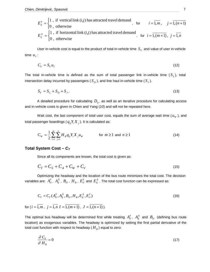
User in-vehicle cost is equal to the product of total in-vehicle time VS and value of user in-vehicle

time Iu :

C S uV V I= (12) The total in-vehicle time is defined as the sum of total passenger link in-vehicle time ( LS ), total

intersection delay incurred by passengers ( DS ), and line haul in-vehicle time ( JS ).

S S S SV L D J= + + , (13)

A detailed procedure for calculating ijD , as well as an iterative procedure for calculating access

and in-vehicle costs is given in Chien and Yang (10) and will not be repeated here.

Wait cost, the last component of total user cost, equals the sum of average wait time ( Wu ), and

total passenger boardings ( jiij XYq ). It is calculated as:

∑∑= =

=m

i

n

jWjiijBW uXYqHC

1 12

1 for 1≥m and 1≥n (14)

Total System Cost – CT Since all its components are known, the total cost is given as: VWAST CCCCC +++= (15)

Optimizing the headway and the location of the bus route minimizes the total cost. The decision

variables are: YiJA , X

IjA , IJB , BH , YiJE and X

IjE . The total cost function can be expressed as:

),,,,,( YiJ

XIjBIJ

XIj

YiJTT EEHBAACC = (16)

for ( mi ,1= , nj ,1= )1(,1 += mI , )1(,1 += nJ ).

The optimal bus headway will be determined first while treating YiJA , X

IjA and IJB (defining bus route

location) as exogenous variables. The headway is optimized by setting the first partial derivative of the total cost function with respect to headway ( BH ) equal to zero:

0 =

B

T

H

C

∂∂

(17)


The optimal bus headway BH is stated as:

∑∑= =

= m

i

n

jW

Nj

Niij

BRB

uXYq

uTH

1 1

2 for 1≥m and 1≥n (18)

All the variables are non-negative and the second derivative of the total cost function with respect to

BH

is always positive. Thus, the objective function ),,,,,( YiJ

XIjBIJ

XIj

YiJTT EEHBAACC = is convex, which

implies that a unique optimal headway exists for any given matrices YiJA , X

IjA and IJB . Therefore, the

minimum total bus route cost can be obtained by substituting the optimal headway in the total cost function. The optimal headway must meet the route capacity constraint that states that the total route capacity should be at least equal to the route passenger demand:

QCH v

B

≥⋅1, (19)

Therefore, the value of BH must satisfy the following:

Q

CH v

B ≤ (20)

Another approach would be to change the bus size, which will turn cause the change in the Bu ,

Wu , BH and the bus route configuration. IV. EXHAUSTIVE SEARCH ALGORITHM The Exhaustive Search (ES) algorithm is developed to determine the optimal bus route location. The algorithm searches all possible bus routes with an optimized headway through a given network, calculates the total cost of each route and selects the one with the minimum total cost. The algorithm has seven basic steps: Step 1: Setting up the network

Identify real, dummy and diagonal links, dimensions of the network, matrices and arrays that

define all input network variables (e.g. ijq , YijP , X

ijP , ijY , ijX and ijT ).

Step 2: Initialization

Set initial values for horizontal matrix XijA by setting the first real horizontal link from the top of

each column to be part of a route. Vertical links in matrix YijA are set to be part of a route as to

connect previously chosen horizontal links, and node matrix ijB is then defined by identifying

nodes in which route links (both horizontal and vertical) intersect. These values define the initial bus route. Set the initial route to be the current route.


Step 3: Calculate optimal headway

Determine the optimal bus headway BH for the current bus route. If the route capacity cannot accommodate the demand, set the capacity headway to be the optimal headway.

Step 4: Calculate the total cost

Calculate the total cost by substituting the optimal headway into the total cost equation.

Step 5: Optimality Test

Compare the total costs of the current and the candidate bus routes. The smaller total cost route becomes the current route.

Step 6: Generate the new candidate bus route

Generate the new candidate bus route by changing the values in matrix XijA and accordingly in

matrices YijA and ijB . Go to Step 3. If all possible bus routes have been generated proceed to

Step 7.

Step 7: Final optimal bus route plan

Calculate the final tables and output data for the global optimal solution. All output data is printed in a separate output file.

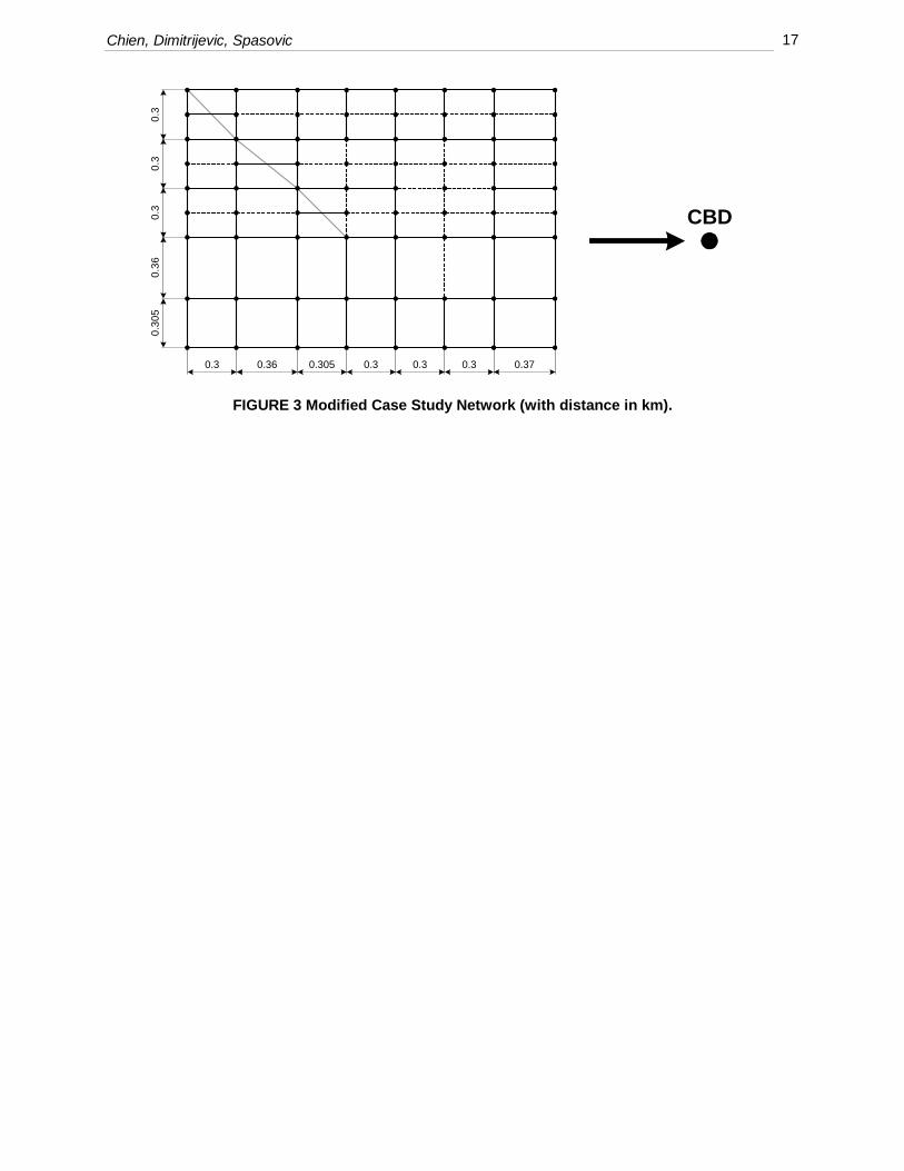
V. CASE STUDY The model is used to design an optimal bus route for the service area whose underlying street network is shown in FIGURE 3. Buses enter the network from the left (west) and moving eastward on the way to the CBD. The busses operate in local operation over the service area and in express operation from the end of the service area to the CBD. The length of the express leg of the trip is 6.43 km. The width of the service area is 1.565 km, while the length is 2.235 km. The network consists of m = 8 rows and n = 7 columns making 56 zones. The passenger density is defined for each zone and it varies from one zone to another. Its values range from 20 and 40 pass/km2. The total demand for the service region is 133 pass/h. Originally there were three diagonal links in the network. These links were transformed into horizontal and vertical links to preserve the pure grid structure. (The gray colored lines showing diagonal links are not part of the modified network.) The lengths of the diagonal links going from the northwest to the southeast corner are 0.425 km, 0.465 km and 0.427 km respectively. The intersection delay is given and it varies anywhere between 30 and 45 sec/veh. All the other parameters of the network are given in TABLE 2. The optimal bus route is shown in FIGURE 4 and is denoted as Route A. Its is 2.506 km long and it operates on the optimal headway of 14.2 min. The one-way trip time including the express line-haul is 15.5 min. Its total cost is $486 /hour. The bus fleet necessary to operate this headway is 2.2 buses. Since in reality the number of buses must be an integer, the fleet size is arbitrarily rounded to two and three busses, the headway recalculated for both values, and the lowest cost route chosen. The fleet of three buses is operated at the headway of 10.6 min and at the total cost of $499/hour. The fleet of two buses is operated at the headway


of 15.9 min yielding the lowest cost of the two at $488/hour. It is recognized that this is an inexact procedure; however one must bear mind that there is no exact method for finding the global optimum for non-linear integer optimization problems.

VI. SENSITIVITY ANALYSIS

A sensitivity analysis was performed to investigate how the model reacts to variations in the values of different parameters. Three parameters were varied:

• Bus size – three bus sizes were considered: 35 pass/veh, 50 pass/veh and 70 pass/veh; the average

hourly bus operating costs for these buses were $60 /hour, $70 /hour and $85 /hour respectively; • Demand – for each zone in the network, the demand density ranged from 70% to 150% of its original

value; • Value of passenger time – the passenger wait time and access time were assumed identical in value

and their values varied from 10 to 15 $/pass-hour. The passenger in-vehicle time ranged from 4 to 10 $/pass-hour. For this calculation, value of in-vehicle time is $5 less than the value of wait time.

The bus route location was not sensitive (i.e. did not change) with a variation in the value of passenger time. The same held when the demand was increased by 50%. However, if the demand was increased by more 50%, the configuration of the bus route changed. The new bus route is shown in FIGURE 5 and labeled as Route B. Route B is 2.929 km long, operates at the optimal headway of 10.2 minutes and has a one-way trip time, including the line-haul, of 17.4 min. The total cost is $837/hour. This change of route configuration indicates that the model is sensitive to variations in demand. Route B is longer then Route A, and this increase in route length resulted in an increase in the in-vehicle cost. However, the reduction in access cost caused by the route location change more than offsets the increase in the in-vehicle time. Passengers originating from zones closer to Route B then to Route A experience decreased access time. Thus, savings in access cost for passengers from zones closer to the Route B became greater than the increase in in-vehicle cost and the increase in access cost for passengers from zones closer to the Route A. This trade-off between the access cost and the in-vehicle cost, caused by the change in demand pattern, resulted in a change of the bus route location from Route A to Route B.

FIGURE 6 shows the relationship between demand and optimal headway. For all three bus sizes,

the optimal headway decreases as the demand increases. Similarly, FIGURE 7 shows a decrease in the headway as the value of passenger time increases. Regardless of the variation in demand or in the value of passenger time, the 35 pass/bus bus size is the most preferable as it yields the minimum total (FIGURES 8 and 9).

VII. CONCLUSIONS

The paper presents a model for optimizing the bus route design in an irregular grid network with diagonal links. Since diagonal streets are prevalent in a majority of urban street networks, the network transformation procedure developed in this paper makes the proposed model more realistic. The majority of previous research studies directed at this issue considered a service area divided into a number of square zones that reflected the underlying iron grid street network. The network transformation procedure presented here facilitates the transfer of those models that were developed for pure grid systems to irregular grid networks as well.

The model enables bus operators to determine the optimal bus route and assist in efficient fleet management. Output data is easy to interpret and supports effective decision-making. The model can be used to analyze different scenarios by varying the value of passenger time, vehicle size and demand. The case study demonstrates that the model is sensitive to the changes in demand patterns, i.e., it can redesign the bus route location in order to minimize the total system cost in response to the change in


demographics and demand density. This is very important point in redesigning bus routes in urban areas that have experienced significant shifts in residential density. Further improvement to the model is possible including an interface with Geographic Information System (GIS) databases containing the real world information on street geometry, the geocodes of the transit service area, and its demographics. This interface would facilitate the calculation of access distances and related costs as well as improve the overall accuracy of model calculations. ACKNOWLEDGEMENTS

This research was partially supported by a grant from the US Department of Transportation,

University Transportation Centers Program, through the National Center for Transportation and Industrial Productivity (NCTIP) at NJIT. This support is gratefully acknowledged but implies no endorsement of the conclusions by these organizations.


�REFERENCES 1. Byrne, B. F., and V. Vuchic. Public Transportation Line Positions and Headways for Minimum Cost.

Traffic Flow and Transportation, Elsevier Publishing Co., New York, N.Y., 1971, pp. 347-360. 2. Chang, S. K., and P. M. Schonfeld. Optimization Models for Comparing Conventional and

Subscription Bus Feeder Services. Transportation Science, 1991, 25, pp. 281-298. 3. Hurdle, V. F. Minimum Cost Locations for Parallel Public Transit Lines. Transportation Science, 7,

1973, pp. 340-350. 4. Spasovic, L. N., and P. M. Schonfeld. A Method for optimizing transit service coverage.

Transportation Research Record 1402, 1993, pp. 28-39. 5. Spasovic, L. N., M. P. Boile, and A. K. Bladikas. Bus Transit Service Coverage for Maximum Profit

and Social Welfare. Transportation Research Record 1451, 1994, pp. 12-22. 6. Wirasinghe, S. C., V. F. Hurdle, and G. F. Newell. Optimal Parameters for a Coordinated Rail and

Bus Transit System. Transportation Science, 1977, 11, pp. 359-374. 7. Welch, W., R. Chisholm, D. Schumacher, and S. R. Mundle. Methodology for Evaluation Out-of-

direction Bus Route Segments. Transportation Research Record 1308, 1991, pp. 43-50. 8. Chien, S., and P. M. Schonfeld. Optimization of Grid Transit System in Heterogeneous Urban

Environment. Journal of Transportation Engineering, ASCE, 123(1), 1997, pp. 28-35. 9. Chien, S., and P. M. Schonfeld. Joint Optimization of a Rail Transit Line and Its Feeder Bus System.

Journal of Advanced Transportation, 32(3), 1998, pp. 253-284. 10. Chien, S., and Z. Yang. Optimal Feeder Bus Routes with Irregular Street Networks. Journal of

Advanced Transportation, Vol. 34, No. 2, Summer 2000, pp. 213-248.


TABLE 1 Variable and Parameter Definition.

Symbol Definition Unit

ija Total access time for passengers originating from zone (i,j) hours

XijA Network horizontal links matrix

YijA Network vertical links matrix

ijB Network node matrix

AC Total passenger access cost $/hour

SC Total supplier cost $/hour

TC Total system cost $/hour

UC Total user cost $/hour

vC Total bus line capacity pass/hour

VC Total in-vehicle cost $/hour

WC Total wait cost $/hour

ijD Minimum access distance for passengers from zone (i,j) km

XijE Passenger attraction matrix for horizontal links

YijE Passenger attraction matrix for vertical links

F Fleet size buses

g Passenger walking speed km/hour

BH Headway hours

JL Line haul distance km

d Length of the horizontal link that replaced the diagonal link km

l Length of the vertical link modified after diagonal link is replaced km

m Number of rows in the network

n Number of columns in the network

XijP Penalty matrix for horizontal links

YijP Penalty matrix for vertical links

Q Total passenger demand pass/hour

ijq Demand density of the zone (i,j) pass/km2


TABLE 2 Variable and Parameter Definition (continued).

Symbol Definition Unit

DS Total intersection delay incurred by passengers hours

JS Total line haul in-vehicle time hours

LS Total route link in-vehicle time hours

VS Total in-vehicle time hours

DT Total route intersection delay hours

ijT Intersection delay matrix hours

JT Line haul travel time hours

LT Total route link travel time hours

RT Round trip travel time hours

Au Value of passenger access time $/hour

Bu Average bus operating cost $/hour

Iu Value of passenger in-vehicle time $/hour

BV Average bus operating speed in the service area km/hour

JV Line haul speed km/hour

ijX Matrix of lengths of horizontal links in the network km

NjX Width of the row j of the network km

ijY Matrix of lengths of vertical links in the network km

NijY Width of the column i of the network km


TABLE 2 Values of Parameters in the Case Study Network.

Variable Description Value

uB Average bus operating cost 70.00 $/veh-hour

uA Value of passenger access time 10.00 $/pass-hour

uW Value of passenger wait time 10.00 $/pass-hour

uI Value of passenger in-vehicle time 5.00 $/pass-hour

Cv Bus Capacity (Bus Size) 50 pass/veh

LJ Line-haul distance 6.43 km

VJ Bus line-haul speed 50 km/hour

VB Bus speed on network streets 40 km/hour

g Passenger access speed to bus route 3.2 km/hour


FIGURE 1 Graphical Interpretation of the Street Network.

FIGURE 2 Transformed Network Representation.

A

G

C

B

D

F

E

CBD

dummy links

nodes

real links

A

X Y

C D

B

G

E

M

F

N

L1 L2 L3 L4 L5

L10L6S1

L8L7 L9


FIGURE 3 Modified Case Study Network (with distance in km).

0.3 0.36 0.305 0.3 0.3 0.3 0.37

0.30

50.

360.

30.

30.

3

CBD


FIGURE 4 Bus Route A.

FIGURE 5 Bus Route B.

Route A

Route A

Route B

Ro

ute B


FIGURE 6 Demand vs. Optimal Headway

FIGURE 7 Value of Passenger Time vs. Optimal Headway

0.0

2.0

4.0

6.0

8.0

10.0

12.0

14.0

16.0

70% 80% 90% 100% 110% 120% 130% 150%

Demand (% of Original Demand)

Op

tim

al H

ead

way

(m

in)

Bus size = 70 pass/veh



Value of Passenger In-vehicle Time ($/hour)

0.0

2.0

4.0

6.0

8.0

10.0

12.0

14.0

16.0

18.0

49

510

611

712

813

914

1015

Value of Passenger Wait/Access Time ($/hour)

Op

tim

al H

ead

way

(m

in)





FIGURE 8 Demand vs. Total Cost

FIGURE 9 Value of Passenger Time vs. Total Cost

0.0

100.0

200.0

300.0

400.0

500.0

600.0

700.0

800.0

900.0

1000.0

70% 80% 90% 100% 110% 120% 130% 150%

Demand (% of Original Demand)

To

tal C

ost

($/

ho

ur)




Value of Passenger In-vehicle Time ($/hour)

0.0

100.0

200.0

300.0

400.0

500.0

600.0

700.0

800.0

49

510

611

712

813

914

1015

Value of Passenger Wait/Access Time ($/hour)

To

tal C

ost

($/

ho

ur)




Bus Route Planning in Urban Grid Commuter Networks

Documents

Transcript of Bus Route Planning in Urban Grid Commuter Networks