Transit Route and Frequency Design: Bi-level Modeling and Hybrid Artificial Bee

Colony Algorithm Approach

W.Y. Szeto*, Y. Jiang

Department of Civil Engineering, The University of Hong Kong, Pokfulam Road, Hong Kong

* email: ceszeto@hku.hk

Abstract

This paper proposes a bi-level transit network design problem where the transit routes and

frequency settings are determined simultaneously. The upper-level problem is formulated as a

mixed integer non-linear program with the objective of minimizing the number of passenger

transfers, and the lower-level problem is the transit assignment problem with capacity

constraints. A hybrid artificial bee colony (ABC) algorithm is developed to solve the bi-level

problem. This algorithm relies on the ABC algorithm to design route structures and a

proposed descent direction search method to determine an optimal frequency setting for a

given route structure. The descent direction search method is developed by analyzing the

optimality condition of the lower-level problem and using the relationship between the lower-

and upper-level objective functions. The step size for updating the frequency setting is

determined by solving a linear integer program. To efficiently repair route structures, a node

insertion and deletion strategy is proposed based on the average passenger demand for the

direct services concerned. To increase the computation speed, a lower bound of the objective

value for each route design solution is derived and used in the fitness evaluation of the

proposed algorithm. Various experiments are set up to demonstrate the performance of our

proposed algorithm and the properties of the problem.

Keywords: Transit route and frequency setting problem; Bus network design; Bi-level

programming; Artificial bee colony algorithm; Mixed integer program; Matheuristics

1. Introduction

Transit network design has received considerable attention over the last two decades due to

its practical importance. For example, in Hong Kong, over 90% of the 11 million daily trips

that people make involve public transport. Hence, a well-designed transit network is

1

important for meeting passenger demand. Guihaire and Hao (2008) and Kepaptsoglou and

Karlaftis (2009) provided comprehensive reviews in this area. Previous works on this topic

focus on route design (e.g., Mandl, 1980; Murray, 2003; Wan and Lo, 2003; Li et al., 2011,

2012), frequency setting (e.g., Furth et al., 1982; LeBlanc, 1988; Hadas and Shnaiderman,

2012), timetabling (e.g., Wong et al., 2008; Fleurent et al., 2004), vehicle scheduling (e.g.,

Bunte et al., 2006), crew scheduling (e.g., Wren and Rousseau, 1993), fare structure (e.g., Li

et al., 2009), fleet size determination (e.g., Li et al., 2008) and a combination of the above

(e.g., Ceder and Wilson, 1986; Lee and Vuchic, 2005; Szeto and Wu, 2010).

The majority of previous studies have considered the optimization of transit route

structures and service frequencies separately. For example, Fernandez and Marcotte (1992),

Constantin and Florian (1995), Zubieta (1998), Gao et al. (2004), Uchida et al. (2005, 2007),

and Leiva et al. (2010) proposed models for optimizing frequencies to achieve different

objectives within an existing transit network, whereas Laporte et al. (2010) and Yu et al.

(2012) focused exclusively on designing route structures. Both transit route structure and

frequency setting determine the level of service (e.g., in terms of in-vehicle congestion and

waiting time at bus stops); more importantly they determine whether the service has sufficient

capacity to meet to passenger demand. Therefore, it is important to simultaneously optimize

the transit route structure and the frequency setting.

In transit network design, it is essential to consider the in-vehicle congestion issue.

In-vehicle congestion leads to increased waiting and travel times, along with the comfort

problem prompted by a lack of seats for passengers. This comfort problem can be particularly

serious if the trip time is long or demand is high. Generally, there are two approaches to

addressing the congestion issue: capacity constraint and the congestion cost function. The

capacity constraint approach (e.g., Kurauchi et al., 2003; Lei and Chen, 2004; Lam et al.,

1999, 2002; Cepeda et al., 2006; Sumalee et al., 2009, 2011; Schmöcker et al., 2008, 2011;

Szeto et al., 2013; Cortés et al., 2013) incorporates capacity constraints in transit assignment

models that disallow flows on transit vehicles to be greater than the corresponding capacity.

The congestion cost function approach (e.g., Spiess and Florian, 1989; de Cea and Fernández,

1993; Lo et al., 2003; Li et al., 2008, 2009, 2011; Sun and Gao, 2007; Teklu, 2008; Szeto et

al., 2011a; Szeto and Jiang, 2014) adopts an unbounded increasing convex function to model

the effect of in-vehicle congestion on waiting time. Although both approaches have been used

in the literature, practically speaking, the former is more realistic because the latter can result

in an unacceptable line flow that is far greater than the corresponding capacity. 2

In addition to the congestion issue, it is important to consider passenger transfers between

transit vehicles, as they can generate passenger inconvenience. The number of passenger

transfers is an important network performance indicator, especially in Hong Kong, for the

following reasons. First, the total number of passenger transfers reflects the number of

passengers without direct services to their destinations, which can indicate inconvenience.

Second, passengers always complain when there are no direct services to their destinations

(Szeto and Jiang, 2012). The total number of passenger transfers also indirectly reflects the

number of complaints regarding lack of direct services. Optimizing the number of passenger

transfers can reduce the number of complaints implicitly. However, very few studies have

considered this number. Baaj et al. (1990) embedded the transfer concept into their route

generation procedures, such that a route with more than two transfers was abandoned.

Similarly, the number of passenger transfers was modeled implicitly in Zhao et al. (2005).

The travel cost calculated in the objective function excluded the travel costs of routes with

more than two transfers, yet they did not optimize the total number of passengers needing to

transfer between transit vehicles. Guan et al. (2006) used the total number of passenger

transfers as a surrogate of transfer and waiting times in passenger line assignment, which is

the lower level problem of their transit network design problem. Jara-Díaz et al. (2012)

considered the total number of passenger transfers to investigate the condition under which a

transit network design with transfers is preferable. Most of the existing studies have used the

total passenger travel time as the objective function. However, there is no guarantee that

minimizing the total number of passenger transfers also minimizes the total passenger travel

time. In some cases, there can be a tradeoff between the total number of passenger transfers

and total passenger travel time (Szeto and Wu, 2010). It is essential to explicit capture the

total number of passenger transfers in the objective function.

This paper proposes a bi-level model for designing transit routes and their frequencies that

explicitly minimizes the total number of passenger transfers in the objective function of the

upper-level problem and incorporates strict capacity constraints to address the in-vehicle

congestion in the lower-level problem. This bi-level model is formulated as a mixed integer

non-linear program that is NP-hard and considers the route choice behavior of passengers

through the lower-level user-equilibrium problem. The model also considers the stop location

choice of each route within each zone of the study area. This model differs from the bi-level

models proposed by Constantin and Florian (1995), Gao et al. (2004), and Uchida et al. (2005,

2007) in the sense that they only considered frequency setting, whereas our model further 3

considers route design and stop location choice.

To solve transit network design problems, exact methods (e.g., Wan and Lo, 2003) and

metaheuristics such as genetic algorithms (GAs) (e.g., van Nes et al., 1988; Bielli et al., 2002;

Chakroborty, 2002; Tom and Mohan, 2003; Ngamchai and Lovell, 2003; Shih et al., 1998;

Fan and Machemehl, 2006a; Mazloumi et al., 2012) and simulated annealing (e.g., Fan and

Machemehl, 2006b; Zhao and Zeng, 2006) have been used. A hybrid artificial bee colony

(ABC) algorithm—a matheuristic that combines a metaheuristic and an exact algorithm—is

developed for the transit network design problem as an improvement to the original ABC

algorithm, a metaheuristic proposed by Karaboga (2005) and motivated by the foraging

behavior of honey bees.

Compared with existing evolutionary algorithms such as GAs, the ABC algorithm has a

better local search mechanism that improves the solution quality. More recently, the ABC

algorithm has been applied to solve complex engineering optimization problems. For example,

Kang et al. (2009) successfully applied an ABC algorithm to the parameter identification of

concrete dam-foundation systems. Karaboga (2009) proposed an ABC algorithm to solve a

digital filter design problem and obtained good results. Karaboga and Ozturk (2009) used an

ABC algorithm to train neural networks for pattern classification, and their results on

benchmark instances showed that such use was efficient. Szeto et al. (2011b) improved the

ABC algorithm to solve a capacitated vehicle routing problem. Szeto and Jiang (2012)

enhanced the ABC algorithm to solve a single-level transit network design problem without

considering the in-vehicle congestion effect. Long et al. (2014) improved the ABC algorithm

to solve a turn restriction design problem. Szeto and Jiang (2012) and Long et al. (2014)

showed that their proposed ABC algorithm is better than the GA for solving their problems,

but it has not yet been improved to solve bi-level transit network design problems that

consider in-vehicle congestion. This study enhances the ABC algorithm to solve this problem.

The proposed algorithm relies on the ABC algorithm to design route structures and a

proposed descent direction search method to determine an optimal frequency setting for a

given route structure. A node insertion and deletion strategy for repairing the route structures

is developed based on average-direct-demand, which is defined as the average passenger

demand on the direct services concerned. The descent direction search method is developed

by analyzing the optimality condition of the lower-level problem and using the relationship

between the lower- and upper-level objective functions. The step size for updating the

frequency setting is determined by solving a linear integer program formed by the derivative 4

obtained by the Lagrange function of the lower-level problem. The Simplex method is used to

solve the lower-level problem. To increase the computation speed, a lower bound of the

objective value for each route design solution is derived and used in the fitness evaluation for

the hybrid ABC algorithm.

Various experiments are conducted to demonstrate the effectiveness of our proposed

algorithm. They illustrate the effects of various node insertion and deletion strategies and the

effects of different parameter values and forms of fitness functions on the performance of the

hybrid ABC algorithm. A realistic case study is conducted to show that under demand

uncertainty, the optimal solution obtained from the hybrid ABC algorithm is better than the

existing bus network design in terms of the average number of passenger transfers, and is

more robust in terms of handling passenger demand. We also use the Winnipeg network to

demonstrate that the performance of our proposed method is better than that of a GA to solve

our problem. The experiments illustrate the effects of different design parameters such as

minimum frequency, maximum fleet size, and the maximum numbers of routes and

intermediate stops on the objective value. The results show that a higher minimum frequency

can lead to a higher number of passenger transfers, and multiple design solutions are possible.

The main contributions of this study are as follows.

1) Proposing a bi-level model to simultaneously solve the transit route design and

frequency setting problems while considering the candidate transit stop location

available in each zone in the study area and two inconvenience factors: transfers

between transit vehicles and in-vehicle congestion.

2) Developing a new matheuristic—the hybrid ABC algorithm—to solve the model.

3) Examining the properties of the bi-level problem and the performance of the

algorithm.

4) Demonstrating the applicability of the proposed model and algorithm in realistic

situations.

The remainder of this paper is organized as follows. Section 2 introduces the bi-level

model. The proposed hybrid ABC method is described in Section 3, and numerical examples

are presented in Section 4. Finally, the conclusions and future research directions are given in

Section 5.

5

2. Bi-level formulation of the problem

Consider a study area with a connected (bus) transit network represented by a directed

graph G with N nodes, E links (or arcs), and one dummy node (node 0) introduced for the

ease of formulating the problem. The study area is separated into many zones, each of which

is represented by a centroid. The centroid is the origin node aggregating the travel demand

within the zone. Each centroid is connected to all of the candidate transit stops and terminals

in that zone, in which a transit terminal for a bus service can be a candidate stop for another

bus service. Each centroid also generates N’ types of travel demand, each of which is

designated to one centroid (or destination node) outside the study area. Each of the N’

centroids is connected to bus terminals or bus stops in their individual zone. Both the bus

terminals and centroids in each of these zones are connected to the transit network in the

study area. The following notations are used in this paper.

Sets

UZ = a set of nodes in the upper-level network, excluding the depot;

Gs = a set of centroids within the study area;

Hm = a set of candidate stops connecting to centroid m;

U = a set of starting bus terminals inside the study area;

V = a set of ending terminals outside the study area;

Gd = a set of centroids/destinations outside the study area;

C = a set of bus terminals and candidate stops within the study area;

ZL = a set of nodes (including centroids) in the lower-level network;

= a set of transfer links or arcs in the lower-level network;

A = a set of transit links in the lower-level network;

= a set of transit links coming out from node i; and

= a set of transit links going into node i.

Indices

, m = indices of nodes;

e = the index of a centroid/destination outside the study area;

e′ = the index of an ending bus terminal outside the study area; and

r = the route index.

RT

iA+

iA-

ji,

6

Parameters

cij = the in-vehicle travel time on the shortest path between nodes i and j;

ca = the in-vehicle travel time on link a;

st = the average time for stopping at a node; emd = the travel demand from node m to centroid e;

W = the maximum bus fleet size allowed for the network;

kcap = the capacity of a bus;

Rmax = the maximum number of routes in the bus network;

fmin = the minimum frequency of a route;

Smax = the maximum number of stops (including the bus terminal) within the study area

on a route;

maxT = the maximum route travel time within the study area; and

= a very large value used in the sub-tour elimination constraint.

Decision Variables

Lower-level decisions

= the number of passenger transfers on transit link t to destination e;

= the flow on link a to destination e;

= the total waiting time at node i for all flows to destination e;

= ;

= .

Upper-level decisions

= the node potential at node , which is needed in the sub-tour elimination

constraint for bus route ;

Xijr = 1 if route r (r = 1 to Rmax) passes through node j immediately after node i, and 0

otherwise;

X0jr = 1 if route r starts at node j, and 0 otherwise;

Xi0r = 1 if route r ends at node i, and 0 otherwise;

X00r = 1 if route r is not available, and 0 otherwise;

fr = the frequency of route r;

= ijrX ; and

p

etv

eav

eiω

v eav

w eiω

irq i

r

X

7

f = .

Functions of decision variables

Tr = the trip time of route r from the starting terminal to the ending terminal;

= 1 if route r connects the terminal that links to centroid e, and 0 otherwise;

= the frequency of link a; and

'eid = the travel demand from node i to bus terminal e′ .

Upper-level problem 2.1.

The upper-level problem is to determine the frequency of and a route structure for each

transit line within the study area. The number of transfers within the study area is unlimited

and their possible locations must remain within the study area. The upper-level problem is

formulated as follows.

d

1, , Gmin

R

et

et T

z vx f q

∈∈

= ∑ ∑ (1)

subject to

for r = 1 to Rmax, (2)

for r = 1 to Rmax, (3)

{ } { }U U0 , 0 ,

0ijr jiri Z i Zi j i j

X X∈ ∪ ∈ ∪≠ ≠

− =∑ ∑ for Uj Z∈ , r = 1 to Rmax, (4)

{ }U 0 ,

1ijri Zi j

X∈ ∪≠

≤∑ , for Uj Z∈ , r = 1 to Rmax, (5)

{ }U 0 ,

1ijrj Zj i

X∈ ∪≠

≤∑ for Uj Z∈ , r = 1 to Rmax, (6)

jjrX = 0 for Uj Z∈ , r = 1 to Rmax, (7)

( )U U

t t,

r ijr iji Z j Z j i

T X c s s∈ ∈ ≠

= + −∑ ∑ for r = 1 to Rmax, (8)

, (9)

[ ]rf

erd

af

0{0}

1jrj U

X∈ ∪

=∑

0{0}

1i ri V

X∈ ∪

=∑

( )max

001

2 1R

r r rr

f T X W=

− ≤∑

8

for r = 1 to Rmax, (10)

max

,ijr

i C j C j iX S

∈ ∈ ≠

≤∑ ∑

for r = 1 to Rmax, (11)

( )t t max

,ijr ij

i C j C j iX c s s T

∈ ∈ ≠

+ − ≤∑ ∑ for r = 1 to Rmax, (12)

{ }

max

U1 0 ,

1m

R

ijrr i H j Z j i

X= ∈ ∈ ∪ ≠

≥∑ ∑ ∑ for sm G∈ , (13)

max

s

cap1

Re e

r r mr m G

f k dd= ∈

≥∑ ∑

for de G∈ , (14)

''

\U

er ie r

i Z VXd

∈

= ∑ for 'e V∈ , and (15)

for U,i j Z∈ , , r = 1 to Rmax. (16)

Objective (1) is to minimize the sum of transfer passengers. Constraint (2) ensures that all

of the bus service routes start from a bus terminal selected from the available locations inside

the study area. Constraint (3) ensures that each of the service routes ends at a bus terminal

selected from the available locations outside the study area. It should be noted that the rth

route is not needed to provide bus services when X00r = 1. Constraint (4) ensures that with the

exception of dummy nodes, any node on a service route has one preceding and one following

node. Constraints (5)-(7) ensure that each node can be visited by a particular route at most

once. Constraint (8) calculates the in-vehicle travel time (including stop time) of a service

route. Constraint (9) ensures that the fleet size used cannot exceed the available fleet size.

Constraint (10) ensures that the frequency of each service route is not less than the minimum

allowable frequency. Constraints (11) and (12) restrict the number of intermediate stops and

the trip time within the study area, respectively. Constraint (13) is the zone covering

constraint, and ensures that at least one of the candidate stops in each zone is served by at

least one transit line. Constraint (14) is the demand constraint, which ensures that there is

enough line capacity to meet passenger demand heading to each destination/centroid outside

of the study area. Constraint (15) determines whether route r ends at terminal e′ . Constraint

(16) is the sub-tour elimination constraint, which is extended from Miller et al. (1960).

In this formulation, the decisions are the route structures and frequencies. However, under

the preceding setting and constraint (13), the route design automatically also considers the

stop location choice in a zone because there is more than one candidate stop in each zone in

general, and a route may not pass through all of them.

( )min 001 r rf X f− ≤

1ir jr ijrq q pX p− + ≤ − i j≠

9

Lower-level problem 2.2.

The lower-level problem requires another network representation to depict the passenger route

choice behavior under a given set of transit routes defined by the upper-level problem. The

network representation for the lower-level problem is extended from the one proposed by

Nguyen and Pallottino (1988). The network is also represented by nodes and links (or arcs).

However, a node may represent a bus stop in a transit line, a boarding node, an alighting node,

or a centroid. A link is used to connect two adjacent nodes. Each link has three attributes:

travel time, frequency, and capacity.

Figure 1 is a graph representation of a centroid connecting one general transit stop served

by n transit lines. Similar to the graphical representation proposed by Nguyen and Pallottino

(1988), there is a pair of boarding and alighting arcs connecting the bus stop of each transit

line, , 1,...,is i n= , to the stop node (as represented by the node defined by the dashed line in

Figure 1) that corresponds to the node in the upper-level network. To ensure that these arcs

are only used for connectivity purposes, the travel time is set to zero and the capacity is set to

a very large number. The frequency of the alighting arc is also set to a very large number,

whereas the frequency of the boarding arc is equal to the frequency with which the passengers

are entering the transit line. Unlike the graphical representation proposed by Nguyen and

Pallottino (1988), we replace the stop node with two other nodes—an alighting node sa and a

boarding node sb—a transfer arc to connect them, a centroid that corresponds to the centroid

in the upper-level network, one access arc, and one egress arc. The boarding (alighting) node

is used to send (receive) passengers to (from) different transit lines and receive (send)

passengers from (to) the centroid via the access (egress) link. The travel times of the access

and egress links are equal to the walking times from the centroid to the transit stops, while the

frequencies and capacities associated with access and egress links are very large (i.e., infinity).

The transfer arc has a travel time of M, a very high frequency, and a very large capacity.

Intuitively, M can be interpreted as the inconvenience cost (expressed as time-equivalent) or

transfer penalty generated by a transfer, and can be calibrated from survey data. When a direct

service is always preferred to a transfer service, M is set to be a large number.

There is no alighting arc, alighting node, or egress arc for a starting terminal and no

boarding arc, boarding node, or access arc for an ending terminal. The consecutive bus stops

of a transit line are connected by a travel arc, in which the travel time is set to be equal to the

in-vehicle travel time plus the stop time at the next stop, and the stop time at each terminal is

10

set to zero. The frequency of a travel arc is set to the frequency of the transit service, whereas

its capacity is the frequency of that arc multiplied by the bus capacity. All of the general

transit stops and terminals are connected through travel arcs.

Because the demand of each origin-destination (OD) pair is fixed and the flow on each link

cannot be greater than that link’s capacity, the total demand between an OD pair may be larger

than the available capacity provided by all transit lines serving this OD pair. Hence, the

lower-level formulation may not provide a feasible solution. To address this issue, a virtual

link (corresponding to a walking path) with a very large capacity, a very high frequency, and a

very long trip time is created to connect each OD pair. The flow on each virtual link at

optimality is then equal to the unserved demand of the corresponding OD pair. In the extreme

case, when the capacity between an OD pair is zero, there is still a feasible and optimal

solution for that OD pair.

Figure 1 A graph representation of a centroid connecting one general transit stop

Based on this network representation, the transit assignment formulation proposed by

Spiess and Florian (1989) can be extended to capture transfer penalty and in-vehicle

congestion as follows.

Alighting arc

Boarding arc

Transfer arc

:

:

Transit line 1

Transit line 2

Transit line n

Access arc Egress arc

s1

s2

sn

sb sa

Centroid

Stop node

11

d L d

2,min : e e

a a ia A e G i Z e G

z c v ω∈ ∈ ∈ ∈

= +∑∑ ∑∑v w (17)

subject to

for L d, ,ia A i Z e G+∈ ∈ ∈ , (18)

for L d,i Z e G∈ ∈ , (19)

capd

ea a

e Gv f k

∈

≤∑ for , (20)

for d,a A e G∈ ∈ , and (21)

for L d,i Z e G∈ ∈ . (22)

The lower-level objective (17) is to minimize the sum of the total in-vehicle travel and stop

times (i.e., the first term of the objective function) and total waiting time (i.e., the second term

of the objective function). Constraint (18), which relates link flow, frequency, and waiting

time, is a relaxed constraint of distributing node flows into the arcs emanating from that node.

Constraint (19) is the flow conservation condition for a node. Constraint (20) ensures that the

flow on each travel arc is not greater than that arc’s capacity, with the capacity constraint used

to model the in-vehicle congestion cost and extra delay due to passenger overloading.

Constraints (21) and (22) are non-negativity conditions.

In the lower-level problem, the following points related to the proposed capacity constraint

must be clarified. First, the capacity constraint must be incorporated into the lower- rather

than the upper-level problem. The capacity constraint is used to model that, due to limited

vehicle capacity, some passengers may not be able to board the first bus that arrives at a bus

stop, and hence may experience extra delays. The capacity constraint is placed in the

lower-level problem to ensure that such delays are considered in passengers’ route choices.

The extra delay of a passenger on a link is equal to the Lagrange multiplier associated with

the capacity constraint, which appears in the equilibrium condition derived from the Karush–

Kuhn–Tucker condition of the lower-level problem. If the capacity constraint were placed in

the upper-level, it would be assumed that passengers would not consider the delay in

determining their route choice because the lower-level problem would be identical to the

transit assignment problem proposed by Florian and Spiess (1989). This behavioral

assumption is unrealistic.

The second point is related to the flow distribution. If the lower-level capacity constraint is

not binding, the formulation reduces to the original strategy formulation (Spiess and Florian,

e ea a iv f ω≤

i i

e e ea a i

a A a A

v v d+ −∈ ∈

= +∑ ∑

a AÎ

0eav ≥

0eiω ≥

12

1989), where the resultant line flow is proportional to the line frequency, strictly following the

assumptions that passengers arrive randomly, headway is exponentially distributed, and

passengers select the first bus from a set of attractive lines that arrives at the bus stop. If the

capacity constraint is binding, the flow distribution may not satisfy those assumptions because

the passengers cannot board the first bus that arrives at the bus stop if it is full. In such cases,

the results are approximations that are acceptable for strategic planning purposes.

The third point is related to the in-vehicle congestion cost. In the proposed model,

passengers only perceive congestion costs if the capacity constraint is binding or buses are

fully occupied. Otherwise, the congestion cost is neglected. However, in reality, passengers

may still perceive in-vehicle congestion costs, such as the cost due to insufficient seat

capacity or in-vehicle crowding, even when the capacity has not been reached. The more

passengers there are inside a bus, the higher the in-vehicle congestion cost. Hence, the

congestion cost should be a continuous and increasing function. In the proposed capacity

constraint method, the in-vehicle congestion cost is a piecewise function, which can be

addressed by developing a continuous, non-linear, and increasing in-vehicle cost function that

can be linearized to reduce the problem to a linear programming problem. However, deriving

this function has been left for future study.

The proposed formulation has three advantages. First, the lower-level problem is a linear

programming problem and can be solved efficiently by existing algorithms. Second, it is easy

for us to identify whether a particular route section is overloaded (by checking whether the

corresponding Lagrange multiplier is positive) and whether the overall transit supply is

sufficient (by checking virtual links carry flow)—all of which makes it easier to design

appropriate improvement strategies. Third, this linear problem allows us to develop an

efficient method for solving the transit network design problem.

3. Solution method

Constraint (9) is non-linear, and the decision variables are both discrete and continuous.

Hence, the bi-level problem is a mixed-integer non-linear problem. It has been noted that a

general network design problem is already NP-hard (Magnanti and Wong, 1984), and it is

well-known that the transit route design problem is NP-hard (Zhao and Gan, 2003; Fan and

Machemehl, 2004; Fan and Mumford, 2010). Our proposed problem includes the frequency

setting problem and a lower-level problem that is more complicated than the general network

design and the transit routing problems. Thus, our problem is also NP-hard. Given the 13

extreme difficulty of solving NP-hard problems for exact solutions, a hybrid artificial bee

colony (ABC) algorithm is proposed to solve the bi-level problem. The hybrid relies on the

original ABC algorithm to solve the route design problem and incorporates a proposed

iterative procedure to determine the number of passenger transfers and the optimal frequency

setting. In the iterative procedure, the linear transit assignment problems (17)-(22) are solved

in each iteration via the Simplex method. Then, a descent direction is obtained using the dual

solutions to the transit assignment problem and used to formulate a linear integer program,

which is solved to give a step size to update the frequency for the next iteration. To alleviate

the computational burden of solving many transit assignment problems, a screening method

based on the lower bound of the upper-level objective function is also developed. Only

potentially good route design solutions are required to find the corresponding optimal

frequency. However, the other solutions are kept for a neighborhood search.

Artificial bee colony (ABC) algorithm 3.1.

The ABC algorithm belongs to a class of evolutionary algorithms inspired by the

intelligent behavior of honey bees finding nectar sources around the hive. This class of

metaheuristics has received increasing attention recently, with variations of bee algorithms

proposed to solve combinatorial problems. However, in all of them, a common search strategy

is applied; that is, complete or partial solutions are considered as food sources and different

groups of bees try to exploit the solution space in the hope of finding good quality nectar, or

high quality solutions, for the hive. They then communicate directly to inform other bees

about the search space and the food sources.

In the ABC algorithm, the colony of bees is divided into employed bees, onlookers, and

scouts. Employed bees are responsible for exploiting available food sources (solutions) and

gathering required information. These bees also share information with onlookers, and each

onlooker selects a food source near the food source chosen by one employed bee. When the

source is abandoned, the employed bee becomes a scout and starts to search for a new source

in the vicinity of the hive. This abandonment happens when the quality of the food source

does not improve for a predetermined number of iterations.

The ABC algorithm is iterative, and starts by associating all employed bees with randomly

generated food sources (solutions). In every iteration, each employed bee selects a food

source in the neighborhood of the currently associated food source using a neighborhood

14

operator, and evaluates its nectar amount (fitness) afterwards. If its nectar amount is better

than that of the currently associated food source, then the employed bee keeps the new food

source and discards the old one; otherwise, the employed bee retains the old food source.

When all of the employed bees have finished this process, they share the nectar information

for the food sources with the onlookers. Each of the onlookers then selects a food source

according to a probability proportional to the nectar amount of that food source. In this study,

we use the traditional roulette wheel selection method (Haupt and Haupt, 2004). Clearly, with

this scheme, good food sources attract more onlookers than bad ones. After all of the

onlookers have chosen their food sources, each of them selects a food source in the

neighborhood of their chosen food sources (through neighborhood operators) and computes

its fitness. The best food source among the particular food source of an employed bee and its

neighboring food sources is the food source of the employed bee. If a solution represented by

a particular food source does not improve for a predetermined number of iterations, then the

food source is abandoned by its associated employed bee and the bee becomes a scout. The

scout then searches randomly for a new food source. This is done by assigning a randomly

generated food source (solution) to this scout. After each new food source is determined,

another iteration of the ABC algorithm begins. The whole process is repeated until the

termination condition is satisfied.

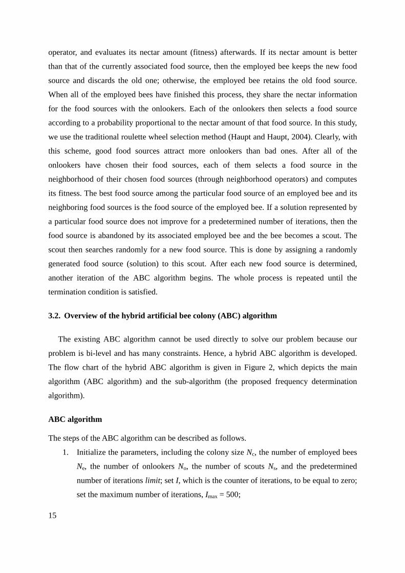
Overview of the hybrid artificial bee colony (ABC) algorithm 3.2.

The existing ABC algorithm cannot be used directly to solve our problem because our

problem is bi-level and has many constraints. Hence, a hybrid ABC algorithm is developed.

The flow chart of the hybrid ABC algorithm is given in Figure 2, which depicts the main

algorithm (ABC algorithm) and the sub-algorithm (the proposed frequency determination

algorithm).

ABC algorithm

The steps of the ABC algorithm can be described as follows.

1. Initialize the parameters, including the colony size Nc, the number of employed bees

Ne, the number of onlookers No, the number of scouts Ns, and the predetermined

number of iterations limit; set I, which is the counter of iterations, to be equal to zero;

set the maximum number of iterations, Imax = 500;

15

2. Perform the initialization phase of employed bees: Generate an initial solution for

each employed bee and set the limit counter for each solution to be zero;

3. Increase the number of iterations by 1, i.e., I = I + 1;

4. Perform the employed bee phase: Conduct a neighborhood search for each solution

found by an employed bee. Evaluate the fitness of each neighbor solution. Replace

the solution by its neighbor solution found by the search and set its limit counter to

zero, if the latter is better. Otherwise, keep the solution of the employed bee, and

increase the limit counter by 1;

5. Perform the onlooker bee phase: Perform the roulette wheel selection to determine

which solution obtained by an employed bee is selected by an onlooker. Then,

conduct a neighborhood search for each solution selected by an onlooker. Evaluate

the fitness of each neighbor solution. Replace the solution by its neighbor solution, if

the latter is better. Otherwise, keep the solution of the employed bee, and increase its

limit counter by 1;

6. Perform the scout bee phase: Replace each solution that fails to improve within limit

successive iterations by a new solution generated randomly;

7. Check the stopping criterion: If maxI I< , return to step 3;

8. Terminate and output the best solution.

16

(a) ABC algorithm (b) Frequency determination algorithm

Figure 2 Flow chart of the hybrid ABC algorithm

For the ABC algorithm in our proposed method, the initialization phase generates a

population of initial solutions by the employed bees. Afterwards, each employed bee is

associated with one randomly generated solution.

The employed and onlooker bee phases are quite similar, as shown in Figure 3. The only

difference lies in the rule for selecting a candidate food source for a neighborhood search. In

the employed bee phase, each employed bee selects its associated solution for a neighborhood

search. In the onlooker bee phase, each onlooker selects a solution based on the fitness value.

Hence, we expect promising solution areas to be visited and explored more frequently. Both

phases require the frequency determination algorithm to determine the frequency associated

No

1. Initialize parameters;I = 0;

4. Perform employed bee phase

5. Perform onlooker bee phase

8. Stop and output the best solution

6. Perform scout bee phase

3. I = I + 1

max7. I I<

2. Initialize employed bees

Yes

ABC algorithmFrequency determination

iii. Solve the transit assignment problem

v. Determine a descent direction

iv. Terminate?

NoYes

No

i. Initialize frequencies

vii. Return frequency setting

Yes

vi. Find the step size and update the frequency for each route

Input solution gat iteration I

ii. Is solution g infeasibleor 1, min ?I

g gLB z≥

17

with each route and evaluate the fitness value of each solution. They both conduct a greedy

selection after evaluating the fitness of the neighbor solution. If the neighbor solution is better

than the food source, the latter is replaced by the former and its limit counter is set to zero.

Otherwise, the current solution is maintained and the limit counter is increased by 1. Finally,

if all of the employed bees or onlookers complete their neighborhood searches, then the

employed or onlooker bee phase is terminated.

Figure 3 Flow chart of the employed bee and onlooker bee phases

In the scout bee phase, all of the food sources are scanned and the source that fails to

improve within limit successive iterations is abandoned and replaced by a newly generated

random solution.

Frequency determination algorithm

For each solution (i.e., route structure) obtained in the employed or onlooker bee phase of

the ABC algorithm, the following procedure is used to determine the frequency setting:

i. Generate the initial frequencies;

Select one neighbor solution for each employed bee

Generate a neighbor solution and repair the solution if necessary

Determine frequencies and evaluate the fitness of each

solution

Replace the solution by its neighbor, if the latter is better

Update limit counters

Employed bee phase

Select one neighbor solution based on fitness proportion

for each onlooker

Onlooker bee phase

18

ii. Decide whether to obtain an optimal frequency for each route: If LBg (the lower bound

of given solution g) is greater than 1,min Igz (the minimum upper-level objective

value until iteration I) or the route design is infeasible, then return the initial

frequency of each route. Otherwise, proceed to the next step;

iii. Solve the lower-level transit assignment problem;

iv. If the termination criterion of the frequency determination algorithm is satisfied, then

stop and return the optimal frequency setting. Otherwise, go to the next step;

v. Determine the descent direction of the lower- and upper-level objective values with

respect to the frequency;

vi. Find the step size of the frequency by solving a linear integer program and update the

frequency with the obtained step size, then go to step iii.

Solution generation and repairing procedures 3.3.

Solution representation in the ABC algorithm

To search all of the possible route structures, the solution representation in the ABC algorithm

should be specifically designed. Figure 4 illustrates the representation scheme used in the

ABC algorithm. One solution consists of 100 elements representing 10 routes, with 10

elements for each route. For example, the first 10 elements represent the first bus route, which

starts at node 1, goes through nodes 18, 15, 10, 12, and 7, and terminates at node 25. Similarly,

route 10 starts at node 16, goes through node 11, and terminates at node 27.

Figure 4 Solution representation scheme

1 18 15 0 0 25 7 12 10 ∙∙∙ ∙∙∙

Route 1

0 0 0 0 0 0

A total of 100 elements

16 11 27

Route 10

0 0

19

Initialization procedures

In the ABC algorithm, new solutions are generated in the initialization and scout bee phases,

both of which adopt the same procedures to generate a random solution, as shown in Figure 5.

To initialize the route elements, the following procedures are carried out sequentially. For

route r, the first node is determined by randomly selecting from the available starting

terminals in the study area. Then, the last node is picked from all of the available ending

terminals 'e , the number of intermediate stops is generated, and a corresponding number of

nodes is inserted between the two terminals. The probability of selecting an intermediate stop

node i is determined based on passenger demand by

U

'

'

ei

eij

j Z

dp d∈

= ∑ , where represents

the probability of choosing node i. If there is more than one stop in a zone, stop i in that zone

is randomly picked. The last step is to set the rest of the elements, if any, to zero.

Figure 5 Solution generation and repairing procedures

Repairing procedures

The solution generated makes it difficult to avoid infeasibility due to the proposed random

operations. Although we can add a penalty to the fitness value of an infeasible solution and

leave the algorithm itself to evolve, according to our preliminary experiments, the solution

quality in terms of the number of feasible solutions and the objective value in the final

iteration is lower than that obtained by the algorithm with the proposed route repairing

procedures. Therefore, we propose the route repairing procedures to provide better (initial)

solutions. The procedures include checking zone covering, stop sequence optimization, and

ip

Initialize routes’ elements

Repair the solution if necessary

Determine the lower bound

Generate a solution

Check zone covering and insert uncovered nodes

Optimize stop sequence

Delete and insert intermediate stops

Repair a solution

20

deleting and inserting intermediate stops.

Checking zone covering

The zone covering procedure is designed to ensure that every demand zone is visited by at

least one route. Because the total number of elements in a solution (which equals the

maximum number of stops multiplied by the maximum number of routes) is greater than the

number of zones in the network, there must be some zones that are visited by more than one

route. However, there is no guarantee that all zones are served or covered in the initialization

procedure. If centroid m is not served, then node i, which is one of the candidate stops

connecting to centroid m, is inserted into the selected route with the number of stops less than

the maximum allowable number of stops and the least travel time increment after inserting

node i. If no route can serve this centroid due to constraint (11) on the maximum number of

stops, a zone served by at least two transit lines is randomly selected and one of the stops in

the zone passing by the lines is replaced by node i. These two steps guarantee that the

zone-covering constraint (13) is satisfied.

Stop sequence optimization

For every generated ABC solution, a descent search heuristic is used to improve the sequence

of stops on each route. The purpose of this sequence-improving process is to minimize the trip

time of each route, as it does not depend on frequencies and is relatively easy to implement.

The outline of the heuristic is as follows:

For each route in the ABC solution

Set i' = 1

While i' ≤ the number of intermediate stops – 1

j' = i' +1

While j' ≤ the number of intermediate stops, do

Exchange the i' th and j'th stops

Evaluate the trip time of the route

If the trip time is reduced,

then set j' = number of intermediate stops + 1, i' = 0

else

undo the exchange and j' = j' + 1 21

endif

endwhile

i' = i' +1

endwhile

Next route in the ABC solution

Deleting and inserting intermediate stops

The stop sequence optimization procedure essentially rearranges the sequence of intermediate

stops to form the shortest path. Nevertheless, some routes may still violate the maximum trip

time constraint (12). Therefore, a stop-removal operation is conducted to eliminate nodes

while ensuring the solution to satisfy the zone covering constraint. Various criteria can be

used in selecting which nodes to delete, such as trip time reduction and the changes in total

flow of the direct services involved after performing the node removal. Different criteria have

different effects on the objective value and the algorithm performance.

We propose the following average-direct-demand 'ierψ to approximate the change in the

upper-level objective value that results from removing node i from route r, which connects

terminal 'e directly:

' '

'' 1

e ieie i rr ie

pp r

d dψd

≠

=+∑

for r = 1 to Rmax, Ui Z∈ , 'e V∈ ,

where 'iepd is a binary indicator variable that is equal to 1 if route p passes both nodes i and

'e . 'iep

p rd

≠∑ calculates the number of transit lines that provide a direct service between node i

and terminal 'e after removing node i from route r. Adding 1 to that number allows us to

consider the case when route r heading to terminal 'e originally passes node i. Hence, the

denominator gives the number of transit lines that provide a direct service between node i and

terminal 'e before removing node i from route r. The demand 'eid is obtained from the

lower-level problem, and is the total flow on the boarding arcs ending at the transit stop

corresponding node i in the upper-level network and heading to the transit stop corresponding

to terminal ' ee H∈ . Overall, this average-direct-demand intends to capture the increase in the

number of passenger transfers due to deleting node i. This average approximates the flow of

each direct service and is determined by evenly splitting the demand between node i and

22

terminal 'e to all of the routes providing direct services for that pair of nodes. This value can

be interpreted as the average increment in the number of transfer passengers when node i is

deleted from route r. Therefore, a node with a smaller ratio is preferred for removal, because a

smaller ratio indicates a lower average increment in the number of passengers who need to

make a transfer.

To compensate for the negative effects of deleting nodes, including reducing service

coverage and increasing the number of passengers who make a transfer, a reverse operation

called node insertion is subsequently conducted to insert as many nodes as possible while

ensuring that the resultant solution satisfies the maximum trip time constraint. The node

chosen for insertion is also based on the proposed average-direct-demand, and a larger value

is preferred.

Lower bound determination and fitness evaluation 3.4.

Fitness is used to reflect a solution’s quality and select candidate solutions for a

neighborhood search. Although the reciprocal of the upper-level objective value can be used

as a fitness measure for the proposed algorithm, it is cumbersome to calculate the upper-level

objective for each solution because the corresponding optimal frequency must be found by the

proposed frequency setting method, which involves solving the lower-level problem many

times. Thus, a lower bound is calculated to determine the minimum number of passenger

transfers for each solution, and then used to replace the upper-level objective value in the

fitness function. Such a bound can be obtained much more quickly than the reciprocal of the

upper-level objective value.

Given a route design solution, the lower bound provides the minimum number of

passenger transfers, which is an optimistic estimation of the upper-level objective function

value. The calculation of the lower bound is based on the assumption that each transit route

has unlimited capacity. Under this condition, the passenger demand 'eid , Ui Z∀ ∈ , 'e V∈ ,

can be met without needing to make a transfer if there is any route connecting nodes i and 'e .

Because summing up all of the served demand provides the maximum total passenger demand

without making a transfer, the minimum number of passenger transfers, or the lower bound,

can be obtained by calculating the difference between the total passenger demand

U

'

\ '

ei

i Z V e Vd

∈ ∈∑ ∑ and the sum of all passengers not making a transfer under the assumption stated

23

above, ( )U

' '

\ '1 e e

i ii Z V e V

NR d∈ ∈

−∑ ∑ , where 'eiNR equals 1 if there is no route connecting i and 'e ,

and 0 otherwise.

If the subscript g is used to denote a route design solution, then the lower bound of solution

g, LBg, can be mathematically expressed as

( )U U

' ' '

\ ' \ '

1e e eg i i i

i Z V e V i Z V e V

LB d NR d恄 恄

= - -槫 槫 , (23)

where

( )max

''

1

1R

ei ie r

r

NR RT=

= −∏ for U \i Z V∈ , 'e V∈ , (24)

U \ , ,

iwr iwr ijr jwrj Z V j i j w

RT X X RT∈ ≠ ≠

= + ∑ for U \i Z V∈ , U \w Z V∈ , w i≠ , r = 1 to Rmax, (25)

ijrRT = l if route r passes through node i and node j, and 0 otherwise.

With the lower bound of route design solution g, gLB , the fitness of solution g, gF , is

calculated via

1 .gg g

FLB P

=+

(26)

gP is a penalty term for solution g and is given by

( )max max

, max ,1 1

max ,0 max ,0R R

g r g r gr r

P T T V Wa β= =

= − + −

∑ ∑ , (27)

where ,r gV is the fleet size for route r in solution g; ,r gT is the trip time on route r in

solution g, and α and β are the penalty parameters related to the maximum trip time constraint

and the fleet size constraint, respectively. The penalty method deals with infeasible solutions

that cannot be repaired by any of the repairing operators. The first term in (27) penalizes the

violation of constraint (12) while the second term penalizes the violation of constraint (9).

Infeasible solutions are kept for neighborhood searches because it is possible for the global

minima to be located close to infeasible solutions. Nevertheless, by varying the penalty

parameter values, it is easy to adjust the probability of searching an infeasible solution region.

When the penalty value is large, the probability is small and vice versa.

Frequency determination procedure 3.5.

The following subsections describe the details of each step in the frequency setting procedure 24

depicted in Figure 2.

Step i: Frequency initialization

This step is conducted to obtain the initial frequency for each route. The initial frequency for

route r is calculated from

,,

,2r g

r gr g

Vf

T= , (28)

where ,r gf is the frequency of route r of solution g. Given trip time ,r gT , the total fleet

should be allocated carefully to meet the minimum frequency and demand conservation

requirements. Thus, we propose the following procedure for allocating buses to determine the

initial frequency of each route.

1. Assign buses according to minimum frequency constraint (10). Given the trip time on a

route, the minimum number of buses required to meet the minimum frequency constraint can

be determined by equation (28);

2. Assign buses according to demand requirement constraint (14). This procedure ensures

that the service capacity provided for each destination e is not less than the demand ending at

destination e, under the assumption that the total service capacity for the study area is not less

than the total demand. In the beginning, all of the transit lines with the same ending terminals

are grouped, and then two frequency values are calculated and compared for each group. One

is the assigned group frequency, which is the sum of the frequencies obtained in step 1. The

other is the required frequency, which is the minimum frequency required to meet the total

demand for each destination group calculated by sd

cap,

em

m Gd

e Gk∈ ∀ ∈∑

. For each group, if the

required frequency is larger than the assigned frequency, then the group frequency is

insufficient and the difference between the required and assigned frequencies is added to the

frequency of the route with the least trip time. The route with the least trip time is chosen

because when one more bus is assigned to that route, it produces the highest increase in the

frequency and the line capacity compared with other routes.

3. Round up the fleet size and recalculate frequencies. After the foregoing two steps, the

number of buses allocated to each route is calculated and rounded up to the nearest integer.

The frequency of each route is then recalculated, which usually ends with a slightly higher

value than the previous result.

25

This procedure handles the frequency-related constraints by determining the fleet size of

each route. Afterwards, if the sum of the fleet size of each route is less than or equal to the

total fleet size defined by constraint (9), then the route structure simultaneously satisfies

constraints (9), (10), and (14); otherwise, the route structure is infeasible and the fitness of the

infeasible solution is penalized. If there are residual buses that have not been allocated to any

route, they are added to the route with the least trip time because at global optimality all buses

must be used.

Step ii: Lower bound screening

After step i, we can identify whether a route structure is feasible. For infeasible solutions, it is

not necessary to search for optimal frequency. For feasible solutions, only potentially good

solutions proceed to obtain optimal frequency. Candidate solutions are identified by

comparing the lower bound with the current best objective value. If the lower bound of a new

solution is larger than the current best objective value found by the hybrid ABC algorithm,

then it is impossible to determine the upper-level objective value of a new solution that is

smaller than the current best objective value by adjusting its frequency and not changing the

route design. In this case, the route solution cannot be globally optimal and it is redundant to

carry out the frequency setting procedure. However, if the lower bound is less than the current

best objective value, then obtaining a better objective value by searching optimal frequency

settings is possible, and hence the solution is potentially good.

Step iii: Solving the transit assignment problem

With an initial frequency and a feasible route structure, the lower-level transit assignment

problem is solved by the Simplex method. Afterwards, both the primal and dual solutions are

recorded. The primal solution indicates the number of transfer passengers and the dual

solution is used, if necessary, to determine the descent direction and step size for updating

frequency in later steps.

Step iv: Termination criteria checking

The following stopping criteria are used:

Criterion (1) 1, 1k

g gz LB ε− ≤ and

Criterion (2) 11, 1, 2k k

g gz z ε+ − ≤ ,

26

where and are predefined maximum acceptable errors and 1,k

gz is the upper-level

objective value of solution g after the kth iteration. Both criteria are derived based on the

definition of the lower bound, which states that the upper-level objective value 1,k

gz cannot

be reduced to a value that is smaller than the lower bound for route structure g.

Criterion (1) is used as a stopping criterion when the frequency is optimal or nearly

optimal. If 1,k

gz and gLB are equal, then the frequency is optimal. If the difference is small,

then the frequency is probably optimal, and is at least nearly optimal.

Criterion (2) is used when two successive objective values are close enough, which implies

that the two successive solutions are probably close enough, and the latest solution is

probably optimal.

Step v: Determination of the descent direction

In this step, the descent direction of the upper-level problem with respect to frequency is

determined. This descent direction is also the descent direction for the lower-level problem

under the condition that the penalty parameter for transfers (i.e., M) is large enough. Hence,

we can rely on the descent direction of the lower-level problem, which is derived as follows.

Descent direction of the lower-level problem

For the ease of presentation, we rewrite the lower-level formulation as a function of the

frequencies in the following vector form and omit the solution subscript g.

(29)

subject to: , (30)

, (31)

, (32)

, (33)

, (34)

where and represent the vectors and , respectively, which are

functions of frequencies. and . For constraints

1ε 2ε

f

( )( ) ( )( )2 1 2min : z h h= +v,w

v f w f

( )( ) ( ) ( )( )1 − ⋅ ≤g v f k f m w f 0

( )( )2 − =g v f d 0

( )( ) ( )3 − ≤g v f c f 0

( ) ≥v f 0

( ) ≥w f 0

( )v f ( )w f eav

eiω

( )( )1e

a aa e

h c v=∑∑v f ( )( )2ei

i eh ω=∑∑w f

27

(30) to (32), , ; ;

; ; ( )( )3ea

ev =

∑g v f and ( ) capaf k = c f . The

dimensions of these matrices are not fixed, but vary with the solutions of the upper-level

problem.

The descent direction is derived based on the necessary Karush–Kuhn–Tucker (KKT)

conditions. At global optimality, the following conditions hold:

( )( )( )( )

( )( )( )( ) ( )( )

( )( ) ( )( )* * * *1 2 3

* *2

h

h

∇ ∇ ∇ ∇ + + + = ∇ − ⋅∇

v v 1 v vT T T

w w

v f g v f g v f g v fπ φ μ 0

w f k f m w f 0 0

(35)

( )( ) ( ) ( )( )

( )( ) ( )

* *1

*3

− ⋅ ⋅ = −

g v f k f m w fπ0

μ g v f c f, (36)

≥

π0

μ, (37)

( )( )

*

*

≥

v f0

w f, (38)

where ( )*v f and ( )*w f stand for the optimal solutions of the lower-level problem and

eiaπ = π , e

iϕ = φ , and [ ]aµ=μ are, respectively, the optimal multipliers for equations

(30), (31), and (32). The sufficient conditions of global optimality at ( ) ( )( )* *,v f w f are also

satisfied because the lower-level problem is a linear programming problem with a convex

solution set (i.e., a convex problem).

To obtain the descent direction of the objective function, we form the Lagrange function L,

differentiate the Lagrange function with respect to f , and substitute ( )* *( ), ( ), , ,v f w f π φ μ to

the derivative to get

( )( )1eav = g v f ( ) [ ]af=k f ( )( ) e

iω = m w f

( )( )2i i

e ea a

a A a A

v v+ −∈ ∈

= − ∑ ∑g v f e

idd =

28

( )( ) ( )( )

( )( ) ( ) ( )( ) ( )( ) ( )( )

( )( ) ( )( ) ( )

* ** *

1 2

* ** * *

* ** *

3 .

L ∂ ∂∇ = ⋅∇ + ⋅∇

∂ ∂∂ ∂ ∂

+ ⋅∇ − ⋅ − − ⋅∇ ∂ ∂ ∂ ∂ ∂ ∂

+ ⋅ ⋅∇ + ⋅∇ − ∂ ∂ ∂

f v w

Tv 1 w

T Tv 2 v

v wh v f h w ff f

k fv wπ g v f m w f k f m w ff f f

c fv vφ g v f μ g v ff f f (39)

Rearranging equation (39), we have

( )( ) ( )( ) ( )( ) ( )( ){ }

( )( ) ( )( ) ( )( ){ }( ) ( )( ) ( )

** * * *

1 1 2 3

** *

2

* .

L ∂∇ = ∇ + ∇ + ∇ + ∇

∂∂

∇ + ⋅ − ⋅∇∂

∂ ∂− ⋅ −

∂ ∂

T T Tf v v v v

Tw w

T T

v h v f π g v f φ g v f μ g v ffw h w f π k f m w ff

k f c fπ m w f μ

f f (40)

Substituting equation (35) into (40), we obtain

( ) ( )( ) ( )*L∂ ∂

∇ = − ⋅ −∂ ∂

T Tf

k f c fπ m w f μ

f f. (41)

Equation (41) provides the steepest ascent direction of the Lagrange function at the current

solution ( )* *( ), ( ), , ,v f w f π φ μ . Accordingly, L−∇f is the steepest descent direction at that

point. Because 2L z∇ =∇f f at ( )* *( ), ( ), , ,v f w f π φ μ , 2L z−∇ = −∇f f at that point. This

implies that L−∇f provides a descent direction of the lower-level objective function with

respect to f at ( )* *( ), ( ), , ,v f w f π φ μ .

Descent direction of the upper-level problem

For the proposed formulation, the lower-level objective function can be decomposed into two

positive and linear terms, where the second term has the coefficient M. That is,

d

2GR

T et

et T

z M v∈∈

= + ∑ ∑C x . (42)

dGR

et

et T

v∈∈

∑ ∑ is the total flow on all the transfer links, and is identical to the objective function

of the upper-level problem; x is the vector for the rest of the decision variables of the

lower-level problem; and C is the vector of the coefficients of x .

29

Proposition 1: When M is greater than the largest element of C, the gradient - L∇f at the

current frequency solution is also a descent direction of the upper-level objective function.

Proof: Without loss of generality, each of the current frequencies is less than infinity.

Moreover, the waiting time for each transit line can only tend to zero when the frequency

tends to infinity. Therefore, one can always reduce the total waiting time and, hence, the

objective value of the lower-level problem by increasing the frequency of at least one transit

line. Therefore, each of the elements of - L∇f is always negative for the current solution,

meaning that the objective value of the lower-level problem for the current frequency solution

can always be reduced by increasing the frequency of at least one transit line. This implies

that we can always find a descent direction, including the steepest descent direction, for the

current frequency solution.

Because we only consider descent directions, we do not need to consider the constraints for

the lower-level problem. Without considering the constraints of the lower-level problem, the

objective value of the lower-level problem can be reduced after the current solution moves

slightly along the steepest descent direction. As M is greater than the largest element of C, it is

more efficient to reduce the value of the second term than that of the first term along the

descent direction. Hence, the value of the second term must be reduced along this direction.

Therefore, L−∇f is a descent direction to the upper-level problem. This completes the proof.

□

Proposition 1 implies that it is possible to reduce the value of the upper-level objective

function by reducing the value of the objective function of the lower-level problem.

Step vi: Step size determination and frequency updating

In addition to the descent direction given by (41), a step size must be determined to update f.

Hence, we investigate the individual component of the gradient of the Lagrange function to

determine a good mathematical property that simplifies the procedure for determining the step

size. The gradient of the Lagrange function is

cap* * * ae eaia i a

i a e ar r r

f kfLf f f

π ω µ ∂∂∂ = − ⋅ ⋅ −

∂ ∂ ∂∑∑∑ ∑ , (43)

30

where r

Lf∂∂

represents the gradient with respect to the frequency of line r and * represents the

solution at optimality. The first term on the right side is defined by the dual solution of the

relaxed node-flow distribution constraint (30). The second term is defined by the dual solution

of the capacity constraint (32). Note that if link a is a boarding arc of transit line r, then

1a

r

ff∂

=∂

; otherwise 0a

r

ff∂

=∂

. Similarly, capcap

a

r

f kk

f

∂ =∂

, if link a is a travel arc of transit line

r and cap 0a

r

f kf

∂ =∂

otherwise. Hence, r

Lf∂∂

is a function that is only influenced by the

frequency of transit line r. Such separable property permits us to adjust the frequency of each

transit line or to determine the step size rf∆ for each line r, separately.

After obtaining the descent direction for each route, the following integer linear program is

proposed to determine the step size:

3min : rr r

Lz ff∆

∂= ∆ ⋅

∂∑V (44)

subject to

max, for 1 to 2

rr

r

Vf r RT

∆∆ = = , (45)

min max, for 1 to r rf f f r R∆ + ≥ = , (46)

( )s

cap d,e er r r m

r m Gf f k d e Gd

∈

∆ + ⋅ ⋅ ≥ ∀ ∈∑ ∑ , (47)

0rr

V∆ =∑ , (48)

where [ ]rV∆ = ∆V and rV∆ is the change in the fleet size of route r. rf∆ is the step size

of the frequency of route r. rV∆ and rf∆ are related through equation (45), which is

derived from (28). The objective of the integer program is to minimize the increase in the

value of the Lagrange function by adjusting the fleet size of each route, which is equivalent to

minimizing the objective value of the lower-level problem by determining the optimal fleet

allocation. Constraints (46) and (47) are derived from the upper-level constraints (10) and

(14). Constraint (48) represents the fleet size conservation constraint. Because the fleet size

rV∆ is an integer decision variable, the problem becomes a linear integer programming

31

problem. Although it is possible to adopt [ ]rf∆ as a vector of continuous decision variables

instead of using ∆V as a vector of integer decision variables, the problem of transforming

optimal continuous solutions into optimal integral solutions is even more complex and

non-trivial. Hence, we adopt ∆V as a vector of decision variables.

Proposition 2: 3z is always a non-positive number at optimality.

Proof: It is easy to observe that the solution at the origin, V 0∆ = , is feasible, as it must

satisfy all of the constraints of the integer program. Moreover, when V 0∆ = , 3z is equal to

0. As the integer programming problem is a minimization type, the objective value of an

optimal solution must not be greater than that of any feasible solution, including V 0∆ = .

Hence, 3z is always non-positive at optimality. This completes the proof. □

The implication of proposition 2 is that the optimal allocation determined by the integer

program must reduce the value of the Lagrange function and hence the value of the upper

objective function of the upper-level problem, if 3z is negative at optimality.

After solving the integer program, the iterative procedure returns to step iii with the

updated frequency obtained by first obtaining krfD from k

rVD using (45) and

1k k kr r rf f f-= + D max for 1 to .r R= (49)

Here, an additional superscript k is introduced, representing the kth iteration of the frequency

found in the iterative frequency determination procedure.

Violation of assumptions

To use the descent direction information derived from (43), we assume: that (i) the optimal

basis remains optimal (ii) M is greater than the largest coefficient in C.

The first assumption requires that each change in frequency is within a certain allowable

range; otherwise swapping between basic and non-basic variables occurs. However, in the

integer program, the exact allowable range is not used. Instead, we use the feasible region

defined by (10) and (14) in the upper-level problem to approximate it. As a result, the

approximation creates a problem when the feasible region of the upper-level problem does not

lie within the allowable range. Consequently, an inappropriate step size is found and the new

32

frequency falls out of the allowable range. The objective value may subsequently increase,

such that it takes extra iterations to reduce the objective value of the linear integer program.

There are two methods for addressing this issue. First, an additional constraint is added to

limit the maximum change for each of krVD . However, if the constraint is too tight, it leads

to more iterations to obtain an optimal allocation. Therefore, a balance decision should be

carefully made. Trial and error testing is more likely to provide hints on where to set the

maximum change for krVD .

Second, we use the results of our sensitivity analysis in the linear programming to derive

additional constraints, which ensure that the basis remains unchanged. Without loss of

generality, we rewrite the lower-level problem in the following compact form:

2min z = ⋅c x (50)

=Ax b , (51)

≥x 0 , (52)

where A is a matrix, b and c are column vectors, and x is a vector of decision

variables in which the elements involve all the elements of the auxiliary variables v and

w .

According to the fundamental results of the sensitivity analysis, at optimality, all

coefficients in row 0 of the final tableau are non-positive (for the minimization problem) and

all of the right sides are non-negative; that is, for the coefficients of the variables v and w

in row 0 of the final tableau, we have:

1B − − ≤c B A c 0 , (53)

where 1−B is the inverse of B and B is the square matrix, which contains the columns from

[ A | I ] that correspond to the set of basic variables (in order) and Bc is the vector of

elements in c that corresponds to the basis variable. For the coefficients of auxiliary

variables in row 0 of the final tableau, we have

1B

− ≤c B 0 . (54)

For the right sides, we have 1− ≥B b 0 . (55)

Given that only the coefficients in (18) and the right side in (20) involve line frequency,

only A and b involve frequency in some of the elements, and thus we only need to

33

consider conditions (53) and (55). After revising the elements involving line frequency by

adding rf∆ to them, we have a revised matrix 'A and a revised column vector 'b , which

are linear functions of [ ]rf∆ . We then have the following two sets of additional linear

constraints for the integer program:

1B − ′ − ≤c B A c 0 and (56)

1− ′ ≥B b 0 . (57)

Note that both 1−B and Bc are known at optimality and c is obtained from the

lower-level problem.

The second assumption is that M is greater than the largest coefficient in C. When this

assumption is met, - L∇f must be a descent direction of the upper-level objective function.

Otherwise, there is no guarantee that - L∇f is also a descent direction of the upper-level

objective function. When - L∇f is not a descent direction of the upper-level objective

function, we may need to switch to using the frequency setting heuristic proposed by Szeto

and Wu (2010) to determine the frequency. This heuristic is time-consuming, as it relies on

solving the lower-level problem many times to determine the descent direction of each line

and the optimal frequency. The details of the frequency setting heuristic are not reported here

but readers can refer to Szeto and Wu (2010) for the details. Alternatively, the method

proposed in this paper can be used as a heuristic to determine frequencies.

Neighbor solution generation 3.6.

Due to the complexity of the problem, specific neighborhood search operators are developed

to generate neighbor solutions. As each route comprises three parts—starting terminal,

intermediate stops, and ending terminal—these neighborhood search operators intend to

mutate all of these parts. Four operators are proposed to achieve this purpose: a) starting

terminal swap, b) ending terminal swap, c) intermediate stop swap, and d) intermediate stop

insertion (Figure 6). The operations are conducted randomly in the neighborhood search

phase.

34

Figure 6 Neighborhood search operations

The starting and ending terminal swap operators are trivial. They randomly select two

routes and exchange the two starting and ending terminals, respectively. Before swapping

their starting and ending terminals, the ending terminals of two candidate routes are checked

to ensure that they are different to generate different solutions. For the intermediate stop swap

and insertion operations, the nodes selected to perturb are based on the proposed

average-direct-demand value. For instance, the node to be transferred is the one that induces

the minimum average-direct-demand increment. Once a candidate node is found, a scanning

procedure is carried out to check whether the selected node is in the receiving route. If so, the

next best node is selected. Note that an intermediate stop deletion operator is not used here

because it does not generate a better solution by itself. It is only used when the route is too

long; that is, we repair the route structure because it violates the travel time constraint or the

constraint on the number of stops.

4. Experiments

To investigate some of the problem’s properties and the performance of the proposed solution

method, a small network was created and tested, after which the proposed method was applied

to solve a realistic bus network problem in Tin Shui Wai (TSW), Hong Kong. The

performance of the proposed algorithm was demonstrated by comparing it with that of a GA

on the Winnipeg network. For the small and TSW networks, the centroid and stop were

23 16 8 15 12 13 28 0 0 0 20 19 13 16 22 21 24 0 0 0 ∙∙∙ ∙∙∙

20 16 8 15 12 13 28 0 0 0 23 19 13 16 22 21 24 0 0 0 ∙∙∙ ∙∙∙

23 16 8 15 12 13 28 0 0 0 20 19 13 16 22 21 24 0 0 0 ∙∙∙ ∙∙∙

23 16 8 15 12 13 24 0 0 0 20 19 13 16 22 21 28 0 0 0 ∙∙∙ ∙∙∙

23 16 8 15 12 13 28 0 0 0 20 19 13 16 22 21 24 0 0 0 ∙∙∙ ∙∙∙

23 16 8 15 19 13 28 0 0 0 20 12 13 16 22 21 24 0 0 0 ∙∙∙ ∙∙∙

23 16 8 15 12 13 28 0 0 0 20 19 13 16 22 21 24 0 0 0 ∙∙∙ ∙∙∙

23 16 8 15 12 13 28 0 0 0 20 12 13 16 19 21 22 24 0 0 ∙∙∙ ∙∙∙

(a) Starting Terminal Swap

(b) Ending Terminal Swap

(c) Intermediate Stop Swap

(d) Intermediate Stop Insertion

Before

After

Before

After

Before

After

Before

After

35

assumed to be identical. The parameters, unless specified, were set as follows: 2000M = ;

c 100N = ; e 50N = ; o 50N = ; limit = 50; the maximum number of iterations was 500;

910a b= = ; and 1 2 0.01ε ε= = . The proposed ABC method was coded in C++ and

complied with Visual Studio 2008, and the lower-level and linear integer programs were

solved by CPLEX 12.4. For all of the tests, 20 runs with different initial seeds were conducted

and the average performances were reported.

Small network experiments 4.1.

Figure 7 shows the small network that we created. The starting bus terminals were nodes 1

and 2. Nodes 7-11 were ending terminals. The study area consisted of nodes 1-6. Each zone in

this example had only one stop. Hence, the passenger demand between stops equaled that

between the corresponding centroids. The passenger demand is given in Appendix I. The

maximum trip time was set to 23 minutes, the total fleet size was 60, the maximum number of

intermediate stops was 3, and the maximum number of routes was 5.

Figure 7 Small network

Benchmark results with multiple solutions

To calculate the benchmark result, a brute force method (that enumerated all possible

solutions) was applied. The frequency determination procedure and the lower bound

screening method were incorporated to speed up the brute force method. The optimal

objective value obtained was 411. From the proposed ABC algorithm, the average objective

value of each run and the lowest objective value both equaled 411, implying that all of the

runs successfully found the optimal objective value.

Table 1 provides the two optimal solutions, which possess different route structures and

2.5

2.8

2.0

2.2

2.5 1.2

2.2

28.5

22.0

29.0

29.0

21.0 2

3

4

6

5

T

7

8

9

10

11

12.6

4.0

1

36

headways that are the reciprocal of the corresponding frequencies. The two structures are

quite similar. The main differences are the frequency setting and the stop sequence of the

fourth route. From the operator’s perspective they may be significantly different in terms of

other criteria such as fuel consumption, emissions, and operation cost. For illustrative

purposes, the fuel cost was estimated by multiplying the frequency by the corresponding trip

time. The fuel cost was HK$634.7.0 and HK$621.7 per hour for solutions 1 and 2,

respectively. If the first design was chosen, a 3% greater fuel cost was spent than if the second

design was chosen, implying that the operator had to select the design wisely. From the

passengers’ perspective, different frequencies and stop sequences indicated different waiting

times and opportunities to find a seat. These two factors also affect passengers’ route choices

in reality, and can be considered in selecting one out of all optimal solutions. Although the

proposed ABC algorithm only kept the best solution over iterations, it was possible to create a

solution pool that contained all of the optimal solutions searched. Hence, it was not difficult to

select an optimal solution that gave the best performance in the other measures.

Table 1 Optimal solutions of the small network

Optimal solution 1 Optimal solution 2

Stop sequence Trip time (min)

Headway (min) Stop sequence Trip time

(min) Headway (min)

1, 3, 2, T, 8 22.8 13.3 1, 3, 2, T, 8 22.8 12.2 1, 3, 2, T, 9 22.8 12.4 1, 3, 2, T, 9 22.8 11.5 1, 3, 2, T, 11 22.8 13.2 1, 3, 2, T, 11 22.8 12.1 2, 5, 6, T, 10 20.2 12.3 2, 6, 5, T, 10 20.2 7.6

2, 4, T, 7 22.0 5.9 2, 4, T, 7 22.0 11.2

Effectiveness of the lower bound screening method and hybrid ABC algorithm

To test the effectiveness of the lower bound screening method, an ABC version that did not

use the screening method was developed. The other procedures were identical, with the

exception of the lower bound screening method. For both versions, the infeasible solutions

were identified and were not used to determine optimal frequency. Although the lower bound

screening method was not used, the lower bounds were still calculated and adopted in the

fitness function. The computation times are shown in Table 2. By comparing both methods,

we found that the lower bound screening method reduced the computation time significantly.

The computational advantage may be due to the following reasons. One is that for the version

37

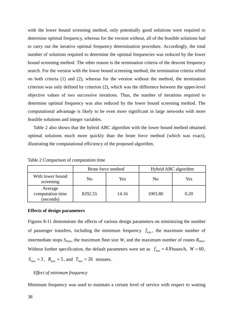
with the lower bound screening method, only potentially good solutions were required to

determine optimal frequency, whereas for the version without, all of the feasible solutions had

to carry out the iterative optimal frequency determination procedure. Accordingly, the total

number of solutions required to determine the optimal frequencies was reduced by the lower

bound screening method. The other reason is the termination criteria of the descent frequency

search. For the version with the lower bound screening method, the termination criteria relied

on both criteria (1) and (2), whereas for the version without the method, the termination

criterion was only defined by criterion (2), which was the difference between the upper-level

objective values of two successive iterations. Thus, the number of iterations required to

determine optimal frequency was also reduced by the lower bound screening method. The

computational advantage is likely to be even more significant in large networks with more

feasible solutions and integer variables.

Table 2 also shows that the hybrid ABC algorithm with the lower bound method obtained

optimal solutions much more quickly than the brute force method (which was exact),

illustrating the computational efficiency of the proposed algorithm.

Table 2 Comparison of computation time

Brute force method Hybrid ABC algorithm With lower bound

screening No Yes No Yes

Average computation time

(seconds) 8292.55 14.16 1003.80 0.20

Effects of design parameters

Figures 8-11 demonstrate the effects of various design parameters on minimizing the number

of passenger transfers, including the minimum frequency minf , the maximum number of

intermediate stops Smax, the maximum fleet size W, and the maximum number of routes Rmax.

Without further specification, the default parameters were set as min 4.8f = buses/h, 60W = ,

max 3S = , max 5R = , and max 26T = minutes.

Effect of minimum frequency

Minimum frequency was used to maintain a certain level of service with respect to waiting

38

time. A higher frequency meant a higher capacity and a shorter waiting time. However, under

the fleet size constraint, increasing the minimum frequency may have resulted in the

deterioration of another type of service level, such as the total number of passenger transfers,

as illustrated in this example. Figure 8 depicts the effect of the minimum frequency setting,

showing that a tighter minimum frequency constraint results in a higher number of passenger

transfers. The frequency requirement was satisfied by cutting the trip time and reducing the

number of stops visited, because the total fleet size must be fixed. Thus, some passengers

received the benefit of a reduced waiting time while others bore an additional transfer cost.

This finding raises an interesting equity research direction for future research. In the extreme

case, when the minimum frequency was greater than 5.4 buses/h, there was no feasible

solution to satisfy the fleet size constraint.

Figure 8 Effect of minimum frequency

Effect of the maximum number of intermediate stops

More intermediate stops may have reduced the number of transfers, at the cost of increasing

the route travel time and reducing the frequency. Figure 9 shows that the total number of

transfers continued to decrease from 661 to 275 when maxS increased from 2 to 4. More

stops could be added to the existing routes by increasing the maximum number of

intermediate stops, such that the existing services could cover more demand locations and

provide more direct services. However, a further increase in maxS did not reduce the number

300

400

500

600

700

800

900

4.8 5 5.2 5.4 5.6

Num

ber

of P

asse

nger

Tra

nsfe

rs

Minimum Frequency(buses/h)

No feasible solutions

when

39

of transfers because no more stops could be added to the existing routes in this range of the

maximum number of intermediate stops allowed. Either the maximum travel time constraint

(i.e., constraint (12)) or the minimum frequency constraint (i.e., constraint (10)) instead of the

constraint on the maximum number of intermediate stops (i.e., constraint (11)) was binding at

optimality. Visiting more stops extended the round trip and total stop times. Moreover, the

prolonged travel time reduced the frequency if the fleet size for the route remained unchanged.

Hence, the number of stops could not be added to each route without limit. The implication of

this result is that practitioners must identify which constraints are critical in improving the

services because the binding constraints are different under different conditions.

Figure 9 Effect of the maximum number of intermediate stops

Effect of the maximum bus fleet size

The effect of the maximum bus fleet size is shown in Figure 10. According to this figure,

there was no feasible solution when 0 55,W< < because the minimum frequency

requirement could not be satisfied, implying that the fleet size was inadequate to provide the

minimum acceptable level of service. When 55 59W≤ < , the number of transfers decreased

with the increase in the fleet size, because more buses were allocated to the existing routes to

serve the demand between any pair of stops on the same bus route, and less demand between

them required a transfer due to the insufficient capacity of the direct services. When 59W ≥ ,

the effect of increasing the fleet size on reducing the number of transfers vanished because all

of the demands between any pair of stops on the same bus route were met. Route capacity was

200250300350400450500550600650700

2 3 4 5 6

Num

ber

of P

asse

nger

Tra

nsfe

rs

Maximum Number of Intermediate Stops

40

no longer the key factor in reducing the number of transfers and the maximum fleet size

constraint was no longer binding. Further reducing the number of transfers required adding

more direct services.

Figure 10 Effect of the maximum bus fleet size

Effect of the maximum number of routes

Figure 11 Effect of the maximum number of routes

To illustrate the effect of the maximum number of routes, maxR was increased from 5 to 9.

The fleet size was adjusted to 120 in this test, because according to preliminary tests no

feasible solution could be found if maxR was greater than 6 under the default setting. The

results are plotted in Figure 11. As expected, the number of transfers decreased with an

0

50

100

150

200

250

300

350

400

5 6 7 8 9

Num

ber

of P

asse

nger

Tra

nsfe

rs

Maximum Number of Routes

300

350

400

450

500

550

600

54 56 58 60 62 64

Num

ber

of P

asse

nger

Tra

nsfe

rs

Maximum Bus Fleet Size

No feasible solutions when

55

41

increase in maxR . More importantly, the number of transfers was successfully eliminated

when maxR was equal to or greater than 8, because more routes provided more direct services

and covered more nodes.

TSW network 4.2.

The main study area was located in Tin Shui Wai (TSW), Hong Kong (Figure 12a). All of

the routes leave TSW through the Tai Lam Tunnel (TLT), located on the south eastern side of

the area, and then continue via the highway, which is connected to urban destinations.

Passengers can transfer either at the TLT station or at other nodes outside the TSW area.

However, due to a lack of systematic design, the existing bus network operates in an

inefficient manner, generating many transfers. Some of the bus services are routed using a low

occupancy rate, which wastes resources and inconveniences passengers. However, from the

passengers’ perspective, ideally, there should be as many routes as possible to provide direct

point-to-point services, but this is infeasible due to the relatively fixed operating cost of the

operator. As with other bus operators, the operating cost was shown to be roughly

proportional to the number of operating vehicles. If a single route zigzags too much and has

too many stops, the travel time is long. The bus operators’ main concern is then how to

restructure the bus routes in TSW to reduce the number of passenger transfers without

increasing the fleet size.

Figure 12b shows the TSW network. The square nodes represent the bus terminals inside

TSW, the circle nodes represent the current bus stop locations, and “T” represents the TLT

bus interchange. The in-vehicle travel times (in minutes) between nodes are shown next to the

corresponding links. As Figure 12b reveals, the TSW area was divided into 23 zones, each of

which had one stop or bus terminal. The stops and terminals in this area are represented by

nodes 1-23 and the seven bus terminals are represented by squared nodes (Figure 12b). All of

the bus routes originating from these terminals terminated at one of the five ending terminals,

nodes 24-28. The demand matrix estimated from the available data is given in Appendix II.

Effects of different forms of fitness functions and penalty parameter values

Because a lower bound is used to approximate the upper-level objective value, the solution

quality may not be reflected accurately. Therefore, the following three different forms of 42

fitness functions are proposed and tested:

(a) Map of Tin Shui Wai (b) The Tin Shui Wai bus network

Figure 12 The study network

151 10g g gF LB P= - - ,

2g I g gF C LB P= - - , and

13gg g

FLB P

=+

.

1gF and 2gF adopt a similar functional form in the sense that both use a constant minus

the lower bound and the penalty term gP . However, an arbitrarily selected large constant (i.e.,

1015) is adopted in 1gF , while an adaptive value, IC , is used in 2gF . IC is determined by

adding a small constant (i.e., 1.0) to the maximum value of ( )g gLB P+ among all of the

solutions obtained in iteration I. In addition to the forms of the fitness functions, the penalty

parameter values affect the probability of searching infeasible solutions. The combined effects

43

of the form of a fitness function and the penalty parameter values are plotted in Figure 13,

assuming that the value of the penalty parameter a is equal to the value of the penalty

parameter β. The y-axis represents the average upper-level objective value and the x-axis is

the log penalty parameter value, demonstrating that by modifying the form of the fitness

function, the performance of our algorithm significantly improves. Although the penalty

values affect the performance, the effect seems to be less than that of the form of the fitness

function. The best average objective value is given by 3gF at 810a b= = . This setting was

adopted in the following experiments.

Figure 13 Effects of various forms of fitness functions and penalty parameter values

Effect of limit

The predefined number limit is used to determine when an employed bee becomes a scout.

This value may be roughly interpreted as the sampling frequency within a solution space. A

higher value means that more neighbor solutions are found and compared. In this test, limit

was increased from 0 to 500. The average upper-level objective values are plotted in Figure

14. When limit equals 0, it represents the scenario that all food sources are abandoned and

regenerated in each iteration. The average objective value decreased initially and then arrived

at the minimum point, when limit equals 150. Afterwards, the average objective value slightly

increased and became varied, indicating that the average algorithm performance worsened if

limit was too large or small. One explanation is that when limit was small, the promising area

in the solution space could not be well exploited, whereas when limit was too large, many

635

640

645

650

655

660

665

670

675

680

7 8 9 10 11

Num

ber

of P

asse

nger

Tra

nsfe

rs

Log Penalty Parameter Value

F1

F2

F3

44

search efforts were trapped in the areas with low solution quality.

Figure 14 Effect of limit

Effect of colony composition

The composition of employed bees and onlookers also affects the performance of the hybrid

ABC algorithm. Given that the total number of iterations and the colony size are fixed,

different percentages of employed bees result in different numbers of initial solutions and

different numbers of onlookers influence the intensity of neighbor solution searching.

Meanwhile, the number of employed bees also reflects the number of scouts, which controls

the maximum number of new solutions generated in each iteration. Figure 15 shows that the

composition has a significant effect on the algorithm performance. In this example, when 50%

of the colony is employed bees, the algorithm achieves the best average objective value.

Either a higher or lower percentage prevents the further improvement of the objective value,

probably because when the percentage of employed bees is low, only a few promising food

sources are generated for onlookers to exploit. In contrast, if the percentage of employed bees

is high, only a few onlookers conduct neighborhood searches to exploit the solution space

near promising food sources.

Effect of different node insertion and deletion strategies

The insertion and deletion of nodes, which is important in improving route structures, is

included in the repairing procedures and the neighborhood search. We propose an

average-direct-demand value, defined as the average passenger demand on the direct services,

500550600650700750800850900950

1000

0 100 200 300 400 500

Num

ber

of P

asse

nger

Tra

nsfe

rs

Limit

45

to select a node to insert or delete. To show the benefit of using the proposed measure in

selecting nodes, three different strategies were compared and the results are presented in Table

3.

Figure 15 Effect of colony combinations

S1: Inserting and deleting nodes based on the proposed average-direct-demand increment

and decrement, respectively.

S2: Inserting and deleting nodes based on the cost increment and decrement, respectively.

S3: Inserting and deleting nodes based on the total direct demand increment and decrement,

respectively.

Table 3 Comparison of the different insertion and deletion strategies

S1 S2 S3

50% demand 311.62 646.05 602.62

(+107.3%) (+93.4%)

100% demand 604.76 1313.99 1207.59

(+117.3%) (+99.7%)

Two scenarios—low and normal demand—were tested. The average upper-level objective

values of 20 runs are reported in Table 3. The number in each pair of braces is the increment

percentage with respect to strategy S1 in the same row and shows that the proposed strategy

S1 outperformed the others in both scenarios. The higher the demand, the more notable the

advantage, because the average-direct-demand took the change in the upper-level objective

600

605

610

615

620

625

630

635

640

645

20% 35% 50% 65% 80%

Num

ber

of P

asse

nger

Tra

nsfe

rs

Percentage of Employed Bees

46

value due to inserting a node into consideration. In contrast, if only the total direct demand or

cost change was considered, the nodes with a higher demand or shorter distance were visited

more frequently, making them more likely to provide excessive services for these nodes and

induce more transfers for other nodes.

Robustness of the obtained solution

The travel demands of the network were estimated, but the real demands may vary from day

to day. To illustrate the robustness of the solution obtained by the proposed algorithm, 1,000

demand matrices were generated by perturbing the estimated demand matrix and used for the

evaluation. For each perturbed demand matrix, its element—the perturbed demand from node

m to destination e—was randomly generated from a uniform distribution [0.8 emd , 1.2 e

md ].

Table 4 compares the best solutions obtained by the hybrid ABC algorithm for the studied

situation using the perturbed demand matrices. ‘Std’ and ‘no.’ stand for ‘standard deviation’

and ‘number’, respectively. According to this table, the design solution obtained by the hybrid

ABC algorithm was significantly better than the existing design, with the former reducing the

number of transfers by 340% on average and successfully eliminating the unserved demand in

all cases. The high unserved demand resulted from a lack of service capacity to meet the total

demand of some destinations and the demand at some stops, where passengers failed to board

any line. These two issues were addressed by the hybrid ABC algorithm.

The detailed solution obtained by the hybrid ABC algorithm is shown in Table 6 and the

existing design is shown in Table 5. Intuitively, there are fewer stops in the proposed design,

reflecting a more efficient meeting of demand. In addition, the headways of the routes are

more evenly distributed for the obtained solution. Compared with the existing design, the

standard deviation of headways for the best design decreased from 2.9 to 2.4 minutes,

indicating that the difference in the level of service, in terms of frequency, among all of the

routes, decreased.

Table 4 Comparison of the solutions under random demand

Average no. of

transfers

Std of no.

of transfers

Average

unserved demand

Std of unserved

demand

Hybrid ABC algorithm 355.491 22.38 0.00 0.00

Current 1563.31 35.95 1350.85 56.18

47

Table 5 Existing route structures and headways

Routes Stop sequence Number of buses

Headway (minute)

1 20, 19, T, 25 12 9.8 2 16, 17, 18, 23, 22, 21, T, 25 17 8.1 3 16, 17, 18, 23, 22, 21, T, 24 19 5.1 4 1, 6, 9, 10, 12, 13, 19, 21,T, 25 19 8.5 5 1, 6, 5, 4, 11,12, 13, 19, T, 24 23 5.3 6 14, 15, 8, 9, 10, 12, 13, 19, T, 24 11 11.1 7 1, 6, 8, 16, 17, 18, 23, 22,21, T, 28 30 4.1 8 14, 13, 12, 10, 8, 16, 17, 18, 23, 22, T, 26 18 11.0 9 7, 6, 1, 2, 3, 4, 11, 12, 13, 19, T, 24 11 12.3 10 9, 10, 11, 5, 6, 8, 16, 17, 18, 23, 22, T, 27 16 11.3

Table 6 Best solution obtained by the proposed ABC algorithm

Routes Stop sequence Number of buses

Headway (minute)

1 14, 13, T, 27 11 11.6 2 16, 1, 11, 13, 21, T, 24 23 5.3 3 20, 23, 18, 16, 15, 14, T, 26 20 9.2 4 7, 5, 1, 6, 9, 8, T, 25 14 12.1 5 9, 5, 6, 8, 16, 17, 22, T, 26 15 12.2 6 7, 1, 2, 3, 4, 12, 13,T, 26 15 12.3 7 16, 8, 18, 20, 22, 23, 13, 12, T, 28 25 6.7 8 23, 18, 16, 15, 10, 12, 13, 19, T, 25 19 8.9 9 1, 2, 3, 4, 5, 7, 9, 14, 19, T, 28 14 9.8 10 16, 23, 6, 10, 11, 15, 17, 21, 19, T, 28 20 8.5

Winnipeg network 4.3.

To evaluate the performance of the proposed hybrid ABC algorithm, it was compared with

that of a GA using the Winnipeg network obtained from Emme 3.4. The network is shown in

Figure 16 (a) and comprises 154 zones, 1067 nodes, and 2995 links. The network is further

divided into seven districts including one central area. In each district, 30 lines are designed

for commuters traveling from their home district to the central area. Each line is allowed to

visit 15 stops at most within 45 minutes. The total fleet size is 1,200 buses with a capacity of

60 passengers per bus.

For a fair comparison, the GA uses the same solution representation, initialization

procedure, and frequency determination procedure as the hybrid ABC algorithm. The 48

population size is set to be equal the colony size. Unlike the hybrid ABC algorithm, the GA

requires crossover and mutation operators to generate new solutions. Nevertheless, the

standard crossover and mutation operators cannot be applied directly because the proposed

solution representation is different from the solution representation in the traditional GA

(Haupt and Haupt, 2004). Thus, the stop crossover operator developed by Szeto and Wu (2010)

was used and the proposed neighborhood operators were adopted as mutation operators.

(a) Winnipeg Network (b) Districts of Winnipeg Network

Figure 16 Winnipeg network

Both algorithms ran 20 times. The computation time of each run was 300 seconds. The

computation performances of the two algorithms is summarized in Table 7. The number

within each pair of brackets in the third column is the percentage improvement of the hybrid

ABC algorithm with respect to the GA in the corresponding measure. The second row shows

that the average number of passenger transfers obtained by the hybrid ABC algorithm was

lower than that of the GA. A t-test was also conducted to examine whether the difference in

their average numbers of passenger transfers is statistically significant. The t-value obtained is

2.093 and hence we can conclude that the difference is significant at the 5% level and the

average performance of the hybrid ABC algorithm is better at this significance level.

By comparing the standard deviations of the number of transfers in 20 runs in the third row

in Table 7, it was concluded that the solution quality obtained by the hybrid ABC algorithm

was much more stable. More importantly, as reflected in the last row, the best solution found

by the hybrid ABC algorithm was superior to that obtained by the GA. The advantage of the

hybrid ABC algorithm may be attributed to a better local search strategy, with a solution space

explored by both employed bees and onlookers. 49

Table 7 Comparison of the computation performance of the GA and hybrid ABC algorithm

Number of passenger transfers GA Hybrid ABC Average 300.4 252.6 (-15.9%)

Standard deviation 47.6 29.0 (-39.0%) Minimum 246.0 216.0 (-12.2%)

Figure 17 shows the average of the best fitness values for 20 runs for the two algorithms

during the computational process. This figure illustrates the average of the best fitness values

obtained by the hybrid ABC algorithm was higher than that of GA almost throughout the

computational process. This implies that the hybrid ABC algorithm could always find a better

feasible solution than the GA using the same computation time. It may be because the hybrid

ABC algorithm has a better local search strategy.

Figure 17 Average of the best fitness values for 20 runs for the GA and hybrid ABC algorithm

5. Conclusions

In this study, we proposed a bi-level model to formulate the transit network design problem.

The network design and frequency settings were considered simultaneously. The number of

passenger transfers was explicitly captured in the upper-level objective function, and the strict

capacity constraint approach was used to handle the congestion effect in the lower-level

problem. The lower-level problem is a congested transit assignment problem with the optimal

strategy concept.

A hybrid ABC algorithm was developed to solve the model. The main algorithm (ABC

0.0000

0.0005

0.0010

0.0015

0.0020

0.0025

0.0030

0.0035

0.0040

0.0045

0 50 100 150 200 250 300Ave

rage

of t

he B

est F

ittne

ss V

alue

s for

20

run

s

Computation Time (Seconds)

GA

Hybrid ABC

50

algorithm) was used to search the solution space of route structures, while the Simplex

method solved the capacity-constrained transit assignment model. A node insertion and

deletion strategy based on an average-direct-demand (i.e., average passenger demand on the

direct services concerned) was proposed to repair route structures, and its effectiveness was

illustrated by a numerical example. A descent search method was proposed for the frequency

setting and a lower bound screening method was proposed to speed up the computation. The

descent direction of the lower-level problem was also a descent direction of the upper-level

objective under certain conditions, and a linear integer program was formed to determine the

step size for updating the frequency setting.

Numerical examples were provided to illustrate the properties of the bi-level problem and

the performance of the proposed algorithm. In particular, the benchmark comparisons verified

that the proposed algorithm could find optimal solutions and that the descent search method

saved considerable computation time. A small experiment was also performed to show the

effects of different design parameters (including minimum frequency, maximum fleet size,

maximum number of routes and intermediate stops) on the objective value and the possibility

of multiple design solutions.

Using the realistic TSW network study, several tests were conducted to illustrate the effects

of the ABC parameters, the functional forms of the fitness function, the penalty parameter

values, and the node insertion and deletion strategies, demonstrating that the solution quality

can be improved by carefully adjusting the ABC parameters. We found that the best solution

obtained from the proposed algorithm was significantly better than the current design in terms

of number of passenger transfers, and was more robust in terms of meeting passenger demand

under demand uncertainty. Finally, the superior performance of the proposed hybrid ABC

algorithm was demonstrated by comparing it with the GA in the Winnipeg network scenario.

This study opens up many research directions. First, the objective of our proposed

problem–minimizing the number of transfers–was set from the perspective of passengers,

which is reasonable if the operator is public and has passengers as its main consideration.

However, the government may also consider the concerns of different stakeholders, including

the operator. Hence, a potential future direction is to extend the proposed model to develop a

multi-objective model that considers such concerns. Second, in terms of decision variables,

the transit fare structure can be incorporated because it is also an important factor influencing

passenger route choices. Third, the constant travel time assumption in the lower-level problem

allowed us to have a linear programming problem that could be efficiently solved by existing 51

algorithms while remaining applicable to large-sized networks, deriving the descent direction

to determine the optimal frequency setting. However, it has been shown that wait/transfer

times at stations are usually increasing functions of the number of passengers boarding and

alighting at stations (Lam et al., 1998; Yin et al., 2004; Li et al., 2009). It would be easy to

extend our proposed model to capture this phenomenon without conceptual difficulty, but it

would be more difficult to develop an “efficient” solution method to solve the resultant

bi-level model. This has thus been left to future study. Finally, the proposed model could be

extended to consider changing demand over time using the time-dependent approach (e.g.,

Szeto and Lo, 2005, 2008, Lo and Szeto, 2009), time space networks (Szeto, 2013), or the

day-to-day dynamic approach (Watling and Cantarella, 2013) to develop good and meaningful

bus service policies that are geared toward serving new development and facilities in Hong

Kong, such as columbarium facilities.

Acknowledgements

This research was jointly supported by a grant (201011159026) from the University Research

Committee, a Research Postgraduate Studentship from the University of Hong Kong, a grant

(71271183) from the National Natural Science Foundation of China, and a grant from the

Central Policy Unit of the Government of the Hong Kong Special Administrative Region and

the Research Grants Council of the Hong Kong Special Administrative Region, China

(HKU7026-PPR-12). The authors are grateful to the three reviewers for their constructive

comments.

References

Baaj, H., Mahmassani, H.S., 1990. TRUST: A LISP program for the analysis of transit route

configurations. Transportation Research Record 1283, 125-135.

Bielli, M., Caramia, M., Carotenuto, P., 2002. Genetic algorithms in bus network optimization.

Transportation Research Part C 10 (1), 19-34.

Bunte, S., Kliewer, N., Suhl, L., 2006. An overview on vehicle scheduling models in public

transport. In: Proceedings of the 10th International Conference on Computer-Aided

Scheduling of Public Transport. Leeds, UK. Springer-Verlag, 2006.

Ceder, A., Wilson, N.H.M., 1986. Bus network design. Transportation Research Part B 20 (4),

331-344.

52

Cepeda, M., Corninetti, R., Florian, M., 2006. A frequency-based assignment model for

congested transit networks with strict capacity constraints: Characterization and

computation of equilibria. Transportation Research Part B 40 (6), 437-459.

Chakroborty, P., Dwivedi, T., 2002. Optimal route network design for transit systems using

genetic algorithms. Engineering Optimization 34 (1), 83-100.

Constantin, L., Florian M., 1995. Optimizing frequencies in a transit network: A nonlinear

bi-level programming approach. International Transactions in Operational Research 2 (2),

149-164.

Cortés, C.E., Jara-Moroni, P., Moreno, E., Pineda, C., 2013. Stochastic transit equilibrium.

Transportation Research Part B 51, 29-44.

de Cea, J., Fernández, E., 1993. Transit assignment for congested public transport systems: an

equilibrium model. Transportation Science 27 (2), 133-147.

Fan, L., Mumford, C.L., 2010. A metaheuristic approach to the urban transit routing problem.

Journal of Heuristics 16 (3), 353-372.

Fan, W., Machemehl, R., 2004. Optimal transit route network design problem: Algorithms,

implementations, and numerical results. Research Report SWUTC/04/167244-1,

Southwest Region University Transportation Center, Center for Transportation Research,

University of Texas at Austin.

http://d2dtl5nnlpfr0r.cloudfront.net/swutc.tamu.edu/publications/technicalreports/167244-

1.pdf [access on 4 Feb 2014].

Fan, W., Machemehl, R., 2006a. Optimal transit route network design problem with variable

transit demand: Genetic algorithm approach. Journal of Transportation Engineering 132

(1), 40-51.

Fan, W., Machemehl, R., 2006b. Using a simulated annealing algorithm to solve the transit

route network design problem. Journal of Transportation Engineering 132 (2), 122-132.

Fernandez, E., Marcotte, P., 1992. Operators-users equilibrium model in a partially regulated

transit system. Transportation Science 26 (2), 93-105.

Fleurent, C., Lessard, R., Seguin, L., 2004. Transit timetable synchronization: evaluation and

optimization. In: Proceedings of the Ninth International Conferences on Computer Aided

Scheduling of Public Transport (CASPT), San Diego, CA.

Floudas, C.A, 1995. Nonlinear and mixed-integer optimization. Oxford University Press, New

York, USA.

Furth, P.G., Wilson, N.H.M., 1982. Setting frequencies on bus routes: theory and practice. 53

Transportation Research Record 818, 1-7.

Gao, Z.Y., Sun, H., Shan, L.L., 2004. A continuous equilibrium network design model and

algorithm for transit systems. Transportation Research Part B 38 (3), 235-250.

Guan, J.F., Yang, H., Wirasinghe, S.C., 2006. Simultaneous optimization of transit line

configuration and passenger line assignment. Transportation Research Part B 40 (10),

885‐902.

Guihaire, V., Hao, J.K., 2008. Transit network design and scheduling: a global review.

Transportation Research Part A 42 (10), 1251-1273.

Hadas, Y., Shnaiderman, M., 2012. Public-transit frequency setting using minimum-cost

approach with stochastic demand and travel time. Transportation Research Part B 46 (8),

1068-1084.

Haupt, R.L., Haupt, S.E., 2004. Practical Genetic Algorithms. John Wiley and Sons. New

York.

Jara-Díaz, S.R., Gschwender, A., Ortega, M., 2012. Is public transport based on transfers

optimal? A theoretical investigation. Transportation Research Part B 46 (7), 808-816.

Kang, F., Li, J., Xu, Q., 2009. Structural inverse analysis by hybrid simplex artificial bee

colony algorithms. Computers and Structures 87 (13-14), 861-870.

Karaboga, D. Basturk, B., 2007. A powerful and efficient algorithm for numerical function

optimization: artificial bee colony (ABC) algorithm. Journal of Global Optimization 39

(3), 459-471.

Karaboga, D., 2005. An idea based on honey bee swarm for numerical optimization. Technical

Report TR06, Computer Engineering Department, Erciyes University, Turkey.

Karaboga, D., 2009. A new design method based on artificial bee colony algorithm for digital

IIR filters. Journal of the Franklin Institute 346 (4), 328-348.

Karaboga, D., Ozturk, C., 2009. Neural networks training by artificial bee colony algorithm

on pattern classification. Neural Network World 19 (3), 279-292.

Kepaptsoglou, K., Karlaftis, M., 2009. Transit route network design problem: Review. Journal

of Transportation Engineering 135 (8), 491-505.

Kurauchi, F., Bell, M., Schmöcker, J.D., 2003. Capacity constrained transit assignment with

common lines. Journal of Mathematical Modelling and Algorithms 2 (4), 309-327.

Lam, W.H.K., Gao, Z.Y., Chan, K.S., Yang, H., 1999. A stochastic user equilibrium

assignment model for congested transit networks. Transportation Research Part B 33 (5),

351-368. 54

Lam, W.H.K., Zhou, J., Sheng, Z.H., 2002. A capacity restraint transit assignment with elastic

line frequency. Transportation Research Part B 36 (10), 919-938.

Laporte, G., Mesa, J.A., Perea, F., 2010. A game theoretic framework for the robust railway

transit network design problem. Transportation Research Part B 44 (4), 447-459.

LeBlanc, L.J., 1988. Transit network design. Transportation Research Part B 22 (5), 383-390.

Lee, Y.J, Vuchic, V.R., 2005. Transit network design with variable demand. Journal of

Transportation Engineering 131 (1), 1-10.

Lei, Q.S., Chen, J., 2004. An algorithm for transit assignment with elastic demand under

capacity constraint. In: Proceedings of the 5th World Congress on Intelligent Control and

Automation (WCICA), 5245-5247.

Leiva, C., Munoz, J.C., Giesen, R., Larrain, H., 2010. Design of limited-stop services for an

urban bus corridor with capacity constraints. Transportation Research Part B 44 (10),

1186-1201.

Li, Z.C., Lam, W.H.K., Sumalee, A., 2008. Modeling impacts of transit operator fleet size

under various market regimes with uncertainty in network. Transportation Research

Record 2063, 18-27.

Li, Z.C., Lam, W.H.K., Wong, S.C., 2009. The optimal transit fare structure under different

market regimes with uncertainty in the network. Networks and Spatial Economics 9 (2),

191-216.

Li, Z.C., Lam, W.H.K., Wong, S.C., 2011. On the allocation of new lines in a competitive

transit network with uncertain demand and scale economies. Journal of Advanced

Transportation 45 (4), 233-251.

Li, Z.C., Lam, W.H.K., Wong, S.C., Sumalee, A., 2012. Design of a rail transit line for profit

maximization in a linear transportation corridor. Transportation Research E 48 (1), 50-70.

Lo, H.K., Szeto, W.Y., 2009. Time-dependent transport network design under cost-recovery.

Transportation Research Part B 43 (1), 142-158.

Long, J.C., Szeto, W.Y., Huang, H.J., 2014. A bi-objective turning restriction design problem

in urban road networks. European Journal of Operational Research 237 (2), 426-439.

Magnanti, T.L., Wong, R.T., 1984. Network design and transportation planning: Models and

algorithms. Transportation Science 18 (1), 1-55.

Mandl, C.E., 1980. Evaluation and optimization of urban public transportation networks.

European Journal of Operational Research 5 (6), 41-47.

Mazloumi, E., Mesbah, M., Ceder, A., Moridpour, S., Currie, G., 2012. Efficient transit 55

schedule design of timing points: A comparison of ant colony and genetic algorithms.

Transportation Research Part B 46 (1), 217-234.

Miller, C.E., Tuker, A.W., Zemlin, R.A., 1960. Integer programming formulation of the

traveling salesman problems. Journal of the ACM 7 (4), 326-329.

Murray, A.T., 2003. A coverage model for improving public transit system accessibility and

expanding access. Annals of Operations Research 123 (1), 143-156.

Ngamchai, S., Lovell, D., 2003. Optimal time transfer in bus transit route network design

using a genetic algorithm. Journal of Transportation Engineering 129 (5), 510-521.

Nguyen, S., Pallottino, S., 1988. Equilibrium traffic assignment for large scale transit

networks. European Journal of Operational Research 37 (2), 176-186.

Schmöcker, J.D., Bell, M.G.H., Kurauchi, F., 2008. A quasi-dynamic capacity constrained

frequency-based transit assignment model. Transportation Research Part B 42 (10),

925-945.

Schmöcker, J.D., Fonzone, A., Shimamoto, H., Kurauchi, F., Bell, M.G.H., 2011.

Frequency-based transit assignment considering seat capacities. Transportation Research

Part B 45 (2), 392-408.

Shih, M.C., Mahmassani, H.S., Baaj, M.H., 1998. A planning and design model for transit

route networks with coordinated operations. Transportation Research Record 1623, 16-23.

Spiess, H., Florian, M., 1989. Optimal strategies: A new assignment model for transit

networks. Transportation Research Part B 23 (2), 83-102.

Sumalee, A., Uchida, K., Lam, W.H.K., 2011. Stochastic multi-modal transport network under

demand uncertainties and adverse weather condition. Transportation Research Part C 19

(2), 338-350.

Sumalee, A., Tan, Z.J., Lam, W.H.K., 2009. Dynamic stochastic transit assignment with

explicit seat allocation model. Transportation Research Part B 43 (8-9), 895-912.

Sun, L.J., Gao, Z.Y., 2007. An equilibrium model for urban transit assignment based on game

theory. European Journal of Operational Research 181 (1), 305-314.

Szeto, W.Y., Jiang Y., 2012. A hybrid artificial bee colony algorithm for transit network design.

Transportation Research Record 2284, 47-56.

Szeto, W.Y., Jiang, Y., Wong, K.I., Solayappan, M., 2013. Reliability-based stochastic transit

assignment with capacity constraints: Formulation and solution method. Transportation

Research Part C 35, 286-304.

Szeto, W.Y., Lo, H.K., 2005. Strategies for road network design over time: robustness under 56

uncertainty. Transportmetrica 1 (1), 47-63.

Szeto, W.Y., Lo, H.K., 2008. Time-dependent transport network improvement and tolling

strategies. Transportation Research Part A 42 (2), 376-391.

Szeto, W.Y., Solayappan, M., Jiang, Y., 2011a. Reliability-based transit assignment for

congested stochastic transit networks. Computer-Aided Civil and Infrastructure

Engineering 26 (4), 311-326.

Szeto, W.Y., Wu, Y.Z., 2010. A simultaneous bus route design and frequency setting problem

for Tin Shui Wai, Hong Kong. European Journal of Operational Research 209 (2),

141-155.

Szeto, W.Y., Wu, Y.Z., Ho, S.C., 2011b. An artificial bee colony algorithm for the capacitated

vehicle routing problem. European Journal of Operational Research 215 (1), 126-135.

Szeto, W.Y., 2013. Routing and scheduling hazardous material shipments: Nash game

approach. Transportmetrica B 1 (3), 237-260 .

Szeto, W.Y., Jiang, Y., 2014. Transit assignment: Approach-based formulation, extragradient

method and paradox. Transportation Research Part B 62, 51-76.

Teklu, F., Sumalee, A., Watling, D., 2007. A genetic algorithm for optimizing traffic control

signals considering routing. Computer-Aided Civil and Infrastructure Engineering 22

(1), 31-43.

Tom, V.M., Mohan, S., 2003. Transit route network design using frequency coded genetic

algorithm. Journal of Transportation Engineering 129 (2), 186-195.

Uchida, K., Sumalee, A., Watling, D.P., Connors, R., 2005. A study on optimal frequency

design problem for multi-modal network using probit-based user equilibrium assignment,

Transportation Research Record 1923, 236-245.

Uchida, K., Sumalee, A., Watling, D.P., Connors, R., 2007. A study on network design

problems for multi-modal networks by probit-based stochastic user equilibrium. Networks

and Spatial Economics 7 (3), 213-240.

van Nes. R., Hamerslag, R., Immers, B.H., 1988. Design of public transport networks.

Transportation Research Record 1202, 74-83.

Watling, D.P., Cantarella, G.E., 2013. Modelling sources of variation in transportation

systems: theoretical foundations of day-to-day dynamic models. Transportmetrica B 1 (1),

3-32.

Wan, Q.K., Lo, H.K., 2003. A mixed integer formulation for multiple-route transit network

design. Journal of Mathematical Modeling and Algorithms 2 (4), 299-308. 57

Wong, R.C.W., Yuen, T.W.Y., Fung, K.W., Leung, J.M.Y., 2008. Optimizing timetable

synchronization for rail mass transit. Transportation Science 42 (1), 57-69.

Wren, A., Rousseau, J.M., 1993. Transportation network design using a cumulative algorithm

and neural network. Transportation Research Record 1364, 37-44.

Yu, B., Yang, Z.Z., Jin, P.H., Wu, S.H., Yao, B.Z., 2012. Transit route network

design-maximizing direct and transfer demand density. Transportation Research Part C 22,

58-75.

Zhao, F., Gan, F., 2003. Optimization of transit network to minimize transfers, Final Report,

Contract No. BD015-02. Research Office, Florida Department of Transportation.

http://www.dot.state.fl.us/research-center/Completed_Proj/Summary_PTO/FDOT_BD015

_02rpt.pdf [access on 4 Feb 2014].

Zhao, F., Ubaka, I., Gan, A., 2005. Transit network optimization: Minimizing transfers and

maximizing services coverage with an integrated simulated annealing and tabu search

method. Transportation Research Record 1923, 180-188.

Zhao, F., Zeng, X., 2006. Simulated annealing-genetic algorithm for transit network

optimization. Journal of Computing in Civil Engineering 20 (1), 57-68.

Zubieta, L., 1998. A network equilibrium model for oligopolistic competition in city bus

services. Transportation Research Part B 32 (6), 413-422.

Appendix I Peak hourly travel demands of the small network

From\To 7 8 9 10 11 Total 1 192 148 102 94 149 685 2 100 74 78 56 102 410 3 87 77 71 46 113 394 4 96 63 49 34 85 327 5 33 24 19 15 34 125 6 19 14 14 9 23 79 Total 527 400 333 254 506 2020

58

Appendix II Peak hourly travel demands of the TSW network

From\To 24 25 26 27 28 Total 1 192 148 102 94 149 685 2 54 39 38 22 54 207 3 47 40 38 27 55 207 4 33 22 21 14 30 120 5 100 74 78 56 102 410 6 87 77 71 46 113 394 7 113 76 71 46 103 409 8 100 76 71 47 117 411 9 96 63 49 34 85 327 10 33 24 19 15 34 125 11 19 14 14 9 23 79 12 156 134 114 69 165 638 13 177 105 90 78 143 593 14 63 48 36 29 59 235 15 102 81 63 39 93 378 16 253 170 150 127 213 913 17 28 20 20 14 27 109 18 76 63 58 38 71 306 19 34 25 22 14 30 125 20 59 39 30 26 49 203 21 36 23 22 15 28 124 22 33 25 20 16 28 122 23 206 184 147 96 209 842 Total 2097 1570 1344 971 1980 7962

59