Broadening the polyethylene molecular weight distribution by controlling the hydrogen concentration...
11
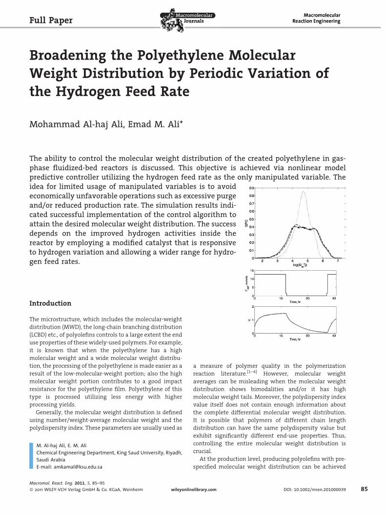
Broadening the Polyethylene Molecular Weight Distribution by Periodic Variation of the Hydrogen Feed Rate Mohammad Al-haj Ali, Emad M. Ali* Introduction The microstructure, which includes the molecular-weight distribution (MWD), the long-chain branching distribution (LCBD) etc., of polyolefins controls to a large extent the end use properties of these widely-used polymers. For example, it is known that when the polyethylene has a high molecular weight and a wide molecular weight distribu- tion, the processing of the polyethylene is made easier as a result of the low-molecular-weight portion; also the high molecular weight portion contributes to a good impact resistance for the polyethylene film. Polyethylene of this type is processed utilizing less energy with higher processing yields. Generally, the molecular weight distribution is defined using number/weight-average molecular weight and the polydispersity index. These parameters are usually used as a measure of polymer quality in the polymerization reaction literature. [1–4] However, molecular weight averages can be misleading when the molecular weight distribution shows bimodalities and/or it has high molecular weight tails. Moreover, the polydispersity index value itself does not contain enough information about the complete differential molecular weight distribution. It is possible that polymers of different chain length distribution can have the same polydispersity value but exhibit significantly different end-use properties. Thus, controlling the entire molecular weight distribution is crucial. At the production level, producing polyolefins with pre- specified molecular weight distribution can be achieved Full Paper M. Al-haj Ali, E. M. Ali Chemical Engineering Department, King Saud University, Riyadh, Saudi Arabia E-mail: [email protected] The ability to control the molecular weight distribution of the created polyethylene in gas- phase fluidized-bed reactors is discussed. This objective is achieved via nonlinear model predictive controller utilizing the hydrogen feed rate as the only manipulated variable. The idea for limited usage of manipulated variables is to avoid economically unfavorable operations such as excessive purge and/or reduced production rate. The simulation results indi- cated successful implementation of the control algorithm to attain the desired molecular weight distribution. The success depends on the improved hydrogen activities inside the reactor by employing a modified catalyst that is responsive to hydrogen variation and allowing a wider range for hydro- gen feed rates. Macromol. React. Eng. 2011, 5, 85–95 ß 2011 WILEY-VCH Verlag GmbH & Co. KGaA, Weinheim wileyonlinelibrary.com DOI: 10.1002/mren.201000039 85
-
Upload
independent -
Category
Documents
-
view
1 -
download
0
Transcript of Broadening the polyethylene molecular weight distribution by controlling the hydrogen concentration...
Full Paper
Broadening the Polyethylene MolecularWeight Distribution by Periodic Variation ofthe Hydrogen Feed Rate
Mohammad Al-haj Ali, Emad M. Ali*
The ability to control the molecular weight distribution of the created polyethylene in gas-phase fluidized-bed reactors is discussed. This objective is achieved via nonlinear modelpredictive controller utilizing the hydrogen feed rate as the only manipulated variable. Theidea for limited usage of manipulated variables is to avoideconomically unfavorable operations such as excessive purgeand/or reduced production rate. The simulation results indi-cated successful implementation of the control algorithm toattain the desired molecular weight distribution. The successdepends on the improved hydrogen activities inside thereactor by employing a modified catalyst that is responsiveto hydrogen variation and allowing a wider range for hydro-gen feed rates.
Introduction
The microstructure, which includes the molecular-weight
distribution (MWD), the long-chain branching distribution
(LCBD) etc., of polyolefins controls to a large extent the end
use properties of thesewidely-used polymers. For example,
it is known that when the polyethylene has a high
molecular weight and a wide molecular weight distribu-
tion, the processing of the polyethylene is made easier as a
result of the low-molecular-weight portion; also the high
molecular weight portion contributes to a good impact
resistance for the polyethylene film. Polyethylene of this
type is processed utilizing less energy with higher
processing yields.
Generally, the molecular weight distribution is defined
using number/weight-average molecular weight and the
polydispersity index. These parameters are usually used as
M. Al-haj Ali, E. M. AliChemical Engineering Department, King Saud University, Riyadh,Saudi ArabiaE-mail: [email protected]
Macromol. React. Eng. 2011, 5, 85–95
� 2011 WILEY-VCH Verlag GmbH & Co. KGaA, Weinheim wileyonlin
a measure of polymer quality in the polymerization
reaction literature.[1–4] However, molecular weight
averages can be misleading when the molecular weight
distribution shows bimodalities and/or it has high
molecular weight tails. Moreover, the polydispersity index
value itself does not contain enough information about
the complete differential molecular weight distribution.
It is possible that polymers of different chain length
distribution can have the same polydispersity value but
exhibit significantly different end-use properties. Thus,
controlling the entire molecular weight distribution is
crucial.
At the production level, producing polyolefins with pre-
specified molecular weight distribution can be achieved
elibrary.com DOI: 10.1002/mren.201000039 85
86
www.mre-journal.de
M. Al-haj Ali, E. M. Ali
through changing the operating conditions during the
production process. This can be achieved using either
multistage processes or a single polymerization reactor. In
multi-stage configuration, two reactors are connected in
series. Usually, in the first reactor the polymerization
reaction takes place in the absence of the chain transfer
agent and/or the comonomer. The polymer is then
transferred to the second reactor where polymerization
goes on in the presence of relatively high concentration of
hydrogen and/or comonomer. This configuration has the
advantage that only one optimized catalyst is required for
the production of various grades. However, this method is
subject tohighoperational costs;[5] besides, thepolymerhas
low homogeneity of the two polymer grades and the final
polymer particle has a core/shell-like structure.[6,7]
The production of polyolefins with a desired MWD in a
single reactor has the advantage of requiring a single
reactor that simplifies process design and reduces the
operational costs. Note that the usage of single reactor
requires operating it cyclically to vary the polymerization
conditions inside it. This type of operation can improve the
performanceof the reacting systemandallowbetter design
and control of the molecular weight distribution.[8,9] The
implementation of a single reactor, compared to imple-
menting two reactors, improves polymer homogeneity and
assures that the ratio of both polymer products in each
particle is equal to the overall ratio of these products.
However, the dynamic operation of the polymerization
reactor is difficult and it is subject toappreciableproduction
of off-specification products. Thus, efficient multivariable
control strategies have to be implemented.
Different control strategies have been developed for
polyolefin polymerization reactors, detailed reviews can be
found in refs.[10–13] Ibrahim and coworkers[14] implemen-
ted neural-network based predictive controller to control
only the temperature of polyethylene polymerization
reactor; however, nothing is mentioned about controlling
polymer properties. Zavala and Biegler[15] optimized the
operation of low-density polyethylene (LDPE) reactor
through deriving a general nonlinear model predictive
control (NLMPC) framework. Thedesignedcontroller,which
is based on a first-principles dynamic model, optimizes
process profitability as well as performs regulation tasks.
The authors compare the performance of this framework to
the traditional NLMPC and concluded that the developed
controller can find better strategies to distribute polymer
production inside the reactor. However, operational
limitations as fouling still affect reactor performance
which is the case when NLMPC is implemented. In this
work, different polymer grades were defined using
molecular weight averages, polymer density and long-
chain branching.
Recently, Al-haj Ali et al.[16] dealt with theMWD issue by
special design of the operating condition in a single reactor.
Macromol. React. Eng
� 2011 WILEY-VCH Verlag Gmb
They indicated thatabroadMWDcanbeachievedbyproper
control of the hydrogen to monomer ratio (X) inside the
reactor. It is found that manipulating both monomer and
hydrogen feed rate simultaneously can help altering X to
achieve the required MWD, however undesirable reactor
operation is observed. For example at high monomer feed
rate, an excessive bleed flow is resulted to regulate the
reactor pressure. On the other hand, at low monomer feed
rate a reduced production rate is obtained. Ali and Al-haj
Ali[17] tried to overcome the undesirable operation by
altering X via manipulating the hydrogen flow rate solely.
Relying on the hydrogen flow rate was a difficult task
because it has a slow dynamics and a limited effect on the
attainable range for X. The reason for the shortcoming
stems from the fact that hydrogen consumption is null and
that the allowable hydrogen feed rate is limited. For this
reason and to overcome these weaknesses, they suggested
using a hydrogen absorption agent to facilitate rapid
hydrogen consumption. In addition, they increased the
allowable hydrogen feed rate to increase the attainable
range for X. The mechanism of H2 consumption by
absorption remains artificial.
In this paperwe continue to investigate the possibility of
MWD broadening without producing undesirable operat-
ing conditions. This will be achieved via manipulating the
hydrogen feed rate exclusively at afixedmonomer feedand
avoiding the use of hypothetical hydrogen consumption.
Here we adopt the same concept of elevated capacity of
hydrogen intake, which is physically possible. In addition
we used another catalyst that is more sensitive to H2
content. The main idea is to design a proper nonlinear
control system that can utilize the available facilities to
produce polymers with predefined MWD. For this purpose
NLMPCwill be utilized due to its appealing features such as
handling constraints and superiority for nonlinear pro-
cesses with a large number of manipulated and controlled
variables. Moreover, model predictive controller became
the most widely used control system in the chemical
industries.[18,19]
The On-Line NLMPC Algorithm
In this work, the structure of the NLMPC version developed
by Ali and Zafiriou[18] that directly utilizes the nonlinear
model for output prediction is used. A usual NLMPC
formulation solves the following on-line optimization:
. 2011,
H & Co
minDuðtkÞ;::::;DuðtkþM�1Þ
XP
i¼1
G yðtkþiÞ�RðtkþiÞ½ �k k2
þXM
i¼1
LDuðtkþi�1Þk k2 (1)
5, 85–95
. KGaA, Weinheim www.MaterialsViews.com

Broadening the Polyethylene Molecular Weight Distribution by Periodic Variation . . .
www.mre-journal.de
subject to
www.M
ATDU ðtkÞ � b (2)
For nonlinear NLMPC, the predicted output, y over
the prediction horizon P is obtained by the numerical
integration of:
dx
dt¼ f ðx;u; tÞ (3)
y ¼ gðxÞ (4)
from tk up to tkþP where x and y represent the states and
the output of the model, respectively. The specific model
used in this work is given in Appendix A. The differential
equations given in the appendix represent the dynamic
behavior of the polyethylene reactor. Numerical integra-
tion of these equations will define the model output to be
incorporated in the NLMPC formulation. The symbols jj. jjin Equation (1) denote the Euclidean norm, k is the
sampling instant, G and L are diagonal weight matrices
and R¼ [r(kþ 1) ��� r(kþ P)]T is a vector of the desired output
trajectory. DU(tk)¼ [Du(tk) . . . Du(tkþM-1)]T is a vector of M
future changes of the manipulated variable vector u that
are to be determined by the on-line optimization. The
control horizon (M) and the prediction horizon (P) are used
to adjust the speed of the response and hence to stabilize
the feedback behavior. G is usually used for trade-off
between different controlled outputs. The input move
suppression, L, on the other hand, is used to penalize
different inputs and thus to stabilize the feedback
response. The objective function [Equation (1)) is solved
on-line to determine the optimumvalue ofDU(tk). Only the
current value of Du, which is the first element of DU(tk), is
implemented on the plant. At the next sampling instant,
the whole procedure is repeated.
To compensate for modeling error and eliminate steady
stateoffset, a regular feedback is incorporatedontheoutput
predictions, y(tkþ1) through an additive disturbance term.
Therefore, the output prediction is corrected by adding to it
the disturbance estimates. The latter is set equal to the
difference between plant and model outputs at present
time k as follows:
dðkÞ ¼ ypðkÞ�yðkÞ (5)
Thedisturbance estimate,d is assumed constant over the
prediction horizon due to the lack of an explicit means of
predicting the disturbance. However, for severe modeling
errors, oropen-loopunstableprocesses the regular feedback
is not enough to improve theNLMPC response. Hence, state
orparameterestimation isnecessary toenhance theNLMPC
performance in the face of model-plant mismatch. In this
aterialsViews.com
Macromol. React. Eng
� 2011 WILEY-VCH Verlag Gmb
work, Kalman filtering (KF) will be incorporated to correct
the model state and thus, to address the robustness issue.
Utilization of the NLMPC with KF requires adjusting an
additional parameter, s. More details on the integration of
KF with the NLMPC algorithm are given elsewhere.[18] In
addition to state estimationbyKF, thepredictedoutputwill
be also corrected by the additive disturbance estimates of
Equation (5).
Themainobjectiveof theNLMPC is to control theMWD. It
is also necessary to maintain an acceptable polymer
production rate. Process stability is another important
issue which is handled through regulating the total gas
pressure and the bed temperature. These two controlled
variables are adapted via separate proportional integral (PI)
control loops. The design and tuning parameters of these
loops are given elsewhere.[19] NLMPC is the most suitable
algorithmfor this case because theMWDcontrol problem is
challenging. First, the process is highly nonlinear. More-
over, the control variable does not have a conventional set
point, but ratheranentireprofile. Thepoints comprising the
profile are interrelated and they are the result of a
continuous polymer formation process. It should be noted
that entire simulations including solution of ordinary
differential equations (ODEs) and optimization are carried
out using Matlab software. In the following simulation
bothNLMPC and PI algorithmswill be implemented. NMPC
will control the MWD by manipulating the hydrogen feed
rate and PI will control the reactor pressure and tempera-
ture by manipulating the bleed flow and cooling water
temperature respectively.
Results and Discussion
It is well known that a specific hydrogen to monomer ratio
(X) produces a certain polymer grade in terms of density,
average molecular weight or melt index. In this paper the
polymer grade is defined by the entire polymer molecular
weight distribution. Moving the MWD from a specific
narrow profile to another one with a different number-
average molecular weight (peak value) is somewhat easy
because it is required tomove X from one value to another.
However, moving the MWD from an initial narrow
distribution to a specific broad one is much more complex
because it requires to switch X between two different
values over a specific period of time. This is essential to
capture the formation of two different polymer grades and
blend them together during synthesis.[16] This broadening
process is relatively easy when metallocene catalysts are
used since it produces polyolefins with narrow molecular
weight distribution. However, the broadening is much
more complicated when Ziegler-Natta (Z-N) catalysts are
utilizedbecause thesemult-sites catalystsproducebroadly-
distributed polymers.
. 2011, 5, 85–95
H & Co. KGaA, Weinheim87

88
www.mre-journal.de
M. Al-haj Ali, E. M. Ali
The previous work indicated that MWD can be adjusted
by altering X. The ratio X can be varied by either
manipulating ethylene (C2) and hydrogen (H2) concentra-
tion simultaneously or manipulating hydrogen solely.
Using both C2 and H2 simultaneously helps to obtain the
required MWD as shown in Figure 1. The simulation in
Figure 1 is reproduced from Ali and Al-haj Ali.[17] However
this approach leads to undesirable plant operations. For
example, the obtained MWD requires altering X, and
consequently C2 between high and low values. At low C2
values the reaction rate diminishes leading to minimal
production rate. On the other hand, high C2 concentration
mandates large C2 intake leading to propagation of the
reactor pressure. To regulate the reactor pressure back to
normal, the PI controller increases the bleed flow rate
dispatching valuable gases in the flare.
a)
0 17 34 51 680
100
200
300
F M1, m
ole/
s
0 17 340
2
4
F H2, m
ole/
s
0 17 34 51 680
0.5
1
1.5
X
0 17 340
10
20
30
BT,
mol
e/s
0 17 34 51 68260
280
300
320
T W, K
Time, hr0 17 34
0
2
4
6
OP
, kg/
s
Time
b)
2 3 4 5 6 70
0.2
0.4
0.6
0.8
1
1.2
GP
C
log(Mw*j)
Figure 1. High average MW using FM1 and FH2; (a) MWD, dotted: initiatarget, dashed: controlled output. (b)Manipulated variables and produline: reference value.
Macromol. React. Eng
� 2011 WILEY-VCH Verlag Gmb
The purpose of the results shown in Figure 1 is to set the
motivation for the rest of the work. It is obvious that
allowing monomer feed to change disturbs the process
operation. Thus it is thoughtful to control X viamanipulat-
ing FH2 exclusively at fixed FC2. However, earlier investiga-
tion[17] indicated that, using FH2 alone, the desired MWD
can be either unachievable or hard to be achieved for two
reasons. The possible attainable range for X is restricted
because the permissible range for H2 feed flow rate is
physically limited. For this reason, some specific X and
consequently some specific MWDs cannot be achieved.
Even within the attainable range for X, moving from one
value of X to another takes long time due to the H2 slow
dynamic inside the reactor. The H2 slow dynamics is
referred to its large residence time caused by the H2
minimal feed flow rate and trivial consumption. For this
51 68
51 68
51 68, hr
l condition, solid:ction rate; dotted
. 2011, 5, 85–95
H & Co. KGaA, Weinhe
reason specific attainable MWD may be
hard to achieve.
In the following we investigate the
ability to control MWDby adjusting only
FH2 using the proposed modification to
overcome the aforementioned limita-
tions. A wider range for the hydrogen
feed rate is considered. In fact, FH2will be
constrained between 0 and 11.6mol � s�1,
which is almost 7 times larger than the
nominal value. In all the following
simulations, Fc, FN2, FM1, and FM2 will be
kept constant. Furthermore, the target
MWD is designed by separate open-loop
analysis. Details of the open-loop analy-
sis can be found elsewhere.[16] In reality,
such desired MWD can be tailored by
process experience, process historical
measurement and design data.
Figure 2 shows the results for tracking
a target MWD with medium average
molecular weight represented by dotted
line. The targeted MWD consists of 104
points where only four representative
points are chosen as set points for the
control system. These points are denoted
by black dots in the figure. The number of
set points is intentionally minimized to
reduce the computational effort required
by NLMPC without sacrificing the latter
performance. Determination of these
points is somewhat iterative in nature;
however few points in the center of the
MWD profile is found to be sufficient. In
this simulation, NLMPC is tuned toM¼ 1,
P¼ 2, L¼ 0, G¼ [10, 10, 10, 10] and a
sampling time of 1 h is employed.
Obviously, NLMPC managed to steer the
im www.MaterialsViews.com

2 3 4 5 6 70
0.1
0.2
0.3
0.4
0.5
0.6
0.7
0.8
0.9
GP
C
log(Mw *j)
a)
0 15 30 430
5
10
15
F H2, m
ole/
s
0 15 30 430
1
2
X
0 15 30 430
5
10
15
BT,
mol
e/s
Time, hr0 15 30 43
3
4
5
OP
, kg/
s
Time, hr
b)
Figure 2. Medium average MW using only FH2; (a) MWD, dotted:initial condition, solid: target, dashed: controlled output. (b)Manipulated variables and production rate; dotted: referencevalue.
2 3 4 5 6 70
0.1
0.2
0.3
0.4
0.5
0.6
0.7
0.8
0.9
1
GP
C
log(Mw*j)
a)
b)
0 50 100 105-5
0
5
10
15
F H2, m
ole/
s
0 50 100 1050
0.2
0.4
0.6
0.8
X0 50 100 105
0
5
10
BT,
mol
e/s
Time, hr0 50 100 105
3
4
5
OP,
kg/
sTime, hr
Figure 3. High average MW using only FH2; (a) MWD, dotted:initial condition, solid: target, dashed: controlled output. (b)Manipulated variables and production rate; dotted line: referencevalue.
Broadening the Polyethylene Molecular Weight Distribution by Periodic Variation . . .
www.mre-journal.de
polymer grade from the initial condition shown by the
dotted line in Figure 2a to the target. The corresponding
manipulated variable response is demonstrated in
Figure 2b, where FH2 is switched between its extreme
values. The latter produced a cyclic reaction in X enough to
bring the formed MWD within the target shape. Figure 2b
shows the transient behavior for the bleed flow induced by
the PI controller to regulate the reactor pressure due to the
variation in the hydrogen partial pressure. Fortunately, the
adaptation in thebleed streamlieswithinacceptable range.
Moreover, Figure 2b illustrates how the production rate
remained very close to the reference value of 3.7 kg � s�1
because the monomer and catalyst feed rates were kept
constant.
Figure 3 depicts another set point tracking case where a
MWD with higher number-average molecular weight is
sought. The NLMPC tuning parameter values are M¼ 1,
P¼ 1, L¼ 0, G¼ [10, 10, 10, 10]. The target MWD and the
significant set points are determined as discussed earlier. It
www.MaterialsViews.com
Macromol. React. Eng
� 2011 WILEY-VCH Verlag Gmb
is clear that NLMPC was successful in moving the polymer
molecular weight distribution form the initial curve to the
desired one. The associated adaptation of the process input
is shown in Figure 3b manifested by swinging action
betweenminimumandmaximumallowablevalues forFH2.
This made the process to operate in a cyclic fashion for X
between 0 and 0.6 leading to the desired MWD. The cyclic
operation produced periodic spikes in the bleed flow
necessary to remove thehydrogenexcess inside the reactor.
Nevertheless, the bleed flow remains within acceptable
range. More important, the process regulation produced
steady polymer production. It should be noted though that
an exact match of the target function is not necessary
especially when we know that the relative error in gel
permeation chromatography (GPC) measurements is
around 10%. An average absolute error of less than 5% in
the MWD profile is considered acceptable in this study. A
long simulation time is used in this plot to demonstrate
howNLMPC recognized thenecessity to operate the process
. 2011, 5, 85–95
H & Co. KGaA, Weinheim89

90
www.mre-journal.de
M. Al-haj Ali, E. M. Ali
in a periodic fashion to keep producing the same desired
MWD over extended period. The first batch of the required
MWD can be collected as early as 40h which is twice the
time required when FM1 is used as shown in Figure 1. This
delay is attributed to the slow dynamic of hydrogen as
mentioned earlier especially when low X is needed as it is
the case in this specific simulation where high average
molecular weight is sought.
To further study the feasibility of achieving the objective
of widening the MWD while maintaining favorable
operation, additional servo problem is investigated. Speci-
fically, a broad MWD with smaller average molecular
weight is examined.Theoutcomeof this test is illustrated in
Figure 4. The value of the NLMPC tuning parameters is
M¼ 1, P¼ 10, L¼ 0, G¼ [10, 10, 10, 10]. Once again, the
hydrogen feed rate was successfully altered to excessively
regulate themolar ratioX in amanner sufficient to produce
the necessary output. Similarly, the purge stream was
2 3 4 5 6 70
0.1
0.2
0.3
0.4
0.5
0.6
0.7
0.8
0.9
1
GP
C
log(Mw*j)
a)
b)
0 25 500
5
10
15
F H2, m
ole/
s
0 25 500
0.5
1
1.5
2
X
0 25 500
5
10
15
BT,
mol
e/s
Time, hr0 25 50
3
4
5
OP,
kg/
s
Time, hr
Figure 4. Low averageMWusing only FH2; (a) MWD, dotted: initialcondition, solid: target, dashed: controlled output. (b) Manipu-lated variables and production rate; dotted line: reference value.
Macromol. React. Eng
� 2011 WILEY-VCH Verlag Gmb
manipulated inresponse to thehydrogencontentvariation.
As usual no excessive drainage of the gases is observed and
steady polymer production is guaranteed. The simulations
show that this distribution is obtainable 23h after the
starting of the change in feed streams flow rate. This is
faster thanwhat it is required for the case of higher average
molecular weight. In fact, lower average molecular weight
demands high X and thus higher H2 partial pressure. It is
common that elevating the hydrogen concentration takes
less time than diminishing because the rate of hydrogen
consumption is marginal.
NLMPC is a model-based controller, thus the accuracy of
the model used influence the feedback performance. To
assess the controller effectiveness in the presence of
modeling error the above cases are repeated. In this case,
�20% error in the catalyst activation (ac),�20% error in the
reaction rate constant, kp1 andþ15% error in the bed mass
(Bw) are injected in the reactormodel. It is expected that this
amount of model uncertainty deteriorates the model
predictions and hence the controller performance. The
simulation results for the same three previous cases under
the impact of the proposed modeling error are shown in
Figure 5. Obviously, themodeling error had its influence on
the resulted MWD in the sense of slight distortion in the
obtained MWD function. Despite the minor distortion in
the resulted distribution, the average error is within
acceptable margin (i.e. 5%). The corresponding variation
in the hydrogen feed rate and production rate for those
three cases is depicted in Figure 6. Thefigure illustrateshow
reasonable variation in the bleed flow and a satisfactory
production rateareobtained.Theconsequencesprovedthat
a Kalman filter was useful to help NLMPC to overpower the
model uncertainty and to drive the process towards the
required target MWD.
All previous tests revealed that the desired MWD can be
attained with consistent polymer production rate and
modest use of the purge stream solely by regulating the
hydrogen feed rate. This successful outcome is obtained
provided that the modified responsive catalyst is utilized
and constant hydrogen consumption by polymerization is
considered.
Despite the satisfactory conclusion, the transient beha-
vior is slower than that when FM1 and FH2 are used
collectively. The speed of response largely depends on the
dynamic activities of the hydrogen and the polymer
formation process. The extent of broadness of the MW
depends primarily onmoving between two extreme values
for X within a specific critical time during polymer
formation. As the extreme values go apart, the MWD
becomes wider and vice versa. The switching time plays a
different rule. Within the critical switching time, a broad
MWD can be obtained. When the switching time departs
away from the critical time either increasing or decreasing,
the formedMWDmoves towardswhatwould be formed at
. 2011, 5, 85–95
H & Co. KGaA, Weinheim www.MaterialsViews.com

2 3 4 5 6 70
0.1
0.2
0.3
0.4
0.5
0.6
0.7
0.8G
PC
log(Mw*j)
a)
b)
c)
2 3 4 5 6 70
0.1
0.2
0.3
0.4
0.5
0.6
0.7
0.8
GP
C
log(Mw*j)
2 3 4 5 6 70
0.1
0.2
0.3
0.4
0.5
0.6
0.7
0.8
GP
C
log(Mw*j)
Figure 5.MWD using only FH2 in the presence of modeling errors;(a) medium average molecular weight, (b) high average molecu-lar weight, (c) low average molecular weight. Solid line: targetMWD.
0 20 40 630
5
10
15
F H2, m
ole/
s
0 20 40 630
1
2
X
0 20 40 630
5
10
15
BT,
mol
e/s
Time, hr0 20 40 63
3
4
5
OP
, kg/
s
Time, hr
a)
b)
c)
0 35 700
10
20
F H2, m
ole/
s
0 35 700
0.5
1
X
0 35 700
5
10
15B
T, m
ole/
s
Time, hr0 35 70
3
4
5
OP
, kg/
s
Time, hr
0 20 40 600
5
10
15
F H2, m
ole/
s
0 20 40 600
1
2
X
0 20 40 600
5
10
15
BT,
mol
e/s
Time, hr0 20 40 60
3
4
5
OP
, kg/
s
Time, hr
Figure 6.Manipulated variables and production rate for the threecases in Figure 5; dotted line: reference value.
Broadening the Polyethylene Molecular Weight Distribution by Periodic Variation . . .
www.mre-journal.de
the extreme value, i.e. narrower. The switching time is very
crucial and essentially difficult to determine. At nominal
production rate, it takes 5 h to produce 7 t of polymer.
However, the rate of polymerization varies during the
operation, especially when periodic forcing is involved.
Furthermore, the amount produced over a certain time
cannot be isolated frompolymers thathas beenwithdrawn
from the reactor as product and what has being created
during that long period of time. Therefore, the perfect time
for switching between two corresponding end values for X
www.MaterialsViews.com
Macromol. React. Eng
� 2011 WILEY-VCH Verlag Gmb
to produce specific broad MWD is difficult to determine.
This makes the control objective challenging. The situation
gets more complex when model-plant mismatch exists.
Conclusion
Nonlinear model predictive control is used to regulate the
entire MWD of polyethylene formed in a single fluidized
bed reactor. A broadMWD is obtained even in the presence
. 2011, 5, 85–95
H & Co. KGaA, Weinheim91

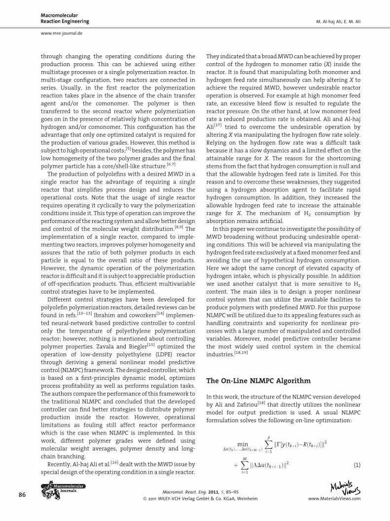
Figure A1. Scheme of the polyethylene reactor.
92
www.mre-journal.de
M. Al-haj Ali, E. M. Ali
of model-plant mismatch by manipulating the hydrogen
feed rate exclusively. The control objective is obtained
while maintaining the bleed flow and production rate
within an acceptable range. This is achieved through
improved hydrogen dynamic pace and wider range for
hydrogencontent inside the reactorbyutilizinganelevated
capacity of the hydrogen feed rate.Moreover, the hydrogen
impact is further improvedbyemployingaZ-Ncatalyst that
is sensitive to small changes in hydrogen concentration
inside thepolymerization reactor. The simulations revealed
the ability of NLMPC to capture the high nonlinearity of the
process and consequently the need to generate cyclic
reactor operation. The periodic operation was found
necessary in order to produce the desired MWD. The cyclic
operation is physically acceptable because it does not
involvevery frequentalterationof thehydrogen feedrate.A
somewhat long time to reach steady state is observed
because the hydrogen content still has slow dynamics
compared to the other process variables.
The main scientific contribution of this paper is the
success in handling this control objective, which requires
forcing the input into cyclic operation, through feedback
control configuration. The prediction feature ofNLMPCwas
themain factor in identifying theprocessbehaviorandthus
anticipates theneed toproduceperiodic feedflowrates. The
second contribution comes from the success in altering X
simply and solelyby regulating thehydrogen feed. Thiswas
achieved bymodifying feed conditions and using a catalyst
with suitable characteristics.
Appendix A: Model Equations
Polyethylene is produced in a fluidized-bed reactor,
Figure A1. Model equations for this reactor were developed
earlier byMcAuley et al.[20] Thismodel is chosen because its
kinetic parameters were validated against plant data.[21]
The definition of the various states and parameters of the
model is given in the section ‘Nomenclature’.
VgdCM1
dt¼ FM1�xM1Bt�RM1 (A.1)
VgdCM2
dt¼ FM2�xM2Bt�RM2 (A.2)
VgdCH2
dt¼ FH2�xH2Bt�FsxH2�RH2 (A.3)
Macromol. React. Eng
� 2011 WILEY-VCH Verlag Gmb
. 2011,H & Co
VgdCN
dt¼ FN�xNBt (A.4)
dYc
dt¼ Fciac�kdYci�OpYci=Bw (A.5)
ðMrCp;rþ BwCp;pÞdT
dt
¼ HFþHG�HR�HT�HP (A.6)
MwCpwdTgdt
¼ FgCpg ðTgi�TgÞ þ FwCpwðTwi�TwoÞ (A.7)
Pt ¼ ðCM1 þ CM2 þ CH þ CNÞRT (A.8)
Tgi ¼ ð PtPt þ DP
ÞT (A.9)
FwCpwðTwi�TwoÞ
¼ 0:5UA½ðTwo þ TwiÞ�ðTgi þ TgÞ� (A.10)
5, 85–95
. KGaA, Weinheim www.MaterialsViews.com
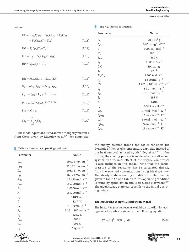
Table A.2. Process parameters.
Broadening the Polyethylene Molecular Weight Distribution by Periodic Variation . . .
www.mre-journal.de
where
Parameter Value
Bw 70� 107 g
Cpp 0.85 cal � g�1 �K�1
E 9000 cal �mol�1
Vg 500m3
Tref 360K
kh 0.005m3 � s�1
DHr �894 cal � g�1
Tab
Par
CM
CM
CH
CN
FM1
FM2
FH
FN
Yc
T
Bt
Fw
Tg
Two
Twi
Fc
www.M
HF ¼ ðFM1CpM1 þ FM2CpM2 þ FHCpH
þ FNCpNÞðTf�TrefÞ (A.11)
HG ¼ FgCpgðTg�TrefÞ (A.12)
HT ¼ ðFg þ BtÞCpgðT�TrefÞ (A.13)
HP ¼ OpCppðT�TrefÞ (A.14)
kd 0 s�1
MrCpr 1 400 kcal �K�1
Fg 8 500mol � s�1
UA 1.263� 105 cal � s�1 �K�1
kp1 85 L �mol�1 � s�1
kp2 3 L �mol�1 � s�1
Tf 293K
DP 3 atm
ac 0.548mol � kg�1
CpH 7.7 cal �mol�1 �K�1
CpM1 11 cal �mol�1 �K�1
CpN 6.9 cal �mol�1 �K�1
CpM2 24 cal �mol�1 �K�1
Cp 18 cal �mol�1 �K�1
HR ¼ Mw1ðRM11 þ RM12ÞDHr (A.15)
Op ¼ Mw1ðRM1Þ þMw2ðRM2Þ (A.16)
RM1 ¼ CM1Yckp1e�E
Rð1=T�1=TrefÞ (A.17)
RM2 ¼ CM2Yckp2e�E
Rð1=T�1=TrefÞ (A.18)
RH2 ¼ CH2kh (A.19)
Cpg ¼X4
j¼1
xjCpj (A.20)
w
Themodel equations listed above are slightly modified
from those given by McAuley et al.[20] For simplicity,
le A.1. Steady-state operating conditions.
ameter Value
1 297.06mol �m�3
2 116.17mol �m�3
105.78mol �m�3
166.23mol �m�3
131.13mol � s�1
3.5100mol � s�1
1.6000mol � s�1
2.5200mol � s�1
5.849mol
82.7 8C
10.39mol � s�1
3.11� 104mol � s�1
324.7K
308K
293K
2 kg �h�1
aterialsViews.com
Macromol. React. Eng
� 2011 WILEY-VCH Verlag Gmb
the energy balance around the cooler considers the
dynamic of the recycle temperature explicitly instead of
the heat removal as used by McAuley et al.[20] In due
course, the cooling process is modeled as a well mixed
system. The thermal effect of the recycle compressor
is also included in this model. Note that the partial
pressure of the reactants can be calculated directly
from the reactant concentrations using ideal gas law.
The steady state operating condition for the plant is
given in Table A.1 and Table A.2. This operating condition
is found by optimization and is discussed elsewhere.[19]
The given steady state corresponds to the initial operat-
ing points.
The Molecular-Weight Distribution Model
The instantaneous molecular weight distribution for each
type of active sites is given by the following equation:
. 2011,
H & Co
ydj ¼ j � q2 � expð�j � qÞ (A.21)
5, 85–95
. KGaA, Weinheim93

94
www.mre-journal.de
M. Al-haj Ali, E. M. Ali
While the cumulative distribution is given by:
aThe Z
dyjdt
¼Op � ðydj �yjÞ
Bw(A.22)
Finally the gel permeation chromatography (GPC) read-
ing of the MWD is calculated by the following:
GPC ¼ j � ydj � lnð10Þ (A.23)
In the above equations, j is the number of repeating units
and q is the chain termination probability, it is defined as
q¼ [sum of chain-termination rates]/[chain propagation
rate] and can be computed from:
q ¼ ktm þ kthX2
ktm þ kthX2 þ kp(A.24)
In the last equation, X denotes the molar ratio of
hydrogen to monomer inside the reactor. This ratio is a
crucial parameter to vary the value of q and consequently
the molecular weight distribution. Careful adjustment of q
is necessary to achieve desired polymer properties as itwill
be discussed in the results section. The parameters in
Equation (A.24) are determined by confidential data taken
from local industry. Note that the expression of q in
Equation (A.24) and the value of its parameters have been
changed from those used in earlier works[16,17] since a
different Z-N catalyst is used.a
Nomenclature
A C
-N catalyst was ad
onstant matrix for linear con-
straints
ac A
ctive site concentration, mol � kg�1b V
ector of upper and lower bounds forthe linear constraints
Bw M
ass of the polymer in the bed, gBt B
leed flow rate, mol � s�1CM1, CM2, CN, CH C
oncentration monomer, co-monomer, nitrogen, and hydro-
gen,mol �m�3
CpM1,CpM2,CpH,CpN H
eat capacity of monomer, co-monomer, hydrogen and nitrogen,
cal �mol�1 �K�1
Cpg, Cpw H
eat capacity of recycle gas andwater cal �mol�1 �K�1
Cpp H
eat capacity of polymer,cal � g�1 �K�1
opted from local industry.
Macromol. React. Eng
� 2011 WILEY-VCH Verlag Gmb
E A
. 2011, 5, 85–95
H & Co. KGaA, Weinheim
ctivation energy for propagation,
cal �mol�1
Fc C
atalyst flow rate, kg � s�1Fw, Fg C
ooling water and recycle flow rate,mol � s�1
FM1, FM2, FN, FH M
onomer, co-monomer, hydrogenand nitrogen flow rate,mol � s�1
Fs F
eed flow rate of the hydrogenabsorbent, mol � s�1
GPC G
el Permeation ChromatographyHF, HG, HP S
ensible heat of fresh feed, recyclegas and product, cal � s�1
HR E
nthalpy generated from ethylenepolymerization, cal � s�1
kd D
eactivation rate constant, 1 � s�1kp1, kp2 P
ropagation rate constant formonomer and co-monomer,
L �mol�1 � s�1
kth R
eaction rate constant for chaintransfer to hydrogen, m3 �mol�1 � s�1
Kp P
ropagation reaction rate constant,m3 �mol�1 � s�1
ktm R
eaction rate constant for chaintransfer tomonomer,m3 �mol�1 � s�1
KF K
alman FilterLCBD L
ong Chain Branching DistributionLDPE L
ow Density PolyethyleneM, Mp C
ontrol horizon, constant matrixMw W
ater holdup in the heat exchanger,mol
MrCpr T
hermal capacitance of the reactionvessel, kcal �K�1
MWD M
olecular Weight DistributionMPC M
odel Predictive ControllerNLMPC N
onlinear Model Predictive Con-troller
Op P
olymer outlet rate, kg � s�1ODE O
rdinary differential EquationP P
rediction horizonPt T
otal pressure, atmPM1, PM2, PN, PH P
artial pressure of monomer, co-monomer, nitrogen and hydrogen,
atm
PI P
roportional Integralq c
hain termination probabilityR Id
eal Gas constant, atmm3 �K�1 �mol�1, also vector of set
points
RM1, RM2, RH C
onsumption rate of monomer, co-monomer, and hydrogen, mol � s�1
T, Tf, Tref B
ed, feed and reference temperature,8C
Tgi, Tg T emperature of recycle streambefore and after cooling, 8C
www.MaterialsViews.com

Broadening the Polyethylene Molecular Weight Distribution by Periodic Variation . . .
www.mre-journal.de
Twi, Two C
www.MaterialsViews.com
ooling water temperature before
and after cooling, 8C
t T ime, sUA O
verall heat transfer coefficientmul-tiplied by the heat transfer area,
cal � s�1 �K�1
Vg G
as holdup in the reactor, m3x V
ector of statesxM1, xM2, xN, xH M
ole fraction ofmonomer, co-mono-mer, nitrogen and hydrogen.
X H
ydrogen to monomer ratioY, Yp V
ector of future outputs overn and P,respectively
Yc N
umber ofmoles of catalyst site,moly, yp V
ector ofmodel outputs, andof plantoutputs
yj,ydj C
umulative and instantaneousmolecular weight distribution
Greek letters
Du V
ector of manipulated variablesDU V
ector of M-future manipulated variablesDHr H
eat of reaction, cal � g�1L I
nput weightG O
utput weights T
uning parameter for Kalman filteringAcknowledgements: The financial support from the ResearchCenter of College of Engineering in King Saud University is greatlyappreciated.
Received: August 17, 2010; Published online: October 21, 2010;DOI: 10.1002/mren.201000039
Macromol. React. Eng
� 2011 WILEY-VCH Verlag Gmb
Keywords: modeling; molecular weight distribution/molar massdistribution; polyethylene (PE)
[1] S. BenAmor, F. Doyle, R. C. McFarlane, J. Proc. Control 2004,14, 349.
[2] C. Chatzidoukas, S. Pistikopoulos, C. Kiparssides, Macromol.React. Eng. 2009, 3, 36.
[3] D. P. Lo, W. H. Ray, Indust. Eng. Chem. Res. 2006, 45, 993.[4] C. Sato, T. Ohtani, N. Hirokazu, Comp. Chem. Eng. 2000,
24, 945.[5] J. B. P. Soares, A. Penlidis, ‘‘Measurement, Mathematical
Modeling and Control of Distribution of MolecularWeight, Chemical Composition and Long-Chain Branchingof Polyolefins Made with Metallocene Catalysts’’, in:Metallocene-Based Polyolefins: Preparation, Propertiesand Technology, J. Scheirs, W. Kaminsky, Eds., John Wiley,New York 2000.
[6] M. Covezzi, G. Mei, Chem. Eng. Sci. 2001, 56, 4059.[7] J. L. Santos, J. M. Asua, J. De la Cal, Indust. Eng. Chem. Res. 2006,
45, 3081.[8] G. R.Meira, J. Macromol. Sci., Rev. Macromol. Chem. 1981, 20, 207.[9] US 5475067 (1995) inv.: R. S. Schiffino.[10] J. P. Congalidis, J. R. Richards, Polym. React. Eng. 1998, 6, 71.[11] G. E. Elicabe, G. R. Meira, Polym. Eng. Sci. 1988, 28, 121.[12] M. Embirucu, E. L. Lima, J. C. Pinto, Polym. Eng. Sci. 1996,
36, 433.[13] J. R. Richards, J. P. Congalidis, Comp. Chem. Eng. 2006, 30,
1447.[14] A. S. Ibrehem,M. A. Hussain, N.M. Ghasem, Chin. J. Chem. Eng.
2008, 16, 84.[15] V. M. Zavala, L. T. Biegler, Comp. Chem. Eng. 2009, 33, 1735.[16] M. Al-haj Ali, E. M. Ali, A. Ajbar, K. Alhumaizi, Kor. J. Chem.
Eng. 2010, 27, 364.[17] E. M. Ali, M. Al-haj Ali, ISA Trans. 2010, 49, 177.[18] E. M. Ali, E. Zafiriou, J. Proc. Control 1993, 3, 97.[19] E. M. Ali, K. Al-Humaizi, A. Ajbar, Ind. Eng. Chem. Res. 2003,
42, 2349.[20] K. B. McAuley, D. A. McDonald, P. J. McLellan, AIChE J. 1995,
41, 868.[21] K. B. McAuley, J. F. MacGregor, A. Hamielec, AIChE J. 1990,
36, 837.
. 2011, 5, 85–95
H & Co. KGaA, Weinheim95