1

BLACK SEA ANNUAL AND INTER-ANNUAL WATER MASS VARIATIONS FROM

SPACE

H. Yildiz∗ (1), O.B. Andersen (2), M. Simav (1), A. Kilicoglu (1), O. Lenk (1)

(1) General Command of Mapping, Tip Fakultesi Caddesi, 06100, Dikimevi, Ankara, Turkey

(2) DTU Space. National Space Institute, Juliane Maries Vej 30, 2100, Copenhagen, Denmark

Phone: +90 312 5952219, hasan.yildiz@hgk.msb.gov.tr

This study evaluates the performance of two widely used GRACE solutions (CNES/GRGS

RL02 and CSR RL04) in deriving annual and inter-annual water mass variations in the Black

Sea for the period 2003-2007. It is demonstrated that the GRACE derived water mass

variations in the Black Sea are heavily influenced by the leakage of hydrological signals from

the surrounding land. After applying the corresponding correction, we found a good

agreement with water mass variations derived from steric corrected satellite altimetry

observations. Both GRACE and altimetry show significant annual water mass variations of

roughly 7 cm amplitude peaking in May and a semi-annual signal of roughly 3 cm peaking in

June and in December. The amplitude of the annual water mass signal varies significantly

from year to year and is significantly larger during 2004-2006 than in 2003 and 2007. This is

also in agreement with the steric corrected altimetry.

Keywords: GRACE, Jason-1, Water Mass Variations, Black Sea

∗ The manuscript solely reflects the personal views of the author and does not necessarily represent the views, positions, strategies or

opinions of Turkish Armed Forces.

2

1. INTRODUCTION

Since the launch of the GRACE twin satellites, results obtained from the analyses of GRACE-

based models have improved the understanding of mass variations and mass transports in the

Earth system, which includes processes in the oceans, atmosphere, hydrosphere, cryosphere

and geosphere. In spite of numereous results published in recent years

(http://www.csr.utexas.edu/grace/publications/citation.html), the quality of GRACE-based

models is still the subject of investigation, due to the fact that the ability of GRACE to

recover mass variations in a region is of major importance for application to studies such as

terrestrial water storage (e.g., Tapley et al. 2004; Wahr et al. 2004) and non-steric sea level

change (Chambers et al. 2004; Fenoglio-Marc et al. 2006; Swenson and Wahr 2007).

In this study, we evaluate the ability of two recent GRACE-based models to recover the

annual and inter-annual water mass (WM) variations in the Black Sea including the Azov Sea.

GRACE-based models from the Center for Space Research at the University of Texas (CSR)

and from the Centre National d’ötudes Spatiales and Groupe de Recherche en Géodesie

Spatiale (CNES/GRGS) are used. These two GRACE solutions were selected because they

are widely used and produced using different techniques. The CSR solutions require

destriping, such as with the decorrelation filter used by Swenson and Wahr (2006), and

Gaussian smoothing to remove the residual spatial noise after decorrelation filtering (Chen et

al. 2008a). However, any smoothing attenuates the signal and introduces a leakage effect from

surrounding regions. Consequently an investigation of the optimal choice of the radius for the

Gaussian smoothing for the region was carried out. CNES/GRGS constrained GRACE

solutions, on the other hand, do not suffer from the striping effect. This is because the

CNES/GRGS coefficients have been computed with a constraint towards a mean gravity field

that optimally reduces the short-wavelength striping of the solutions (Lemoine et al. 2007).

3

Steric corrected Jason-1 satellite altimetry data are used as an independent method of

assessing the performance of these two GRACE-based models.

The Black Sea is an interesting study area because it has relatively strong temporal WM

variations. Furthermore, altimetry data in the Black Sea can be used as an independent tool

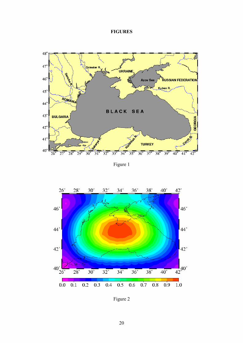
for the evaluation of GRACE-based models. The wide drainage area of the Black Sea (Figure

1) covers a large part of Europe and Asia and provides a total fresh water supply of about 350

km3 yr-1 (Ozsoy and Unluata 1998). River runoff affects the physical characteristics of the

sea, and is strongly dependent on the hydrological cycle over continental Europe (Stanev et al.

2002). The large river runoff into the Black Sea changes from year to year and has also a

semi-annual component. Therefore, not only the annual but also the semi-annual and the

inter-annual components of WM variability of the Black Sea are analyzed.

The leakage effect of land hydrology on the WM variations of the Black Sea is initially

quantified using a land hydrology model. Subsequently, the leakage effects on the two

GRACE solutions are estimated and used to correct them before the WM variations are

derived. Finally, the annual, semi-annual and inter-annual variability is quantified and

compared with Jason-1 based estimates.

2. DATA AND PROCESSING

2.1. GRACE Level-2 Products

Our GRACE time series are from the CNES/GRGS Release-02 (RL02) and CSR Release-04

(RL04) solutions. CNES/GRGS solutions include one hundred and seventy-one 10-day

gravity field solutions expressed in normalized Spherical Harmonic (SH) geopotential

coefficients from degree 2 up to degree and order 50, covering the period from 03 March

4

2003 to 29 December 2007. CSR solutions include fifty-seven monthly gravity field solutions

for the period March 2003 to December 2007, supplied as normalized SH geopotential

coefficients from degree 2 up to degree and order 60. CNES/GRGS solutions are stabilized

towards the EIGEN-GRGS.RL02.MEAN-FIELD mean gravity field at each given epoch,

with a constraint law that depends on the degree and order of each coefficient

(http://bgi.cnes.fr:8110/geoid-variations/README.html). Monthly means from the 10-day

solutions are derived by averaging to be consistent with the temporal resolution of the CSR

solutions.

The SH coefficients of CSR level-2 monthly solutions from degree 2 up to degree and order

50 are used to be consistent with the CNES/GRGS GRACE solutions. The data are

decorrelated by applying a modified version of the Swenson and Wahr (2006) decorrelation

filter called P4M6 (Chen et al. 2007; Chen et al. 2008b). For a given SH of order 6 and above,

this filter fits a polynomial of order 4 and removes this from even and odd pairs of

coefficients. Finally, Gaussian smoothing (Jekeli 1981) is applied. We test various radii for

the Gaussian function, from 500 km to 0 km in order to evaluate which represents the best

agreement wih steric corrected altimetry in the Black Sea.

Since the degree-one coefficients are not part of these GRACE solutions, an estimate of

geocenter motion (Swenson et al. 2008) is added to both GRACE solutions to account for the

degree-one components of the gravity field. For both GRACE solutions, atmospheric pressure

variations over land and ocean tides have been removed using the European Centre for

Meteorological Weather Forecasting (ECMWF) model (http://www.ecmwf.int) and the Finite

Element Solution 2004 (FES2004) (Lyard et al. 2006) model respectively. Barotropic ocean

signals have been removed from CNES/GRGS solutions using the MOG2D-G barotropic

ocean model (Carrère and Lyard 2003). The monthly averages of the MOG2D-G barotropic

5

ocean model output should in principle be restored in the CNES/GRGS monthly solutions

since we are interested in the total ocean mass signal (Lombard et al 2007). However we do

not do that because the applied version of the MOG2D-G model does not cover the Black Sea

(Lemoine, personal communication, 2009).

The Ocean Model for Circulation and Tides (OMCT) baroclinic model (Bettadpur 2007;

Flechtner 2007) have been used to remove non-tidal short-term oceanic mass variations from

the CSR RL04 solutions (Bettadpur 2007). In order to make the CSR solutions consistent with

CNES/GRGS solutions, the monthly averages of the short-term non-tidal oceanic contribution

are restored to CSR solutions using the CSR RL04 GAD products (Bettadpur 2007).

2.2. Scaling Factors for GRACE Derived WM Variations

The Black Sea basin-averaged WM variations from the two GRACE solutions are derived

using averaging kernels (Swenson and Wahr 2002). The averaging kernel used is constructed

by expanding the Black Sea land-sea mask into SH up to degree and order 50 (Figure 2). The

mask is defined as 1 at points inside the Black Sea and 0 outside of it.

Various processing steps, such as the truncation of the spherical harmonic expansion,

decorrelation filtering and smoothing will tend to reduce the amplitude of the real signal. In

order to investigate this, scaling factors were estimated by simulating a uniform 1 cm

synthetic mass signal of the Black Sea, processing it in the same manner as the GRACE

solutions and comparing the retrieved signal with the original one. After expanding the

synthetic signal into SH up to degree and order 50, we obtained 0.65 cm. Therefore a factor of

1.53 (1/0.65) is used to scale basin-average WM time series of the CNES/GRGS solutions, as

6

no further processing is applied. For the CSR solutions, we decorrelate the synthetic signal

using the P4M6 filter and apply a Gaussian smoothing. The decorrelation reduces the basin

average to 0.56 cm, and the Gaussian smoothing with half-widths of 100 km, 200 km, 300 km

and 500 km, reduces it further to 0.22 - 0.53 cm, depending on the filter half-width (Table-1).

Therefore, scaling factors given in Table 1 are used for the various filtered CSR solutions. A

test of the scaling factor for the Caspian Sea revealed slightly different result than the one of

Swenson and Wahr (2007) (2.7 versus 2.4). We believe that the small difference is due to a

different land-sea mask and/or a difference in the P4M6 decorrelation filter.

2.3. Terrestrial Water Mass Variations

Terrestrial water mass (TWM) variability around the Black Sea exceeds the WM variability in

the Black Sea, and any TWM will leak into the sea areas due to the limited degree and order

of the SH expansion and the spatial filtering applied. In order to estimate this leakage,

monthly TWM variability at one degree resolution is derived from NASA’s Global Land Data

Assimilation System (GLDAS) (Rodell et al. 2004;

http://csr.utexas.edu/research/ggfc/dataresources.html). The Noah land surface model version

2.7.1 (Ek et al. 2003) with observed precipitation and solar radiation included was used. Also,

the Climate Prediction Center (NOAA/CPC) land hydrology model was investigated (Fan and

Van den Dool 2005), but problems with the land-sea mask rendered this model unrealistic for

the Black Sea region.

For consistency, GLDAS data were processed like the GRACE-based models (Swenson and

Wahr 2007): GLDAS data were expanded into SH to degree and order 50 for CNES/GRGS

solutions and additionally decorrelated using P4M6 filter and smoothed by a Gaussian filter in

the context of CSR solutions.

7

2.4. Sea Level Data

Monthly altimetry data from the Jason-1 satellite for the period from March 2003 to

December 2007 were extracted from the Version 3.1 of the Radar Altimeter Database System,

applying the standard corrections (Scharroo 2009). The monthly averages of along-track

Jason-1 sea level data were spatially averaged over the Black Sea and the Azov Sea. The

Jason-1 altimetry tracks covering the Black Sea are depicted with black dots in Figure 3. Note

that the inverse barometer (IB) correction was not applied to the altimetry-based sea level

data, in order to be consistent with both GRACE solutions that observe the total sea mass

signal (Lombard et al 2007).

2.5. Steric Heights from WOA05 Seasonal Climatology Data

Steric sea level variations are not associated with WM variations, and in order to determine

and remove the steric contribution to the observed altimetric sea level variations, the monthly

temperature and salinity data on one degree resolution grids from the World Ocean Atlas

2005 (WOA2005) database are used (Locarnini et al. 2006; Antonov et al. 2006). The steric

sea level (SSLWOA05) was estimated by integrating the specific volume anomaly from the

surface to a depth of 300 m, as Tsimplis et al. (2004) suggested that there is no significant

contribution to the specific volume anomaly from water below 300 m in the Black Sea. Depth

contours and grid points used for the SSLWOA5 computation are depicted in Figure 3. Due to

the 300 m depth constraint, the averaged steric sea level variation could only be computed

from 29 out of the 51 grid points in the Black Sea (Figure 3).

3. RESULTS

The leakage effects from the land surrounding the Black Sea are subtracted from the GRACE

derived signals. Then, WM variations at annual and semi-annual scales are quantified by

fitting a bias, annual and semi-annual terms to the monthly basin-average time series and

8

compared with Jason-1 based estimates. A realistic estimate of the magnitude of errors for the

WM estimates cannot be provided as we were unable to obtain realistic estimates of the

magnitudes of the errors for the GLDAS model and the steric effect.

3.1. Leakage Effect from the Surrounding Land

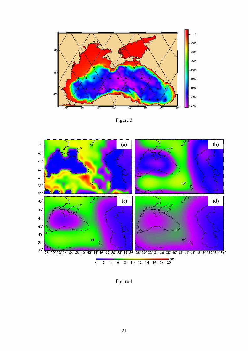
Annual TWM variations from the GLDAS model surrounding the Black and Caspian Seas are

presented in Figure 4 corresponding to different GRACE processing strategies, in order to

demonstrate the importance of accounting for leakage from nearby TWM especially due to

Gaussian smoothing. The figure shows that the TWM signal is considerably larger around the

Black Sea than around the Caspian Sea where Swenson and Wahr (2007) obtained the best

result using a Gaussian smoothing of 300 km. Consequently, the leakage will increase in the

Black Sea with larger smoothing. Figure 4 (a) shows the annual amplitude of TWM variations

derived from the original GLDAS data, which ranges up to 10-20 cm at the southeastern

border of the Black Sea. The truncated, decorrelated and smoothed GLDAS data in Figure 4

are not scaled. In order to quantify the leakage effect, the annual amplitudes of the scaled

basin-average hydrological leakage are presented in Table 2 and Table 3, corresponding to

CNES/GRGS and CSR GRACE solutions, respectively.

Table 2 shows that the effect of smoothing from the truncation of the SH at degree and order

50 (Figure 4 (b)) generates a small hydrological leakage into the sea. Table 3 shows that the

leakage is larger, when decorrelation and a 300-km Gaussian smoothing are applied (Figure 4

(c)). It becomes even larger after a 500-km smoothing is applied (Figure 4 (d)). Therefore, we

investigated the optimal radius of Gaussian smoothing for the CSR solutions. Several half-

widths of Gaussian filters (0 km, 100 km, 200 km, 300 km and 500 km) were tested. Table 3

compares the annual and semi-annual components of the CSR derived WM estimates and

9

Table 4 evaluates them with steric corrected altimetry in terms of RMS difference and

temporal correlation. We found that the larger the half-width of the Gaussian filter, the larger

the amplitude of the WM variations, and hence the larger the amplitude difference between

CSR GRACE and Jason-1 derived WM variations.

The best agreement with Jason derived WM variations was obtained for unsmoothed (but

decorrelated) CSR solutions in terms of amplitude, phase of the annuals signals (Table 3) as

well as rms difference whereas the temporal correlation was equally high for various filtered

CSR solutions (Table 4). Consequently we used the unsmoothed solution for further analyses.

If it was possible to correct for leakage perfectly, the results would not be dependent on the

choice of the smoothing radius for the CSR solutions. However our attempts were not very

successful, which was partly due to the fact that the GLDAS model does not model

groundwater variations whereas GRACE observes the integrated water storage.

3.2. Water Mass Variations on Annual and Semi-Annual Scales

The Jason-1 shows an annual amplitude of 6.8 ± 1.1 cm peaking in June. The steric sea level

from WOA05 has an annual signal with an amplitude of 2.2 ± 0.9 cm peaking in August-

September, which agrees well with values of Stanev et al. (2000) who observed an annual

amplitude of 2.5 cm peaking in mid-August calculated from climatic monthly mean heat

fluxes. The steric correction reduces the amplitude of the Jason-1 time series slightly and

advances the phase by one month. The resulting Jason-1 derived WM signal has an annual

amplitude of 6.5 ± 1.4 cm peaking in May-June.

10

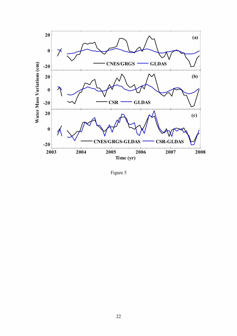
CNES/GRGS WM estimates shows an annual amplitude of 8.2 ± 1.2 cm (Table 2) peaking in

April (Figure 5 (a)). Isolating the Black Sea WM by correcting for the leakage signal (Figure

5 (a)) from CNES/GRGS yields an annual amplitude of 6.4 ± 1.3 cm peaking in May (Table 2

and Figure 5 (c)).

CSR WM estimates have annual amplitudes of 10.7 ± 1.8 cm (Table 3) peaking in April

(Figure 5 (b)). Removing the leakage signal from the CSR solutions yields an annual

amplitude of 7.4 ± 1.9 cm peaking in May (Table 3 and Figure 5 (c)).

Table 5 compares CNES/GRGS and CSR derived WM estimates with the steric corrected

altimetry. There is a fairly good agreement between the both GRACE derived WM estimates

and the Jason-1 derived WM signal in terms of both phase and amplitude and furthermore the

results are consistent with Stanev et al. (2000) who suggested that river runoff into the Black

Sea peaks in May.

The presence of the semi-annual signal is a consequence of a small secondary maximum in

December-January observed in both GRACE derived and Jason-1 derived WM time series

(Figure 6). This maximum is likely explained by the increased precipitation in fall (Stanev et

al. 2000). The Jason-1 derived WM signal has a semi-annual signal with an amplitude of 2.8 ±

1.4 cm peaking in December-January and June-July. CNES/GRGS and CSR GRACE

solutions have semi-annual signals with amplitudes of 2.9 ± 1.3 cm and 2.4 ± 1.9 cm

repectively, both estimates peaking in December-January and June-July.

11

3.3. Inter-Annual Water Mass Variations

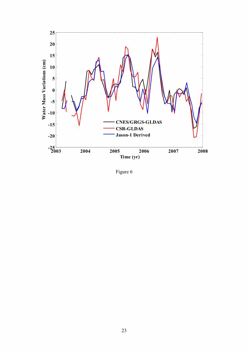
The two GRACE derived WM time series are shown in Figure 6 in comparison with the WM

estimated from steric corrected Jason-1 altimetry. The scaled WM time series from the two

GRACE based estimates have a temporal correlation of 0.84 with an rms difference of 5.4 cm

with each other. The WM time series from CNES/GRGS and CSR solutions show a good

agreement with Jason-1 derived WM (Figure 6) and the temporal correlations are 0.83 and

0.87 with rms differences of 4.6 cm and 4.80 cm, respectively. Figure 6 also shows that the

annual WM varies significantly from year to year. The annual variation is largest in 2004,

2005 and 2006, and significantly reduced in 2003 and 2007. Also the data shows a 10-15 cm

drop in WM during the second half of 2007. This drop can potentially be caused by increasing

evapotranspiration or reduced precipitation over the river drainage basin during the summer

of 2007.

4. CONCLUSION

Two widely used GRACE solutions (CNES/GRGS RL02 and CSR RL04) have been

compared with steric corrected Jason-1 altimetry for the period 2003-2007 in order to assess

their performance in deriving regionally averaged oceanic WM variations at annual and inter-

annual scales in the Black Sea.

The results show that GRACE estimated WM variations in the Black Sea are heavily

influenced by the leakage of hydrological signals from the surrounding land. Consequently,

the CSR solutions which normally require filtering are more affected by leakage than the

CNES/GRGS solutions. GLDAS was applied to study the leakage, but as GLDAS only

models the soil moisture signal in the upper 2 meters of soil and ignores WM variations from

ground water and surrounding open bodies (e.g. the Mediterranean Sea, etc.) it was

12

impossible to precisely quantify and correct for TWM leakage for the Black Sea. Comparison

with WM from satellite altimetry led us to prefer the unsmoothed (no Gaussian filtering)

decorrelated CSR solutions along with and CNES/GRGS solutions for futher investigation.

Good agreement between both GRACE solutions and the steric corrected altimetry was found

in terms of both amplitude and phase. This showed that GRACE can be used to derive water

mass variations in the Black Sea and other regions of comparable size, provided that the

signal leakage from surrounding regions is corrected for. Both GRACE WM estimates show

an annual signal of roughly 7 cm peaking in May and a semi-annual signal of roughly 3 cm

peaking in June and December. Semi-annual signals in Black Sea WM variations are small

but significant, as they modify the shape of the annual signal, creating a secondary maximum

in December.

Similarly, the amplitude of the annual signals varies significantly from year to year and is

significantly larger during 2004-2006 than in 2003 and 2007. These year-to-year variations in

the annual water mass mostly reflect the variations in inflow and outflow of water mass in the

Black Sea through nearby rivers and straits as also suggested by Stanev et al. (2000).

Acknowledgement The authors would like to thank J.L.Chen for providing the monthly GLDAS data and P4M6 decorrelation filter program and the CSR and CNES/GRGS teams for preparing GRACE level-2 products. We also thank Pavel Ditmar, Luciana Fenoglio-Marc and three other anonymous reviewers for their constructive comments.

13

REFERENCES

Andersen OB, Knudsen P, Berry P (2010) The DNSC08GRA global marine gravity field from double retracked

satellite altimetry, J Geod. Doi:10.1007/s00190-009-0355-9.

Antonov JI, Locarnini RA, Boyer TP, Mishonov AV, Garcia HE (2006) World Ocean Atlas 2005, vol. 2,

Salinity, NOAA Atlas NESDIS, vol. 62, edited by S. Levitus, 182 pp, U.S. Gov. Print. Off., Washington, D.C.

Bettadpur S (2007) Level-2 gravity field product user handbook, GRACE 327-734, The GRACE Project, Center

for Space Research, University of Texas at Austin.

Carrère L, Lyard F (2003) Modeling the barotropic response of the global ocean to atmospheric wind and

pressure forcing - comparisons with observations. Geophys Res Lett 30(6): 1275. Doi:10.1029/2002GL016473.

Chambers DP, Wahr J, Nerem RS (2004) Preliminary observations of global ocean mass variations with

GRACE, Geophys Res Lett 31 L13310. Doi:10.1029/2004GL020461.

Chen JL, Wilson CR, Tapley BD, Grand S (2007) GRACE detects coseismic and postseismic deformation from

the Sumatra-Andaman earthquake. Geophys Res Lett 34: L13302. Doi:10.1029/2007GL030356.

Chen JL, Wilson CR, Seo, KW (2008a) S2 tide aliasing in GRACE time-variable gravity solutions, J Geod. DOI

10.1007/s00190-008-0282-1.

Chen JL, Wilson CR, Tapley BD, Blankenship D, Young D (2008b) Antartic regional ice loss from GRACE.

Earth Planet Sci Lett 266: 140-148. Doi:10.1016/j.epsl.2007.10.057.

Ek, MB, Mitchell KE, Lin Y, Rogers E, Grunmann P, Koren V, Gayno G, Tarpley JD (2003) Implementation of

Noah land surface model advances in the National Centers for Environmental Prediction operational mesoscale

Eta model. J Geophys Res 108: 8851. Doi:10.1029/2002JD003296.

Fan, Y, van den Dool H (2005) The Climate Prediction Center global monthly soil moisture data set at 0.5deg

resolution for 1948 - present. J Geophys Res 109: D10102. Doi:1029/2003JD004345.

Fenoglio-Marc L, Kusche J, Becker M (2006) Mass variation in the Mediterranean Sea from GRACE and its

validation by altimetry, steric and hydrologic fields. Geophys Res Let 33: L19606. Doi:10.1029/2006GL026851.

Flechtner F (2007) GRACE AOD1B Product Description Document for Product Releases 01 to 04 (Rev. 3.1,

April 13, 2007), GRACE 327-750, GeoForschungsZentrum Potsdam, Germany.

Jekeli C (1981) Alternative methods to smooth the Earth’s gravity field, Techical Report, Department of

Geodetic Science, Ohio State University, Columbus, Ohio.

14

Lemoine JM, Bruinsma S, Loyer S, Biancale R, Marty JC, Perosanz F, Balmino G (2007) Temporal gravity field

models inferred from GRACE data. J Adv Space Res 39: 1620–1629. doi:10.102/j/asr.2007.03.062.

Locarnini RA, Mishonov AV, Antonov JI, Boyer TP, Garcia HE (2006) World Ocean Atlas 2005, vol. 1,

Temperature, NOAA Atlas NESDIS, vol. 61, edited by S. Levitus, 182 pp., U.S. Gov. Print. Off. Washington,

D.C.

Lombard A, Garcia D, Ramillien G, Cazenave A, Biancale R, Lemoine JM, Flechtner F, Schmidt R, Ishii M

(2007) Estimation of steric sea level variations from combined GRACE and Jason-1 data. Earth and Planetary

Science Letters, 254, 1-2, 194-202.

Lyard F, Lefevre F, Letellier T, Francis O (2006) Modelling the global ocean tides: modern insights from

FES2004. Ocean Dyn 56:394–415. Doi:10.1007/s10236-006-0086-x.

Scharroo R (2009) Radar Altimeter Database System (RADS) Version 3.0 User Manual and Format

Specification, Space Res. Organ. Neth. Utrecht, Netherlands.

Ozsoy E, Unluata U (1998) The Black Sea. In: Robinson A, Brink K (eds) The Sea, vol.11, John Wiley, New

York.

Rodell M, Houser PR, Jambor U, Gottschalck J, Mitchell K, Meng CJ, Arsenault K, Cosgrove B, Radakovich J,

Bosilovich M, Entin JK, Walker JP, Lohmann D, Toll D (2004) The Global Land Data Assimilation System.

Bulletin of American Meteorological Society, 85: 381–394. Doi: 10.1175/BAMS-85-3-381.

Stanev EV, Le Traon PY, Peneva EL (2000) Sea level variations and their dependency on meteorological and

hydrological forcing: Analysis of altimeter and surface data for the Black Sea. J Geophys Res 105: 17203-17216.

Stanev EV, Beckers JM, Lancelot C, Staneva JV, Le Traon PY, Peneva EL, Gregoire M (2002) Coastal–open

Ocean Exchange in the Black Sea: Observations and Modelling. Estuarine, Coastal and Shelf Science 54: 601–

620.

Swenson, S, Chambers D, Wahr J (2008) Estimating geocenter variations from a combination of GRACE and

ocean model output, J Geophys Res 113: B08410.Doi:10.1029/2007JB005338.

Swenson S, Wahr J (2007) Multi-sensor analysis of water storage variations of the Caspian Sea. Geophys Res

Let 34: L16401. Doi:10.1029/2007GL030733.

Swenson S, Wahr J (2006) Post-processing removal of correlated errors in GRACE data. Geophys Res Let 33:

L08402. Doi:10.1029/2005GL025285.

15

Swenson S, Wahr J (2002) Methods for inferring regional surfacemass anomalies from GRACE measurements

of time-variable gravity, J. Geophys. Res,. 107(B9), 2193, doi:10.1029/2001JB000576.

Tapley BD, Bettadpur S, Ries J, Thompson PF, Watkins MM (2004) GRACE measurements of mass variability

in the earth system. Science 305:503–505. doi:10.1126/science.1099192.

Tsimplis MN, Josey SA, Rixen M, Stanev EV (2004) On the forcing of sea level in the Black Sea, J Geophys

Res 109: 1-13. Doi:10.1029/2003JC002185.

Wahr J, Swenson S, Zlotnicki V, Velicogna I (2004) Time-variable gravity from GRACE: first results. Geophys

Res Lett 31:L11501.doi:10.1029/2004GL019779.

16

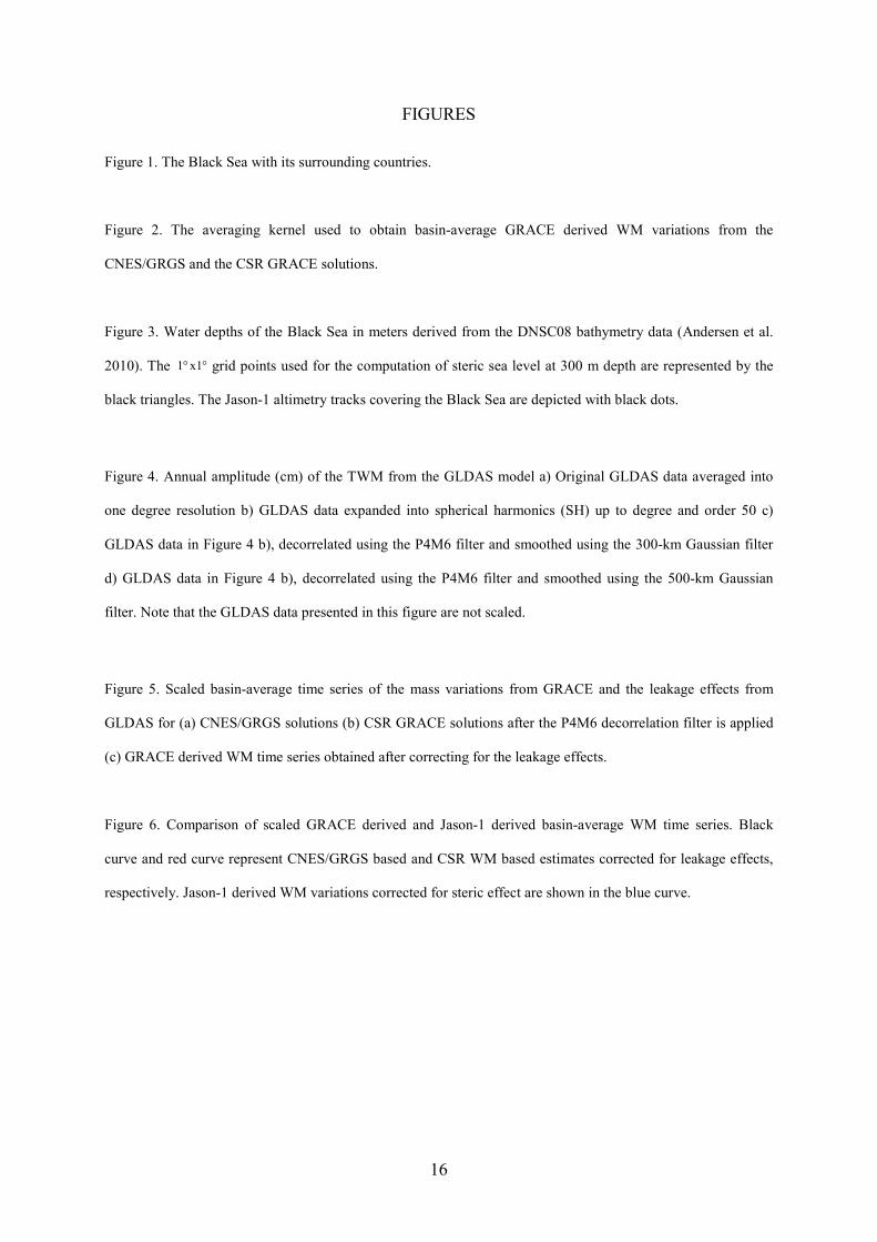
FIGURES

Figure 1. The Black Sea with its surrounding countries.

Figure 2. The averaging kernel used to obtain basin-average GRACE derived WM variations from the

CNES/GRGS and the CSR GRACE solutions.

Figure 3. Water depths of the Black Sea in meters derived from the DNSC08 bathymetry data (Andersen et al.

2010). The °°x11 grid points used for the computation of steric sea level at 300 m depth are represented by the

black triangles. The Jason-1 altimetry tracks covering the Black Sea are depicted with black dots.

Figure 4. Annual amplitude (cm) of the TWM from the GLDAS model a) Original GLDAS data averaged into

one degree resolution b) GLDAS data expanded into spherical harmonics (SH) up to degree and order 50 c)

GLDAS data in Figure 4 b), decorrelated using the P4M6 filter and smoothed using the 300-km Gaussian filter

d) GLDAS data in Figure 4 b), decorrelated using the P4M6 filter and smoothed using the 500-km Gaussian

filter. Note that the GLDAS data presented in this figure are not scaled.

Figure 5. Scaled basin-average time series of the mass variations from GRACE and the leakage effects from

GLDAS for (a) CNES/GRGS solutions (b) CSR GRACE solutions after the P4M6 decorrelation filter is applied

(c) GRACE derived WM time series obtained after correcting for the leakage effects.

Figure 6. Comparison of scaled GRACE derived and Jason-1 derived basin-average WM time series. Black

curve and red curve represent CNES/GRGS based and CSR WM based estimates corrected for leakage effects,

respectively. Jason-1 derived WM variations corrected for steric effect are shown in the blue curve.

17

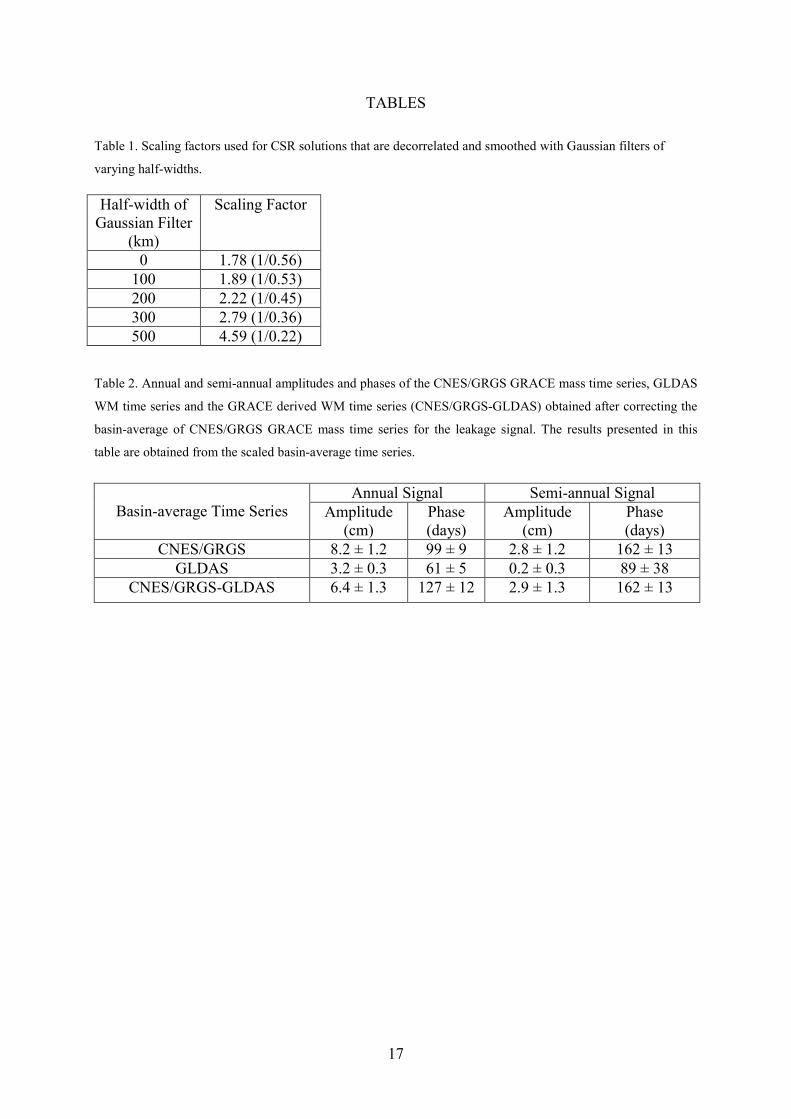
TABLES

Table 1. Scaling factors used for CSR solutions that are decorrelated and smoothed with Gaussian filters of

varying half-widths.

Table 2. Annual and semi-annual amplitudes and phases of the CNES/GRGS GRACE mass time series, GLDAS

WM time series and the GRACE derived WM time series (CNES/GRGS-GLDAS) obtained after correcting the

basin-average of CNES/GRGS GRACE mass time series for the leakage signal. The results presented in this

table are obtained from the scaled basin-average time series.

Half-width of Gaussian Filter

(km)

Scaling Factor

0 1.78 (1/0.56) 100 1.89 (1/0.53) 200 2.22 (1/0.45) 300 2.79 (1/0.36) 500 4.59 (1/0.22)

Annual Signal Semi-annual Signal Basin-average Time Series Amplitude

(cm) Phase (days)

Amplitude (cm)

Phase (days)

CNES/GRGS 8.2 ± 1.2 99 ± 9 2.8 ± 1.2 162 ± 13 GLDAS 3.2 ± 0.3 61 ± 5 0.2 ± 0.3 89 ± 38

CNES/GRGS-GLDAS 6.4 ± 1.3 127 ± 12 2.9 ± 1.3 162 ± 13

18

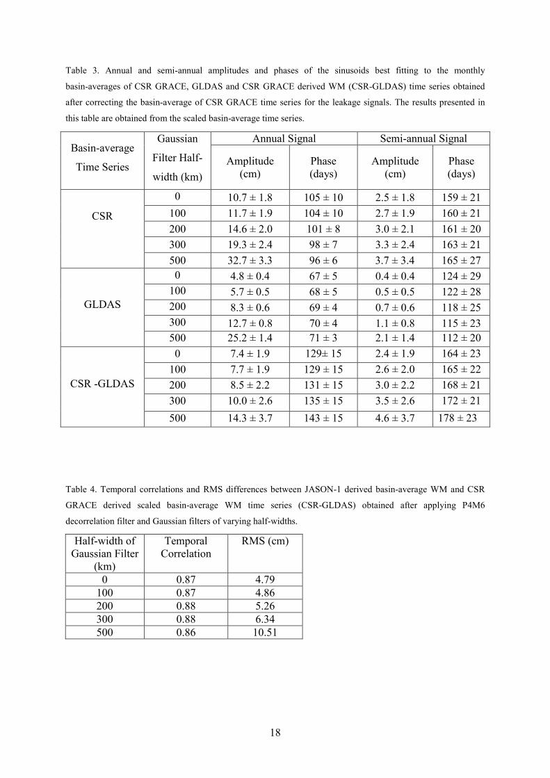
Table 3. Annual and semi-annual amplitudes and phases of the sinusoids best fitting to the monthly

basin-averages of CSR GRACE, GLDAS and CSR GRACE derived WM (CSR-GLDAS) time series obtained

after correcting the basin-average of CSR GRACE time series for the leakage signals. The results presented in

this table are obtained from the scaled basin-average time series.

Table 4. Temporal correlations and RMS differences between JASON-1 derived basin-average WM and CSR

GRACE derived scaled basin-average WM time series (CSR-GLDAS) obtained after applying P4M6

decorrelation filter and Gaussian filters of varying half-widths.

Annual Signal Semi-annual Signal Basin-average

Time Series

Gaussian

Filter Half-

width (km)

Amplitude (cm)

Phase (days)

Amplitude (cm)

Phase (days)

0

10.7 ± 1.8 105 ± 10 2.5 ± 1.8 159 ± 21

100 11.7 ± 1.9 104 ± 10 2.7 ± 1.9 160 ± 21

200 14.6 ± 2.0 101 ± 8 3.0 ± 2.1 161 ± 20

300 19.3 ± 2.4 98 ± 7 3.3 ± 2.4 163 ± 21

CSR

500 32.7 ± 3.3 96 ± 6 3.7 ± 3.4 165 ± 27

0 4.8 ± 0.4 67 ± 5 0.4 ± 0.4 124 ± 29 100 5.7 ± 0.5 68 ± 5 0.5 ± 0.5 122 ± 28

200 8.3 ± 0.6 69 ± 4 0.7 ± 0.6 118 ± 25

300 12.7 ± 0.8 70 ± 4 1.1 ± 0.8 115 ± 23

GLDAS

500 25.2 ± 1.4 71 ± 3 2.1 ± 1.4 112 ± 20

0 7.4 ± 1.9 129± 15

2.4 ± 1.9

164 ± 23 100 7.7 ± 1.9 129 ± 15 2.6 ± 2.0

165 ± 22

200 8.5 ± 2.2 131 ± 15 3.0 ± 2.2 168 ± 21 300 10.0 ± 2.6 135 ± 15 3.5 ± 2.6 172 ± 21

CSR -GLDAS

500 14.3 ± 3.7 143 ± 15 4.6 ± 3.7 178 ± 23

Half-width of Gaussian Filter

(km)

Temporal Correlation

RMS (cm)

0 0.87 4.79 100 0.87 4.86 200 0.88 5.26 300 0.88 6.34 500 0.86 10.51

19

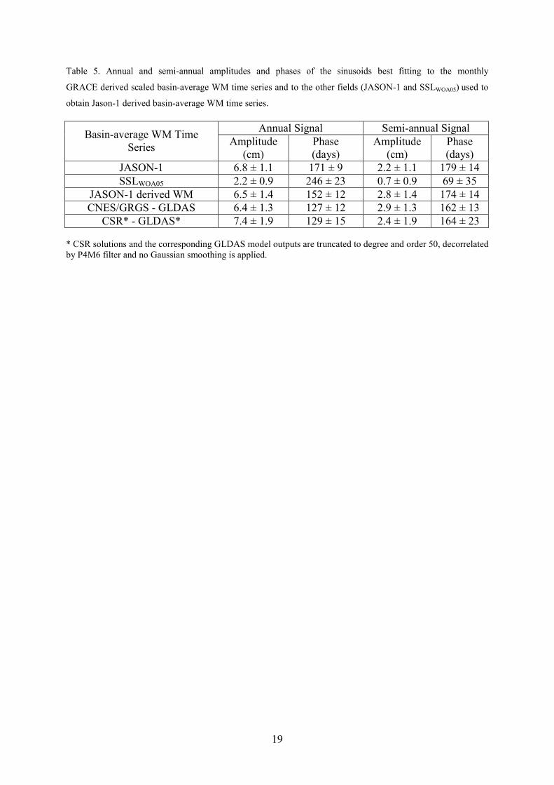
Table 5. Annual and semi-annual amplitudes and phases of the sinusoids best fitting to the monthly

GRACE derived scaled basin-average WM time series and to the other fields (JASON-1 and SSLWOA05) used to

obtain Jason-1 derived basin-average WM time series.

* CSR solutions and the corresponding GLDAS model outputs are truncated to degree and order 50, decorrelated by P4M6 filter and no Gaussian smoothing is applied.

Annual Signal Semi-annual Signal Basin-average WM Time

Series Amplitude

(cm) Phase (days)

Amplitude (cm)

Phase (days)

JASON-1 6.8 ± 1.1 171 ± 9 2.2 ± 1.1 179 ± 14 SSLWOA05 2.2 ± 0.9 246 ± 23 0.7 ± 0.9 69 ± 35

JASON-1 derived WM 6.5 ± 1.4 152 ± 12 2.8 ± 1.4 174 ± 14 CNES/GRGS - GLDAS 6.4 ± 1.3 127 ± 12 2.9 ± 1.3 162 ± 13

CSR* - GLDAS* 7.4 ± 1.9 129 ± 15 2.4 ± 1.9 164 ± 23

20

FIGURES

Figure 1

Figure 2

21

Figure 3

Figure 4

Figure 4

(a) (b)

(c) (d)

22

-20

0

20

(a)

-20

0

20

(b)

2003 2004 2005 2006 2007 2008

-20

0

20

Water M

ass Variations (cm)

(c)

Time (yr)

CNES/GRGS-GLDAS CSR-GLDAS

CNES/GRGS GLDAS

CSR GLDAS

Figure 5

23

2003 2004 2005 2006 2007 2008-25

-20

-15

-10

-5

0

5

10

15

20

25

Time (yr)

Water M

ass Variations (cm)

CNES/GRGS-GLDAS

CSR-GLDAS

Jason-1 Derived

Figure 6