Bisimulation and cocongruence for probabilistic systems

Bisimulation and Cocongruence for Probabilistic Systems

Vincent DanosEquipe PPS

Universite Paris 7 and CNRSParis, France

[email protected]

Josee Desharnais∗

Departement d’InformatiqueUniversite LavalQuebec, Canada

[email protected]

Francois Laviolette∗

Departement d’InformatiqueUniversite LavalQuebec, Canada

[email protected]

Prakash Panangaden†

School of Computer ScienceMcGill University

Montreal, Quebec, [email protected]

February 19, 2005

Abstract

We introduce a new notion of bisimulation, called event bisimulation on labelled Markovprocesses (LMPs) and compare it with the, now standard, notion of probabilistic bisimulation,originally due to Larsen and Skou. Event bisimulation uses a sub σ-algebra as the basic carrierof information rather than an equivalence relation. The resulting notion is thus based on mea-surable subsets rather than on points: hence the name. Event bisimulation applies smoothly forgeneral measure spaces; bisimulation, on the other hand, is known only to work satisfactorily foranalytic spaces. We prove the logical characterization theorem for event bisimulation withouthaving to invoke any of the subtle aspects of analytic spaces that feature prominently in thecorresponding proof for ordinary bisimulation. These complexities only arise when we show thaton analytic spaces the two concepts co-incide.

We show that the concept of event bisimulation arises naturally from taking the co-congruencepoint of view for probabilistic systems. We show that the theory can be given a pleasing cat-egorical treatment in line with general coalgebraic principles. As an easy application of theseideas we develop a notion of “almost sure” bisimulation; the theory comes almost “for free”once we modify Giry’s monad appropriately.

1 Introduction

Markov processes with continuous state spaces or continuous time evolution (or both) arise nat-urally in several fields of physics, biology, economics and computer science. Examples of suchsystems are brownian motion, gas diffusion, population growth models, noisy control systems andcommunications systems.

∗Research supported by NSERC.†Research supported by NSERC (Canada) and EPSRC (U.K.). Research carried out at Computing Laboratory,

Oxford University.

1

Labelled Markov Processes (LMPs) were formulated [BDEP97, DEP02] to study such generalinteracting Markov processes. In an LMP, instead of one transition probability function (or Markovkernel) there are several, each associated with a distinct label1. Each such transition probabilityfunction represents the (stochastic) response of the system to an external stimulus represented bythe label. In our work we do not associate probabilities with these external stimuli; in other words,we do not intend to quantify the behaviour of the environment. Thus, for those familiar withprocess algebra terminology, an LMP is a labelled transition system with probabilistic transitions.The interaction is captured by synchronizing on labels in the manner familiar from process algebra.

The following example, taken from [DGJP03], illustrates these ideas.

Example 1.1 Consider the flight management system of an aircraft. It is responsible for mon-itoring the state of the aircraft – the altitude, windspeed, direction, roll, yaw etc. – periodically(usually several times a second), it also monitors navigational data from satellites and makes cor-rections, as needed, by issuing commands to the engines and the wing flaps. The physical system isa complex continuous real-time stochastic system; stochastic because the response of the physicalsystem to commands cannot be completely deterministic and also because of unexpected situationslike turbulence. From the point of view of the flight management system, however, the system isdiscrete-time and has continuous space. The time unit is the sampling rate. The entire systemconsists of many interacting concurrent components and programming it correctly – letting aloneverifying that the system works – is very challenging. A formal model of this type of software bringsus into the realm of process algebra, because of the concurrent interacting components, stochasticprocesses and real-time systems, the last because the responses have hard deadlines.

This study was initiated by Larsen and Skou [LS91] for discrete processes in a style similarto the queueing theory notion of “lumpability” invented in the late 1950s [KS60]. In a series ofprevious papers [BDEP97, DEP98, DEP02] such Markov processes with continuous state spacesand independently acting components were studied, and the phrase “labelled Markov processes”appeared in print explicitly referring to the continuous state space case. Of course, closely relatedconcepts were already around: for example, Markov decision processes [Put94]. The papers byDesharnais, Edalat and Panangaden gave a definition of bisimulation between LMPs, and gavea logical characterization of this bisimulation. Subsequently an approximation theory was devel-oped [DGJP00, DGJP03, DD03] and metrics were defined [DGJP99, DGJP04, vBW01b, vBW01a].

Before we begin the present paper we will briefly review the prior results. The notion ofprobabilistic bisimulation - henceforth just “bisimulation” - was based on the idea that if twostates are bisimilar then their transition probabilities to bisimulation equivalence classes shouldmatch. This notion works well for the discrete case, but has to be generalized appropriately tothe continuous case. One idea was to mimic this definition exactly with a few measure-theoreticconditions imposed to deal with the fact that not all sets need be measurable. This was the approachfollowed in [DGJP00, DGJP03]. However, in an earlier approach [BDEP97, DEP98, DEP02] theauthors had defined a bisimulation - they called it a “zig-zag” - morphism and then defined abisimulation relation as a span of such morphisms. This also generalizes the discrete case but itturned out to be very painful to prove that one gets a transitive relation and one had to restrict toPolish or analytic spaces. For such cases (analytic subsumes Polish) the two notions coincide.

One of the nice things about the theory was the logical characterization of bisimulation. Therewas already such a theorem for the discrete case in the paper of Larsen and Skou [LS91] but it

1We do not consider internal nondeterminism in the present paper.

2

was not clear that such a theorem would work in the continuous state case2. Not only did such atheorem exist but logical characterization worked with a much more parsimonious logic than onewas led to expect from the discrete case. There turned out to be a very spartan logic:

φ ::== >|φ1 ∧ φ2|〈a〉qφ

which characterises bisimulation for both continuous and discrete systems. There are two strikingthings about this logic: there is no negative construct at all and one only needs binary conjunctioneven though the branching may be uncountable. The proof heavily uses special properties of analyticspaces that a priori have nothing to do with anything logical.

This is an irritating fact: one has to restrict to state-spaces that were analytic. In one sense thisis not very restrictive: almost every process that one can imagine has an analytic state space. Inparticular Rn with the usual Borel sets is analytic, indeed any manifold is analytic. In another senseit is conceptually unsatisfying that these notions specific to measure theory on metric spaces shouldturn out to be so crucial. Why doesn’t the theory work for general measure spaces? Certainly thestatement of the logical characterization theorem does not suggest anything about analytic spaces.

2 The road to event bisimulation

The first attempt to define LMPs for continuous systems [BDEP97] did not have any assumptionsabout the σ-algebra on the state space. LMPs were organized in a category and bisimulationwas defined in terms of spans of particular morphisms of this category, called zig-zag morphisms.However, buried in the proofs was an alternative view of bisimulation as a cospan: in fact this is thegerm of the co-congruence idea that we develop in the present paper. With this definition, one couldprove that the logic L characterizes bisimulation. This was, however, viewed as an intermediatestep at the time: firstly, it was a compromise to use cospans instead of spans of morphisms as isusually done when one wants to define a relation between objects of a category. Spans could notbe used because one could not show that bisimulation was transitive; indeed, this is equivalentto constructing a span given a cospan, and to this day, only analytic spaces have been proven tosatisfy this property [Eda99, Dob03]. Secondly, the definition of bisimulation was not given onthe state-space of a process but, rather, through morphisms in the category: this is not what onewas used to working with in the finite case or in the non-probabilistic case. Consequently, a newrelational definition of bisimulation (called state bisimulation in this paper) was formulated thatlooked like a nice generalization of non-probabilistic bisimulation as well as of finite probabilisticbisimulation. However, for this definition as well, characterization of bisimulation by the logic wasonly proven for analytic spaces.

In this paper, we give a new definition of bisimulation, called event bisimulation, that is equiva-lent with the cospan definition and hence is characterized by the logic. This is proved without anyanalyticity assumption: it works for arbitrary measure spaces. Moreover, it has the nice propertythat the logic yields the biggest possible event bisimulation on any process. We also compare thisdefinition with the state bisimulation mentioned above, and show that the two notions are exactlythe same for countable processes and, more generally, for analytic spaces. More precisely, thelargest state bisimulation is an event bisimulation on these spaces. However, viewed as relationswe show that roughly speaking, the former is finer that the latter, and hence equates fewer states

2In retrospect this seems like a misplaced worry but it was a real worry at the time.

3

than the latter in general (in both analytic and non analytic spaces). The following simple exampleis very useful for intuition.

Example 2.1 Consider a set of states equiped with a σ-algebra that does not separate points.For example, one can take 1, 2, 3, 4 with the σ-algebra, ∅, 1, 2, 3, 4, 1, 2, 3, 4. No matterwhat is the transition function, the identity relation is a state bisimulation, but it is not an eventbisimulation. The reason is that the identity relation distinguishes states that are undistinguishableby the σ-algebra, for example states 1 and 2 are not related whereas no probability function coulddistinguish them because the probability function must respect the σ-algebra in an LMP, by beingmeasurable. Since event bisimulation is based on the σ-algebra, it cannot be finer. This exampleshould be kept in mind for the remaining of the paper.

We believe that event bisimulation is the correct generalization of state bisimulation to thecategory of all LMPs defined for arbitrary measure spaces. This is justified by three arguments:the two notions agree on analytic spaces, event bisimulation is shown to be characterized by thelogic for any measurable space (analytic and non analytic spaces) and finally because transitivityof event bisimulation can be proven categorically without the analyticity assumption.

This new definition also has the advantage to reconcile the two fields of theory of processes andprobability theory; it allows one to use the σ-algebra as a vector of information to define eventbisimulation between processes.

3 Background on LMPs

Labelled Markov processes are probabilistic versions of labelled transition systems. Correspondingto each label a Markov process is defined. The transition probability is given by a Markov kernel.In brief, a labelled Markov process can be described as follows. There is a set of states and aset of labels. The system is in a state at each point in time. The environment selects an action,and the system reacts by moving to another state. The transition to another state is governed bya probabilistic law. For each label there is a transition probability distribution which gives theprobability distribution of the possible final states given the initial state. For discrete state spaces,this is essentially the model developed by Larsen and Skou [LS91].

We extended this to continuous-state systems, thus forcing our formalism to be couched inmeasure-theoretic terms. For instance, we cannot ask for the transition probability to any set ofstates — we need to restrict ourselves to measurable sets. The classical theory of Markov processesis typically carried out in the setting of Polish spaces rather than on abstract measure spaces. Inprevious papers analytic spaces - which generalize Polish spaces - were used. However, in this paperwe eliminate the need for analytic spaces.

A key ingredient in the theory is the Markov kernel, which we sometime call transition kernel.

Definition 3.1 A Markov kernel on a measurable space (S, Σ) is a function τ : S × Σ → [0, 1]such that for each fixed s ∈ S, the set function τ(s, ·) is a (sub-) probability measure, and for eachfixed X ∈ Σ the function τ(·, X) is a measurable function.

One interprets τ(s,X) as the probability of the process starting in state s making a transition intoone of the states in X. The Markov kernel is really a conditional probability : it gives the probabilityof the process being in one of the states of the set X after the transition, given that it was in thestate s before the transition.

4

We will work with transition kernels where τ(s, S) ≤ 1 rather than τ(s, S) = 1. The mathe-matical results go through in this extended case. We view processes where the transition kernelsare only sub-probabilities as being partially defined.

Definition 3.2 A labelled Markov process (LMP) S with label set A is a structure (S, Σ, τa|a ∈A), where S is the set of states, Σ is a σ-algebra on S, and for all a ∈ A

τa : S × Σ −→ [0, 1]

is a Markov kernel.

We will fix the label set to be A once and for all. We will use the following notational convention:we write S = (S, Σ, τ), using the calligraphic font to stand for the LMP and the ordinary capitalfor the state space. We often drop the subscript of τ when convenient since it does not restrict theresults.

The all important notion is that of a zig-zag morphism.

Definition 3.3 A zig-zag morphism f from S to S ′ is a surjective measurable function f : S → S′

satisfying∀a ∈ A, s ∈ S, B ∈ Σ′.τa(s, f−1(B)) = τ ′a(f(s), B).

We originally defined a bisimulation in terms of spans of zig-zags. In order to show transitivitywe had to use a subtle construction due to Edalat [Eda99]. Later we gave the following directrelational definition and finessed the use of that lemma. If R is a binary relation on a set S, we saythat A ⊆ S is R-closed if s ∈ S : ∃a ∈ A.aRs ⊆ A. We denote by Σ(R) the set of R-closed setsin Σ.

Definition 3.4 Given an LMP S, a (state) bisimulation relation R is a binary relation on Ssuch that whenever sRt and C ∈ Σ(R), then for all labels a, τa(s, C) = τa(t, C). We say that s andt are bisimilar if there is any bisimulation R such that sRt.

One can define a simple modal logic and prove that two states are bisimilar if and only if theysatisfy exactly the same formulas. Indeed for finite-state processes one can decide whether two statesare bisimilar and effectively construct a distinguishing formula in case they are not [DGJP02].

As before we assume that there is a fixed set of “actions” A. The logic is called L and has thefollowing syntax:

T | φ1 ∧ φ2 | 〈a〉qφ

where a is an action and q is a rational number between 0 and 1. This is the basic logic withwhich one can establish the logical characterization. The last formula is interpreted as follows. Wesay s |= 〈a〉qφ if s can make an a-transition with probability greater than or equal to the rationalnumber q and end up in a state satisfying φ.

In the analysis of simulation one needs a logic with disjunction, L∨:

L | φ1 ∨ φ2.

The logical characterization theorem uses a remarkably parsimonious logic: no negation, no infini-tary constructs. It works only when the state space is an analytic space. In the present paperwe will show that the new notion of bisimulation leads to the logical characterization theorem forLMPs defined on arbitrary measure spaces.

5

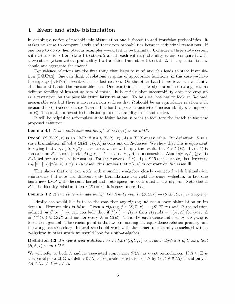
4 Event and state bisimulation

In defining a notion of probabilistic bisimulation one is forced to add transition probabilities. Itmakes no sense to compare labels and transition probabilities between individual transitions. Ifone were to do so then obvious examples would fail to be bisimilar. Consider a three-state systemwith a-transitions from state 1 to states 2 and 3, each with a probability 1

2 , and compare it witha two-state system with a probability 1 a-transition from state 1 to state 2. The question is howshould one aggregate the states?

Equivalence relations are the first thing that leaps to mind and this leads to state bisimula-tion [DGJP03]. One can think of relations as spans of appropriate functions; in this case we havethe zig-zags [DEP02] described in the last section. On the other hand there is a natural familyof subsets at hand: the measurable sets. One can think of the σ-algebra and sub-σ-algebras asdefining families of interesting sets of states. It is curious that measurability does not crop upas a restriction on the possible bisimulation relations. To be sure, one has to look at R-closedmeasurable sets but there is no restriction such as that R should be an equivalence relation withmeasurable equivalence classes (it would be hard to prove transitivity if measurability was imposedon R). The notion of event bisimulation puts measurability front and centre.

It will be helpful to reformulate state bisimulation in order to facilitate the switch to the newproposed definition.

Lemma 4.1 R is a state bisimulation iff (S, Σ(R), τ) is an LMP.

Proof: (S, Σ(R), τ) is an LMP iff ∀A ∈ Σ(R), τ(·, A) is Σ(R)-measurable. By definition, R is astate bisimulation iff ∀A ∈ Σ(R), τ(·, A) is constant on R-classes. We show that this is equivalentto saying that τ(·, A) is Σ(R)-measurable, which will imply the result. Let A ∈ Σ(R). If τ(·, A) isconstant on R-classes, s|τ(s,A) ≥ r ∈ Σ because τ(·, A) is measurable. Also s|τ(s,A) ≥ r isR-closed because τ(·, A) is constant. For the converse, if τ(·, A) is Σ(R)-measurable, then for everyr ∈ [0, 1], s|τ(s,A) ≥ r is R-closed: this implies that τ(·, A) is constant on R-classes.

This shows that one can work with a smaller σ-algebra closely connected with bisimulationequivalence, but note that different state bisimulations can yield the same σ-algebra. In fact onehas a new LMP with the same kernel and state space but with a reduced σ-algebra. Note that ifR is the identity relation, then Σ(R) = Σ. It is easy to see that

Lemma 4.2 R is a state bisimulation iff the identity map i : (S, Σ, τ) → (S, Σ(R), τ) is a zig-zag.

Ideally one would like it to be the case that any zig-zag induces a state bisimulation on itsdomain. However this is false. Given a zig-zag f : (S, Σ, τ) → (S′,Σ′, τ ′) and R the relationinduced on S by f we can conclude that if f(s1) = f(s2) then τ(s1, A) = τ(s2, A) for every Ain f−1(Σ′) ⊆ Σ(R) and not for every A in Σ(R). Thus the equivalence induced by a zig-zag istoo fine in general. The crucial point is that we are making the equivalence relation primary andthe σ-algebra secondary. Instead we should work with the structure naturally associated with aσ-algebra: in other words we should look for a sub-σ-algebra.

Definition 4.3 An event bisimulation on an LMP (S, Σ, τ) is a sub-σ-algebra Λ of Σ such that(S, Λ, τ) is an LMP.

We will refer to both Λ and its associated equivalence R(Λ) as event bisimulation. If Λ ⊆ Σ isa sub-σ-algebra of Σ we define R(Λ) an equivalence relation on S by (s, t) ∈ R(Λ) if and only if∀A ∈ Λ.s ∈ A ⇔ t ∈ A.

6

The phrase “event bisimulation” is meant to suggest that the focus of interest has shifted fromthe individual points of S to the measurable sets, or - to emphasize the probabilistic interpretation- the events. What has happened here is that the notion of bisimulation qua relation has beenreplaced by an arbitrary sub-σ-algebra rather than Σ(R), the sub-σ-algebra generated by a relationR. The key point is that the transition kernels have to have the appropriate measurability propertieswith respect to Λ. We can more sensibly say that Λ, rather than R(Λ), is an event bisimulation.

The similarity with state bisimulation can be made quite striking.

Lemma 4.4 If Λ is an event bisimulation, then the identity function on S defines a zig-zag mor-phism from (S, Σ, τ) to (S, Λ, τ).

If we compare this result to Lemma 4.2, we can see that it fits more nicely in the category of LMPsin that it does not talk about relations. Moreover, we get a perfect correspondence with zig-zags.

Lemma 4.5 If f : (S, Σ, τ) → (S′,Σ′, τ ′) is a zig-zag morphism, then f−1(Σ′) is an event bisimu-lation on S.

In order to facilitate the study of the relation between state and event bisimulation, we needsome elementary mathematical observations connecting σ-algebras and binary relations. Let R bea relation on S, which is a set equipped with a σ-algebra Σ. We write Υ(R) for the R-closed subsetsof S. Then Σ(R) = Σ∩Υ(R). Since Υ(R) is clearly a σ-algebra, Σ(R) is therefore a sub-σ-algebraof Σ.

We have two maps back and forth between sub-σ-algebras and equivalence relations: Λ 7→ R(Λ)and R 7→ Σ(R).

Lemma 4.6 Let (S, Σ) be a measurable space, R a relation on S and Λ ⊆ Σ a sub-σ-algebra. Then(i) Λ ⊆ Σ(R(Λ)).(ii) R ⊆ R(Σ(R)).(iii) If R-equivalence classes are in Σ, then R = R(Σ(R)).

Proof . (i) First let A be in Λ, then A ∈ Σ; also A is R(Λ)-closed. Thus A ∈ Σ ∩ Υ(R(Λ)) =Σ(R(Λ)). (ii) Next, we have [s]R(Σ(R)) = ∩A 3 s with A ∈ Σ and R-closed; and [s]R = ∩B 3 swith B R-closed; so ⊆ follows. Now for ⊇ in (iii), if [s]R itself is in Σ then it qualifies as an A inthe big intersection above and the result follows.

Proposition 4.7 Let (S, Σ) be a measurable space and Λ ⊆ Σ a sub-σ-algebra. Then(i) R(Λ) = R(Υ(R(Λ))).(ii) If Λ ⊆ Σ then R(Λ) = R(Σ(R(Λ))).

Proof . (i) follows from Lemma 4.6 (iii), replacing Σ by Υ(R). (ii) Since Λ ⊆ Σ ∩ Υ(R(Λ)) ⊆Υ(R(Λ)) and by (i) we have R(Λ) ⊇ R(Σ ∩Υ(R(Λ))) ⊇ R(Υ(R(Λ))) = R(Λ).

These lemma and proposition show how to transfer results between sub-σ-algebras and equiv-alence relations.

We presented event bisimulation as a weakening of state bisimulation. Consequently, we wouldlike to prove that the latter is always an event bisimulation. However, this is not actually the casein general: essentially because there is not enough measure theoretic control on the relations usedto define state bisimulation.

We know from Lemma 4.6 that R ⊆ R(Σ(R)). The following lemma shows that if a statebisimulation satisfies the reverse inclusion, then it is an event bisimulation.

7

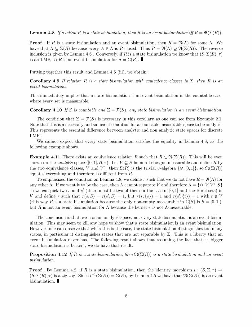
Lemma 4.8 If relation R is a state bisimulation, then it is an event bisimulation iff R = R(Σ(R)).

Proof . If R is a state bisimulation and an event bisimulation, then R = R(Λ) for some Λ. Wehave that Λ ⊆ Σ(R) because every A ∈ Λ is R-closed. Thus R = R(Λ) ⊇ R(Σ(R)). The reverseinclusion is given by Lemma 4.6 . Conversely, if R is a state bisimulation we know that (S, Σ(R), τ)is an LMP, so R is an event bisimulation for Λ = Σ(R).

Putting together this result and Lemma 4.6 (iii), we obtain:

Corollary 4.9 If relation R is a state bisimulation with equivalence classes in Σ, then R is anevent bisimulation.

This immediately implies that a state bisimulation is an event bisimulation in the countable case,where every set is measurable.

Corollary 4.10 If S is countable and Σ = P(S), any state bisimulation is an event bisimulation.

The condition that Σ = P(S) is necessary in this corollary as one can see from Example 2.1.Note that this is a necessary and sufficient condition for a countable measurable space to be analytic.This represents the essential difference between analytic and non analytic state spaces for discreteLMPs.

We cannot expect that every state bisimulation satisfies the equality in Lemma 4.8, as thefollowing example shows.

Example 4.11 There exists an equivalence relation R such that R ⊂ R(Σ(R)). This will be evenshown on the analytic space ([0, 1],B, τ). Let V ⊆ S be non Lebesgue-measurable and define R bythe two equivalence classes, V and V c: then Σ(R) is the trivial σ-algebra ∅, [0, 1], so R(Σ(R))equates everything and therefore is different from R.

To emphasized the condition on Lemma 4.8, we define τ such that we do not have R = R(Λ) forany other Λ. If we want it to be the case, then Λ cannot separate V and therefore Λ = ∅, V, V c, Sso we can pick two s and s′ (there must be two of them in the case of [0, 1] and the Borel sets) inV and define τ such that τ(s, S) = τ(s′, S) = 1, but τ(s, s) = 1 and τ(s′, t) = 1 with t 6∈ V(this way R is a state bisimulation because the only non-empty measurable in Σ(S) is S = [0, 1]),but R is not an event bisimulation for Λ because the kernel τ is not Λ-measurable.

The conclusion is that, even on an analytic space, not every state bisimulation is an event bisim-ulation. This may seem to kill any hope to show that a state bisimulation is an event bisimulation.However, one can observe that when this is the case, the state bisimulation distinguishes too manystates, in particular it distinguishes states that are not separable by Σ. This is a liberty that anevent bisimulation never has. The following result shows that assuming the fact that “a biggerstate bisimulation is better”, we do have that result.

Proposition 4.12 If R is a state bisimulation, then R(Σ(R)) is a state bisimulation and an eventbisimulation.

Proof . By Lemma 4.2, if R is a state bisimulation, then the identity morphism i : (S, Σ, τ) →(S, Σ(R), τ) is a zig-zag. Since i−1(Σ(R)) = Σ(R), by Lemma 4.5 we have that R(Σ(R)) is an eventbisimulation.

8

Another route to the result is without going through zig-zag morphisms.

Lemma 4.13 If R is a state bisimulation, then Σ(R) = Σ(R(Σ(R))).

Proof . Σ(R) ⊇ Σ(R(Σ(R))) because R ⊆ R(Σ(R)). For inclusion, let X ∈ Σ(R), then X isR(Σ(R))-closed and in Σ. Thus it is in Σ(R(Σ(R))).

Alternate proof of Proposition 4.12: An easy application of Proposition 4.7 and Lemma 4.8gives us that R(Σ(R)) is an event bisimulation. The lemma just above and Lemma 4.1 proves thatit is a state bisimulation.

Proposition 4.12 implies that if a state bisimulation is not an event bisimulation, then it can beexpanded to one that is. One example is the identity relation, which is not an event bisimulationwhen Σ does not separate points, but it is a state bisimulation. This is an example of a relationthat sees more differences than Σ can see.

Lemma 4.14 The identity relation I is a state bisimulation; it is an event bisimulation iff Σseparates points.

Proof . Σ(I) = Σ and lemma 4.1 proves the first point. For the second one, suppose I = R(Λ) forsome Λ ⊆ Σ; then Λ separates points in S, so Σ also does; in fact I = R(Σ) in this case.

Conversely if Σ separates points, then I = R(Σ) and obviously (S, Σ, τ) is an LMP, so I is anevent bisimulation.

One interpretation of this is that the correct “identity relation” in measure spaces is the onegenerated by the sigma-algebra rather than the usual one defined on the points.

An important remark has to be made. We know from Proposition 4.12 that the largest statebisimulation is an event bisimulation. We will see in the next section that the largest event bisim-ulation is also a state bisimulation for analytic spaces. We do not know if it is the case for nonanalytic spaces. The question is equivalent to asking if state bisimulation is characterized by thelogic in any LMP. Indeed, we know from previous work [DEP98, DEP02] that state bisimulation ischaracterized by the logic for analytic spaces, and we will prove in Section 5 that event bisimulationis also, for any LMP.

4.1 Analytic spaces

We have already shown that for countable spaces with complete σ-algebras the two notions, stateand event bisimulation coincide. In fact they coincide for the vastly larger class of analytic spaces.Indeed the proofs of logical characterization of bisimulation given in previous papers essentiallyestablish this fact though it is hidden in the proofs. They hinge on the special properties of count-ably generated σ-algebras. The following lemma from [DP01] uses the unique structure theorem ofanalytic spaces. If C ⊆ Σ, we write σ(C) for the smallest σ-algebra containing C.

Lemma 4.15 ([DP01]) Let (S, Σ) be an analytic space. Let C ⊆ Σ be countable and assumeS ∈ C. Then Σ(R(C)) = σ(C).

Lemma 4.16 (Bridge lemma) If Σ is analytic and Λ an event bisimulation such that Λ = σ(C)for some countable C ⊆ Σ, then R(Λ) is a state bisimulation.

9

Proof . By Lemma 4.15, we have Σ(R(Λ)) = σ(Λ) = Λ. Since Λ is an event bisimulation (S, Λ, τ)is an LMP. Consequently, (S, Σ(R(Λ)), τ) is an LMP and hence R(Λ) is a state bisimulation.

This implies that in analytic spaces, the maximal state bisimulation and event bisimulation areequal.

Corollary 4.17 In the countable case, state bisimulation is exactly event bisimulation wheneverthe sigma-algebra considered is the powerset.

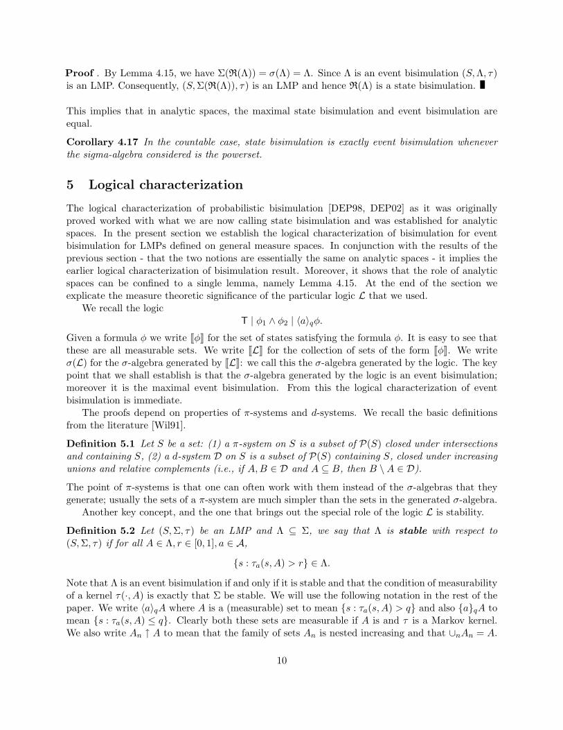
5 Logical characterization

The logical characterization of probabilistic bisimulation [DEP98, DEP02] as it was originallyproved worked with what we are now calling state bisimulation and was established for analyticspaces. In the present section we establish the logical characterization of bisimulation for eventbisimulation for LMPs defined on general measure spaces. In conjunction with the results of theprevious section - that the two notions are essentially the same on analytic spaces - it implies theearlier logical characterization of bisimulation result. Moreover, it shows that the role of analyticspaces can be confined to a single lemma, namely Lemma 4.15. At the end of the section weexplicate the measure theoretic significance of the particular logic L that we used.

We recall the logicT | φ1 ∧ φ2 | 〈a〉qφ.

Given a formula φ we write [[φ]] for the set of states satisfying the formula φ. It is easy to see thatthese are all measurable sets. We write [[L]] for the collection of sets of the form [[φ]]. We writeσ(L) for the σ-algebra generated by [[L]]: we call this the σ-algebra generated by the logic. The keypoint that we shall establish is that the σ-algebra generated by the logic is an event bisimulation;moreover it is the maximal event bisimulation. From this the logical characterization of eventbisimulation is immediate.

The proofs depend on properties of π-systems and d-systems. We recall the basic definitionsfrom the literature [Wil91].

Definition 5.1 Let S be a set: (1) a π-system on S is a subset of P(S) closed under intersectionsand containing S, (2) a d-system D on S is a subset of P(S) containing S, closed under increasingunions and relative complements (i.e., if A,B ∈ D and A ⊆ B, then B \A ∈ D).

The point of π-systems is that one can often work with them instead of the σ-algebras that theygenerate; usually the sets of a π-system are much simpler than the sets in the generated σ-algebra.

Another key concept, and the one that brings out the special role of the logic L is stability.

Definition 5.2 Let (S, Σ, τ) be an LMP and Λ ⊆ Σ, we say that Λ is stable with respect to(S, Σ, τ) if for all A ∈ Λ, r ∈ [0, 1], a ∈ A,

s : τa(s,A) > r ∈ Λ.

Note that Λ is an event bisimulation if and only if it is stable and that the condition of measurabilityof a kernel τ(·, A) is exactly that Σ be stable. We will use the following notation in the rest of thepaper. We write 〈a〉qA where A is a (measurable) set to mean s : τa(s,A) > q and also aqA tomean s : τa(s,A) ≤ q. Clearly both these sets are measurable if A is and τ is a Markov kernel.We also write An ↑ A to mean that the family of sets An is nested increasing and that ∪nAn = A.

10

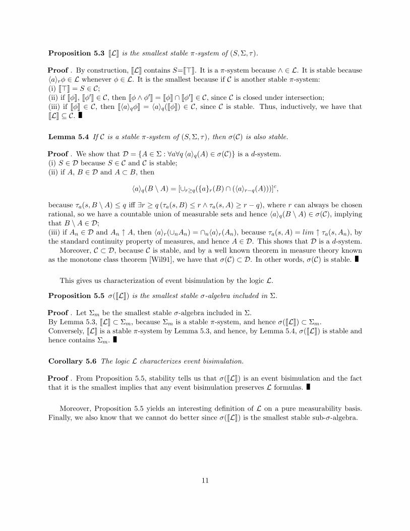
Proposition 5.3 [[L]] is the smallest stable π-system of (S, Σ, τ).

Proof . By construction, [[L]] contains S=[[>]]. It is a π-system because ∧ ∈ L. It is stable because〈a〉rφ ∈ L whenever φ ∈ L. It is the smallest because if C is another stable π-system:(i) [[>]] = S ∈ C;(ii) if [[φ]], [[φ′]] ∈ C, then [[φ ∧ φ′]] = [[φ]] ∩ [[φ′]] ∈ C, since C is closed under intersection;(iii) if [[φ]] ∈ C, then [[〈a〉qφ]] = 〈a〉q([[φ]]) ∈ C, since C is stable. Thus, inductively, we have that[[L]] ⊆ C.

Lemma 5.4 If C is a stable π-system of (S, Σ, τ), then σ(C) is also stable.

Proof . We show that D = A ∈ Σ : ∀a∀q 〈a〉q(A) ∈ σ(C) is a d-system.(i) S ∈ D because S ∈ C and C is stable;(ii) if A, B ∈ D and A ⊂ B, then

〈a〉q(B \A) = [∪r≥q(ar(B) ∩ (〈a〉r−q(A)))]c,

because τa(s,B \ A) ≤ q iff ∃r ≥ q (τa(s,B) ≤ r ∧ τa(s,A) ≥ r − q), where r can always be chosenrational, so we have a countable union of measurable sets and hence 〈a〉q(B \ A) ∈ σ(C), implyingthat B \A ∈ D;(iii) if An ∈ D and An ↑ A, then 〈a〉r(∪nAn) = ∩n〈a〉r(An), because τa(s,A) = lim ↑ τa(s,An), bythe standard continuity property of measures, and hence A ∈ D. This shows that D is a d-system.

Moreover, C ⊂ D, because C is stable, and by a well known theorem in measure theory knownas the monotone class theorem [Wil91], we have that σ(C) ⊂ D. In other words, σ(C) is stable.

This gives us characterization of event bisimulation by the logic L.

Proposition 5.5 σ([[L]]) is the smallest stable σ-algebra included in Σ.

Proof . Let Σm be the smallest stable σ-algebra included in Σ.By Lemma 5.3, [[L]] ⊂ Σm, because Σm is a stable π-system, and hence σ([[L]]) ⊂ Σm.Conversely, [[L]] is a stable π-system by Lemma 5.3, and hence, by Lemma 5.4, σ([[L]]) is stable andhence contains Σm.

Corollary 5.6 The logic L characterizes event bisimulation.

Proof . From Proposition 5.5, stability tells us that σ([[L]]) is an event bisimulation and the factthat it is the smallest implies that any event bisimulation preserves L formulas.

Moreover, Proposition 5.5 yields an interesting definition of L on a pure measurability basis.Finally, we also know that we cannot do better since σ([[L]]) is the smallest stable sub-σ-algebra.

11

U

γ

f

||xxxx

xxxx

xg

""EEEE

EEEE

E

X

α

ΠUΠf

||xxxxxxxxΠg

""EEEE

EEEE

Y

β

ΠX ΠY

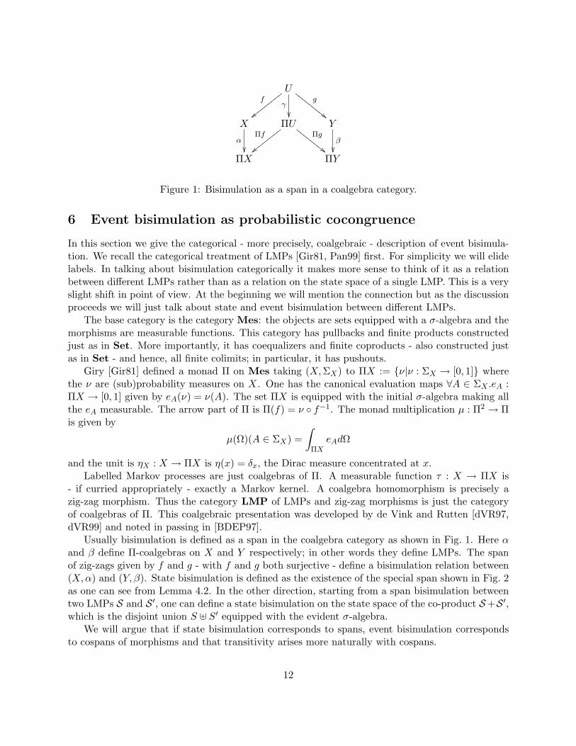
Figure 1: Bisimulation as a span in a coalgebra category.

6 Event bisimulation as probabilistic cocongruence

In this section we give the categorical - more precisely, coalgebraic - description of event bisimula-tion. We recall the categorical treatment of LMPs [Gir81, Pan99] first. For simplicity we will elidelabels. In talking about bisimulation categorically it makes more sense to think of it as a relationbetween different LMPs rather than as a relation on the state space of a single LMP. This is a veryslight shift in point of view. At the beginning we will mention the connection but as the discussionproceeds we will just talk about state and event bisimulation between different LMPs.

The base category is the category Mes: the objects are sets equipped with a σ-algebra and themorphisms are measurable functions. This category has pullbacks and finite products constructedjust as in Set. More importantly, it has coequalizers and finite coproducts - also constructed justas in Set - and hence, all finite colimits; in particular, it has pushouts.

Giry [Gir81] defined a monad Π on Mes taking (X, ΣX) to ΠX := ν|ν : ΣX → [0, 1] wherethe ν are (sub)probability measures on X. One has the canonical evaluation maps ∀A ∈ ΣX .eA :ΠX → [0, 1] given by eA(ν) = ν(A). The set ΠX is equipped with the initial σ-algebra making allthe eA measurable. The arrow part of Π is Π(f) = ν f−1. The monad multiplication µ : Π2 → Πis given by

µ(Ω)(A ∈ ΣX) =∫

ΠXeAdΩ

and the unit is ηX : X → ΠX is η(x) = δx, the Dirac measure concentrated at x.Labelled Markov processes are just coalgebras of Π. A measurable function τ : X → ΠX is

- if curried appropriately - exactly a Markov kernel. A coalgebra homomorphism is precisely azig-zag morphism. Thus the category LMP of LMPs and zig-zag morphisms is just the categoryof coalgebras of Π. This coalgebraic presentation was developed by de Vink and Rutten [dVR97,dVR99] and noted in passing in [BDEP97].

Usually bisimulation is defined as a span in the coalgebra category as shown in Fig. 1. Here αand β define Π-coalgebras on X and Y respectively; in other words they define LMPs. The spanof zig-zags given by f and g - with f and g both surjective - define a bisimulation relation between(X, α) and (Y, β). State bisimulation is defined as the existence of the special span shown in Fig. 2as one can see from Lemma 4.2. In the other direction, starting from a span bisimulation betweentwo LMPs S and S ′, one can define a state bisimulation on the state space of the co-product S+S ′,which is the disjoint union S ] S′ equipped with the evident σ-algebra.

We will argue that if state bisimulation corresponds to spans, event bisimulation correspondsto cospans of morphisms and that transitivity arises more naturally with cospans.

12

(S, Σ, τ)i

yyrrrrrrrrrri

''NNNNNNNNNNN

(S, Σ, τ) (S, Σ(R), τ)

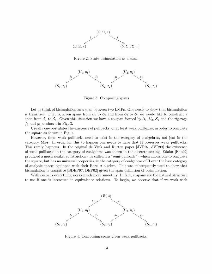
Figure 2: State bisimulation as a span.

(U1, η1)f1

yysssssssssf2

%%KKKKKKKKK(U2, η2)

g1

yysssssssssg2

%%KKKKKKKKK

(S1, τ1) (S2, τ2) (S3, τ3)

Figure 3: Composing spans

Let us think of bisimulation as a span between two LMPs. One needs to show that bisimulationis transitive. That is, given spans from S1 to S2 and from S2 to S3 we would like to construct aspan from S1 to S3. Given this situation we have a co-span formed by U1, U2, S2 and the zig-zagsf2 and g1 as shown in Fig. 3.

Usually one postulates the existence of pullbacks, or at least weak pullbacks, in order to completethe square as shown in Fig. 4.

However, these weak pullbacks need to exist in the category of coalgebras, not just in thecategory Mes. In order for this to happen one needs to have that Π preserves weak pullbacks.This rarely happens. In the original de Vink and Rutten paper [dVR97, dVR99] the existenceof weak pullbacks in the category of coalgebras was shown in the discrete setting. Edalat [Eda99]produced a much weaker construction - he called it a “semi-pullback” - which allows one to completethe square, but has no universal properties, in the category of coalgebras of Π over the base categoryof analytic spaces equipped with their Borel σ-algebra. This was subsequently used to show thatbisimulation is transitive [BDEP97, DEP02] given the span definition of bisimulation.

With cospans everything works much more smoothly. In fact, cospans are the natural structureto use if one is interested in equivalence relations. To begin, we observe that if we work with

(W,ρ)k1

yysssssssssk2

%%KKKKKKKKK

(U1, η1)f1

yysssssssssf2

%%KKKKKKKKK(U2, η2)

g1

yysssssssssg2

%%KKKKKKKKK

(S1, τ1) (S2, τ2) (S3, τ3)

Figure 4: Composing spans given weak pullbacks.

13

X

α

f

""FFFF

FFFF

F Y

β

g

||yyyy

yyyy

yh

""FFFF

FFFF

F Z

γ

k

||yyyy

yyyy

y

ΠX

""FFFFFFFF U

τ

ΠY

||yyyy

yyyy

""FFFF

FFFF

V

η

ΠZ

||yyyy

yyyy

ΠU ΠV

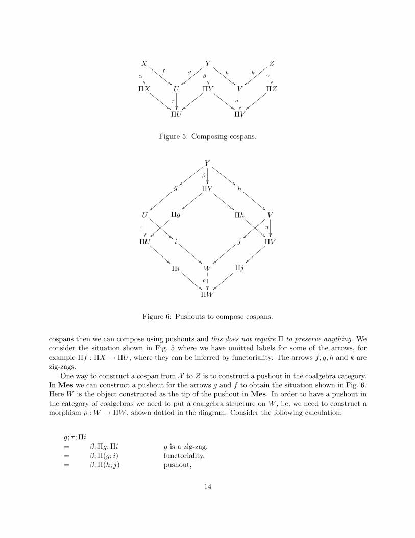
Figure 5: Composing cospans.

Y

||yyyy

yyyy

y

""FFFF

FFFF

F

β

g

zzzz

zzzz

z ΠY

||yyyy

yyyy

""EEEEEEEE h

""DDDD

DDDD

D

U

τ

!!CCCC

CCCC

C Πg

Πh

!!CCCCCCCC V

η

ΠU

!!CCCC

CCCC

i

""DDDDDDDDD j

||zzzz

zzzz

z ΠV

Πi

""EEEEEEEE W

ρ

Πj

||yyyy

yyyy

ΠW

Figure 6: Pushouts to compose cospans.

cospans then we can compose using pushouts and this does not require Π to preserve anything. Weconsider the situation shown in Fig. 5 where we have omitted labels for some of the arrows, forexample Πf : ΠX → ΠU , where they can be inferred by functoriality. The arrows f, g, h and k arezig-zags.

One way to construct a cospan from X to Z is to construct a pushout in the coalgebra category.In Mes we can construct a pushout for the arrows g and f to obtain the situation shown in Fig. 6.Here W is the object constructed as the tip of the pushout in Mes. In order to have a pushout inthe category of coalgebras we need to put a coalgebra structure on W , i.e. we need to construct amorphism ρ : W → ΠW , shown dotted in the diagram. Consider the following calculation:

g; τ ; Πi= β; Πg; Πi g is a zig-zag,= β; Π(g; i) functoriality,= β; Π(h; j) pushout,

14

= β; Πh; Πj functoriality,= h; η; Πj h is a zig-zag.

Thus, the outer square formed by Y, U, V and ΠW commutes and couniversality implies theexistence of the morphism ρ from W to ΠW . It is a routine calculation that this gives a pushout inthe category of coalgebras. This does not require any special properties of Π; it holds in the mostgeneral case, i.e. in Mes.

The categorical definitions can now be given.

Definition 6.1 An event bisimulation on S = (S, Σ, τ) is a surjection in the category of coal-gebras of Π to some T .

We have already noted that such arrows are zig-zags and that a zig-zag induces an event bisimulationon its source. For the case of an event bisimulation between two different LMPs we have.

Definition 6.2 An event bisimulation between S and S ′ is a cospan of surjections in the categoryof coalgebras to some object T .

This can be viewed as ordinary event bisimulation on S + S ′.Since cospans compose, it is clear that viewed as a relation between LMPs event bisimulation

(properly called probabilistic cocongruence) is an equivalence relation. We do not quite have acategory of LMPs with cospans as the morphisms since associativity only holds up to isomorphism:we have a bicategory. One can define a nice epi-mono factorization on the category Mes thatcarries over to the category of coalgebras.

7 Almost sure bisimulation

A major virtue of the categorical presentation of the previous section is that one can modify themonad to deal with other, closely related situations. One does not then have to develop the theoryagain from scratch; one can just use the abstract machinery with a slightly different instantiation.In this section we give an example of this.

In one of the early papers on LMPs [BDEP97] the question of negligible sets was raised. Considerthe LMPs U = ([0, 1],B, τ), where B are the Borel sets and τ(x,A) = λ(A) where λ is Lebesguemeasure; and U ′ with the same state space and σ-algebra but with Markov kernel given by τ ′(x,A) =τ(x,A) if x is irrational and τ ′(x,A) = 0 if x is rational. These two processes behave identically“almost always”: except for a set of measure zero they are bisimilar. If we were to observe thesesystems the probability that we would detect the difference is zero. We would like to formalize thisconcept by introducing a notion of almost sure bisimulation.

There is an obvious gap in the discussion of the last paragraph. According to what measureshould one say that the rationals have measure zero? One immediately thinks of Lebesgue measurein this example but what of other examples? Should the state space come equipped with additionalstructure - perhaps a measure - in order to define what the sets of measure zero are? We introducesuch additional structure, but one does not need to introduce a measure just to define the sets ofmeasure zero. Instead we introduce an axiomatically defined class of negligible sets. This can besmoothly incorporated into Giry’s monad and then one has the notion of almost sure bisimulation“almost free” with the discussion of the previous section.

15

We introduce a new category Mes′ refining the structure of Mes. The purpose of this refinementis to give a means of taking morphisms differing only on negligibly many points to be equal. Inorder to express this, one needs to add to each object a notion of negligible sets N and define:

f ∼ g := ∃N ∈ N : f 6= g ⊆ N (1)

We write A ⊆∈ N to mean, there is an N ∈ N such that A ⊆ N . For instance, f ∼ g can berewritten as f 6= g ⊆∈ N .

7.1 The category Mes′

An object is a triple (S, Σ,N ) where:

• (S, Σ) is an object in Mes,

• N ⊆ Σ is a distinguished set of measurable subsets of S.

An arrow (S, Σ,N )f−→ (T,Λ,M) is:

• is an arrow in Mes,

• such that in addition:

∀M ∈M∃N ∈ N : f−1(M) ⊆ N (2)

This additional condition is obviously stable by composition, so our data actually defines a cate-gory3.

The additional component in objects, N , is to be thought of intuitively as a set of negligiblesets, and will have some closure properties to be specified later on. One can think of the propertiesof Nν , the set of negligible sets defined by a measure ν:

Nν := A ∈ Σ | ν(A) = 0

where (S, Σ) is a measure space. However, for the present we assume nothing about N .Note that one does not demand the stronger condition that f−1(M) ∈ N ; it is enough for

f−1(M) to be included in a negligible set. One could write equivalently f−1(M) ⊆∈ N .This condition will result in a serious restriction on Mes arrows. For instance, random variables

with a finite number of values, say x1, . . . , xn, from (S, Σ,N ) to ([0, 1],B,N (λ)), where λ is theLebesgue measure, will all violate this condition unless for all i, X = xi ⊆∈ N . In particular, nodiscrete random variable from ([0, 1],B,N (λ)) to itself is in Mes′.

One now refines Giry’s monad to take into account the collection of negligible sets. First theobject part:one chooses the additional component N (Π(S, Σ,N )) to be generated (in the sense of the closureproperties to be defined later) by the following particular subsets of measures:

∀A ∈ N .NA := ν | ν(A) > 0. (3)3for N ′′ ∈ N ′′, (gf)−1(N ′′) = f−1(g−1(N ′′)) ⊆ f−1(N ′ ∈ N ′) ⊆ N ∈ N .

16

Since A ∈ N ⊆ Σ, NA ∈ σ(Π(S, Σ)) so our collections of negligible sets are adapted to the σ-algebrastructure. The intent of this definition is that we want to neglect the measures that ascribe nonzeroweight to the negligible sets. Note that if we chose to keep a measure in Mes′ defining negligiblesets, we would have to define such a measure here, without ever using its values on non-negligiblesets.

Second the arrow part:The definition of Π(f) remains the same, but one has to check that condition (2) is satisfied byΠ(f). Suppose then f : (S, Σ,N ) → (S′,Σ′,N ′) and let A be in N ′:

ν ∈ Π(f)−1(NA) ⇔ Π(f)(ν) ∈ NA

⇔ Π(f)(ν)(A) > 0⇔ ν(f−1(A)) > 0

so that Π(f)−1(NA) = ν | ν(f−1(A)) > 0. Now by (2), for some B ∈ N , f−1(A) ⊆ B, henceΠ(f)−1(NA) ⊆ NB, which is what we wanted to prove.

Verifying functoriality of Π is as before. We now have to lift the monad to the refined settingwith the negligible sets.

We need to prove that the natural transformations also are arrows in the new sense.

Lemma 7.1 For all A ∈ Σ:— (i) η−1(NA) = A;— (ii) µ−1(NA) = NNA

.

Proof . (i) a ∈ η−1(NA) ⇔ δa(A) > 0 ⇔ a ∈ A.(ii) P ∈ µ−1(NA) ⇔ µ(P )(A) > 0 ⇔

∫eAdP > 0 ⇔

∫1NA

dP > 0 since NA := eA > 0, thesupport of eA (trivial integration lemma). And the last statement says precisely P (NA) > 0, i.e.,P ∈ NNA

.

From this lemma one deduces readily that both η and µ satisfy (2).We now have constructed a refined version Π′ of Π. Naturality requirements and other condi-

tions are still valid, because they are commutative diagrams and these will continue to hold.The idea of the definition ofN (Π(S, Σ,N )) is that a set of measures is considered to be negligible

if all measures in it “see” a given negligible set. Why are we working with abstract negligibles,as opposed to those given by an actual measure? Well, one doesn’t know how to define such aprobability on Π(S, Σ). When is an N obtainable as an Nν for some ν is not so clear. In any case,such a ν would only intervene in the theory through sets of ν measure 0, so any two equivalent νwould define isomorphic objects.

One now defines the quotient category, Mes′ obtained by identifying arrows that disagree onlyon a negligible set. Objects are as in Mes′; arrows are ∼ equivalence classes.

Lemma 7.2 The equivalence ∼ defined in (1) is stable by composition.

Proof . g ∼ h ⇒ gf ∼ hf : one has g 6= h ⊆ N ′ for some N ′ ∈ N ′, so:

gf 6= hf = f−1(g 6= h) ⊆ f−1(N ′)

17

and for some N ∈ N , f−1(N ′) ⊆ N ∈ N , because f satisfies condition (2).g ∼ h ⇒ fg ∼ fh: again one has g 6= h ⊆ N ′ for some N ′ ∈ N ′, so:

fg 6= fh ⊆ g 6= h ⊆ N ′ ∈ N ′.

Lemma 7.3 (Π respects ∼) Let f , g be arrows from S = (S, Σ,N ) to T = (T,Λ,M), then:f ∼ g ⇒ Π(f) ∼ Π(g).

Proof . Let f , g be as above, ν be in Π(S). By definition of ∼, there exists an N ∈ N (S), suchthat f 6= g ⊆ N . Then one has:

Π(f)(ν) 6= Π(g)(ν) ⇔ ∃B ∈ Λ : ν(f−1(B)) 6= ν(g−1(B))⇒ ∃B ∈ Λ : ν(f−1(B)4 g−1(B)) > 0⇒ ν(N) > 0⇔ ν ∈ eN > 0 ∈ N (Π(S))

Second step: obvious. 4

Third step: f−1(B)4 g−1(B) ⊆ f 6= g ⊆ N .So Π(f) 6= Π(g) ⊆∈ N (Π(S)), or, in other words, Π(f) ∼ Π(g).

As an illustration, we may compute what it means for a kernel k : (S, Σ,N ) → Π(S, Σ,N ) tobe a morphism in Mes′. It has to satisfy two conditions:

1. usual stability wrt measurables: Σ stable (this is the usual measurability condition);

2. stability wrt negligibles: N (sub-) stable under a0.

Proof . Only the second part needs a proof. By definition τ has to satisfy the condition that forall A ∈ N , τ(·, A)−1(NA) ⊆∈ N , which means s | τ(s,A) > 0 = a0(A) ⊆∈ N .

When negligibles are given via some measure ν defined on (S, Σ), that is to say N = Nν , then thecondition amounts to

ν(A) = 0 ⇒ ν(a0(A)) = 0,

which says that “negligiby many points may jump to a negligible set”.

Lemma 7.4 (domination) Suppose τ is a kernel, and ν dominates τ in the sense that for all s,τ(s, ·) ν, then Nν is stable under τ , that is to say:

∀B ∈ Nν : a0(B) ∈ Nν .

Proof . If ν(B) = 0, then for all s, τ(s,B) = 0, so that a0(B) = ∅ ∈ Nν .

The second condition of “stability with respect to negligibles” is seen to be a weaker form of“domination”.

4By additivity, ν(A ∪ B) = ν(A4B) + ν(A ∩ B), so ν(A4B) = 0 implies ν(A ∪ B) = ν(A ∩ B), which impliesν(A) = ν(B) by sandwiching.

18

7.2 Abstract Completion

In measure theory there is a standard notion of completion of a σ-algebra with respect to a measure.The point is that many σ-algebras contain non measurable subsets of sets of measure zero. Thisis very annoying; one would like to say that a subset of a negligible set is also negligible, but onecannot, in general, for silly reasons. The standard example is the Borel algebra and the Lebesguemeasure. There are subsets of sets of Lebesgue measure zero that are not Borel measurable. Thecompletion process adds in all these sets and yields a bigger σ-algebra5. We can describe thiscompletion process in terms of our abstract notion of negligible set: it is here that we need toimpose some axioms on N .

Definition 7.5 (σ-ideal) A σ-ideal N on S is a set of subsets of S which is 1) downward closed(i.e., N ↓= N ), and 2) closed under countable unions.

Definition 7.6 (abstract completion) Given a measurable space (S, Σ), and a σ-ideal N , onedefines the completion of Σ by N :

ΣN := K | ∃A,B ∈ Σ : A ⊆ K ⊆ B &B \A ∈ N

Lemma 7.7 ΣN is a σ-algebra that contains Σ, and (Σ ∩ N ) ↓. Let ν be a subprobability definedon (S, Σ), if ν(N ) = 0, ν has a unique extension to ΣN .

Proof . Σ ⊆ ΣN : any A ∈ Σ verifies A ⊆ A ⊆ A and A \A = ∅ ∈ N , since N is downward closed.(Σ∩N ) ↓⊆ ΣN : any N ∈ (Σ∩N ) ↓verifies ∅ ⊆ N ⊆ N ′ for some N ′ ∈ Σ∩N , and N ′\∅ = N ′ ∈ N .ΣN closed under complements: suppose A ⊆ K ⊆ B, with A,B ∈ Σ and B \ A ∈ N , thenB ⊆ K ⊆ A, and A \ B = B \A ∈ N .ΣN closed under countable unions: suppose Ai ⊆ Ki ⊆ Bi, with Ai, Bi ∈ Σ and Bi \Ai ∈ N , then∪IAi ⊆ ∪IKi ⊆ ∪IBi, and

∪IBi \ ∪IAi ⊆ ∪I(Bi \Ai) ∈ N

The rhs is in N because N is closed under countable unions, and therefore the left hand side alsois in N , since N is downward closed6 .

This completion can also be done when N is not downward closed, by asking that B \ A ⊆∈ N .Then ΣN ↓= ΣN , so that the downward closure is happening during the completion.

8 Conclusions

The main point of this paper is to argue that one should work with probabilistic cocongruencerather than with probabilistic bisimulation. The theory works smoothly for LMPs on generalmeasure spaces: one need not work with analytic spaces. The proof of the logical characterizationof cocongruence is much simpler and more general than the proof of the logical characterization of

5Actually “completion” is a terrible word; there is no reasonable sense in which the resulting σ-algebra is completeexcept that the completion process when applied again adds nothing new.

6The two hand sides are not equal in general: Bi = S, then the lhs is B \ ∪IAi = ∩IAi and the rhs is ∪IAi; e.g. ,I = 0, 1, B0 = B1 = a, b, A0 = a, A1 = b, lhs is ∅, while rhs is a, b.

19

bisimulation. One only needs to invoke the theory of analytic spaces to show that cocongruenceand bisimulation coincide: which they indeed do on analytic spaces.

Indeed, it seems to us that bisimulation defined categorically is a historical anomaly. In thediscrete case bisimulation and cocongruence coincide and one can argue that it makes no difference.However transition systems are coalgebras and cospans should fit the theory better than spans; asindeed is our experience in the probabilistic case. It would be interesting to reformulate the generaltheory in terms of cocongruences.

In the case of probabilistic systems it has been argued that one should use metrics ratherthan equivalence relations [DGJP99, DGJP04]. In the present context a pressing problem is tounderstand the metric analogue of the theory of probabilistic cocongruence.

Acknowledgements

We have benefitted from discussions with Samson Abramsky, Martin Escardo, Gordon Plotkinand each other. Vincent Danos enjoyed the company of Elham Kashefi during the course of thisresearch. Prakash Panangaden acknowledges the crucial role played by bad weather during hisholidays which allowed him to complete this paper. We all like to thank each other for being sucha fun bunch.

References

[BDEP97] R. Blute, J. Desharnais, A. Edalat, and P. Panangaden. Bisimulation for labelled Markovprocesses. In Proceedings of the Twelfth IEEE Symposium On Logic In Computer Sci-ence, Warsaw, Poland., 1997.

[DD03] Vincent Danos and Josee Desharnais. Labeled Markov Processes: Stronger and fasterapproximations. In Proceedings of the 18th Symposium on Logic in Computer Science,Ottawa, 2003. IEEE.

[DEP98] J. Desharnais, A. Edalat, and P. Panangaden. A logical characterization of bisimulationfor labelled Markov processes. In proceedings of the 13th IEEE Symposium On Logic InComputer Science, Indianapolis, pages 478–489. IEEE Press, June 1998.

[DEP02] J. Desharnais, A. Edalat, and P. Panangaden. Bisimulation for labeled Markov pro-cesses. Information and Computation, 179(2):163–193, Dec 2002.

[DGJP99] J. Desharnais, V. Gupta, R. Jagadeesan, and P. Panangaden. Metrics for labeled Markovsystems. In Proceedings of CONCUR99, Lecture Notes in Computer Science. Springer-Verlag, 1999.

[DGJP00] J. Desharnais, V. Gupta, R. Jagadeesan, and P. Panangaden. Approximation of labeledMarkov processes. In Proceedings of the Fifteenth Annual IEEE Symposium On LogicIn Computer Science, pages 95–106. IEEE Computer Society Press, June 2000.

[DGJP02] J. Desharnais, V. Gupta, R. Jagadeesan, and P. Panangaden. The metric analogueof weak bisimulation for labelled Markov processes. In Proceedings of the SeventeenthAnnual IEEE Symposium On Logic In Computer Science, pages 413–422, July 2002.

20

[DGJP03] J. Desharnais, V. Gupta, R. Jagadeesan, and P. Panangaden. Approximating labeledMarkov processes. Information and Computation, 184(1):160–200, July 2003.

[DGJP04] Josee Desharnais, Vineet Gupta, Radhakrishnan Jagadeesan, and Prakash Panangaden.A metric for labelled Markov processes. Theoretical Computer Science, 318(3):323–354,June 2004.

[Dob03] E.-E. Doberkat. Semi-pullbacks and bisimulations in categories of stochastic relations. InJ. C. M. Baeten, J. K. Lenstra, J. Parrow, and G. J. Woeinger, editors, Proceedings of the27th International Colloquium On Automata Languages And Programming, ICALP’03,number 2719 in Lecture Notes In Computer Science, pages 996–1007. Springer-Verlag,July 2003.

[DP01] J. Desharnais and P. Panangaden. Continuous stochastic logic charac-terizes bisimulation for continuous-time Markov processes. Available fromhttp://rl.cs.mcgill.ca/~prakash/pubs.html, 2001.

[dVR97] E. de Vink and J. J. M. M. Rutten. Bisimulation for probabilistic transition systems: Acoalgebraic approach. In Proceedings of the 24th International Colloquium On AutomataLanguages And Programming, 1997.

[dVR99] E. de Vink and J. J. M. M. Rutten. Bisimulation for probabilistic transition systems:A coalgebraic approach. Theoretical Computer Science, 221(1/2):271–293, June 1999.

[Eda99] Abbas Edalat. Semi-pullbacks and bisimulation in categories of Markov processes. Math-ematical Structures in Computer Science, 9(5):523–543, 1999.

[Gir81] M. Giry. A categorical approach to probability theory. In B. Banaschewski, editor, Cate-gorical Aspects of Topology and Analysis, number 915 in Lecture Notes In Mathematics,pages 68–85. Springer-Verlag, 1981.

[KS60] J. G. Kemeny and J. L. Snell. Finite Markov Chains. Van Nostrand, 1960.

[LS91] K. G. Larsen and A. Skou. Bisimulation through probablistic testing. Information andComputation, 94:1–28, 1991.

[Pan99] Prakash Panangaden. The category of markov processes. ENTCS, 22:17 pages, 1999.http://www.elsevier.nl/locate/entcs/volume22.html.

[Put94] Martin L. Puterman. Markov Decision Processes: Discrete Stochastic Dynamic Pro-gramming. Wiley, 1994.

[vBW01a] Franck van Breugel and James Worrell. An algorithm for quantitative verification ofprobabilistic systems. In K. G. Larsen and M. Nielsen, editors, Proceedings of theTwelfth International Conference on Concurrency Theory - CONCUR’01, number 2154in Lecture Notes In Computer Science, pages 336–350. Springer-Verlag, 2001.

[vBW01b] Franck van Breugel and James Worrell. Towards quantitative verification of probabilisticsystems. In Proceedings of the Twenty-eighth International Colloquium on Automata,Languages and Programming. Springer-Verlag, July 2001.

21

[Wil91] David Williams. Probability with Martingales. CUP, Cambridge, 1991.

22

Bisimulation and cocongruence for probabilistic systems

Documents

Transcript of Bisimulation and cocongruence for probabilistic systems