BioOne sees sustainable scholarly publishing as an inherently collaborative enterprise connecting authors, nonprofit publishers, academic institutions,research libraries, and research funders in the common goal of maximizing access to critical research.

Carbon Stocks and Sequestration Rates in Oak-Hickory Forests of Ohio, USAAuthor(s): Tao Yuhua and Roger A. WilliamsSource: Journal of Resources and Ecology, 4(2):115-124. 2013.Published By: Institute of Geographic Sciences and Natural Resources Research, Chinese Academy ofSciencesDOI: http://dx.doi.org/10.5814/j.issn.1674-764x.2013.02.003URL: http://www.bioone.org/doi/full/10.5814/j.issn.1674-764x.2013.02.003

BioOne (www.bioone.org) is a nonprofit, online aggregation of core research in the biological, ecological,and environmental sciences. BioOne provides a sustainable online platform for over 170 journals and bookspublished by nonprofit societies, associations, museums, institutions, and presses.

Your use of this PDF, the BioOne Web site, and all posted and associated content indicates your acceptance ofBioOne’s Terms of Use, available at www.bioone.org/page/terms_of_use.

Usage of BioOne content is strictly limited to personal, educational, and non-commercial use. Commercialinquiries or rights and permissions requests should be directed to the individual publisher as copyright holder.

J. Resour. Ecol. 2013 4 (2) 115-124 DOI:10.5814/j.issn.1674-764x.2013.02.003www.jorae.cn

June, 2013 Journal of Resources and Ecology Vol.4 No.2

Received: 2013-02-27 Accepted: 2013-05-10Foundation: McIntire-Stennis Funds allocated through the McIntire-Stennis Forestry Research Act, USA (OHO00037-MS).The first author: TAO Yuhua. Email: arlenetao12@yahoo.com.cn. * Corresponding author: Roger A. WILLIAMS. Email: williams.1577@osu.edu.

1 IntroductionConcerns regarding climate change and its predicted impacts have created a closer look at forests in regards to forest carbon (C) and the creation of C sinks. Forest ecosystems are a major part of the global C cycle as they are large contributors to the terrestrial C sink by removing approximately 30% of all CO2 emissions from fossil fuel burning and deforestation (Canadell and Raupach 2008) and provide storage of 1240 Pg of C globally in vegetation and soil (Dixon et al. 1994). Forest systems and the forest products they produce create a significant C sink in the United States, equaling as much as 10% of the total US greenhouse gas (GHG) emissions (Birdsey et al. 2006). Because of the relatively large contribution of forests to the global C cycle, they have become recognized for their potential to mitigate CO2 emissions (Brown 2001; Jandl et al. 2007).

For purposes of managing forest for climate change mitigation and development of national C budgets, it is essential to quantify and understand forest C stocks and fluxes. One approach of estimating C stocks and fluxes

include using relationships between variables collected in statistically-based inventories and C stocks, supplemented with models to estimate C pools that are not sampled (Woodbury et al. 2007). In the U.S., data collected by the U.S. Department of Agriculture Forest Service (USDA FS) Forest Inventory and Analysis (FIA) program has served as a foundation for C data for much research (Birdsey 1992; Birdsey and Heath 1995; Hoover et al. 2000; Martin et al. 2001; Goodale et al. 2002; Ney et al. 2002; Woodbury et al. 2006).

C stocks in forests are always changing with succession and forest development (Cropper and Ewel 1984; Turner et al. 1995). Forest growth rates, both long-term and annual, will affect the sequestration rates of C and how this C is stored (Barford et al. 2001). The sequestration of C can theoretically be maximized by maintain the forest ecosystem at its maximum net ecosystem productivity (Fahey et al. 2010). Understanding the sequestration rates of C and how it is accumulated in forest ecosystems is important to the management of C in forests and for climate change mitigation purposes. The attributes of forests that will affect C sequestration and storage – both above- and belowground

Carbon Stocks and Sequestration Rates in Oak-hickory Forests of Ohio, USA

TAO Yuhua1,2 and Roger A. WILLIAMS1*

1 School of Environment and Natural Resources, The Ohio State University, 210 Kottman Hall, 2021 Coffey Road, Columbus, OH 43210, USA;2 Guangxi Eco-Engineering Vocational and Technical College, Liuzhou 545004, China

Abstract:

Key words:

Journal of Resources and Ecology Vol.4 No.2, 2013116

– include forest age, forest density, site quality, and species composition (Barford et al. 2001; Jandl et al. 2006; Schulp et al. 2008).

In order to manage C at the stand level it therefore becomes vital to know how the particular forests are sequestering and storing C. In this paper we present C sequestration models for oak-hickory forests by forest strata that depict the sequestration rate and storage of C. We hope the results of this study will be useful to the management for C in oak-hickory forests.

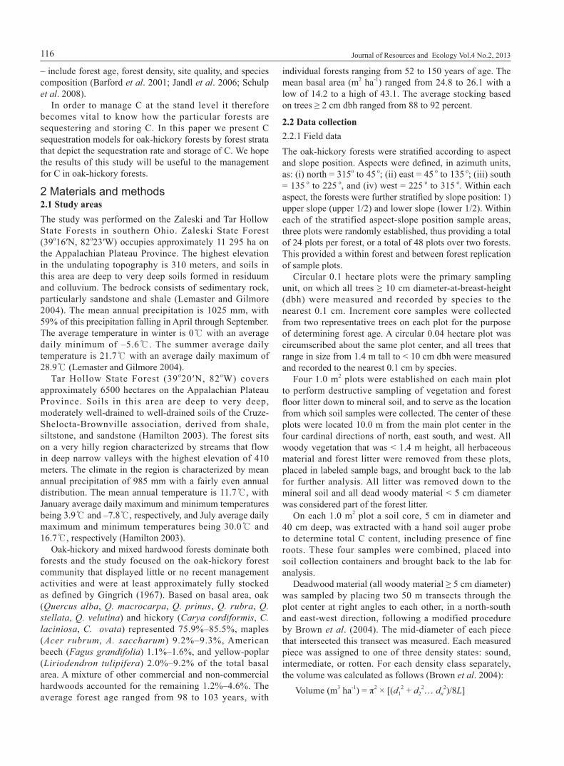
2 Materials and methods2.1 Study areasThe study was performed on the Zaleski and Tar Hollow State Forests in southern Ohio. Zaleski State Forest (39o16′N, 82o23′W) occupies approximately 11 295 ha on the Appalachian Plateau Province. The highest elevation in the undulating topography is 310 meters, and soils in this area are deep to very deep soils formed in residuum and colluvium. The bedrock consists of sedimentary rock, particularly sandstone and shale (Lemaster and Gilmore 2004). The mean annual precipitation is 1025 mm, with 59% of this precipitation falling in April through September. The average temperature in winter is 0 with an average daily minimum of –5.6 . The summer average daily temperature is 21.7 with an average daily maximum of 28.9 (Lemaster and Gilmore 2004).

Tar Hollow State Forest (39o20 ′N, 82oW) covers approximately 6500 hectares on the Appalachian Plateau Province. Soils in this area are deep to very deep, moderately well-drained to well-drained soils of the Cruze-Shelocta-Brownville association, derived from shale, siltstone, and sandstone (Hamilton 2003). The forest sits on a very hilly region characterized by streams that flow in deep narrow valleys with the highest elevation of 410 meters. The climate in the region is characterized by mean annual precipitation of 985 mm with a fairly even annual distribution. The mean annual temperature is 11.7 , with January average daily maximum and minimum temperatures being 3.9 and –7.8 , respectively, and July average daily maximum and minimum temperatures being 30.0 and 16.7 , respectively (Hamilton 2003).

Oak-hickory and mixed hardwood forests dominate both forests and the study focused on the oak-hickory forest community that displayed little or no recent management activities and were at least approximately fully stocked as defined by Gingrich (1967). Based on basal area, oak (Quercus alba, Q. macrocarpa, Q. prinus, Q. rubra, Q. stellata, Q. velutina) and hickory (Carya cordiformis, C. laciniosa, C. ovata) represented 75.9%–85.5%, maples (Acer rubrum, A. saccharum) 9.2%–9.3%, American beech (Fagus grandifolia) 1.1%–1.6%, and yellow-poplar (Liriodendron tulipifera) 2.0%–9.2% of the total basal area. A mixture of other commercial and non-commercial hardwoods accounted for the remaining 1.2%–4.6%. The average forest age ranged from 98 to 103 years, with

individual forests ranging from 52 to 150 years of age. The mean basal area (m2 ha-1) ranged from 24.8 to 26.1 with a low of 14.2 to a high of 43.1. The average stocking based on trees ≥ 2 cm dbh ranged from 88 to 92 percent.

2.2 Data collection2.2.1 Field dataThe oak-hickory forests were stratified according to aspect and slope position. Aspects were defined, in azimuth units, as: (i) north = 315o to 45 o; (ii) east = 45 o to 135 o; (iii) south = 135 o to 225 o, and (iv) west = 225 o to 315 o. Within each aspect, the forests were further stratified by slope position: 1) upper slope (upper 1/2) and lower slope (lower 1/2). Within each of the stratified aspect-slope position sample areas, three plots were randomly established, thus providing a total of 24 plots per forest, or a total of 48 plots over two forests. This provided a within forest and between forest replication of sample plots.

Circular 0.1 hectare plots were the primary sampling unit, on which all trees ≥ 10 cm diameter-at-breast-height (dbh) were measured and recorded by species to the nearest 0.1 cm. Increment core samples were collected from two representative trees on each plot for the purpose of determining forest age. A circular 0.04 hectare plot was circumscribed about the same plot center, and all trees that range in size from 1.4 m tall to < 10 cm dbh were measured and recorded to the nearest 0.1 cm by species.

Four 1.0 m2 plots were established on each main plot to perform destructive sampling of vegetation and forest floor litter down to mineral soil, and to serve as the location from which soil samples were collected. The center of these plots were located 10.0 m from the main plot center in the four cardinal directions of north, east south, and west. All woody vegetation that was < 1.4 m height, all herbaceous material and forest litter were removed from these plots, placed in labeled sample bags, and brought back to the lab for further analysis. All litter was removed down to the mineral soil and all dead woody material < 5 cm diameter was considered part of the forest litter.

On each 1.0 m2 plot a soil core, 5 cm in diameter and 40 cm deep, was extracted with a hand soil auger probe to determine total C content, including presence of fine roots. These four samples were combined, placed into soil collection containers and brought back to the lab for analysis.

Deadwood material (all woody material ≥ 5 cm diameter) was sampled by placing two 50 m transects through the plot center at right angles to each other, in a north-south and east-west direction, following a modified procedure by Brown et al. (2004). The mid-diameter of each piece that intersected this transect was measured. Each measured piece was assigned to one of three density states: sound, intermediate, or rotten. For each density class separately, the volume was calculated as follows (Brown et al. 2004):

Volume (m3 ha-1) = π2 × [(d12 + d2

2… dn2)/8L]

TAO Yuhua, et al.: Carbon Stocks and Sequestration Rates in Oak-hickory Forests of Ohio, USA 117

where d1, d2 etc = diameters of intersecting pieces of dead wood and L = combined length of the two transects. Representative dead wood samples of the three density classes, representing the range of species present, were collected for density (dry weight per green volume) determination.

The aboveground biomass of trees > 1.4 m height was estimated using the equation from Jenkins et al. (2003) for hard maple/oak/hickory/beech forests. This equation uses only measured dbh as the independent variable. The belowground biomass (primarily roots) was estimated using the model for temperate forests by Cairns et al. (1997) that estimates the belowground biomass based on knowledge of aboveground biomass.

2.2.2 Lab analysis and carbon determinations

Vegetation and forest litter grab samples collected from the 1.0 m2 sample plots were dried in ovens at 60 for three days or until constant weight to determine the moisture content of the original plot samples for ovendry weight estimations. A 5.0 g sample was randomly selected from the ovendried vegetation and litter samples for the purpose of C content determination. These samples were ground in a Wiley mill to pass a 2 mm sieve, and processed in an Elementar Americas, Inc., Vario Max Carbon Nitrogen Combustion Analyzer, with a procedure described in the international standard publication ISO10694 (ISO 10694, 1995) to determine the percent C by weight in each sample.

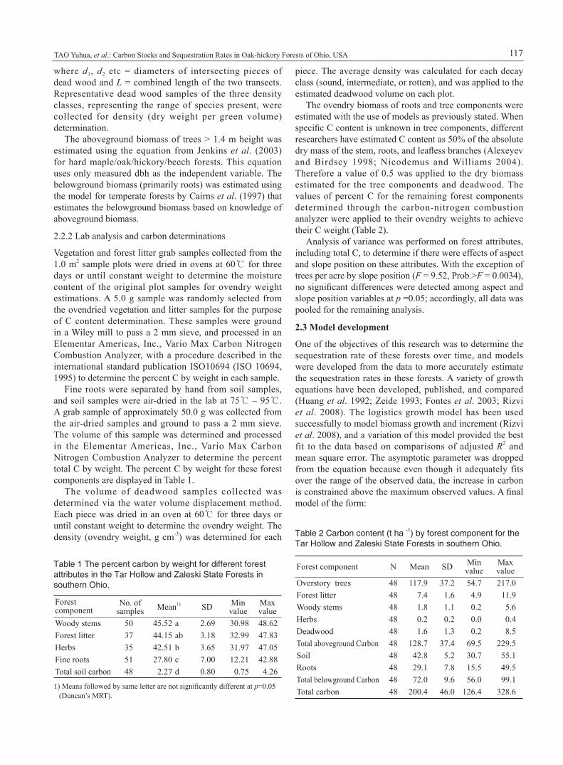
Fine roots were separated by hand from soil samples, and soil samples were air-dried in the lab at 75 – 95 . A grab sample of approximately 50.0 g was collected from the air-dried samples and ground to pass a 2 mm sieve. The volume of this sample was determined and processed in the Elementar Americas, Inc., Vario Max Carbon Nitrogen Combustion Analyzer to determine the percent total C by weight. The percent C by weight for these forest components are displayed in Table 1.

The volume of deadwood samples collected was determined via the water volume displacement method. Each piece was dried in an oven at 60 for three days or until constant weight to determine the ovendry weight. The density (ovendry weight, g cm-3) was determined for each

piece. The average density was calculated for each decay class (sound, intermediate, or rotten), and was applied to the estimated deadwood volume on each plot.

The ovendry biomass of roots and tree components were estimated with the use of models as previously stated. When specific C content is unknown in tree components, different researchers have estimated C content as 50% of the absolute dry mass of the stem, roots, and leafless branches (Alexeyev and Birdsey 1998; Nicodemus and Williams 2004). Therefore a value of 0.5 was applied to the dry biomass estimated for the tree components and deadwood. The values of percent C for the remaining forest components determined through the carbon-nitrogen combustion analyzer were applied to their ovendry weights to achieve their C weight (Table 2).

Analysis of variance was performed on forest attributes, including total C, to determine if there were effects of aspect and slope position on these attributes. With the exception of trees per acre by slope position (F = 9.52, Prob.>F = 0.0034), no significant differences were detected among aspect and slope position variables at p =0.05; accordingly, all data was pooled for the remaining analysis.

2.3 Model development

One of the objectives of this research was to determine the sequestration rate of these forests over time, and models were developed from the data to more accurately estimate the sequestration rates in these forests. A variety of growth equations have been developed, published, and compared (Huang et al. 1992; Zeide 1993; Fontes et al. 2003; Rizvi et al. 2008). The logistics growth model has been used successfully to model biomass growth and increment (Rizvi et al. 2008), and a variation of this model provided the best fit to the data based on comparisons of adjusted R2 and mean square error. The asymptotic parameter was dropped from the equation because even though it adequately fits over the range of the observed data, the increase in carbon is constrained above the maximum observed values. A final model of the form:

Table 2 Carbon content (t ha -1) by forest component for the Tar Hollow and Zaleski State Forests in southern Ohio.

Forest component N Mean SD Minvalue

Maxvalue

Overstory trees 48 117.9 37.2 54.7 217.0 Forest litter 48 7.4 1.6 4.9 11.9 Woody stems 48 1.8 1.1 0.2 5.6 Herbs 48 0.2 0.2 0.0 0.4 Deadwood 48 1.6 1.3 0.2 8.5 Total aboveground Carbon 48 128.7 37.4 69.5 229.5 Soil 48 42.8 5.2 30.7 55.1 Roots 48 29.1 7.8 15.5 49.5 Total belowground Carbon 48 72.0 9.6 56.0 99.1 Total carbon 48 200.4 46.0 126.4 328.6

1) Means followed by same letter are not significantly different at p=0.05 (Duncan’s MRT).

Table 1 The percent carbon by weight for different forest attributes in the Tar Hollow and Zaleski State Forests in southern Ohio.

Forest component

No. ofsamples Mean1) SD Min

valueMaxvalue

Woody stems 50 45.52 a 2.69 30.98 48.62 Forest litter 37 44.15 ab 3.18 32.99 47.83 Herbs 35 42.51 b 3.65 31.97 47.05 Fine roots 51 27.80 c 7.00 12.21 42.88 Total soil carbon 48 2.27 d 0.80 0.75 4.26

Journal of Resources and Ecology Vol.4 No.2, 2013118

Y = e (b1− b2A−1) (1)where Y = carbon (t ha -1), A = age of the forest, and b1 and b2 coefficients to be estimated, was developed to depict the total carbon accumulation within the forest. The first derivative of this model:

Yr = (eb1−b2A−1)(b2A-2) (2)

where Yr = carbon (t ha -1 y -1), would provide the rate of C sequestration in these forests. The model coefficients were estimated using the Non-Linear Procedure, Gauss-Newton method in SAS software, version 9.2 (SAS Institute Inc. 2008).

3 Results All models needed 10 iterations or less to determine the coefficient estimates and the convergence criterion was achieved on all models using the relative offset convergence measure of Bates and Watts to determine convergence. The model coefficients and statistics are displayed in Table 3, and the models (model 1) for aboveground C, belowground

C, aboveground C of merchantable trees, and total C are plotted in Fig. 1. The aboveground C includes forest litter, herbs, and woody stems in the understory. The belowground C includes the total soil C and roots. The merchantable tree C includes the aboveground portion of all trees > 10 cm dbh.

The total belowground C shows a shallow increase in carbon over time compared to other forest strata due to the fact that soil C remains relatively constant, with the majority of the increase attributed to the increase in root system mass (Fig. 1). The majority of the increase in total forest carbon comes from the aboveground portion of these ecosystems as the result of increase in tree size. This is what we would expect since the aboveground portion of the total forest carbon pool is typically the most rapidly changing component as a result of changes in the live biomass (Fahey et al. 2010). For example, within the range of our data, the aboveground C represented 58.5% of the total C within the system at age 50 years to 67.7% of the total C by age 150 years. The predicted carbon yields by forest strata as determined from our models are displayed in Table 4.

The total soil organic carbon (SOC) accounted for 21% of the total C on average within our study, ranging from 14%–33% on individual plots. The mean SOC stock was 42.8 t ha -1 with a range of 30.7–55.1 t ha -1. This is less than what has been reported for SOC in temperate forests

Table 4 The predicted carbon yield (t ha-1) by forest strata for oak-hickory forests in southern Ohio.

1) Includes only the aboveground portion.

Forest age (y)

Carbon (t ha-1)Total Above-

groundBelow-ground

Merchantable trees1)

50 150.0 87.7 63.3 75.2 55 159.7 95.3 65.0 82.8 60 168.3 102.1 66.5 89.7 65 176.0 108.3 67.8 96.0 70 182.8 113.8 69.0 101.8 75 188.9 118.9 70.0 107.0 80 194.5 123.5 70.8 111.9 85 199.5 127.7 71.6 116.3 90 204.1 131.6 72.3 120.4 95 208.2 135.2 73.0 124.2

100 212.1 138.5 73.5 127.7 105 215.6 141.5 74.1 130.9 110 218.9 144.4 74.5 134.0 115 221.9 147.0 75.0 136.8 120 224.7 149.4 75.4 139.4 125 227.3 151.7 75.8 141.9 130 229.7 153.9 76.1 144.3 135 232.0 155.9 76.4 146.4 140 234.2 157.8 76.8 148.5 145 236.2 159.6 77.0 150.5 150 238.1 161.3 77.3 152.3

Fig. 1 Display of models depicting the sequestering of carbon in the total forest, the aboveground portion of the forest, the belowground portion, and the aboveground portion of the merchantable trees in oak-hickory forests of southern Ohio.

60 70 8050 90 100Forest age (y)

Car

bon

(t ha

-1)

0

50

100

200

150

110 120 130 140 150

Total carbon

250

Belowground carbonMerchantable tree carbonAboveground carbon

1) Model: C = e(b1− b2A−1) , where C = carbon (t ha-1), and A = forest age (years).

Table 3 Coefficients and statistics of models1) predicting the rate of carbon storage (t ha-1) for the total forest, the aboveground portion, the belowground portion, and the aboveground portion of merchantable trees (> 11.5 cm dbh) of oak-hickory forests in southern Ohio.

CarbonCoefficients

R2 RMSE F-value Pr.>F

b1 b2

Total 5.704 34.662 0.962 42.67 486.52 <0.0001Aboveground 5.388 45.709 0.942 34.33 317.96 <0.0001Belowground 4.448 14.985 0.985 9.33 1246.51 <0.0001Merchantable tree 5.379 52.896 0.935 33.63 280.61 <0.0001

TAO Yuhua, et al.: Carbon Stocks and Sequestration Rates in Oak-hickory Forests of Ohio, USA 119

in the US, which has ranged anywhere from 48%–56% of the total forest C stock (Turner et al. 1995; Prentice 2001; Woodbury et al. 2006). Oak forests tend to regenerate and establish on sites where long-term soil moisture levels are limited (Hodges and Gardiner 1993; Iverson and Prasad 2003; Williams and Heiligmann 2003) and therefore tend to be concentrated in relatively dry landscape positions. Lal (2005) reports that soils with less moisture typically contain lower SOC, which includes sites located on southerly aspects and coarser soils. While half of the plots occurred on southerly aspects, the majority occurred on the coarse-textured soils that were well drained. The average slope measured on all plots was 35% and ranged from 16%–60%.

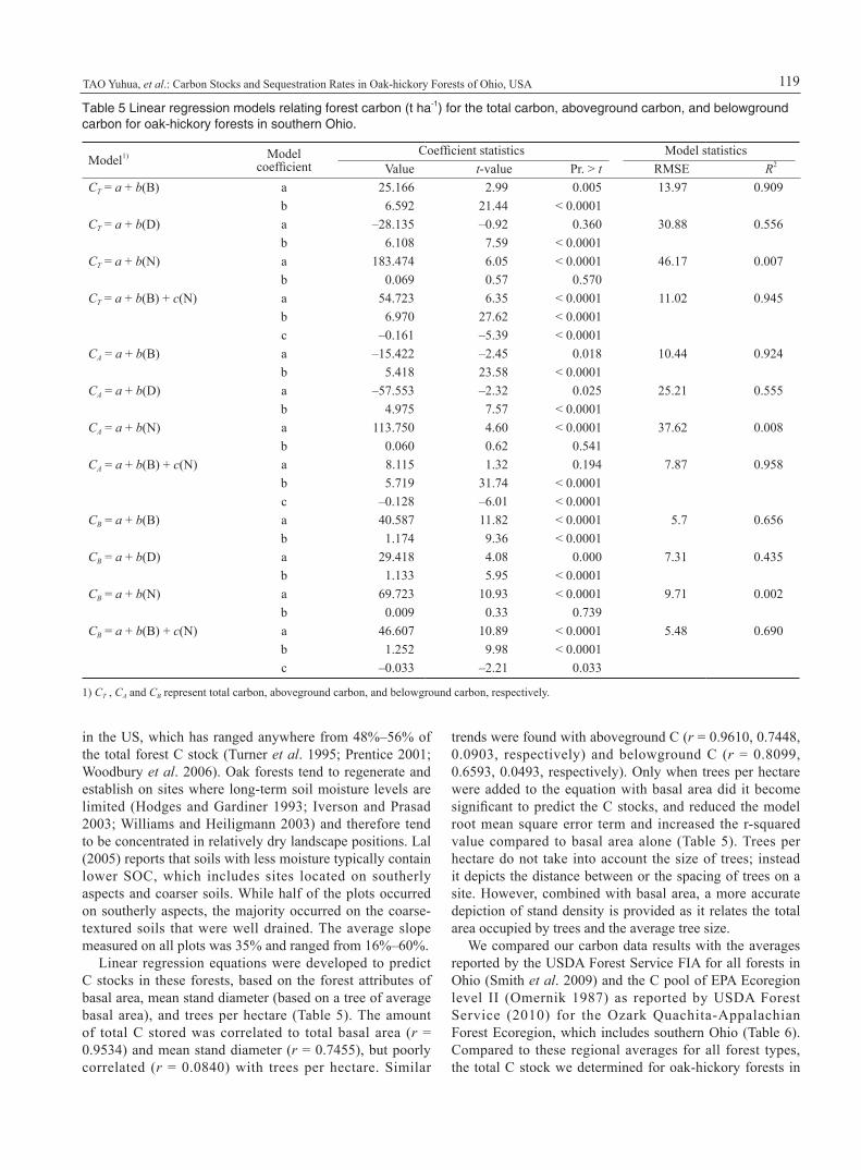
Linear regression equations were developed to predict C stocks in these forests, based on the forest attributes of basal area, mean stand diameter (based on a tree of average basal area), and trees per hectare (Table 5). The amount of total C stored was correlated to total basal area (r = 0.9534) and mean stand diameter (r = 0.7455), but poorly correlated (r = 0.0840) with trees per hectare. Similar

trends were found with aboveground C (r = 0.9610, 0.7448, 0.0903, respectively) and belowground C (r = 0.8099, 0.6593, 0.0493, respectively). Only when trees per hectare were added to the equation with basal area did it become significant to predict the C stocks, and reduced the model root mean square error term and increased the r-squared value compared to basal area alone (Table 5). Trees per hectare do not take into account the size of trees; instead it depicts the distance between or the spacing of trees on a site. However, combined with basal area, a more accurate depiction of stand density is provided as it relates the total area occupied by trees and the average tree size.

We compared our carbon data results with the averages reported by the USDA Forest Service FIA for all forests in Ohio (Smith et al. 2009) and the C pool of EPA Ecoregion level II (Omernik 1987) as reported by USDA Forest Service (2010) for the Ozark Quachita-Appalachian Forest Ecoregion, which includes southern Ohio (Table 6). Compared to these regional averages for all forest types, the total C stock we determined for oak-hickory forests in

Table 5 Linear regression models relating forest carbon (t ha-1) for the total carbon, aboveground carbon, and belowground carbon for oak-hickory forests in southern Ohio.

1) CT , CA and CB represent total carbon, aboveground carbon, and belowground carbon, respectively.

Model1) Modelcoefficient

Coefficient statistics Model statisticsValue t-value Pr. > t RMSE R2

CT = a + b(B) a 25.166 2.99 0.005 13.97 0.909 b 6.592 21.44 < 0.0001

CT = a + b(D) a –28.135 –0.92 0.360 30.88 0.556 b 6.108 7.59 < 0.0001

CT = a + b(N) a 183.474 6.05 < 0.0001 46.17 0.007 b 0.069 0.57 0.570

CT = a + b(B) + c(N) a 54.723 6.35 < 0.0001 11.02 0.945 b 6.970 27.62 < 0.0001c –0.161 –5.39 < 0.0001

CA = a + b(B) a –15.422 –2.45 0.018 10.44 0.924 b 5.418 23.58 < 0.0001

CA = a + b(D) a –57.553 –2.32 0.025 25.21 0.555 b 4.975 7.57 < 0.0001

CA = a + b(N) a 113.750 4.60 < 0.0001 37.62 0.008 b 0.060 0.62 0.541

CA = a + b(B) + c(N) a 8.115 1.32 0.194 7.87 0.958 b 5.719 31.74 < 0.0001c –0.128 –6.01 < 0.0001

CB = a + b(B) a 40.587 11.82 < 0.0001 5.7 0.656 b 1.174 9.36 < 0.0001

CB = a + b(D) a 29.418 4.08 0.000 7.31 0.435 b 1.133 5.95 < 0.0001

CB = a + b(N) a 69.723 10.93 < 0.0001 9.71 0.002 b 0.009 0.33 0.739

CB = a + b(B) + c(N) a 46.607 10.89 < 0.0001 5.48 0.690 b 1.252 9.98 < 0.0001c –0.033 –2.21 0.033

Journal of Resources and Ecology Vol.4 No.2, 2013120

southern Ohio is 77%–88% higher. Species, forest age and density will affect the amount of standing carbon stock (Schulp et al. 2008). According to Smith et al. (2009), 70% of the oak-hickory forests and 83% of all forest types in the North Central Region, of which Ohio is a part, are 80 years of age or younger. The average age weighted on forest area is 63 years for oak-hickory forests and 58 years for all forests within the North Central Region. The average age of oak-hickory forests used in this study was 100 years of age. At age 58 years our models predict a total aboveground C stock of 99.5 t ha -1 and belowground C stock of 66.0 t ha -1, compared to the FIA average of 89.1 t ha -1 and 75.9 t ha -1, respectively, for all forests within the North Central Region.

According to the comparisons in Table 6, forests in our study have greater live aboveground and belowground C stocks, which would reflect the higher basal areas and average tree size and greater root mass at comparatively older ages. When compared to all forests within the region, we would expect oak-hickory forests to contain larger C stocks at a given age since oak and hickory species tend to have relatively higher specific gravities and therefore higher wood densities (Jandl et al. 2007). The average ovendry specific gravity of the oak species that occurred in this study is 0.69 with a range of 0.66–0.72 (Alden 1995). Similarly,

the average specific gravity at 12% moisture content for hickory species measured in this study is 0.69 with a range of 0.66–0.72 (Alden 1995).

One of the objectives of this study was to determine when the C sequestration rates peaked in these forests. Since there is a direct relationship between tree volume and biomass (Hahn 1984; Smith et al. 2003), we compared what has been reported about volume increment in these forests with what we might estimate from our models as to the sequestration rates. Accordingly, we compared the 5-year periodic increment for merchantable volume and total volume reported by Schnur (1937) with that of the 5-year periodic increment of C in the aboveground portion of merchantable trees and the total aboveground C from this study, respectively. To make this comparison, we took the first derivative of the models for merchantable trees and aboveground C, which would provide an estimate of the annual sequestration rates.

It appears that the current annual increment (CAI) of carbon peaks at age 26 years for the aboveground C of merchantable trees, and the mean annual increment (MAI) peaks at age 53 years (Fig. 2). The CAI of carbon for total aboveground C peaks at age 23 years with the MAI reaching the maximum at 46 years (Fig. 3). Schnur (1937) reported

Table 6 Comparison of forest carbon by strata from this study with reported carbon from the USDA Forest Service FIA and the EPA Ozark Ouachita-Appalachian Forest Ecoregion.

Forest StrataAverage reported carbon stocks by forest strata (t ha-1)

This study: oak - hickory forests in Ohio

USDA Forest Service FIA for Ohio (all forest types)

EPA level II ecoregion: Ozark Ouachita-Appalachian Forests

Total aboveground live carbon 117.9 66.3 62.7 Total forest floor carbon 9.4 11.7 11.3 Total deadwood carbon 1.6 11.1 10.7 Total belowground live carbon 29.1 12.6 12.2 Total soil organic carbon 42.8 63.3 55.1 Total carbon 200.4 165.0 152.0

Fig. 2 The current and mean annual increment of sequestered carbon and the cumulative carbon stock of the aboveground portion of merchantable trees in oak-hickory forests of southern Ohio.

Fig. 3 The current and mean annual increment of sequestered carbon and the cumulative carbon stock of total aboveground carbon in oak-hickory forests of southern Ohio.

60 70 8050 90 100Forest age (y)

Tota

l car

bon

stoc

k (t

ha-1)

0

20

40

80

60

110 120 130 140 150

100

Cummulative carbon stockCurrent annual incrementMean annual increment

120

140

160

10 20 300 40

Car

bon

stock

incr

emen

t (t h

a-1 y

-1)

0.0

0.5

1.0

2.0

1.5

2.5

60 70 8050 90 100Forest age (y)

Tota

l car

bon

stoc

k (t

ha-1)

0

20

40

80

60

110 120 130 140 150

100

Cummulative carbon stockCurrent annual incrementMean annual increment

120

140

160

10 20 300 40

Car

bon

stock

incr

emen

t (t h

a-1 y

-1)

0.0

0.5

1.0

2.0

1.5

2.5

3.0180

TAO Yuhua, et al.: Carbon Stocks and Sequestration Rates in Oak-hickory Forests of Ohio, USA 121

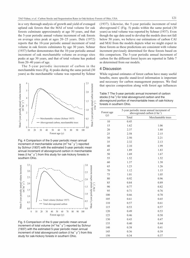
(1937). Likewise, the 5-year periodic increment of total aboveground C (Fig. 5) peaks within the same period (30 years) as total volume was reported by Schnur (1937). Even though the age data used to develop the models does not fall below 50 years, we believe our estimations of carbon CAI and MAI from the models depicts what we might expect in these forests as these predictions are consistent with volume increment previously determined for these forests based on this comparison. The 5-year periodic annual increment of carbon for the different forest layers are reported in Table 7 as determined from our models.

4 DiscussionWhile regional estimates of forest carbon have many useful benefits, more specific stand-level information is important and necessary for carbon management purposes. We find that species composition along with forest age influences

in a very thorough analysis of growth and yield of evenaged upland oak forests that the MAI of total volume for oak forests culminate approximately at age 50 years, and that the 5-year periodic annual volume increment of oak forests on average sites peak at ages 20–25 years. Dale (1972) reports that the 10-year periodic annual increment of total volume in oak forests culminates by age 30 years. Schnur (1937) further demonstrates that the 10-year periodic annual increment of oak merchantable volume on average sites peaks at age 30 years, and that of total volume has peaked from 20–40 years of age.

The 5-year periodic increment of carbon in the merchantable trees (Fig. 4) peaks during the same period (30 years) as the merchantable volume was reported by Schnur

60 70 8050 90 100Forest age (y)

Mea

n 5-

year

per

iodi

c ann

ual v

olum

e inc

rem

ent

(m3 h

a-1 y

-1)

0

1

2

4

3

5

Merchantable volume (Schnur 1937)

Aboveground carbon, merchantable trees

6

10 20 30 40

Mea

n 5-

year

per

iodi

c ann

ual c

arbo

n in

crem

ent

(t ha

-1 y

-1)

0.0

0.5

1.0

2.0

1.5

2.5

Forest age (y)

0.0

0.5

1.0

2.0

1.5

2.5

3.0

Fig. 4 Comparison of the 5-year periodic mean annual increment of merchantable volume (m3 ha-1 y-1) reported by Schnur (1937) with the estimated 5-year periodic mean annual increment of aboveground carbon in merchantable trees (t ha-1 y-1) from this study for oak-hickory forests in southern Ohio.

Fig. 5 Comparison of the 5-year periodic mean annual increment of total volume (m3 ha-1 y-1) reported by Schnur (1937) with the estimated 5-year periodic mean annual increment of total aboveground carbon (t ha-1 y-1) from this study for oak-hickory forests in southern Ohio.

Total volume (Schnur 1937)

Total aboveground carbon

60 70 8050 90 10010 20 30 4000.0

0.5

1.0

2.0

1.5

2.5

3.0

3.5

Mea

n 5-

year

per

iodi

c ann

ual v

olum

e inc

rem

ent

(m3 h

a-1 y

-1)

Mea

n 5-

year

per

iodi

c ann

ual c

arbo

n in

crem

ent

(t ha

-1 y

-1)

Table 7 The 5-year periodic annual increment of carbon stocks (t ha-1) for total aboveground carbon and the aboveground portion of merchantable trees of oak-hickory forests in southern Ohio.

Forest age(y)

5-year periodic mean annual increment of aboveground carbon (t ha-1)

Total Merchantable trees 10 0.45 15 1.62 1.06 20 2.37 1.80 25 2.58 2.15 30 2.50 2.21 35 2.32 2.13 40 2.10 1.99 45 1.89 1.83 50 1.69 1.67 55 1.52 1.52 60 1.37 1.38 65 1.23 1.26 70 1.12 1.15 75 1.01 1.05 80 0.92 0.96 85 0.84 0.89 90 0.77 0.82 95 0.71 0.76

100 0.66 0.70 105 0.61 0.65 110 0.57 0.61 115 0.53 0.57 120 0.49 0.53 125 0.46 0.50 130 0.43 0.47 135 0.40 0.44 140 0.38 0.41 145 0.36 0.39 150 0.34 0.37

Journal of Resources and Ecology Vol.4 No.2, 2013122

the C stocks in forests. Stand age not only influences the aboveground C stock through the relationship of average tree size and forest density but also the accumulation of forest floor C and SOC (Vesterdal et al. 2002; Thuille and Schulze 2006). The rooting depth and litter decomposition properties of a species can influence the amount of organic carbon in the forest floor and soil (Jandl et al. 2007; Schulp et al. 2008), which can also influence the soil pH and thereby affect the understory density and composition (Berg 2000). For example, deeper rooted species such as oak tend to accumulate less organic carbon in the forest floor compared to more shallow rooted species (Jandl et al. 2007; Schulp et al. 2008).

Species composition of the overstory can influence the spatial distribution of trees (Schulp et al. 2008) as the result of tree architecture, shade tolerance and competition differences among species (Poorter et al. 2003; Poorter et al. 2006). The architectural structure displayed by a particular tree species can influence the volume increment in a tree (Hamilton 1969), and hence carbon. The more shade tolerant a species is the denser the crown and more occluded is the light reaching the forest floor (Mourelle et al. 2001), thus having impacts on the forest floor in terms of light, moisture, and temperature conditions. The oak species that dominated the forests in this study are rated as intolerant to intermediate-tolerance to shade conditions and thereby have more sunlight reaching the forest floor compared to forests comprised of more shade tolerant species. In addition, a unique feature that oak forests tend to display in this regard is that their canopy profiles tend to be more extend along the boles compared to other forests (Yang et al. 1999). All of this leads to greater variability in forest composition and structure, thereby influencing standing C stocks.

Even though the number of trees per hectare decline over time, the average tree size and the total basal area increases. C stocks increase with basal area as long as there is a corresponding increase in the average tree size. C stocks are influenced more by the total amount of area contained in basal area and the average size of the trees than it is the number of trees. Basal area is strongly correlated with the wood volume standing in the forest (Martínez Pastur et al. 2008) and hence biomass and carbon.

There is no doubt that the rate of sequestration declines with forest age. The volume increment in forests peaks at relatively young ages and thereafter goes into continual declining increment (Smith and Long 2001; Binkley et al. 2002). We find that the MAI of the total aboveground C peaks early at age of 43 years, and at age 53 years for the aboveground portion of merchantable trees. From our models we also discover that the MAI of the total C sequestered drops from 3.0 t ha -1 y-1 at age 50 years to 2.1 and 1.6 t ha -1 y-1 at ages 100 and 150 years, respectively. Barford et al. (2001) found through the use of eddy covariance methods that 60–80 years old mid-latitude hardwood forests, dominated by Quercus rubra, displayed

an MAI of 2.0 ± 0.4 t ha -1 y-1 of C over an 8-year period. Our models show an MAI of 2.6 ± 0.3 t ha -1 y -1 of C (p = 0.05) from ages 60–80 years.

The patterns of forest C sequestration in these oak-hickory forests follow the patterns of volume increment we expect to see over time. We should expect similar trends in C increment in forests that we see with volume since forest volume and biomass are related (Hahn 1984; Smith et al. 2003). For example we find a strong correlation (r = 0.9983) between the total volume and the total live C reported by Smith et al. (2006) for oak-hickory forests following clearcut harvest in the northeastern U.S. We do not mean to imply that all C within the forest can be accounted for with volume, as volume does not represent other strata in the forest (soil, understory, etc.). However, trees make-up a significant part of the forest, and the live tree biomass (aboveground and roots) in our study on average accounted for 72% of the total C. This knowledge of the relationship between volume and C is beneficial for management purposes as historically forest management has been based upon volume management, growth and yield. This makes any transition from volume-based to C-based management easier to comprehend.

5 ConclusionsForest management in the future will include carbon as a product of the forest, and therefore it is important to understand the carbon dynamics in a forest. A variety of forest attributes such as forest density, age, and species composition will affect these dynamics and how the carbon is stored. Stand-level information on carbon sequestration is necessary for management purposes. Historically forest management has centered upon volume increment as a measure of productivity and basal area as a measure of density, and both have been used in making management decisions. The rate of carbon sequestered and stored within the forest follows similar trends we find with volume increment. The amount of C stocks within a forest is directly related to the amount of basal area. Accordingly, management for C stocks within a forest does not dramatically change what has been performed historically in common forest management practices. While all carbon within a forest system is not contained within trees, trees make up a significant portion of the biomass within the system. Knowledge of the relationship of volume and basal area with carbon will better facilitate carbon management in the future.AcknowledgementsThe authors wish to acknowledge and thank the Ohio Department of Natural Resources, Division of Forestry for their cooperation with this study. We would also like to thank Steven Holton, research technician, for his invaluable assistance in the field collection of the data. This research was financially supported primarily by the Climate, Water, and Carbon Program at The Ohio State University, with additional funds appropriated under the McIntire-Stennis Forestry Research Act, USA. The funding

TAO Yuhua, et al.: Carbon Stocks and Sequestration Rates in Oak-hickory Forests of Ohio, USA 123

sources for this project had no involvement in the study design, collection, analysis and interpretation of the data, in the writing of and the decision to submit this paper.

ReferencesAlden H A. 1995. Hardwoods of North America. Gen. Tech. Rep. FPL–

GTR–83. Madison, WI: U.S. Department of Agriculture, Forest Service, Forest Products Laboratory, 136.

Alexeyev V A. R A Birdsey. 1998. Carbon storage in forests and peatlands of Russia. USDA Forest Service General Technical Report NE-244, 137.

Barford C C, S C Wofsy, M L Goulden, et al. 2001. Factors controlling long- and short-term sequestration of atmospheric CO2 in a mid-latitude forest. Science, 294: 1688-1691.

Berg B. 2000. Litter decomposition and organic matter turnover in northern forest soils. Forest Ecology and Management, 133:13-22.

Binkley D, J L Stape, M G Ryan, et al. 2002. Age-related decline in forest ecosystem growth: An individual- tree, stand-structure hypothesis. Ecosystems, 5:58-67.

Birdsey R A. 1992. Carbon storage and accumulation in United States forest ecosystems. USDA Forest Service, Washington Office, GTR-WO-59, Washington, D.C.

Birdsey R A, L S Heath. 1995. Carbon changes in U.S. forests. In: Joyce L A. (Ed.). Productivity of America’s Forests and Climate Change. USDA Forest Service, Rocky Mountain Forest and Range Experiment Station, GTR-RM-271, Fort Collins, CO., 56-70.

Birdsey R, K Pregitzer, A Lucier. 2006. Forest carbon management in the United States: 1600–2100. Journal of Environmental Quality, 35: 1461-1469.

Brown S. 2001. Measuring carbon in forests: Current status and future challenges. Environmental Pollution, 116: 363-372.

Brown S, D Shoch, T Pearson, M Delaney. 2004. Methods for measuring and monitoring forestry carbon projects in California. Winrock International, for the California Energy Commission, PIER Energy-Related Environmental Research. 500-04-072F, 40.

Burns R M, B H Honkala. (tech. coords). 1990. Silvics of North America: 1. Conifers; 2. Hardwoods. Agriculture Handbook 654. U.S. Department of Agriculture, Forest Service, Washington, DC. 2: 877.

Canadell J G, M R Raupach. 2008. Managing forests for climate change mitigation. Science, 320: 1456-1457.

Cropper, Jr W P, K C Ewel. 1984. Carbon storage patterns in Douglas-fir ecosystems. Canadian Journal of Forest Research, 14: 855-859.

Dixon R K, S Brown, R A Houghton, et al. 1994. Carbon pools and fluxes of global forest ecosystems. Science, 263: 185-190.

Cairns M A, S Brown, E H Helmer, G A Baumgardner. 1997. Root biomass allocation in the world’s upland forests. Oecologia, 111: 1-11.

Fahey T J, P B Woodbury, J J Battles, et al. 2010. Forest carbon storage: ecology, management, and policy. Frontiers in Ecology and the Environment, 8: 245-252.

Fontes L, M Tome, M B Coelho, et al. 2003. Modelling dominant height growth of Douglas-fir (Pseudotsuga menziesii (Mirb.) Franco) in Portugal. Forestry, 76(5): 509-523.

Gingrich S F. 1967. Measuring and evaluating stocking and stand density in Upland Hardwood forests in the Central States. Forest Science, 13: 38-53.

Goodale C L, M J Apps, R A Birdsey, et al. 2002. Forest carbon sinks in the Northern Hemisphere. Ecological Applications, 12: 891-899.

Hahn J T. 1984. Tree volume and biomass equations for the Lake States. Res. Pap. NC-250. St. Paul, MN: U.S. Department of Agriculture, Forest Service, North Central Forest Experiment Station, 10.

Hamilton G J. 1969. The dependence of volume increment of individual trees on dominance, crown dimensions, and competition. Forestry, 42(2): 133-144.

Hamilton S J. 2003. Soil survey of Ross County, Ohio. United States Department of Agriculture, Natural Resource Conservation Service. Washington, D.C., 307.

Hodges J D, E S Gardner. 1993. Ecology and physiology of oak

regeneration. In: Loftis D, C McGee (Eds.). Oak regeneration: serious problems, practical recommendations. Gen.Tech. Rep. SE-84. Asheville, NC: U.S. Department of Agriculture, Forest Service, Southeastern Forest Experiment Station, 319.

Hoover C M, R A Birdsey, L S Heath, S L Stout. 2000. How to estimate carbon sequestration on small forest tracts. Journal of Forestry, 98: 13-19.

Huang S, S J Titus, D P Weins. 1992. Comparison of nonlinear height-diameter functions for major Alberta tree species. Canadian Journal of Forest Research, 22: 1297-1304.

ISO 10694. 1995. Soil quality – Determination of organic and total carbon after dry combustion (elementary analysis). International Organization for Standardization. Geneva, Switzerland, 7.

Iverson L R, A M Prasad. 2003. A GIS-derived integrated moisture index. In: Sutherland E K, Hutchinson T F (Eds.). Characteristics of mixed oak forest ecosystems in southern Ohio prior to the reintroduction of fire. General Technical Report NE-299. Newtown Square, PA: U.S. Department of Agriculture, Forest Service, Northeastern Research Station, 159.

Jandl R, M Lindner, L Vesterdal, et al. 2007. How strongly can forest management influence soil carbon sequestration? Geoderma, 137: 253-268.

Jenkins J, D Chojnacky, L Heath, R Birdsey. 2003. National-scale biomass estimators for United States tree species. Forest Science, 49: 12-35.

Lal R, 2005. Forest soils and carbon sequestration. Forest Ecology and Management, 220: 242-258.

Lemaster D D, G M Gilmore. 2004. Soil survey of Vinton County, Ohio. Natural Resource Conservation Service, US Department of Agriculture, 353.

Martin P H, G J Nabuurs, M Aubinet, et al. 2001. Carbon sinks in temperate forests. Annual Review of Energy and the Environment, 26: 435-465.

Martínez Pastur G J, J M Cellini, M V Lencinas, P L Peri. 2008. Stand growth model using volume increment/basal area ratios. Journal of Forest Science, 54: 102-108.

Mourelle C, M Kellman, L Kwon. 2001. Light occlusion at forest edges: an analysis of tree architectural characteristics. Forest Ecology and Management, 154: 179-192.

Ney R A, J L Schnoor, M A Mancuso. 2002. A methodology to estimate carbon storage and flux in forestland using existing forest and soils databases. Environmental Monitoring and Assessment, 78: 291-307.

Nicodemus M A, R A Williams. 2004. Quantifying aboveground carbon storage in managed forest ecosystems in Ohio. In: Yaussy D A, D M Hix, R P Long, P C Goebel (Eds.). Proc. 14th Central Hardwood Forest Conference. USDA Forest Service General Technical Report NE-316, 232-240.

Omernik J M. 1987. Ecoregions of the conterminous United States. Annals of the Association of American Geographers, 77(1): 118-125.

Poorter L, L Bongers, F. Bongers. 2006. Architecture of 54 moist-forest tree species: traits, trade-offs, and functional groups. Ecology, 87(5):1289-1301.

Poorter L, F Bongers, F J Sterck, H Woll. 2003. Architecture of 53 rain forest tree species differing in adult stature and shade tolerance. Ecology, 84(3): 602-608.

Prentice I C. 2001. The carbon cycle and atmospheric carbon dioxide. Climate Change 2001: The Scientific Basis IPCC, Cambridge University Press, Cambridge, UK, 183-237.

Rizvi R H, D Khare, R S Dhillon. 2008. Statistical models for aboveground biomass of Populus deltoides planted in agroforestry in Haryana. Journal of Tropical Ecology, 49(1): 35-42.

SAS Institute Inc. 2008. Statistical Analysis System software, version 9.2, Cary, NC, USA.

Schnur G L. 1937. Yield, stand, and volume tables for even-aged upland oak forests. US Department of Agriculture, Technical Bulletin No. 560, 87 p.

Schulp C J E, G Nabuurs, P H Verburg, R W de Waal. 2008. Effect of tree species on carbon stocks in forest floor and mineral soil and implications for soil carbon inventories. Forest Ecology and Management, 256:482-490.

Journal of Resources and Ecology Vol.4 No.2, 2013124

Smith F W, J N Long. 2001. Age-related decline in forest growth: an emergent property. Forest Ecology and Management, 144:175-181.

Smith J E, L S Heath, J C Jenkins. 2003. Forest volume-to biomass models and estimates of mass for live and standing dead trees of U.S. forests. General Technical Report NE-298, Newtown Square, PA: U.S. Department of Agriculture, Forest Service, Northeastern Research Station, 57.

Smith J E, L S Heath, K E Skog, R A Birdsey. 2006. Methods for calculating forest ecosystem and harvested carbon with standard estimates for forest types of the United States. General Technical Report NE-343. Newtown Square, PA: U.S. Department of Agriculture, Forest Service, Northeastern Research Station, 216.

Smith W B (tech. coord.), P D. Miles (data coord), C H Perry (map coord.), S A Pugh (data CD coord.). 2009. Forest Resources of the United States, 2007. General Technical Report WO-78. Washington, DC: U.S. Department of Agriculture, Forest Service, Washington Office, 336.

Thuille A, E D Schulze. 2006. Carbon dynamics in successional and afforested spruce stands in Thuringia and the Alps. Global Change Biology, 12: 325-342.

Turner D P, G J Koerper, M E Harmon, J J Lee. 1995. A carbon budget for

forests of the conterminous United States. Ecological Applications, 5(2): 421-436.

USDA Forest Service. 2010. Carbon storage in U.S. forests by EPA Level II Ecoregion and Forest Service RPA Assessment Regions. Available online at www.fia.fs.fed.us/Forest%20Carbon/default.asp; last accessed Aug. 23, 2011.

Vesterdal L, E Ritter, P Gundersen. 2002. Change in soil organic carbon following afforestation of former arable land. Forest Ecology and Management, 169: 137-147.

Williams R A, R B Heiligmann. 2003. Effects of site quality and season of clearcutting on upland hardwood forest composition 38 years after harvest. Forest Ecology and Management, 177: 1-10.

Woodbury P B, J E Smith, L S Heath. 2007. Carbon sequestration in the U.S. forest sector from 1990 to 2010. Forest Ecology and Management, 241: 14-27.

Yang X, J J Witcosky, D R Miller. 1999. Vertical overstory canopy architecture of temperate deciduous hardwood forests in the eastern United States. Forest Science, 45: 349-358.

Zeide B. 1993. Analysis of growth equations. Forest Science, 39: 594-616.