BIG DATA AND DATA ACQUISITION TECHNOLOGIES

big Data anD Data aCQuisition teChnoLogies

FAST FOURIER TRANSFORM ANALYSIS OF PRECIPITATION DATA FOR THE

COLORADO RIVER BASIN

FERNANDO JORGE GONZALEZ VILLARREAL(1) & VICTOR IGNACIO MASTACHE MENDOZA(2)

(1,2) Engineering Institute, National Autonomous University of Mexico, Mexico City,

[email protected]; [email protected]

ABSTRACT The Colorado River flows more than 2400 kilometers, from its source in the Rocky Mountains in the United States through deserts and canyons, to the wetlands of a delta into the Gulf of California in Mexico. Detection of variations over the long term for a series of hydrological variables is an important and critical issue, which is subjected to increasing interest because of the current topic of climate change. This study covers a 70-year time period from 1940 to 2010, using a Fast Fourier Transform (FFT) analysis of 118 daily precipitation sites located throughout the Colorado River basin. Tests for homogeneity and independence were applied to the data series; also a regression analysis was used just in specific cases. The data series of the stations was characterized as a function of frequency domain in order to identify a return rate of hydro-meteorological variables within the basin, verifying the existence of dominant periodic cycles in the data series. Different magnitudes in the precipitation periodicity were also examined. It is concluded that the precipitation of the Colorado River basin behaves in dominant periodic cycles of approximately 10.7 or 12.8 years. Nevertheless, there are three small areas in the basin which react in a different way: the mountains of Arizona showed a dominant period of 8 years; the higher elevations in the state of Colorado, 6.4 years; and the peaks of Wyoming, 4.6 years. These identified areas are the highest peaks where precipitation is more frequent. Besides, the moving average adjusts over a constant 13-year period for the data series of the stations. This suggests that precipitation in the basin completes a cycle every 13 years, verifying the FFT results. The FFT analysis may also be applied for frequency detection of other hydro-climatic variables such as temperature, humidity, streamflow and evapotranspiration. Keywords: Colorado River Basin; Fast Fourier Transform; precipitation; frequency domain; periodic cycles. 1 INTRODUCTION Information about temporal and spatial variability in precipitation time series are extremely important both from a scientific and practical point of view. The debate about climate change has meant that the detection of abrupt or gradual changes in precipitation records has become of increasing interest in the scientific world. In order to be able to make significant conclusions about such changes, long time series of precipitations are needed. However, long and accurate time series are difficult to obtain, as modifications to instrumentation and even minor changes can have profound effects on the precipitation data (De Jongh et al., 2006).

Annual time series are the simplest series in hydrology as it concerns their statistical characteristics. Anderson test of the correlogram is usually applied for testing the independence of a time series. The dependence characteristics of annual time series are basically investigated and presented by two classical statistical computations and relations: the correlogram which is a representation in the time domain, and the spectrum which is a representation in the frequency domain (Salas et al., 1980). Since the technique of spectral analysis gives information on the periodic cycles present in a time series, it is an interesting tool to use when analyzing a long time series of precipitation. Fourier analysis involves fitting climate data with a sum of sine and cosine terms. The disadvantage of this spectral analysis technique is that the series should be stationary, for example, the cycles should persist over the whole time series (De Jongh et al., 2006). Hence, the objectives of this study are:

To identify a return rate of hydro-meteorological variables within the Colorado River Basin; To verify the possible existence of dominant periodic cycles in the data series using a Fast Fourier

Transform analysis; To adjust a simple moving average with the results of the Fourier analysis in order to verify the use

of the Fast Fourier Transform. 2 STUDY AREA AND DATA This study focuses on identification of precipitation trends across the Colorado River Basin. The Colorado River flows more than 2400 kilometers, from its source in the Rocky Mountains in the United States through deserts and canyons, to the wetlands of a delta into the Gulf of California in Mexico. The catchment area

Proceedings of the 37th IAHR World Congress August 13 – 18, 2017, Kuala Lumpur, Malaysia

©2017, IAHR. Used with permission / ISSN 1562-6865 (Online) - ISSN 1063-7710 (Print) 5639

covers 630,000 square kilometers within the states of Arizona, Colorado, Utah, New Mexico, California, Wyoming and Nevada in the United States of America and Baja California and Sonora in the north of Mexico (Srijana and Sajjad, 2012; Christensen et al., 2004). Hoover and Glenn Canyon Dams control the runoff within the Colorado River Basin. The annual average runoff is 22,400 Mm3. The minimum temperature is 0-16°C and the maximum temperature is 52°C. The availability of the rainfall is mostly low. According to operating plans, the basin has been divided into two basins: Upper and Lower. The Rocky Mountains dominate the topography of the Upper Basin, and this is where the Colorado River gets most of its source and discharge of water. On the other hand, the Lower Basin is characterized by flat alluvial valleys, low rainfall and xerophytic vegetation (Oroz Ramos, 2007). Figure 1 shows the map of the study area along with the states, major river networks. It includes the entire Upper Basin and Lower Basin. The construction of hydraulic infrastructure for the control, diversion and storage of the Colorado River began under the premise of having a better use of water to promote the urban and agricultural development of the arid southwestern of the United States. Twenty five storage dams and hundreds of small dams have been built along the river and its tributaries. 248 precipitation gage stations were collected; however, 130 stations were discarded because of the results of the tests of homogeneity and independence, as well as the lack of information over a long period of time. Therefore, this study covers a 70 year time period from 1940 to 2010, using 118 gage stations, with their data series, throughout the Colorado River Basin. This is shown in Figure 2.

Figure 1. Map showing the study area in the Colorado River Basin (USBR, 2016).

3 METHODOLOGY The methodology used in this study is summarized in four steps which are described next:

Homogeneity of data. The statistical analysis of data requires, as the most basic condition, that data are of the same nature as well as the same origin, obtained through observation. A data series is not homogeneous if it presents abrupt changes in the values and they are maintained;

Test of independence. The independence means that the outcome of precipitation in a year does not depend on precipitation values of previous years. Therefore, a data series is independent if the values follow the laws of probability;

Fast Fourier Transform. The data series of the stations is characterized as a function of frequency domain in order to identify a return rate of hydro-meteorological variables within the basin, verifying the existence of dominant periodic cycles in the data series. The Fast Fourier Transform (FFT) is a specialized algorithm that allows the calculation of the Fourier Transform in an efficient way, due to


5640 ©2017, IAHR. Used with permission / ISSN 1562-6865 (Online) - ISSN 1063-7710 (Print)

the computational load and processing time being quite low. In Matlab, the unidimensional Fourier Transform can be calculated by the predefined function “fft”, which calculates the Discrete Fourier Transform through the FFT algorithm (Frigo, 1999). This function provides a base frequency vector founded on a base time vector, so that the representation of the signal in the frequency domain corresponds to the representation of the signal in the time domain;

Simple Moving Average. A moving average is a technique to get an overall idea of the trends in a data set. The moving average is extremely useful for forecasting long-term trends. By doing this, it is hoped that the magnitude of random fluctuations in the data will decrease.

Figure 2. To the left, total of climatological stations in the CRB. To the right, used climatological stations in this paper.

As it was mentioned before, 118 precipitation gage stations were located within the basin and their spatial distribution is shown in table 1. The statistical characteristics of the hydrological series, such as the average, the standard deviation and the correlation coefficients, are affected when the series shows a trend in the average or in the variance Escalante and Reyes (2008). Statistical tests, which measure the homogeneity of a data series, such as the Helmert, Cramer and Student’s t-test show a null hypothesis and a rule to accept or reject it. The Student’s t-test was applied to the data series of 118 precipitation gage stations. In addition, the Anderson Independence test was applied which states that if only 10% of the values exceed the confidence limits, the series is independent and therefore, it is a variable that follows the laws of probability.

Table 1. Distributed climatological stations through the different states of the CRB. State Total Stations

Arizona 36 Colorado 27

Utah 23 New Mexico 14

California 10 Wyoming 5 Nevada 3

3.1 Student’s t-test When the most likely cause of losing homogeneity of a data series is an abrupt change on the average, the Student’s t-test is very useful.



If it is considered a data series for 1, 2, … , , of the site , which is divided into two sets, whose

sizes are , then the proof statistics are defined by the following expression:

21 1

[1]

where, , are the mean and the variance of the first part of the data whose size is . , are the mean and the variance of the second part of the data whose size is .

The absolute value of was compared with the value of the two-tailed Student’s t-distribution, with 2 degrees of freedom and for a level 0.05.

If and only if the absolute value of is greater than the Student’s t-distribution one, it is concluded that the difference between the means has enough evidence of inconsistent, so the data series is not homogeny. 3.2 Anderson independence test The independence means that the outcome of precipitation in a year does not depend on precipitation values of previous years. Due to this, Anderson independence test was applied, which uses the serial autocorrelation coefficient for different delayed time . The following expression estimates the serial autocorrelation coefficient:

∑

∑1 1, 2, … ,

3

[2]

where:

[3]

For an independent series, the population correlogram is equal to zero for 0. However, samples of independent time series, due to sampling variability, have fluctuating around zero but they are not necessarily equal to zero. In such case, it is useful to determine the probability limits for the correlogram of an independent series. The expression to estimate the limits for the 95% probability levels is:

95%1 1.96 1

[4]

The resultant chart with the estimated values for versus the delayed time , with the probability limits is

called correlogram of the sample. If and only if the 10% of the resultant are out of the probability limits, it is concluded that the data series is independent, so it is a variable that follows the laws of probability. 3.3 Fast Fourier Transform A Fourier transform converts a signal in the time domain to the frequency domain (spectrum). The Fast Fourier Transform does not refer to a new or different type of Fourier transform; it refers to a very efficient algorithm for computing the Discrete Fourier Transform (DFT), where periodic signals may be expanded into a series of sine and cosine functions (Huang, 2011). The purpose of the FFT is to perform the representation of a signal, originally acquired in the time domain (time series) as a function of the frequency domain. MATLAB is a numerical computing environment developed by MathWorks that allows matrix manipulations, plotting of functions and data, and implementation of algorithms. (Huang, 2011). FFT computes the discrete Fourier transform using a fast Fourier transform algorithm. In MATLAB, the associated code that generated the particular fft output is: >> L=length(x); >> nfft=2^nextpow2(L); >> y=fft(x,nfft)/L; >> f=(fs/2*linspace(0,1,nfft/2+1))'; >> plot(f,2*abs(y(1:NFFT/2+1)));



This method plot a signal in the frequency domain. The frequency domain representation, or power spectrum, of a signal may show information about a signal that is not readily apparent from the time domain representation (Romberg, 2012). 3.4 Simple moving average A moving average is a technique to get an overall idea of the trends in a data set. The moving average is extremely useful for forecasting long-term trends. By doing this, it is hoped that the magnitude of random fluctuations in the data will decrease. In calculating moving averages for a set of data, it is necessary to first select the number of recorded raw data points to be included in the calculation. The use of moving averages is important because most events that are of interest to us are not instantaneous, but instead, are extended in time. Therefore, data that can be used to identify and quantify these events occur in temporal clusters. Moving average parameters do not only produce appealing visual depictions of the event, but can also significantly improve our ability to identify and understand them (Warner, 2016). 4 RESULTS AND DISCUSSIONS Following the described methodology above, the results of the Student’s t and Anderson test showed that 130 data series of 248 gage stations were not homogeneous and independent data series, respectively. Therefore, this study used 118 homogeneous and independent gage stations throughout the Colorado River Basin. Figure 2 is observed in order to identify the distribution of these stations. Once the homogeneous and independent gage stations were identified, the Fast Fourier Transform analysis was run in MATLAB. This software solved the algorithm shown above for the 118 data series and the results identified that the precipitation in the Colorado River Basin behaves in five periodic cycles: 4.6, 6.4, 8.0, 10.7 and 12.8 years. Figure 3 shows this distribution along the catchment area; however, it can also be observed in Figure 3 that the precipitation tends to respond to the dominant periodic cycle of 12.8 years. Furthermore, this dominant periodic cycle is distributed around the whole Upper and Lower Basin.

Figure 3. Dominated different periodic cycles of precipitation.

There are three small areas in the basin that react in a different way. These identified areas are the highest peaks where precipitation is more frequent:

17 gage stations located on the mountains of Arizona showed a dominant period of 8 years that is equivalent to have 0.125 Hz as a dominant frequency;

6 gage stations located on the higher elevations in the state of Colorado had a dominant period of 6.4 years;



5 gage stations located at the peaks of Wyoming presented a dominant period of 4.6 years. Figure 3 also shows 13 gage stations located around the center of the basin that have a dominant period of 10.7 years. This means that 41 of 118 stations have a different behavior of precipitation. In other words, more than 65% of the gage stations respond to the dominant periodic cycle of 12.8 years. Therefore, it is assumed that this is the behavior of precipitation in the Colorado River Basin. Following the methodology and in order to justify this statement, the moving average analysis was performed with this result. Before adjusting the simple moving average, it was necessary to estimate the volume of the annual precipitation through the Thiessen polygons of the 118 gage stations. Then, the moving average was adjusted over a constant 13 year period for the data series of the stations. Figure 4 shows the results. It can be observed that the annual precipitation with blue bars and the 13 years moving average with a dotted red line.

Figure 4. Simple Moving Average of 13 years for the total volume of precipitation.

It is observed in Figure 4 that the mean of the volume of the precipitation has been 200,000 Hm3. From 1952 to 1980, the moving average looks like a horizontal line which represents an accurate behavior. After 1980, a slight change in the slope can be observed, but this is not enough evidence to state that there is a change in the mean. On the other hand, these results can suggest that precipitation in the Colorado River Basin completes a cycle every 13 years, verifying the FFT results. 5 CONCLUSIONS Summarizing, this study of analyzing historical records of annual hydrological series lead to the following conclusions:

Annual precipitation may be considered in most of the cases as nearly stochastic processes (average does not change in time) provided the inconsistency in observed data and the human-induced changes and natural accidental disruptions (no homogeneity in data) are properly taken into account;

Student’s t and Anderson test showed that 130 data series of 248 gage stations were not homogeneous and independent data series, respectively. Therefore, these tests provide enough evidence of the systematic errors in observed data;

The following statement was verified: the longer a series, the greater is the probability of some no homogeneity being present in data, produced either by human activities or by accidental disruption in nature, plus some systematic errors (inconsistency) (Salas et al., 1980);

The results of the FFT analysis showed that the precipitation in the Colorado River Basin tends to respond to the dominant periodic cycle of 12.8 years. Furthermore, this dominant periodic cycle is distributed around the whole Upper and Lower Basin;

The FFT analysis may also be applied for frequency detection of other hydro-climatic variables such as temperature, humidity, streamflow and evapotranspiration;

The moving average adjusted over a constant 13-year period for the data series of the gage stations and the results could suggest that the precipitation in the Colorado River Basin completes a cycle every 13 years, verifying the FFT results;

Both analysis: FFT and simple moving average can be complementary for studying the dominant periodic cycles in the data series;

There could be some hydro-climatic series exhibiting changes in the statistical characteristics which do not appear to produce tendency. Therefore, further investigations are necessary in order to substantiate claims that such changes are produced by some localized or regional climatic changes;

The objectives of this study were fulfilled.



ACKNOWLEDGEMENTS A debt of gratitude is owed to the National Centers for Environmental Information (NCEI) of the National Oceanic and Atmospheric Administration (NOAA), scientific agency within the United States Department of Commerce, for the submission of all the 248 requested data series, without their help and support, this study would have not been finished successfully and on time. Also, the completion of this study could not have been possible without the expertise of several minds: colleagues, fellows and researchers, who encouraged and offered support throughout this project. The contribution of everyone, specifically their time, dedication, patience, effort and understanding, has been invaluable. REFERENCES Christensen, N.S., Wood, A.W., Voisin, N., Lettenmaier, D.P. & Palmer, R.N. (2004). The Effects of Climate

Change on The Hydrology and Water Resources of The Colorado River Basin. Climatic Change, 337-363. De Jongh, I.L., Verhoest, N.E. & De Troch, F.P. (2006). Analysis of a 105-year Time Series of Precipitation

Observed at Uccle, Belgium. International Journal of Climatology, 2023-2039. Escalante S.C.A. & Reyes C.L. (2008). Técnicas Estadísticas en Hidrología (2da. ed.). Msc Thesis. Facultad

de Ingeniería, Universidad Nacional Autónoma de México. Frigo, M. (1999). A Fast Fourier Transform Compiler. ACM SIGPLAN Conference on Programming Language

Design and Implementation. Atlanta, Georgia: MIT Laboratory for Computer Science, 1-12. Huang, W. (2011). Fast Fourier Transform and MATLAB Implementation. Dallas: University of Texas. Oroz Ramos & L. A. (2007). Política y manejo bilateral en un acuífero transfronterizo de México: el acuífero

Son-01 Valle de San Luis Río Colorado, Sonora, México. Sonora, México: División de Ciencias Biológicas y de la Salud, Universidad de Sonora.

Romberg, F.W. (2012). High-Resolution Time-Frequency Analysis Of Neurovascular Responses To Ischemic Challenges. Phd Thesis. New Haven: School of Medicine, Yale University.

Salas, J.D., Delleur, J.W., Yevjevich, V. & Lane, W.L. (1980). Applied Modeling of Hydrologic Time Series. Colorado: Water Resources Publications.

Srijana, D. & Sajjad, A. (2012). Changing Climatic Conditions in The Colorado River Basin: Implications For Water Resources Management. Journal of Hydrology, 127-141.

USBR, U.D. (2016). Reclamation Managing Water in the West. Obtenido de https://www.usbr.gov/uc/water/rsvrs/ops/aop/ [Accessed 22/21/2016].

Warner, R.A. (2016). Moving Averages for Identifying Trends and Changes in the Data. Optimizing the Display and Interpretation of Data, Chapter 3, 53-73.



DYNAMIC MERGING OF CROWD-SOURCED, RAIN GAUGE, AND RADAR RAINFALL

MEASUREMENTS FOR URBAN STORMWATER MODELING

PAN YANG(1) & TZE LING NG(2)

(1,2) Department of Civil and Environmental Engineering, The Hong Kong University of Science and Technology, Hong Kong, [email protected]; [email protected]

ABSTRACT In this study, rain gauge, radar and crowd-sourced measurements of rainfall intensity are merged to yield a best estimate of the true rainfall field for urban stormwater modeling purposes. Compared with past studies that were limited to merging just rain gauge and radar data, this study incorporates an additional source of data, viz. crowd-sourced measurements which we assume are obtainable from smartphones, surveillance cameras, and even moving cars of common citizens. To merge the three sources, a dynamic weighting method is used. From a theoretical but realistic case study, it is found the addition of crowd-sourced measurements produces more accurate estimates of stormwater flow.

Keywords: Crowd-sourcing; rainfall field merging; urban stormwater modeling; rain gauge; radar.

1 INTRODUCTION Accurate rainfall estimation at high spatial and temporal resolutions is essential for effective urban stormwater modeling and management. Traditionally, rainfall is measured by systems of rain gauges or by radar. Rain gauge observations of rainfall are quite different from radar observations. Typically, rain gauges are highly accurate, but are usually sparsely distributed and insufficient to describe the spatial distributions of rainfall events with adequate precision. Radars can usually capture the spatial variability of a rainfall event well, but their measurements are usually biased with various errors (Mandapaka et al., 2010). Where both rain gauge and radar monitoring systems co-exist, combining their observations through different merging techniques yields more accurate estimates of the true rainfall field. With advances in image processing techniques, it is now possible to measure rainfall intensity from photographic images of rain (Allamano et al., 2015). This makes possible a crowd-sourcing approach to measuring rainfall using smartphones, surveillance cameras and other such devices. This new approach has the potential to provide an additional independent source of rainfall intensity data that if merged with traditional rain gauge and radar data, has the potential to lead to an even better estimate of the true rainfall field. This, in turn, can be expected to result in more accurate modeling of stormwater flow. This study uses a dynamic weighting method to merge the rainfall observations from the three sources, and tests the potential of the merged data for improved stormwater modeling.

2 METHODS To test the dynamic weighting method, the Chollas Creek watershed in the city of San Diego, which has a drainage area of 68 km2, is used as a case study. First, we generate a synthetic rainfall field with a spatial-temporal resolution of 100 m × 100 m × 5 min to represent the ground truth. The ground truth rainfall field is generated by interpolating real 500 m × 500 m × 5 min radar observations to yield the required resolution through kriging. To simulate rain gauge observations, rain gauges are assumed randomly located throughout the study area with a 0.08/km2 density, and further assumed to produce error-free observations. We then simulate crowd-sourced observations following the methods and assumptions in Yang and Ng (2016). For each crowd-sourced observation, we assume a random observation error that is normally distributed with a zero mean and a standard deviation which varies from 0.1 to 0.5 of the ground truth rainfall intensity. To simulate radar observations, we upscale the resolution of the ground truth rainfall field from 100 m × 100 m × 5 min to 500 m × 500 m × 5 min, then add systematic (bias) and random (noise) error components to the resulting rainfall field (Sinclair and Pegram, 2005). To merge the rainfall observations from the three sources, we apply the ordinary kriging (OK) method to interpolate the rain gauge observations to yield a rain gauge rainfall field, and the crowd-sourced observations to yield a crowd-sourced rainfall field. We then merge the rain gauge field and the radar field (from above) using the kriging with external drift (KED) method to produce a new rainfall field, which we shall denote hereafter as KEDgauge. Finally, we merge the KED merged rainfall field with the crowd-sourced rainfall field using a dynamic weighting method, whose weights are adapted dynamically according to the estimation errors of the two source fields (Hasan et al., 2016). This results in a new merged rainfall field incorporating observations from all three sources, which we shall denote hereafter as DW.



To evaluate the skill of the different merged and unmerged rainfall fields as input to stormwater modeling, we feed the rainfall fields an urban drainage model of the Chollas Creek watershed, which have been calibrated and validated against peak flow data from Schiff and Carter (2007). The simulated flow from each of the rainfall fields are then compared with the “true” flow of the creek as obtained from the ground truth rainfall field to evaluate the contribution of the crowd-sourced observations.

3 RESULTS Figure 1 gives the modeled hydrographs at the watershed outlet for a one-hour storm event. It is observed that the stormwater model, when fed with radar estimated rainfall, significantly overestimates the flow, and when fed with rain gauge estimated rainfall, significantly underestimates the flow. It can also be seen that merging the rain gauge and radar data results in an improved prediction of the true hydrograph, but there is still a clear systematic bias. The OK interpolated crowd-sourced rainfall field leads to a good estimation of the stormwater flow, as shown in the hydrograph in Figure 1 and the error statistics in Table 1, though the crowd-sourced rainfall field yields a significant bias in the arriving time of the peak flow, which could be a very costly error for urban stormwater management. On the overall, we find the rainfall field DW to produce the best estimate of the hydrograph. The statistics in Table 1 confirm this.

Table 1. Skill of the different rainfall fields as input to stormwater flow simulation.

Error Statistic Radar Gauge KEDgauge Crowd DW

Relative Error of Peak Flow 1.215 0.483 0.280 0.120 0.144

Relative Error of Storm Volume 0.843 0.508 0.316 0.225 0.133

Root Mean Square Error of Flow (m3/s) 2.270 1.322 0.930 1.250 0.515

Error of Time to Peak (min) -40 32 20 -91 11

Figure 1. Hydrographs of modeled stormwater flow at the Chollas Creek watershed outlet .

4 CONCLUSIONS The results suggest that the rainfall field merging process can benefit from the addition of crowd-sourced rainfall observations. It can also be concluded that the dynamic weighting method used in this study can successfully merge crowd-sourced, rain gauge, and radar rainfall observations. ACKNOWLEDGEMENTS The authors thank The Hong Kong University of Science and Technology for funding support. REFERENCES Allamano, P., Croci, A. & Laio, F. (2015). Toward the Camera Rain Gauge. Water Resources Research, 51,

1744–1757. Hasan, M.M., Sharma, A., Johnson, F., Mariethoz, G. & Seed A. (2016). Merging Radar and In Situ Rainfall

Measurements: An Assessment of Different Combination Algorithms. Water Resources Research, 52, 8384-8398.



3

Mandapaka, P.V., Villarini G., Seo B.C. & Krajewski W.F. (2010). Effect of Radar-Rainfall Uncertainties on the Spatial Characterization of Rainfall Events. Journal of Geophysical Research, 115, D17110.

Schiff, K. & Carter, S. (2007). Monitoring and Modeling of Chollas, Paleta, and Switzer Creeks. Technical Report 513.

Sinclair, S. & Pegram, G. (2005). Combining Radar and Rain Gauge Rainfall Estimates Using Conditional Merging. Atmospheric Science Letters, 6, 19-22.

Yang, P. & Ng, T.L. (2016). Implications of Crowd-Sourcing Urban Rainfall Monitoring Approach for Stormwater Modeling. The Twenty-Ninth KKHTCNN Symposium on Civil Engineering, Hong Kong.



USING UNMANNED AERIAL VEHICLES TO INSPECT SILTATION IN IRRIGATION CANALS

ABUBAKR MUHAMMAD(1), ALI AHMAD(2), SAAD HASSAN(3), SYED M. ABBAS(4), TALHA MANZOOR(5) & KARSTEN BERNS(6)

(1,5) Center for Water Informatics & Technology, Lahore University of Management Sciences (LUMS), Lahore, Pakistan

[email protected] (1,2,3,4,5,6) Department of Electrical Engineering, Lahore University of Management Sciences (LUMS), Lahore, Pakistan

(6) Robotics Research Lab, University of Kaiserslaturen, Germany

ABSTRACT Water supply to the agricultural base in the Indus river basin is through a vast network of irrigation canals that runs thousands of kilometers in length. Most canals undergo deterioration over time due to accumulation of silt and sediment transported by the rivers. Every year a forced closure of the canals is inevitable for canal cleaning, entailing a very large scale and costly operation. This silt removal operation is prone to inefficiencies due to subjective decision making in the cleaning process, shortage of time and lack of verification. In this paper, we summarize the results from using an Unmanned Aerial Vehicle (UAV) to assist in surveying the siltation of canals during annual channel closure. An advanced sensing system and navigation software has been deployed on board the drone to acquire terrain profiles of the canal. The profiles were processed to identify defects in canal linings, locate and estimate silt accumulations and help the human operator to continuously monitor the excavation operation. This paper aims to bridge the theory-to-practice gap by presenting an accessible introduction of this technology to the water practitioners, summarize results from field trials and also narrate the existing practices of canal inspection for further development of automation based solution.

Keywords: Unmanned aerial vehicles; sedimentation; structural inspection; big data; irrigation. 1 INTRODUCTION

The motivation for our work comes from a desire to map the large irrigation canal network in the Indus basin for studying siltation. Water supply to the agricultural base in Pakistan’s Indus river basin is through a vast network of irrigation canals that run more than 50,000 km in length (See Briscoe et al., 2006 for a comprehensive report on Pakistan’s water sector). Most of the canals have mud banks and beds which undergo deterioration over time due to accumulation of silt and sediment transported by the rivers. See Figure 1 for some situations. A forced closure of the canals is inevitable for canal cleaning, yearly, entailing a large scale and costly operation. The extent and precision of silt removal is prone to inefficiencies due to subjective decision making in the process, shortage of time and lack of verification (Waijjen and Bandaragoda, 1992). In this paper, we report our work on developing a semi-autonomous robotic profiling system to increase the efficiency of this process. We have developed a 3D perception system, which is deployed on board an aerial robot to assist the human operator in surveying and cleaning the canal effectively during the annual canal closures. The current manual system decides on cleaning based on measurements taken every 1000 feet. It looks for at least 6 inch silt depth at these data points. Proposed system envisages efficient cost effective cleaning, reduced water discharge variability, and enhanced agricultural productivity.

In a previously published work (Anwar et al., 2015), we have investigated the achievable performance limits of the proposed aerial canal inspection system in theory. We have derived mathematical relationships relating the positioning and sensing uncertainty of robotic inspection vehicles with estimation of the uneven surface profiles and their corresponding enclosed volumes. Via analytical expressions obtained for a one-dimensional toy example we argue how tolerable are the localization and sensor uncertainties, for achieving a desired accuracy in the profile and corresponding volume estimates. The paper also commented that there are two distinct research areas relating to the problem in hand. On one side, there is work in structural inspection suited for precisely defined environments and, on the other, is work on mapping rough uneven surfaces. In our case, canals offer a semi-structured environment which neither provides a geometric uniformity (like bridges and buildings), nor a relaxation in representation (like fields and forests). Therefore, this project offers a unique case study in robotic structural inspection, in addition to its promise in water management.

As a follow up to the theoretical analysis of Anwar et al. (2015), our group has worked on various implementation aspects of the problem that includes navigation, control and processing of acquired data. In this paper, we give an overview of these activities in a manner that is accessible to the water and agriculture



community and therefore aims to bridge the theory-to-practice gap for this new technology. Moreover, we also narrate the existing practices of canal inspection for a wider awareness and feedback on this critical issue, unique to wide scale irrigation practices in the Indus basin. 2 CURRENT PRACTICE OF DESILTING IRRIGATION CHANNELS 2.1 Siltation in Irrigation Channels

Silt has a mud like appearance and consists of dust-like particles of earth, slightly larger than clay and slightly smaller than sand. It is composed of quartz and feldspar, and may occur as soil, as suspended sediment in a surface water body, or as soil deposited at the bottom of a waterway. Silt has strong impacts on the environment. It can change landscapes, it fills up wetlands and waterways and also forms river deltas. Silt in man-made waterways is extremely undesirable. Slow moving water deposits silt on the canal bed. This reduces channel carrying capacity and results in outlets drawing more water than their allotted share due to raised water levels. Silt may be present in waterways in the following forms: 1) Suspended load, which includes silt flowing in water. This silt will eventually settle down in the water bed if the velocity of the water is low, 2) Bed load, which includes larger particles of silt rolling along the stream bed, and 3) deposited load, which is stationary silt deposited on the stream bed.

Figure 1. Examples of irrigation channels in Lahore district (Punjab, Pakistan) during annual inspection for siltation. A small channel with paved banks (Top Left). A small silted channel identified for cleaning (Top

Center). A large distributary canal before silt cleaning (Top Left). Close view of siltation and bank damage (Bottom). (Photographs taken in January 2016).

For measuring suspended load, measurements may be taken at the source during transport or within the

affected area. However, source measurements of erosion may be difficult since the lost material may be a fraction of a millimeter per year, hence the usual approach taken is to measure the sediment while in transport within the stream. This is commonly achieved by sampling the turbidity of the water. Firstly, the correlation between turbidity and sedimentation concentration is determined by making a regression developed by water samples that are filtered, dried and weighed. Then the concentration is multiplied with discharge and integrated over the entire plume. This gives the desired quantity of suspended silt. To distinguish the spill contribution, the background turbidity is subtracted from the spill plume turbidity. This whole process is repeated many times over to get low uncertainty in results Recall that bed load consists of the larger silt particles rolling along the waterbed. Measuring bed load can be done through direct measurements, which consists of digging a hole in the stream bed and removing and weighing the material that drops in. Bed load may also be estimated from samples caught in a device which is lowered to the stream bed for a measured amount of time then brought up for weighing the catch.

Silt deposited on the waterbed can be estimated by measuring the depth of the waterbed and comparing with the depth at canal construction. Bed level can be measured by level gauges in combination with differential gps or levelling apparatus, acoustic bed level detectors or optical bed level detectors. However, the



best and most accurate estimation is achieved after the waterway is dried up through plane surveying techniques.

2.2 Channel Siltation in the Indus Basin

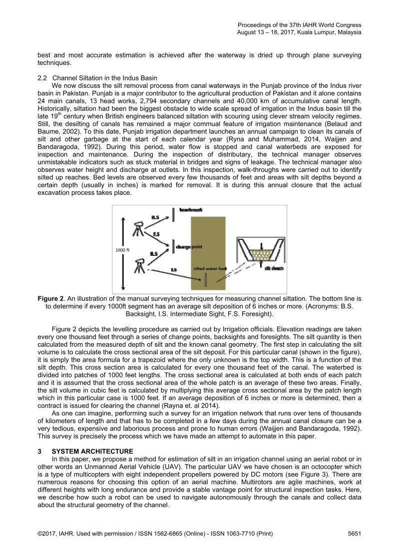
We now discuss the silt removal process from canal waterways in the Punjab province of the Indus river basin in Pakistan. Punjab is a major contributor to the agricultural production of Pakistan and it alone contains 24 main canals, 13 head works, 2,794 secondary channels and 40,000 km of accumulative canal length. Historically, siltation had been the biggest obstacle to wide scale spread of irrigation in the Indus basin till the late 19th century when British engineers balanced siltation with scouring using clever stream velocity regimes. Still, the desilting of canals has remained a major commual feature of irrigation maintenance (Belaud and Baume, 2002). To this date, Punjab irrigation department launches an annual campaign to clean its canals of silt and other garbage at the start of each calendar year (Ryna and Muhammad, 2014, Waijjen and Bandaragoda, 1992). During this period, water flow is stopped and canal waterbeds are exposed for inspection and maintenance. During the inspection of distributary, the technical manager observes unmistakable indicators such as stuck material in bridges and signs of leakage. The technical manager also observes water height and discharge at outlets. In this inspection, walk-throughs were carried out to identify silted up reaches. Bed levels are observed every few thousands of feet and areas with silt depths beyond a certain depth (usually in inches) is marked for removal. It is during this annual closure that the actual excavation process takes place.

Figure 2. An illustration of the manual surveying techniques for measuring channel siltation. The bottom line is

to determine if every 1000ft segment has an average silt deposition of 6 inches or more. (Acronyms: B.S. Backsight, I.S. Intermediate Sight, F.S. Foresight).

Figure 2 depicts the levelling procedure as carried out by Irrigation officials. Elevation readings are taken

every one thousand feet through a series of change points, backsights and foresights. The silt quantity is then calculated from the measured depth of silt and the known canal geometry. The first step in calculating the silt volume is to calculate the cross sectional area of the silt deposit. For this particular canal (shown in the figure), it is simply the area formula for a trapezoid where the only unknown is the top width. This is a function of the silt depth. This cross section area is calculated for every one thousand feet of the canal. The waterbed is divided into patches of 1000 feet lengths. The cross sectional area is calculated at both ends of each patch and it is assumed that the cross sectional area of the whole patch is an average of these two areas. Finally, the silt volume in cubic feet is calculated by multiplying this average cross sectional area by the patch length which in this particular case is 1000 feet. If an average deposition of 6 inches or more is determined, then a contract is issued for clearing the channel (Rayna et. al 2014).

As one can imagine, performing such a survey for an irrigation network that runs over tens of thousands of kilometers of length and that has to be completed in a few days during the annual canal closure can be a very tedious, expensive and laborious process and prone to human errors (Waijjen and Bandaragoda, 1992). This survey is precisely the process which we have made an attempt to automate in this paper. 3 SYSTEM ARCHITECTURE

In this paper, we propose a method for estimation of silt in an irrigation channel using an aerial robot or in other words an Unmanned Aerial Vehicle (UAV). The particular UAV we have chosen is an octocopter which is a type of multicopters with eight independent propellers powered by DC motors (see Figure 3). There are numerous reasons for choosing this option of an aerial machine. Multirotors are agile machines, work at different heights with long endurance and provide a stable vantage point for structural inspection tasks. Here, we describe how such a robot can be used to navigate autonomously through the canals and collect data about the structural geometry of the channel.



Figure 3. An octocopter during canal inspection operation over a channel in LUMS campus (Left). Close-up of the flying machine being configured in lab (Right).

Figure 3 captures how a multirotor will position itself the canal and inspect the geometry of the channel. A

range sensor is deployed on the machine which collects the information about the shape of the canal. A small on board computer is used to collect the data from sensors. The flying robot which we have used in our work is Mikrocopter MK ARF OktoXL 6S12. This aerial machine is an octocopter with a weight lifting capacity of 2500 grams, which is important for mounting sensors and computing platforms to the machine. This machine is equipped with number of sensors like GPS, Accelerometer, Gyroscope and Altimeter. Low level control of this aerial machine is implemented on an on-board flight controller. Based on high level commands given to flight controller, it regulates the speeds of individual motors and performs motion primitives (e.g., move forward). In normal operation mode, these high level commands are sent to the flight controller of aerial machine through a remote which is controlled by a human. But in order to use this machine for an autonomous application, we have interfaced it with a single board computer (ODROID XU4) processing unit which is mounted on the machine to acquire data from sensors, run navigation and path planning algorithms and issue high level control commands to the flight controller.

The software of this high-level processing unit is run on ROS (Robot Operating System) which provides the software backbone for synchronizing all algorithmic tasks for the robot. A long range laser scanner has been mounted in an inverted position at a tilt angle of 60° using a 3D printed modeled part. The laser scanner is a Hokuyo Utm30x with a range of 30 meters, a filed of view of 270° and an angular resolution of 0.25°. The laser scanner is the machine’s most critical unit for navigation as well as mapping the canal geometry. One can say the entire purpose of the project is to give a laser scanner the capability to fly. The whole system is powered through the batteries on this machine. The laser scanner and on board PC requires power on different voltage levels. A voltage regulator has been mounted for the required voltage level conversion.

Figure 4. Odroid single board computer mounted on one aerial machine leg (Left). Laser scanner mounted

underneath robot using a 3D printed mount (Center). Also, seen in pictures is a custom-built voltage regulator attached to another leg. Hokuyo Laser scanner used in this work (Right). All these accessories count towards

the external payload of the robot which must be under 2500g as per specification of the UAV.

4 ALGORITHMS FOR NAVIGATION AND MAPPING 4.1 Overall Information Flow

The overall algorithmic tasks and information processing of the robot system have been captured in the conceptual block diagram of Figure 5. Most of these tasks are running on Ordroid single board computer using ROS. Although, some of the blocks correspond to low-level flight controllers, this distinction has been masked here to better understand the information flow inside the machine. The sensors include GPS, cameras, IMU and laser scanners which report the data via appropriate interfaces to the computing units. Similarly high level commands are communicated to the low-level controller which translates these commands to machine



actuations (the eight DC motors) via appropriate interfaces. The algorithmic block which is most critical for a real-time operation is labelled Path Planning in this chart. All other operations can be performed either online or off-line for the creation of canal structural maps. In current practice we only perform navigation and storage of data in real-time and perform all other tasks for off-line or post-processing. A non-trivial element of this information flow is the ability to store long recordings of sensor data using ROS support and external storage memory modules added to the system.

Figure 5. Algorithmic blocks of the robot system.

The need for this data flow can be understood from the illustrations given in Figure 6 (taken from Anwar

et al., 2015). The flying robot needs to be positioned in the center of the empty waterway for a clear range sensing of its banks and the silted surface (painted red in Left of Figure 6). The flying robot also needs to move forward along the length of the canal to collect more measurements. Critical to correctly interpreting each range measurement is the ability to estimate the robot’s own pose and location with respect to a global coordinate system. The figure emphasizes that the estimates of the surface will always be incorrect but using appropriate algorithmic corrections, the goal of detecting “an average 6 inch deposition or more over a length of 1000 ft” is achievable using very accurate range sensors (Laser scanners) and advanced localization techniques. Much of this achieved using statistical-estimation inspired techniques of probabilistic robotics (Thrun et. al., 2005) and machine learning such as the use of Gaussian Processes (Anwar et al. 2015).

In this paper, we mostly report on the critical on-line processing block of Path Planning. It is also in this unit that most of our research efforts for innovation have been spent. Short descriptions of all other blocks (using standard robotics techniques) are as follows.

1. Odometry: Combines visual information from cameras and measurements from Inertial Measurement Unit (IMU) to generate an estimate of the precise movement of the robot since last update. This only works for short scales but is critical for deducing the position and location of the robot between critical measurments of the canal. Estimates of this unit are locally accurate but globally inaccurate for long runs.

2. Localization / Global Positioning: This is a long-term analog of the odometry unit which provides crude but globally correct updates on the position of the machine. This is mostly use for way-point calculation and overall path planning.

3. Low level control: This corresponds to the flight controller of the machine. We mainly use it as a blackbox for the machine’s aerial stability and flight maneuvers.

4. SLAM: This stands for Simultaneous Localization and Mapping. This block combines the estimates of odometry and global positioning to provide pose corrections for the mapping unit. It can also output a map that can be used for navigation. Currently we do not use this later feature as it is mostly useful for negotiating obstacles in path planning which we have not dealt in the current work.

5. Mapping: Pose corrections determined by the other blocks feed into the mapping unit to transform sensor measurements from the laser scanner in a global coordinate system. Output of this block may be used for generating a CAD or mesh model of the canal or for interpretations related to structural defects such as siltation, which is primarily an off-line task.

6. Path Planning: This block guides the machines to its next position and pose in space to collect information about the canal. This unit is the most critical in designing a forward motion for the



machine to inspect the canal for long stretches without human intervention. Below, we give more details on this important block.

Figure 6. The canal structural inspection as a machine learning problem (Anwar et al., 2015). The cross section (Left) and side view (Right) help understand the typical configuration of the robot with respect to the

empty channel. Noise in sensors and localization capability mean that estimated surfaces will never be completely accurate but the accuracy can be controlled.

4.2 Path Planning and Visual Navigation

The overall information flow for path planning and navigation is given in Figure 7. The sensors (laser scanner being one but the most important example) report data to a way-point calculation algorithm. The way points are smoothed out in a trajectory generation block that provides a reference signal for the feedback controller. The feedback controller is a master controller for the internal flight controller and ensures trajectory tracking with minimal overshoots from the reference trajectory.

Figure 7. Information flow for navigation and path planning tasks. Visual sensors such as laser scanners and cameras are the key inputs. The block marked Laser scanner stands for all other sensors in the path planning

block includng forward looking camera and GPS. 4.2.1 Way point detection

The safe and precise navigation of the robot over the canal needs waypoints for forward motion. The robot takes measurements of the canal as it moves from one point to the other. Currently, many automatically guided vehicles use global navigation methods like GPS for navigating the vehicle in agricultural areas. For some state of the art systems this accuracy can be up to 2cm which should be adequate for canal surveying. However, these type of systems suffer from a serious drawback which make them less useful for canal inspection operations. These devices cannot work in covered environments like tree-covered canals, where GPS signals might be blocked. To cater for this case, methods for local positioning have been devised that rely on laser scanners and cameras. These methods make use of the signature structure of the channel to position itself over the canal, much as a carriage positions itself on a rail but with no contact. The key idea is to detect the center of the canal cross section and position the robot at an appropriate height above the bed which also ensures that the robot does not collide with overhanging obstacles such as trees.

The canal network in the Indus basin is very large and the channel sizes and geometry are variable. The bed-width can vary from 2 meters (for a channel carrying tens of Cubic Ft / sec) to several tens of meters (for a channel carrying over 1000 Cubic Ft / sec). To cater to this requirement, we have developed a center point calculation algorithm for the characteristic laser scan obtained when the robot is moving forward in a direction which is aligned with the length of the channel. The algorithm processes the 2D laser scan point cloud, separates the channel from the background and banks and them determines the center. It is assumed that the canal is in the range of the laser scanner and the shape of the cross-section of the canal is mostly symmetrical. Observing the successive points of a cross section of a scan. The points on the either side of the canal represent opposite slopes. This serves as the guideline to find the center point of the canal. A few examples of the processed scans are given in Figure 8. The example on the right is meant to demonstrate the robustness of the algorithm. Further details of this algorithm can be seen in Ahmad (2016).



Figure 8. Center point calculation from laser scans obtained over two test scenarios. The algorithm output is marked by a red dot. A small lined channel with symmetric geometry and good data fidelity (Left). A large

channel with corrupted measurements and less symmetry.

As mentioned above, this center point calculation requires that the robot is positioned in a reasonably good view of the canal cross section. For this, we use the robot front camera with a modified road detection algorithm reported in computer vision literature. A texture analysis based approach is used to detect canal in an image. This texture analysis based approach has four significant components. First, dominant texture orientation is computed at each and every pixel of image using a Gabor filter bank. Second, a confidence level is computed and assigned to each pixel whose dominant texture orientation is computed in the first step. This confidence level tells us that how reliable is our estimation of dominant texture orientation. Third, a locally adaptive soft voting scheme is used to detect vanishing point in the image. All the pixels with confidently estimated texture orientations vote for possible vanishing point candidates. Fourth, dominant canal edges are detected based on information of vanishing point. Again, a smart voting scheme is used to detect edges of canal by taking into account information of vanishing point and some other measures. Some of the intermediate outputs of the algorithm are sampled in Figure 9.

It can be seen from results reproduced in Figure 10 that our algorithm performs robustly on a range of images despite very high variation is size, illumination and color cue value of different canals. The algorithm successfully detected vanishing point and edges of canal with high confidence. There are some cases in which algorithm failed to detect edges of canal. Most of the cases in which algorithm fails to detect canal in image are because of position and orientation of aerial machine at which image is being captured. An important assumption is that the vanishing point must be in view of aerial machine.

Once the vanishing points are obtained, the output can also be used to infer the relative pose, height and lateral position of the robot with respect to the ground plane and the canal. Further details of this step can be seen in Hassan, (2016).



Figure 9. Intermediate outputs. Gabor filter response at various regions of the image (Left). Imaginary test lines originating from the vanishing point and dominant edge detection on a synthetic image (Right).

Figure 10. Results of vanishing point (green dot) and canal edge detection (blue lines) for various test images.

4.2.2 Trajectory Generation and Tracking

Once we have way points or control points as centers in the laser scanned cross sections of canal, the aerial vehicle needs to be steered accordingly. As the vehicle moves, these points are converted from the robot frame of reference to the world frame of reference using the known transformation from the simulation. Due to uncertainty in center calculation algorithm and the varying shape of canal, these points deviate from the actual center. For generating good steering commands, these points need to be spaced at some distance in a regular fashion. To achieve higher speeds and to avoid laeral oscillations during forward motion, a smooth trajectory is created for navigation using an interpolation algorithm based on B-splines. The details of this algorithm are omitted here for brevity (See Ahmad 2016). Once relative pose of aerial machine with respect to canal is known then next task is to decide appropriate control strategy. The aerial machine is initially positioned in the center of the canal at a desired height by a human operator. The image processing algorithms determine reference locations of the vanishing point, wedge angle and dominating lines representing the canal edges. With an independent altitude hold, the position and orientation of aerial machine with respect to canal are controlled bya control strategy. To track the desired trajectory, we have deployed simple control laws for lateral control (to keep the robot in the center of the canal) and velocity control (to propel the robot in the forward direction). The information flow is captured in the block diagram of Figure 11.



The forward velocity of the robot is controlled by a simple proportional control law:

[1]

For lateral control, a Stanley control based steering law is implemented, which is commonly used in self-driving car technologies. The steering control takes input form the linear velocity control and the current cross track error which is the linear distance between the look ahead point and the nearest trajectory point (See Figure 11) and generates the appropriate yaw velocity value. This steering control is described by the equation given below:

[2] where e(t) is the cross track error and v(t) denotes the linear speed of the robot. k and Kp are tunable parameters which govern how fast the robot is steered towards the trajectory.

Figure 11. Control algorithm. Various variables in the feedback control block diagram (Left) can be understood from the geometric depiction of the Stanely method for trajectory following (Right). LCS stands for

a Local Coordinate System and WCS for a World Coordinate System. 5 EXPERIMENTS

The system described in this paper, including the hardware setup and algorithms have been tested in both a realistic simulation environment and in actual field trials conducted during annual canal closures of 2016 and 2017. Tests in a computer simulation environment were necessary since ground truth information about both the environment and the machine are impossible to obtain in a realistic field test. We recreated canal environments and multicopter models in a physics based simulation engine known as VREP (Ahmad 2016; Saad 2016). Some snapshots of a simulation are reproduced in Figure 12 below. Note that the comparison of ideal performance and ground truth is only possible in such an environment.

Figure 12. Testing the algorithms and methodology in a VREP simulation environment (Left). Results of a trajectory following scenario (Right). The waypoints are the center points calculated from laser scan cross sections, and are plotted in Red. The Blue trajectory is the reference trajectory generated by B-Spline interpolation of the waypoints. Black trajectory is the actual flight of the robot as a result of a particular choice of control algorithm that aimed to track the desired trajectory in Blue.

The system was tried in field at various locations near Lahore in January 2016 and January 2017. In

particular, sites at BRBD canal, Lahore Branch Canal and Khaira distributary were used for data collection



and actual flights. These tests are in progress at the time of writing of this paper. A comprehensive report on these tests is reserved for a later publication. Some snapshots of the field testing are given below in Figure 13 and Figure 14.

Figure 13. A representative segement of the imaged canal, after applying odometry correction to a series of laser scans collected from a field test.

Figure 14. Researchers prepare the octocopter to fly over BRBD canal as curious villagers watch them (Left). Researchers and onlookers follow the robot as it flies over over the large BRBD canal (Center) and over a

storm water drain in LUMS campus (Right). 6 CONCLUSIONS

Siltation inspection and clearning of waterways in the Indus basin is a challenging task requiring a high degree of automation for normal irrigation services to function for agriculture and food production. In this paper, we proposed a solution by which an aerial robot equipped with range measurement sensors can perform the task of long range siltation inspection without human intervention. Key aspects of this technology include a reconfiguration of a UAV platform, integration of various algorithmic robotics technologies and rigorous testing of the algorithms. The most critical aspect of the technology for a long-range autonomous operation is to give the robot the ability to position itself in the center of the canal and to follow the canal structure for long distances. We have demonstrated machine learning, computer vision and feedback control systems based techniques that can accomplish this task using the critical input of range sensors, cameras and precise localization techniques. The system has been integrated and tested both in simulation and in real life with promising results for the deployment of the system for the end user. ACKNOWLEDGEMENTS

This work was funded by LUMS Faculty Initiative Fund (FIF) and German Academic Exchange Service (DAAD) for the collaborative project RoPWat: Robotic Profiling of Waterways between LUMS and University of Kaiserslautern, Germany. REFERENCES Anwar, A., Muhammad, A. & Berns, K. (2015). A Theoretical Framework for Aerial Inspection of Siltation in

Waterways. IEEE/RSJ International Conference on Intelligent Robots and Systems (IROS), Hamburg, Germany, 1-8.

Belaud, G. & Baume, J. P. (2002). Maintaining Equity in Surface Irrigation Network Affected by Silt Deposition. Journal of Irrigation and Drainage Engineering, 128(5), 316-325.

Briscoe, J., Qamar, U., Contijoch, M., Amir, P., & Blackmore, D. (2006). Pakistan's water economy: running dry. World Bank document: Oxford University Press, 1-140.

Hassan, S. (2016). Monocular Vision based Autonomous Canal Following by an Aerial Vehicle. MS Thesis. Lahore University of Management Sciences.

Ryna, G. & Muhammad, A. (2014). Silt Removal from Irrigation Canals in Punjab. Technical Report. Lahore University of Management Sciences.

Thrun, S., Burgard, W. & Fox, D. (2005). Probabilistic robotics. MIT press, 1-647. Waijjen, E. G. V., & Bandaragoda, D. J. (1992). The Punjab Desiltation Campaign during 1992 Canal Closure

Period, Report of a process documentation study. IWMI.



EXPERIMENTAL AIRBORNE ADVANCE RESEARCH LIDAR (EAARL) B: ACCURACY

AND APPLICATION FOR AQUATIC HABITAT MAPPING

DANIELE TONINA(1), JAMES A. MCKEAN(2), ROHAN BENJANKAR(3), WAYNE WRIGHT, JAIME G. GOODE(4), QIUWEN CHEN(5), WILLIAM J. REEDER(6) & JODY WHITE(7)

(1,3,6,7)Center for Ecohydraulics Research, University of Idaho, Boise, USA

[email protected] (2)Rocky Mountain Research Station, US Forest Service, Boise, USA

(4)College of Idaho, Caldwell, USA (5)Center for Eco Environmental Research, Nanjing Hydraulic Research Institute, China

(3)Department of Civil Engineering, Southern Illinois University Edwardsville, Edwardsville, USA

ABSTRACT Water resources management focuses on riverine ecosystem and habitat distributions, but they are limited to short river reaches. It is mainly due to lack of computational power and submerged topography on a watershed scale. Quality of results of those studies depends on accuracy of submerged topography and its spatial resolution. Recent advancement in remote sensing techniques has provided opportunity to extend riverine ecosystem and habitat studies in a watershed sale. The Experimental Advanced Airborne Research Lidar B (EAARL-B) system is a new topobathymetric sensor, which is capable of mapping both terrestrial and aquatic environment at sub-meter resolution. We analyzed accuracy of EAARL-B surveyed topobathymetry by comparing it against high resolution ground surveyed bathymetry based on raster-to-raster approach in the Lemhi River (Idaho, USA). We quantified the performance of the EAARL-B at morphologically different zone, e.g., floodplain, banks, riffle, pools and runs. EAARL-B surveyed topobathymetry is comparable to the field surveyed bathymetry and most of errors are originated at bank zone. Furthermore, errors associated with river bathymetry have negligible impacts on simulated aquatic habitat. Thus, EAARL-B will open the opportunity to manage water resources in watershed scales with fine-resolution scale Keywords: EAARL-B; aquatic habitat; topography; hydrodynamic modeling. 1 INTRODUCTION

Accuracy of submerged topography, resolution and extent dictate results of channel morphology, habitat quality and stream ecosystems of studies (Carbonneau et al., 2012). Furthermore, results of multi-dimensional hydrodynamic models depend on bathymetric accuracy and resolution (Tonina et al., 2013). Understanding of riverine systems and processes are mostly limited by ability to map these systems in a continuous detailed and high-resolution over long stream reaches.

Real time kinematic, RTK, differential global position system, DGPS and near-infrared commercial lidar has been used for mapping of morphological features in shallow systems (Cavalli et al., 2008). The Experimental Advance Airborne Research LiDAR, EAARL (McKean et al., 2009) has been successfully applied to stream systems. A new EAARL system, EAARL-B, has been recently designed and developed for mapping both riverine and terrestrial systems. Here, we analyzed the performance of the EAARL-B system systematically in mapping the bathymetry of the Lemhi River (Idaho, USA).

2 METHODS

2.1 Study area

The Lemhi River Basin (3,260 km2) is located at the Eastern Idaho near the Idaho-Montana boarder. Its annual precipitations range between 230 and 1,016 mm and hydrology is snowmelt dominated. The Lemhi River is a gravel bed stream with bankfull width ranging between 10 and 20 m. For this study, we selected a morphologically complex reach that includes pools, riffles, runs, and vegetated point bars (Figure 1). Substrate varies from fine (sand<2 mm) to very coarse (boulder >256 mm) sediment. The reach is about 235 m long and 10 m wide with bed slope of 0.75%.



Figure 1. Study area (left) and aerial image of reach with zone division (right)

2.2 Bathymetric data

We surveyed a high-resolution sub-meter topography and bathymetry of the study reach using a real-time kinematic global positioning system (RTK GPS). The ground-survey data were separated into three main geomorphologic areas, i.e., channel, floodplain and bank.Each geomorphologic area were further divided into homogenous morphological sub-areas i.e., runs, pools, vertical and sloped banks, and areas with dense tall and short vegetation to quantify the performance of EAARL-B sensor in different context (Figure 1, right Table 1).

Table 1. Geomorphologic areas and sub-areas and their characteristics

Area Sub-area Description

Cha

nnel

(10

0) Riffle-run (101) Riffle/Run dominated channel

Coarse steep run (102)

Steep run with coarse substrates (e.g., cobble, boulder)

Fine shallow run (103) Shallow run with fine substrates (e.g., sand, gravel)

Pool (104) Pools deeper than 0.6 m at base flow Willow-channel (106) Portion of channel under dense willow vegetation

Bank (200)

Vertical bank (201) Vertical bank between (narrow strip) surveyed water edge and top of the bank (floodplain)

Sloped bank (202) Sloped bank between (generally wide) surveyed water edge and top of the bank (floodplain)

Flo

odpl

ain

(300

) Dense tall vegetation (301)

Floodplain covered by dense vegetation (willow species)

Short vegetation (302) Floodplain covered by short vegetation (grass species)

Vegetated bar (303) Vegetated bars, which is flooded during high floods, with grass and few willows

Livestock-stamped (305)

Floodplain covered with short vegetation with unregular livestock-stamp. Some holes are as high as 0.3 m

2.3 Accuracy analysis

EAARL-B accuracy was quantified by comparing ground and EAARL-B surveys with raster-to-raster (1 m resolution) approach for geomorphologic areas channel, bank and floodplain (Skinner, 2011; Woodget et al., 2015). The error between the EAARL-B and ground-survey elevations are reported with root mean square error (RMSE), median error (M), mean error (ME), and correlation coefficient (R2) for the 1:1 line for each morphologic zone and sub-zone.

Study Reach

Salm

on

Riv

er



3 RESULTS AND DISCUSSIONS

RMSEs were 0.14 m, 0.24 and 0.13 m for channel, bank and floodplain, respectively. As expected, bank recorded the lowest R2 compared to channel and floodplain, which is the area with abrupt elevation changes (Figure 2). There were strong (R2>0.9) correlations between EAARL-B and field-survey data for channel and floodplain. However, the estimated RMSE for the bank was lower than the values (0.4 – 0.73 m) reported in Skinner (2011). Furthermore, relatively less numbers of EAARL-B and field-survey points over the bank also resulted in high RMSEs. Majority of errors in channel are observed at cobble (64-256 mm) and boulder (>256 mm) sediment size substrates dominated areas. This indicates EAARL-B system, which has about 0.2 m diameter footprint is not able to capture that variability (McKean et al., 2009).

Figure 2. Bathymetric error distribution (positive +ve indicate higher elevation value for ground-survey) (left).

Frequency distribution (%) of errors, RMSE, median (M), bias (B), number of samples (N) and coefficient of correlation (R2) for channel, bank and floodplain.

Our results shows that simulated habitat quality with EAARL-B bathymetry is comparable with the field-

survey. Majority (nearly 88%) of all grid cells were within ±0.1 suitability index, SI although there were a few localized higher residuals of habitat suitability. Noticeable error occurred in areas of shallow, fast water, and also near the channel bank, where rapid topographical changes were present. Our results are consistent with previous studies, where errors are associated with steep banks and rapid changes in bathymetry (McKean et al., 2009; McKean et al., 2013; McKean et al., 2014).

Figure 3. (a) Residuals of calculated habitat suitability; (b) Frequency histogram

0.0

0.1

0.2

0.3

0.4

0.5

0.6

0.05 0.1 0.2 0.4 0.6 0.8 1

Fre

qunc

y (-

)

Error (m)

ChannelBankFloodplain

Channel Bank Floodplain

M 0.08 0.14 0.06

B 0.01 0.05 -0.01

RMSE 0.14 0.24 0.13

N 2591 633 4202

R2 0.94 0.81 0.96

b.

a.



4 CONCLUSIONS Our study showed that the difference between EAARL-B and the ground surveyed topography is

associated with EAARL-B point density and footprint size. Large errors for bathymetric elevation observed at bank, where EAARL-B has low points density. RMSEs were about 0.14 m in channel with complex geomorphology. The EAARL-B surveyed bathymetry performed comparable results for flow hydraulics and habitat suitability with the field surveyed. The EAARL-B system has shown the ability to support multidimensional modeling to predict different physical processes that affect habitat quality.

REFERENCES Carbonneau, P. E., Fonstad, M. A., Marcus, W. A. & Dugdale, S. J. (2012). Making Riverscapes Real.

Geomorphology, 137(1), 74-86. Cavalli, M., Tarolli, P., Marchi, L. & Dalla Fontana, G. (2008). The Effectiveness of Airborne Lidar Data in the

Recognition of Channel-Bed Morphology. Catena, 73(3), 249-260. Mckean, J. A., Isaak, D. J. & Wright, C. W. (2009). Stream and Riparian Habitat Analysis and Monitoring with

a High-Resolution Terrestrial-Aquatic Lidar. PNAMP Special Publication: Remote Sensing Applications for Aquatic Resource Monitoring. Cook, WA: Pacific Northwest Aquatic Monitoring Partnership. 7-16 pp.

Mckean, J. A., Nagel, D., Tonina, D., Bailey, P., Wright, C. W., Bohn, C. & Nayegandhi, A. (2009). Remote Sensing of Channels and Riparian Zones With a Narrow-Beam Aquatic-Terrestrial LIDAR. Remote Sensing, 1, 1065-1096.

Mckean, J. A. & Tonina, D. (2013). Bed Stability in Unconfined Gravel-Bed Mountain Streams: With Implications for Salmon Spawning Viability in Future Climates. Journal of Geophysical Research: Earth Surface, 118, 1-14.

Mckean, J. A., Tonina, D., Bohn, C. & Wright, C. W. (2014). Effects Of Bathymetric Lidar Errors on Flow Properties Predicted with a Multi-Dimensional Hydraulic Model. Journal of Geophysical Research: Earth Surface, 119(3), 644–664.

Skinner, K. D. (2011). Evaluation of Lidar-Acquired Bathymetric and Topograhic Data Accuracy in Various Hydrogeomorphic Settings in the Deadwood and South Fork Boise Rivers, West-Central Idaho, 2007. U.S. Geological Survey Scientific Investigations Report 2011–5051. Reston, Virginia: U.S. Geological Survey.

Tonina, D. & Jorde, K. (2013). Hydraulic Modeling Approaches for Ecohydraulic Studies: 3D, 2D, 1D and Non-Numerical Models. Ecohydraulics: An Integrated Approach. New Delhi, India: Wiley-Blackwell, 31-66 pp.

Woodget, A. S., Carbonneau, P. E., Visser, F. & Maddock, I. P. (2015). Quantifying Submerged Fluvial Topography Using Hyperspatial Resoluti on UAS Imagery and Structure from Motion Photogrammetry. Earth Surface Processes Landforms, 40, 47-64.



PERFORMANCE OF SATELLITE PRECIPITATION PRODUCTS

FOR 2014/2015 EXTREME FLOOD EVENTS

WAN ZURINA WAN JAAFAR(1), EUGENE ZHEN XIANG SOO(2), SAI HIN LAI(3), TANVIR ISLAM(4) & PRASHANT K. SRIVASTAVA(5)

(1,2,3) Civil Engineering Department, University of Malaya, Kuala Lumpur, Malaysia,

[email protected]; [email protected]; [email protected] (2) Jet Propulsion Laboratory, California Institute of Technology, Pasadena, CA, USA,

[email protected] (2) NASA Goddard Space Flight Center, Greenbelt, MD, USA,

[email protected]

ABSTRACT Climate change is one of the most serious environmental threats in the world. In the past, many researchers had used different ways of collecting climatic information to identify the trends of historical stream flow and other hydro climatic variables. Rain gauge is often used but it is limited by its near-point observation or small spatial coverage. Also, it may fail in providing continuous record of precipitation and give out inaccurate readings due to wind effects and mechanical errors. In this study, three advanced satellite precipitation products (SPPs), CMORPH, TRMM 3B42 Version 7 and PERSIANN are utilized in conjunction with the ground observation to investigate their performance in detecting rain, capturing storms and rainfall pattern during extreme flood events. Also, this study evaluated the spatial distribution of the SPPs using various rainfall interpolation methods. The 2014/2015 extreme flood events in Kelantan, Johor and Langat River Basin are examined. Kelantan and Johor River Basins are chosen due to its largest affected areas by the flood whereas Langat River Basin is included as of the study areas due to its geographic location, i.e. west coast of Peninsular Malaysia. This study eventually investigates performance of those three satellite products during the extreme events with regards to the most affected area and geographic location. Precipitation data for the December 2014 and January 2015 are obtained from the related satellite websites. As for observation data, the data are obtained from the Drainage and Irrigation Department (DID) Malaysia. Generally, all three satellite products can estimate well the actual rainfall in Kelantan river basin compared to the other two river basins during the extreme flood events, regardless of the SPPs used or spatial interpolation methods. The analyses suggest that extensive efforts are necessary to improve the satellite algorithms that can capture the rainfall more effectively. Keywords: Satellite precipitation; extreme flood events; precipitation; rain gauge; climate change. 1 INTRODUCTION

Climate change had disrupted the quality of life and economic growth in every country and can result in severe damage and loss of properties, and occasionally loss of human lives. Many researchers, climatologists and hydrologists had tried to collect the climatic information throughout the water resources management for identifying the trends in the statistics of historical stream flow or other hydro climatic variables (Easterling et al., 1999; Moazami et al., 2013). Flooding is one of the most common natural disasters (Khan et al., 2011; Scofield and Kuligowski, 2003; Seyyedi et al., 2014). In December 2014, a huge tragedy of flood happened in Southeast Asia. This flood event hit certain countries such as Indonesia, Malaysia, Thailand and Philippines where heavy rains fall due to the southeast monsoon blowing across the South China Sea, making the sea warmer than usual. In Malaysia, heavy flood happened from 15th December 2014 – 3rd January 2015 and has been considered as the worst flood event in decade. Most of the rivers in Kelantan, Pahang, Perak and Terengganu had reached dangerous levels. More than 200,000 people were affected and 21 people were killed due to this tragedy (Akasah and Doraisamy, 2015).

Precipitation is one of the fundamental components of the climate system that required for water resource management, hydrologic and ecologic modeling, recharge assessment, and irrigation scheduling (Behrangi et al., 2011; Jiang et al., 2012; Mair and Fares, 2010; Su et al., 2008). It is difficult to determine the amount of rain that fall across the world as the temporal and spatial distribution of rainfall is not even (Gu et al., 2010). Rain gauge had been the only available information from which to derive long records of reference precipitation over many years (Tapiador et al., 2012; Yilmaz et al., 2005). However, rain gauges are considered as point measurement which cannot represent for the environment (de Coning, 2013; Habib et al., 2012). Many regions of the world including developing countries, oceans and mountains are ungauged (Behrangi et al., 2011; Collischonn et al., 2008). Apart from that, the instruments do malfunction and back-up systems may not always provide accurate data (Strangeways, 2004). Rain gauges also may underestimate on



true precipitation due to significant bias arising from coarse spatial resolution, location, wind, and mechanical errors (De Coning, 2013; Groisman and Legates, 1994; Yilmaz et al., 2005).

Precipitation estimated from weather satellite was useful in any hydrological applications as their extensive spatial coverage and finer space and time resolutions. (Moazami et al., 2013; Tian et al., 2009). This estimation can be useful for data sparse and ungauged basins in some developing area or regions such as oceans and mountains where rainfall data cannot be obtained from any resources (De Coning, 2013; Moazami et al., 2013). In the present study, three high resolution satellite precipitation products (SPPs) were implemented including the National Oceanic and Atmospheric Administration Climate Prediction Center morphing technique product (CMORPH) (Joyce et al., 2004), the Tropical Rainfall Measuring Mission (TRMM) Multi-satellite Precipitation Analysis products (TMPA) (Huffman et al., 2007), and the Precipitation Estimation from Remotely Sensed Information using Artificial Neural Networks (PERSIANN) (Hsu et al., 1997; Sorooshian et al., 2000). These SPPs have provided quasi-global high-temporal (≤3 h) and spatial (≤0.25) resolution precipitation maps.

The main focus of this study is to investigate the performance of these SPPs in terms of rainfall pattern and detection capability during the 2014/2015 extreme flood events for the three selected basins (Kelantan, Johor and Langat river basins) which located at different geographical location of Peninsular Malaysia. The scope of this study differs with most of other studies (Liu et al., 2015) in such a way that evaluation of SPP during the extreme events are applied to the three river basins that located at different geographical locations. The extreme events that occurred in 2014/2015 were considered as the worst national flood events of which hugely affected Kelantan and Johor states. Due to this huge tragedy, Kelantan and Johor river basins are chosen as study areas in addition to one more river basin, i.e. Langat river basin, of which relatively less affected as compared to those two river basins. Kelantan, Johor and Langat river basins are located at the northern, southern and southwest of Peninsular Malaysia, respectively. Rainfall distribution patterns in this country is governed by the two monsoon seasons (i.e. northeast and southwest monsoon) and two inter-monsoon seasons whereby the extreme events that occurred in 2014/2015 was due to northeast monsoon season that actually bring in more rainfall compared to southwest monsoon. This research is carried out to investigate performance of SPP in capturing heavy rain spells during the northeast monsoon season whereby according to the geographic location, Kelantan is directly hit by the monsoon thereby the extreme event occurred in this area should be able to be captured by SPP. As for the other two basins, we examine how good the SPPs in detecting the rainfall events at different locations are. Also, five (5) rainfall interpolations methods, including Arithmetic Mean, Thiessen Polygon, Inverse Distance Weighting (IDW), Ordinary Kriging and Spline were adopted in order to evaluate the spatial distribution of the satellites.

2 STUDY AREA

Figure 1. Location of selected study areas.

Three river basins in Peninsular Malaysia were chosen based on their history of great flood and different

geographic location. As shown by Figure 1, Kelantan river basin, Langat river basin and Johor river basin are



three different basins located at different regions of the Peninsular Malaysia, thus experience both northeast and southwest monsoon seasons.

Kelantan river basin is one of the major basins in Malaysia which located at the North-Eastern part of Peninsular Malaysia at latitudes 4° 40' N to 6° 12' N and longitude 101° 20' E to 102° 20' E. The maximum length and breadth of the catchment are 150 km and 140 km, respectively. The river is about 248 km long and drains an area of 13,100 km², occupying more than 85% of the State of Kelantan. The basin has an annual rainfall of about 2,500 mm much of which occurs during the northeast monsoon between mid-October and mid-January. The mean annual temperature at Kota Bharu is 27.5 °C with mean relative humidity of 81%. The mean flow of the Kelantan River measured at Guillemard Bridge (5.76° N, 102.15° E) is 557.5 m3/s. The entire basin contains large areas of tropical forested mountains, lowland forest and limestone hills. Currently, there are many activities involving land use changes from lowland forest to vegetation and urban area. Kelantan has a tropical climate. Southwest and northeast monsoons hit Peninsular Malaysia annually (Sow et al., 2011; Tangang et al., 2007). The northeastern monsoon produced heavy rains and thunderstorms between November and March. From May to September, another monsoon comes from the southwest and hits places like Kelantan directly, bringing the most rainfall to the study area (Saadatkhah et al., 2016). Nonetheless, the maximum rainfall usually takes place through the transition period between the Monsoon seasons, termed as the inter-Monsoon season. During the 2014/2015 flood events, Kelantan was the most serious affected state that had the most evacuees with more than 20,000 people (Akasah and Doraisamy, 2015).

Langat river basin covers the state of Selangor and Negeri Sembilan and also a portion of Federal Territory of Putrajaya, Kuala Lumpur and Klang, and Petaling Jaya district. The basin has a total catchment area of about 2,350 km2. The larger part of the Basin totaling 1,900 km2 occupies the south and south-eastern parts of the state of Selangor. The basin is located between latitudes 1°30ʹ–2°10ʹN and longitudes 103°20ʹ–104°10ʹE. There are three major tributaries – Langat River, Semenyih River, and Labu River. The main river, Langat River has a total length of about 180 kilometers from the main range (Banjaran Titiwangsa) at the Northeast of Hulu Langat District in south-southwest direction, and draining into the Straits of Malacca. Both Langat River and Semenyih River originate from the hilly and forested areas in the western slope of Banjaran Titiwangsa, northeast of Hulu Langat. This water catchment is important as it provides raw water supply and other amenities to approximately 1.2 million people within the basin. The climate of the Langat river basin is equatorial monsoon. In the area, high rainfall and high humidity occurs at various periods throughout the year. The mean areal annual rainfall of this basin is 1994.1 mm. The highest recorded monthly rainfall is about 327.1 mm, occurring in November during northeast monsoon, while the lowest is 97.6 mm in June during southwest monsoon periods.

Johor river basin is the third study area focused in this study. This river basin is located in the southern part of Peninsular Malaysia, located between latitudes 1°30ʹ–2°10ʹN and longitudes 103°20ʹ–104°10ʹE. The catchment covers four districts of Johor State: Kota Tinggi, Kluang, Kulai Jaya and Johor Bahru. It has a surface area of about 1,652 km2. The main river, Johor River is 122.7 km long and originates from Gunung Belumut (the second-highest mountain in Johor) in the north of basin. The river flows in a north–south direction and then south–west into the Strait of Johor. This basin is covered mostly by rubber and oil plant plantation. This catchment has an average annual rainfall of 2500 mm/year. Like Kelantan river basin, the climate in Johor river basin is a tropical monsoon climate, divided into the northeast monsoon (November–February), and the southwest monsoon (May–August) (Sow et al., 2011; Tangang et al., 2007).

3 DATASETS 3.1 Rain gauge Daily rainfall data collected from 1st December 2014 to 31st January 2015 (62 days) at 50 operating rain gauge stations in Kelantan river basin, 28 stations in Langat river basin and 18 stations in Johor river basin were analyzed. All data were collected from the Department of Drainage and Irrigation (DID), Malaysia. 3.2 Satellite precipitation products (SPPs) Three SPPs were used in this study, which are CMORPH, TRMM 3B42V7 and PERSIANN products. The CMORPH product (Joyce et al., 2004) is a pure satellite precipitation product using only satellite uses infrared information about the spatial and temporal evolution of rain clouds and not the rainfall estimates themselves. The TMPA (TRMM Multisatellite Precipitation Analysis) is a combined microwave-infrared precipitation product produced by the National Aeronautics and Space Administration (NASA) (Huffman et al., 2007), providing precipitation for the spatial coverage of 50°N – S at the latitude-longitude resolution. The PERSIANN product estimates the rainfall rate from satellite observations by combining the infrared and passive microwave data using the artificial neural network function (Hsu et al., 1997; Sorooshian et al., 2000). Table 1 summarize the SPP used in this study.



Table 1. Information about satellite precipitation product (SPP).

Satellite Products Spatial

Resolution Temporal

Resolution Spatial

Coverage Data Source Reference

Climate Prediction Center (CPC) morphing technique (CMORPH)

0.25 deg Daily 60°N – S ftp://ftp.cpc.ncep.noaa.gov/precip/global_

CMORPH Joyce et al. (2004)

Tropical Rainfall Measuring Mission (TRMM) 3B42 V7

0.25 deg Daily 50°N – S http://mirador.gsfc.na

sa.gov Huffman et al.

(2007)

Precipitation Estimation from Remotely Sensed Information using Artificial Neural Networks (PERSIANN)

0.25 deg Daily 60°N – S http://www.ngdc.noa

a.gov/

Hsu et al. (1997); Sorooshian et al.

(2000)

4 METHODS 4.1 Interpolation of rain gauge precipitation Rain gauge measurement is considered as a point measurement and it cannot represent the volume of precipitation falling over a given catchment area (de Coning, 2013; Habib et al., 2012). In the present study, a comparative evaluation of a set of interpolation methods was performed for all river basins using the Geographical Information System (GIS) platform. Among the interpolation methods chosen were:

Arithmetic Mean (AM); Thiessen Polygon (TP); Inverse Distance Weighting (IDW); Ordinary Kriging (OK); and Spline (SP).

4.2 Evaluation indices

In order to measure the performance of SPP against the rain gauge datasets, the following quantitative evaluation indices are computed including the coefficient of determination ( ), coefficient of Pearson Correlation ( ), and bias.

1∑∑ ̅

[1]

∑ ̅ ̅

∑ ̅ ∑ ̅

[2]

∑∑

1

[3]

where where and represents satellite/gridded and gauge precipitation, respectively, and is the total number of measurement, is the index of data, ̅ is the average value of and ̅ is the average value of .

Also, five categorical evaluation indices are used including the accuracy ( ), probability of detection ( ), false alarm ratio ( ), critical success index ( ) and Heidke Skill Score ( ) were accessed to discriminate between rain/no-rain events (days). These quantities are computed based on the contingency table (Table 2).

[4]

[5]

[6]



[7]

2 ∙ ∙∙ ∙

[8]

Table 2. Contingency table for comparing gauge and satellite precipitation estimate.

Gauge ≥ Threshold Gauge < Threshold

Satellite ≥ threshold A B

Satellite < threshold C D

5 RESULTS AND ANALYSIS

5.1 Evaluation of SPPs’ estimates

The performances of every SPP in all three river basins are shown in Figure 2. All three satellites show higher (0.651 – 0.909) and (0.807 – 0.954) in Kelantan river basin which is located at the northern part of the Peninsular Malaysia, compared with Langat and Johor river basin. Under Kelantan river basin, these SPP underestimated the actual rainfall precipitation where TRMM 3B42 V7 underestimated about 30% – 40% of the actual rainfall. CMORPH had high ranging from 0.8 – 0.9 but it had the highest negative bias (52 – 55%). In Langat river basin, CMORPH and TRMM perform moderately in terms of and . PERSIANN have relatively low value which is less than 0.2. In Johor river basin, all three SPPs show poor performance with value less than 0.5. Also, it can be seen that TRMM 3B42 V7 and PERSIANN products overestimated the actual rainfall during the extreme event.

In terms of rainfall interpolation methods, for Kelantan river basin, Arithmetic Mean (AM) showed higher and when compared with CMORPH and TRMM satellite observations, whereas the other four methods

(Thiessen polygon (TP), Inverse distance weighting (IDW), Ordinary Kriging (OK) and Spline (SP)) perform moderately and still in acceptable range. In the other two basins, the results are quite close range for all interpolation methods when comparing with all three SPPs.

5.2 Rainfall detection capability

This section presents the capability of each SPP in detecting the precipitation rate using the categorical evaluation indices. The 1 mm/day rainfall threshold was used to discriminate whether it is a rainy or no-rain day. Figure 3 summarizes the skills of every product in all three study areas during the flood events.

Generally, all SPPs (CMORPH, TRMM 3B42V7 and PERSIANN) under study showed an overall good performance. PERSIANN have better POD in Kelantan, Langat and Johor river basins, ranging from 0.846 – 0.962, compared to the TRMM 3B42V7 and CMORPH. However, PERSIANN indicates slightly higher FAR, ranging from 0.154 – 0.39, compared with the other two products, but still in acceptable range.

In terms of accuracy (ACC), the SPPs had high performance with values ranging from 0.726 – 0.839. The capability of SPPs to correctly estimate overall rain and no-rain events was quite high, especially in Langat river basin. TRMM 3B42V7 product was marked by higher ACC values compared to CMORPH and PERSIANN. All precipitation products had a moderate CSI ranging from 0.543 – 0.8, indicating that more than half of the precipitations were correctly estimated. The HSS analysis showed a moderate performance of SPPs on precipitation detection over every basin, where the HSS values were ranging from 0.476 – 0.631. Better HSS performance was found in the both Kelantan and Langat river basins when using TRMM 3B42V7 products.



Figure 2. Comparison of the SPPs performance against rain gauge over Kelantan, Langat and Johor river

basins during 2014/2015 flood events.

0.0

0.1

0.2

0.3

0.4

0.5

0.6

0.7

0.8

0.9

1.0

CMORPH TRMM PERSIANN CMORPH TRMM PERSIANN CMORPH TRMM PERSIANN

Kelantan River Basin Langat River Basin Johor River Basin

R2

(a)

AM

TP

IDW

OK

SP

0.0

0.1

0.2

0.3

0.4

0.5

0.6

0.7

0.8

0.9

1.0



CC

(b)

AM

TP

IDW

OK

SP

-0.8

-0.6

-0.4

-0.2

0.0

0.2

0.4

0.6

0.8

1.0

1.2



Bia

s

(c)

AM

TP

IDW

OK

SP



Figure 3. Comparison of the accuracy (ACC), probability of detection (POD), false alarm ratio (FAR),

critical success index (CSI) and Heidke Skill Score (HSS) for three SPPs versus rain gauge observations over Kelantan, Langat and Johor river basins during 2014/2015 flood events.

5.3 Capturing storm capability

As for this section, the rainfall threshold is increased in order to see the ability of every SPP on how heavy is the rain it can capture. Generally, SPPs perform poorer as the extreme precipitation threshold increases. Among three river basins, all three satellites perform better in Kelantan river basin, compared to Langat and Johor river basins. In Kelantan river basins, as shown in Figure 4, TRMM had the best performance where the HSS ranged from 0.4 to 0.9, indicating that this satellite precipitation estimation at watershed scale was better than chance performance. For CMORPH and PERSIANN, when the storm threshold was less than or equal to 40 mm, the HSS were larger than 0.5, indicating that both satellites captured moderate storms effectively. When the storm threshold was more than or equal to 50 mm, the HSS of CMORPH were not stable. As for PERSIANN, the HSS shows zero at storm threshold more than or equal to 70 mm where this satellite precipitation product could not capture extreme storm effectively at watershed scale.

In Langat river basin, as shown in Figure 5, all three satellites cannot capture heavy storm as in Kelantan river basin. When the storm threshold was less than or equal to 11 mm, the forecast of TRMM and CMORPH satellites showed better than the gauge observations where they showed positive HSS, ranging from 0.4 to 0.7. However, CMORPH did not perform well when the storm threshold was more than 11 mm where the HSS showed less than 0.4. As for TRMM, it did not perform well when the storm threshold was more than 15 mm. PERSIANN did not perform well compared to the other two satellites, where the HSS showed less than 0.4 when the storm threshold was more than 5 mm, and the results became worse as the increase of storm threshold.

In Johor river basin, which is located in the southern part of Peninsular Malaysia, all three satellites could not capture the storm as effective as in Kelantan river basin. Among those three satellites, when the storm threshold was less than 20 mm, the HSS was larger than 0.4. For CMORPH, it seems that this product was not stable at storm threshold more than 12 mm. For PERSIANN, the HSS was around 0.35 to 0.5, however the performance was getting worse when the storm threshold more than 20 mm and showed zero at storm threshold more than or equal to 26 mm (Figure 6).

The results showed that none of the SPPs can be considered ideal for detecting extreme events. Although in previous section on rainfall detection, TRMM showed lower POD compared to PERSIANN product, however, low POD of a product cannot be concluded as no rainfall detection. In fact, the product may have detected precipitation, but below the selected rainfall threshold (AghaKouchak et al., 2011).

0

0.1

0.2

0.3

0.4

0.5

0.6

0.7

0.8

0.9

1

ACC POD FAR CSI HSS ACC POD FAR CSI HSS ACC POD FAR CSI HSS


CMORPH

TRMM

PERSIANN



Figure 4. The Heidke Skill Score (HSS) of three satellite precipitation products (CMORPH, TRMM and

PERSIANN) for storm thresholds ranging from 10 mm to 100 mm in Kelantan river basin.


PERSIANN) for storm thresholds ranging from 1 mm to 20 mm in Langat river basin.


PERSIANN) for storm thresholds ranging from 1 mm to 30 mm in Johor river basin. 6 CONCLUSIONS AND RECOMMENDATIONS

SPPs estimation is crucial to be implemented for various hydrologic models which are very important for regional and global hydrologic prediction and water resources management. Floods are regular natural disasters in Malaysia. However, these satellite estimations were not fully implemented in this country. Therefore, evaluation of atmospheric parameters between ground observation and satellite image should be done by our researchers in Malaysia so that future researcher can make use these alternative data other than rain gauge to predict future event. In the present study, all three satellite precipitation products (SPPs) (CMORPH, TRMM 3B42V7 and PERSIANN) were evaluated against the rain gauge ground observation data

0

0.1

0.2

0.3

0.4

0.5

0.6

0.7

0.8

0.9

0 10 20 30 40 50 60 70 80 90 100

HS

S

Rainfall Threshold (mm)

CMORPH TRMM PERSIANN

0

0.1

0.2

0.3

0.4

0.5

0.6

0.7

0.8

0 1 2 3 4 5 6 7 8 9 10 11 12 13 14 15 16 17 18 19 20

HS

S



0

0.1

0.2

0.3

0.4

0.5

0.6

0.7

0.8

0 1 2 3 4 5 6 7 8 9 10 11 12 13 14 15 16 17 18 19 20 21 22 23 24 25 26 27 28 29 30

HS

S





during the 2014/2015 flood events in three different locations in Peninsular Malaysia. The evaluation was based on the basin scale and daily temporal scales. Among the main conclusions obtained are as follows:

(1) These three SPPs estimated well with the ground observations at daily scales in Kelantan river basin, which is located in the northeast region of the Peninsular Malaysia and had the highest rainfall amount. In the other two basins, CMORPH and TRMM perform moderately. PERSIANN show lower and and have larger overestimation compared to the other two SPPs. Most likely because Kelantan river basin was directly hit by the northeast monsoon, therefore receive higher amount of rainfall and SPPs can estimate well;

(2) In all three river basins, all interpolation methods can be used in evaluating the spatial distribution of the satellite products where the coefficient of determination as the difference between every method is very small;

(3) In terms of rainfall detection capability, there is no SPP that outperform in detecting the rainfall during the extreme events. The general pattern is almost similar in all three river basins. Therefore, all three satellites can still be able to detect the rainfall, regardless of the geographic location and the amount of rainfall fall over the basin. TRMM 3B42V7 performed better as it had the highest accuracy (ACC) and Heidke Skill Score (HSS), better probability of detection (POD), false alarm ratio (FAR) and critical success index (CSI). PERSIANN satellite product received the highest POD value in all three river basins, but the HSS values were not as good as TRMM 3B42V7 products;

(4) As far as the capability in capturing storms is concerned, all three SPPs can capture larger storm (up to 50 mm) in Kelantan river basin compared to Langat and Johor river basins.

Generally, the results indicate that none of the SPPs can fit all the evaluation indices. The conclusions derived from this study are based on the available SPPs and rain gauge datasets. The spatial and temporal uncertainties may exist when comparing different SPPs with the ground observations. Thus, this work was intended to further study on bias-adjustment to improve the applicability of the estimation of SPPs, even some of the latest version of SPPs are still imperfect in estimating the precipitation, especially during the extreme events.

ACKNOWLEDGEMENTS

The authors wish to acknowledge the University of Malaya, Kuala Lumpur, Malaysia for the financial support (FP039-2014B & PG194-2015B). The authors also would like to acknowledge the Department of Irrigation and Drainage Malaysia for providing the daily precipitation data as well as the developers of all SPPs for providing the downloadable data. REFERENCES AghaKouchak, A., Behrangi, A., Sorooshian, S., Hsu, K. & Amitai, E. (2011). Evaluation of Satellite-Retrieved

Extreme Precipitation Rates Across The Central United States. Journal of Geophysical Research: Atmospheres, 116(D2).

Akasah, Z.A. & Doraisamy, S.V. (2015). 2014 Malaysia Flood: Impacts & Factors Contributing Towards The Restoration Of Damages. Journal of Scientific Research and Development, 2(14), 53-59.

Behrangi, A., Khakbaz, B., Jaw, T.C., AghaKouchak, A., Hsu, K. & Sorooshian, S. (2011). Hydrologic evaluation of Satellite Precipitation Products over a Mid-Size Basin. Journal of Hydrology, 397(3–4), 225-237.

Collischonn, B., Collischonn, W. & Tucci, C.E.M. (2008). Daily Hydrological Modeling in The Amazon Basin Using TRMM Rainfall Estimates. Journal of Hydrology, 360(1–4), 207-216.

De Coning, E. (2013). Optimizing Satellite-Based Precipitation Estimation for Nowcasting of Rainfall and Flash Flood Events over the South African Domain. Remote Sensing, 5(11), 5702-5724.

Easterling, D.R., Diaz, H.F., Douglas, A.V., Hogg, W.D., Kunkel, K.E., Rogers, J.C. & Wilkinson, J.F. (1999). Long-term Observations for Monitoring Extremes in the Americas. Climatic Change, 42(1), 285-308.

Groisman, P.Y. & Legates, D.R. (1994). The Accuracy of United States Precipitation Data. Bulletin of the American Meteorological Society, 75(2), 215-227.

Gu, H.-h., Yu, Z.-b., Yang, C.-g., Ju, Q., Lu, B.-h. & Liang, C. (2010). Hydrological Assessment of TRMM Rainfall Data over Yangtze River Basin. Water Science and Engineering, 3(4), 418-430.

Habib, E., Haile, A.T., Tian, Y. & Joyce, R.J. (2012). Evaluation of the High-Resolution CMORPH Satellite Rainfall Product Using Dense Rain Gauge Observations and Radar-Based Estimates. Journal of Hydrometeorology, 13(6), 1784-1798.

Hsu, K.-l., Gao, X., Sorooshian, S. & Gupta, H.V. (1997). Precipitation Estimation from Remotely Sensed Information Using Artificial Neural Networks. Journal of Applied Meteorology, 36(9), 1176-1190.

Huffman, G.J., Bolvin, D.T., Nelkin, E.J., Wolff, D.B., Adler, R.F., Gu, G., Hong, Y., Bowman, K.P. & Stocker, E.F. (2007). The TRMM Multisatellite Precipitation Analysis (TMPA): Quasi-Global, Multiyear, Combined-Sensor Precipitation Estimates at Fine Scales. Journal of Hydrometeorology, 8(1), 38-55.



Jiang, S., Ren, L., Hong, Y., Yong, B., Yang, X., Yuan, F. & Ma, M. (2012). Comprehensive Evaluation of Multi-Satellite Precipitation Products with a Dense Rain Gauge Network and Optimally Merging Their Simulated Hydrological Flows Using The Bayesian Model Averaging Method. Journal of Hydrology, 452–453, 213-225.

Joyce, R.J., Janowiak, J.E., Arkin, P.A. & Xie, P. (2004). CMORPH: A Method that Produces Global Precipitation Estimates from Passive Microwave and Infrared Data at High Spatial and Temporal Resolution. Journal of Hydrometeorology, 5(3), 487-503.

Khan, S.I., Hong, Y., Wang, J., Yilmaz, K.K., Gourley, J.J., Adler, R.F., Brakenridge, G.R., Policelli, F., Habib, S. & Irwin, D. (2011). Satellite Remote Sensing and Hydrologic Modeling for Flood Inundation Mapping in Lake Victoria Basin: Implications for Hydrologic Prediction in Ungauged Basins. IEEE Transactions on Geoscience and Remote Sensing, 49(1), 85-95.

Liu, J., Duan, Z., Jiang, J. & Zhu, A. (2015). Evaluation of Three Satellite Precipitation Products TRMM 3B42, CMORPH, and PERSIANN over a Subtropical Watershed in China. Advances in Meteorology, 2015.

Mair, A. & Fares, A. (2010). Comparison of Rainfall Interpolation Methods in a Mountainous Region of a Tropical Island. Journal of Hydrologic Engineering, 16(4), 371-383.

Moazami, S., Golian, S., Kavianpour, M.R. & Hong, Y. (2013). Comparison of PERSIANN and V7 TRMM Multi-Satellite Precipitation Analysis (TMPA) Products with Rain Gauge Data over Iran. International journal of remote sensing, 34(22), 8156-8171.

Saadatkhah, N., Tehrani, M.H., Mansor, S., Khuzaimah, Z., Kassim, A. & Saadatkhah, R. (2016). Impact Assessment of Land Cover Changes on The Runoff Changes on The Extreme Flood Events in The Kelantan River Basin. Arabian Journal of Geosciences, 9(17), 687.

Scofield, R.A. & Kuligowski, R.J. (2003). Status and Outlook of Operational Satellite Precipitation Algorithms for Extreme-Precipitation Events. Weather and Forecasting, 18(6), 1037-1051.

Seyyedi, H., Anagnostou, E.N., Beighley, E. & McCollum, J. (2014). Satellite-Driven Downscaling Of Global Reanalysis Precipitation Products for Hydrological Applications. Hydrology Earth System Science, 18(12), 5077-5091.

Sorooshian, S., Hsu, K.-L., Gao, X., Gupta, H.V., Imam, B. & Braithwaite, D. (2000). Evaluation of PERSIANN System Satellite–Based Estimates of Tropical Rainfall. Bulletin of the American Meteorological Society, 81(9), 2035-2046.

Sow, K.S., Juneng, L., Tangang, F.T., Hussin, A.G. & Mahmud, M. (2011). Numerical Simulation Of A Severe Late Afternoon Thunderstorm over Peninsular Malaysia. Atmospheric Research, 99(2), 248-262.

Strangeways, I. (2004). Improving Precipitation Measurement. International Journal of Climatology, 24(11), 1443-1460.

Su, F., Hong, Y. & Lettenmaier, D.P. (2008). Evaluation of TRMM Multisatellite Precipitation Analysis (TMPA) and Its Utility in Hydrologic Prediction in the La Plata Basin. Journal of Hydrometeorology, 9(4), 622-640.

Tangang, F.T., Juneng, L. & Ahmad, S. (2007). Trend and Interannual Variability of Temperature in Malaysia: 1961–2002. Theoretical and Applied Climatology, 89(3), 127-141.

Tapiador, F.J., Turk, F.J., Petersen, W., Hou, A.Y., García-Ortega, E., Machado, L.A., Angelis, C.F., Salio, P., Kidd, C., Huffman, G.J. & De Castro, M., (2012). Global Precipitation Measurement: Methods, Datasets and Applications. Atmospheric Research, 104–105, 70-97.

Tian, Y., Peters‐Lidard, C.D., Eylander, J.B., Joyce, R.J., Huffman, G.J., Adler, R.F., Hsu, K.L., Turk, F.J., Garcia, M. &Zeng, J. (2009). Component Analysis of Errors in Satellite-Based Precipitation Estimates. Journal of Geophysical Research: Atmospheres, 114(D24).

Yilmaz, K.K., Hogue, T.S., Hsu, K.-l., Sorooshian, S., Gupta, H.V. & Wagener, T. (2005). Intercomparison of Rain Gauge, Radar, and Satellite-Based Precipitation Estimates with Emphasis on Hydrologic Forecasting. Journal of Hydrometeorology, 6(4), 497-517.



EFFICIENT HANDLING OF BIG DATA FOR TOPOBATHYMETRIC APPLICATIONS:

EXAMPLES FROM LAKE CONSTANCE AND BAVARIA IN EUROPE

FRANK STEINBACHER(1), WERNER BENGER(2), RAMONA BARAN(3), WOLFGANG DOBLER(4) & MARKUS AUFLEGER(5)

(1,2,3,4) AirborneHydroMapping Software GmbH, Innsbruck, Austria,

[email protected] (5) Unit of Hydraulic Engineering, University of Innsbruck, Austria,

(2) Center of Computation & Technology, Louisiana State University, United States of America

ABSTRACT The demand on topobathymetric data is growing quickly due to availability of newly developed airborne LiDAR sensors capturing high quality and resolution data. The data amount acquired is thereby increasing drastically. If the area of interest covers several hundred km², the data amount can quickly reach up to several terabytes, which is on the edge of storage device capacities and efficient data use with available software packages. For example, the topobathymetric point cloud of Lake Constance consists of approximately 10 billion points, which is equivalent to about 700 gigabytes in classical las format. Moreover, the digital surface model for Bavaria with a grid size of 40cm (data from Bavarian mapping agency) comprises about 460 billion grid points equivalent to approximately 3 terabytes in las format. These examples illustrate the requirement of an appropriate file format and software framework to store, visualize, process and analyze topobathymetric data efficiently. We employ a block-structured hierarchy to organize arbitrarily large unsorted point clouds and place them in a spatially ordered level-of-detail scheme allowing for recursive on-demand queries on data sections of interest. As data are much larger than available RAM, our out-of-core technique only loads the minimum amount needed for visualization to achieve interactive rendering rates of 30 frames/sec regardless of zoom level or placement within dataset during 3D camera navigation. The Hierarchical Data Format V5, designed for processing and archival of massive data generated high performance computing, is well suited to describe the complex relationships between data blocks and their meta-data, and to handle arbitrarily large files or file sets transparently and efficiently, optionally providing a multitude of compression schemes crucial for such large data. Interactive rendering is performed by the HydroVISHTM Visualization Shell based on OpenGL Shaders allowing displaying various point-based attributes combined with cartographic information like contour lines.

Keywords: Topobathymetry; software; big data; HDF5; visualization.

1 INTRODUCTION AND BIG DATA EXAMPLES The recent demand on high resolution and high quality geospatial data is growing quickly, which is due to new technical developments on remote and airborne sensors capturing either high resolution images or 3D spatial data. Especially the need for topobathymetric as wells as topographic data is increasing also due to legal regulations, such as the European Water Framework Directive (EU, 2000) requesting repeated surveys along inland water bodies. This directive was one of the triggers for the new development of airborne shallow water hydrographic laser systems, e.g., the RIEGL VQ820-G and VQ880-G. These green laser systems (wavelength 532nm) allow acquiring topobathymetric data covering both the foreland of inland water bodies as well as the water ground to depth of approximately 10 – 12m at the same time. The acquired data are of high accuracy (less than 10cm) and resolution with point densities of ca. 40 – 50 points per square meter. Thus, the amount of acquired data is thereby increasing drastically. So, if the area of interest covers several hundreds of km², the amount of data can quickly reach up to several terabytes, which is hardly on the edge of storage device capacities and efficient use of data with available software packages, such as ArcGIS. For example, the topobathymetric point cloud acquired along the 270km long shoreline of Lake Constance located in the northern Alpine foreland in central Europe consists of approximately 10 billion points (Figure 1). This is equivalent to about 700 gigabytes stored in classical las format. Also, federal mapping institutions managing massive 3D datasets of entire states or provinces are usually splitting these datasets into tiles of km² size. The digital surface model for Bavaria in southern Germany with a grid size of 40cm, data visualized for and provided by the Bavarian mapping agency, comprises about 460 billion grid points equivalent to approximately 3 terabytes in las format (Figure 2). So far, even such a reduced 3D model is split into tiles and had not been visualized as a single entire dataset before. Furthermore, these two examples clearly demonstrate that an appropriate file format as well as software framework are required in order to efficiently store, visualize, process and analyze massive 3D datasets.



Figure 1. Digital terrain model of Lake Constance in central Europe derived from topobathymetric LiDAR along the shoreline reaching depth down to 10m and sonar measurements covering the central part of the lake starting at depth of 5m (upper picture). Detailed section from the terrain model derived from topobathymetric LiDAR alone (lower picture). Location is outlined by the black box in the upper picture.

Figure 2. Overview of the digital surface model for Bavaria in southern Germany with a grid size of 40 x 40 cm colored by RGB values (left) and height (right). The data were visualized for and provided by the Bavarian mapping agency.



2 FILE FORMAT, DATA STRUCTURE AND SOFTWARE PACKAGE 2.1 HDF5 for storing and accessing big data Fast, efficient access to data in persistent storage is a crucial step when dealing with larger-than-RAM data and out-of-core processing when data fragments are loaded on demand. This constraint already limits possible file formats, because not every format is suitable for partial data loading or even just quick data access as they were designed for other purposes. For instance, with small data, the entire dataset can be compressed globally. By making use of repeated patterns found in disjoint locations, high compression ratios can be achieved. But then, subsections of the datasets can no longer be independently read, a requirement coming up with big data that are larger than RAM. While various workarounds can be found for the myriads of file formats specific to the different application domains and scenarios, we found the Hierarchical Data Format V5 (HDF5) to be most suitable as a highly performing, extremely general but still efficient and powerful format. It was originally developed for applications in High Performance Computing with the design constraint to be as fast as raw data I/O, yet providing a portable and self-descriptive platform that is also suitable for long-term archival purposes. Self-descriptivism means that a given HDF5 file can be read and understood without any additional means, all information needed to comprehend a file’s content is contained in the file itself. The core parts of HDF5 are data sets and data groups, roughly comparable to files and directories in a file system. However, HDF5 provides much more descriptive means than mere file systems, as such data sets are modeled as multidimensional arrays (defined via their data space) and arbitrary attributes on both data sets and data groups. This very basic system of building blocks is general and powerful enough to model any kind of application-specific data into this format. An extreme benefit for big data hereby is that data sets can be read by random access, as required by a data processing algorithm or user request. This is in contrast to file formats that require sequential reading, such as the still widely used ASCII text files, which do not allow random access to arbitrary locations without reading the entire file. Furthermore, an important property of HDF5 essential for big data handling is the clear separation of data and meta-data. The meta-information about a data set can be identified without reading the numerical data itself, for instance the topological properties or geometrical shape of a point cloud. From the point of view of HDF5, any application-specific data is just a special case and the art work of data modelling is to cast a specific data type into the building blocks as provided by HDF5. How to formulate a specific data set within this flexible fundament is not unique. HDF5 provides the syntax how to model data, but the semantics, e.g., the choice of names, is left to a higher level above. 2.2 The F5 fiber bundle data model Data sets with a spatio-temporal meaning define their own general category in contrast to, e.g., statistical data in information visualization. Such spatio-temporal data with an intrinsically available geometrical meaning can all be described within the mathematical framework of fiber bundles (Butler and Pendley, 1989). Still such is rarely found in existing software implementations, many applications model specific datasets according to their specific needs and purposes. However, as Butler and Bryson (1992) noted: “The proper abstractions for scientific data are known. We just have to use them.” A fiber bundle hereby is a very abstract but not fully arbitrary concept. It boils down to provide constraints how to do and how not to do things, which when taken seriously guides towards implementations that are not only widely applicable but also highly efficient both in I/O data processing and visualization on modern graphics hardware. Basically, a fiber bundle demands data to be considered as a pair of a so-called base space and a so-called fiber space. Then, some operations can be performed on the base space or the fiber space independently. The result is an infrastructure of reusable, well-tested software components reducing the overall development effort (at the cost of slightly increased effort for a particular case) while gaining stability and flexibility. This becomes essential particularly when dealing with the complexity of out-of-core on-demand processing of big data as compared to simple loading of an entire dataset at once. A very simple case of a fiber bundle is a multidimensional array, e.g., float data [100][100][100]. The base space is described by the dimensions of the array (three integers), and the data values (floating point numbers) describe the fiber space. Extracting a slice or sub-cube from the data array is then a base space operation, multiplying each data value with some factor is a fiber space operation. In the context of physics, a fiber bundle occurs as a manifold with a tangential space. The manifold may be the three-dimensional space or four-dimensional space-time, or just a subset such as the surface of the Earth. The tangential space is attached on each point and constructed from vectors. The tangential space is always a vector space, while the manifold is not, but in many cases the manifold is a Euclidean space, thus a vector space by itself, and both spaces are identified, thus the notions are blurred. Such identification eases software development in the short term, but impedes insight into the actual functional of an algorithm and its applicability to cases where the base space can no longer be considered as vector space (such as a curved surface). Furthermore, both spaces provide different properties: the base space is discretized, i.e., given on distinct locations, whereas the fiber space may contain arbitrary floating point numbers. The base space is well described by a CW-complex, which models the manifold via vertices, edges, faces, three-dimensional cells, defined via their adjacency



relationships. This yields a hierarchical scheme of so-called k-Skeletons containing a set of k-cells, with k being the dimension of the respective object: vertices are 0-cells, edges are 1-cells, triangles are 2-cells, and tetrahedral are 3-cells. This full scheme will only be needed for unstructured meshes of varying cell type, but for most practical cases only a minimal subset is required. In the F5 model (Benger, 2004; Benger et al., 2011), data can be defined on each of those k-Skeletons, and when mapped onto HDF5 each such k-Skeleton is one entry in the file’s directory structure. The F5 model specifically extends the concept of dimensionality of k-Skeletons further into agglomerations of k-cells, such as sets of edges, sets of (e.g.) triangles, sets of (e.g.) tetrahedral, and furthermore sets thereof, and sets of sets. Data can then be defined on each of these Skeletons, which share the property of identical number of elements (index space). The level of agglomeration is described via an integer parameter called index depth in addition to dimensionality (Figure 3). Utilizing this scheme data sets as diverse as point clouds, line sets, triangular meshes, tetrahedral meshes, raster images, and many more can be stored within the same file and data layout (Benger, 2009).

Figure 3. Classification scheme for Skeletons in the F5 model via dimension of its basic elements and level of agglomeration from geometrical primitives. The data organization scheme of the F5 model casts all data into a hierarchy of five levels with actual numerical data only at the terminal nodes of this non-cyclic graph. Figure 4 illustrates the HDF5 directory listing (similar to the listing of file systems) for some, e.g., tetrahedral mesh, which provides vertices, edges, faces and tetrahedral cells. Each of those geometrical primitives are represented via their vertices, a purely topological relationship, which in turn are represented via their numerical values in a suitable coordinate system, thereby defining the geometrical shape of the mesh. The representation scheme is easily exposed in the HDF5 layout and provides a clear distinction between geometry and topology. Furthermore, it supports different coordinate systems in a natural way. Time-dependent data are supported via the top-level group, multiple geometries via the second-level group.

Figure 4. Example of an unstructured mesh modelled in the F5 scheme as it appears in a

file content listing in HDF5.



Practical applications usually require knowledge about the relationships between topological properties of a mesh, such as the edges per triangle or triangles per tetrahedron, etc. As depicted in Figure 5, such information may be added in a natural way to the data organization scheme by specifying the data in a sub-group that bundles them into the same index space, but references another sub-group. All possible relative combinations can thereby be stored including arbitrary attributes on them.

Figure 5. Relative representations of topological properties within an unstructured mesh in the F5 scheme.

A further extension of the topological and geometrical grouping of dataset properties is the support of multi-resolution refinement levels. A multi-resolution representation is crucial for quick access to Big data within an interactive environment. There is no way to display a 10 terabytes dataset at once, but a preview based on resampled low-resolution is sufficient to provide a first impression and allowing navigation into details of interest. Such multi-resolution data are described within the F5 organization scheme via an additional integer parameter on the Skeleton level extending the dimension and index depth by a refinement level. This now three-dimensional indexing scheme on Skeletons results in a replication of geometrical and topological properties of a dataset in various levels of detail. Each such level can remain entirely independent, but similar to mutual references of each topological property to each other, a topological property on one level may also refer to the topological property of another level. By this way, we can specify parent-children-relationships between the elements of these levels, for instance, how many triangles of a fine resolution level correspond to a single triangle on a coarser resolution and vice versa. For the purpose of handling and visualizing huge point clouds, we utilize this functionality to sort points within axis-aligned bounding boxes, a data fragment, in different resolutions and store the relationships between a data fragment and its children on the next higher resolution. The actual production of these refinement levels from raw point cloud data is not unique and an artwork by itself, which is beyond the scope of this article and will be discussed elsewhere. 2.3 Further technical benefits of HDF5 With a common file format like HDF5, data exchange will be highly simplified. Due to the ability to store almost any kind of data in HDF5, no conversions among different file formats are necessary. Some important further benefits, suitable also for data archiving, are as follows. 2.3.1 Generic tools HDF5 comes with some generic tools to inspect the content of an arbitrary HDF5 file. For instance, there exists a couple of command line tools, such as the unix command ‘ls’ to list the content of the file in various details similar to a file system. Analogous to the windows file explorer ‘hdf5view’ or ‘hdf5 compass’ provide a graphical user interface allowing to browse the content of any arbitrary HDF5 files. These tools allow for export of partial sub-datasets or the entire dataset to ASCII. 2.3.2 External fields Additional fields like time stamp, intensity or return number of a laser shot can be stored in individual files. This simplifies the exchange of big data files with other users. For example, if only the xyz coordinates are needed, it is not necessary to send the entire file. Deleting external data fields can easily be done without derogating the remaining HDF5 file. 2.3.3 Data processing via external linking Redundant data can be avoided by referencing to the original data. This has the benefit, especially for big data, to avoid copying of the original input data.



2.3.4 Compression filters Various filters are available depending on the need of the current application. For big data projects, such as Lake Constance or Bavaria, the LZ4 compression was so far extensively used. It provides a very high throughput (decompressing over 1 gigabyte/sec versus e.g., 120 megabytes/sec for ZLIB) and has only a slighter compression rate (Almeida et al., 2014).

3 DATA HANDLING FOR EFFICIENT VISUALIZATION AND ANALYSIS In the F5 data model all data are represented as contiguous arrays. This allows not only for optimal I/O, but also fits perfectly to the data requirements of modern graphics hardware. In the OpenGL graphics, API data are represented via vertex and index buffers, those can be directly loaded from file to RAM to GPU memory. In our visualization environment, the Vish Visualization Shell, we utilize a two-level caching scheme managing data in RAM on first instance, and GPU memory as ultimately second instance. Each level is filled on-demand depending on user interaction and navigation within the 3D space selecting the appropriate data resolution as required for an optimal trade-off between rendering speed and detail displayed on the screen. 3.1 Multi-resolution display The human eye corresponds to ca. 324 million pixels when assuming the average angular resolution of one arc minute over the field of view. Some display walls have been built from multiple screens that achieve resolution comparable to the physiological limits of the eye, but for everyday end-users the limitation of visible detail will be bound to ca. 2 million pixels for a common 1920 x 1200 screen. Thus, there is simply no way that a high resolution point cloud can be seen at once in its full quality, even if technically possible as demonstrated by (Wald et al., 2015). When zooming into a particular detail, then only those data points in the proximity of the object of interest need to be displayed while from a distance a subset of the original data points is sufficient covering a larger geometrical region with increased point size. Ideally, there would always be one data point displayed per pixel, but this will only be the case for orthogonal display of an equidistant point distribution in top view. Practically, point clouds from LiDAR measurements come with varying point density and due to perspective display in a 3D environment it will be required to use a resolution higher than determined by the screen itself. Overlapping points will be clipped automatically by graphics hardware at no cost in rendering speed. The objective for a comfortable user experience must be 30 frames per second, or correspondingly a time constraint of 30ms for the entire rendering algorithm including the selection of the proper resolution out of a set of multiple levels (Figure 6). 3.2 Tiling and fragmentation Modern graphics card hardware can render about 10 million points within 10ms, so that the objective must be to split large datasets beyond this threshold into such smaller, digestible fragments. Various such strategies have their particular benefits and drawbacks. For our purpose, we chose spatially contiguous fragments in axis-aligned bounding boxes such that for each such fragment a local neighborhood exists and can be investigated independently of other fragments (Figures 7 and 8). This choice supports local, quick data analysis without need to access any other data fragment than the particular one, such as computation of the point distribution tensor (Ritter and Benger, 2012), which is essential for both rendering and point cloud classification. To address boundary issues points can be replicated to form zones of overlapping domains such that the non-overlapping central areas always have the same number of neighboring points. 3.3 Tiling and fragmentation For an interactive and appropriate data interpretation respectively analysis and thus a better understanding of the data, it is required to render different data types in a single viewer, such as line sets as contained in cadastral maps, triangular meshes as used for hydraulic modelling or building models, LiDAR point clouds, etc. (Figure 9). Moreover, in practical applications end users often need to measure distances. For a real time interaction with big data and various types of data, a measuring icon, such as a line or polygon, needs to be drawn at interactive frame rates. Any kind of measuring is handled equivalently to external data, such as a cadastral map, and thus can be stored together with the big data in a HDF5 file for later re-use.



Figure 6. Multi-resolution display of a LiDAR point cloud describing a church within a village.

Figure 7. Larger (left) and smaller (right) fragments for the same LiDAR dataset.



Figure 8. Detailed view to neighboring fragments from a LiDAR point cloud.

Figure 9. Height colored digital terrain model and simplified building models (left), and building models

displayed together with LiDAR point cloud (right). 4 RESULTS FROM BAVARIA AND LAKE CONSTANCE The processed topobathymetric LiDAR data set of the shoreline along Lake Constance consists of roughly 530 fragments with a dimension of 1 x 1km, which is equal to about 700 GB in classical las format. The data processing includes detailed point cloud classification for dry ground, water ground, water table, water body, high/medium/low vegetation and buildings, and the extraction of a digital terrain model (Figure 1) and a digital surface model, both with a grid size of 50 x 50cm. Additionally, a high resolution orthophotomosaic with a pixel size of 7cm was generated based on ca. 22000 RGB images acquired simultaneously to the topobathymetric survey. The merged and processed digital surface model dataset of Bavaria consists of approximately 73850 fragments with a dimension of 1 x 1km, thus covering an area of more than 73000km² (Figure 2). The data processing includes the conversion and merging of the original las files for the single DSM square kilometer tiles into a HDF5, file compression, rendering with RGB values (Figure 2 left side) as well as the refinement for multi-resolution display (Figure 6). The final HDF5 data size is equal to about 7 terabytes. 5 CONCLUSIONS The efficient handling, processing and interactive real-time visualization of big data sets as presented herein for Bavaria and Lake Constance (Figures 1 and 2) is very much dependent choice of file format structure (HDF5), data model (F5 fiber bundle), visualization environment (Vish Visualization Shell), and data preparation (fragments, refinement, etc.). This also includes the combination of various original data files of different file format (las, ASCII, shape, etc.) with different content (point data, line sets, triangle meshes, rasters, etc.) into one final data file. Thus, our approach on data handling provides the unique opportunity to perform real-time data evaluation just by the visual inspection of simultaneously visualized datasets (Figure 9). For example, rendering of different data types like line sets, triangular mesh, point cloud, etc. in one viewer is a very helpful way to assess flooding scenarios based on flood way simulations (Figures 10 and 11). The result of such a simulation is primarily a mesh with time dependent water elevation. Furthermore, if a point cloud with additional RGB attributes is available together with a cadastral map, triangular meshes of the



buildings and other suitable data the understanding of a flooding is substantially improved and appropriate planning of protection measures for the potentially flooded areas can be done.

Figure 10. Visualization of hydraulic modelling results (blue) in context of hydraulic mesh,

topobathymetric LiDAR point cloud and breaklines (orange lines).

Figure 11. Visualization of hydraulic modelling results (blue) in context of RGB colored point cloud.

REFERENCES Almeida, S., Oliviera, V., Pina, A. & Melle-Franco, M. (2014). Two High-Performance Alternatives to ZLIB

Scientific-Data Compression. International Conference on Computational Science and Its Applications, 623–638.

European Union (2000). Water Framework Directive, 2000/60/EC, Official Journal of the European Union (OJL) 327.

Benger, W. (2004). Visualization of General Relativistic Tensor Fields via a Fiber Bundle Data Model, PhD Thesis. FU Berlin, Germany.

Benger, W., Ritter, G. & Heinzl, R. (2007). The Concepts of Vish. 4th High-End Visualization Workshop, Obergurgl, Tyrol, Austria, 26-39.

Benger, W. (2009). On Safari in the File Format Jungle - Why Can't You Visualize My Data? Computing in Science and Engineering, 11(6), 98-102, DOI 10.1109/MCSE.2009.202.



Benger, W. (2009). Classifying Data for Scientific Visualization via Fiber Bundles. Ed. Leroy, C. & Rancoita, P.-G., 11th International Conference on Acting Techniques, Theories and Practices , Como, Italy, doi: 10.1142/9789814307529_0109.

Benger, W., Ritter, G., Ritter, M. & Schoor, W. (2009). Beyond the Visualization Pipeline: The Visualization Cascade, Proceedings of High-End Visualization Workshop, Lehmanns Media GmbH, 35-49.

Benger, W., Heinzl, R., Hildenbrand, D., Weinkauf, T., Theisel, H. & Tschumperle, D. (2011). Differential Methods for Multi-Dimensional Visual Data Analysis. Springer Science + Business Media LLC, Chapter C35, 1533–1595, doi: 10.1007/978-0-387-92920-0_35.

Butler, D.M. & Pendley. M.H. (1989). A Visualization Model Based on the Mathematics of Fiber Bundles. Computers in Physics, 3(5), 45-51.

Butler, D.M. & Bryson, S. (1992). Vector-Bundle Classes form Powerful Tool for Scientific Visualization. Computers in Physics, 6(6), 576-584.

Ritter, M. & Benger, W. (2012). Reconstructing Power Cables from LIDAR Data Using Eigenvector Streamlines of the Point Distribution Tensor Field. Journal of WSCG, 20(3), 223-230.

Wald, I., Knoll, A., Johnson, G.P., Usher, W., Pascucci, V. & Papka, M.E. (2015). CPU Ray Tracing Large Particle Data with Balanced P-k-d Trees. In 2015 IEEE Scientific Visualization Conference (SciVis), 57-64, doi 10.1109/SciVis.2015.7429492.



BIG DATA ANALYTICS TOOLS ON MALAYSIA’S CLIMATE CHANGE PROJECTED

DATA TO REINFORCE WATER RISK MANAGEMENT

MOHD ZAKI MAT AMIN(1), MOHAMMAD FIKRY ABDULLAH(2), NURUL HUDA MD ADNAN(3), HARLISA ZULKIFLI(4), MARINI MOHAMAD IDERIS(5) & ZURINA ZAINOL(6)

(1,2,3,5,6) Water Resources and Climate Change Research Centre, National Hydraulic Research Institute of Malaysia, Seri Kembangan,

Selangor, Malaysia, [email protected]; [email protected]; [email protected]; [email protected]; [email protected]

(4) Information Management Division, National Hydraulic Research Institute of Malaysia, Seri Kembangan, Selangor, Malaysia, [email protected]

ABSTRACT Climate change and variability together with non-climatic drivers have had physical impacts on the hydrological cycle, especially in the recent decades. Evolution in the hydroinformatics discipline, with incorporating rapidly expanding body of climate change information is indispensable particularly for sustainable water resources and risk management. As such, the growth of big data analytics technology have enabled stakeholders to quickly process and analyse huge volumes of climate change data and generate accurate insights, which subsequently would open up promising disaster resilience and risk reduction approaches. The National Hydraulic Research Institute of Malaysia (NAHRIM) has been applying big data analytics over 10 billion projected hydroclimate data for the Peninsular Malaysia, downscaled and generated at 6km horizontal spatial resolution from 15 realisations based on the 4th Assessment Report (AR4) of the Intergovernmental Panel on Climate Change (IPCC AR4). Big data technology elevated processing, analysis and visualisation of hydroclimate data that assist in mining and identifying the potential future water related extreme events and their magnitudes, such as extreme rainfalls, floods, storm centers and drought. The analytics system enabled NAHRIM to highlight predictive, scientific and data-driven evidence of climate change impacts on the hydrology of Peninsular Malaysia. Therefore, the analytics and functions of big data indubitably provide support in strategies and decision making process as well as strengthening related policy on water related disaster risk management, resilience and adaptation of climate change, such as National Policy on Climate Change and National Water Resources Policy. Keywords: Big data; climate change; water disaster risk management; disaster risk reduction; decision making tools.

1 INTRODUCTION In recent decades, the occurrences of natural disaster events, which brought catastrophic impacts to the

environment and socio-economics, are increasing as compared to the 20th century. Meteorological and hydrological events, such as storms and floods, are becoming more frequent. In 2015, both categories of disaster events reported about 41% and 42% of the total natural disasters worldwide, respectively. The 2011 flood event in Thailand is recorded as one of the event with the highest losses of USD 43 billion and 813 fatalities (Munich Re, 2016). As in Malaysia, continuous heavy monsoonal rainfall from 14th to 25th December 2014 over the east coast of Peninsular Malaysia had caused widespread floods, especially in the state of Kelantan. This flood event is considered as the worst flood in the history of the state, which thirteen (13) deaths were reported and around 340,000 flood victims were evacuated with an estimated total loss of MYR1.7billion (DID, 2015).

Furthermore, both climatic and non-climatic drivers, such as rapid population growth, increased urbanization, industrialization and pollution, factored the increasing number of water excess as well as water stress events that threatened the sustainability of our water resources. Changes in the climate system are expected to have a wide range of impacts on ecosystems, infrastructure, health systems, the economy, and particularly on natural resources. Subsequently, water-related risks are possibly magnified in the future, thus, early identification and investigation of potential hydro-meteorological extreme events throughout future climate scenarios are essential for providing and disseminating scientific evidence to develop and strengthen water related disaster risk management, resilience and adaptation strategies.

The global climate change agenda has become a key issue in water management all over the world. According to Ishida and Kavvas (2017), climate change impacts on the water-related sector and management needs to be reflected in order to enhance its reliability, and thus, watershed-scale climate change assessment is essential particularly in flood control and water resources management. Climate change projections at very coarse scales are available from various Global Climate Models (GCMs), however, they are unable to resolve significant subgrid scale features essential for climate change impact assessment to hydrologic regimes (Fowler et al., 2007; Kavvas et al., 2007; Ishida and Kavvas, 2017). In general, two (2) fundamental



downscaling approaches for bridging the resolution gaps between GCMs and regional and local scale, the statistical and dynamical methods. The statistical method established fixed empirical relationships across spatial scales between the large-scale climate and local climate. However, the latter makes use of limited area models with progressively higher spatial resolution than the GCM and is able to produce finer resolution information that can resolve atmospheric processes on a smaller scale, but requires intensive computation (Fowler et al., 2007; IPCC, 2013; Ishida and Kavvas, 2017).

Hence, the application of big data technology and predictive analytics can be important tools in mining and processing massive volumes of hydroclimate data generated from intensive and complex computation, particularly in the context of climate change modeling and its relation to climate resilience. As the impacts of climate change are accelerating and the urgent need for effective solutions is required, therefore, emerging role of big data technology in understanding and mitigating climate change risk are considered innovative and effective solutions for climate change (Namrata, 2017). Data-Pop Alliance (2015) and Emmanouil and Nikolaos (2015) have explored the opportunities, challenges and required steps for leveraging this new ecosystem of big data to monitor and detect hazards, mitigate their effects, and assist in relief efforts, which is ultimately to build resilience and maintain hazard equilibrium. Furthermore, the utility and potential of big data for disaster management is growing as the number and access to datasets are expanding rapidly (Beth et al., 2015). Although it is still regarded as an emerging technology (Frey et al., 2016), it has been recognised as a promising approach in order to harness data science and big data for climate action by means of identifying revolutionary new approaches to climate mitigation and adaptation (UN Global Pulse, 2017).

In view of high potential effectiveness and high impact of big data analytics (BDA) technology on socio-economy activities particularly to address the current challenges faced by government agencies, the government of Malaysia has announced the Big Data Analytics (BDA) initiatives in November 2013. Subsequently, in mid-2015, four (4) government agencies have been selected, which includes NAHRIM to participate in a strategic BDA initiatives project entitled "The BDA-Digital Government Open Innovation Network (BDA-DGOIN) and Proof-of-Concept (POC)", which were co-organised by Malaysian Administrative Modernisation and Management Planning Unit (MAMPU), Malaysia Digital Economy Corporation (MDEC) and MIMOS Berhad.

Therefore, this paper emphasised NAHRIM’s first attempt in utilising the technology of big data to analyse our own downscaled hydroclimate data over the Peninsular Malaysia. Further development works are carried out after the POC project in order to provide scientific insights and support resources and water engineering, planning and risk management are also highlighted, particularly in the context of future hydro-meteorological potential impacts and consequences to the safety level of water risk under the climate change conditions. 2 DATA USED AND METHODOLOGY 2.1 Data used - projected hydroclimate data for peninsular Malaysia

A comprehensive study conducted to assess the impact of climate change on the hydrologic conditions of Peninsular Malaysia (NAHRIM, 2014). Fifteen (15) climate projections for the 21st century by three (3) different coupled land-atmosphere-ocean Global Climate Models (ECHAM5 of the Max Planck Institute of Meteorology of Germany, CCSM3 of the National Center for Atmospheric Research (NCAR) of the United States, and MRI-CGCM2.3.2 of the Meteorological Research Institute of Japan) under four (4) different greenhouse gas emission scenarios (B1, A1B, A2, A1FI) based on IPCC AR4 were dynamically downscaled onto 3888 grids at 6 x 6km spatial resolution by means of a Regional Hydroclimate Model of Peninsular Malaysia (RegHCM-PM) (Amin et al., 2017). The model includes a mesoscale atmospheric component and a physically-based hydrology model component, which the atmospheric model component used is the MM5 (the Fifth Generation Mesoscale Model) from NCAR (National Centre for Atmospheric Research) – a non-hydrostatic model, which can be downscaled even to 0.5km spatial resolution (Kavvas et al., 2007; Shaaban et al., 2010; Amin et al., 2017). By coupling MM5 with the physically-based hydrology model known as Watershed Environmental Hydrology Model (WEHY), a realistic estimation and interactions between the atmospheric and land surface hydrologic process can be modelled (Amin et al., 2017).

There are five (5) main projected hydroclimate parameters readily available at these grids, i.e., precipitation, air surface temperature, runoff, evapotranspiration and soil water storage, which are produced at up to hourly temporal increment for 30 years of simulated historical period (1970 – 2000) and 90 years future period of 2010 – 2100 for each fifteen (15) climate change realisations. These data, together with projected streamflow data are also available at basin scale for thirteen (13) river basins in the Peninsular Malaysia. The size of the total projected hydroclimate data are over 10 billion records, which is hugely challenging to be analysed using traditional approaches and methodologies, especially in order to predict the future impacts of these climatic changes to hydrologic conditions and water resources.



2.2 Big data analytics - NAHRIM Hydroclimate Data Analysis Accelerator (N-HyDAA) The term ‘big data’ is generally described and characterised by the amounts (volume), velocity and

variety of data, exhaustive in scope, fine-resolution, relational in nature as well as flexibility in terms of data size extensionality and scalability (Data-Pop Alliance, 2015; Emmanouil and Nikolaos, 2015; Kitchin, 2013). The projected hydroclimate data in NAHRIM is massive in volumes, but not in terms of velocity and variety, as the dataset is already pre-processed and produced in structured and flat file format. In order to utilise, visualize and analyse about 1450 simulation years of projected hydroclimate data, the BDA system in NAHRIM known as NAHRIM Hydroclimate Data Analysis Accelerator (N-HyDAA) was constructed essentially for tracing and identifying specific data pattern, magnitude and extends of extreme hydro-meteorological events throughout the century.

The NAHRIM’s BDA system was established based on Mi-Galactica, a high performance query accelerator that further advances data processing speeds by using Central Processing Unit (CPU) or Graphic Processing Units (GPUs) for massive parallel processing of unpredictable, complex and long-running query workloads developed by MIMOS Berhad (MIMOS, 2016). The developed data processing accelerator system, N-HyDAA addresses the high volume data processing challenges by utilising the following features:

Columnar storage for parallel data processing; Heterogeneous structure query engine using GPU technology; Geo-spatial accelerated processing; Data visualisation system of multi-billion record datasets. For instance, the effectiveness of data processing accelerator was capable to perform quick analytics

and visualisation in only 14 seconds based on one scenario table for the whole 3888 grids, and about 3.5 minutes for all tables and scenarios. Comparatively, the identification of 127 million points for polygon of river basins and regions, and transformation into visualisation in web server takes 4.3 seconds, which is 77 times than other post-GIS systems.

In general, there are currently eight (8) analytics features developed, which four (4) modules are from POC: drought, temperature, rainfall, storm center and streamflow, while three (3) new analytics features: climate change factor (CCF), water stress index (WSI) and WSI simulation are developed to assist engineers, development and utility planners, and main stakeholders in making timely decision and strategies in water-related risk management and development projects. The overall infrastructure of the developed system is generalised in Figure 1.

Figure 1. NAHRIM’s BDA N-HyDAA data warehouse infrastructure.

3 ANALYTICS 1: POTENTIAL IMPACTS

Big data can help significantly in the prevention and preparation of water-related disaster and crisis management. Information derived from big data analysis can help to anticipate crisis or reduce the risks that would arise (Emmanouil and Nikolaos, 2015). The findings from NAHRIM (2014) indicate that future rainstorms will change in temporal and spatial variability, which are mirrored in the formation of runoff and streamflow, leading to intensification of floods and droughts.

Predictive analytics in N-HyDAA functions enable data mining and extractions of possible future rainfall trends, patterns and magnitude either yearly, monthly or even weekly basis, and based on each climate change scenarios concerned. For instance, Figure 2 shows a sample of visualised changes in the projected yearly gridded rainfall for year 2040, 2070 and 2100 extracted from the system. The figure shows that the rainfall magnitude is projected to increase towards the end of the century. At the same time, daily-based



temporal resolution for projected temperature and corresponding projected runoff to the rainfall distribution also can be investigated and visualised. The BDA system accelerated these analytics and visualisations, providing quick insights and identification of potential impacted areas, degree of severity and planning of strategic approaches in short or long-term mitigation and adaptation.

Figure 2. Projected changes in future yearly rainfall depth (in mm) and spatial distribution for year 2040,

2070 and 2100.

Further example, analysis conducted on future rainfall and river flow pattern in Kelantan River basin has detected possible rainfall and flood event in projected time horizon 2030 – 2040, with nearly similar pattern, magnitude and even storm centres with the disastrous flood that hit Kelantan and east coast states in 2014. The histogram in Figure 3 shows the projected basin-averaged daily rainfall (in mm) for the flood period in time horizon 2030 – 2040 (based on average of A1B scenario) that resembles the pattern of 2014 flood, that was identified and generated instantly by the N-HyDAA system. There are two episodes of highest daily basin rainfall identified, 168 mm and 160 mm, during the event in the mentioned period. Concurrently, the system is also able to visualise the rainfall distribution and magnitude during the event as also shown in Figure 3.

Figure 3. (a) Graph of basin averaged projected daily rainfall during the identified flood event in time horizon 2030 – 2040, and (b) the spatial distribution of the two highest rainfall depths during the future projected flood event in Kelantan River basin.

Average basin rainfall: 160.4mm Average basin rainfall: 168.2mm

(a)

(b)



The system also enables us to query and predict the area and extents of extreme, prolonged dry periods that may poses threats to future water resources and supply. Previously, through manual hydrological assessments, NAHRIM has discovered potential future drought years based on drought intensity and recurrences. With BDA system, the areas of possible drought, reduction and changes in rainfall pattern and magnitude can be easily identified and visualised, and thus, proper mitigation and adaptation strategies can be carried out to adhere the impacts. Figure 4 shows the projected three-monthly gridded rainfall in early century for time horizon 2020 – 2030, which has been identified as one of the extreme drought event that may affected the whole peninsular. Almost all states are projected to receive very low rainfall of below 700mm during the first six months of the period mentioned above.

Figure 4. Changes in projected three-month rainfall (in mm) in time horizon 2020 – 2030.

Hence, the extraction and assessment of the future hydroclimate information influences longer term

evaluations of hydro-meteorological hazard and risk reductions in addition of resource management strategies through assumptions about possible precipitation and runoff conditions as these physical variables are translated into assumed variability in future water supplies, demands, and/or operational constraints. 4 ANALYTICS 2: EXPLORING THE SAFETY LEVEL OF WATER RISK 4.1 Climate Change Factor (CCF)

The BDA system is then further developed to analyse degree of vulnerability of water excess and stress due to changes in rain depth and intensity, and its consequence to river flows. NAHRIM (2013) has introduced a method to estimate degree of changes and impacts of future rainfall through derivation of a climate change loading factor or Climate Change Factor (CCF). CCF is generally defined as a ratio of the projected future hydrological data, such as rainfall, to the simulated historical data. By adopting the methodologies derived in NAHRIM (2013), the Generalized Extreme Value (GEV) and Extreme Value Type 1 (EV1) approaches are used to calculate the return periods of maximum daily rainfall events with return periods of 2, 5, 10, 20, 25, 50, 100 and 200-year. The same fundamental probability distributions are also applied in developing 1-day CCF for high flows, while estimation of low flow CCFs are based on GEV and Weibull distribution.

These equations /methodologies are embedded or incorporated into N-HyDAA analytics algorithm, which then are based by custom selection of climate change scenarios, by grid or region, and future 30-year time slices (2010 – 2040, 2040 – 2070 and 2070 – 2100). Figure 5 shows the estimated 1-day maximum rainfall under the average 14 realisations from three (3) emission scenarios (A1B, A2 and B1) for 50-year and 100-year Average Recurrence Interval (ARI) during middle of the century (time horizon 2040 – 2070). The maximum CCF values for both ARI years reach 1.90. The CCF value indicates that there might be an increase of 90% in rainfall depth as compared to baseline/simulated historical years (1970 – 2000). However, it can be seen from the 100-year ARI map that the extents/areas with the maximum CCF values are increasing especially at the northern states, Selangor and Johor Bahru, as compared to 50-year ARI's. However, at the same time, there are places that may have reduction in rainfall amount, as indicated by CCF values lower than 1 (Figure 5).

Whilst analysis based on GEV third quartile distribution yet shows a possibility of higher rainfall intensity and magnitude in future period 2040 – 2070, as depicted in Figure 6. Almost the whole Peninsular Malaysia is analysed to have CCF values of more than 1 in both 50 and 100-year ARI. The areas that are projected with extreme CCF values of 1.9 and above in the return period 100-year are distinctly wider, affecting most of Kedah and Perlis in north, Terengganu and Selangor, as compared to the same ARI in Figure 5. This estimation information is an approach of quantifying the scale of climatic change to surface water systems, which can act as an alarm and indication of future hydro-meteorological condition, and thus, should be integrated into future water-related planning and risk management through strategic adaptive capacity.



Figure 5. Comparison between 50-yr and 100-yr ARI of gridded rainfall CCF for time horizon 2040 – 2070.

Figure 6. Comparison between 50-yr and 100-yr ARI rainfall CCF based on third quartile of GEV distribution

for time horizon 2040 – 2070.

4.2 Water yield and Water Stress Index (WSI) Drought, changing patterns of precipitation and increased evaporation will affect water availability.

Through big data analytic tools, federal and state government agencies, water authorities and stakeholders can have a quick but very informative input on future water yield as compared to historical availability, as an example shown in Figure 7. The figure shows the calculated water yield for historical and future period for 2030, for 80 districts of the entire Peninsular Malaysia, calculated based on simulated future runoff under four (4) different gas emission scenarios (B1, A1B, A2 and A1FI) by means of an average of fourteen (14) projections (A1B, A2 and B1), average A1B, average A2 and average B1. It can be seen from the figure that water yield for year 2030 under average of 14 scenarios, A1B and A2 are expected to increase as compared to historical period (2 billion cubic meters (BCM) to 8 BCM) except for B1, which is expected to decrease by 3 BCM. In terms of temporal variations throughout the whole Peninsular Malaysia, the monthly trends of future water yield based on each scenario are similar to the simulated historical water yield, as depicted in Figure 8. Some monthly future show decreasing yields, though six months, i.e., January, February, March, April, July and October might have increase water yield (from 1% – 13%, 19% – 26%, 27% – 31%, 15% – 27%, 4% – 9% and up to 8% respectively) in the future. In December, the yields are projected to decrease about 3% to 17% (925 million cubic meters (MCM) to 6,196 MCM) in the future scenarios.



Figure 7. Comparison between simulated historical and future water yield (in billion cubic meter, BCM) in

2030 based on average scenarios of A1B, A2, B1 and fourteen scenarios.

Figure 8. Comparison between monthly simulated historical and future water yield (in million cubic meter,

MCM) in 2030 based on average scenarios of A1B, A2, B1 and fourteen scenarios.

Generally, all districts show an increase in future water yields, however a few districts in Pahang (circled in Figure 7) have relatively decreasing yield, which translates to possibly lesser water. The district of Lipis is projected to have 20% less of water under the scenario of an average of 14 projections as compared to the simulated historical value (from 9,645 MCM to 7,698 MCM in the future), -20% based on average A1B, -16% (average A2) and -23% under the average B1 projections. In Jerantut, future water yields under the four (4) groups of average scenarios are also estimated to decrease about 23% – 30% as compared to the simulated historical condition of 13,539 MCM. The decreasing trend of future water yields in the two districts of Pahang can be correlated with the decreasing volume of projected monthly rainfall in 2030 compared to simulated historical rainfall, as shown in Figure 9a and 9b. In Lipis (Figure 9a), the total rainfall based on the scenarios are projected to decrease ranging from 16% – 21%, which monthly rainfall for six (6) months are projected to be significantly lower than the historical values. The same rainfall pattern is projected for Jerantut (Figure 9b), where the future rainfall for each scenario decrease for about 2,880 MCM to 3,635 MCM from the simulated historical value of 17,600 MCM.

Jerantut Lipis



Figure 9. Monthly simulated historical and future rainfall (in million cubic meter, MCM) in 2030 based on

average scenarios of A1B, A2, B1 and fourteen scenarios for district (a) Lipis, and (b) Jerantut.

Furthermore, the Water Stress Index (WSI) approach developed by Pfister et al. (2009) is used to construct water stress indices by means of projected water yield and water demand that is possibly impacted by climate change conditions. WSI is defined as an index calculated based on Stephen Pfister’s model to represent the level of water stress in specific area by means of a ratio of total water demand or consumption against water yield or availability (Brown et al., 2011).

The estimation of WSI is determined by means of water withdrawal to water availability (yield) calculation as given in Eq. [1]. Water to water availability (WTA) is the ratio of total annual freshwater withdrawal (WU) made up of domestic, industrial and agricultural sector, to hydrological (water) availability (WA). The variation factor (VF) is derived to consider variation in precipitation. VF is calculated using Eq. [2] by means of the standard deviations of average monthly (s°month) and annual (s°year) rainfall, in order to calculate a modified WTA (WTA° as in Eq. 3), which is used to differentiate watersheds with strongly regulated flows (SRF) or non-strongly regulated flows (non SRF) (Pfister et al., 2009). Finally, WSI is calculated based on a logistic function as in Eq. [4].

WTA∑

[1]

VF e ° °

[2]

WTA° √VFxWTAforSRFVFxWTAfornonSRF

[3]

WSI

. . °.

[4]

WSI analysis through BDA system in N-HyDAA is carried out for all 80 districts in the Peninsular

Malaysia. Consequently, the constructed district-based WSI are mapped for the respective districts and time horizon for the Peninsular Malaysia, as shown in Figure 10. As to determine the safety level of water yield-water demand, WSI is divided into five (5) stress categories, as shown in Table 1.

(a)

(b)



Table 1. Water Stress Index (WSI) stress categories. Stress Category WSI

Low < 0.1 Medium low 0.1 – 0.2 Moderate 0.2 – 0.5

High 0.5 – 0.8 Extremely high > 0.8

As shown in Figure 10, it can be observed that most WSI in high and extremely high categories are

located in the West Coast of Peninsular Malaysia by year 2030, especially in urbanised and highly populated areas, such as in Penang, Klang Valley and Johor Bahru, as well in irrigation schemes areas, such as Muda Irrigation Scheme (MADA) in Kedah, Kemubu Irrigation Scheme (KADA) in Kelantan and Barat Laut Selangor Integrated Agricultural Development Project (IADA BLS). Under the average of 14 scenarios, for example, the high WSI in Sabak Bernam, Selangor would affect the water supply sustainability at IADA BLS, while the extremely high WSI in Johor Bahru is associated with high water demand due to highly populated and rapid development that would undoubtedly bring challenge in supplying sufficient treated water to consumers.

Figure 10. Water Stress Index (WSI) results for each scenario based on

the districts for year 2030.

5 CONCLUSIONS Climate change studies by various agencies all around the world are in fact, applying the big data

technology analytics in assessing and projecting climate variability in all its complexity and dynamic processes. Concurrently, the field of hydro-climate informatics, sciences and computational sustainability are rapidly growing and continuously changing. The uncertainties of future climate, its impacts to water resources and environment can be quickly processed, analysed and projected as key information in addressing and managing future water-related risks. Through data linkages, data mining and analysis, and predictive analytics, decision making processes are improved and thus, can increase situational awareness amongst



high level decision makers, implementing agencies and local stakeholders in reinforcing our national policy on climate change, water management and disaster risk reduction for sustainable and resilient water resources, such as National Policy on Climate Change and National Water Resources Policy. Possible changes, intensification and impacts to future water resources vulnerability and risk of extreme flood and drought events are identified and visualized through analytics on the hydroclimate projections and development of CCF and WSI. More occurrences of water related events with higher magnitudes are expected in the future, as indicated by CCF values more than 1.9 at wider areas, decreasing trend in water yield and alarming WSI categories of high and extremely high water stress in urbanised and highly populated areas, such as in Klang Valley and Johor Bahru.

Application and enhancements of N-HyDAA in the future, such as incorporating crowd-sourcing inputs, are hugely beneficial, particularly in providing comprehensive monitoring and evaluation system regarding to climate and water related risk management. Besides, with the automated and systematic process, big data technology and analytics have reduced the current manual process by humans and improves quality and efficiency in mainstreaming climate change for a sustainable and resilient future. ACKNOWLEDGEMENTS The authors would like to thank Malaysian Administrative Modernisation and Management Planning Unit (MAMPU) and Malaysia Digital Economy Corporation (MDEC) for the opportunity to involve in the BDA Proof of Concept Project, MIMOS Berhad for providing the accelerating computing platform, Mi-Galactica, and the Ministry of Natural Resources and Environment for funding the development of N-HyDAA. REFERENCES Amin, M.Z.M., Shaaban, A.J., Ercan, A., Ishida, K. Kavvas, M.L., Chen, Z.Q. & Jang, S. (2017). Future

Climate Change Impact Assessment of Watershed Scale Hydrologic Processes in Peninsular Malaysia by a Regional Climate Model Coupled with a Physically-Based Hydrology Model. Science of the Total Environment, 575, 12-22.

Armbruster, W. & MacDonell, M. (2015). Big Data for Big Problems - Climate Change, Water Availability and Food Safety, In EnviroInfo and ICT for Sustainability 2015, Atlantis Press, DOI:10.2991/ict4s-env-15.2015.22.

Beth, T., Bessie, S., Ryan, B. & Christiaan, A. (2015). Chapter Disaster Risk Reduction: Big Data in the Disaster Cycle: Overview of Use of Big Data and Satellite Imaging in Monitoring Risk and Impact of Disasters, UN Development Report 2015.

Brown, A. & Matlock, M.D. (2011). A Review of Water Scarcity Indices and Methodologies, White Paper #106, The Sustainability Consortium, University of Arkansas.

Data-Pop Alliance (2015). Big Data for Resilience: Realising the Benefits for Developing Countries. Synthesis Report.

Department of Irrigation and Drainage (DID). (2015). December 2014 Kelantan’s Flood Report, Department of Irrigation and Drainage Malaysia.

Emmanouil, D. & Nikolaos, D. (2015). Big Data Analytics in Prevention, Preparedness, Response and Recovery in Crisis and Disaster Management, Proceedings of the 29th International Conference on Computers Series: Recent Advances in Computer Engineering Series, 32, 476-482.

Frey, J.G., Brewer, S. & Bird, C.L. (2016). Internet of Food Things, IT as a Utility Network+, UK Food Standards Agency for England.

Fowler, H.J., Blenkinsop, S. & Tebaldi, C. (2007). Review – Linking Climate Change Modelling to Impact Studies: Recent Advances in Downscaling Techniques for Hydrological Modelling. International Journal of Climatology, 27(12), 1547-1578

Intergovernmental Panel on Climate Change (IPCC). (2013). Climate Change 2013: The Physical Science Basis, Contribution of Working Group I to the Fifth Assessment Report of the Intergovernmental Panel on Climate Change, Cambridge Univ. Press, New York.

Ishida, K. & Kavvas, M.L. (2017). Climate Change Analysis on Historical Watershed-Scale Precipitation by Means of Long-Term Dynamical Downscaling. Hydrological Process, 31(1), 35-50.

Kavvas, M.L., Chen, Z.Q., Ohara, N., Shaaban, A.J. & Amin, M.Z.M. (2007). Impact of Climate Change on the Hydrology and Water Resources of Peninsular Malaysia, Proceedings of International Congress on River Basin Management 2007, 528-537.

Kitchin, R. (2013). Big Data and Human Geography: Opportunities, Challenges and Risks. Dialogues in Human Gepgraphy, 3(3), 262-267, DOI: 10.1177/2043820613513388.

MIMOS (2016). MIMOS Query Accelerator (Mi-Galactica). Technology Fact Sheet, MIMOS Berhad. (Online) Available: http://www.mimos.my/wp-content/uploads/2015/07/Fact_Sheet_Mi-Galactica_001-0421A.pdf

Munich Re. (2016). Website of Münchener Rückversicherungs-Gesellschaft, Geo Risks Research, NatCatSERVICE. (Online). Available: https://www.munichre.com/en/reinsurance/business/non-life/natcatservice/.



National Hydraulic Research Institute of Malaysia (NAHRIM). (2014). Extension Study of the Impacts of Climate Change on the Hydrologic Regime and Water Resources of Peninsular Malaysia, National Hydraulic Research Institute of Malaysia, 429.

National Hydraulic Research Institute of Malaysia (NAHRIM). (2013). Technical Guide No.1: Estimation of Future Design Rainstorm under the Climate Change Scenario in Peninsular Malaysia, National Hydraulic Research Institute of Malaysia, 59.

Namrata, B. (2017). Emerging Role of Big Data for Understanding and Mitigating Climate Change Risks. 12th Annual MAFSM Conference 2016, Maryland Association of Floodplain and Stormwater Managers. (Online) Available: http://www.mafsm.org/MAFSM/wp-content/uploads/2017/01.

Pal, K. (2015). How Big Data and Predictive Analytics Can Help Manage Climate Change. (Online). Available: http://www.kdnuggets.com/2015/12/big-data-predictive-analytics-climate-change.html.

Pfister, S., Koehler, A. & Hellweg, S. (2009). Assessing the Environmental Impacts of Freshwater Consumption in LCA. Environmental Science & Technology, 43, 4098-4104.

Shaaban, A.J., Amin, M.Z.M., Chen, Z.Q. & Ohara, N. (2010). Regional Modeling of Climate Change Impact on Peninsular Malaysia Water Resources. Journal of Hydrologic Engineering, 16(12), 1040-1049.

United Nations Global Pulse (2017). Data for Climate Action – An Open Innovation Challenge to Channel Big Data for Climate Solutions. (Online) Available: http://www.unglobalpulse.org/data-for-climate-action.



OPEN DATA FROM PHYSICAL MODEL TESTS: LESSONS LEARNED FROM RELATED

INITIATIVES

JAMES SUTHERLAND(1), CHRIS AWRE(2), GONZALO MALVAREZ(3), ANNA VAN GILS(4) & QUILLON HARPHAM(5)

(1,5) HR Wallingford, Wallingford, UK.

(2) The University of Hull, UK. (3) Universidad "Pablo de Olavide", Seville, Spain.

(4) Deltares, Delft, The Netherlands. [email protected], [email protected], [email protected], [email protected], [email protected]

ABSTRACT

The HYDRALAB network of European physical model laboratories (www.hydralab.eu) has a range of facilities that includes flumes, basins, ice facilities, rotating tanks, and environmental facilities. Each institution has its own data collection system, there are many proprietorial data formats, a shortage of meta-data and no central effort to curate or preserve this data in a findable, accessible, interoperable and reusable (FAIR) way. HYDRALAB+ (2015-2019) is a European Commission Horizon 2020 project to support this network, which requires FAIR data management. HYDRALAB is reviewing the steps taken to make data openly accessible in related disciplines, so that lessons learned can be applied to HDRALAB+. The chosen communities are: (i) the University of Hull’s digital repository, (ii) EMODnet Baltic Checkpoint, (iii) OpenEarth, and (iv) the FP7 projects PEGASO and MEDINA AND THE EU MED project COASTGAP. There is no single solution can deal with all situations: different data types and requirements can best be dealt with different approaches. Standards for meta-data should be applied, but no existing standard covers the range of situations faced by HYDRALAB. All can be extended in a bespoke manner (which can potentially be included in an update of the standard) but it is very likely that more than one standard (and none) will be used in such a diverse community. This is perfectly acceptable, so long as the standard is published. There is also a clear need for guidance on the development of repositories where large volumes of data are collected and an understanding of how much needs to be made available on-line. Although there can be conflicts of interest between institutions that are developing policies for data management and projects that want a uniform approach to data management across all partners, systems today can generally accommodate this. Keywords: Open data, open access, data management, Horizon 2020. 1 INTRODUCTION

We are moving towards an era of more open science, consisting of open source software, open software architecture, open access to data, open access publication, and open collaboration (Sutherland and Evers, 2013). Open access publication and open access to data are increasingly becoming requirements of funding agencies, including the European Commission (EC) Horizon 2020 programme, Research Councils in the UK, the Bill and Melinda Gates foundation and many others. The EC is taking extensive steps promoting the development and uptake of Open Science. For example, the EU Competitiveness Council (May 2016) stresses that “open science entails amongst others open access to scientific publications and optimal reuse of research data”. Moreover, the outcomes of the Open Science Conference (April 2016) were summarised in the ‘Amsterdam Call for Acton on Open Science’, which includes the goals for 2020 of making all scientific publications fully open access and making the sharing of data the standard position (using definitions, standards and infrastructures). Open access to publications is an obligation in Horizon 2020, while open access to data is encouraged (with a pilot being extended to all areas in the 2017 work programme).

The HYDRALAB network of physical model laboratories (www.hydralab.eu) has 24 partners and 8 associated partners across Europe with a range of laboratory facilities that includes flumes, basins, ice facilities, the Coriolis rotating tank, and environmental facilities. The HYDRALAB+ project aimed at strengthening the coherence of experimental hydraulic and hydrodynamic research by improving infrastructure with a focus on adaptation to climate change issues. HYDRALAB+ has three key objectives:



1) to widen the use of, and access to, unique hydraulic and hydrodynamic research infrastructures in the EU through the Transnational Access (TA) programme, which offers researchers the opportunity to undertake experiments in rare facilities to which they would not normally have access,

2) to improve experimental methods to enhance hydraulic and hydrodynamic research and address the future challenges of climate change adaptation, through our programme of Joint Research Activities (JRAs). The JRAs are undertaking R&D to develop and disseminate tools and techniques that will keep European laboratories at the forefront of hydraulic experimentation, and

3) to network with the experimental hydraulic and hydrodynamic research community throughout Europe and share knowledge, best practice and data with the wider scientific community and other stakeholders, including industry and government agencies. Some training will also be provided to the next generation of researchers.

HYDRALAB+ is a voluntary member of the H2020 Open Data Pilot. This requires participants to make their publications open access and their research data Findable, Accessible, Interoperable and Reusable – FAIR for short (EC, 2016). However, each institution had its own data collection system, there are many proprietorial data formats, a shortage of meta-data and no central effort to curate or preserve this data in a FAIR way. General guidelines on FAIR data management can be found in EC (2016), the H2020 online manual section on Open Access and Data Management and the H2020 Annotated Model Grant Agreement.

HYDRALAB is reviewing the steps taken to make data openly accessible in related disciplines, so that lessons learned can be applied to HDRALAB+. The chosen communities were:

Hydra, the University of Hull’s digital repository. Hydra has been developed “to hold, manage, preserve and provide access to the growing body of digital material generated through the research, teaching and administrative activities of the University” (https://hydra.hull.ac.uk/). This system must cope with results from many different fields of research.

EMODnet Baltic Checkpoint, which is (i) examining the data collection, observation, surveying, sampling, and data assembly programs in the Baltic Sea basin, (ii) assessing the usefulness of the data in 11 challenge areas in terms of data uncertainty, availability, accessibility, and adequacy, and (iii) delivering the findings to stakeholders through an internet portal with dynamic mapping features and a stakeholder workshop.

OpenEarth has developed workflows to deal with data management. The raw data coming from the measurement devices is stored in subversion together with a description of the format and the scripts used to process the data. Processing data to standard formats is encouraged, as this allows other people to access and use the data easily. Also, processed data can be stored, such as the significant wave height, or a velocity field derived from a PIV experiment.

Interoperability principles to integrate coastal mapping in science and management, which have been developed and applied in various projects including FP7 projects PEGASO and MEDINA (www.medinaproject.eu), which dealt with integrating advance mapping tools for marine ecosystem indicators (www.medinageoportal.eu) and in EU MED project COASTGAP which further developed integrating data and information from various Regional Governments responsible for coastal engineering in various locations in the Mediterranean.

This paper summarises the approaches of these communities.

2 DATA COLLECTION IN HYDRALAB Traditionally, each institution has used its own data acquisition, storage, and analysis systems. There has

been a shortage of meta-data collected, little standardisation and little consideration of data exchanges. The HYDRALAB initiatives that have considered data exchange and data management are summarised below.

The HYDRALAB-III Data Management Tools report (Wells et al., 2009) made a few recommendations, including build HYDRALAB on existing technologies, develop a strategic view for data management, establish best practice for the documentation and management of data, adopt a standards-based approach to data management (including adopting the EC’s CERIF data model for metadata), and identify a limited number of data formats for data exchange.

The HYDRALAB-III (2006-2010) Joint Research Activity on Composite Modelling (described as the balanced use of physical and numerical models) emphasised the need for protocols for data exchange (Sutherland et al., 2012; Gerritsen et al., 2011).

HYDRALAB-IV (2010-2014) shared meta-data about TA experiments using the UK Environmental Observation Framework (http:www.ukeof.org.uk), which is implementing data services based around the INSPIRE data standards for Environmental Monitoring Facilities. This involved mapping of the data in the HYDRALAB database to the UK-EOF schema, a bulk transfer of HYDRALAB data into the UK-EOF and accessing data from the UK-EOF catalogues through its Representational State Transfer application programme interface (RESTful api). As the HYDRALAB database was mapped to the UK-EOF model, which



in turn is being mapped to INSPIRE EMF (by UK EOF), UK-EOF was used as an intermediary data model (Figure 1).

Figure 1. HYDRALAB IV used UK-EOF as an intermediary data model.

The following concepts have been implemented and demonstrated: Separation of the website from data services, which enables different websites to make use of

Hydralab data. Delegation of services. Hydralab has adopted the UK-EOF catalogue, thereby enabling it to

concentrate on its areas of expertise and jurisdiction. A third party (UK-EOF) is responsible for data back-up, authentication, web services, and demand management.

Benefits of adopting standard data models and web services. Transnational Access Data Management Plans and Data Storage Reports have common formats, with

free-text entries into the sections. Information is required on instrumentation, data acquisition, and measured parameters, but this can be descriptive and need not include any description of data formats or meta-data. These documents provide much of the information that is useful for discovery metadata, and normally describe the location of instruments and the conditions run for each test.

3 DATA MANAGEMENT IN RELATED COMMUNITIES a. Hydra digital repository at the University of Hull

Current research data management (RDM) initiatives at Hull are based on three main trends: The amount of data is growing, Data management is required across more disciplines, and There is an increasing perception of the value of data. The Information Services team provides support for research data management throughout the data life-

cycle. This includes providing guidance, training on data management http://libguides.hull.ac.uk/researchdata, and access to templates for Data Management Plans, such as http://dmponline.dcc.ac.uk. The University of Hull participates in Hydra, a multi-partner, open source initiative that can be applied to all areas of university research. Hydra is based on two assumptions:

1. “No single system can provide the full range of repository-based solutions for a given institution’s needs, yet sustainable solutions require a common repository infrastructure.

2. No single institution can resource the development of a full range of solutions on its own, yet each needs the flexibility to tailor solutions to local demands and workflows.”

Therefore, the University of Hull has enhanced Fedora as a digital repository system, with a range of customised ‘Hydra heads’ to suit different research communities’ needs. Its original use at Hull was as a repository for theses, but it is most commonly used for open access journal articles. Its use is not compulsory for data, but researchers at Hull must put a record in Hydra to record data generated. In this way, data can be



managed through a variety of systems, then metadata shared for discovery through a single point. The repository has disk space to archive data, provided by the university as an investment in the future.

b. EMODnet Baltic Checkpoint

EMODNET (2009-2020) is the European Marine Observation and Data Network, a long term marine data initiative from DG-MARE underpinning its Marine Knowledge 2020 strategy. This has seven data lots: bathymetry, biology, chemistry, geology, human activities, physics, and sea bed habitat. However, the value of data is only realised when it is used and for that, it must be fitted for purpose. The EMODnet Baltic Sea Checkpoint is one of a series of regional projects set up “to assess the quality and adequacy of the current observation monitoring data … by testing the data against specific end-user challenges.” The data adequacy assessments check data accessibility, completeness and coverage, resolution and precision. Limitations in several datasets have been identified, when used for particular challenges. The EMODnet Baltic Checkpoint showed that making data available is not enough, it must be understandable and sufficient to meet the user’s needs. c. OpenEarth

The OpenEarth is an open source initiative to develop tools to handle data and models in earth science and engineering (https://publicwiki.deltares.nl/display/OET/OpenEarth). Five levels of data are defined:

Raw data, collected by scientists, Standard data – either NetCDF with CF (Climate and Forecast) metadata conventions or a

PostgreSQL implementation with PostGIS depending on the data type. The CF conventions provide descriptions of what the data in each variable represents,

Tailored data – which is derived from one or more standard data sources to meet the needs of the professional user, e.g., significant wave height from a surface elevation time series, or a velocity field derived from a PIV experiment,

Graphics of data, using OGC standards, and Catalogue of meta-data records. The raw data coming from the measurement devices is stored in subversion together with a description of

the format and the scripts used to process the data. Conversion to standard formats allows other people to easily access and use the data. For example, the dataset from the large-scale Dutch beach nourishment project the sand motor, is available on line at https://zandmotordata.nl/ using OpenEarth. d. Inter-operable mapping in marine and coastal science

Data interoperability has been implemented in many EC projects, including PEGASO (www.pegasoproject.eu), MEDINA (www.medinaproject.eu), and EU MED project COASTGAP (http://coastgap.facecoast.eu/). The Medina Electronic Infrastructure and Pegaso Spatial Data Infrastructure both rely on OGC standards to cope with many, diverse sensors and users. They also rely on INSPIRE concepts and methods and had to be reliable. The Medina project liaised between mapping people and scientific laboratories. It used INSPIRE directive to standardise meta-data, although there was difficulty in convincing people to collect meta-data and share their data.

The Medina E-Infrastructure (MEI) was a mapping tool (or spatial data infrastructure) to disseminate Medina products and enhance GEOSS (Group on Earth Observations System of Systems) use in marine monitoring. It incorporated INSPIRE, GEOSS and OGC standards. The main interface of the MEI was a map viewer, which had a variety of tools (such as query, measure distance, time slider, synchronization, split screen, and zooming) for exploiting the results, as illustrated in Figure 2.



Figure 2. Schematic view of Medina E-infrastructure (www.medinaproject.eu).

Recommended technologies for future developments include: The ISO 19156:2011 standard on Observations and Measurements (O&M), which defines a

conceptual schema for observations (such as point time series) and for features involved in sampling. Sensor Observation Service (SOS) is a web service interface specification for discovery and access of

sensor observations. Internet of Things (European research cluster on the internet of things, 2015). WaterML 2.0 information model for the representation of water observations data. The use of existing standards is recommended, as there is often no need to reinvent the wheel. Flexibility

is required to accommodate the wide scope of data, which might be inconsistent. Adequate resources must be devoted to data management. e. CEDEX physical model test standardisation

The CEDEX laboratory has developed a standardised way of recording physical model test data. Raw data from every experiment is catalogued, classified and stored, with the information organised into a general test record card, test configuration record card, raw data files, and reports. CEDEX have definitions and protocols for each stage of the process and have effectively created their own ontology. This is in Spanish (which improves the usability by technicians, scientists, and engineers) but does not conform to international standards. 4 DISCUSSION

Many different approaches to data management have been tried in the different hydraulic and environmental research communities considered. In many, there is a reluctance among scientists and engineers to provide meta-data or to adopt international standards. Data management often has a low priority for researchers and demands skills that are not commonly taught as part of an education in research. However, increasing volumes of data are being collected, which makes it more difficult to manage in an ad-hoc way, and the principles of FAIR data management (EC, 2016) being increasingly demanded by funding bodies.

Therefore, there is a pressing need to raise awareness of, and provide training in, data management within the hydraulic and environmental research communities. This should include training PhD students in data management as a matter of course, but also will require the development of data management skills within research teams. This may well require the employment of people with a background in Information Technology, who already have skills needed for data management. However, ways must also be found to reward those who devote time to data management and thereby have less time for data analysis, synthesis, and paper writing. Associating a data manager with the digital object identifier (DOI) of a dataset and collecting citation data when the data is used would be a practical way of doing this.

Journals are now encouraging authors to publish the data that went into a paper. This is already mandatory for some journals and is expected to become more common. The journal may specify a list of



acceptable data repositories. However, this raises the question of what data should go into this repository? Should it be all the data collected in an experiment, or just the data used in the paper? Presumably the latter, but this means that in many cases, all data should go into one repository and some might have to be copied into another, which might have different rules. Some institutions, such as the University of Hull, are developing data repositories for all their projects, while some projects, such as PEGASO, want data from many institutions to go into a single repository. Although this could lead to conflict between different organisations and projects as to which repository to use, in practice, the requirements are generally flexible enough for data to be in one repository, with a corresponding a meta-data record in the other.

What level of processing is required for the data put in a repository? If a graph shows two non-dimensional variables plotted against one another, is it just the numbers used to form the non-dimensional variables that must be published, or the time series used to create those variables? Do we need to supply raw data and calibrated/filtered data, or can we just put the raw data in the repository and leave the reader to work it out for themselves? Ideally, the scripts used for calibration, filtering, and processing should be included in the repository, but this means making them open as well. The requirements are limited today: providing the numbers used to form the non-dimensional variables from the example above is likely to be sufficient. However, the trend is towards requiring more and this is likely to continue.

The publication of data-processing scripts alongside datasets makes the treatment of data and the production of derived parameters (that go into graphs and tables) transparent and open. Some data management systems, such as OpenEarth, already encourage the storage of data and processing scripts in version control systems, such as subversion, which allow the data-processing chain to be followed. This is likely to become more common in future.

Data in a repository must be understandable, which would be helped using documented (preferably standard) formats and meta-data. However, data will continue to be collected in a variety of formats and flexibility is necessary to deal with the variety of data types. There is no single solution for all circumstances or all data types, although initiatives like OpenEarth can be used to convert an increasingly-wide range of data formats into standard formats.

Data that is not in a standard format should still be defined and a minimum level of meta-data is required for the data to be useful in the future (i.e., data must be understood to be interoperable). There is likely to be a move towards the standardisation of data, which is tending to occur at two levels: the structure of the data and its technical implementation (Sutherland and Evers, 2013). Definitions of data structure are independent of the file encoding. For example, ISO19115 outlines the data structure of spatial metadata with its XML encoding given in ISO19139. The supporting (use and discovery) metadata can be given in separate files to the values themselves. This is exhibited in formats such as CSML and XDMF, both of which offer a binary file type (such as HDF5) for high volumes.

Also, directives, such as INSPIRE, provide a legal and technical framework for data interoperability. It includes specifications for the data, discovery, use, and download services and is aimed at making the finding, using and sharing of data easier across the EU. However, for any practitioner wishing to offer a dataset to the wider community, the set of standards on offer is incomplete, overlapping, and highly esoteric.

Good solutions are based on the use of standards, which enable people to work together by establishing common rules and protocols. In recent years, there has been a great increase in commonly used standards, approved by bodies, such as the International Standards Organisation (www.iso.org), the Open Geospatial Consortium (www.opengeospatial.org), or the World-Wide-Web Consortium (www.w3.org) for web applications. The adoption of internationally accepted standards greatly improves interoperability and removes the need to reinvent the wheel. However, existing standards lack depth. For example, a standard might not specify sufficient details to meet the specialist needs of the HYDRALAB community, but it should be possible to expand it to meet those needs, with the hope that the extra HYDRALAB features could be considered for inclusion in the standard in due course.

No single institution can resource the development of a full range of solutions on its own. The adoption of standards allows each organisation to concentrate on its areas of expertise and jurisdiction. A third party is then responsible for maintenance and development of the software covered by the standard. In the example where HYDRALAB made data available through UKEOF, UKEOF is responsible for data back-up, authentication, web services, and demand management.

5 CONCLUSIONS

There is a move towards FAIR data management (Findable, Accessible, Interoperable and Reusable – EC, 2016) that, combined with the greatly increasing volumes of data being collected, will drive the adoption of good practice in data management in the coming years. This will lead to the adoption and development of international standards throughout the data life-cycle.



Standards for meta-data should be applied, but no existing standard covers the range of situations faced by HYDRALAB. All can be extended in a bespoke manner (which can potentially be included in an update of the standard) but it is very likely that more than one standard will be used in such a diverse community. This is perfectly acceptable, so long as the standard is published.

There is also a clear need for guidance on the development of repositories where large volumes of data are collected and an understanding of how much needs to be made available on-line. Although there can be conflicts of interest between institutions that are developing policies and local infrastructures for data management and projects that span different institutions and might want a uniform approach to data management across all partners, systems today tend to be sufficiently flexible to accommodate this.

ACKNOWLEDGEMENTS

The work described in this publication was supported by the European Community’s Horizon 2020 Programme through the grant to the budget of the Integrated Infrastructure Initiative HYDRALAB+, Contract no. 654110. We would like to acknowledge the contributions made by our invited participants Chris Awre, Gonzalo Malvarez and Jens Murawski, who contributed their expertise from outside HYDRALAB community.

REFERENCES EC (2016). Guidelines on FAIR Data Management in Horizon 2020. Version 3.0, July 2016. European Research Cluster on the Internet of Things (2015). IoT Semantic Interoperability: Research

Challenges, Best Practices, Recommendations and Next Steps. European Commission, 48 pp. Gerritsen, H., Sutherland, J., Deigaard, R., Mutlu Sumer, Fortes, J.E.M., Sierra, J.P. & Schmidtke U. (2011).

Composite Modelling of the Interactions between Beaches and Structures. Journal of Hydraulic Research. 49(1), 2-14.

Sutherland, J. & Evers, K.-U. (2013). Foresight study on the physical modelling of wave and ice loads on marine structures.” Proceedings of the 35th IAHR World Congress, Chengdu, China.

Sutherland. J., Gerritsen, H. & Taveira Pinto, F. (2012). Assessment of test cases on composite modelling. Proceedings of 10th International Conference on Hydroinformatics, HIC 2012, Hamburg, Germany.

Wells, S., Sutherland, J. & Millard, K. (2009). Data management tools for HYDRALAB – a review. HYDRALAB report NA3-09-02. Internet: available from http://www.hydralab.eu



BIG DATA TECHNOLOGY IMPLEMENTATION IN MANAGING WATER RELATED DISASTER: NAHRIM’S EXPERIENCE

MOHAMMAD FIKRY ABDULLAH(1), MARDHIAH IBRAHIM(2) & HARLISA ZULKIFLI(3)

(1,2) Water Resources and Climate Change Research Centre, National Hydraulic Research Institute of Malaysia (NAHRIM), Seri Kembangan, Malaysia,

[email protected]; [email protected] (3) Information Management Division, National Hydraulic Research Institute of Malaysia (NAHRIM), Seri Kembangan, Malaysia,

[email protected] ABSTRACT Data explosion related to water and environment have evolved in parallel with the development of data processing technologies that is done either automatically or manually. Water and environment data received should be used comprehensively and collectively through detailed analytic processes by group of experts specialised in water and environment domain. A good data with a good analysis technique can support decision making activities with an aid from experts’ insight, knowledge and experience. The implementation of Big Data Analytics (BDA) to the data received, collected and analysed is not solely an Information Technology (IT) role, but it is a collaboration of the stakeholders such as Top Management team, Subject Matter Expert (SME) team and IT Technical team in determining the input, process and desired output of a BDA project. National Hydraulic Research Institute of Malaysia (NAHRIM) has been involved in the implementation of BDA technology by deliberating Climate Change domain as a case study in the project that consists of hydrologist, civil engineers, and researchers in the field of water resources, climate change and Information Technology. This paper is intended as an information sharing on NAHRIM experience in developing BDA project with the aim to encourage water related agencies or departments to implement BDA technology in water and environmental management. In this paper, we briefly share NAHRIM’s first involvement and participation in BDA project and explain the mechanism and process of implementing our BDA project. Then, we discuss the common issues that arose during the execution of BDA projects and finally, we conclude this paper by presenting several suggestions to carry out BDA projects. Keywords: Big data analytics; water management; disaster; climate change.

1 INTRODUCTION “Data as an asset” is no longer a myth nowadays when the global evolution of data either in the quantitative or qualitative form carries not just monetary value, but also non-monetary value in almost every domain in the society. By understanding the value offered due to the explosion of data from the water domain perspective, those data could assist in preventing man-made disasters like overflowing rivers containing toxic waste and flooding, thus raising public awareness on water conservation and minimising the impacts of drought in arid regions (Cheung and Nuijten, 2014). Therefore, integration of exact tools with an accurate algorithm to find potential values from heterogeneous water datasets in a timely manner to support decision on water resilient is a real challenge. As we enter the age of Big Data, it is clear that we can take advantage of this phenomenon by engaging BDA in water domain. BDA projects are usually rigid and specific to the selected topic, but the results or outcomes generated and produced can be exploited and used by various parties depending on their level of understanding and critical thinking that are beyond the scope. Like many terms used to refer to the rapidly evolving use of technologies and practices, there is no agreed definition of Big Data (Kitchin, 2013). However, researchers in this domain could have conceptualised Big Data by looking at the perspectives of product-oriented, process oriented or cognition-oriented (Ekbia et al., 2015). The product-oriented perspective highlights the novelty of Big Data largely in terms of the attributes of the data themselves, the process-oriented perspective seeks to push the frontiers of computing technologies in handling Big Data structures and relations and the cognition-oriented perspective conceptualises Big Data as something that exceeds human ability to comprehend and therefore required mediation through transdisciplinary work, technological infrastructures, statistical analyses and visualisation techniques to enhance interpretability. As defined by Gartner, Big Data is a high-volume, high-velocity and/or high-variety information assets that demand cost-effective, innovative forms of information processing that enable enhanced insight, decision making, and process automation (Gartner, 2016). This definition covers all the perspectives; product-oriented, process-oriented and cognition-oriented, mentioned before. Nonetheless the definition, BDA is predominantly associated with two ideas: data storage and data analysis (Ward and Barker, 2013). The aim is to minimise hardware and processing costs and to verify the value of Big Data before committing significant resources (Khan et al., 2014).



Due to forces like population growth and climate change, the water cycle and water availability are in time of flux. Some of the ways they are changing are predictable, enabling regions to plan for the changes and take action but some of these changes are more difficult to predict, requiring regions to be flexible and responsive (The Aspen Institute, 2015). From this, it shown that BDA in water related project requires involvement of IT Technical team to manage data storage component and Subject Matter Experts (SME) team to manage data analysis component. Through effective use of data that is often available and already in place, BDA can provide various ways of achieving better water management, more adequate crisis management and even encouraging lower overall water consumption (Cheung and Nuijten, 2014). BDA technology manages water related disaster by monitoring and detecting hazards, mitigate their effects, and assist in relief efforts where the goal is ultimately to build resilience so that vulnerable communities and countries as a complex human ecosystem not just only ‘bounce back’ but also learn to adapt to maintain equilibrium in the face of natural hazards (Data-Pop Alliance, 2015). Comprehending the value and potential offered through BDA technology, in 2015, National Hydraulic Research Institute of Malaysia (NAHRIM) started to implement BDA project focusing on climate change case study which has an impact on managing water related disaster in Malaysia. With the intention to encourage other agencies and departments to optimise the usage of data, NAHRIM would like to share the processes involved in N-HyDAA project through BDA Matrix Table and Gartner Analytics Ascending model which consist of descriptive, diagnostic, predictive, and prescriptive analytics. According to Lifescale Analytics (2015), descriptive analytics is the process of describing quantitatively what can be measured about a related domain. Diagnostic analytics look deeper into what has happened and seeks to understand why a problem or event of interest occurs. In predictive analytics, the analyst or SME will combine current observations into predictions of what will happen in the related domain by using predictive modelling and statistical techniques. The last analytic approach, prescriptive analytics will address decision making and efficiency as soon as a good measure of accuracy on the predictive algorithm is achieved, thus justify the prescriptive interventions. The rest of this paper is organised as follows. Section 2 presents NAHRIM involvement in BDA project. Section 3 discusses the implementation of BDA project and explains the process of implementing BDA in water management. Section 3 discusses some common issues that arose during the execution of Big Data projects and finally, we conclude the paper by presenting several suggestions to carry out BDA projects.

2 NAHRIM INVOLVEMENT NAHRIM as a research institute focusing on research and development (R&D) for water and environment, holds numerous water related and climate change data for Malaysia, either primary or secondary data, collected through sampling activities, modelling, simulation, and other R&D activities. Those data are being used for water and environment planning, to support decision making and to identify new potential R&D areas that can be diversified into various domain such as data projection analysis, climate change impact, sea level rise projection, hydro-climate and water resources related issues (Zulkifli et al., 2015). Malaysia government has acknowledged the Big Data’s potential by specifying BDA project as one of the national agendas. In 2013, the Prime Minister of Malaysia has officially announced the Malaysia BDA initiatives in which Malaysian Administrative Modernisation and Management Planning Unit (MAMPU) has been mandated to implement the BDA pilot projects in government agencies in 2015. This initiative is joined by Malaysia Digital Economy Corporation (MDEC) and MIMOS Berhad as a technology provider for this BDA projects. Four public agencies with five pilot projects were selected to develop Malaysia BDA Proof-of-Concept (POC) and NAHRIM was one of them. NAHRIM’s BDA POC project titled “Projected Hydro-climate Data Analysis and Visualisation for Potential Drought and Flood Events in Peninsular Malaysia” was developed to assist NAHRIM in visualising and analysing almost 1450 simulation-years of projected hydro-climate data for Peninsular Malaysia based on 3888 grids. Other projects were “Islamist Extremist Amongst Malaysians” by Department of Islamic Development Malaysia (JAKIM), “Flood Knowledge Base from a Combination Sensor Data and Social Media” by Department of Irrigation and Drainage (DID), “Data Analytics to Analyse and Build Fiscal Economic Models” and “Sentiment Analysis on Cost of Living gathering from Social Media” by Ministry of Finance (MOF) (Dzazali, 2014). Modules involved in this BDA POC were Drought, Drought & Temperature, Rainfall & Runoff, Storm Centre and Streamflow. We successfully proved the concept of implementing BDA using NAHRIM hydro-climate datasets, comprises of time-series historical, current and projected data, acquired through the modelling of historical data. We were able to visualise 3,888 grids for Peninsular Malaysia, detected extreme rainfall and runoff projection data for 90 years, identified flood flow for 11 river basins and 12 states in Peninsular Malaysia, and traced drought episodes from weekly to annual rainfall data for 90 years. NAHRIM BDA POC project was completed in September 2015, and later in August 2016, NAHRIM BDA project has turned to full project that catered three more modules; Climate Change Factor, Water Stress Index, and Water Stress Index Simulation. With the automated and systematic BDA project, later called NAHRIM Hydro-Climate Data Analysis Accelerator (N-HyDAA) system, reduces the current manual process



by humans and improves the quality and visual of data hence saves more time and cost. It will also have benefited in discovering the vast potential data, sharing information, and producing more effective decision making in timely manner. To ensure the successful project completion, there are two teams involved in this BDA project and they are IT Technical Team and SME Team. IT Technical Team is responsible to provide technology consists of hardware, software and customisation services in developing the system. Meanwhile, SME Team for this project is the backbone or the brain that responsible for the solution, methodology, algorithm regarding of the chosen domain of the business case. SME Team for the project is a mixture of various background of educations and experiences, composed of hydrologist, engineers and IT researchers of NAHRIM’s Water Resources and Climate Change Research Centre and Information Management Division. 3 NAHRIM BDA PROCESS

Our BDA project implementation in managing water related disaster has been through a systematic and thoroughly process to ensure the result and outcome produced from the project will provide a great impact on managing water issues. Viewing from ICT standpoint, BDA implementation is focusing on resolving dedicated business issues by integrating main key players in the proposed business project. The key players in this context referring to SME who are well-versed and expert about the domain choose for the project. Opinions from SME will be the core point on how the project should be understand and developed to cater the issues arise from the business.

SME of NAHRIM’s BDA project play their part in every phase of the development process. Hydrologists and engineers focusing on the arithmetic calculation, parameters selection, analysis and data source while IT researchers deal with the system development, data management and visualisation. This collaboration ensures the project developed met the purpose and objective with results and outcomes that should benefit the users.

The complete process of implementing NAHRIM’s BDA project comprises of six phases; BDA Matrix Process, Requirement Analysis, System Architecture, Data Flow Diagram, System Development and Deployment. Details on every phase of the process are explained in Table 1. In the next section, we will go in depth on three crucial phases of this process; BDA Matric Process, System Architecture and Data Flow Diagram.

Table 1. Detailed process of NAHRIM's BDA project. No Process Explanation

1 BDA Matric Process a. Identifying Business Direction and Business Problem Definition for proposed domain and project.

2 Requirement Analysis a. Develop Requirement Analysis Book to highlight scope of work for the proposed project.

b. Itemised scope of work based on importance of features (Must Have, Should Have, Could Have and Won’t Have).

3 System Architecture a. Designing System Architecture of the project based on Requirement Analysis Book.

4 Data Flow Diagram a. Designing Data Flow Diagram of the system to determine the input data, processing and output data.

5 System Development a. Development of BDA System including system testing.

6 Deployment a. Deploy the System for user practice.

3.1 BDA matric process

NAHRIM’s BDA project started by defining Business Direction and Business Problem Definition which are the main activities that guide the whole development of the project based on MAMPU assessment. In the Business Direction activity, the tasks were to identify Project Objectives of the proposed project based on identified domain or business case. The Key Measures as indicator that reflect the performance of the project also has been identified. In the Business Problem Definition activity, the tasks were to identify Business Function/Problem Area, Business Challenges, Problem Statements, Impact of The Problem, Business Questions and Data Sets Usage. The purpose of Business Function/Problem Area task is to identify the specific domain or business area for the project. The Business Challenges task is to explain the current challenges faced that must be tackled. Statements that will guide us through the implementation of the project is created in Problem Statements task as to ensure the project is on-track with the business direction. Impacts or issues based on business challenges were listed in Impact of the Problem task. In Business Questions task, potential question that could be asked from the project was prognosed and finally datasets required in the project were identified in Data Sets Usage task.

Table 2 shows the essence of NAHRIM’s BDA project over NAHRIM requirement analysis. From Table 2, it shows hydrologist and engineers are the main pillar of this project that lead to the usage and direction of the project to cater issues on the Climate Change domain.



Table 2. NAHRIM's BDA matrix table. Activitiy Task Role

Business Direction

1. Project Objectives

Domain Climate Change has been identified in this project, by focusing on:-

a. Water Security (Water Stress & Water Availability);

b. Weather Extreme Events (Floods & Droughts); c. Disaster Risk Reduction;

To prepare early data & information of potential water related disaster to related Agency for:-

a. Possible issues arise in identified domain; b. Risk management planning;

To ensure an effective & efficient asset and resource management in risk management plan and issues in related domain;

To avoid, reduce and safe guard a high-risk area due to water related disaster and climate change;

To identify and reduce lost (life, properties and ecosystem) due to disaster happened.

NAHRIM’s SME

2. Key Measures

Number of lives that can be saved from hydrometeorology disasters;

Number of loss that can be saved from hydrometeorology disasters;

Number of risk management plan that has been implemented;

Size of potential area affected from hydrometeorology disaster;

Amount of area, infrastructure, life, properties and ecosystem that can be save from hydrometeorology disasters.

NAHRIM’s SME

Business Problem Definition

1. Business Function/ Problem Area

Water related disaster risk management & climate change impacts;

A systematic management and decision making for potential disaster related to hydrometeorology.

NAHRIM’s SME

2. Business Challenges To highlight, use and disseminate disaster information

related to climate change extensively in Malaysia such as flood, drought, sea level rise etc.

NAHRIM’s SME

3. Problem Statements

Citizens concern on hydrometeorological related disasters (pre & post), especially flood which has a high frequency and a large magnitude. Similarly, the occurrence of flash floods in major cities across the country in Malaysia where the cost to fix is very high.

NAHRIM’s SME

4. Impact of the Problem

Loss of life; Loss of properties (Government, Business and People); Loss of incomes and jobs; Loss of ecosystem.

NAHRIM’s SME

5. Business Questions

How many loss of life in the events? How much loss from the events (Government, Business,

and People)? What are the preparation taken by the Government? What are the policies would be taken by the Government

to face potential disaster?

NAHRIM’s SME

6. Data Sets Usage

Hydrometeorology and weather data; Climate change projection data; Landuse data; Department of Stastical’s data; Catchment data; Waterbodies & Water Treatment Plan data; Satellite data; Water Intake data; Infrastructure & Water Resource Facilities data

(Groundwater & Surface); Socio economy data.

NAHRIM’s SME



3.2 System architecture

N-HyDAA is a web-based information system that uses internet web technologies to deliver information and services. In the N-HyDAA project, the design of System Architecture and Data Flow Diagram are prepared based on the Requirement Book gathered during Requirement Analysis phase. Figure 1 shows NAHRIM System Architecture that represents the IT and non-IT components identified and involved in the project. IT components deal with data management, data authorization, data authentication, data storage, operating system, web server and ICT infrastructure to run the system. The non-IT components in NAHRIM’s BDA project involve modules that required Data Accelerator for accelerating data processing and which are:

i. Drought/ Storm Center/ Streamflow/ Rainfall/ Runoff; ii. Climate Change Factor; iii. Water Stress Index; iv. WSI Simulation.

Figure 1. N-HyDAA system architecture.

3.3 Data Flow Diagram

Data Flow Diagram showed in Figure 2 explains the overall flow of data for BDA project that are required in the project. We divided the flow into 5 layers:

i. Data Acquisition; ii. Data Cleaning & Integration; iii. Data Repository; iv. Analytics; v. Presentation. Each data layer performs distinctive function. Data Acquisition layer consists of components to gather

raw, pre-process or unclean input data from all sources, such as rainfall, runoff, streamflow, and so forth. Data Cleansing & Integration layer consists of integration and process components in amending or removing data flow from the sources to the data repository layer in the architecture. Data Repository layer stores data in a columnar storage format for accelerating data parallel processing and improving query performance and extensibility. In Analytics layer, the queried data will be extracted from the repository to make it easier for users to perform big query processing and what-if analysis. Presentation layer gives access to different set of users where it consumes the data through web pages that are defined in the reporting tool (National Hydraulic Research Institute of Malaysia, 2016).



Figure 2. N-HyDAA Data Flow Diagram.

4 ISSUES AND SUGGESTIONS

Implementing BDA technology in water domain does imposed several issues and misconceptions in the initial stage. Below are the lists of misconceptions arose and our suggestions to carry out the BDA projects. 4.1 The thought of completing the V’s

In the case of NAHRIM’s BDA project, the first issue raised was the thought of complying all the Vs (Volume, Velocity, Variety, Veracity, Visualisation, and so forth) for our datasets and had to be fulfilled mandatorily. NAHRIM’s assumption was that BDA project will not be successfully developed if our data did not fall in every criterion of the Vs for BDA. But throughout this project, NAHRIM decided to focus on optimising and exploring our 10 billion hydro-climate simulated projected data in structured format and by the result of the analysis, we were proven wrong as in Volume, Velocity and Visualisation are more than enough to give us the outcomes that we required. Understanding our own data is the key-successful factor of BDA implementation. Based on the data, organisation should know what are the expected result required and the processes involved including identifying the data to be used, type of data, technology, technique to store the data, method to process the data and how to integrate them all to gain insights and depth to solve real problems. 4.2 The role of IT in BDA

Most of the domain owners believe that BDA elements comprise of technical aspects only. The truth is, business owners should be involved at all events of BDA development to solve problems related to their business and field. In NAHRIM case study, we use BDA as a tool to develop an application that can centralised the information and analysis on web application. NAHRIM took advantages of the current BDA technology through outsourcing mechanism by technology provider while NAHRIM SME team focused on providing advices and contents that consist of data, methodology and algorithm in the analysis phase of the project. Our BDA project will not be successful without good cooperation among researchers and engineers in providing the data and it is not subject to technological problems alone. 4.3 The dispersion of data

Unstructured data is one of the data type that revolved around us most rapidly and increasingly. This data type mostly is random and not modelled. Therefore, there is an assumption that only unstructured data is used for BDA. As a data provider, NAHRIM is no exception into thinking that combination of unstructured and structured data is a must to be used for BDA. The initial form of data we collect such as rainfall, runoff and streamflow, are structured data used for hydro-climate projection for the years 2010-2099. These structured data are then analysed through algorithm accelerated by technology provided by IT Technical team. Through this data processing, we able to produce data output such as drought visualization by state, month and year, rainfall patterns, magnitude of storms and so on. In this case, NAHRIM do not intent to use unstructured data since NAHRIM would like to focus on optimising the current structured data. This experience can refute the notion that combination of structured and unstructured is a must to perform BDA. 4.4 The relevancy of BDA

Most BDA use cluttered data, and not all data is valuable for analysation. Because of this criterion, the process employed to analyse the data obtained are often time-consuming starting from the data collection,



data processing and data visualisation. Hence, there is a perception that the result of BDA is nothing else than the data visualisation on the dashboard. The right thought should be “what are the accurate action that business owners and organisations need to take with the analysed data?” Based on NAHRIM experience in applying BDA, we only provide data for analysis. The information that has been generated through this technology is hopefully can help the ministries, government departments and agencies such as Ministry of Natural Resources and Environment (NRE), Ministry of Energy, Green Technology and Water (KeTTHA), Ministry of Agriculture and Agro-based Industry (MOA), Department of Public Works (JKR), Department of Irrigation and Drainage (DID), state governments and private sector to make a strategic planning and immediate action in a holistic manner that lead to sustainable development and climate resilience such as water management issues, drought and flood. 5 CONCLUSIONS

As the aim of Big Data Analytics is to “turn data into insights” for better decision making (Dargam et al., 2015), NAHRIM has responded to Malaysia government initiative to implement BDA technology in managing our datasets that related to water and its environment. We shared briefly NAHRIM involvement in Big Data projects and explained the process of implementing Big Data Analytics which we have completed by identifying our own BDA Matrix Process, Requirement Analysis, System Architecture, Data Flow Diagram, System Development and Deployment. We also have discussed some of the common issues that we have encountered during the execution of Big Data projects and finally, we conclude the paper by presenting several suggestions to carry out big data projects. Throughout this NAHRIM’s BDA project, it shows and indicates that with a correct data, people and technology, BDA concept can be implemented especially in Government sector despite that there are challenges and confusions towards understanding the BDA concept itself. ACKNOWLEDGEMENTS

This project was supported by Malaysian Administrative Modernisation and Management Planning Unit (MAMPU), Malaysia Digitial Economy Coporation (MDEC) and MIMOS Berhad and we are thankful to our team members from NAHRIM as well who provided expertise that greatly assisted the implementation of this project. REFERENCES Cheung, C. & Nuijten, M. (2014). Big Data and The Future of Water Management [PDF Document]. Available:

https://www.rvo.nl/sites/default/files/2014/05/Big%20Data%20and%20the%20Future%20of%20Water%20Management.pdf [Accessed 01/02/2017].

Dargam, F.C.C., Zaraté, P., Ribeiro, R. & Liu, S. (2015). The Role of Decision Making in the Big Data Era. In 1st EWG-DSS International Conference on Decision Support System Technology on Big Data Analytics for Decision Making (ICDSST 2015). Retrieve from http://oatao.univ-toulouse.fr/15327/1/dargam_15327.pdf.

Data-Pop Alliance. (2015). Big data for climate change and disaster resilience: Realising the benefits for developing countries [PDF Document]. Available: http://datapopalliance.org/wp-content/uploads/2015/11/Big-Data-for-Resilience-2015-Report.pdf [Accessed 01/02/2017].

Dzazali, S. (2014). Public Sector Big Data Analytics Initiative: Malaysia’s Perspective. [PowerPoint slides]. Available: http://www.mampu.gov.my/ms/penerbitan-mampu/send/100-forum-asean-cio-2014/275-1-keynote-mampu [Accessed 01/02/2017].

Ekbia, H., Mattioli, M., Kouper, I., Arave, G., Ghazinejad, A., Bowman, T., Suri, V.R., Tsou, A., Weingart, S. & Sugimoto, C.R. (2015). Big Data, Bigger Dilemmas: A Critical Review. Journal of the Association for Information Science and Technology, 66 (8), 1523-1545.

Kitchin, R. (2013). Big Data and Human Geography: Opportunities, Challenges and Risks. Dialogues in human geography, 3(3), 262-267.

Gartner. (2017). Big Data. Available: http://www.gartner.com/it-glossary/big-data [Accessed 01/02/2017]. Lifescale Analytics. (2015). Descriptive to Prescriptive Analysis: Accelerating Business Insights with Data

Analytics [PDF Document]. Available: http://www.lifescaleanalytics.com/~lsahero9/application/files/ 7114/3187/3188/leadbrief_descripprescrip_web.pdf [Accessed 01/02/2017].

National Hydraulic Research Institute of Malaysia (NAHRIM). (2016). NAHRIM Hydro-Climate Data Analysis Accelerator (N-HyDAA) (PJM-16366_N-HyDAA_Final_Report). Seri Kembangan, Selangor: Malaysia.

The Aspen Institute. (2015). Data intelligence for 21st century water management [PDF Doument]. Available: https://assets.aspeninstitute.org/content/uploads/files/content/docs/pubs/2015_Water_Forum_Report_FINAL.pdf [Accessed 01/02/2017].

Ward, J.S. & Barker, A. (2013). Undefined by Data: A Survey of Big Data Definitions. arXiv preprint arXiv:1309.5821.

Zulkifli, H., Kadir, R.A. & Nayan, N.M. (2015). Initial User Requirement Analysis for Waterbodies Data Visualization. International Visual Informatics Conference, 89-98.



ANNUAL VARIATION OF FLOOD RISKS IN THE 109 PRIMARY WATER SYSTEMS IN

JAPAN

TOMOYA KATAOKA(1) & YASUO NIHEI(2)

(1,2) Dept. of Civil Eng., Faculty of Science and Technology, Tokyo University of Science, Noda, Japan [email protected]; [email protected]

ABSTRACT We analyzed the water level and precipitation observed at many observation stations during the fourteen years from 2002 to 2015 in the 109 primary water systems in Japan. Based on this analysis, we evaluated the flood risks from the hourly water level (Risk 1) and the daily precipitation (Risk 2) using the data set of water levels at 1,003 stations and precipitation at 2,095 stations from the database of the Water Information System, Ministry of Land, Infrastructure, Transport and Tourism. The annual variations of both Risk 1 and Risk 2 did not increase linearly to a large extent. The number of Risk 1 among the water-level observation stations and water systems was the highest in 2004 and the lowest in 2008. The highest number of Risk 1 in 2004 was resulted from the landfall of 10 typhoons, which were the most frequent in recorded history. On the other hand, the number for Risk 2 was the highest in 2011 and the lowest in 2008. The highest number for Risk 2 was caused, again, by the landfall of a typhoon. Therefore, the annual variation of Risk 1 and Risk 2 depends on the frequency and magnitude of typhoon landfalls. In addition, five water systems with high flood risks (Tone, Shinano, Kiso, Shingu and Watari Rivers) were identified by comparing the horizontal distributions of Risk 1 and Risk 2. In the future, we will analyze the long-term water level and precipitation data observed at additional stations, and then investigate the trend of flood risks in Japan.

Keywords: Water level; Precipitation; Annual variation; Flood risk; Big data analysis.

1 INTRODUCTION Recently, floods have occurred frequently every year in several Japanese rivers. On one of the tributaries

of the Tone River (Japan’s largest river), which is known as the Kinugawa River, the water level at several observation stations in the river basin rapidly increased on September 10, 2015, as a result of Typhoon Etau (2015). Thus, river levees collapsed due to the overflow of river water. The Midori River was also flooded on June 21, 2016 due to heavy rain and after the crest of river levees fell owing to an earthquake of moment magnitude 7.0 that occurred in Kumamoto and Ooita prefectures on April 14, 2016. Additionally, the Omoto River was flooded on August 30, 2016 due to heavy rain derived from the Typhoon Lionrock (2016). In order to prevent and mitigate flood disasters, we need to understand how a flood risk has varied interannually thus far and/or how it is expected to vary in future. This involves understanding of whether the flood risk increases, as well as examining and assessing the effects of climatic change on the flood risk.

A number of researchers have numerically examined future flood risks by using multiple climate models (e.g. Apel et al., 2004; Hirabayashi et al., 2013; Arnell and Gosling, 2016). Hirabayashi et al. (2013), for instance, had assessed the inter-annual variability of the global flood risk depending on the progress of global warming by the end of the 21st century by using 11 climate models and a global river routing model with an inundation scheme. They demonstrated a large increase of flood frequency in Southeast Asia including Japan, Peninsular India, eastern Africa, and the northern half of the Andes. Hence, it becomes crucial to monitor the long-term fluctuation of water level and precipitation as well as evaluate a flood risk, such as flood frequency.

Since the early 20th century, the Ministry of Land, Infrastructure, Transport and Tourism (MLIT) has constructed an observation network to record river water level and precipitation in the river basins of the 109 primary water systems and has stored massive water level and precipitation data in a database. These data have been used to control floods and to investigate a mechanism by which floods occur each year, but it is not used to evaluate flood risks in these 109 water systems in any previous study. Probably, the usage of this data is useful for understanding the long-term fluctuation of flood risks in Japan.

Here, we attempt to evaluate flood risks using big-data of both river water level and precipitation observed in the river basin of the 109 primary water systems, and to demonstrate an annual variation and horizontal distribution of flood risks in Japan. Furthermore, we investigate the relationship of flood risks evaluated based on water level and precipitation, and thereafter attempt to determine priority regions where floods could be more precisely controlled.



2 DATA AND METHODS

2.1 River water level and precipitation data MLIT has observed the hourly water level and precipitation at multiple stations in the river basins of the

109 primary water systems since 2002. This data can be viewed publicly and downloaded from the website of the Water Information System (WIS) established by MLIT (http://www1.river.go.jp).

The hourly water-level data observed since 1929 is stored in the database of WIS, and the number of water-level observation stations has increased monotonously (Figure 1a). The number had increased gradually until 1997 and increased rapidly from 1998 to 2001, and thereafter remained roughly stationary from 2002 to 2015. Since 2002, the hourly water level has been monitored in river basins of the 109 primary water systems. At present, 1,635 water-level observation stations have been operated in Japan, and have been distributed in the river basins of the 109 primary water systems (Figure 1b). In this study, the design high water level (hereinafter referred to as "DHWL") was used as a threshold value to evaluate flood risk using the hourly water level. Details of the evaluation method of flood risks are shown later in Section 2.2. Thus, we selected the water-level observation stations where DHWL has been recorded in the WIS database as target water-level observation stations. The number and horizontal distribution of target stations are shown in Figure 1a (red solid line) and Figure 1b (red dot), respectively.

Similarly, the hourly precipitation has been observed since 1930 (Figure 2a). The annual variation of the number of precipitation observation stations is similar to that for water-level stations. At present, 2,095 precipitation observation stations are operated in Japan in river basins of the 109 primary water systems (Figure 2b).

Figure 1. Annual variation of the number of water-level observation stations (a) and the locations (b). The

legend of the lines is shown at the upper-right of the panel (a). The black (red) dots in panel (b) denote non-target (target) water-level stations where DHWL was recorded for in the WIS database.

In this study, we selected the water level and precipitation observation stations, where data were

available continuously throughout the fourteen years, from 2002 to 2015, as targets, because of the following three reasons. (1) For the many water level and precipitation observation stations that were added in 2001, the water level and precipitation have been observed in the river basin of the 109 primary water systems since 2002. (2) It is difficult to uniformly analyze the water level data observed at older observation stations because the data might change rapidly due to various reasons, such as the modification of datum level owing to ground subsidence. (3) Several stations were removed in the analysis because of the termination of observation. Consequently, we used the 1,003 water level and 2,095 precipitation observation stations for evaluating flood risks in the fourteen years (i.e. 2002–2015), whose locations are shown in Figures 1b and 2b, respectively.



2.2 Evaluation of flood risks using river water level and precipitation data In this study, two kinds of flood risks were evaluated by using the hourly water level and precipitation data

observed during the fourteen years. (1) Whether the hourly water level at each observation station exceeded DHWL (hereinafter referred to as "Risk 1") and (2) whether the daily precipitation summed from the hourly precipitation data exceeded probable maximum precipitation (PMP) in 200 years (hereinafter referred to as "Risk 2").

Figure 2. Annual transition (a) and locations (b) of precipitation observation stations.

Risk 1 was evaluated by using DHWL recorded in the WIS database at each water-level observation station. In general, DHWL is one of standard levels to build and design a river structure such as a river levee. The height of levee crest, for instance, is designed by adding a freeboard in the range between 0.6 m and 2.0 m according to the magnitude of river discharge to DHWL. Hence, a flood is likely to occur when the water level at each station has exceeded DHWL. Meanwhile, PMP in 200 years was estimated using the daily precipitation at 51 meteorological stations by the Japan Meteorological Agency (JMA), and was used as a threshold value for evaluating Risk 2. The 200-year PMP was estimated by fitting the yearly maximum precipitation observed at each station during the 105 years from 1901 to 2006 to the five types of probability distribution functions (i.e. Gumbel distribution; generalized extreme value distribution; square root exponential type distribution of maximum; log-Pearson type 3 distribution; log-normal distribution). The most suitable probability distribution function was determined by standard least squares criterion. The 200-year PMP tends to be low in the east of Japan and high in the west of Japan (Figure 3), and is in the range of 132–562 mm. In order to consider the horizontal distribution of the 200-year PMP (Figure 3), the flood risk at each precipitation

Figure 3. Probable maximum precipitation in 200 years estimated at the 51 meteorological stations by JMA.



observation station was evaluated by seeing whether the daily precipitation had exceeded the 200-year PMP at the nearest meteorological station. 3 RESULTS

3.1 Evaluation of a flood risk using hourly water level data (Risk 1)

The annual variation in the number of water-level observation stations of Risk 1 is shown using black bars in Figure 4, where the hourly water level exceeded DHWL and the primary water systems of Risk 1 (red bars in Figure 4) did not increase monotonously. The number of water-level observation stations of Risk 1 varied from no stations in 2008 to 22 stations in 2004, and its average for fourteen years was 10 stations corresponding to 1% of all target water-level observation stations (i.e. 1,003 stations). Likewise, the number of water systems of Risk 1 varied from no systems in 2008 to 15 systems in 2004, and its average was 5.8 systems corresponding to 5% of the 109 primary water systems. The number of water-level stations and water systems were both maximized in 2004. This is because 10 typhoons made landfall in Japan, which is the highest number of landfalls in recorded history. On the other hand, the water level did not exceed DHWL at any water-level observation station in 2008 owing to no landfall of typhoons.

Figure 4. Annual variation of the numbers of water-level observation stations (black bar) and water systems (red bar) where the hourly water level exceeded DHWL in each year.

To understand the horizontal distribution of high flood risk water systems, the number of years

(hereinafter known as "flood years") and water-level stations (hereinafter known as "flood stations") of Risk 1 in each water system in the fourteen years were calculated (Figure 5a and 5b, respectively). The 44 water systems corresponding to 40% of the 109 primary water systems had flood stations of Risk 1 in the fourteen years, while the 65 water systems corresponding to roughly 60% of the 109 primary water systems had no flood stations of Risk 1. Furthermore, the number of flood years of 22 water systems were greater than one year, and hence floods occurred frequently in these water systems during the fourteen years. On the other hand, for fourteen years, the total number of flood stations in the 109 primary water systems was 114, corresponding to 11% of the target water-level stations (i.e. 1,003 stations). The floods occurred widely in river basins of 16 water systems because the number of flood stations of each water system was greater than 4. The number of flood years of the Shingu River system was 9 during the 14 years, and this was the highest number of flood years (Figure 5a), while the number of flood stations of Risk 1 was 2 (Figure 5b). In particular, the Takaoka station, which consisted of 2 stations, was the most frequent flood station in the river basin of the Shingu River. This indicates that the floods have occurred locally and frequently in the Shingu River system’s river basin. On the other hand, the number of flood years of the Tone River system was less than that of the Shingu River (Figure 5a), but the Tone River system had the most flood stations of Risk 1 (the number of flood stations was 10; see Figure 5b). This indicates that the floods have occurred widely and frequently in the river basin of the Tone River system. In addition to the Tone River system, it is interesting to note that the number of flood years and stations of Risk 1 were also relatively high in another set of 4 water systems—Yodo, Kikuti, Gokase and Sendai Rivers (i.e. the number of flood years > 1 and the number of flood stations > 4). Therefore, Risk 1 was also high in these water systems.



Figure 5. Horizontal distribution of the numbers of flood years (a) and flood stations (b) of Risk 1. Note that Nyrs and Nstns mean the number of flood years and flood stations, respectively. Gray broken line in panel (b)

means the tracks of all typhoons occurred during the fourteen years. 3.2 Evaluation of a flood risk using hourly precipitation data (Risk 2)

The numbers of precipitation observation stations of Risk 2 (black bars in Figure 6) and primary water systems of Risk 2 (red bars in Figure 6), from which the daily precipitation was calculated from the hourly precipitation data, exceeded the 200-year PMP. It also significantly varied during the fourteen years, but did not increase linearly (Figure 6). The number of precipitation stations varied from 19 stations in 2008 to 266 stations in 2011, and its average was 105 stations corresponding to 5% of all precipitation stations (i.e. 2,095 stations). In addition, the number of water systems varied from 9 systems in 2008 to 49 systems in 2011, and its average was 26 systems, which is 24% of the 109 primary water systems. In 2011, the massive flood disaster occurred in the Kii Peninsula, which is located in the east of Shikoku due to Typhoon Talas (2011).

Figure 6. Annual variation in the number of water-level observation stations (black bar) and water systems (red bar) where the daily precipitation exceeded the 200-year PMP in each year.

As the case with Risk 1, the number of flood years and stations of Risk 2 are shown in Figure 7a and 7b,

respectively. Eighty-six water systems, corresponding to 79% of the 109 primary water systems, had flood stations of Risk 2 in the 14 years, while only 23 water systems, corresponding to 21% of the 109 primary water systems, had no flood stations. The daily precipitation exceeded the 200-year PMP frequently in most of the water systems during the fourteen years. It should be noted that the return period of the 200-year PMP



was remarkably less than 200 years. This is because the 200-year PMP, at a nearest meteorological station, was used for evaluating Risk 2. If the distance between the precipitation station and its nearest meteorological station is farther, the flood risks might be underestimated or overestimated because of the difference of the 200-year PMP. Thus, to more accurately evaluate the flood risk based on precipitation data, we should use the 200-year PMP with higher resolutions. Nevertheless, the 200-year PMP with a low resolution would be useful to relatively evaluate Risk 2 by comparing it with other precipitation observation stations and water systems because the 200-year PMP reflects the horizontal distribution of the 200-year PMP (Figure 3).

Figure 7. The horizontal distribution in the number of flood years (a) and flood stations (b) of Risk 2. Note that Nyrs and Nstns denote the number of flood years and flood stations, respectively. The gray broken line in panel

(b) means that the tracks of all typhoons occurred during the fourteen years.

Focusing on the 17 water systems where the number of flood years of Risk 2 was greater than 6 years (Figure 7a), Risk 2 was relatively high in the center of the main island of Japan and Shikoku. Corresponding to the horizontal distribution of the flood years, the number of flood stations of Risk 2 was also high in those regions, and this was greater than 15 stations. The horizontal distributions of the flood years and stations of Risk 2 were consistent with the occurrence of typhoons during the fourteen years (see the gray broken lines of Figure 7). Consequently, the number of flood years and stations of Risk 2 were also relatively high in the 6 water systems of Tone, Shinano, Kiso, Kuzuryu, Yoshino, and Niyodo rivers (i.e. the number of flood years > 6 years and the number of flood stations > 15 stations). In particular, Risk 2 of the Tone River system for the 6 systems was relatively high, and thus the number of flood years and stations of the Tone River system, which has the largest river basin in Japan were 11 years and 68 stations, respectively. This indicates that the daily precipitation widely exceeded the 200-year PMP and was frequent in the river basin of the Tone river system. 4 DISCUSSION 4.1 Annual variation of the flood risks

At present, both numbers of water systems of Risk 1 and Risk 2 did not increase linearly as expected with the influence of climate changes. Meanwhile, the annual variations of the numbers of water systems and observation stations of Risk 1 both varied significantly according to those of Risk 2. We found that the statistically significant correlation of the numbers of water systems for Risk 1 and Risk 2 with a 95% confidence level by applying a t-test for the correlation coefficient between these annual variations (R = 0.81, N = 14, P = 5.1 10-4 0.05). In addition, the number of observation stations for Risk 1 was statistically significantly correlated with the number of observation stations for Risk 2 (R = 0.64, N = 14, P = 1.4 10-2 0.05). This indicates that the increase in frequency and magnitude of a heavy precipitation event (e.g. typhoons) results in the intensification of flood risks. In fact, the number of flood years and flood stations of Risk 2 were related to the frequency of typhoons occurring (Figure 7). The frequency of precipitation for a short time (e.g., 50 mm/h) has increased linearly in Japan during the 40 years from 1976 to 2016 (JMA website: http://www.jma.go.jp/jma/kishou/info/heavyraintrend.html). Thereby, we will analyze more long-term water level and precipitation data in the near future to examine the trend of flood risks in more details.



4.2 Horizontal distribution of the flood risks The horizontal distribution of the number of years of Risk 1 (Figure 5) was roughly, but not exactly, consistent with that of Risk 2 (Figure 7). From the difference of the horizontal distributions of Risk 1 and Risk 2, the rank of the flood risk can be classified as shown in Table 1. The flood is unlikely to occur, if the number of flood years of Risk 1 and Risk 2 are zero and less than 6 years (i.e. Rank 1 of Table 1), respectively. Hence, the 53 water systems of Rank 1 that are listed in Table 1 would be relatively safe. If the number of flood years of Risk 1 is zero and that of Risk 2 is greater than 6 years (i.e. Rank 2 of Table 1), the flood has not occurred thus far, but the water systems have the potential of the occurrence of floods. The 12 water systems of Rank 2, as listed in Table 1, might be needed to pay attention to the occurrence of floods. If the number of flood years of Risk 1 is greater than 1 year and that of Risk 2 is less than 6 years (i.e. Rank 3 of Table 1), the floods can occur even if it is lower than the 200-year PMP. In the 39 water systems of Rank 3 as listed in Table 1, the rise of the water level would be sensitive to the precipitation. Finally, if the number of flood years of Risk 1 and

Table 1. Rank of the flood risk based on the number of flood years. Rank Risk 1 Risk 2 Water system*

1 Nyrs = 0 Nyrs ≤ 6 Teshio, Yubetsu, Rumoi, Shiribetsu, Shiribeshi-toshibetsu, Kushiro, Tokachi, Takase, Mabechi, Kitakami, Natori, Omono, Mogami, Aka, Kuji, Ara, Tama, Ara, Agano, Seki, Jinzu, Sho, Oyabe, Tedori, Kakehashi, Kiku, Toyo, Yahagi, Shonai, Suzuka, Ibo, Kita, Senndai, Tenjin, Hino, Takatsu, Yoshii, Takahashi, Ashida, Ota, Oze, Saba, Doki, Shigenobu, Hiji, Monobe, Matsuura, Kase, Honmyo, Shira, Midori, Oono, Kimotsuki

2 Nyrs = 0 Nyrs ≤ 6 Hime, Kurobe, Joganji, Kano, Fuji, Abe, Oi, Kino, Kuzuryu, Yoshino, Naka, Niyodo

3 Nyrs > 0 Nyrs > 6 Shokotsu, Tokoro, Abashiri, Ishikari, Mu, Saru, Iwaki, Naruse, Abukuma, Yoneshiro, Koyoshi, Naka, Tsurumi, Sagami, Tenryu, Kumozu, Kushida, Miya, Yura, Yodo, Yamato, Maruyama, Kako, Hii, Gono, Asahi, Onga, Yamakuni, Chikugo, Yabe, Rokkaku, Kikuti, Kuma, Ooita, Banjo, Gokase, Omaru, Ooyodo, Sendai

4 Nyrs > 0 Nyrs > 6 Tone, Shinano, Kiso, Shingu, Watari * "River" is omitted from the name of the water system. Risk 2 are greater than 1 year and 6 years, respectively, the flood is most likely to occur in the river basin. The 5 water systems, as listed in Table 1, were Rank 4. This suggests that the rapid measure to mitigate flood disasters should be conducted in the river basin of these water systems. 5 CONCLUSIONS

We attempted to evaluate flood risks using the hourly river water level and the precipitation observed in the river basin of the 109 primary water systems in Japan during 14 years from 2002 to 2015 by MLIT. In this, the design high water level (DHWL) and probable maximum precipitation for daily precipitation in 200 years (the 200-year PMP) were used as threshold values for evaluating flood risks using the hourly water level (Risk 1) and the precipitation (Risk 2), respectively. Risk 1 and Risk 2 were evaluated by seeing whether the hourly water level (daily precipitation calculated from hourly data) exceeded DHWL (200-year PMP). Here, the annual variations and horizontal distribution of the flood risks were demonstrated based on the frequencies of Risk 1 and Risk 2.

The annual variations of Risk 1 and Risk 2 did not increase significantly linearly. The number of water-level precipitation and water systems of Risk 1 were the highest in 2004 and the lowest in 2008. The highest number of Risk 1 in 2004 resulted from the landfall of 10 typhoons that are the most frequently in recorded history. On the other hand, the numbers for Risk 2 were the highest in 2011 and the lowest in 2008. The highest number of Risk 2 was caused by the landfall of a typhoon. Therefore, the annual variation of Risk 1 and Risk 2 depends on the frequency and magnitude of the landfall of typhoons.

From the horizontal distribution of Risk 1, the 44 water systems corresponding to 40% of the 109 primary water systems had the flood stations of Risk 1 in the 14 years, while the 65 water systems corresponding to 60% of the 109 primary water systems had no flood stations of Risk 1. Considering that the number of flood years and flood stations of Risk 1 were greater than 1 year and 4 stations, we can see that Risk 1 was high in the five water systems (Tone, Yodo, Kikuti, Gokase, and Sendai rivers). Meanwhile, the 86 water systems corresponding to 79% of the 109 primary water systems had the flood stations of Risk 2 in the 14-year period. Focusing on the 17 water systems where the number of flood years of Risk 2 was greater than 6 years (Figure 7a), Risk 2 was relatively high in the center of the main island of Japan and Shikoku. Consequently, the number of flood years and stations of Risk 2 were also relatively high in the 6 water systems of Tone, Shinano, Kiso, Kuzuryu, Yoshino, and Niyodo rivers (i.e. number of flood years > 6 years and number of flood stations >



15 stations). From the difference in the horizontal distribution between Risk 1 and Risk 2, the rank of the flood risks was classified into four ranks from Rank 1 corresponding to lower risk to Rank 4 corresponding to higher risk. Consequently, the five water systems were Rank 4, since both Risk 1 and Risk 2 were high. This suggests that the rapid measures to mitigate a flood disaster should be implemented in the river basin of these water systems. ACKNOWLEDGEMENTS

We are grateful to the River Information Center that manages the website of Water Information System and for providing the hourly water level and precipitation data. REFERENCES Apel, H., Thieken, A.H., Merz, B. & Blöschl, G. (2004). Flood Risk Assessment and Associated Uncertainty.

Natural Hazards and Earth System Science, 4(2), 295-308. Arnell, N.W. & Gosling, S.N. (2016). The Impacts of Climate Change on River Flood Risk at the Global Scale.

Climatic Change, 134(3), 387-401. Japan Meteorological Agency (JMA). Available at: http://www.jma.go.jp/jma/kishou/info/heavyraintrend.html

[Accessed 6 June 2017]. (in Japanese). Hirabayashi, Y., Mahendran, R., Koirala, S., Konoshima, L., Yamazaki, D., Watanabe, S., Kim, H. & Kanae, S.

(2013). Global Flood Risk under Climate Change. Nature Climate Change, 3(9), 816-821.



BIG DATA AND DATA ACQUISITION TECHNOLOGIES

Documents

Transcript of BIG DATA AND DATA ACQUISITION TECHNOLOGIES