Biclustering Algorithms forBiological Data Analysis: A Survey

Sara C. Madeira and Arlindo L. Oliveira

Abstract—A large number of clustering approaches have been proposed for the analysis of gene expression data obtained from

microarray experiments. However, the results from the application of standard clustering methods to genes are limited. This limitation is

imposed by the existence of a number of experimental conditions where the activity of genes is uncorrelated. A similar limitation exists

when clustering of conditions is performed. For this reason, a number of algorithms that perform simultaneous clustering on the row and

column dimensions of the data matrix has been proposed. The goal is to find submatrices, that is, subgroups of genes and subgroups of

conditions, where the genes exhibit highly correlated activities for every condition. In this paper, we refer to this class of algorithms as

biclustering. Biclustering is also referred in the literature as coclustering and direct clustering, among others names, and has also been

used in fields such as information retrieval and data mining. In this comprehensive survey, we analyze a large number of existing

approaches to biclustering, and classify them in accordance with the type of biclusters they can find, the patterns of biclusters that are

discovered, the methods used to perform the search, the approaches used to evaluate the solution, and the target applications.

Index Terms—Biclustering, simultaneous clustering, coclustering, subspace clustering, bidimensional clustering, direct clustering,

block clustering, two-way clustering, two-mode clustering, two-sided clustering, microarray data analysis, biological data analysis,

gene expression data.

�

1 INTRODUCTION

DNA chips and other techniques measure the expressionlevel of a large number of genes, perhaps all genes of

an organism, within a number of different experimentalsamples (conditions) [5]. The samples may correspond todifferent time points or different environmental conditions.In other cases, the samples may have come from differentorgans, from cancerous or healthy tissues, or even fromdifferent individuals. Simply visualizing this kind of data,which is widely called gene expression data or, simply,expression data, is challenging and extracting biologicallyrelevant knowledge is harder still [34].

Usually, gene expression data is arranged in a data

matrix, where each gene corresponds to one row and each

condition to one column. Each element of this matrix

represents the expression level of a gene under a specific

condition, and is represented by a real number, which is

usually the logarithm of the relative abundance of the

mRNA of the gene under the specific condition. Gene

expression matrices have been extensively analyzed in two

dimensions: the gene dimension and the condition dimen-

sion. These analysis correspond, respectively, to analyze the

expression patterns of genes by comparing the rows in the

matrix, and to analyze the expression patterns of samples

by comparing the columns in the matrix.

Common objectives pursued when analyzing geneexpression data include:

1. Grouping of genes according to their expressionunder multiple conditions.

2. Classification of a new gene, given the expression ofother genes, with known classification.

3. Grouping of conditions based on the expression of anumber of genes.

4. Classification of a new sample, given the expressionof the genes under that experimental condition.

Clustering techniques can be used to group either genesor conditions and, therefore, to pursue directly objectives 1and 3 above and, indirectly, objectives 2 and 4. However,applying clustering algorithms to gene expression data runsinto a significant difficulty. Many activation patterns arecommon to a group of genes only under specific experi-mental conditions. In fact, our general understanding ofcellular processes leads us to expect subsets of genes to becoregulated and coexpressed only under certain experi-mental conditions, but to behave almost independentlyunder other conditions. Discovering such local expressionpatterns may be the key to uncovering many geneticpathways that are not apparent otherwise. It is thereforehighly desirable to move beyond the clustering paradigm,and to develop approaches capable of discovering localpatterns in microarray data [6].

The term biclustering was first used by Cheng andChurch [10] in gene expression data analysis. It refers to adistinct class of clustering algorithms that perform simulta-neous row-column clustering. Biclustering algorithms havealso been proposed and used in other application fields.Names such as coclustering, bidimensional clustering, andsubspace clustering, among others, are often used in theliterature to refer to the same problem formulation. One ofthe earliest biclustering formulations is the direct clustering

24 IEEE TRANSACTIONS ON COMPUTATIONAL BIOLOGY AND BIOINFORMATICS, VOL. 1, NO. 1, JANUARY-MARCH 2004

. S.C. Madeira is with the University of Beira Interior, Rua MarquesD’�AAvila e Bolama, 6200-001 Covilha, Portugal. She is also with INESC-ID, Lisbon, Portugal. E-mail: smadeira@di.ubi.pt.

. A.L. Oliveira is with the Instituto Superior Tecnico, Lisbon TechnicalUniversity, Rua Alves Redol 9, Apartado 13069, 1000-029 Lisbon,Portugal. E-mail: aml@inesc-id.pt.

Manuscript received 29 Jan. 2004; revised 19 May 2004; accepted 14 June2004.For information on obtaining reprints of this article, please send e-mail to:tcbb@computer.org, and reference IEEECS Log Number TCBB-0009-0104.

1545-5963/04/$20.00 � 2004 IEEE Published by the IEEE CS, NN, and EMB Societies & the ACM

algorithm introduced by Hartigan [24], also known as blockclustering [36].

What is then the difference between clustering andbiclustering? Why and when should we use biclusteringinstead of clustering? Clustering can be applied to either therows or the columns of the data matrix, separately.Biclustering, on the other hand, performs clustering inthese two dimensions simultaneously. This means thatclustering derives a global model while biclustering producesa local model. When clustering algorithms are used, eachgene in a given gene cluster is defined using all theconditions. Similarly, each condition in a condition clusteris characterized by the activity of all the genes that belong toit. However, each gene in a bicluster is selected using only asubset of the conditions and each condition in a bicluster isselected using only a subset of the genes. The goal ofbiclustering techniques is thus to identify subgroups ofgenes and subgroups of conditions, by performing simulta-neous clustering of both rows and columns of the geneexpression matrix, instead of clustering these two dimen-sions separately. We can then conclude that, unlikeclustering algorithms, biclustering algorithms identifygroups of genes that show similar activity patterns undera specific subset of the experimental conditions. Therefore,biclustering approaches are the key technique to use whenone or more of the following situations applies:

1. Only a small set of the genes participates in a cellularprocess of interest.

2. An interesting cellular process is active only in asubset of the conditions.

3. A single gene may participate in multiple pathwaysthat may or not be coactive under all conditions.

For these reasons, biclustering should identify groups ofgenes and conditions, obeying the following restrictions:

1. A cluster of genes should be defined with respect toonly a subset of the conditions.

2. A cluster of conditions should be defined withrespect to only a subset of the genes.

3. The clusters should not be exclusive and/or ex-haustive: A gene/condition should be able to belongto more than one cluster or to no cluster at all and begrouped using a subset of conditions/genes.

Additionally, robustness in biclustering algorithms isespecially relevant because of two additional characteristicsof the systems under study. The first characteristic is thesheer complexity of gene regulation processes that requirepowerful analysis tools. The second characteristic is thelevel of noise in actual gene expression experiments thatmakes the use of intelligent statistical tools indispensable.

2 DEFINITIONS AND PROBLEM FORMULATION

We will be working with an n bym data matrix, where eachelement aij will be, in general, a given real value. In the caseof gene expression matrices, aij represents the expressionlevel of gene i under condition j. Table 1 illustrates thearrangement of a gene expression matrix.

A large fraction of applications of biclustering algorithmsdeal with gene expression matrices. However, there aremany other applications for biclustering. For this reason, wewill consider the general case of a data matrix, A, with set of

rows X and set of columns Y , where the element aijcorresponds to a value representing the relation betweenrow i and column j. Such a matrix A, with n rows and mcolumns, is defined by its set of rows, X ¼ fx1; . . . ; xng, andits set of columns, Y ¼ fy1; . . . ; ymg. We will use ðX;Y Þ todenote the matrix A. Considering that I � X and J � Y aresubsets of the rows and columns, respectively, AIJ ¼ ðI; JÞdenotes the submatrix of A that contains only the elementsaij belonging to the submatrix with set of rows I and set ofcolumns J .

Given the data matrix A, as defined above, we define acluster of rows as a subset of rows that exhibit similarbehavior across the set of all columns. This means that arow cluster AIY ¼ ðI; Y Þ is a subset of rows defined over theset of all columns Y , where I ¼ fi1; . . . ; ikg is a subset ofrows (I � X and k � n). A cluster of rows ðI; Y Þ can thus bedefined as a k by m submatrix of the matrix A.

Similarly, a cluster of columns is a subset of columns thatexhibit similar behavior across the set of all rows. A columncluster AXJ ¼ ðX; JÞ is a subset of columns defined over theset of all rows X, where J ¼ fj1; . . . ; jsg is a subset ofcolumns (J � Y and s � m). A cluster of columns ðX; JÞcan then be defined as an n by s submatrix of the matrix A.

A bicluster is a subset of rows that exhibit similarbehavior across a subset of columns, and vice versa. Thebicluster AIJ ¼ ðI; JÞ is thus a subset of rows and a subsetof columns where I ¼ fi1; . . . ; ikg is a subset of rows (I � Xand k � n), and J ¼ fj1; . . . ; jsg is a subset of columns(J � Y and s � m). A bicluster ðI; JÞ can be defined as a kby s submatrix of the matrix A.

The specific problem addressed by biclustering algo-rithms can now be defined. Given a data matrix, A, we wantto identify a set of biclusters Bk ¼ ðIk; JkÞ such that eachbicluster Bk satisfies some specific characteristics of homo-geneity. The exact characteristics of homogeneity vary fromapproach to approach, and will be studied in Section 3.

2.1 Weighted Bipartite Graph and Data Matrices

An interesting connection between data matrices and graphtheory can be established. A data matrix can be viewed as aweighted bipartite graph. A graph G ¼ ðV ;EÞ, where V is theset of vertices and E is the set of edges, is said to be bipartiteif its vertices can be partitioned into two sets L and R suchthat every edge in E has exactly one end in L and the otherin R: V ¼ L

SR. The data matrix A ¼ ðX;Y Þ can be viewed

as a weighted bipartite graph where each node ni 2 Lcorresponds to a row and each node nj 2 R corresponds toa column. The edge between node ni and nj has weight aij,denoting the element of the matrix in the intersectionbetween row i and column j (and the strength of theactivation level, in the case of gene expression matrices).

MADEIRA AND OLIVEIRA: BICLUSTERING ALGORITHMS FOR BIOLOGICAL DATA ANALYSIS: A SURVEY 25

TABLE 1Gene Expression Data Matrix

This connection between matrices and graph theory leads to

very interesting approaches to the analysis of expression

data based on graph algorithms.

2.2 Problem Complexity

Although the complexity of the biclustering problem maydepend on the exact problem formulation and, specifically,on the merit function used to evaluate the quality of a givenbicluster, almost all interesting variants of this problem areNP-complete. In its simplest form the data matrix A is abinary matrix, where every element aij is either 0 or 1.When this is the case, a bicluster corresponds to a bicliquein the corresponding bipartite graph. Finding a maximumsize bicluster is therefore equivalent to finding themaximum edge biclique in a bipartite graph, a problemknown to be NP-complete [38]. More complex cases, wherethe actual numeric values in the matrix A are taken intoaccount to compute the quality of a bicluster, have acomplexity that is necessarily no lower than this one since,in general, they could also be used to solve the morerestricted version of the problem, known to be NP-complete. Given this, the large majority of the algorithmsuse heuristic approaches to identify biclusters in manycases preceded by a normalization step that is applied to thedata matrix in order to make more evident the patterns ofinterest. Some of them avoid heuristics but exhibit anexponential worst case runtime.

2.3 Dimensions of Analysis

Given the already extensive literature on biclustering

algorithms, it is important to structure the analysis to be

presented. To achieve this, we classified the surveyed

biclustering algorithms along four dimensions:

. The type of biclusters they can find. The biclustertype is determined by the merit functions that definethe type of homogeneity that they seek in eachbicluster. This analysis is presented in Section 3.

. The way multiple biclusters are treated and thebicluster structure produced. Some algorithms findonly one bicluster, others find nonoverlappingbiclusters, others, more general, extract multiple,overlapping biclusters. This dimension is studied inSection 4.

. The specific algorithm used to identify each biclus-ter. Section 5 shows that some proposals use greedymethods, while others use more expensive globalapproaches or even exhaustive enumeration.

. The domain of application of each algorithm.Biclustering applications range from a number ofmicroarray data analysis tasks to more exoticapplications like recommendation systems, directmarketing and elections analysis. Applications ofbiclustering with special emphasis on biological dataanalysis are addressed in Section 7.

3 BICLUSTER TYPE

An interesting criterion to evaluate a biclustering algorithmconcerns the identification of the type of biclusters thealgorithm is able to find. We identified four major classes:

1. Biclusters with constant values.2. Biclusters with constant values on rows or columns.3. Biclusters with coherent values.4. Biclusters with coherent evolutions.

The first three classes analyze directly the numericvalues in the data matrix and try to find subsets of rowsand subsets of columns with similar behaviors. Thesebehaviors can be observed on the rows, on the columns, orin both dimensions of the data matrix, as in Figs. 1a, 1b, 1c,1d, and 1e. The fourth class aims to find coherent behaviorsregardless of the exact numeric values in the data matrix.As such, biclusters with coherent evolutions view theelements in the data matrix as symbols. These symbolscan be purely nominal, as in Figs. 1f, 1g, and 1h; maycorrespond to a given order, as in Fig. 1i; or representcoherent positive and negative changes relatively to anormal value, as in Fig. 1j.

In the case of gene expression data, constant biclustersreveal subsets of genes with similar expression valueswithin a subset of conditions. A bicluster with constantvalues in the rows identifies a subset of genes with similarexpression values across a subset of conditions, allowingthe expression levels to differ from gene to gene. Similarly,a bicluster with constant columns identifies a subset ofconditions within which a subset of genes present similarexpression values assuming that the expression values may

26 IEEE TRANSACTIONS ON COMPUTATIONAL BIOLOGY AND BIOINFORMATICS, VOL. 1, NO. 1, JANUARY-MARCH 2004

Fig. 1. Examples of different types of biclusters. (a) Constant bicluster, (b) constant rows, (c) constant columns, (d) coherent values (addictivemodel), (e) coherent values (multiplicative model), (f) overall coherent evolution, (g) coherent evolution on the rows, (h) coherent evolution on thecolumns, (i) coherent evolution on the columns, and (j) coherent sign changes on rows and columns.

differ from condition to condition. However, one can beinterested in identifying more complex relations betweenthe genes and the conditions by looking directly at thenumeric values or regardless of them. As such, a biclusterwith coherent values identifies a subset of genes and asubset of conditions with coherent values on both rows andcolumns. On the other hand, identifying a bicluster withcoherent evolutions may be helpful if one is interested infinding a subset of genes that are upregulated or down-regulated across a subset of conditions without taking intoaccount their actual expression values; or if one is interestedin identifying a subset of conditions that have always thesame or opposite effects on a subset of genes.

The simplest biclustering algorithms identify subsets ofrows and subsets of columns with constant values. Anexample of a constant bicluster is presented in Fig. 1a. Thesealgorithms are studied in Section 3.2.

Other biclustering approaches look for subsets of rowsand subsets of columns with constant values on the rows oron the columns of the data matrix. The bicluster presentedin Fig. 1b is an example of a bicluster with constant rows,while the bicluster depicted in Fig. 1c is an example of abicluster with constant columns. Note that in the case of abicluster with constant rows, every row in the bicluster canbe obtained by adding a constant value to each of the otherrows, or by multiplying them by a constant value. Similarly,each of the columns in a bicluster with constant columnscan be obtained by adding a constant to each of the othercolumns, or by multiplying them by a constant value.Section 3.3 studies algorithms that discover biclusters withconstant values on rows or columns.

More sophisticated biclustering approaches look forbiclusters with coherent values on both rows and columns.The biclusters in Figs. 1d and 1e are examples of this type ofbicluster. In both examples, each row can be obtained byadding a constant to each of the rows or by multiplyingeach of the rows by a constant value. Moreover, eachcolumn can also be obtained similarly by adding a constantto each of the columns or by multiplying each of thecolumns by a constant value. These algorithms are studiedin Section 3.4.

The last type of biclustering approaches we analyzedaddresses the problem of finding biclusters with coherentevolutions. The coevolution property can be observed onthe entire bicluster, that is, on both rows and columns of thesubmatrix, as in Figs. 1f and 1j; on the rows of the bicluster,as in Fig. 1g; or on the columns of the bicluster, as in Figs. 1hand 1i. These approaches are addressed in Section 3.5.

According to the specific properties of each problem, oneor more of these different types of biclusters is generallyconsidered interesting. Moreover, a different type of meritfunction should be used to evaluate the quality of thebiclusters identified. The choice of the merit function isstrongly related with the characteristics of the biclusterseach algorithm aims to find. The great majority of thealgorithms we surveyed perform simultaneous clusteringon both dimensions of the data matrix in order to findbiclusters of the previous four classes. However, we alsoanalyzed two-way clustering approaches that use one-wayclustering to produce clusters on each of the two dimen-sions of the data matrix separately. These one-dimensionresults are then combined to produce subgroups of rowsand columns whose properties allow us to consider the finalresult as biclustering. The type of biclusters produced by

these algorithms depends, then, on the distance orsimilarity measure used by the one-way clustering algo-rithms. These algorithms will be considered in Sections 3.2,3.3, 3.4, and 3.5, depending on the type of biclusterproduced.

3.1 Notation

Wewill now introduce some notation used in the remainingof the section. Given the matrix A ¼ ðX;Y Þ, with set of rowsX and set of columns Y , a bicluster is a submatrix ðI; JÞ,where I is a subset of the rows X, J is a subset of thecolumns Y and aij is the value in the matrix A correspond-ing to row the relation between i and column j. We denoteby aiJ the mean of the ith row in the bicluster, aIj the meanof the jth column in the bicluster and aIJ the mean of allelements in the bicluster:

aiJ ¼ 1

jJjXj2J

aij; ð1Þ

aIj ¼1

jIjXi2I

aij; ð2Þ

aIJ ¼ 1

jIjjJ jX

i2I;j2Jaij; ð3Þ

aIJ ¼ 1

jIjXi2I

aiJ ¼ 1

jJ jXj2J

aIj: ð4Þ

3.2 Biclusters with Constant Values

When the goal of a biclustering algorithm is to find aconstant bicluster or several constant biclusters, it is naturalto consider ways of reordering the rows and columns of thematrix in order to group together similar rows and similarcolumns, and discover biclusters with similar values. Sincethis approach only produces good results when it isperformed on nonnoisy data, which does not correspondto the great majority of available data, more sophisticatedapproaches can be used to pursue the goal of findingconstant biclusters. The bicluster in Fig. 1a is an example ofthis type of bicluster.

A perfect constant bicluster is a submatrix ðI; JÞ, where allvalues are equal, for all i 2 I and j 2 J :

aij ¼ �: ð5Þ

Although these “ideal” biclusters can be found in somedata matrices, in real data, constant biclusters are usuallymasked by noise. This means that the values aij found inwhat can be considered a constant bicluster are generallypresented as �ij þ �, where �ij is the noise associated withthe real value � of aij. The merit function used to computeand evaluate constant biclusters is, in general, the variance.

Hartigan [24] introduced a partition-based algorithmcalled direct clustering that became known as BlockClustering. This algorithm splits the original data matrixinto a set of submatrices (biclusters) and uses the variance toevaluate the quality of each bicluster ðI; JÞ:

V ARðI; JÞ ¼X

i2I;j2Jðaij � aIJÞ2: ð6Þ

According to this criterion, a perfect bicluster is asubmatrix with variance equal to zero. Hence, every

MADEIRA AND OLIVEIRA: BICLUSTERING ALGORITHMS FOR BIOLOGICAL DATA ANALYSIS: A SURVEY 27

single-row, single-column matrix ðI; JÞ in the data matrix,which corresponds to each element aij, is an ideal bicluster.As such, and in order to avoid the partitioning of the datamatrix into biclusters with only one row and one column,Hartigan assumes that there are K biclusters within thedata matrix: ðI; JÞk for k 2 1; . . . ; K. The algorithm stopswhen the data matrix is partitioned into K biclusters andthe quality of the resulting biclustering is computed usingthe overall variance of the K biclusters:

VARðI; JÞK ¼XKk¼1

Xi2I;j2J

ðaij � aIJÞ2: ð7Þ

Tibshirani et al. [46] added a backward pruning methodto the block splitting algorithm introduced by Hartigan [24]and designed a permutation-based method to induce theoptimal number of biclusters, K. The merit function used isalso the variance and, consequently, they still find constantbiclusters.

Cho et al. [11] also used the variance to find constantbiclusters together with an alternative measure to enable thediscovery of more complex biclusters (see Section 3.4).

3.3 Biclusters with Constant Values on Rows orColumns

There exists great practical interest in discovering biclustersthat exhibit coherent variations on the rowsor on the columnsof thedatamatrix.As such,manybiclustering algorithms aimat finding biclusters with constant rows or columns. Thebiclusters in Figs. 1b and 1c are examples of perfect biclusterswith constant rows and columns, respectively.

A perfect bicluster with constant rows is a submatrixðI; JÞ, where all the values within the bicluster can beobtained using one of the following expressions:

aij ¼ �þ �i; ð8Þaij ¼ �� �i; ð9Þ

where � is the typical value within the bicluster and �i isthe adjustment for row i 2 I. This adjustment can beobtained either in an additive (8) or multiplicative way (9).

Similarly, a perfect bicluster with constant columns is asubmatrix ðI; JÞ, where all the values within the biclustercan be obtained using one of the following expressions:

aij ¼ �þ �j; ð10Þaij ¼ �� �j; ð11Þ

where � is the typical value within the bicluster and �j is theadjustment for column j 2 J .

This class of biclusters cannot be found simply bycomputing the variance of the values within the bicluster, aswe have seen in Section 3.2, or by computing similaritiesbetween the rows and columns of the data matrix. Thestraightforward approach to identify nonconstant biclustersis to normalize the rows or the columns of the data matrixusing the row mean and the column mean, respectively. Bydoing this, the biclusters in Figs. 1b and 1c would both betransformed into the constant bicluster presented in Fig. 1a.This means that the row and column normalizations allowthe identification of biclusters with constant values on therows or on the columns of the data matrix, respectively, by

transforming these biclusters into constant biclusters beforethe biclustering algorithm is applied.

A variant of this simple normalization approach wasused by Getz et al. [21], who perform a relatively complexnormalization step before their algorithm is applied. Bydoing this, Getz et al. not only manage to find biclusterswith constant rows or constant columns defined, respec-tively, by (9) and (11), but also more complex biclusterswith coherent values (see Section 3.4).

However, other biclustering algorithms that also aim atfinding biclusters with constant rows or constant columnshave different approaches that do not rely on a normal-ization step. Moreover, since perfect biclusters with con-stant rows or columns are hard to find in real data due tonoise, the approaches described in the next paragraphsconsider the possible existence of multiplicative noise, orthat the values in the rows/columns belong to a certaininterval, in order to allow the discovery of nonperfectbiclusters.

Califano et al. [9] aim at finding �-valid ks-patterns. Theydefine a �-valid ks-pattern as a subset of rows, I, with size k,and a subset of columns, J , with size s, such that themaximum and minimum value of each row in the chosencolumnsdiffer less than �. Thismeans that, for each row i 2 I:

max ðaijÞ �min ðaijÞ < �; 8j 2 J: ð12Þ

The number of columns, s, is called the support of theks-pattern. A �-valid ks-pattern is defined as maximal if itcannot be extended into a �-valid k0s-pattern, with k0 > k, byadding rows to its row set, and, similarly, it cannot beextended to a �-valid ks0-pattern, s0 > s, by adding columnsto its column set. The goal is to discover maximal �-validgene expression patterns that are, in fact, biclusters withconstant values on rows, by identifying sets of genes withcoherent expression values across a subset of conditions. Astatistically significance test is used to evaluate the qualityof the patterns discovered.

Sheng et al. [42] tackled the biclustering problem in theBayesian framework, by presenting a strategy based on afrequency model for the pattern of a bicluster and on Gibbssampling for parameter estimation. Their approach not onlyunveils sets of rows and columns, but also represents thepattern of a bicluster as a probabilistic model described bythe posterior frequency of every discretized value discov-ered under each column of the bicluster. They use multi-nomial distributions to model the data under every columnin a bicluster, and assume that the multinomial distribu-tions for different columns in a bicluster are mutuallyindependent. Sheng et al. assumed a row-column orienta-tion of the data matrix and ask that the values within thebicluster are consistent across the rows of the bicluster foreach of the selected columns, although these values maydiffer for each column. By doing this, they manage toidentify biclusters with constant values on the columns.However, the same approach can be followed using thecolumn-row orientation of the data matrix leading to theidentification of biclusters with constant rows.

Segal et al. [41] introduced a probabilistic model, whichis based on the probabilistic relational models (PRMs).These models extend Bayesian networks to a relationalsetting with multiple independent objects such as genes andconditions. By using this approach, Segal et al. also manage

28 IEEE TRANSACTIONS ON COMPUTATIONAL BIOLOGY AND BIOINFORMATICS, VOL. 1, NO. 1, JANUARY-MARCH 2004

to discover a set of biclusters with constant values on theircolumns. However, their approach is more general in thesense that it may also model a dependency of the expressionlevels on specific properties of genes and/or conditions. Byinferring the appropriate dependencies between expressionlevels and gene (or condition) attributes, their approach isable to model biclusters that optimize an expression that iseffectively more general than (11), or even than (13), in thenext section. Moreover, Segal et al. considered the task ofselecting among the many possible PRMs, where each of thepossible models specified the set of parents for eachattribute and the structure of the CPD-tree (ConditionProbability Distribution-tree) [17]. In order to do that, theyconsidered a scoring function, used to evaluate the quality ofdifferent candidate structures relatively to the data. Thehigher the scoring value the better the model.

3.4 Biclusters with Coherent Values

An overall improvement over the methods considered inthe previous section, which presented biclusters withconstant values either on rows or columns, is to considerbiclusters with coherent values on both rows and columns.The biclusters in Figs. 1d and 1e are examples of this type ofbiclusters.

This class of biclusters cannot be found simply byconsidering that the values within the bicluster are given byadditive or multiplicative models that consider an adjust-ment for either the rows or the columns, as it was describedin (8), (9), (10), and (11). More sophisticated approachesperform an analysis of variance between groups and use aparticular form of covariance between both rows andcolumns in the bicluster to evaluate the quality of theresulting bicluster or set of biclusters.

Following the same reasoning of Section 3.3, thebiclustering algorithms that look for biclusters withcoherent values can be viewed as based on an additivemodel. When an additive model is used within thebiclustering framework, a perfect bicluster with coherentvalues, ðI; JÞ, is defined as a subset of rows and a subset ofcolumns, whose values aij can be predicted using thefollowing expression:

aij ¼ �þ �i þ �j; ð13Þ

where � is the typical value within the bicluster, �i is theadjustment for row i 2 I, and �j is the adjustment forcolumn j 2 J . The bicluster in Fig. 1d is an example of abicluster with coherent values on both rows and columns,whose values can be described using an additive model.The biclusters in Figs. 1b and 1c can be considered specialcases of this general additive model where the coherence ofvalues can be observed on the rows and columns of thebicluster, respectively. This means that (8) and (10) arespecial cases of (13) when �i ¼ 0 and �j ¼ 0, respectively.

Other biclustering approaches assume that biclusterswith coherent values can be modeled using a multiplicativemodel to predict the values aij within the bicluster:

aij ¼ �0 � �0i � �0

j: ð14Þ

These approaches are effectively equivalent to theadditive model in (13), when � ¼ logð�0Þ, �i ¼ logð�0

iÞ, and�j ¼ logð�0

jÞ. In this model, each element aij is seen as theproduct between the typical value within the bicluster, �0,the adjustment for row i, �0

i, and the adjustment for column

j, �0j. The bicluster in Fig. 1e is an example of a bicluster

with coherent values on both rows and columns, whosevalues can be described using a multiplicative model.

Furthermore, the biclusters in Figs. 1b and 1c can also be

considered special cases of this multiplicative model since

(9) and (11) are special cases of (14) when �0i ¼ 0 and �0

j ¼ 0,

respectively.Several biclustering algorithms assume either additive or

multiplicative models.Cheng and Church [10] defined a bicluster as a subset of

rowsanda subset of columnswith ahigh similarity score. The

similarity score introduced andcalledmean squared residue,H,was used as a measure of the coherence of the rows and

columns in the bicluster. Given the data matrixA ¼ ðX;Y Þ, abicluster was defined as a uniform submatrix ðI; JÞ having a

low mean squared residue score. A submatrix ðI; JÞ is

considered a �-bicluster if HðI; JÞ < � for some � � 0. In

particular, they aim at finding large and maximal biclusters

with scores below a certain threshold �. In a perfect �-biclustereach row/column or both rows and columns exhibits an

absolutely consistent bias (� ¼ 0). The biclusters in Figs. 1b,

1c, and 1d are examples of this kind of perfect biclusters. This

means that the values in each rowor column canbe generated

by shifting the values of other rows or columns by a common

offset.When this is the case, � ¼ 0 and each element aij can be

uniquely defined by its row mean, aiJ , its column mean, aIj,and the bicluster mean, aIJ . The difference aIj � aIJ is the

relative bias held by the column j with respect to the other

columns in the �-bicluster. The same reasoning applied to the

rows leads to the definition that, in a perfect �-bicluster, the

value of an element, aij, is given by a row-constant plus a

column-constant plus a constant value:

aij ¼ aiJ þ aIj � aIJ : ð15Þ

Note that this corresponds to consider � ¼ aIJ , �i ¼aiJ � aIJ , and �j ¼ aIj � aIJ in (13).

Unfortunately, due to noise in data, �-biclusters may not

always be perfect. The concept of residue was thus

introduced to quantify the difference between the actual

value of an element aij and its expected value predicted

from the corresponding row mean, column mean, and

bicluster mean. The residue of an element aij in the biclusterðI; JÞ, rðaijÞ, and the value of aij in a nonperfect bicluster,

are given by:

rðaijÞ ¼ aij � aiJ � aIj þ aIJ ; ð16Þaij ¼ rðaijÞ þ aiJ þ aIj � aIJ : ð17Þ

In order to assess the overall quality of a �-bicluster,

Cheng and Church defined the mean squared residue, H, of a

bicluster ðI; JÞ as the sum of the squared residues:

HðI; JÞ ¼ 1

jIjjJ jX

i2I;j2JrðaijÞ2: ð18Þ

Cho et al. [11] also used the mean squared residue scoreas the merit function to be minimized in their biclusteringalgorithm. In order to evaluate the homogeneity of abicluster, they used two different measures of residue.The first was the variance used by Hartigan [24]:

MADEIRA AND OLIVEIRA: BICLUSTERING ALGORITHMS FOR BIOLOGICAL DATA ANALYSIS: A SURVEY 29

rðaijÞ ¼ aij � aIJ : ð19Þ

This measure is specially useful to identify biclusterswith constant values as we saw in Section (3.2). For thisreason, Cheng and Church [10] and Yang et al. [51] had alsoused it as residue score to discard constant biclusters, whichthey considered trivial. However, to enable a more efficientdiscovery of biclusters with coherent values defined by theadditive model in (13), Cho et al. [11] used the residuedefined in (18) as a second measure. Since they compute allthe biclusters simultaneously, the merit function minimizedis the total squared residue, which is the sum of the squaredresidues of each bicluster ðI; JÞ:

XI;J

HðI; JÞ: ð20Þ

Note that using expression (19) for the residue makes (6)and (7) equivalent to (18) and (20).

The mean squared residue score defined by Cheng andChurch assumes there are no missing values in the datamatrix. To guarantee this precondition, they replace themissing values by random numbers, during a preprocessingphase. Yang et al. [50], [51] generalized the definition of a�-bicluster to cope with missing values and avoid theinterference caused by the random fillings used by Chengand Church. They defined a �-bicluster as a subset of rowsand a subset of columns exhibiting coherent values on thespecified (nonmissing) values of the rows and columnsconsidered.

The FLOC (FLexible Overlapped biClustering) algorithm

[50], [51] introduced an occupancy threshold, #, and defined a

�-bicluster of # occupancy as a submatrix ðI; JÞ, where for

each row i 2 I,jJ 0

i jjJ j > #, and for each j 2 J ,

jI 0jjjIj > #. jJ 0

i j and jI 0jjare the number of specified elements on row i and column j,

respectively. The volume of the �-bicluster, �IJ , was defined as

the number of specified values of aij. Note that the definition

of Cheng and Church is a special case of this definition when

# ¼ 1. The term basewas used to represent the bias of a rowor

columnwithin a �-bicluster ðI; JÞ. The base of a row i, the base

of a column j, and thebaseof the �-bicluster ðI; JÞare themean

of all specified values in row i, in column j and in the bicluster

ðI; JÞ, respectively. This allows us to redefine aiJ , aIj, aIJ ,

rðaijÞ, andHðI; JÞ, in (1), (2), (3), and (16), respectively, so that

their calculations do not take into account missing values:

aiJ ¼ 1

jJ 0i jXj2J 0

i

aij; ð21Þ

aIj ¼1

jI 0jjXi2I 0j

aij; ð22Þ

aIJ ¼ 1

�IJ

Xi2I 0i ;j2J 0

j

aij; ð23Þ

rðaijÞ ¼aij � aiJ � aIj þ aIJ ; if aij is specified

0; otherwise:

�ð24Þ

Yang et al. also considered that the coherence of abicluster can be computed using the mean residue of all(specified) values. Moreover, they considered that thismean can be either arithmetic, geometric, or the mean ofsquares. The arithmetic mean, defined in (25), was used in

[50]. The mean of squares, defined in (26), was used in [51]and redefines Cheng and Church’s score in (18).

HðI; JÞ ¼ 1

�IJ

Xi2I 0j;j2J 0

i

jrðaijÞj; ð25Þ

HðI; JÞ ¼ 1

�IJ

Xi2I 0j;j2J 0

i

rðaijÞ2: ð26Þ

To access the quality of a biclustering with K biclusters,Yang et al. used the average residue:

1

K

XKk¼1

HðI; JÞk: ð27Þ

Wang et al. [48] also assume the additive model in (13)and seek to discover �-pClusters. Given a submatrix ðI; JÞ ofA, they consider each 2� 2 submatrix M ¼ ðIi1i2 ; Jj1j2Þdefined by each pair of rows i1; i2 2 I and each pair ofcolumns j1; j2 2 J . The pscore(M) is computed as follows:

pscoreðMÞ ¼ jðai1j1 � ai1j2Þ � ðai2j1 � ai2j2Þj: ð28Þ

They consider that the submatrix ðI; JÞ is a �-pCluster iffor any 2� 2 submatrix M � ðI; JÞ, pscoreðMÞ < �. Theyaim at finding �-pClusters (pattern clusters), which are infact biclusters with coherent values. An example of a perfect�-pCluster modeled using an additive model is the onepresented in Fig. 1d. However, if the values aij in the datamatrix are transformed using aij ¼ logðaijÞ this approachcan also identify biclusters defined by the multiplicativemodel in (14). An example of a perfect �-pCluster modeledusing a multiplicative model is the one presented in Fig. 1e.

Kluger et al. [32] also addressed the problem ofidentifying biclusters with coherent values and looked forcheckerboard structures in the data matrix by integratingbiclustering of rows and columns with normalization of thedata matrix. They assumed that after a particular normal-ization, which was designed to accentuate biclusters if theyexist, the contribution of a bicluster is given by a multi-plicative model as defined in (14). Moreover, they use geneexpression data and see each value aij in the data matrix asthe product of the background expression level of gene i,the tendency of gene i to be expressed in all conditions andthe tendency of all genes to be expressed in condition j. Inorder to access the quality of a biclustering, Kluger et al.tested the results against a null hypothesis of no structure inthe data matrix.

Tang et al. [45] introduced the Interrelated Two-WayClustering (ITWC) algorithm that combines the results ofone-way clustering on both dimensions of the data matrixin order to produce biclusters. After normalizing the rowsof the data matrix, they compute the vector-angle cosinevalue between each row and a predefined stable pattern totest whether the row values vary much among the columnsand remove the ones with little variation. After that, theyuse a correlation coefficient as similarity measure tomeasure the strength of the linear relationship betweentwo rows or two columns, to perform two-way clustering.As this similarity measure depends only on the pattern andnot on the absolute magnitude of the spatial vector, ITWCalso identifies biclusters with coherent values defined bythe multiplicative model in (14).

30 IEEE TRANSACTIONS ON COMPUTATIONAL BIOLOGY AND BIOINFORMATICS, VOL. 1, NO. 1, JANUARY-MARCH 2004

Another approach that aims at finding biclusters withcoherent values defined using the multiplicative model in(14) is the Double Conjugated Clustering (DCC) introducedby Busygin et al. [8]. DCC is a two-way clustering approachto biclustering that enables the use of any clusteringalgorithm. Busygin et al. use self-organizing maps (SOMs)and the angle metric (dot product) to compute the similaritybetween the rows and columns when performing one-wayclustering.

Getz et al. [21] introduced the Coupled Two-WayClustering (CTWC) algorithm. When CTWC is applied togene expression data, it aims at finding subsets of genes andsubsets of conditions, such that a single cellular process isthe main contributor to the expression of the gene subsetover the condition subset. This two-way clustering algo-rithm repeatedly performs one-way clustering on the rowsand columns of the data matrix using stable clusters of rowsas attributes for column clustering and vice versa. Anyreasonable choice of clustering method and definition ofstable cluster can be used within the framework of CTWC.Getz et al. used a hierarchical clustering algorithm, whoseinput is a similarity matrix between the rows computedaccording to the column set, and vice versa. The Euclideandistance is used as similarity measure after a preprocessingstep where each column of the data matrix is divided by itsmean and each row is normalized such that its meanvanishes and its norm is one. Due to the normalization step,CTWC also identifies biclusters with coherent valuesdefined using the multiplicative model in (14).

The previous biclustering approaches are based either onadditive or multiplicative models, which evaluate sepa-rately the contribution of each bicluster without taking intoconsideration the interactions between biclusters. In parti-cular, they do not explicitly take into account that the valueof a given element, aij, in the data matrix can be seen as asum of the contributions of the different biclusters to whomthe row i and the column j belong.

Lazzeroni and Owen [34] addressed this limitation byintroducing the plaid model where the value of an elementin the data matrix is viewed as a sum of terms called layers.In the plaid model the data matrix is described as a linearfunction of variables (layers) corresponding to its biclusters.The plaid model is defined as follows:

aij ¼XKk¼0

�ijk�ikjk; ð29Þ

where K is the number of layers (biclusters) and the valueof �ijk specifies the contribution of each bicluster k specified

by �ik and jk. The terms �ik and jk are binary values that

represent, respectively, the membership of row i andcolumn j in bicluster k.

The plaid model described in (29) can be seen as ageneralization of the additive model in (13). We will call thismodel the general additive model. For every element aij, itrepresents a sum of additive models representing thecontribution of each bicluster ðI; JÞk to the value of aij incase i 2 I and j 2 J .

Lazzeroni and Owen [34] want to obtain a plaid model,which describes the interactions between the severalbiclusters on the data matrix and minimizes the followingmerit function:

1

2

Xni¼1

Xmj¼1

ðaij � �ij0 �XKk¼1

�ijk�ikjkÞ2; ð30Þ

where the term �ij0 considers the possible existence of asingle bicluster that covers the whole matrix and thatexplains away some variability that is not particular to anyspecific bicluster.

The notation �ijk makes this model powerful enough toidentify different types of biclusters by using �ijk to representeither �k, �k þ �ik, �k þ �jk, or �k þ �ik þ �jk. In its simplestform, that is when �ijk ¼ �k, the plaidmodel identifies a set ofK constant biclusters (see (5) in Section 3.2). When�ijk ¼ �k þ �ik, the plaid model identifies a set of biclusterswith constant rows (see (8) in Section 3.3). Similarly, when�ijk ¼ �k þ �jk, biclusters with constant columns are found(see (10) inSection3.3). Finally,when�ijk ¼ �k þ �ik þ �jk, theplaid model identifies biclusters with coherent values byassuming the additive model in (13) for every bicluster k towhomrow iandcolumn jbelong. Figs. 2a, 2b, 2c, and2dshowexamples of different types of overlapping biclusters de-scribed by a general additive model where the values in thematrix are seen as a sum of the contributions of the differentbiclusters they belong to.

Segal et al. [40] also assumed the additive model in (13),the existence of a set of biclusters in the data matrix, andthat the value of an element in the data matrix is a sum ofterms called processes (see (29)). However, they assumedthat the row contribution is the same for each bicluster andconsidered that each column belongs to every bicluster.This means that �ik ¼ 0, for every row i in (13), �ijk ¼�k þ �jk and jk ¼ 1, for all columns j and all biclusters k in(29). Furthermore, they introduced an extra degree offreedom by considering that each value in the data matrixis generated by a Gaussian distribution with a variance 2

kthat depends (only) on the bicluster index, k. As such, theywant to minimize (31), where aijk is the sum of the

MADEIRA AND OLIVEIRA: BICLUSTERING ALGORITHMS FOR BIOLOGICAL DATA ANALYSIS: A SURVEY 31

Fig. 2. Overlapping biclusters with general additive model. (a) Constant biclusters, (b) constant rows, (c) constant columns, and (d) coherent values.

predicted value for the element aij in each bicluster k, whichis computed using (29) with the above restrictions. Thischange allows one to consider as less important variationsin the biclusters that are known to exhibit a higher degree ofvariability.

XKk¼1

ðaijk � �ijk�ikÞ2

22k

; ð31Þ

aij ¼XKk¼1

aijk: ð32Þ

Following this reasoning, an obvious extension to (30)that has not been, to our knowledge, used by any publishedapproach, is to assume that rows and columns, whichrepresent, respectively, genes and conditions, in the case ofgene expression data, can also exhibit different degrees ofvariability, that should be considered as having differentweights. The expression to be minimized is therefore:

Xni¼1

Xmj¼1

ðaij � �ij0 �PK

k¼1 �ijk�ikjkÞ2

2ð2iJ þ 2

Ij þ 2IJÞ

; ð33Þ

where 2iJ ,

2Ij, and 2

IJ are the row variance, the columnvariance, and the bicluster variance, respectively. Thisallows one to consider as less important variations in therows, the columns and also the biclusters, that are know toexhibit a higher degree of variability.

Another possibility that has not been, to our knowledge,used by any published approach, is to consider that thevalue of a given element, aij, in the matrix is given by theproduct of the contributions of the different biclusters towhich row i and column j belong, instead of a sum ofcontributions as considered by the plaid model. In thisapproach, which we will call the general multiplicative model,the value of each element aij in the matrix is given by thefollowing expression:

aij ¼YKk¼0

�ijk�ikjk: ð34Þ

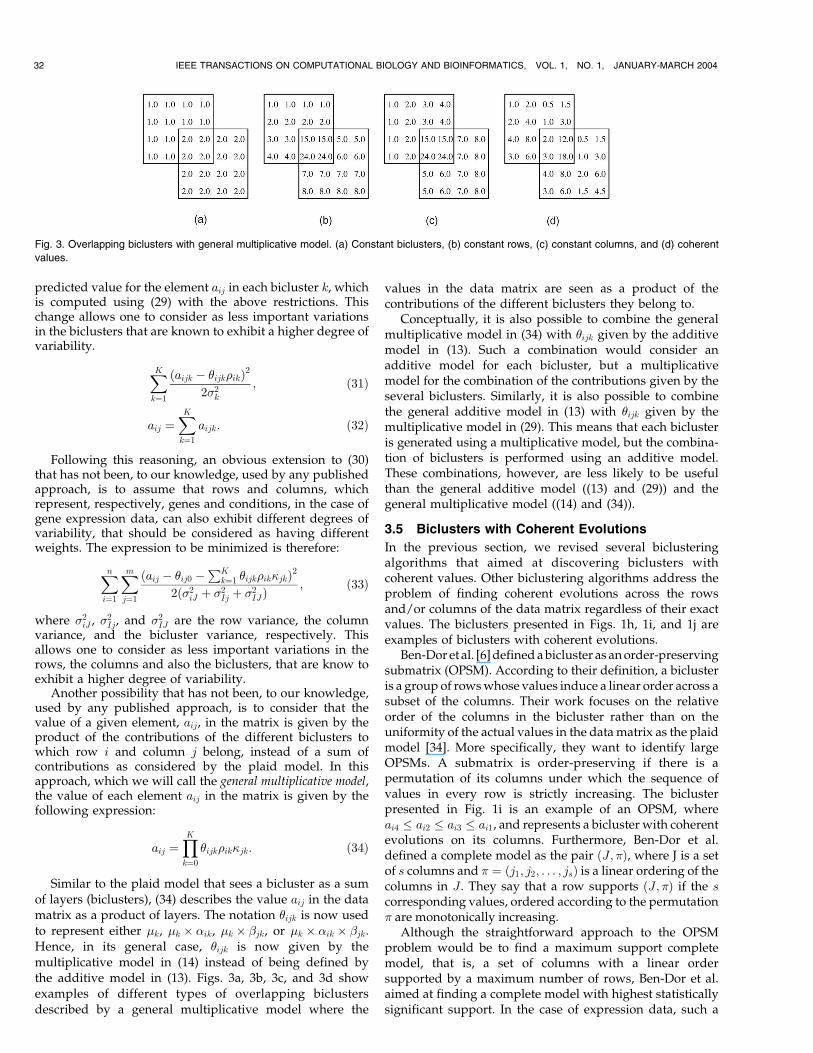
Similar to the plaid model that sees a bicluster as a sumof layers (biclusters), (34) describes the value aij in the datamatrix as a product of layers. The notation �ijk is now usedto represent either �k, �k � �ik, �k � �jk, or �k � �ik � �jk.Hence, in its general case, �ijk is now given by themultiplicative model in (14) instead of being defined bythe additive model in (13). Figs. 3a, 3b, 3c, and 3d showexamples of different types of overlapping biclustersdescribed by a general multiplicative model where the

values in the data matrix are seen as a product of thecontributions of the different biclusters they belong to.

Conceptually, it is also possible to combine the generalmultiplicative model in (34) with �ijk given by the additivemodel in (13). Such a combination would consider anadditive model for each bicluster, but a multiplicativemodel for the combination of the contributions given by theseveral biclusters. Similarly, it is also possible to combinethe general additive model in (13) with �ijk given by themultiplicative model in (29). This means that each biclusteris generated using a multiplicative model, but the combina-tion of biclusters is performed using an additive model.These combinations, however, are less likely to be usefulthan the general additive model ((13) and (29)) and thegeneral multiplicative model ((14) and (34)).

3.5 Biclusters with Coherent Evolutions

In the previous section, we revised several biclusteringalgorithms that aimed at discovering biclusters withcoherent values. Other biclustering algorithms address theproblem of finding coherent evolutions across the rowsand/or columns of the data matrix regardless of their exactvalues. The biclusters presented in Figs. 1h, 1i, and 1j areexamples of biclusters with coherent evolutions.

Ben-Dor et al. [6]definedabicluster as anorder-preservingsubmatrix (OPSM). According to their definition, a biclusteris a group of rowswhose values induce a linear order across asubset of the columns. Their work focuses on the relativeorder of the columns in the bicluster rather than on theuniformity of the actual values in the datamatrix as the plaidmodel [34]. More specifically, they want to identify largeOPSMs. A submatrix is order-preserving if there is apermutation of its columns under which the sequence ofvalues in every row is strictly increasing. The biclusterpresented in Fig. 1i is an example of an OPSM, whereai4 � ai2 � ai3 � ai1, and represents a bicluster with coherentevolutions on its columns. Furthermore, Ben-Dor et al.defined a complete model as the pair ðJ; �Þ, where J is a setof s columns and � ¼ ðj1; j2; . . . ; jsÞ is a linear ordering of thecolumns in J . They say that a row supports ðJ; �Þ if the scorresponding values, ordered according to the permutation� are monotonically increasing.

Although the straightforward approach to the OPSMproblem would be to find a maximum support completemodel, that is, a set of columns with a linear ordersupported by a maximum number of rows, Ben-Dor et al.aimed at finding a complete model with highest statisticallysignificant support. In the case of expression data, such a

32 IEEE TRANSACTIONS ON COMPUTATIONAL BIOLOGY AND BIOINFORMATICS, VOL. 1, NO. 1, JANUARY-MARCH 2004

Fig. 3. Overlapping biclusters with general multiplicative model. (a) Constant biclusters, (b) constant rows, (c) constant columns, and (d) coherent

values.

submatrix is determined by a subset of genes and a subsetof conditions, such that, within the set of conditions, theexpression levels of all genes have the same linear ordering.As such, Ben-Dor et al. addressed the identification andstatistical assessment of coexpressed patterns for large setsof genes, and considered that, in many cases, data containsmore than one such pattern.

Following the same idea, Liu and Wang [35] defined abicluster as an OP-Cluster (Order Preserving Cluster). Theirgoal is also to discover biclusters with coherent evolutionson the columns. Hence, the bicluster presented in Fig. 1i isan example of an OPSM and also of an OP-Cluster.

Murali and Kasif [37] aimed at finding conserved geneexpression motifs (xMOTIFs). They defined an xMOTIF as asubset of genes (rows) that is simultaneously conservedacross a subset of the conditions (columns). The expressionlevel of a gene is conserved across a subset of conditions ifthe gene is in the same state in each of the conditions in thissubset. They consider that a gene state is a range ofexpression values and assume that there are a fixed givennumber of states. These states can simply be upregulationand downregulation, when only two states are considered.An example of a perfect bicluster in this approach is the onepresented in Fig. 1g, where Si is the symbol representingthe preserved state of the row (gene) i.

Murali and Kasif assumed that the data may containseveral xMOTIFs (biclusters) and aimed at finding thelargest xMOTIF: the bicluster that contains the maximumnumber of conserved rows. The merit function used toevaluated the quality of a given bicluster is thus the size ofthe subset of rows that belong to it (subset of rows thatsatisfy the conservation property in the subset of condi-tions). Together with the conservation property, an xMOTIFmust also satisfy size and maximality properties: Thenumber of columns must be in at least an �-fraction of allthe columns in the data matrix, and for every row notbelonging to the xMOTIF, the row must be conserved onlyin a �-fraction of the columns in it. As such, an xMOTIF isdiscarded if the size and maximality conditions are notsatisfied.

Tanay et al. [44] defined a bicluster as a subset of genes(rows) that jointly respond across a subset of conditions(columns). A gene is considered to respond to a certaincondition if its expression level changes significantly at thatcondition with respect to its normal level. Before SAMBA(Statistical-Algorithmic Method for Bicluster Analysis) isapplied, the expression data matrix is modeled as a bipartitegraph whose two parts correspond to conditions (columns)and genes (rows), respectively, with one edge for eachsignificant expression change. Tanay et al. present twostatistical models for the resulting graph. In the simplermodel, they are looking for biclusters that manifest changesrelatively to their normal level, without considering if thechange was an increase or a decrease in the expressionlevel. In the refined model, they look for consistentbiclusters, in which every two conditions must alwayshave the same effect or always have the opposite effect oneach of the genes.

In the simpler model, it is assumed that all the genes in agiven bicluster are regulated (up or down). This means that

their values changed relatively to its normal level, in thesubset of conditions that form the bicluster. The goal is thento find the largest biclusters with the regulation property. Inorder to do that, SAMBA does not try to find any kind ofcoherence on the values aij. It assumes that regardless of itstrue values, aij can be represented by two symbols: S0 orS1, where S1 means change and S0 means no-change. Assuch, the model graph has an edge between a gene and acolumn when there is a change in the expression level ofthat gene in that specific condition. No edge means nochange. A large bicluster is, in this case, one with amaximum number of genes (rows) whose symbol standingfor aij is expected to be S1. The bicluster presented in Fig. 1fis an example of the type of bicluster SAMBA produces, ifwe say that S1 is the symbol that represents a coherentchange relative to normal expression.

In the refined model, the sign of the change is taken intoaccount. This is achieved by assigning a signal cij 2 f�1; 1gto each edge of the graph, and then looking for a biclusterðI; JÞ and an assignment � : I [ J ! f�1; 1g such thatcij ¼ �ðiÞ�ðjÞ. This is equivalent to the selection of a set ofcolumns (conditions) that have always the same or oppositeeffects on the set of rows. As such, the model in Fig. 1jrepresents the type of biclusters that SAMBA can now find.

However, the approach of Tanay et al. is not purelysymbolic since the merit function used to evaluate thequality of a computed bicluster using SAMBA is the weightof the subgraph that models it. Its statistical significance isevaluated by computing the probability of finding atrandom a bicluster with at least its weight. Given that theweight of a subgraph is defined as the sum of the weights ofgene-condition (row-column) pairs in it including edgesand nonedges, weights are assigned to the edges of thebipartite subgraph so that heavy subgraphs correspond tostatistical significant biclusters.

4 BICLUSTER STRUCTURE

Biclustering algorithms assume one of the followingsituations: Either there is only one bicluster in the matrix asin Fig. 4a, or the matrix contains K biclusters, where K is thenumber of biclusters we expect to identify and is usuallydefined apriori.

While most algorithms assume the existence of severalbiclusters [24], [10], [21], [9], [34], [41], [45], [50], [8], [44],[51], [32], [42], [40], [35], [11], others only aim at finding onebicluster. In fact, even though these algorithms can possiblyfind more than one bicluster, the target bicluster is usuallythe best according to some criterion [6], [37].

When the biclustering algorithm assumes the existenceof several biclusters in the data matrix, the followingbicluster structures can be obtained (see Figs. 4b, 4c, 4d, 4e,4f, 4g, 4h, and 4i):

1. Exclusive row and column biclusters (rectangulardiagonal blocks after row and column reorder).

2. Nonoverlapping biclusters with checkerboardstructure.

3. Exclusive-rows biclusters.4. Exclusive-columns biclusters.5. Nonoverlapping biclusters with tree structure.

MADEIRA AND OLIVEIRA: BICLUSTERING ALGORITHMS FOR BIOLOGICAL DATA ANALYSIS: A SURVEY 33

6. Nonoverlapping nonexclusive biclusters.7. Overlapping biclusters with hierarchical structure.8. Arbitrarily positioned overlapping biclusters.

A natural starting point to achieve the goal of identifyingseveral biclusters in a data matrix A is to form a color imageof it with each element colored according to the value of aij.It is natural then to consider ways of reordering the rowsand columns in order to group together similar rows andsimilar columns, thus forming an image with blocks ofsimilar colors. These blocks are subsets of rows and subsetsof columns with similar expression values, hence, biclus-ters. An ideal reordering of the matrix would produce animage with some number K of rectangular blocks on thediagonal (see Fig. 4b). Each block would be nearlyuniformly colored, and the part of the image outside ofthese diagonal blocks would be of a neutral backgroundcolor. This ideal corresponds to the existence of K mutuallyexclusive and exhaustive clusters of rows, and a corre-sponding K-way partitioning of the columns, that is, Kexclusive row and column biclusters. In this structure,every row in the row-block k is expressed within, and onlywithin, those columns in condition-block k. That is, everyrow and every column in the matrix belongs exclusively toone of the K biclusters (see Fig. 4b).

Although this can be the first approach to extract relevantknowledge from gene expression data, it has long beenrecognized that such an ideal reordering will seldom exist inreal data [34]. Facing this fact, the next natural step is toconsider that rows and columnsmaybelong tomore than onebicluster, and assume a checkerboard structure in the datamatrix (see Fig. 4c). By doing this, we allow the existence ofK nonoverlapping and nonexclusive biclusters where eachrow in the data matrix belongs to exactly K biclusters. Thesame applies to columns. Kluger et al. [32] and Cho et al. [11]assumed this structure. The Double Conjugated Clustering(DCC) approach introduced by Busygin et al. [8] can alsoidentify this biclustering structure. However, DCC tends toproduce the structure in Fig. 4b.

Other approaches assume that rows can only belong toone bicluster, while columns, which correspond to condi-tions in the case of gene expression data, can belong to

several biclusters. This structure, which is presented inFig. 4d, assumes exclusive-rows biclusters and was used bySheng et al. [42] and Tang et al. [45]. However, theseapproaches can also produce exclusive-columns biclusterswhen the algorithm uses the opposite orientation of the datamatrix. When this is the case, the columns can only belongto one bicluster while the rows can belong to one or morebiclusters (see Fig. 4e).

The structures presented in Figs. 4b, 4c, 4d, and 4e assumethat the biclusters are exhaustive, that is, that every row andevery column belongs to at least one bicluster. However, wecanconsidernonexhaustivevariationsof these structures thatmake it possible that some rows andcolumnsdonot belong toany bicluster. A nonexhaustive version of the structure inFig. 4b was assumed by Segal et al. [41]. Other exhaustivebicluster structures include the tree structure considered byHartigan [24] and Tibshirani et al. [46] that is depicted inFig. 4f, and the structure in Fig. 4g.Anonexhaustive variationof the structure in Fig. 4g was assumed by Wang et al. [48].None of these structures allow overlapping, that is, none ofthem makes it possible that a particular pair (row, column)belongs to more than one bicluster.

The previous bicluster structures are restrictive in manyways. On one hand, some of them assume that, forvisualization purposes, all the identified biclusters shouldbe observed directly on the data matrix and displayed as acontiguous representation after performing a commonreordering of their rows and columns. On the other hand,others assume that the biclusters are exhaustive, that is, thatevery row and every column in the data matrix belongs toat least one bicluster.

However, it is more likely that, in real data, some rows orcolumns do not belong to any bicluster at all and that thebiclusters overlap in some places. It is, however, possible toenable these twopropertieswithout relaxing thevisualizationproperty if the hierarchical structure proposed by Hartigan[24] is assumed. This structure, depicted in Fig. 4h, requiresthat either the biclusters are disjoint or that one includes theother. Two specializations of this structure are the treestructure presented in Fig. 4f, where the biclusters form a

34 IEEE TRANSACTIONS ON COMPUTATIONAL BIOLOGY AND BIOINFORMATICS, VOL. 1, NO. 1, JANUARY-MARCH 2004

Fig. 4. Bicluster structure. (a) Single bicluster, (b) exclusive row and column biclusters, (c) checkerboard structure, (d) exclusive rows biclusters,(e) exclusive columns biclusters, (f) nonoverlapping biclusters with tree structure, (g) nonoverlapping nonexclusive biclusters, (h) overlappingbiclusters with hierarchical structure, and (i) arbitrarily positioned overlapping biclusters.

tree, and thecheckerboardstructuredepicted inFig.4c,wherethe biclusters and the row and column clusters are all trees.

A more general bicluster structure allows the existence ofK possibly overlapping biclusters without taking intoaccount their direct observation on the data matrix with acommon reordering of its rows and columns. Furthermore,these nonexclusive biclusters can also be nonexhaustive,which means that some rows or columns may not belong toany bicluster. Several biclustering algorithms [10], [34], [21],[9], [45], [44], [6], [37], [40], [35] allow this more generalstructure, which is presented in Fig. 4i.

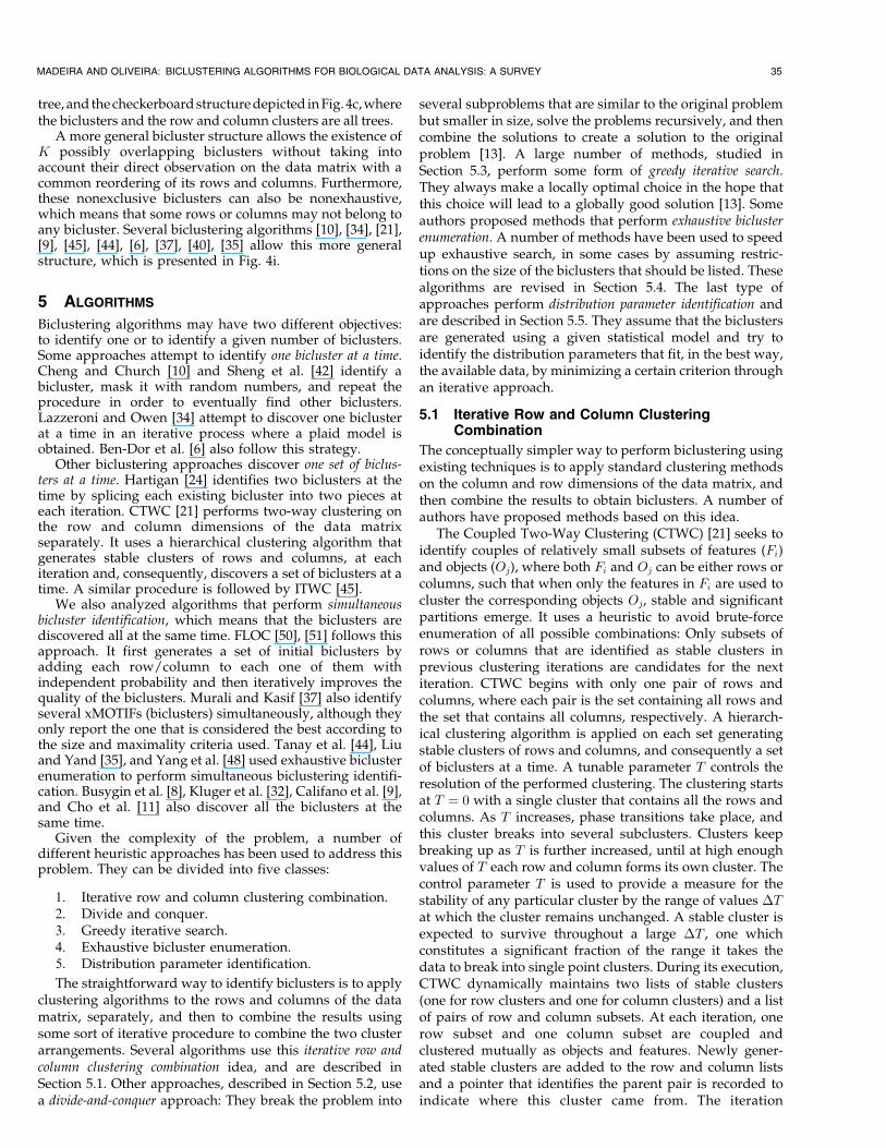
5 ALGORITHMS

Biclustering algorithms may have two different objectives:to identify one or to identify a given number of biclusters.Some approaches attempt to identify one bicluster at a time.Cheng and Church [10] and Sheng et al. [42] identify abicluster, mask it with random numbers, and repeat theprocedure in order to eventually find other biclusters.Lazzeroni and Owen [34] attempt to discover one biclusterat a time in an iterative process where a plaid model isobtained. Ben-Dor et al. [6] also follow this strategy.

Other biclustering approaches discover one set of biclus-ters at a time. Hartigan [24] identifies two biclusters at thetime by splicing each existing bicluster into two pieces ateach iteration. CTWC [21] performs two-way clustering onthe row and column dimensions of the data matrixseparately. It uses a hierarchical clustering algorithm thatgenerates stable clusters of rows and columns, at eachiteration and, consequently, discovers a set of biclusters at atime. A similar procedure is followed by ITWC [45].

We also analyzed algorithms that perform simultaneousbicluster identification, which means that the biclusters arediscovered all at the same time. FLOC [50], [51] follows thisapproach. It first generates a set of initial biclusters byadding each row/column to each one of them withindependent probability and then iteratively improves thequality of the biclusters. Murali and Kasif [37] also identifyseveral xMOTIFs (biclusters) simultaneously, although theyonly report the one that is considered the best according tothe size and maximality criteria used. Tanay et al. [44], Liuand Yand [35], and Yang et al. [48] used exhaustive biclusterenumeration to perform simultaneous biclustering identifi-cation. Busygin et al. [8], Kluger et al. [32], Califano et al. [9],and Cho et al. [11] also discover all the biclusters at thesame time.

Given the complexity of the problem, a number ofdifferent heuristic approaches has been used to address thisproblem. They can be divided into five classes:

1. Iterative row and column clustering combination.2. Divide and conquer.3. Greedy iterative search.4. Exhaustive bicluster enumeration.5. Distribution parameter identification.

The straightforward way to identify biclusters is to applyclustering algorithms to the rows and columns of the datamatrix, separately, and then to combine the results usingsome sort of iterative procedure to combine the two clusterarrangements. Several algorithms use this iterative row andcolumn clustering combination idea, and are described inSection 5.1. Other approaches, described in Section 5.2, usea divide-and-conquer approach: They break the problem into

several subproblems that are similar to the original problembut smaller in size, solve the problems recursively, and thencombine the solutions to create a solution to the originalproblem [13]. A large number of methods, studied inSection 5.3, perform some form of greedy iterative search.They always make a locally optimal choice in the hope thatthis choice will lead to a globally good solution [13]. Someauthors proposed methods that perform exhaustive biclusterenumeration. A number of methods have been used to speedup exhaustive search, in some cases by assuming restric-tions on the size of the biclusters that should be listed. Thesealgorithms are revised in Section 5.4. The last type ofapproaches perform distribution parameter identification andare described in Section 5.5. They assume that the biclustersare generated using a given statistical model and try toidentify the distribution parameters that fit, in the best way,the available data, by minimizing a certain criterion throughan iterative approach.

5.1 Iterative Row and Column ClusteringCombination

The conceptually simpler way to perform biclustering usingexisting techniques is to apply standard clustering methodson the column and row dimensions of the data matrix, andthen combine the results to obtain biclusters. A number ofauthors have proposed methods based on this idea.

The Coupled Two-Way Clustering (CTWC) [21] seeks toidentify couples of relatively small subsets of features (Fi)and objects (Oj), where both Fi and Oj can be either rows orcolumns, such that when only the features in Fi are used tocluster the corresponding objects Oj, stable and significantpartitions emerge. It uses a heuristic to avoid brute-forceenumeration of all possible combinations: Only subsets ofrows or columns that are identified as stable clusters inprevious clustering iterations are candidates for the nextiteration. CTWC begins with only one pair of rows andcolumns, where each pair is the set containing all rows andthe set that contains all columns, respectively. A hierarch-ical clustering algorithm is applied on each set generatingstable clusters of rows and columns, and consequently a setof biclusters at a time. A tunable parameter T controls theresolution of the performed clustering. The clustering startsat T ¼ 0 with a single cluster that contains all the rows andcolumns. As T increases, phase transitions take place, andthis cluster breaks into several subclusters. Clusters keepbreaking up as T is further increased, until at high enoughvalues of T each row and column forms its own cluster. Thecontrol parameter T is used to provide a measure for thestability of any particular cluster by the range of values �Tat which the cluster remains unchanged. A stable cluster isexpected to survive throughout a large �T , one whichconstitutes a significant fraction of the range it takes thedata to break into single point clusters. During its execution,CTWC dynamically maintains two lists of stable clusters(one for row clusters and one for column clusters) and a listof pairs of row and column subsets. At each iteration, onerow subset and one column subset are coupled andclustered mutually as objects and features. Newly gener-ated stable clusters are added to the row and column listsand a pointer that identifies the parent pair is recorded toindicate where this cluster came from. The iteration

MADEIRA AND OLIVEIRA: BICLUSTERING ALGORITHMS FOR BIOLOGICAL DATA ANALYSIS: A SURVEY 35

continues until no new clusters that satisfy some criteriasuch as stability and critical size are found.

The Interrelated Two-Way Clustering (ITWC) [45] is aniterative algorithm based on a combination of the resultsobtained by clustering performed on each of the twodimensions of the data matrix separately. Within eachiteration of ITWC there are five main steps. In the first step,clustering is performed in the row dimension of the matrix.The goal is to cluster n1 rows into K groups, denoted asIi; i ¼ 1; . . . ; K, each of which is an exclusive subset of theset of all rows X. The clustering technique can be anymethod that receives the number of clusters as input. Tanget al. used K-means. In the second step, clustering isperformed in the column dimension of the data matrix.Based on each group Ii; i ¼ 1; . . . ; k, the columns areindependently clustered into two clusters, represented byJi;a and Ji;b. Assume, for simplicity, that the rows have beenclustered into two groups, I1 and I2. The third stepcombines the clustering results from the previous steps bydividing the columns into four groups, Ci, i ¼ 1; . . . ; 4, thatcorrespond to the possible combinations of the columnclusters J1;x and J2;x, x ¼ fa; bg. The fourth step of ITWCaims at finding heterogeneous pairs ðCs; CtÞ, s; t ¼ 1; . . . ; 4.Heterogeneous pairs are groups of columns that do notshare row attributes used for clustering. The result of thisstep is a set of highly disjoint biclusters, defined by the setof columns in Cs and Ct and the rows used to define thecorresponding clusters. Finally, ITWC sorts the rows indescending order of the cosine distance between each rowand a row representative of each bicluster (obtained byconsidering the value 1 in each entry for columns in Cs andCt, respectively). The first one third of rows is kept. Bydoing this, they obtain a reduced row set I 0 for eachheterogeneous group. In order to select the row set I 0 thatshould be chosen for the next iteration they use cross-validation. After this final step, the number of rows isreduced from n1 to n2 and the above steps can be repeatedusing the n2 selected rows until the termination conditionsare satisfied.

The Double Conjugated Clustering (DCC) [8] performsclustering in the rows and columns dimensions/spaces ofthe data matrix using self-organizing maps (SOM) and theangle-metric as similarity measure. The algorithm starts byassigning every node in one space (either a row or acolumn) to a particular node of the second space, which iscalled conjugated node. The clustering is then performed intwo spaces. The first one is called the feature space, havingn dimensions representing the rows of the data matrix. Inthe second space, called the sample space, the roles of thefeatures and samples have been exchanged. This space hasm dimensions, corresponding to the columns of the datamatrix, and is used to perform clustering on the n featureswhich are now the rows of the data matrix.

To convert a node of one space to the other space, DCCmakes use of the angle between the node and each of thepatterns. More precisely, the ith conjugate entry is the dotproduct between the node vector and the ith pattern vectorof the projected space when both the vectors are normalizedto unit length. Formally, they introduce the matrices X1 andX2, which corresponds to the original data matrixX after itscolumns and rows have been normalized to unit length. Thesynchronization between feature and sample spaces is

forced by alternating clustering in both spaces. Theprojected clustering results of one space are used to correctthe positions of the corresponding nodes of the other space.If the node update steps are small enough, both processeswill converge to a state defined by a compromise betweenthe two clusterings. Since the feature and sample spacesmaximize sample and feature similarity, respectively, sucha solution is desirable. DCC works iteratively by perform-ing a clustering cycle, and then transforming each node tothe conjugate space where the next training cycle takesplace. This process is repeated until the number of movedsamples/features falls below a certain threshold in bothspaces. DCC returns two results: one in feature space andone in sample space, each being the conjugate of the other.Since every sample cluster in the feature space correspondsto a feature in the sample space, DCC derives a group ofrows for every group of columns, hence, a set of biclusters.

5.2 Divide-and-Conquer

Divide-and-conquer algorithms have the significant advan-tage of being potentially very fast. However, theseapproaches have the very significant drawback of beinglikely to miss good biclusters that may be split before theycan be identified.

Block clustering was the first divide-and-conquer ap-proachtoperformbiclustering.Blockclustering isa topdown,row and column clustering of the data matrix. The basicalgorithmfor forwardblock splittingwasdue toHartigan [24]who called it direct clustering (see Section 3.2). The blockclustering algorithm begins with the entire data in one block(bicluster). At each iteration, it finds the row or column thatproduces the largest reduction in the total “within block”variance by splitting a given block into two pieces. In order tofind thebest split into twogroups the rowsandcolumnsof thedatamatrix are sortedby rowandcolumnmean, respectively.The splitting continues until a given number K of blocks isobtained or the overall variance within the blocks reaches acertain threshold.

Since the estimation of the optimal number of splicings isdifficult, Duffy and Quiroz [16] suggested the use ofpermutation tests to determine when a given block split isnot significant. Following this direction, Tibshirani et al.[46] added a backward pruning method to the blocksplitting algorithm introduced by Hartigan [24] and de-signed a permutation-based method to induce the optimalnumber of biclusters, K, called Gap Statistics. In theirapproach, the splitting continues until a large number ofblocks are obtained. Some blocks are then recombined untilthe optimal number of blocks is reached. This approach issimilar to the one followed in decision tree algorithms,where the tree is grown until a given depth and is thenpruned.

5.3 Greedy Iterative Search

Greedy iterative search methods are based on the idea ofcreating biclusters by adding or removing rows/columnsfrom them, using a criterion that maximizes the local gain.As such, and although these approaches may make wrongdecisions and loose good biclusters, they have the potentialto be very fast.

Cheng and Church [10] were the first to apply bicluster-ing to gene expression data. Given a data matrix A and amaximum acceptable mean squared residue score (see (18)),

36 IEEE TRANSACTIONS ON COMPUTATIONAL BIOLOGY AND BIOINFORMATICS, VOL. 1, NO. 1, JANUARY-MARCH 2004

� > 0, the goal is to find �-biclusters, that is, subsets of rowsand subsets of columns, ðI; JÞ, with a score no larger than �(see Section 3.4). In order to achieve this goal, Cheng andChurch proposed several greedy row/column removal/addition algorithms that are then combined in an overallapproach that makes it possible to find a given numberK of�-biclusters.

The single node deletion method iteratively removes therow or column that gives the maximum decrease of H. Themultiple node deletion method follows the same idea.However, in each iteration, it deletes all rows and columnswith row/column residue superior to a given threshold.Finally, the node addition method adds rows and columnsthatdonot increase theactual scoreof thebicluster. Inorder tofind a given number,K, of biclusters, greedy node deletion isperformed first and is then followedbygreedynodeaddition.The algorithmdiscovers one bicluster at a time.At each of theK iterations, the algorithms start with an initial bicluster thatcontains all rows and columns. Thismeans that the algorithmstarts with the entire matrix A and stops when no actiondecreasesH or whenH < �. The discovered bicluster is thenreported, and masked with random numbers, so that norecognizable structures remain. The process is repeated untilK biclusters are found.

Although masking previously generated biclusters mightsuggest that it is not possible to find overlapping biclusters,this is in fact possible since the node addition step isperformed using the original values in the data matrix andnot the random ones introduced during the maskingprocess. However, the discovery of highly overlappingbiclusters is not likely, since elements of already identifiedbiclusters have been masked by random noise.

The FLOC (FLexible Overlapped biClustering) algorithm[50], [51] addresses this limitation (see Section 3.4). It is basedon the bicluster definition used by Cheng and Church, butperforms simultaneous bicluster identification. It is alsorobust agains missing values, which are handled by takinginto account the bicluster volume (number of nonmissingelements) when computing the score (see (26)). FLOC avoidsthe introduction of random interference and discovers Kpossibly overlapping biclusters simultaneously.

The algorithm has two phases. In the first phase,K initialbiclusters are generated by adding each row/column toeach one of them with independent probability p. Thesecond phase is an iterative process that improves thequality of these biclusters. During each iteration, each rowand each column is examined to determine the best actionthat can be taken toward reducing the average score residue(see (27)). An action is uniquely defined at any stage withrespect to a row/column and a bicluster. It represents thechange of membership of a row/column with respect to aspecific bicluster: A row/column can be added to thebicluster if it is not yet included in it, or it can be removed ifit already belongs to it. Since there are K biclusters, thereare K potential actions for each row/column. Among theseK actions, the one that has the maximum gain is identifiedand executed. The gain of an action is defined as a functionof the relative reduction of the bicluster residue and therelative enlargement of the bicluster volume. At eachiteration, the set of selected actions is performed according

to a random weighted order that assigns higher probabil-ities of execution to the actions with higher gains. Theoptimization process stops when the potential actions donot improve the overall quality of the biclustering.

Cho et al. [11] introduced two k-means like biclusteringalgorithms that discover k row clusters and l columnclusters simultaneously while monotonically decreasing therespective squared residues defined by Cheng and Church[10] (see (18)). They use the partitioning model proposed byHartigan [24], but optimize global merit functions instead oflocal ones. They also find k� l biclusters simultaneously, asopposed to finding a single bicluster at a time.

The authors partition the matrix A, n�m, into k rowclusters and l column clusters defined, respectively, by thefunctions � : f1; . . . ; ng ! f1; . . . ; kg and : f1; . . . ;mg !f1; . . . ; lg, where �ðiÞ ¼ r implies that row i is in the rowcluster rand ðjÞ ¼ c implies column c is in the columnclusterc. It is also assumed that row cluster r, 1 � r � k, has nr rows,so that n1 þ . . .þ nr ¼ n. Similarly, cluster c, 1 � c � l hasml

columns, so that m1 þ . . .þml ¼ m. This means that everyrow/column belongs to exactly one row/column cluster.Then, they define a row cluster indicatormatrixR, n� k, andacolumncluster indicatormatrixC,m� l. Eachcolumn rofRhas nr nonzeros, each of which equals n�1=2

r . The nonzeros ofC are defined similarly. As every nonzero value in R meansthat row i belongs to a particular row cluster, the first columninR has n1 nonzeros, representing the rows that belong to thefirst row cluster, and so on. Matrix C has a similar structure.WhenR andC are constrained tobe cluster indicatormatricesthe problem of obtaining a global minimum for (18) is NP-hard. Given this, Cho et al. resort to two iterative algorithmsthat monotonically decrease (18) and converge to a localminimum.

The first algorithm is a batch iterative algorithm since, ateach iteration, the column clustering C is updated only afterdetermining the nearest column cluster for every column ofA (likewise for rows). They defined AC ¼ RRTAC andAR ¼ RTACCT , where the columns and rows of thematrices AC and AR play the roles of column clusterprototypes and row cluster prototypes, respectively. Thealgorithm begins with an initialization step. Each iterationinvolves finding the closest column (row) prototype, givenby a column (row) of AC (AR), for each column (row) of Aand setting its column (row) cluster accordingly. Thealgorithm iterates until the decrease in the merit function(18) is smaller than a tolerance � .

The second algorithm is an incremental algorithm, whoseidea is similar to the definition of action in FLOC [50], [51].Cho et al. formulated incremental schemes for movingcolumns (rows) between column (row) clusters if such amove leads to a decrease in themerit function. Each call of theincremental procedures tries to perform such amove for eachrow and column of the data matrix. Since moving a row orcolumn from its current cluster to an empty cluster wouldalways lead to a decrease in themerit function (assuming no-degeneracy), such a move is always made guaranteeing thatno cluster is empty. Although onemove ismade at a time, theauthors suggestmaking a chain ofmoves for obtaining betterlocal minima. Variants of the algorithm perform any move

MADEIRA AND OLIVEIRA: BICLUSTERING ALGORITHMS FOR BIOLOGICAL DATA ANALYSIS: A SURVEY 37

that leads to a decrease in the merit function instead ofinsisting on the best possible move.

Since the difficulty in minimizing (18) is introduced bythe strong structural constraints on R and C, Cho et al.suggest relaxing those constraints to just seek columnorthogonal matrices R and C in order to ease minimization.They then use a spectral approximation for initialization.When this relaxed solution is obtained, it is then necessaryto obtain a biclustering. The authors suggest using k-means,among other techniques, to cluster the rows of R and C andobtain row/column clusters from the clustered R and C.

Ben-Dor et al. [6] addressed the identification of largeorder-preserving submatrices (OPSMs) with maximumstatistical significance (see Section 3.5). In order to do that,they assume a probabilistic model of the data matrix wherethere is a bicluster ðI; JÞ determined by a set of rows I, a setof columns J and a linear ordering of the columns in J .Within each row of ðI; JÞ the order of the elements isconsistent with the linear ordering of J . They define acomplete model as the pair ðJ; �Þ where J is a set of scolumns and � ¼ ðj1; j2; . . . ; jsÞ is a linear ordering of thecolumns in J . A row supports ðJ; �Þ if the s correspondingvalues, ordered according to the permutation �, aremonotonically increasing.

Since an exhaustive algorithm that tries all possiblecomplete models is not feasible, the idea is to grow partialmodels iteratively until they become complete models. Apartial model of order ða; bÞ specifies, in order, the indices ofthe a “smallest” elements < j1; . . . ; ja > and the indices ofthe b “largest” elements < js�ðb�1Þ; . . . ; js > of a completemodel ðJ; �Þ and its size s. The OPSM algorithm focus onthe columns at the extremes of the ordering when definingpartial models, assuming that these columns are moreuseful in identifying the target rows, that is, the rows thatsupport the assumed linear order. The algorithm starts byevaluating all ð1; 1Þ partial models and keeping the best l ofthem. It then expands them to ð2; 1Þ models and keeps thebest l of them. After that, it expands them to ð2; 2Þ models,ð3; 2Þ models, and so on, until it gets l ð½s=2�; ½s=2�Þ models,which are complete models. It then outputs the best one.

Murali and Kasif [37] introduced an algorithm that aimsat finding xMOTIFs. An xMOTIF is a bicluster withcoherent evolutions on its rows (see Section 3.5). The datais first discretized into a set of symbols by using a list ofstatistically significant intervals, for each row. To determinean xMOTIF, it is necessary to compute the set of conservedrows, I, the states that these rows are in, and the set ofcolumns, J , that match the xMOTIF. Given the set ofconserved rows, I, the states of the conserved rows, and onecolumn c that matches a given motif, it is easy to computethe remaining conditions in J simply by checking, for eachcolumn c0, if the rows in I are in the same state in c and c0.Column c is called a “seed” from which the entire motif canbe computed. The motifs are computed starting with a set ofrandomly chosen columns that act as seeds. For eachcolumn, an additional randomly chosen set D of columns isselected, called a discriminating set. The selected biclustercontains all the rows that have states equal in the seedcolumn and in the columns contained in the discriminatingset D. The motif is discarded if less than an �-fraction of the

columns match it. After all the seeds have been used toproduce xMOTIFs, the largest xMOTIF (one with the largestnumber of rows) is returned.

Califano et al. [9] introduced an algorithm that addressesthe problem of finding �-valid ks-patterns (see Section 3.4).Their goal is to find groups of rows that exhibit coherentvalues in a subset of the columns, but do not have anycoherence of values in any of the remaining columns. Afterpreprocessing the data, they use a pattern discoveryalgorithm to discover sets of rows and columns candidatesto be statistically significant biclusters (the other candidatesare discarded). Finally, an optimal set of patterns is chosenamong the statistically significant ones using a greedy setcovering algorithm that adds rows and columns to theexisting patterns so that they become maximal patterns (seeSection 3.4).

The pattern discovery algorithm used considers that eachcolumn of the data matrix is a string and discovers patternsin these strings by allowing all possible string alignments. Adensity constraint is used to limit the impact of randommatches occurring over large distances on the strings andthe strings are prealigned before the algorithm is used. Thealgorithm starts with a single pattern with no rows, all thecolumns, and an offset of zero for each column. The valuesin each column are then sorted and all subsets ofcontinuous values that are �-valid (see Section 3.4) areselected. Nonmaximal subsets that are completely con-tained within another subset are removed. Each subset isconsidered a potential super-pattern of a maximal pattern.All possible maximal combinations of these super-patternsare then created iteratively. As a result, all patterns thatexists in the data matrix are generated hierarchically bypattern combination.

5.4 Exhaustive Bicluster Enumeration

Exhaustive bicluster enumeration methods are based on theidea that the best biclusters can only be identified using anexhaustive enumeration of all possible biclusters existent inthe matrix. These algorithms certainly find the bestbiclusters, if they exist, but have a very serious drawback.Due to their high complexity, they can only be executed byassuming restrictions on the size of the biclusters. As such,these methods perform exhaustive enumeration assumingsome restrictions on the input instances and using efficientalgorithmic techniques designed to make the enumerationfeasible.

Tanay et al. [44] introduced SAMBA (Statistical-Algo-rithmic Method for Bicluster Analysis), a biclusteringalgorithm that performs simultaneous bicluster identifica-tion by using exhaustive enumeration. SAMBA avoids anexponential runtime by restricting the number of rows thebiclusters may exhibit. They use the graph formalismdescribed in Section 2.1, and define as their objective theidentification of a maximum weight subgraph, assumingthat the weight of a subgraph will correspond to itsstatistical significance. Discovering the most significantbiclusters under this weighting schemes is equivalent tothe selection of the heaviest subgraphs in the modelbipartite graph. SAMBA assumes that row vertices haved-bounded degree. This corresponds to a restriction on thesize of the discovered biclusters since the number of rows

38 IEEE TRANSACTIONS ON COMPUTATIONAL BIOLOGY AND BIOINFORMATICS, VOL. 1, NO. 1, JANUARY-MARCH 2004

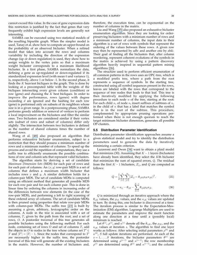
cannot exceed this value. In the case of gene expression datathis restriction is justified by the fact that genes that veryfrequently exhibit high expression levels are generally notinteresting.

SAMBA can be executed using two statistical models ofthe resulting bipartite graph. When the simpler model isused, Tanay et al. show how to compute an upper-bound onthe probability of an observed bicluster. When a refinedmodel that takes into account the rows and columnsvariability by including the direction of the expressionchange (up or down regulation) is used, they show how toassign weights to the vertex pairs so that a maximumweight bicluster corresponds to a maximum likelihoodbicluster. In a first phase, SAMBA normalizes the data,defining a gene as up-regulated or down-regulated if itsstandardized expression level (with mean 0 and variance 1),is, respectively, above 1 or below -1. In the second phase, itfinds the K heaviest bicliques in the graph. This is done bylooking at a precomputed table with the weights of thebicliques intersecting every given column (condition) orrow (gene) and choosing the K best bicliques. In order toimprove the performance, rows (genes) with degreeexceeding d are ignored and the hashing for each row(gene) is performed only on subsets of its neighbors whosesize is in a given range. In a postprocessing phase, SAMBAperforms greedy addition or removal of vertices to performa local improvement on the biclusters and filter the similarones. Two biclusters are considered similar if their vertexsets (subset of rows and subset of columns) differ onlyslightly. The intersection between two biclusters is definedas the number of shared columns times the number ofshared rows.

Wang et al. [48] also proposed an algorithm thatperforms exhaustive bicluster enumeration, subject to arestriction that they should possess a minimum number ofrows and a minimum number of columns. To speed up theprocess and avoid the repetition of computations, they use asuffix tree to efficiently enumerate the possible combina-tions of row and column sets that represent valid biclusters.

The algorithm starts by deriving a set of candidateMaximum Dimension Sets (MDS) for each pair of rows andfor each pair of columns. An ðx; yÞ row-pair MDS is a set ofcolumns that defines a maximum width bicluster thatincludes rows x and y. A similar definition holds for acolumn-pair MDS. The set of candidate MDSs is computedusing an efficient method that generates all possible MDSfor each row pair and for each column pair. This is done inlinear time by ordering the columns in increasing order ofthe differences between row elements (in the case of therow-pair MDS), and performing a left to right scanning ofthese ordered array of columns. The set of candidate MDSsis then pruned using properties that relate row-pair MDSswith column-pair MDSs. The suffix tree [23] is built byassuming a given, arbitrary, lexicographic order on thecolumns. A node in the tree is associated with a set ofcolumns, T , given by the path from the root, and a set ofrows, O. A postorder traversal of this tree generates allpossible biclusters using the following method: For eachnode, containing set of rows O and set of columns T , addthe objects in O to nodes in the tree whose column set T 0 2T and jT 0j ¼ jT j � 1. Since the nodes that correspond to T 0

are necessarily higher in the suffix tree, the postordertraversal of this tree will generate all the existing biclustersin the matrix. However, the number of biclusters and,

therefore, the execution time, can be exponential on thenumber of columns in the matrix.

Liu and Wang [35] also proposed an exhaustive biclusterenumeration algorithm. Since they are looking for order-preserving biclusters with a minimum number of rows anda minimum number of columns, the input data to theiralgorithm is a set of rows with symbols that represent theordering of the values between these rows. A given rowmay then be represented by adbc and another one by abdc.Their goal of finding all the biclusters that, after columnreordering, represent coherent evolutions of the symbols inthe matrix is achieved by using a pattern discoveryalgorithm heavily inspired in sequential pattern miningalgorithms [26].

The structure used to perform efficient enumeration ofall common patterns in the rows uses an OPC-tree, which isa modified prefix tree, where a path from the rootrepresents a sequence of symbols. In the starting tree,constructed using all symbol sequences present in the rows,leaves are labeled with the rows that correspond to thesequence of tree nodes that leads to that leaf. This tree isthen iteratively modified by applying the followingprocedure to each node n of the tree, starting at the root:For each child nc of node n, insert suffixes of subtrees of nc

in the child of n that has a label that matches the symbolthat is in the root of the subtree. This procedure,complemented by appropriate pruning operations per-formed when there is not enough quorum to reach thetarget minimum bicluster dimension, generates all possibleOP-clusters.

5.5 Distribution Parameter Identification

Distribution parameter identification approaches assume agiven statistical model and try to identify the distributionparameters used to generate the data by iterativelyminimizing a certain criterion.

Lazzeroni and Owen [34] want to obtain a plaid modelthat minimizes (30). Assuming that K � 1 layers (biclusters)have already been identified, they select the Kth biclusterthat minimizes the sum of squared errors, Q. The residualfrom the first K � 1 biclusters, Zij, and Q are computed asfollows:

Q ¼ 1

2

Xni¼1

Xmj¼1

ðZij � �ijK�iKjKÞ2; ð35Þ

Zij ¼ aij � �ij0 �XK�1

k¼1

�ijk�ikjk: ð36Þ

Q is minimized through an iterative approach where the�ijK values, the �iK values, and the jK values are updatedin turn. By doing this, one bicluster is discovered at a time.The iteration process is similar to the Expectation-Max-imization (EM) algorithm. Lagrange Multipliers are used toestimate the parameters and improve the merit functionalong one direction at a time until a (possibly local)minimum is reached.

Let �ðsÞ, �ðsÞ, and ðsÞ denote all the �ijK , the �iK , and thejK values at iteration s. The algorithm to find one layerworks as follows: After selecting initial parameters �ð0Þ andð0Þ, S full update iterations are performed. At each of thes ¼ 1; . . . ; S iterations, the bicluster parameters �ðsÞ aredetermined using �ðs�1Þ and ðs�1Þ; the row membership�ðsÞ are determined using �ðsÞ and ðs�1Þ; and the column

MADEIRA AND OLIVEIRA: BICLUSTERING ALGORITHMS FOR BIOLOGICAL DATA ANALYSIS: A SURVEY 39

membership ðsÞ are determined using �ðsÞ and �ðs�1Þ. Atintermediate stages, the values of �ijK describe a “fuzzy”membership function in which �iK and jK are notnecessarily 0 or 1. To update the �ijK values given �iK andjK , the expression in (35) is minimized subject to therestrictions that every row and column has zero mean. Thesame reasoning is applied to estimate the remainingparameters. Given a set of K layers, the �ijk values canthen be reestimated by cycling through k ¼ 1; . . . ; K in turn.

Segal et al. [41] use PRMs (see Section 3.3) to model thejoint distribution of the values of the gene and arraymembership functions (�þ �i þ �j). The estimation of theparameters of the PRMs has two main components:learning the structure of the dependencies and estimationof the parameters of the distribution. Learning the structureof the dependencies between variables is equivalent tolearning the structure of a Bayes network. To further restrictthe different possible structures and the number ofparameters, the authors assume that dependencies betweenvariables can be represented by a CPD-tree [17]. Theselection of the most likely structures is performed usingBayesian model selection techniques. The search is per-formed using an almost-greedy search method, where localminima are avoided by using a variant of simulatedannealing. The search takes place by applying localtransformations to the CPD-trees.

Once the structure is learned, parameter estimation isperformedbyobtaining themaximumlikelihoodestimator ofeach parameter, assuming multinomial distributions for thediscrete parameters and Gaussian distributions for thecontinuous parameters. Since some variables are not ob-servable (namely, the bicluster membership variables), theexpectation-maximizationmethod is applied. In this case,EMis applied by alternating the two following steps: 1) filling inthevaluesobtained for eachhiddenvariable given the currentparameters of the distribution and 2) reestimating theparameters by assuming these guesses are correct using thestandard maximum likelihood estimating procedure.

A more general model proposed by Segal et al. [40]allows overlapping biclusters and uses a similar approachto estimate the parameters of the distributions. However, inthis case, the structure of the dependencies is fixed, sinceactivity levels are assumed to depend on a specific andfixed way on the bicluster assignment variables. As such,the structure estimation phases are not required, and EM isused to estimate the parameters of the distribution. Unlikethe plaid model [34], all the bicluster membership functionsare reestimated at each step of the iteration, leading to abetter fit of the experimental data.

Sheng et al. [42] introduced a biclustering approachbased on Gibbs sampling. The row-column (gene-condition)orientation of the matrix is assumed. The algorithm couldalso be applied on the column-row (condition-gene)orientation. They use multinomial distributions to modelthe data for every column in a bicluster, and assume thatthe multinomial distributions for different columns in abicluster are mutually independent. Gibbs sampling is usedto estimate the parameters of the multinomial distributionsused to model the data.

The algorithm to find one bicluster in the row-columnorientation of the data matrix works as follows: Theinitialization step randomly assigns row labels and conditionlabels the value 1 or 0, where 1 means that the row/columnbelongs to the bicluster and 0means it does not belong. In thesecond step of the algorithm, the goal is to fix the labels of the

columns. In order to do that, for every row i, i ¼ 1; . . . ; n, thelabels for all the other rows are fixed while the Bernoullidistribution for the given row i is computed. A label is thenassigned to row i from the computed distribution. Similarly,step three sets the labels of the columns. The parameters forboth rowand columndistributions are estimatedusingGibbssampling. These steps are iterated for a predefinednumber ofiterations. In order to detect multiple biclusters, Sheng et al.mask the rows that belong to the previously found biclusterby setting the row labels of the foundbiclusterpermanently tozero. Their approach discovers one bicluster at a time and itworks by not considering as candidate rows for any futurebicluster rows that have already been considered. This choiceallows theunmaskeddimensionof the bicluster to be selectedmultiple times. The algorithm is iterateduntil no bicluster canbe found for the unmasked part of the data matrix.

Kluger et al. [32] used a spectral approach to biclusteringby assuming that, after normalization, the matrix contains acheckerboard structure. Supposing there are ways tonormalize the original matrix A and the resulting matrixis A0, the idea is to solve the eigenvalue problem A0TA0x ¼�2x and examine the eigenvectors x. If the constants in aneigenvector can be sorted to produce a step-like structure,the column clusters can be identified accordingly. The rowclusters are found similarly from y satisfying A0A0T y ¼ �2y.More precisely, Kluger et al. show that the checkerboardpattern in a matrix A is reflected in the constant structuresof the pair of eigenvectors x and y that solved the coupledeigenvalue problem A0TA0x ¼ �2x and A0TA0y ¼ �2y, wherex and y have a common eigenvalue. The algorithm dependscritically on the normalization procedure used to transformthe matrix.

Kluger et al. proposed three normalization methods. Thefirst normalization method (independent rescaling of rowsand columns) assumes the nonnormalizedmatrix is obtainedbymultiplyingeach row ibya scalar ri andeach column jbyascalar cj, then ri1=ri2 ¼ mean of row i1/mean of row i2 ¼ai1J=ai2J (see (14)). Assuming thatR is a diagonalmatrixwithentries ri at the diagonal and C is a diagonal matrix definedsimilarly, then the eigen problem can be formulated byrescaling the data matrix: AA � R�1=2AC�1=2. The secondmethod (bistochastization) works by repeating the indepen-dent scaling of rows and columns until stability is reached.The finalmatrixhasall rowssumtoaconstantandall columnssum to a different constant. The third method (log-interac-tions) assumes that if the original rows/columns differ bymultiplicative constants, then after taking their logarithm,theydifferbyadditive constants (see (13) and (14)).Moreover,each row and column is expected to have zeromean. This canbe achieved by transforming each entry as follows: a0ij ¼aij � aIj � aiJ þ aIJ . Note that a0ij is the residue of the eachelement aij of the data matrixA as it was defined in (16).

6 OVERALL COMPARISON OF THE BICLUSTERING

ALGORITHMS

Table 2 presents a summary of the different algorithms inaccordance with the different dimensions of analysisconsidered. The second column presents the type ofbiclusters (see Section 3). Column three lists the biclusterstructure they can produce. The notation used is the one inFig. 4 in Section 4. The last two columns summarizeSection 5 and classify the different algorithms according to

40 IEEE TRANSACTIONS ON COMPUTATIONAL BIOLOGY AND BIOINFORMATICS, VOL. 1, NO. 1, JANUARY-MARCH 2004

the way they discover the biclusters and the approach used.The notation used is the following: iterative row andcolumn clustering combination (Clust-Comb), divide-and-conquer (Div-Conq), greedy iterative search (Greedy),exhaustive bicluster enumeration (Exh-Enum), and distri-bution parameter identification (Dist-Based).

An objective evaluation of the quality and efficiency ofthe different approaches is outside the scope of this surveysince it requires extensive evaluations under controlledconditions. We plan, however, to conduct such evaluationsin the future. Objective evaluations, in terms of the qualityof the biclusters, are presented in the original references.This quality is assessed using one of the three followingmethods:

1. Value of the merit function. Authors that have usedthis approach evaluate the quality of the solution byanalyzing the value of the merit function directly.This is a good indicator of the coherence observed inthe resulting biclusters [24], [46], [10], [34], [50], [48],[51], [11]. In the cases where there is an explicitstatistical model underlying the merit function, thisapproach can also be viewed directly as a statisticalassessment of the quality of the solution [41], [40],[42], [37]. Two-way clustering approaches [21], [45],[8] do not evaluate the quality of the resultingbiclustering directly. Instead, they evaluate thequality of the clustering performed on each of thetwo dimensions separately.

2. Statistical significance of the solution, measuredagainst the null hypothesis. Authors that have usedthis approach assess the quality of the solutions byapplying statistical significance tests. These testsderive the statistical significance of the solutionsselected by the algorithms by computing the prob-ability of random appearance of these biclusters inuncorrelated data, generated in accordance with aspecific distribution [9], [44], [6], [32].

3. Comparison against known solutions. When testedin synthetic data, it is possible to compare thebiclusters obtained with the biclusters that have beenplanted in the synthetic data. Several authors haveused this approach. In real-world data, it is alsosometimes possible (although considerably harder)to identify biclusters that correspond to knownprocesses and to score the solutions by howeffectively they approximate the known solutions.When the solutions are used to perform classifica-tion (gene or sample classification), this classificationcan also be compared with known results [46], [41],[9], [10], [21], [34], [45], [44], [8], [6], [50], [48], [40],[42], [32], [37], [51], [11].

An evaluation of the computational complexity andefficiency of the methods is very difficult to performwithout resorting to extensive benchmarking. In fact, sincethe problem is NP-hard, all the methods resort to heuristicsthat are not easily amenable to direct complexity analysis.Iterative methods, used in the large majority of theapproaches, are heavily dependent not only on thecomputational complexity per iteration that can be com-puted in a relatively straightforward way, but also on thenumber of iterations necessary to reach a solution. Thenumber of iterations cannot, in general, be defined a priori,and represents the major factor constraining the efficiencyof these methods.

Another important issue regards the adequacy of themodels to real data. In this aspect, there is a clear movetoward the use of more flexible merit functions andstructures, reflecting the need to take into account thecomplex interactions between the processes that define thevalues in the matrix. In particular, general additive/multi-plicative models and/or general probabilistic models thatcan model overlapping biclusters are required to modelmore precisely the data that is obtained from geneexpression analysis. This move toward more complex

MADEIRA AND OLIVEIRA: BICLUSTERING ALGORITHMS FOR BIOLOGICAL DATA ANALYSIS: A SURVEY 41

TABLE 2Overall Comparison of the Biclustering Algorithms

models also has an impact on the complexity of thealgorithms required to find optimal solutions.

7 BICLUSTERING APPLICATIONS

Biclustering can be applied whenever the data to analyzehas the form of a real-valued matrix A, where the set ofvalues aij represent the relation between its rows i and itscolumns j, and the goal is to identify subsets of rows withcertain coherence properties in a subsets of the columns.

Most biological applications of biclustering are performedusing gene expression data obtained using microarraytechnologies that allow the measurement of the expressionlevel of thousands of genes in target experimental conditions.Since this technology provides a snapshot of all the genesexpressed in a cell at a given time, and gene expression is thefundamental link between genotype and phenotype, theanalysis of gene expression data is bound to play amajor rolein our understanding of biological processes and systemsincluding gene regulation, development, evolution, anddisease mechanisms [5]. In this application domain, we canuse biclusters to associate genes with specific clinical classesor for classifying genes and samples, among other potentiallyinteresting applications.

The applications of biclustering to biological dataanalysis, including several examples using gene expressiondata and some examples using other biological data, arediscussed in Section 7.1. Section 7.2 presents severalnonbiological applications of biclustering. In fact, althoughthe majority of the recent applications of biclustering are inbiological data analysis, there are several interestingapplication of biclustering in other domains.

7.1 Biological Applications

Reported results of biclustering applied to gene expressiondata have used the data sets in Table 3. All these data setscontain expression data collected from either yeast or

human cells using microarray technologies, which repre-sents the expression level of a set of genes under specificconditions.

Several authors [10], [34], [41], [44], [50], [48], [51], [35],[40] used biclustering to analyze one or several of sixexpression matrices collected from yeast [43], [12], [19], [28],[18], [29] (see Table 3 for details). Other authors [46], [10],[21], [9], [45], [44], [6], [8], [37], [32], [42], [11] analyzed oneor more of eleven different expression matrices withHuman gene expression levels [49], [22], [3], [30], [2], [25],[31], [33], [52], [4], [39] (see Table 3 for details). Interestingly,almost all these data sets contain expression data related tothe study of cancer. Some contain data from canceroustissues at different stages of the disease; others analyze datafrom different individuals suffering from different types ofcancer; and the remaining data sets contain data collectedfrom several individuals with a particular cancer or healthypeople.

These data sets have been used to test the applicability ofbiclustering approaches in three major tasks:

1. Identification of coregulated genes.2. Gene functional annotation.3. Sample classification.

Table 3 summarizes the biclustering applications to gene

expression data analysis and relates the different tasks withthe different datasets used.

A number of authors [10], [34], [21], [41], [44], [6], [50],[48], [40], [51], [35], [11] have studied the application ofbiclustering techniques to the problem of identification ofcoregulated genes. More specifically, the objective was toidentify sets of genes that, under specific conditions,exhibited coherent activations that indicate coregulation.The results of this may be used to simply identify sets ofcoregulated genes or, more ambitiously, to identify specificregulation processes.

42 IEEE TRANSACTIONS ON COMPUTATIONAL BIOLOGY AND BIOINFORMATICS, VOL. 1, NO. 1, JANUARY-MARCH 2004

TABLE 3Gene Expresion Data Sets Analyzed Using Biclustering Techniques and Its Applications

A less obvious application is to use the biclusteringresults directly to perform automatic gene functionalannotation, as proposed by other authors [41], [44], [40].The idea underlying this approach is to use biclusters wherea large majority of genes belong to a specific class in thegene ontology to guess the class of nonannotated genes.

Another significant area of application is related withsample and/or tissue classification [46], [9], [21], [45], [44],[8], [32], [37], [42]. In leukemia diagnosis [21], [37], [42], forinstance, the goal was to identify different responses totreatment, and the group of genes to be used as the mosteffective probe.

All the previous applications of biclustering analyzeddatafrom gene expressionmatrices. However, biclustering can beinteresting in the analysis of other biological data. Liu andWang [35] applied biclustering to a drug activity data set.They wanted to find groups of chemical compounds withsimilar behaviors when subsets of compound descriptorswere taken into account. Lazzeroni et al. [34] analyzednutritional data to identify subsets of foods with similarproperties on a subset of food attributes.

7.2 Other Applications

Apart from interesting biological applications, biclusteringcan also have successfully applications in relevant areassuch as: information retrieval and text mining, collaborativefiltering, recommendation systems, target marketing andmarket research, database research, and data mining.

Biclustering can be useful in collaborative filtering toidentify subgroups of customers with similar preferences orbehaviors toward a subset of products. The goal is toperform target marketing or use the information providedby the biclusters in recommendation systems. Recommen-dation systems and target marketing are important applica-tions in the E-commerce area. Many authors appliedbiclustering to collaborative filtering using data where therows represented customers and the columns movies [50],[51], [48], [47], [27]. The values aij in the data matrix showwhether customer i watched movie j (binary values), orrepresent the rate customer i assigned to movie j (discretevalues). Both Hoffman and Puzicha [27] and Ungar andFoster [47] used approaches similar to the one of Sheng et al.[42]. While Ungar and Foster used the Expectation-Max-imization (EM) algorithm, Hoffman and Puzicha usedGibbs sampling.

Gaul and Schader [20] showed the relevance of bicluster-ing in the market research and marketing by using datamatrices containing data collected during marketing cam-paigns.

In information retrieval and text mining, biclustering canbe used successfully to identify subgroups of documentswith similar properties relatively to subgroups of attributes,such as words or images. This information can be veryimportant in query and indexing in the domain of searchengines. Several authors used data matrices where the rowsrepresented words and the columns documents [14], [7],[15]. In the simpler problem formulations, the values aijshow whether word i is present in document j (binaryvalues). In more complex data, a nonzero element aijindicates the presence of word i in document j using a realvalue that represents its relevance relatively to thatdocument and taking into account its presence in thecollection of documents. In this application domain, thistype of data is called incidence matrix and the termcoclustering is generally used instead of biclustering. The

approaches are similar to the ones analyzed in the previoussections. Dhillon [14], for instance, modeled the data matrixas a bipartite graph as Tanay et al. [44] and used a spectralapproach similar to the one used by Kluger et al. [32].

Biclustering can also be used to perform dimensionalityreduction in databases with tables with thousands ofrecords (rows) with hundreds of fields (columns). Thisapplication of biclustering is what the database communitycalls automatic subspace clustering of high dimensionaldata, which is extremely relevant in data mining applica-tions. This problem was addressed by Agrawal et al. [1].

More exotic applications of biclustering involved theanalysis of data matrices with electoral data [24] and foreignexchange data [34]. Hartigan [24] used electoral data withthe goal of identifying subgroups of rows (countries) withthe same political ideas and electoral behaviors among asubset of the columns (issues). Lazzeroni et al. [34] analyzedforeign exchange data to identify subsets of currencies withsimilar behaviors in subsets of months.

8 CONCLUSIONS

We have presented a comprehensive survey of the models,methods, and applications developed in the field ofbiclustering algorithms. The list of applications presentedis by no means exhaustive, and an all-inclusive list ofpotential applications would be prohibitively long. Fromthe list of models and approaches analyzed in Sections 3, 4,5, and 6, it is our opinion that the scientific community hasalready available a large plethora of models and algorithmsto choose from. In particular, the general additive andmultiplicative frameworks are rich enough to appropriatelymodel very complex interactive processes.

The list of available algorithms is also very extense, andmany combinations of ideas can be adapted to obtain newalgorithms potentially more effective in particular applica-tions. We believe that the systematic organization presentedin this work can be used by the interested researcher as agood starting point to learn and apply some of the manytechniques proposed in the last few years, and some of theolder ones. The list of applications presented, long as it isalready, represents, in our view, only a small fraction of thepotential applications of this type of techniques. Many otherapplications in biological data analysis, gene networkidentification, data mining, and collaborative filteringremain to be explored.

Many interesting directions for future research havebeen uncovered by this review work. The tuning andvalidation of biclustering methods by comparison withknown biological data is certainly one of the most importantopen issues. Another interesting area is the application ofrobust biclustering techniques to new and existing applica-tion domains. Many issues in biclustering algorithm designalso remain open and should be addressed by the scientificcommunity. From these open issues, we select the analysisof the statistical significance of biclusters as one of the mostimportant ones, since the extraction of a large number ofbiclusters in real data may lead to results that are difficult tointerpret.

ACKNOWLEDGMENTS

The authors would like to thank Ana Teresa Freitas formany interesting and fruitful discussions on the subject ofbiclustering algorithms and applications.

MADEIRA AND OLIVEIRA: BICLUSTERING ALGORITHMS FOR BIOLOGICAL DATA ANALYSIS: A SURVEY 43

REFERENCES

[1] R. Agrawal, J. Gehrke, D. Gunopulus, and P. Raghavan,“Automatic Subspace Clustering of High Dimensional Data forData Mining Applications,” Proc. ACM/SIGMOD Int’l Conf.Management of Data, pp. 94-105, 1998.

[2] A.A. Alizadeh, M.B. Eisen, R.E. Davis, C. Ma, I.S. Lossos, A.Rosenwald, J.C. Boldrick, H. Sabet, T. Tran, X. Yu, J.I. Powell, L.Yang, G.E. Marti, T. Moore, J. Hudson, L. Lu, D.B. Lewis, R.Tibshirani, G. Sherlock, W.C. Chan, T.C. Greiner, D.D. Weisen-burger, J.O. Armitage, R. Warnke, R. Levy, W. Wilson, M.R.Grever, J.C. Byrd, D. Botstein, P.O. Brown, and L.M. Staudt,“Distinct Types of Diffuse Large B-Cell Lymphoma Identified byGene Expression Profiling,” Nature, vol. 403, pp. 503-511, 2000.

[3] U. Alon, N. Barkai, D.A. Notterman, K. Gish, S. Ybarra, D. Mack,and A.J. Levine, “Broad Patterns of Gene Expression Revealed byClustering of Tumor and Normal Colon Tissues Probed byOligonucleotide Arrays,” Natural Academy of Sciences, vol. 96,no. 12, pp. 6745-6750, 1999.

[4] S.A. Armstrong, J.E. Staunton, L.B. Silverman, R. Pieters, M.L. denBoer, M.D. Minden, S.E. Sallan, E.S. Lander, T.R. Golub, and S.J.Korsmeyer, “Mll Translocations Specify a Distinct Gene Expres-sion Profile that Distinguishes a Unique Leukemia,” NatureGenetics, vol. 30, pp. 41-47, 2002.

[5] P. Baldi and G.W. Hatfield, DNA Microarrays and Gene Expression.From Experiments to Data Analysis and Modelling. Cambridge Univ.Press, 2002.

[6] A. Ben-Dor, B. Chor, R. Karp, and Z. Yakhini, “Discovering LocalStructure in Gene Expression Data: The Order-Preserving Sub-matrix Problem,” Proc. Sixth Int’l Conf. Computational Biology(RECOMB ’02), pp. 49-57, 2002.

[7] P. Berkhin and J.D. Becher, “Learning Simple Relations: Theoryand Applications,” Proc. Second SIAM Int’l Conf. Data Mining,pp. 420-436, 2002.

[8] S. Busygin, G. Jacobsen, and E. Kramer, “Double ConjugatedClustering Applied to Leukemia Microarray Data,” Proc. SecondSIAM Int’l Conf. Data Mining, Workshop Clustering High Dimen-sional Data, 2002.

[9] A. Califano, G. Stolovitzky, and Y. Tu, “Analysis of GeneExpression Microarays for Phenotype Classification,” Proc. Int’lConf. Computacional Molecular Biology, pp. 75-85, 2000.

[10] Y. Cheng and G.M. Church, “Biclustering of Expression Data,”Proc. Eighth Int’l Conf. Intelligent Systems for Molecular Biology(ISMB ’00), pp. 93-103, 2000.

[11] H. Cho, I.S. Dhillon, Y. Guan, and S. Sra, “Minimum Sum-SquaredResidue Cococlustering of Gene Expression Data,” Proc. FourthSIAM Int’l Conf. Data Mining, 2004.

[12] R.J. Cho,M.J. Campbell, E.A.Winzeler, L. Steinmetz, A. Conway, L.Wodicka, T.G. Wolfsberg, A.E. Gabrielian, D. Landsman, D.J.Lockhart, and R.W. Davis, “A Genome-Wide TranscriptionalAnalysis of the Mitotic Cell Cycle,” Molecular Cell, vol. 2, pp. 65-73, 1998.

[13] T.H. Cormen, C.E. Leiserson, R.L. Rivest, and C. Stein, Introductionto Algorithms, The MIT Electrical Eng, and Computer ScienceSeries, The MIT Press, second ed., 2001.

[14] I.S. Dhillon, “Co-Clustering Documents and Words UsingBipartite Spectral Graph Partitioning,” Proc. Seventh ACMSIGKDD Int’l Conf. Knowledge Discovery and Data Mining (KDD’01), pp. 269-274, 2001.

[15] I.S. Dhillon, S. Mallela, and D.S. Modha, “Information-TheoreticalCoclustering,” Proc. Ninth ACM SIGKDD Int’l Conf. KnowledgeDiscovery and Data Mining (KDD ’03), pp. 89-98, 2003.

[16] D. Duffy and A. Quiroz, “A Permutation Based Algorithm forBlock Clustering,” J. Classification, vol. 8, pp. 65-91, 1991.

[17] N. Friedman and M. Goldszmidt, “Learning Bayesian Networkswith Local Structure,” Learning in Graphical Models, Kluwer,pp. 421-460, 1998.

[18] A.P. Gasch, M. Huang, S. Metzner, D. Botstein, S.J. Elledge, andP.O. Brown, “Genomic Expression Responses to DNA-DamagingAgents and the Regulatory Role of the Yeast ATR Homologmec1p,” Molecular Biology of the Cell, vol. 12, pp. 2987-3003, 2001.

[19] A.P. Gasch, P.T. Spellman, C.M. Kao, O. Carmel-Harel, M.B.Eisen, G. Storz, D. Botstein, and P.O. Brown, “Genomic ExpressionPrograms in the Response of Yeast Cells to EnvironmentalChanges,” Molecular Biology of the Cell, vol. 11, pp. 4241-4257, 2000.

[20] W. Gaul and M. Schader, “A New Algorithm for Two-ModeClustering,” Data Analysis and Information Systems, H. Hermannand W. Polasek, eds., Springer, pp. 15-23, 1996.

[21] G. Getz, E. Levine, and E. Domany, “Coupled Two-WayClustering Analysis of Gene Microarray Data,” Proc. NaturalAcademy of Sciences US, pp. 12079-12084, 2000.

[22] T.R. Golub, D.K. Slonim, P. Tamayo, C. Huard, M. Gaasenbeek,J.P. Mesirov, H. Coller, M.L. Loh, J.R. Downing, M.A. Caligiuri,C.D. Bloomfield, and E.S. Lander, “Molecular Classification ofCancer: Class Discovery and Class Prediction by Gene ExpressionMonitoring,” Science, vol. 286, pp. 531-537, 1999.

[23] D. Gusfield, Algorithms on Strings, Trees, and Sequences. ComputerScience and Computational Biology Series, Cambridge Univ.Press, 1997.

[24] J.A. Hartigan, “Direct Clustering of a Data Matrix,” J. Am.Statistical Assoc. (JASA), vol. 67, no. 337, pp. 123-129, 1972.

[25] I. Hedenfalk, D. Duggan, Y. Chen, M. Radmacher, M. Bittner, R.Simon, P. Meltzer, B. Gusterson, M. Esteller, M. Raffeld, Z.Yakhini, A. Ben-Dor, E. Dougherty, J. Kononen, L. Bubendorf, W.Fehrle, S. Pittaluga, S. Gruvberger, N. Loman, O. Johannsson, H.Olsson, B. Wilfond, G. Sauter, O.P. Kallioniemi, A. Borg, and J.Trent, “Gene-Expression Profiles in Hereditary Breast Cancer,”New England J. Medicine, vol. 344, no. 8, pp. 539-548, 2000.

[26] J. Hipp, U. Guntzer, and G. Nakhaeizadeh, “Algorithms forAssociation Rule Mining—A General Survey and Comparison,”SIGKDD Explorations, vol. 2, no. 1, pp. 58-64, July 2000.

[27] T. Hofmann and J. Puzicha, “Latent Class Models for Collabora-tive Filtering,” Proc. Int’l Joint Conf. Artificial Intelligence, pp. 668-693, 1999.

[28] T.R. Hughes, M.J. Marton, A.R. Jones, C.J. Roberts, R. Stoughton,C.D. Armour, H.A. Bennett, E. Coffey, H. Dai, Y.D. He, M.J. Kidd,A.M. King, M.R. Meyer, D. Slade, P.Y. Lum, S.B. Stepaniants, D.D.Shoemaker, D. Gachotte, K. Chakraburtty, J. Simon, M. Bard, andS.H. Friend, “Functional Discovery via a Compendium ofExpression Profiles,” Cell, vol. 102, pp. 109-126, 2000.

[29] T. Ideker, V. Thorsson, J.A. Ranish, R. Christmas, J. Buhler, J.K.Eng, R. Bumgarner, D.R. Goodlett, ? Aebersold, and L. Hood,“Integrated Genomic and Proteomic Analyses of a SystematicallyPerturbed Metabolic Network,” Science, vol. 292, pp. 929-934, 2001.

[30] V.R. Iyer, M.B. Eisen, D.T. Ross, G. Schuler, T. Moore, J.C.F. Lee,J.M. Trent, L.M. Staudt, J. Hudson Jr., M.S. Boguski, D. Lashkari,D. Shalon, D. Botstein, and P.O. Brown, “The TranscriptionalProgram in the Response of Human Fibroblasts to Serum,” Science,vol. 283, pp. 83-87, 1999.

[31] U. Klein, Y. Tu, G.A. Stolovitzky, M. Mattioli, G. Cattoretti, H.Husson, A. Freedman, G. Inghirami, L. Cro, L. Baldini, A. Neri, A.Califano, and R. Dalla-Favera, “Gene Expression Profiling of B-Cell Chronic Lymphocytic Leukemia Reveals a HomogeneousPhenotype Related to Memory B Cells,” J. Experimental Medicine,vol. 194, pp. 1625-1638, 2001.

[32] Y. Klugar, R. Basri, J.T. Chang, and M. Gerstein, “SpectralBiclustering of Microarray Data: Coclustering Genes and Condi-tions,” Genome Research, vol. 13, pp. 703-716, 2003.

[33] U. Kluger, B. Kacinski, Y. Kluger, O. Mironenko, M. Gilmore-Hebert, J. Chang, A. Perkins, and E. Sapi, “Microarray Analysis ofInvasive and Metatastic Phenotypes in a Breast Cancer Model,”Poster Presented at the Gordon Conf. Cancer, 2001.

[34] L. Lazzeroni and A. Owen, “Plaid Models for Gene ExpressionData,” technical report, Stanford Univ., 2000.

[35] J. Liu and W. Wang, “OP-Cluster: Clustering by Tendency in HighDimensional Space,” Proc. Third IEEE Int’l Conf. Data Mining,pp. 187-194, 2003.

[36] B. Mirkin, “Nonconvex Optimization and its Applications,” Math.Classification and Clustering, Kluwer Academic Publishers, 1996.

[37] T.M. Murali and S. Kasif, “Extracting Conserved Gene ExpressionMotifs from Gene Expression Data,” Proc. Pacific Symp. Biocomput-ing, vol. 8, pp. 77-88, 2003.

[38] R. Peeters, “The Maximum Edge Biclique Problem is NP-Complete,” Discrete Applied Math., vol. 131, no. 3, pp. 651-654,2003.

[39] S.L. Pomeroy, P. Tamayo, M. Gaasenbeek, L.M. Sturla, M. Angelo,M.E. McLaughlin, J.Y. Kim, L.C. Goumnerova, P.M. Black, C. Lau,J.C. Allen, D. Zagzag, J.M. Olson, T. Curran, C. Wetmore, J.A.Biegel, T. Poggio, S. Mukherjee, R. Rifkin, A. Califano, G.Stolovitzky, D.N. Louis, J.P. Mesirov, E.S. Lander, and T.R. Golub,“Prediction of Central Nervous System Embryonal TumourOutcome Based on Gene Expression,” Nature, vol. 415, no. 6870,pp. 436-442, 2002.

44 IEEE TRANSACTIONS ON COMPUTATIONAL BIOLOGY AND BIOINFORMATICS, VOL. 1, NO. 1, JANUARY-MARCH 2004

[40] E. Segal, A. Battle, and D. Koller, “Decomposing Gene Expressioninto Cellular Processes,” Proc. Pacific Symp. Biocomputing, vol. 8,pp. 89-100, 2003.

[41] E. Segal, B. Taskar, A. Gasch, N. Friedman, and D. Koller, “RichProbabilistic Models for Gene Expression,” Bioinformatics, vol. 17,pp. S243-S252, 2001.

[42] Q. Sheng, Y. Moreau, and B. De Moor, “Biclustering MicroarrayData by Gibbs Sampling,” Bioinformatics, vol. 19, pp. ii196-ii205,2003.

[43] P.T. Spellman, G. Sherlock, M.Q. Zhang, V.R. Iyer, K. Anders,M.B. Eisen, P.O. Brown, D. Botstein, and B. Futcher, “Compre-hensive Identification of Cell Cycle-Regulated Genes of the YeastSaccharomyces Cerevisiae by Microarray Hybridization,” Mole-cular Biology of the Cell, vol. 9, pp. 3273-3297, 1998.

[44] A. Tanay, R. Sharan, and R. Shamir, “Discovering StatisticallySignificant Biclusters in Gene Expression Data,” Bioinformatics,vol. 18, pp. S136-S144, 2002.

[45] C. Tang, L. Zhang, I. Zhang, and M. Ramanathan, “InterrelatedTwo-Way Clustering: An Unsupervised Approach for GeneExpression Data Analysis,” Proc. Second IEEE Int’l Symp. Bioinfor-matics and Bioeng., pp. 41-48, 2001.

[46] R. Tibshirani, T. Hastie, M. Eisen, D. Ross, D. Botstein, and P.Brown, “Clustering Methods for the Analysis of DNA MicroarrayData,” technical report, Dept. of Health Research and Policy, Dept.of Genetics, and Dept. of Biochemestry, Stanford Univ., 1999.

[47] L. Ungar and D.P. Foster, “A Formal Statistical Approach toCollaborative Filtering,” Proc. Conf. Automated Learning andDiscovery (CONALD ’98), 1998.

[48] H. Wang, W. Wang, J. Yang, and P.S. Yu, “Clustering by PatternSimilarity in Large Data Sets,” Proc. 2002 ACM SIGMOD Int’l Conf.Management of Data, pp. 394-405, 2002.

[49] J.N. Weinstein, T.G. Myers, P.M. O’Connor, S.H. Friend, A.J.Fornace Jr., K.W. Kohn, T. Fojo, S.E. Bates, L.V. Rubinstein, N.L.Anderson, J.K. Buolamwini, W.W. Van Osdol, A.P. Monks, D.A.Scudiero, E.A. Sausville, D.W. Zaharevitz, B. Bunow, V.N.Viswanadhan, G.S. Johnson, R.E. Wittes, and K.D. Paull, “AnInformation-Intensive Approach to the Molecular Pharmacologyof Cancer,” Science, vol. 275, pp. 343-349, 1997.

[50] J. Yang, W. Wang, H. Wang, and P. Yu, “�-Clusters: CapturingSubspace Correlation in a Large Data Set,” Proc. 18th IEEE Int’lConf. Data Eng., pp. 517-528, 2002.

[51] J. Yang, W. Wang, H. Wang, and P. Yu, “Enhanced Biclustering onExpression Data,” Proc. Third IEEE Conf. Bioinformatics and Bioeng.,pp. 321-327, 2003.

[52] V. Yong, S. Chabot, Q. Stuve, and G. Williams, “Interferon Beta inthe Treatment of Multiple Sclerosis: Mechanisms of Action,”Neurology, vol. 51, pp. 682-689, 1998.

Sara C. Madeira received the BSc degree incomputer science from the University of BeiraInterior in 2000, and the Msc degree in computerengineering and computer science from LisbonTechnical University in 2002. She is currently aPhD student at IST, Lisbon Technical University,and an assistant lecturer in the ComputerScience Department at the University of BeiraInterior. She is also an invited researcher atINESC-ID. Her research interests include bioin-

formatics, data mining, and machine learning.

Arlindo L. Oliveira received the BSc (Eng) andthe MSc degrees in electrical and computerengineering from Lisbon Technical University,and the PhD degree in electrical engineeringand computer science from the University ofCalifornia, Berkeley, in 1994. He is currently anassociate professor at IST, Lisbon TechnicalUniversity. He is also a senior researcher atINESC-ID. His research interests include bioin-formatics, string processing, combinatorial opti-

mization, machine learning, logic synthesis, and automata theory. He isa member of the IEEE and the IEEE Computer Society.

. For more information on this or any other computing topic,please visit our Digital Library at www.computer.org/publications/dlib.

MADEIRA AND OLIVEIRA: BICLUSTERING ALGORITHMS FOR BIOLOGICAL DATA ANALYSIS: A SURVEY 45