Reconstructing the Great Recession∗

Michele BoldrinWashington University in St. LouisFederal Reserve Bank of St Louis

Carlos GarrigaFederal Reserve Bank of St. Louis

Adrian Peralta-AlvaInternational Monetary Fund

Juan M. SanchezFederal Reserve Bank of St. Louis

This draft: March 18, 2014First draft: February 15, 2012

Abstract

This paper evaluates the role of the construction sector in accounting for the per-formance of the U.S. economy during the Great Recession. Despite its small size itis interlinked with other sectors in the economy amplifying changes in the demandfor residential investment on the overall economy. The importance of interlinkages isquantified in a dynamic multi-sector model parameterized to reproduce the boom-bustdynamics of construction employment in the period 2000-10. The model suggests thatthe interlinkages account for a large share of the actual changes in aggregate employ-ment and gross domestic product during the expansion and the recession.

Keywords: Residential investment, multisector models, business cycle accountingJ.E.L. codes: E22, E32, O41

∗The authors are grateful for the stimulating discussions with Bill Dupor, Ayse Imrohoroglu, RodyManuelli, Alex Monge-Naranjo, Jorge Roldos and the seminar participants at the Bank of Canada, SouthernMethodist University, International Monetary Fund, 2012 Wien Macroeconomic Workshop, 2012 ITAMSummer Camp in Macroeconomics, the 2012 SED, Stony Brook, and Queens College CUNY. ConstanzaLiborio, James D. Eubanks and You Chien provided excellent research assistance. The views expressedherein do not necessarily reflect those of the Federal Reserve Bank of St. Louis or those of the FederalReserve System.

1

1 Introduction

Several U.S. macroeconomic aggregates, such as employment and gross domestic product(GDP), have yet to return to pre-Great Recession trends. While there is still no consensuson why the recovery of the U.S. economy has been slow compared with a traditional postwarrecession, some point to the role of the construction sector.1 This sector collapsed as thereal estate bubble burst in 2007, an event commonly believed to be the key factor underlyingthe U.S. Great Recession and the poor economic performance that followed. Constructiongenerally contributes about 5 percent of employment and output, but in this particularepisode, it had an unprecedented decline following the largest expansion in employmentsince the 1950s.

Why the construction sector collapsed is unclear for the simple reason that what createdthe boom in the first place is also unclear. Be that as it may, there is general agreement thatthe bursting of home values did translate into a sudden drop in the demand for a specificasset in which American households had, until then, invested a substantial portion of theirwealth: residential housing. The analysis starts from this (hopefully) incontrovertible factand studies the contribution of the construction sector to U.S. economic growth, particularlyduring the construction boom and the Great Recession.

The macroeconomic impact of the construction sector is derived from its interlinkageswith other productive sectors of the economy. These linkages propagate the effect of a declinein demand for residential investment to the rest of the economy. This paper argues that theconstruction sector has been an important driver of the dynamics of aggregate employmentand output in the U.S. economy through sectoral interlinkages.

A simple way to analyze the contribution of the construction sector to the evolution ofthese aggregate dynamics and, in particular, the slow recovery, is to use input-output tables.Using the requirement matrices allows comparison of the evolution of U.S. employment andgross output with an artificial economy where the construction sector has been completelyeliminated.2 The difference between these paths can be attributed to the construction sector.The elimination of the construction sector implies a lower demand for productive inputs fromother sectors. These other sectors in the economy would have to reduce their respectiverequirements of productive inputs and so forth. Figure 1 clearly illustrates, in fact, thatthe dynamics of employment and gross output for these two economies are very different.

1Leamer (2007), who argues that since World War II the U.S. economy has had eight recessions precededby substantial problems in housing and consumer durables.

2For each year available in the Bureau of Economic Analysis (BEA) and Bureau of Labor Statistics(BLS) requirement tables. The effect of a shock to the construction sector of the size of its total output wascomputed using the corresponding table to calculate the impact of the construction industry on total grossoutput and total employment. Those values were then removed, together with the values of the constructionindustry per se, from the aggregate gross output and value added of the U.S. economy, year by year. In thefigure construction includes real estate and leasing.

2

For the U.S. economy (including construction) total employment increased about 6 percentbetween 2002 and 2006. All that employment growth was lost during the Great Recessionand continued to decline in 2010. In contrast, the economy without a construction sectorhas a slower recovery from the 2001 recession but rapid employment growth in 2005. Thisartificial economy does not start the employment destruction until 2008, and the magnitudeof the employment decline is half that of the other economy. In addition, unlike the economywith construction, the recovery starts in 2010. This exercise shows that the constructionsector was a clear factor contributing to employment growth between 2002 and 2005 andhas dragged since the Great Recession. A similar conclusion can be drawn by analyzing theseries for gross output.

Figure 1: Construction Sector’s Contribution to the Dynamics of Employment and GrossOutput

1998 2000 2002 2004 2006 2008 2010 201297

98

99

100

101

102

103

104

105

106

107Employment

Year

Inde

x, 2

002=

100

Without Construction, Total EffectWith ConstructionWithout Construction, Direct Effect

1998 2000 2002 2004 2006 2008 2010 201290

95

100

105

110

115

120Gross Output

Year

Inde

x, 2

002=

100

Without Construction, Total EffectWith ConstructionWithout Construction, Direct Effect

Source: Authors’ calculations using Bureau of Economic Analysis (BEA) and Bureau of Labor Statistics

(BLS) Requirement Tables.

Our empirical analysis shows the role of sectoral interlinkages in propagating changesin housing demand to other sectors of the economy. A simple accounting input-outputframework reveals that construction accounts for 52 percent of the decline in employmentand 35 percent of the decline in output. The input-output model is static and does not allow

3

for movement in relative prices. To highlight the functioning of the paper’s main mechanismwe construct a simple (static) multisector model. The model reveals that the effects of adecline in housing demand are amplified in the presence of sectoral interlinkages and whenhousing is complementary to other goods. In the absence of these mechanisms, the modelsuggests that a decline in construction should not propagate to other sectors.

To assess the quantitative importance of sectoral interlinkages, we construct a dynamicmultisector model with residential investment and interconnected sectors.3 The presence ofirreversibility constraints introduces an asymmetry between expansions and the recessions.4

During the expansion, the increasing housing demand results in uncharacteristically highGDP levels and growth, driven by extremely high levels of output in the construction andhousing sector and in all related activities. Growth is constrained only by the accumulationof capital and residential structures. The decline in housing demand stops economic growthand the inflated levels of economic activity collapse. As a direct impact, this leaves theeconomy with (potentially) a surplus of equipment (residential structures) appropriate forhousing-related activities but not easily transferable to other productive activities. Therelatively low depreciation of residential structures implies that home values, the constructionsector, and aggregate consumption and investment should take a long time to recover. Whenthe irreversibility constraint binds for an extended period, the asymmetric effect betweenbooms and busts is magnified. In addition, sectoral linkages interact with the final demandfor goods, other than housing, in the case of complementarities (i.e., durables, housing-related expenditures). Hence, a decline in the demand for housing indirectly reduces thedemand of the complementary goods and, thus, the output from these sectors. As a result,the magnitude of the impact on output and total employment can be amplified when thisadditional mechanism operates.

To quantify the contribution of construction to the overall economy, we calibrated a se-quence of demand shifters in consumer preferences to match the dynamics of employmentin construction for different model specifications with and without interlinkages. Qualita-tively the effects are similar in these economies, but quantitatively, the magnitude of theboom-bust cycle in total employment and output is substantially larger with sectoral inter-

3The methodology in our paper is close to that of Davis and Heathcote (2005). They study the dynamicsof residential investment and house prices in a multisector business cycle model. Their model is successfulin reproducing the volatility of residential investment, but they do not focus on the propagation of shocksdue to sectoral interlinkages.

4The analysis abstracts from both the increase in the burden of debt brought about by the decline inhome prices (which is the focus of Garriga et al., 2012b) and the reduction in credit activity it implied, twofactors that are likely to have played (and may still be playing) a major role in the overall process. Althoughthese factors could interact with the sectoral interlinkages, abstracting from them captures the contributionof the real side of the economy in the recession. In the model, a decline in the demand for homes generatesa readjustment of the portfolio and a decline in the demand for intermediate inputs. The lower demand ofintermediate goods deprives the real side of the economy and generates a significant decline in employmentand real activity.

4

linkages. During the boom, both sectors expand and contribute to the growth of outputand employment by 2 percent and 2.5 percent, respectively. During the housing bust, themagnitude depends on the number of periods the irreversibility constraint binds. This am-plifies the asymmetric response between the boom and the bust episode. When this effectis quantitatively important, the decline in output is 3.3 percent and in employment is 3.8percent. For a lower degree of complementarity, the asymmetric effect is not as large butstill significant. To identify the role of interlinkages, we perform two exercises to control forthe contribution of intermediate goods during the construction boom and bust. In thosecases, changes in housing demand consistent with the dynamics in construction employmentplay only a small role in macroeconomic quantities even when the complementarity betweenconsumption goods and housing services is high.

In the model, all changes in employment and output are generated by variations inhousing demand. We can calculate the contribution of construction observed in the databy comparing the magnitudes generated by the model. During the expansion between 2002and 2007, the construction sector accounts for a significant share of growth of employment(between 29 percent and 61 percent) and GDP (between 8 percent and 15 percent). Moreimportantly, its contribution during the Great Recession was between 28 percent and 43percent of employment and 43 percent and 60 percent of GDP.

The burst of the real estate “bubble” might have substantially lowered potential outputand created a substantial “displacement effect” for both labor and capital that may takequite some time to fully absorb. Some researchers have referred to this displacement effectas a worsening of the labor frictions. For example, Arellano et al. (2010) and Ohanian andRaffo (2012) attribute to this factor, most of the recession, whereas total factor productivityhas been less important. Since the model captures a significant decline in employment andoutput, we also perform a business cycle accounting exercise on simulated data from themodel. The model does not have any distortions, but the intersectoral linkages, movementson relative prices across sectors, and the effects on the demand for labor input can beinterpreted as distortions through the lens of the one-sector neoclassical growth model. Thismethodology attributes the recession in our model to the labor wedge. The magnitude ofthe worsening of the labor wedge is about 62 percent of the total change observed in thedata. Importantly, in both our model and the data the worsening is due to the consumerside of the labor wedge and not to differences between wages and the marginal product oflabor.

Note that the causal links discussed here operate in an environment not subject to themarket failures and price-adjustment frictions now standard in business cycle models usedto guide fiscal and mainly monetary policy. In the language of those models, ours is a modelof potential output in which fluctuations of economic activity cannot be counteracted withstandard policy tools. Our findings are important for policy discussions using those modelsbecause they imply that output gaps may not be as large as previously thought.

The contribution of the construction sector cannot fully account for the dynamics of

5

employment and output since 2002. Other relevant factors not incorporated in the analysisare certainly important. Many suggest (Black, 1995; Hall, 2011; Kocherlakota, 2012) thathigh interest rates could be responsible for the slow recovery. These authors argue that evenin models with perfect competition and price flexibility (i.e., lacking the typical frictions inbusiness cycle models), too-high levels of interest rates may result in substantially lower levelsof output and employment. Since some interest rates appear to be currently constrained bythe zero lower bound, such analyses appear particularly pertinent. Others argue that thelevel of uncertainty (Bloom, 2009; Arellano et al., 2010), government policies (Herkenhoffand Ohanian, 2011), and excessive debt overhang in the economy (Garriga et al., 2012a,b;Herkenhoff and Ohanian, 2012; Kehoe et al., 2013) may be responsible for the lacklusterrecovery.

The remainder of the paper is organized as follows. In section 2, we present some empir-ical evidence and perform standard calculations using the input-output matrix of the U.S.economy. Section 3 presents a simple static model of interdependence that is used to illus-trate the key mechanism at work in the analysis. Section 4 presents the quantitative model.Section 5 reports the numerical results and the robustness analysis. Section 6 compares theimplications of the model in terms of business cycle accounting methodology, and Section 7offers some concluding comments.

2 Empirical Analysis

This section explores the role of construction in accounting for aggregate fluctuations in theU.S. using detailed sectorial input-output data for the period 1990-2012. The main findingis that construction played crucial role in the Great Recession. Despite the relatively smalsize of the construction sector, the analysis suggests that its contribution to this recessionwas large due to the size of the shock together with strong interlinkages with other sectors.5

2.1 The role of construction for aggregate fluctuations:1990-2012

According to the National Bureau of Economic Analysis (NBER) dating of recessions, thereare three recessions since 1990. The top panel of Table 1 shows that the 1990-91 recessionwas not severe: since the peak of 1990-Q3 to the trough of 1991-Q1 both employment andincome decline by less than 1 percent. In contrast, the decline in construction was sizeable:It was slightly less than 6 percent for employment and above 7 percent for income. One could

5In the analysis hereafter, the definition of the construction sector does not include “real estate andleasing” because the “construction” sector is quite different than “real estate and leasing.” The analysisperformed including this additional sectors in the definition of construction increases the significance of thissector in accounting for the Great Recession.

6

argue that the role of the construction sector was important, but the recession was relativelymild. The middle panel of Table 1 shows the recession that started in 2000-Q1 and endedin 2001-Q4. This recession was slightly more severe than the previous one: employmentfell by more than 1 percent and income by more than 2 percent. However, the decline ofconstruction was less severe than the aggregate and thus the share of the aggregate declineaccounted by the construction sector was small.

The Great Recession started in 2007:Q4 and lasted until 2009:Q2. During this periodtotal employment decreased abruptly, by roughly 8 million jobs. Table 1 shows that the dropin construction employment and value added account for about 20 percent of the total. Thisis the recession study in this paper because of its severity and the importance of construction.The importance of construction is explained by the large decline in construction employmentand income, both close to 20 percent.

The numbers presented above are a conservative estimate of the role of construction be-cause the importance of interlinkages are not considered. The analysis in the next subsectionuses Input-Output data to incorporate interlinkages into the analysis.

7

Table 1: The role of construction in the last three recessions, direct effect

Employment IncomeConstruction, Total, Construction, Total,

millions millions millions millions

1990-91 RecessionPeak, 1990Q3 5.24 109.6 346.0 7455Trough 1991Q1 4.93 108.7 320.6 7400Change, thousands -0.31 -0.87 -25.4 -54.9Change, % -5.88 -0.79 -7.35 -0.74

Share accounted by construction, % 35.4 46.3

2000-01 RecessionPeak 2000Q1 6.84 132.6 610.4 10870Trough 2001Q4 6.79 131.0 598.7 10629Change, thousands -0.05 -1.55 -11.70 -241.1Changes, % -0.75 -1.17 -1.92 -2.22

Share accounted by construction, % 3.3 4.9

2007-09 RecessionPeak 2007Q4 7.53 137.9 682.3 12586Trough 2009Q2 6.09 131.0 540.5 11852Change, thousands -1.4 -6.9 -141.8 -734.0Changes, % -19.1 -5.0 -20.8 -5.83

Share accounted by construction, % 20.8 19.3

2.2 Construction during the Great Recession

The construction industry went into recession 18 months before the overall economy. Em-ployment fell from 7.7 million in 2006:Q3 to 5.5 million in 2011:Q1; it still has not emergedfrom the trough and the decrease may well continue in the future. Figure 2 shows thatemployment, gross output, and GDP in the construction sector dropped about 30 percentduring this period, with the largest year-to-year decline between 2008 and 2009.

8

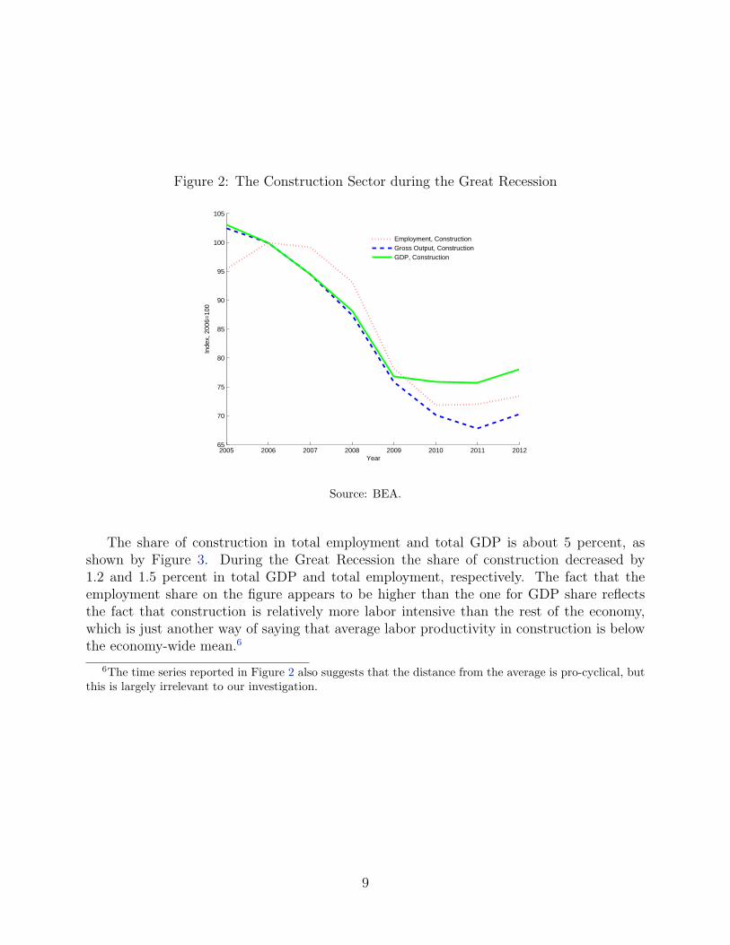
Figure 2: The Construction Sector during the Great Recession

2005 2006 2007 2008 2009 2010 2011 201265

70

75

80

85

90

95

100

105

Year

Inde

x, 2

006=

100

Employment, ConstructionGross Output, ConstructionGDP, Construction

Source: BEA.

The share of construction in total employment and total GDP is about 5 percent, asshown by Figure 3. During the Great Recession the share of construction decreased by1.2 and 1.5 percent in total GDP and total employment, respectively. The fact that theemployment share on the figure appears to be higher than the one for GDP share reflectsthe fact that construction is relatively more labor intensive than the rest of the economy,which is just another way of saying that average labor productivity in construction is belowthe economy-wide mean.6

6The time series reported in Figure 2 also suggests that the distance from the average is pro-cyclical, butthis is largely irrelevant to our investigation.

9

Figure 3: Construction in the U.S. Economy

Share of Construction in the Economy Spending and Redsidential Investment

1940 1950 1960 1970 1980 1990 2000 2010 20203

3.5

4

4.5

5

5.5

6

Year

Per

cent

Sha

re o

f Tot

al

Employment, ConstructionGDP, Construction

1960 1970 1980 1990 2000 2010 2020200

400

600

800

1000

1200

1400

Year

Bill

ions

(Cha

ined

200

9 $)

Private Residential InvestmentSpending on Construction

Source: Authors’ calculations using BEA data.

The dynamics of the demand for construction can be seen in the behavior of privateresidential investment and total spending on construction. The right panel in Figure 3shows that both series have an abrupt decline between 2006 and 2010, while the extent oftheir growth between roughly 1990 and 2006 shows that the real estate boom of those yearswas exceptional by historical standards.

2.3 Construction in an Interlinked Economy

The evidence presented in this section suggests that the total impact of the drop in theconstruction sector on the overall economy could have been even larger due to the presenceof sectorial interlinkages. Figure 4 depicts the share of the gross output of each industrypurchased as intermediate inputs by the construction industry.

10

Figure 4: Construction Purchases from Other Sectors

0 1 2 3 4 5 6 7 8

Agriculture

Mining

Utilities

Construction

Manufacturing

Wholesale

Retail

Trans.& Ware.

Information

Financial

Prof. & Bus.

Educ. & Health

Arts & Rec.

Other Services

Percent of Industry’s Gross Output

Source: 2006 Use matrix from the BEA input-output tables.

One way to interpret the data is to imagine a total collapse of the construction industry.In that case, construction would buy nothing from other industries and the numbers in Figure4 would represent the percentage drop in each industry’s output after such an event whileabstracting from interlinkages between those sectors. For instance, gross output in bothmanufacturing and retail would fall by roughly 6 and 7 percent, respectively. To understandthe aggregate effects of a decline in the final demand for construction it is necessary towork through all the interlinkages. Initially, the construction sector will demand less fromother sectors. As a result, these other sectors will decline their input requirements from thesectors from which they purchase goods. When large sectors such as manufacturing, retail,or professional businesses scale down, there are additional indirect effects on the constructionsector.

By using the requirement matrices from the BEA input-output tables, it is possible tocalculate all the interactions and feedback effects of changes in the demand for a specific

11

sector and the aggregate economy. How does a $1 decline in sector x affects aggregategross output? Figure 5 ranks the sectors according to its amplification (multiplier effects).The two sectors with the largest multipliers are manufacturing (2.4) and agriculture (2.3).Construction is the third largest: In this case, a $1 decline in the construction sector wouldgenerate a $2.1 decline in gross output. The construction sector is larger than agricultureand more volatile than manufacturing.

Figure 5: Sectors’ multipliers

1 1.5 2 2.5

Manufacturing

Agriculture

Construction

Trans. & Ware.

Mining

Information

Leisure & Hosp.

Government

Other services

Utilities

Educ. & Health

Finance

Prof. & Bus.

Wholesale

Retail

Multiplier

Source: 2006 Use matrix from the BEA input-output tables.

The input-output tables provide a framework to measure the contribution of the con-struction sector to the aggregate decline in economic activity during the Great Recession.In Figure 6, to isolate the effect of construction from changes in other sectors we computethe decline in gross output associated with the observed decline in the construction sectorbetween 2006-07 (average of these years) and 2009. The same procedure is used to calculate

12

the impact on employment in Figure 7.7 The choice of the period we analyze is rather con-servative: The share of the reduction in sectoral output mechanically explained by the dropin construction could be substantially larger if the difference between the peak and troughof construction output were used instead. The blue bars in Figure 6 represent the percentchange of gross output and employment for 13 industries and the total economy.

Figure 6: Sectoral changes in Gross Output during the Great Recession

−25 −20 −15 −10 −5 0 5 10

Total

Mining

Utilities

Construction

Manufacturing

Wholesale Trade

Retail

Transportation & Warehousing

Information

Financial Services

Professional & Business

Education & Health

Leisure & Hosp.

Other services

Gross Output, % Change(BEA Requirement Matrix)

Data Simulation

Source: Authors’ calculations using BEA data.

As Figure 6 shows, construction and total gross output declined by 21.3 percent and 6.2percent, respectively. Employment in construction decreased by roughly the same amount asgross output, 21.5 percent, while total employment declined by 4.4 percent during the sameperiod (see Figure 7). The red striped bars in both figures represent the decline attributed

7In this case, the employment requirement matrix from the Bureau of Labor Statistics (BLS) is used.

13

to the construction sector. For example, construction accounts for a significant part of thegross output decline in mining, about 68 percent of it, while it accounts for little of thedecline in the retail sector.

According to this exercise, construction is capable of accounting for about 35 percent ofthe total decline in gross output and about 52 percent of the total decline in employment.These numbers contrast with the direct impact estimates that account for 20.8 percent of thedecline in employment and 19.3 percent of income shown in Table 1. The difference betweenthe direct and total effect of construction is due to the magnifying role of the interlinkages.

Figure 7: Sectoral changes in Employment during the Great Recession

−30 −25 −20 −15 −10 −5 0 5 10

Total

Mining

Utilities

Construction

Manufacturing

Wholesale Trade

Retail

Transportation & Warehousing

Information

Financial Services

Professional & Business

Education & Health

Leisure & Hosp.

Other services

Employment, % Change(BLS Requirement Matrix)

Data Simulation

Source: Authors’ calculations using BLS data.

The construction sector is not only important to account for the Great recession, but alsofor dragging down the overall economy during the recovery. The contribution of constructionto the slow recovery can be studied by performing an input-output exercise similar to that

14

in Figure 6 and 7. Figure 8 shows the growth rate of different sectors if construction wasgrowing at pre-recession levels (or at 2004 levels).

Figure 8: Sectoral changes in Employment and Gross Output during the Recovery

−10 −8 −6 −4 −2 0 2 4

Total nonfarm

Mining

Utilities

Construction

Manufacturing

Wholesale Trade

Retail Trade

Transportation & Warehousing

Information

Financial Services

Professional & Business Services

Education & Health

Leisure & Hosp.

Other Services

Employment, % Change(BLS Requirement Matrix)

Data Simulation

−10 −5 0 5 10 15 20 25 30

Total nonfarm

Mining

Utilities

Construction

Manufacturing

Wholesale Trade

Retail Trade

Transportation & Warehousing

Information

Financial Services

Professional & Business Services

Education & Health

Leisure & Hosp.

Other Services

Gross Output, % Change(BEA Requirement Matrix)

Data Simulation

Source: Authors’ calculations using BEA and BLS data.

The blue bars in Figure 8 display the actual change of gross output and employment in 13industries and the total economy between 2009-10. While the data show that gross outputincreased by 2.4 percent in this period, employment actually continued to decrease by 0.7percent. If construction were growing at its pre-recession levels, total gross output wouldhave increased by more than 10 percent in the 2009-10 recovery and employment would havestill decreased, but at the lower rate of 0.12 percent. The industries that would have grownthe most in terms of gross output in this scenario are wholesale trade (20 percent), retail (10percent), mining (25 percent), and transportation and warehousing (11 percent).

3 Simple Model of Interlinkages

This section presents a simple model to illustrate the transmission mechanism from theconstruction sector to the rest of the economy. As a result, the demand of inputs used toproduce homes falls, but the other sectors also decline from the reduced housing demand. Themodel emphasizes the role of housing demand and intermediate demand from the productivesector and the role of interlinkages amplifying these changes.

15

3.1 Economy

Consider a two-sector economy with a representative consumer. Individual preferences aredefined over goods consumption, c, housing/structures, h, and total employment, n. Theutility index is given by U(c, h, n) = C(c, h) − an1+γ/(1 + γ) where is an aggregator ofconsumption and housing C(c, h) = min{c, θh}. The complementarity of the aggregatorimplies that changes in θ affect the consumption of other goods.8 Goods are produced indifferent sectors (consumption (y) and construction (s)) with production interlinkages. Thatis the output of the goods sector is used as an input to produce homes,my, and some output ofthe housing sector is used to produce goods, ms. A very simple case of sectorial interlinkagescan be constructed using Leontief production functions in each sector. The technologyto produce goods is Y = Ay min{ny,

ms

εy}, and the technology to produce construction is

S = Asmin{ns,my

εs}, where Aj represents the productivity of sector j. The parameters εy

and εs represent the relative intensity of the intermediate input.9 The productivity Aj andthe relative intensity εj in each sector are non-negative. The term w represents the wagerate (labor is mobile across sectors) and p represents the price of housing both measured interms of consumption goods (the numeraire).

A competitive equilibrium in this economy is an allocation {c, h, n, ns,ms, ny,my} andprices {w, p} that satisfy the following: i) the optimization problem of the consumer, ii)maximization of firms’ profits, and iii) market clearing.

c+my = Ay min{ny,ms

εy},

h+ms = As min{ns,my

εs},

ns + ny = n.

The resource constraints for each sector illustrates the role of productive interlinkages. Forexample, goods produced by the housing sector are purchased by consumers and by thegoods sector as an intermediate input. There are some restrictions on parameters to producefeasible output of both goods that will be discuss later.

Since the competitive equilibrium is efficient, it is simpler to solve for the social plannerproblem. The Leontief properties of the technology can be used to determine the requirement

8The example considers an extreme case of complementarity, but some degree of complementarity issufficient for the mechanism to operate.

9As εj → 0, the quantity of the intermediate good required converges to zero, mj → 0. When bothcoefficient converge to zero, the technology to produce goods becomes c = Ayny and the technology toproduce construction is h = Asns. In this case, the interlinkages disappear.

16

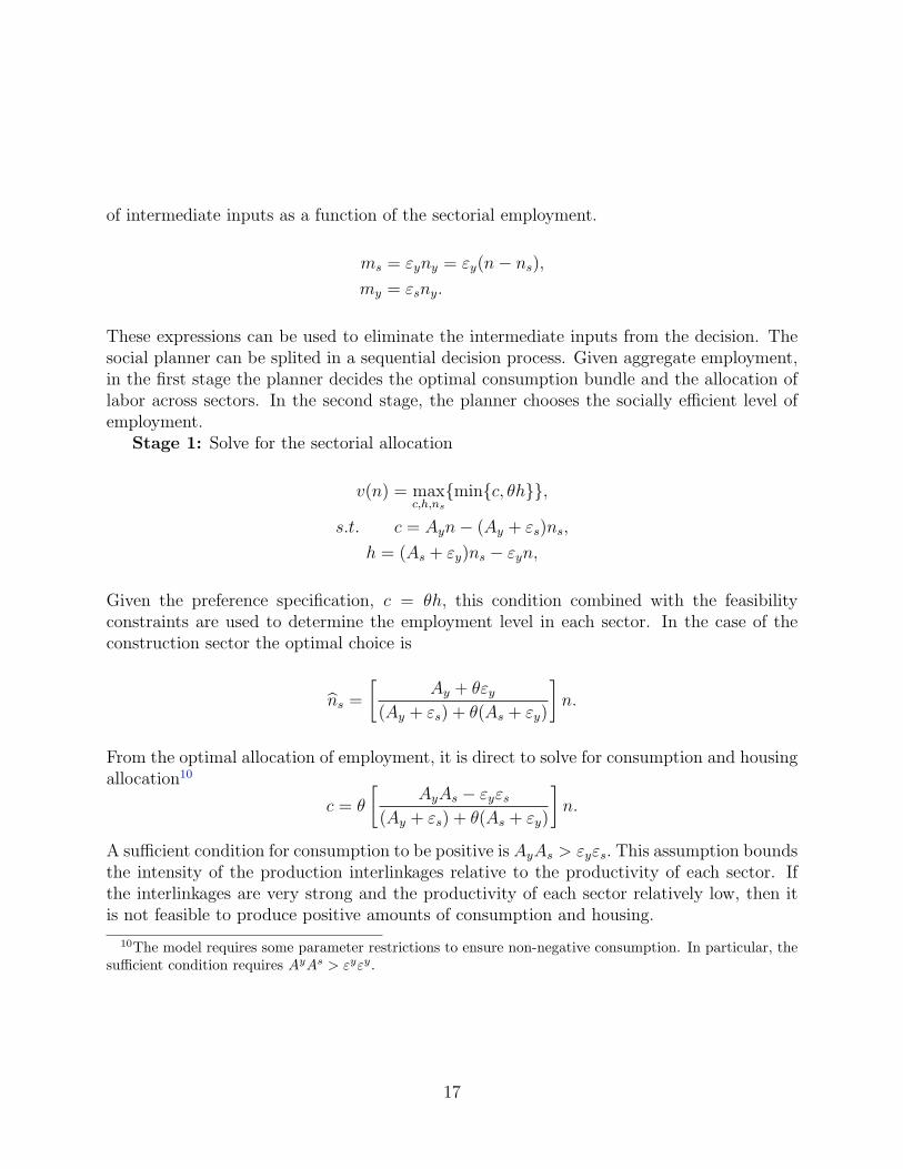
of intermediate inputs as a function of the sectorial employment.

ms = εyny = εy(n− ns),

my = εsny.

These expressions can be used to eliminate the intermediate inputs from the decision. Thesocial planner can be splited in a sequential decision process. Given aggregate employment,in the first stage the planner decides the optimal consumption bundle and the allocation oflabor across sectors. In the second stage, the planner chooses the socially efficient level ofemployment.

Stage 1: Solve for the sectorial allocation

v(n) = maxc,h,ns

{min{c, θh}},

s.t. c = Ayn− (Ay + εs)ns,

h = (As + εy)ns − εyn,

Given the preference specification, c = θh, this condition combined with the feasibilityconstraints are used to determine the employment level in each sector. In the case of theconstruction sector the optimal choice is

ns =

[Ay + θεy

(Ay + εs) + θ(As + εy)

]n.

From the optimal allocation of employment, it is direct to solve for consumption and housingallocation10

c = θ

[AyAs − εyεs

(Ay + εs) + θ(As + εy)

]n.

A sufficient condition for consumption to be positive is AyAs > εyεs. This assumption boundsthe intensity of the production interlinkages relative to the productivity of each sector. Ifthe interlinkages are very strong and the productivity of each sector relatively low, then itis not feasible to produce positive amounts of consumption and housing.

10The model requires some parameter restrictions to ensure non-negative consumption. In particular, thesufficient condition requires AyAs > εyεy.

17

The relative price of construction depends on the Leontief coefficients,

p =(Ay + εs)

(As + εy).

In the model that ignores the interlinkages εj → 0, the price of housing goods is given by theratio of productivities p = Ay/As and the employment allocation nnolink

s = Ayn/(Ay + θAs).This implies

v(n) = θ

[AyAs − εyεs

(Ay + εs) + θ(As + εy)

]n.

Stage 2: Solve for the aggregate employment

maxn

{v(n)− an1+γ

1 + γ}.

The optimal employment level is

n =

[θ

a

(AyAs − εyεs

(Ay + εs) + θ(As + εy)

)] 1γ

,

whereas in the economy with no interlinkages is

nnolink =

[θ

a

(AyAs

Ay + θAs

)] 1γ

.

In this economy, the relative importance of housing affects the aggregate level of employment.Measured economic activity is given by

Y = c+ ph =

[AyAs − εyεsAy + εs

]n(θ).

Notice that value added is proportional to total employment and the scaling factor does notdepend on the parameter θ. The change in value added with the housing shock is

∂Y

∂θ=

[AyAs − εyεsAy + εs

]∂n(θ)

∂θ.

18

Therefore the understanding of the amplification mechanism of sectorial interlinkage dependson the dynamics of aggregate employment. This is analyzed in the next subsection.

3.2 The Role of Interlinkages and Amplification

The goal of this section is to illustrate why considering interlinkages is key for the ampli-fication of shocks to the construction sector. How does changes in housing parameter θaffect aggregate employment n? Under certain parameter restrictions in the model, the in-terlinkages in production can amplify the effects of θ on aggregate employment relative tothe economy where these are not present. Since both economies have different employmentlevels, it is useful to consider the concept of the aggregate employment elasticity to changesin the housing parameter θ. In the model with interlinkages, this elasticity is

ϵn,θ =1

γ

[Ay + εs

(Ay + εs) + θ(As + εy)

]> 0,

whereas in the economy without linkages is

ϵnolinkn,θ =1

γ

[Ay

Ay + θAs

]> 0.

In this stylized economy, a necessary condition to have amplification due to productioninterlinkages ϵn,θ > ϵnolinkn,θ is Asεs > Ayεy.

11 For example, if the construction sector buysinputs from other sectors but those sectors do not use structures as inputs (εs > 0 andεy = 0), this condition is trivially satisfied.12 In the quantitative exercise in Section 5,the interlinkages between productive sectors are parameterized to match the data and thencompared to an economy without interlinkages.

4 Quantitative Model

The previous model is static and very stylized and, although it may give reasonable predic-tions in the very short run (i.e., on impact of a given shock or change in relative prices), itmay also become less reasonable when the time horizon is increased (medium and long-run).Simulating the path of an economy over time by linking a sequence of static input-output

11This condition is related to the irrelevance result in Dupor (1999).12By continuity, for values of εy ≈ 0 this argument also holds.

19

matrices does not allow taking into account either the general equilibrium or the intertem-poral effects of a given shock to initial conditions. The model presented in this section is ageneralization of the static model and allows for both richer dynamics and a certain degreeof substitution between productive inputs. The dynamic model introduces an asymmetrybetween the expansion and the recession due to the irreversibility constraints. This effectcan be amplified in the presence of interlinkages.

4.1 Households

The total population size, Nt, is normalized to 1. Household preferences are defined by atime-separable utility function, u(ct, ht)+ θtht+γv(1−nt), where ct represents consumptiongoods, ht represents housing services, nt represents labor supplied in the market, and γ > 0represents the relative weight of leisure in preferences. Housing provides two sources ofutility; one is complementary to consumption goods and the other is linear by itself. Thisreduced form captures the intrinsic desire to consume homes and in the pricing equation forhousing services appears as a bubble term. This is the term that will be responsible for themovements in housing demand that ultimately propagate to the construction sector and theoverall economy via the interaction across sectors. The utility functions u and v satisfy theusual properties of differentiability and concavity. The sequence of utilities is discounted bythe term β ∈ (0, 1). Housing services are produced according to a technology, H(st, lt), thatcombines the physical structure, st, and land, lt. The technology has constant returns to scaleand satisfies H ′

i > 0, H ′′i < 0, and H ′′

ij > 0. Housing structures depreciate at a constant rate,δs. In each period, the numeraire is the spot price of the manufacturing good. The householdalso invests in structures used by firms. These are rented as an input in the productionfunction (i.e., capital and labor). All investment decisions are subject to an irreversibilityconstraint and have different depreciation rates. These are relevant to generate asymmetriceffects between the booms and the recessions. Formally, the representative consumer chooses{ct, ht, nt, kt+1, st+1, lt+1}∞t=0 to maximize

max∑∞

t=0βt[u(ct, ht) + θtht + v(1− nt)],

s.t. ct + xkt + pstx

st = wtnt + rkt kt + plt(lt − lt+1) + πt,

ht = H(st, lt), (1)

xkt = kt+1 − (1− δk)kt ≥ 0, (2)

xst = st+1 − (1− δs)st ≥ 0, (3)

20

together with the transversality condition and no-Ponzi-game conditions. The prices aredefined as follows: pst is the price of infrastructure, plt is the price of land, wt represents thewage rate, and rt is the gross return on capital. To facilitate computing the rental rate forhousing services, our specification allows land trading, lt, even if in equilibrium there is notrading of land, which is owned by the representative household and inelastically supplied.The term πt represents profits from the productive sector.

The relevant first-order conditions of the consumer problem are

γv′(1− nt)

uc(ct, ht)= wt,∀t,

uc(ct, ht)

βuc(ct+1, ht+1)= 1 + rkt+1 − δk,∀t,

when the irreversibility constraints do not bind, xkt > 0. The relevant conditions for housing

decisions for the case with positive housing investment (xst > 0) satisfy

uh(ct, ht) + θtuc(ct, ht)

= Rt, ∀t,

pst =1

1 + rkt+1

[Rt+1Hs(st, lt) + pst+1(1− δs)],

plt =1

1 + rt+1

[Rt+1Hl(st, lt) + plt+1],

where Rt represents the implicit rental price for housing services measured in terms of con-sumption units at time t. The model predicts no arbitrage between land investment andhousing capital. The last expressions state that the current cost of purchasing a unit ofhousing structures (land) equals the future return of housing services derived from the hous-ing capital (land) valued at market prices and the capitalization.

4.2 Manufacturing Sector

The production sectors incorporate the simplest input-output structure. To operate, eachsector requires, among other things, the output of itself and of the other sector as intermedi-ate inputs. To capture this fact, we deviate from common practice and write all productionfunctions in terms of gross (as opposed to net, i.e., value-added) output, at least initially.Capital goods, which are produced in the manufacturing sector, must be distinguished from

21

the intermediate inputs from the same sector since they last more than one period. Inthe baseline model, capital goods (physical capital and business structures) are used in themanufacturing sector. Both investments satisfy the putty-clay assumption on sector-specificinvestment.

Formally, let mi,j be the intermediate input produced by sector i and used by sectorj. The manufacturing sector operates in a competitive market and uses a technology thatcombines Yt = Ay

tF (kt, nyt ,m

y,yt ,ms,y

t ) to produce its gross output:

Yt = ct + xkt +my,y

t +my,st .

The production function F is a constant returns to scale Cobb-Douglass function. The firm’soptimization problem is

πyt = max

kt,nyt ,m

y,yt ,ms,y

t

Yt − wtnyt − rkt kt −my,y

t − pstms,yt , ∀t,

s.t. Yt = AytF (kt, n

yt ,m

y,yt ,ms,y

t ), ∀t,

where the price of manufacturing’s output is normalized to 1. The constant returns to scaleassumption implies zero equilibrium profits, πy

t = 0, and marginal cost pricing for each input

rkt = AytF1(kt, n

yt ,m

y,yt ,ms,y

t ),

wt = AytF3(kt, n

yt ,m

y,yt ,ms,y

t ),

1 = AytF4(kt, n

yt ,m

y,yt ,ms,y

t ),

pst = AytF5(kt, n

yt ,m

y,yt ,ms,y

t ).

4.3 Construction Sector

The construction sector is also competitive: Its net output consists of residential structures,purchased by the households, while its gross output also includes structures used as anintermediate input in both production sectors. In the baseline case, purely for simplicity,we assume this sector has a fixed stock of capital; hence its value added is split between thewages of labor and the rent accruing to the owner of the fixed capital stock (the representativehouseholds). Implicit in this formulation is a somewhat extreme assumption about themobility of factors from one sector to another: While labor can move freely, the stock ofcapital invested in the construction sector is completely immobile (either way), and variationsin investment activity have an impact on only the manufacturing sector. The technology for

22

gross output,XS

t = xst +ms,s

t +ms,yt = As

tG(nst ,m

st(m

s,st ,my,s

t )),

therefore exhibits decreasing returns to scale in labor and the intermediate input mix. Inthe benchmark economy, we assume G(·) is a constant elasticity of substitution (CES) andthe intermediate inputs aggregator is Cobb-Douglass. The optimization problem of therepresentative firm is now

πst = max

nst ,m

s,st ,my,s

t

pstXSt − wtn

st − pstm

s,st − pytm

y,st , ∀t,

s.t. XSt = As

tG(nst ,m

st(m

s,st ,my,s

t )), ∀t.

The first-order conditions are similar to those of the representative firm in the manufacturingsector and are not repeated here. Note that because of the presence of a fixed stock of capital,firms’ profits are not zero in equilibrium in this sector. It is worth emphasizing that pst reflectsthe cost of producing new structures. The equilibrium price of a house differs from this valuesince it depends on the relative value of structures and land.

4.4 Competitive Equilibrium

The notion of competitive equilibrium is completely standard.Competitive Equilibrium: Given a sequence of values {Ay

t , Ast , θt}∞t=0, a competi-

tive equilibrium consists of allocations {ct, xkt , x

sht , xsy

t , lt, nyt , n

st ,m

s,st ,my,s

t ,my,yt ,ms,y

t }∞t=0, andprices {wt, r

kt , p

lt, p

st , rt, Rt}∞t=0 that satisfy the following:

1. Consumers’ optimization problem,

2. Profit maximization in the manufacturing and construction sector,

3. Clearing of markets:

(a) Labor markets (wt)nt = ny

t + nst , ∀t,

(b) Land markets (plt)lt = lt−1 = l, ∀t,

(c) Market rental capital (rkt )

rkt = AytF1(kt, n

yt ,m

y,yt ,ms,y

t ), ∀t,

23

(d) Goods markets (pct = 1)

ct + xkt +my,y

t +my,st = Ay

tF (kt, nyt ,m

y,yt ,ms,y

t ), ∀t,

(e) Construction of structures (pst)

xsht + xsy

t +ms,st +ms,y

t = AstG(ns

t ,mst(m

s,st ,my,s

t )), ∀t.

We have assumed complete markets from the outset; hence this equilibrium is efficient.The details of the optimization problem solved are discussed in Appendix.

5 Quantitative Analysis

5.1 Parameterization

The quantitative evaluation of the model requires specifying parameter values and functionalforms. The choice of functional forms is relatively general. The utility function is consistentwith unitary income elasticity,

u(c, h,N) =[ηc−ρ + (1− η)h−ρ]−

1−σρ

1− σ,

where the parameter ρ pins down the elasticity of substitution between consumption, c, andhousing services, h; the parameter σ represents the inter-temporal elasticity of substitution:and η represents the relative importance of consumption. The function capturing the util-ity from leisure is logarithmic, as is standard in the real business cycle literature with arepresentative agent,13

v(1− n) = ϱ log(1− n).

The production of housing services is also given by a Cobb-Douglas specification,

h = H(s, l) = zh (s)ϵ (l)1−ϵ

,

13This specification implies a Frisch elasticity of labor equal to 2. Keane and Rogerson (2012) argue thatthis elasticity can be reconciled with lower elasticity estimates at the micro level.

24

where zh represents a transformation factor between stock and the flow and ϵ represents theshare between structures and land. The production of consumption goods uses Cobb-Douglastechnology

F (k, ny,my,y,ms,y) = Ay(k)α1(ny)α2(my,y)α3(ms,y)1−α1−α2−α3 ,

where αi represents the share in production for input i and has constant returns to scale.Notice that the specification allows for substitutability between intermediate goods. Thetechnology used in the construction sector is a CES with diminishing returns to scale

∑i ϑi <

1,

G(ns,ms,s,my,s) = As[γ2 (n

s)−γ1γ4 + (1− γ2)((ms,s)γ3 (my,s)1−γ3

)−γ4]−1/γ4

.

The model parameters are set to match long-run averages of their data counterpartsbetween 1952 and 2000. The implied parameter values are relatively robust to choice of thesample period; however, during the housing boom some of the ratios and long-run averagesdeparted significantly from the historical trend. The model targets need to be adjusted tobe consistent with the data counterparts.

The time unit is a year, as input-output tables are yearly at best. The discount factor isβ = 0.96. The depreciation rates of residential structures and nonresidential capital are δs =0.015 and δy = 0.115, respectively. The weight on leisure, ϱ = 0.33, is such that total hoursworked equal one-third of the time endowment in steady state. The preference parametersare set to match consumption-to-output and housing-to-output ratios. The parameters ofthe production functions are set to satisfy the following:

1. The ratio of gross output in the two sectors, Y s/Y y = 0.08

2. Observed labor share in the construction sector, = 0.7

3. Observed labor share in the manufacturing sector, = 0.65

4. The ratio of consumption to manufacturing gross output, = 0.35

5. Observed shares of intermediates in gross output of own sector (M sy and Mys ), =0.4, 0.007

6. Time allocated to market activities, ny + ns = 1/3

7. The ratio of employment in the two sectors, ny/ns = 16

25

The values of the parameters not mentioned above are displayed in Table 2.

Table 2

Parameter Values

Parameter α1 α2 α3 γ1 γ2 γ3 γ4 Ay As zh ϵ η σ ρ

Value 0.18 0.5 0.035 0.62 0.4 0.04 1.5 2.4 1.74 0.175 0.28 0.435 1 5

The intratemporal elasticity of substitution between consumption and housing servicesis determined by the parameter εch = 1/(1 + ρ). Quantitatively, the value of ρ is an im-portant determinant of the spillover effects from the housing services demand into goods.If consumption services are close substitutes, a decline in the demand for housing servicescan generate an increase in goods consumption, whereas if these are close complements adecline in housing demand translates to the goods sector. Recent papers in an extensiveliterature estimate this elasticity to be less than 1. For example, Flavin and Nakagawa(2008) use a model of housing demand and estimate an elasticity less than 0.2. Other papers(i.e. Song, 2010; Landvoigt, 2011) use alternative model specifications and estimate valuesfor the elasticity to be less than 1. The simulations consider different ranges of elasticitiesεch ∈ {0.17, 0.25}.

The other key parameter is θt, which is used here to affect the demand for housing. Weperform the following exercise. Starting in 2001 the value θt grows to match employmentpatterns in the construction sector. Each new increment is a surprise (i.e., people expectθt not to change after that). The housing boom lasts until 2007, the housing bust lasts 3years, and thereafter θt remains constant forever. Figure 9 summarizes the implied pathfor employment in the construction sector in the model and the data. For the sequence ofdemand shifters, the model can reproduce the observed pattern quite well.

26

Figure 9: Employment Construction Sector (Model and Data)

1998 2000 2002 2004 2006 2008 2010 20120.7

0.8

0.9

1

1.1

1.2

1.3

Ns

DataModel

5.2 Role of Residential Investment in Growth and Employment

The key in this exercise is the behavior of other macroeconomic quantities (output, totalemployment, and intermediate production) during the transition path. They are endoge-nously determined from the initial steady state. The baseline case considers a boom andbust in the construction sector with sectoral adjustments in the interdependent sectors,m = {ms,s

t ,my,st ,my,y

t ,ms,yt }∞t=0. The implications of the boom and bust in construction for

output and total employment are summarized in Figure 10.Boom in housing demand and construction. Upon the arrival of the initial shift in

housing demand, the shock of residential structures is fixed and cannot be adjusted in theshort run. In principle, the higher demand for housing driven by higher values of θ may lower,in relative terms, the marginal utility of consumption. Because of the complementarity, goodsconsumption remains essentially unchanged during the initial period of the boom. Demandis higher, and thus to clear markets, the price of the construction sector must increase. Inthe following periods, the quantity of residential structures can be adjusted. The latterincreases the value of the marginal product of inputs used in production. Higher demand forinputs ultimately means the construction sector expands. The construction sector requires,among its inputs, intermediate goods purchased from the nonhousing sector. This increaseddemand from output of the nonhousing sector results, in equilibrium, in higher investment

27

Figure 10: The Impact of Construction

GDP Employment

2000 2002 2004 2006 2008 2010 2012 2014 2016 2018 20200.98

0.99

1

1.01

1.02

1.03

1.04

−3.3%−3.3%Y

2000 2002 2004 2006 2008 2010 2012 2014 2016 2018 20200.98

0.99

1

1.01

1.02

1.03

1.04

−3.8%−3.8%N

for this sector with higher capital and employment levels and ultimately more output. Theexpansion of the construction sector generates growth in the consumption goods sector andincreases total employment in the economy. All of these forces operate as long as preferencesfor housing continue to increase.

Bust in housing demand and construction. Similar forces operate once the crashin housing demand starts. The decline in the stock of residential structures is boundedby the relatively low rate of depreciation, which forces a strong decline in the price of theconstruction sector. Employment in the construction sector falls dramatically, together withthe demand for all other inputs of this sector. The input-output structure of the model onceagain lowers the demand for the consumption good sector as intermediate demand from theconstruction sector falls. In the short run, the decline in the demand for housing generates avery small and short-lived increase in nonhousing consumption. This effect would be missingin a model including negative wealth effects from a decline in house prices.

The magnitude of quantitative implications depends on the assigned value for the elastic-ity between consumption and housing services. With perfect complementarity, both goodsshould comove perfectly, whereas with both goods close to perfect substitutes, the decline inthe demand for housing could even imply a boom in the goods sector. In the baseline cali-bration, the temporary consumption increase is not sufficient to compensate for the declinein other key macroeconomic aggregates; as a result, GDP falls 3.3 percent and total employ-ment declines 4 percent. The asymmetry between the boom and the bust depends on thesequence of demand shifters but it also depends on the number of periods the irreversibility

28

constraint binds. This amplifies the asymmetric response between the boom and the bustepisode. When this effect is quantitatively important the decline of output is 3.3 percentand the employment decline is 3.8 percent.

The housing boom in the model generates significant movements in total employment.Recall that the sequence of demand parameters, θt, is calculated to replicate the evolutionof employment in the construction sector. Fluctuations in construction employment wereimportant during the Great Recession. Thus, the model can capture their timing and mag-nitude relatively well. In relative terms, the boom drew employment from the goods sectorinto housing, and the bust sent workers outside construction and out of the labor force. Thelong-run value of θ is determined to replicate the decline in employment in the constructionsector; as a result, the long-run level of employment declines relative to the initial steadystate. The temporary decline in employment occurs regardless of the level of the terminalconditions.14 Because of the slow adjustment of the stock of structures combined with the ir-reversibility constraint, there is a significant adjustment and the construction sector remainsinactive for a long period.

To compare the model implications for different elasticity values, it is necessary to re-calculate in each case a sequence of demand for housing {θt} that matches the dynamics ofemployment in the construction sector. The qualitative implications in both cases are thesame, but quantitatively the model with higher complementarity has a larger effect duringthe housing boom and the bust. With a lower degree of complementarity GDP falls 2 percentinstead of 3.3 percent and total employment declines by 2.4 percent instead of 4 percent.

The model also has some implications for the path of other aggregates. As shown inFigure 11, the dynamics are quite similar for the different elasticity parameters. The mostsignificant changes are the evolution of house prices and intermediates produced by theconstruction sector. The change in housing demand generates modest movements in houseprices: a 10 percent increase during the housing boom and a 15 percent decline duringthe bust. Movements in house prices have effects in the production of goods from theconstruction sector. Construction produces more goods as the price increases, but the goodssector responds by demanding less of the construction sector and using more capital.

One should not expect that dynamics of this economy that responds to a single shifter tomatch the data counterparts. For example, the decline in housing demand generates a smallincrease in consumption goods not observed in the data. Adding dimensions that affect thehousehold budget constraint should improve the performance of the model, but it would alsomake it more complicated to interpret the contribution of interlinkages.

14An alternative experiment would be one in which housing demand remains low for a number of periodsbefore returning to the initial steady-state level. We have computed the experiment, and the quantitativeimplications are not very different. However, the long-run level of employment is higher.

29

Figure 11: Summary of Key Aggregates

2000 2005 2010 20150.98

0.99

1

1.01

1.02

C

2000 2005 2010 20150.98

0.99

1

1.01

1.02

K

2000 2005 2010 20150.98

0.99

1

1.01

1.02

S

2000 2005 2010 20150.98

0.99

1

1.01

1.02

H

2000 2005 2010 20150.9

1

1.1

1.2

Ph

2000 2005 2010 20150.98

0.99

1

1.01

1.02

W

2000 2005 2010 20150.95

1

1.05

My

ρ=5ρ=3

2000 2005 2010 20150.95

1

1.05

Ms

30

5.3 The Role of Interlinkages

The interlinkages can be an important driver of aggregate output and total employment dur-ing the housing boom and bust. To isolate the effects of the interlinkages from those derivedpurely from consumers’ demand for housing, we consider two alternative specifications. Thefirst alternative considers the same model calibration and controls for the marginal effectsof the production of intermediate goods to the aggregate. This is done by restricting thesectoral demand of intermediates to be fixed and consistent with the quantities produced inthe initial steady state in 1998 (ms,s

t = ms,s0 ,my,s

t = my,s0 ,my,y

t = my,y0 ,ms,y

t = ms,y0 ). This case

is referred to as “no interlinkages.” A second alternative to identify the impact of housingdemand on employment and activity is to compare the economy with interlinkages with aneconomy that measures everything at the value-added level.15 In the value-added economy,the relevant technologies in the absence of interlinkages are

ct + xkt = Ay

tF (kt, syt , n

yt ),

andxsht + xsy

t = AstG(ns

t).

In both specifications the quantitative experiment is the same. The housing demand shifter isadjusted to generate movements in construction employment consistent with the data. Figure12 compares the key macroeconomic aggregates in the case of interlinkages, no interlinkages,and value added in the case of ρ = 5.

The role of the input-output linkages is clear when we compare the economy subject tothe same sequence {θt} but with no adjustment of intermediate goods. Now, the interme-diates are fixed to the initial steady-state levels. Both sectors are committed to producethe same amount of intermediates every period. During the housing boom, the only way toproduce more homes is to use more capital and labor. Since the intermediates cannot adjust,the prices adjust more, and rents and the price of construction are more volatile (Figure 13).Qualitatively speaking, equilibrium dynamics in this version of the model where intermedi-ates are constrained to be constant are quite similar to those of the baseline experiments.However, the quantitative implications are very different. Since intermediates are constant,the marginal product of labor in the construction sector does not increase as much as inthe baseline experiment, and employment also does not increase as much. The constructionsector expands during the boom, but in this model we do not allow for direct intersectorallinks; in particular, the demand for intermediates of the construction sector from the non-housing sector is not allowed to change. As a result, the nonhousing sector barely changes inthis experiment (all movements are less than one-half of 1 percent). GDP and employment

15See the Appendix for model details.

31

Figure 12: Role of Interlinkages

GDP Employment

2000 2002 2004 2006 2008 2010 2012 2014 2016 2018 20200.98

0.99

1

1.01

1.02

1.03

1.04

−3.3%−3.3%Y

InterlinkagesNo InterlinkagesValue Added

2000 2002 2004 2006 2008 2010 2012 2014 2016 2018 20200.98

0.99

1

1.01

1.02

1.03

1.04

−3.8%−3.8%N

InterlinkagesNo InterlinkagesValue Added

changes are an order of magnitude smaller than in the economy with intersectoral links. Theinput-output linkages operate as total factor productivity changes, amplifying the boom andthe bust. In the value-added model, the change in the demand for housing also generates avery small boom and bust in output and employment. All change is driven by the demandside of the model; the lack of interlinkages fails to amplify the effects in the constructionsector to other sectors in the economy. In these two cases, the irreversibility constraints haveno effects on the dynamics during the housing bust.

An indirect implication of the model is the dynamics of rental prices computed from themarginal rate of substitution between housing and consumption. The models that generatevery small movements in aggregate quantities also require significant movements in the rentalprice. The price increase is necessary to restrain consumers despite the increase in their desireto consume more housing. When the levels of interlinkages are fixed or nonexistent, the lackof adjustment behaves as a negative productivity shifter in each sector. In the model withinterlinkages, the interconnection operates as a positive productivity factor on capital andemployment. The positive response in quantities reduces the movement in the rental price.

The alternative specifications illustrate an important point. The presence of interlink-ages is necessary to generate large aggregate changes from fluctuations in construction.Importantly, notice that both alternative models generate little change in terms of GDPand employment even though the complementarity between consumption and housing is notmodified. This implies that this complementarity is not sufficient to obtain the propagationof shocks to the construction sector highlighted here.

32

Figure 13: Summary of Key Aggregates: Role of Interlinkages

2000 2005 2010 20150.98

0.99

1

1.01

1.02

C

2000 2005 2010 20150.98

0.99

1

1.01

1.02

K

2000 2005 2010 20150.98

0.99

1

1.01

1.02

S

2000 2005 2010 20150.98

0.99

1

1.01

1.02

H

2000 2005 2010 20150.9

1

1.1

1.2

Ph

2000 2005 2010 20150.98

0.99

1

1.01

1.02

W

InterlinkagesValue Added

33

Table 2: Quantitative Implications of Alternative Models

Share of changes accounted for by the construction sector

Expansion 2002-07 Recession 2008-09

Experiment Employment (%) GDP (%) Employment (%) GDP (%)

Lower complem. (ρ = 3) 29.2 8.3 28.3 43.5

Higher complem. (ρ = 5) 61.1 14.9 43.4 60.1

Value added 15.2 1.9 14.3 9.1

Fixed intermediates 14.7 1.5 10.4 5.2

5.4 Quantitative Implications of Alternative Models

The different model specifications point to a similar conclusion: The effect of the constructionsector is significant despite its relatively small share in terms of employment and value added.Table 2 presents a summary of all results presented above. The table shows informationabout the share of the change generated by the different models that occurs during theexpansion and recession. Because changes in the model are due only to changes in thedemand of housing services, we refer to those shares as the share of changes accounted forby the construction sector. The variables considered are employment and GDP. Notice thatwhen all sectors are growing at the same rate, the contribution of each sector must be equalto its share. For instance, if construction employment represents 5 percent of aggregateemployment, we should expect this sector to contribute 5 percent to the expansion of theeconomy. This is not necessarily the case when sectors are growing at different rates.

The left side of Table 2 considers the role of the construction sector in the expansion be-tween 2002 and 2007. Regardless of the complementarity between housing and consumptiongoods, our use of a general equilibrium model with interlinkages reveals that the construc-tion sector accounts for a very significant share of the growth in employment: between 29percent and 61 percent. The contribution of construction to GDP was also larger than itsshare—between 8 percent and 15 percent— but much smaller than for employment. Recallthat this period was usually referred to as the “jobless recovery,” in which most of the growthin employment was created by construction.

The effect of construction was arguably even more important during the Great Recession.The decline in employment generated in the models with interlinkages is between 28 percentand 43 percent of the actual decline during the recession. In the case of GDP, the modelsgenerate between 43 percent and 60 percent of the observed changes during the recession.Thus, construction accounts for very significant shares of the expansion and recession over

34

the past decade.Interlinkages are clearly important in the model. Without these channels (referred to

as “fixed intermediates” or “value added”), changes in the construction sector have muchsmaller effects on aggregate output and total employment, even when consumption goods andhousing services are complements. Recall that the value reported in this case correspondsto ρ = 5.

6 Interlinkages and Business Cycle Accounting

An alternative methodology to identify the sources of the recent recession is business cycleaccounting based on Chari et al. (2007). Recent work, including Arellano et al. (2010) andOhanian and Raffo (2012), documents that the Great Recession can be accounted for mostlyby a worsening of labor market distortions. Both studies find that the labor wedge worsensby about 12 percent during the 2009 recession. Different explanations have been proposedto rationalize the increase in distortions in the labor market. For instance, Arellano et al.(2010) propose a model of imperfect financial markets and firm-level volatility. Their modelcaptures about half of the worsening in the labor wedge.

This wedge can be computed with data on employment, consumption, and wages gener-ated with any model. In particular, the wedge is defined as

Xt = −UNt

UCt

/wt,

where UNt is the marginal disutility measured at the aggregate level of employment, UCt isthe marginal utility of consumption measured at the aggregate level of consumption, andwt is the economy wage. Assuming wages are flexible and considering an aggregate Cobb-Douglass production function with capital share α, the wage can be replaced with

wt =Yt

N(1− α).

Furthermore, using a log utility function for aggregate consumption and the following func-tion for the disutility of aggregate employment,

U(N) = BN

1 + υ

1+υ

,

35

Figure 14: Labor Wedge

2006 2007 2008 2009 2010 2011 2012 2013 2014 2015−0.12

−0.1

−0.08

−0.06

−0.04

−0.02

0

0.02

%∆07−11

= −0.0562

%∆07−11

= −0.0737

%∆07−11

= −0.108

Labor Wedge ( ν=1)Labor Wedge ( ν=0.5)Labor Wedge ( ν=2)

the wedge can be written as

Γt = − B

(1− α)

Ct

Yt

N1+υt .

Notice that the parameters B and α are not important to understand fluctuations inthe labor wedge; only time series of consumption, output, and employment at the aggregatelevel and a value for υ are required. We consider three values of υ = {0.5, 1, 2} and computethe labor wedge implied by our model using simulated data for consumption, output, andemployment. Since our model has multiple sectors, several adjustments in the data arenecessary. Consumption of goods and housing services are aggregated using relative pricesCt = ct +Rtht. Aggregate output is Yt = Ct +Xk

t and total employment is Nt = nyt + ns

t .In the context of the model, any action in terms of implied distortions must be derived

from the input-output structure and changes in relative prices. Figure 12 displays the changesin the labor wedge for our benchmark simulation. The behavior is consistent with the data.The labor wedge worsens during the recession and does not recover quickly. For the casecomputed with υ = 1, which is consistent with the value used by Ohanian and Raffo (2012),the labor wedge worsens 7.4 percent; this is about 62 percent of the total labor wedge changeduring this period.

Notice that our computation of the labor wedge assumes that wages are perfectly flexible.If this condition does not hold, the labor wedge has another component, referred to as the

36

“firm-side” labor wedge in Arellano et al. (2010).16 This wedge is basically the differencebetween the marginal product of labor and the wage. These authors refer to the othercomponent of the labor wedge as the “consumer-side” labor wage, which is basically ourΓt. Arellano et al. (2010) find that (i) the firm-side labor wedge has been fairly flat since2006 and (ii) a worsening of the consumer-side labor wedge accounts for most of the GreatRecession. Recall that there are no frictions in our model, so wages equal the marginalproduct of labor in every period. Thus, not only the behavior of the labor wedge during theGreat Recession but also its decomposition is consistent in our model and the data.

7 Conclusions

This paper analyzes the contribution of the construction sector to U.S. economic growth,particularly during the Great Recession. Historically, the construction sector has been rela-tively small in terms of employment and contribution to GDP, but it is highly interconnectedwith other sectors in the economy. Our empirical analysis reveals these sectoral interlink-ages propagate changes in housing demand, amplifying the effect in the economy. A simpleaccounting input-output framework reveals that construction accounts for 52 percent of thedecline in employment and 35 percent of the decline in output.

The importance of the sectoral interlinkages is illustrated using a simple static multisectormodel. In the model, changes in housing demand have a much larger effect on aggregateactivity when the sectors are interconnected. The presence of irreversibility constraintsintroduces an asymmetry between the expansion and the recession in the dynamic model.The simulation exercise is calibrated to reproduce the boom-bust dynamics of constructionemployment in the 2000-10 period. In the model, during the housing boom all sectors expandand contribute 2 percent and 2.5 percent to the growth of output and employment between,respectively. During the housing bust, the irreversibility constraint binds, amplifying theasymmetric response; the declines in output and employment are 3.3 percent and 3.8 percent,respectively. The asymmetric effect is not as large but still significant with a lower degree ofcomplementarity. These numbers can be used to calculate the contribution of construction inthe observed data. The model suggests that during the expansion (2002-07), the constructionsector accounts for a significant share of the growth in employment (between 29 percentand 61 percent) and GDP (between 8 percent and 15 percent). The construction sector’scontribution was more important during the Great Recession (2008-09) when declines inemployment and GDP ranged between 28 percent and 43 percent and 43 percent and 60percent, respectively.

The presence of intersectoral linkages substantially amplifies the impact of the changesin housing demand. In the model specifications without this mechanism, changes in hous-

16They follow Galı et al. (2007) in this decomposition.

37

ing demand consistent with the dynamics in construction employment have only a smalleffect on macroeconomic quantities. This is true even when the complementarity betweenconsumption goods and housing services is high. A direct implication of this result is thepresence of interlinkages is necessary to generate large aggregate changes from changes inconstruction, and the degree of complementarity is not sufficient to obtain the propagationof adjustments in housing demand to the construction sector highlighted here.

We use this analytical framework to interpret the behavior of the U.S. economy between2007 and 2011. Since in our model the equilibrium is efficient, the behavior of output is alsothe behavior of potential output. Taking into account that both output and potential outputwere affected during the Great Recession, we perform a business cycle accounting exerciseon simulated data from the model. Despite the lack of frictions and distortions in the model,the sectoral linkages and movements of relative prices across sectors attribute the recessionto a worsening in the labor wedge. The magnitude generated by the model accounts for 62percent of the total change observed in the data.

A direct policy implication of our findings is that the output gap could be lower than thehistorical estimates. The historical anomalies in the events during the past five years can beaccounted for by the equally anomalous evolution of housing demand in the previous years.As far as policy is concerned, the basic implication of our research is simple: Estimations ofoutput gaps using pre-2007 trends may lead to misleading policy prescriptions.

This model abstracts from sizable income and wealth effects due to deleveraging andmortgages. As a result, all short-run dynamics are driven entirely by substitution effects. Theinteraction between the financial factors used in Garriga et al. (2012a,b) with the productionstructure of the paper should magnify the importance of the sectoral interlinkages. Theinclusion of wealth effects and frictions from housing finance should be a natural extension.

References

Arellano, Cristina, Yan Bai, and Patrick J. Kehoe, “Financial Markets and Fluctua-tions in Uncertainty,” November 2010. Research department staff report, Federal ReserveBank of Minneapolis.

Black, F., “Interest rates as options,” The Journal of Finance, 1995, 50 (5), 1371–1376.

Bloom, N., “The impact of uncertainty shocks,” Econometrica, 2009, 77 (3), 623–685.

Chari, V. V., P. J. Kehoe, and E.R. McGrattan, “Business Cycle Accounting,” Econo-metrica, 2007.

Davis, Morris A. and Jonathan Heathcote, “Housing And The Business Cycle,” In-ternational Economic Review, 08 2005, 46 (3), 751–784.

38

Dupor, Bill, “Aggregation and irrelevance in multi-sector models,” Journal of MonetaryEconomics, April 1999, 43 (2), 391–409.

Flavin, Marjorie and Shinobu Nakagawa, “A Model of Housing in the Presence ofAdjustment Costs: A Structural Interpretation of Habit Persistence,” American EconomicReview, March 2008, 98 (1), 474–95.

Galı, J., M. Gertler, and J. D. Lopez-Salido, “Markups, Gaps, and the Welfare Costsof Business Fluctuations,” The Review of Economics and Statistics, 2007, 89 (1), 44–59.

Garriga, C., R. E. Manuelli, and A. A. Peralta-Alva, “Market crashes, deleverage,and macroeconomic activity,” 2012. Working Paper, Federal Reserve Bank of Saint Louis.

, , and , “A model of price swings in the housing market,” 2012. Working Papers,Federal Reserve Bank of Saint Louis.

Hall, R. E., “The long slump,” American Economic Review, 2011, 101, 431–469.

Herkenhoff, Kyle F. and Lee E. Ohanian, “Labor Market Dysfunction During the GreatRecession,” August 2011. NBER Working Papers 17313.

and Lee Ohanian, “Foreclosure delay and U.S. unemployment,” 2012. Working Paper2012-017, Federal Reserve Bank of St. Louis.

Keane, Michael and Richard Rogerson, “Micro and Macro Labor Supply Elasticities:A Reassessment of Conventional Wisdom,” Journal of Economic Literature, June 2012,50 (2), 464–76.

Kehoe, Timothy J., Kim J. Ruhl, and Joseph B. Steinberg, “Global Imbalances andStructural Change in the United States,” August 2013. NBER Working Papers 9339.

Kocherlakota, N., “Incomplete labor markets,” 2012. Working Papers, Federal ReserveBank of Minneapolis.

Landvoigt, Tim, “Housing Demand During the Boom: The Role of Expectations andCredit Constraints,” January 2011. Working Paper, Stanford University.

Leamer, Edward E., “Housing IS the Business Cycle,” September 2007. NBER WorkingPaper No. 13428.

Ohanian, L. E. and A. Raffo, “Aggregate hours worked in OECD countries: New mea-surement and implications for business cycles,” Journal of Monetary Economics, Carnegie-NYU-Rochester Conference Series on Public Policy, 2012, 59 (1), 40–56.

39

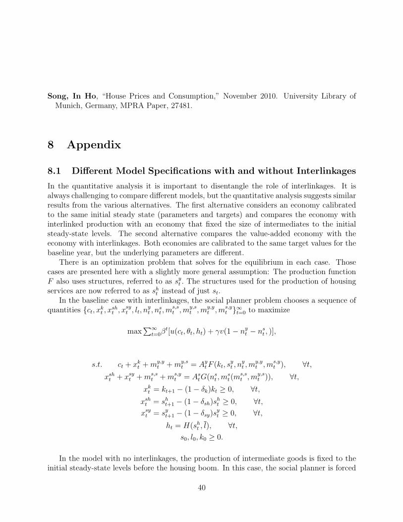
Song, In Ho, “House Prices and Consumption,” November 2010. University Library ofMunich, Germany, MPRA Paper, 27481.

8 Appendix

8.1 Different Model Specifications with and without Interlinkages

In the quantitative analysis it is important to disentangle the role of interlinkages. It isalways challenging to compare different models, but the quantitative analysis suggests similarresults from the various alternatives. The first alternative considers an economy calibratedto the same initial steady state (parameters and targets) and compares the economy withinterlinked production with an economy that fixed the size of intermediates to the initialsteady-state levels. The second alternative compares the value-added economy with theeconomy with interlinkages. Both economies are calibrated to the same target values for thebaseline year, but the underlying parameters are different.

There is an optimization problem that solves for the equilibrium in each case. Thosecases are presented here with a slightly more general assumption: The production functionF also uses structures, referred to as syt . The structures used for the production of housingservices are now referred to as sht instead of just st.

In the baseline case with interlinkages, the social planner problem chooses a sequence ofquantities {ct, xk

t , xsht , xsy

t , lt, nyt , n

st ,m

s,st ,my,s

t ,my,yt ,ms,y

t }∞t=0 to maximize

max∑∞

t=0βt[u(ct, θt, ht) + γv(1− ny

t − nst , )],

s.t. ct + xkt +my,y

t +my,st = Ay

tF (kt, syt , n

yt ,m

y,yt ,ms,y

t ), ∀t,xsht + xsy

t +ms,st +ms,y

t = AstG(ns

t ,mst(m

s,st ,my,s

t )), ∀t,xkt = kt+1 − (1− δk)kt ≥ 0, ∀t,

xsht = sht+1 − (1− δsh)s

ht ≥ 0, ∀t,

xsyt = syt+1 − (1− δsy)s

yt ≥ 0, ∀t,

ht = H(sht , l), ∀t,s0, l0, k0 ≥ 0.

In the model with no interlinkages, the production of intermediate goods is fixed to theinitial steady-state levels before the housing boom. In this case, the social planner is forced

40

to produce the same quantity of intermediates each period (ms,st = ms,s

0 ,my,st = my,s

0 ,my,yt =

my,y0 ,ms,y

t = ms,y0 ). To satisfy the production of the intermediate goods, the social planner

can choose a constrained vector of quantities {ct, xkt , x

sht , xsy

t , lt, nyt , n

st}∞t=0 to maximize

max∑∞

t=0βt[u(ct, θtht) + γv(1− ny

t − nst , )],

s.t. ct + xkt = Ay

tF (kt, syt , n

yt ,m

y,y0 ,ms,y

0 )− (my,y0 +my,s

0 ), ∀t,xsht + xsy

t = AstG(ns

t ,ms0(m

s,s0 ,my,s

0 ))− (ms,s0 +ms,y

0 ), ∀t,xkt = kt+1 − (1− δk)kt ≥ 0, ∀t,

xsht = sht+1 − (1− δsh)s

ht ≥ 0, ∀t,

xsyt = syt+1 − (1− δsy)s

yt ≥ 0, ∀t,

ht = H(sht , l), ∀t,s0, l0, k0,m

s,s0 ,my,s

0 ,my,y0 ,ms,y

0 ≥ 0,

The last case considers the value-added economy where the intermediate goods have beencompletely eliminated. The social planner can choose a constrained vector of quantities{ct, xk

t , xsht , xsy

t , lt, nyt , n

st}∞t=0 to maximize

max∑∞

t=0βt[u(ct, θtht) + γv(1− ny

t − nst , )],

s.t. ct + xkt = Ay

tF (kt, syt , n

yt ), ∀t,

xsht + xsy

t = AstG(ns

t), ∀t,xkt = kt+1 − (1− δk)kt ≥ 0, ∀t,

xsht = sht+1 − (1− δsh)s

ht ≥ 0, ∀t,

xsyt = syt+1 − (1− δsy)s

yt ≥ 0, ∀t,

ht = H(sht , l), ∀t,s0, l0, k0 ≥ 0,

8.2 Calibration of Interlinkages

Interlinkages are calibrated using input-output data. In particular, the information shown inTable A1 is used to calibrate the parameters in the production function of consumption goods

41

and residential structures. In particular, the tables are constructed from the 2010 BEA’s Useinput-output table. The Use table shows the uses of commodities by intermediate and finalusers; rows present the commodities or products, and columns display the industries andfinal users that use them. The sum of the entries in a row is the output of that commodity.The columns show the products consumed by each industry and the three components of“value added”—compensation of employees, taxes on production and imports less subsidies,and gross operating surplus. Value added is the difference between an industry’s output andthe cost of its intermediate inputs, and total value added is equal to GDP.

Table A1 displays input-output values (which are originally in millions of dollars) asa fraction of the industries’ outputs. Construction receives most of its inputs from otherindustries (48.3 percent of its gross output) and less than 1 percent from itself. This is alsotrue for other industries since they receive most of their inputs from themselves (43.0 percentof their total gross output).

Table A1: Coefficients with Respect to Column Industries

Commodities/Industries Construction Other Industries

Construction 0.0009 0.0058

Other industries 0.4828 0.4301

Compensation of employees 0.3625 0.2802

Taxes on production and imports, less subsidies 0.0072 0.0471

Gross operating surplus 0.1466 0.2368

Total 1.0000 1.0000

Source: Use input-output table (BEA).

42