Land-surface-cloud-atmosphere coupling on daily timescales  Alan K Betts, Raymond Desjardins, Anton C.M Beljaars and Ahmed Tawfik

Journal Name: Frontiers in Earth Science

ISSN: 2296-6463

Article type: Original Research Article

First received on: 21 Jan 2015

Frontiers website link: www.frontiersin.org

Atmospheric Science

1

Land-surface-cloud-atmosphere coupling on daily timescales 1

2 3

Alan K. Betts1*, Raymond Desjardins2, Anton C. M. Beljaars3and Ahmed Tawfik4,5 4 5

January 21, 2015 6

7 1Atmospheric Research, Pittsford, Vermont, USA 8 2Agriculture & Agri-Food Canada, Ottawa, Canada 9 3ECMWF, Reading, UK 10 4Currently NCAR, Boulder, Colorado, USA 11 5George Mason University, Center for Ocean-Land-Atmosphere Studies, Fairfax, Virginia, USA 12 13 *Correspondence: 14 Alan K. Betts 15 Atmospheric Research, 16 58 Hendee Lane, 17 Pittsford, Vermont 05763, USA 18 akbetts@aol.com 19 20 Key words 21 land-atmosphere coupling, diurnal climate, Canadian Prairies, cloud radiative forcing, 22 hydrometeorology 23 24 Abstract 25 Our aim is to provide an observational reference for the evaluation of the surface and boundary layer 26 parameterizations used in large-scale models using the remarkable long-term Canadian Prairie hourly 27 dataset. First we use shortwave and longwave data from the Baseline Surface Radiation Network 28 (BSRN) station at Bratt’s Lake, Saskatchewan, and clear sky radiative fluxes from ERA-Interim, to 29 show the coupling between the diurnal cycle of temperature and relative humidity and effective cloud 30 albedo and net longwave flux. Then we calibrate the nearby opaque cloud observations at Regina, 31 Saskatchewan in terms of the BSRN radiation fluxes. We find that in the warm season, we can 32 determine effective cloud albedo to ±0.08 from daytime opaque cloud, and net long-wave radiation to 33 ±8 W/m2 from daily mean opaque cloud. This enables us to extend our analysis to the 55 years of 34 hourly observations of opaque cloud cover, temperature, relative humidity, and daily precipitation 35 from 11 climate stations across the Canadian Prairies. We show the land-surface-atmosphere coupling 36 on daily timescales in summer by stratifying the Prairie data by opaque cloud, relative humidity, 37 surface wind, day-night cloud asymmetry and monthly weighted precipitation anomalies. The multiple 38 linear regression fits relating key diurnal climate variables, the diurnal temperature range, afternoon 39 relative humidity and lifting condensation level, to daily mean net longwave flux, wind-speed and 40 precipitation anomalies have R2 values between 0.61 and 0.69. These fits will be a useful guide for 41 evaluating the fully coupled system in models. 42 43 Citation: Betts, A.K., R. Desjardins, A.C.M. Beljaars and A. Tawfik (2015). Land-surface-cloud-atmosphere coupling on 44 daily timescales. Frontiers in Earth Science (Land-atmosphere interactions). 45

46

2

1. Introduction 47 48

Analysis of the long-term Canadian Prairie data set is transforming our understanding of land-49 atmosphere coupling and more broadly hydrometeorology (Betts et al., 2014b). From the early 1950s 50 to the present, these data contain a remarkable set of hourly observations of opaque or reflective cloud 51 cover in tenths, made by trained observers who have followed the same protocol for 60 years 52 (MANOBS, 2013). Betts et al. (2013) calibrated these opaque cloud observations against multiyear 53 shortwave and longwave radiation data to quantify the impact of clouds. This gives the so-called 54 shortwave and longwave cloud forcing (SWCF, LWCF), as well as net radiation, Rn. Many climate 55 studies have been limited to temperature and precipitation for which long-term records are generally 56 available. Similarly, model climate change analyses typically focus on temperature and precipitation, 57 and it is thought that uncertainties in cloud processes explain much of the spread in modeled climate 58 sensitivity (Flato et al., 2013). In contrast, the Canadian Prairie data have sixty years of hourly records 59 for the fully coupled system of temperature, relative humidity (RH), precipitation, and radiation 60 derived from cloud observations. The diurnal cycle is tightly coupled to clouds and radiation (Betts et 61 al., 2013); but on monthly timescales, temperature and RH are jointly coupled to precipitation, cloud 62 cover and radiation (Betts et al., 2014b). They found that up to 60-80% of the monthly variance in the 63 diurnal temperature range, afternoon RH and lifting condensation level could be explained in terms of 64 monthly anomalies of opaque cloud and precipitation. From this it is clear that four variables, 65 temperature, RH, radiation and precipitation are all essential for understanding hydrometeorology and 66 hydroclimatology. 67 68 The role of clouds and radiative forcing has been missing in much of the literature on land-atmosphere 69 coupling, where the focus has been largely on surface variables, such as soil moisture and albedo 70 (Koster and Suarez, 2001; Koster et al., 2004; Dirmeyer, 2006; Ferguson and Wood, 2011; Ferguson et 71 al., 2012; Koster and Mahanama, 2012; Santanello et al., 2013) following earlier work by Betts and 72 Ball (1995, 1998); Beljaars et al. (1996) and Eltahir (1998). The framework for describing atmospheric 73 controls on soil moisture–boundary layer interactions (Findell and Eltahir, 2003) used two lower-74 atmosphere metrics: the convective triggering potential and low-level humidity, but not the clouds that 75 are part of the tightly coupled boundary layer system. Modeling studies of course highlight the critical 76 role of the cloud and radiation fields on land-surface processes (e.g. Betts, 2004; Viterbo and Betts, 77 2005; Betts, 2007), but the wide variation between models (Dirmeyer et al., 2006; Guo et al., 2006; 78 Koster et al., 2006; Taylor et al., 2013) may reflect in part model errors in the cloud fields. However, 79 while there has been ongoing work to benchmark uncoupled land surface models (Abramowitz, 2012), 80 there are still a lack of appropriate metrics for benchmarking coupled land-atmosphere models. Using 81 the 600 station-years of data from the Canadian Prairies, we can finally begin to develop coupled 82 benchmarking metrics and relationships necessary to test model behavior against observations. 83 84 Betts et al. (2013) showed that there is marked difference between a warm season state with an 85 unstable daytime convective boundary layer (BL), controlled by the SWCF; and a cold season state 86 with surface snow with a stable BL, controlled by the LWCF. Betts et al. (2014a) looked at the rapid 87 transitions that occur with snow cover between the warm season convective BL and the cold season 88 stable BL. This paper will revisit with much greater precision the calibration of the opaque cloud data, 89 for the warm and cold seasons, using 17 years of data from the baseline surface radiation network 90 (BSRN) site at Bratt’s Lake in Saskatchewan, and co-located grid-point data from the European Centre 91 reanalysis known as ERA-Interim. Then we shall examine in more detail the physical processes 92 influencing land-atmosphere coupling and the daily climate in the warm season. The daily timescale 93 analysis framework that we use here was proposed by Betts (2004); and applied in several studies 94

3 using model data from reanalysis (Betts and Viterbo, 2005, Betts, 2006, 2009) and to compare 95 reanalysis and observations over the boreal forest (Betts et al., 2006). It has proved useful for other 96 recent studies of land-atmosphere coupling (Ferguson et al., 2012; Dirmeyer et al., 2014). 97 98 Our intent is to provide an observational reference for the evaluation of both simplified models, and 99 the large-scale models we depend upon for weather forecasting and climate simulation, where most 100 land-surface-BL and cloud processes have to be parameterized. From an analysis perspective, the key 101 addition is having a quantitative estimate of the surface radiation as well as the traditional surface 102 climate variables. In section 2 we outline our analysis framework. In section 3, we first analyze the 103 BSRN and ERA-Interim data to look at the annual cycle of the SWCF and LWCF. We show the warm 104 season coupling between SW and LW radiation and the diurnal ranges of temperature and RH at the 105 BSRN site. Then we calibrate the opaque cloud data at Regina in Saskatchewan against the nearby 106 BSRN data for the cold and warm seasons. In section 4, we merge the 11 Prairie stations to give us 107 about 600 station-years of data, and map how different physical processes affect daily land-surface 108 climate in summer, June, July and August (JJA). Specifically, after stratifying by opaque cloud, we 109 will identify the daily climate signature of wind, relative humidity, the day-night asymmetry of the 110 cloud field, and monthly weighted precipitation anomalies. In section 5 we remap the diurnal climate 111 signatures in terms of surface net longwave and effective cloud albedo, and section 6 summarizes our 112 conclusions. 113

114 2. Data and analysis methods 115

116 2.1 Climate station data 117 118 We analyzed data from the 11 climate stations listed in Table 1: the stations are all at airports across 119 the Canadian Prairies. They have hourly data, starting in 1953 for all stations, except Regina and 120 Moose Jaw which start in 1954. The last year with complete precipitation data (that was available in 121 2012 when these data were processed) is listed after the station name. 122 123 Table 1: Climate stations: location and elevation. 124 125 Station Name Station # Station

ID Province Latitude Longitude Elevation (m)

Calgary (2010) 1 3031093 Alberta 51.11 -114.02 1084 Estevan (2010) 2 4012400 Saskatchewan 49.22 -102.97 581 Lethbridge (2005) 4 3033880 Alberta 49.63 -112.80 929 Medicine Hat (2005) 5 3034480 Alberta 50.02 -110.72 717 Moose Jaw (2010) 6 4015320 Saskatchewan 50.33 -105.55 577 Prince Albert (2010) 7 4056240 Saskatchewan 53.22 -105.67 428 Red Deer (2010) 9 3025480 Alberta 52.18 -113.62 905 Regina (2008) 10 4016560 Saskatchewan 50.43 -104.67 578 Saskatoon (2009) 11 4057120 Saskatchewan 52.17 -106.72 504 Swift Current (1994) 12 4028040 Saskatchewan 50.3 -107.68 817 Winnipeg (2007) 14 5023222 Manitoba 49.82 -97.23 239 126 127 128 129

4 2.2 BSRN data 130 131 Canada’s BSRN station was a Prairie site at Bratt’s Lake, Saskatchewan at 50.204oN, 104.713oW at an 132 elevation of 588 m. We will use it to calibrate the opaque clouds observed at Regina, about 25 km to 133 the north in terms of SWCF and net longwave flux (LWn). We processed the raw 1-min mean BSRN 134 data to hourly means (with standard deviation, max and min) for the 17-year period of 1995-2011. We 135 filtered the long-wave down (LWdn) data, removing from the hourly average extreme values greater 136 than 3 standard deviations of the 1-min data for each month. The data quality is high for the first 14 137 years, and this LW filtering removed less than 0.5% of the 1-min data values. During July- October, 138 2009 and June-August, 2010, the long-wave data appears to have a bias of unknown origin and these 139 data were not used. For shortwave down (SWdn), we removed hourly values at night < ±1W/m2. The 140 dataset includes temperature and pressure for all years, and relative humidity for 2000-2011. 141 142 We have no measurements of the upward components (SWup and LWup). Defining a surface albedo, αs, 143 gives the net shortwave 144 145

SWn = SWdn – SWup = (1- αs) SWdn (1) 146 147

The mean surface albedo for Saskatchewan ranges from about 0.16 in summer to 0.73 in winter (Betts 148 et al. 2014a, b). We calculated an estimate of LWup from the daily mean air temperature, Tk (K), using 149 150 LWup = ε σ Tk

4 (2) 151 152 with σ = 5.67 10-8 and the emissivity ε set to 1. This gives net long-wave as 153 154 LWn = LWdn – LWup (3) 155 156 One objective of this paper is to assess the impact of clouds on the surface radiative balance using 157 long-term observations. In the shortwave budget, we can define an effective cloud transmission (ECT), 158 an effective cloud albedo (ECA) and the shortwave cloud forcing (SWCF) in terms of a downwelling 159 clear-sky flux, SWCdn 160 161

ECT = SWdn/ SWCdn (4) 162 ECA = 1- SWdn/ SWCdn (5) 163 SWCF = SWdn - SWCdn (6) 164 165

The dimensionless ECA and ECT, scaled by SWCdn to give a range from 0 to 1, are very useful 166 measures of the impact of the cloud field on the surface shortwave radiation budget (Betts and Viterbo, 167 2005; Betts, 2009). Using the clear-sky fluxes from nearest grid-point of ERA-Interim as a guide, we 168 will fit an annual curve to SWCdn. Rearranging (5) and combining with (1) gives SWn in terms of two 169 albedos 170 171 SWn = (1- αs)(1-ECA)SWCdn (7) 172 173 Similarly we can define a longwave cloud forcing (LWCF) in terms of a down-welling clear-sky flux 174 LWCdn as 175 176

LWCF = LWdn - LWCdn (8) 177

5

178 We will take LWCdn from the nearest ERA-Interim grid-point. The total cloud forcing (CF) of the 179 downwelling radiative fluxes is the sum 180 181

CF = SWCF + LWCF (9a) 182 183

When there is reflective snow, the surface albedo greatly reduces SWn, which reduces the impact of 184 clouds on the surface radiation budget (SRB). So it is convenient to also define the net cloud forcing as 185 186

CFn = (1- αs) SWCF + LWCF (9b) 187 188 We will return to these radiative budget components in our analysis of the BSRN data in section 3. 189 190 2.3 Climate variables and data processing 191 192 The hourly climate variables include surface pressure (p), dry bulb temperature (T), relative humidity 193 (RH), wind speed and direction, total opaque cloud amount and total cloud amount. The time-base is 194 Local Standard Time (LST). Trained observers have followed the same cloud observation protocol for 195 60 years (MANOBS, 2013). Opaque (or reflective) cloud is defined (in tenths) as cloud that obscures 196 the sun, or the moon and stars at night. The long-term consistency of these hourly opaque cloud 197 fraction observations makes them useful for climate studies. Betts et al. (2013) used four stations, 198 Lethbridge, Swift Current, Winnipeg and The Pas (in the boreal forest), with downward shortwave 199 radiation SWdn to calibrate the daily mean total opaque cloud fraction, OPAQm, in terms of daily 200 SWCF. They also used downward longwave radiation LWdn from Saskatoon and Prince Albert 201 National Park for the calibration of OPAQm to net longwave (LWn) on daily timescales. Here we 202 extend these analyses using the BSRN data, which is 25km from the Regina climate station. 203 204 We generated a file of daily means for all variables, such as mean temperature and humidity, Tm and 205 RHm; and extracted and appended to each daily record the corresponding hourly data at the times of 206 maximum and minimum temperature (Tx and Tn). We merged a file of daily total precipitation (and 207 daily snow depth, not used here). Since occasional hourly data were missing, we kept a count of the 208 number of measurement hours, MeasHr, of valid data in the daily mean. In our results here we have 209 filtered out all days for which MeasHr <20. However with almost no missing hours of data in the first 210 four decades, there are very few missing analysis days; except for Swift Current, where night-time data 211 is missing from June 1980 to May 1986; and Moose Jaw, where night-time measurements ceased after 212 1997. 213 214 From the hourly data we compute the diurnal temperature range between maximum temperature, Tx, 215 and minimum temperature, Tn, as 216 217 DTR = Tx - Tn (10) 218 219 We also define the difference of relative humidity, RH, between Tn and Tx, as 220 221 ΔRH = RHx - RHn ≈ RHtn – RHtx (11) 222 223 where RHx, RHn are the maximum and minimum RH. This approximation is excellent in the warm 224 season, when surface heating couples with a convective BL. Then typically RH reaches a maximum 225

6 near sunrise at Tn and a minimum at the time of the afternoon Tx (Betts et al., 2013). We also derived 226 from p, Tx and RHtx, the lifting condensation level (LCL), the pressure height to the LCL, PLCLtx, 227 mixing ratio (Qtx) and θEtx, all at the time of the maximum temperature. Similarly we derived Qtn, θEtn 228 and PLCLtn at the time of the minimum temperature, Tn. 229 230 This Prairie data set is large and includes the synoptic variability for nearly 600 station-years. For 231 summer (JJA) there are about 54000 days with good data. We will bin the data and generate means for 232 many sub-stratifications, to isolate the climatological coupling between different variables in this fully 233 coupled system. As an estimate of the uncertainty in a mean value, derived from N daily values, we 234 will show the standard error (SE) of the mean, calculated from the standard deviation (SD) as SE = 235 SD/√N. As a result, larger SE values generally indicate a smaller data sample N. For the larger dataset 236 we will not show a mean value unless N>200, and for the much smaller BSRN dataset, we reduced this 237 threshold to N=40. Many plots with a 2-way stratification (e.g showing the dependence of DTR on 238 opaque cloud and wind-speed) may have >500 days in each bin, so the SE of each point is small. We 239 will also use multiple linear regression of the daily data to assess the scatter in quasi-linear 240 relationships. 241 242 2.4 ERA-Interim data 243

244 We used the data for the closest 80km grid-box to Bratt’s Lake, with center at 50.1753oN, 105oW, 245 from ERA-Interim (abbreviated to ERI in Figures). We used 12h forecasts from analyses at 00 and 12 246 UTC for each day. These data have a 3-hrly time step; and we integrated to a daily mean in terms of 247 local time, which is UTC-6. The available fields include the clear-sky and all-sky radiation fluxes, 248 surface sensible and latent heat fluxes and surface stresses, 2-m Tm, Tx, Tn and specific humidity, 249 surface pressure, soil temperature and soil water, as well as the model estimates of low, medium, high 250 and total cloud cover. In this paper we will use only the clear-sky surface radiation. 251 252 2.5 Distinction between warm and cold seasons 253 254 On the Prairies, the freezing point of water gives two sharply contrasting near-surface climate regimes 255 (Betts et al., 2013, 2014a). Figure 1 shows the diurnal cycle of T and RH for Regina, stratified by Tm< 256 > 0oC and by daily mean opaque cloud, OPAQm, on a scale of 0 to 1. The time axis is local standard 257 time. We get a very similar figure (not shown) if we stratify instead based on no snow cover, or snow 258 depth>0; or simply average the months April to October and November to March. When Tm < 0oC, 259 precipitation falls as snow giving the surface a high albedo with low sublimation of the surface ice. 260 This regime is dominated by LWCF (see Figure 3 later). Temperatures drop under clear skies to give a 261 strong shallow stable BL at sunrise; while the daily variation of RH is small, not far below saturation 262 over ice (Betts et al., 2014a). We will find that in this regime LWn depends on near-surface 263 temperature as well as cloud. 264 265 In contrast, in the warm season with Tm > 0oC, there is no snow, plants grow and transpire, increasing 266 atmospheric water vapor. This regime is dominated by SWCF (see Figure 3 later). Minimum 267 temperature varies little, but Tx increases and RHm falls under clear skies (Betts et al., 2013), as the 268 daytime solar heating drives the development of a deep unstable convective BL. We will find that in 269 this regime LWn depends on RHm as well as cloud. 270 271

7 This difference between warm and cold seasons is a fundamental characteristic of the Prairie climate.272

273 274 275 276

In section 3, we will partition the BSRN data into these cold and warm seasons, and show the warm 277 season coupling of the diurnal ranges of T and RH to ECA and LWn. We will calibrate opaque cloud 278 cover Regina with the LW and SW data at the nearby BSRN site. In section 4, we will expand the 279 analysis to the full Prairie data set, focusing on summer as representative of the warm season. The cold 280 season needs a more careful treatment, because on a daily timescale, advective temperature changes 281 are typically larger than the solar forcing of the diurnal cycle (Wang and Zeng, 2014; Betts et al., 282 2014a). We will address the full diurnal cycle over the annual cycle in a later paper. 283 284 285 286 3. Analysis of the BSRN data 287 288 As discussed in section 2.2, we have 17 years of SWdn and LWdn at Bratt’s Lake, Saskatchewan; which 289 we first averaged from 1-min data to hourly means, and then to daily means, which we use here. We 290 compared the climatology of the daily data with the clear sky fluxes calculated by ERA-Interim (ERI) 291 for the same dates. The ERI archive contains surface SWdn, SWn and the surface net clear sky flux 292 SWCn, but not SWCdn so we retrieved SWCdn by first calculating αs from Eq. (1). However in winter 293 with surface snow, this method fails if ERI (1-αs) becomes very small. 294 295

Figure 1. Diurnal cycle of T and RH as a function of opaque cloud, when Tm< 0oC (left) and (right) Tm>0oC

8 3.1 Comparison of ERA-Interim clear-sky fluxes and BSRN on clear days 296 297 The surface SWCdn has a large dependence (range 60 to 370 W/m2) on solar zenith angle and a small 298 dependence (±5 W/m2) on the variable atmospheric absorption by gases and aerosols, which are 299 included in the ERI clear-sky computation, but are not available across the Prairies for our long-term 300 datasets. So we looked for simplified fits to the annual profile, which neglect the variable atmospheric 301 absorption by adjusting the empirical functions used in Betts et al. (2013). We first fitted the ERI clear-302 sky shortwave data with the empirical function 303 304

SWCdn(ERIfit)= 55 + 300*SIN(π DS / 365)1.92 (12) 305 306

where DS = DOY + 14 for DOY < 353, and DOY - 352 for DOY < 353 (adjusted one day for leap 307 years). This fit has a mean annual bias of -0.4±5.4 W/m2, with mean monthly biases that are < ±2.5 308 W/m2. 309 310

311 Figure 2. Clear sky (ECT>0.95) BSRN SWdn, ERA-Interim SWCdn and clear-sky fit used with BSRN data (left) and 312 (right) BSRN LWdn, ERA-Interim LWCdn and the difference, the LWCF. 313 314 Figure 2 (left panel) compares BSRN SWdn for nearly clear days with ECT>0.95 (red dots), and the 315 ERI clear-sky SWCdn flux (blue dots) for the same days. For these nearly clear days, the BSRN 316 measurements are systematically higher than ERI clear sky fluxes by 9.4±4.8 W/m2, despite small 317 amounts of cloud; suggesting that the reanalysis has greater absorption, either from the radiation 318 calculation, or from less absorption by aerosols than the climatological aerosols assumed in ERI. So 319 we shifted equation (12) upward to define an approximate upper bound to the BSRN data 320 321

SWCdn(BSRNfit) = 65 + 310 * (@SIN(@PI * DS / 365))1.92 (13) 322 323 This fit, indicated by the black dots in Figure 2, is used with the BSRN SWdn flux to calculate ECT, 324 ECA and SWCF. The uncertainty in this fit is of the order of ±5 W/m2, because it neglects the 325 variability of atmospheric clear-sky absorption. This is, however, smaller than the estimated bias of the 326 ERI clear-sky fluxes. The data gaps in winter in Figure 2 result from the failure of our method of 327 calculating SWCdn on days when SWdn is small with ERI αs ≈ 1. As a result, the relative uncertainty in 328 SWCdn is larger in winter with snow than in the warm season. 329 330

9 For the same subset of the data, representing nearly clear skies in the daytime (ECT>0.95), the right 331 panel shows the measured LWdn, the ERI clear sky flux, LWCdn, and the LWCF, the difference from 332 equation (7). The annual mean LWCF for these nearly clear-sky conditions is 2.1±11.4 W/m2: much 333 smaller than the ±25 W/m2 variability of LWCdn on monthly timescales, so we will use ERI as an 334 estimate of the clear-sky flux, LWCdn. 335 336 3.2 Mean Annual Cycle of Cloud Forcing 337 338 Figure 3 shows the mean annual cycle of SWCF, LWCF, CF and CFn, binned in 0.1 ranges of ECA. 339 There is a single bin for all the data for which ECA>0.7, and the standard error of the bin means is 340 shown. The top left panel just shows the variation of SWCF with ECA, which follows directly from 341 the definitions (5) and (6). This shows that that the reduction of the surface SW flux by clouds is 342 naturally largest in summer, when SWCdn is largest. The sharp drop in reflective cloud cover between 343 June and July (Betts et al., 2014b) gives the jump in the monthly mean for all data (heavy black curve). 344 The top right panel shows that the 345 LWCF increases with ECA. The 346 impact of clouds on the LWCF is 347 larger in winter than in summer, 348 when the moister atmosphere is 349 itself more opaque to LW 350 radiation. The very small negative 351 values in summer for ECA= 0.05 352 may reflect a small positive bias in 353 LWCdn from ERA-Interim. 354 355 The bottom left panel is the sum of 356 the upper two, which shows that 357 the total cloud forcing of the down-358 welling flux is near zero from 359 November to January, when 360 SWCdn is smallest. The bottom 361 right panel is CFn, the cloud 362 forcing of the net surface radiative 363 flux, defined by (9). For 364 consistency with our 1995-2011 365 analysis period, we used monthly 366 mean values of surface albedo from 367 ERA-Interim, although the annual 368 range from 0.19 in summer to 0.61 369 in winter is slightly less than the range of 0.16 to 0.73, shown in Betts et al. (2014a) for Saskatchewan 370 for the 2000-2001 winter. The impact of reflective snow cover in reducing the net SW fluxes means 371 that CFn becomes positive from November to February (Betts et al., 2013). This reversal of the sign of 372 CFn leads to the two distinct climate states on the Canadian Prairies for the warm and cold seasons (see 373 Figure 1 and Betts et al., 2014a). 374 375 376 377 378

Figure 3. Mean annual cycle of SWCF, LWCF, CF and CFn, stratified by ECA

10 3.3 Coupling between ECA, LWn, DTR and ΔRH on daily timescales for April to October 379 380 Following Betts et al. (2013), we will merge the warm season months, April to October with Tm>0 and 381 no snow cover; and show the climatology of the coupling between the SW and LW radiation field and 382 the diurnal cycle of temperature and humidity. The Bratt’s Lake site has temperature data for the full 383 17-year period, but RH data only for the last 12 years, 2000-2011. For this data set, we extracted Tn, 384 Tx, RHx and RHn. From SWdn and LWdn, we calculated ECA using equations (5) and (13), and LWn 385 using (2) and (3). 386 387 The diurnal climatology is coupled to both daytime and nighttime processes. The daytime rise of 388 temperature from Tn to Tx, and the corresponding fall of humidity from RHx to RHn, is driven by SW 389 heating, as well as the surface energy partition and the growth of the unstable BL. The night-time 390 return back to Tn and RHx is driven by LW cooling and the structure of the stable BL (Betts, 2006). So 391 in the daily climatology, DTR is coupled to both SW and LW processes, which are themselves coupled 392 through the cloud field, as well as details of the BL depth and structure. The data shows the observed 393 diurnal climatology of the coupled land-BL-cloud system. In contrast, models construct their own 394 differing diurnal climatologies from a suite of process models and parameterizations for the surface, 395 BL and cloud components. 396 397 Figure 4 shows a fundamental set of relationships for the coupling between ECA, LWn, DTR and 398 ΔRH on daily timescales. The data has been averaged (with standard error bars) in bins of the x-axis. 399 The upper left pair of panels shows the mean dependence of LWn and DTR on ECA, as well as the 400 subdivision into three RHm ranges with roughly the same number of days: RHm <60, 60-75, >75%. 401

402

403 Figure 4. Coupling between ECA, LWn, DTR and ΔRH on daily timescales for April to October, for the BSRN 404 station at Bratt’s Lake, Saskatchewan. 405 406 The lower left pair of panels are the corresponding plots with the subdivision into three Tm ranges: 0-8, 407 8-16 and 16-24oC. The plots, averaging all the data, show a quasi-linear dependence of LWn and DTR 408 on ECA. The RH partition shows that a more humid atmosphere reduces both DTR and outgoing LWn, 409

11 consistent with reanalysis data (Betts et al., 2006). The temperature partition shows a fall of LWn and 410 DTR at cold mean temperatures, characteristic of April and October, with much less variability with 411 warmer temperatures. 412 413 Multiple linear regression of daily LWn on ECA, RHm and Tm gives (R2 = 0.88) 414 415 LWn = -127.7(±9.3) + 75.0(±1.1) ECA + 0.60(±0.02) RHm - 0.26(±0.03) Tm (14) 416 417 The right panels show the mean dependence of DTR and ΔRH, with the corresponding maximum and 418 minimum values, on ECA (top-right) and LWn (bottom-right). They appear very similar, because LWn 419 and ECA are themselves linearly related (left panels). There is a wide seasonal range of Tx and Tn for 420 the seven months, but the seasonal ranges of DTR, RHx, RHn and ΔRH are small (Betts et al., 2013). 421 The standard error of the bin means for DTR and ΔRH plotted against LWn are slightly smaller than 422 plotted against ECA. There are 3400 days with temperature data and 2400 days with RH data, so there 423 are generally more than a 100 days in each ‘All Data’ bin. Values are omitted from the graphs if there 424 are <40 days in a temperature or RH subdivision. 425 426 We conclude that the DTR increases quasi-linearly with the SW transmission represented by ECT = 1 - 427 ECA, and with increasing outgoing LWn; while ΔRH has a similar non-linear increase. The simple 428 linear regression of DTR on ECA and LWn gives 429 430

DTR = 17.7(±3.6)–14.8(±0.3) ECA (R2=0.48) (15a) 431 DTR = 3.2(±3.1) – 0.146(±0.003) LWn (R2=0.60) (15b) 432

433 We will revisit these DTR regressions later in section 5 with the much larger dataset for the Prairies. 434 The multiple regression fit including the RHm dependence (Figure 4, top center panel), increases the 435 explained variance substantially 436 437 DTR = 16.1(±3.2)–9.0(±0.4) ECA - 0.144 (±0.06) δRHm (R2=0.60) (15c) 438 439 where δRHm is the RH anomaly from the mean of 64.6%. 440 441 3.4 Calibrating opaque cloud data at Regina to SWCF, ECA and LWn 442 443 The Canadian Prairie data is invaluable because of the manual observations of opaque or reflective 444 cloud cover by trained observers. Since these observations are hourly (with very little missing data), 445 the daily mean, OPAQm, is well sampled. Betts et al. (2013) showed a one-to-one correlation between 446 the independent daily mean opaque cloud observations at Regina and Moose Jaw, 64 km apart; which 447 suggests that they are spatially representative for this scale. They also used measured SWdn and LWdn 448 to calibrate OPAQm in terms of ECA and LWn. Here we extend their analysis using the well-calibrated 449 BSRN SWdn and LWdn observations. We will calibrate OPAQm against daily mean LWn, as in Betts et 450 al. (2013). However, the daily mean SWCF and ECA from (5) and (6) depend only on SW reflection 451 and absorption, so we defined a daily SW weighted OPAQSW as 452 453 OPAQSW = SUM (SWCwt*OPAQ) (16) 454 455 using a simple weighting function SWCwt = A * COS(π HNoon/W)4 fitted to the ERI clear-sky flux 456 data (not shown). HNoon is hours from local solar noon, and A, W are the amplitude and width (in 457

12 hours) for the weighting function, which are calculated only for HNoon < ±H. We divided the year into 458 three groups of four months to approximate the change of solar-day length with solar zenith angle over 459 the annual cycle. For these groupings, NDJF, AMSO and MJJA, the parameters (A, W, ±H) are 460 (0.1777, 15, ±7), (0.1333, 20, ±9) and (0.1111, 24, ±11). Each weighting function sums to unity with 461 hourly data. Across the Prairies, the difference between LST, the time-base of the climate observations, 462 and nominal solar time ranges from 0.3 to 1.2 hours for different stations in different provinces. We 463 kept the analysis simple by choosing solar time = LST-1 for all stations. 464 465 The climate station at Regina airport is about 25km north of the BSRN station at Bratt’s Lake, so we 466 merged the daily mean datasets for the period 1995-2011. We found significant differences between 467 warm and cold seasons, which were well separated by sub-setting the data by daily mean temperature 468 Tm < > 0oC, as in Figure 1. 469 470

471 Figure 5. Relation between Opaque cloud at Regina and Bratt’s Lake ECA (left), LWn and stratified by RHm in 472 warm season (middle) and (right) LWn stratified by Tm in cold season. 473 474 475 Figure 5 (left) shows the relation between ECA derived from the BSRN data and OPAQSW, for the 476 warm season above freezing and the cold season below freezing. ECA increases more steeply with 477 increasing opaque cloud in the warm season than the cold season. This division is very similar if we 478 split by the months AMJJASO and NDJFM (not shown). We show the mean and standard error of the 479 binned data, and the quadratic regression fits to the daily data. For the warm season, these are (R2 = 480 0.87) 481 482 ECA = 0.06(±0.08) + 0.02(±0.02) OPAQSW + 0.65(±0.02) OPAQSW 2 (17a) 483 484 For the cold season, these are (R2 = 0.71) 485 486 ECA = 0.07(±0.11) + 0.08(±0.03) OPAQSW + 0.37(±0.03) OPAQSW 2 (17b) 487 488 The uncertainty in ECA on a daily basis is of the order of ±0.08 in the warm season and ±0.11 in the 489 cold season. The standard errors shown for the climatological fits are much smaller because they are 490 reduced by the large number of days. 491 492 Figure 5 (middle) shows the dependence of LWn on opaque cloud and RHm (taken from Regina 493 because RH was not measured at Bratt’s Lake for the first 5 years) for days above freezing (3245 494 days). Increasing atmospheric humidity reduces the outgoing LWn flux for the same cloud cover. The 495

13 temperature dependence is very small when Tm>0oC (not shown). In contrast for temperatures below 496 freezing (2198 days), the humidity dependence is small but the temperature dependence is large, 497 shown in the right panel. The outgoing LWn flux now decreases with colder temperatures, probably 498 because the surface cools under a stable BL in the cold season (Betts et al., 2014a). 499 500 The quadratic fits in the two right panels are the fits to the binned data. Multiple regression on the daily 501 values of LWn on quadratic opaque cloud and RHm in the warm season gives (R2 = 0.91) 502 503

LWn = -128.6(±7.8)+28.1(±1.8)* OPAQm +44.6(±1.8)* OPAQm 2+0.49(±0.01)*RHm (18a) 504

505 Multiple regression on quadratic opaque cloud and Tm in the cold season gives (R2 = 0.82) 506 507

LWn = -89.2(±10.1)+46.8(±2.9)* OPAQm +25.7(±2.6)* OPAQm 2 -0.86(±0.03)*Tm (18b) 508

509 If we merge the data for the whole year, the regression fit is (R2 = 0.89) 510 511 LWn = -112.6±(9.2) +34.1(±1.6)* OPAQm +35.2(±1.5)*OPAQm

2+0.36(±0.01*RHm -0.66(±0.01)*Tm (18c) 512 513 Figure 6 shows the LWn regression fits from Eq. (18). The left panel shows the dependence of LWn on 514 OPAQm, separated into three ranges of RHm, with the regression fits from (18a) for the bin-means of 515 RHm. The right two panels plot the regression fits to LWn against the BSRN LWn from equation (18a) 516 and (18b). They show that OPAQm, a daily mean calculated from the hourly observations of opaque 517 cloud fraction by trained observers, together with daily mean temperature and humidity, gives daily 518 mean LWn to about ±9 W/m2. 519

520 Figure 6. Regression fits based on Eqs. (18a, b) for warm and cold seasons. 521 522 Figure 7 shows the raw daily data for the warm and cold season mapping between OPAQSW and 523 BSRN ECA with the climatological regression fits from Eq. (17). The uncertainty in effective cloud 524 albedo ECA of the order of ±0.08 in the warm season means that on a daily basis, SWn can be 525 estimated to about ±8% from OPAQSW and SWCdn. The uncertainty in ECA is larger in the cold 526 season. One reason may be the larger uncertainty in SWCdn (section 3.1); another may be that our 527 hourly solar-weighted sampling of the cloud field, OPAQSW, involves fewer hours in the cold season 528 than the warm season, and a third may be that with more stratiform clouds of varying thickness, rather 529 than say warm season shallow cumulus, it is harder for observers to estimate opaque cloud fraction. 530 531

14

532 533 534

Combining equations (3) and (7) gives net radiation 535 536 Rn = SWn + LWn = (1- αs)(1-ECA)SWCdn + LWn (19) 537 538 Given opaque cloud cover, Tm and RHm at climate stations, we can use the fits (17) for ECA and (18) 539 for LWn to estimate the climatological dependence of SWn, LWn and Rn. For the summer months 540 (JJA), SWCdn= 343 W/m2, αs = 0.16, so an error of ±0.08 in ECA converts to an error of ±23 W/m2 in 541 SWn. However if the source of error is the uncertainty in the opaque cloud, which has an opposite 542 impact on the LWCF and SWCF, the errors partly cancel in Rn. An uncertainty of ±0.1 in opaque cloud 543 fraction at low cloud cover leads a small uncertainty in Rn of ±1 W/m2, but this increases non-linearly 544 to ±25 W/m2 under nearly overcast conditions. 545 546 547 4. Dependence of daily climate in summer on opaque cloud and other variables 548

549 As noted in Figure 1, warm and cold seasons differ radically in the land-atmosphere coupling. We 550 focus on summer (JJA) as representative of the warm season. Figure 4 shows that ECA and LWn have 551 a tight relationship in the warm season to the diurnal ranges of temperature and RH, which was also 552 noted in Betts et al. (2013). We have only 17 years of the BSRN data, but we have nearly 600 station-553 years of the Prairie data with opaque cloud observations, which we have calibrated to ECA and LWn 554 with equations (17a) and (18a). There is sufficient data in the summer season (nearly 54000 days) to 555 identify several physical processes that give a systematic daily climate signal in the fully coupled 556 surface-BL-atmosphere system. We use OPAQm as the primary stratification, available at all the 557 Prairie climate stations, because of its tight coupling to LWn and the diurnal cycle of temperature 558 (Betts, 2006). Then we sub-stratify by relative humidity, surface wind, day-night asymmetry of the 559 opaque cloud field and monthly precipitation anomalies. 560 561 4.1 Dependence of daily summer climate on opaque cloud, partitioned by mean RH 562 563 Figure 8 shows the partition of the summer data for all 11 Prairie stations, most of which have record 564 lengths over 50 years, using OPAQm and 5 ranges of mean RHm (<50%, 50-60%, 60-70%, 70-80%, 565

Figure 7. BSRN ECA plotted against OPAQSW at Regina for warm and cold seasons with regression fits.

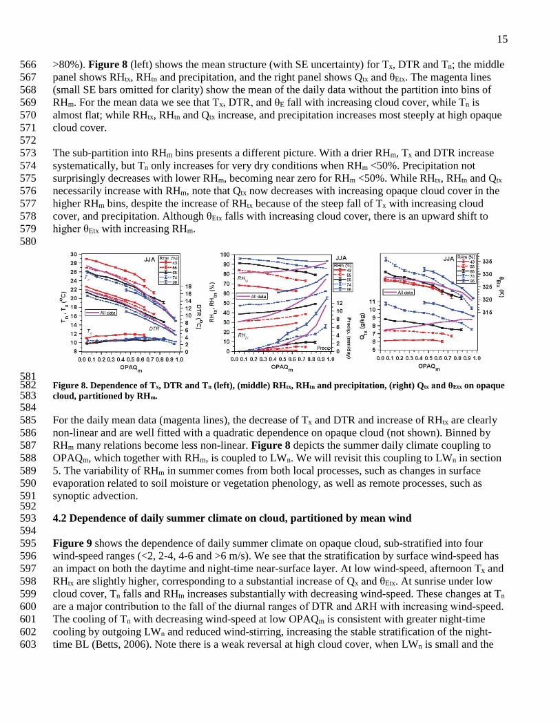
15 >80%). Figure 8 (left) shows the mean structure (with SE uncertainty) for Tx, DTR and Tn; the middle 566 panel shows RHtx, RHtn and precipitation, and the right panel shows Qtx and θEtx. The magenta lines 567 (small SE bars omitted for clarity) show the mean of the daily data without the partition into bins of 568 RHm. For the mean data we see that Tx, DTR, and θE fall with increasing cloud cover, while Tn is 569 almost flat; while RHtx, RHtn and Qtx increase, and precipitation increases most steeply at high opaque 570 cloud cover. 571 572 The sub-partition into RHm bins presents a different picture. With a drier RHm, Tx and DTR increase 573 systematically, but Tn only increases for very dry conditions when RHm <50%. Precipitation not 574 surprisingly decreases with lower RHm, becoming near zero for RHm <50%. While RHtx, RHtn and Qtx 575 necessarily increase with RHm, note that Qtx now decreases with increasing opaque cloud cover in the 576 higher RHm bins, despite the increase of RHtx because of the steep fall of Tx with increasing cloud 577 cover, and precipitation. Although θEtx falls with increasing cloud cover, there is an upward shift to 578 higher θEtx with increasing RHm. 579 580

581 Figure 8. Dependence of Tx, DTR and Tn (left), (middle) RHtx, RHtn and precipitation, (right) Qtx and θEtx on opaque 582 cloud, partitioned by RHm. 583 584 For the daily mean data (magenta lines), the decrease of Tx and DTR and increase of RHtx are clearly 585 non-linear and are well fitted with a quadratic dependence on opaque cloud (not shown). Binned by 586 RHm many relations become less non-linear. Figure 8 depicts the summer daily climate coupling to 587 OPAQm, which together with RHm, is coupled to LWn. We will revisit this coupling to LWn in section 588 5. The variability of RHm in summer comes from both local processes, such as changes in surface 589 evaporation related to soil moisture or vegetation phenology, as well as remote processes, such as 590 synoptic advection. 591 592 4.2 Dependence of daily summer climate on cloud, partitioned by mean wind 593 594 Figure 9 shows the dependence of daily summer climate on opaque cloud, sub-stratified into four 595 wind-speed ranges (<2, 2-4, 4-6 and >6 m/s). We see that the stratification by surface wind-speed has 596 an impact on both the daytime and night-time near-surface layer. At low wind-speed, afternoon Tx and 597 RHtx are slightly higher, corresponding to a substantial increase of Qx and θEtx. At sunrise under low 598 cloud cover, Tn falls and RHtn increases substantially with decreasing wind-speed. These changes at Tn 599 are a major contribution to the fall of the diurnal ranges of DTR and ΔRH with increasing wind-speed. 600 The cooling of Tn with decreasing wind-speed at low OPAQm is consistent with greater night-time 601 cooling by outgoing LWn and reduced wind-stirring, increasing the stable stratification of the night-602 time BL (Betts, 2006). Note there is a weak reversal at high cloud cover, when LWn is small and the 603

16 fall of surface T may be dominated by the evaporation of precipitation. The fall of RHtn with increasing 604 wind-speed may be related to the mixing down of drier air. 605 606

607 608 Figure 9. Coupling of daily climate to opaque cloud and wind-speed 609 610 At higher wind-speeds in the afternoon, θEtx decreases with increasing cloud cover, presumably related 611 to the reduction of the surface Rn with OPAQm, as well as the likelihood of low θE downdrafts at higher 612 precipitation rates. However the small increases in Tx and RHtx with decreasing wind-speed lead to a 613 broad maximum in θEtx for opaque cloud <0.5 (typical of a shallow cumulus field). We can only 614 speculate on the possible causes for this substantial increase of θEtx at low wind speeds. One possible 615 reason is that the near-surface gradients in the superadiabatic layer are stronger in weak winds, giving 616 an increase in Tx and RHtx with respect to the mixed layer. In contrast under strong winds, there may 617 be a near-neutral surface layer for the same cloud cover and radiative forcing. Another possible reason 618 could be that low wind-speeds may be associated with high pressure systems and with reduced 619 advection, and the BL may drift towards a warmer and moister state on sequential days. It is also 620 unclear whether this low wind-speed increase of near-surface θEtx is important for convective 621 development, but it is clearly important for convective parameterization schemes that lift near surface 622 air to saturation to define an ascending moist adiabatic. 623 624 4.3 Dependence of daily summer climate on OPAQm and OPAQSW 625

626 The stratifications in the previous sections were mapped in terms of OPAQm which can be related to 627 LWn, using equation (18a). This section will show how the diurnal cycle changes if the opaque cloud 628 fraction is non-uniform between day and night, so it has a different impact on SWn and LWn which in 629 turn changes Rn given by (19). We define 630 631

ΔOPAQ = OPAQm - OPAQSW (20) 632 633

When ΔOPAQ>0, it is less cloudy in the daytime hours than at night, which gives a positive change to 634 both SWCF and LWCF, as well as Rn; and the reverse for ΔOPAQ<0. It is generally cloudier in the 635 daytime in summer with a mean value of ΔOPAQ = -0.04. 636 637 Figure 10 shows the diurnal cycle impact for three ranges: ΔOPAQ < -0.5; -0.5< ΔOPAQ <0.5 and 638 ΔOPAQ >0.5. The mean values of ΔOPAQ for these three bins are -0.13, 0.00, +0.11. As expected, as 639 ΔOPAQ increases, both Tx and Tn increase (left panel), but the response of DTR is an increase when 640 OPAQm is high, but the change is not well-defined when OPAQm is low. For ΔOPAQ<0, RH 641 increases, and the decrease of ΔRH with OPAQm becomes steeper. The right panel shows that daily Rn 642

17 and afternoon θE both increase with increasing ΔOPAQ: suggesting that the increase of afternoon θE 643 can be viewed as a coupled response to less daytime cloud and higher daily Rn. The small associated 644 increase of precipitation, shown in the middle panel is consistent with this increase of afternoon θE. 645 646

647 648 Figure 10. Coupling of daily climate to OPAQm and ΔOPAQ 649 650 651 4.4 Dependence of daily summer climate on cloud, partitioned by precipitation anomalies 652 653 The land-atmosphere coupling depends on two key processes: Rn which mostly depends on cloud 654 forcing; and the partition of Rn into sensible and latent heat fluxes which depends on the availability of 655 soil water, as well as vegetation phenology and rooting. In this dataset we have no measurements of 656 soil water (or phenology), but we explored whether precipitation anomalies could provide some 657 information on the availability of soil water, and hence the energy partition and the daily climate. Betts 658 et al. (2014b) showed that summer afternoon RHtx and PLCLtx anomalies are strongly correlated on 659 monthly timescales with precipitation anomalies for the current month and preceding two months (Mo-660 1 and Mo-2), as well as the current month opaque cloud anomalies. For MJJA they found using 661 multiple linear regression (with R2 =0.68) 662 663 δRHtx = 4.21(±0.12) δPrecipWT + 4.46(±0.10) δOpaqueCloud (21) 664 665 with δOpaqueCloud in tenths; and δPrecipWT in mm/day, given by 666 667 δPrecipWT = 0.17(±0.02)*δPrecip(Mo-2) + 0.35(±0.02)*δPrecip(Mo-1) + 0.48(±0.02)*δPrecip (22) 668 669 Within the uncertainty of ±0.02, these weighting coefficients are the same for the PLCLtx regression; 670 both for MJJA and for the subset of the summer months, JJA. So this weighted precipitation contains 671 monthly timescale information about the memory of the current climate to current and past 672 precipitation. We can suppose that this correlation with RHtx means that these monthly values of 673 δPrecipWT are related to soil water anomalies. The reasoning here is that we know from surface flux 674 measurements (e.g. Betts and Ball, 1995, 1998) as well as many model studies that there is a chain of 675 processes linking soil water to surface vegetative resistance and transpiration, to the vapor pressure 676 deficit and the LCL of near-surface air (Betts, 2000, 2004; Betts et al., 2004; Betts and Viterbo, 2005; 677 Betts, 2009; Seneviratne at al., 2010; van Heerwaarden et al., 2010; Ferguson et al., 2012). 678 679 For this paper, we calculated the monthly precipitation anomalies for each station from a mean 680 monthly precipitation climatology, found by combining the 11 stations. Then we used equation (22) to 681

18 compute monthly weighted anomalies δPrecipWT for each station. These were used to sort the daily 682 data. This is more primitive than using a vegetation model and daily soil water balance model, but it 683 has the advantage of being entirely observationally based. But the mismatch between the monthly and 684 daily data introduces a significant approximation, because we use δPrecipWT for sorting all the days in 685 the current month, regardless of when it rains during this month. Nonetheless useful climate results 686 will emerge from these composites because the dataset is so large. 687

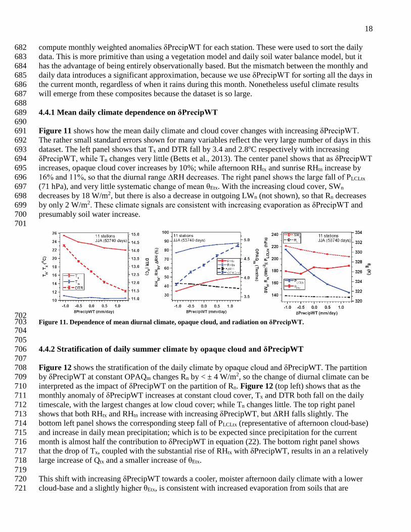
688 4.4.1 Mean daily climate dependence on δPrecipWT 689 690 Figure 11 shows how the mean daily climate and cloud cover changes with increasing δPrecipWT. 691 The rather small standard errors shown for many variables reflect the very large number of days in this 692 dataset. The left panel shows that Tx and DTR fall by 3.4 and 2.8oC respectively with increasing 693 δPrecipWT, while Tn changes very little (Betts et al., 2013). The center panel shows that as δPrecipWT 694 increases, opaque cloud cover increases by 10%; while afternoon RHtx and sunrise RHtn increase by 695 16% and 11%, so that the diurnal range ΔRH decreases. The right panel shows the large fall of PLCLtx 696 (71 hPa), and very little systematic change of mean θEtx. With the increasing cloud cover, SWn 697 decreases by 18 W/m2, but there is also a decrease in outgoing LWn (not shown), so that Rn decreases 698 by only 2 W/m2. These climate signals are consistent with increasing evaporation as δPrecipWT and 699 presumably soil water increase. 700 701

702 Figure 11. Dependence of mean diurnal climate, opaque cloud, and radiation on δPrecipWT. 703 704 705 4.4.2 Stratification of daily summer climate by opaque cloud and δPrecipWT 706 707 Figure 12 shows the stratification of the daily climate by opaque cloud and δPrecipWT. The partition 708 by δPrecipWT at constant OPAQm changes Rn by < ± 4 W/m2, so the change of diurnal climate can be 709 interpreted as the impact of δPrecipWT on the partition of Rn. Figure 12 (top left) shows that as the 710 monthly anomaly of δPrecipWT increases at constant cloud cover, Tx and DTR both fall on the daily 711 timescale, with the largest changes at low cloud cover; while Tn changes little. The top right panel 712 shows that both RHtx and RHtn increase with increasing δPrecipWT, but ΔRH falls slightly. The 713 bottom left panel shows the corresponding steep fall of PLCLtx (representative of afternoon cloud-base) 714 and increase in daily mean precipitation; which is to be expected since precipitation for the current 715 month is almost half the contribution to δPrecipWT in equation (22). The bottom right panel shows 716 that the drop of Tx, coupled with the substantial rise of RHtx with δPrecipWT, results in an a relatively 717 large increase of Qtx and a smaller increase of θEtx. 718 719 This shift with increasing δPrecipWT towards a cooler, moister afternoon daily climate with a lower 720 cloud-base and a slightly higher θEtx, is consistent with increased evaporation from soils that are 721

19 moister, due to higher precipitation on the monthly to seasonal timescale. Comparing with Figure 8, 722 where the data were simply stratified by daily RHm, we see some similarities, but also important 723 differences. For example, Figure 12 shows the increase of Qtx consistent with larger precipitation 724 anomalies and increased evaporation, which is different from the simple RH stratification in Figure 8. 725

726 Figure 12. Stratification of daily climate by opaque cloud and δPrecipWT 727 728 729 5. Dependence of summer climate on ECA and LWn 730

731 We can remap the opaque cloud dependence for the sub-stratifications shown in section 4 in terms of 732 daily mean ECA and LWn using (17a) and (18a). Figure 13 has six panels corresponding to the ECA 733 (top row) and LWn (bottom row) dependence of Tx, Tn and DTR for the RHm, wind speed and 734 precipitation anomaly stratifications shown in Figures 8, 9 and 12. For Tx and DTR, the left pair also 735 shows the mean of all the data (magenta). 736 737 The top row of panels differ from the corresponding panels in Figures 8, 9 and 12 by a small 738 difference between OPAQm and OPAQSW and the quadratic transformation from OPAQSW to ECA 739 given by (17a). However the transformation (18a) from OPAQm to LWn also includes a substantial 740 RHm dependence, which has a big impact on the stratifications that involve RH differences. The 741

20 bottom left panel for the RHm partition shows a collapse of DTR into almost a single line against LWn; 742 the bottom right for the precipitation partition shows a similar but smaller change. Both show a 743 reduction in the spread of Tx, when plotted against LWn. One interpretation of these differences 744 between these ECA and LWn stratifications is that the cooling at night is directly coupled to the LWn; 745 but the daytime partition of the solar flux determines the daytime warming and this is correlated to 746 either RHm or the precipitation anomalies. In contrast, the middle pair shows that the spread of DTR 747 and Tx is slightly increased when plotted against LWn rather than ECA, which is related to the small 748 increase in RH with decreasing wind speed. 749 750

751 Figure 13. ECA (upper row) and LWn (lower row) dependence of Tx, Tn and DTR for the RHm, wind speed and 752 precipitation anomaly stratifications 753 754 We have recovered for this much larger summer dataset, the nearly linear dependence of DTR on ECA 755 and LWn, which was seen in Figure 4 for 12 years of data at a single site for the warm season 756 (AMJJAS). The linear regression fits to the full set of filtered daily data (53740 days) are shown in all 757 panels (cyan) 758 759

DTR = 17.10(±0.02) –16.29(±0.07)*ECA (R2 = 0.53) (23) 760 DTR = 1.95(±0.04) – 0.146(±0.001)*LWn (R2 = 0.61) (24) 761 Tx = 28.05(±0.03) –17.35(±0.09)*ECA (R2 = 0.41) (25) 762 Tx = 12.42(±0.06) – 0.149(±0.001)*LWn (R2 = 0.44) (26) 763

764 The explained variance is much higher for DTR than Tx, because DTR = Tx – Tn and this difference 765 removes much of the daily variability related to the seasonal cycle and synoptic scale variability. 766 Comparing equations (15a) and (15b) with (23) and (24) we see that DTR has the same slope with 767 LWn, while this larger Prairie data set has a larger slope with ECA. Clearly the linear fit is better for 768 the LWn plots, confirming observationally the strong coupling between DTR and daily LWn seen in 769

21 models (Betts, 2004, 2006). The regression of this larger data set on ECA and the anomaly δRHm 770 (from the mean of 63.5%) is 771 772

DTR = 16.30(±0.06)–12.60 (±0.08) ECA - 0.083 (±0.001) δRHm (R2=0.57) (27) 773 774 Comparing with equation (15c) we see here a larger slope with ECA and a reduced slope with δRHm. 775 776 The wind speed dependence of DTR in the center panels increases with decreasing cloud or increasing 777 transmission ECT. We can represent this by adding a term to the multiple linear regression for the 778 product of ECT and the anomaly δWS (from the mean of 3.45m/s). This gives with a small increase in 779 the explained variance 780 781 DTR = 2.02(±0.04)–0.145 (±0.000) LWn – 0.43(±0.01) ECT*δWS (R2=0.63) (28) 782 783 So DTR falls with increasing wind speed by -0.43K/(ms-1) under clear skies. 784 785 The δPrecipWT dependence of DTR and Tx in the bottom right panel is small, with regressions 786 787

DTR = 2.12(±0.04) – 0.144(±0.001)*LWn + 0.30(±0.01) δPrecipWT (R2 = 0.61) (24a) 788 Tx = 12.702(±0.06) – 0.146(±0.001)*LWn + 0.47(±0.02) δPrecipWT (R2 = 0.44) (26a) 789

790 Figure 14 shows the nearly linear dependence of RHtx and PLCLtx on LWn, partitioned by daily wind 791 speed and weighted monthly precipitation anomaly. 792

793 Figure 14. LWn dependence of RHtx and PLCLtx, for the wind speed and precipitation anomaly stratifications. 794 795 The left panel also shows the linear regression fits (cyan) for all the daily data, which are 796 797 RHtx = 84.8(±0.1) + 0.566(±0.002) LWn (R2=0.67) (29) 798 PLCLtx = 7.5(±0.6) – 2.27(±0.01) LWn (R2=0.65) (30) 799 800 For the right panel, adding δPrecipWT (in mm/day), the multiple linear regression gives 801 802

RHtx = 82.9(±0.1) + 0.550(±0.002) LWn + 3.32(±0.05) δPrecipWT (R2=0.69) (31) 803 PLCLtx =16.5(±0.5) - 2.16(±0.01) LWn – 15.5(±0.2) δPrecipWT (R2=0.69) (32) 804

805

22 These linear regression fits for RHx have a higher R2 than the linear fits of DTR on LWn. For fixed 806 LWn, a 1 mm/day increase in the monthly precipitation anomaly, increases daily RHtx by 3.3% and 807 decreases PLCLtx by 15.5 hPa. 808 809 Derived from nearly 54000 days of data, these linear regression fits characterize the coupled surface-810 BL-cloud system over the Prairies on daily timescales; where the afternoon LCL is closely related to 811 cloud-base (Betts et al., 2013), and LWn is tightly coupled to opaque cloud fraction (Figure 6). For 812 model evaluation, this set of relationships, (24) and (28) to (32), describing the quasi-linear coupling 813 between LWn and the key diurnal climate variables DTR, RHtx and PLCLtx, may be the most useful. 814 815 816 6. Summary and Conclusions 817 818 The Prairie data show the observed diurnal climatology of the coupled land-BL-cloud system. In 819 contrast, models construct their own differing diurnal climatologies from a suite of process models and 820 parameterizations for the surface, BL and cloud components. Our broad intent is to provide 821 quantitative guidance based on observations for the evaluation of both simplified models, and the 822 large-scale models that we depend upon for weather forecasting and climate simulation. The control of 823 radiation by SWCF and LWCF is dominant on daily timescales (Betts et al., 2013), although both 824 cloud and precipitation matter on monthly to seasonal timescales (Betts et al. 2014b). So understanding 825 hydrometeorology requires both precipitation and cloud/radiation measurements as well as 826 temperature, RH and pressure data. Temperature, RH and pressure are all needed, because from them 827 we can compute Q, LCL and θE, which feedback on clouds and precipitation in the warm season. This 828 paper has focused primarily on mapping the coupling of clouds and other observables to the daily 829 climate in the warm season. 830 831 We used the Canadian Prairie data from eleven climate stations, which contains nearly 600 station-832 years of well-calibrated relatively homogenous data. Earlier work (Betts et al. 2013) explored the 833 coupling between daily climate and opaque cloud cover over the annual cycle; and used SWdn and 834 LWdn measurements to calibrate the opaque cloud observations in terms of SWCF and LWn. This 835 paper has extended their analysis in several directions. First we noted that the warm and cold season 836 regimes are sharply delineated by the freezing point of water. The diurnal cycle in the winter cold 837 regime with surface snow is dominated by LWCF, so that near-surface minimum temperatures plunge 838 under clear skies. In contrast, when T>0oC, SWCF dominates and maximum temperatures rise in clear 839 skies, while minimum temperatures change little. With this framework, we revisited the calibration of 840 the opaque cloud data in both cold and warm seasons using the high quality BSRN data from Bratt’s 841 Lake, Saskatchewan. Using just the BSRN data we explored the dependence of the diurnal range of T 842 and RH on the radiative drivers. We confirmed the nearly linear dependence of DTR on both ECA and 843 LWn in the warm season, seen in Betts et al. (2013), and earlier in model data (Betts, 2006). We then 844 used multiple regression to relate opaque cloud data at Regina with ECA and LWn at Bratt’s Lake, 845 only 25 km away. We found that LWn could be determined from the daily means of OPAQm and RHm 846 to ±8 W/m2 (R2=0.91) in the warm season (T>0oC); and from the daily means of OPAQm and Tm to 847 ±10 W/m2 (R2=0.87) in the cold season (T<0oC). We derived quadratic relationships between 848 OPAQSW, opaque cloud weighted by the daytime clear-sky SWdn flux, which give effective cloud 849 albedo, ECA to ±0.08 (R2=0.87) in the warm season, and to ±0.11 (R2=0.71) in the cold season. 850 851 We applied these relations between OPAQm and LWn, and OPAQSW and ECA to all eleven Prairie 852 stations, and created a summer (JJA) merge of the eleven Prairie stations to explore sub-stratifications 853

23 of the Prairie data. As noted by Betts et al. (2013, 2014b), cloud cover is the primary driver of daily 854 climate, as it largely determines LWn and Rn. However, the additional sub-stratification by RHm, wind 855 speed, the day-night asymmetry of cloud cover and monthly precipitation anomalies show how other 856 physical processes affect daily land-surface climate in summer. 857 858 The RH stratification shows that Tx and DTR increase systematically with drier RHm, but Tn only 859 increases for very low RHm <50%. Precipitation not surprisingly decreases sharply with lower RHm, 860 becoming near zero for RHm <50%. While θEtx falls with increasing cloud cover, as Tx falls, there is an 861 upward shift with constant cloud but increasing RHm to higher θEtx, consistent with increasing 862 precipitation. The variability of RHm in summer comes from both remote processes, such as synoptic 863 advection, as well as local processes, such as changes in surface evaporation related to soil moisture or 864 vegetation phenology. 865 866 The surface wind-speed stratification has an impact on both the daytime and night-time near-surface 867 layer. At low wind-speed, afternoon Tx and RHtx are slightly higher, giving a substantial increase of Qx 868 and θEtx. One possible reason is that the near-surface gradients in the superadiabatic layer are stronger 869 in weak winds, giving an increase in Tx and RHtx relative to the mixed layer. In contrast under strong 870 winds, there may be a near-neutral surface layer for the same cloud cover and radiative forcing. It is 871 unclear whether this low wind-speed increase of near-surface θEtx is important for convective 872 development. At sunrise, Tn is lower and RHtn is higher at low wind-speed and low cloud cover, 873 consistent with greater night-time cooling by outgoing LWn and reduced wind-stirring giving a more 874 stable stratification in the night-time BL (Betts, 2006). The fall of the diurnal ranges of DTR and ΔRH 875 with increasing wind-speed are heavily influenced by these changes at Tn. The fall of RHtn with 876 increasing wind-speed may be related to the mixing down of drier air into the stable BL. 877 878 The difference, ΔOPAQ, between the two opaque cloud means, daily mean OPAQm (closely related to 879 LWn) and OPAQSW, weighted by the solar clear sky flux (and related to ECA), is a measure of the 880 asymmetry of the cloud field between day and night. ΔOPAQ>0 means it is less cloudy in the daytime 881 hours than at night giving more solar heating and less LW cooling at night. We used ΔOPAQ to sub-882 stratify the data. As expected, as ΔOPAQ increases, both Tx and Tn increase, but the response of DTR 883 is more complex. DTR increases when OPAQm is high, but the change is not well-defined when 884 OPAQm is low. We see that daily Rn and afternoon θE both increase with increasing ΔOPAQ, and there 885 is a small associated increase of precipitation. 886 887 The land-atmosphere coupling depends on two key processes: Rn that mostly depends on cloud 888 forcing, which we know quite well from the opaque cloud data; and the partition of Rn into sensible 889 and latent heat fluxes, which depends on the availability of soil water, as well as vegetation phenology. 890 In this dataset we have no measurements of soil water or phenology, but based on the work of Betts et 891 al. (2014b) we sub-stratified the data using monthly weighted precipitation anomalies as a surrogate 892 for soil moisture anomalies. We found a shift with increasing precipitation anomalies towards cooler, 893 moister afternoon daily climate with a lower cloud-base and a higher θEtx. This is consistent with 894 increased evaporation from soils that are moister because of higher precipitation on the monthly to 895 seasonal timescale. 896 897 Finally we remapped the diurnal changes of temperature from the stratifications based on RHm, wind 898 and precipitation anomalies back onto LWn and ECA. Because LWn is itself dependent on RHm in the 899 warm season, the relationship between DTR and LWn becomes almost independent of RHm and 900 precipitation anomalies. This confirms the fundamental importance of daily LWn in determining the 901

24 diurnal temperature range, independent of the evaporative and advective processes that modify RH. 902 However the afternoon RHtx retains a substantial dependence on precipitation anomalies. We map the 903 quasi-linear coupling between LWn and the key diurnal climate variables DTR, RHtx and PLCLtx using 904 multiple linear regression in equations (24) and (28) to (32), with R2 values ranging from 0.61 to 0.69. 905 These relationships derived from the Prairie daily climate data for this fully coupled system may be the 906 most useful for model evaluation. Although we also derived relationships using multiple linear 907 regression between DTR and ECA and RHm, further exploration of the daytime forcing of the diurnal 908 climate requires the partition of Rn into sensible and latent heat fluxes. We plan to extend this work 909 using surface flux products for the Canadian Prairies (Wang et al., 2013). 910 911 Acknowledgments 912 913 This research was supported by Agriculture & Agri-Food Canada and the Center for Ocean-Land-914 Atmosphere Studies, George Mason University. We thank the civilian and military technicians of the 915 Meteorological Service of Canada and the Canadian Forces Weather Service, who have made reliable 916 cloud observations hourly for 60 years. We thank Devon Worth for processing the Prairie climate data 917 and Jeffrey Watchorn for processing the BSRN data. 918 919 920 References 921 922 Abramowitz, G. (2012). Towards a public, standardized, diagnostic benchmarking system for land 923 surface models, Geosci. Model Dev., 5, 819-827, doi:10.5194/gmd-5-819-2012. 924 925 Beljaars, A.C.M., Viterbo, P., Miller, M.J., and Betts, A.K. 1996: The anomalous rainfall over the 926 United States during July 1993: sensitivity to land surface parameterization and soil moisture 927 anomalies. Mon. Wea. Rev., 124, 362-383. 928 929 Betts, A. K. (2000). Idealized model for equilibrium boundary layer over land. J. Hydrometeorol., 1, 930 507-523. 931 932 Betts, A. K. (2004). Understanding hydrometeorology using global models. Bull. Amer. Meteorol. 933 Soc., 85, 1673-1688. 934 935 Betts, A. K. (2006). Radiative scaling of the nocturnal boundary layer and the diurnal temperature 936 range, J. Geophys. Res., 111, D07105, doi:10.1029/2005JD006560. 937 938 Betts, A. K. (2007). Coupling of water vapor convergence, clouds, precipitation, and land-surface 939 processes, J. Geophys. Res., 112, D10108, doi:10.1029/2006JD008191. 940 941 Betts, A. K. (2009). Land-surface-atmosphere coupling in observations and models. J. Adv. Model 942 Earth Syst., Vol. 1, Art. #4, 18 pp., doi: 10.3894/JAMES.2009.1.4 943 944 Betts, A.K. and Ball, J.H. (1995). The FIFE surface diurnal cycle climate. J. Geophys. Res. 100, 25679-945 25693. 946 Betts A. K. and Ball, J. H. (1998). FIFE surface climate and site-average dataset: 1987-1989. J. Atmos 947 Sci , 55, 1091-1108. 948 949

25 Betts, A. K and Viterbo, P. (2005). Land-surface, boundary layer and cloud-field coupling over the 950 south-western Amazon in ERA-40. J. Geophys. Res., 110, D14108, doi:10.1029/2004JD005702. 951 952 Betts, A. K., Helliker, B., and Berry, J. (2004). Coupling between CO2, water vapor, temperature and 953 radon and their fluxes in an idealized equilibrium boundary layer over land. J. Geophys. Res., 109, 954 D18103, doi:10.1029/2003JD004420. 955 956 Betts, A.K., Ball, J.H., Barr, A.H., Black, T.A., McCaughey, J. H., and Viterbo, P. (2006). Assessing 957 land-surface-atmosphere coupling in the ERA-40 reanalysis with boreal forest data. Agricultural and 958 Forest Meteorology, 140, 355-382, doi:10.1016/j.agrformet.2006.08.009. 959 960 Betts, A.K., Desjardins, R., and Worth, D. (2013). Cloud radiative forcing of the diurnal cycle climate 961 of the Canadian Prairies. J. Geophys. Res. Atmos., 118, 8935–8953, doi:10.1002/jgrd.50593. 962

Betts, A.K., Desjardins, R., Worth, D., Wang, S., and Li, J. (2014a). Coupling of winter climate 963 transitions to snow and clouds over the Prairies. J. Geophys. Res. Atmos., 119, 1118-1139, 964 doi:10.1002/2013JD021168. 965

Betts, A.K., Desjardins, R., Worth, D., and Beckage, B. (2014b). Climate coupling between 966 temperature, humidity, precipitation and cloud cover over the Canadian Prairies. J. Geophys. Res. 967 Atmos., 119, doi:10.1002/2014JD022511. 968

Dirmeyer, P. A. (2006). The hydrologic feedback pathway for land–climate coupling. J. Hydrometeor., 969 7, 857–867. 970

Dirmeyer, P.A., Koster, R.D., and Guo, Z. (2006). Do Global Models Properly Represent the Feedback 971 between Land and Atmosphere? J. Hydrometeor, 7, 1177–1198. doi: 972 http://dx.doi.org/10.1175/JHM532.1 973

Dirmeyer, P. A., Wang, Z., Mbuh, M.J., and Norton, H. E. (2014). Intensified land surface control on 974 boundary layer growth in a changing climate. Geophys. Res. Lett., 41, 1290–1294, doi:10.1002/ 975 2013GL058826. 976 977 Eltahir, E. A. B. (1998). A soil moisture–rainfall feedback mechanism: 1. Theory and observations. 978 Water Resour. Res., 34, 765–776. 979 980 Ferguson, C. R., and Wood, E.F., (2011). Observed land–atmosphere coupling from satellite remote 981 sensing and reanalysis, J. Hydrometeorol, 12, 1221–1254, doi:10.1175/2011JHM1380.1. 982 983 Ferguson, C. R., Wood, E.F., and Vinukollu, R. K. (2012). A global intercomparison of modeled and 984 observed land-atmosphere coupling. J. Hydrometeorol., 13, 749–784, doi:10.1175/JHM-D-11-0119.1. 985 986 Findell, K. L., and Eltahir, E.A.B. (2003). Atmospheric controls on soil moisture–boundary layer 987 interactions. Part I: Framework development. J. Hydrometeor., 4, 552–569. 988 989 Flato, G., Marotzke, J., Abiodun, B., Braconnot, P., Chou, S.C., Collins, W., Cox, P., and Coauthors 990 (2013). Evaluation of Climate Models. In: Climate Change 2013: The Physical Science Basis. 991 Contribution of Working Group I to the Fifth Assessment Report of the Intergovernmental Panel on 992

26 Climate Change [Stocker, T.F., D. Qin, G.-K. Plattner, M. Tignor, S.K. Allen, J. Boschung, A. Nauels, 993 Xia, Y., Bex, V., and Midgley, P.M. (eds.)]. Cambridge University Press, Cambridge, United Kingdom 994 and New York, NY, USA. 995 996 Guo, Z. C., Koster, R. D., Dirmeyer, P.A., Bonan, G., Chan, E., Cox, P., and Coauthors (2006). 997 GLACE: The Global Land–Atmosphere Coupling Experiment. Part II: Analysis. J. Hydrometeor., 7, 998 611–625. 999 1000 Koster, R. D. and Suarez, M. J. (2001). Soil moisture memory in climate models. J. Hydrometeor., 2, 1001 558–570. 1002 1003 Koster, R. D. and Manahama, S.P.P. (2012). Land Surface Controls on Hydroclimatic Means and 1004 Variability. J. Hydrometeor., 13, 1604-1619. 1005 1006 Koster, R. D., Dirmeyer, P.A., Guo, Z., Bonan, G., Chan, E., Cox, P., and Coauthors (2004). Regions 1007 of strong coupling between soil moisture and precipitation. Science, 305, 1138–1140. 1008 1009 Koster, R. D., Guo, Z., Dirmeyer, P.A., Bonan, G., Chan, E., Cox, P., and Coauthors (2006). GLACE: 1010 The Global Land–Atmosphere Coupling Experiment. Part I: Overview. J. Hydrometeor., 7, 590–610. 1011 1012 MANOBS (2013). Environment Canada MANOBS, Chapter 1, Sky. [Available at 1013 http://www.ec.gc.ca/manobs/default.asp?lang=En&n=A1B2F73E-1 ]. 1014 1015 Santanello, J. A., Peters-Lidard, C. D., Kennedy, A., and Kumar, S.V. (2013). Diagnosing the Nature 1016 of Land–Atmosphere Coupling: A Case Study of Dry/Wet Extremes in the U.S. Southern Great Plains. 1017 J. Hydrometeor, 14, 3–24. doi: http://dx.doi.org/10.1175/JHM-D-12-023.1 1018 1019 Seneviratne, S. I., Corti, T., Davin, E. L., Hirschi, M., Jaeger, E. B., Lehner, I., Orlowsky, B., and 1020 Teuling, A. J. (2010). Investigating soil moisture-climate interactions in a changing climate: A review. 1021 Earth. Sci. Rev., 99, 125–161, doi:10.1016/j.earscirev.2010.02.004. 1022

Taylor, C. M., Birch, C. E., Parker, D. J., Dixon, N., Guichard, F., Nikulin, G., and Lister, G.M.S. 1023 (2013). Modeling soil moisture-precipitation feedback in the Sahel: Importance of spatial scale versus 1024 convective parameterization. Geophys. Res. Lett., 40, 6213–6218, doi:10.1002/2013GL058511. 1025

van Heerwaarden, C. C., Vilà Guerau de Arellano, J., Gounou, A., Guichard, F., and Couvreux, F. 1026 (2010). Understanding the daily cycle of evapotranspiration: a method to quantify the influence of 1027 forcings and feedbacks. J. Hydrometeor., 11, 1405–1422. DOI: 10.1175/2010JHM1272.1 1028 1029 Wang, A., and Zeng, X. (2014). Range of monthly mean hourly land surface air temperature diurnal 1030 cycle over high northern latitudes, J. Geophys. Res. Atmos., 119, 5836–5844, 1031 doi:10.1002/2014JD021602. 1032 1033 Wang, S., Yang, Y., Luo, Y., and Rivera, A. (2013). Spatial and seasonal variations in 1034 evapotranspiration over Canada’s landmass. Hydrol. Earth Syst. Sci., 17, 3561–3575, 2013 1035 www.hydrol-earth-syst-sci.net/17/3561/2013/doi:10.5194/hess-17-3561-2013. 1036