Ecology, 94(10), 2013, pp. 2145–2151� 2013 by the Ecological Society of America

Better environmental data may reverse conclusions aboutniche- and dispersal-based processes in community assembly

LI-WAN CHANG,1,2 DAVID ZELENY,3,5 CHING-FENG LI,3 SHAU-TING CHIU,1,4 AND CHANG-FU HSIEH1

1Institute of Ecology and Evolutionary Biology, National Taiwan University, 1 Roosevelt Road, Section 4, Taipei 10617 Taiwan2Technical Service Division, Taiwan Forestry Research Institute, 53 Nanhai Road, Taipei 10066 Taiwan

3Department of Botany and Zoology, Faculty of Sciences, Masaryk University, Kotlarska 2, Brno 61137 Czech Republic4Department of Biology, National Museum of Natural Science, 1 Kuan Chien Road, Taichung 40453 Taiwan

Abstract. Variation partitioning of species composition into components explained byenvironmental and spatial variables is often used to identify a signature of niche- anddispersal-based processes in community assembly. Such interpretation, however, stronglydepends on the quality of the environmental data available. In recent studies conducted inforest dynamics plots, the environment was represented only by readily availabletopographical variables. Using data from a subtropical broad-leaved dynamics plot inTaiwan, we focus on the question of how would the conclusion about importance ofniche- and dispersal-based processes change if soil variables are also included in the analysis.To gain further insight, we introduced multiscale decomposition of a pure spatial component[c] in variation partitioning. Our results indicate that, if only topography is included, dispersal-based processes prevail, while including soil variables reverses this conclusion in favor ofniche-based processes. Multiscale decomposition of [c] shows that if only topography wasincluded, broad-scaled spatial variation prevails in [c], indicating that other as yet unmeasuredenvironmental variables can be important. However, after also including soil variables thispattern disappears, increasing importance of meso- and fine-scaled spatial patterns indicativeof dispersal processes.

Key words: dbMEM; dispersal-based processes; environmental control; Lienhuachih; multiscale spatialanalysis; soil variables; Taiwan; topographical variables; variation partitioning.

INTRODUCTION

Niche-based and dispersal-based processes have been

recognized as the main actors responsible for commu-

nity assembly (Cottenie 2005). The development of

analytical methods that are able to distinguish the

relative imprint of these processes in the structure of real

ecological communities is a continuous challenge. One

of the most promising approaches is the partitioning of

variation in community composition into environmental

and spatial components (Gilbert and Lechowicz 2004).

The theoretical justification behind this is based on an

assumption that environmental control on species

distribution according to the niche theory will result in

the variation of species composition explained by

environmental variables, while dispersal limitation will

generate spatial signatures in community structure that

are detectable by spatial variables (spatial filters). The

use of environmental and spatial predictors in variation

partitioning results in four components being distin-

guished; namely, a pure environmental component [a], a

spatially structured environmental component [b], a

pure spatial component [c], and unexplained variation

[d] (Borcard et al. 1992). In this framework, variation

explained by environment (components [a þ b]) repre-

sents environmental control imposed on species distri-

bution (Chase and Leibold 2003), while variation

explained purely by spatial variables (component [c])

represents partly unmeasured environmental variables

with spatial structure, and partly the legacy of dispersal

limitation (Legendre et al. 2009). If available environ-

mental predictors represent the most important envi-

ronmental drivers of species composition, then the ratio

between components [aþb] and [c] can be interpreted as

the ratio between niche-based and dispersal-based

processes in community assembly (e.g., Gilbert and

Lechowicz 2004). However, recent simulation studies

(Gilbert and Bennett 2010, Smith and Lundholm 2010)

indicate that the ability of variation partitioning to

disentangle these two families of processes has been

overrated and the dichotomy suggested above is

oversimplified. For example, component [b], which is

often quite large, can also carry the legacy of dispersal

processes, in the case that dispersal spatially coincides

with some of the environmental variables (such as

topography; Smith and Lundholm 2010). Still, parti-

tioning of the variation into environmental and spatial

component is seen as an important step toward

disentangling various processes responsible for spatial

community structure (Dray et al. 2012).

Manuscript received 24 November 2012; revised 14 May2013; accepted 11 June 2013. Corresponding Editor: J. B.Yavitt.

5 Corresponding author. E-mail: zeleny@sci.muni.cz

2145

Rep

orts

Recently, the variation partitioning approach has

been applied on data from forest dynamics plots

established by the Smithsonian Institution Center for

Tropical Forest Science (CTFS) and the Chinese Forest

Biodiversity Monitoring Network. Forest dynamics

plots are represented by large spatially contiguous grids

of subplots with permanently tagged and georeferenced

individuals of all woody species (Losos and Leigh 2004).

Legendre et al. (2009) applied variation partitioning of

tree beta diversity into environmental and spatial

components, using data from a Gutianshan forest

dynamics plot (China). Their approach, based on

redundancy analysis of raw abundance data, was

applied by De Caceres et al. (2012), after slight

modification, on a set of 10 forest dynamics plots,

distributed on three continents and ranging from

tropical to temperate zones. Besides introducing the

analytical framework for analysis of forest dynamics

plot data using the variation partitioning method, the

main goal of Legendre et al. (2009) was to ‘‘test

hypotheses about the processes (environmental control

and neutral) that may be responsible for the beta

diversity observed in the plot, by partitioning the effects

of topography and space on the distribution of species at

different spatial scales . . . .’’ Similarly, one of the aims of

the study by De Caceres et al. (2012) was to find out

‘‘what is the contribution of environmentally-related

variation vs. pure spatial and local stochastic variation

to tree beta diversity . . . .’’ Results of such analyses,

however, will be strongly dependent on the quality of

environmental variables used for variation partitioning

(Jones et al. 2008). The assumption that component [c]

represents the role of dispersal limitation holds only in

cases where all relevant environmental variables are

considered; otherwise, an unknown proportion of [c] is

represented by unmeasured environmental variables

(Laliberte et al. 2009, Diniz-Filho et al. 2012). Both

Legendre et al. (2009) and De Caceres et al. (2012) used

only topographical variables (elevation, convexity,

aspect, and slope) derived from the measured elevation

of corners of each grid, which are the standard

components of forest permanent plot data sets. Both

studies acknowledged the lack of other environmental

descriptors, mainly variables describing soil chemistry,

which were not available at the time of their study (or

not for all plots). In the Gutianshan study, Legendre et

al. (2009) assumed that, because of very rough terrain,

topographical variables should play an important role,

and that a large proportion of variation explained by

spatial variables and not explained by the environment

may indicate the operation of other factors such as

neutral processes. De Caceres et al. (2012) were more

careful in their interpretations, arguing that the varia-

tion explained by topography contains at least some

variation derived from environmental control, because,

when compared between plots, it increases with increas-

ing within-plot topographical roughness.

In our study, we focused on the question of how the

quality of environmental data changes the conclusions

drawn from the results of variation partitioning between

environmental and spatial variables. In the context of

previous studies of forest dynamics plots, based only on

topographical variables, we ask whether it is reasonable

to use topography as a surrogate for environment, and

how variation explained by environment will be

improved by also measuring soil variables. Soil proper-

ties are important (e.g., Jones et al. 2008, Baldeck et al.

2013), but not always available, while topography is easy

to measure in the field. Soil and topography is partially

correlated, but each may offer additional information

relevant for plant growth. Our aim is to evaluate how

important the environmental information in soil vari-

ables is and whether inclusion of soil can change or even

reverse conclusions drawn from studies based only on

topography.

Additional insight can be gained from more detailed

analysis of component [c], namely its scale structure.

This analysis is based on an assumption that broad-scale

spatial structures in species data represent imprints of

environmental variables, while fine-scale autocorrelation

is more likely generated by community dynamics,

including dispersal (Dray et al. 2012). Diniz-Filho et

al. (2012) analyzed variation represented by component

[c] evaluating the shape of Moran’s I correlograms and

claimed that their method can distinguish if [c] is

represented by broad-scaled unmeasured environmental

variables or fine-scaled dispersal processes. Here, we

introduce an alternative method to analyze scale

properties of the [c] component, based on its multiscale

decomposition using a scalogram approach (Legendre

and Legendre 2012). Using the available vegetation and

environmental data, we attempt to evaluate whether,

after including topographical variables as environmental

predictors, the spatial information in component [c] is

dominated by broad-scaled or fine-scaled spatial auto-

correlation. Further, we tested how the pattern changes

after also including soil variables, to reveal if soil and

topography captured the most important ecological

drivers of species composition.

Our study is based on detailed information about

topography, soil chemistry, and soil structure, collected

within 25-ha forest dynamics plot in Lienhuachih

(Taiwan), which is topographically very heterogeneous

(within-plot altitudinal range is 164 m). We apply the

same method of variation partitioning into fractions

explained by environmental and spatial variables as used

by Legendre et al. (2009) and De Caceres et al. (2012).

Using these data, the main objectives are (1) to show to

what extent the increase in variation in species

composition is explained by environment if we also

include soil variables in the analysis and how this

changes the conclusion about the importance of niche-

based and dispersal-based processes and (2) to demon-

strate the use of multiscale decomposition of [c]

LI-WAN CHANG ET AL.2146 Ecology, Vol. 94, No. 10R

epor

ts

component to detect whether important environmental

variables were included in the study.

METHODS

Study site.—The study was conducted in the Lien-

huachih Experimental Forest (see Plate 1) in central

Taiwan (238540 N, 1208520 E), which is a part of

international network of forest dynamics plots coordi-

nated by CTFS. The mean annual temperature is 20.88C

and the mean annual precipitation is 2285.0 mm with

pronounced seasonality (89.6% of total rainfall falls in

between May and September) and common typhoons

(Chang et al. 2010). The forest dynamics plot of 25 ha

(500 3 500 m) was set up in 2008, with methodology

following the census manual of Condit (1998). All

woody stems with diameter at breast height (dbh) �1 cmwere measured, tagged, mapped, and identified into

species. The elevation of the plot ranges from 667–845 m

above sea level, with an average slope of 35.38.

Altogether 153 268 individuals and 203 316 stems were

recorded within the plot (6131 individuals/ha and 8133

stems/ha, respectively). The vegetation represents sub-

tropical evergreen broad-leaved forest with important

canopy species including Cyclobalanopsis pachyloma,

Engelhardia roxburghiana, Pasania nantoensis, Schefflera

arboricola, and Schima superba (Chang et al. 2010).

Topographical, soil, and spatial descriptors.—As topo-

graphical descriptors, we used exactly the same type of

variables as Legendre et al. (2009) and De Caceres et al.

(2012), namely, mean elevation, convexity, slope, and

aspect, all derived from measured elevation of four

corners of each 20320 m cell (for details of calculations,

see Appendix S2 in De Caceres et al. 2012 and Appendix

A in this paper). The aspect was further segmented into

east-west and north-south directions, represented by the

sine and cosine of the aspect, respectively. Mean

elevation, convexity, and slope were used to construct

third-degree polynomial equations, creating a total of

nine monomials (see Legendre et al. 2009); in total 11

topographical variables (nine monomials and two

derivatives of aspect) were available for variation

partitioning. Variables calculated here differed slightly

from those used (and reported) by De Caceres et al.

(2012), probably because we used the most recent

version of the updated and corrected data set, while

De Caceres et al. (2012) used an older version (see

Appendix A for comparison).

Soil properties are described by 16 variables, including

soil chemistry (total C and N, C/N ratio, pH in 1 mol/L

KCl, extractable K, Ca, Mg, Fe, Mn, Cu, Zn, and P),

water content and texture (proportion of sand, silt and

clay); see Appendix B for details. Third-degree polyno-

mial equations were constructed for each soil variable,

resulting into 48 monomials used in further analyses.

As spatial descriptors, distance-based Moran’s eigen-

vector maps (dbMEM, previously known as PCNM)

derived from spectral decomposition of the spatial

relationships among grid cells were used (Borcard and

Legendre 2002, Dray et al. 2006). This method produces

linearly independent spatial variables covering a wide

range of spatial scales and allows modeling of any type

of spatial structure (Borcard and Legendre 2002).

Truncation distance was selected to retain links between

horizontal, vertical and diagonal neighboring cells. All

eigenvectors associated with Moran’s I coefficients

larger than the expected values of I were kept in the

analysis (all together 208 eigenvectors).

Statistical analyses.— To decompose the variation of

tree beta diversity into fractions explained by topo-

graphical, soil and spatial predictors, we used variation

partitioning approach based on redundancy analysis

(RDA; Rao 1964). Four variation partitioning analyses

were conducted, namely (1) topographical vs. spatial

variables, (2) soil vs. spatial variables, (3) soil and

topographical vs. spatial variables, and (4) topograph-

ical vs. soil vs. spatial variables. The set of first three

variation partitioning analyses was conducted on both

the original (i.e., not transformed) species composition

matrix and on the Hellinger standardized matrix

(Legendre and Gallagher 2001); this dichotomy aims

to make our results comparable to those of Legendre et

al. (2009), who did not use any standardization, and De

Caceres et al. (2012), who used Hellinger standardiza-

tion. Moreover, De Caceres et al. (2012) compared

different forest dynamics plots in terms of the amount of

beta diversity attributable to particular components of

variation partitioning. As a measure of beta diversity for

a given forest plot, they used total variance in the

Hellinger-standardized species data matrix (Legendre et

al. 2005), which was consequently divided into parts

according to components derived from variation parti-

tioning. To make our results comparable, we report the

results of variation partitioning of Hellinger-standard-

ized species data by both relative values of explained

variation using adjusted R2 (R2adj, Peres-Neto et al. 2006)

and the absolute values of beta diversity attributable to

individual components. Variation partitioning among

separate topographical, soil and spatial variables was

conducted only on Hellinger standardized matrix.

Multiscale decomposition of [c] component was

conducted using a set of partial RDAs. We evaluated

variation in species composition explained separately by

each dbMEM variable in three different scenarios: (1)

without any covariables (i.e., marginal variation ex-

plained by individual dbMEM variables), (2) with

topographical variables as covariables (i.e., variation

explained by dbMEM after accounting for topography),

and (3) with topographical and soil variables as

covariables (i.e., variation explained by dbMEM after

accounting for all available environmental variables).

The significance of each of the 208 dbMEM variables in

each of the three scenarios was tested by Monte Carlo

permutation test (reduced model with 9999 permuta-

tions); Holm’s correction (Holm 1979) was applied to

correct for multiple testing. Scenarios 1–3 differ by

gradually increasing the number of environmental

October 2013 2147EFFECT OF ENVIRONMENTAL DATA QUALITYR

eports

variables entering the analysis as covariables, from no

variables, only topographical, and both topographical

and soil variables. The focus of this analysis is on

relative changes in the distribution of variation ex-

plained by individual dbMEM variables after including

only topographical and both topographical and soil

variables, namely whether the variation explained by

broad-scaled dbMEM variables will decrease after

controlling for environmental variables. Large variation

explained by broad-scaled dbMEM in this analysis

indicates that not all important environmental variables

were included, while significant variation explained by

fine-scale dbMEM variables may indicate imprints of

population processes such as dispersal. Theoretically,

the distribution of the explained variations will change

from right skewed, with a dominance of variation

explained by broad-scaled spatial variables surrogating

unmeasured environmental variables, to left skewed

with a prevalence of variation explained by fine-scaled

spatial variables, indicating dominance of dispersal

processes.

RESULTS

Adding soil variables along with topographical

variables increases the variation explained by the

environment from the 20.7% explained by topography

only to 47.7% explained jointly by topography and soil

(Fig. 1 and Appendix C: Table C1, considering

Hellinger-standardized species data). Soil variables

alone explain 43.5%, which is twice as much as the

variation explained by only topographical variables.

With a non-standardized species matrix, the explained

variation is slightly higher: 24.5% for topographical

variables only, 43.6% for soil only, and 49.0% for both

(Table C1); hereafter, only results on Hellinger-stan-

dardized species data will be reported. Almost all

variation explained by environmental (either topograph-

ical or soil) variables is spatially structured, meaning

that an increase in variation explained by environmental

factors after including soil variables decreases the

variation explained purely by spatial variables (compo-

nent [c]). Component [c] decreases from 37.5% if only

topography is included to 11.3% if both topography and

soil are included, while unexplained variation [d]

remains unaffected by selection of environmental

variables. If examining topographical and soil variables

separately, it becomes obvious that most of the variation

explained by topography is explained also by soil

variables (from the 20.7% explained by topography,

16.6% is shared with soil; Fig. C1 in Appendix C), while

soil explains a considerable amount of variation by itself

(26.9% of variation is not shared with topography, from

a total of 43.5%). From this, we can conclude that if

appropriate soil variables are measured, topographical

variables become highly redundant, because, from the

total variation of 47.7% explained by the environment

(topography and soil), only 4.2% is explained purely by

topography.

If we adopt the approach of De Caceres et al. (2012),

the absolute values of beta diversity explained by

topography in Gutianshan and in Lienhuachih are

comparable (0.096 and 0.092, respectively, see Table

S3 in De Caceres (2012) for the first number and Table

C1 in Appendix C of our paper for the second), while the

part of beta diversity explained by pure space in

Gutianshan is lower than in Lienhuachih (0.105 and

0.166, respectively). Adding soil among environmental

variables in the case of Lienhuachih increases the beta

diversity explained by environment to 0.212 and

decreases those explained by pure space to 0.050.

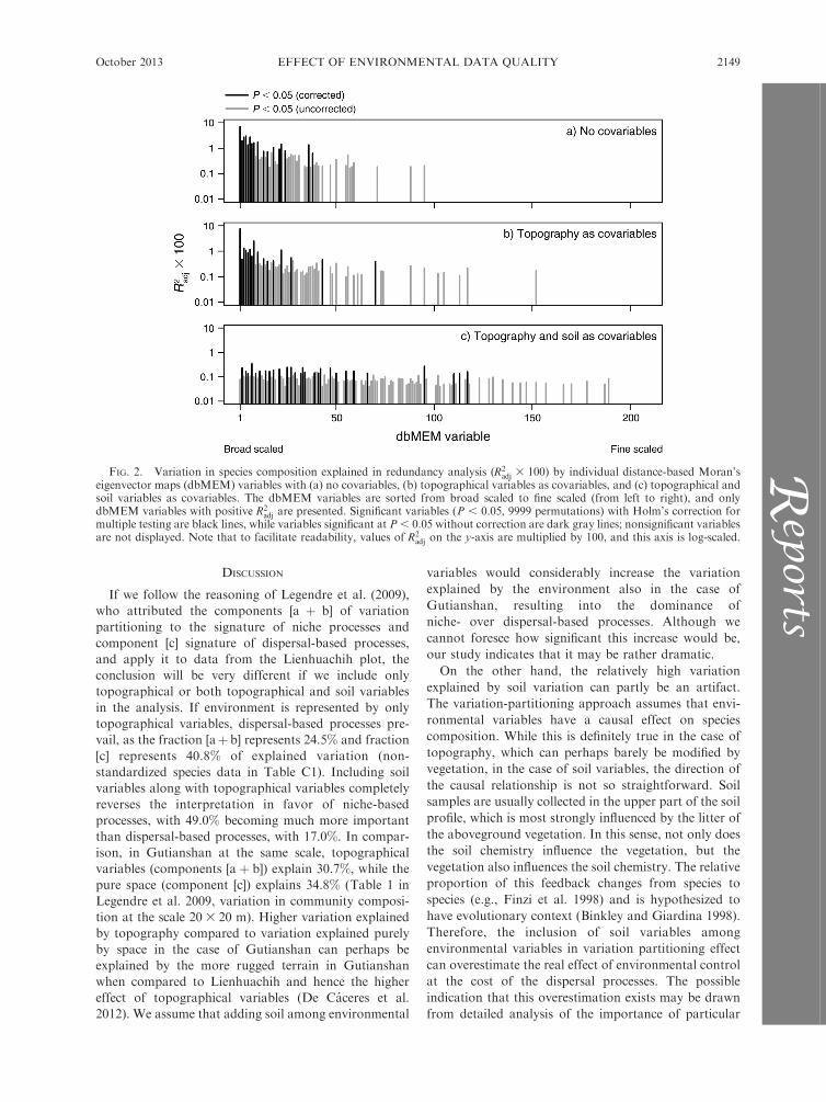
The distribution of variation explained by individual

dbMEM variables (ordered by decreasing spatial scale

from broad- to fine-scaled variables) changed consider-

ably among the three proposed scenarios. If no

covariables were included, the distribution was right

skewed (Fig. 2a), with broad-scaled dbMEM variables

being the most important (with dbMEM 1 explaining

6.8% of variation). Filtering out topographical variables

as covariables has a rather minor effect on the

distribution shape (Fig. 2b), with broad-scaled dbMEM

variables still prevailing. Adding soil variables along

with topographical ones to the covariables changes the

distribution dramatically, decreasing the importance of

broad-scaled dbMEMs in favor of meso- and partly also

fine-scaled dbMEMs (Fig. 2c).

FIG. 1. Results of variation partitioning of species compo-sition into fractions explained by environmental and spatialvariables (see Introduction for explanation of variables),reported as adjusted R2 on percentage scale (R2

adj 3 100).Environmental variables are represented either by onlytopographical, only soil, or both topographical and soilvariables together.

LI-WAN CHANG ET AL.2148 Ecology, Vol. 94, No. 10R

epor

ts

DISCUSSION

If we follow the reasoning of Legendre et al. (2009),

who attributed the components [a þ b] of variation

partitioning to the signature of niche processes and

component [c] signature of dispersal-based processes,

and apply it to data from the Lienhuachih plot, the

conclusion will be very different if we include only

topographical or both topographical and soil variables

in the analysis. If environment is represented by only

topographical variables, dispersal-based processes pre-

vail, as the fraction [aþ b] represents 24.5% and fraction

[c] represents 40.8% of explained variation (non-

standardized species data in Table C1). Including soil

variables along with topographical variables completely

reverses the interpretation in favor of niche-based

processes, with 49.0% becoming much more important

than dispersal-based processes, with 17.0%. In compar-

ison, in Gutianshan at the same scale, topographical

variables (components [a þ b]) explain 30.7%, while the

pure space (component [c]) explains 34.8% (Table 1 in

Legendre et al. 2009, variation in community composi-

tion at the scale 20 3 20 m). Higher variation explained

by topography compared to variation explained purely

by space in the case of Gutianshan can perhaps be

explained by the more rugged terrain in Gutianshan

when compared to Lienhuachih and hence the higher

effect of topographical variables (De Caceres et al.

2012). We assume that adding soil among environmental

variables would considerably increase the variation

explained by the environment also in the case of

Gutianshan, resulting into the dominance of

niche- over dispersal-based processes. Although we

cannot foresee how significant this increase would be,

our study indicates that it may be rather dramatic.

On the other hand, the relatively high variation

explained by soil variation can partly be an artifact.

The variation-partitioning approach assumes that envi-

ronmental variables have a causal effect on species

composition. While this is definitely true in the case of

topography, which can perhaps barely be modified by

vegetation, in the case of soil variables, the direction of

the causal relationship is not so straightforward. Soil

samples are usually collected in the upper part of the soil

profile, which is most strongly influenced by the litter of

the aboveground vegetation. In this sense, not only does

the soil chemistry influence the vegetation, but the

vegetation also influences the soil chemistry. The relative

proportion of this feedback changes from species to

species (e.g., Finzi et al. 1998) and is hypothesized to

have evolutionary context (Binkley and Giardina 1998).

Therefore, the inclusion of soil variables among

environmental variables in variation partitioning effect

can overestimate the real effect of environmental control

at the cost of the dispersal processes. The possible

indication that this overestimation exists may be drawn

from detailed analysis of the importance of particular

FIG. 2. Variation in species composition explained in redundancy analysis (R2adj 3 100) by individual distance-based Moran’s

eigenvector maps (dbMEM) variables with (a) no covariables, (b) topographical variables as covariables, and (c) topographical andsoil variables as covariables. The dbMEM variables are sorted from broad scaled to fine scaled (from left to right), and onlydbMEM variables with positive R2

adj are presented. Significant variables (P , 0.05, 9999 permutations) with Holm’s correction formultiple testing are black lines, while variables significant at P , 0.05 without correction are dark gray lines; nonsignificant variablesare not displayed. Note that to facilitate readability, values of R2

adj on the y-axis are multiplied by 100, and this axis is log-scaled.

October 2013 2149EFFECT OF ENVIRONMENTAL DATA QUALITYR

eports

soil properties and carefully considering if the important

properties are more likely to be derived from geological

substrates or from the effect of aboveground vegetation.

However, the real scale of this overestimation will

perhaps remain unknown, and its quantification will

require an experimental approach.

Multiscale analysis of residual spatial variation in

component [c] shows that topography itself is indeed not

a sufficient descriptor of environmental control on the

vegetation of our study site. The distribution of

variation explained by particular dbMEM variables

sorted from broad-scaled to fine-scaled did not change

much between analysis without any environmental

variables (Fig. 2a) and that including topography as

covariables (Fig. 2b). Both show that there is still a

considerable amount of broad-scaled spatial variation,

indicating that important environmental factors have

not been considered. After including soil variables,

variation explained by broad-scaled spatial variables is

not much higher than that explained by meso- or fine-

scaled variables. Some of the broad-scaled dbMEM

variables, however, remain significant, meaning that

there is still some space for other environmental

variables to play a role, although perhaps these are

not as important as soil.

The dichotomy of broad-scaled spatial variables

representing environmental variables and fine-scaled

spatial variables representing dispersal processes is

indeed simplified, and while it may be close to reality

at certain scales, it cannot be applied universally.

Ecologists tend to measure broad-scaled environmental

variables and ignore (or are unable to measure) the fine-

scaled ones (Dray et al. 2012), although these may also

exist. Similarly, far-distance dispersal may theoretically

result in more broad-scaled spatial community patterns.

Information about the spatial structure of component [c]

offers additional insight in data, but does not offer a

definite answer about the relative role of alternative

processes causing the spatial pattern. Further studies

may focus on the comparison of our method with spatial

autocorrelation analysis approach proposed by Diniz-

Filho et al. (2012) to see if the results are comparable,

and to check its sensitivity and reliability using

community data of known properties.

CONCLUSIONS

In the case study from the Lienhuachih forest

dynamics plot, we have shown that including soil

variables along with topographical variables into

variation partitioning results in a more than two-fold

increase in variation explained by the environment, and

reverses the original conclusion about the dominance of

dispersal-based processes in community assembly in the

prevalence of niche-based ones. Detailed multiscale

decomposition of [c] component indicates that topo-

graphical variables, when included as explanatory

variables, does not explain much of the broad-scaled

spatial pattern in species composition, while including

soil variables does, leaving meso- and fine-scaled spatial

patterns unexplained. However, we also pointed out that

the variation explained by soil variables may be

overestimated, because not only does soil influence the

PLATE 1. View of the Lienhuachih Experimental Forest, Taiwan, from the meteorological tower, taken on 22 August 2011.Photo credit: D. Zeleny.

LI-WAN CHANG ET AL.2150 Ecology, Vol. 94, No. 10R

epor

ts

vegetation, but vegetation also partly influences the

soil properties.

ACKNOWLEDGMENTS

Valuable contributions were made in the field by numerousvolunteers. We also thank the Taiwan Forestry ResearchInstitute (97 AS-7.1.1.F1-G1) and Taiwan Forestry Bureau(tfbm-960226) for financial support. D. Zeleny and C.-F. Liwere supported by the Czech Science Foundation (P505/12/1022). Early version of the manuscript benefited fromcomments of two anonymous reviewers.

LITERATURE CITED

Baldeck, C. A., et al. 2013. Soil resources and topography shapelocal tree community structure in tropical forests. Proceed-ings of the Royal Society B 280:1753.

Binkley, D., and C. Giardina. 1998. Why do tree species affectsoils? The warp and woof of tree-soil interactions. Biogeo-chemistry 42:89–106.

Borcard, D., and P. Legendre. 2002. All-scale spatial analysis ofecological data by means of principal coordinates ofneighbour matrices. Ecological Modelling 153:51–68.

Borcard, D., P. Legendre, and P. Drapeau. 1992. Partialling outthe spatial component of ecological variation. Ecology 73:1045–1055.

Chang, L.-W., J.-H. Hwong, S.-T. Chiu, H.-H. Wang, K.-C.Yang, H.-Y. Chang, and C.-F. Hsieh. 2010. Speciescomposition, size-class structure and diversity of the Lien-huachih forest dynamics plot in a subtropical evergreenbroad-leaved forest in central Taiwan. Taiwan Journal ofForestry Science 25:81–95.

Chase, J. M., and M. A. Leibold. 2003. Ecological niches.University of Chicago Press, Chicago, Illinois, USA.

Condit, R. 1998. Tropical forest census plots: methods andresults from Barro Colorado Island, Panama and acomparison with other plots. Springer, New York, NewYork, USA.

Cottenie, K. 2005. Integrating environmental and spatialprocesses in ecological community dynamics. Ecology Letters8:1175–1182.

De Caceres, M., et al. 2012. The variation of tree beta diversityacross a global network of forest plots. Global Ecology andBiogeography 21:1191–1202.

Diniz-Filho, J. A. F., T. Siqueira, A. A. Padial, T. F. Rangel,V. L. Landeiro, and L. M. Bini. 2012. Spatial autocorrelationanalysis allows disentangling the balance between neutral andniche processes in metacommunities. Oikos 121:201–210.

Dray, S., P. Legendre, and P. R. Peres-Neto. 2006. Spatialmodeling: a comprehensive framework for principal coordi-

nate analysis of neighbour matrices (PCNM). EcologicalModelling 196:483–493.

Dray, S., et al. 2012. Community ecology in the age ofmultivariate multiscale spatial analysis. Ecological Mono-graphs 82:257–275.

Finzi, A. C., C. D. Canham, and N. Van Breemen. 1998.Canopy tree–soil interactions within temperate forests:species effects on pH and cations. Ecological Applications8:447–454.

Gilbert, B., and J. R. Bennett. 2010. Partitioning variation inecological communities: do the numbers add up? Journal ofApplied Ecology 47:1071–1082.

Gilbert, B., and M. J. Lechowicz. 2004. Neutrality, niches, anddispersal in a temperate forest understory. Proceedings of theNational Academy of Sciences USA 101:7654–7656.

Holm, S. 1979. A simple sequentially rejective multiple testprocedure. Scandinavian Journal of Statistics 6:65–70.

Jones, M. M., H. Tuomisto, D. Borcard, P. Legendre, D. B.Clark, and P. C. Olivas. 2008. Explaining variation intropical plant community composition: influence of environ-mental and spatial data quality. Oecologia 155:593–604.

Laliberte, E., A. Paquette, P. Legendre, and A. Bouchard. 2009.Assessing the scale-specific importance of niches and otherspatial processes on beta diversity: a case study from atemperate forest. Oecologia 159:377–388.

Legendre, P., D. Borcard, and P. R. Peres-Neto. 2005.Analyzing beta diversity: partitioning the spatial variationof community composition data. Ecological Monographs 75:435–459.

Legendre, P., and E. D. Gallagher. 2001. Ecologicallymeaningful transformations for ordination of species data.Oecologia 129:271–280.

Legendre, P., and L. Legendre. 2012. Numerical ecology. ThirdEnglish edition. Elsevier Science, Amsterdam, The Nether-lands.

Legendre, P., X. Mi, H. Ren, K. Ma, M. Yu, I.-F. Sun, and F.He. 2009. Partitioning beta diversity in a subtropical broad-leaved forest of China. Ecology 90:663–674.

Losos, E., and E. G. Leigh, editors. 2004. Tropical forestdiversity and dynamism: findings from a large-scale plotnetwork. University of Chicago Press, Chicago, Illinois, USA.

Peres-Neto, P. R., P. Legendre, S. Dray, and D. Borcard. 2006.Variation partitioning of species data matrices estimationand comparison of fractions. Ecology 87:2614–2625.

Rao, C. R. 1964. The use and interpretation of principalcomponent analysis in applied research. Sankhyaa, Series A26:329–358.

Smith, T. W., and J. T. Lundholm. 2010. Variation partitioningas a tool to distinguish between niche and neutral processes.Ecography 33:648–655.

SUPPLEMENTAL MATERIAL

Appendix A

Comparison of environmental data for the Lienhuachih forest plot with those used by De Caceres et al. (2012) (EcologicalArchives E094-200-A1).

Appendix B

Details of soil sample analyses (Ecological Archives E094-200-A2).

Appendix C

Variation partitioning analysis between environmental (only topographical, only soil, or both) and spatial variables (EcologicalArchives E094-200-A3).

October 2013 2151EFFECT OF ENVIRONMENTAL DATA QUALITYR

eports