Ber. Polarforsch. 197 (1 996) ISSN 01 76 - 5027

ARK XI12

TROMS0 - BREMERHAVEN

22.09.1 995 - 29.1 0.1 995

Chief Scientist: Gunther Krause

Contents: Page:

1. Introduction 1.1 Scientific background 1.2 Strategie considerations and narrative of the cruise 1.3 Weather conditions

2. Meteorology 2.1 Turbulente measurements 2.2 Remote sensing of sea ice

3. Physical Oceanography 3.1 Stratification and circulation in the Greenland Sea 3.2 Transport of mass, heat and freshwater

4. Chemistry 4.1 Investigation of nutrients 4.2 Naturally produced volatile halogenated compounds

5. Zooplankton

6. Multidisciplinary sea ice investigations 6.1 Formation of sea ice 6.2 Effect of freezing rate on organism incorporation 6.3 Microcosm Sea ice formation experiment 6.4 Autumn/winter conditions within Arctic sea ice floes

7. Bathymetric mapping in the Fram Strait

8. Joint Research Program at Kiel University 8.1 Pelagic production regimes 8.2 Bentho-pelagic coupling 8.3 List of benthos stations

9. Station list

10. Participants

11. Ship's Crew

12. Participating Institutions

13. Moorings serviced during cruise ARK XI/2

CRUISE REPORT ARK XI12 Tromsa - Bremerhaven

22.9. - 29.10. 1995

' A u t u m n in the Greenland Sea" Chief Scientist: Gunther Krause

1.1 Scientific Background

With the theme "Autumn in the Greenland Sea" the expedition had set out to improve our knowledge of meteorological, physical, chemical and biological pro- cesses during the season of rapidly decreasing solar radiation and onset of the coo- ling phase. Previous field observations during this generally uncomfortable time of the year are fragmentary, and it was intended to close some of the gaps in the annual cycles of processes in the physical and biological arctic environment.

In the polar atmosphere, autumn provides the first strong outbreaks of cold air from Greenland onto a structured sea surface consisting of stretches of Open water and new ice. There is little Information on the near-ground turbulence of the at- mospheric boundary layer which determines the exchange of momentum, heat and water vapour under such conditions.

The principal goal of Physical Oceanography was to study the water mass stratifica- tion just before and possibly during the onset of convection. The measurements of temperature and salinity were supplemented by nutrient sampling for multipara- meter water mass analyses. These investigations continue observations on a long section from 13OW to 1 7 O E with a station spacing of 10 nm at 75ON, occupied 1989 for the first time during the international Greenland Sea project.

Besides nutrient analyses the investigations of Marine Chemistry concentrated on lipids, the energy reserves of copepods for surviving the Polar Night. In a second project naturally produced volatile halogenated organic trace compounds (e.g. chloroform, trichloroethylene and related substances) were studied.

The largest project focused on the role that autumn plays in the vertical flux of par- ticles which originate in the ice-associated and pelagic production and their fate in the sediment.

In addition to the above projects, which were specifically designed to profit from autumn conditions, a bathymetric survey of a region in Fram Strait was planned, and numerous current meter moorings were to be recovered and partly to be de- ployed. That task has fallen to this expedition because only the occasional research ship makes it this far to the north and is able to complete the work due to the ice- Cover.

1.2 Strategie considerations and narrative of the cruise

The onbreak of winter from the Northwest and the rapidly decreasing duration of daylight determined route and schedule of this autumn expedition in the first place. Daylight is followed by the Polar Night at 80° on the 22nd of October. Even at 75ON the times between sunrise and sunset decrease from 12 to 6 hours during the time of the expedition.

Daylight was a necessary preposition for many of the planned investigations. This included all work on the ice, the flight operations with the HELIPOD which carries delicate turbulence Sensors through the air 15 m below a helicopter, the flights with laser altimeter and line-scanner, and the recovery of moorings. In the ice some of the shipbased work which is normally done round the clock relies on day- light as well, e.g. the towing of bottom gear like Agassiz trawl and the epibenthos sledge. Naturally, there has been much pressure On the precious hours of daylight.

Fortunately, the large working group of Kiel University had planned for extensive station work up to 20 hours at few locations. These stations were called the "SFB stations", and they formed the backbone of the daily work during much of the first phase of the expedition. During the daylight time the flight operations and work on the ice could be done in parallel, and it has been possible to interrupt some of these stations to recover moorings.

Compromising on the demand to head North as fast as possible, to ensure daylight for respective work, and to minimize steaming, the following work sequence was adopted (Fig.1 .I):

Complete half of the bathymetric survey Try to recover moorings at 79ON while occupying SFB stations perpendicular to the slope of the Greenland Shelf from East to West In the ice, perform ice investigations parallel to ship operations, fly HELIPOD, laser altimeter, line-scanner and employ bow mast for turbulence measurements Work on stations in the Northeast Water Polynya (NEW) and supply fuel to Eskimonaes summer camp Perform SFB station work along the 2000 m isobath Complete second half of bathymetric survey Revisit mooring sites at 79ON to provide a second chance to recover moorings in the pack ice Steam to 75ON and recover 7 moorings in the area Intensive turbulence measuring campaign, complete ice investigations, SFB station and trawling with Agassiz net Work the long CTD transect at 75ON including several plankton net stations, deploy 1 and recover 2 moorings on depths of 3200 m

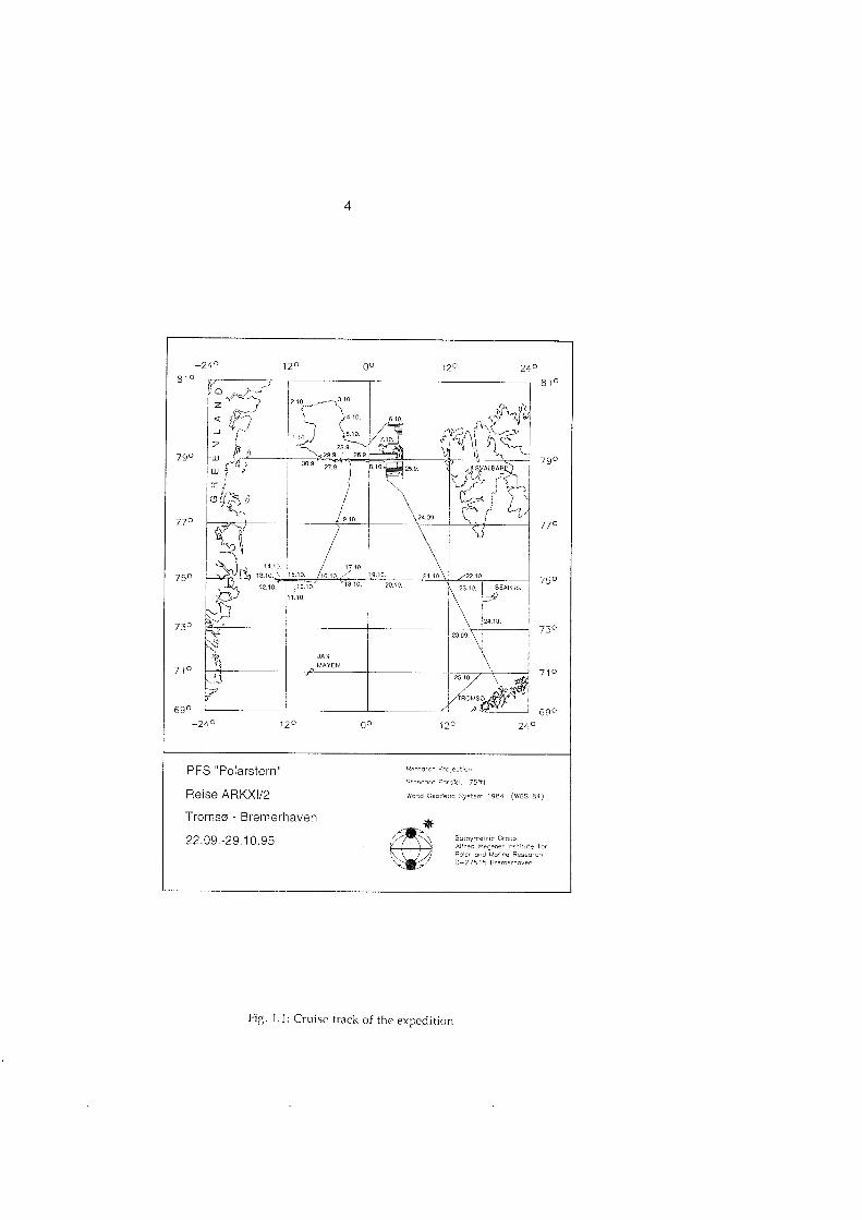
PFS "Polarstern"

Reise ARKXIl2

Tromse - Bremerhaven

22.09.-29.10.95

Fig. 1.1: Cruise track of the expedition

'Polarstern" left Tromsà in the morning of the 22nd of September. Due to a strong and favourable SW wind the bathymetric survey began only 1.5 days later at 79ON. On September 26, we found the first mooring at 790N under such thick and com- pressed pack ice that one could not even think of recovering the instruments, even though free water was tantalizingly close to the east. The Same Situation was found 12 days later, when the area was revisited. Out of five instrument moorings at 7g0N, three were brought on deck. Otherwise the recovery of all the other moored instrument strings on the list has been a great success so late in the season.

Due to an almost 100% coverage by very thick and very large old ice floes in the area of the NEW Polynya the summer camp at Eskimonaes could not be supplied. Only little station work in the vicinity of the planned positions was possible.

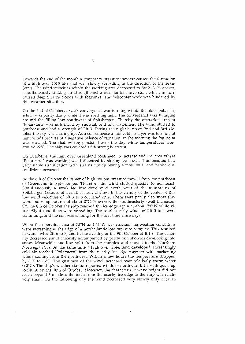
1.3 Weather Conditions

At the southeast side of a large low the wind increased to Bft 8, in gusts 9, when we were leaving the Norwegian fjords. The characteristic height of the waves reached about 3 m. Close to the center of the low the wind speed decreased on the following day to Bft 5, while the first Snow showers appeared and the temperature dropped to O0C.

During the night between 24th and 25th of September the ship arrived at its wor- king area West of Spitsbergen. On the northeast flank of a low that was located West of Spitsbergen the wind shifted to easterly direction with force Bft 5. Over the night the wind velocity rose up to Bft 7 shortly.

On September 26, the wind shifted via north to northwest, while a new low coming from Spitsbergen moved slowly westward. As a result of cold air advection from the northeast Greenland area the temperature dropped below O° for the first time during this journey. The thermometer showed -8OC at noontime. Temporary Snow flurries occurred. The lows were controlled by high rising cold air turbulence. Starting in the northern Greenland Sea the center of this turbulent region moved slowly southward towards the waters of Jan Mayen. Thereby the Fram Strait was influenced by an upper-level-airflow. This and the bottom low were moving southwestward and weakening.

On September 27, the wind shifted shortly to southwest and decreased to a force of Bft 3, when we were in the operation area at 78ON, 5OW. The stratiform clouds broke up simultaneously. On 28th of September a new low moved westward via Bear Island while its pressure dropped below 980 hPa. Heavy warm air advection at the front of this low caused a quick change in weather with snowfall and tempera- tures increasing close to O°C The wind shifted to north and increased to Bft 6. Since the controlling power of the upper level vortex over the Northern Polar Sea was still not diminished this low moved slowly southward while weakening to 1000 hPa in its center.

Towards the end of the month a temporary pressure increase caused the formation of a high over 1015 hPa that was slowly spreading in the direction of the Fram Strait. The wind velocities within the working area decreased to Bft 2 -3. However, simultaneously sinking air strengthened a near bottom Inversion, which in turn caused deep Stratus clouds with fogbanks. The helicopter work was hindered by this weather situation.

On the 2nd of October, a weak convergence was forming within the older polar air, which was partly damp while it was reaching high. The convergence was swinging around the filling low southwest of Spitsbergen. Thereby the operation area of "Polarstern" was influenced by snowfall and low visibilities. The wind shifted to northeast and had a strength of Bft 3. During the night between 2nd and 3rd Oc- tober the sky was clearing up. As a consequence a thin cold air layer was forming at light winds because of a negative balance of radiation. In the morning the fog point was reached. The shallow fog persisted over the day while temperatures were around -9OC. The ship was covered with strong hoarfrost.

On October 4, the high over Greenland continued to increase and the area where "Polarstern" was working was influenced by sinking processes. This resulted in a very stable stratification with Stratus clouds resting almost on it and 'white out' conditions occurred.

By the 6th of October the center of high bottom pressure moved from the northeast of Greenland to Spitsbergen. Therefore the wind shifted quickly to northeast. Simultaneously a weak lee low developed north West of the mountains of Spitsbergen because of a southeasterly airflow. In the vicinity of the center of this low wind velocities of Bft 3 to 5 occurred only. There were partly also Snow sho- wers and temperatures of about O°C However, the southeasterly swell increased. On the 8th of October the ship reached the ice edge again at about 79' N while vi- sual flight conditions were prevailing. The southeasterly winds of Bft 3 to 4 were continuing, and the sun was shining for the first time since days.

When the operation area at 75ON and l lOW was reached the weather conditions were worsening at the edge of a northatlantic low pressure complex. This resulted in winds with Bft 6 to 7, and in the evening of the 9th October of Bft 8. The visibi- lity decreased simultaneously accompanied by partly rain showers developing into Snow. Meanwhile one low split from the complex and moved to the Northern Norwegian Sea. At the Same time a high over Greenland developed. Increasingly cold air reached "Polarstern" from the nearby ice edge together with backening winds coming from the northwest. Within a few hours the temperature dropped by 8 K to -6OC. The gustiness of the wind increased over relatively warm water (+2OC). The ship's weather station reported winds of northwest Bft 8 with gusts up to Bft 10 on the 10th of October. However, the characteristic wave height did not reach beyond 3 m, since the fetch from the nearby ice edge to the ship was relati- vely small. On the following day the wind decreased very slowly only because

another weaker low moved quickly from Iceland to the North Cape. No air traffic was possible in light Snow flurries with low visibilities.

On the following two days the area of operation was influenced by an eastward spreading Greenland high. Light winds from northwest to southwest were blowing, there were little clouds, and at temperatures of -13T there were good vi- sibilities in dry air. The area at the ice edge at about 75OW 9OW was influenced by favourable weather, because the high over Greenland was increasing over 1025 hPa.

On the 14th October the wind came from northwest with Bft 4, the sky was without clouds and the visibility was very good. Towards the middle of the month the area of investigation was influenced shortly by a storm low that was moving slowly to the northeast. The wind which was shifting right to the northeast reached only Bft 6 on the 16th of October, since the low was slowly decreasing. There were heavy Snow showers in a labile layered cold air mass at the backside of the low at -2OC to -4OC air temperature. Because of the relatively small fetch characteristic wave heights of 1 to 2 m were reached. On the following day the wind blew consistently from one direction, but the speed decreased to 4 to 5 Bft.

On October 18 the wind shifted to the right to southeasterly direction because of a low development in the Fram Strait. The wind blew with Bft 7 with Snow showers. A new storm low which developed on the 17th of October in lee of Greenland near Cape Farvel moved under decreasing via Iceland towards the Northern Norwegian Sea. It reached a low pressure of 980 hPa at the 19th of October. "Polarstern" stayed at first at the outer edge on the north side of this cyclone.

On the 20th of October the wind was backing to the northwest and increased within a few hours to Bft 8. This was due to our location at the backside of this storm low. The temperature dropped from -4OC to -8OC simultaneously because of cold air ad- vection. This led to a turbulente development over the 5OC warm sea water. The wave height increased rapidly. During the night of 21st/22nd of October a marked cold air front passed "Polarstern". It caused a sudden shift in the wind direction from West to eastnortheast and an increase in the wind velocity from Bft 3 to Bft 9. There was no work possible at the station due to Snow flurries and crossing seas up to 5 m in height. But the the weather calmed down quickly.

On the way home several cyclones influenced the track of the ship. They develo- ped into storm lows partly below 970 hPa in the vicinity of Iceland. Strong southerly winds prevailed south of 70°N

Bordwetterwarte FS Polarstern ARK XI12 Tromsoe - Bremerhaven 22.9, - 29 10.95

Bordwetterwarte FS Polarstern ARK XI12 Tromsoe - Bremerhaven 22.9. - 29 10.95

-

0 1 2 3 4 5 6 7 8 9 1 0 1 1 1 2

Windstiirke in Beaufort

Fig. 1.2: Frequency distributions of wind direction and wind speed

- Lufttempetatut Tauputii~tstempetati~

Fig. 1.3: Air temperature, dew point temperature and wind velocity

2.1 Turbulence measurements (C. Wamser, W. Cohrs, C. Wode, M. Hofmann, M. Schürmann

Current efforts in numerical climate predictions require that the knowledge of glo- bal near-surface turbulent energy fluxes be improved by about one order of magni- tude. Since the earth's polar regions have great influence on the oceanic deep-sea water circulation, the atmosphere-ocean heat and momentum exchange is also of special interest. Due to the inaccessibility of these regions, most of the relevant pa- rameters, needed for model calculations, are poorly investigated.

In order to help filling this gap, two quite different but complementary meteorolo- gical turbulence measuring systems were operated together for the first time: the helicopter-borne sensor system HELIPOD, and the newly constructed shipborne turbulence measuring system TMS. Both systems aim at high-resolution in-situ measurements of near-surface turbulent fluxes of mass, momentum, sensible and latent heat. The turbulence measurements were supplemented by a helicopter- borne colour line-scan camera, which provided digital Images of the ice Cover in order to record the different ice situations during the flux measurements.

The TMS consists of a 17 m mast, installed on the ship's bow crane. This mast usually is fixed horizontally during the cruise, but for operation it can be moved forward and turned into a vertical position by a hydraulic and a tackle system. At five heights between 3 and 20 m above the sea surface, five USAT sonic sensors (METEK) are mounted to measure the turbulent fluctuations of wind and tempera- ture. Five Pt-100 temperature sensors determine the mean temperature profile. Additionally, a Lyman-alpha hygrometer is installed at a height of 3 m to measure the turbulent humidity signals. An acceleration sensor determines disturbing fre- quencies of mast oscillations or even of slow ship movements.

HELIPOD is an autonomous meteorological turbulence measurement system, about 5 m long and 240 kg in weight, which is constructed for operation on a 15 m rope below almost any helicopter. The system is the first worldwide, and the only one which combines the aerodynamical and logistical advantages of a helicopter as towing aircraft with high-tech meteorological, navigational and technical sensor equipment. HELIPOD possesses an internal power supply, an active rudder stabili- zation, a DGPS-based and an inertial navigation system, and an extensive sensor equipment including real-time data processing and recording. It carries the fol- lowing meteorological sensors: A 5-hole probe for static pressure and wind measu- rements, 2 temperature sensors with different response times, an independent humidity measuring channel containing a humicap (i.e. a capacitive humidity sensor), a dewpoint mirror and a Lyman-alpha sensor, and a radiation thermome- ter for surface temperature measurements.

The navigation system equally comprises sensors with different response times and long-term stabilities: a static and a radar altimeter, an inertial navigation sy-

stem and two different GPS Systems providing the determination of both position and altitude.

As HELIPOD contains some quasi-redundant sensors each with different time be- haviour, even long-term data can be obtained within a wide frequency range through complementary filtering of corresponding signals. For additional impro- vement, the digitizing error of the fast sensors is reduced by storing 10-value aver- ages calculated on-line from a 1000-Hz oversampling.

Meteorological and navigational raw data, technical system Parameters and on-line calculated secondary quantities are recorded in up to 160 channels. Sampling fre- quencies reach from 1 Hz (GPS navigation) up to 100 Hz (turbulent fluctuations of meteorological quantities). Data preprocessing is done simultaneously by different transputers, while the final data storing is real-time controlled by the VC6 main computer. For data storing, magneto-optical discs are used with a recording capacity of 300 MB each side, corresponding to about 3 hours or 450 km flight path length. A special software package allows an on-line display of arbitrary data channels on a laptop computer inside the helicopter and an in-flight calibration of different sen- sors.

The objectives for the HELIPOD operations during ARK XI/2 were:

system tests and calibration flights, measurements of the near-ice edge atmospheric boundary layer structure, airborne near-surface measurements within a stably stratified boundary layer over different types of surfaces and comparison of the results with those, gathered simultaneously by the shipborne TMS, investigations of the dependence of some statistical meteorological properties from different types of flight patterns, comparisons of HELIPOD vertical profiles with data from GPS-wind finding radiosondes.

In total, during the ARK XI/2 cruise 10 different HELIPOD measurements were performed. The locations of the flights are marked in Figure 2.1.

The main objectives of the TMS measurements were the analysis of the turbulent fluxes in the marginal ice Zone and a general in-situ system test. During the whole cruise, the TMS was operated at 8 stations each of 2 to 3 hours duration. At these stations the ship was either at a fixed position in the ice or moved very slowly against the wind. During the measurements, very different structures of ice Cover could be investigated with regard to their influences On the heat, moisture and momentum exchange between the ocean and the atmosphere. All the elements of the TMS including mast, hydraulic and tackle Parts, sensors and the data acquisi- tion system were tested under various meteorological situations.

Figure 2.1: Locations of HELIPOD flight areas during ARK XI/2. The inserted symbols denote in particular: cross: test measurements and calibration flights, triangle: measurements of the near-ice edge boundary layer structure, diamond: HELIPOD, TMS and radiosonde comparisons, Square: test of statistical flight pattern properties.

It turned out that different modes of operation of the ship's propulsion System (main engine, bow and Stern thrusters) cause different vibrations of the ship, which also are conducted to the mast and the Sensors via the bow crane. High reso- lution acceleration measurements provided the spectral distribution of all the va- rious vibrations which possibly may influence the turbulence signals. By means of spectral analysis of the acceleration measurements, two dominant frequencies were detected. These vibrations were mainly caused by the rotation of the main shafts and the thrusters, and they are at 3 and 14 Hz, respectively. The amplitudes of the corresponding acceleration have turned out to be typically about 0.05 g.

The evaluation of the collected HELIPOD and TMS data comprise plausibility checks, elimination of outliers and trends, correction for potential data losses and resulting spectral gaps, cutting of longer time series into sections, spectral analysis of the resulting time series, and finally the calculation of some statistical properties which provide information about the investigated turbulent exchange processes. For this purpose also the weather analyses of the "Polarstern" weather-station are used, as well as some further radiosounding data, satellite images and ice charts.

First steps of data evaluation of both HELIPOD and TMS data were started directly after the measurements on board "Polarstern". Since a total amount of about 2500 MBytes of binary HELIPOD raw data and about 700 MBytes of TMS data were

-25 -20 -15 -10 -5 0 5 Distonce [km]

Figure 2.2: Isotherms of the potential temperature in a vertical plane perpendicular to the marginal ice Zone. The abscissa origin indicates the transition betwcen the ice edge and Open water. Positive distances denote Open water, negative ones denote ice cover. (HELIPOD flieht 8,75.0Â N / 12.8' W, 12'0ctober 1995,10:50 - 12:30 UTC)

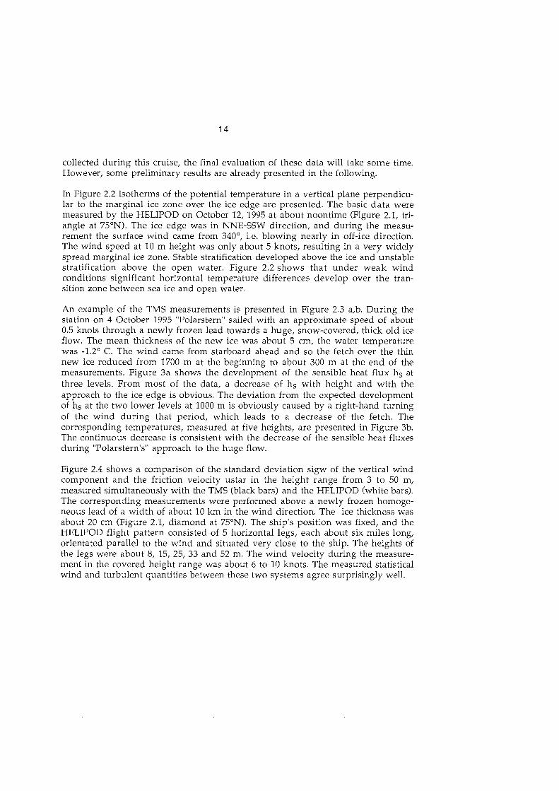
collected during this cruise, the final evaluation of these data will take some time. However, some preliminary results are already presented in the following.

In Figure 2.2 isotherms of the potential temperature in a vertical plane perpendicu- lar to the marginal ice zone over the ice edge are presented. The basic data were measured by the HELIPOD On October 12, 1995 at about noontime (Figure 2.1, tri- angle at 75'N). The ice edge was in NNE-SSW direction, and during the measu- rement the surface wind came from 340° i.e. blowing nearly in off-ice direction. The wind speed at 10 m height was only about 5 knots, resulting in a very widely spread marginal ice zone. Stable stratification developed above the ice and unstable stratification above the Open water. Figure 2.2 shows that under weak wind conditions significant horizontal temperature differences develop over the tran- sition Zone between sea ice and Open water.

An example of the TMS measurements is presented in Figure 2.3 a,b. During the station on 4 October 1995 "Polarstern" sailed with an approximate speed of about 0.5 knots through a newly frozen lead towards a huge, snow-covered, thick old ice flow. The mean thickness of the new ice was about 5 Cm, the water temperature was -1.2' C. The wind came from starboard ahead and so the fetch over the thin new ice reduced from 1700 m at the beginning to about 300 m at the end of the measurements. Figure 3a shows the development of the sensible heat flux hs at three levels. From most of the data, a decrease of hs with height and with the approach to the ice edge is obvious. The deviation from the expected development of hs at the two lower levels at 1000 m is obviously caused by a right-hand turning of the wind during that period, which leads to a decrease of the fetch. The corresponding temperatures, measured at five heights, are presented in Figure 3b. The continuous decrease is consistent with the decrease of the sensible heat fluxes during "Polarstern's" approach to the huge flow.

Figure 2.4 shows a comparison of the standard deviation sigw of the vertical wind component and the friction velocity ustar in the height range from 3 to 50 m, measured simultaneously with the TMS (black bars) and the HELIPOD (white bars). The corresponding measurements were performed above a newly frozen homoge- neous lead of a width of about 10 km in the wind direction. The ice thickness was about 20 cm (Figure 2.1, diamond at 75ON). The ship's position was fixed, and the HELIPOD flight Pattern consisted of 5 horizontal legs, each about six miles long, orientated parallel to the wind and situated very close to the ship. The heights of the legs were about 8, 15, 25, 33 and 52 m. The wind velocity during the measure- ment in the covered height range was about 6 to 10 knots. The measured statistical wind and turbulent quantities between these two Systems agree surprisingly well.

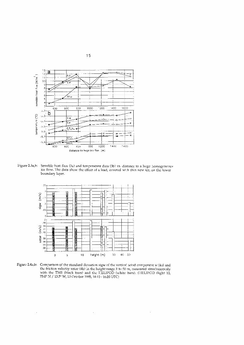
distance t o huge ice floe (m)

Figure 2.3a,b: Sensible heat flux (3a) and temperature data (3b) vs. distance to a huge homogeneous ice flow. The data show the effect of a lead, covered with thin new ice, on the lower boundary layer.

2

.I8 - 16

^ 14 E U 12

L 1 ,T OB

2 06

.04

-02

0

3 5 10 height (m) 30 40 50

Figure 2.4a,b: Comparison of the standard deviation sigw of the vertical wind component W (4a) and the friction velocity ustar (4b) in the height range 3 to 50 m, measured simultaneously with the TMS (black bars) and the HELIPOD (white bars). (HELIPOD flight 10, 75.0' N / 13.5' W, 13 October 1995,14:10 - 16:20 UTC)

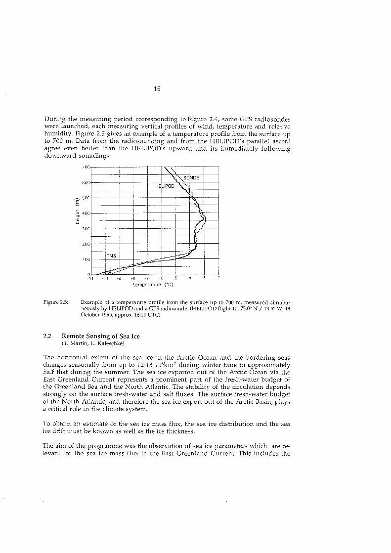
During the measuring period corresponding to Figure 2.4, some GPS radiosondes were launched, each measuring vertical profiles of wind, temperature and relative humidity. Figure 2.5 gives an example of a temperature profile from the surface up to 700 m. Data from the radiosounding and from the HELIPOD's parallel ascent agree even better than the HELIPOD's upward and its immediately following downward soundings.

700

600

- 500 E

400 .- (U .C

300

200

100

0 -1 1 -10 -9 -8 -7 -6 -5 -4 -3 -2

ternperature ('C)

Figure 2.5: Example of a temperature profile from the surface up to 700 m, measured simulta- neously by HELIPOD and a GPS radiosonde. (HELIPOD flight 10,75.0Â N / 13.5O W, 13 October 1995, approx. 16:lO UTC)

2.2 Remote Sensing of Sea Ice (T. Martin, L. Kaleschke)

The horizontal extent of the sea ice in the Arctic Ocean and the bordering seas changes seasonally from up to 12-13 106km2 during winter time to approximately half that during the summer. The sea ice exported out of the Arctic Ocean via the East Greenland Current represents a prominent Part of the fresh-water budget of the Greenland Sea and the North Atlantic. The stability of the circulation depends strongly On the surface fresh-water and salt fluxes. The surface fresh-water budget of the North Atlantic, and therefore the sea ice export out of the Arctic Basin, plays a critical role in the climate System.

To obtain an estimate of the sea ice mass flux, the sea ice distribution and the sea ice drift must be known as well as the ice thickness.

The aim of the Programme was the observation of sea ice Parameters which are re- levant for the sea ice mass flux in the East Greenland Current. This includes the

reception of satellite images and measurement of the sea ice surface structure. The combined processing along with data Sets of sea ice thickness, sea ice concentration, sea ice extension and sea ice drift velocity should give an improved knowledge of the sea ice mass fluxes in this area.

AVHRR satellite images: During the expedition, images of the Advanced Very High Resolution Radiometer (AVHRR) flown on the satellites of the National Oceanic and Atmospheric Administration (NOAA) have been received on board "Polarstern". The AVHRR is sensitive in the visible and thermal infra-red spectral range. The horizontal reso- lution in the nadir view is 1.1 km. All images are processed using routines for cali- bration and rectification on to a stereographic grid. These images were used to de- rive the sea ice distribution, and for planning the flight activities of the laser-alti- meter (see below) as well as for ship navigation.

Sequences of cloud-free images allow the determination of the sea ice motion. Special image processing algorithms track common features in pairs of images. The investigations of the last years show a minimum of the sea ice drift velocity in summertime of 15cm/s. During autumn, the drift velocity increases and reaches a maximum during winter with approximately 30 cm/s.

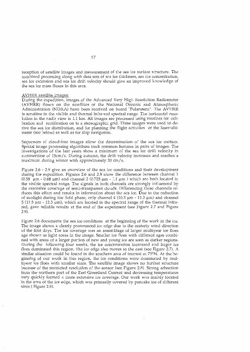
Figure 2.6 - 2.9 give an overview of the sea ice conditions and their development during the expedition. Figures 2.6 and 2.8 show the difference between channel 1 (0.58 pm - 0.68 pm) and channel 2 (0.725 pm - 1.1 [im ) which are both located in the visible spectral range. The signals in both channels are strongly influenced by the extensive coverage of semi-transparent clouds. Differencing these channels re- duces this effect and results in information about the sea ice. Due to the reduction of sunlight during the field phase, only channel 4 (10.3 [im - 11.3 pm) and channel 5 (11.5 pm - 12.5 pm), which are located in the spectral range of the thermal infra- red, gave reliable results at the end of the experiment (see Figure 2.7 and Figure 2.9).

Figure 2.6 documents the sea ice conditions at the beginning of the work in the ice. The image shows a clearly pronounced ice edge due to the easterly wind direction of the first days. The ice coverage was an assemblage of larger multiyear ice floes age shown as light areas in the image. Smaller ice floes with different ages combi- ned with areas of a larger portion of new and young ice are Seen as darker regions. During the following four weeks, the ice concentration increased and larger ice floes dominated this region. The ice edge also moves to the east (see Figure 2.7). A similar situation could be found in the southern area of interest at 75ON. At the be- ginning of our work in this region, the ice conditions were dominated by mul- tiyear ice floes with smaller sizes. The satellite image shows no further structure because of the restricted resolution of the Sensor (see Figure 2.8). Strong advection from the northern Part of the East Greenland Current and decreasing temperatures very quickly formed a more extensive ice coverage. Our work was mainly located in the area of the ice edge, which was primarily covered by pancake ice of different sizes ( Figure 2.9).

Figure 2.7: NOAA-12 AVHRR satellite image of October 24,1995 08:12 GMT channel5 and the ship's track from September 24 to October 8

Figure 2.8: NOAA-14 AVHRR satellite image of October Ist, 1995 12:14 GMT channel 1 - channel2 and the ship's track from October 9 to October 19

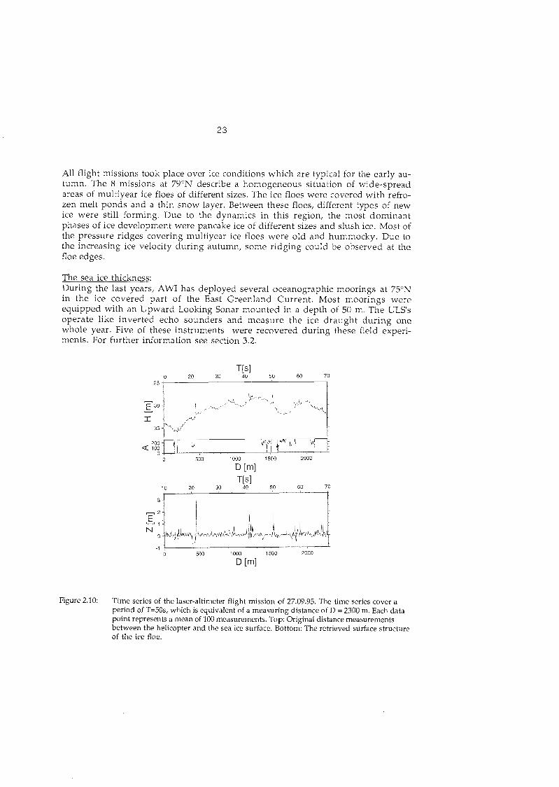
The laser-altimeter: Laser profiling is a remote sensing technique in which the terrain surface elevation along a straight line path is monitored. In sea ice remote sensing, laser profiler data are used to investigate the roughness of the ice surface, in particular, height and spatial distributions of pressure and shear ridges. Profiler data can also be utilized to estimate the thickness of ridged ice. Given the roughness statistics, it is also pos- sible to determine the contribution of form drag on ridges to the momentum transfer from the atmosphere to the pack ice.

The laser profiler used during this experiment was an Ibeo PS 100 EL mounted on a helicopter. The laser diode generates pulses with a wavelength of 905 nm. The ice surface elevation profiles were collected at a sampling rate of 2000 Hz and a vertical resolution of 2 Cm. A flight speed of 80 kn yields a horizontal resolution of 2 cm. During the expedition, we have had 12 flight missions with a total profile length of 1150 km. The table below gives the date and the location of every mission. The laser altimeter measures the distance between the helicopter and the ice surface (Figure 2.10 top). Thus the raw laser profiles express the variation in flight altitude and surface undulation. A criterion for the classification of the signal from the ground is the echo amplitude. Open water and very thin new ice are not detectable with this Instrument. Light Nilas or snow-covered new ice results in lower echo amplitudes than thicker ice. A special filtering method separated the different signal components (See Figure 2.10 bottom). The Zero is set to the mean flat surface of the floe. The deflection of the signal is now equivalent to the height of the ridges on the floe. At 400 m a layer of thin ice is detected. This point represents the border line between two larger multiyear ice floes. We hope that this kind of data will allow us to obtain more knowledge of the freeboard of ice floes in the East Green- land Current.

Table of the flight missions:

Flight Date No. 1 26.09.95 2 27.09.95 3 28.09.95 4 29.09.95 5 02.10.95 6 04.10.95 7 05.10.95 8 08.10.95 9 12.10.95

10 12.10.95 11 13.10.95 12 14.10.95

Start Position Comment

78 59.90 N 03 42.87 W small ice floes in the area of the ice edge 78 56.00 N 05 06.00 W Video flight in the Same area 78 59.00 N 03 59.00 W 79 02.37 N 07 17.36 W 80 32.56 N 05 42.69 W Video flight in the Same area 80 03.04 N 04 18.42 W 79 33.22 N 03 54.73 W Line-scan flight in the Same area 79 02.00 N 02 02.60 W 05 00.00 N 13 00.00 W 75 00.00 N 13 00.00 W 74 59.86 N 14 01.04 W 75 00.00 N 12 50.00 W

All flight missions took place over ice conditions which are typical for the early au- tumn. The 8 missions at 79ON describe a homogeneous situation of wide-spread areas of multiyear ice floes of different sizes. The ice floes were covered with refro- zen melt ponds and a thin Snow layer. Between these floes, different types of nekv ice were still forming. Due to the dynamics in this region, the most dominant phases of ice development were pancake ice of different sizes and slush ice. Most of the pressure ridges covering multiyear ice floes were old and hummocky. Due to the increasing ice velocity during autumn, some ridging could be observed at the floe edges.

The sea ice thickness: During the last years, AWI has deployed several oceanographic moorings at 75ON in the ice covered Part of the Hast Greenland Current. Most moorings were equipped with an Upward Looking Sonar mounted in a depth of 50 m. The ULS's operate like inverted echo sounders and measure the ice draught during one whole year. Five of these Instruments were recovered during these field experi- ments. For further Information See section 3.2.

Figure 2.10: Time series of the laser-altimeter flight mission of 27.09.95. The time series Cover a period of T=50s, which is equivalent of a measuring distance of D = 2300 m. Fach data point represents a mean of 100 measurements. Top: Original distance measurements between the helicopter and the sea ice surface. Bottom: The retrieved surface structure of the ice floe.

3.1 Stratification and circulation in the Greenland Sea (G. Budeus, B. Cisewski, R. Plugge, S. Ronski, S. Ufermann, H. Wehde)

Aims The physical oceanography Programme continued the work performed during the Greenland Sea Project and provided pre-information for ESOP-2, starting in 1996. Thus it has been an important link between the two projects, avoiding an observa- tional gap between them. The measurements aimed at the understanding of the convective urocesses in the central Greenland Sea and their deuendence o n the climatological Status of the Nordic Seas/Arctic Ocean System.

Since the beginning of the Greenland Sea Project in 1988, winter convection has only penetrated to mid-depths of the Greenland Sea. No bottom water renewal could be observed up to now. It is now generally believed that such a renewal does not occur continuously but rather bears the character of a distinct event taking place every 10 to 20 years. Therefore long term efforts are demanded in order to answer the questions whether convective activity in the Greenland Sea has ceased in the last decade or whether it undergoes a normal cycle of necessary preconditi- ons. It is not possible yet to state which preconditions are necessitated to initiate deep convection and bottom water renewal.

Consequently, considerable efforts are undertaken by AWI to repeat a standard transect across the Greenland Sea once per year and to complement these investi- gations by mooring-based measurements.

Methods A prototype self-profiling deep sea instrument for mooring purposes to be em- ployed within the frame of ESOP-2 has been tested during the cruise. Seven test casts have been performed and will be evaluated later.

The methods of the ship-borne oceanographic work are modern standard and are listed below.

CTD, Water sample rosette The CTD-system used is a Seabird 911+, equipped with dual temperature and con- ductivity sensors, and a number of additional optical sensors including chlorophyll and yellow substance fluorescence. The dual sensors allow for an immediate Cross check of calibration consistency and Sensor drift. The water sample rosette was a Seabird Carousel that underwent its first expedition. Its peformance was faultless during an uninterrupted use of about four months. Bottles were 12 1 Niskin with coated steel springs. They proved not to contaminate samples taken for tracer measurements (by K. Abrahamson and A. Ekdahl, Chalmers University Gateborg).

Pot. Temperature / OC

0 100 200 300 400 500 600 700 800

Distance / km

Fig. 3.1: Preliminary data of potential temperature across the Greenland Sea at 7 5 O N. Final calibration may lead to minor changes.

Some salinity checks were performed at sea. We prefer however to do the major part of the in-situ conductivity calibration under laboratory conditions later. Reversing thermometers were used to control the stability of the CTD temperature Sensors. Spacing of the hydrographical stations was generally 10 nautical miles, but was enhanced at certain locations according to prior experience with the hydrogra- phic structure of the Greenland Sea.

Our naming convention for the hydrographic stations is as follows: There is a four character prefix ('arll'), followed by a three digit station number ('xxx', coinciding with the ship's station numbers, except after station 096) and a Cast number ( 'Y') starting with 0 for the first Cast of a station. So 'arll0991' would denominate the se- cond Cast on station 099. First casts are usually to the bottom, later casts usually to smaller depths.

ADCP A ship mounted ADCP (RDI, 150 KHz) has been operated in ice-free areas and on stations in the ice. In most regions a vertical range of slightly less than 400 m has been achieved. The data will be used for transport estimates of the major currents in the Greenland Sea. The north-south transect West of Bjnrn~ya allows to deter- mine the Atlantic Water outflow towards the Barents Shelf.

First resul ts

First results must be Seen as qualitative Information only, since the post-cruise ca- libration of the CTD data could not be applied yet. Therefore no estimates of e.g. watermass volumes or geostrophic speeds are given here. Based on the high pri- mary quality of the data, some immediate conclusions can nevertheless be pre- sented.

Since the standard transect on 75ON has been performed with a high spatial resolu- tion it allows for a sound estimate of the convective Status of the Greenland Sea and of the modifications in the absence of deep water renewal. In the upper layer, no indication of last winter's convection could be observed. This stays in contrast to preceding years, where remnants of convective events could be traced to depths of e.g. about 2000 m in 1989 and 800 m in 1993. From the latter date On, Atlantic Water seems to spread from the boundaries into the Center of the Greenland gyre in a layer close to the suface and to hinder convective activity. The body of fresher and colder water between station 44 and 69 in a depth range from 500 to 1000 m (Fig. 3.1) can be identified as not to stem from last winter's convection. The forma- tion of these waters dates back to at least the winter 1993/94 if not to the preceding one.

Below this layer a temperature maximum is found that might be related to parts of the Arctic outflow which shows a prominent signal over the East Greenland slope. The deeper waters in the Greenland Sea keep changing their properties towards

higher temperatures and salinities, i.e. towards the properties of the Arctic Deep Water. Potential temperatures below -1.20° are not observed anywhere in the deep water any more, and the -1.15OC isotherm is found roughly 200 m deeper than in 1994. Waters with salinities below 34.90 are found only as very small remnants that endure close to the bottom in the center of the Greenland gyre.

3.2 Transport of mass, heat and freshwater (C.H. Darnall, R.A. Woodgate)

The East Greenland Current determines the flow of polar water masses from the Arctic Ocean via the Greenland Sea into the Iceland Sea. This flow gives rise to si- gnificant transports of mass, heat and fresh water. The fresh water transport is es- pecially important in Setting the conditions for water mass formation, as it affects the stability of the water column. Ultimately, it is the export of the newly formed water masses into neighbouring parts of the North Atlantic which determines the role of the Greenland Sea in the global circulation.

To assess these transports of mass, heat and fresh water, current meter moorings have been maintained for several years in the Fram Strait at 79ON and along a transect across the East Greenland Current at 75ON. A long-term measurement Programme is required as the transports are subject to sizeable fluctuations. The seasonal fluctuations are certainly significant, but it is expected that the interan- nual variations are also important.

These mooring arrays have been recovered and partly redeployed during this cruise. Of the 9 planned recoveries, 8 moorings (FWA-2 '94, MI-94, AWI410, 411, 412, 413, 414 and GSM-05), have been successfully retrieved, with all Instruments being recovered without damage. However, one mooring (FWA-1 '94) was under too much ice for recovery despite several visits to the site, and has been left for re- covery by another ship next year. The only two redeployments planned (FWA-1'95, FWA-2'95, both at 79ON) have also been successfully completed.

The moorings recovered are part of an international programme with participa- tion of Germany (AWI, Kiel IfM and Hamburg IfM), USA (APL/UoW) and Norway (Norsk Polar Institute). In total, some 7.5 tonnes of equipment have been recovered, including 23 current meters, 7 SeaCats, 7 ULS (Upward Looking Sonars) and over 10 km of line.

4.1 Investigation of Nutrients (C. Albers, B. Hollmann, M. StŸrcken-Rodewald

The concentrations of the dissolved inorganic nutrients, nitrate, nitrite, phosphate and silicate, were determined during this cruise in high spatial resolution. The dis- tributions of nutrients are closely connected with the biological and physical inves-

tigations. The different water masses with their different nutrient concentrations influence the development of phytoplankton blooms. During this study the varia- bility of nutrients in the surface water was determined to find out whether there was a limitation of phytoplankton growth by nitrate or silicate during this late season of the year.

The change in nutrient concentrations was followed during the Fram Strait tran- sect and the transect across the Greenland shelf, slope and Greenland Sea. In com- parison with similar transects the years ago, the seasonal and interannual variabi- lity was determined. In view of the water mass determination, especially silicate is an excellent tracer of the outflow of upper halocline Arctic surface water along the Greenland slope. This water mass is especially rich in silicate compared to Atlantic and Arctic waters. On 80° and 75' two transects with a high spatial resolution of hydrographic and chemical stations were performed across the Greenland slope and the Greenland Sea to determine the structure of this outflow as well as the nu- trient concentrations and distributions in the entire Greenland Sea. Additionally nutrients were determined on a transect from Bear Island to North N&rway. In co- operation with the ice group and the geologists nutrients were analysed in large numbers of samples from ice cores and various ice types as well as Pore waters.

Water samples taken with CTD casts were analysed immediately on board for nitrate, nitrite, phosphate and silicate with a Technicon Autoanalyzer system accor- ding to standard methods. Nutrients were determined at nearly all stations from usually 24 depths distributed between surface and bottom. The sampling schedule follows standard oceanographic depths, and in addition samples were obtained from casts for biological investigations.

First interpretations of the results give no clear indication on high silicate values along the East Greenland slope neither at 80° nor at 75ON. Unfortunately a tran- sect at 77ON was not possible due to heavy ice conditions. In the surface layer nutri- ents were reduced compared to winter concentrations but never totally exhausted. In the surface water of the East Greenland shelf and across the slope silicate and phosphate values were 2 to 3 times higher than in the central Greenland Sea. These enhanced concentrations are typical for the Polar Water in this region.

4.2 Naturally Produced Volatile Halogenated Organic Compounds (K. Abrahamson)

Obiective: The main objective of our investigations is to understand the fate, distribution and formation of naturally produced volatile halogenated compounds. These com- pounds are ubiquitous trace constituents of the oceans and the atmosphere. Their role in the global circulation of halogens and in atmospheric chemical reactions has been discussed extensively within the last few years in connection with their ability to affect the atmospheric ozone budget.

Bromine is the halogen found most often in marine-derived compounds, even though its concentration is much lower than that for chlorine. The presence of or- gano-chlorine compounds in the marine environment is usually attributed to human activities, through their use as pesticides, anti-freezing agents etc. How- ever, our recent investigations have shown that both macroalgae and microalgae produce chlorinated compounds, too.

Our investigations during ARK XI/2 can be divided in three Parts:

- Formation of halocarbons by pelagic micro-organisms - Estimation of the flux of naturally produced compounds from the sea

surface to the atmosphere - Distribution of halocarbons in the water column

Sam~line: In accordance to the objectives, sea surface water samples were collected through the sea surface inlet of the ship along the cruise track. Also, water from the entire water column was collected from the rosette sampler. In addition water was sam- pled from the multicorer. Table 4.1 summarizes the work performed during the first Part of the cruise. Along the two transects, 75ON, and 75ON to 71°N 38 out of 58 and 14 out of 24 stations were sampled respectively. Due to the relatively long ana- lysis time, 26 minutes, effort was made to sample every other station, and at least 12 different depths. To avoid contamination of the preconcentration unit with micro-organisms, all samples were filtered through a GFC filter prior to analysis.

In order to be able to calculate fluxes of the compounds between the air-sea inter- face, air samples were also analysed.

The formation of naturally produced halocarbons by different-sized micro-orga- nisms, were studied. Surface water was filtered through a filtration unit equipped with 5 different-sized filters, 1000, 150, 12, 2 and 0.4 Pm. Each fraction contained 250 ml. After the filtration of approximately 25 1 of water, during a period of 4 hours, the water from the different compartments was put in 60 ml glass bottles. Care was taken to avoid any headspace volume, in order to minimize losses of the compounds to air. The glass bottles were then put in a refrigerator, with a mean temperature of 0.5OC, and a light intensity of approximately 70 mol photons m-2 s-I. The formation of halocarbons was then measured after 6 to 60 hours. Prior to injection, the water was filtered through a GFC filter, and the chlorophyll content was measured according to standard procedures.

It was also possible to measure the formation rates of halocarbons by two macro-al- gae, Laminaria digifafa and Dilsea sp., collected at Bear Island.

All samples were preconcentrated with a purge-and-trap technique prior to the fi- nal determination with capillary gas chromatography.

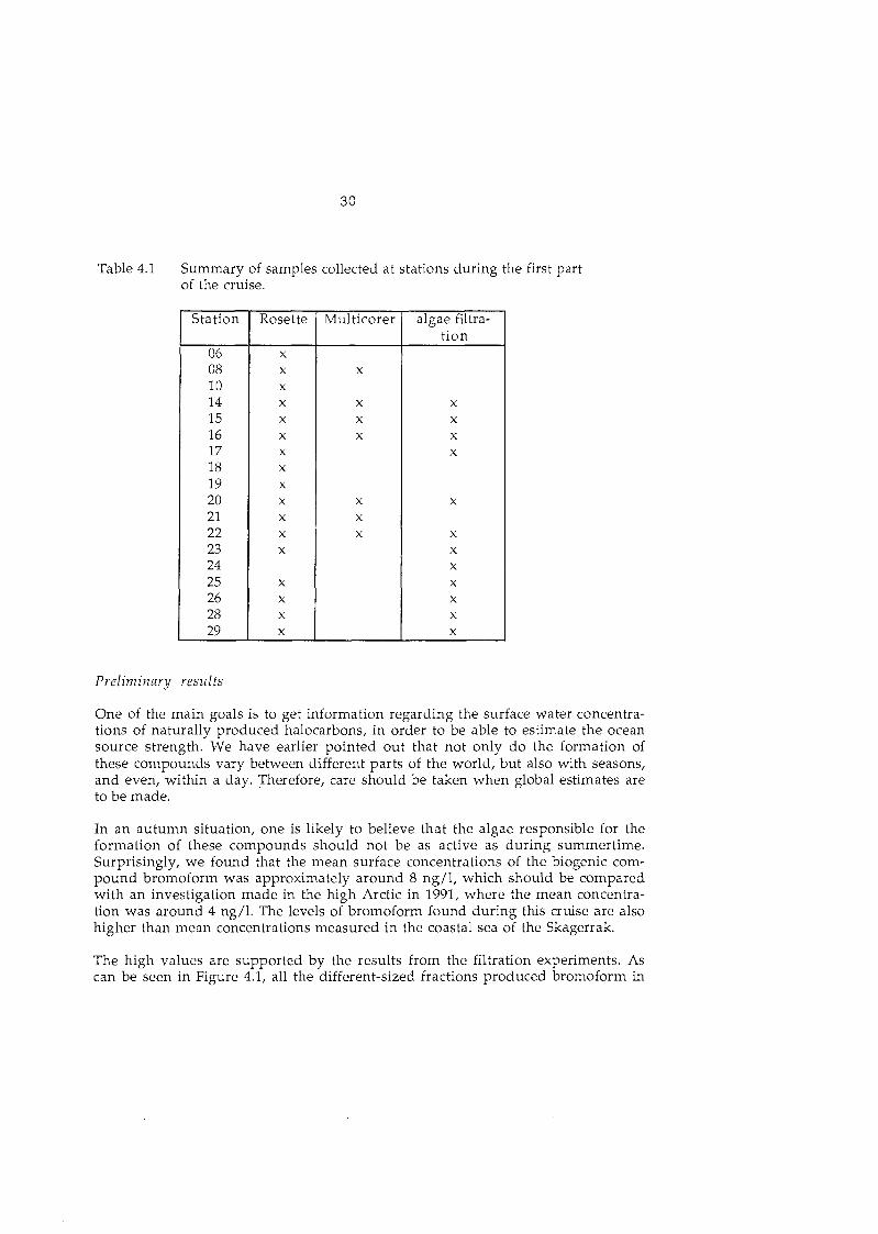
Table 4.1 Summary of samples collected at stations during the first Part of the cruise.

Prel iminary results

One of the main goals is to get information regarding the surface water concentra- tions of naturally produced halocarbons, in order to be able to estimate the ocean source strength. We have earlier pointed out that not only do the formation of these compounds vary between different parts of the world, but also with seasons, and even, within a day. Therefore, care should be taken when global estimates are to be made.

In an autumn situation, one is likely to believe that the algae responsible for the formation of these compounds should not be as active as during summertime. Surprisingly, we found that the mean surface concentrations of the biogenic com- pound bromoform was approximately around 8 ng/l, which should be compared with an investigation made in the high Arctic in 1991, where the mean concentra- tion was around 4 ng/1. The levels of bromoform found during this cruise are also higher than mean concentrations measured in the coastal sea of the Skagerrak.

The high values are supported by the results from the filtration experiments. As can be Seen in Figure 4.1, all the different-sized fractions produced bromoform in

significant amounts. It can also be seen that the ability to produce the two chlorina- ted ethenes trichloroethylene and perchloroethylene increases with decreasing size of the micro-organisms.

The distribution of halocarbons in the water column is exemplified in Figure 4.2. Carbontetrachloride (CC14) is a compound of mainly anthropogenic origin. Con- sequently, the concentration is highest at the surface, and decreases towards the sea floor. The complicated distribution of a compound with both an anthropogenic and a biogenic source is exemplified with the depth profile of perchloroethylene.

ng/ UQ chio h

Trf Per CHBr3

Figure 4.1 The production rates of three halocarbons by different sized micro-organisms (stn 25). Tri: trichloroethylene Per: perchloroethylene CHBr3: bromoform

Depth profiles of two halocarbons (stn 41) Perchloroethylene

4 Carbontetrachloride

500

1000

1500

2000

2500

3000

(C. Albers, H. Auel, B. Niehoff, B. Strohscher)

-

-

-

--

-

-

Bongo-net hauls (mesh size: 200 and 310 um) and Multi-net hauls (mesh size: 150 pm) were performed at 20 and 6 stations respectively. The investigations con- centrated On the vertical distribution, reproduction, overwintering strategies, lipid Storage and composition of dominant copepod species in different parts of the Greenland Sea.

Figure 4.2:

The Northeast Water Polynya on the East Greenland Shelf has been the subject of the International Arctic Polynya Project (IAPP) studies since 1993. During ARK XI/2 Multi-net hauls were taken to study the Stage composition and vertical distri- bution of the overwintering population of herbivorous copepods under autumn conditions. Net samples were fixed in 4% Formalin and transported to AWI for fi- nal evaluation. Together with the Summer data of the previous cruises, this will allow us to estimate the development and growth during the productive season and to reconstruct life cycles of dominant species. The results will also improve

our understanding of the overwintering strategies of different species. About 640 samples of different Calanus species and stages were frozen for later analysis of car- bon and nitrogen content and dry mass. The results will increase knowledge of the standing stock of biomass and the secondary production.

In the Greenland Sea Gyre, Multi-net and Bongo-net hauls were taken to study Calanus hyperboreus, which is a key species in the food web of the Greenland Sea due to its size and abundance. In contrast to other calanoids, gonadogenesis and egg production is based On lipid reserves accumulated during the previous Summer. Observations during ARK XI/2 showed that nearly 50% of the females were ma- ture and produced eggs in October. To study the spawning physiology and molting behaviour in detail, females and copepodid stages IV and V were collected for labo- ratory experiments. Of special interest is the role of the lipid metabolism in the egg formation.

Lipids are of major importance for the survival of zooplankton organisms in polar regions. Extensive lipid storage acts as an energy reserve for overwintering and, in some cases, reproduction. Herbivorous species especially depend On lipid reserves to survive long starvation periods, when the darkness of the polar winter or ice Cover prevent primary production. In addition, lipids are important components of biomembranes.

In order to study the seasonal lipid storage of zooplankton organisms, individuals were collected and sorted On board according to species, ontogenetic Stage and Sex. In total, 360 samples were frozen (-80°C) Their lipid content and composition will be analysed in the Institute for Polar Ecology, Kiel. Research concentrated on the polynya region and two transects (79 and 75ON) in order to elucidate the effects of sea ice coverage On lipid storage. Comparisons between different oceanographic domains, e.g. polar East Greenland Current, arctic Greenland Sea Gyre and boreal- atlantic West Spitsbergen Current, are also possible.

Data obtained under autumn conditions will complete the investigations of seaso- nal energy storage of zooplankton in high latitude ecosystems from late winter, spring and summer. Using these data it is possible to calculate the energy demands of overwintering and the role of lipids for the energy flux within the ecosystem. These results contribute to the ecosystem studies of the Joint Reseach Programme 313 (SFB 313) at Kiel University. In addition, the potential of specific lipid compo- nents as trophic biomarkers will be studied in CO-operation with the AWI.

Wax esters serve as long-term energy reserves, whereas triacylglycerols act as short- term fuels. In order to determine the molecular species of these lipid classes, zoo- plankton samples, especially Calanus spp.. have been stored in dichlormetha- ne/methanol (2/1) at -30°C until gas chromatographic analysis can be performed in Bremerhaven. In comparison to other marine taxa, polar copepods contain highly unsaturated phospholipids, which are very important in maintaining the fluidity of biomembranes even under low ambient temperatures. Investigations should elucidate the composition of these molecular species.

Hitherto, research has focused On larger species that dominate the biomass, e. g. Calanus spp.. The aim during the expedition ARK XI/2 was to determine the fatty arid and fatty alcohol composition of abundant smaller species, e. g. Oithona spp. and Oncaea spp.. Altogether 21 Bongo net hauls were conducted and more than 6300 animals of the species Calanus hyperboreus, Calanus glacialis, Calanus fin- marchicus, Oithona spp. and Oncaea spp. were collected for investigations in Bremerhaven.

6. MULTI-DISCIPLINARY SEA ICE INVESTIGATIONS

The Greenland Sea area is the major outflow region of pack ice from the central Arctic Basin. Our studies aimed to outline the physical, chemical and biological properties in Arctic drifting ice floes in the autumn/winter transition time which is characterized by decreasing air temperature and light intensities.

Our studies focused on three major questions: a) What kind of organisms are in- corporated into newiy forming sea ice, b) What are the characteristics of the sea ice biota in late autumn, and C) What organisms are found in the ice-water interface at this period of the year.

6.1 Formation of sea ice (R. Gradinger, E.J. Ikävalko T. Mock, Q. Zhang)

Studies on the sea ice formation in Antarctica have revealed, that protistan orga- nispts are incorporated already into the initial stages of newly forming sea ice.

During the sea ice formation, a succession of several characteristic stages has been described as the "pancake ice cycle", and suspended particulate matter including microorganisms accumulate in newly forming ice primarily due to physical con- centration mechanisms. It has been shown that algal populations are "scavenged" by frazil ice crystals rising through the water column. Furthermore, incorporation of plankton organisms may be supported by wave fields that pump water through the new ice layer, thus enmeshing cells between ice crystals.

During our cruise we studied the physical (temperature, salinity), chemical (nitrate, nitrite, phosphate, silicate) and bioiogical characteristics (Chlorophyll a/ cell abun- dances, species composition) of different types of new ice (grease ice, pancake ice, nilas ice). Preliminary information On the variability of protists inhabiting the dif- ferent stages of sea ice formation was gained by light microscopy of live material. The most versatile communities were found in pancake ice, with numerous pho- totrophic and heterotrophic flagellates, whereas grease ice was mainly dominated by pennate and centric diatoms. The variability of protist communities in the sur- face water was generally lower than in the other samples studied. Thus, the photo- trophy seems to prevail in the early stages of the sea ice formation, whereas hetero- trophy increases in importance in the later phases.

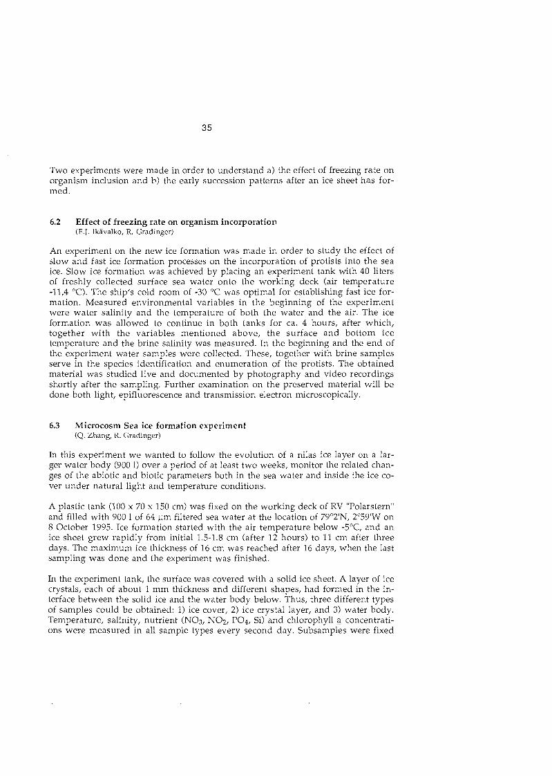
Two experiments were made in order to understand a) the effect of freezing rate on organism inclusion and b) the early succession Patterns after an ice sheet has for- med.

6.2 Effect of freezing rate on organism incorporation (E.J. Ikävalko R. Gradingcr)

An experiment on the new ice formation was made in order to study the effect of slow and fast ice formation processes on the incorporation of protists into the sea ice. Slow ice formation was achieved by placing an experiment tank with 40 liters of freshly collected surface sea water onto the working deck (air temperature -11,4 'C). The ship's cold room of -30 'C was optimal for establishing fast ice for- mation. Measured environmental variables in the beginning of the experiment were water salinity and the temperature of both the water and the air. The ice formation was allowed to continue in both tanks for ca. 4 hours, after which, together with the variables mentioned above, the surface and bottom ice temperature and the brine salinity was measured. In the beginning and the end of the experiment water samples were collected. These, together with brine samples serve in the species identification and enumeration of the protists. The obtained material was studied live and documented by photography and video recordings shortly after the sampling. Further examination On the preserved material will be done both light, epifluorescence and transmission electron microscopically.

6.3 Microcosm Sea ice formation experiment (Q. Zhang, R. Gradinger)

In this experiment we wanted to follow the evolution of a nilas ice layer on a lar- ger water body (900 1) over a period of at least two weeks, monitor the related chan- ges of the abiotic and biotic parameters both in the sea water and inside the ice co- ver under natural light and temperature conditions.

A plastic tank (100 X 70 X 150 cm) was fixed on the working deck of RV "Polarstern" and filled with 900 1 of 64 pm filtered sea water at the location of 79'2'N, 2'59'W on 8 October 1995. Ice formation started with the air temperature below -5OC, and an ice sheet grew rapidly from initial 1.5-1.8 cm (after 12 hours) to 11 cm after three days. The maximum ice thickness of 16 cm was reached after 16 days, when the last sampling was done and the experiment was finished.

In the experiment tank, the surface was covered with a solid ice sheet. A layer of ice crystals, each of about 1 mm thickness and different shapes, had formed in the in- terface between the solid ice and the water body below. Thus, three different types of samples could be obtained: 1) ice Cover, 2) ice crystal layer, and 3) water body. Temperature, salinity, nutrient (NO3, NO2, PO4, Si) and chlorophyll 2 concentrati- ons were measured in all sample types every second day. Subsamples were fixed

0 4 1 2 1 6 Days

b ) S a l i n i t v

0 4 8 1 2 Days

1 6

C) C h l o r o p h y l l - ? ,

0 ' ; 0 4 1 2 1 6

Days

Figures 6 a/b/c: Results of a tank experiment

with borax-buffered formalin (1.0 % final concentration) for further analysis of the abundance of algae and bacteria by light and epifluorescence microscopy.

The air temperature varied in the Course of the experiment between +l° to below -9.5OC. While the temperature of the solid ice sheet followed the air temperature changes but in lower magnitude, the temperature of the water body and the ice cry- stal layer were nearly stable at about -2 to -3OC (Fig. 6.1a). As an effect of the ice growth the salinity of the water body increased with time, while the salinity of the ice sheet decreased due to desalination processes (Fig 6.1b). The chlorophyll a con- centrations in the water column and the ice crystal layer were relatively constant, whereas in the ice cover a decrease was observed (Fig. 6 .1~) .

6.4 Autumnlwinter conditions within Arctic sea ice floes (R. Gradinger, E.J. Ikävalko T . Mock, Q. Zhang)

The Arctic sea ice is inhabited by a diverse community of bacteria, protists and me- tazoa. Our main scientific concern was to determine the physical and chemical properties of the ice cover which correspond to the observed distribution of the biota within the ice column.

At 8 stations ice cores were drilled from Arctic ice floes with a 10 cm ice auger. The vertical distribution of temperature, salinity, nutrients and biological properties (Chlorophyll a/ species abundances and composition) was investigated with a ver- tical resolution of 1 to 20 Cm. A particular emphasis was on a detailed study of the protistan community. In order to survey the versatility of the protists inhabiting the sea ice biota samples were collected from both the ice floes and the beneath lying water column. Thus, the material consists of brine, together with 50 and 10 um net samples. Immediately after the sampling the material was concentrated by a centrifuge, and protists were examined live with an interference microscope. Documentation was done photographically and by video-recording using an in- verted microscope. Based on light and electron microscopical preparations made On board further identification of e.g. scale- and lorica-bearing protists will be done at the University of Helsinki, Finland. A total of three serial dilution experiments were conducted using brine water. These experiments will give estimates for the in-situ growth and grazing rates of sea ice bacteria and protists.

Two experiments (dark survival and salinity tolerante) were conducted to test the reaction of ice algae onto decreasing light and temperatures which are both typical for the autumn/winter transition.

Experiment 1: Dark survival of Arctic aleae (Q. Zhang, R. Gradinger)

Polar marine ecosystems are characterized by strong seasonal and interannual va- riations of environmental factors like the extent of the ice cover and solar irra- diance. With the onset of polar winter, the available light intensities are reduced

to nearly total darkness for periods of up to 6 months. It has been suggested that algae overwinter as resting Spores with reduced metabolic rates. Although winter survival of the ice algal community is necessary for the seeding of the annual spring development, dark survival in polar marine algae has received little atten- tion. Thus, an experiment was designed to investigate the survival strategies of Arctic algae in the darkness over a period of 5 months.

Grease ice was collected at a position of 79'2'N, 2O59'W in the Greenland Sea, mel- ted and filtered through a 64 pm gaze to exclude larger zooplankton. 40 bottles (50 ml each) were filled with the water and stored in the dark at a temperature of +2OC. Measurements on abiotic and biotic Parameters will be carried out every seven days in the first month, every 14 days in following four dark months, and every five days after the total five dark months. In the end of the experiment the algae will be exposed to increasing light intensities at a temperature of +4OC. The microscopical analysis will focus On the identification of different adaptation strategies.

Salinitv tolerance of Arctic alc-ae (Q. Zhang, R. Gradinger)

Particularly during the periods of brine drainage and ice melting microorganisms inhabiting the brine channels of the Arctic sea ice are exposed to strong seasonal variations in the brine salinity. Ice algae are known to have adaptations to low water temperatures and increasing salinity which take place during wintertime in the ice. Earlier studies have demonstrated that Arctic sea ice diatoms are relatively euryhaline and can maintain growth rates of 0.6 to 0.8 divisions per day over a sa- linity range of 10 psu to 50 psu. In the Antarctic, the bottom community of ice al- gae have shown a positive correlation between the growth rate and water salinity, the latter ranging from 11.5 to 34 psu. Culture experiments have revealed that ice algal growth continued even in temperatures of -5.5OC and a brine salinity of 95 psu.

Our experiment was designed to study the response of the growth of Arctic sea ice algae to salinities ranging from 1 to 100 psu. For that purpose ice cores were taken from an Arctic ice floe at the location of 79'59'N, 4'14'W in the Greenland Sea. The bottom 1 cm of two ice cores were let thawn in an excess of 0.2 pm filtered sea water. Salinities of 1, 10, 20,32, 40,50, 60, 70, 80, 100 psu were achieved by the addi- tion of either high salinity brine (124 psu) or low salinity meltwater from the Same ice floe (1 psu salinity). Larger metazoans were excluded by the filtration of the samples through 64 pm gaze. The algae were incubated at a light/dark cycle of 8:16 hours and a temperature of +l°C

The experiment was continued for 19 days. Subsamples (25 ml) were collected 1, 3, 6, 9 and 14 days after the Start and in the end of the experiment. These were fi- xed with borax-buffered formalin (1% final concentration) and will be used for light and epifluorescence microscopical analysis of species abundantes and bio- mass.

Autumn Under The Roof - The Under-ice Community (I. Werner)

The world under an Arctic ice floe is a habitat with special and variable conditions. The underside of the ice is not an even and homogenous surface, but rather cha- racterized by a variety of cracks and crevices, undulations or rafted pieces of other floes. Even entire floes can underlay each other, thus building a complex under-ice landscape. This is the environment for a specialised under-ice community.

During ARK XI/2, a total of 5 ice stations on multi-year ice floes were used to inve- stigate the characteristics of the Arctic under-ice community. Temperature and sa- linity profiles were recorded over the upper 5 metres of the water column under the ice and the underside of the ice was sampled for measurements of chloro- phyll g and the C/N ratio. In order to gather information on the morphology and structure of the habitat as well as on abundance and distribution of under-ice amphipods, a videocamera was deployed under the ice. A pumping System deli- vered quantitative samples of the sub-ice fauna, caught from the waterlayer di- rectly under the ice. Furthermore, under-ice amphipods recovered from Bongo net catches (200 and 310 [im) done by the zooplankton working group were deep- frozen for lipid analyses. On board "Polarstern", experiments with under-ice am- phipods were carried out to gain insights into the feeding ecology and fecal pellet production of this group.

In contrast to the summer situation, where melting processes occur, neither tem- perature nor salinity gradients were measured under the ice floes during this au- tumn expedition. Water temperature ranged from -1.3OC to -1.6OC with salinities of 30.6 to 32.8 psu.

The morphology of the underside of the floes was characterized by a quite smooth structure and only shallow undulations. Dense aggregations of decaying algae were frequently observed in depressions here, as well as patches of algae inside the ice itself. Chlorophyll g concentrations in the lowermost 1 cm of the ice ranged from 0.7 to 195.8 pg/l between stations.

Based on net samples and video observations, Apherusa glacialis was the most abundant species of the under-ice amphipods, followed by Gammarus wilkifzkii, while Onisimus spp. was quite scarce. First results of the feeding experiments indi- cate that A. glacialis is probably the only herbivorous under-ice amphipod, whe- reas the other species are rather omnivorous. G. wilkifzkii showed even a pro- nounced preference for feeding On crustaceans.

There was virtually no makrozooplankton (> 200 km) in the waterlayer below the ice. During the Summer, sometimes dense swarms of pelagic copepods (Calanus glacialis) or pelagic amphipods (Themisfo libellula) can be found here, probably feeding on ice algae sloughing off from the floe. However, a very diverse and abundant community of smaller zooplankton (>50 [im) seems to dominate this habitat during both seasons, e.g. naupliar Stages, cyclopoid copepods (Oifhona spp.)

and above all, several groups of harpacticoid copepods (Tisbe sp., Halectinosorna sp., Microsetella sp.), which are partly described to live also inside the ice.

Further analyses and experimental work on all members of the under-ice commu- nity, which is thought to function as a mediator for the production and transport of organic matter between the ice and the water column will hopefully throw some light onto the cryopelagic coupling processes. In particular, the fecal pellet produc- tion and sedimentation of particles from the ice are important points for the multi- disciplinary approach of the SFB 313.

7. BATHYMETRIC MAPPING IN THE F'RAM STRAIT (U. Lenk, J. Monk, V. Sackmann)

Introduction The area of the Fram Strait between Spitsbergen and Greenland plays a key role for the water exchange between the North Atlantic and the Arctic Ocean and is there- fore subject of investigations of various disciplines. Besides the collecting of sam- ples and the observation of physical Parameters, it is necessary to have reliable depth Information as a description of the sea bottom topography, i.e. bathymetric data available for planning and conducting of detailed studies of the region.

One project of the Bathymetric Group of AWI is concerned with the preparation of bathymetric charts scale 1:100000 of the Fram Strait as a basis for further investiga- tions by other sciences. The surveys conducted during ARK XI/2 were intended to fill existing gaps in the bathymetric data and to provide the opportunity to check and adjust the results of previous surveys with less accurate navigation using the newly gathered data as a reference.

The HYDROSWEEP measurements were started at position 74.B0N, 12.0° on the 23th of September 1995 at 0830 Universal Time Coordinated (UTC). The system was running continuously during the whole cruise with some minor exceptions cau- sed by system failures or the requests of other disciplines to stop the transmission of acoustical signals into the water column, as the HYDROSWEEP signal caused difficulties in finding the moorings deployed in the Greenland Sea for the subse- quent recovery. Another reason for interrupting the logging of data was given when the ship was steaming through heavy ice, and no reasonable signal could be recorded.

As a result of ARK XI/2 about 1205 nautical miles of run lines were sailed resulting in an area of about 10 500 km2 being surveyed.

Data Storage was conducted on a daily basis. The raw bathymetric data is stored on magnetic tape by HYDROSWEEP; additionally, an interface to the VAX-cluster is installed where the profiles are recorded. The latter files are used as the basis for further processing. Navigational data is also stored separately on disk, and all data is time-tagged with regard to UTC in order to relate the different types of data to each other during the subsequent post-processing.

Survev Instrumentation During several expeditions in 1984, 1985, 1987, 1990 and 1991 hydrographic surveys were conducted with RV "Polarstern". Until 1989, the SEABEAM system was used to gather bathymetric data, and positioning was mainly based on the TRANSIT sa- tellite system operated by the US Government Department of Defence.

The TRANSIT satellite system forms a "birdcage" of circular, polar orbits about 1075 km above the Earth. Thus, fixes can only be recorded every few hours depen- ding on the number of available satellites and the latitude of the ship's position. The time gaps between the fixes had to be filled by dead reckoning Systems. Problems involved with these systems include their decreasing accuracy with time, and offsets are likely to occur in the positioning data when the next TRANSIT sa- tellite fix occurs. These offsets can be in the range of several nautical miles.

As a result of the offsets and the overall accuracy of TRANSIT, the accuracy of posi- tioning is likely to be in the range of 500 m and worse in poor conditions, even after substantial interactive post-processing. This accuracy is unacceptable for the planned charts at a scale of 1:100 000, as a displacement of 500 m in position would result in 0.5 cm on the chart.

Nowadays, the NAVSTAR GPS system is used for positioning, and the ATLAS HYDROSWEEP system has replaced the SEABEAM system in 1989. HYDROSWEEP operates at a frequency of 15.5 kHz and measures athwardship oriented profiles consisting out of 59 preformed beams (PFB) from 10 m down to 10 000 m depth.

The opening angle of the swath across the ship's axis varies between 90' and 120° and the aperture along the main axis is about 2'. Thus, the footprint of PFB beam Covers an area of approx. 2' by 2' squared. The system is automatically calibrated for speed of sound in a patented procedure called cross-fan calibration where the mean sound velocity is determined in a Least Squares process by comparison of a swath measured along the ship's main axis to the standard survey cross-profile as obser- ved by the centre beam. In addition to this calibration, a keel sonde is installed for the determination of speed of sound at the surface.

The use of NAVSTAR GPS for navigation and positioning has led to dramatic changes in the seafloor topography from previous surveys in regions with bad na- vigational aids. Today real-time differential positioning with GPS (D-GPS) provi- des absolute positions referenced to the World Geodetic System 1984 (WGS84), with an accuracy of up to k5 ... 6 m, depending on the mode in which the system is operated and the reference station which is used. However, in remote areas such as the Greenland Sea, where no differential reference station is yet available to achieve these high accuracies, positions are only accurate to ±I0 m. During the commissioning phase of GPS, there was no full coverage by the system, and the si-

tuation was similar to the time when navigation was based on TRANSIT, i.e. the gaps had to be bridged by dead reckoning Systems, and offsets resulted from new fi- xes.

As the overall accuracy of positioning is now far better than at the beginning of hy- drographic surveys on board "Polarstern", it is possible to check existing low accu- racy data using the new high accuracy data as a reference.

Survev operation In order to achieve the best coverage of the survey area, a box survey was planned prior to the expedition (see Fig. 1.1) with regards to the time schedule and altered according to the conditions prevailing On the cruise.

During the actual survey operation, the system has additionally to be observed to ensure the best results possible and to prevent a break-down of the system. One major error source in bathymetry is the use of a wrong value for the mean speed of sound. As the quality of the determined depth is directly dependent on quality of the latter value, it is of vital importance to check the applied sound speed value in regions with a hillocky underwater topography.

Problems were observed when the sea bottom is flat without much topographic variation. In case that a wrong value for the speed of sound is used, the measured profiles will be bent symmetrically to the centre beam. If the speed of sound used by the system is too high, both ends of the profile will be bent upwards, and if the va- lue is too small, they will be bent downwards. This will result in an apparently symmetric shape of the sea bottom indicated by contour lines which are parallel to the ship's track.

To check the data obtained, the measured cross-profiles are displayed on-line, and a bottom map is scrolling over a screen. In addition, on-line charts are plotted in or- der to observe the quality of the data by comparing of adjacent swath-profiles and to check the coverage achieved by neighboured swathes.

Svstem Test In addition to the normal survey operations, a system test was performed as it seems that there are still some systematic errors causing distortions in the measu- red profiles. These distortions occur symmetrically to the centre beam of HYDRO- SWEEP near the pre-formed beams No. 14 and 46 and result in an hill-like effect. They are sometimes referred to as "the dikes of the profiles". The manufacturer of HYDROSWEEP, STN ATLAS ELECTRONIC, Bremen, Germany, asked to record deep sea data from a flat sea bed in order to investigate these distortions which also occur On other research vessels with HYDROSWEEP. This data will be processed after the cruise at ATLAS for further improvements of the system.

8.1 Pelagic production regimes of Open water, marginal ice Zone and under the ice (0. Haupt, G. Donner, M.Krumbholz)

Planktological research within the SFB 313 at Kiel University focused on processes that control the formation and modification of particles in the upper layers of the Northern North Atlantic, their settling through the water column and their fate before they finally reach the deep sea floor. The investigations conducted during ARK XI/2 focused On the relation between pelagic processes and vertical particle fluxes in the marginal ice Zone of the Greenland Sea. Special attention is given to the pelagic and ice-associated production regimes which are expected to differ with respect to quantity and composition of matter exported from the euphotic zone.

Stations had been sampled at 2000 m, 1200 m, 800 m and 200 m depth on a transect normal to the continental slope within the marginal ice zone. Also a slope parallel transect at 2000 m depth from 80°30' to 79ON with ice cover from about 10/10 to 1/10 were sampled. Water from different depth was taken with a rosette water sampler and filtered to measure phytoplankton biomass, suspended particulated matter (Seston), elements (C, N, P, Si) and algal pigments (HPLC analysis). Water samples for microscopic investigations of species composition were fixed with borax-buffered formalin. At two mooring positions at 75ON with water depths of 400 m and 3000 m which were already investigated during the summer cruise ARK X-1 for long term explorations of the seasonality and the interannual variability of bentho-pelagic coupling. Additionally, water samples were collected along a tran- sect at 75ON extending from 13O40'W to 17OE with a total of 19 stations to measure the already mentioned planktological Parameters within the upper 500 m of the water column.

First results of chlorophyll measurements show a system state which is typical for low light conditions in fall. In the northern Part of the Eastern Greenland Sea we found values mostly below 0.1 microgram per liter and chlorophyll a/phaeopig- ment ratios of about 1 within the upper 100 m.

The area at 75ON shows chlorophyll values below 1 microgram per liter and a more divers chlorophyll a/phaeopigment ratio with mean values greater 1. Figure 8.1 shows the chlorophyll 3 and phaeopigment distribution of the 75' transect. Highest chlorophyll 3 values were found in the upper cold Arctic water mass in the mar- ginal ice zone. Depending On the ice cover the low light level of the surface layer results in a sharp decrease of chlorophyll concentration with increasing depth. Chlorophyll 2 as well as phaeopigment concentrations shows homogeneous ten- dency in deeper water layers of the warmer atlantic water masses. Relatively high pigment concentrations in a depth of about 60 to 100 m may be caused by fecal pellets and aggregates rather then by living phytoplankton cells.

latitude

Fig. 8.1: Vertical distribution of chlorophyll a (a) and phaeopigments (b) at 75ON

Measurements of vertical particle fluxes from the various regimes in the marginal ice Zone Within the last years the field work of the SFB 313 has focused on the seasonally ice-covered region of the Greenland Sea. Measurements of vertical flux in this region are conducted to collect particles exported by different pelagic production regimes in relation to seasonal retreat of the ice. During this cruise, moorings which were deployed in cooperation with AWI in 1994 during the expedition ARK X/l were recovered successfully with a total of 4 sediment traps (AWI 413- 4/OG 7 at 3000 m and AWI 410-2/OG 8 at 400 m depth). A mooring deployed in Mai 1995 at 75ON, 3O55'W with RV Johan Hjort (OG 9) was also successfull reco- vered. A first look at the collected material in the sampling glasses shows a clear annual cycle of vertical particle flux with high rates during spring and summer.

A long term mooring (OG 10, collecting time 1 year) at a position of 75¡03.4'N 04'35.7'W was deployed with 3 sediment traps in 500, 1000 and 2000 m depth as well as 3 current meters each about 20 m below the traps. This area is within the seasonal ice-covered Part of the Greenland Sea. Because of the influence and the variability of the ice Cover on the production of biogenic matter we predict a direct relation between the location of the marginal ice Zone and the sedimentation of organic particles. The mooring will be recovered in August 1996.

Experimental studies with dominant organisms -

To analyse changes in pigment signature and composition of other biogenic com- pounds and for comparison with sediment trap samples, experiments for fecal pel- let production were made on board with the dominant zooplankton species (copepods, amphipods and euphausiids) to analyse changes in pigment signature and composition of other biogenic compounds and for comparison with sediment trap samples.

Dominant copepods (Calanus hyperboreus and Calanus glacialis) were sampled with a Bongo Net and cultivated for different experiments which will be conducted at Kiel University

8.2 Bentho-pelagic coupling (Angelika Brandt, Jör Stefan Berg, Michael Gedamke, Angela Lunau, Eberhard Sauter, Annette Scheltz, Klaus Schnack, Susanne Wanner)

Background Quality and quantity of organic carbon reaching the seafloor have a direct effect on the benthic community. Organic particles are enriched in the BNL (bottom nephe- loid layer) and in the upper sediment layer, where they are the main food source for benthic organisms. Composition and quality of these particles are influenced by the vertical sedimentation, by lateral advection, by biological and chemical modifi- cation of the particles in the water column and at the seafloor, by the bottom topo- graphy, as well as the seasonal deposition of particles due to spring blooms and the production of ice algae at the floes margins.

Objectives Our work will focus On the interactions between the BNL and the upper sediment layer. In this respect it is crucial to investigate composition, abundance, diversity, and community patterns of benthic organisms, which take up organic particles, in- corporate them into the sediment by biodeposition and bioturbation processes and also play an irnportant role in the recirculation of organic material by resuspen- sion. Therefore we will also try to scrutinize the interaction of the amount, the composition and the flux of particles in the BNL and the patterns and activity ob- served in the benthic communities.

Moreover our program encompasses work on the following aspects:

0 evaluation of the degree of bentho-pelagic coupling along the Northeast Greenland continental margin

* investigations of the composition, abundance and diversity of macrobenthic communities, especially peracarid crustaceans and polychaetes (which are most important in terms of numbers) and seafloor/BNL-properties

* assessment of micro- and mesoscale dispersion patterns of benthic populations investigation of metabolic activities and bioturbation potential of the total sediment communities by measurements of biochemical parameters at certain sites, as well as the macro- and megabenthic (i.e. sponges) communities

* the analyses of BNL characteristics in terms of the amount and composition of particles in relation to near bed current velocities and direction impact of biodeposition and bioentrainment on the particle composition in the sediment in in situ experiments

In order to reach these goals, a normal transect at 79ON, at 2000 m, 1200 m, 800 m, and 200 m depth had been sampled, and additionally a slope parallel transect in about 2000 m depth consisting of 4 stations and extending from 80°30' to 79ON, off the Greenland continental slope. We hope that this slope parallel transect will cover different conditions of particle supply to the benthos due to variable surface production in areas of permanent ice cover, ice edge situations and Open water. The normal transect will provide information on the depth distribution and dis- persion patterns of benthic communities and characteristics of the BNL. Addi- tionally we will investigate bentho-pelagic coupling processes at 2 revisited SFB- mooring stations at 75O, NE Greenland.

A Set of various benthos equipment has been used to serve our purposes. For faunistic studies and comparison the giant box corer, the Agassiz trawl and an epibenthic sledge with a newly constructed supranet at about 1 m above the bottom (additionally to the epinet), will be employed. The vertical distribution of chemical and biogeochemical parameters will be assessed by deploying a multiple corer and a newly designed 02-profiler called "Floorian". For the characterization of the BNL a modified bottom water sampler will retrieve water samples and thus provide in

formation on current velocity and direction within the last meter of the BNL, i.e. just above the sediment water interface.

First results

AGT (Agassiz trawl) During last year's cruise of "Polarstern" into the arctic waters some evidence of high sponge densities was found. Sponges are filter-feeding organisms that feed on phytoplankton, detritus and bacteria. Some of the sedimentary organic matter will eventually reach the BNL, where it might be available to sponges. However, size classes of the consumed particles as well as the composition of the food and the influence of the flow velocity to the particle retention rate are only known for very few species (see e.g. Witte, U., 1995). Therefore we have only little information about the possible contribution of sponges to sediment formation. These question will be approached in a laboratory study with living sponges (Geodia mesotriaena) that were caught in the Greenland Sea.

On five stations we employed the Agassiz-Trawl, three of these were taken on the transect from 2000 m to 200 m depth onto the Greenland shelf. The three trawls on the transect running perpendicular to the shelf were taken at 1200 m, 700 m and 200 m depth. All three trawls were successful, but no or only few sponges came up with it. At the 1200 m station, most of the catch consisted of fine mud, but we also found some shrimps and bottom living fishes (e.g. ray). The trawl contained Ophiuroidea and Priapulida, we tried to keep them alive in aquaria. Actinians, brittle stars, decapods and some fish were sampled at the 700 m station. The diver- sity and biomass was highest in the 200 m trawl, where we found 3 species of spon- ges, several amphipod species, 1 Sclerocrangon ferox, many Heliometra, 5 Holo- thuroidea and a few polychaetes. All of the Heliometra died after 20 days of being kept in the aquaria, although they have been observed feeding. The water volume might have been too small, and flow velocities too weak for these animals.

Two further trawls were taken 75ON at 800 m and 400 m depth. The first one at 800 m was very successful as the catch consisted almost completly of sponges (Geodia mesotriaena) and a few octocorals. Except for five sponges, all of them are still alive in aquaria for later experiments in the laboratory. About 900 m2 of seafloor were sampled, therefore I could calculate a sponge density in this area of about 0.3 individuals per m2- The last trawl taken consisted of two Gorgonocephali in very good condition, few fishes, and some sponges.

BWS (bottom-water sampler) In order to receive information about the hydrodynamic sorting of the organic matter near the seafloor, we took samples from 7 cm, 12 Cm, 20 cm and 40 cm height above the seafloor with the bottom-water sampler. The water was filtered to analyse its content of chlorophyll, POC (particulate organic carbon), PON (particulate organic nitrogen), and total supended matter. 200 ml of each sample were fixed with formalin to Count bacteria and phytoplankton (e.g. diatomes). On

each deployment of the BWS, a video camera was installed in 40 cm height above the seafloor as well as a current and a turbidity profiler. The hydrodynamic sorting of the organic matter is crucial for the benthic animals, because it determines the quantity and quality of food they receive. The whole sedimentation regime is in- fluenced by the hydrodynamic processes near the seafloor.

At seven out of nine stations we took water samples and employed the video ca- mera with the BWS. At the 1200 m station of the slope-normal transect, the BWS could not be employed because of the strong ice drift. At the last station at 75ON (water depth: 400 m) the control unit broke down so that we could not get samples at that station either. The 200 m station remarkably showed very good video ima- ges of different species of mysids and 1-2 amphipod species. The parallel EBS-hau1 at that station enabled us to determine the most frequent mysid as Boreomysis arc- t ica .

The chlorophyll contents of the water samples were already analysed on board. As expected for this time of the year, the chlorophyll a and phaeopigment values of the water were very low in all samples taken.

EBS (epibenthic sledge) Within the macrobenthic communities, peracarid crustaceans play as important a role as polychaetes, as they occur in large numbers and are usually quite diverse. In order to catch a high number of individuals, an epibenthic sledge was employed, which was first modified after a construction of Rothlishberg & Pearcy (Roth- lishberg & Pearcy, 1977). This sledge originally consisted of a single box. Its opening measures 33 X 100 cm and is at about 25 cm above the bottom. As many peracarids are vagile (e.g. Amphipoda, Isopoda, Cumacea migrate in the water column during the nichts), or exhibit a suprabenthic mode of living (Mysidacea), an additional supranet with the Same size was constructed and fixed above the epinet (Brandt & Barthel) 1995). It extends from 1 m to 1.33 m above the ground and helps to separate supra- and epifauna more clearly.

In total the epibenthic sledge had been employed at 10 stations, 8 of these have been sampled successfully. At 80°30' about 2000 m depth, the sledge did not work properly and came up damaged. The second failure occurred at about 75ON around 2800 m depth.

Up to now it has only been possible to analyse the content of the supranets of the samples. As well as varying numbers of decapods, euphausiaceans, chaetognaths, ostracods and calanoid copepods, peracarids have been sampled at all successful EBS-stations. Within the Amphipoda, most species belong to the families Ampe- liscidae, Amphilochidae, Calliopidae, Eusiridae, Isaeidae, Lysianassidae, Parda- liscidae, and Stegocephalidae. All Cumacea found in the supranet were specimens of the genus Diastylis (Diastylidae). Eurycope was the most frequent isopod genus in the supranet, however, a single, well preserved specimen of the deep-sea isopod Munnopsis typica (Sars) was found at station 37-018. Other common isopod fami- lies were the Ilyarachnidae, Nannoniscidae, and Munnidae; the Mysidacea were all

members of the family Mysidae, the most frequent genera were Boreornysis, Eryt-- throps, and Pseudomma. Only a single species of Tanaidacea, Sphyrapus anorm- lus (Sars), was found in the supranet.

The following table shows the differences in the supranets at the different stations. The values are total numbers collected and are not yet standardized for a 1000 m haul.

Peracarida in the supranet of the EBS

Station 1 Amphipoda 1 Cumacca 1 Isopoda 1 Mysidacca 1 Tanaidacea 1 S u m 37-008 I 37 I 0 I 39

"The higher number of Peracarida at station 37-027 is an artifact, as the supranet contained some se- diment in the cod end and must have been trawled partly upside down.

GKG (giant box corer) To investigate the relationship between surface production and benthic commu- nity structure, the macrobenthos was sampled quantitatively with a box corer (50 X

50 cm surface). The box corer was employed at 9 stations, in total 25 cores were sampled. From each core 3 fractions were sampled:

- 1) the surface water above the sediment, - 2) and a 25 X 25 cm subsample of the first cm of sediment, and - 3) the next 5 cm of sediment.

These samples were sieved, fixed and partly sorted on board of "Polarstern". Some living polychaetes (eg. Onuphis conchylega) were kept in aquaria for further obser- vations at home. Additionally, smaller amounts of sediment were taken for de- termination of various sediment Parameters.

A very preliminary investigation of the infaunal distribution shows an impove- rished community. This might be due to low food supply. Total abundance is esti- mated to 500 - 5000 animals/m2. The main dominant infaunal taxa are polychaetes, followed in abundance by other groups including crustaceans, sipunculids, mussles and holothurians. Within the polychaete fauna, important families are Spionidae,

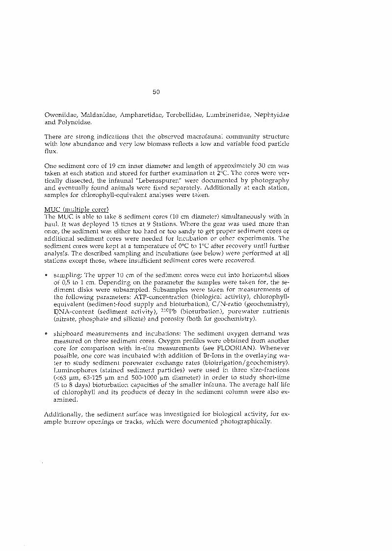
Oweniidae, Maldanidae, Ampharetidae, Terebellidae, Lumbrineridae, Nephtyidae and Polynoidae.

There are strong indications that the observed macrofaunal community structure with low abundance and very low biomass reflects a low and variable food particle flux.

One sediment core of 19 cm inner diameter and length of approximately 30 cm was taken at each station and stored for further examination at 2OC. The cores were ver- tically dissected, the infaunal "Lebensspuren" were documented by photography and eventually found animals were fixed separately. Additionally at each station, samples for chlorophyll-equivalent analyses were taken.

MUC (multiple corer) The MUC is able to take 8 sediment cores (10 cm diameter) simultaneously with in haul. It was deployed 15 times at 9 Stations. Where the gear was used more than once, the sediment was either too hard or too sandy to get proper sediment cores or additional sediment cores were needed for incubation or other experiments. The sediment cores were kept at a temperature of O0C to 1° after recovery until further analysis. The described sampling and incubations (see below) were perforrned at all stations except those, where insufficient sediment cores were recovered.

sampling: The upper 10 cm of the sediment cores were cut into horizontal slices of 0,5 to 1 Cm. Depending on the parameter the samples were taken for, the se- diment disks were subsampled. Subsamples were taken for measurements of the following Parameters: ATP-concentration (biological activity), chlorophyll- equivalent (sediment-food supply and bioturbation), C/N-ratio (geochemistry), DNA-content (sediment activity), ^OPb (bioturbation), porewater nutrients (iitrate, phosphate and silicate) and porosity (both for geochemistry).

shipboard measurements and incubations: The sediment oxygen demand was measured on three sediment cores. Oxygen profiles were obtained from another core for comparison with in-situ measurements (see FLOORIAN). Whenever possible, one core was incubated with addition of Br-Ions in the overlaying wa- ter to study sediment porewater exchange rates (bioirrigation/geochemistry). Luminophores (stained sediment particles) were used in three size-fractions (<63 Pm, 63-125 Pm and 500-1000 um diameter) in order to study short-time (5 to 8 days) bioturbation capacities of the smaller infauna. The average half life of chlorophyll and its products of decay in the sediment column were also ex- amined.

Additionally, the sediment surface was investigated for biological activity, for ex- ample burrow openings or tracks, which were documented photographically.

Floorian ( 0 7 profiler) The diffusiGi boundary layer (DBL) is easily disturbed and compaction of sediment might occur during the coring process, for example of a MUC. Also, quality of sam- ples changes during recovery from the seafloor to the surface. These were the rea- sons for the development of in situ measuring methods.

On this cruise we were able for the first time to deploy the newly developed oxygen in-situ profiler FLOORIAN in deeper water. In contrast to free falling lander sy- stems, FLOORIAN is capable of measuring under ice covered water, because it is deployed via the winch. The device also records a resistivity profile of the sedi- ment. Additionally two cores for laboratory experiments and porewater analyses are taken at each deployment.

FLOORIAN was deployed at eight locations. Four in-situ measurements were per- formed in the Fram Strait, and four at 75ON (where two deployments failed).

The in-situ data (Figure 8.2) will be used to calculate the fluxes of oxygen and organic carbon, respectively. Together with oxygen profiles taken from cores (measured On board), we will obtain information about the oxygen-penetration depth. These were 3-12 cm at shallower localities (e.g 37-014, 800 m; 37-016, 190 m) and some decimeters at deeper stations (e.g. 37-025, 2800 m).

Sometimes oxygen profiles show subsiduary maxima, which might be caused by oxygen irrigated due to burrows of infaunal animals (e.g. polychaetes).

The fingerprint-like resistivity profiles (figure 8.2) characterize the respective sedi- ment and also determine sediment porosity.

Literature Brandt, A. & D. Barthel (1995): An improved supra- and epibenthic sledge for catching Peracarida (Crustacea, Malacostraca). Ophelia 43 (1).

Rothlisberg, P. C. & W. G. Pearcy (1977): An epibenthic sampler to study the ontogeny of vertical migration of Pandalus jordani (Decapoda, Caridea). - Fish. Bull. U. S. 74: 994-997.

Witte, U. (1995): Reproduktion, Energiestoffwechsel und Biodeposition dominanter Porifera aus der Tiefsee des Europäische Nordmeeres, Berichte aus dem Sonderforschungsbereich 313, Nr. 53: 1-83.

0 M

f^ M C; 0

.M U

03 U U")

4A 03 01

U3

E. 01 bo >-,

0

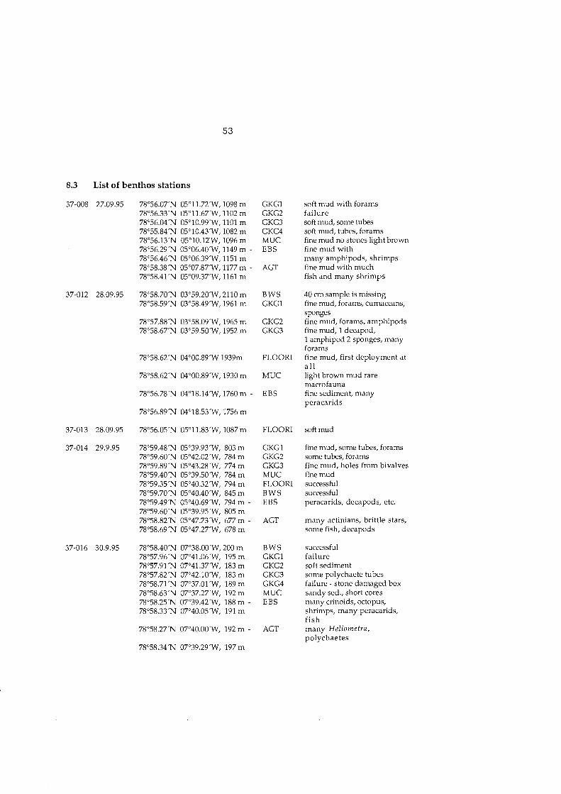
8.3 List of benthos stations

GKGl GKG2 GKG3 GKG4 MUC EBS

AGT

B W S GKGl

GKG2 GKG3

FLOORI

MUC

EBS

FLOORI

GKG 1 GKG2 GKG3 MUC FLOORI B W S EBS

AGT

B W S GKG1 GKG2 GKG3 GKG4 MUC EBS

AGT

soft rnud with forams failure soft mud, some tubes soft mud, tubes, forams fine rnud no stones light brown fine rnud with many amphipods, shrimps fine rnud with much fish and many shrimps

40 cm sample is missing fine mud, forams, cumaceans, spnges fine mud, forams, amphipods fine mud, 1 decapod, 1 amphipod 2 spnges, many forams fine mud, first deployment at a l l light brown rnud rare macrofauna fine sediment, many peracarids

soft rnud

fine mud, some tubes, forams some tubes, forams fine mud, holes from bivalves fine rnud successful successfu1 peracarids, decapods, etc.

many actinians, brittle stars, some fish, decapods

successful failure soft sediment some polychaete tubes failure - stone damaged box sandy sed., short cores many crinoids, octopus, shrimps, many peracarids, fish many Heliomefra, polychaetes

EBS many pantopods, crustaceans, polychaetes

crustaceans, ophiuroids, ray, polychaetes

EBS

BWS GKG1

successful very coarse sediment, surface slightly damaged small samples, very coarse sed. very coarse, much sand, stones stony sed., short cores no cores but in-situ profiles failure, sledge was upside down; coarse sed. with forarns

GKG2 GKG3 MUC FLOORI EBS

GKG1 GKG2 GKG3 MUC MUC BWS EBS

hard, corase sed., - megafauna high sand content high sand content failure second trial instead FLOORI successful many forams, sponge spicules peracarids, polychaetes

BWS GKG1 GKG2 GKG3 MUC MUC

successful big tubes, sponge, forarns many cumacea, 1 hydrozoa cumacea, forams, fine rnud fine mud, rare rnacrofauna

GKG1 GKG2 GKG3 MUC MUC EBS

fine mud, many forams failure fine mud, rnany forams failure, no sediment fine, sandy mud, many forams failure, sledge damaged

BWS FLOORI

successful in-situ profiles

GKG1 GKG2 GKG3 GKG4 GKG5 MUC MUC MUC MUC

hard sediment, many stones -"-polychaetes, bivalves failure, empty box failure, empty box hard sediment, forams hard sediment, many stones failure, no sediment failure, no sediment hard sediment

37-027 12.10.95 75'00.45'N 12'38.57'W, 745 m - AGT many sponges (Geodia) 75'00.50'N 12'39.32 W, 745 m 74O58.34.N 12'56,45'W, 424 m - EBS sporiges, crustaceans 74'58.49'N 12'57.31 W, 401 m

37-030 14.10.95 74O59.52'N 12'46.15W, 568 m FLOORI many rnatted sponge needles

37-032 14.10.95 75O00.10'N 12'54.59W, 390 m B WS failure, control unit broke down 75O00.18'N 1Z054.57W, 390m - AGT many big stones,gorgonocephali 75'00.22-N 12'55.48W, 371 m

37-053 17.10.95 75O00.ll'N 04'07.83'W, 3587 m FLOORI failure

37-062 19.10.95 75O00.06'N 00°21.65'E 3727m FLOORI failure (blocked by big stone?)

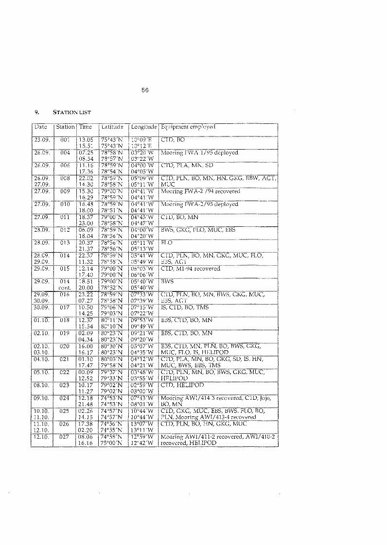
9. STATION LIST

Date Station Time Latitude

75'43'N 75'43'N 78O58'N 78'57'N 78O59'N

-

78O54'N 78'59'N 78'58'N 79'00'N 78'59'N 78'59'N 78'51 'N P

79'00'N 78'58'N P

78O59'N 7g056'N P

78'56'N 78'56'N 78'59'N 7g058'N P

79'00'N 79'00'N 79O00'N 78O52'N 78O59'N 78'58'N 79O06'N 79'03'N P

80°11' 80°10' 80°23' 80°23' P

80°30' 80°23' P

80°03' 79O58'N - 79O37'N 79O33'N 79O02'N 79'02'N P

74'53'N 74'53'N 74'57'N 74O57'N 74O56'N 74'55'N 74O58'N 75'00'N -

Longitude 1 Equipment employed '. $

10°12' 1 i 3

03'2O'W 1 Mooring FWA-1/95 deployed 03'22'W 5 1 ~ -

04O00'W i CTD, PLA, MN, SD i 04OO5'W 1 05'09'W 1 CTD, PLN, BO, MN, HN, GKG, EBW, A G T , ~ 05'1 1 'W 1 MUC 04'41 'W 1 Mooring FWA-2 /94 recovered 1 04'41 'W

V 1 04O41'W 1 Moorine FWA-2/95 deployed l

A J

04'45'W Â CTD, BO, MN 1 04'47'W 1 1

0 9 0 4 9 ' w L 09O21'W S EBS, CTD, BO, MN

. . 13Oll'W 1 12'59'W Mooring AWI/411-2 recovered, AWI/410-2 12'42'W , recovered, HELIPOD

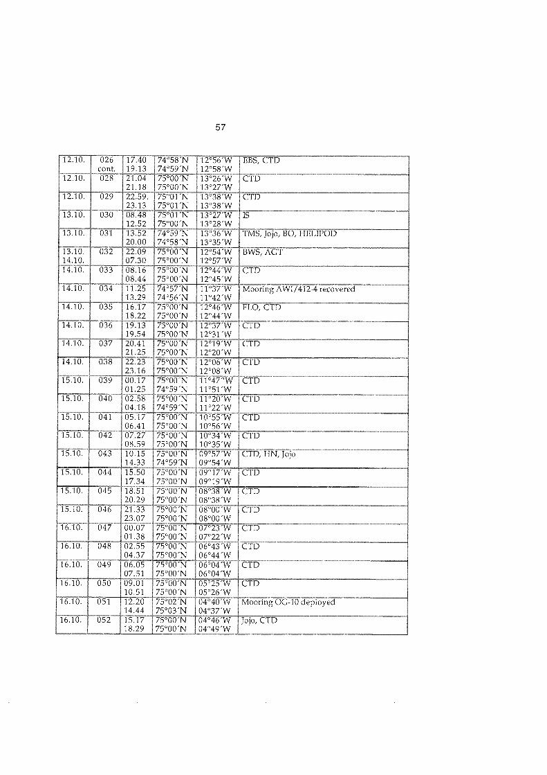
026 cont. - 028 -

029

030

031

032

033

034

035

036

037

038 P

039 -

040

041 --

042 -

043 P=

044

045 W.--

046 P.

047 ---U.

048 P

049

050

051

052

EBS, CTD

CTD

CTD

TMS, Jojo, BO, HELIPOD

BWS, AGT

CTD

Mooring AWI/412-4 recovered

FLO, CTD

CTD

CTD

CTD

CTD

CTD

CTD P---

CTD

V CTD

CTD -- CTD

C T D ~

CTD

Mooring OG-10 deployed

Jojo, CTD

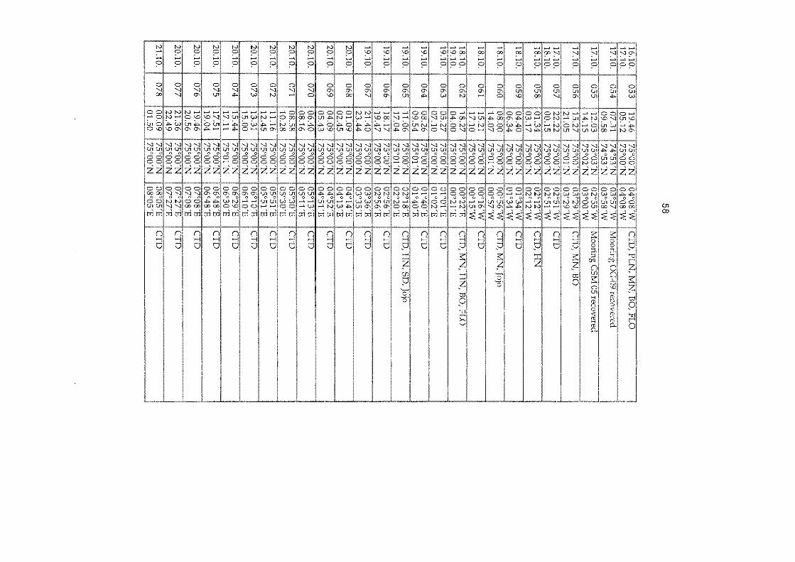
1 7 . 5 4 175OOO'N 1 11°56' 1 21.10. 085 19.16 75'00'N 12'36'E CTD

20.29 75O00'N 12'34'E 22.10. 086 06.14 75'00'N 13'15'E CTD

07.24 75'00'N 13'15'E 2 .10 . 1 087 108.49 175OOO'N 13O52'E CTD, MN, B 0

l j 13.30 175OOl'N j 13O49'E 1 22.10. 088 14.50 75'00'N 14031rE CTD

15.39 75'00'N 14'31 'E

23.13 73'20'N 16'59'E L4.10. 1 103 100.29 173OlO'N 117OOO'E CTD

j_____fO0.48 ~ 7 3 Â ° 1 0 ' ~ 1 7 0 0 1 r 1 -

17'00'E CTD

17'00'E 8 CTD

17'00'E 1 17O01'E CTD

- 1 7O0 1 'E

17O00'E 1 17'00'E 1 CTD 17'01'E 1 17O00'E CTD 17OOO'E ..

17O00'E CTD i

Abrahamsson, Katarina Albers. Carola Auel, Holger Berg, Jör Stefan Böhm Joachim Brandt, Angelika Budkus, Gereon Cisewski, Boris Cohrs, Wolfgang Darnall, Clark Donner, Gabriele Ekdahl, Anja Erdmann, Hilger Gedamke, Michael Gradinger, Rolf Haupt, Olaf Hofmann, Michael Hollmann, Beate Ikävalko Eira Johanna Jensen, Stefan Kaleschke, Lars Köhler Herbert Krause, Gunther Krumbhoiz, Marita Lahrmann, Uwe Lunau, Angela Martin, Thomas Mock, Thomas Monk, JŸrge Niehoff, Barbara Plugge, Rainer Riewesell, Christian Ronski, Stephanie Sackmann, Volker Sauter, Eberhard Scheltz, Annette Schnack, Klaus Schreiber, Detlev Schürmann Mathias Strohscher, Birgit Stürcken-Rodewald Marthi Takizawa, Takatoshi Ufermann, Susanne Wamser, Christian Wanner, Susanne Wehde, Henning Werner, Iris Wode, Christian Woodgate, Rebecca Zhang, Qing

AMK AWI Ir0 SFB 313 HSW IPO AWI AWI AWI APL SFB 313 AMK DWD SFB 313 IPO SFB 313 IMK AWI UNI HELSINKI SFB 313 AWI DWD AWI SFB 313 HSW GEOMAR AWI SFB AWI AWI AWI HSW AWI AWI SFB 313 SFB 313 SFB 313 HSW Aerodata AWI AWI JAMSTEC AWI AWI GEOMAR AWI IPO - SFB 313 Ih4K AWI PO

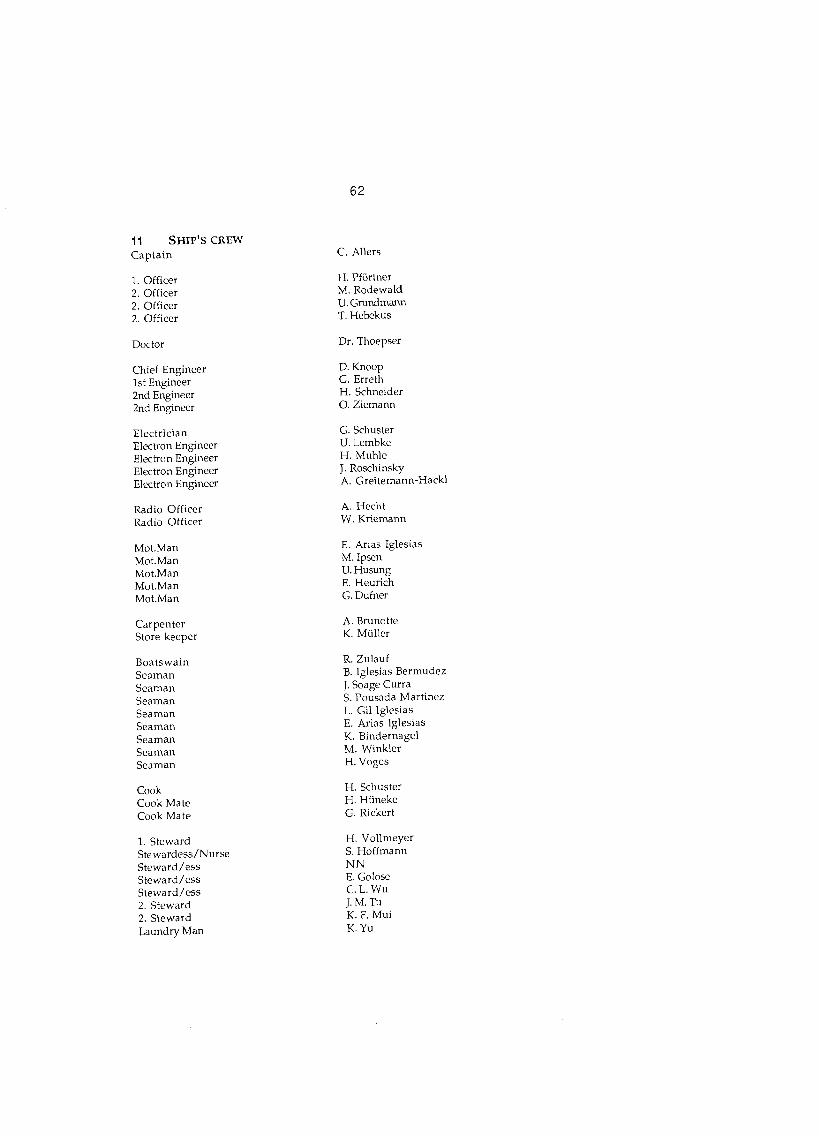
11 SHIP'S CREW Captain

1. Officer 2. Officer 2. Officer 2. Officer

Doctor

Chief Engineer Ist Engineer 2nd Engineer 2nd Engineer

Electrician Electron Engineer Electron Engineer Electron Engineer Electron Engineer

Radio Officer Radio Officer

Carpenter Store keeper

Boatswain Seaman Seaman Seaman Seaman Seaman Seaman Seaman Seaman

Cook Cook Mate Cook Mate

1. Steward Stewardess/Nurse Steward/ess Steward/ess Steward/ess 2. Steward 2. Steward Laundry Man

C. Allers

H. Pförtne M. Rodewald U. Grundmann T. Hebekus

Dr. Thoepser

D. Knoop G. Erreth H. Schneider 0. Ziemann

G. Schuster U. Lembke H. Muhle J. Roschinsky A. Greitemann-Hack1

A. Hecht W. Kriemann

E. Arias Iglesias M. Ipsen U. Husung E. Heurich G. Dufner

A. Brunotte K. Mülle

R. Zulauf B. Iglesias Bermudez J. Soage Curra S. Pousada Martinez L. Gil Iglesias E. Arias Iglesias K. Bindernagel M. Winkler H. Voges

H. Schuster H. Hünek G. Rickert

H. Vollmeyer S. Hoffmann N N E. Golose C. L. Wu J. M. Tu K. F. Mui K. Yu

AWI

Aerodata

DWD

GEOMAR

IfMHH

IMK

SFB 313

UNI

Alfred-Wegener-Institut fü Polar- und Meeresforschung Columbusstraß 27568 Bremerhaven

Aerodata Flugmeßtechni GmbH Rebenring 33 38106 Braunschweig

Deutscher Wetterdienst Hamburg Seewetteramt Bernhard-Nocht-Straß 76 20359 Hamburg

GEOMAR Forschungszentrum fü marine Geowissenschaften Universitä Kiel Wischhofstraß 1-3 24148 Kiel

Helicopter-Service Wasserthal GmbH Kätnerwe 43 22393 Hamburg

Institut fü Meereskunde Universitat Hamburg Troplowitzstraß 7 22529 Hamburg

Institut fü Meteorologie und Klimatologie Universitat Hannover Herrenhäuse Straß 2 30419 Hannover

Institut fü Polarökologi Universitä Kiel Wischhofstraf3e 1-3, Gebäud 12 24184 Kiel

Universitä Kiel Sonderforschungsbereich 313 Olshausenstraß 40 24118 Kiel

University of Helsinki Hydrobiol. Laboratory P.O. Box 4 FIN-00014 Helsinki

J AMSTEC

APL

AMK

Japan Marine Science and Technology Center JAMSTEC Headquarters 2-15 Natsushima-Cho YOKOSUKA 237 JAPAN

Norwegian Polar Institute Dept. of Analyt. and Marine Chemistry Postboks 5072, Majorstua N-0301 Os10

Polar Science Center Applied Physics Laboratory University of Washington HN-10 Seattle, WA 98195

Chalmers University of Technology and University of Götebor Analytical and Marine Chemistry S-412 96 Götebor

Second Institute of Oceanography State Oceanic Administration P.O.Box 1207 Hangzhou, Zhejiang, 310012

13. Moorings serviced during "Polarstern" cruise ARK XI12

Name Latitude Idegrees

RECOVERED

Fahrbach, AW1

AWI 410-2 74 57.7N

AWI 411-2 74 59.8N

AWI 412-4 74 57.5N

AWI 414-4 74 52.6N

Meincke, IfM HH

MI-94 79 0.2N

GSM-05 75 2.3N

Aagaard, APL

FWA-2 '94 78 59.3N

SFB, Kiel

OG-9 74 52.9N

DEPLOYED

Aagaard, APL

FWA-1 '95 78 57.1N

SFB, Kiel

OG-10 75 3.4N

Longitude Idegrees

12 5 8 . W

12 31.9W

11 36.9W

10 37.1W

7 45.6W

6 1.6W

2 54.9W

4 4 0 . W

3 56.9W

3 22.3W

4 40.6W

4 3 5 . m

Depth /m Instruments (corrluncorr)

2 Current Meters 1 Sediment Trap 1 ULS 3 Current Meters 1 ULS 4 Current Meters 1 ULS 4 Current Meters 3 Sediment Traps 1 Transmissometer 1 ULS 4 Current Meters 1 u L s

2 Current Meters 1 ULS 1 Current Meter 5 Seacats 1 Thermistor Chain 1 ADCP

3 Current Meters 2 Seacats 1 ULS

2 Sediment Traps

2 Current Meters 1 Seacat 1 ULS

2 Current Meters 1 Seacat 1 ULS

3 Current Meters 3 Sediment Traps