LUND UNIVERSITY

PO Box 117221 00 Lund+46 46-222 00 00

Benchmark of Femlab, Fluent and Ansys

Verdier, Olivier

2004

Link to publication

Citation for published version (APA):Verdier, O. (2004). Benchmark of Femlab, Fluent and Ansys. (Preprints in Mathematical Sciences; Vol.LUTFMA-5039-2004). [Publisher information missing].

Total number of authors:1

General rightsUnless other specific re-use rights are stated the following general rights apply:Copyright and moral rights for the publications made accessible in the public portal are retained by the authorsand/or other copyright owners and it is a condition of accessing publications that users recognise and abide by thelegal requirements associated with these rights. • Users may download and print one copy of any publication from the public portal for the purpose of private studyor research. • You may not further distribute the material or use it for any profit-making activity or commercial gain • You may freely distribute the URL identifying the publication in the public portal

Read more about Creative commons licenses: https://creativecommons.org/licenses/Take down policyIf you believe that this document breaches copyright please contact us providing details, and we will removeaccess to the work immediately and investigate your claim.

BENCHMARK OF FEMLAB, FLUENT

AND ANSYS

OLIVIER VERDIER

Preprints in Mathematical Sciences2004:6

Centre for Mathematical SciencesMathematics

CE

NT

RU

MSC

IEN

TIA

RU

MM

AT

HE

MA

TIC

AR

UM

3

CONTENTS

1 Introduction 3

2 Case Descriptions 42.1 Structural Mechanics Cases . . . . . . . . . . . . . . . . . . . . . . . 4

2.1.1 Elliptic Membrane . . . . . . . . . . . . . . . . . . . . . . . 42.1.2 Built-in Plate . . . . . . . . . . . . . . . . . . . . . . . . . . 52.1.3 Square Supported Plate . . . . . . . . . . . . . . . . . . . . . 6

2.2 Fluid Mechanics Test Cases . . . . . . . . . . . . . . . . . . . . . . . 72.2.1 Backward Facing Step . . . . . . . . . . . . . . . . . . . . . . 72.2.2 Cylinder Flow in 2D . . . . . . . . . . . . . . . . . . . . . . 9

3 Measurements : Computational Results 103.1 Experimental Procedure . . . . . . . . . . . . . . . . . . . . . . . . . 103.2 How to Read the Results . . . . . . . . . . . . . . . . . . . . . . . . . 113.3 Structural Mechanics . . . . . . . . . . . . . . . . . . . . . . . . . . . 12

3.3.1 Elliptic Membrane . . . . . . . . . . . . . . . . . . . . . . . 123.3.2 Built-in Plate . . . . . . . . . . . . . . . . . . . . . . . . . . 143.3.3 Supported Plate . . . . . . . . . . . . . . . . . . . . . . . . . 14

3.4 Fluid Mechanics . . . . . . . . . . . . . . . . . . . . . . . . . . . . . 143.4.1 Backstep . . . . . . . . . . . . . . . . . . . . . . . . . . . . . 153.4.2 Cylinder 2D . . . . . . . . . . . . . . . . . . . . . . . . . . . 16

4 Conclusions 18

References 19

1 INTRODUCTION

This is a benchmark of Femlab 3.0a, Ansys 7.1 and Fluent 6.1.18. We also conductedsome tests with the former version 2.3 of Femlab. This was done in order to compare theperformance and reliability of these programs under two sets of problems. The first setis composed of two and three dimensional structural mechanics benchmarks which aretaken from the benchmark documentation of Ansys. Some of them are also part of theNAFEMS benchmarks. The second set is composed of two dimensional standard fluidmechanics benchmarks to test the incompressible Navier-Stokes model in laminar mode.

4

All the tests were run on the same machine in order to be able to effectively comparethe performances. Each case was set up with an artificially large number of degrees of free-dom. This was done in order to have an idea of the behaviour of the tested programs onheavy industrial problems, while keeping the geometry simple and disposing of measuredor theoretical reference quantities.

We begin with the description of the test cases, we then give some information aboutthe experimental procedure and finally give the results of the measurements.

2 CASE DESCRIPTIONS

2.1 Structural Mechanics Cases

2.1.1 Elliptic Membrane

The original case is an elliptic membrane with an elliptic hole in its center (cf. figure 1).An outward pressure load is applied on the external edge. Because of the symmetry of theproblem, only a quarter of the elliptic membrane is simulated. So the case is a quarter ofan elliptic membrane with a slipping boundary condition on two edges (to account for thesymmetry), plus a pressure load on its outer edge. Figure 2 on page 13 shows the resultingdeformation of the membrane. A reference for this case is [Barlow and Davis, 1986].

Figure 1: The whole elliptic membrane

Olivier Verdier

5

A

B

CD

1.75 m

1.0 m

2.0 m 1.25 m

GeometryThe membrane is 0.1 m thin.(We use the plane-stress model)

MaterialE = 2.10 · 105 MPaν = 0.3

Constraints and LoadsThe boundary conditions, as indicated on the picture, come from horizontal andvertical symmetry: no vertical displacement on the lower edge (CD) and no hori-zontal displacement on the left edge (AB).A pressure

P = −10 MPa

is applied on the outer edge (BC).

Quantities to be measuredThe value of σy at the point D is to be measured. Its theoretical value is

σy = 92.7 MPa

2.1.2 Built-in Plate

A rectangular plate with built-in edges is subjected to a uniform pressure load on the topand bottom surfaces. Due to the symmetry of the problem only an eighth of the plate issimulated. The reference for this case is [Timoshenko and Woinowsky-Knieger, 1959].

6

x

z

y

L

H

D C

BA

EF

GH

Geometry and MaterialH = 1.27 · 10−2 mL = 1.27 · 10−1 mE = 6.89 · 104 MPaν = 0.3

Face ConstraintsFace Description Constraintx = 0 ux = 0x = L ux = 0y = 0 uy = 0y = L uy = 0z = H ux = uy = 0z = 0 P = −3.447 MPa

Edge ConstraintsEdge ConstraintCG uz = 0HG uz = 0

Quantities to be measuredQuantity Location Theoreticaluz-1 D 4.190 · 10−4 mσy-2 B − 2.040 · 102 MPaσy-3 A 9.862 · 101 MPa

2.1.3 Square Supported Plate

The eigenmodes of a plate supported on its lower edges are well known analytically. Thetest case consisted in finding the ten first eigenmodes and eigenvalues and to compare thelatter to the theoretical values. The first three eigenvalues should be zero (solid mode)

Olivier Verdier

7

because the solid is free to move the horizontal plane. The last three modes (8, 9 and10) are plane modes (no displacement in the vertical direction). For more details, cf.[NAFEMS, 1989].

x

z

y

L

H

Geometry and MaterialL = 10 mH = 1 mE = 200 · 103 MPaν = 0.3ρ = 8000 kg/m3

ConstraintsNo vertical displacement is allowed (uz = 0) on the four lower edges

Quantities to be measuredThe three first eigenmodes are plane modes with eigenvalue zero. The next seveneigenvalues should be measured. Here are their theoretical values:Eigenvalue nb 4 5 6 7 8 9 10Frequency (Hz) 45.897 109.44 109.44 167.89 193.59 206.19 206.19

The last three eigenmodes are plane modes.

2.2 Fluid Mechanics Test Cases

The following test cases were used to compare Fluent and Femlab. All the flows are mod-elled by the incompressible Navier-Stokes equations and they are under laminar regime.

2.2.1 Backward Facing Step

The backstep problem is a classic test in fluid mechanics. It consists of an inflow of fluidthat passes a step. Below that step a loop should be observed (see fig. 5 on page 15). Moredetails can be found in [Rose and Simpson, 2000].

8

0.005 m

0.08 m

0.01 m

0.06 m0.02 m

GeometryHeight of the step:

H = 0.005 m

Properties of the fluidη = 1.79 · 10−5 m2/sρ = 1.23 kg/m2

Boundary ConditionsThe boundary condition on the inflow (leftmost boundary, in red) is:

−→v = 6s(1− s)−→v0

where ‖v0‖ = 0.544 m/s and −→v0 is horizontal.The outflow condition is a zero pressure (rightmost boundary, in blue)

p = 0

The other boundary condition are set to no-slip. This means−→v = 0 on the bound-ary.

Reynolds Number

Re = 150

Quantities to be measuredThe length of the loop is to be measured (cf. fig. 5 on page 15). In nondimensionalform, the ratio of the length of the loop divided by the height of the step (H) isapproximatively 7.93 according to experimental data.

Olivier Verdier

9

2.2.2 Cylinder Flow in 2D

The cylinder flow test case is similar to the backstep one, except for the geometry. TheReynolds number has to be sufficiently low (below 200) to get a physically meaningfulstationary solution. If the Reynolds number is too high, Femlab finds a solution althoughthe regime is clearly unstable. This instability can be observed using the time dependentsolver in Femlab.

2.20 m

A B0.20 m

0.21 m

0.20 m

D = 0.10 m

GeometryThe cylinder has a diameter

D = 0.10 m

Fluid Propertiesη = 10−3 m2/sρ = 1 kg/m2

Boundary Conditions‖v0‖ = 0.3 m/s and −→v0 is horizontal.The boundary condition on the inflow (leftmost boundary, in red) is:

−→v = 4s(1− s)−→v0

where s parametrises the left boundary.The outflow condition is a zero pressure (rightmost boundary, in blue)

p = 0

The other boundary condition are set to no-slip. This means−→v = 0 on the bound-ary.

Quantities to be measuredWe define the mean velocity by

v̄ =2

3‖v0‖

10

We then define the non-dimensional force of the fluid on the cylinder:

~c =2~F

%v̄2D

We can then define the drag coefficient cD and the lift coefficient cL to be the xand y coordinates of the non-dimensional force ~c:

cD = cx

cL = cy

We also define the recirculation length La which is the distance on the line{y = 0.2} between the right border of the cylinder and the first point wherethe horizontal velocity is positive (cf. figure 7 on page 16). The pressure drop∆P is defined as the difference of the pressures on the left and right border of thecylinder:

∆P = PA − PB

All these quantities are taken from [Turek and Schäfer, 1996]. The values that wewill choose as “theoreticals” for the precision measurements are the followings:

cD cL La/D ∆P ( N/m)

5.58 1.07 · 10−2 8.46 · 10−1 1.174 · 10−1

Reynolds Number

Re =v̄D

η= 20

3 MEASUREMENTS : COMPUTATIONAL RESULTS

3.1 Experimental Procedure

All the computations were carried out on the same computer which caracteristics can befound on table 2 on the next page.

Mesh Settings The generated meshes were always isotropic and homogeneous in the fourtested programs for the performance tests except for some of the measures in thecylinder 2d and 3d cases.

Olivier Verdier

11

Mesh Convergence The mesh convergence investigations were carried out using the“Mesh Parameters...” option in Femlab 3, using the whole range from “Extremelycoarse” to “Extremely fine” and sometimes even more. The only exception is thegraph labelled "Dense Mesh" on figure 8 on page 17, on which the mesh is denseraround the cylinder.

It should be emphasised that there are is no way to modify a mesh in Fluent withoutlosing all the boundary conditions and other settings. As a result it is very difficultto investigate the mesh convergence in Fluent.

Table 1 Versions of the tested programs

Program Version

Fluent 6.1.18Ansys 7.1Femlab 2.3 2.3Femlab 3.0a 3.0-207

Table 2 Computer Characteristics

Manufacturer Fujitsu-SiemensProcessor Intel P4 2.4GHzRAM 1GBOS MS Windows XP

3.2 How to Read the Results

Precision The precision for a given quantity Q and its corresponding theoretical valueQtheor is computed according to the following formula:

precision = − log

(∣∣∣∣1− Q

Qtheor

∣∣∣∣)

The measured quantity in the measurement tables are always given in this form.Note that a precision above the theoretical precision (which is usually 2 or 3) doesnot mean that the precision is really better than the theoretical precision.

12

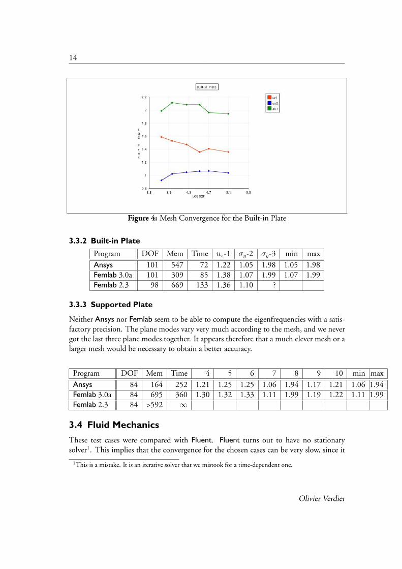
Mesh Convergence On the mesh convergence graphs the precision is representedagainst the log of the number of degrees of freedom.

Units If not explicitly mentioned, the units are always SI units. The units of the perfor-mance tables are the following:

Denomination Units

DOF (Degrees of Freedom) ThousandsMem (Peak Memory) MegaByteTime (CPU Time) Second

The peak memory is the maximum memory used by the process during the com-putation.

Out of Memory When the peak memory measurement is preceded by “>”, it meansthat the computation process could not be completed because of an out of memoryerror.

Missing Measures Missing measure are indicated by a “?” sign. It means that thequantity could not be measured with a sufficient accuracy.

Measure Accuracy All the measures were taken with 4 significant digits.

3.3 Structural Mechanics

Ansys and Femlab are comparable in CPU time and memory usage on the structuralmechanics cases, except in the Supported Plate case where Ansys turns out to be muchmore efficient in time and memory for the same accuracy as Femlab. Note also that theresults vary very much according to the numerical solver used. The sovers on Femlab 3have been carefully tuned in order to obtain the best perfomances. Such a possibility doesnot seem to be available in Ansys.

3.3.1 Elliptic Membrane

Program DOF Mem Time σy

Ansys 74 180 10 2.67Femlab 3.0a 76 135 9 3.12

Femlab 2.3 85 380 33 2.97Femlab 3.0a 89 152 13 3.19

Olivier Verdier

13

Figure 2: Deformation of the Elliptic Membrane

Figure 3: Mesh Convergence for the Elliptic Membrane

14

Figure 4: Mesh Convergence for the Built-in Plate

3.3.2 Built-in Plate

Program DOF Mem Time uz-1 σy-2 σy-3 min max

Ansys 101 547 72 1.22 1.05 1.98 1.05 1.98Femlab 3.0a 101 309 85 1.38 1.07 1.99 1.07 1.99Femlab 2.3 98 669 133 1.36 1.10 ?

3.3.3 Supported Plate

Neither Ansys nor Femlab seem to be able to compute the eigenfrequencies with a satis-factory precision. The plane modes vary very much according to the mesh, and we nevergot the last three plane modes together. It appears therefore that a much clever mesh or alarger mesh would be necessary to obtain a better accuracy.

Program DOF Mem Time 4 5 6 7 8 9 10 min max

Ansys 84 164 252 1.21 1.25 1.25 1.06 1.94 1.17 1.21 1.06 1.94Femlab 3.0a 84 695 360 1.30 1.32 1.33 1.11 1.99 1.19 1.22 1.11 1.99Femlab 2.3 84 >592 ∞

3.4 Fluid Mechanics

These test cases were compared with Fluent. Fluent turns out to have no stationarysolver1. This implies that the convergence for the chosen cases can be very slow, since it

1This is a mistake. It is an iterative solver that we mistook for a time-dependent one.

Olivier Verdier

15

endeavours to find an asymptotic solution from a nonstationary solver. This implies thatthe performances of Fluent are very sensitive to the given precision which was 10 −5 on allthe cases. We will also see in both 2D cases that Femlab is more accurate even used with anon-stationary solver and also that Fluent does not converge, no matter how long we letit iterate. At last we tested Fluent with very large numbers of elements but the precisionis not improved.

3.4.1 Backstep

Fluent gets the loop with a remarkably poor accuracy. Femlab yields better results evenwhen used with a non stationary solver. Only a few hundreds of elements is needed toFemlab to achieve a better accuracy than that of Fluent.

Figure 5: The loop behind the step

Figure 6: Mesh Convergence for the Backstep

16

Program DOF Mem Time Loop

Fluent 83 55 146 0.79Femlab 2.3 100 >602 ∞Femlab 3.0a 96 445 630 2.02

Femlab 2.3 25 322 77 1.85Femlab 3.0a 25 136 77 1.90

3.4.2 Cylinder 2D

The first computations are carried out using a homogeneous mesh. The last two line,however, are results of computations with refined mesh around the cylinder. One shouldbe careful about these last two results, though, since the refinement methods are not thesame.

We tried to let Fluent iterate for a very long time (about 20000 iterations) and still theresidual remains above 10−5. The subsequent results for Fluent are not better than thosepresented here.

We also used Femlab 3 for a non-stationary simulation of this case and the precision isthe same as in the stationary one. Moreover the solution converges fairly quickly to thestationary one (whereas Fluent does not converges at all if the residual tolerance is chosenbelow 10−5).

Figure 7: The recirculation area at the back of the cylinder

Olivier Verdier

17

Figure 8: Mesh convergence for the Cylinder 2D Case

18

Program DOF Mem Time cD cL La ∆P

Fluent 50 62 140 1.42 0.48 ? ?Femlab 3.0a 50 213 62 2.71 0.48 1.81 1.59Femlab 2.3 101 >623 ∞Femlab 3.0a 101 414 142 2.49 0.00 1.68 2.12

Fluent 109 67 450 1.97 0.00 ? ?Femlab 3.0a 101 371 108 4.75 2.13 1.91 3.07

4 CONCLUSIONS

Femlab 3 represents a very significant stride compared to the previous version 2.3. Inmost cases, the old version could not even carry out the computations without an "Outof memory" error message.

Femlab 3 performances are comparable, both from the precision, CPU time and mem-ory usage, to those of Ansys, except for the eigenfrequency analysis, where Ansys is moreefficient.

Surprisingly enough, and despite all our endeavours, Fluent does not yield any accurateresults. For the backstep case, for instance, the precision of Femlab with a few hundredsdegrees of freedom is better than that of Fluent with eighty thousands. Moreover fordifficult problems like that of computing the force exerted on the cylinder, in the 2Dcase, a very good accuracy is needed to capture the right lift coefficient which is, in non-dimensional form, approximately one percent of the drag coefficient. There is apparentlyno hope for Fluent to get even a rough idea of this coefficient, no matter how long wewait or how refined the mesh is.

REFERENCES

Barlow, J. and G. A. O. Davis. 1986. Selected FE Benchmarks in Structural and ThermalAnalysis. Technical report NAFEMS.

NAFEMS. 1989. The Standard NAFEMS Benchmarks. Technical report NAFEMS.

Rose, Alan and Ben Simpson. 2000. Laminar, Constant-Temperature Flow over a Back-ward Facing Step. In 1st NAFEMS Workbook of CFD Examples.

Timoshenko, S. and S. Woinowsky-Knieger. 1959. Theory of Plates and Shells. McGraw-Hill Book Co. Inc.

Turek, S. and M. Schäfer. 1996. Benchmark Computations of Laminar Flow arounda Cylinder. In Flow Simulation with High-Performance Computers II, ed. E. H.

Olivier Verdier

19

Hirschel. Vol. 52 of Notes on Numerical Fluid Mechanics Vieweg pp. 547–566.http://www.mathematik.uni-dortmund.de/htmldata1/featflow/ture/paper/

benchmark_results.ps.gz

20

Olivier Verdier

Preprints in Mathematical Sciences 2004:6ISSN 1403-9338

LUTFMA-5039-2004

MathematicsCentre for Mathematical Sciences

Lund UniversityBox 118, SE-221 00 Lund, Sweden

http://www.maths.lth.se/