Behaviour of NOx sensors at their end of life - DiVA Portal
84
IN DEGREE PROJECT MECHANICAL ENGINEERING, SECOND CYCLE, 30 CREDITS , STOCKHOLM SWEDEN 2020 Behaviour of NOx sensors at their end of life JOSE MATHEW KTH ROYAL INSTITUTE OF TECHNOLOGY SCHOOL OF INDUSTRIAL ENGINEERING AND MANAGEMENT
-
Upload
khangminh22 -
Category
Documents
-
view
2 -
download
0
Transcript of Behaviour of NOx sensors at their end of life - DiVA Portal

IN DEGREE PROJECT MECHANICAL ENGINEERING,SECOND CYCLE, 30 CREDITS
, STOCKHOLM SWEDEN 2020
Behaviour of NOx sensors at their end of life
JOSE MATHEW
KTH ROYAL INSTITUTE OF TECHNOLOGYSCHOOL OF INDUSTRIAL ENGINEERING AND MANAGEMENT

A Master Thesis Report on
Behaviour of NOx sensors at their end of life
Jose Mathew
Performed in Engine after treatment control group
(NCFF) at
Scania CV AB, Södertalje, Sweden.
Master of Science Thesis TRITA-ITM-EX 2020:532
KTH Industrial Engineering and Management
Machine Design
SE-100 44 STOCKHOLM


Examensarbete TRITA-ITM-EX 2020:532
NOx-sensorns beteende vid livslängdens slut
Jose Mathew
Godkänt
2020-09-30
Examinator
Andreas Cronhjort
Handledare
Dan Edlund, Andreas Cronhjort
Uppdragsgivare
Scania CV AB
Kontaktperson
Dan Edlund
Sammanfattning NOx-sensorn är grundläggande i det moderna efterbehandlingssystemet och dess pålitlighet
är avgörande för att kunna leva upp till rådande emissionslagkrav. Livslängden samt
sensorns beteende i slutet av denna varierar betydligt. Om en NOx sensor med oberäkneligt
beteende inte upptäcks av fordonets styrsystemet kan det orsaka omfattande
verkstadsbesök eller i värsta fall brott mot emissionslagkrav. Examensarbetet involverar
identifiering av olika sensorfellägen, tidiga tecken till dessa fellägen, förstå och identifiera
förhållanden mellan olika sensorparametrar och analysera sensorbeteendet vid
sensorlivslängdens slutskede.
NOx sensorn är en relativt ny sensor och fordonsindustrin har ännu inte en fullständig
förståelse för dess beteende. Litteraturstudien täcker olika fellägena så som fastnat värde,
förskjutet värde, förstärkning av värdet, felaktiga svängningar samt långsam respons. Även
effekterna av åldrande i NOx sensorn beskrivs. Litteraturstudien diskuterar också diagnoser
av sensorer i allmänhet samt diagnoser specifikt för NOx sensorer. Uppsatsarbetet
involverar också en experimentell studie där NOx sensorer utsätts för statiska och
fluktuerande gasflöden i en motortestbädd.
Fellägen i NOx sensorer kan observeras i parametrarna för NOx-värde och oxidationsnivå. I
den version av NOx sensorn som användes observerades det också att parametrarna felaktig
NOx och felaktig O2 visar samma felkod samtidigt. Dock är inte parametrarna för felaktig
NOx och felaktig O2 relaterade till parametrarna för värmningsstatus, felaktig värmare och
värmeelementets temperatur. Sensorns status gällande ogiltiga NOx-mätningar är större än

eller lika med antalet ogiltiga O2-mätningar. Resultatet gäller framför allt sensormodell
Continental 2.8 NOx sensorer. Även logik för en monitor gällande felaktiga svängningar
utvecklas baserat på standardavvikelse och NOx statusparametern för ogiltig mätning.
Nyckelord
NOx sensor, felfunktioner, oscillerande felmätare, diagnos av sensorer

Master of Science Thesis TRITA-ITM-EX 2020:532
Behaviour of NOx sensors at their end of life
Jose Mathew
Approved
2020-09-30
Examiner
Andreas Cronhjort
Supervisor
Dan Edlund, Andreas Cronhjort
Commissioner
Scania CV AB
Contact person
Dan Edlund
Abstract
The NOx sensor is essential in the modern after-treatment system and the reliability of
the sensor is crucial for any emission-based legislation. The life span of a sensor varies a
lot as well as the behaviour previous to its end of life. If a NOx sensor with erratic
behaviour is not discovered by the control system it may cause extensive workshop
effort or in worst case exceed legal requirements. The thesis work involves identifying
different sensor failure modes, precursors to these failure modes, understanding and
identifying relationships between different sensor parameters, and analysing the sensor
behaviour especially towards the end of life.
The NOx sensor is a relatively new sensor and the vehicle industry does not yet have a
complete understanding of its behaviour. The literature study covers the different
failure modes namely stuck, offset, gain, oscillations, and slow response and their causes
along with the effects of ageing in NOx sensors. It also discusses the diagnosis of faulty
sensors in general and faulty NOx sensors. The thesis work also involves an
experimental study where the NOx sensors are subjected to static and transient gas flow
tests in an engine testbed.
Failure modes in NOx sensors are observable in NOx concentration and actual oxidation
measurement parameters. It was also observed in the version of the NOx sensor used
that Error NOx and Error O2 parameters show the same fault code at the same time.
Although, the Error NOx and Error O2 parameters are not related to the heater
parameters, Heater status, Error heater, and Temperature of heating element. The
number of invalid flags set in NOx status is greater than or equal to the number of

invalid flags in O2 status. The mentioned parameters are concerning Continental 2.8
NOx sensors. The logic for the oscillatory fault monitor is developed based on standard
deviation and an invalid flag check on the NOx status parameter.
Keywords
NOx sensor, failure modes, oscillatory fault monitor, diagnosis of sensors


Acknowledgements
This thesis work would not have been a success without the help and support from a lot
of people and I would like to thank all of them for their endless support and guidance.
Firstly, I would like to thank my parents for their immense love and encouragement to
do my master’s studies at KTH.
I would like to thank Dan Edlund and Peter Lindqvist for their constant guidance and
supervision throughout the thesis. I would also like to thank Christer Lundberg for his
suggestions and ideas in building the logic for the oscillatory faultmonitor. I also thank
Robin Nyström for giving me the opportunity to do the thesis work and also making
the onboarding process and our stay at Scania smooth. The cell technicians in test cell
F1 were of huge help during the experiments and I would like to thank them for their
support and assistance during the testing phase. The engine after-treatment controls
team was one of the best teams to work with at Scania, I thank the team for providing
me a great working environment at Scania.
I would also like to thank Dr. Andreas Cronhjort, my examiner and supervisor at
KTH for his motivation and guidance especially through the tough times during the
pandemic outbreak. I also thank the administrative staff at KTH for handling the
paperwork regarding my thesis.
Last but not least I would like to thank my friends and colleagues for their support to
improve my skillset and finish my thesis and master’s studies fruitfully.
v

Nomenclature
Abbreviations
CDF Cumulative Distributive Function
ECU Engine Control Unit
FMI Failure Mode Indicator
FTA Fault Tree Analysis
IC Internal Combustion
ICDF Inverse Cumulative Distributive Function
LNT Lean NOx Traps
MATLAB Matrix Laboratory
NOx Nitrogen Oxides
NW Nadaraya-Watson
OBD On-Board Diagnostics
SCR Selective Catalytic Reduction
SCU Sensor Control Unit
SNA Signal Not Available
SNS Smart NOx Sensor
STD Standard Deviation
SVM Support Vector Machine
Y SZ Yttria Stabilized Zirconia
vi

NOMENCLATURE
Notations
µ Mean of values of the standard deviation array
F Faraday’s constant (A-s/mol)
I Current (A)
N Number of samples of the standard deviation array
p Partial pressure (bar)
R Gas constant (J/mol-K)
T Temperature (K)
Us Sensor signal (V)
V Voltage (V)
vii

Contents
List of Tables x
List of Figures xi
1 Introduction 11.1 Background . . . . . . . . . . . . . . . . . . . . . . . . . . . . . . . . . . 1
1.2 Scope and objective . . . . . . . . . . . . . . . . . . . . . . . . . . . . . 2
1.3 Research methods . . . . . . . . . . . . . . . . . . . . . . . . . . . . . . 3
1.4 Thesis outline and structure . . . . . . . . . . . . . . . . . . . . . . . . . 4
2 Literature study 62.1 NOx sensors . . . . . . . . . . . . . . . . . . . . . . . . . . . . . . . . . 7
2.2 Ageing of NOx sensors . . . . . . . . . . . . . . . . . . . . . . . . . . . 9
2.3 Failure modes in NOx sensors . . . . . . . . . . . . . . . . . . . . . . . 13
2.4 Diagnosis of faulty sensors . . . . . . . . . . . . . . . . . . . . . . . . . 19
2.5 Diagnosis of faulty NOx sensors . . . . . . . . . . . . . . . . . . . . . . 20
3 Experimental study 223.1 Experimental setup . . . . . . . . . . . . . . . . . . . . . . . . . . . . . 22
3.1.1 Siemens Dynamometer . . . . . . . . . . . . . . . . . . . . . . . 22
3.1.2 Scania Engine . . . . . . . . . . . . . . . . . . . . . . . . . . . . 22
3.1.3 NOx Router . . . . . . . . . . . . . . . . . . . . . . . . . . . . . . 23
3.2 Experimental procedure . . . . . . . . . . . . . . . . . . . . . . . . . . . 25
4 Results and analysis 294.1 NOx Sensor parameters . . . . . . . . . . . . . . . . . . . . . . . . . . . 29
4.1.1 NOx concentration . . . . . . . . . . . . . . . . . . . . . . . . . . 30
4.1.2 Actual oxidation factor . . . . . . . . . . . . . . . . . . . . . . . . 33
viii

CONTENTS
4.1.3 Error Heater . . . . . . . . . . . . . . . . . . . . . . . . . . . . . 374.1.4 Error NOx and Error O2 . . . . . . . . . . . . . . . . . . . . . . . 384.1.5 Heater status . . . . . . . . . . . . . . . . . . . . . . . . . . . . . 404.1.6 NOx status and O2 status . . . . . . . . . . . . . . . . . . . . . . 414.1.7 Temperature of heating element . . . . . . . . . . . . . . . . . . 454.1.8 Mass flow and torque variations . . . . . . . . . . . . . . . . . . 46
4.2 Oscillatory fault monitor . . . . . . . . . . . . . . . . . . . . . . . . . . . 474.2.1 Formulation of the logic for the monitor . . . . . . . . . . . . . . 484.2.2 Coding the oscillatory fault monitor in ECU . . . . . . . . . . . . 574.2.3 Defining thresholds for the monitor . . . . . . . . . . . . . . . . . 59
5 Conclusions 615.1 Discussions . . . . . . . . . . . . . . . . . . . . . . . . . . . . . . . . . . 615.2 Future Work . . . . . . . . . . . . . . . . . . . . . . . . . . . . . . . . . 63
References 64
ix

List of Tables
3.1.1 Specifications of the engine . . . . . . . . . . . . . . . . . . . . . . . . . . 23
x

List of Figures
2.1.1 Schematic representation of an amperometric NOx sensor [18] . . . . 7
2.2.1 Percent change versus time by sensor and average by location -
Location 1 and Locations 2L and 2R [11] . . . . . . . . . . . . . . . . . 10
2.2.2V-I characteristics of measuring electrode on fresh sensor [7] . . . . . 11
2.2.3V-I characteristics of measuring electrode on aged sensor [7] . . . . . 12
2.2.4Current-voltage characteristics change after durability [8] . . . . . . 12
2.3.1 Plots of samples of normal and faulty signals [6] . . . . . . . . . . . . 14
2.3.2Relation betweenO2 andNOx concentrationswith Ip1 and Ip2 currents
[16] . . . . . . . . . . . . . . . . . . . . . . . . . . . . . . . . . . . . . . 15
2.3.3Results of De-NOx reaction on ESC Mode 6 (1,650 rpm, 75% load) [2] 16
2.3.4Approximate first order response behavior of NOx sensor [10] . . . . 17
2.3.5Clogging of diffusion barrier due to Mg molecules [3] . . . . . . . . . . 18
2.4.1 Pressure sensor showing normal operating behaviour and erratic
sensor behaviour [14] . . . . . . . . . . . . . . . . . . . . . . . . . . . . 20
3.1.1 Scania DC13 166 engine . . . . . . . . . . . . . . . . . . . . . . . . . . . 23
3.1.2 Process schema of NOx router . . . . . . . . . . . . . . . . . . . . . . . 24
3.1.3NOx router with upstream NOx sensors . . . . . . . . . . . . . . . . . 25
3.1.4NOx router with downstream NOx sensors . . . . . . . . . . . . . . . . 25
3.2.1 Experimental setup . . . . . . . . . . . . . . . . . . . . . . . . . . . . . 27
4.1.1 Negative offset in NOx measurements observed in Sensor 3 . . . . . . 31
4.1.2Oscillatory fault in NOx measurements observed in Sensor 2 . . . . . 31
4.1.3Oscillatory and stuck faults in NOx measurements observed in Sensor 8 32
4.1.4Oscillatory fault and positive offset in NOx measurements observed in
Sensor 10 . . . . . . . . . . . . . . . . . . . . . . . . . . . . . . . . . . . 32
4.1.5 Stuck fault in NOx measurements observed in Sensor 6 . . . . . . . . . 33
xi
LIST OF FIGURES
4.1.6Oscillatory fault in actual oxidation factor measurements observed in
Sensor 2 . . . . . . . . . . . . . . . . . . . . . . . . . . . . . . . . . . . . 34
4.1.7 Stuck fault in actual oxidation factormeasurements observed in Sensor 3 35
4.1.8Oscillatory fault in actual oxidation factor measurements observed in
Sensor 9 . . . . . . . . . . . . . . . . . . . . . . . . . . . . . . . . . . . . 35
4.1.9 Stuck fault in actual oxidation factormeasurements observed in Sensor 6 36
4.1.10Oscillatory fault in actual oxidation factor measurements observed in
Sensor 10 . . . . . . . . . . . . . . . . . . . . . . . . . . . . . . . . . . . 36
4.1.11Transition in fault code of error heater parameter observed in Sensor 8 38
4.1.12Transition in fault code of error NOx and error heater parameters
observed in Sensor 6 . . . . . . . . . . . . . . . . . . . . . . . . . . . . . 40
4.1.13Transitions in fault code of heater status parameter observed in Sensor 8 41
4.1.14Invalid signals in NOx status and O2 status parameters observed in
Sensor 2 . . . . . . . . . . . . . . . . . . . . . . . . . . . . . . . . . . . . 42
4.1.15Transitions in fault codes in NOx status and O2 status parameters
observed in Sensor 3 . . . . . . . . . . . . . . . . . . . . . . . . . . . . . 43
4.1.16Invalid flags set in NOx status and O2 status parameters at oscillatory
faults observed in Sensor 10 . . . . . . . . . . . . . . . . . . . . . . . . 45
4.1.17Transition in status of temperature of heating element parameter
observed in Sensor 8 . . . . . . . . . . . . . . . . . . . . . . . . . . . . 46
4.1.18Setting of fault codes in error NOx and error O2 parameters with
variations in torque and mass flow observed in Sensor 8 . . . . . . . . 47
4.2.1 Inverse Cumulative Distributive Function for the engine out sensors
with sampling time of 1 second . . . . . . . . . . . . . . . . . . . . . . . 49
4.2.2Inverse Cumulative Distributive Function for the engine out sensors
with sampling time of 10 seconds . . . . . . . . . . . . . . . . . . . . . 49
4.2.3Inverse Cumulative Distributive Function for the tail pipe sensors with
sampling time of 1 second . . . . . . . . . . . . . . . . . . . . . . . . . . 50
4.2.4Inverse Cumulative Distributive Function for the tail pipe sensors with
sampling time of 10 seconds . . . . . . . . . . . . . . . . . . . . . . . . 51
4.2.5Inverse Cumulative Distributive Function for the engine out sensors
considering the invalid flag criteria at a sampling time of 1 second . . 52
4.2.6Inverse Cumulative Distributive Function for the engine out sensors
considering the invalid flag criteria at a sampling time of 10 seconds . 52
xii

LIST OF FIGURES
4.2.7 Inverse Cumulative Distributive Function for the tail pipe sensors
considering the invalid flag criteria at a sampling time of 1 second . . 53
4.2.8Inverse Cumulative Distributive Function for the tail pipe sensors
considering the invalid flag criteria at a sampling time of 10 seconds . 53
4.2.9Maximum standard deviation values in 30 minutes for engine out
sensors at sampling time of 1 second . . . . . . . . . . . . . . . . . . . 55
4.2.10Maximum standard deviation values in 30 minutes for engine out
sensors at sampling time of 10 seconds . . . . . . . . . . . . . . . . . . 55
4.2.11Maximumstandarddeviation values in 30minutes for tail pipe sensors
at sampling time of 1 second . . . . . . . . . . . . . . . . . . . . . . . . 56
4.2.12Maximumstandarddeviation values in 30minutes for tail pipe sensors
at sampling time of 10 seconds . . . . . . . . . . . . . . . . . . . . . . . 56
4.2.13Defining threshold standard deviation value for engine out sensors . . 59
4.2.14Defining threshold standard deviation value for tail pipe sensors . . . 60
xiii

Chapter 1
Introduction
This chapter explains the background of the thesis work along with its scope and
objective. It also discusses about the different researchmethods used and the structure
and outline of the thesis as well.
1.1 Background
Nitrogen Oxide (NOx) emissions from automobiles have ill-effects on the environment
and human health. It is capable of reducing the regional air quality by increasing
ground-level ozone and thereby increasing smog concentrations [10]. This scenario
has created huge demands on automobile manufacturers to improve the emission-
quality [12].The present and the future legislation has to meet stringent emission
regulations andwould require amore complex exhaust after-treatment system [17]. An
on-boardNOxmeasurement device will provide efficient NOx conversionwith the help
of NOx catalyst and system optimization [12]. The performance of the de-NOx system
and the NOx measurement devices have to be improved substantially to meet these
legislation demands [6]. NOx sensors are a vital part of the exhaust after-treatment
system of an automobile. Failure modes of the sensor may lead to extensive workshop
support and also might fail to meet the legal requirements. The NOx sensors used by
Scania today have a guaranteed life span but many sensors are used even after this
time has passed. The sensor can sometimes behave erratic during its service period or
beyond its guaranteed lifetime and will have to be replaced.
1

CHAPTER 1. INTRODUCTION
NOx sensors show different types of erratic behaviour when it approaches its end of
life. This erratic behaviour fails to measure the correct amount of NOx in the exhaust
gas and may lead to the generation of false control signals which will be sent to the
after-treatment system. This will lead to incorrect dosing of urea and NOx present in
the exhaust gas will not be treated properly. As a consequence, the catalyst efficiency
of the NOx after-treatment system will decrease. Therefore, the performance of the
exhaust after-treatment system may be questioned because of this erratic behaviour
[10][6]. Catalyst efficiency is affected even if there is one-second slowly responding
measurement [10]. The NOx sensor is capable of sending quite a lot of information
apart from the NOx measurement. This includes the validity of the measurement,
working status of the sensor and its components, and so on. This information can
bemade to use to find if there are any precursors to the erratic behaviour shown by the
sensors. To access this information healthy and aged NOx sensors will be subjected to
static and transient gas flows. This would also confirm if there is a correlation in sensor
behaviour in transient and static gas flows. Scania’s existing On-Board Diagnostics
(OBD) system has the potential to identify a few of the erratic behaviour shown by
the NOx sensor. It would be beneficial if additional algorithms are formulated to
accommodate the missing functionalities and if there are alternative approaches to
identify the fault codes in the existing OBD system.
1.2 Scope and objective
The NOx sensor is essential in the modern after-treatment system and the reliability
of the sensor is crucial for any emission-based legislation [16]. The NOx sensor
is relatively a new sensor and the vehicle industry does not have a complete
understanding of the behaviour of NOx sensors especially towards its end of life.
Moreover, the automotive industry has the most knowledge in this regard when
compared to the sensor manufacturer. There is also a broad concern in the industry
about the inaccurate and absent fault modes shown by the sensor. If a NOx sensor with
a failure mode or erratic behaviour is not detected by the control system, it may lead
to extensive workshop support and breach of legal emission requirements [13].
The goal of the thesis is to get a comprehensive understanding of the failure
modes and behaviour of faulty and healthy NOx sensors in static and transient gas
flow/compositions. Based on these experiments, an understanding of the precursors
2

CHAPTER 1. INTRODUCTION
of a broken sensor and the basics for identifying erratic behaviour by the OBD system
can be derived. The following research questions were formulated to align with the
goals of the thesis:
• What are the different erratic behaviour or failure modes shown by a NOx sensor
towards the end of their life?
• What are the possible reasons for the different failure modes in NOx sensors?
• What are the effects of ageing in NOx sensors?
• How does a healthy and an aged/faulty sensor behave during static and transient
gas flow tests?
• Scania has fault monitors for most of the failure modes of the NOx sensors but
not for an oscillatory fault and therefore what logic and parameters should form
the basis for the oscillatory fault monitor?
The research questions stated above are answered in this thesis work and are explained
in this thesis report. These questions are answered through literature study, meetings,
and discussions with engineers who are proficient in the field, experiments in engine
testbeds, data analysis and visualisations and coding in MATLAB.
1.3 Research methods
There are several research methods available to solve the research questions
mentioned in the previous section. The important research methods among them
are literature study, experimental study, and data analysis. The data analysis can be
further divided into multiple parts. They are relying on data from faulty NOx sensors
from trucks, experimental data frompreviously performed experiments, and data from
engine testbed experimental study. Data from NOx sensors from trucks does not
provide flexibility of performing customised tests and explore sensor characteristics.
Experimental data from previously performed experiments does not have all sensor
parameters recorded. The experiment was performed in a ’NOx test rig’ where NOx
gas of known concentration was passed through the NOx sensor. Only one NOx level
(475 ppm) was studied and the measurement was carried out only for a few 100
seconds. The experiment did not account for the transient behaviour of the exhaust
gas. Therefore to overcome these limitations, experiments were performed in the
3
CHAPTER 1. INTRODUCTION
engine testbed studying four NOx levels and recording all sensor parameters along
with performing transient gas flow tests.
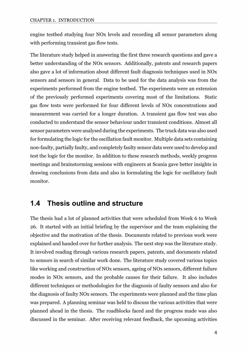
The literature study helped in answering the first three research questions and gave a
better understanding of the NOx sensors. Additionally, patents and research papers
also gave a lot of information about different fault diagnosis techniques used in NOx
sensors and sensors in general. Data to be used for the data analysis was from the
experiments performed from the engine testbed. The experiments were an extension
of the previously performed experiments covering most of the limitations. Static
gas flow tests were performed for four different levels of NOx concentrations and
measurement was carried for a longer duration. A transient gas flow test was also
conducted to understand the sensor behaviour under transient conditions. Almost all
sensor parameterswere analysed during the experiments. The truck datawas also used
for formulating the logic for the oscillation faultmonitor. Multiple data sets containing
non-faulty, partially faulty, and completely faulty sensor data were used to develop and
test the logic for the monitor. In addition to these research methods, weekly progress
meetings and brainstorming sessions with engineers at Scania gave better insights in
drawing conclusions from data and also in formulating the logic for oscillatory fault
monitor.
1.4 Thesis outline and structure
The thesis had a lot of planned activities that were scheduled from Week 6 to Week
26. It started with an initial briefing by the supervisor and the team explaining the
objective and the motivation of the thesis. Documents related to previous work were
explained and handed over for further analysis. The next step was the literature study.
It involved reading through various research papers, patents, and documents related
to sensors in search of similar work done. The literature study covered various topics
like working and construction of NOx sensors, ageing of NOx sensors, different failure
modes in NOx sensors, and the probable causes for their failure. It also includes
different techniques or methodologies for the diagnosis of faulty sensors and also for
the diagnosis of faulty NOx sensors. The experiments were planned and the time plan
was prepared. A planning seminar was held to discuss the various activities that were
planned ahead in the thesis. The roadblocks faced and the progress made was also
discussed in the seminar. After receiving relevant feedback, the upcoming activities
4

CHAPTER 1. INTRODUCTION
were initiated. The test cells were unavailable during the planned weeks and the
experiments had to be rescheduled for later dates.
Progress was made in designing the logic for oscillatory fault monitor until the
experiments started. Data from completely faulty, partially faulty, and non-faulty
sensors were used to set a starting point for the algorithm formulation. The
experiments were then carried out in the engine testbed and lasted for a week. The
faulty NOx sensors were subjected to static and transient gas flow tests. The sensors
are exposed to constant exhaust flowwith a predetermined value of NOx concentration
in case of a static gas flow test. The sensors are subjected to standard driving cycles
in case of a transient gas flow test. The data is then extracted from all the tests
and analysed for relationships between different sensor parameters. The results of
the analysis were presented in the halfway thesis presentation. The oscillatory fault
monitor was the prioritised task after the presentation. Using the experimental data
and truck data, cumulative and inverse cumulative probability distributive functions
were plotted in MATLAB to arrive at logic for the oscillatory fault algorithm. The
research questions were answered through the above tasks marking the achievement
of thesis objectives.
5

Chapter 2
Literature study
The literature study is conducted based on the research questions formulated. It is
mostly focused on relevant research papers and patents regarding NOx sensors and
diagnosing its erratic behaviour. To gain a better understanding of the NOx sensors,
research papers that explain the construction and working of NOx sensors are studied.
The literature study is also beneficial in identifying different failure modes that are
possible within a NOx sensor and in any sensor in general. Various technical reports
from Scania and the sensor manufacturers were also helpful in understanding the
possible causes of sensor failure modes. They also helped in deepening the knowledge
onNOx sensors and also presented experimental resultswhich proved to be a very good
starting point.
It is also interesting to find out that there are a few patents published that perform
diagnosis on some of the erratic behaviours. There are also patents published with
similar erratic behaviour but not on a NOx sensor. Research papers that emphasise on
the effects of ageing onNOx sensors are also studied. Some of the literature also covers
the experimental study on NOx sensors. The sensors are subjected to experiments
and the effects of ageing and performance of fault diagnosis algorithms are analysed.
Various literature that performs fault diagnosis on sensors is also studied to gain an
understanding of how the fault tree mechanism work which would be beneficial in
formulating the algorithm for NOx sensor diagnosis.
6
CHAPTER 2. LITERATURE STUDY
2.1 NOx sensors
Stefan Cartsens et al. states the different areas where NOx sensors are used. NOx
sensors found their way in the vehicle industry by its application in the lean-burn,
stratified charge gasoline passenger cars then onto diesel cars, and finally in and light
and heavy-duty diesel engines. The first generation NOx sensors were developed by
NGK and are currently taken over by other manufacturers as well [18]. Scania uses
NOx sensors manufactured by Continental and Bosch [9]. The most recent area of
application ofNOx sensors is in the urea-SCR systems for light and heavy-duty vehicles
[13]. A NOx sensor is typically used in the downstream of the SCR catalyst to measure
the NOx content and make sure it satisfies the OBD requirements. The conversion
rate of the catalytic converter can be found out by using two sensors, one upstream
and one downstream of the catalyst [18]. The most common type of NOx sensor that is
commercially available are the Yttria Stabilized Zirconia (YSZ) electrochemical sensors
that is similar to oxygen sensors in theworking principle and in construction [18].
Construction
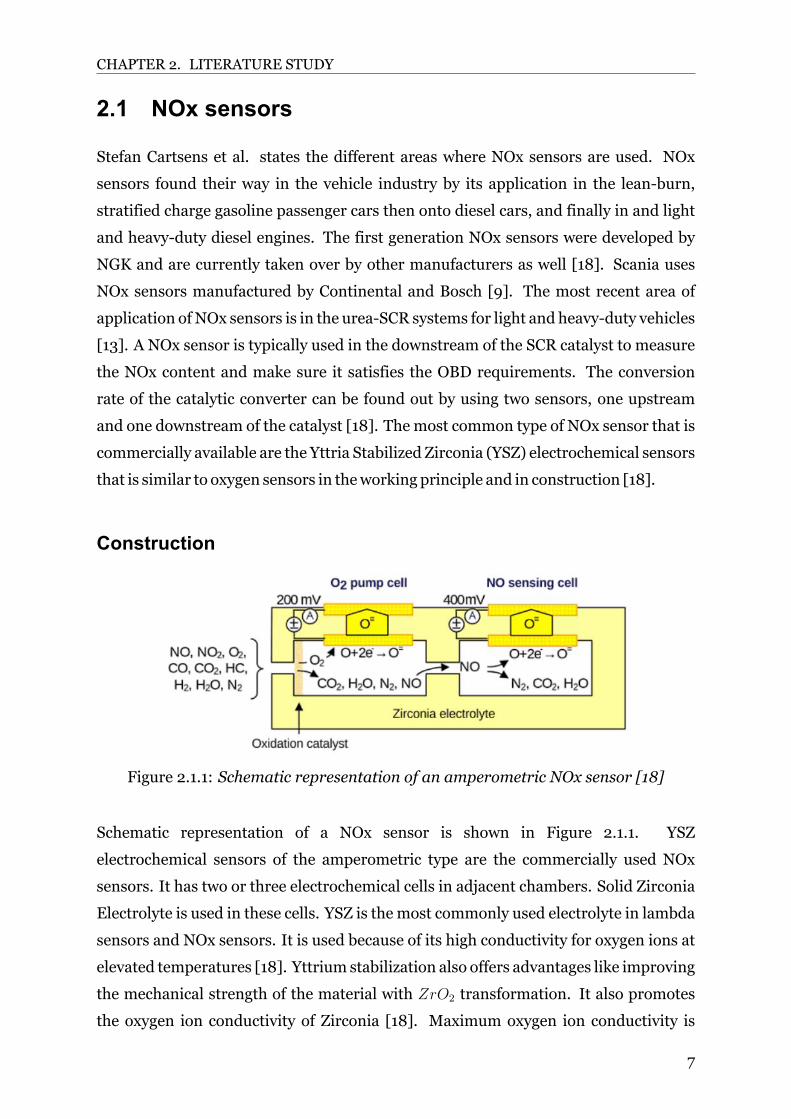
Figure 2.1.1: Schematic representation of an amperometric NOx sensor [18]
Schematic representation of a NOx sensor is shown in Figure 2.1.1. YSZ
electrochemical sensors of the amperometric type are the commercially used NOx
sensors. It has two or three electrochemical cells in adjacent chambers. Solid Zirconia
Electrolyte is used in these cells. YSZ is the most commonly used electrolyte in lambda
sensors and NOx sensors. It is used because of its high conductivity for oxygen ions at
elevated temperatures [18]. Yttrium stabilization also offers advantages like improving
the mechanical strength of the material with ZrO2 transformation. It also promotes
the oxygen ion conductivity of Zirconia [18]. Maximum oxygen ion conductivity is
7

CHAPTER 2. LITERATURE STUDY
achieved from 800 °C - 1200 °C. Separation to Y-lean and Y-rich areas occurs at
this temperature range which leads to a reduction in oxygen conductivity. Oxygen
conductivity can be reduced to 40% at 950 °C after 2500 hours and therefore NOx
sensors are operated slightly above 930 °C [18].
A dividing wall is made of YSZ ceramics that separates the two chambers with different
oxygen partial pressure. The oxygen ions cannot move through the gaps in crystal
lattice unless the ceramic wall temperature is at least 600 °C. The oxygen ions move
from the chamber with higher partial pressure to the chamber with the lower partial
pressure [18]. Similar to a lambda sensor, on connecting the walls with electrodes,
the movement of ions can be confirmed using voltage measurements. Equation 2.1
describes the reduction of oxygen molecules to oxygen ions which occurs in the higher
pressure chamber.
O2 + 4e− = 2O2− (2.1)
Based on Equation 2.1, the sensor voltage can be calculated using the Nernst equation
as shown in Equation 2.2.
Us = (RT/4F )ln(pref/pexh) (2.2)
Where Us represents the sensor signal (V), T is the temperature (K), p is the partial
pressure of oxygen, R is the gas constant = 8.314 J/mol-K and F is the Faraday’s
constant = 96485 A-s/mol. NOx sensors should include at least two oxygen pump
cells. The purpose of the first pump is to remove excess oxygen from the exhaust gas
and the second pumpmeasures the oxygen concentration from theNOxdecomposition
[18].
Working
The NOx sensor will have at least two chambers or cells. The first cell pumps out the
oxygen present in the exhaust so that it does not interfere with NOx measurement in
the second cell and also detects the exhaust oxygen level. On applying a bias voltage of
-200 mV to - 400 mV, O2 in the first cell is reduced and O2− ions are pumped through
YSZ. Oxygen concentration can be found out on calibrating the pumping current in the
8

CHAPTER 2. LITERATURE STUDY
first cell. The reducing catalyst in the second cell cause the NOx in the remaining gas to
decompose into N2 and O2. Similar to the first pump cell, a bias voltage of -400 mV is
applied to the electrode, and the pumping current of this cell would represent the NOx
concentration in the exhaust [18]. To avoid cross-interference all HC and CO should be
oxidized before the NOx cell and allNO2 should be converted to NO before the sensing
cell.
2.2 Ageing of NOx sensors
Ageing is referred to as the phenomena where the NOx sensor loses its sensitivity with
time from being heated [9]. There can be different reasons for the ageing of sensors.
One of them is the reduced conductivity due to the tendency of YSZ electrolyte to
phase separate. It can also be due to the accumulation of Yttrium at surfaces and
other borders, rate of change in resistance, exposed surface areas and micro-pores as
a result of the diffusion of heater metal and electrodes can also be a reason for the
ageing phenomena. The effects of clogging and poisoning can be considered as forms
of ageing [9].
John E. et al. has conducted a study to show howNOx sensors perform under different
types of exhaust conditions. The study also address the durability of the sensor. The
sensors were subjected to engine operation of 6000 hours and they were placed at
three different locations. The locations are immediately after the exhaust (location
1), between the DPF and SCR (location 2) and immediately after the clean-up catalyst
(location 3). The sensor and analyzer readings at location 1 were strongly correlated
and increased with time. At location 2, it suggests that the sensor degradation varies
differently for each sensor. It is because the rate of change in observed values with
respect to model predicted values are varying among the different sensors [11].
Tests for calibration errorswere also conducted and results show that calibration errors
increased with time and it was also interesting to see the same sensors produced
extremely different results for the ageing experiments [11]. The sensors located at
location 1 degraded less when compared to the sensors located at location 2. The
variation of percent change in degradation with time by sensor and average by location
is shown in Figure 2.2.1. After 6000 hours, sensors at location 1 and 2 were degraded
5 to 6 percent and 7 to 11 percent respectively. One possible reason for the difference
in sensor degradation is that sensors at location 2 are exposed to lube oil ash which
9

CHAPTER 2. LITERATURE STUDY
causes relatively more degradation than the sensors at location 1. The temperature
and pressure difference between the two locations are very small and sensors at both
locations are placed before the SCR and were not exposed to urea or ammonia. Hence,
these factors might not be responsible for the difference in sensor degradation [11].
John E. et al. also performed experiments to analyse the effects of operating modes
on the sensor response. It was found that there was an increase in percent deviation
with an increase in speed which may be due to the back-pressure increase. The sensor
response did not vary with variations in torque. It was also concluded that the sensor
performance degrades over time [11].
Figure 2.2.1: Percent change versus time by sensor and average by location - Location1 and Locations 2L and 2R [11]
10

CHAPTER 2. LITERATURE STUDY
Nobuhide Kato et al. performed tests with a fresh and a 300 hours-aged sensor on
a model gas apparatus and found out that the aged sensor showed approximately a
35% reduction in NOx sensitivity. A similar decrease was also found in a thermal
cycle test where the sensitivity decreased to 35% after 50 hours and then it saturated
at that value. The V-I characteristics of measuring electrodes of a fresh and aged
sensor are shown in Figures 2.2.2 and 2.2.3. On analysing the V-I characteristics of
the pump cell, it was concluded that the decrease in NOx output is due to the decline in
NOx decomposition catalytic activity of the measuring electrode. It was also observed
that there was no major deterioration of NOx decomposition catalytic activity in the
auxiliary pumps [7]. Hisashi Sasaki et al. found out that the Zirconia impedance of
the cell increased with ageing and at high temperatures of the element. An increase in
grain resistance on ageing was found to be the reason for the impedance increase. This
phenomenonmay be due to the Zirconia phase transformation at some sites [16].
Figure 2.2.2: V-I characteristics of measuring electrode on fresh sensor [7]
Yusukie Kawamoto et al. investigated the durability and V-I characteristics of the
relevant electrodes for aged and healthy sensors and are shown in Figure 2.2.4.
NOx concentration is calculated from the current at a specified voltage in limiting
current type sensors. On the basis of the comparison tests, it was found that there was
a decrease in the current at the control voltage for an aged sensor in the case of a sensor
11

CHAPTER 2. LITERATURE STUDY
Figure 2.2.3: V-I characteristics of measuring electrode on aged sensor [7]
Figure 2.2.4: Current-voltage characteristics change after durability [8]
electrode. Electrical property analysis, component analysis, and microstructural
analysis was done on healthy and aged sensors to understand the reason for the
deterioration of sensor output. The electrical property analysis confirmed that there
was an increase in dissociative adsorption resistance and charge transfer resistance
on ageing and these two modes are responsible for durability deterioration of the
sensor. It was also interesting to note that the electrolyte resistance did not change
on ageing [8]. The component analysis of the sensor electrode suggests that the NOx
active sites consisting of Platinum or Rhodium are decreased due to the movement
12

CHAPTER 2. LITERATURE STUDY
of Gold molecules onto the sensor electrode surface. The transfer of Gold molecules
from the interior of the senor to its surface was one of the major factors leading to the
dissociative adsorption resistance increase [8]. The microstructure analysis indicated
that the agglomeration of noble metal particles in the electrode as the main cause of
the increase in charge transfer. When dispersed particles stick to each other and form
large clusters to minimize surface energy is called agglomeration. Agglomeration of
particles cause a decreased number of three-phase boundaries on the electrodes as a
result of loss in specific electrode surface areas [8]. Thaddaeus Delebinski et al. has
investigated the qualitative behaviour of the NOx sensor. The tolerance increase with
a decrease in NOx concentrations and an aged sensor has more tolerance than the new
sensor.
On the basis of the used hours and the NOx level, an ageing correction factor is
introduced called ageing compensation to obtain reliable NOx measurements even
after ageing of the sensors [9]. Scania developed age compensation for the older
version of NOx sensors, but the new sensors have an in-built age compensation.
2.3 Failure modes in NOx sensors
The unusual behaviour of a system due to damage in the mechanical component can
be called fault [6]. In NOx sensors these failure modes can be due to electrode heating,
ageing of heaters, clogging, damage in diffusion barriers, or combinations of any of
these reasons [9]. NOx sensor fault or sensor fault, in general, includes the following
[6], [9]:
• Drift fault: A positive or negative change in the linear reaction results in a gain
fault.
• Spike fault: The presence of spikes in the sensor output signal can be termed as
a spike fault.
• Stuck fault: When the sensor output gets stuck at a fixed value, it can be termed
as a stuck fault.
• Offset fault: Changing the zero level of the sensor permanently and the level may
change to positive or negative levels.
• Slow response: NOx sensors have a response time in order of seconds and if the
13

CHAPTER 2. LITERATURE STUDY
response time is more than that, it is called a slow response of the sensor.
• Unstable values: When the sensor output changes or oscillates between a high
and a low value in slow or occasional intervals can be termed as unstable values.
Figure 2.3.1: Plots of samples of normal and faulty signals [6]
Figure 2.3.1 shows a few of the above-mentioned failure modes. A. Pezzini et al. has
described offset or gain errors are due to mechanical or electrical failure or due to
sensor poisoning. They can also be the reasons if there is an overheating or no heating
up of the sensors as well. The consequence of this failure mode is quite severe. It
can be seen when the sensor output gives incorrect NOx concentration, A/F ratio, and
rich/lean switch. As a result, it leads to issues related toNOx release like failing tomeet
the legal emission requirements. It may also lead to issues in regenerating Lean NOx
Traps (LNT). The catalyst within the sensor is the crucial component that may cause
the system to fail in case of thermal deactivation or Sulphur poisoning events in the
catalyst [13]. Charlotte Holmen et al. claims that a crack within the sensor can lead to
an offset error in the sensor output. Asmentioned earlier, theNOx sensor consists of at
least two chamberswhere one chamber is connected to the exhaust pipe to facilitate the
flow of exhaust gas and the second chamber contains reference gas of predetermined
concentration. The oxygen concentration or the NOx concentration in the exhaust gas
is correlated with the oxygen pumping current to or from the first chamber. Therefore,
if a crack occurs in the first chamber in the sensors it results in leakage of oxygen from
14
CHAPTER 2. LITERATURE STUDY
the exhaust or air sides. It is also possible that if a crack occurs in the second chamber,
it leads to leakage of oxygen from the exhaust side. These two possibilities may be the
reason for the offset error in a NOx sensor [19].
A small crack in the reference chamber can lead to poor measurement results from the
NOx sensor. In an event of a crack in the reference chamber, oxygen leaks into the
chamber while the oxygen is being pumped out. This leads to an increase in the time
required to pump when compared to an intact sensor. Hence, a crack in the second
chamber results in the failure of theNOx sensor [19]. Hisashi Sasaki et al. suggests that
a non-zero sensor output atNOx=0ppm is defined as the offset error. This error is due
to the presence of residual oxygen in the chamber where NO is dissociated to calculate
the amount of NO. Offset stability under all measurement conditions is crucial for the
OBD system. On reducing the leakage current using a high-side heater offset error was
reduced [16]. It was also found out that NOx offsets increased with an increase in cell
temperature of the NO dissociation chamber. Variation of the cell temperature with
external temperature fluctuation, water present in the chamber dissociates and gives
rise to an offset [16]. NOx offset is also affected by the hex nut of the NOx sensor.
The hex nut gets heated due to the exhaust gas heating the sensor boss. It leads to
a variation in the temperature distribution of the element through which NOx offset
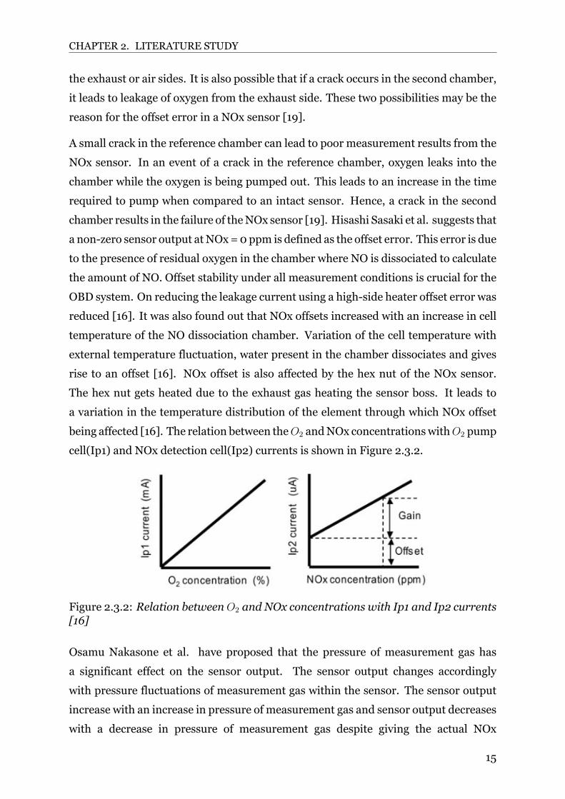
being affected [16]. The relation between theO2 andNOx concentrationswithO2 pump
cell(Ip1) and NOx detection cell(Ip2) currents is shown in Figure 2.3.2.
Figure 2.3.2: Relation betweenO2 and NOx concentrations with Ip1 and Ip2 currents[16]
Osamu Nakasone et al. have proposed that the pressure of measurement gas has
a significant effect on the sensor output. The sensor output changes accordingly
with pressure fluctuations of measurement gas within the sensor. The sensor output
increase with an increase in pressure of measurement gas and sensor output decreases
with a decrease in pressure of measurement gas despite giving the actual NOx
15

CHAPTER 2. LITERATURE STUDY
concentration [17]. This increase or decrease in NOx concentration levels leads to a
gain fault which is dependent on the pressure of measurement gas. Hisashi Sasaki
et al.compensated gain errors in NOx sensors by introducing pressure compensation
parameters and hence suggesting that pressure of the measurement gas is a crucial
factor causing the gain errors in NOx sensors.
C.C. Chou et al. investigated the different levels of oscillation in NOx measurements
for a downstream NOx sensor where urea dosage is varied by a crankshaft-link pump.
It was observed that the complete reaction of NOx took place when there was a
stoichiometric urea solution injection. However, NOx measurement fluctuated and
increased when a higher amount of urea was injected due to cross-sensitivity as shown
in Figure 2.3.3. The sensor output had less noise at the stoichiometric point with
the lowest NOx emission and no ammonia leakage. Oscillations were observed to be
large when less urea was injected. It was concluded that lower NOx emissions can be
achieved through higher urea dosages at fast pump speeds [2].
Figure 2.3.3: Results of De-NOx reaction on ESC Mode 6 (1,650 rpm, 75% load) [2]
Hisashi Sasaki et al. states that minimizing the gas flow to the sensing element can
result in a slower response time of the sensor. Typical first-order responses of NOx
sensors are shown in Figure 2.3.4.
16

CHAPTER 2. LITERATURE STUDY
Figure 2.3.4: Approximate first order response behavior of NOx sensor [10]
Fast and slow response NOx sensors can be distinguished from the curves in Figure
2.3.4. On the usage of heated gas, faster response of NOx sensors was reported
[16]. Dave Wagner [20] has some interesting findings regarding the occurrence of
negative measurements by the sensor. In an atmosphere where target gases of the
sensor are present, the instrument will be zeroed and it gives a negative measurement
corresponding to the concentration of contaminant present when measuring in an
essentially clean environment. Negative cross-interference can be another possible
reason for negative readings by the sensor. The sensor shows negative readings if
it is exposed to negative cross-interference producing gas [20]. Peter J Hesketh [5]
has some interesting findings in the positive and negative shifts in the sensor output
due to the presence of water molecules. In the case of low water levels, the sensor
output decreases if there is an increase in water. It is because of the increased pumping
efficiency of the pumping cell. The sensors also show a drastic reduction in the
measurement giving a negative response when the concentration of water is reduced
significantly [5]. Negative measurements of high magnitude indicate that there has
been a reversal in the direction of pumping current in the second pump cell. Reduction
in the effective potential of the second cell is indicated by the reversal of the pumping
current [5]. This reduction in the cell potential may be due to potential double-layer
phenomena or electrode polarization effects [5].
17

CHAPTER 2. LITERATURE STUDY
David Wieland [22] have explained the possible reasons and causes an increase and
decrease in sensor outputs. An increase in sensor output is mainly due to decreased
diffusion resistance. This may be due to change, clogging, or crack in the diffusion
barriers. It can be caused by fuel/oil additives or due to excess gas cooling or thermal
shock by water [22]. A decrease in sensor output is also due to variation in diffusion
resistance and also due to low decomposition of NO at the catalyst. Change in diffusion
resistance is due to the same reasonsmentioned in case of an increase in sensor output.
A decrease in NO decomposition can be due to several reasons. It can be due to
deterioration of catalytic activity or due to peel off. It may be caused by contamination,
oxidation, and very low temperature. An increase in impedancemay also lead to a shift
in the reference voltage which will also lead to a decrease in sensor output [22].
Chemical reaction or deposition on the surface of the sensor element impacting the
sensor output is called sensor poisoning [3]. Sensor output characteristics can have
permanent and temporary impacts of poisoning. Non-reversible contamination has
a permanent effect whereas temporary impact can form or vanish under particular
exhaust conditions. Clogging in the barriers due to poisoning of Magnesium,
Aluminium and Sodium can cause a linear gain reduction in NOx measurements.
Clogging of the diffusion barrier by Magnesium molecules is shown in Figure
2.3.5.
Figure 2.3.5: Clogging of diffusion barrier due to Mg molecules [3]
An increase in diffusion resistance due to clogging of solublemetals also lead to a linear
gain reduction in NOx and O2 measurements [3]. Silicon poisoning can lead to O2
gain reduction at higher oxygen concentrations. Clogging of the electrode by Silicone
introduces an offset in the NOxmeasurement. Silicone causes a reduction in electrode
18
CHAPTER 2. LITERATURE STUDY
diffusivity [3]. Soluble salts of Magnesium which is present in lube oil additives and
after-treatment components can cause sensor output deterioration. Poisoning due to
Magnesium may lead to permanent damage of the NOx sensor [18].
2.4 Diagnosis of faulty sensors
Research has been done in diagnosing faulty sensors and multiple approaches were
adopted to do the same. Sana Ullah Jan et al. discuss the possible faults that can occur
in a sensor namely, erratic, drift, hard-over, spike, and stuck faults. These fault signals
were sampled using an Adruino Uno microcontroller and MATLAB. 100 samples of
each fault were obtained when the fault signals were simulated in normal data. The
faults were then diagnosed using data classification in ’one-versus-rest’ method using
a Support Vector Machine (SVM). SVM was trained and tested using the statistical
time-domain features extracted from a sample [6]. Zongxiao Yang et al. presents a
fault prediction approach using Fault Tree Analysis (FTA). The causal relationships
from FTA provide the base for the fault propagationmodel. Process variables stored in
the knowledge base have the information about system failure obtained from the fault
propagation model. Using the information from the knowledge base, the prediction
system identifies the reasons for system malfunctioning using the sensor information
[23]. S. J. Wellington et al. describes a sensor validation and fusion scheme using
Nadaraya-Watson (NW) statistical estimator. Valid sensor readings provide the base
to the sensor validation scheme. Pattern matching techniques are employed to find
the inconsistent measurement vector with the training data. The sensor(s) which were
found to be defective would be masked and would not participate in measurements.
In this case, measurements would be done by the remaining sensors. The algorithm is
capable of handling bias errors, hard over errors, drift faults, and erratic faults. It can
be applied to an array consisting of three to five sensors [21].
Hemmerlein et al. has proposed a method to diagnose erratic pressure sensors in
an IC engine. The control computer samples the first pressure values near a peak
value and calculates the pressure error values for a reference pressure. The variance of
these pressure error values is then calculated. If the variance exceeds a predetermined
variance threshold, the error counter gets incremented. Also, if the variance is less
than the variance threshold, the error counter will be decremented. A fault code will
be logged and a limp-home fueling algorithm would be executed if the error counter
19

CHAPTER 2. LITERATURE STUDY
exceeds a predefined counter value. The algorithm provides a method to diagnose
pressure sensor failures in an electronically controlled fuel systemof the IC engine [14].
Figure 2.4.1 shows the comparison of a pressure sensor exhibiting erratic behaviour
and operating under normal conditions. The ’Curve 180’ represents normal operating
behaviour and ’Curve 182’ represents erratic sensor behaviour in the pressure sensor.
Figure 2.4.1: Pressure sensor showing normal operating behaviour and erraticsensor behaviour [14]
2.5 Diagnosis of faulty NOx sensors
Researches and algorithms have already been developed to diagnose faulty NOx
sensors. Patents and research papers are published that cover diagnosis of some of the
fault modes of NOx sensors. Thaddaeus Delebinski et al. proposed that offset error
can be monitored during engine overrun. Engine overrun occurs when the engine is
slowing down on closing the throttle valve. The Engine does not produce any NOx
emissions during overrun and if the NOx sensor is measuring a concentration than the
set threshold, offset failure mode would be set [4]. Rajagopalan et al. proposed an
algorithm to determine the high or low offset in NOx measurements. The preliminary
check for offset fault starts would be determining fuel flow to the engine has stopped.
it can be determined through different ways like deceleration fuel cut-off or clutch
20

CHAPTER 2. LITERATURE STUDY
fuel cut-off. Ideally, NOx production should not take place if the fuel flow is stopped.
Therefore, NOx measurements should be significantly low in case of fuel cut-off and
this becomes a baseline for determining an offset fault in NOx sensor [15]. A timer
records the amount of time if the NOx level is above an upper threshold and is called
the upper limit timer. Similarly, another timer records the amount of time if the NOx
level is below anegative threshold and is called the lower limit timer. these timer values
are then compared with predetermined timer values and sets high offset or low offset
fault if the timer value exceeds the predetermined timer value [15].
An algorithm is also developed to check if unexpected peaks occur and if the
measurement gets stuck. The average of the peak is calculated when there is a rise
in NOx concentration. This calculated peak is then compared with a reference peak.
The peak failure would be set if the calculated peak is very less than the reference peak.
In the case of a stuck fault, the difference between the maximum and minimum NOx
concentration is calculated. This difference is then compared with a threshold and
stuck fault would be set if the difference is less than the threshold [4].
Mintah et al. proposed an algorithm to detect the slow response of theNOx sensor. For
this the fuel used and the nitrogen oxides content should have a correlation between
them. In simple terms, the nitrogen oxide produced should correspond to the fuel used
by the engine. Based on the fact the nitrogen oxides in the exhaust is a by-product of
combustion of the fuel used by the engine. Therefore, the rate of fuel usage by the
engine would track nitrogen oxide content. If there is a delay in NOx content response
when compared with the fuel rate, it suggests that the nitrogen oxide is defective with
a slow response [1]. The derivatives of fuel used and the NOx content produced is
compared within the algorithm. Error counter would be triggered if the derivatives
cross the pre-determined threshold. The system would report a failure mode if the
error counter exceeds a pre-determined counter value [1]. Rajagopalan et al. have also
proposed an algorithm for the slow response of the NOx sensor based on the fuel flow.
Changes in fuel flow should be reflected in the NOx measurements by the sensor. A
fully functional NOx sensor responds to fuel flow changes in 0.5 seconds - 1 second.
Whereas, a NOx senor with slow response fault would take approximately 20 seconds
to respond to fuel flow changes [15].
21

Chapter 3
Experimental study
This chapter explains the experimental setup, different equipment used for the
experiments, and how the experiments were carried out. The first section explains the
experimental setup and the various apparatus used for performing the experiments in
detail. The second section deals with the experimental procedure explaining how the
equipment was used to carry out the experiments.
3.1 Experimental setup
The experimental study is a crucial part of the thesis work and there were multiple
apparatus used to carry out the study. The names of the devices used and their role in
the experiments are explained in this section.
3.1.1 Siemens Dynamometer
The dynamometer used for loading is manufactured by Siemens. It is an electric
machine with a rated torque of 4500 Nm and rated speed of approximately 1700 rpm.
The rated power of the machine is 800 kW.
3.1.2 Scania Engine
A Scania DC13 166 engine was used to perform the experiments. The engine and all
other measurement equipment were placed in the test cell at Scania.
The specifications of the engine are shown in table 3.1.1.
22

CHAPTER 3. EXPERIMENTAL STUDY
Table 3.1.1: Specifications of the engine
Parameter SpecificationMake Scania DC13 166Type Inline 6-cylinderFuel DieselPower 540 hkTorque 2700 Nm
Firing order 1-5-3-6-2-4Displacement 13 l
Bore 130 mmStroke 160 mm
Idle speed 500 rpmMax speed 2400 rpm
The Scania DC13 166 engine is shown in figure 3.1.1.
Figure 3.1.1: Scania DC13 166 engine
3.1.3 NOx Router
NOx router is a Scania in-house manufactured device which is used to mount multiple
NOx sensors that can performmeasurements at the same time. The NOx router is able
to handle five upstream and five downstream sensors at the same time. The router
is divided into five subnets and each subnet is capable of handling an upstream and
a downstream sensor. The NOx router is connected to the CAN for analysing and
retrieving the measurements through AVL Puma. The process schema of the NOx
router is shown in Figure 3.1.2.
23

CHAPTER 3. EXPERIMENTAL STUDY
Figure 3.1.2: Process schema of NOx router
The NOx router gives information on the following NOx sensor parameters:
• NOx concentration (ppm)
• Actual oxidation factor (%O2)
• Error heater given as FMI
• Error NOx given as FMI
• Error O2 given as FMI
• Status of heater
• Status of NOx signal
• Status of O2 signal
• Status power in range
• Status of temperature of heating element
• Operation hour
All these sensor parameters are displayed on thewindow inAVLConcerto are classified
on different subnets. Live feed of parameter change can be seen in the window and
thereby understanding the working status of the sensor and its components. The NOx
router with sensors mounted is shown in Figures 3.1.3 and 3.1.4.
24

CHAPTER 3. EXPERIMENTAL STUDY
Figure 3.1.3: NOx router with upstream NOx sensors
Figure 3.1.4: NOx router with downstream NOx sensors
3.2 Experimental procedure
Themain objective of the experiments is to observe the behaviour of faultyNOx sensors
and for the purpose ten faulty NOx sensors were selected. These ten sensors showed
either a stuck or oscillatory behaviour when used in trucks and also when they were
subjected to a static gas flow test in the NOx test rig. In the static test performed in the
NOx test rig, the sensors were exposed to NOx gas of known concentration (475 ppm),
25

CHAPTER 3. EXPERIMENTAL STUDY
and the measurement was taken for a few 100 seconds. The data was transferred to
MATLAB after stopping the data acquisition. Four sensors were tested at a time in the
NOx test rig and a total of 36 NOx sensors were investigated in the entire experiment.
The errors that were observed in the sensors were stuck value, regular oscillating value,
random oscillating value, noisy sensors, and occasional level oscillations.
Ten sensors out of the 36 faulty NOx sensors were selected for the experiments in the
engine testbed. These 10 sensors were reported to have stuck, regular oscillations and
random oscillations, occasional oscillations and noise faults, or a combination of these
faults. There were mainly two sets of experiments performed in the engine testbed
and they are ’Static gas flow test’ and ’Transient gas flow test’. The static gas flow test
performed in the engine testbed was an extension to the static gas flow test performed
in the NOx test rig. The static gas flow test performed in the engine testbed was done
by running the engine at a constant speed and torque to generate a predetermined
value of NOx concentration. Four levels of NOx concentrations were tested during
the experiments and the NOx levels were approximately 500 ppm, 1000 ppm, 1500
ppm, and 2000 ppm. Each NOx level was run for approximately 30 minutes. The
NOx level was selected as the test criteria because to observe the erratic behaviour in
NOx concentrations at different levels and to ascertain the failure mode in the sensor.
The faulty NOx sensors were not subject to transient gas flow tests previously. In
the transient gas flow test, the sensors were exposed to exhaust gas flow with the
engine being simulated with standard driving cycles. Both tests were done in two
sets. The first set comprised of six sensors which had three engine-out and three
tail-pipe sensors. The second set contained a total of four sensors which had two
engine-out and two tail-pipe sensors. A setup called NOx router was used to mount
the sensors. Multiple sensors were mounted using the NOx router at engine-out and
tail-pipe locations. A healthy or a non-faulty sensor was also mounted along with the
faulty sensors in the NOx router at both locations. Moreover, analysers are also run in
parallel for more accurate NOx measurements. A HORIBA analyser and FTA analyser
was used at engine-out and tail-pipe locations respectively.
26

CHAPTER 3. EXPERIMENTAL STUDY
Figure 3.2.1: Experimental setup
Figure 3.2.1 shows the experimental setup used for the study. The setup consists of
a Scania DC13 166 engine connected to a Siemens Dynamometer. The exhaust pipe
was connected to the silencer with NOx sensors mounted upstream and downstream
through the NOx router. The electrical connections from all measuring equipment
were connected to the CAN. The connections from the CAN then go the computers
that are set up within the test cells where the live measurement can be seen and
then later be retrieved for analysis. For the first set of faulty sensors, static and
transient tests are done according to the following procedure. Starting with the
static test, the sensors were mounted onto the NOx router at engine-out and tail-
pipe locations. The engine, dynamometer, and the various measuring and auxiliary
equipment were ensured to be functioning properly. The HORIBA and FTA analysers
were then started and calibrated. The engine was started and ran on load for some
time to warm up the engine. Torque and speed values were set to produce exhaust
that contains approximately 500 ppm of NOx. The levels were allowed to stabilise and
then measurements were taken for 30 minutes. The torque and speed values were
then changed to produce 1000 ppm, 1500 ppm and 2000 ppm of NOx concentration
in the exhaust gas and each NOx level was run for 30 minutes. The engine and
the measurements were stopped and the measurement data was extracted from AVL
Puma. The data was then transferred to MATLAB and verified all parameters were
logged properly. The sensors were then subjected to transient gas flow tests. The
27

CHAPTER 3. EXPERIMENTAL STUDY
procedure until setting the torque and speed is the same as that of the static gas flow
test. Instead of setting a predetermined speed and torque, a test file with a standard
driving cycle is loaded and simulated. These standard driving cycles mimic real-life
driving scenarios. The driving cycles used for the experiments were twin WHTC with
conditioning, Asphalt - Munich (full load), and Asphalt - ICA (half load). Data was
then extracted and verified similar to that of the static gas flow test. After finishing
the first set of experiments, the sensors were removed from the NOx router and the
second set of sensors were mounted onto the NOx router. Similar experiments with
static and transient gas flow tests were done on these sensors as well. The extracted
data was sampled at a sampling frequency of 10 Hz for transient gas flow tests and 1
Hz for static gas flow tests. The data was then analysed investigating relations between
different sensor parameters and precursors to failure.
28

Chapter 4
Results and analysis
This section deals with the analysis of the experimental data and truck data and the
results obtained from the experimental study. The section is divided into two parts.
The first part deals with the parameter study of the different NOx sensor parameters.
The second part deals with the formulation of an algorithm for the oscillatory fault
monitor.
4.1 NOx Sensor parameters
NOx sensor sends a lot of information and some of this information would be useful in
predicting the failure of aNOx sensor. This information can be retrieved fromdifferent
sensor parameters. The different NOx parameters that would be analysed are:
• NOx concentration (ppm)
• Actual oxidation factor (%O2)
• Error heater given as FMI
• Error NOx given as FMI
• Error O2 given as FMI
• Status of heater
• Status of NOx signal
• Status of O2 signal
29

CHAPTER 4. RESULTS AND ANALYSIS
• Status of temperature of heating element
The tenNOx sensorswere subjected to static gas flow tests and three different transient
gas flow tests. TwinWHTC is themain transient gas flow test and the asphalt tests were
mainly done to analyse sensor behaviour over longer runs and to deepen the analysis.
For better understanding, the ten sensors can be numbered and named as Sensor 1,
Sensor 2,...Sensor 9, and Sensor 10. Sensors 1,2,3,7 and 8 are upstream NOx sensors.
Sensors 4,5,6,9 and 10 are downstream NOx sensors. Analysis of each NOx sensor
parameter that is mentioned above with all these tests was done to find relationships
between different parameters and to predict the failure of sensors.
4.1.1 NOx concentration
TheNOx concentration parameter gives the amount of NOx content in the exhaust gas.
It is measured in parts per million (ppm). Apart from a healthy NOx sensor, HORIBA
and FTA analysers were also used as references for upstream and downstream sensors.
They were used to give more accurate NOx measurements than a NOx sensor.
Five upstream NOx sensors were subjected to static and transient gas flow tests.
Three of these sensors (Sensors 1,3,7) showed a negative offset in NOx concentration
measurements in the case of static and transient gas flow tests. These sensors did
not show oscillatory or stuck faults in NOx concentration during the experiments. It
was also observed that the negative offset tends to increase with an increase in NOx
concentration in static gas flow tests which is suspected to be a gain fault. The negative
offset in NOx measurements observed in Sensor 3 during the static test is shown in
Figure 4.1.1.
Sensor 2 showed oscillatory behaviour in both static and transient gas flow tests.
The NOx measurements were oscillating throughout the measurement cycle. The
oscillatory fault in NOx measurements observed in Sensor 2 during the transient test
(WHTC) is shown in Figure 4.1.2.
Sensor 8 showed a combination of stuck and oscillatory faults in NOx concentration
measurements. Although, the oscillatory behaviour dominated in theWHTC test. The
sensor showed slightly different behaviour in the two asphalt tests. In the first asphalt
test, the sensor showed oscillatory fault till half-way of the experiment and the NOx
measurement became -200 ppm after that point. The second asphalt test showed NOx
concentration of -200ppm throughout the test except for a small duration (roughly 320
30

CHAPTER 4. RESULTS AND ANALYSIS
Figure 4.1.1: Negative offset in NOx measurements observed in Sensor 3
Figure 4.1.2: Oscillatory fault in NOx measurements observed in Sensor 2
seconds). The sensor might have broken completely in the middle of the first asphalt
test and could be the reason for indicating -200 ppm for NOx concentration in the
second half of the first asphalt test and throughout the second asphalt test. Figure
4.1.3 shows the sensor failing in the middle of the first asphalt test.
The five downstream sensors would ideally give very low values of NOx concentration
because of the catalytic action in treating the NOx. Sensor 5 shows a slight negative
offset in NOx concentration in both static and transient gas flow tests. The profile of
the plots and the values are comparable. Sensor 10 on the other hand shows a positive
offset in NOx concentrations. The sensor shows a positive offset of values around 500
31

CHAPTER 4. RESULTS AND ANALYSIS
Figure 4.1.3: Oscillatory and stuck faults in NOx measurements observed in Sensor 8
ppm to 1000 ppm. Although the same sensor shows oscillatory behaviour in transient
gas flow tests when there are huge variations in NOx content and the sensor shows a
positive offset in case of no or low variations. Figure 4.1.4 shows the combination of
positive offset and oscillatory faults in NOx measurements shown by Sensor 10 during
a transient gas flow test.
Figure 4.1.4: Oscillatory fault and positive offset in NOx measurements observed inSensor 10
Sensor 4 shows oscillatory fault throughout the transient tests. Sensor 9 shows amix of
oscillatory and stuck faults but the stuck fault dominates over the oscillatory fault. The
NOx concentration is stuck at -200 ppmmost of the time during the experiments. The
32

CHAPTER 4. RESULTS AND ANALYSIS
sensor shows some intermittent oscillatory behaviour in between the transient tests.
Sensor 6 shows stuck fault during both static and transient tests. During the static test,
the NOx concentration value is stuck at 3064 ppm throughout the measurement cycle.
The NOx concentration gives stuck values at two different values during transient
gas flow tests. The measurement is stuck at 3064 ppm and 2615 ppm whilst the
measurement is stuck mainly at 2615 ppm with minor variations or spikes in between
the measurement. Figure 4.1.5 shows stuck fault in NOx measurements observed in
Sensor 6 during transient gas flow test.
Figure 4.1.5: Stuck fault in NOx measurements observed in Sensor 6
4.1.2 Actual oxidation factor
The actual oxidation factor parameter gives the measurement of percent oxygen
present in the exhaust gas. It ismeasured in percentages. The actual oxidation factor of
a faulty sensor is compared to that of a healthy sensor. For the upstream NOx sensors,
Sensor 2 exhibits oscillatory behaviour in oxygen concentrationmeasurements similar
to that of NOxmeasurements. This may help in concluding Sensor 2 has an oscillatory
fault in both NOx and oxygen concentration measurements. Oscillatory fault in actual
oxidation factor measurements observed in Sensor 2 during the transient gas flow test
is shown in Figure 4.1.6.
Sensor 7 does not report any fault mode in the measurement of the actual oxidation
factor. Sensor 8 displays a combination of stuck and oscillatory faults in static and
transient gas flow tests. Although, the stuck fault is found to be more in static test and
33

CHAPTER 4. RESULTS AND ANALYSIS
Figure 4.1.6: Oscillatory fault in actual oxidation factor measurements observed inSensor 2
oscillatory fault dominates over stuck in theWHTC test. Similar to NOx concentration,
Sensor 8 shows negative oxidation factor values in between the first asphalt test and
in almost the whole of the second asphalt test. Sensor 1 and Sensor 3 show very
interesting behaviour in themeasurement of the actual oxidation factor. In static tests,
both the sensors give stable NOx measurements with a slight negative offset when
compared to a healthy sensor. The actual oxidation factor gets stuck at particular
values and does not traverse through a change in values like that of a healthy sensor.
Similarly in transient tests, the actual oxidation factor gets stuck at certain values
whereas the healthy sensor shows a variation in values in transient conditions. Stuck
fault in actual oxidation factor measurements observed in Sensor 3 during transient
gas flow test is shown in Figure 4.1.7.
In the case of the tail-pipe sensors, Sensor 4 shows oscillatory behaviour in both static
and transient tests similar to its behaviour in NOx concentration. Sensor 5 shows
an oscillatory fault in the oxidation factor measurements towards the middle of the
static test and lasts till the end of the test. Only occasional oscillations are found
in the transient gas flow tests. This may indicate the sensor may be partially faulty.
Sensor 9 shows regular or partly regular oscillations in oxidation factor measurements
throughout the static and transient gas flow tests despite the stuck values in NOx
concentration. Figure 4.1.8 shows an oscillatory fault in actual oxidation factor
measurements observed in Sensor 9 during the static gas flow test.
34

CHAPTER 4. RESULTS AND ANALYSIS
Figure 4.1.7: Stuck fault in actual oxidation factor measurements observed in Sensor3
Figure 4.1.8: Oscillatory fault in actual oxidation factor measurements observed inSensor 9
Sensor 6 displays stuck faults in the oxidation factor similar to NOx concentration.
The oxidation factor gets stuck at 21.55% and 21% at NOx concentrations 3064 ppm
and 2615 ppm respectively. Figure 4.1.9 shows actual oxidation factor measurement
getting stuck at 2615 ppm in Sensor 6 during the transient gas flow test.
35

CHAPTER 4. RESULTS AND ANALYSIS
Figure 4.1.9: Stuck fault in actual oxidation factor measurements observed in Sensor6
Sensor 10 does not exhibit stuck or oscillatory faults in static tests but the sensor shows
some oscillatory behaviour in transient test at locations where NOx concentration
showed the oscillatory fault. Oscillatory faults without any positive offsets in actual
oxidation factor measurements were observed in Sensor 10 unlike NOxmeasurements
during transient gas flow tests were observed and are shown in Figure 4.1.10.
Figure 4.1.10: Oscillatory fault in actual oxidation factor measurements observed inSensor 10
36

CHAPTER 4. RESULTS AND ANALYSIS
4.1.3 Error Heater
Error heater parameter corresponds to the Failure Mode Indicator (FMI) detected in
the heater part of the sensor. It shows three values that correspond to the error status
of the heater. The three values are:
• Code:3 - Short circuit
• Code:5 - Open wire
• Code:31 - No error
The healthy sensors showed code:31 throughout the measurement for all the tests.
For all the sensors, except Sensor 8 showed code:31 throughout the measurement for
both static and transient gas flow tests. As seen in the description, it indicates that
there is no error in the heater part of the NOx sensor. Some sensors showed stuck
or oscillatory faults in NOx concentrations and oxidation factor, but the Error heater
parameter shows ’No error’ showing there might not be any dependency of the heater
or any of the heater parameters with these faults. However, Sensor 8 showed a change
in the Error heater parameter during the first asphalt test. The value changed from ’31’
to ’5’ during the experiment. Interestingly, the NOx concentration shifts to -200 ppm
and the actual oxidation factor also shifts to negative value around the same time. In
the second asphalt test, the Error heater parameter has the Code:5 most of the time.
Therefore, it can be assumed that when the Error heater corresponds to code:5, the
NOx concentration value corresponds to -200 ppm and the actual oxidation factor
also takes a negative value. It can also be interpreted in a way that when the NOx
concentration is -200 ppm, one of the possible reasons can be an ’Open wire’ error in
the heater part of the NOx sensor. The change in fault code and NOx measurements
observed in Sensor 8 is shown in Figure 4.1.11.
37

CHAPTER 4. RESULTS AND ANALYSIS
Figure 4.1.11: Transition in fault code of error heater parameter observed in Sensor8
4.1.4 Error NOx and Error O2
Error NOx parameter corresponds to the FMI detected in the NOx sensing part of the
sensor and similarly Error O2 parameter corresponds to the FMI detected in the O2
sensing part of the sensor. Like the Error heater parameter, Error NOx and Error O2
has three code values describing the errors and they are:
• Code:3 - Short circuit
• Code:5 - Open wire
• Code:31 - No error
Similar to Error heater parameter, ErrorNOx andErrorO2 parameters showed code:31
throughout the measurement for static and transient gas flow tests. In case of the
upstream NOx sensors, Sensors 1,2,3 and 7 showed code: 31 for both parameters for
static and transient gas flow tests which means there is no error in the NOx and O2
sensing parts of the sensor. It also means that the oscillatory fault might not be due
to the errors within the NOx and O2 sensing parts of the sensor as there are no errors
reported at an event of oscillations.
38

CHAPTER 4. RESULTS AND ANALYSIS
However, Sensor 8 showed a change in code towards the end of the WHTC test. The
sensor shows a fault code: 3 for error NOx and error O2 towards the end of the
measurement cycle and lasts around 93 seconds. As mentioned earlier, fault code:3
implies a short circuit error in the NOx and O2 sensing parts of the sensor. It was also
interesting to note that both Error NOx and Error O2 occur at the same time which
means theymight be dependent on each other and they occur simultaneously. TheNOx
measurement and actual oxidation factor corresponding to fault code:3 was mostly
3064 ppm and 21.55% respectively. During the asphalt tests, the Sensor reports a fault
code:5 in Error heater, but the Error NOx and Error O2 parameters do not report any
error. Also, in the asphalt-ICA test, Sensor 8 reports fault code:3 for Error NOx and
Error O2 in between the test for a small duration and the Error heater does not report
any error during this occasion. This means that the Error heater parameter is not
related to Error NOx and Error O2 parameters and they do not go hand in hand.
Similar sensor parameter characteristics can be seen for the downstream NOx sensors
as well. Sensors 5,9 and 10 shows code:31 throughout the measurement for static and
transient gas flow tests indicating no errors within the NOx and O2 sensing parts of
the sensor. Although, Sensors 4 and 6 showed fault code:3 in Error NOx and Error O2
corresponding to short circuit error within the NOx andO2 sensing parts of the sensor.
Likewise, the upstream sensors, the error codes in Error NOx and Error O2 occur
simultaneously. Another interesting observation that wasmade during the experiment
is that fault code:3 would be the set when the NOx measurement approaches 3064
ppm and the code is set to 31 when there is a transition of NOx measurement from
3064 ppm, but fault code:3 would be retained for about 0.3-0.7 seconds when the
transition begins. Figure 4.1.12 shows the change in fault codes in Error NOx and Error
O2 parameters along with their variations in NOx measurements and actual oxidation
factor observed in Sensor 6. It is also interesting to note that Error NOx and Error O2
parameters do not have any errors when the sensor exhibits a stuck fault.
39

CHAPTER 4. RESULTS AND ANALYSIS
Figure 4.1.12: Transition in fault code of error NOx and error heater parametersobserved in Sensor 6
4.1.5 Heater status
The ’Heater status’ parameter indicates the status of the heater during the warm-up
process. The parameter has three values indicating the different heating modes within
the heater of the sensor and they are:
• Code:0 - Automatic mode
• Code:1 - Heat up slope 3 or 4
• Code:2 - Heat up slope 1 or 2
• Code:3 - Heater off/Preheat mode
The healthy sensors were operating in the automatic mode of heating throughout the
measurement cycles for static and transient gas flow tests. All sensors except Sensor 8
showed code:0 which implies the sensors were operating in automatic mode of heating
in both static and transient gas flow tests. During events of the oscillatory fault and
stuck fault in some cases, the parameter did not change its value indicating the heater
status parameter might not be able to predict oscillatory or stuck faults. However,
as seen in the error heater parameter, the heater status parameter also changes its
value in the asphalt tests. The heater status parameter changes its value between 0,1
and 2 when the error heater corresponds to open wire error in the heater part of the
sensor. Figure 4.1.13 shows the transitions that occurred in Sensor 8 along with the
corresponding NOx measurement at the event of failure.
40
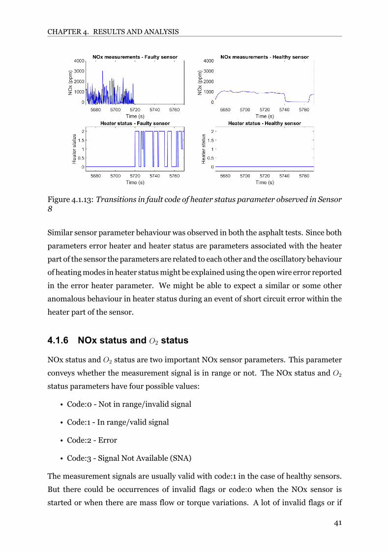
CHAPTER 4. RESULTS AND ANALYSIS
Figure 4.1.13: Transitions in fault code of heater status parameter observed in Sensor8
Similar sensor parameter behaviour was observed in both the asphalt tests. Since both
parameters error heater and heater status are parameters associated with the heater
part of the sensor the parameters are related to each other and the oscillatory behaviour
of heatingmodes in heater statusmight be explainedusing the openwire error reported
in the error heater parameter. We might be able to expect a similar or some other
anomalous behaviour in heater status during an event of short circuit error within the
heater part of the sensor.
4.1.6 NOx status and O2 status
NOx status and O2 status are two important NOx sensor parameters. This parameter
conveys whether the measurement signal is in range or not. The NOx status and O2
status parameters have four possible values:
• Code:0 - Not in range/invalid signal
• Code:1 - In range/valid signal
• Code:2 - Error
• Code:3 - Signal Not Available (SNA)
The measurement signals are usually valid with code:1 in the case of healthy sensors.
But there could be occurrences of invalid flags or code:0 when the NOx sensor is
started or when there are mass flow or torque variations. A lot of invalid flags or if
41

CHAPTER 4. RESULTS AND ANALYSIS
the measurement signal is completely invalid, it suggests that the sensor is completely
faulty and the measurements are not valid. An increase in invalid flags under normal
driving conditions suggests that the sensor is partially faulty and is approaching
failure. The variation or occurrence of invalid flags in NOx status and O2 status
varies from sensor to sensor depending upon the grade of the faultiness of the sensor.
These observations were made during the experiments and data analysis from the
measurement data from trucks. This can be seen in the upcoming sections.
In the case of the upstream NOx sensors, Sensors 2 and 8 show invalid signals
throughout the measurement. Sensors 1 and 3 show a mix of valid and invalid signals
in static and transient gas flow tests. Sensor 7 showed valid signals in static gas
flow tests, but a mix of valid and invalid signals during the transient gas flow tests.
Sensor 2 had oscillatory faults throughout the measurement in static and transient gas
flow tests which account for the invalid signals in NOx status and O2 status. Invalid
signals in NOx status and O2 status parameters along with their corresponding NOx
measurements and actual oxidation factor measurements observed in Sensor 2 are
shown in Figure 4.1.14.
Figure 4.1.14: Invalid signals in NOx status and O2 status parameters observed inSensor 2
Sensor 8 showed a combination of stuck and oscillatory faults and also the sensor was
expected to be completely broken during the asphalt tests. Invalid flags were set in
NOx status and O2 status due to these reasons. Also, when the sensor showed error
codes in Error heater, Error NOx, and Error O2 parameters, invalid flags were set in
NOx status and O2 status. Sensors 1 and 3 behaved similarly in static and transient
42
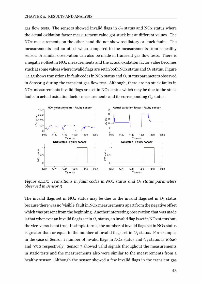
CHAPTER 4. RESULTS AND ANALYSIS
gas flow tests. The sensors showed invalid flags in O2 status and NOx status where
the actual oxidation factor measurement value got stuck but at different values. The
NOx measurements on the other hand did not show oscillatory or stuck faults. The
measurements had an offset when compared to the measurements from a healthy
sensor. A similar observation can also be made in transient gas flow tests. There is
a negative offset in NOx measurements and the actual oxidation factor value becomes
stuck at some valueswhere invalid flags are set in bothNOx status andO2 status. Figure
4.1.15 shows transitions in fault codes inNOx status andO2 status parameters observed
in Sensor 3 during the transient gas flow test. Although, there are no stuck faults in
NOx measurements invalid flags are set in NOx status which may be due to the stuck
faults in actual oxidation factor measurements and its corresponding O2 status.
Figure 4.1.15: Transitions in fault codes in NOx status and O2 status parametersobserved in Sensor 3
The invalid flags set in NOx status may be due to the invalid flags set in O2 status
because therewas no ’visible’ fault inNOxmeasurements apart from the negative offset
which was present from the beginning. Another interesting observation that wasmade
is thatwhenever an invalid flag is set inO2 status, an invalid flag is set inNOx status but,
the vice-versa is not true. In simple terms, the number of invalid flags set in NOx status
is greater than or equal to the number of invalid flags set in O2 status. For example,
in the case of Sensor 1 number of invalid flags in NOx status and O2 status is 10620
and 9710 respectively. Sensor 7 showed valid signals throughout the measurements
in static tests and the measurements also were similar to the measurements from a
healthy sensor. Although the sensor showed a few invalid flags in the transient gas
43

CHAPTER 4. RESULTS AND ANALYSIS
flow tests which may be due to torque or mass flow variations or due to very small
oscillations within the measurements.
Similar sensor behaviour is also seen in downstream NOx sensors. Sensors 4,6 and
9 show invalid flags in NOx status and O2 status throughout the measurement cycle
in both the tests suggesting the sensor is completely faulty. Sensors 5 and 10 show a
mix of valid and invalid signals in static and transient gas flow tests. Sensor 4 has an
oscillatory fault in both NOx concentration and actual oxidation factor measurements
which might be the reason for invalid flags in NOx status and O2 status. Sensor 5
shows stuck fault throughout the measurement along with error codes in Error NOx
and Error O2 parameters. Both of these factors account for the invalid flags in NOx
status and O2 status. Sensor 9 showed a combination of stuck and oscillatory fault
in NOx measurement and oscillatory faults in actual oxidation factor measurements.
These behaviour suggest the sensor is faulty andwould be the reason for the occurrence
of invalid flags.
Sensor 5 behaves similar to that of Sensors 1 and 3. In static tests, there seems to
be a negative offset in NOx measurement and there were oscillatory faults present in
actual oxidation factor measurements in the middle of the test and lasted until the end
where invalid flagswere set. In transient tests, the sensor showed invalid flags at points
where there were oscillations in actual oxidation factor measurements despite good
NOx measurements. Sensor 10 showed a positive offset in NOx measurements during
the static gas flow test and no invalid flags were set during the course. The sensor
showed a positive offset and some oscillatory behaviour in transient gas flow tests.
Invalid flags were set when there oscillatory faults and not at positive offsets. Figure
4.1.16 shows invalid flags being set in NOx status andO2 status at oscillatory faults and
not in positive offsets in Sensor 10. From these observations, it can be concluded that
invalid flags are set when there is an oscillatory or stuck faults and they are not set at
positive or negative offsets.
44

CHAPTER 4. RESULTS AND ANALYSIS
Figure 4.1.16: Invalid flags set in NOx status and O2 status parameters at oscillatoryfaults observed in Sensor 10
4.1.7 Temperature of heating element
The ’Temperature of heating element’ parameter or the ’Sensor at temperature’
indicates whether the heater element of the sensor is within the manufacturer’s
specified range for accurate measurements. This parameter also has four possible
values and they are:
• Code:0 - Not in range
• Code:1 - In range
• Code:2 - Error
• Code:3 - Signal Not Available (SNA)
The healthy sensors showed code:1 for the Temperature of heating element indicating
the measurement signal is in range. Similar to Heater status and Error heater
parameters, all sensors except Sensor 8 showed Temperature of heater element are
in-range for accurate measurements for all static and transient gas flow tests. It
also means that oscillatory faults or stuck faults to an extent is not dependent on
this particular heater parameter. The Temperature of heating element showed a
change in value during the asphalt tests as seen in Error heater and Heater status
parameters. The Temperature of heating element parameter showed code:0 when the
Error heater parameter reported an open wire error in the heater part of the sensor.
Code:0 suggests that the Temperature of heating element is not in range for accurate
45

CHAPTER 4. RESULTS AND ANALYSIS
measurements. Figure 4.1.17 shows the change in the status of the Temperature of
heating element parameter in Sensor 8 during the transient gas flow test. Conclusions
drawn from Heater status and Error heater can also be applied in this case as well
as the Temperature of heating element parameter is also related to the heater of the
sensor.
Figure 4.1.17: Transition in status of temperature of heating element parameterobserved in Sensor 8
4.1.8 Mass flow and torque variations
Along with the sensor parameters, engine parameters such as torque and mass flow
are also studied in search of precursors to sensor failure. Not many observations or
conclusionswere drawn through this study. Although itwas found that the short circuit
error that occurs in the error NOx and error O2 parameters usually occur when the
torque and mass flow is low. It was also observed that the shift in fault codes was not
instantaneous. A transition from ’no error’ state to an ’error’ state and vice-versa takes
sometime after the change in mass flow and torque occurs. Figure 4.1.18 shows the
setting of fault codes in error NOx and error O2 parameters with variations in torque
and mass flow observed in Sensor 6 during the transient gas flow test.
46

CHAPTER 4. RESULTS AND ANALYSIS
Figure 4.1.18: Setting of fault codes in error NOx and error O2 parameters withvariations in torque and mass flow observed in Sensor 8
4.2 Oscillatory fault monitor
In the previous sections, different types of failure modes were discussed. There
are monitors to determine a few of those mentioned faults like the stuck fault,
offset fault, etc. The oscillatory fault is one of the significant faults that have to be
monitored by the ECU. From the experiments and also from the truck data it can be
inferred that oscillatory fault is prominent in occurrence in NOx sensors. Therefore,
a monitoring system for oscillatory fault would be beneficial. This section discusses
about formulating a logic for the oscillatory fault monitor.
The logic for the oscillatory faultmonitormainly is based on the concept of the standard
deviation of the measurement signal. The ’Standard deviation’ theory was based on
the patent that detects oscillations in an erratic pressure sensor operation in a fuel
system of an IC engine [14] where the variance of the measurement signal was used
as the decision criteria. Mathematically, the standard deviation is the square root
of variance. Results from previous static gas flow tests also proved that standard
deviation could be used as a measure to differentiate between faulty sensors and
healthy sensors. Although, standard deviation alone is not enough to distinguish
the partially faulty sensors or sensors approaching failure with the healthy sensors.
Therefore, an additional parameter is also used along with the standard deviation
criteria to identify the partially faulty sensors and this would be beneficial in replacing
the sensors at the right time. The additional NOx sensor parameter that was used
47

CHAPTER 4. RESULTS AND ANALYSIS
in the logic was the ’NOx status’ parameter. The invalid flags that occur in the NOx
status were of prime interest. From the experiments and the data from trucks, it was
observed that the invalid flags in NOx status occurs at events of oscillations and spikes.
This correlation helps is defining additional criteria to determine the partially faulty
sensors.
4.2.1 Formulation of the logic for the monitor
The logic formulation initially started with taking the standard deviation of the
measurement signal for the first 30minutes after the sensor was started. The sampling
timewas varied to get the best results. Sampling times of 1 second and 10 seconds were
used for this study. The measurement data used for the study are from NOx sensors
used in trucks which were reported to have some faulty behaviour. Measurement data
from a NOx sensor without any fault was also used as a reference for the same. A code
was written in MATLAB to execute this logic and to understand the failure. The code
initially loads themeasurement data file intoMATLAB. The code filters out the SNAs as
the sensor is inactive when NOx status is in SNA and finds the monitor start time. The
monitor start time is calculated by adding 60 seconds from the point where the NOx
status changes its value from SNA (code:194). This addition of 60 seconds is to avoid
the initial ’spiky’ behaviour when the NOx sensor is started up. The NOx status shows
invalid signals (code:254) during this period of time and since it is not because of the
faultiness in the sensor, the measurement during this period is avoided. The monitor
end time is calculated by adding 30 minutes to the monitor start time. The standard
deviation of all the NOx measurement values is then calculated for a sampling time of
1 second and 10 seconds. The standard MATLAB function ’std()’ is used to find the
standard deviation of the measurement samples. The standard deviation values of the
measurement samples are stored in an array. The ’Cumulative Distributive Function
(CDF)’ of this array is taken and plotted. Then, the ’Inverse CDF (ICDF)’ is plotted to
understand how the standard deviation values vary from sensor to sensor and also to
differentiate between partially faulty sensors and completely faulty sensors.
In the case of the engine-out sensors, there are six curves in the graph that depicts
six sensors with different degrees of oscillatory fault. Figures 4.2.1 and 4.2.2 show the
inverse cumulative distributive functions of the engine-out sensor for sampling time 1
second and 10 seconds respectively.
48
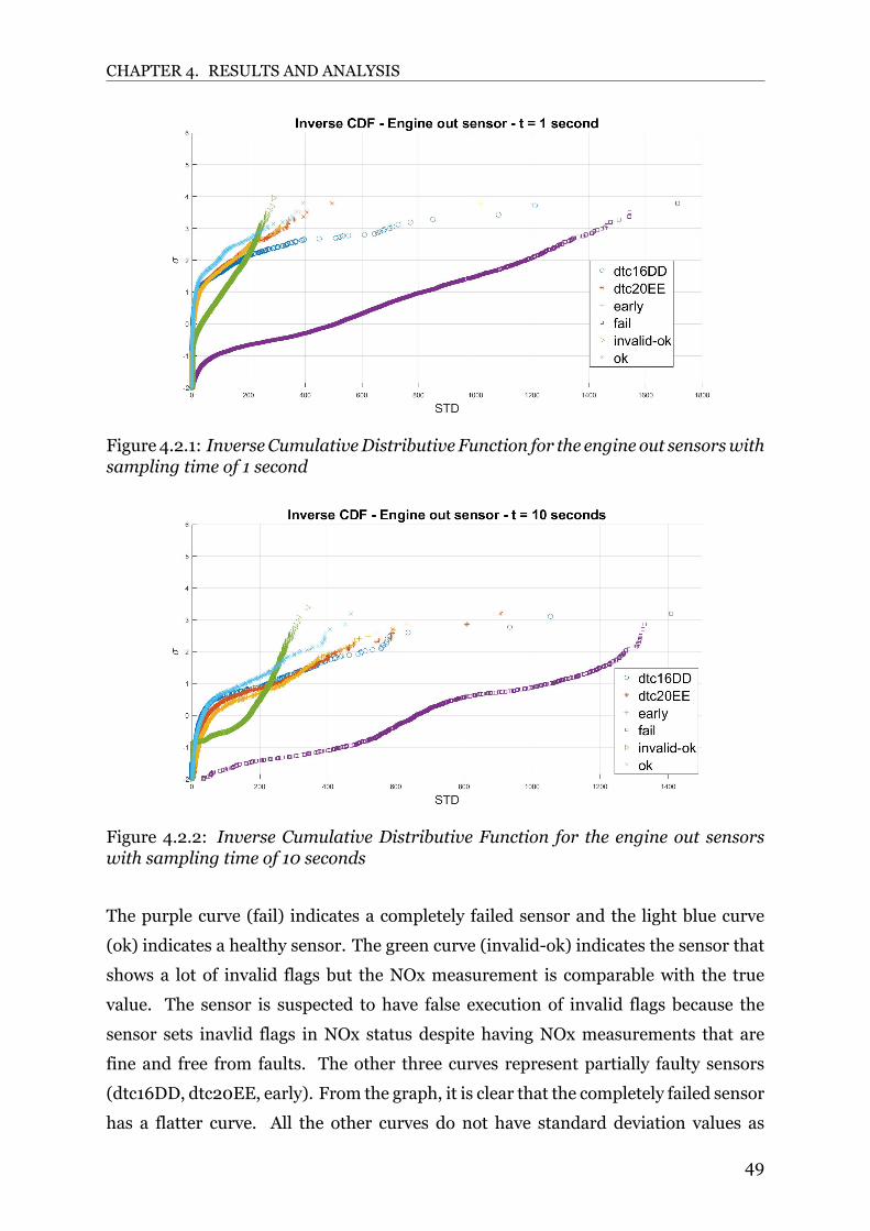
CHAPTER 4. RESULTS AND ANALYSIS
Figure 4.2.1: InverseCumulativeDistributive Function for the engine out sensorswithsampling time of 1 second
Figure 4.2.2: Inverse Cumulative Distributive Function for the engine out sensorswith sampling time of 10 seconds
The purple curve (fail) indicates a completely failed sensor and the light blue curve
(ok) indicates a healthy sensor. The green curve (invalid-ok) indicates the sensor that
shows a lot of invalid flags but the NOx measurement is comparable with the true
value. The sensor is suspected to have false execution of invalid flags because the
sensor sets inavlid flags in NOx status despite having NOx measurements that are
fine and free from faults. The other three curves represent partially faulty sensors
(dtc16DD, dtc20EE, early). From the graph, it is clear that the completely failed sensor
has a flatter curve. All the other curves do not have standard deviation values as
49
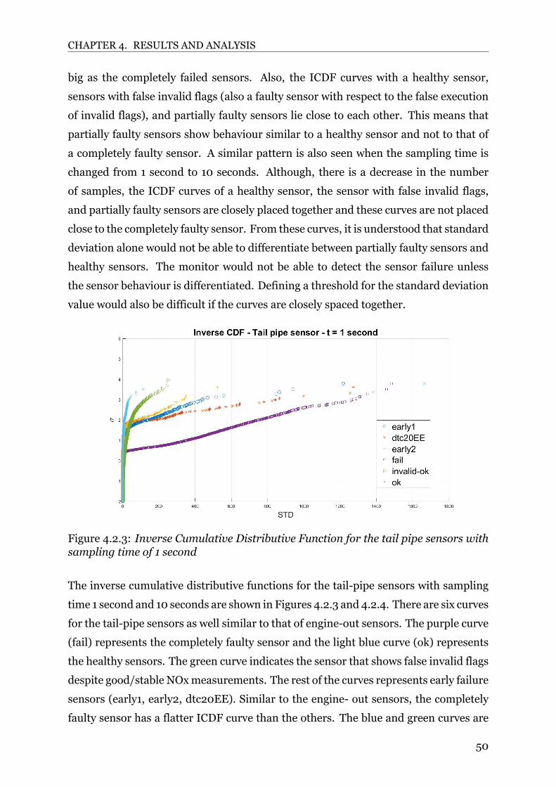
CHAPTER 4. RESULTS AND ANALYSIS
big as the completely failed sensors. Also, the ICDF curves with a healthy sensor,
sensors with false invalid flags (also a faulty sensor with respect to the false execution
of invalid flags), and partially faulty sensors lie close to each other. This means that
partially faulty sensors show behaviour similar to a healthy sensor and not to that of
a completely faulty sensor. A similar pattern is also seen when the sampling time is
changed from 1 second to 10 seconds. Although, there is a decrease in the number
of samples, the ICDF curves of a healthy sensor, the sensor with false invalid flags,
and partially faulty sensors are closely placed together and these curves are not placed
close to the completely faulty sensor. From these curves, it is understood that standard
deviation alone would not be able to differentiate between partially faulty sensors and
healthy sensors. The monitor would not be able to detect the sensor failure unless
the sensor behaviour is differentiated. Defining a threshold for the standard deviation
value would also be difficult if the curves are closely spaced together.
Figure 4.2.3: Inverse Cumulative Distributive Function for the tail pipe sensors withsampling time of 1 second
The inverse cumulative distributive functions for the tail-pipe sensors with sampling
time 1 second and 10 seconds are shown in Figures 4.2.3 and 4.2.4. There are six curves
for the tail-pipe sensors as well similar to that of engine-out sensors. The purple curve
(fail) represents the completely faulty sensor and the light blue curve (ok) represents
the healthy sensors. The green curve indicates the sensor that shows false invalid flags
despite good/stable NOxmeasurements. The rest of the curves represents early failure
sensors (early1, early2, dtc20EE). Similar to the engine- out sensors, the completely
faulty sensor has a flatter ICDF curve than the others. The blue and green curves are
50

CHAPTER 4. RESULTS AND ANALYSIS
Figure 4.2.4: Inverse Cumulative Distributive Function for the tail pipe sensors withsampling time of 10 seconds
closely spaced suggesting that the healthy sensor and the sensor with false invalid flags
give more or less similar measurements despite the comparatively huge number of
invalid flags shown by the sensor. The three early failure curves lie in between the
false invalid flag sensor and the completely faulty sensor but closer to the invalid flag
sensor curves or towards stable NOx measurements. All the curves except the purple
curve lie close to each other on changing sampling time from 1 second to 10 seconds.
This concludes that a shorter sampling timewould be better to separate healthy sensors
from the partially faulty sensors. The separation would still be difficult with only the
standard deviation criteria and it would also be difficult in defining the threshold.
Since the partially faulty NOx sensors could not be differentiated from the healthy
NOx sensors, an additional criterion is introduced. The code is modified by adding an
additional parameter check and it is added before calculating the standard deviation of
samples. The code checks for ’invalid flag’ inNOx status and if the condition is true, the
standard deviation of the measurement sample is calculated for a sampling time of 1
second and 10 seconds. All the other parts of the code remain the samewhen compared
to the initial study using standard deviation.
On considering the invalid flags along with standard deviation, better separation of
curveswas established. There is no light blue curve that corresponds to healthy sensors
as they did not show any invalid flags. The false invalid flag sensor had similar standard
deviation values when compared with the healthy sensor and it could be used as the
51

CHAPTER 4. RESULTS AND ANALYSIS
reference in this case. For sampling times 1 second and 10 seconds, the partially faulty
sensor curves lie closer to the completely faulty sensor and away from the false invalid
flag sensor. Better separation of the partially faulty sensors from the healthy/reference
sensor and the threshold could be defined with respect to the reference sensor.
The inverse cumulative distributive functions for the engine-out sensors with the
invalid flag criteria at sampling time 1 second and 10 seconds are shown in Figures
4.2.5 and 4.2.6.
Figure 4.2.5: Inverse Cumulative Distributive Function for the engine out sensorsconsidering the invalid flag criteria at a sampling time of 1 second
Figure 4.2.6: Inverse Cumulative Distributive Function for the engine out sensorsconsidering the invalid flag criteria at a sampling time of 10 seconds
52

CHAPTER 4. RESULTS AND ANALYSIS
Figures 4.2.7 and 4.2.8 show the inverse cumulative distributive functions of the tail-
pipe sensor for sampling time 1 second and 10 seconds respectively.
Figure 4.2.7: Inverse Cumulative Distributive Function for the tail pipe sensorsconsidering the invalid flag criteria at a sampling time of 1 second
Figure 4.2.8: Inverse Cumulative Distributive Function for the tail pipe sensorsconsidering the invalid flag criteria at a sampling time of 10 seconds
Much better separation of curves was established on including the invalid flag criteria
when compared to the engine-out sensors. The false invalid flag sensor is used as
the reference for stable NOx measurements in this case as well as there is no curve
representing a healthy sensor. The partially faulty sensors lie closer to the completely
faulty sensor and away from the reference sensor curve for sampling times of 1 second
53
CHAPTER 4. RESULTS AND ANALYSIS
and 10 seconds. The threshold value for standard deviation can also be defined with
respect to the reference sensor curve.
Combining the criteria of invalid flags in NOx status and standard deviation of these
’invalid’ NOx measurements would help detect the oscillatory faults in the NOx sensor
at earlier stages by themonitor. Itwouldhelp save the sensor fromcatastrophic failures
which might affect other components of the exhaust after-treatment system. The
additional criteria improve the detection capability of the monitor because, without
the criteria, the oscillations or spiky behaviour gets averaged out on considering the
completemeasurement cycle. On including the criteria, themonitor finds the standard
deviation at locations where invalid flags are found. Since invalid flags correspond to
oscillatory or spiky faults, the standard deviation value would be higher which could be
detected by themonitor. On the other hand, in case of a false invalid flag, the algorithm
would find the standard deviation to be low when compared to the threshold and it
would not be reported as a fault by the monitor. The difference in standard deviation
values on considering the invalid flag criteria with false invalid flag sensor and the
faulty sensors. The standard deviation values are low for the false invalid flag sensor
when compared to the faulty sensor thereby, a useful logic for the fault monitor.
For further analysis of the standard deviation values, themaximum standard deviation
values from the different sensors at every half an hour during a driving cycle are
analysed by plotting their inverse cumulative distributive functions. This helps in
defining a lower limit and an upper limit value of standard deviation value where the
threshold could be defined. This analysis is also done for sampling time 1 second and 10
seconds as well. It also helps in determining what category of errors(for eg: dtc20EE,
dtc20DD, etc) should be captured by the fault monitor.
Figures 4.2.9 and 4.2.10 shows inverse cumulative distributive functions of the
maximum standard values that occur in 30 minutes of a driving cycle for the engine-
out sensors at a sampling time of 1 second and 10 seconds respectively. In case of the
engine out sensors, it is observed that on changing the sampling time from 1 second to
10 seconds, themagnitude of standard deviation values decreases because of averaging
in a sample of a bigger size. The purple cross markers denote the upper limit and
any standard deviation value towards the right side of the curve is considered as a
standard deviation value from a completely faulty sensor whereas the curve with the
green triangle markers indicates a healthy sensor and any standard deviation value to
54

CHAPTER 4. RESULTS AND ANALYSIS
Figure 4.2.9: Maximum standard deviation values in 30 minutes for engine outsensors at sampling time of 1 second
Figure 4.2.10: Maximum standard deviation values in 30 minutes for engine outsensors at sampling time of 10 seconds
the left can be considered belongs to a non-faulty sensor. The band for the threshold
for standard deviation can be defined between 200 and 1400 approximately. Defining
a threshold value for the standard deviation between 200 and 1400 would enable the
monitor to detect faults from partially faulty sensors which would classify the sensors
further into faulty and non-faulty sensors.
Inverse cumulative distributive functions of the maximum standard deviation values
for the tail-pipe sensors at a sampling time of 1 second and 10 seconds are shown in
55

CHAPTER 4. RESULTS AND ANALYSIS
Figure 4.2.11: Maximum standard deviation values in 30minutes for tail pipe sensorsat sampling time of 1 second
Figure 4.2.12: Maximumstandard deviation values in 30minutes for tail pipe sensorsat sampling time of 10 seconds
Figures 4.2.11 and 4.2.12. The averaging pattern is also seen the in case of the tail-pipe
sensors on increasing the sampling time from 1 second to 10 seconds. The standard
deviation values are comparatively lower than in the case of the engine out sensors. The
completely faulty sensors, the purple cross markers lie close to a standard deviation
value of 1200 and the healthy sensors, the green triangle markers have a very small
value and lie close to 20. Therefore, all standard deviation values from a sensor less
than20 are considered to be non-faulty andmore than 1200 are considered to be faulty.
The threshold would be defined in between these two values.
56

CHAPTER 4. RESULTS AND ANALYSIS
Multiple approaches and standards could be used when defining the thresholds for
the engine-out and tail-pipe sensors. From the plots that were shown in the previous
sections the threshold values for the engine-out sensors would bemore than that of the
tail-pipe sensors because of the catalytic action that occurs before the tail-pipe sensor.
Although if we consider the fact both engine-out and tail-pipe sensors work the same,
defining a common threshold value would be a good choice especially when the after-
treatment system runs without the catalyst.
4.2.2 Coding the oscillatory fault monitor in ECU
The analysis done previously was performed using the standard MATLAB command
for standard deviation which is ’std()’. When transferring this logic into ECU for
implementing the monitor, there are limitations to storage and also in the usage of
these ’advanced’ mathematical functions. Therefore, the code has to be altered in such
a way that it can be easily implemented in the ECU considering all these limitations.
The code initially runs through different measurement data files first separating the
different driving cycles and running the monitor for the first 30 minutes of sensor
activity when the sensor is active. The code initially searches for the calculation
start time where their NOx status parameter changes its value from SNA to valid or
invalid. The sensor becomes active at this point of time and the calculation end time
is calculated by adding 30 minutes to the start time. This logic is executed using
loops within MATLAB. Instead of using the std() function, a different approach is
used to execute the logic in the ECU. The standard deviation for the sample can be
mathematically expressed as shown in Equation 4.1.
STD =
Σ(xi − µ)2
N − 1(4.1)
Where xi denotes each element in the dataset, µ indicates the mean of all values in the
dataset and N indicates the number of samples in the dataset. Furthermore, the mean
of the dataset i.e. µ can be expressed as shown in Equation 4.2.
µ =Σxi
N(4.2)
57

CHAPTER 4. RESULTS AND ANALYSIS
On expanding the numerator under the square root of Equation4.1, Equation 4.3 is
obtained.
Σ(xi − µ)2 = Σ(x2i + µ2 − 2µxi) (4.3)
Equation 4.4 can be further expanded into Equations 4.4 and 4.5.
Σ(xi − µ)2 = Σx2i + Σµ2 − Σ2µxi (4.4)
Σ(xi − µ)2 = Σx2i +Nµ2 − 2µΣxi (4.5)
On substituting Equation 4.2 in Equation 4.5, Equation 4.6 is obtained.
Σ(xi − µ)2 = Σx2i +
(Σxi)2
N− 2
(Σxi)2
N(4.6)
Equation 4.6 can be further simplified as shown in Equation 4.7.
Σ(xi − µ)2 =NΣx2
i − (Σxi)2
N(4.7)
On substituting Equation 4.7 in Equation 4.1, the simplified equation of standard
deviation is obtained as shown in Equation 4.8.
STD =
NΣx2
i − (Σxi)2
N(N − 1)(4.8)
Equation 4.8 is now simplified and mainly dependent on three variables N, Σx2i and
Σxi. On using this approach, three variables or residuals within the ECU storage
would be used to compute the standard deviation. For the execution of this logic,
three residuals should be allocated for N, Σxi and Σx2i . On each tick the NOx
measurement and the square of NOx measurement is added onto the Σxi and Σx2i
residuals respectively and when the sampling time is reached, the standard deviation
would be calculated. There are a few advantages to using this logic. Variable N would
be used to keep track of the sampling timeused. The first one ismemory saving because
there are only two variables used to calculate the standard deviation. Secondly, this
58

CHAPTER 4. RESULTS AND ANALYSIS
approach is independent of the sampling time. The standard deviation value would be
calculated at the end of the pre-defined sampling time. This logic can also be extended
by adding the ’invalid flag’ criteria as well. The additional condition is defined before
the storage of NOx measurement into residuals occurs. The condition checks for an
occurrence of an invalid flag in theNOx status parameter and the storage into residuals
and standard deviation calculation occur if the condition is true. This approach also
gives similar results to that of the standardMATLAB function ’std()’, thereby validating
the results of this approach. This approach has a limitation concerning the storage
capacity or data type of the residuals in the ECU. If the sampling time is increased,
there is a risk of an overflow of data from the residuals as the residuals are not capable
of handling data of large sizes.
4.2.3 Defining thresholds for the monitor
After the logic is set, the threshold definition is an important step that completes the
logical design of the monitor. ’Six sigma’ approach is used to define the thresholds
for the engine-out and tail-pipe sensors. Defining the thresholds for the oscillatory
fault monitor was one of the main reasons to plot the inverse cumulative distributive
function. The Y-axis of the inverse cumulative distributive function plots is scaled
between -2σ and 6σ. In order to find the threshold, a straight line is extrapolated from
the healthy sensor curve and the threshold standard deviation value would be where
the line meets the 6σ value.
Figure 4.2.13: Defining threshold standard deviation value for engine out sensors
59
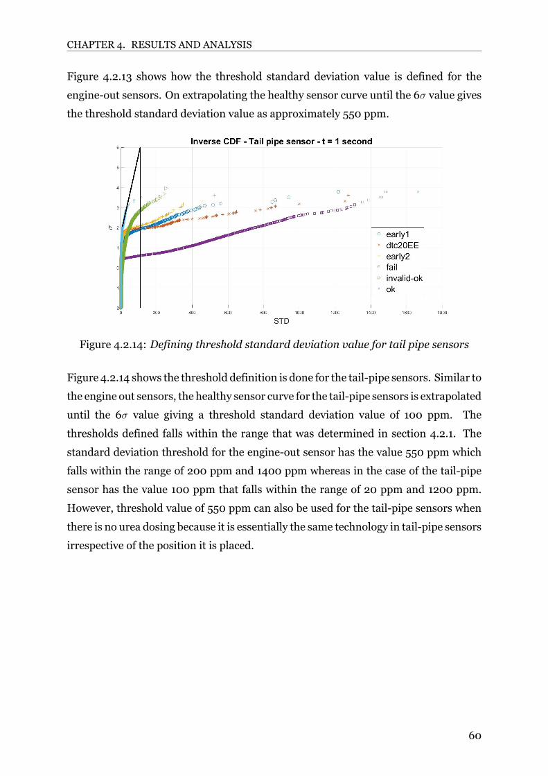
CHAPTER 4. RESULTS AND ANALYSIS
Figure 4.2.13 shows how the threshold standard deviation value is defined for the
engine-out sensors. On extrapolating the healthy sensor curve until the 6σ value gives
the threshold standard deviation value as approximately 550 ppm.
Figure 4.2.14: Defining threshold standard deviation value for tail pipe sensors
Figure 4.2.14 shows the threshold definition is done for the tail-pipe sensors. Similar to
the engine out sensors, the healthy sensor curve for the tail-pipe sensors is extrapolated
until the 6σ value giving a threshold standard deviation value of 100 ppm. The
thresholds defined falls within the range that was determined in section 4.2.1. The
standard deviation threshold for the engine-out sensor has the value 550 ppm which
falls within the range of 200 ppm and 1400 ppm whereas in the case of the tail-pipe
sensor has the value 100 ppm that falls within the range of 20 ppm and 1200 ppm.
However, threshold value of 550 ppm can also be used for the tail-pipe sensors when
there is no urea dosing because it is essentially the same technology in tail-pipe sensors
irrespective of the position it is placed.
60

Chapter 5
Conclusions
The thesis work mainly aimed at analysing the behaviour of NOx sensors towards
their end of life. This objective was further broken down into different research
questions that were answered during the course of the thesis work. These research
objectives were answered through literature study, experiments, data analysis, coding
inMATLAB, and drawing conclusions from all these researchmethods. The thesis also
aimed at providing a better understanding of NOx sensors in terms of its construction,
working, and failure modes.
5.1 Discussions
The thesis aimed at gaining a better understanding of NOx sensors especially towards
their end of life. Stuck, oscillations, offset, gain, spike and slow response are the major
faults that can be seen in NOx sensors. The definition of these faults along with their
possible causes are discussed in this thesis. The effects of ageing on NOx sensors
especially on NOx sensitivity is discussed as well as the reasons and factors affecting
the change in NOx sensitivity. These research questions are mainly answered through
the literature study that involved going through research papers and patents that gave
good insights into the previous work done in this area of study. This part also covered
logic or algorithms used in the diagnosis of sensors in general and also the diagnosis
of faulty NOx sensors. The logic behind monitors that encounters stuck, offset and
slow response in NOx measurements are studied to understand how the monitoring
systemworks and also to develop a base to develop the fault monitor for the oscillatory
faults.
61

CHAPTER 5. CONCLUSIONS
Static and transient gas flow tests were conducted to understand the behaviour of a
healthy and faulty sensor during these tests. Ten faulty NOx sensors were studied
during these experiments and eight NOx sensor parameters were analysed in search
of precursors to identify a faulty sensor. Relationships between different NOx sensor
parameters were found out during the experimental study. Error NOx and Error O2
parameters show the same fault code at the same time and invalid flags were reported
in NOx status andO2 status. The heater parameters Heater status and Temperature of
heating element status showed invalid signals on encountering a fault code in the Error
heater parameter. Although, it was found that the heater parameters are not related
to the Error NOx and Error O2 parameters. It is also advisable to have a fault monitor
over the actual oxidation factor measurements as well. It is because in some cases the
invalid flags set in NOx status is due to the invalid flags set in O2 status which might
be due to failure modes in the actual oxidation factor measurements.
The development of logic for the oscillatory fault monitor is one of the core parts of this
thesis work. It would be a very vital contribution to Scania on developing a monitor
for one of the most recurring faults in NOx sensors. The base idea for the logic is
monitoring the standard deviation of the measurement signal which is derived from
a pressure sensor based patent. However, the concept of standard deviation alone was
not effective in separating partially faulty sensors from a healthy sensor. Therefore,
the criteria was modified by the addition of an invalid check in the NOx status. This
modification helped in separating the partially faulty sensors from healthy sensors and
would contribute in predicting when the sensors approach failure. If a sensor reports a
false invalid flag despite a good/stable measurement, the monitor would not set a fault
code as the standard deviation would not be as high as in the case of a faulty sensor.
The logic was rewritten in such a way that it is supported by the ECU on using three
variables to calculate the standard deviation. This approach would save storage space
considerably and only basic mathematical operations are required to execute the logic.
Using the ’Six- sigma’ approach the threshold standard deviation values for the engine-
out and tail-pipe sensors are 550 ppm and 100 ppm respectively.
62

CHAPTER 5. CONCLUSIONS
5.2 Future Work
This thesis work is mainly based on gaining a better understanding of the NOx sensors
during its guaranteed lifetime and beyond this period as well. This understanding was
mainly done through parameter study. The work can be further extended by studying
additional parameters especially the ones related to the engine and how they affect the
NOx sensor parameters. The extended study can also include studying the NOx sensor
parameters under different transient and static gas flow tests to analyse the pointwhere
the NOx sensor shows erratic behaviour. Further testing data would help to converge
to the point of failure in NOx sensors and would help in predicting NOx sensor failure.
Experiments related to ageing of NOx sensors could also be performed to analyse the
change in NOx sensitivity in sensors and also to find out reasons for the same.
Coding the logic for the oscillatory faultmonitor in the ECUwould be the next step. The
logic fromMATLAB scripts has to be verified and transferred to the ECU. Performance
optimisation of the code would also be part of future work. The formulation of
additional criteria for the oscillatory fault monitor would also be beneficial in the fault
detection capability of the monitor. There are multiple ways to calculate standard
deviation and investigating these methods to arrive at the best method could also
be included in future work. Methods to overcome the limitation of data overflow
in residuals on increasing the sampling time would be beneficial in having a better
performing fault detection monitor.
63

Bibliography
[1] Brian Y. Mintah Jason K. Bloms, Purvarag Shah and Wackerlin, D. Diagnostic
systemandmethod for nitrogenoxide sensor. US9,261,481B2. Feb. 2016.URL:
https : / / https : / / patents . google . com / patent / US9261481B2 / en ? oq =
us9261481b2.
[2] Chou, C. C., Kuo, T. F., Tsai, T.H., Su, Y.H., Lu, J.H., andKu, Y. Y. “Model-based
Analysis of the Oscillatory NOx in Urea Selective Catalytic Reduction Systems”.
In: JSAE/SAE Small Engine Technologies Conference Exhibition. Society of
Automotive Engineers of Japan, Nov. 2017.
[3] Christian Stahl, Markus Bräunlein. NOx-Sensor poisoning. Application note.
Continental AG, 2015.
[4] Delebinski, Thaddaeus, Seebode, Joern, Henning, Lars, Pfeifer, Andreas,
Lindner, Adrian, Kolly, Claude, Vonarb, Regis, Philipp, Thorben, Bauer, Peter,
and Pietschmann, Karsten. “Calibration Process for SCR Only TIER4i Engine
for Construction Equipment”. In: SAE 2012 Commercial Vehicle Engineering
Congress. SAE International, Sept. 2012. DOI: https://doi.org/10.4271/
2012-01-1954. URL: https://doi.org/10.4271/2012-01-1954.
[5] Hesketh, Peter J. Chemical sensors 7 -and- MEMS/NEMS 7. The
Electrochemical Society, 2006.
[6] Jan, Sana, Lee, Young, Shin, Jungpil, and Koo, Insoo. “Sensor Fault
Classification Based on Support Vector Machine and Statistical Time-Domain
Features”. In: IEEE Access PP (May 2017). DOI: 10 . 1109 / ACCESS . 2017 .
2705644.
[7] Kato, Nobuhide, Kokune, Nobuyuki, Lemire, Bertrand, and Walde, Tim. “Long
Term Stable NOx Sensor with Integrated In-Connector Control Electronics”. In:
International Congress Exposition. SAE International,Mar. 1999. DOI: https:
64

BIBLIOGRAPHY
//doi.org/10.4271/1999-01-0202. URL: https://doi.org/10.4271/1999-
01-0202.
[8] Kawamoto, Yusukie, Todo, Yusuke, Shimokawa, Hironobu, Aoki, Keiichiro,
Kawai, Masashi, and Ide, Koji. “Development of High Accuracy NOx Sensor”.
In:WCX SAEWorld Congress Experience. SAE International, Apr. 2019. DOI:
https://doi.org/10.4271/2019-01-0749. URL: https://doi.org/10.4271/
2019-01-0749.
[9] Lindqvist, Peter. Understanding NOx sensors. Technical report 7059324.
Scania CV AB, 2019.
[10] Manchur, Travis B. and Checkel, M. David. “Time Resolution Effects on
Accuracy of Real-Time NOx Emissions Measurements”. In: SAE Transactions
114 (2005), pp. 259–275. ISSN: 0096736X, 25771531. URL: http://www.jstor.
org/stable/44720957.
[11] Orban, John E., Naber, Steven J., Sharp, Christopher A., Khair, Magdi K.,
and McGill, Ralph N. “Long-Term Aging of NOx Sensors in Heavy-Duty
Engine Exhaust”. In: Powertrain Fluid Systems Conference Exhibition. SAE
International, Oct. 2005. DOI: https://doi.org/10.4271/2005- 01- 3793.
URL: https://doi.org/10.4271/2005-01-3793.
[12] “Performance of Thick Film NOx Sensor on Diesel and Gasoline Engines”. In:
SAETransactions 106 (1997), pp. 1246–1253. ISSN: 0096736X, 25771531.URL:
http://www.jstor.org/stable/44730751.
[13] Pezzini, A., Canova, M., Onori, S., Rizzoni, G., and Soliman, A. “A Methodology
for Fault Diagnosis of Diesel NOx Aftertreatment Systems”. In: IFAC
Proceedings Volumes 42.8 (2009). 7th IFAC Symposium on Fault Detection,
Supervision and Safety of Technical Processes, pp. 911–916. ISSN: 1474-6670.
DOI: https://doi.org/10.3182/20090630-4-ES-2003.00150. URL: http:
//www.sciencedirect.com/science/article/pii/S1474667016358931.
[14] Rodney J. Hemmerlein, Stephen West. Apparatus and method for diagnosing
erratic pressure sensor operation in a fuel system of an internal combustion
engine. US 6,293,251 B1. Sept. 2001. URL: https://patents.google.com/
patent/US6293251B1/en.
65

BIBLIOGRAPHY
[15] Sai S.V. Rajagopalan, Sterling Heights; Yue-Yun Wang; Scott T Feldmann.
Offset and slow response diagnostic methods for NOx sensors in vehicle
exhaust treatment applications. US 8,930,121 B2. Jan. 2015. URL: https://
patents.google.com/patent/US6293251B1/en.
[16] Sasaki, Hisashi, Scholl, David, Parsons, Mike, Inagaki, Hiroshi, Shiotani,
Koji, Visser, Jaco, Zawacki, Garry, Kawai, TakeshiI, Teramoto, Satoshi, and
Kubinski, David. “Development of an Al2O3/ZrO2-Composite High-Accuracy
NOx Sensor”. In: SAE 2010 World Congress Exhibition. SAE International,
Apr. 2010. DOI: https://doi.org/10.4271/2010- 01- 0041. URL: https:
//doi.org/10.4271/2010-01-0041.
[17] Sasaki, Osamu Nakasone; Yuichi.Method of correcting output of NOx sensor.
US 7,875,165 B2. Jan. 2011. URL: https : / / patents . google . com / patent /
US7875165/un.
[18] Stefan Carstens, W. Addy Majewski. NOx Sensors. 2019. URL: https : / /
dieselnet.com/tech/sensors_nox.php.
[19] Svenningstorp, Charlotte Holmen;Henrik. Diagnosis of a cracked multi-
chamber solid-electrolyte gas sensor. US 2009/0321279 A1. Dec. 2009. URL:
https://patents.google.com/patent/US20090321279.
[20] Wagner, Dave.Why do I see negative readings onmy gasmonitor? 2019. URL:
https://www.indsci.com/blog-search/why-do-i-see-negative-readings-
on-my-gas-monitor/.
[21] Wellington, S.J., Atkinson, J.K., and Sion, R.P. “Sensor validation and fusion
using the Nadaraya-Watson statistical estimator”. In: Proceedings of the Fifth
International Conference on Information Fusion. Institution of Electronic and
Electrical Engineers, 2002, pp. 321–326. URL: https://eprints.soton.ac.
uk/22591/.
[22] Wieland, David.O2REG Self diagnosis. Technical report. Vitesco Technologies,
2019.
[23] Yang, Z., Yuan, X., Feng, Z., Suzuki, K., and Inoue, A. “A Fault Prediction
Approach for Process Plants using Fault Tree Analysis in Sensor Malfunction”.
In: 2006 International Conference on Mechatronics and Automation. June
2006, pp. 2415–2420. DOI: 10.1109/ICMA.2006.257729.
66

TRITA TRITA-ITM-EX 2020:532
www.kth.se