Environmental Modelling & Software 22 (2007) 1075e1088www.elsevier.com/locate/envsoft

Bayesian Networks and participatory modellingin water resource management

A. Castelletti*, R. Soncini-Sessa

Dipartimento di Elettronica e Informazione, Politecnico di Milano, Piazza L. da Vinci, 32, I-20133 Milano, Italy

Received 26 May 2006; accepted 8 June 2006

Available online 4 August 2006

Abstract

Bayesian Networks (Bns) are emerging as a valid approach for modelling and supporting decision making in the field of water resource man-agement. Based on the coupling of an interaction graph to a probabilistic model, they have the potential to improve participation and allowintegration with other models. The wide availability of ready-to-use software with which Bn models can be easily designed and implementedon a PC is further contributing to their spread. Although a number of papers are available in which the application of Bns to water-related prob-lems is investigated, the majority of these works use the Bn semantics to model the whole water system, and thus do not discuss their integrationwith other types of model. In this paper some pros and cons of adopting Bns for water resource planning and management are analyzed byframing their use within the context of a participatory and integrated planning procedure, and exploring how they can be integrated with othertypes of models.� 2006 Elsevier Ltd. All rights reserved.

Keywords: Bayesian Networks; Participatory modelling; Model integration; Water resources planning; Decision making

1. Introduction

The last decade has witnessed a growing interest in the ap-plication of graphical models, such as Bayesian Networks(Bns), in environmental and natural resource modelling. Thisnew trend is closely linked to the recognition that participationand uncertainty have a key role in integrated natural resourcemanagement and that there is a need for tools and methodol-ogies that make it easier to handle them.

In the environmental field, many authors have illustratedthe use of Bns starting with Varis (1995), who first generalizedand rearranged the mathematical framework provided by Pearl(1988) to fit the features of environmental resource systems.Applications range from ecological issues, such as fisheriesand related problems (Kuikka et al., 1999; Borsuk et al.,

* Corresponding author. Tel.: þ39 0223999632; fax: þ39 0223993412.

E-mail addresses: castelle@elet.polimi.it (A. Castelletti), soncini@elet.

polimi.it (R. Soncini-Sessa).

1364-8152/$ - see front matter � 2006 Elsevier Ltd. All rights reserved.

doi:10.1016/j.envsoft.2006.06.003

2002; Little et al., 2004), to the assessment of the effects ofclimate changes on crop production (Gu et al., 1996). In thewater resource context they have been used by Batchelorand Cain (1999) in irrigated and rainfed farming system mod-elling, by Varis and Kuikka (1997) to investigate the effect ofclimate change on surface waters and by Borsuk et al. (2001,2004) in studying the eutrophication of river estuaries. Theworks of Baran and Jantunen (2004) and Bromley et al.(2005) focus particularly on Bns as tools to support and im-prove participation.

The majority of these works use Bns to model the wholesystem being studied and thus do not discuss their integrationwith other types of models. In this paper the pros and cons ofadopting Bns for modelling either part of or the whole systemare analyzed, by framing the modelling activity within thecontext of a participatory and integrated planning procedure,and exploring the integration of Bns with other types ofmodels. We first consider the problem of decision making inthe field of water management in a general perspective, re-gardless of the modelling approach adopted. Then we will

1076 A. Castelletti, R. Soncini-Sessa / Environmental Modelling & Software 22 (2007) 1075e1088

go through the process of model construction and compareBns with other types of models, indicating the distinct charac-teristics of the Bn modelling approach.

In this paper only two uses of Bns are considered:

(1) for modelling, when they are used to describe the systembeing studied;

(2) for aiding decision making, when they include decisionand utility nodes, and are employed as a decision supportsystem (DSS).

A third use does exist, however: Bns can be used as a visu-alization tool to summarize simply the outcomes of more com-plex models. This tool may be part of a more complex DSS, orthe DSS itself, and in this case it can be traced back to the sec-ond use. However, in both cases the Bn will not be perceivedby Decision Makers and stakeholders as a model of the realsystem, since this role is conceptually and psychologicallyplayed by the underlying more complex model. Since the pa-per aims at analysing the role of Bns in participatory model-ling within a decision making process, it is apparent why itwill not focus on this third use. The paper is organized as fol-lows: the structure and alternative ways of using Bayesian Net-works are described in the first section. We evaluate theirusefulness by looking at the problem of decision making inwater resource planning in a general perspective; therefore,in the second section we introduce a Participatory and Inte-grated Planning (PIP) procedure, highlighting the key role ofparticipatory modelling. The third section is entirely devotedto this latter topic, and we go through the construction of a wa-ter system model, showing where participation comes in, howthe model is an aggregation of models which describes thesubsystems that constitute the water system, and how thetype of each one of these models can be selected from four dif-ferent types, one of which is the Bn. At that point we will haveall the necessary ingredients to focus on the role of Bn in watermanagement in the last section.

2. Bayesian Networks

Bayesian Networks (also known as Belief Networks orBayesian Belief Networks) are a powerful modelling tech-nique that replicates the essential features of plausible reason-ing (reasoning in conditions of uncertainty) in a consistent,efficient and mathematically sound way (Charniak, 1991).They were first developed by the artificial intelligence and ma-chine learning community (Pearl, 1986, 1988 and Jensen,1996) and successfully applied in the fields of medical diagno-sis (Andreassen et al., 1991 and Hamilton et al., 1994) andsystem maintenance and reliability (see for instance Hecker-man et al., 1995 and Yu et al., 1999). The mathematical back-ground of the approach is extensively covered by the above-mentioned references and by Neapolitan (1990), Lauritzen(1996), Pearl (2000) and Jensen (2001). Here, we only providesome essential notions about the structure and use of BayesianNetworks that are useful background knowledge for this paper

and this Special Issue on Bns in environmental managementand planning.

Bns provide a framework for graphically representing thelogical relationship between variables and for quantifyingthe strength of this relationship using conditional probabilities.Strictly speaking, Bns are directed acyclic graphs (DAGs), inwhich nodes represent random variables and the lack of arcsbetween two nodes represents the conditional probabilistic in-dependence of the two unlinked variables. This structure isnone other than a factorization of a joint probability distribu-tion (Lauritzen and Spiegelhalter, 1988). In practice, given twonodes A and B, a directional arc from A to B can be informallyregarded as indicating that A causes B, so A and B are usuallysaid to be parent and child, respectively. A node which doesnot have any parents is called a root node and represents aninput variable. A node without children is a leaf node and con-stitutes an output variable. Each node in the network is asso-ciated with a finite set of discrete,1 mutually exclusivevalues (in jargon ‘‘states’’), which represent all the possibleconditions of the node, and can be either quantitative or qual-itative. To distinguish this meaning of ‘‘state’’ from the oneused in System Theory (see Section 4.1.2), which we usewidely in the following, consistently we write it within quota-tion marks. For each node (except the root nodes) a conditionalprobability table (CPT) is specified, which lists the probabilitythat the variable associated to the node will assume a particularvalue, given the values taken on by the variables associated toits parents. Root nodes, not being caused, may only be associ-ated with unconditional probabilities.

To be more concrete, consider a very simple example con-cerning the water quality of a lake. Agricultural and civil prac-tices are responsible for the production of nitrogenous andphosphorous loads, respectively, which reach the lake throughsurface runoff and drainage flow. The result is an increase inthe trophic level that leads to an alteration of the water qualityof the lake. These causeeeffect relationships are described bythe network in Fig. 1. To simplify the example even further,we assume that each variable takes its value in a binary set,whose values are high and low.

Once the topology of the Bn is given, its structure is com-pletely defined, but, in order that it be used as a quantitativemodel, its CPTs have to be populated, i.e. filled in with prob-ability values. These may be derived from data, elicited fromexperts or (a case that is not of interest in this paper) obtainedby simulating other models. For example, the CPTs associatedto the trophic level and water quality nodes are depicted inFig. 2. Populating CPTs with numbers is conceptually thesame as calibrating any other model, though there is one im-portant difference: the conditional probability values in theCPT of each node are independent of the values in the CPTsof the others, and as a consequence, they can be locally up-dated. This property allows the use of the best information cur-rently available for each variable to populate the relevant CPT,

1 The set could also be continuous. However, since all the applications pre-

sented in this Special Issue refer to discrete sets, we will only consider those.

1077A. Castelletti, R. Soncini-Sessa / Environmental Modelling & Software 22 (2007) 1075e1088

to keep it updated as more data or knowledge becomes avail-able, and to operate interactively and on-line.

2.1. How Bns can be used

Once the a priori probability of a number of variables (of-ten the input variables) is specified, it is possible to calculatethe a priori probabilities (a priori beliefs) for all the nodes inthe network (belief propagation). This can be done by em-ploying basic probability calculus and Bayes’ Theorem (Pearl,1988; Peot and Shachter, 1991; Huang and Darwiche, 1996).The a priori belief is modified (making it an a posteriori be-lief) as new knowledge about the system is obtained, in theform of an observation of the values (evidence) assumed byone or more variables. Hence, the a priori beliefs aresubstituted by the observation values for these variables, and

L

L

L

LL

L

H

H

H

HH

H

phosph. load

nitr. load

trophiclev.

trophic lev.

waterquality

0.0

0.0

0.0

1.0

1.0

1.0 0.2

0.8

0.5

0.5

0.7

0.3

(a)

(b)

Fig. 2. The conditional probability tables of (a) the trophic level and (b) the

water quality; where L¼ low and H¼ high.

nitrogenousload

phosphorousload

trophiclevel

waterquality

Fig. 1. The Bn that represents the lake in the example.

the beliefs about the others are updated through beliefpropagation.

To return to the example, if the a priori beliefs of the nitrog-enous and phosphorous loads are those shown in Fig. 3a, thea priori beliefs about trophic level and water quality will bethe ones in Fig. 3b. On the contrary, if a high phosphorousload is observed, the a posteriori beliefs about trophic leveland water quality will be the ones shown in Fig. 3c.

Belief propagation is a computational tool for using Bnmodels in probabilistic inference, which is essentially the pur-pose for which Bns were conceived. They can be used either in‘‘bottom-up’’ reasoning to address diagnostic tasks or in ‘‘top-down’’ reasoning for descriptive/explanatory purposes. In thefirst case, the evidence of an effect is given and the most likelycause is inferred. In the second, the probability of an effect iscomputed once the evidence for one or more of its causes isprovided.

These two types of inference can be illustrated with ourlake example. Bottom-up reasoning occurs, for instance,when a low value of water quality is observed, and so the as-sociated probability is set to 1. There are three possible causesfor this evidence: the nitrogenous load is high; the phospho-rous load is high; both are high. To find out the most likelycause, the belief is propagated upwards from the outcome tocompute the a posteriori probability of each explanation (seeFig. 4a). Hence, the Bn model is used as a diagnostic tool.

Top-down reasoning is necessary if one wonders what thewater quality would be if both the pollutant loads were high.In this case the probability of the outcome (water quality)can be computed by propagating the evidence of the inputs(results are given in Fig. 4b). Here the network is used in anexplanatory way, which is definitively the most interesting ap-plication for planning and managing water resources. Note infact that, depending on whether the evidence of the inputs isdirectly observed or assumed a priori, the network can beused either to forecast the outcomes, as new evidence becomesavailable over time, or to perform a ‘‘what if’’ analysis by

L L

L L

L L

H H

H H

H H

phosph. load nitr. load

trophiclev.

trophiclev.

waterquality

waterquality

0.0

1.0

0.1

0.1

0.9

0.9

0.2

0.8

0.7

0.7

0.3

0.3

(a)

(b)

(c)

Fig. 3. (a) The a priori beliefs about phosphorous and nitrogenous loads; (b)

the consequent a priori belief about trophic level and water quality; (c) the

a posteriori belief about the same variables when there is evidence that the

phosphorous load is high; L¼ low and H¼ high.

1078 A. Castelletti, R. Soncini-Sessa / Environmental Modelling & Software 22 (2007) 1075e1088

updating the network with different sets of evidence and thenassessing their effects on the outcomes. In the latter case,when the input variables are uncertain and cannot be decided(i.e. they are uncontrollable), as they are in the example, eachset of evidence defines a different evaluation scenario.

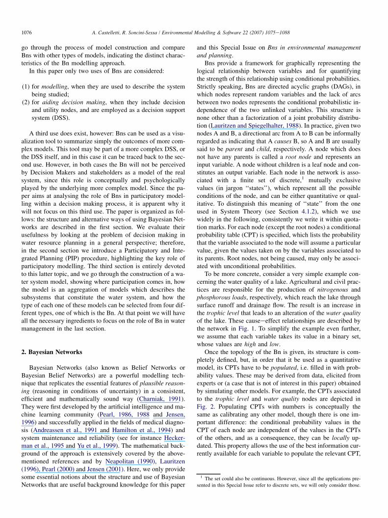
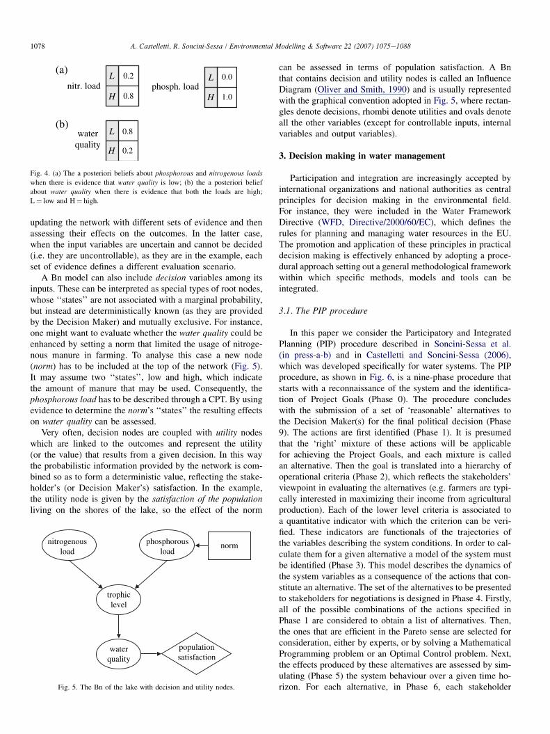
A Bn model can also include decision variables among itsinputs. These can be interpreted as special types of root nodes,whose ‘‘states’’ are not associated with a marginal probability,but instead are deterministically known (as they are providedby the Decision Maker) and mutually exclusive. For instance,one might want to evaluate whether the water quality could beenhanced by setting a norm that limited the usage of nitroge-nous manure in farming. To analyse this case a new node(norm) has to be included at the top of the network (Fig. 5).It may assume two ‘‘states’’, low and high, which indicatethe amount of manure that may be used. Consequently, thephosphorous load has to be described through a CPT. By usingevidence to determine the norm’s ‘‘states’’ the resulting effectson water quality can be assessed.

Very often, decision nodes are coupled with utility nodeswhich are linked to the outcomes and represent the utility(or the value) that results from a given decision. In this waythe probabilistic information provided by the network is com-bined so as to form a deterministic value, reflecting the stake-holder’s (or Decision Maker’s) satisfaction. In the example,the utility node is given by the satisfaction of the populationliving on the shores of the lake, so the effect of the norm

L

LL

H

HHphosph. loadnitr. load

waterquality

0.0

1.0

0.2

0.2

0.8

0.8

(a)

(b)

Fig. 4. (a) The a posteriori beliefs about phosphorous and nitrogenous loads

when there is evidence that water quality is low; (b) the a posteriori belief

about water quality when there is evidence that both the loads are high;

L¼ low and H¼ high.

nitrogenousload

phosphorousload

trophiclevel

waterquality

populationsatisfaction

norm

Fig. 5. The Bn of the lake with decision and utility nodes.

can be assessed in terms of population satisfaction. A Bnthat contains decision and utility nodes is called an InfluenceDiagram (Oliver and Smith, 1990) and is usually representedwith the graphical convention adopted in Fig. 5, where rectan-gles denote decisions, rhombi denote utilities and ovals denoteall the other variables (except for controllable inputs, internalvariables and output variables).

3. Decision making in water management

Participation and integration are increasingly accepted byinternational organizations and national authorities as centralprinciples for decision making in the environmental field.For instance, they were included in the Water FrameworkDirective (WFD, Directive/2000/60/EC), which defines therules for planning and managing water resources in the EU.The promotion and application of these principles in practicaldecision making is effectively enhanced by adopting a proce-dural approach setting out a general methodological frameworkwithin which specific methods, models and tools can beintegrated.

3.1. The PIP procedure

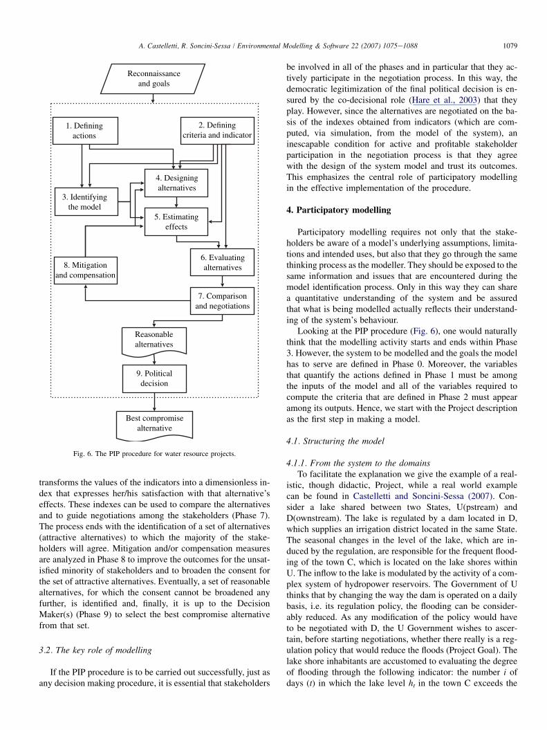
In this paper we consider the Participatory and IntegratedPlanning (PIP) procedure described in Soncini-Sessa et al.(in press-a-b) and in Castelletti and Soncini-Sessa (2006),which was developed specifically for water systems. The PIPprocedure, as shown in Fig. 6, is a nine-phase procedure thatstarts with a reconnaissance of the system and the identifica-tion of Project Goals (Phase 0). The procedure concludeswith the submission of a set of ‘reasonable’ alternatives tothe Decision Maker(s) for the final political decision (Phase9). The actions are first identified (Phase 1). It is presumedthat the ‘right’ mixture of these actions will be applicablefor achieving the Project Goals, and each mixture is calledan alternative. Then the goal is translated into a hierarchy ofoperational criteria (Phase 2), which reflects the stakeholders’viewpoint in evaluating the alternatives (e.g. farmers are typi-cally interested in maximizing their income from agriculturalproduction). Each of the lower level criteria is associated toa quantitative indicator with which the criterion can be veri-fied. These indicators are functionals of the trajectories ofthe variables describing the system conditions. In order to cal-culate them for a given alternative a model of the system mustbe identified (Phase 3). This model describes the dynamics ofthe system variables as a consequence of the actions that con-stitute an alternative. The set of the alternatives to be presentedto stakeholders for negotiations is designed in Phase 4. Firstly,all of the possible combinations of the actions specified inPhase 1 are considered to obtain a list of alternatives. Then,the ones that are efficient in the Pareto sense are selected forconsideration, either by experts, or by solving a MathematicalProgramming problem or an Optimal Control problem. Next,the effects produced by these alternatives are assessed by sim-ulating (Phase 5) the system behaviour over a given time ho-rizon. For each alternative, in Phase 6, each stakeholder

1079A. Castelletti, R. Soncini-Sessa / Environmental Modelling & Software 22 (2007) 1075e1088

transforms the values of the indicators into a dimensionless in-dex that expresses her/his satisfaction with that alternative’seffects. These indexes can be used to compare the alternativesand to guide negotiations among the stakeholders (Phase 7).The process ends with the identification of a set of alternatives(attractive alternatives) to which the majority of the stake-holders will agree. Mitigation and/or compensation measuresare analyzed in Phase 8 to improve the outcomes for the unsat-isfied minority of stakeholders and to broaden the consent forthe set of attractive alternatives. Eventually, a set of reasonablealternatives, for which the consent cannot be broadened anyfurther, is identified and, finally, it is up to the DecisionMaker(s) (Phase 9) to select the best compromise alternativefrom that set.

3.2. The key role of modelling

If the PIP procedure is to be carried out successfully, just asany decision making procedure, it is essential that stakeholders

Reconnaissanceand goals

1. Definingactions

2. Definingcriteria and indicator

4. Designingalternatives

3. Identifyingthe model

5. Estimatingeffects

6. Evaluatingalternatives

7. Comparisonand negotiations

8. Mitigationand compensation

9. Politicaldecision

Reasonablealternatives

Best compromisealternative

Fig. 6. The PIP procedure for water resource projects.

be involved in all of the phases and in particular that they ac-tively participate in the negotiation process. In this way, thedemocratic legitimization of the final political decision is en-sured by the co-decisional role (Hare et al., 2003) that theyplay. However, since the alternatives are negotiated on the ba-sis of the indexes obtained from indicators (which are com-puted, via simulation, from the model of the system), aninescapable condition for active and profitable stakeholderparticipation in the negotiation process is that they agreewith the design of the system model and trust its outcomes.This emphasizes the central role of participatory modellingin the effective implementation of the procedure.

4. Participatory modelling

Participatory modelling requires not only that the stake-holders be aware of a model’s underlying assumptions, limita-tions and intended uses, but also that they go through the samethinking process as the modeller. They should be exposed to thesame information and issues that are encountered during themodel identification process. Only in this way they can sharea quantitative understanding of the system and be assuredthat what is being modelled actually reflects their understand-ing of the system’s behaviour.

Looking at the PIP procedure (Fig. 6), one would naturallythink that the modelling activity starts and ends within Phase3. However, the system to be modelled and the goals the modelhas to serve are defined in Phase 0. Moreover, the variablesthat quantify the actions defined in Phase 1 must be amongthe inputs of the model and all of the variables required tocompute the criteria that are defined in Phase 2 must appearamong its outputs. Hence, we start with the Project descriptionas the first step in making a model.

4.1. Structuring the model

4.1.1. From the system to the domainsTo facilitate the explanation we give the example of a real-

istic, though didactic, Project, while a real world examplecan be found in Castelletti and Soncini-Sessa (2007). Con-sider a lake shared between two States, U(pstream) andD(ownstream). The lake is regulated by a dam located in D,which supplies an irrigation district located in the same State.The seasonal changes in the level of the lake, which are in-duced by the regulation, are responsible for the frequent flood-ing of the town C, which is located on the lake shores withinU. The inflow to the lake is modulated by the activity of a com-plex system of hydropower reservoirs. The Government of Uthinks that by changing the way the dam is operated on a dailybasis, i.e. its regulation policy, the flooding can be consider-ably reduced. As any modification of the policy would haveto be negotiated with D, the U Government wishes to ascer-tain, before starting negotiations, whether there really is a reg-ulation policy that would reduce the floods (Project Goal). Thelake shore inhabitants are accustomed to evaluating the degreeof flooding through the following indicator: the number i ofdays (t) in which the lake level ht in the town C exceeds the

1080 A. Castelletti, R. Soncini-Sessa / Environmental Modelling & Software 22 (2007) 1075e1088

flooding threshold h along a given horizon H (e.g. the last 20years), i.e.

i¼Xt˛H

gtðhtÞ ð1aÞ

where gt is a binary variable, defined as:

gtðhtÞ ¼�

1 if ht > h0 otherwise

ð1bÞ

The value i(A0) assumed by the indicator in correspondenceto the current regulation policy (alternative A0) is easy to ob-tain, since the historical trajectory of the lake levels was re-corded over the horizon H. To estimate the value i(Aj) thatthe indicator would assume in correspondence to any otherpolicy Aj, we need the trajectory of the lake levels that wouldhave resulted if the policy Aj had been used over H, and this, inturn, requires a model of the lake.

The exact framing of the Project goals, for which the model isbeing identified, is the starting point of any modelling exercise.The model identification then proceeds with the definition of theboundaries of the system being modelled and the choice of thelevel of detail that will be used in its description. Contributionsfrom stakeholders are very important here in order to complete,and in some cases to substitute, socio-economic and physicalanalyses of the system. In this example, the stakeholders mightsuggest that we enlarge the system to include both the upstreamcatchment, where melting snow, rainfall, and releases from hy-dropower reservoirs contribute to generating the inflow to thelake, and the downstream users, as the release decisions dependon their water demand. The lake can thus be considered as a com-ponent of a larger system. Generally, any water system can beseen as an aggregate of individual components. Each of thesecomponents serves a precise function and the decompositionof the system must be based on the identification of thesefunctions, which should be those that are most relevant to themodelling aims. The decomposition of the system into intercon-nected components and the individuation of the topology of theirinterconnections is the first step in formalizing a description ofreality. The result is not yet a model, just a logical organizationof the available knowledge (forethought, theories, information,data relating to the system) into sets of information (domains),each of which contains information about a component, regard-less of the type of model that will be adopted to describe it in thefuture. The domain is the first level of abstraction from reality,and does not require hypotheses about the mathematical rela-tionships among the variables. To form the domain we must sim-ply define the data which will be used and how they will berepresented. As a consequence, many different models can beassociated with the same domain.

A lake, for instance, is a complex system in which a numberof physical and chemical processes take place. The lake do-main is the set of all the information that pertains to it (inflow,release, level, chemical characteristics of the water, biota, al-gae, topography, the water authority, etc.), and includes the in-formation sources. On the other hand, the model of the lake isa simplified representation of reality that should reproduce the

characteristics that are relevant from the point of view of theproblem for which it is created. In our example the aim isthe reduction of flooding and so only the quantities that influ-ence the lake level e either directly or indirectly e are chosenfrom those available within the domain (i.e. inflow, release,level). These are the candidate variables for the model andhave to be carefully defined, by specifying how and whenthey are measured. For instance, the inflow to the lake couldbe considered either as the entire volume of water feedingthe lake or as the separate contribution of each individual trib-utary. These definitions must be communicated to the stake-holders, and understood and shared by them in such a waythat in successive phases their meaning is always clear.

When the components, the topology that maps how they areinterlinked, their domains, and finally the variables withineach of their domains have been well defined, one can proceedwith the construction of each component model.

4.1.2. From the domain to its model: the causal networkIn this step the causeeeffect relationships that link the vari-

ables must be identified. Once again the process develops bytrial and error, working with the stakeholders interested inthe component being described. When the system is notwell-known (for didactic purposes we will pretend that thelake is not) the best way to proceed is to construct, by trials,a causal network. This type of representation guarantees trans-parency in the construction of the model and helps in explain-ing its creation to the stakeholders, since it reflects an intuitivecognitive procedure which is inductive and which most peoplecan understand. When the stakeholders are not used to the for-mal language of graphics, the network can be constructedmanually, in a participatory way, by writing the names ofthe variables on pieces of paper and asking the stakeholdersto arrange them so that the causes precede the effects (Hodg-son, 1992). In our example the level2 ht þ 1 at the beginning ofday tþ 1 depends on the net volume of water that enters thelake during day t (the interval [t, tþ 1]), i.e. it depends onthe difference between the inflow at þ 1 and the release rt þ 1

in the same interval. The latter is produced by the release de-cision ut that is made by the regulator at time t, while the for-mer is the sum of the natural inflow 3t þ 1 and the volume wt

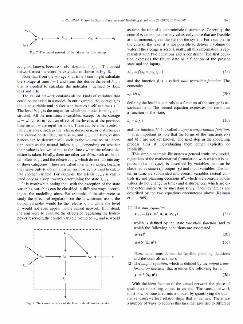
that will be released from the hydropower reservoirs on dayt. These causeeeffect relationships are represented with thecausal network in Fig. 7.

However, it is easy to see that this network does not yetconstitute a good description of reality. As a matter of fact,if the regulator of the lake were to decide to release a verylarge volume ut, the volume rt þ 1 that would actually be re-leased would differ according to whether the lake were fullor empty (if the lake were empty, rt þ 1 would be nil). There-fore, rt þ 1 is influenced not only by the decision ut, but also bythe volume st that is stored in the lake at the time of the deci-sion. Similarly, ht þ 1 is not completely defined once at þ 1 and

2 In the symbol of a variable the subscript denotes the time at which it

assumes a deterministic value.

1081A. Castelletti, R. Soncini-Sessa / Environmental Modelling & Software 22 (2007) 1075e1088

rt þ 1 are known, because it also depends on st þ 1. The causalnetwork must therefore be extended as shown in Fig. 8.

Note that from the storage st at time t one might calculatethe storage at time tþ 1 and from this derive the level ht þ 1

that is needed to calculate the indicator i defined by Eqs.(1a) and (1b).

The causal network contains all the kinds of variables thatcould be included in a model. In our example, the storage st isthe state variable and in fact it influences itself at time tþ 1.The level ht þ 1 is the output for which the model is being con-structed. All the non-caused variables, except for the storagest e which is, in fact, an effect of the level ht at the previoustime instant e are input variables. These can be either control-lable variables, such as the release decision ut, or disturbancesthat cannot be decided, such as wt and 3t þ 1. In turn, distur-bances can be deterministic, such as the volume wt, or uncer-tain, such as the natural inflow 3t þ 1, depending on whethertheir value is known or not at the time t when the release de-cision is taken. Finally, there are other variables, such as the to-tal inflow at þ 1 and the release rt þ 1, which do not fall into anyof these categories. These are called internal variables, becausethey serve only to obtain a partial result which is used to calcu-late another variable. For example, the release rt þ 1 is calcu-lated only as a step towards determining the state st þ 1.

It is worthwhile noting that, with the exception of the statevariables, variables can be classified in different ways accord-ing to the modelling aims. For example, if the aim were tostudy the effects of regulation on the downstream users, theoutput variables would be the release rt þ 1, while the levelht would not even appear in the causal network. If, instead,the aim were to evaluate the effects of regulating the hydro-power reservoir, the control variable would be wt, and ut would

rt+1ht+1at+1

wt

t+1

ut

ε

Fig. 7. The causal network of the lake at the first attempt.

rt+1

ht+1

st+1

s t

at+1

wt

t+1

ut

ε

Fig. 8. The causal network of the lake in the definitive version.

assume the role of a deterministic disturbance. Generally, thecontrol ut cannot assume any value, only those that are feasibleat that moment, given the state of the system. For example, inthe case of the lake, it is not possible to deliver a volume ofwater if the storage is zero. Usually, all this information is rep-resented with two equations and a constraint. The first equa-tion expresses the future state as a function of the presentstate and the inputs,

stþ1 ¼ f ðst;ut;wt; 3tþ1Þ ð2aÞ

and the function f($) is called state transition function. Theconstraint,

ut˛UðstÞ ð2bÞ

defining the feasible controls as a function of the storage is as-sociated to it. The second equation expresses the output asa function of the state,

ht ¼ hðstÞ ð2cÞ

and the function h($) is called output transformation function.It is important to note that the forms of the functions f($)

and h($) are not yet known. The next step in the modellingprocess aims at individuating them either explicitly orimplicitly.

This simple example illustrates a general truth: any model,regardless of the mathematical formulation with which it is ex-pressed (i.e. its type), is described by variables that can beclassified as state (xt), output (yt) and input variables. The lat-ter, in turn, are subdivided into control variables (actual con-trols ut, and planning decisions up, which are controls whosevalues do not change in time) and disturbances, which are ei-ther deterministic wt or uncertain 3t þ 1. Their dynamics aredescribed by the two equations encountered above (Kalmanet al., 1969):

(1) The state equation,

xtþ1 ¼ ftðxt;up;ut;wt;3tþ1Þ ð3aÞ

which is defined by the state transition function, and towhich the following conditions are associated.

up˛Up ð3bÞ

ut˛U tðxt;upÞ ð3cÞ

These conditions define the feasible planning decisionsand the controls at time t.

(2) The output equation, which is defined by the output trans-formation function, that assumes the following form:

yt ¼ htðxt;upÞ ð3dÞ

With the identification of the causal network the phase ofqualitative modelling comes to an end. The causal networkmust now be translated into a model, by quantifying the qual-itative causeeeffect relationships that it defines. There area number of ways to address this task that give rise to different

1082 A. Castelletti, R. Soncini-Sessa / Environmental Modelling & Software 22 (2007) 1075e1088

types of models. We present these different model types inSection 4.2, but before doing so, in the next section, we as-sume that the models of the components have already beenidentified, in order to show how the model of the whole systemis finally obtained.

4.1.3. From the component models to the system modelOnce a model of the form (3) has been specified for each

one of the components, the model of the whole water systemis obtained by interlinking all the component models on thebasis of a topology that expresses the interconnections be-tween the components. Technically, the output of a componentmodel becomes an input to the models of the components thatare logically downstream of it. Thus, the model of the wholewater system retains the form (3), since it is the union ofmodels of that same form.

4.2. Types of models

We return now to the different types of models that can beused to describe each individual component. They can be clas-sified according to the degree to which a priori information isinvolved in the quantification of the causeeeffect relationshipsthat appear in the causal network of the component. A prioriinformation comes in the form of theories provided by scien-tific disciplines or empirical knowledge obtained directly fromstakeholders and experts. When dealing with a lake, one hasinformation from the first category, since hydrology and hy-draulics provide a well-structured and established system ofknowledge to describe its behaviour. However, for didacticreasons, we will assume for a while that no a priori informa-tion is available.

4.2.1. Bayesian NetworksWhen there is no theory that the modeller can draw upon

for support when (s)he is quantitatively formulating the model,the only information (s)he may hope to obtain is statistical

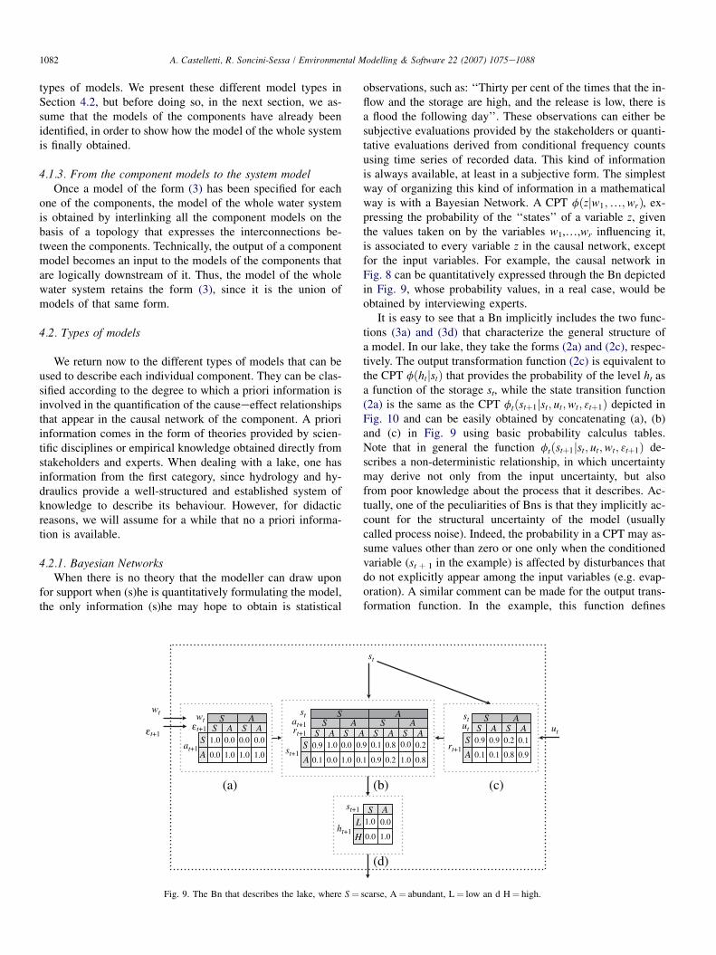
observations, such as: ‘‘Thirty per cent of the times that the in-flow and the storage are high, and the release is low, there isa flood the following day’’. These observations can either besubjective evaluations provided by the stakeholders or quanti-tative evaluations derived from conditional frequency countsusing time series of recorded data. This kind of informationis always available, at least in a subjective form. The simplestway of organizing this kind of information in a mathematicalway is with a Bayesian Network. A CPT fðzjw1;.;wrÞ, ex-pressing the probability of the ‘‘states’’ of a variable z, giventhe values taken on by the variables w1,.,wr influencing it,is associated to every variable z in the causal network, exceptfor the input variables. For example, the causal network inFig. 8 can be quantitatively expressed through the Bn depictedin Fig. 9, whose probability values, in a real case, would beobtained by interviewing experts.

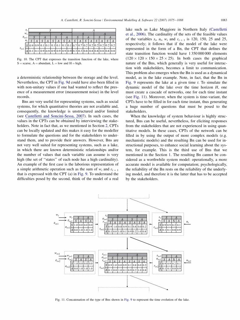
It is easy to see that a Bn implicitly includes the two func-tions (3a) and (3d) that characterize the general structure ofa model. In our lake, they take the forms (2a) and (2c), respec-tively. The output transformation function (2c) is equivalent tothe CPT fðhtjstÞ that provides the probability of the level ht asa function of the storage st, while the state transition function(2a) is the same as the CPT ftðstþ1jst; ut;wt; 3tþ1Þ depicted inFig. 10 and can be easily obtained by concatenating (a), (b)and (c) in Fig. 9 using basic probability calculus tables.Note that in general the function ftðstþ1jst; ut;wt; 3tþ1Þ de-scribes a non-deterministic relationship, in which uncertaintymay derive not only from the input uncertainty, but alsofrom poor knowledge about the process that it describes. Ac-tually, one of the peculiarities of Bns is that they implicitly ac-count for the structural uncertainty of the model (usuallycalled process noise). Indeed, the probability in a CPT may as-sume values other than zero or one only when the conditionedvariable (st þ 1 in the example) is affected by disturbances thatdo not explicitly appear among the input variables (e.g. evap-oration). A similar comment can be made for the output trans-formation function. In the example, this function defines

S

S

S

SSSS

SS

S

SS

SSS

A

A

A

A A

AAA

AAAA

AAA

SS A A

L

H

(a) (b) (c)

(d)

rt+1

rt+1

ht+1

st+1

st+1

stst

st

at+1

at+1wt

wt

t+1 utut

1.0

1.0

1.01.0

1.0

1.0

1.01.0

1.00.0

0.0 0.00.0

0.0

0.0

0.0

0.00.00.9

0.90.9

0.9

0.90.90.10.1

0.1

0.1

0.1

0.1

0.2

0.2

0.20.8

0.8

0.8

εt+1ε

Fig. 9. The Bn that describes the lake, where S¼ scarse, A¼ abundant, L¼ low an d H¼ high.

1083A. Castelletti, R. Soncini-Sessa / Environmental Modelling & Software 22 (2007) 1075e1088

a deterministic relationship between the storage and the level.Nevertheless, the CPT in Fig. 9d could have also been filled inwith non-unitary values if one had wanted to reflect the pres-ence of a measurement error (measurement noise) in the levelrecords.

Bns are very useful for representing systems, such as socialsystems, for which quantitative theories are not available and,consequently, the knowledge is unstructured and/or limited(see Castelletti and Soncini-Sessa, 2007). In such cases, thevalues in the CPTs can be obtained by interviewing the stake-holders. Note in fact that, as we mentioned in Section 2, CPTscan be locally updated and this makes it easy for the modellerto formulate the questions and for the stakeholders to under-stand them, and to provide their answers. However, Bns arenot very well suited for representing systems, such as a lake,in which there are known deterministic relationships and/orthe number of values that each variable can assume is veryhigh (the set of ‘‘states’’ of each node has a high cardinality).An example of the first case is the laborious representation ofa simple arithmetic operation such as the sum of wt and 3t þ 1

that is expressed with the CPT (a) in Fig. 9. To understand thedifficulties posed by the second, think of the model of a real

S

SSS

S

SSS

AA

AA

A

AAA

SSSSSSSS AAAAAAAA

st+1

stwt

t+1ut

0.90.90.90.90.90.9

0.90.9

0.1

0.10.10.10.10.10.1

0.1

0.20.20.20.20.20.2

0.80.80.80.80.80.8

0.70.7

0.30.3

ε

Fig. 10. The CPT that expresses the transition function of the lake, where

S¼ scarse, A¼ abundant, L¼ low and H¼ high.

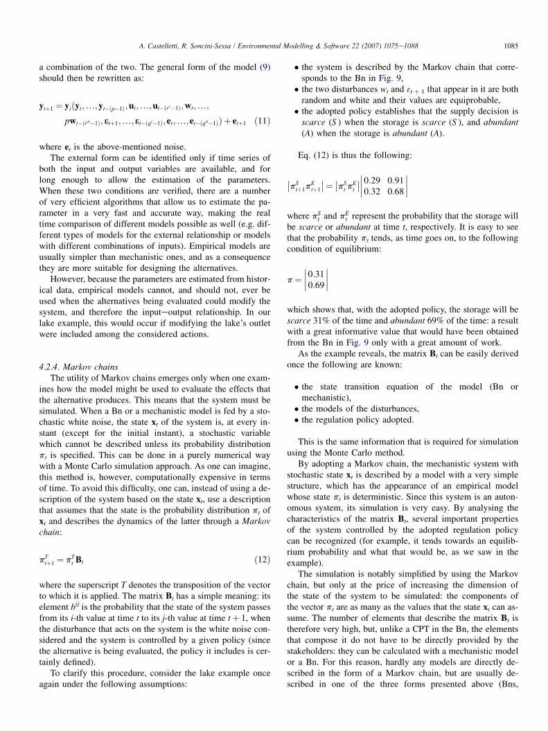
lake such as Lake Maggiore in Northern Italy (Castellettiet al., 2006). The cardinality of the sets of the feasible valuesof the variables st, ut, wt and 3t þ 1 is 120, 150, 25 and 25,respectively; it follows that if the model of the lake wererepresented in the form of a Bn, the CPT that defines thestate transition function would have 1 350 000 000 elements(120� 120� 150� 25� 25). In both cases the graphicalnature of the Bns, which generally is very useful for interac-tion with stakeholders, becomes a limit to communication.This problem also emerges when the Bn is used as a dynamicalmodel, as in the lake example. Note, in fact, that the Bn inFig. 9 represents the lake at a given time t. To simulate thedynamic model of the lake over the time horizon H, onemust create a cascade of networks, one for each time instant(see Fig. 11). Moreover, when the system is time-variant, theCPTs have to be filled in for each time instant, thus generatinga huge number of questions that must be posed to thestakeholders.

When the knowledge of system behaviour is highly struc-tured, Bns can be useful, nevertheless, for eliciting responsesfrom the stakeholders that are not experienced in using quan-titative models. In these cases, CPTs of the network can befilled in by using the output of more complex models (e.g.mechanistic models) and the resulting Bn can be used for in-structional purposes, to enhance social learning about the sys-tem, for example. This is the third use of Bns that wementioned in the Section 1. The resulting Bn cannot be con-sidered as a worthwhile system model: operationally, a moreaccurate model is available for computation; psychologically,the reliability of the Bn rests on the reliability of the underly-ing model, and therefore it is the latter that has to be acceptedby the stakeholders.

S

S

SSSS

SS

S

SS

SSS

S

S

SSSS

SS

S

SS

SSS

A

A

A A

AAA

AAAA

AAA

A

A

A A

AAA

AAAA

AAA

SS

SS

A A

A A

wt+1wt+1

st+2

rt+1

rt+1

st+1st+1

st+1

stst

at+1

at+1

wt wt

t+1

rt+2

rt+2

ut

ut+1

ut

at+2

at+2 ut+1

1.0

1.0

1.01.01.01.0

1.0

1.0

1.0

1.01.0 1.01.0

1.0

0.0

0.0 0.00.0

0.0

0.00.0

0.0

0.0 0.00.0

0.0

0.00.0

0.9

0.90.9

0.9

0.90.9

0.9

0.90.9

0.9

0.90.9

0.10.1

0.1

0.1

0.1

0.1

0.10.1

0.1

0.1

0.1

0.1

0.2

0.2

0.2

0.2

0.2

0.2

0.80.8

0.8

0.80.8

0.8

ε

t+2ε

t+1ε

t+2ε

Fig. 11. Concatenation of the type of Bns shown in Fig. 9 to represent the time evolution of the lake.

1084 A. Castelletti, R. Soncini-Sessa / Environmental Modelling & Software 22 (2007) 1075e1088

4.2.2. Mechanistic modelsWhen the knowledge about the system to be modelled is

well established, meaning that there are theories that explainits internal processes in a quantitative way, it is rational touse this knowledge to build a quantitative model that describesthe mechanisms operating within the system. Because of theway it is derived, this type of model is called a mechanisticmodel.

For example, in the case of the lake, physics teaches thata simple mass conservation equation describes the storagedynamics:

stþ1 ¼ st þwt þ 3tþ1� rtþ1 ð4ÞHydraulics provides the functional relationship (stageedis-

charge relation) linking the release rt þ 1 to the storage st whenthe dam is completely open,

rtþ1 ¼ NðstÞ ð5Þ

where N(st) generally assumes the form:

NðstÞ ¼ asbt ð6Þ

with a and b being two positive parameters. When the dam isin operation the release rt þ 1 also depends on the release de-cision ut: in general, rt þ 1 is equal to ut, whenever it is phys-ically possible and the legal constraints that must be obeyedpermit it. By saying s is the storage level above which thedam must be completely opened for precautionary reasons,the release rt þ 1 can be expressed as follows:

rtþ1 ¼

8<:

NðstÞ If st > s�NðstÞ if ut > NðstÞut otherwise

otherwiseð7Þ

Finally, the output transformation function linking thelevels and the storage can be derived once the lake’s bathym-etry and its shores’ altimetry are known.

ht ¼ hðstÞ ð8ÞNote that, once the disturbances wt and 3t þ 1 are known, the

above equations define a deterministic mechanistic model. Inorder for such a model to be equivalent to the Bn presentedin the previous section, the process and output noises (whichare implicitly included in the Bn) must somehow also be in-cluded in this model. These noises can be modelled as randomdisturbances or added to the corresponding equation. Outputnoise always implies a measurement error and is added toEq. (8); the process noise accounts for the simplifications in-troduced in modelling the state transition function (4), suchas the adoption of a stageedischarge relation to describe therelease as a function of the storage. Hydraulics teaches usthat this one-to-one relationship only holds in a permanentflow regime, when the storage does not vary in time, whilein practice the storage is not at all stationary. Mechanisticmodels are commonly used in water resource modelling andit is plausible that some of the stakeholders (e.g. hydropowermanagers) have had experience with, or are currently using,

a model of this type. This might suggest to the modeller thatit would be unwise to force them to move to a new type ofmodel, such as a Bn. However, when the construction of themodel has to be started from scratch, one should considerthat mechanistic models may contain a high number of param-eters that could make their identification not at all easy. Esti-mating so many parameters might require ad hoc and highlytime consuming techniques, and a wide variety of data, whichoften have to be collected through expensive measurementcampaigns.

4.2.3. Empirical modelsIn many cases the construction of a Bn, or of a mechanistic

model, proves to be an operation that is too costly to justifywith the aims of the model. A case in point is the catchmentmodel. The processes that take place within a catchment basinand transform precipitation into inflow are very complex, andthus Bns and mechanistic models that represent them areequally complex. However, when the alternative being evalu-ated does not directly involve the catchment, as in the lake ex-ample, the stakeholders may mainly be interested in a modelthat produces precise and reliable outputs (namely inflows)in response to given inputs, rather than an accurate and realis-tic description of the system’s internal mechanisms.

In cases such as this it can be a good idea to simply identifya model that describes the relationship between the input andthe output of the system (inputeoutput relationship), such asthe following:

ytþ1 ¼ ytðyt;.;yt�ðp�1Þ;ut;.;ut�ðr0�1Þ;

wt;.;wt�ðr00�1Þ;3tþ1;.;3t�ðq�1ÞÞ ð9Þ

which explains the output at time tþ 1 on the basis of thevalues that the input and output variables assumed in a suitablenumber of preceding time steps. Eq. (9) is called the externalform or representation, while in contrast, the pair of Eqs.(3a)e(3d) is called the internal form or representation.

For example, it is easy to see that in the case of the lakethere is a representation of the form:

htþ1 ¼ ytðht;ut;wt; 3tþ1Þ ð10Þ

that can be obtained by manipulating Eqs. (4), (7) and (8).Since one does not have any information about the structure

of the system, the external form has to be fixed a priori ina class of functions such that each one of its functions canbe identified by specifying a finite (and small) number of pa-rameters. Both linear (PARMAX model) and non-linear (e.g.Neural Network) relationships may be adopted, dependingon the component that is to be modelled and on the data avail-able. Note that this model is also deterministic, once the dis-turbances wt and 3t þ 1 are known. In order to transform itinto a stochastic model, a noise must be included in its expres-sion. However, because the internal structure of the model isnot available, it is not possible to distinguish between processand measurement noise. Therefore, the noise term will be

1085A. Castelletti, R. Soncini-Sessa / Environmental Modelling & Software 22 (2007) 1075e1088

a combination of the two. The general form of the model (9)should then be rewritten as:

ytþ1 ¼ ytðyt;.;yt�ðp�1Þ;ut;.;ut�ðr0�1Þ;wt;.;

pwt�ðr00�1Þ;3tþ1;.;3t�ðq0�1Þ; et;.;et�ðq00�1ÞÞ þ etþ1 ð11Þ

where et is the above-mentioned noise.The external form can be identified only if time series of

both the input and output variables are available, and forlong enough to allow the estimation of the parameters.When these two conditions are verified, there are a numberof very efficient algorithms that allow us to estimate the pa-rameter in a very fast and accurate way, making the realtime comparison of different models possible as well (e.g. dif-ferent types of models for the external relationship or modelswith different combinations of inputs). Empirical models areusually simpler than mechanistic ones, and as a consequencethey are more suitable for designing the alternatives.

However, because the parameters are estimated from histor-ical data, empirical models cannot, and should not, ever beused when the alternatives being evaluated could modify thesystem, and therefore the inputeoutput relationship. In ourlake example, this would occur if modifying the lake’s outletwere included among the considered actions.

4.2.4. Markov chainsThe utility of Markov chains emerges only when one exam-

ines how the model might be used to evaluate the effects thatthe alternative produces. This means that the system must besimulated. When a Bn or a mechanistic model is fed by a sto-chastic white noise, the state xt of the system is, at every in-stant (except for the initial instant), a stochastic variablewhich cannot be described unless its probability distributionpt is specified. This can be done in a purely numerical waywith a Monte Carlo simulation approach. As one can imagine,this method is, however, computationally expensive in termsof time. To avoid this difficulty, one can, instead of using a de-scription of the system based on the state xt, use a descriptionthat assumes that the state is the probability distribution pt ofxt and describes the dynamics of the latter through a Markovchain:

pTtþ1 ¼ pT

t Bt ð12Þ

where the superscript T denotes the transposition of the vectorto which it is applied. The matrix Bt has a simple meaning: itselement bij is the probability that the state of the system passesfrom its i-th value at time t to its j-th value at time tþ 1, whenthe disturbance that acts on the system is the white noise con-sidered and the system is controlled by a given policy (sincethe alternative is being evaluated, the policy it includes is cer-tainly defined).

To clarify this procedure, consider the lake example onceagain under the following assumptions:

� the system is described by the Markov chain that corre-sponds to the Bn in Fig. 9,� the two disturbances wt and 3t þ 1 that appear in it are both

random and white and their values are equiprobable,� the adopted policy establishes that the supply decision is

scarce (S ) when the storage is scarce (S ), and abundant(A) when the storage is abundant (A).

Eq. (12) is thus the following:

��pStþ1pE

tþ1

��¼ ��pSt pE

t

������0:29 0:910:32 0:68

����where pS

t and pEt represent the probability that the storage will

be scarce or abundant at time t, respectively. It is easy to seethat the probability pt tends, as time goes on, to the followingcondition of equilibrium:

p¼����0:310:69

����which shows that, with the adopted policy, the storage will bescarce 31% of the time and abundant 69% of the time: a resultwith a great informative value that would have been obtainedfrom the Bn in Fig. 9 only with a great amount of work.

As the example reveals, the matrix Bt can be easily derivedonce the following are known:

� the state transition equation of the model (Bn ormechanistic),� the models of the disturbances,� the regulation policy adopted.

This is the same information that is required for simulationusing the Monte Carlo method.

By adopting a Markov chain, the mechanistic system withstochastic state xt is described by a model with a very simplestructure, which has the appearance of an empirical modelwhose state pt is deterministic. Since this system is an auton-omous system, its simulation is very easy. By analysing thecharacteristics of the matrix Bt, several important propertiesof the system controlled by the adopted regulation policycan be recognized (for example, it tends towards an equilib-rium probability and what that would be, as we saw in theexample).

The simulation is notably simplified by using the Markovchain, but only at the price of increasing the dimension ofthe state of the system to be simulated: the components ofthe vector pt are as many as the values that the state xt can as-sume. The number of elements that describe the matrix Bt istherefore very high, but, unlike a CPT in the Bn, the elementsthat compose it do not have to be directly provided by thestakeholders: they can be calculated with a mechanistic modelor a Bn. For this reason, hardly any models are directly de-scribed in the form of a Markov chain, but are usually de-scribed in one of the three forms presented above (Bns,

1086 A. Castelletti, R. Soncini-Sessa / Environmental Modelling & Software 22 (2007) 1075e1088

mechanistic models, and empirical models) and then derivedfrom these.

5. The Bns’ role in water management

The previous sections focused on the key role of participa-tory modelling in water resource decision making and intro-duced four types of models, from which the modeller mustselect one to model each of the components of the water sys-tem being considered. Defining a few precise selection criteriais far from easy (see Jakeman et al., in press).

The social acceptance of a model, i.e. whether it is widelyand regularly applied in the same or similar contexts, mightundoubtedly make it more appealing and encourage its adop-tion, thus simplifying the work of the modeller. However,stakeholders might have experience with the use of a differentmodel and be reluctant to move from it. The model’s accuracy,in terms of quantitative performance indexes (e.g. explainedvariance), would be the selection criterion naturally adoptedby any modeller, but may be this would convince only thestakeholders that have strong technical expertise. In short,the selection has to be made by weighting social acceptanceand accuracy with other relevant issues, which in the authors’experience include:

1. Ease of identification. I order to foster stakeholder partic-ipation in the model building process it is of primal impor-tance that the model can be easily identified. This meansthat its parametric expression (i.e. the meta-model) mustbe legible and quickly understood by the stakeholders,and that empirical and/or mathematical methods (algo-rithms) to estimate its parameters must be available;

2. Integration potential. Water systems are generally com-posed of many components (catchment, reservoir, farms,fish, etc.), which may also be different in nature (physical,social, economic, ecological, etc.). Since the model of thewhole system is obtained by integrating the models of thecomponents, the latter must be such that integration istechnically feasible, without any loss of information or ac-curacy. Obviously, this condition may be satisfied byadopting the same type of model for all the components,but this restriction is unnecessarily rigid, as we will ex-plain further on.

3. Dynamics and parsimoniousness. Within a water system,dynamical components are not the exception but therule. These components must be described with dynamicalmodels and, when their management has to be considered,in the Phase of Designing Alternatives (Phase 4 in Fig. 6),an Optimal Control problem has to be solved. The compu-tational burden for its solution increases exponentiallywith the dimension (i.e. the number of state variables) ofthe whole water system model. Therefore, the type ofmodel selected should be able to capture concisely the es-sential elements of the complexity of the component, with-out being too mathematically abstruse, or losingtransparency and reliability for the stakeholders, owingto the many simplifications that are introduced. When

this is not possible, good practice would be first to builda model (evaluation model ) for estimating the effects inPhase 5 and then to obtain a parsimonious version (screen-ing model ) for designing the alternatives in Phase 4 (seethe example in (Chappell et al., 2001)).

If we now reconsider the features of Bns presented in Sec-tion 4.2.1 in the light of these issues, it is clear that Bns do notalways meet the above requirements. Consequently, forcingtheir use as a general modelling tool, with no regard for thefeatures of the individual component being modelled, may re-sult not only in poor performances, in terms of the accuracy ofthe system description, but also in the loss of a sense of owner-ship and of stakeholder confidence in the model. A Bn is atype of model that provides a simplified semantics that isuseful when knowledge about the system to be modelled ispoor or unstructured, and mainly empirical in nature. Whenthis is the case, Bns are definitively a well-suited tool for quan-tifying this a priori information. Their identification might besometimes facilitated by their structural properties, but it couldbecome critical when the number of values required to de-scribe the system variables correctly is fairly high. Moreover,Bns lose some of their potential when the system being con-sidered is dynamic, and includes recursive decisions (e.g. a reg-ulation policy). Therefore, we suggest that the use of Bns belimited to the components of a water system that have thesecharacteristics (unstructured knowledge, system variableswith a low number of values, an absence of dynamics), andthat other types of models be adopted for the other compo-nents. This is possible because Bns can easily be integratedwith other types of models, by expressing them in the generalform of Eq. (3), as shown in Fig. 10. For instance, in the lakeexample it is convenient to describe the upstream catchmentwith an empirical model, the lake with a mechanistic modeland the irrigation district with a Bn. The resulting model ofthe whole water system can therefore be used firstly to derivea Markov chain for designing the alternatives, and then to sim-ulate the system behaviour for estimating the effects of the al-ternatives. An example of integrating different types of modelscan be found in Castelletti and Soncini-Sessa (2007).

Finally, note that the use of Bns, in the form of InfluenceDiagrams, as Decision Support Systems (see Section 2.1), im-plies that all the components of the water system are describedas Bns. It should now be clear why this approach is weak: itcan only be applied when the system is non-dynamical or, ifdynamical, when it is stationary and the time horizon overwhich the alternatives are evaluated is not too long. However,there is another issue that contributes to this weakness: Bn-based DSSs can only be of value in supporting the decisionmaking procedure for comparing the alternatives, and not fornegotiations. If one is using a Bn (i.e. an Influence Diagram),alternatives can only be compared by running a sequence of‘‘what if’’ inquiries: the first alternative is specified by usingevidence to define a given combination of values of the deci-sion nodes, and the corresponding utilities are calculatedthrough belief propagation; a second alternative is then speci-fied by changing the evidence, and the process is repeated until

1087A. Castelletti, R. Soncini-Sessa / Environmental Modelling & Software 22 (2007) 1075e1088

all the alternatives to be compared have been evaluated. Ina negotiation process, however, after the evaluation of the firstalternative, each stakeholder should be able to say if (s)he issatisfied with it or not. This can be done with an Influence Di-agram as long as it contains as many utility nodes as there arestakeholder viewpoints. The critical point comes afterwardswhen, in order to broaden consent, one has to ascertain if thereis any alternative that increases the utilities of the unsatisfiedstakeholders without lowering the utilities of the satisfiedones. This type of search can be performed exhaustivelywith a sequence of ‘‘what if’’ inquiries only when the numberof alternatives is finite and very small. However, wheneverthere is a dynamical component in the system that is to be con-trolled (e.g. a reservoir), the number of alternatives is infinite.Besides, in a participatory process the number of actions thatcompose an alternative is generally significant and thus, due tocombinatory effects, the number of alternatives to be exam-ined is very high. Therefore, for negotiations, more complexand flexible tools are required, which can be based on Mathe-matical Programming or Optimal Control.

6. Conclusions

In the last decade Bns have captured the interest of the en-vironmental modelling community thanks to their friendly se-mantics and the graphical support they provide, which isuseful for interaction with stakeholders. The wide availabilityof ready-to-use software that allows Bn models to be designedand implemented on a PC has further contributed to theirspread. In this paper, we have illustrated the pros and consof their use in water resource planning and management, bycontextualizing their application within a Participatory and In-tegrated Planning procedure (PIP). We argued that Bns arewell suited for modelling system components for whichknowledge is poor or unstructured, and mainly empirical innature. Moreover, the value of their use as stand-alone Deci-sion Support Systems (DSSs) is limited, since it requiresthat all components be modelled with Bns, and since this ap-plication is definitively unsuitable when the reasonable alter-native has to be determined via negotiations.

Acknowledgement

The present work was carried out within the Project COFIN2004 Sistemi di supporto alle decisioni per la pianificazione egestione di serbatoi e laghi regolati [Contract2004132971_004] partly funded by the Italian Ministry ofEducation, University and Research.

References

Andreassen, S., Jensen, F., Olesen, K., 1991. Medical expert systems based on

causal probabilistic networks. International Journal of Biomedical Com-

puting 28, 1e30.

Baran, E., Jantunen, T., 2004. Stakeholder consultation for bayesian decision

support systems in environmental management. In: Proceedings of ECO-

MOD, September 15e16, Penang, Malaysia.

Batchelor, C., Cain, J., 1999. Application of belief networks to water manage-

ment studies. Agricultural Water Management 4 (1), 51e57.

Borsuk, M., Reichert, P., Burkhardt-Holm, P., 2002. A Bayesian belief network

for modelling brown trout (Salmo trutta) populations in Switzerland. In:

Rizzoli, A., Jakeman, A. (Eds.), Integrated Assessment and Decision Sup-

port, Proceedings of First Biennial meeting of IEMSS, June 24e27,

Lugano, CH.

Borsuk, M., Stow, C., Higdon, D., Reckhow, K., 2001. A Bayesian hierarchical

model to predict benthic oxygen demand from organic matter loading in

estuaries and coastal zones. Ecological Modelling 143, 165e181.

Borsuk, M., Stow, C., Reckhow, K., 2004. A Bayesian network of eutrophica-

tion models for synthesis, prediction, and uncertainty analysis. Ecological

Modelling 173, 219e239.

Bromley, J., Jackson, N., Clymer, O., Giacomello, A., Jensen, F., 2005. The

use of Hugin to develop Bayesian Network as an aid to integrated water

resource planning. Environmental Modelling & Software 20, 231e242.

Castelletti, A., Cellina, F., Soncini-Sessa, R., Weber, E., 2006. Comprehensive

testing and application of the pip procedure: the Verbano project case study.

Topics on System Analysis and Integrated Water Resource Management.

Elsevier, Amsterdam, NL, Ch. 12.

Castelletti, A., Soncini-Sessa, R., 2007. Coupling real time control and socio-

economic issues in participatory river basin planning. Environmental Mod-

elling & Software 22 (8), 1114e1128.

Castelletti, A., Soncini-Sessa, R., 2006. A procedural approach to strengthen-

ing integration and participation in water resource planning. Environmen-

tal Modelling & Software 12 (10), 1455e1470.

Chappell, N., McKenna, P., Bidin, K., Douglas, I., Walsh, R., 2001. Parsimo-

nious modelling of water and suspended-sediment flux from nested-catch-

ments affected by selective tropical forestry. Changes and Disturbance in

Tropical Rainforest in SoutheEast Asia. Imperial College Press, London,

UK, Ch, pp. 107e122.

Charniak, E., 1991. Bayesian networks without tears. AI Magazine 12 (4),

50e63.

Directive 2000/60/EC of the European Parliament and of the Council estab-

lishing a framework for Community action in the field of water policy.

Official Journal 327, 2000. European Commission, Brussels, B.

Gu, Y., McNicol, J., Peiris, D., Crawford, J., Marshall, B., Jefferies, R., 1996.

A belief network-based system for predicting future crop production. AI

Applications 10 (1), 13e24.

Hamilton, P., Anderson, N., Bartels, P., Thompson, D., 1994. Expert system

support using bayesian belief networks in the diagnosis of fine needle as-

piration biopsy specimens of the breast. Journal of Clinical Pathology 47,

329e336.

Hare, M., Letcher, R., Jakeman, A., 2003. Participatory modelling in natural

resource management: a comparison of four case studies. Integrated

Assessment 4 (2), 62e72.

Heckerman, D., Mamdani, A., Wellman, M., 1995. Real world applications of

Bayesian networks. Communication of the ACM 38 (3), 24e26.

Hodgson, A., 1992. Hexagons for systems thinking. European Journal of

Operational Research 59 (1), 220e230.

Huang, C., Darwiche, A., 1996. Inference in belief networks: a procedural

guide. International Journal of Approximate Reasoning 15 (3), 225e263.

Jakeman, A., Letcher, R., Norton, J. Ten interactive steps in model develop-

ment and evaluation. Environmental Modelling & Software, in press.

Jensen, F., 1996. An Introduction to Bayesian Networks. Springer-Verlag,

Heidelberg, D.

Jensen, F., 2001. Bayesian Networks and Decision Graphs. Springer-Verlag,

Heidelberg, D.

Kalman, R., Falb, P., Arbib, M., 1969. Topics in Mathematical System Theory.

McGraw-Hill, New York, NY.

Kuikka, S., Hilden, M., Gislason, H., Hansson, S., Sparholt, H., Varis, O.,

1999. Modeling environmentally driven uncertainties in Baltic cod (Gadus

morhua) management by Bayesian influence diagrams. Canadian Journal

of Fisheries and Aquatic Sciences 56, 629e641.

Lauritzen, S., 1996. Graphical Models. Clarendon Press, Oxford, UK.

Lauritzen, S., Spiegelhalter, D., 1988. Local computations with probabilities

on graphical structures and their application to expert systems (with

discussion). Journal of the Royal Statistical Society 50, 157e224.

1088 A. Castelletti, R. Soncini-Sessa / Environmental Modelling & Software 22 (2007) 1075e1088

Little, L., Kuikka, K., Punt, A., Pantus, F., Davies, C., Mapstone, B.,

2004. Information flow among fishing vessels modelled using

a Bayesian network. Environmental Modelling & Software 19,

27e34.

Neapolitan, R., 1990. Probabilistic Reasoning in Expert Systems: Theory and

Algorithms. John Wiley, New York, NY.

Oliver, R., Smith, J., 1990. Influence Diagrams, Belief Nets and Decision

Analysis. John Wiley, New York, NY.

Pearl, J., 1986. Fusion, propagation, and structuring in Belief Networks. Arti-

ficial Intelligence 29, 241e288.

Pearl, J., 1988. Probabilistic Reasoning in Intelligent Systems: Networks of

Plausible Inference. Morgan Kaufmann, San Mateo, CA.

Pearl, J., 2000. Causality: Models, Reasoning, and Inference. Cambridge

University Press, Cambridge, UK.

Peot, M., Shachter, R., 1991. Fusion and propagation with multiple observa-

tions in belief networks. Artificial Intelligence 48 (3), 299e318.

Soncini-Sessa, R., Castelletti, A., Weber, E. Integrated and participatory water

resources management. Theory. Elsevier, Amsterdam, NL, in press-a.

Soncini-Sessa, R., Cellina, F., Pianosi, F., Weber, E. Integrated and participatory

water resources management. Practice. Elsevier, Amsterdam, NL, in press-b.

Varis, O., 1995. Belief networks for modelling and assessment of environmen-

tal change. Environmetrics 6, 439e444.

Varis, O., Kuikka, S., 1997. Bayesian approach to expert judgment elicitation

with case studies on climatic change impact assessment on surface waters.

Climatic Change 37 (3), 539e563.

Yu, D., Nguyen, T., Haddawy, P., 1999. Bayesian network model for reliability

assessment of power systems. IEEE Transaction on Power Systems 14,

426e432.