Battle of the Water Calibration NetworksAvi Ostfeld1; Elad Salomons2; Lindell Ormsbee3; James G. Uber4; Christopher M. Bros5; Paul Kalungi6;

Richard Burd7; Boguslawa Zazula-Coetzee8; Teddy Belrain9; Doosun Kang10; Kevin Lansey11; Hailiang Shen12;Edward McBean13; Zheng Yi Wu14; Tom Walski15; Stefano Alvisi16; Marco Franchini17; Joshua P. Johnson18;

Santosh R. Ghimire19; Brian D. Barkdoll20; Tiit Koppel21; Anatoli Vassiljev22; Joong Hoon Kim23;Gunhui Chung24; Do Guen Yoo25; Kegong Diao26; Yuwen Zhou27; Ji Li28; Zilong Liu29; Kui Chang30;

Jinliang Gao31; Shaojian Qu32; Yixing Yuan33; T. Devi Prasad34; Daniele Laucelli35;Lydia S. Vamvakeridou Lyroudia36; Zoran Kapelan37; Dragan Savic38; Luigi Berardi39; Giuseppe Barbaro40;

Orazio Giustolisi41; Masoud Asadzadeh42; Bryan A. Tolson43; and Robert McKillop44

Abstract: Calibration is a process of comparing model results with field data and making the appropriate adjustments so that both resultsagree. Calibration methods can involve formal optimization methods or manual methods in which the modeler informally examines alter-native model parameters. The development of a calibration framework typically involves the following: (1) definition of the model variables,coefficients, and equations; (2) selection of an objective function to measure the quality of the calibration; (3) selection of the set of data to beused for the calibration process; and (4) selection of an optimization/manual scheme for altering the coefficient values in the direction ofreducing the objective function. Hydraulic calibration usually involves the modification of system demands, fine-tuning the roughness valuesof pipes, altering pump operation characteristics, and adjusting other model attributes that affect simulation results, in particular those thathave significant uncertainty associated with their values. From the previous steps, it is clear that model calibration is neither unique nor astraightforward technical task. The success of a calibration process depends on the modeler’s experience and intuition, as well as on themathematical model and procedures adopted for the calibration process. This paper provides a summary of the Battle of the Water CalibrationNetworks (BWCN), the goal of which was to objectively compare the solutions of different approaches to the calibration of water distributionsystems through application to a real water distribution system. Fourteen teams from academia, water utilities, and private consultantsparticipated. The BWCN outcomes were presented and assessed at the 12th Water Distribution Systems Analysis conference in Tucson,Arizona, in September 2010. This manuscript summarizes the BWCN exercise and suggests future research directions for the calibrationof water distribution systems. DOI: 10.1061/(ASCE)WR.1943-5452.0000191. © 2012 American Society of Civil Engineers.

CE Database object headings: Water distribution systems; Calibration; Hydraulic models; Optimization.

Author keywords: Water distribution systems; Calibration; Model; Optimization; Network.

1Faculty of Civil and Environmental Engineering, Technion—IsraelInstitute of Technology, Haifa 32000, Israel (corresponding author).E-mail: ostfeld@techunix.technion.ac.il

2OptiWater, 6 Amikam Israel St., Haifa 34385, Israel.3Univ. of Kentucky, College of Engineering, Dept. of Civil Engineering,

345F Raymond Building, Lexington, KY 40506-0281.4Dept. of Civil and Environmental Engineering, 765 Baldwin Hall,

PO Box 210071, Univ. of Cincinnati, Cincinnati, OH 45221-0071.5MWH UK, Dominion House, Temple Court, Birchwood, Warrington,

WA3 6GD, UK.6MWH UK, Dominion House, Temple Court, Birchwood, Warrington,

WA3 6GD, UK.7Veolia Water UK, Tamblin Way, Hatfield, Herts, AL10 9EZ, UK.8Veolia Water UK, Tamblin Way, Hatfield, Herts, AL10 9EZ, UK.9Veolia Water UK, Tamblin Way, Hatfield, Herts, AL10 9EZ, UK.10Dept. of Civil Engineering and Engineering Mechanics, Univ. of

Arizona, Tucson, AZ 85721.11Dept. of Civil Engineering and Engineering Mechanics, Univ. of

Arizona, Tucson, AZ 85721.Note. This manuscript was submitted on April 27, 2011; approved on

August 17, 2011; published online on August 19, 2011. Discussion periodopen until February 1, 2013; separate discussions must be submitted forindividual papers. This paper is part of the Journal of Water ResourcesPlanning andManagement, Vol. 138, No. 5, September 1, 2012. © ASCE,ISSN 0733-9496/2012/5-523-532/$25.00.

12School of Engineering, Univ. of Guelph, Guelph, ON, N1G 2W1,Canada.

13School of Engineering, Univ. of Guelph, Guelph, ON, N1G 2W1,Canada.

14Bentley Systems, Inc., 27 Siemon Company Dr., Suite 200W,Watertown, CT 06795.

15Bentley Systems, Inc., 27 Siemon Company Dr., Suite 200W,Watertown, CT 06795.

16Dept. of Engineering, Univ. of Ferrara, 44122 Ferrara, Italy.17Dept. of Engineering, Univ. of Ferrara, 44122 Ferrara, Italy.18Civil and Environmental Engineering Dept., Michigan Tech Univ.,

Houghton, MI 49931.19Driftmier Engineering Center, Univ. of Georgia, Athens, GA 30602.20Civil and Environmental Engineering Dept., Michigan Tech Univ.,

Houghton, MI 49931.21Dept. of Mechanics, Faculty of Civil Engineering, Tallinn Univ. of

Technology, Tallinn, Estonia.22Dept. of Mechanics, Faculty of Civil Engineering, Tallinn Univ. of

Technology, Tallinn, Estonia.23School of Civil, Environmental and Architectural Engineering, Korea

Univ., Seoul, Korea.24Water Resources Research Division, Korea Institute of Construction

Technology (KICT), Kyeonggi-do, Korea.25School of Civil, Environmental and Architectural Engineering, Korea

Univ., Seoul, Korea.

JOURNAL OF WATER RESOURCES PLANNING AND MANAGEMENT © ASCE / SEPTEMBER/OCTOBER 2012 / 523

J. Water Resour. Plann. Manage. 2012.138:523-532.

Dow

nloa

ded

from

asc

elib

rary

.org

by

Uni

vers

ity o

f E

xete

r on

09/

05/1

3. C

opyr

ight

ASC

E. F

or p

erso

nal u

se o

nly;

all

righ

ts r

eser

ved.

Introduction

The Battle of the Water Calibration Networks (BWCN) is thethird in a series of “Battle Competitions” dating back to the Battleof the Network Models (BNM) (Walski et al. 1987) and, morerecently, the Battle of the Water Sensor Networks (BWSN) (Ostfeldet al. 2008).

Calibration is a process of comparing model results with mea-sured data and making the appropriate adjustments so that both re-sults agree. It usually involves analyzing why the model does notagree with measured data and then making the adjustments. Thecalibration objective is typically set such that the calibration pro-cess adjusts the model coefficient values within their feasibledomains in the direction of reducing the calibration objective.Calibration methods can involve formal optimization methods ormanual methods in which the modeler informally examines alter-native model parameters (Ormsbee and Lingireddy 1997).

Water distribution system hydraulic models are based on equa-tions of mass continuity and energy. The calibration process “tunes”system demands, roughness of pipes, pump operation characteris-tics, and other model characteristics such that model predicted val-ues match reliable system data over a set of operational conditions.

Calibration, however, is far from being a technical problem asstated by Whittemore (2001): “Model efficacy depends heavily onexperience and, in this sense, can be described as an art. Whilemodel formulation is more related to science, calibration hasaspects more related to art. Good calibrations are more than curvefitting exercises that simply align model simulations with observedconstituent behavior.” This nature of calibration was also noted byWalski (1990) and Savic et al. (2009).

The BWCN called for teams/individuals from academia, con-sulting firms, and utilities to address the challenge of water distri-bution system calibration by proposing, and applying, a calibrationmethodology to a real water distribution system. The results ofthe BWCN were presented at a special session of the 12th WaterDistribution Systems Analysis (WDSA 2010) conference inTucson, Arizona, in September 2010.

The objective of this manuscript is to summarize the outcomeof the BWCN effort and to highlight future directions for researchon the calibration of water distribution systems. This paper de-scribes the following: (1) the BWCN rules and data, (2) a synopsisof the teams’ calibration approaches, (3) a comparison of the cal-ibration results, and (4) conclusions and future research directions.

Problem Description

The municipality of C-Town is in need of a calibrated hydraulicsimulation model for its water distribution system. To accomplish

this task, the city has performed fire-flow tests and gathered data,with due diligence given to accuracy.

Data

The following presents the available information for C-Townas provided to the participants. All data are incorporated inC-Town.inp (U.S. EPA 2002, version 2.00.12) and C-Town.xlsas supplemental files to this manuscript.

Network topology and mode of operation: The networktopology is extracted from the C-Town geographic informationsystem (GIS). The C-Town district meter areas (DMAs) andthe system mode of operation are described in Figs. 1 and 2,respectively.

Elevations, pipes, pump curves, control rules, control valves,tanks, and sources: Junction elevations are extracted from a recentfield survey or digital elevation model with an accuracy of �1 m;pipe diameters and lengths, as well as the original manufacturerpump curves, are taken from the municipality GIS and file archives;pipe type and age are provided as best estimates; control rulesare programmed into the programmable logic controllers (PLCs)of the pumping stations; records of the control rules are available;there are several pressure-reducing valves (PRVs) in the systemwhose settings are checked annually; all of the tanks are cylindrical,with tank diameters and minimum and maximum levels as reportedin the municipality master plan document; the network is suppliedfrom a constant headwater source; and, for some pipes, the lengthsare more than the Euclidian distance between the upstream anddownstream nodes as intermediate vertices were not availablethrough the GIS system.

Isolation valves: It may be assumed that every pipe in thenetwork has an isolation valve. Unless explicitly stated, all valvesmay be assumed to be fully open. Construction activity was on-going in DMA2 (Fig. 1) during the calibration tests, which requiredisolating portions of the system. It is entirely possible that one ormore valves in this part of the system may not have been fully re-opened following the upgrades. Fire-flow data were collected afterthe upgrades.

Demands and supervisory control and data acquisition(SCADA): Monthly water demands taken from billing recordsare given at each junction; hourly tank levels and pumping stationflows are available for a period of 168 h (1 week).

Fire-flow tests: Fire-flow tests were conducted at each of theDMAs separately during the evening. It can be assumed that thebasic system demands (excluding the observed hydrant demands)at the time of the fire-flow tests approximately correspond tothe demands during hour 1 of the provided 1-week SCADA timeseries.

26College of Architecture and Civil Engineering, Beijing Univ. ofTechnology, Beijing, China.

27College of Architecture and Civil Engineering, Beijing Univ. ofTechnology, Beijing, China.

28College of Architecture and Civil Engineering, Beijing Univ. of Tech-nology, Beijing, China.

29College of Architecture and Civil Engineering, Beijing Univ. ofTechnology, Beijing, China.

30Harbin Institute of Technology, Harbin, Hei Longjiang, China.31Harbin Institute of Technology, Harbin, Hei Longjiang, China.32Harbin Institute of Technology, Harbin, Hei Longjiang, China.33Harbin Institute of Technology, Harbin, Hei Longjiang, China.34School of Computing, Science and Engineering, Univ. of Salford,

Salford, Greater Manchester, UK.35 Technical Univ. of Bari, Dept. of Civil and Environmental Engineer-

ing, Bari, Italy.

36Univ. of Exeter, Centre for Water Systems, Exeter, UK.37Univ. of Exeter, Centre for Water Systems, Exeter, UK.38Univ. of Exeter, Centre for Water Systems, Exeter,

UK.39Technical Univ. of Bari, Dept. of Civil and Environmental Engineer-

ing, Bari, Italy.40“Mediterranea” Univ. of Reggio Calabria, Faculty of Engineering,

Reggio Calabria, Italy.41Technical Univ. of Bari, Dept. of Civil and Environmental Engineer-

ing, Bari, Italy.42Dept. of Civil and Environmental Engineering, Univ. of Waterloo,

Waterloo, ON, Canada.43Dept. of Civil and Environmental Engineering, Univ. of Waterloo,

Waterloo, ON, Canada.44Dept. of Civil and Environmental Engineering, Univ. of Waterloo,

Waterloo, ON, Canada.

524 / JOURNAL OF WATER RESOURCES PLANNING AND MANAGEMENT © ASCE / SEPTEMBER/OCTOBER 2012

J. Water Resour. Plann. Manage. 2012.138:523-532.

Dow

nloa

ded

from

asc

elib

rary

.org

by

Uni

vers

ity o

f E

xete

r on

09/

05/1

3. C

opyr

ight

ASC

E. F

or p

erso

nal u

se o

nly;

all

righ

ts r

eser

ved.

Assessment

Participants were required to submit an EPANET (U.S. EPA 2002)input file with their calibrated system for the 168 h corresponding

to the times recorded in the SCADA data file. The BWCN rulesprovided a variety of possible measures for calibration assessment:1. Maximum sum of squared relative errors (SSRE) and standard

deviation errors for the estimated pipe roughness values, node

Fig. 1. C-Town layout

Fig. 2. C-Town system operation mode: the system is fed from a large seasonal reservoir (R1); the water is pumped through pumping station S1 to thelower tanks (T1 and T2); flow to T2 is controlled by a valve (V2), which is operated according to T2 levels; two pumping stations (S2 and S3) drawwater from T2 to two higher tanks (T3 and T4); the two other stations (S4 and S5) pump water from T1 to T5, T6, and T7

JOURNAL OF WATER RESOURCES PLANNING AND MANAGEMENT © ASCE / SEPTEMBER/OCTOBER 2012 / 525

J. Water Resour. Plann. Manage. 2012.138:523-532.

Dow

nloa

ded

from

asc

elib

rary

.org

by

Uni

vers

ity o

f E

xete

r on

09/

05/1

3. C

opyr

ight

ASC

E. F

or p

erso

nal u

se o

nly;

all

righ

ts r

eser

ved.

demands, node pressures, fire-flow pressure tests, tank levels,pipe flows, and pumping station flow rates.

2. Ability of the calibrated model to successfully predict the re-sultant pressures and flows associated with an independentlyapplied demand pattern and operating conditions.

3. Ability of the calibrated model to successfully predict theresultant pressures and flows associated with random failurescenarios.

Contributions

Fourteen teams participated in the BWCN. This section gives abrief description of each team’s calibration approach.• Bros and Kalungi (2010) and Burd et al. (2010) adopted anengineering judgment trial-and-error approach.

• Kang and Lansey (2010) used the weighted least squares (WLS)method based on the Jacobian matrix, which provides analyticalexpressions for the sensitivities of the measurements to inputparameters. The primary benefit of WLS is computation speedcompared with random-sampling optimization approaches, whichwould be critical especially for real-time demand estimation.

• Shen and McBean (2010) linked a genetic algorithm with MonteCarlo simulations. The Monte Carlo simulations identifiedparameters to feed the calibration process, and the genetic algo-rithm minimized the discrepancy between observed and simu-lated data.

• Wu and Walski (2010) combined engineering judgment withoptimization tools in an overall progressive approach, whichfirst utilized the fire-flow test data to identify roughness, pumpcurves, and partly closed valves; then used SCADA data to backout demand patterns for each DMA; and finally made adjust-ments based on the entire system. They relied heavily on visua-lization tools and experience to identify problems and evaluatesolutions.

• Alvisi and Franchini (2010) combined an automatic heuristicoptimization process based on the SCE-UA (Shuffled ComplexEvolution–University of Arizona; Duan et al. 1992), manualrefinement, and the Monte Carlo–Latin hypercube approach(McKay et al. 1979),with the latter identifying themost influentialinput parameters (e.g., pipe roughness values) on the measuredoutput pressures, pipe flows, and tank water levels.

• Johnson et al. (2010) presented a flow-sequential sector-specificlumped algorithm (FSL) for calibrating the pipe roughnessvalues and user demands.

• Koppel and Vassiljev (2010) utilized the Levenberg-Marquardtalgorithm (LMA) (Levenberg 1944; Marquardt 1963) with prop-er parameter domain adjustments for partial derivative computa-tions (Koppel and Vassiljev 2009).

• Kim et al. (2010) used the metaheuristic harmony search (HS)(Geem et al. 2001), which is based on imitating a musicalprocess of searching for the best state of harmony.

• Diao et al. (2010) introduced a heuristic methodology coupledwith engineering judgment based on identifying dominantscenarios whose influence on the hydraulic system performanceis substantial.

• Chang et al. (2010) adopted a two-stage genetic algorithm(Goldberg 1989) process in which the nodal demands were firstcalibrated, followed by the pipe resistance coefficients.

• Prasad (2010) developed an artificial immune heuristicpopulation-based algorithm entitled clonal selection algorithm(CLONALG), which is based on evolving a population ofcandidate solutions using a clonal selection principle.

• Laucelli et al. (2010) implemented preliminary topologicalanalysis of the network to spatially decompose and simplifythe C-Town model. This stage reduced the model size by ap-proximately 50%, leading to substantial computational savings(without compromising mass and energy balance equations) andenabling easier analysis of the results. The BWCN problem wasthen solved using a multiobjective optimization approach withthree objectives targeting the minimization of different typesof absolute relative error measures. The parsimony of the cali-bration procedure is noteworthy, as only eight parameters (ofpipe roughness, valve coefficients, pump speed factor, and valueranges) have been calibrated. This is important for avoiding po-tential model overfitting (Kapelan 2010).

• Asadzadeh et al. (2010) used optimization algorithms based ondynamically dimensioned search (DDS) in which the fire-flowtest measurements were first fitted using the multiobjectivePareto archived DDS (PA-DDS) algorithm (Asadzadeh andTolson 2009) after which the demand pattern multipliers werecalibrated using the single objective DDS algorithm (Tolsonand Shoemaker 2007).

Calibration Results

The BWCN result assessments are presented in Figs. 3 –11. Fig. 3describes examples of demands and pressures matching for oneof the junctions (Junction 9). The correspondence between themodeled (predicted) and true (measured) demands/pressures forthe ith system’s node are quantified through

SSREi ¼XT

t¼1

ðgmi;t − gei;tÞ2ðgei;tÞ2

∀ i ∈ N (1)

where SSREi = sum of squared relative errors of the ith system’snode; T = number of time steps, indexed t; N = number of systemnodes, indexed i; gmi;t = modeled (predicted) demand/pressure at theith node at time t; and gei;t = true (measured) demand/pressure atthe ith node at time t. The SSRE in Fig. 3 for the demands is equalto 6.903, and for the pressures, it is equal to 0.630.

Fig. 4 presents the SSRE demand node distribution curves forall teams. Each team’s curve is formulated by top-down sortingof all its node SSRE outcomes and by assigning each SSRE valueits corresponding accumulated fraction. For example, referringto Kim et al., no SSRE values are above ∼46 (i.e., ∼46 is themaximum obtained SSRE value at any of the nodes), 0.6 ofthe SSRE values are above ∼23, and all SSRE outcomes areabove ∼19. All node SSRE values for all teams were summedup. Fig. 5 shows the best three SSRE accumulated team demandoutcomes: Alvisi and Franchini (lowest, first), Diao et al.(second), and Koppel and Vassiljev (third). Fig. 6 describes theteam SSRE pressures node distribution curves, Fig. 7 shows thethree lowest SSRE accumulated team pressures matching,and Fig. 8 presents the accumulated tank SSRE water levelsmatching.

Three areas were selected to compare the calibration of thesubmitted models to the true model. Parameters were used todetermine how well the models calibrated pipe roughnesses,identified throttled valves, and reproduced fire-flow test results(Figs. 9–11).

For the pipe roughness results, each pipe’s error was determinedfrom the square difference between the submitted model’s rough-ness and the true model’s roughness for the individual pipe, nor-malized with respect to the square of the true model’s roughness.

526 / JOURNAL OF WATER RESOURCES PLANNING AND MANAGEMENT © ASCE / SEPTEMBER/OCTOBER 2012

J. Water Resour. Plann. Manage. 2012.138:523-532.

Dow

nloa

ded

from

asc

elib

rary

.org

by

Uni

vers

ity o

f E

xete

r on

09/

05/1

3. C

opyr

ight

ASC

E. F

or p

erso

nal u

se o

nly;

all

righ

ts r

eser

ved.

The SSRE for each pipe was calculated for each submission(Fig. 9). Pipes along the path from pumping station S3 to tankT4 in DMA2 were handled differently because of the differentmethods used to identify the throttled valves along this path(see next section).

To assess how well each submission accounted for the throttledvalves, the total head loss along that path was used as a metric.Head loss was calculated for each submission along the path frompumping station S3 to tank T4 in DMA2 and compared with thehead loss along the same path in the true model. The SSRE wascalculated for each submission (Fig. 10).

For each of the fire-flow tests, the collected data at the test pointswere compared with the values predicted by each submitted model.The data included fire-flow pressures, static pressures, tank flows,and pump flows. The SSRE for each parameter and flow conditionwas calculated (Fig. 11).

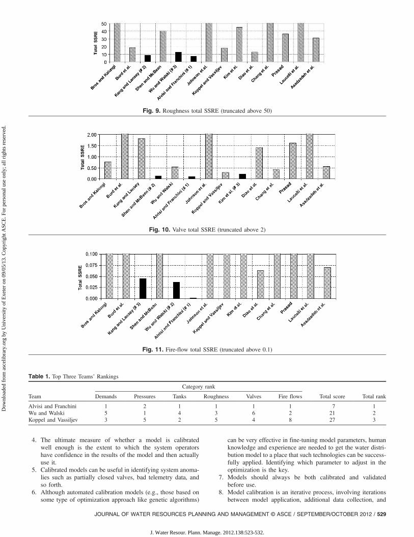
Table 1 summarizes the ranks of the top three teams, Alvisi andFranchini (1), Wu and Walski (2), and Koppel and Vassiljev (3),assuming equal weights for all calibration rank categories. Thetop three teams adjusted pipe roughnesses, pump curves, and pumpstate change times. Alvisi and Franchini have also added minorlosses.

Fig. 3. Examples of demands and pressures matching for Junction 9 with SSRE values of 6.903 and 0.630, respectively

Fig. 5. Top three nondimensional SSRE demands fitting distributions

Fig. 4. (Color) Nondimensional SSRE demands fitting distributions (truncated above 50)

JOURNAL OF WATER RESOURCES PLANNING AND MANAGEMENT © ASCE / SEPTEMBER/OCTOBER 2012 / 527

J. Water Resour. Plann. Manage. 2012.138:523-532.

Dow

nloa

ded

from

asc

elib

rary

.org

by

Uni

vers

ity o

f E

xete

r on

09/

05/1

3. C

opyr

ight

ASC

E. F

or p

erso

nal u

se o

nly;

all

righ

ts r

eser

ved.

Observations

The BWCN was a vital experience to all participants. This sectionpresents a summary of the BWCN insights:1. One should always remember that a model is a simplification

of a real system and not the real system itself. Hence, it isimportant that educators explain and reinforce the point toengineering students that models are not reality and that theirresults should always be validated (i.e., tested against newdata/operating conditions) using intuitive common sense.

2. Part of the value of model calibration lies in the additionalinsights gained through the process about the system, not justa better model. From this perspective, an important aspectcan be the analysis of the existing network topology to accountfor the actual observability of the different parts of the network(i.e., pipes, nodes, and segments) as a consequence of theavailable measurements and observations.

3. The necessary accuracy of the model calibration is dependenton the proposed model application and prediction variables ofinterest. For example, a more detailed model with accurateflow/velocity estimates is required for a water quality problemthan for a general planning application.

Fig. 6. (Color) Nondimensional SSRE pressures fitting distributions (truncated above 50)

Fig. 7. Top three nondimensional SSRE pressures fitting distributions

Fig. 8. Tank total SSRE (truncated above 50)

528 / JOURNAL OF WATER RESOURCES PLANNING AND MANAGEMENT © ASCE / SEPTEMBER/OCTOBER 2012

J. Water Resour. Plann. Manage. 2012.138:523-532.

Dow

nloa

ded

from

asc

elib

rary

.org

by

Uni

vers

ity o

f E

xete

r on

09/

05/1

3. C

opyr

ight

ASC

E. F

or p

erso

nal u

se o

nly;

all

righ

ts r

eser

ved.

4. The ultimate measure of whether a model is calibratedwell enough is the extent to which the system operatorshave confidence in the results of the model and then actuallyuse it.

5. Calibrated models can be useful in identifying system anoma-lies such as partially closed valves, bad telemetry data, andso forth.

6. Although automated calibration models (e.g., those based onsome type of optimization approach like genetic algorithms)

can be very effective in fine-tuning model parameters, humanknowledge and experience are needed to get the water distri-bution model to a place that such technologies can be success-fully applied. Identifying which parameter to adjust in theoptimization is the key.

7. Models should always be both calibrated and validatedbefore use.

8. Model calibration is an iterative process, involving iterationsbetween model application, additional data collection, and

Fig. 9. Roughness total SSRE (truncated above 50)

Fig. 10. Valve total SSRE (truncated above 2)

Fig. 11. Fire-flow total SSRE (truncated above 0.1)

Table 1. Top Three Teams’ Rankings

Team

Category rank

Total score Total rankDemands Pressures Tanks Roughness Valves Fire flows

Alvisi and Franchini 1 2 1 1 1 1 7 1Wu and Walski 5 1 4 3 6 2 21 2Koppel and Vassiljev 3 5 2 5 4 8 27 3

JOURNAL OF WATER RESOURCES PLANNING AND MANAGEMENT © ASCE / SEPTEMBER/OCTOBER 2012 / 529

J. Water Resour. Plann. Manage. 2012.138:523-532.

Dow

nloa

ded

from

asc

elib

rary

.org

by

Uni

vers

ity o

f E

xete

r on

09/

05/1

3. C

opyr

ight

ASC

E. F

or p

erso

nal u

se o

nly;

all

righ

ts r

eser

ved.

human reflection. From this angle, appropriate procedures forreducing the hydraulic model size can help in speeding upthe simulations performed for calibration (e.g., topologicalobservability analysis).

9. Water distribution system staff and operators should be part ofthe team involved in the model calibration, including field datacollection efforts.

10. Simulations over extended periods produced by the calibratedmodel should be used carefully to assess the effect of differentdesign or management decisions on the long-term behavior ofthe system.

11. Water distribution systems with many control rules are diffi-cult to calibrate, and, in general, it is more difficult to repro-duce their behaviors. Small errors on the timing of systemcontrol actions may have a significant effect on water levelsin the tanks, implying errors on the status of the system, whichcan force all the parameters subject to calibration towardpossibly anomalous values.

12. Water distribution model results, especially time simulations,are highly sensitive to model pump curves. Pump suction/discharge head and flows should be collected to obtainaccurate pump curves. For those instances in which the dataare partially known, pump curves should also be calibrated.

13. Sensitivity analysis can be very helpful in identifying thosemodel parameters that have the greatest effect on modelpredictions.

14. Any one of the assumptions used to force the model to fitcould be wrong. It is essential to check the accuracy of databy contacting operators and other corporate data sources.

15. Large customers should be identified and logged separatelyso that their influence on the domestic demand pattern isexcluded.

16. Sufficient data should be provided to allow different consump-tion patterns to be established for customer types.

17. Calibration for a single day does not necessarily replicate per-formance across the full 7-day period and especially betweenseasons.

18. SCADA missing values should be checked before sensitivityanalysis or calibration.

19. Water balances of tank level and pump flows should be reliedon to estimate water demand pattern factors, highlightingsituations in which pumps can switch within the time intervalused to perform the water balance.

20. Pump curve calibration can be improved by measuring pumphead over a range of flows.

21. Fire-flow tests need to be conducted at appropriate locationsfor better pipe roughness calibration.

22. Some model output variables (e.g., water levels in some tanks)can be highly affected even by very small perturbations/errorsin some specific parameters (e.g., pump speeds).

23. Modelers should possess a level of skepticism of field datathat appear inconsistent and challenge the accuracy of suchdata.

Future Research Directions

The BWCN highlighted the following areas that need furtherconsideration and research efforts:1. Calibration for the right reasons: A calibration problem is

inherently “ill posed or underconstrained” as there are moreunknowns than there are equations. As such, there are,mathematically, an infinite number of solutions that willprovide a good match between measured and modeled data.

The calibration process typically alters system demands,fine-tunes pipe roughnesses, and modifies pump operationcharacteristics until satisfactory matching is attained betweenmeasured and modeled data. Once such a solution is received,how can one tell that the system is really calibrated (i.e., per-haps the entire process was simply a “curve fitting” exercise),or in other words, how can one discriminate between twocalibration solutions that resulted in the same matching value?A possible way to address this issue is to extend the model’scalibration matrix from data matching to, for example, themodel’s ability to successfully predict the resultant pressureand flows associated with an independently applied demandpattern and operating conditions, and to effectively predictthe resultant pressure and flows associated with random abnor-mal/failure scenarios. These two latter criteria were posed tothe participants as possible assessment avenues for C-Townbut were eventually not incorporated.

2. Uncertainty inclusion: Calibration models usually treat theunknown calibration parameters (i.e., state parameters, suchas demands, and space parameters, such as roughnesses) asdeterministic. Inclusion of uncertainty in the model param-eters and exploring the influence on the calibrated modeloutputs is important as it enables estimating model predictionerrors. The assessment of both model parameter and predic-tion uncertainties can be accomplished using some analytical(e.g., first-order secondmoment)or sampling-based (e.g.,MonteCarlo simulation)methods, either as part of the postoptimization-based calibration procedure (Kapelan 2010) or as part of theoptimization process itself (Kapelan et al. 2007).

3. Calibration size problem reduction: This point can be per-ceived in different ways, such as by means of aggregationmethodologies and preliminary topological analysis. Likeaggregation methods for water distribution system operation(Ulanicki et al. 1996) and water quality (Perelman and Ostfeld2008), similar methodologies for water distribution systemhydraulic calibration are required for reducing the calibrationsize problems, which, in turn, eases their application and helpsavoid model overfitting. This challenge has two dimensions:clustering of calibration data and construction of an equivalentreduced-size system for performing the calibration tasks.To accomplish meaningful calibration (i.e., determine piperoughness coefficients and valve states) and avoid unnecessarysimulations for large water distribution systems, a study oftopological observability is considered to be necessary (Ozawa1987; Carpentier and Cohen 1993; Giustolisi and Berardi2011). In particular, a preliminary analysis of network obser-vability (i.e., pipes, nodes, and segments), according to theavailable measurements, can significantly reduce the searchspace (roughness and valve states) while reducing the networksimulation problem and, consequently, the required computa-tional time. This is even more important when the calibrationproblem is solved by using multiobjective optimization thatrequires multiple network simulation runs for several candi-date solutions.

4. Leakage data: Incorporation of leakage may be included inhydraulic calibration efforts because leakage directly affectsnodal demand allocation and pump curve characterizations.

5. Calibration data value: The effect of different field dataon model calibration should be investigated; for example,pipe flow data would be more valuable for demand predic-tion than pressure measurements, whereas pressures providebetter information for pipe roughness estimation. The effectof instrumentation type, number, and location would besignificant.

530 / JOURNAL OF WATER RESOURCES PLANNING AND MANAGEMENT © ASCE / SEPTEMBER/OCTOBER 2012

J. Water Resour. Plann. Manage. 2012.138:523-532.

Dow

nloa

ded

from

asc

elib

rary

.org

by

Uni

vers

ity o

f E

xete

r on

09/

05/1

3. C

opyr

ight

ASC

E. F

or p

erso

nal u

se o

nly;

all

righ

ts r

eser

ved.

Conclusions

This paper provides a summary of the BWCN, the goal of whichwas to objectively compare the solutions derived using differentmethods and approaches to the problem of calibration of waterdistribution systems. Participants were asked to apply a calibrationmethodology to a real water distribution system. Fourteen teamsfrom academia, utilities, and private consultants participated.The BWCN outcomes were assessed at the 12th Water DistributionSystems Analysis (WDSA 2010) conference in Tucson, Arizona, inSeptember 2010.

Calibration results were assessed with respect to the state var-iables of demands, pressures, and tank water levels, and for systemparameters such as roughness coefficients. Teams’ performanceswere ranked and equally weighted with regard to the evaluatedcalibration categories. The BWCN concluded with announcingthe top (best) three teams’ rank outcomes.

The success of the teams is attributed to the experience andintuition of the modelers and to the adopted methodologies. As themethodologies were tested on only one case study, it is difficult toidentify/recommend a particular approach over another.

As a result of the BWCN, teams’ observations and futureresearch directions were identified. These directions are expectedto serve as guidelines and benchmarks for future applications andresearch developments in water distribution system calibration.

Supplemental Data

The supplemental material data include the following files, whichare available online in the ASCE Library (www.ascelibrary.org):

C-Town.inp—EPANET input file (version 2.00.12) distributedto participants;

C-Town.xls—data file distributed to participants;C-Town_True_Network.inp—EPANET (version 2.00.12) cali-

brated (true) network; andC-Town_True_Data.xls—calibrated (true) data.In addition, the following changes were made to the “real”

system:1. INP file

1.1. Set pipe’s roughness to 1001.2. Set duration to 0 and hydraulic and reporting time steps

to 11.3. Removed all patterns1.4. Removed unused curves1.5. Set status of all pumps to “OPEN” and opened valve V2.1.6. “Raised” the pump curves according to the affinity laws

1.6.1. Curve 8 (DMA1)—10%1.6.2. Curves 10 and 11 (DMA2 and 5)—5%1.6.3. Curve 9 (DMA3 and 5)—2%

1.7. Control rule changes1.7.1. “ON” level for pump PU2 set to 2.5 (was 1)1.7.2. “ON” level for pump PU8 set to 2.5 (was 1.5)

1.8. Set all demands to 02. Excel file (SCADA data)

2.1. Set two data blocks to zero (marked in yellow)2.2. Set one data block with fixed value (marked in green)

References

Alvisi, S., and Franchini, M. (2010). “Calibration and sensitivity analysisof the C-Town pipe network model.” Proc., 12th Water DistributionSystems Analysis Symp., K. Lansey, C. Choi, A. Ostfeld, and I. Pepper,eds., ASCE, Reston, VA.

Asadzadeh, M., and Tolson, B. A. (2009). “A new multi-objective algo-rithm, Pareto archived DDS.” Proc., 11th Annual Conf. Companionon Genetic and Evolutionary Computation Conf.: Late BreakingPapers (GECCO’09) Association for Computing Machinery (ACM),New York, 1963–1966.

Asadzadeh, M., Tolson, B. A., and McKillop, R. (2010). “A two stageoptimization approach for calibrating water distribution systems.”Proc., 12th Water Distribution Systems Analysis Symp., K. Lansey,C. Choi, A. Ostfeld, and I. Pepper, eds., ASCE, Reston, VA.

Bros, M., and Kalungi, P. (2010). “Battle of the water calibration networks-MWH UK.” Proc., 12th Water Distribution Systems AnalysisSymp., K. Lansey, C. Choi, A. Ostfeld, and I. Pepper, eds., ASCE,Reston, VA.

Burd, R., Zazula-Coetzee, B., and Belrain, T. (2010). “Battle of the watercalibration networks (BWCN).” Proc., 12th Water Distribution SystemsAnalysis Symp., K. Lansey, C. Choi, A. Ostfeld, and I. Pepper, eds.,ASCE, Reston, VA.

Carpentier, P., and Cohen, G. (1993). “Applied mathematics in watersupply network management.” Autom.: J. Int. Fed. Autom. Control,29(5), 1215–1250.

Chang, K., Gao, J., Qu, S., and Yuan, Y. (2010). “Research on water dis-tribution network calibration using heuristics algorithm and pipelineresistance coefficient empirical model.” Proc., 12th Water DistributionSystems Analysis Symp., K. Lansey, C. Choi, A. Ostfeld, and I. Pepper,eds., ASCE, Reston, VA.

Diao, K., Zhou, Y., Li, J., and Liu, Z. (2010). “A component status changesoriented calibration method for zonal management water distributionnetworks.” Proc., 12th Water Distribution Systems Analysis Symp.,K. Lansey, C. Choi, A. Ostfeld, and I. Pepper, eds., ASCE, Reston, VA.

Duan, Q., Sorooshian, S., and Gupta, V. K. (1992). “Effective and efficientglobal optimization for conceptual rainfall runoff models.” WaterResour. Res., 28(4), 1015–1031.

Geem, Z. W., Kim, J. H., and Loganathan, G. V. (2001). “A new heuristicoptimization algorithm: Harmony search.” Simulation, 76(2), 60–68.

Giustolisi, O., and Berardi, L. (2011). “Water distribution network calibra-tion using enhanced GGA and topological analysis.” J. Hydroinf.,13(4), 621–641.

Goldberg, D. E. (1989). Genetic algorithms in search, optimization andmachine learning, Addison Wesley, Reading, MA.

Johnson, J. P., Ghimire, S. R., and Barkdoll, B. D. (2010). “Flow-sequentialsector-specific lumped algorithm for water network calibration.” Proc.,12th Water Distribution Systems Analysis Symp., K. Lansey, C. Choi,A. Ostfeld, and I. Pepper, eds., ASCE, Reston, VA.

Kang, D., and Lansey, K. (2010). “The battle of the water calibration net-works (BWCN): Roughness and demand estimation based on weightedleast squares (WLS) method.” Proc., 12th Water Distribution SystemsAnalysis Symp., K. Lansey, C. Choi, A. Ostfeld, and I. Pepper, eds.,ASCE, Reston, VA.

Kapelan, Z. (2010). Calibration of water distribution system hydraulicmodels, LAP Lambert Academic Publishing, Saarbrücken, Germany,284.

Kapelan, Z., Savic, D. A., and Walters, G. A. (2007). “Calibration ofwater distribution hydraulic models using a Bayesian-type procedure.”J. Hydraul. Eng., 133(8), 927–936.

Kim, J. H., Chung, G., and Yoo, D. G. (2010). “Calibration of C-Townnetwork using harmony search algorithm.” Proc., 12th Water Distribu-tion Systems Analysis Symp., K. Lansey, C. Choi, A. Ostfeld, andI. Pepper, eds., ASCE, Reston, VA.

Koppel, T., and Vassiljev, A. (2009). “Calibration of a model of anoperational water distribution system containing pipes of differentage.” Adv. Eng. Software, 40(8), 659–664.

Koppel, T., and Vassiljev, A. (2010). “Calibration of water distributionnetwork for BWCN.” Proc. Water Distribution Systems AnalysisSymp., K. Lansey, C. Choi, A. Ostfeld, and I. Pepper, eds., ASCE,Reston, VA.

Laucelli, D. et al. (2010). “Calibration of water distribution system usingtopological analysis.” Proc., 12th Water Distribution Systems AnalysisSymp., K. Lansey, C. Choi, A. Ostfeld, and I. Pepper, eds., ASCE,Reston, VA.

JOURNAL OF WATER RESOURCES PLANNING AND MANAGEMENT © ASCE / SEPTEMBER/OCTOBER 2012 / 531

J. Water Resour. Plann. Manage. 2012.138:523-532.

Dow

nloa

ded

from

asc

elib

rary

.org

by

Uni

vers

ity o

f E

xete

r on

09/

05/1

3. C

opyr

ight

ASC

E. F

or p

erso

nal u

se o

nly;

all

righ

ts r

eser

ved.

Levenberg, K. (1944). “A method for the solution of certain non-linearproblems in least squares.” Q. Appl. Math., 2, 164–168.

Marquardt, D. W. (1963). “An algorithm for least-squares estimationof nonlinear parameters.” J. Soc. Ind. Appl. Math. Control, 11(2),431–441.

McKay, M. D., Conover, W. J., and Beckman, R. J. (1979). “A comparisonof three methods for selecting values of input variables in the analysis ofoutput from a computer code.” Technometrics, 211, 239–245.

Ormsbee, L. E., and Lingireddy, S. (1997). “Calibrating hydraulic networkmodels.” J. Am. Water Works Assoc., 89(2), 42–50.

Ostfeld, A. et al. (2008). “The Battle of the Water Sensor Networks: Adesign challenge for engineers and algorithms.” J. Water Resour. Plann.Manage., 134(6), 556–568.

Ozawa, T. (1987). “The principal partition of a pair of graphs and itsapplications.” Discrete Appl. Math., 17 (1–2), 163–186.

Perelman, L., and Ostfeld, A. (2008). “Water distribution system aggrega-tion for water quality analysis.” J. Water Resour. Plann. Manage.,134(3), 303–309.

Prasad, T. D. (2010). “A clonal selection algorithm for the C-Townnetwork calibration.” Proc., 12th Water Distribution Systems AnalysisSymp., K. Lansey, C. Choi, A. Ostfeld, and I. Pepper, eds., ASCE,Reston, VA.

Savic, D. A., Kapelan, Z. S., and Jonkergouw, P. M. R. (2009). “Quo vadiswater distribution model calibration?” Urban Water J., 6(1), 3–22.

Shen, H., and McBean, E. (2010). “Hydraulic calibration for a small waterdistribution network.” Proc., 12th Water Distribution Systems AnalysisSymp., K. Lansey, C. Choi, A. Ostfeld, and I. Pepper, eds., ASCE,Reston, VA.

Tolson, B. A., and Shoemaker, C. A. (2007). “Dynamically dimensionedsearch algorithm for computationally efficient watershed model calibra-tion.” Water Resour. Res., 43(1), W01413.

Ulanicki, B., Zehnpfund, A., and Martinez, F. (1996). “Simplifica-tion of water distribution network models.” Proc., 2nd Int. Conf. onHydroinformatics, InternationalWaterAssociation, Zurich, Switzerland,493–500.

U.S. EPA. (2002). “EPANET.” ⟨http://www.epa.gov/ORD/NRMRL/wswrd/epanet.html⟩ (Mar. 13, 2011).

Walski, T. M. (1990). “Sherlock Holmes meets Hardy Cross or modelcalibration in Austin, Texas.” J. Am. Water Works Assoc., 82(3),34–38.

Walski, T. M. et al. (1987). “Battle of the network models: Epilogue.”J. Water Resour. Plann. Manage., 113(2), 191–203.

Whittemore, R. (2001). “Is the time right for consensus on model calibra-tion guidance?” J. Environ. Eng., 127(2), 95–96.

Wu, Z. Y., and Walski, T. (2010). “Progressive optimization approach forcalibrating EPS hydraulic models.” Proc., 12th Water DistributionSystems Analysis Sym., K. Lansey, C. Choi, A. Ostfeld, and I. Pepper,eds., ASCE, Reston, VA.

532 / JOURNAL OF WATER RESOURCES PLANNING AND MANAGEMENT © ASCE / SEPTEMBER/OCTOBER 2012

J. Water Resour. Plann. Manage. 2012.138:523-532.

Dow

nloa

ded

from

asc

elib

rary

.org

by

Uni

vers

ity o

f E

xete

r on

09/

05/1

3. C

opyr

ight

ASC

E. F

or p

erso

nal u

se o

nly;

all

righ

ts r

eser

ved.