Predicting Mobile Application Power Consumption

By

Michael Chang

A Thesis Submitted in Partial Fulfillment

of the Requirements for the Degree of

Master of Science

in the Faculty of Graduate Studies (Computer Science) Program

University of Ontario Institute of Technology

May 2018

© Michael Chang, 2018

1

Abstract

Michael Chang

Master of Science

Faculty of Graduate Studies

University of Ontario Institute of Technology

2018

We present an analysis of battery consumption to predict the average consumption rate of any

given application. We explain the process and techniques used to gather the data, and present

over 25000 readings collected over 3 months. We then use iterative proportional fitting to predict

the consumptions rates, discuss the issues with the collected data, and highlight the attempts

made to alleviate the problems. Lastly, we discuss the limitations and challenges of this

approach, and suggest changes that may be required in order to produce more accurate results.

2

Acknowledgement

I would like to thank my supervisor Dr. Mark Green for the opportunity to work on this

project. Exploring new ideas and problems has been a challenging endeavour, but he has

provided the insight, guidance, and motivation required to tackle these issues. Dr. Green has

assisted me in turning an idea into a project, guided me through the research process, and

provided valuable assistance whenever frustrating issues occurred

I would also like to thank my family and friends for all of their assistance and support.

My parents Eva and William, and my brother Jeremy are instrumental in giving me the chance to

be here. Nancy, Dameon, and A.J. were my rubber ducks whenever I had to troubleshoot a

problem.

3

Table of Contents 1. Introduction .......................................................................................................................................... 6

2. Literature Review ............................................................................................................................... 10

2.1. Battery Life ................................................................................................................................. 10

2.2. Prediction.................................................................................................................................... 19

2.3. Battery Application Review ....................................................................................................... 27

2.4. Hardware Limitations ................................................................................................................. 31

3. Battery Application ............................................................................................................................ 34

3.1. Battery Application Design ........................................................................................................ 34

3.2. Work Completed ........................................................................................................................ 34

4. Iterative Proportional Fitting ............................................................................................................. 39

4.1. Table Preprocessing ................................................................................................................... 39

4.2. Perform IPF ................................................................................................................................. 41

5. Analysis ............................................................................................................................................... 47

5.1. Additional Preprocessing ........................................................................................................... 47

5.2. Active Usage with Data .............................................................................................................. 49

5.3. Idle Usage with Data .................................................................................................................. 50

5.4. Active Usage with Wi-Fi ............................................................................................................. 51

5.5. Idle Usage with Wi-Fi ................................................................................................................. 52

6. Verification ......................................................................................................................................... 54

7. Result Analysis .................................................................................................................................... 59

8. Discussion and Challenges ................................................................................................................. 64

8.1. Insufficient information gathered ............................................................................................. 64

8.2. Extend Period of Observation .................................................................................................... 64

8.3. Different Techniques Required .................................................................................................. 65

8.4. Expanding Acceptable Results ................................................................................................... 65

8.5. Identifying Applications ............................................................................................................. 66

8.6. Future Work ................................................................................................................................ 66

9. Conclusion .......................................................................................................................................... 68

Bibliography ................................................................................................................................................ 69

4

List of Figures Figure 1: Older smartphones from 1993-2003 [1]. ....................................................................................... 7

Figure 2: Energy saving with different email sizes (left) and energy saving with different inbox sizes

(right). Figure provided by Xu et al. [4]. .................................................................................................... 13

Figure 3: Outline of ad blocking test scenario. Figure provided by Albasir et al. [6]................................. 14

Figure 4: Home page of DU Battery Saver ................................................................................................. 28

Figure 5: Settings page of DU Battery Saver .............................................................................................. 28

Figure 6: Home page of Battery Doctor ..................................................................................................... 29

Figure 7: Advertisements of Battery Doctor ............................................................................................... 29

Figure 8: Main menu of Battery Saver........................................................................................................ 30

Figure 9: Estimated battery readings since the last charge of the device .................................................... 35

Figure 10: Visual representation of how much each application contributed to the 3% drain ................... 43

Figure 11: Visual representation of how much each application contributed to the 2% drain, based on the

updated weight/consumption values ........................................................................................................... 45

Figure 12: Prediction results for active data readings ................................................................................. 55

Figure 13: Prediction results for idle data readings .................................................................................... 56

Figure 14: Prediction results for active Wi-Fi readings .............................................................................. 56

Figure 15: Prediction results for idle Wi-Fi Readings ................................................................................ 57

Figure 16: Prediction results for active data readings after removing duplicate entries ............................. 60

Figure 17: Prediction results for idle data readings after removing duplicate entries ................................. 60

Figure 18: Prediction results for active Wi-Fi readings after removing duplicate entries ......................... 61

Figure 19: Prediction results for idle Wi-Fi readings after removing duplicate entries .............................. 62

5

List of Tables Table 1: List of test cases performed by each device. Power consumption values for each scenario are

collected. ..................................................................................................................................................... 17

Table 2: Table of context factors observed within Peltonen et al.'s [20] study. ......................................... 26

Table 3: List of information retrieved from BatteryManager Class............................................................ 36

Table 4: Sample set of data retrieved from application. The number of application columns and their

names have been altered for visual purposes .............................................................................................. 38

Table 5: Sample database readings prior to IPF reformatting ..................................................................... 40

Table 6: Sample of reformatted table for IPF ............................................................................................. 41

Table 7: Sample dataset for IPF example ................................................................................................... 42

Table 8: First row of Data ........................................................................................................................... 42

Table 9: Initial weight/consumption rate of applications ............................................................................ 42

Table 10: Weight/consumption rate of applications after one iteration of IPF ........................................... 44

Table 11: Second Row of Data ................................................................................................................... 44

Table 12: Weight/consumption rate of applications after two iterations of IPF ......................................... 45

Table 13: Sample set of estimated battery consumption values after IPF has been performed .................. 45

Table 14: Table of local application ID, application name, and estimated consumption rate on active

usage with data. Only applications with an estimated consumption rate greater than 0.01 are shown. ...... 50

Table 15: Table of local application ID, application name, and estimated consumption rate on idle usage

with data. Only applications with an estimated consumption rate greater than 0.01 are shown. ................ 51

Table 16: Table of local application ID, application name, and estimated consumption rate on active

usage with Wi-Fi. Only applications with an estimated consumption rate greater than 0.01 are shown. ... 52

Table 17: Table of local application ID, application name, and estimated consumption rate on idle usage

with Wi-Fi. Only applications with an estimated consumption rate greater than 0.01 are shown. ............. 53

Table 18: Sample data for verification example ......................................................................................... 54

Table 19: Sample consumption rates for verification example ................................................................... 54

Table 20: Summary statistics of calculated percentage error for each type of reading............................... 58

Table 21: The number of readings before and after removing any entries with the same applications open

.................................................................................................................................................................... 59

Table 22: Summary statistics of calculated percentage error for each type of reading after removing

duplicate readings ....................................................................................................................................... 63

Table 23: Sample table list illustrating a negative consumption rate .......................................................... 63

6

1. Introduction

The rapid development of technology has led to a shift in how we communicate with the

world. Computers themselves have also changed significantly since their inception, from

analogue machines, to large electromechanical computers and transistor computers. Nowadays,

many people own personal computers, varying from desktops to laptops. In addition, they are

also using smaller, portable computers such as tablets and smartphones. Each iteration of devices

enabled us to accomplish tasks that were previously not possible. The rise of smartphones has

enabled us to remain connected with everything, regardless of our location. They are capable of

accessing the internet, with applications ranging from social media networks to banking services.

With over 3 billion users as of June 2014 [1], this technology has affected a significant portion of

the world. However, the smartphone itself was also developed through a series of iterations.

Initially, smartphones were large, bulky, expensive, and only used in enterprise settings.

One of the first multipurpose phones was the IBM Simon, released in 1993 [1]. The purpose of

this device was to create a “Swiss Army Knife” phone that combined many features. It

functioned as a mobile phone, a PDA and a fax machine. The device was much larger than the

modern-day smartphone and costed $899 USD, the equivalent of approximately $1500 USD in

2017.

Development of smartphones continued, with devices such as the Nokia 9110,

Blackberry 5810, and the Palm Treo 600. Each device introduced functions that would become

standard features on modern smartphones, such as keyboards, e-mail, web browsing, and

coloured screens. Another notable inclusion is the Palm Pilot, a personal digital assistance device

(PDA). While the Palm Pilot was not a phone, it offered many smartphone features such as

7

calendars, contact lists, e-mail and web browsing. These devices were then used in conjunction

with the cellphones of that time.

The major shift into modern smartphones came from Apple in 2007, when the iPhone

was released [1]. The Apple Smartphone featured a 3.5-inch capacitive touch screen, and

combined the aspects of a phone, an iPod, and internet access. It also removed features such as

keyboards and stylus’ in favour of touchscreen interaction. The following year, the Android

operating system was released on the HTC Dream. Android is an open source mobile operating

system. While the initial adoption of Android was slow, as of 2016 it represents 81.7% of the

smartphone market.

Figure 1: Older smartphones from 1993-2003 [1].

8

The smartphone can be viewed as an extension of the computer, allowing us to perform

the same tasks on a pocket-sized device. Developers have embraced this medium and created

accessible mobile equivalents of the online services that we use. In addition, they are also

creating new, unique applications by leveraging the variety of sensors on the device. However,

they must compensate for the lack of resources in comparison to traditional computers.

Despite the rapid growth of this technology, this service has not been perfected and has

substantial room for improvement. A large amount of research has led to the current state of

smartphones, and much more is required to tackle the outstanding issues that remain. One of the

biggest issues that researchers face is the limitations due to battery life. While smartphones are

capable of many tasks, their battery dictates how much they can accomplish. This problem can

be addressed in a few ways. Developing energy efficient applications would reduce the strain on

the battery. This could be accomplished by creating best practices and encouraging developer

adherence. However, the challenge of this approach is enforcing these practices upon the

community. As applications can be created by anyone, it would be impossible to ensure that all

applications meet strict, energy-related guidelines. Instead of monitoring how applications are

created, a more viable alternative would be to monitor how applications are run. By examining

how energy is consumed on a device, feedback can be given to the user on how to extend their

usage.

The research question to answer is can an application monitor a user’s device to

determine the average consumption rate of every application? The proposed solution would track

the active applications and remaining battery percentage on a user’s device, also known as the

state of charge (SOC). These readings would then be analyzed in order to determine how much

battery life each application consumes. This information is currently unavailable to developers

9

programmatically due to limitations of the Android API. Access to this information can provide

a foundation for predictive methods that manage battery consumption based on user behaviour.

Examining battery life is an important component of smartphone progression, as it is the power

source of the device. The small nature of mobile devices limits the size of the battery, therefore

energy conservation and consumption optimization play an integral part in addressing this issue.

As user expectations of smartphone functionality increases, a greater strain will be placed on its

battery. Therefore, it is important to examine areas of battery conservation to ensure a user can

complete their tasks before their battery is depleted.

While battery saving applications and other conservation techniques exist, battery life

continues to be an issue, meaning current implementations are insufficient. The majority of

battery saving applications approach the problem by suppressing and limiting the user’s

functions. They provide a convenient hub to toggle the resource-heavy functionality of the

device. However, this approach limits the user experience, as they must manually alter and

manage their levels of consumption. In addition, this is also a tedious process that users can

forget to do during their daily routine.

My contributions to the topic are as follows: Designed an application that reads in user

battery information and saves it to a server, analysed the data in order to predict the consumption

rates of each application, discussed the limitations of this approach and changes that may be

required, and created a set of sample data lasting 3 months for future use.

10

2. Literature Review

The idea of using prediction with battery saving applications originates from examining

how prediction was used in other applications. In many cases, prediction was used to reduce wait

times and preserve battery life. However, these were part of larger projects, where battery life

was not the primary objective. The repeated mention of battery life in many articles was a clear

indicator of its importance to mobile applications, leading to the combination of both concepts.

2.1. Battery Life

One of the most prominent issues with smartphones is battery life, with 37% of user

stating it is their biggest problem [2]. As more powerful smartphones are developed, concerns

with battery life increase. Users should be able to utilize their device as they wish for a full day

before a recharge is required. However, this is often not the case, leading to a change in our

activities to preserve battery life. This concern was not evident on desktop computers, as they

have a constant source of power. With the rise of smartphone services, it is one of the biggest

challenges faced by developers. While research into more efficient batteries is possible, another

area of research focuses on improving the efficiency of applications.

For software developers, the solution to preserving battery life is dependent on the

efficiency of the application. Each application may have different shortcomings that cause this,

varying for each case. However, a consistent problem that can affect many applications are no-

sleep energy bugs. Pathak et al. [3] define no-sleep bugs as energy consuming errors that stem

from mismanagement of power control APIs. The components of a smartphone are either off or

idle, unless an application explicitly instructs it to remain on. The resulting process requires

11

developers to constantly enable and disable components when developing their applications. This

ultimately leads to errors when a component should be disabled but is not turned off. The

smartphone’s battery will be depleted at an increased rate, unnecessarily powering a component.

A variety of no-sleep bugs have been recorded and categorized into three groups. Pathak

et al. note that their list is not definitive, and more bugs can exist. No-sleep code paths define

code paths in an application that wake the component, but do not release it after use. This

represents the majority of known no-sleep bugs from the findings of Pathak et al. No-sleep race

condition occurs in multi-threaded applications, where one thread switches the component on,

and another switches it off. Lastly, no-sleep dilation bugs occur when the awoken component is

intended to be put to sleep, but the time required to do so is unnecessarily long.

The solution proposed by Pathak et al. [3] is to create a compile-time dataflow analysis

solution that can detect no-sleep energy bugs. Dataflow analysis is defined as a set of techniques

that analyze the effects of program properties throughout a given program, managed within a

control flow graph. Their solution focuses on the sections where smartphone component power is

managed. If all of those sections have end points that turn off the components, the program is

free of no-sleep bugs. To test their application, they ran their analysis on 86 different android

applications. In addition to the 12 known energy bugs detected, 30 new types of bugs were

discovered. Pathak et al. note that this area of research is relatively new, and they are making the

first advances towards understanding and detecting no sleep bugs.

Focusing on a specific type of application, Xu et al. [4] examined the built-in email

clients of Windows Phone and Android to determine areas of improvement. Windows phone

uses Microsoft Exchange, while Android uses Gmail. Gmail is one of the most popular

12

applications on a mobile device, with over 50 million users per month [5]. With such a large user

base, it is important that Gmail and other email applications are optimized for functionality,

accessibility, and power consumption. Unfortunately, functionality and power consumption can

be contradicting. Functionality requires the application to be constantly checking for new

messages, but continually syncing is extremely resource intensive. Finding a balance between

these two concerns is not only limited to email, and can be practical for other applications.

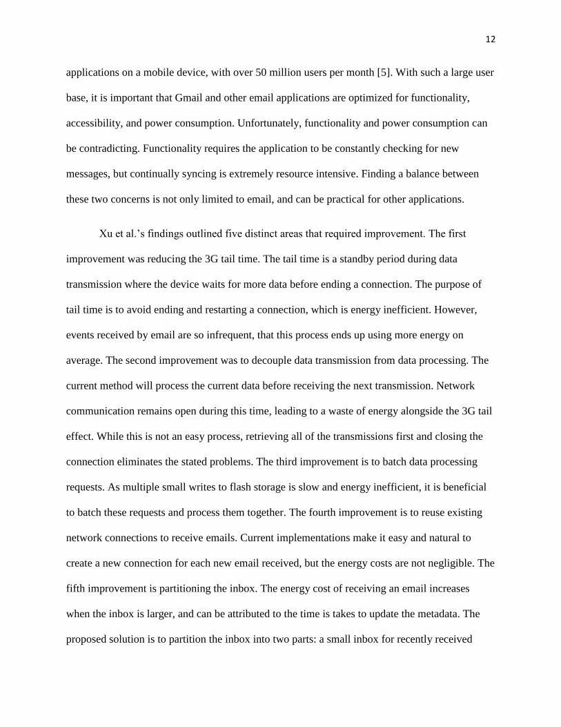
Xu et al.’s findings outlined five distinct areas that required improvement. The first

improvement was reducing the 3G tail time. The tail time is a standby period during data

transmission where the device waits for more data before ending a connection. The purpose of

tail time is to avoid ending and restarting a connection, which is energy inefficient. However,

events received by email are so infrequent, that this process ends up using more energy on

average. The second improvement was to decouple data transmission from data processing. The

current method will process the current data before receiving the next transmission. Network

communication remains open during this time, leading to a waste of energy alongside the 3G tail

effect. While this is not an easy process, retrieving all of the transmissions first and closing the

connection eliminates the stated problems. The third improvement is to batch data processing

requests. As multiple small writes to flash storage is slow and energy inefficient, it is beneficial

to batch these requests and process them together. The fourth improvement is to reuse existing

network connections to receive emails. Current implementations make it easy and natural to

create a new connection for each new email received, but the energy costs are not negligible. The

fifth improvement is partitioning the inbox. The energy cost of receiving an email increases

when the inbox is larger, and can be attributed to the time is takes to update the metadata. The

proposed solution is to partition the inbox into two parts: a small inbox for recently received

13

emails, and a large one for the remainder. As most new messages will interact with recent

messages, there is no need to search through old emails. Xu et al. implemented these changes

and proceeded to observe the change in energy consumption. Their findings indicated an average

energy reduction of 49.9%.

Figure 2: Energy saving with different email sizes (left) and energy saving with different inbox sizes (right).

Figure provided by Xu et al. [4].

Beyond applications, web browsing can also have a large impact on energy consumption.

Most modern webpages are populated with a variety of detail beyond traditional text. Pictures,

videos, and animations are placed throughout the site, which require significantly more resources

to generate in terms of both bandwidth and energy. This is evident in [6], a study on the energy

and bandwidth costs of web advertisements on smartphones. Another study [7] examines and

characterizes resource usage for web browsing as a whole.

While users generally dislike advertisements distracting them from a webpage, the study

of Albasir et al. [6] gives users another reason to detest them. As shown in Figure 3, the energy

consumption of advertisements was measured by examining a number of news websites under

two conditions. The first condition used the built-in web browser on the device to access

14

websites, measuring the amount of energy and bandwidth consumed. In the second scenario, the

same websites were revisited on a different browser designed to display the webpage without ad

traffic. The results indicated that advertisements can take up to 50% of the traffic required to

load the page. In addition, the energy consumption of ad generation represented approximately 6

– 18% of the total energy from web browsing. While this study only examined a small number of

news websites, it highlights an opportunity to improve battery life for mobile users.

Figure 3: Outline of ad blocking test scenario. Figure provided by Albasir et al. [6].

The study of Qian et al. [7] also examines resource usage, but their area of focus is

broader, focusing on the 500 most popular websites. Instead of targeting a specific component,

they are examining the entire web browsing process such as protocol overhead, TCP connection

15

management, web page content, traffic timing dynamics, caching efficiency, and compression

usage. The objective is to measure these components in order to characterize how energy and

bandwidth is consumed, allowing them to pinpoint areas of improvement.

Their process begins by collecting data from the landing pages of the 500 most popular

websites. To analyze these websites, they have created a measurement tool called UbiDump.

UbiDump runs on mobile devices and is able to accurately reconstruct all web transfers made.

After this information is collected, Qian et al. perform statistical analysis on the information

based on the previous processes stated. This section is extremely detailed as it explains each

component, how it is measured, and provides “what if” scenarios that propose changes to the

current implementation and describe the outcome. Based on their findings, they provide a list of

recommendations that can improve the inefficiencies they discovered. Some of their suggested

changes are similar to the work of Xu et al. [4], such as reusing connections and caching.

Woo et al. [8] examine caching in their study, as minimal work has been done to optimize

the content caching in cellular networks. The increasing number of high speed base stations has

made network accessibility more convenient for users. However, the problem surfacing with

cellular networks is that all user traffic has to pass a limited number of gateways at core

networks before reaching the wired internet. Simply increasing the physical backhaul bandwidth

is not feasible for centralized architectures such as this. To circumvent this, optimization

strategies must be considered. Their study focuses on three types of caching: conventional web

caching, prefix-based web caching, and TCP-level redundancy elimination. Conventional web

caching places information at the Digital Unit Aggregation (DUA) component of the cellular

network architecture. However, this approach suffers from two problems. The first problem is

that it “…cannot suppress duplicate objects that are uncacheable or that have different URLs

16

(i.e., aliases)”. Secondly, it is difficult to handle handovers from the mobile device to the DUA

while the content is being delivered. Prefix-based web caching can overcome the first problem

that web caching has, suppressing the duplicate and aliased objects. The drawback of this

approach is that it’s efficiency and rate of false positives was initially unknown, but is addressed

by Woo et al. later in the study. Lastly, TCP redundancy elimination can also handle the issues of

traditional web caching, but suffers from a complex implementation and high computational

overhead.

The first part of the study was to analyze the TCP and application-level characteristics of

the traffic, while the second part was comparing the effectiveness of the three types of web

caching. Based on the results, 59.4% of the traffic is redundant with TCP-level redundancy

elimination if we have infinite cache. In regards to caching options, standard web caching only

achieved 21.0-27.1% bandwidth savings with infinite cache, while prefix-based web caching

produced 22.4-34.0% bandwidth savings with infinite cache. In addition, TCP-RE achieved the

highest bandwidth savings of 26.9-42.0% with only 512 GB of memory cache.

Li et al. [9] perform an analysis of energy consumption on android smartphones, focusing

on how the device is used as opposed to the applications running. To maintain consistency, an

additional battery with a fixed voltage source is attached to a smartphone instead of using the

traditional lithium-ion battery. A series of test cases are then performed on three different

Android devices, and the electric current is measured with a multimeter. In each device’s test

case, the smartphone was set to 50% brightness, and all applications were closed.

17

Test Case

50% brightness screen

Opening GPS

Opening Wi-Fi

Wi-Fi Download (2.55

Mpbs)

GSM Download

(35kpbs)

Opening Bluetooth

Bluetooth Searching

Devices

Bluetooth sending data

CPU Single thread

CPU multithreads

CPU stress condition

Opening terminal

Calling

Incoming call

Sending a message

Taking a picture

Playing music

Playing video

Table 1: List of test cases performed by each device. Power consumption values for each scenario are

collected.

The power consumption of each test case is recorded, and the results are analysed. In

addition, additional test cases are performed with varying screen brightness. With the data

collected, energy consumption models for screen brightness are provided. However, models for

the other test case modules such as CPU, GPS, Wi-Fi and Bluetooth were unable to be

determined. As each module has a variety of states which were rapidly changing, an accurate

model could not be calculated for each case. Instead a general function is provided to

approximate the power consumption of any given state.

18

Hoque at al. [10] present an analysis of the battery in order to examine charging

mechanisms, state of charge estimation techniques, battery properties, and the charging

behaviour of both devices and users, using data collected from the Carat [11] application. Carat

is an application that tracks the applications you’re using, but does not measure energy

consumption directly. The first analysis examines the charging techniques of smartphones and

the charging rates. The charging mechanisms, battery voltage and charging rates of the devices

are outlined. In addition, two additional charging mechanisms that are variants of the established

CC-CV and DLC methods are identified. The second part of the analysis examines battery

properties such as the changes in its capacity, temperature when charging, and battery health.

The results indicated a linear relationship between the remaining battery capacity and final

voltage, and a decrease in battery temperature over time as the device charged. In addition, the

health of the battery did not indicate increases in battery temperature.

Kim et al. [12] discuss the differences between battery and energy consumption,

explaining how they are not always equal. When the battery discharges, portions of the stored

energy become unavailable. Energy-saving techniques do not take this measurement into

account, leading to incorrect calculations. Kim et al. propose that battery consumption should be

the metric considered when proposing a savings plan. They design an application to calculate

battery consumption, and evaluate their model with a series of test cases. The test cases include

many power hungry applications, but their consumptions rates and periods of activity differ. The

analysis examines the relationship between the systemwide power consumption and unavailable

energy. In the initial trial, an increase in power consumption also increased the unavailable

energy, and in some cases reduced the actual delivered energy by over 50%. When applying the

measurement technique to the test cases with scaling governors that manage CPU frequency and

19

voltage, certain scenarios even indicated battery consumption can decrease when energy

consumption increases.

Lee et al. [13] focus specifically on battery aging, and the importance of quantifying the

process. They propose an online scheme that tracks battery degradation without the use of any

external equipment. The scheme functions by logging the amount of time required to charge the

battery, comparing its results to the duration of charging a new battery. A set of different lithium-

ion batteries with different ages are measured to set a baseline charge time. The focus on the

analysis is based on the middle region, charge levels approximately between 40%-80%. This is

due to the linear charge rate in the given period. To calculate the battery efficiency, the scheme

predicts the middle region of the battery, the theoretical charge time of the region, and uses the

actual charging time of the given range. The accuracy of the efficiency measurements were 0.94

+/- 0.05 with a range from 0.82 to 0.99.

2.2. Prediction

Many people may be familiar with smartphone prediction due to its use on their

keyboard. However, the applications of prediction extend well beyond such a simple use. The

primary benefit of prediction is speed, and a reduced wait time is always welcomed by users.

Higgins et al. [14] examine prediction on smartphones and illustrate how and when it can be

used. They have designed an API that leverages the uncertainty level in their prediction before

making a decision. The API can use three different methods when determining the predictive

error rate, each with a different drawback. Their API is used and tested on two applications: a

network selection, and a speech recognition application. The network selection application is

used to determine if the smartphone should transmit data over cellular, WiFi or both mediums,

20

based on latency, bandwidth, dwell time, and energy usage. In the speech recognition system, the

API is used to determine if the recognition should be performed on the device, the remote server,

or both, based on latency, bandwidth, dwell time, application compute time, and energy usage.

For both applications, a scenario to use both options exists because Higgins et al. consider the

benefits of redundant strategies, as they understand the uncertainty of predictive approaches.

Their results for the network selection application resulted in a 21% reduced wait time over

cellular-only strategies, and 44% for Wi-Fi preferred and adaptive strategies. For speech

recognition, there were varying results depending on the energy usage. Redundant strategies are

still beneficial for low to mid-energy cost scenarios, but prove to be too energy consuming for

high-cost scenarios. In addition, their API reduced recognition delay in the no-cost energy

scenario by 23%. While their study showcases the benefits of prediction, it fails to illustrate

where and how it can be used. Other research into the topic provides better examples of its

practicality.

One notable example of prediction use is in mobile exercise applications. Kotsev et al.

[15] have begun using prediction to determine when users will exercise. They believe that users

have exercise patterns that are affected by a variety of factors such as the season, weather, and

even their mentality such as New Year’s Resolutions. By predicting a pattern, researchers can

develop a better understand of what motivates users to exercise, allowing them to create better

tools to increase motivation. Their work begins with analyzing a dataset generated from over

10000 users, with the goal of identifying as many different factors as possible. The dataset

provided information such as the type of activity performed, the country the user is from, their

social connectivity, when they exercise, and how long their exercise for. While their research is

inconclusive, they identify the top 10 features that can be used to predict future behaviour, which

21

are runs per week, mean runs per week, max runs per week, min runs per week, average runs per

week, 2 elapsed hours, min distance, min elapsed hours, mean speed, and max speed.

Bulut et al. [16] have also utilized prediction in a unique way, creating a crowdsourced

line wait-time monitoring system with smartphones. Its implementation at grocery stores,

DMV’s and banks would allow users to make informed choices in time-sensitive environments.

Known as LineKing, it has been tested at a coffee shop at the State University of New York at

Buffalo. Customers who enter the shop will establish a connection with the service, where any

connection lasting longer than 2 minutes but less than 20 is deemed a customer. The wait-time

calculation is completed on the server side of the application, taking the time of the day, the day

of the week, and seasonality into account. The estimated wait times are accurate within 2-3

minutes.

LineKing is comprised of two components, a client-side and a server-side. The client side

is comprised of three subcomponents: phone-state-receiver, wait-time-detection, and data-

uploader. The phone-state-receiver is comprised of a variety of receivers registered to monitor

various events for the application. The most notable event is the device entering and exiting the

shop. The wait-time-detection component can use either location sensing or WiFi sensing to

detect the user’s presence at the shop. In order to preserve battery life, the component begins

monitoring the device under two conditions: if the user opens the application to check the wait-

time or if the user is physically close to the shop. Once a condition is triggered, the application

begins to monitor the user’s location. For location sensing, if the user is within a specific range

of the shop, the application will set a proximity alert to register the timestamp of entering the

shop. If they are outside of the specified range, the application will estimate the arrival time of

the user, and recheck their location at that time. If the user does not travel towards the shop after

22

a certain amount of time, the monitoring will cease. In the Wi-Fi sensing approach, the

application will monitor Wi-Fi beacons periodically to determine when the user enters and leaves

the shop. Their calculation in this approach takes into account the time delay of the scanning

period. Lastly, the data-uploader component is responsible for uploading the wait-times to the

estimation system.

The server-side component is the service that calculates the wait-time, and is comprised

of four components: the web service, pre-processor, model-builder, and wait-time forecaster. The

web service is the interface between the smartphone and the server, accepting wait-times from

the smartphone and delivering wait-time estimations. The pre-processor model receives wait

times from the web service, and is mainly responsible for removing outliers within the data. The

model builder builds a model from the collected data, which the wait-time forecaster uses to

estimate future wait times. The wait-time forecaster is a novel solution that takes multiple factors

into consideration such as the time of the day, weekday vs. weekend, and seasonality of the

business to generate an estimated wait-time. The process begins with a nearest neighbour

estimation (NNE), which attempts to predict the wait-time by comparing the current situation to

the collected data of wait-times. This process is then further improved by using a statistical time-

series forecasting method referred to as the Holt-Winters method. While Bulut et al. state that

their implementation received positive user feedback, the section is rather vague and does not

provide any statistical data to support this.

The next case of prediction aims to fix the disconnecting nature of smartphone usage.

Mobile cloud computing has become a popular approach to application design, giving

smartphones even more utility. However, the unreliable nature of wireless communication

hinders an otherwise effective method. To address this problem, Gordon et al. [17] present a

23

concept to maintain full or partial utility during offline periods by predicting when they will

occur. This is accomplished by observing the user’s behaviour over time, based on the motion

sensor signals on the smartphone. The signals retrieved can be categorized into six motion

classes: standing, sitting, walking, climbing stairs, running, and ‘other’. In addition to user

behaviour, network connectivity states are also monitored. By observing the user’s behaviour in

parallel to network connectivity states, patterns leading to transitions in network connectivity can

be discovered. Once an offline prediction has been made, this information is sent to relevant

applications. The applications are then assessed to determine the threshold of connectivity

required to maintain the current user experience. Certain applications may only require low

speeds and bandwidth, whereas video or music streaming applications will require much more.

Once the level of connectivity is established, the applications will decide which resources to

prefetch and cache in preparation for the offline period. This decision is similarly dependent on

assessing what is required for optimal performance.

To explain their concept Gordon et al. use an example of a student going for a run vs.

going to school. When the student travels, he uses a music streaming service. The beginning of

both trips are the same, and but the paths diverge when the student runs through a park with

limited reception. As this is part of an ongoing routine, a repeat of those signals will indicate that

offline caching is required. The objective of this concept is to predict the behaviour early enough

that the user’s experience is uninterrupted. In this case, the runner will be able to jog through the

park while still listening to his music. In their study, they were able to successfully predict 100%

of the disconnection events approximately 8 minutes before they occurred. However, Gordon et

al. discloses that the data set used was from one person, and that results can vary.

24

A few studies focused specifically on using prediction to study battery life. Li et al. [18]

frame their research question in a unique approach, opting to determine how close to one week a

user’s smartphone can survive on one charge. The analysis began by developing a prediction

model that calculates how long the battery life can be extended, taking into account the type of

hardware and user behaviour. The hardware considered are the CPU, display brightness, the

radio, and Wi-Fi, while user behaviour is based on an application’s running time. The prediction

model is then evaluated through a series of test cases, comparing the prediction results to the

measured power from established power models. The average application power error of the

prediction model is 7.31%.

The next component examined user behaviour based on application usage. With their

own data set and using Fuzzy C-Means clustering algorithm, 6 different user classification types

are established. The classification types are based on the types of applications they used: utilities,

news and magazines, email, games, media, photography, browser, social-networking, weather,

phone call, SMS, and sleep mode. The results indicated the battery life for users using only one

specific category are difficult to increase, sleep mode was the biggest contributor to a battery’s

lifetime, and that battery life can be extended up to 40% by adjusting application usage. For

users who barely use their device, limiting themselves to only phone calls and SMS would

extend their battery from 66.28 hours to 147.3 hours, more than 6 days. Lastly, Li et al. discuss

improvements in hardware that could increase battery life.

Rattagan et al. [19] examine prediction and battery life together, evaluating online power

estimations from battery monitoring units. They discuss the current methods of online and offline

monitors, indicating the pros and cons of each. While online methods are more feasible and

scalable, their results have a higher error rate due to three problems that are not taken into

25

consideration: battery capacity degradation, asynchronous power consumption behaviour, and

the effect of state of charge difference in hardware training. The battery capacity of a device will

decrease after usage, while online methods use the original battery capacity value without taking

this into account. Asynchronous power consumption refers to readings where power

consumption is misattributed to a given component or resource. Lastly, the effect of state of

charge (SOC) difference in hardware training refers to the power consumption estimation of the

hardware at different battery percentages. While the consumption rate should be uniform

regardless of the state of charge, that is not the case for online battery monitoring units.

The proposed solution is a semi-online power estimation method that addresses the three

discussed issues. Battery capacity degradation is accommodated by using both the charging and

discharging data to approximate the current battery capacity. For asynchronous power

consumption, the voltage differences in readings are applied to determine if this is occurring.

Lastly, Rattagan et al. examine a variety of different SOC values to determine an optimal SOC

that has a minimal effect on the accuracy of power estimates. The solution reduced the error rates

of power estimates by 86.66%. In addition, Rattangan et al. note that accounting for battery

capacity degradation had the largest effect in producing more accurate results.

Peltonen et al. [20] attempt to construct energy models of smartphone usage through

crowdsourcing, whereas most research focused on a singular device or system. They use a subset

of data collected from Carat [11], a collaborative energy diagnostic system. The data contains

11.2 millions samples from approximately 150 000 Android devices. The dataset also provides

energy rates that can be used to calculate battery consumption. Within this dataset, they identify

13 different context factors, 5 of which are user-changeable settings and 8 are subsystem state

information. The context factors, their type, and the unit of measurement are shown in Table 2.

26

Context Factor Type of Context Factor Unit of Measurement

Mobile Data Status System setting

Connected, disconnected,

connecting, or disconnecting

Mobile Network Type System setting

LTE, HSPA, GPRS, EDGE, or

UMTS

Network Type System setting None, Wi-Fi, mobile, or wimax

Roaming System setting Enabled, or disabled

Screen Brightness System setting 0-255, or “automatic” (-1)

Battery Health Subsystem state

Varies depending on the Li-Ion

battery type

Battery Temperature Subsystem state Degrees Celsius

Battery Voltage Subsystem state Volts

CPU Use Subsystem state Percent

Distance Traveled Subsystem state Metre (between two samples)

Mobile Data Activity Subsystem state None, out, in, or inout

Wi-Fi Link Speed Subsystem state Mbps

Wi-Fi Signal Strength Subsystem state dBm

Table 2: Table of context factors observed within Peltonen et al.'s [20] study.

With the substantial set of data collected, Peltonen et al. perform a thorough analysis

creating battery models, calculating each context factor’s impact on energy consumption,

quantifying the type of impact typical values of context factors have on energy consumption, and

many other in-depth evaluations. The impact of pairs of context factors, and how different

combinations of active context factors can affect battery consumption are also evaluated. The

results illustrate how different system settings can affect battery consumption, and they have

released their dataset for others to use.

Anguita et al. [21] attempt to use machine learning to overcome battery limitations. They

propose sensors can be used to predict the actions of the user. They use an existing machine

learning framework and modify it to meet the resource constraints of a smartphone. Their

implementation is then validated in a series of test cases where the framework predicts whether

27

the user is walking, walking upstairs, walking downstairs, sitting, standing, or laying. While the

test cases are outside the scope of traditional application monitoring, they illustrate the usage of

machine learning is feasible for mobile devices, and the resource requirements can be reduced.

2.3. Battery Application Review

The purpose of reviewing the current battery management applications was to determine

the functionality that is currently offered, and to check that prediction is not an established

approach. DU Battery Saver [22], Battery Doctor [23], and Battery Saver applications were

retrieved from the Google Play Store, using the search tag battery saver and battery life. They

were the highest rated applications, top results from searches, and had a minimum rating of

4.5/5.0. In addition, DU Battery Saver and Battery Doctor have over 8 million downloads

respectively as of May 2018. Battery Saver is no longer available in the Google Play Store as of

May 2018, and the number of downloads was not recorded.

The DU Battery Saver [22] offers a significant amount of functionality, providing a main

page showing the battery percentage, battery remaining, and the temperature of the device as

shown in Figure 4. The fix now feature will cause the device to close unused applications that are

draining resources to extend the battery life. Within the main page, the mode option allows the

user to change the current profile. The smart button reveals a set of options that determine which

applications are needlessly using resources, freeing them up to conserve battery. Included here is

a whitelist of applications that won’t be terminated. A list of profiles is also available, altering

the functionality of the device based on the user’s needs. A table of switches is provided to

quickly enable/disable features such as Wi-Fi, data, display brightness, and ringtones. In

addition, the settings page in Figure 5 provides a variety of reminder features. Alongside these

28

features, the application is also visually appealing as well. Icons are used within the main menu,

and animations are provided when it is scanning for applications that are using resources.

Figure 4: Home page of DU Battery Saver

Figure 5: Settings page of DU Battery Saver

The issue with this application comes from the boost and toolbox options on the main

menu. The toolbox is a list of advertisements, while boost claims that there is trash on the device,

and advertises for another application. While many of the features on the device are beneficial,

these components are obstructive and unnecessary. In addition, notifications advertising the other

applications were also periodically appearing. Lastly, no prediction-based functions were

observed on the application.

29

The Battery Doctor [23] application lacks the design appeal of DU Battery Saver, and

provides similar features. The application monitors the battery consumption, and notifies the user

when background applications are consuming excessive battery life. A highlight of application

battery usage, power remaining, battery level history, and device temperature are also provided

on the main page. Tabs on the bottom of the application lead to charging history, battery profiles,

and a consumption page of the applications that are running. A settings page also provided a low

power notifications, Wi-Fi toggling, and an ignore list. However, beyond these features, the

application was not as appealing as The Battery Doctor. The application would constantly note

that the battery was draining fast, as shown in Figure 6, even though the optimize now button

was recently used. However, the biggest issue was the amount of advertisements throughout the

entire application. In some cases, they blended in with some of the features, which could confuse

users. Figure 7 provides an example of how intrusive the ads on the application were.

Figure 6: Home page of Battery Doctor Figure 7: Advertisements of Battery Doctor

30

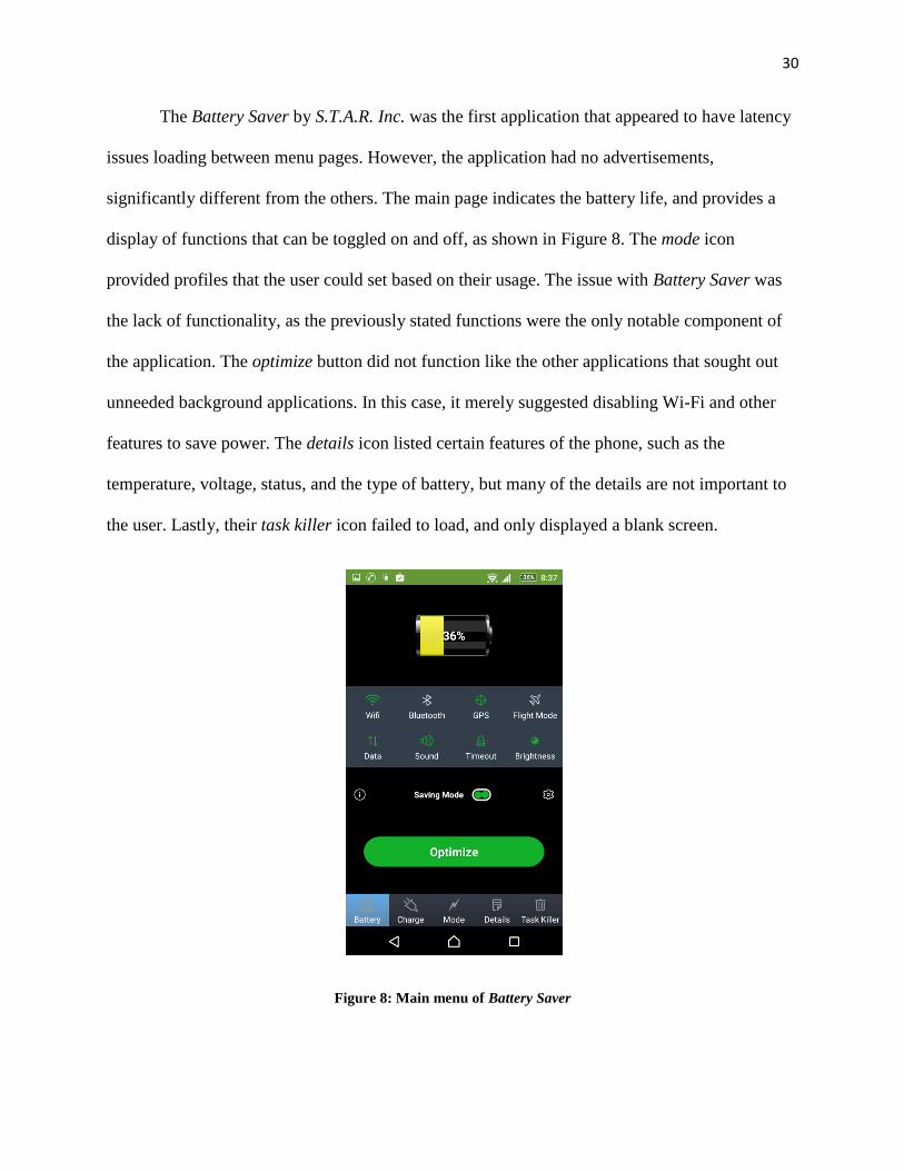
The Battery Saver by S.T.A.R. Inc. was the first application that appeared to have latency

issues loading between menu pages. However, the application had no advertisements,

significantly different from the others. The main page indicates the battery life, and provides a

display of functions that can be toggled on and off, as shown in Figure 8. The mode icon

provided profiles that the user could set based on their usage. The issue with Battery Saver was

the lack of functionality, as the previously stated functions were the only notable component of

the application. The optimize button did not function like the other applications that sought out

unneeded background applications. In this case, it merely suggested disabling Wi-Fi and other

features to save power. The details icon listed certain features of the phone, such as the

temperature, voltage, status, and the type of battery, but many of the details are not important to

the user. Lastly, their task killer icon failed to load, and only displayed a blank screen.

Figure 8: Main menu of Battery Saver

31

The current functions of battery saving applications require the user to constantly make

changes. Profile switching, toggling settings, and removing background applications were

popular features over multiple applications, but would require repeated interaction whenever a

change was needed. The most autonomous feature was a timer for profiles settings, which would

revert back to default after a period of time. The tools that were implemented provide insight into

the types of battery-related settings that need to be toggled. By creating an application that uses

prediction, these established modifications can be used more efficiently.

2.4. Hardware Limitations

While applications provide an important role in battery conservation, the hardware

component is equally as important. Developers do not have the same level of control over

hardware, but their limitations must be considered. Rajaraman et al. [24] address this by breaking

down the power consumption of live streaming on a smartphone device. Recording videos and

streaming is a resource intensive task that rapidly drains the battery. By identifying where and

how resources are consumed, improvements can be made to reduce the battery strain.

Rajaraman et al. indentify the anatomy of the smartphone power consumption by

measuring the drain rate over a series of trials, broken down into three sections: display, video

camera, and wireless communication. The initial trial measures the device in an idle state on

airplane mode and the screen powered off. In each section’s subsequent trial, additional

components of the device are activated and the drain rate is logged. Examples of the components

include the camera mode used to record the video, the brightness of the screen, and how the

video is streamed to the internet. Once this information is collected, the data is evaluated to

determine the components with the greatest drain rate. These components are then examined in

32

order to determine a more energy efficient approach. Their analysis indicated the greatest power

consumption involved turning on the camera in focus mode, but not when it is recording in shoot

mode. The consumption from focus mode also does not scale with the quality of the video,

indicating the power drawn from this process does not come from the image sensor of the

camera, but from external hardware components.

Brocanelli et al. [25] design a configuration to assist in battery consumption, but the

motivation came from a hardware perspective. While investigating smartphone idle periods, they

observed that the device was significantly more active than expected. The processor would

awaken to execute functions related to the Radio Interface Layer Daemon (RILD). The main

objective of RILD is to communicate with the baseband processor in order to deliver voice calls

SMS, or network data. Without RILD active, the device would not receive any notifications

when idling. RILD is normally performed on the application processor, which is repeatedly

awakened during idle periods. If RILD can be executed elsewhere, the consumption can be

significantly reduced.

Brocanelli et al. propose that the RILD functions be performed on a microcontroller

instead of the application processor. While app-based notifications would still require the

application processor, notifications regarding voice calls and SMS can be shifted to the

microcontroller, similar to how traditional feature phones functioned. The implementation

involves attaching an additional microcontroller to their smartphone through the micro-USB

port, but state that an internal approach is also possible. When their implemented Smart on

Demand energy saving mode is active, the RILD functions are shifted from the application

processor to the microcontroller. The microcontroller handles the communication with the

baseband and application processors, allowing the application processor to sleep and only

33

awaken for smart app updates. Their results indicated the configuration reduced energy

consumption by up to 42%.

34

3. Battery Application

3.1. Battery Application Design

The proposed application is comprised of two main components. The first component is

the client-side interface, while the second component is the server-side that handles the majority

of the processing. The primary purpose of the client-side application is to collect relevant battery

information and send it to the server. Other features could be provided in the future, but

collecting data to analyze is currently the only mandatory feature. The application was developed

using the Android API, as the test device was an Android smartphone.

The server-side of the application is where the data acquired from the client-side is stored

and processed. The purpose of the server-side component is to reduce the storage and processing

strain on the device. The data stored on the server-side will be used to predict the draining rates

of applications after a certain amount of information is collected. Readings will be sent to the

server at 5-minute intervals.

3.2. Work Completed

The initial step of my contribution was to create an application that could perform

periodic battery reading for a device. By receiving periodic readings of the device, it would be

possible to track the user’s behaviour. Initially, the goal was to gather the percentage of the

battery that each application consumes, information provided through Android’s user interface in

Figure 9. However, this data is unobtainable programmatically; therefore alternative methods

had to be pursued.

35

Figure 9: Estimated battery readings since the last charge of the device

The next step involved examining the Android API to determine what type of battery

information could be retrieved. The BatteryManager class provided information on the battery of

the device, but did not include a list of active applications. A full list of information collected

from the BatteryManager class is shown in Table 3.

36

Date date of reading, taken outside the scope of the BatteryManager Class

Data tracks if the device was using cellular data or Wi-Fi, taken outside the scope of the BatteryManager Class

Health the health of the battery. All reading showed it was in good health

icon_small unused, referenced the resource ID of an icon but all results were NULL

Level current battery percentage, same value as percentage column

plugged if the device was charging or discharging

present unused, indicated whether a battery was present

Scale unused, indicated the maximum battery level of 100

Status unused, indicates whether device is charging, discharging or full. Similar information provided by plugged column

technology unused, indicates the type of battery

temperature unused, indicates the temperature of the device

voltage unused, indicates the current battery voltage level

percentage the current state of charge

Table 3: List of information retrieved from BatteryManager Class

Further examination into retrieving an application list revealed that this was no longer

possible. The functions that provide this information was deprecated as of API level 21, Android

5.0. While reading through multiple sources regarding the deprecation, a user named Jared

Rummler [26] provides a workaround to the current issue, allowing users to retrieve the list of

running applications. The provided class functions by utilizing the ps toolbox command of

Android, a program that contains simplified functionality of Linux commands. The ps command

provides information regarding the processes open on the device, which are used to generate a

list of applications currently running.

The proposed application is divided into two components, the client side and the server

side. The client-side application collects the data from the user and sends the information to the

server. All of the collection is completed in background tasks; therefore the front-end of the

application is primarily empty. The application uses two android services to complete the process

37

which are triggered when the application is opened. A service is a process of an application used

to complete background actions [27]. This approach was necessary as the application will not

always be open and in the foreground. The data must still be accessible even if the user is

running another application or not using the device. This also eliminates concerns regarding

background applications that are terminated due to inactivity.

The two services are kept separate so they can each run on independent schedules. The

first service is used to take a snapshot of the battery information, along with a list of running

applications. This information is then saved onto a local SQLite database within the application

itself. The second service is used to upload the recorded information onto a server. This process

keeps a timestamp log of the last upload to minimize the information transferred.

The server side component of the application is comprised of two parts, a set of PHP

scripts and the MySQL Database. The information from the device is sent to a PHP script on the

server, which makes the appropriate MySQL calls to transfer the data to the appropriate MySQL

database table. The MySQL database contains the information sent from the device. Each row in

the database contains the timestamp of the snapshot, the information in Table 3, and a binary

value for each application on the device during the collection period. The number 1 indicates that

the application was active, while a 0 means it was inactive. A sample of readings is provided in

Table 4. Note that the usage of data or Wi-Fi is omitted from the readings. This information was

subsequently added as it was personally tracked instead of programmatically recorded. An SMS

was sent to the device whenever the device switched between cellular data or Wi-Fi. In the

unlikely event that a notification was forgotten, the rows of data in the affected timeslots were

removed from the analysis.

38

Table 4: Sample set of data retrieved from application. The number of application columns and their names

have been altered for visual purposes

date health icon_small level plugged present scale status technology temperature voltage percentage App01 App02 App03 App04 App05 App06 App07

01/09/2017 0:04 2 NULL 86 0 1 100 3 Li-ion 236 4018 86 1 1 1 1 0 1 1

01/09/2017 0:09 2 NULL 86 0 1 100 3 Li-ion 226 4021 86 1 1 1 1 0 1 1

01/09/2017 0:14 2 NULL 85 0 1 100 3 Li-ion 220 4019 85 1 1 1 1 0 1 1

01/09/2017 0:19 2 NULL 85 0 1 100 3 Li-ion 215 3989 85 1 1 1 1 0 1 1

01/09/2017 0:24 2 NULL 85 0 1 100 3 Li-ion 211 4014 85 1 1 1 1 0 1 1

01/09/2017 0:29 2 NULL 84 0 1 100 3 Li-ion 242 3949 84 1 1 1 1 0 1 1

01/09/2017 0:34 2 NULL 82 0 1 100 3 Li-ion 294 3908 82 1 1 1 1 0 1 1

01/09/2017 0:39 2 NULL 81 0 1 100 3 Li-ion 313 3911 81 1 1 1 1 0 1 1

01/09/2017 0:44 2 NULL 79 0 1 100 3 Li-ion 339 3775 79 1 1 1 1 0 1 1

01/09/2017 0:49 2 NULL 78 0 1 100 3 Li-ion 348 3893 78 1 1 1 1 0 1 1

01/09/2017 0:54 2 NULL 76 0 1 100 3 Li-ion 344 3846 76 1 1 1 1 0 1 1

01/09/2017 0:59 2 NULL 74 0 1 100 3 Li-ion 359 3863 74 1 1 1 1 0 1 1

01/09/2017 1:04 2 NULL 72 0 1 100 3 Li-ion 364 3841 72 1 1 1 1 0 1 1

01/09/2017 7:39 2 NULL 64 0 1 100 3 Li-ion 236 3686 64 1 1 1 1 0 1 1

01/09/2017 7:44 2 NULL 62 0 1 100 3 Li-ion 262 3835 62 1 1 1 1 0 1 1

01/09/2017 7:49 2 NULL 62 0 1 100 3 Li-ion 244 3837 62 1 1 1 1 0 1 1

39

4. Iterative Proportional Fitting

4.1. Table Preprocessing

Over 25000 readings were collected during a 3-month period using a Sony Xperia Z. An

iterative proportional fitting (IPF) was then performed on the dataset, revealing the percentage

consumed by each application. IPF is performed by averaging out the usage of each application

over an extended period of time, with repeated iterations of the same data. The readings

originally collected by the devices were gathered in 5-minute intervals, and need to be

reformatted for IPF.

A script reads through the entire database table one row at a time in order to create a new

table suitable for IPF. The script reads a new row, comparing it to the previous one to check if

their timestamps are within 10-minutes and if their charging state is the same. The 10-minute

window exists due to a variance in the time each reading is logged by the application. The

charging state also affects consumptions rates, therefore only rows with a discharging battery are

evaluated. Once the row is determined to meet the criteria, it is then evaluated based on its

battery percentage. If the SOC of the current row is the same as the previous one, a new row

entry is not yet created for the reformatted table. Instead, a temporary row is created with the

current timestamp, the present column changed to represent the number of minutes between the

two readings, the interval value set to 1 to indicate 1 set of readings has elapsed, and the binary

readings of the application columns changed to represent the number of minutes they have been

active, which is equal to the number of minutes between the two readings. If subsequent readings

also have the same SOC, the date is changed to the latest timestamp, the time difference between

the latest two readings is added to the temporary row’s present column, the interval value is

40

increased by 1, and the binary readings of active applications in the current row are converted

into minutes and added to the existing temporary row.

If the SOC of the current row is lower than the previous one, a new row is created for the

reformatted table. First, the temporary row is updated with the new information from this row.

The temporary row is then written to a new file, and then cleared. This process is repeated until

the entire table has been parsed. A difference between the old table and new, reformatted table is

shown in Table 5 and Table 6.

date data plugged present interval percentage App01 App02 App03 App04

03/09/2017 23:54 2 0 1 1 50 0 1 1 1

03/09/2017 23:59 2 0 1 1 50 1 0 1 1

04/09/2017 0:09 2 0 1 1 50 1 0 0 1

04/09/2017 0:14 2 0 1 1 50 0 1 1 1

04/09/2017 0:19 2 0 1 1 50 1 1 1 1

04/09/2017 0:24 2 0 1 1 49 1 1 1 1

04/09/2017 0:29 2 0 1 1 47 1 1 1 1

04/09/2017 0:34 2 0 1 1 46 1 1 1 1

04/09/2017 0:39 2 0 1 1 46 1 0 1 1

04/09/2017 0:44 2 0 1 1 46 1 1 1 1

04/09/2017 0:49 2 0 1 1 45 1 1 0 1

04/09/2017 0:54 2 0 1 1 44 1 1 1 1

Table 5: Sample database readings prior to IPF reformatting

41

date data plugged present interval percentage App01 App02 App03 App04

04/09/2017 0:24 2 0 30 5 1 25 15 20 30

04/09/2017 0:29 2 0 5 1 2 5 5 5 5

04/09/2017 0:34 2 0 5 1 1 5 5 5 5

04/09/2017 0:49 2 0 15 3 1 15 10 10 15

04/09/2017 0:54 2 0 5 1 1 5 5 5 5

Table 6: Sample of reformatted table for IPF

4.2. Perform IPF

Once the preprocessing is complete, IPF can be performed on the data. To begin, each

application in the table is assigned a weight/consumption value of 1. This value represents the

battery consumption per minute. The entire table is then examined one row at a time in order to

perform IPF. Each row contains the timestamp, the percentage drained, and the amount of time

each application was running during that period. The next step is to calculate the updated

consumption values of each running application based on the current row. To begin, the

estimated total consumption of the active applications need to be calculated. Multiplying the

number of minutes each application is active by its respective weight value and summing them

will provide this value. To calculate the updated consumption values of an application, the

battery percentage drained is multiplied by the application’s current consumption value and

divided by the estimated total consumption of the active applications. This process is then

repeated with every other active application, allowing the value of the battery drained to be

divided proportionally to the weighted values of the active applications and the amount of time

they are active. This process is repeated many times over the dataset to create estimated

percentage values. A sample set of data is used to illustrate the process of IPF and how it

functions.

42

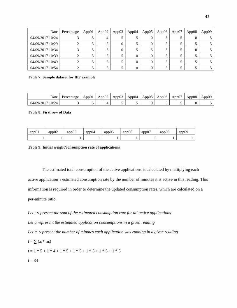
Date Percentage App01 App02 App03 App04 App05 App06 App07 App08 App09

04/09/2017 10:24 3 5 4 5 5 0 5 5 0 5

04/09/2017 10:29 2 5 5 0 5 0 5 5 5 5

04/09/2017 10:34 3 5 5 0 5 5 5 5 0 5

04/09/2017 10:39 2 5 5 5 0 0 5 5 5 5

04/09/2017 10:49 2 5 5 5 0 0 5 5 5 5

04/09/2017 10:54 2 5 5 5 0 0 5 5 5 5

Table 7: Sample dataset for IPF example

Date Percentage App01 App02 App03 App04 App05 App06 App07 App08 App09

04/09/2017 10:24 3 5 4 5 5 0 5 5 0 5

Table 8: First row of Data

app01 app02 app03 app04 app05 app06 app07 app08 app09

1 1 1 1 1 1 1 1 1

Table 9: Initial weight/consumption rate of applications

The estimated total consumption of the active applications is calculated by multiplying each

active application’s estimated consumption rate by the number of minutes it is active in this reading. This

information is required in order to determine the updated consumption rates, which are calculated on a

per-minute ratio.

Let t represent the sum of the estimated consumption rate for all active applications

Let a represent the estimated application consumptions in a given reading

Let m represent the number of minutes each application was running in a given reading

t = ∑ (ai * mi)

t = 1 * 5 + 1 * 4 + 1 * 5 + 1 * 5 + 1 * 5 + 1 * 5 + 1 * 5

t = 34

43

The battery percentage consumed by all open applications in the timestamp is 3%. The

following formula is used to determine the percentage that each individual application

consumed.

Let px represent the total percentage of battery consumed in a given reading

Let ay represent the estimated application consumption

ay1 = px * (ay / t)

app01 = 3 * (1 / 34) = 0.0882

app02 = 3 * (1 / 34) = 0.0882

app03 = 3 * (1 / 34) = 0.0882

app04 = 3 * (1 / 34) = 0.0882

app05 = 3 * (1 / 34) = not running

app06 = 3 * (1 / 34) = 0.0882

app07 = 3 * (1 / 34) = 0.0882

app08 = not running

app09 = 3 * (1 / 34) = 0.0882

Figure 10: Visual representation of how much each application contributed to the 3% drain

0.4412

0.3529

0.4412

0.4412

0.0000

0.4412

0.4412

0.0000 0.4412

Battery Drained 3%

App01

App02

App03

App04

App05

App06

App07

App08

App09

44

app01 app02 app03 app04 app05 app06 app07 app08 app09

0.0882 0.0882 0.0882 0.0882 1 0.0882 0.0882 1 0.0882

Table 10: Weight/consumption rate of applications after one iteration of IPF

Date Percentage App01 App02 App03 App04 App05 App06 App07 App08 App09

04/09/2017 10:29 2 5 5 0 5 0 5 5 5 5

Table 11: Second Row of Data

With the second row of data, the battery percentage consumed by all open applications is

2%. The same formula is used to determine both the estimated total consumption and percentage

that each application used.

t = ∑ (ai * mi)

t = 0.0882 * 5 + 0.0882 * 5 + 0.0882 * 5 + 0.0882 * 5 + 0.0882 * 5 + 1 * 5 + 0.0882 * 5

t = 7.646

ay1 = px * (ay / t)

app01 = 2 * (0.0882 / 7.646) = 0.02307

app02 = 2 * (0.0882 / 7.646) = 0. 02307

app03 = not running

app04 = 2 * (0.0882 / 7.646) = 0. 02307

app05 = not running

app06 = 2 * (0.0882 / 7.646) = 0. 02307

app07 = 2 * (0.0882 / 7.646) = 0. 02307

app08 = 2 * (1 / 7.646) = 0.26157

app09 = 2 * (0.0882 / 7.646) = 0. 02307

45

Figure 11: Visual representation of how much each application contributed to the 2% drain, based on the

updated weight/consumption values

app01 app02 app03 app04 app05 app06 app07 app08 app09

0.00252 0.00252 0.0882 0.00252 1 0.00252 0.00252 0.00252 0.00252

Table 12: Weight/consumption rate of applications after two iterations of IPF

This process is repeated with each subsequent row, and then repeated with the entire

dataset hundreds of times to normalize the data. The resulting data will contain estimated

consumption rates for each application. These values will approximately satisfy any row of the

original dataset. Multiplying the consumption rates of each active application in a given row by

the number of minutes they were active and summing them will produce the percentage drained

value of the row.

app01 app02 app03 app04 app05 app06 app07 app08 app09

0.023492 0.023492 0.243619

0.243619

0.23892 0.023492 0.023492 0.03892 0.023492

Table 13: Sample set of estimated battery consumption values after IPF has been performed

0.11535 0.11535 0

0.11535

0

0.11535

0.11535

1.30785

0.11535

Battery Drained 2% App01

App02

App03

App04

App05

App06

App07

App08

App09

46

After running iterating through the entire dataset one-thousand times, the resulting

consumption rates of each application are shown in Table 13. However, due to the small sample

size of data in the example, the values shown are not as accurate as they could be. A larger

dataset is used to illustrate the accuracy of this model.

47

5. Analysis

5.1. Additional Preprocessing

Three months of data was collected between September 3rd

2017 and December 7th

2017. Approximately two months of data is used for IPF, while the remaining month is used for

verification purposes. Readings prior to November 5th

, 2017 were used in the analysis, while the

remaining readings were used for the verification process. All readings were collected on a 2013

Sony Xperia Z. Only my personal device was used due to the type of information collected. As

the device is constantly monitoring when and how the user interacts with their smartphone, a lot

of personal information is extracted. Requesting approval from the University of Ontario

Institute of Technology Research Ethics Board would be a challenging endeavour that may have

required alterations to our collection process. As the limitations of the Android Software

Development Kit had already restricted the process, we made the decision to only collect from

my smartphone. This device was an ideal choice for the process, as the motivation for this

project stems from my experiences with this smartphone and its battery limitations. Only

collecting from one device will not impact IPF results, as each reading is tied to their respective

device.

The collected data was separated in two ways based on initial observations, Data or Wi-

Fi, and active or Idle. Data and Wi-Fi was personally logged whenever there was a switch

between the two modes. This would primarily occur when entering and leaving a building with

Wi-Fi access. Prior readings had indicated a difference in battery consumption; therefore these

attributes were recorded in the analyzed readings. Active and idle were also two attributes

discovered with preliminary readings. Initial baseline readings were established, with the device

48

unplugged and unused overnight. These readings illustrated a difference in consumption between

an active and idle device, as well as idle consumption between data and Wi-Fi.

Readings were divided between data and Wi-Fi before the preprocessing step in 4.1.

After the readings have been grouped, they are divided into active or idle readings. In order to

divide the results into active and idle usage, a script was used to parse through the table and

evaluate the readings based on the amount drained in a given period. The script functioned by

reading in a set of data. A set of data contained all of the readings within a given period that were

a maximum of 10 minutes apart. If all of the readings had an interval value of 1, and the number

of readings was greater than two, the set would be marked as active as it would indicate the

battery is draining by at least 1% every 5-10 minutes in a row. Similarly, if all readings had an

interval value of 3 or greater, with more than two readings in the set, it would indicate an

inactive period as the battery is draining slowly. If these conditions are not met, the script breaks

down the set information further and evaluates the rows with more specific parameters to

determine if they are active or idle.

After creating active and idle sets of data, IPF can then be performed to estimate

application usage. Results were gathered for active usage with data, idle usage with data, active

usage on Wi-Fi and idle usage on Wi-Fi.

49

5.2. Active Usage with Data

AppID Name Consumption rate per 5 minutes

165 droid.apps.maps 1.932657974

207 com.facebook.orca:browser 1.039852759

232 .katana:browser 1

190 com.android.captiveportallogin 0.765539191

197 com.facebook.orca:optsvc 0.603819035

40 com.google.android.syncadapter 0.599690383

75 com.sonyericsson.android.socia 0.522840798

77 com.sonymobile.providers.topco 0.47484536

55 com.ebay.kijiji.ca 0.473368041

278 com.brainium.sudoku.free 0.472535403

49 <pre-initialized> 0.365676633

256 com.google.android.apps.paidta 0.290160356

274 com.google.android.instantapps 0.261453193

166 com.boardgamegeek 0.258780575

85 com.google.android.gms.feedbac 0.258010442

229 com.guruse.LiveItGoodPlus 0.252240552

51 com.sonyericsson.album 0.233795264

81 com.facebook.katana:browser 0.200093306

205 com.ncix.app.android 0.132652856

71 com.facebook.katana:videoplaye 0.106030167

67 com.sonymobile.photoanalyzer 0.101657199

20 com.sonymobile.camerawidget 0.071377667

1 com.sonymobile.cameracommon 0.0489846

2 com.android.systemui 0.0489846

4 com.google.android.googlequick 0.0489846

6 com.sonyericsson.textinput.uxp 0.0489846

7 com.sonymobile.mx.android 0.0489846

8 com.sonymobile.googleanalytics 0.0489846

11 com.google.android.gms 0.0489846

13 com.android.smspush 0.0489846

17 com.google.android.gms.persist 0.0489846

48 com.example.alphabatterylifeap 0.0489846

93 com.google.android.tts 0.043937749

87 com.mobisystems.office 0.039739665

92 com.android.providers.partnerb 0.038270562

277 ileged_process1 0.026942868

90 com.android.partnerbrowsercust 0.021359353

50

80 com.sonyericsson.organizer 0.014464093

89 com.sonymobile.playanywhere 0.012146442

122 com.sonyericsson.metadataclean 0.012146442

126 com.sonyericsson.music:service 0.012146442

127 com.sonyericsson.music 0.012146442

185 com.sonyericsson.setupwizard 0.012146442

186 com.sonyericsson.simcontacts 0.012146442

249 com.spotify.music 0.012146442

Table 14: Table of local application ID, application name, and estimated consumption rate on active usage

with data. Only applications with an estimated consumption rate greater than 0.01 are shown.

5.3. Idle Usage with Data

AppID Name Consumption rate per 5 minutes

124 ca.transcontinental.android.sh 1.701331

37 com.google.android.youtube 0.910289

82 com.sonyericsson.soundenhancem 0.278741

87 com.mobisystems.office 0.278741

92 com.android.providers.partnerb 0.191252

55 com.ebay.kijiji.ca 0.165383

50 com.google.android.apps.docs 0.161907

58 com.sonyericsson.android.camer 0.150943

93 com.google.android.tts 0.138551

62 com.sonymobile.entrance 0.129608

28 com.mobisystems.fileman 0.094909

71 com.facebook.katana:videoplaye 0.09078

63 com.sonyericsson.conversations 0.089973

90 com.android.partnerbrowsercust 0.085423

219 com.passportparking.mobile.tor 0.07842

109 com.google.android.apps.messag 0.074704

194 com.timeplay 0.05798

94 com.sonymobile.tasks 0.052979

98 com.sonymobile.cameracommon.we 0.052766

88 com.andrewshu.android.reddit 0.044894

27 com.sonyericsson.xhs 0.042999

21 com.android.vending 0.039414

23 com.sonymobile.ree 0.029569

51

203 com.google.android.apps.docs.e 0.028461

38 com.google.android.talk 0.028132

184 com.sonyericsson.lockscreen.ux 0.016484

Table 15: Table of local application ID, application name, and estimated consumption rate on idle usage with

data. Only applications with an estimated consumption rate greater than 0.01 are shown.

5.4. Active Usage with Wi-Fi

AppID Name Consumption rate per 5 minutes

97 com.mobisystems.office:search 1.359471

37 com.google.android.youtube 1.07199

197 com.facebook.orca:optsvc 1

213 d.process.media 1

278 com.brainium.sudoku.free 1

169 android.youtube 0.889995

89 com.sonymobile.playanywhere 0.840852

92 com.android.providers.partnerb 0.760955

44 com.android.exchange 0.631718

103 com.google.android.configupdat 0.631718

122 com.sonyericsson.metadataclean 0.631718

126 com.sonyericsson.music:service 0.631718

127 com.sonyericsson.music 0.631718

163 com.android.email 0.631718

215 com.mobisystems.office.recentF 0.548113

138 csson.organizer 0.545455

152 .ebay.kijiji.ca 0.526994

49 <pre-initialized> 0.507042

98 com.sonymobile.cameracommon.we 0.5

51 com.sonyericsson.album 0.354524

90 com.android.partnerbrowsercust 0.30964

254 social.services 0.243819

256 com.google.android.apps.paidta 0.204825

113 com.android.documentsui 0.159741

114 com.android.externalstorage 0.159741

36 tv.twitch.android.app 0.138225

9 com.sonyericsson.home 0.135621

190 com.android.captiveportallogin 0.120099

52

144 com.sonymobile.entrance:com.so 0.110327

43 com.google.android.gms.unstabl 0.10019

174 com.mobisystems.office:pdf 0.067779

55 com.ebay.kijiji.ca 0.033984

1 com.sonymobile.cameracommon 0.026574

2 com.android.systemui 0.026574

4 com.google.android.googlequick 0.026574

6 com.sonyericsson.textinput.uxp 0.026574

7 com.sonymobile.mx.android 0.026574

8 com.sonymobile.googleanalytics 0.026574

11 com.google.android.gms 0.026574

13 com.android.smspush 0.026574

17 com.google.android.gms.persist 0.026574

48 com.example.alphabatterylifeap 0.026574

259 com.facebook.katana:notificati 0.026574

Table 16: Table of local application ID, application name, and estimated consumption rate on active usage

with Wi-Fi. Only applications with an estimated consumption rate greater than 0.01 are shown.

5.5. Idle Usage with Wi-Fi

AppID Name Consumption rate per 5 minutes

156 com.fivemobile.cineplex 1.469046

124 ca.transcontinental.android.sh 0.848586

113 com.android.documentsui 0.74905

216 ndroid.incallui 0.723009

165 droid.apps.maps 0.721754

33 com.ypg.rfd 0.623563

140 ny.nfx.app.sfrc 0.53125

67 com.sonymobile.photoanalyzer 0.341133

139 oid.smartsearch 0.315703

130 n.mShop.android 0.3

82 com.sonyericsson.soundenhancem 0.25

40 com.google.android.syncadapter 0.233619

116 sonymobile.dlna 0.214826

44 com.android.exchange 0.202419

119 com.google.android.marvin.talk 0.192747

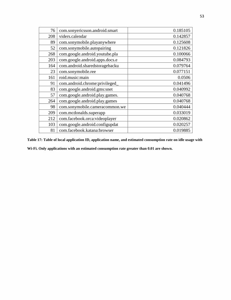
53

76 com.sonyericsson.android.smart 0.185105

208 viders.calendar 0.142857

89 com.sonymobile.playanywhere 0.125608

52 com.sonymobile.autopairing 0.121826

268 com.google.android.youtube.pla 0.100066

203 com.google.android.apps.docs.e 0.084793

164 com.android.sharedstoragebacku 0.079764

23 com.sonymobile.ree 0.077151

161 roid.music:main 0.0506

91 com.android.chrome:privileged_ 0.041496

83 com.google.android.gms:snet 0.040992

57 com.google.android.play.games. 0.040768

264 com.google.android.play.games 0.040768

98 com.sonymobile.cameracommon.we 0.040444

209 com.mcdonalds.superapp 0.033019

212 com.facebook.orca:videoplayer 0.020862

103 com.google.android.configupdat 0.020257

81 com.facebook.katana:browser 0.019885

Table 17: Table of local application ID, application name, and estimated consumption rate on idle usage with

Wi-Fi. Only applications with an estimated consumption rate greater than 0.01 are shown.

54

6. Verification

To verify the accuracy of the results, the generated values are compared to the last month

of recorded readings. A given reading has the percentage drained and the amount of time each

application was active for. With the consumption rates calculated through IPF and adjusting for

their length of activity, summing the calculated rates will give an approximation of the

percentage drained.

Date Percentage App01 App02 App03 App04 App05 App06 App07 App08 App09

05/10/2017 11:29 2 5 10 0 5 0 5 10 5 5

Table 18: Sample data for verification example

AppID Name Consumption rate per 1 minute

1 App01 0.02

2 App02 0.02

3 App03 0.06

4 App04 0.08

5 App05 0.22

6 App06 0.02

7 App07 0.06

8 App08 0.04

9 App09 0.08

Table 19: Sample consumption rates for verification example

Let Appx represent the amount of time an application is active in a given reading

Let ratex represent the estimated consumption rate per 1 minute of an application

Percentage Drained (PD) = 2.0%

Predicted Percentage Drained (PPD) = App01 * rate01 + App02 * rate02 + App03 * rate03 + App04 * rate04 +

App05 * rate05 + App06 * rate06 + App07 * rate07 + App08 * rate08 + App09 * rate09

PPD = 0.02 * 5 + 0.02 * 10 + 0.06 * 0 + 0.08 * 5 + 0.22 * 0 + 0.02 * 5 + 0.06 * 10 + 0.04 * 5 + 0.08 * 5

55

PPD = 0.1 + 0.2 + 0 + 0.4 + 0 + 0.1 + 0.6 + 0.2 + 0.4

PPD = 2.0%

Figure 12, Figure 13, Figure 14, and Figure 15 represent the accuracy of each type of

reading. Each value in the table is the percentage error between the estimated and actual

percentage drained. Any result that is not 0 indicates an incorrect estimation. The active data and

active Wi-Fi results are more varied in comparison to idle readings. This is because idle readings

primarily have a drain rate of 1%. Meanwhile, active readings have a diverse set of drain rates;

therefore the estimations are more inaccurate. A set of summary statistics are also provided in

Table 20.

Figure 12: Prediction results for active data readings

0

50

100

150

200

250

300

350

0 50 100 150 200 250 300

Pe

rce

nta

ge E

rro

r (%

)

Active Data Readings

Active Data Prediction

56

Figure 13: Prediction results for idle data readings

Figure 14: Prediction results for active Wi-Fi readings

0

100

200

300

400

500

600

0 50 100 150 200 250

Pe

rce

nta

ge E

rro

r (%

)

Idle Data Readings

Idle Data Prediction

0

50

100

150

200

250

0 50 100 150 200 250 300

Pe

rce

nta

ge E

rro

r (%

)

Active Wi-Fi Readings

Active Wi-Fi Prediction

57

Figure 15: Prediction results for idle Wi-Fi Readings

0

200

400

600

800

1000

1200

1400

1600

0 100 200 300 400 500 600 700 800

Pe

rce

nta

ge E

rro

r (%

)

Idle Wi-Fi Readings

Idle Wi-Fi Prediction

58

Type of Reading Mean Median Mode Range Standard Deviation

Active Data 53.89064557 49.53829753 20.00933062 298.652528 49.2808488

Idle Data 65.3578 48.09168 34.03614 524.5064 80.42148

Active Wi-Fi 56.55833 57.20596 57.20596 197.5374 25.61456

Idle Wi-Fi 125.6349 52.71312 44.16126 1425.947 204.44

Table 20: Summary statistics of calculated percentage error for each type of reading

59

7. Result Analysis

The results gathered appeared to be extremely volatile, as many of the values are

significantly different from their expected results. A notable problem within the dataset was

duplicate readings with different percentage drain rates. Multiple rows would have the exact

same applications active, but have varying percentage drain rates. This would impact the results

of IPF, as it is attempting to average out applications that drain at different rates. Similarly, many

rows would be nearly identical, but have minor differences. However, the corresponding

applications to these differences have negligible consumption rates, effectively making these

rows identical. These readings were removed and IPF was performed again in an attempt to

produce accurate results. Table 21 indicates the difference in row entries before and after

removing the duplicate entries.

Readings Old Amount After removing duplicate entries

Active Data Analysis 899 172

Active Data Verification 258 77

Idle Data Analysis 279 269

Idle Data Verification 206 177

Active Wi-Fi Verification 632 85

Active Wi-Fi November 254 161

Idle Wi-Fi Analysis 1303 731

Idle Wi-Fi Verification 684 362 Table 21: The number of readings before and after removing any entries with the same applications open

60

Figure 16: Prediction results for active data readings after removing duplicate entries

Figure 17: Prediction results for idle data readings after removing duplicate entries

0

20

40

60

80

100

120

140

160

0 10 20 30 40 50 60 70 80 90

Pe

rce

nta

ge E

rro

r (%

)

Active Data Readings

Active Data Prediction (Duplicates Removed)

0

100

200

300

400

500

600

700

800

900

0 50 100 150 200

Pe

rce

nta

ge E

rro

r (%

)

Idle Data Readings

Idle Data Prediction (Duplicates Removed)

61

Figure 18: Prediction results for active Wi-Fi readings after removing duplicate entries

0

50

100

150

200

250

300

350

400

0 20 40 60 80 100 120 140 160 180

Pe

rce

nta

ge E

rro

r (%

)

Active Wi-Fi Readings

Active Wi-Fi Prediction (Duplicates Removed)

62

Figure 19: Prediction results for idle Wi-Fi readings after removing duplicate entries

0

2000

4000

6000

8000

10000

12000

14000

0 50 100 150 200 250 300 350 400

Pe

rce

nta

ge E

rro

r (%

)

Idle Wi-Fi Readings

Idle Wi-Fi Prediction (Duplicates Removed)

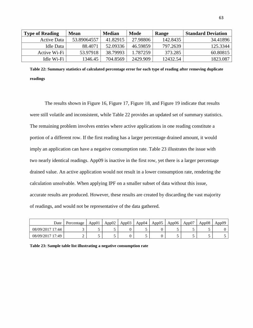
63

Type of Reading Mean Median Mode Range Standard Deviation

Active Data 53.89064557 41.82915 27.98806 142.8435 34.41896

Idle Data 88.4071 52.09336 46.59859 797.2639 125.3344

Active Wi-Fi 53.97918 38.79993 1.787259 373.285 60.80815

Idle Wi-Fi 1346.45 704.8569 2429.909 12432.54 1823.087

Table 22: Summary statistics of calculated percentage error for each type of reading after removing duplicate

readings

The results shown in Figure 16, Figure 17, Figure 18, and Figure 19 indicate that results

were still volatile and inconsistent, while Table 22 provides an updated set of summary statistics.

The remaining problem involves entries where active applications in one reading constitute a

portion of a different row. If the first reading has a larger percentage drained amount, it would

imply an application can have a negative consumption rate. Table 23 illustrates the issue with

two nearly identical readings. App09 is inactive in the first row, yet there is a larger percentage

drained value. An active application would not result in a lower consumption rate, rendering the

calculation unsolvable. When applying IPF on a smaller subset of data without this issue,

accurate results are produced. However, these results are created by discarding the vast majority

of readings, and would not be representative of the data gathered.

Date Percentage App01 App02 App03 App04 App05 App06 App07 App08 App09

08/09/2017 17:44 3 5 5 0 5 0 5 5 5 0

08/09/2017 17:49 2 5 5 0 5 0 5 5 5 5

Table 23: Sample table list illustrating a negative consumption rate

64

8. Discussion and Challenges

A detailed explanation of the data aggregation process, analysis, and results were presented.

Utilizing IPF to determine the average consumption rates of applications was not possible with the data

recorded. Calculating a single average rate of consumption for an application resulted in inaccurate

results. While an accurate and reliable solution was not determined, the experience allowed us to

document notable limitations both in data collection and analysis. This information will hopefully provide

others with insight into an alternative approach.

8.1. Insufficient information gathered

Tracking if an application was active or inactive, and using data or Wi-Fi was insufficient in

determining its consumption rate. While the information we can collect from a device is limited, our

approach was unable to calculate the average consumption rate. One issue is the list of active applications

is not an indicator that each one was utilized at an equal rate. A previously used application may be

running in the background unused, but is still picked up as an active application. If a user switches the

foreground application and uses something else, the previous application is not immediately closed. This

is a limitation that needs to be worked around, as only collecting the singular foreground application

would not be representative of the applications draining the battery.

8.2. Extend Period of Observation

IPF currently grouped readings based on the SOC decreasing after 5-10 minutes elapsed.

However, it may be necessary to extend readings for a longer duration and examine the changes within

that period. Observing the change in battery over the course of 30 minutes may provide insight that isn’t

considered in shorter durations.

65

8.3. Different Techniques Required

An alternative approach is needed to analyze the data provided. As previously mentioned in

Table 23, similar readings will have different consumption values, but the reading with fewer

applications active will have a greater value. This highlights the challenge of utilizing IPF to

determine an application’s consumption rate. In addition, readings with the same applications

open but different percentage drained values presented another problem. These readings could be

averaged out to a single consumption value; however the percentage drained for these readings

can vary from 1%-4%. The verification process of these entries would be inaccurate.

8.4. Expanding Acceptable Results

A single consumption rate for an application in each scenario may be insufficient.

Predicting a range of acceptable consumption values for each application may lead to higher

accuracy during the verification process. This approach would also solve the issue of similar

readings with different drain rates as shown in Table 23. A range of acceptable values would

accommodate the differences in these readings. However, this approach may also present

ineffective information if an application has a large range of acceptable results. It would also be

unable to predict the given consumption rate at a specific reading.

66

8.5. Identifying Applications

Two issues occurred when attempting to identify applications based on their name. The

first issue was a character limit in the database table. A 30 character limit was set for the

application name column, leading to a few incomplete names. However, the larger problem was

identifying what an application was used for. While the popular applications were easily

identified, many of the applications that were unused or had a low consumption were harder to

determine. While this did not impact the results of determining consumption rates, being able to

identify the applications and what they do would be useful. There did not appear to be a

centralized location to search for applications and their purpose. A community-driven website

where this information is collected would prove useful for future work in this field.

8.6. Future Work

There are still improvements to make and issues to solve before the application is fully

functional. The application currently collects the list of active applications separately from the

remaining battery data. Merging the collection process into one table would reduce the

preprocessing time. Future implementations for the client-side component would include general

functions that battery saving applications have, such as toggling Wi-Fi, data, GPS, display

settings, Bluetooth, and audio. However, the immediate problem to solve is finding a method of

accurately predicting the consumption rates of applications based on the limitations of the

Android API. A prediction algorithm on user behaviour was not observed within the scope of

this project, but would be the next step in providing meaningful feedback to the user. Once

67

enough time has passed and the user’s pattern is established, a prediction algorithm with accurate

consumption rates can advise the user based on the collected information.

While users will generally follow specific patterns, there will definitely be unpredictable

usage that must be addressed. An example would be a user commuting to work. They would

normally read the news on their phone, but decided to stream videos today. As videos consume a

lot of energy, it would lead to a significant adjustment to the expected usage of the device. If this

would cause the battery to deplete before a recharge is possible, the application would be forced

to interrupt and notify the user. If this can be implemented efficiently, users with older devices

would have a helpful tool that can manage their battery for them.

The database of collected information can also be re-examined in the future and is

publicly available (https://github.com/Changer628/Predicting-Mobile-Application-Power-

Consumption). A significant amount of data was collected, and can be used again with

alternative prediction methods. Certain aspects such as the battery temperature and voltage were

not used within this analysis, but may provide the additional resources required for more

accurate results. In addition, this information is not restricted to examining application

consumption rates, and may be useful in other areas of research as well. The readings represent a

user’s interaction with their smartphone for a period of 3 months. They provide insight into the

types of applications that were used, along with the amount of time they are accessed for.

Research that examines user behaviour would find this dataset useful.

68

9. Conclusion

As applications and smartphone devices become increasingly powerful, battery life remains a

large problem for users. Smartphones are capable of integrating many aspects of a user’s life,

leading us to become more dependent on them. As such, it is crucial they remain powered

throughout a user’s entire day, leading to research and examination on this topic. The current

implementations provide the changes that need to be made, but rely on repeated human

interaction. As people may forget and not be vigilant in these changes, they are not used

efficiently. The proposed application would be a first step in overcoming these challenges and

automating this process.

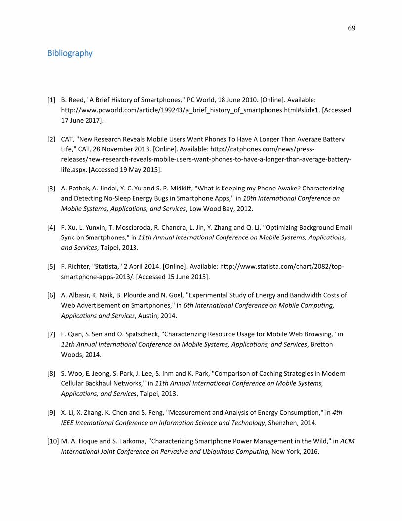
69

Bibliography

[1] B. Reed, "A Brief History of Smartphones," PC World, 18 June 2010. [Online]. Available:

http://www.pcworld.com/article/199243/a_brief_history_of_smartphones.html#slide1. [Accessed

17 June 2017].

[2] CAT, "New Research Reveals Mobile Users Want Phones To Have A Longer Than Average Battery

Life," CAT, 28 November 2013. [Online]. Available: http://catphones.com/news/press-

releases/new-research-reveals-mobile-users-want-phones-to-have-a-longer-than-average-battery-

life.aspx. [Accessed 19 May 2015].

[3] A. Pathak, A. Jindal, Y. C. Yu and S. P. Midkiff, "What is Keeping my Phone Awake? Characterizing

and Detecting No-Sleep Energy Bugs in Smartphone Apps," in 10th International Conference on

Mobile Systems, Applications, and Services, Low Wood Bay, 2012.

[4] F. Xu, L. Yunxin, T. Moscibroda, R. Chandra, L. Jin, Y. Zhang and Q. Li, "Optimizing Background Email

Sync on Smartphones," in 11th Annual International Conference on Mobile Systems, Applications,

and Services, Taipei, 2013.

[5] F. Richter, "Statista," 2 April 2014. [Online]. Available: http://www.statista.com/chart/2082/top-

smartphone-apps-2013/. [Accessed 15 June 2015].

[6] A. Albasir, K. Naik, B. Plourde and N. Goel, "Experimental Study of Energy and Bandwidth Costs of

Web Advertisement on Smartphones," in 6th International Conference on Mobile Computing,

Applications and Services, Austin, 2014.

[7] F. Qian, S. Sen and O. Spatscheck, "Characterizing Resource Usage for Mobile Web Browsing," in

12th Annual International Conference on Mobile Systems, Applications, and Services, Bretton

Woods, 2014.

[8] S. Woo, E. Jeong, S. Park, J. Lee, S. Ihm and K. Park, "Comparison of Caching Strategies in Modern

Cellular Backhaul Networks," in 11th Annual International Conference on Mobile Systems,

Applications, and Services, Taipei, 2013.

[9] X. Li, X. Zhang, K. Chen and S. Feng, "Measurement and Analysis of Energy Consumption," in 4th

IEEE International Conference on Information Science and Technology, Shenzhen, 2014.

[10] M. A. Hoque and S. Tarkoma, "Characterizing Smartphone Power Management in the Wild," in ACM

International Joint Conference on Pervasive and Ubiquitous Computing, New York, 2016.

70

[11] "Carat," Carat Team, 12 March 2018. [Online]. Available:

https://play.google.com/store/apps/details?id=edu.berkeley.cs.amplab.carat.android&hl=en.

[Accessed 22 May 2018].

[12] M. Kim, Y. G. Kim and S. W. Chung, "Measuring Variance between Smartphone Energy Consumption

and Battery Life," Computer, pp. 59-65, 16 August 2013.

[13] J. Lee, Y. Chon and H. Cha, "Evaluating Battery Aging on Mobile Devices," in 52nd Annual Design

Automation Conference, New York, 2015.

[14] B. D. Higgins, K. Lee, J. Flinn, T. Giuli, B. Noble and C. Peplin, "The Future is Cloudy: Reflecting

Prediction Error in Mobile Applications," in 2014 6th International Conference on Mobile

Computing, Applications and Services (MobiCASE), Austin, 2014.

[15] G. Kotsev, L. T. Nguyen, M. Zeng and J. Zhang, "User Exercise Pattern Prediction through Mobile

Sensing," in 6th International Conference on Mobile Computing, Applications and Services

(MobiCASE), Austin, 2014.

[16] M. F. Bulut, Y. S. Yilmaz, M. Demirbas, N. Ferhatosmanoglu and H. Ferhatosmanoglu, "LineKing:

Crowdsourced Line Wait-Time Estimation Using Smartphones," in 2012 4th International

Conference on Mobile Computing, Applications and Services (MobiCASE), Seattle, 2012.

[17] D. Gordon, S. Frauen and M. Beigl, "Reconciling Cloud and Mobile Computing using Predictive

Caching," in 2013 5th International Conference on Mobile Computing, Applications and Services

(MobiCASE), Paris, 2013.

[18] Y. Li, B. Luo, H. Chen and W. Shi, "One Charge for One Week: Hype or Reality?," in International

Green Computing Conference (IGCC), Dallas, 2014 .

[19] E. Rattagan, E. T. Chu, Y.-D. Lin and Y.-C. Lai, "Semi-Online Power Estimation for Smartphone

Hardware Components," in 10th IEEE International Symposium on Industrial Embedded Systems

(SIES), Siegen, 2015.

[20] E. Peltonen, E. Lagerspetz, P. Nurmi and S. Tarkoma, "Energy Modeling of System Settings:," in IEEE

International Conference on Pervasive Computing and Communications (PerCom), St. Louis, 2015.

[21] D. Anguita, A. Ghio, L. Oneto and S. Ridella, "Smartphone Battery Saving by Bit–Based Hypothesis

Spaces and," in International Joint Conference on Neural Networks (IJCNN), Beijing, 2014.

[22] "DU Battery Saver - Battery Charger & Battery Life," DU APPS STUDIO, 22 May 2018. [Online].

Available: https://play.google.com/store/apps/details?id=com.dianxinos.dxbs&hl=en. [Accessed 22

May 2018].

71

[23] "Battery Doctor(Battery Saver)," Cheetah Mobile Inc., 18 May 2018. [Online]. Available:

https://play.google.com/store/apps/details?id=com.ijinshan.kbatterydoctor_en. [Accessed 22 May

2018].

[24] S. V. Rajaraman, M. Siekkinen and M. A. Hoque, "Energy Consumption Anatomy of Live Video," in

CANDARW: The Fifth International Symposium on Computing and Networking Workshops, Aomori,

2017.

[25] M. Brocanelli and X. Wang, "Making Smartphone Smart on Demand for Longer Battery Life," in IEEE

37th International Conference on Distributed Computing Systems (ICDCS), Atlanta, 2017.

[26] J. Rummler, "GitHub," GitHub, 2016. [Online]. Available:

https://github.com/jaredrummler/AndroidProcesses. [Accessed 2nd February 2016].

[27] "Services," [Online]. Available: https://developer.android.com/guide/components/services.html.

[Accessed 22 June 2017].