BASICS ON THE THEORY OF INTEREST

CURSO DE MATEMÁTICA FINANCIERA TEORÍA Y EJERCICIOS

BASICS ON THE THEORY OF INTEREST

Applications to the Spanish financial market

Laura González‐Vila Puchades

Maite Mármol Jiménez

Francesc J. Ortí Celma

José B. Sáez Madrid

Departament de Matemàtica Econòmica, Financera i Actuarial

Universitat de Barcelona

i

PROLOGUE

This manuscript is intended for readers who are interested in knowing the basic concepts and mathematical tools that are currently used in financial markets. It is aimed at both university students who will require this knowledge when they start working in these markets and professionals who already work in them.

The book comprises four units. Unit 1, Financial transactions and financial regimes, deals with the time value of money as a main idea, as well as other related concepts such as financial capital, financial equivalence, simple and compound interest, annual effective interest rate, etc. Unit 2 is devoted to Annuities. In particular, level or constant annuities and varying annuities, both in geometric and in arithmetic progression are explained. A sound grounding of the first two units is essential to understand Unit 3 and Unit 4 which analyze Loans and Bonds, respectively. The manuscript concludes with some information sources.

Practically all the concepts introduced in the book are followed by illustrative examples. On the one hand, academic examples addressed to understand the theoretical foundations are stated. Additionally, the examples are supplemented with real examples taken from the financial market so that the reader can understand their practical and professional application. In this regards, all real applications considered are based on the Spanish financial market.

Furthermore, in order to assimilate properly the concepts in each unit, a set of problems to be solved is proposed, alongside a list of the correct answers.

The recommended approach for using this book is to read each unit, work on the embedded examples, and then to practice by solving the set of problems.

Please note that all content, as well as any mistakes that might be found, are the sole and exclusive responsibility of the authors. Should you find any errors, we would appreciate if you could let us know at [email protected].

The authors Barcelona, January 2021

iii

TABLE OF CONTENTS

Page

UNIT 1. FINANCIAL TRANSACTIONS AND FINANCIAL REGIMES

1. Financial transaction: Definition, elements and classification .................................................................. 1

1.1. Financial capital ................................................................................................................................. 1

1.2. Definition of financial transaction ..................................................................................................... 3

1.3. Elements of a financial transaction ................................................................................................... 3

1.4. Classification of financial transactions .............................................................................................. 5

2. Equilibrium in a financial transaction ........................................................................................................ 6

2.1. Financial equivalence ........................................................................................................................ 6

2.2. Financial equivalence representation ............................................................................................... 7

2.3. Accumulation and discount functions ............................................................................................... 8

2.4. Interest prices ................................................................................................................................. 10

3. Financial regime: Definition and classification ........................................................................................ 13

3.1. Definition of financial regimes ........................................................................................................ 13

3.2. Classification of financial regimes ................................................................................................... 13

4. Simple financial regimes .......................................................................................................................... 14

4.1. Simple interest regime .................................................................................................................... 14

4.2. Simple discount regime ................................................................................................................... 16

5. Compound financial regimes ................................................................................................................... 21

5.1. Compound interest with a constant interest rate regime .............................................................. 21

5.2. Compound interest with variable interest rates regime ................................................................. 27

5.3. Equivalent effective interest rates .................................................................................................. 29

5.4. Annual effective interest rate and TAE ........................................................................................... 31

6. Financial value ......................................................................................................................................... 36

6.1. Financial value at any moment in time ........................................................................................... 36

6.2. Present value and final value .......................................................................................................... 40

Unit 1 Problems ........................................................................................................................................... 44

UNIT 2. ANNUITIES

1. Definition and classification .................................................................................................................... 51

1.1. Definition ......................................................................................................................................... 51

1.2. Classification .................................................................................................................................... 52

2. Level or constant annuities ..................................................................................................................... 55

2.1. Definition ......................................................................................................................................... 55

iv

2.2. Financial value of the Non‐deferred immediate annuity with 𝑛 payments and period 𝑃 .............. 56

2.3. Financial value of the Non‐deferred immediate perpetuity with period 𝑃 ................................... 64

3. Annuities with payments in geometric progression ............................................................................... 66

3.1. Definition ......................................................................................................................................... 66



4. Annuities with payments in arithmetic progression ............................................................................... 73

4.1. Definition ......................................................................................................................................... 73



Unit 2 Problems ........................................................................................................................................... 81

UNIT 3. LOANS

1. Definition and classification .................................................................................................................... 85

1.1. Definition ......................................................................................................................................... 85

1.2. Classification .................................................................................................................................... 86

2. Outstanding loan balance. Other concepts ............................................................................................. 88

2.1. Outstanding loan balance ............................................................................................................... 88

2.2. Other concepts ................................................................................................................................ 91

3. Loan repaid by a single repayment ......................................................................................................... 94

4. Interest‐only loan .................................................................................................................................... 99

5. Amortizing loans with level repayments ............................................................................................... 105

6. Changes during the lifetime of the loan ................................................................................................ 118

Unit 3 Problems ......................................................................................................................................... 125

UNIT 4. BONDS

1. Definition and related concepts. Classification ..................................................................................... 131

1.1. Definition and related concepts .................................................................................................... 131

1.2. Classification .................................................................................................................................. 138

2. Zero‐coupon bonds ............................................................................................................................... 139

2.1. General characteristics .................................................................................................................. 139

2.2. Letras del Tesoro ........................................................................................................................... 140

3. Coupon bonds ....................................................................................................................................... 143

3.1. General characteristics .................................................................................................................. 143

3.2. Bonos y Obligaciones del Estado ................................................................................................... 146

Unit 4 Problems ......................................................................................................................................... 153

INFORMATION SOURCES .......................................................................................................................... 155

UNIT 1.

FINANCIAL TRANSACTIONS AND FINANCIAL REGIMES

1. Financial transaction:Definition, elements and classification

2. Equilibrium in a financial transaction

3. Financial regime: Definition and classification

4. Simple financial regimes

5. Compound financial regimes

6. Financial value

1. Financial transaction: Definition, elements and classification

1.1. Financial capital

1.2. Definition of financial transaction

1.3. Elements of a financial transaction

1.4. Classification of financial transactions

1.1. Financial capital

Prior to defining the concept of a financial transaction, we shouldhighlight that in a financial context it is not enough to just talk of a specificamount of money. It is also necessary to state when this amount will beavailable. This latter information is related to what is called the timevalue of money.

One of the core principles of finance states that money that is available atpresent is worth more than the same amount in the future, due to itspotential earning capacity. That is to say, the sooner any amount ofmoney is received, the more valuable it will be (time preference theory).

Unit 1. Financial transactions and financial regimes

1

BASI

CS

ON

TH

E TH

EOR

Y O

F IN

TER

EST.

App

licat

ions

to th

e Sp

anis

h fin

anci

al m

arke

t. L.

Gon

zále

z-Vi

la, M

. Már

mol

, F.J

. Ortí

& J

.B. S

áez

Bearing this idea in mind, we now define financial capital as anymonetary quantity at a specific moment in time:

𝐶,𝑇 𝐶 0,𝑇 0

where 𝐶 is the amount of money, which we will express in €, and 𝑇 is themoment in the future when the money will be available, which we willmeasure in years.

Financial capital is usually called payment(s) or repayment(s)depending on the economic agent who hands it over.

Example 1.

€500 available today is indicated as 500, 0

€1,000 available in one year is indicated as 1,000, 1

€350 available in fifteen months is indicated as 350,



Any financial capital can be represented graphically on the real line, fromthe origin 𝑇 0.



Example 2. The first, second and third financial capital contained inExample 1 can be represented on the real line, usually called a timeline,in the following way:

500 1,000 350

10 1512

years

2

BASI

CS

ON

TH

E TH

EOR

Y O

F IN

TER

EST.

App

licat

ions

to th

e Sp

anis

h fin

anci

al m

arke

t. L.

Gon

zále

z-Vi

la, M

. Már

mol

, F.J

. Ortí

& J

.B. S

áez



1.2. Definition of financial transaction

A financial transaction can be defined as the exchange, betweeneconomic agents, of payment(s) and repayment(s) at different momentsin time.

All financial transactions have the same elements: Personal Elements,Material Elements and Formal Elements.

1.3. Elements of a financial transaction

1) Personal elements

These are economic agents who partake in the financial transaction.

Active party or lender: this is the party that transfers payment(s) fora specific term. In exchange for this financial service, the active partyor lender receives a remuneration or price.

Passive party or borrower: this is the party that is committed toreturn payment(s) received and to pay a remuneration or price.



2) Material elements

Payment(s) handed over by the active party. When returned by thepassive party, including the price, the material element is calledrepayment(s).

3) Formal elements

Deals or conditions that are agreed on by lender and borrower. Theseconditions govern the financial transaction and specify, among otherthings, how the price is calculated, when this price is paid and the way inwhich the payment(s) that has been lent will be repaid by the borrower.

Example 3. Today, Juan deposits €10,000 in a fixed-term deposit, offeredby Bank Z, in exchange for receiving €10,500 in 13 months from now.The elements of this financial transaction are:

Personal elements

Active party or lender: Juan.

Passive party or borrower: Bank Z.

3

BASI

CS

ON

TH

E TH

EOR

Y O

F IN

TER

EST.

App

licat

ions

to th

e Sp

anis

h fin

anci

al m

arke

t. L.

Gon

zále

z-Vi

la, M

. Már

mol

, F.J

. Ortí

& J

.B. S

áez



For lending €10,000 today, in 13 months Juan will receive aremuneration, paid by Bank Z, of €500 in addition to repayment of the€10,000.

Material elements

Payment: €10,000 today or 10,000, 0

Repayment: €10,500 in 13 months or 10,500,

Formal element

The fixed term deposit agreement, signed by both parties, which laysout the conditions of this financial transaction.

Example 4. A company discounts today, at Bank Z, a trade bill with a face value of €2,500 which matures in 90 days, receiving €2,450. Now the elements are:

Personal elements

Active party or lender: Bank Z.

Passive party or borrower: The company.

For receiving €2,450 today, in exchange for €2,500 that will beavailable in 90 days, the company pays a price of €50. When thetrade bill matures, Bank Z will receive €2,500.

* This kind of transaction will be described in detail in Section 4.2 of this unit.

Material elements

Payment: €2,450 today or 2,450, 0

Repayment: €2,500 in 90 days or 2,500,

Formal element

The discount agreement, signed by both parties, that includes theconditions of this financial transaction.



4

BASI

CS

ON

TH

E TH

EOR

Y O

F IN

TER

EST.

App

licat

ions

to th

e Sp

anis

h fin

anci

al m

arke

t. L.

Gon

zále

z-Vi

la, M

. Már

mol

, F.J

. Ortí

& J

.B. S

áez

1.4. Classification of financial transactions

Financial transactions can be classified by considering different aspects.

Regarding the number of payment(s) and repayment(s) that the lenderand the borrower exchange:

1) Simple financial transaction

Both parties hand over only one payment and one repayment to theother.

2) Partially complex financial transaction

The active or the passive party gives the other party only onepayment or repayment while the other party transfers a set ofpayments or repayments to the former.

3) Complex financial transaction

Both parties transfer several payments or repayments to the other.



Example 5.

The financial transactions included in Examples 3 and 4 are simple.

A loan to be repaid in monthly instalments over the next 3 years is apartially complex financial transaction.

A pension scheme in which the active party will deposit different amountsin exchange for a guaranteed lifelong income, starting from the momentof retirement, is a complex financial transaction.

Regarding the party that is the focus of the study of the financialtransaction:

1) Interest (or accumulation) financial transaction

Financial capital is lent with the aim of receiving a greater amount ofcapital at the end of the term. In this case, the remuneration that isreceived by the active party is called interest.

2) Discount financial transaction

Financial capital that will be available in the future is anticipated at aprior moment in time. The price of such anticipation, which is paid bythe passive party, is now called a discount.



5

BASI

CS

ON

TH

E TH

EOR

Y O

F IN

TER

EST.

App

licat

ions

to th

e Sp

anis

h fin

anci

al m

arke

t. L.

Gon

zále

z-Vi

la, M

. Már

mol

, F.J

. Ortí

& J

.B. S

áez

Example 6.

The financial transaction included in Example 3 is an interest financialtransaction. The interest paid by the active party is equal to €500.

The financial transaction of Example 4 is a discount financial transaction.The active party pays a discount of €50.




2.1. Financial equivalence

2.2. Financial equivalence representation

2.3. Accumulation and discount functions

2.4. Interest prices

2.1. Financial equivalence

The economic agents involved in a financial transaction (lender andborrower) agree, in accordance with certain conditions, the payment(s)and repayment(s) to be exchanged.

Therefore, both parties consider them to be financially equivalent, that isto say, financial equivalence has been agreed on payment(s) andrepayment(s). We will symbolize financial equivalence by the symbol ~.


6

BASI

CS

ON

TH

E TH

EOR

Y O

F IN

TER

EST.

App

licat

ions

to th

e Sp

anis

h fin

anci

al m

arke

t. L.

Gon

zále

z-Vi

la, M

. Már

mol

, F.J

. Ortí

& J

.B. S

áez

2.2. Financial equivalence representation

Financial equivalence is represented in different ways, depending on thekind of financial transaction considered.

1) Simple financial transaction

Payment: 𝐶,𝑇

Repayment: 𝐶 ,𝑇′

Financial equivalence:𝐶,𝑇 ~ 𝐶 ,𝑇′

2) Partially complex financial transaction

Payment: 𝐶,𝑇Repayments: 𝐶 ,𝑇 , 𝐶 ,𝑇 ,⋯ , 𝐶 ,𝑇

Financial equivalence:𝐶,𝑇 ~ 𝐶 ,𝑇 , ,⋯,



Or alternatively:

Payments: 𝐶 ,𝑇 , 𝐶 ,𝑇 ,⋯ , 𝐶 ,𝑇

Repayment: 𝐶 ,𝑇′

Financial equivalence:

𝐶 ,𝑇, ,⋯,

~ 𝐶 ,𝑇′



3) Complex financial transaction

Payments: 𝐶 ,𝑇 , 𝐶 ,𝑇 ,⋯ , 𝐶 ,𝑇

Repayments: 𝐶 ,𝑇 , 𝐶 ,𝑇 ,⋯ , 𝐶 ,𝑇

Financial equivalence:

𝐶 ,𝑇, ,⋯,

~ 𝐶 ,𝑇 , ,⋯,

7

BASI

CS

ON

TH

E TH

EOR

Y O

F IN

TER

EST.

App

licat

ions

to th

e Sp

anis

h fin

anci

al m

arke

t. L.

Gon

zále

z-Vi

la, M

. Már

mol

, F.J

. Ortí

& J

.B. S

áez

2.3. Accumulation and discount functions

Let us consider a simple financial transaction of interest. The active partygives the passive party the financial capital 𝐶,𝑇 with the aim ofobtaining the financial capital 𝐶 ,𝑇′ , where 𝐶 𝐶 and 𝑇 𝑇. Thus, itcould be said that over the term of the financial transaction, 𝑡 𝑇 𝑇,the amount 𝐶 grows and becomes 𝐶 .

We define the accumulation function (or factor), denoted by 𝑓 𝑡 , asthe function that represents the way in which money grows as timegoes by.



In this way, the accumulation factor 𝑓 𝑡 can be understood as the finalamount obtained after 𝒕 years from an initial amount of €𝟏. So, wewrite:

𝐶 𝐶 𝑓 𝑡

Graphically:𝐶 𝐶 𝐶 𝑓 𝑡

𝑇′𝑇

Since 𝐶 𝐶 , it follows that in an interest financial transaction, theaccumulation function is greater than 1, i.e. 𝑓 𝑡 1.

That is:

𝑓 𝑡𝐶𝐶

Note that the accumulation factor is a function that depends on 𝒕 insuch a way that the greater the term of the financial transaction, thegreater the accumulated value, 𝐶 .

Finally, since 𝐶,𝑇 and 𝐶 ,𝑇′ are financially equivalent, the financialaccumulation factor can also be defined as the function that allows usto obtain the amount of money at 𝑻′ , 𝑪 , which is equivalent to 𝑪 at𝑻.



8

BASI

CS

ON

TH

E TH

EOR

Y O

F IN

TER

EST.

App

licat

ions

to th

e Sp

anis

h fin

anci

al m

arke

t. L.

Gon

zále

z-Vi

la, M

. Már

mol

, F.J

. Ortí

& J

.B. S

áez

Graphically:

𝐶 𝐶′ 𝑣 𝑡 𝐶

𝑇′𝑇

So, we write:𝐶 𝐶′ 𝑣 𝑡

To define the discount factor, we consider a simple financial transactionof discount. In this operation, a financial capital available at a futuremoment, 𝐶 ,𝑇′ , is anticipated at a previous moment in time, 𝑇. So, theamount at 𝑇, 𝐶, satisfies the relationship 𝐶 𝐶′ .

We define the discount function (or factor) and denote it by 𝑣 𝑡 , asthe function that allows us to obtain the amount of money at time 𝑻 ,𝑪, which is equivalent to 𝑪′ at time 𝑻′.



From the definition of the discount factor, it follows that

𝑣 𝑡𝐶𝐶′

and so it is straightforward to see that 𝑣 𝑡



Following similar reasoning to that in the case of the accumulation factor,it is also possible to affirm the following:

• The discount function represents the way in which money decreasesas it is anticipated from a future moment in time to a previous one.

• The discount factor 𝑣 𝑡 can be understood as the initial amountobtained by anticipating €𝟏 available in 𝒕 years.

• The discount factor is a decreasing function with respect to 𝒕.

Note also that the discount function is less than 1: 𝑣 𝑡 1.

9

BASI

CS

ON

TH

E TH

EOR

Y O

F IN

TER

EST.

App

licat

ions

to th

e Sp

anis

h fin

anci

al m

arke

t. L.

Gon

zále

z-Vi

la, M

. Már

mol

, F.J

. Ortí

& J

.B. S

áez

Accumulation function Discount function

Function that represents the way in which money grows as time goes by

Function that represents the way in which money decreases as it is anticipated from a future moment in time to a previous one

Final amount obtained after 𝒕 years from an initial amount of €𝟏

Initial amount obtained by anticipating €𝟏 available in 𝒕 years

𝑓 𝑡 1 𝑣 𝑡 1

𝑓 𝑡𝐶𝐶


Function that increases with respect to 𝒕 Function that decreases with respect to 𝒕

Function that allows us to obtain theamount of money at time 𝑇′ , 𝐶 , whichis equivalent to 𝐶 at the previous time 𝑇

Function that allows us to obtain the amount of money at time 𝑇 , 𝐶, which is equivalent to 𝐶′ at the later time 𝑇′



2.4. Interest prices

Given the simple financial transaction 𝐶,𝑇 ~ 𝐶 ,𝑇′ , with 𝑇 𝑇, wecan define the following interest prices.

1) Total interest. This is the total benefit obtained by the lender throughthe financial transaction, expressed in monetary units.

∆𝐶 𝐶 𝐶

Example 7. In the financial transaction 2,000, 0 ~ 2,320, 2 , the totalinterest is:

∆𝐶 2,320 2,000 €320

This means that in exchange for €2,000 given today, the lender receivesa total remuneration of €320 in 2 years.



10

BASI

CS

ON

TH

E TH

EOR

Y O

F IN

TER

EST.

App

licat

ions

to th

e Sp

anis

h fin

anci

al m

arke

t. L.

Gon

zále

z-Vi

la, M

. Már

mol

, F.J

. Ortí

& J

.B. S

áez

Example 8. In the financial transaction 2,000, 0 ~ 2,320, 2 , the unitprice is:

𝐼∆𝐶𝐶

𝐶 𝐶

𝐶2,320 2,000

2,0000.16 ≡ 16%

This means that for each euro given by the active party, they receive€0.16 in 2 years. Therefore, this interest could also be called 16%biennial*. Alternatively, we can also say that for each €100 given, €16 arereceived.* Biennial means once every 2 years. Biannual means twice every year.

2) Unit price of interest or effective interest rate. This is the benefitobtained for each monetary unit invested in the financial transaction.

𝐼∆𝐶𝐶

𝐶 𝐶

𝐶



3) Unit and mean price of interest or nominal interest rate. This isthe benefit obtained for each monetary unit and year.

𝑖𝐼

𝑇 𝑇𝐶 𝐶

𝐶 𝑇′ 𝑇𝐶 𝐶

𝐶 𝑡

Example 9. In the financial transaction 2,000, 0 ~ 2,320, 2 , the unit andmean price is:

𝑖𝐼

𝑇 𝑇𝐶 𝐶

𝐶 𝑇′ 𝑇0.16

20.08 ≡ 8%

This means that for each €100 given and for each year that the financialtransaction lasts, the lender receives €8.



11

BASI

CS

ON

TH

E TH

EOR

Y O

F IN

TER

EST.

App

licat

ions

to th

e Sp

anis

h fin

anci

al m

arke

t. L.

Gon

zále

z-Vi

la, M

. Már

mol

, F.J

. Ortí

& J

.B. S

áez

NOTE: When the term of a financial transaction is expressed in days orby calendar dates, the value of 𝑡 depends on the criterion used. Ingeneral, there are 4 criteria:

• If 𝑡 1,

• If 𝑡 1, it is necessary to add, to the number of whole years, theremaining fraction of the year that will be calculated according to oneof the previous criteria.

Criterion Meaning

30360

Numerator: All months have 30 days

Denominator: Always 360

𝐴𝑐𝑡360

Numerator: Actual days of the transaction


𝐴𝑐𝑡365



𝐴𝑐𝑡𝐴𝑐𝑡


Denominator: 365 or 366 (if it is a leap year)



Example 10. Obtain the term (in years) that exists between January 18 and April 18 of a leap year.

Criterion 𝑡30

360

𝐴𝑐𝑡360

𝐴𝑐𝑡365


𝑡12 30 30 18

36090

3600.25

𝑡13 29 31 18

36091

3600.2527

𝑡13 29 31 18

36591

3650.249315

𝑡13 29 31 18

36691

3660.248634



12

BASI

CS

ON

TH

E TH

EOR

Y O

F IN

TER

EST.

App

licat

ions

to th

e Sp

anis

h fin

anci

al m

arke

t. L.

Gon

zále

z-Vi

la, M

. Már

mol

, F.J

. Ortí

& J

.B. S

áez


3.1. Definition of financial regimes

3.2. Classification of financial regimes

3.1. Definition of financial regimes

A financial regime is the formal expression of the set of deals orconditions that both parties agree on in a financial transaction. Theserefer to how the price of the transaction is calculated and when it is paid.


3.2. Classification of financial regimes

Depending on how the price is calculated:

1) Simple financial regimes. These are those in which the term of thefinancial transaction is considered as a single period and, therefore,the price is calculated only once. Simple financial regimes are used inshort-term financial transactions.

2) Compound financial regimes. These are those in which the term ofthe financial transaction is split into periods and, therefore, the price iscalculated for each of them.

Regarding the economic agent:

1) Interest financial regime. The financial transaction is studied fromthe perspective of the active party.

2) Discount financial regime. The financial transaction is analyzed fromthe point of view of the passive party.

As a consequence of both classifications, we will study the followingfinancial regimes:

INTEREST DISCOUNT

SIMPLE SIMPLE INTEREST SIMPLE DISCOUNT

COMPOUND COMPOUND INTEREST WITH A CONSTANT INTEREST RATE

COMPOUND INTEREST WITH VARIABLE INTEREST RATES



13

BASI

CS

ON

TH

E TH

EOR

Y O

F IN

TER

EST.

App

licat

ions

to th

e Sp

anis

h fin

anci

al m

arke

t. L.

Gon

zále

z-Vi

la, M

. Már

mol

, F.J

. Ortí

& J

.B. S

áez


4.1. Simple interest regime

4.2. Simple discount regime

4.1. Simple interest (payable in arrears) regime

If a financial transaction is ruled by a simple interest regime, it means thatboth the active and the passive party have agreed on the following:

1) The total price of the transaction, ∆𝐶, is proportional to the initialamount, 𝐶, and to the term of the operation, 𝑡 𝑇 𝑇, through arate, measured as per 1: 𝑖 0.

∆𝐶 𝐶 𝑖 𝑇 𝑇 𝐶 𝑖 𝑡2) The total price is received at the end of the financial transaction 𝑇′,

with the repayment of the initial amount, so the final amount repaid is𝐶′.

𝐶 𝐶 ∆𝐶Thus, the formal expression of both conditions is:

𝐶 𝐶 𝐶 𝑖 𝑡


which is equivalent to:

𝐶 𝐶 1 𝑖 𝑡



The simple interest regime is commonly used for short-term financialtransactions such as current accounts, savings accounts, fixed-termdeposits, loads repaid through a simple repayment, etc.

Since:

𝐶 𝐶 1 𝑖 𝑡 𝐶

𝑇′𝑇

It turns out that the accumulation function of the simple interest regime is:

𝑓 𝑡𝐶′𝐶

1 𝑖 𝑡

14

BASI

CS

ON

TH

E TH

EOR

Y O

F IN

TER

EST.

App

licat

ions

to th

e Sp

anis

h fin

anci

al m

arke

t. L.

Gon

zále

z-Vi

la, M

. Már

mol

, F.J

. Ortí

& J

.B. S

áez

Furthermore, we can obtain the following interest prices.

Total price of interest:

∆𝐶 𝐶 𝐶 𝐶 𝑖 𝑡

Unit price of interest or effective interest rate:

𝐼∆𝐶𝐶

𝐶 𝑖 𝑡 𝐶

𝑖 𝑡

Unit and mean price of interest or nominal interest rate:

𝑖𝐼𝑡

𝑖 𝑡 𝑡

𝑖



Example 11. Determine the final capital and interest prices obtained byinvesting €8,000 in a fixed-term deposit, which matures in 91 days (usethe Act/365 criterion), at an annual simple interest rate of 1.75%.

8,000 𝐶

91/3650

The final amount is:

𝐶 𝐶 1 𝑖 𝑡 8,000 1 0.017591

365 €8,034.90

The interest prices are:∆𝐶 8,034.90 8,000 €34.90

𝐼∆𝐶𝐶

𝑖 𝑡 0.017591

3650.004363 ≡ 0.4363%

𝑖𝐼𝑡

0.00436391

365

0.0175 ≡ 1.75%

Effective rate earned in 91 days

Nominal rate

Total price



15

BASI

CS

ON

TH

E TH

EOR

Y O

F IN

TER

EST.

App

licat

ions

to th

e Sp

anis

h fin

anci

al m

arke

t. L.

Gon

zále

z-Vi

la, M

. Már

mol

, F.J

. Ortí

& J

.B. S

áez

Example 12. How many years will it take to double capital invested todayat an annual simple interest rate equal to 5%?


2𝐶 𝐶 1 0.05 𝑡 ⇔ 2 1 0.05 𝑡 ⇔ 1 0.05 𝑡

𝑡 20 years

𝐶 𝐶 2𝐶

𝑡0



4.2. Simple (commercial) discount regime

In a financial transaction ruled by a simple discount regime, the activeand passive parties agree on the following:

1) A financial capital available at a future moment, 𝐶 ,𝑇′ , is anticipatedat a previous moment, 𝑇. The total price of the transaction, ∆𝐶, isproportional to the final amount, 𝐶′, and to the term of the operation,𝑡 𝑇 𝑇, through a rate, measured as per 1: 𝑑 0.

∆𝐶 𝐶′ 𝑑 𝑇 𝑇 𝐶′ 𝑑 𝑡2) The total price is paid at the beginning of the financial transaction, 𝑇,

and is deducted from the final amount, so the amount 𝐶 is received.

𝐶 𝐶 ∆𝐶Thus, the formal expression of both conditions is:

𝐶 𝐶 𝐶′ 𝑑 𝑡

𝐶 𝐶′ 1 𝑑 𝑡



Face value𝑡 𝑇 𝑇

Maturity or Due date

16

BASI

CS

ON

TH

E TH

EOR

Y O

F IN

TER

EST.

App

licat

ions

to th

e Sp

anis

h fin

anci

al m

arke

t. L.

Gon

zále

z-Vi

la, M

. Már

mol

, F.J

. Ortí

& J

.B. S

áez

The simple discount regime is commonly used to discount bills ofexchange, trade bills or commercial bills. A bill of exchange is adocument issued by the seller (drawer) and accepted/signed by thebuyer (drawee) for the value of goods delivered by the former.

This document obliges the buyer to pay a particular amount of money(face value of the bill of exchange) at a particular time (maturity or duedate) in the short-term.

Once the bill of exchange has been issued and accepted, its owner (theseller of the goods) can either keep it until its maturity date and receiveits face value at that moment from the buyer, or discount (and give) it ata bank and receive a lower amount than the face value. This is why wesay that in the simple discount regime, a financial capital available at afuture moment is anticipated at a previous moment in time.

If the bill of exchange is discounted, the bank (its new owner) will havethe right to receive its face value, from the buyer, on its maturity date.



Graphically:

In this case, since we are studying the financial transaction from theperspective of the passive party, it makes sense to obtain the discountfunction, which is:


1 𝑑 𝑡

𝑇′𝑇

𝐶 𝐶′ 1 𝑑 𝑡 𝐶

Moreover, it is possible to obtain the following discount prices.

Total price of discount:

∆𝐶 𝐶 𝐶 𝐶′ 𝑑 𝑡



17

BASI

CS

ON

TH

E TH

EOR

Y O

F IN

TER

EST.

App

licat

ions

to th

e Sp

anis

h fin

anci

al m

arke

t. L.

Gon

zále

z-Vi

la, M

. Már

mol

, F.J

. Ortí

& J

.B. S

áez

Unit price of discount or effective discount rate:

𝐷∆𝐶𝐶′

𝐶′ 𝑑 𝑡 𝐶′

𝑑 𝑡

Unit and mean price of discount or nominal discount rate:

𝑑𝐷𝑡

𝑑 𝑡 𝑡

𝑑



Example 13. Determine the amount obtained by the discount of a tradebill with a face value of €3,200, if it matures in 3 months and a simplediscount regime at an annual discount rate of 4.50% is applied.Determine also the discount prices.

So, the amount obtained is:

𝐶 𝐶′ 1 𝑑 𝑡 3,200 1 0.04503

12 €3,164

312

0

𝐶 3,200

Discount prices:

∆𝐶 3,200 3,164 €36

𝐷∆𝐶𝐶′

363,200

0.01125 ≡ 1.125%

𝑑𝐷𝑡

0.011253 12⁄

0.045 ≡ 4.50%

Effective rate payed within 3

months

Nominal rate

Total price



18

BASI

CS

ON

TH

E TH

EOR

Y O

F IN

TER

EST.

App

licat

ions

to th

e Sp

anis

h fin

anci

al m

arke

t. L.

Gon

zále

z-Vi

la, M

. Már

mol

, F.J

. Ortí

& J

.B. S

áez

When applying the simple interest regime, the price is paid at the end ofthe financial transaction, at an interest rate 𝑖; but in the simple discountregime, the price is paid at the beginning, at a discount rate 𝑑.

So, from the perspective of the borrower, a question may arise:

What is the maximum annual simple interest rate I would have to payin a simple interest regime to borrow the same initial amount that Iobtained in the simple discount regime, and then repay this amountwith the face value of the trade bill when it matures?

In order to answer this question, let us find the equivalence between therates, 𝑖 and 𝑑.

Simple interest regime: 𝐶 𝐶 1 𝑖 𝑡

Simple discount regime: 𝐶 𝐶′ 1 𝑑 𝑡

By replacing the second expression into the first one, we get:

𝐶 𝐶 1 𝑑 𝑡 1 𝑖 𝑡 ⟺ 1 1 𝑑 𝑡 1 𝑖 𝑡

𝑖𝑑

1 𝑑 𝑡1 𝑖 𝑡1

1 𝑑 𝑡⇔ 𝑖 𝑡

𝑑 𝑡1 𝑑 𝑡



Example 14. With the information contained in Example 13, find theequivalent annual simple interest rate.

By using the previous expression:

𝑖𝑑

1 𝑑 𝑡0.045

1 0.045 3/120.045512 ≡ 4.5512%

This result could also be obtained by using the formal expression of thesimple interest regime, 𝐶 𝐶 1 𝑖 𝑡 , and substituting all theknown magnitudes except 𝑖:

3,200 3,164 1 𝑖3

12 ⟺ 𝑖 0.045512 ≡ 4.5512%

This means that, for the borrower, discounting a trade bill with a facevalue of €3,200 and maturity in 3 months at an annual discount rate of4,50%, is equivalent to borrowing €3,200 for 3 months at an annualsimple interest rate of 4.55%, and then repaying it with the face value ofthe trade bill when it matures.

It can also be understood that this financial transaction results in aprofitability of a 4.55% annual simple interest rate for the bank.



19

BASI

CS

ON

TH

E TH

EOR

Y O

F IN

TER

EST.

App

licat

ions

to th

e Sp

anis

h fin

anci

al m

arke

t. L.

Gon

zále

z-Vi

la, M

. Már

mol

, F.J

. Ortí

& J

.B. S

áez

Financial impact of the initial commissions on the commercialdiscount

Sometimes, when the simple discount regime is used, not only is thenominal discount rate, 𝑑 , charged but so is an initial fee. This fee,measured as per 1, 𝑔 , is applied to the face value of the commercial billin such a way that we calculate the amount 𝐶 that the borrower will finallyreceive as follows:

𝐶 𝐶 1 𝑑 𝑡 𝑔 𝐶

𝐶 𝐶 1 𝑑 𝑡 𝑔

If a simple discount transaction has an initial fee, in order to obtain theequivalent annual simple interest rate, it is necessary to use the knownexpression of the simple interest regime.

NOTE: If the term of the financial transaction, 𝑡, is expressed in days orby calendar dates, the criterion Act/360 will be used for thedetermination of the term, unless stated otherwise.



Example 15. A company has a portfolio of bills of exchange with a facevalue of €12,500 and a due date of 96 days. Today, it discounts theportfolio at its bank and is charged with an annual simple discount rate of6%. The financial transaction involves an initial fee of 0.7% of the facevalue. Calculate:

1) The amount obtained by the company after discounting the portfolio.

2) The equivalent annual simple interest rate of this financial transaction.Use the criterion Act/365.

So, the amount obtained by the company is:

𝐶 𝐶 1 𝑑 𝑡 𝑔 12,500 1 0.0696

3600.007 €12,212.50

96360

0

𝐶 12,500

𝑑 0.06𝑔 0.007 €12,500



20

BASI

CS

ON

TH

E TH

EOR

Y O

F IN

TER

EST.

App

licat

ions

to th

e Sp

anis

h fin

anci

al m

arke

t. L.

Gon

zále

z-Vi

la, M

. Már

mol

, F.J

. Ortí

& J

.B. S

áez

where 12,500 0.06 €200 is the total discount paid and

12,500 0.007 €87.5 is the initial fee.

To calculate the equivalent annual simple interest rate, it is necessary touse the simple interest regime expression:


12,500 12,212.5 1 𝑖96

365⟺ 1 𝑖

96365

1.023541

𝑖 0.089507 ≡ 8.9507%

NOTE: The expression 𝑖 obtained in the previous pages cannot

be used in this case because it does not consider situations in whichthere exists an initial fee. Hence, it is necessary to use the generalexpression of the simple interest rate.



A compound interest regime arises when the term of the financialtransaction is split into periods, and the interest is calculated at the end ofthese periods and is simultaneously reinvested in order to earn additionalinterest in the following periods.

For this regime, we consider the following variables:

𝑝 : length (in years) of the period into which the term of the transaction issplit, it will be called capitalization period.

𝑚: capitalization frequency, number of periods of length 𝑝 in 1 year.

Thus, 𝑚 .


5.1. Compound interest with a constant interest rate regime

5.2. Compound interest with variable interest rates regime

5.3. Equivalent effective interest rates

5.4. Annual effective interest rate and TAE

5.1. Compound interest with a constant interest rate regime


21

BASI

CS

ON

TH

E TH

EOR

Y O

F IN

TER

EST.

App

licat

ions

to th

e Sp

anis

h fin

anci

al m

arke

t. L.

Gon

zále

z-Vi

la, M

. Már

mol

, F.J

. Ortí

& J

.B. S

áez

𝑛: number of capitalization periods in the term of the transaction. So,𝑛 𝑚 𝑡.

𝑖 : nominal interest rate, annual interest rate applied each period.

𝐼 : effective interest rate per period. 𝐼 𝑖 𝑝, and since 𝑝 , it

turns out that:

𝐼𝑖𝑚

Example 16. The nominal interest rate is 6% and the term of the financialtransaction is 5 years, 𝑡 5 :

• If it is split into 6-month periods: 𝑝 years, 𝑚 2,

𝑛 2 5 10 periods, 𝑖 0.06 and 𝐼 0.03 ≡ 3%.

• If it is split into quarters (or 3-month periods): 𝑝 years, 𝑚 4,

𝑛 4 5 20 quarters, 𝑖 0.06 and 𝐼 0.015 ≡ 1.5%.



It is worth noting how banks advertise both nominal and effective interest rates.

For nominal interest rates:

And for effective interest rates:

annuallyquarterly

semi-annuallymonthly

…

convertiblecompounded

payableaccumulated

…

nominalannual

𝑖 %

𝐼 %

annualquarterly

semi-annualmonthly

…

(effective) interest rate



22

BASI

CS

ON

TH

E TH

EOR

Y O

F IN

TER

EST.

App

licat

ions

to th

e Sp

anis

h fin

anci

al m

arke

t. L.

Gon

zále

z-Vi

la, M

. Már

mol

, F.J

. Ortí

& J

.B. S

áez

𝑖 0.015 ≡ 1.5%

𝐼 0.008 ≡ 0.8%

𝐼 . 0.16 ≡ 16%

𝑖 0.04 ≡ 4%

𝑖 0.021 ≡ 2.1%

Example 17. For the following statements, write down the correspondinginterest rate:

• 1.5% annual interest rate compounded monthly.

• 0.8% semi-annual interest rate.

• Biennial interest rate of 16%.

• Nominal interest rate convertible quarterly equal to 4%.

• 2.1% annual interest rate accumulated every two months.



Now, we obtain the formal expression corresponding to the compoundinterest regime by first considering its conditions.

If a financial transaction is governed by a regime of compound interestwith a constant interest rate, it means that both the active and thepassive party have agreed on the following:

1) The term of the financial transaction, 𝑡 𝑇 𝑇, is split into 𝑛 periodsof length 𝑝 (in years). So, 𝑡 𝑛 𝑝. The interest is calculated at theend of each period by an effective interest rate, measured as per 1,𝐼 0, applied on the amount accumulated at the beginning ofthe period. The interest for each period is added to theaforementioned amount in such a way that the accumulated amountat the end of a period is the same as the initial amount of the followingperiod.

2) Although the price is calculated in each period, the total price is onlyreceived once, at the end of the financial transaction, 𝑇 .

Graphically:



23

BASI

CS

ON

TH

E TH

EOR

Y O

F IN

TER

EST.

App

licat

ions

to th

e Sp

anis

h fin

anci

al m

arke

t. L.

Gon

zále

z-Vi

la, M

. Már

mol

, F.J

. Ortí

& J

.B. S

áez

Hence, the accumulated amount at the end of each period will be:

𝐶

𝑇 𝑇 𝑛𝑝𝑇𝐼

𝑇 2𝑝𝑇 𝑝 𝑇 𝑛 1 𝑝

𝐶 𝐶 𝐶′…

𝐼 𝐼

𝐶

…𝑇 3𝑝

𝐶

𝐼

Time Accumulated amount

𝑇 𝐶

𝑇 𝑝 𝐶 𝐶 𝐶 𝐼 𝐶 1 𝐼

𝑇 2𝑝 𝐶 𝐶 𝐶 𝐼 𝐶 1 𝐼 𝐶 1 𝐼

𝑇 3𝑝 𝐶 𝐶 𝐶 𝐼 𝐶 1 𝐼 𝐶 1 𝐼

… …

𝑇 𝑇 𝑛𝑝 𝐶′ 𝐶 1 𝐼

As we saw, 𝑛 𝑚 𝑡, so we can rewrite the above expression as:

𝐶′ 𝐶 1 𝐼



Many financial transactions are governed by a compound interest regime,both at a constant interest rate and at variable interest rates. Examplesinclude investment funds, pension schemes and loans; all of which sharea common characteristic, that of being arranged in medium or long-termoperations.

Since:

𝐶 𝐶 𝐶 1 𝐼

𝑇′𝑇

It turns out that the accumulation function of the compound interestregime would be:

𝑓 𝑡𝐶′𝐶

1 𝐼



24

BASI

CS

ON

TH

E TH

EOR

Y O

F IN

TER

EST.

App

licat

ions

to th

e Sp

anis

h fin

anci

al m

arke

t. L.

Gon

zále

z-Vi

la, M

. Már

mol

, F.J

. Ortí

& J

.B. S

áez

As we will see later, this regime can also be used in discounttransactions. So, the discount function associated with the compoundinterest rate is:


1 𝐼

which, on the timeline, can be represented graphically as:

𝑇′𝑇

𝐶 𝐶′ 1 𝐼 𝐶

𝑇′𝑇

𝐶 𝐶

1 𝐼

1 𝐼

𝐶 𝐶′ 1 𝐼

𝐶 𝐶 1 𝐼

Discount:

Accumulation:

𝐼𝑖𝑚

𝑛 𝑚 𝑡

Summarizing:



12,000 𝐶

50TODAY

𝑚 4𝑖 0.03

𝐼0.03

40.0075

Example 18. An investor deposits €12,000 today in a savings accountthat pays a nominal interest rate compounded quarterly of 3%. He makesno further deposits or withdrawals until he closes the account, 5 yearsafter he opened it. How much money does the investor receive when hecancels the account?

The amount obtained is:

𝐶 𝐶 1 𝐼 12,000 1 0.0075 €13,934.21



25

BASI

CS

ON

TH

E TH

EOR

Y O

F IN

TER

EST.

App

licat

ions

to th

e Sp

anis

h fin

anci

al m

arke

t. L.

Gon

zále

z-Vi

la, M

. Már

mol

, F.J

. Ortí

& J

.B. S

áez

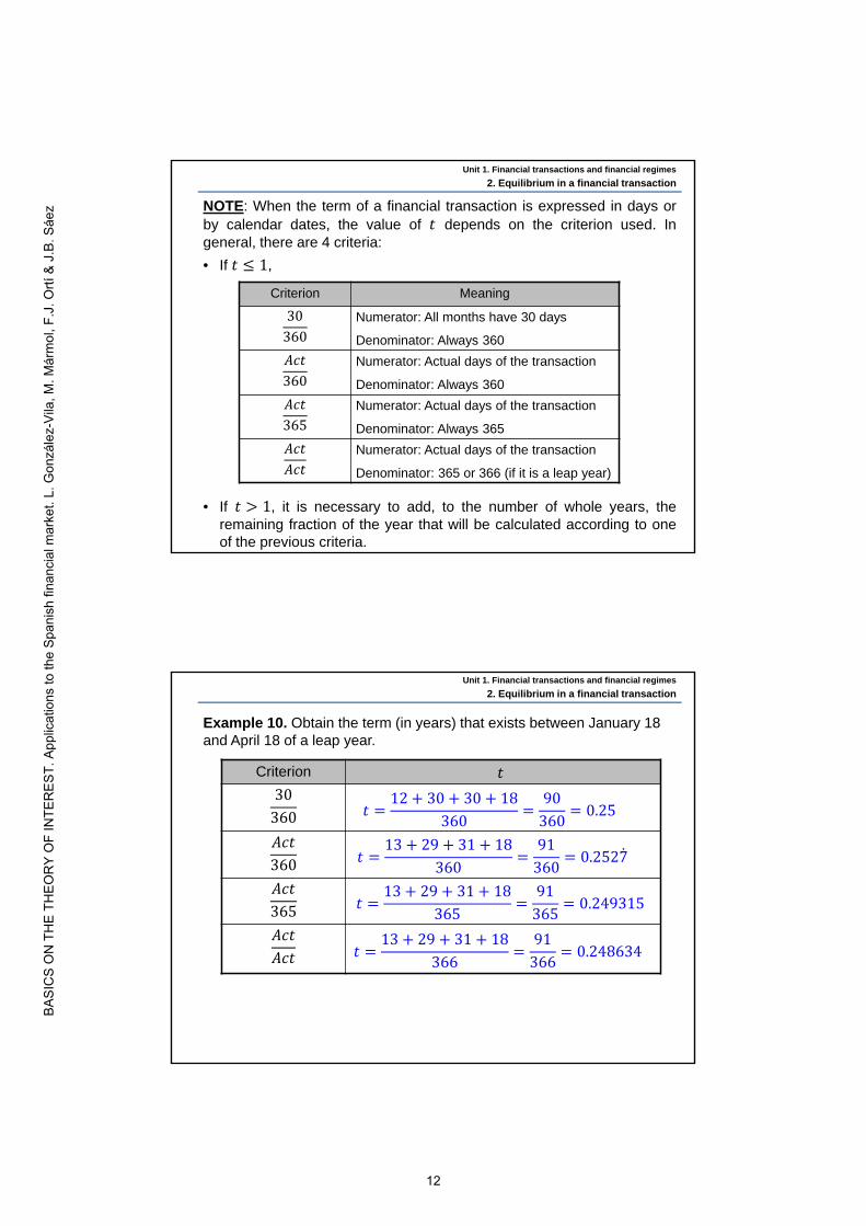
Example 19. What deposit made today will provide a payment of €1,800in 1 and a half years if the financial transaction is governed by a 0.2%semi-annual effective interest rate?

The deposit is:

𝐶 𝐶′ 1 𝐼 1,800 1 0.002 . €1,789.24

1.50TODAY

𝐶 1,800 𝑚 2𝐼 0.002



Example 20. How many years will it take to double capital invested todayat a nominal interest rate of 5% compounded annually?

𝐶 𝐶 2𝐶

𝑡0

𝑚 1𝑖 0.05

𝐼0.05

10.05

𝐶 𝐶 1 𝐼

2𝐶 𝐶 1 0.05 ⟺ 2 1.05 ⟺ 𝑡ln2

ln1.0514.21 years



26

BASI

CS

ON

TH

E TH

EOR

Y O

F IN

TER

EST.

App

licat

ions

to th

e Sp

anis

h fin

anci

al m

arke

t. L.

Gon

zále

z-Vi

la, M

. Már

mol

, F.J

. Ortí

& J

.B. S

áez

5.2. Compound interest with variable interest rates regime

All the conditions in this regime are the same as in the regime above.However, the interest rate varies over the term of the financialtransaction.

In such a situation, it is easy to check that:

𝐶′ 𝐶 1 𝐼

𝐶

𝑇 𝑇 𝑛𝑝𝑇 𝑇 2𝑝𝑇 𝑝 𝑇 𝑛 1 𝑝

𝐶 𝐶 𝐶′… 𝐶

…𝑇 3𝑝

𝐶

𝐼 𝐼 𝐼 𝐼



Example 21. Bank Z offers a fixed-term deposit for 3 years at an interestrate convertible semi-annually. The nominal interest rate changes everyyear. If it is 1.5%, 1.4% and 1.3%, for the first, second and third year,respectively, and €2,500 is deposited today, what will the accumulatedamount be?

So, the accumulated amount is:

2,500

0 21 3

𝐶′

𝑖 0.015

𝐼0.015

20.0075

𝑖 0.014

𝐼0.014

20.007

𝑖 0.013

𝐼0.013

20.0065

2,537.64

2,573.29

1 0.007 1 0.0065 €2,606.85𝐶 2,500 1 0.0075



27

BASI

CS

ON

TH

E TH

EOR

Y O

F IN

TER

EST.

App

licat

ions

to th

e Sp

anis

h fin

anci

al m

arke

t. L.

Gon

zále

z-Vi

la, M

. Már

mol

, F.J

. Ortí

& J

.B. S

áez

Example 22. An account is governed by compound interest. The annualinterest rate for the first 2 years is 2%, for the next 3 years the nominalinterest rate is 2.2% compounded semi-annually and for the last year thequarterly effective interest rate is 0.5%.

• Find the accumulated value at the end of 6 years if the initial amount is €4,600.

𝐶 4,600 1 0.02 1 0.011 1 0.005

𝐶 €5,213.50

• Find the initial amount that should have been deposited to have an accumulated value of €5,250 at the end of 6 years.

In this case, by discounting, we will have:

4,600

0 52 6

𝐶′𝐼 0.02 𝐼 0.005𝑖 0.022

𝐼0.022

20.011



𝐶 5,250 1 0.005 1 0.011 1 0.02

𝐶 €4,632.20

• Find the annual effective interest rate that would have been paid overthe 6 years in order to get €5,213.50 by depositing €4,600.

5,213.50 4,600 1 𝐼

𝐶

0 52 6

5,250𝐼 0.02 𝐼 0.005𝑖 0.022

𝐼0.022

20.011

4,600

0 6

5,213.50

𝐼



28

BASI

CS

ON

TH

E TH

EOR

Y O

F IN

TER

EST.

App

licat

ions

to th

e Sp

anis

h fin

anci

al m

arke

t. L.

Gon

zále

z-Vi

la, M

. Már

mol

, F.J

. Ortí

& J

.B. S

áez

𝐼5,213.50

4,6001 0.021085 ≡ 2.1085%

We have the same initial and accumulated amounts by using severalinterest rates over the term of the financial transaction as well as by usinga single annual effective rate for the whole term. So, it could be said thatthis single rate, 𝐼 , is equivalent to all the other interest rates applied overthe 6 years.



5.3. Equivalent effective interest rates

Let us consider a financial transaction governed by an effective interestrate of frequency 𝑚, 𝐼 . The initial amount deposited is 𝐶 and the

accumulated value after 𝑡 years is 𝐶′. That is to say:

𝐶 𝐶 1 𝐼

We want to find the effective interest rate with capitalization frequency 𝑘,

𝐼 , that should be applied to the same initial amount, 𝐶, over the same

term of 𝑡 years, in order to arrive at the same final amount, 𝐶′. Thus:

𝐶 𝐶 1 𝐼

If we equate the 2 expressions, we obtain the relationship betweeneffective interest rates of different capitalization frequencies, 𝑚 and 𝑘,also called equivalent effective interest rates.

1 𝐼 1 𝐼or, equivalently:



29

BASI

CS

ON

TH

E TH

EOR

Y O

F IN

TER

EST.

App

licat

ions

to th

e Sp

anis

h fin

anci

al m

arke

t. L.

Gon

zále

z-Vi

la, M

. Már

mol

, F.J

. Ortí

& J

.B. S

áez

𝐼 1 𝐼 ⁄ 1

This means that a monetary amount invested at either of the two effectiveinterest rates will generate the same final capital, regardless of thetransaction term and of the capital invested.

That is the reason why it is said that 𝐼 and 𝐼 are equivalent and it issymbolized as:

𝐼 ~ 𝐼



Example 23. Calculate the semi-annual effective interest rate equivalentto a nominal interest rate compounded monthly that equals 4%.

𝑚 12, 𝑖 0.04 ⟺ 𝐼0.04

120.003, 𝑘 2

𝐼 1 0.003 1 0.020167 ≡ 2.0167%

𝐼 1 𝐼 1

Example 24. A fund has earned an effective interest rate for a two-yearperiod of 14%. Find the nominal interest rate convertible biennially andthe annual effective interest rate that has governed the fund. In this casewe have:

𝑚 0.5, 𝐼 . 0.14 ⟺ 𝑖 . 0.5 0.14 0.07, 𝑘 1

𝐼 1 0.14.

1 0.067708 ≡ 6.7708%



30

BASI

CS

ON

TH

E TH

EOR

Y O

F IN

TER

EST.

App

licat

ions

to th

e Sp

anis

h fin

anci

al m

arke

t. L.

Gon

zále

z-Vi

la, M

. Már

mol

, F.J

. Ortí

& J

.B. S

áez

5.4. Annual effective interest rate and TAE

The most commonly used effective interest rate in the market is theannual one, i.e. 𝐼 . By using the expression obtained previously, it isstraightforward to see that the annual effective interest rate equivalent tothe effective interest rate with capitalization frequency 𝑚 is:

𝐼 1 𝐼 1

It is also possible to obtain the annual effective interest rate of anyoperation through the expression of the compound interest regime if theinitial amount, the accumulated value and the term of the financialtransaction are known.

𝐶 𝐶 1 𝐼 ⇒ 𝐼𝐶′𝐶

1



Example 25. By investing €15,500 in a financial product for 1 year and 3months an investor receives €15,555.24. Find the annual effectiveinterest rate associated with this financial transaction.

𝐼15,555.24

15,500 1 0.0028501 ≡ 0.28501%

15,500 15,555.24

13

120



31

BASI

CS

ON

TH

E TH

EOR

Y O

F IN

TER

EST.

App

licat

ions

to th

e Sp

anis

h fin

anci

al m

arke

t. L.

Gon

zále

z-Vi

la, M

. Már

mol

, F.J

. Ortí

& J

.B. S

áez

Since 1990, the Bank of Spain has obliged banks and other financialinstitutions to inform about the TAE (tasa anual equivalente) of anyfinancial transaction.

The TAE, which is more a legal than a financial concept, is the annualeffective interest rate associated with a financial transaction once thecosts and fees indicated by the Bank of Spain have been taken intoaccount.

The aim of this rule is to facilitate comparisons among different financialproducts, offered by several financial institutions, by obliging theseinstitutions to inform about the same information, the TAE.

The TAE was first defined by the Ministerial Order of 12/12/1989. Thecosts and fees that have to be considered in order to calculate the TAE ofa financial transaction have changed over time.

If a financial transaction does not charge fees or costs, both the TAE andthe annual effective interest rate, 𝐼 , are exactly the same.

Most developed countries have laws in force that use similar concepts.For example, in the UK, the concept of effective APR (annualpercentage rate) is used.



NOTE: If neither costs nor fees exist,𝑇𝐴𝐸 𝐼

Nominal interest(with frequency 𝒎 )

TAE (Tasa anual equivalente)

Effective interest(with frequency 𝒎 )

Effective interest(with frequency 𝒌 )

NOTE: If 𝑚 1, the nominal interest and the annual effective interest are equal

Annual effective interest

If 𝑘 1

𝑖

𝐼𝑖𝑚

𝐼

𝐼

𝐼 1 𝐼 1

𝐼 1 𝐼 1

𝑇𝐴𝐸

If 𝐶 , 𝐶 and 𝑡 are known

𝐼𝐶′𝐶

1

𝐼

𝑇𝐴𝐸 𝐼 including costs and fees



32

BASI

CS

ON

TH

E TH

EOR

Y O

F IN

TER

EST.

App

licat

ions

to th

e Sp

anis

h fin

anci

al m

arke

t. L.

Gon

zále

z-Vi

la, M

. Már

mol

, F.J

. Ortí

& J

.B. S

áez

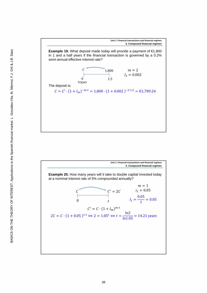
Example 26. Brian borrows €9,000 from Bank X. The loan will be repaidby a single repayment made 6 months from now. The nominal interestrate of the loan is 6% payable monthly and the application fee is €100,payable when the loan is given.

• Find the amount to be paid by Brian in 6 months.

𝐶 9,000 1 0.005 €9,273.40

• Find the annual effective rate of the loan.

𝐼 1 0.005 1 0.061678 ≡ 6.1678%

9,000 𝐶′

612

0

𝑖 0.06

𝐼0.0612

0.005



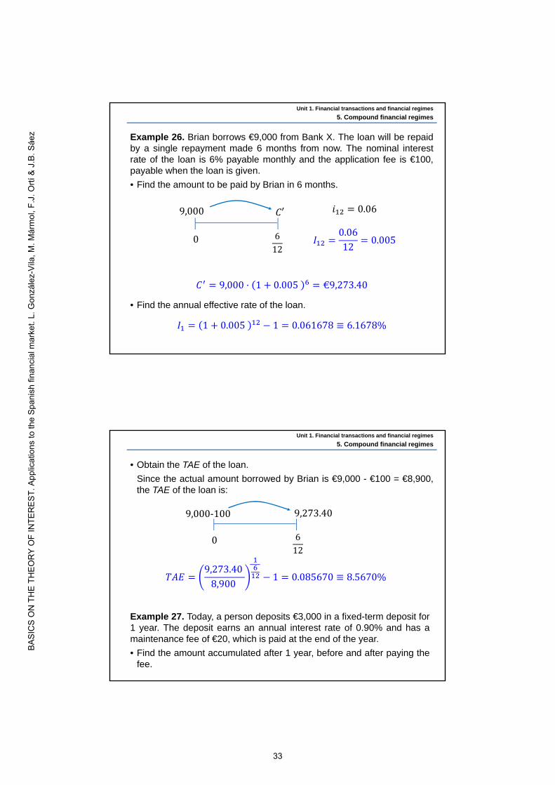
• Obtain the TAE of the loan.

Since the actual amount borrowed by Brian is €9,000 - €100 = €8,900,the TAE of the loan is:

9,273.40

612

0

𝑇𝐴𝐸9,273.40

8,900 1 0.085670 ≡ 8.5670%

9,000-100

Example 27. Today, a person deposits €3,000 in a fixed-term deposit for1 year. The deposit earns an annual interest rate of 0.90% and has amaintenance fee of €20, which is paid at the end of the year.

• Find the amount accumulated after 1 year, before and after paying thefee.



33

BASI

CS

ON

TH

E TH

EOR

Y O

F IN

TER

EST.

App

licat

ions

to th

e Sp

anis

h fin

anci

al m

arke

t. L.

Gon

zále

z-Vi

la, M

. Már

mol

, F.J

. Ortí

& J

.B. S

áez

Before paying the maintenance fee:

𝐶 3,000 1 0.0090 €3,027And after paying it:

𝐶 3,000 1 0.0090 20 €3,007

• What is the annual effective interest rate of the deposit?

𝐼 0.0090• Obtain the TAE of the deposit.

In order to calculate the TAE, the maintenance fee has to beconsidered.

3,000 𝐶′

10𝐼 0.0090

3,007

10𝐼

3,007 3,000

1 0.002333 ≡ 0.2333%

3,000



Example 28. Obtain the TAE of a pension scheme which, for a paymentof €6,000 on 20th December of year A, will provide a guaranteed incomeof €9,609.91 on 17th May of year A+12 (use the criterion Act/365).

Since no fees or other costs exist, the TAE and the annual effective rateof the pension scheme are equal.

6,000 9,609.91

17.05. A 1220.12. A

0 12148365

𝐼 𝑇𝐴𝐸9,609.91

6,000 1

0.0387 ≡ 3.87%



34

BASI

CS

ON

TH

E TH

EOR

Y O

F IN

TER

EST.

App

licat

ions

to th

e Sp

anis

h fin

anci

al m

arke

t. L.

Gon

zále

z-Vi

la, M

. Már

mol

, F.J

. Ortí

& J

.B. S

áez

Example 29. Let us suppose you want to invest €30,000 in this fixed-term deposit offered by bank Z.

1‐YEAR TERM DEPOSIT

2.50 Receive interest every 3 months

No fees or other costs exist

%

TAE (1)

Do I have to have any other product besides the bank deposit?If you are a new customer, you will only have to open an AA account that does not have any kind of costs or fees.

Is interest reinvested in the same deposit?No, interest will be paid into your AA account quarterly.

(1) Nominal interest rate of 2.48% (TAE 2.50%) payable for 12 months.Example: By investing €30,000, upon maturity of the deposit the client will have received €744.00.



• Check the calculation of the TAE.

• Calculate the total interest you are supposed to have at the maturity ofthe deposit.

• Explain why the amount calculated in the previous section is not equalto the one that the advert says.

Since the interest received every three months is not reinvested in thefixed-term deposit, it turns out that the total interest is:

1st quarter: 30,000 . €186

2nd quarter: 30,000 0.0062 €186 …

At the maturity of the fixed-term deposit: 186 4 €744

𝑚 4, 𝑖 0.0248 ⟺ 𝐼0.0248

40.0062, 𝑘 1

𝐼 1 0.0062 1 0.02503 ≡ 2.50%

𝐶 30,000 1 0.0062 30,000 1 0.025 €30,750

𝑌 30,750. 30,000 €750



35

BASI

CS

ON

TH

E TH

EOR

Y O

F IN

TER

EST.

App

licat

ions

to th

e Sp

anis

h fin

anci

al m

arke

t. L.

Gon

zále

z-Vi

la, M

. Már

mol

, F.J

. Ortí

& J

.B. S

áez

Example 30. A relative of yours has applied for the following online fastloan today 07/03/A.

365

256751 78.96 7,896%

500

TAE

Obtain the TAE (use the criterion Act/365):

For how long?

€500

25 days

Borrowed amount

500€Fees

175€Total to repay

675€Maturity date

01/04/A

Speed micro‐credit

How much money do you need? Total

transparency

100% online

Get your money in 4 business hours



6.1. Financial value at any moment in time

So far simple financial transactions, i.e., those ones with a singlepayment and a single repayment, have been analyzed.

Now we will study complex financial transactions (either partially or totallycomplex), in which we will have several payments or repayments.

In this latter situation, it may be useful to financially value the set ofpayments or repayments at a specific moment in time.

When financially valuing this set, it is replaced by a single amount offinancial capital that, somehow, represents the set. This single amount iscalled the financial value (or financial sum) associated with the set ofpayments or repayments (depending on what we are considering) and itcould be said that both, the set and its financial value, are financiallyequivalent.

6. Financial value

6.1. Financial value at any moment in time

6.2. Present value and final value


36

BASI

CS

ON

TH

E TH

EOR

Y O

F IN

TER

EST.

App

licat

ions

to th

e Sp

anis

h fin

anci

al m

arke

t. L.

Gon

zále

z-Vi

la, M

. Már

mol

, F.J

. Ortí

& J

.B. S

áez

In order to perform a financial valuation, the idea of the time value ofmoney has to be taken into account and, consequently, a financial regimewill have to be considered.

NOTE: From now on, unless otherwise indicated, to determine financialvalues (or financial sums), we will use the compound interest regime.

Given the set of payments or repayments 𝐶 ,𝑇 , ,⋯, and the

effective interest rate 𝐼 , its financial value (or financial sum) at

moment 𝑇′ is defined as the financial capital 𝐶 ,𝑇′ where:

𝐶 𝐶 1 𝐼

It can be written as:


6. Financial value

𝐶 ,𝑇 , ,⋯, ~ 𝐶 ,𝑇′

↓𝐼

Graphically,

𝐶

𝑇′

𝐶

𝑇

𝐶

𝑇

𝐶

𝑇

. . .

. . .


6. Financial value

𝐶𝐶

𝐶⋮

Example 31. Find the financial sum at 𝑇 4 of the following set ofrepayments if an annual effective interest rate of 5% is considered:

6,000, 1 , 3,500, 2.5 , 8,000, 5 On the timeline, we have:

6,000

1 2.5 5

3,500 8,000

0

37

BASI

CS

ON

TH

E TH

EOR

Y O

F IN

TER

EST.

App

licat

ions

to th

e Sp

anis

h fin

anci

al m

arke

t. L.

Gon

zále

z-Vi

la, M

. Már

mol

, F.J

. Ortí

& J

.B. S

áez

So:

𝐶 6,000 1 0.05 3,500 1 0.05 .

8,000 1 0.05

𝐶 €18,330.55

The financial value at 𝑇 4 is the financial capital:

𝐶 ,𝑇′ 18,330.55, 4

Furthermore, for the interest rate given:

6,000, 1 , 3,500, 2.5 , 8,000, 5 ~ 18,330.55, 4

𝐶′

𝑇 4

6,000

1 2.5 5

3,500 8,000

0𝐼 0.05


6. Financial value

Example 32. Today, Mary deposits €1,750 in a bank account. In 6months’ time, Mary will deposit an additional amount of €1,000; and in 1year, further €2,000.

• Find the account balance in 2 and a half years if the account pays anominal interest rate compounded semi-annually equal to 4.92%.

First, we draw the payments on the timeline.

• Then, we calculate the financial value at 𝑇 2.5

𝐶 1,750 1 0.0246 . 1,000 1 0.0246

2,000 1 0.0246 . €5,229.46

2.5

1,750

0 1612

𝐶′1,000 2,000

𝑖 0.0492

𝐼0.0492

20.0246


6. Financial value

38

BASI

CS

ON

TH

E TH

EOR

Y O

F IN

TER

EST.

App

licat

ions

to th

e Sp

anis

h fin

anci

al m

arke

t. L.

Gon

zále

z-Vi

la, M

. Már

mol

, F.J

. Ortí

& J

.B. S

áez

• If Mary withdraws €300 in 8 months, what will the account balance bein 2 and a half years?

𝐶 1,750 1 0.0246 . 1,000 1 0.0246

300 1 0.0246 2,000 1 0.0246 . €4,901.50

• Find the account balance in 2 and a half years if the account pays anominal interest rate equal to 4.92% compounded semi-annually for thefirst 6 months and a 0.25% monthly interest rate for the rest of the term.

𝐶′ 𝑖 0.0492

𝐼0.0492

20.0246

2.5

1,750

0 1612

1,000 2,000

812

300


6. Financial value

𝐶 1,750 1 0.0246 . 1 0.0025

1,000 1 0.0025

2,000 1 0.0025 . €5,057.48• Write the equation that allows us to calculate the annual effective

interest rate which is equivalent to those that are paid over the 2 and ahalf years in the previous example.

As this annual effective interest rate will give the same accumulatedvalue:

1,750 1 𝐼 . 1,000 1 𝐼 2,000 1 𝐼 . 5,057.48

𝐶′

2.5

1,750

0 1612

1,000 2,000

𝐼 0.0025𝐼 0.0246


6. Financial value

39

BASI

CS

ON

TH

E TH

EOR

Y O

F IN

TER

EST.

App

licat

ions

to th

e Sp

anis

h fin

anci

al m

arke

t. L.

Gon

zále

z-Vi

la, M

. Már

mol

, F.J

. Ortí

& J

.B. S

áez

Example 33. A person plans to invest in the following payment-in-kinddeposit offered by Bank Z. Find the interest of this deposit (value of thelaptop).

Fixed‐term deposit Amount: €90,000 Term: 6 months TAE: 1,40%

https://www.pexels.com/

For the purposes of personal income tax, the laptop is considered remuneration in kind. There is no cash remuneration.

9,000

612

0

Interest90,000

We have to consider thatthe laptop is received at thebeginning of the financialtransaction.

You should only make this deposit if you really want to have the laptop and if it is worth more than€623.43 on the market.

The person and the bank consider that payments and repaymentsinvolved in the financial transaction are equivalent:

90,000, 0 ~ Interest, 0 , 90,000, 1

It means that their financial value must be equal. So, by valuing at 0:

90,000 Interest 90,000 1 0.014

Interest €623.43


6. Financial value

6.2. Present value and final value

If the financial value of the set of payments or repayments is made at afixed origin, which is usually denoted as 0, the value obtained is calledthe present value of the set and we represent it by 𝑉 .

That is to say, given the set 𝐶 ,𝑇 , ,⋯, and the effective interestrate 𝐼 , its present value is:

• Present value:

𝑉 𝐶 1 𝐼

Graphically:

𝐶 ,𝑇 , ,⋯, ~ 𝑉 , 0↓𝐼𝟎

𝑉𝐶

𝑇

𝐶

𝑇

𝐶

𝑇

𝐶

𝑇

. . .

. . .


6. Financial value

40

BASI

CS

ON

TH

E TH

EOR

Y O

F IN

TER

EST.

App

licat

ions

to th

e Sp

anis

h fin

anci

al m

arke

t. L.

Gon

zále

z-Vi

la, M

. Már

mol

, F.J

. Ortí

& J

.B. S

áez

Similarly, if the financial value of the set of payments or repayments iscalculated at a final moment, 𝑇 , the amount obtained is called the final(or accumulated) value of the set and we represent it by 𝑉 .

• Final (or accumulated) value:

𝑉 𝐶 1 𝐼

Graphically:

𝐶 ,𝑇 , ,⋯, ~ 𝑉 ,𝑇↓𝐼

𝑉𝐶

𝑇

𝐶

𝑇

𝐶

𝑇

𝐶

𝑻𝒏

. . .

. . .


6. Financial value

It is worth remarking that since, for the given interest rate 𝐼 :

𝐶 ,𝑇 , ,⋯, ~ 𝑉 , 0and:

𝐶 ,𝑇 , ,⋯, ~ 𝑉 ,𝑇

it turns out that:

𝑉 , 0 ~ 𝑉 ,𝑇

The same equivalence holds for the financial valuation at any moment,𝑇′.

Therefore, once the present value (or the final value) of a set ofpayments or repayments has been obtained, we can find thefinancial value (or financial sum) of the set at any moment in time bysimply using an accumulation or discount factor, depending on when thefinancial value has to be calculated.


6. Financial value

41

BASI

CS

ON

TH

E TH

EOR

Y O

F IN

TER

EST.

App

licat

ions

to th

e Sp

anis

h fin

anci

al m

arke

t. L.

Gon

zále

z-Vi

la, M

. Már

mol

, F.J

. Ortí

& J

.B. S

áez

Example 34. For the set of payments:

6,000, 1 , 3,500, 2.5 , 8,000, 5with an annual effective interest rate of 5%:

• Find the present value.

𝑉 6,000 1 0.05 3,500 1 0.05 .

8,000 1 0.05

𝑉 €15,080.59

6,000

1 2.5 5

3,500 8,000

𝟎

𝐼 0.05

𝑉


6. Financial value

• Find the final value (at 𝑇 5)

𝑉 6,000 1 0.05 3,500 1 0.05 . 8,000

𝑉 €19,247.08

6,000

1 2.5 5

3,500 8,000

0

𝐼 0.05

𝑉


6. Financial value

42

BASI

CS

ON

TH

E TH

EOR

Y O

F IN

TER

EST.

App

licat

ions

to th

e Sp

anis

h fin

anci

al m

arke

t. L.

Gon

zále

z-Vi

la, M

. Már

mol

, F.J

. Ortí

& J

.B. S

áez

6,000

1 2.5 5

3,500 8,000

0

𝑉 15,080.59 𝑉 19,247.08

𝑉 19,247.08 1 0.05 €15,080.59

𝑉 15,080.59 1 0.05 €19,247.08


6. Financial value

• Check that, for the given interest, 𝐼 0.05, the present and the finalvalues of the set of payments are equivalent:

15,080.59 , 0 ~ 19,247.08 , 5

43

BASI

CS

ON

TH

E TH

EOR

Y O

F IN

TER

EST.

App

licat

ions

to th

e Sp

anis

h fin

anci

al m

arke

t. L.

Gon

zále

z-Vi

la, M

. Már

mol

, F.J

. Ortí

& J

.B. S

áez

UNIT 1 PROBLEMS

1. A person deposits €2,500 in an account at SA Bank today. He will get €2,750 in 2 years. Find the total price, the unit price and the unit and mean price. Explain the results obtained.

2. A financial transaction began on February 17th of a leap year and ended on July 10th of the same year. Find the term of the transaction by using the 30/360, Actual/360, Actual/365 and the Actual/Actual methods.

3. You invest €3,000 at an annual simple interest rate of 2.5%. Find the accumulated value after 91 days by using the Actual/365 criterion. Calculate the total interest, the nominal interest rate and the effective interest rate.

4. Mary borrows €2,000 from Mark at a 5% annual simple interest rate and agrees to repay the loan in 9 months. What is the amount that Mary is required to repay to Mark?

5. How many years will it take for €500 to increase to €600 at a 4.5% annual simple interest rate?

6. At what annual rate of simple interest will €8,000 increase to €8,128.05 in 182 days? Consider the Actual/365 criterion.

7. What initial amount will earn interest of €100 in 6 months at an annual simple interest rate of 3.20%?

8. A trade bill with a face value of €9,000 that matures in 2 months is discounted. The bank applies a simple discount regime at an annual rate of 6%.

a) Calculate the amount received by the passive party. b) Find the total price, the unit price and the unit and mean price of the financial transaction. c) How much would be received if there was an initial fee of 0.5% of the face value?

9. The amount obtained by discounting a commercial bill under the simple discount regime is €1,000. Find the face value of the commercial bill if its due date is in 62 days and the annual discount rate applied is 5.95%. What would the face value be if the financial transaction involved initial expenses equal to 0.7% of the face value?

10. A company has a bill of exchange with a face value of €3,000 and a maturity of 3 months from now. It trades the bill at its bank and obtains €2,963.25.

a) Find the simple annual discount rate applied by the bank. b) Find the equivalent simple interest rate of this financial transaction.

11. A company discounts a portfolio of bills of exchange today. The portfolio has a face value of €12,500 and matures in 31 days. The bank charges a simple annual discount rate equal to 6% and an initial fee of 0.7% and it uses the Act/360 criterion. Calculate the profitability obtained by the bank if simple interest regime is considered (use the Act/365 criterion).

44

BASI

CS

ON

TH

E TH

EOR

Y O

F IN

TER

EST.

App

licat

ions

to th

e Sp

anis

h fin

anci

al m

arke

t. L.

Gon

zále

z-Vi

la, M

. Már

mol

, F.J

. Ortí

& J

.B. S

áez

12. A company wants to buy a car in 3 months. The car will have a price of €29,700. In order to make this future payment, the company performs the following financial transactions today:

It cancels a bank account that was opened with €10,000 9 months ago. The account has paid an annual simple interest rate of 3.50%.

It discounts a portfolio of bills of exchange at an annual simple discount rate of 6% and an initial fee of 0.4%. The face value of the portfolio is €20,000. 40% of the portfolio matures in 6 months and the rest in 9 months.

a) Find the amount obtained by the company today when cancelling the bank account. b) Find the amount obtained by the company today when discounting the portfolio. c) Does the company have enough money today to buy the car? If it does not, the company will

invest the amount obtained with the above financial transactions in a fixed‐term deposit, from today until the moment of purchasing the car. What is the minimum annual simple interest rate that the fixed‐term deposit must pay in order for the company to be able to buy the car?

13. A woman invests €6,320 today. Her investment grows according to a nominal interest rate compounded quarterly that is equal to 3.20%.

a) Find her balance after 3 and a half years. b) How much interest does she earn? c) How long will €6,320 have to be invested to obtain a balance of €7,471.16?

14. On his fifth birthday, a boy received an inheritance from his aunt. The inheritance grew to €32,168 by the time he was 18 years old. If the money grew by compound interest at a semi‐annual effective interest rate of 1.15%, find the amount of the inheritance.

15. Mr. Smith deposits €1,750 in a bank account for 2 years and 3 months. How much money will he receive when he closes the bank account if it is governed by:

a) A 4.5% nominal interest rate compounded annually? b) A semi‐annual (biannual) effective rate equalling 2.15%? c) An 8% biennially effective interest rate? d) An annual interest rate of 4% convertible quarterly (every three months)? e) A monthly interest rate of 0.35%? f) A 3.60% nominal interest rate accumulated every four months? g) A 0.8% effective interest rate every two months?

16. A financial asset has a face value of €1,000 and matures in 2 years. Today, you buy it for €945.73. Find the annual effective interest rate associated with this financial transaction.

17. Suppose that the growth of money is ruled by compound interest at an annual rate of 5% payable semi‐annually. How much money must you invest today in order to have a balance of €23,000 3 and a half years from now?

18. An investor deposits €9,000 today in a savings account that accumulates interest at varying rates. For the first 2 years, the nominal interest rate is 2% compounded quarterly. For the next 1 and a half years, a 0.3% monthly interest rate is applied. For the rest of the term, the interest rate is equal to an annual 4%. What is the investor’s balance at the end of 6 years? 19. Bank Z offers a savings account with varying interest rates for 3 years. For the first 8 months the monthly effective interest rate is 0.2%, for the next 9 months the nominal interest rate compounded semi‐annually is 2% and for the rest of the term the annual effective interest rate is 3%.

45

BASI

CS

ON

TH

E TH

EOR

Y O

F IN

TER

EST.

App

licat

ions

to th

e Sp

anis

h fin

anci

al m

arke

t. L.

Gon

zále

z-Vi

la, M

. Már

mol

, F.J

. Ortí

& J

.B. S

áez

a) What deposit made into this account today will provide a balance of €10,000 in 3 years? b) If you deposit €5,500 today:

b.1) Find the accumulated value in 3 years. b.2) Find the annual effective interest rate that should have been paid over the 3 years in order

to achieve the same accumulated value.

20. Find the following equivalent interest rates:

a) Quarterly effective interest rate equivalent to 6% nominal interest compounded quarterly? b) Annual effective rate equivalent to an annual interest rate of 7.2% convertible monthly? c) Nominal interest rate compounded semi‐annually equivalent to a 5.9% biennially effective

interest rate. d) Interest rate compounded quarterly equivalent to an interest rate of 8% payable semi‐

annually.

21. Find the effective interest rate over a three‐year period (triennially) that is equivalent to an annual effective rate of 3% the first year, 2% the second year and 1% the third year.

22. Calculate the annual effective interest rate and the TAE of a loan of €3,000, to be repaid by a single repayment in 3 months, if a nominal interest rate of 6.75% accumulated monthly has been agreed and there is an application fee that equals 2% on the principal, which is paid by the borrower when the loan is given.

23. Find the annual effective interest rate and the TAE of a financial transaction in which, by investing €8,250 on October 8th of a given year, €9,156 is obtained on October 21st two years later. Consider that at the moment of investing, a fee of 3% of the initial amount is paid by the investor. (Use the Actual/365 criterion).

24. If you invest €10,000 today in a financial product offered by Bank Triple Z, you will obtain an accumulated profitability of 15% in 4 and a half years.

a) Find the annual effective interest rate and the TAE of this financial product. b) What would the effective annual interest and the TAE of this financial product be if at its

maturity you had to pay a management fee of 1% on the invested amount?

25. After saving for some years, an investor has €20,000 and he is offered 3 different alternatives to invest this amount.

Alternative 1: open a fixed‐term deposit that pays a 4% nominal interest rate compounded monthly.

Alternative 2: buy a bill of exchange with a face value of €20,500 and maturity within 8 months.

Alternative 3: invest in a bank account that offers an annual simple interest rate of 7%, in which no interest is earned on the first €8,000.

a) Calculate the amount accumulated after 8 months according to the 3 alternatives. b) Find the TAE of the 3 alternatives if none of them has fees or costs.

26. In order to buy a small apartment, you are given two different alternatives today.

Alternative A: A €24,000‐payment in 2 and a half years and €100,000 in 5 years.

Alternative B: A single payment of €120,000 in 3 years. If the current interest rate is equal to 6% annual, which alternative do you prefer?

46

BASI

CS

ON

TH

E TH

EOR

Y O

F IN

TER

EST.

App

licat

ions

to th

e Sp

anis

h fin

anci

al m

arke

t. L.

Gon

zále

z-Vi

la, M

. Már

mol

, F.J

. Ortí

& J

.B. S

áez

27. A person must pay €6,000 in 1 year and €5,000 in 4 and a half years. Obtain the capital that must be paid within 2 years at an annual interest rate of 5% in order to cancel both debts.

28. Susan deposited €9,800 in a bank account 18 months ago. 6 months later, she deposited €3,300 more. Finally, 2 months ago, she made an additional deposit of €4,500.

a) If the bank account was governed by an interest rate of 2.5% compounded semi‐annually, what is the balance of the account today (accumulated value)?

b) What would the balance of the account be today if it had been governed by the following interest rates: an annual effective interest rate of 2% for the first 3 months, a 2.4% annual interest rate convertible monthly for the next year, and a 1.3% semi‐annual interest rate for the rest of the term?

29. A Bank offers a savings account with varying interest rates for 3 years: for the first 8 months the monthly effective interest rate is 0.2%, for the next 9 months the nominal interest rate compounded quarterly is 1% and for the rest of the term the annual interest rate is 3%.

a) If you deposit €5,500 today: a.1) Find the accumulated value in 3 years. a.2) Find the annual effective interest rate that should have been paid over the 3 years in order

to get the same accumulated value. b) If you deposit today €5,500, in 6 months you withdraw €2,000 and in 1 year you deposit

€1,000: b.1) Find the balance in 3 years. b.2) Write the equation that allows you to calculate the annual effective interest rate that

should have been paid over the 3 years in order to get the same accumulated value. c) What deposit made today will provide for a payment of €1,000 in 10 months and another of

€2,000 in 1 and a half years? __________________________________________________________________________________

Answers

1. ∆𝐶 €250. This means that in exchange for €2,000 given today, the person receives a total remuneration of €250 in 2 years. 𝐼 0.10 ≡ 10%. This means that for each euro given by the person, he/she receives €0.10 in 2 years. 𝑖 0.05 ≡ 5%. That is to say, for each €100 given and for each year that the financial transaction lasts, the person receives €5.

2.

Criterion 𝑡

30360

𝑡 0.3972

𝐴𝑐𝑡360

𝑡 0.4

𝐴𝑐𝑡365

𝑡 0.394521

47

BASI

CS

ON

TH

E TH

EOR

Y O

F IN

TER

EST.

App

licat

ions

to th

e Sp

anis

h fin

anci

al m

arke

t. L.

Gon

zále

z-Vi

la, M

. Már

mol

, F.J

. Ortí

& J

.B. S

áez


𝑡 0.393443

3. 𝐶 €3,018.70 ∆𝐶 €18.70 𝐼 0.006233 ≡ 0.6233% 𝑖 0.025 ≡ 2.5%. 4. 𝐶 €2,075.

5. 𝑡 4. 4. 6. 𝑖 0.0321 ≡ 3.21%. 7. 𝐶 €6,250. 8. a) 𝐶 €8,910.

b) ∆𝐶 €90 𝐷 0.001 ≡ 1% 𝑑 0.06 ≡ 6%. c) 𝐶 €8,865.

9. If there are no expenses 𝐶′ €1,010.36. When expenses exist, 𝐶′ €1,017.55. 10. a) 𝑑 0.0490 ≡ 4.90%.

b) 𝑖 0.049608 ≡ 4.9608%. 11. 𝑖 0.145014 ≡ 14.5014%. 12. a) 𝐶 €10,262.50.

b) 𝐶 €19,140. c) No, there is not enough money today. 𝑖 0.040473 ≡ 4.0473%.

13. a) 𝐶 €7,065.85.

b) ∆𝐶 €745.85. c) 𝑡 5.25.

14. 𝐶 €23,895.22. 15. a) 𝐶 €1,932.19.

b) 𝐶 €1,925.80. c) 𝐶 €1,908.27. d) 𝐶 €1,913.95. e) 𝐶 €1,923.12. f) 𝐶 €1,896.73. g) 𝐶 €1,948.75.

16. 𝐼 0.028292 ≡ 2.8292%. 17. 𝐶 €19,349.10. 18. 𝐶 €10,903.63. 19. a) 𝐶 €9,252.32.

b) b.1) 𝐶′ €5,944.46. b.2) 𝐼 0.026242 ≡ 2.6242%.

48

BASI

CS

ON

TH

E TH

EOR

Y O

F IN

TER

EST.

App

licat

ions

to th

e Sp

anis

h fin

anci

al m

arke

t. L.

Gon

zále

z-Vi

la, M

. Már

mol

, F.J

. Ortí

& J

.B. S

áez

20. a) 𝐼 0.015 ≡ 1.5%.

b) 𝐼 0.074424 ≡ 7.4424%. c) 𝑖 0.028869 ≡ 2.8869%. d) 𝑖 0.079216 ≡ 7.9216%.

21. 𝐼 ⁄ 0.061106 ≡ 6.1106%.

22. 𝐼 0.069628 ≡ 6.9628% 𝑇𝐴𝐸 0.159654 ≡ 15.9654%. 23. 𝐼 0.052519 ≡ 5.2519% 𝑇𝐴𝐸 0.037346 ≡ 3.7346%. 24. a) 𝐼 0.031546 ≡ 3.1546% 𝑇𝐴𝐸 0.031546 ≡ 3.1546%.

b) 𝐼 0.031546 ≡ 3.1546% 𝑇𝐴𝐸 0.029545 ≡ 2.9545%. 25.

Alternative a) Accumulated amount b) TAE

1 €20,539.60 0.040742 ≡ 4.0742%

2 €20,500.00 0.037733 ≡ 3.7733%

3 €20,560.00 0.042293 ≡ 4.2293%

26. Since the present values of alternatives A and B are, respectively, €95,472.40 and €100,754.31, as a buyer you should choose alternative A.

27. €10,725.85. 28. a) 𝐶 €18,073.80. b) 𝐶 €18,054.05.

29. a) a.1) 𝐶′ €5,900.42.

a.2) 𝐼 0.023701 ≡ 2.3701%. b) b.1) 𝐶′ €4,832.66. b.2) 5,500 1 𝐼 2,000 1 𝐼 . 1,000 1 𝐼 4,832.66.

c) 𝐶 €2,931.30

49

BASI

CS

ON

TH

E TH

EOR

Y O

F IN

TER

EST.

App

licat

ions

to th

e Sp

anis

h fin

anci

al m

arke

t. L.

Gon

zále

z-Vi

la, M

. Már

mol

, F.J

. Ortí

& J

.B. S

áez

UNIT 2.

ANNUITIES

1. Definition and classification

2. Level or constant annuities

3. Annuities with payments in geometric progression

4. Annuities with payments in arithmetic progression

1.1. Definition

An annuity is a set of payments (or repayments), 𝐶 ,𝑇 , ,⋯, ,made at equal intervals in time. Common examples of annuities includehouse rents, mortgage payments on homes, salaries earned by workersor instalments paid for cars.

The interval between annuity payments is called the annuity period, 𝑃,and the number of annuity periods in 1 year is named the annuityfrequency, 𝑀, with the relationship 𝑀 1/𝑃. Furthermore, 𝑛 is thenumber of payments of the annuity.

Graphically:

𝑃 𝑃

𝐶

𝑇

𝐶

𝑇

𝐶

𝑇

𝐶

𝑇

. . .

. . .

𝐶

𝑇

𝐶

𝑇

𝑃 𝑃


1.1. Definition

1.2. Classification

Unit 2. Annuities

51

BASI

CS

ON

TH

E TH

EOR

Y O

F IN

TER

EST.

App

licat

ions

to th

e Sp

anis

h fin

anci

al m

arke

t. L.

Gon

zále

z-Vi

la, M

. Már

mol

, F.J

. Ortí

& J

.B. S

áez

Example 1.

Repayments made by a borrower, at the end of each quarter, to repay aloan over the next 10 years are an annuity with 𝑃 1/4, 𝑀 4 and 𝑛40.

The rent paid for a flat at the beginning of each month over 5 years is anannuity with 𝑃 1/12, 𝑀 12 and 𝑛 60.

1.2. Classification

Annuities can be classified by considering different aspects.

1) Depending on the number of payments, 𝑛 :• Temporary annuity: If 𝑛 is a finite number.• Perpetuity: If payments last forever, i.e. 𝑛 is infinite.

2) Depending on the structure of the amounts 𝐶 :• Constant or level annuity: If 𝐶 𝐶,∀𝑟 1,2, … ,𝑛• Non-level annuity: If the amounts are not constant.

Unit 2. Annuities


3) Depending on the fixed origin, 0:• Non-deferred annuity: The fixed origin and the annuity origin are

both the same.• Deferred annuity: The fixed origin is earlier than the annuity origin.

Unit 2. Annuities


4) Depending on the annuity period:• Monthly annuity: If 𝑀 12• Quarterly annuity: If 𝑀 4• Semi-annual annuity: If 𝑀 2• Etc.

5) Depending on when the payments are made each annuity period:• Immediate annuity: If payments are made at the end of each

annuity period.• Annuity-due: If payments are made at the beginning of each period.

52

BASI

CS

ON

TH

E TH

EOR

Y O

F IN

TER

EST.

App

licat

ions

to th

e Sp

anis

h fin

anci

al m

arke

t. L.

Gon

zále

z-Vi

la, M

. Már

mol

, F.J

. Ortí

& J

.B. S

áez

Example 2.

Draw the following annuities on the timeline:

• A monthly non-deferred immediate annuity, consisting of level paymentsover the next 5 years, equal to €150.

150

112

150 150. . .

. . .

150 150

02

12

312

412

5 years41112

1 2 3 4 60 months59

150𝑛 60

Unit 2. Annuities


• A 2-year-deferred annuity composed of semi-annual immediatepayments to be made for 12 years. The first payment is equal to €300whereas the rest will increase in such a way that each payment is 5%greater than the previous one.The first payment is: 𝐶 300The second payment is:

𝐶 300 300 0.05 300 1 0.05 300 1.05The third payment is:

𝐶 300 1.05 1.05 300 1.05

And so on.

So, graphically:

• A non-deferred perpetuity-due that will pay €70 a month from now on.

2 . . . 0 212

3 14 years1312

4 5 6 7 28 half years27

𝑛 243

12

4

. . .

8

70

112

. . .

. . .

70 70

02

12

312

412

years

1 2 3 4 months

70𝑛 → ∞

Unit 2. Annuities


53

BASI

CS

ON

TH

E TH

EOR

Y O

F IN

TER

EST.

App

licat

ions

to th

e Sp

anis

h fin

anci

al m

arke

t. L.

Gon

zále

z-Vi

la, M

. Már

mol

, F.J

. Ortí

& J

.B. S

áez

• A twenty-payment quarterly annuity-due that is deferred 1 year with thefirst payment equal to €600 and the payments increasing by €20 eachquarter.

• A constant non-deferred annuity-due, to be paid annually over the next25 years, with payments of €1,250.

1

. . .

. . . 0 114

124

134

6 years534

1 2 3 4 24 quarters23

𝑛 20

1,250

1

1,250. . .

. . .

1,250 1,250

0 2 3 25 years24

1,250𝑛 25

2

Unit 2. Annuities


NOTE

Annuities are commonly not named as in the previous example. Thismeans that, from the information given in each financial transaction whichinvolves annuities, we will have to be able to determine all of the annuitycharacteristics. More particularly:

• If an annuity is deferred, it will be explicitly stated (using thecorresponding term or a synonym). If nothing is said, it must beassumed that the annuity is non-deferred.

• If the annuity is due, this is stated explicitly (using this term or asynonym) So, if nothing is stated, it must be understood that the annuityis immediate.

Unit 2. Annuities


54

BASI

CS

ON

TH

E TH

EOR

Y O

F IN

TER

EST.

App

licat

ions

to th

e Sp

anis

h fin

anci

al m

arke

t. L.

Gon

zále

z-Vi

la, M

. Már

mol

, F.J

. Ortí

& J

.B. S

áez

Example 3.Draw on the timeline the annuities involved in the following financialtransactions:

• A loan of €250,000 to be repaid with constant payments at the end ofeach month over the next 25 years.

𝐶

112

𝐶. . .

. . .

𝐶 𝐶

02

12

312

412

25 years

1 2 3 4 300 months

𝐶𝑛 300

Unit 2. Annuities


• A person wants to save for retirement by depositing €2,000 at thebeginning of each quarter, for 10 years.

0

. . .

. . . 14

24

34

10 years934

1 2 3 4 40 quarters39

𝑛 401

2.1. Definition

An annuity is level or constant if all the payments or amounts have thesame value, i.e.:

𝐶 𝐶, ∀𝑟


2.1. Definition

2.2. Financial value of the Non-deferred immediate annuity with npayments and period P

2.3. Financial value of the Non-deferred immediate perpetuity withperiod P

Unit 2. Annuities

55

BASI

CS

ON

TH

E TH

EOR

Y O

F IN

TER

EST.

App

licat

ions

to th

e Sp

anis

h fin

anci

al m

arke

t. L.

Gon

zále

z-Vi

la, M

. Már

mol

, F.J

. Ortí

& J

.B. S

áez

2.2. Financial value of the Non-deferred immediate annuity with n

payments and period P

We begin by calculating the present value. From it, the final oraccumulated value of the annuity will be obtained.

First, let us consider an example.

Unit 2. Annuities


Example 4. Find the present value of the first annuity drawn in example 2if an annual effective interest rate equal to 2% is considered.

We had a monthly non-deferred immediate annuity, with level paymentsover the next 5 years equal to €150. Graphically:

150

112

150 150. . .

. . .

150 150

02

12

312

412

5 years41112

1 2 3 4 60 months59

150

𝑛 60𝐼 0.02

Although it is not necessary, to have an easier expression, let uscalculate the monthly effective interest rate that it is equivalent to 𝐼0.02 (note that the annuity frequency is 𝑀 12).

𝐼 1 0.02 ⁄ 1 0.001652

So, the present value is:

𝑉 150 1 0.001652 150 1 0.001652

⋯ 150 1 0.001652

𝑉 €8,561.72

Unit 2. Annuities


Calculating the present value in this way is an annoying task. So, we are going to look for a formula which will allow us to evaluate annuities more easily.

56

BASI

CS

ON

TH

E TH

EOR

Y O

F IN

TER

EST.

App

licat

ions

to th

e Sp

anis

h fin

anci

al m

arke

t. L.

Gon

zále

z-Vi

la, M

. Már

mol

, F.J

. Ortí

& J

.B. S

áez

In general, the graph of a non-deferred immediate annuity with 𝑛payments and period 𝑃 is:

NOTE: When evaluating annuities, we must bear in mind that theeffective interest rate that appears in the formulas must have thesame frequency as the annuity, that is, 𝑀.

The present value of the annuity, 𝑉 , with the effective interest rate 𝐼 is:

𝑉 𝐶 1 𝐼 𝐶 1 𝐼 ⋯ 𝐶 1 𝐼

𝑉 𝐶 1 𝐼

It can be demonstrated that this sum is equal to:

𝑉 𝐶1 1 𝐼

𝐼

𝐶

𝑃

𝐶. . .

. . .

𝐶

0 2𝑃 3𝑃 𝑛𝑃

𝐶

𝑛 1 𝑃

𝐶

Unit 2. Annuities


Explanation of the formula of the present value of a level non-deferredimmediate annuity with 𝑛 payments and period 𝑃 (frequency 𝑀)

𝑉 𝐶1 1 𝐼

𝐼

𝐶

𝑃

𝐶. . .

. . .

𝐶


𝐶

𝑛 1 𝑃

Amount of the level (or constant)

payment

Effective interest rate to determine the present value, whose frequency is the same as that of the annuity, 𝑴

Number of constant payments (this must be a natural number, that is, it cannot have decimals)

The present value obtained with this formula is

ALWAYS one period before the first payment of the

annuity

The expression is usually written as 𝑎 | and, as a result, in general:

𝑉 𝐶 𝑎 |

𝑉

Unit 2. Annuities


57

BASI

CS

ON

TH

E TH

EOR

Y O

F IN

TER

EST.

App

licat

ions

to th

e Sp

anis

h fin

anci

al m

arke

t. L.

Gon

zále

z-Vi

la, M

. Már

mol

, F.J

. Ortí

& J

.B. S

áez

Example 5. For the first annuity illustrated in Example 2, find its presentvalue if an annual effective interest rate equal to 2% is considered.

The graph of the annuity is:

with 𝐶 150, 𝑀 12 and 𝑛 60.

The monthly effective interest rate is 𝐼 0.001652.

So, by using the formula we just saw:

𝑉 150 𝑎 | . 1501 1 0.001652

0.001652€8,561.72

150

112

150 150. . .

. . .

150 150

02

12

312

412

5 years41112

1 2 3 4 60 months59

150𝑉

Unit 2. Annuities


Example 6. For the loan in Example 3, find the amount of constantpayments if the loan is governed by an annual interest rate of 4.80%accumulated monthly.The loan has a principal of €250,000 and it will be repaid by constantpayments at the end of each month over the next 25 years.

with 𝑀 12 and 𝑛 300.In this case, the interest rate we use to value is 𝑖 0.0480. So, themonthly effective interest rate is:

𝐼0.0480

120.004

Now, by using the formula for the present value:

250,000 𝐶 𝑎 | .

𝐶

112

𝐶. . .

. . .

𝐶 𝐶

02

12

312

412

25 years

1 2 3 4 300 months

𝐶𝟐𝟓𝟎,𝟎𝟎𝟎

Unit 2. Annuities


58

BASI

CS

ON

TH

E TH

EOR

Y O

F IN

TER

EST.

App

licat

ions

to th

e Sp

anis

h fin

anci

al m

arke

t. L.

Gon

zále

z-Vi

la, M

. Már

mol

, F.J

. Ortí

& J

.B. S

áez

250,000 𝐶1 1 0.004

0.004And so, by isolating 𝐶, we get:

𝐶 €1,432.49This means that to pay off the amount borrowed at the interest rateagreed, the borrower has to pay €1,432.49 at the end of each month, forthe next 25 years.

Unit 2. Annuities


We can also calculate the accumulated (or final) value of the annuityfrom its present value.

𝐶

𝑃

𝐶. . .

. . .

𝐶


𝐶

𝑛 1 𝑃

𝑉

𝑽𝒇

𝑉 𝑉 1 𝐼

Unit 2. Annuities


being 𝑡 the term (in years) between 0 and 𝑛𝑃.

59

BASI

CS

ON

TH

E TH

EOR

Y O

F IN

TER

EST.

App

licat

ions

to th

e Sp

anis

h fin

anci

al m

arke

t. L.

Gon

zále

z-Vi

la, M

. Már

mol

, F.J

. Ortí

& J

.B. S

áez

Example 7. For the annuity in Example 4, find its accumulated value if anannual effective interest rate equal to 2% is considered.

We already saw that the annuity graph on the timeline is:

and the monthly effective interest rate is 𝐼 0.001652.

Therefore, from its present value, the accumulated value will be:

𝑉 8,561.72 1 0.001652 €9,452.83

150

112

150 150. . .

. . .

150 150

02

12

312

412

5 years41112

150

𝑉

Unit 2. Annuities


Example 8. Dr Collins has been depositing €300 at the end of eachtrimester for the last 10 years in a savings account that is governed by a1.20% nominal interest rate paid quarterly. What is the savings accountbalance today, just after making the corresponding deposit?

From the given interest rate 𝑖 0.0120, we determine the quarterlyeffective interest rate:

𝐼0.0120

40.003

Now, from the formula we already know:

300 𝑎 | .

0

. . .

. . . 14

24

34

10 years

1 2 3 4 40 quarters

1

11,292.02

𝑉

𝑉

1 0.003𝑉 €12,729.43

Unit 2. Annuities


𝑛 40𝑀 4𝐶 300

TODAY

60

BASI

CS

ON

TH

E TH

EOR

Y O

F IN

TER

EST.

App

licat

ions

to th

e Sp

anis

h fin

anci

al m

arke

t. L.

Gon

zále

z-Vi

la, M

. Már

mol

, F.J

. Ortí

& J

.B. S

áez

Example 9. An investor wishes to accumulate €100,000 at the time of herlast deposit in a pension scheme by contributing, from now on, with anamount 𝐶 at the end of each 6-month period for 18 years. If the annualeffective interest rate of the pension scheme is 1.5%, what amount isnecessary for her to reach her goal?

Bearing in mind that 𝑀 2 and 𝑛 36, we first draw the annuity on thetimeline.

Then, from the given interest rate 𝐼 0.0150, we determine the semi-annual effective interest rate:

𝐼 1 0.0150 ⁄ 1 0.007472

𝑉

𝟏𝟎𝟎,𝟎𝟎𝟎

. . . 0

. . .

12

1 112

18 years1712

2

1 2 3 4 36 half years35

𝐶 𝐶𝐶 𝐶𝐶 𝐶

Unit 2. Annuities


Now, from the formula:

𝐶 𝑎 | .

𝑉

1 0.007472 100,000

Unit 2. Annuities


100,000 𝐶1 1 0.007472

0.007472 1 0.007472

And, by isolating 𝐶, we get:

𝐶 €2,431.21

61

BASI

CS

ON

TH

E TH

EOR

Y O

F IN

TER

EST.

App

licat

ions

to th

e Sp

anis

h fin

anci

al m

arke

t. L.

Gon

zále

z-Vi

la, M

. Már

mol

, F.J

. Ortí

& J

.B. S

áez

NOTE:

So far, for level annuities, we have obtained a formula from which it iseasy to calculate the present value and the accumulated value of atemporary non-deferred immediate annuity.

In order to obtain the present value and the accumulated value of a:

• temporary deferred immediate annuity

• temporary non-deferred annuity-due

• temporary deferred annuity-due

we will use exactly the same formula and the proper accumulation ordiscount factor, depending on the moment in time for which we needthe value of the annuity.

Unit 2. Annuities


Summarizing:

In order to properly calculate the financial value (present, accumulated orat any other moment) of any level annuity, the following steps should befollowed:

1. Draw the annuity on the timeline.

2. Think of where you want the annuity to be financially valued.

3. Check if the capitalization frequency of the given interest rate is equalto the annuity frequency. If it is not, then obtain the equivalent interestrate.

4. Use the formula 𝑎 | .

5. Reflect on where the financial value obtained with the above formulais placed.

6. If needed, correct this financial value with an accumulation factor or adiscount factor, so as to arrive to the financial value at the desiredmoment.

Unit 2. Annuities


62

BASI

CS

ON

TH

E TH

EOR

Y O

F IN

TER

EST.

App

licat

ions

to th

e Sp

anis

h fin

anci

al m

arke

t. L.

Gon

zále

z-Vi

la, M

. Már

mol

, F.J

. Ortí

& J

.B. S

áez

. . .

. . . 1

162

172 1

22

3

80 80 80 80

.a 0061523080V0 ·. . 2 21 006152 333€85

, . 6 49647€

, .1 08350

·. . 2 1785333 1 006152

Value at :T 2

𝑉𝑉

Example 10. Find the present value and the accumulated value of asemi-annual immediate annuity to be paid for 15 years, after a 2-yeardeferment. The amount of each payment is €80 and a monthly effectiveinterest of 1% is applied.

Semi-annual effective rate equivalent to 𝐼 0.01:

𝐼 1 0.01 ⁄ 1 0.06152Present value:

Accumulated (final) value:

𝑉 =

0

Unit 2. Annuities


𝑛 30𝑀 2𝐶 80

Example 11. Find the present value and the final value, under an annualinterest rate of 4% payable quarterly, of a non-deferred quarterly annuity-due to be paid for 5 years, with payments of €125.

Quarterly effective interest rate:

𝑖 0.04 → 𝐼0.04

40.01

. . .

. . .14

12

3

44

5

125

14

125125 125

0

𝑉𝑉

Present value:

Accumulated value:

.a 00120125V0 , . , 11 0 01 278 25€2

. , , , . 20278 25 1 0 01 2 779902 €

, .2 25569Value at :T 14

𝑉

Unit 2. Annuities


𝑛 20𝑀 4𝐶 125

63

BASI

CS

ON

TH

E TH

EOR

Y O

F IN

TER

EST.

App

licat

ions

to th

e Sp

anis

h fin

anci

al m

arke

t. L.

Gon

zále

z-Vi

la, M

. Már

mol

, F.J

. Ortí

& J

.B. S

áez

Example 12. Let us consider an annuity-due payable for 8 years after a6-month deferment. It has level payments of €350 a month. Obtain itspresent value and its accumulated value at an annual interest rate of 4%compounded monthly.

. . .V0

. . . 5

812

6

812

612

712

350 350 350

.a 000396350 . , .

5

1 0003 28 23996 €

· ., . . , .

12 8528 23996 1 0003 39 65324 €

, .28 71377Value at :T 5

12

V0

𝑉

0

𝑉

Monthly effective interest rate:

𝑖 0.04 → 𝐼0.0412

0.003Present value:

Accumulated value:

512

Unit 2. Annuities


𝑛 96𝑀 12𝐶 350

A perpetuity is an annuity with an infinite term. That is to say, a perpetuityhas payments that last forever. Therefore, it makes no sense to calculateaccumulated values for perpetuities.

Graphically:

𝐶

𝑃

. . .

. . .

𝐶

0 2𝑃 3𝑃

𝐶𝑉

2.3. Financial value of the Non-deferred immediate perpetuity with

period P

Unit 2. Annuities


The present value of the annuity, 𝑉 , with the effective interest rate 𝐼 is:

𝑉 𝐶 1 𝐼 𝐶 1 𝐼 ⋯

𝐶 1 𝐼

64

BASI

CS

ON

TH

E TH

EOR

Y O

F IN

TER

EST.

App

licat

ions

to th

e Sp

anis

h fin

anci

al m

arke

t. L.

Gon

zále

z-Vi

la, M

. Már

mol

, F.J

. Ortí

& J

.B. S

áez

Alternatively, by using the formula we already know, it is also possible towrite:

𝑉 lim→

𝐶 𝑎 | 𝐶 lim→

1 1 𝐼𝐼

So:

The present value obtained with this formula is ALWAYS given oneperiod before the first payment of the annuity.

𝑉 𝐶1𝐼

Unit 2. Annuities


Example 13. What would you be willing to pay today for an infinitestream of constant end-of-month payments of €1,000, if the annualinterest rate compounded monthly was 1.5%?

Graphically:

From the given interest rate, we obtain the monthly effective interestrate:

So, the present value of the infinite stream of payments is:

𝑉 1,0001

0.00125 €800,000

1,000

112

. . .

. . .

1,000

0 312

1,000𝑉

212

𝑀 12𝑖 0.015

𝐼 . 0.00125

Unit 2. Annuities


65

BASI

CS

ON

TH

E TH

EOR

Y O

F IN

TER

EST.

App

licat

ions

to th

e Sp

anis

h fin

anci

al m

arke

t. L.

Gon

zále

z-Vi

la, M

. Már

mol

, F.J

. Ortí

& J

.B. S

áez

The annual effective interest rate is:

So, the present value is:

500.

500

12

. . .

. . .

500

0 212

500𝑉

112

𝑀 1𝐼 0.01

𝐼 1 0.01 1 0.0201

12

𝑉 €25,124.381 0.0201 .

Example 14. An investment made today will provide for €500 a yearforever, with the first payment being made 6 months from today. If asemi-annual effective interest rate equal to 1% is used, find the amountinvested.

First, we draw the perpetuity on the timeline.

Unit 2. Annuities


3.1. Definition

We now consider annuities with payments that vary in a geometricprogression. In this case, the payments of the annuity are:

𝐶 𝐶 𝑞 ,𝑞 0, ∀𝑟This means that, from a first payment, 𝐶 , any payment is obtained bymultiplying the preceding one by a constant, 𝑞, called the common ratio.

If 𝑞 1 , the payments of the annuity increase; if 0 𝑞 1 , theydecrease.


3.1. Definition



Unit 2. Annuities

66

BASI

CS

ON

TH

E TH

EOR

Y O

F IN

TER

EST.

App

licat

ions

to th

e Sp

anis

h fin

anci

al m

arke

t. L.

Gon

zále

z-Vi

la, M

. Már

mol

, F.J

. Ortí

& J

.B. S

áez

Example 15. It is forecast that the turnover of an SME will be, at the endof this year, €700,000. Then, it will rise by 2% annually and cumulativelyfor the next 9 years. Find the general expression of the turnover for these10 years.

The first year’s turnover is:𝐶 700,000

The second year’s is:𝐶 700,000 700,000 0.02 700,000 1.02

The third is:𝐶 700,000 1.02 1.02 700,000 1.02

So, 𝐶 700,000, 𝑞 1.02 and, in general:

𝐶 700,000 1.02 , ∀𝑟 1,2, … , 10

Unit 2. Annuities




As we did for level annuities, we begin by calculating the present value.From it, the final or accumulated value of the annuity will be obtained.

Unit 2. Annuities


Graphically:

𝐶

𝑃

𝐶 𝑞. . .

. . .

𝐶 𝑞


𝐶 𝑞

𝑉𝑉

67

BASI

CS

ON

TH

E TH

EOR

Y O

F IN

TER

EST.

App

licat

ions

to th

e Sp

anis

h fin

anci

al m

arke

t. L.

Gon

zále

z-Vi

la, M

. Már

mol

, F.J

. Ortí

& J

.B. S

áez

The present value of the annuity, 𝑉 , with the effective interest rate 𝐼 , is:

𝑉 𝐶 1 𝐼 𝐶 1 𝐼 ⋯ 𝐶 1 𝐼

𝐶 1 𝐼 𝐶 𝑞 1 𝐼

It can be demonstrated that this expression turns into:

𝑉𝐶 ·

1 𝑞 · 1 𝐼1 𝐼 𝑞

if 𝑞 1 𝐼

𝐶 · 𝑛 · 𝑞 if 𝑞 1 𝐼

And for the accumulated (final) value of the annuity:

𝑉 𝑉 1 𝐼

Unit 2. Annuities


Explanation of the formula for the present value of a non-deferredimmediate annuity with 𝑛 payments in geometric progression and period 𝑃(frequency 𝑀)

𝑉 𝐶 ·1 𝑞 · 1 𝐼

1 𝐼 𝑞

𝐶

𝑃

𝐶 𝑞. . .

. . .

𝐶 𝑞


𝐶 𝑞

Amount of the first payment


Number of payments (this must be a natural number, that is, it

cannot have decimals)



annuity

𝑉

𝑉 𝐶 · 𝑛 · 𝑞

Common ratio of the geometric progression

Unit 2. Annuities


68

BASI

CS

ON

TH

E TH

EOR

Y O

F IN

TER

EST.

App

licat

ions

to th

e Sp

anis

h fin

anci

al m

arke

t. L.

Gon

zále

z-Vi

la, M

. Már

mol

, F.J

. Ortí

& J

.B. S

áez

Example 16. For the annuity in Example 15, find:

• Its present value (today) if an annual interest rate equal to 1.5% isapplied.

The graph of the annuity on the timeline is:

The given interest rate is 𝐼 0.015. That is, it has the same frequencyas that of the annuity. Moreover, 𝑞 1.02 1 𝐼 1.015. Thus, wecan write:

𝑉 700,000 ·1 1.02 · 1 0.015

1 0.015 1.02€7,051,456.63

1

. . .

. . . 0 2 3 10

𝑉

𝑀 1𝑛 10

𝑉

Unit 2. Annuities


• Its present value (today) if an annual interest rate equal to 2% isapplied.

In this case, we have 𝐼 0.02. Therefore, 𝑞 1 𝐼 1.02 and thepresent value would be:

𝑉 700,000 · 10 · 1.02 €6,862,745.10

• Its accumulated value, in 10 years, with both the interest rates givenabove.

For 𝐼 0.015:

𝑉 7,051,456.63 · 1 0.015 €8,183,503.30

And for 𝐼 0.02:

𝑉 6,862,745.10 · 1 0.02 €8,365,647.98

Unit 2. Annuities


69

BASI

CS

ON

TH

E TH

EOR

Y O

F IN

TER

EST.

App

licat

ions

to th

e Sp

anis

h fin

anci

al m

arke

t. L.

Gon

zále

z-Vi

la, M

. Már

mol

, F.J

. Ortí

& J

.B. S

áez

Unit 2. Annuities


NOTE:

For annuities with payments in geometric progression, we have aformula from which it is easy to calculate the present value and theaccumulated value of a temporary non-deferred immediate annuity.

Now, as it was done for level annuities, in order to obtain the presentvalue and the accumulated value when having payments in geometricprogression of a:




we will use the already used formula and the proper accumulation ordiscount factor, depending on the moment in time for which we needthe value of the annuity.

Summarizing:

In order to properly calculate the financial value (present, accumulated orat any other moment) of any annuity with payments in geometricprogression, the following steps should be followed:




4. Use the formula of the present value.


6. If needed, correct this financial value with an accumulation factor or adiscount factor, in order to arrive to the financial value at the desiredmoment.

Unit 2. Annuities


70

BASI

CS

ON

TH

E TH

EOR

Y O

F IN

TER

EST.

App

licat

ions

to th

e Sp

anis

h fin

anci

al m

arke

t. L.

Gon

zále

z-Vi

la, M

. Már

mol

, F.J

. Ortí

& J

.B. S

áez

Example 17. On 1st of January of year A, Sarah inherited an annuity-duewith monthly payments to be received for 10 years. The first payment was€2,000 and the payments decreased by an accumulative 0.2% eachmonth. Find the value of the bequest at the moment Sarah began toreceive it, by using an annual effective interest rate of 3%.

We will draw the annuity on the timeline considering that the paymentsvary in a geometric progression with a common ratio, 𝑞 1 0.0020.998 and 𝐶 2,000.

So, since 𝑛 120, 𝐶 2,000 0.998 , ∀𝑟 1,2, … , 120.

112

𝑉

. . .

. . .112

212

11

912

100

Unit 2. Annuities


Furthermore, from 𝐼 0.03, we can calculate the monthly effectiverate.

𝐼 1 0.03 ⁄ 1 0.002466

We see that 𝑞 0.998 1 𝐼 1.002466. So, we can write:

2,000 · . · .

. .

If we wanted to obtain the accumulated value of the inheritance atmoment 10, we would have to calculate:

𝑉 · 1 0.002466

𝑉 €186,212.98

Unit 2. Annuities


𝑉 186,212.98 · 1 0.002466 €169,614.21

71

BASI

CS

ON

TH

E TH

EOR

Y O

F IN

TER

EST.

App

licat

ions

to th

e Sp

anis

h fin

anci

al m

arke

t. L.

Gon

zále

z-Vi

la, M

. Már

mol

, F.J

. Ortí

& J

.B. S

áez

As for all perpetuities, it makes no sense to calculate the accumulatedvalue. In regards to the present value, graphically:

. . .

. . . 0

𝑉


period P

Unit 2. Annuities


And, by using the effective interest rate 𝐼 , we have:

𝑉 𝐶 1 𝐼 𝐶 𝑞 1 𝐼 ⋯

𝑉 𝐶 𝑞 1 𝐼

𝐶 𝐶 𝑞𝐶 𝑞

𝑃 2𝑃 3𝑃

Alternatively, it is also possible to write:

𝑉 lim→

𝐶 𝑞 1 𝐼

And, in this case:

𝑉 𝐶1

1 𝐼 𝑞 if 𝑞 1 𝐼

The present value obtained with this formula is ALWAYS one periodbefore the first payment of the annuity.

Unit 2. Annuities


72

BASI

CS

ON

TH

E TH

EOR

Y O

F IN

TER

EST.

App

licat

ions

to th

e Sp

anis

h fin

anci

al m

arke

t. L.

Gon

zále

z-Vi

la, M

. Már

mol

, F.J

. Ortí

& J

.B. S

áez

Example 18. Let us consider a non-deferred quarterly immediateperpetuity. Its payments increase each quarter by 1% cumulatively, andthe first is €200. Find its present value under a nominal interest rate of6% convertible quarterly.

The payments vary in geometric progression with a common ratio, 𝑞1.01 and 𝐶 200. So, 𝐶 200 1.01 . Graphically:

𝑀 4 𝑖 0.06 → 𝐼 . 0.015

24

. . .

. . .

200 1.01 200 1.01

0 34

200

14

𝑉

Since 𝑞 1.01 1 𝐼 1.015:

𝑉 2001

1 0.015 1.01€40,000

Unit 2. Annuities



4.1. Definition



Unit 2. Annuities

4.1. Definition

In an annuity with payments varying in arithmetic progression, thefollowing is true:

𝐶 𝐶 𝑟 1 ℎ, ∀𝑟This means that from a first payment, 𝐶 , any other payment can beobtained by adding a constant, ℎ, called the common difference, to thepreceding one.

If ℎ 0, the payments of the annuity increase; if ℎ 0, they decrease.

73

BASI

CS

ON

TH

E TH

EOR

Y O

F IN

TER

EST.

App

licat

ions

to th

e Sp

anis

h fin

anci

al m

arke

t. L.

Gon

zále

z-Vi

la, M

. Már

mol

, F.J

. Ortí

& J

.B. S

áez

Example 19. On her first birthday, Martha's parents deposit €900 in abank account. They will keep making deposits on Martha's birthday untilshe turns 18, with every deposit being €100 greater than the previousone. Find the amount of the last deposit.

The first deposit is:𝐶 900

The second one is:𝐶 900 100

The third is:𝐶 900 100 100 900 2 100

The fourth is:𝐶 900 2 100 100 900 3 100

So, 𝐶 900, ℎ 100 and, in general:

𝐶 900 𝑟 1 100, ∀𝑟 1,2, … , 18Consequently, the last deposit is:

𝐶 900 17 100 €2,600

Unit 2. Annuities




Again, we begin by calculating the present value. From it, the final oraccumulated value of the annuity will be obtained.

Graphically:

𝐶

𝑃

𝐶 𝑛 1 ℎ. . .

. . .

𝐶 2ℎ


𝐶 ℎ

𝑉𝑉

Unit 2. Annuities


74

BASI

CS

ON

TH

E TH

EOR

Y O

F IN

TER

EST.

App

licat

ions

to th

e Sp

anis

h fin

anci

al m

arke

t. L.

Gon

zále

z-Vi

la, M

. Már

mol

, F.J

. Ortí

& J

.B. S

áez

The present value of the annuity, 𝑉 , with the effective interest rate 𝐼 , is:

𝑉 𝐶 1 𝐼 𝐶 1 𝐼 ⋯ 𝐶 1 𝐼

𝐶 1 𝐼 𝐶 𝑟 1 ℎ 1 𝐼

It can be demonstrated that this expression becomes:

𝑉 𝐶 𝑛 · ℎℎ𝐼

· 𝑎 |𝑛 · ℎ𝐼

And for the accumulated (or final) value of the annuity:

𝑉 𝑉 1 𝐼

Unit 2. Annuities


Explanation of the formula of the present value of a non-deferredimmediate annuity with 𝑛 payments in arithmetic progression and period𝑃 (frequency 𝑀)

𝑉 𝐶 𝑛 · ℎℎ𝐼

·1 1 𝐼

𝐼𝑛 · ℎ𝐼

𝐶

𝑃

𝐶 𝑛 1 ℎ. . .

. . .

𝐶 2ℎ


𝐶 ℎ

Amount of the first payment


Number of payments (this must be a natural number, that is, it

cannot have decimals)



annuity

𝑉

Common difference of the arithmetic progression

Unit 2. Annuities


75

BASI

CS

ON

TH

E TH

EOR

Y O

F IN

TER

EST.

App

licat

ions

to th

e Sp

anis

h fin

anci

al m

arke

t. L.

Gon

zále

z-Vi

la, M

. Már

mol

, F.J

. Ortí

& J

.B. S

áez

Example 20. For the annuity contained in Example 19, and for an annualeffective interest rate equal to 2.5%, find:

• Its financial value when Martha was born.

The graph of the annuity on the timeline is:

The given interest rate is 𝐼 0.025. Since it has the same frequencyas that of the annuity, we can write:

𝑉 900 18 · 100100

0.025· 𝑎 | .

18 · 1000.025

€24,167.54

𝑉 𝑀 1𝑛 18

𝑉

1

. . .

. . . 0 2 3 18

900 900 17 100900 100 900 2 100

Unit 2. Annuities


• Its accumulated value when Martha is 18 years old.

𝑉 24,167.54 · 1 0.025 €37,693.11

𝑉𝑉

1

. . .

. . . 0 2 3 18

900 900 17 100900 100 900 2 100

Unit 2. Annuities


76

BASI

CS

ON

TH

E TH

EOR

Y O

F IN

TER

EST.

App

licat

ions

to th

e Sp

anis

h fin

anci

al m

arke

t. L.

Gon

zále

z-Vi

la, M

. Már

mol

, F.J

. Ortí

& J

.B. S

áez

Unit 2. Annuities


NOTE:

For annuities with payments in arithmetic progression, we have aformula from which it is easy to calculate the present value and theaccumulated value of a temporary non-deferred immediate annuity.

As it was done for level annuities and for annuities with payments ingeometric progression, to obtain the present value and the accumulatedvalue when having payments in arithmetic progression of a:




we will use the formula we just saw and the proper accumulation ordiscount factor, depending on the moment in time for which we needthe value of the annuity.

Summarizing:

In order to properly calculate the financial value (present, accumulated orat any other moment) of any annuity with payments in arithmeticprogression, the following steps should be followed:




4. Use the formula of the present value.


6. If needed, correct this financial value with an accumulation factor or adiscount factor, in order to arrive at the financial value at the desiredmoment.

Unit 2. Annuities


77

BASI

CS

ON

TH

E TH

EOR

Y O

F IN

TER

EST.

App

licat

ions

to th

e Sp

anis

h fin

anci

al m

arke

t. L.

Gon

zále

z-Vi

la, M

. Már

mol

, F.J

. Ortí

& J

.B. S

áez

Example 21. Given the following set of payments:

300 𝑟 1 25 , 3𝑟2 ,…,

• Draw it on the timeline.

The first payment is: 300, 3

The second payment is: 300 25, 4

The third one is: 300 2 25, 4

And so on. Therefore, the set constitutes a temporary annuity withpayments in arithmetic progression made every 6-month period, and𝐶 300, ℎ 25, 𝑀 2, 𝑛 11.

𝑉𝑉

300 300 10 25

12

3

300 25

4 12

4

300 2 25

12

8. . .

. . .

30

Unit 2. Annuities


• For a 3% nominal interest rate payable semi-annually, find its presentvalue (at 𝑇 0 and the accumulated value at the moment of the lastpayment.

From 𝑖 0.03, the semi-annual effective interest rate is:

𝐼0.03

20.015

So:

300 11 · 25.

· 𝑎 | .·

.

𝑉 €3,880.18

For the accumulated value, we simply use the proper accumulationfactor. Thus:

𝑉 3,880.18 1 0.015 €4,997.75

𝑉 1 0.015

Unit 2. Annuities


78

BASI

CS

ON

TH

E TH

EOR

Y O

F IN

TER

EST.

App

licat

ions

to th

e Sp

anis

h fin

anci

al m

arke

t. L.

Gon

zále

z-Vi

la, M

. Már

mol

, F.J

. Ortí

& J

.B. S

áez

Graphically:


period P

By using the effective interest rate 𝐼 , we have:

𝑉 𝐶 𝑟 1 ℎ 1 𝐼

𝐶

𝑃

. . .

. . .

𝐶 2ℎ

0 2𝑃 3𝑃

𝐶 ℎ

𝑉

Unit 2. Annuities


Alternatively, it is also possible to write:

𝑉 lim→

𝐶 𝑟 1 ℎ 1 𝐼

And, in this case:

The present value obtained with this formula is ALWAYS one periodbefore the first payment of the annuity.

As for all perpetuities, it makes no sense to calculate the accumulatedvalue.

𝑉𝐶𝐼

ℎ

𝐼

Unit 2. Annuities


79

BASI

CS

ON

TH

E TH

EOR

Y O

F IN

TER

EST.

App

licat

ions

to th

e Sp

anis

h fin

anci

al m

arke

t. L.

Gon

zále

z-Vi

la, M

. Már

mol

, F.J

. Ortí

& J

.B. S

áez

Example 22. Let us consider a monthly immediate perpetuity. It is paidafter a 2-year deferment and its payments increase by €500 a month withthe first one being €6,000. Find its present value if an annual effectiveinterest rate equal to 8% is applied.

The payments vary in arithmetic progression with a common difference,ℎ 500 and 𝐶 6,000. So, 𝐶 6,000 𝑟 1 500. Graphically:

𝑉

𝑀 12

21

12

. . .

. . . 0 2

312

22

122

6,000 2 5006,000 5006,000

Monthly effective interest rate:

𝐼 1 0.08 ⁄ 1 0.006434Therefore, the present value of the perpetuity will be:

6,0000.006434

5000.006434

𝑉 €11,154,652.14

𝑉 1 0.006434

Unit 2. Annuities


80

BASI

CS

ON

TH

E TH

EOR

Y O

F IN

TER

EST.

App

licat

ions

to th

e Sp

anis

h fin

anci

al m

arke

t. L.

Gon

zále

z-Vi

la, M

. Már

mol

, F.J

. Ortí

& J

.B. S

áez

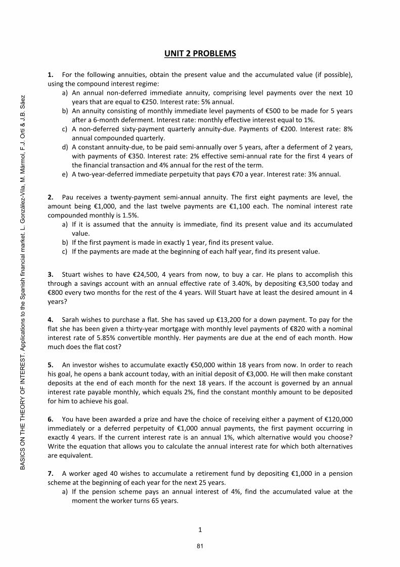
1

UNIT 2 PROBLEMS

1. For the following annuities, obtain the present value and the accumulated value (if possible), using the compound interest regime:

a) An annual non‐deferred immediate annuity, comprising level payments over the next 10 years that are equal to €250. Interest rate: 5% annual.

b) An annuity consisting of monthly immediate level payments of €500 to be made for 5 years after a 6‐month deferment. Interest rate: monthly effective interest equal to 1%.

c) A non‐deferred sixty‐payment quarterly annuity‐due. Payments of €200. Interest rate: 8% annual compounded quarterly.

d) A constant annuity‐due, to be paid semi‐annually over 5 years, after a deferment of 2 years, with payments of €350. Interest rate: 2% effective semi‐annual rate for the first 4 years of the financial transaction and 4% annual for the rest of the term.

e) A two‐year‐deferred immediate perpetuity that pays €70 a year. Interest rate: 3% annual.

2. Pau receives a twenty‐payment semi‐annual annuity. The first eight payments are level, the amount being €1,000, and the last twelve payments are €1,100 each. The nominal interest rate compounded monthly is 1.5%.

a) If it is assumed that the annuity is immediate, find its present value and its accumulated value.

b) If the first payment is made in exactly 1 year, find its present value. c) If the payments are made at the beginning of each half year, find its present value.

3. Stuart wishes to have €24,500, 4 years from now, to buy a car. He plans to accomplish this through a savings account with an annual effective rate of 3.40%, by depositing €3,500 today and €800 every two months for the rest of the 4 years. Will Stuart have at least the desired amount in 4 years? 4. Sarah wishes to purchase a flat. She has saved up €13,200 for a down payment. To pay for the flat she has been given a thirty‐year mortgage with monthly level payments of €820 with a nominal interest rate of 5.85% convertible monthly. Her payments are due at the end of each month. How much does the flat cost? 5. An investor wishes to accumulate exactly €50,000 within 18 years from now. In order to reach his goal, he opens a bank account today, with an initial deposit of €3,000. He will then make constant deposits at the end of each month for the next 18 years. If the account is governed by an annual interest rate payable monthly, which equals 2%, find the constant monthly amount to be deposited for him to achieve his goal. 6. You have been awarded a prize and have the choice of receiving either a payment of €120,000 immediately or a deferred perpetuity of €1,000 annual payments, the first payment occurring in exactly 4 years. If the current interest rate is an annual 1%, which alternative would you choose? Write the equation that allows you to calculate the annual interest rate for which both alternatives are equivalent. 7. A worker aged 40 wishes to accumulate a retirement fund by depositing €1,000 in a pension scheme at the beginning of each year for the next 25 years.

a) If the pension scheme pays an annual interest of 4%, find the accumulated value at the moment the worker turns 65 years.

81

BASI

CS

ON

TH

E TH

EOR

Y O

F IN

TER

EST.

App

licat

ions

to th

e Sp

anis

h fin

anci

al m

arke

t. L.

Gon

zále

z-Vi

la, M

. Már

mol

, F.J

. Ortí

& J

.B. S

áez

2

b) At the age of 65, the worker decides to give the accumulated amount to the pension scheme in exchange for constant repayments at the end of the following 15 years. Find the amount of the constant repayments assuming that the same interest rate is applied (as in the previous 25 years).

c) If the pension scheme had paid an annual interest rate of 4% for the first 10 years and then it had decreased to an annual 3.5%, what would have been the accumulated value at the moment the worker was 65 years old?

8. A loan with a principal of €150,000 will be repaid over the next 30 years with end‐of‐month level repayments. If its interest rate is compounded monthly and is equal to 4.80%, find the amount of the level repayments. 9. All of the following problems are related to annuities with payments in geometric progression:

a) A person purchased an immediate annuity with annual payments for 10 years. The first payment was €500 and the rest of the payments increased cumulatively by 8% a year. The purchase price was based on an annual interest rate of 3% compounded quarterly. Find that price.

b) The first of 40 payments of a monthly annuity occurs in exactly 1 year and is equal to €300. The payments increase so that each payment is 0.35% greater than the preceding payment. b.1) Find the present value of this annuity with an annual effective rate of interest of 4.20%. b.2) Find its present value if a nominal interest rate of 4.20% compounded monthly is

considered. c) A person is entitled to receive 12 semi‐annual payments at the beginning of each 6‐month

period. The payments decrease by an accumulative semi‐annual 2%, with the third one equal to €7,000. The nominal interest rate is 2.5% convertible monthly. Find the present value of all these payments and their accumulated value at the moment of the last one.

d) Quarterly perpetuity‐due, deferred 1 year. The first payment is €1,000 and subsequent ones increase by 1% cumulatively every quarter. Find its present value with a quarterly effective interest rate equal to 1.20%.

10. For the purchase of a luxury good today, 10 annual payments have been agreed. The first payment will be €2,500 and then the payments will rise by 12% annually and cumulatively. If an annual interest rate equal to 6% governs the transaction, find the value of the good today if:

a) The first payment is made in exactly 1 year. b) The first payment is due today. c) The first payment matures in 4 years.

11. A person has been making deposits in a savings account at the beginning of each year for 30 years. The first deposit was €2,000, subsequently they increased cumulatively by 3% per year until the twenty‐fourth payment, and after that they stayed level at €4,000. Find the accumulated amount in the account at the end of 30 years if the annual effective interest rate has been 3.2% for the entire term.

12. An investor wants to have €200,000 in 20 years. In order to obtain this amount, the investor will deposit the necessary amounts in a savings fund from now on, at the beginning of each month. The amounts will increase in such a way that each amount is 0.25% greater than the previous one. The fund will pay an annual effective interest rate equal to 2.5% for the first 3 years and a 3% nominal

82

BASI

CS

ON

TH

E TH

EOR

Y O

F IN

TER

EST.

App

licat

ions

to th

e Sp

anis

h fin

anci

al m

arke

t. L.

Gon

zále

z-Vi

la, M

. Már

mol

, F.J

. Ortí

& J

.B. S

áez

3

interest rate accumulated monthly for the rest of the term. Find the value of the first and the last amounts deposited by the investor in the fund.

13. A loan with a principal of €150,000 will be repaid over the next 30 years with end‐of‐month repayments. They will increase monthly by an accumulative 0.30%. If an interest rate compounded monthly and equal to 4.80% has been agreed, find the amount of the first and last repayments.

14. All of the following problems are related to annuities with payments in arithmetic progression: a) The following 20 end‐of‐month deposits have been made in an account earning a semi‐

annual effective interest rate of 6%: the first one was €300 while the subsequent deposits increased by €50 each month. What is the balance in the account at the end of the twentieth month?

b) Consider an immediate annuity with annual payments for 20 years. The payments are level throughout the first 10 years, the amount being €1,000. Then, the eleventh payment is €100 greater than the preceding one, the twelfth payment is €100 greater than the eleventh, and so on. Find the present value of this annuity if the annual effective interest rate is 3%.

c) The following semi‐annually payments are to be made: €2,750 today, €2,850 6 months from now, €2,950 in a year, and so on, until a final payment of €4,150. Using an annual effective interest rate equal to 10%, find the financial value of these payments today, and at the end of the 6‐month period when the last payment will be made.

d) Fran purchases a perpetuity. The perpetuity pays €100 at the end of each quarter for the first 11 years and then the payments increase by €5 each quarter. Find the purchase price if it is determined using a nominal interest rate quarterly compounded of 5%.

15. A loan with a principal of €150,000 will be repaid over the next 30 years with end‐of‐month repayments, which will increase by €2 monthly. If an interest rate compounded monthly and equal to 4.80% has been agreed, find the amount of the first and the last repayments.

Formulas

𝐶 𝐶 𝐶 𝑎 | 𝐶1 1 𝐼

𝐼 𝐶 ∙

1𝐼

𝐶 𝐶 ∙ 𝑞

⎩⎨

⎧𝐶 ∙1 𝑞 ∙ 1 𝐼

1 𝐼 𝑞1 𝐼 𝑞

𝐶 ∙ 𝑛 ∙ 𝑞 1 𝐼 𝑞

𝐶

1 𝐼 𝑞 𝑞 1 𝐼

𝐶 𝐶 𝑟 1 ℎ 𝐶 𝑛 ∙ ℎℎ𝐼

∙ 𝑎 |𝑛 ∙ ℎ𝐼

𝐶𝐼

ℎ𝐼

__________________________________________________________________________________

83

BASI

CS

ON

TH

E TH

EOR

Y O

F IN

TER

EST.

App

licat

ions

to th

e Sp

anis

h fin

anci

al m

arke

t. L.

Gon

zále

z-Vi

la, M

. Már

mol

, F.J

. Ortí

& J

.B. S

áez

4

Answers 1. a) 𝑉 €1,930.43 𝑉 €3,144.47. b) 𝑉 €21,174.84 𝑉 €40,834.84. c) 𝑉 €7,091.22 𝑉 €23,266.51. d) 𝑉 €2,963.37 𝑉 €3,905.60. e) 𝑉 €2,199.39.

2. a) 𝑉 €19,580.38 𝑉 €22,747.02. b) 𝑉 €19,434.16. c) 𝑉 €19,727.69.

3. The savings account balance will be €24,486.74. So, Stuart will not have the desired amount. 4. €152,196.97. 5. €175.95. 6. For the given interest of 1% annual, the best alternative is to choose the single payment of €120,000 because the present value of the perpetuity is €97,059.01. The equation is 120,000 1,000 1 𝐼 .

7. a) €43,311.74. b) €3,895.51. c) €40,890.02.

8. €787. 9. a) €6,052.68.

b) b.1) 𝑉 €11,531.01. b.2) 𝑉 €11,507.28.

c) 𝑉 €73,536.94 𝑉 €84,364.34. d) 𝑉 €482,423.51.

10. a) €30,595.39.

b) €32,431.12. c) €25,688.48.

11. €147,612.66. 12. 𝐶 €458.24 𝐶 €832.26.

13. 𝐶 €497.60 𝐶 €1,458.53. 14. a) €16,670.28.

b) 𝑉 €18,213.91. c) 𝑉 €36,893.89 𝑉 €75,404.90. d) 𝑉 €26,757.01.

15. 𝐶 €511.40 𝐶 €1,229.40.

84

BASI

CS

ON

TH

E TH

EOR

Y O

F IN

TER

EST.

App

licat

ions

to th

e Sp

anis

h fin

anci

al m

arke

t. L.

Gon

zále

z-Vi

la, M

. Már

mol

, F.J

. Ortí

& J

.B. S

áez

UNIT 3.

LOANS


2. Outstanding loan balance. Other concepts

3. Loan repaid by a single repayment

4. Interest-only loan

5. Amortizing loan with level repayments

6. Changes during the lifetime of the loan


1.1. Definition

1.2. Classification

1.1. Definition

A loan is a financial transaction by which a person, called the lender oractive party, gives another person, called the borrower or passive party,a monetary amount, 𝐶, called the principal of the loan. In exchange forthe loan, the borrower undertakes to repay the borrowed amount in aspecific term, either through a single repayment or through a set ofrepayments, plus the payment of interest.

Therefore, at the time of arranging the loan, there exists a financialequivalence between the financial capital that the lender lends(payment) and the financial capital that the borrower repays(repayments), as a result of the deals that have been agreed by bothparties. This financial equivalence is ruled by the compound interestfinancial regime with the effective interest rate agreed on the loan, 𝐼 .

Unit 3. Loans

85

BASI

CS

ON

TH

E TH

EOR

Y O

F IN

TER

EST.

App

licat

ions

to th

e Sp

anis

h fin

anci

al m

arke

t. L.

Gon

zále

z-Vi

la, M

. Már

mol

, F.J

. Ortí

& J

.B. S

áez

Thus, a loan can be represented by:

Payment: 𝐶, 0Repayments: 𝛼 ,𝑇 , ,…,

Graphically:

Unit 3. Loans


C

nT0

1

1T

2

2T

3

3T

1n

1nT

nr

rT

......

......

If the effective interest rate of the loan is 𝐼 , then the financialequivalence between the payment and repayments can be expressed as:

𝐶, 0 ~ 𝛼 ,𝑇 , ,…,

↓𝐼

1.2. Classification

Loans can be classified by considering different aspects.

Regarding how the principal of the loan is repaid:

1) Loan with a single repayment of the principal.

The principal 𝐶 is paid off by a single repayment at the end of thefinancial transaction.

2) Loan with periodic repayments (amortizations) of the principal.

The principal 𝐶 is paid off by periodic repayments made over theagreed term.

Regarding how the interest on the loan is paid:

1) Loan with a single payment of interest.There is only a single payment of interest, usually paid at the end ofthe financial transaction.

2) Loan with periodic payments of interest.Payments of interest are made periodically during the agreed term.

Unit 3. Loans


86

BASI

CS

ON

TH

E TH

EOR

Y O

F IN

TER

EST.

App

licat

ions

to th

e Sp

anis

h fin

anci

al m

arke

t. L.

Gon

zále

z-Vi

la, M

. Már

mol

, F.J

. Ortí

& J

.B. S

áez

More particularly, we will study the following three types of loans:

1) Loan with single repayment of the principal 𝐶 and single payment ofinterest 𝑌. In short: loan repaid by a single repayment.Graphically:

being the financial equivalence: 𝐶, 0 ~ 𝐶 ,𝑇′ with 𝐶 𝐶 𝑌

2) Loan with a single repayment of the principal 𝐶 and periodic paymentsof interest 𝑌 . For short: interest-only loan.Graphically:

Unit 3. Loans


'T0

CC Y

'T np0 3p2 p

3Y nY C

. . .

. . . 1nY

1n pp

1Y 2YC

with:

3) Loan with periodic repayments of the principal 𝐴 and periodicpayments of interest 𝑌 . In short: amortizing loan. Specifically, we willsee loans repaid with level repayments that are comprised of paymentof interest and repayment of principal: amortizing loan with levelrepayments.

with: 𝐶, 0 ~ 𝛼, 𝑟𝑝 , ,…, and 𝛼 𝐴 𝑌

In this case, the sum of all the periodic repayments of the principal isequal to the principal of the loan, that is:

Unit 3. Loans


𝐶, 0 ~ 𝑌 , 𝑟𝑝 , 𝐶,𝑛𝑝 , ,…,

np0 2 p

n nA Y

. . .

. . . 1 1n nA Y

1n pp

1 1A Y 2 2A Y

C

1

n

rr

C A

87

BASI

CS

ON

TH

E TH

EOR

Y O

F IN

TER

EST.

App

licat

ions

to th

e Sp

anis

h fin

anci

al m

arke

t. L.

Gon

zále

z-Vi

la, M

. Már

mol

, F.J

. Ortí

& J

.B. S

áez


2.1. Outstanding loan balance

2.2. Other concepts

2.1. Outstanding loan balance

The outstanding balance at any moment 𝜏 of the loan is the total amountthat the borrower must repay to the lender in order to totally cancel theloan at that moment, by considering only the payment and repaymentsinvolved in the financial equivalence (disregarding any fees or costs):

We consider two approaches to computing the outstanding loan balanceat moment 𝜏, 𝑂𝐿𝐵 : the prospective method and the retrospectivemethod. It will later be shown that the two methods are equivalent.

Unit 3. Loans

𝐶, 0 ~ 𝛼 ,𝑇 , ,…,↓𝐼

Retrospective method: the retrospective outstanding loan balance at 𝜏is the financial value of the principal of the loan at 𝜏, minus the financial

value at 𝜏 of all the repayments made up to and including this moment, atthe same interest rate, 𝐼 , agreed on the loan.

Past of the financial transaction Future of the financial transaction

C

nT0

1

1T

2

2T

3

3T

1n

1nT

n......

......

1 1

r

r

m m Tretm r m

TOLB C I I

Unit 3. Loans


𝐶, 0 ~ 𝛼 ,𝑇 , ,…,↓𝐼

88

BASI

CS

ON

TH

E TH

EOR

Y O

F IN

TER

EST.

App

licat

ions

to th

e Sp

anis

h fin

anci

al m

arke

t. L.

Gon

zále

z-Vi

la, M

. Már

mol

, F.J

. Ortí

& J

.B. S

áez

1

r

r

m Tpror m

TOLB I

Prospective method: The prospective outstanding loan balance at 𝜏 is

the financial value at 𝜏 of all the remaining repayments from time 𝜏 (notincluded) until the end of the loan, at the same interest rate, 𝐼 , agreedon the loan.

C

nT0

1

1T

2

2T

3

3T

1n

1nT

n......

......

Past of the financial transaction Future of the financial transaction

PROPERTY

The retrospective and prospective outstanding loan balances at anymoment 𝜏 are equal.

ret proOLB OLB

Unit 3. Loans


Example 1. A loan with a principal of €60,000, paid today, will be repaidthrough annual level repayments at the end of the following 15 years. It isruled by an annual effective interest rate equal to 6%.

• Find the amount of the level repayments.

60,000

0 . . .

. . .

1 2 3 14 15

15 0 0660 000 ., a

The annual effective rate is: 1 0 06I .

€6,177.77

And the amount of the level repayments can be obtained from:

Unit 3. Loans


89

BASI

CS

ON

TH

E TH

EOR

Y O

F IN

TER

EST.

App

licat

ions

to th

e Sp

anis

h fin

anci

al m

arke

t. L.

Gon

zále

z-Vi

la, M

. Már

mol

, F.J

. Ortí

& J

.B. S

áez

Unit 3. Loans


• Find the retrospective and the prospective outstanding loan balance 5years after being given.

By considering the definition of the retrospective outstanding loanbalance, we have:

0 . . .

. . .60,000

1 2 5 14 15. . .

. . .

6 7

560,000 1 0.06 55 0.066,177.77 1 0.06a €45,468.895 retOLB

And taking into account its definition, the retrospective outstanding loanbalance after 5 years of being paid is:

5 proOLB 10 0.066,177.77 a €45,468.89

0 . . .

. . .60,000

1 2 5 14 15. . .

. . .

6 7

5.560,000 1 0.06 5.55 0.066.177,77 1 0.06a €46,813.095.5 retOLB

15

2

0.5 0.55.5 5 1 0.06 45,468.9 1 0.06 €46.813.09 ret retOLB OLB

• Find the retrospective and the prospective outstanding loan balance 5and a half years after being paid out.

Following similar reasoning to that explained above, the retrospectiveoutstanding loan balance at 5.5 years is:

It is worth pointing out that 𝑂𝐿𝐵 . can also be calculated from theoutstanding loan balance at year 5:

Unit 3. Loans


90

BASI

CS

ON

TH

E TH

EOR

Y O

F IN

TER

EST.

App

licat

ions

to th

e Sp

anis

h fin

anci

al m

arke

t. L.

Gon

zále

z-Vi

la, M

. Már

mol

, F.J

. Ortí

& J

.B. S

áez

Finally, the prospective outstanding loan balance at 5.5 years is:

5.5 proOLB 0.510 0.066,177.77 1 0.06a €46,813.09

0 . . .

. . .60,000

1 2 5 14 15. . .

. . .

6 715

2

Unit 3. Loans


2.2. Other concepts

For all the loans that will be studied in this unit, not only will we analyzefinancial equivalence and the outstanding loan balance, but also thefollowing concepts:

1) Repayment(s).

2) Outstanding principal.

3) Value of the loan.

4) Lender effective interest rate.

5) Borrower effective interest rate.

6) TAE of the loan.

Unit 3. Loans


Repayment(s)

Amount(s) repaid by the borrower included in the financial equivalence.They may be comprised of both the payment of interest and therepayment (amortization) of the principal, depending on the kind of loanconsidered.

91

BASI

CS

ON

TH

E TH

EOR

Y O

F IN

TER

EST.

App

licat

ions

to th

e Sp

anis

h fin

anci

al m

arke

t. L.

Gon

zále

z-Vi

la, M

. Már

mol

, F.J

. Ortí

& J

.B. S

áez

Outstanding principal (or non-repaid principal of the loan), 𝑂𝑃The outstanding principal at moment 𝜏 is that part of the principal of the

loan that has not been repaid yet at moment 𝜏. The principal of the loan

minus the outstanding principal at 𝜏 is equal to the repaid principal of the

loan until moment 𝜏.

Value of the loan, 𝑉

This is the financial value at 𝜏 of the outstanding repayments of the loan,using the current market interest rate.

Unit 3. Loans


PROPERTY

If the current market interest rate is equal to the interest rate agreed onthe loan, 𝐼 , the value of the loan and the outstanding balance of theloan are both equal. Otherwise, they are not.

In addition to interest, loans may have some associated expenses andfees, such as, among others:

Application or booking fee.

Arrangement fee (also known as Initial, Underwriting, Administrative,Processing Product, Completion, etc. fee).

Management expenses.

Loan broker fee.

Related taxes.

Maintenance expenses of associated products (credit cards, bankaccounts, ...).

Life insurance premiums.

Early repayment fee.

Land Registry and Public Notary expenses (for mortgages)

Appraisal expenses, Home insurance premiums and Mortgage defaultinsurance premiums (for mortgages).

Depending on the expenses taken into account, there are 3 differenteffective interest rates.

Unit 3. Loans


92

BASI

CS

ON

TH

E TH

EOR

Y O

F IN

TER

EST.

App

licat

ions

to th

e Sp

anis

h fin

anci

al m

arke

t. L.

Gon

zále

z-Vi

la, M

. Már

mol

, F.J

. Ortí

& J

.B. S

áez

Lender effective interest rate

Effective interest rate for the lender, taking into consideration not only theprincipal of the loan and all the repayments agreed in the financialequivalence but also the fees paid by the borrower in benefit of the lenderand all the expenses the lender has over the lifespan of the loan.

Unit 3. Loans


Given that, over the term of the loan, unexpected repayments, fees orexpenses, which are not known at the moment of awarding the loan, mayappear, these two effective interest rates can change throughout the lifeof the loan. Furthermore, for a specific loan, the borrower effectiveinterest rate may not be the same for every borrower.

Borrower effective interest rate

Effective interest rate for the borrower, taking into account not only theprincipal of the loan and all the repayments agreed in the financialequivalence, but also all the fees and expenses that are paid both inorder to obtain the loan and during the term of the loan.

Unit 3. Loans


TAE (Tasa anual equivalente) of the loan

As we saw in Unit 1, Spanish financial institutions must inform about theTAE of any financial transaction. The TAE is the annual effective interestrate associated with a financial transaction once the costs and feesindicated by Spanish laws in force have been considered. These costsand fees are known (or can be estimated) at the beginning of thefinancial transaction and banks have to inform their clients on the TAEwhen this transaction is offered.

We also said that most developed countries have laws in force thatcontain similar concepts. For example, in the case of credit agreementsfor consumers, the European Directive 2008/48/EC introduces theconcept of annual percentage rate (APR) of charge.

Since we focus on the Spanish financial market, we define the TAE of aloan as the annual effective interest rate associated with this loan whenconsidering the costs and fees known at the moment of agreeing on theloan. But only costs and fees indicated by Spanish laws in force have tobe taken into account.

The TAE of a loan is calculated when the loan is awarded and it does notchange over the term of the loan.

93

BASI

CS

ON

TH

E TH

EOR

Y O

F IN

TER

EST.

App

licat

ions

to th

e Sp

anis

h fin

anci

al m

arke

t. L.

Gon

zále

z-Vi

la, M

. Már

mol

, F.J

. Ortí

& J

.B. S

áez

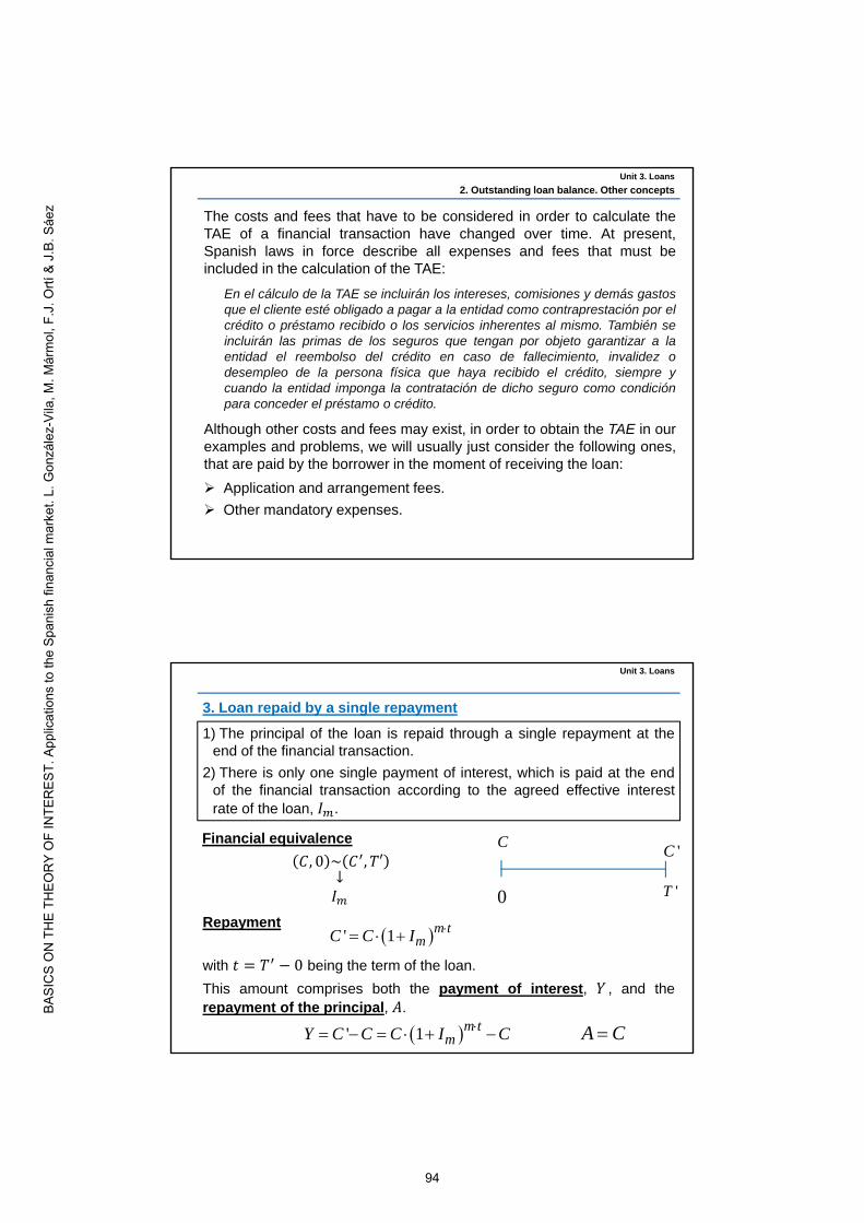
Unit 3. Loans


The costs and fees that have to be considered in order to calculate theTAE of a financial transaction have changed over time. At present,Spanish laws in force describe all expenses and fees that must beincluded in the calculation of the TAE:

En el cálculo de la TAE se incluirán los intereses, comisiones y demás gastosque el cliente esté obligado a pagar a la entidad como contraprestación por elcrédito o préstamo recibido o los servicios inherentes al mismo. También seincluirán las primas de los seguros que tengan por objeto garantizar a laentidad el reembolso del crédito en caso de fallecimiento, invalidez odesempleo de la persona física que haya recibido el crédito, siempre ycuando la entidad imponga la contratación de dicho seguro como condiciónpara conceder el préstamo o crédito.

Although other costs and fees may exist, in order to obtain the TAE in ourexamples and problems, we will usually just consider the following ones,that are paid by the borrower in the moment of receiving the loan:

Application and arrangement fees.

Other mandatory expenses.

'T0

C'C

' 1 m tmC C I

Repayment

with 𝑡 𝑇 0 being the term of the loan.

This amount comprises both the payment of interest, 𝑌 , and therepayment of the principal, 𝐴.

1) The principal of the loan is repaid through a single repayment at theend of the financial transaction.

2) There is only one single payment of interest, which is paid at the endof the financial transaction according to the agreed effective interestrate of the loan, 𝐼 .

Financial equivalence

𝐶, 0 ~ 𝐶 ,𝑇′↓𝐼

' 1 m tmY C C C I C A C


Unit 3. Loans

94

BASI

CS

ON

TH

E TH

EOR

Y O

F IN

TER

EST.

App

licat

ions

to th

e Sp

anis

h fin

anci

al m

arke

t. L.

Gon

zále

z-Vi

la, M

. Már

mol

, F.J

. Ortí

& J

.B. S

áez

Now we obtain the outstanding loan balance and the outstandingprincipal at 3 different moments in time:

• At the beginning of the loan, 0.

• At any moment between its beginning and its end, 𝜏 ∈ 0,𝑇′ .

• At the end of the loan, 𝑇′ .

'T0

C 'COutstanding loan balance

1 mmC I

'' 1 m TmC I

0OLB C

' 0TOLB

• At 0:

• At 𝜏: OLB

• At 𝑇 :

Unit 3. Loans


Outstanding principal

0OP C

' 0TOP

• At 0:

• At 𝜏: OP C

• At 𝑇 :

Outstanding loan balance vs. outstanding principal over the term ofthe loan

0 'T

C

OLBOP

'Y C C C'

The outstanding loan balance and the outstanding principal are equal at 0 and at 𝑇

A C

The two are different at 𝜏 ∈ 0,𝑇′ . This is because the outstanding loanbalance takes into consideration the accrued interest until moment 𝜏 andthe outstanding principal does not.

Unit 3. Loans


𝜏

95

BASI

CS

ON

TH

E TH

EOR

Y O

F IN

TER

EST.

App

licat

ions

to th

e Sp

anis

h fin

anci

al m

arke

t. L.

Gon

zále

z-Vi

la, M

. Már

mol

, F.J

. Ortí

& J

.B. S

áez

Moment Outstanding loan balance Outstanding principal

0 𝐶 𝐶

𝜏Retrospective 𝐶 1 𝐼

𝐶Prospective 𝐶′ 1 𝐼

𝑇′ 0 0

Summarizing:

Unit 3. Loans


Value of the loan, 𝑉If the current market interest rate is denoted by 𝐼 , the financialvalue at 𝜏 of the outstanding repayments of the loan is:

The lender effective interest rate, the borrower effective interest rateand the TAE of the loan can be obtained as described in subsection 2.2.

'' 1

m TMarketmV C I

Example 2. A loan with a principal of €30,000 will be repaid through asingle repayment, which includes interest and the principal, in 4 years. Ifits annual effective rate is 7.5%, it has a €300 initial fee and the borrowerpays €600 of mandatory expenses at the beginning of the loan.

• Find the amount of the single repayment and split it into interest andprincipal.

40

30,000 'C

4' 30,000 1 0.075 €40,064.07 C

1 0.075I

So:

' 40,064.07 30,000 €10,064.07 Y C C

€30,000A

Unit 3. Loans


96

BASI

CS

ON

TH

E TH

EOR

Y O

F IN

TER

EST.

App

licat

ions

to th

e Sp

anis

h fin

anci

al m

arke

t. L.

Gon

zále

z-Vi

la, M

. Már

mol

, F.J

. Ortí

& J

.B. S

áez

• Obtain the outstanding loan balance 2 and a half years after beinglent.

• Find the outstanding principal after 2 and a half years of being lent.

• If today, 2 and a half years after the principal was borrowed, the currentmarket interest rate is an annual 6%, what is the financial value of theloan?

2.5 OLB

2.530,000 1 0.075 €35,945.33

1.540,064.07 1 0.075 €35,945.33

2.5 €30,000OP

40

30,000 40,064.07

2.5

1.52.5 40,064.07 1 0.06 €36,711 V

Unit 3. Loans


• Determine the borrower effective interest rate and the TAE of theloan.

To determine the borrower effective interest rate, we not only considerthe single repayment but also all other fees and expenses.

Graphically:

If we calculate the value at moment 0, we will have:

Unit 3. Loans


30,000 , 0 ~ 300, 0 , 600, 0 , 40,064.07, 4

Principal of the loan

Mandatory expenses

Initial fee

Single repayment

↓Borrower effective interest rate, 𝐼

4130,000 900 40,064.07 1 I

1 0.083217 8.3217% I

40

30,000

40,064.07600300


Mandatory expenses

Initial fee

Single repayment

97

BASI

CS

ON

TH

E TH

EOR

Y O

F IN

TER

EST.

App

licat

ions

to th

e Sp

anis

h fin

anci

al m

arke

t. L.

Gon

zále

z-Vi

la, M

. Már

mol

, F.J

. Ortí

& J

.B. S

áez

As for the TAE, since Spanish current laws say that both the initial feeand the mandatory expenses have to be considered, we have the sameequation:

So:

• 2 and a half years after the loan is granted, the borrower decides tocompletely cancel it. Determine the borrower effective interest rate ifat that time he pays an early repayment fee of 0.25% on theoutstanding principal.

In order to totally cancel the loan the borrower pays its outstanding loanbalance, , and the early repayment fee:

To obtain the borrower effective interest rate, we consider all thepayments and repayments involved in the financial transaction.

Unit 3. Loans


4130,000 900 40,064.07 1 I

0.083217 8.3217% TAE

2.5 €35,945.33OLB

30,000 0.0025 €75

Unit 3. Loans


2.5130,000 900 35,945.33 75 1 I

1 0.089085 8.9085% I

Graphically:

If we value at moment 0, we have:

2.50

30,000 35,945.33

600300


Mandatory expenses

Initial fee

Outstanding loan balance

Early repayment fee75

98

BASI

CS

ON

TH

E TH

EOR

Y O

F IN

TER

EST.

App

licat

ions

to th

e Sp

anis

h fin

anci

al m

arke

t. L.

Gon

zále

z-Vi

la, M

. Már

mol

, F.J

. Ortí

& J

.B. S

áez

1) The principal of the loan is repaid through a single repayment at theend of the financial transaction.

2) The term of the loan is split into 𝑛 periods of length 𝑝, 𝑝 , and

payments of interest are made at the end of each period according tothe agreed effective interest rate, 𝐼 .


↓𝐼

np0 3p2 p

Y Y

. . .

. . . Y

1n pp

Y YCC

𝐶, 0 ~ 𝑌, 𝑟𝑝 , 𝐶,𝑛𝑝 , ,…,

1 nmn Im

C Y a C I

Unit 3. Loans


The periodic payments of interest are level (constant):

𝑌 𝐶 𝐼The single repayment of the principal, 𝐴, that is paid at the end of theloan, is:

𝐴 𝐶

Unit 3. Loans




• At the end of each period of the loan: 𝑟𝑝.

• At a specific moment within a period of the loan: 𝜏 ∈ 𝑟𝑝, 𝑟 1 𝑝 .

• At the end of the loan, 𝑛𝑝 . rp 1r p

NOTE: We will always consider, unless otherwise stated, that the payment of interest 𝑌 has just been made.

99

BASI

CS

ON

TH

E TH

EOR

Y O

F IN

TER

EST.

App

licat

ions

to th

e Sp

anis

h fin

anci

al m

arke

t. L.

Gon

zále

z-Vi

la, M

. Már

mol

, F.J

. Ortí

& J

.B. S

áez


0OLB C• At 0:

np0 rp2 p

Y Y

. . .

. . . Y

1n pp

Y YCC

. . .

. . .

1r p

Y

1 1 r rm mr Im

C I Y a I

( )1 n rI mn r mY a C I

• At 𝑟𝑝: rpOLB

C

C

Unit 3. Loans


rpOLB OLB

0npOLB • At 𝑛𝑝:

• At 𝜏:

rp 1r p


0OP C

0npOP

• At 0:

• At 𝜏: OP C

• At 𝑛𝑝:

rpOP C• At 𝑟𝑝:

The outstanding loan balance and the outstanding principal are equal at0, at 𝑛𝑝 and at the end of each period once the payment of interest hasbeen made.

Unit 3. Loans


1 m rprp mOLB OLB I

100

BASI

CS

ON

TH

E TH

EOR

Y O

F IN

TER

EST.

App

licat

ions

to th

e Sp

anis

h fin

anci

al m

arke

t. L.

Gon

zále

z-Vi

la, M

. Már

mol

, F.J

. Ortí

& J

.B. S

áez

0 np

C

OLBOP

mY C I

p 2 p

A C

. . .. . . rp


Unit 3. Loans


The outstanding loan balance and the outstanding principal are differentat a specific moment 𝜏 within a period of the loan. This is because theoutstanding loan balance takes into consideration the accrued interestuntil moment 𝜏 and the outstanding principal does not.

𝜏

Summarizing:


0 𝐶 𝐶

𝑟𝑝Retrospective 𝐶

𝐶Prospective 𝐶

𝜏 𝐶

𝑛𝑝 0 0

rp 1r prpOLB OLB

Unit 3. Loans


1 m rprp mOLB OLB I

101

BASI

CS

ON

TH

E TH

EOR

Y O

F IN

TER

EST.

App

licat

ions

to th

e Sp

anis

h fin

anci

al m

arke

t. L.

Gon

zále

z-Vi

la, M

. Már

mol

, F.J

. Ortí

& J

.B. S

áez

Unit 3. Loans




( )1 1Market

m

n r m rpMarket Marketm mn r I

V Y a C I I

np0 rp2 p

Y

. . .

. . . Y

1n pp

C

. . . 1r p

Y

40.12

0.034

I

4 5,000 0.03 €150 Y C I

4 0.12i

Example 3. A loan with a principal of €5,000 will be repaid with quarterlypayments of interest and a lump sum payment of the principal in 2 years.The nominal rate of interest payable quarterly is 12%, there is an initialfee of 1.5% of the principal and the borrower pays mandatory expensesof €135 when the loan is awarded. Find:

• The amount of the quarterly payments of interest.

The quarterly effective interest rate of the loan is:

So, the amount of the quarterly payments of interest is:

• The outstanding loan balance and the outstanding principal 6months (2 quarters) after the beginning of the loan.

20 9

12

6

12

150 150

. . .

. . . 150

91

123

12

150 1505,0005,000

Unit 3. Loans


102

BASI

CS

ON

TH

E TH

EOR

Y O

F IN

TER

EST.

App

licat

ions

to th

e Sp

anis

h fin

anci

al m

arke

t. L.

Gon

zále

z-Vi

la, M

. Már

mol

, F.J

. Ortí

& J

.B. S

áez

612

2 €5,000 OLB OP

Immediately 6 months after the beginning of the loan, a payment ofinterest of €150 is made. Therefore, at that moment, the outstandingloan balance and the outstanding principal are equal. That is to say:

• The outstanding loan balance and the outstanding principal 7months after the beginning of the loan.

To obtain the outstanding loan balance after 7 months, we can considerthe outstanding loan balance after 6 months and the accumulationfactor for 1 month, i.e.:

And the outstanding principal after 7 months is equal to the principal ofthe loan:

612

OLB 712

OLB

9

126

127

12

1

127

12

45,000 1 0.03 €5,049.51 OLB

€5,000

Unit 3. Loans


150

201

150

. . .

. . . 150

31

123

12

1505,0005,000

. . .

. . .

1V

1 44 1 0.10 1 0.024114 I1 0.10I

41 4 0.024114150 5,000 (1 0.024114) V a €5,110.96

• The value of the loan 1 year after being awarded, if the market interestrate at that moment is 10% annual effective.

The quarterly effective interest rate equivalent to the market interestrate of a 10% annual effective rate is:

So:

Unit 3. Loans


103

BASI

CS

ON

TH

E TH

EOR

Y O

F IN

TER

EST.

App

licat

ions

to th

e Sp

anis

h fin

anci

al m

arke

t. L.

Gon

zále

z-Vi

la, M

. Már

mol

, F.J

. Ortí

& J

.B. S

áez

• The equation that allows us to obtain the borrower effective interestrate.

To determine the borrower effective interest rate, we consider all thequarterly payments of interest, 𝑌 €150, the lump sum repayment ofthe principal, 𝐴 𝐶 €5,000, initial fee, 5,000 0.015 €75, andmandatory expenses, €135.

Drawing all this financial capital on the timeline:

Since the payments of interest are made quarterly, a quarterly effectiveinterest rate has to be used. If we value at 0:


Mandatory expenses

Initial feeQuarterly

payments of interest

Repayment of the principal

150. . .1505,000

5,000

13575

20 . . .3

12

4

8485,000 135 75 150 5,000 (1 )Ia I

Unit 3. Loans


Using a suitable software, 𝐼 can be obtained.

• The equation that allows us to calculate the TAE of the loan.

In this case, since Spanish current laws say that both the initial fee andcompulsory expenses have to be included in the calculation of the TAE,we have the same equation and interest rate as in the previousquestion.

The TAE will be the effective interest rate equivalent to 𝐼 , i.e.:

41 1 0.03614 1 0.15258 15.258% TAE I

Unit 3. Loans


4 0.03614I

104

BASI

CS

ON

TH

E TH

EOR

Y O

F IN

TER

EST.

App

licat

ions

to th

e Sp

anis

h fin

anci

al m

arke

t. L.

Gon

zále

z-Vi

la, M

. Már

mol

, F.J

. Ortí

& J

.B. S

áez


1) The term of the loan is split into 𝑛 periods of length 𝑝, 𝑝 .

2) The loan is repaid through level repayments, 𝛼, at the end of eachperiod according to the agreed effective interest rate, 𝐼 .

3) These level repayments include the payment of interest correspondingto each period and a partial repayment (amortization) of the principal ofthe loan.

Level repayment of period 𝑟

Partial repayment (amortization) of principal of period 𝑟

𝛼 𝑌 𝐴

Payment of interest of period 𝑟

Unit 3. Loans


np0 3p2 p

. . .

. . .

1n pp

C

Unit 3. Loans


↓𝐼

𝐶, 0 ~ 𝛼, 𝑟𝑝 , ,…, n ImC a

n Im

C

a

As we previously saw: 𝛼 𝑌 𝐴

• The payment of interest made at the end of the period 𝑟 is:

• The partial repayment (amortization) of principal made at the end of period 𝑟 is:

In addition to these relationships, there are also other obvious ones. We illustrate them with an example.

1r r mY OP I

r rA Y

105

BASI

CS

ON

TH

E TH

EOR

Y O

F IN

TER

EST.

App

licat

ions

to th

e Sp

anis

h fin

anci

al m

arke

t. L.

Gon

zále

z-Vi

la, M

. Már

mol

, F.J

. Ortí

& J

.B. S

áez

11 YA C

50 321

22 YA 33 YA 55 YA

4

44 YA

Just after the moment of making the3rd repayment (at the end of the 3rd

period), the outstanding principal isequal to the sum of all the pendingrepayments of principal.

Alternatively, it is equal to the principal ofthe loan minus all the repayments ofprincipal made since that moment.

Example 4. Let us consider an amortizing loan with 5 level repayments.

1

n

r ss r

OP A

1 2 3 4 5A A A A A

1 1r r rOP OP A

1

r

r ss

OP C A

1

n

rr

C A

3 4 5OP A A

3 1 2 3OP C A A A Part of the principal repaid at the end of the 3rd period

4 3 4OP OP A

Unit 3. Loans


All the concepts related to an amortizing loan with level repayments canbe grouped in its amortization table or amortization schedule.

r r r rr Y A OP

𝑟 Level repayment

Payment of interest Repayment of principal


0

1

2

3

… … … … …

n

rY

1 mY C I

2 1 mY OP I

3 2 mY OP I

1n n mY OP I

1 1A Y

2 2A Y

3 3A Y

n nA Y

rA rOP

0OP C

1 0 1OP OP A

2 1 2OP OP A

3 2 3OP OP A

0nOP

Unit 3. Loans


106

BASI

CS

ON

TH

E TH

EOR

Y O

F IN

TER

EST.

App

licat

ions

to th

e Sp

anis

h fin

anci

al m

arke

t. L.

Gon

zále

z-Vi

la, M

. Már

mol

, F.J

. Ortí

& J

.B. S

áez

Example 5. Construct the amortization table for a loan with a principal of€1,000 to be repaid with constant semiannual installments over 3 years,if the loan is governed by 8% annual interest compounded semiannually.

First, we calculate the amount of the level repayments (installments):

So, the amortization table of the loan is:

61 1 0.041,000 €190.76

0.04

2

0.080.04

2 I2 0.08i

r

0

1

2

3

4

5

6

190.76

190.76

190.76

190.76

190.76

190.76

40.00 150.76 849.24

rY rA rOP

33.97 156.79 692.4527.69 163.07 529.38

21.17 169.59 359.7914.39 176.37 183.427.34 183.42 0

1,000.00

Unit 3. Loans


In the previous amortization table, it can be seen that even though theamount of the repayment 𝛼 is constant, as time goes by the payment of

interest, 𝑌 , decreases and the repayment (amortization) of principal, 𝐴 ,increases. This is because the payment of interest made at the end of aperiod is calculated by applying the effective interest rate to theoutstanding principal at the beginning of the period, and this outstandingprincipal gradually decreases from period to period.

Unit 3. Loans


11

rrA A q

1 mq I 1 1 A Y mC I

11 1 r

r mA A I

PROPERTY

In amortizing loans with level repayments, repayments (amortizations)of principal vary in geometric progression, i.e.:

with the common ratio and the first element given by:

107

BASI

CS

ON

TH

E TH

EOR

Y O

F IN

TER

EST.

App

licat

ions

to th

e Sp

anis

h fin

anci

al m

arke

t. L.

Gon

zále

z-Vi

la, M

. Már

mol

, F.J

. Ortí

& J

.B. S

áez

1 150.76A 2 156.79A 3 163.07A

4 169.59A 5 176.37A 6 183.42A

1 11 1 150.76 1.04r r

r mA A I

3 13 150.76 1.04 163.07A

6 16 150.76 1.04 183.42A

Example 6. In the amortization table contained in example 5 weobtained:

The interest rate for this loan was 𝐼 0.04.

In this case, the following is satisfied:

Thus, for instance:

Unit 3. Loans




• At the end of each period of the loan: 𝑟𝑝

• At a specific moment within a period of the loan: 𝜏 ∈ 𝑟𝑝, 𝑟 1 𝑝

• At the end of the loan, 𝑛𝑝 .rp 1r p

NOTE: We will always consider, unless otherwise stated, that the level repayment 𝛼 has just been made.

Unit 3. Loans


108

BASI

CS

ON

TH

E TH

EOR

Y O

F IN

TER

EST.

App

licat

ions

to th

e Sp

anis

h fin

anci

al m

arke

t. L.

Gon

zále

z-Vi

la, M

. Már

mol

, F.J

. Ortí

& J

.B. S

áez


0OLB C• At 0:

rpOLB OLB

• At 𝑛𝑝:

• At 𝜏:

rp 1r p

• At 𝑟𝑝: rpOLB In r m

a

1 1r rm mr Im

C I a I

np0 rp2 p

. . .

. . .

1n pp

C

. . .

. . .

1r p

0npOLB

Unit 3. Loans


1 m rprp mOLB OLB I


• At 0:

• At 𝜏:

• At 𝑛𝑝:

• At 𝑟𝑝:

rOP OP

r rpOP OLB0OP C

0nOP

The outstanding loan balance and the outstanding principal are equal at0, at 𝑛𝑝 and at the end of each period once the level repayment hasbeen made.

Right after paying the level repayment corresponding to period r, theoutstanding loan balance does not contain accrued interest, i.e. it isonly composed of principal. This is the reason why the outstandingprincipal and the outstanding loan balance are equal.

Unit 3. Loans


109

BASI

CS

ON

TH

E TH

EOR

Y O

F IN

TER

EST.

App

licat

ions

to th

e Sp

anis

h fin

anci

al m

arke

t. L.

Gon

zále

z-Vi

la, M

. Már

mol

, F.J

. Ortí

& J

.B. S

áez

0 np

C

OLBOP

p 2 p . . .

1Y

1A

A closer look of the first repayment

C


Unit 3. Loans


The outstanding loan balance and the outstanding principal are differentat a specific moment 𝜏 within a period of the loan. This is because theoutstanding loan balance takes into consideration the accrued interestuntil moment 𝜏 and the outstanding principal does not.

𝜏

In r ma

1 1r rm mr Im

C I a I


0 𝐶 𝐶

𝑟𝑝Retrospective

𝑂𝐿𝐵Prospective

𝜏 𝑂𝐿𝐵

𝑛𝑝 0 0

rp 1r prpOLB OLB

Summarizing:

Unit 3. Loans


1 m rprp mOLB OLB I

110

BASI

CS

ON

TH

E TH

EOR

Y O

F IN

TER

EST.

App

licat

ions

to th

e Sp

anis

h fin

anci

al m

arke

t. L.

Gon

zále

z-Vi

la, M

. Már

mol

, F.J

. Ortí

& J

.B. S

áez

Unit 3. Loans




1Market

m

m rpMarketmn r I

V a I

np0 rp2 p . . .

. . .

1n pp . . . 1r p

Example 7. A mortgage of €125,000 is being amortized with levelrepayments at the end of each month for 15 years, at a 6% interest rateconvertible monthly. The borrower pays the bank an initial fee equal to2% of the principal of the loan and initial obligatory expenses of €550.Your are asked to:

• Obtain the amount of the level monthly repayments.

The loan interest rate is:

Therefore:

0 . . .

. . .125,000

1

12

2

12

3

12

1114

12 15

Unit 3. Loans


1801 1 0 005125 000

0 005

.,

.

€1,054.82

120.06

0.00512

I12 0.06i

111

BASI

CS

ON

TH

E TH

EOR

Y O

F IN

TER

EST.

App

licat

ions

to th

e Sp

anis

h fin

anci

al m

arke

t. L.

Gon

zále

z-Vi

la, M

. Már

mol

, F.J

. Ortí

& J

.B. S

áez

• Calculate the outstanding loan balance and the outstandingprincipal 6 years after the loan was lent.

Six years after securing the loan, 72 months have gone by and, asusual, we consider that the repayment has just been made.

For the outstanding loan balance:

This moment is the end of a period, so the outstanding principal and theoutstanding loan balance are equal.

0 . . .

. . .125,000

1

12

2

126

1114

12 15. . .

. . .

16

12

26

12

6 OLB

72 7272 0.005125,000 1 0.005 1,054.82 1 0.005 a

0.0051081,054.82 a€87,859.66

€87,859.66

72 months

Unit 3. Loans


72 6 €87,859.66 OP OLB

• Find the outstanding loan balance and the outstanding principal 6years and half a month (or 72.5 months) after the loan was lent.

Unit 3. Loans


In this case, since we are considering a moment in time between 6 and

6 , to obtain the outstanding loan balance after 6 years and half a

month, we can take the outstanding loan balance after 6 years (72months) and the accumulation factor for half a month, i.e.:

0 . . .

. . .125,000

1

12

2

126

1114

12 15. . .

. . .

16

12

26

12

6 years & half a month

6OLB 0.512

6OLB

16

126

0.56

12

72 months 73 months

0.512

0.5

687,859.66 1 0.005 €88,079.04

OLB

112

BASI

CS

ON

TH

E TH

EOR

Y O

F IN

TER

EST.

App

licat

ions

to th

e Sp

anis

h fin

anci

al m

arke

t. L.

Gon

zále

z-Vi

la, M

. Már

mol

, F.J

. Ortí

& J

.B. S

áez

Unit 3. Loans


The outstanding principal after 6 years and half a month is the same asthe outstanding principal after 6 years.

• Split the level repayment made 2 years after the loan was given intopayment of interest and repayment (amortization) of principal.

We are going to see two different ways of splitting the repayments intopayment of interest and repayment of principal.

First way

The repayment made after 2 years is the 24th, so:

𝛼 1,054.82 𝑌 𝐴

We first calculate the repayment (amortization) of principalcorresponding to the 24th month, 𝐴 , by considering that in amortizingloans with level repayments, repayments (amortizations) of principalvary in a geometric progression:

72.5 72 €87,859.66 OP OP

11 1 r

r mA A I 1 1 mA Y C I with

1 1,054.82 125,000 0.005 €429.82 A

Y1=625

1429.82 1,,005 rrA

24 124 429.82 1.005 €482.07 A

24 24 1,054.82 482.07 €572.75 Y A

In our example:

Therefore:

Second way

In this case, from:𝛼 1,054.82 𝑌 𝐴

we first calculate the payment of interest corresponding to the 24th

month, 𝑌 , by considering that in amortizing loans with levelrepayments:

Unit 3. Loans


1r r mY OP I

113

BASI

CS

ON

TH

E TH

EOR

Y O

F IN

TER

EST.

App

licat

ions

to th

e Sp

anis

h fin

anci

al m

arke

t. L.

Gon

zále

z-Vi

la, M

. Már

mol

, F.J

. Ortí

& J

.B. S

áez

23 23 0.0051571,054.82 €114,550.76 OP OLB a

24 114,550.76 0.005 €572.75 Y

24 1,054.82 572.75 €482.07 A

And for 𝑟 24,

It follows that:

And then:

• Obtain the repaid principal 10 years after the loan was secured, justafter the repayment of the corresponding 𝛼.

First, we calculate the outstanding principal after 10 years. Once it hasbeen calculated, the repaid principal at that moment will be thedifference between the loan principal and the outstanding principal.

𝑌 𝑂𝑃 0.005

Unit 3. Loans


0 . . .

. . .125,000

1

12

2

1211

912

11

1412

15. . .

. . .

101

1012

120 months

120 10 0.005601,054.82 €54,561.16 OP OLB a

125,000 54,561.16 €70,438.84 So, the repaid principal after 10 years is:

• Obtain the value of the loan 10 years after being awarded, if the marketinterest rate is 10% annual effective.

The monthly effective interest rate equivalent to 10% annual effective is:

10V

0 . . .

. . .125.000

1

12

2

1211

912

11

1412

15. . .

. . .

101

1012

1 1212 1 0.10 1 0.007974 I1 0.10I

10 0.007974601,054.82 V a €50,144.56

Unit 3. Loans


114

BASI

CS

ON

TH

E TH

EOR

Y O

F IN

TER

EST.

App

licat

ions

to th

e Sp

anis

h fin

anci

al m

arke

t. L.

Gon

zále

z-Vi

la, M

. Már

mol

, F.J

. Ortí

& J

.B. S

áez

• Write the equation that allows us to obtain the TAE of the loan.

To determine the TAE, we consider all the monthly repayments andcosts and fees known at the moment of awarding the loan. The initialfee is 125,000 0.02 €2,500, and the obligatory expenses, €550.


Obligatory expenses

Initial fee

Level repayments

125,000

2,500. . .

01

1215. . .

Since the level repayments are made monthly, a monthly effectiveinterest rate has to be used. If we value at 0:

or equivalently:12180125,000 550 2,500 1,054.82 Ia

18012

12

1 1125,000 550 2,500 1,054.82

I

I

550

Unit 3. Loans


Using a suitable software, the monthly effective interest rate, 𝐼 can beobtained.

The TAE would be the annual effective interest rate equivalent to 𝐼 ,i.e.:

1212(1 ) 1 0.06578 6.578% TAE I

Unit 3. Loans


12 0.005323I

115

BASI

CS

ON

TH

E TH

EOR

Y O

F IN

TER

EST.

App

licat

ions

to th

e Sp

anis

h fin

anci

al m

arke

t. L.

Gon

zále

z-Vi

la, M

. Már

mol

, F.J

. Ortí

& J

.B. S

áez

Amortizing loans with level repayments can be agreed with a waitingterm. This means that there is a term before the repayments 𝛼 begin,during which no amount of the principal is repaid. There may be twodifferent situations:

• Partial waiting term: there is an initial waiting term in which onlypayments of interest, 𝑌 𝐶 𝐼 , are made at the end of each period.When the waiting period finishes, 𝑛 level repayments, 𝛼, that includepayment of interest and repayment (amortization) of principal, are paid.

• Total waiting term: there is an initial waiting term in which no amountis paid (neither payment of interest nor repayment of principal). Whenthe waiting period finishes, 𝑛 level repayments, 𝛼, that include paymentof interest and repayment (amortization) of principal, are paid.

Amortizing loans with a waiting term

Unit 3. Loans


1 dm md I n Im m

C C I a a I

0 dp2 p . . .

. . .

d n pp

mC IC mC I

1d p. . .

mC I. . .

n ImC a

• Partial waiting term

Supposing that the waiting term lasts 𝑑 periods:

1 11

d

dmm mn I

m m

IC C I a I

I

This expression is the same as the one we obtained for the case of aloan without a waiting term. This is because, once the partial waiting termends, the outstanding principal is 𝐶, which has to be repaid through 𝑛level repayments of amount 𝛼.

Waiting period: 𝑑payments of interest

𝑛 level repayments that include payment of interest and repayment (amortization) of principal

Unit 3. Loans


116

BASI

CS

ON

TH

E TH

EOR

Y O

F IN

TER

EST.

App

licat

ions

to th

e Sp

anis

h fin

anci

al m

arke

t. L.

Gon

zále

z-Vi

la, M

. Már

mol

, F.J

. Ortí

& J

.B. S

áez

Example 8. A loan with a principal of €10,000 will be repaid with levelrepayments at the end of every 6-month period. The term of the loan is10 years, with the first 2 being a partial waiting term. If the interest rate is5% semiannual. Find:

• The amount of the semiannual payments of interest made in thewaiting period.

• The amount of the level repayments to be made once the waitingperiod finishes.

The outstanding principal at the end of the waiting term is 𝐶€10,000. So:

• Graph the loan on the timeline.

2 0.05I 10,000 0.05 €500 Y

16 0.0510,000 €922.70 a

Unit 3. Loans


0 21 . . .

. . .

1012

50010.000

. . .

. . .500 500

12

2

922,7

3

922,7

12

9

922,7 922,7

1 dmn Im

C a I

or equivalently:

1 dm n Im

C I a

0 dp2 p . . .

. . .

d n pp

C

1d p. . .

• Total waiting term

Supposing that the waiting term lasts 𝑑 periods:

No amount is paid 𝑛 level repayments that include payment of interest and repayment (amortization) of principal

Unit 3. Loans


117

BASI

CS

ON

TH

E TH

EOR

Y O

F IN

TER

EST.

App

licat

ions

to th

e Sp

anis

h fin

anci

al m

arke

t. L.

Gon

zále

z-Vi

la, M

. Már

mol

, F.J

. Ortí

& J

.B. S

áez

Example 9. A person borrows €10,000. The loan is governed by anannual rate of 8% and is being amortized through 60 constantrepayments at the end of each month after a total waiting period of 2years in which no payments are made. Find the amount of the constantrepayment.

The interest rate for the loan is:

So, the amount of the level repayments is:

0 2212

. . .

. . .

112

10,000

. . .

212

2

1112

6

112

2 7

No amount is paid 60 level repayments that include payment of interest and repayment (amortization) of principal

1 0.08I 1 1212 1 0.08 1 0.006434 I

2460 0.00643410,000 1 0.006434a €234.95

Unit 3. Loans


During the lifetime of a loan, some changes with respect to the conditionsinitially agreed may occur. These changes can be, among others:

• Variation of the repayment.

• Variation of the term of the loan.

• Variation of the interest rate.

• Partial repayment of the outstanding principal.

• Total repayment of the outstanding principal.

In any of these situations the following steps will be followed:

1. Obtain the outstanding principal of the loan at the time of the change ofthe condition.

2. Apply the condition that has to be modified.

3. Recalculate the new corresponding variable (repayment, term, etc.).


Unit 3. Loans

118

BASI

CS

ON

TH

E TH

EOR

Y O

F IN

TER

EST.

App

licat

ions

to th

e Sp

anis

h fin

anci

al m

arke

t. L.

Gon

zále

z-Vi

la, M

. Már

mol

, F.J

. Ortí

& J

.B. S

áez

Example 10. 5 years ago a loan of principal €60,000 was given. The loanwas agreed with periodic payments of interest every 2 months and a singlerepayment of the principal 15 years after its grant. The rest of the conditionswere:

• Annual interest rate: 2.4% payable every 2-month periods.

• Arrangement fee: 1% of the principal.

• Initial mandatory mortgage default insurance: €1,000.

• Early repayment fee: 0.5% of the principal that is amortized at that time.

Today, after the corresponding interest payment, an early repayment of€9,000 is made. Determine:

a) The amount of the payments of interest over the first 5 years.

b) Equation that allows obtaining the TAE of the loan.

In order to obtain the TAE, only the initial conditions which were agreed forthe loan have to be taken into account.

6 60.024

0.024 0.0046

i I 0.004 60,000 €240Y

Unit 3. Loans


Since the payments of interest are made every 2-month period, an effectiveinterest rate for a 2-month period has to be used. If we evaluate at 0:

From this equation, and using a suitable software, the effective interest rate

for a 2-month period, 𝐼 , can be obtained.

The TAE would be the annual effective interest rate equivalent to 𝐼 , i.e.:

TODAY

Unit 3. Loans


0 . . .

. . .

60,000

240 240 240 240 240 60,000

1

6

2

6 589

615. . .

. . .6001,000


Arrangement fee

Mortgage default insurance

90

9066

6

1 160 000 1 000 600 240 60 000 1

I, , , I

I

66(1 ) 1TAE I

119

BASI

CS

ON

TH

E TH

EOR

Y O

F IN

TER

EST.

App

licat

ions

to th

e Sp

anis

h fin

anci

al m

arke

t. L.

Gon

zále

z-Vi

la, M

. Már

mol

, F.J

. Ortí

& J

.B. S

áez

c) The amount of the payments of interest to be made from todayonwards.

First, we calculate the outstanding principal today:

After the partial repayment of the principal, the new outstandingprincipal is:

NEW 0.004 51,000 €204 Y

So, the amount of the new payments of interest is:

5 5 €60,000 OP OLB

NEW 60 000 9 000 €51 000 OP , , ,

d) Equation that allows us to obtain the borrower effective interest rateby considering the partial early repayment made today.

We have to consider the principal of the loan and all the repaymentsmade by the borrower.

Graphically:

Unit 3. Loans


Valuing at 0:

30306

66

6030 906

6 66

1 160 000 600 1 000 240 9 045 1

1 1204 1 51 000 1

I. . . I

I

II . I

I

Unit 3. Loans


0 . . .

. . .

60,000

240 240 240 9,000 204 204 51,000

1

6

2

6 589

615. . .

. . .6001,000


Early repayment

fee45Arrangement fee

Mortgage default insurance

120

BASI

CS

ON

TH

E TH

EOR

Y O

F IN

TER

EST.

App

licat

ions

to th

e Sp

anis

h fin

anci

al m

arke

t. L.

Gon

zále

z-Vi

la, M

. Már

mol

, F.J

. Ortí

& J

.B. S

áez

Example 11. Let us consider a loan with a principal of €150,000. It wasagreed that it would be repaid over 20 years with level repayments at theend of each month, by applying a 5.64% compounded monthly interestrate.

• Find the amount of the level repayments.

The interest rate for the loan is:

So, the amount of the level repayments is:

0 . . .

. . .150,000

1

12

2

12

3

1220

1119

12

Unit 3. Loans


120.0564

0.004712

I12 0.0564i

2401 1 0 0047150 000

0 0047

.,

.

€1,043.73

• Today, 5 years after the loan was awarded, once the correspondinglevel repayment has been made, the lender and the borrower agreethat from now on the level repayment will change to €1,500. If the restof the initial conditions remain the same, find the new term of the loan.

First, we calculate the outstanding principal 5 years (60 months) afterthe loan was given:

If from now on the level repayments will be €1,500, we have todetermine how long this amount has to be paid to be able to repay thecurrent outstanding principal, 𝑂𝑃 , that is to say:

This means that 107 repayments of €1,500 and an additionalrepayment of the necessary amount to totally repay the loan will bemade. The new term is therefore 108 months.

60 60 180 0 00471 043 73 €126 584 61 .OP OLB , . a , .

0 0047126 584 61 1 500 n ., . , a 107 75 n .

Unit 3. Loans


121

BASI

CS

ON

TH

E TH

EOR

Y O

F IN

TER

EST.

App

licat

ions

to th

e Sp

anis

h fin

anci

al m

arke

t. L.

Gon

zále

z-Vi

la, M

. Már

mol

, F.J

. Ortí

& J

.B. S

áez

Example 12. Let us consider the loan included in example 11 with itsinitial conditions.

Today, 5 years after the loan was given, once the corresponding levelrepayment has been made, lender and borrower agree to reduce theterm of the loan by 6 years. If the rest of the initial conditions remain thesame, find the amount of the new repayments.

We know, from example 11, that the outstanding principal today is:

The initial term of the loan was 20 years and therefore today there are 15years left. However, since lender and borrower agree to reduce the termby 6 years, it will now be just 9 more years (108 months).

The amount of the new repayments has to be calculated by consideringthe current outstanding principal and the number of future repayments tobe made:

TODAY €126 584 61OP , .

1081 1 0 0047126 584 61

0 0047

., .

.

€1 497 31 , .

Unit 3. Loans


Example 13. Let us consider again the loan included in example 11 withits initial conditions.

Today, 5 years after the loan was given, once the corresponding levelrepayment has been made, a change in the interest rate of the loan isagreed. It will be the last published Euribor plus a differential of 2.25%.

If the rest of the initial conditions remain the same, and the last publishedEuribor is 0.55%, find the amount of the new repayments.

We know, from example 11, that the outstanding principal today is:

The new interest rate to be applied from today on is:

The new level repayment that must be made to repay the outstandingprincipal with the new interest rate is:

TODAY €126 584 61OP , .

12 0.0055 0.0225 0.028 i 120.028

0.002312

I

Last Euribor published

Differential

1801 1 0 0023

126 584 610 0023

., .

.

€862 05 .

Unit 3. Loans


122

BASI

CS

ON

TH

E TH

EOR

Y O

F IN

TER

EST.

App

licat

ions

to th

e Sp

anis

h fin

anci

al m

arke

t. L.

Gon

zále

z-Vi

la, M

. Már

mol

, F.J

. Ortí

& J

.B. S

áez

Example 14. Let us consider once again the loan included in example 11with its initial conditions.

Five years after the loan was awarded, besides the corresponding levelrepayment, the borrower paid an extra €25,000 to partially repay theoutstanding principal.

• If the rest of the initial conditions remain the same, find the amount ofthe new repayments.

We know, from example 11, that the outstanding principal 5 years afterthe loan was secured is:

After the partial repayment of the principal, the new outstandingprincipal is:

The amount of the new level repayments, 𝛼′, will be that which, paidmonthly over 15 years, will repay €101,584.61:

NEW 126 584 61 25 000 €101 584 61 OP , . , , .

180 0 0047101 584 61 ., . ' a €837 60 ' .

60 €126 584 61OP , .

Unit 3. Loans


• Two years and 3 months after making the partial payment of theprincipal (see the previous section), once the corresponding levelrepayment has been made, the borrower decides to totally repay theloan. If there is no early repayment fee, obtain the amount that theborrower must pay.

The amount that the borrower must pay is the outstanding principal 7years and 3 months (87 months) after the loan was awarded. Since theloan was initially agreed for 240 months, there are 153 months left.Therefore, the outstanding principal at that moment is:

37

12

87 153 0 0047837 60 €91 242 81

.OP OLB . a , .

Unit 3. Loans


123

BASI

CS

ON

TH

E TH

EOR

Y O

F IN

TER

EST.

App

licat

ions

to th

e Sp

anis

h fin

anci

al m

arke

t. L.

Gon

zále

z-Vi

la, M

. Már

mol

, F.J

. Ortí

& J

.B. S

áez

Unit 3. Loans


• Write the equation that allows us to obtain the borrower effectiveinterest rate by considering the previous sections, that there was aninitial fee equal to 2% of the principal and that the borrower paidmandatory initial expenses of €2,000.

To determine the borrower effective interest rate, we consider theprincipal of the loan and all the repayments made.

Drawing the financial capital on the timeline:

Using a monthly effective interest rate:

150,0002,0003,000

91,242.8125,000


Initial expenses

Initial fee

Level repayments before the partial

repayment

Partial early repayment

Level repayments after the partial

repayment

Total early repayment

. . .1,043.73 1,043.73 837.60 837.60. . .

0 212

. . .112

. . . 51

512

37 +

12

12

12

601260

60 8712 1227

150 000 3 000 2 000 1 043 73 25 000 1

837 60 1 91 242 81 1

I

I

, , , , . a , I

. a I , . I

12240150 000 3 000 2 000 1 043 73 I, , , , . a

1212(1 ) 1 TAE I

By using a suitable software, the borrower effective interest rate, 𝐼 ,can be obtained.

• With all the information given above, write the equation that allows us toobtain the TAE of the loan.

In order to obtain the TAE, only the initial conditions which were agreedfor the loan have to be taken into account.

Since the level repayments are made monthly, a monthly effectiveinterest rate has to be used. If we evaluate at 0:

From this equation, and using a suitable software, the monthly effectiveinterest rate, 𝐼 , can be obtained.

The TAE would be the annual effective interest rate equivalent to 𝐼 ,i.e.:

Unit 3. Loans


124

BASI

CS

ON

TH

E TH

EOR

Y O

F IN

TER

EST.

App

licat

ions

to th

e Sp

anis

h fin

anci

al m

arke

t. L.

Gon

zále

z-Vi

la, M

. Már

mol

, F.J

. Ortí

& J

.B. S

áez

UNIT 3 PROBLEMS

1. A loan with a principal of €18,000 will be repaid through a single repayment, 3 years after it has been given. This single repayment includes the payment of interest accrued during the term and the repayment of the principal. The interest of the loan is an annual effective rate of 5.5%, it has an initial fee equal to 1.5% on the principal and the borrower pays mandatory initial expenses of €150. Obtain:

a) The amount of the single repayment. Split it into payment of interest and repayment of principal.

b) The annual effective interest rate of the loan, the borrower annual effective interest rate and the TAE of the loan.

c) The outstanding principal and the repaid principal 1 year and 2 months after the loan has been lent.

d) The amount to be paid by the borrower, in order to totally cancel the loan, 1 year and 2 months after it has been given.

e) The value of the loan, 1 year and 2 months after it has been awarded, if the current interest on the market is:

e.1) 5.5% annual effective rate. e.2) 6.25% annual effective rate.

2. A person borrowed €50,000 2 years ago. It was agreed that the loan would be repaid by a single repayment, including the payment of interest and the repayment of principal, to be made 4 years after it was given. The interest on the loan is 1% monthly effective. Furthermore, there was an arrangement fee of 2% on the principal. Determine:

a) The repayment amount to be made by the borrower 4 years after the loan was awarded. b) The payment of interest and repayment of principal included in the above repayment. c) The amount to be paid by the borrower today to cancel the loan. d) The annual effective interest rate of the loan and the TAE of the loan. e) Today the borrower makes an extra repayment of €15,000. Calculate the amount that will

cancel the loan at its maturity taking into account this extra repayment. f) The equation that allows us to obtain the borrower annual effective interest rate considering

the extra repayment described above. g) Does the value of the TAE change as a result of considering the extra repayment of €15,000?

3. A loan of a principal of €90,000 will be repaid with quarterly payments of interest and a lump‐sum repayment of the principal in 5 years. The nominal rate of interest payable quarterly is 6%. Find:

a) The amount of the quarterly payments of interest. b) The repayment that will be made by the borrower at the end of the last quarter. c) The repayment that totally cancels the loan 3 years after it has been awarded, once the

corresponding payment of interest has been made. d) The amount to be paid by the borrower, in order to totally cancel the loan, 3 years and 1

month after it has been given. e) 4 years after the principal has been lent, once the corresponding payment of interest has

been made, the interest rate of the loan changes to a nominal interest rate of 6.80% payable quarterly. What is the new amount of payments of interest?

4. 6 years ago a loan with a principal of €48,000, at a nominal interest rate of 4.5% compounded monthly, was agreed. The loan is being repaid through payments of interest at the end of each month and a single repayment of principal 10 years after it was awarded. Today, once the

125

BASI

CS

ON

TH

E TH

EOR

Y O

F IN

TER

EST.

App

licat

ions

to th

e Sp

anis

h fin

anci

al m

arke

t. L.

Gon

zále

z-Vi

la, M

. Már

mol

, F.J

. Ortí

& J

.B. S

áez

corresponding payment of interest has been made, the borrower makes a partial repayment of the principal of €5,000. Obtain:

a) The amount of the monthly payments of interest over the first 6 years. b) The outstanding principal and the outstanding loan balance 1 month ago, just after making

the corresponding payment of interest. c) The outstanding principal and the outstanding loan balance 5 years and 11.5 months after

the loan was agreed. d) The amount of the monthly payments of interest to be made from now on. e) The equation that allows us to obtain the TAE of the loan if there was an initial fee of 1% of

the principal paid by the borrower. f) The equation that allows us to obtain the borrower effective interest rate by considering the

initial fee, the partial repayment of the principal made today and taking into account that at the moment of partial repayment the borrower pays an early repayment fee of 0.25% on the €5,000.

5. A loan of €170,000 will be amortized with level repayments at the end of each month for 20 years, at an annual interest rate payable monthly equal to 3.60%. Obtain:

a) The amount of the level repayments. b) The first 2 rows and the last 2 rows of the amortization table. c) The outstanding principal, the outstanding loan balance and the repaid principal 1 year after

the loan is awarded, right after paying the corresponding level repayment. What is the outstanding loan balance 1 year after the loan is awarded, just before paying the corresponding level repayment?

d) The outstanding principal and the outstanding loan balance 1 year and half a month after it is given.

e) The payment of interest and the repayment (amortization) of principal included in the 15th level repayment.

f) The value of the loan 1 year after it is awarded, if the current market interest rate is equal to an annual 3.84% payable monthly.

g) The equation that allows us to calculate the TAE of the loan if there exists an initial fee of 3% on the principal of the loan.

6. A person is awarded a loan with the following characteristics:

Principal: 60,000€.

Interest rate: 4.8% annual convertible every two months.

It will be amortized in level repayments at the end of every 2 months.

Term: 12 years, with the first 2 being a partial waiting term in which only payments of interest, at the end of every two months, are to be made.

Initial fee: 1% of the principal.

Early repayment fee: 0.25% of the principal that is amortized at that time. Find:

a) The amount of the payments of interest to be made during the first 2 years and the amount of the level repayments over the rest of the term.

b) The equation that allows us to obtain the TAE of the loan. c) The outstanding principal of the loan 6 years after it was agreed, once the corresponding

repayment has been made. d) The repaid principal of the loan 6 years and 1 month after it was agreed. e) If the borrower decides to totally cancel the loan 6 years and a month after it was agreed:

e.1) the outstanding loan balance at that moment. e.2) the equation that allows us to obtain the borrower effective interest rate.

126

BASI

CS

ON

TH

E TH

EOR

Y O

F IN

TER

EST.

App

licat

ions

to th

e Sp

anis

h fin

anci

al m

arke

t. L.

Gon

zále

z-Vi

la, M

. Már

mol

, F.J

. Ortí

& J

.B. S

áez

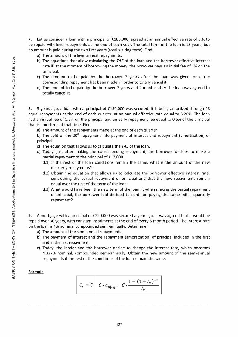
7. Let us consider a loan with a principal of €180,000, agreed at an annual effective rate of 6%, to be repaid with level repayments at the end of each year. The total term of the loan is 15 years, but no amount is paid during the two first years (total waiting term). Find:

a) The amount of the level annual repayments. b) The equations that allow calculating the TAE of the loan and the borrower effective interest

rate if, at the moment of borrowing the money, the borrower pays an initial fee of 1% on the principal.

c) The amount to be paid by the borrower 7 years after the loan was given, once the corresponding repayment has been made, in order to totally cancel it.

d) The amount to be paid by the borrower 7 years and 2 months after the loan was agreed to totally cancel it.

8. 3 years ago, a loan with a principal of €150,000 was secured. It is being amortized through 48 equal repayments at the end of each quarter, at an annual effective rate equal to 5.20%. The loan had an initial fee of 1.5% on the principal and an early repayment fee equal to 0.5% of the principal that is amortized at that time. Find:

a) The amount of the repayments made at the end of each quarter. b) The split of the 20th repayment into payment of interest and repayment (amortization) of principal. c) The equation that allows us to calculate the TAE of the loan. d) Today, just after making the corresponding repayment, the borrower decides to make a

partial repayment of the principal of €12,000. d.1) If the rest of the loan conditions remain the same, what is the amount of the new

quarterly repayments? d.2) Obtain the equation that allows us to calculate the borrower effective interest rate,

considering the partial repayment of principal and that the new repayments remain equal over the rest of the term of the loan.

d.3) What would have been the new term of the loan if, when making the partial repayment of principal, the borrower had decided to continue paying the same initial quarterly repayment?

9. A mortgage with a principal of €220,000 was secured a year ago. It was agreed that it would be repaid over 30 years, with constant instalments at the end of every 6‐month period. The interest rate on the loan is 4% nominal compounded semi‐annually. Determine:

a) The amount of the semi‐annual repayments. b) The payment of interest and the repayment (amortization) of principal included in the first

and in the last repayment. c) Today, the lender and the borrower decide to change the interest rate, which becomes

4.337% nominal, compounded semi‐annually. Obtain the new amount of the semi‐annual repayments if the rest of the conditions of the loan remain the same.

Formula

𝐶 𝐶 𝐶 𝑎 | 𝐶1 1 𝐼

𝐼

__________________________________________________________________________________

127

BASI

CS

ON

TH

E TH

EOR

Y O

F IN

TER

EST.

App

licat

ions

to th

e Sp

anis

h fin

anci

al m

arke

t. L.

Gon

zále

z-Vi

la, M

. Már

mol

, F.J

. Ortí

& J

.B. S

áez

Answers

1. a) €21,136.34. Payment of interest: €3,136.34. Repayment of principal: €18,000.

b) Annual effective interest rate of the loan: 5.5%. Borrower annual effective interest rate: 6.3335%. TAE: 6.3335%.

c) Outstanding principal: €18,000. Repaid principal: €0.

d) €19,160.21.

e)

e.1) €19,160.21.

e.2) €18,912.98.

2. a) €80,611.30.

b) Payment of interest: €30,611.30.

Repayment of principal: €50,000.

c) €63,486.73.

d) Annual effective interest rate of the loan: 12.6825%.

TAE: 13.2531%.

e) €61,565.28.

f) . . . . ,I I 2 41 150000 1000 15000 1 61565 28 1 .

g) The TAE is the same, since the partial repayment of €15,000 does not have to be included in its calculation.

3. a) €1,350. b) €91,350. c) €90,000. d) €90,447.77. e) €1,530

4. a) €180. b) Outstanding principal: €48,000. Outstanding loan balance: €48,000.

c) Outstanding principal: €48,000. Outstanding loan balance: €48,089.92.

d) €161.25.

e) , ,I I 12

1201212048 000 480 180 48 000 1a and TAE I 12

121 1 .

f) , , .I I 12

72127248 000 480 180 5 01250 1a

. ,I I I 12

72 12012 124816125 1 43 000 1a

.

128

BASI

CS

ON

TH

E TH

EOR

Y O

F IN

TER

EST.

App

licat

ions

to th

e Sp

anis

h fin

anci

al m

arke

t. L.

Gon

zále

z-Vi

la, M

. Már

mol

, F.J

. Ortí

& J

.B. S

áez

5. a) €994.69. b)

r Level repayment

Payment of interest

Repayment of principal


0 170,000.00 1 994.69 510.00 484.69 169,515.31 2 994.69 508.55 486.14 169,029.17 … … … … …

239 994.69 5.94 988.75 991.71 240 994.69 2.98 991.71 0.00

c) Outstanding principal: €164,086.87. Outstanding loan balance: €164,086.87. Repaid principal: €5,913.13. Outstanding loan balance just before paying the corresponding level repayment:

€165,081.56.

d) Outstanding principal: €164,086.87. Outstanding loan balance: €164,332.82.

e) Repayment (amortization) of principal: €505.45. Payment of interest: €489.24.

f) €160,809.14.

g) , , . I 12240170 000 5 100 99469 a and TAE I 12

121 1 .

6. a) Amount of interest payments: €480. Amount of level repayments: €1,263.05.

b) a a, , .I I I 6 6

12612 6060 000 600 480 1 26305 1 and TAE I

661 1 .

c) €39,372.23. d) €20,627.77. e)

e.1) €39,529.41.

e.2) ,, a , . a , .I I I I 6 6

12 36 56 612 2460 000 600 480 1 26305 1 39 62784 1 .

7. a) €22,845.96. b) Equation for the TAE and for the borrower effective interest rate:

, , , . a I I1

2113180 000 1 800 22 845 96 1

c) €141,868.70. d) €143,253.17.

8. a) €4,197.82. b) Repayment (amortization) of principal: €2,906.75. Payment of interest: €1,291.07.

129

BASI

CS

ON

TH

E TH

EOR

Y O

F IN

TER

EST.

App

licat

ions

to th

e Sp

anis

h fin

anci

al m

arke

t. L.

Gon

zále

z-Vi

la, M

. Már

mol

, F.J

. Ortí

& J

.B. S

áez

c) , , , . a I 448150 000 2 250 4 19782 and TAE I 4

41 1 .

d)

d.1) €3,780.04. d.2) a a, , , . , , .I II I

4 4

12 124 412 36150 000 2 250 4 19782 12 060 1 3 78004 1 .

d.3) The new term of the loan would have been 32 quarters.

9. a) €6,328.95 b) Repayment (amortization) of principal in the first level repayment: €4,400.00. Payment of interest in the first level repayment: €1,928.95. Repayment (amortization) of principal in the last level repayment: €6,204.85. Payment of interest in the last level repayment: €124.10.

c) €6,583.10.

130

BASI

CS

ON

TH

E TH

EOR

Y O

F IN

TER

EST.

App

licat

ions

to th

e Sp

anis

h fin

anci

al m

arke

t. L.

Gon

zále

z-Vi

la, M

. Már

mol

, F.J

. Ortí

& J

.B. S

áez

UNIT 4.

BONDS

1. Definition and related concepts. Classification

2. Zero-coupon bonds

3. Coupon bonds


1.1. Definition and related concepts

1.2. Classification

1.1. Definition and related concepts

There are two main ways for a company or a government entity to obtainfinancing: ask a bank for a loan or issue bonds and sell them to thepublic.

Graphically:A company issues

200,000 bonds with a unit value equal to €10,000

If there are enough buyers willing to buy the bonds andthe company sells each bond at a unit price equal to10,000€, it will receive €2,000,000,000.

Each of these parts represents €10,000(face value of the bond).

Unit 4. Bonds

131

BASI

CS

ON

TH

E TH

EOR

Y O

F IN

TER

EST.

App

licat

ions

to th

e Sp

anis

h fin

anci

al m

arke

t. L.

Gon

zále

z-Vi

la, M

. Már

mol

, F.J

. Ortí

& J

.B. S

áez

A bond is a financial product (security) issued by a company or agovernment entity (bond issuer) that promises certain payment(s) atfuture date(s) to the owner of the bond (bondholder).

The company or government entity that issues the bonds outlines howmuch money it wants and specifies a length of time, along with theinterest it is willing to pay. Investors who buy bonds are then lendingmoney to the issuer and become its creditors through the bonds that theyhold.

NOTE: As we will see later, the issue price of bonds is not, in general,equal to their face value.

So, bonds are nothing more than loans, in which there is only oneborrower (the bond issuer) but there are many lenders (thebondholders).

Amount of money the bond issuer wants=

Number of bonds issued x Issue price

Unit 4. Bonds


The term of the bond is the length of time from the issue date until thedate of the last payment. The date of this last payment is called thematurity date or redemption date.

The payment(s) made by the bond issuer in exchange for the moneyborrowed can include both interest and the redemption amount.

The redemption amount of a bond is the amount that the bondholderreceives on the bond maturity date, excluding interest (if there is any) .

All bonds issued by a company or a government entity at the samemoment in time have the same face value. The face value of a bond isprinted on it and represents the debt the bond issuer owes to thebondholder. As for bonds with periodic payments of interest (coupons),these are calculated by considering the face value and the effectiveinterest rate of the bond. Since, from the issue date, it is known howthe coupons will be calculated, bonds are also called fixed-incomesecurities.

It is worth highlighting that, in general, the face value of a bond is notequal to neither its issue price nor its redemption value.

Unit 4. Bonds


132

BASI

CS

ON

TH

E TH

EOR

Y O

F IN

TER

EST.

App

licat

ions

to th

e Sp

anis

h fin

anci

al m

arke

t. L.

Gon

zále

z-Vi

la, M

. Már

mol

, F.J

. Ortí

& J

.B. S

áez

After their issue (primary market), bonds can be bought and sold onorganized markets (secondary market). In order to be able to identifybonds from each issue unequivocally on any market, they are assignedan alphanumeric reference of 12 characters, called an ISIN (InternationalSecurities Identification Number) code.

NOTE: In the Spanish financial market, which is the only one that we willconsider when studying bonds, bonds have different names such as, forexample, bonos, obligaciones, pagarés de empresa, Letras del Tesoro,etc.

Some of the concepts we have just introduced have a specific notation.Let us now see what that is.

Unit 4. Bonds


0 : Issue date

' :T Maturity or redemption date

:C Face value of a bond. It is also called the par value

:eC Issue price of a bond

• If 𝐶 𝐶 the bond is issued at a premium (or above par)The difference 𝐶 𝐶 is called the original issue premium

• If 𝐶 𝐶 the bond is issued at par

• If 𝐶 𝐶 the bond is issued at a discount (or below par)The difference 𝐶 𝐶 is called the original issue discount

:aC Redemption amount

• If 𝐶 𝐶 the bond is redeemable at a premium (or above par)The difference 𝐶 𝐶 is called the redemption premium

• If 𝐶 𝐶 the bond is redeemable at par

• The case 𝐶 𝐶 makes no sense

The original issue premium and the original issue discount can also be expressed as a percentage of the face value.

The redemption premium can also be expressed as a percentage of the face value.

Unit 4. Bonds


133

BASI

CS

ON

TH

E TH

EOR

Y O

F IN

TER

EST.

App

licat

ions

to th

e Sp

anis

h fin

anci

al m

arke

t. L.

Gon

zále

z-Vi

la, M

. Már

mol

, F.J

. Ortí

& J

.B. S

áez

Unit 4. Bonds


Example 1. Obtain the issue price and the redemption amount of 1 bondof an issuance in which bonds have a face value of €3,000. Considerthat they are issued at a discount, with an original issue discount of €30and they are redeemable at a premium, with a redemption premiumequal to 2% of the face value.

3,000 30 €2,970 eC

3,000 2%ꞏ3,000 €3,060 aC

This is equivalent to saying that the bonds have an original issuediscount of 1% or that they have been issued at a price of 99%.

This is equivalent to saying that the bonds have a redemption premium of€60 or that they are redeemable at a price of 102%.

3,000 500,000 €1,500,000,000

3,060 500,000 €1,530,000,000

2,970 500,000 €1,485,000,000

Example 2. Let us suppose that in the previous issuance, 500,000 bondswere issued.

Obtain the face value issued, the amount obtained through the issuanceof bonds and the total redemption amount to be paid by the bond issuer.

We determined:

So:

Total redemption amount:

Face value issued:

Amount obtained through the issuance of bonds:

Unit 4. Bonds


€2,970eC €3,060aC

134

BASI

CS

ON

TH

E TH

EOR

Y O

F IN

TER

EST.

App

licat

ions

to th

e Sp

anis

h fin

anci

al m

arke

t. L.

Gon

zále

z-Vi

la, M

. Már

mol

, F.J

. Ortí

& J

.B. S

áez

€2,000AC

Since not all bonds have the same face value, expressing the price inmonetary units is not informative enough. This is why, in order to avoidmisunderstandings, the price of a bond on a financial market isexpressed as a percentage of its face value.

Example 3. Let us suppose that the prices of two different bonds, A andB, at moment 𝜏 are:

If their respective face values are:

Bond A is currently being sold/purchased on the market at a price greaterthan its face value. More specifically, its current price expressed as apercentage of its face value is:

€2,100AP €2,700BP

€3,000BC

Unit 4. Bonds


:P Price paid for a bond when it is purchased at any moment 𝜏 after its issue

P

2.1001.05 105%

2.000 AP

Moreover, there are other interest rates related to bonds:

Bond issuer interest rate

This is the interest rate for the bond issuer, taking into account the totalamount received when issuing the bonds, payments made to thebondholders over the term of the bonds and all the expenses associatedwith the issue of the bonds.

There is a single bond issuer interest rate for each issuance of bondsand it can usually be calculated when bonds are issued.

:mI Effective interest rate for bonds in the same issue (or coupon interest rate).

Unit 4. Bonds


Similarly, the current price of bond B expressed as a percentage of itsface value is:

2.7000.9 90%

3.000 BP

135

BASI

CS

ON

TH

E TH

EOR

Y O

F IN

TER

EST.

App

licat

ions

to th

e Sp

anis

h fin

anci

al m

arke

t. L.

Gon

zále

z-Vi

la, M

. Már

mol

, F.J

. Ortí

& J

.B. S

áez

Bondholder interest rate

This is the interest rate for a specific bondholder, taking into account theamounts paid when purchasing the bonds, the payments received fromthe bond and all the expenses associated with the bonds over the termthey have been held.

Bondholders can either buy bonds at the moment of their issue or at anyother moment after being issued.

Furthermore, bondholders can either hold the bonds until their maturitydate or sell them at an earlier moment.

This is why the bondholder interest rate may not be the same for everybondholder.

Unit 4. Bonds


Internal rate of return (IRR) or yield to maturity (YTM) of a bond atmoment 𝝉After their issue, bonds can be bought and sold on organized markets.

The internal rate of return of a bond at moment 𝜏 is the interest rateassociated to the purchase of this bond by considering:

1) that it is purchased at a price 𝑃 ,

2) that the bondholder who buys the bond at that moment will hold it untilits maturity (thus receiving all the associated payments),

3) and without taking into account any kind of expenses.

On a given day, different bondholders can obtain different IRRs on bondsof the same issuance. So, in order to have information for this issuanceon the market, an average of all those IRRs is calculated and published.

This published IRR is known as the average internal rate of return oraverage interest rate and it may change every day.

Unit 4. Bonds


136

BASI

CS

ON

TH

E TH

EOR

Y O

F IN

TER

EST.

App

licat

ions

to th

e Sp

anis

h fin

anci

al m

arke

t. L.

Gon

zále

z-Vi

la, M

. Már

mol

, F.J

. Ortí

& J

.B. S

áez

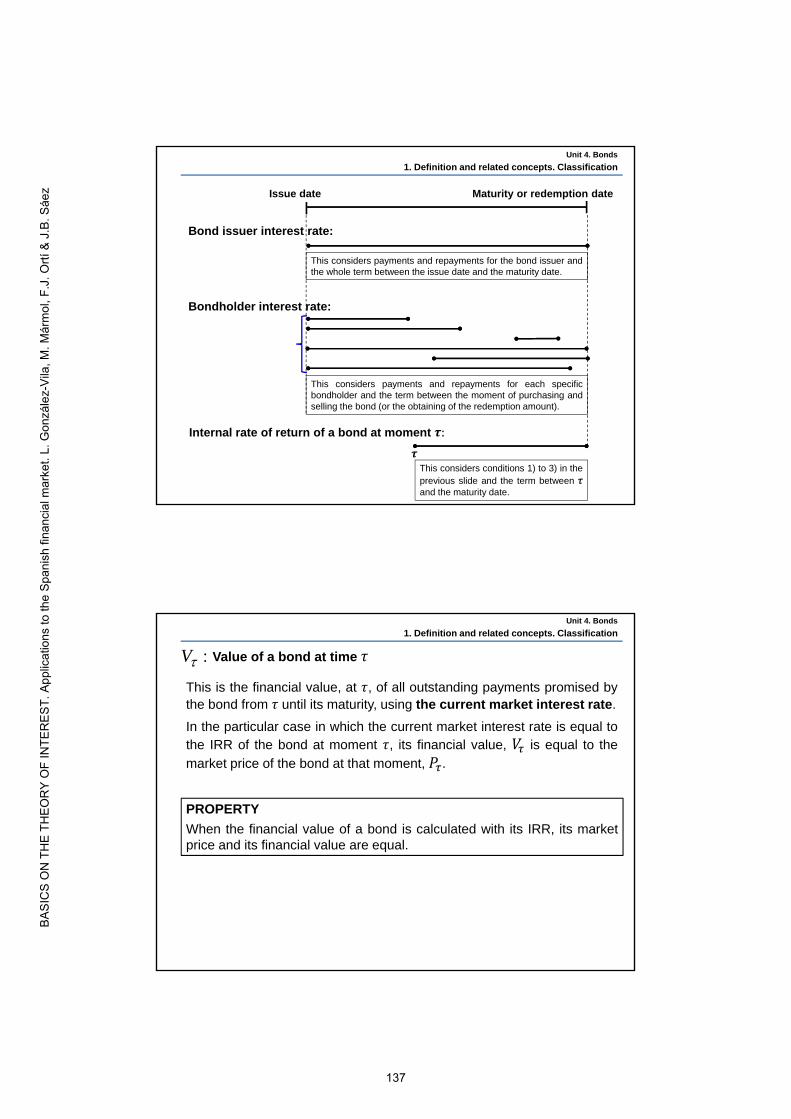
Issue date Maturity or redemption date

Bond issuer interest rate:

Bondholder interest rate:

Internal rate of return of a bond at moment 𝝉:

This considers payments and repayments for the bond issuer andthe whole term between the issue date and the maturity date.

This considers payments and repayments for each specificbondholder and the term between the moment of purchasing andselling the bond (or the obtaining of the redemption amount).

This considers conditions 1) to 3) in theprevious slide and the term between 𝜏and the maturity date.

Unit 4. Bonds


𝝉

:V Value of a bond at time 𝜏

This is the financial value, at 𝜏, of all outstanding payments promised bythe bond from 𝜏 until its maturity, using the current market interest rate.

In the particular case in which the current market interest rate is equal tothe IRR of the bond at moment 𝜏, its financial value, 𝑉 is equal to the

market price of the bond at that moment, 𝑃 .

Unit 4. Bonds


PROPERTY

When the financial value of a bond is calculated with its IRR, its marketprice and its financial value are equal.

137

BASI

CS

ON

TH

E TH

EOR

Y O

F IN

TER

EST.

App

licat

ions

to th

e Sp

anis

h fin

anci

al m

arke

t. L.

Gon

zále

z-Vi

la, M

. Már

mol

, F.J

. Ortí

& J

.B. S

áez

1.2. Classification

Bonds can be classified by considering different aspects.

Regarding the issuer:

1) Bonds issued by a government entity

These bonds are usually called public debt.

In Spain the central agency which issues public debt is the TesoroPúblico but other regional or local governments may also issue bonds.

2) Bonds issued by companies

This kind of bonds are issued by large private companies with animportant position on the market, such as Banks, electric supplycompanies, etc. These bonds are called private debt.

As we said earlier, we will only be focusing on the Spanish financialmarket. Furthermore, we will only study the public debt and, moreparticularly, the public debt issued by the Tesoro Público.

Unit 4. Bonds


Taking into account the number of times that the bond issuer paysinterest to the bondholders.

1) Zero-coupon bonds or (pure) discount bonds or implicit yieldbonds

These are bonds that only promise a single payment on a fixed maturitydate. In the Spanish financial market, this single payment is equal to theface value of the bond. Thus, the interest for the bondholder is thedifference between the face value received at maturity and the issueprice.

Zero-coupon bonds issued in Spain by the Tesoro Público are namedLetras del Tesoro, often translated as Treasury Bills or T-Bills.

2) Coupon bonds

These are bonds that promise periodic payments of interest made by thebond issuer prior to and on the maturity or redemption date, as well as anadditional redemption payment. In this case, coupon bonds issued by theTesoro Público are called Bonos del Estado or Obligaciones del Estado.

Unit 4. Bonds


138

BASI

CS

ON

TH

E TH

EOR

Y O

F IN

TER

EST.

App

licat

ions

to th

e Sp

anis

h fin

anci

al m

arke

t. L.

Gon

zále

z-Vi

la, M

. Már

mol

, F.J

. Ortí

& J

.B. S

áez

2.1. General characteristics

1) Zero-coupon bonds are issued at a discount, i.e., the issue price islower* than the face value. These are (pure) discount bonds.

2) They are redeemable at par, that is to say, the redemption amount isequal to the face value.

3) The difference between the issue price and the redemption amount onthe maturity date is the implicit interest earned by the bondholder*.They are implicit yield bonds.

'T0

eC C

tTerm of the financial transaction

Graphically:



2.2. Letras del Tesoro

Unit 4. Bonds

* In an environment ofpositive interest rates.

In order to calculate:

• the bond issuer interest rate,

• the bondholder interest rate and

• the internal rate of return of a bond

the term of the financial transaction, 𝑡, has to be taken into account:

• If 𝑡 is lower than or equal to 1 year, the simple interest regime will haveto be used.

• If 𝑡 is greater than 1 year, the compound interest regime will have to beused.

Unit 4. Bonds


139

BASI

CS

ON

TH

E TH

EOR

Y O

F IN

TER

EST.

App

licat

ions

to th

e Sp

anis

h fin

anci

al m

arke

t. L.

Gon

zále

z-Vi

la, M

. Már

mol

, F.J

. Ortí

& J

.B. S

áez

2.2. Letras del Tesoro

• These are zero-coupon bonds issued by the Tesoro Público.

• Their face value is €1,000.

• Their issue price is established by auction.

• The Tesoro currently issues 4 types of Letras del Tesoro, each with adifferent maturity: 3, 6, 9 and 12 months; but years ago there were 18-month Letras del Tesoro.

• The term of the financial transaction is always calculated using thecriterion Act/360.

Conditions and results of issuances of Letras del Tesoro are shown onthe website of the Tesoro Público (www.tesoro.es).

Once Letras del Tesoro are on the secondary market (BME Renta Fija),the information for a particular day can be found on the website of BME(www.bmemarketdata.es).

Unit 4. Bonds


Example 4. Obtain the average interest rate for 1-year Letras del Tesorothat were sold/bought on the 16th of October 2015, by considering thatthey matured on 14th of October 2016 and that their price was €999.86.

Unit 4. Bonds


364360

100 99.986

99.986

i

364 days (less than 1 year)

36499.986 1 100

360

i 0.00014 0.014% i

14/10/2016

999.861,000

16/10/2015

By using the simple interest regime:

* Letras began to be issued in 1987 and up to this issue in October 2015had always had a positive interest rate. However, the economicenvironment changed and the very next issue, which took place onNovember 17th, 2015, had a negative interest rate. Ever since then, thesame has been happening.

140

BASI

CS

ON

TH

E TH

EOR

Y O

F IN

TER

EST.

App

licat

ions

to th

e Sp

anis

h fin

anci

al m

arke

t. L.

Gon

zále

z-Vi

la, M

. Már

mol

, F.J

. Ortí

& J

.B. S

áez

Example 5. Find the price today, on the secondary market, of a 1-yearLetra del Tesoro, with maturity in 330 days, supposing that the averageinterest rate published today is 0.132%:

Or alternatively:

P0

0 330

360

100

TODAY Maturity date

0330

1 0.00132 100360

P 0 99.879%P

Unit 4. Bonds


0330

1 0.00132 1,000360

P 0 €998.79P

Issue date

Example 6. Check the average interest rate of the 9-month Letras delTesoro that were issued on the 15th of December 2020, by consideringthe following information:

Unit 4. Bonds


Moment at which the transaction takes place. Onthe primary market the settlement date is 3 workingdays after the trade date (auction date).

It means that 4,484,730 Letras were bid(requested) at the auction.

Remember: The face value of Letras del Tesoro is €1,000.

It means that only 950,040 Letraswere sold/bought.

MM/DD/YYYY

www.tesoro.esRetrieved on 18th December 2020

141

BASI

CS

ON

TH

E TH

EOR

Y O

F IN

TER

EST.

App

licat

ions

to th

e Sp

anis

h fin

anci

al m

arke

t. L.

Gon

zále

z-Vi

la, M

. Már

mol

, F.J

. Ortí

& J

.B. S

áez

Unit 4. Bonds


266 days (less than 1 year)

10th Sept. 2021

100.496 100

18th Dec. 2020

266100.496 1 100

360

i 0.006680 0.668% i

Letras del Tesoro from this issue will be sold and bought on thesecondary market until its maturity. In order to see how they were tradedon a specific day, it is necessary to check the Public Debt and PrivateFixed Income Daily Bulletin for that day at www.bmemarketdata.es, andlook for their ISIN.

Unit 4. Bonds


Example 7. 143 days ago, an investor bought 28 Letras del Tesoro at aprice of 99.125%. Today, he sells them on the secondary market at aprice of 99.829%.

a) Find the total amount obtained by the investor when selling the Letrasdel Tesoro.

The total amount obtained today is:

b) Find the annual interest rate for this bondholder.

1,000ꞏ0.99829 28 €27,952.12

143991.25 1 998.29

360

i

0.01788 1.788% i

991.25 998.29

0143

360TODAY

142

BASI

CS

ON

TH

E TH

EOR

Y O

F IN

TER

EST.

App

licat

ions

to th

e Sp

anis

h fin

anci

al m

arke

t. L.

Gon

zále

z-Vi

la, M

. Már

mol

, F.J

. Ortí

& J

.B. S

áez

Unit 4. Bonds


c) If the investor had paid a fee of 1% of the purchase price when hebought the Letras del Tesoro, what would his annual interest rate havebeen?

143991.25 9.91 1 998.29

360

i

0.00722 0.722% i

991.25 + 9.91998.29

0 143360

TODAY

d) Find the annual interest rate today for these Letras if they mature in 37days.

3799.829 1 100

360

i

0.01667 1.667% i

99.829100

0TODAY

37360

Unit 4. Bonds


3. Coupon bonds


3.2. Bonos and Obligaciones del Estado

1) The issue price of coupon bonds may be equal to or different fromtheir face value.

2) The redemption amount is paid at maturity of the bonds and it can beequal to or different from their face value.

3) The bond issuer pays the bondholder, at the end of each period 𝑝, the amount 𝑌, called a coupon, which is calculated by applying the

effective interest rate of the bonds, 𝐼 , to their face value, 𝐶.


143

BASI

CS

ON

TH

E TH

EOR

Y O

F IN

TER

EST.

App

licat

ions

to th

e Sp

anis

h fin

anci

al m

arke

t. L.

Gon

zále

z-Vi

la, M

. Már

mol

, F.J

. Ortí

& J

.B. S

áez

NOTE: The name “coupon" is due to the fact that, years ago, bondsliterally had coupons attached to them. Bondholders received interest bystripping off the coupons and giving them to the bond issuer. This is notthe case nowadays since bonds are kept electronically.

Graphically:

'np T0 3p2 p

Y Y

. . .

. . . Y

1n pp

Y YaCeC

where the coupon (or interest) for each period is:

mY C I

Unit 4. Bonds

3. Coupon bonds

Unit 4. Bonds

3. Coupon bonds

www.meridianfinancialpartners.com/Retrieved on 29th July 2020

144

BASI

CS

ON

TH

E TH

EOR

Y O

F IN

TER

EST.

App

licat

ions

to th

e Sp

anis

h fin

anci

al m

arke

t. L.

Gon

zále

z-Vi

la, M

. Már

mol

, F.J

. Ortí

& J

.B. S

áez

To obtain:

• the bond issuer effective interest rate,

• the bondholder effective interest rate and

• the internal rate of return of a bond

the compound interest regime will always be used.

Once the coupons bonds have been issued, they can be exchanged onorganized markets (secondary markets). If an investor wants to buy orsell one (or more) bond(s) at moment 𝜏, they will have to pay or receivethe market price of this bond at moment 𝜏, 𝑃 .This price can be determined by summing the amount of the accruedinterest and the “clean” price of the bond

Unit 4. Bonds

3. Coupon bonds

Accrued interest: Proportional part of the coupon corresponding to thebond that has been generated from the moment when the last couponwas paid until the moment 𝜏.

Clean price (or ex-coupon price) of the bond: Price of the bond setas a result of the interaction of supply and demand in the market.

Market price at 𝜏,

𝑃Accrued interest Clean (ex-coupon) price= +

NOTE: The market price is often called the “dirty” price.

Unit 4. Bonds

3. Coupon bonds

On the other hand, recall we said that the financial value of a bond at 𝜏 isthe financial value of all outstanding payments promised by the bondfrom 𝜏 to its maturity, using the current market interest rate. So, when acoupon bond is considered:

Financial value at 𝜏, 𝑉

=

Financial value at 𝜏 of remaining coupons +

Financial value at 𝜏 of redemption amount

145

BASI

CS

ON

TH

E TH

EOR

Y O

F IN

TER

EST.

App

licat

ions

to th

e Sp

anis

h fin

anci

al m

arke

t. L.

Gon

zále

z-Vi

la, M

. Már

mol

, F.J

. Ortí

& J

.B. S

áez

3.2. Bonos and Obligaciones del Estado

• These are both securities issued by the Tesoro Público.

• Their face value is €1,000 which is paid on the maturity date, i.e. theyare redeemable at par.

• Their issue price is established by auction.

• The Tesoro currently issues Bonos with maturity terms of 3 and 5 years(approximately) and Obligaciones with maturity terms of 10, 15, 30 and50 years (approximately).

• Coupons are paid in arrears annually, once the bonds have beenissued, with the moment of the last coupon being the maturity date.

• The term of the financial transaction is always calculated by using theAct/Act criterion.

Conditions and results of issuances of Bonos and Obligaciones delEstado are shown on the website of the Tesoro Público (www.tesoro.es).

Once these securities are on the secondary market (BME Renta Fija) theinformation for a particular day can be found on the website of BME(www.bmemarketdata.es).

Unit 4. Bonds

3. Coupon bonds

Example 8. An investor buys an Obligación del Estado for €1,008.80today (15th May A). The Obligación pays an annual coupon of 2.10% andmatures on 31st January A+6.

a) Find the amount of the annual coupon of the Obligación.

1,000 0.0210 €21 Y

Purchase price

6 annual coupons

Face value

2121

1,0001,008.802121 . . .

. . . 31/01/A+631/01/A+531/01/A+231/01/A+131/01/A

15/05/A

b) Depict all the payments and repayments associated with the purchaseof the Obligación.

Since the last coupon is received by the bondholder on the maturitydate, we locate all the remaining coupons going backwards from thelast one.

Unit 4. Bonds

3. Coupon bonds

146

BASI

CS

ON

TH

E TH

EOR

Y O

F IN

TER

EST.

App

licat

ions

to th

e Sp

anis

h fin

anci

al m

arke

t. L.

Gon

zále

z-Vi

la, M

. Már

mol

, F.J

. Ortí

& J

.B. S

áez

c) Obtain the amount of the accrued interest of the Obligación right afterreceiving the coupon corresponding to 31st January A+1.

Right after receiving the coupon corresponding to 31st January A+1, theaccrued interest of the Obligación is, obviously, 0.

Unit 4. Bonds

3. Coupon bonds

d) Obtain the amount of accrued interest on the Obligación today,knowing that year A is a leap year.

105AI = 21 = €6.03

366

Accrued interest, AI 21

105 days

31/01/A 31/01/A+115/05/A

261 days

NOTE: If year A was not a leap year, the denominator would be 365.

Example 9. Let us suppose that the information for an issue of Bonos delEstado today, 22nd August A, on the secondary market is that containedin the following table.

a) Find the financial value today of a Bono from this issue by using itsIRR.

So, we first draw all the remaining coupons from today to the maturitydate, as well as the face value.

Coupon interest Maturity date Ex-coupon price IRR

1.01% 31/10/A+4 98.723% 1.325%

Unit 4. Bonds

3. Coupon bonds

Financial value at 𝜏, 𝑉

=

Financial value at 𝜏 of remaining coupons +

Financial value at 𝜏 of redemption amount

147

BASI

CS

ON

TH

E TH

EOR

Y O

F IN

TER

EST.

App

licat

ions

to th

e Sp

anis

h fin

anci

al m

arke

t. L.

Gon

zále

z-Vi

la, M

. Már

mol

, F.J

. Ortí

& J

.B. S

áez

5 annual coupons

Face value

10.1010.10

1,000

10.1010.10

31/10/A-1

22/08/A

31/10/A+431/10/A+331/10/A+231/10/A+131/10/A

10.10

Since the last coupon is received by the bondholder on the maturitydate, we locate all the remaining coupons going backwards from thelast one.

22/08/AV295 days

So:

295365

522/08/A 5 0.0132510.10 1,000 1 0.01325 1 0.01325V a

22/08/A €995.39V

Unit 4. Bonds

3. Coupon bonds

295AI = 10.10 = €8.16

365 €987.23exP =

22/08/A 8.16 987.23 €995.39P

Unit 4. Bonds

3. Coupon bonds



b) Determine the market price today of a Bono from this issue.

It is important to highlight that since the financial value of the bond at 𝜏has been calculated with its IRR, this financial value and the market priceof the bond at 𝜏 are equal. This was already said in a previous property.

As stated earlier, real information on prices and interest rates for Bonosand Obligaciones del Estado on the secondary market can be found atwww.bmemarketdata.es, in the Public Debt and Private Fixed IncomeDaily Bulletin.

148

BASI

CS

ON

TH

E TH

EOR

Y O

F IN

TER

EST.

App

licat

ions

to th

e Sp

anis

h fin

anci

al m

arke

t. L.

Gon

zále

z-Vi

la, M

. Már

mol

, F.J

. Ortí

& J

.B. S

áez

We already know the reason why bond prices are expressed as apercentage of bond face values. But, why are prices agreed (and laterpublished) without including the accrued interest? Why are they agreed(and published) as ex-coupon prices? Why not publish the total price thatthe buyer paid when the bond was purchased?

To answer this question, first we have to make it clear that when couponsare paid by the issuer, the payment is made to the current owner of thebond. However, it may be that the current owner has not had the bond forthe whole period over which the coupon has been generated because thebond was purchased on the secondary market after payment of theprevious coupon. So, the new owner would not be entitled to receive thewhole coupon and a part of it (the accrued interest until the moment atwhich the bond was sold/purchased) should be paid to the former owner.

In order to avoid either the issuer or the current owner paying theaccrued interest to the former owner, and to make things as easy aspossible, it is paid by the buyer to the seller when the bond ispurchased/sold.

Unit 4. Bonds

3. Coupon bonds

Including the coupon in published prices would cause them to be affectedby the number of days since the date of the last coupon, resulting in non-comparable information.

Unit 4. Bonds

3. Coupon bonds

Example 10. Let us consider two Bonos del Estado: A and B, fromdifferent issuances but with the same ex-coupon price today, which isequal to 90% (€900). Furthermore, both bonds pay annual coupons at anannual effective interest rate equal to 3%, i.e.

Moreover, suppose that whereas bond A paid its previous coupon 15days ago, bond B paid it 360 days ago.

For both bonds, obtain the market price that a buyer has to pay today.

NOTE: Consider that we are not in a leap year.

= €30Y



149

BASI

CS

ON

TH

E TH

EOR

Y O

F IN

TER

EST.

App

licat

ions

to th

e Sp

anis

h fin

anci

al m

arke

t. L.

Gon

zále

z-Vi

la, M

. Már

mol

, F.J

. Ortí

& J

.B. S

áez

Bond A:

Bond B:

It may seem that the price of bond A is greater than that of bond B.However, since the new owner will recover the accrued interest paid tothe seller when receiving the coupon paid by the issuer, both bonds havethe same price, as is shown by the ex-coupon price.

15AI = 30 = €1.23

365 €900exP = 1.23 900 €901.23 TODAYP

360AI = 30 = €29.59

365 €900exP = 29.59 900 €929.59 TODAYP

Unit 4. Bonds

3. Coupon bonds

Unit 4. Bonds

3. Coupon bonds

Example 11. An SME has the following securities:

• 6 Letras del Tesoro. The SME bought them on the secondary market 93days ago at a unit price of €998.23.

• 8 Bonos del Estado. They were bought at the moment of their issue, 3years and 240 days ago, they will be redeemed 5 years after their issueand their annual interest rate is equal to 3%. Their unit issue price was€1,014 and the SME paid purchasing expenses of 0.5% of this price.

Obtain:

a) The bondholder annual interest rate for the Letras, taking into accountthat they are sold today at a unit price of €999.01 with selling expensesof 0.2% of the face value.

First, we consider all the payments and repayments associated with thepurchase of 1 Letra (it would be equivalent to considering all theLetras).

150

BASI

CS

ON

TH

E TH

EOR

Y O

F IN

TER

EST.

App

licat

ions

to th

e Sp

anis

h fin

anci

al m

arke

t. L.

Gon

zále

z-Vi

la, M

. Már

mol

, F.J

. Ortí

& J

.B. S

áez

The term is less than 1 year, so we use the simple interest regime.

Selling price

999.01

0.00473 0.473% i

Purchase price

2.00 Selling expenses

0 93360

TODAY

998.23

93998.23 1 999.01 2.00

360i

Unit 4. Bonds

3. Coupon bonds

b) Total amount obtained by the SME if it sells the Bonos del Estadotoday, on the secondary market, at an ex-coupon price of 98.9%.

To calculate the market price today per Bono we consider:



In order to better understand how the accrued interest has to beobtained, let us draw all the payments and repayments related to 1Bono since the moment it was issued until its maturity date on thetimeline.

So:

and

The total amount received today when selling the Bonos del Estado is:

1,008.73ꞏ8 €8,069.84

Issue price 30

1,0143030

240365

3 +

TODAY

0 1 2 3 4 5

30 30

Annual coupons

240AI = 30 = €19.73

365

TODAY 19.73 989 €1,008.73 P

Face value

1,000

Unit 4. Bonds

3. Coupon bonds

151

BASI

CS

ON

TH

E TH

EOR

Y O

F IN

TER

EST.

App

licat

ions

to th

e Sp

anis

h fin

anci

al m

arke

t. L.

Gon

zále

z-Vi

la, M

. Már

mol

, F.J

. Ortí

& J

.B. S

áez

c) The equation that allows us to calculate the annual interest rate for theSME, I1, associated with the purchase of 1 Bono del Estado.

By considering the following timeline:

Issue price

3 annual coupons

30

1,0143030

1,008.73

0 240365

31 2 3TODAY

125 days

Selling price

240365

1

3131,014 5.07 30 1,008.73 1 Ia I

Unit 4. Bonds

3. Coupon bonds

Purchasing expenses

5.07

d) The equation that allows us to calculate the annual interest today onthe secondary market for this Bono del Estado.

We have to consider all the remaining coupons from today until thematurity of the Bono (in 1 year and 125 days) and its face value at thatmoment.

Furthermore, we have to bear in mind that the market price today is€1,008.73

Unit 4. Bonds

3. Coupon bonds

Let us denote the annual interest rate of these Bonos by I1. Theequation that allows us to obtain this is:

30 30

1,000

125 days240 days

240365

1

21 121,008.73 30 1,000 1 1Ia I I

1,008.73

0 125365

1TODAY

125365

152

BASI

CS

ON

TH

E TH

EOR

Y O

F IN

TER

EST.

App

licat

ions

to th

e Sp

anis

h fin

anci

al m

arke

t. L.

Gon

zále

z-Vi

la, M

. Már

mol

, F.J

. Ortí

& J

.B. S

áez

UNIT 4 PROBLEMS

NOTE: Unless stated otherwise, all the years that appear are not leap years.

1. For a 1‐year Letra del Tesoro with a settlement date of 12th May of year A: a) Obtain the average rate when it was issued by considering that it matures on 11th May of year A+1 and the average price resulting from the auction was 99.835%. b) Find its price on the secondary market today (9th January A+1), supposing that its internal rate of return (IRR) today is 0.142%.

2. 92 days ago, a small enterprise bought 10 Letras del Tesoro at a price of 99.223%. Today, it sells them on the secondary market at a price of 99.742%.

a) Find the total amount obtained by the small enterprise when selling these Letras del Tesoro. b) If the small company paid a fee of 0.5% of the purchase price when it bought the Letras del Tesoro and today it has to pay a selling fee equal to 0.5% of their selling price, what is the annual interest rate for the company (bondholder)? c) If these Letras del Tesoro mature in 178 days, find their internal rate of return (IRR) today.

3. An investor buys 25 Obligaciones del Estado today that mature in 4 years and 85 days. They pay an annual coupon of 2.35%.

a) For 1 Obligación, find the amount of the annual coupons. b) For 1 Obligación, on the timeline draw all the payments and repayments that the investor

will make or receive if the Obligación is kept until its maturity and a purchasing fee equal to 0.3% of its face value is paid today.

c) If the IRR today for 1 of these Obligaciones is equal to 2.578%, obtain its financial value. d) Determine the amount of the accrued interest of 1 of these Obligaciones today. e) What is its ex‐coupon price today?

NOTE: Remember that when the financial value of a bond is calculated with its IRR, its market price and its financial value are equal.

f) What is the total amount paid by the investor today when buying the Obligaciones? g) Write the equation that allows obtaining the annual effective interest rate for the investor

(bondholder), associated with the purchase of 1 Obligación, if he keeps it until the maturity.

4. A company has 84 Obligaciones del Estado paying annual coupons of 3.25% which mature in 6 years and 195 days.

a) Obtain the accrued interest of 1 Obligación today if the last coupon was received 170 days ago. b) If the ex‐coupon price of 1 Obligación today is 102.45%, find the total amount that the company would receive today if it sold all its Obligaciones. c) Write the equation that allows us to obtain the internal rate of return (IRR) today for one of these Obligaciones.

5. An SME has 10 Bonos del Estado. They were bought at the moment of their issue, 2 years and 125 days ago, and they will be redeemed 5 years after their issue. Their annual interest (coupon) rate is equal to 2.90% and their unit issue price was €1,002.57. Obtain:

a) The total amount obtained by the SME if it sells the Bonos del Estado, on the secondary market today, at an ex‐coupon price of 98.9%.

153

BASI

CS

ON

TH

E TH

EOR

Y O

F IN

TER

EST.

App

licat

ions

to th

e Sp

anis

h fin

anci

al m

arke

t. L.

Gon

zále

z-Vi

la, M

. Már

mol

, F.J

. Ortí

& J

.B. S

áez

b) The equation that allows us to calculate the annual interest rate for the SME, associated with the purchase of 1 Bono del Estado (bondholder effective interest rate). c) The equation that allows us to calculate the internal rate of return (IRR) today for these Bonos del Estado.

Formula

𝐶 𝐶 𝐶 𝑎 | 𝐶1 1 𝐼

𝐼

__________________________________________________________________________________

Answers

1. a) 0.163%.

b) 99.952%.

2. a) €9,974.20 b) ‐1.867%.

c) 0.523%.

3. a) €23.50 b)

c) €1,008.94. d) €18.03 e) 99.091%

f) €25.298,50

g) 280365

1

51 151 008 94 3 23 50 1 000 1 1 Ia I I, . . ,

4. a) €15,14. b) €87,329.76.

c) 170365

1

71 171 039 64 32 50 1 000 1 1 Ia I I, . . ,

5. a) €9,989.30

b) 125365

1

2121 002 57 29 998 93 1Ia I , . ,

c) 125365

1

31 13998 93 29 1 000 1 1Ia I I . ,

154

BASI

CS

ON

TH

E TH

EOR

Y O

F IN

TER

EST.

App

licat

ions

to th

e Sp

anis

h fin

anci

al m

arke

t. L.

Gon

zále

z-Vi

la, M

. Már

mol

, F.J

. Ortí

& J

.B. S

áez

INFORMATION SOURCES

ALEGRE, P. & SANCHO, T. Ejercicios resueltos de matemática de las operaciones financieras. 2ª. ed. Madrid: AC, 2005.

BADÍA, C., GALISTEO, M., PONS, M.A., PREIXENS, T. & SARRASÍ, F.J. Matemàtica financera. Anàlisi d’operacions de finançament. Barcelona: Universidad de Barcelona, 2015.

Banco de España. [online]. Available at www.bde.es

Bolsas y Mercados Españoles Market Data. [online]. Available at www.bmemarketdata.es/

Circular 5/2012, de 27 de junio, del Banco de España, a entidades de crédito y proveedores de servicios de pago, sobre transparencia de los servicios bancarios y responsabilidad en la concesión de préstamos. Available at https://www.boe.es/eli/es/cir/2012/06/27/5, retrieved on 31st December 2020.

DIRECTIVE 2008/48/EC OF THE EUROPEAN PARLIAMENT AND OF THE COUNCIL of 23 April 2008 on credit agreements for consumers and repealing Council Directive 87/102/EEC. Available at https://eur‐lex.europa.eu/, retrieved on 31st December 2020.

FINAN, M.B. A basic course in the theory of interest and derivatives market. Russellville: Arkansas Tech University, 2009.

Ley 5/2019, de 15 de marzo, reguladora de los contratos de crédito inmobiliario. Available at https://www.boe.es/eli/es/l/2019/03/15/5, retrieved on 31st December 2020.

Orden de 12 de diciembre de 1989, sobre tipos de interés y comisiones, normas de actuación, información a clientes y publicidad de las Entidades de crédito. Available at https://www.boe.es/eli/es/o/1989/12/12/(1), retrieved on 31st December 2020.

TERCEÑO, A., SÁEZ, J., BARBERÁ, M.G., ORTÍ, F., DE ANDRÉS, J. & BELVIS, C. Matemática financiera. Barcelona: Pirámide, 1997.

Tesoro Público. [online]. Available at www.tesoro.es

VAALER L.J.F. & DANIEL, J.W. Mathematical interest theory. 2nd. ed. Washington DC: Mathematical Association of America, 2009.

155

BASI

CS

ON

TH

E TH

EOR

Y O

F IN

TER

EST.

App

licat

ions

to th

e Sp

anis

h fin

anci

al m

arke

t. L.

Gon

zále

z-Vi

la, M

. Már

mol

, F.J

. Ortí

& J

.B. S

áez

BASICS ON THE THEORY OF INTEREST

Documents

Transcript of BASICS ON THE THEORY OF INTEREST