Bp

Ta

b

c

d

a

ARRAA

JJJO

KIPT

Drpwmor

(

1d

The Quarterly Review of Economics and Finance 50 (2010) 395–407

Contents lists available at ScienceDirect

The Quarterly Review of Economics and Finance

journa l homepage: www.e lsev ier .com/ locate /qre f

arriers to skill acquisition in Brazil: Public and private school studentserformance in a public university entrance exam�

iago Cavalcanti a,c,∗, Juliana Guimaraesb,c, Breno Sampaiod

Faculty of Economics, University of Cambridge, Sidgwick Avenue CB3 9DD, United KingdomNewnham College, University of Cambridge, United KingdomPIMES/UFPE, BrazilDepartment of Economics, University of Illinois, United States

r t i c l e i n f o

rticle history:eceived 7 July 2009eceived in revised form 5 May 2010ccepted 3 August 2010vailable online 12 August 2010

EL classification:012411

a b s t r a c t

This paper uses a novel data set to quantify the difference in performance of public and private schoolstudents in an entrance test exam of the major public university in Brazilian Northeast (Universidade Fed-eral de Pernambuco – UFPE). Although there are many public universities in Brazil, from our knowledge,there is no study that uses data on entrance test scores at such universities to evaluate the determinantsof students’ performance and the barriers for public school students to get in the good universities. Thedata set has detailed information on individual and school characteristics, and family background. Wefound that test scores of public school students are on average about 4.2–17% lower than those taken byprivate school students, depending on the set of controls. This result is robust when we address problemsrelated to attrition, omitted variables (e.g., cognitive ability), and unobservable selectivity. We also show

eywords:nequalityublic and private schoolsest scores

that once students get into the university, those from public schools perform as well as those from pri-vate schools. In addition, the proportion of public school students that gets into the university is roughlythe same as the proportion of students doing the entrance exam. However, there is a strong barrier forpublic school students to get into high competitive majors. The fraction of students from public schoolsthat gets into high competitive majors such as law, medicine, and electronic engineering is almost null.

titatiannestees

1

ft

Our findings provide quansystem is an important ch

© 2010 The Board of Tru

“The new middle classes have more schooling than their parents;some have gone to mushrooming private universities. But they areless educated than the old middle class that benefited from elitistpublic universities - and that makes moving into the upper classhard.” The Economist, Aug 16th, 2007. Adiós to poverty, hola to

consumption.

� This paper has benefited from financial support of Conselho Nacional deesenvolvimento Cientfico e Tecnológico (CNPq-Brazil). We thank two anonymous

eferees, Werner Baer, Pedro Portugal, Donald Pianto, Eduardo Ribeiro, Yony Sam-aio, and Bhaskar Vira for comments, and Todd Elder for sharing STATA routinesith us. We have also benefited from comments by audiences at Brazilian Econo-etric Society Annual Meeting, and at the Workshop at University of Cambridge

n Policy, Economy and Development in Latin America. We are responsible for anyemaining error.∗ Corresponding author.

E-mail addresses: tvdvc2@cam.ac.uk (T. Cavalcanti), jgc29@cam.ac.ukJ. Guimaraes), sampaio2@uiuc.edu (B. Sampaio).

LtisBFirtews

d

062-9769/$ – see front matter © 2010 The Board of Trustees of the University of Illinoisoi:10.1016/j.qref.2010.08.001

ve evidence to the common view that the Brazilian elitist high educationl for inequality persistence. of the University of Illinois. Published by Elsevier B.V. All rights reserved.

. Introduction

Brazil is one of the most unequal countries in the world. Datarom the World Development Indicators (World Bank, 2007) showhat among 122 countries Brazil is the fourth most unequal. Onlyesotho, Haiti, and Bolivia have an income Gini index that is higherhan what is observed in Brazil. In addition, not only the level ofnequality is high in the country, but at the same time there is lowocial intergenerational mobility by international standards (seeourguignon, Ferreira, & Menéndez, 2003; Ferreira & Veloso, 2006).or instance, Ferreira and Veloso (2006) show that the probabil-ty that a black son of a father from the lowest wage quintile willemain in this quintile is about 47%, which is roughly twice than

he analogous probability for a white son. This indeed is a strongvidence of low equality of opportunities in the country. However,hile the level of inequality is high in Brazil it has been decreasing

ince 1995 and this decline has been amplified in the last years.1

1 Barros, Carvalho, Franco, and Mendonca (2009) show that the Gini coefficienteclined from 0.593 in 2001 to 0.552 in 2007; moreover, the ratio of average

. Published by Elsevier B.V. All rights reserved.

3 of Eco

BchiwtDtPcdtwcIsn

vatpagdismneeOTtprudisat

ip

A

r

s

vn

bWeanm

CB

N

pat

obpcotclu

ocFagtcpeaboa2tlttts

mtn(

96 T. Cavalcanti et al. / The Quarterly Review

This paper studies the issue of inequality of opportunities inrazil. There exists a large literature which shows that public edu-ation is favorable for growth because it increases the level ofuman capital and at the same time it tends to produce a more even

ncome distribution.2 More egalitarian societies are also associatedith less social conflicts and individuals have a lower tendency

o report themselves happy when inequality is high (e.g., Alesina,iTella, & MacCulloch, 2004). Therefore, it is important to study

he sources of inequalities and to quantify them. According tosacharopoulos (1999) the average returns to invest in high edu-ation is quite high in Brazil (about 20%) when compared to someeveloped (e.g., United States) and developing (e.g., Chile) coun-ries. For updated values see Psacharopoulos and Patrinos (2004),ho also show that the average returns to investment in high edu-

ation in Brazil is high compared to other developing countries.3

n a recent article, Menezes-Filho, Fernandes, and Picchetti (2006)how that although human capital has been growing in Brazil it hasot contributed much to reduce wage inequality in the country.

In Brazil there are private and public universities as well as pri-ate and public schools. There is no tuition at public universitiesnd they in general have a better quality than their private coun-erpart, which implies that there is a high competition to get inublic universities. Students have to take an entrance exam to beccepted in a public university and they must choose their under-raduate major before taking the entrance exam.4 Investigating theeterminants of scores in this exam allows us to evaluate inequal-

ty of education among students, in particular, those that did theirecondary degree at a public or private school. Although there areany public universities in Brazil,5 from our knowledge, there is

o study that uses data on entrance test scores at universities tovaluate the determinants of students’ performance.6 Is the differ-nce in ETS due to family background and school characteristics?r is it due to unobservable variables, such as ability and effort?hose are important questions since researchers have shown thatest scores that evaluate cognitive skills and knowledge are keyredictor of future wages, and this effect has being growing inecent years due to skill biased technological change.7 We use anique data set on students’ entrance test scores (ETS) at Universi-ade Federal de Pernambuco (UFPE), which is the major University

n Brazilian Northeast,8 to evaluate quantitatively differences incores between public and private school students. The data setllows also to evaluating students in their first academic year athe university. Do students from public school perform worse than

ncome of the 10% richer and the 40% declined 5.2 percentage points over the sameeriod.2 See Galor and Zeira (1993). For a recent reference, see Doepke (2004) andlexopoulos and Cavalcanti (in press).3 Resende and Wyllie (2006) provide a survey and some new estimates for the

eturns of schooling in Brazil.4 In Brazil there is not much optional disciplines in undergraduate courses and

ome are major specific since the first semester.5 In the Education Ministry web site in August 2010 there were 58 Federal Uni-

ersities listed. There are also some important public universities that are State andot Federal ones.6 An exception and interesting work is Emilio, Belluzo, and Alves (2004), who use

inary model to study the determinants of access to the university of São Paulo.altenberg and Vandenberghe (2007) is also an interesting and related study on

quality of opportunity in education in Brazil. They use a different data set and studydifferent question. They found that in order to implement an equality of opportu-ity policy across pupils of different socio-economic backgrounds, it is necessary toultiply current spending by 6.8 on the lowest achieving pupils.7 See Murnane, Willett, and Levy (1995) and Murphy and Peltzman (1997). See

uri and de Menezes-Filho (2005) for evidences on how test scores affect wages inrazil.8 Ferreira and Veloso (2006) show that intergenerational mobility is lower in theortheast than in the richest Brazilian region (Southeast).

tpowevstwpci

mfiittas

ocsAo

nomics and Finance 50 (2010) 395–407

rivate school students in the university? It might be that only highbility public school students get into the university and thereforehey might perform better than private school students.

The dataset used in this article is rich with detailed informationn individual characteristics (e.g., race, age, and gender), familyackground (e.g., mother’s years of schooling and family income),revious school characteristics (e.g., public or private, if it has lablasses), and the colleges they applied for. We found that test scoresf public school students are on average about 4.2–17% lower thanhose taken by private school students, depending on the set ofontrol variables.9 This result is robust when we deal with prob-ems such as attrition, omitted variables (e.g., cognitive ability), andnobservable selectivity.

Section 2 describes in detail how we address the problem ofmitted variables and unobservable selectivity. Here we briefly dis-uss our two approaches to deal with such econometrics problem:irstly, we use the National Exam for High School Students (ENEM),s a proxy for students’ cognitive ability. The ENEM exam is moreeneral that the Entrance Test Exam and emphasizes logical ques-ions. The problem to use the ENEM as a proxy for unobservableharacteristics is that this exam is not mandatory and in our sam-le less than half of the students took this exam. In addition, thisxam would also capture important differences between privatend public schools. Finally, we also use the technique developedy Altonji, Elder, and Taber (2005) to investigate the potential sizef any bias on the estimated coefficient of the public school vari-ble due to unobservable selectivity (see more on this on Section). This approach is very attractive in non-experimental data and inhe absence of valid instruments. It has also been applied in prob-ems similar to ours. Altonji et al. (2005), for instance, applied thisechnique to investigate the effects of Catholic schools on students’est scores in the United States and Goyal (2009) use the techniqueo study the gap in students’ test scores between private and publicchools in India.10

Another important result is that family background (e.g.,other’s years of schooling and family income) is a key predic-

or of test scores. Our econometric exercises, therefore, show thatot only public school students have a less favorable backgrounde.g., lower family income and lower parent’s education level) andherefore have a lower score in the entrance test exam, but they alsoerform worse than private school students in this exam given theirbserved and unobserved individual characteristics. They performorse even when we control for the ENEM exam or school fixed

ffects (e.g., school’s neighborhood), which would capture a highariation in differences in scores between private and public schooltudents. Interestingly, we also show that once students get intohe university, those from public schools perform better than (or as

ell as) those from private schools. Therefore, it does not seem thatublic school students lack cognitive skills to perform well in edu-ation, but they lack specific preparation that is necessary to do welln the entrance exam. Consequently, either improving the quality

9 In a cross-country study using the Programme for International Student Assess-ent (PISA) student-level achievement database, Fuchs and Woessmann (2007)

nd that students perform better in privately operated schools, but private fundings not decisive. The difference seems to be explained by the difference in organiza-ion in the two systems. Using a decomposition approach McEwan (2008) showshat school reforms might have strong impact on students’ outcome. For instance,ccording to him Chile’s large-scale school reforms had a strong impact on testcores gap between indigenous and non-indigenous population.10 For two recent applications, see Bellows and Miguel (2009), who study the effectf households that experienced intense war violence on the probability of attendingommunity meetings and voting in Sierra Leone, and Kingdon and Teal (2010), whotudy the effects of teacher unionization on student achievement in India. See alsoltonji et al. (2008) who investigate how the effects of Swan-Ganz Catheterizationn mortality in intensive care unit (ICU) patients.

of Eco

ottt

dpaiiesffpMnS3Gts

idWrtswc

2

s(qra

lme

l

wcsvdddirdwt

t

t

ybt

wefieEaQqt[tcqeaFl

oabafvdqtwsdiw

oopbsItcpptdin quality,17 do so. Therefore, financial issue might be a key con-straint in parents’ choice of sending their children to a private or apublic school in Brazil. However, there might be some exemptions.It might be the case that parents with a very bright child might

T. Cavalcanti et al. / The Quarterly Review

f education in public schools by providing a better preparation forhe entrance exam or facilitating access for public school studentso get into public universities would improve the equality of oppor-unities in education for students to acquire a university degree.

Finally, we also show that the proportion of public school stu-ents that gets into the university is roughly the same as theroportion of students doing the entrance exam. However, there isstrong barrier for public school students to get into high compet-

tive majors. The fraction of students from public schools that getsnto high competitive majors such as law, medicine, and electronicngineering is almost null. For instance, in medicine only 6% of thetudents are from public schools. This number is equal to 7 and 5or law and electronic engineering, respectively. On the other hand,or less competitive majors the percent of students that came fromublic schools is much higher. It is, for instance, more than 65% inusic, 64% in geography, 56% in history, and 50% in domestic eco-

omics. Data from the 2005 Brazilian National Household Sampleurvey (PNAD), show that electrical and civil engineers make abouttimes more than domestic economists and high school teachers.11

iven wage differentials among occupations, our empirical evalua-ions suggest that Brazil’s public university system is an importantource of inequality persistence.

This paper proceeds as follows. Section 2 defines our empir-cal strategies and discusses some econometric issues. Section 3escribes the dataset. Section 4 presents our empirical estimates.e use both ordinary least squares (OLS) procedure and quantile

egression. The later is particularly useful to determine whetherhere are any heterogeneity in the responses of the entrance testcores to different school systems (public or private). In this section,e also evaluate how students perform in the university. Section 5

oncludes.

. Empirical strategy

It is expected that in an university entrance exam the students’core depends on their effort to study for the exam, cognitive abilitye.g., capacity to learn and pay attention to academic activities),uality of the teachers that prepared the student for this exam,esources available (e.g., access to books and news), environmentt home and at school, among other variables.12

Our goal is to estimate the difference in the quality of the pub-ic and private schools using data from entrance test scores in the

ajor university in Brazil’s Northeast. We estimate the followingquation:

n(ETSi) = ˇ0 + ˇ1 ∗ publici + ˇ′2X1i + ˇ′

3X ′2 + εi, (1)

here ETSi is the entrance test score of student i, publici is an indi-ator variable that takes value 1 if the student comes from a publicchool and zero otherwise, X1i is a vector of family backgroundariables such as mother’s education and family income of stu-ent i, and X2i is a vector of school characteristics of student i. Weefine public school students as those who took at least two aca-emic years, including the last year, of their high school education

n a public school.13 In Section 4.2.3, we show that our results are

obust to the definition of the variable Public. In this subsection, weefine two variables: (i) Full Public, which characterizes studentsho study their entire high school education in a public institu-

ion; and (ii) Partial Public, denoting the students who did at least 1

11 Data from the same survey show that doctors make on average four times morehan high school teachers.12 Lazear (2001) presents a model of the educational production function. See alsohe recent article by Rivkin, Hanushek, and Kain (2005).13 In Brazil the high school education is composed of three academic years.

er

F�

oow

nomics and Finance 50 (2010) 395–407 397

ear of their high school education in a public school. We show thatoth variables have a negative and statistically significant effect onest scores.

Our estimation method is, first, ordinary least squares (OLS)here standard errors are robust to the presence of het-

roskedasticity. We also analyze quantile regression estimates,rst introduced by Koenker and Basset (1978).14 The least squaresstimator specifies and estimates the conditional mean function,[Y/X = x] = xˇ, where Y is a univariate random variable and x isvector of covariates with the associated parameter vector ˇ.

uantile regression specifies and estimates a family of conditionaluantile functions F−1

y/x (�/x) = xˇ(�); where F is the conditional dis-ribution function of Y given X and �, a quantile in the interval0,1].15 Thus, quantile regression provides several summary statis-ics of the conditional distribution function, rather than just oneharacteristic, namely, the mean. This descriptive advantage ofuantile regression allows us to characterize and distinguish theffects of covariates, for example, the variable public, on the uppernd lower quantiles of the distribution of the entrance test scores.urthermore, quantile regression is also a robust technique to out-iers in the dependent variable.

Three econometric caveats are important to mention. First,bserve that rigourously we must transform the dependent vari-ble, y = ETS, to ln (y/10 − y) instead of ln(y), since the ETS is boundedy 0 and 10. Notice, however, that the OLS estimator is not equivari-nt to monotonic transformation and therefore we cannot recoverrom the transformed model the true effect of each independentariable on the ETS (see Papke & Wooldridge, 1996). Nevertheless,ue to the equivariance property of the quantiles, estimation ofuantile regression function for continuous fractional data is rela-ively simple (see Machado & Silva, 2006; Powell, 1986), speciallyhen there are no mass point at 0 and 10, which is the case of our

ample. Quantitatively, estimations with the transformed variableid not differ significantly from the ones presented here. Since it

s easier to interpret the coefficients of the model presented in (1),e just report estimation results for the untransformed model.16

In addition, it is difficult to estimate the impact of public schooln students’ score because there are unobservable characteristicsf students and schools that are correlated with each other. Arerivate schools really better than public ones, or is it simply thatetter students attend private schools? Here we are not comparingchools among one system, either only public or private schools.t could be the case that the best public (or private) schools, havehe best teachers, and also the brightest students. Our goal is toompare the performance of students between a set of public andrivate schools. It is important to highlight that in Brazil usuallyoor parents are financially constrained and therefore cannot sendheir children to a private school. Parents that can send their chil-ren to a private school, in general, because of known differences

14 See Koenker (2005) for more details on quantile regression estimation and infer-nces. Koenker and Hallock (2001) is an excellent heuristic surveys of quantileegression.15 In our case, we have Qln(ETS)(�|X) = X′ˇ(�), � ∈ (0, 1), where X = [1 public X1X2].unction Qln(ETS)(�|X) is the conditional quantile distribution of ln(ETS) given X and.16 The results of the transformed model are available upon request.17 See, for instance, Menezes-Filho (2007). He shows that not only the proficiencyf public school students is lower than private school students, but also the fractionf college educated teachers are lower in public than in private schools. Teachers’age are also lower in public than private schools.

3 of Eco

mpsvbctettspdstfeseipico

autind

opsTgtbwtdptcso

s

st

aps(

vaabaa

2Ctcmwbl

Cae

wsCepc

3

diiettuPFtji

98 T. Cavalcanti et al. / The Quarterly Review

ake an extra effort to send this child to a private school, whilearents with children that are struggling at school might decide toend them to a public one even if they could afford to pay a pri-ate school.18 We believe that this effect is marginal, but this couldias the estimated coefficient, ˇ1, of the variable public. Specifi-ally, we might have that the error term, ε, is not orthogonal tohe regressors, X = [1 public X1X2]. A final difficulty in interpretingstimates of Eq. (1) steams from the fact that not everyone takeshis college entrance exams. The data set includes only studentshat actually sat for the college admission exam. Since the deci-ion to take the exams is likely to be correlated with a student’sotential score, the estimates of Eq. (1) would not reflect the trueifference among public and private school students. However,ince take-up rates are likely to be much larger for private schoolhan public school students, our estimation misses most low per-orming public school students that never bother to sign-up for thentrance exam. Therefore, in this case if we find that public schooltudents perform worse than private school ones in this entrancexam, in practice our results would underestimate the negativempact of public schools.19 There are two ways to circumvent theroblems raised above. First, if we can control for students abil-

ty in regression (1), then the bias might vanish. Alternatively, wean use standard instrumental variable techniques to address therthogonality problem.

In order to control for students’ cognitive ability we use the scoret ENEM.20 Contrary to the Entrance Exam (Vestibular) which eval-ates students in their knowledge of specific subjects (see belowhe subjects), the ENEM exam is more general and emphasizes log-cal questions. The difficulty in this approach is that this exam isot mandatory21 and in our sample less than half of the studentsid this exam.

The potential problem of unobservable selectivity implies thatur OLS regression might not be capturing the exogenous effects ofublic schools on test scores. In order to address this problem, thetandard approach is to use instrumental variable (IV) techniques.he validity of this procedure, however, depends on the presence ofood instruments for the variable public, such that: the instrumen-al variable should be correlated with the variable public and shoulde orthogonal to the error term of the regression equation (1). Sincee do not have a valid instrument and it is very hard to address

he bias coming from unobservable variables in non-experimentalata, we use the technique developed by Altonji et al. (2005). Theyropose a procedure to investigate the potential size of any bias due

o unobservable variables of the estimated coefficient of some spe-ific variable, in our case the variable public, due to unobservableelectivity.22 In their paper they propose the idea that “selection onbservables is the same as selection on unobservables” (Altonji et al.,

18 See Neal (2002) for a summary and some references on the effects of publicchools on students performance in test scores.19 In fact, Emilio et al. (2004) find that the correction for this selection bias has amall impact on the coefficients of a probit model on the determinants of the accesso the University of São Paulo.20 National Exam for High School Students.21 There are some incentives for students to do this exam. There are some schol-rship provided by the Brazilian government for public school students to study atrivate universities (PROUNI). Students are selected for this scholarship according toome criteria, and one of them is the score at the ENEM exam. Also, some universitiesincluding some public ones) are using the score at ENEM to recruit students.22 We also tested as an instrument for the dummy variable public the indicatorariable that takes value 1 if the student’s house has more than one air conditionernd takes value zero otherwise. The sign and statistical significance of the vari-ble public were robust to such approach. However, this indicator variable mighte correlated with unobservable variables that affect the entrance test score suchs father’s and/or mother’s ability. Therefore, we do not report results using suchpproach, since such instrument might not be valid.

aauceap

uPdgtsr

a

t

nomics and Finance 50 (2010) 395–407

005, p. 154), which, in our case, is equivalent to the condition thatov(ε, Public)/Var(ε) = Cov(ˇ2X, Public)/Var(ˇ2X), where X is a vec-or of observable characteristics, and ε is the error term potentiallyorrelated with Public. This is a valid procedure when the point esti-ates are sensitive to the inclusion of additional control variables,hich corresponds to our case, since when we introduce family

ackground variables the estimated coefficient of the variable Pub-ic decreases in magnitude (see Section 4.1). The biased from OLS is

ov(ε, ˜Public)/Var(˜Public), where tildes denote the residuals fromregression of Public on X, and can be assessed by the following

quation23:

Cov(ε, ˜Public)

Var(˜Public)= Cov(ε, Public)

Var(˜Public)= Cov(ε, Public)

Cov(ˇ2X, Public)Var(ˇ2X)

Var(ε)

× Cov(ˇ2X, Public)Var(ˇ2X)

Var(ε)

Var(˜Public)

= Cov(ˇ2X, Public)Var(ˇ2X)

Var(ε)

Var(˜Public),

here the first equality follows if ε and X are orthogonal and theecond equality follows from the fact that Cov(ε, Public)/Var(ε) =ov(ˇ2X, Public)/Var(ˇ2X). Therefore, instead of trying to find anxogenous variation on the variable Public, we will calculate theotential bias coming from unobservable variables to see if resultsould be different.

. The data

We use a data set on students entrance test scores at Universi-ade Federal de Pernambuco (UFPE) which is the major University

n Brazilian Northeast. UFPE is a public university in which theres no tuition fees and the main entrance requirement is a test thatvaluates students on all subjects of high school years. The studentsook the entrance test (vestibular) in 2005 and they are requiredo choose their major before they take the exam. The exam eval-ates students in many subjects, such as: Mathematics, Biology,hysics, Chemistry, Portuguese, a foreign language (either English,rench or Spanish), Literature, Geography, and History. There arewo rounds. In the first round, students are evaluated in all sub-ects and the score in this round is an average of the performancen all subjects. In the second round, the subjects are major specificnd the final score is an weighted average of the score in the firstnd second round. In order to be able to compare all students, wese only the score of the first round.24 We use two data sets. Oneomes from COVEST,25 which is the institution that organizes thentrance exam. In order to sign in for this exam, students mustnswer a questionnaire with questions about family background,ersonal and school characteristics.

In order to evaluate the students in the university, we alsose data from SIGA,26 which has information on students’ Gradeoint Average (GPA). University student record data are rich withetailed information on individual characteristics, family back-

round, the colleges they applied for, and their previous school. Ourwo main variables are: students’ scores on the entrance test, andtudents’ GPA in their first academic year at the university. Scoresange from 0 to 10. The explanatory variables can be divided into,

23 The bias is given by p lim ˇ1 = ˇ1 + (Cov(ε,˜Public)/Var(˜Public)) and it is positives long as the variable Public is not orthogonal to the error term ε.24 Also, students are required to have a minimum grade in the first round to go tohe second round.25 Commission of Selective and Training Process.26 SIGA is the Academic Information System at UFPE.

T. Cavalcanti et al. / The Quarterly Review of Economics and Finance 50 (2010) 395–407 399

Table 1Summary statistics: sample average and sample standard deviation.

Variables Whole sample Private Public

�X �X �X �X �X �X

Observations 54,877 34,717 20,160Entrance test score 4.36 1.38 4.63 1.40 3.88 1.21First year GPA 7.58 1.38 7.59 1.38 7.57 1.39Age 20.54 5.40 19.65 4.66 22.11 6.19Female 0.56 0.49 0.549 0.497 0. 571 0.49Married 0.07 0.25 0.049 0.21 0.099 0.299Father education 11.61 4.40 13.04 4.04 9.288 3.93Mother education 11.78 4.46 13.27 4.08 9.38 3.95Working father 0.58 0.49 0.67 0.47 0.45 0.49Working mother 0.50 0.50 0.57 0.49 0.36 0.48Family income 1620.45 2072.07 2189.49 2374.73 711.64 895.0Working student 0.27 0.44 0.21 0.41 0.38 0.48Living with parents 0.80 0.40 0.83 0.37 0.75 0.42Whites 0.43 0.49 0.48 0.49 0.33 0.47Asians 0.05 0.21 0.049 0.21 0.043 0.20Natives 0.02 0.13 0.014 0.12 0.022 0.14pardos 0.38 0.48 0.33 0.47 0.45 0.49Blacks 0.09 0.29 0.06 0.23 0.09 0.28Catholics 0.54 0.50 0.57 0.49 0.48 0.49Protestants 0.22 0.41 0.16 0.36 0.30 0.46Jewish 0.002 0.04 0.002 0.046 0.001 0.031Afro-religion 0.006 0.08 0.006 0.078 0.005 0.073Other religions 0.09 0.29 0.096 0.29 0.081 0.273Atheist 0.11 0.31 0.108 0.311 0.112 0.315Hours worked 1.69 2.92 1.261 2.565 2.43 3.32Internet user 0.35 0.47 0.479 0.499 0.135 0.34Reading 0.29 0.45 .222 0.415 0.389 0.487Lab. classes 0.36 0.48 .462 0.498 0.197 0.397

0006

Pgssppftdpf

3

tTRdWTn2

ooR2

a

ttat

matfstysma

fpmm3m

t

Foreign language 0.04 0.20Private classes 0.40 0.49Supletivo 0.03 0.18ENEM score 5.79 1.77

ersonal Information such as age, gender, marital status, race, reli-ion, number of children, parents schooling, parents employmenttatus, family income, hours worked and Academic History such aschool attended (so we can identify the type of school if private orublic, catholic or other), if had lab classes, foreign language classes,reparation classes to the entrance test and the college they appliedor, among others. It is important to emphasize that our goal is noto measure the impact of public schools on cognitive ability of stu-ents. Our goal is to investigate whether there are any barrier toublic school students to get in at the university after we controlor observed students’ characteristics.

.1. Summary statistics

Table 1 contains summary statistics of the key variables used inhis article. Data are from 56,723 students who took the Entranceest to Universidade Federal de Pernambuco (UFPE) in 2005.oughly 5400 students are admitted per year. In general, most stu-ents that are admitted choose to pursue academic studies at UFPE.e dropped the observations with missing values on test score.

his leaves the sample with 54,877 students with roughly equalumbers of males and females. Among those, 34,717 (63%) and0,160 (37%) come from private and public schools, respectively.

Our sample consists of students 20 years old on average, most

f them single and still living with their parents. The majority ofur students classify themselves as white or pardos27 (about 81%).egarding religion, more than 50% of the students are catholics,1% are protestants, 11% declared themselves as Atheists, and less

27 Due to interbreeding of races (blacks and whites, natives and whites and blacksnd natives) individuals classify themselves as brown or pardos.

amsl

2

.059 0.236 0.014 0.118

.461 0.498 0.3 0.458

.034 0.181 0.034 0.182

.22 1.70 5.05 1.65

han 1% are Jewish. Students were also queried about their accesso educational resources. In our sample 34% of the students hadccess to internet, 36% had additional lab classes, and only 4% ofhe students had foreign languages classes.

The monthly average family income is R$1,620.00 (around 4.5inimum wages).28 Notice however that the income distribution

cross families is very unequal as shown by the standard devia-ion. In addition, the mean family income is about 3 times higheror private school students than for students that attended publicchools. Parents have around 11 years of education, and mothershat send their children to a private school have on average 4 moreears of schooling than mothers that send their children to a publicchool. Almost 60% of their fathers are working while 50% of theirothers have paid jobs. On average 27% of students are working

round 1.6 h per day.In Brazil, there is an alternative way to get a high school degree

or students with a large age/grade distortion. This Supletivo (Sup-lementary) method offers short-term courses with a condensedaterial for different grades. The students can get, for instance,iddle school diploma in a 1 year course. In our sample about

% of students got their secondary school degree with a Supletivoethod.The main explanatory variable is the student’s achievement on

he entrance test, which ranges from 0 to 10. The average test score

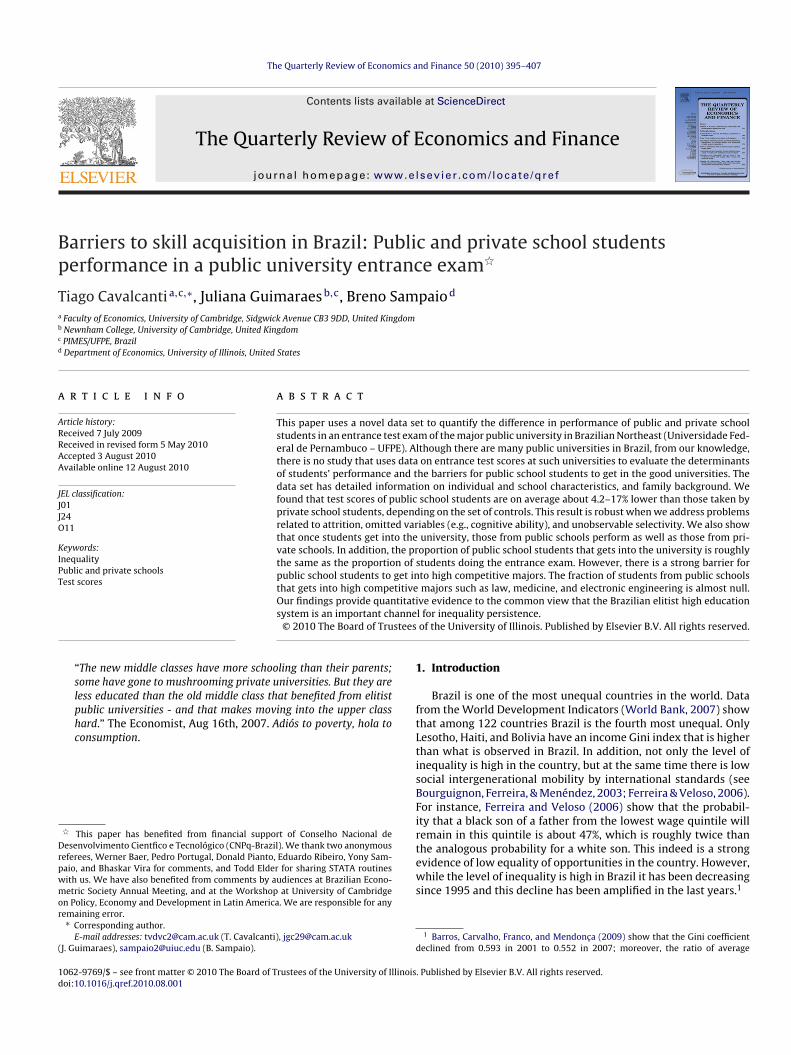
mong all students is 4.36. Fig. 1 shows the empirical density esti-ate of the entrance test score for students from private and public

chools. It shows that public school students score distribution isocated to the left of that for private school students. This implies

28 The Real/Dollar exchange rate in the period of when the data was collected was.856. This translates into a monthly average family income of US$ 567.22.

400 T. Cavalcanti et al. / The Quarterly Review of Eco

Fsto

ttfIdstots

4

4

mtgsIsadccamdQsb

tssew

uf(ac

ssigdrwaptllmie

i7firqdn(ws

cvomoit(c

vsmaihoaf

ig. 1. Empirical density of the entrance test score. Students from private schools:olid blue line. Students from public schools: dotted red line. (For interpretation ofhe references to color in this figure legend, the reader is referred to the web versionf the article.)

hat there is a large mass of public school students on low scoreshan private school students. The average test score is also loweror public school students (3.88) than for private school ones (4.63).n this paper we study the following important questions: Is theifference in the entrance test scores between public and privatetudents due to family background and school characteristics? Or ishis difference explained by unobservable effort and ability? More-ver, once the students from public schools get in the university, dohey have a performance similar to those that come from privatechools?

. Basic results

.1. OLS results

Table 2 presents results for the specifications using the OLS esti-ation procedure. The first noticeable result is the negative sign of

he coefficient of the indicator variable public, which strongly sug-ests that, public schools have a negative effect on entrance testcores when compared to private schools. In all regressions of partof Table 2, the coefficient of the dummy public is negative and alsotatistically different from zero at 99% confidence level.29 The signnd statistical significance of this variable is robust to the intro-uction of family background variables30 (column (3)), and schoolharacteristics (column (4)). Observe also that the R-squared indi-ates that the most complete specification (column (4)) capturesbout 30% of the total variability in the entrance test scores. In ourost parsimonious specification, in column (1), the public school

ummy explains about 7% of total variability in score performances.uantitatively, we have from column (1) that test scores of public

chool students are on average about 17% lower than those takeny private school students. However, once we control for individ-

29 The t-critical value for 99% confidence level is 2.58.30 The difference of column (1) and (2) is that in column (2) we control for whetherhe public school is a federal or a military School. There are two federal schools in theample and one military school. Federal and military schools have in general goodcores in standardized test. Although they are public there is a very competitiventrance exam in those schools, which bias the sample. In fact, observe that oncee control for those schools the absolute value of the public dummy increases.

twti

cpo

r

nomics and Finance 50 (2010) 395–407

al and family characteristics, such as mother’s years of schooling,amily income, and religion,31 this effect decreases from 17% to 7%see column (3)). It decreases further to 6% once we control fornother set of variables, such as whether the school has or not lablasses (see column (4)).

In columns (3) and (4), all other additional controls displaytability as to the sign, size and significance of the associated regres-ion coefficient, except the variable age, number of children, familyncome, and the dummy for Asian students. Regarding family back-round, we observe that mother’s years of schooling is an importanteterminant of the entrance test score. This is consistent with twoecent studies (Bourguignon et al., 2003; Ferreira & Veloso, 2006),hich show, using household survey data, that parent education isstrong predictor of schooling and intergenerational educationalersistence in Brazil is high by international standards. Quantita-ively, we also observe the strong impact of the variable foreignanguage on test scores. The fact that students studied a foreignanguage increases their scores in about 10%. Foreign language

ight indicate student’s ability and learning capabilities, but it ismportant to highlight that in the entrance exam students are alsovaluated on either English or Spanish.

Interestingly, the dummy for races are negative for native Brazil-ans and blacks. On average native Brazilians and blacks score about.7% and 2.7% lower than whites, respectively, after we controlor family background, individual and school characteristics. Thiss particularly important since some universities in Brazil haveecently implemented some affirmative policies and introduceduotas for black and native Brazilian students. Observe that theummy for Asian descendent is also negative and statistically sig-ificant once we control for school characteristics (columns (4) and5)). In addition, notice that Pardos score about 0.6% higher thanhites and this coefficient is statistically significant in all regres-

ions.In Table 2 part II, we address any attrition problem. In our most

omplete specification (column (4)) we miss about 22% of obser-ations relatively to the more parsimonious model. Therefore, inrder to evaluate how the coefficient change when we includeore controls, we estimate specifications (2) and (3) using the same

bservations as in column (4). Estimated coefficients are reportedn Table 2, columns (5) and (6). We notice that the coefficient ofhe indicator variable public does not change in sign, magnitudethe absolute value of this coefficient increases in column (6) whenompared to column (3)), and statistical significance.

Table 2 shows that the magnitude of the point estimate of theariable public are sensitive to the inclusion of observable regres-ors, ranging from −18.9% in models with no control to −6% inodels that include detailed controls. Private schools are therefore

pparently more advantaged on the basis of observable character-stics that positively affect academic performance. It is not clear,owever, if private school students have also advantages in termsf unobservable characteristics (i.e., motivation, effort, cognitivebility) that are correlated with test scores and are not controlledor in the regressions presented so far. It is important to recall alsohat we are considering only students that are taking exams ande might be missing low performing students that do not sign up

o take this exam, and the share of such students might be largern public than in private schools.

The last row of Table 2 reports the estimated bias in the mostomplete specification (column (4)), using Altonji et al. (2005)rocedure. The bias is equal to −0.018, which is an evidencef a negative correlation of unobservable variables in the test

31 We include five indicator variables for religion and the Catholic religion is theeference group. They are: Protestant, Jewish, Atheist, Afro-Religions, and others.

T. Cavalcanti et al. / The Quarterly Review of Economics and Finance 50 (2010) 395–407 401

Table 2Determinants of the entrance test score – OLS estimation.

Part I Part II, attrition

(1) (2) (3) (4) (5) (6)

Public −0.176** −0.189** −0.072** −0.060** −0.189** −0.089**

(−10.63) (−12.93) (−10.31) (−8.99) (−12.60) (−10.20)Age 0.002* −0.011** 0.001*

(1.93) (−11.56) (1.71)Married 0.010 0.030** 0.008

(0.79) (4.55) (0.99)Gender (female = 1) −0.036** −0.049** −0.034

(−7.23) (−9.73) (−7.31)Number of children −0.044** 0.016** −0.044

(−7.36) (3.42) (−7.55)Hours worked −0.007** −0.009** −0.007

(−8.16) (−13.05) (−8.15)Asian −0.003 −0.013* −0.005

(−0.59) (−1.94) (−0.94)Natives −0.077** −0.077** −0.079**

(−7.94) (−7.84) (−8.08)Pardos 0.008** 0.008** 0.008**

(2.93) (2.60) (2.53)Blacks −0.022** −0.019** −0.022**

(−3.45) (−3.59) (−3.92)Living with parents −0.041** −0.033** −0.042**

(−7.49) (−9.79) (−7.91)Religion No No Yes Yes No YesMother’s schooling 0.008** 0.004** 0.007**

(13.27) (7.91) (13.99)Father’s schooling 0.007** 0.004** 0.006**

(7.92) (6.38) (7.29)Working mother 0.005 0.006** 0.006

(1.55) (2.00) (1.47)Working father 0.016** 0.009** 0.013**

(6.29) (4.23) (5.61)Monthly family income 2.3e−0.5** 1.7e−05** 2.3e−05**

(6.15) (6.00) (6.27)Internet user 0.058**

(10.48)Lab classes 0.035**

(4.35)Foreign language 0.104**

(11.92)Reading habit (yes = 1) 0.059**

(20.77)Supletivo −0.101**

(−5.00)Number of tests taken 0.101**

(18.59)Private preparation classes 0.065**

(10.44)Non-12th grade students −0.030*

(−1.79)Federal and military schools No Yes Yes Yes Yes YesN. of observ. 54877 54877 44782 42615 42615 42615Adjusted R2 0.068 0.088 0.158 0.294 0.089 0.174

A these

seowPt

r

o

etsv

Estimated bias

ll specifications include a constant, not reported. T-statistics are presented in paren* Significant at the 90% confidence level.

** Significant at the 95% confidence level.

core equation and the variable Public, which suggests that thestimated effect of public schools on student’s performance isverestimated.32 However, our estimated coefficient is −0.06, thenith a bias of −0.018, the lower bound coefficient of the variable

ublic would be −0.042. In addition, the ratio of the coefficient of

he variable Public and the estimated bias is:

atio = −0.06−0.018

= 3.333.

32 Given the assumption that the selection of observables is similar to the selectionf unobservables, we just need to check this for the most complete specification.

4

tsi

−0.018

s, using heteroskedasticity-consistent standard errors clustered at the school level.

This implies that the effects of unobservable variables on thestimated coefficient of the variable Public would have to be 3.333imes stronger than the effect of the observable variables on thisame coefficient in order to explain the entire negative effect of theariable Public on test scores. We believe that this is rather unlikely.

.2. Robustness

In this subsection, we perform several robustness exercises. Inhe first part, we control for students’ cognitive ability and use thecore at the ENEM (National Exam for High School students) as anndependent variable in the model. As we argued previously, the

402 T. Cavalcanti et al. / The Quarterly Review of Economics and Finance 50 (2010) 395–407

Table 3Summary statistics: sample average and sample standard deviation.

Variables Whole sample ENEM No ENEM

�X �X �X �X �X �X

Observations 54,877 23,807 31,070Public 0.37 0.48 0.36 0.48 0.37 0.48Entrance test score 4.36 1.38 4.74 1.47 4.06 1.23Age 20.54 5.40 18.92 2.99 21.78 6.41Female 0.56 0.49 0.60 0.49 0.52 0.50Married 0.07 0.25 0.02 0.16 0.10 0.30Father education 11.61 4.40 11.87 4.41 11.40 4.38Mother education 11.78 4.46 12.15 4.46 11.50 4.43Working father 0.58 0.49 0.64 0.48 0.55 0.50Working mother 0.50 0.50 0.53 0.50 0.47 0.50Family income 1620.45 2072.07 1705.42 2185.36 1556.56 1980.248Working student 0.27 0.44 0.21 0.44 0.28 0.41Living with parents 0.80 0.40 0.85 0.40 0.76 0.42Whites 0.43 0.49 0.44 0.49 0.43 0.49Asians 0.05 0.21 0.05 0.21 0.05 0.21Natives 0.02 0.13 0.02 0.12 0.02 0.14pardos 0.38 0.48 0.39 0.48 0.38 0.48Blacks 0.09 0.29 0.09 0.28 0.09 0.29Catholics 0.54 0.50 0.59 0.49 0.56 0.49Protestants 0.22 0.41 0.21 0.41 0.22 0.41Jewish 0.002 0.04 0.001 0.04 0.002 0.04Afro-religion 0.006 0.08 0.004 0.07 0.007 0.08Other religions 0.09 0.29 0.08 0.27 0.09 0.29Atheist 0.11 0.31 0.11 0.31 0.11 0.31Hours worked 1.69 2.92 0.91 2.21 2.26 3.23Internet user 0.35 0.47 0.37 0.48 0.33 0.47Reading 0.29 0.45 0.29 0.45 .28 0.45Lab. classes 0.36 0.48 0.37 0.48 .462 0.498Foreign language 0.04 0.20 0.04 0.20 0.04 0.20

0.40.0

EaTsTP

4

aotgptoTspoIithatt

t

ttdto

pen(eoap(ttte

pcE

Private classes 0.40 0.49Supletivo 0.03 0.18

NEM exam is more general than the Vestibular and it also evalu-tes students in logical questions. A caveat must be added, however.his exam is not mandatory and this might bias our results. In theecond part, we control for city fixed effects and school fixed effects.he third part investigate how other definitions of our variableublic affect test scores.

.2.1. Cognitive ability (ENEM exam)It is important to emphasize that the ENEM score already

bsorbs good variation in characteristics (observable and non-bservable) that affect students academic performance. Therefore,he control for the ENEM score is a demanding exercise to investi-ate whether or not public schools impact negatively on studentserformance at public university entrance exams. The problem ofhe ENEM exam, as we mentioned previously, is that less than halff the students that did the entrance test exam did the ENEM.his can bias the results once we control for the ENEM, since thetudents that did this test were not randomly assigned. Table 3rovides summary statistics in which we can compare statisticsf the students who did take and who did not take the ENEM.33

ndeed, there are important differences such as the level of monthlyncome and the entrance test score,34 which are larger for thosehat took the ENEM exam than those that did not. Interestingly,

owever, the fraction of public school students in the two samplesre roughly the same and the Mann–Whitney test does not rejecthe null hypothesis of equality of distributions. Therefore, it seemshat better students with a more favorable family background took

33 We also run a probit model to study the determinants of taking the ENEM. Forhe sake of space, we do not report results here.34 As well as mother’s and father’s education, among other variables.

sbaa

t

5 0.49 0.36 0.481 0.10 0.05 0.21

he ENEM exam, but the distribution of public school students ofhose that did take and did not take the exam are not statisticallyifferent.35 Therefore, it is not straightforward to identify the direc-ion of the bias of the variable public due to the no random choicef taking or not the ENEM.

With this caveat in mind, Table 4, Part I, contains the estimatedarameters of our model when we introduce the score at the ENEMxam as an independent variable to control for any omission in cog-itive ability. We estimate similar regression to those in columns2)–(4) of Table 2, but we add the ENEM student’s score as anxplanatory variable. Parameters are reported in columns (1)–(3)f Table 4. Since we lose about half of the observations when wedd the ENEM score, for comparison reasons we also estimate inart II of Table 4 the model without the ENEM score (columns4)–(6)), but with the same observations of columns (1)–(3). Noticehat the model with the variable ENEM explains about 70% of theotal variability in the entrance test scores, while the model withhe most complete specification, but without the ENEM controlxplains about 36% of such variability.

Observe that the magnitude of the coefficient of the variableublic decreases in magnitude, but it is still negative and statisti-ally different from zero (at 99% confidence level) once we add theNEM student’s score as a regressor.36 Test scores of public school

tudents are on average about 5.6–3.7% lower than those takeny private school students once we control for the ENEM scores,nd depending whether or not we control for family backgroundnd school characteristics. Notice that contrary to other variables,

35 In fact, the entrance test score for those that took the ENEM is large than thosehat did not do the ENEM for both public and private school students.36 Compare the first row of columns (1)–(3) with the first row of columns (4)–(6).

T. Cavalcanti et al. / The Quarterly Review of Economics and Finance 50 (2010) 395–407 403

Table 4Determinants of the entrance test score – ENEM exam.

Part I Part II

(1) (2) (3) (4) (5) (6)

Public −0.056** −0.042** −0.037** −0.246** −0.135** −0.085**(−12.38) (−9.07) (−7.09) (−10.96) (−11.31) (−8.35)

Age 0.001* −0.006** 0.011** −0.018**(1.89) (−9.55) (7.47) (−11.96)

Married −0.006 0.006 0.005 0.045**(−0.64) (0.62) (0.38) (2.99)

Gender (female = 1) 0.026** 0.017** −0.046** −0.059**(7.75) (4.20) (−7.37) (−9.05)

Number of children −0.032** 0.005 −0.089** 0.053**(−5.76) (1.01) (−7.75) (5.68)

Hours worked −0.007** −0.005** −0.010** −0.009(−9.89) (−10.27) (−9.10) (−10.89)

Asian 0.006 0.003 −0.004 −0.018*(1.62) (0.66) (−0.53) (−1.65)

Natives −0.002 −0.004 −0.069** −0.065**(−0.26) (−0.50) (−3.47) (−4.27)

Pardos 0.002 0.001 0.001 −0.001**(0.96) (0.09) (0.01) (−0.23)

Blacks −0.001 −0.002 −0.025** −0.020**(−0.35) (−0.63) (−3.32) (−2.74)

Living with parents −0.014** −0.011** −0.040** −0.027**(−4.74) (−3.76) (−6.29) (−5.41)

Religion No Yes Yes No Yes YesMother’s schooling 0.001* 0.001 0.007** 0.004**

(3.28) (1.21) (13.19) (7.42)Father’s schooling 0.001** 0.001** 0.008** 0.005**

(2.68) (3.32) (11.89) (10.19)Working mother 0.001 0.002 0.009 0.007**

(0.66) (0.84) (1.64) (1.99)Working father 0.005** 0.003 0.012** 0.005

(2.68) (1.81) (3.55) (1.52)Monthly family income 3.1e−0.6** 3.3e−0.6** 2.3e−0.5** 1.6e−0.5**

(3.22) (3.64) (6.74) (6.39)Internet user 0.002 0.051**

(0.74) (8.30)Lab classes 0.001 0.031**

(0.37) (3.63)Foreign language 0.013* 0.080**

(1.96) (7.54)Reading habit (yes = 1) 0.025 0.053**

(11.94) (14.00)Supletivo −0.034* −0.072**

(−3.58) (−5.70)Number of tests taken 0.030** 0.120**

(8.85) (19.04)Private preparation classes 0.035** 0.074**

(10.41) (14.87)Non-12th grade students −0.059** −0.040

(−3.22) (−0.94)ENEM score 0.149** 0.147** 0.139**

(94.78) (92.18) (152.09)Federal and military schools Yes Yes Yes Yes Yes YesN. of observ. 23807 20277 19464 23807 20277 19464

A these(

sai

4

ue

c

tFob

Adjusted R2 0.714 0.716Estimated bias

ll specifications include a constant, not reported. T-statistics are presented in paren*) and (**) indicate same confidence level as in Table 2.

uch as race, gender, mother’s schooling, among others, the signnd statistical significance of the variable public are robust to thentroduction of ENEM test score.37

.2.2. City fixed effects and school fixed effectsHere we use the most complete specification reported on col-

mn (4) of Table 2 to investigate the effects of city and school fixedffects. The first part of Table 5 reports the estimated coefficient of

37 For instance, the coefficient of the variables blacks and natives are not statisti-ally different from zero when we add the variable ENEM.

aIrivtlfi

0.726 0.144 0.239 0.364−0.012

s, using heteroskedasticity-consistent standard errors clustered at the school level.

he variable Public when we control for city and school fixed effects.or the sake of space we do not report the estimated coefficientsf the other variables. The introduction of city fixed effects mighte important for the variable Public because in small cities therere less choice for students in terms of schools than in large cities.n addition, it might be the case that there are more public schoolselative to private schools in small cities than in large cities and

f schools in small cities have less quality than in large cities, theariable Public might be capturing a “small city” effect. We observehat the estimated coefficient, which captures the effects of pub-ic schools on scores, is most unchanged when we introduce cityxed effects (Table 5, row (1)). It decreases in absolute value from

404 T. Cavalcanti et al. / The Quarterly Review of Economics and Finance 50 (2010) 395–407

Table 5Determinants of the entrance test score – city and school fixed effects.

Coeff. on Public Robust t-value City fixed effects School fixed effects Estimated bias Ratio

(1) −0.057** −16.52 Yes No −0.015 3.8(2) −0.023** −3.52 No Yes −0.010 2.3(3) −0.021** −3.13 Yes Yes −0.009 2.333

All specifications include a constant and the variables used in column (4) of Table 2. (*) and (**) indicate same confidence level as in Table 2.

Table 6Determinants of the entrance test score – definition of the variable Public.

Public Robust t-value Number of observations Adjusted R2

−8.82 42,587 0.29

A . (*) and (**) indicate same confidence level as in Table 2.

6c

pnetdtiafi2ni

motesoss

4

aws(hdeTtott

4

S

ec

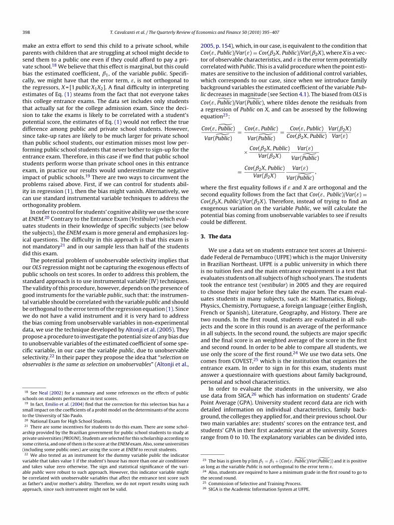
Fig. 2. Quantile regression estimates for the indicator variable public. Dependentvae

ttviatl

weOtfc

Coeff. on full Public Robust t-value Coeff. on partial

(1) −0.071** −10.97 −0.047**

ll specifications include a constant and the variables used in column (4) of Table 2

% to 5.7% and it is also statistically different from zero at usualonfidence level.

We also introduce school fixed effects to get rid of sortingroblems associated with different qualities of schools, differenteighborhoods and parental backgrounds This is also a demandingxercise, since this would capture schools effects, such as the wayhe schools are run and the quality of teachers, which might explainifference in scores between private and public school students;his would also capture neighborhood effects, such as crime raten the school’s neighborhood and average academic performancemong schools. Interestingly, we observe that the estimated coef-cient for the variable Public decreases in magnitude from 6% to.1% when we introduce school and city fixed effects, but it is stillegative and statistically different from zero at usual confidence

ntervals (Table 5, rows (2) and (3)).We also estimated the bias of the variable Public using the

ethod proposed by Altonji et al. (2005). We found that the effectf unobservable variables would have to be at least 2.3 larger thanhe effect of all observed variables, including city and school fixedffects, in order for the effect of the variable Public on student’score to vanish. We believe that the results above corroboratedur previous finding that public schools have a negative effect ontudent’s score, even when we control for family background andchool characteristics.

.2.3. Definition of the variable PublicFinally, we change the criterion of the definition of the vari-

ble Public. Previously, we defined public school students as thoseho took at least 2 years, including the last year, of their high

chool education in a public school. Now, we define two variables:i) Full Public, which characterizes students who study their entireigh school education in a public institution; and (ii) Partial Public,enoting the students who did at least 1 year of their high schoolducation in a public school. Results are reported on the last row ofable 5. We observe that both coefficients are negatively and statis-ically different from zero at 99% confidence level. The coefficientf the variable Full Public is about 1.51 larger than the coefficient ofhe variable Partial Public. Therefore, results seem to be robust tohe definition of our variable public school (Table 6).38

.3. Quantile results

In this subsection we analyze the quantile regression estimates.ince quantile regression procedures produce one point estima-

38 For this regression, we do not calculate the bias of the estimated public schoolffects on test scores because the procedure developed by Altonji et al. (2005)onsiders only one endogenous variable.

fTstwm

ariable: entrance test score. The solid line corresponds to the quantile estimatend the shaded area the 95% confidence interval. The dotted line represents the OLSstimate.

ion for each quantile, for the sake of space, we focus only onhe coefficient of the indicator variable public.39 We use the sameariables used in column (4) of Table 2, and results are displayedn Fig. 2. This plot shows the quantile regression (QR) estimatess well as the 95% confidence intervals. For comparison reasons,he least square estimate is presented by the dotted horizontaline.

Quantile regression provides the appropriate tool to determinehether there are any difference in marginal responses of the

ntrance test score to different school systems (public or private).bserve that the coefficient of the dummy variable public is nega-

ive for all quantiles (including the confidence interval) and it variesrom −5.2% to −7% as we move from low to high quantiles of theonditional Test Score distribution. Therefore, not only studentsrom public schools have on average lower scores on the Entranceest Exam, but also students that have higher conditional scoresuffer from a greater penalty for attending public schools compared

o low conditional score students. We may conclude that studentsith high performance in the entrance test scores would benefitost by moving from public to private schools.

39 Upon request we provide the quantile estimation for the other parameters.

T. Cavalcanti et al. / The Quarterly Review of Economics and Finance 50 (2010) 395–407 405

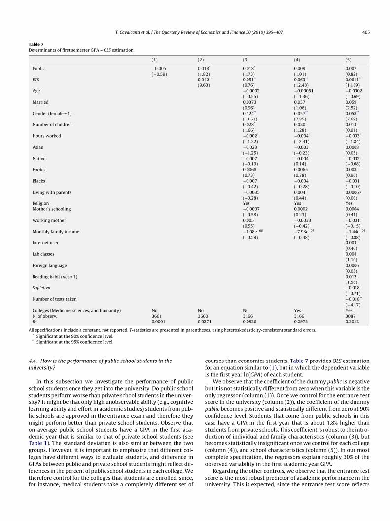
Table 7Determinants of first semester GPA – OLS estimation.

(1) (2) (3) (4) (5)

Public −0.005 0.018* 0.018* 0.009 0.007(−0.59) (1.82) (1.73) (1.01) (0.82)

ETS 0.042** 0.051** 0.063** 0.0611**

(9.63) (9.76) (12.48) (11.89)Age −0.0002 −0.00051 −0.0002

(−0.55) (−1.36) (−0.69)Married 0.0373 0.037 0.059

(0.96) (1.06) (2.52)Gender (female = 1) 0.124** 0.057** 0.058**

(13.51) (7.85) (7.69)Number of children 0.028* 0.020 0.013

(1.66) (1.28) (0.91)Hours worked −0.002* −0.004* −0.003*

(−1.22) (−2.41) (−1.84)Asian −0.023 −0.003 0.0008

(−1.25) (−0.23) (0.05)Natives −0.007 −0.004 −0.002

(−0.19) (0.14) (−0.08)Pardos 0.0068 0.0065 0.008

(0.73) (0.78) (0.96)Blacks −0.007 −0.004 −0.001

(−0.42) (−0.28) (−0.10)Living with parents −0.0035 0.004 0.00067

(−0.28) (0.44) (0.06)Religion Yes Yes YesMother’s schooling −0.0007 0.0002 0.0004

(−0.58) (0.23) (0.41)Working mother 0.005 −0.0033 −0.0011

(0.55) (−0.42) (−0.15)Monthly family income −1.08e−06 −7.93e−07 −1.44e−06

(−0.59) (−0.48) (−0.88)Internet user 0.003

(0.40)Lab classes 0.008

(1.10)Foreign language 0.0006

(0.05)Reading habit (yes = 1) 0.012

(1.58)Supletivo −0.018

(−0.71)Number of tests taken −0.018**

(−4.17)Colleges (Medicine, sciences, and humanity) No No No Yes YesN. of observ. 3661 3660 3166 3166 3087R2 0.0001 0.0271 0.0926 0.2973 0.3012

A nthes

4u

sssllmodTglGftf

cfi

bospccsdb(

ll specifications include a constant, not reported. T-statistics are presented in pare* Significant at the 90% confidence level.

** Significant at the 95% confidence level.

.4. How is the performance of public school students in theniversity?

In this subsection we investigate the performance of publicchool students once they get into the university. Do public schooltudents perform worse than private school students in the univer-ity? It might be that only high unobservable ability (e.g., cognitiveearning ability and effort in academic studies) students from pub-ic schools are approved in the entrance exam and therefore they

ight perform better than private school students. Observe thatn average public school students have a GPA in the first aca-emic year that is similar to that of private school students (seeable 1). The standard deviation is also similar between the tworoups. However, it is important to emphasize that different col-

eges have different ways to evaluate students, and difference inPAs between public and private school students might reflect dif-

erences in the percent of public school students in each college. Weherefore control for the colleges that students are enrolled, since,or instance, medical students take a completely different set of

co

su

es, using heteroskedasticity-consistent standard errors.

ourses than economics students. Table 7 provides OLS estimationor an equation similar to (1), but in which the dependent variables the first year ln(GPA) of each student.

We observe that the coefficient of the dummy public is negativeut it is not statistically different from zero when this variable is thenly regressor (column (1)). Once we control for the entrance testcore in the university (column (2)), the coefficient of the dummyublic becomes positive and statistically different from zero at 90%onfidence level. Students that come from public schools in thisase have a GPA in the first year that is about 1.8% higher thantudents from private schools. This coefficient is robust to the intro-uction of individual and family characteristics (column (3)), butecomes statistically insignificant once we control for each collegecolumn (4)), and school characteristics (column (5)). In our most

omplete specification, the regressors explain roughly 30% of thebserved variability in the first academic year GPA.

Regarding the other controls, we observe that the entrance testcore is the most robust predictor of academic performance in theniversity. This is expected, since the entrance test score reflects

406 T. Cavalcanti et al. / The Quarterly Review of Economics and Finance 50 (2010) 395–407

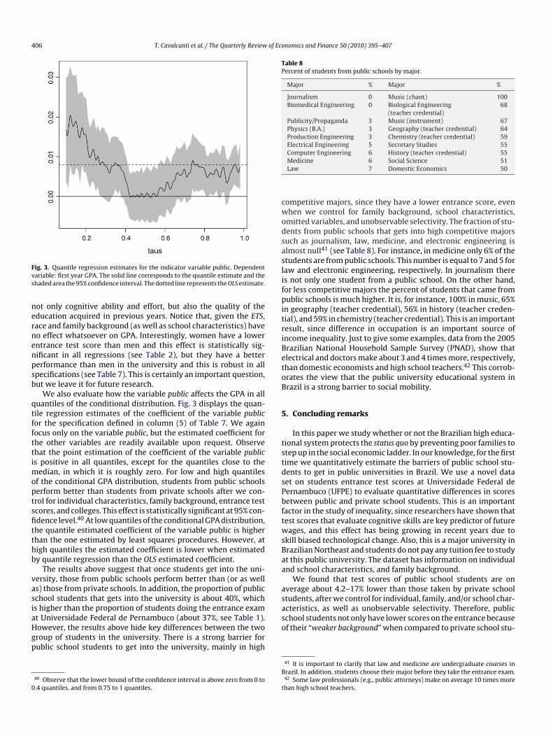
Fvs

nernenpsb

qtffttimoptsfitthb

vasiaHgp

0

Table 8Percent of students from public schools by major.

Major % Major %

Journalism 0 Music (chant) 100Biomedical Engineering 0 Biological Engineering

(teacher credential)68

Publicity/Propaganda 3 Music (instrument) 67Physics (B.A.) 3 Geography (teacher credential) 64Production Engineering 3 Chemistry (teacher credential) 59Electrical Engineering 5 Secretary Studies 55Computer Engineering 6 History (teacher credential) 55

cwodsaslifpitriBetoB

5

tstdsPbftwsBaa

average about 4.2–17% lower than those taken by private schoolstudents, after we control for individual, family, and/or school char-acteristics, as well as unobservable selectivity. Therefore, public

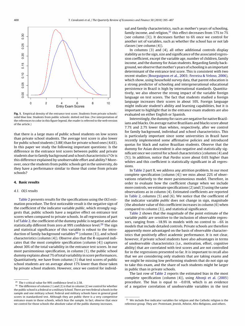
ig. 3. Quantile regression estimates for the indicator variable public. Dependentariable: first year GPA. The solid line corresponds to the quantile estimate and thehaded area the 95% confidence interval. The dotted line represents the OLS estimate.

ot only cognitive ability and effort, but also the quality of theducation acquired in previous years. Notice that, given the ETS,ace and family background (as well as school characteristics) haveo effect whatsoever on GPA. Interestingly, women have a lowerntrance test score than men and this effect is statistically sig-ificant in all regressions (see Table 2), but they have a bettererformance than men in the university and this is robust in allpecifications (see Table 7). This is certainly an important question,ut we leave it for future research.

We also evaluate how the variable public affects the GPA in alluantiles of the conditional distribution. Fig. 3 displays the quan-ile regression estimates of the coefficient of the variable publicor the specification defined in column (5) of Table 7. We againocus only on the variable public, but the estimated coefficient forhe other variables are readily available upon request. Observehat the point estimation of the coefficient of the variable publics positive in all quantiles, except for the quantiles close to the

edian, in which it is roughly zero. For low and high quantilesf the conditional GPA distribution, students from public schoolserform better than students from private schools after we con-rol for individual characteristics, family background, entrance testcores, and colleges. This effect is statistically significant at 95% con-dence level.40 At low quantiles of the conditional GPA distribution,he quantile estimated coefficient of the variable public is higherhan the one estimated by least squares procedures. However, atigh quantiles the estimated coefficient is lower when estimatedy quantile regression than the OLS estimated coefficient.

The results above suggest that once students get into the uni-ersity, those from public schools perform better than (or as wells) those from private schools. In addition, the proportion of publicchool students that gets into the university is about 40%, whichs higher than the proportion of students doing the entrance exam

t Universidade Federal de Pernambuco (about 37%, see Table 1).owever, the results above hide key differences between the tworoup of students in the university. There is a strong barrier forublic school students to get into the university, mainly in high

40 Observe that the lower bound of the confidence interval is above zero from 0 to.4 quantiles, and from 0.75 to 1 quantiles.

so

B

t

Medicine 6 Social Science 51Law 7 Domestic Economics 50

ompetitive majors, since they have a lower entrance score, evenhen we control for family background, school characteristics,

mitted variables, and unobservable selectivity. The fraction of stu-ents from public schools that gets into high competitive majorsuch as journalism, law, medicine, and electronic engineering islmost null41 (see Table 8). For instance, in medicine only 6% of thetudents are from public schools. This number is equal to 7 and 5 foraw and electronic engineering, respectively. In journalism theres not only one student from a public school. On the other hand,or less competitive majors the percent of students that came fromublic schools is much higher. It is, for instance, 100% in music, 65%

n geography (teacher credential), 56% in history (teacher creden-ial), and 59% in chemistry (teacher credential). This is an importantesult, since difference in occupation is an important source ofncome inequality. Just to give some examples, data from the 2005razilian National Household Sample Survey (PNAD), show thatlectrical and doctors make about 3 and 4 times more, respectively,han domestic economists and high school teachers.42 This corrob-rates the view that the public university educational system inrazil is a strong barrier to social mobility.

. Concluding remarks

In this paper we study whether or not the Brazilian high educa-ional system protects the status quo by preventing poor families totep up in the social economic ladder. In our knowledge, for the firstime we quantitatively estimate the barriers of public school stu-ents to get in public universities in Brazil. We use a novel dataet on students entrance test scores at Universidade Federal deernambuco (UFPE) to evaluate quantitative differences in scoresetween public and private school students. This is an importantactor in the study of inequality, since researchers have shown thatest scores that evaluate cognitive skills are key predictor of futureages, and this effect has being growing in recent years due to

kill biased technological change. Also, this is a major university inrazilian Northeast and students do not pay any tuition fee to studyt this public university. The dataset has information on individualnd school characteristics, and family background.

We found that test scores of public school students are on

chool students not only have lower scores on the entrance becausef their “weaker background” when compared to private school stu-

41 It is important to clarify that law and medicine are undergraduate courses inrazil. In addition, students choose their major before they take the entrance exam.42 Some law professionals (e.g., public attorneys) make on average 10 times morehan high school teachers.

of Eco

dotttgigasatcntwotfsppe

R

A

A

A

A

B

B

B

C

D

E

as

F

F

F

G

G

H

K

K

KK

L

M

M

M

M

M

M

N

P

P

P

P

R

Rivkin, S. G., Hanushek, E. A., & Kain, J. F. (2005). Teachers, schools, and academicachievement. Econometrica, 73(2), 417–458.

T. Cavalcanti et al. / The Quarterly Review

ents but also because of the low quality of public schools43 or lackf preparation for the entrance test exam. Using quantile regressionechniques, we also show that students with high performance inhe entrance test scores would benefit most by moving from publico private schools. Another important result is that family back-round (e.g., mother’s years of schooling and household’s income)s a key predictor of test scores. Finally, we show that once studentset into the university, those from public schools perform as wells those from private schools. In addition, the proportion of publicchool students that gets into the university is roughly the sames the proportion of students doing the entrance exam. However,here is a strong barrier for public school students to get into highompetitive majors, such as law, medicine, and electronic engi-eering is almost null. Our results are therefore consistent withhe political economy view (e.g., Fernandez & Rogerson, 1995),hich suggests that public university education involves a transfer

f resources toward higher income families which in turn strengthhe persistence of inequality and decrease social mobility. There-ore, policies toward to improve the quality of education in publicchools by providing a better preparation for the entrance exam orolicies that facilitate access for public school students to get intoublic universities would improve the equality of opportunities inducation for students to acquire a university degree.

eferences

lesina, A., DiTella, R., & MacCulloch, R. (2004). Inequality and happiness: Are Euro-peans and Americans different? Journal of Public Economics, 88, 2009–2042.

lexopoulos, J., & Cavalcanti, T. (in press). Cheap Home Goods and Persistent Inequal-ity. Economic Theory.

ltonji, J. G., Elder, T., & Taber, C. R. (2005). Selection on observed and unobservedvariables: Assessing the effectiveness of catholic schools. Journal of PoliticalEconomy, 113(1), 151–184.

ltonji, J. G., Elder, T., & Taber, C. R. (2008). Using selection on observed variablesto assess bias from unobservables when evaluating Swan-Ganz catheterization.American Economic Review: Papers & Proceedings, 98(2), 345–350.

arros, R., Carvalho, M., Franco, S., & Mendonca, R. (2009). Determinantes da Quedana Desigualdade de Renda no Brasil. In Texto para Discussão 1460, IPEA.

ellows, J., & Miguel, E. (2009). War and local collective action in Sierra Leone. Journalof Public Economics, 93(11–12), 1144–1157.

ourguignon, F., Ferreira, F., & Menéndez, M. (2003). Inequality of outcomes andinequality of opportunities in Brazil. World Bank Policy Research Working Paper3174.

uri, A. Z., & de Menezes-Filho, N. A. (2005). A Relacão entre Desempenho Escolar e os

Salários no Brasil. Mimeo, Universidade de São Paulo.

oepke, M. (2004). Accounting for fertility decline during the transition to growth.Journal of Economic Growth, 9(3), 347–383.

milio, D. R., Belluzo, W., Jr., & Alves, D. C. O. (2004). Uma Análise Econométrica dosDeterminantes do Acesso à Universidade de São Paulo. Pesquisa e PlanejamentoEconômico, 34(2), 275–305.

43 See Hanushek (1995) for some explanation of differences in quality of publicnd private schools in developing country, as well as some policy that can reduceuch gap in quality.

W

W

nomics and Finance 50 (2010) 395–407 407

ernandez, R., & Rogerson, R. (1995). On the political economy of education subsi-dies. Journal of Political Economy, 62, 249–262.

erreira, S. G., & Veloso, F. A. (2006). Intergenerational mobility of wages in Brazil.Brazilian Review of Econometrics, 26(2), 181–212.

uchs, T., & Woessmann, L. (2007). What accounts for international differences instudent performance? A re-examination using PISA data. Empirical Economics,32(2–3), 433–464.

alor, O., & Zeira, J. (1993). Income distribution and macroeconomics. Review ofEconomics Studies, 60, 35–52.

oyal, S. (2009). Inside the house of learning: The relative performance of publicand private schools in Orissa. Education Economics, 17(3), 315–327.

anushek, E. A. (1995). Interpreting recent research on schooling in developingcountries. The World Bank Research Observer, 10(2), 227–246.

ingdon, G., & Teal, F. (2010). Teacher unions, teacher pay and student performancein India: A pupil fixed effects approach. Journal of Development Economics, 91(2),278–288.

oenker, R. (2005). Quantile regression, Econometric Society monographs. CambridgeUniversity Press.

oenker, R., & Basset, G. (1978). Regression quantiles. Econometrica, 46, 33–50.oenker, R., & Hallock, K. (2001). Quantile regression: An introduction. Journal of

Economic Perspectives, 15, 143–156.azear, E. (2001). Educational production. Quarterly Journal of Economics, CXVI(3),

777–803.achado, J. A. F., & Silva, J. M. S. (2006). Quantiles for fractional data. Mimeo, Univer-

sidade Nova de Lisboa.cEwan, P. J. (2008). Can schools reduce the indigenous test score gap? Evidence

from Chile. Journal of Development Studies, 44(10), 1506–1530.enezes-Filho, N. (2007). Os Determinantes do Desempenho Escolar do Brasil. Mimeo,

Instituto Futuro Brasil.enezes-Filho, N., Fernandes, R., & Picchetti, P. (2006). Rising human capital but

constant inequality: The education composition effect in Brazil. Revista Brasileirade Economia, 60(4), 407–424.

urnane, R. J., Willett, J. B., & Levy, F. (1995). The growing importance of cog-nitive skill in wage determination. Review of Economics and Statistics, 77(2),251–266.

urphy, K. M., & Peltzman, S. (1997). School performance and the youth labormarket. Journal of Labor Economics, 22(2), 299–325.

eal, D. (2002). How vouchers could change the market for education. Journal ofEconomic Perspectives, 16(4), 25–44.

apke, L. E., & Wooldridge, J. M. (1996). Econometric methods for fraction responsevariable with an application to 401(k) plan participation rates. Journal of AppliedEconometrics, 11, 619–632.

owell, J. L. (1986). Censored regression quantiles. Journal of Econometrics, 32,143–155.

sacharopoulos, G. (1999). Returns to investment in education: A global update.World Development, 22(9), 1325-l343.

sacharopoulos, G., & Patrinos, H. A. (2004). Returns to investment in education: Afurther update. Education Economics, 12(2), 111–134.

esende, M., & Wyllie, R. (2006). Retornos para Educacão no Brasil: EvidênciasEmpíricas Adicionais. Economia Aplicada, 10(3), 349–365.

altenberg, F. D, & Vandenberghe, V. (2007). What does it take to achive equality ofopportunity in education? An empirical investigation based on Brazilian data.Economics of Education Review, 26, 710–724.

orld Bank. (2007). World development indicators. Washington, DC: World Bank.