Barkhausen Noise: Elementary Signals, Power Laws, and Scaling Relations

Barkhausen noise: Elementary signals, power laws, and scaling relations

Djordje Spasojevic, 1 Srdjan Bukvic, 1 Sava Milosevic, 1,2 and H. Eugene Stanley 21Faculty of Physics, University of Belgrade, P.O. Box 368, 11001 Belgrade, Serbia

2Center for Polymer Studies and Department of Physics, Boston University, Boston, Massachusetts 02215~Received 29 January 1996; revised manuscript received 7 June 1996!

We report extensive measurements, with sufficiently large statistics, of the Barkhausen noise ~BN! in thecase of the commercial VITROVAC 6025 X metal glass sample. Applying a very scrutinized numericalprocedure, we have extracted over one million of the BN elementary signals from the raw experimental data,whereby we made a rather precise estimation of the relevant power law exponents. In conjunction with theexperimental part of the work, we have recognized a generic shape of a single BN elementary signal ~BNES!,and we have put forward, without invoking any existing model of BN, a simple mathematical expression forBNES. Using the proposed expression for BNES in a statistical analysis, we have been able to predict scalingrelations and an elaborate formula for the power spectrum. We have also obtained these predictions within thegeneralized homogeneous function approach to the BNES’s probability distribution function, which we havesubstantiated by the corresponding data collapsing analysis. Finally, we compare all our findings with resultsobtained within the current experimental and theoretical research of BN. @S1063-651X~96!13409-7#

PACS number~s!: 05.40.1j, 75.60.Ej, 05.90.1m, 02.50.Wp

I. INTRODUCTION

The Barkhausen noise ~BN! is a classical physical phe-nomenon which is manifested as a series of jumps in mag-netization of a ferromagnetic sample when it is exposed to avarying external magnetic field. These changes induce volt-age changes in a surrounding coil, and consequently they canbe transformed into acoustic noise. Since its discovery @1#,BN has been incessantly investigated ~see, for instance, thereviews @2–4#! because of its vast practical importance ~suchas for various types of magnetic recordings @5# and for non-invasive material characterization techniques @6#! and be-cause of its major conceptual importance for understandingdynamics of ferromagnets on the magnetic domain scale.These investigations have shown that BN is a very complexphysical phenomenon with many different appearanceswhich depend on kind of ferromagnetic specimen understudy, character of quenched in defects, external field drivingrate, thermal effects, strength of the demagnetization fields,and other experimental details.

At present there are several conceptually different ~and toa certain extent incoherent! theoretical approaches to the ex-planation of BN. The first of the current theoretical ap-proaches we would like to bring forward here is that onewhich analyzes BN as a consequence of the domain-wall~DW! motion. Accordingly, BN has been investigated via asingle-degree-of-freedom model @7# in which individual DWis moving ~in a random walk manner! through a spatiallyrandom coercive field. The Langevin equation approach @7#has been developed further in a number of papers @8–10# andthoroughly reviewed by Bertotti @11,12#. In a different ap-proach, the DW motion and domain nucleation have beenexperimentally and theoretically investigated in relation toBN in ultrathin ferromagnetic films @13#.

Recently, the concept of the self-organized criticality~SOC! @14,15# has acquired a distinguished role in the con-temporary BN investigations. Since the appearance of theSOC concept, many questions related to its application to

BN has been raised which initiated many different studiesand even antagonistic interpretations. The applicability of theSOC concept to BN was investigated by Meisel and Cote@16,17# who offered qualitative arguments and specific mea-surements ~in various materials, starting with a metal glasssample! in support to the relevance of the SOC concept forthe explanation of BN. They augmented their arguments byperforming the Jensen, Christensen, and Fogedby ~JCF! typeof analysis @18# of statistical characterization of the observedBN. Besides, the avalanchelike topological rearrangementsof cellular domain patterns in magnetic garnet films wereinvestigated by Babcock and Westervelt @19#, who inter-preted the obtained findings in the framework of the SOCconcept. Finally, BN has been investigated as a fractal timesignal @20# and subsequently simulated via a SOC model@21# by Geoffroy and Porteseil.

Concurrently, there are approaches that put under doubtthe relevance of the SOC concept to BN. Thus, O’Brien andWeissman @22# have pointed out that the 1/f noise andpower-law distributions are not necessarily evidences ofSOC, but rather the consequences of scaling properties ofquenched disorder in material. In this spirit, they have per-formed experimental and computational analyses of thefourth-order signal correlations ~dubbed the second spectra!,which was expected to reveal violations of the detailed bal-ance in self-organization caused by an external driving. Themain conclusion of these analyses is that the most statisticalcharacterization of BN is consistent with the single-degree-of-freedom models of Allesandro et al. @7#. On the otherhand, within a many-degree-of-freedom model approach@23–25#, it has been recently argued that features of BN canbe adequately described by the zero-temperature random-field Ising ~RFI! model, and that the observed scaling in BNshould be a consequence of the vague proximity to a plainold critical point ~which in the model studied is determinedby a critical value of the width of the random-field distribu-tion @24#!. The role of material defects for the explanation ofBN has been also emphasized in the approach of Urbach

PHYSICAL REVIEW E SEPTEMBER 1996VOLUME 54, NUMBER 3

541063-651X/96/54~3!/2531~16!/$10.00 2531 © 1996 The American Physical Society

et al. @26#, who exploited concept of rough-surfaces growthto describe the DW motion, with the conclusion that long-range demagnetization fields strongly affect the character ofBN.

Despite the vast list of the BN facets that have been in-vestigated, so far the question whether the BNES’s probabil-ity function is a generalized homogeneous function ~GHF!has not been widely attacked and analyzed. Similarly, therehas been a little attention payed to the form of individual BNsignals and consequences which their form might have to theglobal BN. In this paper, we report on extensive measure-ments ~with sufficiently large statistics! of BN in the case ofa commercial VITROVAC 6025-X metal glass sample. Inthe course of these measurements, we have introduced manyexperimental precautions and scrutinized numerical methodsin order to eliminate effects of the extrinsic noise. In thisway, we have been able to extract a proper average form ofthe individual BN signals from the experimental data and,what is more important, to provide evidences that theBNES’s probability distribution is a GHF. Our theoreticaltreatment of the problem has been first focused on investiga-tion of power-law behaviors of BN and their relations withan analytical expression which describes the obtained aver-age shape of BNES’s. After providing qualitative theoreticalarguments which support the accepted signal form, we havecarried out an analysis of the JCF @18# type ~which does nottake into account any specific origin of the noise signal!, andwe have obtained various scaling relations ~satisfied uponinserting the experimental values of scaling exponents!, aswell as an expression for the power spectrum whose numeri-cal presentation is in agreement with our experimental re-sults. Then, we have analyzed the hypothesis that theBNES’s probability distribution function is a GHF and wehave expounded on consequences which such an assumptionimplies. Thus, it appears that power-law behaviors of BN,and, in particular, all scaling relations can be obtained asconsequences of the GHF property of the BNES’s probabil-ity distribution function and that other consequences, such asthe data collapsing of numbers of events, can serve as ad-equate experimental confirmations of the GHF hypothesis.

This paper is organized as follows. In Sec. II we firstdescribe our experimental setup. Then we elaborate on thenumerical procedure utilized for analysis of the recordeddata, and present our experimental results. In Sec. III wedevelop our inductive theoretical approach to BN andpresent a detailed comparison of the theoretically and experi-mentally obtained results. In Sec. IV, we provide evidencesthat the BNES’s probability distribution function is a gener-alized homogeneous function which enable us to rederive allscaling relations ~obtained in Sec. III! in the spirit of thestandard critical phenomena. Finally, we give an overall dis-cussion of the utilized experimental method and the unfoldedtheory within the present knowledge about the Barkhausennoise.

II. EXPERIMENTAL ANALYSIS

A. Experimental setup

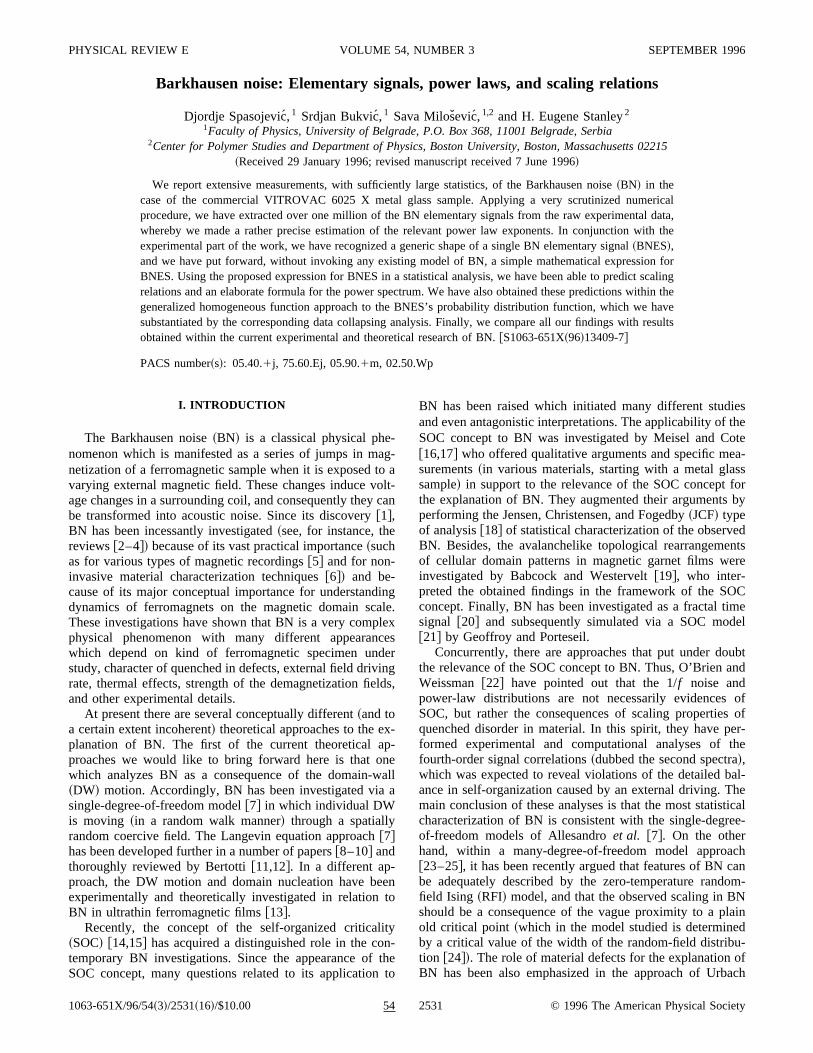
We have used the experimental setup which is schemati-cally depicted in Fig. 1, and here we give a brief descriptionof the parts of the setup. A signal generator ~Krohn-hite 5400

B! provided sinusoidal current for the driving solenoid Swhich produced a magnetic field, H5H0sin(2pf0t), that con-tinuously drew a specimen ~located within the pickup coilC) through a B-H loop. A small driving frequencyf 050.03 Hz has been used to prevent ~or, more precisely, toreduce significantly! overlapping of the Barkhausen pulses.The length of the solenoid S was 20 cm, while its innerdiameter was 5 cm, and it consisted of 675 turns of a copperwire ~0.5 mm in diameter!. The maximal strength of themagnetic field H0, produced by S , was about 160 A m21

~which is approximately four times larger than the meanEarth magnetic field!, and this small field was oriented or-thogonally to the local Earth magnetic field.

We have performed our measurements on a quasi-two-dimensional as-cast metal glass sample ~a commercial VIT-ROVAC 6025 X produced by Vacuum Schmeltz!, with lin-ear dimensions 4 cm 3 1 cm 3 0.003 cm. The Barkhausenpulses @see Fig. 2~a!#, which correspond to the jumps in mag-netization of the specimen, were collected as induced voltagepulses via the pickup coil C ~of length 5.5 cm, with rectan-gular cross section 12 mm3 2 mm!. The specimen wasplaced inside the coil in such a way that there was no me-chanical tension. The pickup coil C , with the resistanceR530 V, comprised of 300 turns of copper wire and itsmagnetic coupling with S was weak. The pickup coil C , aswell as the inserted specimen, were placed in the middle ofthe solenoid S .

Electric signal from the pickup coil C has been amplified~with a gain of 2000! through a low-noise differential ampli-fier. Trains of the Barkhausen pulses were monitored, to-gether with the driving current, on a HAMEG 205-3 digitalstorage scope. In order to improve quality and the duration ofthe recorded signal, an analog-to-digital ~A/D! converter~made by Electronic Design, model ED 2000 with high-speed module ED 2019, compatible with the Burr-Browncard, model PCI-20023M-1!, with the 12-bit resolution, hasbeen used for the data collection. The A/D converter had theinput range 25 V to 15 V, with the maximal rate of 300 000samples per second, permitting, in a single run, collection ofas many samples as the computer memory could accept. Wehave found that the sampling rate of 200 000 samples per

FIG. 1. A schematic depiction of the setup used in the experi-mental course of this work. The ballast resistor of 200 V has beenused to reduce the influence of Barkhausen noise on the currentwhich flows through the driving solenoid S .

2532 54SPASOJEVIC, BUKVIC, MILOSEVIC, AND STANLEY

second provided a good balance between resolution of peaksand the number of peaks recorded during a single run. Withrespect to this problem, we would like to emphasize that theamplifier cutoff frequency ~100 kHz! has been chosen to pre-vent aliasing effect in the power spectrum @27#.

The achieved quality of the Barkhausen noise measure-ment, obtained in the way described above, was accompa-nied by undesirable sensitivity to the low-level electric andmagnetic extrinsic noise. To minimize this concomitantnoise, the driving solenoid S , the pickup coil C , and theamplifier, were enclosed in a double-wall Permalloy Cham-ber ~made by Vacuum Schmeltz!, which reduced the externalmagnetic fields ~including the Earth’s magnetic field!, atleast by a factor of 10 000. Finally, a copper chamber ~whichis not shown in Fig. 1! has been used as an additional Fara-day cage to minimize external electric fields. As a result,amplitude of the overall extrinsic noise was not larger than 4counts of the A/D converter, that is, signal-to-noise ratio wasabout 500. Finally, the care was taken so as to record the

entire set of data at the constant temperature equal to20 °C.

B. Numerical processing of recorded data

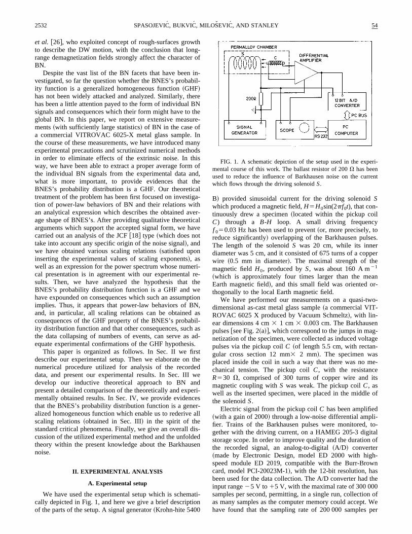
We drove the sample studied through B-H loop for 10 hbefore any recording was done, in order to achieve the sta-tionary regime of the hysteresis loop cycling. Then, we havecollected our experimental data in a small interval of H ~cen-tered at the value H50), which encloses the correspondingcoercive field Hc owing to the fact that our specimen is a softmagnet. During a single recording, which lasted about 0.6sec, we got 128 kB of data ~131 072 points of the digitizedvoltage!, and we present here results of statistical averagingover 200 successive single recordings obtained ~within 2 h ofmeasurement! under identical experimental conditions. InFig. 2~a! we present a typical train of Barkhausen pulses bythe line drawn through a set of 4096 successively recordedpoints. The presented set belongs to one of the 200 single

FIG. 2. ~a! A typical train of Barkhausen pulses observed in an as-cast commercial VITROVAC 6025 X metallic glass ribbon ~with lineardimensions 4 cm31 cm30.003 cm!. The train is presented by the line drawn through 4096 points ~of digitized voltage, recorded at thesampling rate of 200 000 samples per second!. The unit on the ordinate axis is 1 count of the A/D converter, which is equivalent to thevoltage of 5/2048 V. The huge offset, of about 2000 counts, appears as a consequence of the fact that the voltage of 0 V corresponds to the2048th count of the A/D converter. For the sake of comparison, an elementary signal of the form ~8! is presented in the inset ~where the timeand voltage units are arbitrary!. ~b! Power spectrum ~in arbitrary units! of the train of Barkhausen pulses shown in the preceding graph. Thehigh value ~close to 107) of the f50 harmonic is a consequence of the huge offset of the recorded train of pulses. ~c! The positions ofbaseline ~the lower horizontal line parallel to the time axis! and the discrimination level ~the upper horizontal line! for a nontypical train ofBarkhausen pulses. The nontypical train of small Barkhausen pulses has been chosen here intentionally since the two lines ~the baseline andthe discrimination level! would be otherwise indistinguishable in a figure that would present a typical train of Barkhausen pulses. ~d! A hugesingle Barkhausen signal which lasted 0.002 sec ~located, approximately, between 0.0075 sec and 0.0095 sec!.

54 2533BARKHAUSEN NOISE: ELEMENTARY SIGNALS . . .

recordings, while the time counting has been shifted, for thesake of convenience, to the beginning of the train of pulses.One can notice that in the recorded train there are severalclusters of big pulses and a multitude of small pulses hardlydistinguishable from the concomitant extrinsic noise.

After the data collection, we have performed numericalprocessing of the raw recorded data. There are several rea-sons for this processing. First, the data collected by thepickup coil were of millivolts in magnitude, and they had tobe amplified in order to be adjusted to the input range of theanalog-to-digital converter. The applied signal amplificationinevitably introduces various types of distortions since theamplified signal is the convolution of the amplifier charac-teristic and of the input signal power spectrum. These distor-tions are potentially of the greatest influence on the mostfrequent short-lasting, and small ~in magnitude!, signals. Toeliminate these distortions, we have performed a deconvolu-tion procedure, using the fast Fourier transform ~FFT!method, based on known characteristic of the amplifier used.Within this procedure, it was possible to introduce cutoff atany desired frequency ~below the imposed hardware fre-quency cutoff!, and we have investigated the influence of thefrequency cutoff choice. Thus, we have found that the data,important for the further analysis, remain stable under varia-tion of the frequency cutoff, and, for this reason, in whatfollows we present our results obtained for the deconvolveddata with the cutoff frequency set at the hardware value 100kHz.

The necessity for the numerical processing of the originaldata stems also from the inevitable presence of undesirableextrinsic noise. There are many kinds of extrinsic noise, suchas the exterior fields, the thermal noise, the electric networknoise, and the noise that originates from the computer com-ponents. The presence of the undesirable noise can be no-ticed in the power spectrum of the typical unprocessed sig-nal, which appears as the white noise at frequencies higherthan 50 kHz @see Fig. 2~b!#. In order to reduce the effect ofthe extrinsic noise, we have applied the Wiener filteringmethod @27#, but it turned out to be an excessive step, that is,it did not change final results, which can be explained by therelatively high signal-to-noise ratio. One can also see in Fig.2~b! that there is no so-called aliasing effect ~which waseliminated by the suitable choice of the amplifier cutoff fre-quency!.

In the concluding part of this subsection, we shall providea usable definition of a single BN signal within the recordedtrains of pulses. To this end, we first have to define baselineof a train of pulses. It appears to be most appropriate tochoose for a baseline the horizontal line, in the counts ~ofvoltage! vs time plane, which has maximum number of in-tersects with the train line. In other words, the baseline cor-responds to the count b l of the A/D converter that most fre-quently occurs in a given train of pulses ~this definition iscorrect only in a case of a slowly varying external field!.Having defined the baseline, we point out that above this linethere are both the BN pulses and the extrinsic noise pulses,whereas below the baseline one can find only pulses of theextrinsic noise ~if we neglect the inverse BN pulses, whichappear to be almost improbable events under the describedexperimental conditions!. Hence, we can numerically ana-lyze the extrinsic noise pulses which appear below the base-

line, and, in particular, we can thereby estimate the corre-sponding extrinsic noise standard deviation s ~supposingthat the noise is symmetrical in respect with the baseline!. Todiscriminate the BN pulses from the extrinsic noise, we es-tablish a discrimination level at the value bd5b l1dd , wheredd is a quantity that is proportional to s @see Fig. 2~c!#. Inwhat follows, we present all our results for dd /s51 ~with acomment that our analysis for the power law exponents hasshown that they are not sensitive to particular values of theratio dd /s). Finally, we define as a single BN signal eachpart of the recorded line of pulses above the discriminationlevel that ranges between its two consecutive intersectionswith the discrimination level @see, for instance, a huge BNsignal presented in Fig. 2~d!#. Applying the foregoing proce-dure, we have extracted 1 078 796 elementary signals fromthe experimental data, which has rendered the basis for ourstatistical analysis.

C. Experimental results

Three basic physical quantities that describe a single BNsignal are signal duration, area of the signal, and energy re-leased during the signal occurrence. To define these quanti-ties, we denote BN by F(t) as a function of time t . Thesignal duration T is the time interval, between the first t f andthe last moment t l , in which the signal is above the discrimi-nation level. The area of a signal A is the area between signaland the baseline b l , which can be written in the formA5* t f

t l @F(t)2b l#dt , and which is proportional to the sum of

the ordinates of the discrete form of the function F(t)2b l .Physically, the area of a signal is proportional to the changein the specimen magnetization occurring during the signalduration. Finally, the signal energy E is proportional to theintegrated squared signal, that is, E}* t f

t l @F(t)2b l#2dt .

The self-similar appearance of the experimental resultsfor BN @Fig. 2~a!# implies that there should exist variousscaling laws, and in this spirit one can expect that the prob-ability distributions P(T), P(A), and P(E), of the threequantities defined in the preceding paragraph, should be ofthe power-law type

P~T !;T2a, P~A !;A2t, P~E !;E2e, ~1!

where a ,t , and e are the corresponding critical exponents.Our experimental results related to these distributions arepresented in Figs. 3–5, respectively, from which we obtainthe following values for the critical exponents

a52.2260.08, t51.7760.09, e51.5660.05. ~2!

Besides the distributions ~1!, within a complete analysis,it is important to establish the joint distributions, which inpractice means to find joint histograms. Thus, in Fig. 6 wepresent a log-log plot of our experimental results in the form:signal area vs signal duration, which means that every pointin the figure represents a single BN signal. Similarly, in Fig.7 and Fig. 8 we present joint histograms for energy-durationand energy-area distributions, respectively. From these threefigures, one may gain insight into the joint probabilitiesP(A ,T), P(E ,T), and P(E ,A), as they are approximatelyproportional to the number of points per unit area in the


respective planes. In addition, from the same figures, one cansee that the corresponding pairs of quantities are not relatedby single functions @for instance, in the simple formA5 f (T)#, although, on the other hand, one may see thateach pair displays a significant linear correlation in the log-log plot. Therefore, it is appropriate to assume validity of thefollowing power laws:

A;Tg1, E;Tg2, E;Ag3. ~3!

The least-square fit of our data gives the following values forthe critical exponents:

g151.5160.01, g252.0360.02, g351.3660.01.~4!

We have tested the validity of assumption ~3!, that is, of thecorresponding linearity in the log-log plots, by evaluating thepertinent linear correlation Pearson’s coefficients

r~A ,T !50.946, r~E ,T !50.871, r~E ,A !50.988,~5!

which appears to be satisfactorily high since in the ideal casethese coefficients should be equal to one @27#. Furthermore,we have calculated the more informative Spearman rank-order correlation coefficients

rs~A ,T !50.886, rs~E ,T !50.783, rs~E ,A !50.985,~6!

which again turns out to be satisfactorily high, as it is knownthat in an ideal case these coefficients should be equal to one

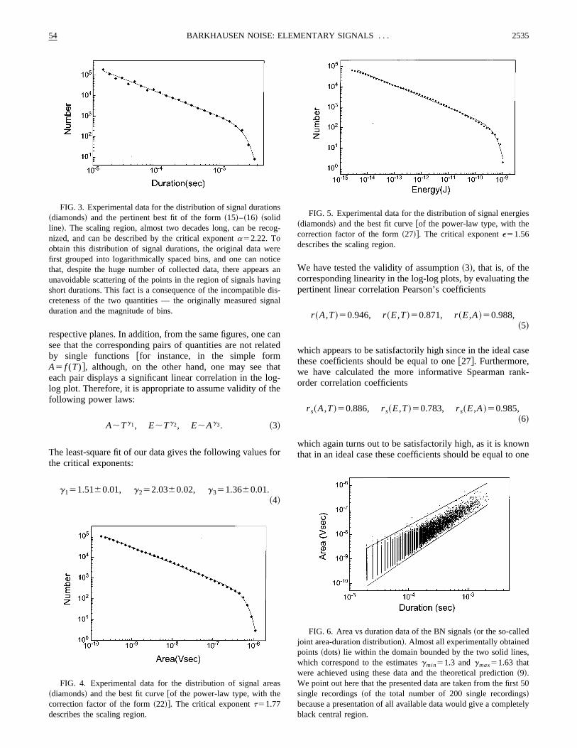
FIG. 3. Experimental data for the distribution of signal durations~diamonds! and the pertinent best fit of the form ~15!–~16! ~solidline!. The scaling region, almost two decades long, can be recog-nized, and can be described by the critical exponent a52.22. Toobtain this distribution of signal durations, the original data werefirst grouped into logarithmically spaced bins, and one can noticethat, despite the huge number of collected data, there appears anunavoidable scattering of the points in the region of signals havingshort durations. This fact is a consequence of the incompatible dis-creteness of the two quantities — the originally measured signalduration and the magnitude of bins.

FIG. 4. Experimental data for the distribution of signal areas~diamonds! and the best fit curve @of the power-law type, with thecorrection factor of the form ~22!#. The critical exponent t51.77describes the scaling region.

FIG. 5. Experimental data for the distribution of signal energies~diamonds! and the best fit curve @of the power-law type, with thecorrection factor of the form ~27!#. The critical exponent e51.56describes the scaling region.

FIG. 6. Area vs duration data of the BN signals ~or the so-calledjoint area-duration distribution!. Almost all experimentally obtainedpoints ~dots! lie within the domain bounded by the two solid lines,which correspond to the estimates gmin51.3 and gmax51.63 thatwere achieved using these data and the theoretical prediction ~9!.We point out here that the presented data are taken from the first 50single recordings ~of the total number of 200 single recordings!because a presentation of all available data would give a completelyblack central region.


@27#. Thus, we may conclude that results ~5! and ~6! of bothtests confirm that our experimental data do satisfy the powerlaws ~3!.

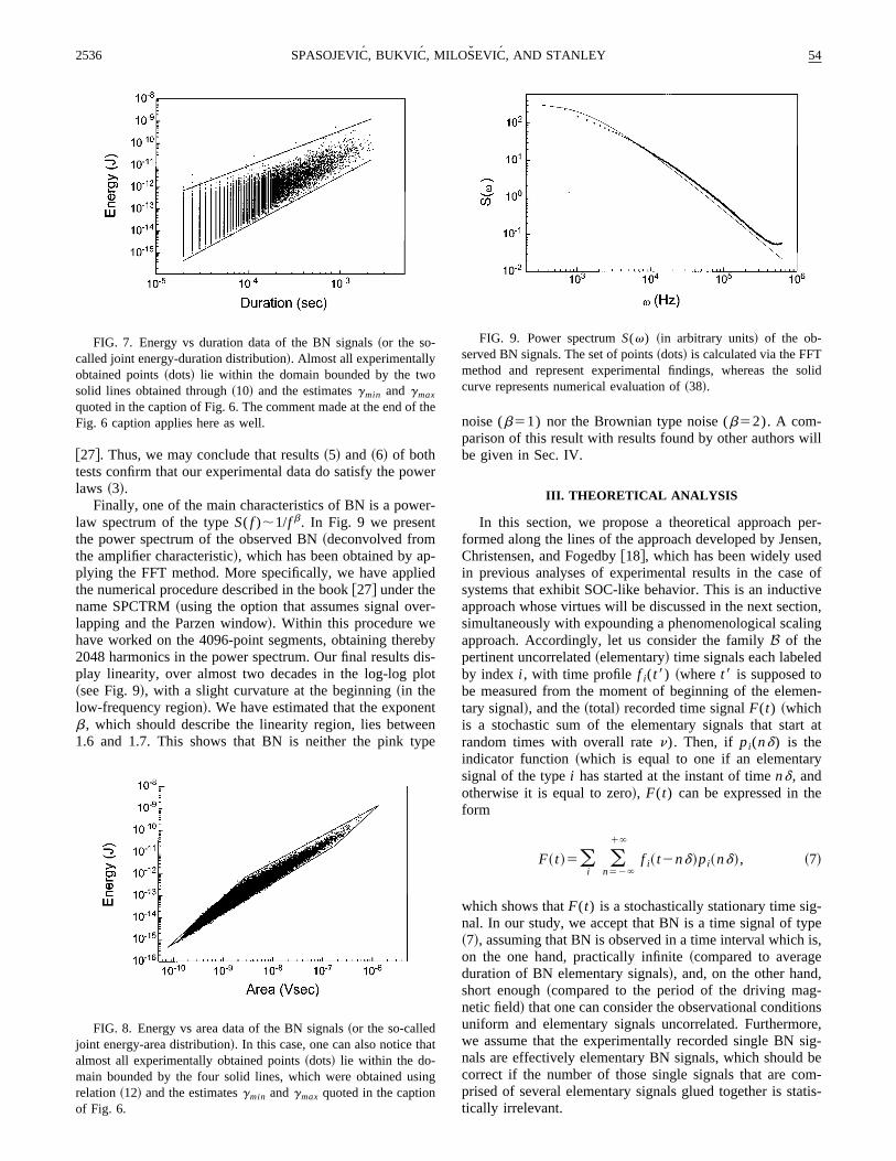
Finally, one of the main characteristics of BN is a power-law spectrum of the type S( f );1/f b. In Fig. 9 we presentthe power spectrum of the observed BN ~deconvolved fromthe amplifier characteristic!, which has been obtained by ap-plying the FFT method. More specifically, we have appliedthe numerical procedure described in the book @27# under thename SPCTRM ~using the option that assumes signal over-lapping and the Parzen window!. Within this procedure wehave worked on the 4096-point segments, obtaining thereby2048 harmonics in the power spectrum. Our final results dis-play linearity, over almost two decades in the log-log plot~see Fig. 9!, with a slight curvature at the beginning ~in thelow-frequency region!. We have estimated that the exponentb , which should describe the linearity region, lies between1.6 and 1.7. This shows that BN is neither the pink type

noise (b51) nor the Brownian type noise (b52). A com-parison of this result with results found by other authors willbe given in Sec. IV.

III. THEORETICAL ANALYSIS

In this section, we propose a theoretical approach per-formed along the lines of the approach developed by Jensen,Christensen, and Fogedby @18#, which has been widely usedin previous analyses of experimental results in the case ofsystems that exhibit SOC-like behavior. This is an inductiveapproach whose virtues will be discussed in the next section,simultaneously with expounding a phenomenological scalingapproach. Accordingly, let us consider the family B of thepertinent uncorrelated ~elementary! time signals each labeledby index i , with time profile f i(t8) ~where t8 is supposed tobe measured from the moment of beginning of the elemen-tary signal!, and the ~total! recorded time signal F(t) ~whichis a stochastic sum of the elementary signals that start atrandom times with overall rate n). Then, if p i(nd) is theindicator function ~which is equal to one if an elementarysignal of the type i has started at the instant of time nd , andotherwise it is equal to zero!, F(t) can be expressed in theform

F~ t !5(i

(n52`

1`

f i~ t2nd !p i~nd !, ~7!

which shows that F(t) is a stochastically stationary time sig-nal. In our study, we accept that BN is a time signal of type~7!, assuming that BN is observed in a time interval which is,on the one hand, practically infinite ~compared to averageduration of BN elementary signals!, and, on the other hand,short enough ~compared to the period of the driving mag-netic field! that one can consider the observational conditionsuniform and elementary signals uncorrelated. Furthermore,we assume that the experimentally recorded single BN sig-nals are effectively elementary BN signals, which should becorrect if the number of those single signals that are com-prised of several elementary signals glued together is statis-tically irrelevant.

FIG. 7. Energy vs duration data of the BN signals ~or the so-called joint energy-duration distribution!. Almost all experimentallyobtained points ~dots! lie within the domain bounded by the twosolid lines obtained through ~10! and the estimates gmin and gmaxquoted in the caption of Fig. 6. The comment made at the end of theFig. 6 caption applies here as well.

FIG. 8. Energy vs area data of the BN signals ~or the so-calledjoint energy-area distribution!. In this case, one can also notice thatalmost all experimentally obtained points ~dots! lie within the do-main bounded by the four solid lines, which were obtained usingrelation ~12! and the estimates gmin and gmax quoted in the captionof Fig. 6.

FIG. 9. Power spectrum S(v) ~in arbitrary units! of the ob-served BN signals. The set of points ~dots! is calculated via the FFTmethod and represent experimental findings, whereas the solidcurve represents numerical evaluation of ~38!.


Power-law behavior related to the time signal F(t) of thetype ~7! depends on the characteristics of the distribution ofelementary signals. It may happen that there exists someprominent subfamily of elementary signals ~having specificshape! such that it has a dominant statistical weight in thedistribution of elementary signals. In such a case, performingstatistical analysis, one can neglect the presence of elemen-tary signals which do not belong to the subfamily and try torelate the properties of the time signal F(t) to the specificshape of the subfamily elementary signals. A visual inspec-tion of the typical train of elementary signals @see Fig. 2~a!#can hardly detect existence of a subfamily of specific signals.However, a more elaborate numerical investigation of theavailable experimental data can demonstrate that a subfamilyin fact exists. To this end, one should first rescale eachBNES f i(t8) ~by appropriate dilation, or contraction, of itsduration time and voltage amplitude! so that the rescaledsignal f i8(t8) acquires unit duration and area, which eventu-ally makes signals’ shapes suitable for mutual comparison.Then, one should perform a straightforward averaging of therescaled signals within its own set, so that the value f a(t8) ofthe function obtained in this way, at the moment t8, is theaverage of f i8(t8).

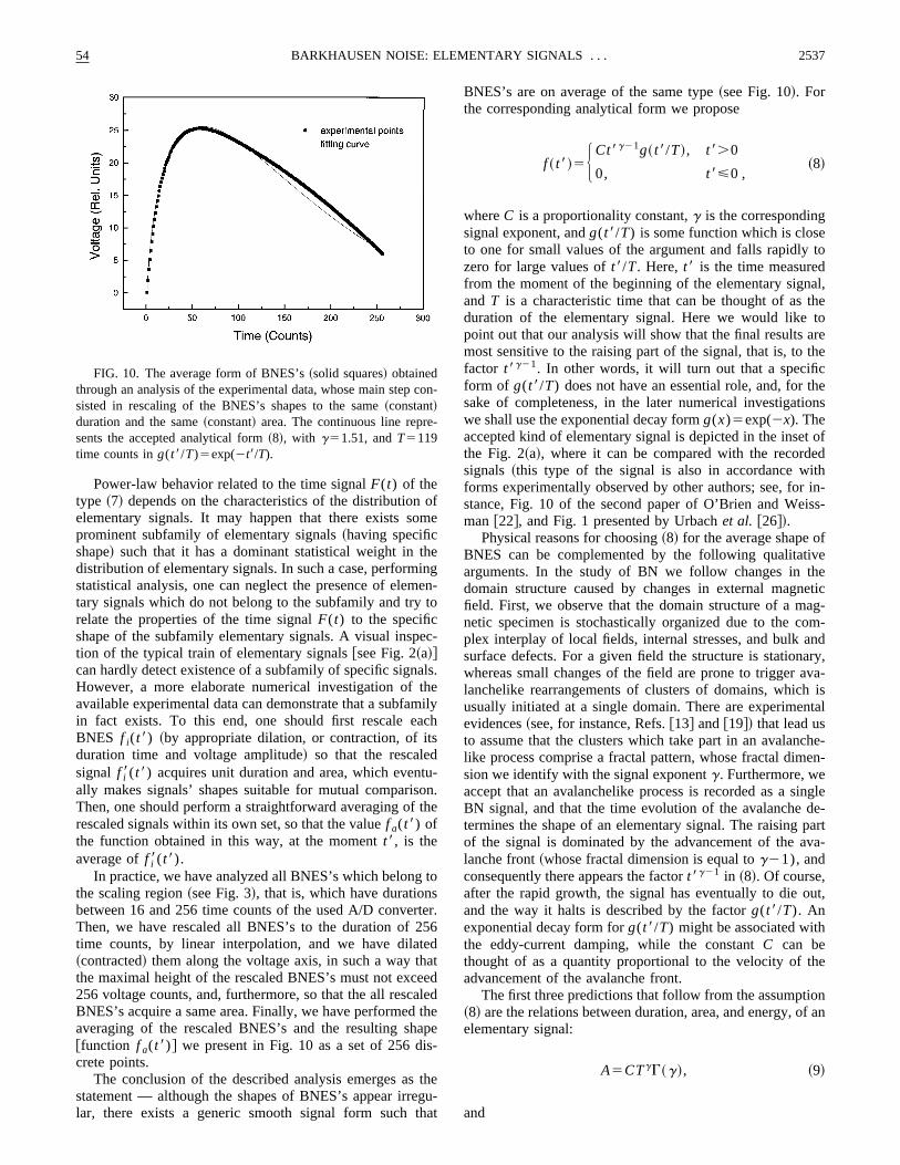
In practice, we have analyzed all BNES’s which belong tothe scaling region ~see Fig. 3!, that is, which have durationsbetween 16 and 256 time counts of the used A/D converter.Then, we have rescaled all BNES’s to the duration of 256time counts, by linear interpolation, and we have dilated~contracted! them along the voltage axis, in such a way thatthe maximal height of the rescaled BNES’s must not exceed256 voltage counts, and, furthermore, so that the all rescaledBNES’s acquire a same area. Finally, we have performed theaveraging of the rescaled BNES’s and the resulting shape@function f a(t8)# we present in Fig. 10 as a set of 256 dis-crete points.

The conclusion of the described analysis emerges as thestatement — although the shapes of BNES’s appear irregu-lar, there exists a generic smooth signal form such that

BNES’s are on average of the same type ~see Fig. 10!. Forthe corresponding analytical form we propose

f ~ t8!5HCt8g21g~ t8/T !, t8.0

0, t8<0 ,~8!

where C is a proportionality constant, g is the correspondingsignal exponent, and g(t8/T) is some function which is closeto one for small values of the argument and falls rapidly tozero for large values of t8/T . Here, t8 is the time measuredfrom the moment of the beginning of the elementary signal,and T is a characteristic time that can be thought of as theduration of the elementary signal. Here we would like topoint out that our analysis will show that the final results aremost sensitive to the raising part of the signal, that is, to thefactor t8g21. In other words, it will turn out that a specificform of g(t8/T) does not have an essential role, and, for thesake of completeness, in the later numerical investigationswe shall use the exponential decay form g(x)5exp(2x). Theaccepted kind of elementary signal is depicted in the inset ofthe Fig. 2~a!, where it can be compared with the recordedsignals ~this type of the signal is also in accordance withforms experimentally observed by other authors; see, for in-stance, Fig. 10 of the second paper of O’Brien and Weiss-man @22#, and Fig. 1 presented by Urbach et al. @26#!.

Physical reasons for choosing ~8! for the average shape ofBNES can be complemented by the following qualitativearguments. In the study of BN we follow changes in thedomain structure caused by changes in external magneticfield. First, we observe that the domain structure of a mag-netic specimen is stochastically organized due to the com-plex interplay of local fields, internal stresses, and bulk andsurface defects. For a given field the structure is stationary,whereas small changes of the field are prone to trigger ava-lanchelike rearrangements of clusters of domains, which isusually initiated at a single domain. There are experimentalevidences ~see, for instance, Refs. @13# and @19#! that lead usto assume that the clusters which take part in an avalanche-like process comprise a fractal pattern, whose fractal dimen-sion we identify with the signal exponent g . Furthermore, weaccept that an avalanchelike process is recorded as a singleBN signal, and that the time evolution of the avalanche de-termines the shape of an elementary signal. The raising partof the signal is dominated by the advancement of the ava-lanche front ~whose fractal dimension is equal to g21), andconsequently there appears the factor t8g21 in ~8!. Of course,after the rapid growth, the signal has eventually to die out,and the way it halts is described by the factor g(t8/T). Anexponential decay form for g(t8/T) might be associated withthe eddy-current damping, while the constant C can bethought of as a quantity proportional to the velocity of theadvancement of the avalanche front.

The first three predictions that follow from the assumption~8! are the relations between duration, area, and energy, of anelementary signal:

A5CTgG~g !, ~9!

and

FIG. 10. The average form of BNES’s ~solid squares! obtainedthrough an analysis of the experimental data, whose main step con-sisted in rescaling of the BNES’s shapes to the same ~constant!duration and the same ~constant! area. The continuous line repre-sents the accepted analytical form ~8!, with g51.51, and T5119time counts in g(t8/T)5exp(2t8/T).


E5C2S T2 D 2g21

G~2g21 !, ~10!

where

G~g !5E0

`

xg21g~x !dx , ~11!

which, for the specific form g(x)5exp(2x) is in fact thestandard gamma function. Then, eliminating duration T from~9! and ~10!, one obtains the relation

E5

C1/gG~2g21 !

@2gG~g !#221/g A221/g, ~12!

between the energy and the area of an elementary signal.Once derived, the relation ~9! may be considered as the de-fining relation the for signal exponent g of BNES, providingthat the constant C is known @see Eq. ~13!#. Thus, the signalexponent g can be conceived as a quantity which discrimi-nates between the possible shapes of BNES’s, and in whatfollows we accept such an attitude.

Analyzing our experimental findings, we came to the con-clusion that the BN signal duration T and the signal exponentdimension g should be considered as the two stochasticquantities, and we denote their joint distribution byP(g ,T). By inspection of Figs. 6–8, one may also concludethat the distribution P(g)5*P(g ,T)dT should be rathernarrow, ranging between some lower limit gmin and upperlimit gmax . Using the data for the joint distribution of theBN signal area A and duration T ~see Fig. 6!, we have esti-mated these two limits and the constant C of ~8!:

gmin51.3060.03, gmax51.6360.03,

C50.00460.001. ~13!

Thus, one may conclude that the BN signals should be dis-tributed, with respect to their area and duration, between thetwo boundaries depicted in Fig. 6, which are obtained bysubstituting the values of C , gmin ~for upper border line! andgmax ~for lower border line! into ~9!. Furthermore, using~10!, ~12!, and ~13!, we have obtained, in the same manner,the boundaries depicted in Fig. 7 and Fig. 8 for the energy-duration and energy-area joint distributions of the BN sig-nals, respectively. The achieved rather precise prediction forboundaries of the energy-duration and energy-area distribu-tions of BN signals ~obtained through quantities estimatedfrom the area-duration distribution! serves as a confirmationof validity of the assumed form ~8! for an elementary signal.

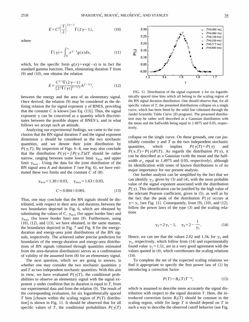
The next question, which we are going to answer, iswhether one may consider the two stochastic quantities gand T as two independent stochastic quantities. With this aimin view, we have evaluated P(guT), the conditional prob-abilities to observe an elementary signal with the signal ex-ponent g under condition that its duration is equal to T , fromour experimental data and from the relation ~9!. The result ofthe corresponding evaluation, for six logarithmically spacedT bins @chosen within the scaling region of P(T) distribu-tion# is shown in Fig. 11. It should be observed that for allspecific values of T , the conditional probabilities P(guT)

collapse on the single curve. On these grounds, one can jus-tifiably consider g and T as the two independent stochasticquantities, which implies P(guT)5P(g) andP(g ,T)5P(g)P(T). As regards the distribution P(g), itcan be described as a Gaussian ~with the mean and the half-width sg equal to 1.4975 and 0.05, respectively!, althoughits identification with some of known distributions is of nomajor importance for our present analysis.

Our further analysis can be simplified by the fact that wecan identify g1, given by ~3! and ~4!, with the most probablevalue of the signal exponent associated with the distributionP(g). This identification can be justified by the high value ofthe relevant Pearson coefficient, given in ~5!, as well as bythe fact that the peak of the distribution P(g) occurs atg5g1 ~see Fig. 11!. Consequently, from ~9!, ~10!, and ~12!,follow the power laws of the type ~3! and the scaling rela-tions

g252g121, g3522

1

g1. ~14!

Hence, we can see that the values 2.02 and 1.34, for g2 andg3, respectively, which follow from ~14! and experimentallyfound value g151.51, are in a very good agreement with thevalues quoted in ~4!, which corroborates the scaling relations~14!.

To complete the set of the expected scaling relations wefind it appropriate to specify the first power law of ~1! byintroducing a correction factor

P~T !5B t~T !T2a, ~15!

which is assumed to describe more accurately the signal dis-tribution with respect to the signal duration T . Here, the in-troduced correction factor B t(T) should be constant in thescaling region, while for large T it should depend on T insuch a way to describe the observed cutoff behavior ~see Fig.

FIG. 11. Distribution of the signal exponent g for six logarith-mically spaced time bins which all belong to the scaling region ofthe BN signal duration distribution. One should observe that, for allspecific values of T , the presented distributions collapse on a singlecurve, which has been fitted by the solid line ~obtained through theJandel Scientific Table Curve 2D program!. The presented distribu-tion may be rather well described as a Gaussian distribution withthe mean and the halfwidth being equal to 1.4975 and 0.05, respec-tively.


3!. We are going to use the following phenomenologicalstretched-exponential form for the correction factor:

B t~T !5B0texp@2~T/Tc!1/s t# , ~16!

where B0t is a constant, Tc is a characteristic cutoff time, ands t is the corresponding exponent. The stretched-exponentialform ~16! has been used in a similar content in the work @24#,and its relevance to the phenomenon studied has been arguedalso by Alessandro et al. @7#. To assert values of the con-stants in ~16!, we have minimized x2 of our experimentaldata and the form ~15! performing the Nelder-Mead downhillsimplex method in multidimensions ~see Ref. @27# and theprogram Amoeba given therein!. Here we remind the readerthat we have grouped our data into logarithmically spacedbins, so that the number N(T0) of single BN signals in a bincentered at T0 is given by

N~T0!'NET0 /l

T0l

P~T !dT , ~17!

where N is the total number of signals, while l is the bin size.Hence, we have obtained the critical exponent a52.22 @see~2!#, and the correction factor parameters

Tc5~2.460.2!1023 sec, s t50.2860.08, ~18!

where the quoted errors were estimated via 100 Monte Carlosimulations with the confidence level being equal to 0.68@27#. In Fig. 3 we present the curve of the form ~15!–~16!,with Tc and s t given by ~18! and with a52.22 andB0t50.4760.07, and one can see that this curve fits the ex-perimental data in a very satisfactory way. However, wewould like to point out that the values ~18! were extractedfrom the distribution tail, that is, for signals of long durationswhose statistics is relatively meager, and, for this reason, onecould expect a deviation from ~18! in a experiment with alarger statistics. Similarly, it should be emphasized that theform ~16! cannot stay valid in the entire region pertaining tosignals of short durations ~in our case, for T,1025 sec!, sothat an experiment performed in such a region would requirea different correction factor.

The foregoing discussion of the duration distributionpower law, ~15! and ~16!, together with the specific assump-tion ~8! about the elementary BN signal shape, implies adefinite form for the area distribution P(A). To find it, westart with the following equality

P~Aug !dA5P~Tug !dT , ~19!

which relates the conditional probabilities P(Aug) andP(Tug)5P(T) to observe a BN signal of area A and dura-tion T ~with a proviso that the signal exponent is g),whereby one can derive the expression

P~Aug !5

1

gB tF S A

CG~g !D 1/gG

3@CG~g !#~a21 !/gA2@11 ~a21 !/g#. ~20!

Next, taking into account that P(A)5*P(Aug)P(g)dg , andsince the distribution P(g) is narrow ~see Fig. 11!, one mayconjecture that P(A) is approximately given by the right

hand side of ~20! with g being replaced by g1. Performingthis replacement, one can recognize that ~20! is, in fact, ofthe form ~15!, with

t511

a21

g1, ~21!

and

Ba~A !5B0aexp@2~A/Ac!1/sa# , ~22!

where B0a5(B0t /g1)@CG(g1)#(a21)/g1 and

Ac5CG~g1!Tcg1, sa5g1s t. ~23!

Inserting the best fit parameters for the duration distribution(a , Tc , s t , and B0t) in ~21! and ~23! one finds t51.81,B0a50.0144, Ac57.731027 Vsec, and sa50.42, whereasthe best fit of the experimental data gives, respectively,t51.7760.09 @see ~2!# and

B0a50.014160.003, Ac5~6.162 !31027 V sec,

sa50.4360.1, ~24!

which has been obtained following the same numerical pro-cedure @27# applied in the case of the duration distribution.

In a similar way, one can obtain the scaling relation

e511

a21

2g121, ~25!

for the critical exponent e of the energy distribution of theBN signal, as well as the scaling relation

e511

~t21 !~a21 !

2a2t21, ~26!

that follows by eliminating g1 from ~21! and ~25!. Insertingthe experimental findings for a and g1 in ~25!, we obtaine51.61, which is in a good agreement with the valuee51.56 found experimentally @see ~2!#. Applying the sameapproach that led us to the formula ~22!, we obtain for theenergy distribution the form of the correction factor

Be~E !5B0eexp@2~E/Ec!1/se# , ~27!

where

B0e5@B0t212a/~2g121 !#@C2G~2g121 !#~a21 !/~2g121 !

and

Ec5C2G~2g121 !~Tc/2!2g121, se5~2g121 !s t.~28!

Inserting the best fit parameters for the duration distributionin ~28! one finds B0e50.004,Ec54.0310210 J, andse50.56, whereas the best fit of the experimental data gives,respectively,

B0e5~4.360.6!31023, Ec5~462 !310210 J,

se50.660.2, ~29!


which has been obtained following again the same numericalprocedure @27# applied in the case of the duration distribu-tion.

In the final part of this section, we would like to expoundon our theoretical predictions about the power spectrum ofthe BN signal. Thus, we start with the autocorrelation func-tion CF(t0) of the total signal F(t)

CF~ t0!5^F~ t !F~ t1t0!&5nE dgE dTP~g ,T !Cg ,T~ t0!,

~30!

where

Cg ,T~ t0!5E2`

1`

f g ,T~ t8! f g ,T~ t81t0!dt8, ~31!

which is the autocorrelation function of the elementary sig-nal f g ,T . Therefore, the power spectrum S(v) of the totalsignal F(t), as a function of the angular frequencyv52p f , is

S~v !5E2`

1`

CF~ t0!e2ivt0dt05n^Sg ,T~v !&

5nE dgE dTP~g ,T !u f g ,T~v !u2. ~32!

Here, Sg ,T(v) is the power spectrum of the elementary sig-nal f g ,T(t8),

Sg ,T~v !5u f g ,T~v !u2, ~33!

and f g ,T(v) is the Fourier transform of the elementary signal

f g ,T~v !5E2`

1`

f g ,T~ t8!e2ivt8dt8, ~34!

which for the exponentially decaying elementary signal fac-tor g(x)5exp(2x) has the specific form @28#

f g ,T~v !5

CTgG~g !

@11~vT !2#g/2 exp@2igarctan~vT !# . ~35!

Hence, using our assumption ~8!, related to the shape of el-ementary signals, we obtain

f g ,T~v !5

f g , v/v0 T~v0!

S v

v0D g , f g ,T~v !5S TT0D

g

f g ,T0S TT0 v D ,~36!

where we have introduced new time and frequency unitsT0 and v0, respectively. Using the latter forms and ~15! in~32! one can obtain

S~v !5nE dgP~g !E dT

B tS T

~v/v0!DT2aU f g ,T0S TT0 v0D U2

S v

v0D 2g2a11 S TT0D

2g

5nE dgP~g !E dS TT0DT012aS TT0D2g2a B tS ~T/T0!

~v/v0!T0D

S v

v0D 2g2a11 U f g ,T0S TT0 v0D U2. ~37!

If we now define dimensionless quantities T5T/T0 andv5v/v0, we finally obtain our general expression for thepower spectrum

S~v !5nT012aE dg

P~g !

v2g2a11E dTB t

3S TvT0D T2g2au f g ,T0

~ Tv0!u2. ~38!

One might conclude from ~38! that the power spectrumexponent b satisfies the scaling relation

b52g12a11, ~39!

providing one assumes that P(g) can be approximated bythe delta function d(g2g1) and that the integral over T in~38! is, for high frequencies v , approximately a constant.

However, inserting data from ~2! and ~4! in ~39! one findsthat b51.80, which deviates from the experimentally ob-tained value b51.621.7. Therefore, in order to check thevalidity of the expression ~38!, we have evaluated S(v)~with the time unit T0 and the frequency unit v0 chosen so asto achieve stability in the corresponding numerical calcula-tions! using ~38! and approximating P(g) with the best fit tothe Gaussian form. Results of this calculation are presentedin Fig. 9 as a continuous line, whereby we have found thecorresponding power-law exponent b51.6760.01. The lat-ter value is in accord with experimental finding for b anddeviates from the value b51.80 which followed from thescaling relation ~39!. The deviation can be now attributed tothe assumptions that have brought about ~39!. Hence, it ap-pears that the integral over T in ~38! is weakly dependent onv and g . Besides, the second source of difference betweenthe two values for b ~1.67 vs 1.80! springs from the finitewidth of the P(g) distribution. Indeed, if we take P(g) to be


of a Gaussian type ~instead of being a delta function!, andperform the requisite lengthy calculation, we get a negativecorrection term on the right hand side of ~39!, so that insteadof g1 there appears g12sg

2 lnv. In other words, g1 gets thelogarithmic correction term, and if we take sg50.05 and, forinstance, v5105, we get b51.74, which is closer to theexperimental finding b51.621.7.

IV. DISCUSSION

In this work we have performed extensive measurements,with reliably large statistics, of the Barkhausen noise ~BN! inthe case of a commercial VITROVAC 6025-X metal glasssample. We have demonstrated that the BN phenomenon canbe described by well defined critical exponents ~see, for in-stance, Figs. 3–5! which satisfy a set of scaling relations.The observed power laws for the quantities T ,A ,E , and fortheir joint distributions, may be interpreted as a manifesta-tion of the vicinity to some critical point ~see, for instance,@23#!. Although our findings may not be sufficient to eithervalidate existence of the critical point, or to locate it in termsof some relevant parameters, nevertheless the establishedpower-law behaviors, the set of scaling relations ~being sat-isfied with our experimental findings!, and the data collaps-ing of the type presented in Fig. 11, make us wonderwhether, in the BN case, there exists also a generalized ho-mogeneous function ~GHF! with a concomitant data collaps-ing ~in an analogy with the standard critical phenomena@29#!. Here we argue, and provide evidences, that the prob-ability distribution of BNES’s is a GHF. With this goal inmind, we first introduce the scaling Sb ~for b.0), within theset B of all possible BNES’s, such that when it is applied tothe i BNES of the shape f i(t8) it gives the Sbi BNES of theshape

f Sbi~ t8!5bx f i~ t8by!, ~40!

where b is the scaling parameter, while x and y are thescaling exponents. Next, we put forward the following scal-ing hypothesis — if p(i ,l) denotes the probability density toobserve the i BNES when the system is at the ‘‘distance’’l from the critical point, then for some specific exponents(x ,y) @see Eq. ~40!# there exist additional exponents z andw0 such that

dp~Sbi ,bzl !5bw0dp~ i ,l !, ~41!

which is, in fact, the GHF statement.To acquire possibility to verify experimentally the above

GHF statement, we introduce the probability densityP(T ,A ,E ,l) of obtaining BNES’s with given T , A , E , andl via

dP~T ,A ,E ,l !5P~T ,A ,E ,l !dTdAdE5EG

dp~ i ,l !,

~42!

where G is the set of all BNES’s having T , A , and E withinthe limits T,T(i),T1dT , A,A(i),A1dA , andE,E(i),E1dE . Accordingly, one may prove that theprobability density P(T ,A ,E ,l) is the generalized homoge-neous function

P~b2yT ,bx2yA ,b2x2yE ,bzl !5bwP~T ,A ,E ,l !, ~43!

where

w5w023~x2y !, ~44!

which, with z5z/y and w5w/y , and with the another scal-ing parameter c5b2y, can be rewritten in a more convenientform,

P~cT ,caAA ,caEE ,call !5caPP~T ,A ,E ,l !, ~45!

where

aA512 x , aE5122 x , al52 z , aP52w .~46!

To prove ~43!, we start with the auxiliary relations be-tween the duration T , area A , energy E , and Fourier trans-form f (v) of the original i BNES and the scaled Sbi BNES,

T~Sbi !5b2yT~ i !, ~47a!

A~Sbi !5bx2yA~ i !, ~47b!

E~Sbi !5b2x2yE~ i !, ~47c!

f Sbi~v !5bx2y f i~vb2y!, ~47d!

which can be verified in few steps. Indeed, to obtain ~47a!,one has to notice that the duration T of BNES is defined byT5t l2t f , where t f and t l are the first and the last moments,respectively, of the time interval when BNES is above thediscrimination level bd . Besides, one has to keep in mindthat T displays only minor changes if the discriminationlevel bd is changed. Thus, one can make the choicebd5b l1ddb

x ~see Sec. II B!, in the case of the scaled SbiBNES, and thereby one obtains ~47a!. In order to obtain~47b!–~47d!, one has to perform the change of the variablet→t85byt in the integrals which appear in definitions ofA , E , and f (v), given in Sec. III. Next, we return to theproof of ~43!, and to this end we write

P~b2yT ,bx2yA ,b2x2yE ,bzl !

5

dP~b2yT ,bx2yA ,b2x2yE ,bzl !

d~b2yT !d~bx2yA !d~b2x2yE !5

*G8dp~ i ,bzl !

b3~x2y !dTdAdE,

~48!

where Sb image of G is the set G8 of all BNES’s having T ,A , and E within the limits b2yT,T(i),b2y(T1dT), bx2yA,A(i),bx2y(A1dA), and b2x2yE,E(i),b2x2y(E1dE). Then, using ~41! and the relation

EG8

dp~ i ,bzl !5EG

dp~Sbi ,bzl !

dp~ i ,l !dp~ i ,l !5bw0E

G

dp~ i ,l !,

~49!

one obtains ~43!.In what follows we are going to demonstrate that the

power laws ~1! for the P(T), P(A), and P(E) distributions,


and all scaling relations of Sec. III, can be obtained from~43! if one chooses the scaling exponents aA , aE , al , andaP in the following way:

aP52

eat122e2a2t

~12t !~12e !, aA5

12a

12t, aE5

12a

12e,

al51/sT, ~50!

where a , t , and e are the scaling exponents of ~1! and sT isthe exponent of ~16!. Indeed, for the duration distributionP(T) we have

P~T !5E dAE dEP~T ,A ,E ,l !

5TaP1aA1aEE dS ATaAD E dS ETaED PS 1, ATaA, ETaE, l

TalD ,

~51!

whereby one can see that P(T) exhibits a power-law behav-ior, with the correction term ~given by the integral of the lastrelation! and with the scaling exponent a given by

a52~aP1aA1aE!. ~52!

In a similar way, one can show that the distributions P(A)and P(E) obey power-law behavior as well, with the expo-nents t and e given by

t52

aP1aE11

aA, e52

aP1aA11

aE. ~53!

Finally, starting with Eqs. ~52! and ~53!, one can obtain thefirst three relations of ~50!. As regards the correction term ofthe power law ~16!, one may conjecture that the fourth rela-tion of ~50! stays valid and that the cutoff parameter Tc of~16! might serve as the parameter l which measures distancefrom the critical point ~at which the system should exhibitthe pure power laws, with the cutoffs removed!. As to thestretched-exponential form ~16! for the correction term, wecan say that this form ~being specific! does not follow fromthe general scaling hypothesis ~41!.

The power laws of the form ~3! also follow from thescaling hypothesis ~41! with the identification

g15aA , g25aE , g35aE /aA, ~54!

between the set of experimental exponents g1, g2, and g3and the set of theoretical exponents aA and aE , which can beverified by recalling that the average area ^A&T of theBNES’s, of the duration T , satisfies

^A&T5

*dA*dEP~T ,A ,E ,l !A

*dA*dEP~T ,A ,E ,l !

5TaA*dv2v2*dv3P~1,v2 ,v3 ,l/T

al!

*dv2*dv3P~1,v2 ,v3 ,l/Tal!

, ~55!

whereby the first equality of ~54! follows. The remaining twoequalities of ~54! follow in analogous way. Then, combiningthe first two relations of ~46!, the second and the third rela-

tion of ~50!, and ~54!, we retrieve the scaling relations ~14!,~21!, and ~25!. In a similar way one may also derive relations~23! and ~28!, with the remark that Ac and Ec might also playthe role of the parameter l .

To make the present derivation of the scaling relationscomplete, we are going to rederive the scaling relation ~39!,which relates the exponent g1 and the duration exponent awith the exponent b of the power spectrum. To this end, westart with

S~v !5nE dp~ i ,l !u f i~v !u2

5nE dTE dAE dEP~T ,A ,E ,l !*Gdp~ i ,l !u f i~v !u2

*Gdp~ i ,l !,

~56!

and use ~43!, together with

EG

dp~ i ,l !5ESb21~SbG!

dp„i ,~b21!zl8…

5EG8

dp„Sb21i8,~b21!zl8…

dp~ i8,l8!dp~ i8,l8!

5b2w0EG8

dp~Sbi ,bzl !, ~57!

where l85bzl and i85Sbi , and

EG

dp~ i ,l !u f i~v !u2

5b2~y2x !2w0EG8

dp~Sbi ,bzl !u f Sbi~b

yv !u2, ~58!

to obtain

S~v !5nb2~y2x !2wE dTE dA

3E dEP~b2yT ,bx2yA ,b2x2yE ,bzl !

3

*G8dp~Sbi ,b

zl !u f Sbi~byv !u2

*G8dp~Sbi ,b

zl !, ~59!

which for b5v21/y, and with the rescaled variablesv15vT , v25vg1A , and v35vg2, becomes

S~v !5nv2~2g12a11 !E dv1E dv2

3E dv3P~v1 ,v2 ,v3 ,vzl8!

3

*G8~ i8,v zl8!u f i8~1 !u2

*G8~ i8,v zl8!

. ~60!

Hence, we can see that ~39! can be obtained also within theGHF approach.


Having verified that the scaling relations obtained in theSec. III follow also from the GHF hypothesis ~41!, we aregoing to show that this hypothesis, as could have been ex-pected, implies data collapsing in the case of the probabilitydistribution functions. Indeed, performing suitable integra-tion of the distribution P(T ,A ,E ,l) and with a change ofvariables one can find

P~A ,T !Ta1g15w1~A/Tg1!5E dv3PS 1, ATg1

,v3 ,l

TalD ,~61!

P~E ,T !Ta1g25w2~E/Tg2!5E dv2PS 1,v2 ,

E

Tg2,

l

TalD ,~62!

P~E ,A !At1g35w3~E/Ag3!5E dv1PS v1,1,

E

Ag3,

l

Aal /g1D ,~63!

which are correct for a fixed l , and may be correct also inthe case of a weak dependence on l .

The first approach one might have in mind in order tocheck whether our experimental data collapse in accordancewith the above relations is to study the quantityN l(A0 ,T0)T0

t1g1, where N l(A0 ,T0)5N*dT*dAP(A ,T) isthe number of elementary signals which belong to a linearbin centered at the values A0 and T0. Such a procedure is,however, inconvenient since the relevant distributions are ofa power-law type, so that all data practically lie in the firstlinear bin. Therefore, in order to group experimental data ina suitable form, one has to separate data in the logarithmi-cally spaced bins, that is, to integrate NP(A ,T)Ta1g1 withinthe limits A0 /dA,A,A0dA and T0 /dT,T,T0dT , wheredA and dT determine the size of a logarithmic bin. In such away one obtains the following data-collapsing relations:

N~A ,T !Ta215f1~A/T

g1!, ~64!

N~E ,T !Ta215f2~E/T

g2!, ~65!

N~E ,A !At215f3~E/A

g3!, ~66!

where, for instance,

f1~A0 /T0g1!5E

A0 /T0dA

A0dA/T0dvw1~v !. ~67!

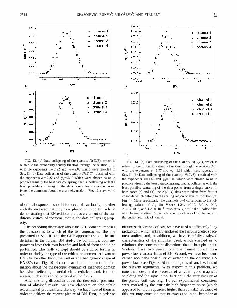
In Figs. 12–14 we present our experimental data scaled ac-cording to the relations ~64!–~66!, respectively. In each casethe data have been taken from four different ‘‘channels,’’that is, from four different families of logarithmic bins de-fined by four corresponding values of T0 and A0, which be-long to the pertinent power-law regions of Figs. 3 and 4. Itfollows that the degree of data collapsing depends on thechoice of values for the critical exponents. Thus, one couldargue that the choice of the critical exponents values whichproduces the best data collapsing is the most proper choicefor the problem under study. Furthermore, one could claimthat such a choice is, in fact, the best way to evaluate criticalexponents. However, such a procedure of obtaining criticalexponents involves a very intricate numerical calculations

which definitely increases uncertainty of final results. Forinstance, in the present case, according to the foregoing pro-cedure @whose final results are depicted in Figs. 12~b!, 13~b!,and 14~b!#, we have found the following set: a52.22,g151.55, g252.15, g351.46, and t51.68 ~in which onlythe critical exponent a coincides with the straightforwardmeasurement, whereas the rest are somewhat changed!. Thisset of exponents, unfortunately, does not satisfy the scalingrelations to the same degree which was observed in the caseof critical exponents derived directly from the joint distribu-tions. The discrepancy may be ascribed to the accumulatednumerical error during the course of determination of datathat were finally scaled, as well as to the possibility that theentire experiment was not performed close enough to theassumed critical point ~which could have brought about in-accurate critical exponents!. In short, the above set of values

FIG. 12. ~a! Data collapsing of the quantity N(A ,T), which isrelated to the probability density function through the relation ~64!,with the exponents a52.22 and g151.51 which were reported inSec. II. ~b! Data collapsing of the quantity N(A ,T), obtained withthe exponents a52.22 and g151.55 which were chosen so as toproduce visually the best data collapsing, that is, collapsing with theleast possible scattering of the data points from a single curve. Inboth cases ~a! and ~b!, the N(A ,T) data were taken from four Tchannels which belong to the scaling region of duration distribution~cf. Fig. 3!. More specifically, the channels 1–4 correspond to thefollowing values of T0 ~in secs! 9.723 1025, 1.593 1024,2.613 1024, and 7.033 1024, respectively, while the ‘‘halfwidth’’of a channel is dT51.28, which reflects a choice of 14 channels onthe entire duration axis of Fig. 3.


of critical exponents should be accepted cautiously, togetherwith the message that they have played an important role indemonstrating that BN exhibits the basic element of the tra-ditional critical phenomena, that is, the data collapsing prop-erty.

The preceding discussion about the GHF concept imposesthe question as to which of the two approaches ~the onepresented in Sec. III and the GHF approach! should be un-dertaken in the further BN study. To our minds, both ap-proaches have their own benefits and both of them should beperformed. The GHF concept should be studied further inorder to clarify the type of the critical phenomena relevant toBN. On the other hand, the well established generic shape ofBNES’s ~see Fig. 10! should bear definite amount of infor-mation about the mesoscopic dynamic of magnetic domainbehavior ~reflecting material characteristics!, and, for thisreason, it deserves to be pursued in the future.

After the long discussion about the theoretical presenta-tion of obtained results, we now elaborate on few subtleexperimental problems and the way we have treated them inorder to achieve the correct picture of BN. First, in order to

minimize distortions of BN, we have used a sufficiently longpickup coil which entirely enclosed the ferromagnetic speci-men studied, and, in addition, we have carefully analyzedcharacteristics of the amplifier used, which enabled us toeliminate the concomitant distortions that it brought about.Without these two precautions one cannot obtain clearpower-law characteristics of BN. Second, we have been con-cerned about the possibility of extending the observed BNpower laws ~see Figs. 3–5! in the regions of small values ofthe relevant arguments. With respect to this problem, wenote that, despite the presence of a rather good magneticshielding and the signal amplification in the very vicinity ofthe pickup coil ~see Fig. 1!, our experimental conditionswere marked by the extrinsic high-frequency noise ~whichappeared for the frequencies higher than 50 kHz!. Because ofthis, we may conclude that to assess the initial behavior of

FIG. 13. ~a! Data collapsing of the quantity N(E ,T), which isrelated to the probability density function through the relation ~65!,with the exponents a52.22 and g252.03 which were reported inSec. II. ~b! Data collapsing of the quantity N(E ,T), obtained withthe exponents a52.22 and g252.15 which were chosen so as toproduce visually the best data collapsing, that is, collapsing with theleast possible scattering of the data points from a single curve.Here, the comment about the channels, made in Fig. 12, stays validtoo.

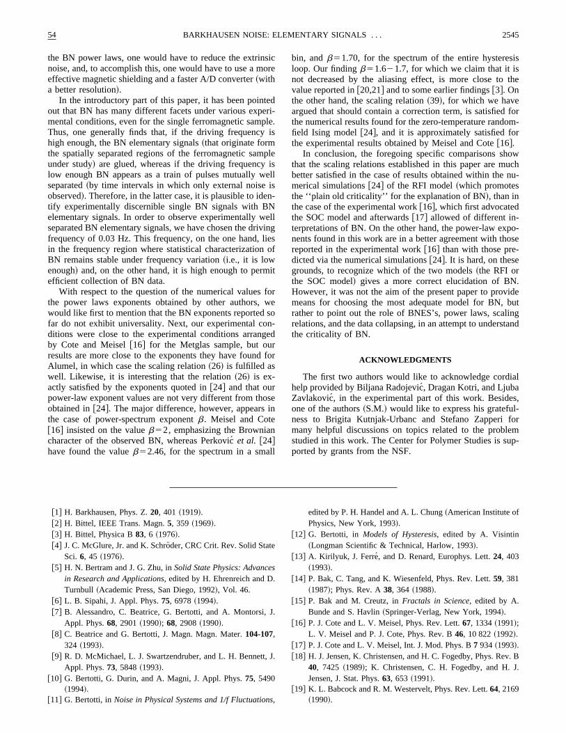
FIG. 14. ~a! Data collapsing of the quantity N(E ,A), which isrelated to the probability density function through the relation ~66!,with the exponents t51.77 and g351.36 which were reported inSec. II. ~b! Data collapsing of the quantity N(E ,A), obtained withthe exponents t51.68 and g351.46 which were chosen so as toproduce visually the best data collapsing, that is, collapsing with theleast possible scattering of the data points from a single curve. Inboth cases ~a! and ~b!, the N(E ,A) data were taken from four Achannels which belong to the scaling region of area distribution ~cf.Fig. 4!. More specifically, the channels 1–4 correspond to the fol-lowing values of A0 ~in V sec! 1.243 1029, 3.013 1029,7.303 1029, and 4.293 1028, respectively, while the ‘‘halfwidth’’of a channel is dA51.56, which reflects a choice of 14 channels onthe entire area axis of Fig. 4.


the BN power laws, one would have to reduce the extrinsicnoise, and, to accomplish this, one would have to use a moreeffective magnetic shielding and a faster A/D converter ~witha better resolution!.

In the introductory part of this paper, it has been pointedout that BN has many different facets under various experi-mental conditions, even for the single ferromagnetic sample.Thus, one generally finds that, if the driving frequency ishigh enough, the BN elementary signals ~that originate formthe spatially separated regions of the ferromagnetic sampleunder study! are glued, whereas if the driving frequency islow enough BN appears as a train of pulses mutually wellseparated ~by time intervals in which only external noise isobserved!. Therefore, in the latter case, it is plausible to iden-tify experimentally discernible single BN signals with BNelementary signals. In order to observe experimentally wellseparated BN elementary signals, we have chosen the drivingfrequency of 0.03 Hz. This frequency, on the one hand, liesin the frequency region where statistical characterization ofBN remains stable under frequency variation ~i.e., it is lowenough! and, on the other hand, it is high enough to permitefficient collection of BN data.

With respect to the question of the numerical values forthe power laws exponents obtained by other authors, wewould like first to mention that the BN exponents reported sofar do not exhibit universality. Next, our experimental con-ditions were close to the experimental conditions arrangedby Cote and Meisel @16# for the Metglas sample, but ourresults are more close to the exponents they have found forAlumel, in which case the scaling relation ~26! is fulfilled aswell. Likewise, it is interesting that the relation ~26! is ex-actly satisfied by the exponents quoted in @24# and that ourpower-law exponent values are not very different from thoseobtained in @24#. The major difference, however, appears inthe case of power-spectrum exponent b . Meisel and Cote@16# insisted on the value b52, emphasizing the Browniancharacter of the observed BN, whereas Perkovic et al. @24#have found the value b52.46, for the spectrum in a small

bin, and b51.70, for the spectrum of the entire hysteresisloop. Our finding b51.621.7, for which we claim that it isnot decreased by the aliasing effect, is more close to thevalue reported in @20,21# and to some earlier findings @3#. Onthe other hand, the scaling relation ~39!, for which we haveargued that should contain a correction term, is satisfied forthe numerical results found for the zero-temperature random-field Ising model @24#, and it is approximately satisfied forthe experimental results obtained by Meisel and Cote @16#.

In conclusion, the foregoing specific comparisons showthat the scaling relations established in this paper are muchbetter satisfied in the case of results obtained within the nu-merical simulations @24# of the RFI model ~which promotesthe ‘‘plain old criticality’’ for the explanation of BN!, than inthe case of the experimental work @16#, which first advocatedthe SOC model and afterwards @17# allowed of different in-terpretations of BN. On the other hand, the power-law expo-nents found in this work are in a better agreement with thosereported in the experimental work @16# than with those pre-dicted via the numerical simulations @24#. It is hard, on thesegrounds, to recognize which of the two models ~the RFI orthe SOC model! gives a more correct elucidation of BN.However, it was not the aim of the present paper to providemeans for choosing the most adequate model for BN, butrather to point out the role of BNES’s, power laws, scalingrelations, and the data collapsing, in an attempt to understandthe criticality of BN.

ACKNOWLEDGMENTS

The first two authors would like to acknowledge cordialhelp provided by Biljana Radojevic, Dragan Kotri, and LjubaZavlakovic, in the experimental part of this work. Besides,one of the authors ~S.M.! would like to express his grateful-ness to Brigita Kutnjak-Urbanc and Stefano Zapperi formany helpful discussions on topics related to the problemstudied in this work. The Center for Polymer Studies is sup-ported by grants from the NSF.

@1# H. Barkhausen, Phys. Z. 20, 401 ~1919!.@2# H. Bittel, IEEE Trans. Magn. 5, 359 ~1969!.@3# H. Bittel, Physica B 83, 6 ~1976!.@4# J. C. McGlure, Jr. and K. Schroder, CRC Crit. Rev. Solid State

Sci. 6, 45 ~1976!.@5# H. N. Bertram and J. G. Zhu, in Solid State Physics: Advances

in Research and Applications, edited by H. Ehrenreich and D.Turnbull ~Academic Press, San Diego, 1992!, Vol. 46.

@6# L. B. Sipahi, J. Appl. Phys. 75, 6978 ~1994!.@7# B. Alessandro, C. Beatrice, G. Bertotti, and A. Montorsi, J.

Appl. Phys. 68, 2901 ~1990!; 68, 2908 ~1990!.@8# C. Beatrice and G. Bertotti, J. Magn. Magn. Mater. 104-107,

324 ~1993!.@9# R. D. McMichael, L. J. Swartzendruber, and L. H. Bennett, J.

Appl. Phys. 73, 5848 ~1993!.@10# G. Bertotti, G. Durin, and A. Magni, J. Appl. Phys. 75, 5490

~1994!.@11# G. Bertotti, in Noise in Physical Systems and 1/f Fluctuations,

edited by P. H. Handel and A. L. Chung ~American Institute ofPhysics, New York, 1993!.

@12# G. Bertotti, in Models of Hysteresis, edited by A. Visintin~Longman Scientific & Technical, Harlow, 1993!.

@13# A. Kirilyuk, J. Ferre, and D. Renard, Europhys. Lett. 24, 403~1993!.

@14# P. Bak, C. Tang, and K. Wiesenfeld, Phys. Rev. Lett. 59, 381~1987!; Phys. Rev. A 38, 364 ~1988!.

@15# P. Bak and M. Creutz, in Fractals in Science, edited by A.Bunde and S. Havlin ~Springer-Verlag, New York, 1994!.

@16# P. J. Cote and L. V. Meisel, Phys. Rev. Lett. 67, 1334 ~1991!;L. V. Meisel and P. J. Cote, Phys. Rev. B 46, 10 822 ~1992!.

@17# P. J. Cote and L. V. Meisel, Int. J. Mod. Phys. B 7 934 ~1993!.@18# H. J. Jensen, K. Christensen, and H. C. Fogedby, Phys. Rev. B

40, 7425 ~1989!; K. Christensen, C. H. Fogedby, and H. J.Jensen, J. Stat. Phys. 63, 653 ~1991!.

@19# K. L. Babcock and R. M. Westervelt, Phys. Rev. Lett. 64, 2169~1990!.


@20# O. Geoffroy and J. L. Portseil, J. Magn. Magn. Mater. 97, 198~1991!; 97, 205 ~1991!.

@21# O. Geoffroy and J. L. Portseil, J. Magn. Magn. Mater. 133, 1~1994!.

@22# K. P. O’Brien and M. B. Weissman, Phys. Rev. A 46 R4475~1992!; Phys. Rev. E 50, 3446 ~1994!.

@23# J. P. Sethna, K. Dahmen, S. Kartha, J. A. Krumhansl, B. W.Roberts, and J. D. Shore, Phys. Rev. Lett. 70, 3347 ~1993!; K.Dahmen and J. P. Sethna, ibid. 71, 3222 ~1993!; K. Dahmen,S. Kartha, J. A. Krumhansl, B. W. Roberts, J. P. Sethna, and J.D. Shore, J. Appl. Phys. 75, 5946 ~1994!.

@24# O. Perkovic, K. Dahmen, and J. P. Sethna, Phys. Rev. Lett. 75,

4528 ~1995!.@25# K. Dahmen and J. P. Sethna, Phys. Rev. B 53, 14 872 ~1996!.@26# J. S. Urbach, R. C. Madison, and J. T. Markert, Phys. Rev.

Lett. 75, 276 ~1995!.@27# W. H. Press, B. P. Flannery, S.A. Teukolsky, and W. T. Vet-

terling, Numerical Recipes ~Cambridge University Press, Cam-bridge, 1990!.

@28# A. P. Prudnikov, Yu. A. Brychkov, and O. I. Marychev, Inte-grals and Series ~Nauka, Moscow, 1981! ~in Russian!.

@29# H. Eugene Stanley, Introduction to Phase Transitions andCritical Phenomena ~Clarendon Press, Oxford, 1971!.


Barkhausen Noise: Elementary Signals, Power Laws, and Scaling Relations

Documents

Transcript of Barkhausen Noise: Elementary Signals, Power Laws, and Scaling Relations