BANKING PRODUCTIVITY ANDECONOMIC FLUCTUATIONS: Colombia

1998-2000.

Andres F. Arias1

University of California, Los Angeles

September, 2001

1This paper is ongoing research for my dissertation at UCLA. I want to thank myadvisor Lee Ohanian and also Costas Azariadis and Gary Hansen for their valuable helpand support. I also thank all the participants at the macro proseminars at UCLA fortheir comments and feedback. Special thanks to Rocio Mora at Banco de la Republicain Colombia for kindly providing the data. All errors are my own.

Abstract

I build a general equilibrium, Þnancial accelerator model that incorporates anexplicit technology for the intermediary sector. A credit multiplier emerges be-cause of a borrowing constraint that is a function of asset prices, internal fundsand lending rates. With this Þnancial friction I show that small changes in theproductivity and intermediation costs of banks generate large and persistent ßuc-tuations in economic activity. The transmission channel relies on the role thatassets and internal funds play as collateral. After a negative shock hits Þnancialintermediation productivity, the resulting credit crunch and economic slowdowninduce a fall in asset prices and internal fund accumulation. This further modiÞesthe present and future volume of collateral, thereby amplifying and propagatingthe initial shock. I argue that changes in banking regulation in Colombia in thelate 1990s increased intermediation costs, reduced banking productivity and in-duced a credit channel story that Þts the theoretical model presented here. Thisnew regulation enhanced the credit crunch and economic slowdown that was al-ready underway. Colombian data on loan/deposit interest rate spreads, creditvolume, asset prices and economic activity support this argument.

Keywords: Financial accelerator, banking productivity, intermediation costs,borrowing limit, credit crunch, ampliÞcation, propagation.

JEL: E32, E42, E44, G21.

1. INTRODUCTION

During the last three and a half years the economic performance of Colombia hasbeen disastrous. The unemployment rate has ßuctuated around 18% in the sevenmost important cities (and above 15% overall). The average growth rate for theyears 1998,1999 and 2000 was negative. In addition, an asset price plunge beganin late 1997. This situation contrasts with the early nineties when Colombia grewat rates exceeding 4% and was catalogued as one of the top emerging marketsin the world. This economic downturn has been accompanied by a severe crisisin the Þnancial sector that began in late1997 or early 1998 [See Arias (2000)].Since then, real credit has suffered a severe crunch. Between January of 1998 andJanuary of 2001 the stock of real credit fell 30%. Between July of 1999 and Mayof 2000 more than 30% of the Þnancial systems stock of assets was capitalized bythe government.1 Many other Þnancial intermediary institutions failed and wereliquidated or bailed-out by the government. The Þscal cost of the bail out hasbeen estimated at 6% of GDP.23

In order to alleviate the Þnancial distress and to Þnance the bail-out, theColombian government issued new banking regulation towards the end of 1998.4

For instance, whenever the outstanding value of a home mortgage debt exceededthe market value of the home, debtors were given the right to repay completely thedebt by giving back their home to the Þnancial institution that issued the credit.The Þnancial institution receiving the home was given the right to a loan from thegovernment equivalent to the value of the corresponding loss. The loan is to berepaid at six month intervals during a ten year period at an interest rate equal toforecasted inßation by the central bank plus Þve percentage points.5 Additionally,an upper bound of 1.5 times the current bank interest rate was imposed on unpaidhome mortgage credits.6 The new regulation also prohibited banks from translat-ing home mortgage repayment request expenditures to individual debtors.7 Oneof the most controversial regulatory changes was a new tax on Þnancial transac-

1Source: Banco de la Republica, Subgerencia de Estudios Economicos. See Arias (2000).2Source: Foresight Colombia, July 4, 2000.3The banking crisis in Colombia was parallel to a currency crisis. In 1999 the exchange rate

regime (a target zone) collapsed and the exchange rate was allowed to ßoat freely.4Decree 2331, of November 16,1998. The new regulation can be consulted in:

http://juriscol.banrep.gov.co:8080/cgi/normas_buscar.pl5Article 14 of Decree 2331.6Article 15 of Decree 2331.7Article 16 of Decree 2331.

tions aimed at Þnancing the bail-out and capitalization of troubled institutions.Indeed, as of November 17, 1998 most Þnancial transactions were to be taxed ata 2 per 1000 rate.8 This rate was later risen to 3 per 1000.The purpose of all this new regulation was to aid a troubled Þnancial system.

Whether this was accomplished has not yet been determined. What is clear isthat the spread between the loan and deposit interest rates in Colombia system-atically rose to higher levels in 1999, just after the new banking regulation andÞnancial transaction tax was introduced. It is argued in this paper that this hikein the loan-deposit interest rate spread reßects a rise in intermediation costs andÞnancial inefficiency attributable to the new banking regulation. In other words,the new regulation and the 2/1000 Þnancial transaction tax tightened banking op-erational constraints and introduced additional costs into Þnancial intermediationactivity. Consequently, Þnancial intermediaries suffered a productivity meltdownas they lost operational versatility and additional real resources were required tooperate with and implement the new regulations and tax.9 As a result, Þnancialintermediaries had to charge a higher loan-deposit interest rate spread in equilib-rium, as observed in the data. While aimed at alleviating Þnancial distress, thenew regulation actually reduced the productivity of Þnancial intermediaries andincreased intermediation costs.This negative productivity shock to Þnancial institutions exacerbated the credit

crunch and corresponding economic contraction that was already underway. Butthis did not occur in a linear fashion. Interestingly, it seems that the Nov./1998shock was signiÞcantly ampliÞed and propagated into the future. Indeed, the datashow that after 1998 the economic contraction has been longer lived and morepersistent than most previous downward economic ßuctuations in Colombia. Thispaper pursues the idea that due to the new banking regulation of Nov./1998 and toborrowing constraints attributable to the credit crunch that was already underway,what otherwise would have been a regular and short-lived economic contractionbecame the biggest economic downfall of recent Colombian history.I suggest a general equilibrium model capable of replicating recent macroeco-8Articles 29 and 30 of Decree 2331.9In addition to the new banking regulation of Nov. 1998, between 1996 and 1999 new

regulation was also passed in Colombia ordering bankers to verify that deposits beyond a certainvolume did not come from illicit activities [Articles 102-107 from the Organic Statute of theFinancial System; Law 365 of 1997, articles 9,24 and 25; Law 526 of 1999, article11]. In carryingout this police work, Colombian bankers have to spend additional time and resources beforethey can accept and intermediate a deposit. This can be interpreted as an additional negativeproductivity shock to the Colombian Þnancial system.

nomic regularities in Colombia. The model shows how a negative productivityshock to Þnancial intermediaries, interpreted as a perverse regulatory change forthe Þnancial system, is ampliÞed and propagated in macro aggregates due to creditconstraints. On an empirical level the contribution of the paper is a qualitativeand quantitative approximation to the recent macroeconomic behavior of Colom-bia, in the light of its new banking regulation. In fact, it can be claimed that thepunchline of the paper is that the qualitative and quantitative predictions of themodel are in line with the recent behavior of macroeconomic variables in Colom-bia if it is accepted that the new banking regulation of Nov/1998 was a negativeproductivity shock to its Þnancial system. Nonetheless, the model applies to anyother episode where the banking sector experiences a productivity shock. Thus,on a theoretical level the contribution of the paper is important for evaluating thewelfare impact of regulatory changes and policies that modify the productivity ofbanks in environments with Þnancial frictions.The paper is organized as follows. The next section brießy relates the paper

to the existing literature. Section three presents the empirical facts regardingthe macroeconomic behavior of Colombia before and after the new banking reg-ulation of Nov/1998. In section four I argue that this new regulation induced arise in intermediation costs and a corresponding slump of banking productivityin Colombia. Section Þve suggests a theoretical model that rationalizes how anegative productivity shock to the Þnancial system can account for the observedmacroeconomic behavior in Colombia during the period 1998-2000. In section sixI use the model to implement a numerical experiment that simulates the responseof the artiÞcial economy to an adverse productivity shock in the Þnancial system.The idea there is to replicate qualitatively, and to some extent quantitatively, themacroeconomic behavior of Colombia after the Nov/1998 regulation and the as-sociated negative productivity shock to Þnancial intermediation. The last sectionconcludes.

2. LINKS TO THE LITERATURE

Links between banking productivity and regulation in the Þnancial arena havebeen established in the literature. The idea is that with the tightening of reg-ulatory constraints, banks tend to loose versatility in their operations and, con-sequently, experience a fall in productivity. On the other hand, a deregulatoryprocess increases competitive forces in the Þnancial system so that banks notallocating their resources efficiently would perish unless they could become more

like their efficient competitors by producing more output with existing inputs.[Semenick (2001), pp. 122].Berg, Forsund and Jansen (1992) Þnd a productivity fall in Norwegian banks

prior to the deregulation of the Norwegian Þnancial system in the 1980s. Theyalso document a fast productivity increase in the post-deregulation years up to1989. Their results indicate that the observed productivity gains were mainly dueto the convergence of inefficient banks towards the production possibilities frontierrather than a shift of the frontier itself. Berg et. al. (1993) expanded the study toFinland and Sweden. Zaim (1995) documents similar results for Turkish banks.Bhattacharya, Lovell and Sahay (1997) Þnd that the impact of liberalization onthe productivity of Indian banks depends on the type of ownership. Gilbert andWilson (1998) argue that privatization of Korean Þnancial institutions, rather thanderegulation of deposit interest rates, induced an increase in banking productivity.Leightner and Lovell (1998) Þnd that the average bank in Thailand experiencedrapid total factor productivity growth between 1989 and 1994, as the Þnancialand foreign exchange systems of this country were liberalized. Khumbakar et. al(2001) study Spanish savings banks between 1986 and 1995, a period during whichthe Spanish banking industry went through major regulatory reforms. They Þndhigh levels of technical inefficiency but high rates of productivity growth due tofrontier shifts attributable to the deregulatory process.In a recent paper Semenick (2001) computes the Malmquist index of U.S. com-

mercial banks with more than US$ 500 million in assets for the period 1980-1989.10

He divides his sample into those banks that are allowed statewide branching,those with limited branching and those constrained to unit branching. He Þndsthat during the 1980s the three groups of banks exhibit cumulated productivitygrowth rates of 4.6%, 3.2% and -0.3%, respectively. In short, his results indicatethat banks facing tighter branching constraints exhibit less productivity growththan those facing looser branching regulation. Humphrey (1991) studies the re-lationship between deregulation and banking productivity in the US during the1980s. He Þnds that between 1977 and 1987 productivity growth of U.S. banksranges between -0.07% and 0.6% per year. He attributes this variation to thederegulation of the 1980s. Other studies that Þnd positive productivity growth10The Malmquist index is computed with data envelopment analysis. The latter is a lin-

ear programming methodology that constructs a non-parametric, piecewise-linear, best practicefrontier from observable input and output data [Semenick (2001), pp. 122]. The index de-composes productivity ßuctuations into two elements: i) expansion of the frontier (technologicalchange) and ii) convergence towards the frontier (efficiency change or catching up).

in U.S. banks during the 1980s (the decade of Þnancial deregulation) are Hunterand Timme (1991) and Bauer, Berger and Humphrey (1993). Tirtiroglu, Danielsand Tirtiroglu (1998) look at a longer time period,1946 -1995, and document anegative overall impact of regulation over U.S. commercial banking TFP growth.In contrast, some studies have found negative or zero productivity growth rates

in the U.S. during the 1980s, the era of deregulation. Elyasiani and Mehdian(1995) Þnd a productivity regress in U.S. banks between 1979 and 1986, the preand post deregulation years. Humphrey and Pulley (1997) average data between1977 and 1988 and also Þnd productivity regress in U.S. banks during the 1980s.Note that these results contradict the expected mapping between deregulation andproductivity growth. However, by studying only two spaced years or by averagingout data these authors could have overlooked major productivity ßuctuations inU.S. banks during the years in between [see Semenick 2001]. These Þndings couldalso indicate that banks face difficulties in their adjustment towards the increasedcompetition and freedom created by deregulation [Khumbakar et. al. (2001)].Other studies that document zero or negative productivity growth rates in U.S.banks during the 1980s are: Berger and Humphrey (1992), Humphrey (1993),Bauer, Berger and Humphrey (1993) and Wheelock and Wilson (1999).11 Inany case, all the substantial empirical evidence documenting some link betweenproductivity of Þnancial intermediaries and regulatory changes in the bankingarena motivates and is relevant to the idea behind this paper.An environment that articulates some sort of credit channel seems the appro-

priate theoretical structure to study the recent Colombian case given the ongoingcredit crunch and contraction of the Colombian economy at the time the newbanking regulation was issued. Studies using Þnancial accelerator models andcredit channel stories have already shown that conditions and frictions in Þnan-cial markets play a key role in explaining an economys reaction to exogenousmacroeconomic shocks.12 These types of models can be classiÞed in two cate-11Very good surveys of all these studies can be found in Khumbakar et. al (2001) and Semenick

(2001).12A Þnancial accelerator is a self-feeding, internal Þnance mechanism that propagates and

ampliÞes shocks. Usually, in this literature the Þrms ability to Þnance its production plan is anincreasing function of the value of its assets. When the value of these assets increases (eitherbecause the price of assets increases or because the Þrm reinvests more proÞts), the Þrm is ableto expand its production plan (either because some external Þnance premium falls or becauseborrowing limits become less stringent). A higher level of production and investment increasesasset demand (and asset prices) and/or earnings (and reinvestment of proÞts), thus increasingeven further the value of the Þrms assets and its ability to expand its production plan. And so

gories: i) agency cost models13 and ii) borrowing limit models14. Unfortunately,the role of productivity ßuctuations in the Þnancial sector has been overlooked bythese studies. The reason is that existing Þnancial accelerator or credit channelmodels lack an appropriate representation of the banking technologies throughwhich resources are intermediated. Indeed, most of these models treat Þnancialintermediation as a costless, invisible and intangible activity. This basically boilsdown to assuming that the Þnancial intermediary is simply an additional con-straint in the economy [Chari, Jones and Manuelli. (1995)].15

The model suggested in this paper blends the Þnancial regulation - bankingproductivity empirical link and the Þnancial accelerator literature in an attemptto replicate the recent macroeconomic behavior in Colombia. It builds upon theborrowing limit-Þnancial accelerator idea by using an environment similar to theone suggested by Kocherlakota (2000). A different feature is that banks operatewith a costly intermediation technology. For every unit of deposits they accept, afraction is lost in the intermediation process. This intermediation cost creates aspread between the deposit and lending rates. It also determines the productivityof intermediation. Naturally, a lower cost implies a higher productivity.The model economy is populated by many households. Each one has access

to a technology that needs land, internal funds and external funds (from banks)to operate. To avoid the risk of default banks impose a credit constraint on thehousehold: it cannot borrow beyond the value of its collateralizable resources(value of landholdings plus internal funds). This credit constraint pushes up thevalue of land. Whenever the borrowing constraint binds, land will be valued notonly because of its direct contribution to output (as an input of production), butalso because it contributes indirectly to output through the role that it playsas collateral. Accumulating an additional unit of land increases the households

on. The Þnancial accelerator mechanism is at work. It is the basic source of propagation andampliÞcation of shocks.13e.g.: Bernanke and Gertler (1989), Bernanke and Gertler (1990), Carlstrom and Fuerst

(1997), Bernanke, Gertler and Gilchrist (1999).14e.g.: Scheinkman andWeiss (1986), Kiyotaki and Moore (1997), Cooley and Quadrini (1999),

Cooley, Marimon and Quadrini (2000), Schneider and Tornell (2000), Kocherlakota (2000),Caballero and Krishnamurthy (2000), Aghion, Bacchetta and Banerjee (2000a, 2000b), Mendoza(2001).15Models with costly intermediation technologies have been used elsewhere in the literature

for banks to play a non-trivial macroeconomic role [Edwards and Vegh (1997) pp. 246; see alsoKing and Plosser (1984), Diaz-Gimenez et. al. (1993) and Cole and Ohanian (2000)]. But thisliterature assumes that the Þnancial system is frictionless and, hence, Þnancial intermediationactivities have a negligible macroeconomic effect.

future volume of collateral. More collateral tomorrow increases the future avail-ability of external funds, thereby expanding future output indirectly. This featureof the asset is not present in the Kocherlakota (2000) model either.The punchline of the theoretical model suggested here is a credit channel that

ampliÞes and propagates small, transitory shocks to banking productivity. In fact,small changes in the productivity of the intermediation technology generate largeand persistent ßuctuations in economic activity. The credit channel arises becauseborrowing constraints that depend on asset prices, internal funds and lending ratesinduce static and dynamic credit multipliers a-la Kiyotaki and Moore (1997).The transmission mechanism is triggered by a rise in lending rates that tightensborrowing constraints on impact. The credit crunch is magniÞed and propagatedby the fall in asset prices and internal fund accumulation that accompanies thelower level of economic activity and that further tightens the credit limit on impactand in the future.

3. COLOMBIA 1998-2000

Figures 1-5 present the evolution of the following macroeconomic variables inColombia16: i) real GDP cycle (1977:I-2000:III), ii) stock prices in real terms(1991:01-2001:01), iii) gross and net of non-performing loans stock of real credit(1992:01-2001:06), iv) ex-post real loan rate (1990:01-2000:02) and v) loan/depositinterest rate spread (1986:01-2000:12). When Þnancial distress erupted in Colom-bia (end of 1997, beginning of 1998) its GDP entered into a cyclical contraction,asset prices plunged, real credit was crunched and the real loan rate increasedsigniÞcantly. As is well documented by the empirical literature [see Caprio andKlingebiel (1996), Demirguc-Kunt and Detragiache (1997), Kaminsky and Rein-hart (1998, 1999), Kaminsky (1999) and Demirguc-Kunt, Detragiache and Gupta(2000)], this macroeconomic behavior is typical of credit crunch and Þnancial dis-tress episodes. Note also that during the initial phase (or year) of the crisis theloan/deposit interest rate spread did not display any drastic ßuctuation. There isonly an isolated hike in June of 1998.But in 1999, just after the new banking regulation of Nov/1998 was introduced,

the loan/deposit interest rate spread systematically rose to higher levels. For in-stance, the average spread between the nominal annual loan rate and the nominalannual 3-month certiÞcate of deposit rate between Jan/1986 and Dec/1998 was16A detailed description of the data is available in the Data Appendix.

997 basis points. The corresponding average spread for the period Jan/1999-Dec/2000 was 1166 basis points, a 17% increase with respect to the pre-1999average. The average spread for the period Jan/2000-Dec/2000 was 1423 basispoints, a 43% increase with respect to the pre-1999 average.After the regulation was issued, the economic contraction became wider and

longer lived than most other previous downward economic ßuctuations in Colom-bia (and only comparable to the mid-80s recession). Indeed, when the new Þ-nancial transaction tax and banking regulation were implemented in the fourthquarter of 1998, GDP was already 1.8% below trend. By the Þrst and secondquarters of 1999, it declined further to 4.5% and 6.3% below trend, respectively.Moreover, in the following quarters (and until 2000:III) GDP remained between4.7% and 5.5% below its pre-1998:III trend value.In a similar fashion, after the implementation of the banking regulatory changes,

asset prices maintained their downward momentum. In fact, by January of 2001real stock prices had fallen to their 1991 level. This means that between Decemberof 1997 and January of 2001 a 60% fall in real stock prices was observed, with 26of these percentage points being lost after December of 1998 (the date of the newregulation). To put the severity of this crash in perspective, in the U.S. between1929 and 1932 (the Great Depression) the S&P Index fell about 68% in real terms[Cole and Ohanian (2000)]. Another familiar stock market crash episode is thatof Japan in the early nineties when the Nikkei Index fell about 55% in real termsbetween 1989 and 1992 [Cole and Ohanian (2000)].17 The Colombian asset priceplunge exceeds that of Japan and is close to the one experienced during the GreatDepression in the U.S.Additionally, once the new banking regulation was in place real credit was

further crunched in Colombia after a slight recovery in the third quarter of 1998.For instance, comparing the total stock of real credit in January of 2001 withits corresponding value in December of 1997 reveals a 30% fall, with 24 of thesepercentage points being lost after December of 1998 (the date of the new regula-tion). These numbers are higher if non-performing loans are not considered. Therealized real loan interest rate also displayed another peak around the time of thenew regulation. While the average for this rate between Jan/1990 and Dec/1997was 14.68%, by the fourth quarter of 1998 this rate had more than doubled toan average of 33.32%.18 On the eve of the Great Depression the U.S. commer-17There have been stronger stock market crashes. For example, the decline in Thai equity

prices (in dollars) since their 1995 peak exceeds 80% [Kaminsky and Reinhart (1998)].18The corresponding monthly values are 34.62%, 33.08% and 32.26% in October, November

cial paper realized real interest rate rose 70% from 5.6% in the fourth quarter of1927 to 9.5% in the fourth quarter of 1928 [Romer (1993)]. Yet, in Colombia thecorresponding jump was more than 100%.In sum, the macroeconomic effects of the initial credit crunch and the asso-

ciated economic contraction were enhanced dramatically after the new bankingregulation and Þnancial transaction tax were implemented. Were the regulatorychanges responsible for the observed macroeconomic behavior? The next sec-tion tries to answer this question. The underlying idea is that the new bankingregulation and Þnancial transaction tax of November of 1998 constitute a neg-ative productivity shock to Þnancial intermediation that was also ampliÞed andpropagated, turning what otherwise would have been a regular, short lived, eco-nomic contraction into the deepest, downward, economic swing of recent historyin Colombia. Why was this shock ampliÞed and propagated? Section Þve willsuggest a theoretical model with a Þnancial imperfection that may answer thisquestion.

4. BANKING PRODUCTIVITY IN COLOMBIA AFTERTHE NOV/98 REGULATION

To pursue the argument that the regulatory changes of Nov/1998 turned out tobe an adverse productivity shock to the Þnancial system, Þrst consider a bankthat uses a constant returns to scale (crs) technology to intermediate resources.Suppose that the bank accepts deposits at given rate R, uses the intermediationtechnology to provide loans at rate ρ and, for every unit of deposits, loses z ∈ [0, 1)units in the corresponding intermediation process. Under this environment banksbehave competitively and are price takers so that in every period they solve thefollowing static problem:

Maxdt (1 + ρt)(1− zt)dt − (1 +R)dtFree entry and exit drives proÞts to zero and in equilibrium banks produce

where the relative price of their output (1 + ρ) equals their marginal cost:

1 + ρt =1 +R

1− ztor:

and December of 1998, respectively.

1 + ρt1 +R

=1

1− ztIntermediation cost z creates a spread between the lending and deposit rates.

In fact, the spread or ratio between the gross lending rate and the gross depositrate is a metric of the inverse of the average (and marginal) productivity of deposits[1/(1−z)]. The higher the productivity of the Þnancial system, the lower the ratiobetween the gross lending rate and the gross deposit rate and vice-versa. Thisresult is important because it provides a simple way to measure productivitychanges in the Þnancial sector using observed data of the gross lending rate togross deposit rate ratio or spread.Using this result, Þgure 6 measures the inverse productivity of the Þnancial

system in Colombia during the period Jan/1986-Dec/2000. In particular, it showsthe behavior of the ratio between the gross annual nominal loan rate and the grossannual nominal 3-month certiÞcate of deposit rate.19 Note that this ratio displaysa fairly steady pattern until January of 1999. Beginning in January of 1999, lessthan two months after the new banking regulation and Þnancial transaction taxwas introduced, this ratio took a dramatic hike. For instance, between Jan/1986and Dec/1998 the average for this ratio was 1.33. The average for this ratio duringthe period Jan/1999-Dec/2000 was 1.81. This represents a 33.14% increase withrespect to the pre-1999 average. The average for this ratio during the periodJan/2000-Dec./2000 was 2.17. This represents a 63.36% increase with respect tothe pre-1999 average.Assuming the Þnancial structure of the economy is as simple as the one sug-

gested in the previous paragraphs, it is possible to back up the correspondingpercentage change in the productivity of the banking sector (1− z) with the per-centage change in the ratio between the gross loan and deposit interest rates. Lety = (1 + ρ)/(1 +R). Hence:

·y

y= −

·(1− z)(1− z)

19The annual nominal loan rate is tasa activa total sistema (monthly average) calculated bySuperintendencia Bancaria in Colombia. Two different annual nominal deposit rates are used:tasa de interes de los CDT a 90 dias, total sistema (monthly average) and tasa de interes delos CDT a 90 dias, bancos y CF (monthly average). Source is Banco de la Republica. Periodis 1986:01-2000:12. See Data Appendix.

where · symbolizes a derivative with respect to time. As expected, any changein the ratio between the gross loan and deposit interest rates maps back intoan equiproportional opposite sign change in Þnancial intermediation productivity.Thus, the data reveal a drastic negative productivity shock to Þnancial intermedi-aries in Colombia right after the new banking regulation was issued. According tothe data, if the Þnancial system of Colombia were as simple as the one suggestedabove, the banking productivity meltdown following the regulatory changes ofNov/1998 would range from 30% to 60%!This evidence might have some ßaws. First, the Colombian Þnancial system

is far more complex than the one depicted above and the Jan/1999 rise in theloan-deposit interest rate spread might be capturing other phenomena like i) thesudden deterioration of loan quality, ii) an increase of banking risk due to theincrease in macroeconomic instability (i.e. frequent and high swings in the realinterest rate) and the maturity mismatch between deposits and loans and/or iii) anincrease in noncompetitive practices as several banks failed and were removed fromthe market.20 Furthermore, it can be argued that the fact that the jump in thespread coincides with the implementation of the new banking regulation is simply acoincidence. In fact, the three phenomena mentioned above also occurred aroundthe time the new regulation was being implemented. Hence, a very skepticalreader might argue that the behavior of the domestic loan-deposit interest ratespread after Nov/1998 does not necessarily imply, for a more realistic Þnancialsector, that the productivity of Þnancial intermediaries fell back 30%-60% due tothe banking regulation issued in that date.However, three important facts support the claim that there is an element

of response in the Colombian loan-deposit interest rate spread to the regulatorychanges of Nov/1998. First, the new banking regulation of Nov/1998 was a majorchange in the rules of the banking arena game in Colombia. Second, the spreadjump occurs some days after and not days before or at the same time the newregulation was issued. Third, the range of the spread jump (30%-60%) is bigenough so as to allow, among other phenomena, for the presence of a negativeproductivity shock in the Þnancial system of the Colombian economy.20Using panel data techniques and monthly data available for 22 commercial banks for the

period 1992-1996, Steiner, Barajas and Salazar (2000) Þnd that non-Þnancial expenses are astatistically signiÞcant component of the loan-deposit interest rate spread in Colombia andthat, on average, non-Þnancial expenses explain 27.6% of such spread. However, they also Þndthat the rest of the spread is explained by non-performing loans (34.4%), reserve requirements(22.1%) and market power (15.9%).

Figure 7 provides additional evidence that the Jan/1999 loan-deposit interestrate spread jump implies, at least partially, a productivity regress of the Colom-bian Þnancial sector due to the Nov/1998 banking regulation. SpeciÞcally, thispicture shows the quarterly evolution of a proxy for labor productivity in the Þ-nancial sector of the Colombian economy during the period Mar/1992-Dec/2000.The proxy is constructed as the ratio between the stock of real credit (includingnon-performing loans) from the whole Þnancial system and the number of Þnan-cial sector employees in the seven main metropolitan areas.21 In order to obtainlabor productivity proxies for the different types of Þnancial institutions that existin Colombia, the stock of real credit from the whole system is also disaggregatedinto credit from banks, credit from savings and mortgage loan institutions (CAV),credit from Þnancial corporations (CF) and credit from companies of commercialÞnance (CFC).The labor productivity indicator fell 4.59% for the whole system between

Dec/1997 and Dec/1998, the Þrst year of Þnancial distress. This is not surpris-ing. In particular, the labor productivity indicator increased 9.12% for banks andfell 29.16%, 11.93% and 14.35% for CAV, CF and CFC, respectively, during thatÞrst year of crisis. This is not surprising either if one thinks that Þnancial dis-tress erupted more severely in the three latter types of Þnancial institutions thanin banks. Between Dec/1998 and Dec/2000, the period comprising the Þrst twoyears in which the new regulation was in effect, the labor productivity proxy fell18.78% for the whole system. This represents, for each of these two years, a fallin Þnancial intermediation productivity twice as large as the one observed duringthe Þrst year of the crisis. Furthermore, during this period the labor productiv-ity proxy fell 3.79%, 54.83%, 9.28% and 32.96% for banks, CAV, CF and CFC,respectively. It is also worth noting the sharp falls in labor productivity of thewhole system and of banks in the Þrst and fourth quarters of 1999, the Þrst yearduring which the regulation was in place.The story is very simple. When Þnancial distress erupted towards the end

of 1997, labor productivity in the Colombian Þnancial sector began to erode asa whole (4.6%). Even though the labor productivity of banks was still growing,21During credit crunch episodes the level of Þnancial activity is better proxied by the outstand-

ing stock of real credit (including non-performing loans) rather than by the corresponding ßowof new real credit. The reason is that possible disintermedation amid Þnancial distress mightyield negative new credit ßows for some years. Additionally, monitoring clients or dealing withnon-performing loans also represents activity for the banking sector and this is not captured bythe ßow of new loans.

that of the other type of Þnancial institutions was falling sufficiently so as todrive down the whole systems labor productivity level. After the new bankingregulation was in place in December of 1998, labor productivity of all types ofÞnancial institutions began to plunge and continued to do so during the next twoyears. In fact, during this period the system as a whole lost almost an additionalone Þfth (18.8%) of its former labor productivity level. The biggest contribution tothis fall came from savings and mortgage loans institutions. As above, the evidencesuggests that the new banking regulation of Nov/1998 constitutes a visible andsigniÞcant negative productivity shock to Þnancial intermediation in Colombia.In the next section a model capable of rationalizing the empirical facts of

sections two and three is suggested. The ultimate objective is to construct anartiÞcial economy in which to study the effects of a negative banking productivityshock similar to the one observed in Colombia towards the end of 1998, and tocompare the response of this artiÞcial economy to that observed in Colombiaduring the years 1999 and 2000, the post shock/post-regulation years.

5. MODEL

This section suggests a theoretical model that predicts a macroeconomic behaviorsimilar to the one observed in Colombia between the end of 1997 and the endof 2000. Again, the idea is to use this model in order to replicate qualitativelyand quantitatively the response of the main macro aggregates in Colombia to thenegative productivity shock to Þnancial intermediaries in late 1998.

5.1. Basic Assumptions

The economy is inhabited by an inÞnite number of identical, inÞnitely-lived, risk-averse entrepreneurial households. The mass of households has measure 1. Inevery period households have access to a riskless technology that needs land andinternal and external funds as inputs to produce Þnal good as output. The threeinputs are complementary in production. Internal funds and land are accumulatedby the household from one period to the other. External funds are supplied by abanking sector in the form of intraperiod loans at rate ρ. Total land supply is Þxedat 1. Internal funds represent installed physical capital belonging to the householdwhile external funds should be interpreted as working capital provided by Þnancialintermediaries. One possible motivation for this loan-in-the-production functionassumption is that Þrms usually need to pay for some intermediate inputs (or

labor services) in advance of production and must rely on the liquidity providedby banks to do so. Without these liquid external funds Þrms could not operatetheir technologies. In this sense, external funds can be understood as a differentinput of production.Banks operate with a costly, crs, intermediation technology. For every unit

of deposits they accept, a fraction z is lost in the intermediation process. Notethat this cost determines the productivity of intermediation. Of course, a lowercost implies a higher productivity. It is assumed that banks take intraperioddeposits from international Þnancial markets at rate R. This rate is exogenouslydetermined by supply and demand conditions in foreign credit markets.Even though the households technology is riskless (i.e. free of shocks), fund-

ing the household is risky for the bank. In every period the household has theoption of running away with the proceeds from the project (i.e. the technologysoutput) without paying back the loan to the bank. But in doing so the householdmust leave its total assets (i.e. land plus undepreciated internal funds) behind.Moreover, default is not penalized with market exclusion. Banks know of this pos-sibility and so they take care not to let the household borrow more than the valueof its landholdings plus undepreciated internal funds. In other words, to avoid therisk of default banks impose a natural credit constraint on the household. Thehousehold cannot borrow beyond the value of its collateralizable resources (valueof landholdings plus undepreciated internal funds).Note that agents can trade in three markets [relative price of each market

in (·)]: i) Þnal good (1), ii) land (q) and iii) loans (ρ). The order of events inevery period is very simple. When the household wakes up in any given periodit has some internal funds (x) and some landholdings (l). At the same time theproductivity of the banking sector [i.e. its intermediation cost (z)] is revealed.The levels of z and R determine the equilibrium lending rate (ρ) that will becharged by banks for any intraperiod loan. Additionally, the price of land (q) hasbeen simultaneously determined in the land market.Since the marginal cost of a loan (1+ ρ) is known at this point, the household

now determines its optimal demand for external funds or loans (b∗). However,because of the credit constraint, the volume of loans that the household Þnallyreceives (b) need not be equal to the optimal volume (b∗). If the outstanding valueof debt associated to the optimal loan volume (1+ρ)b∗ is less than or equal to thehouseholds total volume of collateralizable resources [ql+ (1− δ)x where δ is thedepreciation rate of internal funds], then the household is not credit constrainedand its demand for loans is satiated completely:

b = b∗ ! ql + (1− δ)x(1 + ρ)

Otherwise, the households credit constraint binds and the volume of externalfunds received is equivalent to:

b =ql + (1− δ)x(1 + ρ)

< b∗

The volume of loans extended to the households determines the volume ofdeposits (d) taken by domestic banks from international Þnancial markets. Withx, l and b the household operates its technology F (x, b, l). After production takesplace, resources available to the household in terms of Þnal good are given byF (x, b, l) + (1 − δ)x + ql. The household allocates these resources to four uses:i) consumption (c), ii) accumulation of internal funds (x"), iii) purchasing of landfor next period (ql") and iv) repayment of the outstanding debt [(1 + ρ)b].Note that it is optimal for the household to repay the loan because the credit

constraint imposed by Þnancial intermediaries is simply an incentive compatibilityconstraint aimed at repayment. Keeping in mind that default is not penalized withmarket exclusion, whenever the household ßees at the end of a period withoutpaying back its debt it receives a payoff equivalent to:

F (x, b, l)

However, if it stays and pays back the loan, it will obtain a payoff equivalentto:

F (x, b, l) + ql + (1− δ)x− (1 + ρ)bIncentive compatibility with repayment requires:

F (x, b, l) ! F (x, b, l) + ql + (1− δ)x− (1 + ρ)bor:

b ! ql + (1− δ)x(1 + ρ)

which is simply the credit constraint imposed by banks on households. Thus, itis always optimal for households to repay any loan extended to them. As in othercredit limit models, borrowing is so tightly constrained by the level of collateralthat default never occurs in equilibrium.

5.2. Households Problem

Formally, the household solves the following sequential problem:

Maxct,bt,xt+1,lt+1 E0∞!t=0

βtU(ct)

s.t.ct + xt+1 + qtlt+1 + (1 + ρt)bt = F (xt, bt, lt) + (1− δ)xt + qtlt

bt(1 + ρt) ! qtlt + (1− δ)xtct, xt, lt " 0qt, ρt given

x0, l0 = 1 given

It is assumed that Fij(x, b, l) = Fji(x, l, b) > 0 # i, j = 1, 2, 3. In other words,land, internal funds and external funds are complementary inputs in the pro-duction technology. The complementarity assumption between land and internalfunds is also used by Kocherlakota (2000). More on this complementarity assump-tion ahead. Note also that if the constraint is binding, any fall in asset (i.e. land)prices, in landholdings or in internal fund volume and any lending rate hike willtighten the constraint.Let λt represent the Kuhn-Tucker multiplier associated to the borrowing con-

straint. λt can be interpreted as the shadow price of collateral. Optimality con-ditions for the household are:

λt =U "(ct)[F2(xt, bt, lt)− (1 + ρt)]

(1 + ρt)(1)

U "(ct) = βEtU "(ct+1)[F1(xt+1, bt+1, lt+1) + (1− δ)] + λt+1(1− δ) (2)

qtU"(ct) = βEtU "(ct+1)[F3(xt+1, bt+1, lt+1) + qt+1] + λt+1qt+1 (3)

Equation (1) is a key result of the model. It establishes that if F2(xt, bt, lt) >(1+ρt) then λt > 0 and the borrowing constraint binds. Contrarily, if F2(xt, bt, lt) =(1+ ρt) then λt = 0 and the borrowing constraint does not bind. Simply put, theentrepreneurial household always wants a level of external funds that equates themarginal productivity of this input to the gross loan rate. The latter is simplythe marginal cost of external funds. Of course, optimality dictates that marginal

productivity and cost of external funds always be equated. However, if the opti-mal level of external funds exceeds the borrowing limit, this optimality conditionis not possible. In this case the household will take as higher a loan volume as itcan and the borrowing constraint will bind. Moreover, the marginal productivityof external funds will exceed its marginal cost (or gross loan rate) and an ineffi-ciency will result in the economy. As a result, the demand for external funds willbe determined in the following way:

If F2

"xt,qtlt + (1− δ)xt

(1 + ρt), lt

#> 1 + ρt then bt =

qtlt + (1− δ)xt(1 + ρt)

and λt > 0 (4)

If F2

"xt,qtlt + (1− δ)xt

(1 + ρt), lt

#≤ 1 + ρt then bt $ F2(xt, bt, lt) = (1 + ρt) and λt = 0

The Euler Equation governing the consumption-internal fund accumulationdecision of the household follows from equations (1) and (2):

U "(ct) = βEtU "(ct+1)[F1(xt+1, bt+1, lt+1) + (1− δ) (5)

+[F2(xt+1, bt+1, lt+1)− (1 + ρt+1)](1− δ)(1 + ρt+1)

]

The left hand side (lhs) of (5) captures the marginal loss of utility from ac-cumulating an additional unit of internal funds for next period. The right handside (rhs) captures the expected present discounted value of the correspondingmarginal utility gain. As (5) states, along the optimal consumption-internal fundaccumulation path the marginal loss and gain of accumulating an additional unitof internal funds must always be equated. Note, however, that the marginalbeneÞt of accumulating an additional unit of x has two components. The Þrstone is standard and is presented in the Þrst line of (5). Since x is an input ofproduction, accumulating an additional unit of x rises next periods output inF1(xt+1, bt+1, lt+1) and its undepreciated part can be sold for (1− δ). The secondcomponent reveals the value of internal funds as collateral and is presented in thesecond line of (5). Accumulating an additional unit of x loosens next periodscredit constraint in (1 − δ)/(1 + ρt+1). Each of these additional units of avail-able external funds generate a net gain of [F2(xt+1, bt+1, lt+1) − (1 + ρt+1)] unitsof output to the entrepreneurial household. Note that this gain is only relevantif the borrowing constraint is binding [i.e. only if F2(xt+1, bt+1, lt+1) > (1 + ρt+1)

and λt > 0]. In consequence, as long as the borrowing constraint binds the collat-eral properties of internal funds enhance their marginal contribution to output.Equation (5) is very important to the story of the paper. It dictates consumptionsmoothing to the household. Hence, it also captures the households incentive tocut internal fund accumulation whenever there is a reduction in revenues such asthe one that results after a credit crunch is triggered by a lending rate hike dueto a fall in banking productivity.The pricing equation for land follows from (1) and (3):

qtU"(ct) = βEtU "(ct+1)[F3(xt+1, bt+1, lt+1) + qt+1 (6)

+[F2(xt+1, bt+1, lt+1)− (1 + ρt+1)]qt+1

(1 + ρt+1)]

The lhs of (6) captures the marginal utility loss from buying an additional unitof land for next period. The rhs portrays the expected present discounted valueof the corresponding marginal utility gain. As shown by (6), along the optimalconsumption-land accumulation path the marginal loss and gain of buying anadditional unit of land must always be equated. As with internal funds, themarginal beneÞt of purchasing an additional unit of land comes from two sources.The Þrst source is typical and is presented in the Þrst line of (6). Since land is aninput of production, purchasing an additional unit of land increases next periodsoutput in F3(xt+1, bt+1, lt+1) and, afterwards, that unit of land can be sold for qt+1.The second source comes from the value of land as collateral and is presented inthe second line of (6). Buying an additional unit of l loosens next periods creditconstraint in qt+1/(1 + ρt+1). Each of these additional units of available externalfunds generate a net gain of [F2(xt+1, bt+1, lt+1) − (1 + ρt+1)] units of output tothe entrepreneurial household. Again, note that this gain is only relevant if theborrowing constraint is binding [i.e. only if F2(xt+1, bt+1, lt+1) > (1 + ρt+1) andλt > 0]. In sum, as long as the credit constraint binds the collateral properties ofland enhance its marginal contribution to output.Iterating forward on (6) and imposing a no-bubble condition reveals an ex-

pression for the price of land (see technical appendix):

qt = Et

$ ∞%j=1

βjU "(ct+j)U "(ct)

&F3(xt+j , bt+j , lt+j)

j−1'i=1

Ωt+i

()(7)

where:

Ωt =F2(xt, bt, lt)

(1 + ρt)

As usual, the price of land is given by the expected present discounted value ofits forever ßow of future rental payments. Discounting is done with the stochasticdiscount factor as with any other asset. As expected, future rental paymentsto land include not only its future direct contribution to output as an input ofproduction [F3(xt+j, bt+j, lt+j)], but also its future cumulated indirect contribution

to output as collateral*j−1+i=1

Ωt+i

,. Of course, lands indirect contribution to future

output as collateral is only relevant if the borrowing constraint binds at least forsome future period [i.e. if F2(xt+j , bt+j , lt+j) > (1 + ρt+j) and Ωt+j > 1 for some j" 1].Equation (7) is a nice result because it shows that credit constrained agents

value assets not only for their future direct rental payments but also for theirfuture role as collateral. But equation (7) also reveals the reason for assumingcomplementarity in the three inputs of production x,b and l. As evidenced in (7),rental payments to land are an increasing function of the marginal productivity ofland (l) and external funds (b). Complementarity between x and (b, l) implies thata reduction in internal fund accumulation (i.e. a fall in x") reduces F3(x", b", l")and F2(x", b", l") or Ω". Hence, a credit crunch that induces a cut in x" also inducesa fall in future rental payments to land and, consequently, a fall in its currentprice (q), thus triggering the credit multipliers (more on the credit multiplierahead). Complementarity is what articulates the transmission channel from thecredit crunch to asset prices and back to the credit constraint. Of course, eithercomplementarity between x and l or between x and b is enough to do the trick.But assuming both generates a bigger kick out of the credit multiplier.

5.3. Financial Structure and Banks Problem

Banks are modelled in the same way as in section four, where it was arguedthat the new banking regulation of Nov/1998 in Colombia induced a negativeproductivity shock to Þnancial intermediaries. Banks own a crs technology tointermediate resources from international Þnancial markets to domestic entrepre-neurial household projects. SpeciÞcally, banks accept deposits from foreign creditmarkets at rate R. This rate is exogenously determined by demand and supplyconditions in those markets. Banks use the intermediation technology to provide

intraperiod safe loans to domestic households at rate ρ. Note that (1 + ρ) is therelative price of banking output.The intermediation technology is costly in the sense that, for every unit of

deposits, z ∈ [0, 1) units are lost in the intermediation process. Recall that thiscaptures the idea that in order to intermediate deposits into loans, banks have tocarry out a variety of costly activities like evaluating creditors, managing deposits,renting buildings, maintaining ATMs, etc. [Edwards and Vegh (1997)]. Thus, inevery period the volume of intermediated resources is given by:

I = (1− z)dThis technological speciÞcation is similar to the one used by Cole and Ohanian

(2000). In their paper the intermediation technology is G(D,Z) where D is unin-stalled physical capital, Z is intermediation capital (in Þxed supply), G(·) ex-hibits crs and D − G(D,Z) " 0 captures resources used in the intermediationprocess. Under the technology speciÞed here there is no intermediation capitalbut there is a productivity parameter (1− z) playing an analogous role. There isno uninstalled physical capital either but deposits d play the same role. Finally,under this speciÞcation resources lost in the intermediation process are given byd− I = d− (1− z)d = zd < d.With crs in the intermediation technology it is possible to assume an atomistic

structure in the banking industry. This assumption is also consistent with the factthat Þrms of many sizes coexist in the Þnancial sector. Under this environmentbanks behave competitively and are price takers. Formally, in every period bankssolve the following static problem:

Maxdt (1 + ρt)(1− zt)dt − (1 +R)dtFree entry and exit will drive proÞts to zero so that in equilibrium banks

produce where the relative price of their output (1+ρ) equals marginal cost. Thisis:

1 + ρt =1 +R

1− zt (8)

Equation (8) is crucial to the results of the paper because it shows that anyshock to banking productivity is transmitted to the borrowing constraint throughthe lending rate (ρ). Note that the intermediation cost (z) also creates a spreadbetween the lending and the deposit rates:

1 + ρt1 +R

=1

1− ztThis last equation shows that the ratio between the gross lending rate and

the gross deposit rate is a metric of the inverse of the average (and marginal)productivity of deposits [1/(1− z)]. The higher the productivity of the Þnancialsystem, the lower the ratio between the gross lending rate and the gross depositrate. Recall that this result was important in section three because it provided away to measure productivity changes in the Þnancial sector using observed data.Finally, it is assumed that z ∈ [0, 1) moves according to a stochastic process

Γ. In other words, the intermediation cost ßuctuates randomly through time.

5.4. Market Clearing Conditions

In this economy markets clear if:

bt = (1− zt)dt =⇒ loans market (9)

lt = 1 =⇒ land market (10)

ct+ xt+1 = F [xt, (1− zt)dt, 1] + (1− δ)xt− (1 +R)dt =⇒ final good market(11)

At this point equilibrium concepts must be deÞned. First a stationary equilib-rium for the non-stochastic version of the model is introduced. Next, a recursivecompetitive equilibrium for the stochastic version of the model is deÞned. Thelatter facilitates the solution for the numerical experiment below.

5.5. Stationary Equilibrium

Under the non-stochastic version of the model z must be set at its unconditionalmean E(z).

DeÞnition 1. A stationary equilibrium is the vector ζss = (css, xss, lss, bss, dss, zss, qss, ρss)that solves:

bss =qsslss + (1− δ)xss

1 + ρssif F2

"xss,

qsslss + (1− δ)xss1 + ρss

, 1

#> 1 + ρss (1ss)

bss $ F3(xss, lss, bss) = 1 + ρss otherwise

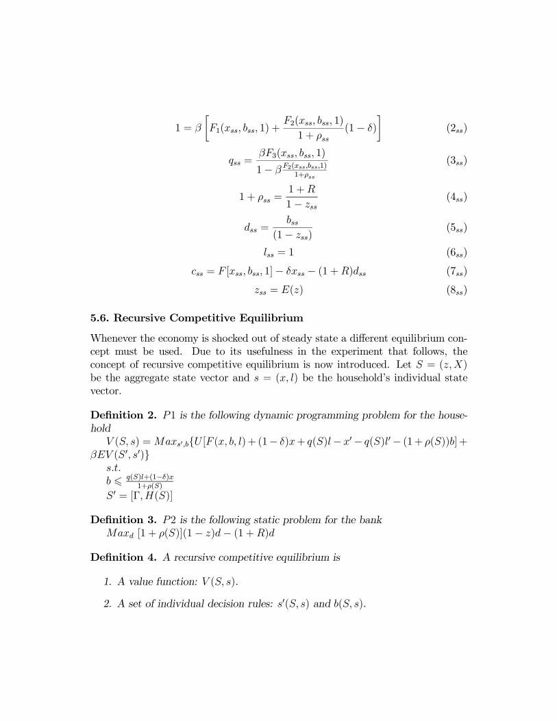
1 = β

"F1(xss, bss, 1) +

F2(xss, bss, 1)

1 + ρss(1− δ)

#(2ss)

qss =βF3(xss, bss, 1)

1− β F2(xss,bss,1)1+ρss

(3ss)

1 + ρss =1 +R

1− zss (4ss)

dss =bss

(1− zss) (5ss)

lss = 1 (6ss)

css = F [xss, bss, 1]− δxss − (1 +R)dss (7ss)

zss = E(z) (8ss)

5.6. Recursive Competitive Equilibrium

Whenever the economy is shocked out of steady state a different equilibrium con-cept must be used. Due to its usefulness in the experiment that follows, theconcept of recursive competitive equilibrium is now introduced. Let S = (z,X)be the aggregate state vector and s = (x, l) be the households individual statevector.

DeÞnition 2. P1 is the following dynamic programming problem for the house-holdV (S, s) =Maxs!,bU [F (x, b, l)+ (1− δ)x+ q(S)l− x"− q(S)l"− (1+ ρ(S))b] +

βEV (S ", s")s.t.b ! q(S)l+(1−δ)x

1+ρ(S)

S " = [Γ,H(S)]

DeÞnition 3. P2 is the following static problem for the bankMaxd [1 + ρ(S)](1− z)d− (1 +R)d

DeÞnition 4. A recursive competitive equilibrium is

1. A value function: V (S, s).

2. A set of individual decision rules: s"(S, s) and b(S, s).

3. A demand for deposits: d(S).

4. A set of pricing functions: q(S) and ρ(S).

5. A stochastic process and an aggregate law of motion: [Γ,H(S)].

such that:

Given (4) and (5), (1) and (2) solve (P1). Given (4), (3) solves (P2). Markets clear:

1. l"(z,X,X, 1) = 1

2. b(z,X,X, 1) = (1− z)d(z,X)

Aggregate Consistency: x"(z,X,X, 1) = H(z,X).

5.7. Credit Channel

In this economy there is a credit channel which is articulated by a static anddynamic multiplier a-la-Kiyotaki and Moore (1997). The multipliers propagateand amplify any change in banking productivity. Consider an adverse productiv-ity shock to banks meaning that their intermediation cost goes up. This wouldinduce a contemporaneous hike in the loan rate charged by banks in equilibrium.The jump in the loan rate immediately tightens the borrowing limit of the house-hold. As a result, households suffer a crunch in the volume of external funds orworking capital available to them. Their ability to Þnance production is reducedwith this credit crunch. As their revenue falls, they instantaneously reduce theiraccumulation of internal funds in an attempt to smooth out consumption. Recallthat land is an asset and, as such, its price is given by the present discounted valueof its forever ßow of future rental payments. As shown previously, these rentalpayments have two components. The Þrst one comes from the direct contributionof land to future output as an input of production. The second one comes fromlands indirect contribution to output as collateral (recall that accumulating moreland today increases external fund availability tomorrow and, thereby, tomorrowsoutput, as long as the borrowing constraint binds). Not surprisingly, these rentalpayments are an increasing function of the future marginal productivity of land

and external funds. Since internal funds are complementary to both land and ex-ternal funds, the instantaneous reduction in internal fund accumulation implies afall in the future marginal productivity of land and external funds. Consequently,the future ßows of direct and indirect (or collateral-based) rental payments toland fall. As a result, in the period of the shock the price of land falls. Thisreduces the value of land on impact and, hence, tightens even further the bor-rowing constraint. The credit crunch is enhanced and revenue and internal fundaccumulation fall even more; and so on. This story is repeated again and again.This is the static multiplier. It basically magniÞes the initial impact of the shock.But this is not the end of the story. The reduction in internal fund accu-

mulation reduces the volume of collateral available for next period. Thus, theborrowing constraint of next period is also tightened even if the shock has van-ished and the lending rate has returned to its normal level. This propagates thecredit crunch or reduced availability of external funds into the next period. Hence,household revenue and internal fund accumulation fall in the period following theshock. And so on. The story told above is repeated in the periods after the shock.This is the dynamic multiplier. It propagates into future periods the effect of theshock. The economy takes longer to converge back to the steady state than in aÞnancially frictionless setup.

6. NUMERICAL EXPERIMENT

In this section the credit channel of the theoretical model is studied within anumerical experiment that aims at replicating the negative productivity shockendured by Þnancial intermediaries in Colombia after the new banking regulationwas issued. First the assumptions (i.e. functional forms and parameter values)for the numerical experiment are presented. Then the results are discussed.

6.1. Functional Forms and Parameter Values

For this experiment the following functional forms and assumptions are used:

U(c) = log(c) F (x, l, b) = xαl1−α +Ab z" iid uniform [0, z]

Note that external funds yield output through a linear technology while inter-nal funds and land are combined in a Cobb-Douglas technology. As the readerwill see, this is just a simplifying assumption to facilitate the choice of parame-ter values. If A = 1 the example reduces to the one suggested by Kocherlakota(2000).Under this setup external funds are neither a complement nor a substitute to

internal funds and land. As said earlier, the lack of complementarity between in-ternal and external funds will reduce the kick obtained from the credit multipliers.Yet, the multipliers are still present due to the complementarity between internalfunds and land. Recall that this complementarity assumption is enough to do thetrick.Note that the loan demand decision is taken according to the following rule:

If A = (1 + ρt) =⇒ bt ∈ [0,∞]If A > (1 + ρt) =⇒ bt −→∞If A < (1 + ρt) =⇒ bt = 0

Parameter values are set so that A > (1+ ρt) # t. This is guaranteed with thefollowing condition:

A =(1 +R)

1− z + ε

where ε is an arbitrarily small number. In other words, A is constructedso that it always exceeds the highest possible gross loan rate of the economy.The important point to note is that, under these circumstances, in every periodthe household will want the highest loan volume it can get. Consequently, itsborrowing constraint will be binding in every period:

bt =qtlt + (1− δ)xt

1 + ρt# t

In the technical appendix it is shown that a sufficient condition to satisfy theno-bubble condition is βF2(xt, bt, lt) < (1 + ρt) # t. Under the present setup thisis equivalent to βA < (1 + ρt) # t. To guarantee that this condition is satisÞed atall times β is deÞned as:

β =(1 + ρss)

A− ε

where ρss is the steady state loan interest rate.The following parameter values were used for the experiment:

TABLE 1Primitive Parameter Value

δ 0.025α 0.5R 0.019z 0.0385ε 0.001

=⇒Parameter Resulting Value

β 0.978ρss 0.039A 1.0608

Each period should be thought of as a quarter. The value for R implies aquarterly deposit interest rate of 1.9% which is equivalent to the average quar-terly ex-post deposit real interest rate in Colombia for the period January/1990-February/2000.22 This rate should be associated to the safe quarterly rate thatany depositor obtains in international Þnancial markets. The value for z was cho-sen so that the steady state quarterly loan interest rate is 3.9%, which coincideswith the average quarterly ex-post loan real interest rate in Colombia for the pe-riod January/1990-Febreuary/2000.23 The value for ε implies a gross return toloans (i.e. A) of 6.1% in every period and a value for β of 0.978. The quarterlydepreciation rate is set at 2.5% and the elasticity of Þnal output to both internalfunds and land is 0.5. This last value was chosen as a benchmark so that outputis neither land nor internal fund intensive. One caveat regarding parameter val-ues applies. These are just reasonable numbers used to implement a quantitativeexercise. There is no calibration whatsoever to long-run empirical regularities.This is future work and so speciÞc quantitative responses should be taken withcaution.

6.2. Results

Initially the economy is set at its steady state ζss = (css, xss, lss, bss, dss, zss, qss, ρss),which is the solution to:

bss =qss + (1− δ)xss

1 + ρss

1 =

"βαxα−1ss +

A(1− δ)1 + ρss

#22The corresponding annual rate is 8%.23The corresponding annual rate is 16.5%.

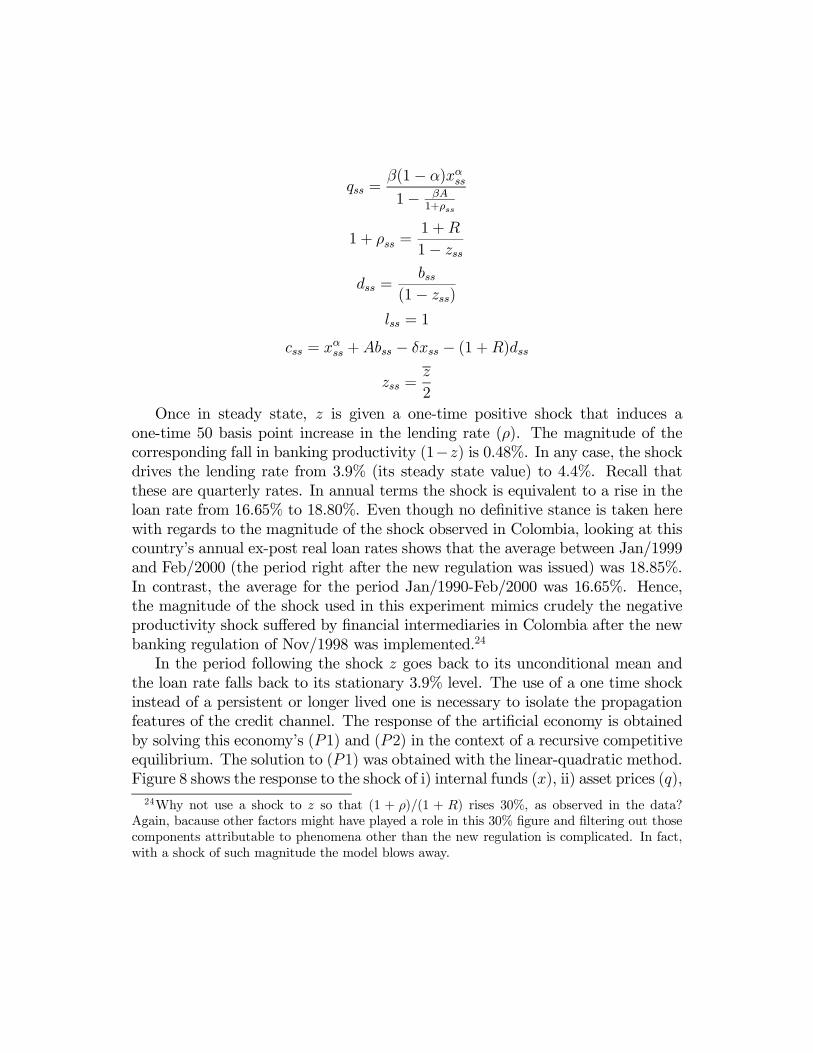
qss =β(1− α)xαss1− βA

1+ρss

1 + ρss =1 +R

1− zssdss =

bss(1− zss)

lss = 1

css = xαss +Abss − δxss − (1 +R)dss

zss =z

2

Once in steady state, z is given a one-time positive shock that induces aone-time 50 basis point increase in the lending rate (ρ). The magnitude of thecorresponding fall in banking productivity (1−z) is 0.48%. In any case, the shockdrives the lending rate from 3.9% (its steady state value) to 4.4%. Recall thatthese are quarterly rates. In annual terms the shock is equivalent to a rise in theloan rate from 16.65% to 18.80%. Even though no deÞnitive stance is taken herewith regards to the magnitude of the shock observed in Colombia, looking at thiscountrys annual ex-post real loan rates shows that the average between Jan/1999and Feb/2000 (the period right after the new regulation was issued) was 18.85%.In contrast, the average for the period Jan/1990-Feb/2000 was 16.65%. Hence,the magnitude of the shock used in this experiment mimics crudely the negativeproductivity shock suffered by Þnancial intermediaries in Colombia after the newbanking regulation of Nov/1998 was implemented.24

In the period following the shock z goes back to its unconditional mean andthe loan rate falls back to its stationary 3.9% level. The use of a one time shockinstead of a persistent or longer lived one is necessary to isolate the propagationfeatures of the credit channel. The response of the artiÞcial economy is obtainedby solving this economys (P1) and (P2) in the context of a recursive competitiveequilibrium. The solution to (P1) was obtained with the linear-quadratic method.Figure 8 shows the response to the shock of i) internal funds (x), ii) asset prices (q),24Why not use a shock to z so that (1 + ρ)/(1 + R) rises 30%, as observed in the data?

Again, bacause other factors might have played a role in this 30% Þgure and Þltering out thosecomponents attributable to phenomena other than the new regulation is complicated. In fact,with a shock of such magnitude the model blows away.

iii) the loan rate (ρ), iv) the loan volume (b), v) output (Y ) and vi) consumption(c).Table 2 presents the percent deviation from steady state of variables ρ, x, q, b, Y

and c during the ten periods that follow the shock. On impact, asset prices (q),credit (b) and output (Y ) fall almost 9% while consumption (c) falls only 7%.This is a consequence of the households desire to smooth consumption. Yet, thereal loan rate (ρ) only rose 50 basis points (a 12.82% increase25). Note also thatthe shock vanishes immediately and the loan rate returns to its stationary levelin the period following the shock. Yet, internal funds (x), asset prices (q), theloan volume (b), output (Y ) and consumption (c) remain considerably depressedand below their stationary levels for several periods after the shock. For instance,in the period following the shock internal funds (x) fall more than 12%. This isexpected because in order to smooth consumption after a negative income shock,the household cuts internal fund accumulation. A very interesting response is thatof consumption. As evidenced from table 2 the response of consumption displaysa hump. Consumption falls contemporaneously with the shock but falls even morein the period after the shock. Furthermore, in the following periods consumptionremains below its impact or shock-period level.

TABLE 2: Percent Deviations from Steady Stateperiod ↓ / variable −→ ρ x q b Y c

t +12.82% 0 -8.79% -8.91% -8.89% -7.06%t+ 1 0 -12.42% -8.63% -8.77% -8.77% -8.79%t+ 2 0 -12.20% -8.48% -8.61% -8.61% -8.63%t+ 3 0 -11.97% -8.32% -8.46% -8.45% -8.47%t+ 4 0 -11.76% -8.17% -8.31% -8.30% -8.32%t+ 5 0 -11.55% -8.03% -8.16% -8.15% -8.17%t+ 6 0 -11.34% -7.88% -8.01% -8.00% -8.02%t+ 7 0 -11.13% -7.74% -7.86% -7.86% -7.87%t+ 8 0 -10.93% -7.60% -7.72% -7.72% -7.73%t+ 9 0 -10.73% -7.46% -7.58% -7.58% -7.59%

25This is equivalent to a 0.48% rise in the gross loan rate (1 + ρ) and also to a 0.48% fall inbanking productivity (1− z).

Are these responses of the artiÞcial economy similar to those observed inColombia after the new banking regulation was implemented? Between the Þrstquarter of 1999 and the third quarter of 2000 real GDP in Colombia has been, onaverage, 5.24% below its pre-1998:III trend, with a maximum deviation of -6.3% inthe second quarter of 1999.26 This is less than what the artiÞcial economy displays.Between December of 1998 and January of 2001 stock prices in the Colombianeconomy have fallen a little more than 40% in real terms. This is a considerableplunge but still below what the artiÞcial economy predicts (66%). Between De-cember of 1998 and January of 2001 total real credit in Colombia was crunched30%. This number is also overshot by the prediction of the artiÞcial economy(67%). But, again, speciÞc quantitative results from the artiÞcial economy shouldbe taken cautiously given that the model was not calibrated to long-run empiricalregularities. Moreover, available macroeconomic data for the period following thenew banking regulation (the shock) is limited given that it was only implementedtwo and a half years ago. One caveat also applies. Parameter alpha was set at0.5 so as to avoid any bias towards land or internal fund intensiveness. A properchoice of alpha can yield results more close to those in the data.In any case, the results are illustrative of the propagation and ampliÞcation

features of the model because this speciÞc setup allows the borrowing constraint toarticulate an extreme case of ampliÞcation and propagation. Indeed, if there wereno Þnancial friction and the borrowing constraint were slack, the level of externalfunds (b) would not affect the level of household revenue and consumption.27 Thereason is simple. For the credit constraint to be slack, it must be the case thatA = 1+ρ. Thus, the net gain from receiving an additional unit of b is zero. Thisis different to the binding constraint case where the net gain from an additionalunit of b is A− (1+ρ) > 0. In consequence, in the absence of a binding borrowingconstraint the one-time shock to intermediation costs z and the correspondinggross loan rate hike drive to zero the volume of loans on impact (because withthe shock A < 1 + ρ). However, household revenue, internal fund accumulationand consumption remain unchanged as net resources for the household do notchange. Asset prices also remain unchanged because the future ßow of directrental payments to land (i.e. of marginal productivity of land) has not changedand, since the credit constraint is always slack, the future ßow of indirect (orcollateral-based) rental payments to land is zero and has not changed either. In26The deviations from trend are: 99:I=-4.5%, 99:II=-6.3%, 99:III=-5.5%, 99:IV=-5.4%, 00:I=-

4.7%, 00:II=5.5%, 00:III=-4.9%.27Also, the level of external funds demanded and supplied is indeterminate.

the period following the shock the gross loan rate returns to its stationary leveland the loan volume may jump to any level because its value is indeterminate.Yet, household revenue, internal fund accumulation, asset prices and consumptionremain unchanged. Contrarily, if the borrowing constraint binds, the shock givesbirth to a long-lived and more than proportional response in every macroeconomicvariable. Hence, the Þnancial friction arising from a binding borrowing constraintintroduces an extreme case of ampliÞcation and propagation in this economy dueto the credit channel explained in section 5.

7. CONCLUSION

Economic performance in Colombia during the last three years has been disap-pointing. The unemployment rate is currently above 15%. The average economicgrowth rate for the years 1998,1999 and 2000 was negative. Asset prices havebeen falling since the end of 1997. This situation contrasts with the early ninetieswhen Colombia grew at rates exceeding 4% and was catalogued as one of the topemerging markets in the world. This economic downturn has been accompaniedby a severe crisis in the Þnancial sector that began in the end of 1997 or early1998. Indeed, real credit suffered a severe crunch starting in January of 1998 andthe real loan rate took a big hike around the same time. In order to alleviate Þ-nancial distress and to Þnance the bail-out, the Colombian government issued newbanking regulation towards the end of 1998. Whether Þnancial distress in Colom-bia was alleviated or not is a question that has not yet been answered. Whatis true though is that in January of 1999, less than two months after the newregulation was issued, the spread between the domestic loan and deposit interestrates increased considerably.This paper argues that this hike in the loan-deposit interest rate spread re-

ßects a rise in intermediation costs attributable to the new banking regulation.The new regulation and the 2/1000 Þnancial transaction tax tightened bankingoperational constraints and added costs to Þnancial intermediation activity. Con-sequently, Þnancial intermediaries suffered a productivity meltdown as they lostoperational versatility and additional real resources were required to implementand continue to operate under the new regulations and tax. As a result, Þnancialintermediaries had to charge a higher loan-deposit interest rate spread in equilib-rium, as observed in the data. While aimed at alleviating Þnancial distress, thenew regulation ended up reducing the productivity of Þnancial intermediaries andincreasing intermediation costs.

Not surprisingly, this negative productivity shock enhanced the credit crunchand corresponding economic contraction that was already underway. The en-hancement, however, did not proceed in a linear way. The data show that theeffects of the shock were ampliÞed and propagated into the future. SpeciÞcally,the contraction of GNP became wider and longer lived than most previous down-ward economic ßuctuations. Asset prices maintained a downward trend. Realcredit was further crunched after a slight recovery in the third quarter of 1998.Additionally, the real loan rate displayed another peak around the time of thenew regulation. In sum, the macroeconomic effects of the initial credit crunchand Þnancial distress were signiÞcantly ampliÞed and propagated after the newbanking regulation and Þnancial transaction tax were implemented.This paper suggests a general equilibrium, Þnancial accelerator model that

incorporates an explicit technology for the intermediary sector and explains howa negative productivity shock to Þnancial intermediaries is ampliÞed and propa-gated due to credit constraints. This Þnancial imperfection articulates static anddynamic credit multipliers that amplify and propagate productivity shocks to Þ-nancial intermediaries. The credit channel arises because of borrowing constraintsthat depend on asset prices, internal funds and lending rates. The transmissionmechanism is triggered by a rise in lending rates that tightens borrowing con-straints on impact. The credit crunch is magniÞed and propagated by a fall inasset prices and internal fund accumulation that accompanies the lower level ofeconomic activity and that further tightens the credit limit on impact and in thefuture. The qualitative predictions of the model are in line with the recent behav-ior of macroeconomic variables in Colombia if one accepts that the new bankingregulation of 1998 was a negative productivity shock to its Þnancial system. Inshort, due to the new regulation and to Þnancial imperfections (speciÞcally creditconstraints), what otherwise would have been a regular and short-lived economiccontraction, became the biggest economic downfall of recent Colombian history.Some questions and issues remain open for further research. It seems reason-

able to think that the Þnancial sector is constantly exposed to productivity shocks.If so, why did credit limits or Þnancial imperfections kick in only with this lastproductivity shock? In other words, why did previous productivity shocks to Þ-nancial intermediaries not generate large and persistent ßuctuations as the onerecently observed in Colombia? Maybe previous shocks were negligible or reallysmall and did not generate signiÞcant real effects. After all, the last shock stemsfrom major regulatory changes in the banking arena. Another possibility is thatborrowing constraints did not bind when previous shocks arrived. In contrast,

the last shock arrived in the middle of an economic contraction and credit crunchwhen credit limits are more likely to be binding. These are just tentative answersto be explored in further research.Another issue that arises has to do with the life-span of the productivity shock

from the new banking regulation. Is this shock transitory or permanent? If itis transitory, is it also very persistent? If the shock is permanent or transitorybut very persistent then the enhanced macroeconomic effects that are observed inColombia need not be the result of a Þnancial friction but simply a direct conse-quence of the life-span of the shock. It would be difficult to argue that the shockwas perceived as permanent since the new regulation was issued as an emergencymechanism to temporarily alleviate ongoing Þnancial distress and to Þnance thebail-out of troubled institutions. The regulation is still operating but some ofits decrees (especially the Þnancial transaction tax) are expected to disappear atsome point in the future, as initially announced by the government. On the otherhand, evaluating the persistence of the shock is difficult because new elements havebeen added to the original regulation after it was implemented in November 17 of1998. For instance, the government recently decreed an increase of the Þnancialtransaction tax rate from 2 per 1000 to 3 per 1000. In any case, it is reasonableto assume that Þnancial intermediaries eventually Þnd a way to adapt to the newregulation until the associated productivity effects vanish completely. If so, theshock should not be very persistent and the credit multipliers articulated by theborrowing constraint are relevant in explaining the ampliÞcation and propagationof the shock, as observed in the data. Again, this is just a tentative answer. Arigorous evaluation of the life-span of the shock is left for future research.

8. BIBLIOGRAPHY

1. AGHION, P., BACCHETTA, P. and A. BANERJEE, 2000, A SimpleModel of Monetary Policy and Currency Crises, EER, vol. 44, pp. 728-738.

2. AGHION, P., BACCHETTA, P. and A. BANERJEE, 2000, Capital Mar-kets and the Instability of Open Economies, manuscript, CEPR.

3. AIYAGARI, R., 1993, Explaining Financial Market Facts: The Importanceof Incomplete Markets and Transaction Costs, Federal Reserve Bank ofMinneapolis Quarterly Review, vol. 17, no. 1, pp. 17-31.

4. ARIAS, A. 2000, The Colombian Banking Crisis: Macroeconomic Conse-quences and What to Expect, Borradores Semanales de Economia, No 158,Banco de la Republica, Colombia.

5. BAUER, P., BERGER, A. and D. HUMPHREY, 1993, Efficiency and Pro-ductivity Growth in U.S. Banking, in The Measurement of Productive Effi-ciency: Techniques and Applications, ed. Harold O. Fried, C.A. Knox Lovelland Shelton S. Schmidt, Oxford, Oxford University Press, pp. 386-413.

6. BERG, S., FORSUND, F. and E. JANSEN, 1992, Malmquist Indices ofProductivity Growth during the Deregulation of Norwegian Banking, 1980-1989, Scandinavian Journal of Economics, vol. 94, pp. 211-228.

7. BERG, S., FORSUND, F., HJALMARSSON, E. and M. SUOMINEN,1993,Banking Efficiency in Nordic Countries, Journal of Banking and Finance,vol. 17, pp. 371-388.

8. BERGER, A. and D. HUMPHREY, 1992, Measurement and EfficiencyIssues in Commercial Banking, in Measurement Issues in the Services Sec-tors, ed. Zvi Griliches, Chicago: NBER, University of Chicago Press, pp.245-279.

9. BERGER, A. and L. MESTER, 1999, What Explains the Dramatic Changesin Cost and ProÞt Performance of the U.S. Banking Industry? WorkingPaper no. 99-1, Federal Reserve Bank of Philadelphia.

10. BERNANKE, B., 1983, Non-monetary Effects of the Financial Crisis inPropagation of the Great Depression, AER, 73, pp. 257-276.

11. BERNANKE, B. and M. GERTLER, 1989, Agency Costs, Net Worth andBusiness Fluctuations, AER, vol. 79, no.1, pp. 14-31.

12. BERNANKE, B. and M. GERTLER, 1990, Financial Fragility and Eco-nomic Performance, QJE, vol. 105, no.1, pp. 87-114.

13. BERNANKE, B., GERTLER, M. and S. GILCHRIST, 1999, The FinancialAccelerator in a Quantitative Business Cycle Framework, in Handbook ofMacroeconomics, vol. 1, ed. J. B. Taylor and M. Woodford, Elsevier ScienceB.V.

14. BHATTACHARYA, J., M. GUZMAN, E. HUYBENS and B. SMITH,1994, Monetary, Fiscal and Bank Regulatory Policy in a Simple Mone-tary Growth Model, Center for Analytic Economics, Working Paper no.94-14.

15. BHATTACHARYA, A., LOVELL, C.A. and P. SAHAY, 1997, The Impactof Liberalization on the Productive Efficiency of Indian Commercial Banks,European Journal of Operational Research, vol. 98, pp. 332-345.

16. BOYD, J. and B. SMITH, 1995, The Evolution of Debt and Equity Marketsin Economic Development, Federal Reserve Bank of Minneapolis ResearchDepartment, Working Paper no. 542.

17. CABALLERO, R. and A. KRISHNAMURTHY, 2000, Emerging MarketCrises: An Asset Markets Perspective, manuscript, MIT.

18. CAPRIO, G. and D. KLINGEBIEL, 1996, Bank Insolvency: Bad Luck,Bad Policy or Bad Banking? in Annual World Bank Conference on Devel-opment Economics, Washington D.C., The World Bank, pp. 79-104.

19. CARLSTROM, C. and T. FUERST, 1997, Agency Costs, Net Worth andBusiness Fluctuations: A Computable General EquilibriumAnalysis, AER,vol. 87, no. 5, pp. 893-910.

20. CHARI, V., JONES, L. and R. MANUELLI, 1995, The Growth Effects ofMonetary Policy, Federal Reserve Bank of Minneapolis Quarterly Review,vol. 19, no. 4, pp. 18-32.

21. COLE, H. and L. OHANIAN, 2000, Re-Examining the Contribution ofMoney and Banking Shocks to the U.S. Great Depression, forthcoming inNBER Macro Annual.

22. COOLEY, T. and V. QUADRINI, 1999, Monetary Policy and the FinancialDecisions of Firms, manuscript, NYU.

23. COOLEY, T., MARIMON, R. and V. QUADRINI, 2000, Aggregate Con-sequences of Limited Contract Enforceability, manuscript, NYU.

24. CORSETTI, G., PESENTI, P. and N. ROUBINI, 1998,Paper Tigers? AModel of the Asian Crisis, manuscript, NBER, December.

25. DEMIRGUC-KUNT, A. and E. DETRAGIACHE, 1997, The Determinantsof Banking Crises: Evidence from Developed and Developing Countries,World Bank Working Paper no. 1828, September.

26. DEMIRGUC-KUNT, A., DETRAGIACHE, E. and P. GUPTA, 2000, In-side the Crisis: An Empirical Analysis of Banking Systems in Distress,World Bank Working Paper no. 2431, August.

27. DIAMOND, P. A., 1965, National Debt in a Neoclassical Growth Model,AER, 32, pp. 233-240.

28. DIAMOND, D., 1984, Financial Intermediation and Delegated Monitor-ing, Review of Economic Studies, 51, pp. 393-414.

29. DIAMOND, D. and P. H. DYBVIG, 1983, Bank Runs, Deposit Insurance,and Liquidity, JPE, Vol. 91, no. 3.

30. DIAZ-GIMENEZ, J., PRESCOTT, E., FITZGERALD, T. and F. ALVAREZ,1992, Banking in Computable General Equilibrium Economies, JEDC,vol. 16, pp. 533-559.

31. EDWARDS, S. and C. VEGH, 1997, Banks and Macroeconomic Distur-bances Under Predetermined Exchange Rates, JME, vol. 40, pp. 239-278.

32. ELYASIANI, E.and S. MEHDIAN, 1995, The Comparative Efficiency Per-formance of Small and Large U.S. Commercial Banks in the Pre- and Post-deregulation Eras, Applied Economics, vol. 27, pp. 1069-1079.

33. GALOR, O., 1992, A Two-Sector Overlapping-Generations Model : AGlobal Characterization of the Dynamical System, Econometrica, Vol. 60,no. 6, pp. 1351-1386.

34. GARBER, P. and S. WEISBROD, 1992, The Economics of Banking, Liq-uidity and Money, D.C. Heath and Company, Lexington, Massachusetts.

35. GILBERT, R. A. and P. W. WILSON, 1998, Effects of Deregulation on theProductivity of Korean Banks, Journal of Economics and Business, vol. 50,no. 2, pp. 133-156.

36. HAYASHI, F. and E. PRESCOTT, 2000, The 1990s in Japan: A LostDecade, Paper presented at the Great Depressions of the 20th CenturyConference, October 2000, Federal Reserve Bank of Minneapolis.

37. HUMPHREY, D., 1991, Productivity in Banking and Effects from Dereg-ulation, Economic Review, vol. 77, pp. 16-28.

38. HUMPHREY, D., 1993, Cost and Technical Change: Effects from BankDeregulation, Journal of Productivity Analysis, vol. 4, pp. 5-34.

39. HUMPHREY, D. and L. PULLEY, 1997, Banks Responses to Deregula-tion: ProÞts, Technology and Efficiency, JMCB, vol. 29, pp. 73-93.

40. HUNTER,W. and S. TIMME, 1991, Technological Change and ProductionEconomies in Large U.S. Commercial Banking, Journal of Business, vol. 64,pp. 339-362.

41. KAMINSKY, G., 1999, Currency and Banking Crises: The Early Warningsof Distress, IMF Working Paper no. 178, December.

42. KAMINSKY, G. and C. REINHART, 1999, The Twin Crises: The Causesof Banking and Balance of Payments Problems, AER, vol. 89, no. 3, pp.473-500.

43. KAMINSKY, G. and C. REINHART, 1998, Financial Crises in Asia andLatin America: Then and Now, AER: Papers and Proceedings, May, vol.88, pp. 444-448.

44. KHUMBAKAR, S., LOZANO-VIVAS, A., LOVELL, C.A. and I. HASAN,2001, The Effects of Deregulation on the Performance of Financial Insti-tutions: The Case of Spanish Savings Banks, JMCB, vol. 33, no. 1, pp.101-120.

45. KING, R. and C. I. PLOSSER, 1984, Money, Credit and Prices in a RealBusiness Cycle, AER, vol. 74, no. 3, pp. 363-380.

46. KIYOTAKI, N. and J. MOORE, 1997, Credit Cycles, JPE, vol. 105, no.2, pp. 211-248.

47. KOCHERLAKOTA, N., 2000, Creating Business Cycles Through CreditConstraints, Federal Reserve Bank of Minneapolis Quarterly Review, vol24, No. 3, pp. 2-10.

48. KRUGMAN, P., 1998, What Happened to Asia? manuscript, MIT, Jan-uary.

49. LEIGHTNER, J. and C. A. LOVELL, 1998, The Impact of Financial Lib-eralization on the Performance of Thai Banks, Journal of Economics andBusiness, vol. 50, pp. 115-131.

50. MENDOZA, E., 2001, Credit, Prices, and Crashes: business Cycles with aSudden Stop, manuscript, Duke University.

51. ROJAS-SUAREZ, L. and S. WEISBROD, 1996, Banking Crises in LatinAmerica: Experiences and Issues, in Banking Crises in Latin America,Inter-American Development Bank, John Hopkins University Press, Balti-more, Maryland.

52. ROMER, C., 1993, The Nation in Depression, JEP, Spring, pp. 41-59.

53. SCHEINKMAN, J. and L. WEISS, 1986, Borrowing Constraints and Ag-gregate Economic Activity, Econometrica, vol. 54, no. 1, pp. 23-46.

54. SCHNEIDER, M. and A. TORNELL, 2000, Balance Sheet Effects, BailoutGuarantees and Financial Crises, manuscript, UCLA.

55. SEMENICK, I. M., 2001, A Nonparametric Approach for Assessing Pro-ductivity Dynamics of Large U.S. Banks, JMCB, vol. 33, no. 1, pp. 121-139.

56. STEINER, R., BARAJAS, A. and N. SALAZAR, 2000, Structural Reformsand Bank Spreads in the Colombian Banking System, in Why So High?Understanding Interest Rate Spreads in Latin America, ed. Philip Brockand Liliana Rojas-Suarez, Inter-American Development Bank, WashingtonD.C.

57. TIRTIROGLU, D., DANIELS, K. and E. TIRTIROGLU, 1998, Total Fac-tor Productivity Growth and Regulation in U.S. Commercial Banking Dur-ing 1946-1995: An Empirical Investigation, Journal of Economics and Busi-ness, vol. 50, pp. 171-189.

58. TOWNSEND, 1979, Optimal Contracts and Competitive Markets withCostly State VeriÞcation, JET, vol. 21, pp.265-293.

59. WHEELOCK, D. and P. WILSON, 1999, Technical Progress, Inefficiency,and Productivity Change in U.S. Banking, 1984-1993, JMCB, vol. 31, pp.212-234.

60. ZAIM, O., 1995, The Effect of Financial Liberalization on the Efficiencyof Turkish Commercial Banks, Applied Financial Economics, vol. 5, pp.257-264.

9. TECHNICAL APPENDIX

In this appendix I show the derivation of equation (7). Equation (6), whichdictates optimality in land accumulation, is:

qtU"(ct) = βEtU "(ct+1)[F3(xt+1, bt+1, lt+1) + qt+1 (6)

+[F2(xt+1, bt+1, lt+1)− (1 + ρt+1)]qt+1

(1 + ρt+1)]

This is:

qtU"(ct) = βEtU "(ct+1)[F3(xt+1, bt+1, lt+1) + qt+1 (6.1)

+F2(xt+1, bt+1, lt+1)

(1 + ρt+1)qt+1 − qt+1]

Let Ωt = F2(xt, bt, lt)/(1 + ρt). With this notation equation (6.1) is:

qtU"(ct) = βEtU "(ct+1)[F3(xt+1, bt+1, lt+1) + Ωt+1qt+1] (6.2)

or:

qt = βEt

-U "(ct+1)U "(ct)

F3(xt+1, bt+1, lt+1)

.+ βEt

-U "(ct+1)U "(ct)

Ωt+1qt+1

.(6.3)

Using (6.3) to substitute for qt+1 in (6.3) implies:

qt = βEt

-U "(ct+1)U "(ct)

F3(xt+1, bt+1, lt+1)

.(6.4)

+βEt

-U "(ct+1)U "(ct)

Ωt+1

"βEt+1

"U "(ct+2)U "(ct+1)

F3(xt+2, bt+2, lt+2)

#+ βEt+1

"U "(ct+2)U "(ct+1)

Ωt+2qt+2

##.Using the law of iterated expectations (6.4) becomes:

qt = βEt

-U "(ct+1)U "(ct)

F3(xt+1, bt+1, lt+1)

.(6.5)

+β2Et

-U "(ct+2)U "(ct)

Ωt+1F3(xt+2, bt+2, lt+2)

.+β2Et

"U "(ct+2)U "(ct)

Ωt+1Ωt+2qt+2

#

Using (6.3) to substitute for qt+2 in (6.5) implies:

qt = βEt

-U "(ct+1)U "(ct)

F3(xt+1, bt+1, lt+1)

.(6.6)

+β2Et

-U "(ct+2)U "(ct)

Ωt+1F3(xt+2, bt+2, lt+2)

.

+β2Et

U "(ct+2)U "(ct)Ωt+1Ωt+2

βEt+2 4U !(ct+3)U !(ct+2)F3(xt+3, bt+3, lt+3)

5+βEt+2

4U !(ct+3)U !(ct+2)Ωt+3qt+3

5 Using the law of iterated expectations (6.6) becomes:

qt = βEt

-U "(ct+1)U "(ct)

F3(xt+1, bt+1, lt+1)

.(6.7)

+β2Et

-U "(ct+2)U "(ct)

Ωt+1F3(xt+2, bt+2, lt+2)

.+β3Et

-U "(ct+3)U "(ct)

Ωt+1Ωt+2F3(xt+3, bt+3, lt+3)

.+β3Et

"U "(ct+3)U "(ct)

Ωt+1Ωt+2Ωt+3qt+2

#After additional iterations and imposing the no bubble condition:

Limj→∞Et

&U "(ct+j)U "(ct)

qt+j−1βjj'i=1

Ωt+i

(= 0 (6.8)

equation (7) is obtained:

qt = Et

$ ∞%j=1

βjU "(ct+j)U "(ct)

&F3(xt+j , bt+j , lt+j)

j−1'i=1

Ωt+i

()(7)

Note that a sufficient condition for (6.8) to hold is:

βΩt ! 1 ∀tThis is:

βF2(xt, bt, lt)

(1 + ρt)! 1 ∀t

10. DATA APPENDIX

GDP cycle: Seasonally adjusted quarterly gross domestic product in mil-lions of 1994 pesos (quarterly values are not annualized). Seasonal adjust-ment was done with the X-11 ARIMA method. Linear trend was calcu-lated by Þtting an OLS line between seasonally adjusted GDP in 1977:Iand 1998:II. HP trend was calculated with λ = 1600. Source is DANE inColombia. Period is 1977:I-2000:III.

Asset prices in real terms (Dec./97=100): Monthly closing value ofthe Bogota Stock Market Index (IBB). To deßate and obtain the real valuesthe CPI (1998:12 =100) was used. Resulting values were normalized by theDecember/1997 value. Source is Banco de la Republica in Colombia. Periodis 1991:01-2001:01.

Real credit volume (Dec./97=100): Monthly opening value in mil-lions of pesos of the total stock of credit (gross and net of non-performingloans) from the Þnancial system [Banks, Savings and Mortgage Loan In-stitutions (CAV), Financial Corporations (CF), Companies of CommercialFinance (CFC), Leasing Companies, Cooperative Organisms and Special In-stitutions]. To deßate and obtain the real values the CPI (1998:12 =100)was used. Each observation was normalized by the December/1997 value.Source is Banco de la Republica in Colombia. Period is 1992:01-2001:06.

Real loan rate: Monthly values of the ex-post real annual loan interestrate. This rate is calculated as (1 + il)/(1 + π)− 1, where il is the observednominal annual loan interest rate and π is the realized annual inßation rate.The nominal annual loan rate used is tasa activa total sistema (monthlyaverage) calculated by Superintendencia Bancaria in Colombia. Inßationrates were calculated with the CPI (1998:12 =100). Source is Banco de laRepublica. Period is 1990:01-2000:02.

Loan/deposit interest rate spreads: Monthly basis point difference be-tween the nominal annual loan interest rate and the nominal annual 3-monthCOD interest rate: il − id. The nominal annual loan rate is tasa activa to-tal sistema (monthly average) calculated by Superintendencia Bancaria inColombia. The nominal annual 3-month COD rate is tasa de interes delos CDT a 90 dias, total sistema (monthly average). Source is Banco de laRepublica. Period is 1990:01-2000:12.

Inverse productivity of Þnancial system: Monthly ratio between thegross nominal annual loan interest rate and the gross nominal annual 3-month COD interest rate: (1+ il)/(1+ id). The nominal annual loan rate istasa activa total sistema (monthly average) calculated by Superintenden-cia Bancaria in Colombia. The nominal annual 3-month COD rate is tasade interes de los CDT a 90 dias, total sistema (monthly average). Sourceis Banco de la Republica. Period is 1986:01-2000:12.

Labor productivity of Þnancial system: Quarterly ratio between theopening real stock of credit (in millions of pesos and gross of non-performingloans) and the number of employees in the Þnancial sector in the seven mainmetropolitan areas. To deßate and obtain real credit values the CPI (1998:12=100) was used. Source for employment is DANE - Encuesta Nacional deHogares. Source for credit volume is Banco de la Republica. Period is3/1/1992-12/1/2000.

11. FIGURES

Figure 1a

Quarterly GDP vs. Linear Trend(millions of 1994 pesos)

7,000,000

9,000,000

11,000,000

13,000,000

15,000,000

17,000,000

19,000,000

21,000,000

77:I

78:I

79:I

80:I

82:I

83:I

84:I

85:I

87:I

88:I

89:I

90:I

92:I

93:I

94:I

95:I

97:I

98:I

99:I

Figure 1b

GDP: % Dev. fromTrend

-8.00%

-6.00%

-4.00%

-2.00%

0.00%

2.00%

4.00%

6.00%

8.00%

10.00%

77:I

78:I

79:I

80:I

82:I

83:I

84:I

85:I

87:I

88:I

89:I

90:I

92:I

93:I

94:I

95:I

97:I

98:I

99:I

Figure 2

Asset Prices in Real Terms (Dec/97=100)

0.00

20.00

40.00

60.00

80.00

100.00

120.00

140.00

160.00

Jan-

91

Jul-9

1

Jan-

92

Jul-9

2

Jan-

93

Jul-9

3

Jan-

94

Jul-9

4

Jan-

95

Jul-9

5

Jan-

96

Jul-9

6

Jan-

97

Jul-9

7

Jan-

98

Jul-9

8

Jan-

99

Jul-9

9

Jan-

00

Jul-0

0

Jan-

01

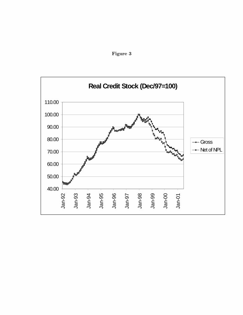
Figure 3

Real Credit Stock (Dec/97=100)

40.00

50.00

60.00

70.00

80.00

90.00

100.00

110.00

Jan-

92

Jan-

93

Jan-

94

Jan-

95

Jan-

96

Jan-

97

Jan-

98

Jan-

99

Jan-

00

Jan-

01

Gross

Net of NPL

Figure 4

Ex-Post Real Loan Rate

0.00%

5.00%

10.00%

15.00%

20.00%

25.00%

30.00%

35.00%

40.00%

Jan-90

Jan-91

Jan-92

Jan-93

Jan-94

Jan-95

Jan-96

Jan-97

Jan-98

Jan-99

Jan-00

Figure 5

Loan vs. 3-month COD Int. Rate Spread

2.00

4.00

6.00

8.00

10.00

12.00

14.00

16.00

18.00

Jan-86

Jan-87

Jan-88

Jan-89

Jan-90

Jan-91

Jan-92

Jan-93

Jan-94

Jan-95

Jan-96

Jan-97

Jan-98

Jan-99

Jan-00

Figure 6

Inverse Productivity in Financial Sector

0.90

1.10

1.30

1.50

1.70

1.90

2.10

2.30

2.50

Jan-

86

Jan-

87

Jan-

88

Jan-

89

Jan-

90

Jan-

91

Jan-

92

Jan-

93

Jan-

94

Jan-

95

Jan-

96

Jan-

97

Jan-

98

Jan-

99

Jan-

00

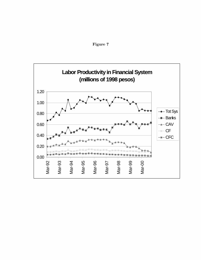
Figure 7

Labor Productivity in Financial System(millions of 1998 pesos)

0.00

0.20

0.40

0.60

0.80

1.00

1.20

Mar

-92

Mar

-93

Mar

-94

Mar

-95

Mar

-96

Mar

-97

Mar

-98

Mar

-99

Mar

-00

Tot Sys

Banks

CAV

CF

CFC

Figure 8

0 20 40 60 80 10085

90

95

100

105Imp-Resp. of X

0 20 40 60 80 10090

95

100

105Imp-Resp. of q

10 20 30 40 50 60 70 80 90 100

100

105

110

115Imp-Resp. of lrate

0 20 40 60 80 10090

95

100

105Imp-Resp. of loans

0 20 40 60 80 10090

92

94

96

98

100

102Imp-Resp. of Y

0 20 40 60 80 10090

92

94

96

98

100

102Imp-Resp. of C