Bachelor of Business Administration (BBA) BBA-3 - e-Gyanagar

Bachelor of Business Administration (BBA)

BBA-3 MANAGERIAL ECONOMICS

Block – 4MARKET STRUCTURE

UNIT-10 MARKET STRUCTURE: PERFECT COMPETITION

UNIT-11 MARKET STRUCTURE: IMPERFECT COMPETITION

Subject Experts

Prof. Nripendra Narayan Sarma, Maniram Dewan School of Management, KKHSOU.Prof. U. R Dhar, Retd. Professor, Dept of Business Administration, GU.Prof. Mukulesh Baruah,Director, Assam Institute of Management.

Course Co-ordinator : Dr. Smritishikha Choudhury, Asst. Prof., KKHSOU

Dr. Chayanika Senapati, Asst. Prof., KKHSOU

SLM Preparation Team

UNITS

10

11

CONTRIBUTORS

Dr. Bhaskar Sarmah

Dr. Bhaskar Sarmah

Editorial TeamContent : Dr. Chandrama Goswami, KKHSOU

Structure, Format & Graphics: Dr. Chayanika Senapati, KKHSOUDr. Smritishikha Choudhury,KKHSOU

July , 2017

ISBN : 978-81-934003-5-7

This Self Learning Material (SLM) of the Krishna Kanta Handiqui State Open University

is made available under a Creative Commons Attribution-Non Commercial-Share Alike 4.0 License

(international): http://creativecommons.org/licenses/by-nc-sa/4.0/

Printed At-:

UNIT 10 : MARKET STRUCTURE: PERFECTCOMPETITION

UNIT STRUCTURE10.1 Learning Objectives

10.2 Introduction

10.3 Concept of Market and Revenue Curves

10.3.1 Classification of Market Structure

10.3.2 Concepts of Total Revenue, Average Revenue and

Marginal Revenue

10.4 Perfect Competition

10.4.1 Equilibrium of Firm in the Short-run

10.4.2 Equilibrium of the Industry in the Short-run

10.5 Perfect Competition: Long-run Analysis

10.5.1 Equilibrium of Firm in the Long-run

10.5.2 Equilibrium of the Industry in the Long-run

10.6 Let Us Sum Up

10.7 Further Reading

10.8 Answers to Check Your Progress

10.9 Model Questions

10.1 LEARNING OBJECTIVES

After going through this unit, you will be able to-

define market

classify market into different forms

discuss perfect competition and equilibrium of a firm and industry

both in the short-run and in the long-run.

10.2 INTRODUCTION

We all buy and sell various kinds of products in a market. In general,

whenever we talk of a market, we have a place in mind, where buyers

interact with sellers and buy goods and services in exchange of money. In

this unit, we shall try to get a deeper insight into this concept ‘market’. We

1

shall try to define the term market in business and economics sense, and

shall discuss the evolution of this concept. We shall also try to explain the

classification of markets on the basis of different parameters.Again, we

shall make an attempt to explain the equilibrium of a firm / industry under

one of the major market structures: viz, perfect competition. This unit will

be helpful for us in relating the theoretical principles of market with the day-

to-day maket envirionment.

10.3 CONCEPT OF MARKET AND REVENUE CURVES

As we have said, by the term market, we in general understand a

particular place or locality where goods are sold and purchased. However,

in economics, the term ‘market’ does not mean a particular geographical

place or locality. Thus, to define market in economics, the concept of a

particular place or locality is not much important. What is important is the

contact between the buyers and the sellers so that transaction (i.e., sale

and purchase of commodities) can take place at an agreed price.

Thus, the essentials of a market are: a) commodity which is to be

dealt with; b) the existence of buyers and sellers; c) a place, be it a certain

region, a country or the entire world; and d) a communication between

buyers and sellers, which ensures only one price for a commodity at a

time.

EVOLUTION OF MARKET: When goods were exchanged for

goods in the barter system, markets were very simple. But with the

evolution of time, increasing needs and with improvement in science and

technology, markets have become complex. Medium of Exchange has

evolved from goods to money (metallic and paper); and from money it is

now taking the shape of ‘plastic money’ or ‘electronic money’. Similarly

the geographic coverage of a market has also widened from the local market

to the global market. Today, advancement in telecommunication has brought

the concept of electronic commerce, which facilitates business on a global

scale.

Goods: Those, whichare tangible; like –books, foods, torchlight, batteries etc.Services: Those,which are intangible;like- the services of abarber, cobbler,lawyer, nurse etc.

Barter System: Thesystem where good sand services wereexchanged directlywithout using aseparate unit ofaccount or medium ofexchangePlastic money orelectronic money:Credits cards, Debitcards, etc. whichfacilitate cashlesstransaction.

2

10.3.1 Classification of Market Structure

Market structure refers to the type of market in which firms

operate. Market structure may be classified:

On the basis of area as local, national and world markets;

On the basis of time, as market price on any particular day

or moment; short-period price, long-period price, or secular

maket price covering a generation; and

On the basis of nature of competition – perfect competition

and imperfect competition.

Here, we shall basically discuss market structure on the

basis of nature of competition. Nature of competition can be

distinguished based on the following three criteria:

a) Number of Sellers in the industry,

b) Entry barriers into the industry, and

c) Nature of the product.

Thus, based on these above criteria, classification of market

structure has been shown in the following tree diagram 10.1:

Figure 10.1: Classification of Market Structure

Thus, we have discussed that the market structure can

broadly be classified into two major categories – perfect competition,

imperfect competition. Market structure under imperfect competition

can be further classified as monopoly, monopolistic competition and

3

oligopoly. In the following table 10.1, we shall try to look at the

individual characteristics of these market structure with regard to

the above three criteria.

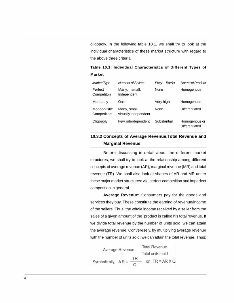
Table 10.1: Individual Characteristcs of Different Types of

Market

Market Type Number of Sellers Entry Barrier Nature of Product

Perfect Many, small, None Homogenous Competiton Independent

Monopoly One Very high Homogenous

Monopolistic Many, small, None Differentiated Competition virtually independent

Oligopoly Few, interdependent Substantial Homogenous orDifferentiated

10.3.2 Concepts of Average Revenue,Total Revenue andMarginal Revenue

Before discussing in detail about the different market

structures, we shall try to look at the relationship among different

concepts of average revenue (AR), marginal revenue (MR) and total

revenue (TR). We shall also look at shapes of AR and MR under

these major market structures: viz, perfect competition and imperfect

competition in general.

Average Revenue: Consumers pay for the goods and

services they buy. These constitute the earning of revenue/income

of the sellers. Thus, the whole income received by a seller from the

sales of a given amount of the product is called his total revenue. If

we divide total revenue by the number of units sold, we can attain

the average revenue. Converesely, by multiplying average revenue

with the number of units sold, we can attain the total revenue. Thus:

4

where, AR = Average revenue, TR = Total Revenue, Q= Total

units sold.

Marginal Revenue: Marginal revenue on the other hand is

the net revenue earned by selling an additional unit of the product.

Thus:

where, MR = Marginal revenue, TR = Total Revenue, Q= Total units

sold, Ä means change in.

Now we will discuss the shapes of the average and marginal

revenue curves under perfect and imperfect competition.

AR and MR Curves of a Firm under Perfect

Competition: A firm under perfect competition has to accept the

prevailing market price and can sell any amount of output in the

market at that price. Thus, a firm under perfect competition will earn

AR, TR and MR similar to the following table 10.2

Table 10.2: Total, Average and Marginal Revenue Schedules

Number of Price or Total Revenue Marginal

units sold (Q) Average (AR x Q) Revenue

Revenue

(1) (2) (3) (4)

1 14 14 14

2 14 28 14

3 14 42 14

4 14 56 14

5 14 70 14

Based on the above schedule, the shapes of AR and MR curves of

a perfect competitive firm has been shown in the following figure

10.2:

Change in Total RevenueMarginal Revenue =

Change in Total units sold

5

Figure 10.2: AR and MR Curves of a Firm under Perfect Competition

It can be seen from figure 10.2 that the firm’s AR and MR

curves are the same. The slope of the curves is horizontal.

AR and MR Curves of a Firm under Imperfect

Competition: Unlike perfect competition, a firm under imperfect

competition does not have to sell all its amount at a fixed market

price. This means that the firm can sell more units of the product as

its price falls. We have shown a hypothetical schedule of AR, TR

and MR in table 10.3 in the next page.

Table 10.3: Total, Average and Marginal Revenue Schedules

Number of Price or Total Revenue Marginal

units sold (Q) Average (AR x Q) Revenue

Revenue

(1) (2) (3) (4)

1 20 20 20

2 19 38 18

3 18 54 16

4 17 68 14

5 16 80 12

Based on the above schedule, the shapes of AR and MR

curves of a firm under imperfect competition has been shown in the

following figure:

6

Figure 10.3: AR and MR Curves of a Firm under Imperfect Competition

It can be seen from figure 10.3 that unlike perfect competition,

the firm’s AR and MR curves under imperfect competition are not

the same. It is to be noted that both the curves are downward sloping.

Again, the slope of the marginal revenue curve is twice as much

steeper as that of the average revenue curve. This is because it

can be seen from the above table 10.3 that as sale increases by

one unit, average revenue falls by one unit of price (as its number of

units sold increases by one unit), marginal revenue falls by two units

of price. Thus if we draw a perpendicular line on the y-axis from

any point of the AR curve, say AB as in figure 10.3, the MR curve will

cut it in the middle. Thus, AC = half of AB.

LET US KNOW

In real market situation, perfect competition rarely exists.

Many economists, therefore, question the usefulness

of studying perfect competition. Though unreal, the

study of perfect competition helps us to understand as to what may

happen, if such a situation actually arises. And secondly, it also helps

us to understand the real imperfect market structure – how much

they deviate from perfect competition. In many advanced countries

the markets of home and car insurance, internet service providers

are highly competitive, though not perfectly competitive. Again, the

Perpendicular: Astraight line which make900 angle on the axis onwhich it is drawn. Sucha line will also beparallel to the other axis.Thus, a perpendicularline drawn on y-axis willbe a parallel line to thex-axis.

7

market of products like detergents, toothpastes etc. constitute the

examples of monopolistic competition. In Indian context, the Indian

Railways constitutes the example of monopoly in case of passenger

carriage through railways. On the other hand, the market of passenger

cars can be said to be good example of oligopoly.

ACTIVITY 10.1

Try to give some examples of the market structures

like: Monopoly, monopolistic competition and oligopoly.

Justify your choice of examples based on the criteria

mentioned in table 10.1.

.......................................................................................................................

................................................................................................................

CHECK YOUR PROGRESS

Q1: Define market. (Answer within 50 words)

.............................................................................................

........................................................................................................

................................................................................................................

.......................................................................................................................

................................................................................................................

Q2: What are the different categories of a product? Give examples

of each of the categories. (Answer within 50 words)

......................................................................................................................

................................................................................................................

.......................................................................................................................

................................................................................................................

.......................................................................................................................

10.4 PERFECT COMPETITION

Perfect competition is described as the market structure having no

rivalry among the individual firms. Thus, the concept of perfect competition

8

is totally opposite to our general idea, where we mean by competition ‘rivalry’

among the individual firms. In the subsequent sections, we shall discuss

equilibrium of firm and industry both in the short run and in the long run

under this market structure.

Again, under perfect competition firms face two cost conditions:

identical cost conditions and differential cost conditions. We shall be

confining our discussion only to identical cost conditions. Identical cost

conditions will help us generalize our discussion from an individual firm to

all other firms and thereby to industry as a whole. We shall now look at the

assumptions on which this market structure rests.

Assumptions of Perfect Competition: The assumptions of perfect

competition are as follows:

• Large number of sellers and buyers: Presence of large number of

buyers and sellers implies that it is not possible either for the individual

firms or the individual buyers to affect the price or output in the market.

That means, in perfect competition, individual firms have zero market

power. Thus, an individual firm under perfect competition is a price taker.

• Product homogeneity: This assumption of perfect competition

ensures that neither the buyers nor the sellers have any ground to

differentiate among the products and, hence, ask for a different price.

(For the concept of product homogeneity, please refer to ‘Let us know’

in the next page).

• Free entry and exit of firms: This assumption is supplementary to

the assumption of large number of sellers in the industry.

• Profit maximisation: The only goal of a firm in perfect competition is

profit maximization.

• No government intervention: There is no government intervention

in the market in any form like: tariffs, subsidies, rationing of production

or demand, etc.

The fulfilment of these above five conditions forms a market structure

known as ‘pure competition’. This market form is different from perfect

competition, which requires the fulfilment of the following additional

assumptions:

Identical CostCondition assumesthat the firms in theindustry face similarcost conditions. Thus,it becomes possible togeneralise from afirm’s analysis to theanalysis of the wholeindustry.

The reverse is the casewith differential costcondition.

9

• Perfect mobility of factors of production: The factors of production

including labour are fully mobile. Thus, labourers are fully mobile between

different jobs and there is no labour union.

• Perfect knowledge: All sellers and buyers possess complete knowledge

of the conditions of the market. Information is free and costless.

LET US KNOW

Product Homogenity: It is the quality of goods,

services or factors which ensures that they cannot

be differentiated in the minds of suppliers and

consumers. A range of commodities is said to be homogeneous if all

of them in that range are perfect substitutes for each other. The

commodities may be physically distinct but economically

homogeneous. The more the degree of homogeneity of products, the

more will be the substitutability among them.

Short-run: It is that period of time which is too short for all economic

agents (firm, industry or a buyer) to fully respond to a change. In our

present analysis of market, short-run is the period in which a) no firm

can enter into or exit from the industry, and b) the individual firms

cannot make any adjustments to its fixed factor of production.

Long-run: It is that period of time which is sufficient for all economic

agents to fully adjust to a change. The firms and industry can change

both the variable and the fixed factors of production during this period.

CHECK YOUR PROGRESS

Q 3: State whether the following statements are True

or False.(T/F)

(a) Absence of government intervention under perfect

competition implies that fiscal instruments like subsidies, tax etc

are not utilised by government to regulate the market.(T/F)

(b) Perfect mobility of factors of production is a feature of pure

competition. (T/F)

10

Q 4: What is the basic difference between short-run and long-run in terms of

the change in factory of production?

..........................................................................................................................................

..........................................................................................................................................

..........................................................................................................................................

..........................................................................................................................................

10.4.1 Equilibrium of a Firm in the Short-run

We shall now discuss the equilibrium of an individual firm

and the industry both in the short run and in the long run. Here we

shall utilize different cost concepts .

While discussing the assumptions of perfect competition,

we have seen that the only goal of the firm is profit maximisation.

Profit is calculated by: TR – TC (TR = Total Revenue and TC =

Total Cost). Thus, the firm will produce that output which yields the

maximum profit. Now, as the price is constant, hence marginal

revenue and average revenue are constant and equal to price. The

equilibrium of a firm may be shown graphically in two ways: either

by using TR and TC curves, or by using MR and MC (MR = Marginal

revenue and MC = Marginal Cost) curves.

Using TR and TC Curves: The following figure 10.4

describes the equilibrium of a firm using TR and TC curves. The

TR curve is a straight line through origin O, which means that price

is constant at any level of output and TR (TR = Price x Quantity)

increases proportionate to sales. This means that as sales increase,

total revenue will also increase by the same proportion.

11

Figure 10.4: Firm’s Equilibrium in the Short-run: TR & TC Approach

In the above figure, the shape of the TC curve reflects the U

shape of AC (Average Cost) curve (we have already discussed the

shapes of the different cost curves in the previous chapter). We

also know that the prime motto of a business firm is to earn maximum

profits. The profit maximising firm will attain equilibrium at the output

level, where profit (gap between TR and TC) is maximum, i.e., at

the level of output where tangents drawn to the TC and TR curves

are parallel. In figure 10.4, Xe is that point and thus is the equilibrium

point. At output levels smaller than X1 and larger than X2, the firm

will incur losses. Because, in both the cases, total cost of the firm

will be more than total revenue the firm earns. To the left of a, (the

point where quantity is X1), it can be seen that that the Total Cost

(TC) curve lies above the Total Revenue (TR) curve, and hence the

firm will suffer losses. Similarly, towards the right of b, the same

thing is observed.

Using MR and MC Curves: This approach of explaining

equilibrium of firm is more beneficial as it uses price as an explicit

variable; and also helps in explaining the behavioural rule that leads

to profit maximisation. Following figure 10.5 explains equilibrium of

firm using this approach:

12

Figure 10.5: Firm’s Equilibrium in the Short-run :MR & MC Approach

The firm attains equilibrium at that output level, where

price=MC above the level of SAC (SAC means short-run average

cost). In figure 10.5, e is that point and hence is the equilibrium point

and x0 is the equilibrium output. At any point left to x0 output level,

say at x1, revenue is greater than marginal cost (x1e1 > x1h ), and

this induces the firm to increase the output level to x0. Similarly, any

point right to x0 output level, say x2, the marginal cost of the firm is

above revenue (x2e2 > x2g), and this induces the firm to reduce output

to the level x0.

In figure 10.5, at point e, MR=MC, which means that the short

run profit is maximised at the equilibrium output level, x0. In fact, this

is the first condition that must be fulfilled for firm’s equilibrium.

However, fulfilment of this condition does not always mean that the

firm will necessarily be in equilibrium. It is possible, that in certain

situations, MR=MC, but the firm is not in equilibrium. The next figure

10.6 explains this point. It is clear from the above figure 10.6 that the

first condition of firm’s equilibrium, i.e. MR=MC is fulfilled at two

points: e1 and e0. The firm however, will not attain equilibrium at e1,

P = MR

13

since profit is not maximised. The firm attains equilibrium at e0, since

profit is maximized x0 > x1.

Figure 9.6:MR=MC Is Not the Sufficient Condition of Firm’s Equilibrium

Thus, from the above figure it is clear that a second condition

is required for firm’s equilibrium. This condition can be stated as:

MC cuts MR from below. Thus, we derive two conditions of firm’s

equilibrium:

a) MC = MR; and

b) MC cuts MR from below.

In case of figure 9.5, the firm earns excess profits of an

amount of eB (price x0e – SAC x0B) per unit of output. And as the

total output sold is 0x0 or AB, the excess profit earned by the firm

amounts to the shaded area CABe. It is to be kept in mind that the

firm, however, does not always earns excess profits while in short

run equilibrium. To the contrary, the firm may have to suffer losses

in the short-run while in equilibrium. This point has been explained

with the help of the next figure 9.7.

14

Figure 10.7: Firm’s Short-run Equilibrium with Losses

It can be seen in figure 10.7 that the firm suffers losses.

This is because, at equilibrium point e (MR = MC; and MC cuts MR

from below), cost per unit X0C > revenue X0e. This means that the

firm suffers total losses eC per unit of output. Thus, the firm suffers

a total loss of AeCB.

CHECK YOUR PROGRESS

Q 5: MR = MC. Is this condition alone sufficient for

a firm’s equilibrium? Explain in about 50 words.

----------------------------------------------------------------------------------------

----------------------------------------------------------------------------------------

----------------------------------------------------------------------------------------

---------------------------------------------------------------------

Q 6: When does a firm under perfect competition earn excess proifts?

Can the firm earn such excess profits in the long-run as well?

(Answer in about 40 words)

----------------------------------------------------------------------------------------

----------------------------------------------------------------------------------------

----------------------------------------------------------------------------------------

----------------------------------------------------------------------------------------

15

In the subsequent sections, we shall discuss industry

equilibrium. It is to be noted here that all along we have utilized

SMC curves for discussing firm’s equilibrium. We have not derived

firm’s supply curve. This is because we have assumed that the

price is given and there are large numbers of firms; hence, it is

unlikely that an individual firm will influence either industry supply or

demand. But in case of the industry as a whole, the industry can

influence the market demand or supply by changing the price. Hence,

to discuss industry’s equilibrium, it becomes imperative to deduce

the industry supply curve.

As we have discussed firm’s equilibrium under identical cost

conditions in the above, hence derivation of a firm’s supply curve

will help us derive the industry’s supply curve as well.

Derivation of the Firm’s Supply Curve: Figure 10.8

depicted in the following shows how much a firm produces under

perfect competition at a given price. By varying the price, we get

different levels of output, and this gives firm’s short run supply curve

as has been shown by panel (b) in figure 10.8.

Figure 10.8: Derivation of Short-run Supply Curve of a Firm

Pric

e, C

ost

16

In the above figure, the minimum output the firm produces

is 0X0, where price P0 is equal to the minimum point on the AVC

curve. For any price below P0, the firm’s revenue does not even

cover the variable cost, and it does not pay the firm to produce any

output. From panel (a), for different levels of the price, we get different

quantities supplied by equating price to MC. In figure 10.8 (b) we

plot these prices and quantities to get the supply curve.

In the above, while deriving the short run supply curve of the

firm we have assumed that the minimum price P0 is equal to the

minimum AVC. That is, we have assumed that the revenues of the

firm must cover variable costs. In the long run, unless the revenues

of the firm cover the fixed costs as well, the firm cannot stay in

production.

Derivation of the Industry Supply Curve: As we have

assumed identical cost conditions, hence the market supply curve

can be obtained by lateral summation (horizontal addition) of short

run supply curves (i.e., short run marginal cost curves) of all individual

firms in the industry. This has been explained with the help of figure

10.9 as has been shown in the next page.

Figure 10.9: Derivation of Short-run Industry Supply Curve

Pric

e, C

ost

17

In figure 10.9, we reproduce the panel (a) of figure 9.8, which

describes the supply curve (MC curve) of a single firm. Now if we

suppose that there are 500 such firms in the industry, the

multiplication of each output level of the individual firms will give us

the short-run industry supply curve. Thus, OQ3 = 500 x OX3; OQ2 =

500 x OX2 and so on. While putting these different quantities OQ3,

OQ2, OQ1 and OQ0 against the respective prices P3, P2, P1 and P0,

we get the industry supply curve SRS as has been shown in panel

(b) of the figure 10.9.

Derivation of the Industry Demand Curve: We know that

to explain equilibrium, we need to consider both the demand and

the supply curve. We have derived the short-run industry supply

curve. Now, let us see how is the shape of the industry supply curve?

We have already seen that the demand curve of a competitive firm

is horizontal straight line. But the shape of the industry’s demand

curve is negatively sloped. This has been shown in the following

figure 10.10.

Figure 10.10: Short-run Demand curve under Perfect Competition

In panel (a) of the figure the industry demand curve has been

depicted, and in panel (b), the firm’s demand curve has been shown.

Pric

e &

Cos

t

18

The demand curve for the industry as a whole is downward sloping,

because the industry can, as a whole, change the market price,

thus affecting consumers’ demand. Therefore, the demand curve

of industry (DD) represents the general law of demand.

10.4.2 Industry Equilibrium in the Short-run

The industry equilibrium in the short run is attained at the

point where the short-run demand curve intersects with the short-

run supply curve. This has been shown in Figure 10.11. In figure

10.11, e is the point where demand curve dd intersects the supply

curve ss. Hence, e is the equilibrium point. Q* is the equilibrium

quantity and P* is the equilibrium price.

It is to be noted here that though no individual firm can exert

any influence on price, the collective action of suppliers and demanders

determines the price.

Figure 10.11: Determination of Equilibrium Price under Perfect Competition

Pric

e &

Cos

t

19

CHECK YOUR PROGRESS

Q 7: State whether the following statements true or

false. (T/F)

(a) Under identical cost condition, it is possible to

derive the industry supply curve through lateral summation

of the individual firms’ supply curves. (T/F)

(b) In the long-run, a firm willl continue its production even when

its revenue does not cover fixed costs, but the variable costs

are covered. (T/F)

Q 8: Unlike firm’s horizontal demand curve, the industry’s demand

curve is negatively sloped. Why? (Answer in about 50 words)

.................................................................................................................

................................................................................................................

.................................................................................................................

.................................................................................................................

10.5 PERFECT COMPETITION: LONG-RUN ANALYSIS

So far we have discussed the short-run equilibrium analysis of a

firm and industry under perfect competition. In the subsequent sections,

we shall discuss the long-run equilibrium analysis of a firm and industry

under this market structure.

10.5.1 Equilibrium of a Firm in the Long-run

In the long-run, entry and exit of firms may take place. Again,

in the long-run, existing firms can adjust the quantities of their fixed

inputs as well. Thus, in the long-run we expect two things: (1) existing

firms will make adjustments in their output and costs. (2) if after

these adjustments, a firm is still unable to cover its total costs, it will

exit the industry. And if existing firms are earning super normal profits,

then new firms will be lured into the industry.

20

Thus, for a competitive firm to be in equilibrium in the

long-run, the following three conditions must be fulfilled:

Price = Marginal Cost

Price = Average Cost

LMC curve cuts LAC curve from below.

Again, as both the marginal cost and the average cost is

equal to price, hence both these conditions can be combined as:

Price = Marginal Cost = Average Cost.

In the earlier course, you have already known the shapes

and concepts of different cost curves. Thus, conceptually we have

learnt that the marginal cost can be equal to average cost only at

the point where the average cost is neither falling nor rising, i.e., at

the minimum point of the average cost curve.

This gives us the condition of long-run equilibrium for a firm as:

Price = Marginal Cost = Minimum Average Cost.


This has been explained in the following figure 9.12.

Figure 10.12: Long-run Equilibrium of a Firm under Perfect Competition

21

In the above figure 9.12, LAC is the long-run average cost

curve and the LMC is the long-run marginal cost curve. The firm is

in equilibrium at point e, where LMC curve cuts the LAC curve at its

minimum. Corresponding to this equilibrium level, the equilibrium

price is 0P*, and the equilibrium quantity is 0Q*. At this equilibrium

level, the firm earns only normal profit.

The firm will not attain equilibrium at any other price or quantity

level. Above the equilibrium price 0P*, let us consider price 0P1. At

this price level, the firm’s marginal cost will be higher than its average

cost. Thus, the firm earns super-normal profits. This means that all

the firms will earn super-normal profits; and this will attract entry of

new firms to the industry. Thus, entry of new firms will ultimately

lead the price to be settled at the level 0P*. Similarly, below price

level 0P* as well, the firm does not attain equilibrium. Say, at price

0P2, the marginal cost of the firm will be below the average cost

curve. This means that the firm will incur loss at price level 0P2.

This means that all the firms will incur losses at this level. This will

force some firms to exit from the industry. Thus, exit of firms will

ultimately lead to increase in the price level to 0P*.

Thus, we can conclude from the above discussion, that a

firm under perfect competition in the long run will be in equilibrium,

when:

Price = MC = Minimum AC, and LMC curve cuts LAC curve

from below.

10.5.2 Industry Equilibrium in the Long-run

In the above, we have seen how a firm under perfect

competition attains equilibrium in the long-run. An industry in the

long-run attains equilibrium when the following three conditions are

satisfied:

the long-run supply and demand for the product of the industry

are equal;

22

all firms in the industry are in equilibrium; and

there is neither the tendency for the new firms to enter the

industry nor the existing firms to leave it.

Figure10.13: Industry Equilibrium in the Long-run

Panel (b) of the figure 10.13 depicts industry equilibrium in

the long run. The long-run supply curve LRS intersects the

long-run demand curve LRD at point E and hence long-run

equilibrium is established at this point. Therefore, 0X* is the

equilibrium quantity of the industry and 0P* is the equilibrium price.

Corresponding to this point E, the firm’s equilibrium has been shown

in panel (a) of the figure. The firm attains equilibrium at point e,

where the LAC curve intersects the LMC curve. Corresponding to

this equilibrium level, the equilibrium quantity is 0Q*, and the

equilibrium price 0P*. As the firm has attained equilibrium at the

minimum point of the LAC curve, hence the firm is earning normal

profit only. Again, as we have assumed identical cost conditions,

hence all the firms will be in equilibrium at this level and will be

earning only normal profits. The equilibrium of all firms with normal

profit ensures that there is neither the tendency of the existing firms

to exit from the industry nor new firms are attracted to enter the

industry.

23

Thus, we have seen that under perfect competition when

the industry attains equilibrium in the long-run, all the three conditions

are satisfied; i.e.,

the long-run supply and demand for the product of the industry

are equal;


there is neither the tendency for the new firms to enter the industry

nor the existing firms to leave it.

CHECK YOUR PROGRESS

Q 9: State the conditions under which a firm under

perfect competition attains equilibrium in the long-

run. (Answer in about 30 words)

.............................................................................................................

.............................................................................................................

.............................................................................................................

10.6 LET US SUM UP

The essentials of a market are:

a commodity which is to be dealt with;

the existence of buyers and sellers;

a place, be it a certain region, a country or the entire world; and

a communication between buyers and sellers, which ensures only

one price for a commodity at a time.

The market structure can broadly be classified into two categories –

perfect competition and imperfect competition.

Market structure under imperfect competition can be further classified

into – monopoly, monopolistic competition and oligopoly.

Market structure can be distinguished based on the three criteria:

number of sellers in the industry;

24

entry barriers into the industry;

nature of the product

Two conditions must be fulfilled for a firm to be in equilibrium. These are:

MC = MR; and

MC cuts MR from below.

And under perfect competition, a firm can earn excess profit or incur

losses while attaining short-run equilibrium.

The conditions of long-run equilibrium for a firm are:

Price = Marginal Cost = Minimum Average Cost.


Under perfect competition when the industry attains equilibrium in the

long run, when three conditions are satisfied :

the long run supply and demand for the product of the industry are

equal;


there is neither the tendency for the new firms to enter the industry

nor the existing firms to leave it.

10.7 FURTHER READINGS

1) Ahuja, H. L. (2006). Modern Economics. New Delhi: S. Chand & Co.

2) Chopra, P.N. (2008). Micro Economics. Ludhiana: Kalyani Publishers.

3) Dewett, K.K. (2005). Modern Economic Theory. New Delhi: S.Chand &

Co.

4) Koutsoyiannis, A. (1979). Modern Microeconomics. New Delhi:

Macmillan India.

5) Sundharam, K.P. M. & Vaish, M.C. (1997). Microeconomic Theory. New

Delhi: S. Chand & Co.

25

10.8 ANSWERS TO CHECK YOURPROGRESS

Ans to Q No 1: A market can be defined as a place or a common platform,

where buyers and sellers interact to exchange goods and services

at an agreed price.

Ans to Q No 2: Products include:

Goods : Those, which are tangible; like – books, foods, torch light,

batteries etc.

Services : Those, which are intangible; like- the services of a barber,

cobbler, lawyer, nurse etc.

Ans to Q No 3: (a) True (b) False

Ans to Q No 4: The basic difference between short-run and long-run is

that during short-run an economic agent (a firm or an industry) can

change only the variable factor of production. But in the long-run an

economic agent can change both the variable and the fixed factors

of production.

Ans to Q No 5: No. This is because, it is possible that a firm fulfills the

condition of MR=MC, but yet its profit may not be maximised. This

may occur when the short-run MC curve cuts the MR curve when it

(MC curve) is still falling, and hence minimum cost has not been yet

achieved.

Ans to Q No 6: A firm under perfect competition can earn excess profit

only in the short-run. The earning of profit by an individual firm will

attract new firms into the industry. As a result, in the long-run, a firm

will be able to earn normal profit only.

Ans to Q No 7: (a) True (b) False

Ans to Q No 8: Unlike the horizontal demand curve of a pefect competitive

firm, the demand curve for the industry as a whole is downward

sloping. This is because, the industry can as a whole change the

market price; thus affecting consumers’ demand. Thus, the demand

curve of industry represents the general law of demand.

26

Ans to Q No 9: A firm under perfect competition attains equilibrium in the

long-run when two conditions are fulfilled: first, Price = MC = Minimum

AC, and secondly, LMC curve cuts LAC curve from below.

10.9 MODEL QUESTIONS

Q 1: What are the basic the criteria of market classification?

Q 2: What is the difference between pure competition and perfect

competition?

Q 3: What is product homegenity?

Q 4: Describe the price and output determination of a firm in the short-

run under perfect competition.

Q 5: Discuss the price and output determination of an industry in the short-


Q 6: Explain the price and output determination of firm in the long-run under

perfect competition.

Q 7: Analyse the price and output determination of an industry in the long-


*** ***** ***

27

REFERENCES (FOR ALL UNITS)

1) Ahuja, H.L. (2003). Advanced Economic Theory; New Delhi: S. Chand

& Company Ltd., India.

2) Ahuja, H.L. (2006). Modern Economics; New Delhi: S. Chand &

Company Ltd., India.

3) Ahuja, H.L. (2010), “Business Economics “, 11th Editon, S. Chand &

Company Ltd., India.

4) Chopra, P.N. (2008). Micro Economics; New Delhi: Kalyani Publishers.

5) D. D. Chaturvedi, S. L. Gupta (2012), “Business Economics”, 3rd

Edition, International Book House, India.

6) Dewett, K.K. (2005). Modern Economic Theory; New Delhi: S Chand

& Sons.

7) Jhingan, M.L. (1986). Micro Economic Theory; New Delhi: Konark

Publications.

8) Koutsoyiannis (2008), “Modern Economics”, 2nd Edition, Macmillan

Press Ltd

9) Koutsoyiannis, A (1979). Modern Microeconomics; New Delhi:

Macmillan.

10) Mankar V G, (1999), “Business Economics”, 1st Edition,Macmillan India

11) Sundharam, K.P.M. & Valish, M.C. (1997). Microeconomic Theory;

New Delhi: S. Chand & Sons.

28

29

UNIT 11: MARKET STRUCTURE: IMPERFECTCOMPETITION

UNIT STRUCTURE

11.1 Learning Objectives

11.2 Introduction

11.3 Monopoly: Basic Concepts

11.3.1 Demand and Marginal Revenue Curves

11.3.2 Short-run and equilibrium of the Monopoly Firm

11.3.3 Long run Equilibrium of the Monopoly Firm

11.3.4 Price Discrimination: Degree and Possibility

11.4 Monopolistic Competition: Definition and Assumptions

11.4.1 Equilibrium of a Firm: Short-run

11.4.2 Equilibrium of a Firm: Long-run

11.4.3 Group Equilibrium

11.4.4 Concept of Excess Capacity

11.5 Concepts of Oligopoly and Duopoly

11.6 Let us Sum Up

11.7 Further Readings




After going through this unit, you will be able to:

define monopoly, and monopolistic competition

discuss various issues relating to monopoly.

explain price discrimination and its various degrees, possibility and

profitability aspects.

discuss monopolistic competition and briefly enumerate the

meaning and basic features of oligopoly and duopoly.

30

11.2 INTRODUCTION

In the earlier unit, we have already come across the terms ‘market

and ‘market equilibrium’. We have known that based on certain

characteristics, market structures can be broadly classified into two

categories: perfect competition and imperfect competition. Again, an

imperfectly competitive market structure can be further divided as: monopoly,

monopolistic competition and oligopoly. These markets structures can again

be segmented into different types. In this unit, we will discuss basically two

major imperfect market structures: monopoly and monopolistic

competitions. We shall try to define these market structures, discuss

relevant issues therein and explain graphically how firms / industry attain

equilibrium under these.

11.3 MONOPOLY: BASIC CONCEPTS

In the earlier unit, we had discussed about perfect competition. We

have seen that perfect competition is the market structure where there

exists a large number of buyers and sellers and in which the influencing

power of any seller is nil. The monopoly is just the opposite of perfect

competition. The word ‘monopoly’ has come from the Greek words monos

polein, which means ‘alone to sell’. This single seller is called a monopolist.

The term is also sometimes used for a single group of sellers that acts as

a price setter, although often a group is called a cartel. Thus, in simple

terms, monopoly can be described as the market structure where there is

only one supplier of the product, which has no close substitute in the market.

As there is only one seller of the product, therefore, the concept of

firm and industry is the same in monopoly. In reality, the existence of a

monopoly firm is as much rare as perfect competition. However, in some

of our remote villages, where there is only one doctor, he may be seen as a

monopoly supplier of medical services in the locality.

Cartel: A group of firmsacting together to controloutput and price

31

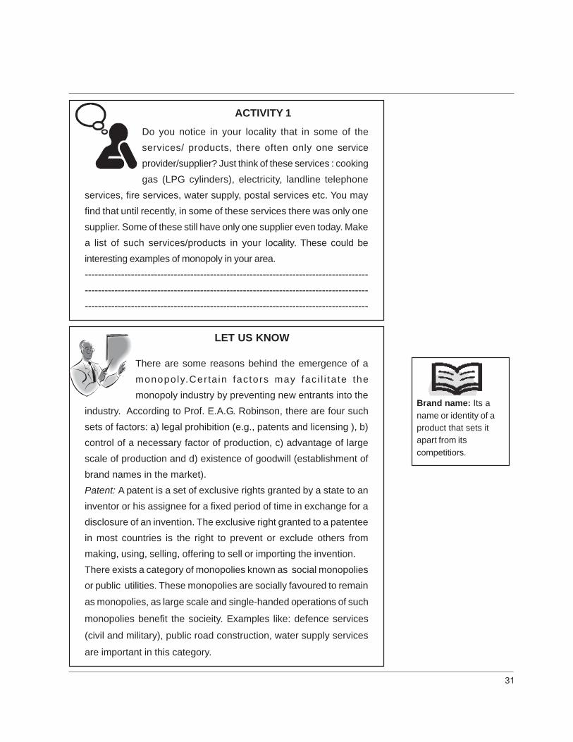
ACTIVITY 1Do you notice in your locality that in some of theservices/ products, there often only one serviceprovider/supplier? Just think of these services : cookinggas (LPG cylinders), electricity, landline telephone

services, fire services, water supply, postal services etc. You mayfind that until recently, in some of these services there was only onesupplier. Some of these still have only one supplier even today. Makea list of such services/products in your locality. These could beinteresting examples of monopoly in your area.------------------------------------------------------------------------------------------------------------------------------------------------------------------------------------------------------------------------------------------------------------------

LET US KNOW

There are some reasons behind the emergence of amonopoly.Cer ta in factors may fac i l i ta te themonopoly industry by preventing new entrants into the

industry. According to Prof. E.A.G. Robinson, there are four suchsets of factors: a) legal prohibition (e.g., patents and licensing ), b)control of a necessary factor of production, c) advantage of largescale of production and d) existence of goodwill (establishment ofbrand names in the market).Patent: A patent is a set of exclusive rights granted by a state to aninventor or his assignee for a fixed period of time in exchange for adisclosure of an invention. The exclusive right granted to a patenteein most countries is the right to prevent or exclude others frommaking, using, selling, offering to sell or importing the invention.There exists a category of monopolies known as social monopoliesor public utilities. These monopolies are socially favoured to remain

as monopolies, as large scale and single-handed operations of such

monopolies benefit the socieity. Examples like: defence services

(civil and military), public road construction, water supply services

are important in this category.

Brand name: Its aname or identity of aproduct that sets itapart from itscompetitiors.

32

11.3.1 Demand and Marginal Revenue Curves Under Monopoly

The discussion about demand (or, average revenue) and the

marginal revenue curves becomes necessary for the equilibrium

analysis. Unlike perfect competition, the monopoly firm can control

the price or output in the market; it can control either price or

output,but not both. The monopolist can sell larger amount of the

product in the market by charging a lower price and vice versa. This

characteristic of the monopolist ensures a downward sloping

demand curve - exhibiting the general law of demand (the law of

demand has already been discussed in earlier unit . The shape of

the demand curve and the marginal revenue curve of the monopolist

firm has been shown with the help of the following figure 11.1

Y

Price

AR

0 Quantity X

MR

Figure 11.1: AR and MR Curve of a Monopoly Firm

In the above figure 11.1, it can be seen that the monopolist demand

curve AR slopes downward. The MR curve also slopes downward

and lies below the AR curve. The MR curve slopes at a much steeper

rate than the AR curve. We have already discussed in earlier unit

that under imperfect competition, the slope of the MR curve is twice

as much steeper as the slope of the demand curve.

33

LET US KNOW

Shape of Cost Curves:The shape of cost curvesunder

monopoly are not much different from those under

perfect competition. The only difference is that a firm

under perfect competition can purchase any quantity of

factors of production at constant price, but the monopolist may

have to pay higher prices for more such factors of production.

This induces the MC curve of the monopolist to rise at a higher

rate than that of the perfectly competitive firm. The monopolist

will not have any fixed cost curve in the long run,like perfectly

competititve firm, but will have both the variable cost curves

and the fixed cost curves in the short run.

11.3.2 Short Run Equilibrium of the Monopoly Firm

The price-output equilibrium can be easily explained with the help of

the following figure 11.2. In figure 11.2 , AR is average revenue or

demand curve,

Figure 11.2: Short-run Equilibrium of a Monopoly Firm

34

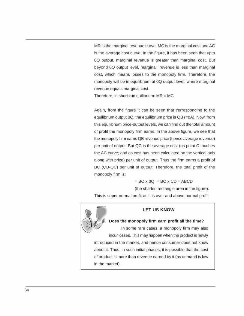
MR is the marginal revenue curve, MC is the marginal cost and AC

is the average cost curve. In the figure, it has been seen that upto

0Q output, marginal revenue is greater than marginal cost. But

beyond 0Q output level, marginal revenue is less than marginal

cost, which means losses to the monopoly firm. Therefore, the

monopoly will be in equilibrium at 0Q output level, where marginal

revenue equals marginal cost.

Therefore, in short-run quilibrium: MR = MC

Again, from the figure it can be seen that corresponding to the

equilibrium output 0Q, the equilibrium price is QB (=0A). Now, from

this equilibrium price-output levels, we can find out the total amount

of profit the monopoly firm earns. In the above figure, we see that

the monopoly firm earns QB revenue price (hence average revenue)

per unit of output. But QC is the average cost (as point C touches

the AC curve; and as cost has been calculated on the vertical axis

along with price) per unit of output. Thus the firm earns a profit of

BC (QB-QC) per unit of output. Therefore, the total profit of the

monopoly firm is:

= BC x 0Q = BC x CD = ABCD

(the shaded rectangle area in the figure).

This is super normal profit as it is over and above normal profit

LET US KNOW

Does the monopoly firm earn profit all the time?In some rare cases, a monopoly firm may also

incur losses. This may happen when the product is newly

introduced in the market, and hence consumer does not know

about it. Thus, in such initial phases, it is possible that the cost

of product is more than revenue earned by it (as demand is low

in the market).

35

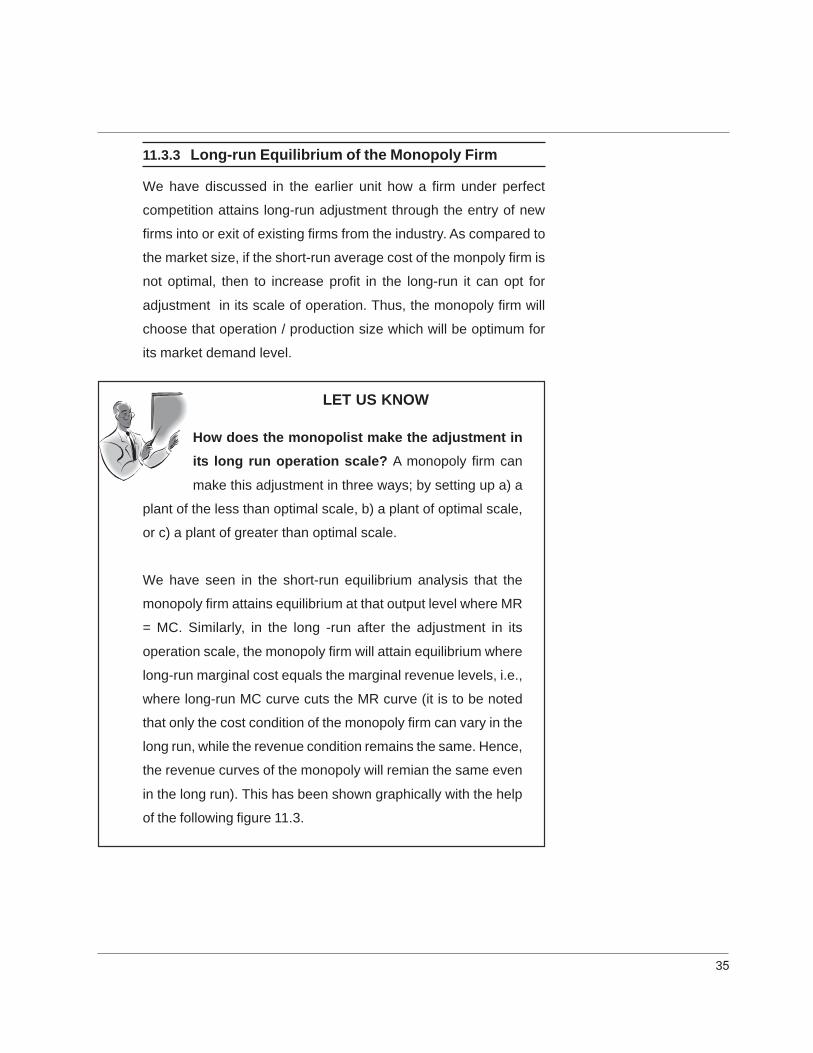
11.3.3 Long-run Equilibrium of the Monopoly Firm

We have discussed in the earlier unit how a firm under perfect

competition attains long-run adjustment through the entry of new

firms into or exit of existing firms from the industry. As compared to

the market size, if the short-run average cost of the monpoly firm is

not optimal, then to increase profit in the long-run it can opt for

adjustment in its scale of operation. Thus, the monopoly firm will

choose that operation / production size which will be optimum for

its market demand level.

LET US KNOW

How does the monopolist make the adjustment inits long run operation scale? A monopoly firm can

make this adjustment in three ways; by setting up a) a

plant of the less than optimal scale, b) a plant of optimal scale,

or c) a plant of greater than optimal scale.

We have seen in the short-run equilibrium analysis that the

monopoly firm attains equilibrium at that output level where MR

= MC. Similarly, in the long -run after the adjustment in its

operation scale, the monopoly firm will attain equilibrium where

long-run marginal cost equals the marginal revenue levels, i.e.,

where long-run MC curve cuts the MR curve (it is to be noted

that only the cost condition of the monopoly firm can vary in the

long run, while the revenue condition remains the same. Hence,

the revenue curves of the monopoly will remian the same even

in the long run). This has been shown graphically with the help

of the following figure 11.3.

36

Figure 11.3: Long-run Equilibrium of a Monopoly Firm

From the above figure it can be seen that the long-run marginal

cost curve (LMC) and the marginal revenue curve (MR)

intersect at point E. So, point E is the long-run equilibrium point.

Corresponding to this equilibrium level, equilibrium output is 0Q,

and the equilibrium price is 0A.

ACTIVITY 2

What profit does the monpoly firm earn in the long-run? We have already seen in section 6.3.2 the total

profit the monopoly firm earns while attaining short-

run equilibrium. Now with the help of the above figure 6.3 and

the previous discussion about the short-run equilibrium of the

monpoly firm, find out the total profit the monopoly firm will earn

in the long-run.

---------------------------------------------------------------------------------

---------------------------------------------------------------------------------

---------------------------------------------------------------------------------

37

11.3.4 Price Discrimination : Degree and Possibility

An important feature of monopoly form of market is that the

monopolist can charge different prices for the same good at the

same time for reasons not associated with differences with cost.

This is known as price discrimination. Let us consider the following

example. A tea producer has a manufacturing plant in Dibrugarh.

He sells tea at a per unit cost of Rs. 12 in Dibrugarh. He also sells it

at the Guwahati market at a per unit price of Rs 15. He charges Rs

3 more in the Guwahati market to cover his transportation cost of

Rs 3 per unit of the product. As the difference in the prices between

these two markets is equal to the difference in the transport cost,

hence we can not call this as price discrimination. But if for example,

the producer sells tea at a unit price of more than Rs 15 (say Rs 17)

in the Guwahati market then we can say that the producer is

practising price discrimination.

Degree of Price DiscriminationBritish economist ,A C Pigou in his book The Economics of Welfare

(1920) has identified three degrees of discriminating power of a

monopoly firm leading to three types of price discrimination.

First degree price discrimination: First degree price

discrimination occurs when the monopoly firm charges a different

price for each of the individual unit of the product, even to the same

consumer. The maximum price that a consumer is willing to pay for

a unit of output is called the reservation price. The perfectly

discriminating monopolist charges the reservation price for each

unit of the output. The first degree discriminition is also called perfect

price discrimination. This type of price discrimination is very difficult

to implement.

Second degree price discrimination: This degree of price

discrimination occurs when the monopolist is able to charge several

different prices for different ranges or groups of output. For example,

38

we need to pay monthly electricity bills based on different prices

charged for different slabs of energy consumption. Say we need to

pay Rs. 2 for first 100 units of electricity consumption in a month.

Again, a higher price, say, Rs.2.50 can be charged for subsequent

units (starting from 101st unit to a certain limit). This type of price

discrimination is also seen in case of telephone bills for different

units of calls. Magazines also offer different price range for different

period of subscription order.

Third degree price discrimination: The third degree price

discrimination occurs when the monopolist partitions the market

into two or more groups of customers and charges different prices

to the different groups (the price is uniform for member within a

group). For example, an office stationery supplier can charge

different prices from different offices.

ACTIVITY 3

You have thus come to know about the concept of price

discrimation and its different types. Now, from your

own observation, try to give some examples of price

discrimination. Also, try to justify as to which type (degree) of

price discrimination your examples will fit?

---------------------------------------------------------------------------------

---------------------------------------------------------------------------------

---------------------------------------------------------------------------------

---------------------------------------------------------------------------------

---------------------------------------------------------------------------------

Possibility for Price DiscriminationOperation of price discrimination requires the fulfillment of the

following conditions:

The seller of the product must have monopoly power.

The market must be divided into sub-markets with different

price elasticities

39

The buyer of a product can not resell the product to another

buyer, or the sub-markets are separate.

CHECK YOUR PROGRESS

Q.1 : Tick whether the following are true (T) or false

(F).

(i) Price discrimination is of four degrees. (T / F)

(ii) Differences in prices of a product in two separate markets

due to difference in transportation cost is called price

discrimination.(T / F)

Q.2 : Fill in the blank:(i) The word ‘monopoly’ has come from the Greek words

monos polein, which means ____________.

(ii) The Economics of Welfare was written by ________.

(iii) Another name of first degree of price discrimination is

_________.

11.4 MONOPOLISTIC COMPETITION : DEFINITIONAND ASSUMPTIONS

Monopolistic competition is the mid-way between the two extreme market

forms we have already discussed, i.e., perfect competition and monopoly.

The term monopolistic competition was first used by E. H. Chamberlin in

his book “TheTheory of Monopolistic Competition”. Monopolistic competition

refers to a market structure in which there are many firms selling closely

related, similar but not identical products. This market structure is much

more realistic than the other two market stuctures we have discussed

already. The assumptions of this market form are:

Large number of sellers and buyers:This is the first assumption of

monopolistic competition. Presence of large number fo firms/sellers

implies that each seller can satisfy only a small share of the market

demand. And the sellers face stiff competition in the market.

40

Differentiated products that are close substitutes: The producers

under monopolistic competition produce differentiated products. But the

products offered by individual producer is a close substitute of another.

Free entry and exit from the market: Free entry and exit from the

industry is also another important feature of monopolistic competition.

This feature though sounds similar with perfect competition, yet is

technically different. Because under perfect competition, a firm entering

new into the industry has to produce indentical products already existing

in the industry. But in case of monopolistic competition, new firms may

introduce new products in the market.Such new products may have

some difficulty in competing with the established brands.

Selling Cost: Every firm under monopolistic competition may incur

individual selling costs (cost on advertisement, etc) to promote its

product.

Imperfect knowledge: Imperfect knowledge on the part of the

consumers about the products of different sellers is also an important

feature. This is important because even when two products of two

different sellers may be identical in terms of quality, but the monopolistic

firms try to show variabillity in them to attract the consumers towards

the product. This becomes possible when the consumer does not have

perfect knowledge about the products of different sellers.

11.4.1 Equilibrium of a Firm: Short Run

As in monopoly, firms under monopolistic competition face a

downward sloping demand curve. But this does not mean that

monopolistically competitive firms are likely to earn large profits.

Monopolistic competition is also similar to perfect competition: as

there is free entry, the potential to earn profits will attract new firms

with competing brands, driving economic profits down to zero.

However the condition of short-run equilibrium of a monopolistic

competitive firm is similar to that of a monopoly firm, i.e.

Marginal Revenue = Marginal Cost

This has been explained with the help of the following figure 11.4.

41

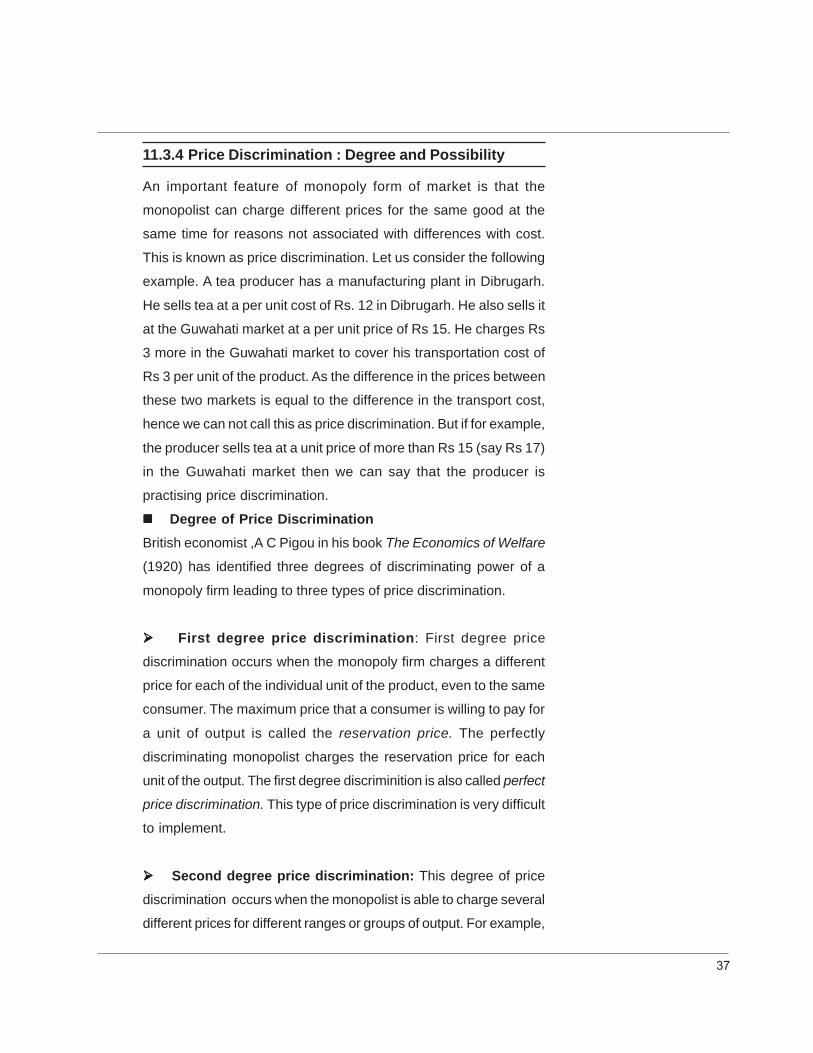
Figure 11.4: Short-run Equilibrium of a Monopolistic Firm

In figure 11.4, AR is the average revenue and MR is the marginal

revenue curve. SAC and SMC are short-run average cost and short-

run marginal cost curves respectively. The firm attains equilibrium

at point E, where SMC curve intersects the MR curve.

Corresponding to this equilibrium point E, 0Q is the equilibrium output

and QC (or 0A) is the equilibrium price. It can be seen from the

figure that the cost per unit of output is QD, while the revenue earned

per unit of output is QC. Thus the firm earns CD amount of profit

per unit of output. This amounts to a total profit of ABCD (DC X 0Q

or BD). Such short-run profit earned by individual firms under

monopolistiic firms is termed as excess profits or supernormal profit.

However it is also possible that a firm under monopolistic competition

can earn either a) normal profit or b) incur losses while attaining

short-run equilibrium. These have been shown with the help of figures

11.5 and 11.6.

42

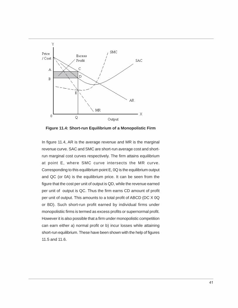
Figure 11.5: Short-run Equilibrium ( incurring Losses)

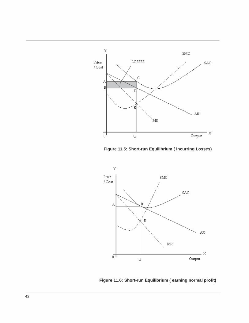
Figure 11.6: Short-run Equilibrium ( earning normal profit)

43

ACTIVITY 4

From figure 10.5 you can see that at the monopolistic

firm attains equilibrium at point E. Corresponding to

this equilibrium point E, the equilibrium quantity is 0Q

while the equilibrium price is 0A. You will also notice that at this

equilibrium level, the firm incurs total losses of ABCD as price

earned per unit (0B) is less than the cost incurred per unit of

production (QC). You are to describe this equilibrim (incurring

losses) process of the monopolistic firm. (You can take help of

the discussion of firm’s equilibrium with excess profit (explained

with the help of figure 11.4)) for the purpose.

---------------------------------------------------------------------------------

---------------------------------------------------------------------------------

---------------------------------------------------------------------------------

---------------------------------------------------------------------------------

---------------------------------------------------------------------------------

ACTIVITY 5From figure 11.6 you can see that the monopolistic

firm attains equilibrium at point E. Corresponding to

this equilibrium point E, the equilibrium quantity is 0Q

while the equilibrium price is 0A. You will also notice

that at this equilibrium level, the firms earns normal profit as

price earned per unit (0A) is equal to cost incurred per unit of

production (QB). You are to describe this equilibrium (earning

normal profit) process of the monopolistic firm. (You can take

help of the discussion of firm’s equilibrium with excess profit

(explained with the help of figure 11.4)) for the purpose.

---------------------------------------------------------------------------------

---------------------------------------------------------------------------------

---------------------------------------------------------------------------------

---------------------------------------------------------------------------------

---------------------------------------------------------------------------------

11.4.2 Equilibrium of a Firm: Long Run

In the above discussion we have seen how an individual firm may

earn profit in the short-run. Such earning of profits encrourages other

firms to enter into the industry. As new firms enter the industry and

as they introduce competing brands, existing firms will lose market

share and sales; its demand curve will shift down. Thus, entry of

new firms will ultimately lead to disappering of any super-normal

profit. Therefore, firms in the long-run will be earning only normal

profit. This has been shown graphically with the help of the following

figure 11.7.

Figure 11.7: Long-run Equilibrium of a FirmFrom the above figure it is seen that the firm attains equilibrium at

poing E where marginal revenue equals marginal cost. Thus, 0Q is

the equilibrium level of output and 0A is the equilibrium level of price.

This is, in fact, is also long-run equilibrium because at the equilibrium

price (0A), the long-run average cost curve (LAC) is tangent to the

the average revenue (AR), which means that the firm earns only

normal profit.

Thus, from the above discussion we have seen that a firm under

monopolistic market structure will attain equilibrium:

In the short-run when: Marginal Revenue = Marginal cost

In the long-run when : Marginal Revenue = Marginal cost; and

Long-run Average Cost = Average Revenue

44

45

CHECK YOUR PROGRESSQ.3: Tick whether the following are true (T) or false

(F).

(i) The firm under monopolistic competition faces a downward

sloping demand curve.(T / F)

(ii) A firm under monopolistic competition can earn super normal

profits even in the long run.(T / F)

Q.4: Fill in the Blanks:(i) Monopolistic competition is similar to perfect competition as there

are ..........................and..........................

Q.5: Mention the conditions of long-run equilibrium of a monopolistic

firm.

-------------------------------------------------------------------------------------

-------------------------------------------------------------------------------------

-------------------------------------------------------------------------------------

-------------------------------------------------------------------------------------

11.4.3 Group Equilibrium

So far we have discussed how an indiviudal firm under monopolistic

competition attains equilibrium in the short-run as well as in the

long-run. Let us now discuss ‘group equilibrium’.

LET US KNOW

There is a difference between the concepts ‘group’ and

‘industry’. Group refers to a number of firms producing

products which are close substitutes to each other.

Industry,on the other hand,refers to the firms which produce

identical products. Thus, in the case of perfect competition, we

use the term ‘industry’, while in this unit (in case of monopolistic

competition), we have used the term ‘group’.

Product differentiation necessitates a redefinition of industry.This

is because heterogeneous products cannot be summed to form

46

market demand and supply scedules as in case of

homogeneous products.In view of this ,E.Chamberlin uses the

concept of ‘product group’ in lien of industry while analysing

equilibrium in a monopolistic market.Such ‘product group’

includes products which are close technological and economic

substitutes .But still, product differentiation allows each firm to

charge a different price.There can be no unique equilibrium price

but a equilibrium cluster of prices which will reflect the

preferences of the consumers for the product of the differnt firms

in the group.

However, in this analysis of group equilibrium, Chamberlin shows

the determination of a unique equilibrium price.This has been made

possible by what he called two ‘heroic assumptions’.These are:

i) all firms in the group have identical cost conditions giving rise to

identical cost curves;

ii) consumers preferences are evenly distributed among product

so that all firms have identical demand curves.

These two assumptions also enabled Chamberlin to analyse the

equilibrium of the firm and the group in the same diagram.

Chamberlin develops three distinct models of equilibrium.

First Model: In the first model, it is shown that although firms can

earn super normal profit in the short run, in the long run the group

equilibrium will occur with new firms entering the market whereby

all firms will enjoy only normal profits.

Second Model: In the second model , it is shown how in the long

run the group will atain equilibrium with price adjustment, instead of

new entry. At the equilibrium level of output all the firms will earn just

the normal profit. Here, Chamberlin introduces a new demand curve

which is called the ‘actual sales curve’ or ‘share of the market’ along

with the typical downward sloping individual perceived demand

curve.The ‘actual sales curve’ shows the actual sales of the firm at

each price after accounting for the adjustment of price of other firms

in the group.

47

Third Model: The third model is a combination of the above two

.Here the group attains equilibrium in the long run by both price

adjustment and entry and exit of firms. At the equilibrium level of

output , as usual, all firms earn just the normal profit.

LET US KNOW

Chamberlin used a different approach to decsribe group

equilibrium. For the analysis he adopted two main

assumptions:

‘Uniformity assumption’: He assumes that the demand and

cost curves of all the products in the group are uniform. However,

this does not mean that the products of the firms will not

differentiate.

‘Symmetry assumption’: This assumption means that the

number of firms in the group are so large that the individual

decision of a firm regarding price and output is unlikely to have

any effect on its rivals. The name ‘symmetry’ to this assumption

was given by Stigler.

11.4.4 Concept of Excess Capacity

From our long-run equilibrium analysis, it is clear that a firm under

monopolistic competition attains equilibrium at the point when the

two conditions are satisfied, viz.:

Long-run Marginal Revenue = Long-run Marginal cost; and

Long-run Average Cost = Long-run Average Revenue

Now let us reconsider the following figure 11.8 (a) which represents

the long-run equilibrim of a firm under monopolistic competition.

48

Figure 11.8: Excess Capacity

From the above figure 11.8 (a) we can see that a firm under

monopolistic competition attains long-run equilibrium at point E.

Again, it can be seen that corresponding to this point, the long-run

average cost curve (LAC) is tangent to the average revenue curve

(AR) at point B. But at point B, the firm’s average cost is not minimum.

This means the firm is producing at a point where optimum cost

(the lowest possible level of average cost) has not arrived. Hence it

can not be said as optimal cost level from society’s point of view.

Again we can see from the figure that the firm’s lowest possible

average cost is arrived at point C of the LAC curve. Corresponding

to this lowest average cost, the firm’s output is 0W. But the firm’s

equilibrium is 0Q, which is less than the optimal output level by

QW. Hence QW represents excess capacity of output which exists

under monopolistic competition. Why does it happen? This is

because as the demand curve of the firm is downward sloping, it is

not possible that the firm’s long-run average cost curve be tangent

at its optimum point (c) This becomes possible only in case of

perfect competition, where the firm faces a horizontal demand curve.

This has been shown with the help of panel (b) of the same figure.

But as the demand curve of the monopolistic firm becomes flatter

in the long-run, the quantum of the excess capacity will get reduced.

49

CHECK YOUR PROGRESS

Q.6. What is the difference betwee the concepts

‘group’ and ‘industry’?

------------------------------------------------------------------------------------------

------------------------------------------------------------------------------------------

------------------------------------------------------------------------------------------

------------------------------------------------------------------------------------------

----------------------------------------------------------------------------------------

Q.7 The demand curve of the monopolistic firm does not touch the

long-run average cost curve at its lowest point at the point of equiribrium.

Why?

------------------------------------------------------------------------------------------

------------------------------------------------------------------------------------------

------------------------------------------------------------------------------------------

------------------------------------------------------------------------------------------

------------------------------------------------------------------------------------------

11.5 CONCEPTS OF OLIGOPOLY AND DUOPOLY

In the previous units and in the earlier sections of this unit, we have

so far discussed the market structures like perfect competition, monopoly

and the imperfect competition. Thus, we have come to know that perfect

competition is actually an ideal market structure which rarely exists in

practice. The opposite of this market structure is the monopoly, where

there exists only one seller in the market. While existence of monopoly can

also be a reality though rare, monopolistic competition reflects the most

practical market situation we find in reality.

The above three are undoubtedly the most prominent market

structures dealt with in Economics. However, there still exists a few market

structures. Oligopoly and duopoly are among them. Let us first deal with

oligopoly. Oligopoly, is a market form where the market or the industry is

controlled or dominated by small group of sellers/companies also known

as oligopolists. Thus, it is very much clear that in this form of market, there

50

exists more than one seller but at the same time the number of sellers is

not as large as is found in a perfectly competitive market. It is much like

monopoly where the small group is made up of major sellers/companies

which collectively exert control over the supply of a particular product (good

or service) and its price in the market. Since the number of competitors in

an oligopoly is few, each of the oligopolist is most likely to be aware of the

actions of the others and hence the decision of one company influences

and is influenced by the decision of the others. Hence, strategic planning by

the oligopolists’ needs to consider the responses of other market players

as well.

Underlying assumptions: Oligopoly rests on the following

assumptions:

Existence of a few firms: There exists a few firms in the market.

Control over supply and price: Each firm produces a large share of

the total volume of the product; so it can affect the price by its own

action.

Entry of New Firms: No doubt it is very difficult for a new firm to enter

into the market but it is not completely blocked. Financially sound firm

can only enter into the market.

Competition in quality: The firms compete with each other in the quality

of the product also. The firms spend a sufficient amount on the research.

Interdependence: In Oligopoly there is an interdependence on each

other. Because the policies of each firm affect the price and output of

other firm.

Advertising: A heavy amount is spent on the advertisement by the

oligopoly to attract the consumers.

LET US KNOW

A very good example of the oligopoly form of competition

is the auto industry. Let us consider the case of small

passenger cars. The players in the market in this

segment include: Maruti Suzuki, Tata, Hyundai, Honda, Fiat, Hindustan

51

Motors, Toyota, Chevrolet, Ford, Volkswagen etc. Now, you can easily

guess that huge investment worth thousands of crores of rupees is

needed to make into this industry. As such, there exist high entry

barrier in this form of market. Again, even when the pricing decisions

of the products of these companies are taken by the individual industry

concerned, yet the influence of other brands of products of other

manufacturers of the industry can not be ruled out.

Another example of the oligopoly form of market is the ‘cartel’. The

cartel is a type of oligopoly in which the participating firms may employ

restrictive tactics such as collusion and market sharing to escalate prices

and restrict production just as in a monopoly. The OPEC (Organization

of the Petroleum Exporting Countries) which has a prominent effect on

the international oil prices is an example of cartel.

Collusive Oligopoly: One of the important characteristic of oligopoly

is collusion, where rival firms enter into an agreement in mutual interest on

various accounts such as price, market share etc. That is in order to avoid

uncertainty caused by interdependence and to avoid price wars cut throat

competition, firms under oligopoly enter into an agreement for a uniform price

output policy to be followed by them. This agreement may be either formal

(open) or tacit (secret). When a number of producers (or sellers) enter into a

formal agreement, it is called explicit (open) collusion; and when collusion is

done secretly, it is known as tacit collusion. When firms enter into such collusive

agreemnets formally or secretly, collusive oligopoly is said to prevail.

Collusive oligopoly are of two types:

(a) Cartels and,

(b) Price Leadership

The most commonly found form of explicit collusion is known as cartels. The

aim of such collusion is to reduce competition and increase profits of individual

firms; i.e. firms jointly fix a price and output policy through agreements. The

52

aim of such collusion is to reduce competition and increase profits of individual

members. However, now a days governments do not encourage cartels

because it creates monopoly like situations.

Under price leadership one firm sets the price and others follow it. The one

who sets the price is a price leader and the others who follow it are followers.

The follower firm adopt the price of the leader; even though at times they

need to depart from their profit maximising position.

Duopoly: Duopoly is said to occur when there are only two firms which

control the total supply of the market. Each firm produces the large share of

the total out put and it can affect the price of the market. If both firm are

producing the similar commodity it will be called pure duopoly. On the other

hand, if there is some difference in their products then it will be called

differential duopoly. Duopoly is also called as the simplest form of oligopoly.

LET US KNOW

The most popular example of duopoly is between Visa

and Mastercard who exercise a major control over theelectronic payment processing market in the world. If you

have a credit/debit card, you must have seen any of the logos as shownalongside.

Pepsi and Coca-cola are the two major shareholders in the softdrinks market. In the market, there are so many brands of soft drinks,e.g., Limca, Mirinda, Sprite, Fanta, Lehar etc. You can find that thebrands are either from CocoCola or Pepsi. Of course, there are otherbrands in the market which are not from these companies, but theirmarket shares in terms of the global soft drink market are not muchsignificant.

Similarly, in the commercial jet aircraft market, Airbus and Boeing

are the main leaders. duopolies in the commercial jet aircraft market.

53

The duopoly market structure may be studied on two basic grounds:

a) by ignoring any mutual dependence between the two sellers and b)

recognising mutual dependence between the two sellers. The Cournot-

Edgeworth solutions explains the duopoly market situations by ignoring

mutural dependence between the two sellers. On the other hand, Chamberlin

explains the model of the duopoly market when we assume that there is

mutual dependence between the two sellers.

CHECK YOUR PROGRESS

Q 8: State whether the following statements are

True or False.

(a) Duopoly is a variety of oligopoly where there are more than

two firms in the industry. (T/F)

(b) In oligopoly, there exists high degree of entry barriers. (T/F)

(d) ‘Product group’ is found in oligopoly. (T/F)

Q 9: What type of entry barriers does there exist in the oligopoly

market?

--------------------------------------------------------------------------------------

--------------------------------------------------------------------------------------

Q 10: Define the term oligopoly.

---------------------------------------------------------------------------------------

---------------------------------------------------------------------------------------

---------------------------------------------------------------------------------------

11.6 LET US SUM UP

Thus, in this unit we have discussed -

What a monopoly market structure is. We have discussed that

monopoly can be described as the market structure where there is only

one supplier of the product, which has no close substitute in the market.

54

The equilibriuim of a monopoly both in the short-run and in the long-run.

The concept of price discrimination and its various types.

About monopolistic competition.

The equilibriuim of a monopolistic firm and its group both in the short-

run and in the long-run.

The concept of excess capacity under this market structure.

Some of the managerial economics pricing techniques: pioneer pricing

and cost-plus pricing.

Oligopoly, is a market form where the market or the industry is controlled

or dominated by small group of sellers/companies also known as

oligopolists.

Duopoly is said to occur when there are only two firms which control the

total supply of the market.

If both firm are producing the similar commodity it will be called pure

duopoly.

11.7 FURTHER READINGS

1) Dewett, K.K: Modern Economic Theory, S.Chand & Sons, 22nd Ed., 2005.

2) Chopra, P.N.: Micro Economics, Kalyani Publishers, 2nd Ed, 2008.

3) Ahuja, H L: Modern Economics, S. Chand, 12th Ed., 2006.

4) Ahuja, H.L.: Managerial Economics, S.Chand, 1st Ed., 2007.

5) Mankar, V.G.: Business Economics, MacMillan, 1999.


Check Your Progress

Ans to Q No 1: (i) False (ii) False

55

Ans to Q No 2: (i) Alone to sell (ii) A C Pigou (iii) Perfect

price discrimination

Ans to Q No 3: (i) True (ii) False

Ans to Q No 4: Large number of sellers in the industry and no entry/exit

barrier.

Ans to Q No 5 : A firm under monopolistic firm attains long-run equilibrium

when the following two conditions are fulfilled:

Marginal Revenue = Marginal cost; and

Long-run Average Cost = Average Revenue

Ans to Q No 6: The difference between ‘group’ and ‘industry’ is that ‘group’

refers to a number of firms producing products which are close substitutes

to each other. Industry, on the other hand, refers to the firms which produce

identical products.

Ans to Q No 7: As the demand curve of the firm is downward sloping and

hence under monpolistic competition, it is not possible that the firm’s long-

run average cost curve be tangent to its average curve. This becomes

possible only in case of perfect competition, where the firm faces a horizontal

demand curve

Ans to Q No 8: (a) False (b) True (d) False

Ans to Q No 9: Theoretically, entry of new firms in the oligopolistic form of

market is not completely blocked. However, entry barrier to the industry

is considerably very high, because only financially sound firm can only

enter into the market.

Ans to Q No 10: Oligopoly, is a market form where the market or the industry

is controlled or dominated by small group of sellers/companies also

known as oligopolists.


1. Discuss the concept of price discrimination.

2. What are the different degrees of price discrimination?

3. What is excess capacity? Why does it arise?

4. Following data are given for a certain product:

56

Variable cost per unit: Rs. 11; Fixed Cost: Rs. 275,000; Expected sales

volume: 1,15,000 units. The manufacturer aims a profit of 12% per

unit. Calculate the Mark-up price of the product.

5. Write a short note on oligopoly form of market.

6. Describe how monopoly firm attains equilibrium in the long-run.

7. How does a firm under monopolistic competition attain equilibrium in

the short run and in the long run?

8. How does a group under monopolistic competion attain equilibrium in

the long run?

*** ***** ***

57

UNIT 12: MACRO ECONOMICS AND SELECTEDMACRO AGGREGATES

UNIT STRUCTURE

12.1 Learning Objectives

12.2 Introduction

12.3 Basic Concepts of National Income

12.4 Gross National Product(GNP), Net National Product(NNP), Per

Capita Income(PCI), Disposable Income

12.5 Importance of the study of National Income

12.6 Methods of National Income Measurement

12.7 Difficulties in Measurement of National Income

12.8 Circular flow of National Income

12.9 GDP deflator

12.10 Index Numbers: Concept and uses

12.11 Construction of Simple Index Numbers

12.12 Construction of Weighted Index Numbers

12.12.1 Laspeyres’ Index Number

12.12.2 Paasche’s Index Number

12.12.3 Fisher’s Index Number

12.13 Base Shifting, Splicing and Deflating

12.14 Let Us Sum Up

12.15 Further Readings




After going through this unit you will be able to

describe the basic concepts of national income

give the concepts of gross national product, net national product,

per capita income, disposable income

explain the importance of national income.

58

explain the difficulties in the measurement of National Income

describe the uses of index numbers

12.2 INTRODUCTION

Macroeconomics is that branch of economics which deals with the

performance, structure, behaviour and decision making of an economy as

a whole. It studies aggregate indicators such as GDP, unemployment,

national income, inflation, savings, inveastment, price indices etc. While

macro economics is a broad field of study, we discuss here two aggregates-

National income and Index numbers.

In this unit we are going to discuss the basic concepts of national income.

Along with the basic concepts we will further discuss the Gross National

Product (GNP), Net National Product (NNP), Per Capita Income(PCI),

Disposable Income etc. We will also make a discussion about the methods

of measurement of natioonal income and the importance of the study of

national income.This unit deliberates on index numbers. Index numbers are

the indicators of the various trends in an economy. Price index numbers

indicate the position of prices whether they are rising or falling and at what

rate. Similarly, index numbers regarding agricultural production indicates

the trend of change whether it is rising or falling at what rate over a period of

time. An index number is an economic data figure reflecting price or quantity

compared with a standard or base value. The base usually equals 100 and

the index number is usually expressed as 100 times the ratio to the base

value.

After going through this unit, you will be able to discuss the different

concepts relating to index numbers, construct simple and wighted, discuss

the concepts of base shifting, splicing and deflating of index numbers.

12.3 BASIC CONCEPTS OF NATIONAL INCOMENational income can be viewed from different angles and, depending

on the purpose of study, various concepts of national income are used

that basically proxy the same entity. In addition, there are various aggregates

59

that are derived from the broad concept of national income. The different

aggregates that are used to indicate the economic status of a nation and

other related aggregates are explained in this section in a simple manner.

National Income is one of the basic concepts in macroeconomics.

National Income means the total income of the nation, The aggregate

economic performance of the whole economy is measured by the national

income data.

National Income or Gross Domestic Income refers to the money

value of all final goods and services produced by the normal residents of

a country while working both within or outside the domestic territory of a

country in an accounting year. National Income also includes net factor

income from abroad.

Symbolically,

Y = PG + PS

Where, Y = National Income

P = Price

G = Goods

S = Service

Traditional Definitions of National Income :

Marshall

"The labour and capital of a country acting on its natural resources produce

annually a certain net aggregate of commodities, material and immaterial

including services of all kinds..... This is the true net annual income or

revenue of the country or national dividend."

Pigou

"National income is that part of objective income of the community,

including of course income derived from abroad, which can be measured

in money."

Fisher

"The national dividend or income consists solely of services as received

by ultimate consumers, whether from their material or from their human

environments. Thus, a piano, or an over coat made for me this year is not

60

a part of this year's income, but an additions to the capital. Only the

services rendered to me during this year by these things are income."

KEYNESIAN APPROACH TO NATIONAL INCOME

Keynes has suggested three approaches to national income :

(1) Income - Expenditure approach : According to this approach, national

income is equal to total expenditure on consumption and investment

goods.

(2) Factor - Income approach : According to this approach, national

income is measured as the aggregate of incomes received by all

the factors of production.

(3) Sales proceeds minus cost approach : According to this approach,

national income is defined as the aggregate sales proceeds minus

cost.

12.4 GROSS NATIONAL PRODUCT(GNP), NET NATIONALPRODUCT(NNP), PER CAPITA INCOME(PCI), DISPOSABLEINCOME

Gross National Product (GNP) : When we add the net factor

income from abroad to the figure of GDP we get the Gross National

Product of the country. The net factor income from abroad refers to the

surplus of factor income earned from foreign countries by the residents

of the country over the factor income earned by the foreigners within the

domestic territory of the country. This surplus may be positive or negative.

Thus, we may write :

GNP = GDP + Net Factor Income from Abroad

Net National Product (NNP) : During the process of production

a part of the capital assets get used up. This is called wear and tear of

capital or consumption of capital or simply the depreciation of capital. In

order to find out the net addition made to the national output we must

deduct this depreciation from the GNP. Thus, NNP of a country is its GNP

less depreciation.

NNP = GNP- Depreciation

61

The NNP of a country may be viewed in two alternative ways. It

may be seen as a sum of payments made to the factors of production

engaged in the production of the national output or as the market value

of the national output. The former will give us NNP at factor cost and the

latter will give us NNP at market price. In a country where Government

plays no role in the market, there cannot be any difference between the

two. But with government intervention a discrepancy between the two

arises . More specifically, in the NNP at market price, indirect tax gets

included in the valuation of the product , while subsidies get left out.

Therefore, indirect taxes and subsidies account for the differences between

the two. We can obtain NNP at factor cost from NNP at market price by

deducting indirect taxes but adding subsidies to it.

NNP at factor cost = NNP at market price – Indirect Taxes +

Subsidies

We may note here that the NNP at factor cost is popularly known

as the National Income of a country.

The relation among the above concepts of national income can

be shown with the help of the following figure 14.1

12.5 IMPORTANCE OF THE STUDY OF NATIONAL INCOME

The study of national income statistics is very important. It helps in

analysing the actual performance of the economy and in preparing future

policies. The increasing importance of the study of the national income is

due to the following reasons :

(i) Index of Economic structure : An important index of the economic

structure of the economy is national income estimates. National in-

come estimates tell us how incomes are earned and spent in the

country. The knowledge about the relative importance of various sec-

tors of the economy and their contribution to national income are also

provided by national income estimates.

(ii) Economic Welfare Indicator : National income figures are an indicator

of the economic welfare of the people of a country. With the help of

62

these figures, we can compare the standard of living of the people of

various countries. We can also compare the standard of living of the

people of the same country at different times.

(iii) Measures Aggregate Yield : National income statistics measure the

aggregate yield of the economic policy for development.

(iv) Tools for Economic Planning : National income estimates are the tools

for economic planning. Because for framing an economic plan, a prior

knowledge of the trends in national income is required.

(v) Provide Information about Inflationary and Deflationary gaps : National

income estimates provide information about inflationary and deflation-

ary gaps in the economy. National income estimates also assist in

formulating anti-inflationary and anti-deflationary policies.

(vi) Helpful in the Allocation of burden of international payments : National

income estimates help in allocating the burden of international pay-

ments among different nations.

(vii) Determination of Subscription and Quotas : National income estimates

enable us to determine the subscriptions and quotas of different coun-

tries to international organisations like IMF, IBRD, etc.

(viii) Help in the Determination of Grants-in-Aid : National income estimates

help the federal government to determine the amount of grants-in-aid

to be provided to the state governments.

(ix) Basis of Budgetary Policies : On the basis of national income statis-

tics, government prepare their budgets and make necessary changes

in the taxation and borrowing policies.

(x) Importance in Defence and Development : National income estimates

help in determining the proper allocation of national product between

defence and development of the economy.

(xi) Depreciation Provision : National income estimates guide us to make

provision for reasonable depreciation to maintain the capital stock of

the country.

(xii) Helpful to the government : National income estimates help the gov-

ernment in making future plans for the expansion of public sectors.

(xiii) Important for less developed or developing countries : National income

63

estimates throw light on the importance and backwardness of vari-

ous sectors of the less developed or developing economics and help

in formulating appropriate economic polices.

(xiv) Help in Economic Analysis : National income estimates help us in

analysing the functioning, growth and anatomy of the economy.

(xv) Basis of Social Accounting : The basis of social accounting or na-

tional income accounting is the national income figures.

CHECK YOUR PROGRESS

Q 1: Define national income.

.............................................................................................................

.............................................................................................................

Q 2: State the Keynesian apprach to national income

.............................................................................................................

.............................................................................................................

12.6 METHODS OF NATIONAL INCOME MEASUREMENT

The income of a country can be viewed from three different

angles. It can be viewed from the side of production, distribution or

dispension. This necessitates different methods and data for the calcula-

tion of national income. The basic idea about these methods are pre-

sented in this section.

There are three approaches to the measurement of National Income.

These are:

A) Output Approach

B) Income Approach

C) Expenditure Approach

A) Output Approach : In this approach the aggregate value added in the

different sectors of the economy is worked out. Here the national income

accounting authority calculate the total value of the output produced in the

economy during the accounting period by taking into account the values

64

added at each stage of production in the various sectors of the economy.

Such a method is known as the Value Added Method. This method involves

the following steps:

i) Identification of the producing enterprises and classification of them

into various industrial sectors according to their activities;

ii) Estimation of the net value added by each producing enterprise,

industrial sector and then adding up of the net values created by all

the sectors for the economy as a whole.

The value added method may be illustrated with the help of a simple

example. Let us take Bread as the final product and see how values are

added at different stages of production until it reaches the hands of the

ultimate consumers. This has been shown in the following table 12.1

Table 12.1: Product : Bread(Value in Rs.Crore)Item Buyer Seller Value Value Added

Wheat Flour Mills Farmers 100 100

Flour Bakeries Flour Mills 150 50

Bread Wholesalers Bakeries 175 25

Bread Retailers Wholesalers 200 25

Bread Consumers Retailers 220 20

Total Value Added 220

B) Income Approach : Also known as the Income Method, in this approach

the sum of the incomes derived from different economic activities is

estimated. Steps involved in this approach are as follows :

i) Identification and classification of the producing enterprises that

employ factor inputs (i.e enterprises in the Primary , Secondary and

Tertiary Sectors);

ii) Classification of factor payments (i.e wages, interest, profit etc.);

iii) Estimation of factor payments and aggregation of the same for the

economy as a whole.

When we add the factor payments in all the industrial sectors we

get the domestic factor income. Then by adding the net factor income from

abroad to it we get the National Income of the country. Thus,

65

National Income = Compensation to the employees + Mixed in-

come of the self employed + All kinds of rent including imputed rent + All

interest payments + All profits + Net factor income from abroad.

C) Expenditure Approach : The expenditure approach aggregates the

consumption and investment expenditures occurring in the country during

the accounting period to obtain the domestic expenditure at current price.

It takes into account only the final purchases. The final expenditure on

GDP consists of private final consumption expenditure, government final

expenditure, gross fixed capital formation, change in stocks/inventories

(unsold stock of goods consisting of raw materials, semi finished and

finished products during the accounting period) and net exports of goods

and services. Therefore,

GDP at market price = Private consumption expenditure + Private

Investment expenditure + Government

expenditure + Exports – Imports

GNP at market price = GDP at market price + Net factor income from

abroad

National Income = GNP at market price -Depreciation – Indirect

Taxes + Subsidies

From the above we can observe that the three approaches look

at the three different phases of the circular flow of national income. These

phases are- production, distribution and disposition. Although each

approach requires different data and methods, they give rise to identical

results as they estimate the same entity. The choice of a particular method

depends on the nature of the sector and availability of data.

Important Inclusions and Exclusions : In the calculation of

national income we need to be careful to include certain incomes/activities

and exclude some others. Some of the important inclusions and exclusions

are noted below :

Inclusions :

i. Value of production for self consumption;

ii. Own account production of fixed assets by government, enterprise

and household;

66

iii. Imputed rent of owner occupied house;

iv. Purchase of new house by consuming households;

v. Work in progress at the site of production;

vi. Capital repairs like major alterations of the old buildings or adding

a new room to the existing building;

Exclusions :

i. Transfer payments;

ii. Windfall gains and losses;

iii. Corporate tax and income tax should not be included separately;

iv. Duties and taxes paid from wealth or past savings;

v. All expenditures on the purchase of old shares and bonds from

other people or new shares and bonds from producing enterprises;

and

vi. All expenditures on intermediate goods and services.

ACTIVITY 15.1

Illustrate the Value Added method of accounting giving

your own example.

.......................................................................................................................

.....................................................................................................................

.....................................................................................................................

.....................................................................................................................

.....................................................................................................................

12.7 DIFFICULTIES IN MEASUREMENT OF NATIONAL INCOME

There are many difficulties in measuring national income of a country.

Some of these difficulties are discussed below:

Non Monetary Transactions

The first problem in National Income accounting relates to the

treatment of non-monetary transactions such as the services of housewives

to the members of the families. For example, if a man employs a maid

67

servant for household work, payment to her will appear as a positive item in

the national income. But, if the man were to marry the maid servant, she

would be performing the same job as before but without any extra payments.

In this case, the national income will decrease as her services performed

remains the same as before.

Problem of Double Counting

Only final goods and services should be included in the national

income accounting. But, it is very difficult to distinguish between final goods

and intermediate goods and services. The difference between final goods

and services and intermediate goods and services depends on the use of

those goods and services. If by mistake one good or service is calculated in

the national income estimates at its intermediate stage and it is calculated

again at its final stage it is called as double counting. So there are possibilities

of double counting in national income estimates.

The Underground Economy

The underground economy consists of illegal and uncleared

transactions where the goods and services are themselves illegal such as

drugs, gambling, smuggling, and prostitution. Since, these incomes are not

included in the national income, the national income seems to be less than

the actual amount as they are not included in the accounting.

Petty Production

There are large numbers of petty producers and it is difficult to include

their production in national income because they do not maintain any account.

Public Services

Another problem is whether the public services like general

administration, police, army services, should be included in national income

or not. It is very difficult to evaluate such services.

Transfer Payments

In economics, a transfer payment (or government transfer or simply

transfer) is a redistribution of income in the market system. These payments

are considered to be non-exhaustive because they do not directly absorb

68

resources or create output. In other words, the transfer is made without any

exchange of goods or services. Individuals get pension, unemployment

allowance and interest on public loans etc. are examples of transfer

payments. But these payments create difficulty in the measurement of

national income as they are not given for any production or service in the

present period. These earnings are a part of individual income and they are

also a part of government expenditures.

Capital Gains or Loss

When the market prices of capital assets change and the owners make

capital gains or loss, such gains or losses are not included in national income.

Price Changes

National income is the money value of goods and services. Money

value depends on market price, which often changes. The problem of

changing prices is one of the major problems of national income accounting.

Due to price rises the value of national income for particular year appears to

increase even when the production is decreasing.

Wages and Salaries paid in Kind

Additional payments made in kind may not be included in national

income. But, the facilities given in kind are calculated as the supplements of

wages and salaries on the income side.

Illiteracy and Ignorance

Due to illiteracy and ignorance of many sections of people; information

regarding household and individual income are not available to a large extent.

This is specially visible in case of small scale agriculture and other cottage

industry or business. As a result, there arises immense difficulties in the

measurement of national income.

Apart from these, there are some other aspects or segments where national

income accounting face difficulties. These are:

Second hand transactions;

Environment damages;

Calculation of depreciation;

Inadequate and unreliable statistics; etc.

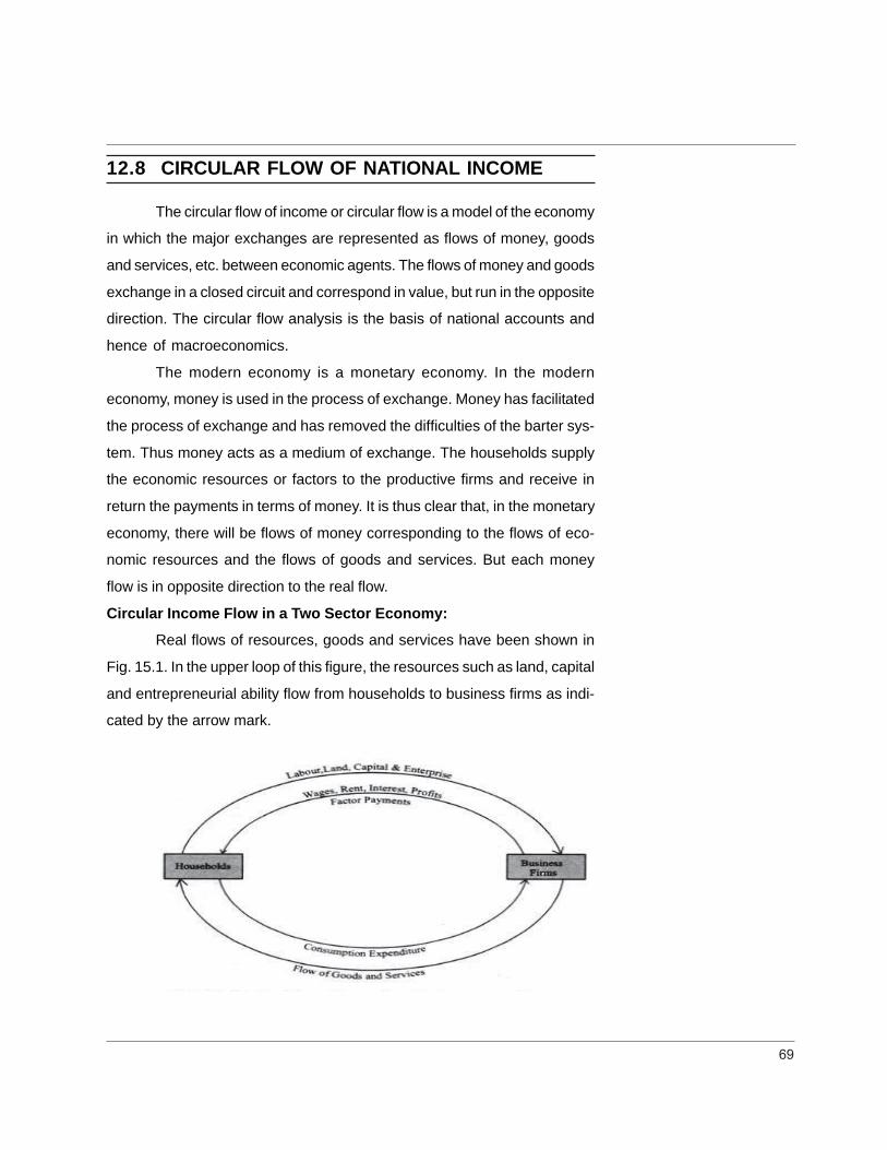
69

12.8 CIRCULAR FLOW OF NATIONAL INCOME

The circular flow of income or circular flow is a model of the economy

in which the major exchanges are represented as flows of money, goods

and services, etc. between economic agents. The flows of money and goods

exchange in a closed circuit and correspond in value, but run in the opposite

direction. The circular flow analysis is the basis of national accounts and

hence of macroeconomics.

The modern economy is a monetary economy. In the modern

economy, money is used in the process of exchange. Money has facilitated

the process of exchange and has removed the difficulties of the barter sys-

tem. Thus money acts as a medium of exchange. The households supply

the economic resources or factors to the productive firms and receive in

return the payments in terms of money. It is thus clear that, in the monetary

economy, there will be flows of money corresponding to the flows of eco-

nomic resources and the flows of goods and services. But each money

flow is in opposite direction to the real flow.

Circular Income Flow in a Two Sector Economy:

Real flows of resources, goods and services have been shown in

Fig. 15.1. In the upper loop of this figure, the resources such as land, capital

and entrepreneurial ability flow from households to business firms as indi-

cated by the arrow mark.

70

In opposite direction to this, money flows from business firms to the

households as factor payments such as wages, rent, interest and profits. In

the lower part of the figure, money flows from households to firms as con-

sumption expenditure made by the households on the goods and services

produced by the firms, while the flow of goods and services is in opposite

direction from business firms to households.

Thus we see that money flows from business firms to households

as factor payments and then it flows from households to firms. Thus there

is, in fact, a circular flow of money or income. This circular flow of money

will continue indefinitely week by week and year by year. This is how the

economy functions. It may, however, be pointed out that this flow of money

income will not always remain the same in volume.

In other words, the flow of money income will not always continue at

a constant level. In the year of depression, the circular flow of money in-

come will contract, i.e., will become lesser in volume, and in years of pros-

perity it will expand, i.e., will become greater in volume.

This is so because the flow of money is a measure of national in-

come and will, therefore, change with changes in the national income. In

year of depression, when national income is low, the volume of the flow of

money will be small and in years of prosperity when the level of national

income is quite high, the flow of money will be large.

In order to make our analysis simple and to explain the central is-

sues involved, we take many assumptions. In the first place, we assume

that neither the households save from their incomes, nor the firms save

from their profits. We further assume that the government does not play

any part in the national economy.

In other words, the government does not receive any money from

the people by way of taxes, nor does the government spend any money on

the goods and services produced by the firms or on the resources and

services supplied by the households. Thirdly, we assume that the economy

neither imports goods and services, nor exports anything.

In other words, in our above analysis we have not taken into account

the role of foreign trade. In fact we have explained above the flow of money

71

that occurs in the functioning of a closed economy with no savings and no

role of government.

12.9 GDP DEFLATOR

The GDP deflator is a tool used to measure the level of price change

over time so that current prices can be accurately compared to historical

prices. That is, it eliminates the effect of price change over time.

There are two variables that are needed to calculate the GDP deflator.

Nominal GDP – which is the Gross Domestic Product (GDP) of the current

year in current prices

Real GDP –which is the Gross Domestic Product (GDP) after it has been

adjusted to reflect the historical changes in prices. The real GDP takes into

consideration the inflation and deflation between the present year and the

year that is being compared. This means that the effect of price changes

are negated so that previous years figures can be compared with current

numbers.

GDP deflator = –––––––––––– x 100

12.10 INDEX NUMBERS: CONCEPT AND USES

Dear learners, you might have often come across situations like

the people making hue and cry over rising prices of goods and commodities.

How do we analyse the rising prices in Economics? What tools do we

use? To analyse the rising prices, rather change in the price levels, we use

the tool ‘index numbers’ in Economics. Index numbers are one of the most

frequently used statistical tools in the field of Economics and other social

sciences. Index numbers represents the ‘state of happening’ in certain

variables like the general price level, the wholesale price level, wage rate of

labours, retail sales volume, wholesale sales volume, export and imports

of a country etc. On such accounts, the index numbers are aptly termed as

‘barometers of economic activity’.

Nominal GDP

Real GDP

72

We can define an index number as a statistical measure designed

to show changes in a variable or a group of related variables with reference

to time, geographic location or other entities like income, profession etc. As

a statistical measure, an index number is calculated as a ratio of the current

value to a base value (also called as reference value) and is expressed in

percentage. It should be kept in mind that the index number is more

commonly called as an index.

Thus, an index number is a statistical device (measure) with a

purpose of showing average changes in one or more related variables (like

price or quantity) between two periods of time (say, between 1991 and 1996)

or two places like cities (say, Delhi and Mumbai) or countries (say, India and

Japan). For example, we may be interested in knowing which city of India

out of Delhi, Mumbai, Kolkata and Chennai is the costliest or the cheapest

in terms of price level. A tourist may be interested in knowing about the cost

of living at different tourist places. Consumer price index number or cost of

living index number helps in taking such decisions.

Let us consider the following table showing the changes in the

wholesale prices of primary articles, manufactured products and

commodities across all categories in India with reference to the price levels

of 1981-82. This means, 1981-82 is the base year prices, i.e., (the index of

prices of 1981-82=100).

Table 12.1: Index Numbers of Wholesale Prices in India

Base year 1981-82 (=100)Period Primary articles Manufacture All commodities

productsJuly, 1992 237.6 222.6 226.6October, 1992 237.1 229.3 232.4January, 1993 235.0 228.6 231.6April, 1993 234.2 231.2 234.6June, 1993 234.9 233.5 237.7

Source: Centre for Monitoring Indian Economy, July, 1993.

From Table 12.1 it can be seen that compared to the 1981-82 price

levels, the price level of primary goods (primary goods comprises food

items, non-food items and minerals) in January, 1993 has increased by

73

234.2 percent or 2.342 times of the 1981-82 price levels of the corresponding

period (i.e., January, 1982).

Thus, we have seen that index numbers give us a comparative

picture over a period of time. This means that index numbers essentially

reflects upon the changes in the variable or the group of related variables

over a period of time. For example, if the index of industrial production was

215.1 in 1992-93 (base year: 1980-81), it means that the industrial production

in that year increased by 2.151 times compared to 1980-81. It should

however be noted that this does not mean that compared to 1980-81, all

the sectors of the industry witnessed similar trend of progress. The index

of 1992-93 reflects an ‘average picture’ of the industrial sector. It does not

necessary imply that all the sectors of the economy witnessed similar

progress. This means that a few sectors of the industrial sectors might

have performed above the average level, while a few might have performed

below that level. According to Croxton and Cowden, “Index numbers are

devices which measures the change in the level of a phenomenon with

respect to time, geographical location or some other characteristics.”

It should be kept in mind that different commodities are measured in

different units. For example, rice and wheat are measured in kilograms,

cloth in meters and milk in liters etc. Index numbers attempt some averages

relating to commodities which are measured in different units. For purpose

of comparison, we are interested in knowing relative changes. These relative

changes are expressed in percentage terms.

Uses of Index Numbers: Index numbers are constructed with

various aims and purposes. Index numbers constructed are put into several

uses. Some of them are described below:

The most commonly used types of index numbers are those that relate

to changes in level in prices of a commodity or a group of commodities.

Such index numbers are price index numbers. Price index numbers

are useful in studying price movements with a view to analyzing their

causes, as well as to determine their effects on the economy. To

determine economic relationships, it is often useful to compare

changes in the market price level with changes in other series, such

74

as gold, bank deposits, bank loans, and the physical volume of

production.

Indices of physical changes over a period of time in production, in

marketing, in sales, in imports and exports, and so on have important

uses. Such index numbers over a period of time are known as index

time series. These index numbers are extremely useful in the study of

the movement of the characteristics over time, in the study of seasonal

and cyclic behaviour, and in the study of business cycles, etc.

Index numbers can be used for forecasting future trend in demand of

commodities or in volume of production etc. Index numbers of industrial

and agricultural production not only reflect the trend but also are useful

in forecasting production. Index numbers of unemployment which

reflect the trend of unemployment are useful in determining factors

leading to unemployment and in forecasting future trends.

Index numbers which reflect the general price level, and in particular,

the consumer price index numbers are useful in determining the

quantum of additional wages or dearness allowances to compensate

for the changes in the cost of living. The Government of India and

most of the State Governments have index linked formulae for grant of

dearness allowances to their employees.

The changes in consumer price index can be used to determine the

real income over a period. Suppose that a person's income in 1980

was 150 times than that in 1970, that is, there is an increase of 50% in

money income. Suppose that the cost of living index number in 1980

was 175 times than that in 1970, that is, there is an increase of 75%.

Then the person's real income in 1980 is %7.85175150

of his income

in 1970. Thus index numbers are useful in determining the real income.

75

CHECK YOUR PROGRESS

Q3: State whether the following statements are

True (T) or False (F).

(i) Index numbers are specialized averages to measure relative

changes. (T/F)

(ii) Index numbers measure net change in related variables over

time. (T/F)

(iii) Simple index numbers require weights in their construction.

(T/F)

(iv) Index numbers do not indicate the trend of change in the

economy. (T/F)

Q4: Fill in the blanks:

(i) Index number is a statistical device to express ................. change

in related variable.

(ii) An index number is a .......................... average.

12.11 CONSTRUCTION OF SIMPLE INDEX NUMBERS

In general we are interested in general price level rather than on the

price level of any particular item. So we have to consider a number of items

at the same time. If each commodity is of different qualities then all such

qualities have also to be taken into consideration. We have to consider

simultaneously a number of items or commodities together for measuring

change in price or production.

The sources of data must be reliable and care should be taken in

selecting the sources of data. For example, official publications as well as

other reliable unofficial reports from producers and merchants should be

considered for computing index for production. If retail food prices are being

considered, then prices in stores, not in wholesale markets, are to be taken

into consideration.

Now we shall discuss how to construct simple index numbers from

a given set of data, like prices of certain commodities, production of certain

commodities etc.

76

There are two methods of constructing simple index numbers. These

are:

Simple aggregate method and

Method of simple average of relatives.

Remember that all items in a simple index number are assigned

equal weights. These are unweighted index numbers.

Simple Aggregate Method: In this case each item is given equal weights.

If we give an equal weight to each item it means the same thing, whether

each item is given a weight or not. It is the simplest method of

constructing index numbers.

Simple aggregate method to find price index numbers: We use the

following three steps to find price index number.

Step 1: Find the sum of the current year (that is, given period) prices of

all the items included in the list. If 1 denote the current year, then find

1p .

Step 2: Find the sum of the base year prices of all the items included in

the list. If 0 denote the base year, then find 0p .

Step 3: Use the formula .1000

110 p

pp

Exercise 1: Find the price index number, using simple aggregate method,

for the following information.

Prices (in Rupees)

Commodities Units 2000 2005

Wheat Quintal 800 1200

Rice Quintal 1200 1600

Milk Litres 12 18

Tea Kilograms 100 120

Clothing Metres 30 40

Meat Kilograms 80 120

Solution: Represent prices of 2005 (current year) as 1p and that of

2000 (base year) as 0p and reconstruct the table as follows:

77

Commodities p0 p1

Wheat 800 1200

Rice 1200 1600

Milk 12 18

Tea 100 120

Clothing 30 40

Meat 80 120

22220p 30981p

Therefore, the price index of 2005 with base year 2000 is:

4.13910022223098

10p

Thus the increase in prices (or price level) is 139.40 - 100 = 39.4%.

Exercise 2: The prices of three commodities A, B and C increased from

Rs.50, Rs.7 and Rs.3 in 2005 to Rs.52, Rs.8 and Rs.5 respectively in 2006.

Using the simple aggregate method, find by how much on an average the

prices have increased?

Solution: We know construct the following table:

Commodities Price in 2005 (p0 ) Price in 2006 ( p1)

A 50 52

B 7 8

C 3 5

600p 651p

Therefore, the price index of 2006 with respect to the base period 2005 is:

33.1081006065100

0

120062005 p

pp

This shows that the price index of current year 2006 with respect to base

year 2005 is 108.33%. Hence the price increase in one year is 108.33 - 100

= 8.33%.

Simple aggregate method to find quantity index numbers: We use

the following three steps to find quantity index number.

Step 1: Find the sum of the current year (that is, given period) quantity

or volume produced, consumed or transacted of all the items included

in the list. If 1 denote the current year, then find 1q .

78

Step 2: Find the sum of the base year quantity or volume produced,

consumed or transacted of all the items included in the list. If 0 denote

the base year, then find 0q .

Step 3: Use the formula .1000

110 q

qq

Method of Simple Average of Relatives: In this method, average of

the relatives is obtained by using any one of the measures of central

tendency. In particular, here we shall use arithmetic mean for averaging

the relatives. We shall discuss briefly this method only for price relatives.

Similar formulas on quantity index number and value index number can

be obtained considering quantity and value relatives instead of price

relative. There are few questions to find quantity and value index numbers

in the section "Possible Questions". You should work out those problems

with the help of the problems on price index numbers which are solved

below.

Method of Simple Average of Price Relatives:

We know that a price relative is nothing but the ratio of current year

prices to those in the base year. Taking the arithmetic mean of the price

relatives, we get the following formula for price index number:

Npp

p100

0

1

10

where N stands for number of commodities included in the index numbers.

Steps to calculate price index numbers by Simple Average of Price Relatives

Method:

Step 1: Find percentage price relative for each commodity, that is, 1000

1

pp

Step 2: Find the sum of these percentage price relatives, that is,

1000

1

pp

.

79

Step 3: Divide 1000

1

pp

by the total number of commodities included

in the list.

Exercise 3: Give the solution of Exercise 1 using the Simple Average of

Price Relatives.

Solution: We construct the following table:

Sl Commo- Units Prices Price Relative

No. dities (in Rupees) 1000

1

pp

2000 p0 2005 p1

1 Wheat Quintal 800 1200 00.150100800

1200

2 Rice Quintal 1200 1600 33.13310012001600

3 Milk Litres 12 18 00.1501001218

4 Tea Kilograms 100 120 00.120100100120

5 Clothing Metres 30 40 33.1331003040

6 Meat Kilograms 80 120 00.15010080

120

N = 6 66.8361000

1

pp

Hence, the price index number of 2005 with respect to base year 2000 is:

.44.1396

66.836100

0

1

10 Npp

p

80

Exercise 4: Give the solution of Exercise 2 using the Simple Average of

Price Relatives.

Solution: We first prepare the following table:

Sl No. Commo-dities Prices (in Rupees) Price Relative

2005 p0 2006 p1 100pp

0

1

1 A 50 52 104.001005052

2 B 7 8 29.14110078

3 C 3 5 66.66110035

N=3 95.384100pp

0

1

Hence, the price index number of 2006 with respect to base year 2005 is:

.32.1283

95.384100

0

1

10 Npp

p

12.12 CONSTRUCTION OF WEIGHTED INDEX NUMBERS

In weighted index number each item is given weight according to

the importance it occupies in the list. There are two groups of methods to

calculate index number of this category: (a) Weighted aggregate method

and (b) Weighted average of price relative methods. In this unit, we will

study three types of weighted aggregate method. These methods are

popularly known as (1) Laspeyre's Method, (2) Paasche's Method and (3)

Fisher's Method. All the methods are used to calculate weighted index

numbers. The main difference between the Laspeyre's Method and

Paasche's Method is that Laspeyre's uses base year quantities of

commodities as their relative weights, while Paasche's uses current year

quantities of commodities as their relative weights for preparing a price index.

81

12.12.1 Laspeyre's Index Number

Laspeyre's Price Index Number: It uses base year quantities as

the weights. Accordingly, the formula is

10000

01

qpqpPL

Laspeyre's Quantity Index Number: If we multiply the quantities by

the base year price, then we get Laspeyre's quantity index number.

Accordingly the formula for Laspeyre's quantity index number is:

10000

01

pqpqQL

Steps to Calculate Weighted Index Number by Laspeyre's Method:

Step 1: Multiply current year price )( 1p with the base year quantity

)( 0q to get 01qp for each item/ commodity.

Step 2: Multiply base year price )( 0p with the base year quantity to

get 00qp for each item/ commodity.

Step 3: Add all 01qp and 00qp separately to get 01qp and 00qp .

Step 4: Divide 01qp by 00qp and multiply by 100 to obtain

Laspeyre’s price index number.

Exercise 5: Find Laspeyre's price index number from the following

data.

Price (in Rs) Quantity bought in units

Commodity 1995 1996 1995 1996

A 50 52 10 12

B 7 9 3 4

C 3 5 7 6

Solution: Represent prices and quantities in current year by 1pand 1q respectively and represent prices and quantities in base

year by 0p and 0q respectively. Let us construct the following table

following the steps 1-3.

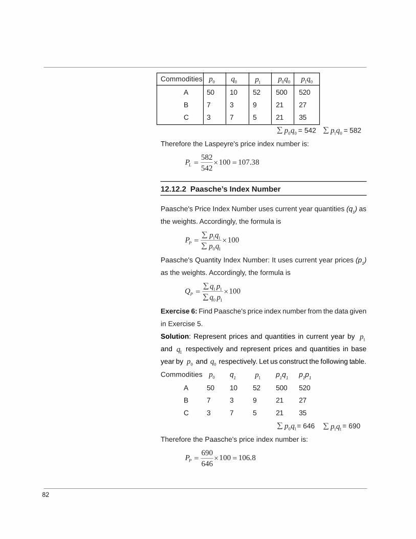
82

Commodities 0p 0q 1p 00qp 01qp

A 50 10 52 500 520

B 7 3 9 21 27

C 3 7 5 21 35

00qp = 542 01qp = 582

Therefore the Laspeyre's price index number is:

38.107100542582

LP

12.12.2 Paasche’s Index Number

Paasche's Price Index Number uses current year quantities (q1) as

the weights. Accordingly, the formula is

10010

11

qpqpPP

Paasche's Quantity Index Number: It uses current year prices (p1)

as the weights. Accordingly, the formula is

10010

11

pqpqQP

Exercise 6: Find Paasche's price index number from the data given

in Exercise 5.

Solution: Represent prices and quantities in current year by 1pand 1q respectively and represent prices and quantities in base

year by 0p and 0q respectively. Let us construct the following table.

Commodities 0p q1 1p p1q1 p1p1

A 50 10 52 500 520

B 7 3 9 21 27

C 3 7 5 21 35

10qp = 646 11qp = 690

Therefore the Paasche's price index number is:

8.106100646690

PP

83

Remark: You have noticed that the value of Laspeyre's index number

(107.38) and the value of Paasche's index number (106.8) are

different for the same data. The difference has arisen because of

differences in weights.

12.12.3 Fisher’s Index Number

The Fisher's price index number is nothing but the geometric mean

of the Laspeyre's and Paasche's price index numbers. Hence the

formula for Fisher's price index number is:

)1(100

100100

10

11

00

01

10

11

00

01

qpqp

qpqp

qpqp

qpqpPPP PLF

Similarly, the Fisher's quantity index number is given by:

)2(100

100100

10

11

00

01

10

11

00

01

pqpq

pqpq

pqpq

pqpqQQQ PLF

Exercise 7: Find Fisher's price index number from the data given in

Exercise 5.

Solution: We have already found that for the given data,

38.107LP and 8.106PP .

Hence the Fisher's price index number is:

09.1078.10638.107FP

84

CHECK YOUR PROGRESS

Q 5: State whether the following statements are

true (T) or False (F).

(i) There are two types of index numbers: simple or unweighted

and weighted index numbers.(T / F)

(ii) There are two methods of constructing simple index

numbers: simple aggregate method and simple average

relatives. (T / F)

(iii) We the same index number whether we use simple

aggregate method or simple average of price relatives'

method. (T / F)

(iv) Laspeyre's uses current year quantities as weights. (T / F)

(v) Paasche's uses base year quantities as weights. (T / F)

Q 6: Fill up the blanks.

(i) In Laspeyre's method of finding price index number we use

........................ quantities as weights.

(ii) In Paasche's method of finding price index number we use

.......................... quantities as weights.

(iii) 10000

01

qpqpI is ........................ weighted index number.

(iv) 10010

11

qpqpI is ........................ weighted index number

12.13 BASE SHIFTING, SPLICING AND DEFLATING

In this section, we shall briefly discuss the concepts of base shifting,

splicing and deflating.

Base Shifting: In Statistics, we often require to change the reference

base of an index number series from one time period to another without

returning to the original raw data and recomputing the eniture series. The

change in reference base period is usually referred to as ‘base shifting’.

85

ACTIVITY 12.1The Ministry of Statistics, Government of India has

changed the base for the calculation of GDP from time

to time. Undertake an exercise on tracking such

changes since 1990.

---------------------------------------------------------------------

--------------------------------------------------------------------------------------

--------------------------------------------------------------------------------------

--------------------------------------------------------------------------------------

--------------------------------------------------------------------------------------

Base shifting is undertaken for two important reasons. a) The

previsous base (i.e., the base year currently in practice) has become too

old is not much relevant for making comparision in the present times. By

shifting the series, the series is presented to be ‘current’ and more relevant

to the present times. b) When different data are presented for comparision

pertaining to the different time periods, it becomes necessary to first make

them comparable with the ‘time’ dimension. For example, it would be

irrevalent to compare the GDP estimates of a country of 1850, 1920, 1950

and 2010 without any statistical treatment. For making the comparision

effective, the data must be first worked out to one base year (say, 2010).

This is particularly important when we compare them in one single graph.

Splicing: Splicing means combining two or more series of

overlapping index numbers to obtain a single index number on a common

base. Sometimes, a series of index numbers is available for a period of

time, which has been substantially revised including shifting of the base

year. It may also happen that the weights assigned to the series have become

out dated. As such, new weights may be assigned and the series is worked

out anew. In such cases, two series would result, the old one and the new

one. Now, it may become necessary to convert the two series into one

continuous series. This is done with the help of splicing.

Splicing can be done only if the index numbers are constructed with

86

the same items and have an overlapping year. Splicing like base shifting will

give accurate result of the index numbers, use simple geometric mean and

satisfy the circular test. In splicing of index numbers, we find a common

factor by which the spliced index number series is multiplied to get a common

base.

Deflating: Deflating means adjusting, correcting or reducing a value

which is inflated. Thus, in defilating, we make adjustments for the effect of

changing price levels. You know that a rise in price levels essentially reduces

the real purchasing power of money. So, to compare the value of money (or

its purchasing power), in different time peirods, we need to adjust the rate

of inflation during the given peirod. This is done through deflating. Deflating

is a technique of converting a series of values calculated at current prices

into constant prices of a given year. This is particularly desirable in the case

of an economy which has inflationary trends because in such an economy,

the increase in the prices of commodities over a period of years means a

fall in their real incomes. For example, a rise in money income may not

amount to a rise in real income. As such, it becomes necessary to adjust or

correct nominal wages in accordance with the rise in the corresponding

price index to arrive at the real income. The purchasing power is given by

the reciprocal of the index number and consequently the real income is

obtained on dividing the money or nominal income by the corresponding

appropriate price index and multiplying the result by 100.

12.14 LET US SUM UP

National Income means the total income of the nation, The aggregate

economic performance of the whole economy is measured by the

national income data.

National Income refers to the money value of all final goods and

services produced by the normal residents of a country while

working both within or outside the domestic territory of a country

in an accounting year.

87

National Income also includes net factor income from abroad.

Keynes has suggested three approaches to national income :

(1) Income - expenditure approach : According to this approach, national

income is equal to total expenditure on consumption and investment

goods.

(2) Factor - income approach : According to this approach, national

income is measured as the aggregate of incomes received by all

the factors of production.

(3) Sales proceeds minus cost approach : According to this approach,

national income is defined as the aggregate sales proceeds minus

cost.

Modern economists consider three aspects of national income and

emphasise the fundamental identity between these three aspects.

These three aspects are : (a) product aspect (b) income aspect,

and (c) expenditure aspect.

When we add the net factor income from abroad to the figure of

GDP we get the Gross National Product of the country.

NNP of a country is its GNP less depreciation.

Per Capita Income is a measure of the amount of money that is

being earned per person in a certain area.

Transfer payments are those payments that do not correspond to

any productive work.

Personal Disposable Income is that portion of the personal income

of the residents of the country that is at its command or disposal.

Factor income earned by the private enterprises and workers within

the domestic territory and foreign countries and current transfers

from government and net transfers from outside the country

constitute the Private Income of the residents of a country.

The study of national income statistics is very important. It helps

in analysing the actual performance of the economy and in preparing

future policies.

Index number is a statistical measure or device with a purpose of

showing average change in one or more related variables over

88

time and space.

Price index numbers are more commonly used. It measures relative

changes in prices over a time period.

We can have either simple or weighted index number. Simple index is

also called unweighted index number or index number with equal weights.

In this unit, we have discussed about the simple index numbers as well

as weighted index number.

We have learnt about two methods of constructing simple index

numbers: Simple aggregate method and Method of simple average of

relatives. The formula to find index number using simple aggregate

method is given by .1000

110 p

pp

Again, the formula to find price index number using the method of simple

averages of relatives is given by N

pp

p100

0

1

10 .

We have also leant about weighted index numbers. There are two groups

of methods to calculate index number of this category: (a) Weighted

aggregate method and (b) Weighted average of price relative methods.

We briefly discussed about three types of weighted aggregate method.

These methods are popularly known as (1) Laspeyre's Method, (2)

Paasche's Method and (3) Fisher's Method.

We have also learnt about the test of adequacy of index numbers. We

mentioned three properties that a good index number should have.

Fisher's index number satisfies both the time reversal and factor reversal

tests and hence it is known as Fisher's Ideal Index Number.

89

12.15FURTHER READING

1) NCERT (2007) : Introductory Macroeconomics (Textbook in

Economics for Class XII), New Delhi.

2) Bakerman, W. (1993) : An Introduction to National Income Analysis,

3rd Ed., New Delhi: Universal Book Stall.

3) Rana, K.C. & Verma, K.N. (2009). Macroeconomic Analysis, Jalandhar:

Vishal Publications.


Ans. to Q No. 1: National Income means the total income of the nation,

The aggregate economic performance of the whole economy is

measured by the national income data.

National Income refers to the money value of all final goods and

services produced by the normal residents of a country while working

both within or outside the domestic territory of a country in an

accounting year. National Income also includes net factor income

from abroad.

Ans. to Q No. 2: Keynes has suggested three approaches to national

income :

(1) Income - expenditure approach : According to this approach,

national income is equal to total expenditure on consumption

and investment goods.

(2) Factor - income approach : According to this approach, national

income is measured as the aggregate of incomes received by

all the factors of production.

(3) Sales proceeds minus cost approach : According to this

approach, national income is defined as the aggregate sales

proceeds minus cost.

Ans to Q No 3: (i) True (ii) True (iii) False (iv) False

Ans to Q No 4: (i) average (ii) specialized

90

Ans to Q No 5: (i) True (ii) True (iii) False (iv) False

(v) False

Ans to Q No 6: (i) base year (ii) current year (iii) Laspeyre's (iv) Paasche’s


Q1: What is meant by national income? State briefly the Keynesian

approach to national income.

Q2: Distinguish between:

(a) Gross National Product and Net National Product

(b) National Income at Market Prices and National Income at Factor

Cost.

(c) Personal Income and Personal Disposable Income.

(d) Traditional Approach and Modern Approach of national income

Q3: Explain the following concepts

(a) National Income.

(b) Personal Income.

(c) Disposable Income.

(d) Value Added Method.

Q 4: Discuss the modern approach to national income. Can we say it

as an improvement over the traditional approach. Give reasons.

Q 5: Discuss the importance of national income.

Q 6: Explain the meaning of an index number and its main characteristics.

Q 7: "Index numbers are economic barometers". Why are index numbers

so called? Explain.

Q 8: Explain the method of construction of unweighted index numbers by

Simple Aggregate Method.

Q 9: Explain the method of construction of unweighted index numbers by

Simple Aggregate of Price Relative Method.

Q 10: The exchange rate of a US dollar was Rs.44.00 in July 2008 and

was Rs.50.00 in February 2009. Find the price relative.

Q 11: The production of rice in Assam in the month of January 2008 was

91

3608 tonnes and that in February 2009 was 3700 tonnes. Find the

quantity relative.

Q 12: The following table shows the prices of the commodities consumed

in 1970 and 1978.

1970 1978

Commodities Unit Price (Rs) Price (Rs)

A kilogram 4.00 4.60

B litre 8.00 8.75

C metre 7.00 8.00

D kilogram 14.00 16.00

E litre 3.00 4.00

Find the price index number using:

(a) simple aggregate method

(b) method of simple aggregate of price relatives.

Q 13: The production of rice, milk, cloth, wheat and petrol are given in the

following table. Taking 1980 as base year, compute quantity index number

using:


(b) method of simple aggregate of quantity relatives.

Quantity produced

Commodities Unit 1980 1990

Rice kilogram 400000 700000

Milk litre 800000 905000

Cloth metre 100000 105000

Wheat kilogram 140000 160000

Petrol litre 300500 400000

Q 14: What do you mean by tests of index numbers?

Q 15: Explain the important criterion or test that a good index number

should satisfy.

Q 16: The prices and quantity of five commodities are given in the following

table. Taking 2000 as base year, compute value index number using:


(b) method of simple aggregate of value relatives.

92

Comm- 2000 2002

odities Price (Rs) Quantity (Kg) Price (Rs) Quantity (Kg)

A 400 10 700 12

B 800 15 1905 17

C 100 5 125 5

D 140 7 160 7

E 300 6 400 6

Q 17: Find Laspeyre's and Paasche's price and quantity index number from

the following data. Also find the Fisher's price and quantity index

numbers.

Base year Current year

Commo- Price (Rs) Quantity (kg) Price (Rs) Quantity (kg)

dities p0 q0 p1 q1

A 5 25 6 30

B 10 5 15 4

C 3 40 2 50

D 6 30 8 35

Q 18: The following table shows the price quantity of the commodities

consumed in 2000 and 2006.

Commo- 2000 2006

dities Price (Rs) Quantity (kg) Price (Rs) Quantity (kg)

I 400 35 460 35

II 800 10 1000 10

III 300 15 50 12

IV 4000 10 5000 8

V 50 20 300 20

Find the following index numbers.

(1) Laspeyre's Price and Quantity index numbers.

(2) Paasche's Price and Quantity index numbers.

(3) Fisher's Price and Quantity index numbers.

*** ***** ***

Bachelor of Business Administration (BBA) BBA-3 - e-Gyanagar

Documents

Transcript of Bachelor of Business Administration (BBA) BBA-3 - e-Gyanagar