BACC Assessment of Climate Change in the Baltic Sea Basin
496
Regional Climate Studies Series Editors: H.-J. Bolle, M. Menenti, I. Rasool
Transcript of BACC Assessment of Climate Change in the Baltic Sea Basin

Regional Climate Studies
Series Editors: H.-J. Bolle, M. Menenti, I. Rasool

The BACC Author Team
Assessment of Climate Changefor the Baltic Sea Basin
123

The BACC Author TeamThe International BALTEX SecretariatGKSS-ForschungszentrumGeesthacht GmbHMax-Planck-Str. 1D-21502 [email protected]
ISBN: 978-3-540-72785-9 e-ISBN: 978-3-540-72786-6
Regional Climate Studies ISSN: pending
Library of Congress Control Number: 2007938497
c© 2008 Springer-Verlag Berlin Heidelberg
This work is subject to copyright. All rights are reserved, whether the whole or part of the material is concerned, specifically the rights oftranslation, reprinting, reuse of illustrations, recitation, broadcasting, reproduction on microfilm or in any other way, and storage in databanks. Duplication of this publication or parts thereof is permitted only under the provisions of the German Copyright Law of September9, 1965, in its current version, and permission for use must always be obtained from Springer. Violations are liable to prosecution under theGerman Copyright Law.
The use of general descriptive names, registered names, trademarks, etc. in this publication does not imply, even in the absence of a specificstatement, that such names are exempt from the relevant protective laws and regulations and therefore free for general use.
Cover design: deblik, Berlin
Printed on acid-free paper
9 8 7 6 5 4 3 2 1
springer.com

Preface
Climate change and its impact on our life, our en-vironment and ecosystems in general, are in thesedays at the forefront of public concern and polit-ical attention. The Intergovernmental Panel onClimate Change (IPCC) reports have amply doc-umented that anthropogenic climate change is anongoing trend, which will continue into the futureand may be associated with grave implications.Thus, one conclusion to be drawn is clear – thedriver for this climate change should be curtailedto the extent socially responsible and sustainable.We need to strongly reduce the emissions of radia-tively active gases into the atmosphere.
However, even the most optimistic emission re-duction scenarios envision only a limited success inthwarting climate change. What is possible is tolimit this change, but it can no longer be avoidedaltogether. Even if the challenging goal of a sta-bilization of global mean temperature at an upperlimit of 2 C above pre-industrial levels at the endof this century will be met, significant pressureson societies and ecosystems for adaptation will bethe result. Thus, adaptation to recent, ongoingand possible future climate change is unavoidable.
The BACC initiative has dealt with these pres-sures for the region of the Baltic Sea Basin, whichincludes the Baltic Sea and its entire water catch-ment, covering almost 20% of the European conti-nent. BACC has collected, reviewed and summa-rized the existing knowledge about recent, ongoingand possible futures regional climate change andits impact on marine and terrestrial ecosystemsin this region. The acronym BACC stands forBALTEX Assessment of Climate Change for theBaltic Sea Basin and denotes an initiative withinBALTEX (Baltic Sea Experiment), which is aRegional Hydrometeorology Project within the
Hans von Storch (Chairman)
Global Energy and Water Cycle Experiment(GEWEX) of the World Climate Research Pro-gram (WCRP).
The first chapter of the book places the initia-tive in context, clarifies a few key concepts andsummarizes the key results; Chapters 2 to 5 doc-ument the knowledge about recent and ongoingchanges in meteorological, oceanographical, hy-drological and cryospherical variables, about sce-narios of possible future climatic conditions, aboutchanges in terrestrial and freshwater ecosystems,and about changes in marine ecosystems. A seriesof appendices provide background material rele-vant in this context.
Two remarkable aspects of the BACC initia-tive should be mentioned. The first is the accep-tance of this report by the Helsinki Commission(HELCOM) as a basis for its intergovernmentalmanagement of the Baltic Sea environment. Basedon this BACC report, HELCOM has compiled itsown conclusions “Climate Change in the Baltic SeaArea – HELCOM Thematic Assessment in 2007”.The second aspect is the fact that the BACC re-port was made possible by the voluntary effort ofmany individuals and institutions – without ded-icated payment from scientific agencies, govern-ments, NGOs, industries or other possibly vestedinterests. We think this adds significantly to thecredibility of this effort, which we expect will beused as a blueprint for assessments of other regionsin the world.
The success of BACC has convinced BALTEXthat it would be worth to redo the effort in aboutfive years time – assuming that significantly moreknowledge has been generated, and that climatechange has emerged even more clearly from the“sea of noise” of natural climate variability.
V


The BACC Author Team
The BACC Author Team consists of more than 80 scientists from 13 countries, covering various disci-plines related to climate research and related impacts. Each chapter of the book is authored by one tofour lead authors and several contributing authors. While the former established the overall conception,did much of the writing and are largely responsible for the assessment parts of the chapters, the lattercontributed pieces of information of various extent to the contents of the book. In order to highlightthe teamwork character of this book, both lead and contributing authors of each chapter are mentionedas an author group at the beginning of each chapter, rather than attributing individual section or textcontributions to individual contributing authors. Lead authors are mentioned first followed by con-tributing authors, ordered alphabetically. The authors of annexes, by contrast, are named individuallyon top of each annex, section or sub-section within the annex part.
The following authors list firstly gives the lead authors of Chaps. 1 to 5, followed by an alphabeticallyordered list of all other contributing and annex authors.
Lead Authors
Chapter 1: Introduction and Summary
Hans von StorchInstitute for Coastal Research, GKSS Research Centre Geesthacht, Germany
Anders OmstedtEarth Sciences Centre – Oceanography, Göteborg University, Sweden
Chapter 2: Past and Current Climate Change
Raino HeinoFinnish Meteorological Institute, Helsinki, Finland
Heikki TuomenvirtaFinnish Meteorological Institute, Helsinki, Finland
Valery S. VuglinskyRussian State Hydrological Institute, St. Petersburg, Russia
Bo G. GustafssonEarth Sciences Centre – Oceanography, Göteborg University, Sweden
Chapter 3: Projections of Future Anthropogenic Climate Change
L. Phil GrahamRossby Centre, Swedish Meteorological and Hydrological Institute, Norrköping, Sweden
Chapter 4: Climate-related Change in Terrestrial and Freshwater Ecosystems
Benjamin SmithDepartment of Physical Geography and Ecosystems Analysis, Lund University, Sweden
VII

VIII The BACC Author Team
Chapter 5: Climate-related Marine Ecosystem Change
Joachim W. DippnerBaltic Sea Research Institute Warnemünde, Germany
Ilppo VuorinenArchipelago Research Institute, University of Turku, Finland
Contributing Authors
Anto AasaInstitute of Geography, University of Tartu, Estonia
Rein AhasInstitute of Geography, University of Tartu, Estonia
Hans AlexanderssonSwedish Meteorological and Hydrological Institute, Norrköping, Sweden
Philip AxeOceanographic Services, Swedish Meteorological and Hydrological Institute, Västra Frolunda, Sweden
Lars BärringRossby Centre, Swedish Meteorological and Hydrological Institute, Norrköping, Sweden; andDepartment of Physical Geography and Ecosystems Analysis, Lund University, Sweden
Svante BjörckDepartment of Geology, GeoBiosphere Science Centre, Lund University, Sweden
Thorsten BlencknerDepartment of Ecology and Evolution, Erken Laboratory, Uppsala University, Sweden
Agrita BriedeDepartment of Geography, University of Latvia, Riga, Latvia
Terry V. CallaghanAbisko Scientific Research Station, Royal Swedish Academy of Sciences, Abisko, Sweden; andDepartment of Animal and Plant Sciences, University of Sheffield, UK
John CappelenData and Climate Division, Danish Meteorological Institute, Copenhagen, Denmark
Deliang ChenEarth Sciences Centre, Göteborg University, Sweden
Ole Bøssing ChristensenDanish Climate Centre, Danish Meteorological Institute, Copenhagen, Denmark
Gerhard DahlmannFederal Maritime and Hydrographic Agency, Hamburg, Germany
Darius DaunysCoastal Research and Planning Institute, University of Klaipeda, Lithuania
Jacqueline de ChazalDepartment of Geography, Catholic University of Louvain, Louvain-la-Neuve, Belgium

The BACC Author Team IX
Jüri ElkenMarine Systems Institute, Tallinn University of Technology, Estonia
Malgorzata FalarzDepartment of Climatology, University of Silesia, Sosnowiec, Poland
Juha FlinkmanFinnish Institute of Marine Research, Helsinki, Finland
Eirik J. FørlandDepartment of Climatology, Norwegian Meteorological Institute, Oslo, Norway
Jari HaapalaFinnish Institute of Marine Research, Helsinki, Finland
Lars HåkansonDepartment of Hydrology, Uppsala University, Sweden
Antti HalkkaDepartment of Biological and Environmental Sciences, University of Helsinki, Finland
Marianne HolmerInstitute of Biology, University of Southern Denmark, Odense, Denmark
Christoph HumborgDepartment of Applied Environmental Science, Stockholm University, Sweden
Hans-Jörg IsemerInternational BALTEX Secretariat, GKSS Research Centre Geesthacht, Germany
Jaak JaagusInstitute of Geography, University of Tartu, Estonia
Anna-Maria JönssonDepartment of Physical Geography and Ecosystems Analysis, Lund University, Sweden
Seppo KellomäkiFaculty of Forest Sciences, University of Joensuu, Finland
Lev KitaevInstitute of Geography, Russian Academy of Sciences, Moscow, Russia
Erik KjellströmRossby Centre, Swedish Meteorological and Hydrological Institute, Norrköping, Sweden
Friedrich KösterDanish Institute for Fisheries Research, Technical University of Denmark, Lyngby, Denmark
Are KontEstonian Institute of Ecology, University of Tartu, Estonia
Valentina KrysanovaDepartment of Global Change and Natural Systems, Potsdam Institute for Climate Impact Research,Potsdam, Germany
Ain KullInstitute of Geography, University of Tartu, Estonia
Esko KuusistoFinnish Environment Institute, Helsinki, Finland

X The BACC Author Team
Esa LehikoinenDepartment of Biology, University of Turku, Finland
Maiju LehtiniemiFinnish Institute of Marine Research, Helsinki, Finland
Göran LindströmResearch and Development – Hydrology, Swedish Meteorological and Hydrological Institute,Norrköping, Sweden
Brian R. MacKenzieDanish Institute for Fisheries Research, Technical University of Denmark, Charlottenlund, Denmark
Ülo ManderInstitute of Geography, University of Tartu, Estonia
Wolfgang MatthäusBaltic Sea Research Institute Warnemünde, Germany
H.E. Markus MeierResearch and Development – Oceanography, Swedish Meteorological and Hydrological Institute,Norrköping, Sweden; and Department of Meteorology, Stockholm University, Sweden
Mirosław MiętusDepartment of Meteorology and Climatology, University of Gdańsk, Poland; andInstitute of Meteorology and Water Management – Maritime Branch, Gdynia, Poland
Anders MobergDepartment of Physical Geography and Quaternary Geology, Stockholm University, Sweden
Flemming MøhlenbergDHI – Water · Environment · Health, Hørsholm, Denmark
Christian MöllmannInstitute for Hydrobiology and Fisheries Science, University of Hamburg, Germany
Kai MyrbergFinnish Institute of Marine Research, Helsinki, Finland
Tadeusz NiedźwiedźDepartment of Climatology, University of Silesia, Sosnowiec, Poland
Peeter NõgesInstitute for Environment and Sustainability, European Commission, Joint Research Centre, Ispra,Italy
Tiina NõgesInstitute of Agricultural and Environmental Sciences, Estonian University of Life Sciences, Tartu,Estonia
Øyvind NordliNorwegian Meteorological Institute, Oslo, Norway
Sergej OleninCoastal Research and Planning Institute, Klaipeda University, Lithuania
Kaarel OrvikuMerin Ltd, Tallinn, Estonia

The BACC Author Team XI
Zbigniew PruszakInstitute of Hydroengineering, Polish Academy of Sciences, Gdansk, Poland
Maciej RadziejewskiFaculty of Mathematics and Computer Science, Adam Mickiewicz University, Poznan, Poland; andResearch Centre of Agriculture and Forest Environment, Polish Academy of Sciences, Poznan, Poland
Jouni RäisänenDivision of Atmospheric Sciences, University of Helsinki, Finland
Egidijus RimkusDepartment of Hydrology and Climatology, Vilnius University, Lithuania
Burkhardt RockelInstitute for Coastal Research, GKSS Research Centre Geesthacht, Germany
Mark RounsevellSchool of Geosciences, University of Edinburgh, UK
Kimmo RuosteenojaFinnish Meteorological Institute, Helsinki, Finland
Viivi RussakAtmospheric Physics, Tartu Observatory, Estonia
Ralf ScheibeGeographical Institute, University of Greifswald, Germany
Doris SchiedekBaltic Sea Research Institute Warnemünde, Germany
Corinna SchrumGeophysical Institute, University of Bergen, Norway
Henrik SkovDHI – Water · Environment · Health, Hørsholm, Denmark
Mikhail SofievFinnish Meteorological Institute, Helsinki, Finland
Wilhelm SteingrubeGeographical Institute, University of Greifswald, Germany
Ülo SuursaarEstonian Marine Institute, University of Tartu, Estonia
Piotr TryjanowskiDepartment of Behavioural Ecology, Adam Mickiewicz University, Poznan, Poland
Timo VihmaFinnish Meteorological Institute, Helsinki, Finland
Norbert WasmundBaltic Sea Research Institute Warnemünde, Germany
Ralf WeisseInstitute for Coastal Research, GKSS Research Centre Geesthacht, Germany

XII The BACC Author Team
Joanna WibigDepartment of Meteorology and Climatology, University of Łódź, Poland
Annett WolfCentre for Geobiosphere Science, Lund University, Sweden

Acknowledgements
The BACC Author Team appreciates the workof the BACC Science Steering Committee (SSC)which contributed in various ways to the projectby giving advice, providing material and review-ing parts of earlier manuscript versions. BACCSSC members include Sten Bergström, SwedishMeteorological and Hydrological Institute, Nor-rköping, Sweden; Jens Hesselbjerg Christensenand Eigil Kaas, both at Danish MeteorologicalInstitute, Copenhagen, Denmark; Zbigniew W.Kundzewicz, Research Centre for Agricultural andForest Environment, Polish Academy of Sciences,Poznan, Poland; Jouni Räisänen, Helsinki Uni-versity, Finland; Markku Rummukainen, SwedishMeteorological and Hydrological Institute, Nor-rköping, Sweden; Morten Søndergaard, Copen-hagen University, Denmark; and Bodo von Bodun-gen, Baltic Sea Research Institute Warnemünde,Germany.
An in-depth review of the main book chapterswas conducted by several independent evaluatorsas part of the BACC process which improved thebook material significantly. We highly appreciatethis valuable contribution to BACC.
The BACC project benefited from countlesscomments by many scientists on earlier versionsof the book’s manuscript. The BACC Conferenceheld at Göteborg University in May 2006, wherea first version of the material had been presentedfor discussion to the scientific community and theinterested public, was highly instrumental in fos-tering improvement of the BACC material and theBACC Author Team likes to express its gratitudeto all who participated actively at the Conferenceand for all helpful comments received.
We thank Hartmut Graßl in his capacity as theformer BALTEX Scientific Steering Group chair-man for initiating both the BACC review pro-cess and the cooperation between BACC and theHelsinki Commission (HELCOM).
The cooperation of BACC with HELCOMturned out to be of high mutual benefit and theBACC Author Team appreciates the HELCOMSecretariat staff’s continuous interest and coop-eration. It is our particular pleasure to thankJanet F. Pawlak at Marine Environmental Con-sultants, Denmark, and Juha-Markku Leppänen,Professional Secretary at the HELCOM Secre-tariat in Helsinki, for their enthusiasm and excel-lent contributions to the progress of the BACCproject.
The BACC Author Team would like to thankHans-Jörg Isemer for keeping up the communi-cation between BALTEX, BACC and HELCOM,and for being the never-stopping engine in thewhole preparation process of this book. Withouthis enthusiasm, the BACC process would not havebeen as efficient as it was.
The final shaping and editing of the hugeBACC material according to the publisher’s re-quirements turned out to be a major effort. TheBALTEX Secretariat at GKSS Research Cen-tre Geesthacht undertook to coordinate and per-form this editing process and we would liketo thank the Secretariat’s staff Marcus Recker-mann and Hans-Jörg Isemer, painstakingly sup-ported by Silke Köppen, for skilfully coordinat-ing and conducting this editing process. Nu-merous figures in this book needed to be re-drawn or had to be graphically enhanced, whichwas excellently performed by Beate Gardeike(GKSS, Institute for Coastal Research). Partsof earlier versions of the manuscript neededmajor language editing and we like to appre-ciate the meticulous work by Susan Beddig,Hamburg. Last but not least, we thankfullyhighlight the major contribution by Sönke Rauwho accurately established the print-ready bookmanuscript, thereby eliminating several errors andpatiently adding all, even last-minute, changes tothe manuscript.
XIII

XIV Acknowledgements
Permissions
Every effort has been made to trace and acknowledge copyright holders. Should any infringementshave occurred, apologies are tendered and omissions will be rectified in the event of a reprint of thebook.
Contents
Preface V
The BACC Author Team VII
Acknowledgements XIII
1 Introduction and Summary 11.1 The BACC Approach . . . . . . . . . . . . . . . . . . . . . . . . . . . . . . . . . . . . . 1
1.1.1 General Background – The Global Context . . . . . . . . . . . . . . . . . . . . . 11.1.2 Climate Change Definition . . . . . . . . . . . . . . . . . . . . . . . . . . . . . . 11.1.3 The BACC Initiative and the HELCOM link . . . . . . . . . . . . . . . . . . . . 2
1.2 The Baltic Sea – Geological History and Specifics . . . . . . . . . . . . . . . . . . . . . . 21.2.1 Geological History of the Baltic Sea . . . . . . . . . . . . . . . . . . . . . . . . . 21.2.2 Oceanographic Characteristics . . . . . . . . . . . . . . . . . . . . . . . . . . . . 31.2.3 Climate Characteristics . . . . . . . . . . . . . . . . . . . . . . . . . . . . . . . . 61.2.4 Terrestrial Ecological Characteristics . . . . . . . . . . . . . . . . . . . . . . . . . 91.2.5 Marine Ecological Characteristics . . . . . . . . . . . . . . . . . . . . . . . . . . . 10
1.3 Trends, Jumps and Oscillations – the Problem of Detecting AnthropogenicClimate Change and Attributing it to Causes . . . . . . . . . . . . . . . . . . . . . . . . 121.3.1 The Concepts of Formal Detection and Attribution . . . . . . . . . . . . . . . . . 131.3.2 Homogeneity of Data . . . . . . . . . . . . . . . . . . . . . . . . . . . . . . . . . . 131.3.3 Stationarity of Data – Trends, Oscillations and Jumps . . . . . . . . . . . . . . . 14
1.4 Scenarios of Future Climate Change . . . . . . . . . . . . . . . . . . . . . . . . . . . . . 161.4.1 Scenarios – Purpose and Construction . . . . . . . . . . . . . . . . . . . . . . . . 161.4.2 Emission Scenarios . . . . . . . . . . . . . . . . . . . . . . . . . . . . . . . . . . . 191.4.3 Scenarios of Anthropogenic Global Climate Change . . . . . . . . . . . . . . . . 201.4.4 Regional Anthropogenic Climate Change . . . . . . . . . . . . . . . . . . . . . . 22
1.5 Ongoing Change and Projections for the Baltic Sea Basin – A Summary . . . . . . . . . 231.5.1 Recent Climate Change in the Baltic Sea Basin . . . . . . . . . . . . . . . . . . . 231.5.2 Perspectives for Future Climate Change in the Baltic Sea Basin . . . . . . . . . . 241.5.3 Changing Terrestrial Ecosystems . . . . . . . . . . . . . . . . . . . . . . . . . . . 261.5.4 Changing Marine Ecosystems . . . . . . . . . . . . . . . . . . . . . . . . . . . . . 28
1.6 References . . . . . . . . . . . . . . . . . . . . . . . . . . . . . . . . . . . . . . . . . . . . 31
2 Past and Current Climate Change 352.1 The Atmosphere . . . . . . . . . . . . . . . . . . . . . . . . . . . . . . . . . . . . . . . . 35
2.1.1 Changes in Atmospheric Circulation . . . . . . . . . . . . . . . . . . . . . . . . . 352.1.1.1 Changes in Large-scale Atmospheric Flow Indices . . . . . . . . . . . . 352.1.1.2 Description of Regional Circulation Variations . . . . . . . . . . . . . . 37
2.1.2 Changes in Surface Air Temperature . . . . . . . . . . . . . . . . . . . . . . . . . 392.1.2.1 Annual and Seasonal Area Averaged Time Series . . . . . . . . . . . . . 412.1.2.2 Information Drawn from the Longest Instrumental Time Series . . . . . 422.1.2.3 Temperature Trends in Sub-regions and Relationships with Atmo-
spheric Circulation . . . . . . . . . . . . . . . . . . . . . . . . . . . . . . 442.1.2.4 Mean Daily Maximum and Minimum Temperature Ranges . . . . . . . 452.1.2.5 Changes in Seasonality . . . . . . . . . . . . . . . . . . . . . . . . . . . 46
2.1.3 Changes in Precipitation . . . . . . . . . . . . . . . . . . . . . . . . . . . . . . . . 482.1.3.1 Observed Variability and Trends During the Recent 50 Years . . . . . . 482.1.3.2 Long-term Changes in Precipitation . . . . . . . . . . . . . . . . . . . . 50
XV
XVI Contents
2.1.3.3 Changes in Number of Precipitation Days . . . . . . . . . . . . . . . . . 522.1.3.4 Interpretation of the Observed Changes in Precipitation . . . . . . . . . 53
2.1.4 Changes in Cloudiness and Solar Radiation . . . . . . . . . . . . . . . . . . . . . 532.1.4.1 Cloudiness and Sunshine Duration . . . . . . . . . . . . . . . . . . . . . 542.1.4.2 Components of the Radiation Budget . . . . . . . . . . . . . . . . . . . 56
2.1.5 Changes in Extreme Events . . . . . . . . . . . . . . . . . . . . . . . . . . . . . . 592.1.5.1 Definition of Extremes . . . . . . . . . . . . . . . . . . . . . . . . . . . . 592.1.5.2 Temperature Extremes . . . . . . . . . . . . . . . . . . . . . . . . . . . 602.1.5.3 Precipitation Extremes – Droughts and Wet Spells . . . . . . . . . . . . 642.1.5.4 Extreme Winds, Storm Indices, and Impacts of Strong Winds . . . . . 66
2.2 The Hydrological Regime . . . . . . . . . . . . . . . . . . . . . . . . . . . . . . . . . . . 722.2.1 The Water Regime . . . . . . . . . . . . . . . . . . . . . . . . . . . . . . . . . . . 72
2.2.1.1 Annual and Seasonal Variation of Total Runoff . . . . . . . . . . . . . . 722.2.1.2 Regional Variations and Trends . . . . . . . . . . . . . . . . . . . . . . 722.2.1.3 Floods . . . . . . . . . . . . . . . . . . . . . . . . . . . . . . . . . . . . 762.2.1.4 Droughts . . . . . . . . . . . . . . . . . . . . . . . . . . . . . . . . . . . 772.2.1.5 Lakes . . . . . . . . . . . . . . . . . . . . . . . . . . . . . . . . . . . . . 77
2.2.2 Ice Regime . . . . . . . . . . . . . . . . . . . . . . . . . . . . . . . . . . . . . . . 792.2.2.1 Ice Events and Ice Thickness in Rivers . . . . . . . . . . . . . . . . . . 792.2.2.2 Ice Events and Ice Thickness in Lakes . . . . . . . . . . . . . . . . . . . 792.2.2.3 Ice Conditions in Rivers and Lakes in Finland . . . . . . . . . . . . . . 82
2.2.3 Snow Cover . . . . . . . . . . . . . . . . . . . . . . . . . . . . . . . . . . . . . . . 822.3 The Baltic Sea . . . . . . . . . . . . . . . . . . . . . . . . . . . . . . . . . . . . . . . . . 87
2.3.1 Hydrographic Characteristics . . . . . . . . . . . . . . . . . . . . . . . . . . . . . 872.3.1.1 Temperature . . . . . . . . . . . . . . . . . . . . . . . . . . . . . . . . . 882.3.1.2 Salinity and Saltwater Inflows . . . . . . . . . . . . . . . . . . . . . . . 93
2.3.2 Sea Level . . . . . . . . . . . . . . . . . . . . . . . . . . . . . . . . . . . . . . . . 962.3.2.1 Main Factors Affecting the Mean Sea Level . . . . . . . . . . . . . . . . 962.3.2.2 Changes in the Sea-level from the 1800s to Today . . . . . . . . . . . . 972.3.2.3 Influence of Atmospheric Circulation . . . . . . . . . . . . . . . . . . . . 99
2.3.3 Sea Ice . . . . . . . . . . . . . . . . . . . . . . . . . . . . . . . . . . . . . . . . . . 992.3.3.1 Ice Extent . . . . . . . . . . . . . . . . . . . . . . . . . . . . . . . . . . 1002.3.3.2 Length of the Ice Season . . . . . . . . . . . . . . . . . . . . . . . . . . 1012.3.3.3 Ice Thickness . . . . . . . . . . . . . . . . . . . . . . . . . . . . . . . . . 1022.3.3.4 Large-scale Atmospheric Forcing on the Ice Conditions . . . . . . . . . 1022.3.3.5 Summary . . . . . . . . . . . . . . . . . . . . . . . . . . . . . . . . . . . 104
2.3.4 Coastal Erosion . . . . . . . . . . . . . . . . . . . . . . . . . . . . . . . . . . . . . 1052.3.4.1 Western Part of the South Baltic Sea Coast . . . . . . . . . . . . . . . . 1052.3.4.2 Middle Part of the South Baltic Sea Coast . . . . . . . . . . . . . . . . 1062.3.4.3 South-eastern Part of the South Baltic Sea Coast . . . . . . . . . . . . 1072.3.4.4 Summary . . . . . . . . . . . . . . . . . . . . . . . . . . . . . . . . . . . 108
2.3.5 Wind Waves . . . . . . . . . . . . . . . . . . . . . . . . . . . . . . . . . . . . . . 1082.4 Summary of Observed Climate Changes . . . . . . . . . . . . . . . . . . . . . . . . . . . 1102.5 References . . . . . . . . . . . . . . . . . . . . . . . . . . . . . . . . . . . . . . . . . . . . 112
3 Projections of Future Anthropogenic Climate Change 1333.1 Introduction to Future Anthropogenic Climate Change Projections . . . . . . . . . . . . 1333.2 Global Anthropogenic Climate Change . . . . . . . . . . . . . . . . . . . . . . . . . . . . 133
3.2.1 Global Warming in the 21st Century . . . . . . . . . . . . . . . . . . . . . . . . . 1343.2.2 Geographical Distribution of Anthropogenic Climate Changes . . . . . . . . . . . 1383.2.3 Global Sea Level Rise . . . . . . . . . . . . . . . . . . . . . . . . . . . . . . . . . 1393.2.4 Global Warming and Sea Level Rise After the Year 2100 . . . . . . . . . . . . . . 139

Contents XVII
3.3 Anthropogenic Climate Change in the Baltic Sea Basin: Projections from GlobalClimate Models . . . . . . . . . . . . . . . . . . . . . . . . . . . . . . . . . . . . . . . . . 1403.3.1 Global Climate Model Experiments . . . . . . . . . . . . . . . . . . . . . . . . . . 1403.3.2 Simulation of Present-day Climate from Global Climate Models . . . . . . . . . . 1423.3.3 Projections of Future Climate from Global Climate Models . . . . . . . . . . . . 147
3.3.3.1 Temperature and Precipitation . . . . . . . . . . . . . . . . . . . . . . . 1473.3.3.2 Atmospheric and Oceanic Circulation . . . . . . . . . . . . . . . . . . . 1493.3.3.3 Large-scale Wind . . . . . . . . . . . . . . . . . . . . . . . . . . . . . . 151
3.3.4 Probabilistic Projections of Future Climate Using Four Global SRES Scenarios . 1523.4 Anthropogenic Climate Change in the Baltic Sea Basin: Projections from Statistical
Downscaling . . . . . . . . . . . . . . . . . . . . . . . . . . . . . . . . . . . . . . . . . . . 1563.4.1 Statistical Downscaling Models . . . . . . . . . . . . . . . . . . . . . . . . . . . . 1563.4.2 Projections of Future Climate from Statistical Downscaling . . . . . . . . . . . . 157
3.4.2.1 Temperature . . . . . . . . . . . . . . . . . . . . . . . . . . . . . . . . . 1573.4.2.2 Precipitation . . . . . . . . . . . . . . . . . . . . . . . . . . . . . . . . . 157
3.5 Anthropogenic Climate Change in the Baltic Sea Basin: Projections from RegionalClimate Models . . . . . . . . . . . . . . . . . . . . . . . . . . . . . . . . . . . . . . . . . 1593.5.1 Interpreting Regional Anthropogenic Climate Change Projections . . . . . . . . . 159
3.5.1.1 Simulation of Present-day Climate from Regional Climate Models . . . 1593.5.1.2 Regional Climate Models and Anthropogenic Climate
Change Experiments . . . . . . . . . . . . . . . . . . . . . . . . . . . . . 1603.5.2 Projections of Future Climate from Regional Climate Models . . . . . . . . . . . 161
3.5.2.1 Temperature . . . . . . . . . . . . . . . . . . . . . . . . . . . . . . . . . 1613.5.2.2 Precipitation . . . . . . . . . . . . . . . . . . . . . . . . . . . . . . . . . 1663.5.2.3 Wind . . . . . . . . . . . . . . . . . . . . . . . . . . . . . . . . . . . . . 1693.5.2.4 Snow . . . . . . . . . . . . . . . . . . . . . . . . . . . . . . . . . . . . . 172
3.6 Projections of Future Changes in Climate Variability and Extremes for the BalticSea Basin . . . . . . . . . . . . . . . . . . . . . . . . . . . . . . . . . . . . . . . . . . . . 1753.6.1 Interpreting Variability and Extremes from Regional Anthropogenic
Climate Change Projections . . . . . . . . . . . . . . . . . . . . . . . . . . . . . . 1753.6.2 Projections of Future Climate Variability and Extremes . . . . . . . . . . . . . . 175
3.6.2.1 Temperature Variability and Extremes . . . . . . . . . . . . . . . . . . 1753.6.2.2 Precipitation Extremes . . . . . . . . . . . . . . . . . . . . . . . . . . . 1773.6.2.3 Wind Extremes . . . . . . . . . . . . . . . . . . . . . . . . . . . . . . . 178
3.7 Projections of Future Changes in Hydrology for the Baltic Sea Basin . . . . . . . . . . . 1803.7.1 Hydrological Models and Anthropogenic Climate Change . . . . . . . . . . . . . 1803.7.2 Interpreting Anthropogenic Climate Change Projections for Hydrology . . . . . . 1803.7.3 Country Specific Hydrological Assessment Studies . . . . . . . . . . . . . . . . . 1823.7.4 Baltic Sea Basinwide Hydrological Assessment . . . . . . . . . . . . . . . . . . . 188
3.7.4.1 Projected Changes in Runoff . . . . . . . . . . . . . . . . . . . . . . . . 1893.7.4.2 Projected Changes in Evapotranspiration . . . . . . . . . . . . . . . . . 193
3.7.5 Synthesis of Projected Future Hydrological Changes . . . . . . . . . . . . . . . . 1933.8 Projections of Future Changes in the Baltic Sea . . . . . . . . . . . . . . . . . . . . . . . 194
3.8.1 Oceanographic Models and Anthropogenic Climate Change . . . . . . . . . . . . 1943.8.2 Projected Changes in Sea Ice . . . . . . . . . . . . . . . . . . . . . . . . . . . . . 1943.8.3 Projected Changes in Sea Surface Temperature and Surface Heat Fluxes . . . . . 1953.8.4 Projected Changes in Sea Level and Wind Waves . . . . . . . . . . . . . . . . . . 1963.8.5 Projected Changes in Salinity and Vertical Overturning Circulation . . . . . . . 198
3.9 Future Development in Projecting Anthropogenic Climate Changes . . . . . . . . . . . . 2013.10 Summary of Future Anthropogenic Climate Change Projections . . . . . . . . . . . . . . 2033.11 References . . . . . . . . . . . . . . . . . . . . . . . . . . . . . . . . . . . . . . . . . . . . 205

XVIII Contents
4 Climate-related Change in Terrestrial and Freshwater Ecosystems 2214.1 Introduction . . . . . . . . . . . . . . . . . . . . . . . . . . . . . . . . . . . . . . . . . . . 2214.2 Non-Climatic Drivers of Ecosystem Changes . . . . . . . . . . . . . . . . . . . . . . . . . 222
4.2.1 Atmospheric Pollutants . . . . . . . . . . . . . . . . . . . . . . . . . . . . . . . . 2224.2.2 Land Use . . . . . . . . . . . . . . . . . . . . . . . . . . . . . . . . . . . . . . . . 223
4.2.2.1 Projected Future Changes in European Land Use . . . . . . . . . . . . 2244.2.2.2 Land Use Change in the Baltic Sea Basin . . . . . . . . . . . . . . . . . 2244.2.2.3 Projected Combined Impacts of Land Use and Climate
Change on Ecosystems . . . . . . . . . . . . . . . . . . . . . . . . . . . 2254.3 Terrestrial Ecosystems . . . . . . . . . . . . . . . . . . . . . . . . . . . . . . . . . . . . . 226
4.3.1 Phenology . . . . . . . . . . . . . . . . . . . . . . . . . . . . . . . . . . . . . . . . 2264.3.1.1 Recent and Historical Impacts . . . . . . . . . . . . . . . . . . . . . . . 2274.3.1.2 Potential Future Impacts . . . . . . . . . . . . . . . . . . . . . . . . . . 229
4.3.2 Species and Biome Range Boundaries . . . . . . . . . . . . . . . . . . . . . . . . 2304.3.2.1 Methodological Remark . . . . . . . . . . . . . . . . . . . . . . . . . . . 2314.3.2.2 Recent and Historical Impacts . . . . . . . . . . . . . . . . . . . . . . . 2314.3.2.3 Potential Future Impact . . . . . . . . . . . . . . . . . . . . . . . . . . . 234
4.3.3 Physiological Tolerance and Stress . . . . . . . . . . . . . . . . . . . . . . . . . . 2354.3.3.1 Acclimatisation and Adaptability . . . . . . . . . . . . . . . . . . . . . . 2354.3.3.2 Plant Resource Allocation . . . . . . . . . . . . . . . . . . . . . . . . . . 2364.3.3.3 Recent and Historical Impacts . . . . . . . . . . . . . . . . . . . . . . . 2364.3.3.4 Potential Future Impacts . . . . . . . . . . . . . . . . . . . . . . . . . . 237
4.3.4 Ecosystem Productivity and Carbon Storage . . . . . . . . . . . . . . . . . . . . 2394.3.4.1 Recent and Historical Impacts . . . . . . . . . . . . . . . . . . . . . . . 2394.3.4.2 Potential Future Impacts . . . . . . . . . . . . . . . . . . . . . . . . . . 240
4.3.5 Forest Productivity . . . . . . . . . . . . . . . . . . . . . . . . . . . . . . . . . . . 2414.3.5.1 Forest Resources in the Baltic Sea Basin . . . . . . . . . . . . . . . . . 2414.3.5.2 Objective of the Assessment . . . . . . . . . . . . . . . . . . . . . . . . 2424.3.5.3 Sensitivity of Main Tree Species to Climate Change . . . . . . . . . . . 2434.3.5.4 Impact of Climate Change on Forest Growth and Stocking . . . . . . . 2444.3.5.5 Conclusion with the Management Implications . . . . . . . . . . . . . . 245
4.3.6 Arctic Ecosystems . . . . . . . . . . . . . . . . . . . . . . . . . . . . . . . . . . . 2464.3.6.1 Introduction . . . . . . . . . . . . . . . . . . . . . . . . . . . . . . . . . 2464.3.6.2 Characteristics of Arctic Ecosystems . . . . . . . . . . . . . . . . . . . . 2474.3.6.3 Recent Ecosystem Changes . . . . . . . . . . . . . . . . . . . . . . . . . 2484.3.6.4 Projected Ecosystem Changes . . . . . . . . . . . . . . . . . . . . . . . 2494.3.6.5 Implications . . . . . . . . . . . . . . . . . . . . . . . . . . . . . . . . . 251
4.3.7 Synthesis – Climate Change Impacts on Terrestrial Ecosystemsof the Baltic Sea Basin . . . . . . . . . . . . . . . . . . . . . . . . . . . . . . . . . 253
4.4 Freshwater Ecosystems . . . . . . . . . . . . . . . . . . . . . . . . . . . . . . . . . . . . . 2564.4.1 Mechanisms of Response to Climate Change . . . . . . . . . . . . . . . . . . . . . 256
4.4.1.1 Water Temperature . . . . . . . . . . . . . . . . . . . . . . . . . . . . . 2564.4.1.2 Ice Regime . . . . . . . . . . . . . . . . . . . . . . . . . . . . . . . . . . 2564.4.1.3 Stratification . . . . . . . . . . . . . . . . . . . . . . . . . . . . . . . . . 2574.4.1.4 Hydrology . . . . . . . . . . . . . . . . . . . . . . . . . . . . . . . . . . 2574.4.1.5 Ecosystem Transformations . . . . . . . . . . . . . . . . . . . . . . . . . 2574.4.1.6 Impacts of Non-Climatic Anthropogenic Drivers . . . . . . . . . . . . . 258
4.4.2 Recent and Historical Impacts . . . . . . . . . . . . . . . . . . . . . . . . . . . . 2584.4.2.1 Physical Responses . . . . . . . . . . . . . . . . . . . . . . . . . . . . . 2584.4.2.2 Ice . . . . . . . . . . . . . . . . . . . . . . . . . . . . . . . . . . . . . . . 2594.4.2.3 Hydrology . . . . . . . . . . . . . . . . . . . . . . . . . . . . . . . . . . 2594.4.2.4 Chemical Responses . . . . . . . . . . . . . . . . . . . . . . . . . . . . . 2604.4.2.5 Biological Responses . . . . . . . . . . . . . . . . . . . . . . . . . . . . . 261

Contents XIX
4.4.3 Potential Future Impacts . . . . . . . . . . . . . . . . . . . . . . . . . . . . . . . 2624.4.3.1 Physical Responses . . . . . . . . . . . . . . . . . . . . . . . . . . . . . 2624.4.3.2 Hydrology . . . . . . . . . . . . . . . . . . . . . . . . . . . . . . . . . . 2624.4.3.3 Chemical Responses . . . . . . . . . . . . . . . . . . . . . . . . . . . . . 2634.4.3.4 Biological Responses . . . . . . . . . . . . . . . . . . . . . . . . . . . . . 264
4.4.4 Synthesis – Climate Change Impacts on Freshwater Ecosystems of the Baltic SeaBasin . . . . . . . . . . . . . . . . . . . . . . . . . . . . . . . . . . . . . . . . . . 265
4.5 Nutrient Fluxes from Land Ecosystems to the Baltic Sea . . . . . . . . . . . . . . . . . . 2664.5.1 Agriculture and Eutrophication . . . . . . . . . . . . . . . . . . . . . . . . . . . . 266
4.5.1.1 Pollution Load to the Baltic Sea . . . . . . . . . . . . . . . . . . . . . . 2664.5.1.2 Change in Land Use and Agricultural Production Intensity . . . . . . . 2674.5.1.3 Nutrient Losses from Agricultural Catchments . . . . . . . . . . . . . . 2694.5.1.4 Modelling Approaches . . . . . . . . . . . . . . . . . . . . . . . . . . . . 2704.5.1.5 Influence of Changes in Land Use and Agricultural Intensity on Nutri-
ent Runoff . . . . . . . . . . . . . . . . . . . . . . . . . . . . . . . . . . 2714.5.1.6 Potential Future Impact of Climate Change on Nutrient Runoff . . . . 2714.5.1.7 Measures for Further Decrease of Nutrient Flows to the Baltic Sea . . . 274
4.5.2 Organic Carbon Export from Boreal and Subarctic Catchments . . . . . . . . . . 2764.5.2.1 Oligotrophic Character of Boreal Watersheds . . . . . . . . . . . . . . . 2764.5.2.2 Potential Future Impacts . . . . . . . . . . . . . . . . . . . . . . . . . . 276
4.5.3 Synthesis – Climate Change Impacts on Nutrient Fluxes from Land Ecosystemsto the Baltic Sea . . . . . . . . . . . . . . . . . . . . . . . . . . . . . . . . . . . . 280
4.6 Conclusions and Recommendations for Research . . . . . . . . . . . . . . . . . . . . . . 2804.7 Summary . . . . . . . . . . . . . . . . . . . . . . . . . . . . . . . . . . . . . . . . . . . . 2824.8 References . . . . . . . . . . . . . . . . . . . . . . . . . . . . . . . . . . . . . . . . . . . . 284
5 Climate-related Marine Ecosystem Change 3095.1 Introduction . . . . . . . . . . . . . . . . . . . . . . . . . . . . . . . . . . . . . . . . . . . 3095.2 Sources and Distribution of Nutrients . . . . . . . . . . . . . . . . . . . . . . . . . . . . 309
5.2.1 Current Situation . . . . . . . . . . . . . . . . . . . . . . . . . . . . . . . . . . . . 3095.2.2 Regional Nutrient Trends . . . . . . . . . . . . . . . . . . . . . . . . . . . . . . . 310
5.3 Contaminants (Chemical Pollution) . . . . . . . . . . . . . . . . . . . . . . . . . . . . . . 3135.3.1 Chemical Pollution in the Baltic Sea: Past and Present Status . . . . . . . . . . 3135.3.2 Contaminant Loads and their Effects in Baltic Sea Organisms . . . . . . . . . . . 3155.3.3 Climate Change Related Implications . . . . . . . . . . . . . . . . . . . . . . . . 316
5.4 Bacteria . . . . . . . . . . . . . . . . . . . . . . . . . . . . . . . . . . . . . . . . . . . . . 3185.5 Phytoplankton . . . . . . . . . . . . . . . . . . . . . . . . . . . . . . . . . . . . . . . . . 319
5.5.1 Physical and Chemical Factors . . . . . . . . . . . . . . . . . . . . . . . . . . . . 3205.5.2 Phytoplankton Trends . . . . . . . . . . . . . . . . . . . . . . . . . . . . . . . . . 321
5.5.2.1 Diatom Spring Bloom . . . . . . . . . . . . . . . . . . . . . . . . . . . . 3215.5.2.2 Cyanobacteria Summer Bloom . . . . . . . . . . . . . . . . . . . . . . . 3225.5.2.3 Other Phytoplankton . . . . . . . . . . . . . . . . . . . . . . . . . . . . 3245.5.2.4 Reactions to Future Anthropogenic Climate Change . . . . . . . . . . . 324
5.6 Zooplankton . . . . . . . . . . . . . . . . . . . . . . . . . . . . . . . . . . . . . . . . . . . 3255.7 Benthos . . . . . . . . . . . . . . . . . . . . . . . . . . . . . . . . . . . . . . . . . . . . . 329
5.7.1 Large Scale Benthic Zonation of the Baltic Sea . . . . . . . . . . . . . . . . . . . 3295.7.2 Long-term Trends in the Shallow Benthic Zones . . . . . . . . . . . . . . . . . . . 3305.7.3 Long-term Trends in the Sub-halocline Areas . . . . . . . . . . . . . . . . . . . . 3315.7.4 Conceptual Model of Natural and Human-induced Changes in the Sub-halocline
Areas of the Baltic Sea . . . . . . . . . . . . . . . . . . . . . . . . . . . . . . . . . 3315.7.5 Climate Change Related Implications . . . . . . . . . . . . . . . . . . . . . . . . 333
5.8 Fish . . . . . . . . . . . . . . . . . . . . . . . . . . . . . . . . . . . . . . . . . . . . . . . 334

XX Contents
5.8.1 Baltic Fisheries, their Management and their Effects on Exploited Populationsand the Ecosystem . . . . . . . . . . . . . . . . . . . . . . . . . . . . . . . . . . . 334
5.8.2 Effects of Climate Variability and Anthropogenic Climate Change . . . . . . . . 3385.9 Marine Mammals . . . . . . . . . . . . . . . . . . . . . . . . . . . . . . . . . . . . . . . . 341
5.9.1 Introduction . . . . . . . . . . . . . . . . . . . . . . . . . . . . . . . . . . . . . . 3415.9.2 History of Baltic Seals . . . . . . . . . . . . . . . . . . . . . . . . . . . . . . . . . 3415.9.3 Climate Change Consequences for the Baltic Ice Breeding Seals . . . . . . . . . . 3435.9.4 Harbour Porpoise and Harbour Seal . . . . . . . . . . . . . . . . . . . . . . . . . 3445.9.5 Future Projections . . . . . . . . . . . . . . . . . . . . . . . . . . . . . . . . . . . 345
5.10 Sea Birds . . . . . . . . . . . . . . . . . . . . . . . . . . . . . . . . . . . . . . . . . . . . 3455.10.1 Introduction . . . . . . . . . . . . . . . . . . . . . . . . . . . . . . . . . . . . . . 3455.10.2 Prehistorical and Historical Bird Communities of the Baltic Sea . . . . . . . . . . 3455.10.3 Impacts of Earlier Climate Variability . . . . . . . . . . . . . . . . . . . . . . . . 3465.10.4 Anthropogenic Climate Change Impacts on Birds – Predictions . . . . . . . . . . 3475.10.5 Available Studies . . . . . . . . . . . . . . . . . . . . . . . . . . . . . . . . . . . . 3485.10.6 Fluctuations in Population Levels . . . . . . . . . . . . . . . . . . . . . . . . . . . 3485.10.7 Phenological Changes . . . . . . . . . . . . . . . . . . . . . . . . . . . . . . . . . 3505.10.8 Breeding and Population Sizes . . . . . . . . . . . . . . . . . . . . . . . . . . . . 3515.10.9 What Might Happen in the Future? . . . . . . . . . . . . . . . . . . . . . . . . . 351
5.11 Summary . . . . . . . . . . . . . . . . . . . . . . . . . . . . . . . . . . . . . . . . . . . . 3525.11.1 Increase of Nutrients . . . . . . . . . . . . . . . . . . . . . . . . . . . . . . . . . . 3535.11.2 Increase of Temperature . . . . . . . . . . . . . . . . . . . . . . . . . . . . . . . . 3545.11.3 Decrease of Salinity . . . . . . . . . . . . . . . . . . . . . . . . . . . . . . . . . . 356
5.12 References . . . . . . . . . . . . . . . . . . . . . . . . . . . . . . . . . . . . . . . . . . . . 358
A Annexes 379A.1 Physical System Description . . . . . . . . . . . . . . . . . . . . . . . . . . . . . . . . . . 379
A.1.1 Baltic Sea Oceanography . . . . . . . . . . . . . . . . . . . . . . . . . . . . . . . 379A.1.1.1 General Features . . . . . . . . . . . . . . . . . . . . . . . . . . . . . . . 379A.1.1.2 External Water Budget and Residence Time . . . . . . . . . . . . . . . 382A.1.1.3 Processes and Patterns of Internal Water Cycle . . . . . . . . . . . . . . 382
A.1.2 Atmosphere . . . . . . . . . . . . . . . . . . . . . . . . . . . . . . . . . . . . . . . 386A.1.2.1 Atmospheric Circulation . . . . . . . . . . . . . . . . . . . . . . . . . . 386A.1.2.2 Surface Air Temperature . . . . . . . . . . . . . . . . . . . . . . . . . . 388A.1.2.3 Precipitation . . . . . . . . . . . . . . . . . . . . . . . . . . . . . . . . . 388A.1.2.4 Clouds . . . . . . . . . . . . . . . . . . . . . . . . . . . . . . . . . . . . 390A.1.2.5 Surface Global Radiation . . . . . . . . . . . . . . . . . . . . . . . . . . 390
A.1.3 Hydrology and Land Surfaces . . . . . . . . . . . . . . . . . . . . . . . . . . . . . 392A.1.3.1 General Characteristics of the Baltic Sea Basin . . . . . . . . . . . . . . 392A.1.3.2 River Basins . . . . . . . . . . . . . . . . . . . . . . . . . . . . . . . . . 393A.1.3.3 Lakes and Wetlands . . . . . . . . . . . . . . . . . . . . . . . . . . . . . 395A.1.3.4 Ice Regimes on Lakes and Rivers . . . . . . . . . . . . . . . . . . . . . . 395A.1.3.5 Snow Cover . . . . . . . . . . . . . . . . . . . . . . . . . . . . . . . . . . 395
A.2 The Late Quaternary Development of the Baltic Sea . . . . . . . . . . . . . . . . . . . . 398A.2.1 Introduction . . . . . . . . . . . . . . . . . . . . . . . . . . . . . . . . . . . . . . 398A.2.2 The Glacial to Late-Glacial Baltic Sea . . . . . . . . . . . . . . . . . . . . . . . . 399A.2.3 The Post Glacial Baltic Sea . . . . . . . . . . . . . . . . . . . . . . . . . . . . . . 402
A.3 Ecosystem Description . . . . . . . . . . . . . . . . . . . . . . . . . . . . . . . . . . . . . 408A.3.1 Marine Ecosystem . . . . . . . . . . . . . . . . . . . . . . . . . . . . . . . . . . . 408
A.3.1.1 The Seasonal Cycle of the Marine Ecosystems . . . . . . . . . . . . . . 408A.3.1.2 External Input . . . . . . . . . . . . . . . . . . . . . . . . . . . . . . . . 411
A.3.1.2.1 Atmospheric Load . . . . . . . . . . . . . . . . . . . . . . . . . 411A.3.1.2.2 Aquaculture and Eutrophication . . . . . . . . . . . . . . . . . 420
Contents XXI
A.3.1.3 External Pressures . . . . . . . . . . . . . . . . . . . . . . . . . . . . . . 423A.3.1.3.1 Sea Traffic . . . . . . . . . . . . . . . . . . . . . . . . . . . . . 423A.3.1.3.2 Tourism . . . . . . . . . . . . . . . . . . . . . . . . . . . . . . . 425
A.3.2 Terrestrial and Freshwater Ecosystems . . . . . . . . . . . . . . . . . . . . . . . . 431A.3.2.1 Catchment Area of the Baltic Sea . . . . . . . . . . . . . . . . . . . . . 431A.3.2.2 Climate and Terrestrial Ecosystems . . . . . . . . . . . . . . . . . . . . 432A.3.2.3 Outline of the BIOMASS Forest Growth Model . . . . . . . . . . . . . 434A.3.2.4 Outline of the EFISCEN Forest Resource Model . . . . . . . . . . . . . 435A.3.2.5 Climate Scenarios Used in SilviStrat Calculations . . . . . . . . . . . . 435
A.4 Observational Data Used . . . . . . . . . . . . . . . . . . . . . . . . . . . . . . . . . . . 436A.4.1 Atmosphere . . . . . . . . . . . . . . . . . . . . . . . . . . . . . . . . . . . . . . . 436A.4.2 Ocean . . . . . . . . . . . . . . . . . . . . . . . . . . . . . . . . . . . . . . . . . . 436
A.4.2.1 Hydrographic Characteristics . . . . . . . . . . . . . . . . . . . . . . . . 436A.4.2.2 Sea Level Variability . . . . . . . . . . . . . . . . . . . . . . . . . . . . . 437A.4.2.3 Optical Properties . . . . . . . . . . . . . . . . . . . . . . . . . . . . . . 437
A.4.3 Runoff . . . . . . . . . . . . . . . . . . . . . . . . . . . . . . . . . . . . . . . . . . 437A.4.4 Marine Ecosystem Data . . . . . . . . . . . . . . . . . . . . . . . . . . . . . . . . 438
A.4.4.1 HELCOM . . . . . . . . . . . . . . . . . . . . . . . . . . . . . . . . . . 438A.4.4.2 ICES . . . . . . . . . . . . . . . . . . . . . . . . . . . . . . . . . . . . . 439A.4.4.3 Other Observational Data used in Chap. 5 . . . . . . . . . . . . . . . . 439
A.4.5 Observational and Model Data for Anthropogenic Input . . . . . . . . . . . . . . 440A.5 Data Homogeneity Issues . . . . . . . . . . . . . . . . . . . . . . . . . . . . . . . . . . . 441
A.5.1 Homogeneity of Temperature Records . . . . . . . . . . . . . . . . . . . . . . . . 442A.5.2 Homogeneity of Precipitation Records . . . . . . . . . . . . . . . . . . . . . . . . 442A.5.3 Homogeneity of Other Climatic Records . . . . . . . . . . . . . . . . . . . . . . . 443
A.6 Climate Models and Scenarios . . . . . . . . . . . . . . . . . . . . . . . . . . . . . . . . . 443A.6.1 The SRES Emissions Scenarios . . . . . . . . . . . . . . . . . . . . . . . . . . . . 444
A.6.1.1 A1FI, A1T and A1B Scenarios . . . . . . . . . . . . . . . . . . . . . . . 444A.6.1.2 A2 Scenario . . . . . . . . . . . . . . . . . . . . . . . . . . . . . . . . . 444A.6.1.3 B1 Scenario . . . . . . . . . . . . . . . . . . . . . . . . . . . . . . . . . . 445A.6.1.4 B2 Scenario . . . . . . . . . . . . . . . . . . . . . . . . . . . . . . . . . . 445
A.6.2 Climate Models . . . . . . . . . . . . . . . . . . . . . . . . . . . . . . . . . . . . . 445A.6.2.1 Atmosphere–Ocean General Circulation Models (GCMs) . . . . . . . . 445A.6.2.2 Regional Climate Models (RCMs) . . . . . . . . . . . . . . . . . . . . . 445
A.7 North Atlantic Oscillation and Arctic Oscillation . . . . . . . . . . . . . . . . . . . . . . 446A.8 Statistical Background: Testing for Trends and Change Points (Jumps) . . . . . . . . . 449
A.8.1 A Trend or a Change Point – a Property of a Random Process GeneratingLimited Time Series . . . . . . . . . . . . . . . . . . . . . . . . . . . . . . . . . . 449
A.8.2 Serial Dependency and its Effect on the Accuracy of Conventional Tests . . . . . 451A.8.3 Pre-whitening and Monte Carlo Approaches to Overcome the Serial Dependency
Problem . . . . . . . . . . . . . . . . . . . . . . . . . . . . . . . . . . . . . . . . . 453A.9 References . . . . . . . . . . . . . . . . . . . . . . . . . . . . . . . . . . . . . . . . . . . . 454
Acronyms and Abbreviations 469

The Baltic Sea Basin on 1 April 2004, as seen from the SeaWiFS satellite (NASA/Goddard SpaceFlight Center, GeoEye)

1 Introduction and SummaryHans von Storch, Anders Omstedt
In this introductory chapter, we describe the mis-sion and the organisational structure of BACC,the “BALTEX Assessment of Climate Change inthe Baltic Sea Basin” (www.baltex-research.eu/BACC/). Short introductions of the specifics ofthe Baltic Sea Basin, in terms of geological his-tory, climate, marine and terrestrial ecosystems aswell as some aspects of the economic condition, areprovided. The different assessments of instation-arities in the observational record are reviewed,and the concept of “climate change scenarios” isworked out. Finally, the key findings of the fourmain Chaps. 2 to 5 are summarised.
1.1 The BACC Approach
1.1.1 General Background – The GlobalContext
In the last two decades the concept of anthro-pogenic climate change, mainly related to the re-lease of greenhouse gases, has been firmly estab-lished, in particular through the three1 assess-ment reports by the Intergovernmental Panel Cli-mate Change IPCC (Houghton et al. 1990, 1992,1996, 2001). This insight is based on remark-able advances in science and technology relatedto climate studies. Important progress has beenmade, for example with respect to the climatearchives, correcting data, making data availablethrough data centres, process understanding andmodelling. The result of these efforts is an in-creased understanding of the key aspects of cli-mate dynamics and of climate change on the globalscale. These efforts culminated in the famous as-sertion of the IPCC, according to which the hy-pothesis that recent climate change is entirely dueto natural causes can be rejected with very lit-tle risk (global detection), and its conclusion thatthe elevated greenhouse gas concentrations are thebest single explanatory factor. These findings re-fer mostly to variables and phenomena linked to
1The editorial deadline for his book was in 2006 prior tothe publication of the 4th IPCC Assessment Report, whichis therefore not referenced throughout this book. State-ments in this book made with reference to the 3rd IPCCReport are consistent with the assessment of the 4th IPCCreport.
the thermal climate regime, e.g. temperature it-self, number of frost days, ice and snow.
The situation is less clear when regional scales(less than 107 km2) are considered. For smallerscales, the weather noise is getting larger, so thatthe detection of systematic changes becomes dif-ficult or even impossible. In general, very few ef-forts have been made. For the Baltic Sea Basin norigorous detection studies have been carried out;however, under the influence of this assessmentfinding, efforts have now been launched do dealwith such questions.
1.1.2 Climate Change Definition
In this book we address the problem of “climatechange”, which is unfortunately differently un-derstood in different quarters (e.g. Bärring 1993;Pielke 2004). The problem is that “inconstancy”(Mitchell et al. 1966) is an inherent property ofthe climate system. Some use the term “climatechange” to refer to “all forms of climatic incon-stancy, regardless of their statistical nature (orphysical causes)” (Mitchell et al. 1966). Also,the Intergovernmental Panel on Climate Change(IPCC) defines climate change broadly as “anychange in climate over time whether due to natu-ral variability or as a result of human activity.” Incontrast, the United Nation’s Framework Conven-tion on Climate Change (UNFCCC) defines cli-mate change as “a change of climate that is at-tributed directly or indirectly to human activitythat alters the composition of the global atmo-sphere, and that is in addition to natural climatevariability over comparable time periods”. Obvi-ously, it is rather important which definition isused, in particular when communicating with thepublic and the media (Bärring 1993; Pielke 2004).
BACC has decided to essentially follow theIPCC-definition, and to add explicitly “anthro-pogenic” to the term “climate change” when hu-man causes are attributable, and to refer to “cli-mate variability” when referring to variations notrelated to anthropogenic influences.
1

2 1. Introduction and Summary
1.1.3 The BACC Initiative and the HELCOMlink
The purpose of the BACC assessment is to pro-vide the scientific community with an assessmentof ongoing climate variations in the Baltic SeaBasin. An important element is the comparisonwith the historical past, whenever possible, to pro-vide a framework for the severity and unusualnessof the variations, whether it may be seen as climatevariability or should be seen as anthropogenic cli-mate change. Also, changes in relevant environ-mental systems due to climate variations are as-sessed – such as hydrological, oceanographic andbiological changes. The latter studies also take ac-count of, and attempt to differentiate, the impactsof changes in other driving factors that co-varywith climate sensu stricto, including atmosphericCO2 concentrations but also acidification, pollu-tion loads, nutrient deposition, land use changeand other factors.
The overall format is similar to the IPCC pro-cess, with author groups for the individual chap-ters, an overall summary for policymakers, and areview process. The review process has been or-ganised by the former chair of the BALTEX Sci-ence Steering Group, Professor Hartmut Graßl,Hamburg.
Altogether, the BACC team comprises morethan 80 scientists from 13 nations, most of thembased in the countries around the Baltic Sea, span-ning a spectrum of disciplines from meteorology,oceanography and atmospheric chemistry to ecol-ogy, limnology and human geography. Each of theChaps. 1 to 5 has one or more “lead authors”, whohad the responsibility of organising the work oftheir assessment groups, consisting of contributorsfrom almost all countries in the Baltic Sea Basin.These groups had the task of considering all rele-vant published work in their assessment, not onlyin English but also as far as possible in all of themany languages of the region.
When the BACC initiative was well underway,a contact with the Helsinki Commission, or HEL-COM, was established2. It turned out that HEL-COM was in need for a climatic assessment of the
2HELCOM is assessing and dealing with environmentalconditions of the Baltic Sea from all sources of pollutionthrough intergovernmental co-operation between Denmark,Estonia, the European Community, Finland, Germany,Latvia, Lithuania, Poland, Russia and Sweden. HELCOMis the governing body of the “Convention on the Protectionof the Marine Environment of the Baltic Sea Area” – moreusually known as the Helsinki Convention.
Baltic Sea area. It was agreed that the BACCreport may become a basis for HELCOM’s assess-ment of climate change – which eventually becametrue: the findings of the BACC report were sum-marized and put in context in the “HELCOM The-matic Assessment in 2007: Climate Change in theBaltic Sea Area” (Baltic Sea Environment Pro-ceedings No. 111)3. This Thematic Assessmentwas formally adopted at the annual Meeting ofthe Helsinki Commission by the representatives ofthe Baltic Sea coastal countries in March 2007. Itwas announced that this assessment will serve asa background document to the HELCOM BalticSea Action Plan to further reduce pollution to thesea and restore its good ecological status, “which isslated to be adopted at the HELCOM MinisterialMeeting in November 2007”.
1.2 The Baltic Sea – Geological Historyand Specifics
In the following a very brief introduction into thespecifics of the Baltic Sea Basin is provided; forfurther details, refer to the Annexes.
1.2.1 Geological History of the Baltic Sea
Since the last deglaciation of the Baltic Sea Basin,which ended 11,000–10,000 cal yr BP, the BalticSea has undergone many very different phases.The nature of these phases was determined bya gradually melting Scandinavian Ice Sheet, theglacio-isostatic uplift within the basin, the chang-ing geographic position of the controlling sills, thevarying depths and widths of the thresholds be-tween the Baltic Sea and the land surface of theBaltic Sea Basin, and the changing climate. Dur-ing these phases, salinity varied greatly as did thewater exchange with the North Sea.
In the first phase, at the end of the glacia-tion and during the Younger Dryas, the Baltic IceLake (BIL) located in front of the last receding icesheet was formed. It was repeatedly blocked fromthe ocean, and at least twice, the damming failedat the location of Billingen, with dramatic conse-quences. The final drainage of the BIL was a turn-ing point in the late geologic development of theBaltic Sea: a warmer climate, a rapidly retreatingice sheet and direct contact with the saline sea inthe west characterised the starting point for theYoldia Sea stage, which would last approximately
3www.helcom.fi/stc/files/Publications/Proceedings/bsep111.pdf

1.2. The Baltic Sea – Geological History and Specifics 3
Fig. 1.1. The Baltic Sea-North Sea region with depth contours indicated (from Omstedt et al. 2004a)
900 years, followed by the Ancylus Lake trans-gression, which started around 10,700 cal yr BP.The Ancylus transgression ended abruptly with asudden lowering of the Baltic water level at ca.10,200 cal yr BP.
A rapid spread of saline influence throughoutthe Baltic Sea Basin occurred between 9,000–8,500 cal yr BP. The phase of the Littorina Seais reflected in increased organic content in thesediments. With the increased saline influence,aquatic primary productivity clearly increased inthe Baltic Sea. During 8,500–7,500 cal yr BP thefirst and possibly most significant Littorina trans-gression set in. The extent of this and the next twotransgressions was of the order of at least 10m inthe inlet areas, with a large increase in water depthat all critical sills. This allowed a significant fluxof saline water into the Baltic Sea. The increas-ing salinity, in combination with the warmer cli-mate of the mid-Holocene, induced a rather differ-ent aquatic environment. In terms of richness anddiversity of life, and therefore also primary pro-ductivity, the biological culmination of the BalticSea was possibly reached during the period 7,500–
6,000 cal yr BP. The high productivity, in com-bination with increased stratification due to highsalinities in the bottom water, caused anoxic con-ditions in the deeper parts of the Baltic Sea.
A last turning point in Baltic Sea developmenttook place after about 6,000 cal yr BP: the trans-gression came to an end almost everywhere alongthe Baltic Sea coast line. Due to uplift, a renewedregression occurred, which went along with shal-lower sills and a reduced flux of marine water intothe basin. Baltic sediments suggest that since thensalinities in the Baltic Sea have decreased.
1.2.2 Oceanographic Characteristics
The Baltic Sea is one of the largest brackish seas inthe world4. It is a semi-enclosed basin with a to-tal area of 415,000 km2 and a volume of 21,700 km2
(including Kattegat; Fig. 1.1). The Baltic Sea ishighly dynamic and strongly influenced by large-scale atmospheric circulation, hydrological pro-cesses in the catchment area and by the restricted
4A detailed description of the Baltic Sea is given in An-nex 1

4 1. Introduction and Summary
Fig. 1.2. Conceptual model of the Baltic Sea. On the left are processes that force the exchange and mixingand on the right processes that distribute the properties within the Baltic Sea (from Winsor et al. 2001)
water exchange due to its narrow entrance area. Itcan be divided into a number of different areas; theKattegat, the Belt Sea, the Öresund, the BalticProper, the Bothnian Bay, the Bothnian Sea, theGulf of Finland and the Gulf of Riga. The BalticProper includes the sill areas at its entrance, theshallow Arkona Basin, the Bornholm Basin andthe waters up to the Åland and Archipelago Seas.
The complex bathymetry of the Baltic Sea, withits narrow straits connecting the different basins,strongly influences currents and mixing processes(Fig. 1.2). The inflow of freshwater, mainly fromrivers into the Baltic Sea, can be described asthe engine which drives the large-scale circulation.This inflow generally causes a higher water levelin the Baltic Sea than in the Kattegat. The dif-ferences in water level force the brackish surfacewater out of the Baltic Sea. On its way towardsthe Skagerrak, the brackish water becomes in-creasingly saline, since the surface water becomesmixed with underlying water and fronts. As com-pensation for the water entrained into the surfacecurrents, dense bottom water originating from theSkagerrak and Kattegat flows into the Baltic Seaand fills the deeps.
The large scale circulation of the Baltic Sea isdue to a non-linear interaction between the estu-arine circulation and the exchange with the NorthSea. Figure 1.3 represents a conceptual descrip-tion of the long-term mean circulation (see alsoAnnex 1). Added to the estuarine circulation arelarge fluctuations, caused by changing winds andwater level variations. These influence the waterexchange with the North Sea and between the sub-basins, as well as transport and mixing of waterwithin the various sub-regions of the Baltic Sea.
The Baltic Sea has a positive water balance.The major water balance components are inflowsand outflows at the entrance area, river runoff andnet precipitation. Changes in water storage alsoneed to be considered. Minor terms in the long-term budget are volume change by groundwaterinflow, thermal expansion, salt contraction, landuplift and ice export.
The salt balance is maintained by an outflow oflow saline water in the surface layer, and a vari-able inflow of higher saline water at depth. Thispattern leads to a permanent stratification of thecentral Baltic Sea water body, consisting of an up-per layer of brackish water with salinities of about

1.2. The Baltic Sea – Geological History and Specifics 5
Fig. 1.3. Conceptual model of the Baltic Sea mean circulation. Deep layer circulation below the halocline isgiven in the lower part of the figure (by courtesy of J. Elken, for details see also Annex 1.1)
8.2
8.0
7.8
7.6
7.4
7.2
7.0
Sal
inity
1900 1920 1940 1960 1980 2000Year
Fig. 1.4. Baltic Sea mean salinity (psu) averaged ver-tically and horizontally and presented as 5 years run-ning means (from Winsor et al. 2001, 2003)
6–8 and a more saline deep water layer of about10–145. Figure 1.4 illustrates the long-term BalticSea mean salinity of 7.7 and its rather slow varia-tion with an amplitude of 0.5 and a time scale ofabout 30 years.
5The salinity is given according to the Practical SalinityUnit (psu) defined as a pure ratio without dimensions orunits. This is standard since 1981 when UNESCO adoptedthe scale.
Fig. 1.5. The maximum ice extent in mild, average, severe,and extremely severe winters is marked analogously withdarker colours for the more severe ice winters (redrawn fromSeinä and Palosuo 1996, see also Fig. 2.59)
The temperature undergoes a characteristic an-nual cycle. During spring, a thermocline develops,separating the warm upper layer from the cold in-termediate water. This thermocline restricts ver-tical exchange within the upper layer until lateautumn. Sea ice is formed every year, with a long-

6 1. Introduction and Summary
Fig. 1.6. Mean monthly patterns of sea level air pressure during 1979 to 2001 for January, April, Julyand October (from top left to bottom right ). The maps were kindly provided by Per W. Kållberg, SwedishMeteorological and Hydrological Institute (SMHI), Norrköping, Sweden, and are extracted from the ERA-40re-analysis data set (Uppala et al. 2005)
term average maximum coverage of about half ofthe surface area and with large inter-annual vari-ations (Fig. 1.5).
On average, the Baltic Sea is almost in thermo-dynamic equilibrium with the atmosphere. Thedominating fluxes, with respect to annual means,are the sensible heat, the latent heat, the net longwave radiation, the solar radiation to the open wa-ter and the heat flux between water and ice. Mi-nor terms, in relation to long term means, are heatfluxes associated with the differences between in-flows and outflows, river runoff and precipitation.
1.2.3 Climate Characteristics
The climate of the Baltic Sea is strongly influ-enced by the large scale atmospheric pressure sys-
tems that govern the air flow over the region:The Icelandic Low, the Azores High and the win-ter high/summer low over Russia. The westerlywinds bring, despite the shelter provided by theScandinavian Mountains, humid and mild air intothe Baltic Sea Basin. The climate in the south-western and southern parts of the basin is mar-itime, and in the eastern and northern parts of thebasin it is sub-arctic. The long-term mean circula-tion patterns are illustrated in Fig. 1.6. Westerlywinds dominate the picture, but the circulationpattern shows a distinct annual cycle, with strongwesterlies during autumn and winter conditions.The atmospheric circulation is described in moredetail in Annexes 1.2 and 7.
The mean near-surface air temperature of theBaltic Sea Basin is, on average, several degrees

1.2. The Baltic Sea – Geological History and Specifics 7
�
���
�
���� ���� ���� ���� ���
���� �����������
�����������������������
�
����
�
�
���� ���� ���� ���� ���
������������������������
�
����
�
�
���� ���� ���� ���� ���
����������������������
���
�
���
����� ���� ���� ���� ���
���������������������� ���
��
��
�
�
���
���������������������� �
� ! � � � ! � " # $
%�&'���()���� ��
Fig. 1.7. Climate statistics of the Stockholm mean annual air temperature for individual sub-periods during1800 to 2000. (a) Sub-period mean values and trend, (b) maximum, (c) minimum, and (d) variance of individualannual means within each sub-period. The sub-period lengths used are 15 years (blue bars) and 10 years (redbars). (e) shows the mean, maximum and minimum seasonal cycle based on sub-period values (from Omstedtet al. 2004b)
higher than that of other areas located at the samelatitudes. The reason is that warm ocean currentsbring heat through the Gulf Stream and the NorthAtlantic Drift to high latitudes along the Euro-pean coast. The distribution of surface air temper-atures is closely linked to the land-sea distributionand the general atmospheric circulation.
The climate variability and trends evident in200 years of Stockholm temperature records areillustrated in Fig. 1.7. The mean temperature forthe whole period is 6.5 C, and the mean tem-peratures for sub-periods show a clear positivetrend, with the last decade standing out as un-usually warm. The increase in the mean sub-period temperature starts at the beginning of the20th century, as did the increase in maximum airtemperatures. However, high maximum tempera-tures were also recorded at the beginning of the19th century. The sub-period minimum tempera-tures were lowest in the mid 19th century. No cleartrend can be discerned in either the maximum orminimum temperatures or in their variance. Thestatistical trend is drawn as a linear trend over the
whole period, but closer inspection indicates thatthe 19th and 20th centuries behaved differently.
The magnitude of the Stockholm annual airtemperature cycle (defined as the difference be-tween the summer and the winter seasonaltemperatures, Tsw) appear in Fig. 1.8. For a largeindex, we would expect a more continental climateinfluence, while a smaller index would indicate astronger maritime influence. The mean magnitudeof the annual cycle is 18.6 C, with a decreasingtrend over the entire period. The figure indicatesthat in the 19th century up to 1850, the magnitudeof the annual cycle was larger; thereafter, the am-plitude was below average with particularly lowvalues at around 1900 and at the end of the 20th
century.The annual temperature cycles for some se-
lected stations in the Baltic Sea Basin are illus-trated in Fig. 1.9. The annual mean surface airtemperature differs by more than 10 C in the area.The coldest regions are north-east Finland, andthe most maritime region is in the south-westernpart (Northern Germany and Denmark).

8 1. Introduction and Summary
�
�
������
��
��
���� ���� ���� ���� ���
������ �����������
��������������������������
���� ���� ���� ���� ���
������������������������
�
����
����
���� ���� ���� ���� ���
��������������������������
�
����
����
���� ���� ���� ���� ���
������������������������ ��
�
����
����
�*+����%��������� ��
Fig. 1.8. Climate statistics of the magnitude of the seasonal Stockholm air temperature cycle, Tsw index, forindividual sub-periods during 1800 to 2000. (a) Mean magnitude and trend, (b) maximum, (c) minimum, and(d) variance of the annual cycle within each sub-period. The sub-period lengths used are 15 years (blue bars)and 10 years (red bars) (from Omstedt et al. 2004b)
Fig. 1.9. Mean annual cycle of surface air temperature, Ta ( C) for the period 1961 to 1990 at Sodankylä(northern Finland, blue), Norunda (mid-Sweden, red ), Lindenberg (eastern Germany, black) and Schleswig(northern Germany, green). The station name is plotted together with the long-term annual mean value ofTa. Except for Schleswig, data were provided by the respective station managers in the context of CEOP, theCoordinated Enhanced Observing Period of GEWEX, see also www.gewex.com/ceop. Data for Schleswig aretaken from Miętus (1998) (by courtesy of Hans-Jörg Isemer, see also Annex 1.2)

1.2. The Baltic Sea – Geological History and Specifics 9
Fig. 1.10. Cloud frequencies over Scandinavia and the Baltic Sea for July during 1991 to 2000 (from Karlsson2001, see also Annex 1.2 and Karlsson 2003)
Cloudiness, precipitation and humidity all showdistinct annual cycles, with large regional variabil-ity. This is illustrated by the cloud climate as de-termined from satellite data, shown in Fig. 1.10.The cloud frequencies in July show large variationsfrom year to year. Also, there is a high degreeof regional variability, with high cloud frequenciesin the north and low cloud frequencies above theBaltic Sea. The cloud climate reflects the meanatmospheric circulation, the land-sea distributionand the topography.
1.2.4 Terrestrial Ecological Characteristics
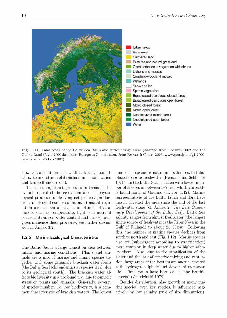
The Baltic Sea Basin comprises watersheds drain-ing the Fennoscandian Alps in the west and north,the Erz, Sudetes and western Carpathian Moun-tains in the south, uplands along the Finnish-Russian border and the central Russian Highlandsin the east. The basin spans some 20 degrees oflatitude, and climate types range from alpine tomaritime to sub-arctic. The Baltic Sea Basin canbe divided roughly into a south-eastern temper-ate part and a northern boreal part, as shownin Fig. 1.11. In the south-eastern part, charac-terised by a cultivated landscape, the river water
runs into the Gulf of Riga and the Baltic Proper.The northern boreal part is characterised by conif-erous forest and peat. The natural vegetation ismainly broadleaved deciduous forest in the low-land areas of the southeast and conifer-dominatedboreal forest in northern parts. Cold climate landsand tundra occur in the mountainous areas and inthe sub-arctic far north of the catchments region.Wetlands and lakes are a significant feature of theboreal and sub-arctic zones.
Extensive changes in land use have taken placeduring last centuries, paralleled by a considerableincrease in the number of people living in theBaltic Sea Basin. Industrialisation and growingcities have changed the landscape, and much ofthe forest has been converted to farmland. Onlyin the northern parts does forest still dominate thelandscape. Approximately half of the total catch-ment area consists today of forest, most of theremainder being agricultural land.
Many plant species are temperature sensitiveand cold-limit range boundaries can be correlatedto the minimum temperature. The main reason isassumed to be the result of ice formation in planttissue leading to death. Some other plants aremore correlated with growing season heat sums.
10 1. Introduction and Summary
Fig. 1.11. Land cover of the Baltic Sea Basin and surroundings areas (adapted from Ledwith 2002 and theGlobal Land Cover 2000 database, European Commission, Joint Research Centre 2003; www.gem.jrc.it/glc2000,page visited 26 Feb 2007)
However, at southern or low-altitude range bound-aries, temperature relationships are more variedand less well understood.
The most important processes in terms of theoverall control of the ecosystem are the physio-logical processes underlying net primary produc-tion, photosynthesis, respiration, stomatal regu-lation and carbon allocation in plants. Severalfactors such as temperature, light, soil nutrientconcentration, soil water content and atmosphericgases influence these processes; see further discus-sion in Annex 3.2.
1.2.5 Marine Ecological Characteristics
The Baltic Sea is a large transition area betweenlimnic and marine conditions. Plants and ani-mals are a mix of marine and limnic species to-gether with some genuinely brackish water forms(the Baltic Sea lacks endemics at species level, dueto its geological youth). The brackish water af-fects biodiversity in a profound way due to osmoticstress on plants and animals. Generally, povertyof species number, i.e. low biodiversity, is a com-mon characteristic of brackish waters. The lowest
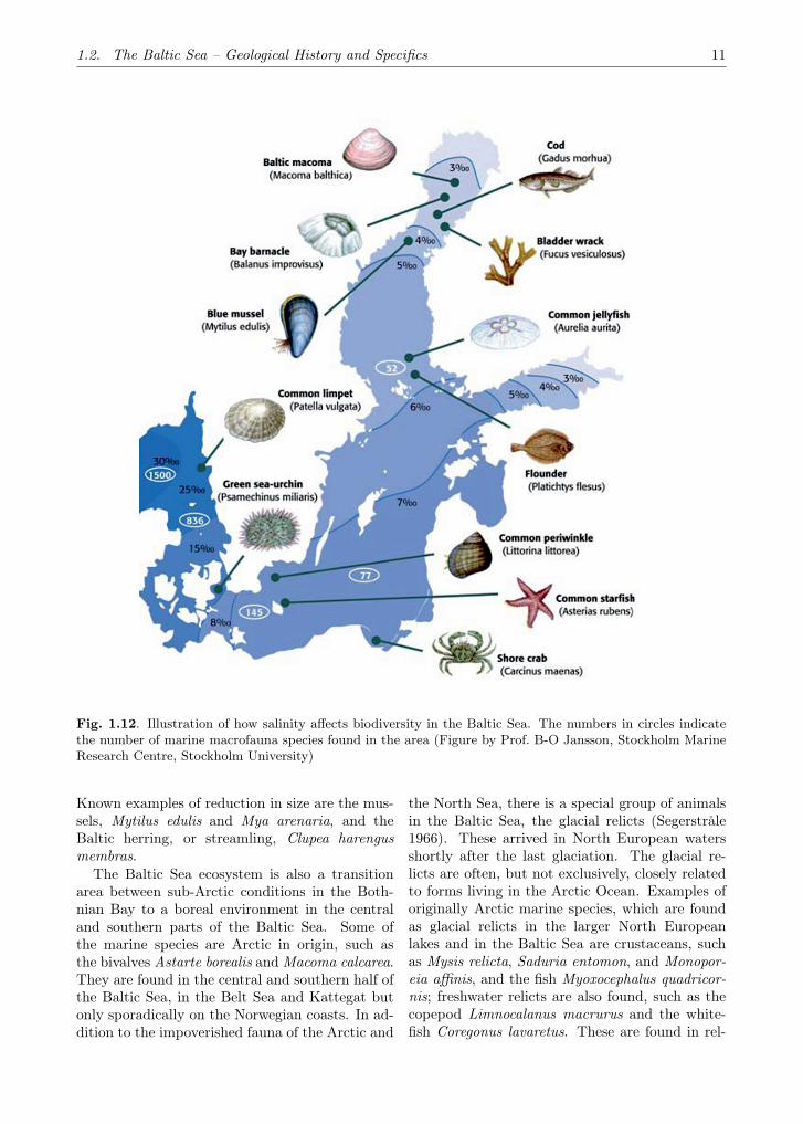
number of species is not in mid salinities, but dis-placed close to freshwater (Remane and Schlieper1971). In the Baltic Sea, the area with lowest num-ber of species is between 5–7 psu, which currentlyis found north of Gotland (cf. Fig. 1.12). Marinerepresentatives of the Baltic fauna and flora havemostly invaded the area since the end of the lastfreshwater stage (cf. Annex 2: The Late Quater-nary Development of the Baltic Sea). Baltic Seasalinity ranges from almost freshwater (the largestsingle source of freshwater is the River Neva in theGulf of Finland) to about 25–30 psu. Followingthis, the number of marine species declines fromsouth to north and east (Fig. 1.12). Marine speciesalso are (submergent according to stratification)more common in deep water due to higher salin-ity there. Also, due to the stratification of thewater and the lack of effective mixing and ventila-tion, large areas of the bottom are anoxic, coveredwith hydrogen sulphide and devoid of metazoanlife. These zones have been called “the benthicdeserts” (Zmudzinski 1978).
Besides distribution, also growth of many ma-rine species, even key species, is influenced neg-atively by low salinity (rule of size diminution).
1.2. The Baltic Sea – Geological History and Specifics 11
Fig. 1.12. Illustration of how salinity affects biodiversity in the Baltic Sea. The numbers in circles indicatethe number of marine macrofauna species found in the area (Figure by Prof. B-O Jansson, Stockholm MarineResearch Centre, Stockholm University)
Known examples of reduction in size are the mus-sels, Mytilus edulis and Mya arenaria, and theBaltic herring, or streamling, Clupea harengusmembras.
The Baltic Sea ecosystem is also a transitionarea between sub-Arctic conditions in the Both-nian Bay to a boreal environment in the centraland southern parts of the Baltic Sea. Some ofthe marine species are Arctic in origin, such asthe bivalves Astarte borealis and Macoma calcarea.They are found in the central and southern half ofthe Baltic Sea, in the Belt Sea and Kattegat butonly sporadically on the Norwegian coasts. In ad-dition to the impoverished fauna of the Arctic and
the North Sea, there is a special group of animalsin the Baltic Sea, the glacial relicts (Segerstråle1966). These arrived in North European watersshortly after the last glaciation. The glacial re-licts are often, but not exclusively, closely relatedto forms living in the Arctic Ocean. Examples oforiginally Arctic marine species, which are foundas glacial relicts in the larger North Europeanlakes and in the Baltic Sea are crustaceans, suchas Mysis relicta, Saduria entomon, and Monopor-eia affinis, and the fish Myoxocephalus quadricor-nis; freshwater relicts are also found, such as thecopepod Limnocalanus macrurus and the white-fish Coregonus lavaretus. These are found in rel-

12 1. Introduction and Summary
atively cool deep water, or in the benthos, whichmakes them particularly vulnerable to deep wa-ter anoxia. Freshwater species, naturally, haveentered the Baltic Sea via river mouths. Theycontinue to do so, and many of them are confinedto littoral and shallow water, such as the perch,roach and pike, which thrive among the reef beds,but also can be very numerous among truly marineflora, e.g. in the bladder wrack. A description ofbasic structure and function of this mosaic mixtureof species can be found in the Annex 3: EcosystemDescription.
Anthropogenic impact is changing the BalticSea, not only through contaminants, which havecaused reproduction disorders in some key species,such as seals and the white tailed eagle, but alsodue to eutrophication, which has contributed toanoxia, dead bottoms and disrupted deep wa-ter food chains, and has caused local disappear-ance of bladder wrack, and increased blooms ofcyanobacteria in the surface layer of the open wa-ter. So far, these influences have not caused anyspecies extinctions, but they have considerablychanged species distribution patterns, especially inthe coastal areas and deep basins (Leppäkoski andOlenin 2001). On the other hand, the Baltic Seais a relatively young sea, thus having many vacantniches, and immigrant species arrive with surpris-ing frequency. The first great wave of non-nativespecies came after the building of the inland water-way systems at the end of the 18th to the beginningof the 19th centuries, which connected ultimatelyPontocaspian brackish water areas with the BalticSea, e.g. bringing in the hydrozoan Cordylophoracaspia and the zebra mussel Dreissena polymorpha(Olenin 2002). The most recent wave of immi-gration appeared after the collapse of the SovietUnion and the subsequent increase in sea traffic(e.g. the arrival of the Pontocaspian cladoceranCercopagis pengoi ). The “original” low biodiver-sity of the Baltic Sea is thus disappearing rapidly.
Some species occupy several different habitatsduring their lifetimes; e.g. the Baltic herringspawns in the littoral, often next to freshwateroutlets; it feeds in the pelagial in the summer andwhile young, but on the bottom during winter andwhen it has grown larger. Finally, it may eventurn predator of other fish. A striking exampleof species utilising widely different habitats duringtheir lives are the Arctic waterfowl, which overwin-ter in the Southern Baltic Sea Basin and NorthernEurope, and migrate through the Baltic Sea twicea year in millions, making spectacular sights. In
environmental management of the Baltic Sea, onemust therefore be able to cover a species duringthe entire life cycle and in every habitat it will useduring its lifetime, taking into account the extrememobility of some species.
1.3 Trends, Jumps and Oscillations – theProblem of Detecting AnthropogenicClimate Change and Attributing it toCauses
People perceive climate not as something station-ary – they even think it should be stationary –and the deviation from this assumed stationarityis taken as evidence for climate change, in mostcases as adverse anthropogenic climate change6.This is related to a duality of the term “climate”.One meaning is the geophysically defined statis-tics of weather, which are objectively describedby observations and – within limits – by dynam-ical models. This “geophysical construct” is whatthis assessment report is about. However, the al-ternative meaning of a “social construct” refers towhat people think about climate, how they per-ceive it7. For the definition of climate policy, itmay be questioned whether the key driver is thesocial construct or the geophysical construct of cli-mate.
This Assessment Report of Climate Changefor the Baltic Sea Basin emphasises the need fora rigorous discrimination between long-term sys-tematic changes, related to anthropogenic drivers(foremost greenhouse gas emissions, but also aero-sol emissions or land-use change), and naturalvariations at shorter time-scales, related to inter-nal climate dynamics and to identify the mostprobable causes of the systematic changes. The
6The complaints that weather is less predictable thanit was in the old days seem to be part of our culture (e.g.Rebetez 1996). An interesting episode in the history ofideas occurred during the 19th and early 20th century, whenscientists, and to some extent the public and policymak-ers, were discussing whether ongoing events were an ex-pression of systematic change or natural variability (e.g.Williamson 1770; Brückner 1890; Stehr et al. 1996; Pfisterand Brändli 1999, Kincer 1933, Callendar 1938). In thosedays, those who claimed that the trends and clustering ofextreme events were man-made seem to have been moresuccessful in their arguments.
7Thus, there are – even if just emerging – efforts todescribe these perceptions scientifically and to understandthe social implications of our views of climate and of cli-mate change. Examples of such studies dealing with thissocial construct are Glacken (1967); Kempton et al. (1995);Kempton and Craig (1993); von Storch and Stehr (2000)and Bray and von Storch (1999).

1.3. Trends, Jumps and Oscillations – the Problem of Detecting Anthropogenic Climate Change 13
technical terms are “detection” and “attribution”(Hasselmann 1993; Zwiers 1999; IDAG 2005). Forchanges on the global and continental scales, alarge body of literature has come into being inthe last few years; also in the IPCC AssessmentReports this issue plays an important if not dom-inant role. These efforts led to the famous state-ment in the Third Assessment Report (Houghtonet al. 1996): “The balance of evidence suggeststhat there is a discernible human influence onglobal climate.” However, for specific regions andimpact variables, successful detection has rarelybeen claimed.
With respect to the Baltic Sea Basin, no formaldetection and attribution studies appear to havebeen carried out so far. It seems that – at leastat present – a methodically sound detection of an-thropogenic climate change signals in the BalticSea Basin due to increased greenhouse gas con-centrations has not been achieved (see Chap. 2).This is probably due to the unfavourable signal-to-noise ratio of anthropogenic signals (whose ex-istence on the global scale is well established, atleast in terms of air temperature, see IPCC Assess-ment mentioned above) and natural variability (asfor instance related to the NAO). Instead, manystudies have attempted to detect trends in recentdecades, and sometimes claims are made that suchtrends are due to global climate change when theyare “statistically significant” (see also Sect. 1.3.3).
1.3.1 The Concepts of Formal Detection andAttribution
Detection is formally a statistical test dealingwith the null hypothesis that the recent changesof climate are within the limits of natural vari-ations. Usually, the variable considered is thechange during the past few, say two or three,decades. This change can take the form of a trendduring that time. The test has to be done in a verylarge multi-dimensional space (spanned by verymany locations and variables). Scenarios preparedwith climate models help to sort out those dimen-sions along which a favourable sign-to-noise ratiois expected for changes related to elevated green-house gas and aerosol concentrations. We have al-ready mentioned that the regional signal-to-noiseratios at the present level of anthropogenic climatechange are seemingly too small for a successful de-tection. Another requirement is the availability ofenough observational data to determine the distri-bution of natural variations. This is probably not
such a severe limitation for Baltic Sea Basin stud-ies, where several data series extending for morethan 100 or even 200 years exist (see Chap. 2).Also, climate model simulations may over or un-der estimate the level of natural variability.
Attribution is formally a statistical fit basedon the assumption that the “signal” of climatechange is made up additively of contributions ofdifferent influences. Each influence is a functionof quantifiable forcings, e.g. the concentration ofgreenhouse gas concentrations. Then, given thetime-dependent forcings, a best mix of contribu-tions to the observed change is determined. Thecoefficients in this fit are subjected to a statisti-cal test – however having the desired outcome asthe null-hypothesis and not as an alternative hy-pothesis. Thus, a successful attribution, in thisformal sense, is a less powerful argument than asuccessful detection, which would feature the de-sired outcome as an alternative hypothesis.
Usually, attribution makes sense only after asuccessful detection. In some cases, however, thisis not possible, for instance because of insufficientobservational data for determining the level of nat-ural variability. Using attribution in cases wherethe signal-to-noise ratio is insufficient for a for-mal detection, one can at least determine to whatextent the recent changes are consistent with thehypothesis of anthropogenic forcing. Most claimsof ongoing regional anthropogenic climate changeare based on such reasoning.
Chapter 2 (see summary in Sect. 1.5.1) reportson a number of such studies. With regard to eco-logical change (Chaps. 4 and 5, Sects. 1.5.3 and1.5.4) such efforts have rarely been done; in thatacademic environment it has been common to re-late the emergence of signals to elevated levels ofgreenhouse gases and anthropogenic aerosols with-out an adequate statistical analysis.
1.3.2 Homogeneity of Data
An obvious requirement for a meaningful statisti-cal analysis of observational data with respect totheir temporal development, the existence of breakpoints, jumps, regime shifts, cycles or stochas-tic characteristics, is that the data are quality-controlled and homogeneous (see also Annex 5).Quality control means ensuring that the data areobserved at the ascribed location and time or thatthey are recorded using prescribed protocols andinstruments. It happens, for instance, that logbooks of ships list incorrect locations, for instance
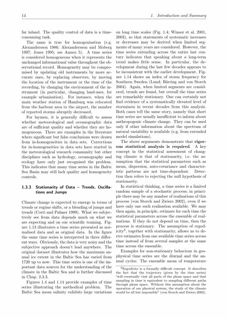
14 1. Introduction and Summary
far inland. The quality control of data is a time-consuming task.
The same is true for homogenisation (e.g.Alexandersson 1986; Alexandersson and Moberg1997; Jones 1995; see Annex 5). A time seriesis considered homogeneous when it represents theunchanged informational value throughout the ob-servational record. Homogeneity may be compro-mised by updating old instruments by more ac-curate ones, by replacing observers, by movingthe location of the instrument or the time of therecording, by changing the environment of the in-strument (in particular, changing land-uses, forexample urbanisation). For instance, when themain weather station of Hamburg was relocatedfrom the harbour area to the airport, the numberof reported storms abruptly decreased.
For laymen, it is generally difficult to assesswhether meteorological and oceanographic dataare of sufficient quality and whether they are ho-mogeneous. There are examples in the literaturewhere significant but false conclusions were drawnfrom in-homogeneities in data sets. Correctionsfor in-homogeneities in data sets have started inthe meteorological research community but otherdisciplines such as hydrology, oceanography andecology have only just recognised the problem.This indicates that many time series in the BalticSea Basin may still lack quality and homogeneitycontrols.
1.3.3 Stationarity of Data – Trends, Oscilla-tions and Jumps
Climate change is expected to emerge in terms oftrends or regime shifts, or a blending of jumps andtrends (Corti and Palmer 1999). What we subjec-tively see from data depends much on what weare expecting and on our scientific training. Fig-ure 1.13 illustrates a time series presented as nor-malised data and as original data. In the figurethe same time series is interpreted in three differ-ent ways. Obviously, the data is very noisy and thesubjective approach doesn’t lead anywhere. Theoriginal dataset illustrates how the maximum an-nual ice extent in the Baltic Sea has varied from1720 up to now. This time series is one of the im-portant data sources for the understanding of theclimate in the Baltic Sea and is further discussedin Chap. 2.3.3.
Figures 1.4 and 1.14 provide examples of timeseries illustrating the methodical problem. TheBaltic Sea mean salinity exhibits large variations
on long time scales (Fig. 1.4; Winsor et al. 2001,2003), so that statements of systematic increasesor decreases may be derived when limited seg-ments of many years are considered. However, thetime series extending across the entire last cen-tury indicates that speaking about a long-termtrend makes little sense. In particular, the de-velopment during the last few decades appears tobe inconsistent with the earlier development. Fig-ure 1.14 shows an index of storm frequency forSouthern Sweden (Lund; Bärring and von Storch2004). Again, when limited segments are consid-ered, trends are found, but overall the time seriesare remarkably stationary. One can certainly notfind evidence of a systematically elevated level ofstorminess in recent decades from this analysis.Both cases tell the same story, namely that shorttime series are usually insufficient to inform aboutanthropogenic climate change. They can be usedonly if other information about the spectrum ofnatural variability is available (e.g. from extendedmodel simulations).
The above arguments demonstrate that rigor-ous statistical analysis is required. A keyconcept in the statistical assessment of chang-ing climate is that of stationarity, i.e. the as-sumption that the statistical parameters such asmean, dispersion, auto-covariance and character-istic patterns are not time-dependent. Detec-tion then refers to rejecting the null hypothesis ofstationarity.
In statistical thinking, a time series is a limitedrandom sample of a stochastic process; in princi-ple there may be any number of realisations of thisprocess (von Storch and Zwiers 2002), even if wehave only one such realisation available. We maythen again, in principle, estimate for each time thestatistical parameters across the ensemble of real-isations. If they do not depend on time, then theprocess is stationary. The assumption of ergod-icity8, together with stationarity, allows us to de-rive estimates from one available time series acrosstime instead of from several samples at the sametime across the ensemble.
Examples for non-stationary behaviour in geo-physical time series are the diurnal and the an-nual cycles: The ensemble mean of temperature
8Ergodicity is a formally difficult concept. It describesthe fact that the trajectory (given by the time series)“will eventually visit all parts of the phase space and thatsampling in time is equivalent to sampling different pathsthrough phase space. Without this assumption about theoperation of our physical system, the study of the climatewould be all but impossible” (von Storch and Zwiers 2002).

1.3. Trends, Jumps and Oscillations – the Problem of Detecting Anthropogenic Climate Change 15
Fig. 1.13. Climate change can be detected by trends, oscillations and jumps or regime shifts. In this figure thesame data sets is used and normalised (Figs. a–c). The original data set is illustrated in Fig. (d), for detailssee Omstedt and Chen (2001)
at 6:00 in the morning is markedly different fromthe ensemble mean at 18:00 in the evening. Timeseries with phase-fixed cycles are not stationary;they may represent cyclo-stationary9 processes,however. But there may be quasi-periodic be-haviour, with variable phases, periods and ampli-tudes, which are not in conflict with the conceptof stationarity. Examples are autoregressive pro-cesses of the 2nd order with little damping (vonStorch and Zwiers 2002). Similarly, jumps andbreak points do not contradict stationarity, as longas the time between these events is random.
Thus, for a break point, a jump or a regime shiftto qualify as evidence for climate change, it needs
9Cyclo-stationary processes are instationary processes,which have parameters, such as the mean or the variance,which depend cyclically on time. The weather is consideredcyclo-stationary, with two main cycles, the annual and di-urnal cycle. Minor cycles are related to atmospheric tides(see also von Storch and Zwiers 2002).
to be markedly different from previous such events.If such events have not happened for a very longtime, then it would be good evidence – as long assuch events are not related to inhomogeneities inthe data gathering process.
One may assume that anthropogenic climatechange emerges as a mixture of jumps and trends;in scenarios it takes a form something like slowlyincreasing trends, but in local variables jumps alsomay be possible. Therefore, much emphasis ison the detection of trends. The key questionis whether the most recent trend, during the pe-riod when we expect the anthropogenic signal tobe strongest, is larger than previously recordedtrends. If the time evolution has not been moni-tored for a long enough time to derive an appro-priate distribution of past trends, then formal de-tection studies cannot be done.
Therefore, many studies adopt to the concept ofsignificance of trends, i.e., testing the null hypoth-
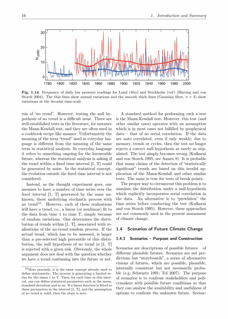
16 1. Introduction and Summary
Fig. 1.14. Frequency of daily low pressure readings for Lund (blue) and Stockholm (red ) (Bärring and vonStorch 2004). The thin lines show annual variations and the smooth thick lines (Gaussian filter, σ = 3) showvariations at the decadal time-scale
esis of “no trend”. However, testing the null hy-pothesis of no trend is a difficult issue. There arewell-established tests in the literature, for instancethe Mann-Kendall test, and they are often used ina cookbook recipe like manner. Unfortunately themeaning of the term “trend” used in everyday lan-guage is different from the meaning of the sameterm in statistical analysis. In everyday languageit refers to something ongoing for the foreseeablefuture, whereas the statistical analysis is asking ifthe trend within a fixed time interval [1, T] couldbe generated by noise. In the statistical concept,the evolution outside the fixed time interval is notconsidered.
Instead, as the thought experiment goes, oneassumes to have a number of time series over thefixed interval [1, T] generated by the same un-known, these underlying stochastic process withno trend10. However, each of these realisationswill have a trend, i.e., a linear (or nonlinear) fit tothe data from time 1 to time T, simply becauseof random variations. One determines the distri-bution of trends within [1, T], associated with re-alisations of the no-trend random process. If theactual trend, which has to be assessed, is largerthan a pre-selected high percentile of this distri-bution, the null hypothesis of no trend in [1, T]is rejected with a given risk. Obviously, the wholeargument does not deal with the question whetherwe have a trend continuing into the future or not.
10More precisely, it is the same concept already used todefine stationarity: The process is generating a limited se-ries for the times 1 to T. Then, for each time in this inter-val, one can define statistical parameters such as the mean,standard deviation and so on. If a linear function is fitted tothese parameters in the interval [1, T], and the assumptionof no trend is valid, then the slope is zero.
A standard method for performing such a testis the Mann-Kendall test. However, this test (andother similar ones) operates with an assumptionwhich is in most cases not fulfilled by geophysicaldata – that of no serial correlation. If the dataare auto correlated, even if only weakly, due tomemory, trends or cycles, then the test no longerrejects a correct null hypothesis as rarely as stip-ulated. The test simply becomes wrong (Kulkarniand von Storch 1995, see Annex 8). It is probablethat many claims of the detection of “statisticallysignificant” trends are based on this invalid ap-plication of the Mann-Kendall and other similartests. The same is true for tests of break points.
The proper way to circumvent this problem is tosimulate the distribution under a null-hypothesiswhich explicitly incorporates serial correlation inthe data. An alternative is to “prewhiten” thetime series before conducting the test (Kulkarniand von Storch 1995). However, these approachesare not commonly used in the present assessmentof climate change.
1.4 Scenarios of Future Climate Change
1.4.1 Scenarios – Purpose and Construction
Scenarios are descriptions of possible futures – ofdifferent plausible futures. Scenarios are not pre-dictions but “storyboards”, a series of alternativevisions of futures, which are possible, plausible,internally consistent but not necessarily proba-ble (e.g. Schwartz 1991; Tol 2007). The purposeof scenarios is to confront stakeholders and poli-cymakers with possible future conditions so thatthey can analyse the availability and usefulness ofoptions to confront the unknown future. Scenar-

1.4. Scenarios of Future Climate Change 17
Fig. 1.15. Some typical atmospheric model grid resolutions with corresponding land masks. Left: T42 usedin global models, right: 50 km grid used in regional models (by courtesy of Ole Bøssing-Christensen, DanishMeteorological Institute)
ios allow implementing measures now to avoid un-wanted futures; they also may be used to increasechances for the emergence of favourable futures.
In daily life, we frequently operate with scenar-ios. For instance, when planning in spring for achildren’s birthday party next summer, we con-sider the scenarios of an outdoor party on a sunnyday or an indoor party on a rainy day. Both sce-narios are possible, plausible and internally consis-tent. Planning for a snowy day, on the other hand,is not considered, as this would be an inconsistentscenario.
In climate research, scenarios have been usedwidely since the introduction of the IPCC processat the end of the 1980s (Houghton et al. 1990,1992, 1996, 2001). These scenarios are built ina series of steps. This series begins with scenar-ios of emissions of radiatively active substances,i.e., greenhouse gases, such as carbon dioxide ormethane, and aerosols. These scenarios dependon a variety of developments unrelated to climateitself, in particular on population growth, effi-ciency of energy use and technological develop-ment. Many of these factors are unpredictable;therefore, a variety of sometimes ad-hoc assump-tions enter these scenarios (Tol 2007).
In the next steps, the construction of scenariosis less ad-hoc, as they essentially process the emis-sions scenarios. The first step is to transform theemissions into atmospheric concentrations, which
are then fed into global climate models11. Thus,possible, plausible and internally consistent futureemissions are used to derive estimates of possi-ble, plausible and internally consistent future cli-mate, i.e., seasonal means, ranges of variability,
11There are different types of climate models (cf.McGuffie and Henderson-Sellers 1997; Crowley and North1991; von Storch and Flöser 2001; Müller and von Storch2005). In their simplest form they are energy balance mod-els, which describe in a rather schematic way the flux andfate of energy entering the atmosphere as solar radiationand leaving it as long and short wave radiation. Thesemodels are meant to be conceptual tools of minimum com-plexity for describing the fundamental aspects of the ther-modynamic engine “climate system”. At the other end ofthe range of complexity are the highly complex tools con-taining as many processes and details as is can be processedon a contemporary computer. Being limited by the compu-tational resources, these models grow in complexity in time– simply because the computers continually become morepowerful. Such models are supposed to approximate thecomplexity of the real system. They simulate a sequenceof hourly, or even more frequently sampled, weather, withvery many atmospheric, oceanic and cryospheric variables– such as temperature, salinity, wind speed, cloud watercontent, upwelling, ice thickness etc. From these multipletime series, the required statistics (= climate) are derived.Thus, working with simulated data is similar to workingwith observed data. The only, and significant, differenceis that one can perform experiments with climate models,which is not possible with the real world. However, presentday climate models are coarse, and several processes relatedto the water and energy cycles are not well understood ordescribed in these models. Direct observations are there-fore the main source for the understanding of the climate.
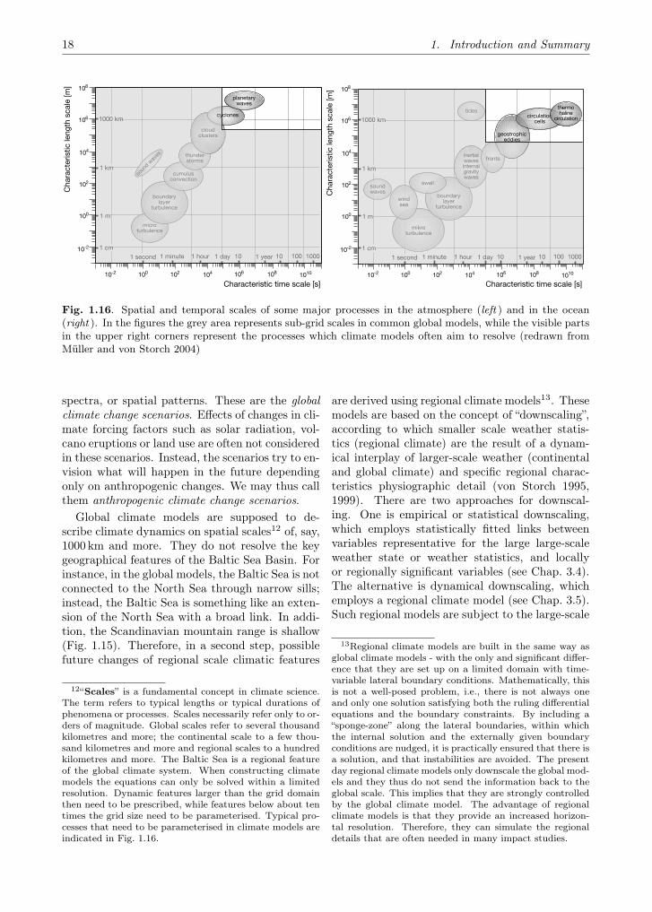
18 1. Introduction and Summary
Fig. 1.16. Spatial and temporal scales of some major processes in the atmosphere (left ) and in the ocean(right ). In the figures the grey area represents sub-grid scales in common global models, while the visible partsin the upper right corners represent the processes which climate models often aim to resolve (redrawn fromMüller and von Storch 2004)
spectra, or spatial patterns. These are the globalclimate change scenarios. Effects of changes in cli-mate forcing factors such as solar radiation, vol-cano eruptions or land use are often not consideredin these scenarios. Instead, the scenarios try to en-vision what will happen in the future dependingonly on anthropogenic changes. We may thus callthem anthropogenic climate change scenarios.
Global climate models are supposed to de-scribe climate dynamics on spatial scales12 of, say,1000 km and more. They do not resolve the keygeographical features of the Baltic Sea Basin. Forinstance, in the global models, the Baltic Sea is notconnected to the North Sea through narrow sills;instead, the Baltic Sea is something like an exten-sion of the North Sea with a broad link. In addi-tion, the Scandinavian mountain range is shallow(Fig. 1.15). Therefore, in a second step, possiblefuture changes of regional scale climatic features
12“Scales” is a fundamental concept in climate science.The term refers to typical lengths or typical durations ofphenomena or processes. Scales necessarily refer only to or-ders of magnitude. Global scales refer to several thousandkilometres and more; the continental scale to a few thou-sand kilometres and more and regional scales to a hundredkilometres and more. The Baltic Sea is a regional featureof the global climate system. When constructing climatemodels the equations can only be solved within a limitedresolution. Dynamic features larger than the grid domainthen need to be prescribed, while features below about tentimes the grid size need to be parameterised. Typical pro-cesses that need to be parameterised in climate models areindicated in Fig. 1.16.
are derived using regional climate models13. Thesemodels are based on the concept of “downscaling”,according to which smaller scale weather statis-tics (regional climate) are the result of a dynam-ical interplay of larger-scale weather (continentaland global climate) and specific regional charac-teristics physiographic detail (von Storch 1995,1999). There are two approaches for downscal-ing. One is empirical or statistical downscaling,which employs statistically fitted links betweenvariables representative for the large large-scaleweather state or weather statistics, and locallyor regionally significant variables (see Chap. 3.4).The alternative is dynamical downscaling, whichemploys a regional climate model (see Chap. 3.5).Such regional models are subject to the large-scale
13Regional climate models are built in the same way asglobal climate models - with the only and significant differ-ence that they are set up on a limited domain with time-variable lateral boundary conditions. Mathematically, thisis not a well-posed problem, i.e., there is not always oneand only one solution satisfying both the ruling differentialequations and the boundary constraints. By including a“sponge-zone” along the lateral boundaries, within whichthe internal solution and the externally given boundaryconditions are nudged, it is practically ensured that there isa solution, and that instabilities are avoided. The presentday regional climate models only downscale the global mod-els and they thus do not send the information back to theglobal scale. This implies that they are strongly controlledby the global climate model. The advantage of regionalclimate models is that they provide an increased horizon-tal resolution. Therefore, they can simulate the regionaldetails that are often needed in many impact studies.

1.4. Scenarios of Future Climate Change 19
state simulated by the global models along thelateral boundaries and sometimes in the interior.With horizontal grid sizes of typically 10 to 50 km,such models resolve features with minimum scalesof some tens to a few hundred kilometres. Theyalso simulate the emergence of rare events, such asstrong rainfall episodes and strong windstorms.
Methodologically, the anthropogenic climatechange scenarios are conditional predictions. Af-ter the emissions scenarios are given, no furtherad-hoc decisions are required. Significant assump-tions are only required for the design of the emis-sion scenarios. These assumptions refer to socio-economic processes, which lead to emissions.
When dealing with regional or local scenarios,one has to keep in mind that not only global cli-mate changes, but also that regional and local cli-mate conditions change, for example due to chang-ing regional and local land use – which may or maynot be on a scale comparable to global changes.When assessing impacts of climate change, thesehave to be compared to the influence of changingusage of the local and regional environment givenby another set of scenarios (e.g. Grossmann 2005,2006; Bray et al. 2003) – e.g. land use, but alsothe release of anthropogenic substances.
1.4.2 Emission Scenarios
A number of emission scenarios have been pub-lished as an “IPCC Special Report on EmissionsScenarios” (SRES; www.grida.no/climate/ipcc/emission) prepared by economists and other so-cial scientists for the Third Assessment Report ofthe IPCC. They utilise scenarios of greenhouse gasand aerosol emissions or of changing land use:
(A1) a world of rapid economic growth and rapidintroduction of new and more efficient tech-nology,
(A2) a very heterogeneous world with an empha-sis on family values and local traditions,
(B1) a world of “dematerialisation” and introduc-tion of clean technologies,
(B2) a world with an emphasis on local solutionsto economic and environmental sustainabil-ity.
The scenarios do not anticipate any specific miti-gation policies for avoiding climate change. Theauthors emphasise that “no explicit judgmentshave been made by the SRES team as to theirdesirability or probability”.
The Scenarios A2 and B2 are widely used.Therefore, we explain the socio-economic back-ground of these scenarios in more detail (for a sum-mary for the other two scenarios, refer to Müllerand von Storch 2004): SRES describes the A2-scenario as follows: “. . . characterised by lowertrade flows, relatively slow capital stock turnover,and slower technological change. The world “con-solidates” into a series of economic regions. Self-reliance in terms of resources and less emphasison economic, social, and cultural interactions be-tween regions are characteristic for this future.Economic growth is uneven and the income gapbetween now-industrialised and developing partsof the world does not narrow.
People, ideas, and capital are less mobile so thattechnology diffuses more slowly. International dis-parities in productivity, and hence income percapita, are largely maintained or increased in abso-lute terms. With the emphasis on family and com-munity life, fertility rates decline relatively slowly,which makes the population the largest amongthe storylines (15 billion by 2100). Technologicalchange is more heterogeneous. Regions with abun-dant energy and mineral resources evolve moreresource-intensive economies, while those poor inresources place a very high priority on minimizingimport dependence through technological innova-tion to improve resource efficiency and make useof substitute inputs. Energy use per unit of GDPdeclines with a pace of 0.5 to 0.7% per year.
Social and political structures diversify; someregions move toward stronger welfare systems andreduced income inequality, while others move to-ward “leaner” government and more heteroge-neous income distributions. With substantialfood requirements, agricultural productivity is oneof the main focus areas for innovation and re-search, development efforts, and environmentalconcerns. Global environmental concerns are rel-atively weak.”
In B2, there is “. . . increased concern for envi-ronmental and social sustainability. Increasingly,government policies and business strategies at thenational and local levels are influenced by envi-ronmentally aware citizens, with a trend towardlocal self-reliance and stronger communities. Hu-man welfare, equality, and environmental protec-tion all have high priority, and they are addressedthrough community-based social solutions in addi-tion to technical solutions. Education and welfareprograms are pursued widely, which reduces mor-tality and fertility. The population reaches about

20 1. Introduction and Summary
Fig. 1.17. Scenarios of possible, plausible, internally consistent but not necessarily probable future emissionsof carbon dioxide (a representative of greenhouse gases; in gigatons) and of sulfur dioxide (a representative ofanthropogenic aerosols; in megatons). A1, B1, A2 and B2 are provided by SRES, IS92a is a scenario used inthe Second Assessment Report of the IPCC in 1995 (Nakićenović and Swart 2000)
10 billion people by 2100. Income per capita growsat an intermediate rate. The high educational lev-els promote both development and environmentalprotection. Environmental protection is one of thefew truly international common priorities. How-ever, strategies to address global environmentalchallenges are not of a central priority and are thusless successful compared to local and regional en-vironmental response strategies. The governmentshave difficulty designing and implementing agree-ments that combine global environmental protec-tion. Land-use management becomes better in-tegrated at the local level. Urban and transportinfrastructure is a particular focus of communityinnovation, and contributes to a low level of car de-pendence and less urban sprawl. An emphasis onfood self-reliance contributes to a shift in dietarypatterns toward local products, with relatively lowmeat consumption in countries with high popula-tion densities. Energy systems differ from regionto region. The need to use energy and other re-sources more efficiently spurs the development ofless carbon-intensive technology in some regions.Although globally the energy system remains pre-dominantly hydrocarbon-based, a gradual transi-tion occurs away from the current share of fossilresources in world energy supply.”
Expected emissions of greenhouse gases andaerosols into the atmosphere are derived fromthese assumptions and descriptions. Figure 1.17shows the expected SRES scenarios for carbondioxide (a representative of greenhouse gases; ingigatons per year) and sulfur dioxide (a repre-sentative of anthropogenic aerosols; in megatons
sulfur). The SRES scenarios are not unanimouslyaccepted by the economic community. Some re-searchers find the scenarios internally inconsistent.A documentation of the various points raised isprovided by the Select Committee of EconomicAffairs of the House of Lords in London (2005).A key critique is that the expectation of economicgrowth in different parts of the world is based onmarket exchange ranges (MER) and not on pur-chasing power parity (PPP). Another aspect is theimplicit assumption in the SRES scenarios thatthe difference in income between developing anddeveloped countries will significantly shrink untilthe end of this century (Tol 2006, 2007). Theseassumptions, the argument is, lead to an exagger-ation of expected future emissions.
1.4.3 Scenarios of Anthropogenic GlobalClimate Change
The emission scenarios are first transformed intoscenarios of atmospheric loadings of greenhousegases and aerosols. Then, the global climate mod-els derive from these concentrations – without anyother externally set specifications – sequences ofhourly weather, typically for one hundred years.A large number of relevant variables are calcu-lated for the troposphere, the lower stratosphereand the oceans, but also at the different bound-aries of land, air, ocean and sea ice – such as airtemperature, soil temperature, sea surface tem-perature, precipitation, salinity, sea ice coverageor wind speed. Global climate models are sub-ject to some degree of systematic error, so-called
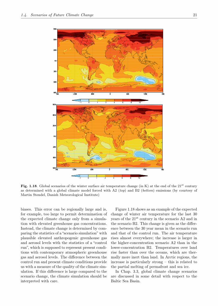
1.4. Scenarios of Future Climate Change 21
Fig. 1.18. Global scenarios of the winter surface air temperature change (in K) at the end of the 21st centuryas determined with a global climate model forced with A2 (top) and B2 (bottom) emissions (by courtesy ofMartin Stendel, Danish Meteorological Institute)
biases. This error can be regionally large and is,for example, too large to permit determination ofthe expected climate change only from a simula-tion with elevated greenhouse gas concentrations.Instead, the climate change is determined by com-paring the statistics of a “scenario simulation” withplausible elevated anthropogenic greenhouse gasand aerosol levels with the statistics of a “controlrun”, which is supposed to represent present condi-tions with contemporary atmospheric greenhousegas and aerosol levels. The difference between thecontrol run and present climate conditions provideus with a measure of the quality of the climate sim-ulation. If this difference is large compared to thescenario change, the climate simulation should beinterpreted with care.
Figure 1.18 shows as an example of the expectedchange of winter air temperature for the last 30years of the 21st century in the scenario A2 and inthe scenario B2. This change is given as the differ-ence between the 30 year mean in the scenario runand that of the control run. The air temperaturerises almost everywhere; the increase is larger inthe higher-concentration scenario A2 than in thelower-concentration B2. Temperatures over landrise faster than over the oceans, which are ther-mally more inert than land. In Arctic regions, theincrease is particularly strong – this is related tothe partial melting of permafrost and sea ice.
In Chap. 3.3, global climate change scenariosare discussed in some detail with respect to theBaltic Sea Basin.
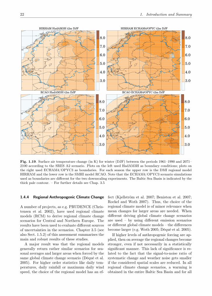
22 1. Introduction and Summary
HIRHAM HadAM3H t2m DJF
3.0
4.0
5.0
6.0
7.0
8.0
HIRHAM ECHAM4/OPYC t2m DJF
3.0
4.0
5.0
6.0
7.0
8.0
RCAO HadAM3H t2m DJF
3.0
4.0
5.0
6.0
7.0
8.0
RCAO ECHAM4/OPYC t2m DJF
3.0
4.0
5.0
6.0
7.0
8.0
Fig. 1.19. Surface air temperature change (in K) for winter (DJF) between the periods 1961–1990 and 2071–2100 according to the SRES A2 scenario. Plots on the left used HadAM3H as boundary conditions; plots onthe right used ECHAM4/OPYC3 as boundaries. For each season the upper row is the DMI regional modelHIRHAM and the lower row is the SMHI model RCAO. Note that the ECHAM4/OPYC3 scenario simulationsused as boundaries are different for the two downscaling experiments. The Baltic Sea Basin is indicated by thethick pale contour. – For further details see Chap. 3.5
1.4.4 Regional Anthropogenic Climate Change
A number of projects, as e.g. PRUDENCE (Chris-tensen et al. 2002), have used regional climatemodels (RCM) to derive regional climate changescenarios for Central and Northern Europe. Theresults have been used to evaluate different sourcesof uncertainties in the scenarios. Chapter 3.5 (seealso Sect. 1.5.2) of this assessment summarises themain and robust results of these studies.
A major result was that the regional modelsgenerally return rather similar scenarios for sea-sonal averages and larger areas when forced by thesame global climate change scenario (Déqué et al.2005). For higher order statistics like daily tem-peratures, daily rainfall or maximum daily windspeed, the choice of the regional model has an ef-
fect (Kjellström et al. 2007; Beniston et al. 2007;Rockel and Woth 2007). Thus, the choice of theregional climate model is of minor relevance whenmean changes for larger areas are needed. Whendifferent driving global climate change scenariosare used – by using different emission scenariosor different global climate models – the differencesbecome larger (e.g. Woth 2005; Déqué et al. 2005).
If higher levels of anthropogenic forcing are ap-plied, then on average the regional changes becomestronger, even if not necessarily in a statisticallysignificant manner. This lack of significance is re-lated to the fact that the signal-to-noise ratio ofsystematic change and weather noise gets smallerif the considered spatial scales are reduced. In allregional climate change scenarios, a warming isobtained in the entire Baltic Sea Basin and for all
1.5. Ongoing Change and Projections for the Baltic Sea Basin – A Summary 23
seasons (Christensen and Christensen 2003). Thewarming is most pronounced in the northern andeastern parts of the basin during winter, togetherwith a dramatic reduction in the snow cover, andto the south in summer. Precipitation increasesin winter and decreases in southern areas in sum-mer in many scenarios. In general, the projectedchanges also increase with greenhouse gas emis-sions.
As an example, the expected changes of winter(DJF) mean temperatures are shown in Fig. 1.19(see also Chap. 3.5). The different model config-urations (two global models, two regional models)indicate that when the snow cover retreats to thenorth and to the east, the climate in the Baltic SeaBasin undergoes large changes. A common fea-ture in all regional downscaling experiments is thestronger increase in wintertime temperatures com-pared to summertime temperatures in the north-ern and eastern part of the Baltic Sea Basin (e.g.Giorgi et al. 1992; Jones et al. 1997; Christensen etal. 2001; Déqué et al. 2005; Räisänen et al. 2004).For further discussion, refer to Chap. 3.5.
Frequency distributions tend to become broaderwith respect to summer rainfall (Christensen andChristensen 2003), North Sea winter wind speeds(Woth 2005) and continental summer daily tem-peratures (Kjellström 2004). On the other hand,frequency distributions of daily temperatures be-come narrower in eastern and northern Europeduring winter (Kjellström 2004).
1.5 Ongoing Change and Projections forthe Baltic Sea Basin – A Summary
The following provides a summary of the mainfindings which are presented and discussed inChaps. 2 to 5 of this book. No specific referencesare given – they are all listed in the detailed ac-count of the following chapters.
Many of the conclusions depend on the timeperiod studied. A frequent deficiency of contem-porary literature is the lack of discrimination be-tween climate variability and anthropogenic cli-mate change. Also, only a few long time serieshave been quality controlled and are homogeneous.Here, we repeat the main and most robust find-ings.
When considering the ecological state of theBaltic Sea Basin, assessments of anthropogenic cli-mate change need to distinguish between effectscaused by factors such as nutrient and contami-nant discharges, eutrophication, over-fishing, land
use change, and air pollution. At present no re-gional studies for the Baltic Sea Basin have beenfound that can attribute robustly recent trends inclimate to increased greenhouse gases. The ob-served changes in the thermal conditions are, how-ever consistent with the global signals, which havebeen attributed reliably to human causes, andconsistent with the projections available for theregion.
1.5.1 Recent Climate Change in the Baltic SeaBasin
The variability of the large scale atmospheric cir-culation has a strong influence on the surfaceclimate (temperature, precipitation, wind speed,etc.) of the Baltic Sea Basin. During the 200 yearsstudied, the 19th and 20th centuries’ climates dif-fer in several ways. Towards the end of the 19th
century, the Little Ice Age ended in the region,and during the period 1871–2004 there were signif-icant positive trends in the mean temperature forthe northern and southern Baltic Sea Basin, be-ing 0.10 C/decade on the average north of 60◦ Nand 0.07 C/decade on the average south of 60◦ N.With regard to annual mean temperatures, therewas an early 20th century warming that culmi-nated in the 1930s. This was followed by a coolingthat ended in the 1960s and then another warminguntil the present. The warming is characterisedby a pattern where mean daily minimum temper-atures have increased more than mean daily max-imum temperatures. Spring is the season showingthe strongest warming. The number of cold nightshas decreased and the number of warm days hasincreased, with the strongest change during thewinter season.
The variability in atmospheric circulationhas a strong influence on the surface climate innorthern Europe. From about the 1960s until the1990s, westerly airflow intensified during winter-time. This increased frequency of maritime airmasses contributed to higher wintertime temper-atures and enhanced precipitation at regions ex-posed to westerlies, especially during the 1990s.On a centennial timescale it can be seen that re-lationships between large scale atmospheric circu-lation and surface climate elements show strongtemporal variability.
Over the latter part of the 20th century, on av-erage, northern Europe has become wetter. Theincrease in precipitation is not spatially uniform.Within the Baltic Sea Basin, the largest increases
24 1. Introduction and Summary
have occurred in Sweden and on the eastern coastof the Baltic Sea. Seasonally, the largest increaseshave occurred in winter and spring. Changesin summer are characterised by increases in thenorthern and decreases in the southern parts ofthe Baltic Sea Basin. In wintertime, there is anindication that the number of heavy precipitationevents has increased.
Characteristics of cloudiness and solar ra-diation show remarkable inter-annual and inter-decadal variability in the Baltic Sea Basin. A de-crease in cloudiness and an increase in sunshineduration was observed in the south (Poland) whileopposite trends were revealed in the north (Esto-nia). In the 1990s, all these trends changed theirsign. Long-term observations in Estonia show thatan improvement in air quality (i.e. a decrease inthe aerosol emissions to the atmosphere) reversedthe decreasing trend in atmospheric transparencyand direct radiation during the 1990s. Presently,atmospheric transparency is at the same level asin the 1930s.
Centennial time series from southern Scandi-navia reveal no long-term trend in storminessindices. There was a temporary increase in the1980s–1990s. In the Baltic Sea Basin, differentdata sources give slightly different results with re-spect to trends and variations in the extreme windclimate, especially concerning small-scale extremewinds. At the same time, there are indications ofincreasing impact from extreme wind events. Butthis increasing impact results from a complex in-teraction between climate and development trendsthat increase the exposure to damage and/or thevulnerability of nature and society.
The inter-annual variability in river water in-flow is considerable, but no statistically significanttrend can be found in the annual time series forthe period 1921–1998.
The analysis of the long-term dynamics of thedates of the start and ending of ice eventsand the duration of ice coverage for the riversof the Russian part of the Baltic Sea Basin showeda stable positive trend from the middle of the 20th
century to its end.As to the maximal ice cover thickness, a neg-
ative tendency has been established for all Polishand Russian lakes studied. In Finland, both de-creasing and increasing trends can be found in themaximum ice thickness time series.
A recent decrease in snow cover durationand water equivalent has been observed in thesouthern parts of all the Fennoscandian countries,
while the opposite trend prevails in the north.Changes of snow depth are quite similar, i.e. adecrease in the southwestern regions and an in-crease in the north-eastern regions.
During the 20th century, the Baltic Sea meansalinity decreased during the 1980s and 1990s,but similar decreases had also appeared earlier inthe century. No long-term trend was found for the20th century.
There are indications of a sea level rise in the20th century compared to the 19th century.
A climate warming can be detected from thetime series of the maximum annual extent ofsea ice and the length of the ice season inthe Baltic Sea. On the basis of the ice extent, theshift towards a warmer climate took place in thelatter half of the 19th century. This gradual shifthas been identified as the ending of the Little IceAge in the Baltic Sea Basin.
Coastal damages appearing in various regionsof the southern Baltic Sea generally result froma combination of strong storms, sea-level rise andthe decreasing trend in ice cover in the winter, i.e.at times when the most intensive storms occur.
1.5.2 Perspectives for Future Climate Changein the Baltic Sea Basin
Projections of future climate change have beenconstructed with a series of dynamical models ofthe regional climate system. Most of these mod-els simulate only the atmosphere and prescribe seasurface temperature and sea ice conditions; in thisrespect, the model used by the Swedish Meteoro-logical and Hydrological Institute (SMHI) is sig-nificantly more sophisticated and an improvementover most other models as it includes a dynamicalmodel of the Baltic Sea itself and regional lakes.
The skill of these models has been demonstratedby their ability to reconstruct the main character-istics of the recent climate. However, the repro-duction of recent climate is not perfect, in par-ticular with respect to regional water and energybalances. Also, even a perfect performance withpresent conditions would be no proof that themodels can do a realistic job in describing pos-sible future climate conditions. There is, how-ever, no alternative to the model-based approach(cf. Müller and von Storch 2004), but it is pru-dent to closely monitor the changing climate con-ditions closely and to compare these changes withthe projections provided by the various models.Also, when the simulated changes are comparable

1.5. Ongoing Change and Projections for the Baltic Sea Basin – A Summary 25
or smaller than the model biases, scenarios shouldbe considered with care. One such example is pre-cipitation over the Baltic Sea Basin, where thedifferences between present day simulations andobserved precipitation are often larger than thesimulated regional manifestation of global climatechange.
Increasing greenhouse gas concentrations areexpected to lead to a substantial warming of theglobal climate during this century. Cubasch etal. (2001) estimated the annual globally aver-aged warming from 1990 to 2100 to be in therange of 1.4 to 5.8 C. This range in temperaturechange takes into account differences between cli-mate models and a range of anthropogenic emis-sions scenarios, but it excludes other uncertainties(for example, in natural variability or in the car-bon cycle) and should not be interpreted as givingthe absolute lowest and highest possible changesin the global mean temperature during the periodconsidered.
Projected future warming in the Baltic SeaBasin generally exceeds the global mean warm-ing in global climate model (GCM) simulations.Looking at the annual mean from an ensembleof 20 GCM simulations, regional warming overthe Baltic Sea Basin would be 0.9 C higher thanglobal mean warming, or some 50% larger in rela-tive terms. In the northern areas of the basin, thelargest simulated warming is generally in winter;further south the seasonal cycle of warming is lessclear. However, the relative uncertainty in the re-gional warming is larger than that in the globalmean warming. Taking the northern areas of thebasin as an example, the warming from the late20th century to the late 21st century could rangefrom as low as 1 C in summer (lowest scenario forsummer) to as high as 10 C in winter (highest sce-nario for winter). The simulated warming wouldgenerally be accompanied by an increase in precip-itation in the Baltic Sea Basin, except for in thesouthernmost areas in summer. The uncertaintyfor precipitation change is, however, larger thanthat for temperature change, and the coarse reso-lution of GCMs does not resolve small-scale vari-ations of precipitation change that are induced bythe regional topography and land cover.
A more geographically detailed assessment offuture anthropogenic climate change in the BalticSea Basin requires the use of statistical or dynam-ical downscaling methods. Yet, as only a lim-ited number of GCM simulations have been down-scaled by regional climate models (RCMs) or sta-
tistical downscaling methods, the range of resultsderived from those downscaling experiments doesnot fully reflect the range of uncertainties in theGCM projections. Accepting this, the range ofresults from available downscaling studies is pre-sented below as it gives an indication of plausiblefuture changes. All values refer to changes pro-jected for the late 21st century, represented hereas differences in climate between the years 1961–1990 and 2071–2100. All references to “north-ern” and “southern” areas of the Baltic Sea Basinare defined by the subregions shown in Fig. 3.12(Chap. 3).
Consistent with GCM studies, all availabledownscaling studies also indicate increases intemperature during all seasons for every subre-gion of the Baltic Sea Basin. Combined resultsshow a projected warming of the mean annualtemperature by some 3 to 5 C for the total basin.Seasonally, the largest part of this warming wouldoccur in the northern areas of the Baltic Sea Basinduring winter months and in the southern areasduring summer months. Corresponding changesin temperatures would be 4 to 6 C in winter and3 to 5 C in summer, as estimated from a matrixof regional climate model experiments. As notedabove, these ranges most probably underestimatethe real uncertainty. The diurnal temperaturerange – the difference between daily maximumand minimum temperature – would also decrease,most strongly in autumn and winter months. Suchlevels of warming would lead to a lengthening ofthe growing season, defined here as the continu-ous period when daily mean temperature exceeds5 C. An example from one RCM indicates that thegrowing season length could increase by as muchas 20 to 50 days for northern areas and 30 to 90days for southern areas by the late 21st century.The range depends on which of the different emis-sions scenarios is used.
Projected changes in precipitation fromdownscaling studies also depend both on differ-ences in greenhouse gas emissions scenarios anddifferences between climate models. Moreover,precipitation results are more sensitive than tem-perature results to the statistical uncertainty indetermining climatological means from a limitednumber of simulated years, particularly at regionalscales. Seasonally, winters are projected to be-come wetter in most of the Baltic Sea Basin andsummers to become drier in southern areas formany scenarios. Northern areas could generallyexpect winter precipitation increases of some 25

26 1. Introduction and Summary
to 75% while the projected summer changes liebetween −5 and 35%. Southern areas could ex-pect increases ranging from some 20 to 70% dur-ing winter while summer changes would be nega-tive, showing decreases of as much as 45%. Takentogether, these changes lead to a projected in-crease in annual precipitation for the entire basin.In broad terms, these results are consistent withGCM studies of precipitation change, although theprojected summer decrease in the southern areasof the basin tends to be larger and extend fur-ther north in the available RCM studies than inmost reported GCMs. This difference reflects thefact that the few GCM simulations that have beendownscaled by RCMs also show this pattern of pre-cipitation change.
Projected changes in wind differ widely be-tween various climate models. Differences in thecirculation patterns of the driving GCMs are par-ticularly important for the modelled outcome ofthis variable. From the RCM results presentedhere, only those driven by the ECHAM4/OPYC3GCM show statistically significant changes forprojected future climate scenarios. For mean dailywindspeed over land areas, this would amount toa mean increase of some 8% on an annual basisand a maximum mean seasonal increase of up to12% during winter. The corresponding mean sea-sonal increase over the Baltic Sea in winter, whena decrease in ice cover would enhance near-surfacewinds, would be up to 18%. For RCMs drivenby the HadAM3H GCM, the changes are smalland not statistically significant. Modelled changesin extreme wind generally follow the same pat-tern as for the mean wind; however, the spatialresolution of both GCMs and RCMs is far toocoarse to accurately represent the fine scales ofextreme wind. As the downscaled projections dif-fer widely, there is no robust signal to be seen inthe RCM results. Looking at projected changes inlarge-scale atmospheric circulation from numerousGCMs, and thereby changes in wind, they indicatethat an increase in windiness for the Baltic SeaBasin would be somewhat more likely than a de-crease. However, the magnitude of such a changeis still highly uncertain and it may take a long timebefore greenhouse gas (GHG) induced changes inwindiness, if ever, will emerge from backgroundnatural variability. It can be noted, moreover, thatECHAM4/OPYC3 is one of the GCMs that giveshigher values for changes in wind.
Hydrological studies show that increases inmean annual river flow from the northernmost
catchments would occur together with decreasesin the southernmost catchments. Seasonally, sum-mer river flows would tend to decrease, while win-ter flows would tend to increase by as much as50%. The southernmost catchments would be af-fected by the combination of both decreased sum-mer precipitation and increased evapotranspira-tion. Oceanographic studies show that the meanannual sea surface temperatures could increase bysome 2 to 4 C by the end of the 21st century. Iceextent in the sea would then decrease by some 50to 80%. The average salinity of the Baltic Sea isprojected to decrease between 8 and 50%. How-ever, it should be noted that these oceanographicfindings are based upon only four regional scenariosimulations using two emissions scenarios and twoglobal models.
1.5.3 Changing Terrestrial Ecosystems
The changing climate and other associated envi-ronmental and anthropogenic changes may be ex-pected to affect the structure and functioning ofecosystems and threaten the services they provideto society. We assess the potential impacts of thechanging environment on terrestrial and freshwa-ter ecosystems of the Baltic Sea Basin, aiming toevaluate the hypotheses:
• that climate change and other associated envi-ronmental change over recent decades has af-fected the ecosystems and their services; and
• that ongoing climate change will cause (further)changes in the ecosystems and their servicesover the remainder of the 21st century.
In order to highlight the most compelling andsocietally-relevant aspects of ecosystem change,the analysis focuses on:
• processes and indicators of particular diag-nostic value for the attribution of ecosystemchanges to identifiable forcing factors; for ex-ample, changes in phenology, species distribu-tions and the seasonality of physical, chemicaland biological phases in lakes;
• ecosystems and functions of sectorial relevance;for example, productivity and carbon storage inforests; and
• uncertainty associated with ecological com-plexity and limitations to process understand-ing; for example, regarding stress responses tochanging climatic extremes.
1.5. Ongoing Change and Projections for the Baltic Sea Basin – A Summary 27
Significant changes in climate, including increas-ing temperatures and changing precipitation pat-terns, have occurred over the Baltic Sea Basinin recent decades (Chap. 2). Other associatedchanges include the continuously rising atmo-spheric CO2 concentrations, and increases in de-position loads of atmospheric pollutants, includ-ing nitrogen compounds and other acidifying pol-lutants. A variety of ecosystem impacts of thesechanges have been identified (hypothesis 1), in-cluding the following:
An advancement of spring phenological phasessuch as budburst and leaf expansion is apparentfor many plant species, likely reflecting increas-ing mean temperatures. Many species also showdelayed autumn phases, but trends are less consis-tent. Phenological trends are stronger in northernEurope than for Europe as a whole, possibly re-flecting stronger climate warming.
Species distributional shifts tracking isothermalmigration are apparent for both plant and animalspecies. Possibly related changes include weakermigratory behaviour, for example in some birdspecies. Treeline advance has been observed inthe Fennoscandian mountain range.
Increased growth and vigour of vegetation athigh northern latitudes generally is apparent fromsatellite observations and can be attributed to in-creased growing season warmth and an extendedgrowing season. Other observations, such as treering data, support the existence of a positivegrowth trend. The magnitude of the trend withinthe Baltic Sea basin is representative for high lat-itude areas in Eurasia, and strong compared withsimilar latitudes in North America.
Physiological stress related to the combinedeffects of atmospheric pollutants and extremeweather events such as spring frosts and droughtare a possible explanation for late 20th-centurydieback in boreal and temperate forests.
Degradation of discontinuous permafrost in thesubarctic north may be causing a shift towardsa greater representation of wet habitats in tun-dra. Possible consequences include an increasedrelease of methane through (anaerobic) decompo-sition, which would accelerate greenhouse forcing.
Climate-related changes in lakes includinghigher water temperatures, advancement of icebreak-up, lower water levels and increased influxesof dissolved organic matter from land have conse-quences for lake ecosystems, including dominanceshifts in phytoplankton communities, higher sum-mer algal biomass, and shifts in trophic state.
Climate scenarios described in Chap. 3 consis-tently point to increased temperatures through-out the Baltic Sea Basin by the end of the 21st
century compared with the present. Precipitationscenarios are more variable but generally point toincreased precipitation in winter, with southernareas experiencing decreased rainfall in summer.Combined with the effect of higher temperatureson evapotranspiration, this suggests that ecosys-tems of the temperate zone may face increasinglyunfavourable water budgets during the growingseason in the future. Potential impacts of theseand other associated environmental changes (hy-pothesis 2) include the following:
Extrapolation of recent phytophenologicaltrends suggests that extension of the vegetationperiod by 2–6 weeks, depending on the climate sce-nario, is likely over much of the Baltic Sea Basin.
Further changes in the distributions of somespecies may be expected, but for many species,lags associated with population and communityprocesses, dispersal limitations etc. are likely.Wholesale biome shifts, such as the northward dis-placement of the temperate-boreal forest bound-ary, will be slow compared to the rate of isothermmigration. Natural and semi-natural vegetation ofthe future may be of a transient character, e.g. ag-ing conifer stands with an increased representationof broadleaved trees in the younger age classes.Changes may be especially marked in subarcticand alpine areas, with forest invading areas thatare currently tundra. Increased local richness islikely as species associated with the forest extendtheir ranges northward and upslope.
Modelling studies generally point to increasingecosystem production and carbon storage capacitythroughout the region of the Baltic Sea Basin inthe next 50–100 years, in conjunction with a longergrowing season, increased atmospheric CO2 con-centrations and the stimulation of mineralisationprocesses in warmer soils. However, increased au-tumn and winter temperatures may be detrimentalto hardening processes in trees, increasing suscep-tibility to spring frost damage. Growing seasondrought stress may reduce or inhibit productionenhancement in temperate parts of the region.
The potential impact of climatic change onthe incidence of pest and pathogen outbreaks af-fecting vegetation is still largely open. It seemsreasonable to assume that harmful insects andfungi from central and southern Europe may ex-pand into the Baltic Sea Basin in the warmingclimate. Warmer water temperatures combined

28 1. Introduction and Summary
with longer stratified and ice-free periods in lakesmay be expected to accelerate eutrophication, in-creasing phytoplankton production and shiftingthe phytoplankton community structure towardsspecies with higher temperature optima, includ-ing cyanobacteria. Shallow lakes and lake lit-toral zones may be particularly sensitive to climatewarming. Increasing influxes of humic substancesin runoff from boreal catchments would steepenlight attenuation, with negative impacts on peri-phyton and benthic communities in lakes. Cold-water fish species may be extirpated from muchof their present range while cool- and warm-waterspecies expand northwards.
Uncertainties associated with the assessment offuture ecosystem changes are substantial and in-clude uncertainties due to understanding of the bi-ological phenomena being modelled or projected,including system-internal feedbacks and complex-ity, as well as variation among climate and green-house gas emission scenarios on which the assess-ments are based. The most important source ofuncertainty with regard to many impacts is the fu-ture development in non-climatic, anthropogenicdrivers of ecosystem dynamics including deposi-tion of atmospheric pollutants, land use changes,changes in forest management and agriculturalpractices, changes in human populations, marketsand international trade, and technological devel-opment.
1.5.4 Changing Marine Ecosystems
The Baltic Sea is not a steady state system and ex-ternal drivers acting on different time scales forcemajor changes in the marine ecosystem structureand function. Postglacial isostatic and eustaticprocesses have shaped the Baltic Sea’s coastline,topography, basic chemistry and sedimentary en-vironment on millennium scales (see Annex 2).Climate variability acts on all time scales and, atleast over the last 150 years, overlaps with humanactivities in the drainage basin and the coastalzone, leading to considerable changes in the bio-geochemistry of this semi-enclosed sea. Thus, theemerging impacts of anthropogenic climate change(Chap. 2) cannot be separated at this time fromnatural variability and from other anthropogenicinfluences.
Studies of past and present ecosystem changeshave demonstrated the sensitivity of the marineecosystem to temperature variations. For in-stance, Northern Baltic annual peaks of the most
abundant cladoceran species were found to co-varywith surface water temperature. The higher tem-peratures during the 1990s were associated witha shift in dominance within the open sea cope-pod community from Pseudocalanus sp. to Acar-tia spp. Increased production and survival ratesof sprat and herring populations during the last5–10 years co-varied with high temperatures andhigh NAO indices. In the earlier warming periodin Fennoscandia between 1870–1940, many rangeshifts in birds were observed, regarding both thenorthern and southern borders as well as springand autumn migration. Furthermore, extremewinter temperatures have long been documentedto influence water bird mortality in the Baltic Sea,and winter conditions in the Baltic Sea Basin areknown to determine the range of land birds as wellas water birds. Spring migration has generally oc-curred earlier in recent years, although there is ahigh variation between and within species.
Also, past changes in salinity have been as-sociated with marked changes of the ecosystem.An increase in salinity during the first half ofthe century resulted in a spread of several ma-rine species (e.g. mesozooplankton, barnacles, jel-lyfish, larvaceans) towards the northern and east-ern parts of the Baltic Sea. Correspondingly, thedecrease in salinity after the late 1970s in thenorthern Baltic Sea was reflected in a biomass de-cline of the large neritic copepod species and an in-crease of the freshwater cladoceran species. In thedeep basins of the open Baltic Sea, the decreasein salinity resulted in reduced standing stocks ofPseudocalanus elongatus, an important player inthe pelagic food web. In contrast, temperature-sensitive species increased their population sizes.A retreat towards the south has been found in ben-thic fauna, e.g. Scoloplos armiger. The decreasein herring and sprat growth has been related to asalinity-mediated change in the copepod commu-nity. The cod, a top predator in the pelagic foodchain and a key species in the Baltic Proper whichusually regulates the sprat and herring stocks, hasseen a decrease. This decrease and the climat-ically enhanced sprat reproductive success haveinduced a switch from cod-domination to sprat-domination.
Eutrophication is a phenomenon of the recentpast; still it has been documented to change thebiota. Several monitoring programmes have beentargeted to follow it since the 1970s, mainly be-cause it poses a direct threat to health (toxic algalblooms) and biota (anoxic bottoms develop hydro-

1.5. Ongoing Change and Projections for the Baltic Sea Basin – A Summary 29
gen sulphide). Changes of phytoplankton biomassand species composition reflect eutrophication andclimatic changes simultaneously. A further twistemerges from the fact that eutrophication itselfmay be promoted directly by climatic factors, suchas runoff and rainfall. There is some evidence thatincreased primary production has led to an in-crease of biomass at higher trophic levels (e.g. zoo-plankton and fish). This trend has been especiallyclear in benthos. Above the halocline, macrofaunabiomass in the 1990s was about five-fold comparedwith conditions in the 1920s–30s. The deep basinsof the Baltic Sea are frequently exposed to hypoxiaand anoxia, which results in periodic extinctionand recolonisation of bottom fauna.
Anthropogenic climate change scenarios forthe Baltic Sea Basin (see Chap. 3) describe anincrease in temperature, especially during winter-time, and an increase in rainfall in the northernpart of the runoff area. The consequence of in-creasing precipitation is twofold. Increasing pre-cipitation results in a decrease in salinity and inan increase of nutrient leakage and associated eu-trophication (see also Sect. 1.5.3).
Projected increased temperatures, espe-cially during winter months, will lead to changesin growth and reproduction parameters for faunaand flora, many of which are of boreal origin,i.e., adapted to low temperatures. The followingchanges are considered possible:
• Increased temperatures stimulate pelagic bacte-ria growth more than primary production, thusthe ratio between bacteria biomass to phyto-plankton is expected to increase with increasingtemperature in eutrophic waters.
• Diatom spring blooms are subject to specieschange when winters become milder. Further-more, it has been suggested that the diatombloom itself may disappear after milder wintersand be replaced by dinoflagellates.
• Increasing summertime temperatures may en-hance cyanobacterial blooms.
• Elevated winter temperatures may prevent con-vection in late winter and early spring with theresult that nutrients are not mixed into the up-per euphotic zone.
Modelling studies describe the extinction of south-ern subpopulations of the Baltic ringed seal as aprobable effect of expected diminishing ice coversuitable for breeding. The grey seal, however, hasbeen shown to have the capability of breeding ex-tensively on land, even in the Baltic Sea Basin.
Expected decreases of salinity of the BalticSea will modify its ecology in several ways. Themost important changes will probably be seen inspecies distributions (both horizontal and verti-cal), though growth and reproduction are alsolikely to be affected. The lower limit of approx-imate salinity tolerance is 2 psu for Praunus flex-uosus, Neomysis vulgaris and Gammarus locustaand 3 psu for Corophium volutator ; for Palaemonadspersus and Idotea baltica it is 5.5 psu; for Pon-toporeia femorata and Harmothoe sarsi it is 6 psu;for Pygospio elegans and Laomedea lovéni it is7 psu; and for Terebellides strömii and Fabriciasabella it is 7.5 psu. Thus, along the completerange of Baltic Sea surface salinity we can ex-pect decreases of species number due to changesin species distributions (see also Fig. 1.12).
A decrease of marine fauna is expected to oc-cur first in the northern Baltic Sea surface area,because of the expected intensified rainfall in thenorthern part of the watershed. In the westernBaltic Sea the common starfish (Asterias rubens)and common shore crab (Carcinus maenas) areamong the species expected to decrease if salinitydecreases.
We are likely to meet a reversed situation ascompared to changes in the 1950s when salinitywas rising. Some of this expected trend has al-ready been documented as species like cod, whichneed a certain level of salinity during a certainlife stage, display low reproductive success in theBaltic Sea. Cod eggs need a minimum salinity of11.5 psu for buoyancy, which they usually find inthe halocline regions of the deep Baltic Sea basins.Due to low salinity but also low oxygen concen-trations in the deep water, cod eggs are frequentlyexposed to lethal oxygen conditions in the layerwhere they are neutrally buoyant.
Finally, decreasing salinity enables all freshwa-ter species to enlarge their distributions in theBaltic Sea. Because of its ecological and evolu-tionary history, the Baltic Sea predominantly re-ceives species originating from both the adjacentinland waters and the oceanic coasts but also fromremote seas. Most of the recent invaders in theBaltic Sea originate from warmer climates. In con-ditions of increasing water temperature, not onlyspontaneously spreading European invaders butalso exotics from warmer regions of the world canbe expected to become established in the BalticSea.
Two target species, known to cause severechanges in invaded ecosystems, most likely will
30 1. Introduction and Summary
spread with climatic warming. The zebra musselDreissena polymorpha may penetrate to the Gulfof Bothnia. The North American jelly comb Mne-miopsis leidyi, which recently invaded the Blackand Caspian Seas, may invade the Baltic Sea andcause changes its pelagic system.
In addition, the combination of decreasingsalinity and increasing temperature will clearly re-duce the general fitness of native benthic speciesand their adaptability to cope with other stressors,e.g. low oxygen or chemical pollution.
Accelerated eutrophication is an expectedconsequence of anthropogenic climate change inthe Baltic Sea due to freshwater runoff determin-ing most of the nutrient load entering it, especiallyin the near coastal areas.
Eutrophication is expected to enhance the pro-duction and biodiversity in the ecosystem up toa certain point, after which a collapse will ap-pear due to several mechanisms such as chemi-cal (anoxia) and biotic interactions (competition,predation, exploitation). After this, a new eco-logical balance will develop, which will be charac-terised by low biodiversity and high variability dueto episodic outbursts of dominant species. Someeffects of eutrophication are clear and predictable,such as the general increase of primary production,but other effects, such as species-specific interac-tions are extremely hard to predict because of thenonlinearity and complexity of the marine ecosys-tem. In Chap. 5, a variety of possible effects andongoing changes are discussed.

1.6. References 31
1.6 References
Alexandersson H (1986) A homogeneity test applied to precipitation data. J Climatol 6:661–675Alexandersson H, A Moberg (1997) Homogenization of Swedish temperature data. Part I: A homo-
geneity test for linear trends. Int J Climatol 17:25–34Bärring L (1993) Climate – change or variation? Climatic Change 25:1–13Bärring L, von Storch H (2004) Scandinavian storminess since about 1800. Geophys Res Lett 31
L20202 doi:101029/2004GL020441:1–4Beniston M, Stephenson DB, Christensen OB, Ferro CAT, Frei C, Goyette S, Halsnæs K, Holt T, Jylhä
K, Koffi B, Palutikof J, Schöll R, Semmler T, Woth K (2007) Future extreme events in Europeanclimate: An exploration of regional climate model projections. Climatic Change 81:71–95
Bray D, von Storch H (1999) Climate Science. An empirical example of postnormal science. Bull AmMet Soc 80:439–456
Bray D, Hagner C, Grossmann I (2003) Grey, Green, Big Blue: Three regional development scenar-ios addressing the future of Schleswig–Holstein. GKSS-Report 2003/25, GKSS Research Center,Geesthacht, Germany
Brückner E (1890) Klimaschwankungen seit 1700 nebst Bemerkungen über die Klimaschwankungender Diluvialzeit (Climate variations since 1700 and remarks on climate variations during diluvialtime). Geographische Abhandlungen. Hrsg. von Prof Dr. A. Penck in Wien. Wien and Olmütz,E.D. Hölzel (in German)
Callendar GS (1938) The artificial production of carbon dioxide and its influence on temperature.Q J Roy Met Soc 64:223–239
Christensen JH, Christensen OB (2003) Severe summertime flooding in Europe. Nature 421:805–806Christensen JH, Räisänen J, Iversen T, Bjørge D, Christensen OB, Rummukainen M (2001) A syn-
thesis of regional climate change simulations – A Scandinavian perspective. Geophys Res Lett28:1003–1006
Christensen JH, Carter T, Giorgi F (2002) PRUDENCE employs new methods to assess europeanclimate change. EOS 83:147
Corti S, Molteni F, Palmer TN (1999) Signature of recent climate change in frequencies of naturalatmospheric circulation regimes. Nature 398:799–802
Crowley TJ, North GR (1991) Paleoclimatology. Oxford University Press, New YorkCubasch U, Meehl GA, Boer GJ, Stouffer RJ, Dix M, Noda A, Senior CA, Raper S, Yap KS (2001)
Projections of future climate change. In: IPCC Climate Change 2001: The Scientific Basis. Con-tribution of Working Group I to the Third Assessment Report of the Intergovernmental Panel onClimate Change. Cambridge University Press, Cambridge New York, pp. 525–582
Déqué M, Jones RG, Wild M, Giorgi F, Christensen JH, Hassell DC, Vidale PL, Rockel B, Jacob D,Kjellström E, de Castro M, Kucharski F, van den Hurk B (2005) Global high resolution versusLimited Area Model climate change projections over Europe: Quantifying confidence level fromPRUDENCE results. Clim Dyn 25,6:653–670
Giorgi F, Marinucci M, Visconti G (1992) A 2 × CO2 climate change scenario over Europe generatedusing a Limited Area Model nested in a general circulation model 2. Climate change scenario. JGeophys Res 97:10011–10028
Glacken CJ (1967) Traces on the Rhodian Shore. University of California PressGrossmann I (2006) Three scenarios of the greater Hamburg region. Futures 38,1:31–49Grossmann I (2005) Future Perspectives for the Lower Elbe Region 2000-2030: Climate Trends and
Globalisation. PhD thesis, Hamburg UniversityHasselmann K (1993) Optimal fingerprints for the detection of time dependent climate change. J
Clim 6: 1957–1971Houghton JT, Jenkins GJ, Ephraums JJ (eds) (1990) Climate Change. The IPCC scientific assess-
ment. Cambridge University PressHoughton JT, Callander BA, Varney SK (eds) (1992) Climate Change 1992. Cambridge University
Press

32 1. Introduction and Summary
Houghton JT, Meira Filho LG, Callander BA, Harris N, Kattenberg A, Maskell K (eds) (1996) Cli-mate Change 1995. The Science of Climate Change. Cambridge University Press, Cambridge NewYork
Houghton JT, Ding Y, Griggs DJ, Noguer M, van der Linden PJ, Dai X, Maskell K, Johnson CA(2001) Climate Change 2001: The Scientific Basis. Cambridge University Press, Cambridge NewYork
House of Lords, Select Committee on Economic Affairs (2005) The Economics of Climate Change.Volume I: Report 2nd Report of Session 2005–06. Authority of the House of Lords, London, UK; TheStationery Office Limited, HL Paper 12-I (www.publications.parliament.uk/pa/ld/ldeconaf.htm)
IDAG (2005) Detecting and attributing external influences on the climate system. A review of recentadvances. J Clim 18:1291–1314
Jones PD (1995) The Instrumental Data Record: Its accuracy and use in attempts to identify the“CO2 Signal”. In: von Storch H, Navarra A (eds) Analysis of Climate Variability: Applications ofstatistical techniques. Springer, Berlin Heidelberg New York, pp. 53–76
Jones RG, Murphy JM, Noguer M, Keen AB (1997) Simulation of climate change over Europe using anested regional-climate model 2. Comparison of driving and regional model responses to a doublingof carbon dioxide. Q J Roy Met Soc 123:265-292
Karlsson KG (2001) A NOAA AVHRR cloud climatology over Scandinavia covering the period 1991–2000. SMHI Reports Meteorology and Climatology No 97
Karlsson KG (2003) A 10 year cloud climatology over Scandinavia derived from NOAA advanced veryhigh resolution radiometer imagery. Int J Climatol 23:1023–1044
Kempton W, Craig PP (1993) European perspectives on Global Climate Change. Environment 35:16–45
Kempton W, Boster JS, Hartley JA (1995) Environmental values in American Culture. MIT Press,Cambridge London
Kincer JB (1933) Is our climate changing? A study of long-term temperature trends. Mon Wea Rev61:251–259
Kjellström E (2004) Recent and future signatures of climate change in Europe. Ambio 23:193–198Kjellström E, Bärring L, Jacob D, Jones R, Lenderink G, Schär C (2007) Modelling daily temperature
extremes: Recent climate and future changes over Europe. Climatic Change 81:249–265Kulkarni A, von Storch H (1995) Monte Carlo experiments on the effect of serial correlation on the
Mann-Kendall-test of trends. Met Zeitschrift 4 NF:82–85Ledwith M (2002) Land cover classification using SPOT Vegetation 10-day composite images – Baltic
Sea Catchment basin. GLC2000 Meeting, Ispra, Italy, April 18–22Leppäkoski E, Olenin S (2001) The meltdown of biogeographical peculiarities of the Baltic Sea: The
interaction of natural and manmade processes. Ambio 30 4-5:202-209McGuffie K, Henderson-Sellers A (1997) A climate modelling primer, 2nd ed. Wiley & Sons, Chich-
ester, Great BritainMiętus M (ed) (1998) The Climate of the Baltic Sea Basin. Marine Meteorology and Related Oceano-
graphic Activities. Report No. 41. WMO/TD-No. 933. World Meteorological Organization,Geneva
Mitchell JM Jr, Dzerdzeevskii B, Flohn H, Hofmeyr WL, Lamb HH, Rao KN, Wallén CC (1966) Cli-matic Change. WMO Technical Note No 79, World Meteorological Organization, Geneva
Müller P, von Storch H (2004) Computer Modelling in Atmospheric and Oceanic Sciences: Buildingknowledge. Springer, Berlin Heidelberg New York
Nakićenović N, Swart R (eds) (2000) Emissions Scenarios. A Special Report of Working Group III ofthe Intergovernmental Panel on Climate Change. Cambridge Univ. Press, Cambridge New York
Olenin S (2002) Black Sea–Baltic Sea invasion corridors. In: Briand F (ed) Alien marine organisms in-troduced by ships in the Mediterranean and Black Seas. CIESM Workshops Monograph. ComissionInternationale pour l’Exploration Scientifique de la mer Mediterranee, Monaco, pp. 29–33

1.6. References 33
Omstedt A, D Chen (2001) Influence of atmospheric circulation on the maximum ice extent in theBaltic Sea. J Geophys Res 106:4493–4500
Omstedt A, Elken J, Lehmann A, Piechura J (2004a) Knowledge of the Baltic Sea Physics gainedduring the BALTEX and related programmes. Progr Oceanogr 63:1–28
Omstedt A, Pettersen C, Rodhe J, Winsor P (2004b) Baltic Sea climate: 200 yr of data on air tem-perature, sea level variations, ice cover, and atmospheric circulation. Clim Res 25:205–216
Pfister C, Brändli D (1999) Rodungen im Gebirge – Überschwemmungen im Vorland: Ein Deu-tungsmuster macht Karriere (Uprooting in mountain areas – Flooding in the foreland: The careerof an interpretation pattern). In: Sieferle RP, Greunigener H (eds) Natur-Bilder. Wahrnehmungenvon Natur und Umwelt in der Geschichte. Campus, Frankfurt New York, pp. 9–18 (in German)
Pielke R jr (2004) What is climate change? Issues in Science and Technology Summer 2004, pp. 1–4Räisänen J, Hansson U, Ullerstig A, Döscher R, Graham LP, Jones C, Meier HEM, Samuelsson P,
Willén U (2004) European climate in the late twenty-first century: Regional simulations with twodriving global models and two forcing scenarios. Clim Dyn 22:13–31
Rebetez M (1996) Public expectation as an element of human perception of climate change. ClimaticChange 32:495–509
Remane A, Schlieper C (1971) Biology of Brackish Water. E. Schweizerbart’sche Verlagsbuchhand-lung (Nägele u. Obermiller), Stuttgart
Rockel B, Woth K (2007) Extremes of near-surface wind speed over Europe and their future changesas estimated from an ensemble of RCM simulations. Climatic Change 81:267–280
Schwartz P (1991) The art of the long view. John Wiley & SonsSegerstråle SG (1966) Adaptational problems involved in the history of the glacial relicts of Eurasian
and North America. Rev Roum Biol- Zoologie: 11:59-66Seinä A, Palosuo E (1996) The classification of the maximum annual extent of ice cover in the Baltic
Sea 1720-1995. Meri Report Series of the Finnish Institute of Marine Research 20:79–91Stehr N, von Storch H, Flügel M (1996) The 19th century discussion of climate variability and climate
change: Analogies for present day debate? World Res Rev 7:589–604Tol RSJ (2006) Exchange rates and climate change: An application of FUND. Climatic Change 75:
59–80Tol RSJ (2007) Economic scenarios for global change. Proceedings IV, GKSS School on Environmental
Research. Springer, Berlin Heidelberg New York (in press)Uppala SM, Kållberg PW, Simmons AJ, Andrae U, da Costa Bechtold, V, Fiorino M, Gibson, JK,
Haseler J, Hernandez, A, Kelly GA, Li X, Onogi K, Saarinen S, Sokka N, Allan RP, Andersson E,Arpe K, Balmaseda MA, Beljaars ACM, van de Berg L, Bidlot J, Bormann N, Caires S, ChevallierF, Dethof A, Dragosavac M, Fisher M, Fuentes M, Hagemann S, Hólm E, Hoskins BJ, IsaksenL, Janssen PAEM, Jenne R, McNally AP, Mahfouf JF, Morcrette JJ, Rayner NA, Saunders RW,Simon P, Sterl A, Trenberth KE, Untch A, Vasiljevic D, Viterbo P, Woollen J (2005) The ERA-40re-analysis. Q J Roy Met Soc 131:2961-3012.doi:10.1256/qj.04.176
von Storch H (1995) Inconsistencies at the interface of climate impact studies and global climate re-search. Meteorol Zeitschrift 4 NF, pp. 72–80
von Storch H (1999) The global and regional climate system. In: von Storch H, Flöser G (eds) An-thropogenic Climate Change. Springer, Berlin Heidelberg New York, pp. 3–36
von Storch H, Flöser G (eds) (2001) Models in Environmental Research. Proceedings of the SecondGKSS School on Environmental Research. Springer, Berlin Heidelberg New York
von Storch H, Stehr N (2000) Climate change in perspective. Our concerns about global warminghave an age-old resonance. Nature 405:615
von Storch H, Zwiers FW (2002) Statistical Analysis in Climate Research. Cambridge UniversityPress, Cambridge New York
Williamson H (1770) An attempt to account for the change of climate which has been observed in theMiddle Colonies in North America. Trans Am Phil Soc 1:272
Winsor P, Rodhe J, Omstedt A (2001) Baltic Sea ocean climate: An analysis of 100 yr of hydrographicdata with focus on the freshwater budget. Clim Res 18:5–15

34 1. Introduction and Summary
Winsor P, Rodhe J, Omstedt A (2003) Erratum: Baltic Sea ocean climate: an analysis of 100 yr ofhydrographical data with focus on the freshwater budget. Clim Res 25:183
Woth K (2005) Projections of North Sea storm surge extremes in a warmer climate: How impor-tant are the RCM driving GCM and the chosen scenario? Geophys Res Lett:32 L22708 doi:101029/2005GL023762
Zmudzinski L (1978) The evolution of macrobenthic deserts in the Baltic Sea. 11th Conference ofBaltic Oceanographers, vol. 2. Rostock, pp. 780–794
Zwiers FW (1999) The detection of climate change. In: von Storch H, Flöser G (eds) AnthropogenicClimate Change. Springer, Berlin Heidelberg New York, pp. 163–209
2 Past and Current Climate Change
Raino Heino, Heikki Tuomenvirta, Valery S. Vuglinsky, Bo G. Gustafsson, Hans Alexandersson,Lars Bärring, Agrita Briede, John Cappelen, Deliang Chen, Malgorzata Falarz, Eirik J. Førland, JariHaapala, Jaak Jaagus, Lev Kitaev, Are Kont, Esko Kuusisto, Göran Lindström, H.E. Markus Meier,Miroslaw Miętus, Anders Moberg, Kai Myrberg, Tadeusz Niedźwiedź, Øyvind Nordli, Anders Omstedt,Kaarel Orviku, Zbigniew Pruszak, Egidijus Rimkus, Viivi Russak, Corinna Schrum, Ülo Suursaar,Timo Vihma, Ralf Weisse, Joanna Wibig
2.1 The Atmosphere
This section describes long-term observed climaticchanges in atmospheric parameters. The focus ison surface climate conditions, but changes in at-mospheric circulation are discussed as they oftenare behind climatic variability seen on regional andlocal scales. For a summary introduction on meanatmospheric states and conditions in the BalticSea Basin see Annex 1.2 with sections on thegeneral atmospheric circulation (A.1.2.1), surfaceair temperature (A.1.2.2), precipitation (A.1.2.3),clouds (A.1.2.4), and global radiation (A.1.2.5).
As time periods from several decades to a coupleof centuries are described, there are severe limita-tions to availability (see Annex 4) and quality ofdata (Annex 5). Figure 2.1 is a map that can beused to locate sites mentioned in Sect. 2.1.
2.1.1 Changes in Atmospheric Circulation
The Baltic Sea Basin is an area of permanent ex-change of air masses of different physical features,which results in great variability of weather, fromday to day and from year to year. The climateof this region is controlled by large pressure sys-tems that govern the air flow over the continent:The Icelandic Low, the Azores High and the win-ter high/summer low over Russia.
The influence exerted by the Icelandic Low, inspite of the shelter provided by the ScandinavianMountains, was predominant in the last WMOnormal period 1971–2000 (Miętus 1998b; see alsoChap. 1 and Annex 1.2.1). The characteristics ofwind over the Baltic Sea and the adjacent coastalregion are described in detail by Miętus (1998b).Changes in strong winds and storminess are dis-cussed in Sect. 2.1.5.4.
2.1.1.1 Changes in Large-scale Atmospheric FlowIndices
The North Atlantic Oscillation (NAO) is a cir-culation factor strongly influencing the climate ofEurope. The NAO expresses the intensity of thepressure gradient between the Azores High and theIcelandic Low. The NAO and a hemispheric cir-culation pattern, the Arctic Oscillation (AO), aredescribed in Annex 7.
The influence of the NAO on Northern Eu-ropean climate is strongest during the wintermonths. A time series of the winter NAO indexis shown in Annex 7 (see also Fig. 2.2). Dur-ing the last two centuries the variability of theNAO has been rather irregular. However, startingfrom about the 1960s there has been a positivetrend which peaked during the 1990s. This timeperiod of strengthening NAO has influenced theclimate of the Baltic Sea Basin by increasing thefrequency of mild humid westerlies (see the follow-ing Sects. 2.1.2–2.1.5).
There are many indices that can be used fordescribing circulation changes. Figure 2.2 showsthree zonal indices for the December to March(DJFM) seasonal average (Moberg et al. 2005).In addition to the North Atlantic Oscillation In-dex for the period 1821–2000 (Jones et al. 1997),a Central European zonal index for 1786–1995(Jones et al. 1999; Slonosky et al. 2000, 2001)and a Fennoscandian zonal index for 1891–1999by Tuomenvirta et al. (2000) are also shown. Allthree smoothed series have their largest values inthe 1990s, due to many individual years after 1989having high index values. Hence, the westerlywind flow from the North Atlantic in winter wasparticularly strong during the last decade of the20th century.
A review of time series of different circulationindices over Europe (Slonosky et al. 2000, 2001;Niedźwiedź 2000b) shows that atmospheric pro-
35

36 2. Past and Current Climate Change
Va
Tr
So
Vr
OuKn
HäKj
DoNi
Be
Sa Ne
OkOs
Up
St
No TbCo Lu
Ha Ko HlGd
PoPm Ch
Sn
Km Wr
Kr
Za
Ka LoWa Si
Pu
Lw
Vi
KuZ e
VbVs
Ta
JoHe
Ri
TtVo
Ti Na
Jy
Pe
Hg
Sz
Gö
Fa
Fig. 2.1. Approximate location of sites (stations, lakes etc.) discussed in Sect. 2.1. See Table 2.1 for a listof sites. The borders of regions used in calculating area-averages for air temperature (southern and northernBaltic Sea Basin land areas) in Sect. 2.1.2 are marked with lines
cesses have varied a lot in the past two cen-turies. Periods with strong zonal circulation inten-sity were separated by episodes with more frequentblocking. This variability differed from season toseason. During the 1950s and 1960s zonal circu-lation was weak and had negative values. Duringthe winter (December to February) 1988/1989 thestrength of the zonal circulation reached a max-imum. Only during winter there is a significantincrease through the latter half of 20th century.
Changes in atmospheric circulation coveringthe Northern Hemisphere have been examined
using the macroscale circulation classification ofDzerdzeevskiy over the Baltic Sea Basin and thenorthern part of the East European plain duringthe 20th century (Dzerdzeevskiy 1968; Titkova andKononova 2006).
Whether the observed changes in NAO – or inother circulation patterns – are caused by anthro-pogenic influence is unknown. Climate modelscannot reproduce the observed changes, which, onthe other hand, seem to be quite large to have beencaused only by natural variability, e.g. see Osborn(2004) and references therein.

2.1. The Atmosphere 37
Table 2.1. Sites (stations, lakes etc.) shown in Fig. 2.1
Site Abbrev. Country Site Abbrev. Country
Copenhagen Co Denmark Tromsø Tr NorwayNordby No Denmark Værnes Vr NorwayTranebjerg Tb Denmark Vardø Va NorwayNarva Na Estonia Chojnice Ch PolandTallinn Ta Estonia Gdánsk Gd PolandTartu Tt Estonia Hala Gąsienicowa Hg PolandTiirikoja Ti Estonia Hel Hl PolandVilsandi Vs Estonia Kalisz Ka PolandVõru Vo Estonia Karkonosze Mountains Km PolandHelsinki He Finland Koszalin Ko PolandJokioinen Jo Finland Kraków Kr PolandJyväskylä Jy Finland Łódź Lo PolandKajaani Kn Finland Pommerania Pm PolandOulu Ou Finland Pulawy Pu PolandSodankylä So Finland Siedlce Si PolandHamburg Ha Germany Snieżka Sn PolandPotsdam Po Germany Szczecin Sz PolandRiga Ri Latvia Warszawa Wa PolandKaunas Ku Lithuania Wroclaw Wr PolandVilnius Vi Lithuania Zakopane Za PolandZemaiciai Upland Ze Lithuania St. Petersburg Pe RussiaBergen Be Norway Falsterbo Fa SwedenDombås Do Norway Göteborg Gö SwedenKjøremsgrende Kj Norway Härnösand Hä SwedenNesbyen Ne Norway Lund Lu SwedenNigardsbreen Ni Norway Stockholm St SwedenOksøy Ok Norway Uppsala Up SwedenOslo Os Norway Visby Vb SwedenSamnanger Sa Norway Lwów Lw Ukraine
2.1.1.2 Description of Regional CirculationVariations
A lot of different circulation descriptions on theregional scale exist for many countries or regionswithin the Baltic Sea Basin. Good examples arestudies concerning monthly circulation climatol-ogy for Sweden (Chen 2000), with an explanationof its influence on climate and ecosystems (Chenand Hellström 1999; Blenckner and Chen 2003).
Another view on circulation changes are pro-vided by studying winds at the 500 hPa isobariclevel (corresponds roughly to a height level of 5kilometers) over Estonia during 1953–1998, usingdata registered at the Tallinn Aerological Station(Keevallik and Rajasalu 2001). Wind velocity atthe 500 hPa level showed significant inter-annualvariability, while variations in the meridional com-ponent were somewhat larger than those in thezonal component. A significant change in circula-

38 2. Past and Current Climate Change
1800 1850 1900 1950 2000- 0.8
- 0.6
- 0.4
- 0.2
0
0.2
0.4
0.6
0.8
1
1.2
No
rmal
ized
circ
ula
tio
nin
dex
un
its
Year
Fennoscandian zonal indexCentral European zonal indexNorth Atlantic Oscillation index
Fig. 2.2. Three zonal circulation index time series based on average DJFM (December to March) pressuregradient data. The line style associated with each index is given in the figure legend. The data are smoothedto highlight variability on timescales longer than 10 years. Each series is normalized by subtracting the meanand dividing by the standard deviation for the 1961–1990 period. Data sources used include: Fennoscandianzonal index from Moberg et al. (2005), Central European zonal index from Jones et al. (1999) and Slonosky etal. (2000, 2001), North Atlantic Oscillation index from Jones et al. (1997)
tion was found in winter (December to February),when the zonal component of the wind velocity in-creased. The end of winter and the beginning ofspring was a key period in climate warming in Es-tonia which was analysed in more detail using thewind velocity components at two isobaric levels –850 and 500 hPa (Keevallik 2003). A significantchange of +1.04m/s was found for the zonal com-ponent at the 850 hPa level over Tallinn in Febru-ary for the period 1955–1995. Using circulation in-dices based on daily sea-level pressure data for theperiod 1946–1997 over Estonia, Tomingas (2002)also detected an intensification of westerly windsduring winter, and a decreasing trend in April,June, September and the summer season (June toAugust).
Information about circulation variability existsfor the Odra and Vistula basins in Poland for theperiod 1873–2004 (Niedźwiedź 1981, 1996, 2000b,2005). Among the circulation indices based onthe frequency of circulation patterns, Niedźwiedź(1993) calculated one simply on the basis of thecirculation types’ frequency by using the modifiedmethod proposed by Murray and Lewis (1966).
The following types are most important: W –zonal, S – meridional, and C – cyclonicity index(see Fig. 2.3). Some regional indices for CentralEurope are also calculated on the basis of merid-ional and zonal pressure differences, using griddedor station data (Ustrnul 1997; Miętus et al. 2004).They were also compared with circulation indicesfor other regions in the Baltic Sea Basin andwith European Circulation Patterns “Grosswetter-lagen” (Hess and Brezowsky 1977; Kaszewski andFilipiuk 2003).
A deep minimum in the frequency of the west-ern sector air flow above Poland (Niedźwiedź2003a) was observed in the period 1962–1982(Fig. 2.3). Since 1983 western circulation has beenmore and more frequent with a maximum around1990. Ustrnul (1997) also found a positive trendin the zonal (westerly) index over the Baltic SeaBasin during the period 1901–1995. The S indexdescribes the South–North transport of air massesthat can provide large contrasts in temperature– best known as a heat wave or cold outbreak.The S index displays a rather steady behaviour(Fig. 2.3).

2.1. The Atmosphere 39
1870 1890 1910 1930 1950 1970 1990
W index
S index
C index
-200
-150
-100
-50
0
50
100
150
200
Fig. 2.3. Variability of circulation indices in Poland based on frequency of circulation types (Niedźwiedź2003a). The curves are smoothed by the 11-years’ moving averages
The cyclonicity index (C index) based on thefrequency of cyclonic and anticyclonic circulationtypes was also elaborated for Poland (Fig. 2.3).Anticyclonic situations were generally more fre-quent than cyclonic ones (negative values of C).A maximum for cyclonic activity was observed inthe period 1958–1981 that coincided with a rel-atively wet period with several floods in Poland(1958, 1960, 1970, 1977, and 1980). The greatestanticyclonicity (C=−230) was connected with thestrong droughts in 1920 and 1921.
The highest cyclonicity in the southern part ofthe Baltic Sea Basin was observed in spring andwinter. Anticyclones were most frequent in au-tumn and sometimes in summer. Taking into ac-count all three indices for Poland (Fig. 2.3), thelargest variability after smoothing can be observedin cyclonicity, while the smallest is typical for themeridional S index.
The variability of atmospheric circulation hasa strong influence on the surface climate over thewhole Baltic Sea Basin. There is a number of pa-pers discussing relationships between atmosphericcirculation and local surface climate characteris-tics (Bartkeviciene 2002; Chen and Li 2004; Degir-mendžic et al. 2002; Jaagus 2006a,b; Jönsson andHolmquist 1995; Kożuchowski et al. 1992, 1994,2000; Kożuchowski and Marciniak 1988, 1990;Kożuchowski and Żmudzka 2002; Marsz 1999;Miętus 1999; Moberg et al. 2005; Niedźwiedź etal. 1994; Omstedt and Chen 2001; Stankunaviciusand Bartkeviciene 2002; Twardosz and Niedźwiedź2001; Ustrnul and Czekierda 2001; Ustrnul 1998;Werner and von Storch 1993; Wibig 1999, 2000,2001).
Utilising long-term observational series, it hasbeen shown that the relationship between atmo-
spheric circulation and surface climate character-istics show strong temporal variability, indicat-ing that relationships are not stable (Chen andHellström 1999; Chen 2000; Jacobeit et al. 2001;Slonosky et al. 2001). For example, there is astrong correlation between the strength of thezonal circulation and winter temperatures over theBaltic Sea Basin, but the strength of the correla-tion has varied with time. The influence of west-erly winds in the 1990s certainly contributed tothe mild winters in the same period. Mild wintersof the 1930s, on the contrary, occurred during aperiod with low values in zonal indices (CentralEuropean and Fennoscandian indices in Fig. 2.2and Polish W index in Fig. 2.3), exemplifying thenon-stationary nature of the relations between cir-culation and temperature.
2.1.2 Changes in Surface Air Temperature
The Baltic Sea Basin is a region with consider-able variations of surface air temperature, bothregionally and in time, see Annex 1.2.2 for abrief overview. Due to anthropogenic emissions ofgreenhouse gases, the interest in variations of airtemperature near the surface has increased in re-cent decades. However, when local or regional airtemperatures near the surface are measured, theanthropogenic effect cannot be identified directly.What is measured is the combined effect of an an-thropogenic warming trend superimposed upon alarge natural variability of the climate system. Itis this combined temperature variability and trendthat is analysed in this section. Strongly tem-perature related phenomena are also discussed inSect. 2.1.5.2 (extremes) as well as in Sects. 2.2.1.5and 2.2.2 (inland waters).
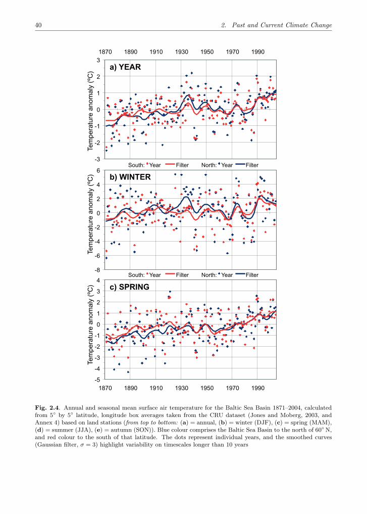
40 2. Past and Current Climate Change
-3
-2
-1
0
1
2
31870 1890 1910 1930 1950 1970 1990
-8
-6
-4
-2
0
2
4
6
-5
-4
-3
-2
-1
0
1
2
3
4
1870 1890 1910 1930 1950 1970 1990
Tem
pera
ture
ano
mal
y (º
C)
Tem
pera
ture
ano
mal
y (º
C)
Tem
pera
ture
ano
mal
y (º
C)
South: Year Filter North: Year Filter
South: Year Filter North: Year Filter
a) YEAR
b) WINTER
c) SPRING
Fig. 2.4. Annual and seasonal mean surface air temperature for the Baltic Sea Basin 1871–2004, calculatedfrom 5◦ by 5◦ latitude, longitude box averages taken from the CRU dataset (Jones and Moberg, 2003, andAnnex 4) based on land stations (from top to bottom: (a) = annual, (b) = winter (DJF), (c) = spring (MAM),(d) = summer (JJA), (e) = autumn (SON)). Blue colour comprises the Baltic Sea Basin to the north of 60◦ N,and red colour to the south of that latitude. The dots represent individual years, and the smoothed curves(Gaussian filter, σ = 3) highlight variability on timescales longer than 10 years

2.1. The Atmosphere 41
-3
-2
-1
0
1
2
3
-4
-3
-2
-1
0
1
2
3
4
1870 1890 1910 1930 1950 1970 1990
1870 1890 1910 1930 1950 1970 1990
Tem
pera
ture
ano
mal
y (º
C)
Tem
pera
ture
ano
mal
y (º
C)
South: Year Filter North: Year Filter
d) SUMMER
e) AUTUMN
Fig. 2.4. cont.
2.1.2.1 Annual and Seasonal Area Averaged TimeSeries
The changes of the Baltic Sea Basin mean temper-atures during 1871–2004 are inferred here using agridded data set with a 5◦ by 5◦ (latitude, longi-tude) resolution (Jones and Moberg 2003, see An-nex 4). For this analysis, all 5◦ grid boxes with atleast 50% of the box area belonging to the BalticSea Basin were considered. Two area-averaged se-ries have been calculated (Fig. 2.4), one includ-ing all selected Baltic Sea Basin grid boxes northof 60◦ N and one including those south of 60◦ N,thus establishing a northern and southern BalticSea Basin surface air temperature record, respec-tively. All data are anomalies from the 1961–1990standard normal.
In terms of temperature variations, the BalticSea Basin has been a relative uniform area during
the period 1871–2004 (Fig. 2.4a). A striking fea-ture in the annual mean series is the early 20th cen-tury warming, which is a marked increase in tem-perature that culminated in the 1930s. This early20th century warming was followed by a smallercooling that culminated in the 1960s and then an-other distinct warming lasting to the end of theseries.
Spring is the only season for which the end ofthe series is clearly warmer than the maximum ofthe 1930s when analysed on a decadal time scale(Fig. 2.4c). The early 20th century warming ismore pronounced in the northern area than in thesouthern, especially during winter (Fig. 2.4b).
For the period 1871–2004, the largest seasonaltrends in the Baltic Sea Basin are observed for thespring. Trends in all seasons are positive and mostof them are significant at the 0.05 level (Table 2.2).For the northern area the trend in winter is as

42 2. Past and Current Climate Change
Table 2.2. Linear surface air temperature trends (K per decade) in the period 1871–2004 for the BalticSea Basin, its northern (latitude > 60◦ N) and southern area (latitude < 60◦ N). Trends written in bold aresignificant at the 0.05 level. The trends were also tested by the non-parametric Mann-Kendall test. The resultswere consistent with the linear trend test
Data sets Year Winter Spring Summer Autumn
Northern area 0.10 0.09 0.15 0.06 0.08Southern area 0.07 0.10 0.11 0.03 0.06
high as 0.09 C/decade, but as the variability isparticularly large in this season, the trend is non-significant.
Annual warming trends (1871–2004) for thenorthern and southern Baltic Sea Basin, with val-ues of 0.10 and 0.07 C/decade, respectively, arelarger than the trend for the entire globe (1861–2000), which is about 0.05 C/decade (IPCC2001). Neither the Baltic Sea Basin temperatureseries nor the global series show a monotonoustemperature increase on the decadal time scale.
The main differences between the Baltic SeaBasin and global series are: (i) The early 20th cen-tury maximum occurs in the 1930s for the Baltic,whereas for the globe it occurs in the 1940s. (ii)For the Baltic Sea Basin, the maximum at theend of the series is of about the same magnitudeas the one earlier in the 20th century, whereas forthe globe the maximum at the end of the series issignificantly higher (IPCC 2001) than that in the1940s. (iii) The variability of annual mean temper-ature of the Baltic Sea Basin series is about fivetimes larger than the variability of the global meantemperatures. The warming trend characteristicin the Baltic Sea Basin has been observed to ex-tend further to the Arctic (Førland et al. 2002;Overland et al. 2004).
2.1.2.2 Information Drawn from the LongestInstrumental Time Series
The Little Ice Age, sometimes defined to be the pe-riod 1500–1850 (Ogilvie and Jónsson 2001), man-ifested itself in a dramatic way in the early tomid 18th century. Well known is the advance ofthe glacier Nigardsbreen in western Norway. Theglacier destroyed much farmland and many farm-houses before its advance stopped in 1748 (Nordli2001).
According to a reconstruction by Nordli et al.(2003) spring-to-summer air temperatures werevery low in the early 1740s, and this is also con-
firmed by a dip in the Uppsala summer air temper-ature series (Moberg and Bergström 1997). How-ever, the main reason for the glacier advanceseems rather to be mild winters in the 1720sand 1730s (Moberg and Bergström 1997; Tarandand Nordli 2001) and a predominance of westerlywinds (Bergström 1990), which led to accumula-tion of snow on the western Norwegian glaciers.This scenario is in line with the conclusion drawnby Nesje and Dahl (2003).
The Stockholm air temperature series showswarm intervals in the 1770s and in the 1790s(Moberg et al. 2002). In the 1770s summer tem-peratures contributed heavily to the high annualvalues, whereas in the 1790s it was mainly the win-ter temperatures that contributed (Fig. 2.5). Thewarm decade of the 1770s is also seen in the St. Pe-tersburg series (Jones and Lister 2002; Moberg etal. 2000). At the end of the 18th century a changetowards colder climate is seen, with low tempera-tures in the first decade of the 19th century for allseasons. The temperature then increased in thefollowing decades, but in the late 1830s and early1840s another severe cold period started.
The second half of the 19th century startedwith increased annual air temperatures, and, for-tunately for agriculture in the northern areas,summer temperatures contributed much to thisincrease. However, the 1850s was the last decadewith summers above normal before the onset of thecold period 1860–1920. The most severe decadewithin this period was the 1860s. The year 1867was the coldest year in the entire Stockholm tem-perature series (Fig. 2.5). In Finland, the spring of1867 was exceptionally cold, e.g. the break-up oflake ice was delayed by more than a month to mid-June (Simojoki 1940), and harvests were lost, lead-ing to the death of about 8% of the Finnish popu-lation (Jantunen and Ruosteenoja 2000). The coldperiod after the 1860s was broken by several mildwinters around 1910, followed by the early 20th
century warming (e.g. Alexandersson 2002).

2.1. The Atmosphere 43
1750 1800 1850 1900 1950 2000
4
5
6
7
8
Stockholm
°C
Annual
8
6
4
2
0
DJF
0
2
4
6
8
MAM
12
14
16
18
20
JJA
1750 1800 1850 1900 1950 2000
2
4
6
8
10
SON
Fig. 2.5. Annual and seasonal mean surface air temperatures ( C) in Stockholm 1756–2004, calculated fromthe homogenised daily mean temperature series by Moberg et al. (2002) after a correction for a suspectedpositive bias in summer temperatures before 1859 (Moberg et al. 2003). The correction is the same as used byMoberg et al. (2005). Smoothed curves (Gaussian filter, σ = 3) highlight variability on timescales longer than10 years
The St. Petersburg (Jones and Lister 2002) andthe Vilnius series (Bukantis and Rimkus 2005) alsohave decadal air temperature maxima and minima(not shown here) roughly in the same years as forthe Stockholm series. But there is a notable dif-ference: The annual maximum of the 1930s at St.Petersburg and Vilnius is not higher than the max-ima in the 1890s and 1910s, and, for the winterseason, local maxima occur in the 1920s. This dif-fers from the situation in the western and northernparts of the Baltic Sea Basin.
The temperature trends since the start of theVilnius series in 1777 have been examined byBukantis et al. (2001) and Bukantis and Rimkus
(2005). A significant trend in the annual val-ues, 0.6 C for the whole period of observa-tion, arises mostly from warming in the coldseason (November–March), amounting to 1.0 C(Fig. 2.6).
In Poland, long-term homogeneous time se-ries of air temperature have been reconstructedfor Warsaw, 1779–1998 (Lorenc 2000), Szczecin,1838–1992 (Kożuchowski and Miętus 1996),Gdańsk and Hel, both 1851–1995 (Miętus 1998a)and Koszalin, 1848–1990 (Miętus 2002). Thereis a statistically significant increase of air tem-perature in the range of 0.54–0.56 C/100 yearsin Warsaw, Gdańsk and Hel. Szczecin temper-

44 2. Past and Current Climate Change
-0,04-0,020,000,020,040,060,080,100,120,14
1 2 3 4 5 6 7 8 9 10 11 12
Tem
p. t
ren
d [
°C/d
eca
de]
Month
Fig. 2.6. Trends in monthly mean surface air temperature of the Vilnius series during the period 1777–2000
ature series show a larger increase of 1.1 C/100years. Warming is strongest in winter, in therange of 1.1 C/100 years in Gdańsk and Hel,1.2 C/100 years in Warsaw and 1.3 C/100 yearsin Szczecin.
2.1.2.3 Temperature Trends in Sub-regions and Re-lationships with Atmospheric Circulation
Many analyses of temperature trends and varia-tions have been based on data from the moderninstrumental period, from about 1870 to present.Moberg et al. (2005) studied the temperature dif-ference between the two 30 year periods, 1971–2000 and 1891–1920, for 6 individual time series inFennoscandia (Vardø and Kjøremsgrende in Nor-way, Oulu and Helsinki in Finland, Uppsala andStockholm in Sweden). Annual mean changes var-ied from +0.49 to +0.82 C. These changes weresignificant for all stations except for Kjørems-grende. Also for spring, all differences were sig-nificant except for Kjøremsgrende. For the otherseasons, most of the station trends were not sig-nificant.
The annual temperature increase from the mid-dle of the 19th century to the 1930s or 1940s(see Sect. 2.1.2.1) is characteristic for most of theBaltic Sea Basin. The average warming amountsto almost 1.5 C in Denmark since 1870 (Cappelenand Christensen 2005) and to 0.7–1.0 C in Esto-nia since about 1850 (Jaagus 1996, 1998) and inFinland (Tuomenvirta 2004).
The last decades of the 20th century and thefirst years of the 21st century are also charac-terised by a pronounced temperature increase. Forexample, in Denmark and Estonia the warmingstarted around 1990 (Cappelen and Christensen
2005; Jaagus 1996, 1998), whereas the warm-ing started around 1980 in Sweden and Norway(Alexandersson 2002; Hanssen-Bauer and Nordli1998). For Poland the mean surface air temper-ature in the decade 1991–2000 was 0.7 C higherthan in the previous normal period 1931–1960 (De-girmendžić et al. 2004). Ševkunova et al. (1999)found that the region with the strongest warmingin the 1980s and the 1990s is located in the easternBaltic Sea Basin south and east of Tallinn and St.Petersburg.
Temperature trends during the second half ofthe 20th century have been examined for Polandby Degirmendžić et al. (2004), and for Esto-nia (10 stations) by Jaagus (2006a). Significantpositive linear trends of 0.2 C/decade and 0.2–0.3 C/decade for annual temperatures are ob-served in Poland and Estonia, respectively. Forindividual months the trends vary considerably,being significant only for March (0.6 C/decade)and May (0.3 C/decade) for Poland. In Estonia,March also experiences the largest trend, amount-ing to 1 C/decade.
Temperature variability in the Baltic Sea Basinis strongly affected by changes in the atmosphericcirculation patterns. For southwestern Swedenand western Denmark, Chen (2000) showed that asmuch as 70% of the total variance in the monthlymean January surface air temperatures between1873 and 1994 can be accounted for by a linearcombination of three circulation indices; southerlywind, vector wind speed and westerly shear vor-ticity. Moberg et al. (2005) found, for temper-atures averaged over Fennoscandia, correlationswith a zonal circulation index in the range +0.44and +0.75 in the October to March half-year andnegative correlations of between −0.23 and −0.36
2.1. The Atmosphere 45
in the summer months during June to August.Stronger westerly winds in winter thus generallybring milder air towards Fennoscandia, whereasin summer they bring cooler air.
Polish, Lithuanian, and Estonian studies alsoreveal that the strongest correlations betweenwind flow indices and surface air temperature oc-cur during winter when zonal indices are used(Jaagus 2006a; Bartkeviciene 2002). For the tran-sitional seasons, spring and autumn, correlationswith temperature are stronger with meridionalcirculation indices than with zonal indices (De-girmendžić et al. 2004; Kożuchowski et al. 1992,1994, 2000; Kożuchowski and Marciniak 1988,1990; Kożuchowski and Żmudzka 2002; Marsz1999; Miętus 1999; Niedźwiedź and Ustrnul 1994;Ustrnul 1998; Wibig 2000, 2001). Miętus and Fil-ipiak (2002) demonstrated the influence of NorthAtlantic sea surface temperatures (SST) on ther-mal conditions in Poland. The strongest connec-tion between SST and air temperature in Polandexists during winter season, the weakest one dur-ing spring.
However, when comparing the influence ofNorth Atlantic SST and atmospheric circulationon the temperature in Poland Miętus and Filip-iak (2002) conclude that the influence of circu-lation (described by the pressure field) is domi-nant over SST forcing. Degirmendžić et al. (2004)also present evidence from Poland supporting thehypothesis that “the real warming observed inthe last decade of the 20th century has exceededcirculation-induced changes of temperature”.
2.1.2.4 Mean Daily Maximum and MinimumTemperature Ranges
Trends and changes occurring at the high and lowends of the air temperature range can have a greatimpact on society. It is well known that, after1950, the minimum air temperature on a globalscale has increased more than the maximum tem-perature (e.g. Karl et al. 1993; Easterling et al.1997). Consequently, this has led to a decreasein the Daily Temperature Range (DTR), definedas DTR = Tx − Tn, where Tx and Tn are themean daily maximum and minimum air tempera-tures, respectively. For extreme temperatures seeSect. 2.1.5.2.
By examining the period 1951–1998 for 9 homo-geneous series from Poland, Wibig and Głowicki(2002) found that annual mean values of Tn in-creased significantly during this period for all sta-
tions, with trends ranging from 0.14 C (Zakopane)to 0.31 C (Kalisz) per decade, whereas trends ofTx did not increase significantly. This change hasled to a decrease in DTR, although significant onlywith 5 of the 9 series. Seasonally, both Tn and Txwarmed significantly during winter (December toFebruary) and spring (March to May), but withonly minor changes in DTR. However, a decreaseof DTR is observed for the autumn (Septemberto November), although this is not due to an in-creased Tn but rather a decreased Tx.
The time evolution of Tx and Tn for Fennoscan-dia has been studied by Tuomenvirta et al. (2000)over the period 1910–1995. The largest variationsoccurred in winter (December to February) withthe warm 1988–1995 period surpassing even thewarm 1930s for both Tx and Tn. For the annualmeans of Tx and Tn, however, the 1988–1995 pe-riod was at about equal as warm as the 1930s.Both the spring Tx and Tn have warmed markedlythroughout the 20th century, although only the Tnwarming is significant.
The Fennoscandian DTR (Fig. 2.7) decreasedduring the 20th century, although not steadily. Forexample, the 1940s was a decade with large pos-itive anomalies for spring, summer and the an-nual mean. Overall, there was a decrease in DTRfrom 1910–1939 to 1966–1998 in spring, summerand autumn, resulting in a statistically significantdecrease of the annual mean, albeit without anysignificant decreases in the seasonal values. Theoverall decrease of the Fennoscandian DTR duringthe 20th century has been related to an increase incloudiness and to an intensification of westerly cir-culation.
Over most of the 20th century, four stationsin Poland (Łódź, Puławy, Zakopane and Śnieżka)showed a linear warming of annual Tn that waslarger than that of Tx, resulting in a decreasein DTR for all four seasons (Wibig and Głowicki2002). The decrease in DTR is significant in springand autumn for all four stations. The strongestwarming was found during mid- and late winterfor both Tx and Tn. Broadly consistent resultswere obtained by Miętus and Filipak (2004), whoanalysed the variability of thermal conditions inthe coastal region of the Gulf of Gdańsk during theperiod 1951–1998. They proved that the increasein mean daily minimum air temperature (close toor higher than 0.2 C/decade) was definitely higherthan that of the mean daily maximum tempera-ture (between 0.1–0.2 C/decade) at three of thefour stations.

46 2. Past and Current Climate Change
Fig. 2.7. Annual anomalies of Fennoscandian area-averaged daily temperature range (DTR) for the period1910–2000 (baseline is the 1961–1990 average) (updated from Tuomenvirta et al. 2000)
2.1.2.5 Changes in Seasonality
Information on changing seasonality can be drawnfrom long-term temperature series. Here, we de-scribe results for a cross-section from the west(Norway) to the east (East European Plain) acrossthe Baltic Sea Basin.
For Norway, using a Fourier transformation ofseven homogenised monthly temperature series,Grimenes and Nissen (2004) modelled the annualair temperature cycle during the period 1871–1990. These calculations were used to define in-dices for the length of the growing season (periodwhen daily mean temperature, Tm, is equal to orexceeds 5 C), the frost-free season (period whenTm > 0 C), the summer ‘half-year’ (period whenTm is larger than the annual mean temperature),and the hot season d2Tm
dt2 ≤ 0 as well as the heatsum (sum of Tm during the growing season).
Growing season length and frost-free seasonlength show positive trends for all stations in theperiod analysed (Table 2.3). This implies thatthe average level of the annual temperature cyclehas been shifted upwards towards higher temper-atures. Also, the length of the summer half-yearand the hot season show positive trends, whichindicates that the shape of the annual tempera-ture cycle has changed. The inflection points ofthe curve have shifted towards earlier dates in thespring and later dates in the autumn. The summerand winter ‘halves’ of the curves have become moreasymmetric, with the summer side becoming moreU-shaped and the winter curve more V-shaped.
A substantial increase in the heat sum (Ta-ble 2.3) illustrates the combined effect of thecurve’s change in shape and level. The varying,
and in part smaller changes, in winter strengthshow that the positive trend described by the for-mer quantities relates less to the changes in wintertemperatures than to changes in summer temper-atures.
Jones et al. (2002) studied seasonal indices backto the 18th century, using homogenised daily airtemperature series from Stockholm, Uppsala andSt. Petersburg. For the sub-period after 1870,their results are broadly consistent with those ofGrimenes and Nissen (2004): The length of thegrowing season and the heat sum have increased,whereas the length of the cold season and thefrost degrees have decreased. The lengthening ofthe growing season in Northern Europe is also re-ported by Chen et al. (2006) and Linderholm et al.(2005). According to Jones et al. (2002), there islittle relationship between the temperature of thegrowing (and also frost) season and its duration.However, day degree counts were found to be verystrongly correlated (r > 0.9) to average extendedsummer (May to September) and extended winter(October to April) temperatures.
Jaagus and Ahas (2000) studied long-termtrends in climatic seasons during the period 1891–1998 for Tartu, Estonia. In addition to the fourmain seasons – spring, summer, autumn and win-ter – four intermediate seasons have also been de-fined; between autumn and winter (late autumn,early winter), and between winter and spring (latewinter, early spring). A general tendency is thatthe start of the climatic seasons in the spring half-year (late winter, early spring, spring and sum-mer) start earlier, whereas the climatic seasons inthe autumn half-year (autumn, late autumn, earlywinter and winter) start later. But among those,

2.1. The Atmosphere 47
Fig. 2.8. Linear trend of the start date of early spring during the period 1946–1995, expressed in days. Stationswith a trend significant at the p < 0.05 level are marked with black dots (adapted from Jaagus et al. 2003)
Table 2.3. Means and trends of various indices (Grimenes and Nissen 2004, see text for definitions) for 1871to 1990. Trends are shown as days/100 years or day-degrees/100 years
Growth season Frost free season Summer half-year hot season Heat sumlength (days) length (days) length (days) length (days) (day degrees)
Mean Trend Mean Trend Mean Trend Mean Trend Mean Trend
Oksøy 211 14.6 175 8.6 154 26.0 2416 188Oslo 184 12.8 243 14.8 177 5.2 162 18.3 2271 152Bergen 218 20.7 174 8.8 153 27.4 2362 258Dombås 138 12.7 193 14.7 177 8.1 162 28.9 1343 118Værnes 176 10.8 251 8.9 176 6.4 158 21.7 1895 119Tromsø 129 17.4 202 14.8 163 6.4 130 10.1 1170 258Vardø 112 16.3 189 18.9 170 4.0 142 7.3 868 178
only the start of late autumn (+8 days) and win-ter (+17 days) have shifted significantly. Signifi-cant are also rather large changes of duration forsummer (+11 days), early winter (+18 days), andwinter (−30 days) (Jaagus and Ahas 2000).
In the East European Plain, using a similarmethodology, the climatic seasons have been anal-ysed for two periods, a long period (1881–1995)and a short period (1946–1995), using 12 and 73stations, respectively (Jaagus et al. 2003). Themost remarkable changes during the shorter pe-
riod were detected in the Baltic Sea Basin partof the Plain (Fig. 2.8), where the start of earlyspring (when daily mean air temperature perma-nently rises above zero) has moved towards an ear-lier start by up to one month.
As a consequence, the duration of winter (whendaily mean air temperature permanently drops be-low zero) has dramatically decreased, and dura-tion of early spring has increased. Similar resultsare also reported by Kożuchowski et al. (2000) for8 stations in Poland during the period 1931–1998.

48 2. Past and Current Climate Change
For some of the stations winter is shortened bymore than 30 days during this period. Also Marke-vičiene (1998) reports a reduction of the length ofthe winter by about 30 days in Vilnius, althoughthe period analysed is much longer (> 200 years).
2.1.3 Changes in Precipitation
Atmospheric circulation and characteristics of airmasses (humidity, stability) largely determine theoccurrence and rate of precipitation. Although at-mospheric processes have a governing role, orog-raphy greatly influences spatial distribution andintensity of precipitation, e.g. enhancing rainfallon the windward side of mountains and hills (e.g.Tveito et al. 1997 and Annex 1.2.3). Furthermore,the effect of the underlying surface, e.g. a contrastbetween the Baltic Sea and adjacent land, can beseen in the regional distribution of precipitation(Annex 1.2.3).
Precipitation measured with gauges is usuallyan underestimation of true precipitation. There isa substantial undercatch, especially for solid pre-cipitation, frequent light rainfall events or windyconditions (Førland and Hanssen-Bauer 2000).Different mean climatological estimates for theBaltic Sea Basin (for the whole basin as well asseparate estimates for the land surface and seapart) are available in the published literature; seeAnnex 1.2.3 for a brief discussion.
It is thus possible that also changes in otherfactors, such as gauge design, type of precipita-tion, wind conditions, etc. contribute to trends inthe measured precipitation (see Annex 5). Studiesputting recent precipitation changes in the per-spective of multi-decadal variability are compli-cated by homogeneity problems of the time series.Many studies have addressed this question (e.g.Alexandersson 1986; Hanssen-Bauer and Førland1994; Heino 1994; Peterson et al. 1998; Tuomen-virta 2001; Groisman et al. 2001; Wijngaard et al.2003). Despite efforts at homogenisation, uncer-tainties are related to the long-term records.
Modern measurement technologies like satel-lites and radar have so far been able to produceonly short time series that are not free from un-certainties, either (e.g. Koistinen and Michelson2002; Michelson et. al 2005). In this section wewill present variability and trends based on precip-itation measurements with gauges. Precipitationextremes are discussed in Sect. 2.1.5.3 and someother precipitation-related variables (e.g. runoff,snow cover) in Sect. 2.2.
2.1.3.1 Observed Variability and Trends During theRecent 50 Years
Folland et al. (2001) report in the Third Assess-ment Report of the Intergovernmental Panel onClimate Change (IPCC TAR) that precipitationhas increased by about 12% in all land areas be-tween latitudes 55◦ N and 85◦ N during the 20th
century. A closer look reveals that the generalhigh-latitude increase is broken into a complexpattern of changes in northern Europe (New etal. 2001).
In the Baltic Sea Basin, there has been an in-crease of precipitation in the period 1976–2000compared to the period 1951–1975 (Beck et al.2005, see Fig. 2.9). However, the pattern of changeis far from uniform. The largest increases occurredin Sweden and on the eastern coast of the BalticSea, while southern Poland has received some-what less precipitation on average. As precipita-tion varies greatly both spatially and temporally(Annex 1.2.3), it is difficult to establish long-termtrends. Because of poor data-coverage in west-ern parts of Norway, the map does not reflect theconsiderable precipitation increase which was ob-served in this area during the second half of the20th century (Hanssen-Bauer 2005). On the otherhand, over some areas there is a small artificialenhancement in precipitation increase due to im-proved techniques for measuring precipitation; e.g.in Finland this amounts to a few percent.
There are distinct patterns of seasonal changes,with spring precipitation increasing over large ar-eas around the Baltic Sea. For example, an in-crease of more than 15% in spring has occurred incentral Sweden, but in some regions in southernPoland spring precipitation has decreased. Rain-fall amounts during summer have shown a smalldecrease over areas mainly in western and south-ern parts of the Baltic Sea Basin, but some in-crease has occurred in regions around the north-ern Baltic Proper as well as in southern Finlandand northern Sweden. In autumn there has beenan increase almost in the entire Baltic Sea Basin,yet there are regions showing a small decrease,particularly in Germany and Poland. The sea-son with the largest increases is winter. The mainarea of increase stretches from Norway, Denmarkand Germany in the west to the Baltic States andRussia in the east.
Førland et al. (1996) performed an analysis ofprecipitation changes based on well over a thou-sand stations during the standard normal periods

2.1. The Atmosphere 49
DJF MAM
SONJJA
<0.950.95-1.001.01-1.051.06-1.101.11-1.151.16-1.20
ANNUAL
Fig. 2.9. Annual and seasonal precipitation ratios between the periods 1976–2000 and 1951–1975 based onVASClimO (Variability Analysis of Surface Climate Observations) data (Beck et al. 2005)
1931–1960 and 1961–1990, covering a large part ofthe Baltic Sea Basin. In Førland et al. (1996) thegeneral features are similar to Fig. 2.9, but thereare more details over the Scandinavian countriesdue to better station coverage. The spatial pat-tern of differences suggests that atmospheric cir-culation changes have been the main cause. Anincrease in humid westerlies during the colder halfof the year produces an orographic signal whereregions exposed to westerlies and which receive alarge part of the precipitation in autumn and win-ter receive more precipitation. In accordance withthis, some leeward sides of mountains and hillsshow a decrease.
The most recent changes are reported in na-tional studies. In Sweden, the 1990s were on aver-age 8% wetter than during the 1961–1990 normal
period (Alexandersson and Eggertsson Karlström2001). All seasons except autumn became rainier.Northern and south-western Sweden show localmaxima of positive anomalies. In Denmark as awhole the period 1990–2004 was on average 5%wetter than the 1961–1990 normal period (Cappe-len and Christensen 2005). In Finland Hyvärinenand Korhonen (2003) compared measured precip-itation amounts at drainage level between the pe-riods 1961–1990 and 1991–2000.
A majority of the studied areas showed an in-crease of measured precipitation with only a fewbasins showing no change or a decrease. The in-crease occurred mainly during the cold season,with a small increase also during summer. Innorthern Finland during the period 1991–2000,the largest positive anomalies of drainage basin

50 2. Past and Current Climate Change
Visandi Võru Narva40
30
20
10
0
-10
-20
mm
1 2 3 4 5 6 7 8 9 10 11 12
Fig. 2.10. Trend of monthly precipitation (mm/month) at three Estonian stations (Vilsandi, Võru and Narva)during 1951–2000 (Jaagus 2006a)
annual precipitation were up to 50–80mm (∼ 10–17%) above the standard normal. However, insome cases even half of the difference between theperiods 1961–1990 and 1991–2000 can be due toimprovements in measurements (Solantie and Ju-nila 1995; Tuomenvirta 2004).
Franke et al. (2004) analysed precipitationtrends in Saxony, eastern Germany. The mostnotable features of the trend analysis for the pe-riod 1951–2000 were: A marked decrease in sum-mer rainfall (−10 to −30%) and a significant in-crease in winter precipitation (10 to 20%). InPoland, during the period 1951–2000 a positvetrend (+2.85mm/decade) in annual area averagedprecipitation remains insignificant (Degirmendžićet al. 2004), but there is a significant increase inMarch and also a significant decrease in the ratioof summer and annual precipitation totals.
In Estonia, the second half of the 20th cen-tury is characterised by a statistically significantincrease in annual precipitation by 10–25% (80–180mm) at 8 out of 9 studied stations (Jaagus2006a). The increase in annual precipitation re-sults partly from the introduction of wetting cor-rections. Therefore, the real increase may beup to 5–15%. Among the individual months, astatistically significant increase in precipitationis revealed during the period from October toMarch and in June, whereby trends vary muchbetween stations and months, especially in sum-mer (Fig. 2.10). In Vilnius, Lithuania, cold seasonprecipitation has increased and warm season pre-cipitation has decreased during the last fifty years(Bukantis and Rimkus 2005).
2.1.3.2 Long-term Changes in Precipitation
This section discusses evidence concerning precip-itation changes based on Baltic Sea Basin recordscovering time periods of more than a century.
In Norway Hanssen-Bauer and Førland (1998)identified 13 regions having uniform long-termtrends and decadal variability. Data for the pe-riod 1896–2004 show increasing trends in annualprecipitation of between 3 to 18% per 100 years(Hanssen-Bauer 2005). Positive trends were sta-tistically significant in 9 of the 13 regions. The in-crease has been somewhat larger during the latterhalf of the record. In southern Norway, the long-term increase is significant only during autumn,while in northern parts of the country spring aswell as summer and/or winter precipitation haveincreased.
In Sweden, Busuioc et al. (2001) identified fourregions with similar long-term variability. Fig-ure 2.11 shows annual and seasonal precipitationtrends for Sweden (Alexandersson 2004). The in-creasing trend is significant at the annual leveland in all seasons except summer. Alexanders-son (2002) divided the country into four regionsaccording to the drainage basins and comparedannual totals between the periods 1860–1920 and1921–2001.
The analysed increase ranges from 23% in theGulf of Bothnia drainage basin to 15% in the Both-nian Sea basin and 7% in basins in southern Swe-den (south of 60◦ N). Seasonally, the largest in-crease has taken place in northern Sweden duringwinter.

2.1. The Atmosphere 51
ANNUAL, 643 mm (1961-90)
-250
-200
-150
-100
-50
0
50
100
150
200
250
1860 1880 1900 1920 1940 1960 1980 2000
-250
-200
-150
-100
-50
0
50
100
150
200
250
WINTER, 133 mm (1961-90)
-120-80-40
04080
120
1860 1880 1900 1920 1940 1960 1980 2000
-120-80-4004080120
SPRING, 115 mm (1961-90)
-120-80-40
04080
120
1860 1880 1900 1920 1940 1960 1980 2000
-120-80-4004080120
SUMMER, 203 mm (1961-90)
-120-80-40
04080
120
1860 1880 1900 1920 1940 1960 1980 2000
-120-80-4004080120
AUTUMN, 193 mm (1961-90)
-120-80-40
04080
120
1860 1880 1900 1920 1940 1960 1980 2000
-120-80-4004080120
Fig. 2.11. Anomaly time series of annual and seasonal precipitation over Sweden, 1860–2004 (reference period1961–1990). Curves represent variations in the time scale of about ten years (updated from Alexandersson2004)

52 2. Past and Current Climate Change
1880 1900 1920 1940 1960 1980 2000
450
500
550
600
650
700
750
800
850
900
950
mm
Fig. 2.12. Variation of annual precipitation amount over Denmark, 1874–2004. The curve represents variationsin the time scale of about thirty years (Cappelen and Christensen 2005)
Somewhat contrary to its western neighbours,annual precipitation totals over Finland do notshow any significant long-term trend during theperiod 1894–2002 (Tuomenvirta 2004). There aredecadal fluctuations of about ±30mm in annualprecipitation, one of which shows a rise of about10mm (∼ 2%) from the 1940s to the 1990s. Itmay well be that averaging over the whole coun-try (an area of more than 330,000 km2) smoothesout some regional trends that are visible e.g. inFinnish discharge records (Hyvärinen 2003). Fig-ure 2.12 shows the annual accumulated precipi-tation over Denmark (Cappelen and Christensen2005). There has been a statistically significantincrease of approximately 100mm (≈ 15%) since1870.
Analysis of spatial mean annual precipitationin Estonia during the period 1866–1995 indicatesa weak and insignificant increasing trend. The in-crease has been larger in autumn and winter, andis absent in spring and summer. Attention hasbeen paid to the analysis of periodical fluctuationsof precipitation in Estonia. Using spectral analy-sis, rather regular periodicity with cycles of 50–60,25–33 and 5–7 years was detected (Jaagus 1992,1998; Jaagus and Tarand 1998).
The long-term precipitation series from Latviashow increases during both the cold (Nov–Mar)and the warm (Apr–Oct) seasons, with a more pro-nounced increase during the cold season (Lizuma2000; Briede and Lizuma 2002). The significanceof precipitation trends shows spatial variability.
A long time series of precipitation from Vilnius,Lithuania (Bukantis and Rimkus 2005) shows a
large multi-decadal fluctuation from dry to wetduring the first decades of the 20th century. Theslight long-term increasing trend in annual pre-cipitation results from an increase during the coldseason (Nov–Mar) and a slight decrease during thewarm season (Apr–Oct).
Kozuchowski (1985) examined the variationin precipitation during the period 1881–1980 inPoland. A slight increase in annual totals wasdiscovered. The increase was accompanied bya growth of dispersion of precipitation totals.Niedźwiedź and Twardosz (2004) combined threetime series from Poland (Kraków, Warszawa, Wro-claw) and one from the Ukraine (Lwów) to repre-sent temporal variability of precipitation to thenorth of the Carpathian and Sudeten mountains.Over this very long time period (1855–2002), thereis no clear long-term trend in annual totals. Thesecond half of the 20th century has a somewhathigher mean level than the earlier time periods,mainly due to a recent increase during winter.
2.1.3.3 Changes in Number of Precipitation Days
Besides total amount, also frequency and intensityof precipitation need to be considered (see alsoSect. 2.1.5.3 on precipitation extremes). A simpleparameter describing frequency is the number ofprecipitation days, i.e. days when daily precipita-tion is equal to or exceeds e.g. 0.1mm or 1.0mm.The limit of 0.1mm is quite sensitive to factorssuch as observer accuracy, observation intervaland evaporation characteristics of the precipi-tation gauge (Heino 1994; Tveito et al. 2001).

2.1. The Atmosphere 53
Heino (1994) did not find any significant trendsin the Finnish data. Bukantis and Valiuskeviciene(2005) found an increasing trend in the number ofannual precipitation days in the entire Lithuanianterritory for the period 1925–2003. Kożuchowskiand Żmudzka (2003) reported an increase in thenumber of precipitation days in Poland duringthe last hundred years. In general, autumn andwinter showed increasing trends, continuing untilMarch. Førland (2000) studied changes in thedistribution of daily precipitation in southernand western Norway. He found a high covariancebetween probability of rain, total precipitation,and probability of heavy precipitation. During the20th century at Samnanger (60◦ 28′ N, 5◦ 54′ E),where the annual precipitation has increasedby 18%, the number of days with precipitation≥ 0.1mm (≥ 1.0mm) has increased by 19%(13%). There are many studies on changes oftotal precipitation in Northern Europe, but thereis a lack of information concerning systematicchanges in intensity of daily precipitation.
2.1.3.4 Interpretation of the Observed Changes inPrecipitation
Some of the century-scale precipitation time seriesfrom the Baltic Sea Basin display increasing pre-cipitation. Over the whole northern hemispherelatitude band 55◦ N–85◦ N, the increase was some-what steeper during the first half of the centurythan after the 1950s, whereas in the Baltic SeaBasin it appears that the increasing trend has beenlarger during the latter half of the 20th century.Winter is usually the season with the largest in-crease. Homogeneity problems combined with thefact that precipitation varies to a high degree spa-tially and temporally, make accurate estimation oflong-term precipitation trends difficult.
The latter half of the 20th century is charac-terised by decadal scale fluctuations, but there isevidence of an increase in annual precipitation to-tals over most of Northern Europe. The observedincrease is not uniform and there are also regionslacking statistically significant trends (e.g. in Fin-land and southeastern Norway). The increase ismostly concentrated in the cold season from Oc-tober to March. As precipitation amounts displaylarge temporal and spatial variability, there is alsovariability in trends from month to month and be-tween regions. During summer, convective precip-itation processes dominate and there is less spatialcoherence of trends between regions during the lat-
ter half of the 20th century. Both increasing (e.g.Sweden) and decreasing (e.g. Poland) trends inlarge area averages can be found in summertime.
There are many studies relating precipitationto atmospheric circulation (e.g. Kożuchowski andMarciniak 1988; Wibig 1999; Busuioc et al.2001; Ustrnul and Czekierda 2001; Twardosz andNiedźwiedź 2001; Johansson and Chen 2003), andweak links with remote sea surface temperaturesalso have been found (Feddersen 2003). Dur-ing wintertime, part of the increase in precipita-tion can be attributed to more frequent westerlyand/or cyclonic circulation related to large-scalechanges in atmospheric circulation (Busuioc et al.2001; Keevallik 2003; Degirmendžić et al. 2004).Similarly, some of the differences between summermonths have been attributed to changes in circu-lation patterns (Busuioc et al. 2001). Because oflarge natural variability and somewhat inconsis-tent signals from future climate simulations (seeChap. 3), it is difficult to attribute the observedincrease of precipitation in northern Europe to fac-tors other than changes in atmospheric circulation(Schmith 2001). Although the causes of precipita-tion fluctuations cannot be identified, these fluctu-ations can still have remarkable local and regionalimpacts.
2.1.4 Changes in Cloudiness and SolarRadiation
Nearly all physical processes and phenomena inthe atmosphere have originated and are driven bysolar energy. Net radiation describes the amountof solar and atmospheric radiation energy ab-sorbed by the Earth’s surface. Spatial distribu-tion of solar radiation is, first of all, determinedby latitude, but the role of clouds is very signifi-cant, especially in the ground-level fluctuations ofsolar radiation. Cloudiness is, in turn, influencedby atmospheric circulation. See Annexes 1.2.4 and1.2.5 on mean cloudiness and global radiation, re-spectively, in the Baltic Sea Basin.
Long-term changes observed in cloudiness andsolar radiation have so far hardly been studied.The IPCC Third Assessment Report (IPCC 2001)refers only to a few articles dealing with changesin cloudiness in Europe. They indicate an in-crease in cloud cover during different periods dur-ing the 20th century. Little information can befound about changes in global radiation and othercomponents of the radiation budget.
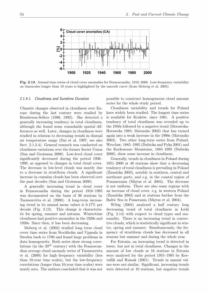
54 2. Past and Current Climate Change
-6
-4
-2
0
2
4
6
[%]
Cloud cover anomalies (CA)
1900 1920 1940 1960 1980 2000
Fig. 2.13. Annual time series of cloud cover anomalies for Fennoscandia, 1910–2000. Low-frequency variabilityon timescales longer than 10 years is highlighted by the smooth curve (from Moberg et al. 2005)
2.1.4.1 Cloudiness and Sunshine Duration
Climatic changes observed in cloudiness over Eu-rope during the last century were studied byHenderson-Sellers (1986, 1992). She detected agenerally increasing tendency in total cloudiness,although she found some remarkable spatial dif-ferences as well. Later, changes in cloudiness werestudied in relation to decreasing trends in diurnalair temperature range (Dai et al. 1997; see alsoSect. 2.1.2.4). General research was conducted oncloudiness variations over the former Soviet Union(Sun and Groisman 2000). Low-level cloud coversignificantly decreased during the period 1936–1990, as opposed to changes in total cloud cover.The decrease in low-level clouds was mostly dueto a decrease in stratiform clouds. A significantincrease in cumulus clouds has been observed overthe past decades (Sun and Groisman 2000).
A generally increasing trend in cloud coverin Fennoscandia during the period 1910–1995was documented on the basis of 36 stations byTuomenvirta et al. (2000). A long-term increas-ing trend in its annual mean values is 0.17% perdecade (Fig. 2.13). This change is characteris-tic for spring, summer and autumn. Wintertimecloudiness had positive anomalies in the 1920s and1930s. Since then, it has been decreasing.
Moberg et al. (2003) studied long–term cloudcover time series from Stockholm and Uppsala inSweden back to 1780 and found large problems indata homogeneity. Both series show strong corre-lations (in the 20th century) with the Fennoscan-dian average cloud anomaly series of Tuomenvirtaet al. (2000) for high–frequency variability (lessthan 10-year time scales), but the low-frequencycorrelations (longer than 10-year time scales) werenearly zero. The authors concluded that it was not
possible to construct homogeneous cloud amountseries for the whole study period.
Cloudiness variability and trends for Polandhave widely been studied. The longest time seriesis available for Kraków, since 1861. A positivetendency of total cloudiness was revealed up tothe 1950s followed by a negative trend (Morawska-Horawska 1985; Matuszko 2003) that has turnedagain into a weak increase in the 1990s (Matuszko2003). Two other long-term series from Poland,Wrocław, 1885–1995 (Dubicka and Pyka 2001) andthe Karkonosze Mountains, 1885–1995 (Dubicka2000), show some increase in cloudiness.
Generally, trends in cloudiness in Poland during1951–2000 at 48 stations show that a decreasingtendency of total cloudiness is prevailing in Poland(Żmudzka 2003), notably in southern, central andnortheast parts, and e.g. in the coastal region ofPommerania (Miętus et al. 2004). The decreaseis not uniform. There are also some regions withan increase of cloud cover, e.g. in western Poland(Żmudzka 2003) and at stations further from theBaltic Sea in Pomerania (Miętus et al. 2004).
Wibig (2004) analysed a half century longdecreasing trend of total cloudiness in Łódź(Fig. 2.14) with respect to cloud types and sea-sonality. There is an increasing trend in convec-tive clouds, which is statistically significant in win-ter, spring and summer. Simultaneously, the fre-quency of stratiform clouds has decreased in allseasons but summer and during the whole year.
For Estonia, an increasing trend is detected inlower, but not in total cloudiness. Changes in theamount of low clouds at 16 stations in Estoniawere analysed for the period 1955–1995 by Kee-vallik and Russak (2001). Trends in annual val-ues were not similar. Significant, increasing trendswere detected at 10 stations, but negative trends

2.1. The Atmosphere 55
4
5
6
7
8
1950 1960 1970 1980 1990 2000
Lódz (total)
Tõravere (low level)
Clo
ud
ines
s (t
enth
s)
Fig. 2.14. Long-term variability of the mean annual total cloudiness in Łódź at noon during 1951–2000 (Wibig2004) and annual mean low cloudiness at Tartu-Tõravere in 1955–2004
were found for two stations, possibly due to in-accuracies in observations. The amount of lowclouds has increased in March, June and Septem-ber, while it decreased in some stations in May andOctober. At Tartu-Tõravere, the monthly meanamount of low clouds has significantly increasedin March, June and September, as has the annualmean (Russak 1998). During the earlier time pe-riod, 1964–1986, the amount of low clouds fromApril to September increased by as much as 11%(Russak 1990).
The increase in the amount of low clouds in Es-tonia was primarily a result of an increase in theoccurrence of stratus and stratocumulus clouds.This increase was especially notable in March(Russak 1999; Keevallik and Russak 2001). Kee-vallik (2003) demonstrated that March has beenthe month with most significant climate changesin Estonia. The amount of low clouds at the Ti-irikoja and Tartu-Tõravere station increased by0.55 and 0.60 tenths per decade in March during1955 to 1995, respectively. Since the beginningof the 1990s a decreasing amount of low cloudshas been observed at the Tartu-Tõravere station(Fig. 2.14).
Long-term changes in cloudiness in Lithuaniawere studied by Stankunavićius (1998) for the pe-riod 1925–1995. There was a decrease in totalcloud cover in the eastern and central parts inthe 1960s and the beginning of the 1970s and anincrease in the Zemaiciai Upland. The major-ity of these trends is not statistically significant.Low cloudiness shows a more pronounced negativetrend from the 1940s up to the beginning of the21st century. Some stations in the hilly easternand flat northern parts of Lithuania indicate a de-
crease in cloudiness by up to 1–1.2 tenths per 25years. Seasonal differences are also significant. Anegative trend in total and low cloudiness prevailsduring the cold season (October–February), whilea positive trend is evident during the rest of a year,especially in March.
Sunshine duration depends very much oncloudiness. It can be assumed that an increase incloudiness is closely related to a decrease in sun-shine duration. A very long series for sunshineduration in Copenhagen is available since 1876(Laursen and Cappelen, 1998; Cappelen, 2005).The lowest level was found at the end of the 19th
century, rising to the highest level in the middleof the last century, followed by a slight decreasein the 1960s and 1970s and an overall increasefrom the 1980s to present (Fig. 2.15). Now themean level of annual sunshine duration is nearlyof the same magnitude as in the middle of the lastcentury. All seasons show more or less the sametrends.
The longest time series of sunshine duration inEstonia is available from Tartu, dating back to1901. Substantial fluctuations have been observedduring the 20th century, although no general trendexists (Jaagus 1998). The sunniest period wasin the 1940s. After that, sunshine duration de-creased significantly up to the 1980s. The latestincrease in sunshine duration started in the 1990s.Corresponding time series for Helsinki, Finland(Heino 1994) as well as for Riga, Latvia (Lizuma2000) show much of the same features as in Tartu(Fig. 2.15).
There are long-term low frequency fluctuationscausing trends of different signs at different timeintervals. For example, annual sunshine dura-
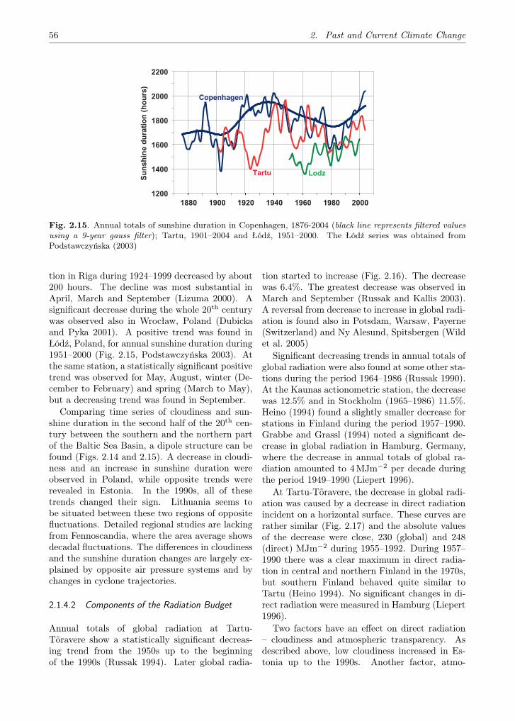
56 2. Past and Current Climate Change
Fig. 2.15. Annual totals of sunshine duration in Copenhagen, 1876-2004 (black line represents filtered valuesusing a 9-year gauss filter); Tartu, 1901–2004 and Łódź, 1951–2000. The Łódź series was obtained fromPodstawczyńska (2003)
tion in Riga during 1924–1999 decreased by about200 hours. The decline was most substantial inApril, March and September (Lizuma 2000). Asignificant decrease during the whole 20th centurywas observed also in Wrocław, Poland (Dubickaand Pyka 2001). A positive trend was found inŁódź, Poland, for annual sunshine duration during1951–2000 (Fig. 2.15, Podstawczyńska 2003). Atthe same station, a statistically significant positivetrend was observed for May, August, winter (De-cember to February) and spring (March to May),but a decreasing trend was found in September.
Comparing time series of cloudiness and sun-shine duration in the second half of the 20th cen-tury between the southern and the northern partof the Baltic Sea Basin, a dipole structure can befound (Figs. 2.14 and 2.15). A decrease in cloudi-ness and an increase in sunshine duration wereobserved in Poland, while opposite trends wererevealed in Estonia. In the 1990s, all of thesetrends changed their sign. Lithuania seems tobe situated between these two regions of oppositefluctuations. Detailed regional studies are lackingfrom Fennoscandia, where the area average showsdecadal fluctuations. The differences in cloudinessand the sunshine duration changes are largely ex-plained by opposite air pressure systems and bychanges in cyclone trajectories.
2.1.4.2 Components of the Radiation Budget
Annual totals of global radiation at Tartu-Tõravere show a statistically significant decreas-ing trend from the 1950s up to the beginningof the 1990s (Russak 1994). Later global radia-
tion started to increase (Fig. 2.16). The decreasewas 6.4%. The greatest decrease was observed inMarch and September (Russak and Kallis 2003).A reversal from decrease to increase in global radi-ation is found also in Potsdam, Warsaw, Payerne(Switzerland) and Ny Alesund, Spitsbergen (Wildet al. 2005)
Significant decreasing trends in annual totals ofglobal radiation were also found at some other sta-tions during the period 1964–1986 (Russak 1990).At the Kaunas actionometric station, the decreasewas 12.5% and in Stockholm (1965–1986) 11.5%.Heino (1994) found a slightly smaller decrease forstations in Finland during the period 1957–1990.Grabbe and Grassl (1994) noted a significant de-crease in global radiation in Hamburg, Germany,where the decrease in annual totals of global ra-diation amounted to 4 MJm−2 per decade duringthe period 1949–1990 (Liepert 1996).
At Tartu-Tõravere, the decrease in global radi-ation was caused by a decrease in direct radiationincident on a horizontal surface. These curves arerather similar (Fig. 2.17) and the absolute valuesof the decrease were close, 230 (global) and 248(direct) MJm−2 during 1955–1992. During 1957–1990 there was a clear maximum in direct radia-tion in central and northern Finland in the 1970s,but southern Finland behaved quite similar toTartu (Heino 1994). No significant changes in di-rect radiation were measured in Hamburg (Liepert1996).
Two factors have an effect on direct radiation– cloudiness and atmospheric transparency. Asdescribed above, low cloudiness increased in Es-tonia up to the 1990s. Another factor, atmo-
1200
1400
1600
1800
2000
2200
1880 1900 1920 1940 1960 1980 2000
Su
nsh
ine
du
rati
on
(h
ou
rs)
Copenhagen
Tartu Lodz
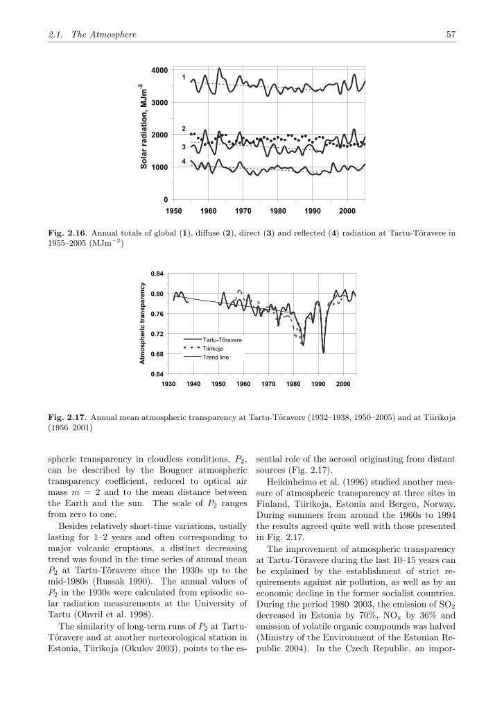
2.1. The Atmosphere 57
0
1000
2000
3000
4000
1950 1960 1970 1980 1990 2000
1
2
3
4
So
lar
rad
iati
on
, MJm
-2
Fig. 2.16. Annual totals of global (1), diffuse (2), direct (3) and reflected (4) radiation at Tartu-Tõravere in1955–2005 (MJm−2)
0.64
0.68
0.72
0.76
0.80
0.84
1930 1940 1950 1960 1970 1980 1990 2000
Atm
osp
her
ic t
ran
spar
ency
Tartu-Tõravere
Tiirikoja
Trend line
Fig. 2.17. Annual mean atmospheric transparency at Tartu-Tõravere (1932–1938, 1950–2005) and at Tiirikoja(1956–2001)
spheric transparency in cloudless conditions, P2,can be described by the Bouguer atmospherictransparency coefficient, reduced to optical airmass m = 2 and to the mean distance betweenthe Earth and the sun. The scale of P2 rangesfrom zero to one.
Besides relatively short-time variations, usuallylasting for 1–2 years and often corresponding tomajor volcanic eruptions, a distinct decreasingtrend was found in the time series of annual meanP2 at Tartu-Tõravere since the 1930s up to themid-1980s (Russak 1990). The annual values ofP2 in the 1930s were calculated from episodic so-lar radiation measurements at the University ofTartu (Ohvril et al. 1998).
The similarity of long-term runs of P2 at Tartu-Tõravere and at another meteorological station inEstonia, Tiirikoja (Okulov 2003), points to the es-
sential role of the aerosol originating from distantsources (Fig. 2.17).
Heikinheimo et al. (1996) studied another mea-sure of atmospheric transparency at three sites inFinland, Tiirikoja, Estonia and Bergen, Norway.During summers from around the 1960s to 1994the results agreed quite well with those presentedin Fig. 2.17.
The improvement of atmospheric transparencyat Tartu-Tõravere during the last 10–15 years canbe explained by the establishment of strict re-quirements against air pollution, as well as by aneconomic decline in the former socialist countries.During the period 1980–2003, the emission of SO2
decreased in Estonia by 70%, NOx by 36% andemission of volatile organic compounds was halved(Ministry of the Environment of the Estonian Re-public 2004). In the Czech Republic, an impor-

58 2. Past and Current Climate Change
-2000
-1000
0
1000
2000
1960 1970 1980 1990 2000
Net radiation
Net long-wave radiation
Net
rad
iati
on
(M
Jm -2
)
1960 1970 1980 1990 2000
Fig. 2.18. Annual totals of net and net long-wave radiation (MJm−2) at Tartu-Tõravere during 1962–2001(Russak and Kallis 2003)
tant source of anthropogenic aerosol in CentralEurope, the emission of SO2 was reduced by 86%and NOx by 55% in 1989–2000 (Hejkrlik 2002). Atpresent, the atmospheric transparency in Estoniahas reached the level it had in the 1930s.
No significant trend was found in time seriesof diffuse radiation during the same period fromthe 1950s up to the beginning of the 1990s (Rus-sak and Kallis 2003). But a decreasing trendhas become evident during the latest 10–15 years(Fig. 2.16). It can be explained by a decrease inboth cloudiness and atmospheric turbidity. A sig-nificant decrease of diffuse radiation by 4 MJm−2
per decade was observed in Hamburg during theperiod 1964–1990 (Liepert 1996).
As a result of a decrease in global radiation,the radiation reflected from the surface has alsodecreased at Tartu-Tõravere (Fig. 2.16) (Russakand Kallis 2003). Time series from central andsouthern Finland during the period 1960–90 alsoshow a small decline or no change, whereas in So-dankylä, northern Finland, there is a clear drop ofabout 200 MJm−2 (Heino 1994).
The main reason for the decrease in reflectedradiation at Tartu-Tõravere was a decrease inground surface albedo. In the Baltic Sea Basin,annual mean albedo is highly correlated with theduration of snow cover, especially with snow con-ditions in March and April (Tooming 1995). Ac-cording to the analysis of snow data from nearlya hundred observation points in Estonia, the du-ration of permanent snow cover shortened on av-
erage by 33 days during 1962–1995 (Toomingand Kadaja 1995, 2000a,b; see also Sect. 2.2.3).At Tartu-Tõravere, the annual mean albedo de-creased from 0.29 to 0.25 in 1955–1992 (Russakand Kallis 2003).
During the years 1955–1992, the decrease in an-nual totals of reflected radiation was 216 MJm−2,which is rather close to the decrease in globalradiation. In the budget of solar radiation (netshort-wave radiation), these changes compensateeach other and, as a result, there is no significanttrend in the time series of solar radiation absorbedby the surface, also called net short-wave radia-tion, and the solar radiation budget on the ground(Russak and Kallis 2003).
A breakpoint in the described trends has beenfound at Tartu-Tõravere for the early 1990s: So-lar radiation and transparency of the cloud-freeatmosphere began to increase while low cloudi-ness started to decrease. This kind of change maybe related to the diminishing atmospheric aerosolcontent (air pollution) during recent decades.Changes in the aerosol content lead to the changesin absorption and scattering of radiation, as wellas in the amount of possible condensation nucleiand thus in genesis and development of cloudiness.Another plausible explanation for the decrease inlow cloudiness could be related to changes in at-mospheric circulation.
The radiation budget (net radiation) at the sur-face can be expressed as an algebraic sum of in-coming radiation fluxes and outgoing radiation
2.1. The Atmosphere 59
fluxes. In addition to solar radiation, infrared ra-diation of the atmosphere and the ground surfacecontribute to net radiation. Time series of annualtotals of net radiation demonstrate a highly sig-nificant increasing trend at Tartu-Tõravere during1962–2001 (Fig. 2.18) (Russak and Kallis 2003).As described above, no trend was found in theshort-wave part of the radiation budget. The in-crease in net long-wave radiation was very sim-ilar to the increase in net radiation (Fig. 2.18).Also, the absolute values of the increase were close:−267MJm−2 in net radiation and +303MJm−2 innet long-wave radiation.
Unlike solar radiation, no breakpoint was foundneither in the time series of net radiation nor forthat of net long-wave radiation. Significant trendsin net long-wave radiation were found in Decem-ber, January and in the summer months. In Marchand April, when the changes in solar radiationwere largest, no significant trends could be de-tected in long-wave radiation. This indicates thatpossibly different factors are causing the changesin solar and infrared radiation.
The increase in long-wave radiation was morerapid during the first three decades (1960 to 1990)and slower during the last decade. The observedincrease in the infrared radiation budget couldhave been caused by the decrease in the infraredradiation emitted by the ground surface or by theincrease in atmospheric radiation (or both). Thereare no causes leading to a possible decrease in theoutgoing infrared radiation. No decreasing trendswere noted either in the time series of the surfaceor in air temperature. The annual mean temper-ature increased by 1.8 C at Tartu-Tõravere dur-ing that period. Therefore, it can be surmisedthat the increase occurred in atmospheric counter-radiation. An increase in cloudiness, as well asin the concentration of both the greenhouse gasesand the optically active aerosol in the infraredspectral area, should be considered as possible fac-tors causing the increase in the counter-radiation.
2.1.5 Changes in Extreme Events
As the climate changes, the characteristics of ex-tremes may also change (Trenberth 1999; Easter-ling et al. 2000; Beniston and Stephenson 2004).For many impact applications and decision sup-port systems extreme events are much more im-portant than the mean climate (Mearns et al.1984; Wise 1999). Changes in extremes may bedue to the mean effect (e.g. Wigley 1985), the vari-
ance effect (e.g. Katz and Brown 1992), a combina-tion of the mean and variance effects (e.g. Brownand Katz 1995) or the structural change in shapeof distribution (e.g. Beniston 2004).
2.1.5.1 Definition of Extremes
Extreme climate events can be defined as eventsthat occur with extraordinary low frequency dur-ing a certain period of time (rarity), events withhigh magnitude (intensity) or duration, and eventscausing sizeable impacts such as losses (severity).According to the IPCC (2001, p. 790), an extremeclimate event is an average of a number of weatherevents over a certain period of time, an averagewhich itself is extreme (e.g. rainfall over a season).Some indices for maxima/minima during a certainperiod of time, magnitude (a threshold of a vari-able) and rarity have been developed and used tostudy the changes in climate extremes (e.g. Joneset al. 1999). A recent project funded by the Eu-ropean Union studied 64 climate indices during1801–2000 in Europe, focusing on the trend of cli-mate extremes (Chen et al. 2006).
While some of the climatic extremes are well de-scribed by meteorological variables/indices, othersmay not be easily defined with data of only a sin-gle meteorological variable. For example, freezingrain is a special combination of low temperatureand rain that produces major damages throughice loading on wires and structures. Snow dam-age to forests is another example (Solantie 1994).Landslides are known to be affected by heavy rains(e.g. Schuster 1996). However, their occurrence isalso determined by geological and geomorphologicconditions (Brunsden 1999). Yet another type ofclimate extreme occurs when meteorological con-ditions that may seem more or less normal froma purely anthropocentric perspective neverthelesscould induce a strong impact on other species.Such ecological climate extremes may not be easyto identify as climate extremes. The dependenceon factors other than meteorological data makesit difficult to disentangle the specific contributionof weather/climate in producing the impacts andto describe the combinations of extremes. Often,there are no long term homogeneous data to usein climate change studies. Therefore, the next sec-tion will focus on the indices which are well definedby meteorological data.

60 2. Past and Current Climate Change
2.1.5.2 Temperature Extremes
Data sets enabling studies on changes in extremetemperature events have been collected by theprojects ECA1 (Klein Tank et al. 2002b), andSTARDEX2 (Haylock and Goodess 2004). Re-cently, in a series of papers (Klein Tank and Kön-nen 2003; Frich et al. 2002; Haylock and Goodess2004; Moberg and Jones 2005) trends in severalcold and warm temperature extremes in Europewere described. Earlier studies on mean minimumand maximum temperatures are available fromBrázdil et al. (1996) and Heino et al. (1999) forcentral Europe, and Miętus and Owczarek (1994)for the Polish coast. A more extensive study, tak-ing into consideration seasonal changes of severalindices of cold and warm temperature extremesin Poland, was presented by Wibig and Głow-icki (2002). Seasonal changes in mean maximumand minimum temperatures in Fennoscandia wereanalysed by Tuomenvirta et al. (1998). Thereare also papers describing extremes at individualstations in the Baltic Sea Basin (Piotrowicz andDomonokos 2002; Jones and Lister 2002; Moberget al. 2002; Bergström and Moberg 2002).
There are about 100 stations taken into con-sideration in papers analysing temperature ex-tremes in the Baltic Sea Basin: the ECA dataset(Klein Tank et al. 2002b); Tuomenvirta et al.(1998); Miętus and Owczarek (1994); Brázdil etal. (1996); Wibig and Głowicki (2002); Heino etal. (1999); Cracow – Piotrowicz and Domonokos(2002); Stockholm – Moberg et al. (2002); Uppsala– Bergström and Moberg (2002); St. Petersburg –Jones and Lister (2002).
In the second half of the 20th century, the num-ber of days with minimum temperature below 0 C,i.e. frost days, strongly decreased in the Baltic SeaBasin. The decrease was the strongest in south-ern Norway and Denmark, at some places exceed-ing 8 days per decade (Nesbye and Tranebjerg).Figure 2.19 shows the annual trends calculatedfor part of the ECA dataset (Klein Tank et al.2002a) including all stations from 10 countries inthe Baltic Sea Basin (Norway, Sweden, Finland,Denmark, Germany, Poland, Latvia, Lithuania,Estonia and Russian Federation), with five ad-ditional Polish stations (Łódź, Siedlce, Chojnice,
1European Climate Assessment & Dataset, seehttp://eca.knmi.nl
2Statistical and Regional Dynamical Downscaling ofExtremes for European Regions, see www.cru.uea.ac.uk/projects/stardex/
Śnieżka and Zakopane) considered. The strongestdecrease is observed in the south-western part ofthe Baltic Sea Basin and is getting weaker towardsthe northeast. The average annual trends for thecountries considered here are listed in Table 2.4.The strongest decrease in number of frost days wasobserved in winter and spring. During autumn, aslight increasing trend was observed (Klein Tankand Können 2003; Wibig and Głowicki 2002).
Warming can also be seen in the falling percent-age of days with a minimum temperature abovethe site and day-specific 90th percentile and be-low the site and day-specific 10th percentile (warmand cold nights, Figs. 2.20 and 2.21). The in-crease in frequency of days with minimum tem-perature above the threshold is the strongest inthe western part of Baltic Sea Basin, it is weak-ening towards the east and north during winterand spring (Fig. 2.20). Seasonally, the weakestincrease is observed in summer, when there arealso regions experiencing a decrease, and similarbehaviour occurs in autumn, too. Comparable re-sults were obtained by Moberg and Jones (2005).
Together with increasing frequency of warmnights, the frequency of cold nights is decreasing(Fig. 2.21). The falling tendencies are strongestin the western part and somewhat weaker or evenpositive in the east. In autumn, an increase inthe number of cold nights is observed in easternPoland, Latvia, Lithuania, Estonia, Finland andRussia (map not shown).
There are no statistically significant changes inthe duration of cold waves (i.e. the number of daysin intervals of at least 6 days with mean daily tem-perature at least 5 C lower than the mean valuefor this calendar day on the basis of the 1961–1990period). In spring, some decreasing trends can beobserved in Fennoscandia, and in autumn increas-ing trends occurred in the former Soviet Unioncountries (Klein-Tank and Können 2003). Thechanges in cold extremes generally follow changesin mean temperature, but the warming in springis usually stronger than in winter, and cooling ten-dencies in autumn are more evident.
The annual number of summer days (days withmaximum temperature above 25 C) has under-gone a weak increase in the western part of theBaltic Sea Basin. The increase is significant onlyin southern Germany (Fig. 2.19). In the east, a de-crease is observed. Similar results were presentedby Moberg and Jones (2005).
Warming can be seen also in changes in thenumbers of days with a maximum temperature

2.1. The Atmosphere 61
Fig. 2.19. Annual trends of number of frost days (on the left ) and hot days (on the right ), both expressedin days/year. The ECA dataset for the period 1951–2000 (Klein Tank et al. 2002a) and five Polish stations(Wibig and Głowicki 2002) were used
Table 2.4. The country average trend values (days/year) for the annual number of frost days in the secondhalf of the 20th century
Country Change per decade Country Change per decade(days/year) (days/year)
Norway −3.9 Sweden −3.3Finland −2.8 Denmark −5.7Germany −3.9 Poland −3.8Latvia and −5.0 Estonia −5.9Lithuania
above the site and day-specific 90th percentileand below the site and day-specific 10th percentile(warm and cold days, Figs. 2.22 and 2.23). Thestrongest increase in warm days has occurred inwinter and spring in the southern part of the BalticSea Basin region, exceeding 2% per decade, witha maximum above 4% at Nordby (Fig. 2.22). De-creasing trends can be observed in the eastern partof the analysed region in summer and autumn.
The frequency of cold days is mostly decreasingduring winter (Fig. 2.23) and even more stronglyin spring (map not shown). These falling trendsare strongest in the western part of the Baltic SeaBasin, whereas some increase in cold days occursin the northeast. Summer trends are generallypositive. During autumn, the increasing trendsdominate more clearly than during summer.
In the STARDEX project, the heat wave dura-tion index was calculated as the number of daysin intervals of at least 6 days with a maximumtemperature at least 5 C higher than the meanvalue for this calendar day during the 1961–1990period. For the period 1958–2000, an increase inwinter is evident in the whole Baltic Sea Basin,whereas during summer the opposite trend canbe observed. The frequency of warm spells is in-creasing in Denmark and Germany and the south-ernmost parts of Norway and Sweden. In therest of Scandinavia, the frequency of warm spellswere decreasing during the study period. In thesouth-eastern part, variations are weak and posi-tive trends are mixed with negative ones.
In the ECA project the thresholds for extremeevents were defined by similar methods as used in

62 2. Past and Current Climate Change
Fig. 2.20. Trends of percentage (fractions of unity) of days with minimum temperature above site andday-specific 90th percentile (winter on left, summer on right ), days/year. The ECA dataset for the period1951–2000 was used (Klein Tank et al. 2002a)
Fig. 2.21. As Fig. 2.20 but for days with minimum temperature below site and day-specific 10th percentile
Figs. 2.19–2.23 but the period analysed was 1946–2004. The calculated trends are a little differentfrom the ones described above. They are weaker(probably because at the end of the forties themaximum temperatures were relatively high), andthe summer increase in heat waves in Germany isnot noticeable.
Changes in warm extremes are strongest in win-ter and spring, following the observed changes inmean temperature. In summer, opposite trendsare observed within Baltic Sea Basin. Most of in-creasing trends are observed in western and south-ern parts of Baltic Sea Basin, whereas coolingtrends characterise eastern and northern parts.

2.1. The Atmosphere 63
Fig. 2.22. As in Fig. 2.20 but for number of days with maximum temperature above site and day-specific 90th
percentile (winter on left, summer on right )
Fig. 2.23. As in Fig. 2.20 but for number of days with maximum temperature below site and day-specific 10th
percentile
These trends are broadly consistent with changesin mean temperature observed e.g. in Poland, Es-tonia and Latvia (see Sect. 2.1.2).
As the main reasons for temporal and spatialdifferences in trends, the following three are mostoften mentioned. The first one is contemporarywarming. Jones et al. (1999) have shown that
winter and summer temperature extremes corre-late well with mean winter and summer tempera-tures. The second one can be related to changesin atmospheric circulation, e.g. NAO variability.
Tuomenvirta et al. (1998) have shown that sea-sonal mean minimum and maximum daily tem-peratures are positively correlated with the NAO

64 2. Past and Current Climate Change
index. Thirdly, the intensity of temperature ex-tremes is also related to cloud cover (Tuomenvirtaet al. 2000). In Fennoscandia during winter andautumn cloud cover prevents cooling. During sum-mer cloud cover strongly diminishes the probabil-ity of warm extremes, but is somewhat favourableto cold extremes.
2.1.5.3 Precipitation Extremes – Droughts and WetSpells
On the global scale, trends in extremes of pre-cipitation are not as clear as those concerningtemperature extremes. Some authors are con-vinced that the frequency of extreme precipitationevents shows an increasing trend over large areas(IPCC 2001; Frich et al. 2002; Kundzewicz et al.2004; Groisman et al. 2005). Extremes related toprecipitation can manifest themselves as extremedrought or prolonged wet spells and heavy rainfallevents.
The intensity of (atmospheric) drought is usu-ally measured by the annual maximum of consec-utive dry days i.e. days with precipitation < 1mm(CDD) (see also Sect. 2.2.1.4 for a hydrologicaldescription of droughts). A significant decreasingtrend in global series of CDD was noticed (Frichet al. 2002), but over the Baltic Sea Basin trendmaps show a mixed pattern with positive and neg-ative changes (see also Sect. 2.1.3.3). In the secondhalf of the 20th century the CDD trends over theBaltic Sea Basin were close to zero and mainly notsignificant, as was shown by Haylock and Goodess(2004) for winters during the period 1958–1999.ECA results indicate some positive trends of CDDin Germany during summer for the period 1946–2004 (Klein Tank and Können 2003). A slightlydecreasing non-significant trend was observed inSweden (Alexandersson 2002, 2004) and Norway(Førland 2000). In Finland and the eastern sideof the Baltic Sea Basin, the number of such daysshows no significant trend (Heino 1994).
In Poland the number of days without precip-itation averaged for the whole country was anal-ysed by Niedźwiedź (2000a). A significant nega-tive trend was found, the trend analysis revealeda decline from on average 208 days in the period1951–1955 to about 190 days in 1995–1999. The“least rainy” years with 238 days without precip-itation were 1951, 1953, 1959 and 1982. Atmo-spheric droughts in Poland in the period 1891–1995 were investigated by Mager et al. (2000).During this period 75 events occurred, when atmo-
spheric water balance (precipitation minus poten-tial evaporation) was severely negative indicatingdrought (Mager et al. 2000).
The frequency of droughts during the secondhalf of the 20th century was slightly lower thanduring the previous period. The longest droughtslasted 13 months from March 1953 to March 1954,and from November 1958 to November 1959. Twoperiods with a high frequency of droughts can bedistinguished: 1950–1954 (5 years) and 1988–1993(6 years) and two periods without droughts: 1936–1939 and 1965–1968.
Most of the droughts covered only part ofPoland. But some of them were associated withthe large blocking anticyclones and covered morethan 85% of the area of Poland and extended toneighbouring countries. The greatest extent ofcoverage was during the droughts of 1992 (92%)and 1951, 1959 and 1982 (91%). More than 87%of the territory of Poland was covered during thedroughts in 1921 and 1947 (Mager et al. 2000).
Among different indices of heavy rainfall events,the most popular is the number of days with pre-cipitation exceeding some threshold, e.g. the fre-quency of days with precipitation equal to or largerthan 10 mm (R10). For this index an increas-ing trend is observed globally (Frich et al. 2002).Heino et al. (1999) analysed the long-term vari-ability of such an index for selected stations incentral and Eastern Europe. An increasing trendwas observed only in German mountain stationsand in western Norway.
However, the situation in the Baltic Sea Basinis more complex. In Poland, the opposite trendwas observed in the second half of the 20th cen-tury (Fig. 2.24). An above-average (> 25 days)number of days with precipitation 10 mm was ob-served during two periods: 1958–1981 and 1994–1998. An absolut maximum (34 days) was foundin 1966 and a secondary maximum in 1997 (30days), when a large flood occurred in southernPoland. A similar trend is revealed in the fre-quency of days with precipitation ≥ 30mm. Thisis contrary to variations in the northern part ofthe Baltic Sea Basin and in southern Poland. Thewettest place in Poland (Hala Gąsienicowa, 1520 ma.s.l.), on the northern slope of the Tatra Moun-tains, has experienced an increasing trend of 0.5days/decade in the frequency of days with pre-cipitation ≥ 10mm. This increase in orographicprecipitation is connected with the positive trendof frequency of air-flow from the northern sector(Niedźwiedź 2003a,b,c).

2.1. The Atmosphere 65
1950 1960 1970 1980 1990 2000
35
30
25
20
15
Day
s
Fig. 2.24. Frequency of days with precipitation ≥ 10mm (averaged for Poland) during the second half of the20th century
Fig. 2.25. The linear trend in number of precipitation events above the 90th percentile (R90N) during winter(December to February) for 1958–2000. A ‘+’ signifies an increase and a ‘©’ shows a decrease. The size of thesymbol is linearly proportional to the magnitude of the trend. Units are days/year and the maximum trendmagnitude is shown in the top right (from Haylock and Goodess 2004, modified)
Heavy precipitation events can also be de-scribed using the number of events above the 90th
percentile (R90N), using the period 1961–1990 asa baseline (Haylock and Goodess 2004). The num-ber of such days increased significantly in winter inScandinavia and in Germany (Fig. 2.25). During
summer, increasing trends are observed in Scandi-navia and the northern part of European Russiawhile decreasing trends are found in the south-ern part of the Baltic Sea Basin. The propor-tion of total rainfall from events above the 90th
and 95th percentiles was analysed by Groisman et
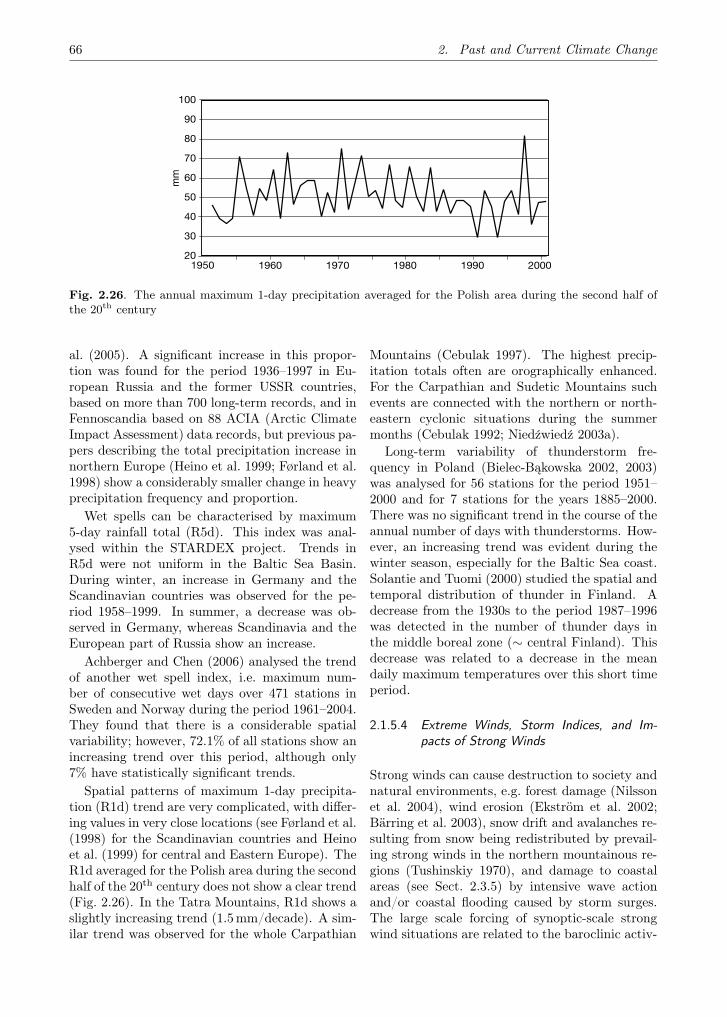
66 2. Past and Current Climate Change
1950 1960 1970 1980 1990 2000
100
90
80
70
60
50
40
30
20
mm
Fig. 2.26. The annual maximum 1-day precipitation averaged for the Polish area during the second half ofthe 20th century
al. (2005). A significant increase in this propor-tion was found for the period 1936–1997 in Eu-ropean Russia and the former USSR countries,based on more than 700 long-term records, and inFennoscandia based on 88 ACIA (Arctic ClimateImpact Assessment) data records, but previous pa-pers describing the total precipitation increase innorthern Europe (Heino et al. 1999; Førland et al.1998) show a considerably smaller change in heavyprecipitation frequency and proportion.
Wet spells can be characterised by maximum5-day rainfall total (R5d). This index was anal-ysed within the STARDEX project. Trends inR5d were not uniform in the Baltic Sea Basin.During winter, an increase in Germany and theScandinavian countries was observed for the pe-riod 1958–1999. In summer, a decrease was ob-served in Germany, whereas Scandinavia and theEuropean part of Russia show an increase.
Achberger and Chen (2006) analysed the trendof another wet spell index, i.e. maximum num-ber of consecutive wet days over 471 stations inSweden and Norway during the period 1961–2004.They found that there is a considerable spatialvariability; however, 72.1% of all stations show anincreasing trend over this period, although only7% have statistically significant trends.
Spatial patterns of maximum 1-day precipita-tion (R1d) trend are very complicated, with differ-ing values in very close locations (see Førland et al.(1998) for the Scandinavian countries and Heinoet al. (1999) for central and Eastern Europe). TheR1d averaged for the Polish area during the secondhalf of the 20th century does not show a clear trend(Fig. 2.26). In the Tatra Mountains, R1d shows aslightly increasing trend (1.5mm/decade). A sim-ilar trend was observed for the whole Carpathian
Mountains (Cebulak 1997). The highest precip-itation totals often are orographically enhanced.For the Carpathian and Sudetic Mountains suchevents are connected with the northern or north-eastern cyclonic situations during the summermonths (Cebulak 1992; Niedźwiedź 2003a).
Long-term variability of thunderstorm fre-quency in Poland (Bielec-Bąkowska 2002, 2003)was analysed for 56 stations for the period 1951–2000 and for 7 stations for the years 1885–2000.There was no significant trend in the course of theannual number of days with thunderstorms. How-ever, an increasing trend was evident during thewinter season, especially for the Baltic Sea coast.Solantie and Tuomi (2000) studied the spatial andtemporal distribution of thunder in Finland. Adecrease from the 1930s to the period 1987–1996was detected in the number of thunder days inthe middle boreal zone (∼ central Finland). Thisdecrease was related to a decrease in the meandaily maximum temperatures over this short timeperiod.
2.1.5.4 Extreme Winds, Storm Indices, and Im-pacts of Strong Winds
Strong winds can cause destruction to society andnatural environments, e.g. forest damage (Nilssonet al. 2004), wind erosion (Ekström et al. 2002;Bärring et al. 2003), snow drift and avalanches re-sulting from snow being redistributed by prevail-ing strong winds in the northern mountainous re-gions (Tushinskiy 1970), and damage to coastalareas (see Sect. 2.3.5) by intensive wave actionand/or coastal flooding caused by storm surges.The large scale forcing of synoptic-scale strongwind situations are related to the baroclinic activ-

2.1. The Atmosphere 67
ity concentrated in the North Atlantic storm trackand to the phase of the North Atlantic Oscillation(Marshall et al. 2001; Rogers 1997) that influencesthe overall intensity of the westerly winds. In thissection it is thus relevant to look at a larger re-gion extending to the west of the Baltic Sea Basin.While there are comparatively few studies focusingonly on the Baltic Sea Basin, there are numerousstudies discussing the general wind climate andstorminess of this larger region.
The most straightforward way to investigatewind extremes would seemingly be to analyserecords of wind observations. However, anemome-ters were only relatively recently introduced asthe standard instrument. Before that, stationsequipped with anemometers were less commonand instrument problems were more frequent.Instead, wind strength was recorded using theBeaufort scale where the data is based on semi-quantitative observations of the surrounding envi-ronment according to set rules. Observations atland stations are very sensitive to the surround-ing terrain and vegetation, and any changes arelikely to result in inhomogeneities in the observa-tion record. Hence, coastal stations at very ex-posed locations are most likely to show long-termhomogeneity. The WASA (Waves and Stormsin the North Atlantic) project (Carretero et al.1998) carried out comprehensive analyses of sev-eral records of wind observations in the North At-lantic and North Sea and stressed the problemsof finding long-term homogeneous wind data. In-stead, they suggest that geostrophic wind calcu-lated from three sea-level pressure records couldbe used, see Alexandersson et al. (1998) for detailsabout the calculations. Alternatively, for longertime-series when three suitable station recordsmay not be available, they suggest the use ofstorminess indices (Schmith et al. 1998) based onthe frequency of low pressure or a strong pressuretendency between consecutive observations of sea-level pressure at a single station.
Other approaches towards indirectly getting ahandle on long-term variations in synoptic scalewind extremes in the North Atlantic/North Searegion are based on analysing wave heights (e.g.Vikebø et al. 2003) and storm surges (Bijl et al.1999) or the micro-seismic activity resulting fromlarge storm waves hitting the coastline (Greve-meyer et al. 2000).
During the early 1990s, there were signs ofa strengthening of the North Sea wind climate.Early suggestions towards this end were put forth,
for example, by Schmidt and von Storch (1993)based on an analysis of the geostrophic wind overthe German Bight derived from three sea-levelpressure stations’ records. This coincided with anincrease of the North Atlantic Oscillation (NAO,see Annex 7) index (Hurrell 1995), beginning inthe mid 1960s. This increased NAO, however,came to an end around 1995 (Jones et al. 1997).Alexandersson et al. (2000) came to the same con-clusion; they furthermore noted that the wind cli-mate peaked around 1990 and they continued bypointing out that this peak does in fact resemblethe situation in the early part of the 20th century.Using four different storminess indices to anal-yse long sea-level pressure records from Lund andStockholm, Bärring and von Storch (2004) con-cluded that there is no long-term trend in stormi-ness indices over southern Scandinavia. They con-clude that there was a temporary increase in the1980s–1990s. A similar increase during the 1980s–1990s can be seen in several other analyses ofrelatively short time series, such as microseisms(Grevemeyer et al. 2000), wave height off mid-Norway (Vikebø et al. 2003) or storm surge data(Bijl et al. 1999).
Figure 2.27 shows storminess indices, as definedby Bärring and von Storch (2004), for seven sta-tions in the Baltic Sea Basin. The large-scale spa-tial gradient towards lower surface air pressure inthe north is evident in the top panel (counts oflow pressure situations below 980 hPa). The in-creased windiness during the 1980s–1990s is evi-dent at all stations and most pronounced at thenorthern stations. In addition, the northern sta-tions, especially Härnösand and Kajaani, show aperiod of enhanced storminess during the 1950s.
Alexandersson and Vedin (2002) suggest thatover the period 1880–2001 there is a weak de-creasing trend in the incidence of geostrophicstorm situations (geostrophic wind speed exceed-ing 25m s−1) over southern Sweden. They com-ment that this decreasing trend may not be ro-bust because trustworthy wind observations atSwedish coastal stations do not show this decreas-ing trend in wind measurements. However, thisdecreasing trend comes mainly from a period oflower incidence during the 1980s and around 2000,combined with increased incidence during 1910s–1920s. Extending this analysis to include moregeostrophic wind triangles shows (Fig. 2.28) thatthere is a difference between the southern andnorthern (central) Baltic Sea Basin. In southernSweden (the Göteborg–Visby–Falsterbo triangle)
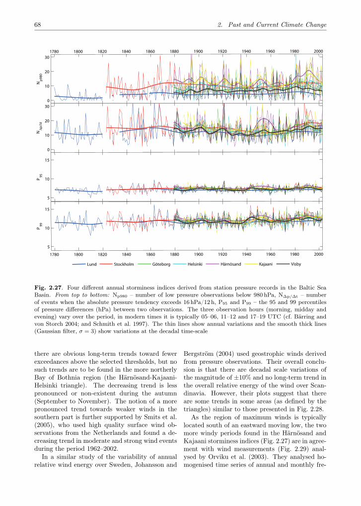
68 2. Past and Current Climate Change
1780 1800 1820 1840 1860 1880 1900 1920 1940 1960 1980 2000
0
10
20
30
Np9
80
0
10
20
30
N∆p
/∆t
5
10
15
P95
1780 1800 1820 1840 1860 1880 1900 1920 1940 1960 1980 2000
5
10
15
P99
Lund Stockholm Göteborg Helsinki Härnösand Kajaani Visby
Fig. 2.27. Four different annual storminess indices derived from station pressure records in the Baltic SeaBasin. From top to bottom: Np980 – number of low pressure observations below 980 hPa, N∆p/∆t – numberof events when the absolute pressure tendency exceeds 16 hPa/12 h, P95 and P99 – the 95 and 99 percentilesof pressure differences (hPa) between two observations. The three observation hours (morning, midday andevening) vary over the period, in modern times it is typically 05–06, 11–12 and 17–19 UTC (cf. Bärring andvon Storch 2004; and Schmith et al. 1997). The thin lines show annual variations and the smooth thick lines(Gaussian filter, σ = 3) show variations at the decadal time-scale
there are obvious long-term trends toward fewerexceedances above the selected thresholds, but nosuch trends are to be found in the more northerlyBay of Bothnia region (the Härnösand-Kajaani-Helsinki triangle). The decreasing trend is lesspronounced or non-existent during the autumn(September to November). The notion of a morepronounced trend towards weaker winds in thesouthern part is further supported by Smits et al.(2005), who used high quality surface wind ob-servations from the Netherlands and found a de-creasing trend in moderate and strong wind eventsduring the period 1962–2002.
In a similar study of the variability of annualrelative wind energy over Sweden, Johansson and
Bergström (2004) used geostrophic winds derivedfrom pressure observations. Their overall conclu-sion is that there are decadal scale variations ofthe magnitude of ±10% and no long-term trend inthe overall relative energy of the wind over Scan-dinavia. However, their plots suggest that thereare some trends in some areas (as defined by thetriangles) similar to those presented in Fig. 2.28.
As the region of maximum winds is typicallylocated south of an eastward moving low, the twomore windy periods found in the Härnösand andKajaani storminess indices (Fig. 2.27) are in agree-ment with wind measurements (Fig. 2.29) anal-ysed by Orviku et al. (2003). They analysed ho-mogenised time series of annual and monthly fre-

2.1. The Atmosphere 69
1880 1900 1920 1940 1960 1980 20000
2
4
6
8
10
Exce
edan
ces
(%)
Härnösand−Kajaani−Helsinki
1880 1900 1920 1940 1960 1980 20000
2
4
6
8
10
Exce
edan
ces
(%)
Härnösand−Helsinki−Stockholm
1880 1900 1920 1940 1960 1980 20000
2
4
6
8
10
Exce
edan
ces
(%)
Härnösand−Visby−Göteborg
1880 1900 1920 1940 1960 1980 20000
2
4
6
8
10
Exce
edan
ces
(%)
Göteborg−Visby−Falsterbo
Fig. 2.28. The relative frequency (%) of days where the maximum geostrophic winds exceed selected thresh-olds: blue: 20 m s−1; green: 25 m s−1; red: 30 m s−1. The maximum is based on pressure readings in themorning, midday and evening. The smooth lines (Gaussian filter, σ = 9) show variations at the 30-yeartime-scale
quency of strong winds observed for the period1948–2003 at three Estonian stations located onthe coast of the Baltic Proper and the Gulf of Riga.The main feature of these time series is the two pe-riods of increased frequency of strong winds, dur-ing the 1950s and from the late 1970s to the mid1990s. However, their conclusion of an overall in-creased frequency of strong winds along the Esto-nian coast during 1948–2003 supports the notionof different overall trends in the pressure basedstorminess indices and trustworthy time-series ofwind measurements also noted by Alexanderssonand Vedin (2002).
The NCEP–NCAR (National Centres for Envi-ronmental Predictions – National Centre for At-mospheric Research) Reanalysis dataset shows, incontrast to the direct observational evidence dis-
cussed above, a clear trend towards an intensifi-cation of both the Pacific and the Atlantic stormtracks (Chang and Fu 2002). This increase may,however, be overestimated (Harnik and Chang2003). Such an overestimation may influence stud-ies using this data set. Although the NCEP–NCAR Reanalysis dataset may overestimate anincreasing trend, the sign of the trend is in agree-ment with the ECMWF (European Centre forMedium-Range Weather Forecasts) ERA-15 Re-analysis dataset, especially with respect to strongwind cyclones (7 Beaufort and above) (Hanson etal. 2004), even though they concluded that theERA-15 data provide more comprehensive repre-sentation of the northern cyclone climatology.
Nevertheless, the increased wave height foundby Bauer (2001) when forcing a wave model with

70 2. Past and Current Climate Change
1950 1960 1970 1980 1990 2000
40
30
20
10
0
Fre
quen
cy o
f sto
rm d
ays
Fig. 2.29. Annual frequency of ‘storm days’ at Vilsandi, Saaremaa Island, Estonia, derived from homogenisedwind measurements. A day was designated as a ‘storm day’ when mean wind speed during a single observation(10 minutes) was 15 m s−1 or higher (adapted from Orviku et al. 2003)
ERA-15 data is consistent with the increased windspeed over the North Sea (Siegismund and Schrum2001). Weisse et al. (2005) used NCEP–NCARReanalysis to force a regional climate model andconcluded that the model is capable of reproduc-ing impact-relevant storm indices. Their resultsare consistent with previous analyses based onreanalysis data in that they find an increase inthe number of storms over the North Sea, al-though this increase has levelled off. For the BalticSea they find a weak but statistically significanttrend towards increasing frequency of strong windevents (wind speed exceeding 17.2m s−1, Beau-fort 8). This trend corresponds to one additionalexceedance every 10 years.
Pryor and Barthelmie (2003) report on positivetrends in winds at the 850 hPa level over the BalticSea Basin region. Their results show that thetrend in annual mean wind speed is weak, in ex-cess of 0.25m s−1 per decade, but for strong windsthe trend becomes more pronounced. This conclu-sion is further strengthened in their recent analysiswhere Pryor et al. (2005) found a similar positivetrend in windspeed measured at 10 meter heightlevel from the ECMWF ERA-40 reanalysis overthe Baltic Sea.
However, a comparison of storminess indices de-rived from station pressure readings with indicescalculated from the corresponding gridbox of aRCM (Regional Climate Model) simulation usingNCEP–NCAR reanalysis data as boundary condi-tions shows a very good agreement in the high-frequency variability, i.e. variability at the intra-
annual and few years time-scale). However, thereseems to be some discrepancy in overall lineartrends (Fig. 2.30), mainly induced by the simu-lated values being too low for the first 10 to 15years.
On a much smaller spatial scale than the synop-tic scale cyclonic storms, strong winds may arisein connection with severe local storms of differentorigins. For these systems the problems of directmeasurements become even more obvious becausethere is little chance that local wind maxima passover a meteorological station. Even though re-cent radar and satellite techniques have improvedthe situation, indirect measurements and compi-lations of documentary information on the impactare still the main data sources for studying varia-tions of over time. To a large extent, informationon these phenomena are scattered and focus onthe description of the impact of individual eventsand/or an analysis of the meteorological condi-tions that lead to the event. Tornadoes (over land)or waterspouts (over water) are associated withadvection of warm tropical air to high latitudesmostly caused by southern cyclones during sum-mer. They form in a frontal zone where the airtemperature gradient is very high and thunder-storms frequently occur. Downdraft is a differentphenomenon associated with thunderstorms; it isformed by vigorous downward flow of cold air hit-ting the ground ahead of the thunderstorm.
During recent years the incidence in Europe oflocally strong winds has gained increasing inter-est (e.g. Brooks et al. 2003; Dotzec 2003; Teitti-

2.1. The Atmosphere 71
5
15
25
N|∆
p|>
16hP
a/12
h
6
10
14
P95
(|∆p
|)
1880 1900 1920 1940 1960 1980 2000
6
10
14
P99
(|∆p
|)
1880 1900 1920 1940 1960 1980 2000
0
10
20
30
Np<
980h
Pa
Kajaani
Fig. 2.30. The same four storminess indices as in Fig. 2.27 for the station Kajaani, Finland. Blue curves arebased on pressure observations and red curves are calculated from the nearest gridbox of a RCM simulationforced by NCEP reanalysis data (Weisse et al. 2005)
nen 2000; Groenemeijer 2005). Dobrovolný andBrázdil (2003) provide a time-series of strong lo-cal winds associated with convective storms in theCzech Republic. The time-series is largely basedon historic documents and extends all the wayback to AD 500, and the authors conclude thatthe variations are consistent with the temperaturevariations during the same period.
Lithuania was hit by a very strong tornado in1981, and Marcinoniene (2003) analyses the syn-optic situation associated with this event and usesa 52 year record of tornado incidence as a referenceseries. In Estonia, tornadoes occur 2–3 times peryear as an average (Merilain and Tooming 2003;Tooming and Merilain 2004). They also present alist of tornadoes observed in Estonia since 1795and provide a tentative map of tornado tracks(Tooming and Merilain 2004). Although torna-
does in Estonia have been observed much morefrequently during recent decades, it doesn’t meanthat this is a real trend. The main reason forhigher reported frequency of tornadoes is proba-bly better communication.
To sum up, different data sources give slightlydifferent results with respect to trends and vari-ations in the extreme wind climate. There isnonetheless a consistent picture across most datasources of an intensification of the wind climateduring the 1980s–mid 1990s. While analyses basedon the NCEP–NCAR reanalysis dataset tend soshow an increasing trend for the period since 1948,geostrophic wind series based on pressure observa-tions suggest a downward trend from the early 20th
century, at least in southern Scandinavia. Eventhough the reanalysis system itself is constant inthe NCEP–NCAR reanalysis, the long-term in-

72 2. Past and Current Climate Change
creasing trend in data may be exaggerated becauseincomplete observational data during the earlypart of the reanalysis period and the introductionof new observational systems, together with thepositive wind climate anomaly during the 1980s–1990s, may partly explain this positive trend. Thedownward trend in geostrophic winds is strongestin the southern part of the region and hardly dis-cernible in the north. This suggests that it maybe due to shifts in the storm tracks; some sup-port of this may be found in wind observations.The single station pressure based storminess in-dices show clear decadal scale variations but noclear long-term trend. Thus, it is not possible todraw any definitive conclusion regarding long-termtrends in the extreme wind climate over the BalticSea Basin.
Information on extreme local winds is with fewexceptions available as scattered and descriptivestudies. There is an emerging interest in compilinglong-term and consistent observational datasetsfrom various sources. Such datasets will becomeinstrumental for analysing trends and variations inlocal extreme winds. As yet, they are not exten-sive enough for allowing any firm general conclu-sion regarding trends and variations of small-scaleextreme winds in the Baltic Sea Basin.
At the same time there are clear indications ofincreasing impact from extreme wind events. Butthis increasing impact results from a complex in-teraction between climate and development trendsthat increase the exposure to damage and/or thevulnerability of nature and society.
2.2 The Hydrological Regime
Several rivers, lakes and some observational sta-tions for different hydrological parameters arementioned in Sect. 2.2, the locations of which areindicated in Fig. 2.31. See Table 2.5 for a relatedlist.
2.2.1 The Water Regime
2.2.1.1 Annual and Seasonal Variation of TotalRunoff
The river inflow into the Baltic Sea has attractedthe attention of many scientists. Mikulski (1970)made the earliest rather comprehensive study,which, however, extended only over the period1961–1970. Bergström and Carlsson (1994) anal-ysed the period 1950–1990, based on dischargedata from around 200 rivers, covering 86% of the
total Baltic Sea Basin. They arrived at an aver-age inflow of 14,151m3 s−1 or 446 km3 y−1. This isequivalent to a water layer of 118 cm over the sur-face of the Baltic Sea, and is roughly three timesthe amount of annual evaporation.
Within the BALTEX programme, the runoff tothe Baltic Sea during the period 1921–1998 wasanalysed (Fig. 2.32). The mean for the whole pe-riod was 14,119m3 s−1 or 445 km3 y−1. Unlike thestudies referred to above, the runoff to the DanishBelts and Sounds are not included. This explainsmost of the difference in the mean value for theperiod 1950–1990, because the runoff to the Beltsand Sounds is only about 37km3 y−1. See alsoAnnex 1.3 for more details on runoff to the BalticSea.
The interannual variability in runoff is con-siderable. The wettest year, 1924, had a meanannual runoff of 18,167 m3 s−1, while the corre-sponding value for the driest year, 1976, was only10,553m3 s−1. Even the decadal means vary quitea lot, between 14,582 m3 s−1 for the 1990s and12,735m3 s−1 for the 1940s. It is noteworthy, thatno statistically significant trend can be found inthe series.
2.2.1.2 Regional Variations and Trends
Most detailed analyses of runoff trends have beenmade in Sweden (Lindström and Bergström 2004).The study included a total of 61 discharge serieswith the longest one (at the outlet of Lake Vänern)starting in 1807, but most of them being confinedto the 20th century. The last two decades havebeen very wet in Sweden, with runoff anomalies ofabout +8% compared with the period 1901–2002.However, they are matched by similar levels in the1920s. The 1970s was the driest decade, with ananomaly of −9%. A linear trend for annual runofffrom 1901–2002 shows an increase by about 5%over the whole period, but the trend is not signifi-cant. Records from the 19th century indicate thatthe runoff was even higher than in the 20th cen-tury, although temperatures were generally ratherlow. On the contrary, recent decades have beencharacterised by a combination of high tempera-ture and high runoff.
Hisdal et al. (2003) analysed a Nordic data set,encompassing 152 stations in the period 1961–2002, 140 stations in 1941–1960 and 90 stationsin 1920–1940. Over one third of these stations areoutside the Baltic Sea Basin, e.g. in Norway andwestern parts of Denmark. The stations were di-

2.2. The Hydrological Regime 73
Fig. 2.31. Location of rivers (R), lakes (L) and stations discussed in Sect. 2.2. See Table 2.5 for a list of sites(by courtesy of Jonas Sjögren, SMHI)
vided into those suitable for the analysis of i) onlyannual values, ii) annual and monthly values, andiii) annual, monthly and daily values. As to theannual values, this Nordic data set gave positivetrends in 1920–2002 at several stations in Den-mark, southern Sweden and Lapland.
However, trends at only two stations, both inthe south, were significant. Negative trends wererather seldom and regionally scattered. For theperiod 1941–2002, the number of significant posi-tive trends was 17, in 1961–2002 it was 19. Most ofthese trends were at stations located in northern
Sweden. There were even fewer negative trends inthese periods than in 1920–2002.
As to seasonal runoff, significant positive trendswere rather common in winter (DJF) and in spring(MAM) during the period 1941–2002 in the wholenorthern part of the Baltic Sea Basin In summerand autumn significant positive trends were ratherrare, as were negative trends in all seasons.
Annual and monthly runoff from Finland intothe Baltic Sea in 1912–2003 were recently anal-ysed (Fig. 2.33). The mean annual flow was2413m3 s−1, with a maximum of 3589m3 s−1 in
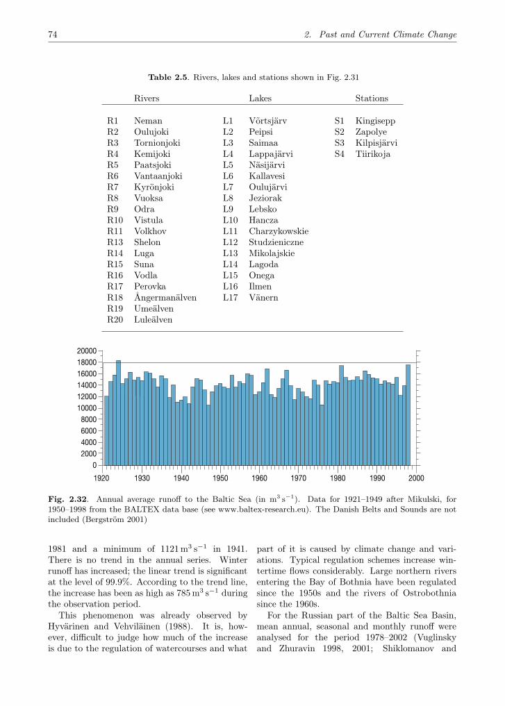
74 2. Past and Current Climate Change
Table 2.5. Rivers, lakes and stations shown in Fig. 2.31
Rivers Lakes Stations
R1 Neman L1 Võrtsjärv S1 KingiseppR2 Oulujoki L2 Peipsi S2 ZapolyeR3 Tornionjoki L3 Saimaa S3 KilpisjärviR4 Kemijoki L4 Lappajärvi S4 TiirikojaR5 Paatsjoki L5 NäsijärviR6 Vantaanjoki L6 KallavesiR7 Kyrönjoki L7 OulujärviR8 Vuoksa L8 JeziorakR9 Odra L9 LebskoR10 Vistula L10 HanczaR11 Volkhov L11 CharzykowskieR13 Shelon L12 StudzieniczneR14 Luga L13 MikolajskieR15 Suna L14 LagodaR16 Vodla L15 OnegaR17 Perovka L16 IlmenR18 Ångermanälven L17 VänernR19 UmeälvenR20 Luleälven
2000018000160001400012000100008000600040002000
0
20001920 1930 1940 1950 1960 1970 1980 1990
Fig. 2.32. Annual average runoff to the Baltic Sea (in m3 s−1). Data for 1921–1949 after Mikulski, for1950–1998 from the BALTEX data base (see www.baltex-research.eu). The Danish Belts and Sounds are notincluded (Bergström 2001)
1981 and a minimum of 1121 m3 s−1 in 1941.There is no trend in the annual series. Winterrunoff has increased; the linear trend is significantat the level of 99.9%. According to the trend line,the increase has been as high as 785 m3 s−1 duringthe observation period.
This phenomenon was already observed byHyvärinen and Vehviläinen (1988). It is, how-ever, difficult to judge how much of the increaseis due to the regulation of watercourses and what
part of it is caused by climate change and vari-ations. Typical regulation schemes increase win-tertime flows considerably. Large northern riversentering the Bay of Bothnia have been regulatedsince the 1950s and the rivers of Ostrobothniasince the 1960s.
For the Russian part of the Baltic Sea Basin,mean annual, seasonal and monthly runoff wereanalysed for the period 1978–2002 (Vuglinskyand Zhuravin 1998, 2001; Shiklomanov and

2.2. The Hydrological Regime 75
Fig. 2.33. Annual (top) and February (bottom) runoff (m3 s−1) from the Finnish territory to the Baltic Seaduring 1912 to 2002
Georgievsky 2002). Compared to the long-termmean values, the annual flows have increased insome basins south and southwest of the Gulf ofFinland by about one third. In the rivers of theKarelian Isthmus, this increase has been 3–11%.
The increase in winter runoff has been remark-able: 40–140% in the basins south and southwestof the Gulf of Finland, and 6–44% in the Kare-lian Isthmus, in Karelia and in the territory ad-jacent to Lake Ladoga, the biggest lake in Eu-rope. Summer and autumn runoff have also in-creased in the southern and south-western riverbasins (by 6–70%), whereas in some rivers north-ward and eastward of the Gulf of Finland theyhave decreased by 2–14%. The spring runoff de-creased in the former region by 2–25%, while it
increased by 4–16% in some Karelian rivers and inthe Volkhov River.
Monthly data analysis shows that runoff duringwinter months (December–March) has greatly in-creased in all the study rivers except the VuoksaRiver. Figure 2.34 gives an example of mean an-nual and winter runoff values from observationsites in the Russian territory.
An increase of wintertime runoff has also beenobserved in Estonia (Velner and al. 2004). Thesame trend has occurred in all major rivers inLatvia, but the annual runoff of several Latvianrivers decreased during 1960–1999 (Briede andLizuma 2004). In Belarus, the winter runoff in-creased markedly and spring flows decreased in theperiod 1988–2002 (Nekrasova 2004).
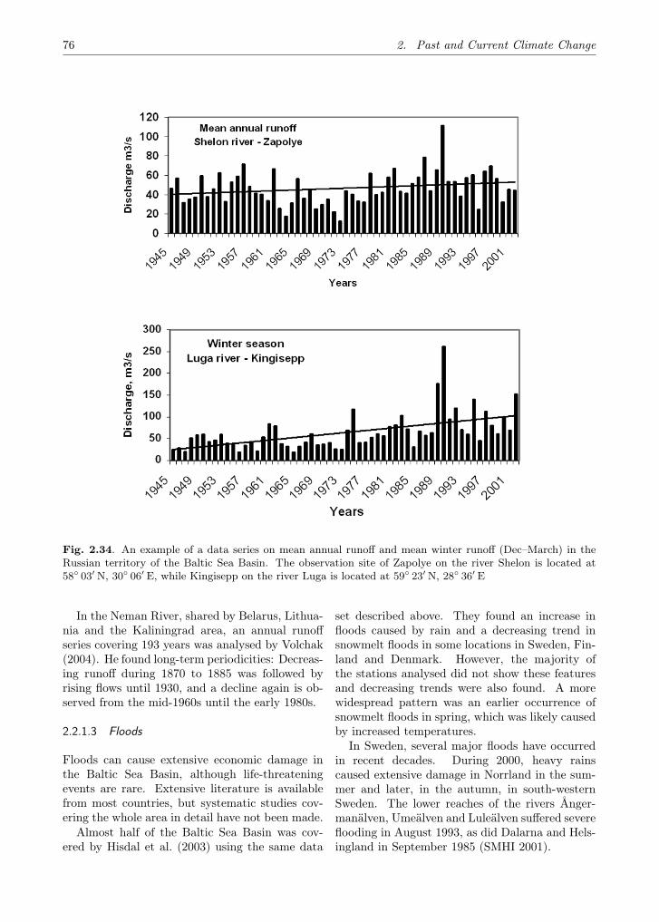
76 2. Past and Current Climate Change
Fig. 2.34. An example of a data series on mean annual runoff and mean winter runoff (Dec–March) in theRussian territory of the Baltic Sea Basin. The observation site of Zapolye on the river Shelon is located at58◦ 03′ N, 30◦ 06′ E, while Kingisepp on the river Luga is located at 59◦ 23′ N, 28◦ 36′ E
In the Neman River, shared by Belarus, Lithua-nia and the Kaliningrad area, an annual runoffseries covering 193 years was analysed by Volchak(2004). He found long-term periodicities: Decreas-ing runoff during 1870 to 1885 was followed byrising flows until 1930, and a decline again is ob-served from the mid-1960s until the early 1980s.
2.2.1.3 Floods
Floods can cause extensive economic damage inthe Baltic Sea Basin, although life-threateningevents are rare. Extensive literature is availablefrom most countries, but systematic studies cov-ering the whole area in detail have not been made.
Almost half of the Baltic Sea Basin was cov-ered by Hisdal et al. (2003) using the same data
set described above. They found an increase infloods caused by rain and a decreasing trend insnowmelt floods in some locations in Sweden, Fin-land and Denmark. However, the majority ofthe stations analysed did not show these featuresand decreasing trends were also found. A morewidespread pattern was an earlier occurrence ofsnowmelt floods in spring, which was likely causedby increased temperatures.
In Sweden, several major floods have occurredin recent decades. During 2000, heavy rainscaused extensive damage in Norrland in the sum-mer and later, in the autumn, in south-westernSweden. The lower reaches of the rivers Ånger-manälven, Umeälven and Luleälven suffered severeflooding in August 1993, as did Dalarna and Hels-ingland in September 1985 (SMHI 2001).

2.2. The Hydrological Regime 77
In general, flood peaks seem to have increasedmore in Sweden than the average annual valuesof runoff. The clearest increase has taken place inthe central parts of the country, and the same ten-dency can be found in the north. In south-easternSweden, there is a decreasing rather than an in-creasing trend (Lindström and Bergström 2004).
In Finland, the worst well-documented floodtook place in the Lake District in 1899. The year1898 had already been wet, and in the winter of1899 an unusual amount of snow accumulated.Water levels in the central lakes of the area roseto 2 to 2.5m above the mean (Hyvärinen and Ka-jander 2005). Another major flood occurred inthe Lake District in 1924, as did smaller ones in1974 and 1981. In southern Finland, the largestflood of the 20th century occurred in the springof 1966, while in northern Finland, extremes oc-curred in 1943 (River Oulujoki), in 1968 (RiverTornionjoki), 1973 (River Kemijoki) and in 2000(River Paatsjoki).
In large river basins in northern Finland, theincrease in spring flood peaks has been estimatedto be about 0.5% per one per cent of drained area(Hyvärinen and Vehviläinen 1988). The effects ofdrainage attenuate in the course of years. Thisis partly due to the growth of forest on drainedlands, and the water bearing capacity of the ditchnetwork also tends to weaken.
By far the most devastating floods in the BalticSea Basin have been the deluges in the Odra Basinin 1997 (with estimated damages of 6 billion Euro)and in the Vistula Basin in 2001 (damages ofaround 3 billion Euro). The latter two eventswere followed by the Elbe flood in 2002 (estimateddamage of 15 billion Euro), the Elbe river be-ing a neighbouring catchment to the Baltic SeaBasin.
These events have stimulated an intensive dis-cussion about flood causes and new strategies forflood risk management. The proposed strategiesclearly show the need for an integrated flood riskmanagement including structural and, even moreimportant, non-structural measures. In addition,these events further stimulated research concern-ing the possible role of climate change and of landuse changes. De Roo et al. (2003) studied histor-ical land use in the Odra Basin. They found thatthe total area of forested land increased between1780 and 2001 – contrary to common assumptions.The area of arable land decreased, while the ex-tent of urban areas grew considerably. Overall,the land use changes between 1780 and 2001 have
increased peak discharges, but their impact is notconsidered very large.
The possible impact of the North Atlantic Os-cillation (NAO) on floods in the Baltic Sea Basinwas also discussed. Wrzesinski (2004) analysed 17data series, widely distributed over the Baltic SeaBasin. He found that in the northern part of thearea a positive stage of the NAO rather often indi-cates an early start of spring high water and above-average flood peaks. The opposite is true in thesouthern part of the Baltic Sea Basin.
2.2.1.4 Droughts
Droughts do not usually cause major damage inthe Baltic Sea Basin, although small flows and lowsoil moisture storage may be harmful to agricul-ture, particularly in the southern parts of the area.
Hisdal et al. (2003) found a slight trend towardsprolonged droughts in southern Scandinavia afterthe 1960s. In Denmark, a trend analysis of thetime series of annual minimum values in 1874–1998gave decreasing trends at 16 stations (of whichthree were significant at the 95% level) and in-creasing trends at 22 stations, six of these beingsignificant.
In Finland the most serious 20th centurydrought occurred during 1940–42. In 1941 and1942, the mean annual countrywide discharge wasonly 49% and 57%, respectively, of the long-termaverage. These were the two driest years of thewhole century. The drought in 2002 and 2003 hitmost of Sweden and Finland with a considerablereduction of hydropower production.
Farat et al. (1998) analysed droughts in Polandin the period 1951–90. Fourteen droughts wereisolated and described; the highest frequency ofdrought occurrence was noted in the decades1951–60 and 1981–90. None of the events was de-scribed as an outstanding one.
2.2.1.5 Lakes
The seasonal changes of the total water vol-ume in lakes and reservoirs is dominated by thestrong and rather regular variation in Swedish andFinnish water bodies, with a considerable humaneffect by regulation. In Lakes Ladoga and Onega,the seasonal variation is rather small. In con-trast, the water volume of Lake Ilmen (mean area1350 km2) varies strongly, because the annual am-plitude of water level can be up to six meters.
An analysis of runoff generation in the BalticSea Basin should, in fact, take into account the

78 2. Past and Current Climate Change
Fig. 2.35. The average water temperature in August in Lake Saimaa (Finland) in the period 1924–2000(Korhonen 2002)
change in the water storage of lakes. In a dry year,lakes increase the annual runoff into the BalticSea, while in a wet year, they decrease it. If this‘lake correction’ is included, the true runoff gen-eration in the Finnish territory in 1981 was about3880m3 s−1 and in 1941 only 850m3 s−1, whilethe flows into the Baltic Sea were 3589 m3 s−1 and1121m3 s−1, as cited above.
Long-term variations of lake levels in the BalticSea Basin have not been analysed as widely as thevariations of river discharges. One of the reasonsis that many lakes are regulated, and the changesof their levels do not correctly reflect variationsin climatic or physiographic factors. The levels ofthe largest lakes have, however, been of consid-erable interest, mainly because there are a lot ofeconomic interests along their shorelines. In LakeVänern (Sweden), the most extreme water levelsince regulation started in 1938 occurred in thebeginning of 2001 (Weyhenmeyer and Sonesten2002). It exceeded the previous record by 40 cm.In Lake Saimaa (Finland), the flood of 1899 hasheld the record since the observations started in1847. In Lake Ladoga, the highest level was mea-sured in 1924, the lowest in 1940.
Mild winters have increased the levels of somelakes in recent decades. Regulation for hydropower production typically has the same effect,which makes the analysis of the real causes of thistrend difficult. Long-term periodicities have beenfound in several lakes; e.g. the levels of Lake Peipsihave been found to follow cycles of 20–30 years
(Jaani and Beljazo 2003) and the levels of Saimaa,Ilmen and Onega to fluctuate with the periodicityof 28–32 years (Masanova and Filatova 1985). Onthe other hand, Kuusisto (1982) found no evidenceof long-term regularities in the annual water levelsof Ladoga and Saimaa in the period of 1859–1956.The first autocorrelation coefficients for the annuallevels were, not surprisingly, significant (99.9%):Ladoga 0.66 and Saimaa 0.47, but e.g. the seven-year periodicity, generally believed to exist by peo-ple living on the shores of Lake Ladoga, did notoccur.
Thermal regimes of the lakes in the Baltic SeaBasin have been extensively studied, and long ob-servation series on water temperatures are avail-able. In Finland, the first systematic surface wa-ter observations began in Lake Saimaa at Lau-ritsala in 1916. These observations are still con-tinuing and thus they represent the longest con-tinuous water temperature observation series inFinland. A significant increase in the number ofsurface water temperature stations took place in1961, when many water temperature stations wereestablished.
The analysis of the surface water observationsof eight sites in Finland did not show many signif-icant long-term changes in the surface water tem-perature until the year 2000 (Korhonen 2002). ForLake Saimaa many variables (such as average sur-face water temperature of June, July, August, thenumber of days exceeding 10 C 15 C and 18 C thetemperature sum of June–September) show signif-
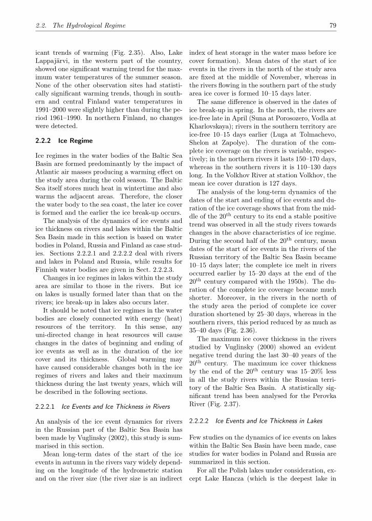
2.2. The Hydrological Regime 79
icant trends of warming (Fig. 2.35). Also, LakeLappajärvi, in the western part of the country,showed one significant warming trend for the max-imum water temperatures of the summer season.None of the other observation sites had statisti-cally significant warming trends, though in south-ern and central Finland water temperatures in1991–2000 were slightly higher than during the pe-riod 1961–1990. In northern Finland, no changeswere detected.
2.2.2 Ice Regime
Ice regimes in the water bodies of the Baltic SeaBasin are formed predominantly by the impact ofAtlantic air masses producing a warming effect onthe study area during the cold season. The BalticSea itself stores much heat in wintertime and alsowarms the adjacent areas. Therefore, the closerthe water body to the sea coast, the later ice coveris formed and the earlier the ice break-up occurs.
The analysis of the dynamics of ice events andice thickness on rivers and lakes within the BalticSea Basin made in this section is based on waterbodies in Poland, Russia and Finland as case stud-ies. Sections 2.2.2.1 and 2.2.2.2 deal with riversand lakes in Poland and Russia, while results forFinnish water bodies are given in Sect. 2.2.2.3.
Changes in ice regimes in lakes within the studyarea are similar to those in the rivers. But iceon lakes is usually formed later than that on therivers; ice break-up in lakes also occurs later.
It should be noted that ice regimes in the waterbodies are closely connected with energy (heat)resources of the territory. In this sense, anyuni-directed change in heat resources will causechanges in the dates of beginning and ending ofice events as well as in the duration of the icecover and its thickness. Global warming mayhave caused considerable changes both in the iceregimes of rivers and lakes and their maximumthickness during the last twenty years, which willbe described in the following sections.
2.2.2.1 Ice Events and Ice Thickness in Rivers
An analysis of the ice event dynamics for riversin the Russian part of the Baltic Sea Basin hasbeen made by Vuglinsky (2002), this study is sum-marised in this section.
Mean long-term dates of the start of the iceevents in autumn in the rivers vary widely depend-ing on the longitude of the hydrometric stationand on the river size (the river size is an indirect
index of heat storage in the water mass before icecover formation). Mean dates of the start of iceevents in the rivers in the north of the study areaare fixed at the middle of November, whereas inthe rivers flowing in the southern part of the studyarea ice cover is formed 10–15 days later.
The same difference is observed in the dates ofice break-up in spring. In the north, the rivers areice-free late in April (Suna at Porosozero, Vodla atKharlovskaya); rivers in the southern territory areice-free 10–15 days earlier (Luga at Tolmachevo,Shelon at Zapolye). The duration of the com-plete ice coverage on the rivers is variable, respec-tively; in the northern rivers it lasts 150–170 days,whereas in the southern rivers it is 110–130 dayslong. In the Volkhov River at station Volkhov, themean ice cover duration is 127 days.
The analysis of the long-term dynamics of thedates of the start and ending of ice events and du-ration of the ice coverage shows that from the mid-dle of the 20th century to its end a stable positivetrend was observed in all the study rivers towardschanges in the above characteristics of ice regime.During the second half of the 20th century, meandates of the start of ice events in the rivers of theRussian territory of the Baltic Sea Basin became10–15 days later; the complete ice melt in riversoccurred earlier by 15–20 days at the end of the20th century compared with the 1950s). The du-ration of the complete ice coverage became muchshorter. Moreover, in the rivers in the north ofthe study area the period of complete ice coverduration shortened by 25–30 days, whereas in thesouthern rivers, this period reduced by as much as35–40 days (Fig. 2.36).
The maximum ice cover thickness in the riversstudied by Vuglinsky (2000) showed an evidentnegative trend during the last 30–40 years of the20th century. The maximum ice cover thicknessby the end of the 20th century was 15–20% lessin all the study rivers within the Russian terri-tory of the Baltic Sea Basin. A statistically sig-nificant trend has been analysed for the PerovkaRiver (Fig. 2.37).
2.2.2.2 Ice Events and Ice Thickness in Lakes
Few studies on the dynamics of ice events on lakeswithin the Baltic Sea Basin have been made, casestudies for water bodies in Poland and Russia aresummarized in this section.
For all the Polish lakes under consideration, ex-cept Lake Hancza (which is the deepest lake in

80 2. Past and Current Climate Change
Fig. 2.36. Long-term changes in the ice cover duration of the river Volkhov at station Volkhov during 1946to 2000 (Vuglinsky 2000)
Fig. 2.37. Changes in maximum ice cover thickness in the river Perovka at station Goncharovo during 1979to 2001 (Vuglinsky 2000)
the European Lowland), a strong negative trendof the ice cover duration (from 0.8 to 0.9 daysper year on average) was ascertained for the pe-riod 1961–2000. The respective trend of the du-ration of the freeze-up period (which on averageis shorter compared to the other Polish lakes) ofLake Hancza was less and amounted 0.4 day/yearon average, mainly due to the set-back of this pro-cess at the end of the 20th century (Marszelewskiand Skowron 2006).
For the Russian lakes with observation peri-ods of 80–106 years (Lakes Ilmen and Onega, re-spectively), trends have been discovered towardschanges in characteristics of ice events and max-imal ice thickness during the years 1980–2000 onthe background of a long-term variability of thementioned quantities. Linear trends indicatinglater date of ice formation (positive trend) before1980 and earlier date of ice cover break-up (nega-tive trend) after 1980 have been discovered. But
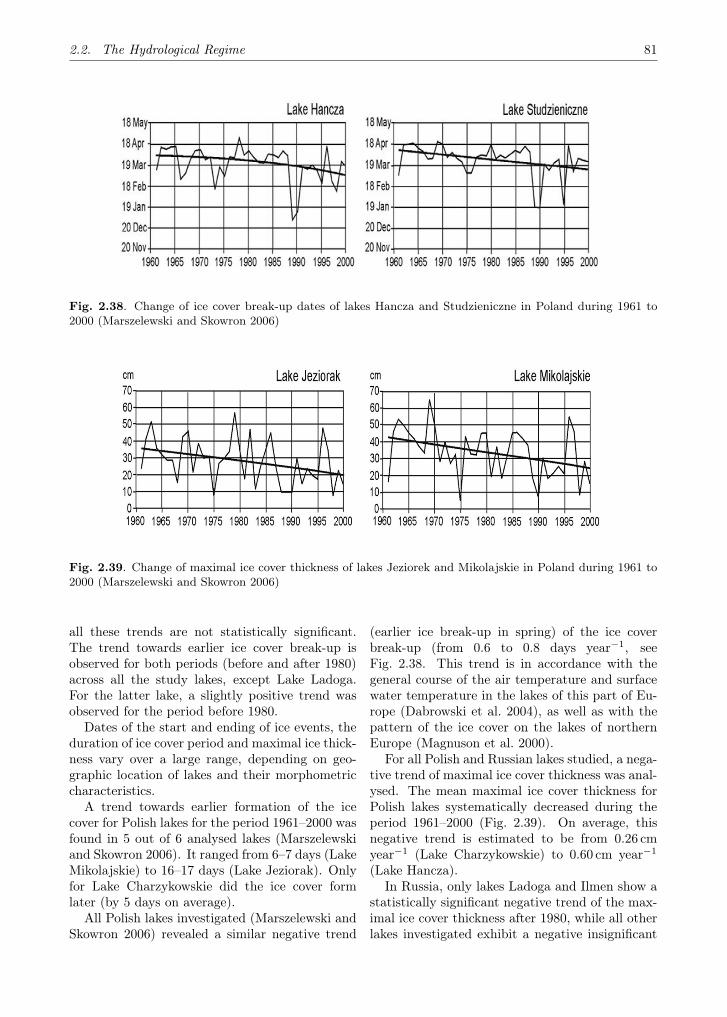
2.2. The Hydrological Regime 81
Fig. 2.38. Change of ice cover break-up dates of lakes Hancza and Studzieniczne in Poland during 1961 to2000 (Marszelewski and Skowron 2006)
Fig. 2.39. Change of maximal ice cover thickness of lakes Jeziorek and Mikolajskie in Poland during 1961 to2000 (Marszelewski and Skowron 2006)
all these trends are not statistically significant.The trend towards earlier ice cover break-up isobserved for both periods (before and after 1980)across all the study lakes, except Lake Ladoga.For the latter lake, a slightly positive trend wasobserved for the period before 1980.
Dates of the start and ending of ice events, theduration of ice cover period and maximal ice thick-ness vary over a large range, depending on geo-graphic location of lakes and their morphometriccharacteristics.
A trend towards earlier formation of the icecover for Polish lakes for the period 1961–2000 wasfound in 5 out of 6 analysed lakes (Marszelewskiand Skowron 2006). It ranged from 6–7 days (LakeMikolajskie) to 16–17 days (Lake Jeziorak). Onlyfor Lake Charzykowskie did the ice cover formlater (by 5 days on average).
All Polish lakes investigated (Marszelewski andSkowron 2006) revealed a similar negative trend
(earlier ice break-up in spring) of the ice coverbreak-up (from 0.6 to 0.8 days year−1, seeFig. 2.38. This trend is in accordance with thegeneral course of the air temperature and surfacewater temperature in the lakes of this part of Eu-rope (Dabrowski et al. 2004), as well as with thepattern of the ice cover on the lakes of northernEurope (Magnuson et al. 2000).
For all Polish and Russian lakes studied, a nega-tive trend of maximal ice cover thickness was anal-ysed. The mean maximal ice cover thickness forPolish lakes systematically decreased during theperiod 1961–2000 (Fig. 2.39). On average, thisnegative trend is estimated to be from 0.26 cmyear−1 (Lake Charzykowskie) to 0.60 cm year−1
(Lake Hancza).In Russia, only lakes Ladoga and Ilmen show a
statistically significant negative trend of the max-imal ice cover thickness after 1980, while all otherlakes investigated exhibit a negative insignificant

82 2. Past and Current Climate Change
Table 2.6. Trends in time series of ice phenomena and ice thickness for three Russian lakes P1: pre 1980 period,P2: post 1980 period. + positive non-significant trend, − negative non-significant trend, ++ statisticallysignificant positive trend (at p < 0.05), −− statistically significant negative trend (at p < 0.05) (Vuglinsky etal. 2002)
Lake Ice-on Ice break-up Ice cover Maximal ice coverduration thickness
P1 P2 P1 P2 P1 P2 P1 P2Ladoga (central part) + − + − − − − −−Onega at station + − −− − − − + −PetrozavodskIlmen at station + − − − − − + −−Voitsy
trend. Maximal ice cover thickness of the Russianlakes had the most pronounced response to climatewarming in wintertime during the last decades ofthe 20th century (Gronskaya 2000). Trends in timeseries of ice phenomena and maximal ice coverthickness for the Russian lakes are shown in Ta-ble 2.6 for the periods before and after 1980.
2.2.2.3 Ice Conditions in Rivers and Lakes inFinland
The ice break-up date has become earlier and thefreezing date later at many observation sites inFinland during the last few decades. The trendsare statistically significant mainly in those siteswhich have records at least since the late 19th cen-tury (Kuusisto and Elo 2000). Trends of seriesthat started later are in most cases not statisticallysignificant. In the longest series, which started inthe late 17th century, the ice break-up has moved6–9 days earlier per hundred years (Fig. 2.40).
Freezing has been delayed since the late 19th
century, in most cases by 0 to 8 days per century.Also, the duration of ice cover has significantlyshortened at the sites with the longest records(Fig. 2.41).
Not all of the longest freezing and duration ofice cover trends are statistically significant. Thetrends of break-up are stronger, because the vari-ation of break-up date is smaller than that of thefreezing date. The large variation of freezing dateshides the trends of freezing. There are no statisti-cally significant trends found in northern Laplandbut the time series from this part of the countryare still relatively short.
Both decreasing and increasing trends can befound in the maximum ice thickness time series.At about half of the sites the trends are statisti-cally significant. The maximum thicknesses havemostly increased in eastern and northern Finlandand decreased in southern Finland. The serieswith records since the 1960s had a significant trendof 2–3 cm per ten years; for longer series the trendwas mainly 1–2 cm per ten years. The time seriesof ice and snow thickness are rather short, abouttwenty years, thus no long-term analysis can bemade. In the 1980s there was much snow andsnow ice in southern and central Finland. Thus,the snow ice thickness has in most cases decreasedfrom the 1980s to the year 2000 in southern andcentral Finland. In northern Finland, the snow icethickness has increased in some places during thetwenty year period.
2.2.3 Snow Cover
Snowfalls occur every winter in the Baltic SeaBasin and seasonal snow cover is formed exceptin the south-western regions. Typical durationsof snow cover over most areas are between fourand six months (except for regions on the south-ern coast of the Baltic Sea). Snow cover is a reg-ularly varying feature of the land areas. It af-fects the winter and spring climate in several ways.Mean snow conditions as well as regional varia-tions and extremes are described in more detail inAnnex 1.3.5.
Annual Northern Hemisphere (NH) averagecontinental snow cover extent has decreased byabout 10% from 1966 to 2000 (see Folland et al.
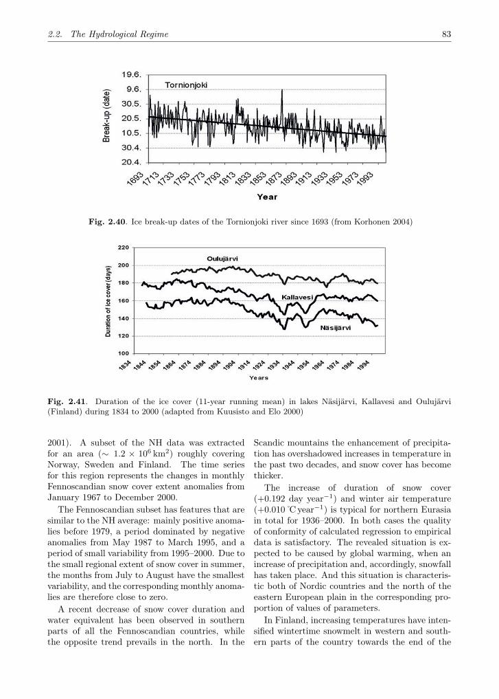
2.2. The Hydrological Regime 83
Fig. 2.40. Ice break-up dates of the Tornionjoki river since 1693 (from Korhonen 2004)
Fig. 2.41. Duration of the ice cover (11-year running mean) in lakes Näsijärvi, Kallavesi and Oulujärvi(Finland) during 1834 to 2000 (adapted from Kuusisto and Elo 2000)
2001). A subset of the NH data was extractedfor an area (∼ 1.2 × 10⁶ km2) roughly coveringNorway, Sweden and Finland. The time seriesfor this region represents the changes in monthlyFennoscandian snow cover extent anomalies fromJanuary 1967 to December 2000.
The Fennoscandian subset has features that aresimilar to the NH average: mainly positive anoma-lies before 1979, a period dominated by negativeanomalies from May 1987 to March 1995, and aperiod of small variability from 1995–2000. Due tothe small regional extent of snow cover in summer,the months from July to August have the smallestvariability, and the corresponding monthly anoma-lies are therefore close to zero.
A recent decrease of snow cover duration andwater equivalent has been observed in southernparts of all the Fennoscandian countries, whilethe opposite trend prevails in the north. In the
Scandic mountains the enhancement of precipita-tion has overshadowed increases in temperature inthe past two decades, and snow cover has becomethicker.
The increase of duration of snow cover(+0.192 day year−1) and winter air temperature(+0.010 C year−1) is typical for northern Eurasiain total for 1936–2000. In both cases the qualityof conformity of calculated regression to empiricaldata is satisfactory. The revealed situation is ex-pected to be caused by global warming, when anincrease of precipitation and, accordingly, snowfallhas taken place. And this situation is characteris-tic both of Nordic countries and the north of theeastern European plain in the corresponding pro-portion of values of parameters.
In Finland, increasing temperatures have inten-sified wintertime snowmelt in western and south-ern parts of the country towards the end of the

84 2. Past and Current Climate Change
Fig. 2.42. Spatial variability of trends of the durations of snow cover (days year−1) during 1936–2000 (adaptedfrom Kitaev et al. 2006)
Table 2.7. Mean maximum water equivalents of snow (Lmax) in six river drainage basins in Finland
Drainage basin Lmax (mm) Lmax (mm) Difference (%)1961–1990 1991–2005
Vantaanjoki 109 77 −29Kyrönjoki 92 70 −24Vuoksi 146 154 +5Oulujoki 162 186 +15Kemijoki 175 195 +11Paatsjoki 149 178 +19
period 1946–2001, while on the contrary, in east-ern and northern Finland the maximum snow stor-age has increased (Heino 1994; Hyvärinen 2002).This can also be seen from the snow observa-tion series of the Finnish Environment Institute.The Vantaanjoki basin on the southern coast andthe Kyrönjoki basin in southern Ostrobothnia hadmuch less snow in 1991–2005 as compared to 1961–1990. The Vuoksi basin, covering a large part ofeastern Finland, had a slight increase of snow stor-age.
The three other basins located in northern Fin-land show a clear increase of mean maximum wa-ter equivalents. In the Finnish snow data, thereare also some indications that the variability ofsnow conditions has increased (Table 2.7).
However, it is too early to claim that the mea-ger snow cover in southern Finland is alreadyan indicator of climate change. The mild win-ters are connected with a marked predominance
of south-westerly winds due to a high NAO index(Annex 7). With a low NAO index, southeast-erly winds will dominate and bring abundant oro-graphic precipitation particularly to the Uusimaaregion. Even with a high NAO value, interruptionsare highly probable (Solantie 2000).
In Sweden, the snow conditions have polarizedin a similar way as in Finland: there is moresnow in the north, while snow cover has becomethinner in the southern part of the country (StenBergström, SMHI, pers. comm.). Larsson (2004)analysed over 40 stations in Sweden in 1900–2003and could not find large changes in snow condi-tions. In 1961–2003 snow cover days, however,decreased in southern Sweden by 20–40%. In Nor-way, snow accumulation has increased in some ar-eas at high altitudes.
Changes of snow parameters have, of course,local features. Examining a parity of dura-tion of snow cover and air temperature (Kitaev

2.2. The Hydrological Regime 85
Fig. 2.43. Time series of spatial mean duration of snow cover in western 5–15◦ E (A), central 15–25◦ E (B),eastern 25–45◦ E (C) parts of Northern Europe during 1891/92–2000/01, and its linear trends
et al. 2006), it is possible to allocate three areas(Fig. 2.42). The first is north of 63–65◦ N, wherethe long-term increase of duration of snow coveroccurs on a background of a reduction of air tem-perature. The second is the Scandinavian Penin-sula to the west of 15–20◦ E, where there is a grad-ual increase of air temperature and the duration ofthe snow period decreases accordingly. The thirdarea is a part of the eastern European plain southof 60–63◦ N, where the increase of both air temper-ature and duration of snow cover simultaneouslytake place.
This situation corresponds to features of trendsfor western (5–15◦ E), central (15–25◦ E) and east-ern (25–45◦ E) parts of the northern area of theBaltic Sea Basin (Fig. 2.43). Values of regionaltrends are different (−0.146, 0.382 and 0.198 dayyear−1) with however similar multi-year variationof snow cover duration.
A longer time perspective of changes in snowcover is provided by station observations of thenumber of days when the ground is more than
half-covered by snow. Figure 2.44 shows six longstation records of annual anomalies of the num-ber of days with snow cover. The time series showthat the trends can be very different in differentparts of Fennoscandia.
In Estonia the decrease of the duration of snowcover has been more intense in western and centralparts, exceeding in some regions one day per year.The trends are lower in the northeastern part ofEstonia. In the period 1961/62–2000/01, negativetrends were observed also in snow cover depth andin water equivalent (Tooming and Kadaja 2006).The decrease of spatial mean snow depth was high-est in February, 0.30–0.33 cm per year varying insome extent in different types of observations, fol-lowed by March. The decrease of spatial meanmaximum water equivalent was 0.68mm per year.The highest decrease was in February (Fig. 2.45).
Snow cover duration showed a negative trendfor a 50-year period all over the territory of Latvia.The snow cover duration has decreased on av-erage by 12 days during 1945–1996, but it was

86 2. Past and Current Climate Change
Fig. 2.44. Anomaly time series of the number of days with snow cover (more than half of the ground covered bysnow) per year for six stations in Fennoscandia (Left from top to bottom: Tromsö, Norway; Östersund, Sweden;Nesbyen, Norway; Right from top to bottom: Sodankylä, Finland; Uppsala, Sweden; Växjö, Sweden). Theanomalies are with reference to the period 1961–90. Station averages for this period are given in parentheses.The number of snow covered days are calculated for the period from August 1 to July 31 in the followingyear and plotted against the latter calendar year (data source: the national meteorological services of Sweden,Norway and Finland)
statistically significant only for three stations(Draveniece 1998). No regularities were found inregard to the spatial distribution of the decreaseof snow cover duration. Further, the snow coverduration for March was analysed for the stationPriekuli, and it was found that the monthly de-crease during 1945–1996 comprised almost half ofthe seasonal value. If time series of the durationof snow cover were extended to around 70 years,these were smaller and statistically insignificant.
When analysing the trends of climatic snowcover indices in Lithuania for 1925–1996, a generaltendency of reduced quantity of snow in winterthroughout the Lithuanian territory was observed.
This may be associated with the change of atmo-spheric circulation peculiarities, i.e., an increase inthe number of days with cyclonic circulation. Inthe last decades of the 20th century a permanentsnow cover in Lithuanian territory tends to occurearlier and disappear earlier than in the middle ofthe century.
In Poland, snow cover trends in the 20th cen-tury and their relations to the changes of mainclimatic factors were studied by Falarz (2004a,b).There was a slight negative trend in the durationof the snow cover (up to −4 days/10 years) andits depth (up to −13 cm/10 years) during the 50investigated winter seasons in the majority of the

2.3. The Baltic Sea 87
Fig. 2.45. Slopes of linear trends of snow cover duration in days per year (A) and snow cover water equivalentin February in mm per year (B) in Estonia for the period 1961/62 to 2001/02 (from Tooming and Kadaja2006)
Polish areas, which is statistically significant (atthe 0.05 error level) at some points. A positivetrend was observed in areas with a typically thicksnow cover. Over the longer periods (60–108 win-ter seasons) all trends were close to zero. An in-creasing trend in the variability (expressed by thevariation coefficient) of snow cover depth and du-ration has been observed in the lowland area ofPoland since 1950s or 1960s. In the mountainousarea the snow cover variability diminishes towardsthe end of the 20th century.
Thus, it is possible to allocate three areas withspecial conditions of long-term changes in snowcover. In the first area – the western part of Scan-dinavia, Poland, Lithuania, Latvia and Estonia –increasing regional winter temperatures lead to anincrease in the liquid proportion of precipitationduring wintertime and, as a result, in a decreasein snow storage. In the second area, in the northof Scandinavia, the snow storage increases in ac-cordance with a long-term decrease of winter airtemperature. In the third area, in the northwest ofthe eastern European plain, snow storage increasesin accordance with the increase in winter temper-atures and precipitation (Kitaev et al. 2006).
2.3 The Baltic Sea
2.3.1 Hydrographic Characteristics
Hydrographic measurements in the Baltic Seastarted in the 18th century (Fonselius and Valder-rama 2003). In the 19th century, titration of salin-ity was introduced, and in the last decade of the1800s, hydrographic measurements were initiatedin several Baltic Sea countries at coastal stationsand lightships. Early deep-sea expeditions werecarried out in the summer of 1871 by Germany(Meyer et al. 1873) and in 1877 by Sweden (Pet-tersson 1893). Regular offshore observations oftemperature and salinity at some important deepstations (Fig. 2.46) were established in the begin-ning of the 20th century after an initiative of OttoPettersson (Fonselius and Valderrama 2003). Inthe beginning, only one to two cruises were con-ducted per year, and the measurements were inter-rupted during the two world wars. From the 1950sonwards the number of stations increased, andsampling was continuously intensified (Fig. 2.47),with observations made irregularly, both in timeand space (Janssen et al. 1999).
Lenz (1971) and Bock (1971) created maps ofthe temporally averaged vertical and horizontaldistributions of temperature and salinity in theBaltic Sea, using monitoring data from 1902–1956.Recently, Janssen et al. (1999) provided an im-proved climatology of the Baltic Sea hydrogra-phy from an extended data base from 1900–1996.This climatology consists of monthly 3-d griddeddata with a horizontal resolution of approximately

88 2. Past and Current Climate Change
Fig. 2.46. Station map for long-term observations in the Baltic Sea deep basins (from Fonselius and Valderrama2003)
10 km. About 3.1 million measurements of tem-perature and 2.9 million measurements of salinitywere used. Further information on the hydrogra-phy of the Baltic Sea is given in Annex 1.1.
2.3.1.1 Temperature
The most detailed knowledge of temperature fromobservations is derived for the sea surface (SST),since sampling at the surface is easiest and thusmost intense (Fig. 2.47). In addition to observa-tions made in the framework of research and mon-itoring experiments, routine observations of SSTare carried out on merchant ships. These datahave been used to map the SST (and ice condition)with high temporal resolution since 1960s. The
Swedish Meteorological and Hydrological Institute(SMHI) and the Finnish Institute of Marine Re-search (FIMR) published weekly and half weeklycharts already in early 1970s. The German Hy-drographic Services (BSH, IOW) have publishedweekly temperature charts since 1996, based onremote sensing data (www.bsh.de).
Furthermore, coarser data sets like COADS(Comprehensive Ocean Atmosphere Data Set,Woodruff et al. 1998; Woodruff 2001) or ReynoldsSSTs (Reynolds and Smith 1994; since 1981) areavailable for the Baltic Sea, with 1◦–2◦ resolution,and have been used as indicators for Baltic Seasurface climate and its variability (Janssen 2002;Dippner et al. 2000). Especially in wintertime,high correlations between SST and air tempera-

2.3. The Baltic Sea 89
0 50 100 150 200 2500
0.5
1
1.5
2
2.5
3
3.5
4x 10
5 Number of observations
N
Depth (m)
15˚
15˚
20˚
20˚
25˚
25˚
30˚
55˚ 55˚
60˚ 60˚
65˚ 65˚
0 1 5 10 50 100 1000
Fig. 2.47. Number of observations since 1900 per year and vertical level (from Janssen et al. 1999)
ture anomalies are found (Tinz 1996). Similarlyto ice conditions, strong relations between win-ter SST anomalies and climatic indicators like theNorth Atlantic Oscillation (NAO) Index or theArctic Oscillation (AO) Index were detected by anumber of authors (e.g. Tinz 1996; Janssen 2002).
In light of the strong air–sea heat exchange andslow circulation, this is not surprising (Stigebrandtand Gustafsson 2003). The correlations betweenSST anomalies and air pressure pattern are weakerduring the summer months (Janssen 2002).
High resolution monitoring of sea surface tem-perature variability from remote sensing enablesthe establishment of multi-year data sets thatallow for resolving meso-scale structures, inter-annual variability and shift of seasonal cycles(Siegel et al. 1999; recently extended to cover1990–2004, see Siegel et al. 2005). Their analy-
sis demonstrated that the late 1990s were char-acterised by warmer summers and colder winterscompared to the years before and after. The moredetailed analysis was able to detect anomalies inseasonal extremes as well as an increase in annualmean sea surface temperature of 0.8 C, and insome areas of the Baltic Sea even higher increases,during most of the period analysed (1990–2004).
Omstedt and Nohr (2004) found an increase inair temperature and wind speed and a decrease incloudiness and relative humidity over the BalticSea during the period 1970–2002. Despite an at-mospheric warming of 1 C, no trend in the mod-elled mean (averaged over the whole Baltic Seaand all depths) Baltic Sea water temperature wasidentified (Fig. 2.48). Omstedt and Nohr ex-plained this by the heat balance, which indicatedno trend in the net heat loss. However, the period
Year
Leve
l
Number of Observations
1900 1910 1920 1930 1940 1950 1960 1970 1980 1990
2
4
6
8
10
12
14
16
181
5
10
50
100
500
1000
5000
10000
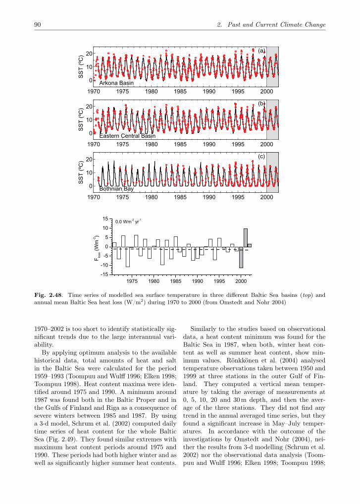
90 2. Past and Current Climate Change
Fig. 2.48. Time series of modelled sea surface temperature in three different Baltic Sea basins (top) andannual mean Baltic Sea heat loss (W/m2) during 1970 to 2000 (from Omstedt and Nohr 2004)
1970–2002 is too short to identify statistically sig-nificant trends due to the large interannual vari-ability.
By applying optimum analysis to the availablehistorical data, total amounts of heat and saltin the Baltic Sea were calculated for the period1959–1993 (Toompuu and Wulff 1996; Elken 1998;Toompuu 1998). Heat content maxima were iden-tified around 1975 and 1990. A minimum around1987 was found both in the Baltic Proper and inthe Gulfs of Finland and Riga as a consequence ofsevere winters between 1985 and 1987. By usinga 3-d model, Schrum et al. (2002) computed dailytime series of heat content for the whole BalticSea (Fig. 2.49). They found similar extremes withmaximum heat content periods around 1975 and1990. These periods had both higher winter and aswell as significantly higher summer heat contents.
Similarly to the studies based on observationaldata, a heat content minimum was found for theBaltic Sea in 1987, when both, winter heat con-tent as well as summer heat content, show min-imum values. Rönkkönen et al. (2004) analysedtemperature observations taken between 1950 and1999 at three stations in the outer Gulf of Fin-land. They computed a vertical mean temper-ature by taking the average of measurements at0, 5, 10, 20 and 30 m depth, and then the aver-age of the three stations. They did not find anytrend in the annual averaged time series, but theyfound a significant increase in May–July temper-atures. In accordance with the outcome of theinvestigations by Omstedt and Nohr (2004), nei-ther the results from 3-d modelling (Schrum et al.2002) nor the observational data analysis (Toom-puu and Wulff 1996; Elken 1998; Toompuu 1998;
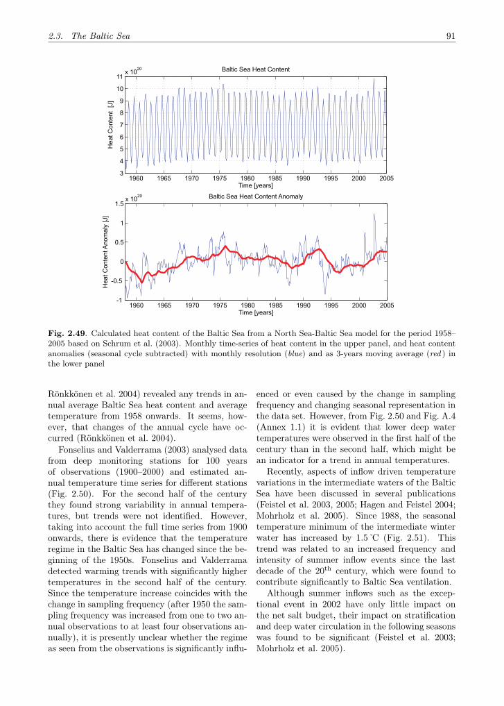
2.3. The Baltic Sea 91
1960 1965 1970 1975 1980 1985 1990 1995 2000 20053
4
5
6
7
8
9
10
11x 10
20
Time [years]
Hea
tCon
tent
[J]
Baltic Sea Heat Content
1960 1965 1970 1975 1980 1985 1990 1995 2000 2005-1
-0.5
0
0.5
1
1.5x 10
20
Time [years]
Hea
tCon
tent
Ano
mal
y[J
]
Baltic Sea Heat Content Anomaly
Fig. 2.49. Calculated heat content of the Baltic Sea from a North Sea-Baltic Sea model for the period 1958–2005 based on Schrum et al. (2003). Monthly time-series of heat content in the upper panel, and heat contentanomalies (seasonal cycle subtracted) with monthly resolution (blue) and as 3-years moving average (red ) inthe lower panel
Rönkkönen et al. 2004) revealed any trends in an-nual average Baltic Sea heat content and averagetemperature from 1958 onwards. It seems, how-ever, that changes of the annual cycle have oc-curred (Rönkkönen et al. 2004).
Fonselius and Valderrama (2003) analysed datafrom deep monitoring stations for 100 yearsof observations (1900–2000) and estimated an-nual temperature time series for different stations(Fig. 2.50). For the second half of the centurythey found strong variability in annual tempera-tures, but trends were not identified. However,taking into account the full time series from 1900onwards, there is evidence that the temperatureregime in the Baltic Sea has changed since the be-ginning of the 1950s. Fonselius and Valderramadetected warming trends with significantly highertemperatures in the second half of the century.Since the temperature increase coincides with thechange in sampling frequency (after 1950 the sam-pling frequency was increased from one to two an-nual observations to at least four observations an-nually), it is presently unclear whether the regimeas seen from the observations is significantly influ-
enced or even caused by the change in samplingfrequency and changing seasonal representation inthe data set. However, from Fig. 2.50 and Fig. A.4(Annex 1.1) it is evident that lower deep watertemperatures were observed in the first half of thecentury than in the second half, which might bean indicator for a trend in annual temperatures.
Recently, aspects of inflow driven temperaturevariations in the intermediate waters of the BalticSea have been discussed in several publications(Feistel et al. 2003, 2005; Hagen and Feistel 2004;Mohrholz et al. 2005). Since 1988, the seasonaltemperature minimum of the intermediate winterwater has increased by 1.5 C (Fig. 2.51). Thistrend was related to an increased frequency andintensity of summer inflow events since the lastdecade of the 20th century, which were found tocontribute significantly to Baltic Sea ventilation.
Although summer inflows such as the excep-tional event in 2002 have only little impact onthe net salt budget, their impact on stratificationand deep water circulation in the following seasonswas found to be significant (Feistel et al. 2003;Mohrholz et al. 2005).
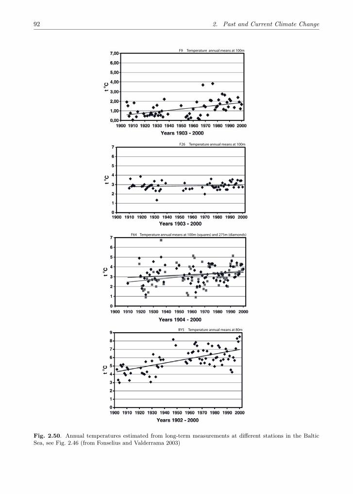
92 2. Past and Current Climate Change
F9 Temperature annual means at 100m
F26 Temperature annual means at 100m
F64 Temperature annual means at 100m (squares) and 275m (diamonds)
BY5 Temperature annual means at 80m
Fig. 2.50. Annual temperatures estimated from long-term measurements at different stations in the BalticSea, see Fig. 2.46 (from Fonselius and Valderrama 2003)

2.3. The Baltic Sea 93
BY15 Temperature annual means at 100m (squares) and 200m (diamonds)
BY31 Temperature annual means at 100m (squares) and 400m (diamonds)
Fig. 2.50. cont.
2.3.1.2 Salinity and Saltwater Inflows
During the 20th century, salinity showed only weakand statistically non-significant trends at all mon-itoring stations (Fonselius and Valderrama 2003;see also Fig. A.4 in Annex 1.1). The Baltic Seamean salinity (integrated vertically as well as hor-izontally) during the 20th century has been re-constructed and analyzed by Toompuu and Wulff(1996), Winsor et al. (2001, 2003), and Meier andKauker (2003).
In the study by Winsor et al. (2001), the es-timated mean salinity was calculated by first us-ing salinity profiles from all major sub-basins ofthe Baltic Sea for the period 1977–1987, a pe-riod with good coverage in all sub-basins. Thenthe mean was compared with data from the Got-land Deep (BY15), a station that has observationsover more than 100 years. The comparison illus-trated that the station BY15 represents the BalticSea well and, based on data from this station,the mean salinity was reconstructed for the 20th
century (Fig. 2.52). In the study by Meier andKauker (2003) salinities of the 20th century were
calculated utilising a three-dimensional circulationmodel forced with reconstructed atmospheric sur-face data (Kauker and Meier 2003).
The mean salinity averaged for the entire Balticwas estimated to be 7.7 (Winsor et al. 2003) or7.4 psu (Meier and Kauker 2003). The mean salin-ities calculated from climatological data (Janssenet al. 1999) amount to 7.2–7.4 psu for differentmonths. Daily and decadal variations have max-imum amplitudes of 0.1 and 0.5 psu, respectively.No long-term trend was found during the 20th
century. On longer time scales salinity varia-tions were much larger. The maximum salinityduring the Littorina Sea stage (6,000–5,000BP)was very likely between 10 and 15 psu due to in-creased cross-section areas of the inlets (Öresundand Darss) and due to a 15–60% lower freshwatersupply than at present (Gustafsson and Westman2002).
Long records of water exchange variations be-tween the North Sea and Baltic Sea have been cal-culated from sea level data by Stigebrandt (1984)and Winsor et al. (2001). Andersson (2002) andEkman (1999) showed that substantial variations
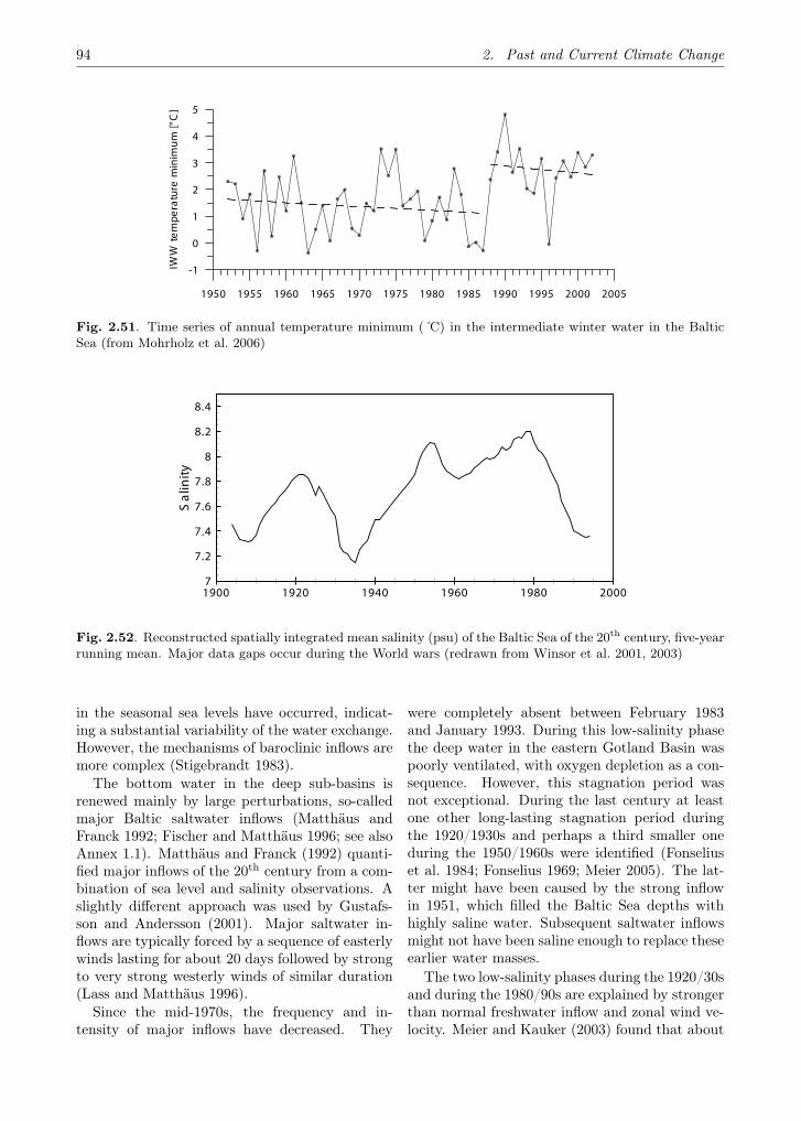
94 2. Past and Current Climate Change
1950 1955 1960 1965 1970 1975 1980 1985 1990 1995 2000 2005
-1
0
1
2
3
4
5
IWW
tem
pera
ture
min
imum
[°C
]
Fig. 2.51. Time series of annual temperature minimum ( C) in the intermediate winter water in the BalticSea (from Mohrholz et al. 2006)
Salinity
1900 1920 1940 1960 1980 20007
7.2
7.4
7.6
7.8
8
8.2
8.4
Fig. 2.52. Reconstructed spatially integrated mean salinity (psu) of the Baltic Sea of the 20th century, five-yearrunning mean. Major data gaps occur during the World wars (redrawn from Winsor et al. 2001, 2003)
in the seasonal sea levels have occurred, indicat-ing a substantial variability of the water exchange.However, the mechanisms of baroclinic inflows aremore complex (Stigebrandt 1983).
The bottom water in the deep sub-basins isrenewed mainly by large perturbations, so-calledmajor Baltic saltwater inflows (Matthäus andFranck 1992; Fischer and Matthäus 1996; see alsoAnnex 1.1). Matthäus and Franck (1992) quanti-fied major inflows of the 20th century from a com-bination of sea level and salinity observations. Aslightly different approach was used by Gustafs-son and Andersson (2001). Major saltwater in-flows are typically forced by a sequence of easterlywinds lasting for about 20 days followed by strongto very strong westerly winds of similar duration(Lass and Matthäus 1996).
Since the mid-1970s, the frequency and in-tensity of major inflows have decreased. They
were completely absent between February 1983and January 1993. During this low-salinity phasethe deep water in the eastern Gotland Basin waspoorly ventilated, with oxygen depletion as a con-sequence. However, this stagnation period wasnot exceptional. During the last century at leastone other long-lasting stagnation period duringthe 1920/1930s and perhaps a third smaller oneduring the 1950/1960s were identified (Fonseliuset al. 1984; Fonselius 1969; Meier 2005). The lat-ter might have been caused by the strong inflowin 1951, which filled the Baltic Sea depths withhighly saline water. Subsequent saltwater inflowsmight not have been saline enough to replace theseearlier water masses.
The two low-salinity phases during the 1920/30sand during the 1980/90s are explained by strongerthan normal freshwater inflow and zonal wind ve-locity. Meier and Kauker (2003) found that about

2.3. The Baltic Sea 95
Fig. 2.53. Upper panel: Annual mean river runoff to the Baltic Sea (thin line). In addition, the 4-year runningmean (thick line) and the total mean for the period 1902–1998 (horizontal line) are shown. Middle panel: 4-year running mean reconstructed (solid ) and observed (dashed ) zonal wind speed anomalies at Landsort.Lower panel: 4-year running mean uncorrected salinity in a reference simulation (solid ), in a simulation withclimatological monthly mean river runoff and precipitation of 1902–1970 (dashed ), and in a simulation withclimatological monthly mean river runoff and precipitation of 1902–1970 and with 4-year high-pass-filteredsea level pressure and associated surface wind (dotted ). The shaded ranges indicate periods with positivelyanomalous 4-year running mean runoff, which are related to stagnation phases (from Meier and Kauker 2003)
half of the decadal variability of the average salin-ity of the Baltic is related to the accumulatedfreshwater inflow (Fig. 2.53). Thus, the freshwa-ter inflow plays a dominant role for the averagesalinity in the Baltic. This model result is sup-ported by the analysis of long records of obser-vations (Samuelsson 1996; Schinke and Matthäus1998; Matthäus and Schinke 1999; Winsor et al.2001).
Another significant part of the decadal vari-ability of salinity is caused by the low-frequencyvariability of the zonal wind (Meier and Kauker2003). The wind stress anomaly is balanced by asea-level slope anomaly between the Kattegat andthe central Baltic Sea. Consequently, an anoma-lous barotropic pressure gradient hampers saltwa-ter inflows through the Danish straits (Schrum2001).

96 2. Past and Current Climate Change
Again, the model results are supported by ob-servations (Zorita and Laine 2000). The analysisby Zorita and Laine (2000) of the link betweenthe large-scale atmospheric circulation and annualsalinity revealed that roughly one half of the salin-ity variability is correlated to the meridional at-mospheric pressure gradient over the North At-lantic, and thus to the strength of the westerlyzonal winds. Lass and Matthäus (1996) found ananomalous west wind component at the stationKap Arkona between August and October for sea-sons without major Baltic Sea inflow compared tothe corresponding seasons with major Baltic Seainflow during 1951–1990. They suggested that inyears without major Baltic Sea inflow the prevail-ing easterly winds empying the Baltic Sea prior tothe main inflow event are reduced It is assumedthat the remaining decadal variability shown inFig. 2.53 is caused by such high-frequency windfluctuations (Meier and Kauker 2003).
The impact of other external factors on thevariability of salinity has been studied as well.A change of the seasonality of the freshwater in-flow caused by river regulation has no significantimpact on the variability of the average salinity(Meier and Kauker 2003), because the typical re-sponse time scale of about 20–30 years (Winsor etal. 2001; Stigebrandt and Gustafsson 2003; Dööset al. 2004; Meier 2005, 2006) is much larger thanone year. A rigid ice lid covering the entire BalticSea surface area has only a small impact on saltwa-ter inflows according to Meier and Kauker (2003).Neither do decadal variations of the sea level inthe Kattegat have an impact.
However, the high-frequency variability of thesea level in the Kattegat is very important for thelong-term behaviour of the average salinity. Forinstance, Stigebrandt (1983) found that approxi-mately one half of the salt transport into the BalticSea is carried out by the dispersive mode associ-ated with barotropic fluctuations.
Another important mechanism determining thelength of low-salinity phases might be vertical dif-fusion (Stigebrandt 2003). Axell (1998) showedthat variations in the energy supply to mixingare closely related to wind speed variations andfound substantial variations in the vertical diffu-sion. However, long records are not yet available.
2.3.2 Sea Level
2.3.2.1 Main Factors Affecting the Mean Sea Level
Investigations of sea level variations have a longtradition in all countries at the Baltic Sea. Thefindings of various authors (e.g. Stenij and Hela1947; Hela 1948, 1950; Lisitzin 1957; Lazarenko1961; Lisitzin 1966a,b, 1974; Krauss 1974; Kalas1993; Stigge 1993; Ekman 1994; Samuelsson andStigebrandt 1996; Carlsson 1998a,b; Ekman 1999;Plag and Tsimplis 1999; Johansson et al. 2001; An-dersson 2002; Baerens 2003; Ekman 2003; Fengeret al. 2001; Johansson et al. 2004; Dailidien etal. 2005; Raudsepp 1998; Suursaar et al. 2002,2006) help us to understand the reasons for simi-larities as well as differences in the sea level fluctu-ations between various coastal regions of the BalticSea.
Sea level is dependent on a series of factors. Thelong-term trend in sea level observation recordsfrom most locations in the Baltic Sea is dominatedby the composite of isostatic change due to post-glacial rebound and eustatic (and steric) global,or at least North Atlantic, sea level change. It israther difficult to separate between the two effects,but using satellite based positioning, GPS (GlobalPositioning System), yields promising results forthe isostatic uplift by direct measurements (Jo-hansson et al. 2002). However, the time seriesare still rather short and the accuracy is still ofthe same order of magnitude as the eustatic sealevel change, i.e. 1–2 mm yr−1. Other methodsuse various geological shoreline displacement data,for example, comparing the difference in shorelinedisplacement around lakes (Påsse 1998). The iso-static uplift varies from approximately zero in thesouthern Baltic Sea to a maximum uplift in Both-nian Bay of about 10 mm yr−1 (Johansson et al.2002).
Thus, the spatial variations of long-term sealevel change are mainly due to post-glacial re-bound of the Scandinavian land plate and the eu-static sea level rise. The latter is larger only onthe southern Baltic Sea coast, which sinks moreslowly (Lisitzin 1957; Lisitzin 1966b; Ekman 1996;Johansson et al. 2004). Consequently, the net sealevel rise was estimated to be about 1.7 mm peryear in the southeastern Baltic Sea while it re-verses to −9.4mm per year in the northwesternGulf of Bothnia (Vermeer et al. 1988). One ofthe most significant parts of the above-mentionedstudies was the elimination of meteorological ef-

2.3. The Baltic Sea 97
1770 1800 1830 1860 1890 1920 1950 1980
180190200210220230240250260270280290300
Ann
ual a
vera
ge (c
m)
Fig. 2.54. The sea level in Stockholm 1774–2002. The linear trend is computed for 1774–1884 and extrapolatedto 2002 (reproduced from Ekman 1999, recomputed and extended)
Fig. 2.55. The annual mean water level and the 15-year moving averages in Klaipeda (Dailidiene et al. 2004)
fects on sea level. The effect of meteorologicalfactors on mean sea level was studied by Lisitzin(1966b) and Carlsson (1998a,b).
2.3.2.2 Changes in the Sea-level from the 1800s toToday
The eustatic increase in sea level was found to ac-celerate at many Baltic Sea tide gauge stations atthe end of the 20th century (Kalas 1993; Stigge1993; Kont et al. 1997; Johansson et al. 2001;Fenger et al. 2001; Ekman 2003; Johansson etal. 2004; Suursaar et al. 2006). An illustrativeexample is the sea level time series from Stock-holm shown in Fig. 2.54. There is a long-termdecrease in sea level as discussed above, but it isalso evident that the sinking rate is lower during
the past 100 years than before. As postglacial re-bound does not change on these short time-scales,the reason must be of oceanographic nature. Thiswas noted by Ekman (1999), who attributed thechange to an increased eustatic sea level rise ofabout 1mm/yr in the 20th century compared tothe 19th century. It seems from the figure thatan even greater eustatic sea level rise has occurredduring the past 20–30 years.
This recent acceleration has been remarkedupon in several recent investigations. Dailidieneet al. (2004) showed that sea level rose in theKlaipeda Strait region in toto by about 13.6 cmin 100 years (1898–2001, see Fig. 2.55). However,the rate of sea level rise (1.36 mm year−1) in theLithuanian region during this period is similar tothe rate of global mean sea level rise, which is
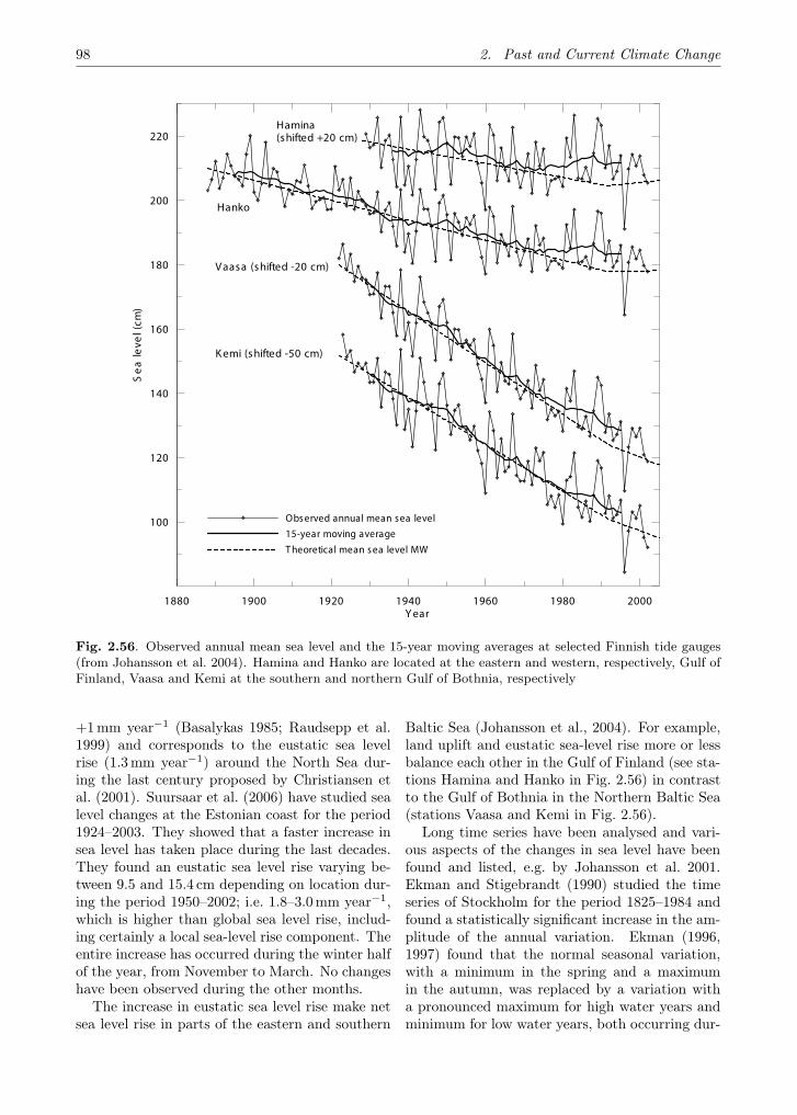
98 2. Past and Current Climate Change
1880 1900 1920 1940 1960 1980 2000Y ear
100
120
140
160
180
200
220S
ea
leve
l(cm
)
Obs erved annual mean sea level
15-year moving average
T heoretical mean s ea level MW
V aasa (s hifted -20 cm)
Hanko
Hamina(shifted +20 cm)
K emi (s hifted -50 cm)
Fig. 2.56. Observed annual mean sea level and the 15-year moving averages at selected Finnish tide gauges(from Johansson et al. 2004). Hamina and Hanko are located at the eastern and western, respectively, Gulf ofFinland, Vaasa and Kemi at the southern and northern Gulf of Bothnia, respectively
+1mm year−1 (Basalykas 1985; Raudsepp et al.1999) and corresponds to the eustatic sea levelrise (1.3mm year−1) around the North Sea dur-ing the last century proposed by Christiansen etal. (2001). Suursaar et al. (2006) have studied sealevel changes at the Estonian coast for the period1924–2003. They showed that a faster increase insea level has taken place during the last decades.They found an eustatic sea level rise varying be-tween 9.5 and 15.4 cm depending on location dur-ing the period 1950–2002; i.e. 1.8–3.0mm year−1,which is higher than global sea level rise, includ-ing certainly a local sea-level rise component. Theentire increase has occurred during the winter halfof the year, from November to March. No changeshave been observed during the other months.
The increase in eustatic sea level rise make netsea level rise in parts of the eastern and southern
Baltic Sea (Johansson et al., 2004). For example,land uplift and eustatic sea-level rise more or lessbalance each other in the Gulf of Finland (see sta-tions Hamina and Hanko in Fig. 2.56) in contrastto the Gulf of Bothnia in the Northern Baltic Sea(stations Vaasa and Kemi in Fig. 2.56).
Long time series have been analysed and vari-ous aspects of the changes in sea level have beenfound and listed, e.g. by Johansson et al. 2001.Ekman and Stigebrandt (1990) studied the timeseries of Stockholm for the period 1825–1984 andfound a statistically significant increase in the am-plitude of the annual variation. Ekman (1996,1997) found that the normal seasonal variation,with a minimum in the spring and a maximumin the autumn, was replaced by a variation witha pronounced maximum for high water years andminimum for low water years, both occurring dur-

2.3. The Baltic Sea 99
1860 1880 1900 1920 1940 1960 1980 2000
Y e a r
-4
-2
0
2
4
Se
a le
vel (
cm)
1 3
14
15
16
17
18
NA
O in
de
x (hP
a)
S ea leve l, H els ink i
N A O index
Fig. 2.57. De-trended annual mean sea level at Helsinki and the annual mean NAO index, 15-year runningaverages (from Johansson et al. 2001)
ing the winter. Ekman (1998) considered the sea-sonal sea level variation in wintertime using Stock-holm monthly sea level data, and found some sta-tistically significant secular changes, these beingdue to the changes in wind conditions over thetransition area between the Baltic Sea and theNorth Sea. Johansson et al. (2001) have shownthat the maxima of sea levels have increased sig-nificantly. The increase is proportionally largest inthe nodal area of the specific uninodal oscillationsof the Baltic Sea. It is possible that the changesin maxima are due to changes in large-scale mete-orological and hydrological factors. However, noessential trends were found for minima.
2.3.2.3 Influence of Atmospheric Circulation
Andersson (2002) and Ekman (2003) used the his-torical sea level time series from Stockholm todemonstrate the key role played by winter cli-mate, especially that of wind forcing. Andersson(2002) pointed out that there exists a relation be-tween the Stockholm sea level and the North At-lantic Oscillation (NAO) winter values. Johanssonet al. (2001, 2004) studied the Baltic Sea waterbalance and its correlation with the NAO indexand confirmed that the sea level variability alongthe Finnish coast correlated with the NAO index(Fig. 2.57).
A close correlation between atmospheric circu-lation and sea level fluctuations was also found atthe Estonian coast (Suursaar et al. 2006). Higher
intensity of westerly wind indices (NAO and AOindices, frequency of the zonal circulation) is re-lated to higher sea level. The closest correla-tion – above 0.6 – was detected during the win-ter months. A similar correlation was revealedbetween monthly mean sea level and number ofstorm days (Suursaar et al. 2006).
Andersson (2002) and Janssen (2002) analysedsea level variations in the Baltic Sea with respectto correlations to NAOWI (NAO Winter Index).Andersson (2002) considered the period 1825–1997while Janssen (2002) confined his investigation to1890–1993. They both found variable correlationswith time with a maximum at the end of the series,which corresponds well to an increased potential ofNAOWI for the regional winter situation in recentdecades.
2.3.3 Sea Ice
The ice climate in the Baltic Sea can be charac-terised by several variables, including the extentand thickness of the ice cover and the duration ofthe ice season. All these are important for winternavigation and travel on the ice, and for centuriesthere has been interest in monitoring these vari-ables (e.g. Sass 1866). The historical record of theice break-up dates has also been used to recon-struct the climate for the last 500 years (Tarandand Nordli 2001). The advance in sea ice researchduring the last ten years is summarised in Vihmaand Haapala (2005) and Omstedt et al. (2004a).
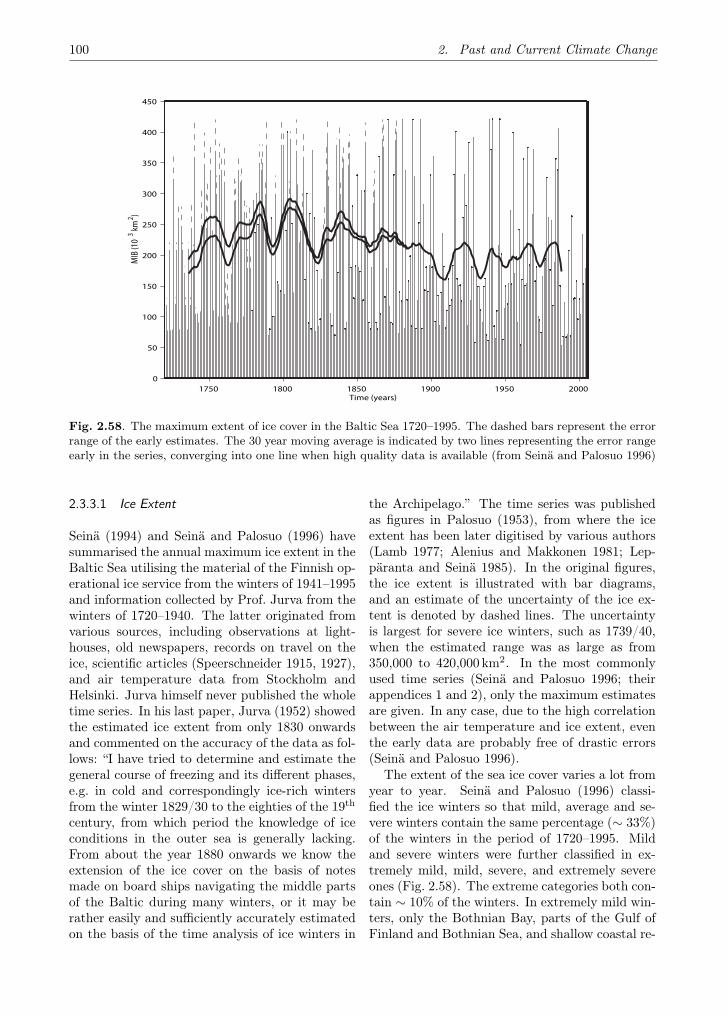
100 2. Past and Current Climate Change
1750 1800 1850 1900 1950 20000
50
100
150
200
250
300
350
400
450
MIB
(10
3 km2 )
Time (years)
Fig. 2.58. The maximum extent of ice cover in the Baltic Sea 1720–1995. The dashed bars represent the errorrange of the early estimates. The 30 year moving average is indicated by two lines representing the error rangeearly in the series, converging into one line when high quality data is available (from Seinä and Palosuo 1996)
2.3.3.1 Ice Extent
Seinä (1994) and Seinä and Palosuo (1996) havesummarised the annual maximum ice extent in theBaltic Sea utilising the material of the Finnish op-erational ice service from the winters of 1941–1995and information collected by Prof. Jurva from thewinters of 1720–1940. The latter originated fromvarious sources, including observations at light-houses, old newspapers, records on travel on theice, scientific articles (Speerschneider 1915, 1927),and air temperature data from Stockholm andHelsinki. Jurva himself never published the wholetime series. In his last paper, Jurva (1952) showedthe estimated ice extent from only 1830 onwardsand commented on the accuracy of the data as fol-lows: “I have tried to determine and estimate thegeneral course of freezing and its different phases,e.g. in cold and correspondingly ice-rich wintersfrom the winter 1829/30 to the eighties of the 19th
century, from which period the knowledge of iceconditions in the outer sea is generally lacking.From about the year 1880 onwards we know theextension of the ice cover on the basis of notesmade on board ships navigating the middle partsof the Baltic during many winters, or it may berather easily and sufficiently accurately estimatedon the basis of the time analysis of ice winters in
the Archipelago.” The time series was publishedas figures in Palosuo (1953), from where the iceextent has been later digitised by various authors(Lamb 1977; Alenius and Makkonen 1981; Lep-päranta and Seinä 1985). In the original figures,the ice extent is illustrated with bar diagrams,and an estimate of the uncertainty of the ice ex-tent is denoted by dashed lines. The uncertaintyis largest for severe ice winters, such as 1739/40,when the estimated range was as large as from350,000 to 420,000 km2. In the most commonlyused time series (Seinä and Palosuo 1996; theirappendices 1 and 2), only the maximum estimatesare given. In any case, due to the high correlationbetween the air temperature and ice extent, eventhe early data are probably free of drastic errors(Seinä and Palosuo 1996).
The extent of the sea ice cover varies a lot fromyear to year. Seinä and Palosuo (1996) classi-fied the ice winters so that mild, average and se-vere winters contain the same percentage (∼ 33%)of the winters in the period of 1720–1995. Mildand severe winters were further classified in ex-tremely mild, mild, severe, and extremely severeones (Fig. 2.58). The extreme categories both con-tain ∼ 10% of the winters. In extremely mild win-ters, only the Bothnian Bay, parts of the Gulf ofFinland and Bothnian Sea, and shallow coastal re-
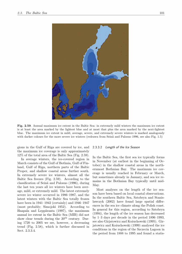
2.3. The Baltic Sea 101
Fig. 2.59. Annual maximum ice extent in the Baltic Sea: in extremely mild winters the maximum ice extentis at least the area marked by the lightest blue and at most that plus the area marked by the next-lightestblue. The maximum ice extent in mild, average, severe, and extremely severe winters is marked analogouslywith darker colours for the more severe ice winters (redrawn from Seinä and Palosuo 1996, see also Fig. 1.5)
gions in the Gulf of Riga are covered by ice, andthe maximum ice coverage is only approximately12% of the total area of the Baltic Sea (Fig. 2.59).
In average winters, the ice-covered region inMarch consists of the Gulf of Bothnia, Gulf of Fin-land, Gulf of Riga, northern parts of the BalticProper, and shallow coastal areas further south.In extremely severe ice winters, almost all theBaltic Sea freezes (Fig. 2.59). According to theclassification of Seinä and Palosuo (1996), duringthe last ten years all ice winters have been aver-age, mild, or extremely mild. The latest extremelysevere ice winter occurred in 1986–1987, and thelatest winters with the Baltic Sea totally frozenhave been in 1941–1942 (certainly) and 1946–1947(most probably; Simojoki 1952). According toHaapala and Leppäranta (1997), the maximumannual ice extent in the Baltic Sea (MIB) did notshow clear trends during the 20th century. Dur-ing 1720 to 2005 we see, however, a decreasingtrend (Fig. 2.58), which is further discussed inSect. 2.3.3.4.
2.3.3.2 Length of the Ice Season
In the Baltic Sea, the first sea ice typically formsin November (at earliest in the beginning of Oc-tober) in the shallow coastal areas in the north-ernmost Bothnian Bay. The maximum ice cov-erage is usually reached in February or March,but sometimes already in January, and sea ice re-mains in the Bothnian Bay typically until mid-May.
Most analyses on the length of the ice sea-son have been based on local coastal observations.In the southern Baltic Sea, Sztobryn and Stanis-lawczyk (2002) have found large spatial differ-ences in the sea ice climate along the Polish coast.In general for this region, according to Sztobryn(1994), the length of the ice season has decreasedby 1–3 days per decade in the period 1896–1993,see also Girjatowicz and Kożuchowski (1995). Gir-jatowicz and Kożuchowski (1999) analysed the iceconditions in the region of the Szczecin Lagoon inthe period from 1888 to 1995 and found a statis-

102 2. Past and Current Climate Change
tically significant decreasing trend in the durationof the ice season.
In the northern Baltic Sea, Haapala and Lep-päranta (1997) analysed ice time series from theFinnish coast and concluded that the length ofthe ice season shows a decreasing trend during1889–1994, as also does the probability of annualice occurrence in Utö (Northern Baltic Proper).Tarand (1993) and Tarand and Nordli (2001) haveaddressed the break-up dates of sea ice in the portof Tallinn. On the basis of time series over thelast 500 years, they concluded that the break-updates have become earlier since about the mid 19th
century and that the changes have been particu-larly large during the latest decades. This wasfound also by Jaagus (2006b), who analysed datafrom nine Estonian stations in the period 1949/50–2003/04. The largest decrease, by more than amonth, in the duration of the ice season was ob-served in the West Estonian Archipelago, whileon the southern coast of the Gulf of Finland thedecrease has been insignificant. A statistically sig-nificant change towards later dates of freezing wasdetected only at four stations at the west coast ofEstonia (Jaagus 2006b).
Jevrejeva (2000) analysed the sea ice and airtemperature time series along the Estonian coastin the period of 1900–1990. The results indicatedthat, at the end of the study period, the date ofa stabilised transition of the air temperature tosub-zero values was some 8–14 days later than inthe early 1900s, while the onset date of meltingair temperatures has become 10–15 days earlier.The number of days with sea ice has decreased by5–7 days per century in the Gulf of Finland, andby 5–10 days in the Gulf of Riga. These changeshave been associated with a climatic warming of0.5–1.0 C in Estonia in November–April in the pe-riod of 1900–1990; the warming has, however, beenstatistically significant at 99.9% confidence levelonly at one of the eight stations analysed by Jevre-jeva (2000). Analysing the historical record of icebreak-up at the port of Riga in 1529–1990, Jevre-jeva (2001) detected a decreasing trend of about2.0 days per century for the break-up dates for se-vere winters (statistically significant at the 99.9%level). For mild and average winters, no statisti-cally significant trends were detected.
Considering the whole Baltic Sea, Jevrejeva etal. (2004) did a comprehensive analysis of 20th cen-tury time series at 37 coastal stations around thesea. In general, the observations show a tendencytowards milder ice conditions, where the largest
change is in the length of the ice season, whichhas decreased by 14–44 days in a century, which,in turn, is largely due to the earlier ice break-up.
2.3.3.3 Ice Thickness
Accurate data on the ice thickness is almost en-tirely restricted to the zone of land-fast ice. Inthe Bothnian Bay, the level ice thickness is typi-cally 65–80 cm (Alenius et al. 2003), and it reaches30–50 cm even in mild winters. In the Skagerrakand the coastal areas of Germany and Poland theannual maximum ice thickness varies from 10 to50 cm (BSH 1994).
In their analysis of 37 time series from thecoastal stations around the Baltic Sea, Jevrejeva etal. (2004) did not find any consistent change in theannual maximum ice thickness. According to Haa-pala and Leppäranta (1997), the level-ice thicknessin the Baltic Sea did not show clear trends dur-ing the 20th century. Seinä (1993) and Launiainenet al. (2002) reported an increasing trend in themaximum annual ice thickness off Kemi (north-ernmost Gulf of Bothnia) during the 20th centuryuntil the 1980s; in more southerly locations in theGulf of Bothnia no clear trends were observed forthe same period. In all stations, decreasing trendshave been observed since the 1980s. In the Gulfof Finland, the maximum annual ice thickness hashad a decreasing trend off Helsinki and Loviisa(Alenius et al. 2003). From the point of view ofwinter navigation, an important climatological pa-rameter is the distance that ships have to cruisein sea ice thicker than some threshold value. Lau-niainen et al. (2002) calculated the annual maxi-mum distance from the harbour of Hamina (east-ern Gulf of Finland) to a zone of sea ice less than10 cm thick. The results for the period from 1951to 2000 strongly depended on the air temperature,with short distances in 1990s.
In the drift ice regions, where most of the sea-icemass locates, we do not have accurate data on theice thickness. During the last ten years, many fieldstudies have concentrated on the mapping of theice thickness, but no systematic long-term mea-surements of the ice thickness have been carriedout.
2.3.3.4 Large-scale Atmospheric Forcing on the IceConditions
During the last decade, increasing attention hasbeen paid to the relationship between the inter-annual variations in the Baltic Sea ice conditions

2.3. The Baltic Sea 103
1950 1955 1960 1965 1970 1975 1980 1985 1990 1995 2000 2005−4
−3
−2
−1
0
1
2
3
4
Nor
mal
ized
MIB
ano
mal
y an
d D
JFM
NA
O−
inde
x
Time (years)
Fig. 2.60. Time series of North Atlantic Oscillation index (Rogers 1984) (line) and the annual maximum iceextent of the Baltic Sea, MIB (Seinä and Palosuo 1996) (bars). The MIB is presented as an anomaly of thenormalised time series
and the indices of the North Atlantic Oscillation(NAO) and Arctic Oscillation (AO). Read moreon NAO and AO in Annex 7. The relationship be-tween the large-scale atmospheric circulation andthe Baltic Sea ice conditions can be illustrated bycomparing the NAO winter index and the MIB(Fig. 2.60). Although the MIB is fairly well corre-lated with the winter NAO index (Fig. 2.60), mov-ing correlation analyses have demonstrated thatthe relationship is not constant in time (Omstedtand Chen 2001; Janssen 2002; Meier and Kauker2004; Schrum and Janssen 2002; Chen and Li2004). The 31-year moving correlation is high dur-ing the 1940s and 1980s but quite low during the1920s (Meier and Kauker 2002). Changes in theNAO-MIB relationship are explained by changesin the location of the atmospheric pressure pat-terns (Koslowski and Loewe 1994; Kauker andMeier 2003; Chen and Li 2004). Kauker and Meier(2003) found that 87% of the observed air tem-perature variance at Stockholm (and consequentlymost of the MIB variance) is explained by NAOand a sea level pressure pattern similar to the Bar-ents Sea Oscillation, which describes shifts of theIcelandic low pressure center toward the BarentsSea (Skeie 2000).
According to Yoo and D’Odorico (2002), NAOseems to affect mostly the late-winter tempera-ture (January–March), with a significant impactalso on the mid-spring (April–May) period, whenthe air temperature is strongly correlated to theice break-up dates. The results of Jevrejeva andMoore (2001) suggest that, from the point of viewof ice break-up in the Baltic Sea, AO is an indexsomewhat more essential than NAO: time series ofice break-up date reflect variations in the winterAO index in the 13.9-year period, but not in theNAO 7.8-year period. Calculating cross-waveletpower for the time series, Jevrejeva et al. (2003)found out that the times of largest variance in theBaltic Sea ice conditions were in excellent agree-ment with significant power in the AO at 2.2–3.5,5.7–7.8, and 12–20 year periods (previously Ale-nius and Makkonen (1981) had detected the mostdistinct cycles in the MIB at the periods of 3.5,5.2, 8, and 13 years).
It is noteworthy that Jevrejeva et al. (2003)found similar patterns also with the Southern Os-cillation Index and El Niño sea surface tempera-ture series (Nino3). Also, according to Omstedt etal. (2004b), 90% of the variance of the time seriesis for the time scales shorter than 15 years. A con-

104 2. Past and Current Climate Change
cern of these studies is, however, that they haveassumed the long-term time series of the MIB ashomogeneous in accuracy (see Sect. 2.3.3.1).
Jaagus (2006b) analysed the freezing and break-up dates near the Estonian coast in relation tolarge-scale atmospheric circulation. NAO indices,the AO index, several teleconnection indices andfrequencies of the circulation forms were used todescribe circulation conditions. Generally, no cor-relation was found between the circulation and thedate of the first appearance of sea ice. The circu-lation has the strongest relationship with the dateof ice break-up and the length of the ice season.They have a high negative correlation with thecharacteristics of the intensity of the zonal circu-lation. The highest value is present in the caseof the sea ice break-up and the AO index for thetotal winter period (December–March): −0.73 asa mean of nine stations.
According to Jaagus (2006b), February is thekey month when the circulation plays a main rolein determining sea ice conditions for the spring.High intensity of westerlies in winter (February)causes earlier ice melting in the Baltic Sea. Us-ing the conditional Mann-Kendall test, Jaagus(2006b) demonstrated that the significant trendsin sea ice near the Estonian coast during 1949/50–2003/04 are caused by the increasing intensity ofwesterlies in winter, especially in February, and bythe corresponding decrease in frequency of merid-ional circulation types during the same time inter-val.
From the point of view of climatology, the mostrelevant parameter for describing the ice condi-tions is the total mass of ice, but we lack gooddata on it over large regions. Over a small region,such as the coastal areas of Schleswig-Holstein(Germany), the ice thickness and concentrationcan be observed sufficiently accurately. Koslowskiand Loewe (1994) calculated the areal ice volume,which can be visualised as an equivalent ice thick-ness in a partly ice-covered sea. Analogously todegree days (accumulated degrees of frost), theyfurther calculated the accumulated areal ice vol-ume, and showed that in the period from 1879 to1992 it was negatively correlated with the NAOwinter index. Weak ice winters were related toa NAO winter index exceeding 1, and strong icewinters were related to a NAO winter index lessthan −1. Koslowski and Loewe (1994) also note-worthily pointed out that, depending on the exactlocation and size of the high and low pressure ar-eas, in rare cases a strong ice winter in the south-
western Baltic Sea can develop even in spite of ahigh NAO winter index.
On the basis of the data on the accumu-lated areal ice volume from the 1878–1993 period,Koslowski and Glaser (1995) reconstructed the icewinter severity since 1701 for the southwesternBaltic Sea, and Koslowski and Glaser (1999) ex-tended the calculations for the period from 1501to 1995. The present-day ice winter regime haslasted since about 1860, while from about 1760to about 1860 the ice winters were much more se-vere. Around 1800 the ice production in the south-western Baltic Sea was three times larger than itis today (Koslowski and Glaser 1999). Accordingto Omstedt and Chen (2001), the shift towardsa warmer climate took place in 1877, associatedwith a period of an increased low-pressure activ-ity (Omstedt et al. 2004b). This shift in climatewas identified as the ending of the Little Ice Age inthe Baltic Sea region. Omstedt and Chen (2001)also found that a colder climate is associated withhigher variability in the ice extent and with ahigher sensitivity of the ice extent to changes inwinter air temperature. They further developeda statistical model that links the ice extent anda set of atmospheric circulation indices. Consid-ering the possibilities to make climate-scale pre-dictions for the future sea ice conditions, Omst-edt and Chen (2001) argue that such a statisti-cal model could be a useful tool in estimating themean conditions of the ice extent on the basis ofatmospheric pressure fields, which are producedapplying a climate model. Tinz (1996) found anexponential relation between the ice extent andthe air temperature; applying it and climate modelpredictions, he forecasted a drastic decrease in theBaltic Sea ice cover in the next 100 years.
2.3.3.5 Summary
A climate warming can be detected from the timeseries of the maximum annual extent of sea iceand the length of the ice season in the Baltic Sea.On the basis of the ice extent, the shift towardsa warmer climate took place in the latter half ofthe 19th century. During the last ten years, allice winters have been average, mild, or extremelymild. The record of the length of the ice seasonshows a decreasing trend by 14–44 days in the lat-est century, the exact number depending on thelocation around the Baltic Sea. The indices of AOand NAO correlate with the ice extent, the dateof ice break-up, and the length of the ice season.
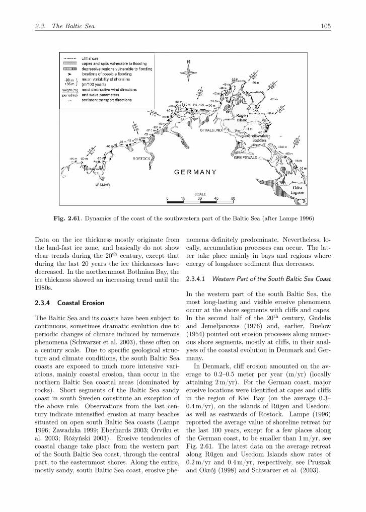
2.3. The Baltic Sea 105
Fig. 2.61. Dynamics of the coast of the southwestern part of the Baltic Sea (after Lampe 1996)
Data on the ice thickness mostly originate fromthe land-fast ice zone, and basically do not showclear trends during the 20th century, except thatduring the last 20 years the ice thicknesses havedecreased. In the northernmost Bothnian Bay, theice thickness showed an increasing trend until the1980s.
2.3.4 Coastal Erosion
The Baltic Sea and its coasts have been subject tocontinuous, sometimes dramatic evolution due toperiodic changes of climate induced by numerousphenomena (Schwarzer et al. 2003), these often ona century scale. Due to specific geological struc-ture and climate conditions, the south Baltic Seacoasts are exposed to much more intensive vari-ations, mainly coastal erosion, than occur in thenorthern Baltic Sea coastal areas (dominated byrocks). Short segments of the Baltic Sea sandycoast in south Sweden constitute an exception ofthe above rule. Observations from the last cen-tury indicate intensified erosion at many beachessituated on open south Baltic Sea coasts (Lampe1996; Zawadzka 1999; Eberhards 2003; Orviku etal. 2003; Różyński 2003). Erosive tendencies ofcoastal change take place from the western partof the South Baltic Sea coast, through the centralpart, to the easternmost shores. Along the entire,mostly sandy, south Baltic Sea coast, erosive phe-
nomena definitely predominate. Nevertheless, lo-cally, accumulation processes can occur. The lat-ter take place mainly in bays and regions whereenergy of longshore sediment flux decreases.
2.3.4.1 Western Part of the South Baltic Sea Coast
In the western part of the south Baltic Sea, themost long-lasting and visible erosive phenomenaoccur at the shore segments with cliffs and capes.In the second half of the 20th century, Gudelisand Jemeljanovas (1976) and, earlier, Buelow(1954) pointed out erosion processes along numer-ous shore segments, mostly at cliffs, in their anal-yses of the coastal evolution in Denmark and Ger-many.
In Denmark, cliff erosion amounted on the av-erage to 0.2–0.5 meter per year (m/yr) (locallyattaining 2m/yr). For the German coast, majorerosive locations were identified at capes and cliffsin the region of Kiel Bay (on the average 0.3–0.4 m/yr), on the islands of Rügen and Usedom,as well as eastwards of Rostock. Lampe (1996)reported the average value of shoreline retreat forthe last 100 years, except for a few places alongthe German coast, to be smaller than 1 m/yr, seeFig. 2.61. The latest data on the average retreatalong Rügen and Usedom Islands show rates of0.2 m/yr and 0.4 m/yr, respectively, see Pruszakand Okrój (1998) and Schwarzer et al. (2003).

106 2. Past and Current Climate Change
Fig. 2.62. Long-term shoreline changes along the Polish coast (an average rate) during 1875 to 1979 (A),1960 to 1983 (B) and 1971 to 1983 (C) (after Zawadzka 1999)
2.3.4.2 Middle Part of the South Baltic Sea Coast
The behaviour of about 500 km of dunes and cliffson the Polish coast, comprising a significant cen-tral part of the southern Baltic Sea coast, also in-dicates enhanced and accelerated erosion. The av-erage rate of coastal retreat during the 100 yearscovering the period between 1875–1979 was 0.12meter per year (m/yr) (Fig. 2.62A). During theperiod 1960–1983 (Fig. 2.62B) the average rate ofretreat increased to 0.5m/yr, and between 1971–1983 it reached 0.9m/yr (Fig. 2.62C). The erosionpersisted over an increasing lengths of the coast-line: 61% in the 100-year period, 72% in the 24-year period and 74% in the 13-year period. Thedune/cliff foot was eroded at a less intensive pace
and in the period 1960–1983, when it retreated ata rate of 0.16m/yr and in the period 1971–1983, at0.3 m/yr (Zawadzka 1994). The process of trans-formation of the coastal zone proceeded with si-multaneous erosive and accretive processes. Theanalysis of changes in the land area showed a de-crease in the recovery of eroded beaches and dunes.In the 100-year period, the recovery of eroded landencompassed over 69% of the destroyed area, inthe period 1960–1983 it was 20%, and in the pe-riod 1971–1983 only 14%. These data clearly doc-ument that processes of erosion are intensifyingand accelerating, although they are to some ex-tent explained by the difference in the lengths ofthe time periods in question, where a longer pe-riod offers more opportunity for recovery. These

2.3. The Baltic Sea 107
Period: 01.03.–30.11.2002
ObsMen = 0,94 [m] HinMen = 0,87 [m] Bias = 0,01 [m] Rmse = 0,4 [m] Stdev = 0,4 [m] Cor = 0,78 NObs = 4111
6.0
5.0
4.0
3.0
2.0
1.0
0.0 0.0 1.0 2.0 3.0 4.0 5.0 6.0 7.0
270
99
37
13
5
2
1
0
0
observed wave height [m]
mod
el w
ave
heig
ht [m
]
Fig. 2.63. Scatterplot showing observed (x-axis) and hindcast (y-axis) significant wave height (in meter) nearArkona for March to November 2002. Colors indicate the number of observed and model values. The totalnumber of pairs is 4111. Some error statistics are provided in the upper left corner (from Augustin 2005)
erosive processes are now present over about 74%of the length of the Polish part of the Baltic Seacoast.
Since the beginning of the 20th century upto present, coastal defence systems have beencontinuously installed, which indicates that thebeaches are particularly affected by marine ero-sion. Various types of coastal protection struc-tures are present along 26% of the Polish coast.About 98 km of the coast is under the influenceof groynes, while 41 km are protected by light andheavy revetments. The Hel Peninsula is protectedalong 34% of its length. Coastal protection mea-sures are especially intense in the middle and west-ern part of the open Polish coastline, where coastaldefense structures are built along 71 km out of126 km of the coastline (Pruszak 2001).
2.3.4.3 South-eastern Part of the South Baltic SeaCoast
Similar tendencies of coastal evolution are also ob-served on other segments of the eastern part ofthe southern Baltic Sea. In Latvia, practicallyall cliffs have been subject to various degrees oferosion over the past 50–100 years. In the last50–60 years, long-term cliff erosion has been 0.5–0.6m/yr, reaching a maximum of 1–1.5m/yr alongparticular stretches of the coast. Since 1980–81,rates of coastal erosion along Latvia’s coast have
increased 2–5 fold, reaching 1.5–4m/yr (Eber-hards 2003). Simultaneously, all of Latvia’s ma-rine hydrological stations indicate a trend of ris-ing mean sea level during the second half of thelast century (see also Sect. 2.3.2). A similar situ-ation is also observed along the Lithuanian coast(Zilinskavas et al. 2001). In recent years a seriesof very heavy storms completely destroyed sandybeaches in and around Palanga (Lithuania), whichwere not being eroded previously.
The increasing activity of coastal processeshas also been observed along the Estonian coast-line during the last decades (Orviku 1992, 1993;Orviku et al. 2003; Raukas et al. 1994). The re-sults of comparing maps from different times aswell as results from field measurements in test ar-eas clearly reveal an increased activity of both ero-sion and accumulation processes (Rivis 2004). Dueto such processes, a part of the coastline, asidefrom migration, is subject to continuous transfor-mation and change of shape. For instance, shoreprocesses during the last century have caused thenorthwesternmost point of Harilaid Peninsula onSaaremaa (Estonia) to migrate to the northeastand to change its shape.
The decrease in duration or even absence of icecover in the Baltic Sea in recent decades (Jaagus2003) has enhanced coastal erosion. The activ-ity of shore processes has increased significantlyin Estonia since the 1980s. In the last 20 years,
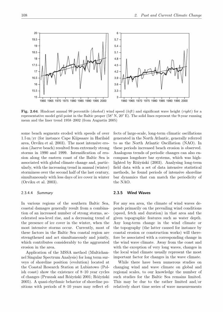
108 2. Past and Current Climate Change
1960 1965 1970 1975 1980 1985 1990 1995 2000 1960 1965 1970 1975 1980 1985 1990 1995 2000
20
19.5
19
18.5
18
17.5
17
16.5
16
15.5
15
6
5.7
5.4
5.1
4.8
4.5
4.2
3.9
3.6
3.3
3
Fig. 2.64. Hindcast annual 99 percentile (dashed ) wind speed (left ) and significant wave height (right ) for arepresentative model grid point in the Baltic proper (58◦ N, 20◦ E). The solid lines represent the 9-year runningmean and the liner trend 1958–2002 (from Augustin 2005)
some beach segments eroded with speeds of over1.5m/yr (for instance Cape Kiipsaare in Harilaidarea, Orviku et al. 2003). The most intensive ero-sion (Jaerve beach) resulted from extremely strongstorms in 1990 and 1999. Intensification of ero-sion along the eastern coast of the Baltic Sea isassociated with global climate change and, partic-ularly, with the increasing trend in annual (winter)storminess over the second half of the last century,simultaneously with less days of ice cover in winter(Orviku et al. 2003).
2.3.4.4 Summary
In various regions of the southern Baltic Sea,coastal damages generally result from a combina-tion of an increased number of strong storms, ac-celerated sea-level rise, and a decreasing trend ofthe presence of ice cover in the winter, when themost intensive storms occur. Currently, most ofthese factors in the Baltic Sea coastal region arestrengthened and act simultaneously and jointly,which contributes considerably to the aggravatederosion in the area.
Application of the MSSA method (Multichan-nel Singular Spectrum Analysis) for long term sur-veys of shoreline position (evolution) located atthe Coastal Research Station at Lubiatowo (Pol-ish coast) show the existence of 8–10 year cyclesof changes (Pruszak and Różyński 2001; Różyński2005). A quasi-rhythmic behavior of shoreline po-sitions with periods of 8–10 years may reflect ef-
fects of large-scale, long-term climatic oscillationsgenerated in the North Atlantic, generally referredto as the North Atlantic Oscillation (NAO). Inthese periods increased beach erosion is observed.Analogous trends of periodic changes can also en-compass longshore bar systems, which was high-lighted by Różyński (2003). Analysing long-termfield data with a set of data intensive statisticalmethods, he found periods of intensive shorelinebar dynamics that can match the periodicity ofthe NAO.
2.3.5 Wind Waves
For any sea area, the climate of wind waves de-pends primarily on the prevailing wind conditions(speed, fetch and duration) in that area and thegiven topographic features such as water depth.Any long-term change in the wind climate orthe topography (the latter caused for instance bycoastal erosion or construction works) will there-fore be associated with a corresponding change inthe wind wave climate. Away from the coast andwith the exception of very long waves, changes inthe local wind climate usually represent the mostimportant factor for changes in the wave climate.
While there have been numerous studies onchanging wind and wave climate on global andregional scales, to our knowledge the number ofsuch studies for the Baltic Sea remains limited.This may be due to the rather limited and/orrelatively short time series of wave measurements

2.3. The Baltic Sea 109
1960 1965 1970 1975 1980 1985 1990 1995 2000 1960 1965 1970 1975 1980 1985 1990 1995 2000
1960 1965 1970 1975 1980 1985 1990 1995 20001960 1965 1970 1975 1980 1985 1990 1995 2000
6
5.7
5.4
5.1
4.8
4.5
4.2
3.9
3.6
3.3
3
20
18
16
14
12
10
8
6
4
2
0
2
18
1.6
1.4
1.2
1
0.8
0.6
0.4
0.2
30
27
24
21
18
15
12
9
6
3
0
Fig. 2.65. Statistics (dashed ) of severe wave events at a representative model grid point (58◦ N, 20◦ E) in theBaltic proper. Upper left: Hindcast annual 99 percentile significant wave height in meters. Lower left: Thenumber of events per year that exceed the 45-year average 99 percentile significant wave height. Upper right:The yearly average duration of events in hours that exceeds the long-term average 99 percentile significantwave height. Lower right: The yearly averaged intensity, i.e. the difference between the maximum wave heightof an event exceeding the long-term average 99 percentile significant wave height in meters and the long-termaverage 99 percentile significant wave height. The solid lines represent the 9-year running mean and the linertrend 1958–2002 (from Augustin 2005)
in the Baltic Sea available so far, which hampersany reliable analysis of long-term changes. Whileit may be speculated that long-term changes inthe Baltic Sea wave climate may have been sim-ilar to observed long-term changes in storminess(Sect. 2.1.5.4), there are no long-term measure-ments that would directly allow for a test of thishypothesis.
An indirect and somewhat limited alternativeis provided by the analysis of wave hindcasts. Toour knowledge the longest wave hindcast availablefor the Baltic Sea is a recently completed simula-tion with the wave model WAM (WAMDI 1988) at
about 5×5 km horizontal resolution for the period1958–2002. The wave climate of this hindcast andits long-term changes are described in Augustin(2005).
As the quality of any wave model simulationdepends to a large extent on the quality of thedriving wind fields, some efforts were made to ob-tain reasonable wind fields. The technique is basedon a downscaling of global re-analysis data and isdescribed in von Storch et al. (2000) and Feser etal. (2001). A comparison of observed and down-scaled wind fields can be found in Weisse et al.(2005, 2003). A comparison between the observed

110 2. Past and Current Climate Change
storm indices from Bärring and von Storch (2004)and those derived from the downscaled wind fieldsused to drive the wave hindcast for the Baltic Seacan be found in Sect. 2.1.5.4 (Figs. 2.27 and 2.30).In general, a good agreement can be inferred. Inparticular, the interannual and long-term variabil-ity appears to be reasonably captured while thereremain some biases for some of the indices. Dis-crepancies appear to be larger at the beginning ofthe hindcast period.
Figure 2.63 shows a comparison between ob-served and hindcast wave height near Arkona,Germany (54◦ 43.0N, 013◦ 44.5E) for the some-what brief period March to November 2002.Although there is considerable scatter betweenmodel and observations, the hindcast appears tobe calibrated, i.e. there is no systematic bias. Inparticular, the frequency of over- and underesti-mating severe events seems to be similar, althoughthis cannot be concluded with confidence from thelimited material available.
As an example for the hindcast changes inthe wind and wave climate in the Baltic proper,Fig. 2.64 shows an analysis of the annual 99 per-centiles of wind speed and significant wave height.Both time series show remarkable short-term fluc-tuations and, considered over the entire 1958–2002period, display increases of about 1m/s and 0.3min the 99 percentile wind speed and significantwave height, respectively. When compared to thestorm indices of Alexandersson et al. (2000) andBärring and von Storch (2004), this behavior isin agreement with the observed tendency towardmore storminess, and the linear increase of signif-icant wave height over the hindcast period maypossibly reflect the upward branch of long-termfluctuations in observed storminess.
The increase of hindcast annual 99 percentilesof significant wave height may be caused by morefrequent, more severe, and/or longer lasting ex-treme events. To identify how the characteristicsof extreme wave events have changed, Augustin(2005) computed the annual number of extremeevents, their average duration and mean intensityrelative to a given threshold (Fig. 2.65). It can beinferred that for the Baltic proper the changes areprimarily caused by an increase in the frequencyof severe wave events while their duration and in-tensity revealed no significant trend.
Summarising, the analysis of existing long-termatmosphere observations and wave hindcasts forthe Baltic Sea suggests that the storm and waveclimate in the Baltic Sea has undergone consider-
able variations in the past. Although wave hind-cast results show an increase in the frequency of se-vere sea states for the period 1958–2002, the anal-ysis of long-term atmospheric data suggests thatthis increase is within the natural variability ofthe records and may reflect the upward branch ofobserved long-term variations in Baltic Sea stormi-ness.
2.4 Summary of Observed ClimateChanges
The variability in atmospheric circulation hasa strong influence on the surface climate in north-ern Europe (temperature, precipitation, windspeed, etc.). From about the 1960s until the 1990swesterly air flow has intensified during wintertime.This increased frequency of maritime air masseshas contributed to higher wintertime temperaturesand enhanced precipitation in regions exposed towesterly winds, especially during the 1990s. Ona hundred year timescale relationships betweenlarge-scale atmospheric circulation and surface cli-mate elements show strong temporal variability.
During the period 1871–2004 there were signif-icant positive trends in the annual mean tem-perature for the northern and southern BalticSea Basin, being 0.10 C/decade on average to thenorth of 60◦ N and 0.07 C/decade to the south of60◦ N. These trends are larger than the trend forthe entire globe, which amounts to 0.05 C/decade(1861–2000). The annual mean temperaturesshow an early 20th century warming that culmi-nated in the 1930s. This was followed by a slightercooling that finished in the 1960s, followed byanother strong warming until present. Warmingis characterised by a pattern where mean dailyminimum temperatures have increased more thanmean daily maximum temperatures.
Spring is the season showing the most linearand strongest warming, whereas wintertime tem-perature increase is irregular but larger than insummer and autumn. A general tendency is thatthe start of the climatic seasons in the spring half-year (e.g. spring, growing season, summer) startearlier, whereas the climatic seasons in the autumnhalf-year (e.g. autumn, frost season, winter) startlater. Changes in extreme temperatures havebroadly followed changes in mean temperatures.The number of cold nights has decreased, whilethe number of warm days has increased. Thesechanges have been stronger during winter thanduring summer.
2.4. Summary of Observed Climate Changes 111
Over the latter part of the 20th century, on av-erage, northern Europe has become wetter. Theincrease in precipitation is not spatially uniform.Within the Baltic Sea Basin the largest increaseshave occurred in Sweden and on the eastern coastof the Baltic Sea. Seasonally, the largest increaseshave occurred in winter and spring. Changesin summer are characterised by increases in thenorthern and decreases in the southern parts ofthe Baltic Sea Basin. In wintertime, there is anindication that the number of heavy precipitationevents has increased.
Characteristics of cloudiness and solar ra-diation have remarkable inter-annual and inter-decadal variations in the Baltic Sea Basin. A de-crease in cloudiness and increase in sunshine dura-tion was observed in the south (Poland), while op-posite trends were revealed in the north (Estonia).In the 1990s, all these trends changed their sign.Long-term observations in Estonia show that animprovement in air quality (i.e. a decrease in theaerosol emissions to the atmosphere) reversed de-creasing trends in atmospheric transparency anddirect radiation during the 1990s. At present, theatmospheric transparency is at the same level asin the 1930s.
Hundred-year time series from southern Scan-dinavia reveal that there is no long-term trend instorminess indices. There was a temporary in-crease of storm activity in the 1980s–1990s. Inthe Baltic Sea Basin on the whole, different datasources give slightly different results with respectto trends and variations in the extreme wind cli-mate, especially concerning small-scale extremewinds. At the same time, there are indicationsof an increasing impact of extreme wind events.However, this increasing impact results from acomplex interaction between climate and develop-ment trends that increase the exposure to damageand/or the vulnerability of nature and society.
The inter-annual variability in water inflow(river runoff to the Baltic Sea) is considerable, but
no statistically significant trend can be found inthe annual time series for the period of 1921–1998.
The analysis of the long-term dynamics of thedates of the start and ending of ice eventsand duration of the ice coverage for riversof the Russian territory of the Baltic Sea Basinshowed a stable positive trend from the middle ofthe 20th century to its end.
As to the maximal ice cover thickness, a neg-ative trend has been analysed for all Polish andRussian study lakes. In Finland, both decreasingand increasing trends can be found in the maxi-mum ice thickness time series.
A recent decrease in snow cover durationand water equivalent has been observed in thesouthern parts of all the Fennoscandian countries,while the opposite trend prevails in the north.Changes of snow depth are quite similar, i.e. de-crease in south-west regions and increase in thenorth-east regions.
The Baltic Sea mean salinity during the 20th
century decreased during the 1980s and 1990s, butsimilar decreases also appeared earlier in the 20th
century. No long-term trend was found during the20th century.
There are indications of a more rapid eustaticsea level rise in the 20th century than in the 19th
century.A climate warming can be detected from the
time series of the maximum annual extent ofsea ice and the length of the ice season inthe Baltic Sea. On the basis of the ice extent, theshift towards a warmer climate took place in thelatter half of the 19th century. This gradual shifthas been identified as the ending of the Little IceAge in the Baltic Sea Basin.
Coastal damages appearing in various regionsof the southern Baltic Sea generally result froma combination of strong storms, their increasednumber, accelerated sea-level rise and a decreas-ing trend of the presence of ice cover in winter,when the most intensive storms occur.

112 2. Past and Current Climate Change
2.5 References
Achberger C, Chen D (2006) Trend of extreme precipitation in Sweden and Norway during 1961–2004.Research Report C72, Earth Sciences Centre, Göteborg University, Sweden
Alenius P, Makkonen L (1981) Variability of the annual maximum ice extent of the Baltic Sea. Mete-orol Atmos Phys 29:393–398
Alenius P, Seinä A, Launiainen J, Launiainen S (2003) Sea ice and related data sets from the BalticSea. AICSEX – Metadata Report. Meri Report Series of the Finnish Institute of Marine Research49:3–13
Alexandersson H (1986) A homogeneity test applied to precipitation data. Int J Climatol 6:661–675Alexandersson H (2002) Temperature and precipitation in Sweden 1860–2001. SMHI Meteorologi No
104Alexandersson H (2004) Variationer och trender i nederbörden (1860–2003) (Variabilities and trends
in precipitation, 1860—2003). Faktablad nr 22 Sveriges Meteorologiska och Hydrologiska Institut,Norrköping, Sverige (in Swedish)
Alexandersson H, Vedin H (2002) Stormar det mera nu? (Do we have more storms today?) SMHIVäder och Vatten, 10:18 (in Swedish)
Alexandersson H, Schmith T, Iden K, Tuomenvirta H (1998) Long-term variations of the storm cli-mate over NW Europe. Global Atmosphere and Ocean Systems 6:97–120
Alexandersson H, Tuomenvirta H, Schmith T, Iden K (2000) Trends of storms in NW Europe derivedfrom an updated pressure data set. Clim Res 14:71–73
Alexandersson H, Eggertsson Karlström C (2001) Temperaturen och nederbörden i Sverige 1961–1990(Temperature and precipitation in Sweden 1961–1990). Referensnormaler – utgåva 2. SMHI Rap-porter 99 Sveriges Meteorologiska och Hydrologiska Institut, Norrköping, Sverige (in Swedish)
Andersson HC (2002) Influence of long-term regional and large-scale atmospheric circulation on theBaltic sea level. Tellus A 54:76–88
Augustin J (2005) Das Seegangsklima der Ostsee zwischen 1958–2002 auf Grundlage numerischerDaten (Sea state climate of the Baltic Sea 1958–2002 based on numerical data). Diploma thesis.Institute for Coastal Research, GKSS Research Center, Geesthacht, Germany (in German)
Axell LB (1998) On the variability of Baltic Sea deepwater mixing. J Geophys Res C: Oceans103(C10):21667–21682
Baerens C, Baudler H, Beckmann BR, Birr HD, Dick S, Hofstede J, Kleine E, Lampe R, Lemke W,Meinke I, Meyer M, Müller R, Müller-Navarra SH, Schmager G, Schwarzer K, Zenz T (2003) DieWasserstände an der Ostseeküste. Entwicklung – Stumfluten – Klimawandel (Water levels at theBaltic Sea coast. Trends – storm surges – climate change). In: Hupfer P, Hartt J, Horst S, StiggeHJ (eds) Die Küste (The Coast) Archive for research and technology on the North Sea and BalticSea coast. Boyens & Co, Heide in Holstein (in German)
Bärring L, von Storch H (2004) Scandinavian storminess since about 1800. Geophys Res Lett 31L20202 doi:101029/2004GL020441
Bärring L, Jönsson P, Mattsson JO, Åhman R (2003) Wind erosion on arable land in Scania, Swedenand the relation to the wind climate – A review. Catena 52:173–190
Bartkeviciene G (2002) The impact of North Atlantic oscillation on the Lithuanian climate. Doctoralthesis. Vilnius University (In Lithuanian, summary in English)
Basalykas A (1985) Žeme – žmonijos planeta (The Earth – the habitation of mankind) Mokslas Vilnius(in Lithuanian)
Bauer E (2001) Interannual changes of the ocean wave variability in the North Atlantic and in theNorth Sea. Clim Res 18:63–69
Beck C, Grieser J, Rudolf B (2005) A New Monthly Precipitation Climatology for the Global LandAreas for the Period 1951 to 2000. (Published in Climate Status Report 2004, pp. 181–190. GermanWeather Service, Offenbach, Germany)
Beniston M (2004) The 2003 heat wave in Europe. A shape of things to come? Geophys Res Lett 31:2022–2026

2.5. References 113
Beniston M, Stephenson DB (2004) Extreme climatic events and their evolution under changing cli-matic conditions. Glob Plan Change 44:1–9
Bergström H (1990) The early climatological records of Uppsala. Geografiska Annaler 72A,2:143–149Bergström S (2001) Variability and change in precipitation and runoff to the Baltic Sea. A Workshop
on Climate variability and change in the Baltic Sea area. KNMI De Bilt, The Netherlands, 12November 2001, pp. 43
Bergström S, Carlsson B (1994) River Runoff to the Baltic Sea. Ambio 23:280–287Bergström H, Moberg A (2002) Daily air temperature and pressure series for Uppsala (1722–1998).
Clim Change 53:213–252Bielec-Bąkowska Z (2002) Zróżnicowanie przestrzenne i zmienność wieloletnia występowania burz w
Polsce (1949–1998) (Spatial distribution and the long-term variability of thunderstorm occurrencein Poland (1949–1998)). Wydawnictwa Uniwersytetu Śląskiego Katowice (in Polish)
Bielec-Bąkowska Z (2003) Long-term variability of thunderstorm occurrence in Poland in the 20th
century. Atmos Res 67–68:35–52Bijl W, Flather R, de Ronde JG, Schmith T (1999) Changing storminess? An analysis of long-term
sea level data sets. Clim Res 11:161–172Blenckner T, Chen D (2003) Comparison of the impact of regional and North Atlantic atmospheric
circulation on an aquatic ecosystem. Clim Res 23:131–136Bock KH (1971) Monatskarten des Salzgehaltes der Ostsee dargestellt für verschiedene Tiefenhorizonte
(Monthly maps of salinity at different depth levels of the Baltic Sea). Dt Hydrogr Z, ErgänzungsheftReihe B, 12, 147 pp (in German)
Brázdil R, Budíková M, Auer I, Böhm R, Cegnar T, Faško P, Lapin M, Gajic-Čapka M, Zaninovič K,Koleva E, Niedźwiedź T, Ustrnul Z, Szalai S, Weber RO (1996) Trends of maximum and minimumdaily temperatures in central and southeastern Europe. Int J Climatol 16:765–782
Briede A, Lizuma L (2002) Long-term seasonal changes of runoff and its relation to climatic variabilityin Latvia. XXII Nordic Hydrological Conference NHP, report No 47:623–631
Briede A, Lizuma L (2004) Long-term and seasonal changes of runoff and its relation to climatic vari-ability in Latvia. XXIII Nordic Hydrological Conference, Tallinn, Estonia. NHP Report 48:623–630
Brooks HE, Lee JW, Craven, JP (2003) The spatial distribution of severe thunderstorm and tornadoenvironments from global reanalysis data. Atmos Res 67–68:73–94
Brown BG, Katz RW (1995) Regional analysis of temperature extremes: Spatial analog for climatechange? J Clim 8:108–119
Brunsden D (1999) Some geomorphological considerations for the future development of landslidemodels. Geomorphology 30:13–24
BSH (1994) Eisbeobachtungen an den Hauptfahrwassern der Küste von Mecklenburg-Vorpommernin den Wintern 1956/57 bis 1989/90 (Sea ice observations at the main shipping routes of theMecklenburg-Vorpommern coast during the winter seasons from 1956/57 until 1989/90). Bundesamtfür Seeschifffahrt und Hydrographie, Hamburg und Rostock (in German)
Buelow K (1954) Allgemeine Kuestendynamik und Kuestenrueckgang (General dynamics of coast andretreat of shores). Geologie, Heft 10, Berlin (in German)
Bukantis A, Rimkus E (2005) Climate variability and change in Lithiuania. Acta Zoologica Lituanica15:100–104
Bukantis A, Valiuskeviciene L (2005) Dynamics of extreme air temperature and precipitation, and de-termining factors in Lithuania in the 20th century. The Geographical Yearbook 38,1:6–17 (in Lithua-nian, summary in English)
Bukantis A, Rimkus E, Stankunavičius G (2001) Klimato svyravimu poveikis fiziniams geografiniamsprocesams Lietuvoje (The influence of climatic variations on recent physical geographical processesin Lithuania). In: Lietuvos klimato svyravimai ir kaita, pp. 27–107 (in Lithuanian)
Busuioc A, Chen D, Hellström C (2001) Temporal and spatial variability of precipitation in Swedenand its link with the large scale atmospheric circulation. Tellus 53A 3:348–367
Cappelen J (2005) DMI Monthly Climate Data Collection 1860–2004, Denmark, Faroe Islands andGreenland DMI Technical Report 05–05

114 2. Past and Current Climate Change
Cappelen J, Christensen JH (2005) DMI’s bidrag til Danmarks 4 nationale afrapportering til FN’sklimakonvention UNFCC (DMI’s contribution to Denmarkťs 4th National Report to the UN ClimateConvention UNFCC). Danmarks Klimacener rappport 05–05 (In 2005 also to be published as a partof fourth National Communication of Denmark on Climate change. The Danish EnvironmentalProtection Agency) (in Danish)
Carlsson M (1998a) A coupled three-basin sea level model for the Baltic Sea. Cont Shelf Res 18:1015–1038
Carlsson M (1998b) The mean sea-level topography in the Baltic Sea determined by oceanographicmethods. Mar Geodes 21:203–217
Carretero JC, Gomez M, Lozano I, de Elvira AR, Serrano O, Iden K, Reistad M, Reichardt H, KharinV, Stolley M, von Storch H, Gunther H, Pfizenmayer A, Rosethal W, Stawarz M, Schmith T, KaasE, Li T, Alexandersson H, Beersma J, Bouws E, Komen G, Rider K, Flather R, Smith J, Bijl W,de Ronde J, Mi tus M, Bauer E, Schmidt H, Langenberg H (1998) Changing waves and storms inthe northeast Atlantic? Bull Am Met Soc 79:741–760
Cebulak E (1997) Variability of Precipitation in Selected Regions of the Carpathians in the Years1951–1995. Acta Geophys Pol 70:65–76
Cebulak E (1992) Influence of synoptic situations on maximum daily precipitation in upper Vistulabasin. Folia Geographica, Series Geographica Physica 23:81–95 (in Polish with English summary)
Chang EKM, Fu Y (2002) Interdecadal variations in Northern Hemisphere. Winter storm track in-tensity. J Clim 15:642–658
Chen D (2000) A monthly climatology for Sweden and its application to a winter temperature casestudy. Int J Climatol 20:1067–1076
Chen D, Hellström C (1999) The influence of the North Atlantic Oscillation on the regional tempera-ture variability in Sweden: Spatial and temporal variations. Tellus 51A:505–516
Chen D, Li X (2004) Scale-dependent relationship between maximum ice extent in the Baltic Sea andatmospheric circulation. Global Planet Change 41(3–4):275–283
Chen D, Moberg A, Jones PD, Jacobeit J, Lister D (2006) Trend atlas of the EMULATE indices Re-search Report, C73 Earth Sciences Centre Göteborg, University Göteborg Sweden 165 pp
Christiansen J, Bartoldy J, Hansen T, Lillie S, Nielsen J, Nielsen N, Pejrup M (2001) Salt marchaccretion during sea-level rise and outlook on the future. In: Jørgensen AM, Fenger J, Halsnæs K(eds) Climate change research – Danish Contributions. Danish Climate Centre, Copenhagen, pp.26–276
Dabrowski M, Marszelewski W, Skoworn R (2004) The trends and dependencies between air and watertemperatures in the lakes located in Northern Poland in the years 1961–2000. Hydrol Earth SystSci 8,1:79-87
Dai A, DelGenio AD, Fung IY (1997) Clouds precipitation and temperature range. Nature 386: 665–666
Dailidiene I, Stankevičius A, Tilickis B (2004) Peculiarities of the long-term water level fluctuationsin the south-eastern part of the Baltic Sea and the Curonian Lagoon. Geodesy and Cartography30,2:58–64 (in Lithuanian with English summary)
Dailidiene I, Davuliene L, Tilickis B, Stankevičius A, Myrberg K (2006) Sea level variability at theLithuanian coast of the Baltic Sea. Boreal Env Res 11:109-121
Danilovich I (2004) Influence of climate warming on hydrological regime of lakes and reservoirs inBelarus during 1988–2002. 23th Nordic Hydrological Conference, Tallinn, Estonia. NHP Report48:691–695
De Roo A, Schmuck G, Perdigao V, Thielen J (2003) The influence of historic land use changes andfuture planned land use scenarios on floods in the Oder catchment. Physics and Chemistry of theEarth 28:1291–1300
Degirmendžić J, Kożuchowski K, Żmudzka E (2002) Uwarunkowania cyrkulacyjne zmienności tem-peratury powietrza w Polsce w okresie 1951–2000 (Circulation requirements of the air temperaturevariations in Poland in the period 1951–2000) Przegląd Geofizyczny 47, 1–2:93–98 (in Polish)
2.5. References 115
Degirmendžić J, Kożuchowski K, Żmudzka E (2004) Changes of air temperature and precipitation inPoland in the period 1951–2000 and their relationship to atmospheric circulation. Int J Climatol24:291–310
Dippner J, Kornilovs G, Sidrevics L (2000) Long-term variability of zooplankton in the Central BalticSea. J Mar Syst 25:23–31
Dobrovolný P, Brázdil R (2003) Documentary evidence on strong winds related to convective stormsin the Czech Republic since ad 1500. Atmos Res 67–8:95–116
Döös K, Meier HEM, Döscher R (2004) The Baltic haline conveyor belt or the overturning circulationand mixing in the Baltic. Ambio 33:261–266
Dotzec N (2003) An updated estimate of tornado occurrence in Europe. Atmos Res 67–8:153–161Draveniece A (1998) Characteristics of Snow Cover in Latvia. Master thesis, University of Latvia,
Riga (in Latvian)Dubicka M (2000) Variability in cloud cover of the Karkonosze Mountains over the last century. Ge-
ographia Polonica 73:117–124Dubicka M, Pyka JL (2001) Selected problems of climate in Wroc aw during the 20th century. Studies
in Geography Warsaw. University Press 29:101–112 (in Polish with English abstract)Dzerdzeevskiy BL (1968) Circulating mechanisms in the atmosphere of the northern hemisphere in
the 20th century. Data of Meteorological Studies, Atmospheric circulation, MoscowEasterling D, Horton B, Jones P, Peterson T, Karl T, Parker D, Salinger J, Razuvayev V, Plummer
N, Jameson P, Folland C (1997) Maximum and minimum temperature trends for the globe. Science277:364–366
Easterling DR, Meehl GA, Parmesan C, Changnon SA, Karl TR, Mearns LO (2000) Climate extremes:Observations modeling and impacts. Science 289:2068–2074
Eberhards G (2003) The sea coast of Latvia. Morphology Structure. Coastal processes. Risk zone.Forecast. Coastal protection and monitoring. Latvijas Universitate, Riga (in Latvian with extendedEnglish summary)
Ekman M (1994) Deviation of mean sea level from the mean geoid in the transition area between theNorth Sea and the Baltic Sea. Mar Geodes 17:161–168
Ekman M (1996) Extreme annual means in the Baltic Sea level during 200 years. Summer institutefor Historical Geophysics, Åland Islands, Small Publications in Historical Geophysics 2
Ekman M (1997) Anomalous winter climate coupled to extreme annual means in the Baltic Sea duringthe last 200 years. Summer institute for Historical Geophysics, Åland Islands, Small Publicationsin Historical Geophysics 3
Ekman M (1998) Secular change of the seasonal sea level variation in the Baltic Sea and secular changeof the winter climate. Geophysica 34:131–140
Ekman M (1999) Climate changes detected through the world’s longest sea level series. Glob PlanetChange 21,4:215–224
Ekman M (2003) The World’s longest sea level series and winter oscillation index for Northern Europe1774–2000. Small publications in Historical Geophysics 12:1–31
Ekman M, Stigebrandt A (1990) Secular change of the seasonal variation in sea level and the pole tidein the Baltic Sea. J Geophys Res 95:5379-5383
Ekström M, Jönsson P, Bärring L (2002) Synoptic patterns associated with major wind erosion eventsin southern Sweden (1973–1991). Clim Res 23:51–66
Elken J (1998) Hydrography and water exchange. In: Tarand A, Kallaste T (eds) Country case studyon climate change impacts and adaptation assessments in the Republic of Estonia 6. Baltic Sea andEstonian coast: Potential impacts of climate variability and change on the dynamics, hydrographyand related biology of the Baltic Sea. Stockholm Environment Institute, Tallinn Centre, pp. 104–107
Falarz M (2004a) Variability and trends in the duration and depth of snow cover in Poland in the 20th
century. Int J Climatol 24:1713–1727Falarz M (2004b) Changes in the duration and depth of snow cover in Poland in the 20th century and
their climatic causes. EMS Annual Meeting Abstracts, vol. 1, 00081Farat R, Kepinska-Kasprzak M, Kowalczak P, Mager P (1998) Droughts in Poland. A Newsletter of
the International Drought Information Center. 10/1:7–10
116 2. Past and Current Climate Change
Feddersen H (2003) Predictability of seasonal precipitation in the Nordic region. Tellus A 55,5:385–400
Feistel R, Nausch G, Mohrholz V, Lysiak-Pastuszak E, Seifert T, Matthäus W, Krüger S, SehestedHansen I (2003) Warm waters of summer 2002 in deep Baltic Proper. Oceanologica 45:571–592
Feistel R, Nausch G, Hagen E (2006) Unusual inflow activity 2002/3 and varying deep-water proper-ties. Oceanologia 48:21–35
Fenger J, Buch E, Jacobsen PR (2001) Monitoring and impacts of sea level rise at Danish coasts andnears shore infrastructures. In: Jørgensen AM, Fenger J, Halsnæs K (eds) Climate change research– Danish Contributions. Danish Climate Centre, Copenhagen pp. 237–254
Feser F, Weisse R, von Storch H (2001) Multi-decadal atmospheric modeling for Europe yields multi-purpose data. Eos Transact 82:305–310
Fischer H, W Matthäus (1996) The importance of the Drogden Sill in the Sound for major Balticinflows. J Mar Sys 9:137–157
Folland CK, Karl TR, Christy JR, Clarke RA, Gruza GV, Jouzel J, Mann ME, Oerlemans J, SalingerMJ, Wang SW (2001) Observed Climate Variability and Change. In: Houghton JT et al. (eds) Cli-mate Change (2001) The Scientific Basis Contribution of Working Group I to the Third AssessmentReport of the Intergovernmental Panel on Climate Change. Cambridge University Press, pp. 99-181
Fonselius S (1969) Hydrography of the Baltic deep basins III, Fishery Board. Sweden, Ser. Hydrogr.Rep. No 23:1–97
Fonselius S, Valderrama J (2003) One hundred years of hydrographic measurements in the Baltic Sea.J Sea Res 49:229-241
Fonselius S, Szaron J, Öström B (1984) Long-term salinity variations in the Baltic Sea deep water.Rapports et Procès-Verbaux des Réunions, International Council for the Exploration of the Sea185:140–149
Førland EJ (2000) Trends in precipitation intensity in Norway and the nordic region during the 20th
Century. ECAC 2000: 3rd European Conference on Applied Climatology, 16–20 October 2000. Pisa,Italy, pp. 1–6
Førland EJ, Hanssen-Bauer I (2000) Increased precipitation in the Norwegian Arctic: True or false?Clim Change 46:485–509
Førland EJ, van Engelen A, Hanssen-Bauer I, Heino R, Ashcroft J, Dahlström B, Demarée G, Frich P,Jónsson T, Miętus M, Müller-Westermeier G, Palsdottir T, Tuomenvirta H, Vedin H (1996) Changesin “normal” precipitation in the North Atlantic region (second edition). DNMI-Report 7/96 Klima
Førland EJ, Alexandersson J, Dahlström H, Drebs A, Frich P, Hanssen-Bauer I, Heino R, HelminenJ, Jónsson T, Nordli PØ, Pálsdóttir T, Schmith T, Tuomenvirta H, Tveito OE, Vedin H (1998)Relating extreme weather to atmospheric circulation using a regionalised dataset. Final Report(1996–1998) DNMI-Report 17/98 Klima
Førland EJ, Hanssen-Bauer I, Jónsson T, Kern-Hansen C, Nordli PØ, Tveito OE, Vaarby Laursen E(2002) Twentieth-century variations in temperature and precipitation in the Nordic Arctic. PolarRecord 38:203–210
Franke J, Goldberg V, Eichelmann U, Freydank E, Bernhofer C (2004) Statistical analysis of regionalclimate trends in Saxony, Germany. Clim Res 27:145–150
Frich P, Alexander LV, Della-Marta P, Gleason B, Haylock M, Klein-Tank A, Peterson T (2002) Ob-served coherent changes in climatic extremes during the second half of the 20th Century. Clim Res19:193–212
Girjatowicz KP, Kożuchowski K (1995) Contemporary changes of Baltic Sea ice. Geographia Polonica65:43–50
Girjatowicz KP, Kożuchowski K (1999) Variations of thermic and ice conditions in the Szczecin La-goon region. In: Järvet A (ed) Publ 2nd Workshop on the Baltic Sea Ice Climate, Dept Geography,Univ Tartu, 84:69-73
Grabbe GC, Grassl H (1994) Solar radiation in Germany – observed trends and an assessment of thecauses. Part II: Detailed trend analysis for Hamburg. Beitr Phys Atmosph 2:31–37
Grevemeyer I, Herber R, Essen HH (2000) Microseismological evidence for a changing wave climatein the northeast Atlantic Ocean. Nature 408:349-352

2.5. References 117
Grimenes AA, Nissen Ø (2004) Mathematical modelling of the annual temperature wave based onmonthly mean temperatures; and comparisons between local climate trends at seven Norwegianstations. Theor Appl Climatol 78:229–246
Groenemeijer P, Teittinen J, Punkka AJ (2005) The meteorological environment of significant torna-does in northern and central Europe. Poster P15R16, 32nd Conference on Radar Meteorology, 24–29October 2005. Albuquerque, New Mexico, USA
Groisman PY, Rankova EY (2001) Precipitation trends over the Russian permafrost-free zone: Re-moving the artefacts of pre-processing. Int J Climatol 21:657–678
Groisman PY, Knight RW, Easterling DR, Karl TR, Hegerl TC, Razuvaev VN (2005) Trends in in-tense precipitation in the climate record. J Clim 18:1326–1350
Gronskaya TP (2000) Ice thickness in relation to climate forcing in Russia. Verh. Internat. VereinLimnol 27,5:2800–2802
Gudelis WK, Jemeljanovas EM (1976) Bierega Bałtyjskowo Moria (Baltic Sea shores) Geołogija Bał-tyjskowo Moria Vilnius Part 6:142–160 (in Lithuanian)
Gustafsson BG, Andersson HC (2001) Modeling the exchange of the Baltic Sea from the meridionalatmospheric pressure difference across the North Sea. J Geophys Res-Oceans 106,C9:19731–19744
Gustafsson BG, Westman P (2002) On the causes for salinity variations in the Baltic Sea during thelast 8500 years. Paleoceanography 17:1040
Haapala J, Leppäranta M (1997) The Baltic Sea ice season in changing climate. Boreal Env Res 2:93–108
Hagen E, Feistel R (2004) Observations of low-frequency current fluctuations in deep water of theEastern Gotland Basin/Baltic Sea. JGR 109 C03044 doi:101019/2003JC002017
Hanson CE, Palutikof JP, Davies TD (2004) Objective cyclone climatologies of the north Atlantic –A comparison between the ECMWF and NCEP reanalyses. Clim Dyn 22:757–769
Hanssen-Bauer I (2005) Regional temperature and precipitation series for Norway: Analyses of time-series updated to 2004 met. no Report 15/2005 Climate Norwegian Meteorological Institute, Oslo
Hanssen-Bauer I, Førland EJ (1994) Homogenizing long Norwegian precipitation series. J Clim 7:1001–1013
Hanssen-Bauer I, Nordli Ø (1998) Annual and seasonal temperature variations in Norway 1876–1997.DNMI-report 25/98
Harnik N, Chang EKM (2003) Storm track variations as seen in radiosonde observations and reanal-ysis data. J Clim 16:480–495
Haylock MR, Goodess CM (2004) Interannual variability of European extreme winter rainfall andlinks with large-scale circulation. Int J Climatol 24:759–776
Heikinheimo MJ, Ohvril H, Venäläinen A, Skartvelt A, Olseth JA, Laine V, Teral H, Arak M, Teral K(1996) Recent variations of atmospheric turbidity at selected sites in Finland, Estonia and Norwayas revealed by surface solar radiation measurements. Geophysica 32:195–215
Heino R (1994) Climate in Finland during the period of meteorological observations. Finnish Meteo-rological Institute, Contributions 12
Heino R, Brázdil R, Førland EJ, Tuomenvirta H, Alexandersson H, Beninston M, Pfister C, RebetezM, Roesner S, Rosenhagen G, Rösner S, Wibig J (1999) Progress in study of climatic extremes inNorthern and Central Europe. Climatic Change 42:151–181
Hejkrlik L (2002) Recent changes in air pollution in the Czech Republic. Fourth European Conferenceon Applied Climatology ECAC 2002, Brussels, 12.11.2002-15.11.2002, Abstract Volume
Hela I (1948) On the stress of the wind on the water surface. Geophysica 3:146–161Henderson-Sellers A (1986) Cloud changes in a warmer Europe. Climatic Change 8:25–52Henderson-Sellers A (1992) Continental cloudiness changes this century. GeoJournal 27:255–262Hess P, Brezowsky H (1977) Katalog der Gro�wetterlagen Europas 1881–1976 (Catalogue of the
Gro�wetterlagen of Europe). Berichte des Deutschen Wetterdienstes Nr 113 Bd 15, Selbstver-lag des Deutschen Wetterdienstes, Offenbach am Main (in German)
Hisdal H, Holmqvist E, Hyvärinen V, Jónsson P, Kuusisto E, Larsen SE, Lindström G, Ovesen N,Roald LA (2003) Long time series. A review of Nordic studies. Report by the CWE Long TimeSeries Group, CHIN/Nordic Council of Ministers, Reykjavík

118 2. Past and Current Climate Change
Hisdal H, Holmqvist E, Kuusisto E, Lindström H, Roald LA (2004) Has streamflow changed in theNordic countries? Järvet A (ed) NHP Report No 48:633–643
Hurrell JW (1995) Decadal trends in the north-Atlantic oscillation – regional temperatures and pre-cipitation. Science 269:676–679
Hyvärinen V (2003) Trends and Characteristics of Hydrological Time Series in Finland. Nordic Hy-drology 34:71–90
Hyvärinen V, Kajander J (2005) Rivers and lakes of Fennoscandia. In: Seppälä M (ed) The PhysicalGeography of Fennoscandia. Oxford University Press, Great Britain
Hyvärinen V, Korhonen J (eds) (2003) Hydrological Yearbook 1996–2000. The Finnish Environment599, Finnish Environment Institute, Helsinki, Finland
Hyvärinen V, Vehviläinen B (1988) The effects of climatic fluctuations and man on discharge inFinnish river basins. IAHS Publication 130:97–103
IPCC (2001) Climate Change 2001: The Scientific Basis. Contribution of Working Group I to theThird Assessment Report of the Intergovernmental Panel on Climate Change (Houghton JT, Y Ding,DJ Griggs, M Noguer, PJ van der Linden, X Dai, K Maskell, and CA Johnson (eds)). CambridgeUniversity Press, Cambridge New York
Jaagus J (1992) Periodicity of precipitation in Estonia. Man and Nature. In: Kaare T et al (eds)Estonian Geographical Society, Tallinn, pp. 43–53
Jaagus J (1996) Climatic trends in Estonia during the period of instrumental observations and climatechange scenarios. Estonia in the system of the global climate change. Institute of Ecology, 4:35–48
Jaagus J (1998) Climatic fluctuations and trends in Estonia in the 20th century and possible climatechange scenarios. In: Kallaste T, Kuldna P (eds) Climate change studies in Estonia. Tallinn,Stockholm Environment Institute, Tallinn Centre, pp. 7–12
Jaagus J (2003) Muutused Eesti rannikumere jääoludes 20 sajandi teisel poolel (Changes in sea iceconditions near the Estonian coast during the second half of the 20th century). PublicationesInstituti Geographici Universitatis Tartuensis 93:143–152 (in Estonian)
Jaagus J (2006a) Climatic changes in Estonia during the second half of the 20th century in relationshipwith changes in large-scale atmospheric circulation. Theor Appl Climatol 83:77–88
Jaagus J (2006b) Trends in sea ice conditions on the Baltic Sea near the Estonian coast during theperiod 1949/50–2003/04 and their relationships to large-scale atmospheric circulation. Boreal EnvRes 11:169–183
Jaagus J, Ahas R (2000) Space-time variations of climatic seasons and their correlation with the phe-nological development of nature in Estonia. Clim Res 15:207–219
Jaagus J, Tarand A (1998) Precipitation. Periodical fluctuations and a seasonal shift. Country casestudy on climate change impacts and adaptation assessments in the Republic of Estonia. In: TarandA, Kallaste T (eds) Report to the UNEP/GEF project No GF/2200-96-45. Tallinn, StockholmEnvironment Institute, Tallinn Centre, pp. 21–23
Jaagus J, Truu J, Ahas R, Aasa A (2003) Spatial and temporal variability of climatic seasons on theEast European Plain in relation to large-scale atmospheric circulation. Clim Res 23:111–129
Jaani A, Belzano V (2003) Long-term water level fluctuations of Lake Peipsi (Chudskoe) and theirextra-terrestrial reasons. Uurimusi Eesti klimaast. Jaagus J (ed) Publicationes Instituti GeographiciUniversitatis Tartuensis 93:254–266
Jacobeit J, Jönsson P, Bärring L, Beck C, Ekström M (2001) Zonal indices for Europe 1780–1995 andrunning correlations with temperature. Climatic Change 48:219-241
Janssen F (2002) Statistical Analysis of multi-year variability of the hydrography in North Sea andBaltic Sea. PhD thesis, University of Hamburg (in German)
Janssen F, Schrum C, Backhaus J (1999) A climatological dataset for temperature and salinity in theNorth Sea and the Baltic Sea. Dt Hydrogr Z, Suppl 9
Jantunen J, Ruosteenoja K (2000) Weather conditions in northern Europe in the exceptionally coldspring season of the famine year 1867. Geophysica 36:69–84
Järvet A (2004) Influence of hydrological factors and human impact on the ecological state of shallowlake Võrtsjärv in Estonia. Dissertationes Geographicae Universitatis Tartuensis 19

2.5. References 119
Jevrejeva S (2000) Long-term variability of sea ice and air temperature conditions along the Estoniancoast. Geophysica 36:17–30
Jevrejeva S (2001) Severity of winter seasons in the northern Baltic Sea between 1529 and 1990: re-construction and analysis. Clim Res 17:55–62
Jevrejeva S, Moore JC (2001) Singular Spectrum Analysis of Baltic Sea ice conditions and large-scaleatmospheric patterns since 1708. J Geophys Res 28:4503–4506
Jevrejeva S, Moore JC, Grinsted A (2003) Influence of the Arctic Oscillation and El Niño–SouthernOscillation (ENSO) on ice conditions in the Baltic Sea: The wavelet approach. J Geophys Res 108doi 101029/2003JD003417
Jevrejeva S, Drabkin VV, Kostjukov J, Lebedev AA, Leppäranta M, Mironov U Ye, Schmelzer N,Sztobryn M (2004) Baltic Sea ice season in the 20th century. Clim Res 25:217–227
Johansson B, Chen D (2003) The influence of wind and topography on precipitation distribution. Acase study in Sweden. Int J Climatol 23:1523–1535
Johansson C, Bergström H (2004) Variabiliteten i vindens energiinnehåll över Skandinavien mellan1900–2000 (Variability in wind energy over Scandinavia during 1900–2000). Elforsk Rapport No04:36. Elforsk AB SE-10153 Stockholm, Sweden (in Swedish)
Johansson JM, Davis JL, Scherneck HG, Milne GA, Vermeer M, Mitrovica JX, Bennet RA, JonssonB, Elgered G, Elósegui P, Koivula H, Poutanen M, Rönnäng BO, Shapiro II (2002) Continuous GPSmeasurements of postglacial adjustment in Fennoscandia 1 Geodetic results. J Geophys Res 107 B82157 101029/2001JB000400
Johansson M, Boman H, Kahma KK, Launiainen J (2001) Trends in sea level variability in the BalticSea. Boreal Env Res 6:159–179
Johansson M, Kahma KK, Boman H, Launiainen J (2004) Scenarios for sea level on the Finnish coast.Boreal Env Res 9:153–166
Jones PD, Lister DH (2002) The daily temperature record for St Petersburg (1743–1996). ClimaticChange 53:253–267
Jones PD, Moberg A (2003) Hemispheric and large-scale surface air temperature variations: An ex-tensive revision and update to 2001. J Clim 16:206–223
Jones PD, Jónsson T, Wheeler D (1997) Extension to the north Atlantic oscillation using early instru-mental pressure observations from Gibraltar and south-west Iceland. Int J Climatol 17: 1433–1450
Jones PD, Davies TD, Lister DH, Slonosky V, Jónsson T, Bärring L, Jönnson P, Maheras P, Kolyva-Machera F, Barriendos M, Martin-Vide J, Alcoforado MJ, Wanner H, Pfister C, Schuepbach E,Kaas E, Schmith T, Jacobeit J, Beck C (1999) Monthly mean pressure reconstructions for Europefor the 1780–1995 period. Int J Climatol 19:347–364
Jones PD, Horton EB, Folland CK, Hulme M, Parker DE, Basnett TA (1999) The use of indices toidentify changes in climatic extremes. Climatic Change 42:131–149
Jones PD, Briffa KR, Osborn T, Moberg A, Bergstrøm H (2002) Relations between circulationstrength and the variability of growing-season and cold season climate in northern and centralEurope. The Holocene 12 No 6:643–656
Jönsson P, Holmquist B (1995) Wind direction in southern Sweden 1740–1992: Variation and corre-lation with temperature and zonality. Theor Appl Climatol 51:183–198
Jurva R (1952) On the variations and changes of freezing in the Baltic during the last 120 years.Fennia 75:17–24
Kahma KK, Boman H, Johansson MM, Launiainen J (2003) The North Atlantic Oscillation and sealevel variations in the Baltic Sea. ICES Marine Science Symposia: Hydrobiological variability inthe ICES area 1990–1999. Edinburgh, Scotland, 8–10 August 2001: Actes du Symposium: Posterspresented at the Symposium 219:365–366
Kalas M (1993) Characteristic of sea level changes on the Polish Coast of the Baltic Sea in the lastforty-five years. International Workshop, Sea Level Changes and Water Management 19–23 April1993, Noorsdwijerhout Nederlands, pp. 51–61
Karl TR, Jones PD, Knight RW, Kukla G, Plummer N, Razuvayev V, Gallo KP, Lindseay J, CharlsonRJ, Peterson TC (1993) A new perspective on recent glogal warming: Asymmetric trends of dailymaximum and minimum temperature. Bull Am Met Soc 74:1007–1023

120 2. Past and Current Climate Change
Kaszewski BM, Filipiuk E (2003) Variability of atmospheric circulation in Central Europe in the sum-mer season 1881–1998 (on the basis of the Hess-Brezowski classification) Meteorologische Zeitschrift12:123–130
Katz RW, Brown BG (1992) Extreme events in a changing climate: Variability is more importantthan averages. Climatic Change 21:289–302
Kauker F, Meier HEM (2003) Modeling decadal variability of the Baltic Sea: 1 Reconstructing at-mospheric surface data for the period 1902–1998. J Geophys Res 108(C8) 3267 doi:101029/2003JC001797
Keevallik S (2003) Changes in spring weather conditions and atmospheric circulation in Estonia (1955–95). Int J Climatol 23:263–270
Keevallik S, Rajasalu R (2001) Winds on the 500 hPa isobaric level over Estonia (1953–1998). PhysChem Earth (B) 26:425–429
Keevallik S, Russak V (2001) Changes in the amount of low clouds in Estonia (1955–1995) Int J Cli-matol 21:389–397
Kitaev L, Razuvaev V, Heino, R, Forland E (2006) Duration of snow cover over Northern Europen.Russian Meteorology and Hydrology 3:95–100
Klein Tank AMG, Können GP (2003) Trends in indices of daily temperature and precipitation ex-tremes in Europe 1946–99. J Clim 16:3665–3680
Klein Tank AMG, Wijngaard J, van Engelen A (2002a) Climate of Europe: Assessment of observeddaily temperature and precipitation extremes. KNMI, De Bilt, The Netherlands (data and metadataavailable at http://ecaknminl)
Klein Tank AMG, Wijngaard JB, Können GP, Böhm R, Demarée G, Gocheva A, Mileta M, PashiardisS, Hejkrlik L, Kern-Hansen C, Heino R, Bessemoulin P, Müller-Westermeier G, Tzanakou M, SzalaiS, Pálsdóttir T, Fitzgerald D, Rubin S, Capaldo M, Maugeri M, Leitass A, Bukantis A, Aberfeld R,van Engelen AFV, Førland E, Mi tus M, Coelho F, Mares C, Razuvaev V, Nieplova E, Cegnar T,Antonio López J, Dahlström B, Moberg A, Kirchhofer W, Ceylan A, Pachaliuk O, Alexander LLV,Petrovic P (2002b) Daily dataset of 20th century surface air temperature and precipitation seriesfor the European Climate Assessment. Int J Climatol 22:1441–1453
Koistinen J, Michelson DB (2002) BALTEX weather radar-based precipitation products and their ac-curacies. Bor Env Res 7:253–263
Kont A, Ratas U, Puurmann E (1997) Sea-level rise impact on coastal areas of Estonia. ClimaticChange 36:175–184
Korhonen J (2002) Water temperature conditions of lakes and rivers in Finland in the 20th century(Ch 8) In: Suomen vesistojen lampoolot 1900-luvulla. Soumen Ympäristö 566
Korhonen J (2004) Analysis of lake ice cover observations in Finland. 23th Nordic Hydrological Con-ference, Selected Articles Vol 2 Tartu, pp. 685–690
Koslowski G, Glaser R (1995) Reconstruction of the ice winter severity index since 1701 in the westernBaltic. Climatic Change 31:79–98
Koslowski G, Glaser R (1999) Variations in reconstructed ice winter severity in the western Baltic from1501 to 1995 and their implications for the North Atlantic Oscillation. Climatic Change 41:175–191
Koslowski G, Loewe P (1994) The western Baltic Sea ice seasons in terms of mass-related severityindex 1879-1992. Tellus 46A:66–74
Kożuchowski K (1985) Variation in precipitation in the years 1881–1980 in Poland. Acta GeographicaLodziensia No 48 (in Polish)
Kożuchowski K, Marciniak K (1988) Variability of mean monthly temperature and semi-annual pre-cipitation totals in Europe in relation to hemisphere circulation patterns. Int J Climatol 8:191–199
Kożuchowski K, Marciniak K (1990) The influence of global circulation patterns on inter-annual tem-perature changes in Europe. Meteorol Z 40:237–240
Kożuchowski K, Miętus M (1996) Historia zmian klimatu w Szczecinie (The history of climate vari-ability in Szczecin) In: Kożuchowski K (ed) Współczesne zmiany klimatyczne. Klimat Szczecinai współczesne zmiany klimatyczne w rejonie Morza Bałtyckiego (Contemporary climate changes.Climate of Szczecin and contemporary climate changes in the Baltic Sea region). UniwersytetSzczeciński, Rozprawy i Studia, T. (CCXCVIII), pp. 45–60 (in Polish)
2.5. References 121
Kożuchowski K, Żmudzka E (2002) The warming in Poland: The range and seasonality of changes inair temperature during the half of the 20th century. Miscellanea Geographica vol. 10
Kożuchowski K, Żmudzka E (2003) 100-year series of areally averaged temperatures and precipitationtotals in Poland. Studia geograficzne 75 Acta Universitatis Wratislaviensis No 2542:116–122
Kożuchowski K, Wibig J, Maheras P (1992) Connections between air temperature and precipitationand the geopotential height of the 500 hPa level in a meridional cross-section in Europe. Int JClimatol 12:343–352
Kożuchowski K, Trepińska J, Wibig J (1994) The air temperature in Cracow from 1826 to 1990: Per-sistence fluctuations and the urban effect. Int J Climatol 14:1035–1049
Kożuchowski K, Degirmendžić J, Fortuniak K, Wibig J (2000) Trends to changes in seasonal aspectsof the climate in Poland. Geographia Polonica 73 No 2:7–24
Krauss W (1974) Two-dimensional seiches and stationary drift currents in the Baltic Sea. ICES SpecialMeeting on Models of Water Circulation in the Baltic. Paper 10
Kundzewicz Z, Graczyk D, Pińskwar I, Radziejewski M, Szwed M, Bärring L, Giannakopoulos Ch,Holt T, Palutikof J, Leckerbusch GC, Ulbrich U, Schwarb M (2004) Changes in the occurrence ofextremes part I. Climatic background. Papers on Global Change IGBP 11:9–20
Kuusisto E (1982) Euroopan suurimman järven hydrologiaa (The hydrology of the largest lake inEurope) Vesitalous 1:10–12 (in Finnish)
Kuusisto E, Elo AR (2000) Lake and river ice variables as climate indicators in Northern Europe.Verh Internat Verein Limnol 27:2761–2764
Lamb HH (1977) Climate: Present, past and future. Vol 2: Climatic history and the future. Methuen& Co Ltd London
Lampe R (1996) Küsten und Küstenschutz in Mecklenburg-Vorpommern (Coast and coastal protec-tion in Mecklenburg-Vorpommern). Erdkundeunterricht 9:364–372 (in German)
Larsson M (2004) Syns den globala uppvärmning i den svenska snöstatistiken? (Can global warmingbe detected in Swedish snow statistics?) Examen arbete vid Institutionen for geovetenskaper Nr.90, Uppsala universitetet (in Swedish)
Lass HU, Matthäus W (1996) On temporal wind variations forcing salt water inflows into the BalticSea. Tellus 48A:663–671
Launiainen J, Seinä A, Alenius P, Johansson M, Launiainen S (2002) Atmospheric reflections to theBaltic Sea ice climate. In: Omstedt A, Axell L (eds) Fourth Workshop on the Baltic Sea Ice Climate,Norrköping, Sweden. SMHI Oceanografi No 72:19–30
Laursen EV, Cappelen J (1998) Observed hours of bright sunshine in Denmark – with climatologicalstandard normals 1961–90. DMI Technical Report 98-4
Lazarenko NN (1961) (Fluctuations of water level) Gidrometizdat Leningrad (in Russian)Lenz W (1971) Monatskarten der Temperatur der Ostsee dargestellt für verschiedene Tiefenhorizonte
(Monthly temperature maps for various depths levels in the Baltic Sea). Dt Hydrogr Z, Ergänzung-sheft, Reihe B 11 (in German)
Leppäranta M, Seinä A (1985) Freezing maximum annual ice thickness and break up of ice on theFinnish coast during 1830–1984. Geophysica 21:87–104
Liepert BG (1996) Regionale Klimadiagnose mittels Messungen der solaren Strahlung (Regional cli-mate diagnosis using solar radiation measurements). PhD dissertation, University of Munich (inGerman)
Linderholm H, Walther A, Chen D (2005) Trend of growing season length over the great Baltic searegion. Research Report C69, Earth Sciences Centre, Göteborg University, Sweden
Lindström G, Bergström S (2004) Runoff trends in Sweden 1807–2002. Hydrological Sciences Journal49:69–83
Lisitzin E (1957) The annual variation of the slope of the water surface in the Gulf of Bothnia. Com-mentationes Physico-Mathematicae, Societas Scientiarum Fennica XX 6:1–20
Lisitzin E (1966a) Land uplift in Finland as a Sea level problem. Ann. Acad. Sci Fennicae A III 90:237–239
Lisitzin E (1966b) Mean sea level heights and elevation systems in Finland. Societas ScientariumFennica, Commentationes physico-Mathematica 32 No 4
122 2. Past and Current Climate Change
Lisitzin E (1974) Sea-level changes. Elsevier Oceanography Serie 8, ElsevierLizuma L (2000) An analysis of a long-term meteorological data series in Riga. Geographical articles/
Folia Geographica VIII. Living with Diversity in Latvia, Riga, Societas Geographica Latviensis, pp.53–60
Lorenc H (2000) Studia nad 220-letnią (1779–1998) serią temperatury powietrza w Warszawie orazocena jej wiekowych tendencji (Analysis of the 220 year (1779–1998) air temperature record fromWarshaw and assessment of its centennial tendencies). Materiały Badawcze IMGW, S. Meteorologia31 (in Polish)
Mager M, Kuźnicka M, Kępińska-Kasprzak M, Farat R (2000) Changes in the intensity and frequencyof occurrence of droughts in Poland (1891–1995) Geographia Polonica 73:41–47
Magnuson JJ, Robertson DM, Benson BJ, Wynne RH, Livingstone DM, Arai T, Assel RA, Barry RG,Card V, Kuusisto E, Granin NG, Prowse TD, Stewart KM, Vuglinsky VS (2000) Historical trendsin lake and river cover in the Northern Hemisphere. Science 289:1743–1746
Marcinoniene I (2003) Tornadoes in Lithuania in the period of 1950–2002 including analysis of thestrongest tornado of 29 may 1981. Atmos Res 67:475–484
Markevičiene I (1998) Klimato elementu kintamumas Lietuvos teritorijoje (The variability andchanges of climatic elements in Lithuanian territory). In: Metu terminiai sezonai, pp. 110–132(in Lithuanian)
Marshall J, Kushner Y, Battisti D, Chang P, Czaja A, Dickson R, Hurrell J, McCartney M, SaravananR, Visbeck M (2001) North Atlantic climate variability: Phenomena impacts and mechanisms. IntJ Climatol 21:1863–1898
Marsz AA (1999) Oscylacja Północnoatlantycka a reżim termiczny zim na obszarze północno-zachodniej Polski i na polskim wybrzeżu Bałtyku. (North Atlantic Oscillation and thermic regimeof the winters on the NW Poland and polish Baltic shore) Przegląd Geograficzny 71: 225–245
Marszelewski W, Skowron R (2006) Ice cover as an indicator of winter air temperature changes: casestudy of the Polish Lowland lakes. Hydrol Sci J 51,2:336—349
Masanova MD, Filatova IV (1985) Probability structure of interannual water level change in north-western lakes. In Problemy Issledovaniya Krupnyh Ozer. Leningrad, 81–84 pp
Matuszko D (2003) Cloudiness changes in Cracow in the 20th century. Int J Climatol 23:975–984Matthäus W, Franck H (1992) Characteristics of major Baltic inflows – A statistical analysis. Conti-
nent Shelf Res 12:1375–1400Matthäus W, Schinke H (1999) The influence of river runoff on deep water conditions of the Baltic
Sea. Hydrobiologia 393:1–10Mearns LO, Katz RW, Schneider SH (1984) Extreme high-temperature events: Changes in their prob-
abilities with changes in mean temperature. J Clim Appl Met 23:1601–1613Meier HEM (2005) Modeling the age of Baltic Sea water masses: Quantification and steady state
sensitivity experiments. J Geophys Res 110 C02006 doi: 101029/2004JC002607Meier HEM (2006) Baltic Sea climate in the late 21st century – a dynamical downscaling approach
using two global models and two emission scenarios. Clim Dyn 27:39-68Meier HEM, Kauker F (2002) Simulating Baltic Sea climate for the period 1902–1998 with the Rossby
Centre coupled ice-ocean model. Reports Oceanography 30, Swedish Meteorological and Hydrolog-ical Institute, Norrköping, Sweden
Meier HEM, Kauker F (2003) Modeling decadal variability of the Baltic Sea: 2. Role of freshwa-ter inflow and large-scale atmospheric circulation for salinity. J Geophys Res 108(C11) 3368doi:101029/2003JC001799
Merilain M, Tooming H (2003) Dramatic days in Estonia. Weather 58:119-125Meyer HA, Möbius K, Karsten G, Hensen V (1873) Die Expedition zur physikalisch-chemischen und
biologischen Untersuchung der Ostsee im Sommer 1871 auf SM Avisodampfer Pommerania. Jahres-bericht der Commission zur wissenschaftlichen Untersuchung der deutschen Meere. (The expeditionto investigate the physics, chemistry and biology of the Baltic Sea in summer 1871 on “SM Aviso-dampfer Pommerania”. Annual report of the commission for the scientific exploration of the Germanoceans). Verlag Wiegandt & Hempel, Berlin (in German)

2.5. References 123
Michelson DB, Jones CG, Landelius T, Collier CG, Haase G, Heen M (2005) ‘Down-to-Earth’ mod-elling of equivalent surface precipitation using multisource data and radar. Q J Roy Met Soc 131:1093–1112
Miętus M (1998a) O rekonstrukcji i homogenizacji wieloletniej serii średniej miesięcznej temperaturyze stacji w Gdańsku-Wrzeszczu, 1851–1995 (On the reconstruction and homogenization of the longterm record of mean monthly air temperature at Gdańsku-Wrzeszczu, 1851–1995). Wiadomo ciIMGW, XXI(XLII), 2:41–63 (in Polish)
Miętus M (ed) (1998b) The climate of the Baltic Sea Basin. World Meteorological Organization,Marine Meteorology and Related Oceanographic Activities, Rep No 41 WMO/TD-No933
Miętus M (1999) Rola cyrkulacji atmosferycznej w kształtowaniu warunków klimatycznych i oceano-graficznych w polskiej strefie brzegowej Morza Bałtyckiego (The impact of atmospheric circulationon climatic and oceanographic conditions in the Polish coastal zone of the Baltic Sea). MateriałyBadawcze IMGW, ser Meteorologia 29 (in Polish)
Miętus M (2002) O ciągłości i jednorodności wieloletnich serii klimatologicznych na przykładzie rezul-tatów pomiarów w Koszalinie (On the homogeneity of long term climatic records and the example ofmeasurements in Koszalin). In: Wójcik G, Marciniak K (eds) Działalności naukowa Prof Wł Gor-czyńskiego i jej kontynuacja (The scientific activity of Prof Wł Gorczyńskiego and its continuation).UMK Toruń, pp. 321–336 (in Polish)
Miętus M, Filipiak J (2002) Struktura czasowo-przestrzennej zmienności warunków opadowych w re-jonie Zatoki Gdańskiej (The structure of spatio-temporal variability of pluvial conditions in the Gulfof Gdansk region). Materiały Badawcze IMGW, S Meteorologia 34 (in Polish)
Miętus M, Filipiak J (2004) The temporal and spatial patterns of thermal conditions in the area ofthe southwestern coast of the Gulf of Gdańsk (Poland) from 1951 to 1998. Int J Climatol 24:499–509
Miętus M, Owczarek M (1994) Variability of mean annual amplitude of air temperature in relation tothe mean cloudiness on the Polish coast since 1945. In: Heino R (ed) Climate Variations in Europe.Proceedings of the European Workshop held in Kirkkonummi (Majvik), Finland, 15–18 May 1994.Publ of the Academy of Finland 3/94:128–135
Miętus M, Filipiak J, Owczarek M (2004) Klimat wybrzeża południowego Bałtyku. Stan obecny i per-spektywy zmian (The climate of the Baltic Sea coast. Present conditions and future perspectives.)In: Cyberski J (ed) Środowisko Polskiej Strefy Południowego Bałtyku – stan obecny i przewidywanezmiany w przededniu integracji europejskiej (The environment of the Polish zone of the southernBaltic Sea – Present conditions and projected changes in the perspective of European integration).Gdańsk, Wyd. Gdańskie, pp. 11–44 (in Polish, with English summary)
Mikulski Z (1970) Inflow of river waters to the Baltic Sea in 1961–1970. Nordic Hydrology 4:216–227Ministry of Environment of the Estonian Republic (2004) www.envir.eeMoberg A, Bergström H (1997) Homogenisation of Swedish Temperature Data. Part III: The long
temperature record from Stockholm and Uppsala. Int J Climatol 17:667–699Moberg M, Jones PD (2005) Trends in indices for extremes in daily temperature and precipitation in
central and western Europe 1901–1999. Int J Climatol 25:1149-1172Moberg A, Jones PD, Barriendos M, Bergstrøm H, Camuffo D, Cocheo C, Davis TD, Demaree G,
Martin-Vide J, Maugeri M, Rodriguegues R, Verhoeve T (2000) Day-to-day temperature variabilitytrends in 160– to 275–year-long European instrumental records. J Geophys Res 105:22849–22868
Moberg A, Bergström H, Krigsman JR, Svanered O (2002) Daily air temperature and pressure seriesfor Stockholm (1756–1998). Climatic Change 53:171–212
Moberg A, Alexandersson H, Bergström H, Jones PD (2003) Were the southern Swedish summer tem-peratures before 1860 as warm as measured? Int J Climatol 23:1495–1521
Moberg A, Tuomenvirta H, Nordli Ø (2005) Recent Climatic Trends. In: Seppälä M (ed) Chapter 7:The Physical Geography of Fennoscandia. Oxford Regional Environments Series, pp. 113–133
Mohrholz V, Dutz J, G Kraus (2006) The impact of exceptionally warm summer inflow events on theenvironmental conditions in the Bornholm Basin. J Mar Syst 60:285–301
Morawska-Horawska M (1985) Cloudiness and sunshine in Cracow 1861–1980 and its contemporarytendencies. Int J Climatol 5:633–642

124 2. Past and Current Climate Change
Nekrasova L (2004) Influence of climate fluctuation during 1988–2002 on a hydrological regime of therivers of Belarus. XXIII Nordic Hydrological Conference, Tallinn, Estonia. NHP Report 48:696–703
Nesje A, Dahl SO (2003) The ‘Little Ice Age’ – only temperature? The Holocene 13:139-145New M, Todd M, Hulme M, Jones P (2001) Precipitation measurements and trends in the twentieth
century. Int J Climatol 21:1899-1922Niedźwiedź T (1981) Sytuacje synoptyczne i ich wpływ na zróżnicowanie przestrzenne wybranych el-
ementów klimatu w dorzeczu górnej Wisły (Synoptic situations and their influence on spatial dif-ferentiation of the selected climatic elements in the Upper Vistula basin), Rozprawy HabilitacyjneUniwersytetu Jagiellońskiego, nr 58, Kraków (in Polish)
Niedźwiedź T (1993) Changes of atmospheric circulation (using the P, S, C, M indices) in the Winterseason and their influence on air temperature in Cracow “Early Meteorological Records in Europe– Methods and Results”, Zeszyty Naukowe UJ – Prace Geograficzne 95:107–113
Niedźwiedź T (1996) Long-Term Variability of the Zonal Circulation Index above the Central Europe.In: Obr bska-Starkel B, Niedźwiedź T (eds) Proceedings of the International Conference ClimDynam and the Global Change Perspective, October 17–20 1995, Kraków, Zeszyty Naukowe UJ –Prace Geograficzne, 102:213–219
Niedźwiedź T (2000a) Dynamics to selected extreme climatic events in Poland. Geographia Polonica73:25–39
Niedźwiedź T (2000b) Variability of the atmospheric circulation above the Central Europe in the lightof selected indices. In: Obrębska-Starkel B (ed) Reconstructions of Climate and its Modelling, PraceGeograficzne, Institute of Geography of the Jagiellonian University Cracow 107:379-389
Niedźwiedź T (2003a) The extreme precipitation in Central Europe and its synoptic background. Pa-pers on Global Change, Warszawa IGBP 10:15–29
Niedźwiedź T (2003b) Extreme precipitation events on the northern side of the Tatra Mountains.Geographia Polonica 76:13–21
Niedźwiedź T (2003c) Variability of Atmospheric Circulation in Southern Poland in the 20th Century.In: Pyka JL, Dubicka M, Szczepankiewicz-Szmyrka A, Sobik M, Błaś M (eds) Man and Climate inthe 20th Century. Acta Universitatis Wratislaviensis No 2542 Studia Geograficzne 75:230–240
Niedźwiedź T (2005) Catalogue of synoptic situations in the upper Vistula river basin (1873–2004).Computer file available at: Department of Climatology, Faculty of Earth Sciences, University ofSilesia, Bedzinska 60, 41–200 Sosnowiec, Poland; [email protected]
Niedźwiedź T, Twardosz R (2004) Long-term variability of precipitation at selected stations in CentralEurope. Papers on Global Change IGBP, 11:73–100
Niedźwiedź T, Ustrnul Z (1994) Maximum and Minimum Temperatures in Poland and the Variabilityof Atmospheric Circulation. Proceedings of the meeting of the Comission on Climatology of theIGU, 15–20 August 1994, Brno pp. 420–425
Niedźwiedź T, Ustrnul Z, Cebulak E, Limanówka D (1994) Long-Term Climate Variations in SouthernPoland Due to Atmospheric Circulation Variability. In: Heino R (ed) Climate Variations in EuropeProceedings of the European Workshop on Climate Variations held in Kirkkonummi (Majvik), 15–18May 1994, Painatuskeskus Helsinki, pp. 263–277
Nilsson C, Stjernquist I, Bärring L, Schlyter P, Jönsson AM, Samuelsson H (2004) Recorded stormdamage in Swedish forests 1901–2000. Forest Ecol Manag 199:165–173
Nordli PØ (2001) Reconstruction of Nineteenth Century summer temperatures in Norway by proxydata from farmers’ diaries. Climatic Change 48:201–218
Nordli Ø, Lie Ø, Nesje A, Dahl SO (2003) Spring-Summer Temperature Reconstruction in westernNorway 1734–2003: A data-synthesis approach. Int J Climatol 23:1821–1841
Ogilvie A, Jónsson T (2001) “Little Ice Age” Research: A Perspective from Iceland. Climatic Change48:219-241
Ohvril H, Okulov O, Jaagus J (1998) Atmospheric transparency in Estonia during last 60 years. In:Proceedings of the 2nd International Conference on Climate and Water. Espoo, Finland, 17–20 Aug1998, 2:682–690
Okulov O (2003) Variability of atmospheric transparency and precipitable water in Estonia duringlast decades. PhD theses in Geophysics, Dissertationes Geophysicales Universitatis Tartuensis
2.5. References 125
Omstedt A, Chen D (2001) Influence of atmospheric circulation on the maximum ice extent in theBaltic Sea. J Geophys Res 106:4493–4500
Omstedt A, Nohr C (2004) Calculating the water and heat balances of the Baltic Sea using oceanmodelling and available meteorological hydrological and ocean data. Tellus 56:400–414
Omstedt A, Elken J, Lehmann A, Piechura J (2004a) Knowledge of the Baltic Sea Physics gainedduring the BALTEX and related programmes. Progr Oceanogr 63:1–28
Omstedt A, Pettersen C, Rodhe J, Windsor P (2004b) Baltic Sea climate: 200 yr of data on air tem-perature sea level variation ice cover and atmospheric circulation. Clim Res 25:205–216
Orviku K (1992) Characterization and evolution of Estonian seashores. Summary of doctoral thesis.University Tartu.
Orviku K (1993) The present state of Estonian coasts and evolution tendencies. Proceedings of theInternational Coastal Congress ICC-Kiel ’92 (Kiel Germany) pp. 621–624
Orviku K, Jaagus J, Kont A, Ratas U, Rivis R (2003) Increasing activity of coastal processes associ-ated with climate change in Estonia. J Coast Res 19:364–375
Osborn TJ (2004) Simulating the winter North Atlantic Oscillation: The roles of internal variabilityand greenhouse gas forcing. Clim Dyn 22:605–623, data available at: www.cruueaacuk/∼timo/proj-pages/nao_update.htm
Overland JE, Spillane MC, Percival DB, Wang M, Mofjeld HO (2004) Seasonal and Regional Variationof Pan-Arctic Surface Air Temperature over the Instrumental Record. J Clim 17:3263–3282
Palosuo E (1953) A treatise on severe ice conditions in the Baltic Sea. Publ Finnish Institute of MarineResearch, No 156
Påsse T (1998) Lake-tilting a method for estimation of isostatic uplift. Boreas 27:69–80Peterson TC, Easterling DR, Karl TR, Groisman P, Nicholls N, Plummer N, Torok S, Auer I, Boehm
R, Gullet D, Vincent L, Heino R, Tuomenvirta H, Mestre O, Szentimrey T, Salinger J, Førland EJ,Hanssen-Bauer I, Alexandersson H, Jones P, Parker D (1998) Homogeneity adjustments of in situatmospheric climate data: A review. Int J Climatol 18:1493–1517
Pettersson O (1893) Resultaten av den svenska hydrografiska expeditionen år 1877 (Results from theSwedish hydrographic expedition in 1877). Kungliga Svenska Vetenskaps-akademiens Handligar.Bandet 25. 1:73–161 (in Swedish)
Piotrowicz K, Domonkos P (2002) Fluctuations in annual sums of winter cold days and summer warmdays with selected central European stations as examples and their connection to the large scalecirculation. Prace Geograficzne 110:25–45
Plag HP, Tsimplis MN (1999) Temporal variability of the seasonal sea-level cycle in the North Sea andBaltic Sea in relation to climate variability. Glob Planet Change 20:173–203
Podstawczyńska A (2003) Variability of sunshine duration in Łódź in 1951–2000. Man and Climate inthe 20th Century, Studia Geograficzne 75, Acta Universitatis Wratislaviensis 2542:282–291
Pruszak Z (2001) Vulnerability and Adaptation of Polish coast to impact of sea-level rise (SLR),Archives of Hydro-Engineering and Environmental Mechanics 48:73–90
Pruszak Z, Okrój T (1998) Sediment transport between land and sea around the Southern Baltic.International Decade for Natural Disaster Reduction (INDR), German INDR-Series No 13 pp. 18
Pruszak Z, Różyński G (2001) Data-driven analysis and modeling of shoreline evolution trends. Pro-ceedings International Conference on Coastal Research through Large Scale Experiments – CD’01ASCE Lund pp. 741–750
Pryor SC, Barthelmie RJ (2003) Long-term trends in near-surface flow over the Baltic. Int J Climatol23:271–289
Pryor SC, Barthelmie RJ, Schoof JT (2005) The impact of non-stationarities in the climate system onthe definition of ‘a normal wind year’: A case study from the Baltic. Int J Climatol 25:735–752
Raudsepp U (1998) Climatic aspects of the sea level variations in Estonia. In: Climate change studiesin Estonia. Tallinn: Stockholm Environment Institute Tallinn Centre, 1998, pp. 79-84
Raudsepp U, Toompuu A, Kõuts T (1999) A stochastic model for the sea level in the Estonian costalarea. J Mar Syst 22:69-87
Raukas A, Bird ED, Orviku K (1994) The provenance of beaches on the Estonian islands of Hiiumaaand Saaremaa. Proceedings Estonian Academy of Sciences, Geology 43:81–92

126 2. Past and Current Climate Change
Reynolds RW, Smith TM (1994) Improved global sea surface temperature analyses. J Clim 7:929-948Rivis R (2004) Changes in shoreline positions on the Harilaid Peninsula, West Estonia, during the
20th century. Proceedings of the Estonian Academy of Sciences. Biology, Ecology 53:179-193Rogers JC (1984) The accociation between the North Atlantic Oscillation and the Southern Oscillation
in the northern hemisphere. Mon Weather Rev 112:1999-2015Rogers JC (1997) North Atlantic storm track variability and its association to the North Atlantic
Oscillation and climate variability of northern Europe. J Clim 10:1635–1647Rönkkönen S, Ojaveer E, Raid T, Viitasalo M (2004) Long-term changes in Baltic herring (Clupea
harengus membras) growth in the Gulf of Finland. Can J Fish Aquat Sci 61:219-229Różyński G (2003) Coastal nearshore morphology in terms of large data sets, DSc thesis, IBW PAN
Publishers, GdańskRóżyński G (2005) Long-term shoreline response of a nontidal barred coast. Coast Eng 52:79–91Russak V (1990) Trends of solar radiation cloudiness and atmospheric transparency during recent
decades in Estonia. Tellus 42:206–210Russak V (1994) Is the radiation climate in the Baltic Sea region changing? Ambio 23:160–163Russak V (1998) Seasonal peculiarities of long-term changes in radiation regime in Estonia. In:
Kallaste T, Kuldna P (eds) Climate change studies in Estonia. Stockholm Environment Institute,Tallinn, pp. 13–20
Russak V (1999) Muutustest kliimaelementide aegridades varakevadises Eestis (Changes in time seriesof some climate elements in Estonia in early spring). Publicationes Instituti Geographici Universi-tatis Tartuensis, 85:52–59 (in Estonian)
Russak V, Kallis A (2003) Eesti kiirguskliima teatmik (Handbook of Estonian solar radiation climate).Eesti Meteoroloogia ja Hüdroloogia Instituut, Tallinn, 384 (in Estonian)
Samuelsson M (1996) Interannual salinity variations in the Baltic Sea during the period 1954–1990.Continent Shelf Res 16:1463–1477
Samuelsson M, Stigebrandt A (1996) Main characteristics of long-term sea level variability in theBaltic Sea. Tellus 48:672–683
Sass AF (1866) Untersuchungen über die Eisbedeckung des Meeres an den Küsten der Inseln Öselund Moon (Investigations on sea ice cover at the coasts of the islands Ösel and Moon). Bulletin del’Academie Imperiale des Sciences de St-Petersbourg No 9:145–188 (in German)
Schinke H, Matthäus W (1998) On the causes of major Baltic inflows. An analysis of long time series.Continent Shelf Res 18:67–97
Schmidt H, von Storch H (1993) German bight storms analyzed. Nature 365:791–791Schmith T (2001) Global warming signature in observed winter precipitation in Northwestern Europe?
Clim Res 17:263–274Schmith T, Alexandersson H, Iden K, Tuomenvirta H (1997) North Atlantic pressure observations
1868–1995. (WASA dataset 10; CD-ROM included) Technical Report No 97-3. Danish Meteorolog-ical Institute Copenhagen, Denmark
Schmith T, Kaas E, Li TS (1998) Northeast Atlantic winter storminess 1875–1995 re-analysed. ClimDyn 14:529–536
Schrum C (2001) Regionalization of climate change for the North Sea and Baltic Sea. Clim Res 18:31–37
Schrum C, Janssen F (2002) Decadal variability in Baltic Sea ice development. Analysis of modelresults and observations. Fourth Workshop on Baltic Sea Ice Climate, Norrköping, Sweden 22–24May 2002, SMHI, Oceanografi 72:49–58
Schrum C, Martinez-Lopez B, Siegismund F (2002) Modellierte Klimatologie von Wärmeinhalt undSalzgehalt in Nordsee und Ostsee (Modelled climatological heat content and salinity in the North andBaltic Seas). Berichte aus dem Zentrum für Meeres- und Klimaforschung der Universität Hamburg,Reihe B 45, 205 pp. (in German)
Schrum C, Hübner U, Jacob D, Podzun R (2003) A coupled atmosphere/ice/ocean model for theNorth Sea and the Baltic Sea. Clim Dyn 21:131–151
2.5. References 127
Schuster RL (1996) Socio-economic significance of landslides: In: Turner AK, Schuster RL (eds) Land-slides: Investigation and Mitigation: Sp. Rep. 247, Transportation Research Board, National Re-search Council. National Academy Press, Washington DC, pp. 12–31
Schwarzer K, Diesing M, Larson M, Niedermeyer R, Schumacher W, Furma czyk K (2003) Coastlineevolution at different time scales-examples from the Pomeranian Bight, Southern Baltic Sea. MarGeol 194:79-101
Seinä A (1993) Ice time series of the Baltic Sea. Proc 1st Workshop of the Baltic Sea Ice Climate,Tvärminne, Finland, 24–26 August 1993. Dept of Geophysics, Univ of Helsinki, Report Series inGeophysics 27:87–90
Seinä A (1994) Extent of ice cover 1961–1990 and restrictions to navigation 1981–1990 along theFinnish Coast. Finnish Marine Research No 262.
Seinä A, Palosuo E (1996) The classification of the maximum annual extent of ice cover in the BalticSea 1720–1995. Meri – Report Series of the Finnish Institute of Marine Research 20:79–910
Ševkunova E, Meštšerskaja A, Jaani A (1999) Baltikum kui kliimamuutuste eriline piirkond (TheBaltic area – a specific region of climate change). Publicationes Instituti Geographici Universi-tatis Tartuensis 85:156–163 (in Estonian with summary in English)
Shiklomanov I, Georgievsky V (2002) The influence of anthropogenic climate changes on hydrologicalregime and water resources. In: Climate changes and their consequences. St. Petersburg Nauka (inRussian)
Siegel H, Gerth M, Tiesel R, Tschersich G (1999) Seasonal and interannual variations in satellite de-rived sea surface temperature of the Baltic Sea in the 1990s. Dt Hydrogr Z 51:407–422
Siegel H, Gerth M, Tschersich G (2006) Sea surface temperature development of the Baltic Sea in theperiod 1990–2004. Oceanologia 48:119-131
Siegismund F, Schrum C (2001) Decadal changes in the wind forcing over the North Sea. Clim Res18:39-45
Simojoki H (1940) Über die Eisverhältnisse der Binnenseen Finnlands (On the ice conditions of Finnishlakes). Mitteilungen des Meteorologischen Institutes der Universität Helsinki 43 (in German)
Simojoki H (1952) Die Eisverhältnisse in den Finnland umgebenden Meeren in den Wintern 1946–50(Sea ice conditions in Finnish coastal waters in the winters 1946–1950). Publ Finnish Institute ofMarine Research No 154 (in German)
Skeie P (2000) Meridional flow variability over the Nordic sea in the Arctic Oscillation framework.Geophys Res Lett 27:2569-2572
Slonosky VC, Jones PD, Davies TD (2000) Variability of the surface atmospheric circulation over Eu-rope 1774–1995. Int J Climatol 20:1875–1897
Slonosky VC, Jones PD, Davies TD (2001) Atmospheric circulation and surface temperature in Eu-rope from the 18th century to 1995. Int J Climatol 21:63–75
SMHI (2001) Erfarenheter av sommarens översvämningar (Experience of the summer flooding).Regeringsrapport 18 (in Swedish)
Smits A, Klein-Tank AMG, Können GP (2005) Trends in storminess over the Netherlands 1962–2002.Int J Climatol 25:1331–1344
Solantie R (1994) Effect of weather and climatological background on snow damage of forests in South-ern Finland in November 1991. Silva Fennica 28:203–211
Solantie R (2000) Snow depth on January 15th and March 15th in Finland 1919–1998 and its implica-tions for soil frost and forest ecology. Finnish Meteorological Institute, Meteorological Publications176
Solantie R, Junila P (1995) The correction of precipitation measurements based on comparisons be-tween Tretyakov and Wild gauges. Finnish Meteorological Institute, Meteorological Publications33, 142 pp (in Finnish with summary in English)
Solantie R, Tuomi T (2000) On the Areal and Temporal Distribution of Thunder in Finland. Geo-physica 36:49-68
Speerschneider CIH (1915) Om isforholdene i Danske farvande i aeldre og nyere tid aarene 690–1860(On ice conditions in Danish waters in past and recent times, the years 690–1860). Publikationerfra det Danske Meteorologiske Institut Meddelelser Nr 2, Copenhagen (in Danish)

128 2. Past and Current Climate Change
Speerschneider CIH (1927) Om isforholdene i Danske farvande aarene 1861–1906 (On ice conditionsin Danish waters for the years 1861–1906). Publikationer fra det Danske Meteorologiske InstitutMeddelelser Nr 6, Copenhagen (in Danish)
Stankunavičius G (1998) Cloudiness. In: The variability of changes of climatic elements in Lithuanianterritory 110–132 (in Lithuanian)
Stankunavičius G, Bartkevicien G (2002) The extreme circulation conditions in North Atlantic. PartI: The centers of action. Geography 38:22–33 (in Lithuanian with English summary)
Stenij SE and Hela I (1947) Suomen merenrannikoiden vedenkorkeuksien lukuisuudet (Frequency ofthe water heights on the Finnish coasts). Merentutkimuslaitoksen julkaisu (Finnish Marine Re-search) 138 (in Finnish with English summary)
Stigebrandt A (1983) A model for the exchange of water and salt between the Baltic and the Skagerrak.J Phys Oceanogr 13:411–427
Stigebrandt A (1984) Analysis of an 89-year-long sea level record from the Kattegat with special refer-ence to the barotropically driven water exchange between the Baltic and the sea. Tellus 36:401–408
Stigebrandt A (2003) Regulation of the vertical stratification length of stagnation periods and oxygenconditions in the deeper deepwater of the Baltic proper. In: Fennel W, Hentzsch B (eds) MarineScience Reports, Baltic Sea Research Institute, Warnemünde 54:69–80
Stigebrandt A, Gustafsson BG (2003) Response of the Baltic Sea to climate change – Theory andobservations. J Sea Res 49:243–256
Stigge HJ (1993) Sea level changes and high-water probability on the German Baltic Coast. Interna-tional Workshop, Sea Level Changes and Water Management 19–23 April 1993. NoorsdwijerhoutNederlands, pp. 19–29
Sun B, Groisman PY (2000) Cloudiness variations over the former Soviet Union. Int J Climatol20:1097–1111
Suursaar Ü, Kullas T, Otsmann M (2002) A model study of the sea level variations in the Gulf of Rigaand the Väinameri Sea. Cont Shelf Res 22:2001–2019
Suursaar Ü, Jaagus J, Kullas T (2006) Past and future changes in sea level near the Estonian coastin relation to changes in wind climate. Boreal Env Res 11:123–142
Sztobryn M (1994) Long-term changes in ice conditions at the Polish coast of the Baltic Sea, Proc.IAHR Ice Symposium, Norwegian Inst. Techn, pp. 345–354.
Sztobryn M, Stanislawczyk I (2002) Changes of sea ice climate during the XX century – Polish coastalwaters. In: Omstedt A, Axell L (eds) Fourth Workshop on the Baltic Sea Ice Climate. Norrköping,Sweden, SMHI, Oceanografi No 72:69–76
Tarand A (1993) The Tallinn time series of ice break-up as a climate indicator. Report Series inGeophysics University of Helsinki, Finland 27:91–93
Tarand A, Nordli PO (2001) The Tallinn temperature series reconstructed back half a millennium byuse of proxy data. Climatic Change 48:189-199
Teittinen JJ (2000) Tornadoes in Finland during the years 1997-1999. Poster P39. 20th Conferenceon Severe Local Storms. Orlando, Florida, USA, 11–16 September 2000
Tinz B (1996) On the relation between annual maximum extend of ice cover in the Baltic Sea and sealevel pressure as well as air temperature field. Geophysica 32:319-341
Titkova TB, Kononova NK (2006) Relationship between snow accumulation anomalies and generalatmospheric circulation. Annals of Russian Academy of Sciences, Series Geography 1:35–46
Tomingas O (2002) Relationship between atmospheric circulation indices and climate variability inEstonia. Boreal Env Res 7:463–469
Tooming H (1995) Dependence of surface albedo on snow cover duration and other snow parametersin Estonia. Meteorol Zeitschrift NF 4:62–66
Tooming H, Kadaja J (1995) Changes in snow cover and surface albedo in Estonia during the last 100years. Meteorol Zeitschrift NF 4:67–71
Tooming H, Kadaja J (2000a) Snow cover and surface albedo in Estonia. Meteorol Zeitschrift NF9:97–102
Tooming H, Kadaja J (2000b) Eesti lumikatte atlas (Snow cover atlas of Estonia). EMHI, Tallinn,pp. 305 (in Estonian)
2.5. References 129
Tooming H, Kadaja J (2006) (eds) Eesti Lumikatte Teatmik – Handbook of Estonian snow-cover. Es-tonian Meteorological and Hydrological Institute, Tallinn-Saku
Tooming H, Merilain M (2004) A tornado map for Estonia. J Meteorol 29:51–57Toompuu A (1998) Total amount of heat and salt in the Baltic. In: Tarand A, Kallaste T. Tallinn
(eds) Country case study on climate change impacts and adaptation assessments in the Republic ofEstonia Sea: 6. Baltic Sea and Estonian coast: Potential impacts of climate variability and change onthe dynamics hydrography and related biology of the Baltic Sea. Stockholm Environment Institute,Tallinn Centre, pp. 110–115
Toompuu A, Wulff F (1996) Optimum spatial analysis of monitoring data on temperature salinity andnutrient concentrations in the Baltic Proper. Env Monit Assess 43:283–308
Trenberth KE (1999) Conceptual Framework for Changes of Extremes of the Hydrological Cycle withClimate Change. Climatic Change 42:327–339
Tuomenvirta H (2001) Homogeneity adjustments of temperature and precipitation series. Finnish andNordic data. Int J Climatol 21:495–506
Tuomenvirta H (2004) Reliable estimation of climatic variations in Finland. Finnish MeteorologicalInstitute Contribution No 43
Tuomenvirta H, Alexandersson H, Drebs A, Frich P, Nordli PØ (1998) Trends in Nordic and Arcticextreme temperatures. DNMI-Report 13/98 Klima
Tuomenvirta H, Alexandersson H, Drebs A, Frich P, Nordli PØ (2000) Trends in Nordic and Arctictemperature extremes and ranges. J Clim 13:977–990
Tushinskiy GK (1970) Soviet Union regions with avalanche dangers. Moscow State University,Moscow
Tveito OE, Førland EJ, Dahlström B, Elomaa E, Frich P, Hanssen-Bauer I, Jónsson T, Madsen H,Perälä J, Rissanen P, Vedin H (1997) Nordic Precipitation maps. DNMI-Report 22/97 KLIMA
Tveito OE, Førland EJ, Alexandersson H, Drebs A, Jonsson T, Vaarby-Laursen E (2001) Nordic cli-mate maps. DNMI report 06/01 KLIMA
Twardosz R, Nied wied T (2001) Influence of synoptic situations on the precipitation in Kraków.(Poland) Int J Climatol 21:467–481
Ustrnul Z (1997) Zmienność cyrkulacji atmosfery na półkuli północnej w XX wieku (Variability ofatmospheric circulation in Northern Hemisphere during the 20th century). Materia y BadawczeSeria: Meteorologia – 27, IMGW, Warszawa (in Polish)
Ustrnul Z (1998) Zmienność temperatury powietrza na wybranych stacjach Europy Środkowej na tlewarunków cyrkulacyjnych (Variability of air temperature at the selected stations in Central Europepresented on the circulation conditions background). Acta Universitatis Lodziensis, Folia Geograph-ica Physica 3, pp. 307—318 (in Polish with summary in English)
Ustrnul Z, Czekierda D (2001) Circulation background of the atmospheric precipitation in CentralEurope (based on the Polish example). Meteorologische Zeitschrift 10:103–111
Velner H, Pärnapuu M, Saks A (2004) Water-flow and management of rivers in Estonia. 23th NordicHydrological Conference, Tallinn, Estonia. NHP Report 48:466–473
Vermeer M, Kakkuri J, Mälkki P, Boman H, Kahma KK, Leppäranta M (1988) Land uplift and sealevel variability sepctrum using fully measured monthly means of tide gauge readings. FinnishMarine Research 256:1–75
Vihma T, Haapala (2005) Sea Ice. In: BALTEX Phase 1, State of the Art Report. InternationalBALTEX Secretariat Publication 31:32–59
Vikebø F, Furevik T, Furnes G, Kvamsto NG, Reistad M (2003) Wave height variations in the NorthSea and on the Norwegian continental shelf 1881–1999. Continent Shelf Res 23:251–263
Volchak A (2004) Calculation and forecast of the annual discharge of the Neman River in Byelorussia.Proceedings of the Fourth Study Conference on BALTEX Bornholm Denmark 24–28 May 2004.International BALTEX Secretariat Publication 29:141–142
von Storch H, Langenberg H, Feser F (2000) A spectral nudging technique for dynamical downscalingpurposes. Mon Wea Rev 128:3664–3673
Vuglinsky VS (2000) Extremely early and late dates of lake freezing and ice break-up in Russia. Pro-ceedings of the 27. Limnological Congress in Dublin, vol. 27. Stuttgart, pp. 2793–2795
130 2. Past and Current Climate Change
Vuglinsky VS (2002) Peculiarities of ice events in Russian Arctic rivers. Hydrolog Process 16:905–913Vuglinsky VS, Zhuravin SA (1998) The estimation of river inflow into the Baltic Sea – provision with
information peculiarities of forming variability. Proceedings of the Second Study Conference ofBALTEX. International BALTEX Secretariat Publication 11:231–232
Vuglinsky VS, Zhuravin SA (2001) Long-term variations of inflow to the Gulf of Finland from the NevaRiver basin and the Lake Ladoga role in its control Proceedings of the Third Study Conference ofBALTEX. International BALTEX Secretariat Publication 20:247–248
Vuglinsky VS, Gronskaya TP, Lemeshko NA (2002) Long-term characteristics of ice events and icethickness on the largest lakes and reservoirs of Russia. “Ice in the Environment”: Proceedingsof the 16th International Symposium on Ice, v. 3, pp. 88–91
The WAMDI Group (1988) The WAM model – a third generation ocean wave prediction model. JPhys Oceanogr 18:1776–1810
Weisse R, Feser F (2003) Evaluation of a method to reduce uncertainty in wind hindcasts performedwith regional atmosphere models. Coastal Eng 48:211–225
Weisse R, von Storch H, Feser F (2005) Northeast Atlantic and North Sea storminess as simulated bya regional climate model 1958–2001 and comparison with observations. J Clim 18:465–479
Werner PC, von Storch H (1993) Interannual variability of central European mean temperature inJanuary–February and its relation to large-scale circulation. Clim Res 3:195–207
Weyhenmeyer G, Sonesten L (2002) Klimat och vattenstånd under 2001 (Climate and water level in2001). In: Christensen A, (2002) Vänern – Årsskrift. Vänerns vattenvårdsförbund Report 22 (inSwedish)
Wibig J (1999) Precipitation in Europe in relation to circulation patterns at the 500 hPa level. Int JClimatol 19:253–269
Wibig J (2000) Oscylacja Północnoatlantycka i jej wpływ na kształtowanie pogody i klimatu (NorthAtlantic oscillation and its impact on weather and climate). Przegląd Geofizyczny R 45:121–137 (inPolish)
Wibig J (2001) Wpływ cyrkulacji atmosferycznej na rozkład przestrzenny anomalii temperatury powi-etrza i opadów w Europie (Impact of the atmospheric circulation on spatial distributions of airtemperature and precipitation anomalies in Europe). Wydawnictwo Uniwersytetu Łódzkiego, Łódź,pp. 208 (in Polish)
Wibig J (2004) Long-term variability of cloudiness and its relation to precipitation on the example ofŁódź. Institute of Geophysics, Polish Academy of Science, Monographic Volume E-4 (377) Potentialclimate changes and sustainable water management, pp. 25–32
Wibig J, Głowicki B (2002) Trends of minimum and maximum temperature in Poland. Clim Res 20:123–133
Wigley TML (1985) Impact of extreme events. Nature 316:106–107Wijngaard JB, Klein Tank AMG, Können GP (2003) Homogenity of 20th century European daily tem-
perature and precipitation series. Int J Climatol 23:679–692Wild M, Gilgen H, Roesch A, Ohmura A, Long CN, Dutton EG, Forgan B, Kallis A, Russak V,
Tsvetkov A (2005) From dimming to brightening: Decadal changes in solar radiation at earth’ssurface. Science 308:847–850
Winsor P, Rodhe J, Omstedt A (2001) Baltic Sea ocean climate: An analysis of 100 yr of hydrographicdata with focus on the freshwater budget. Clim Res 18:5–15
Winsor P, Rodhe J, Omstedt A (2003) Erratum: Baltic Sea ocean climate: An analysis of 100 yr ofhydrographical data with focus on the freshwater budget. Clim Res 25:183
Wise (1999) Workshop report of the Workshop on Economic and social impacts of climate extremes:Risks and benefits, October 14–16, 1999. Amsterdam, pp. 39
Woodruff SD (2001) Quality control in recent COADS updates. Proceedings of International Work-shop on preparation, processing and use of historical marine meteorological data. Tokyo, Japan,28–29 November 2000. Japan Meteorological Agency and the Ship & Ocean Foundation pp. 49–53
Woodruff SD, Diaz HF, Elms JD, Worley SJ (1998) COADS Release 2 data and metadata enhance-ments for improvements of marine surface flux fields. Phys Chem Earth 23:517–527,www.cdc.noaa.gov/coads/egs_paper.html
2.5. References 131
Wrzesinski D (2004) Flow regimes of rivers of northern and central Europe in various circulation pe-riods of the North Atlantic Oscillation (NAO). XXIII Nordic Hydrological Conference, Tallinn,Estonia, NHP Report 48:671–679
Yoo JC, D’Odorico P (2002) Trends and fluctuations in the dates of ice break-up of lakes and riversin Northern Europe: The effect of the North Atlantic Oscillation. J Hydrol 268:100–112
Zawadzka E (1994) South Baltic coastal changes during last 100 years. Book of Abstracts of ICCE’94Kobe, pp. 568–569
Zawadzka E (1999) Development tendencies of the Polish south Baltic coast (in Polish). GTN Gdansk,pp. 147
Zilinskavas G, Jarmalavicius D, Minkevicius V (2001) (Aeolian processes on the marine coast). TheInstitute of Geography, Vilnius (in Lithuanian with English summary)
Żmudzka E (2003) Wielkość zachmurzenia w Polsce w drugiej połowie XX wieku (Cloudiness in Polandin the 2nd half of the 20th century). Prz. Geof. XLVIII 3–4:159–185 (in Polish)
Zorita E, Laine A (2000) Dependence of salinity and oxygen concentrations in the Baltic Sea on large-scale atmospheric circulation. Clim Res 14:25–41


3 Projections of Future Anthropogenic ClimateChange
L. Phil Graham, Deliang Chen, Ole Bøssing Christensen, Erik Kjellström, Valentina Krysanova,H. E.Markus Meier, Maciej Radziejewski, Jouni Räisänen, Burkhardt Rockel, Kimmo Ruosteenoja
3.1 Introduction to Future AnthropogenicClimate Change Projections
This chapter focuses on summarising projectionsof future anthropogenic climate change for theBaltic Sea Basin. This includes the science ofclimate change and how future projections aremade, taking into account anthropogenic influenceon greenhouse gases (GHG). Looking forward to-ward future climates requires using state-of-the-art modelling tools to represent climate processes.
The chapter begins with an overview of thecurrent understanding of global anthropogenic cli-mate change and how this is applied for projec-tions into the 21st century. Important processesfor the global climate and their representationin global climate models (GCMs) are introduced.Projected global changes are summarised and thenput into specific context for the Baltic Sea Basin.This includes discussion of the performance of suchmodels for the present climate. A range of futureclimate outcomes is presented, originating fromusing several GCMs and from using a set of differ-ent projected GHG emissions scenarios.
Due to the coarse scales of GCMs, downscalingtechniques are used to produce detailed results onregional to local scales. Methods for both statis-tical downscaling and dynamical downscaling us-ing regional climate models (RCMs) are described.Results for the key climate variables of precipita-tion and temperature, and others, are summarisedfor the Baltic Sea Basin. Projections of anthro-pogenic climate change are further coupled to hy-drological and oceanographic processes via mod-els to assess basinwide climate change impacts.Hydrological modelling shows how climate-drivenchanges impact on the distribution and timing ofrunoff into the Baltic Sea. Oceanographic mod-elling shows corresponding changes in water tem-perature, sea ice, salinity and sea levels.
3.2 Global Anthropogenic Climate Change
Before presenting anthropogenic climate changeprojections for the Baltic Sea Basin, it is necessary
to give a brief overview of the current understand-ing of global anthropogenic climate change dur-ing and after the 21st century. In our discussion,we draw heavily on the IPCC Third AssessmentReport (IPCC 2001a), particularly its chapter onprojections of future anthropogenic climate change(Cubasch et al. 2001).
Changes in the global climate can occur bothas a result of natural variability and as a responseto anthropogenic forcing. Part of the natural vari-ability is forced, that is, caused by external factorssuch as solar variability and volcanic eruptions;part is unforced, that is, associated with the in-ternal dynamics of the climate system. The mostimportant source of anthropogenic climate forcingis changes in the atmospheric composition. In-creases in CO2 and other greenhouse gases makethe atmosphere less transparent for thermal radi-ation and therefore tend to warm up the surfaceand the troposphere.
However, human activities have also increasedthe concentrations of several aerosol types. Thenet effect of anthropogenic aerosols is thought tobe to cool the global climate, although this effect isquantitatively much less well known than the im-pact of increasing greenhouse gases. The relativeimportance of aerosol-induced cooling, as opposedto greenhouse-gas-induced warming, is likely todecrease in the future.
External factors that may cause changes inthe global climate are commonly compared interms of globally averaged radiative forcing. Ra-diative forcing measures, in approximate terms,the change in the energy balance of the Earth–atmosphere system that a given change in exter-nal conditions would induce with no compensatingchanges in climate (for the exact definition, seeIPCC 2001a, p. 795). Positive radiative forcingtends to increase and negative forcing decrease theglobal mean temperature. The magnitude of thetemperature response depends on several feedbackprocesses acting in the climate system and needsto be estimated with climate models. Model sim-ulations suggest that the ratio of the response tothe magnitude of the forcing is approximately the
133
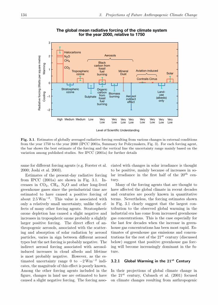
134 3. Projections of Future Anthropogenic Climate Change
;�<> ����)& ����)& ? @ ����? @
����? @
����? @
����? @
����? @
����? @
����? @
����? @
!�� � A�
������A$)�(
%� ' �'>���� E ��
FA��G���� ��I� &
I ���AI)�A
�)����<
;�A ���� ��#"�;
�"
�(��( �'>���� E �� F� &���
�)����<�)A'>�(�
"�<�������� �I� &I ���AI)�A
�)����<
� A��
?����)��
��A��� � �A�
!J��(� �����)���
� �(���A������)�
K��
��(�J
��I
����
<��*
�((�
�'��
��L
)���
�&�(
���
Q
�
�
T�
T
�
A��<
*��
&��
<
?�J�A� I������(�I���U�����(�����<
�������������� �����������������������������������������������������������������
!�� � A�������(�II��(
Fig. 3.1. Estimates of globally averaged radiative forcing resulting from various changes in external conditionsfrom the year 1750 to the year 2000 (IPCC 2001a, Summary for Policymakers, Fig. 3). For each forcing agent,the bar shows the best estimate of the forcing and the vertical line the uncertainty range mainly based on thevariation among published studies. See IPCC (2001a) for further details
same for different forcing agents (e.g. Forster et al.2000; Joshi et al. 2003).
Estimates of the present-day radiative forcingfrom IPCC (2001a) are shown in Fig. 3.1. In-creases in CO2, CH4, N2O and other long-livedgreenhouse gases since the preindustrial time areestimated to have caused a positive forcing ofabout 2.5Wm−2. This value is associated withonly a relatively small uncertainty, unlike the ef-fects of many other forcing agents. Stratosphericozone depletion has caused a slight negative andincreases in tropospheric ozone probably a slightlylarger positive forcing. The direct effect of an-thropogenic aerosols, associated with the scatter-ing and absorption of solar radiation by aerosolparticles, varies in sign between different aerosoltypes but the net forcing is probably negative. Theindirect aerosol forcing associated with aerosol-induced increases in cloud albedo and lifetimeis most probably negative. However, as the es-timated uncertainty range 0 to −2Wm−2 indi-cates, the magnitude of this effect is poorly known.Among the other forcing agents included in thefigure, changes in land use are estimated to havecaused a slight negative forcing. The forcing asso-
ciated with changes in solar irradiance is thoughtto be positive, mainly because of increases in so-lar irradiance in the first half of the 20th cen-tury.
Many of the forcing agents that are thought tohave affected the global climate in recent decadesand centuries are poorly known in quantitativeterms. Nevertheless, the forcing estimates shownin Fig. 3.1 clearly suggest that the largest con-tribution to the observed global warming in theindustrial era has come from increased greenhousegas concentrations. This is the case especially forthe last few decades when the increase in green-house gas concentrations has been most rapid. Es-timates of greenhouse gas emissions and concen-trations for the rest of the 21st century (discussedbelow) suggest that positive greenhouse gas forc-ing will become increasingly dominant in the fu-ture.
3.2.1 Global Warming in the 21st Century
In their projections of global climate change inthe 21st century, Cubasch et al. (2001) focusedon climate changes resulting from anthropogenic

3.2. Global Anthropogenic Climate Change 135
changes in the atmospheric composition. Theyestimated that changes in greenhouse gas andaerosol concentrations would raise the global meantemperature1 by 1.4–5.8 C between the years 1990and 2100. The lower limit of this uncertainty inter-val is approximately twice the global mean warm-ing observed in the 20th century. The upper limitis similar to the difference between present-dayand ice-age conditions (e.g. Weaver et al. 1998).The wide uncertainty interval takes into accounttwo sources of uncertainty: that due to the futureemissions of greenhouse gases and aerosol precur-sors, and that associated with the response of theglobal mean temperature to a given change in theatmospheric composition. These two factors arediscussed in more detail below. It is importantto note that there are additional sources of un-certainty that may not be adequately accountedfor by this range of projected changes, such as theconversion of emissions to atmospheric concentra-tions of GHGs and aerosols. Such issues are alsofurther discussed below.
Projections of future anthropogenic climatechange require estimates of future greenhouse gasand aerosol concentrations. Such estimates aredependent on information about future emissions.Because the emissions depend on factors such aspopulation growth, economic growth, structure ofeconomy, methods for producing energy and so on,precise prediction of them is impossible. Instead,several emissions scenarios are used. Such sce-narios are based on alternative but plausible andinternally consistent sets of assumptions aboutthe demographic, socioeconomic and technologi-cal changes that together determine the evolutionof emissions in the future.
A comprehensive set of emissions scenarios, theso-called SRES (Special Report on Emissions Sce-narios) scenarios were developed and described byNakićenović et al. (2000). The SRES scenarioswere built around four narrative storylines thatdescribe the evolution of the world in the 21st
century. Altogether, 40 different emissions sce-narios were constructed, 35 of which were detailedenough to be used in anthropogenic climate changeprojections. Six of these (A1B, A1T, A1FI, A2, B1and B2) were chosen by the IPCC as illustrativemarker scenarios. The main underlying assump-tions behind these scenarios are described in An-nex 6.
1The temperature discussed here and in the followingrefers to the two-meter level air temperature, if not other-wise stated.
The various SRES emissions scenarios remainrelatively similar during the early parts of the 21st
century. In particular, they all indicate an increasein global CO2 emissions in the next few decades(Fig. 3.2a), as a result of increasing energy con-sumption required by increasing population andworld economy. Towards the late 21st century, thescenarios tend to diverge. Some of them (e.g. A1FIand A2) project a strong increase in CO2 emissionsthroughout the century, leading by the year 2100to emissions several times larger than today. Insome other scenarios (e.g. A1T and B1), however,the CO2 emissions peak by the mid-21st centuryand fall below the present level by the year 2100.These differences are reflected in the CO2 concen-trations derived from the emissions (Fig. 3.2b). Inthe year 2100, the B1 emission scenario is calcu-lated to lead to a CO2 level of about 550 parts permillion (ppm), as compared to a present-day levelof about 375 ppm. The corresponding value for thehighest scenario (A1FI) is about 970 ppm. How-ever, even for the B1 scenario with the largest de-crease in CO2 emissions after 2050, the CO2 con-centration still continues to rise slowly in the endof the 21st century.
The SRES scenarios also describe the emis-sions of several other greenhouse gases, includingmethane (CH4) and nitrous oxide (N2O). The re-sulting concentrations are quite variable across thescenarios, particularly for CH4 which has a rela-tively short lifetime and therefore responds rapidlyto changes in emissions. The A2 scenario is cal-culated to lead to a CH4 concentration of about3700 parts per billion (ppb) in the year 2100 (ascompared to 1760 ppb in the year 2000), while thecorresponding value for the B1 scenario is below1600 ppb. For N2O, all the SRES scenarios in-dicate an increase in the atmospheric concentra-tion, although the rate of the increase dependson the projected emissions that vary substantiallyamong the scenarios. Many of the scenarios alsoindicate an increase in average tropospheric ozone(O3) concentration, as a result of increases in pol-lutants that participate in the formation of O3.Most of the SRES scenarios suggest that the neteffect from changes in non-CO2 greenhouse gaseswill strengthen the global warming during thiscentury; this effect is likely to be smaller than thatof increasing CO2, but it is not negligible.
Anthropogenic increases in atmospheric aerosolconcentrations, which are thought to have sup-pressed the greenhouse-induced warming duringthe 20th century (Mitchell et al. 2001), will not
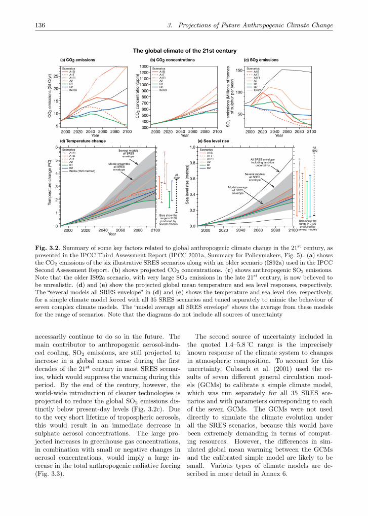
136 3. Projections of Future Anthropogenic Climate Change
������� �
�
�
��
��
���� �� �� ��� ��� ���
W���
!�F!�%!� +!F�F+���
�"
��&
����
���
�X(�
�Z�
��
���������������
������� ��Q��
���
����
����
���
���
���
���
���
��
Q����� �� �� ��� ��� ���
!�F!�%!� +!F�F+���
�"
��
����
(��(
� ��
''
&�
���������������������
������� ����
���
��
��� �� �� ��� ��� ���
!�F!�%!� +!F�F+���
�"
��&
����
���
���AA
� ��
� I�(
���
� I
��)A
'>)
��'
����
����
����������������
W���
W���
W���
������� ��
�
Q
�
���� �� �� ��� ��� ���
!� +!�F!�%!F�F+�����%!K�&�(> ��
%�&
'��
�()�
���>
��<�
�� �
�
� ���� ���!��������
��J���A�& ��A��AA��K\���J�A '�
� ��A�����&�A��AA��K\���J�A '�
F�����> @�(>����<��������'� �)������
��J���A�& ��A�
!AA+��
������� ����
���
���
��
��
������ �� �� ��� ��� ���
!�F!�%!� �!F�F
���
�A�J�
A����
���&
�(��
��
�����������������
��J���A�& ��A��AA��K\���J�A '�
� ��A��J���<��AA��K\���J�A '�
F�����> @�(>����<��������'� �)������
��J���A�& ��A�
!AA+��
!AA��K\����J�A '����A)���<�A�������
)����(���(�
��������������������������������!��
Fig. 3.2. Summary of some key factors related to global anthropogenic climate change in the 21st century, aspresented in the IPCC Third Assessment Report (IPCC 2001a, Summary for Policymakers, Fig. 5). (a) showsthe CO2 emissions of the six illustrative SRES scenarios along with an older scenario (IS92a) used in the IPCCSecond Assessment Report. (b) shows projected CO2 concentrations. (c) shows anthropogenic SO2 emissions.Note that the older IS92a scenario, with very large SO2 emissions in the late 21st century, is now believed tobe unrealistic. (d) and (e) show the projected global mean temperature and sea level responses, respectively.The “several models all SRES envelope” in (d) and (e) shows the temperature and sea level rise, respectively,for a simple climate model forced with all 35 SRES scenarios and tuned separately to mimic the behaviour ofseven complex climate models. The “model average all SRES envelope” shows the average from these modelsfor the range of scenarios. Note that the diagrams do not include all sources of uncertainty
necessarily continue to do so in the future. Themain contributor to anthropogenic aerosol-indu-ced cooling, SO2 emissions, are still projected toincrease in a global mean sense during the firstdecades of the 21st century in most SRES scenar-ios, which would suppress the warming during thisperiod. By the end of the century, however, theworld-wide introduction of cleaner technologies isprojected to reduce the global SO2 emissions dis-tinctly below present-day levels (Fig. 3.2c). Dueto the very short lifetime of tropospheric aerosols,this would result in an immediate decrease insulphate aerosol concentrations. The large pro-jected increases in greenhouse gas concentrations,in combination with small or negative changes inaerosol concentrations, would imply a large in-crease in the total anthropogenic radiative forcing(Fig. 3.3).
The second source of uncertainty included inthe quoted 1.4–5.8 C range is the impreciselyknown response of the climate system to changesin atmospheric composition. To account for thisuncertainty, Cubasch et al. (2001) used the re-sults of seven different general circulation mod-els (GCMs) to calibrate a simple climate model,which was run separately for all 35 SRES sce-narios and with parameters corresponding to eachof the seven GCMs. The GCMs were not useddirectly to simulate the climate evolution underall the SRES scenarios, because this would havebeen extremely demanding in terms of comput-ing resources. However, the differences in sim-ulated global mean warming between the GCMsand the calibrated simple model are likely to besmall. Various types of climate models are de-scribed in more detail in Annex 6.

3.2. Global Anthropogenic Climate Change 137
������� ���
��
��< �
�*&
��
W�������
��
�
�
�
�
�
Q
�
�
!� +!�F!�%!F�F+���+���+���
� ��A�����&�A��AA��K\���J�A '�
Fig. 3.3. Best-estimate historical anthropogenic radiative forcing up to the year 2000 followed by radiativeforcing for the six illustrative SRES scenarios. The shading shows the envelope of the forcing that encompassesthe full set of 35 SRES scenarios. Forcing estimates for three earlier scenarios (IS92a, IS92c and IS92e) arealso shown (IPCC 2001a, Technical Summary, Fig. 19)
The computed evolution of the global meantemperature, presented as differences from 1990,is shown in Fig. 3.2d. The differences among theSRES scenarios remain relatively modest duringthe first decades of the century but grow rapidlythereafter, when the different emission and con-centration projections diverge. Averaging the re-sults of the seven models, the estimate of warmingfrom the year 1990 to the year 2100 is 2.0 C for thelowest and 4.6 C for the highest SRES scenario. Adirect comparison of these numbers with the fullrange of 1.4–5.8 C would suggest that differencesbetween emission scenarios are a larger source ofuncertainty in century-scale global warming thandifferences among climate models. However, be-cause the set of seven models used for generat-ing these temperature projections did not includethe least and most sensitive of all climate models,Cubasch et al. (2001) concluded that the uncer-tainties related to emission scenarios and climatemodels are of comparable importance.
The 1.4–5.8 C range should not be interpretedas giving the absolutely lowest and highest possi-ble global mean temperature changes by the year2100. In fact, several sources of uncertainty areexcluded or included only partially. One factorthat is excluded is the uncertainty related to de-riving the concentrations of CO2 and other green-house gases from emissions. Due to uncertainties
in modelling the carbon cycle and particularly itsresponse to anthropogenic climate changes, the ac-tual CO2 concentration resulting from the highA1FI emissions scenario in the year 2100 might beas low as 820 ppm or as high as 1250 ppm, as com-pared to the estimate used of 970 ppm (Prentice etal. 2001). The full uncertainty in estimating theradiative effects of atmospheric aerosols is also ex-cluded, although the relative importance of thisuncertainty will decrease when the greenhouse-gas-induced warming becomes increasingly domi-nant over the aerosol-induced cooling (Wigley andRaper 2001). Moreover, as noted above, the rangedoes not necessarily capture the total uncertaintyassociated with climate models. Similarly, al-though a wide range of different emission scenariosare used, it is not inconceivable that the real emis-sions would fall outside this range. For example,because the SRES scenarios exclude new policymeasures to control greenhouse gas emissions, suc-cess in international climate policy could in prin-ciple allow the emissions to fall below the SRESinterval, or become less for some certain world de-velopment alternative.
The 1.4–5.8 C range also excludes natural cli-mate variability which could either amplify orcounteract the anthropogenic warming. Modelsimulations (e.g. Bertrand et al. 2002) and re-cent estimates of past climate variability (Moberg

138 3. Projections of Future Anthropogenic Climate Change
et al. 2005) suggest that the natural variations ofglobal mean temperature may amount to a fewtenths of C per century. This is not negligible,but considering the wide uncertainty interval inanthropogenic warming it only represents a rela-tively small additional uncertainty. On the otherhand, natural climate variability increases towardssmaller spatial scales. It may therefore have a sub-stantial effect on regional climate changes, partic-ularly in the near future when the anthropogenicforcing is still relatively weak (e.g. Hulme et al.1999).
Despite the excluded uncertainties, tempera-ture changes that fall somewhere in the middle ofthe 1.4–5.8 C range seem to be more likely thanchanges that fall at the extremes or outside ofthis range. Wigley and Raper (2001) estimatedprobability distributions of future global warmingby assuming equal likelihood for all 35 SRES sce-narios and a log-normal probability distributionfor climate sensitivity approximately representingthe models used by Cubasch et al. (2001). UnlikeCubasch et al. (2001), they also allowed for un-certainty in the carbon cycle and aerosol forcing,but they found these additional sources of uncer-tainty to be of only secondary importance. Theyestimated the 5–95% uncertainty range of globalwarming from 1990–2100 as 1.7–4.9 C, with a me-dian of 3.1 C. The corresponding 5–95% range forthe warming in 1990–2070 was 1.3–3.3 C and thatfor 1990–2030 0.5–1.2 C. However, their analysismakes several simplifying assumptions, so that theactual uncertainty ranges may be wider.
3.2.2 Geographical Distribution of Anthropo-genic Climate Changes
Global warming is expected to vary both geo-graphically and seasonally (Cubasch et al. 2001).Continents are generally expected to warm morerapidly than the oceans, so that nearly all landareas are likely to warm faster than the globalaverage (Fig. 3.4a). Particularly strong warm-ing is projected for Northern Hemisphere high-latitude areas in winter, not only over land buteven more over the Arctic Ocean, where the warm-ing is greatly amplified by reduced sea ice. Mostother ocean areas are likely to warm less rapidlythan the global average. The simulated warmingtends to be particularly modest over the South-ern Ocean and in the northern North Atlantic.In these areas, the ocean is well-mixed to greatdepths, and surface warming is therefore retarded
by the slow warming of the deep ocean. In addi-tion, most models simulate a decrease in the NorthAtlantic thermohaline circulation. This also actsto reduce the warming in the northern North At-lantic and actually leads in some models to localcooling in this area. Although the large-scale pat-terns of temperature change are reasonably sim-ilar between various models (e.g. Harvey 2004),there are substantial variations at smaller horizon-tal scales. These variations are caused mostly bydifferences in the models themselves, but also byunforced variability (“noise”) superimposed on theforced anthropogenic climate change signal (e.g.Räisänen 2001a). The variation between differentGCM simulations within the Baltic Sea Basin isaddressed in more detail in Sect. 3.3.
There will likely be a slight increase in theglobally averaged precipitation during this cen-tury. Most models suggest a 1–2% increase inglobal precipitation for each 1 C increase in globalmean temperature (Cubasch et al. 2001; Räisä-nen 2001a). However, more so than with temper-ature, precipitation changes will vary geographi-cally (Cubasch et al. 2001; Räisänen 2001a; Har-vey 2004; see also Fig. 3.4b). High-latitude ar-eas are expected to experience a general increasein precipitation, particularly in winter, when in-creases are also likely in many mid-latitude areas.Increases are also expected in most tropical re-gions, although there is less consistency in pre-cipitation change between different models at lowlatitudes than at high latitudes (Cubasch et al.2001; Giorgio et al. 2001; Räisänen 2001a). Bycontrast, most subtropical regions and many re-gions in the lower midlatitudes are likely to suffer adecrease in mean precipitation. Simulated precip-itation changes have a lower signal-to-noise ratiothan temperature changes. Precipitation changeswill therefore be more difficult to discern from nat-ural variability than temperature changes, at leastduring the early stages of anthropogenic climatechange. Partly for the same reason, precipita-tion changes are generally less consistent amongthe models than temperature changes, althoughthe agreement tends to be better at high latitudesthan at low latitudes (Räisänen 2001a).
The patterns of anthropogenic climate changeshown in Fig. 3.4b were generated by averagingthe results of 20 climate models. These are givenin a normalized form as the ratio of the local tem-perature or precipitation change to the change inthe global mean temperature. This way of pre-sentation is justified by the model-based evidence
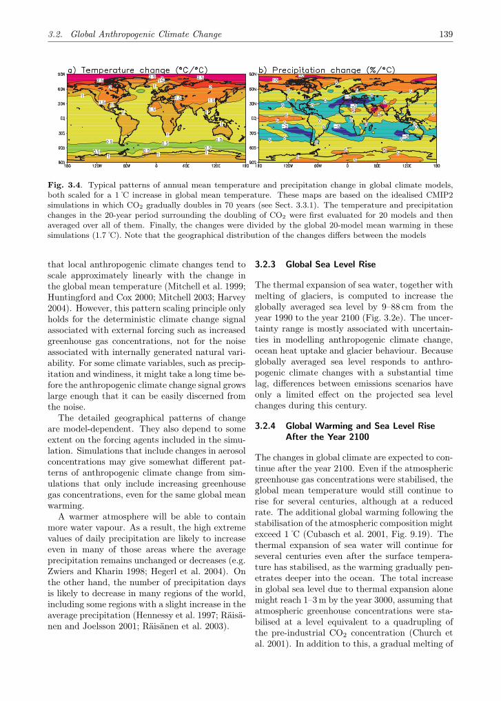
3.2. Global Anthropogenic Climate Change 139
Fig. 3.4. Typical patterns of annual mean temperature and precipitation change in global climate models,both scaled for a 1 C increase in global mean temperature. These maps are based on the idealised CMIP2simulations in which CO2 gradually doubles in 70 years (see Sect. 3.3.1). The temperature and precipitationchanges in the 20-year period surrounding the doubling of CO2 were first evaluated for 20 models and thenaveraged over all of them. Finally, the changes were divided by the global 20-model mean warming in thesesimulations (1.7 C). Note that the geographical distribution of the changes differs between the models
that local anthropogenic climate changes tend toscale approximately linearly with the change inthe global mean temperature (Mitchell et al. 1999;Huntingford and Cox 2000; Mitchell 2003; Harvey2004). However, this pattern scaling principle onlyholds for the deterministic climate change signalassociated with external forcing such as increasedgreenhouse gas concentrations, not for the noiseassociated with internally generated natural vari-ability. For some climate variables, such as precip-itation and windiness, it might take a long time be-fore the anthropogenic climate change signal growslarge enough that it can be easily discerned fromthe noise.
The detailed geographical patterns of changeare model-dependent. They also depend to someextent on the forcing agents included in the simu-lation. Simulations that include changes in aerosolconcentrations may give somewhat different pat-terns of anthropogenic climate change from sim-ulations that only include increasing greenhousegas concentrations, even for the same global meanwarming.
A warmer atmosphere will be able to containmore water vapour. As a result, the high extremevalues of daily precipitation are likely to increaseeven in many of those areas where the averageprecipitation remains unchanged or decreases (e.g.Zwiers and Kharin 1998; Hegerl et al. 2004). Onthe other hand, the number of precipitation daysis likely to decrease in many regions of the world,including some regions with a slight increase in theaverage precipitation (Hennessy et al. 1997; Räisä-nen and Joelsson 2001; Räisänen et al. 2003).
3.2.3 Global Sea Level Rise
The thermal expansion of sea water, together withmelting of glaciers, is computed to increase theglobally averaged sea level by 9–88 cm from theyear 1990 to the year 2100 (Fig. 3.2e). The uncer-tainty range is mostly associated with uncertain-ties in modelling anthropogenic climate change,ocean heat uptake and glacier behaviour. Becauseglobally averaged sea level responds to anthro-pogenic climate changes with a substantial timelag, differences between emissions scenarios haveonly a limited effect on the projected sea levelchanges during this century.
3.2.4 Global Warming and Sea Level RiseAfter the Year 2100
The changes in global climate are expected to con-tinue after the year 2100. Even if the atmosphericgreenhouse gas concentrations were stabilised, theglobal mean temperature would still continue torise for several centuries, although at a reducedrate. The additional global warming following thestabilisation of the atmospheric composition mightexceed 1 C (Cubasch et al. 2001, Fig. 9.19). Thethermal expansion of sea water will continue forseveral centuries even after the surface tempera-ture has stabilised, as the warming gradually pen-etrates deeper into the ocean. The total increasein global sea level due to thermal expansion alonemight reach 1–3m by the year 3000, assuming thatatmospheric greenhouse concentrations were sta-bilised at a level equivalent to a quadrupling ofthe pre-industrial CO2 concentration (Church etal. 2001). In addition to this, a gradual melting of
140 3. Projections of Future Anthropogenic Climate Change
the Greenland ice sheet appears likely if the localwarming in Greenland exceeds 3 C (Huybrechtsand De Wolde 1999). This would increase theglobal sea level by about 7m. For a mid-rangescenario with a warming of 5.5 C in Greenland,about 3m of this increase would be realized by theyear 3000 (Church et al. 2001, Fig. 11.16). A de-crease in the mass of the West Antarctic Ice Sheetcould also potentially increase the global sea level,by up to 6m for a complete melting of the icesheet. Whether changes in this ice sheet are likelyto make a significant contribution to global sealevel rise during the next millennium is, however,still debated (Church et al. 2001).
3.3 Anthropogenic Climate Change in theBaltic Sea Basin: Projections fromGlobal Climate Models
Global climate models, also known as general cir-culation models (the acronyme GCM is used inboth meanings and the two terms are used in-terchangeably in this text) are used for numeri-cal simulations of the global climate. These mod-els aim to represent all the physical processes ofthe atmosphere, land surface and oceans whichare thought to be important for determining theevolution of climate on time scales extending upto several centuries. Modelling over climatologicaltime scales on a global basis is computationally de-manding, and this constrains the resolution thatcan be used in the models. The horizontal reso-lution of GCMs tends to be some 300 km in theatmosphere and often about 150 km in the oceans.This is sufficient for the models to reproduce themajor atmospheric and oceanic circulation pat-terns and trends for climatological variables overcontinental scales.
3.3.1 Global Climate Model Experiments
This section addresses projections of 21st centuryanthropogenic climate change in the Baltic SeaBasin using simulations made with global atmos-phere–ocean general circulation models (GCMs).The focus is on changes in time mean tempera-ture and precipitation. However, to help the in-terpretation of the temperature and precipitationchanges, changes in the atmospheric circulationand in the North Atlantic thermohaline circula-tion are also discussed briefly.
Before proceeding to specific aspects for theBaltic Sea Basin, some general issues related to
anthropogenic climate change simulations are dis-cussed. Three main questions are addressed inthis introductory subsection: (i) what kind of an-thropogenic climate change experiments have beenmade with GCMs, (ii) which sets of model exper-iments are used in this assessment, and (iii) howanthropogenic climate changes are estimated fromthe simulations.
Anthropogenic climate change experiments canbe broadly divided into two classes: scenario ex-periments and sensitivity experiments. Scenarioexperiments are conducted to provide plausibleprojections of future climate. A prerequisite forthis is that the external forcing used in the sim-ulations – changes in the concentrations of differ-ent atmospheric greenhouse gases and aerosols – isconsistent with a plausible and internally consis-tent emissions scenario, such as one of the SRESscenarios. By contrast, sensitivity experiments aremainly motivated by the need to study model be-haviour. The forcing in these experiments is usu-ally simple, such as an increase in atmosphericCO2 with no other changes.
In this section, results from both sensitivity ex-periments and scenario experiments on anthro-pogenic climate changes in the Baltic Sea Basinare discussed. In addition to results extractedfrom published literature, some updates of ear-lier calculations are presented. These updates arebased on two sets of model simulations: the so-called CMIP2 experiments (Meehl et al. 2000),and experiments based on the SRES forcing sce-narios available from the IPCC Data DistributionCentre (http://ipcc-ddc.cru.uea.ac.uk/).
CMIP2, the second phase of the Coupled ModelIntercomparison Project, is an intercomparison ofstandard idealised anthropogenic climate changeexperiments made with many climate models. Forthis assessment, CMIP2 results for 20 models wereavailable. Each model has been used to maketwo 80-year simulations: a control simulation withconstant (approximately present-day) CO2 con-centration and an increased greenhouse gas sim-ulation with gradually (1% per year compound)increasing CO2.
The increase in CO2 concentration in theCMIP2 greenhouse runs, with a doubling over 70years, is faster than that projected to occur underany of the SRES scenarios. On the other hand,the concentrations of other greenhouse gases suchas CH4 and N2O are kept constant in CMIP2, al-though increases in these gases are actually likelyto amplify the global warming in the real world.
3.3. Anthropogenic Climate Change in the Baltic Sea Basin 141
As a result, the rate of global warming in theCMIP2 greenhouse runs compares well with sim-ulations based on mid-range SRES forcing scenar-ios. The same conclusion holds for the main geo-graphic patterns of anthropogenic climate change.This is both because the increase in CO2 is pro-jected to be the main cause of anthropogenic cli-mate change during this century and because thegeographic patterns of simulated anthropogenicclimate change tend to be reasonably insensitive tothe exact nature of the forcing (Boer and Yu 2003;Harvey 2004). Anthropogenic climate changes inthe CMIP2 simulations are reported in Sect. 3.3.3.
The main limitation of the CMIP2 data set inthe context of projecting anthropogenic climatechanges is the fact that the experiments are basedon a single forcing scenario and lack aerosol ef-fects. As a result, this set of simulations will tendto underestimate the uncertainty of anthropogenicclimate changes in the real world.
An analysis of the temperature and precipita-tion changes in the Baltic Sea Basin in the SRESsimulations is given in Sect. 3.3.4. This analysisis based on a smaller number of models than areavailable in CMIP2, but it allows us to explore howthe simulated anthropogenic climate changes de-pend on the assumed evolution of greenhouse gasand aerosol emissions. Readers interested in quan-titative, internally consistent projections of an-thropogenic climate change in the Baltic Sea Basinshould primarily use the SRES-based informationin Sect. 3.3.4, rather than the CMIP2-based re-sults in Sect. 3.3.3. In addition, the SRES-basedGCM simulations are more directly comparablewith the regional climate model results reportedin Sect. 3.5 than the CMIP2 simulations.
The models used in this section are listed inTable 3.1. CMIP2 simulations are available for20 models and SRES simulations for seven mod-els. One of the SRES models (CCSR/NIES2) is,however, excluded for most of the analysis as ex-plained below. Most of the models in the SRESdata set also participated in CMIP2. However,the SRES data set includes a more recent ver-sion of the Canadian Centre for Climate Mod-elling and Analysis model (CGCM2) than CMIP2(CGCM1).
Model-based estimates of anthropogenic cli-mate change are usually computed from the dif-ference in climate between two simulated periods,a scenario period and a control period. In tran-sient scenario simulations, which typically spanthe whole time range from some time in the 19th
or 20th century to the late 21st century, the con-trol period is often chosen as 1961–1990, corre-sponding to the presently used WMO normal pe-riod. One or more scenario periods are chosenfrom later times in the same continuous simula-tion, as demonstrated in Fig. 3.5. In sensitiv-ity experiments, a separate control run with noanthropogenic forcing is often made to estimatethe control period climate, as already mentionedfor the CMIP2 simulations. In neither case areanthropogenic climate changes estimated by com-paring simulated future climate directly with ob-served present-day climate, due to systematic er-rors in the models. Differences between simulatedand observed present-day climate are often com-parable to, or in some cases even larger than, dif-ferences between simulated future and present-dayclimates. However, if model errors are assumed tohave similar effects on the simulated present-dayand future climates, their net effect approximatelyvanishes when taking the difference.
The performance of models in simulating pre-sent-day climate provides one means for estimat-ing their reliability. Prior to presenting model-based projections of future anthropogenic cli-mate change, the simulation of present-day cli-mate in the Baltic Sea Basin is therefore discussed(Sect. 3.3.2). It is difficult to compress the evalu-ation of model-simulated climate into a single fig-ure of merit, and it is even more difficult to con-vert this information to a quantitative estimate ofmodel credibility in simulating anthropogenic cli-mate changes. This is partly because the mod-els are complex, but also because good perfor-mance in simulating the present climate in somearea might hide compensating errors between dif-ferent parts of the model. In fact, models thatsimulate the present climate with similar skill maysimulate widely different changes in climate whenforced with increased greenhouse gas concentra-tions (e.g. Murphy et al. 2004; Stainforth et al.2005). Thus, when anthropogenic climate changesimulations are available for several models, a com-parison between the simulated changes probablygives a more direct measure of uncertainty thanan evaluation of the control climates. However, itis important to remember the caveat that anthro-pogenic climate changes in the real world may inprinciple fall outside the range of model results.
In what follows, the ability of global climatemodels to simulate the present climate in theBaltic Sea area (Sect. 3.3.2) is first addressed. Af-ter this, model-simulated anthropogenic climate

142 3. Projections of Future Anthropogenic Climate Change
Fig. 3.5. Estimation of anthropogenic climate changes from a model-simulated time series (in this case, thesummer mean temperature in northern Europe in the HadCM3 simulation forced by the SRES-A2 scenario).The first horizontal line shows the mean of the time series for years 1961–1990, and the remaining three lines themeans for periods 2010–2039, 2040–2069 and 2070–2099. Temperature changes for the latter 30-year periodsare calculated by subtracting the mean for 1961–1990 from the mean in the corresponding period
changes in the region are addressed (Sects. 3.3.3–3.3.4). The aims in Sect. 3.3.3 are more qualita-tive than quantitative. The purpose is to give anoverview of the typical features of anthropogenicclimate change in the Baltic Sea Basin in green-house gas experiments and of the intermodel dif-ferences, but the results are not intended to beinterpreted as quantitative anthropogenic climatechange projections for the real world. Exam-ples of such quantitative projections are given inSect. 3.3.4 for different SRES emission scenarios.
3.3.2 Simulation of Present-day Climate fromGlobal Climate Models
Although the global geographic distributions ofpresent-day temperature and precipitation clima-tes are generally well simulated by GCMs, biaseson the regional scale may be substantial (McAva-ney et al. 2001; Giorgi et al. 2001). Model per-formance in simulating the climate in northernEurope has been the subject of several studies,including multi-model intercomparisons by Räisä-nen (1994, 2000) and Jylhä et al. (2004). In thissubsection, these earlier studies are complementedand updated by presenting some results specifi-cally tailored for the Baltic Sea Basin. Area means
of simulated temperature and precipitation werethen calculated over the land area in the BalticSea Basin, indicated by shading in Fig. 3.9. Themodel results were compared with observationalestimates derived from the University of East An-glia Climate Research Unit (CRU) climatology(New et al. 1999) representing the period 1961–1990.
Figure 3.6 compares the seasonal cycles of tem-perature and precipitation, as averaged over theland area in the Baltic Sea Basin, between theCMIP2 control simulations and the CRU analy-sis. The variation between the models is large. Ina few extreme cases, simulated monthly temper-atures differ by about 8–10 C from the observa-tional estimate. The largest cold and warm bi-ases tend to occur in the winter half-year, fromNovember to April, but in one model there is alsoa very large warm bias in summer. However, be-cause the simulated temperatures are distributedon both sides of the observed values, the 20-modelmean temperatures are mostly close to those ob-served. A slight average cold bias is present inmost months of the year, but this bias is gener-ally small compared with the differences amongthe models. The only exception is spring, whenthe cold bias is about 2 C.

3.3. Anthropogenic Climate Change in the Baltic Sea Basin 143
Table
3.1
.M
odel
suse
din
Sec
t.3.3
.T
he
colu
mns
label
edas
CM
IP2
and
SR
ES
indic
ate
the
model
runs
incl
uded
inth
eanaly
sis
of
the
CM
IP2
and
the
SR
ES
sim
ula
tions
inSec
ts.3.3
.2–3.3
.4.
The
atm
osp
her
icre
solu
tion
incl
udes
both
the
hori
zonta
land
the
ver
tica
lre
solu
tion.
The
form
eris
expre
ssed
eith
eras
deg
rees
lati
tude×
deg
rees
longit
ude
or
as
asp
ectr
altr
unca
tion
and
the
appro
xim
ate
equiv
ale
nt
gri
dsi
ze(i
npare
nth
eses
).In
the
IPSL-C
M2
model
,th
em
erid
ionalgri
dhas
50
poin
tsev
enly
dis
trib
ute
din
the
sine
ofla
titu
de
and
the
act
ualre
solu
tion
isth
eref
ore
coars
erth
an
3.6
◦in
hig
hla
titu
des
.T
he
ver
tica
lre
solu
tion
isgiv
enas
“Lm
m”,w
her
em
mis
the
num
ber
ofle
vel
s.T
he
last
colu
mn
indic
ate
sw
het
her
flux
adju
stm
ents
are
use
dfo
rth
ehea
t(H
),fr
eshw
ate
r(W
)and
mom
entu
m(M
)fluxes
,re
spec
tivel
y
MO
DEL
NA
ME
CO
UN
TRY
OF
OR
IGIN
REFER
EN
CE
CM
IP2
SR
ES
AT
MO
SP
HER
ICR
ESO
LU
TIO
NFLU
XA
DJ.
AR
PE
GE
/O
PA
2Fra
nce
Bart
hel
etet
al.
(1998)
XT
31
(3.9
◦×
3.9
◦ )L19
–
BM
RC
bA
ust
ralia
Pow
eret
al.
(1993)
XR
21
(3.2
◦×
5.6
◦ )L17
HW
CC
SR
/N
IES1
Japan
Em
ori
etal.
(1999)
XT
21
(5.6
◦×
5.6
◦ )L20
HW
CC
SR
/N
IES2
Japan
Noza
wa
etal.
(2000)
X(A
1FI,
A2
,B
1,B
2)
T21
(5.6
◦×
5.6
◦ )L20
HW
CG
CM
1C
anada
Fla
toet
al.
(2000)
XT
32
(3.8
◦×
3.8
◦ )L10
HW
CG
CM
2C
anada
Fla
toand
Boer
(2001)
A2,B
2T
32
(3.8
◦×
3.8
◦ )L10
HW
CSIR
OM
k2
Aust
ralia
Hir
stet
al.
(2000)
XA
2,B
1,B
2R
21
(3.2
◦×
5.6
◦ )L9
HW
M
CSM
1.0
USA
Bov
ille
and
Gen
t(1
998)
XT
42
(2.8
◦×
2.8
◦ )L18
–
EC
HA
M3/LSG
Ger
many
Voss
etal.
(1998)
XT
21
(5.6
◦×
5.6
◦ )L19
HW
M
EC
HA
M4/O
PY
C3
Ger
many
Roec
kner
etal.
(1999)
XA
2,B
2T
42
(2.8
◦×
2.8
◦ )L19
HW
GFD
LR
15
aU
SA
Manabe
etal.
(1991)
XR
15
(4.5
◦×
7.5
◦ )L9
HW
GFD
LR
30
aU
SA
Knuts
on
etal.
(1999)
XA
2,B
2R
30
(2.2
5◦×
3.7
5◦ )
L14
HW
GIS
S2
USA
Russ
elland
Rin
d(1
999)
X4.0
◦×
5.0
◦L9
–
GO
ALS
Chin
aZhang
etal.
(2000)
XR
15
(4.5
◦×
7.5
◦ )L9
HW
M
HadC
M2
UK
Johns
etal.
(1997)
X2.5
◦×
3.7
5◦
L19
HW
HadC
M3
UK
Gord
on
etal.
(2000)
XA
1FI,
A2,B
1,B
22.5
◦×
3.8
◦L19
–
INM
Russ
iaD
iansk
yand
Volo
din
(2002)
X4.0
◦×
5.0
◦L21
–
IPSL-C
M2
Fra
nce
Bra
connot
etal.
(1997)
X3.6
◦ s×
5.6
◦L15
–
MR
I1Japan
Tokio
kaet
al.
(1995)
X4.0
◦×
5.0
◦L15
HW
MR
I2Japan
Yukim
oto
etal.
(2000)
XT
42
(2.8
◦×
2.8
◦ )L30
HW
M
PC
MU
SA
Wash
ingto
net
al.
(2000)
XA
2,B
2T
42
(2.8
◦×
2.8
◦ )L18
–

144 3. Projections of Future Anthropogenic Climate Change
Fig. 3.6. Average seasonal cycles of (a) temperature and (b) precipitation over the total land area of theBaltic Sea Basin. The thin solid lines represent the control run climates of the 20 individual CMIP2 modelsand the thick solid line the 20-model mean. The dashed lines give observational estimates derived directlyfrom the CRU climatology (New et al. 1999). For precipitation, a corrected observational estimate is also given(dotted, see text for details)
A more detailed look at different parts of theBaltic Sea Basin reveals that temperature biasesvary across the region. In winter, in particular,there is a marked contrast between the easternparts (Finland and western Russia) and the north-western parts (particularly central and northernSweden) of the basin. In the former area, averagesimulated winter temperatures are 1–4 C belowthe observed values, in the latter several C abovethem (see Fig. 2 in Räisänen 2000). Räisänen(2000) attributed the warm bias in north-westernScandinavia to the relatively coarse resolution ofthe models, which allows the influence of the At-lantic Ocean to extend further inland in the sim-ulations than in reality. He likewise noted thatthe smoothening and lowering of the Scandina-vian mountains associated with the coarse reso-lution might also contribute to the warm bias inthis area.
The seasonal cycle of precipitation is simulatedless well by the models than that of temperature(Fig. 3.6b). The scatter among the models is largein all seasons, but it is particularly pronounced inlate summer (July–August). A few of the mod-els simulate an annual minimum of precipitationin this time of the year, in contrast to the maxi-mum shown by observations, but there are also afew models with an over-pronounced summer max-imum in precipitation.
Verification of model-simulated precipitation iscomplicated by the tendency of gauge measure-ments to underestimate the actual precipitation,particularly in winter when much of the precipita-tion falls as snow. The CRU analysis is based inmost regions on uncorrected measurements (Newet al. 1999) and it thus also suffers from thisproblem. Figure 3.6b therefore also shows a cor-rected precipitation estimate, which was obtainedby multiplying the uncorrected CRU values withcoefficients based on the work of Rubel and Hantel(2001), as detailed in Jones and Ullerstig (2002)and Räisänen et al. (2003) (see also Sect. 2.1.3).The correction is relatively small in summer butit amounts to about 40% in winter and 19% in theannual mean (Räisänen et al. 2003). The 20-modelmean simulated annual precipitation is 30% abovethe uncorrected observational estimate, but only9% above the corrected estimate. If the correctionis not too small, a large majority of the modelssimulate too much precipitation in winter and inspring (Fig. 3.6b).
The ability of GCMs to simulate small-scale re-gional variations in precipitation is severely lim-ited by the coarse resolution of these models. Thisis particularly evident in the vicinity of high orog-raphy, such as the Scandinavian mountains. Ob-servations show a very steep contrast betweenabundant precipitation on the western slopes of
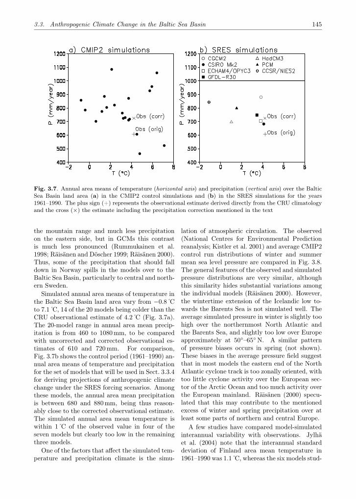
3.3. Anthropogenic Climate Change in the Baltic Sea Basin 145
Fig. 3.7. Annual area means of temperature (horizontal axis) and precipitation (vertical axis) over the BalticSea Basin land area (a) in the CMIP2 control simulations and (b) in the SRES simulations for the years1961–1990. The plus sign (+) represents the observational estimate derived directly from the CRU climatologyand the cross (×) the estimate including the precipitation correction mentioned in the text
the mountain range and much less precipitationon the eastern side, but in GCMs this contrastis much less pronounced (Rummukainen et al.1998; Räisänen and Döscher 1999; Räisänen 2000).Thus, some of the precipitation that should falldown in Norway spills in the models over to theBaltic Sea Basin, particularly to central and north-ern Sweden.
Simulated annual area means of temperature inthe Baltic Sea Basin land area vary from −0.8 Cto 7.1 C, 14 of the 20 models being colder than theCRU observational estimate of 4.2 C (Fig. 3.7a).The 20-model range in annual area mean precip-itation is from 460 to 1080mm, to be comparedwith uncorrected and corrected observational es-timates of 610 and 720mm. For comparison,Fig. 3.7b shows the control period (1961–1990) an-nual area means of temperature and precipitationfor the set of models that will be used in Sect. 3.3.4for deriving projections of anthropogenic climatechange under the SRES forcing scenarios. Amongthese models, the annual area mean precipitationis between 680 and 880mm, being thus reason-ably close to the corrected observational estimate.The simulated annual area mean temperature iswithin 1 C of the observed value in four of theseven models but clearly too low in the remainingthree models.
One of the factors that affect the simulated tem-perature and precipitation climate is the simu-
lation of atmospheric circulation. The observed(National Centres for Environmental Predictionreanalysis; Kistler et al. 2001) and average CMIP2control run distributions of winter and summermean sea level pressure are compared in Fig. 3.8.The general features of the observed and simulatedpressure distributions are very similar, althoughthis similarity hides substantial variations amongthe individual models (Räisänen 2000). However,the wintertime extension of the Icelandic low to-wards the Barents Sea is not simulated well. Theaverage simulated pressure in winter is slightly toohigh over the northernmost North Atlantic andthe Barents Sea, and slightly too low over Europeapproximately at 50◦–65◦ N. A similar patternof pressure biases occurs in spring (not shown).These biases in the average pressure field suggestthat in most models the eastern end of the NorthAtlantic cyclone track is too zonally oriented, withtoo little cyclone activity over the European sec-tor of the Arctic Ocean and too much activity overthe European mainland. Räisänen (2000) specu-lated that this may contribute to the mentionedexcess of winter and spring precipitation over atleast some parts of northern and central Europe.
A few studies have compared model-simulatedinterannual variability with observations. Jylhäet al. (2004) note that the interannual standarddeviation of Finland area mean temperature in1961–1990 was 1.1 C, whereas the six models stud-
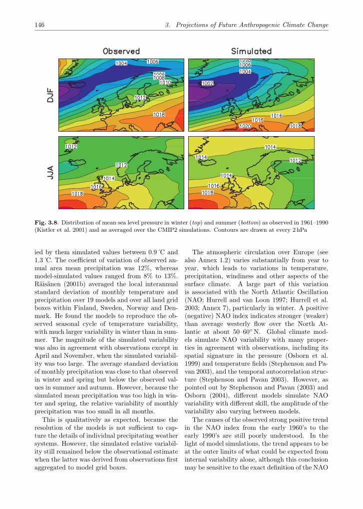
146 3. Projections of Future Anthropogenic Climate Change
Fig. 3.8. Distribution of mean sea level pressure in winter (top) and summer (bottom) as observed in 1961–1990(Kistler et al. 2001) and as averaged over the CMIP2 simulations. Contours are drawn at every 2 hPa
ied by them simulated values between 0.9 C and1.3 C. The coefficient of variation of observed an-nual area mean precipitation was 12%, whereasmodel-simulated values ranged from 8% to 13%.Räisänen (2001b) averaged the local interannualstandard deviation of monthly temperature andprecipitation over 19 models and over all land gridboxes within Finland, Sweden, Norway and Den-mark. He found the models to reproduce the ob-served seasonal cycle of temperature variability,with much larger variability in winter than in sum-mer. The magnitude of the simulated variabilitywas also in agreement with observations except inApril and November, when the simulated variabil-ity was too large. The average standard deviationof monthly precipitation was close to that observedin winter and spring but below the observed val-ues in summer and autumn. However, because thesimulated mean precipitation was too high in win-ter and spring, the relative variability of monthlyprecipitation was too small in all months.
This is qualitatively as expected, because theresolution of the models is not sufficient to cap-ture the details of individual precipitating weathersystems. However, the simulated relative variabil-ity still remained below the observational estimatewhen the latter was derived from observations firstaggregated to model grid boxes.
The atmospheric circulation over Europe (seealso Annex 1.2) varies substantially from year toyear, which leads to variations in temperature,precipitation, windiness and other aspects of thesurface climate. A large part of this variationis associated with the North Atlantic Oscillation(NAO; Hurrell and van Loon 1997; Hurrell et al.2003; Annex 7), particularly in winter. A positive(negative) NAO index indicates stronger (weaker)than average westerly flow over the North At-lantic at about 50–60◦ N. Global climate mod-els simulate NAO variability with many proper-ties in agreement with observations, including itsspatial signature in the pressure (Osborn et al.1999) and temperature fields (Stephenson and Pa-van 2003), and the temporal autocorrelation struc-ture (Stephenson and Pavan 2003). However, aspointed out by Stephenson and Pavan (2003) andOsborn (2004), different models simulate NAOvariability with different skill, the amplitude of thevariability also varying between models.
The causes of the observed strong positive trendin the NAO index from the early 1960’s to theearly 1990’s are still poorly understood. In thelight of model simulations, the trend appears to beat the outer limits of what could be expected frominternal variability alone, although this conclusionmay be sensitive to the exact definition of the NAO

3.3. Anthropogenic Climate Change in the Baltic Sea Basin 147
index and to the magnitude of the simulated inter-nal variability (Osborn 2004; Selten et al. 2004).This suggests that the trend might have been atleast in part externally forced. However, it is notclear whether the trend can be attributed to in-creased greenhouse gas concentrations, since mostmodels simulate only modest changes in NAO inresponse to greenhouse gas forcing (Räisänen andAlexandersson 2003; Osborn 2004). Stratosphericozone depletion might also have affected the trendin the NAO index (Volodin and Galin 1999), butrecent model results do not support the idea thatit would have made a major contribution (Shin-dell et al. 2001; Gillett et al. 2003). Scaife et al.(2005) show that the observed NAO trend is repro-duced well in a climate model simulation with aprescribed increasing trend in stratospheric west-erlies resembling that observed from 1965 to 1995.However, their study does not explain why thestratospheric winds changed. Similarly, althoughstudies by Hurrell et al. (2004), Hoerling et al.(2004) and Selten et al. (2004) suggest that theobserved trend in the NAO index has been partlytriggered by changes in the distribution of sea sur-face temperature in the tropical Indian Ocean, thecause of these changes (internal variability or an-thropogenic forcing) is still unclear.
3.3.3 Projections of Future Climate fromGlobal Climate Models
In this and the following subsection, we assessGCM-simulated anthropogenic climate changes innorthern and central Europe in general and withinthe Baltic Sea Basin in particular. The aim of thissubsection is to give an overview of the tempera-ture and precipitation changes typically simulatedby GCMs when forced by increasing greenhousegas concentrations, of the differences in the modelprojections and of the factors that may affect thesimulated temperature and precipitation changesand the intermodel differences. Most of this sub-section is based on the idealised CMIP2 simula-tions, which are available for a significantly largernumber of models than simulations based on themore detailed SRES forcing scenarios.
3.3.3.1 Temperature and Precipitation
The globally and annually averaged warming atthe time of the doubling of CO2 in the CMIP2 sim-ulations varies from 1.0 to 3.1 C, with a 20-modelmean of 1.7 C. The 20-model mean in north-ern Europe is about 2.5 C, or 50% larger than
the global mean warming, with somewhat greaterwarming in winter than in summer (left columnof Fig. 3.9). The warming in winter typically in-creases from southwest to northeast, from the At-lantic Ocean towards the inner parts of Eurasiaand the Arctic Ocean. The warming in summerhas a slight tendency to increase towards south-east, but the gradient in this season is weakerthan in winter. The changes in spring and autumnare generally between those in winter and summer(e.g. Räisänen 2000). The simulated annual pre-cipitation increases, on the average, by about 10%in northern Europe (middle column of Fig. 3.9). InCentral Europe, including the southernmost partsof the Baltic Sea Basin, the average model resultssuggest an increase in precipitation in winter but adecrease in summer. In northern Europe, precip-itation increases in most models throughout theyear, but less in summer than in the other seasons(Räisänen 2000, 2001b).
All the CMIP2 models simulate an increasein both the annual area mean temperature andthe annual area mean precipitation in the BalticSea Basin land area. However, the magnitude ofthe changes varies substantially among the mod-els (Fig. 3.10a). The range in annual tempera-ture change is from 0.7 C to 6.9 C with a mean of2.6 C, and that in precipitation change from 3%to 22% with a mean of 8%. One of the models(CCSR/NIES2) simulates much larger increasesin both temperature and precipitation than anyof the others. This model also stands out as theone with the largest global mean warming in theCMIP2 data set (3.1 C, to be compared with thesecond largest value of 2.1 C).
Some variation between the anthropogenic cli-mate changes simulated by the various modelswould be expected simply as a result of theinternal variability that accompanies the forcedanthropogenic climate change in the simulations(Cubasch et al. 2001; Räisänen 2000, 2001a).However, the differences in change between themodels are too large to be explained by this fac-tor alone. An estimation of internal variability inthe CMIP2 simulations using the method of Räisä-nen (2001a) suggests that only about 7% of theintermodel variance in Baltic Sea Basin land areaannual mean temperature change is due to inter-nal variability. For annual precipitation change,the corresponding fraction is 17%. This impliesthat most of the differences in precipitation changeand, particularly, temperature change are directlycaused by the differences between the models. The

148 3. Projections of Future Anthropogenic Climate Change
Fig. 3.9. Changes in temperature (left ), precipitation (middle) and sea level pressure (right ) around the timeof the doubling of CO2 (model years 61–80) as averaged over the CMIP2 models. Results are shown for winter(DJF = December–January–February), summer (JJA = June–July–August) and the annual mean (ANN). Thecontour interval is 1 C for changes in temperature, 5% for changes in precipitation and 0.5 hPa for changes insea level pressure. The shading indicates the Baltic Sea Basin land area
same conclusion also generally holds for seasonaltemperature and precipitation changes, althoughthe relative importance of internal variability islarger on the seasonal than on the annual timescale.
The changes in temperature and precipitationtend to be positively correlated (Fig. 3.10a). Thisis the case in winter, spring and autumn, butnot in summer. As argued by Räisänen (2000),the positive correlation in winter and in the tran-sitional seasons is consistent with the Clausius–Clayperon relationship. The larger the increase intemperature, the larger the increase in the capa-bility of air to bring moisture from lower latitudesand the Atlantic Ocean to northern Europe. Thelack of positive correlation in summer is consis-
tent with the smaller relative importance of atmo-spheric moisture transport, as opposed to the localevaporation, in providing the precipitating waterin this season (Numaguti 1999). In addition, feed-backs associated with soil moisture and/or cloudi-ness may play a role. When evaporation becomesrestricted by a drying out of the soil, this tendsto induce both a decrease in precipitation and anincrease in temperature due to increased sensibleheat flux and increased solar radiation allowed byreduced cloudiness (Wetherald and Manabe 1995;Gregory et al. 1997).
The simulated annual mean warming in theBaltic Sea Basin is strongly correlated (r = 0.8, al-though this is reduced to r = 0.6 if CCSR/NIES2is excluded) with the global mean warming as
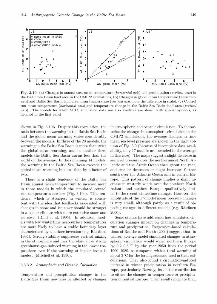
3.3. Anthropogenic Climate Change in the Baltic Sea Basin 149
Fig. 3.10. (a) Changes in annual area mean temperature (horizontal axis) and precipitation (vertical axis) inthe Baltic Sea Basin land area in the CMIP2 simulations, (b) Changes in global mean temperature (horizontalaxis) and Baltic Sea Basin land area mean temperature (vertical axis; note the difference in scale), (c) Controlrun mean temperature (horizontal axis) and temperature change in the Baltic Sea Basin land area (verticalaxis). The models for which SRES simulation data are also available are shown with special symbols, asdetailed in the first panel
shown in Fig. 3.10b. Despite this correlation, theratio between the warming in the Baltic Sea Basinand the global mean warming varies considerablybetween the models. In three of the 20 models, thewarming in the Baltic Sea Basin is more than twicethe global mean warming, and in another threemodels the Baltic Sea Basin warms less than theworld on the average. In the remaining 14 models,the warming in the Baltic Sea Basin exceeds theglobal mean warming but less than by a factor oftwo.
There is a slight tendency of the Baltic SeaBasin annual mean temperature to increase morein those models in which the simulated controlrun temperatures are low (Fig. 3.10c). This ten-dency, which is strongest in winter, is consis-tent with the idea that feedbacks associated withchanges in snow and ice cover should be strongerin a colder climate with more extensive snow andice cover (Rind et al. 1995). In addition, mod-els with low wintertime near-surface temperaturesare more likely to have a stable boundary layercharacterized by a surface inversion (e.g. Räisänen1994). Strong stability suppresses vertical mixingin the atmosphere and may therefore allow stronggreenhouse-gas-induced warming in the lowest tro-posphere even if the warming at higher levels ismodest (Mitchell et al. 1990).
3.3.3.2 Atmospheric and Oceanic Circulation
Temperature and precipitation changes in theBaltic Sea Basin may also be affected by changes
in atmospheric and oceanic circulation. To charac-terise the changes in atmospheric circulation in theCMIP2 simulations, the average changes in timemean sea level pressure are shown in the right col-umn of Fig. 3.9 (because of incomplete data avail-ability, only 17 models are included in the averagein this case). The maps suggest a slight decrease insea level pressure over the northernmost North At-lantic and the Arctic Ocean throughout the year,and smaller decreases or slight increases furthersouth over the Atlantic Ocean and in central Eu-rope. This pattern of change implies a slight in-crease in westerly winds over the northern NorthAtlantic and northern Europe, qualitatively simi-lar to the recent wintertime changes. However, theamplitude of the 17-model mean pressure changesis very small, although partly as a result of op-posing changes in different models (e.g. Räisänen2000).
Some studies have addressed how simulated cir-culation changes impact on changes in tempera-ture and precipitation. Regression-based calcula-tions of Rauthe and Paeth (2004) suggest that, inwinter, average model-simulated changes in atmo-spheric circulation would warm northern Europeby 0.2–0.6 C by the year 2050 from the period1900–1980, as compared with a total warming ofabout 3 C for the forcing scenario used in their cal-culations. They also found a circulation-inducedincrease in winter precipitation in northern Eu-rope, particularly Norway, but little contributionto either the changes in temperature or precipita-tion in central Europe. Their results indicate that,
150 3. Projections of Future Anthropogenic Climate Change
although circulation changes may make some con-tribution to European temperature and precipita-tion changes, they are not likely to be the dom-inant agent of change. Similarly, Stephenson etal. (2006) found that changes in the NAO indexonly have a minor effect on the changes in wintertemperature and precipitation in the CMIP2 simu-lations. In another study, Jylhä et al. (2004) com-pared the simulated temperature changes in Fin-land under the SRES A2 and B2 forcing scenarioswith the changes in the westerly component of thegeostrophic wind. In all seasons except for sum-mer, they found a positive correlation between thetwo parameters, with models with a larger increasein westerly flow simulating larger warming. How-ever, they only studied results from five models.
In summary, results from global climate mod-els would suggest that changes in the atmosphericcirculation are likely to have only a secondary im-pact on future changes in temperature and pre-cipitation in the Baltic Sea Basin. On the otherhand, simulations with regional climate models(see Sect. 3.5) indicate that circulation changesmay nevertheless be very important for some as-pects of anthropogenic climate change, such aschanges in average and extreme wind speeds andthe regional details of precipitation change inmountainous areas.
The relatively modest role that circulationchanges appear to play in most anthropogenicclimate change simulations is in apparent con-trast with recently observed interdecadal varia-tions in climate. In particular, a persistently posi-tive phase of the NAO has been pointed out as themain cause of the series of mild winters that hascharacterised the climate in northern Europe sincethe late 1980’s (Tuomenvirta and Heino 1996; Räi-sänen and Alexandersson 2003; Sect. 2.1.2.1). Ifthe model results are realistic, they imply that therecent circulation changes, particularly the strongpositive trend in NAO from the 1960’s to the1990’s, cannot be necessarily extrapolated to thefuture. At least in some climate models, NAOtrends comparable to that recently observed oc-cur purely as a result of internal climate variability(e.g. Selten et al. 2004). On the other hand, somestudies (Shindell et al. 1999; Gillett et al. 2003)have suggested that current climate models mayunderestimate the sensitivity of the atmosphericcirculation to greenhouse gas forcing.
Another significant source of uncertainty for fu-ture anthropogenic climate change in Europe is thebehaviour of the North Atlantic Ocean circulation.
At present, the Atlantic Ocean transports about1.2PW of heat poleward of 25◦ N, or 20–30% ofthe total heat flux carried by the atmosphere–ocean system at this latitude (Hall and Bryden1982). The large northward heat transport in theAtlantic Ocean is one of the reasons for the rel-atively mild climate in northern and central Eu-rope, as compared with other regions in the samelatitude zone. Much of the oceanic heat transportis due to the so-called thermohaline circulation(THC). This circulation includes the Gulf Streamand the North Atlantic Drift at the surface, and asouthward return flow in the deep ocean. The sur-face and deep currents are connected by convectivesinking of water that is thought to occur at severallocations in the northernmost North Atlantic.
In experiments with increased greenhouse gasconcentrations, most GCMs simulate a decreasein the strength of the THC. This is caused bya decrease in the density of the surface waterin the northern North Atlantic, which suppressesocean convection. Both increased water tempera-ture and reduced salinity associated with increasedprecipitation and river runoff may reduce the wa-ter density, but the precise mechanisms seem tobe model-dependent (Cubasch et al. 2001). Moreimportantly, the magnitude of the change differsgreatly between different models. While most ofthe models studied by Cubasch et al. (2001) sim-ulated a 30–50% decrease in the THC by the year2100 when forced with a middle-of-the-range forc-ing scenario, some of them showed only a smalldecrease and one (Latif et al. 2000) no decreaseat all. None of these models simulated a completeshutdown of the THC in the 21st century, althoughsome simulations (e.g. Stocker and Schmittner1997; Stouffer and Manabe 2003) suggest that thismight be possible later.
Another important question is the sensitivity ofthe European climate to changes in the THC. Insome simulations with increasing greenhouse gasconcentrations, weakening of the THC leads toslight local cooling in the northern North Atlantic.However, the cooling is generally limited to a smallarea. Thus, higher temperatures are simulated inEurope despite reduced THC intensity (as shownby the results presented in this report), althoughthe decrease in THC may act to reduce the mag-nitude of regional warming.
However, there have been at least two modelsimulations in which changes in the THC have leadto slight cooling along the north-western coasts ofEurope. In the GISS2 CMIP2 simulation (Rus-

3.3. Anthropogenic Climate Change in the Baltic Sea Basin 151
Fig. 3.11. Differences in percent between control and scenario for the seasonal means of the geostrophic windspeed from 17 CMIP2 GCM simulations. The mean and the error bar (± one standard deviation) of thechanges in the 17 GCMs are also plotted (from Chen et al. 2006)
sell and Rind 1999), slight cooling is simulated innorthern and western Scandinavia. Most of theBaltic Sea Basin warms up even in this model, butthe warming is weaker than in the other CMIP2simulations. A later version of the same modelsimulates stronger warming in northern Europe(Russell et al. 2000), but results similar to those ofRussell and Rind (1999) were recently reported foranother model by Schaeffer et al. (2004). In bothcases the cooling in northern Scandinavia is an ex-tension of stronger cooling in the sea area betweenScandinavia and Svalbard. Schaeffer et al. (2004)show that the cooling is caused by a local expan-sion of sea ice triggered by a shutdown of oceanconvection in this area. Other convection sites re-main active in their model, so that the overall in-tensity of the THC is only moderately reduced.Their analysis suggests that the impact of THCchanges on the atmospheric climate depends notonly on the overall change in THC intensity butalso on the regional details of the change. The at-mospheric climate appears to be particularly sen-sitive to changes in ocean convection near the iceedge.
In summary, there is uncertainty in both thefuture changes in the Atlantic THC and the sen-sitivity of the European climate to these changes.However, models give at most very limited sup-port to the idea that changes in the THC wouldturn the greenhouse-gas-induced warming to cool-ing. Furthermore, the risk of cooling appears to
decrease with increasing distance from the north-western coastlines of Europe.
3.3.3.3 Large-scale Wind
Analysis of surface wind at regional scale forpresent climate is rare, as are such studies in theanthropogenic climate change context. This is dueto the facts that homogeneous wind measurementshardly exist (Achberger et al. 2006) and analysisof model simulations is usually focused on tem-perature and precipitation. The few works deal-ing with change in wind concern wind high upin the atmosphere (Pryor and Barthelmie 2003),surface wind (10m) from reanalysis (Pryor et al.2005a; “reanalysis” is described in Sect. 3.5.1.1),or geostrophic wind derived from surface pres-sure data (Alexandersson et al. 2000; see alsoSect. 2.1.5.4). Recently, Chen and Achberger(2006) analysed surface wind measurements at afew Swedish stations in relation to the large scalegeostrophic wind over the Baltic Sea. They ex-pressed this in terms of circulation indices (Chenet al. 2006; see also Fig. 3.16) as well as grid-ded 10m wind in relation to the geostrophic windof the NCEP reanalysis for the grid box overStockholm (57.5–60◦ N, 15–17.5◦ E). They con-cluded that there is a strong relationship be-tween the observed station and the grid surfacewind speeds, as well as with the geostrophic windspeeds. This opens the possibility of estimating
152 3. Projections of Future Anthropogenic Climate Change
changes in regional surface wind using informationon geostrophic wind derived from surface pres-sure data. They used simulated sea level pressurefrom the standardised global climate model simu-lations of the CMIP2 project (Meehl et al. 2000;see Sect. 3.3.1) to estimate changes in the surfacewind over the Baltic region centered around Stock-holm.
The GCM-simulated changes in the geostrophicwind are estimated by comparing means from thelast 30-year period in the enhanced greenhouseruns with means from the entire 80-year period inthe control runs. The last 30 years of the CMIP2scenario approximately represent the period whendoubling of CO2 from present day levels is reached,and the difference between the future and presentclimates can be considered as a response to thedoubled CO2.
Since 17 different GCMs were used, the spreadof the estimates can be taken as a measure of theuncertainty associated with global climate models(Chen et al. 2006). Figure 3.11 displays the rela-tive change in geostrophic wind. As there existsa close linear relationship between the large scalegeostrophic and the grid surface (10m) winds overthe period 1948–2004, the percent change in thegeostrophic wind speed would reflect the percentchange in the surface wind if the linear relationalso holds in the future. Whether this assump-tion will be valid or not depends on the changes inthe vertical stability of the atmosphere. The ma-jority of models indicate an increase in the windspeed, mainly caused by an increased westerlywind. With the help of a t-test at the 5% level, itwas determined that none of the negative changesare considered significant, while some of the pos-itive changes in each season are significant (2, 2,3, 3 and 5 of 17 for winter, spring, summer, au-tumn and annual means, respectively). The meanchanges for winter, spring, summer, autumn andannual means are 3.5%, 2.6%, 4.9%, 5% and 3.8%,respectively.
3.3.4 Probabilistic Projections of Future Cli-mate Using Four Global SRES Scenarios
According to present understanding, it is likelythat future radiative forcing will fall within therange defined by the four SRES scenarios B1, B2,A2 and A1FI (for a brief description of the scenar-ios, see Annex 6). Therefore, it is reasonable toemploy this set of SRES scenarios in constructinganthropogenic climate change projections, instead
of a single CMIP2 or SRES scenario. Each SRESscenario is based on internally consistent assump-tions about future development, in contrast to theidealised CMIP2 scenario.
In this subsection we concentrate on present-ing anthropogenic climate change projections forthe time period 2070–2099, relative to the baselineperiod 1961–1990. This is a commonly studied pe-riod as the ratio of climate change signal to noisedue to internal variability is higher than for ear-lier years. Moreover, the various SRES scenariosdo not diverge much until the middle of the 21st
century (Fig. 3.2d). Scenarios for time periodsearlier than 2070–2099 will be discussed briefly atthe end of this subsection.
As far as the authors are aware, there existsno published research dealing with SRES-basedclimate projections just for the Baltic Sea Basin.Therefore, we have carried out the same calcula-tions made in Ruosteenoja et al. (2007), tailoringthe analysis for this region.
In the IPCC Data Distribution Centre, SRES-forced simulations were available for seven GCMs(Table 3.1). Of these models, CCSR/NIES2 sim-ulates very large increases in temperature andprecipitation compared to the remaining models(Fig. 3.10a), the projections of the other six mod-els being much closer to one another. Further-more, the control climate of CCSR/NIES2 is fartoo cold. Giorgi and Mearns (2002) suggestedthat, in order for a GCM to have good reliabil-ity in simulating regional anthropogenic climatechange, the model should simulate the present-dayclimate with a small bias and climate projectionsshould not be too different from those given byother GCMs. CCSR/NIES2 fails to fulfill eitherof these conditions. In addition, the spatial res-olution of that model is lower than in any otherGCM for which SRES runs are available (see Ta-ble 3.1). Consequently, we omit CCSR/NIES2 inthis analysis. The six models incorporated in theanalysis have a horizontal grid spacing of ∼ 400 kmor smaller in the Baltic Sea Basin.
The responses to the A2 and B2 forcing sce-narios have been simulated by all six of the mod-els (see Table 3.1). The low-forcing B1 responsewas available for HadCM3 and CSIRO Mk2, whilethe high-forcing A1FI response was only avail-able for HadCM3. Furthermore, HadCM3 was theonly model for which ensemble runs were avail-able, the ensemble size being three for the A2 andtwo for the B2 scenario. For most of the mod-els, projections for the highest (A1FI) and lowest

3.3. Anthropogenic Climate Change in the Baltic Sea Basin 153
Fig. 3.12. The four subregions employed in representing the probability intervals of temperature and precip-itation change
(B1) forcing scenario were composed employing asuper-ensemble pattern-scaling technique, devel-oped and assessed in Ruosteenoja et al. (2007).This method uses linear regression to representthe relationship between the local GCM-simulatedtemperature/precipitation response and the globalmean temperature change simulated by a sim-ple climate model. The method has several ad-vantages, for example, the noise caused by natu-ral variability is reduced, and the method utilisesthe information provided by GCM runs performedwith various forcing scenarios effectively. Thesuper-ensemble method proved especially useful ina situation with only one A2 and one B2 simula-tion available for an individual GCM. In such acase, the conventional time-slice scaling from anindividual GCM response would excessively trans-fer noise to the scaled response.
In anthropogenic climate change impact re-search, it is generally not adequate only to con-sider a deterministic estimate of the change, butit is also of interest to know a range inside whichthe projected anthropogenic climate change is ex-pected to fall. We constructed 95% probability in-tervals of spatially averaged temperature and pre-cipitation change for two maritime and two conti-nental regions of the Baltic Sea Basin. In winter inparticular, there is a distinct south-west to north-
east gradient in the geographical distribution ofaverage model-simulated temperature change.
The mean of 20 CMIP2 simulations is givenin Fig. 3.9, and a qualitatively similar patternwas obtained by averaging the six SRES simu-lations (not shown). Therefore, both the BalticSea and the continental runoff area were dividedinto a south-western and north-eastern subregion(Fig. 3.12). The NE maritime region covers theGulf of Finland and the Gulf of Bothnia, the SWregion the Baltic Proper. Considering hydrolog-ical applications, the two continental subregionscorrespond to the runoff areas of the maritime sub-regions. In individual GCMs horizontal resolutionis much coarser than in Fig. 3.12, and thereforethe results are not sensitive to the details of thesubdivision.
Since we have analysed six GCMs only, mod-elled anthropogenic climate change projections ap-plied as such do not give a statistically represen-tative picture of regional anthropogenic climatechange. Instead, we have fitted the normal (Gaus-sian) distribution to the set of model projections.The validity of the normal distribution approxi-mation was assessed in Ruosteenoja et al. (2007).In all, the projections of the various GCMs werefound to follow the normal distribution fairly well.Utilising the Gaussian approximation, we can con-
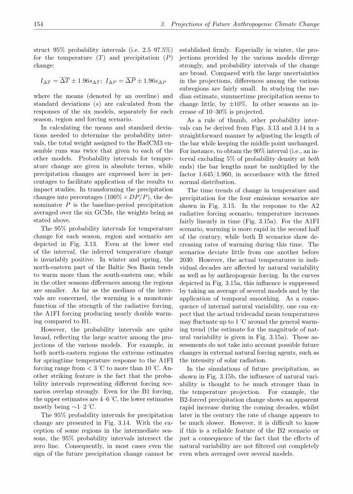
154 3. Projections of Future Anthropogenic Climate Change
struct 95% probability intervals (i.e. 2.5–97.5%)for the temperature (T ) and precipitation (P )change:
I∆T = ∆T ± 1.96s∆T ; I∆P = ∆P ± 1.96s∆P
where the means (denoted by an overline) andstandard deviations (s) are calculated from theresponses of the six models, separately for eachseason, region and forcing scenario.
In calculating the means and standard devia-tions needed to determine the probability inter-vals, the total weight assigned to the HadCM3 en-semble runs was twice that given to each of theother models. Probability intervals for temper-ature change are given in absolute terms, whileprecipitation changes are expressed here in per-centages to facilitate application of the results toimpact studies. In transforming the precipitationchanges into percentages (100%×DP/P ), the de-nominator P is the baseline-period precipitationaveraged over the six GCMs, the weights being asstated above.
The 95% probability intervals for temperaturechange for each season, region and scenario aredepicted in Fig. 3.13. Even at the lower endof the interval, the inferred temperature changeis invariably positive. In winter and spring, thenorth-eastern part of the Baltic Sea Basin tendsto warm more than the south-eastern one, whilein the other seasons differences among the regionsare smaller. As far as the medians of the inter-vals are concerned, the warming is a monotonicfunction of the strength of the radiative forcing,the A1FI forcing producing nearly double warm-ing compared to B1.
However, the probability intervals are quitebroad, reflecting the large scatter among the pro-jections of the various models. For example, inboth north-eastern regions the extreme estimatesfor springtime temperature response to the A1FIforcing range from < 3 C to more than 10 C. An-other striking feature is the fact that the proba-bility intervals representing different forcing sce-narios overlap strongly. Even for the B1 forcing,the upper estimates are 4–6 C, the lower estimatesmostly being ∼1–2 C.
The 95% probability intervals for precipitationchange are presented in Fig. 3.14. With the ex-ception of some regions in the intermediate sea-sons, the 95% probability intervals intersect thezero line. Consequently, in most cases even thesign of the future precipitation change cannot be
established firmly. Especially in winter, the pro-jections provided by the various models divergestrongly, and probability intervals of the changeare broad. Compared with the large uncertaintiesin the projections, differences among the varioussubregions are fairly small. In studying the me-dian estimate, summertime precipitation seems tochange little, by ±10%. In other seasons an in-crease of 10–30% is projected.
As a rule of thumb, other probability inter-vals can be derived from Figs. 3.13 and 3.14 in astraightforward manner by adjusting the length ofthe bar while keeping the middle point unchanged.For instance, to obtain the 90% interval (i.e., an in-terval excluding 5% of probability density at bothends) the bar lengths must be multiplied by thefactor 1.645/1.960, in accordance with the fittednormal distribution.
The time trends of change in temperature andprecipitation for the four emissions scenarios areshown in Fig. 3.15. In the response to the A2radiative forcing scenario, temperature increasesfairly linearly in time (Fig. 3.15a). For the A1FIscenario, warming is more rapid in the second halfof the century, while both B scenarios show de-creasing rates of warming during this time. Thescenarios deviate little from one another before2030. However, the actual temperatures in indi-vidual decades are affected by natural variabilityas well as by anthropogenic forcing. In the curvesdepicted in Fig. 3.15a, this influence is suppressedby taking an average of several models and by theapplication of temporal smoothing. As a conse-quence of internal natural variability, one can ex-pect that the actual tridecadal mean temperaturesmay fluctuate up to 1 C around the general warm-ing trend (the estimate for the magnitude of nat-ural variability is given in Fig. 3.15a). These as-sessments do not take into account possible futurechanges in external natural forcing agents, such asthe intensity of solar radiation.
In the simulations of future precipitation, asshown in Fig. 3.15b, the influence of natural vari-ability is thought to be much stronger than inthe temperature projection. For example, theB2-forced precipitation change shows an apparentrapid increase during the coming decades, whilstlater in the century the rate of change appears tobe much slower. However, it is difficult to knowif this is a reliable feature of the B2 scenario orjust a consequence of the fact that the effects ofnatural variability are not filtered out completelyeven when averaged over several models.

3.3. Anthropogenic Climate Change in the Baltic Sea Basin 155
Fig. 3.13. Seasonal GCM-driven 95% probability intervals of absolute temperature change (vertical bars)from 1961–1990 to 2070–2099 for four subregions (defined in Fig. 3.12), derived from SRES-forced simulationsperformed with six GCMs. Intervals are given separately for the A1FI (red ), A2 (black ), B2 (blue) and B1(green) scenarios. The dot in the centre of the bar denotes the median of the interval
Fig. 3.14. Seasonal GCM-derived 95% probability intervals of precipitation change in percent. Intervals aregiven separately for the A1FI (red ), A2 (black ), B2 (blue) and B1 (green) scenarios. The dot in the centre ofthe bar denotes the median of the interval

156 3. Projections of Future Anthropogenic Climate Change
Fig. 3.15. Annual mean temperature (left) and precipitation anomalies for Finland relative to the mean ofthe baseline period 1961–1990. Before the 1980’s the anomalies are based on observations, after that on themean of projections given by four GCMs (HadCM3, ECHAM4, NCAR-PCM and CSIRO-Mk2). Projectionsare given separately for the A1FI, A2, B2 and B1 SRES radiative forcing scenarios. Curves are smoothedby applying 30-year running means. The vertical bars on the left indicate the 95% probability intervals fordifferences between two arbitrarily-chosen 30-year mean temperatures/precipitations in a millennial controlrun with unchanged atmospheric composition, performed with two coupled GCMs (left bar – HadCM3; rightbar – CGCM2); these bars give a measure for internal natural variability (adapted from Jylhä et al. 2004)
Climate models are evolving continuously, andwe can anticipate that their ability to simulate theresponse to anthropogenic climate forcing will im-prove. The results discussed in this subsection arebased on a fairly small number of climate models.In the future, new more accurate models are likelyto improve our picture of expected anthropogenicclimate change.
3.4 Anthropogenic Climate Change in theBaltic Sea Basin: Projections fromStatistical Downscaling
Statistical downscaling (also called empiricaldownscaling) is a way to infer local informationfrom coarse scale information by constructing em-pirical statistical links between large scale fieldsand local conditions (e.g. Zorita and von Storch1997). Such statistical links can be used to de-velop detailed local climate scenarios based uponthe output from global climate models. A numberof statistical downscaling studies have been per-formed for the Baltic Sea Basin during the lastfew years (Hanssen-Bauer et al. 2005). Statisti-cal downscaling often involves analysis of observedpredictands and predictors, establishing downscal-ing models between the two, and applying them toglobal climate model outputs. This section focuses
on the last step for the Baltic region. Special at-tention is paid to future projections.
3.4.1 Statistical Downscaling Models
Most of the downscaling studies for the Baltic SeaBasin have so far been focused on monthly meantemperature and precipitation (e.g. Murphy 1999,2000), although other variables have also beenused as predictands.
For example, Linderson et al. (2004) tried todevelop downscaling models for several monthlybased statistics of daily precipitation (e.g. 75 and95 percentiles and maximum values for daily pre-cipitation) in southern Sweden, but found thatskillful models can only be established for monthlymean precipitation and frequency of wet days.Kaas and Frich (1995) developed downscalingmodels for monthly means of daily temperaturerange (DTR) and cloud cover (CC) for 10 Nordicstations. Omstedt and Chen (2001), Chen and Li(2004), and Chen and Omstedt (2005) developeddownscaling models for annual maximum sea icecover over the Baltic Sea and sea level near Stock-holm. Even the phytoplankton spring bloom ina Swedish lake has been linked to large scale at-mospheric circulation and may thus be projectedby statistical downscaling (Blenckner and Chen2003).

3.4. Anthropogenic Climate Change in the Baltic Sea Basin 157
Several large scale climate variables have beenused as predictors of the statistical models. Due toits strong influences on the local climate (e.g. Chenand Hellström 1999; Busuioc et al. 2001a,b), at-mospheric circulation is usually the first candidateas predictor. Among various ways to character-ize the circulation, the Sea Level Pressure (SLP)based geostrophic wind and vorticity, u, v and ζ(see Fig. 3.16), are widely used (e.g. Chen 2000;Linderson et al. 2004).
Fig. 3.16. Map showing the predictor domain of thestatistical model (adapted from Chen et al. 2006)
In their downscaling study of CC and DTR,Kaas and Frich (1995) stated that the inclusion oftropospheric temperature information among thepredictors is of fundamental importance for es-timating greenhouse gas induced changes. Theythus used both the 500–1000 hPa thickness andthe sea level pressure (SLP) fields as predictors.Several potential “signal-bearing” predictors havebeen tested for downscaling precipitation. Hell-ström et al. (2001) used large-scale absolute hu-midity at 850 hPa (q850) as predictor for precipita-tion, in addition to circulation indices. They con-clude that changes in q850 seem to convey much ofthe information on precipitation changes projectedby ECHAM4. Linderson et al. (2004) tested sev-eral predictors for monthly mean precipitation andfrequency of wet days, including large-scale pre-cipitation, humidity and temperature at 850 hPaand a thermal stability index. They concludedthat large-scale precipitation and relative humid-ity at 850 hPa were the most useful predictors inaddition to the SLP based predictors u, v and ζ.Relative humidity was more important than pre-cipitation for downscaling frequency of wet days,while large-scale precipitation was more importantfor downscaling precipitation.
3.4.2 Projections of Future Climate fromStatistical Downscaling
3.4.2.1 Temperature
Benestad (2002b, 2004) downscaled temperaturescenarios for localities in northern Europe using17 climate simulations from 10 different global cli-mate models, mainly based on the emission sce-nario IS92a. A total of 48 downscaled temper-ature scenarios were produced by using differentglobal simulations, predictors and predictor do-mains. Though the models show a considerablespread concerning projected warming rates, someresults seem to be robust. The projected warm-ing rates are generally larger inland than along thecoast. The 48 scenario ensemble mean projectedJanuary warming rate during the 21st century in-creases from slightly below 0.3 C per decade alongthe west coast of Norway to more than 0.5 C perdecade in inland areas in Sweden, Finland andNorway (Benestad 2002b). This is shown in termsof probabilities by Benestad (2004), who concludesthat under IS92a, the probability of a Januarywarming of 0.5 C per decade or more is less than10% along the Norwegian west coast, but morethan 70% in some inland areas in Sweden and Fin-land. Another robust signal is that the projectedwarming rates in Scandinavia are larger in winterthan in summer. Some models also show a ten-dency for larger warming rates at higher latitudes,though distance to the open sea seems to be moreimportant than latitude.
3.4.2.2 Precipitation
Some statistically downscaled scenarios for precip-itation were produced applying only SLP-basedpredictors (Busuioc et al. 2001b, Benestad 2002b).These may be used to evaluate possible conse-quences of changes in the atmospheric circula-tion for future precipitation but not for estimat-ing the total effect of increased concentrations ofgreenhouse-gases on precipitation conditions. Thefollowing is thus focused on precipitation studiesincluding additional predictors.
Hellström et al. (2001) used the SLP-based pre-dictors (geostrophic wind and vorticity: u, v, ζ)and large-scale q850 to deduce precipitation sce-narios for Sweden from the global models HadCM2and ECHAM4/OPYC3. Changes in precipitationconditions were projected by studying the differ-ences between 10-year control and scenario time-slices. The downscaled precipitation scenarios for
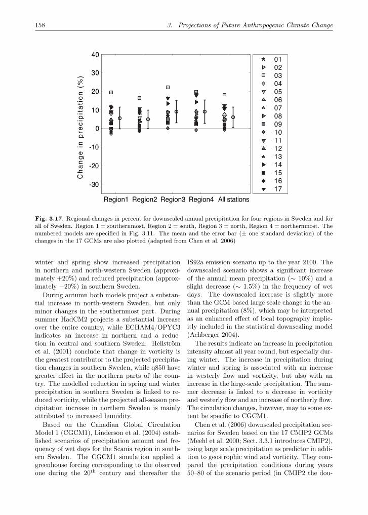
158 3. Projections of Future Anthropogenic Climate Change
Region1 Region2 Region3 Region4 All stations
-30
-20
-10
0
10
20
30
40
Ch
an
ge
in
pre
cip
ita
tio
n (
%)
0102030405060708091011121314151617
Fig. 3.17. Regional changes in percent for downscaled annual precipitation for four regions in Sweden and forall of Sweden. Region 1 = southernmost, Region 2 = south, Region 3 = north, Region 4 = northernmost. Thenumbered models are specified in Fig. 3.11. The mean and the error bar (± one standard deviation) of thechanges in the 17 GCMs are also plotted (adapted from Chen et al. 2006)
winter and spring show increased precipitationin northern and north-western Sweden (approxi-mately +20%) and reduced precipitation (approx-imately −20%) in southern Sweden.
During autumn both models project a substan-tial increase in north-western Sweden, but onlyminor changes in the southernmost part. Duringsummer HadCM2 projects a substantial increaseover the entire country, while ECHAM4/OPYC3indicates an increase in northern and a reduc-tion in central and southern Sweden. Hellströmet al. (2001) conclude that change in vorticity isthe greatest contributor to the projected precipita-tion changes in southern Sweden, while q850 havegreater effect in the northern parts of the coun-try. The modelled reduction in spring and winterprecipitation in southern Sweden is linked to re-duced vorticity, while the projected all-season pre-cipitation increase in northern Sweden is mainlyattributed to increased humidity.
Based on the Canadian Global CirculationModel 1 (CGCM1), Linderson et al. (2004) estab-lished scenarios of precipitation amount and fre-quency of wet days for the Scania region in south-ern Sweden. The CGCM1 simulation applied agreenhouse forcing corresponding to the observedone during the 20th century and thereafter the
IS92a emission scenario up to the year 2100. Thedownscaled scenario shows a significant increaseof the annual mean precipitation (∼ 10%) and aslight decrease (∼ 1.5%) in the frequency of wetdays. The downscaled increase is slightly morethan the GCM based large scale change in the an-nual precipitation (8%), which may be interpretedas an enhanced effect of local topography implic-itly included in the statistical downscaling model(Achberger 2004).
The results indicate an increase in precipitationintensity almost all year round, but especially dur-ing winter. The increase in precipitation duringwinter and spring is associated with an increasein westerly flow and vorticity, but also with anincrease in the large-scale precipitation. The sum-mer decrease is linked to a decrease in vorticityand westerly flow and an increase of northerly flow.The circulation changes, however, may to some ex-tent be specific to CGCM1.
Chen et al. (2006) downscaled precipitation sce-narios for Sweden based on the 17 CMIP2 GCMs(Meehl et al. 2000; Sect. 3.3.1 introduces CMIP2),using large scale precipitation as predictor in addi-tion to geostrophic wind and vorticity. They com-pared the precipitation conditions during years50–80 of the scenario period (in CMIP2 the dou-

3.5. Anthropogenic Climate Change in the Baltic Sea Basin 159
bling of CO2 occurs in year 70) with an 80-yearcontrol run, and concluded that the ensemble ofscenarios suggests an overall increase in annualprecipitation, as shown in Fig. 3.17. The increasein precipitation is more significant in northernthan in southern Sweden. This overall positivetrend can be attributed to the increased large-scaleprecipitation and the westerly wind. The seasonalprecipitation in autumn, winter and spring is ex-pected to increase, whereas there is an indicationof decreasing summer precipitation in the south-ern half of the country. The estimated uncertaintyis nearly independent of region. However, there isa seasonal dependence; the estimates for wintershow the highest level of confidence, and the esti-mate for summer the least.
3.5 Anthropogenic Climate Change in theBaltic Sea Basin: Projections fromRegional Climate Models
Dynamical downscaling describes the process ofdownscaling from global scales to regional or lo-cal scales using dynamical models. For climatestudies, this typically consists of applying a cou-pled atmosphere–land surface model to a limitedarea of the globe at scales considerably finer thanthose used for global climate models. For example,horizontal scales are typically some tens of kilo-metres versus hundreds of kilometres for GCMs.Like statistical downscaling, dynamical downscal-ing requires driving inputs from a global model.However, dynamical downscaling differs from sta-tistical downscaling in that it includes explicit rep-resentation of physical processes for every gridsquare included in its domain. Critical variablesfrom GCM simulations define driving inputs at theboundaries of the regional climate model (RCM)domain.
3.5.1 Interpreting Regional AnthropogenicClimate Change Projections
Regional climate modelling has been developedand used for dynamical downscaling of GCM re-sults over the past 15 years. The first studies forEurope, including the southern half of the BalticSea Basin, were those of Giorgi et al. (1990) andGiorgi and Marinucci (1991). Since their introduc-tion, the spatial and temporal resolution of RCMshas become finer and the level of output detailhas increased considerably (e.g. Giorgi et al. 1992;
Christensen et al. 1998; Jones et al. 1995 and 1997;Christensen et al. 2007).
Only a few studies have specifically focusedon the Baltic Sea Basin (e.g. Jacob et al. 2001;Räisänen and Joelsson 2001; Kjellström and Ru-osteenoja 2007), but a succession of EuropeanUnion funded research projects with focus on re-gional downscaling over Europe has produced ahost of European-wide studies with results rele-vant for the Baltic Sea Basin (i.e. Regionalization,RACCS, MERCURE, PRUDENCE, MICE, EN-SEMBLES).
There is uncertainty associated with regionalanthropogenic climate change projections, whichcan be summarised as the combination of biasesrelated to the formulation of the regional climatemodel, lateral boundary conditions and initial con-ditions from the driving global model, and choiceof emissions scenario. This section first addressesthe question of the formulation of the RCMs byreviewing experiments in which the RCMs shouldrepresent the present climate. This is followed byan inventory of available RCMs and anthropogenicclimate change experiments, and then results forprojections of the future climate.
3.5.1.1 Simulation of Present-day Climate fromRegional Climate Models
An important step in climate modelling is to eval-uate how well models perform for the present cli-mate (e.g. Achberger et al. 2003). This typicallyconsists of performing model simulations for ret-rospective observed periods using boundary con-ditions that best represent observations. In lieu ofactual observations at RCM boundaries, “reanaly-sis” data are often used. These data sets consistof results from numerical weather prediction mod-els that are driven (and constrained) by as manyactual observations as possible to produce repre-sentation of meteorological variables on a uniformmodel grid at sub-daily time scales (Uppala et al.2005). Reanalysis data produced within Europeto date include ERA-15 (1979–1993) and ERA-40(1957–2001). Other reanalysis data that are com-monly used are the NCEP reanalysis data (1948–present, Kalnay et al. 1996; Kistler et al. 2001).
The subject of RCM evaluation was the themeof the European project MERCURE, which usedreanalysis data from ERA-15 as reported by Hage-mann et al. (2002, 2004) for the Baltic Sea Basin.Five regional models were analysed. In gen-eral, temperature and precipitation values aver-
160 3. Projections of Future Anthropogenic Climate Change
aged over larger areas like the Baltic Sea Basinmatched closely with results from observationsand the driving reanalysis data. For the BalticSea Basin the authors concluded that although av-erage precipitation is generally overestimated tosome extent, except during summer, the annualcycle is well described. For temperature, two ofthe models show a very close match to the ob-served annual cycle, while two of the others showan exaggerated seasonal cycle with biases of ±2 Cfor individual months. For other quantities, likemodel generated runoff, evapotranspiration andsnowpack, the agreement between individual mod-els and observations is not as good as for temper-ature and precipitation. Examples include bothunder- and overestimations for individual monthsas well as leads and lags of up to 2 months in thetiming of the seasonal cycles. A further conclusionwas that the higher resolution of RCMs resulted inmore realistic smaller-scale variation as comparedto GCMs, for example better orographic precipi-tation and better temporal detail. Additional as-pects of the same simulations were analysed byFrei et al. (2003) and by Vidale et al. (2003).
A prominent deficiency of European climatesimulations is a tendency toward excessive summerdrying that most RCMs show, especially in south-eastern Europe, but also in the southern part ofthe Baltic Sea Basin for some RCMs. This is char-acterised by temperatures that are too high andboth precipitation and evapotranspiration that aretoo low. This was also noted in the first Europeanmulti-RCM project using reanalysis data, as re-ported in Christensen et al. (1997). Jones et al.(2004), using another RCM, attributed this phe-nomenon to model deficiencies, in particular forcloud and radiation processes.
In summary, RCMs have been shown to repro-duce the mean climate and observed climate vari-ability over Europe for the last decades. This in-cludes not just the large-scale circulation but alsoother variables. For instance, near-surface temper-ature is most often simulated to within 1–2 C fromthe observations over areas similar in size to theBaltic Sea Basin. Also, the seasonal cycle of pre-cipitation is reproduced to within the uncertaintiesgiven by the observational data sets. Despite thisagreement between the observed and simulated cli-mate, individual RCMs do show more substantialerrors for some variables in different regions andseasons. Furthermore, extreme values are by theirnature difficult to validate and an extensive evalu-ation of model performance in terms of simulating
extreme conditions is lacking. However, it can benoted that errors in simulating extreme conditionsoften tend to be larger than errors in mean condi-tions. This is discussed in more detail in Sect. 3.6.
An example of a common deficiency in theRCMs is the inability of RCMs to simulate highwind speeds over land without an additional gustparameterization (Rockel and Woth 2007).
3.5.1.2 Regional Climate Models and Anthro-pogenic Climate Change Experiments
Regional anthropogenic climate change projec-tions covering the entire Baltic Sea Basin first be-came available with the work reported by Jones etal. (1995, 1997). A general compilation of RCMsand earlier studies was undertaken by the IPCC(Giorgi et al. 2001). Since then, a number of sim-ulations have been performed, some of which arecompared in Christensen et al. (2001) and Rum-mukainen et al. (2003) for the Nordic region.
In the European project PRUDENCE, ten dif-ferent regional climate models were used to carryout more than 25 experiments, a majority ofwhich were based on a common global anthro-pogenic climate change experiment (Christensenet al. 2007). The PRUDENCE matrix of exper-iments addressed some of the uncertainties men-tioned above (Déqué et al. 2007). These most re-cent studies were based on anthropogenic climatechange simulations using a 30-year period as a con-trol to represent the present climate and a 30-yearfuture period based on a documented emissionsscenario.
A summary of the RCM future climate simu-lations referred to in the following discussion isshown in Table 3.2. Here, and in Sect. 3.6, fo-cus is on reporting projections for the key vari-ables of temperature, precipitation, wind andsnow. The ability of the RCMs to reproducethe control climate, typically for the period 1961–1990, is first discussed. Future climate scenarioexperiments for the period 2071–2100 are thenpresented. In addition to material from pub-lished literature, this includes the most recentlyavailable results from the PRUDENCE data cen-tre (http://prudence.dmi.dk/). Seasonal averagesare highlighted from two specific PRUDENCERCMs – RCAO and HIRHAM – that wereused to downscale simulations from two GCMs– HadCM3/HadAM3H and ECHAM4/OPYC3– forced by the SRES-A2 emissions scenario(Nakićenović et al. 2000; see also Annex 6). Thus,

3.5. Regional Climate Models and Anthropogenic Climate Change Experiments 161
a range of experiment results reflecting some of theuncertainties originating from both boundary con-ditions and RCM formulation differences is pre-sented.
In addition, scatter plots for different subre-gions of the Baltic Sea Basin that include simu-lations addressing further aspects of uncertaintyare presented to illustrate a more comprehensivespread of anthropogenic climate change projec-tions in the region. This includes simulationswith numerous RCMs, GCM ensemble simulationsdownscaled with the same RCM, RCM simula-tions with different horizontal resolution, and sim-ulations using additional emissions scenarios. Itshould be noted, however, that the GCMs andemissions scenarios reported here are only a subsetof those available (cf. Sect. 3.3).
3.5.2 Projections of Future Climate fromRegional Climate Models
3.5.2.1 Temperature
The air temperature discussed below refers to thetwo-meter level air temperature in the models.This corresponds to a typical height common tomost observation stations.
Temperature, control climate
Temperature biases in the Baltic Sea Basin forcontrol experiments downscaled with RCMs havebeen shown to be generally positive for the winterseason when compared to observations (Räisänenet al. 2003; Giorgi et al. 2004a). However, thesebiases are typically less than 2 C. An exception islarger warm biases in the mountainous interior ofnorthern Scandinavia. These larger biases, whichare also seen in the global models (cf. Sect. 3.3.3),may partly be related to the fact that the ob-servations come primarily from cold valley sta-tions while RCM output is averaged from grid-boxes covering a range of elevations, as discussedin Räisänen et al. (2003). The milder winter cli-mate shown in these studies can be related to theexcessive north–south pressure gradient over theNorth Atlantic inherited from the global models(cf. Sect. 3.3.3). It should be noted that the sizeand even sign of the temperature bias is sensitiveto the boundary conditions (cf. Fig. 3.6a).
Regarding summer temperature, Räisänen et al.(2003) and Giorgi et al. (2004a) found a relativelylarge bias (1–2 C) in summer temperature specific
to the south-eastern part of the Baltic Sea Basin,while biases in spring and autumn were small forthe entire region. Vidale et al. (2007) also showeda positive bias in temperature in the south-easternpart of the Baltic Sea Basin for one of the RCMsthat they analysed. This bias in the south-easternpart of the Baltic Sea Basin is thought to be re-lated to the summer drying bias mentioned abovefor the reanalysis boundary experiments in south-eastern Europe (cf. Sect. 3.5.1.1).
Seasonal cycle of temperature, future climate
In future scenarios, as snow cover retreats northand east, the climate in the Baltic Sea Basin un-dergoes large changes, particularly during the win-ter season. A common feature in all regional down-scaling experiments is the stronger increase in win-tertime temperatures compared to summertimetemperatures in the northern and eastern partsof the Baltic Sea Basin (e.g. Giorgio et al. 1992;Jones et al. 1997; Christensen et al. 2001; Déquéet al. 2007), as shown in Fig. 3.18. This patternof anthropogenic climate change is also seen fromthe global climate models (e.g. Fig. 3.9), but here,with higher horizontal resolution, regional featureshave a more pronounced impact on the results.For instance, the strong reduction in sea ice in theBothnian Bay (presented in Sect. 3.8) leads to asubstantial increase in air temperature over theBothnian Bay.
The projected temperature change for summeris shown in Fig. 3.19. Warming in this seasonis most pronounced further south in Europe, andconsequently, it is to the south of the Baltic Seathat the warming is strongest in the Baltic SeaBasin. Figures 3.20 and 3.21 show a wider rangeof RCM model results, whereby additional exper-iments are included as outlined in the figure cap-tion. These figures summarise change in temper-ature against change in precipitation for northernand southern subregions of the Baltic Sea Basin.In some models the summertime warming southof the Baltic Sea is as large, or even larger, thanthat during winter.
As seen in Fig. 3.19, a local maximum over theBaltic Sea stands out in the experiments forcedwith boundary conditions from HadAM3H. Thisfeature is associated with a strong increase inBaltic Sea SSTs (sea surface temperatures) forthese experiments, which is larger than in any ofthe other GCMs discussed in Sect. 3.3.4 (Kjell-ström and Ruosteenoja 2007).
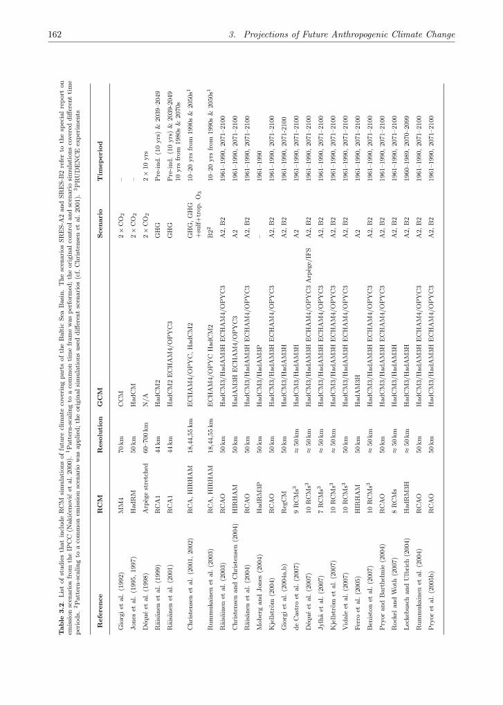
162 3. Projections of Future Anthropogenic Climate Change
Table
3.2
.Lis
tof
studie
sth
at
incl
ude
RC
Msi
mula
tions
of
futu
recl
imate
cover
ing
part
sof
the
Balt
icSea
Basi
n.
The
scen
ari
os
SR
ES-A
2and
SR
ES-B
2re
fer
toth
esp
ecia
lre
port
on
emis
sion
scen
ari
os
from
the
IPC
C(N
akic
enov
icet
al.
2000).
1Patt
ern-s
caling
toa
com
mon
tim
efr
am
ew
as
per
form
ed;th
eori
gin
alco
ntr
oland
scen
ari
osi
mula
tions
cover
eddiff
eren
tti
me
per
iods.
2Patt
ern-s
caling
toa
com
mon
emis
sion
scen
ari
ow
as
applied
;th
eori
gin
alsi
mula
tions
use
ddiff
eren
tsc
enari
os
(cf.
Chri
sten
sen
etal.
2001).
3P
RU
DE
NC
Eex
per
imen
ts
Refe
rence
RC
MR
eso
luti
on
GC
MScenari
oT
imeperi
od
Gio
rgiet
al.
(1992)
MM
470
km
CC
M2×
CO
2–
Jones
etal.
(1995,1997)
HadR
M50
km
HadC
M2×
CO
2–
Deq
ue
etal.
(1998)
Arp
ege
stre
tched
60–700
km
N/A
2×
CO
22×
10
yrs
Rais
anen
etal.
(1999)
RC
A1
44
km
HadC
M2
GH
GP
re-ind.(1
0yrs
)&
2039–2049
Rais
anen
etal.
(2001)
RC
A1
44
km
HadC
M2
EC
HA
M4/O
PY
C3
GH
GP
re-ind.
(10
yrs
)&
2039-2
049
10
yrs
from
1980s
&2070s
Chri
sten
sen
etal.
(2001,2002)
RC
A,H
IRH
AM
18,4
4,5
5km
EC
HA
M4/O
PY
C,H
adC
M2
GH
G,G
HG
10–20
yrs
from
1990s
&2050s1
+su
lf+
trop.
O3
Rum
muka
inen
etal.
(2003)
RC
A,H
IRH
AM
18,4
4,5
5km
EC
HA
M4/O
PY
CH
adC
M2
B22
10–20
yrs
from
1990s
&2050s1
Rais
ain
enet
al.
(2003)
RC
AO
50
km
HadC
M3/H
adA
M3H
EC
HA
M4/O
PY
C3
A2,B
21961–1990,2071–2100
Chri
sten
sen
and
Chri
sten
sen
(2004)
HIR
HA
M50
km
HadA
M3H
EC
HA
M4/O
PY
C3
A2
1961–1990,2071–2100
Rais
anen
etal.
(2004)
RC
AO
50
km
HadC
M3/H
adA
M3H
EC
HA
M4/O
PY
C3
A2,B
21961–1990,2071–2100
Mober
gand
Jones
(2004)
HadR
M3P
50
km
HadC
M3/H
adA
M3P
–1961–1990
Kje
llst
rom
(2004)
RC
AO
50
km
HadC
M3/H
adA
M3H
EC
HA
M4/O
PY
C3
A2,B
21961–1990,2071–2100
Gio
rgiet
al.
(2004a,b
)R
egC
M50
km
HadC
M3/H
adA
M3H
A2,B
21961–1990,2071-2
100
de
Cast
roet
al.
(2007)
9R
CM
s3≈
50
km
HadC
M3/H
adA
M3H
A2
1961–1990,2071–2100
Deq
ue
etal.
(2007)
10
RC
Ms3
≈50
km
HadC
M3/H
adA
M3H
EC
HA
M4/O
PY
C3
Arp
ege/
IFS
A2,B
21961–1990,2071–2100
Jylh
aet
al.
(2007)
7R
CM
s3≈
50
km
HadC
M3/H
adA
M3H
EC
HA
M4/O
PY
C3
A2,B
21961–1990,2071–2100
Kje
llst
rom
etal.
(2007)
10
RC
Ms3
≈50
km
HadC
M3/H
adA
M3H
EC
HA
M4/O
PY
C3
A2,B
21961–1990,2071–2100
Vid
ale
etal.
(2007)
10
RC
Ms3
50
km
HadC
M3/H
adA
M3H
EC
HA
M4/O
PY
C3
A2,B
21961–1990,2071–2100
Fer
roet
al.
(2005)
HIR
HA
M50
km
HadA
M3H
A2
1961–1990,2071–2100
Ben
isto
net
al.
(2007)
10
RC
Ms3
≈50
km
HadC
M3/H
adA
M3H
EC
HA
M4/O
PY
C3
A2,B
21961–1990,2071–2100
Pry
or
and
Bart
hel
mie
(2004)
RC
AO
50
km
HadC
M3/H
adA
M3H
EC
HA
M4/O
PY
C3
A2,B
21961–1990,2071–2100
Rock
eland
Woth
(2007)
8R
CM
s≈
50
km
HadC
M3/H
adA
M3H
A2,B
21961–1990,2071–2100
Lec
keb
usc
hand
Ulb
rich
(2004)
HadR
M3H
≈50
km
HadC
M3/H
adA
M3H
A2,B
21960–1989,2070–2099
Rum
muka
inen
etal.
(2004)
RC
AO
50
km
HadC
M3/H
adA
M3H
EC
HA
M4/O
PY
C3
A2,B
21961–1990,2071–2100
Pry
or
etal.
(2005b)
RC
AO
50
km
HadC
M3/H
adA
M3H
EC
HA
M4/O
PY
C3
A2,B
21961–1990,2071–2100
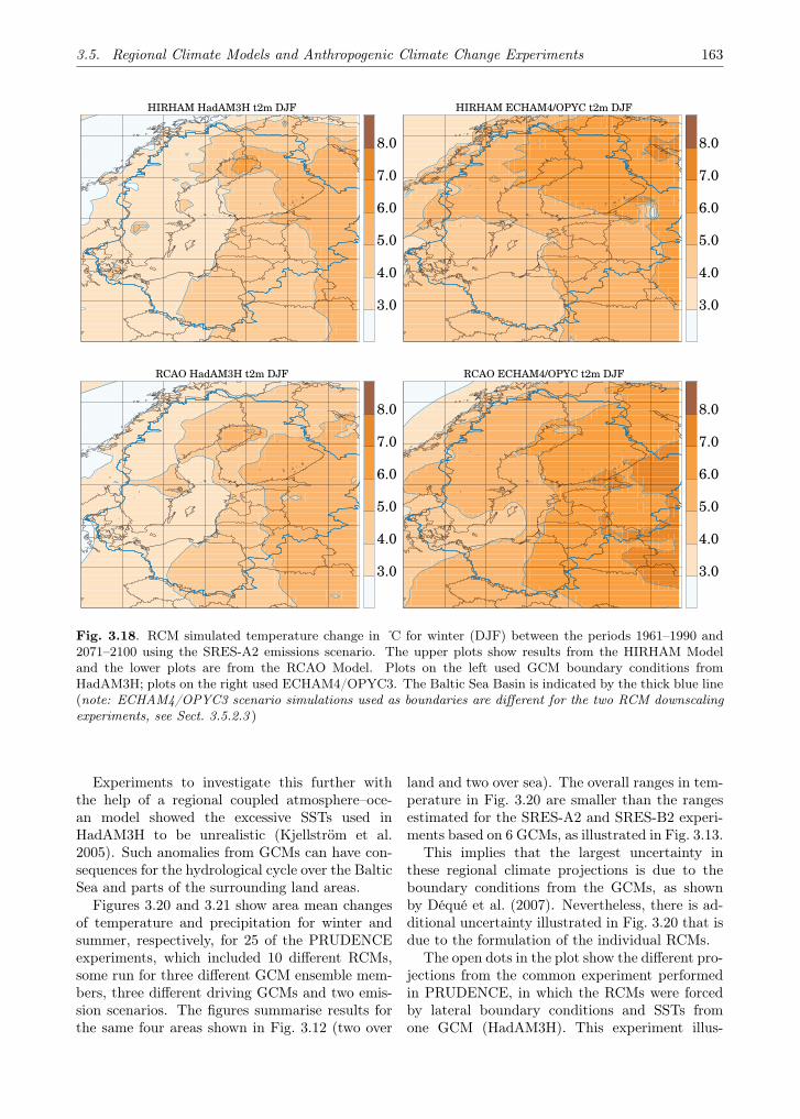
3.5. Regional Climate Models and Anthropogenic Climate Change Experiments 163
HIRHAM HadAM3H t2m DJF
3.0
4.0
5.0
6.0
7.0
8.0
HIRHAM ECHAM4/OPYC t2m DJF
3.0
4.0
5.0
6.0
7.0
8.0
RCAO HadAM3H t2m DJF
3.0
4.0
5.0
6.0
7.0
8.0
RCAO ECHAM4/OPYC t2m DJF
3.0
4.0
5.0
6.0
7.0
8.0
Fig. 3.18. RCM simulated temperature change in C for winter (DJF) between the periods 1961–1990 and2071–2100 using the SRES-A2 emissions scenario. The upper plots show results from the HIRHAM Modeland the lower plots are from the RCAO Model. Plots on the left used GCM boundary conditions fromHadAM3H; plots on the right used ECHAM4/OPYC3. The Baltic Sea Basin is indicated by the thick blue line(note: ECHAM4/OPYC3 scenario simulations used as boundaries are different for the two RCM downscalingexperiments, see Sect. 3.5.2.3 )
Experiments to investigate this further withthe help of a regional coupled atmosphere–oce-an model showed the excessive SSTs used inHadAM3H to be unrealistic (Kjellström et al.2005). Such anomalies from GCMs can have con-sequences for the hydrological cycle over the BalticSea and parts of the surrounding land areas.
Figures 3.20 and 3.21 show area mean changesof temperature and precipitation for winter andsummer, respectively, for 25 of the PRUDENCEexperiments, which included 10 different RCMs,some run for three different GCM ensemble mem-bers, three different driving GCMs and two emis-sion scenarios. The figures summarise results forthe same four areas shown in Fig. 3.12 (two over
land and two over sea). The overall ranges in tem-perature in Fig. 3.20 are smaller than the rangesestimated for the SRES-A2 and SRES-B2 experi-ments based on 6 GCMs, as illustrated in Fig. 3.13.
This implies that the largest uncertainty inthese regional climate projections is due to theboundary conditions from the GCMs, as shownby Déqué et al. (2007). Nevertheless, there is ad-ditional uncertainty illustrated in Fig. 3.20 that isdue to the formulation of the individual RCMs.
The open dots in the plot show the different pro-jections from the common experiment performedin PRUDENCE, in which the RCMs were forcedby lateral boundary conditions and SSTs fromone GCM (HadAM3H). This experiment illus-
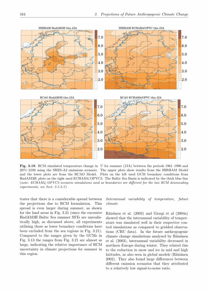
164 3. Projections of Future Anthropogenic Climate Change
HIRHAM HadAM3H t2m JJA
2.0
3.0
4.0
5.0
6.0
7.0
HIRHAM ECHAM4/OPYC t2m JJA
2.0
3.0
4.0
5.0
6.0
7.0
RCAO HadAM3H t2m JJA
2.0
3.0
4.0
5.0
6.0
7.0
RCAO ECHAM4/OPYC t2m JJA
2.0
3.0
4.0
5.0
6.0
7.0
Fig. 3.19. RCM simulated temperature change in C for summer (JJA) between the periods 1961–1990 and2071–2100 using the SRES-A2 emissions scenario. The upper plots show results from the HIRHAM Modeland the lower plots are from the RCAO Model. Plots on the left used GCM boundary conditions fromHadAM3H; plots on the right used ECHAM4/OPYC3. The Baltic Sea Basin is indicated by the thick blue line(note: ECHAM4/OPYC3 scenario simulations used as boundaries are different for the two RCM downscalingexperiments, see Sect. 3.5.2.3 )
trates that there is a considerable spread betweenthe projections due to RCM formulation. Thisspread is even larger during summer, as shownfor the land areas in Fig. 3.21 (since the excessiveHadAM3H Baltic Sea summer SSTs are unrealis-tically high, as discussed above, all experimentsutilising those as lower boundary conditions havebeen excluded from the sea regions in Fig. 3.21).Compared to the ranges given by the GCMs inFig. 3.13 the ranges from Fig. 3.21 are almost aslarge, indicating the relative importance of RCMuncertainty in climate projections for summer inthis region.
Interannual variability of temperature, futureclimate
Räisänen et al. (2003) and Giorgi et al (2004a)showed that the interannual variability of temper-ature was simulated well in their respective con-trol simulations as compared to gridded observa-tions (CRU data). In the future anthropogenicclimate change simulations analysed by Räisänenet al. (2003), interannual variability decreased innorthern Europe during winter. They related thisto the reduction in snow and ice in mid and highlatitudes, as also seen in global models (Räisänen2002). They also found large differences betweendifferent emission scenarios that they attributedto a relatively low signal-to-noise ratio.

3.5. Regional Climate Models and Anthropogenic Climate Change Experiments 165
1 2 3 4 5 6
10
20
30
40
50
60
Temperature change (K)
Prec
ipita
tion
chan
ge (
%) LAND/NE
1 2 3 4 5 6
10
20
30
40
50
60
Temperature change (K)
Prec
ipita
tion
chan
ge (
%) LAND/SW
1 2 3 4 5 6
10
20
30
40
50
60
Temperature change (K)
Prec
ipita
tion
chan
ge (
%) SEA/NE
1 2 3 4 5 6
10
20
30
40
50
60
Temperature change (K)
Prec
ipita
tion
chan
ge (
%) SEA/SW
Fig. 3.20. Changes in winter (DJF) area mean temperature and precipitation for the areas defined in Fig. 3.12The “©” symbol denotes 7 RCMs from the common PRUDENCE experiment based on the same GCM(HadAM3H). The “×” symbol denotes other regional downscaling experiments from PRUDENCE, which in-cluded different driving GCMs, different emission scenarios, higher horizontal resolution and several ensemblemembers
Giorgi et al. (2004b) found increasing interan-nual variability south of the Baltic Sea duringsummer (JJA) and autumn (SON) in two futurescenarios, SRES–A2 and SRES–B2. Schär et al.(2004) and Vidale et al. (2003) also found increas-ing interannual summer (JJA) temperature vari-ability for Central Europe, including the southernpart of the Baltic Sea Basin. The standard de-viation of the interannual variability increased by20 to 80% between the different RCMs in theirstudy, all of which used the same emissions sce-nario. They linked this to the dynamics of soil-moisture storage and the associated feedbacks onthe surface energy balance and precipitation.
Diurnal temperature range, future climate
The diurnal temperature range (DTR) is definedas the average difference between daily maxi-
mum and minimum temperatures. In future an-thropogenic climate change scenarios, both Chris-tensen et al. (2001) and Rummukainen et al.(2003) found a stronger decrease of the DTR infall and winter than during summer for the Nordicregion. The reduction around 2050 amounts to0.6 ± 0.4 C in winter, where the central value isthe mean from all experiments and the range isgiven by the spread within the ensemble.
Räisänen et al. (2003) also found a larger changein DTR in northern Europe during the periodlate autumn to spring than in summer. The re-duction of DTR in their scenarios, analysed overSweden for the period 2071–2100, was of the or-der of 1 C for the winter months. They alsonoted that the night-to-day temperature variabil-ity in northern Europe is small during mid-winterand that much of the simulated changes in DTRmay be affected by irregular day-to-day variations.
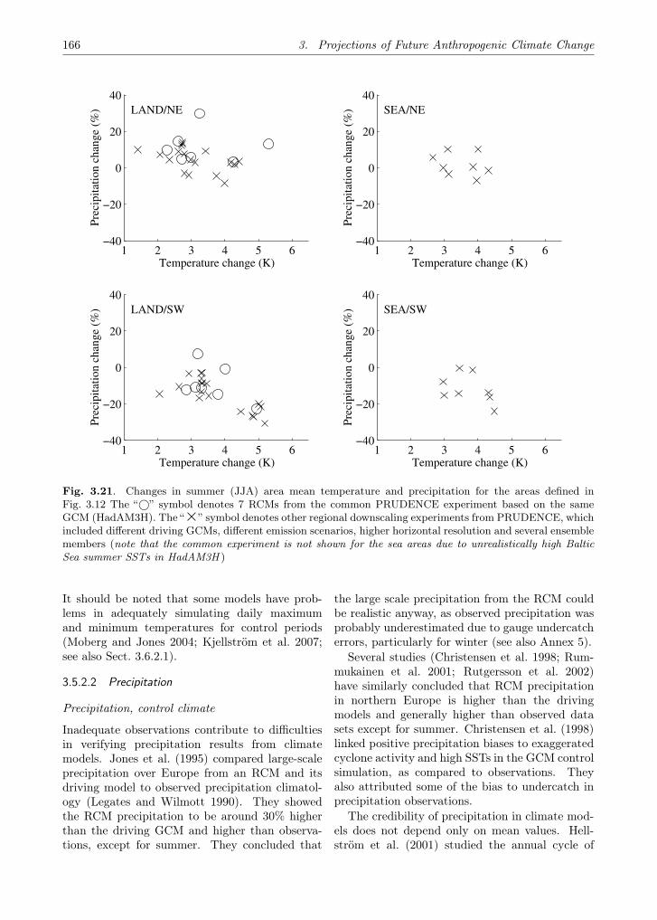
166 3. Projections of Future Anthropogenic Climate Change
1 2 3 4 5 6−40
−20
0
20
40
Temperature change (K)
Prec
ipita
tion
chan
ge (
%) LAND/NE
1 2 3 4 5 6−40
−20
0
20
40
Temperature change (K)
Prec
ipita
tion
chan
ge (
%) LAND/SW
1 2 3 4 5 6−40
−20
0
20
40
Temperature change (K)
Prec
ipita
tion
chan
ge (
%) SEA/NE
1 2 3 4 5 6−40
−20
0
20
40
Temperature change (K)
Prec
ipita
tion
chan
ge (
%) SEA/SW
Fig. 3.21. Changes in summer (JJA) area mean temperature and precipitation for the areas defined inFig. 3.12 The “©” symbol denotes 7 RCMs from the common PRUDENCE experiment based on the sameGCM (HadAM3H). The “×” symbol denotes other regional downscaling experiments from PRUDENCE, whichincluded different driving GCMs, different emission scenarios, higher horizontal resolution and several ensemblemembers (note that the common experiment is not shown for the sea areas due to unrealistically high BalticSea summer SSTs in HadAM3H )
It should be noted that some models have prob-lems in adequately simulating daily maximumand minimum temperatures for control periods(Moberg and Jones 2004; Kjellström et al. 2007;see also Sect. 3.6.2.1).
3.5.2.2 Precipitation
Precipitation, control climate
Inadequate observations contribute to difficultiesin verifying precipitation results from climatemodels. Jones et al. (1995) compared large-scaleprecipitation over Europe from an RCM and itsdriving model to observed precipitation climatol-ogy (Legates and Wilmott 1990). They showedthe RCM precipitation to be around 30% higherthan the driving GCM and higher than observa-tions, except for summer. They concluded that
the large scale precipitation from the RCM couldbe realistic anyway, as observed precipitation wasprobably underestimated due to gauge undercatcherrors, particularly for winter (see also Annex 5).
Several studies (Christensen et al. 1998; Rum-mukainen et al. 2001; Rutgersson et al. 2002)have similarly concluded that RCM precipitationin northern Europe is higher than the drivingmodels and generally higher than observed datasets except for summer. Christensen et al. (1998)linked positive precipitation biases to exaggeratedcyclone activity and high SSTs in the GCM controlsimulation, as compared to observations. Theyalso attributed some of the bias to undercatch inprecipitation observations.
The credibility of precipitation in climate mod-els does not depend only on mean values. Hell-ström et al. (2001) studied the annual cycle of
3.5. Regional Climate Models and Anthropogenic Climate Change Experiments 167
precipitation in Sweden and Hanssen-Bauer et al.(2003) focused on regional variability in Norway.Both concluded that RCM simulations improvedsignificantly, according to the driving GCM. Rum-mukainen et al. (2001) further concluded that al-though a large part of RCM biases can be at-tributed to the driving models, the RCMs addedvalue to GCM simulations.
However, division of precipitation into inten-sity classes reveals a “drizzle problem”, which isthat the models exhibit too many days with lightprecipitation (defined as less than 1mm day−1)and too few dry days (defined as less than 0.1 mmday−1), compared to observations (Christensen etal. 1998). The problem was shown to be more pro-nounced at finer RCM resolutions. According toRäisänen et al. (2003), relative interannual vari-ability of precipitation from RCMs seems to beunderestimated in the Baltic area, probably con-nected to the unrealistically high number of rainydays.
In more recent studies, Hagemann and Jacob(2006) compared the PRUDENCE RCM resultsto two observed precipitation databases that at-tempt to correct for gauge undercatch (CMAP,Xie and Arkin 1997; and GPCP, Huffman et al.1997). They showed annual precipitation valuesfor the Baltic Sea Basin to be close to an aver-age of the two databases. They argued that theaverage of the two databases should exhibit realis-tic corrections for winter precipitation. Kjellströmand Ruosteenoja (2007) also compared Baltic SeaBasin precipitation to observed databases (GPCPas above; and CRU, New et al. 1999). Their anal-ysis of the seasonal cycle showed a general over-estimation of winter precipitation. They also sug-gested that observational databases over the seamay be biased toward high summer precipitationdue to erroneous influence of coastal precipitation.
Winter precipitation, future climate
As with results from global model experiments,regional projections for winter precipitation showincreases over most of Europe (e.g. Déqué et al.1998). Details of the geographical distributionfor precipitation changes vary with different RCMsimulations, however. The main source of dis-agreement in the RCM results is likely the differ-ent large-scale anthropogenic climate change sig-nals from the GCM simulations employed. Thesedifferences are not just due to the consequences ofdifferent model formulations, but are also due to
the fact that slow climate variations like the NAOcan have different phases in the global simulationsused to drive the RCMs.
The analysis by Déqué et al. (2007) of the mul-tiple PRUDENCE simulations systematically at-tributes variations in results to different RCMs,emissions scenarios, GCM boundaries and varia-tion between GCM ensemble members. For winterprecipitation over the Baltic area, GCM boundaryconditions are estimated to account for some 61%of the total variance and the choice of RCM forsome 34% (Déqué, pers. comm. 2005). In sum-mer, these roles are reversed with 74% of the vari-ation attributable to choice of RCM for the Balticarea. However, there is an even wider distribu-tion between choice of RCM, GCM and emissionsscenario for most other European subregions.
This can be illustrated through an examina-tion of Fig. 3.22, which shows winter precipita-tion change. The large-scale anthropogenic cli-mate change in the ECHAM4/OPYC3 simulationleads to an intensification of the zonal flow, basi-cally increasing the number and intensity of low-pressure systems from the Atlantic that hit Nor-way. The HadAM3H model turned the flow ina more south-easterly direction, leading to a de-crease in precipitation in mid-Norway.
Simulations from the PRUDENCE common ex-periment tend to agree about an increase of morethan 25% in a southwest to northeast band fromEngland to Finland. In Fig. 3.20 this increase inwinter precipitation can also be seen in the foursubregions. The ECHAM4/OPYC3 experimentsusing the RCAO (Räisänen et al. 2003, 2004) andHIRHAM models (Christensen and Christensen2004) show less agreement, as seen in Fig. 3.22.While both simulations exhibit increased precipi-tation of over 25% for most of northern Europe,the increase in precipitation is larger and coversan area much farther east in the RCAO simula-tion.
It is important to note that the boundary fieldsfor these two sets of simulations are the same forthe control period but not for the scenario period.The two simulated 2071–2100 time periods havedifferent NAO phases, which is reflected in thedownscaling results (see e.g. Ferro 2004). Hence,the larger difference between the two RCM pro-jections using ECHAM4/OPYC3 scenario simula-tions compared to the two RCM projections usingHadAM3H simulations can be attributed to dif-ferences in large-scale circulation in two differentECHAM4/OPYC3 scenario simulations.

168 3. Projections of Future Anthropogenic Climate Change
HIRHAM HadAM3H precip DJF
-30
-10
10
30
50
70
90
HIRHAM ECHAM4/OPYC precip DJF
-30
-10
10
30
50
70
90
RCAO HadAM3H precip DJF
-30
-10
10
30
50
70
90
RCAO ECHAM4/OPYC precip DJF
-30
-10
10
30
50
70
90
Fig. 3.22. RCM simulated precipitation change in percent for winter (DJF) between the periods 1961–1990and 2071–2100 using the SRES-A2 emissions scenario. The upper plots show results from the HIRHAMModel and the lower plots are from the RCAO Model. Plots on the left used GCM boundary conditions fromHadAM3H; plots on the right used ECHAM4/OPYC3. The Baltic Sea Basin is indicated by the thick red line(note: ECHAM4/OPYC3 scenario simulations used as boundaries are different for the two RCM downscalingexperiments, see Sect. 3.5.2.3 )
Summer precipitation, future climate
For future summers, regional anthropogenic cli-mate change simulations show increases in precip-itation for northern parts of the Baltic Sea Basinand decreases to the south, as shown in Fig. 3.23for four simulations. This results in only a smallaverage change for the basin as a whole. The di-viding line between increase and decrease for thefull range of PRUDENCE simulations generallygoes across the southern half of Norway and Swe-den continuing eastward through the Baltic coun-tries (Kjellström and Ruosteenoja 2007).
As discussed above (Sect. 3.5.2.1) SSTs fromsimulations driven by HadAM3H show a large
anomalous summer heating of the Baltic Sea,which in turn leads to a local increase in precip-itation (Kjellström and Ruosteenoja 2007). Rep-resentation of summer precipitation over parts ofthe Baltic Sea Basin is therefore particularly sen-sitive to how thermal conditions in the Baltic Seaitself are input to the RCMs.
Precipitation and temperature, future scenarios
Figures 3.20 and 3.21 provide a comprehensivecomparison of the projected anthropogenic climatechange signals in temperature and precipitationbetween RCMs in the northern and southern sub-

3.5. Regional Climate Models and Anthropogenic Climate Change Experiments 169
HIRHAM HadAM3H precip JJA
-30
-10
10
30
50
70
90
HIRHAM ECHAM4/OPYC precip JJA
-30
-10
10
30
50
70
90
RCAO HadAM3H precip JJA
-30
-10
10
30
50
70
90
RCAO ECHAM4/OPYC precip JJA
-30
-10
10
30
50
70
90
Fig. 3.23. RCM simulated precipitation change in percent for summer (JJA) between the periods 1961–1990 and 2071–2100 using the SRES-A2 emissions scenario. The upper plots show results from the HIRHAMModel and the lower plots are from the RCAO Model. Plots on the left used GCM boundary conditions fromHadAM3H; plots on the right used ECHAM4/OPYC3. The Baltic Sea Basin is indicated by the thick red line(note: ECHAM4/OPYC3 scenario simulations used as boundaries are different for the two RCM downscalingexperiments, see Sect. 3.5.2.3 )
regions of the Baltic Sea Basin. The trend is forwintertime climate to become milder and generatemore precipitation in both sub-regions. As dis-cussed for the GCMs in Sect. 3.3.3.1, there tendsto be a positive correlation between increasingtemperature and precipitation, particularly overthe north-eastern land area in most RCMs – thewarmer the wetter. During summer there is nosuch correlation in the north, where all models getwarmer to a different degree and most get wetterby between 5 to 20%. In the south, there is a ten-dency of an inverse correlation for summer – thewarmer the drier.
3.5.2.3 Wind
To date, studies on future wind changes usingRCMs were based mainly on two sets of sim-ulations. One such set was performed withinSWECLIM (Swedish Regional Climate ModellingProgramme) and is described in detail by Rum-mukainen et al. (2000; 2004). The other set ismore recent and includes eight different RCMsfrom the PRUDENCE project (Christensen et al.2002). The results presented below focus mostlyon results from the same two RCAO control sim-ulations discussed above for temperature and pre-cipitation. Wind speed in the following discus-sion refers to the mean velocity of the near surface
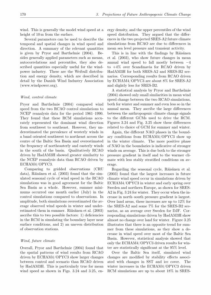
170 3. Projections of Future Anthropogenic Climate Change
wind. This is generally the model wind speed at aheight of 10m from the surface.
Several parameters can be used to describe thetemporal and spatial changes in wind speed anddirection. A summary of the relevant quantitiesis given by Pryor and Barthelmie (2004). Be-sides generally applied parameters such as means,autocorrelations and percentiles, they also de-scribed quantities especially useful for the wind-power industry. These are the Weibull distribu-tion and energy density, which are described indetail by the Danish Wind Industry Association(www.windpower.org).
Wind, control climate
Pryor and Barthelmie (2004) compared windspeed from the two RCAO control simulations toNCEP reanalysis data for the period 1961–1990.They found that these RCM simulations accu-rately represented the dominant wind directionfrom southwest to southeast. However, they un-derestimated the prevalence of westerly winds ina band oriented southwest to northeast across thecentre of the Baltic Sea Basin and overestimatedthe frequency of northeasterly and easterly windsin the south of the basin. Qualitatively RCAOdriven by HadAM3H showed greater similarity tothe NCEP reanalysis data than RCAO driven byECHAM4/OPYC3.
Comparing to gridded observations (CRUdata), Räisänen et al. (2003) found that the sim-ulated seasonal cycle of wind speed in the RCAOsimulations was in good agreement for the BalticSea Basin as a whole. However, summer mini-mums occurred one month earlier (July) in thecontrol simulations compared to observations. Inamplitude, both simulations overestimated the av-erage observed wind speeds in winter and under-estimated them in summer. Räisänen et al. (2003)ascribe this to two possible factors: 1) deficienciesin the RCM in simulating the boundary layer nearsurface conditions, and 2) an uneven distributionof observation stations.
Wind, future climate
Overall, Pryor and Barthelmie (2004) found thatthe spatial patterns of wind results from RCAOdriven by ECHAM4/OPYC3 show larger changesbetween control and scenario than RCAO drivenby HadAM3H. This is particularly true for meanwind speed as shown in Figs. 3.24 and 3.25, en-
ergy density, and the upper percentiles of the windspeed distribution. They argued that the differ-ences in the two projected SRES-A2 future climatesimulations from RCAO are due to differences inmean sea level pressure and transient activity.
This is in line with the findings by Räisänenet al. (2003), who show future changes in meanannual wind speed to fall mostly between −4to +4% over Scandinavia for RCAO driven byHadAM3H for both SRES-A2 and SRES-B2 sce-narios. Corresponding results from RCAO drivenby ECHAM4/OPYC3 are about 8% for SRES-A2and slightly less for SRES-B2.
A statistical analysis by Pryor and Barthelmie(2004) showed only small similarities in mean windspeed change between the two RCAO simulations,both for winter and summer and even less so in theannual mean. They ascribe the large differencesbetween the anthropogenic climate change signalsto the different GCMs used to drive the RCM.Figures 3.24 and Fig. 3.25 show these differencesrelated to choice of GCM for summer and winter.
Again, the different NAO phases in the bound-ary conditions from ECHAM4/OPYC3 show upin the winter climate. The more positive phaseof NAO in the boundaries is indicative of strongerwinds on average. This is due both to the strongerpressure gradient in itself and to the warmer cli-mate with less stably stratified conditions on av-erage.
Regarding the seasonal cycle, Räisänen et al.(2003) found that the largest increases in futureclimate wind speed occur in simulations driven byECHAM4/OPYC3 in winter and early spring overSweden and northern Europe, as shown for SRES-A2 in Fig. 3.24 for winter. They occur when the in-crease in north–south pressure gradient is largest.Over land areas, these increases are up to 12% forthe SRES-A2 and some 7% for the SRES-B2 sce-narios, as an average over Sweden for DJF. Cor-responding simulations driven by HadAM3H showalmost no change over land for winter. Figure 3.25illustrates that there is an opposite trend for sum-mer from these simulations, as they show a de-crease in wind speed over most of the Baltic SeaBasin. However, statistical analysis showed thatonly the ECHAM4/OPYC3 driven results for win-ter are statistically significant at the 95% level.
Over the Baltic Sea itself, simulated windchanges are modified by stability effects associ-ated with changes in SST and ice cover. Thewinter increases in the ECHAM4/OPYC3 drivenRCM simulations are up to about 18% in SRES-

3.5. Regional Climate Models and Anthropogenic Climate Change Experiments 171
HIRHAM HadAM3H w10m DJF
-10
-6
-2
2
6
10
14
18
HIRHAM ECHAM4/OPYC w10m DJF
-10
-6
-2
2
6
10
14
18
RCAO HadAM3H w10m DJF
-10
-6
-2
2
6
10
14
18
RCAO ECHAM4/OPYC w10m DJF
-10
-6
-2
2
6
10
14
18
Fig. 3.24. RCM simulated wind speed change in percent for winter (DJF) between the periods 1961–1990and 2071–2100 using the SRES-A2 emissions scenario. The upper plots show results from the HIRHAMModel and the lower plots are from the RCAO Model. Plots on the left used GCM boundary conditions fromHadAM3H; plots on the right used ECHAM4/OPYC3. The Baltic Sea Basin is indicated by the thick blue line(note: ECHAM4/OPYC3 scenario simulations used as boundaries are different for the two RCM downscalingexperiments, see Sect. 3.5.2.3 )
A2 and 13% in SRES-B2, as an average overthe entire Baltic Sea for DJF. CorrespondingHadAM3H driven simulations show an increase ofless than 5%, as an average over the entire BalticSea. The largest increases occur over the centraland northern part of the sea, where ice cover de-creases in the scenario runs. Summer changes overthe Baltic Sea show a decrease of up to 7% forECHAM4/OPYC3 driven simulations and an in-crease of about 5% for HadAM3H driven simula-tions, as an average over the entire Baltic Sea forJJA.
Regarding the latter, this reflects the largeincrease in Baltic Sea SSTs discussed above
(Sect. 3.5.2.1), which leads to reduced surface sta-bility and thereby higher wind speed (Räisänen etal. 2003).
Pryor and Barthelmie (2004) interpreted futurewind changes with respect to the use of wind asan energy source by defining wind resource classescalculated from energy density in each model gridcell. This is defined as “poor” for energy densityless than 70 Wm−2, or “good” for energy densitygreater than 140Wm−2. Using these definitions,Pryor and Barthelmie (2004) found that the num-ber of grid cells rated as “poor” decreased and thenumber of grid cells rated as “good” increased foralmost all the simulations they analysed.

172 3. Projections of Future Anthropogenic Climate Change
HIRHAM HadAM3H w10m JJA
-10
-6
-2
2
6
10
14
18
HIRHAM ECHAM4/OPYC w10m JJA
-10
-6
-2
2
6
10
14
18
RCAO HadAM3H w10m JJA
-10
-6
-2
2
6
10
14
18
RCAO ECHAM4/OPYC w10m JJA
-10
-6
-2
2
6
10
14
18
Fig. 3.25. RCM simulated wind speed change in percent for summer (JJA) between the periods 1961–1990and 2071–2100 using the SRES-A2 emissions scenario. The upper plots show results from the HIRHAMModel and the lower plots are from the RCAO Model. Plots on the left used GCM boundary conditions fromHadAM3H; plots on the right used ECHAM4/OPYC3. The Baltic Sea Basin is indicated by the thick blue line(note: ECHAM4/OPYC3 scenario simulations used as boundaries are different for the two RCM downscalingexperiments, see Sect. 3.5.2.3 )
3.5.2.4 Snow
Snow, control climate
Räisänen et al. (2003) found that the mean annualduration of snow season as simulated by RCAO isin good agreement with the observations of Raaband Vedin (1995) for Sweden. The mean annualmaximum water content of the RCM snow packtends to be slightly too low in southern Swedenand slightly too high in northern Sweden. A largepositive bias occurs for the inland of northern Swe-den (looking specifically at two available observa-tion stations). This was attributed to orographiceffects. In reality much of the precipitation in the
north falls on the western side of the Scandina-vian mountains. Due to orographic smoothing, theRCMs tend to generate more precipitation on theeastern side of the actual mountain divide.
Christensen et al. (1998) examined the depen-dence of snow cover on RCM resolution and foundthat a higher resolution significantly increasessnow cover and delays spring snow melt due tothe more realistic description of mountain topog-raphy. Räisänen et al. (2003) showed that dif-ferences due to GCM driving models were foundto be modest, except for southern Sweden whereECHAM4/OPYC3 driven simulations show moresnow and a longer snow season than for HadAM3Hdriven simulations. Jylhä et al. (2007) evaluated

3.5. Regional Climate Models and Anthropogenic Climate Change Experiments 173
HIRHAM HadAM3H snow DJF
10
30
50
70
90
110
HIRHAM ECHAM4/OPYC snow DJF
10
30
50
70
90
110
RCAO HadAM3H snow DJF
10
30
50
70
90
110
RCAO ECHAM4/OPYC snow DJF
10
30
50
70
90
110
Fig. 3.26. RCM simulated snow depth reduction in percent for winter (DJF) between the periods 1961–1990 and 2071–2100 using the SRES-A2 emissions scenario. The upper plots show results from the HIRHAMModel and the lower plots are from the RCAO Model. Plots on the left used GCM boundary conditions fromHadAM3H; plots on the right used ECHAM4/OPYC3. The Baltic Sea Basin is indicated by the thick red line(note: ECHAM4/OPYC3 scenario simulations used as boundaries are different for the two RCM downscalingexperiments, see Sect. 3.5.2.3 )
an ensemble mean of results from seven differentPRUDENCE RCM simulations and found goodagreement with the observations of Heino and Ki-taev (2003) for the simulated number of days withsnow cover (see also Annex 1.3.5).
Snow, future climate
Since snow changes follow changes in tempera-ture, there is a general decrease in snow vari-ables due to atmospheric warming in the RCMfuture scenarios. Results described by Räisänenet al. (2003) show a future decrease in meanannual maximum snow water equivalent every-where over northern Europe from RCAO simula-tions. ECHAM4/OPYC3 driven results show aclear north–south gradient in change of snow wa-
ter equivalent for both scenarios with only smalldeviations over Swedish inland areas. Reductionin snow water equvalent is some 60 to 80% in thesouthern part of the Baltic Sea Basin up to aboutlatitude 62◦ N, some 40 to 60% between 62◦ N and66◦ N, and less than 40% north of 66◦ N. Thereis also a clear region with relatively small changesdown to 20% east of the Scandinavian mountains.For northern areas of the Baltic Sea Basin differ-ences in results due to different driving GCMs aresmall, as shown in Fig. 3.26. Further south, forexample in Denmark, the differences are larger inrelative terms (Fig. 3.26) but small in absoluteterms (Fig. 3.27).
Giorgi et al. (2004b) also found a general de-crease in snow depth in their simulations with an-other RCM. There is a general decrease over the
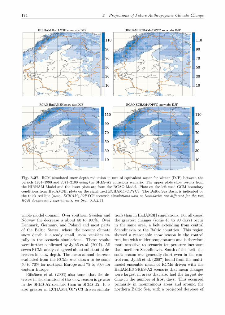
174 3. Projections of Future Anthropogenic Climate Change
HIRHAM HadAM3H snow abs DJF
10
30
50
70
90
110
HIRHAM ECHAM4/OPYC snow abs DJF
10
30
50
70
90
110
RCAO HadAM3H snow abs DJF
10
30
50
70
90
110
RCAO ECHAM4/OPYC snow abs DJF
10
30
50
70
90
110
Fig. 3.27. RCM simulated snow depth reduction in mm of equivalent water for winter (DJF) between theperiods 1961–1990 and 2071–2100 using the SRES-A2 emissions scenario. The upper plots show results fromthe HIRHAM Model and the lower plots are from the RCAO Model. Plots on the left used GCM boundaryconditions from HadAM3H; plots on the right used ECHAM4/OPYC3. The Baltic Sea Basin is indicated bythe thick red line (note: ECHAM4/OPYC3 scenario simulations used as boundaries are different for the twoRCM downscaling experiments, see Sect. 3.5.2.3 )
whole model domain. Over southern Sweden andNorway the decrease is about 50 to 100%. OverDenmark, Germany, and Poland and most partsof the Baltic States, where the present climatesnow depth is already small, snow vanishes to-tally in the scenario simulations. These resultswere further confirmed by Jylhä et al. (2007). Allseven RCMs analysed agreed about substantial de-creases in snow depth. The mean annual decreaseevaluated from the RCMs was shown to be some50 to 70% for northern Europe and 75 to 90% foreastern Europe.
Räisänen et al. (2003) also found that the de-crease in the duration of the snow season is greaterin the SRES-A2 scenario than in SRES-B2. It isalso greater in ECHAM4/OPYC3 driven simula-
tions than in HadAM3H simulations. For all cases,the greatest changes (some 45 to 90 days) occurin the same area, a belt extending from centralScandinavia to the Baltic countries. This regionshowed a reasonable snow season in the controlrun, but with milder temperatures and is thereforemore sensitive to scenario temperature increasesthan northern Scandinavia. South of this belt, thesnow season was generally short even in the con-trol run. Jylhä et al. (2007) found from the multi-model ensemble mean of RCMs driven with theHadAMH3 SRES-A2 scenario that mean changeswere largest in areas that also had the largest de-cline in the number of frost days. This occurredprimarily in mountainous areas and around thenorthern Baltic Sea, with a projected decrease of

3.6. Projections of Future Changes in Climate Variability and Extremes 175
more than 60 snow cover days. They also foundthat the portion of days with only a thin snowcover increases.
3.6 Projections of Future Changes inClimate Variability and Extremesfor the Baltic Sea Basin
In the previous section, mean changes in atmo-spheric parameters were described. Such changesdo not imply per se that extreme values alsochange in the same way. The occurrence of ex-tremes is of great interest due to their considerableimpact on mankind – e.g. droughts, floods andstorms. Reinsurance companies, for instance, un-dertake their own investigations on extremes, sincewindstorms and floods are the two natural hazardsthat have caused the highest economic losses overEurope during the past century (Munich Re Group1999).
3.6.1 Interpreting Variability and Extremesfrom Regional Anthropogenic ClimateChange Projections
A common way to interpret climate variability andchanges in extremes from regional anthropogenicclimate change projections is to study the changein the distribution of key variables. Changes inmean and/or variance of the distribution func-tion lead to different future projections. For somequantities, such as temperature, a normal distri-bution may be applied. More difficult to interpretare those quantities that generally cannot be ap-proximated by a normal distribution, such as pre-cipitation.
Some examples of how to interpret changes tonormally distributed temperature are as follows:
• Increase in mean shifts the distribution functionto a warmer climate. There will be fewer coldand more hot days, and more hot extremes.
• Decrease in mean shifts the distribution to acolder climate with fewer hot and more colddays, and more cold extreme events.
• Increase in variance broadens the distributionfunction, resulting in a larger variability of tem-peratures, but also in both more cold and ex-tremely cold days and more hot and extremelyhot days.
• Decrease in variance narrows the distributionfunction, leading to less variability and fewerextreme events, both cold and hot.
For more quantitative assessment of futurechanges, the percentiles of a distribution functioncan be calculated. Change in percentile values be-tween 1st to 5th and between 95th to 99th are com-monly used to define changes in extremes. Thepercentiles can be calculated either directly fromthe empirical distributions or from fitted distribu-tion functions. As another approach for investigat-ing changes in extremes, one can define a thresh-old value for the chosen variable and then deter-mine the number of events exceeding this thresh-old for both present and future climates. For ex-ample, evaluating the number of times that thewind speed exceeds a certain value can be used toassess changes in storm events.
3.6.2 Projections of Future Climate Variabilityand Extremes
3.6.2.1 Temperature Variability and Extremes
Temperature variability and extremes, controlclimate
Overestimation of maximum temperatures in sum-mer dominates in central and southern Europe andis associated with excessive drying of soils in theRCMs, as discussed in Sect. 3.5.1.1 (e.g. Vidaleet al. 2007). In northern Europe, including theBaltic Sea Basin, the problem of dry soils andexcessively high temperatures was not as large,and most PRUDENCE RCMs instead tended tounderestimate the highest daily maximum tem-peratures (Kjellström et al. 2007). Räisänen etal. (2003) discussed the underestimation of hightemperatures during summer in northern Europe,which they related to an over-representation ofcloudy and rainy conditions in the RCAO simu-lations.
In winter, Räisänen et al. (2003) found that 30-year average minimum temperatures were too lowfor Sweden. Kjellström et al. (2007) showed thatRCAO produces a cold bias for the 1st percentileof the daily minimum temperatures over Scandi-navia during winter, while the other RCMs ex-hibit a warm bias for these extreme temperatures.Further, they found that all the RCMs overesti-mate the 5th percentile of diurnal average temper-ature for the 1961–1990 period when compared tothe long observational records of daily tempera-tures in Stockholm, Uppsala and St. Petersburg,as shown in Fig. 3.28. Jylhä et al. (2007) foundthat the PRUDENCE RCMs generally capture theobserved spatial patterns in the annual number of

176 3. Projections of Future Anthropogenic Climate Change
frost days (defined as days with a minimum airtemperature below 0 C) and freezing point days(defined as days with a minimum air temperaturebelow 0 C and a maximum temperature above0 C, i.e. days during which the air temperaturecrosses the 0 C threshold).
Kjellström et al. (2007) further compared thesimulated daily maximum and minimum temper-atures from the control climate of ten differentRCMs to observations from a large number of Eu-ropean stations. They found considerable biases insome of the models. Taken as regional averages,these biases fall within ±3 C in most regions forthe 95th and 5th percentiles of daily maximum andminimum temperatures in summer and winter, re-spectively. A general tendency is that the biasesare smaller for the more central percentiles thanfor the more extreme ones, and biases in the ex-tremes are substantially larger than biases in theseasonal averages reported in Sect. 3.5.2.1. Thisimplies that the conclusions regarding extremesare not as robust as those regarding seasonal av-erages.
Summertime warm temperatures, future climate
Kjellström (2004) investigated how probabilitydistributions of diurnal averaged temperatureschange in four different future scenarios. It wasfound that the asymmetry of these distributionschanges differently depending on location and sea-son. For summer, the changes are almost uniformover northern Scandinavia, while there are largedifferences between different parts of the proba-bility distributions in the southern parts of theBaltic Sea Basin. The differences are manifestedas a larger change of, for instance, the 99th per-centile than the median, implying larger than av-erage temperature increase on the warmest days.It was noted that the largest differences are foundin areas where projected changes to components ofthe hydrological cycle are large, such as for cloudcover and soil moisture.
For the same set of simulations Räisänen et al.(2004) investigated changes in 30-year averagesof yearly maximum and minimum temperatures.They found increases in maximum temperaturesthat were similar to the increases in summer meantemperatures for the Baltic Sea and Sweden whilethe maximum temperatures increased more thanthe average south of the Baltic Sea. The changesrelated to heat waves investigated by Beniston etal. (2007) showed that while the duration of heat
waves (defined as the maximum length of all heatwaves) increased only slightly, the number, fre-quency (defined as the total length of all heatwaves) and intensity of heat waves increased sub-stantially (by more than a factor of 5) in the BalticSea Basin.
Kjellström et al. (2007) showed that the differ-ences between RCM projections of daily maximumtemperatures are larger than differences betweenmean temperatures. For the Baltic Sea Basin someRCMs project the 95th percentile of daily maxi-mum temperature to increase by 3 to 5 C, while inothers the increase lies from 5 to more than 10 C.They also found that, although there is a largeinter-model variability, the anthropogenic climatechange signal is well beyond natural variability, asderived from the long series of daily temperaturemeasurements in Stockholm, Uppsala and St. Pe-tersburg, as seen in Fig. 3.28.
Wintertime cold temperatures, future climate
A snow covered surface is a crucial requirementto attain really low temperatures. The large win-tertime temperature increase projected for north-eastern Europe in Sect. 3.5.2.1 is to a large extentrelated to the withdrawal of the snow cover. Tem-peratures on the coldest days increase dramati-cally in the future scenarios. For instance, Kjell-ström (2004) showed individual daily increases ofmore than 15 C in parts of eastern Europe andRussia, while the average daily temperatures in-crease more modestly by 3 to 7 C. The largestdifferences between the increase of temperature onthe coldest days and the increase in the medianwere found to be similar to the area where thelength of the snow season decreases the most (cf.Sect. 3.5.2.4).
Ferro et al. (2005) showed some of the complexchanges in the probability distributions for dailyminimum temperatures in the Baltic Sea Basin,including greater changes on the coldest days ascompared to the mean. Räisänen et al. (2004)showed a high degree of nonlinearity between theaverage increase in winter temperature and the in-crease in the 30-year average of yearly minimumtemperatures. They also pointed out the fact thatthe average minimum temperatures in the controlrun simulations were too cold over Sweden, a factthat could contribute to the large anthropogenicclimate change signal (see above). However, theyconcluded that this is unlikely to be the only causeof the large increases.

3.6. Projections of Future Changes in Climate Variability and Extremes 177
�( U' �^
T��Q T���� T������
�
�
�
Q
�
TQ
T�
'��
�$�
���%
�
�( U' �^
T��Q T���� T������
�
�
�
Q
�
TQ
T�
'��
���!
���%
�
Fig. 3.28. Daily mean temperature deviation from the 1961–1990 observed median in C, values of which areshown along the top. Shown are the 5th percentile for winter on the left and the 95th percentile for summer onthe right. Three stations are given – Stockholm (St), Uppsala (Up) and Saint Petersburg (SP). Three boxplotsare shown for each station; the left shows the observed spread between different overlapping 30-year periodsfrom the last 200 years, the middle shows the spread between the different RCMs for the control period, andthe right shows RCM spread for the future SRES-A2 simulations. In each boxplot the box extends from thelower to the upper quartile, with the line inside the box denoting the median. The vertical lines extend fromthe lower (upper) quartile to the minimum (maximum) value. Values of the 1961–1990 observed median areshown along the top (based on data from Kjellström et al. 2007)
Kjellström et al. (2007) found, similarly to thecase for high temperatures in summer, a largerinter-model variability for extremely low temper-atures than for the mean. Some RCMs projectchanges in the 5th percentile of daily average tem-peratures of 4 to 7 C while in others the changesare 7 to 12 C in the Baltic Sea Basin. Again, andeven more pronounced, it was shown that the pro-jected changes of minimum temperatures are welloutside of the observed climate variability duringthe last 200 years, as seen in Fig. 3.28.
3.6.2.2 Precipitation Extremes
Due to its very nature as infrequent, sporadicevents occurring on small spatial scales, simulatingextreme precipitation in RCMs is much more dif-ficult than simulating mean precipitation. Hence,care has to be taken to extract meaningful resultsfrom RCM studies. To date, only limited evalua-tion has been performed.
Precipitation extremes, control climate
Christensen et al. (1998) investigated heavy pre-cipitation (defined as exceeding 10mm day−1) inan RCM at two different resolutions (57 km and19 km) and its driving GCM. The results werecompared to observations over the Nordic coun-tries. The RCM simulations showed a more repre-
sentative number of high-intensity rain days thanthe GCM, with the finer resolution simulationshowing the highest number.
Christensen et al. (2002) compared results fromRCM simulations at 22 km resolution to 20 yearsof gridded observations over Denmark (Scharling2000). They also showed high-intensity events tobe more frequent with higher spatial resolution,but the regional model did not produce a sufficientnumber of extreme events even though the meanprecipitation was realistic (see also Christensenand Christensen 2004). However, in contrast tothe driving GCM, the high-resolution RCM sim-ulation showed a realistic annual variation of thedecay exponent (i.e. the exponent of an exponen-tial fit to the probability of exceedance as a func-tion of daily precipitation values). Räisänen et al.(2003) concluded that extreme precipitation wasunderestimated in RCMs. Semmler and Jacob(2004) looked at daily precipitation over the Ger-man state of Baden–Württemberg and found real-istic magnitudes and regional variation for 10-yearreturn periods compared to gridded observations.
Available validation studies are thus insufficientto provide definite statements about the relativemerits of different regional climate models, or atwhat resolution they could best be applied. How-ever, the studies do show that RCMs provide morerealistic descriptions of extreme precipitation thanGCMs.

178 3. Projections of Future Anthropogenic Climate Change
Precipitation extremes, future climate
Christensen et al. (2001) compiled results of sev-eral independent regional simulations showingthat heavy precipitation (defined as exceeding10mm day−1) increased significantly over Scan-dinavia following a similar but less significant in-crease in mean precipitation over the same area.Räisänen and Joelsson (2001) showed that spa-tial aggregation of a simple statistic, the annual-maximum precipitation event, increased the sta-tistical significance. Their 10-year simulationsshowed a significant increase of this quantity whenaveraged over the entire RCM domain, which en-compassed central and northern Europe. Themethod was extended in Räisänen et al. (2004)and applied to 30-year simulations (as presentedin Sect. 3.5). Christensen et al. (2002) found thatthe decay exponent decreased in summer, whichindicates more intense extreme rainfall, althoughthe statistical significance of this result was notassessed.
Some results for projected future changes inprecipitation extremes are common for severaldownscaling experiments. The decrease of sum-mer precipitation in southern Europe is seen inseveral numerical experiments (Cubasch et al.2001; Giorgi et al. 2001). However, in spiteof this reduction the extreme precipitation gen-erally shows an increase (e.g. Christensen andChristensen 2003, 2004; Räisänen and Joelsson2001; Räisänen et al. 2004; Beniston et al. 2007).Christensen and Christensen (2004) similarly showa larger increase for heavy precipitation thanmean precipitation for two river catchments in theBaltic Sea Basin, Oder and Torne, as simulatedwith two different driving models, HadAM3H andECHAM4/OPYC3. This result was also found toapply over the entire Baltic Sea Basin and theBaltic Sea itself; however, the anomalous increasein Baltic Sea SSTs from HadAM3H are problem-atic for this experiment (see Sect. 3.5.2.1).
A further analysis over Europe in Beniston etal. (2007) shows that several models share the ten-dency to exhibit increasingly positive changes forhigher return periods (see also Kjellström 2004).However, some models (e.g. HadRM3H) have suchlarge reductions in precipitation frequency thateven the highest extremes have negative changes.Räisänen et al. (2004) found that the projectedfuture reduction in precipitation in Central andSouthern Europe is due to a reduction in precipita-tion frequency and not in intensity. They showed
that average intensity changes only slightly, whileextreme values tend to increase. Winter precip-itation extremes were also analysed by Benistonet al. (2007). For most of Europe, including theBaltic Sea Basin, extreme winter precipitation wasshown to increase, roughly proportional to the in-crease in mean precipitation.
3.6.2.3 Wind Extremes
Characteristics of changes in wind extremes canbe expressed by several different parameters, forexample as changes in the upper percentiles (e.g.90th, 95th, 99th) of the daily mean wind or ofthe daily maximum wind speed. For calcula-tions of higher wind speeds additional techniquesare needed, such as gust parameterisation. Us-ing such parameterisations, the number of stormpeak events can be determined. Another methodfor assessing changes in storm events is applying acombination of maximum wind speed and pressurechanges (Leckebusch and Ulbrich 2004).
Wind extremes, control climate
Rockel and Woth (2007) studied the 99th per-centile of daily mean wind speed for SRES-A2 sce-nario simulations from eight different RCMs. Fornorth-eastern Europe monthly averages of the 99th
percentile from all the control simulations variedbetween about 13 to 17 m s−1 for January and 10to 12m s−1 for July (Fig. 3.29). However, overland these quantities can only be used to assessa qualitative change in wind speed, as regionalmodels are hardly producing wind speeds above17m s−1 (cf. Sects. 3.5.1.1 and 3.5.2.3).
Wind extremes, future climate
An increase of strong winds over the whole BalticSea Basin was reported by Pryor and Barthelmie(2004). They investigated the change in the 90th
percentile and found an increase in the southernpart of the Baltic Sea Basin and southern to mid-Sweden of up to 0.7 m s−1 over land areas. Overthe northern part of the basin, the increase waslower, less than 0.4m s−1. The largest increaseoccurs over the Baltic Sea itself, with more than0.7m s−1. These numbers were taken from theRCAO simulation driven by ECHAM4/OPYC3;values from the corresponding simulation drivenby HadAM3H are generally lower as discussedbelow (see also Sect. 3.5.2.3). Following Pryor

3.6. Projections of Future Changes in Climate Variability and Extremes 179
6
8
10
12
14
16
18
1 2 3 4 5 6 7 8 9 10 11 12
win
dsp
eed
[m/s
]
month
CTRL
-3
-2
-1
0
1
2
3
1 2 3 4 5 6 7 8 9 10 11 12
win
dsp
eed
[m/s
]
month
SA2-CTRL
Fig. 3.29. 99th percentile of daily mean wind speed over Scandinavian land area from eight different RCMsdriven by HadAM3H boundary conditions. The plot on the left shows results for the present climate (1961–1990). The plot on the right shows change in future climate for the SRES-A2 scenario (scenario 2071–2100minus present day 1961–1990). Open circles denote outliers (i.e. where the distance from either the lower 25%or the upper 75% quartile is larger than 1.5 times the interquartile distance) (from Rockel and Woth 2007)
and Barthelmie, the differences in future changeof extreme wind speed may be indicative of achange in the NAO teleconnection patterns. Inagreement with dynamic scales, up to 50% ofthe interannual variability in the 90th percentilewinter wind speeds in the Baltic Sea Basin canbe attributable to variations in NAO (Pryor andBarthelmie 2003).
Rockel and Woth (2007) studied daily meanwind speed over land for SRES-A2 scenario sim-ulations from eight different RCMs. Looking atthe 90th percentile, half of the models determine afuture increase in wind speed of around 1 m s−1 inFebruary and a decrease of around 1m s−1 in Aprilover north-eastern Europe (Fig. 3.29). Individualmodels show values of up to 2 m s−1 (July) andnearly −2m s−1 (April). For September the 99th
percentile of wind speed decreases between 0 andabout 1m s−1, with a model mean of 0.5m s−1.
Generally, the changes in extreme wind speedfollow those in mean wind speed (Räisänen etal. 2003). RCAO driven by ECHAM4/OPYC3shows an increase of about 8%; in terms of an-nual maximum wind speed, the projected changesover Sweden are 8% and 6% for the SRES-A2 andSRES-B2 scenarios, respectively. RCAO drivenby HadAM3H shows a decrease of about 4%; thecorresponding changes in annual maximum windspeed are −3% and −2% over Sweden for theSRES-A2 and SRES-B2 scenarios, respectively.
However, only the results from the RCAO sim-ulations driven with ECHAM4/OPYC3 are sta-tistically significant at the 95% level. The large-scale geographical patterns of change and differ-ences between the different simulations of annualmaximum wind speed broadly follow those of theannual mean wind speed (Räisänen et al. 2004).The largest increases occur in northern Europe inthe regions of western Norway and Sweden.
The results described above are based directlyon model calculated wind. As such, this windspeed does not realistically reflect the occurrenceof wind peaks or gusts. Gusts occur on finertemporal and spatial scales than those resolvedby RCMs. Thus, a sub-grid parameterisation isnecessary to properly account for them. For twoof the eight RCMs used in PRUDENCE, maxi-mum wind speed results included gust parameteri-sation. Rockel and Woth (2007) studied the futurechange in the number of storm peak events (de-fined as wind speeds greater than 17.2 m s−1) forthe SRES-A2 scenario with HadAM3H boundaryconditions. They found an increase of about 10%over the southern part of the Baltic Sea Basin anda decrease of about 10% in the northern part forboth models. In the middle of the Baltic Sea Basinthe two models show opposite behaviour. Onegives a decrease of about 10%, whereas the othershows storm peak events to increase by about 10%.As the same gust parameterisation is implemented

180 3. Projections of Future Anthropogenic Climate Change
in both models, other differences in the modelsmust be responsible for these discrepancies.
3.7 Projections of Future Changes in Hy-drology for the Baltic Sea Basin
Hydrological regimes vary according to how thelocal and regional climate varies; looking towardfuture climate, both change and variability in cli-mate will produce changes in hydrological condi-tions. This section focuses on the hydrologicalresponse to projected changes in climate for theBaltic Sea Basin. Hydrological studies focusingon anthropogenic climate change are often asso-ciated with analysing impacts to water resources,thus combining the science of anthropogenic cli-mate change with applications for society. Thefollowing hydrological assessment strives primarilyto summarise responses of the hydrological systemand does not attempt to cover the full details ofthe studies on impacts included in the literature,although some overlap is unavoidable.
Most studies conducted within the Baltic SeaBasin do not cover the entire basin. Many areoften of national interest and concentrate only oncertain river basins. Therefore to be complete, ashort summary of relevant studies is included here,even though they do not address the continentalscale of the full Baltic Sea Basin.
3.7.1 Hydrological Models and AnthropogenicClimate Change
Although both global and regional climate mod-els include representation of the hydrological cycleand resolve the overall water balance, they typi-cally do not provide sufficient detail to satisfacto-rily address how a changing climate can impacton hydrology (Varis et al. 2004). Due to this,hydrological models are used to further investi-gate hydrological responses to anthropogenic cli-mate change. Many researchers have estimatedhow hydrological conditions may change with an-ticipated climate change for a host of differentdrainage basins around the world (e.g. Arnell 1999;Bergström et al. 2001; Gellens and Roulin 1998;Grabs et al. 1997; Hamlet and Lettenmaier 1999;Kaczmarek et al. 1996; Sælthun et al. 1998; Ve-hviläinen and Huttunen 1997). The common ap-proach for such studies is to first evaluate represen-tative anthropogenic climate changes from the cli-mate models and then to introduce these changesto a hydrological model for the basin in question.
Many such studies were based on anthropogenicclimate change results from global general circula-tion models (GCMs), some used statistical down-scaling methods, and more recent studies includedresults from regional climate models (RCMs).
3.7.2 Interpreting Anthropogenic ClimateChange Projections for Hydrology
Transferring the signal of anthropogenic climatechange from climate models to hydrological mod-els is not a straightforward process. In a perfectworld one would simply use outputs from climatemodels as inputs to hydrological models, but me-teorological variables from climate models are of-ten subject to systematic biases. For example, inthe Alpine region of Europe, many RCMs exhibita dry summertime precipitation bias on the orderof 25% (Frei et al. 2003). For northern Europe,including parts of the Baltic Sea Basin, precip-itation biases tend toward overestimation (Hage-mann et al. 2004; see also Sect. 3.5.1.1). Hydrolog-ical regimes are particularly sensitive to precipita-tion, and such biases strongly affect the outcomeof hydrological model simulations. Uncertaintiesin observations further complicate the analysis ofprecipitation biases.
Due to climate model biases, most studies ofthe hydrological response to anthropogenic cli-mate change to date have resorted to the practiceof adding the change in climate to an observationaldatabase that is then used as input to hydrologicalmodels to represent the future climate (Andréas-son et al. 2004; Bergström et al. 2001; Kilsby etal. 1999; Lettenmaier et al. 1999; Middelkoop etal. 2001; Sælthun et al. 1999). This common ap-proach for impacts modelling has been referred toas the delta change approach (Hay et al. 2000),and variations of this approach have been the defacto standard in anthropogenic climate changeimpacts modelling for some time. According toArnell (1998), this requires two important assump-tions. One is that the base condition represents astable climate both for the present and for a futurewithout anthropogenic climate change. Secondly,the atmospheric model scenarios represent just thesignal of anthropogenic climate change, ignoringmulti-decadal variability. However, the longer thetime period of climate model simulations, the moremulti-decadal variability is smoothed out.
A major disadvantage of the delta change ap-proach is that representation of extremes fromfuture climate scenarios effectively gets filtered
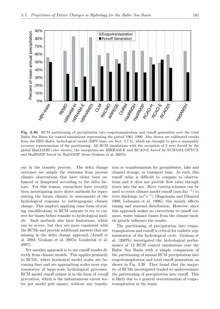
3.7. Projections of Future Changes in Hydrology for the Baltic Sea Basin 181
\J�' (����'���(� �K)� II�X�����(� �
��_
��_
��_
��_
��_
�_
Q�_
�_
��_
�_
^��
���(
� I�&
����
���)
�A�'
����
'�(�
(� �
;F
����
��
K\�
";
+K;
!��;
;+K
;!�
��
?�K
!��
"!K
^\X
\�
;K
�;
��K
�Q;
;��
K�
Q^K
�!"
�;K
�!"
�\K
�!"
�
;��
!�Q;
;+K
;!�
�\
Fig. 3.30. RCM partitioning of precipitation into evapotranspiration and runoff generation over the totalBaltic Sea Basin for control simulations representing the period 1961–1990. Also shown are calibrated resultsfrom the HBV-Baltic hydrological model (HBV-base; see Sect. 3.7.4), which are thought to give a reasonablyaccurate representation of the partitioning. All RCM simulations with the exception of 3 were forced by theglobal HadAM3H (also shown); the exceptions are HIRHAM-E and RCAO-E forced by ECHAM4/OPYC3,and HadRM3P forced by HadAM3P (from Graham et al. 2007b)
out in the transfer process. The delta changeextremes are simply the extremes from presentclimate observations that have either been en-hanced or dampened according to the delta fac-tors. For this reason, researchers have recentlybeen investigating more direct methods for repre-senting the future climate in assessments of thehydrological response to anthropogenic climatechange. This employs applying some form of scal-ing (modification) to RCM outputs to try to cor-rect for biases before transfer to hydrological mod-els. Such methods also have limitations, whichcan be severe, but they are more consistent withthe RCMs and provide additional answers that aremissing in the delta change approach (Arnell etal. 2003; Graham et al. 2007a; Lenderink et al.2007).
Yet another approach is to use runoff results di-rectly from climate models. This applies primarilyto RCMs, where horizontal model scales are be-coming finer and are approaching scales more rep-resentative of large-scale hydrological processes.RCM model runoff output is in the form of runoffgeneration, which is the instantaneous excess wa-ter per model grid square, without any transla-
tion or transformation for groundwater, lake andchannel storage, or transport time. As such, thisrunoff value is difficult to compare to observa-tions and it does not provide flow rates throughrivers into the sea. River routing schemes can beused to route climate model runoff (mmday−1) toriver discharge (m3 s−1) (Hagemann and Dümenil1999; Lohmann et al. 1996); this mainly affectstiming and seasonal distribution. However, sincethis approach makes no corrections to runoff vol-umes, water balance biases from the climate mod-els greatly influence the results.
The partitioning of precipitation into evapo-transpiration and runoff is critical for realistic rep-resentation of the hydrological cycle. Graham etal. (2007b) investigated the hydrological perfor-mance of 13 RCM control simulations over theBaltic Sea Basin with a simple comparison ofthe partitioning of annual RCM precipitation intoevapotranspiration and total runoff generation, asshown in Fig. 3.30. They found that the major-ity of RCMs investigated tended to underestimatethe partitioning of precipitation into runoff. Thisis likely due to a general overestimation of evapo-transpiration in the basin.
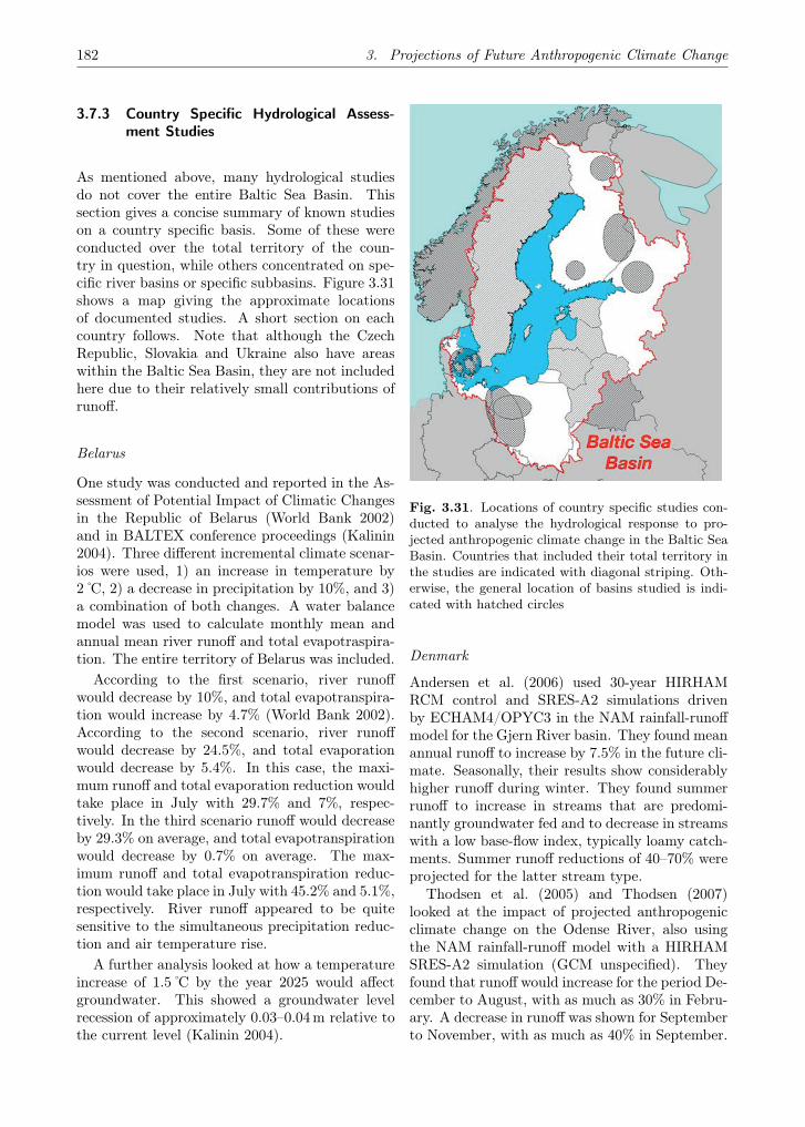
182 3. Projections of Future Anthropogenic Climate Change
3.7.3 Country Specific Hydrological Assess-ment Studies
As mentioned above, many hydrological studiesdo not cover the entire Baltic Sea Basin. Thissection gives a concise summary of known studieson a country specific basis. Some of these wereconducted over the total territory of the coun-try in question, while others concentrated on spe-cific river basins or specific subbasins. Figure 3.31shows a map giving the approximate locationsof documented studies. A short section on eachcountry follows. Note that although the CzechRepublic, Slovakia and Ukraine also have areaswithin the Baltic Sea Basin, they are not includedhere due to their relatively small contributions ofrunoff.
Belarus
One study was conducted and reported in the As-sessment of Potential Impact of Climatic Changesin the Republic of Belarus (World Bank 2002)and in BALTEX conference proceedings (Kalinin2004). Three different incremental climate scenar-ios were used, 1) an increase in temperature by2 C, 2) a decrease in precipitation by 10%, and 3)a combination of both changes. A water balancemodel was used to calculate monthly mean andannual mean river runoff and total evapotraspira-tion. The entire territory of Belarus was included.
According to the first scenario, river runoffwould decrease by 10%, and total evapotranspira-tion would increase by 4.7% (World Bank 2002).According to the second scenario, river runoffwould decrease by 24.5%, and total evaporationwould decrease by 5.4%. In this case, the maxi-mum runoff and total evaporation reduction wouldtake place in July with 29.7% and 7%, respec-tively. In the third scenario runoff would decreaseby 29.3% on average, and total evapotranspirationwould decrease by 0.7% on average. The max-imum runoff and total evapotranspiration reduc-tion would take place in July with 45.2% and 5.1%,respectively. River runoff appeared to be quitesensitive to the simultaneous precipitation reduc-tion and air temperature rise.
A further analysis looked at how a temperatureincrease of 1.5 C by the year 2025 would affectgroundwater. This showed a groundwater levelrecession of approximately 0.03–0.04m relative tothe current level (Kalinin 2004).
Fig. 3.31. Locations of country specific studies con-ducted to analyse the hydrological response to pro-jected anthropogenic climate change in the Baltic SeaBasin. Countries that included their total territory inthe studies are indicated with diagonal striping. Oth-erwise, the general location of basins studied is indi-cated with hatched circles
Denmark
Andersen et al. (2006) used 30-year HIRHAMRCM control and SRES-A2 simulations drivenby ECHAM4/OPYC3 in the NAM rainfall-runoffmodel for the Gjern River basin. They found meanannual runoff to increase by 7.5% in the future cli-mate. Seasonally, their results show considerablyhigher runoff during winter. They found summerrunoff to increase in streams that are predomi-nantly groundwater fed and to decrease in streamswith a low base-flow index, typically loamy catch-ments. Summer runoff reductions of 40–70% wereprojected for the latter stream type.
Thodsen et al. (2005) and Thodsen (2007)looked at the impact of projected anthropogenicclimate change on the Odense River, also usingthe NAM rainfall-runoff model with a HIRHAMSRES-A2 simulation (GCM unspecified). Theyfound that runoff would increase for the period De-cember to August, with as much as 30% in Febru-ary. A decrease in runoff was shown for Septemberto November, with as much as 40% in September.
3.7. Projections of Future Changes in Hydrology for the Baltic Sea Basin 183
They also found that extremes would be more pro-nounced, both at high flows and at low flows.
Estonia
A coordinated study using the same set of anthro-pogenic climate change scenarios generated by twoGCMs was reported in the Country Case Studyon Anthropogenic Climate Change Impacts andAdaptation Assessments in the Republic of Esto-nia (Tarand and Kallaste 1998) and other publi-cations (Kallaste and Kuldna 1998; Järvet et al.2000; Roosaare 1998). Additionally, another studyusing five incremental scenarios was conducted forthe Lake Võrtsjärv (Järvet 1998).
The MAGICC model (Wigley and Raper 1987;1992a; 1992b) and SCENGEN program were usedfor anthropogenic climate change scenario genera-tion in the country case study (Keevallik 1998).Three alternative IPCC GHG emissions scenar-ios (IS92a, IS92c, IS92e) were combined with re-sults of two GCM experiments (HadCM2 andECHAM3). As a result, six anthropogenic climatechange scenarios up to year 2100 were preparedfor modelling anthropogenic climate change im-pact on river runoff. The three IPCC scenarioswere qualitatively labeled as MIN (IS92c), MID(IS92a) and MAX (IS92e), as used in the discus-sion below.
Several different hydrological models and toolswere used for the analysis of river runoff, evapo-transpiration, groundwater and water supply. Thewater balance model WATBAL was used for riverrunoff with a monthly time step. The entire ter-ritory of Estonia, subdivided into western Estoniawith strong influence from the Baltic Sea, and cen-tral and eastern Estonia with a more continentalclimate. The territory was further subdivided into36 river basins. In some studies the watershed ofthe Väike-Emajogi River was studied in greaterdetail.
Evapotranspiration was shown to increase un-der all six scenarios studied. The predictedchanges would affect evapotranspiration more inthe cold season than in the growing season. How-ever, the change in the magnitude is much smalleron the annual scale, as the cold season evapotran-spiration constitutes only 10–13% of the annualevapotranspiration. The most significant increasewas simulated using the ECHAM3-MAX scenario.In absolute values, the ECHAM3-MAX scenariopredicted evapotranspiration increases of 16mmin June and about 4mm in January.
The modelled changes in the mean annualrunoff in different basins and scenarios range from−1% to +74%. The largest increases were foundfor the Emajogi River, and for a number of smallriver basins. An increase in total annual runoff by20–40% (HadCM2-MID) and 30–60% (ECHAM3-MID) was modelled for the year 2100.
Seasonal dynamics of runoff were analysed forseveral rivers and showed the projected runoff in-crease in winter to have the largest impact. Themaximum increase for the Emajogi River was pro-jected for April or May (depending on the modeland scenario). Runoff maximums in spring wereshown to decrease considerably in the central andwestern parts of Estonia. This is related to theprojection that the duration of snow cover wouldalso decrease considerably. Among the single riverbasins studied, the projection for the small LoveRive on the Saaremaa Island stands out; it showedthe lowest increase in every scenario.
Groundwater recharge was shown to increaseon average by 20–40% according to these simu-lations with a maximum increase of up to 75%increase. The ratio of the groundwater contri-bution to river runoff would increase from 30 to40%. The modelling results also indicated a riseof long-term mean annual groundwater levels byabout 0.5–0.8m in northern Estonia, and 0.2–0.4 m in southern Estonia. Furthermore, consider-able changes would occur in the seasonal dynamicsof the groundwater regime, with rising water lev-els in spring and autumn. This would tend towardan earlier onset of flooding.
Finland
As outlined by Bergström et al. (2003), threemajor studies concerning anthropogenic climatechange and hydrology have been conducted in Fin-land. The Nordic research programme on ClimateChange and Energy Production (CCEP; Sælthunet al. 1998) was carried out during 1991–1996. Themultidisciplinary Finnish Research Programme onClimate Change (SILMU) was carried out dur-ing 1991–1995 (SILMU 1996; Vehviläinen andHuttunen 1997) and more recently, the ILMAVAproject (ILMAVA 2002). Additional studies havefocused on hydrological impacts and design floods(Tuomenvirta et al. 2000).
The CCEP research programme used an an-thropogenic climate change scenario based on sta-tistically downscaled information from four differ-ent General Circulation Models. The SILMU sce-

184 3. Projections of Future Anthropogenic Climate Change
narios were based on an intercomparison study ofGCM simulation results (Räisänen 1994). For theILMAVA project (ILMAVA 2002), two SRES sce-narios (A2 and B2; Nakićenović et al. 2000) fromthe HadCM3 GCM were used.
All of the studies used the operational wa-tershed models of the Finnish Environment In-stitute (SYKE; Vehviläinen 1994), which arebased on a Finnish version of the HBV-model(Bergström 1976). All studies thus far have usedthe delta change approach for transferring the an-thropogenic climate change signal from climatemodels to hydrological models and have relied onGCM models.
The drainage basins used for hydrological stud-ies were selected to represent different regions ofFinland, as shown in Fig. 3.31. Starting withthe CCEP project, subbasins from southern andnorthern Finland were used. In the SILMUproject, a similar selection of drainage basins waschosen, but larger areas in the southeast were in-cluded. For the ILMAVA project, basins produc-ing most of Finland’s hydropower were chosen.
The trend of results from the more recentILMAVA project is similar to results from the ear-lier CCEP and the SILMU projects. The pro-jected anthropogenic climate change was shown tostrongly affect the seasonal distribution of runoffand other water balance terms. With increasedtemperature, snow cover diminishes or almost van-ishes in southern Finland, and its duration be-comes shorter. Frequent thawing periods resultin increased occurrence of winter floods and de-creased spring floods. Summers become drier dueto the longer summer season, and increases occurin both evapotranspiration and lake evaporation.
There are differences between the results ofthese studies, as seen for changes in runoff. An-nual runoff from the Kemihaara subbasin (Kemi-joki basin, northern Finland) was found to in-crease by 2% in the CCEP project, whereas inthe SILMU project essentially no annual changewas found. Results from ILMAVA showed an-nual runoff in this sub-basin to increase by 5 to8%. In the Oulujoki drainage basin (mideasternFinland), the CCEP project reported nearly nochange in annual runoff, but results from the IL-MAVA project showed an annual increase of 2 to7%. For the Vuoksi drainage basin (south-easternFinland), changes in annual runoff varied between−1 to +4% (CCEP), −2% (SILMU) and 0 to +8%(ILMAVA). These differences were due primarilyto differences of climate scenarios, especially re-
garding precipitation. However, it was also foundthat results were quite sensitive to how evapotran-spiration and lake evaporation are represented.
Results from the SILMU project also showedthat changes in maximum flows for large basinswith a high concentration of lakes depend stronglyon the location of the site within the lake sys-tem. For upper subbasins of large basins andbasins without lakes, the maximum discharge de-creased by 20 to 60% due to smaller spring floods.However, maximum inflows to the central lakesof large basins increased by some 3 to 17%, assnowmelt and precipitation accumulate into theselakes during winter, when no evaporation takesplace. Thus, due to increased volume accumulat-ing in large lakes, the maximum discharge of thelakes would increase.
Germany
No specific studies were found for German basinsflowing into the Baltic Sea. However, runoff fromGerman territory is included in projections of thehydrological response for the Oder River. See re-lated studies under Poland.
Latvia
Related studies were reported in the Third Na-tional Communication of the Republic of Latviaunder the United Nations Framework Conven-tion on Climate Change (Ministry of Environmen-tal Protection and Regional Development 2001),BALTEX conference proceedings (Butina et al.1998a), and Proceedings of the Second Interna-tional Conference on Climate and Water (Butinaet al. 1998b; Jansons and Butina 1998).
Anthropogenic climate change scenarios fromthe UKMO GCM transient scenario (Murphy andMitchell 1994) and the GENESIS GCM (Thomp-son and Pollard 1995) scenario were used. Theresults of the GENESIS GCM were represented inthe form of monthly corrections to meteorologicalparameters received from maps of low resolution(Henderson-Sellers and Hansen 1995). Doubling ofthe atmospheric CO2 concentration was assumed.The climate scenario predicts a 3–3.5 C rise in airtemperature and a 20–25% increase in precipita-tion.
All of Latvia was included in the Third NationalCommunication. Studies by Butina et al. (1998b)were done in the Liulupe basin (17,600 km2),its subbasin Viesite-Sudrabkalni, and the Berze
3.7. Projections of Future Changes in Hydrology for the Baltic Sea Basin 185
basin. Hydrological assessments were made usingthe HBV hydrological model (Bergström 1995).
According to the assessment in the Third Na-tional Communication, groundwater levels in thelowest coastal zone of Riga Bay could rise by 50–70 cm. Risk of floods would increase in the lowerreaches of the large rivers Liulupe, Daugava andGauja. Rising groundwater level could cause se-rious problems to people living in lowlands in thecoastal zone where elevation above sea level is only0.7 to 2.0m.
Butina et al. (1998b) reported that, due tohigher temperatures, more winter precipitationwould fall as rain instead of snow. The springsnowmelt would shift from April to February oreven earlier. River flow would be higher during allseasons according to the GENESIS scenario, butnot for the UKMO GCM scenario. The UKMOGCM transient scenario showed river flow to in-crease by 11% on average (ranging from −7 to+36%), while, according to the GENESIS sce-nario, river flow would increase on average by 83%(ranging from 55 to 120%).
Jansons and Butina (1998) used the same sce-narios to investigate changes in runoff and nutrientload for the small agricultural Berze catchment.According to the GENESIS scenario, annual flowwould increase by 57%, but the UKMO GCM sce-nario showed no significant increase in flow. Floodpeaks increased by 32% with GCM GENESIS in-put, while the UKMO GCM scenario predicteda decrease in flood peaks. The GCM GENESISscenario generated an increase in summer flow,whereas a moderate decrease was projected usingthe UKMO GCM scenario.
Lithuania
Studies were reported in Lithuania’s Second Na-tional Communication under the Framework Con-vention on Climate Change (Ministry of the En-vironment 2003) and in BALTEX conference pro-ceedings (Rimkus 2001). The National Communi-cation used scenario results from the GFDL GCM.Rimkus used results from five GCMs over Lithua-nia; these were HadCM2, ECHAM4, CGCM1,GFDL-R15 and CSIRO-Mk2.
According to the GFDL model, the averagesummer temperature by 2050 would exceed therecent average by 1.7 C, and the average win-ter temperature would be 1.2–1.3 C higher. Thesummer precipitation would increase slightly un-til 2020 and then start decreasing in the subse-
quent period. The amount of summer precipita-tion by 2050 would be 5–6% lower than the presentlevel, and the winter precipitation would be 5–6.5% higher.
No hydrological models were used for the assess-ment described in the Second National Communi-cation; only analysis of the climate model outputswas carried out. This included assessment of pos-sible effects over all of Lithuania. One outcomefrom this study was that the extensive wetlands ofthe country would become dryer with acceleratedsuccession.
Rimkus (2001) used an analysis of regressionlinks between climate variables. Data from thenearest grid points were used to assess changes insnow water equivalent in Lithuania. Two caseswere analysed: 1) the mean temperature for thesnow accumulation period would rise by 1.5 Cand precipitation would rise by 8 mm (as expectedaround the year 2040); 2) the mean temperature ofthe snow accumulation period would rise by 3.0 Cand precipitation would increase by 14 mm (as ex-pected around the year 2065).
Results from Rimkus (2001) showed that maxi-mum snow depth in Lithuania would decrease sig-nificantly under anthropogenic climate change sce-narios. For the reference period 1961–1990, max-imum snow water equivalent was 40 mm on aver-age, ranging from 21 to 60mm. Average maximumsnow water equivalent would decrease to 34 mm,with temperature and precipitation increasing by1.5 C and 8 mm, respectively. Average maximumsnow water equivalent would decrease to 28 mm,with temperature and precipitation increasing by3.0 C and 14 mm, respectively.
Norway
In addition to the Nordic research programme onClimate Change and Energy Production (CCEP;Sælthun et al. 1998) during 1991-1996 (see alsoFinland and Sweden), two national projects on an-thropogenic climate change and hydrological im-pacts have been performed in Norway (Bergströmet al. 2003). These were “Climate change andwater resources” (Sælthun et al. 1990) conductedprior to CCEP, and “Climate change and energyproduction potential” (Roald et al. 2002; Skaugenet al. 2002; Skaugen and Tveito 2002), which wascarried out during 2000–2002.
Sælthun et al. (1990) used anthropogenic cli-mate change scenarios based on the NCAR model(Washington and Meehl 1989). No downscaling

186 3. Projections of Future Anthropogenic Climate Change
procedure was applied. Two climate scenarioswere used: one based on what was considered themost probable changes of precipitation and tem-perature, and one based on greater changes. Asdescribed under Finland, CCEP used an anthro-pogenic climate change scenario based on statis-tically downscaled information from four differ-ent General Circulation Models (Sælthun et al.1998). Local and regional climate scenarios havealso been studied in the RegClim project since1997. This has focused mainly on results originat-ing from ECHAM4/OPYC3 simulations using theIPCC IS92a scenario. Regional downscaling fromboth statistical techniques (Hanssen-Bauer et al.2000, 2001; Benestad 2002a) and RCM modelling(Bjørge et al. 2000) was used.
Runoff simulations were performed with theHBV Model (Bergström 1995). Evapotranspi-ration was estimated according to temperaturebased methods developed by Sælthun et al. (1990),which were further improved in later studies(Sælthun 1996). In Sælthun et al. (1990) 7 basinswere used, in Sælthun et al. (1998) 10 basins, andin Roald et al. (2002) 42 basins. These basins aredistributed over all of Norway and represent dif-ferent hydrological regimes. Future water balancechanges for the whole of Norway were also includedin Roald et al. (2002), Engen-Skaugen et al. (2005)and Roald et al. (2006).
Sælthun et al. (1990) concluded that correctmodelling of evapotranspiration is important whenit comes to estimating the future water balance(Fossdal and Sælthun 1993). The annual evapo-transpiration increase was 40–55mm in mountain-ous areas, 45–100mm in transitional areas and 50to 110mm in lowland areas. The correspondingincrease in annual runoff for mountainous areaswas more than 750mm. In lowland and forestedinland basins, annual runoff was shown to decreasein response to increased evapotranspiration. Thewettest scenario resulted in increased runoff overall of Norway, up to 15% on the west coast.
Sælthun et al. (1998) drew similar conclusions.Evapotranspiration was shown to increase due toincreased summer temperature and longer snowfree periods. Annual evapotranspiration would in-crease between 100 and 200mm over 100 years,and precipitation would increase between 15 and20% for the same period. An evapotranspirationincrease of 100mm would counterbalance the pre-cipitation increase in areas where present annualprecipitation is less than 700mm. The annualrunoff would therefore increase in western areas
and decrease in inland areas. Results from Roaldet al. (2002) showed that runoff would increaseover almost all of Norway, following the same pat-tern as the increase in precipitation.
The scenarios in Sælthun et al. (1990) andSælthun et al. (1998) showed a drastic change inthe seasonal distribution of runoff, with increasesin winter, reduced spring flood peaks with earlieroccurrence and decreases in summer. The changeswere mostly controlled by the effect of tempera-ture on snow processes. The seasonal distributionwould not change much in coastal regions that donot have stable snow cover under the present cli-mate. The largest changes were shown for thelower elevations of regions that now have a sta-ble snow cover during winter. Roald et al. (2002)showed that summer runoff would decrease andautumn runoff would increase, especially on thewest coast.
Sælthun et al. (1990) concluded that melting ofNorwegian glaciers would increase and the sum-mer discharge in glacier basins would thereforeincrease. Most of the glaciers would also expe-rience a negative mass balance, resulting in re-duced volume. The long-term effect would be re-duced summer runoff in basins that have glacierstoday. However, high altitude glaciers in mar-itime climates with high precipitation might main-tain their volume and even grow. In Roald et al.(2002), simulations suggested that glaciers wouldaccumulate and the effect on runoff would be neg-ative, as opposed to a state of equilibrium.
Poland
Kaczmarek et al. (1997) used data from severalGCMs with their hydrological model CLIRUN(Kaczmarek 1996; Kaczmarek 1993) for studyingthree middle-size catchments in Poland. Thesewere followed up by additional studies with up-dated models (Kaczmarek 2003; Kaczmarek 2004).De Roo and Schmuck (2002) report on studiesusing different incremental scenarios. The earlystudies by Kaczmarek focused on the Warta basin,which is the largest tributary to the Oder River.De Roo and Schmuck analysed the entire Oderbasin. Later studies by Kaczmarek covered otherregions of Poland.
Kaczmarek et al. (1997) noted that current (i.e.1997) climate models did not offer the degree ofwatershed specific information required for hydro-logical modelling. Moreover, the results for riverflow showed great differences depending on the
3.7. Projections of Future Changes in Hydrology for the Baltic Sea Basin 187
different models used (Kaczmarek 1996). Gutry-Korycka (1999) also noted that the informationfrom GCMs was not sufficient for definite projec-tions of the influence of warming on river flow inthe second half of the 21st century. Similarly, re-sults on hydrological drought frequency differedconsiderably between the models, both in magni-tude and direction (Kaczmarek and Jurak 2003).
De Roo and Schmuck (2002) used the LIS-FLOOD Model in their studies together with sevendifferent incremental scenarios. They looked at,1) annual precipitation increases of 15% and 22%,2) annual precipitation decreases of 10% and 15%,3) an average annual temperature increase and de-crease of 1 C and 4) a combined 15% increasein precipitation and 1 C increase in temperature.They reported that a 15% increase in precipitationshowed a sharp increase in maximum discharge of600–900m3 s−1 at all major gauge locations. Adecrease in precipitation by 10% resulted in a de-crease of peak discharge of 430–560 m3 s−1. A pre-cipitation decrease by 15% led to a decrease ofpeak discharge of 590–810 m3 s−1.
Kaczmarek (2003) studied the influence of cli-mate change on the water balance in Poland forthe period 2030-2050 using the CLIRUN3 hy-drological model and two anthropogenic climatechange scenarios: GFDL (warm and dry) andGISS (warm and wet). They projected a de-crease in river flow and soil moisture in summerand autumn. The flood season would also shiftfrom March–April to January–February, in accor-dance with results from the EU project “Impact ofClimate Change on Water Resources in Europe”(from the 4th Framework Programme).
Kaczmarek (2004) stated that although it is cer-tain that a warmer climate will accelerate the hy-drological cycle, less is known about impacts atriver basin levels. In the maritime parts of Europe,he reports a tendency toward increasing stream-flow during winter. Furthermore, a reduction dur-ing low flow periods is expected, which could leadto increased drought frequency and, in most catch-ments, increased flood frequency. For Poland it-self, projected flow characteristics vary betweenmodels and scenarios.
Russia
Two studies were reported in Meteorology and Hy-drology (Kondratyev and Bovykin 2003; Meleshkoet al. 2004), one study in Water Resources (Grig-oryev and Trapeznikov 2002), and one study in an
INTAS Report (Kondratyev 2001). The study per-formed by Meleshko et al. (2004) covers the entireBaltic Sea Basin and is summarised in Sect. 3.7.4.Kondratyev and Bovykin (2003) used climate sce-narios from ECHAM4/OPYC3 calculated for theLake Ladoga drainage basin (258,000 km2) for theperiod 2001–2100 (Arpe et al. 2000; Golitsyn etal. 2002). They coupled this to a model of hy-drological regimes and nutrient fluxes for the sys-tem catchment and lake. This was applied forthe much smaller Lake Krasnoye and its drainagebasin (168 km2) with the help of regression equa-tions (Kondratyev et al. 1998; Kondratyev andBovykin 2000). For Kondratyev (2001), eight dif-ferent incremental scenarios were used instead.
According to Kondratyev and Bovykin (2003),a moderate increase in river discharge was pro-jected for Lake Krasnoye. Snow water equivalentwas shown to decrease by 25–28%. Soil moisturein the watershed would increase by 7–8% in au-tumn and winter, and decrease by 10–18% in sum-mer. Spring floods would start earlier. The lakelevel would be characterised by earlier spring max-imums and a 10 cm lower water level in summer,as compared to the 1964–1984 reference period.
Results from Kondratyev (2001) summarisedcharacteristics of annual runoff, maximum waterdischarge in the tributaries, soil moisture in au-tumn, and numerous nutrient transport variablesfor the Lake Krasnoye catchment. Their findingsshowed mean annual runoff changes from −26%to +35%, maximum runoff changes from −59%to +66% and autumn soil moisture changes from−26% to +14%.
Grigoryev and Trapeznikov (2002) used prob-abilistic incremental scenarios for Lake Ladoga.They applied a transfer function model with cli-mate characteristics as input and water level in thelake as output. According to their probabilisticclimate scenario, the water level in Lake Ladogawould decrease by 50 cm.
Sweden
Sweden also participated in the Nordic researchprogramme on Climate Change and Energy Pro-duction (CCEP; Sælthun et al. 1998) during 1991–1996 (see also Finland and Norway). This re-sulted, among others, in a comprehensive studyof evapotranspiration effects (Lindström et al.1994). Sensitivity studies of climate change ef-fects on hydrology were conducted in an earlystudy of effects on river regulation (Carlsson and

188 3. Projections of Future Anthropogenic Climate Change
Sanner 1996). From 1997 to 2003, hydrologi-cal impacts studies concerning anthropogenic cli-mate change were mainly produced within theSwedish Regional Climate Modelling Programme(SWECLIM; Bergström et al. 2001; Gardelin etal. 2002a; Gardelin et al. 2002b; Graham et al.2001; Andréasson et al. 2002; Andréasson et al.2004). Most recently, hydrological impact stud-ies were conducted within the EU PRUDENCEproject (Graham et al. 2007a).
As described under Finland, the CCEP re-search programme used an anthropogenic cli-mate change scenario based on statistically down-scaled information. The anthropogenic climatechange scenarios from SWECLIM came primar-ily from RCM modelling. Most simulationswere based on three different GCMs, HadCM2,HadAM3H and ECHAM4/OPYC3, downscaledwith the Rossby Centre regional climate modelsRCA (Rummukainen et al. 2001; Jones et al. 2004)and RCAO (Döscher et al. 2002). Some use ofstatistically downscaled scenarios was also made(Bergström et al. 2003). Earlier SWECLIM sim-ulations were based on business as usual (BaU)emissions scenarios (Houghton et al. 1992), whilemore recent simulations used the SRES (A2 andB2) scenarios (Nakićenović et al. 2000).
The HBV hydrological model was used in theSwedish studies (Bergström et al. 2001; Grahamet al. 2001). Particular effort was placed on de-veloping appropriate representation of evapotran-spiration processes and on the interface used fortransferring anthropogenic climate change infor-mation from climate models to hydrological mod-els. Most studies to date used the delta change ap-proach for transferring the signal of anthropogenicclimate change to hydrological models. The PRU-DENCE studies also investigated the use of pre-cipitation scaling.
Six test basins representing different climateand hydrological regimes in Sweden were initiallychosen for impacts analysis within both CCEPand SWECLIM. They were later supplementedby two additional basins, the Lule River Basin,representing a high degree of river regulation,and Lake Vänern, the basin containing Sweden’slargest lake. Limited analyses to address soil frostand groundwater dynamics were also made in theSvartberget experimental forest site in northernSweden. In the last year of SWECLIM, a hydro-logical model was developed to conduct hydrolog-ical change studies over all of Sweden using some1000 subbasins.
Results from the HBV model using eight differ-ent regional climate simulations from RCA1 andfour simulations from RCAO were reported byAndréasson et al. (2004). A general tendency isthe shift in the runoff regime towards decreasingspring flood peaks and increasing autumn and win-ter flows. Mean annual change in runoff from thesimulations shows increasing runoff in northernbasins and decreasing runoff in southern basins.In the northernmost basin (Suorva) there is lit-tle impact on the magnitude of spring runoff assnow accumulation is less affected in this region.However, the timing of snowmelt is affected in allbasins. Summer flows are severely reduced in thetwo southernmost basins, Blankaström and Torse-bro.
The more recent RCAO scenario results gener-ally show higher runoff during winter and lowerspring runoff than results from the earlier RCA1scenarios. The relative range of changed runoffbetween different simulations is larger towards thesouth of the country. This may be explained partlyby increasing rates of projected evapotranspira-tion further south and associated uncertainty inmodelling changes to future evapotranspiration.For a majority of the basins, the RCA1-HadCM2simulations show greater impact on runoff thanfor RCA1-ECHAM4/OPYC3 simulations. Re-garding RCAO simulations, impacts driven byECHAM/OPYC3 are generally larger than thosedriven by HadAM3H.
Attempts to make some assessment of extremeflows were included in Bergström et al. (2001),Gardelin et al. (2002a) and Andréasson et al.(2004). These papers present changes in 100-yearflood events obtained from hydrological modellingand frequency analysis. They report a decreasein the frequency of high spring floods and an in-crease in the frequency of flooding events for au-tumn and winter in many basins. However, suchconclusions are subject to great uncertainty as thedelta change approach used for these studies doesnot provide good representation of changes in vari-ability coming from the climate models.
3.7.4 Baltic Sea Basinwide HydrologicalAssessment
Studies addressing the hydrological response toanthropogenic climate change specifically for theBaltic Sea Basin are not numerous. On a globalscale, IPCC (2001b) presented hydrological mod-elling results for all continents. On a Euro-
3.7. Projections of Future Changes in Hydrology for the Baltic Sea Basin 189
pean scale, Arnell (1999), Strzepek and Yates(1997), Lehner et al. (2001) and Meleshko et al.(2004) presented hydrological modelling resultsthat include the Baltic Sea Basin. On regionalscales, Graham (1999b) presented early resultsthat specifically address the Baltic Sea Basin.These were updated to include improved methodsand newer RCM scenarios in Graham (2004) andto include an ensemble of RCM models in Gra-ham et al. (2007b). Finally, both Hagemann andJacob (2007) and Graham et al. (2007b) presentresults for the Baltic Sea Basin using runoff rout-ing methods. A summary of results from thesestudies follows below. All used the delta changeapproach, unless otherwise noted.
3.7.4.1 Projected Changes in Runoff
Included in the global scale results presentedby the IPCC are maps showing change in an-nual runoff at the end of the 21st century frommacroscale hydrological modelling. Results us-ing two different GCM simulations (HadCM2,HadCM3) are shown there in mm yr−1 (IPCC2001b, Fig. TS-3). Although the two simulationsshow contradictory trends for other regions aroundthe globe, results for the Baltic Sea Basin arequalitatively similar. The trend shown is for in-creased annual runoff in the north of the basinand decreased runoff in the south. Magnitudesrange from up to +150mm yr−1 in the north to−150mm yr−1 in the south. For comparison, theobserved total mean annual runoff to the BalticSea is some 280mm yr−1 (Bergström and Carls-son 1994). Close examination of the IPCC maps,however, reveals that the location where projectedrunoff change goes from positive to negative variesconsiderably between the two simulations. For in-stance, in Finland for simulations using HadCM2 apositive change in runoff is shown, while for sim-ulations using HadCM3 much of the country isshown with a negative change.
More detail is found in Arnell (1999), wherethe results from macroscale hydrological modellingusing four different GCM simulations (based onHadCM2 and CCC) are shown. In this case, theprojected future climate is the middle of the 21st
century, the 2050s. Here again, an increase inrunoff is simulated for the northern areas of theBaltic Sea Basin and a decrease is simulated forthe southern areas. Results are expressed in termsof percent change in annual runoff and range fromsome +50% to −25% for the Baltic Sea Basin.
Although Arnell (1999) comments that there arelarge areas of agreement over Europe between thesimulations, he specifically notes that discrepan-cies are high in the eastern Baltic region. Resultsfor this area show a reduction of runoff by up to20% in one simulation and an increase of over 25%in another simulation. Arnell (1999) also notesthat by the 2050s snow cover at the end of Marchwill have disappeared across eastern Poland, Be-larus, Ukraine and the Baltic sea coast. This isbroadly comparable to more recent findings fromRCMs (see Sect. 3.5.2.4).
Meleshko et al. (2004) used results fromseven GCMs (CGCM2, CSIRO-Mk2, CSM1.4,ECHAM4/OPYC3, GFDL-R30-c, HadCM3 andPCM). They applied a simple balance equationto define annual discharge for large river basinsfrom GCM inputs of precipitation and evapotran-spiration. This was done for the entire Baltic SeaBasin. Projections using the ensemble of sevenGCMs showed an overall increase in total riverrunoff to the Baltic Sea of 1.9% for the period2041–2060 and 5.7% for the period 2080–2099.
Graham (1999b) presented results using theHBV-Baltic hydrological model (Graham 1999a)together with climate model simulations from theRCA Model (Rummukainen et al. 1998). HBV-Baltic is a large-scale hydrological modelling ap-plication that covers the total Baltic Sea Basinup to its outflow into Öresund and the DanishBelts, as shown in Fig. 3.32. Three RCM simula-tions representing “business as usual” GHG emis-sions scenarios with forcing from two differentGCM simulations (HadCM2, ECHAM4/OPYC3)were presented. Two of these simulations used ahorizontal resolution of 88 km and were referredto as RCA88-H and RCA88-E for HadCM2 andECHAM4/OPYC3 forcing, respectively. The ef-fects from the RCA88-E scenario simulations werequite different to those from RCA88-H, particu-larly in the southern Baltic river basins. Totalriver discharge to the Baltic Sea decreased consid-erably for the RCA88-E simulation but increasedsomewhat for the RCA88-H simulation. Theseearly simulations were based on 10-year time peri-ods for the present compared to 10-year time pe-riods for the future, which are relatively short interms of representing interannual variability.
In Graham (2004) and Graham et al. (2007b), anumber of additional hydrological response simu-lations were carried out using HBV-Baltic. Theseused 30-year time periods to represent both thefuture climate and the control climate (present

190 3. Projections of Future Anthropogenic Climate Change
Fig. 3.32. Basin boundariesfor HBV-Baltic. The five mainBaltic Sea drainage basins areshown with thick lines (adaptedfrom Graham 1999a)
climate). Graham et al. (2007b) used many of theRCM simulations from PRUDENCE (Christensenet al. 2007; see Sect. 3.5.1.2). This showed the en-semble of RCMs driven by the same GCM with thesame GHG emissions scenario to result in a rangeof potential outcomes that follow similar meantrends. Based on the SRES-A2 emissions scenario(see Annex 6), Fig. 3.33 shows results of river dis-charge summarised as total inflows to the five mainsubregional Baltic Sea drainage basins and for thetotal Baltic Sea Basin. Results using nine RCMsimulations with global forcing from HadAM3H(referred to as the common PRUDENCE experi-ment in Sect. 3.5.2) are shown in the left plot ofthe figure. Results using 2 RCM simulations withglobal forcing from ECHAM4/OPYC3 are shownin the right plot of the figure.
General trends in the north show increases inwintertime river flow coupled with somewhat lowerand earlier springtime peak flows. This reflects thesubstantial changes that warmer temperatures willinflict on the snow regime in the north. Trends in
the south show more pronounced effects on sum-mertime river flow. River flow to the Gulf of Fin-land exhibits a combination of these effects, de-pending on which simulations one examines, eventhough these flows are highly dictated by the out-flow from Lake Ladoga. River flow to the totalBaltic Sea Basin is an integration of the combinedeffects to the five main sub-drainage basins.
The range of outcomes helps to characterisethe uncertainty contributed from using differentRCMs. As shown in Fig. 3.33 for RCMs driven byHadAM3H, this range is fairly narrow for muchof the year. However, during late summer andautumn months larger deviations occur, which ismost obvious in the plot for the total Baltic SeaBasin. Although it is not easily seen from theplots, much of this deviation originates from theGulf of Finland and other eastern drainage basins.
According to Kjellström and Ruosteenoja(2007), the climate change signal for precipita-tion in this area is affected by different approachesin the RCMs for representing feedback from the

3.7. Projections of Future Changes in Hydrology for the Baltic Sea Basin 191
Fig. 3.33. Mean river discharge from HBV-Baltic using the delta change approach for RCM-A2 scenarios at∼ 50 km resolution, driven by global forcing from HadAM3H (left ) and ECHAM4/OPYC3 (right ). The plotssummarise results using nine different RCMs with HadAM3H forcing and two RCMs with ECHAM4/OPYC3.The scenarios represent future climate for the period 2071–2100 compared to the control period 1961–1990(adapted from Graham et al. 2007b)
Baltic Sea itself. In particular, anomalously highsea surface temperatures can have an effect (SSTs;see also Sect. 3.5.2.2). One of the two modelsthat shows the greatest increase in river flow fromthe eastern side of the Baltic sea Basin is alsothe model that Kjellström and Ruosteenoja (2007)show to produce the greatest precipitation changein that region due to anomalous SSTs.
Effects on modelled river discharge from usingdifferent GCMs to drive the RCMs are seen bycomparing the left and right plots in Fig. 3.33,although not as many simulations were availableusing ECHAM4/OPYC3. According to these re-sults, forcing with ECHAM4/OPYC3 produceda considerably different river discharge responsethan simulations with forcing from HadAM3H.

192 3. Projections of Future Anthropogenic Climate Change
�����
���
�T�
�_�
�����
�T�T��
����
�T�T�
��
�T�T�T��
����
�T�T�
�_�
����
�T�T�
"�������"�
"���������
#!������$����
"�����%�� ��
#!������&��
�����"��������'������"���
�!�$� �"#��! ���)�A�!�$� �"#��! ���)�A
����������������
Fig. 3.34. Modelled percent volume change in river discharge from HBV-Baltic simulations using RCMscenarios for the period 2071–2100 compared to the control period 1961–1990. This is summarised by seasonfor the five main Baltic Sea drainage basins (Fig. 3.32); December, January, February (DJF); March, April, May(MAM); June, July, August (JJA), and September, October, November (SON). Each bar represents the rangeof results between the simulations performed for SRES-A2 forced by HadAM3H (H/A2, 9 simulations), SRES-B2 forced by HadAM3H (H/B2, 3 simulations), SRES-A2 forced by ECHAM4/OPYC3 (E/A2, 2 simulations),and SRES-B2 forced by ECHAM4/OPYC3 (E/B2, 2 simulations) (created with results from Graham 2004 andGraham et al. 2007b)
River discharge in general tends to be higher forthe ECHAM4/OPYC3 driven simulations. Suchdifferences were also reported by Graham (2004),where simulations from the SRES-B2 scenarioswere presented as well. There it was observed thatthe GCM model used for boundary conditions hasas much impact on total river flow as the emissionsscenarios used.
Changes in river flow to the Baltic Sea are fur-ther summarised in Fig. 3.34 as percent volumechange per season. This figure includes resultsbased on RCMs using two different GHG emissionsscenarios (SRES-A2, SRES-B2) and two differ-ent GCMs (HadAM3H, ECHAM4/OPYC3). Thelength of each bar in the figure shows the rangeof results for each case, although the number ofsimulations varies between the cases (see figurecaption for detail). Qualitatively, there are over-all similarities between the different simulations.In many instances, the results tend to fall withinthe same sign (positive or negative) for the givenseasons. However, the degree of similarity variesamong the different subregions. The considerabledifferences obtained by using different GCMs are
also apparent in these plots (e.g. compare H/A2results to E/A2 results). This figure also showsthat the largest range of uncertainty with respectto the relative change in volume occurs in the Gulfof Riga drainage basin, as evidenced by numerouslong bars.
Two runoff routing schemes have been appliedto the Baltic Sea Basin to date. These are theRCroute scheme (Graham 2002; Graham et al.2007b) and the HD Model (Hagemann and Dü-menil 1999; Graham et al. 2007b; Hagemann andJacob 2007). Both of these were used to producerouted river flow directly from RCM results. Asstated above, hydrological response studies fromriver routing techniques are highly influenced byRCM biases. Therefore they are best used whenconverted to percent change in river discharge, asdone in the reported literature. It was reportedthat despite large differences in individual RCMsimulations, the overall signal of the ensemblemean response was in agreement between RCrouteand the HD Model (Graham et al. 2007b). Thesewere also qualitatively in agreement with the var-ious results using HBV-Baltic as presented above.

3.7. Projections of Future Changes in Hydrology for the Baltic Sea Basin 193
However, choosing a single RCM from this groupof results as a basis for further impact studieswould result in quite different answers dependingon the RCM used.
There is a notable difference between the tworiver routing approaches in that RCroute usesrunoff generation directly from the RCMs andthe HD Model performs its own re-partitioning ofRCM precipitation into runoff and evapotranspira-tion (Hagemann and Jacob 2007). This is a likelyexplanation to why results from the HD Modelshow a narrower range of uncertainty around themean than those from RCroute, as it effectivelyfilters out some of the biases in precipitation par-titioning in the RCMs.
3.7.4.2 Projected Changes in Evapotranspiration
Although evapotranspiration is a critical compo-nent of the water balance, comprehensive anthro-pogenic climate change effects on this variable arelittle reported for the Baltic Sea Basin. One rea-son for this is that there is a large amount of un-certainty associated with evapotranspiration andprojected future climates (Bergström et al. 2001).
Hydrological studies typically include calcula-tion of their own estimates of evapotranspiration,both for the present climate and for future cli-mates. This has shown to produce reasonable es-timates for present climates as calibration can beperformed against observations of river flow. How-ever, using the same calibrated evapotranspirationparameterisations for the future can be suspect,particularly for temperature based methods.
For this reason, delta change techniques havecome into use for estimating evapotranspirationas well (Andréasson et al. 2004; Lenderink et al.2007). There are various ways to perform such es-timates, but a main objective is that the annualpercent change in evapotranspiration matches theannual percent change as simulated by climatemodels, while preserving the water balance inthe hydrological simulations. This approach wasapplied by Graham (2004); estimates of futurechange in evapotranspiration from four simula-tions for the Baltic Sea Basin are presented fromthat work in Table 3.3.
3.7.5 Synthesis of Projected Future Hydrolog-ical Changes
Many different studies using numerous models andapproaches to evaluating projections of hydrolog-ical change within the Baltic Sea Basin are sum-
marised above. The studies were conducted ona broad range of scales, using different levels ofdetail and different future scenario simulations.Although it is difficult to assemble such an ar-ray of results into definite conclusions, there arecommon signals and similarities shown. A funda-mental conclusion is that the assumed projectedfuture anthropogenic climate changes provide thegreatest source of uncertainty for projected futurehydrological changes.
Some robust findings are that snow and coldweather processes were shown to be sensitiveto anthropogenic climate change throughout theBaltic Sea Basin. Warmer temperatures willimpact greatly on snowpack volumes and dura-tion, resulting in considerable impact to timing ofrunoff. Simultaneous increases and/or decreasesin precipitation will strongly affect correspondingrunoff volumes. However, the response of evapo-transpiration is a key process in determining howrunoff volumes will change and how groundwaterlevels will in turn be affected.
Further conclusions are that there will be anorth–south gradient in how projected future hy-drological changes occur over the Baltic Sea Basin,and effects during cold months show larger rela-tive change than for warm months. According toanalyses using an ensemble of RCM anthropogenicclimate change scenarios, the following conclud-ing remarks were made by Graham et al. (2007b)for scenario simulations for the period 2071–2100compared to control simulations for the period1961–1990.
• On average for the total basin, summer riverflows show a decrease of as much as 22%, whilewinter flows show an increase of up to 54%.
• On the large scale, annual river flows show anincrease in the northernmost catchments of theBaltic Sea Basin, while the southernmost catch-ments show a decrease.
• The occurrence of medium to high river flowevents shows a higher frequency.
• High flow events show no pronounced increasein magnitude on the large scale.
• The greatest range of variation in flow due todifferent RCMs occurs during summer to au-tumn.
The authors point out, however, that there are de-ficiencies in the methods used for performing hy-drological response studies. Although the deltachange approach may provide usable estimates ofmean changes, representation of changes to ex-
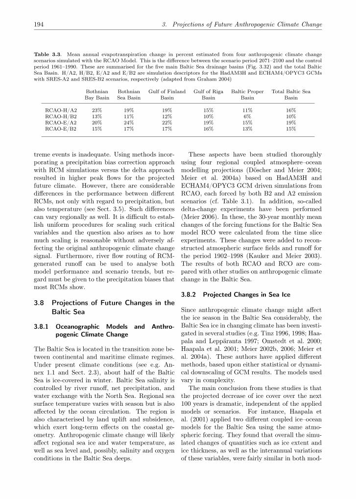
194 3. Projections of Future Anthropogenic Climate Change
Table 3.3. Mean annual evapotranspiration change in percent estimated from four anthropogenic climate changescenarios simulated with the RCAO Model. This is the difference between the scenario period 2071–2100 and the controlperiod 1961–1990. These are summarised for the five main Baltic Sea drainage basins (Fig. 3.32) and the total BalticSea Basin. H/A2, H/B2, E/A2 and E/B2 are simulation descriptors for the HadAM3H and ECHAM4/OPYC3 GCMswith SRES-A2 and SRES-B2 scenarios, respectively (adapted from Graham 2004)
Bothnian Bothnian Gulf of Finland Gulf of Riga Baltic Proper Total Baltic SeaBay Basin Sea Basin Basin Basin Basin Basin
RCAO-H/A2 23% 19% 19% 15% 11% 16%RCAO-H/B2 13% 11% 12% 10% 6% 10%RCAO-E/A2 20% 24% 22% 19% 15% 19%RCAO-E/B2 15% 17% 17% 16% 13% 15%
treme events is inadequate. Using methods incor-porating a precipitation bias correction approachwith RCM simulations versus the delta approachresulted in higher peak flows for the projectedfuture climate. However, there are considerabledifferences in the performance between differentRCMs, not only with regard to precipitation, butalso temperature (see Sect. 3.5). Such differencescan vary regionally as well. It is difficult to estab-lish uniform procedures for scaling such criticalvariables and the question also arises as to howmuch scaling is reasonable without adversely af-fecting the original anthropogenic climate changesignal. Furthermore, river flow routing of RCM-generated runoff can be used to analyse bothmodel performance and scenario trends, but re-gard must be given to the precipitation biases thatmost RCMs show.
3.8 Projections of Future Changes in theBaltic Sea
3.8.1 Oceanographic Models and Anthro-pogenic Climate Change
The Baltic Sea is located in the transition zone be-tween continental and maritime climate regimes.Under present climate conditions (see e.g. An-nex 1.1 and Sect. 2.3), about half of the BalticSea is ice-covered in winter. Baltic Sea salinity iscontrolled by river runoff, net precipitation, andwater exchange with the North Sea. Regional seasurface temperature varies with season but is alsoaffected by the ocean circulation. The region isalso characterised by land uplift and subsidence,which exert long-term effects on the coastal ge-ometry. Anthropogenic climate change will likelyaffect regional sea ice and water temperature, aswell as sea level and, possibly, salinity and oxygenconditions in the Baltic Sea deeps.
These aspects have been studied thoroughlyusing four regional coupled atmosphere–oceanmodelling projections (Döscher and Meier 2004;Meier et al. 2004a) based on HadAM3H andECHAM4/OPYC3 GCM driven simulations fromRCAO, each forced by both B2 and A2 emissionscenarios (cf. Table 3.1). In addition, so-calleddelta-change experiments have been performed(Meier 2006). In these, the 30-year monthly meanchanges of the forcing functions for the Baltic Seamodel RCO were calculated from the time sliceexperiments. These changes were added to recon-structed atmospheric surface fields and runoff forthe period 1902–1998 (Kauker and Meier 2003).The results of both RCAO and RCO are com-pared with other studies on anthropogenic climatechange in the Baltic Sea.
3.8.2 Projected Changes in Sea Ice
Since anthropogenic climate change might affectthe ice season in the Baltic Sea considerably, theBaltic Sea ice in changing climate has been investi-gated in several studies (e.g. Tinz 1996, 1998; Haa-pala and Leppäranta 1997; Omstedt et al. 2000;Haapala et al. 2001; Meier 2002b, 2006; Meier etal. 2004a). These authors have applied differentmethods, based upon either statistical or dynami-cal downscaling of GCM results. The models usedvary in complexity.
The main conclusion from these studies is thatthe projected decrease of ice cover over the next100 years is dramatic, independent of the appliedmodels or scenarios. For instance, Haapala etal. (2001) applied two different coupled ice–oceanmodels for the Baltic Sea using the same atmo-spheric forcing. They found that overall the simu-lated changes of quantities such as ice extent andice thickness, as well as the interannual variationsof these variables, were fairly similar in both mod-

3.8. Projections of Future Changes in the Baltic Sea 195
Fig. 3.35. Mean number of ice days averaged for regional downscaling simulations of HadAM3H andECHAM4/OPYC3: control (left panel ), B2 scenario (middle panel ), and A2 scenario (right panel ) (adaptedfrom Meier et al. 2004a)
els. However, looking in more detail, differenceswere also reported, such as the spatial distribu-tions of ice thickness.
RCAO results suggest that the Baltic Sea ice ex-tent may decrease by 57 or 71% towards the endof the 21st century in the B2 and A2 scenarios,respectively (Meier et al. 2004a). The BothnianSea, large areas of the Gulf of Finland and Gulfof Riga, and the outer parts of the south-westernarchipelago of Finland would become ice-free inthe mean. The length of the ice season would de-crease by 1–2 months in the northern parts and2–3 months in the central parts of the Baltic Sea(Fig. 3.35).
None of the simulated winters in 2071–2100 arecompletely ice-free due to a non-linear sensitivityof the simulated sea ice cover on the winter meanair temperature (Fig. 3.36). Severe ice winters areprojected to be more sensitive to anthropogenicclimate change than mild ice winters. These re-sults are in accordance with earlier studies basedon uncoupled ice-ocean modelling (Meier 2002b).
However, based upon the variability of the en-tire 20th century, an ice-free winter was found as-suming changes of atmospheric surface variablescorresponding to an A2 scenario (Meier 2006). Us-ing the process-oriented PROBE-Baltic model andresults from the first simulations with the RCAmodel, Omstedt et al. (2000) found that the sce-nario simulation indicates a maximum ice extentclose to the observed long-term minimum and thatthere is no ice during 3 out of 10 winters. Miętuset al. (2004) also report that the ice season is likely
to become shorter due to higher sea water temper-ature.
In addition to scenarios, sensitivity studies wereperformed (e.g. Omstedt and Nyberg 1996; Om-stedt et al. 1997; Meier 2002b, 2006). These stud-ies show that the summer heat content may affectonly the subsequent ice season. The time scaleof the upper layer heat content amounts to a fewmonths at the maximum. The sensitivity of icecover and ice thickness to changes in salinity isrelatively small.
3.8.3 Projected Changes in Sea Surface Tem-perature and Surface Heat Fluxes
The ensemble average annual mean sea surfacetemperature (SST) increases by 2.9 C from 1961–1990 to 2071–2100. The ensemble consists ofthe four RCAO scenario simulations describedby Räisänen et al. (2004). The SST increase isstrongest in May and June (Fig. 3.37), and inthe southern and central Baltic Sea (Döscher andMeier 2004). Details of the spatial SST patternsin the scenarios can partly be explained by seaice reduction. In the northern basins the futureyear-to-year variability of mean SST was projectedto increase because of melting ice. Results basedon coupled and uncoupled ocean simulations arerather similar, as seen for example in Fig. 3.37(Meier 2006).
All RCAO scenarios showed changes in the sea-sonal cycle of atmosphere–to–ocean heat transfer(Döscher and Meier 2004). There is a reduced heat

196 3. Projections of Future Anthropogenic Climate Change
Fig. 3.36. Scatterplot of annual maximum ice extent in the Baltic Sea and winter mean (December throughFebruary) air temperature at Stockholm: RCAO-H (plus signs), RCAO-E (triangles), control (blue), B2 (green),and A2 (red ). RCAO-H and RCAO-E denote simulations using RCAO with lateral boundary data fromHadAM3H and ECHAM4/OPYC3, respectively (from Meier et al. 2004a)
loss in autumn, increased heat uptake in spring,and reduced heat uptake in summer. The overallheat budget change is characterised by increasedsolar radiation (due to reduced cloudiness and re-duced surface albedo in winter), which is balancedby changes in the remaining heat flux components,i.e. net longwave radiation (out of the ocean) isincreased, sensible heat flux (out of the ocean) isreduced, and latent heat flux (out of the ocean) isincreased.
To date, dynamical downscaling experiments ofBaltic Sea climate were only performed for limitedperiods. As the time slices were too short to prop-erly spin up initial stratification for future climate,Meier (2002a) investigated the uncertainty of SSTscenarios caused by the unknown future salinity,comparing scenarios with and without spin-up. Hefound that area mean SST changes do not differmuch and that horizontal anomaly patterns aresimilar. However, some local differences were notnegligible. The largest positive and negative dif-ferences were found in winter and summer, respec-tively, both in the Bothnian Bay.
Sensitivity studies showed that the heat contentof the Baltic Sea is much more sensitive to changesin the wind forcing than the heat content of the
North Sea (Schrum and Backhaus 1999). How-ever, the opposite is true for the heat flux fromthe water to the atmosphere during autumn, be-cause advective and atmospheric heat flux changesare working in the same direction in the Baltic Seabut in opposite directions in the North Sea.
3.8.4 Projected Changes in Sea Level andWind Waves
In the following, scenarios of mean sea level andstorm surges are discussed separately, becausemany studies focus only on mean sea level changes.
Sea level change is not expected to be geograph-ically uniform in the Baltic Sea, so informationabout its distribution is needed for the assess-ments of the impact on coastal regions. It is there-fore important to analyse the long-term trend inchanges of sea level, to study the variability of an-nual mean sea level in regions of interest, and toassess the importance of the corresponding meteo-rological and oceanographic parameters, especiallywind distributions, as well as air and water tem-peratures.
Since the end of the 19th century a possiblyanthropogenic climate change related eustatic sea

3.8. Projections of Future Changes in the Baltic Sea 197
��� �� ��� !'� ��� �)� �)A !)< ��' "�( # J $��
�
Q
�
��
%��>
��<�
�` �
c
Fig. 3.37. Mean annual cycle of monthly sea surface temperature change: RCAO-H/B2 (blue solid line),RCAO-H/A2 (black solid line), RCAO-E/B2 (green solid line), and RCAO-E/A2 (red solid line). Dashed linesdenote the corresponding RCO scenarios (adapted from Meier 2006)
level rise of about 1 mm yr−1 has been observedat the Swedish station Stockholm (Ekman 1988).Other long-term sea level records indicate similartrends (Church et al. 2001; Sect. 2.3.2).
Utilising different methods, several studies sug-gest an accelerated sea level rise by the end ofthe 21st century. For instance, using a statisti-cal downscaling method Heyen et al. (1996) founda slight increase of Baltic sea level anomalies inwinter when air pressure from a GCM greenhouseexperiment is downscaled. It was found that aglobal mean sea level rise of 50 cm from 1990 to2080 would lead to a sea level rise of 33–46 cm inDanish waters (Fenger et al. 2001).
It can be expected that by the year 2100 manyregions currently experiencing a relative fall in sealevel will instead have a rising relative sea level(Fenger et al. 2001). Johansson et al. (2004) cal-culated mean sea level scenarios for the 21st cen-tury at the Finnish coast. They considered landuplift, the projected global average sea level riseand the projected trends of the leading sea levelpressure component in GCM scenarios. The latterwas used to estimate changes of the water balanceassociated with changes of the NAO.
Johansson et al. (2004) concluded that the pasttrend of decreasing mean sea level in the Gulf ofFinland (Sect. 2.3.2) will not continue in the futurebecause the accelerated global average sea levelrise will balance the land uplift. Indeed, land upliftand the global average sea level rise, according toChurch et al. (2001), seem to be the dominantcontributions to the future changes of mean sealevel in the Baltic Sea (Meier et al. 2004b).
Model studies concerning future sea levels havebeen carried out as well. The local hydrodynam-
ically driven sea level change component in thesemi-enclosed sub-basins of the Estonian coastalsea due to changes in wind climate was analysedon the basis of sensitivity and scenario runs of a2D hydrodynamic model (Suursaar et al. 2006). Itwas demonstrated that every change in long-termwind regime (e.g. in average wind speed, variabil-ity or directional distribution) has an effect on theestablished sea level regime; the effect is differentalong the coastline, and it depends on coastlineconfiguration. Following the observed trend to-wards an increase in atmospheric westerlies, thehydrodynamic model simulations predicted an in-crease of up to 5–6 cm in annual means in somewindward bays of the Gulf of Riga, if the aver-age wind speed increases by 1–2 m s−1. This localsea level rise component could be up to 9–11 cmin winter months, while in summer a sea level riseis unlikely. Further enhancement of the seasonalsignal in sea level variations in the form of lowerreturn periods for extreme sea level events is an-ticipated.
In dynamical downscaling experiments for theentire Baltic Sea performed at the Rossby Centreusing either HadCM2 or ECHAM4/OPYC3, in-creased winter mean sea levels were found mainlyin the gulfs (Meier 2001; Meier et al. 2004b).These changes follow approximately the windspeed changes averaged over the Baltic Sea sur-face (see e.g. Räisänen et al. 2004).
However, compared to land uplift and the globalaverage sea level rise, wind induced seasonal sealevel changes may be smaller. The downscalingexperiments indicate that in the future climatethe risk of coastal inundation may be largest inthe eastern and southern parts of the Baltic Sea

198 3. Projections of Future Anthropogenic Climate Change
(Meier et al. 2004b). This agrees with Miętus etal. (2004), who project a Baltic sea level rise of 33–125 cm in the 21st century (75 cm on average) atthe Polish coast due to global sea level rise (Churchet al. 2001) and changes in atmospheric circulationpatterns.
In the scenarios there is no overall agreementwhether the intensity or frequency of storm surgeswill increase in future climate in addition to themean sea level rise. Using statistical downscal-ing, Baerens and Hupfer (1999) found that stormsurges at the German Baltic Sea coast will notchange significantly.
However, regional wind changes could have ad-ditional impact on surge heights (Meier 2006). Forinstance, the 100-year surge in the Gulf of Rigacould change from the present 2m to a future 1.9–3.3m relative to the mean sea level for the period1903–1998 (Fig. 3.38). The future range comesfrom using different scenarios. Although modelledwind speed changes are rather uniform with sim-ilar percent changes in mean and extreme windspeeds (Räisänen et al. 2004), extreme sea levelswill increase significantly more than the mean sealevel (Meier et al. 2004b; Meier 2006).
Miętus (1999) studied an ECHAM3 time-sliceexperiment using statistical downscaling (underdoubled CO2-concentration as compared to thelate 1980s) and found no statistically significantchanges in mean wave height but an increase inwave height range (see also Miętus 2000). In-creased wind speed variability and increased oc-currence of strong and very strong winds werealso projected. More frequent north-western andsouth-western wind may increase the amount ofwater in the Baltic Sea at the Polish coast andchange the gradient of the water surface. Thiswould also lead to a sea level rise of about 0.07–0.09 cm year−1 at the Polish coast as well as to in-creased wave amplitudes and higher levels of stormsurges. Increased sea level variability is projected,most notably at the eastern part of the coast. An-other approach, using ECHAM1-LSG and transferfunctions and a CO2-trebling scenario for the late2060s, also shows a clear increase in sea level (Mię-tus 1999).
Several studies have focused on the assessmentof the impact of rising mean sea level and in-creased storm surge frequency on coastal processeslike erosion and sediment transport. For instance,Orviku et al. (2003) concluded that the mostmarked coastal changes in Estonia result from acombination of strong storms, high sea levels in-
duced by storm surges, ice free seas and unfrozensediments, all of which enhance erosion and trans-port of sediments above the mean sea level andinland relative to the mean coastline. Kont etal. (2003) selected seven case study areas char-acterising all shore types of Estonia for sea levelrise vulnerability and adaptation assessment. Ac-cording to their scenarios the longest coastline sec-tion recession (6.4 km) would occur on the west-ern coast of the Estonian mainland. Meier et al.(2006a) combined the results of calculated sea levelchanges in the Baltic Sea with scenarios of globalaverage sea level rise, land uplift and digital el-evation models to estimate flood prone areas infuture climate. Regional and local maps of floodprone areas can serve as decision support for spa-tial planning. The planning of cities located atthe eastern and south-eastern coasts of the Balticproper, the Gulf of Riga and the Gulf of Finlandwould be especially affected.
Using surface winds from the Rossby Cen-tre scenarios and a simplified wave model, sce-nario simulations of the wave climate have beenperformed (Meier et al. 2006a). Meier et al.(2006a) found that the annual mean significantwave height and the 90th percentile may increaseby about 0–0.4 and 0–0.5 m, respectively. In allscenarios performed, the largest increases werefound in the Gulf of Bothnia and in the east-ern Gotland Sea when lateral boundary data fromECHAM4/OPYC3 were applied.
3.8.5 Projected Changes in Salinity and Verti-cal Overturning Circulation
The long spin-up time and the positive bias ofprecipitation and runoff in many control simula-tions of state-of-the-art regional climate models(cf. Sects. 3.5 and 3.7) make it difficult to per-form projections for salinity. In several studies,future stratification was spun up in long simula-tions. Omstedt et al. (2000) and Meier (2002a)carried out 100-year long scenario simulations us-ing the repeated atmospheric forcing of a time sliceexperiment.
Assuming that the variability of the 20th cen-tury will not change, 100-year long delta-changeexperiments were performed by Meier (2006).Thereby, the negative impact of the positive biasof the freshwater inflow is avoided. However, itwas assumed there that the hydrological changesare large compared to the model biases, which isactually not the case.
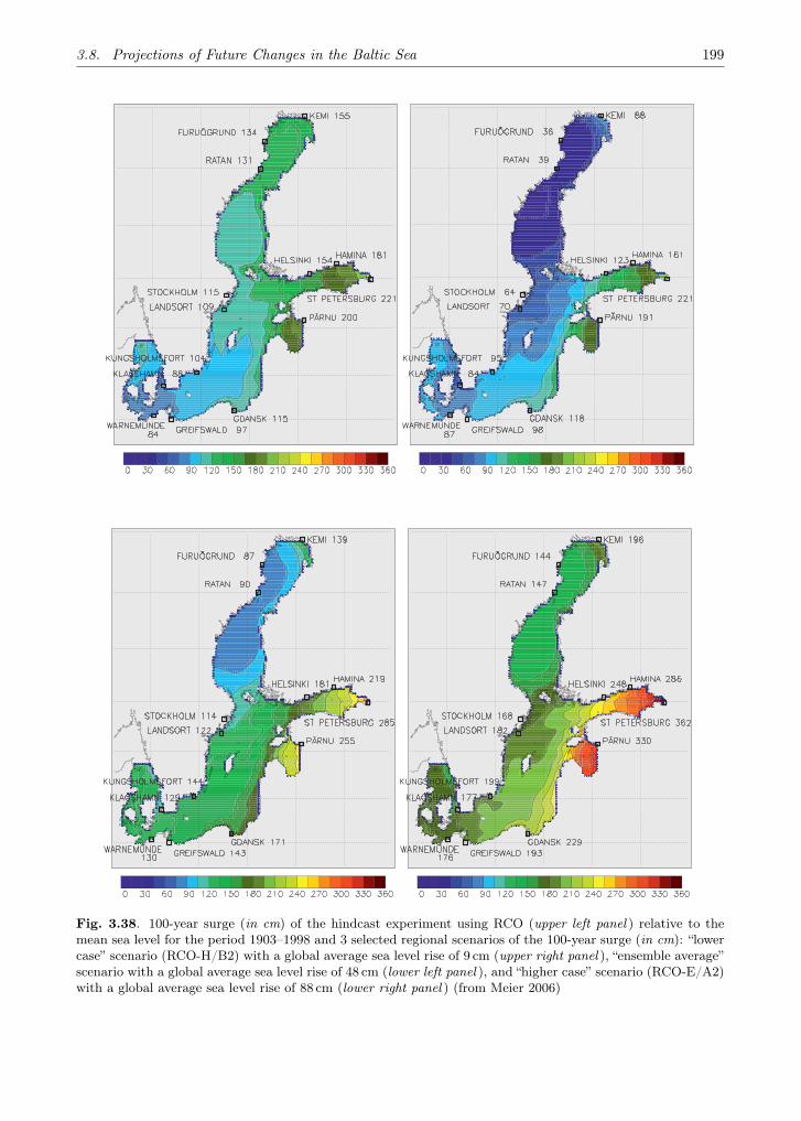
3.8. Projections of Future Changes in the Baltic Sea 199
Fig. 3.38. 100-year surge (in cm) of the hindcast experiment using RCO (upper left panel ) relative to themean sea level for the period 1903–1998 and 3 selected regional scenarios of the 100-year surge (in cm): “lowercase” scenario (RCO-H/B2) with a global average sea level rise of 9 cm (upper right panel ), “ensemble average”scenario with a global average sea level rise of 48 cm (lower left panel ), and “higher case” scenario (RCO-E/A2)with a global average sea level rise of 88 cm (lower right panel ) (from Meier 2006)

200 3. Projections of Future Anthropogenic Climate Change
Fig. 3.39. Median profiles of salinity at Gotland Deep for 16 future climate projections from RCO for theperiod 2071–2100 (colored lines) and for the present climate for the period 1961–1990 (black solid line, shadedareas indicate the ±2 standard deviation band calculated from two-daily values for 1903–1998 ). The projectionsinclude A2 and B2 emissions scenarios from 7 different RCMs driven by 5 GCMs. Effects of both wind andfreshwater inflow changes are included. A detailed discussion of salinity biases of the RCO model is given byMeier (2006) (from Meier et al. 2006b)
In projections performed at the Rossby Cen-tre (Räisänen et al. 2004) the total mean annualriver flow to the Baltic Sea changes between −2and +15% of present-day flow (Graham 2004). Insome of the scenarios, the monthly mean windspeed over sea increases, especially in winter andspring, up to 30%. Both increased freshwater in-flow and increased mean wind speeds could causethe Baltic Sea to drift into a new state with sig-nificantly lower salinity (Fig. 3.39).
However, even with the highest projected fresh-water inflow, the Baltic Sea will not be trans-formed into a freshwater sea, because the re-lationship between freshwater supply and aver-age salinity of the final steady-state is non-linear(Meier and Kauker 2003b). A pronounced halo-cline would still be expected to remain and sep-arate the upper and lower layers in the BalticProper, limiting the impact of direct wind-inducedmixing to the surface layer. Although salinityin the entire Baltic Sea might be significantlylower at the end of the 21st century, stabilityand deep water ventilation will very likely changeonly slightly (Fig. 3.40) because only the changingwind-induced mixing alters vertical and horizontalgradients of density on time scales longer than 20years (Meier 2006).
Sixteen salinity projections were performed byMeier et al. (2006b) using seven RCMs, five driv-ing global models and two emissions scenarios(Fig. 3.39). These results show mean salinity
change by the end of the 21st century (2071–2100)to range between +4 and −45%, although the pos-itive change is not statistically significant. Thissubstantial range in results is mainly due to dif-ferences in precipitation and wind speed changesin the Baltic Sea Basin from the different simu-lations. However, several of the scenario simula-tions suggest that future salinity will be consid-erably lower compared to the simulated variabil-ity of present climate. Salinity changes will havelarge impacts on species distributions, growth andreproduction of organisms (see Chap. 5).
Based upon model simulations, the sensitivityof the average steady-state salinity to the exter-nal forcing (e.g. freshwater supply, wind speed andamplitude of the sea level in Kattegat) has beenestimated in several studies (e.g. Stigebrandt 1983;Gustafsson 1997; 2000b, 2004; Schrum 2001; Meierand Kauker 2003b; Rodhe and Winsor 2002, 2003;Stigebrandt and Gustafsson 2003; Meier 2005).
It was found that the sensitivity of the steady-state salinity to the freshwater supply is non-linear. In different model approaches the resultsagree rather well. For instance, the sensitivityof the three-dimensional general circulation modelRCO (Meier and Kauker 2003b) is only slightlyhigher than the sensitivity of the process orientedmodel by Stigebrandt (1983). Even with 100%increased freshwater supply the Baltic Sea can-not be classified as a freshwater sea. Further,the sensitivity in different sub-basins was stud-

3.9. Future Development in Projecting Anthropogenic Climate Changes 201
Fig. 3.40. Median profiles of age at Gotland Deep: RCO hindcast simulation for 1961–1990 (black solidline, the shaded area indicates the range between the first and third quartiles) and four scenario simulations for2071–2100 (dotted line: RCO-H/B2, dashed line: RCO-H/A2, dash-dotted line: RCO-E/B2, long-dashed line:RCO-E/A2) (adapted from Meier 2006). The age is the time elapsed since a particle left the sea surface andis a measure of deep water renewal
ied when the changing freshwater supply is non-uniform (Stigebrandt and Gustafsson 2003). Incontrast to these investigations, Rodhe and Win-sor (2002, 2003) found a much larger sensitivity tofreshwater inflow. An explanation could be that inthe empirical model of Rodhe and Winsor (2002)the freshwater content anomaly depends only onthe freshwater supply and not on the wind forcing,as found by Meier and Kauker (2003a).
Meier (2005) investigated not only the sensitiv-ity of modelled salinity but also the sensitivity ofmodelled age to freshwater supply, wind speed andamplitude of the sea level in Kattegat (Fig. 3.40).In steady-state the average salinity of the BalticSea is most sensitive to perturbations of freshwa-ter inflow. Increases in freshwater inflow and windspeed both result in decreased salinity, whereasincreases in the Kattegat sea level results in in-creased salinity. The average age is most sensitiveto perturbations of the wind speed. Especially, de-creased wind speed causes significantly increasedage of the deep water. On the other hand, theimpact of changing freshwater or sea level in Kat-tegat on the average age is comparatively small,suggesting invariance of stability and ventilationin the steady-state. Immediately after the onsetof increased freshwater inflow, the saltwater inflowinto the Baltic Sea drops significantly due to in-creased recirculation (Meier 2005). After the typ-ical response time scale, the vertical overturningcirculation partially recovers.
3.9 Future Development in Projecting An-thropogenic Climate Changes
Global climate models play a central role in pro-jecting future anthropogenic climate change, bothby providing estimates of change on large horizon-tal scales and by providing the large-scale infor-mation needed by various downscaling methods.Further improvement of these models is thereforeessential. This concerns especially the parameter-isation of sub-grid scale phenomena (such as cloudprocesses, radiative transfer, convection, small-scale mixing in the atmosphere and the ocean, aswell as the exchange of heat, water and momen-tum between the atmosphere and the other com-ponents of the climate system) which are cruciallyimportant for the response of climate to externalforcing. Success in improving global climate mod-els will require huge efforts from the internationalcommunity, focusing not only on modelling per sebut also on collecting and making widely availabledetailed observations that will help to guide thedevelopment of the models.
Model improvements are also needed for re-gional climate models. Even if the horizontal reso-lution is better in those models than in the globalclimate models, they still have the problem of pa-rameterisation of sub-grid scale processes. It islikely that in the next five to ten years horizon-tal resolutions of only a few kilometres will be-come common. Even at such finer scales, manyphenomena remain unresolved, including individ-
202 3. Projections of Future Anthropogenic Climate Change
ual clouds. Reanalysis-driven experiments withregional climate models can be compared to high-resolution gridded datasets. Since the horizontalresolution in the models is likely to improve, theobservational datasets also need to be representedon finer grids. In this way errors and systematicbiases can be identified, leading to further im-provements in model formulation. Furthermore,global climate models can benefit from improvedparameterisations in regional climate models sincethe horizontal resolution in the global models will,in a few years time, be close to that of today’sregional models.
Climate models should evolve to also includeother processes than those of the more “tradi-tional” physical climate system. Complex interac-tion and feedback processes involving the biogeo-chemical cycles makes it necessary to introduceother model components to the climate models.Examples of such components are, among oth-ers: fully coupled models of atmospheric chem-istry, aerosol models, interactive vegetation mod-els, models describing the carbon cycle, and mod-els including marine chemistry.
Despite the efforts put into improving climatemodels, it is likely that the projections from differ-ent models will continue to differ for many years tocome, particularly on regional scales. Therefore,it is also important to ask how to best deal withthese differences. Is it reasonable to assume thatall models give equally likely projections, or shouldthe projections be weighted according to modelquality (e.g. in simulating present-day climate)?First steps toward the latter direction have beentaken (e.g. Giorgi and Mearns 2002, 2003; Mur-phy et al. 2004), but as yet there is only limitedunderstanding of which aspects of the present-dayclimate simulation matter most for simulation ofprojected anthropogenic climate changes. On theother hand, it is also important to evaluate thepossibility that the behaviour of the real climatesystem might fall outside the range of conventionalmodel results (e.g. Allen and Ingram 2002; Stain-forth et al. 2005).
Both statistical and dynamical downscalinghave proved to have added value for assessing re-gional climate in comparison with global models,although they may show different results. Com-parison of future scenarios downscaled by the twoapproaches may form a basis for assessing un-certainties associated with the downscaling. Thetwo approaches have different advantages and dis-advantages due the nature of the methods used.
While the dynamical approach may have prob-lems with biases, the statistical approach basi-cally avoids this problem as it is a data-basedmethod. However, being physically based, dy-namical methods realistically simulate non-lineareffects and other dynamical features, whereas sta-tistical methods often lack the full range of thetrue variability. Therefore, choice of the approachto be used depends mainly on the questions tobe addressed. One important advantage of thestatistical approach is that it can deal with localscales, including site scale. In the interim beforethe resolution of RCMs is considerably improved,it provides an alternative way to create the localanthropogenic climate change scenarios needed formany impact studies.
Hydrological studies have shown that biases inprecipitation from climate models make it difficultto directly use meteorological outputs in hydro-logical and water resources oriented applications.Evapotranspiration is also a source of much un-certainty, both in climate models and hydrologicalmodels. The combination of biases in meteoro-logical variables and the need for high resolutionhas to date precluded using the actual hydrolog-ical components from climate models for detailedassessment of hydrological impacts. Continuedwork to improve the hydrological processes in bothglobal and climate models, including river routingtechniques, is needed.
Such development, together with finer resolu-tion, as mentioned above, would serve to enhancethe quality and utility of climate model simula-tions, particularly if it leads to better represen-tation of extreme hydrological events. Recognis-ing that biases may be around for some time tocome, hydrological development should also focuson improved methods to filter out biases withoutmisrepresenting the anthropogenic climate changesignal coming from climate models.
Regarding ocean processes, the shortcomings ofglobal models are limiting for many variables. Forinstance, sea level scenarios for the Baltic Sea re-main rather uncertain due to the large uncertaintyof the global average sea level rise. In addition,overestimation of precipitation by regional climatemodels considerably affects salinity in the BalticSea. Salinity is not only biased by the erroneousfreshwater surplus; mixing also has a considerableimpact.
As mixing is approximately proportional tothe third power of the wind speed, any windspeed biases strongly impact on Baltic Sea cli-

3.10. Summary of Future Anthropogenic Climate Change Projections 203
mate. Consequently, mixing and other variables,such as sea level extremes, are typically underes-timated as RCMs commonly underestimate highwind speeds.
To improve scenarios for the Baltic Sea, thehorizontal resolution of ocean models should beincreased such that mesoscale processes are in-cluded. Description of important processes likesaltwater plume dynamics, entrainment and inter-leaving needs to be improved as well. Thus, fur-ther work to improve Baltic Sea models shouldfocus on advanced mixing parameterisations (e.g.including Langmuir circulation and breaking of in-ternal waves) and the coupling between ocean andstate–of–the–art wave models.
3.10 Summary of Future AnthropogenicClimate Change Projections
Increasing greenhouse gas (GHG) concentrationsare expected to lead to a substantial warming ofthe global climate during this century. Cubaschet al. (2001) estimated the annual globally av-eraged warming from 1990 to 2100 to be in therange of 1.4 to 5.8 C. This range in temperaturechange takes into account differences between cli-mate models and a range of anthropogenic emis-sions scenarios, but it excludes other uncertainties(for example, in the carbon cycle) and should notbe interpreted as giving the absolute lowest andhighest possible changes in the global mean tem-perature during the period considered.
Projected future warming in the Baltic SeaBasin generally exceeds the global mean warm-ing in GCM (global climate model) simulations.Looking at the annual mean from an ensemble of20 GCM simulations, regional warming over theBaltic Sea Basin would be some 50% higher thanglobal mean warming. In the northern areas ofthe basin, the largest warming is generally simu-lated in winter; further south the seasonal cycle ofwarming is less clear.
However, the relative uncertainty in the re-gional warming is larger than that in the globalmean warming. Taking the northern areas of thebasin as an example, the warming from late 20th
century to late 21st century could range from aslow as 1 C in summer (lowest scenario for sum-mer) to as high as 10 C in winter (highest sce-nario for winter). The simulated warming wouldgenerally be accompanied by an increase in pre-cipitation in the Baltic Sea Basin, except in thesouthernmost areas in summer. The uncertainty
for precipitation change is, however, larger thanthat for temperature change, and the coarse reso-lution of GCMs does not resolve small-scale vari-ations of precipitation change that are induced bythe regional topography and land cover.
A more geographically detailed assessment offuture anthropogenic climate change in the BalticSea Basin requires the use of statistical or dynam-ical downscaling methods. Yet, as only a lim-ited number of GCM simulations have been down-scaled by RCMs (regional climate models) or sta-tistical downscaling methods, the range of resultsderived from such downscaling experiments doesnot fully reflect the range of uncertainties in theGCM projections. Accepting this, the range ofresults from available downscaling studies is pre-sented below as it gives an indication of plausiblefuture changes. All values refer to changes pro-jected for the late 21st century, represented hereas differences in climate between the years 1961–1990 and 2071–2100. All references to “northern”and “southern” areas of the Baltic Sea Basin aredefined by the subregions shown in Fig. 3.12.
Consistent with GCM studies, all availabledownscaling studies also indicate increases in tem-perature during all seasons for every subregion ofthe Baltic Sea Basin. Combined results show aprojected warming of the mean annual tempera-ture by some 3 to 5 C for the total basin. Sea-sonally, the largest part of this warming would oc-cur in the northern areas of the Baltic Sea Basinduring winter months and in the southern areasof the Baltic Sea Basin during summer months.Corresponding changes in temperatures would be4 to 6 C in winter and 3 to 5 C in summer, asestimated from a matrix of regional climate modelexperiments.
As noted above, these ranges most probablyunderestimate the real uncertainty. The diurnaltemperature range – the difference between dailymaximum and minimum temperature – woulddecrease, most strongly in autumn and wintermonths. Such levels of warming would lead to alengthening of the growing season, defined hereas the continuous period when daily mean tem-perature exceeds 5 C. Taking an example fromone RCM indicates that the growing season lengthcould increase by as much as 20 to 50 days fornorthern areas and 30 to 90 days for southern ar-eas by the late 21st century. The range dependson the range of different emissions scenarios used.
Projected changes in precipitation from down-scaling studies also depend both on differences in

204 3. Projections of Future Anthropogenic Climate Change
GHG emissions scenarios and differences betweenclimate models. Moreover, precipitation resultsare more sensitive than temperature results to thestatistical uncertainty in determining climatolog-ical means from a limited number of simulatedyears, particularly at regional scales. Seasonally,winters are projected to become wetter in most ofthe Baltic Sea Basin and summers to become drierin southern areas for many scenarios. Northernareas could generally expect winter precipitationincreases of some 25 to 75%, while the projectedsummer changes lie between −5 and 35%. South-ern areas could expect increases ranging from some20 to 70% during winter, while summer changeswould be negative, showing decreases of as muchas 45%.
Taken together, these changes lead to a pro-jected increase in annual precipitation for the en-tire basin. In broad terms, these results are con-sistent with GCM studies of precipitation change,although the projected summer decrease in thesouthern areas of the basin tends to be larger andextend further north in the available RCM stud-ies than in most reported GCMs. This differencereflects the fact that the few GCM simulationsthat have been downscaled by RCMs also showthis pattern of summer precipitation change.
Projected changes in wind differ widely betweenvarious climate models. Differences in the circula-tion patterns of the driving GCMs are particularlyimportant for the modelled outcome of this vari-able. From the RCM results presented here, onlythose driven by the ECHAM4/OPYC3 GCM showstatistically significant changes for projected fu-ture climate scenarios. For mean daily wind speedover land areas, this would amount to a mean in-crease of some 8% on an annual basis and a maxi-mum mean seasonal increase of up to 12% duringwinter. The corresponding mean seasonal increaseover the Baltic Sea in winter, when decrease in icecover enhances near-surface winds, would be up to
18%. For RCMs driven by the HadAM3H GCM,the changes are small and not statistically signif-icant. Modelled changes in extreme wind gener-ally follow the same pattern as for the mean wind;however, the spatial resolution of both GCMs andRCMs is far too coarse to accurately represent thefine scales of extreme wind.
As the downscaled projections for wind dif-fer widely, there is no robust signal seen in theRCM results. Looking at projected changes inlarge-scale atmospheric circulation from numerousGCMs, they indicate that an increase in windinessfor the Baltic Sea Basin would be somewhat morelikely than a decrease. However, the magnitude ofsuch a change is still highly uncertain and it maytake a long time before projected GHG-inducedchanges in windiness, if ever, emerge from back-ground natural variability. It can be noted, more-over, that ECHAM4/OPYC3 is one of the GCMsthat gives higher values of change in large-scalewind.
Hydrological studies using climate change pro-jections show that increases in mean annual riverflow from the northernmost catchments would oc-cur together with decreases in the southernmostcatchments. Seasonally, summer river flows wouldtend to decrease, while winter flows would tend toincrease, by as much as 50%. The southernmostcatchments would be affected by the combinationof both decreased summer precipitation and in-creased evapotranspiration. Oceanographic stud-ies show that mean annual sea surface tempera-tures could increase by some 2 to 4 C by the end ofthe 21st century. Ice extent in the sea would thendecrease by some 50 to 80%. The average salinityof the Baltic Sea could range between present dayvalues and decreases of as much as 45%. However,it should be noted that these oceanographic find-ings, with the exception of salinity, are based upononly four regional scenario simulations using twoemissions scenarios and two global models.

3.11. References 205
3.11 References
Achberger C (2004) Recent and future regional climate variations in Sweden in relation to large-scalecirculation. Earth Sciences Centre, A92. Göteborg University
Achberger C, Linderson ML, Chen D (2003) Performance of the Rossby Centre regional Atmosphericmodel in Southern Sweden: Comparison of simulated and observed precipitation. Theor App Cli-matol 76:219–234
Achberger C, Chen D, Alexandersson H (2006) The surface winds of Sweden during 1999–2000. Int JClimatol 26:159–178
Alexandersson H, Tuomenvirta H, Schmith T, Iden K (2000) Trends of storms in NW Europe derivedfrom an updated pressure data set. Clim Res 14:71–73
Allen MR, Ingram WJ (2002) Constraints on future changes in climate and the hydrologic cycle. Na-ture 419:224–232
Andersen HE, Kronvang B, Larsen SE, Hoffmann CC, Jensen TS, Rasmussen EK (2006) Climate-change impacts on hydrology and nutrients in a Danish lowland river basin. Sci Total Env 365:223–237
Andréasson J, Gardelin M, Bergström S (2002) Modelling hydrological impacts of climate change inthe Lake Vänern region in Sweden. Vatten 58:25–32
Andréasson J, Bergström S, Carlsson B, Graham LP, Lindström G (2004) Hydrological change – cli-mate change impact simulations for Sweden. Ambio 33:228–234
Arnell NW (1998) Climate change and water resources in Britain. Climatic Change 39:83–110Arnell NW (1999) The effect of climate change on hydrological regimes in Europe: A continental
perspective. Glob Env Change 9:5–23Arnell NW, Hudson DA, Jones RG (2003) Climate change scenarios from a regional climate model:
Estimating change in runoff in southern Africa. J Geophy Res 108:4519, doi: 10.1029/2002JD002782Arpe K, Bengtsson L, Golitsyn GS (2000) Analysis of changes in hydrological regime on the Lake
Ladoga watershed and in the discharge of the Neva River in 20th and 21st centuries using a globalclimate model. Russ Meteorol Hydrol 12:5–13
Baerens C, Hupfer P (1999) Extremwasserstände an der deutschen Ostseeküste nach Beobachtungenund in einem Treibhausgasszenario (Extreme water levels at the German Baltic Sea coast accordingto observations and a greenhouse gas scenario). Die Küste 61:47–72 (in German)
Barthelet P, Terray L, Valcke S (1998) Transient CO2 experiment using the ARPEGE/OPAICE nonflux corrected coupled model. Geophys Res Lett 25:2277–2280
Benestad RE (2002a) Empirically downscaled multimodel ensemble temperature and precipitation sce-narios for Norway. J Clim 15:3008–3027
Benestad RE (2002b) Empirically downscaled climate scenarios for northern Europe. Clim Res 21:105–125
Benestad RE (2004) Tentative probabilistic temperature scenarios for northern Europe. Tellus A 56:89–101
Beniston M, Stephenson DB, Christensen OB, Ferro CAT, Frei C, Goyette S, Halsnæs K, Holt T,Jylhä K, Koffi B, Palutikof J, Schöll R, Semmler T, Woth K (2007) Future extreme events ineuropean climate: An exploration of regional climate model projections. Climatic Change 81:71–95
Bergström S (1976) Development and application of a conceptual runoff model for Scandinavian catch-ments. Doctoral thesis, Department of Water Resources Engineering, Institute of Technology, LundUniversity
Bergström S (1995) The HBV Model In: Singh VP (ed) Computer Models of Watershed Hydrology.Water Resources Publications, Highlands Ranch Colorado
Bergström S, Carlsson B (1994) River runoff to the Baltic Sea: 1950–1990. Ambio 23:280–287Bergström S, Carlsson B, Gardelin M, Lindström G, Pettersson A, Rummukainen M (2001) Climate
change impacts on runoff in Sweden – assessments by global climate models dynamical downscalingand hydrological modelling. Clim Res 16:101–112
Bergström S, Andréasson J, Beldring S, Carlsson B, Graham LP, Jónsdóttir JF, Engeland K, Tu-runen MA, Vehviläinen B, Førland E J (2003) Climate Change Impacts on Hydropower in the

206 3. Projections of Future Anthropogenic Climate Change
Nordic Countries – State of the art and discussion of principles. CWE Report no 1, CWE Hydro-logical Models Group, Rejkjavik, Iceland
Bertrand C, Van Ypersele JP, Berger A (2002) Are natural climate forcings able to counteract theprojected anthropogenic global warming? Climatic Change 55:413–427
Bjørge D, Haugen JE, Nordeng TE (2000) Future climate in Norway. DNMI Research Report no 103Blenckner T, Chen D (2003) Comparison of the impact of regional and North Atlantic atmospheric
circulation on an aquatic ecosystem. Clim Res 23:131–136Boer GJ, Yu B (2003) Climate sensitivity and response. Clim Dyn 20:415–429Boville BA, Gent PR (1998) The NCAR climate system model version One. J Clim 11:1115–1130Braconnot P, Marti O, Joussaume S (1997) Adjustment and feedbacks in a global coupled ocean–
atmosphere model. Clim Dyn 13:507–519Busuioc A, Chen D, Hellström C (2001a) Temporal and spatial variability of precipitation in Sweden
and its link with the large scale atmospheric circulation. Tellus 53A,3:348–367Busuioc A, Chen D, Hellström C (2001b) Performance of statistical downscaling models in GCM val-
idation and regional climate estimates: Application for Swedish precipitation. Int J Climatol 21:557–578
Butina M, Melnikova G, Stikute I (1998a) Potential impact of climate change on the hydrologicalregime in Latvia. In: Raschke E, Isemer HJ (eds) Conference Proceedings of the Second StudyConference on BALTEX, International BALTEX Secretariat Publication No 11
Butina M, Melnikova G, Stikute I (1998b) Potential impact of climate change on the hydrologicalregime in Latvia. In: Lemmelä R, Helenius N (eds) Proceedings of the Second International Con-ference on Climate and Water. Espoo, Finland 17–20 August 1998, 3:1610–1617
Carlsson B, Sanner H (1996) Modelling influence of river regulation on runoff to the Gulf of Bothnia.Nord Hydrol 27:337–350
Chen D (2000) A monthly circulation climatology for Sweden and its application to a winter temper-ature case study. Int J Climatol 20:1067–1076
Chen D, Achberger C (2006) Past and future atmospheric circulation over the Baltic region based onobservation reanalysis and GCM simulations. Research Report C74 Earth Sciences Centre GöteborgUniversity, Sweden
Chen D, Hellström C (1999) The influence of the North Atlantic Oscillation on the regional tempera-ture variability in Sweden: Spatial and temporal variations. Tellus 51A,4:505–516
Chen D, Li X (2004) Scale dependent relationship between maximum ice extent in the Baltic Sea andatmospheric circulation. Glob Planet Change 41:275–283
Chen D, Omstedt A (2005) Climate-induced variability of sea level in Stockholm: Influence of airtemperature and atmospheric circulation. Adv Atmos Sci 20,5:655–664
Chen D, Achberger C, Räisänen J, Hellström C (2006) Using statistical downscaling to quantify theGCM-related uncertainty in regional climate change scenarios: A case study of Swedish precipitation.Adv Atmos Sci 23,1:54–60
Christensen JH, Christensen OB (2003) Severe summertime flooding in Europe. Nature 421:805–806Christensen JH, Machenhauer B, Jones RG, Schär C, Ruti PM, Castro M, Visconti G (1997) Valida-
tion of present-day regional climate simulations over Europe: LAM simulations with observed bound-ary conditions. Clim Dyn 13:489–506
Christensen JH, Räisänen J, Iversen T, Bjørge D, Christensen OB, Rummukainen M (2001) A syn-thesis of regional climate change simulations – a Scandinavian perspective. Geophys Res Lett 28:1003–1006
Christensen JH, Carter TR, Giorgi F (2002) Prudence employs new methods to assess European cli-mate change. EOS 83:147
Christensen JH, Carter TR, Rummukainen M (2007) Evaluating the performance and utility of re-gional climate models: The PRUDENCE project. Climatic Change 81:1–6
Christensen OB, Christensen JH (2004) Intensification of extreme European summer precipitation ina warmer climate. Glob Planet Change 44:107–117
Christensen OB, Christensen JH, Machenhauer B, Botzet M (1998) Very-high-resolution regional cli-mate simulations over Scandinavia present climate. J Clim 11:3204–3229

3.11. References 207
Christensen OB, Christensen JH, Botzet M (2002) Heavy precipitation occurrence in Scandinavia in-vestigated with a regional climate model. In: Beniston M (ed) Climatic Change: Implications forthe hydrological cycle and for water management. Kluwer
Church JA, Gregory JM, Huybrechts P, Kuhn M, Lambeck K, Nhuan MT, Qin D, Woodworth PL(2001) Changes in sea level. In: IPCC Climate Change 2001: The scientific basis contributionof working group I to the Third Assessment Report of the Intergovernmental Panel on ClimateChange. Cambridge University Press, Cambridge New York
Cubasch U, Meehl GA, Boer GJ, Stouffer RJ, Dix M, Noda A, Senior CA, Raper S, Yap KS (2001)Projections of future climate change. In: IPCC Climate Change 2001: The scientific basis contribu-tion of working group I to the Third Assessment Report of the Intergovernmental Panel on ClimateChange. Cambridge University Press, Cambridge New York
De Castro M, Gallardo C, Jylhä K, Tuomenvirta H (2007) The use of a climate-type classification forassessing climate change effects in Europe from an ensemble of nine regional climate models. ClimChange 81:329–341
De Roo A, Schmuck G (2002) Assessment of the effects of engineering, land use and climate scenarioson flood risk in the Oder catchment. European Commission, Joint Research Centre, Institute forEnvironment and Sustainability
Déqué M, Rowell DP, Lüthi D, Giorgi F, Christensen JH, Rockel B, Jacob D, Kjellström E, De Cas-tro M, Van Den Hurk B (2007) An intercomparison of regional climate simulations for Europe:Assessing uncertainties in model projections. Climatic Change 81:53–70
Déqué M, Marquet P, Jones RG (1998) Simulation of climate change over Europe using a global vari-able resolution general circulation model. Clim Dyn 14:173–189
Diansky NA, Volodin EM (2002) Simulation of present-day climate with a coupled atmosphere–oceangeneral circulation model. Izvestia Atmos Ocean Phys 38:732–747
Döscher R, Meier HEM (2004) Simulated sea surface temperature and heat fluxes in different climatesof the Baltic Sea. Ambio 33:242–248
Döscher R, Willén U, Jones C, Rutgersson A, Meier HEM, Hansson U, Graham LP (2002) The devel-opment of the regional coupled ocean–atmosphere model RCAO. Boreal Env Res 7:183–192
Ekman M (1988) The world’s longest continued series of sea level observations. Pure Appl Geophys127:73–77
Emori S, Nozawa T, Abe-Ouchi A, Numaguti A, Kimoto M, Nakajima T (1999) Coupled ocean–at-mosphere model experiments of future climate change with an explicit representation of sulfateaerosol scattering. J Met Soc Jpn 77:1299–1307
Engen-Skaugen T, Roald LA, Beldring S, Førland EJ, Tveito OE, Engeland K, Benestad R (2005)Climate change impacts on water balance in Norway. Research Report No 1/2005 Climate Nor-wegian Meteorological Institute Oslo
Fenger J, Buch E, Jacobsen PR (2001) Monitoring and impacts of sea level rise at Danish coasts andnear shore infrastructures. In: Jørgensen AM, Fenger J, Halsnæs K (eds) Climate change research– Danish Contributions. Danish Climate Centre Copenhagen, pp. 237–254
Ferro CAT (2004) Attributing variation in a regional climate change modelling experiment. PRU-DENCE working note available at http://prudence.dmi.dk/public/publications/analysis_of_vari-ance.pdf
Ferro CAT, Hannachi A, Stephenson DB (2005) Simple techniques for describing changes in probabil-ity distributions of weather and climate. J Clim 18:4344–4354
Flato GM, Boer GJ (2001) Warming asymmetry in climate change experiments. Geophys Res Lett 28:195–198
Flato GM, Boer GJ, Lee WG, McFarlane NA, Ramsden D, Reader MC, Weaver AJ (2000) The Ca-nadian centre for climate modelling and analysis global coupled model and its climate. Clim Dyn 16:451–467
Forster PM, De F, Blackburn M, Glover R, Shine KP (2000) An examination of climate sensitivityfor idealised climate change experiments in an intermediate general circulation model. Clim Dyn 16:833–849
208 3. Projections of Future Anthropogenic Climate Change
Fossdal ML, Sælthun NR (1993) Energy planning models – climate change. Report from a Nordic ex-pert meeting. NVE-report 08/1993 Norwegian Water Resources and Energy Administration, Oslo
Frei C, Christensen JH, Déqué M, Jacob D, Jones RG, Vidale PL (2003) Daily precipitation statisticsin regional climate models: Evaluation and intercomparison for the European Alps. J Geophys Res108,D3, 4124 doi: 101029/2002JD002287
Gardelin M, Andreasson J, Carlsson B, Lindström G, Bergström S (2002a) Modelling av effekter avklimatförändringar på tillrinningen till vattenkraftsystemet (Modelling of effects of climate changeon inflow to the hydropower system). Elforsk Report 02:27 Elforsk Stockholm (in Swedish)
Gardelin M, Bergström S, Carlsson B, Graham LP, Lindström G (2002b) Climate change and waterresources in Sweden – analysis of uncertainties. In: Beniston M (ed) Climatic Change: Implicationsfor the Hydrological Cycle and for Water Management. Advances in Global Change Research.Kluwer, Dordrecht
Gellens D, Roulin E (1998) Streamflow response of Belgian catchments to IPCC climate change sce-narios. J Hydrol 210:242–258
Gillett NP, Zwiers FW, Weaver AJ, Stott PA (2003) Detection of human influence on sea-level pres-sure. Nature 422:292–294
Giorgi F, Marinucci M (1991) Validation of a regional atmospheric model over Europe: Sensitivity ofwintertime and summertime simulations to selected physics parameterizations and lower boundaryconditions. Q J Roy Met Soc 117:1171–1206
Giorgi F, Mearns LO (2002) Calculation of average uncertainty range and reliability of regional cli-mate changes from AOGCM simulations via the “reliability ensemble averaging” (REA) method.J Clim 15:1141–1158
Giorgi F, Mearns LO (2003) Probability of regional climate change based on the Reliability EnsembleAveraging (REA) method. Geophys Res Lett 30 12 1629 (doi:101029/2003GL017130)
Giorgi F, Marinucci M, Visconti G (1990) Use of a limited area model nested in a general circulationmodel for regional climate simulation over Europe. J Geophys Res 95:18413–18431
Giorgi F, Marinucci M, Visconti G (1992) A 2 × CO2 climate change scenario over Europe generatedusing a limited area model nested in a general circulation model 2 Climate change scenario. JGeophys Res 97:10011–10028
Giorgi F, Hewitson B, Christensen J, Hulme M, von Storch H, Whetton P, Jones R, Mearns L, Fu C(2001) Regional climate information – evaluation and projections. In: IPCC Climate Change 2001:The Scientific Basis Contribution of Working Group I to the Third Assessment Report of the Inter-governmental Panel on Climate Change. Cambridge University Press, Cambridge New York
Giorgi F, Bi XQ, Pal J (2004a) Mean interannual variability and trends in a regional climate changeexperiment over Europe I: Present-day climate (1961–1990). Clim Dyn 22:733–756
Giorgi F, Bi XQ, Pal J (2004b) Mean interannual variability and trends in a regional climate changeexperiment over Europe II: Climate change scenarios (2071–2100). Clim Dyn 23:839–858
Golitsyn GS, Efimova LK, Mokhov II (2002) Izmenenija temperatury i osadkov v bassejne Ladozh-skogo ozera po raschetam klimaticheskoj modeli obshchej cirkuljacii v XIX–XXI vekah (Changes oftemperature and precipitation on the Lake Ladoga watershed in 19th – 21st centuries simulated bya general circulation model). Izvestia RGO 134,6:80–87 (in Russian)
Gordon C, Cooper C, Senior CA, Banks H, Gregory JM, Johns TC, Mitchell JFB, Wood RA (2000)The simulation of SST, sea ice extents and ocean heat transports in a version of the Hadley Centrecoupled model without flux adjustments. Clim Dyn 16:147–166
Grabs WE, Daamen K, Gellens D, Grabs W, Kwadijk JCJ, Lang H, Middlekoop H, Parmet BWAH,Schädler B, Schulla J, Wilke K (1997) Impact of Climate Change on Hydrological Regimes andWater Resources Management in the Rhine Basin. CHR-Report no I–16, International Commisionfor the Hydrology of the Rhine Basin (CHR) Lelystad
Graham LP (1999a) Modeling runoff to the Baltic Sea. Ambio 28:328–334Graham, LP (2004) Climate change effects on river flow to the Baltic Sea. Ambio 33:235–241Graham LP (1999b) Modeling the large-scale hydrologic response to climate change in the Baltic
Basin. In: Elíasson J (ed) Proceedings from the Northern Research Basins 12th InternationalSymposium and Workshop, Reykjavík Iceland 23–27 August, pp. 99–110

3.11. References 209
Graham LP (2002) A simple runoff routing routine for the Rossby Centre Regional Climate Model.In: Killingtveit A (ed) Proceedings from XXII Nordic Hydrological Conference, Røros Norway 4–7August, Nordic Hydrological Programme Report 47:573–580
Graham LP, Rummukainen M, Gardelin M, Bergström S (2001) Modelling Climate Change Impactson Water Resources in the Swedish Regional Climate Modelling Programme. In: Brunet M, López D(eds) Detecting and Modelling Regional Climate Change and Associated Impacts. Springer, BerlinHeidelberg New York, pp. 567–580
Graham LP, Andréasson J, Carlsson B (2007a) Assessing climate change impacts on hydrology froman ensemble of regional climate models, model scales and linking methods – a case study on theLule River Basin. Climatic Change 81:293–307
Graham LP, Hagemann S, Jaun S, Beniston M (2007b) On interpreting hydrological change from re-gional climate models. Climatic Change 81:97–122
Gregory JM, Mitchell JFB, Brady AJ (1997) Summer drought in northern midlatitudes in a time-dependent CO2 climate experiment. J Clim 10:662–686
Grigoryev AS, Trapeznikov JA (2002) The water level in the Ladoga Lake in the conditions of poten-tial climate change. Water Resource 29:174–178 (in Russian)
Gustafsson BG (1997) Interaction between Baltic Sea and North Sea. Dt Hydrogr Z 49:163–181Gustafsson BG (2000) Time-dependent modeling of the Baltic entrance area. 2. Water and salt ex-
change of the Baltic Sea. Estuaries 23:253–266Gustafsson BG (2004) Sensitivity of Baltic Sea salinity to large perturbations in climate. Clim Res
27:237–251Gutry-Korycka M (1999) Ekstremalne stany systemu hydrologicznego w perspektywie ocieplenia kli-
matu (fakty czy hipotezy). In: Komitet Narodowy PAN IGBP Global Change 1999 Zmiany izmienność klimatu Polski – ich wpływ na gospodarkę ekosystemy i człowieka (Changes and vari-ability of Poland’s climate – their influence on economy, ecosystems and people). Łódź Conferenceproceedings (in Polish)
Haapala J, Leppäranta M (1997) The Baltic Sea ice season in changing climate. Boreal Env Res 2:93–108
Haapala J, Meier HEM, Rinne J (2001) Numerical investigations of future ice conditions in the BalticSea. Ambio 30:237–244
Hagemann S, Dümenil L (1999) Application of a global discharge model to atmospheric model simu-lations in the BALTEX region. Nordic Hydrology 30:209–230
Hagemann S, Jacob D (2007) Gradient in the climate change signal of European discharge predictedby a multi-model ensemble. Climatic Change 81:309–327
Hagemann S, Machenhauer B, Christensen OB, Déqué M, Jacob D, Jones R, Vidale PL (2002)Intercomparison of water and energy budgets simulated by regional climate models applied overEurope. Max-Planck-Institute for Meteorology Rep 338. Hamburg, Germany
Hagemann S, Machenhauer B, Jones R, Christensen OB, Déqué M, Jacob D, Vidale PL (2004)Evaluation of water and energy budgets in regional climate models applied over Europe. Clim Dyn23:547–567
Hall MM, Bryden HL (1982) Direct estimates and mechanisms of ocean heat transport. Deep-Sea Res29:339–359
Hamlet AF, Lettenmaier D (1999) Effects of climate change on hydrology and water resources in theColumbia River Basin. J Am Water Resour Assoc 35:1597–1623
Hanssen-Bauer I, Tveito OE, Førland EJ (2000) Temperature scenarios for Norway: Empirical Down-scaling from the ECHAM4/OPYC3 GSDIO integration. DNMI Report no 24/00 KLIMA NorwegianMeteorological Institure Oslo Norway
Hanssen-Bauer I, Tveito OE, Førland EJ (2001) Precipitation scenarios for Norway Empirical down-scaling from ECHAM4/OPYC3 DNMI Report no 10/01 KLIMA Norwegian Meteorological InstituteOslo Norway
Hanssen-Bauer I, Førland E, Haugen JE, Tveito OE (2003) Temperature and precipitation scenariosfor Norway: Comparison of results from dynamical and empirical downscaling. Clim Res 25:15–27
210 3. Projections of Future Anthropogenic Climate Change
Hanssen-Bauer I, Achberger C, Benestad R, Chen D, Førland E (2005) Empirical–statistical downsca-ling of climate scenarios over Scandinavia: A review. Clim Res 29:255–268
Harvey LDD (2004) Characterizing the annual-mean climatic effect of anthropogenic CO2 and aerosolemissions in eight coupled atmosphere–ocean GCMs. Clim Dyn 23:569–599
Hay LE, Wilby RL, Leavesley GH (2000) A comparison of delta change and downscaled GCM scenar-ios for three mountainous basins in the United States. J Am Water Res Ass 36:387–398
Hegerl GC, Zwiers FV, Stott P, Kharin VV (2004) Detectability of anthropogenic changes in annualtemperature and precipitation extremes. J Clim 17:3683–3700
Heino R, Kitaev L (2003) INTAS project (2002–2005): Snow cover changes over Northern Eurasiaduring the last century: Circulation consideration and hydrological consequences (SCCONE).BALTEX Newsletter 5: 8–9
Hellström C, Chen D, Achberger C, Räisänen J (2001) A Comparison of climate change scenarios forSweden based on statistical and dynamical downscaling of monthly precipitation. Clim Res 19:45–55
Henderson-Sellers A, Hansen AM (1995) Climate Change Atlas. Atmospheric and Oceanographic Sci-ences Library 17. Kluwer
Hennessy KJ, Gregory JM, Mitchell JFB (1997) Changes in daily precipitation under enhanced green-house conditions. Clim Dyn 13:667–680
Heyen H, Zorita E, von Storch H (1996) Statistical downscaling of monthly mean North Atlantic air-pressure to sea level anomalies in the Baltic Sea. Tellus 48A:312–323
Hirst A, O’Farrell SP, Gordon HP (2000) Comparison of a coupled ocean–atmosphere model with andwithout oceanic eddy-induced advection Part I: Ocean spinup and control integrations. J Clim 13:139–163
Hoerling MP, Hurrell JW, Xu T, Bates GT, Phillips A (2004) Twentieth century North Atlantic cli-mate change Part II: Understanding the effect of Indian Ocean warming. Clim Dyn 23:391–405
Houghton JT, Callendar BA, Varney SK (eds) (1992) Climate Change 1992 – The Supplementary Re-port to the IPCC Scientific Assessment. Intergovernmental Panel on Climate Change. CambridgeUniversity Press
Huffman GJ, Adler RF, Arkin A, Chang A, Ferraro R, Gruber A, Janowiak J, Joyce RJ, Mc Nab A,Rudolf B, Schneider U, Xie P (1997) The Global Precipitation Climatology Project (GPCP) com-bined precipitation data set. Bull Am Met Soc 78:5–20
Hulme M, Barrow EM, Arnell NW, Harrison PA, Johns TC, Downing TE (1999) Relative impacts ofhuman-induced climate change and natural variability. Nature 397:688–691
Huntingford C, Cox PM (2000) An analogue model to derive additional climate change scenarios fromexisting GCM simulations. Clim Dyn 16:575–586
Hurrell JW, Van Loon H (1997) Decadal variations in climate associated with the North Atlantic Os-cillation. Climatic Change 36:301–326
Hurrell JW, Kushnir Y, Ottersen G, Visbeck M (eds) (2003) The North Atlantic Oscillation: ClimateSignificance and Environmental Impact. Geophys Monogr Series 134
Hurrell JW, Hoerling MP, Phillips A, Xu T (2004) Twentieth century North Atlantic climate changePart I: Assessing determinism. Clim Dyn 23:371–389
Huybrechts P, De Wolde J (1999) The dynamic response of the Greenland and Antarctic ice sheets tomultiple-century climatic warming. J Clim 12:2169–2188
ILMAVA Project (2002) Effect of Climate Change on Energy Resources in Finland Final report onthe Ilmava Project within the Climtech Programme. Tammelin B, Forsius J, Jylhä J, JärvinenP, Koskela J, Tuomenvirta H, Turunen MA, Vehviläinen B, Venäläinen A, Finnish MeteorologicalInstitute Helsinki (in Finnish)
IPCC (2001a) Climate Change 2001: The scientific basis contribution of Working Group I to the ThirdAssessment Report of the Intergovernmental Panel on Climate Change. Cambridge University Press,Cambridge New York
IPCC (2001b) Climate Change 2001: Impacts, adaptation and vulnerability. Contribution of WorkingGroup II to the Third Assessment Report of the Intergovernmental Panel on Climate Change.Cambridge University Press, Cambridge New York

3.11. References 211
Jacob D, Van Den Hurk B, Andrae U, Elgered G, Fortelius C, Graham LP, Jackson S, Karstens U,Köpken C, Lindau R, Podzun R, Rockel B, Rubel F, Sass B, Smith R, Yang X (2001) A compre-hensive model inter-comparison study investigating the water budget during the BALTEX-PIDCAPperiod. Meteorol Atmos Phys 77:19–43
Jansons V, Butina M (1998) Potential impacts of climate change on nutrient loads from small catch-ments. In: Lemmelä R, Helenius N (eds) Proceedings of the Second International Conference onClimate and Water, Espoo Finland 17–20 August 1998, 2
Järvet A (1998) An assessment of the climate change impact on groundwater regime. In: Kallaste T,Kuldna P (eds) Climate Change Studies in Estonia, Ministry of Environment Republic of Estonia,SEI Tallinn
Johansson MM, Kahma KK, Boman H, Launiainen J (2004) Scenarios for sea level on the Finnishcoast. Boreal Env Res 9:153–166
Johns TC, Carnell RE, Crossley JF, Gregory JM, Mitchell JFB, Senior CA, Tett SFB, Wood RA(1997) The second Hadley Centre Coupled ocean–atmosphere GCM: Model description spinup andvalidation. Clim Dy 13:103–134
Jones CG, Ullerstig A (2002) The representation of precipitation in the RCA2 model (Rossby CentreAtmosphere Model Version 2). SWECLIM Newsletter 12:27–39
Jones CG, Willén U, Ullerstig A, Hansson U (2004) The Rossby Centre Regional Atmospheric Cli-mate Model – Part I: Model climatology and performance for the present climate over Europe.Ambio 33:199–210
Jones RG, Murphy JM, Noguer M (1995) Simulation of climate-change over Europe using a nestedregional climate model, 1. Assessment of control climate including sensitivity to location of lateralboundaries. Q J Roy Met Soc 121:1413–1449
Jones RG, Murphy JM, Noguer M, Keen AB (1997) Simulation of climate change over Europe using anested regional climate model, 2. Comparison of driving and regional model responses to a doublingof carbon dioxide. Q J Roy Met Soc 123:265–292
Joshi M, Shine K, Ponater M, Stuber N, Sausen R, Li L (2003) A comparison of climate response todifferent radiative forcings in three general circulation models: Towards an improved metric ofclimate change. Clim Dyn 20:843–854
Jylhä K, Tuomenvirta H, Ruosteenoja K (2004) Climate change projections for Finland during the21st century. Boreal Env Res 9:127–152
Jylhä K, Fronzek S, Tuomenvirta H, Carter TR, Ruosteenoja K (2007) Changes in frost and snow inEurope and Baltic sea ice by the end of the 21st century. Climatic Change (in press)
Järvet A, Jaagus J, Roosaare J, Tamm T, Vallner L (2000) Impact of climate change on water bal-ance elements in Estonia. Estonia Geographical Studies 8:35–55
Kaas E, Frich P (1995) Diurnal temperature range and cloud cover in the Nordic countries: Observedtrends and estimates for the future. Atmos Res 37:211–228
Kaczmarek Z (1993) Water balance model for climate impact analysis. Acta Geophys Pol 41:423–437Kaczmarek Z (1996) Wpływ klimatu na bilans wody (Impact of climate on water balance). In: Kacz-
marek Z (ed) Wpływ niestacjonarności i globalnych procesów geofizycznych na zasoby wodne PolskiOficyna (The impact of nonlinearity and global geophysical processes on water resources in Poland).Wydawnicza Politechniki Warszawskiej Warszawa, 33–53 (in Polish)
Kaczmarek Z (2003) Wpływ klimatu na gospodarkę wodną (Impact of climate on water management).In: Komitet Prognoz “Polska 2000 Plus” (ed) Czy Polsce grożą katastrofy klimatyczne? IGBP PANWarszawa, 32–52 (in Polish)
Kaczmarek Z (2004) Climate change and European water resources. In: Liszewska M (ed) Potentialclimate changes and sustainable water management. Publ Inst Geophys Pol Acad Sc 377:33–38
Kaczmarek Z, Jurak D (2003) Assessment and prediction of hydrological droughts. Glob Change 10:79–95
Kaczmarek Z, Napiórkowski J, Strzepek KM (1996) Climate change impacts on the water supply sys-tem in the Warta River Catchment Poland. Int J Water Resour Dev 12:165–180
Kaczmarek Z, Napiórkowski J, Jurak D (1997) Impact of climate change on water resources in Poland.Publ Inst Geophys Pol Acad Sc E-1
212 3. Projections of Future Anthropogenic Climate Change
Kalinin M (2004) Climate and Water Resources of Belarus. In: Isemer HJ (ed) Conference Proceedingsof the Fourth Study Conference on BALTEX, International BALTEX Secretariat Publication No 29
Kallaste T, Kuldna P (1998) Climate Change Studies in Estonia. Ministry of Environment Republicof Estonia SEI Tallinn
Kalnay E, Kanamitsu M, Kistler R, Collins W, Deaven D, Gandin L, Iredell M, Saha S, White G,Woollen J, Chelliah M, Zhu Y, Ebisuzaki W, Higgins W, Janowiak J, Mo KC, Ropelweski C, WandJ, Leetma A, Reynolds R, Jenne R, Joseph D (1996) The NCEP/NCAR 40 reanalysis project. BullAm Met Soc 77:437–471
Kauker F, Meier HEM (2003) Modeling decadal variability of the Baltic Sea Part 1: Reconstructingatmospheric surface data for the period 1902–1998. J Geophys Res 108(C8) 3267 doi:101029/2003JC001797
Keevallik S (1998) Climate change scenarios for Estonia. In: Tarand A, Kallaste T (eds) Country casestudy on climate change impacts and adaptation assessments in the Republic of Estonia. Ministryof Environment Republic of Estonia SEI Tallinn
Kilsby CG, O’Connell PE, Fallows CS, Hashemi AM (1999) Generation of precipitation scenarios forassessing climate change impacts on river basin hydrology. In: Balabanis P, Bronstert A, CasaleR, Samuels P (eds) Proceedings from Ribamod – River Basin Modelling Management and FloodMitigation Concerted Action – Final Workshop Wallingford United Kingdom 26–27 February 1998.Office for Official Publications of the European Communities
Kistler R, Kalnay E, Collins W, Saha S, White G, Woollen J, Chelliah M, Ebisuzaki W, KanamitsuM, Kousky V, Van Den Dool H, Jenne R, Fiorino M (2001) The NCEP/NCAR 50-year reanal-ysis: Monthly means CD-ROM and documentation. Bull Am Met Soc 82:247–268
Kjellström E (2004) Recent and future signatures of climate change in Europe. Ambio 33:193–198Kjellström E, Ruosteenoja K (2007) Present-day and future precipitation in the Baltic Sea region as
simulated in a suite of regional climate models. Climatic Change 81:281–291Kjellström E, Döscher R, Meier HEM (2005) Atmospheric response to different sea surface tempera-
tures in the Baltic Sea: Coupled versus uncoupled regional climate model experiments. Nord Hydrol36:397–409
Kjellström E, Bärring L, Jacob D, Jones R, Lenderink G, Schär C (2007) Modelling daily temperatureextremes: Recent climate and future changes over Europe. Climatic Change 81:249–265
Knutson TR, Delworth TL, Dixon KW, Stouffer RJ (1999) Model assessment of regional surface tem-perature trends (1949–1997). J Geophys Res 104:30981–30996
Kondratyev S (2001) Final Report of the Institute of Limnology RAS to the Project “The Impact oflong-term changes in the weather on the dynamics of lakes in the United Kingdom Finland andRussia”, No 96–1749
Kondratyev S, Bovykin I (2000) Hydrologic response of small lake and its drainage basin to precipi-tation and air temperature changes. Proc of Univ of Joensuu Karelian Inst 129:423–427
Kondratyev S, Bovykin V (2003) The effect of possible climatic changes on the hydrological regime ofa catchment – lake system (in Russian). Sov Meteorol Hydrol 10:86–96
Kondratyev S, Gronskaya T, Wirkkala RS, Bovykin I, Yefremova L, Ignatieva N, Raspletina G,Chernykh O, Gayenko M, Markova E, Aksenchuk I (1998) Lake Ladoga and its drainage basin:GIS development and application. Univ of Joensuu Karelian Inst Working Papers 5:109–118
Kont A, Jaagus J, Aunap R (2003) Climate change scenarios and the effect of sea-level rise for Esto-nia. Glob Planet Change 36:1–15
Latif M, Roeckner E, Mikolajewicz U, Voss R (2000) Tropical stabilisation of the thermohaline circu-lation in a greenhouse warming simulation. J Clim 13:1809–1813
Leckebusch G, Ulbrich U (2004) On the relationship between cyclones and extreme windstorm eventsover Europe under climate change. Glob Planet Change 44:181–193
Legates DR, Wilmott CJ (1990) Mean seasonal and spatial variability in gauge-corrected global pre-cipitation. Int J Climatol 10:111–127
Lehner B, Henrichs T, Döll P, Alcamo J (2001) EuroWasser – Model-based assessment of Europeanwater resources and hydrology in the face of global change. Kassel World Water Series 5. Centerfor Environmental Systems Research, University of Kassel, Germany
3.11. References 213
Lenderink G, Buishand A, Van Deursen W (2007) Estimates of future discharges of the river Rhineusing two scenario methodologies: Direct versus delta approach. Hydrol Earth Sys Sci 33:1145–1159
Lettenmaier DP, Wood AW, Palmer RN, Wood EF, Stakhiv EZ (1999) Water resources implicationsof global warming: A US regional perspective. Climatic Change 43:537–579
Linderson ML, Achberger C, Chen D (2004) Statistical downscaling and scenario construction of pre-cipitation in Scania southern Sweden. Nord Hydrol 35:261–278
Lindström G, Gardelin M, Persson M (1994) Conceptual Modelling of Evapotranspiration for Simu-lations of Climate Change Effects. SMHI Reports Hydrology No 10, Swedish Meteorological andHydrological Institute, Norrköping, Sweden
Lohmann D, Nolte-Holube R, Raschke E (1996) A large-scale horizontal routing model to be coupledto land surface parameterization schemes. Tellus 48A:708–721
Manabe S, Stouffer RJ, Spelman MJ, Bryan K (1991) Transient responses of a coupled ocean–atmosphere model to gradual changes of atmospheric CO2 Part I: Annual mean response. J Clim 4:785–818
McAvaney BJ, Covey C, Joussaume S, Kattsov V, Kitoh A, Ogana W, Pittman AJ, Weaver AJ,Wood RA, Zhao ZC (2001) Model evaluation. In: IPCC: Climate change 2001: The scientificbasis. Contribution of Working Group I to the Third Assessment Report of the IntergovernmentalPanel on Climate Change. Cambridge University Press, Cambridge New York
Meehl GA, Boer GJ, Covey C, Latif M, Stouffer RJ (2000) The Coupled Model IntercomparisonProject (CMIP). Bull Am Met Soc 81:313–318
Meier HEM (2001) The first Rossby Centre regional climate scenario for the Baltic Sea using a 3Dcoupled ice–ocean model. Reports Meteorology and Climatology No95, SMHI Norrköping Sweden
Meier HEM (2002a) Regional ocean climate simulations with a 3D ice-ocean model for the Baltic SeaPart 1: Model experiments and results for temperature and salinity. Clim Dyn 19:237–253
Meier HEM (2002b) Regional ocean climate simulations with a 3D ice-ocean model for the Baltic SeaPart 2: Results for sea ice. Clim Dyn 19:255–266
Meier HEM (2005) Modeling the age of Baltic Sea water masses: Quantification and steady statesensitivity experiments. J Geophys Res 110 C02006 doi:101029/2004JC002607
Meier HEM (2006) Baltic Sea climate in the late twenty-first century: A dynamical downscaling ap-proach using two global models and two emissions scenarios. Clim Dyn 27:39–68 DOI 101007/s00382–006–0124–x
Meier HEM, Kauker F (2003a) Modeling decadal variability of the Baltic Sea Part 2: Role of fresh-water inflow and large-scale atmospheric circulation for salinity. J Geophys Res 108,C11, 3368 doi:101029/2003JC001799
Meier HEM, Kauker F (2003b) Sensitivity of the Baltic Sea salinity to the freshwater supply. ClimRes 24:231–242
Meier HEM, Döscher R, Halkka A (2004a) Simulated distributions of Baltic sea-ice in warming cli-mate and consequences for the winter habitat of the Baltic ringed seal. Ambio 33:249–256
Meier HEM, Broman B, Kjellström E (2004b) Simulated sea level in past and future climates of theBaltic Sea. Clim Res 27:59–75
Meier HEM, Broman B, Kallio H, Kjellström E (2006a) Projections of future surface winds sea levelsand wind waves in the late 21st century and their application for impact studies of flood prone areasin the Baltic Sea region. In: Schmidt-Thome P (ed) Special Paper 41, Geological Survey of FinlandHelsinki Finland
Meier HEM, Kjellström E, Graham LP (2006b) Estimating uncertainties of projected Baltic Seasalinity in the late 21st century. Geophys Res Lett 33, L15705 doi:101029/2006GL026488
Meleshko VP, Kattsov VM, Govorkova VA, Malevsky-Malevich SP, Nadyozhina ED, Sporyshev PV(2004) Anthropogenic climate change in XXI century in Northern Eurasia. Sov Meteorol Hydrol 7:5–26 (in Russian)
Middelkoop H, Daamen K, Gellens D, Grabs W, Kwadijk JCJ, Lang H, Parmet BWAH, Schädler B,Schulla J, Wilke K (2001) Impact of climate change on hydrological regimes and water resourcesmanagement in the Rhine Basin. Clim Change 49:105–128

214 3. Projections of Future Anthropogenic Climate Change
Miętus M (1999) Rola regionalnej cyrkulacji atmosferycznej w kształtowaniu warunków klimatycznychi oceanograficznych w polskiej strefie brzegowej Morza Bałtyckiego (The influence of regional atmo-spheric circulation on climate and oceanographic conditions in the Polish coastal zone). InstytutMeteorologii i Gospodarki Wodnej Warszawa (in Polish with English Summary)
Miętus M (2000) Climatic and oceanographic conditions in the southern Baltic area under an increas-ing CO2 concentration. Geogr Polon 73:89–97
Miętus M, Filipiak J, Owczarek M (2004) Klimat wybrzeża południowego Bałtyku Stan obecny i per-spektywy zmian (Climate at the seashore of the southern Baltic Sea. Present conditions and futurechanges). In: Cyberski J (ed) Środowisko polskiej strefy południowego Bałtyku – stan obecny iprzewidywane zmiany w przededniu integracji europejskiej. Wydawnictwo Gdańskie Gdańsk, pp. 11–44 (in Polish)
Ministry of Environmental Protection and Regional Development (2001) The Third National Com-munication of the Republic of Latvia under the United Nations Framework Convention on ClimateChange
Ministry of the Environment (2003) Lithuania’s Second National Communication under the Frame-work Convention on Climate Change
Mitchell JFB, Manabe S, Meleshko V, Tokioka T (1990) Equilibrium climate change – and its impli-cations for the future In: Houghton JT et al. (eds) Climate Change. The IPCC Scientific Assessment.Cambridge University Press, Cambridge New York, pp. 131–172
Mitchell JFB, Johns TC, Eagles M, Ingram WJ, Davis RA (1999) Towards the construction of cli-mate change scenarios. Climatic Change 41:547–581
Mitchell JFB, Karoly DJ, Hegerl GC, Zwiers FW, Allen MR, Marengo J (2001) Detection of climatechange and attribution of causes. In: IPCC Climate Change 2001: The Scientific Basis Contributionof Working Group I to the Third Assessment Report of the Intergovernmental Panel on ClimateChange. Cambridge University Press, Cambridge New York
Mitchell TD (2003) Pattern scaling: An examination of the accuracy of the technique for describingfuture climate. Clim Change 60:217–242
Moberg A, Jones P (2004) Regional climate model simulations of daily maximum and minimum near-surface temperatures across Europe compared with observed station data 1961–1990. Clim Dyn 23:695–715
Moberg A, Sonechkin DM, Holmgren K, Datsenko NM, Karlén W (2005) Highly variable NorthernHemisphere temperatures reconstructed from low- and high-resolution proxy data. Nature 433:613–617
Munich Re Group (1999) Topics 2000 Natural catastrophes – the current position. Münchener Rück-versicherungs-Gesellschaft, pp. 66, www.munichre.com
Murphy J (1999) An evaluation of statistical and dynamical techniques for downscaling local climate.J Clim 12:2256–2284
Murphy J (2000) Predictions of climate change over Europe using statistical and dynamical downscal-ing techniques. Int J Climatol 20:489–501
Murphy JM, Mitchell JFB (1994) Transient response of the Hadley Centre coupled ocean–atmospheremodel to increasing carbon dioxide Part I Control climate and flux correction. J Clim 8:36–47
Murphy JM, Sexton DMH, Barnett DN, Jones GS, Webb MJ, Collins M, Stainforth DA (2004) Quan-tification of modelling uncertainties in a large ensemble of climate change simulations. Nature430:768–772
Nakićenović N, Alcamo J, Davis G, De Vries B, Fenhann J, Gaffin S, Gregory K, Grübler A, JungTY, Kram T, La Rovere EL, Michaelis L, Mori S, Morita T, Pepper W, Pitcher H, Price L, RiahiK, Roehrl A, Rogner HH, Sankovski A, Schlesinger M, Shukla P, Smith S, Swart R, Van Rooi-jen S, Victor N, Dadi Z (2000) Emission scenarios A Special Report of Working Group III of theIntergovernmental Panel on Climate Change. Cambridge University Press, Cambridge New York
New M, Hulme M, Jones P (1999) Representing twentieth-century space-time climate variability,Part I: Development of a 1961–90 mean monthly terrestrial climatology. J Clim 12:829–856

3.11. References 215
Nozawa T, Emori S, Takemura T, Nakajima T, Numaguti A, Abe-Ouchi A, Kimoto M (2000) Coup-led ocean–atmosphere model experiments of future climate change based on IPCC SRES scenarios.Preprints 11th Symposium on Global Change Studies. 9–14 January 2000 Long Beach USA
Numaguti A (1999) Origin and recycling processes of precipitating water over the Eurasian continent:Experiments using an atmospheric general circulation model. J Geophys Res 104:1957–1972
Omstedt A, Chen D (2001) Influence of atmospheric circulation on the maximum ice extent in theBaltic Sea. J Geophys Res 106,C3:4493–4500
Omstedt A, Nyberg L (1996) Response of Baltic Sea ice to seasonal interannual forcing and to climatechange. Tellus 48A:644–662
Omstedt A, Gustafsson B, Rodhe J, Walin G (2000) Use of Baltic Sea modelling to investigate thewater cycle and the heat balance in GCM and regional climate models. Clim Res 15:95–108
Omstedt A, Meuller L, Nyberg L (1997) Interannual seasonal and regional variations of precipitationand evaporation over the Baltic Sea. Ambio 26:484–492
Orviku K, Jaagus J, Kont A, Ratas U, Rivis R (2003) Increasing activity of coastal processes associ-ated with climate change in Estonia. J Coastal Res 19:364–375
Osborn TJ (2004) Simulating the winter North Atlantic Oscillation: The roles of internal variabilityand greenhouse gas forcing. Clim Dyn 22:605–623
Osborn TJ, Briffa KR, Tett SFB, Jones PD, Trigo RM (1999) Evaluation of the North Atlantic Os-cillation as simulated by a coupled climate model. Clim Dyn 15:685–702
Power SB, Colman RA, McAvaney BJ, Dahni RR, Moore AM, Smith NR (1993) The BMRC cou-pled atmosphere/ocean/sea-ice model. BMRC Research Report No 37, Bureau of MeteorologyResearch Centre Melbourne Australia
Prentice IC, Farquhar GD, Fasham MJR, Goulden ML, Heimann M, Jaramillo VJ, Kheshgi HS, LeQuéré C, Scholes RJ, Wallace DWR (2001) The carbon cycle and atmospheric carbon dioxide. In:IPCC Climate Change 2001: The Scientific Basis Contribution of Working Group I to the ThirdAssessment Report of the Intergovernmental Panel on Climate Change: Cambridge UniversityPress, Cambridge New York
Pryor SC, Barthelmie RJ (2003) Long-term trends in near-surface flow over the Baltic. Int J Climatol23,3:271–289
Pryor SC, Barthelmie RJ (2004) Use of RCM simulations to assess the impact of climate change onwind energy availability. Risø-R-1477(EN) Risø National Laboratory Roskilde Denmark
Pryor SC, Barthelmie RJ and JT Schoof (2005a) The Impact of non-stationarities in the climate sys-tem on the definition of a normal wind year: A case study from the Baltic. Int J Climatol 25,6:735–752
Pryor SC, Barthelmie RJ, Kjellström E (2005b) Analyses of the potential climate change impact onwind energy resources in northern Europe using output from a Regional Climate Model. Clim Dyn25,7–8:815–835
Raab B, Vedin H (1995) Climate Lakes and Rivers. National Atlas of Sweden, vol. 14. SNA Publish-ing Box 45209 S–10430, Stockholm, Sweden
Rauthe M, Paeth H (2004) Relative importance of Northern Hemisphere circulation modes in predict-ing regional climate change. J Clim 17:4180–4189
Rimkus E (2001) Prognosis of maximum snow water equivalent changes in Lithuania. In: Meywerk J(ed) Conference Proceedings of the Third Study Conference on BALTEX, International BALTEXSecretariat Publication No 20
Rind D, Healy R, Parkinson C, Martinson D (1995) The role of sea ice in 2×CO2 climate sensitivityPart I: The total influence of sea ice thickness and extent. J Clim 8:449–463
Roald LA, Beldring S, Væringstad T, Engeset R, Skaugen TE, Førland E (2002) Scenarios of annualand seasonal runoff for Norway based on climate scenarios for 2030–2049. Norwegian Water Re-sources and Energy Directorate Consultancy Report A 10, Norwegian Meteorological Institute Re-port no 19/02 KLIMA
Roald LA, Beldring S, Skaugen TE, Førland EJ, Benestad R (2006) Climate change impacts instreamflow in Norway. NVE Consultancy-report A 1-2006 Norwegian Water Resources and EnergyDirectorate Oslo

216 3. Projections of Future Anthropogenic Climate Change
Rockel B, Woth K (2007) Extremes of near-surface wind speed over Europe and their future changesas estimated from an ensemble of RCM simulations. Climatic Change 81:267–280
Rodhe J, Winsor P (2002) On the influence of the freshwater supply on the Baltic Sea mean salinity.Tellus 54A:175–186
Rodhe J, Winsor P (2003) Corrigendum: On the influence of the freshwater supply on the Baltic Seamean salinity. Tellus 55A:455–456
Roeckner E, Bengtsson L, Feichter J, Lelieveld J, Rodhe H (1999) Transient climate change simula-tions with a coupled atmosphere–ocean GCM including the tropospheric sulfur cycle. J Clim 12:3004–3032
Roosaare J (1998) Local-scale spatial interpretation of climate change impact on river runoff in Es-tonia. In: Lemmelä R, Helenius N (eds) Proceedings of the Second International Conference onClimate and Water Espoo Finland 17–20 August 1998, 1
Rubel F, Hantel M (2001) BALTEX 1/6-degree daily precipitation climatology 1996–1998. MeteorolAtmos Phys 77:155–166
Rummukainen M, Räisänen J, Ullerstig A, Bringfelt B, Hansson U, Graham LP, Willén U (1998) RCA– Rossby Centre regional atmospheric climate model: Model description and results from the firstmulti-year simulation. Reports Meteorology and Climatology 83, Swedish Meteorological and Hy-drological Institute, Norrköping Sweden
Rummukainen M, Bergström S, Källén E, Moen L, Rodhe J, Tjernström M (2000) SWECLIM: Thefirst three years. Reports Meteorology and Climatology 94, Swedish Meteorological and Hydro-logical Institute Norrköping Sweden
Rummukainen M, Räisänen J, Bringfelt B, Ullerstig A, Omstedt A, Willén U, Hansson U, Jones C(2001) A regional climate model for northern Europe: Model description and results from thedownscaling of two GCM control simulations. Clim Dyn 17:339–359
Rummukainen M, Räisänen J, Bjørge D, Christensen JH, Christensen OB, Iversen T, Jylhä K, Ólaf-sson H, Tuomenvirta H (2003) Regional climate scenarios for use in Nordic water resources studies.Nord Hydrol 34:399–412
Rummukainen M, Bergström S, Persson G, Rodhe J, Tjernström M (2004) The Swedish RegionalClimate Modelling Programme SWECLIM: A review. Ambio 4–5:176–182
Ruosteenoja K, Tuomenvirta H, Jylhä K (2007) GCM-based regional temperature and precipitationchange estimates for Europe under four SRES scenarios applying a super-ensemble pattern-scalingmethod. Climatic Change 81:193–208
Russell GL, Rind D (1999) Response to CO2 transient increase in the GISS coupled model Regionalcoolings in a warmer climate. J Clim 12:531–539
Russell GL, Miller JR, Rind D, Ruedy RA, Schmidt G, Sheth S (2000) Comparison of model and ob-served regional temperature changes during the past 40 years. J Geophys Res 105:14891–14898
Räisänen J (1994) A comparison of the results of seven GCM experiments in northern Europe. Geo-physica 11:3–30
Räisänen J (2000) CO2-induced climate change in northern Europe: Comparison of 12 CMIP2 ex-periments. Reports Meteorology and Climatology 87, Swedish Meteorological and HydrologicalInstitute, Norrköping Sweden
Räisänen J (2001a) CO2-induced climate change in CMIP2 experiments Quantification of agreementand role of internal variability. J Clim 14:2088–2104
Räisänen J (2001b) Hiilidioksidin lisääntymisen vaikutus Pohjois-Euroopan ilmastoon globaaleissa il-mastomalleissa (The impact of increasing carbon dioxide on the climate of northern Europe in globalclimate models). Terra 113:139–151 (in Finnish with English abstract, figure and table captions)
Räisänen J (2002) CO2-induced changes in interannual temperature and precipitation variability in19 CMIP2 experiments. J Clim 15:2395–2411
Räisänen J, Alexandersson H (2003) A probabilistic view on recent and near future climate change inSweden. Tellus 55A:113–125
Räisänen J, Joelsson R (2001) Changes in average and extreme precipitation in two regional climatemodel experiments. Tellus 53A:547–566

3.11. References 217
Räisänen J, Döscher R (1999) Simulation of present-day climate in Northern Europe in the HadCM2OAGCM. Reports Meteorology and Climatology 84, Swedish Meteorological and Hydrological In-stitute, Norrköping Sweden
Räisänen J, Rummukainen M, Ullerstig A, Bringfelt B, Hansson U, Willén U (1999) The First RossbyCentre Regional Climate Scenario: Dynamical Downscaling of CO2-induced Climate Change in theHadCM2 GCM. Reports Meteorology and Climatology 85, Swedish Meteorological and HydrologicalInstitute, Norrköping Sweden
Räisänen J, Rummukainen M, Ullerstig A (2001) Downscaling of greenhouse gas induced climatechange in two GCMs with the Rossby Centre regional climate model for northern Europe. Tel-lus 53A:168–191
Räisänen J, Hansson U, Ullerstig A, Döscher R, Graham LP, Jones C, Meier M, Samuelsson P,Willén U (2003) GCM driven simulations of recent and future climate with the Rossby Centrecoupled atmosphere – Baltic Sea regional climate model RCAO SMHI Reports Meteorology andClimatology 101, SMHI SE 60176 Norrköping, Sweden
Räisänen J, Hansson U, Ullerstig A, Döscher R, Graham LP, Jones C, Meier M, Samuelsson P, Wil-lén U (2004) European climate in the late 21st century: Regional simulations with two drivingglobal models and two forcing scenarios. Clim Dyn 22:13–31
Sælthun NR (1996) The “Nordic” HBV model – version developed for the project Climate change andEnergy Production. NVE publication no 7/1996 Norwegian Water Resources and Energy Adminis-tration Oslo
Sælthun NR, Bogen J, Hartman Flood M, Laumann T, Roald LA, Tvede AM, Wold B (1990) Climatechange impacts on Norwegian water resources. NVE publication V42 Norwegian Water Resourcesand Energy Administration Oslo
Sælthun NR, Aittoniemi P, Bergström S, Einarsson K, Jóhannesson T, Lindström G, Ohlsson PE,Thomsen T, Vehviläinen B, Aamodt KO (1998) Climate Change Impacts on Runoff and Hydropowerin the Nordic Countries. TemaNord 1998:522 Nordic Council of Ministers Copenhagen
Sælthun NR, Bergström S, Einarsson K, Jóhannesson T, Lindström G, Thomsen T, Vehviläinen B(1999) Potential Impacts of climate change on floods in Nordic hydrological regimes. In: BalabanisP, Bronstert A, Casale R, P Samuels (eds) Proceedings from Ribamod – River Basin ModellingManagement and Flood Mitigation. Wallingford United Kingdom 26–27 February 1998. Office forOfficial Publications of the European Communities
Scaife AM, Knight JR, Vallis GK, Folland CK (2005) A stratospheric influence on the winter NAOand North Atlantic surface climate. Geophys Res Lett 32 L18715
Schaeffer M, Selten FM, Opsteegh JD, Goosse H (2004) The influence of ocean convection patternson high-latitude climate projections. J Clim 17:4316–4329
Scharling M (2000) Klimagrid – Danmark normaler 1961–90 måneds- og årsværdier Nedbør 10 × 1020 × 20 & 40 × 40 km temperatur og potentiel fordampning 20 × 20 & 40 × 40 km (Climate gridDenmark. Climate normals 1961–90, monthly and annual values. Precipitation 10 × 10 20 × 20 &40 × 40 km. Temperature and potential evaporation 20 × 20 & 40 × 40 km). Danish MeteorologicalInstitute Technical Report 00-11 (in Danish)
Schrum C (2001) Regionalization of climate change for the North Sea and Baltic Sea. Clim Res 18:31–37
Schrum C, Backhaus JO (1999) Sensitivity of atmosphere–ocean heat exchange and heat content inthe North Sea and the Baltic Sea. Tellus 51A:526–549
Schär C, Vidale PL, Lüthi D, Frei C, Häberli C, Liniger MA, Appenzeller C (2004) The role of in-creasing temperature variability for European summer heat waves. Nature 427:332–336
Selten FM, Branstator GW, Dijkstra HA, Kliphuis M (2004) Tropical origins for recent and futureNorthern Hemisphere climate change. Geophys Res Lett 31 L21205 (doi: 101029/2004GL020739)
Semmler T, Jacob D (2004) Modeling extreme precipitation events – a climate change simulation forEurope. Glob Planet Change 44:119–127
Shindell DT, Schmidt GA, Miller RL, Rind D (2001) Northern Hemispheric climate response togreenhouse gas ozone solar and volcanic forcing. J Geophys Res 106:7193–7210

218 3. Projections of Future Anthropogenic Climate Change
Shindell DT, Miller RL, Smith GA, Pandolfo L (1999) Simulation of recent northern winter climatetrends by greenhouse-gas forcing. Nature 399:452–455
SILMU (1996) The Finnish Research Programme on Climate Change. Final Report (Roos J ed) EditaHelsinki
Skaugen TE, Tveito OE (2002) Heating degree-days – Present conditions and scenario for the period2021–2050. DNMI Report no 01/02 KLIMA Norwegian Meteorological Institute Oslo Norway
Skaugen TE, Astrup M, Roald LA, Førland EJ (2002) Scenarios of extreme precipitation of duration1 and 5 days for Norway caused by climate change. Norwegian Water Resources and Energy Direc-torate Consultancy Report A 7
Stainforth DA, Alna T, Christensen C, Collins M, Fauli N, Frame DJ, Kettleborough JA, Knight S,Martin A, Murphy JM, Pianl C, Sexton D, Smith LA, Spicer RA, Thorpe AJ, Allen MR (2005)Uncertainty in the predictions of the climate response to rising levels of greenhouse gases. Nature433:403–406
Stephenson DB, Pavan V (2003) The North Atlantic Oscillation in coupled climate models: A CMIP1evaluation. Clim Dyn 20:381–399
Stephenson DB, Pavan V, Collins M, Junge MM, Quadrelli R and Participating CMIP2 ModellingGroups (2006) North Atlantic Oscillation response to transient greenhouse gas forcing and theimpact on European winter climate: A CMIP2 multi-model assessment. Clim Dyn 27:401–420
Stigebrandt A (1983) A model for the exchange of water and salt between the Baltic and the Skagerrak.J Phys Oceanogr 13:411–427
Stigebrandt A, Gustafsson BG (2003) Response of the Baltic Sea to climate change – Theory andobservations. J Sea Res 49:243–256
Stocker TF, Schmittner A (1997) Influence of CO2 emission rates on the stability of the thermohalinecirculation. Nature 388:862–865
Stouffer RJ, Manabe S (2003) Equilibrium response of thermohaline circulation to large changes inatmospheric CO2 concentration. Clim Dyn 20:759–773
Strzepek KM, Yates DN (1997) Climate change impacts on the hydrologic resources of Europe: Asimplified continental scale anlaysis. Climatic Change 36:79–92
Suursaar Ü, Jaagus J, Kullas T (2006) Past and future changes in sea level near the Estonian coastin relation to changes in wind climate. Boreal Env Res 11:123–142
Tarand A, Kallaste T (eds) (1998) Country Case Study on Climate Change Impacts and AdaptationAssessments in the Republic of Estonia Ministry of Environment Republic of Estonia. SEI Tallinn
Thodsen H (2007) The influence of climate change on stream flow in Danish rivers. J Hydrol 333:226–238
Thodsen H, Erichensen A, Lumborg U, Edelvang K (2005) Effekt af afstrømnings ændringer somfølge af klima ændringer på salinitet og næringsstofforhold i Odense Fjord (The effect of climatechange induced changes of river flow on salinity and nutrient conditions in the Odense fjord (inDanish)) Abstracts from Det 13 Danske Havforskermøde Copenhagen
Thompson SL, Pollard D (1995) A global climate model (GENESIS) with a land-surface-transferscheme (LSX) Part 1: Present-day climate. J Clim 8:732–761
Tinz B (1996) On the relation between annual maximum extent of ice cover in the Baltic Sea levelpressure as well as air temperature field. Geophysica 32:319–341
Tinz B (1998) Sea ice winter severity in the German Baltic in a greenhouse gas experiment. DeutschHydr Z 50:33–45
Tokioka T, Noda A, Kitoh A, Nikaidou Y, Nakagawa S, Motoi T, Yukimoto S, Takata K (1995) Atransient CO2 experiment with the MRI CGCM Quick Report. J Meteorol Soc Jpn 73:817–826
Tuomenvirta H, Heino R (1996) Climatic changes in Finland – recent findings. Geophysica 32:61–75Tuomenvirta H, Uusitalo K, Vehviläinen B, Carter T (2000) Ilmastonmuutos mitoitussade ja patotur-
vallisuus: Arvio sadannan ja sen ääriarvojen sekä lämpötilan muutoksista Suomessa vuoteen 2100(Climate change, design, precipitation and dam safety: Estimation of the changes of extreme pre-cipitation and temperature in Finland until 2100). Ilmatieteenlaitoksen raportteja 2000:4 Helsinki(in Finnish)

3.11. References 219
Uppala SM, Kållberg PW, Simmons AJ, Andrae U, Da Costa Bechtold V, Fiorino M, Gibson JK,Haseler J, Hernandez A, Kelly GA, Li X, Onogi K, Saarinen S, Sokka N, Allan RP, Andersson E,Arpe K, Balmaseda MA, Beljaars ACM, Van De Berg L, Bidlot J, Bormann N, Caires S, ChevallierF, Dethof A, Dragosavac M, Fisher M, Fuentes M, Hagemann S, Hólm E, Hoskins BJ, IsaksenL, Janssen PAEM, Jenne R, McNally AP, Mahfouf JF, Morcrette JJ, Rayner NA, Saunders RW,Simon P, Sterl A, Trenberth KE, Untch A, Vasiljevic D, Viterbo P, Woollen J (2005) The ERA-40Reanalysis. Q J Roy Met Soc 131:2961–3012 doi:101256/qj04176
Varis O, Kajander T, Lemmelä R (2004) Climate and water: From climate models to water resourcesmanagement and vice versa. Climatic Change 66:321–344
Vehviläinen B (1994) The watershed simulation and forecasting system in the National Board of Wa-ters and the Environment. Publications of Water and Environment Research Institute 17 Helsinki
Vehviläinen B, Huttunen M (1997) Climate change and water resources in Finland. Boreal Env Res 2:3–18
Vidale PL, Lüthi C, Frei C, Seneviratne S, Schär C (2003) Predictability and uncertainty in a re-gional climate model. J Geophys Res 108(D18) 4586 doi:101029/2002JD002810
Vidale PL, Lüthi C, Wegmann R, Schär C (2007) European climate variability in a heterogeneousmulti-model ensemble. Climatic Change 81:209–232
Volodin EM, Galin VY (1999) Interpretation of winter warming on Northern Hemisphere continentsin 1977–94. J Clim 12:2947–2955
Voss R, Sausen R, Cubasch U (1998) Periodically synchronously coupled integrations with theatmosphere–ocean general circulation model ECHAM3/LSG. Clim Dyn 14:249–266
Washington WM, Meehl GA (1989) Climatic sensitivity due to increased CO2: Experiments with acoupled atmosphere and ocean general circulation model. Clim Dyn 4:1–38
Washington WM, Weatherly JW, Meehl GA, Semtner AJ Jr, Bettge TW, Craig AP, Strand WG Jr,Arblaster J, Wayland VB, James VB R, Zhang Y (2000) Parallel climate model (PCM) control andtransient simulations. Clim Dyn 16:755–774
Weaver AJ, Eby M, Fanning AF, Wiebe EC (1998) Simulated influence of carbon dioxide orbital forc-ing and ice sheets on the climate of the Last Glacial Maximum. Nature 394:847–853
Wetherald RT, Manabe S (1995) The mechanisms of summer dryness induced by greenhouse warming.J Clim 8:3096–3108
Wigley TML, Raper SCB (1987) Thermal expansion of sea water associated with global warming.Nature 330:127–131
Wigley TML, Raper SCB (1992a) Implications for climate and sea level rise of revised IPCC emissionsscenarios. Nature 357:293–300
Wigley TML, Raper SCB (1992b) Implications of revised IPCC emissions scenarios. Nature 357:127–131
Wigley TML, Raper SCB (2001) Interpretation of high projections for global-mean warming. Science293:451–455
World Bank (2002) Republic of Belarus Ministry of Natural Resources and Environmental Protection:Assessment of potential impact of climatic changes in the Republic of Belarus and vulnerability andadaptation of social and economic systems to climate change. Minsk
Xie P, Arkin PA (1997) Global precipitation: A 17-year monthly analysis based on gauge observations,satellite estimates, and numerical model outputs. Bull Am Met Soc 78:2539–2558
Yukimoto S, Endoh M, Kitamura Y, Kitoh A, Motoi T, Noda A (2000) ENSO-like interdecadal vari-ability in the Pacific Ocean as simulated in a coupled GCM. J Geophys Res 105:13945–13963
Zhang X, Shi G, Liu H, Yu Y (eds) (2000) IAP global ocean–atmosphere–land system model. SciencePress Beijing China
Zorita E, von Storch H (1997) A survey of statistical downscaling techniques. GKSS 97/E/20Zwiers FW, Kharin VV (1998) Changes in the extremes of the climate simulated by CCC GCM2
under CO2 doubling. J Clim 11:2200–2222


4 Climate-related Change in Terrestrialand Freshwater Ecosystems
Benjamin Smith, Anto Aasa, Rein Ahas, Thorsten Blenckner, Terry V. Callaghan, Jacqueline deChazal, Christoph Humborg, Anna Maria Jönsson, Seppo Kellomäki, Ain Kull, Esa Lehikoinen,Ülo Mander, Peeter Nõges, Tiina Nõges, Mark Rounsevell, Mikhail Sofiev, Piotr Tryjanowski,Annett Wolf
4.1 Introduction
Ecosystems on land, whether in a comparativelynatural state or artificially constructed and man-aged, are a fundamental part of the environmentin which most humans live. They also provideor help to control a variety of resources and in-tangible values vital to the health and economicconditions of human society (e.g. Costanza et al.1997). These so-called ecosystem services, whichare particularly important in a relatively popu-lous region such as that of the Baltic Sea Basin,include the provision of food, fibre and wood prod-ucts. Ecosystems also contribute to controllingwater supplies, air and water quality, and condi-tions for the maintenance of biodiversity. Throughtheir part in the Earth’s carbon, water and energycycles they may ameliorate – or exacerbate – cli-mate change.
Chapter 2 demonstrates that climatic condi-tions over much of the Baltic Sea Basin have un-dergone changes in recent decades. The changesare likely to continue, possibly at an increasingrate, over the coming century. In concert withadjustments in other environmental and socio-economic factors, these changes seem likely to in-fluence the structure and functioning of ecosys-tems, and to impact the services they provide tosociety.
In the present chapter we assess the potentialimpacts of the changing environment on terrestrialand freshwater ecosystems of the Baltic Sea catch-ment area (Annex 3.2.1). Through a synthesis ofavailable studies from the Baltic region and otherclimatically-comparable regions of the world, weaim to evaluate two hypotheses:
1. that climate change over recent decades has af-fected ecosystems within the Baltic Sea Basin,impacting the services they provide; and
2. that ongoing climate change will cause furtherchanges in the regional ecosystems and theirservices over the remainder of the 21st century.
Where possible we attempt to distinguish im-pacts of climate from those of other drivers ofecosystem processes, such as atmospheric carbondioxide (CO2) concentrations, nutrient depositionrates, as well as changes in human land use andland management; we review the potential role ofland use change on ecosystem changes in Sect. 4.2.As terrestrial, freshwater and marine ecosystemsdo not exist in isolation from each other, we alsoaddress one of the major links between them: nu-trient fluxes from land ecosystems to the BalticSea and the eutrophication of freshwater and ma-rine habitats due to pollution loads from agricul-ture (Sect. 4.5).
To confine our scope, we do not address allclasses of ecosystem impacts, but focus on:
1. processes and indicators of particular diag-nostic value for the attribution of ecosystemchanges to changing environmental conditions;
2. ecosystems and functions of particular socio-economic relevance; and
3. uncertainty associated with ecological com-plexity and limitions to process understanding.
Under the first category of impacts, we synthe-sise the evidence for changes in phenology, focus-ing particularly on shifts in spring phenologicalphases in plants, such as budburst and leaf un-folding (Sect. 4.3.1). In Sect. 4.3.2 we evaluate theevidence for shifting species distributions as earlyindicators of ongoing changes in ecosystem struc-ture. Section 4.3.6 reviews climate-change impactson arctic and subarctic ecosystems, considered es-pecially sensitive to climate change.
Under the second category of impacts, we syn-thesise understanding of the effects of chang-ing climate and atmospheric CO2 concentrationson ecosystem productivity and carbon sequestra-tion capacity (Sect. 4.3.4). Forests account formore than half of the total land area of theBaltic Sea Basin. A separate treatment focuseson potential climate impacts on forest resources(Sect. 4.3.5).
221
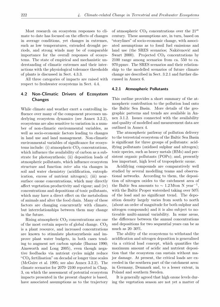
222 4. Climate-related Change in Terrestrial and Freshwater Ecosystems
Most research on ecosystem responses to cli-mate to date has focused on the effects of changesin average conditions, yet changes in extremes,such as low temperatures, extended drought pe-riods, and strong winds may be of comparableimportance for the overall responses of ecosys-tems. The state of empirical and mechanistic un-derstanding of climatic extremes and their inter-actions with the physiological tolerance thresholdsof plants is discussed in Sect. 4.3.3.
All three categories of impacts are raised withrespect to freshwater ecosystems in Sect. 4.4.
4.2 Non-Climatic Drivers of EcosystemChanges
While climate and weather exert a controlling in-fluence over many of the component processes un-derlying ecosystem dynamics (see Annex 3.2.2),ecosystems are also sensitive to variation in a num-ber of non-climatic environmental variables, aswell as socio-economic factors leading to changesin land use and land management. Non-climaticenvironmental variables of significance for ecosys-tems include: (i) atmospheric CO2 concentrations,which influence the availability of carbon as a sub-strate for photosynthesis; (ii) deposition loads ofatmospheric pollutants, which influence ecosystemstructure and function inter alia via changes insoil and water chemistry (acidification, eutroph-ication, excess of nutrient nitrogen); (iii) near-surface ozone concentrations, which may directlyaffect vegetation productivity and vigour; and (iv)concentrations and depositions of toxic pollutants,which may have a direct effect on the metabolismof animals and alter the food chain. Many of thesefactors are changing concurrently with climate,but interrelationships between them may changein the future.
Rising atmospheric CO2 concentrations are oneof the most certain aspects of global change. CO2
is a plant resource, and increased concentrationsare known to stimulate photosynthesis and im-prove plant water budgets, in both cases tend-ing to augment net carbon uptake (Bazzaz 1990;Ainsworth and Long 2005), even though nega-tive feedbacks via nutrient cycles might reduce“CO2 fertilisation” on decadal or longer time scales(McGuire et al. 1995; see also Annex 3.2.2). Theclimate scenarios for 2070–2100 reported in Chap.3, on which the assessment of potential ecosystemimpacts presented in the present chapter is based,have associated assumptions as to the trajectory
of atmospheric CO2 concentrations over the 21st
century. These assumptions are, in turn, based on“storylines” of socio-economic change, with associ-ated assumptions as to fossil fuel emissions andland use (the SRES scenarios; Nakićenović andSwart 2000). Projected CO2 concentrations by2100 range among scenarios from ca. 550 to ca.970 ppmv. The SRES scenarios and their relation-ship to the modelled scenarios of future climatechange are described in Sect. 3.2.1 and further dis-cussed in Annex 6.
4.2.1 Atmospheric Pollutants
This outline provides a short summary of the at-mospheric contribution to the pollution load ontothe Baltic Sea Basin. More details of the geo-graphic patterns and trends are available in An-nex 3.1.2. Issues connected with the availabilityand quality of modelled and measurement data areoutlined in Annex 4.
The atmospheric pathway of pollution deliveryto the terrestrial ecosystem of the Baltic Sea Basinis significant for three groups of pollutants: acid-ifying pollutants (oxidised sulphur and nitrogen);toxic species, such as heavy metals (HMs) and per-sistent organic pollutants (POPs); and, presentlyless important, high level of tropospheric ozone.
Acidifying compounds are comparatively wellstudied by several modelling teams and observa-tional networks. According to them, the deposi-tion of nitrogen oxides to the catchment area ofthe Baltic Sea amounts to ∼ 1.2Mton N year−1,with the Baltic Proper watershed taking over 50%of the load and no significant trend. The depo-sition density largely varies from south to north(about an order of magnitude for both sulphur andnitrogen compounds) and it is also subject to no-ticeable multi-annual variability. In some areas,the difference between the annual concentrationsand depositions for two sequential years can be asmuch as 20–30%.
The ability of the ecosystems to withstand theacidification and nitrogen deposition is generalisedvia a critical load concept, which quantifies themaximum amount of acidic and nutrient deposi-tion that the ecosystem can sustain without ma-jor damage. At present, the critical loads are ex-ceeded in the southern part of the catchment area:in Germany, Denmark and, to a lesser extent, inPoland and southern Sweden.
It is generally agreed that high ozone levels dur-ing the vegetation season are not yet a matter of

4.2. Non-Climatic Drivers of Ecosystem Changes 223
primary concern for Baltic Sea Basin ecosystems,except for the most south-western areas in Ger-many and Denmark. They can, however, becomemore significant in a warming climate.
Information about the toxic species is much lessprecise – both from observational and from mod-elling points of view. The density of observationsis insufficient, while the modelling estimates fromdifferent studies can differ greatly. It is, however,plausible that the total deposition onto the BalticSea catchment area is at least 1.2–1.5 kt yr−1 forlead (Pb) and at least 100 t yr−1 for cadmium(Cd).
Persistent toxic species, such as mercury (Hg),polychlorinated biphenyls (PCBs) and hexachloro-cyclohexanes (HCHs), are even more difficult toevaluate due to contradictions of different studiesand methodologies. For Hg, one can only esti-mate the order of magnitude of deposition densityto be 5–10 µ g m−2 yr−1 in the south of the areaand a few times lower in the north. For PCBs,the observed mean deposition flux at the Swedishwest coast is about 0.5–1 µ g PCB-sum m−2 yr−1
with a pronounced downward trend. The valuesfor the sum of α- and γ-HCH do not have cleartrends, fluctuating between 1 and 4 µ g HCH-summ−2 yr−1.
4.2.2 Land Use
Land use and land cover change, including bothconversions (complete replacement of one landcover type with another, e.g. forest to cultivatedland) and modifications (more subtle changes incover or management practices, e.g. intensifica-tion of agricultural land), in association with cli-mate change, are recognised as primary driversof global change (Guo 2000; Hansen et al. 2001;Grunzweig et al. 2003; Körner 2003; Lambin etal. 2003; Duraiappah et al. 2005; Lepers et al.2005). Indeed, some authors have proposed thatland use change is likely to be a more importantdriver than climate change, at least for the nearfuture (Sala et al. 2000; Slaymaker 2001; Sala etal. 2005). Ecosystem changes associated with landuse and land cover change are complex, involvinga number of feedbacks (Duraiappah et al. 2005;Lepers et al. 2005). For example, conversion offorest to agricultural land works as a driver of cli-mate change, by representing a major contribu-tor to greenhouse gas release to the atmospherevia losses of biomass and soil carbon (Gitz andCiais 2003; Canadell et al. 2004; Levy et al. 2004)
and, additionally, through a ‘land use amplifiereffect’ (Gitz and Ciais 2003), where the overallglobal carbon sequestration (‘sink’) capacity is de-creased. In contrast, reforestation, and other landuse or land management changes such as modifi-cations to agricultural practices, can work to miti-gate climate change through carbon sequestration(Lal 2003; Jones and Donnelly 2004; King et al.2004; Lal 2004; Wang et al. 2004; de Koning et al.2005). Land use change also drives other ecosys-tem changes in combination, or above and beyondclimate change, such as biodiversity changes, soilerosion, and land and water pollution (Lambin etal. 2003). Hansen et al. (2001) provide some ex-amples of feedbacks between climate, land use andbiodiversity, emphasising the importance of nottreating these factors in isolation.
For instance, Hansen et al. (2001) describe sit-uations in which land use change works to modifyspecies response to climatic changes by alteringdispersal routes. Alterations can represent bothbarriers to and facilitation for species dispersal.For example, when native vegetation is cleared foragriculture, a barrier can be created, limiting dis-persal for native species, while on the other handfacilitating access for exotic species. Climate andland use can also jointly influence disturbancessuch as wildfire, flooding and landslides. The twodisturbances may amplify each other; for example,logging can further dry fuels and increase the prob-ability of wildfire during periods of drought con-ditions. Alternatively, the two disturbances maycounteract each other, such as is the case wheregrazing reduces fire frequency and intensity. Landcover change can also directly affect climate: suchis the case where deforestation over large areascauses reductions in transpiration, cloud forma-tion, rainfall and increased evaporation. This canlead to vegetation shifts, such as the replacementof forests by shrubs and grassland.
Despite the recognised importance of land usechange in driving global change, it is rarely in-cluded in current global climate models (Hansenet al. 2001; Holman et al. 2005a; Levy et al. 2004;Zebisch et al. 2004). This limitation is attributedto an insufficient understanding of the underlyingcauses and prospective consequences of land useand land cover change at the global scale (Hansenet al. 2001; Lambin et al. 2001; Lambin et al.2003). However, much progress has been made inthis area, both in terms of a better understandingof the underlying processes as well as in the de-velopment of more sophisticated models (Lambin

224 4. Climate-related Change in Terrestrial and Freshwater Ecosystems
et al. 2003). Several studies incorporating land usechange have been undertaken at local and regionalscales, some of which are discussed in further de-tail in the following section. The explicit inclusionof land use change in analyses of climate changecould therefore lead to some unexpected outcomes(Hansen et al. 2001). Consequently, many im-pact studies of climate change may represent in-adequate estimates of projected changes.
4.2.2.1 Projected Future Changes in EuropeanLand Use
There have been a number of recent developmentsin future European land use scenarios and theirapplication, often based on the global SRES sto-rylines of the IPCC (Nakićenović and Swart 2000),or alternative scenario frameworks such as theMillennium Ecosystem Assessment scenarios (Car-penter et al. 2005). Other developments have beenlargely carried out on regional or local scales, ei-ther representing down-scaled versions or modi-fications of the SRES scenarios (Holman et al.2005a,b; Ewert et al. 2005; Rounsevell et al. 2005;van Meijl et al. 2005; Abildtrup et al. 2006; Ver-burg et al. 2006).
Worldwide, most regional and global scenariosindicate an expansion of agricultural land over thecoming decades due to the trade-off between foodsupply and demand as moderated by internationaltrade, with the biggest changes occurring in thetropics (Alcamo et al. 2006). Conversely, mostEuropean scenarios show agricultural land aban-donment (Ewert et al. 2005; Rounsevell et al. 2005;Verburg et al. 2006). Land abandonment scenar-ios tend to assume that increases in the supplyof agricultural goods due to the effect of tech-nological development on productivity will offsetchanges in food demand (Ewert et al. 2005; Roun-sevell et al. 2005; Verburg et al. 2006). Scenariosfor which agricultural land abandonment does notoccur are often characterised by yield reductionsarising from extensification of the agricultural pro-duction system. It is likely that both agricul-tural land abandonment and extensification wouldcreate opportunities for ecosystems and conserva-tion (Rounsevell et al. 2005), although the loss ofmountain pastures to regrowing forests is regardedas a negative impact in terms of biodiversity (Dirn-bock et al. 2003; Giupponi et al. 2006).
Forest scenarios tend to mirror agricultural sce-narios in that forested areas are often merely in-directly determined from the assumed expansion
or contraction of agricultural land (Alcamo et al.2006). In Europe, agricultural land abandonmentwould create the conditions for potential reforesta-tion (Kankaanpää and Carter 2004; Rounsevell etal. 2006a).
4.2.2.2 Land Use Change in the Baltic Sea Basin
There have been no climate change impact stud-ies on land use that have focused on the Baltic seaBasin as a geographic region. However, a numberof studies that have been undertaken at the Euro-pean scale allow targeted conclusions to be drawnfor the Baltic Sea Basin (for example see Audsleyet al. 2006; Ewert et al. 2005; Rounsevell et al.2005; Rounsevell et al. 2006b). It is important torecognise that the Baltic Sea Basin, like other Eu-ropean regions, is strongly dependent on drivingforces that operate at global and European scales,so that examining the response of the Baltic SeaBasin within European-wide studies is an appro-priate methodology.
Most studies find that the socio-economic sce-nario assumptions have a greater effect on futureland use than the climate change scenarios. Evenfor agriculture, which might be expected to besensitive to crop yield changes, there are win-ners and losers at the European scale with lit-tle overall change in agricultural production po-tential (Rounsevell et al. 2005). At the regionalscale, however, there may be large changes in landuse. Most agricultural scenarios present an argu-ment for decreasing agricultural areas, often as aresult of crop yield increases due to technologicaldevelopment rather than climate change (Roun-sevell et al. 2005; Audsley et al. 2006), and theseeffects are greatest in scenarios that are charac-terised by free markets. Reductions in agriculturalareas for food production are often compensatedsomewhat by increases in areas for bio-energy pro-duction and forests and small increases in urbanand nature conservation areas (Rounsevell et al.2006b). Such changes are also important for land-scapes and ecosystems. Some scenarios, however,suggest that the Baltic Sea Basin will respond dif-ferently. Audsley et al. (2006) indicate that Fin-land’s agricultural area may increase significantlyin response to the yield gains resulting from cli-mate change. Whether such changes would berealised in practice is debatable when simultane-ously the agricultural areas of the rest of Europeare decreasing (Rounsevell et al. 2006b), but it re-mains a possibility. Policy would probably play a
4.2. Non-Climatic Drivers of Ecosystem Changes 225
strong role in moderating this change, as increas-ing agricultural areas have negative environmentalconsequences not least for biodiversity (Berry etal. 2006).
It would seem logical for the land use of Swedenand Finland to respond in similar ways. However,Audsley et al. (2006) suggest that southern Swe-den will be very similar to Denmark (for whichmost future scenarios suggest constant agricul-tural land use) and good for agriculture, whereasthe north of Sweden remains cold even in the A1FIscenario (Sect. 3.3.4). Although Finland is at ahigher latitude than much of Sweden, it has amuch warmer summer and a huge area of Finlandhas higher yields of wheat than the south of Swe-den in the A1FI climate. Therefore, whereas theagricultural area in Sweden doubles, the area inFinland increases ten-fold under the A1FI scenario(Audsley et al. 2006).
4.2.2.3 Projected Combined Impacts of Land Useand Climate Change on Ecosystems
Relatively few studies have attempted to coupleland use and climate change scenarios in the anal-ysis of impacts on ecosystem processes, goods andservices. Global scale studies include the Millen-nium Ecosystem Assessment (Reid et al. 2005)and the studies by Sala et al. (2000) and WorldResources Institute (2000). Global scale scenar-ios are not appropriate, however, for the analysisof ecosystem impacts at local to regional scales.Moreover, there has been increasing interest inregional scale studies to promote development ofsimilarly-scaled policies and to enable stakehold-ers to engage with climate-related issues at a scalewhere they interact in terms of daily activities andmanagement (Holman et al. 2005b). Only a fewsuch studies have been undertaken at the regionalor local scale, and many of these are very recent,with some of the work still under review or cur-rently in press (Dirnbock et al. 2003; Stefanescuet al. 2004; Holman et al. 2005a,b; Scheller andMladenoff 2005; Giupponi et al. 2006; Harrison etal. 2006; Lavorel et al. 2006; Metzger et al. 2006;Schröter et al. 2005; Rounsevell et al. 2006b).
The limited available literature suggests thatthe effects of land use change on species at re-gional scales work to further fragment the overallclimate driven trends (Holman et al. 2005b; delBarrio et al. 2006; Harrison et al. 2006; Roun-sevell et al. 2006a). The degree of fragmentationdepends on where the land use changes occur, the
relative ‘hostility’ of the new environment to thespecies, and the species dispersal ability. Habitatfragmentation is exacerbated when species haverelatively low dispersal distances (del Barrio et al.2006). Furthermore, land use change can favoursome species over others, depending on the rela-tive hostility of the new environment (Giupponiet al. 2006). For example, projected agriculturalabandonment and increases in forest in the ItalianAlps resulted in an increase in the distribution offorest species (e.g. Ostrya carpinifolia) and a de-crease in the distribution of open habitat species(e.g. Crex crex and Chorthippus dorsatus). Berryet al. (2006) argue that northern latitude countrieswithin Europe will become increasingly importantfor biodiversity and species conservation as theranges of species distributions move northward inresponse to climate change. As northern latitudecountries are also the most likely to be sensitiveto the effects of climate change on land use (es-pecially agriculture), these regions could play aprominent role in adaptation strategies to mitigatethe negative effects of future climate and land usechange on Europe’s natural heritage.
Two studies examined projected changes at theEuropean level. The ATEAM project (Schröter etal. 2005) focused on a number of goods and ser-vices for the region as a whole (e.g. soil organic car-bon, carbon sequestration, wood production, car-bon storage, water resources, biodiversity changes)while the ACCELERATES project (Rounsevell etal. 2006a) focused on biodiversity changes in agri-cultural areas only. Three studies examined pro-jected changes at local and/or regional scales (Hol-man et al. 2005b; Lavorel et al. 2006; Rounsevellet al. 2006a).
Within the ATEAM project, projected changesin forests as a result of climate change, landuse and management were modelled using theinventory-based, European Forest InformationScenario Model (EFISCEN) (Karjalainen et al.2002; see also Annex 3.2.4). Growing stock, in-crement, age-class distribution and carbon stocksin above- and below-ground biomass were all sim-ulated. Projected changes in carbon balance wereestimated using a modified version of the LPJmodel (Sitch et al. 2003; Zaehle et al. 2007). Thetotal area of European forests was projected to in-crease by up to 6% by 2080, particularly in theB2 scenario. All scenarios projected an increasein forest growth, especially in northern Europeand in the economically-oriented A scenarios. Theintensity of management had the greatest influ-
226 4. Climate-related Change in Terrestrial and Freshwater Ecosystems
ence over increment in comparison to the effectsof land use or climate change, with increases be-ing the greatest in the most intensively managedareas. The effect of land use change on incrementvaried substantially across the scenarios, depend-ing on the extent of forest change. In the A1FIscenarios there were little changes in forest area,whereas in the B2 scenario, forest area increasedby 32%. Although timber harvesting exceeded for-est increment for the A1FI scenario in the sec-ond half of the 21st century, all scenarios showedan overall increase in growing stock compared topresent levels. Management had the greatest in-fluence on growing stock, whereas, depending onthe scenario, management accounted for 60–80%of the difference in growing stock between 2000and 2100, climate change accounting for 10–30%of the difference, with land use change accountingfor only 5–22%.
In terms of carbon balance, the combined landuse and climate change scenarios showed an over-all increased uptake of carbon up to 2050, with ashift towards carbon release towards the end of thecentury. In northern Europe, increased warming,mainly in winter, enhanced soil respiration morethan net primary production in all scenarios, de-creasing the sink, or turning it into a net carbonsource. Results from southern Europe were lessclear, with a mixture of increases in carbon up-take and carbon neutral projections. Land usechange was shown to contribute greatly to the in-creased carbon uptake in the first half of the cen-tury as a result of increased carbon sequestrationdue to reforestation in former agricultural areas.Socio-economic scenarios also showed a great dealof variation in projected carbon balances. Thisinfluence of differing socio-economic scenarios andassociated changes in land use suggests that deci-sions regarding socio-economics and land use aredrivers of the European terrestrial carbon balanceof comparable importance to climate change.
4.3 Terrestrial Ecosystems
4.3.1 Phenology
Phenology has been in the focus of scientists in theBaltic region since the early studies of Carl Linné.Over the last 300 years, phenologists have ob-served a wide range of plant, bird, insect, fish andanimal species using different observation meth-ods in the Baltic region (Schnelle 1955; Leith 1974;Schults 1981). The long time series of phenological
data that have been recorded have great potentialto characterise the impacts of the changing climateon ecosystems. In this section we focus on plantphenology, since phytophenological data are mostreadily available for different countries and for thebest-known indicator species.
Phenological observation programmes mostcommonly observe phases of spring such as bud-burst, leaf unfolding and flowering, as well as sum-mer phases such as ripening of fruit and harvest-ing. There are fewer observations on autumn phe-nological phases – including leaf colouring and leafabscission – and the data quality is much lower. Itis therefore complicated to use autumn-phase dataas climate change indicators (Chuine et al. 2003).Apart from their relevance as climate change indi-cators, spring and autumn leaf phenological phasesare key determinants of growing season length andprimary production in deciduous vegetation. Therelevance of leaf phenological changes to the pro-ductivity and functioning of ecosystems is furtherdiscussed in Sect. 4.3.4.
Temperature is the main triggering factor forspring and summer phenological events in temper-ate zones. Two classes of temperature parametershave a high correlation with both spring and sum-mer phases and have therefore been used in mostphenological analyses and models. The first com-prises positive (> 0 C) temperatures (mean, cu-mulative etc.) during the growing season, whichhave a direct triggering influence on plant phe-nology (Chuine et al. 2003; Schwartz 2003). Thesecond class of parameter is the chilling factor,i.e. the sub-zero temperatures during the previ-ous winter, as spring phenology is very depen-dent on the temperature regime during winter dor-mancy. The physiological and biochemical mecha-nisms controlling onset and release from dormancyhave so far not been thoroughly studied (Chuineet al. 2003). Apart from temperature, the pheno-logical development of plants is also influenced byother environmental factors (e.g. radiation, mois-ture, soil, landscape, ecosystem type) and humanimpacts such as pollution, land use and urban heatislands (Schnelle 1955; White et al. 2002; Schwartz2003). In the Baltic Sea Basin, snow cover is animportant factor for spring phenology, dampeningtemperature variation and isolating plants frompotentially harmful weather extremes.
In the present climate, the temperature vari-ability is generally determined by atmospheric cir-culation (Sect. 2.1.1 and Annex 1.2). Analysisof the correlation between phenological phases –
4.3. Terrestrial Ecosystems 227
flowering of coltsfoot (Tussilago farfara), unfold-ing of birch leaves (Betula pendula), flowering oflilac (Syringa vulgaris) – and circulation patternsin Europe (Aasa et al. 2004) has shown that in theBaltic Sea Basin, spring phenology is primarily in-fluenced by the North Atlantic oscillation (NAO)index during winter (December–March) and theArctic oscillation (AO) index during the first threemonths of the year (January–March). This wasevidenced by a measured correlation (Pearson r)stronger than −0.5 in the Baltic Sea Basin.
4.3.1.1 Recent and Historical Impacts
The databases on which the following assessmentis based provide relatively good coverage of Ger-many, Poland, the Baltic States and Russia. Rele-vant data from the Scandinavian countries, whichceased carrying out plant phenological observationprograms in the 1950s and 1960s, are not avail-able for recent decades. The only data publiclyavailable from the Scandinavian countries is fromthe International Phenological Gardens (IPG) net-work, which has phenological observation stationsin most of Central and Western Europe, and op-erates some stations in Scandinavia. For Finland,some long-term phenological time series are avail-able from the national Phenology Research Pro-gramme (www.fmnh.helsinki.fi/seurannat/fenolo-gia).
Analysis of trends in phenological time seriesover the last 50 years in the Baltic Sea Basin showsa tendency for spring to arrive earlier and au-tumn later. This conclusion is based on data fromthe International Phenological Gardens (IPG) net-work. Studies have shown that the length of thephenological growing season, as determined by leafunfolding and leaf fall of various tree species, haslengthened significantly during the period 1951 to1996 (Menzel and Fabian 1999). On average, thespring arrival trend was negative (arriving earlier)and the autumn trend positive (arriving later).The mean trend of the 616 spring phases studiedover all of Europe changed by −2 days per decade;the 178 autumn phases changed by +1.6 days perdecade during the study period. As a result, theaverage growing season was extended by 3.6 daysper decade in the study area.
Chmielewski and Rötzer (2001) used the IPGdataset to analyse changes in the phenologicalgrowing season for 1968-1998 over Europe. Theydetermined the beginning of the growing seasonby means of a combined leafing index (Betula
pubescens, Prunus avium, Sorbus aucuparia andRibes alpinum) and the end of the growing seasonby the mean leaf fall date of four species (Betulapubescens, Prunus avium, Salix smithiana, Ribesalpinum). For Europe as a whole, the analysisidentified a significant (P < 0.05) lengthening ofthe growing season, by 2.7 days per decade. Forthe Baltic Sea Basin (southern Fennoscandia, Den-mark and northern Poland) the trends were muchstronger in most of the stations: the growing sea-son lengthened by 4.5 days per decade, as the onsetof spring shifted significantly earlier.
Phenological trends in central and eastern Eu-rope were studied within the EU project POSI-TIVE (Menzel 2002), which mapped phenologicaltrends on the southern and eastern coasts of theBaltic Sea using data sets from weather services(DWD, EMHI) and the Russian Geographical So-ciety, covering the period 1951–1998 (Ahas et al.2002; Scheifinger et al. 2003). Analyses of commonplant and tree species in this area showed thatthe highest rate of change appeared in the earlyspring phases (e.g. pollination of hazel [Corylusavellana] and coltsfoot [Tussilago farfara]), whichnow occur 10–20 days earlier than 50 years ago (anaverage change of 2–4 days per decade). Springphases (birch leaf unfolding, lilac and apple treesin full bloom) have undergone smaller changes,now occurring 5–15 days earlier than 50 yearsago (Ahas et al. 2002). Linear regression mapsof birch leaf unfolding (Fig. 4.1) show the higheststatistically-significant slope for a linear regressionagainst time, ranging from −4.2 to −7.3 days perdecade in the Baltic region. The slope of lilac (Sy-ringa vulgaris) flowering is steepest in the Balticregion (−2.6 days per decade), likewise showing arelatively steep slope over the northern part of theEastern European Plain (−2.1 days per decade).Lime (Tilia cordata) shows a significant trend to-wards earlier flowering in the summer in the Balticregion. Similar results to the above were mappedwithin the EU Programme European PhenologicalNetwork (van Vliet 2003; van Vliet et al. 2003).
Table 4.1 presents slopes of linear trends (daysper year) at selected stations within the Baltic SeaBasin (Ahas et al. 2002). The early spring phases,such as blossoming of hazel or coltsfoot, havegreater slopes than the late spring and summerphases. The statistically significant (P < 0.05)trends tend to have a negative value.
Trends in Estonian phenological time serieshave been studied in several projects, taking ad-vantage of the very good available series of obser-
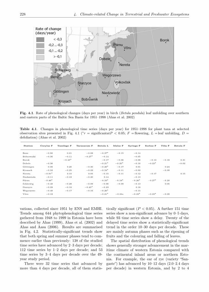
228 4. Climate-related Change in Terrestrial and Freshwater Ecosystems
Fig. 4.1. Rate of phenological changes (days per year) in birch (Betula pendula) leaf unfolding over southernand eastern parts of the Baltic Sea Basin for 1951–1998 (Ahas et al. 2002)
Table 4.1. Changes in phenological time series (days per year) for 1951–1998 for plant taxa at selectedobservation sites presented in Fig. 4.1 (�r = significantatP < 0.05; F = flowering, L = leaf unfolding, D =defoliation) (Ahas et al. 2002)
Station Corylus F Tussilago F Taraxacum F Betula L Malus F Syringa F Sorbus F Tilia F Betula F
Benz −0.90 0.01 −0.08 −0.37� −0.15 −0.14
Bobrowniki −0.36 −0.11 −0.27� −0.14 −0.05
Borok −0.45� −0.17 −0.06 −0.08 −0.13 −0.18 0.31
Dobele −0.36 −0.21� −0.25� −0.16 −0.23� −0.02
Göttingen 0.06 0.20 −0.30 −0.26� −0.17 0.01 0.24
Kronach −0.32 −0.25 −0.22 −0.34� −0.11 −0.02 −0.09
Nereta −0.91� 0.10 0.05 −0.15 −0.11 −0.12 −0.17 0.15
Niedzwiedz −0.11 −0.18 −0.20 0.14 −0.13
Pärnu −0.46� −0.33� −0.18� −0.26� −0.27� −0.20
Schleswig −0.40 −0.28 −0.09 −0.06 −0.09 −0.13 0.05
Starzyce −0.29 −0.16 −0.45� −0.23 0.18
Wegorzewo −0.40 −0.17 −0.16 −0.26� −0.15
Võru −0.18 −0.21� −0.24� −0.23� −0.23� −0.09
vations, collected since 1951 by ENS and EMHI.Trends among 644 phytophenological time seriesgathered from 1948 to 1999 in Estonia have beendescribed by Ahas (1999), Ahas et al. (2002) andAhas and Aasa (2006). Results are summarisedin Fig. 4.2. Statistically-significant trends showthat both spring and summer phases tend to com-mence earlier than previously: 138 of the studiedtime series have advanced by 2–3 days per decade;112 time series by 1–2 days per decade; and 53time series by 3–4 days per decade over the 49-year study period.
There were 32 time series that advanced bymore than 4 days per decade, all of them statis-
tically significant (P < 0.05). A further 151 timeseries show a non-significant advance by 0–5 days,while 93 time series show a delay. Twenty of thedelayed time series show a statistically-significanttrend in the order 10–30 days per decade. Theseare mainly autumn phases such as the ripening offruits and the colouring and falling of leaves.
The spatial distribution of phenological trendsshows generally stronger advancement in the mar-itime climate of western Estonia compared withthe continental inland areas or northern Esto-nia. For example, the ear of rye (variety “San-gaste”) has advanced by 10–12 days (2.0–2.4 daysper decade) in western Estonia, and by 2 to 4

4.3. Terrestrial Ecosystems 229
Fig. 4.2. The distribution of trends over the period 1951–1999 in the Estonian phytophenological time seriesaccording to the size and significance of changes (Ahas and Aasa 2004). Classes are in days per 49 years
days (0.4–0.8 days per decade) in eastern Estonia(Ahas and Aasa 2006).
In the Estonian phenological dataset, the dis-tribution of phenologically early and late springswas also analysed. These were determined using athreshold of values greater or less than 1 standarddeviation in all spring phases, i.e. measurementsoutside of the +/− 1 standard deviation thresholdwere considered either early or late, accordingly.
Results (Fig. 4.3) show that at the beginning ofthe studied period (1950s) there were more delayedphases, reaching a peak in 1955 with a total of 87delayed phases. The number of delayed time seriesdecreased between 1955 and 1995. Years that areearlier by more than 1 standard deviation begin todominate after 1980, reaching a peak in 1989, with77 advanced phases. In 1990, 1991, 1992 and 1993,a majority of the time series was also advanced(Ahas and Aasa 2004; Ahas and Aasa 2006).
Historical changes in phenological time series inEstonia have also been studied. During the period1919–1996 the mean change in spring phenophaseswas an advance of 2–5 days per decade (Ahas 1999;Ahas et al. 1998)
Taken together, phytophenological time seriesfrom the Baltic Sea Basin show a marked trend to-wards an advancement of spring and early springphases in recent decades, indicative of the effectsof a warming climate on plants. The phenological
trends appear to be generally somewhat strongerin the Baltic Sea Basin compared to Europe asa whole, possibly reflecting a stronger warmingtrend in northern Europe (Sect. 2.1.2). As indica-tors of ecosystem responses to climate, phytophe-nological trends for the Baltic Sea Basin clearlysupport the hypothesis that recent climate changehas impacted the functioning of ecosystems there.
4.3.1.2 Potential Future Impacts
Extrapolation of the average effect of climatewarming suggests that a rise in mean temperatureby 1 C will lengthen the phenological growing sea-son by 5 days in temperate Europe (Chmielewskiand Rötzer 2001). Predictions based on GCM-modelled climate scenarios suggested that snow-drop (Galanthus nivalis) flowering would occur 2weeks earlier if atmospheric CO2 concentrationsdoubled by 2035, and one month earlier if CO2
levels tripled by 2085 in northern Germany (Maakand von Storch 1997).
The scenarios of +2 C and −2 C temperaturerise used in the Estonian analysis showed that inthese cases the phenological development of na-ture remains within the limits of natural variation(Ahas et al. 2000). The case of a 4 C warmerspring has also been studied, with results suggest-ing that the common spring phases will still re-

230 4. Climate-related Change in Terrestrial and Freshwater Ecosystems
Fig. 4.3. The percentage of values larger or smaller than ±1 standard deviation in the summarised phenologicalcalendar of three selected stations in Estonia (Pärnu, Türi and Võru) (Ahas and Aasa 2004)
main within the limits of extreme (warm) yearssuch as 1975, 1989 and 1990 (Ahas et al. 2000).Several authors have pointed out that the phe-nological development of nature is relatively flexi-ble since many species and their phenological vari-eties adapt to the wide natural variations of springweather in temperate regions. However, manyphenological models predict that global warmingand earlier springs will result in an increased riskof frost damage for species throughout Europe (seealso Sect. 4.3.3).
Linkosalo et al. (2000) studied frost-damagerisks with a chill-triggered model in Finland, show-ing that increased frost risk would occur dur-ing earlier (warmer) springs. A light-climate-triggered model did not, however, predict thoserisks (Linkosalo et al. 2000). Statistical analysisof data from the POSITIVE project showed thatthe risk of late frost damage for plants in CentralEurope has been lower in the last decade comparedto previous decades (Scheifinger et al. 2003).
Climate scenarios for the Baltic Sea Basin gen-erally point to a 3–5 C rise in average tempera-tures by the end of the 21st century (Chap. 3).For many species, this could lead to an extensionof the growing season in the order of weeks, a sig-nificant change in conditions for growth, especiallyin northern areas where the growing season is cur-rently shortest.
4.3.2 Species and Biome Range Boundaries
Species and biome range boundaries are depen-dent on a wide range of environmental factors, in-cluding climate and meteorological events. There-fore, species and biome ranges are potentially verysensitive to climate changes, particularly changesin temperatures, precipitation patterns (especiallyreduced precipitation leading to drought stress), aswell as the incidence of extreme events like stormsand floods. Moreover, recent observed speciesrange shifts may be tied to the influence of large-scale weather systems, such as NAO in the case ofthe Baltic Sea Basin (Annex 7).
In the following assessment, we focus mainlyon changes in ecosystems related to temperatureand precipitation. However, it should be borne inmind that, even in the case of range shifts cor-related with changes in temperature and precip-itation, other factors may play a role as drivingforces. Examples include UV-B radiation (Cum-mins 2003), or atmospheric CO2 concentrations,which may affect the carbon balance of vegetation.
Species responses to environmental gradientstypically differ in a community setting comparedto the fundamental physiological response due tothe secondary effects on individual vigour of com-petition, impacts of pests and diseases and otherbiotic factors. Natural disturbances (e.g. wildfires,floods) may likewise modify responses. Finally,

4.3. Terrestrial Ecosystems 231
the present distribution of many species is moreevidently tied to land use, habitat fragmentation(e.g. Hill et al. 1999) or the absence of suitablehabitats due to human activities than to speciesresponses to bioclimatic gradients. Anthropogenicfactors are likely to play an important role infuture range shifts as well as species extinctions(Pounds et al. 1999; Williams et al. 2003).
4.3.2.1 Methodological Remark
Evidence for distributional changes at the species,community or population level are often derivedby comparing two surveys at discrete points intime. Background changes between the surveyevents are rarely addressed. Yet without con-sideration of how much background variation isplausible between years, or even within years, anyapparent “trend” cannot be robustly ascribed toclimate change or any other specific driving fac-tor (Sparks and Tryjanowski 2005). Species’ be-haviour at those specific time points can affectconclusions, because changes in the distributionof species are associated not only with climate butalso with major changes in habitats (Pounds et al.1999; Warren et al. 2001; Konvicka et al. 2003).Apparent range margin shifts can be a possibleresponse to the influence of both factors.
4.3.2.2 Recent and Historical Impacts
Changes in species distributions
Distributional shifts are the potential result, atgeographic scales, of two very different mecha-nisms operating at the local scale: expansion intonew areas; for example, areas that have becomefavourable as a result of climatic amelioration; andlocal extinction, which reduces the distribution.We discuss each of these mechanisms in turn, andevaluate their potential role in recent and histori-cal distributional changes of species in the BalticSea Basin.
There is evidence of changes in the distributionof terrestrial species throughout the world (Parme-san et al. 1999; Walther et al. 2002) consistentwith recent global warming (Grabherr et al. 1994;Pounds et al. 1999), although consensus on a gen-eral, causal link has not yet been achieved (Jensen2003).
Globally, many studies have focused on speciesabundances and distributions to corroborate pre-dicted systematic shifts related to shifts in climatic
regimes, often based on species-specific physiolog-ical thresholds of temperature and precipitationtolerance (e.g. Woodward 1987; Sykes et al. 1996;Grace et al. 2002). Some commonly invoked mech-anisms are described in Annex 3.2.2. A certain in-herent resilience is reported for some communitytypes, such as treeline forests, while the magnitudeof elevational shifts of alpine plant species lags be-hind the isothermal shift. By contrast, some but-terflies appear to track decadal warming quickly(Parmesan et al. 1999).
For the Baltic Sea Basin there are a few exam-ples of species showing both latitudinal and alti-tudinal shifts of the species distributional range.Changing temperatures are known to have pro-duced shifts in species range limits in historicaltimes. For example, the Scandinavian distribu-tions of beech (Fagus), lime (Tilia), oak (Quer-cus) and spruce (Picea) have generally trackedgrowing-season heat sums over the last 8000 years,based on pollen observations and vegetation modelsimulations (Bradshaw et al. 2000). The cur-rent rate of climate change is rapid comparedwith changes of similar magnitude in the past.Walther et al. (2005) report new observations ofnaturally-regenerating holly (Ilex aquifolium), aspecies purported to be a climatic indicator, eastand northward of the previously reported naturallimit (Iversen 1944). The new observations coin-cide with an advance of the 0 C January isolinesince the 1940’s.
Kullman (2002) reported upslope range shiftsof 100–150m by near-treeline birch (Betulapubescens ssp. czerepanovii), Scots pine (Pinussylvestris), Norway spruce (Picea abies), rowan(Sorbus aucuparia) and willow (Salix spp.) in theSwedish part of the Scandes mountain range, iden-tifying a 0.8 C increase in mean temperature sincethe late 19th century as the most important cause.Increased height growth by existing krummholz in-dividuals was a more important contributing fac-tor to apparent treeline advance than establish-ment of new individuals at higher elevations. Aftera slight retardation during some cooler decades af-ter 1940, a new active phase of tree-limit advancehas occurred with a series of exceptionally mildwinters and some warm summers during the 1990s(Kullman 1993, 1997, 2002). The magnitude of to-tal 20th century tree-limit rise varies with topocli-mate and is mainly confined to wind-sheltered andsnow-rich segments of the landscape. Thickeningof birch tree stands in the “advance belt” has pro-foundly altered the general character of the sub-

232 4. Climate-related Change in Terrestrial and Freshwater Ecosystems
alpine/low alpine landscape and provides a posi-tive feedback loop for further progressive changeand resilience to short-term cooling episodes. Allupslope tree-limit shifts and associated landscapetransformations during the 20th century have oc-curred without appreciable time lags, which con-stitutes knowledge fundamental to the generationof realistic models concerning vegetation responsesto potential future warming. The new and ele-vated pine tree-limit may be the highest duringthe past 4000 14C years. Thus, it is tentativelyinferred that the 20th century climate is unusuallywarm in a late-Holocene perspective.
Animals, within their lifetime, mainly followchanges in habitat structure; for this reason,changes in animal species ranges can be predictedfrom plants and plant community changes overtime. However, the availability of data to com-pare historical and current distribution are in somecases much better for animal species than forplants, and this is true in the case of the BalticSea Basin countries. For instance, changes inthe bird fauna of Finland were summarised byBrommer (2004). He analysed changes in rangemargins of birds breeding in Finland from pub-lished atlas data for a 12-year period (1974–1979to 1986–1989). The change in range margin wasstatistically corrected for range size change withinFinland using linear regression. For species pre-dominantly occurring in southern Finland (n =116), the corrected range margin shift was 18.8 kmnorthwards, which may be related to climatechange. Northerly species (n = 34) showed nosuch significant range margin shift.
In a fresh overview on climate change impactsin Finland, Pöyry and Toivonen (2005) report thatover 100 new butterfly and moth species have beenrecorded in Finland during the last decade (seealso Parmesan et al. 1999). Some originally uni-voltine moths (having a single generation per year)have become multivoltine (more than one genera-tion per year).
Many recent range shifts of animals to thenorth may be connected with climate warming.For the majority of bird species showing recentrange shifts within the Baltic Sea Basin, theshift is to the north, suggesting a climatologicalexplanation (Lehikoinen et al. 2003; Tomiałojćand Stawarczyk 2003; Tryjanowski and Winiecki2003). However, it should be noted that somesouthern species – which should be favoured byclimate warming – are becoming rarer, while somenorthern species have extended their distribution
southwards (Lehikoinen et al. 2003; Tomiałojćand Stawarczyk 2003; Tryjanowski and Winiecki2003).
Among mammals, an interesting example isshown by Sachanowicz and Ciechanowski (2006)which links the first winter record of a migratorybat (Pipistrellus nathusii ) in Poland and recordsfrom other countries to climate changes. It is sus-pected that for migratory bats changes in distribu-tion ranges, relocation of wintering areas, as wellas the timing of hibernation may be similar tothose well described for birds.
An example of uphill shifts is the distribution ofbutterflies observed in the Czech Republic (Kon-vicka et al. 2003) within a study region includingareas belonging to the Baltic Sea Basin (north-ern Moravia, Silesia). Recent butterfly distribu-tions were compared with historical (1950–1980)data, showing that altitude shifts in the distribu-tion of Czech butterflies are already detectable onthe coarse scales of standard distribution maps.The species undergoing altitudinal advance showno consistent patterns with regard to habitat af-filiations, conservation status or mountain versusnon-mountain distribution, which renders climaticchange as the most likely explanation for the dis-tributional shifts.
Tryjanowski et al. (2005) demonstrated that thewhite stork (Ciconia ciconia) has increased its ele-vational range during the last 30 years in the Pod-hale region, Poland. An answer to the questionof why white storks, traditionally wetland species,have increased their altitudinal breeding range byat least 500 m in upland and mountain areas withrelatively small water bodies, is likely to be com-plex: firstly, because the species has the biologicalpotential to colonise mountain areas; secondly, be-cause storks appear to follow habitat and/or cli-mate changes. During the study period, manyarable fields in the Podhale region were abandonedand/or converted to pasture following the collapseof communism. This, together with climatologi-cal factors (changes in temperatures and runoff),created new habitat and offered new foraging op-portunities for storks. Hence, when climatologicalconditions improved, and after saturation of loweraltitude nest sites, the storks expanded to higherground, and occupied new areas.
Consequences of species range shifts on longertime scales could be extinction (Thomas et al.2004). Palaeontological data clearly support thehypothesis that major extinction events in the pastwere related, at least in part, to changes in tem-
4.3. Terrestrial Ecosystems 233
perature regimes. For example, pollen data revealrange fluctuations in trees correlated with environ-mental changes through the Holocene (e.g. Brad-shaw et al. 2000). However, individual longevity,high intra-population genetic diversity and the po-tential for high rates of pollen flow might maketree species comparatively resistant to extinction(Hamrick 2004).
There is some evidence of imminent rangeretraction via local extinction for tree species.The primeval forest of Białowieża National Park,Poland, is considered to be a unique remnant ofa mixed broadleaf-conifer forest type that oncedominated lowland regions of central-eastern Eu-rope. Norway spruce occurs as a codominantspecies in the forest, close to its inferred clima-tological (“warm”) limit (Dahl 1990). The speciesis currently in decline due to regeneration failure(Walankiewicz 2002).
The historical past of southwest Finnish birds,including the archipelago areas, was studied byLehikoinen et al. (2003), who found indicationsof possible past extinctions (cormorant [Phalacro-corax carbo], grey heron [Ardea cinerea], bittern[Boturus stellaris], red kite [Milvus milvus]) thatco-occur with the coldest period of the “LittleIce Age” and/or intensification of human impacts.Similarly, changes in Polish avifauna during pre-and historical times have been linked to changedclimatological regimes in the past (Bocheński1993; Tomiałojć and Stawarczyk 2003), while Na-jbar and Szuszkiewicz (2005) linked a strong de-cline in the European pond turtle (Emys orbicu-laris) with reproduction failure (egg freezing) as aresult of declining snow cover in recent years.
Climate-related invasions
The clearest evidence for a climatic trigger forlarge-scale changes in ecosystem structure occurswhere a suite of species with different histories ofintroduction spread en-masse during periods of cli-matic amelioration (Walther et al. 2002). Withclimate change, non-native species from adjacentareas may cross barriers and become new elementsof the local biota. In cases where long distanceshave been covered, such movements have oftenbeen mediated by human activity. A permanentestablishment in the native ecosystem may not bepossible without changes in local conditions.
To our knowledge there are no data on inva-sions forced by climate change in the Baltic SeaBasin. However, some cases of geographical range
expansion in invertebrates could be interpreted asresponses, in part, to climate change. An exampleis the wasplike spider (Argiope bruennichi ), pre-viously restricted to southeastern Europe, whichin recent decades has expanded its geographicalrange to the northern parts of Europe, colonisingmany new sites in Germany, Poland, Denmark andSweden (Scharff and Langemark 1997; Barabaszand Górz 1998; Jonsson and Wilander 1999). Themost important factors causing rapid geographi-cal expansion of the wasplike spider are: climatechange, especially increase of the number of sunnyand dry days in summer; floods of large rivers inEurope; and the establishment of large open habi-tats due to deforestation and drainage (Scharff andLangemark 1997; Barabasz and Górz 1998). Sim-ilarly, weather-regime changes were noted amongimportant factors controlling invasion of parts ofEurope – including the Baltic Sea Basin – by theleaf miner moth (Cameraria ohridella), an impor-tant pest of horse-chestnut trees (Sefrová and La-suvka 2001), and by moths (e.g. Palmqvist 1999).Expansion of Mediterranean dragonflies into cen-tral Europe has likewise been linked to climatewarming during recent decades (Ott 2001). It isimportant to bear in mind that evidence, of thekind presented above, for a climatic driving forcefor invasions is circumstantial and in many casesnot well documented.
Changes in migratory distributional status
Apart from effecting absolute changes in species’geographical ranges, climate changes may influ-ence relationships between wintering and breedingparts of the geographical ranges of migratory an-imal species, especially birds, but potentially alsobats and migratory insects. Examples of the lat-ter include certain butterfly and moth species inFinland (e.g. many Nymphalids), which depend onnorthward migration from southern populations.
Mild winters during recent years appear to haveproduced a tendency towards shorter migratorydistances to wintering places, and even to winter-ing in breeding areas. Birds can change migratorybehaviour in many ways (Fiedler 2003). Selectedexamples are increased proportions of sedentaryindividuals in the local populations, as notedfor waterfowl such as mute swan (Cygnus olor),great crested grebe (Podiceps cristatus), grey-lag goose (Anser anser), and a number of otherspecies (Švažas et al. 2001; Fiedler 2003), andfor passerines like stonechat (Saxicola torquata),

234 4. Climate-related Change in Terrestrial and Freshwater Ecosystems
chiffchaff (Phylloscopus collybita), starling (Stur-nus vulgaris) and many others. These findingswere obtained by direct visual observations, as wellas by strict analysis of ringing data sets (Švažaset al. 2001; Fiedler 2003; Tomiałojć and Stawar-czyk 2003). Other effects that have been observedin conjunction with changing climatic patterns in-clude changes in migratory directions and changesin the proportions of individuals with stronger orweaker migratory activity, as well as changes inthe timing of movements to breeding and winter-ing areas (Fiedler 2003).
Changes in biome boundaries
Altitudinal shifts of vegetation are well-documen-ted for many parts of the Earth. Higher tem-peratures and longer growing seasons, associatedwith climate change, have released new areas forcolonisation by certain plant species (e.g. Parme-san et al. 1999). However, data for the BalticSea Basin are scarce and current studies onlyseem to permit one robust conclusion concern-ing biome-level range displacements, namely thatendemic mountain plant species are threatenedby the upward migration of more competitivesub-alpine shrubs and tree species, to some ex-tent as a result of recent climate change (Kull-man 2003; see Changes in species distributions,above).
4.3.2.3 Potential Future Impact
As noted above, the direct impacts of climatechanges on species distributional limits (e.g. viaphysiological tolerance limits) are compoundedwith indirect effects, changes in non-climatic en-vironmental factors, and – of perhaps overridingimportance in the Baltic Sea Basin – the activ-ities of humans. Given this complexity, futurechanges in species and biome distributions are ex-tremely difficult to predict or to model, althoughmany new technologies are being developed (e.g.Thuiller 2003; Araújo et al. 2005; Sparks and Try-janowski 2005; Koca et al. 2006). In general terms,however, we may suspect that climate change ofthe magnitude described in Chap. 3 will accen-tuate the processes, already underway for somespecies, of colonising new habitats and localitiesrendered favourable by warmer temperatures andother forms of climatic amelioration. This mightresult in increasingly detectable northerly and up-slope shifts in species and biome boundaries.
The unprecedented rate of climate modificationexpected in the coming century has important im-plications for the likehood of large-scale biogeo-graphical change. Many species, especially treesand large animals, react to environmental varia-tion with lags (Saether et al. 2005). Most trees,for example, have a generation time in the orderof decades, and limited dispersal distances, mostseeds spreading only a few metres from the par-ent tree. Palynological records show that manytree species can nevertheless spread by rates of150–500m year−1 during periods of range expan-sion (Huntley 1991; Grace et al. 2002), but thisstill amounts to only a fraction of the averagerate of isotherm migration anticipated for the com-ing century (Chap. 3). Even if the seed dispersalof some species is able to keep up with climatechange, local dominance shifts may be delayedby the long generation times, competition withresident species, required changes in soil struc-ture, hydrology, chemistry, litter depth, require-ments for mycorrhizae and other factors (Sykesand Prentice 1995; Huntley 1991; Malanson andCairns 1997). Of course, human intervention, in-cluding the planting of “new” species in the con-text of commercial forestry, may accelerate rangedisplacements for certain species (Lindner 2000).
Patterns of change in distributions are oftenasymmetrical, with species from warmer climates(lower latitudes or altitudes) invading fastest(Walther et al. 2002). This could produce tran-sient assemblages lacking modern analogues, suchas a temporary beech (Fagus sylvatica) dominatedcommunity within a “window of opportunity” fol-lowing a warming-driven decline in Norway spruce,and prior to beech chilling failure, simulated by aforest dynamics model for southern Sweden (Sykesand Prentice 1995).
A number of model-based studies have exploredpotential changes in species distributions under fu-ture climate and/or atmospheric CO2 concentra-tions. Most such studies of relevance to the BalticSea Basin have been concerned with major treespecies.
The temperature changes predicted by climatemodels for the coming 50–100 years represent ageneral northward and eastward shift of the po-tential equilibrium ranges of species in climaticspace. Using a static bioclimatic model, Sykeset al. (1996) examined the potential effects ontree species distributions of a climate scenario de-rived from the average of four GCM runs based ondoubled CO2 forcing. The model predicted sub-
4.3. Terrestrial Ecosystems 235
stantial northward and eastward displacements inthe ranges of the boreal forest dominants Norwayspruce and Scots pine. The warm range limitsof both species were predicted to migrate some1200 km northwards across Sweden, and to re-treat eastwards from southwestern Germany to theBelaussian-Russian border. Broadleaved decidu-ous tree species, especially birch, hazel, ash, aspen,oak and elm were correspondingly predicted to in-crease their potential cover in southern Scandi-navia and northern parts of central Europe. Beechwas predicted to colonise most parts of Scandi-navia and the eastern Baltic Sea Basin, areas fromwhich it is currently absent. The climate scenar-ios used in these studies were of generally strongerwarming over the Baltic Sea Basin than recent as-sessments describe (Chap. 3). More recent resultsusing the same model suggest that range shifts willbe qualitatively similar but smaller (Bradshaw etal. 2000).
Koca et al. (2006) used a process-based dynamicvegetation model (Smith et al. 2001) to assess po-tential vegetation changes for Sweden under fourregional climate model-derived scenarios for thelate 21st century (Räisänen et al. 2003). The cli-mate scenarios, generated by the RCAO modelunder SRES A2 and B2 scenarios, may be seenas representative of the range of RCM scenariosdescribed in Sect. 3.5, and for overall projectedtrends as synthesised in Chap. 3. Lags imposedby tree generation times and competition betweenresident and colonising species are taken into ac-count by the model. As in earlier studies usingstatic vegetation models (Sykes and Prentice 1995;Bradshaw et al. 2000), expansion of boreal forestinto alpine areas, and an increased northern ex-tent of deciduous broadleaved species (beech, limeand oak) are predicted. Spruce and pine exhibitregeneration failure in southern Sweden, but re-main present in declining abundance to the end ofthe 21st Century. The overall pattern throughoutthe boreo-nemoral and boreal zone is of an increas-ing regeneration of broadleaved species within age-ing conifer-dominated stands. A modern analogyto this type of transient vegetation may be old-growth remnants of Białowieża Forest in Poland,where regeneration failure in Norway spruce hasbeen linked to climate warming, while broadleavedtrees (principally lime and ash) are gaining indominance (Walankiewicz 2002; see Changes inspecies distributions, above).
Using a stand dynamic model, Kozak et al.(2002) predicted increasing dominance of Euro-
pean beech over Norway spruce in conjunctionwith a 2 C increase in mean annual tempera-ture in the Bieszczady Mountains in southeast-ern Poland. However, the simulated dominanceshifts were gradual, with a new equilibrium beingachieved first after several centuries of simulatedvegetation dynamics.
4.3.3 Physiological Tolerance and Stress
Temperature, precipitation and light are the mainfactors affecting the large-scale distribution ofplant species (see Annex 3.2.2). A temperatureincrease is generally expected to increase the pri-mary production (Saxe et al. 2001; Sect. 4.3.4; An-nex 3.2.2). A simultaneously increased frequencyof extreme climatic events could, however, leadto an increased number of stressful weather sit-uations, reducing the net primary production viavegetation damage. In this context, it is impor-tant to recognise that different species have dif-ferent physiological tolerance limits. Stressful sit-uations must therefore be defined in relation tospecies- and provenance-specific adaptations, notfrom a climatological point of view (Gutschick andBassiriRad 2003).
Plants become stressed when the physiologi-cal tolerance is exceeded, and this causes long-term changes in metabolism and resource allo-cation. The physiological processes can be al-tered for several months after ambient conditionshave returned to normal. Both a sudden and ex-treme change in weather conditions and a longerperiod of unfavourable conditions, exceeding theendurance capacity of the organism, can becomestressful. The intensity, duration, frequency andcombination of stressful weather events determinethe long-term impact on plant performance. Thismakes the impact of climate change on ecosystemstructure and functioning inherently difficult to as-sess. Ecosystem modelling is required in order todevelop management strategies, aiming to reducethe risk for damage and achieve long-term sustain-ability in forestry, agriculture and nature conser-vation.
4.3.3.1 Acclimatisation and Adaptability
One reason that an extreme weather event is notthe same as an extreme situation for plants, andvice versa, is that the plants have the ability toacclimatise and adapt to changing weather condi-tions (Kozlowski and Pallardy 2002). Through ac-climatisation, the range of tolerance is adjusted to

236 4. Climate-related Change in Terrestrial and Freshwater Ecosystems
avoid harmful stress. An example is the hardinessstatus of plants, a reflection of seasonal changesin temperature and light conditions. Trees fromcool temperate climates in Scandinavia can toler-ate −30 C during midwinter when the trees arefully hardened, but a temperature backlash be-low −5 C can be very harmful in spring when thetrees have started to deharden (Larcher 1995). Ac-climatisation thus creates temporal thresholds intolerance to weather conditions.
The impact of climate on the performance of anindividual plant will be affected by local conditionsin topography, water availability and interactionwith neighbouring organisms. Through adapta-tion, plant individuals can adjust to long-term siteconditions. For instance, the root-shoot ratio canchange in response to altered water availability.The rate of climate change will affect the adapta-tion ability, and plants at different life stages maydiffer in their ability to respond to altered con-ditions. At any given site, differences in species-specific capacity for acclimatisation and adaptabil-ity will affect the risk for weather-induced damage.Events exceeding the acclimatisation capacity ofplants act as strong selection forces (Gutschick andBassiriRad 2003). Over time, genetic adaptationsof species, as well as changes in species abundance,will result. A prerequisite is, however, that evo-lutionary adaptations are possible and sufficientlyrapid to compensate for the changes in climate(Saxe et al. 2001).
4.3.3.2 Plant Resource Allocation
Damage to plants affects the allocation of car-bohydrates and nutrients. Damage causes directcosts for healing and renewal of plant parts. In-direct costs result from a lowered efficiency of re-source uptake or utilisation, sometimes mediatedvia altered symbiotic relationships (McLaughlinand Shriner 1980). In the event of subsequentattacks by pests and pathogens, an increasedamount of resources must be allocated to de-fence. The total cost of chemical resistance de-pends not only on synthesis, but also on com-pound turnover rates and costs of transport andstorage. These costs and the resultant effects onplant vitality are difficult to estimate. One rea-son is that the genetically-determined growth ratesof plant species covary with stress resistance andresilience to damage by affecting the basic allo-cation between growth, storage and defence (cf.Chapin et al. 1990; MacGillivray et al. 1995; Heil
2001; Shudo and Iwasa 2001). Another reason isthat the costs are regulated by damage severity,determined by the discrepancy between plant tol-erance and the weather situation. For instance,a spring frost damage causing disruption of cellmembranes can be reversed, but the consump-tion of energy and water is increased during re-pair (Linder and Flower-Ellis 1992; Sutinen et al.2001). Irreversible frost damage, causing losses offoliage, can cause a long-term reduction in photo-synthetic capacity. New leaves that are producedin a second flush could substantially reduce thecarbon storage (McLaughlin and Shriner 1980).Frost damage can also cause necroses on bark androots that demand resources for repair, and thenecroses will be susceptible to pathogenic fungiuntil healed (Schoeneweiss 1975).
4.3.3.3 Recent and Historical Impacts
Dieback and decline have been reported duringthe late 20th century for several nemoboreal treespecies, often in relation to the negative impactof air pollution. In general, it has been difficultto trace the cause and effect relationships due tointeractions among abiotic stress factors and for-est biogeochemistry (Nihlgård 1997). An exam-ple related to climatic effects is drought duringlate summer that can enhance the onset of win-ter hardening. This can result in an insufficientstorage of carbohydrates that increases the riskfor frost damage during spring (Sakai and Larcher1987). Furthermore, a severe frost damage thatkills parts of the root system can lower the abil-ity to withstand summer drought, in turn loweringthe capacity for winter hardening. This feedbackloop has been found to initiate dieback of north-ern hardwood forests in North America during the20th century (Auclair et al. 1996). In Sweden, boththe resin flow of Norway spruce (Barklund et al.1995) and dieback of oak (Barklund 1994) havebeen related to combined effects of mild winters,frost episodes and summer drought. By sortingthe stress factors in a chronological order, theycan be divided into predisposing, triggering andcontributing factors. Predisposing factors increasethe susceptibility to damage caused by triggeringfactors. Climate change can become a very impor-tant predisposing factor as the trees may lose theirsite adaptation, affecting resistance and resilience(Larsen 1995). The acute damage is commonlytriggered by an extreme weather event, such astemperature backlashes. The predisposition deter-

4.3. Terrestrial Ecosystems 237
mines the strength of the triggering factor neededto induce visible damage (Saxe 1993). Oppor-tunistic pests and pathogens can attack trees thatare weakened by damage, contributing to declinedvitality or even mortality.
Strong winds are a significant agent of distur-bance in forests, with a potential link to climatechange. For Europe as a whole, disturbance-related damage in forests has generally increasedin the last century, and part of this trend might bedue to changes in the wind climate, although thisconclusion is speculative (Schelhaas et al. 2003).The European trend is reflected, for example, inSwedish (Nilsson et al. 2004) and Danish (Holms-gaard 1986) time series of forest wind damage.In Sweden, changes in forest management prac-tices, forest cover and tree structural propertieshave been invoked as likely contributing factors(Nilsson et al. 2004). It should be recalled, how-ever, that statistically-significant trends in stormfrequency or intensity have not been shown for thelast century in the Baltic Sea Basin or its subre-gions (Sect. 2.1.5.4), nor do current scenarios agreeon the direction or magnitude of future changes(Sect. 3.6.2.3).
4.3.3.4 Potential Future Impacts
Even though plants have the ability to acclimateand adapt, some of the expected changes describedin Chap. 3 will increase the general risk for stress-ful weather events in comparison with the currentclimate in the Baltic Sea Basin. These climaticconditions are described below, in a seasonal or-der, together with their potential impact on veg-etation. The impact on forest ecosystems is high-lighted, as tree individuals are long-lived: treesthat are young today will most probably experi-ence a changing climate during their lifetime, andthey will have to endure sequentially stressful andpotentially damaging weather situations.
Higher winter temperatures and frost episodes
Due to winter hardening, changes in the risk forfrost damage in plants do not equate simply tochanges in annual mean temperature, mean andminimum temperatures of the coldest month ornumber of frost days. Damage occurs during frostepisodes when the plants are not adequately hard-ened. This can happen at any time of the year,but is common after a longer period of warmertemperatures during spring when dehardening has
been initiated. Higher winter temperatures caninduce changes in plant phenology, as thermal re-quirements for dehardening and budburst will befulfilled earlier (Sect. 4.3.1). The impact will de-pendent on species-specific reactions to tempera-ture and light conditions (Heide 1993). Speciesthat are strongly regulated by light will be lessaffected than species that are strongly regulatedby temperature. In a warmer climate, the lati-tudinal variation in light and temperature can bean important factor for modifying the risk for frostdamage. At the end of the 21st century, deharden-ing and budburst of Norway spruce has been pro-jected to occur already in the beginning of the yearin the southern part of Sweden. At that time, theseasonal temperature progression is slow and thefrequency of temperature backlashes is high, thusthe risk for spring frost damage will increase. Theeffect will be gradually less pronounced towardsthe north of Sweden, as the onset of deharden-ing and budburst will occur closer to the springequinox, when the seasonal temperature progres-sion is faster (Jönsson et al. 2004).
Heat spells and reduced summer precipitation
An increased frequency of heat spells, reducedsummer precipitation, and increased summerevapotranspiration, as anticipated by many sce-narios – especially for temperate areas of theBaltic Sea Basin (Sect. 3.5.2) – increase the riskfor drought stress. Soil water potential, ambi-ent light intensity, temperature and wind influ-ence the severity. Plants respond immediately towater shortage by osmotic adjustments and clo-sure of stomata (Kozlowsky and Pallardy 2002).This lowers the transpiration, as well as the pho-tosynthesis and uptake of mineral nutrients. Milddrought does not completely inhibit photosynthe-sis, and this may increase the carbohydrate re-serves and levels of defence compounds as the de-mand for shoot growth is reduced. Long termdrought, however, reduces the carbohydrate re-serves as maintenance respiration exceeds produc-tion (Larcher 1995). This non-linear response, af-fected by the duration and frequency of droughtstress, will have an impact on tree vitality. By af-fecting leaf area, drought can lower photosyntheticcapacity even between seasons (Tesche 1992; Löfand Welander 2000). Furthermore, changes in cli-matic conditions that increase the severity of heatspells and drought will tend to increase the riskfor forest fires (McGuire et al. 2007).
238 4. Climate-related Change in Terrestrial and Freshwater Ecosystems
Changes in autumn and winter precipitation
In areas with an increased precipitation during au-tumn and winter, the risk for waterlogging will in-crease. This can cause anaerobic root conditionsand may kill parts of the root system. As a con-sequence, the plants will become more susceptibleto drought stress and attacks by pathogens. Somewoody plant species have the ability to adapt bychanges in root structure, promoting oxygen trans-port to the roots, or by adjusting the metabolismto anaerobic conditions (Kozlowski and Pallardy2002).
Due to climate change, a reduction in snowcover is expected (Sect. 3.5.2.4). In regions with athin snow cover and low winter temperatures, thesoil could be deeply frozen. In a simulation of soilfrost in Finland at the end of the 21st century, theprobability of frozen ground during midwinter wasprojected to increase in the southern part due to areduced snow cover. Further north, the soil frostdepth was projected to be reduced (Venäläinen etal. 2001), an effect of higher winter temperaturesin combination with a sufficiently insulating snowcover (Sect. 3.5.2.4). Soil frost increases the riskfor winter desiccation, occurring when the treesare exposed to higher temperatures in spring andthe transpiration is increased but the frozen wa-ter cannot be taken up (Larcher 1995; Sutinen etal. 2001). The transpiration increase is more pro-nounced in evergreen tree species, making conifersmore sensitive than broadleaf trees.
Strong winds
The risk for storm damage is affected by windproperties, in combination with other climatologi-cal factors. Several future climate scenarios pointto increased average wind speeds and frequenciesof strong wind events, especially in southern partsof the Baltic basin. However, uncertainty remainshigh (Sects. 3.5.2.3 and 3.6.2.3). The tree anchor-age capacity is reduced by unfrozen soil conditionsand high soil water content (Peltola et al. 1999).Both conditions are expected to increase in mostparts of the Baltic Sea Basin due to warmer wintertemperatures and increased precipitation duringautumn and winter. Wind throw is one of the ma-jor threats in forestry, causing large losses in woodproduction and timber quality. The risk for subse-quent damage to living trees by pests, such as theNorway spruce bark beetle (Ips typographus), isalso increased (Wermelinger 2004). Furthermore,
the remaining trees may incur severe root damagecaused by wind-swaying, and thereby a decreasedability to take up water and nutrients. Root dam-age also reduces future storm stability, and the riskfor wind throw by the next storm is markedly in-creased (Nielsen 2001). The risk for wind throw isrelated to the forest age structure and manage-ment, with older and newly-thinned forests be-ing more sensitive. Conifers are in general morevulnerable than deciduous broadleaved trees, asmost storm events occur when the broadleaveshave shed their leaves, reducing the wind impact.Differences in root structure make Norway sprucemore prone to wind throw than Scots pine.
Geographical and temporal patterns of change
By combining climate modelling with ecosystemmodelling, geographical patterns and gradients in-dicating the risk for weather events exceeding thephysiological tolerance of different species can bedistinguished. However, as discussed in severalreview articles, improved understanding of phys-iological processes is needed in order to reducemodel uncertainties. At the individual tree level,the carbon allocation and storage is poorly un-derstood, and current models lack the capacityto account for responses to complex and non-standard situations (Lacointe 2000; LeRoux et al.2001). Tree nutrient status affects carbon alloca-tion, responses to stressful situations and attacksby pests and pathogens (Nihlgård 1997; Anderssonet al. 2000). Thus, the impact of climate changeon root uptake ability, mycorrhizal symbiosis, de-composition and weathering of mineral nutrientsneeds to be considered. Plant performance willalso be affected by the direct impact of climateon the performance of pests and pathogens (Ayresand Lombardero 2000; Strand 2000; Volney andFleming 2000). A major problem is the lack ofknowledge regarding dose-response relationships,and the lack of quantitative knowledge about com-bined effects of biotic and abiotic conditions onecosystem structure and functioning (Loehle andLeBlanc 1996; Kickert et al. 1999; Hänninen etal. 2001; Karnosky 2003). For instance, the pro-ductivity of boreal conifer forests may be overesti-mated by about 40% if the effects of frozen soil andthe energetic costs for repairing reversible frostdamage are not considered (Bergh et al. 1998).
In the discussion of adaptation options, such asthe selection of species and provenances when re-planting forest, it is necessary to consider a range
4.3. Terrestrial Ecosystems 239
of climate change scenarios (Jönsson 2005). Thecentral question is how the frequency, severity andduration of potentially harmful climatic conditionswill change over time. The answer must relateto the species-specific ability for acclimatisation,local adaptation and genetic adaptation by natu-ral selection. It is important to establish whetheran increased risk for damage will be permanentand perhaps aggravated over time, or if the effectis temporary. Assessments of impact magnitudeand subsequent predisposition to damage by otherstress factors are needed. And last, but not least,the impact of climate change on nutrient avail-ability and species-specific interactions with sym-bionts, pests and pathogens requires attention.
4.3.4 Ecosystem Productivity and CarbonStorage
Climate changes affect biogeochemical cyclingwithin ecosystems by modifying the rates andmodes of individual ecosystem processes. Thephysiological processes of photosynthesis and res-piration in plants are of fundamental importanceto the overall ecosystem response, controlling thenet primary production (NPP), which drives in-dividual growth, vegetation structural develop-ment, substrate input to litter, soil organic matterpools, and the entire terrestrial food chain. Non-climatic environmental drivers controlling NPPinclude atmospheric CO2 concentrations, tropo-spheric ozone, soil nutrient status and pH. The lat-ter are in turn subject to modification through de-position of atmospheric pollutants, especially ni-trogen oxides and other acidifying compounds (seeAnnex 3.1.2.1).
Overall responses of ecosystem biogeochemi-cal exchanges to environmental shifts are charac-terised by the differential temporal signatures ofmany constituent processes. Short-term physio-logical responses, such as the direct response of netphotosynthesis to a change in temperature, may bemodified by longer-term changes in, for example,plant structure, population dynamics, vegetationspecies composition and soil organic matter stoi-chiometry (Shaver et al. 2000). Disturbances andstress responses may further modify ecosystem ex-changes, both via mortality and adjustments inthe vigour of individuals (see Sect. 4.3.3).
The major mechanisms by which climate andother environmental drivers influence terrestrialecosystem biogeochemistry are outlined in An-nex 3.2.2.
4.3.4.1 Recent and Historical Impacts
Evidence that vegetation activity has generally in-creased at high northern latitudes since the early1980s is apparent in optical measurements of landsurface “greenness” (normalised difference vegeta-tion index, NDVI) performed by satellites (My-neni et al. 1997; Tucker et al. 2001). The satellite-based trends have been independently reproducedas changing growing season length and NPP by aclimate-driven vegetation model, confirming thatthe trends are a result of climate forcing and pri-marily increased average temperatures since the1980s (Lucht et al. 2002). Changed allocation pat-terns related to soil resource availability may alsoplay a role in the observed greenness trend, as hasbeen shown for European Russia (Lapenis et al.2005). Growth trends consistent with NDVI timeseries have also been seen in tree-ring data fromnorthern forests (Kaufmann et al. 2004). NDVItrends for the Baltic Sea Basin are representativefor high northern latitudes in Eurasia, and arestrong compared with similar latitudes in NorthAmerica (Tucker et al. 2001).
Leaf phenological changes were described inSect. 4.3.1. Long-term observations point to anincreased growing season, with spring having ad-vanced by 6 days and autumn delayed by 5 dayson average for Europe from the 1960s to the 1990s.For Scandinavia the advance may be smaller butin the same direction. The change is mainly re-lated to temperature (Menzel and Fabian 1999).For forest trees in general, spring phenology hasadvanced by 3 days in a decade (Root et al. 2003).
Several studies point to recent productivity in-creases for ecosystems within or near the BalticSea Basin. Overall growth trends for Europeanforest ecosystems have been positive during thelast 50 years (Spieker et al. 1996). Climate changes(increased temperatures and an extended grow-ing season) are one likely cause, although otherfactors, including the fertilisation effect of anthro-pogenic nitrogen deposition, and changed silvicul-tural management, are likely to play a role (Mundet al. 2002). Alekseev and Soroka (2002) observedup to 78% elevated growth (annual radial incre-ment) for the latter half of the 20th century com-pared with the previous century based on den-drochronology of Scots pine trees from the north-west Kola Peninsula, the northernmost extent ofthat species’ range. The increases were substan-tial for young trees (0–20 years) and progressivelysmaller for older trees, but trees > 100 years still

240 4. Climate-related Change in Terrestrial and Freshwater Ecosystems
showed 10% growth enhancement. Synergistic ef-fects of increased temperatures and CO2 concen-trations were suggested as a likely explanation forthe growth increases. At least part of recent ob-served treeline advance (see Sect. 4.3.2) is due toheight increases and increased vigour on the partof stunted individuals above the main tree front,as opposed to seedling establishment beyond thecurrent species limit (Kullman 2002; Grace et al.2002).
In some cases, recent climate change may beassociated with growth reductions. Based on den-drochronology, Dittmar et al. (2003) showed a de-clining growth trend for beech at higher altitudesin central Europe during the last 50 years. Cor-relations with climate parameters suggest that anincreased preponderance of wet, cloudy summerscoupled with late frosts reduced vigour and growthfor this species. The negative growth trend wasmost pronounced for the period 1975–1995, eventhough increasing CO2 levels, N deposition andan extended growing season would all be expectedto have positive impacts on production. Inter-decadal growth anomalies in Scots pine growingnear treeline in northern Sweden have been relatedto changing growing season length and interferenceof recent warm, wet winters with the hardening-dehardening cycles (Linderholm 2002). Setbacksin the general pattern of treeline advance in theSwedish Scandes have been attributed to stress as-sociated with short-term climatic extremes in thecontext of a generally milder winter climate (Kull-man 1997; see also Sect. 4.3.3).
4.3.4.2 Potential Future Impacts
Changes in ecosystem productivity and carbonstorage under future global change scenarios forthe Baltic Sea Basin have been explored in a va-riety of studies. Apart from changing climate,changes in other environmental factors (e.g. CO2,N deposition) and human management and landuse have been considered. Most studies point togenerally increasing productivity for the next 50–100 years (Kellomäki and Kollström 1993; Laschet al. 2002; Nabuurs et al. 2002; Bergh et al. 2007;Koca et al. 2006; Morales et al. 2007; see alsoSect. 4.3.5). This general trend for northern Eu-rope is not necessarily reflected in southern Eu-rope, where some studies suggest that increaseddrought may reduce ecosystem production in thefuture (Schröter et al. 2005; Morales et al. 2007;Zaehle et al. 2007). Bergh et al. (2007) explored
effects on production of Norway spruce and Scotspine of four regional climate model (RCM) scenar-ios for 2070–2100 for Sweden and Finland. NPPstimulation, according to a process-based produc-tion model, ranged from 10–50% for both speciesand was especially pronounced for younger standsof Scots pine and under the SRES A2 scenario,which represented higher CO2 concentrations andstronger greenhouse forcing than the alternativeB2 scenarios. An extended growing season was themost important factor underlying the predictedproduction increases. CO2-stimulation of produc-tion was most important in southern and cen-tral Sweden and southern Finland, and coincidedwith increased summer water deficits there, sug-gesting a positive influence of increased CO2 con-centrations on plant water economy (Drake et al.1997). Middle-aged Norway spruce stands showedthe lowest increase in NPP, mainly as an effectof water demand caused by larger needle biomassand transpiration.
Koca et al. (2006) used a dynamic vegetationmodel driven by the same set of RCM scenariosas in the Bergh et al. (2007) study to explore cou-pled changes in forest species composition, struc-ture, production and carbon storage in Sweden.Overall increases in NPP were predicted to aug-ment biomass stocks, especially under an extendedgrowing season in northern Sweden. In the south,NPP increases were reduced by increased sum-mer soil water deficits. Increased light extinctionin a denser canopy and a longer growing seasonwere predicted to shift the competitive balance inmixed coniferous and broadleaved stands in favourof broadleaved trees, especially early successionaltrees such as birch (Betula spp.). This suggeststhat broadleaved trees may become a more impor-tant component of northern European forests un-der climate change, even if shifts in species rangelimits are not assumed to occur.
The future productivity increases suggested bymost studies may not necessarily be accompa-nied by net carbon sequestration by ecosystems,since rising temperatures might amplify decom-position and mineralisation processes even morestrongly than plant production, depleting soil car-bon stocks. Simulations with a biogeochemicalmodel under a range of climate scenarios repre-sentative for the regional climate trends discussedin Sect. 3.5 suggest that ecosystems of the south-ern Baltic Sea Basin may switch from sinks tosources of carbon by the end of the 21st century,while more northerly ecosystems are likely to re-

4.3. Terrestrial Ecosystems 241
Fig. 4.4. Simulated net carbon exchange (NEE, kgC m−2 yr−1) by ecosystems of the Baltic Sea Basin underthe modern climate (1961–1990) and a representative regional climate model scenario (A2) for 2071–2100.Negative values represent a net uptake of carbon by ecosystems (sequestration), positive values a net releaseto the atmosphere (emission) (adapted from Morales et al. 2007)
main sinks (Koca et al. 2006; Morales et al. 2007;Fig. 4.4). Far northerly and mountain areas areprojected to increase in sink strength as borealtrees advance onto extant non-vegetated or tun-dra areas (Fig. 4.4; see also Sect. 4.3.6).
A number of studies have explored the poten-tial for changes in forest management to modifyclimate effects on forest yield (e.g. Nabuurs et al.2002; Lasch et al. 2002). Studies incorporatingalternative forest management scenarios indicatethat adaptive management, including choice ofthe climatically best-adapted species and changedthinning and felling regimes, can impact produc-tivity as much as climate change alone (Lindner2000; Lasch et al. 2002).
Potential impacts of ongoing climate change onforest production are addressed in further detailin the following section.
4.3.5 Forest Productivity
4.3.5.1 Forest Resources in the Baltic Sea Basin
Following the FAO guidelines (UN-ECE/FAO2000), forest is defined as a land area covered bynatural or planted populations of woody speciesor trees, which can grow taller than 7 m in standswith a canopy closure of more than 10%. Theforests in the Baltic Sea Basin represent mainlythe boreal coniferous forests above and the tem-perate deciduous forests below 60 degrees of lati-tude (Table 4.2).
These conditions are characterised by a clearsouth–north gradient in temperature and west–east gradient in humidity. Low temperature andlow nitrogen supply are the main limiting factorsfor forest growth in the boreal forests, whereas wa-ter limits forest growth in the temperate parts ofthe Baltic Sea Basin.

242 4. Climate-related Change in Terrestrial and Freshwater Ecosystems
Table 4.2. Country-by-country presentation of the features of the current forests in the Baltic Sea Basin(UN-ECE/FAO 2000, Pisarenko et al. 2001, Federal Forest Inventory 2005, Karvinen et al. 2005)
Country Forest area, M ha Total volume, Total growth, Total felling, Felling,Mm3 Mm3 per year Mm3 per year % of growth
Boreal coniferousforest zone
Estonia 2.016 322 10.1 4.0 40Finland 19.082 1904 75.0 53.0 71Latvia 2.884 542 17.8 8.2 46Lithuania 1.978 374 12.8 5.8 45Russian Federation 16.440 2557 45.2 13.4 30Sweden 27.264 2994 103.4 67.8 66Total 69.668 8693 264.3 152.2 58
Temperate deciduousforest zone
Belarus 2.620 401 12.3 3.2. 26Denmark 0.223 30 1.9 1.2 65Germany 0.697 193 6.9 3.2 46Poland 8.942 1974 58.0 32.2 56Total 12.483 2597 79.1 39.8 50Grand total 82.150 11.290 343.4 192.0 56
In the Baltic Sea Basin, most of the forests aremanaged and forestry is mainly based on nativetree species, which invaded this region after thelast glacial period. However, many forested partsof the region have been cleared through land usepractices. Only in northern Europe (e.g. Swe-den, Finland, northwestern Russia) do forests stilldominate the landscape (see Annex 3.2.2). Es-pecially in the temperate parts of the Baltic SeaBasin, the current tree species composition is de-termined by past land use and management ac-tivities rather than by natural factors (Ellenberg1986).
The total forest area in the Baltic Sea Basin isca. 82 Mha. The total volume of stem wood is ca.11,290 Mm3, representing mainly Scots pine andNorway spruce (together more than 70%). Theproportion of deciduous trees is ca. 30% of the to-tal volume, representing mainly birch. The roleof deciduous trees in the species composition ismore dominant in the temperate parts of BalticSea Basin than in the boreal parts, since the tem-perate parts coincide with the transition betweenthe temperate deciduous forest zone and the bo-real coniferous forests. The role of exotic speciesis most important in the temperate forest zone,but even there, their role is small compared to thenative species. In the central European lowland,Norway spruce is widely used in forestry outsideits natural distribution area, but it is currently do-ing quite well in these conditions. The forests in
Finland and Sweden cover ca. 43% (by volume) ofthe total forest resources in the Baltic Sea Basin.
Throughout the region, growth exceeds cuttingswith increasing stocking and maturing of forestresources. In the foreseeable future, the forest re-sources are expected to increase further due to theafforestation of agricultural land (see Sect. 4.2.2)and enhanced growth. The long time scale of for-est production (rotation length of 40–160 years de-pending on species and region) implies that sig-nificant climate change will occur within the lifespan of the existing tree stands. On the otherhand, the forests in the Baltic Sea Basin are alsosubject to a variety of other anthropogenic influ-ences such as nitrogen deposition, sulphur emis-sion, ozone depletion, and changes caused by un-balanced game populations, which are likely to in-teract with climatic change to bring about a com-plex series of responses that will differ from placeto place. However, the genetic variability of mostcommon tree species is probably large enough toaccommodate the mean changes in temperatureand precipitation (Beuker et al. 1996, Persson andBeuker 1997).
4.3.5.2 Objective of the Assessment
The following assessment of the climate change im-pacts on forests in the Baltic Sea Basin aims atidentifying how the climate change may alter theforest growth and forest resources.

4.3. Terrestrial Ecosystems 243
Forest growth refers to the rate of stem woodgrowth excluding other organs of trees (foliage,branches, roots). In this context, forest resourcesrefer to the stocking of stem wood in forests ata specific point of time, and the term indicatesthe accumulation of stem growth during the pe-riod before the specific point of time. When themass of stem wood plus the mass of other treeorgans are multiplied by their fractional carboncontent, one obtains the carbon storage in trees.The carbon storage in trees plus the carbon insoil (above- and below-ground litter, humus in thesoil profile) gives the total carbon storage in forestecosystems.
This assessment utilises widely the findings ofthe SilviStrat project (Kellomäki and Leinonen2005), which addressed climate change impactsthroughout Europe, including the boreal and tem-perate forests in the Baltic Sea Basin. The as-sessment builds on simulations by the BIOMASSmodel used in the SilviStrat project, applying aset of GCM-based climate change scenarios. Theseclimate scenarios correspond closely to the averageof the scenarios presented in Chap. 3; e.g. an in-crease of 3–4 C in the annual mean temperature,and a 10–30% increase in the annual precipita-tion in Finland. The climate change impacts onthe physiological performance of trees were fur-ther translated to the growth of stem wood andthe consequent stocking of stem wood by applyingthe EFISCEN model. The BIOMASS and EFIS-CEN models and the climate scenarios used in theSilviStrat project, are outlined in Annex 3.2.
4.3.5.3 Sensitivity of Main Tree Species to ClimateChange
Coniferous species
The left panel of Fig. 4.5 shows that there isa strong gradient in the growth response to thechanges in stem wood growth of Scots pine fromnorth to south. In the northern boreal forests,temperature is the only important driving forcefor the climate response, with generally positiveeffects on tree growth (Bergh et al. 2003), whereasin the temperate forests in the southern part of theBaltic Sea Basin, precipitation becomes more im-portant and temperature increase may have bothpositive and negative effects (Lindner et al. 2005).
However, the regional differences are pro-nounced. In northern Finland, temperature af-fected increments very strongly and there was alarge positive growth response. In southern Fin-
land, the general growth response was smaller anddecreasing precipitation had a clear negative ef-fect on growth (Kellomäki and Väisänen 1997). Innorthern Germany, the growth decline under hightemperature and low precipitation was in relativeterms as high as the growth increases in the north(Lasch et al. 2002). However, the response wasquite different in the continental sites in Germanycompared to the maritime sites in the Netherlands,where the growth of Scots pine was less drought-limited than in northern Germany (Lindner et al.2005).
Regarding Norway spruce (the right panel ofFig. 4.5), a water limitation of growth and thussensitivity to changes in precipitation can be ex-pected when moving from colder high latitudeto warmer southern boreal forests, as was thecase for Scots pine (Bergh et al. 2005). Thetemperature response of Norway spruce is muchmore pronounced under a lower level of precip-itation (Bradshaw et al. 2000; Lindner et al.2005). The stronger temperature response of Nor-way spruce at low precipitation indicates that un-der water limitation the temperature-induced in-crease in evapotranspiration demand cannot bemet. Water stress was thereby simulated to re-duce the productivity of Norway spruce (Lindneret al. 2005). These findings are supported by twolarge-scale optimal nutrition experiments in north-ern and southern Sweden. The aim of these ex-periments was to demonstrate the potential yieldof Norway spruce under given climatic conditionsand non-limiting soil water by optimising the nu-tritional status of the stands (Bergh et al. 1999).In the southern study site (Asa), irrigation hada positive effect on stem growth, while no sucheffect was observed at the northern site Flakali-den. When the temperature response shows anoptimum, there is normally also a clear sensitiv-ity to changes in precipitation because of the in-teractions between water supply, temperature andevapotranspiration (Lindner et al. 2005).
Deciduous species
Regarding the deciduous trees, in the boreal zonethe growth of birch was sensitive to the temper-ature increase, similarly to the response of theconiferous species; i.e. a strong positive effect ofincreasing temperatures in the north and muchsmaller temperature sensitivity with a maximumresponse at the temperature increase of 3–4 C inthe south. There was very little sensitivity to the
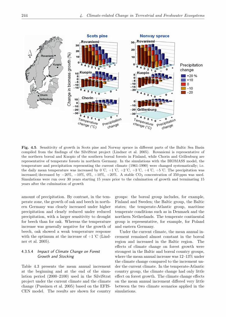
244 4. Climate-related Change in Terrestrial and Freshwater Ecosystems
Fig. 4.5. Sensitivity of growth in Scots pine and Norway spruce in different parts of the Baltic Sea Basincompiled from the findings of the SilviStrat project (Lindner et al. 2005). Rovaniemi is representative ofthe northern boreal and Kuopio of the southern boreal forests in Finland, while Chorin and Grillenburg arerepresentative of temperate forests in northern Germany. In the simulations with the BIOMASS model, thetemperature and precipitation representing the current climate (1961-1990) were changed systematically; i.e.the daily mean temperature was increased by 0 C, +1 C, +2 C, +3 C, +4 C, +5 C. The precipitation wasincreased/decreased by −20%, −10%, 0%, +10%, +20%. A stable CO2 concentration of 350 ppm was used.Simulations were run over 30 years starting 15 years prior to the culmination of growth and terminating 15years after the culmination of growth
amount of precipitation. By contrast, in the tem-perate zone, the growth of oak and beech in north-ern Germany was clearly increased under higherprecipitation and clearly reduced under reducedprecipitation, with a larger sensitivity to droughtfor beech than for oak. Whereas the temperatureincrease was generally negative for the growth ofbeech, oak showed a weak temperature responsewith the optimum at the increase of +1 C (Lind-ner et al. 2005).
4.3.5.4 Impact of Climate Change on ForestGrowth and Stocking
Table 4.3 presents the mean annual incrementat the beginning and at the end of the simu-lation period (2000–2100) used in the SilviStratproject under the current climate and the climatechange (Pussinen et al. 2005) based on the EFIS-CEN model. The results are shown for country
groups: the boreal group includes, for example,Finland and Sweden; the Baltic group, the Balticstates; the temperate-Atlantic group, maritimetemperate conditions such as in Denmark and thenorthern Netherlands. The temperate continentalgroup is representative, for example, for Polandand eastern Germany.
Under the current climate, the mean annual in-crement remained almost constant in the borealregion and increased in the Baltic region. Theeffects of climate change on forest growth werestrongest in the Baltic and boreal country groups,where the mean annual increase was 12–13% underthe climate change compared to the increment un-der the current climate. In the temperate-Atlanticcountry group, the climate change had only littleeffect on forest growth. The climate change effectson the mean annual increment differed very littlebetween the two climate scenarios applied in thesimulations.

4.3. Terrestrial Ecosystems 245
Table 4.3. Mean annual increment (m3 ha−1 yr−1) in 2001–2005 (current climate) and 2096–2100 (currentclimate and two climate scenarios), baseline management (Pussinen et al. 2005; Annex 3.2.5)
Region and 2001–2005 2096–2100country group
current climate current climate ECHAM4 HadCM2
Boreal 3.9 3.9 4.4 (+13%) 4.4 (+13%)Baltic 5.5 6.2 6.9 (+12%) 7.0 (+13%)Temperate-Atlantic 8.5 5.8 5.9 (+2%) 5.9 (+3%)Temperate-continental 7.4 6.2 6.6 (+6%) 6.7 (+7%)
Table 4.4. Average regional growing stock m3 ha−1 in 2000 (current climate) and 2100 (current climate andtwo climate scenarios), baseline management (Pussinen et al. 2005). The baseline management indicates thecutting rate, which is driven by the demand approximately at the current rate (Annex 3.2.5)
Region and 2000 2100country group
current climate current climate ECHAM4 HadCM2
Boreal 114 151 185 (+22%) 182 (+20%)Baltic 197 208 239 (+15%) 240 (+15%)Temperate-Atlantic 209 461 480 (+4%) 485 (+5%)Temperate-continental 255 389 421 (+8%) 418 (+8%)
Table 4.4 presents the average growing stock forthe country groups at the beginning and at the endof the simulation period for current climate con-ditions and two climate scenarios. Under the cur-rent climate, the average growing stock increasedthroughout the Baltic Sea Basin, e.g. by ca. 20% inthe boreal forests. In the temperate-Atlantic coun-try group, the growing stock more than doubledbetween 2000 and 2100 even under the current cli-mate, while the increase in the Baltic states wassmaller (ca. 15%) due to the relatively high fellingsthere.
Under both of the climate change scenarios usedin the simulations, the increase in growing stockwas higher than under the current climate, par-ticularly in the boreal and Baltic states. In thetemperate-Atlantic region, the climate change hadonly little effect on growing stock and the mainpart of the increase was due to cuttings, whichwere substantially smaller than the growth.
The findings on the climate change impacts ofgrowth and stocking imply that the carbon se-questration in the forests in the Baltic Sea Basinmight increase even under the current climate.This sequestration is further enhanced under the
climate change in linear relation to the increasein growth and stocking induced by the climatechange (Karjalainen et al. 2002). The increasinggrowth and stocking imply also an increase in thelitter input into the soil and thus a potential in-crease in the amount of carbon in the soil pro-file. This increase is most probably realised forthe northern parts of the Baltic Sea Basin, but inthe southern parts the enhancement of decompo-sition of soil organic matter may exceed the en-hancement in litter production, resulting in littlechange, or a decrease, in soil carbon storage (Kar-jalainen et al. 2002; Lasch et al. 2005; see alsoSect. 4.3.4).
4.3.5.5 Conclusion with the ManagementImplications
The model simulations show that in the northernboreal zone, temperature is the main limiting fac-tor for tree growth. Changes in precipitation willnot affect growth very much (Bergh et al. 1999,2003). Any systematic increase in temperaturewill strongly stimulate growth and thus have onlypositive effects. At the other end of the climatic

246 4. Climate-related Change in Terrestrial and Freshwater Ecosystems
gradient, in the southern parts of the Baltic SeaBasin, tree growth is strongly water limited (Laschet al. 2002, 2005).
Under such conditions, any increase in tempera-ture will further enhance the water deficit and willthus lead to decreasing growth. Between these twoextremes, it is the relationship between water sup-ply and temperature that determines the overallresponse to the changes in climate.
Some species are more adapted to dry condi-tions than others, with a consequence that thesimulation results often showed a temperatureresponse optimum; i.e. small increases in tem-perature were positive for tree growth, but astronger warming would lead to a water deficitand consequently declining growth (Lindner et al.2005). Hence, the temperature response optimumis higher and the general impact of rising temper-ature is more on the positive side, when precip-itation is concurrently increased. Under reducedprecipitation the temperature response optimumis lower and the main effect of increasing temper-atures is negative (Lindner et al. 2005).
In the temperate-continental zone, the forestgrowth is, in general, more constrained by wa-ter than by temperature, but the effect of el-evated CO2 may counteract or offset potentialnegative effects of changes in the climate (Free-man et al. 2005; Lindner et al. 2005). Problemsmay also be encountered with changes in the fre-quency and amplitude of extreme events such asdrought events, storms and spring and summerfrosts (CCIRG 1996, pp. 84–85; Sect. 4.3.3), withconsequent biotic damages in forests.
The question of how climate change will impactmajor outbreaks of pests and pathogens is still toa large extent open. Nevertheless, many damagingfungi and insects may expand their distribution tothe Baltic Sea Basin from central Europe and fromfurther south (Parry 2000; see also Sect. 4.3.2). Onthe other hand, there is empirical evidence thatelevated CO2 and temperature may increase theresistance of deciduous species to herbivory andthus reduce the risk of forest damages (Mattsonet al. 2004).
In the Baltic Sea Basin, there are only a fewtree species of economic importance in forestryat present (principally Scots pine, Norway spruce,birch and oak). However, changes in tree speciescomposition may be an appropriate adaptive man-agement strategy. The following changes in treespecies composition may be considered in imple-menting adaptive management strategies.
• Incorporation of other indigenous tree species,currently of minor importance in forestry, butwith high potential for timber production orcarbon sequestration under climate change.
• An increased share of broadleaved species, be-cause broadleaved species are assumed to per-form better under the climate change.
• Substitution of species sensitive to drought andto late spring frosts with more drought-tolerantand frost-resistant tree species or provenances.
• Replacement of low-productivity tree popula-tions with high-productivity ones whenever thecurrent population does not make full use of thepotential productivity of a site.
The tree species choice is a basis for an appropriateadaptive management strategy, which further in-cludes the adjustment of thinning (intensity, inter-val, pattern) to the changing productivity. In thiscontext, the regulation of the rotation period isan effective way to manage the timber productionand carbon budget of forests. Over the rotation,the timing and intensity of thinning determine thegrowth rate and stocking, which control the rateof carbon sequestration and the amount of car-bon retained in trees and soils. In most Europeancountries, growing stock is still increasing, becausetimber harvest (thinning, final felling) is below theincrement. This implies that the total carbon stor-age in the forest ecosystems is increasing. On theother hand, the age-class distribution of the forestsin the Baltic Sea Basin is shifting towards the olderage classes, and the overall length of rotation isincreasing. This implies that the rate of carbonsequestration is declining. However, replacementof over-mature old forests with new fast-growingones with the objective of carbon sequestration inthe biomass of the new stand is not always an ap-propriate option, as old forests and their specificcharacteristics are generally thought to have ben-efits for the conservation of biodiversity.
4.3.6 Arctic Ecosystems
4.3.6.1 Introduction
The arctic/subarctic region in northern Fenno-scandia, together with comparable environmentsin high mountain areas of Scandinavia and centralEurope, represents a minor proportion of the totalBaltic Sea Basin (Annex 3.2.1). However, arcticand alpine areas are of particular interest in an en-vironmental change context because they tend toexhibit a particularly close connectivity between
4.3. Terrestrial Ecosystems 247
climate, on the one hand, and ecosystem structureand function, on the other, providing sensitive in-dicators of the effects of climate change on ecosys-tems (Chapin et al. 2006). One reason for this isthe lower direct impact of local human activities,for example through land use, compared with bo-real and temperate parts of the region. The rateof climate warming in the arctic region is alreadyfaster than elsewhere, and this trend is projectedto increase (ACIA 2005). Many aspects of arcticecosystems are vulnerable to climatic and environ-mental change (Callaghan et al. 2004b), and arc-tic ecosystems are expected to undergo large andrapid changes. Some of these changes, for examplein biodiversity of migratory species and in climateforcing, will have consequences outside the Arctic.
Arctic terrestrial ecosystems interact with theclimate system by exchanging water, energy andtrace gases between the biosphere and atmosphere.Historically, these interactions have resulted incooling. Low, snow-covered vegetation reflects 60–80% of incoming solar radiation in winter, and 8–15% in summer (McGuire et al. 2007). The po-sition of the circumarctic tree line has a substan-tial influence on global climate, with effects ex-tending to the tropics (Bonan et al. 1992; Thomasand Rowntree 1992; Foley et al. 1994; McGuire etal. 2007). Due to constraints on decomposer ac-tivity by low soil temperatures and often anoxicconditions, a sizeable proportion of all carbon se-questered in photosynthesis is stored in tundrasoils, which contain about 12% of global soil car-bon (Jonasson et al. 2001). Further carbon storesexist in permafrost.
Major concerns about the impacts of climateand other environmental changes on arctic ecosys-tems focus on changes in biodiversity, which couldhave implications for the sustainable use of natu-ral resources by northern peoples, and changes inecosystem function, which could enhance globalwarming. The tangible services that are providedby the subarctic ecosystems of Finland and Swe-den include products from the domesticated rein-deer (meat, skins, bone for handicrafts), firewood,berries, tourism, as well as hunting and fishing(Laine et al. 2003). Additional services include thesequestration of CO2 (that might otherwise enterthe atmosphere and contribute to greenhouse forc-ing), and a catalogue of habitats and biodiversityof great conservation value.
As explained below, “subarctic” is commonlyused to denote high-latitude tundra-dominatedvegetation in Fennoscandia. For convenience,
however, we employ the term “arctic” when refer-ring to arctic and subarctic areas collectively.
4.3.6.2 Characteristics of Arctic Ecosystems
Compared with Russia and Canada, the arctic ar-eas of Sweden and Finland are small: togetherwith similar areas of mainland Norway they coverabout 300,000 km2 (Fig. 1.11, Chap. 1). If astrict definition of arctic vegetation is applied(CAVM Team 2003), then arctic tundra ecosys-tems do not occur in northern Sweden and Fin-land despite their high latitudes, because the arc-tic species found there only occur at higher ele-vations and are a result of altitudinal effects onclimate. However, subarctic vegetation charac-terised by open forests of low-stature trees andtundra-like vegetation at higher elevations are ex-tensive. The treelines are usually formed by small,polycormic and twisted mountain birch (Betulapubescens ssp. czerepanovii). The arctic regionis characterised by low levels of net primary pro-duction, largely because of low nutrient availabil-ity and a short growing season, but also becausewoody plant species are restricted in distributionand stature. Surprisingly, although biodiversity isgenerally acknowledged to be low in the Arctic, atotal of over 7200 terrestrial and freshwater speciesof animals, plants and fungi occur in an area of22,705 km2, situated between 68◦ and 70◦ N sur-rounding the Kevo Subarctic Research Institute innorthern Finland (Callaghan et al. 2004b). Wet-land areas and lakes are extensive: wetlands con-tain vast stores of carbon and many of the peat-lands, particularly in Finland, are exploited.
Recent climate warming has been relativelymoderate in subarctic Finland and Sweden: meanannual temperatures have increased by about1 C since the beginning of the instrumentalrecord, with the most consistent warming in spring(Kohler and Brandt 2004; Sect. 2.1.2). There havebeen two discrete periods of warming and, since2000, some cooling is apparent in some northernareas (Callaghan et al. 2004b), supported by re-cent observations of phenology in the region (seebelow).
The warming in northern Sweden is associatedwith an increase in length of the growing season(defined by temperature thresholds) of up to threeweeks (Holmgren and Tjus 1996). Precipitationin the region is extremely variable, particularlyin northern Sweden, where there are major gra-dients from a minimum of about 300mm year−1

248 4. Climate-related Change in Terrestrial and Freshwater Ecosystems
in the rain-shadow of the Abisko Alps to about1000mm year−1 close to the Swedish–Norwegianborder (see also Annex 1.2.3). There has been apositive increase in snow depth at Abisko of 20 mmper 10 years over the period 1914–2004 (Kohler etal. 2006).
Contaminant concentrations in the Subarcticare relatively small, but there is some tendencyto increase towards the east. Mean annual to-tal deposition of nitrogen varied between 0.01 and0.06 gNm−2 between 1988 and 1998 at Abisko,with no apparent trends. At Kevo, northern Fin-land, sulphur deposition has clearly decreased inrecent decades, while the annual nitrate depositionhas remained low throughout the period 1980–1996 (Kulmala et al. 1998).
Infrastructure development over the past 60years has had a major impact on habitat frag-mentation and reindeer pastures, and this trendis expected to accelerate (ACIA 2004), with in-creasing impacts on wildlife (Nelleman et al. 2001).Exploitation of natural resources has had smallerimpacts, and forest expansion during the last cen-tury might be more related to reduced dependenceon natural resources such as firewood (Emanuels-son 1987; Laine et al. 2003) and abandonment ofagricultural land (Eilertsen 2002) than to climatechange. Reindeer populations rose in the latterhalf of the 20th century and caused damage tovegetation in some areas (Bernes 1996) but aregenerally decreasing at present.
4.3.6.3 Recent Ecosystem Changes
Compared with many other northern areas, mon-itoring and research into the subarctic ecosystemsof northern Finland and Sweden have been exten-sive, due to the accessibility of the area, a rela-tively advanced infrastructure for research, and along history of settlement by indigenous and non-indigenous populations. A number of long timeseries of data relevant to the ecosystem impacts ofclimate change exist. Recent changes have beendetected in both ecosystem structure and function.Attributing causes of these changes is difficult, butcurrent environmental manipulation experimentsare contributing both to understanding of currentchanges and projection of future changes, as out-lined below.
Species performance
Monitoring of plant performance for Diapen-sia lapponica (Molau 1996) and Carex bigelowii
(Callaghan et al. 1996) and retrospective anal-yses of the growth and growing point dynamicsof the vascular cryptogam Lycopodium annotinumhave provided climate-related growth records forat least two decades (Callaghan et al. 1996).These analyses show individualistic responses ofthe plants to climate variability. D. lapponica wasretarded by increased precipitation (Molau 1996).C. bigelowii showed an apparent cyclical pattern inflowering on a 3–4 year cycle, but no overall trendfrom 1984 to 2000 (Brooker et al. 2001). L. annot-inum showed a strong buffering ability against cli-matic variations, which led to stable clonal growth.
Monitoring records reveal a breakdown in thecyclical nature of lemming and vole populations inFennoscandia since the 1990s and this has been at-tributed to changing winter snow conditions thataffect feeding, nesting and breeding under thesnow during winter (Yoccoz and Ims 1999). Fur-ther south, arctic fox and snowy owl have de-clined severely in the past decades in northernFennoscandia (Angerbjörn et al. 2001).
While some northern specialist species are de-clining in the Baltic Sea Area, some species withsouthern distributions are extending their rangesnorthwards. Moose and red fox have increased inabundance in the north (Hersteinsson and Mac-Donald 1992), while North American mink is be-coming an invasive species in some areas (Bernes1996).
There is some evidence that insect pest out-breaks resulting from increased populations and,to some extent, range shifts (Tenow 1996) in re-sponse to climate warming (McGuire et al. 2007;Chapin et al. 2005; Juday et al. 2005) are increas-ing in the boreal forest and forest tundra and arecausing major disturbances. Recent large and ex-tensive outbreaks of insect pests such as the au-tumn moth (Epirrita autumnata) in Fennoscandiaare associated with warmer winters (Juday et al.2005; Callaghan et al. 2004a): the winter min-imum temperature is critical as eggs are killedby temperatures below −36 C (Neuvonen et al.2001).
Ecosystem structure
As noted in Sect. 4.3.2, the tree line has ad-vanced in general in the Swedish part of the Scan-des mountain range over the last century (Kull-man 2002). In the Abisko area, there has beenan increase (1940s to 1980s) in tree line altitudeof 20–50 m (Sonesson and Hoogeseger 1983), and
4.3. Terrestrial Ecosystems 249
a recent study using aerial photography founda ca. 20m average increase between 1959 and2000 (Hållmarker 2002), giving rates of increaseof about 0.5m year−1, or 40m per C of meansummer air temperature (Callaghan et al. 2004b).
Reindeer herding influences vegetation dynam-ics, including tree line, locally (Helle 2001; Tøm-mervik et al. 2004). Large-scale overexploita-tion by reindeer in the Swedish mountains is notevident (Moen and Danell 2003), and reindeerthere have smaller impacts on vegetation thanthose imposed by small rodents, even in non-peakyears for rodent populations (Olofsson et al. 2004),but over-exploitation is evident elsewhere (Bernes1996).
Ecosystem functioning
Satellite monitoring of the greening of vegetationhas recorded a delay in the onset of the growingseason in many northern areas of Fennoscandiaover the last few decades (Stöckli and Vidale 2004;Høgda et al. 2001; see also Sect. 4.3.1). The on-set of autumn has been delayed even more so thatthere has been an overall increase in the length ofgrowing season in the Scandes, as also noted forhigh-latitude areas of the northern hemisphere asa whole (Myneni et al. 1997; Høgda et al. 2001).In contrast, some areas in the very north of theBaltic Sea Basin are experiencing a shortening ofthe growing season. Independent observations onthe ground have generally failed to identify anyphenological trends in 144 species above the tree-line in the past 10 years in the northern Scan-des (Molau et al. 2005). This is also the case forthe date of bud burst by mountain birch over thepast 70 years in the Scandes (Karlsson et al. 2003)and over the past 20 years in the north of Finland(Høgda et al. 2001).
Analysis of satellite images also reveals areas inthe Scandes where there have been increases bothin plant production and carbon storage in recentdecades (Myneni et al. 2001; Nemani et al. 2003).
In the north of the Baltic Sea Basin, discon-tinuous/sporadic permafrost, often occurring be-neath small, local raised areas (palsas) in mires,is degrading (Christensen et al. 2004; Malmeret al. 2005). A recent analysis of Western Ut-sjoki (3, 370 km2 study area) in northern Finlandsuggested that the palsas are disappearing at ahigh rate (Luoto and Seppälä 2003). Associatedwith a degradation of discontinuous permafrostin a subarctic Swedish mire, many dry habitats
and their vegetation have been lost, and therehas been a shift towards a greater abundance ofwet habitats with higher methane (CH4) emissionsover the past 30 years (Christensen et al. 2004;Malmer et al. 2005). This trend contrasts withthat found in areas of continuous permafrost inarctic North America and Russia, where warming-induced permafrost thaw leads to drying (Smith etal. 2005) and increased carbon emissions (Oechelet al. 1998).
In Scandinavia, mountain areas have been mod-elled to be small carbon sinks (Zhuang et al. 2003;Koca et al. 2006; Wolf et al. 2007b). Availablemeasurements of the carbon balance are contra-dictory: a Finnish mire showed a small releaseof 32 ± 10 gCm−2 year−1 (Saarnio et al. 2003),whereas a subarctic mire in northern Finland wasa carbon sink of 7 ± 5 gCm−2 year−1 (Aurela etal. 2002). Uncertainties are high, both due to un-derstanding and implementation of carbon cyclingprocesses in models (e.g. respiration), and due tothe high spatial variability in carbon sink or sourcepatterns (Christensen et al. 1999). The questionof whether arctic areas of the Baltic Sea Basin cur-rently act as a net source or sink of carbon remainsunresolved.
4.3.6.4 Projected Ecosystem Changes
Within the last 15 years, environmental manipula-tion experiments, measurements of carbon fluxesin the field, remote sensing and modelling havegiven important insights into the future responsesof ecosystem structure and function to changes inclimate and other environmental factors such asatmospheric CO2 concentrations, UV-B radiation,herbivory and plant nutrient availability.
Species performance
Analyses of current patterns of biodiversity in theArctic in relation to latitudinal/temperature gra-dients suggest that species richness will be sensi-tive to changes in climate and will increase over-all as forest displaces tundra and species associ-ated with the forest extend their ranges north-wards and upslope (Callaghan et al. 2004a; seealso Sect. 4.3.2). At the same time, the dominanceand abundance patterns of many species over thelandscape will change in accordance with changingmosaics of moisture and snow cover. Some speciesmay be expected to decline near their southernrange margins. Specialisations of current arctic
250 4. Climate-related Change in Terrestrial and Freshwater Ecosystems
plant and animal species to extreme environmentsare likely to constrain their abilities to competewith species invading from the south. As the lati-tudinal temperature gradient within the Arctic issteeper than for any other biome, and outlier pop-ulations of more southerly species frequently existin favourable microenvironments far north of theircentres of distribution, the migration northwardsand local increases in abundance are very likelyto occur more rapidly in the Arctic than in otherbiomes (Callaghan et al. 2004a).
Experiments throughout the Arctic, includingthe Subarctic of Sweden and Finland, showed thattundra plant species generally responded posi-tively to experimental summer air warming, show-ing increased growth (Molau 2001; Arft et al. 1999;Press et al. 1998; Parsons et al. 1994; Shaver andJonasson 1999); changes in phenology (Welker etal. 1997; Alatalo and Totland 1997; Jones et al.1997; Stenström et al. 1997) and increased repro-ductive success (Molau 1997). However, some re-sponses of reproductive effort were delayed (Arftet al. 1999; Molau 2001). Increases in the growthof woody plants led to changes in the architec-ture and height of the vegetation (Arft et al.1999; Press et al. 1998). Species composition ofplant communities changed as species and speciesgroups responded individualistically (van Wijk etal. 2003), as dominance changed (Press et al.1998), as some species declined and, occasionally,as new species became established (Robinson etal. 1998). Soil warming showed only transitoryincreases of nitrogen mineralisation and associ-ated increases in plant growth in northern Sweden(Hartley et al. 1999).
Experimental elevation of summer temperaturehas shown that many invertebrates can increasepopulation growth as long as there is no desic-cation. Insects in particular are very likely toquickly expand their ranges (Virtanen and Neu-vonen 1999). Some species, such as aphid specieson Svalbard, can change their life history to takeadvantage of summer air warming (Strathdee etal. 1995). Increases in ice-crust formation duringwarmer winters is likely to reduce winter survivalrates of a range of animals, including soil-dwellingspringtails (Coulson et al. 2000), small mammals(Aars and Ims 2002), and large herbivores suchas reindeer (Aanes et al. 2000; Klein 1999; Syroe-chovski and Kuprionov 1995).
The effects of increased precipitation on plantsare less consistent than those of air warming, andnon-significant in a meta-analysis (Dormann and
Woodin 2002). For the Baltic Sea Basin, experi-ments showed no response for arctic dwarf shrubsand Calamagrostis lapponica (Parsons et al. 1994;Press et al. 1998), whereas for evergreen speciesthere was an effect of water addition (Phoenix etal. 2001). Mosses benefit from moderate summerwatering (Potter et al. 1995; Phoenix et al. 2001;Sonesson et al. 2002) and nitrogen fixation ratesby blue-green algae associated with the moss Hy-locomium splendens were increased (Solheim et al.2002).
Shading (simulating competition) for 6 yearsclearly disadvantaged some plant species in an ex-periment in Swedish Lapland (Graglia et al. 1997),and flowering of the dwarf heather-like shrubCassiope tetragona ceased when it was shaded(Havström et al. 1995). In a nearby experimentin a birch forest understory community, shadingby increased growth of vascular plants probablyreduced the cover of the moss Hylocomium splen-dens (Potter et al. 1995). Similar experimentsthroughout the Arctic suggest that mosses andlichens could become less abundant when vascularplants increase their growth in response to warm-ing (Cornelissen et al. 2001; van Wijk et al. 2003),although warming in summer and winter snow ad-dition increased the biomass of Sphagnum fuscumin the Subarctic (Dorrepaal et al. 2004).
Addition of nutrients (simulating increased de-composition as a response to soil warming) in-creased canopy height of tundra vegetation (Presset al. 1998), but the response was individualistic(Parsons et al. 1994): the grass Calamagrostis lap-ponica was stimulated by a factor of more than 18(Press et al. 1998); graminoids are generally re-sponsive to nutrient addition (Cornelissen et al.2001; van Wijk et al. 2003).
CO2 enrichment experiments have shown thatresponses of arctic plants are generally early andtransient (Gwynn-Jones et al. 1997), although ef-fects on microbial communities (Johnson et al.2002) and frost hardiness (Beerling et al. 2001)could have longer-term consequences. For ex-ample, CO2 enrichment and increased temper-atures influenced mycorrhizal colonisation in adwarf shrub ecosystem (Olsrud et al. 2004), withpotential consequences for plant nutrient uptake,allocation and long-term carbon storage in the soil.The lack of a growth response in mosses (Sones-son et al. 1996) and lichens (Sonesson et al. 1995)may be a result of down-regulation as an aspect ofadaptation to the high levels of CO2 that these or-ganism groups experience, even under present-day

4.3. Terrestrial Ecosystems 251
ambient CO2 levels, in their habitual microenvi-ronments close to the ground surface (up to 1000ppm: Sonesson et al. 1992).
Ecosystem structure
Most information on plant responses to climatewarming is limited to the short-term and small-plot scales. Even the longest time scales – upto two decades – of some monitoring studiesare relatively short compared to generation timesand successional rates in arctic vegetation. Be-cause of great longevity and a prevalence of clonalgrowth habits among arctic species, it is difficultto extrapolate plant responses from the individualplant to the population. Magnitudes of responsemay also vary between sites (Henry and Molau1997; Karlsson et al. 2003; Jonasson et al. 1999).Process-based modelling may offer the greatest po-tential to explore structural dynamics in the longterm and on geographically extensive scales.
Model projections for Finland and Sweden un-der a scenario of a ca. 5 C increase in average tem-perature combined with a 25% increase in precipi-tation (SRES-B2 scenario from the REMO RCM;Keup-Thiel et al. 2006) suggest that, by 2100, bo-real forest could dominate 75% of grid cells on a0.5 × 0.5◦ grid now dominated by tundra and/orshrubs (Wolf et al. 2007b). Alpine heath mightdecrease by as much as 75–84% of its current ex-tent in the Swedish mountain areas in the next 100years as a consequence of tree line shifts (Moen etal. 2004). However, there is great uncertainty, asthe models do not currently have the ability topredict impacts of changing land use, hydrologi-cal changes due to thawing permafrost, and insectdamage (but see Wolf et al. 2007a, c).
Vegetation models suggest an increase in treecover and a decrease of tundra vegetation inthe next 100 years (Fig. 4.6; Wolf et al. 2007b;Moen et al. 2004). Factors that could enhanceor mitigate forest advance into tundra includeherbivory (Cairns and Moen 2004), disturbanceevents such as forest fires (McGuire et al. 2007),and constraints on tree line advance such as inertia(Chapin et al. 2005), human activities (Vlassova2002), geographical barriers, and inappropriatesoil conditions (Callaghan et al. 2004a).
Trophic level structure is simpler in the Arc-tic than elsewhere, and climate warming is ex-pected to change the abundance of keystonespecies, which is expected to lead to ecologicalcascades. The dynamics and assemblages of ver-
tebrate predators in the Arctic are almost en-tirely based on lemmings and other small rodents.The lack of population peaks since the 1990s inFennoscandia have already contributed to loss ofpredators such as the arctic fox and snowy owl(Bernes 1996). Reductions in the abundance oflemmings also affects the populations of geese andwaders that are used as alternative prey by foxes(Summers and Underhill 1987).
Ecosystem functioning
Models of net primary production estimate an in-crease of ca. 44% over the next 100 years in thenon-forested area of Sweden and Finland (Wolfet al. 2007b). The projected increases in NPPare likely to be constrained in some areas by in-creased disturbance as detailed above (McGuire etal. 2007; Callaghan et al. 2004a). In the wider areadefined by Greenland in the west and the Rus-sian European Arctic in the east, NPP and car-bon storage in vegetation and soils are projectedto increase less (46% and 0.04 PgC, respectively)between 1960 and 2080 than in other areas of theArctic globally (Sitch et al. 2003; Callaghan et al.2004a).
Expansion of shrubs into tundra, displacementof tundra by the boreal forest, and earlier leaf-out might decrease albedo in both summer andwinter (Wolf et al. 2007b) and should cause sub-stantial heating of the atmosphere (a positive feed-back to climate) that will also accelerate the sub-sequent replacement of tundra by boreal forest(McGuire et al. 2007). The advance of shrubs andforest onto the tundra will cause complex inter-actions between the generally expected negativefeedback of longer-term carbon sequestration andthe positive feedback of reduced albedo. Mod-els suggest that there will be a clear increase inNPP in the Scandes (Wolf et al. 2007b), but interms of carbon sequestration this might be off-set by increases in soil respiration and increaseddisturbance (see Sect. 4.3.4). The uncertaintiessurrounding model predictions of future carbonstorage are high, at least in quantitative terms(Callaghan et al. 2004a).
4.3.6.5 Implications
Climate warming is likely to lead to greater pro-duction, northwards expansion of agriculture andgreater choice of crops in the Arctic as a whole.However, moisture stress and diseases such as

252 4. Climate-related Change in Terrestrial and Freshwater Ecosystems
Fig. 4.6. Vegetation changes under a future climate scenario for northern Europe. Projected changes ofdominant vegetation within 0.5× 0.5◦ grid cells according to a dynamic vegetation model (adapted from Wolfet al. 2007b)
potato blight might reduce yields in some areas(Juday et al. 2005). Increases in the forested areaand shrublands, together with increased forestproduction in the Fennoscandian Subarctic (Wolfet al. 2007b) suggest potential increases in for-est industries (although increased pest outbreaksand fire might reduce this potential) while inno-vation would lead to improved adaptation by lo-cal people to ecosystem changes (Chapin et al.2006).
Reindeer herding is likely to be negatively in-fluenced by future changes in climate conditions.Lichens, which are an important food source forreindeer, will decrease with the predicted increaseof biomass of vascular plants (Cornelissen et al.2001). However, the increase in shrubby vegeta-tion in other areas might provide food for reindeerthere. The earlier onset of spring greening willhave an impact on the foraging patterns of rein-deer. Due to such large changes in vegetation,there will be a need for adaptation by reindeerherders; for example, in the choice of routes tomove between winter and summer grazing lands,the timing of migration and the selection of newpastures.
Conservation management will become increas-ingly important, but decisions need to be made
about the goals and methods of conservation in thefuture (Usher et al. 2005; Klein et al. 2005). Cur-rent concepts of conservation of threatened speciesneed to take into account the likelihood that somecurrently widespread arctic species are likely tobe disadvantaged by climate warming, while somecurrently rare species might become more com-mon. Current protected areas protect against di-rect human actions, not against climate changeleading to vegetation-zone shifts and changes inbiodiversity (Usher et al. 2005; Callaghan et al.2004a).
Tourism (see also Annex 3.1.3.2), an importantactivity for the economy of the European Subarc-tic, might be affected in various ways: while hith-erto scenic mountains and ski slopes might be cov-ered by forest – which could deter some tourists –ecotourism might increase as northern landscapesand their wildlife become ever more exotic.
The present uncertainty involved in calculatingthe magnitude and even sign of future radiativeforcing from trace gas emissions for the region, andof balancing the possible opposing feedbacks fromtrace gas fluxes and albedo (see above), preventsa definitive statement from being made about thefuture “ecosystem service” of feedbacks to the cli-mate system.

4.3. Terrestrial Ecosystems 253
4.3.7 Synthesis – Climate Change Impacts onTerrestrial Ecosystems of the Baltic SeaBasin
A number of observed and potential impacts onterrestrial ecosystems of the Baltic Sea Basinemerge from the above review. These are sum-marised in Table 4.5. The robustness with whichit can be stated that any particular class of im-pact has occurred, is occurring or is likely to oc-cur in the future naturally depends on the extentof the available data and mechanistic understand-ing. Some classes of impacts are supported by di-rect observations, others inferred indirectly fromobservations, models, or findings in other regionswith comparable climates and ecosystems. Someare reported in a single study, others in multiplestudies spanning different sites, regions, species orbiomes. For some types of impacts, the mechanismof response to climate and other factors is well un-derstood, while for others, the climate connectionremains tenuous or speculative.
To help guide policy and adaptation decisionsand the setting of research priorities, we charac-terise robustness in terms of three levels of con-fidence for recent historical impacts, and two forpotential future impacts. Our criteria are as fol-lows:
High confidence – this categorisation is reservedfor recent and historical impacts only, in caseswhere the impact has been described based onobservations or measurements of several species,ecosystems or localities (depending on the natureof the impact) within the Baltic Sea Basin; and/orthe impact has been observed in other comparableregions and the mechanism of climate response iswell understood.
Medium confidence – in the case of recent andhistorical impacts, the impact has been describedbased on a few/occasional observations or mea-surements within the Baltic Sea Basin and themechanism of response to climate is well under-stood. Projected future impacts are designatedthis confidence level where the impact has beenprojected or modelled for the Baltic Sea Basin us-ing several approaches and the mechanism of re-sponse to climate change is well understood.
Low confidence is assigned to recent or historicalimpacts for which a mechanism of climate responsehas been proposed in the absence of irrefutable ob-servations. In the case of projected future impacts,this confidence level is assigned where the impact
has been hypothesised for the Baltic Sea Basin, orprojected or modelled in a single study.
Major sources of uncertainty emerging from thereview are listed in the table. These include tech-nical and methodological aspects of uncertainty(e.g. the quantity or quality of available data),but also uncertainties related to the limited under-standing of mechanisms, and to the role of antag-onistic processes and non-climatic driving forceswith the potential to ameliorate or reverse the pre-dicted impact.
A general conclusion that may be drawn isthat climate change during the last 30–50 yearshas already given rise to measurable changes incommunities and ecosystems of the Baltic SeaBasin. Robust indicators of change include the ad-vancement of spring phenological phases in certainplant species, changed migratory patterns and be-haviour – for example in migratory birds – upslopedisplacement of the alpine treeline, and increasedland-surface greenness as plants and ecosystemsadjust to improved growth conditions and a richercarbon supply.
Many of the current trends may be expectedto continue for at least some decades into thefuture, as atmospheric CO2 concentrations con-tinue to rise, and the climate continues to warm.However, future projections are intrinsically un-certain, and for a number of impacts, currenttrends may be broken or reversed due to system-internal feedbacks, shifts in controlling processes,non-climatic drivers and system transformations– perhaps most importantly, in conjunction withthe appearance of novel pathogens, pests or inva-sive species.
Nearly all of the ecosystems of the region areto a greater or lesser extent managed, and the cli-matic impact may in many cases be ameliorated(or enhanced) through human intervention – forexample, via adaptive species choice in forestry.The most important source of uncertainty with re-gard to many impacts is the future development innon-climatic, anthropogenic drivers of ecosystemprocesses, including greenhouse gas emissions, de-position rates of atmospheric pollutants, land usechanges and their underlying socio-economic con-trols: human populations, markets, internationaltrade, and technological development.

254 4. Climate-related Change in Terrestrial and Freshwater Ecosystems
Table 4.5. Climate change impacts on terrestrial ecosystems of the Baltic Sea Basin. ✓✓✓= high confidence; ✓✓=medium confidence; ✓= low confidence (see main text)
Class of impact Impact of recent climatechange (Hypothesis 1)
Projected impact offuture climate change(Hypothesis 2)
Relevant uncertainties
Phenology
Shift towards earlier springand summer phases inplants
Advancement by 5–20 daysover last 50 years in manyspecies ✓✓✓
Advancement by 1–3 weeksdepending on temperatureincrease ✓✓
Increased risk fortemperature backlashescould modify responses
Shift towards later autumnphases in plants
Delay by 5–30 days overlast 50 years in somespecies ✓✓
Delay by 1–3 weeksdepending on temperatureincrease ✓✓
Data quality
Extension ofphytophenological growingperiod
Extension by ca. 20 daysover last 50 years in manyspecies ✓✓✓
Extension by 2–6 weeksdepending on temperatureincrease ✓✓
1. As above2. Effects of pollutants,
UV-B, O3
Biogeography andcommunity structure
Changed speciesdistributions
Cold limit range boundaryshifts tracking isothermmigration for some plantand animal species ✓✓
1. Continued cold limitrange boundary shifts✓✓
2. Range retraction nearwarm limit ✓
1. Impacts of changingclimate extremes
2. Impacts of non-climateabiotic drivers
3. Population/communitylags
4. Trophic interactions,e.g. effects of pests,pathogens, predators,herbivores
5. Changing disturbanceregimes
6. Land use, habitatfragmentation, specieschoice in agricultureand forestry
7. Poorly characterisedbackground variation
Changed migratorypatterns and behaviour
Reduced migratorydistance, direction,increased proportions ofsedentary individuals etc.in some birds, bats andinsects ✓✓✓
No studies
Changed biomedistributions
Treeline advance inFennoscandian Mountains,mainly via increasedstature of existingindividuals ✓✓✓
1. Treeline advance inmountain areas ✓✓
2. Lagged northward shiftof boreal and nemoralforest zones, withwider transition zone ✓
3. Increased broadleavedcomponent in borealforest ✓
4. Displacement of tundraplants by grasses andtrees ✓✓
1. As for speciesdistributions (above)
2. Hydrologicaltransformations intundra
Exotic species invasions Invasions of southernEuropean invertebratesinto central/northernEurope ✓✓
No studies
Animal population cycles Breakdown in populationcycles of arctic rodents dueto reduced snow cover ✓✓
No studies
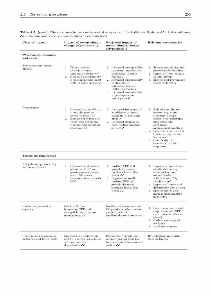
4.3. Terrestrial Ecosystems 255
Table 4.5. (cont.) Climate change impacts on terrestrial ecosystems of the Baltic Sea Basin. ✓✓✓= high confidence;✓✓= medium confidence; ✓= low confidence (see main text)
Class of impact Impact of recent climatechange (Hypothesis 1)
Projected impact offuture climate change(Hypothesis 2)
Relevant uncertainties
Physiological toleranceand stress
Tree stress and forestdieback 1. Climate-related
dieback in sometemperate species ✓✓
2. Increased susceptibilityto pathogens and insectpests in some species ✓
1. Increased susceptibilityto spring temperaturebacklashes in someregions ✓
2. Increased susceptibilityto drought intemperate parts ofBaltic Sea Basin ✓
3. Increased susceptibilityto pathogens andinsect pests ✓
1. System complexity andprocess understanding
2. Impacts of non-climateabiotic drivers
3. Species and provenancechoice in forestry
Disturbance1. Increased vulnerability
to and damage bystorms in forest ✓✓
2. Increased frequency ofinsect pest outbreaksin forest and subalpinewoodland ✓✓
1. Increased frequency ofwindthrow in forest,particularly southernareas ✓
2. Increased damage bybark beetles (Norwayspruce) ✓
1. Role of non-climatefactors, e.g. standstructure, specieschoice, tree structuralproperties andanchorage,management practices
2. Future trends in stormtracks, strengths andfrequency
3. Complexity ofsecondary trophicresponses
Ecosystem functioning
Net primary productivityand forest growth 1. Increased land surface
greenness, NPP andgrowing season lengthsince 1980’s ✓✓✓
2. Increased forest growth✓✓✓
1. Further NPP andgrowth increases innorthern Baltic SeaBasin ✓✓
2. Negative to smallpositive NPP andgrowth change insouthern Baltic SeaBasin ✓✓
1. Impacts of non-climateabiotic drivers e.g.N-deposition andmineralisation,acidification, CO2“fertilisation”
2. Impacts of stress anddisturbance (see above)
3. Species choice andmanagement practicein forestry
Carbon sequestrationcapacity
Net C sink due toincreasing NPP andchanged forest cover andmanagement ✓✓
Northern areas remain netCO2 sinks, southern areasgenerally switch tosmall-moderate sources ✓✓
1. Future changes in soilrespiration and NPP(with uncertainties asabove)
2. Carbon exchange ofwetlands
3. Land use changes
Greenhouse gas exchangein tundra and boreal soils
Increased soil respirationand CH4 release associatedwith permafrostdegradation ✓✓
Permafrost degradation/reduced ground frost leadto liberation of inactive soilcarbon ✓✓
Hydrological transforma-tions in tundra

256 4. Climate-related Change in Terrestrial and Freshwater Ecosystems
4.4 Freshwater Ecosystems
In temperate aquatic ecosystems, most of the eco-logically important factors are affected by climatechange. These include changes in temperature;evapotranspiration; the availability of water andlimiting nutrients; the frequency and magnitudeof precipitation, wind, storm and fire events; thelength of the ice-free season; the depth of themixed layer; the period of nutrient limitation.These factors can be broken down into two cat-egories that in reality are strongly interrelated:changes in the variability of climatic patterns; andchanges in the mean trends of climatic patterns(Choi 1998). In general, many water quality prob-lems may be exacerbated by climatic change, par-ticularly those relating to eutrophication and age-ing processes, oxygen depletion, salinisation, andacidification. However, extreme uncertainties ex-ist at any case-specific level (Varis and Kuikka1997). These are often related to special lake orcatchment characteristics. In the search for a moregeneral framework to group and structure climaticresponses of lake ecosystems, a conceptual modelhas been developed (Blenckner 2005), which con-sists of two main components: a Landscape Fil-ter comprising the features of geographical posi-tion, catchment characteristics and lake morphol-ogy, and an Internal Lake Filter, comprising thefeatures of lake history and biotic/abiotic interac-tions. The inclusion of both the landscape and in-ternal interactions help explain different responsesof individual lakes to climatic change and varia-tion (for details see Blenckner 2005). We begin bydiscussing general mechanisms by which climatechanges impact freshwater ecosystems, then go onto review recent and potential future changes inlakes of the Baltic Sea Basin.
4.4.1 Mechanisms of Response to ClimateChange
4.4.1.1 Water Temperature
Water temperatures (Sect. 2.2.1.5) have showna strong, coherent increase in conjunction withwarming air temperatures across European lakes.A faster temperature rise in the spring (due to ear-lier ice-out dates) precedes the beginning of springstratification, which may influence nutrient cy-cling (Schindler et al. 1990; Abgeti and Smol 1995)and phytoplankton dynamics. Consequently, ef-fects of higher water temperatures on the lake mix-ing regime could lead to dimictic lakes (fully mixed
twice a year) turning into warm monomictic lakes(Schindler 1996; Blenckner et al. 2002a).
In general, temperature affects all physiologicalprocesses and, therefore, the growth of organisms.The manner in which physiological rates changewith respect to temperature is generally in goodagreement with an Arrhenius formulation (Sharpeand DeMichele 1977; Lin 1995; Choi 1998). Forexample, the zooplankton found in lakes can tol-erate fairly high summer temperatures, yet smallincreases in the winter temperature, in some lakessignificantly related to the timing of ice break-up(Jassby et al. 1990), strongly affected the over-wintering and seasonal dynamics (George and He-witt 1999) of zooplankton taxa such as Daphniaand Eudiaptomus through a strong temperature-dependent growth rate (Lampert and Muck 1985).
The survival and growth of fish species dependsstrongly on temperature (Magnuson et al. 1990;De Stasio et al. 1996; Magnuson et al. 1997).Thermal limits of some fish species, altered byglobal warming, can induce changes in distribu-tion (Magnuson et al. 1990; Carpenter et al. 1992).Temperature-induced changes in the growth rateof predatory fish may result in cascading effectsthrough the entire food web (Carpenter et al.1985).
4.4.1.2 Ice Regime
The timing of ice freeze and break-up are recordedin some of the longest and most widespread lim-nological datasets and have been used as indica-tors for regional climate change (Robertson et al.1992; Assel and Robertson 1995). Ice dynamicsare driven by several meteorological variables, ofwhich air temperature has been shown to be themost important (Palecki and Barry 1986; Robert-son et al. 1992; Vavrus et al. 1996; Livingstone1997). According to Lithuanian data (Bukantis etal. 2001), lakes are the best indicators of thermalconditions in the pre-winter period (November–December) because the early ice-cover may lastuntil spring even if the winter is warm. This is onereason for the scatter in the winter temperature-ice-cover duration relationship.
A long-term trend towards shorter periods ofice-cover due to a later freezing and an earlier icebreak-up has been reported for lakes around theNorthern Hemisphere (Palecki and Barry 1986;Kuusisto 1987; Assel and Robertson 1995; Liv-ingstone 1997; Magnuson et al. 2000; Assel et al.2003). The trend towards an earlier ice-out in-
4.4. Freshwater Ecosystems 257
creases the ice-free period and raises lake tempera-tures in spring in Canadian (Schindler et al. 1990)and European (Gerten and Adrian 2000; Straile2000; Livingstone and Dokulil 2001) lakes. Innorthern Europe, the duration of the ice-coveredperiod and the timing of freeze and break-upgreatly affect lake systems (Salonen et al. 1984;Weyhenmeyer et al. 1999; Järvinen et al. 2002),in particular the succession events in plankton dy-namics (Weyhenmeyer et al. 1999).
4.4.1.3 Stratification
Most temperate deep lakes are stratified duringsummer, with a warm surface water (epilimnion)and cold deep water (hypolimnion). The mostcrucial triggering factors for the timing of phyto-plankton blooms are light and turbulence, both ofwhich are influenced by stratification and there-fore directly affected by climatic variation andchange. Consequently, strong relationships be-tween the timing of phytoplankton blooms and thewinter climate have been found in European lakes(Adrian et al. 1995; Müller-Navarra et al. 1997;Weyhenmeyer et al. 1999; Gerten and Adrian2000). Differences in the individual lake responsedepend on the morphometry of the lake (a compo-nent of the landscape filter). For example, in LakeConstance (Germany), a large and deep lake gen-erally lacking ice-cover, the spring bloom only oc-curs under stratified conditions, because reducedmixing increases light availability for phytoplank-ton, extending transport down to only 20m, asopposed to 100 m or more with no stratification(Gaedke et al. 1998).
Generally, an enlarged mixing depth increasesthe extinction of incoming light, which is attenu-ated abiotically within the mixed layer. This leadsto a decrease in phytoplankton production, aver-aged over the mixed layer, with increasing mix-ing depth (Huisman et al. 1999; Diehl 2002). Bycontrast, in shallow lakes with a smaller mixingdepth, the phytoplankton spring bloom is asso-ciated with ice-cover disappearance (determinedby winter climate), influencing the light availabil-ity. This has been observed for Müggelsee, Ger-many (Gerten and Adrian 2000) and Lake Erken(Weyhenmeyer et al. 1999). Later in the year,conditions in the lake appear to be more com-plex and stratification becomes the predominanttriggering factor. Longer periods of stratifica-tion can promote a dominance of potentially toxiccyanobacteria (George and Harris 1985; George
et al. 1990; Hyenstrand et al. 1998). Higher wa-ter temperatures prolong the stratification period,which creates favourable conditions for buoyantphytoplankton such as cyanobacteria. Addition-ally, large cyanobacterial colonies (besides otherphytoplankton groups) are resistant to grazing byzooplankton, especially in eutrophic lakes. Thesetwo mechanisms could promote the dominance ofcyanobacteria in stratified lakes at warmer tem-peratures. Longer periods of summer stratificationand higher hypolimnetic temperature are also pre-dicted to cause increased hypolimnetic anoxia, orat least lower oxygen concentrations (Magnuson etal. 1997), and this can enhance the nutrient releasefrom the sediment (Pettersson et al. 2004).
4.4.1.4 Hydrology
The hydrological water residence time, anothermain component of the filter concept, determinesthe persistence of a climatic signal stored in lakes.For example, this factor influences the recyclingof phosphorus, the main limiting nutrient in lakes.Stratified lakes with a water residence time longerthan one year have a higher potential to undergo aclimate-induced eutrophication because additionalphosphorus released from the sediment becauseof hypoxia and/or enhanced microbiological pro-cesses is recycled repeatedly. By contrast, in lakeswith short residence times (months), phosphorusreleased from the sediment is flushed out relativelyquickly and therefore contributes less to climate-induced eutrophication. Decreases in water res-idence time, for example through an increase inprecipitation with a higher associated runoff, candecrease concentrations of nutrients, as water res-idence time scales the rate of the ecosystem re-sponse to chemical inputs (Carpenter et al. 1992and literature cited therein) and to climate changeand variability. The water level of closed lakes,where the hydraulic load is counterbalanced byevaporation and rather stable seepage, serves asone of the best indicators of long-term climaticvariation (Kilkus 1998).
4.4.1.5 Ecosystem Transformations
Climatic changes relevant at a species level arelikely to vary at the ecosystem scale among lakes(Petchey et al. 1999). Weak links in food web in-teractions, in particular, dampen oscillations be-tween consumers and resources (McCann et al.1998). This implies that not all responses at a spe-cific trophic level are propagated to lower trophic

258 4. Climate-related Change in Terrestrial and Freshwater Ecosystems
levels or have significant impacts on ecosystemprocesses (Pace et al. 1999). Additionally, a pro-longation of the climate signal due to food webinteractions is possible as the signal of winter cli-mate can be detected in the clear water phasein early summer (Straile and Adrian 2000) or insummer phytoplankton composition and biomass(Weyhenmeyer 2001; Blenckner et al. 2002b). Asystem approach is necessary to examine the cas-cading effects in response to climatic change andvariability. The magnitude of a climate-driven re-sponse of an autotrophic organism does not nec-essarily have to be mediated or cascaded to theheterotroph species, or vice versa.
Another example indicates that a consecutiveperiod of five mild winters led to a completechange of the spring phytoplankton bloom, from adominance of diatoms and cryptophytes to a domi-nance of cyanobacteria, in a German lake (Adrianet al. 1995). This illustrates, furthermore, thatthe response of phytoplankton, and probably alsoother lake biota, to climatic variation might betotally decoupled from a warming trend (climaticchange), as many ecosystem processes are non-linear.
Furthermore, the non-linear responses of ani-mals and plants to environmental variables, in-cluding climate (May 1986; Mysterud et al. 2001),may cause progressive changes to be interruptedby drastic switches to a contrasting ecosystemstate (Scheffer et al. 2001). One such exampleis the shift between the clear water (macrophytedominated) and the turbid (plankton dominated)state of shallow lakes. A recent study in a Swedishlake showed that climate variability alone cannotexplain such a shift, but is likely to contribute toa multi-causal stress and, therefore, reduces theresilience of the clear-water state in shallow lakes(Hargeby et al. 2004).
4.4.1.6 Impacts of Non-Climatic AnthropogenicDrivers
In the past 40–50 years, many lakes, particularlyin Europe and North America, have been sub-jected to anthropogenic increases in the supplyof nutrients and other substances (e.g. organicpollutants). This supply decreased somewhat inthe late 1980s and early 1990s. While improve-ments in waste-water treatment over the last fewdecades have reduced inputs of nutrients frompoint sources, the increase in nutrients from dif-fuse sources is still a major problem and, for many
lakes, remains the predominant concern. Addi-tionally, catchment alteration, acidification, damregulation, agriculture and the water-borne sani-tation solution can complicate a separation of thevarious influences on ecosystems (Andersson andArheimer 2003; see also the comments of Jeppesenet al. 2003; van Donk et al. 2003). It is thereforeoften difficult to clearly distinguish between the in-dependent effects of climate and direct human im-pact on important lake and catchment processes.
Multiple stress factors, such as climate changetogether with ozone depletion and acidifica-tion, may alter ultraviolet light and tempera-ture regimes in freshwater ecosystems. Changesin underwater UV and temperature can signifi-cantly influence the composition of the zooplank-ton community and ultimately food web dynamics(Persaud and Williamson 2005). Phytoplanktoncommunities experience climate change indirectlythrough changes in lake level, ice-out time, strat-ification, nutrient inputs and zooplankton grazing(Anneville et al 2004). Among other effects, globalwarming could accelerate eutrophication processes(Knight and Staneva 2002, Blenckner et al. 2002b,Malmaeus et al. 2006). The key limitation to pre-dicting effects of climate change on ecosystems liesin the understanding of how biotic interactions willrespond (Winder and Schindler 2004).
4.4.2 Recent and Historical Impacts
4.4.2.1 Physical Responses
Studies on global climate have revealed that thenorthern hemisphere is becoming warmer, wintersare becoming wetter and summers drier (IPCC2001). The same overall trends are apparent forthe Baltic Sea and its catchment, though withsome regional variation; e.g. with regard to thesummer precipitation trend (Chap. 2.1.3). Thesechanges are partly reflected in the increasing trendof the North Atlantic Oscillation index (NAO;Sect. 2.1.1.1 and Annex 7).
The NAO seems to affect mostly the late-winterand mid-spring temperature period. The winterNAO (NAOw) has a weak, though significant, ef-fect on the regime of spring temperature in theBaltic Sea Basin and explains the most significantfluctuating components embedded in the cryophe-nological records (Yoo and D’Odorico 2002). FromApril until November, water temperature in theEstonian lake Võrtsjärv was significantly corre-lated with air temperature and the water temper-

4.4. Freshwater Ecosystems 259
ature in spring was significantly correlated withthe NAOw (Nõges 2004). Comparing the 1960sand the 1980s, the mean surface water tempera-ture in May–October in Lithuanian lakes did notdiffer, while it increased from the 1980s to 1990swith the greatest difference (0.8 C) occurring inApril (Pernaravičiute 2003).
4.4.2.2 Ice
A warmer winter air temperature strongly ad-vances the timing of the ice break-up (Yoo andD’Odorico 2002). From Middle Sweden to Ger-many, the difference in the timing of the ice break-up during the last 30 years has been up to onemonth (Gerten and Adrian 2001; Weyhenmeyer2004). In the large Swedish lakes Vänern, Vät-tern and Mälaren, the number of years with-out continuous winter ice-cover has increased inthe 1990s compared with earlier decades (Wey-henmeyer 2001). In northern Sweden (north of62◦ N), the change is weaker or even totally absent(Blenckner et al. 2004). During the last 30 years,there has been a clear trend towards a greater vari-ation in the ice break-up dates in the south of Swe-den compared to the north, with a distinct changein the relationship at around 62◦ N (Blenckner etal. 2004). This tendency was less pronounced forthe timing of ice freeze and totally absent for theice break-up dates of the Finnish lakes (Blenckneret al. 2004).
Since 1880, the number of ice-free days on LakeOnega (Russia) has declined only marginally from225 to 217 (Filatov et al. 2003). Trends towards ashorter ice-free period have also been observed, forexample on the Russian Kola Peninsula over theperiod 1930-1998 (Kozlov and Berlina 2002) and inthe Estonian lake Võrtsjärv over the period 1923–1998 (Järvet 1999). In Võrtsjärv this phenomenonwas caused mainly by advancement of the freez-ing date, while on the Kola peninsula the causewas both a delayed ice break-up in spring and ad-vanced freezing in the autumn/winter period. Fur-ther trends are discussed in Sect. 2.2.2. In Võrt-sjärv, the duration of ice-cover correlated nega-tively with the NAOw (Nõges 2004). Addition-ally, year-to-year variability in ice break-up datesin Europe could be related to climatic (NAOw)variation (Weyhenmeyer et al. 1999; Gerten andAdrian 2000; Yoo and D’odorico 2002), while theNAO signal has been detected even in the ice char-acteristics of the world’s largest (by volume) lake,Lake Baikal (Livingstone 1999).
The tendency towards an earlier ice break-upcan have strong ecosystem effects. An examplefrom northern Germany showed that a series ofmild winters with earlier ice break-up led to an ear-lier stratification and a dominance shift from di-atoms to cyanobacteria (Adrian et al. 1995). Polarlakes are early detectors of environmental changebecause snow and ice-cover variation markedly af-fect all ecological variables (Quayle et al. 2002).
4.4.2.3 Hydrology
As discussed in Chap. 3, global warming in theBaltic Sea Basin may bring about higher amountsof winter and spring precipitation, primarily in thenorthern part of the catchment. In Estonia andSweden the amount of spring and winter precip-itation correlates with the NAOw, but the rela-tionship was lacking in other seasons (Nõges 2004;Weyhenmeyer 2004). In general, changes in pre-cipitation can influence lake water level dynamics.Long-term changes in water levels with a period-icity of 20–30 years have been reported for manyEuropean lakes; e.g. Peipsi and Võrtsjärv in Esto-nia (Nõges et al. 2005); the majority of Belarus-sian lakes (UNFCCC 2003b); Saimaa in Finland;Ilmen, Onega and Ladoga in Russia (Masanovaand Filatova 1985; Malinina et al. 1985); andMüggelsee in Germany (Behrendt et al. 1987).
Peipsi and Võrtsjärv showed a strong positiverelationship between the NAOw and the waterlevel. In the very shallow Võrtsjärv (mean depth2.8 m), the annual mean amplitude of the wa-ter level is equal to half of the mean lake depth,and the absolute range of water level fluctuations(3.2 m) even exceeds mean depth, which clearlyhas a strong influence on the ecosystem dynam-ics (Nõges and Nõges 2004). In low-water years,the water column is better illuminated, while bothphosphorus release and denitrification increase be-cause of more frequent resuspension of bottom sed-iments bringing about substantially higher phos-phorus concentration and resulting in a lower ni-trogen:phosphorus ratio. This favours the devel-opment of nitrogen-fixing cyanobacteria (Nõges etal. 2003). In the deeper Peipsi (mean depth 7.1 m),such effects are not as obvious.
Climate-induced changes in hydrology of boreallakes and rivers may change the growth conditionsof aquatic macrophytes as well as decompositionand accumulation of detritus. When a spring flooddoes not occur, the littoral detritus from previ-ous growing seasons will more likely accumulate

260 4. Climate-related Change in Terrestrial and Freshwater Ecosystems
at aquatic plant-stands and will therefore be sub-jected to anaerobic decomposition and probablyimprove the substrate supply for methanogenicbacteria. In two Finnish lakes, Alinen Rautjärviand Ekojärvi, methane emission in dense standsof three emergent macrophyte species (Equisetumfluviatile, Schoenoplectus lacustris and Phragmitesaustralis) was even more limited by temperaturethan by substrate. Thus, not only changes in theflooding pattern but also higher summer temper-atures can accelerate methane emissions from bo-real lakes (Kankaala et al. 2005).
4.4.2.4 Chemical Responses
Climate change affects the hydrological regime (asdescribed above) and thus also nutrient loadingsinto lakes. In warm and dry years, the nutrientloading usually decreases while in-lake concentra-tions may still increase because of increased waterevaporation and a more intensive release from sedi-ments at low water stages (Magnuson et al. 1997).In a study of the three largest lakes in Sweden(Vänern, Vättern and Mälaren), synchronous rela-tionships between the winter climate (here NAOw)and water chemistry were restricted to variablesclosely linked to surface water temperature, i.e. re-active silica and pH in May (Weyhenmeyer 2004).
Additionally, a warm winter was found to in-crease the winter discharge and the associatedload of phosphorus and nitrogen into one basinof Mälaren. In nearby Lake Erken, nitrate con-centrations were much lower in late winter dur-ing the warm period, the 1990s, compared to thecold period, 1975–1980 (Pettersson et al. 2004).In summer, elevated phosphate and ammoniumconcentrations in the hypolimnion were observedand resulted in significantly higher phosphate andchlorophyll a levels in autumn during the warmperiod, compared to the cold period (Petterssonet al. 2004).
In the River Vantaanjoki watershed in southernFinland, increased temperature and precipitationin recent decades were responsible for an increasedcontribution of diffuse nutrient losses to the totalnutrient load (Bouraoui et al. 2004). In Lithua-nian lakes, the increase in concentrations of to-tal nitrogen and total phosphorus over the period1993–2002 was insignificant (Anon 2002). Due tothe high spatial variability of soil and precipitationin Lithuania, the most vulnerable region is in thewest of the country, where the annual precipita-tion is highest (800–900mm) and associated with
annual loads of nitrogen up to four times highercompared to Middle Lithuania (Tumas 2000).
Long-term changes in loadings of nutrients andorganic matter to the Estonian lake Võrtsjärv re-sulted both from changes in agricultural prac-tices and from the climate change (Nõges et al.2007). The analysis of detrended time series re-vealed significant positive correlations between theamount of precipitation and annual loadings ofammonium, phosphate and dissolved organic car-bon (DOC). Both water discharge and solute con-centrations increased during wet years.
Peatlands occupy approximately 15% of borealand subarctic regions, contain approximately onethird of the world’s soil carbon pool, and supplymost of the DOC entering boreal lakes and rivers(see Sect. 4.6). Changes in temperature, water ta-bles and discharge could affect delivery of DOC todownstream ecosystems, where it exerts significantcontrol over productivity, biogeochemical cycles,and attenuation of visible and UV radiation (Pas-tor et al. 2003; see also Sect. 4.5.2). The annualpotential net carbon sequestration rate of forests,peat-producing wetlands and lake sediments in theBaltic Sea Basin has been estimated at 30–60,8–55 and 10–51 tC km−2, respectively (Jansson etal. 1999). In Estonian lakes, mean accumulationof CO2-C is estimated to be only 0.54 tC km−2
(UNFCCC 1995). It has been shown that lakesin northern Sweden are CO2-supersaturated andtherefore constitute net sources of CO2 to the at-mosphere (Jonnsson et al. 2003).
Per unit of electricity produced, the hydro-electric reservoirs emit much less CO2 than theSwedish combustion plants, while their emissionis also much lower compared to natural lakes(Bergström et al. 2004). In a study of some 80,000lakes in the boreal zone of Sweden, it was esti-mated that 30–80% of the total organic carbonentering the lakes was lost, mainly due to min-eralisation and subsequent CO2 emission to theatmosphere, the exact proportion depending onresidence time and water temperature (Algestenet al. 2004).
However, despite the controlling effect of watertemperature, hydrological changes and catchmentcharacteristics (see also Sobek et al. 2003) can beof greater importance than interannual temper-ature fluctuations for the rate of carbon cycling(Algesten et al. 2004). The relative emission ofCO2 from boreal lakes (a major CO2 source) incomparison to boreal forests (currently considereda net CO2 sink) may be of considerable importance

4.4. Freshwater Ecosystems 261
for the CO2 concentration of the atmosphere andfuture climatic forcing.
4.4.2.5 Biological Responses
Climate change may clearly affect the timing of thedevelopment of ecosystem components in spring.In a German lake (Plusssee), the timing of phyto-and zooplankton maxima (clear-water phase) wasnegatively related to water temperature: under atemperature increase, both maxima occurred ear-lier. The intensity of the spring algal maximumwas negatively related to its timing, whereas noclear relationship between the zooplankton max-imum and its timing could be observed (Müller-Navarra et al. 1997). In Võrtsjärv (Estonia), thephytoplankton biomass in spring was positively re-lated to the NAOw, while during wet summers andautumns, phytoplankton biomass was lower due toan elevated water level (Nõges 2004). In shallowlakes, the effects of winter climate on plankton areshort-lived, and are soon overtaken by the prevail-ing weather and by biotic interactions (Adrian etal. 1999).
In deep lakes, however, the winter climate sig-nal (here the NAOw) can persist until late summer(Gerten and Adrian 2001). Distribution, composi-tion and species diversity of diatoms in subarcticLapland are markedly regulated by temperatureand other climate-related factors (Weckström andKorhola 2001).
The 20th century arctic warming has causedchanges in overall species richness of benthic andplanktonic diatoms in lakes of Finnish Lapland. Aparticularly strong relationship was found betweenspring temperatures and the compositional struc-ture of diatoms, depending on lake type and catch-ment characteristics and reflected by several otherbiological indicators, such as chrysophytes andzooplankton, suggesting that entire lake ecosys-tems have been affected (Sorvari et al. 2002).
The timing of the clear-water phase (CWP) isassociated with a warmer winter climate (Müller-Navarra et al. 1997; Gerten and Adrian 2000;Straile and Adrian 2000; Straile 2002). However,this may be difficult to totally separate from man-agement actions (fish removal and nutrient reduc-tions) occurring at the same time (Jeppesen et al.2003). A strong relationship between the onset ofthe CWP and NAOw was found in 28 central Eu-ropean lakes and 71 shallow Dutch lakes (Straileand Adrian 2000; Scheffer et al. 2001). This ear-lier onset was combined with an earlier summer
decline of Daphnia (Straile 2000), which illustratesthe fact that winter climatic variation affects suc-cessional events even in summer.
A higher summer phytoplankton biomass wasrelated to higher winter air temperature in a smalllake in northern Germany, probably due to thehigher grazing pressure on zooplankton during latespring and the faster development of zooplanktiv-orous fish (Müller-Navarra et al. 1997). A similarpattern was found in the biomanipulated BautzenReservoir (Germany), where the water tempera-ture during early summer probably influenced themortality of daphnids through predation of young-of-the-year (YOY) fish (Benndorf et al. 2001). InMüggelsee, the annual peak abundance of twothermophile zooplankton species increased signif-icantly in the warm period (Gerten and Adrian2002). In Lake Ilmen (Russia), low zooplanktonbiomass has been related to hydrometeorologicalconditions. Also, zoobenthos have been favouredby high water levels, especially if such conditionslast for several years.
Nevertheless, over the period 1952–2001, therehave been no major qualitative changes in thezoobenthos, only changes in the quantitativerepresentation of some groups (Andreeva 2003).Ichthyophenological time series from Estonia re-veal that the commencement of spawning for pikeand bream has advanced by 6 and 8 days, respec-tively, over the period 1951–1996 (Ahas 1999).Increasing water temperature in spring in Esto-nian inland waters affected the spawning condi-tions of roach and bream differently. Over the pe-riod 1951–1990, the spawning of bream shifted 10days earlier with an unchanged spawning temper-ature.
In contrast, no shift in the spawning time ofroach has been observed. The difference betweenspawning times of roach and bream decreased from22 to 13 days and the difference in average temper-atures at the onset of spawning by about 3 C. Inyears with higher water levels during March andApril, both fish species started to spawn earlier(Nõges and Järvet 2005).
In Danish lakes, warm early summers most of-ten lead to a higher abundance of planktivorousfish (YOY) and, thereby, increased grazing pres-sure on large-bodied zooplankton (Jeppesen et al.2003). Autumn spawners such as vendace in Swe-den’s largest lakes will have difficulties in adaptingto climate warming, whereas spring spawners suchas smelt and pike-perch benefit from the higherspring water temperature.

262 4. Climate-related Change in Terrestrial and Freshwater Ecosystems
However, the responses depend on the trophicstatus of the lake: in a eutrophic lake the ef-fects are not as clear, as the predation pressurefrom other species may become too high (Ny-berg et al. 2001). In Peipsi (Estonia/Russia) thestock of smelt may seriously suffer when low wa-ter level, prolonged periods of calm, hot weatherand strong cyanobacterial blooms coincide, caus-ing night-time hypoxia (Kangur et al. 2003). Ad-ditionally, a sharp decline of vendace in Peipsi andother lakes in the region in the 1990s was evi-dently connected to winter climate (Sarvala et al.1999; Kangur et al. 2003): mild winters in the late1980s and early 1990s, when Peipsi had no per-manent ice-cover and the bottom was exposed tothe action of waves, led to a high mortality of ven-dace eggs on spawning grounds (Pihu and Kangur2000). The eggs can be injured mechanically orburied under sediments, which causes mass mor-tality (Sterligova et al. 1988).
A 200-year sediment core from the alpine LakeChuna on the Kola Peninsula revealed a decreaseof cold-stenothermal chironomid taxa in the up-permost sediment layers, which can be explainedby warming during the 20th century (Ilyashuk andIlyashuk 2001).
4.4.3 Potential Future Impacts
4.4.3.1 Physical Responses
As described in Chap. 3, most climate change sce-narios for the eastern part of the Baltic Sea Basinare characterised by increasingly mild winters witha decrease in snow cover (Kondratyev et al. 2002,Filatov et al. 2003, Järvet 2004). The increase ofmonthly mean air temperature will be in the rangeof 3–5 C in the next 100 years, with the winterperiod showing the largest changes. However, in-consistencies among scenarios are high; for exam-ple, the predicted annual temperature change forthe Baltic Sea Basin ranges from 0.7 C to 6.9 C,and precipitation change from 3% to 22%, amongGCMs included in the CMIP2 series of simulations(see Sect. 3.3.3).
A series of combined climate-lake modellingstudies of European lakes showed that continu-ously increasing air temperatures led to similartrends in surface water temperature, resulting inlonger stratification periods and shorter ice-coverperiods or no ice at all as a result of strong changesin the mixing regime (Blenckner et al. 2004; Pers-son et al. 2005). Climate change experiments sim-
ulated a 1–2 month shorter lake ice season in theNordic area for the 2070s. All simulations showthe largest changes for southern-central Sweden,southwestern Baltic States and western Norway(Räisänen et al. 2001). These results were in rea-sonable agreement with the ice season length ob-served in 37 Swedish lakes (Rummukainen et al.2001). A shortening of the winter ice-cover pe-riod by the year 2050 has also been projected fortwo Russian lakes, Ladoga and Onega (Filatov etal. 2003) and for Estonian rivers (Jaagus 1997).A more intensive water mixing is projected forLadoga and Onega, leading to a decrease of thehypolimnion thickness and an associated decreasein dissolved oxygen concentrations by 2050 (Fila-tov et al. 2003). A deepening of the thermoclineas a result of a warmer climate has also been dis-cussed for Scandinavian lakes (Stendera and John-son 2005).
4.4.3.2 Hydrology
The simulation of hydrological parameters forlakes varies due to a large scatter in the projectedsimulations of precipitation (see Chap. 3). Simu-lations for Lakes Ladoga and Onega with two fu-ture scenarios (1: doubling of greenhouse gases; 2:doubling of greenhouse gases, taking into accountthe direct effect of atmospheric aerosols) projectedan increase in mean annual precipitation and to-tal evaporation, but a decrease of runoff, over theperiod 2000–2050 (Filatov et al. 2003). Similartrends were predicted for the Upper Volga catch-ment area bordering with the Baltic Sea Basin,where the surface runoff in spring was projectedto become higher compared to the present day.
In contrast, summer and autumn runoff couldbe suppressed in the future due to higher transpi-ration rates associated with a larger proportion ofdeciduous trees in forests. Decreased summer pre-cipitation in combination with an increased evap-otranspiration would result in decreased groundwater recharge and a lower water level for theVolga River and Upper Volga lakes (Oltchev et al.2002). In contrast, projections for the Lake Ilmen-River Volkhov catchment point to runoff increasesof 45% and 66% for 2050 and 2100, respectively,compared to the period 1981–1990 (Kondratyev etal. 2002).
In a modelling study of river flows (Lehner andDöll 2001), only a few areas, such as southernFinland and northern Russia, showed consistentdecreases in drought frequencies under a range
4.4. Freshwater Ecosystems 263
of future climate scenarios (from the ECHAM4and HadCM3 GCMs). By contrast, Scandinavia,Lithuania, Latvia, Estonia, northern Belarus andRussia, most of Germany and the Alpine regiongenerally tended towards a higher drought risk sit-uation by the 2070s.
A significant redistribution of seasonal runoffhas been projected for the eastern part of theBaltic Sea Basin. The most important changeswould take place during the colder half of the year.Frequent melting periods decrease snow and iceaccumulation during winter that will result in anearlier commencement of snowmelt in spring anda lower maximum runoff, while winter runoff min-ima will disappear (Jaagus 1997; Kont et al. 2002;Oltchev et al. 2002; UNFCCC 2003a; Ziverts andApsite 2005). All models simulate drier soils insummer (Oltchev et al. 2002; Kondratyev et al.2002; Järvet 2004) and an increase in river runoffduring autumn. In the western part of Estonia,the runoff maximum in autumn is expected to ex-ceed the spring maximum. On Saaremaa Islandin the west-Estonian archipelago, the runoff max-imum in spring will disappear, and the annual cy-cle will consist of a single cold half-year maximumand a warm half-year minimum (Kont et al. 2002;UNFCCC 2003a).
Changes in temperature and precipitation willalso affect lake water levels. Simulations of threelakes from northern Europe (Bysjön, Sweden;Karujärv and Viljandi, Estonia) show that the lakewater level is more sensitive to decreases than toincreases in precipitation. Increased precipitationresults in increased runoff, but this is largely com-pensated by increased outflow and changes in lakelevel are therefore small (Vassiljev 1998).
Significant changes in lake water levels can beattributed to the displacement of the boundariesof climatic seasons even without visible deviationsof the annual averages of temperature and precip-itation from their long-term standards (Grigor’evand Trapeznikov 2002). According to model sim-ulations, reductions in winter (November–April)precipitation have a stronger impact on lake levelsthan changes in summer (May–October) precip-itation (Vassiljev 1998). Despite the prospecteddecrease in the annual runoff, an increase in lakewater level for the coming 50-year period was pre-dicted for Lakes Ladoga and Onega (Filatov et al.2003).
4.4.3.3 Chemical Responses
A warmer and wetter future climate will affect wa-tershed processes: reduced soil frost and increas-ing precipitation in winter will increase nutrientleaching from the soil and accelerate the eutroph-ication of water bodies. Despite abandonment ofa substantial proportion of previously cultivatedlands and decreased use of fertilisers in Estonia,wintertime nutrient losses are currently almost ashigh as during former years because of increasedwater discharge and surface runoff in winter. In-creases in water discharge in winter together withthe still large nutrient pool in soils may explainthe fact that nutrient concentrations in lakes havedecreased less than expected in conjunction withreduced fertiliser application (Nõges and Nõges2004). The time-lag between catchment changesand the responses in lakes is difficult to predict.However, the delay before terrestrial vegetationand soil covers are in balance with the new climaticconditions will presumably amount to at least 100–200 years (Karlsson et al. 2005).
Climate warming simulations for Lake Batorinoin Belarus performed with the LakeWeb model(Håkanson et al. 2003) showed a significant in-crease in total phosphorus concentrations as morephosphorus became bound in organisms with shortturnover times (phyto-, bacterio-, and zooplank-ton). Longer summer stratification will increasehypolimnetic anoxia (Stendera and Johnson 2005)in some lakes, which is a precondition for iron-bound and aluminium-bound phosphorus releasefrom lake sediments (Pettersson 1986). Enhancedremineralisation of nutrients and higher diffusionrates at higher temperatures combined with thelonger ice-free period will enhance nutrient avail-ability to algae, especially in lakes with a long wa-ter residence time (Blenckner et al. 2002a).
Future projections in Belarus (UNFCCC2003b) take into account the effect of peoplespending more time in recreational zones aroundrivers, lakes, and water reservoirs. This higher an-thropogenic load could lead to lower water qualityand aggravation of the epidemiological situationin the sense of viral and bacterial contamination.A more intensive eutrophication in the next 50years as a result of climate change has also beenprojected for the Lake Ladoga and Lake Onegaregion (Filatov et al. 2003). In contrast, a studyfor Lithuania (UNFCCC 2002) showed a decreaseof more than 20% in nitrogen washed into surfacewaters in conjunction with a 2 C temperature in-
264 4. Climate-related Change in Terrestrial and Freshwater Ecosystems
crease, as a result of a reduced meltwater amount,and, consequently, smaller surface and subsurfacerunoff. Nitrogen washout is not necessarily a sim-ple function of affluence but could also be climate-driven: net nitrification rate and the formationof mineral N increased in experimental droughttreatments of N-fertilised forest soils (Smolanderet al. 2004).
Malmaeus et al. (2006) used a regional climatemodel coupled to a physical lake model and aphosphorus model to simulate three lakes in Swe-den. Responses of lake phosphorus content to awarmer future climate differed according to wa-ter residence time. In lakes with a short residencetime, the simulations showed no future changes inthe phosphorus concentration, regardless of lakedepth. By contrast, for a lake with a longer wa-ter residence time (Lake Erken), the concentrationof dissolved phosphorus in the epilimnion almostdoubled in spring and autumn under the warmestclimate scenario, increasing the potential for phy-toplankton production accordingly.
The most important flux intensifying the phos-phorus cycle is the enhanced diffusion due to alonger stratification period. This leads to a highermineralisation with elevated bacterial activity, re-sulting in decreased oxygen concentrations andhigher rates of diffusion. As a consequence, ad-ditional available phosphate increases the phyto-plankton biomass in Lake Erken, which then set-tles out and contributes to the enhancement ofthe cycle. The implication would be that in LakeErken, and in other eutrophic lakes with long wa-ter residence times, eutrophication problems maybecome serious in the future, and that manage-ment may need to take action today in order tomaintain good water quality in these lakes.
Changes in affluence are likely to affectallochthonous dissolved organic matter inputs(Stendera and Johnson 2005). Experiments withlarge mesocosms (Pastor et al. 2003) showed thatthe DOC budget of boreal peatlands was con-trolled largely by changes in discharge rather thanby any effect of warming or position of the wa-ter level. At a critical discharge rate, the DOCbudget switched from net export to net retention.The same study showed that if the current decreas-ing trend of the discharge from peatlands contin-ues, DOC retention and concentration in bogs andfens will increase, while export will decrease. Thewarming trend during the past 20 years has like-wise caused an increase in DOC concentrations inUnited Kingdom peatlands (Freeman et al. 2001),
where, in the absence of changes in discharge, theDOC export increased.
4.4.3.4 Biological Responses
The direct impact of a temperature increase onbiota strongly depends on the extent of the in-crease. In a microcosm experiment, warming by3 C had no effect on phytoplankton size structureand very minor effects on chlorophyll a and totalphytoplankton biovolume (Moss et al. 2003). Bio-volumes of some phytoplankton groups decreasedand abundance of cyanobacteria did not change,suggesting that fears of dominant cyanobacte-ria summer blooms in future may not be realis-tic, at least in shallow, unstratified lakes domi-nated by macrophytes. In contrast, an experimentwith natural plankton communities grown at 10and 20 C (Rae and Vincent 1998) showed that astronger temperature increase could considerablyinfluence the plankton community structure.
A food web simulation of warmer conditions forLake Batorino in Belarus (the mean annual epil-imnetic temperature was raised by 2 C and therange in weekly epilimnetic temperatures was in-creased by the exponent 1.1) predicted higher pri-mary and secondary production, increases in al-gal volumes and bacterioplankton biomass, anda reduced macrophyte cover, suggesting a signifi-cant change in the structure of the lake foodweb(Håkanson et al. 2003). Warming is likely to accel-erate eutrophication processes in northern lakes,and thereby shift the species composition of phyto-plankton assemblages toward species with highertemperature optima (for example, cyanobacteria),posing a substantial risk for deteriorated drink-ing water quality (UNFCCC 2003b). An increasein cyanobacterial dominance under warmer condi-tions, increased spring growth and an earlier de-cline of the summer cyanobacteria bloom was alsopredicted by a phytoplankton model for Bassenth-waite Lake, UK, while the overall productivity ofthe lake remained unchanged (Elliott et al. 2005).
It is likely that the impacts of climate changewill be more pronounced in littoral zones of lakesthan in pelagic zones, because aquatic macro-phytes have access to nutrients in the sedimentrendered available under higher surface water tem-peratures. A three-year study carried out in twoexperimental ponds in Finland, one covered witha greenhouse (Kankaala et al. 2000, 2002; Ojala etal. 2002), showed that the emergent macrophytesemerged earlier and grew better in the warmer
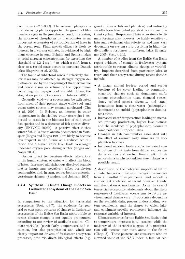
4.4. Freshwater Ecosystems 265
conditions (+2.5–3 C). The released phosphorusfrom decaying plants supported the growth of fila-mentous algae in the greenhouse pond, illustratingthe uptake of phosphorus by macrophytes as animportant accelerator of eutrophication of lakes inthe boreal zone. Plant growth efficacy is likely toincrease in a warmer climate, as evidenced by highplant coverage in some Belgian and Spanish lakesat total nitrogen concentrations far exceeding thethreshold of 1.2–2mg l−1 at which a shift from aclear to a turbid state occurs in northern Danishlakes (Sagrario et al. 2005).
The fauna of sublittoral zones in relatively shal-low lakes may be affected by stronger oxygen de-pletion caused by the deepening of the thermoclineand hence a smaller volume of the hypolimnioncontaining the oxygen pool available during thestagnation period (Stendera and Johnson 2005)
Generally, cold-water species may be extirpatedfrom much of their present range while cool- andwarm-water species may expand northward (Chuet al. 2005). In Belarus, an increase in watertemperature in the shallow water reservoirs is ex-pected to result in the biomass loss of cold-waterfish species and in a decrease of fish species diver-sity (UNFCCC 2003b). A positive effect is thatwinter fish-kills due to anoxia documented in Võrt-sjärv (Nõges and Nõges 1999) are likely to becomeless frequent in the future as a reduced ice du-ration and a higher water level leads to a largerunder-ice oxygen pool during winter (Nõges andNõges 2004).
Besides direct temperature effects, alterationsin the humic content of water will affect the biotaof lakes. Increased allochthonous dissolved organicmatter inputs may negatively affect periphytoncommunities and, in turn, reduce benthic macroin-vertebrate richness (Stendera and Johnson 2005).
4.4.4 Synthesis – Climate Change Impacts onFreshwater Ecosystems of the Baltic SeaBasin
In comparison to the situation for terrestrialecosystems (Sect. 4.3.7), the evidence for gen-eral or consistent patterns of change in freshwaterecosystems of the Baltic Sea Basin attributable torecent climate change is not equally pronouncedaccording to our review of available studies. Cli-mate variables (particularly temperature and in-solation, but also precipitation and wind) areclearly important drivers of freshwater ecosystemprocesses, both via direct biological effects (e.g.
growth rates of fish and plankton) and indirectlyvia effects on lake hydrology, stratification and nu-trient cycling. Responses of lake ecosystems to cli-mate forcings may, however, be highly sensitive tolake and catchment characteristics and may varydepending on system state, resulting in highly in-dividualistic responses in different lakes (Blenck-ner 2005; Sect. 4.4.1).
A number of studies from the Baltic Sea Basinreport evidence of change in freshwater systemsattributable to recent climate change or variabil-ity. Impacts described from particular lakes orrivers and their ecosystems during recent decadesinclude:
• A longer annual ice-free period and earlierbreakup of ice cover leading to communitystructure changes such as dominance shiftsamong phytoplankton taxa, changed succes-sions, reduced species diversity, and trans-formations from a clear-water (macrophyte-dominated) to turbid (phytoplankton-domina-ted) state.
• Increased water temperatures leading to increa-sed primary production, higher lake biomassand the incidence of phytoplankton blooms insome northern European lakes.
• Changes in fish communities associated withthe effect of warmer early summers on zoo-plankton biomass.
• Increased nutrient loads and/or increased con-tributions of nutrients from diffuse sources un-der a warmer and wetter climate, with domi-nance shifts in phytoplankton assemblages as apossible result.
A description of the potential impacts of futureclimate changes on freshwater ecosystems emergesfrom a handful of experimental and modellingstudies, extrapolation of recent observed trends,and elucidation of mechanisms. As in the case ofterrestrial ecosystems, statements about the likelyresponses of freshwater ecosystems to future en-vironmental change vary in robustness dependingon the available data, process understanding, sys-tem complexity, and the degree to which lake-and catchment-specific parameters influence theresponse variable of interest.
Climate scenarios for the Baltic Sea Basin pointto temperature increases in all seasons, while themajority of the scenarios suggest that precipita-tion will increase over most areas in the future(Chap. 3). These patterns are consistent with anelevated value of the NAO index, a familiar sce-
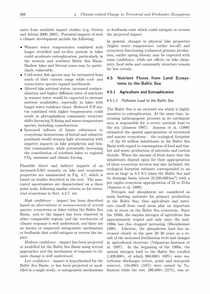
266 4. Climate-related Change in Terrestrial and Freshwater Ecosystems
nario from available impact studies (e.g. Gertenand Adrian 2000, 2001). Potential impacts of sucha climate development include the following:
• Warmer water temperatures combined withlonger stratified and ice-free periods in lakescould accelerate eutrophication, particularly inthe western and southern Baltic Sea Basin.Shallow lakes and littoral zones may be partic-ularly vulnerable.
• Cold-water fish species may be extirpated frommuch of their current range while cool- andwarm-water species expand northwards.
• Altered lake nutrient status: increased reminer-alisation and higher diffusion rates of nutrientsin warmer water would be expected to increasenutrient availability, especially in lakes withlonger water residence times. Reduced N:P sta-tus combined with higher temperatures couldresult in phytoplankton community structureshifts favouring N-fixing and warm-temperaturespecies, including cyanobacteria.
• Increased influxes of humic substances toecosystems downstream of boreal and subarcticpeatlands would steepen light attenuation withnegative impacts on lake periphyton and ben-thic communities, while potentially increasingthe contribution of northern lakes to regionalCO2 emissions and climate forcing.
Plausible direct and indirect impacts of anincreased-NAO scenario on lake and ecosystemproperties are summarised in Fig. 4.7, which isbased on studies described in the text. The asso-ciated uncertainties are characterised on a threepoint scale, following similar criteria as for terres-trial ecosystems in Sect. 4.3.7, viz:
High confidence – impact has been describedbased on observations or measurements of severalspecies, ecosystems or lakes within the Baltic SeaBasin; and/or the impact has been observed inother comparable regions and the mechanism ofclimate response is well understood; and there areno known or suspected antagonistic mechanismsor feedbacks that could mitigate or reverse the im-pact.
Medium confidence – impact has been projectedor modelled for the Baltic Sea Basin using severalapproaches and the mechanism of response to cli-mate change is well understood.
Low confidence – impact is hypothesised for theBaltic Sea Basin; or has been projected or mod-elled in a single study; or antagonistic mechanisms
or feedbacks exist which could mitigate or reversethe projected impact.
In general, changes in physical lake properties(higher water temperature, earlier ice-off) andecosystem functioning (enhanced primary produc-tion, earlier spring bloom) may be expected withsome confidence, while net effects on lake chem-istry, food webs and community structure remainfar less certain.
4.5 Nutrient Fluxes from Land Ecosys-tems to the Baltic Sea
4.5.1 Agriculture and Eutrophication
4.5.1.1 Pollution Load to the Baltic Sea
The Baltic Sea is an enclosed sea which is highlysensitive to eutrophication. At the same time, in-creasing anthropogenic pressure in its catchmentarea is responsible for a severe nutrient load tothe sea (Jansson 1997). Jansson et al. (1999)estimated the spatial appropriation of terrestrialand marine ecosystems – the ecological footprint– of the 85 million inhabitants in the Baltic SeaBasin with regard to consumption of food and tim-ber and waste production of nutrients and carbondioxide. When the amount of fresh water that theinhabitants depend upon for their appropriationof these ecosystem services was also included, theecological footprint estimate corresponded to anarea as large as 8.5–9.5 times the Baltic Sea andits drainage basin (about 22,500,000 km2) with aper capita ecosystem appropriation of 22 to 25 ha(Jansson et al. 1999).
Nitrogen and phosphorus are considered asmain limiting nutrients for primary productionin the Baltic Sea; thus agriculture and nutri-ents runoff from rural areas play an importantrole in stress on the Baltic Sea ecosystem. Sincethe 1950s, the surplus nitrogen of agriculture hasapproximately tripled and only since the mid-1980s has this stopped increasing (Rheinheimer1998). Likewise, the phosphorus load has in-creased clearly in the past 20–30 years as a re-sult of the increased fertilisation level and changesin agricultural structure (Valpasvuo-Jaatinen etal. 1997). In the beginning of the 1990s, theannual nitrogen load to the Baltic Sea totalled1,409,000 t, of which 980,000 t (69%) were wa-terborne discharges (rivers, point and non-pointsources), 134,000 t (10%) were caused by N2-fixation while the rest, 296,000 t (21%), was at-
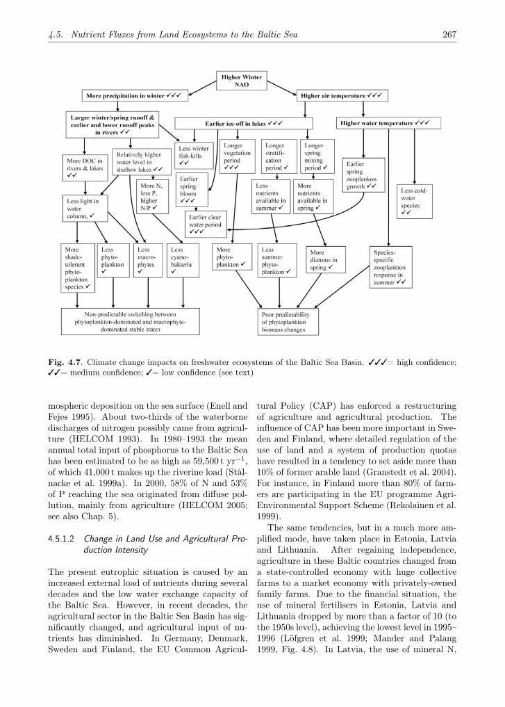
4.5. Nutrient Fluxes from Land Ecosystems to the Baltic Sea 267
Fig. 4.7. Climate change impacts on freshwater ecosystems of the Baltic Sea Basin. ✓✓✓= high confidence;✓✓= medium confidence; ✓= low confidence (see text)
mospheric deposition on the sea surface (Enell andFejes 1995). About two-thirds of the waterbornedischarges of nitrogen possibly came from agricul-ture (HELCOM 1993). In 1980–1993 the meanannual total input of phosphorus to the Baltic Seahas been estimated to be as high as 59,500 t yr−1,of which 41,000 t makes up the riverine load (Stål-nacke et al. 1999a). In 2000, 58% of N and 53%of P reaching the sea originated from diffuse pol-lution, mainly from agriculture (HELCOM 2005;see also Chap. 5).
4.5.1.2 Change in Land Use and Agricultural Pro-duction Intensity
The present eutrophic situation is caused by anincreased external load of nutrients during severaldecades and the low water exchange capacity ofthe Baltic Sea. However, in recent decades, theagricultural sector in the Baltic Sea Basin has sig-nificantly changed, and agricultural input of nu-trients has diminished. In Germany, Denmark,Sweden and Finland, the EU Common Agricul-
tural Policy (CAP) has enforced a restructuringof agriculture and agricultural production. Theinfluence of CAP has been more important in Swe-den and Finland, where detailed regulation of theuse of land and a system of production quotashave resulted in a tendency to set aside more than10% of former arable land (Granstedt et al. 2004).For instance, in Finland more than 80% of farm-ers are participating in the EU programme Agri-Environmental Support Scheme (Rekolainen et al.1999).
The same tendencies, but in a much more am-plified mode, have taken place in Estonia, Latviaand Lithuania. After regaining independence,agriculture in these Baltic countries changed froma state-controlled economy with huge collectivefarms to a market economy with privately-ownedfamily farms. Due to the financial situation, theuse of mineral fertilisers in Estonia, Latvia andLithuania dropped by more than a factor of 10 (tothe 1950s level), achieving the lowest level in 1995–1996 (Löfgren et al. 1999; Mander and Palang1999, Fig. 4.8). In Latvia, the use of mineral N,

268 4. Climate-related Change in Terrestrial and Freshwater Ecosystems
Fig. 4.8. Application of fertilisers in Estonia in 1953–1994 (adapted from Mander and Palang 1999)
P and K fertilisers decreased from 159 to 29, from108 to 11, and from 172 to 24 kt yr−1, respectively,over the period 1989–1994 (Rivza 1997).
Poland has the largest agricultural area pro-portion among the Baltic Basin countries (Ta-ble 4.6) and contributes the largest amount ofnutrients among all the countries in the BalticSea Basin (247,000 tN yr−1 and 12,200 tP yr−1 in1993, around 60% of total nitrogen and 35% of to-tal phosphorus came from agricultural non-pointsources; Dzikiewicz 2000). However, due to thechanging economic and socio-political order, con-sumption of commercial fertilisers in Poland hasdecreased to less than half since 1988 (Žylicz 1997;Stålnacke et al. 2004).
Although several estimations have been madeon changes in land-use structure in the BalticSea Basin since the mid-1990s (Table 4.6), wecould not find clear data on this situation. Atthe local level, the increase in the proportion ofabandoned agricultural lands has been remark-able (Rivza 1997; Mander et al. 2000a); however,there is strong evidence that during the last 3–5years many set-aside areas have been taken intoagricultural use again. This is especially the casein Lithuania, Latvia and Estonia, where the EUfarmer-supporting schemes encourage farmers tointensify their agricultural activities.
Some data suggest that despite changing landuse in some countries, no significant decrease in

4.5. Nutrient Fluxes from Land Ecosystems to the Baltic Sea 269
Table 4.6. Population, total land area and agricultural land use in the Baltic Basin countries in 1993 (afterKhalili et al. 1997)
Population Total area Arable land Pastures Total agricultural area106 103 ha 103 ha 103 ha 103 ha %
Denmark 5.2 4,300 2,540 197 2,740 64Sweden 8.6 45,000 2,780 576 3,361 7Finland 5.1 33,800 2,580 106 2,692 8Russia� 9.0 31,480 4,699 1,045 5,810 18Estonia 1.5 4,500 1,114 243 1,400 30Latvia 2.6 6,500 1,687 819 2,530 39Lithuania 3.8 6,500 2,300 1,173 3,524 59Poland 38.5 31,300 14,305 4,047 18,715 60Germany�� 4.5 3,900 1,963 740 2,656 68
Total 78.9 167,280 33,968 8,946 43,428 26
�Data from 2000 after Granstedt et al. 2004��Data from 1995 about Mecklenburg–Vorpommern and Schleswig-Holstein (Khalili et al. 1997)
Table 4.7. Population, loads of nitrogen, nitrogen load per capita and percent of the total nitrogen load inthe Baltic Sea Basin countries in 2000 (after Granstedt et al. 2004)
Population Total N loads N load per capita Shares of N load×103 103 kg N yr−1 kg N capita−1 % of total
Denmark 5,155 62,240 12 7Sweden 8,500 175,610 21 21Finland 4,938 146,560 30 18Russia� 9,028 53,720 6 7Estonia 1,595 32,990 21 4Latvia 2,606 54,070 21 7Lithuania 3,446 35,560 10 4Poland 37,764 229,990 6 28Germany� 3,300 31,510 10 4
Total 76,332 822,250
total annual nitrogen loads into the Baltic Sea hasoccurred in the period 1995–2000 (Granstedt etal. 2004). The only exceptions were Latvia, Es-tonia and Russia, the countries having the proba-bly largest decrease in agricultural and fertilisa-tion intensity. Of the calculated total nitrogenload in 2000, 24% originates from Estonia, Latvia,Lithuania and Russia, 28% from Poland, 21% fromSweden and 18% from Finland (Table 4.7). How-ever, per-capita output levels of nitrogen are al-most four times higher for Sweden and Finlandthan for Poland.
4.5.1.3 Nutrient Losses from Agricultural Catch-ments
In agricultural catchments, drainage accounts forthe major part of both nitrogen and phosphorusloads to rivers. According to Behrendt and Ba-chor (1998), in Mecklenburg-Vorpommern, Ger-many, this proportion is up to 90% for nitrogenand about 75% for phosphorus. In some catch-ments, even storm-water events did not contributewith more phosphorus than the drainage water(up to 0.25 kgP ha−1 yr−1; Gelbrecht et al. 2005).Depending mainly on management practice, espe-

270 4. Climate-related Change in Terrestrial and Freshwater Ecosystems
cially fertilisation and livestock density, land usestructure, soil and climatic conditions, the av-erage annual losses of nitrogen in the countriesaround the Baltic Sea in 1994–1997 ranged from 5to 75 kgN ha−1 yr−1 (Vagstad et al. 2004), beinghigher in the beginning of 1990s (up to 105 kgNha−1 yr−1 in Norway; Bechmann et al. 1998; andup to 100 kgN ha−1 yr−1 in Denmark; Kronvanget al. 1995). In the Baltic states, the value did notexceed 25 kgN ha−1 yr−1 (Mander et al. 1998; Jan-sons et al. 2003), except in the case of pig slurryapplications (Vagstad et al. 2000).
Phosphorus losses in Lithuania, Latvia and Es-tonia ranged between 0.1 and 0.32 kgP ha−1 yr−1
(Mander et al. 1998; Sileika et al. 2002, 2005; Iitalet al. 2005). In Denmark, the average annual lossof phosphorus from 270 agricultural watershedswas 0.29 kgP ha−1 yr−1 (Kronvang et al. 1995).Nitrogen and phosphorus losses similar to thosein Denmark and Norway have been found in agri-cultural watersheds in southern Sweden (Johnssonand Hoffmann 1998), whereas the mean annual to-tal phosphorus losses in agricultural catchmentsin southern Finland attained 2 kgP ha−1 yr−1
(Valpasvuo-Jaatinen et al. 1997; Rekolainen et al.1999).
Comparison of annual median losses of totalnitrogen and phosphorus in Danish agriculturalcatchments and undisturbed catchments revealedan average loss ratio of 14:1 for total N (23.4 and1.7 kgN ha−1, respectively) and 4:1 for total P(0.29 and 0.070 kgP ha−1). The values of bothtotal N and total P losses from undisturbed catch-ments in Denmark are at the same level as lossesfrom forested catchments in Finland (see Lepistöet al. 1995; Kortelainen et al. 1997). However,the major part (on average 79%) of the nitrogentransported from the catchments consisted of or-ganic nitrogen (Kortelainen et al. 1997) whereasmineral nitrogen (mainly in nitrate form) is themajor part of total N transported from agricul-tural catchments.
Landscape factors play a significant role in nu-trient leaching and transport from catchments.Several studies indicate that in mosaic (in somecases hilly) landscapes, export rates of both to-tal phosphorus and total nitrogen from the diver-sified small catchments tend to be lower than innon-mosaic areas (Rybak 2002). Uuemaa et al.(2007) found a significant correlation between var-ious landscape metrics and nutrient losses fromcatchments: landscapes with higher diversity(higher edge and patch density, higher value of
Shannon and Simpson indices, lower value of thecontagion index) tended to release less nitrogenand phosphorus than more homogeneous land-scapes.
The concept of critical source areas (Weld et al.2001) helps to identify regions within the catch-ment area from which the losses of nutrients havethe highest probability. Heathwaite et al. (2000)demonstrate that areas most vulnerable to phos-phorus loss are limited to small, well-defined ar-eas of watersheds (< 20% area) near the streamchannel. In contrast to phosphorus, larger areascontribute to nitrate leaching and generally occuron the upper boundaries of the watershed (60%).
Riparian buffer zones are the most significantparts in watersheds controlling both nitrogen andphosphorus flows (Vought et al. 1994; Mander etal. 1997; Kuusemets and Mander 2002). Weller etal. (1996) demonstrate that a hectare of riparianwetland can be many times more important in re-ducing phosphorus than an agricultural hectare isin producing phosphorus.
4.5.1.4 Modelling Approaches
Various empirical models have been elaboratedand used to describe and forecast the nitrogen andphosphorus losses from agricultural catchments.The HBV-model (Graham and Bergström 2001)for water balance modelling and, based on it,the HBV-N model (Arheimer and Wittgren 2002;Arheimer et al. 2004a,b) for nitrogen cycling havebeen successfully used for large watersheds. Alarge variety of models have served to describe nu-trient flows in small agricultural catchments (An-dersen et al. 1999; Rekolainen et al. 1999; Man-der et al. 2000a,b; Kronvang et al. 1999; Müller-Wohlfeil et al. 2002; Wendland et al. 2002; Kron-vang et al. 2003; Granlund et al. 2004; Andersenet al. 2005).
Mander et al. (2000a) present a simple empiricalmodel which incorporates land-use pattern, fertil-isation intensity, soil parameters and water dis-charge and accurately describes variation of totalN and total P runoff in both the whole catchmentof the Porijõgi river (258 km2, southern Estonia)and its agricultural subcatchments (R2 varies from0.95–0.99 for N to 0.49–0.93 for P; Fig. 4.9). Dur-ing the period 1987–1997, abandoned lands of thiscatchment area increased from 1.7 to 10.5% andarable land decreased from 41.8 to 23.9%. At thesame time, the runoff of total inorganic N and to-tal P decreased from 25.9 to 5.1 and 0.32 to 0.13 kg

4.5. Nutrient Fluxes from Land Ecosystems to the Baltic Sea 271
ha−1 yr−1, respectively. In small agricultural sub-catchments, the rate of fertilisation was found tobe the most important factor for nitrogen runoff,whereas in larger mosaic watersheds, land-use pat-tern plays the main role (Mander et al. 2000a).
Another approach to the analysis of changesin nutrient flows in agricultural catchments is theconcept of potential excess nutrients, the differ-ence between inputs to and outputs from the nu-trient pools (see Bechmann et al. 1998; Garten andAshwood 2003). Kull et al. (2005) assessed the po-tential excess nitrogen (PEN) under different land-use categories based on a GIS model and com-pared modelling results with observed data fromthe Porijõgi river catchment in southern Estonia(see also Fig. 4.9). In this study, negative val-ues of PEN denote land-cover categories as poten-tial nitrogen sinks and positive values as potentialnitrogen sources (Fig. 4.10). Due to the signif-icant decrease in agriculture from 1987 to 1997,the average PEN in the Porijõgi river basin hasdecreased several times (Mander et al. 2000a,b).The source areas embraced 50.1% of the catch-ment in 1987, while by 2001 this area had droppedto 17.8% of the total area (Kull et al. 2005;Fig. 4.10). In agricultural subcatchments withoutriparian buffers, the PEN value decreased from 1.5in 1987 to −14 kg ha−1 in 2001, whereas in anotheragricultural subcatchment with excessive bufferstrips, average PEN values decreased from −8.5to −18.5 kg ha−1 (Fig. 4.10). Thus, the potentialnutrient excess analysis can provide us with a clearindicator of changes in nutrient flows driven by theland-use changes and/or climatic fluctuations.
4.5.1.5 Influence of Changes in Land Use and Agri-cultural Intensity on Nutrient Runoff
Changes in land use and agricultural intensity in-fluence nutrient runoff in contradictory ways. It isobvious that the effect is different in catchmentsof different sizes. At the local level, in small agri-cultural catchments, the decreasing load relativelyquickly results in decreasing runoff (Johnsson andHoffmann 1998; Mander et al. 1998, 2000a,b; Iitalet al. 2003, 2005; Kronvang et al. 2005). Decreasein phosphorus losses is often due to decrease innumbers of livestock per catchment area (Sileikaet al. 2002).
However, in catchments with relatively lowlosses and/or well established ecotechnologicalmeasures (riparian buffers, constructed wetlands),decreasing load may not result in significant water
quality improvement. For instance, lowering in-puts into riparian buffer zones may cause outwashof accumulated nutrients (Kuusemets et al. 2001).In larger catchments there is a remarkable lackof response to the significant decrease in agricul-tural pressure (Grimvall et al. 2000; Tumas 2000;Stålnacke et al. 1999a,b, 2003, 2004; Räike et al.2003).
4.5.1.6 Potential Future Impact of Climate Changeon Nutrient Runoff
Changes in climate patterns and related runoffregimes can significantly influence the nutrientlosses from catchments. In some cases this influ-ence can play an even more important role thanthe change in anthropogenic loads in watersheds(see Andersson and Arheimer 2003; Sileika et al.2005). The most important effects of climatechange are expected through changes in the tim-ing of seasonal and annual events (spring runoff,autumn low flow, ice and snow cover formation,etc.), frequency and severity of extreme events(floods, droughts, erosion), thresholds and ranges.Changes to the climate in the Baltic Sea Basinwill not only affect the total amount of freshwaterflowing into the sea, but also the distribution ofthe origin and nutrient content of these flows.
Graham (2004) has analysed effects of four cli-mate change scenarios on river runoff to the BalticSea. The resulting change in total mean annualriver flow to the Baltic Sea ranges from +2 to+15% of present-day flow according to the differ-ent climate scenarios for the coming 50-year pe-riod. The magnitude of changes within differentsub-regions of the basin varies considerably, withthe most severe mean annual changes ranging from+30 to +40%. Common to all of the scenariosevaluated is a general trend of reduced river flowfrom the south of the Baltic Sea Basin togetherwith increased river flow from the north (Sect 3.7).
Another study on climate change scenarios(HadCM2-IS92a and ECHAM3TR-IS92a as basic,and HadCM2-IS92c and ECHAM3TR-IS92e as ex-treme versions) show similarly clear trends: snowpacks will decrease and snow-melt will occur ear-lier with climate warming. A reduced influenceof snow-melt on stream discharge will increase thesynchronisation between precipitation and streamdischarge (Kull and Oja 2001). The basic (IS92a)scenarios from the latter study show comparableclimate trends to the overall trends among scenar-ios as synthesised in Chap. 3.

272 4. Climate-related Change in Terrestrial and Freshwater Ecosystems
Porijõgi whole catchment
0
5
10
15
20
25
30
35
1987 1988 1989 1990 1991 1992 1993 1994 1995 1996 1997
kg N
ha
-1 y
r-1
0
5
10
15
20
25
30
35
40
45
% a
rab
le l
and
N losses calculated N losses measured % arable land
y = 0,915x + 0,212
R2 = 0,991P<0.001
Porijõgi whole catchment
0,00
0,10
0,20
0,30
0,40
1987 1988 1989 1990 1991 1992 1993 1994 1995 1996 1997
kg P
ha
-1 y
r-1
0
5
10
15
20
25
30
35
40
45
% a
rab
le l
and
P losses calculated P losses measured % arable land
y = 0,660x + 0,053
R2 = 0,492P<0.05
Upper course
0,0
0,5
1,0
1,5
2,0
2,5
3,0
3,5
1987 1988 1989 1990 1991 1992 1993 1994 1995 1996 1997
kg N
ha
-1 y
r-1
-5
5
15
25
35
45
% a
rab
le l
and
N losses calculated N losses measured % arable land
R2 = 0,0074
Upper course
0,00
0,05
0,10
0,15
0,20
1987 1988 1989 1990 1991 1992 1993 1994 1995 1996 1997
kg P
ha
-1 y
r-1
0
5
10
15
20
25
30
35
40
45
% a
rab
le l
and
P losses calculated P losses measured % arable land
R2 = 0,0094
Sipe ditch
0,0
1,0
2,0
3,0
4,0
5,0
6,0
7,0
8,0
9,0
1987 1988 1989 1990 1991 1992 1993 1994 1995 1996 1997
kg N
ha
-1 y
r-1
0
10
20
30
40
50
60
70
% a
rab
le la
nd
N losses calculated N losses measured % arable land
y = 1,152x - 0,439
R2 = 0,947P< 0.001
Sipe ditch
0,00
0,05
0,10
0,15
0,20
0,25
0,30
0,35
0,40
1987 19881989 19901991 1992 19931994 19951996 1997
kg P
ha
-1 y
r-1
0
10
20
30
40
50
60
70
% a
rab
le l
and
P losses calculated P losses measured % arable land
y = 0,867x - 0,005
R2 = 0,926P<0.001
Vända ditch
0
10
20
30
40
50
60
70
1987 1988 1989 1990 1991 1992 1993 1994 1995 1996 1997
kg N
ha
-1 y
r-1
0
10
20
30
40
50
60
70
80
% a
rab
le la
nd
N losses calculated N losses measured % arable land
y = 1,066x - 1,345
R2 = 0,993P<0.001
Vända ditch
0,00
0,50
1,00
1,50
2,00
1987 1988 1989 1990 1991 1992 1993 1994 1995 1996 1997
kg P
ha
-1 a
-1
0
10
20
30
40
50
60
70
80
% a
rab
le la
nd
P losses calculated P losses measured % arable land
y = 0,575x + 0,11
R2 = 0,686P<0.01
Fig. 4.9. Relationships between the measured (y) and modelled (x) total inorganic nitrogen and total phos-phorus flows in subcatchments of a small river in southeastern Estonia over the period 1987–1997 (adaptedfrom Mander et al. 2000a)
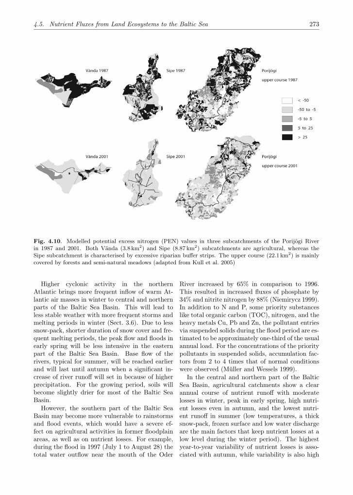
4.5. Nutrient Fluxes from Land Ecosystems to the Baltic Sea 273
Fig. 4.10. Modelled potential excess nitrogen (PEN) values in three subcatchments of the Porijõgi Riverin 1987 and 2001. Both Vända (3.8 km2) and Sipe (8.87 km2) subcatchments are agricultural, whereas theSipe subcatchment is characterised by excessive riparian buffer strips. The upper course (22.1 km2) is mainlycovered by forests and semi-natural meadows (adapted from Kull et al. 2005)
Higher cyclonic activity in the northernAtlantic brings more frequent inflow of warm At-lantic air masses in winter to central and northernparts of the Baltic Sea Basin. This will lead toless stable weather with more frequent storms andmelting periods in winter (Sect. 3.6). Due to lesssnow-pack, shorter duration of snow cover and fre-quent melting periods, the peak flow and floods inearly spring will be less intensive in the easternpart of the Baltic Sea Basin. Base flow of therivers, typical for summer, will be reached earlierand will last until autumn when a significant in-crease of river runoff will set in because of higherprecipitation. For the growing period, soils willbecome slightly drier for most of the Baltic SeaBasin.
However, the southern part of the Baltic SeaBasin may become more vulnerable to rainstormsand flood events, which would have a severe ef-fect on agricultural activities in former floodplainareas, as well as on nutrient losses. For example,during the flood in 1997 (July 1 to August 28) thetotal water outflow near the mouth of the Oder
River increased by 65% in comparison to 1996.This resulted in increased fluxes of phosphate by34% and nitrite nitrogen by 88% (Niemirycz 1999).In addition to N and P, some priority substanceslike total organic carbon (TOC), nitrogen, and theheavy metals Cu, Pb and Zn, the pollutant entriesvia suspended solids during the flood period are es-timated to be approximately one-third of the usualannual load. For the concentrations of the prioritypollutants in suspended solids, accumulation fac-tors from 2 to 4 times that of normal conditionswere observed (Müller and Wessels 1999).
In the central and northern part of the BalticSea Basin, agricultural catchments show a clearannual course of nutrient runoff with moderatelosses in winter, peak in early spring, high nutri-ent losses even in autumn, and the lowest nutri-ent runoff in summer (low temperatures, a thicksnow-pack, frozen surface and low water dischargeare the main factors that keep nutrient losses at alow level during the winter period). The highestyear-to-year variability of nutrient losses is asso-ciated with autumn, while variability is also high

274 4. Climate-related Change in Terrestrial and Freshwater Ecosystems
in late winter and spring. Under climate change,variability of nutrient losses is expected to increasemainly in winter and spring when the duration offrozen surfaces, amount of snow-pack water, dura-tion and continuity of certain weather types, oc-currence of strong night frost events and the num-ber of soil freeze-thaw cycles is changing. Shorterperiod of frozen surface and increased numbers ofsoil freeze-thaw cycles will lead to more intensiveleaching from arable land.
Responses of nutrient losses to climate changewill be faster and more direct in small agriculturalcatchments, while dynamics in large catchmentsare more complicated due to internal material cy-cles (Mander et al. 2000b; Stålnacke et al. 2004).
Milder winters (increase of air temperature inFebruary from −7.9 to −5.5 C during the period1950–1997 in Tartu, Estonia) and a change in theprecipitation pattern in recent decades have influ-enced the mean annual water discharge in morecontinental parts of the Baltic Sea Basin (Man-der et al. 2000b). In the Porijõgi River catchmentarea, southern Estonia (see Figs. 4.9 and 4.10),the change in the annual runoff pattern resulted inmore intensive material flow during colder seasonsand decreased water runoff in summer. The mostsignificant change in the mean monthly nutrientrunoff pattern is that of total inorganic nitrogen(TIN). In all subcatchments except the forestedPorijõgi upper course, a significant decrease in in-organic nitrogen runoff has been observed. Dueto increased surface flow caused by melting snowduring milder winters, the TIN losses are still high,but rapidly decrease in spring. During the growingseason, the intensive uptake by plants minimisesnitrogen losses. Likewise, nitrogen losses in sum-mer show the lowest variation (Mander et al. 1998;Fig. 4.11).
In the whole Porijõgi River catchment and inits upper course, the annual patterns of monthlyrunoff of phosphorus show only minor changes(Fig. 4.12). However, winters in the last decadehave been milder, resulting in a shorter periodwith permanent snow cover. Frozen surface andsnow melting water with wet precipitation give riseto increased surface flow. As shown in Fig. 4.12,this mostly affects the intensively cultivated Sipeand Vända subcatchments. Due to more fre-quent periods with thawing soil in winter, thephosphorus particles are exposed to surface flowfor a longer period, with total monthly phos-phorus runoff in winter months therefore remain-ing at a high level. By contrast, less intensive
tillage in spring and autumn has reduced phos-phorus losses in those periods (Mander et al.1998).
In addition to clearly water budget-based ex-planations, long term cyclicity in water discharge,which varies in frequency (from 13 to 43 years)among different rivers (Tsirkunov et al. 1992;Klavinš et al. 2002), plays a certain role in thenutrient regime of rivers. However, there are noclear explanations for these kinds of cyclicity.
4.5.1.7 Measures for Further Decrease of NutrientFlows to the Baltic Sea
During the past 15 years or so, EU and nationalpolicy actions have been adopted to decrease thenutrient load and threats of eutrophication in theBaltic Sea. On the other hand, there has been adramatic change in agricultural policy and prac-tices since the beginning of 1990s in the easternpart of the Baltic Sea Basin. Despite all of thesemeasures, the quality of the Baltic Sea is not sig-nificantly improving.
In particular, the ecological quality in estuar-ies and coastal lagoons has not improved, despitereduced nutrient loads in the catchments and de-creasing riverine loads. Therefore, additional mea-sures are planned by several authorities. Amongthem, sustainable agricultural practices (widerpracticing of ecological agriculture and imple-mentation of environment-friendly crop rotations;Paulsen et al. 2002; Granstedt et al. 2004) andchanges in agricultural practices (high-tech solu-tions like GPS-supported fertilisation schemes; im-plementation of shallow injection technique whenusing liquid manure; Sundell 1997) should be men-tioned as measures targeted to decrease loadingsin the catchments.
Several ecotechnological measures will help tocontrol nutrient flows from the catchments to thewater bodies. Maintenance, sustainable manage-ment and restoration of wetlands is the widely-used ecotechnological practice at the catchmentlevel (Weller et al. 1996; Gustafson et al. 1998;Arheimer and Wittgren 2002; Paludan et al. 2002).
In addition, riparian buffers are already com-mon practice in several countries (Kuusemets andMander 2002). Jansson et al. (1998) have calcu-lated that existing natural wetlands in the BalticSea Basin can retain an amount of nitrogen whichcorresponds to about 5–13% of annual total (nat-ural and anthropogenic) N emissions entering theBaltic Sea.

4.5. Nutrient Fluxes from Land Ecosystems to the Baltic Sea 275
Fig. 4.11. Changes in total inorganic nitrogen (TIN) fluxes in the Porijõgi catchment. For subcatchmentcharacteristics, see Fig. 4.10 (after Mander et al. 1998)
Fig. 4.12. Changes in total phosphorus fluxes in the Porijõgi catchment. For subcatchment characteristicssee Fig. 4.10 (after Mander et al. 1998)

276 4. Climate-related Change in Terrestrial and Freshwater Ecosystems
Likewise, the existing wetlands can significantlydecrease the phosphorus emissions (Weller et al.1996). Constructed wetlands play an importantrole while effectively retaining both nitrogen andphosphorus from both diffuse and point sourcesof pollution (Arheimer et al. 2004b). Constructedwetlands can also help in terms of stabilising thebalance between N and P in purified wastewater,while relatively cheap and widely used phosphorussedimentation in conventional purification systemshas increased the proportion of nitrogen relative tophosphorus transported to the Baltic Sea (Grenet al. 1997; Laznik et al. 1999). Nitrogen removalwith conventional techniques is, however, a verycostly measure, the benefits of which are not al-ways reliable (Turner et al. 1999).
4.5.2 Organic Carbon Export from Boreal andSubarctic Catchments
The catchment area of the Baltic Sea can beroughly divided into a south-eastern part, drain-ing into the Gulf of Riga and the Baltic Proper,that is characterised by a cultivated landscapewith a temperate climate, and a northern borealpart, characterised by coniferous forests and peat,draining into the Bothnian Bay, Bothnian Sea andGulf of Finland. The northern part also includessubarctic watersheds in the very northern catch-ment of the Bothnian Bay (Fig. 1.11, Chap. 1;Table 4.8). In general, the specific runoff is twiceas high in the catchments of the Bothnian Bayand Bothnian Sea as in the south-eastern part ofthe Baltic Sea catchment, whereas the catchmentof the Gulf of Finland, which is dominated com-pletely by the Neva River, has an intermediate spe-cific runoff (Table 4.8).
In this section we describe the potential effectsof global warming on the land–sea fluxes of dis-solved constituents (C, N, P, Si) in these borealand subarctic watersheds of the Baltic Sea anddiscuss their implications for the marine ecosys-tem of the Baltic Sea, as well as potential positiveand negative feedbacks to global warming.
4.5.2.1 Oligotrophic Character of Boreal Water-sheds
The Baltic Sea is often described as one of themost eutrophicated seas, although it should be em-phasised here that > 60% of the river water enter-ing the Baltic Sea comes from the subcatchmentsof the Bothnian Bay, the Bothnian Sea and theGulf of Finland (Table 4.8). The water from these
subcatchments has an oligotrophic (Bothnian Bayand Bothnian Sea) to slightly mesotrophic (Gulf ofFinland) character, as for example the Neva River.The much lower cover of cultivated landscape inthe watersheds of the northern catchments com-pared to the south-eastern catchment (Table 4.8)is clearly reflected in the trophic status of theserivers, expressed here as dissolved inorganic nitro-gen (DIN) and phosphorus (DIP) concentrations,which are in the same range or sometimes evenlower than in the respective basins of the BalticSea (Humborg et al. 2003). The DIN and DIPconcentrations of major rivers entering the Gulfof Bothnia are shown in Fig. 4.13 and comparedwith those from the major monitoring stations ofthe Bothnian Bay (BO3) and the Bothnian Sea(USB5).
Especially the phosphorous concentrations inthe rivers are extremely low and can explain theP-limitation observed in the receiving waters ofthe Bothnian Bay (Hagström et al. 2001). Thelow DIP concentrations in unperturbed rivers canpartly be explained by the high iron concentra-tions of these rivers (Ingri et al. 2005). How-ever, the seasonal variations of the dissolved con-stituents are much lower in the heavily regulatedrivers, as for example the Luleälven, Skellefteälvenor Indalsälven, as compared to the unregulatedrivers in the area, of which only a few are left –for example the rivers Torneälven, Kalixälven andRåneälven. Damming has reduced the nutrientland–sea fluxes of nearly all dissolved constituentsincluding nutrients and carbon, which can beexplained mainly by changes in the weatheringregime as a result of changes in hydrology and sur-face water-groundwater interactions in these heav-ily dammed rivers (Humborg et al. 2000, 2002).
4.5.2.2 Potential Future Impacts
Runoff is the leading environmental variable deter-mining land–sea fluxes of dissolved constituents,as also observed for the more eutrophicated wa-tersheds of the Baltic Sea Basin (Vagstad et al.2004). Over the next century, runoff is estimatedto increase by 15% averaged over the entire BalticSea Basin and between 10% and 40% for the catch-ments of the Bothnian Bay, Bothnian Sea and theGulf of Finland (Graham 2004; Sect. 3.7). Themost prominent effect of global warming with re-spect to watershed exports of matter is thereforelikely to be a significant increase in fluxes of dis-solved constituents such as nutrients (N, P, Si) as
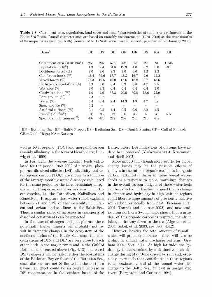
4.5. Nutrient Fluxes from Land Ecosystems to the Baltic Sea 277
Table 4.8. Catchment area, population, land cover and runoff characteristics of the major catchments in theBaltic Sea Basin. Runoff characteristics are based on monthly measurements (1970–2000) at the river mouthsof 84 major rivers (see Fig. A.36) (source: MARE-Nest, www.mare.su.se/nest; page visited 20 January 2006)
Basin1 BB BS BP GF GR DS KA All
Catchment area (×103 km2) 263 227 573 428 134 29 81 1,735Population (×106) 1.3 2.4 54.8 12.3 4.0 5.2 3.0 83.1Deciduous forest (%) 3.0 2.0 2.3 3.0 6.0 1.2 2.2Coniferous forest (%) 43.4 59.6 17.7 43.3 16.7 2.6 42.2Mixed forest (%) 27.3 19.6 10.0 17.6 16.8 2.7 15.6Herbaceous vegetation (%) 5.3 3.0 8.4 0.9 6.8 4.7 2.5Wetlands (%) 9.0 3.3 0.4 0.4 0.4 0.4 1.0Cultivated land (%) 4.0 4.9 57.3 20.0 50.8 78.6 22.9Bare ground (%) 2.3 0.7 – – – – 0.1Water (%) 5.4 6.4 2.4 14.3 1.9 4.7 12Snow and ice (%) 0.2 – – – – – –Artificial surfaces (%) 0.1 0.5 1.4 0.5 0.6 5.2 1.5Runoff (×109m3) 108 93 124 109 33 6 35 507Specific runoff (mm m−2) 409 410 217 252 245 210 442
1BB =Bothnian Bay; BP =Baltic Proper; BS =B othnian Sea; DS = Danish Straits; GF =Gulf of Finland;GR = Gulf of Riga; KA =Kattega
well as total organic (TOC) and inorganic carbon(mainly alkalinity in the form of bicarbonate; Lud-wig et al. 1999).
In Fig. 4.14, the average monthly loads calcu-lated for the period 1969–2002 of nitrogen, phos-phorus, dissolved silicate (DSi), alkalinity and to-tal organic carbon (TOC) are shown as a functionof the average monthly water discharge calculatedfor the same period for the three remaining unreg-ulated and unperturbed river systems in north-ern Sweden, i.e. the Torneälven, Kalixälven andRåneälven. It appears that water runoff explainsbetween 71 and 97% of the variability in nutri-ent and carbon land sea-fluxes to the Baltic Sea.Thus, a similar range of increases in transports ofdissolved constituents can be expected.
In the case of nitrogen and phosphorus, thesepotentially higher imports will probably not re-sult in dramatic changes in the ecosystem of thenorthern basins of the Baltic Sea, since the con-centrations of DIN and DIP are very close to eachother both in the major rivers and in the Gulf ofBothnia, as discussed above (Fig. 4.13). IncreasedDSi transports will not affect either the ecosystemsof the Bothnian Bay or those of the Bothnian Sea,since diatoms are not Si limited in the northernbasins; an effect could be an overall increase inDSi concentrations in the southern basins of the
Baltic, where DSi limitations of diatoms have in-deed been observed (Yurkovskis 2004; Kristiansenand Hoell 2002).
More important, though more subtle, for globalchange issues may be the possible effects ofchanges in the ratio of organic carbon to inorganiccarbon (alkalinity) fluxes in these boreal water-sheds as a response to global warming: changesin the overall carbon budgets of these watershedscan be expected. It has been argued that a changein climate and hydrology in high latitude regionscould liberate large amounts of previously inactivesoil carbon, especially from peat (Freeman et al.2001; Tranvik and Jansson 2002), and new stud-ies from northern Sweden have shown that a greatdeal of this organic carbon is respired, mainly inlakes, on its way down to the sea (Algesten et al.2004; Sobek et al. 2003; see Sect. 4.4.2).
However, besides the total amount of runoff –which will probably increase – there will also bea shift in annual water discharge patterns (Gra-ham 2004; Sect. 3.7). At high latitudes the hy-drology is characterised by a distinctive peak dis-charge during May/June driven by rain and, espe-cially, snow melt that contributes in these regionsto approximately half of the annual water dis-charge to the Baltic Sea, at least in unregulatedrivers (Bergström and Carlsson 1994).

278 4. Climate-related Change in Terrestrial and Freshwater Ecosystems
Fig. 4.13. Long-term (1980–2000) annual median river nutrient concentration in major rivers running into theBothnian Bay and Bothnian Sea: (upper panels) dissolved inorganic nitrogen (DIN), (lower panels) dissolvedinorganic phosphorus (DIP); whiskers indicate 25th and 75th percentile; horizontal axis gives month of year(adapted from Humborg et al. 2003)
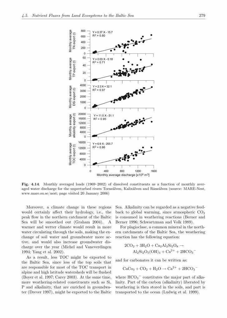
4.5. Nutrient Fluxes from Land Ecosystems to the Baltic Sea 279
Fig. 4.14. Monthly averaged loads (1969–2002) of dissolved constituents as a function of monthly aver-aged water discharge for the unperturbed rivers Torneälven, Kalixälven and Råneälven (source: MARE-Nest,www.mare.su.se/nest; page visited 20 January 2006)
Moreover, a climate change in these regionswould certainly affect their hydrology, i.e., thepeak flow in the northern catchment of the BalticSea will be smoothed out (Graham 2004). Awarmer and wetter climate would result in morewater circulating through the soils, making the ex-change of soil water and groundwater more ac-tive, and would also increase groundwater dis-charge over the year (Michel and Vaneverdingen1994; Yang et al. 2002).
As a result, less TOC might be exported tothe Baltic Sea, since less of the top soils thatare responsible for most of the TOC transport inalpine and high latitude watersheds will be flushed(Boyer et al. 1997; Carey 2003). At the same time,more weathering-related constituents such as Si,P and alkalinity, that are enriched in groundwa-ter (Drever 1997), might be exported to the Baltic
Sea. Alkalinity can be regarded as a negative feed-back to global warming, since atmospheric CO2
is consumed in weathering reactions (Berner andBerner 1996; Schwartzman and Volk 1989).
For plagioclase, a common mineral in the north-ern catchments of the Baltic Sea, the weatheringreaction has the following equation:
2CO2 + 3H2O + Ca2Al2Si2O8 →Al2Si2O5(OH)4 + Ca2+ + 2HCO3
−
and for carbonates it can be written as:
CaCo3 + CO2 + H2O → Ca2+ + 2HCO3−
where HCO3− constitutes the major part of alka-
linity. Part of the carbon (alkalinity) liberated byweathering is then stored in the soils, and part istransported to the ocean (Ludwig et al. 1999).

280 4. Climate-related Change in Terrestrial and Freshwater Ecosystems
Thus, the anticipated increase in TOC exporthaving a potentially positive feedback to globalwarming (Freeman et al. 2001, 2004) will proba-bly be partly compensated by an increase in al-kalinity export. Moreover, increasing tempera-tures will likely lead to increases in forested ar-eas (e.g. Kullman 2002; Koca et al. 2006; see alsoSects. 4.3.2, 4.3.4 and 4.3.5), so that changes invegetation belts in the northern parts of the BalticSea Basin towards wetlands, taiga (boreal conif-erous forests) and broadleaved forest can be ex-pected. This anticipated change in land coverwould likewise lead to an increase in fluxes ofweathering-related dissolved constituents (DSi, P,alkalinity), since it has been found that vegetationcover in watersheds of northern Sweden has a pos-itive effect on weathering-related constituents inriver waters (Humborg et al. 2004).
However, an increase in alkalinity export to theoceans in response to changes in rainfall and landuse has been observed in the Mississippi watershed(Raymond and Cole 2003) and the possible nega-tive feedback to global warming has been empha-sised (Ittekkot 2003). Thus, a major unresolvedquestion appears to be whether a change in alka-linity exports accompanying changes in the land-scapes associated with global warming is also anissue in high latitude watersheds, such as thosedraining into the northern basins of the Baltic Sea.
4.5.3 Synthesis – Climate Change Impacts onNutrient Fluxes from Land Ecosystemsto the Baltic Sea
Nitrogen and phosphorus losses from agriculturein the Baltic Sea Basin have increased markedlyover the last 50 years, but have stabilised sincethe mid-1980s. The main causes for the recent sta-bilisation are probably reduced fertiliser use andagricultural land abandonment, in both cases as-sociated with more stringent agricultural and en-vironmental policy, and with the transition to amarket economy in former eastern bloc countries.
Milder winters and changing precipitation pat-terns since the 1950s have influenced water dis-charge to the Baltic Sea. Over continental areas,the net effect seems to be a reduction in nutrientrunoff, while a tendency towards longer dry pe-riods interspersed with intensive rain seasons hascaused an increase in transport of dissolved or-ganic carbon from forests and wetland areas tothe water bodies.
Water runoff explains between 71 and 97% ofthe variability in nutrient and carbon land-seafluxes to the Baltic Sea. Future changes in cli-mate patterns and related runoff regimes can sig-nificantly influence export rates. Trends will besensitive to changes in the timing of seasonal andannual events (spring runoff, autumn low flow, iceand snow cover); the frequency and severity of ex-treme events (floods, droughts, erosion); as well asto climatic thresholds and ranges.
Climate scenarios for the next century point tomoderate increases in mean annual river flow tothe Baltic Sea (Sect. 3.7). Common to all scenar-ios is a general trend of reduced river flow fromagriculture-dominated southern and continentalareas, with increased flows in largely forestednorthern catchments. In contrast, southern areasmay become more vulnerable to rainstorms andflood events, with severe effects on agriculture informer floodplain areas, as well as nutrient losses.The balance between these counteractive forcingsin their effects on total and regional nutrient ex-port rates to the Baltic Sea is difficult to predict.
A reduced influence of snow melt will increasethe synchronisation between precipitation andstream discharge, reducing and extending sum-mertime base flow while increasing wintertimerunoff. Springtime peak flows and floods arelikely to become less intense. Shorter periods withfrozen surfaces and more frequent freeze-thaw cy-cles would further promote leaching during winterfrom arable land, especially in northern areas.
Organic carbon loads in runoff from boreal andsubarctic catchments will be sensitive to the coun-teractive effects of increased total water dischargeand changed seasonality, leading to less intensiveflushing events of top soils but deeper infiltra-tion, potentially decreasing TOC fluxes and in-creasing alkalinity fluxes. The net effect of thesecontrasting mechanisms on net carbon exports tothe Baltic Sea remains uncertain.
4.6 Conclusions and Recommendationsfor Research
This chapter sought to evaluate, through literaturereview and synthesis, two hypotheses. The firstof these asserts that climate change over recentdecades has already impacted terrestrial and fresh-water ecosystems of the Baltic Sea Basin. Thishypothesis receives clear support, even allowingfor the many uncertainties. Phenological events,species distributions and migration behaviour are
4.6. Conclusions and Recommendations for Research 281
readily-observed indicators of biological changes,with straightforward relationships to large-scaleclimate.
Numerous species and populations from theBaltic Sea Basin exhibit shifts in these parame-ters consistent with climate warming and the pole-ward migration of isotherms. Changes in ecosys-tem functioning have been registered by satellites,as well as land-based surveys such as forest inven-tories and treeline studies. It is apparent that treesare growing taller and lusher compared with afew decades ago; net primary productivity has in-creased, the ecosystems are net carbon sinks. Thelikely cause is an extended growing season associ-ated with higher average temperatures. With re-gard to freshwater ecosystems, reductions in win-ter ice cover and duration, as well as higher wa-ter temperatures and secondary effects of thesechanges on lake nutrient cycles have most likelycontributed to biological changes such as domi-nance shifts of species in some lakes.
The second hypothesis of this chapter is thatclimate changes simulated by models for the nextcentury will have ongoing ecosystem impacts.This hypothesis likewise receives general supportfrom our analysis. Based on both experimentaland modelling studies, we may cautiously concludethat current trends in terrestrial ecosystem func-tioning will continue for some decades into the fu-ture. Based on developments in abiotic variablesalone, forest production is likely to increase atleast over northern parts of the Baltic Sea Basin.Over the southern continental area, water stressmay offset the positive effects of temperature andCO2 increases on productivity. Northern terres-trial ecosystems will continue to sequester carbon,while southern areas may switch from carbon sinksto sources by the end of the 21st century.
However, uncertainties are relatively high con-cerning soil carbon turnover, especially for theextensive peatlands of the boreal and subarcticzones. Changes in disturbance regimes, and vul-nerability of species and ecosystems to climatic ex-tremes and to pest and pathogen attacks are moredifficult to predict but could significantly modifytrends, for example in forest productivity. Con-clusions concerning future changes in freshwaterecosystems are more speculative. Warmer watertemperatures combined with longer stratified andice-free periods in lakes may be expected to ac-celerate eutrophication, increasing phytoplanktonproduction and causing potential dominance andsuccessional shifts. Shallow lakes and lake littoral
zones may be particularly vulnerable to the im-pacts of warming.
For several of the ecosystem functions addressedin this chapter, the trajectory of future changes re-mains elusive, due either to a limited understand-ing of the driving mechanisms, the complexity ofecosystem structure and dynamics, or because ofuncertainties concerning the future course of non-climatic drivers such as land use and agriculturalpractices. The complexity of biological and abioticinteractions in lakes prohibits general conclusionsabout the responses of populations and communi-ties to climate forcing. Land-sea nutrient fluxeswill be sensitive to future changes in runoff, butalso to regional patterns of agricultural land use,fertiliser loads and ecotechnological practice. Ex-port rates of total organic carbon in runoff fromboreal and subarctic peatlands are significant forthe carbon balance of the Baltic Sea, but it is un-clear whether changing rainfall patterns and tem-perature will amplify or attenuate TOC loads inthe future.
Numerous areas of uncertainty emerge from oursynthesis. These fall into three main categories;firstly, limitations to current understanding of themechanisms by which species and ecosystems re-spond to climate change; secondly, factors witha potential to modify climate responses that aredifficult to characterise because of their episodicor species-specific nature – for example, impactsof pests, pathogens and climatic extremes; andfinally, sensitivities to non-climatic covariates ofclimate change, such as land use, forest manage-ment, agricultural practices, pollutant depositionrates and technology development.
The further elucidation and constrainment ofthese uncertainties constitute fertile ground forresearch, especially as many of them surroundecosystem functions of sectoral or societal impor-tance: forest growth, net carbon emission, waterquality, habitat conservation. We would identifythe following key questions for research:
• How will the distribution and abundance ofpests and pathogens respond to climate change,and what consequences will this have for thefunctioning of natural and managed ecosys-tems?
• Given current greenhouse gas emissions scenar-ios, their associated socio-economic storylines,and the changes in climate and ecosystem func-tioning they are expected to lead to, what arethe likely trajectories and spatial patterns of
282 4. Climate-related Change in Terrestrial and Freshwater Ecosystems
land use change within the Baltic Sea Basin?What consequences will these, in turn, have forspecies distributions, carbon sequestration, wa-ter runoff and land-sea nutrient fluxes?
• What are the likely future anthropogenic loadsof nitrogen and phosphorus to terrestrial andfreshwater ecosystems, and what consequenceswill they have for ecosystem functioning?
• How will changes in hydrology, soil thermal dy-namics, biogeochemistry, microtopography andvegetation affect the contribution of extantpeatland areas to greenhouse forcing, not for-getting the carbon exports of these areas to theBaltic Sea?
• What changes in disturbance regimes will re-sult from future climate variability, especiallyextreme events like storms, spring temperaturebacklashes, extended drought periods or a suc-cession of extreme summers? What will bethe consequences for ecosystems, taking into ac-count feedback mechanisms such as insect pestoutbreaks and herbivore pressure in forests?What will be the consequences for water qualityin lakes and land runoff?
4.7 Summary
The changing climate and other associated envi-ronmental and anthropogenic changes may be ex-pected to affect the structure and functioning ofecosystems and threaten the services they provideto society.
We assess the potential impacts of the changingenvironment on terrestrial and freshwater ecosys-tems of the Baltic Sea Basin, aiming to evaluatethe hypotheses:
1. that climate change and other associated en-vironmental change over recent decades haveaffected the ecosystems and their services; and
2. that ongoing climate change will cause (fur-ther) changes in the ecosystems and their ser-vices over the remainder of the 21st century.
In order to highlight the most compelling andsocietally-relevant aspects of ecosystem change,the analysis focuses on:
1. processes and indicators of particular diag-nostic value for the attribution of ecosystemchanges to identifiable forcing factors; for ex-ample, changes in phenology, species distribu-tions and the seasonality of physical, chemicaland biological phases in lakes;
2. ecosystems and functions of sectorial relevance;for example, productivity and carbon storagein forests; and
3. uncertainty associated with ecological com-plexity and limitations to process understand-ing; for example, regarding stress responses tochanging climatic extremes.
Significant changes in climate, including increas-ing temperatures and changing precipitation pat-terns, have occurred over the Baltic Sea Basinin recent decades (Chap. 2). Other associatedchanges include the continuously rising atmo-spheric CO2 concentrations and increases in de-position loads of atmospheric pollutants, includ-ing nitrogen compounds and other acidifying pol-lutants. A variety of ecosystem impacts of thesechanges have been identified (hypothesis 1), in-cluding the following:
• An advancement of spring phenological phasessuch as budburst and leaf expansion is appar-ent for many plant species, likely reflecting in-creasing mean temperatures. Many species alsoshow delayed autumn phases, but trends areless consistent. Phenological trends are strongerin northern Europe than for Europe as a whole,possibly reflecting stronger climate warming.
• Species distributional shifts tracking isother-mal migration are apparent for both plant andanimal species. Possibly related changes in-clude weaker migratory behaviour, for exam-ple in some bird species. Treeline advance hasbeen observed in the Fennoscandian mountainrange. Increased growth and vigour of vegeta-tion at high northern latitudes generally is ap-parent from satellite observations and can beattributed to increased growing season warmthand an extended growing season. Other obser-vations, such as tree ring data, support the ex-istence of a positive growth trend. The magni-tude of the trend within the Baltic Sea Basin isrepresentative for high latitude areas in Eurasiaand is strong compared with similar latitudes inNorth America.
• Physiological stress related to the combined ef-fects of atmospheric pollutants and extremeweather events such as spring frosts anddrought are a possible explanation for late 20th-century dieback in boreal and temperate forests.
• Degradation of discontinuous permafrost in thesubarctic north may be causing a shift towards agreater representation of wet habitats in tundra.Possible consequences include an increased re-

4.7. Summary 283
lease of methane through (anaerobic) decompo-sition, which would accentuate greenhouse forc-ing.
• Climate-related changes in lakes includinghigher water temperatures, advancement of icebreak-up, lower water levels and increased in-fluxes of dissolved organic matter from landhave consequences for lake ecosystems, includ-ing dominance shifts in phytoplankton commu-nities, higher summer algal biomass, and shiftsin trophic state.
Climate scenarios described in Chap. 3 consis-tently point to increased temperatures through-out the Baltic Sea Basin by the end of the 21st
century, compared with today. Precipitation sce-narios are more variable but generally point toincreased precipitation in winter, with southernareas experiencing decreased rainfall in summer.Combined with the effect of higher temperatureson evapotranspiration, this suggests that ecosys-tems of the temperate zone may face increasinglyunfavourable growing season water budgets in thefuture. Potential impacts of these and other as-sociated environmental changes (hypothesis 2) in-clude the following:
• Extrapolation of recent phytophenologicaltrends suggests that extension of the vegetationperiod by 2–6 weeks, depending on the climatescenario, is likely over much of the Baltic Seacatchment area.
• Further changes in the distributions of somespecies may be expected, but for many species,lags associated with population and communityprocesses, dispersal limitations etc. are likely.Wholesale biome shifts, such as the north-ward displacement of the temperate-boreal for-est boundary, will be slow compared to therate of isotherm migration. Natural and semi-natural vegetation of the future may be of atransient character, e.g. ageing conifer standswith an increased representation of broadleavedtrees in the younger age classes. Changes maybe especially marked in subarctic and alpineareas, with forest invading areas that are cur-rently tundra. Increased local richness is likelyas species associated with the forest extendtheir ranges northward and upslope.
• Modelling studies generally point to increas-ing ecosystem production and carbon storage
capacity throughout the Baltic Sea Basin inthe next 50–100 years, in conjunction with alonger growing season, increased atmosphericCO2 concentrations and the stimulation of min-eralisation processes in warmer soils. However,increased autumn and winter temperatures maybe detrimental to hardening processes in trees,increasing susceptibility to spring frost damage.Growing season drought stress may reduce orinhibit production enhancement in temperateparts of the region.
• The potential impacts of climatic change on theincidence of pest and pathogen outbreaks af-fecting vegetation is still largely open. It seemsreasonable to assume that harmful insects andfungi from central and southern Europe may ex-pand into the Baltic Sea Basin in the warmingclimate.
• Warmer water temperatures combined withlonger stratified and ice-free periods in lakesmay be expected to accelerate eutrophication,increasing phytoplankton production and shift-ing the phytoplankton community structure to-wards species with higher temperature optima,including cyanobacteria. Shallow lakes and lakelittoral zones may be particularly sensitive toclimate warming. Increasing influxes of hu-mic substances in runoff from boreal catchmentswould steepen light attenuation, with negativeimpacts on periphyton and benthic communi-ties in lakes. Cold-water fish species may be ex-tirpated from much of their present range whilecool- and warm-water species expand north-wards.
Uncertainties associated with the assessment offuture ecosystem changes are substantial and in-clude uncertainties due to insufficient understand-ing of the biological phenomena being modelled orprojected including system-internal feedbacks andcomplexity, as well as variation among climate andgreenhouse gas emissions scenarios on which theassessments are based.
The most important source of uncertainty withregard to many impacts are the future develop-ment in non-climatic, anthropogenic drivers ofecosystem dynamics, including deposition of at-mospheric pollutants, land use changes, changesin forest management and agricultural practices,changes in human populations, markets and inter-national trade, and technological development.

284 4. Climate-related Change in Terrestrial and Freshwater Ecosystems
4.8 References
Aanes R, Saether BE, Øritsland NA (2000) Fluctuations of an introduced population of Svalbard rein-deer: The effects of density dependence and climatic variation. Ecography 23:437–443
Aars J, Ims RA (2002) Climatic and intrinsic determinants of population demography: The winterdynamics of tundra vole populations. Ecology 83:3449–3456
Aasa A, Jaagus J, Ahas R, Sepp M (2004) The influence of atmospheric circulation on plant pheno-logical phases in central and eastern Europe. Int J Climatol 24:1551–1564
Abgeti MD, Smol JP (1995) Winter limnology: A comparison of physical chemical and biological char-acteristics in two temperate lakes during ice cover. Hydrobiologia 304:221–234
Abildtrup J, Audsley E, Fekete-Farkas M, Giupponi C, Gylling M, Rosato P, Rounsevell M (2006)Socio-economic scenario development for the assessment of climate change impacts on agriculturalland use: A pairwise comparison approach. Env Sci Pol 9:101–115
ACIA (2004) Impacts of a Warming Arctic. Cambridge University Press, CambridgeACIA (2005) Arctic Climate Impact Assessment. Cambridge University Press, New YorkAdrian R, Deneke R, Mischke U, Stellmacher R, Lederer P (1995) A long-term study of the Heiligensee
(1975–1992) Evidence for effects of climatic change on the dynamics of eutrophied lake ecosystems.Arch Hydrobiol 133:315–337
Adrian R, Walz N, Hintze T, Hoeg S, Rusche R (1999) Effects of ice duration on plankton successionduring spring in a shallow polymictic lake. Freshwat Biol 41:621–632
Ahas R (1999) Long-term phyto- ornitho- and ichthyophenological time-series analysis in Estonia. IntJ Biometeorol 42:119–124
Ahas R, Aasa A (2004) Attribution of Estonian phyto- ornitho- and ichthyophenological trends withparameters of changing climate. 16th Conference on Biometeorology and Aerobiology 23–27 August2004, Vancouver Canada http://ams.confex.com/ams/pdfpapers/78288.pdf
Ahas R, Aasa A (2006) The effects of climate change on the phenology of selected Estonian plant,bird and fish populations. Int J Biometeorol 51:17–26
Ahas R, Tarand A, Meitern H (1998) Temporal variability of the phenological time series in Esto-nia. In: Ahas R, Tarand A, Meitern H (eds) Country Case Study on Climate Change Impactsand Adaptation. Assessments in the Republic of Estonia. Report to the UNEP/GEF Project NoGF/2200-96-45 Stockholm Environment Institute – Tallinn, pp. 28–30
Ahas R, Jaagus J, Aasa A (2000) The phenological calendar of Estonia and its correlation with meanair temperature. Int J Biometeorol 44:159–166
Ahas R, Aasa A, Menzel A, Fedotova VG, Scheifinger H (2002) Changes in European spring phenol-ogy. Int J Climatol 22:1727–1738
Ainsworth EA, Long SP (2005) What have we learned from 15 years of free-air CO2 enrichment(FACE)? A meta-analytic review of the responses of photosynthesis canopy properties and plantproduction to rising CO2. New Phytologist 165:351–372
Alatalo JM, Totland Ø (1997) Response to simulated climatic change in an alpine and subarcticpollen-risk strategist Silene acaulis. Glob Change Biol 3 S1:74–79
Alcamo J, Kok K, Busch G, Priess J, Eickhout B, Rounsevell M, Rothman D, Heistermann M (2006)Searching for the future of land: Scenarios from the local to global scale. In: Lambin EF,Geist H (eds) Land-use and Land-cover Change: Local Processes Global Impacts. The IGBP Series.Springer, Berlin Heidelberg New York
Alekseev A, Soroka AR (2002) Scots pine growth trends in northwestern Kola Peninsula as an indica-tor of positive changes in the carbon cycle. Climatic Change 55:183–196
Algesten G, Sobek S, Bergstrom AK, Agren A, Tranvik LJ, Jansson M (2004) Role of lakes for organiccarbon cycling in the boreal zone. Glob Change Biol 10:141–147
Andersen HE, Kronvang B, Larsen SE (1999) Agricultural practices and diffuse nitrogen pollution inDenmark: Empirical leaching and catchment models. Water Sci Tech 39:257–264
Andersen HE, Kronvang B, Larsen SE (2005) Development validation and application of Danish em-pirical phosphorus models. J Hydrol 304:355–365

4.8. References 285
Andersson FO, Ågren GI, Führer E (2000) Sustainable tree biomass production. Forest Ecol Manag132:51–62
Andersson L, Arheimer B (2003) Modelling of human and climate impact on nitrogen load in aSwedish river 1885–1994. Hydrobiologia 497:63–77
Andreeva EA (2003) The present state of macrozoobenthos in Lake Ilmen. In: Simola H, TerzhevikAY, Viljanen M, Holopainen IK (eds) Proceedings of 4th International Lake Ladoga Symposium2002, University of Joensuu, Publications of Karelian Institute 138
Angerbjörn A, Tannerfeldt M, Lundberg H (2001) Geographical and temporal patterns of lemmingpopulation dynamics in Fennoscandia. Ecography 24:298–308
Anneville O, Souissi S, Gammeter S, Straile D (2004) Seasonal and inter-annual scales of variabilityin phytoplankton assemblages: Comparison of phytoplankton dynamics in three peri-alpine lakesover a period of 28 years. Freshwat Biol 49:98–115
Anon (2002) State of Environment. The Ministry of Environment of the Republic of Lithuania, VilniusAraújo MB, Pearson RG, Thuiller W, Erhard M (2005) Validation of species-climate impact models
under climate change. Glob Change Biol 11:1504–1513Arft AM, Walker MD, Gurevitch J, Alatalo JM, Bret-Harte MS, Dale M, Diemer M, Gugerli F, Henry
GHR, Jones MH, Hollister RD, Jónsdóttir IS, Laine K, Lévesque E, Marion GM, Molau U, MølgaardP, Nordenhäll U, Raszhivin V, Robinson CH, Starr G, Stenström A, Stenström M, Totland Ø,Turner PL, Walker LJ, Webber PJ, Welker JM, Wookey PA (1999) Response patterns of tundraplant species to experimental warming: A meta-analysis of the International Tundra Experiment.Ecol Monogr 69:491–511
Arheimer B, Wittgren HB (2002) Modelling nitrogen removal in potential wetlands at the catchmentscale. Ecol Eng 19:63–80
Arheimer B, Andersson L, Larsson M, Lindström G, Olsson J, Pers BC (2004a) Modelling diffuse nu-trient flow in eutrophication control scenarios. Water Sci Tech 49:37–45
Arheimer B, Torstensson G, Wittgren HB (2004b) Landscape planning to reduce coastal eutrophica-tion: Agricultural practices and constructed wetlands. Landsc Urban Plann 67:205–215
Assel RA, Robertson DM (1995) Changes in winter air temperature near Lake Michigan 1851–1993as determined from regional ice records. Limnol Oceanogr 40:165–176
Assel RA, Cronk K, Norton D (2003) Recent trends in Laurentian Great lakes ice cover. ClimaticChange 57:185–204
Auclair AND, Lill JT, Revenga C (1996) The role of climate variability and global warming in thedieback of northern hardwoods. Water Air Soil Pollut 91:163–186
Audsley E, Pearn KR, Simota C, Cojocaru G, Koutsidou E, Rounsevell MDA, Trnka M, Alexandrov V(2006) What can scenario modelling tell us about future European scale land use and what not?Agr Ecosyst Env 9:148–162
Aurela M, Laurila T, Tuovinen J (2002) Annual CO2 balance of a subarctic fen in northern Europe:Importance of the wintertime efflux. J Geophys Res 107:4607
Ayres MP, Lombardero MJ (2000) Assessing the consequences of global change for forest disturbancefrom herbivores and pathogens. Sci Total Environ 262:263–286
Barabasz B, Górz A (1998) Argiope bruennichi (Scopoli 1772) Rare and insufficiently examined spiderspecies in Poland. Fragmenta Faunistica 41:255–267
Barklund P (1994) Svårtolkad ekdöd (Oak dieback). In: Ekfrämjandet 50 år Wallin and Dahlholmboktryckeri. AB Lund, Sweden (in Swedish)
Barklund P, Ericsson A, Gemmel P, Johansson U, Olsson M, Walheim M, Åhman G (1995) Bark ochvedskador hos granar med kådflöde – kådflödessjukan hos gran (Bark and wood damage with resinflow in Norway Spruce - Resin flow disease in Norway Spruce). Swedish University of AgriculturalSciences (SLU), Report Info/Skog. 15, Alnarp, Sweden (in Swedish)
Bazzaz FA (1990) The response of natural ecosystems to the rising global CO2 levels. Ann Rev EcolSystemat 21:167–196
Bechmann M, Eggestad HO, Vagstad N (1998) Nitrogen balances and leaching in four agriculturalcatchments in southeastern Norway. Env Poll 102 S1:439–499
286 4. Climate-related Change in Terrestrial and Freshwater Ecosystems
Beerling DJ, Terry AC, Mitchell PL, Jones DG, Lee JA, Callaghan TV (2001) Time to chill: Effects ofsimulated global change on leaf ice nucleation temperatures of sub-Arctic vegetation. Am J Bot 88:628–633
Behrendt H, Bachor A (1998) Point and diffuse load of nutrients to the Baltic Sea by river basins ofnortheast Germany (Mecklenburg–Vorpommern). Water Sci Tech 38:147–155
Behrendt H, Stellmacher R, Oldberg M (1987) Long-term changes in water quality parameters of ashallow eutrophic lake and their relations to meteorologic and hydrologic elements. In Soloman SI,Beran M, Hogg W (eds) The Influence of Climate Change and Climatic Variability on the HydrologicRegime and Water Resour. IAHS Publications 168:535–544
Benndorf J, Kranich J, Mehner T, Wagner A (2001) Temperature impact on the midsummer declineof Daphnia galeata: An analysis of long-term data from the biomanipulated Bautzen Reservoir(Germany). Freshwat Biol 46:199–211
Bergh J, McMurtrie RE, Linder S (1998) Climatic factors controlling the productivity of Norwayspruce: A model-based analysis. Forest Ecol Manag 110:127–139
Bergh J, Linder S, Lundmark T, Elfving B (1999) The effect of water and nutrient availability on theproductivity of Norway spruce in northern and southern Sweden. Forest Ecol Manag 119:51–62
Bergh J, Freeman M, Sigurdsson BD, Kellomäki S, Laitinen K, Niinistö S, Peltola H, Linder S (2003)Modelling the short-term effects of climate change on the productivity of selected tree species inNordic countries. Forest Ecol Manag 183:327–340
Bergh J, Linder S, Bergström J (2005) Potential production of Norway spruce in Sweden. Forest EcolManag 204:1–20
Bergh J, Räisänen J, Freeman M, Linder S (2007) Effects of global change on net primary productionin northern Europe – a model-based analysis on regional climate scenarios. Glob Change Biol (inpress)
Bergström AK, Algesten G, Sobek S, Tranvik L, Jansson M (2004) Emission of CO2 from hydroelec-tric reservoirs in northern Sweden. Arch Hydrobiol 159:25–42
Bergström S, Carlsson B (1994) River runoff to the Baltic Sea: 1950–1990. Ambio 23:280–287Berner EK, Berner RA (1996) Global Environment: Water Air and Geochemical Cycles. Prentice-
Hall, Upper Saddle River, NJ, USABernes C (1996) The Nordic Arctic Environment – Unspoilt Expoited Polluted? The Nordic Council
of Ministers, CopenhagenBerry PM, Rounsevell MDA, Harrison PA, Audsley E (2006) Assessing the vulnerability of agricul-
tural land use and species to climate change and the role of policy in facilitating adaptation. EnvSci Pol 9:189–204
Beuker E, Kolström M, Kellomäki S (1996) Changes in wood production of Picea abies and Pinussylvestris under a warmer climate: Comparison of field measurements and results of a mathematicalmodel. Silva Fennica 30:239–246
Blenckner T (2005) A conceptual model of climate related effects on lake ecosystems. Hydrobiologia533:1–14
Blenckner T, Omstedt A, Rummukainen M (2002a) A Swedish case study of contemporary and pos-sible future consequences of climate change on lake function. Aquat Sci 64:171–184
Blenckner T, Pettersson K, Padisak J (2002b) Lake plankton as tracer to discover climate signals.Verh Proc Trav SIL 28:1324–1327
Blenckner T, Järvinen M, Weyhenmeyer G (2004) Atmospheric circulation and its impact on ice phe-nology in Scandinavia. Boreal Env Res 9:371–380
Bocheński Z (1993) Catalogue of fossil and subfossil birds of Poland. Acta Biol Cracov 36:329–460Bonan GB, Pollard D, Thompson SL (1992) Effects of boreal forest vegetation on global climate. Na-
ture 359:716–718Bouraoui F, Grizzetti B, Granlund K, Rekolainen S, Bidoglio G (2004) Impact of climate change on
the water cycle and nutrient losses in a Finnish catchment. Climatic Change 66:109–126Boyer EW, Hornberger GM, Bencala KE, McKnight DM (1997) Response characteristics of DOC
flushing in an alpine catchment. Hydrolog Process 11:1635–1647

4.8. References 287
Bradshaw RHW, Holmqvist BH, Cowling SA, Sykes MT (2000) The effects of climate change on thedistribution and management of Picea abies in southern Scandinavia. Can J Forest Res 30:1992–1998
Brommer JE (2004) The range margins of northern birds shift polewards. Annales Zoologici Fennici41:391–397
Brooker RW, Carlsson BÅ, Callaghan TV (2001) Carex bigelowii Torrey ex Schweinitz (C. rigidaGood., non Schrank; C. hyperborea Drejer) Biological Flora of the British Isles. J Ecol 89:1072–1095
Bukantis A, Gulbinas Z, Kazakevicius S, Kilkus K, Mikelinskiene A, Morkunaite R, Rimkus E,Samuila M, Stankunavicius G, Valiuškevicius G, Zaromskis R (2001) Klimato svyravim? poveikisfiziniams geografiniams procesams Lietuvoje (The Influence of Climatic Variations on Physical Ge-ographical Processes in Lithuania) Monograph, Geografijos Inst., Vilnius (in Lithuanian)
Cairns DM, Moen J (2004) Herbivory influences tree lines. J Ecol 92:1019–1024Callaghan TV, Carlsson BÅ, Svensson BM (1996) Some apparently paradoxical aspects of the life cy-
cles demography and population dynamics of plants from the subarctic Abisko area. Ecol Bull 45:133–143
Callaghan TV, Björn LO, Chernov Y, Chapin T, Christensen TR, Huntley B, Ims RA, Johansson M,Jolly D, Jonasson S, Matveyeva N, Panikov N, Oechel W, Shaver G, Schaphoff S, Sitch S, Zöckler C(2004a) Climate change and UV-B impacts on Arctic tundra and polar desert ecosystems. Ambio 33:385–479
Callaghan TV, Johansson M, Heal OW, Saelthun NR, Barkved L, Bayfield N, Brandt O, Brooker R,Christiansen HH, Hoye TT, Humlun O, Järvinen A, Jonasson C, Kohler J, Magnusson B, MeltofteH, Mortensen L, Neuvonen S, Pearce I, Rasch M, Turner L, Hasholt B, Huhta E, Leskinen E,Nielsen N, Siikamäki P (2004b) Environmental changes in the North Atlantic region: SCANNETas a collaborative approach for documenting understanding and predicting changes. Ambio SpecialReport 13:39–50
Canadell JG, Ciais P, Cox P, Heimann M (2004) Quantifying understanding and managing the carboncycle in the next decades. Climatic Change 67:147–160
Carey SK (2003) Dissolved organic carbon fluxes in a discontinuous permafrost subarctic alpine catch-ment. Permafrost & Periglacial Processes 14:161–171
Carpenter SR, Kitchell JF, Hodgson JR (1985) Cascading trophic interactions and lake productivity.BioScience 35:634–639
Carpenter SR, Fisher SG, Grimm NB, Kitchell JF (1992) Global change and freshwater ecosystems.Ann Rev Ecol Systemat 23:119–139
Carpenter SR, Pingali PL, Bennett EM, Zurek MB (2005) Ecosystems and Human Well-being – Sce-narios. Island Press, Washington, D.C.
CAVM Team (2003) Circumpolar Arctic Vegetation Map Scale 1:7500000 Conservation of Arctic Floraand Fauna (CAFF). Map No 1, US Fish & Wildlife Service, Anchorage, Alaska
CCIRG (1996) Review of the Potential Effects of Climate Change in the United Kingdom. UK ClimateChange Impacts Review Group (CCIRG). HMSO, London
Chapin FS III, Schultze ED, Mooney HA (1990) The ecology and economics of storage in plants. AnnRev Ecol Systemat 21:423–447
Chapin FS III, Berman M, Callaghan TV, Convey P, Crépin AS, Danell K, Ducklow H, Forbes B,Kofinas G, McGuire AD, Nuttall M, Virginia R, Young O, Zimov SA, Christensen T, GodduhnA, Murphy EJ, Wall D Zöckler C (2005) Polar systems. In: Hassan R, Scholes R, Ash N (eds)Ecosystems and Human Well-Being: Current State and Trends. Volume I: Millennium EcosystemAssessment Series. Island Press, Washington DC, pp. 717–743
Chapin FS III, Hoel M, Carpenter SR, Lubchenco J, Walker B, Callaghan TV, Folke C, Levin SA,Mäler KG, Nilsson C, Barrett S, Berkes F, Crépin AS, Danell K, Rosswall T, Starrett D, XepapadeasA, Zimov SA (2006) Building resilience and adaptation to manage Arctic change. Ambio 35:198–202
Chmielewski FM, Rötzer T (2001) Response of tree phenology to climate change across Europe. AgrForest Meteorol 108:101–112
Choi JS (1998) Lake ecosystem responses to rapid climate change. Env Monit Assess 49:281–290Christensen TR, Jonasson S, Callaghan TV, Havström M (1999) On the potential CO2 release from
tundra soils in a changing climate. Appl Soil Ecol 11:127–134
288 4. Climate-related Change in Terrestrial and Freshwater Ecosystems
Christensen TR, Johansson T, Åkerman JH, Mastepanov M, Malmer N, Friborg T, Crill P, SvenssonBH (2004) Thawing sub-arctic permafrost: Effects on vegetation and methane emissions. GeophysRes Lett 31:L04501
Chu C, Mandrak NE, Minns CK (2005) Potential impacts of climate change on the distributions ofseveral common and rare freshwater fishes in Canada. Diversity & Distributions 11:299–310
Chuine I, Kramer K, Hänninen H (2003) Plant development models. In: Schwartz MD (ed) Phenol-ogy: An Integrative Environmental Science. Kluwer, pp. 217–235
Cornelissen JHC, Callaghan TV, Alatalo JM, Michelsen A, Graglia E, Hartley AE, Hik DS, HobbieSE, Press MC, Robinson CH, Henry GHR, Shaver GR, Phoenix GK, Gwynn Jones D, JonassonS, Chapin FS III ,Molau U, Neill C, Lee JA, Melillo JM, Sveinbjörnsson B, Aerts R (2001) Globalchange and Arctic ecosystems: Is lichen decline a function of increases in vascular plant biomass? JEcol 89:984–994
Costanza R, d’Arge R, de Groot R, Farber S, Grasso M, Hannon B, Limburg K, Naeem S, O’NeillRV, Paruelo J, Raskin RG, Sutton P, van den Belt M (1997) The value of the world’s ecosystemservices and natural capital. Nature 387:253–260
Coulson SJ, Leinass HP, Ims RA, Søvik G (2000) Experimental manipulation of winter surface icelayer: The effects on a high arctic soil microarthropod community. Ecography 23:299–306
Cummins CP (2003) UV-B radiation climate change and frogs – the importance of phenology. AnnalesZoologici Fennici 40:61–67
Dahl E (1990) Probable effects of climatic change due to the greenhouse effect on plant productivityand survival in North Europe. In: Holten JI, Paulsen G, Oechel WC (eds) Effects of Climate Changeon Terrestrial Ecosystems. Norwegian Institute for Nature Research, Trondheim, pp. 81–83
de Koning F, Olschewski R, Veldkamp E, Benitez P, Lopez-Ulloa M, Schlichter T, de Urquiza M(2005) The ecological and economic potential of carbon sequestration in forests: Examples fromSouth America. Ambio 34:224–229
de Stasio BT, Hill DK, Kleinhans JM, Nibbelink NP, Magnuson JJ (1996) Potential effects of globalclimate change on small north-temperate lakes: Physics fish and plankton. Limnol Oceanogr41:1136–1149
del Barrio G, Harrison PA, Berry PM, Butt N (2006) Impacts of climate change on species’ distribu-tions in a temperate and a Mediterranean area: Comparison and implications for policy. Env SciPol 9:129–147
Diehl S (2002) Phytoplankton light and nutrients in a gradient of mixing depths: Theory. Ecology 83:386–398
Dirnbock T, Dullinger S, Grabherr G (2003) A regional impact assessment of climate and land-usechange on alpine vegetation. J Biogeogr 30:401–417
Dittmar C, Zech W, Elling W (2003) Growth variations of common beech (Fagus sylvatica L) underdifferent climatic and environmental conditions in Europe – a dendroecological study. Forest EcolManag 173:63–78
Dormann CF, Woodin SJ (2002) Climate change in the Arctic: Using plant functional types in ameta-analysis of field experiments. Funct Ecol 16:4–17
Dorrepaal E, Aerts R, Cornelissen JHC, Callaghan TV, Logtestijn RSP (2004) Summer warming andincreased winter snow cover affect Sphagnum fuscum growth structure and production in a sub-arcticbog. Glob Change Biol 10:93–104
Drake BG, Gonzalez-Meler MA, Long SP (1997) More efficient plants: A consequence of rising atmo-spheric CO2? Ann Rev Plant Physiol Plant Mol Biol 48:609–639
Drever JI (1997) The Geochemistry of Natural Waters. Prentice HallDuraiappah A, Naeem S, Agardy T, Ash NJ, Cooper HD, Díaz S, Faith DP, Mace G, McNeely JA,
Mooney HA, Oteng-Yeboah AA, Pereira HM, Polasky S, Prip C, Reid WV, Samper C, Schei PJ,Scholes R, Schutyser F, van Jaarsveld A (2005) Ecosystems and Human Well-being: BiodiversitySynthesis. Island Press, Washington DC
Dzikiewicz M (2000) Activities in nonpoint pollution control in rural areas of Poland. Ecol Eng 14:429–434
4.8. References 289
Eilertsen SM (2002) Utilization of abandoned coastal meadows in northern Norway by reindeer. PhDthesis, University of Tromsø, Norway
Ellenberg H (1986) Vegetation Mitteleuropas mit den Alpen, 4th ed. Ulmer, Stuttgart, GermanyElliott JA, Thackeray SJ, Huntingford C, Jones RG (2005) Combining a regional climate model with
a phytoplankton community model to predict future changes in phytoplankton in lakes. FreshwatBiol 50:1404–1411
Emanuelsson U (1987) Human influence on vegetation in the Torneträsk area during the last threecenturies. Ecol Bull 38:95–111
Enell M, Fejes J (1995) The nitrogen load to the Baltic Sea – Present situation acceptable future loadand suggested source reduction. Water Air Soil Pollut 85:877–882
Ewert F, Rounsevell MDA, Reginster I, Metzger MJ, Leemans R (2005) Future scenarios of Europeanagricultural land use: Estimating changes in crop productivity. Agr Ecosyst Environ 107:101–116
Federal Forest Inventory (2005) The Federal Forest Inventory, Bundesministerium für ErnährungLandwirtschaft und Verbraucherschutz, Germany, http://www.bundeswaldinventur.de, site visitedin August 2005
Fiedler W (2003) Recent changes in migratory behaviour of birds: A compilation of field observationsand ringing data. In: Berhold P, Gwinner E, Sonnenschein E (eds) Avian Migration. Springer,Berlin Heidelberg New York
Filatov NN, Nazarova LY, Salo YA (2003) Climate changes and Water Resour in the region of thelargest European lakes. In: Simola H, Terzhevik AY, Viljanen M, Holopainen IK (eds) Proceedingsof 4th International Lake Ladoga Symposium, 2002, University of Joensuu, Publications of TheKarelian Institute 138:31–36
Foley JA, Kutzbach JE, Coe MT, Levis S (1994) Feedbacks between climate and boreal forests duringthe Holocene epoch. Nature 371:52–54
Freeman C, Fenner N, Ostle NJ, Kang H, Dowrick DJ, Reynolds B, Lock MA, Sleep D, Hughes S,Hudson J (2004) Export of dissolved organic carbon from peatlands under elevated carbon dioxidelevels. Nature 430:195–198
Freeman C, Evans CD, Monteith DT, Reynolds B, Fenner N (2001) Export of organic carbon frompeat soils. Nature 412:785–785
Freeman M, Morén AS, Strömmer M, Linder S (2005) Climate change impacts on forests in Europe:Biological impact mechanisms. In: Kellomäki S, Leinonen S (eds) Management of European ForestsUnder Changing Climatic Conditions. University of Joensuu, Faculty of Forestry Research, Notes163:46–115
Gaedke U, Ollinger D, Bäuerle E, Straile D (1998) The impact of the interannual variability in hydro-dynamic conditions on the plankton development in Lake Constance in spring and summer. ArchHydrobiol, Special Issues Advancing Limnology 53:565–585
Garten CT Jr, Ashwood TL (2003) A landscape level analysis of potential excess nitrogen in east-central North Carolina. Water Air Soil Pollut 146:3–21
Gelbrecht J, Lengsfeld H, Pöthig R, Opitz D (2005) Temporal and spatial variation of phosphorusinput retention and loss in a small catchment of NE Germany. J Hydrol 304:151–165
George DG, Harris GP (1985) The effect of climate on long-term changes in the crustacean zooplank-ton biomass of Lake Windermere UK. Nature 316:536–539
George DG, Hewitt DP, Lund JW, Smyly WJP (1990) The relative effects of enrichment and climatechange on the long-term dynamics of daphnia in Esthwaite Water, Cumbria. Freshwat Biol 23:55–70
George DG, Hewitt DP (1999) The influence of year-to-year variations in the winter weather on thedynamics of Daphnia and Eudiaptomus in Esthwaite Water, Cumbria. Funct Ecol 13:45–54
Gerten D, Adrian R (2000) Climate-driven changes in spring plankton dynamics and the sensitivityof shallow polymictic lakes to the North Atlantic Oscillation. Limnol Oceanogr 45:1058–1066
Gerten D, Adrian R (2001) Differences in the persistency of the North Atlantic Oscillation signalamong lakes. Limnol Oceanogr 46:448–455
Gerten D, Adrian R (2002) Species-specific changes in the phenology and peak abundance of freshwa-ter copepods in response to warm summers. Freshwat Biol 47:2163–2173

290 4. Climate-related Change in Terrestrial and Freshwater Ecosystems
Gitz V, Ciais P (2003) Amplifying effects of land-use change on future atmospheric CO2 levels. GlobBiogeochem Cy 17
Giupponi C, Ramanzin M, Sturaro E, Fuser S (2006) Climate and land use changes biodiversity andagri-environmental measures in the Belluno province, Italy. Env Sci Pol 9:163–173
Grabherr G, Gottfried M, Pauli H (1994) Climate effects on mountain plants. Nature 369:448Grace J, Berninger F, Nagy L (2002) Impacts of climate change on the tree line. Ann Bot 90:537–544Graglia E, Jonasson S, Michelsen A, Schmidt IK (1997) Effects of shading nutrient application and
warming on leaf growth and shoot densities of dwarf shrubs in two arctic-alpine plant communities.Ecoscience 4:191–198
Graham LP (2004) Climate change effects on river flow to the Baltic Sea. Ambio 33:235–241Graham LP, Bergström S (2001) Water balance modelling in the Baltic Sea drainage basin – analysis
of meteorological and hydrological approaches. Meteorol Atmos Phys 77:45–60Granlund K, Rankinen K, Lepistö A (2004) Testing the INCA model in a small agricultural catch-
ment in southern Finland. Hydrol Earth Syst Sci 8:717–728Granstedt A, Seuri P, Thomsson O (2004) Effective recycling agriculture around the Baltic Sea. Ekol-
ogiskt Landbruk 41Gren IM, Söderqvist T, Wulff F (1997) Nutrient reductions to the Baltic Sea: Ecology costs and ben-
efits. J Env Manag 51:123–143Grigor’ev AS, Trapeznikov YA (2002) Level of Lake Ladoga at possible climate changes. Water Resour
29:155–159Grimvall A, Stålnacke P, Tonderski A (2000) Time scales of nutrient losses from land to sea – a Eu-
ropean perspective. Ecol Eng 14:363–371Grunzweig JM, Sparrow SD, Chapin FS (2003) Impact of forest conversion to agriculture on carbon
and nitrogen mineralization in subarctic Alaska. Biogeochemistry 64:271–296Guo QF (2000) Climate change and biodiversity conservation in Great Plains agroecosystems. Glob
Env Change 10:289–298Gustafson A, Fleischer S, Joelsson A (1998) Decreased leaching and increased retention potential co-
operative measures to reduce diffuse nitrogen on a watershed level. Water Sci Tech 38:181–189Gutschick VP, BassiriRad H (2003) Extreme events as shaping physiology ecology and evolution of
plants: Toward a unified definition and evaluation of their consequences. New Phytologist 160:21–42
Gwynn-Jones D, Lee JA, Callaghan TV (1997) Effects of enhanced UV-B radiation and elevated car-bon dioxide concentrations on a sub-Arctic forest heath ecosystem. Plant Ecol 128:243–249
Hagström Å, Azam F, Kuparinen J, Zweifel UL (2001) Pelagic plankton growth and resource limita-tions in the Baltic Sea. In: Wulff F, Rahm L, Larsson P (eds) A Systems Analysis of the Baltic Sea.Springer, Berlin Heidelberg New York, pp. 177–210
Håkanson L, Ostapenia A, Parparov A, Hambright D, Boulion VV (2003) Management criteria forlake ecosystems applied to case studies of changes in nutrient loading and climate change. Lakes &Reservoirs: Research & Management 8:141–155
Hållmarker M (2002) Skogsgränsförändringar i Abisko (Forest limit changes in Abisko). Masters thesisin Environmental Science, Gothenburg University, Sweden (in Swedish)
Hamrick JL (2004) Response of forest trees to Global Environ Changes. Forest Ecol Manag 197:323–335
Hänninen H, Beuker E, Johnsen Ø, Leinonen I, Murray M, Sheppard L, Skrøppa T (2001) Impactsof climate change on cold hardiness of conifers. In: Bigras FJ, Colombo SJ (eds) Conifer ColdHardiness. Kluwer, Dordrecht, pp. 305–327
Hansen AJ, Neilson RP, Dale VH, Flather CH, Iverson LR, Currie DJ, Shafer S, Cook R, BartleinPJ (2001) Global change in forests: Responses of species communities and biomes. BioScience 51:765–779
Hargeby A, Blindow I, Hansson LA (2004) Shifts between clear and turbid states in a shallow lake:Multi-causal stress from climate nutrients and biotic interactions. Arch Hydrobiol 161:433–454
Harrison PA, Berry PM, Butt N, New M (2006) Modelling climate change impacts on species’ distri-butions at the European scale: Implications for conservation policy. Env Sci Pol 9:116–128

4.8. References 291
Hartley AE, Neill C, Melillo JM, Crabtree R, Bowles FP (1999) Plant performance and soil nitrogenmineralization in response to simulated climate change in subarctic dwarf shrub heath. Oikos 86:331–343
Havström M, Callaghan TV, Jonasson S (1995) Effects of simulated climate change on the sexual re-productive effort of Cassiope tetragonal. In: Callaghan TV, Oechel WC, Gilmanov T, Molau U,Maxwell B, Tyson M ,Sveinbjörnsson B, Holtén JI (eds) Global Change and Arctic TerrestrialEcosystems. Proceedings of Papers Contributed to the International Conference, 21–26 August1993, Oppdal, Norway. European Commission Ecosystems Research Report 10, pp. 109–114
Heathwaite L, Sharpley A, Gburek W (2000) A conceptual approach for integrating phosphorus andnitrogen management at watershed scales. J Env Qual 29:158–166
Heide OM (1993) Daylength and thermal time responses of budburst during dormancy release in somenorthern deciduous trees. Physiol Plantarum 88:531–540
Heil M (2001) The ecological concept of cost of induced systemic resistance (ISR). Eur J Plant Pathol107:137–146
HELCOM (1993) Second Baltic Sea Pollution Load Compilation. Baltic Sea Environment Proceedings45. HELCOM, Helsinki, Finland
HELCOM (2005) Nutrient Pollution to the Baltic Sea in 2000. Baltic Sea Environment Proceedings100. HELCOM, Helsinki, Finland
Helle T (2001) Mountain birch forests and reindeer husbandry. In: Wielgolaski FE (ed) Nordic Moun-tain Birch Ecosystems. Man and Biosphere Series. The Parthenon Publishing Group, New York,pp. 279–291
Henry GHR, Molau U (1997) Tundra plants and climate change: The International Tundra Experi-ment (ITEX). Glob Change Biol 3, Suppl 1:1–9
Hersteinsson P, MacDonald DW (1992) Interspecific competition and the geographical distribution ofred and arctic foxes Vulpes vulpes and Alopex lagopus. Oikos 64:505–515
Hill JK, Thomas CD, Huntley B (1999) Climate and habitat availability determine 20th centurychanges in a butterfly’s range margin. Proc Roy Soc London, Series B 266:1197–1206
Høgda KA, Karlsen SR, Solheim I (2001) Climatic change impact on growing season in Fennoscandiastudied by a time series of NOAA AVHRR NDVI data. Proceedings of IGARSS 9–13 July 2001,Sydney, Australia
Holman IP, Rounsevell MDA, Shackley S, Harrison PA, Nicholls RJ, Berry PM, Audsley E (2005a)A regional multi-sectoral and integrated assessment of the impacts of climate and socio-economicchange in the UK: Part I. Methodology. Climatic Change 71:9–41
Holman IP, Rounsevell MDA, Shackley S, Harrison PA, Nicholls RJ, Berry PM, Audsley E (2005b)A regional multi-sectoral and integrated assessment of the impacts of climate and socio-economicchange in the UK: Part II. Results. Climatic Change 71:43–73
Holmgren B, Tjus M (1996) Summer air temperatures and tree line dynamics at Abisko. EcologicalBulletins 45:159–169
Holmsgaard E (1986) Historical development of wind damage in conifers in Denmark. In: Communi-ties CotE (ed) Minimizing Wind Damage to Coniferous Stands. Løvenholm Castle, Denmark, pp.2–4
Huisman J, Jonker RR, Zoneveld C, Weissing FJ (1999) Competition for light between phytoplanktonspecies: Experimental tests of mechanistic theory. Ecology 80:211–222
Humborg C, Conley DJ, Rahm L, Wulff F, Cociasu A, Ittekkot V (2000) Silicon retention in riverbasins: Far-reaching effects on biogeochemistry and aquatic food webs in coastal marine environ-ments. Ambio 29:45–50
Humborg C, Blomqvist S, Avsan E, Bergensund Y, Smedberg E, Brink J, Mörth CM (2002) Hydro-logical alterations with river damming in northern Sweden: Implications for weathering and riverbiogeochemistry. Glob Biogeochem Cy 16:1039
Humborg C, Danielsson Å, Sjöberg B, Green M (2003) Nutrient land–sea fluxes in oligotrophic andpristine estuaries of the Gulf of Bothnia, Baltic Sea. Estuar Coast Shelf Sci 56:783–795
292 4. Climate-related Change in Terrestrial and Freshwater Ecosystems
Humborg C, Smedberg E, Blomqvist S, Mörth CM, Brink J, Rahm L, Danielsson Å, Sahlberg J (2004)Nutrient variations in boreal and subarctic Swedish rivers: Landscape control of land–sea fluxes.Limnol Oceanogr 49:1871–1883
Huntley B (1991) How plants respond to climate change: Migration rates individualism and the con-sequences for plant communities. Ann Bot 67:15–22
Hyenstrand P, Blomqvist P, Pettersson A (1998) Factors determining cyanobacterial success inaquatic systems – a literature review. Arch Hydrobiol. Special Issues Advancing Limnology 51:41–62
Iital A, Stålnacke P, Deelstra J, Loigu E, Pihlak M (2005) Effects of large-scale changes in emissionson nutrient concentrations in Estonian rivers in the Lake Peipsi drainage basin. J Hydrol 304:261–273
Iital A, Loigu E, Vagstad N (2003) Nutrient losses and N &P balances in small agricultural watershedsin Estonia. Nord Hydrol 34:531–542
Ilyashuk BP, Ilyashuk EA (2001) Response of alpine chironomid communities (Lake Chuna KolaPeninsula northwestern Russia) to atmospheric contamination. J Paleolimnol 25:467–475
Ingri J, Widerlund A, Land M (2005) Geochemistry of major elements in a pristine boreal river sys-tem; Hydrological compartments and flow paths. Aquat Geochem 11:57–88
IPCC (2001) Climate Change 2001: The Scientific Basis. Cambridge University Press CambridgeIttekkot V (2003) A new story from the ol’ man river. Science 301:56–58Iversen J (1944) Viscum, Hedera and Ilex as climatic indicators. A contribution to the study of past-
glacial temperature climate. Geologiska Föreningens Förhandlingar 66:463–483Jaagus J (1997) The impact of climate change on the snow cover pattern in Estonia. Climatic Change
36:65–77Jansons V, Busmanis P, Dzalbe I, Kirsteina D (2003) Catchment and drainage field nitrogen balances
and nitrogen loss in three agriculturally influenced Latvian watersheds. Eur J Agron 20:173–179Jansson A, Folke C, Langaas S (1998) Quantifying the nitrogen retention capacity of natural wetlands
in the large-scale drainage basin of the Baltic Sea. Landsc Ecol 13:249–262Jansson A, Folke C, Rockström J, Gordon L (1999) Linking freshwater flows and ecosystem services
appropriated by people: The case of the Baltic Sea drainage basin. Ecosystems 2:351–366Jansson BO (1997) The Baltic Sea: Current and future status and impact of agriculture. Ambio 26:
424–431Järvet A (1999) Ice regime of Lake Võrtsjärv and its long-term changes. In: Jaagus J (ed) Uurimusi
Eesti Kliimast. Publicationes Instituti Geographici Universitatis Tartuensis 85:171–179Järvet A (2004) Influence of hydrological factors and human impact on the ecological state of shallow
Lake Võrtsjärv in Estonia. Dissertationes Geographicae Universitatis Tartuensis 19:1–119Järvinen M, Rask M, Ruuhijärvi J, Arvola L (2002) Temporal coherence in water temperature and
chemistry under the ice of boreal lakes (Finland). Water Resour 36:3949–3956Jassby AD, Powell TM, Goldman CR (1990) Interannual fluctuations in primary production: Direct
physical effects and the trophic cascade at Castle Lake, California. Limnol Oceanogr 35:1021–1038Jensen MN (2003) Consensus on ecological impacts remains elusive. Science 299:38Jeppesen E, Sondergard M, Jensen JP (2003) Climatic warming and regime shifts in lake food webs
– some comments. Limnol Oceanogr 48:1346–1349Johnson D, Campbell CD, Lee JA, Callaghan TV, Gwynn-Jones D (2002) Nitrogen storage (commu-
nication arising): UV-B radiation and soil microbial communities. Nature 416:82–83Johnsson H, Hoffmann M (1998) Nitrogen leaching from agricultural land in Sweden. Ambio 27:481–
488Jonasson S, Michelsen A, Schmidt IK, Nielsen EV (1999) Responses in microbes and plants to
changed temperature nutrient and light regimes in the Arctic. Ecology 80:1828–1843Jonasson S, Chapin FS III, Shaver GR (2001) Biogeochemistry in the Arctic: Patterns processes and
controls. In: Schulze ED, Heimann M, Harrison SP, Holland EA, Lloyd JJ, Prentice IC, SchimmelD (eds) Global Biogeochem Cy in the Climate System. Academic Press, San Diego, pp. 139–150
Jones MH, Bay C, Nordenhäll U (1997) Effects of experimental warming on arctic willows (Salix spp):A comparison of responses from the Canadian High Arctic, Alaskan Arctic, and Swedish Subarctic.Glob Change Biol 3, Suppl. 1:55–60

4.8. References 293
Jones MB, Donnelly A (2004) Carbon sequestration in temperate grassland ecosystems and the influ-ence of management climate and elevated CO2. New Phytologist 164:423–439
Jonnsson A, Karlsson J, Jansson M (2003) Sources of carbon dioxide supersaturation in clearwaterand humic lakes in northern Sweden. Ecosystems 6:224–235
Jonsson LJ, Wilander P (1999) Is the wasp like spider, Argiope bruennichi, established in Sweden?Entomologisk Tidskrift 120:17–22
Jönsson AM (2005) Tracing the impact of adverse environmental conditions on the frost sensitivity intrees. J Sustain Forest 21:3–73
Jönsson AM, Linderson ML, Stjernquist I, Schlyter P, Bärring L (2004) Climate change and the effectof temperature backlashes causing frost damage in Picea abies. Glob Plan Change 44:195–207
Juday GP, Barber V, Vaganov E, Rupp S, Sparrow S, Yarie J, Linderholm H, Berg E, D’Arrigo R,Duffy P, Eggertsson O, Furyaev VV, Hogg EH, Huttunen S, Jacoby G, Kaplunov VYa, KellomakiS, Kirdyanov AV, Lewis CE, Linder S, Naurzbaev MM, Pleshikov FI, Savva YuV, Sidorova OV,Stakanov VD, Tchebakova NM, Valendik EN, Vedrova EF, Wilmking M (2005) Forests, land man-agement and agriculture. In: ACIA (ed) Arctic Climate Impact Assessment. Cambridge UniversityPress, New York, pp. 781–862
Kangur K, Möls T, Milius A, Laugaste R (2003) Response of phytoplankton communities to alterednutrient content and water level fluctuations in the large shallow Lake Peipus. In: Simola H,Terzhevik AY, Viljanen M, Holopainen IK (eds) Proceedings of 4th International Lake LadogaSymposium 2002. University of Joensuu, Publications of Karelian Institute 138:148–153
Kankaala P, Ojala A, Tulonen T, Haapamäki J, Arvola L (2000) Response of littoral vegetation onclimate warming in the boreal zone; an experimental simulation. Aquat Ecol 34:433–444
Kankaala P, Ojala A, Tulonen T, Arvola L (2002) Changes in nutrient retention capacity of borealaquatic ecosystems under climate warming: A simulation study. Hydrobiologia 469:67–76
Kankaala P, Käki T, Mäkelä S, Ojala A, Pajunen H, Arvola L (2005) Methane efflux in relation toplant biomass and sediment characteristics in stands of three common emergent macrophytes inboreal mesoeutrophic lakes. Glob Change Biol 11:145–153
Kankaanpää S, Carter T (2004) Construction of European Forest Land Use Scenarios for the 21st
Century. The Finnish Environment Institute, HelsinkiKarjalainen T, Pussinen A, Liski J, Nabuurs GJ, Erhard M, Eggers T, Sonntag M, Mohren GMJ
(2002) An approach towards an estimate of the impact of forest management and climate changeon European forest sector carbon budget: Germany as a case study. Forest Ecol Manag 162:87–103
Karlsson J, Jonsson A, Jansson M (2005) Productivity of high-latitude lakes: Climate effect inferredfrom altitude gradient. Glob Change Biol 11:710–715
Karlsson PS, Bylund H, Neuvonen S, Heino S, Tjus M (2003) Climatic response of budburst in themountain birch at two areas in northern Fennoscandia and possible responses to global change.Ecography 26:617–625
Karnosky D (2003) Impacts of elevated atmospheric CO2 on forest trees and forest ecosystems: Knowl-edge gaps. Environ Int 29:161–169
Karvinen S, Välkky E, Torniainen T (2005) Idän Metsätieto Luoteis-Venäjän Metsätalouden Tasku-tieto Metla, Kopijyvä, Kuopio, Finland (Eastern Forest Information. Handbook on northwesternRussian Forest Economy, in Finnish)
Kaufmann RK, D’Arrigo RD, Laskowski C, Myneni RB, Zhou L, Davi NK (2004) The effect of grow-ing season and summer greenness on northern forests. Geophys Res Lett 31:L09205
Kellomäki S, Kollström M (1993) Computations on the yield of timber by Scots pine when subjectedto various levels of thinning under changing climate in southern Finland. Forest Ecol Manag 59:237–255
Kellomäki S, Leinonen S (2005) Management of European Forests Under Changing Climatic Condi-tions. Final Report of the Project “Silvicultural Response Strategies to Climatic Change in Manage-ment of European Forests” funded by the European Union under the Contract EVK2-2000-00723(SilviStrat). University of Joensuu, Faculty of Forestry Research. Notes 163:1–4–27
Kellomäki S, Väisänen H (1997) Modelling the dynamics of the forest ecosystem for climate changestudies in the boreal conditions. Ecol Model 97:121–140

294 4. Climate-related Change in Terrestrial and Freshwater Ecosystems
Keup-Thiel E, Göttel H, Jacob D (2006) Regional climate simulations for the Barents Sea region. Bo-real Env Res 11:1–12
Khalili M, Ebbersten S, Mosiej J, Kull A, Palang H (1997) The changing face of agriculture – Landuse and farm structure. In: Bodin, B, Ebbersten S (eds) Food and Fibres. Sustainable Agriculture,Forestry and Fishery. A Sustainable Baltic Region, Session 4 Baltic University Programme, UppsalaUniversity, pp. 11–14
Kickert RN, Tonella G, Simonov A, Krupa SV (1999) Predictive modeling of effects under globalchange. Env Poll 100:87–132
Kilkus K (1998) Ezeru vandens lygis klimato svyravimai indikatoriniu savybiu analize. (Lake lev-els and climatic fluctuations: Analysis of indicatory qualities) Geografijos metrastis 31:53–61 (inLatvian)
King JA, Bradley RI, Harrison R, Carter AD (2004) Carbon sequestration and saving potential asso-ciated with changes to the management of agricultural soils in England. Soil Use Manag 20:394–402
Klavins M, Briede A, Rodionov V, Kokorite I, Frisk T (2002) Long-term changes of the river runoffin Latvia. Boreal Env Res 7:447–456
Klein DR (1999) The roles of climate and insularity in establishment and persistence of Rangifertarandus populations in the high Arctic. In: Hofgaard A, Ball JP, Danell K, Callaghan TV (eds)Animal responses to global climate change in the North. Ecol Bull 47:96–104
Klein DR, Baskin LM, Bogoslovskaya LS, Danell K, Gunn A, Irons DB, Kofinas GP, Kovacs KM,Magomedova M, Meehan RH, Russell DE, Valkenburg P (2005) Management and conservationof wildlife in a changing arctic environment. In: ACIA (ed) Arctic Climate Impact Assessment,Cambridge University Press, New York, pp. 597–648
Knight CG, Staneva MP (2002) Climate change research in central and eastern Europe. GeoJournal57:117–137
Koca D, Smith B, Sykes MT (2006) Modelling regional climate change effects on Swedish ecosystems.Climatic Change 78:381–406
Kohler J, Brandt O (2004) Regional Assessment of Climatic Variability for SCANNET Stations.Scandinavian/North European Network of Terrestrial Field Bases Work package 5. Report to theEU, NPI, Tromsø, Norway
Kohler J, Brandt O, Johansson M, Callaghan T (2006) A long-term arctic snow depth record fromAbisko, northern Sweden, 1913–2004. Polar Res 25:1–113
Kondratyev SA, Efimova LK, Markova EG (2002) Estimation of hydrological regime of drainage basinchanges and inflow in the Lake depend on climatic fluctuations. In: Rumyantsev VA, Drabkova VG(eds) Lake Ladoga Past, Present and Future. Nauka, St. Petersburg, pp. 269–282
Kont A, Jaagus J, Oja T, Järvet A, Rivis R (2002) Biophysical impacts of climate change on someterrestrial ecosystems in Estonia. GeoJournal 57:169–181
Konvicka M, Maradova M, Benes J, Fric Z, Kepka P (2003) Uphill shifts in distribution of butterfliesin the Czech Republic: Effects of changing climate detected on a regional scale. Glob Ecol Biogeogr12:403–410
Körner C (2003) Ecological impacts of atmospheric CO2 enrichment on terrestrial ecosystems. PhilTrans Roy Soc Lond A 361:2023–2041
Kortelainen P, Saukkonen S, Mattsson T (1997) Leaching of nitrogen from forested catchments in Fin-land. Glob Biogeochem Cy 11:627–638
Kozak I, Menshutkin V, Jóźwina M, Potaczała G (2002) Computer simulation of fir forest dynamicsin the Bieszczady Mountains in response to climate change. J Forest Sci 48:425–431
Kozlov MV, Berlina NG (2002) Decline in length of the summer season in the Kola Peninsula, Russia.Climatic Change 54:387–398
Kozlowski TT, Pallardy SG (2002) Acclimation and adaptive responses of woody plants to environ-mental stresses. Bot Rev 68:270–334
Kristiansen S, Hoell EE (2002) The importance of silicon for marine production. Hydrobiologia 484:21–31
Kronvang B, Grant R, Larsen SE, Svendsen LM, Kristensen P (1995) Non-point-source nutrient lossesto the aquatic environment in Denmark – impact of agriculture. Mar Freshwat Res 46:167–177

4.8. References 295
Kronvang B, Svendsen LM, Jensen JP, Dørge J (1999) Scenario analysis of nutrient management atthe river basin scale. Hydrobiologia 410:207–212
Kronvang B, Bechmann M, Pedersen ML, Flynn N (2003) Phosphorus dynamics and export instreams draining micro-catchments: Development of empirical models. Zeitschrift für Pflanzen-ernährung and Bodenkunde 166:469–474
Kronvang B, Jeppesen E, Conley DJ, Søndergaard M, Larsen SE, Ovesen NB, Carstensen J (2005)Nutrient pressures and ecological responses to nutrient loading redusctions in Danish streams, lakesand coastal waters. J Hydrol 304:274–288
Kull A, Oja T (2001) Influence of climate change on nutrient flows in boreonemoral floodplain ecosys-tem. In: Villacampa Y, Brebbia CA, Uso JL (eds) Ecosystems and Sustainable Development III.Advances in Ecological Sciences 10 WIT Press, Southampton, pp. 585–594
Kull A, Kull A, Uuemaa E, Kuusemets V, Mander Ü (2005) Modelling of excess nitrogen in smallrural catchments. Agr Ecosyst Environ 108:45–56
Kullman L (1993) Tree limit dynamics of Betula pubescens ssp. tortuosa in relation to climate vari-ability: evidence from central Sweden. J Veget Sci 4:765–772
Kullman L (1997) Tree-limit stress and disturbance. A 25-year survey of geoecological change in theScandes mountains of Sweden. Geografiska Annaler 79A:139–165
Kullman L (2002) Rapid recent range-margin rise of tree and shrub species in the Swedish Scandes.J Ecol 90: 68–77
Kullman L (2003) Recent reversal of Neoglacial climatic cooling trend in the Swedish Scandes as evi-denced by birch tree-limit rise. Glob Planet Change 36:77–88
Kulmala A, Leinonen L, Ruoho-Airola T, Salmi T, Waldén J (1998) Air quality trends in Finland. In:Air Quality Measurements 1998. Finnish Meteorological Institute, Helsinki, pp. 1–91
Kuusemets V, Mander Ü (2002) Nutrient flows and management of a small watershed. Landsc Ecol17 Suppl 1: 59–68
Kuusemets V, Mander Ü, Lõhmus K, Ivask M (2001) Nitrogen and phosphorus variation in shallowgroundwater and assimilation in plants in complex riparian buffer zones. Water Sci Tech 44:615–622
Kuusisto E (1987) An analysis of the longest ice observation series made on Finnish lakes. Fennica17:123–132
Lacointe A (2000) Carbon allocation among tree organs: A review of basic processes and representa-tion in functional-structural tree models. Ann Forest Sci 57:521–533
Laine K, Skre O, Wielgolaski FE (2003) Human Interactions with the Mountain Birch Ecosystem:Implications for Sustainable Development (HIBECO) Final report to the EU. Oulu University,Finland
Lal R (2003) Offsetting global CO2 emissions by restoration of degraded soils and intensification ofworld agriculture and forestry. Land Degrad Dev 14:309–322
Lal R (2004) Soil carbon sequestration to mitigate climate change. Geotherma 123:1–22Lambin EF, Turner BL, Geist HJ, Agbola SB, Angelsen A, Bruce JW, Coomes OT, Dirzo R, Fischer
G, Folke C, George PS, Homewood K, Imbernon J, Leemans R, Li XB, Moran EF, Mortimore M,Ramakrishnan PS, Richards JF, Skanes H, Steffen W, Stone GD, Svedin U, Veldkamp TA, VogelC, Xu JC (2001) The causes of land-use and land-cover change: Moving beyond the myths. GlobalEnviron Change – Human and Policy Dimensions 11:261–269
Lambin EF, Geist HJ, Lepers E (2003) Dynamics of land-use and land-cover change in tropical re-gions. Annu Rev Environ Resour 28:205–241
Lampert W, Muck P (1985) Multiple aspects of food limitation in zooplankton communities: TheDaphnia-Eudiaptomus example. Arch Hydrobiol Beiheft Ergebnisse Limnologie 21:311–321
Lapenis A, Shvidenko A, Shepaschenko D, Nilsson S, Aiyyer A (2005) Acclimation of Russian foreststo recent changes in climate. Glob Change Biol 11:2090–2102
Larcher W (1995) Physiological Plant Ecology 3rd ed. Springer, Berlin Heidelberg New YorkLarsen JB (1995) Ecological stability of forests and sustainable silviculture. Forest Ecol Manag 73:
75–84

296 4. Climate-related Change in Terrestrial and Freshwater Ecosystems
Lasch P, Lindner M, Erhard M, Suckow F, Wenzel A (2002) Regional impact assessment on foreststructure and functions under climate change – the Brandenburg case study. Forest Ecol Manag162:73–86
Lasch P, Badeck FW, Suckow F, Lindner M, Mohr P (2005) Model-based analysis of managementalternatives at stand and regional level in Brandenburg (Germany). Forest Ecol Manag 207:59–74
Lavorel S, Quétier F, Thébault A, Daigney S, Davies ID, De Chazal J, VISTA consortium (2006) Vul-nerability to land use change of services provided by alpine landscapes. In: Price MF (ed) GlobalChange in Mountain Regions. Sapiens Publishing Perth UK, pp. 215–216
Laznik M, Stålnacke P, Grimvall A, Wittgren HB (1999) Riverine input of nutrients to the Gulf ofRiga – temporal and spatial variation. J Mar Syst 23:11–25
Lehikoinen E, Gustafsson E, Aalto T, Alho P, Klemola H, Laine J, Normaja J, Numminen T, RainioK (2003) Varsinais-Suomen Linnut (Birds of Southwest Finland). Turun lintutieteellinen yhdistysry Turku, Finland (in Finnish)
Lehner B, Döll P (2001) Europe’s droughts today and in the future. In: Lehner B, Henrichs T, Döll P,Alcamo J (eds) EuroWasser. Model-based Assessment of European Water. Resour and Hydrologyin the Face of Global Change. Center for Environmental Systems Research. University of Kassel,Germany
Leith H (1974) Phenology and Seasonality Modeling. Springer, Berlin Heidelberg New YorkLepers E, Lambin EF, Janetos AC, DeFries R, Achard F, Ramankutty N, Scholes RJ (2005) A syn-
thesis of information on rapid land-cover change for the period 1981–2000. BioScience 55:115–124Lepistö A, Andersson L, Arheimer B, Sundblad K (1995) Influence of catchment characteristics
forestry activities and deposition on nitrogen export from small forested catchments. Water AirSoil Pollut 84:81–102
LeRoux X, Lacointe A, Escobar-Gutiérrez A, LeDizès S (2001) Carbon-based models of individualtree growth: A critical appraisal. Ann Forest Sci 58:469–506
Levy PE, Cannell MGR, Friend AD (2004) Modelling the impact of future changes in climate CO2
concentration and land use on natural ecosystems and the terrestrial carbon sink. Glob Env Change14:21–30
Lin P (1995) Adaptations to Temperature in Fish: Salmonids Centrarchids and Percids. PhD thesis.University of Toronto, Canada
Linder S, Flower-Ellis JGK (1992) Environmental and physiological constrains to forest yield. In:Teller A, Mathy P, Jeffers JNR (eds) Responses of Forest Ecosystems to Environmental Changes.Elsevier, London, pp. 149–164
Linderholm HW (2002) Twentieth-century Scots pine growth variations in the central Scandinavianmountains related to climate change. Arctic Antarct Alpine Res 34:440–449
Lindner M (2000) Developing adaptive forest management strategies to cope with climate change.Tree Physiology 20:299–307
Lindner M, Lasch P, Badeck F, Beguiristain P, Junge S, Kellomäki S, Peltola H, Gracia C, SabateS, Jäger D, Lexer M, Freeman F (2005) SilviStrat model evaluation exercises. In: Kellomäki S,Leinonen S (eds) Management of European Forests under Changing Climatic Conditions. Universityof Joensuu, Faculty of Forestry. Research Notes 163
Linkosalo T, Carter TR, Häkkinen R, Hari P (2000) Predicting spring phenology and frost damagerisk of Betula spp under climatic warming: A comparison of two models. Tree Physiology 20:1175–1182
Livingstone DM (1997) Break-up dates of alpine lakes as proxy data for local and regional air tem-peratures. Climatic Change 37:407–439
Livingstone DM (1999) Ice-break up on southern Lake Baikal and its relationship to local and regionalair temperatures in Siberia and the North Atlantic Oscillation. Limnol Oceanogr 44:1486–1497
Livingstone DM, Dokulil MT (2001) Eighty years of spatially coherent Austrian lake surface temper-atures and their relationship to regional air temperature and the North Atlantic Oscillation. LimnolOceanogr 46:1220–1227
Loehle C, LeBlanc D (1996) Model-based assessments of climate change effects on forests: A criticalreview. Ecol Model 90:1–31
4.8. References 297
Löf M, Welander NT (2000) Carry-over effects on growth and transpiration in Fagus sylvatica L.seedlings after drought at various stages of development. Can J Forest Res 30:468–475
Löfgren S, Gustafson A, Steineck S, Stålnacke P (1999) Agricultural development and nutrient flowsin the Baltic states and Sweden after 1988. Ambio 28:320–327
Lucht W, Prentice IC, Myneni RB, Sitch S, Friedlingstein P, Cramer W, Bousquet P, Buermann W,Smith B (2002) Climatic control of the high-latitude vegetation greening trend and Pinatubo effect.Science 296:1687–1689
Ludwig W, Amiotte-Suchet P, Probst JL (1999) Enhanced chemical weathering of rocks during thelast glacial maximum: A sink for atmospheric CO2? Chem Geol 159:147–161
Luoto M, Seppälä M (2003) Thermokarst ponds as indicators of the former distribution of palsas. inFinnish Lapland. Permafrost and Periglacial Processes 14:19–27
Maak K, von Storch H (1997) Statistical downscaling of monthly mean air temperature to the begin-ning of flowering of Galanthus nivalis L in Northern Germany. Int J Biometeorol 41:5–12
MacGillivray CW, Grime JP, The ISP Team (1995) Testing predictions of the resistance and re-silience of vegetation subjected to extreme events. Funct Ecol 9:640–649
Magnuson JJ, Meissner JD, Hill DK (1990) Potential changes in thermal habitat of Great Lakes fishafter global climate warming. Trans Am Fish Soc 119:254–264
Magnuson JJ, Webster KE, Assel RA, Bowser CJ, Dillon PJ, Eaton JD, Evans HE, Fee EJ, Hall RI,Mortsch LR, Schindler DW, Quinn FH (1997) Potential effects of climate changes on aquatic ecosys-tems: Laurentian Great Lakes and Precambrian Shield Region. In: Cushing CE (ed) FreshwaterEcosystems and Climate Change in North America. A Regional Assessment. Wiley, New York, pp.7–53
Magnuson JJ, Robertson DM, Benson BJ, Wynne RH, Livingstone DM, Arai T, Assel RA, Barry RG,Card VV Kuusisto E, Granin NG, Prowse TD, Stewart KM, Vuglinski VS (2000) Historical trendsin lake and river ice cover in the Northern Hemisphere. Science 289:1743–1746
Malanson GP, Cairns DM (1997) Effects of dispersal population delays and forest fragmentation ontree migration rates. Plant Ecol 131:67–79
Malinina TI, Filatova IV, Filatov NN (1985) Long-term changes in the elements of water budget ofLake Ladoga. In: Problemy Issledovaniya Krupnyh Ozer. Nauka, Leningrad, pp. 79–81
Malmaeus JM, Blenckner T, Markensten H, Persson I (2006) Lake phosphorus dynamics and climatewarming: A mechanistic model approach. Ecol Model 190:1–14
Malmer N, Johansson T, Olsrud M, Christensen TR (2005) Vegetation climatic changes and net car-bon sequestration in a North-Scandinavian subarctic mire over 30 years. Glob Change Biol 11:1895–1909
Mander Ü, Palang H (1999) Landscape changes in Estonia: Causes, processes and consequences. In:Krönert R, Baudry J, Bowler IR, Reenberg A (eds) Land-Use Changes and Their EnvironmentalImpact in Rural Areas in Europe. MAB Series, Vol 24. The Parthenon Publishing Group Paris, pp.165–187
Mander Ü, Kuusemets V, Lõhmus K, Mauring T (1997) Efficiency and dimensioning of riparian bufferzones in agricultural catchments. Ecol Eng 8:299–324
Mander Ü, Kull A, Tamm V, Kuusemets V, Karjus R (1998) Impact of climatic fluctuations and landuse change on runoff and nutrient losses in rural landscapes. Landsc Urban Plann 41:229–238
Mander Ü, Kull A, Kuusemets V (2000a) Nutrient flows and land use change in a rural catchment: Amodelling approach. Landsc Ecol 15:187–199
Mander Ü, Kull A, Kuusemets V, Tamm T (2000b) Nutrient runoff dynamics in a rural watershed:Influence of land use changes climatic fluctuations and ecotechnological measures. Ecol Eng 14:405–417
Masanova MD, Filatova IV (1985) Probability structure of interannual water level changes in north-western lakes. In: Problemy Issledovaniya Krupnyh Ozer Nauka Leningrad, pp. 81–84 (in Russian)
Mattson WJ, Kuokkanen K, Niemelä P, Julkunen-Tiitto R, Kellomäki S, Tahvanainen J (2004) Ele-vated CO2 alters birch resistance to Lagomorpha herbivores. Glob Change Biol 10:1402–1413
May RM (1986) When two and two do not make four: Nonlinear phenomena in ecology. Proceedingsof the Royal Society of London B 228:241–266
298 4. Climate-related Change in Terrestrial and Freshwater Ecosystems
McCann K, Hastings A, Huxel G (1998) Weak trophic interactions and the balance of nature. Nature395:794–798
McGuire AD, Chapin FS III, Wirth C, Apps M, Bhatti J, Callaghan T, Christensen TR, Clein JS,Fukuda M, Maximov T, Onuchin A, Shvidenko A, Vaganov E (2007) Responses of high latitudeecosystems to global change: Potential consequences for the climate system. In: Canadell JG, PatakiD, Pitelka LF (eds) Terrestrial Ecosystems in a Changing World. The IGBP Series. Springer, BerlinHeidelberg New York, pp. 297–310
McGuire AD, Melillo JM, Joyce LA (1995) The role of nitrogen in the response of forest net primaryproduction to elevated atmospheric carbon dioxide. Ann Rev Ecol Systemat 26:473–503
McLaughlin SB, Shriner DS (1980) Allocation of resources to defence and repair Plant Disease V:407–431
Menzel A (2002) Final Report (Feb 2000–June 2002) of the EU project POSITIVE (EVK2-CT-1999-00012). Technische Universiät München, Munich.
Menzel A, Fabian P (1999) Growing season extended in Europe. Nature 397:659Metzger MJ, Rounsevell MDA, Acosta-Michlik L, Leemans R, Schröter D (2006) The vulnerability of
ecosystem services to land use change. Agr Ecosyst Environ 114:64–85Michel FA, Vaneverdingen RO (1994) Changes in hydrogeologic regimes in permafrost regions due to
climatic-change. Permafrost and Periglacial Processes 5:191–195Moen J, Danell Ö (2003) Reindeer in the Swedish mountains: An assessment of grazing impacts. Am-
bio 32: 397–402Moen J, Aune K, Edenius L, Angerbjörn A (2004) Potential effects of climate change on treeline po-
sition in the Swedish mountains. Ecol Soc 9,1:16Molau U (1996) Climatic impacts on flowering growth and vigour in an arctic-alpine cushion plant
Diapensia lapponica under different snow cover regimes. Ecol Bull 45:210–219Molau U (1997) Phenology and reproductive success in arctic plants: Susceptibility to climate change.
In: Oechel WC, Callaghan T, Gilmanov T, Holtén JI, Maxwell B, Molau U, Sveinbjörnsson B(eds) Global Change and Arctic Terrestrial Ecosystems. Springer, Berlin Heidelberg New York,pp. 153–170
Molau U (2001) Tundra plant responses to experimental and natural temperature changes. Memoirsof National Institute of Polar Research, Tokyo, Special Issue 54:445–466
Molau U, Nordenhäll U, Eriksen B (2005) Onset of flowering and climate variability in an alpine land-scape: A 10-year study from Swedish Lapland. Am J Bot 92:422–431
Morales P, Hickler T, Rowell DP, Smith B, Sykes MT (2007) Changes in European ecosystem produc-tivity and carbon balance driven by Regional Climate Model output. Glob Change Biol 13:108–122
Moss B, McKee D, Atkinson D, Collings SE, Eaton JW, Gill AB, Harwey I, Hatton K, Heyes T, Wil-son T (2003) How important is climate? Effects of warming nutrient addition and fish on phyto-plankton in shallow lake microcosms. J Appl Ecol 40:782–792
Müller A, Wessels W (1999) The flood in the Odra River 1997 – Impact of suspended solids on waterquality. Acta Hydrochimica and Hydrobiologica 27:316–320
Müller-Navarra DC, Güss S, von Storch H (1997) Interannual variability of seasonal succession eventsin a temperate lake and its relation to temperature variability. Glob Change Biol 3:429–438
Müller-Wohlfeil DI, Jørgensen JO, Kronvang B, Wiggers L (2002) Linked catchment and scenarioanalysis of nitrogen leaching and loading: A case study from a Danish catchment-fjord system,Mariager Fjord. Phys Chem Earth 27:691–699
Mund M, Kummetz E, Hein M, Bauer GA, Schulze ED (2002) Growth and carbon stocks of a spruceforest chronosequence in central Europe. Forest Ecol Manag 171:275–296
Myneni RB, Keeling CD, Tucker CJ, Asrar G, Nemani RR (1997) Increased plant growth in the north-ern high latitudes from 1981 to 1991. Nature 386:698–702
Myneni RB, Dong J, Tucker CJ, Kaufmann RK, Kauppi PE, Liski J, Zhou L, Alexeyev V, HughesMK (2001) A large carbon sink in the woody biomass of northern forests. Proceedings of theNational Academy of Sciences, USA 98:14784–14789
Mysterud A, Stenseth NC, Yoccuz NG, Langvatn R, Steinheim G (2001) Nonlinear effects of large-scale climatic variability on wild and domestic herbivores. Nature 410:1096–1099
4.8. References 299
Nabuurs GJ, Pussinen A, Karjalainen T, Erhard M, Kramer K (2002) Stemwood volume incrementchanges in European forests due to climate change – a simulation study with the EFISCEN model.Glob Change Biol 8:304–316
Najbar B, Szuszkiewicz E (2005) Reproductive ecology of the European pond turtle Emys orbicularis(Linnaeus 1758) (Testudines: Emydidae) in western Poland. Acta Zoologica Cracoviensa 48A:11–19
Nakićenović N, Swart R (2000) Emissions Scenarios. A Special Report of Working Group III of theIntergovernmental Panel on Climate Change. Cambridge University Press, Cambridge
Nellemann C, Kullerud L, Vistnes J, Forges BC, Kofinas GP, Kaltenborn BP, Gron O, Henry D,Magomedova M, Lambrechts C, Bobiwash R, Schei PJ, Larsen TS (2001) GLOBIO – Global Method-ology for Mapping Human Impacts on the Biosphere. United Nations Environment Programme
Nemani RR, Keeling CD, Hashimoto H, Jolly WM, Piper SC, Tucker CJ, Myneni RB, Running SW(2003) Climate-driven increases in global terrestrial net primary production from 1982 to 1999.Science 300:1560–1563
Neuvonen S, Ruohomäki K, Bylund H, Kaitaniemi P (2001) Insect herbivores and herbivory effectson mountain birch dynamics. In: Wielgolaski FE (ed) Nordic Mountain Birch Ecosystems. Manand Biosphere Series. The Parthenon Publishing Group, New York, pp. 207–222
Nielsen CN (2001) Vejledning i styrkelse af stormfasthed og sundhed i na letræbevoksninger (Guideto the assessment of storm resilience and health in broadleaved forest stands). Dansk SkovbrugsTidsskrift 86:216–263 (in Danish)
Niemirycz E (1999) The pollution load from the River Odra in comparison to that in other Polishrivers in 1988–1997. Acta Hydrochimica and Hydrobiologica 27:286–291
Nihlgård B (1997) Forest decline and environmental stress In: Brune D, Chapman DV, Gwynne MD,Pacyna JM (eds) The Global Environment; Science Technology and Management. ScandinaviaScience, Oslo, pp. 422–440
Nilsson C, Stjernquist I, Bärring L, Schlyter P, Jönsson AM, Samuelsson H (2004) Recorded stormdamage in Swedish forests 1901–2000. Forest Ecol Manag 199:165–173
Nõges P, Järvet A (2005) Climate driven changes in the spawning of roach (Rutilus rutilus L) andbream (Abramis brama L) in the Estonian part of the Narva River basin. Boreal Env Res 10:45–55
Nõges P, Kägu M, Nõges T (2007) Role of climate and agricultural practice in determining the matterdischarge into large shallow Lake Võrtsjärv, Estonia. Hydrobiologia 581:125-134
Nõges T (2004) Reflection of the changes of the North Atlantic Oscillation Index and the Gulf StreamPosition Index in the hydrology and phytoplankton of Võrtsjärv, a large, shallow lake in Estonia.Boreal Env Res 9: 401–408
Nõges T, Nõges P (1999) The effect of extreme water level decrease on hydrochemistry and phyto-plankton in a shallow eutrophic lake. Hydrobiologia 408/409:277–283
Nõges T, Nõges P (2004) Large shallow temperate lakes Peipsi and Võrtsjärv: Consequences of eu-trophication and climate change. In: Wassmann P, Olli K (eds) Drainage Basin Nutrient Inputsand Eutrophication: An Integrated Approach. University of Tromsø, Norway, pp. 290–301
Nõges T, Nõges P, Laugaste R (2003) Water level as the mediator between climate change and phy-toplankton composition in a large shallow temperate lake. Hydrobiologia 506:257–263
Nõges T, Järvet A, Laugaste R, Loigu E, Leisk Ü, Tõnno I, Nõges P (2005) Consequences of catch-ment processes and climate changes on the ecological status of large shallow temperate lakes. In: Ra-machandra TV, Ahalya N, Rajasekara Murthy C (eds) Aquatic Ecosystems. Conservation Restora-tion and Management. Capital Publishing Company, New Delhi, pp. 88–99
Nyberg P, Bergstrand E, Degerman E, Enderlein O (2001) Recruitment of pelagic fish in an unstableclimate: Studies in Sweden’s four largest lakes. Ambio 30:559–564
Oechel WC, Vourlitis GL, Hastings SJ, Ault RP, Bryant P (1998) The effects of water table manipu-lation and elevated temperature on the net CO2 flux of wet sedge tundra ecosystems. Glob ChangeBiol 4:77–90
Ojala A, Kankaala P, Tulonen T (2002) Growth response of Equisetum fluviatile to elevated CO2 andtemperature. Env Exp Bot 47:157–171
Olofsson J, Hulme PE, Oksanen L, Suominen O (2004) Importance of large and small mammalianherbivores for the plant community structure in the forest tundra ecotone. Oikos 106:324–334

300 4. Climate-related Change in Terrestrial and Freshwater Ecosystems
Olsrud M, Melillo JM, Christensen TR, Michelsen A, Wallander H, Olsson PA (2004) Response ofericoid mycorrhizal colonization and functioning to global change factors. New Phytologist 162:459–470
Oltchev A, Cermak J, Gurtz J, Tishenko A, Kiely G, Nadezhdina N, Zappa M, Lebedeva N, VitvarT, Albertson JD, Tatarinov F, Tishenko D, Nadezhdin V, Kozlov B, Ibrom A, Vygodskaya N,Gravenhorst G (2002) The response of the water fluxes of the boreal forest region at the Volga’ssource area to climatic and land-use changes. Phys Chem Earth 27:675–690
Ott J (2001) Expansion of Mediterranean Odonata in Germany and Europe – consequences of climaticchanges. In: Walther GR, Burga CA, Edwards PJ (eds) Fingerprints of Climate Change – AdaptedBehaviour and Shifting Species Ranges. Kluwer Academic/Plenum Publications, New York,pp. 89–111
Pace ML, Cole JJ, Carpenter SR, Kitchell JF (1999) Trophic cascades revealed in diverse ecosystems.Trends Ecol Evol 14:483–488
Palecki MA, Barry RG (1986) Freeze-up and break-up of lakes as an index of temperature changesduring the transition season: A case study for Finland. J Appl Meteorol 25:893–902
Palmqvist G (1999) Intressanta fynd av storfjärilar (Macrolepidoptera) i Sverige 1998 (Interesting ob-servations of large butterflies and moths in Sweden). Entomologisk Tidskrift 120:59–74 (in Swedish)
Paludan C, Alexeyev FE, Drews H, Fleischer S, Fuglsang A, Kindt T, Kowalski P, Moos M, Rad-lowski A, Stromfors G, Westberg V, Wolter K (2002) Wetland management to reduce Baltic Seaeutrophication. Water Sci Tech 45:87–94
Parmesan C, Ryrholm N, Stefanescu C, Hill JK, Thomas CD, Descamon H, Huntley B, Kaila L, Kull-berg J, Tammaru T, Tennent WJ, Thomas JA, Warren M (1999) Poleward shifts in ranges ofbutterfly species associated with regional warming. Nature 399:579–583
Parry M (2000) Assessment of Potential Effects and Adaptation for Climate Change in Europe. TheEurope Acacia Project. Report of a Concerted Action of the Environment Programme of the Re-search Directorate General of the Commission of the European Communities. Jackson EnvironmentInstitute, University of East Anglia, UK
Parsons AN, Welker JM, Wookey PA, Press MC, Callaghan TV, Lee JA (1994) Growth responses offour sub-Arctic dwarf shrubs to simulated environmental change. J Ecol 82:307–318
Pastor J, Solin J, Bridgham SD, Updegraff K, Harth C, Weishampel P, Dewey B (2003) Global warm-ing and the export of dissolved organic carbon from boreal peatlands. Oikos 100:380–386
Paulsen HM, Volkgenannt U, Schnug E (2002) Contribution of organic farming to marine environ-ment protection. Landbauforschung Völkenrode 52:211–218
Peltola H, Kellomäki S, Väisänen H (1999) Model computations of the impact of climatic change onthe windthrow risk of trees. Climatic Change 41:17–36
Pernaraviciute B (2003) Peculiarities of the thermal regime of Lithuanian lakes. In: Lake Ecosystems,Biological Processes, Anthropogenic Transformation, Water Quality. Materials of the II Interna-tional Scientific Conference, September 22–26, 2003. Minsk, Belarus
Persaud AD, Williamson CE (2005) Ultraviolet and temperature effects on planktonic rotifers andcrustaceans in northern temperate lakes. Freshwat Biol 50:467–476
Persson B, Beuker E (1997) Distinguishing between the effects of changes in temperature and lightclimate using provenance trials with Pinus sylvestris in Sweden. Can J Forest Res 27:572–579
Persson I, Blenckner T, Dokulil M, Hewitt D, Jones I, Leppäranta M (2005) Modeled thermal re-sponse of three European lakes to a probable future climate. Verh Proc Trav SIL 29:667–671
Petchey OL, McPhearson PT, Casey M, Morin PJ (1999) Environmental warming alters food-webstructure and ecosystem function. Nature 402:69–72
Pettersson K (1986) The fractional composition of phosphorus in lake sediments of different charac-teristics. In: Sly PG (ed) Sediments and Water Interactions. Springer, Berlin Heidelberg New York,pp. 149–155
Pettersson K, Grust K, Weyhenmeyer GB, Blenckner T (2004) Seasonality of chlorophyll and nutri-ents in Lake Erken – effects of weather conditions. Hydrobiologia 506–509:75–81

4.8. References 301
Phoenix GK, Gwynn-Jones D, Callaghan TV, Sleep D, Lee JA (2001) Effects of global change on asub-Arctic heath: Effects of enhanced UV-B radiation and increased summer precipitation. J Ecol89:256–267
Pihu E, Kangur A (2000) Main changes in the ichthyocenosis of Lake Peipus since the 1950s. Pro-ceedings of the Estonian Academy of Sciences. Biology, Ecology 49:81–90
Pisarenko AI, Strakhov V, Päivinen R, Kuusela K, Dyakun FA, Sdobnova VV (2001) Developmentof Forest Resources in the European Part of the Russian Federation. European Forest InstituteResearch Report 11. Brill Academic Publishers, Leiden, The Netherlands.
Potter JA, Press MC, Callaghan TV, Lee JA (1995) Growth responses of Polytrichum commune andHylocomium splendens to simulated environmental change. New Phytologist 131:533–541
Pounds JA, Fogden MPL, Campbell JH (1999) Biological response to climate change on a tropicalmountain. Nature 398:611–615
Pöyry J, Toivonen H (2005) Climate change adaptation and biological diversity. FINADAPT WorkingPaper 3. Finnish Environmental Institute Mimeographs 333, Helsinki
Press MC, Potter JA, Burke MJW, Callaghan TV, Lee JA (1998) Response of a subarctic dwarf shrubheath community to simulated environmental change. J Ecol 86:315–327
Pussinen A, Meyer J, Zudin S, Lindner M (2005) European mitigation potential. In: Management ofEuropean forests under changing climatic conditions. In: Kellomäki S, Leinonen S (eds) Manage-ment of European Forests Under Changing Climatic Conditions. University of Joensuu, Faculty ofForestry. Res Notes 163
Quayle WC, Peck LS, Peat H, Ellis-Evans JC, Harrigan PR (2002) Extreme responses to climatechange in antarctic lakes. Science 295:645
Rae R, Vincent WF (1998) Effects of temperature and ultraviolet radiation on microbial foodwebstructure: Potential responses to global change. Freshwat Biol 40:747–758
Räike A, Pietiläinen OP, Rekolainen S, Kauppila P, Pitkänen H, Niemi J, Raateland A, Vuorenmaa J(2003) Trends of phosphorus nitrogen and chlorophyll? concentrations in Finnish rivers and lakesin 1975–2000. Sci Total Env 310:47–59
Räisänen J, Rummukainen M, Ullerstig A (2001) Downscaling of greenhouse gas induced climatechange in two GCMs with the Rossby Centre regional climate model for northern Europe. Tel-lus 53A:168–191
Räisänen J, Hansson U, Ullerstig A, Döscher R, Graham LP, Jones C, Meier M, Samuelsson P, WillenU (2003) GCM Driven Simulations of Recent and Future Climate With the Rossby Centre Cou-pled Atmosphere–Baltic Sea Regional Climate Model RCAO. Reports Meteorology and Climatology(RMK) No 101. Swedish Meteorological and Hydrological Institute, Norrköping, Sweden
Raymond PA, Cole JJ (2003) Increase in the export of alkalinity from North America’s largest river.Science 301:88–91
Reid WV, Mooney HA, Cropper A, Capistrano D, Carpenter SR, Chopra K, Dagupta P, Dietz T,Duraiappah AK, Hassan R, Kasperson R, Leemans R, May RM, McMichael AJ, Pingali P, SamperC, Scholes R, Watson RT, Zakri AH, Shidong Z, Ash NJ, Bennett E, Kumar P, Lee MJ, Raudsepp-Hearne C, Simons H, Thonell J, Zurek MB (2005) Ecosystems and Human Well-being: SynthesisIsland Press, Washington DC
Rekolainen S, Grönroos J, Bärlund I, Nikander A, Laine Y (1999) Modelling the impacts of manage-ment practices on agricultural phosphorus losses to surface waters of Finland. Water Sci Tech 39:265–272
Rheinheimer G (1998) Pollution in the Baltic Sea. Naturwissenschaften 85:318–329Rivza B (1997) Economic social and environmental conditions in Latvian rural areas. Ambio 26:439–
441Robertson DM, Ragotzkie RA, Magnuson JJ (1992) Lake ice records used to detect historical and fu-
ture climate changes. Climatic Change 21:407–427Robinson CH, Wookey PA, Lee JA, Callaghan TV, Press MC (1998) Plant community responses to
simulated environmental change at a high Arctic polar semidesert. Ecology 79:856–866Root TL, Price JT, Hall KR, Schneider SH, Rosenzweig C, Pounds JA (2003) Fingerprints of global
warming on wild animals and plants. Nature 421:57–60

302 4. Climate-related Change in Terrestrial and Freshwater Ecosystems
Rounsevell MDA, Ewert F, Reginster I, Leemans R, Carter T (2005) Future scenarios of Europeanagricultural land use. II. Projecting changes in cropland and grassland. Agr Ecosyst Env 107:117–135
Rounsevell MDA, Berry PM, Harrison PA (2006a) Future environmental change impacts on ruralland use and biodiversity: A synthesis of the ACCELERATES project. Env Sci Pol 9:93–100
Rounsevell MDA, Reginster I, Araújo MB, Carter TR, Dendoncker N, Ewert F, House JI, Kankaan-pää S, Leemans R, Metzger MJ, Schmit C, Smith P, Tuck G (2006b) A coherent set of future landuse change scenarios for Europe. Agr Ecosyst Environ 114:57–68
Rummukainen M, Räisänen J, Bringfelt B, Ullerstig A, Omstedt A, Willén U, Hansson U, Jones C(2001) A regional climate model for northern Europe: Model description and results from thedownscaling of two GCM control simulations. Clim Dyn 17:339–359
Rybak J (2002) Seasonal and long-term export rates of nutrients with surface runoff in the river Jorkacatchment basin (Masurian Lakeland Poland). Polish J Ecol 50:439–458
Saarnio S, Järviö S, Saarinen T, Vasander H, Silvola J (2003) Minor changes in vegetation and carbongas balance in a boreal mire under a raised CO2 or NH4/NO3 supply. Ecosystems 6:46–60
Sachanowicz K, Ciechanowski M (2006) First winter record of migratory bat Pipistrellus nathusii(Keyserling and Blasius 1839) (Chiroptera: Vespertilionidae) in Poland: Yet more evidence of globalwarming? Mammalia 70:168–169
Saether BE, Lande R, Engen S, Weimerskirch H, Lillegaard M, Altwegg R, Becker PH, Bregnballe T,Brommer JE, McCleery R, Merila J, Nyholm E, Rendell W, Robertson RR, Tryjanowski P, VisserME (2005) Generation time and temporal scaling of bird population dynamics. Nature 436:99–102
Sagrario MG, Jeppesen E, Gomà J, Søndergaard M, Jensen JP, Lauridsen T, Landkildehust F (2005)Does high nitrogen loading prevent clear-water conditions in shallow lakes at moderately high phos-phorus concentrations? Freshwat Biol 50:27–41
Sakai A, Larcher W (1987) Frost Survival of Plants Ecological Studies 62. Springer, Berlin HeidelbergNew York
Sala OE, Chapin FS III, Armesto JJ, Berlow E, Bloomfield J, Dirzo R, Huber Sanwald E, HuennekeLF, Jackson RB, Kinzig A, Leemans R, Lodge DH, Mooney HA, Oesterheld M, Leroy Poff N, SykesMT, Walker BH, Walker M, Wall DH (2000) Global biodiversity scenarios for the year 2100. Science287:1770–1774
Salonen K, Arvola L, Rask M (1984) Autumnal and vernal circulation of small forest lakes in SouthernFinland. Verh Proc Trav SIL 22:103–107
Sarvala J, Helminen H, Auvinen H (1999) Portrait of a flourishing freshwater fishery: Pyhäjärvi a lakein SW-Finland. Boreal Env Res 3:329–345
Saxe H (1993) Triggering and predisposing factors in the “Red” decline syndrome of Norway spruce(Picea abies). Trees 8:39–48
Saxe H, Cannell MGR, Johnsen Ø, Ryan MG, Vourlitis G (2001) Tree and forest functioning in re-sponse to global warming. New Phytologist 149:369–400
Scharff N, Langemark S (1997) Argiope bruennichi (Scopoli) in Denmark (Araneae; Araneidae). En-tomologiske Meddelelser 65:179–182
Scheffer M, Straile D, van Nes EH, Hosper H (2001) Climatic warming causes regime shifts in lakefood webs. Limnol Oceanogr 46:1780–1783
Scheifinger H, Menzel A, Koch E, Peter C (2003) Trends of spring time frost events and phenologicaldates in Central Europe. Theor Appl Climatol 74:41–51
Schelhaas MJ, Nabuurs GJ, Schuck A (2003) Natural disturbances in the European forests in the 19th
and 20th centuries. Glob Change Biol 9:1620–1633Scheller RM, Mladenoff DJ (2005) A spatially interactive simulation of climate change harvesting
wind and tree species migration and projected changes to forest composition and biomass in northernWisconsin USA. Glob Change Biol 11:307–321
Schindler DW (1996) Widespread effects of climate warming on freshwater ecosystems in North Amer-ica. Hydrolog Process 11:1044–1069

4.8. References 303
Schindler DW, Beaty KG, Fee EJ, Cruikshank DR, DeBruyn ER, Findlay DL, Linsey GA, ShearerJA, Stainton MP, Turner MA (1990) Effects of climate warming on lakes of the central borealforest. Science 250:967–970
Schnelle F (1955) Pflanzen-Phänologie (Plant Phenology). Akademische Verlagsgesellschaft Geest andPortig KG, Leipzig, Germany (in German)
Schoeneweiss DF (1975) Predisposition stress and plant disease. Ann Rev Phytopathol 13:193–211Schröter D, Cramer W, Leemans R, Prentice C, Araújo MB, Arnell NW, Bondeau A, Bugmann H,
Carter TR, Garcia CA, de la Vega-Leinert AC, Erhard M, Ewert F, Glendining M, House JI,Kankaanpää S, Klein RJT, Lavorel S, Lindner M, Metzger MJ, Meyer J, Mitchell TD, Reginster I,Rounsevell M, Sabaté S, Sitch S, Smith B, Smith J, Smith P, Sykes MT, Thonicke K, Thuiller W,Tuck G, Zaehle S, Zierl B (2005) Ecosystem service supply and vulnerability to global change inEurope. Science 310:1333–1337
Schults GE (1981) Obshtshaja Fenologija (Principles of Phenology). “Nauka” Leningradskoje Otde-lenije, Leningrad (in Russian)
Schwartz MD (ed) (2003) Phenology: An Integrative Environmental Science Tasks for Vegetation.Science 39 Kluwer Academic Publishers Dordrecht, The Netherlands.
Schwartzman DW, Volk T (1989) Biotic enhancement of weathering and the habitability of Earth.Nature 340:457–460
Sefrová H, Lasuvka Z (2001) Dispersal of the horse-chesnut leaf miner Cameraria ohridella Deschkaand Dimić 1986, in Europe: Its course, ways and causes (Lepidoptera: Gracillaridae) EntomologischeZeitschrift 111: 194–198
Sharpe PJH, DeMichele DW (1977) Reaction kinetics of poikilotherm development. J Theor Biol 64:649–670
Shaver GR, Jonasson S (1999) Response of Arctic ecosystems to climate change: Results of long-termfield experiments in Sweden and Alaska. Polar Res 18:245–252
Shaver GR, Canadell J, Chapin FS III, Gurevitch J, Harte J, Henry G, Ineson P, Jonasson S, MelilloJ, Pitelka L, Rustad L (2000) Global warming and terrestrial ecosystems: A conceptual frameworkfor analysis. BioScience 50:871–882
Shudo E, Iwasa Y (2001) Inducible defence against pathogens and parasites: Optimal choice amongmultiple options. J Theor Biol 209:233–247
Sileika AS, Kutra G, Berankiene L (2002) Phosphate run-off in the Nevezis River (Lithuania). EnvMonit Assess 78:153–167
Sileika AS, Gaigalis K, Kutra G, Smitiene A (2005) Factors affecting N and P losses from small catch-ments (Lithuania). Env Monit Assess 102:359–374
Sitch S, Smith B, Prentice IC, Arneth A, Bondeau A, Cramer W, Kaplan JO, Levis S, Lucht W,Sykes MT, Thonicke K, Venevsky S (2003) Evaluation of ecosystem dynamics plant geography andterrestrial carbon cycling in the LPJ dynamic global vegetation model. Glob Change Biol 9:161–185
Slaymaker O (2001) Why so much concern about climate change and so little attention to land usechange? Canadian Geographer 45:71–78
Smith B, Prentice IC, Sykes MT (2001) Representation of vegetation dynamics in modelling of terres-trial ecosystems: Comparing two contrasting approaches within European climate space. Glob EcolBiogeogr 10:621–637
Smith LC, Sheng Y, MacDonald GM, Hinzman LD (2005) Disappearing arctic lakes. Science 308:1429Smolander A, Barnette L, Kitunen V, Lumme I (2004) N and C transformations in long-term N-
fertilized forest soils in response to seasonal drought. Appl Soil Ecol 29:225–235Sobek S, Algesten G, Bergström AK, Jansson M, Tranvik LJ (2003) The catchment and climate reg-
ulation of pCO2 in boreal lakes. Glob Change Biol 9:630–641Solheim B, Johanson U, Callaghan TV, Lee JA, Gwynn Jones D, Bjorn LO (2002) The nitrogen fix-
ation potential of arctic cryptogam species is influenced by enhanced UV-B radiation. Oecologia133:90–93
Sonesson M, Hoogesteger J (1983) Recent treeline dynamics (Betula pubescens Ehrh ssp tortuosa(ledeb) Nyman) in northern Sweden. Nordicana 47:47–54

304 4. Climate-related Change in Terrestrial and Freshwater Ecosystems
Sonesson M, Gehrke C, Tjus M (1992) CO2 environment microclimate and photosynthesis character-istics of the moss Hylocomium splendens in a subarctic habitat. Oecologia 92:23–29
Sonesson M, Callaghan TV, Björn LO (1995) Short term effects of enhanced UV-B and CO2 onlichens at different latitudes. Lichenologist 27:547–557
Sonesson M, Callaghan TV, Carlsson BA (1996) Effects of enhanced ultra-violet radiation and carbondioxide concentrations on the moss Hylocomium splendens. Glob Change Biol 2:67–73
Sonesson M, Carlsson BA, Callaghan TV, Halling S, Björn LO, Bertgren M, Johansson U (2002)Growth of two peat-forming mosses in subarctic mires: Species interactions and effects of simu-lated climate change. Oikos 99:151–160
Sorvari S, Korhola A, Thompson R (2002) Lake diatom response to recent Arctic warming in FinnishLapland. Glob Change Biol 8:171–181
Sparks TH, Tryjanowski P (2005) The detection of climate impacts: Some methodological considera-tions. Int J Climatol 25:271–277
Spiecker H, Mielikäinen K, Köhl M, Skovsgaard JP (1996) Growth Trends in European Forests – Stud-ies From 12 Countries. EFI–Research Report No 5. Springer, Berlin Heidelberg New York
Stålnacke P, Grimvall A, Sundblad K, Tonderski A (1999a) Estimation of riverine loads of nitrogenand phosphorus to the Baltic Sea 1970–1993. Environ Monit Assess 58:173–200
Stålnacke P, Grimvall A, Sundblad K, Wilander A (1999b) Trends in nitrogen transport in Swedishrivers. Environ Monit Assess 598:47–72
Stålnacke P, Grimvall A, Libiseller C, Laznik M, Kokorite I (2003) Trends in nutrient concentrationsin Latvian rivers and the response to the dramatic change in agriculture. J Hydrol 283:184–205
Stålnacke P, Vandsemb SM, Vassiljev A, Grimwall A, Jolankai G (2004) Changes in nutrient levels insone Eastern European rivers in response to large-scale changes in agriculture. Water Sci Tech 49:29–36
Stefanescu C, Herrando S, Páramo F (2004) Butterfly species richness in the north-west Mediter-ranean basin: The role of natural and human-induced factors. J Biogeogr 31:905–915
Stendera S, Johnson RK (2005) Does climate change confound lake recovery? Eos Transactions.AGU, 86, Joint Assembly Supplement, Abstract NB32D-04
Stenström M, Gugerli F, Henry GHR (1997) Response of Saxifraga oppositifolia L to simulated cli-mate change at three contrasting latitudes. Glob Change Biol 3, Suppl 1:44–54
Sterligova OP, Pavlovskiy SA, Komulainen SF (1988) Reproduction of coregonids in the eutrophi-cated Lake Sjamozero, Karelian ASSR. Finnish Fisheries Research 9:485–488
Stöckli R, Vidale PL (2004) European plant phenology and climate as seen in a 20-year AVHRR land-surface parameter dataset. Int J Rem Sens 25:3303–3330
Straile D (2000) Meteorological forcing of plankton dynamics in a large and deep continental Europeanlake. Oecologia 122:44–50
Straile D (2002) North Atlantic Oscillation synchronizes food-web interactions in central Europeanlakes. Proceedings of the Royal Society of London B 269:391–395
Straile D, Adrian R (2000) The North Atlantic Oscillation and plankton dynamics in two Europeanlakes – two variations on a general theme. Glob Change Biol 6:663–670
Strand JF (2000) Some agrometeorological aspects of pest and disease management for the 21st cen-tury. Agr Forest Meteorol 103:73–82
Strathdee AT, Bales JS, Strathdee FC, Block WC, Coulson SJ, Webb NR, Hodkinson ID (1995) Cli-matic severity and the response to temperature elevation of arctic aphids. Glob Change Biol 1:23–28
Summers RW, Underhill LG (1987) Factors relating to breeding populations of Brent Geese Branta bbernicla and waders (Charadrii) on the Taimyr Peninsula. Bird Study 34:161–171
Sundell B (1997) The future of agriculture in the Baltic Sea region: Sustainable agriculture and newtechnological development. Ambio 26:412–414
Sutinen ML, Arora R, Wisniewski M, Ashworth E, Strimbeck R, Palta J (2001) Mechanisms of frostsurvival and freeze-damage in nature. In: Bigras FJ, Colombo SJ (eds) Conifer Cold Hardiness.Kluwer, Dordrecht, pp. 89–120
Svazas S, Meissner W, Serebryakov V, Kozulin A, Grishanov G (2001) Changes of wintering sites ofwaterfowl in Central and Eastern Europe. OMPO and Institute of Ecology, Vilnius, Lithuania
4.8. References 305
Sykes MT, Prentice IC (1995) Boreal forest futures: Modelling the controls on tree species range limitsand transient responses to climate change. Water Air Soil Pollut 82:415–428
Sykes MT, Prentice IC, Cramer W (1996) A bioclimatic model for the potential distributions of northEuropean tree species under present and future climates. J Biogeogr 23:203–233
Syroechovski EE, Kuprianov AG (1995) Wild reindeer of the arctic Eurasia: Geographical distribu-tion numbers and population structure. In: Grønlund E, Melander O (eds) Swedish–Russian TundraEcology – Expedition 94: A Cruise Report. Swedish Polar Res Secretariat, Stockholm
Tenow O (1996) Hazards to a mountain birch forest – Abisko in perspective. Ecol Bull 45:104–114Tesche M (1992) Immediate and long-term (memory) responses of Picea abies to a single growing
season of SO2-exposure or moderate drought. Forest Ecol Manag 51:179–186Thomas CD, Cameron A, Green RE, Bakkenes M, Beaumont LJ, Collingham YC, Erasmus BF, De
Siqueira MF, Grainger A, Hannah L, Hughes L, Huntley B, van Jaarsveld AS, Midgley GF, MilesL, Ortega-Huerta MG, Townsend Peterson A, Phillips OL, Williams SE (2004) Extinction risk fromclimate change. Nature 427:145–148
Thomas G, Rowntree PR (1992) The boreal forest and climate. Q J Roy Met Soc 118:469–497Thuiller W (2003) BIOMOD: Optimising predictions of species distributions and projecting potential
future shifts under global change. Glob Change Biol 10:2020–2027Tomiałojć L, Stawarczyk T (2003) Awifauna Polski Rozmieszczenie, Liczebność i Zmiany (Avifauna
in Poland. Distribution, population and variability). Pro Natura, Wrocław, Poland (in Polish)Tømmervik H, Johansen B, Tombre I, Thannheiser D, Høgda KA, Gaare E, Wielgolaski FE (2004)
Vegetation changes in the Nordic mountain birch forest: The influence of grazing and climatechange. Arctic Antarct Alpine Res 36:323–332
Tranvik LJ, Jansson M (2002) Climate change – terrestrial export of organic carbon. Nature 415:861–862
Tryjanowski P, Winiecki A (2003) Ptaki jako wskaźnik stepowienia Wielkopolski. In: Banaszak J (ed)Stepowienie Wielkopolski – Pół Wieku Później. Wyd Akademii Bydgoskiej, Bydgoszcz, Poland, pp.175–184 (in Polish)
Tryjanowski P, Sparks T, Profus P (2005) Uphill shifts in the distribution of the white stork Ciconiaciconia in southern Poland: The importance of nest quality. Diversity and Distributions 11:219–223
Tsirkunov VV, Nikanorov AM, Laznik MM, Dongwei Z (1992) Analysis of long-term and seasonalriver water-quality changes in Latvia. Water Res 26:1203–1216
Tucker CJ, Slayback DA, Pinzon JE, Los SO, Myneni RB, Taylor MG (2001) Higher northern lati-tude normalized difference vegetation index and growing season trends from 1982 to 1999. Int JBiometeorol 45:184–190
Tumas R (2000) Evaluation and prediction of nonpoint pollution in Lithuania. Ecol Eng14:443–451Turner K, Georgiou S, Gren IM, Wulff F, Barrett S, Söderqvist T, Bateman IJ, Folke C, Langaas S,
Zylicz Z, Mäler KG, Markowska A (1999) Managing nutrient fluxes and pollution in the Baltic: Aninterdisciplinary simulation study. Ecological Economics 30:333–352
UN-ECE/FAO (2000) Contribution to the Global Forest Resource Assessment – Forest Resources inEurope, CIS, North America, Australia, Japan and New Zealand. United Nations Publications,Geneva, Timber and Forest Study Papers No 17:1–445
UNFCCC (1995) Estonia’s First National Communication Under the UN Framework Convention onClimate Change. UNFCCC, Bonn, Germany, http://unfccc.int
UNFCCC (2002) The First National Communication of the Republic of Lithuania on Climate Change.UNFCCC, Bonn, Germany, http://unfccc.int
UNFCCC (2003a) Estonia’s Third National Communication Under the UN Framework Convention onClimate Change. UNFCCC, Bonn, Germany, http://unfccc.int
UNFCCC (2003b) Lithuania’s Second National Communication Under the Framework Convention onClimate Change. UNFCCC, Bonn, Germany, http://unfccc.int
Usher MB, Callaghan TV, Gilchrist G, Heal B, Juday JP, Loeng H, Muir MAK, Prestrud P (2005)Principles of conserving the Arctic’s biodiversity. In: ACIA. 2005. Arctic Climate Impact Assess-ment. Cambridge University Press, New York, pp. 539–596

306 4. Climate-related Change in Terrestrial and Freshwater Ecosystems
Uuemaa E, Roosaare J, Mander Ü (2007) Landscape metrics as indicators of river water quality atcatchment scale. Nordic Hydrology 38:125–138
Vagstad N, Jansons V, Loigu E, Deelstra J (2000) Nutrient losses from agricultural areas in the Gulfof Riga drainage basin. Ecol Eng 14:435–441
Vagstad N, Stålnacke P, Andersen HE, Deelstra J, Jansons V, Kyllmar K, Loigu E, Rekolainen S,Tumas R (2004) Regional variations in diffuse nitrogen losses from agriculture in the Nordic andBaltic regions. Hydrol Earth Syst Sci 8:651–662
Valpasvuo-Jaatinen P, Rekolainen S, Latostenmaa H (1997) Finnish agriculture and its sustainability:Environmental impacts. Ambio 26:448–455
van Donk E, Santamaria L, Mooij WM (2003) Climate warming causes regime shifts in lake foodwebs: A reassessment. Limnol Oceanogr 48:1350–1353
van Meijl H, van Rheenen T, Tabeau AB, Eickhout B (2005) The impact of different policy environ-ments on land use in Europe. Agr Ecosyst Environ 114:21–38
van Vliet AJH (2003) Toward a multifunctional European phenology network. In: Schwartz MD (ed)Phenology: An Integrative Environmental Science Tasks for vegetation science. Kluwer, Dordrecht,pp. 105–117
van Vliet AJH, de Groot RS, Bellens Y, Braun P, Bruegger R, Bruns E, Clevers J, Estreguil C, Flech-sig M, Jeanneret F, Maggi M, Martens P, Menne B, Menzel A, Sparks T (2003) The EuropeanPhenological Network. Int J Biometeorol 47:202–212
van Wijk MT, Clemmensen KE, Shaver GR, Williams M, Callaghan TV, Chapin FS III, CornelissenJHC, Gough L, Hobbie SE, Jonasson S, Lee JA, Michelsen A, Press MC, Richardson SJ, RuethH (2003) Long term ecosystem level experiments at Toolik Lake, Alaska and at Abisko, NorthernSweden: Generalisations and differences in ecosystem and plant type responses to global change.Glob Change Biol 10:105–123
Varis O, Kuikka S (1997) BENE-EIA: A Bayesian approach to expert judgment elicitation with casestudies on climate change impacts on surface waters. Climatic Change 37:539–563
Vassiljev J (1998) The simulated response of lakes to changes in annual and seasonal precipitation:Implication for Holocene lake-level changes in northern Europe. Clim Dyn 14:791–801
Vavrus SJ, Wymne RH, Foley JA (1996) Measuring the sensitivity of southern Wisconsin lake ice toclimate variations and lake depth using a numerical model. Limnol Oceanogr 41:822–831
Venäläinen A, Tuomenvirta H, Heikinheimo M, Kellomäki S, Peltola H, Strandman H, Väisänen H(2001) Impact of climate change on soil frost under snow cover in a forested landscape. Climate Res17:63–72
Verburg PH, Schulp CJE, Witte N, Veldkamp A (2006) Downscaling of land use changes to assess thedynamics of European landscapes. Agr Ecosyst Environ 114:39–56
Virtanen T, Neuvonen S (1999) Climate change and macrolepidopteran biodiversity in Finland.Chemosphere Glob Change Sci 4:439–448
Vlassova TK (2002) Human impacts on the tundra-taiga zone dynamics: The case of the Russianlesotundra. Ambio Special Report 12:30–36
Volney WJA, Fleming RA (2000) Climate change and impacts of boreal forest insects. Agr EcosystEnv 82:283–294
Vought LBM, Dahl J, Pedersen CL, Lacoursiere JO (1994) Nutrient retention in riparian ecotones.Ambio 23:342–348
Walankiewicz W (2002) The Number and Composition of Snags in the Pine-Spruce Stands of theBialowieza National Park, Poland. USDA Forest Service General Technical Report PSW-GTR-181:489–500
Walther GR, Post E, Convey P, Menzel A, Parmesan C, Beebee TCJ, Fromentin JM, Hoegh-GuldbergO, Bairlein F (2002) Ecological responses to recent climate change. Nature 416:389–395
Walther GR, Berger S, Sykes MT (2005) An ecological “footprint” of climate change. Proceedings ofthe Royal Society of London B 272:1427–1432
Wang SQ, Liu JY, Yu GR, Pan YY, Chen QM, Li KR, Li JY (2004) Effects of land use change onthe storage of soil organic carbon: A case study of the Qianyanzhou Forest Experimental Station inChina. Climatic Change 67:247–255
4.8. References 307
Warren MS, Hill JK, Thomas JA, Asher J, Fox R, Huntley B, Roy DB, Telfer MG, Jeffcoate S, Hard-ing P, Jeffcoate G, Willis SG, Greatorex-Davies JN, Moss D, Thomas CD (2001) Rapid responsesof British butterflies to opposing forces of climate and habitat change. Nature 414:65–69
Weckström J, Korhola A (2001) Patterns in the distribution composition and diversity of diatom as-semblages in relation to ecoclimatic factors in Arctic Lapland. J Biogeogr 28:31–45
Weld JL, Sharpley AN, Beegle DB, Gburek VJ (2001) Identifying critical source areas of phosphorusexport from agricultural watersheds. Nutrient Cycling in Agroecosystems 59:29–38
Welker JM, Molau U, Parsons AN, Robinson CH, Wookey PA (1997) Responses of Dryas octopetalato ITEX environmental manipulations: A synthesis with circumpolar comparisons. Glob ChangeBiol 3, Suppl 1:61–73
Weller CM, Watzin MC, Wang D (1996) Role of wetlands in reducing phosphorus loading to surfacewater in eight watersheds in the Lake Champain basin. Env Manag 20:731–739
Wendland F, Kunkel R, Grimvall A, Kronvang B, Müller-Wohlfeil DI (2002) The SOIL-N/WEKUmodel system – a GIS-supported tool for the assessment and management of diffuse nitrogen leachingat the scale of river basins. Water Sci Tech 45:285–292
Wermelinger B (2004) Ecology and management of the spruce bark beetle Ips typographus – a reviewof recent research. Forest Ecol Manag 202:67–82
Weyhenmeyer GA (2001) Warmer winters: Are planctonic algal populations in Sweden’s largest lakesaffected? Ambio 30:565–571
Weyhenmeyer GA (2004) Synchrony in relationships between the North Atlantic Oscillation and waterchemistry among Sweden’s largest lakes. Limnol Oceanogr 49:1191–1201
Weyhenmeyer GA, Blenckner T, Pettersson K (1999) Changes of the plankton spring outburst relatedto the North Atlantic Oscillation. Limnol Oceanogr 44:1788–1792
White MA, Nemani RR, Thornton PE, Running SW (2002) Satellite evidence of phenological differ-ences between urbanized and rural areas of the eastern United States deciduous broadleaf forest.Ecosystems 5:260–277
Williams SE, Bolintho EE, Fox S (2003) Climate change in Australian tropical rainforests: An im-pending environmental catastrophe. Proceedings of the Royal Society of London Series B 270:1887–1892
Winder M, Schindler DE (2004) Climatic effects on the phenology of lake processes. Glob ChangeBiol 10:1844–1856
Wolf A, Blyth E, Harding R, Jacob D, Keup E, Goettel H, Callaghan T (2007a) Sensitivity of anecosystem model to hydrology and temperature. Climatic Change DOI: 10.1007/s10584-007-9339-z
Wolf A, Callaghan TV, Larson K (2007b) Future changes in vegetation and ecosystem function of theBarents Region. Climatic Change (in press)
Wolf A, Kozlov MV, Callaghan TV (2007c) Impact of non-outbreak insect damage on vegetation innorthern Europe will be greater than expected during a changing climate. Climatic Change DOI:10.1007/s10584-007-9340-6
Woodward FI (1987) Climate and Plant Distribution. Cambridge University Press, CambridgeWorld Resources Institute (2000) World Resources 2000–2001. People and Ecosystems: The Fraying
Web of Life. World Resources Institute, Washington DCYang DQ, Kane DL, Hinzman LD, Zhang XB, Zhang TJ, Ye HC (2002) Siberian Lena River hy-
drologic regime and recent change. J Geophys Res – Atmospheres 107 D23, 4694, doi:10.1029/2002JD002542
Yoccoz NG, Ims RA (1999) Demography of small mammals in cold regions: The importance of envi-ronmental variability. Ecological Bulletins 47: 137–144
Yoo J, D’Odorico P (2002) Trends and fluctuations in the dates of ice break-up of lakes and rivers inNorthern Europe: The effect of the North Atlantic Oscillation. J Hydrol 268:100–112
Yurkovskis A (2004) Long-term land-based and internal forcing of the nutrient state of the Gulf ofRiga (Baltic Sea). J Mar Syst 50:181–197
Zaehle S, Bondeau A, Carter TR, Cramer W, Erhard M, Prentice IC, Reginster I, Rounsevell MDA,Sitch S, Smith B, Smith PC, Sykes M (2007) Projected changes in terrestrial carbon storage inEurope under climate and land use change 1990–2100. Ecosystems 10:380–401

308 4. Climate-related Change in Terrestrial and Freshwater Ecosystems
Zebisch M, Wechsung F, Kenneweg H (2004) Landscape response functions for biodiversity – assess-ing the impact of land-use changes at the county level. Landsc Urban Plann 67:157–172
Zhuang Q, McGuire AD, Melillo JM, Clein JS, Dargaville RJ, Kicklighter DW, Myneni RB, Dong J,Romanovsky VE, Harden J, Hobbie JE (2003) Carbon cycling in extratropical terrestrial ecosystemsof the Northern Hemisphere during the 20th century: A modeling analysis of the influences of soilthermal dynamics. Tellus B 55:751–776
Ziverts A, Apsite E (2005) Simulation of daily runoff and water level for the Lake Butrnieks. In:Merkuryev Y, Zobel R, Kerckhoffs E (eds) Proceedings 19th European Conference on Modelling andSimulation. European Council for Modelling and Simulation. Riga, Latvia
Zylicz T (1997) Agriculture and environment in Poland. Ambio 26:445–447

5 Climate-related Marine Ecosystem ChangeJoachim W. Dippner, Ilppo Vuorinen, Darius Daunys, Juha Flinkman, Antti Halkka, FriedrichW. Köster, Esa Lehikoinen, Brian R. MacKenzie, Christian Möllmann, Flemming Møhlenberg,Sergej Olenin, Doris Schiedek, Henrik Skov, Norbert Wasmund
5.1 Introduction
This chapter deals with climate-related changes inthe marine ecosystem of the Baltic Sea. The BalticSea is often described as one of the world’s largestbrackish water bodies. It has a unique combina-tion of oceanographic, climatic, and geographicfeatures. Most important in this context is: thesea is a nearly enclosed area having a water resi-dence time of 30 years, due to restricted water ex-change through the Danish Straits. It is situatedin northern Europe and has, therefore, some arc-tic characteristics and a pronounced seasonality. Itis affected alternately by continental and marineclimatic effects. It has a catchment area approxi-mately four times larger than the sea itself, whileit is as the same time very shallow, with an averagedepth of only 56m, having thus a relatively smallwater body. Seasonal vertical mixing of the waterreaches a depth of 30–50m and contributes to re-suspension of nutrients and pollutants. In deeperparts, a permanent halocline appears, below whichanoxia is common and interrupted only by majorinflows of North Sea water.
The ecology of the Baltic Sea is often describedas highly sensitive, which, again, is due to theseinteracting environmental factors. For most ofthe animal and plant species found in the BalticSea, the distribution limits are set by horizon-tal and vertical isohalines, thus the biota is of-ten living close to environmental conditions thatare lethal. Further peculiarities are due to the rela-tively young age of the sea (the recent stage is onlyabout 8,000 years old), which, in turn, contributesto the fact that new species are constantly beingreported. The young age of the sea is also seen inthe relatively poor adaptation of marine species tothe low salinity, causing them often to be smallerthan representatives of the same species from theNorth Sea.
The human-induced change in the marineecosystem of the Baltic Sea cannot be neglected,since it is caused by ca. 85 million people. A listof the 149 most significant pollution sources (“hotspots”) around the Baltic Sea was first drawn up
by Baltic Marine Environment Protection Com-mission (HELCOM) under the Baltic Sea JointComprehensive Environmental Action Programme(JPC) in 1992. Today, 95 hot spots or sub-hotspots remain on the list, following the deletion of54 by the end of 2002. It will be a question oftime, investment and remediation projects in en-vironmental policy to continue the reduction of thehot spots (HELCOM 2003b). HELCOM has pub-lished four five-year periodic reviews of the stateof the Baltic Sea since 1993 (HELCOM 1993b).
Climate induced changes in marine ecosystemsinclude changes in nutrient cycling, contaminantdistribution and changes at all trophic levels frombacteria up to sea birds and marine mammals. Inpreparing this chapter the co-authors were askedto take a look at the whole published monitoringdata set and, additionally, to review also other,national, data sets, also those not available in En-glish. One of the most important sources hasbeen the data set of the Baltic Marine Envi-ronment Protection Commission (HELCOM). An-other large international source of informationused by authors of this chapter are fish and fish-eries data of the International Council for the Ex-ploration of the Sea (ICES). The authors wereasked to consider whether anthropogenic climatechange can be seen in their data sets and, secondly,if the predictions presented in Chap. 3 come true,what the ecological consequences will be.
5.2 Sources and Distribution of Nutrients
5.2.1 Current Situation
The sources and distribution of nutrients andother substances are documented in various HEL-COM assessment reports and pollution load com-pilations (HELCOM 1990, 1996, 2002, 2005). Ni-trogen and phosphorus enter the Baltic Sea areaeither as waterborne or as airborne input. The to-tal input in the year 2000 was 1,009,700 tons of ni-trogen and 34,500 tons of phosphorus (HELCOM2005). 75% of the nitrogen entered the Baltic Seavia waterborne inputs and 25% via atmosphericdeposition, whereas the estimated airborne input
309

310 5. Climate-related Marine Ecosystem Change
Table 5.1. Estimates of nitrogen input in tons into surface waters of the Baltic Sea in 2000, partitioned intomajor source categories (after HELCOM 2005)
Sub-region Natural background Diffuse sources Point sources Total load
Bothnian Bay 40819 30935 2351 74105Bothnian Sea 37682 32289 3728 73699Archipelago Sea 2610 6906 136 9652Gulf of Finland 67330 44635 14518 126483Gulf of Riga 16834 40006 1573 58413Baltic Proper 69699 219957 48534 338190Belt Sea 7314 40079 2984 50377Kattegat 17231 69279 4811 91321Total Baltic Sea 259519 484086 78635 822240
Table 5.2. Estimates of phosphorus input in tons into surface waters of the Baltic Sea in 2000, partitionedinto major source categories (after HELCOM 2005)
Sub-region Natural background Diffuse sources Point sources Total load
Bothnian Bay 2479 1574 67 4120Bothnian Sea 2078 1445 98 3621Archipelago Sea 88 723 4 815Gulf of Finland 1463 2380 1526 5369Gulf of Riga 380 1089 268 1737Baltic Proper 3770 12530 5798 22098Belt Sea 216 822 189 1227Kattegat 489 1477 266 2232Total Baltic Sea 10963 22040 8216 41219
of phosphorus was on the order of 1–5%. Thesources of waterborne input of nitrogen were 58%from agriculture and managed forestry, 32% fromnatural background sources and 10% from pointsources, whereas the contributors of phosphorusinput were 53% from agriculture and managedforestry, 27% from natural backgrounds and 20%from point sources (HELCOM 2005). The sourcesof nitrogen and phosphorus input for the BalticSea sub-regions are displayed in Tables 5.1 and5.2.
These tables clearly show that the part of theBaltic Sea area with low population density andlow agriculture and forestry activities supplies al-most no nutrients, with concentrations thought tobe near the natural background level. In someareas damming may even have reduced nutrientoutput by rivers to below the natural level. Thishas been claimed e.g. for silica (Humborg et al.2000).
5.2.2 Regional Nutrient Trends
Bothnian Bay and Bothnian Sea
Concerning the hydrochemistry, the two sub-basins of the Baltic Sea, the Bothnian Bay andthe Bothnian Sea, are quite different in termsof stoichiometry (Fonselius 1978). In the Both-nian Bay the concentrations of nitrate, nitriteand silicate are rather high, whereas phospho-rus concentrations are low. This results in highDSi:DIN:DIP ratios in wintertime, exceeding theRedfield ratio for phytoplankton. In contrast, inthe Bothnian Sea the Redfield ratios are “normal”for DIN:DIP but much higher for DSi:DIN, ap-proximately 67:16:1. Long-term changes in con-centrations and Redfield ratios are small withinnatural variations (HELCOM 2002). In the deepwater of the Bothnian Bay in the 1980s, the annualmean phosphate concentrations decreased – par-allel to the bottom salinity – towards 0.05 µ mol/l

5.2. Sources and Distribution of Nutrients 311
and have stabilised around this value since 1993.The nitrate and nitrite concentrations seem tohave decreased from 1993 onwards. No trend insilicate concentration is apparent since 1990. Inthe Bothnian Sea annual mean phosphate concen-tration in deep water has increased by 0.2 µ mol/l,whereas nitrate and nitrite concentrations tendedto decrease in the period 1994 to 1998. For thedeep water it is typical that phosphorus is out ofphase with nitrate and nitrite changes, a patternseen for the past 20 years (HELCOM 2002).
Archipelago Sea
In the Archipelago Sea the concentration of bothN and P increased during the 1970s and 1980s(Pitkänen et al. 1987; Kirkkala et al. 1998) due tointensification of agriculture and fish farming, andeutrophication has proceeded during the 1990s,when winter concentrations of phosphate and totalphosphorus slightly increased in the surface layer(Bonsdorff et al. 1997; Kirkkala et al. 1998). Incontrast, the P concentration near larger townshas decreased due to the introduction of phospho-rus stripping at municipal wastewater treatmentplants.
Gulf of Finland
The River Neva is the dominant source of nitro-gen. The Neva water spreads along the northerncoast of the Gulf of Finland and follows the generalcirculation pattern as documented in Annex 1.1.This pattern is less distinct for the phosphate dis-tribution. All nutrients show pronounced seasonalvariations, with maximum concentrations in win-ter and minimum concentrations after the springbloom. The spring bloom is nitrogen-limited andthe excess DIP remaining after the spring bloom isavailable for the development of a summer bloomof e.g. diazotrophic cyanobacteria. The long-termtrends in the surface layer show a decrease in DIPconcentrations and an increase in DIN concentra-tions in the Gulf of Finland from the late 1970sto the early 1990s. The opposite trends appearin the mid-to-late 1990s, when an increase in DIPconcentrations and a decrease in DIN concentra-tions have been observed. The same trends havebeen observed in the bottom layer. It is remark-able that the nutrient reserves in the bottom lay-ers in the Gulf of Finland are much higher thanin other basins of the Baltic Sea. Heiskanen et al.(2000) argued that the reason for the high accu-
mulation of nutrients in the bottom layer is theintense production in the euphotic layer and itssedimentation.
Gulf of Riga
The Gulf of Riga is a large estuary which isstrongly controlled by the inflow of the River Dau-gava. This results in the high nutrient concentra-tions in the southern part near the river mouth andin lower nutrient levels in the northwestern partwhere the Gulf is influenced by the water exchangewith the Baltic Proper. From the mid 1970s to1991 winter nitrate concentrations increased sig-nificantly, followed by a gradual decrease from1992 onwards. Winter phosphate concentrationsincreased continuously from 1981–1998. Winterconcentrations in silicate show no trend between1988 and 1998, although an increase can be iden-tified since 1995. The periods of rising and fallingnitrate concentrations coincide with correspond-ing changes in river runoff. This indicates that theriver input is the main driving factor of the long-term dynamics of the nitrogen pool in the Gulfof Riga (Yurkovskis 1998) and the correspondingbiological response (Dippner and Ikauniece 2001).
Baltic Proper
Observations of nutrient distributions in the BalticProper go back to the mid 1930s (Fonselius andValderrama 2003), for which sporadic observationsexist. Systematic observations started in the mid-dle of the 1950s, and the actual situation, trendsand changes have been documented in numerouspublications (e.g. Nehring 1984, 1989; Nausch etal. 1999; Fonselius and Valderrama 2003; Voss etal. 2005). The Baltic Proper exchanges water inthe east with the Bothnian Sea, the Gulf of Fin-land and the Gulf of Riga and in the west withthe Belt Sea. Major rivers influencing the nutri-ent distributions are the River Oder and the RiverVistula.
In the period from 1986–1998 no apparent trendcould be observed in the input of the River Oderfor the nitrogen concentration, and a decrease inphosphate concentration occurred in the same pe-riod. In contrast, the inflow of the River Vis-tula shows an increase in both nitrate and phos-phate concentrations for the period from 1979–1998. The situation in the Baltic Proper is quitedifferent, especially in the central basin, the deepGotland Sea.
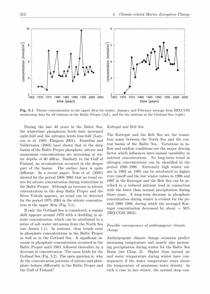
312 5. Climate-related Marine Ecosystem Change
1965 1970 1975 1980 1985 1990 1995 2000 2005time [years]
2
4
6
8
10
con
cen
trat
ion
[m
mo
l/m
3 ]
1965 1970 1975 1980 1985 1990 1995 2000 2005time [years]
2
3
4
5
6
con
cen
trat
ion
[m
mol
/m3 ]
Fig. 5.1. Nitrate concentration in the upper 30 m for winter, January and February average from HELCOMmonitoring data for all stations in the Baltic Proper (left ), and for the stations in the Gotland Sea (right )
During the last 40 years in the Baltic Sea,the wintertime phosphorus levels have increasedeight-fold and the nitrogen levels four-fold (Lars-son et al. 1985; Elmgren 2001). Fonselius andValderrama (2003) have shown that in the deepbasins of the Baltic Proper phosphate, nitrate andammonium concentrations are increasing at wa-ter depths of 80–400m. Similarly to the Gulf ofFinland, an accumulation occurred in the deeperpart of the basins. The surface layer is quitedifferent. In a recent paper, Voss et al. (2005)showed for the period 1969–2001 that no trend ex-ists for nitrate concentration during wintertime inthe Baltic Proper. Although an increase in nitrateconcentration in the deep Baltic Proper and theRiver Vistula appears, no trend can be detectedfor the period 1975–2001 in the nitrate concentra-tion in the upper 30m (Fig. 5.1).
If only the Gotland Sea is considered, a regimeshift appears around 1970 with a doubling in ni-trate concentration, which can be attributed to aseries of salt water intrusions from the North Sea(see Annex 1.1). In contrast, clear trends existin phosphate concentrations in the Baltic Properas well as in the Gotland Sea. A significant in-crease in phosphate concentration occurred in theBaltic Proper until 1983, followed thereafter by adecrease in concentration. The same holds for theGotland Sea (Fig. 5.2). The open question is: whydo the concentration patterns of nitrate and phos-phate behave differently in the Baltic Proper andthe Gulf of Finland?
Kattegat and Belt Sea
The Kattegat and the Belt Sea are the transi-tion zones between the North Sea and the cen-tral basins of the Baltic Sea. Variations in in-flow and outflow conditions are the major drivingfactor which influences inter-annual variability innutrient concentrations. No long-term trend innitrogen concentrations can be identified in theperiod 1980–1998. Extremely high winter val-ues in 1994 an 1995 can be attributed to higherriver runoff and the low winter values in 1996 and1997 in the Kattegat and the Belt Sea can be as-cribed to a reduced nutrient load in connectionwith the lower than normal precipitation duringthose years. A long-term decrease in phosphateconcentration during winter is evident for the pe-riod 1980–1998, during which the averaged Kat-tegat concentration decreased by about ∼ 50%(HELCOM 2002).
Possible consequences of anthropogenic climatechange
Anthropogenic climate change scenarios predictincreasing temperature and mostly also increas-ing precipitation during winter for the Baltic SeaBasin (see Chap. 3). Higher than normal airand water temperature during winter have con-sequences if the water temperature stays abovethe temperature of maximum water density. Insuch a case in late winter, the normal deep con-
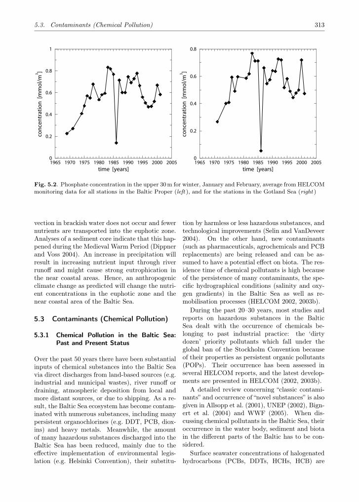
5.3. Contaminants (Chemical Pollution) 313
1965 1970 1975 1980 1985 1990 1995 2000 2005time [years]
0
0.2
0.4
0.6
0.8
1
con
cen
trat
ion
[m
mol
/m3 ]
1965 1970 1975 1980 1985 1990 1995 2000 2005time [years]
0
0.2
0.4
0.6
0.8
con
cen
trat
ion
[m
mol
/m3 ]
Fig. 5.2. Phosphate concentration in the upper 30 m for winter, January and February, average from HELCOMmonitoring data for all stations in the Baltic Proper (left ), and for the stations in the Gotland Sea (right )
vection in brackish water does not occur and fewernutrients are transported into the euphotic zone.Analyses of a sediment core indicate that this hap-pened during the Medieval Warm Period (Dippnerand Voss 2004). An increase in precipitation willresult in increasing nutrient input through riverrunoff and might cause strong eutrophication inthe near coastal areas. Hence, an anthropogenicclimate change as predicted will change the nutri-ent concentrations in the euphotic zone and thenear coastal area of the Baltic Sea.
5.3 Contaminants (Chemical Pollution)
5.3.1 Chemical Pollution in the Baltic Sea:Past and Present Status
Over the past 50 years there have been substantialinputs of chemical substances into the Baltic Seavia direct discharges from land-based sources (e.g.industrial and municipal wastes), river runoff ordraining, atmospheric deposition from local andmore distant sources, or due to shipping. As a re-sult, the Baltic Sea ecosystem has become contam-inated with numerous substances, including manypersistent organochlorines (e.g. DDT, PCB, diox-ins) and heavy metals. Meanwhile, the amountof many hazardous substances discharged into theBaltic Sea has been reduced, mainly due to theeffective implementation of environmental legis-lation (e.g. Helsinki Convention), their substitu-
tion by harmless or less hazardous substances, andtechnological improvements (Selin and VanDeveer2004). On the other hand, new contaminants(such as pharmaceuticals, agrochemicals and PCBreplacements) are being released and can be as-sumed to have a potential effect on biota. The res-idence time of chemical pollutants is high becauseof the persistence of many contaminants, the spe-cific hydrographical conditions (salinity and oxy-gen gradients) in the Baltic Sea as well as re-mobilisation processes (HELCOM 2002, 2003b).
During the past 20–30 years, most studies andreports on hazardous substances in the BalticSea dealt with the occurrence of chemicals be-longing to past industrial practice: the ‘dirtydozen’ priority pollutants which fall under theglobal ban of the Stockholm Convention becauseof their properties as persistent organic pollutants(POPs). Their occurrence has been assessed inseveral HELCOM reports, and the latest develop-ments are presented in HELCOM (2002, 2003b).
A detailed review concerning “classic contami-nants” and occurrence of “novel substances” is alsogiven in Allsopp et al. (2001), UNEP (2002), Bign-ert et al. (2004) and WWF (2005). When dis-cussing chemical pollutants in the Baltic Sea, theiroccurrence in the water body, sediment and biotain the different parts of the Baltic has to be con-sidered.
Surface seawater concentrations of halogenatedhydrocarbons (PCBs, DDTs, HCHs, HCB) are

314 5. Climate-related Marine Ecosystem Change
Table 5.3. Concentrations of dissolved trace metals (ng/kg) from the North Atlantic and the Baltic Sea.1Kremling and Streu (2001), 2Pohl et al. 1993, 3Pohl and Hennings 1999, 4Dalziel 1995 (after HELCOM2003b)
Element North Atlantic Baltic Sea Factor
Hg 0,15–0,34 5–63 ∼ 20Cd 4 (+ − 2)1 12–163 ∼ 4Pb 7 (+ − 2)1 12–203 ∼ 3Cu 75 (+ − 10)2 500–7003 ∼ 10Zn 10–751 600–1,0003 ∼ 10–50
generally relatively low, thus not allowing for esti-mation of any temporal trends (HELCOM 2003b);however, regional differences are obvious (Wodarget al. 2004). Spatial differences are also notable forpetroleum and other hydrocarbons (e.g. PAHs),with hot spots mainly in the south-western BalticSea. Heavy metal concentrations in Baltic Seawater have decreased in the 1980s (Kremling andStreu 2000), but since the mid 1990s their con-centrations have been on the same level and arestill clearly higher than in the North Atlantic (Ta-ble 5.3). Concentrations of cadmium, lead andzinc are on average higher in the south-westernparts of the Baltic Sea, where atmospheric depo-sition of heavy metals is greater and waste con-taining high levels of heavy metals has previouslybeen dumped (HELCOM 2003b).
Sediments are a further potential source oforganochlorines. PCB measurements in dated sed-iment cores from the Baltic Proper showed in-creased or constant concentrations during the lastdecades (Jonsson 2000). Recently formed sedi-ments from the Baltic Proper can contain 10 timesmore cadmium and mercury than the deeper lay-ers, 3–5 times more lead and zinc, and about 2times more copper. Studies of sediments fromthe Baltic Proper show metal concentrations ris-ing during the 1950s and reaching a peak in the1960s and 1970s.
Although metal concentrations have decreasedsince the 1980s, they are still significantly higherthan in the 1940s (Borg and Jonsson 1996). It hasbeen suggested that re-suspension of sedimentedorganic matter and associated pollutants may re-main a substantial source in the Baltic Sea for avery long time (Wulff and Rahm 1993; Jonsson etal. 1996; Nilsson et al. 2003). Dioxins accumulatein sediments close to their main sources, such as
old pulp and paper mills, chemical plants includingvinyl chloride or biocide manufacturing, and har-bours. Information concerning regional distribu-tion of dioxin in surface sediments is limited sincedata are not available from all parts of the BalticSea (HELCOM 2004).
Petroleum-derived hydrocarbons in the BalticSea environment have different sources and arecomposed of numerous single substances. The bi-ologically most harmful group are the polycyclicaromatic hydrocarbons (PAHs). Their spatial dis-tribution patterns suggest that their concentra-tions in the Baltic Sea are about three times thosein the North Sea, and that atmospheric depositionis their main source. Highest PAH concentrationsin the sediment have been found in the westernand southern Baltic Sea (Lübeck Bight, Mecklen-burg Bight, Arkona Basin and Gulf of Gdansk).In sediment cores from Mecklenburg Bight (south-western Baltic Sea), increasing PAH concentra-tions were detected between 6 and 10 cm (corre-sponding to the period between 1945 and 1965),reflecting a higher anthropogenic influence duringthat time (Dannenberger 1996; Kowalewska andKonat 1997; Milukaite and Gulbinskas 1997; Wittand Trost 1999). Another quantifiable PAH sourceare oil spills caused by accidents causing severedamage in form of mass stranding and mortalityof oiled seabirds. They also may result in sub-lethal effects on various organisms as the BalticCarrier accident in 2001 has shown (StorstrømsAmt, DK 2002). Oil pollution is expected to in-crease in the coming 10–20 years due to increasingtrade in oil between the Baltic Sea states, increas-ing fleets, old vessels, inferior control, unqualifiedcrews, and general difficulties in implementing in-ternational treaties (HELCOM 2003a, see also An-nex 3.1.3.1).
5.3. Contaminants (Chemical Pollution) 315
5.3.2 Contaminant Loads and their Effects inBaltic Sea Organisms
In general, it can be stated that since the 1970s,levels of several organochlorines, notably DDTs,have declined in biota as a result of their use be-ing banned or restricted (HELCOM 2002, 2003b).Polychlorinated biphenyls (PCBs) have also de-clined, though generally at a much slower rate,probably reflecting, in part, their continued re-lease into the environment from old equipmentand waste dumps. Levels of dioxins have also de-creased but slowly. In recent years the levels ofboth dioxins and PCBs appear to be the same orhave even increased in some species. An overviewconcerning multiple chemical body burdens in se-lected fish species, birds, mammals and inverte-brates of the Baltic Sea is given in the followingreports: Allsopp et al. (2001); HELCOM (2002,2003b, 2004); WWF (2005).
Owing to the decrease in PCBs and DDTs, thefecundity of the white-tailed sea eagle populationhas increased since the beginning of the 1980s, andthe proportion of successful reproducing pairs hasincreased to a level close to that prior to 1950(HELCOM 2002). Shell thickness of guillemoteggs from Stora Karlsö in the central Baltic Properhas increased since the 1970s (Bignert et al. 1995,2004) and has now returned to the level prior to1940. In the 1960s the eggshells were much thin-ner, attributable to severe DDT pollution of theBaltic marine environment.
Baltic marine mammals, on the other hand,continue to exhibit reproductive disorders, indi-cating that the levels of hazardous substances suchas PCBs and dioxin continue to cause ecologi-cal harm (Selin and VanDeveer 2004; HELCOM2003b, 2004; Routti 2005). Ringed and grey sealsfrom the Baltic have been suffering from patholog-ical impairments, including reproductive distur-bances, which have resulted in a depressed repro-ductive capacity (Nyman et al. 2003). Many fe-male seals have been unable to produce pups dueto uterine occlusion related to PCBs and dioxinsin the environment (Reijnders 2003). Studies onseals fed with PCB-contaminated fish have impliedalterations in the immune system induced by con-taminants in the fish (Ross et al. 1995; de Swartet al. 1996).
When comparing important fish and shellfishspecies from the Baltic Sea it is obvious that tissuelevels of typical organochlorines have decreased(Table 5.4). For heavy metals, such a clear com-
mon trend is not visible: although lead concentra-tions show significant declining trends, cadmiumis still increasing in most of the indicator speciesand copper concentrations show no changes (Ta-ble 5.4). This may partly result from the fact thatbioavailability of heavy metals is salinity depen-dent and that several other factors may have aninfluence on their distribution (Szefer 2002).
Regarding temporal and spatial trends in pollu-tion loads, differences among species are obvious(Table 5.4). Baltic cod (Gadus morhua), for in-stance, often contains higher amounts comparedto other fish species, due to it being predatory,and particularly high fat content, which tends toaccumulate contaminants (Schneider et al. 2000;Falandysz 2003; Roots 2003). From a study per-formed in 2001 it is evident that cod physiology isaffected by contaminants and regional differencesin the biological responses are apparent probablybecause of differences in contamination level andpatterns (Schnell et al. 2003). An overview ofother studies on the effects of pollutants in dif-ferent fish species and invertebrates is given inLehtonen and Schiedek (2006) and Lehtonen et al.(2006).
In regard to dioxin, studies have revealed thatsome of the fish caught in the Baltic Sea, e.g. her-ring (Clupea harengus L.), exceed the new EU lim-its on concentrations of dioxin in food and live-stock feed. The most contaminated herring werefound in the Gulf of Bothnia, including herring inthe Bothnian Sea (Fig. 5.3) and salmon (Salmosalar L.) in the Bothnian Bay (HELCOM 2004).Salmon at the Polish coast also showed elevatedlevels (Piskorska – Pliszczynska et al. 2004).
In recent years levels of some other substancessuch as TBT (tributyltin, an antifouling agent),PBDEs (polybrominated diphenyl ethers, primar-ily used as fire retardants) or synthetic musk com-pounds have increased (Alaee et al. 2003; HEL-COM 2003b; Marsh et al. 2004; Luckenbach etal. 2004). Studies on fish (e.g. herring, flounderor pikeperch), sea birds, harbour porpoises andblue mussels document that TBT is still presentin considerable concentrations in the Baltic Sea,despite restrictions in its use (Kannan and Fa-landysz 1997; Kannan et al. 1999; Strand et al.2003). Imposex and intersex reproductive andgender disorders induced by TBT are for instancewidespread in the Danish Straits and coastal ar-eas (Strand and Jacobsen 2002; HELCOM 2003b).High butyltin concentrations have also been foundin sediments and biota from marinas in the Gulf
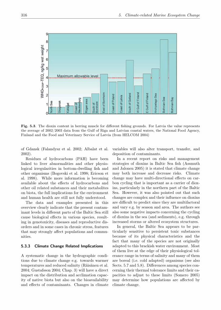
316 5. Climate-related Marine Ecosystem Change
Fig. 5.3. The dioxin content in herring muscle for different fishing grounds. For Latvia the value representsthe average of 2002/2003 data from the Gulf of Riga and Latvian coastal waters, the National Food Agency,Finland and the Food and Veterinary Service of Latvia (from HELCOM 2004)
of Gdansk (Falandysz et al. 2002; Albalat et al.2002).
Residues of hydrocarbons (PAH) have beenlinked to liver abnormalities and other physio-logical irregularities in bottom-dwelling fish andother organisms (Bogovski et al. 1998; Ericson etal. 1998). While more information is becomingavailable about the effects of hydrocarbons andother oil related substances and their metaboliteson biota, the full implications for the environmentand human health are still not fully understood.
The data and examples presented in thisoverview clearly indicate that the present contam-inant levels in different parts of the Baltic Sea stillcause biological effects in various species, result-ing in genotoxicity, diseases and reproductive dis-orders and in some cases in chronic stress, featuresthat may strongly affect populations and commu-nities.
5.3.3 Climate Change Related Implications
A systematic change in the hydrographic condi-tions due to climate change e.g. towards warmertemperatures and reduced salinity (Räisänen et al.2004; Gustafsson 2004; Chap. 3) will have a directimpact on the distribution and acclimation capac-ity of native biota but also on the bioavailabilityand effects of contaminants. Changes in climate
variables will also alter transport, transfer, anddeposition of contaminants.
In a recent report on risks and managementstrategies of dioxins in Baltic Sea fish (Assmuthand Jalonen 2005) it is stated that climate changemay both increase and decrease risks. Climatechange may have multi-directional effects on car-bon cycling that is important as a carrier of diox-ins, particularly in the northern part of the BalticSea. However, it was also pointed out that suchchanges are complex and their influence on dioxinsare difficult to predict since they are multifactoraland vary e.g. by season and area. The authors seealso some negative impacts concerning the cyclingof dioxins in the sea (and sediments), e.g. throughincreased storms or altered ecosystem structures.
In general, the Baltic Sea appears to be par-ticularly sensitive to persistent toxic substancesbecause of its physical characteristics and thefact that many of the species are not originallyadapted to this brackish water environment. Mostof them live at the edge of their physiological tol-erance range in terms of salinity and many of themare boreal (i.e. cold adapted) organisms (see alsoSects. 5.7 and 5.8). Differences among species con-cerning their thermal tolerance limits and their ca-pacities to adjust to these limits (Somero 2005)may determine how populations are affected byclimate change.

5.3. Contaminants (Chemical Pollution) 317
Tab
le5.
4:Tem
pora
lan
dsp
atia
ltr
ends
ofco
ntam
inan
tlo
ads
(diff
eren
the
avy
met
als,
DD
T,P
CB
s)in
diffe
rent
fish
spec
ies
and
blue
mus
sels
inth
eB
alti
cSe
aba
sed
onda
tafr
omH
ELC
OM
(200
2,20
03b)
Cd
Cu
Pb
ΣD
DT
PC
B
Her
ring
Incr
ease
,4–6
%(a
nnua
lly)
but
sign
ifica
ntde
crea
sein
som
ear
eas
(Gul
fof
Fin
land
,Bot
hnia
nB
ay)
Spat
iald
istr
ibut
ion:
Kat
tega
t<
Bot
hnia
nSe
a
±ov
erpa
st15
year
s,hi
ghes
tco
ncen
trat
ion,
Bot
hnia
nSe
a
Dec
reas
e,3–
6%(a
nnua
lly)
Spat
iald
istr
ibut
ion:
Bot
hnia
nB
ay<
Bal
tic
Pro
per
<K
atte
gat
Dec
reas
esinc
e19
80s,
9–14
%K
atte
gat
and
Bot
hnia
nSe
a;5–
11%
Bal
tic
Pro
per
(ann
ually
)Sp
atia
ldi
stri
buti
on:
Bot
hnia
nB
ay<
sout
hern
Bal
tic
Dec
reas
e,3–
10%
(ann
ually
)in
mos
tpa
rts
ofth
eB
alti
cSe
aSp
atia
ldistr
ibut
ion:
Hig
hest
conc
entr
atio
ns:
sout
hern
Bal
tic
(Ger
man
/Pol
ish
coas
t)
Cod
Dec
reas
e,10
%(a
nnua
lly)
±ov
erpa
st15
year
sD
ecre
ase,
6%(a
nnua
lly)
duri
ngpa
st20
year
sD
ecre
ase
sinc
e19
80s,
9–14
%K
atte
gat
and
Bot
hnia
nSe
a;5–
11%
Bal
tic
Pro
per
(ann
ually
)
Dec
reas
e,3–
10%
(ann
ually
),bu
tov
erpa
st10
year
sde
crea
seha
sce
ased
inth
eB
alti
cP
rope
r.In
fluen
ceof
loca
lso
urce
s
Per
chIn
crea
se10
%(a
nnua
lly)
Bal
tic
Pro
per
±ov
erpa
st15
year
sD
ecre
ase
duri
ngpa
st20
year
sD
ecre
ase
sinc
e19
80s,
9–14
%K
atte
gat
and
Bot
hnia
nSe
a;5–
11%
Bal
tic
Pro
per
(ann
ually
)
Dec
reas
eov
erpa
st15
year
s,In
fluen
ceof
loca
lso
urce
s
Blu
em
uss
elIn
crea
se10
%(a
nnua
lly)
Bal
tic
Pro
per;
Spat
iald
istr
ibut
ion:
Kat
tega
t<
Pol
ish
coas
t,B
alti
cP
rope
r
±ov
erpa
st15
year
s,C
once
ntra
tion
sin
the
soft
tiss
ues
are
upto
one
orde
rof
mag
nitu
dehi
gher
than
infis
h
Dec
reas
esinc
e19
80s,
9–14
%K
atte
gat
and
Bot
hnia
nSe
a;5–
11%
Bal
tic
Pro
per
(ann
ually
)Sp
atia
ldi
stri
buti
on:
Kat
tega
t<
Gda
nsk
Bay
Dec
reas
eov
erpa
st15
year
s,Sp
atia
ldistr
ibut
ion:
Low
est
offG
otla
nd,hi
ghes
tG
dans
kB
ay,I
nflue
nce
oflo
calso
urce
s
318 5. Climate-related Marine Ecosystem Change
The combination of higher temperature andlower salinity will clearly reduce the general fit-ness of marine species and may favour freshwaterspecies and the invasion of non-native species. Thepresence of chemical pollutants is likely to add ad-ditional stress to biota, as studies from other es-tuaries have shown (Lanning et al. 2006). Balticblue mussels clearly respond to changes in temper-ature or salinity, e.g. in terms of metabolic ratesand enzyme activities (Pfeifer et al. 2005). Theprojected change in abiotic factors may also havean influence on those processes involved in themetabolism of toxic substances: higher temper-atures result in increased turnover rates or gener-ally higher metabolic rates. Higher temperaturesand/or lower salinity will affect the species’ abil-ity to deal with toxic substances and the differentphysiological regulation processes involved in thedetoxification of hazardous substances.
On the other hand, bioavailability of specificcontaminants (e.g. metals) is greatly affected bysalinity (McLusky et al. 1986; Depledge 1990).Numerous studies have shown an increasing metaluptake by diverse aquatic organisms at reducedsalinities (Hall et al. 1995; Wright 1995; Lee etal. 1998). Thus, altered prevailing abiotic condi-tions will also regulate the extent of exposure oforganisms to toxic substances in different areas ofthe Baltic Sea. The projected changes in the hy-drographic conditions will also affect resuspensionprocesses of sediment bound chemical pollutants.
Bearing in mind the complex hydrographic con-ditions in the Baltic Sea (Annex 1.1), chemicalpollution has to be seen as a further factor actingupon the Baltic Sea. In the past years we onlyhave started to understand how multiple stressors(e.g. salinity, temperature and chemical pollution)in combination may affect marine ecosystems andits biota. The different forecasts concerning fu-ture changes in key abiotic factors (temperature,salinity) due to climate change will be a new chal-lenge. More experimental studies and modellingefforts are needed to test various scenarios con-cerning transport, transfer and cycling of chemi-cal pollutants and to assess the counteracting ef-fects on important Baltic species, the impact ontheir well-being and fitness and, presumably, alsoon whole populations.
5.4 Bacteria
Heterotrophic bacteria are a natural component ofall aquatic ecosystems and play a substantial role
in biogeochemical processes both in the pelagicand benthic environment. Indeed, key aspects ofthe carbon and nitrogen cycles such as anaerobicfermentation of organic carbon and fixation of at-mospheric nitrogen are carried out solely by bac-teria. A conspicuous feature of the Baltic ecosys-tem is the regular occurence of summer blooms ofnitrogen-fixing cyanobacteria. Their role in theBaltic and their reaction to climate change aredealt with in the following section.
Pelagic bacteria, which occur in densities be-tween 105 and 107 ml−1, primarily rely on dis-solved organic matter released from phytoplank-ton, but under oligotrophic conditions they arecompeting with phytoplankton for inorganic nu-trients and constitute the basis of a microbial-based food web (Fenchel 1988). A significantpart of “pelagic” bacteria may occur attached toparticles, and aggregates of Nodularia spumigenacan support 103 times higher concentrations thanfree-living bacteria (Hoppe 1981), probably due toleaking organic material (Paerl and Gallucci 1985).In the Baltic Sea the intra-annual variation ingrowth of pelagic bacteria was shown to be due tocombined effects of temperature, quality of organicsubstrate and competition (Wikner and Hagström1999), and on a smaller time scale diel variation ingrowth rate in the Bothnian Sea was explained byavailability of phosphate (Hagström et al. 2001).Pelagic bacteria are grazed by nanoplanktonicflagellates, and recent studies suggest that virusesrepresent an additional control agent by infestingbacteria and causing cell lysis (Tuomi and Kuupo1999). Comparative studies have shown a hugevariation in the relative importance of grazing andviral control (Fisher and Velmirov 2002; Bettarellet al. 2003).
The biogeochemical cycle of inorganic nitrogen(the two main species being NO3
− and NH4+)
consists of a complex array of processes whichare mediated primarily by bacteria. Organic ni-trogen is mineralised to ammonia (ammonifica-tion), which in turn is oxidised to nitrate (nitri-fication) which may be denitrified to N2 (Herbert1999). The processes take place within sediments,even though denitrification has been demonstratedin the water column (i.e. at the oxic-anoxic in-terface) in the Baltic Sea (Rönner and Sörensen1985; Brettar and Rheinheimer 1991). Besidesdenitrification, also anaerobic ammonium oxida-tion by bacteria using NO2
− as oxidised substrate(“anammox”) contributes to N2 production andthus nitrogen excape from sediments and the wa-

5.5. Phytoplankton 319
ter column (Dalsgaard et al. 2003; Kuypers et al.2003; Engström et al. 2005). The anammox pro-cess seemingly is ubiquitous in the marine envi-ronment, but the importance to nitrogen loss doesvary greatly (Dalsgaard et al. 2005). In the Baltic,anammox was measured in sediments at Tväminnein spring and autumn, but the process was notfound to contribute significantly to nitrogen re-duction (Hietanen and Kuparinen 2005).
Under anoxic conditions denitrification andanammox can be limited by nitrate and nitriteavailability, and other bacteria (e.g. Desulfovib-rio) use SO4
2− as electron acceptor to utilise or-ganic compounds (Jørgensen 1977). The productof this respiration is the highly soluble and toxicH2S. Sulfate reduction occurs widely in anaer-obic sediments in the Baltic Sea (Mudryk et al.2000; Boeschker et al. 2001). Various aerobic oranaerobic autotrophic bacteria can, in turn, utiliseH2S as an energy source, and under oxic condi-tions H2S is oxidised to sulphate. An overviewof biogeochemical processes including intermedi-ate reactions (reduction of iron and manganese) isgiven by Jørgensen (1996). The suite of bacteria-mediated processes is to a large extent controlledby availability of oxygen, which, in turn, is de-termined by the balance between oxygen demandand physical transport processes (e.g. major Balticsaltwater inflows) and vertical mixing that deliveroxygen to the bottom water.
Oxygen demand below the pycnocline (includ-ing sediments) is overall regulated by the mag-nitude of sedimentation of organic particles thatoriginates from primary production. Hence,changes in pelagic primary production, e.g. dueto variation in light or nutrient availability, invari-ably will result in changes in sedimentation rateand thus oxygen demand below the pycnocline.
Effects of temperature increase
Increase in temperature stimulates the metabolicprocesses of bacteria, provided that other fac-tors such as substrate or oxygen are not limiting(Autio 1998). As bacteria play prominent rolesin aquatic ecosystems, small changes in temper-ature can have disproportionately larger implica-tions in the functioning of marine systems and, ul-timately, also global consequences for the carboncycle (Sarmiento et al. 1998).
Several studies have demonstrated that the ac-tivity of pelagic bacteria (and other pelagic het-erotrophs) is stimulated more than primary pro-
duction under temperature increase due to differ-ences in the temperature dependence of photosyn-thesis and respiration (e.g. Pomeroy and Deibel1986). This finding is in accordance with obser-vations that the ratio of bacteria biomass to phy-toplankton biomass increases with temperature ineutrophic aquatic systems (Laws 2003). In olig-otrophic systems (i.e. primary production below5 mg C m−3 d−1) temperature had no influenceon the ratio, which may be attributed to substratelimitation (Pomeroy and Wiebe 2001). A higheractivity of the heterotrophic communities will in-crease recycling and mineralisation in surface wa-ters, and, in turn, sedimentation of organic mat-ter may decrease as projected for the open oceans(Laws et al. 2000). Likewise, processes belowthe pycnocline such as denitrification, and proba-bly anammox in anoxic waters, will be stimulatedby temperature increase provided that oxidisingagents are not limiting. Other climate-related fac-tors leading to changes in nutrient runoff, verti-cal mixing, and insolation may confound directtemperature effects (see Chap. 3). Hence, in-tegrated effects cannot be predicted without ad-vanced modelling efforts.
Like their pelagic counterparts, the specific ac-tivity (per cell or biomass) of both aerobic andanaerobic benthic bacteria increases with temper-ature, but due to (seasonal) temperature adapta-tion effects the change cannot be predicted fromshort term experiments, e.g. in temperature gradi-ents (Thamdrup et al. 1998; Arnosti et al. 1998).Overall, seasonal changes in oxygen uptake oftencorrelate with temperature (Banta et al. 1995).However, other important controls on benthic oxy-gen uptake and mineralisation include the input oforganic matter from primary production, oxygenconcentration in bottom water (which primarilyis controlled by physical processes in the BalticSea) and irrigating activity of the infauna (Ras-mussen and Jørgensen 1992). Hence, direct effectson bacterial activity of a small temperature in-crease in bottom water probably will be of minorimportance compared to changes in sedimentationof organic matter and, especially, physical trans-port and mixing processes.
5.5 Phytoplankton
Phytoplankton, i.e. the autotrophs suspended inthe pelagial, constitute the base of the pelagic foodweb but also feed benthic areas. Changes in phy-toplankton composition and biomass are, there-

320 5. Climate-related Marine Ecosystem Change
fore, of decisive importance for the whole ecosys-tem. The detection of these changes is not sim-ple because phytoplankton is subject to high nat-ural variability in time and space (PEX 1989). Ifthe typical spring, summer and autumn bloomsare not adequately sampled, no reliable seasonalor annual means can be calculated. Therefore,trend analyses are possible only on the basis ofdata of sufficient spatial and temporal coverage.The monitoring programme of HELCOM was es-pecially designed for this trend monitoring.
When HELCOM was established in 1974, eu-trophication was identified as the main threat forthe Baltic Sea (Larsson et al. 1985). Changes inphytoplankton biomass and species compositiondo, however, not only reflect effects of eutrophi-cation but also of climatic changes. These effectscannot easily be separated. The most importantphysical and chemical factors influenced by cli-matic change and affecting phytoplankton growthare discussed.
5.5.1 Physical and Chemical Factors
Nutrient availability is one of the most importantfactors for phytoplankton growth. An increase inthe concentrations of the growth-limiting nutrients(N, P) leads to increased phytoplankton biomass.The heaviest nutrient input into the Baltic Seaoccurred in the 1970s, mainly by wastewaters andfertilisers. This caused a stronger phytoplanktongrowth, which is also reflected in an increase inchlorophyll a concentrations (Wasmund and Uhlig2003) and a reduction of the water transparency(Secchi depth, cf. Sanden and Hakansson 1996).The nutrient conditions are, however, not onlydependent on anthropogenic impact, but also onclimatic influences, i.e. rainfall and river runoff.Nausch et al. (1999) found a correlation betweenfreshwater runoff and nitrate plus nitrite concen-trations in the surface water of the Kattegat andBelt Sea area.
Also, internal processes like re-mineralisationand re-solution, influence the availability of nu-trients for phytoplankton growth. Anoxic bottomwater in the deep basins is a typical feature of theBaltic Sea. Under these conditions, phosphorus isliberated from the sediment (cf. Nürnberg 1984).Kuparinen and Tuominen (2001) found a negativecorrelation between mean oxygen and phosphateas well as silicate concentrations within the hy-poxic water volume, indicating an anoxic release ofphosphorus and silicate. Hypoxic or anoxic condi-
tions allow the reduction of nitrate to ammonium(Kuparinen and Tuominen 2001) and oxidation ofammonium with nitrite (anammox). Sporadic in-flows of saline North Sea water (see Annex 1.1) re-plenish the oxygen in the deep water layers of theBaltic Sea. The re-oxygenation fixes the phospho-rus in the sediment by adsorption onto Fe(OH)3and therefore counteracts eutrophication (Conleyet al. 2002).
After a salt water inflow, ammonium is oxidizedto nitrate and thus “bursts” of high NO3 levelsappear in deep waters (Kuparinen and Tuominen2001). Convective and diffusive processes trans-port the nutrients into the upper water layerswhere they promote phytoplankton growth. There-solution of phosphorus during stagnation peri-ods may be more important for the year-to-yearvariation in the phosphorus pool than the exter-nal phosphorus load by eutrophication (Conley etal. 2002).
Carbon dioxide is the main source material forphotosynthesis. In the water, it exists as dis-solved CO2, as carbonic acid and as the ionsHCO3
− and CO32−. The concentration of free
CO2 decreases with increasing pH. HCO3−, which
is the dominant total carbon species in moder-ately alkaline water, can also be used by somealgae (Crotty et al. 1994; Tortell et al. 1997).Wasmund (1996) showed in culture experimentsthat Nodularia harveyana grew well at pH7.5–9.0, whereas the chlorophyceae Tetrastrum sp.was retarded at pH8.5–9.0. Shapiro (1990) dis-cussed the dependency of the cyanobacteria onhigh pH and/or low CO2 concentrations compre-hensively.
Light is the decisive condition for photosyn-thesis. Low light intensities limit algal growth,for example during the night, in winter and ingreater water depths. If light intensity is veryhigh, e.g. at noontime and near the water surface,it depresses photosynthesis by destruction of thephotosynthetic apparatus. Long-term changes inmean light intensities are much lower than diurnal,seasonal or depth-dependent variation and, there-fore, of lower influence on biomass trends. Rus-sak (1994) reported on decreasing trends of radi-ation in the Baltic Sea Basin from 1955 to 1992(Sect. 2.1.4.2). Also, the decreased water trans-parency (Sanden and Hakansson 1996) reducedthe light availability for the algae. Nevertheless,algal biomass shows an increasing trend, becauseeutrophication is over-compensating the reductionin light intensity.

5.5. Phytoplankton 321
Temperature has only little direct effect on algalgrowth. Phytoplankton grows to high biomassesalready at temperatures a little above the watermelting point but is inhibited if the temperatureexceeds the natural range. Of course, the individ-ual species have their typical temperature pref-erences (Hegseth and Sakshaug 1983; Wasmund1994). Therefore, significant global warming maychange the species composition.
The indirect effect of temperature via its influ-ence on the water stratification is also of impor-tance. Some algae prefer a stable stratificationand others a mixed water column. Deep convec-tive mixing in autumn and spring is of decisive im-portance for nutrient circulation. It is only possi-ble if the water temperature falls during cold win-ters below the temperature of maximum density.In mild winters, a complete convective circulationdoes not occur and the warming of the water inspring leads immediately to a stratification with-out preceding spring overturn. This is disadvan-tageous for species which prefer turbulent water(Wasmund et al. 1998).
The Medieval Warm Period (1000–1250 AD)and the modern warm period (since 1850) are cor-related with laminated sediments rich in organiccarbon in the deep Baltic Sea basins, indicatinganoxic conditions caused by a stable halocline andreduced vertical mixing (Leipe et al. 2005). Dur-ing a cold period, including the “Little Ice Age”(1250–1850), oxic conditions dominated due tolower salinity and vertical mixing, leading to lightgrey and homogeneous sediment horizons. Theoxygenation of the sediments affects the nutrientconcentrations as stated above.
Wind causes turbulent mixing that may have astronger impact on the stratification of the watercolumn than convective mixing. Therefore, since1989, the reduced convective mixing after “mild”winters may be replaced by increased turbulentmixing. In very cold winters, turbulent mixing isreduced by the ice cover. After the cold period(approximately 1250–1850, according to Leipe etal. 2005), the area covered by ice tends to decrease(FIMR 2003).
5.5.2 Phytoplankton Trends
The above-mentioned factors are the main abioticfactors that influence phytoplankton biomass andcomposition. They may also have indirect impactvia selective stimulation of grazers or competi-tors. The coincidences of different phytoplank-
ton groups with abiotic factors are compiled inTable 5.5. Of course, the taxonomic groups arenot ecological groups and their members may re-act in different ways. But generalisation on theclass level proved to be appropriate and useful.Therefore, the following analyses on trends in phy-toplankton composition refer primarily to phyto-plankton groups instead of species.
5.5.2.1 Diatom Spring Bloom
For historical examinations, the siliceous microfos-sil stratigraphy in sediments may be used. Thismay reflect changes in salinity and temperature.The transition from the freshwater Ancylus Laketo the brackish Litorina stage of the Baltic Sea(ca. 7,000–7,500 BP, see also Annex 2) was indi-cated by a shift from freshwater to brackish di-atom species (Bianchi et al. 2000). A change to-wards a colder climate occurred 700–850 years ago,indicated by a change in abundance from Pseu-dosolenia calcar-avis to Thalassiosira hyperboreavar. lacunosa and Thalassiosira baltica (Andrén etal. 2000). This correlates with the onset of the coldperiod in the 13th century. After a period of warm-ing (1850–1950), diatom composition changed inthe colder years 1950–1960: Andrén et al. (2000)found an increase in Thalassiosira cf. levanderi,Cyclotella choctawhatcheeana, Pauliella taeniataand Coscinodiscus granii, but an extinction ofPseudosolenia calcar-avis and T. hyperborea var.lacunosa in sediment cores of the Gotland Basin.The spring-bloom species Thalassiosira levanderiand Pauliella taeniata prefer cold water. At thepresent stage, eutrophication plays an importantrole especially for phytoplankton growth whereasbenthic diatoms decrease due to higher turbidity.Recent monitoring data reveal that spring bloomsare dominated by Skeletonema costatum and Tha-lassiosira baltica after mild winters or by Pauliellataeniata and Chaetoceros species after cold winters(Hajdu et al. 1997).
A period of mild winters commenced in 1988, asshown by increasing mean surface water temper-atures. Since 1988/89, the typical diatoms disap-peared from the spring bloom in the Baltic Proper(Fig. 5.4). Of course, the phytoplankton datashow a strong fluctuation due to undersampling(e.g. complete miss of the bloom in 1983). How-ever, the silicate consumption during the springseason (Fig. 5.4) indicates that a diatom bloomregularly occurred until 1988 and failed to appearin the 1990s, except for the cold winter in 1996.
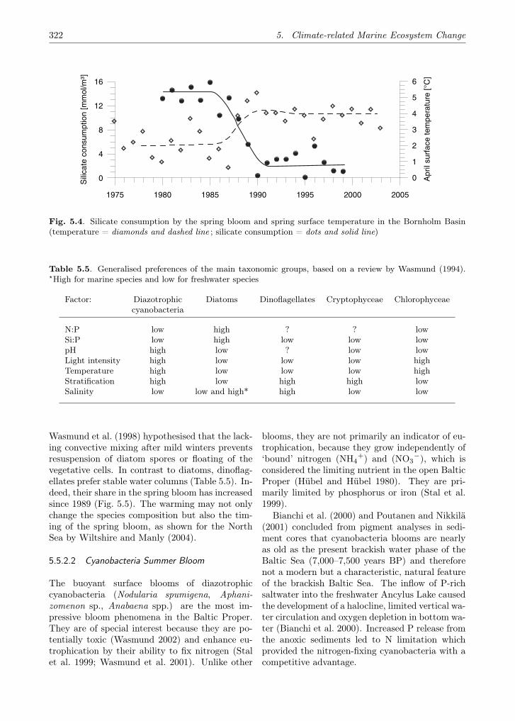
322 5. Climate-related Marine Ecosystem Change
1975 1980 1985 1990 1995 2000 2005
0
4
8
12
16S
ilica
te c
onsu
mpt
ion
[mm
ol/m
³]
0
1
2
3
4
5
6
Apr
il su
rfac
e te
mpe
ratu
re [°
C]
Fig. 5.4. Silicate consumption by the spring bloom and spring surface temperature in the Bornholm Basin(temperature = diamonds and dashed line ; silicate consumption = dots and solid line)
Table 5.5. Generalised preferences of the main taxonomic groups, based on a review by Wasmund (1994).�High for marine species and low for freshwater species
Factor: Diazotrophic Diatoms Dinoflagellates Cryptophyceae Chlorophyceaecyanobacteria
N:P low high ? ? lowSi:P low high low low lowpH high low ? low lowLight intensity high low low low highTemperature high low low low highStratification high low high high lowSalinity low low and high* high low low
Wasmund et al. (1998) hypothesised that the lack-ing convective mixing after mild winters preventsresuspension of diatom spores or floating of thevegetative cells. In contrast to diatoms, dinoflag-ellates prefer stable water columns (Table 5.5). In-deed, their share in the spring bloom has increasedsince 1989 (Fig. 5.5). The warming may not onlychange the species composition but also the tim-ing of the spring bloom, as shown for the NorthSea by Wiltshire and Manly (2004).
5.5.2.2 Cyanobacteria Summer Bloom
The buoyant surface blooms of diazotrophiccyanobacteria (Nodularia spumigena, Aphani-zomenon sp., Anabaena spp.) are the most im-pressive bloom phenomena in the Baltic Proper.They are of special interest because they are po-tentially toxic (Wasmund 2002) and enhance eu-trophication by their ability to fix nitrogen (Stalet al. 1999; Wasmund et al. 2001). Unlike other
blooms, they are not primarily an indicator of eu-trophication, because they grow independently of‘bound’ nitrogen (NH4
+) and (NO3−), which is
considered the limiting nutrient in the open BalticProper (Hübel and Hübel 1980). They are pri-marily limited by phosphorus or iron (Stal et al.1999).
Bianchi et al. (2000) and Poutanen and Nikkilä(2001) concluded from pigment analyses in sedi-ment cores that cyanobacteria blooms are nearlyas old as the present brackish water phase of theBaltic Sea (7,000–7,500 years BP) and thereforenot a modern but a characteristic, natural featureof the brackish Baltic Sea. The inflow of P-richsaltwater into the freshwater Ancylus Lake causedthe development of a halocline, limited vertical wa-ter circulation and oxygen depletion in bottom wa-ter (Bianchi et al. 2000). Increased P release fromthe anoxic sediments led to N limitation whichprovided the nitrogen-fixing cyanobacteria with acompetitive advantage.

5.5. Phytoplankton 323
Fig. 5.5. Summary plot of significant trends 1979/1980–1999 in mean spring biomass in the Eastern GotlandSea (station BMP J1) for diatoms (a) and dinoflagellates (b) and for summer biomass in the Bornholm Sea(station BMP K2) for cyanobacteria (c), exemplified by the LOESS smoother (Cleveland and Devlin 1988).Upper and lower lines represent the approximative pointwise 95% confidence limits for the trend line. Y-axisrepresents 10log Biomass (in mg m−3) (from Wasmund and Uhlig 2003)
During the Little Ice Age nitrogen-fixingcyanobacteria might have been depressed. Thewarming since 1850 has promoted cyanobacteriablooms not only by its direct effect but, again,by stronger stratification, formation of a perma-nent halocline, oxygen deficit in the bottom waterand resulting liberation of phosphorus (Leipe etal. 2005). The same mechanism functioned also inrecent stagnation periods.
Cyanobacteria blooms have been reported al-ready in the mid of the 19th century (Lindström1855; Pouchet and de Guerne 1885), as stated byFinni et al. (2001). In the 1920s, several Aphani-zomenon blooms were recorded. The first record ofan open-sea bloom in which Nodularia was iden-tified as dominant is that of Rothe (1941) fromJuly/August 1938 in the southern Baltic Sea. Ac-cording to Poutanen and Nikkilä (2001), a strongincrease occurred in the early 1960s, especially ow-ing to an increase in Nodularia spumigena in thenorthern Baltic Proper.
Hübel and Hübel (1980) noted that Nodulariablooms have occurred regularly in coastal watersof the southern Baltic Sea since 1969, when a pe-riod of warm summers began. Horstmann (1975)reported on increased mass occurrences of Aph-anizomenon and Nodularia in the Baltic Proper.It was just in this period, from the late 1960sto the early 1980s, that the strongest increase in
phosphorus and nitrate concentrations in the sur-face water was recorded (see Sect. 5.2). Whenthe Baltic Monitoring Programme of HELCOMstarted in 1979, the cyanobacteria blooms had al-ready reached a very high intensity (HELCOM1996).
No further significant increase in cyanobacte-rial summer biomass could be found in the centralBaltic Sea (Wasmund and Uhlig 2003), in contrastto the Gulf of Finland (Kahru et al. 2000; Suikka-nen et al. 2007) and the Gulf of Riga (Balode1999). Struck et al. (2004) found increased ni-trogen fixation from 1969–73 to 1989–93, indicat-ing an increase in the importance of diazotrophiccyanobacteria in this eutrophication period. Onthe other hand, they reported a strong decrease inpotential summer nitrogen fixation from the peri-ods 1989–93 to 1994–98.
From interpretations of satellite images, Kahru(1997) found large areas covered by cyanobacteriablooms in 1982–1984 and 1991–1994. Satellite im-ages have the advantage of a synoptic view on largeareas but the disadvantage is that they overratesurface accumulations. Depth-integrated samplesare less patchy than the eddy-like surface struc-tures suggest. After some wind, these buoyant sur-face blooms disappear by suspension in the uppermixed layer. Combined satellite and ground truthdata suggest that no general increase in cyanobac-

324 5. Climate-related Marine Ecosystem Change
teria blooms occurred in the open Baltic Proper,but they may have increased in some Gulfs duringthe last 25 years.
Climatic factors may have a higher impacton cyanobacteria bloom variability than eutroph-ication. Wasmund (1997) found that strongblooms were formed only if water temperature ex-ceeded 16 C, provided that global radiation was> 120W m−2 (daily mean) and wind speed was< 6m s−1. According to Stal et al. (2003), dailyintegrals of photon irradiance, rather than tem-perature, determined the onset of bloom forma-tion. The summers of 1985–1988 had a verylow average sunshine duration and therefore noblooms developed, whereas sunny summers pro-moted cyanobacteria blooms (Kahru et al. 1994).However, Finni et al. (2001) stated that hot sum-mers are not the only reason for high cyanobac-teria abundances. Storms may terminate Nodu-laria blooms, whereas Aphanizomenon is affectedless (Stal et al. 2003). Therefore, wind conditionsmay have high relevance for the ratio of Nodu-laria (toxic) to Aphanizomenon (non-toxic) in theblooms. Computer simulations of cyanobacteriablooms by Janssen et al. (2004) revealed goodagreement with the satellite data of Kahru et al.(1994). The blooms were mainly determined bythe excess inorganic phosphorus in the surfacelayer, which depends on the depth of the mixedlayer in winter and on the persistence of coastalupwelling. This, in turn, depends on the winterNAO. High NAO leads to high wind stress, lowice cover, deep mixing, upwelling, high excess inor-ganic phosphorus and, finally, to a high potentialfor a cyanobacteria bloom. In contrast, Kuparinenand Tuominen (2001) claimed that stormy wintershelped to bind phosphorus to particles and, finally,to the sediments. Salt water inflows give rise tohigher overall nitrate levels but lower phosphatelevels (Kuparinen and Tuominen 2001), thus in-hibiting cyanobacteria growth.
5.5.2.3 Other Phytoplankton
Besides diatom and cyanobacteria blooms, thereare other components in the phytoplankton whichshow long-term changes. Nehring (1998) reported16 non-indigenous phytoplankton species, whichhave become an integrated part of the pelagicsystem of the North Sea since the beginning ofthe 20th century. Among them, 10 thermophilicspecies were first recorded in the recent periodof relatively mild winters. Some of these species
also invaded the Kattegat and the Belt Sea, likeGyrodinium cf. aureolum (Partensky and Sournia1986), Alexandrium minutum (Nehring 1994) andGymnodinium catenatum (Nehring 1997). The po-tentially toxic dinoflagellate Prorocentrum mini-mum invaded the Baltic Sea from the Oslofjord in1979, became established in the southern BalticProper in 1982 and formed its first bloom in KielBight in 1983 (Theede 1984). It tolerates a widesalinity and temperature range (Hajdu et al. 2005)and is obviously not directly related to globalwarming.
5.5.2.4 Reactions to Future Anthropogenic ClimateChange
Future climatic change will influence several envi-ronmental factors which have different impacts onphytoplankton productivity and sometimes maycompensate each other. At present, nutrient andlight limit phytoplankton growth, but if theiravailability increases, also CO2 can become a lim-iting factor.
The anthropogenic rise in CO2 may increaseprimary production, especially in nutrient-rich wa-ters. The acidification of the water due to airpollution and acid rain will enhance the CO2
availability because of the pH-dependent equilib-rium between the different carbon species. Theintensified primary production will increase thepH. If the effect of external acidification over-compensates the effect of increased primary pro-duction, a decrease in pH in the water will result.As cyanobacteria lose competitiveness in acid wa-ter, other algal groups like diatoms may benefit.The influence of acidification on other chemicaland biological elements like heavy metal mobilisa-tion or viral activity cannot be assessed here.
Warming will directly inhibit cold-water species(mostly spring-bloom diatoms such as Thalas-siosira levanderi, Pauliella taeniata and Chaeto-ceros spp.) but enhance warm-water species oc-currence, like that of the bloom-forming toxiccyanobacteria (Nodularia spumigena). Newspecies originating from warmer seas may establishthemselves and displace native species. Reducedice cover and earlier stabilisation of the water col-umn in spring will shift the start of the springbloom, which will influence the food-supply forzooplankton and the whole food-web.
Both higher temperature and higher freshwa-ter inflow strengthen stratification. If the uppermixed layer becomes shallower, the phytoplankton

5.6. Zooplankton 325
receives more light and productivity will increase(Doney 2006). On the other hand, stronger verti-cal stratification of the water column will reducevertical transport processes (e.g. exchange of nu-trients and dissolved gases, upwards transport ofcysts/spores, sedimentation, vertical migration ofplankton), which may reduce productivity. In anycase, cyanobacteria blooms may benefit from thissituation.
Although no robust result concerning windspeed exists (see Chap. 3), it can be stated in gen-eral that increasing wind speed would counteractthese processes. Reduced convective mixing dueto warming might be compensated by increasedturbulent mixing due to increased wind and re-duced ice cover. This may help diatoms but dis-turb surface accumulations of cyanobacteria. Thepromotion of the diatoms is supported if the up-welling deep water is rich in CO2 and low in pH,as explained above.
Stronger freshwater inflow into the northernBaltic Sea and reduced salt water inflow from theNorth Sea would displace the permanent haloclineto greater depths. This would result in a largerarea of oxygenated sediments (at 70–100m depthin the central Baltic Sea Basins), expanding notonly the colonisation area for macrofauna (Ger-lach 1994) but also the area of the vital seedbedsfor phytoplankton. Full circulation of the watercolumn in winter would not only be possible incoastal areas and the Gulf of Riga but also atthe slopes of the basins. Phosphorus and silicatewould be bound in these oxic sediments, whereasnitrate would be liberated. This might lead toincreased nitrogen:silicate and nitrogen:phosphateratios, which reduce diatoms and nitrogen-fixingcyanobacteria.
Continuing anthropogenic eutrophication willimport mainly nitrogen and phosphorus and there-fore also raise the nitrogen:silicate ratio, whichis disadvantageous for diatoms but beneficial fordinoflagellates. Of course, reduced salinity alsohas a direct influence on the species composition.Freshwater species will further penetrate into theBaltic Sea. A retreat of polyhalobic species fromthe southern Baltic Sea might, however, not oc-cur because reduced precipitation would preventa salinity decrease in this area.
Basically, phytoplankton biomass and speciescomposition are influenced by different mecha-nisms. Their reaction depends on the overwhelm-ing climatic impact factor. This can be temporallyand spatially different. If ongoing eutrophication
is enhanced e.g. by stronger weathering and elu-tion of nutrients by precipitation or by increasedanoxic conditions in deep water, a higher phyto-plankton biomass and frequent blooms may be ex-pected. As some of the blooms are toxic, theyhave strong impact on fisheries and fish farming.Inherently, blooms decrease the recreational valueof the sea and therefore affect tourism (see alsoAnnex 3.1.3.2), which is of high economic value(Wasmund 2002). Changes in the timing of theblooms and in species composition disturb the ex-isting food web, provoking changes in the highertrophic levels.
5.6 Zooplankton
We review studies that combine mesozooplankton,long-term observations, and climatic environmen-tal effects. Relationships between Baltic Sea zoo-plankton and its physical and chemical environ-ment have been extensively studied (for an earlyreview see, e.g. Ackefors 1981), also using long-term monitoring observations (e.g. Lumberg 1976;Simm 1976; Sidrevits 1980; Kostrichina 1977,1984; Kostrichina and Sidrevits 1977; Kostrichinaand Yurkovskis 1982; Lumberg and Ojaveer 1997),but papers referring to climatic environmental fac-tors only started to appear in 1990s; a single ex-ception by Segerstråle (1969) is discussed later inthis section. Periodic assessments by HELCOM(e.g. HELCOM 2002) include chapters on zoo-plankton temporal change and its environmentalcauses in various parts of the Baltic Sea, but noeffort has been done to combine long-term obser-vations of zooplankton with climatic effects. Per-shing et al. (2004) reviewed the studies on cli-mate variability and zooplankton in the NorthAtlantic. They stated that, following the ini-tial pulse of climatic factors, several interactingmechanisms, directly and indirectly, cause vari-ation of zooplankton populations. In the BalticSea, salinity (Ranta and Vuorinen 1987), eutroph-ication (Vuorinen and Ranta 1988), temperature(Viitasalo et al. 1995), planktivory by pelagic fish(Rudstam et al. 1994) and a non-indigenous alienplanktonic invertebrate (Ojaveer et al. 2004), havebeen considered as possible controllers of long-term changes in abundance. Currently, climaticfactors have also been hypothesised to control zoo-plankton indirectly (Hänninen et al. 2000, 2003;Möllmann et al. 2003b, 2005; Vuorinen et al. 2003,2004). Surprisingly, there are no long term stud-ies of zooplankton and phytoplankton in relation
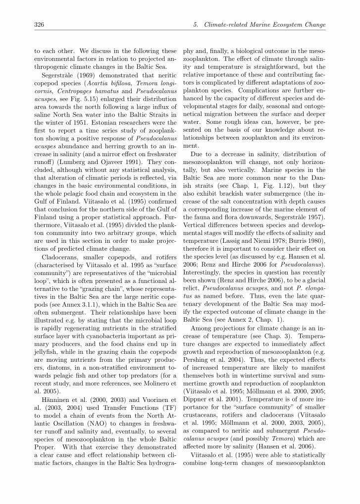
326 5. Climate-related Marine Ecosystem Change
to each other. We discuss in the following theseenvironmental factors in relation to projected an-thropogenic climate changes in the Baltic Sea.
Segerstråle (1969) demonstrated that neriticcopepod species (Acartia bifilosa, Temora longi-cornis, Centropages hamatus and Pseudocalanusacuspes, see Fig. 5.15) enlarged their distributionarea towards the north following a large influx ofsaline North Sea water into the Baltic Straits inthe winter of 1951. Estonian researchers were thefirst to report a time series study of zooplank-ton showing a positive response of Pseudocalanusacuspes abundance and herring growth to an in-crease in salinity (and a mirror effect on freshwaterrunoff) (Lumberg and Ojaveer 1991). They con-cluded, although without any statistical analysis,that alteration of climatic periods is reflected, viachanges in the basic environmental conditions, inthe whole pelagic food chain and ecosystem in theGulf of Finland. Viitasalo et al. (1995) confirmedthat conclusion for the northern side of the Gulf ofFinland using a proper statistical approach. Fur-thermore, Viitasalo et al. (1995) divided the plank-ton community into two arbitrary groups, whichare used in this section in order to make projec-tions of predicted climate change.
Cladocerans, smaller copepods, and rotifers(characterised by Viitasalo et al. 1995 as “surfacecommunity”) are representatives of the “microbialloop”, which is often presented as a functional al-ternative to the “grazing chain”, whose representa-tives in the Baltic Sea are the large neritic cope-pods (see Annex 3.1.1), which in the Baltic Sea areoften submergent. Their relationships have beenillustrated e.g. by stating that the microbial loopis rapidly regenerating nutrients in the stratifiedsurface layer with cyanobacteria important as pri-mary producers, and the food chains end up injellyfish, while in the grazing chain the copepodsare moving nutrients from the primary produc-ers, diatoms, in a non-stratified environment to-wards pelagic fish and other top predators (for arecent study, and more references, see Molinero etal. 2005).
Hänninen et al. (2000, 2003) and Vuorinen etal. (2003, 2004) used Transfer Functions (TF)to model a chain of events from the North At-lantic Oscillation (NAO) to changes in freshwa-ter runoff and salinity and, eventually, to severalspecies of mesozooplankton in the whole BalticProper. With that exercise they demonstrateda clear cause and effect relationship between cli-matic factors, changes in the Baltic Sea hydrogra-
phy and, finally, a biological outcome in the meso-zooplankton. The effect of climate through salin-ity and temperature is straightforward, but therelative importance of these and contributing fac-tors is complicated by different adaptations of zoo-plankton species. Complications are further en-hanced by the capacity of different species and de-velopmental stages for daily, seasonal and ontoge-netical migration between the surface and deeperwater. Some rough ideas can, however, be pre-sented on the basis of our knowledge about re-lationships between zooplankton and its environ-ment.
Due to a decrease in salinity, distribution ofmesozooplankton will change, not only horizon-tally, but also vertically. Marine species in theBaltic Sea are more common near to the Dan-ish straits (see Chap. 1, Fig. 1.12), but theyalso exhibit brackish water submergence (the in-crease of the salt concentration with depth causesa corresponding increase of the marine element ofthe fauna and flora downwards, Segerstråle 1957).Vertical differences between species and develop-mental stages will modify the effects of salinity andtemperature (Lassig and Niemi 1978; Burris 1980),therefore it is important to consider their effect onthe species level (as discussed by e.g. Hansen et al.2006; Renz and Hirche 2006 for Pseudocalanus).Interestingly, the species in question has recentlybeen shown (Renz and Hirche 2006), to be a glacialrelict, Pseudocalanus acuspes, and not P. elonga-tus as named before. Thus, even the late quar-tenary development of the Baltic Sea may mod-ify the expected outcome of climate change in theBaltic Sea (see Annex 2, Chap. 1).
Among projections for climate change is an in-crease of temperature (see Chap. 3). Tempera-ture changes are expected to immediately affectgrowth and reproduction of mesozooplankton (e.g.Pershing et al. 2004). Thus, the expected effectsof increased temperature are likely to manifestthemselves both in wintertime survival and sum-mertime growth and reproduction of zooplankton(Viitasalo et al. 1995; Möllmann et al. 2000, 2005;Dippner et al. 2001). Temperature is of more im-portance for the “surface community” of smallercrustaceans, rotifers and cladocerans (Viitasaloet al. 1995; Möllmann et al. 2000, 2003, 2005),as compared to neritic and submergent Pseudo-calanus acuspes (and possibly Temora) which areaffected more by salinity (Hansen et al. 2006).
Viitasalo et al. (1995) were able to statisticallycombine long-term changes of mesozooplankton
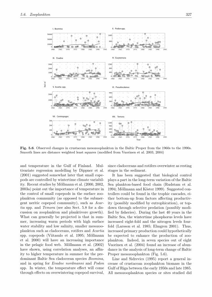
5.6. Zooplankton 327
I. Bosmina II. Podonspp.
010000
30000
50000
1960 1965 1970 1975 1980 1985 1990 19950
800
1600
1960 1965 1970 1975 1980 1985 1990 1995
III. Evadne IV . Eurytemora
0
1000
2000
3000
1960 1965 1970 1975 1980 1985 1990 19950
400
800
1200
1960 1965 1970 1975 1980 1985 1990 1995
V. Acartia spp. VI. Pseudocalanus
0
1000
2000
1960 1965 1970 1975 1980 1985 1990 19950
300
600
900
1960 1965 1970 1975 1980 1985 1990 1995
VII. Centropages
Ind.
/m3
VIII. Temora
0
100
200
300
1960 1965 1970 1975 1980 1985 1990 1995
Year
0
300
600
900
1200
1960 1965 1970 1975 1980 1985 1990 1995
Year
Fig. 5.6. Observed changes in crustacean mesozooplankton in the Baltic Proper from the 1960s to the 1990s.Smooth lines are distance weighted least squares (modified from Vuorinen et al. 2003, 2004)
and temperature in the Gulf of Finland. Mul-tivariate regression modelling by Dippner et al.(2001) suggested somewhat later that small cope-pods are controlled by wintertime climate variabil-ity. Recent studies by Möllmann et al. (2000, 2002,2003a) point out the importance of temperature inthe control of small copepods in the surface zoo-plankton community (as opposed to the submer-gent neritic copepod community), such as Acar-tia spp. and Temora (see also Sect. 5.8 for a dis-cussion on zooplankton and planktivore growth).What can generally be projected is that in sum-mer, increasing warm periods with high surfacewater stability and low salinity, smaller mesozoo-plankton such as cladocerans, rotifers and Acartiaspp. copepods (Viitasalo et al. 1995; Möllmannet al. 2000) will have an increasing importancein the pelagic food web. Möllmann et al. (2002)have shown, using correlation analyses, an affin-ity to higher temperature in summer for the pre-dominant Baltic Sea cladoceran species Bosmina,and in spring for Evadne nordmanni and Podonspp. In winter, the temperature effect will comethrough effects on overwintering copepod survival,
since cladocerans and rotifers overwinter as restingstages in the sediment.
It has been suggested that biological controlplays a part in the long-term variation of the BalticSea plankton-based food chain (Rudstam et al.1994; Möllmann and Köster 1999). Suggested con-trollers could be found in the trophic cascades, ei-ther bottom-up from factors affecting productiv-ity (possibly modified by eutrophication), or top-down through selective predation (possibly modi-fied by fisheries). During the last 40 years in theBaltic Sea, the wintertime phosphorus levels haveincreased eight-fold and the nitrogen levels four-fold (Larsson et al. 1985; Elmgren 2001). Thus,increased primary production could hypotheticallybe expected to enhance the production of zoo-plankton. Indeed, in seven species out of eightVuorinen et al. (2004) found an increase of abun-dance in the analysis of long-term change of BalticProper mesozooplankton (Fig. 5.6).
Line and Sidrevics (1995) report a general in-crease of crustacean zooplankton biomass in theGulf of Riga between the early 1950s and late 1985.All mesozooplankton species or sites studied did

328 5. Climate-related Marine Ecosystem Change
Fig. 5.7. Abundance of two neritic copepod species (Pseudocalanus and Temora, total) and seawater salinity(psu) (Gotland deep, 200 m) in the central Baltic Proper from 1979 to 2003 (Finnish Institute of MarineResearch)
not, however, show a simultaneous increase, leav-ing some room for further speculation. There arepossible negative effects also by e.g. cyanobacteria(for an extensive list of examples from the BalticSee, see Karjalainen 2005), therefore it would besimplistic to assume a linear increase of zooplank-ton due to enhanced primary production.
The importance of fluctuations in crustaceanmesozooplankton species composition and, espe-cially, in the abundance of the neritic copepods,Pseudocalanus and Temora, lies in their impact asfish food. We want to stress the difference be-tween zooplankton species in the interaction be-tween zooplankton and fish growth; for a full dis-cussion see Sect. 5.8. Extensive changes in thenumbers of pelagic predatory fish, Clupea harengusmembras and Sprattus sprattus, the Baltic herringand sprat, have been hypothesised to affect zoo-plankton, top-down (Rudstam et al. 1994; Möll-mann et al. 2000; Möllmann and Köster 2002),because they are selective predators of Pseudo-calanus and Temora, respectively (Flinkman et al.1992; Kornilovs et al. 2001). This could eventuallylead to density dependent growth limitation of clu-peids as hypothesised by Cardinale and Arrhenius(2000) and Cardinale et al. (2002). A third formof regulation of planktivores, bottom up, could beestablished by low salinity driven scarcity of ner-itic copepods (as hypothesised by e.g. Flinkmanet al. 1998), this also leading to growth limitationof planktivores. It has been shown (e.g. Sjöblom1961; Aneer 1975; Flinkman et al. 1992, 1998)that neritic copepods are not only the most pre-
ferred food of Baltic herring and sprat but alsocontain the most energy. Therefore, the shiftsin abundances of these species, driven by salinitychanges, are the most important factors affectinggrowth and condition of the most important fishstocks in the Baltic. Locally, the match betweenneritic copepods and salinity may be incomplete(Fig. 5.7), however, it has been firmly establishedby independent researchers over large areas. Re-cent work by Rönkkönen et al. (2004) and Möll-mann et al. (2005) further establishes the fact thatgrowth and condition of Baltic forage fish are infact mostly bottom-up controlled, as suggested byFlinkman (1999).
It may well be that all these regulating ef-fects (top-down control of zooplankton, density-dependent food limitation of clupeids, and lowsalinity driven scarcity of large neritic copepods)are acting simultaneously, but so far nobody hasbeen able to measure their relative importance. Inaddition to controlling available food, the salin-ity changes of course determine the osmoregula-tion stress to clupeids. It is well known that sub-optimal salinities increase energy expenditure inclupeids (Hettler 1976), which in turn may re-sult in diminished body size (Hoar 1952; Cana-garatnam 1959). Salinity also dictates the cod re-production window in the Baltic Sea (Wieland etal. 1994). Cod is the most important predatorof Baltic clupeids; hence a top-down regulatorypathway has been suggested as a major contrib-utor to clupeid growth (Bagge 1989; Bagge et al.1994; Aro 2000). For a long time, quality of avail-

5.7. Benthos 329
able food, i.e. crustacean mesozooplankton, couldbe statistically and consistently shown to be themost important factor in clupeid growth and con-dition in the Baltic Sea. However, recent workby Casini et al. (2006) reveals the effects of den-sity dependent factors as well. This means thatthe clupeids are indeed capable of reducing theirfavourable food by predation to an extent that itaffects their own growth.
Conclusion
Salinity generally controls Baltic Sea biodiver-sity (Kändler 1949; Remane and Schlieper 1958)and is projected to decrease with expected cli-mate change due to increased rainfall and runoff.Segerstråle (1969) demonstrated neritic copepodspecies (Acartia bifilosa, Temora longicornis, Cen-tropages hamatus and Pseudocalanus acuspes, seeFig. 5.15) to enlarge their distribution area to-wards the north following a large amount of salineNorth Sea water penetrating the Baltic Straitsin the winter of 1951. A reversal of the neriticspecies distribution is expected as a consequenceof the predicted decrease in Baltic Sea salinity.The physiological mechanism is most likely the os-motic advantage provided for the neritic species bythe higher salinity of the incoming seawater. Za-jaczkowski and Legezynska (2001) demonstratedthe lethality of low salinity to Calanus spp. in anice combination of field sampling (in the freshwa-ter runoff of a melting glacier) and laboratory ex-periments. The importance of salinity as a control-ling factor has been restated by developing statis-tical methods using time series data from variousnational monitoring programmes. Finnish datawere used by Vuorinen and Ranta (1987, 1988);Ranta and Vuorinen (1990); Viitasalo (1992); Vi-itasalo et al. (1994); Viitasalo et al. (1995); Vuori-nen et al. (1998). Data from the Gulf of Fin-land, the Gulf of Riga, and the Baltic Proper wereanalysed somewhat later using Estonian (Lumbergand Ojaveer 1991; Ojaveer et al. 1998) and Lat-vian time series (Dippner et al. 2000; Möllmannet al. 2000; Ikauniece 2001; Kornilovs et al. 2001;Möllmann and Köster 2002; Möllmann et al. 2002;Hänninen et al. 2003; Möllmann et al. 2003b).
Another projected large scale environmentalchange is an increase in temperature, especiallyin winter. The plankton community close to thesurface consists generally of smaller species andgroups than the above-mentioned submergent ner-itic community. Therefore, we may expect sub-
stantial changes, probably increased production,also in other than neritic zooplankton, such assmall estuarine copepods (Acartia, Eurytemora),cladocerans (Podon, Pleopsis, Evadne but also thenewly established Cercopagis) and rotifers (Syn-chaeta and Keratella). Concluding, both salinitydecrease and temperature increase will have a pro-found effect on zooplankton in the way describedin this section. Several complicating factors can,however, change the pelagic ecosystem in unex-pected ways. Radiation changes may, in additionto the complicating factors discussed above, causea new mismatch between phyto- and zooplanktonproduction, because temperature and light havedifferent effects on timing of phytoplankton andzooplankton reproduction. There might also bechanges in predator-prey relationships, caused bystock changes in planktivores, herring and sprat,and even new introduced predator species, such asthe comb jelly Mnemiopsis leidyi.
5.7 Benthos
5.7.1 Large Scale Benthic Zonation of theBaltic Sea
In the Baltic Sea, salinity has a strong impact onspecies distribution and therefore on structure andcomposition of benthic communities. Many ma-rine species reach their limit of distribution alongthe salinity gradient on the way from the entrancetowards the inner, oligohaline parts of the BalticSea. Not only species richness, but also diversityof benthic functional guilds (defined by feeding be-haviour, motility and sediment modifying ability,sensu Pearson 2001) decline along the Baltic Seasalinity gradient (Bonsdorff and Pearson 1999).
On the other hand, there is a pronounced ver-tical benthic zonation in the Baltic Sea due tostrong stratification of the water column, relevantbathymetric changes in dissolved oxygen concen-trations and other environmental factors (Demeland Mulicki 1954; Shurin 1968; Theede et al. 1969;Elmgren 1978; Zmudzinski 1978; Cederwall 1979;Järvekülg 1979; Brey 1986; Rumohr 1987; Lep-päkoski and Bonsdorff 1989; Olenin 1997; Laineet al. 1997; Laine 2003). The shallow part of theBaltic above the halocline with well-oxygenatedwater is comparatively rich in bottom macrofauna,while the deeper anoxic part below the haloclinerepresents a “benthic desert” (sensu Zmudzinski1978) without macrobenthic organisms. The shal-low part and the benthic desert are separated
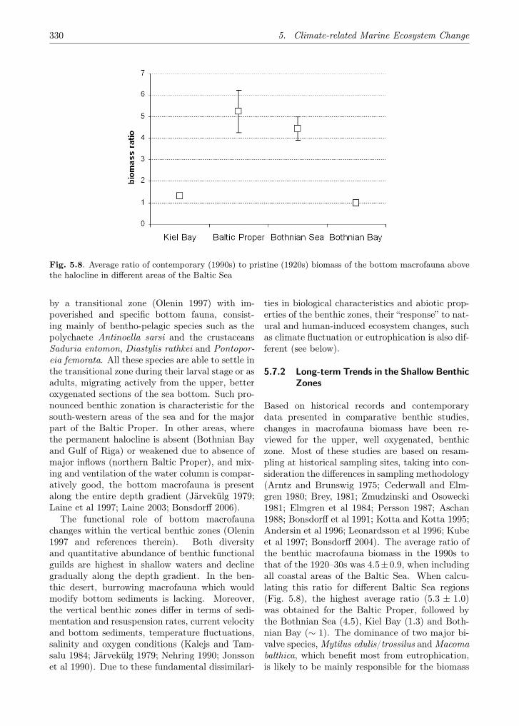
330 5. Climate-related Marine Ecosystem Change
Fig. 5.8. Average ratio of contemporary (1990s) to pristine (1920s) biomass of the bottom macrofauna abovethe halocline in different areas of the Baltic Sea
by a transitional zone (Olenin 1997) with im-poverished and specific bottom fauna, consist-ing mainly of bentho-pelagic species such as thepolychaete Antinoella sarsi and the crustaceansSaduria entomon, Diastylis rathkei and Pontopor-eia femorata. All these species are able to settle inthe transitional zone during their larval stage or asadults, migrating actively from the upper, betteroxygenated sections of the sea bottom. Such pro-nounced benthic zonation is characteristic for thesouth-western areas of the sea and for the majorpart of the Baltic Proper. In other areas, wherethe permanent halocline is absent (Bothnian Bayand Gulf of Riga) or weakened due to absence ofmajor inflows (northern Baltic Proper), and mix-ing and ventilation of the water column is compar-atively good, the bottom macrofauna is presentalong the entire depth gradient (Järvekülg 1979;Laine et al 1997; Laine 2003; Bonsdorff 2006).
The functional role of bottom macrofaunachanges within the vertical benthic zones (Olenin1997 and references therein). Both diversityand quantitative abundance of benthic functionalguilds are highest in shallow waters and declinegradually along the depth gradient. In the ben-thic desert, burrowing macrofauna which wouldmodify bottom sediments is lacking. Moreover,the vertical benthic zones differ in terms of sedi-mentation and resuspension rates, current velocityand bottom sediments, temperature fluctuations,salinity and oxygen conditions (Kalejs and Tam-salu 1984; Järvekülg 1979; Nehring 1990; Jonssonet al 1990). Due to these fundamental dissimilari-
ties in biological characteristics and abiotic prop-erties of the benthic zones, their “response” to nat-ural and human-induced ecosystem changes, suchas climate fluctuation or eutrophication is also dif-ferent (see below).
5.7.2 Long-term Trends in the Shallow BenthicZones
Based on historical records and contemporarydata presented in comparative benthic studies,changes in macrofauna biomass have been re-viewed for the upper, well oxygenated, benthiczone. Most of these studies are based on resam-pling at historical sampling sites, taking into con-sideration the differences in sampling methodology(Arntz and Brunswig 1975; Cederwall and Elm-gren 1980; Brey, 1981; Zmudzinski and Osowecki1981; Elmgren et al 1984; Persson 1987; Aschan1988; Bonsdorff et al 1991; Kotta and Kotta 1995;Andersin et al 1996; Leonardsson et al 1996; Kubeet al 1997; Bonsdorff 2004). The average ratio ofthe benthic macrofauna biomass in the 1990s tothat of the 1920–30s was 4.5±0.9, when includingall coastal areas of the Baltic Sea. When calcu-lating this ratio for different Baltic Sea regions(Fig. 5.8), the highest average ratio (5.3 ± 1.0)was obtained for the Baltic Proper, followed bythe Bothnian Sea (4.5), Kiel Bay (1.3) and Both-nian Bay (∼ 1). The dominance of two major bi-valve species, Mytilus edulis/trossilus and Macomabalthica, which benefit most from eutrophication,is likely to be mainly responsible for the biomass

5.7. Benthos 331
increase found in many shallow areas of the BalticSea. Their absence in the Bothian Bay may ex-plain the almost unchanged situation in this partof the Baltic.
In the southern part of the Baltic Sea, reducedpredation of benthos-feeding fish on M. balthicaand Mytilus edulis has been suggested as an expla-nation for increasing trends in zoobenthos biomass(Persson 1981, 1987; Brey 1986). This hypothesiswas not tested quantitatively, however a decline inbenthic-feeding fish stocks could blur the eutroph-ication effect.
5.7.3 Long-term Trends in the Sub-haloclineAreas
The deep basins of the Baltic Sea are fre-quently exposed to hypoxia and anoxia, causingperiodic extinction of the bottom macrofauna.In the Bornholm Basin, the previously bivalve-dominated benthic community progressively be-come polychaete-dominated (Leppäkoski 1975).In the early 1950s, the Arctic element clearly dom-inated below 85m, this depth forming a boundarylayer between the Arctic relict community and thezoogeographically more heterogeneous M. balthicacommunity, typical for most of the Baltic Sea. Inthe early 1970s, cosmopolitan and Atlantic-borealspecies comprised more than 90% of the total den-sity (Leppäkoski 1975). Thus, the deeper partsof the southern Baltic have lost their most fasci-nating biogeographical peculiarity, namely that ofoffering hospitable conditions for the marine post-glacial relicts, and thereby also their close zoo-geographical connection with Arctic shallow-waterbiomes. At present, the Bornholm Basin (if notdenfaunated due to oxygen deficiency) is linkedwith boreal areas by the most euryhaline represen-tatives of the Atlantic and North Sea soft-bottomfauna (Leppäkoski and Olenin 2001 and referencestherein).
Drastic changes in species and functional guildcomposition took place also in the central andnorthern sub-halocline areas of the Baltic Sea.Figure 5.9 shows a gradual disappearance of theinfaunal polychaete worm Scoloplos armiger fromthe inner sub-halocline parts of the Baltic Properduring the past five decades. In 1954–1956, S.armiger was the most abundant polychaete in theNorthern Basin in areas below 100m depth, beingfound even at 450 m in the Landsort Deep (An-dersin et al. 1978). In the 1960s, the species wasbiomass dominant in the eastern Gotland Basin
within the depth range of 100–140m (Järvekülg1979); however, it had already vanished from themore northern areas. By the end of the 1980s tothe beginning of the 1990s, the distribution of S.armiger was restricted to depths of 99–124 m onthe south-eastern slope of the Gotland Basin (anarea around station BY 9, Olenin 1997).
Long-term observations showed that S. armigercan not survive in the central parts of the BalticSea if salinity is less than 10.5 psu and oxygen isless than 0.5ml/l (Järvekülg 1979; Olenin 1997).Recolonisation of defaunated bottoms depends onlarvae supply from the “healthier” areas with es-tablished populations. Thus, the most distantpenetration limits of S. armiger ever recorded inthe sub-halocline areas of the Baltic Proper, in themid-1950s, (Northern Basin and Landsort Deep)most probably were caused by the exceptionallyintensive inflow of saline water in November–December of 1951 (Matthäus and Frank 1992). Al-though very little is known about the reproductionstrategy of S. armiger in the Baltic Sea, it may besuggested that the 1951 inflow could have broughtpelagic larvae of S. armiger from southern sub-halocline areas. Since then, a gradual decline insalinity, oxygen depletion and enlargement of hy-drogen sulphate zones eliminated S. armiger fromthe northern and central sub-halocline areas of theBaltic Proper.
5.7.4 Conceptual Model of Natural and Hu-man-induced Changes in the Sub-halo-cline Areas of the Baltic Sea
In contrast to fully marine ecosystems, in the in-ner parts of the Baltic Sea the benthic functionalguilds are often represented by a single species(Olenin 1997; Bonsdorff and Pearson 1999). Dis-appearance of such a key species would resultin the loss of a functional group which, in turn,may essentially change the biogeochemical cyclingof the system, affecting microbial life, bioturba-tion activity, release of nutrients and formation oflaminated sediments. Analysis of data on distri-bution of bottom macrofauna species (Järvekülg1979; Olenin 1997; Laine et al. 1997; Laine 2003)and their functional guilds (Olenin 1997) showsthat during recent decades the polychaete worm S.armiger was the only infaunal species in the largehypoxic areas below the halocline in the centraland northern parts of the Baltic Proper which wasable to perform bioturbation of bottom sediments.This polychaete feeds in “conveyor belt” mode,

332 5. Climate-related Marine Ecosystem Change
Fig. 5.9. Distribution limits of Scoloplos armiger in the sub-halocline areas of the Baltic Proper from the1950s to the early 1990s: BB – Bornholm Basin, SF – Slupsk Furrow, GdB – Gdansk Basin, EG – EasternGotland Basin, LD – Landsort Deep, NB - Northern Basin; BY 9 – location of a sampling station in thesouth-eastern part of the eastern Gotland Basin; isobaths of 50 m (line) and 100 m (dark areas) are indicated.The saline water inflow paths are shown with black arrows and the major inflow intensities, Q are given in thediagram on the right (from Franck and Matthäus 1992)
translocating particles from some cm depth withinthe sediment up onto the surface (Rice 1986).
Disappearance of that species from the north-ern and central sub-halocline areas of the BalticProper coincided with the increased developmentof the laminated sediments (Jonsson et al. 1990)in the same areas with all ensuing consequences,like trapping of PCBs (Jonsson 2000; Skei at al.2000). This allows the assumption that the evo-lution of laminated sediments largely depends onthe absence/presence of that key-species. A veryapproximate estimation based on the particle re-working rate of Scoloplos spp. (0.51 g per indi-vidual day−1; Lee and Swartz 1980), mean den-sity (200 ind. m−2, Järvekülg 1979; Olenin 1997and references therein) and area occupied by theS. armiger population in 1950s (ca. 50, 000 km2,based on Andersin et al. 1978; Järvekülg 1979;Olenin 1997) results in 1.9× 10⁹ tons of reworkedsediments annually. This number gives a roughestimate on the extent of the bioturbation processperformed by a single species and its importancein biogeochemical cycling of elements.
The causal chain analysis of events in the sub-halocline areas of the Baltic Sea is presented in
Fig. 5.10. This scheme shows that the NorthAtlantic Oscillation governs the frequency andintensity of the saline water inflows into theBaltic Sea (e.g. Hänninen et al 2000 and refer-ences therein), which, through the chain of relatedevents, may effect the success of the recolonisationof the sub-halocline bottoms by the polychaeteS. armiger. An “inoculating” inflow should occurduring the spawning season of S. armiger (usu-ally September–December), when its pelagic lar-vae appear in the plankton (Järvekülg 1979 andreferences therein). The inflow should be strongenough to bring the larvae pool up to the GotlandBasin and even further, to the inner sub-haloclineareas of the Baltic Proper. Recolonisation of thepreviously defaunated sub-halocline bottoms bythe S. armiger population would result in sedimentreworking activity, which, in turn, could cause re-lease of PCBs into the water column (Skei at al.2000).
In contrast, the decrease in number and in-tensity of inflows reduces the opportunities to re-colonise the benthic desert; the absence of macro-faunal organisms able to perform bioturbationleads to formation of laminated sediments, which
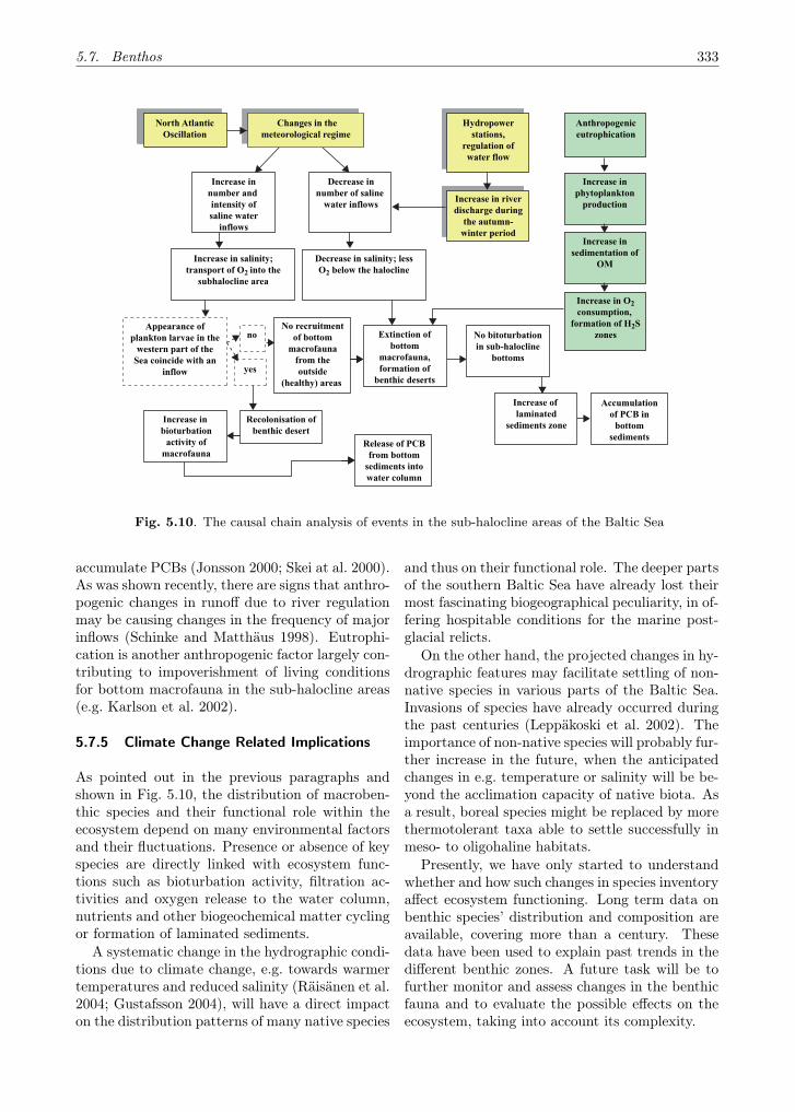
5.7. Benthos 333
North AtlanticOscillation
Hydropowerstations,
regulation ofwater flow
Increase in riverdischarge during
the autumn-winter period
Anthropogeniceutrophication
Increase inphytoplankton
production
Increase insedimentation of
OM
Increase in O2consumption,
formation of H2Szones
Increase innumber and intensity ofsaline water
inflows
Decrease innumber of saline
water inflows
Increase in salinity;transport of O2 into the
subhalocline area
Decrease in salinity; lessO2 below the halocline
Increase of laminated
sediments zone
Accumulationof PCB in
bottomsediments
No bitoturbationin sub-halocline
bottoms
Extinction ofbottom
macrofauna,formation of
benthic deserts
Release of PCBfrom bottom
sediments intowater column
Increase in bioturbation
activity ofmacrofauna
no
yes
Recolonisation ofbenthic desert
No recruitmentof bottom
macrofaunafrom theoutside
(healthy) areas
Appearance ofplankton larvae in the
western part of theSea coincide with an
inflow
Changes in themeteorological regime
Fig. 5.10. The causal chain analysis of events in the sub-halocline areas of the Baltic Sea
accumulate PCBs (Jonsson 2000; Skei at al. 2000).As was shown recently, there are signs that anthro-pogenic changes in runoff due to river regulationmay be causing changes in the frequency of majorinflows (Schinke and Matthäus 1998). Eutrophi-cation is another anthropogenic factor largely con-tributing to impoverishment of living conditionsfor bottom macrofauna in the sub-halocline areas(e.g. Karlson et al. 2002).
5.7.5 Climate Change Related Implications
As pointed out in the previous paragraphs andshown in Fig. 5.10, the distribution of macroben-thic species and their functional role within theecosystem depend on many environmental factorsand their fluctuations. Presence or absence of keyspecies are directly linked with ecosystem func-tions such as bioturbation activity, filtration ac-tivities and oxygen release to the water column,nutrients and other biogeochemical matter cyclingor formation of laminated sediments.
A systematic change in the hydrographic condi-tions due to climate change, e.g. towards warmertemperatures and reduced salinity (Räisänen et al.2004; Gustafsson 2004), will have a direct impacton the distribution patterns of many native species
and thus on their functional role. The deeper partsof the southern Baltic Sea have already lost theirmost fascinating biogeographical peculiarity, in of-fering hospitable conditions for the marine post-glacial relicts.
On the other hand, the projected changes in hy-drographic features may facilitate settling of non-native species in various parts of the Baltic Sea.Invasions of species have already occurred duringthe past centuries (Leppäkoski et al. 2002). Theimportance of non-native species will probably fur-ther increase in the future, when the anticipatedchanges in e.g. temperature or salinity will be be-yond the acclimation capacity of native biota. Asa result, boreal species might be replaced by morethermotolerant taxa able to settle successfully inmeso- to oligohaline habitats.
Presently, we have only started to understandwhether and how such changes in species inventoryaffect ecosystem functioning. Long term data onbenthic species’ distribution and composition areavailable, covering more than a century. Thesedata have been used to explain past trends in thedifferent benthic zones. A future task will be tofurther monitor and assess changes in the benthicfauna and to evaluate the possible effects on theecosystem, taking into account its complexity.

334 5. Climate-related Marine Ecosystem Change
5.8 Fish
Fishing is the most direct impact by humans onthe Baltic Sea ecosystem. The annual removal ofhundreds of thousands of tonnes of fish from theBaltic has direct effects on populations and theirdynamics (ICES 2004b), as outlined below.
As described above, oceanographic conditionsin the brackish Baltic Sea are strongly linked toatmospheric forcing. The unusual period of a per-sistently high North Atlantic Oscillation (NAO)index since the late 1980s, with a dominance ofwesterly weather, resulted in an increase in wa-ter temperatures and decreasing salinity and oxy-gen conditions due to increased runoff and a lowfrequency of water intrusions from the North Sea(Fonselius and Valderrama 2003; Matthäus andNausch 2003). Climate has been shown to affectrecruitment of Baltic fish stocks, e.g. Brander andMohn (2004) demonstrated the negative associ-ation of the high NAO-period during the 1990sand cod recruitment, and MacKenzie and Köster(2004) showed the positive association with spratrecruitment. Similarly, herring recruitment is re-lated to the NAO (Axenrot and Hansson 2003).Furthermore, climate has been shown to causefluctuations in growth of Baltic herring and sprat(Möllmann et al. 2003a; 2005; Rönkkönen et al.2004).
This section will review the primary impactsof fishing and climate variability and change onthe Baltic Sea ecosystem. Much more detailedsummaries of how fishing and climate impact theBaltic Sea and other marine ecosystems can befound in the reports by HELCOM, ICES advi-sory and working groups (Advisory Committeeon Ecosystems, Working Group on Ecosystem Ef-fects of Fishing Activities; www.ices.dk) and inthe scientific literature (Jennings and Kaiser 1998;MacKenzie et al. 2007).
5.8.1 Baltic Fisheries, their Management andtheir Effects on Exploited Populationsand the Ecosystem
The fish community in the Baltic Sea has muchfewer species than other marine areas of compara-ble size. The main reason for the low number ofspecies is low salinity, which imposes a physiolog-ical stress on marine organisms and on freshwa-ter species inhabiting coastal areas (Voipio 1981;HELCOM 2002).
The few species in the ecosystem are reflectedalso in the commercial catches, which are dom-inated by sprat, herring, and cod (ICES 2004).Several other species are exploited such as floun-der, plaice, salmon, eel, and near shore coastalspecies such as whitefish, pikeperch and smelt, buttheir catches are much lower (ICES 2004b).
Baltic fisheries were managed by the Interna-tional Baltic Sea Fisheries Commission (IBFSC)until 2005, after which bilateral negotiations be-tween the EU Commission and Russia have re-placed IBFSC. The most important commercialspecies have quotas and other regulations (e.g.mesh sizes, closed seasons/areas) intended to pro-mote long-term sustainability of the populationsand the ecosystem. The scientific advice formaking management decisions about internationalfisheries primarily comes from the InternationalCouncil for the Exploration of the Sea (ICES2004a; Daw and Gray 2005). Management of thefisheries is partly disaggregated spatially to reflectlocal differences in both the fisheries and biologyof the target species (e.g. growth rates, maturity,migration patterns, and genetic stock differentia-tion). As a result, separate quotas are assigned fordifferent sub-divisions of the Baltic (Fig. 5.11).
Effects of fishing on populations and the ecosystem
The most direct impact of fishing on fish pop-ulations is the mortality of large numbers andbiomass of fish. Fish landings increased substan-tially during the 20th century (Fig. 5.12), primar-ily due to increases in fishing effort and technol-ogy (Bagge et al. 1994). Combined catches for thethree most important species now exceed several100,000 tonnes annually. Adult mortality ratesdue to fishing for some populations (e.g. cod insubdivisions 22–24; cod and sprat in subdivisions25–28) are typically at least 2–4 fold higher thanestimates of natural mortality rates (ICES 2003).Fishing is therefore the dominant mortality sourcefor adults of the most abundant species (ICES2003).
High fishing mortalities reduce and limit thegrowth of populations, which will decrease if fish-ing mortality rates remain too high for long. In ex-treme cases, biomass levels can fall to levels whichmay not be sustainable. Such a situation presentlyexists for many Baltic cod and salmon popula-tions, yet they continue to be exploited (ICES2004b).

5.8. Fish 335
Fig. 5.11. Map of the Baltic Sea showing the ICES subdivisions. The HELCOM definition for the Baltic Seaincludes the Kattegat and subdivisions 22-32. Black areas show deep basins of the eastern Baltic Sea wherecod spawning occurs (from Bagge et al. 1994)
Fishing also affects many second-order at-tributes of populations (HELCOM 2002). Theseinclude size and age structure, genetic compositionand fish life-history (Olsen et al. 2004). Fishingtypically removes the largest and oldest individu-als within populations (Pauly et al. 1998). In ad-dition, since fishing is a size-selective activity, fish-ing tends to preferentially kill the fastest growingindividuals, which are the first within a popula-tion to attain a size which is retained by a givenmesh size. After several years of fishing, the older,larger fish become rare and populations are typi-cally dominated by small fish.
These changes in population structure have con-sequences for stock productivity because many bi-ological attributes such as spawning time and lo-cation, migratory behaviour, and individual fe-cundity are size and age dependent (Marshall etal. 2003). For example, spawning time and lo-cation largely determine the environmental con-ditions (e.g. temperature, salinity, food supply)
subsequently experienced by eggs, larvae and ju-veniles. As a result the removal of specific sizeand age components from a population can reducethe probability that eggs and larvae encounterfavourable environmental conditions for survival(Heath and Gallego 1998; Begg and Marteinsdot-tir 2002). Moreover, the characteristics of eggsand larvae (e.g. size, buoyancy, yolk sac size) pro-duced by females of different sizes and ages are notequal (Nissling et al. 1994; Nissling et al. 1999),and these variations can affect survival when en-vironmental conditions vary. Interactions betweenfemale characteristics, egg characteristics and en-vironmental conditions appear to exist for easternBaltic cod, with higher recruitment in years witha higher proportion of older fish (Jarre-Teichmannet al. 2000; Köster et al. 2005), particularly inyears when oxygen conditions in the deeper layersof cod spawning areas are low (Vallin and Nissling2000). Similar interactions are evident in otherfish stocks (Marshall et al. 2003).

336 5. Climate-related Marine Ecosystem Change
Fig. 5.12. Total international landings of the three commerically most important fish species (cod, herring,sprat) in the Baltic Sea during the 20th century. Triangles: cod; squares: sprat; circles: herring (data source:Sparholt 1994; ICES 2004b)
Fishing can also reduce the genetic variabil-ity within a fish species. For example, the east-ern Baltic cod population is genetically distinctfrom other cod populations in the Atlantic Ocean(Nielsen et al. 2001) and physiologically adaptedfor reproduction in low salinity (Nissling andWestin 1997). However in some years even theseadaptations are insufficient to ensure reproduc-tive success (Köster et al. 2001; MacKenzie et al.2002a). Continued high fishing pressure in combi-nation with frequent periods of environmental con-ditions detrimental for egg survival suggest thatthis population will collapse (Jonzen et al. 2002;ICES 2004b). If the eastern Baltic cod popula-tion were to collapse, then recovery would be veryslow or perhaps impossible even under low or nofishing mortality. Long recovery time is expectedbecause the local genotypes (Nielsen et al. 2001)would be eliminated and because cod immigratingfrom more saline areas (e.g. Belt Sea, Kattegat)are not adapted to reproduce in the brackish con-ditions of the more easterly parts of the Baltic Sea(Nissling and Westin 1997; Vallin et al. 1999).
Another species whose genetic diversity in theBaltic Sea is threatened is salmon. Many Balticsalmon populations which spawn in specific riversare greatly reduced and may not recover un-der present levels of exploitation (ICES 2004b).Salmon populations in the Baltic Sea are stressednot only by fishing mortality, which has been re-duced in recent years (ICES 2004c), but also by
ecological changes associated with habitat damagein rivers and outbreaks of the disease M74 (ICES2004c). This disease caused many fatalities of ju-venile salmon and is believed to be partly relatedto the nutritional value of prey organisms.
In addition to these direct effects of fishing ontarget populations, fishing has impacts on non-target species and the ecosystem. These effectsinclude the bycatch of non-target species (e.g. fishspecies, marine mammals and seabirds; (HEL-COM 2002) and changes in food web structure andspecies interactions (Pauly et al. 1998; Jackson etal. 2001). Food web changes in the Baltic Searesemble a trophic cascade as observed in otherecosystems (e.g. Frank et al. 2005). The removalof cod biomass has affected the production andsurvival of cod prey such as herring and sprat(Sparholt 1994; Gislason 1999; ICES 2003a). Theabundance of these two species increased duringthe late 1980s and 1990s partly because the codpopulation and predation rate fell (Köster et al.2003). Further, increased planktivore populations,especially of sprat, have negatively affected thedynamics of major Baltic Sea zooplankton popula-tions, i.e. the copepods Pseudocalanus acuspes andTemora longicornis (Rudstam et al. 1994; Möll-mann and Köster 2002). Despite the importanceof these fishery-induced interactions, a large partof the changes in Baltic Sea food web structure wasrelated to the opposing effects of climate variabil-ity on decreasing cod and increasing sprat recruit-
5.8. Fish 337
ment (see below). Additionally, zooplankton de-velopment is strongly affected by climate-inducedchanges in hydrography (see Sect. 5.6).
Multi-decadal and century scale variability: a viewfrom the past
Fish populations in Baltic Sea coastal areas andrivers have been exploited by local fishermensince at least the medieval period (Enghoff 1999;MacKenzie et al. 2002a). For example, majorherring fisheries near Rügen and in the Øresundsupported significant economies and trade amongBaltic towns in the medieval period (Sahrhage andLundbeck 1992; Holm and Bager 2001; Alheit andHagen 2001).
These fisheries were based primarily on the fall-spawning Rügen herring. This subpopulation isnow essentially extinct although the reasons forthis disappearance are not clear (Parmanne et al.1994). Large marine and estuarine fauna suchas sturgeon, many salmon populations, seals andharbour porpoises used to be common but over-exploitation and habitat loss have reduced abun-dances, in many cases (e.g. sturgeon) to near ex-tinction (Elmgren 1989; HELCOM 2002; MacKen-zie et al. 2002a). As a result, the present fish andmarine mammal community differs considerablyfrom that which existed only 100–150 years ago.
Perceptions of biodiversity and biomass, andconsequently the past effects of exploitation, thatare based on information from only the last fewdecades of the 20th century can therefore be highlybiased when considered in a longer historical per-spective (Jackson et al. 2001). Fisheries manage-ment strategies which aim to sustain and recoverpopulations should be aware of historical levelsand variations in species abundances to avoid the“shifting baseline syndrome” (Pauly 1995; Jacksonet al. 2001).
A comparison of the Baltic Sea ecosystem of to-day with that in the early 1900s shows that it expe-rienced two major changes during the 20th century.As noted above, the abundance of marine mam-mals has been drastically reduced (Elmgren 1989)and is only slowly recovering (HELCOM 2002).These animals consumed fish as prey, and as a re-sult of the decline in their biomass, predation bymarine mammals must now be lower. Reducedpredation by these species may have led to an in-crease in the biomass of the Baltic fish commu-nity (Thurow 1997), particularly if the reductionin mammal predation rates has not been compen-
sated by increased predation among the remainingspecies.
Second, the Baltic Sea underwent eutrophica-tion during the 20th century, and this process hasstimulated primary production (HELCOM 2002).Presumably some of this production has beentransferred to higher trophic levels (Nixon 1995),including the fish community. For example, pro-duction of benthic fish species in the Kattegat in-creased between the 1950s and 1990s as a resultof eutrophication (Nielsen and Richardson 1996).Similar changes may have occurred in the centraland northern Baltic Sea (ICES subdivisions 25-32; Fig. 5.11) although the links have not beenquantified (Hansson 1985; HELCOM 2002). Nev-ertheless, these two impacts (eutrophication, re-duction of marine mammal populations) on theBaltic ecosystem suggest that part of the increasein fish landings (Fig. 5.12) may be due to changesin the structure and productivity of the ecosystem(Elmgren 1989; Thurow 1997; MacKenzie et al.2002a).
Quantifying the consequences of these changesand of long-term variability in climate on Balticfish populations requires longer time series offish biomass and landings data than thosepresently available. New inter-disciplinary (ma-rine ecological-maritime historical) approaches arestarting to address this issue (Holm et al. 2001;MacKenzie et al. 2002a; MacKenzie et al. 2002b).One approach is to extend analytical biomass es-timates back from the 1960s and 1970s to earlierdecades of the 1900s (Eero et al. 2005, 2007). Thistechnique has been applied successfully to otherfish stocks (Pope and Macer 1996; Toresen andØstvedt 2000). The second approach is to recoverand interpret historical fishery data (landings, ef-fort, fishery taxes, and regulations) from variousarchival and archaeological sources. These meth-ods can potentially provide valuable informationabout the Baltic fisheries since at least the 1500s(Otterlind 1984; Enghoff 1999; MacKenzie et al.2002b; MacKenzie et al. 2002a).
The two approaches will enable investigation ofhow abundances and distributions varied when ex-ploitation was lower and during combinations ofenvironmental conditions (e.g. Little Ice Age, Me-dieval Warm Period) which differ from those ob-served in the late 20th century and which may oc-cur again as a consequence of anthropogenic cli-mate change. For example, archaeological evi-dence shows that fishermen on Bornholm capturedcod during the Atlantic Warm Period (ca. 8,000–

338 5. Climate-related Marine Ecosystem Change
5,000 BP) when both temperature and salinitywere considerably higher in the Baltic Sea than atpresent (Enghoff et al. 2007). Knowledge of rea-sons for past fluctuations could help understandand forecast how fish populations might react tofuture combinations of exploitation and anthro-pogenic climate change.
Conclusions
Fishing and hunting have been impacting tar-geted populations for centuries and have influ-enced Baltic Sea biodiversity and food webs. Somepopulations have been severely reduced in size.The combination of high fishing and environmen-tal stresses makes populations of some species(cod, salmon) vulnerable to collapse and has re-duced others to near extinction (sturgeon). Incontrast, abundances of some other fish popula-tions are high. These include herring and spratstocks, whose main predator (cod) is now rela-tively rare, and whose production has increaseddue to favourable environmental conditions in thelast 5–10 years.
5.8.2 Effects of Climate Variability and An-thropogenic Climate Change
This review concentrates on the effect of climatevariability on recruitment of Eastern Baltic codand sprat (both being the target of extensivemultidisciplinary studies during the last decade;STORE 2003) and growth of herring and sprat.As climate variability can affect animals both di-rectly (through physiology) and indirectly throughchanges in their biological environment (Ottersenet al. 2004), the review is grouped according todirect and indirect responses of recruitment andgrowth to climate-induced changes in the physicalenvironment. Effects of climate change on someother Baltic fish populations, including flatfish,migratory and coastal fish species and glacial relictspecies are summarized elsewhere (MacKenzie etal. 2007).
Direct effects on cod and sprat recruitment – influ-ences of hydrographic conditions on egg and larvalsurvival
The survival of fish early life stages in the BalticSea is known to be sensitive to hydrographic con-ditions in the spawning areas (Bagge et al. 1994;Parmanne et al. 1994; Wieland et al. 1994). Eggs
of Eastern Baltic cod successfully develop onlyin deep water layers with oxygen concentrations> 2ml/l and a salinity of > 11psu. These thresh-olds are the basis for the so-called reproductivevolume (RV), i.e. the water volume sustaining codegg development (Plikshs et al. 1993; MacKenzieet al. 2000). The climate-induced decrease in RVsince the 1980s has caused high cod egg mortality,especially in the eastern basins, i.e. Gdansk Deepand Gotland Basin (MacKenzie et al. 2000; Kösteret al. 2003).
Due to a different specific gravity, sprat eggsfloat shallower than cod eggs (Nissling et al. 2003),and consequently their survival is less affected bypoor oxygen conditions. However, sprat eggs oc-cur at depths where the water temperature is af-fected by winter cooling (Wieland and Zuzarte1991), and egg and larval development is in-fluenced by extremely low water temperatures.Consequently, weak year classes of Baltic sprathave been associated with severe winters (Nissling2004), resulting in temperatures of below 4 Cin the intermediate water layer during spawning.The absence of severe winters since 1986/1987 andrelated favourable thermal conditions for sprat eggsurvival thus contributed to the generally high re-productive success of Baltic sprat during the 1990s(Köster et al. 2003).
Behaviour studies show that cod larvae exposedto oxygen concentrations below 2ml/l are mostlyinactive or moribund (Nissling 1994). Although animpact of the environment on larval survival canthus be expected, no direct effect of hydrographyon observed larval abundance could be detected(Köster et al. 2001). Consequently, other factorssuch as food availability might be critical for larvalsurvival (see below). The same may be true forsprat, where the relationship between temperatureand larval survival during the 1990s is most likelya result of enhanced plankton production at highertemperatures (Köster et al. 2003; Baumann et al.2006; Voss et al. 2006, see below).
Indirect effects on cod and sprat recruitment – in-fluences of mesozooplankton abundance on larvalsurvival
The effect of food availability on growth and sur-vival of cod larvae has been investigated usinga coupled hydro/trophodynamic individual-basedmodel (Hinrichsen et al. 2002). Model results sug-gest that the co-occurrence of peak prey and lar-val abundances is critical for high survival rates.

5.8. Fish 339
The decline of the P. acuspes stock during the1980s/90s, a result of low salinity and oxygenconditions (Möllmann et al. 2000, 2003b), prob-ably caused a food-limitation for early cod larvae.Model simulations including P. acuspes nauplii asprey resulted in high survival rates, whereas omit-ting P. acuspes resulted in low survival (Hinrich-sen et al. 2002). Thus, low P. acuspes availabilityhas contributed to the low recruitment of cod sincethe late 1980s, and to the lack of recovery despiteimproved egg survival after the major inflow in1993.
In contrast to cod, sprat larvae prey mainly onthe copepod Acartia spp. (Voss et al. 2003). Bau-mann et al. (2006) observed August temperaturesin surface waters to explain most of the variabil-ity in sprat recruitment. These correlations maybe due to food availability and match-mismatchwith the food production. Voss et al. (2006) com-puted an index of larval mortality which suggests ahigher survival of sprat larvae born in spring thanin summer. This survival pattern could be linkedto the seasonal variability in prey abundance. Theadvantage for summer-born larvae was due to theprogressed state of the Acartia spp. population.While in spring mostly nauplii are abundant andonly very low concentrations of larger copepoditesand adult Acartia spp. can be found, the situationis the reverse in summer. These results suggestthat the increased Acartia spp. availability duringthe critical stage of late larvae has contributed tothe high reproductive success and, eventually, tothe unusually high sprat stock during the 1990s(Voss et al. 2006).
Indirect effects on cod and sprat recruitment – in-fluences of predation by clupeids on egg survival
A substantial predation on cod eggs by clupeidshas been observed in the Bornholm Basin. Eggpredation is most intense by sprat at the begin-ning of the cod spawning season (Köster and Möll-mann 2000a). After cessation of their spawning inspring, the largest part of the sprat populationleaves the basin, resulting in a reduced predationpressure on cod eggs. In parallel, herring return tothe Bornholm Basin from their coastal spawningareas to feed, including on cod eggs (Köster andMöllmann 2000a).
The drastic increase in the sprat stock dur-ing the 1990s has increased the potential of codegg predation mortality. However, the shift incod peak spawning time from spring to summer
(Wieland et al. 2000) resulted in a decreasing pre-dation pressure by sprat. Additionally, a declinein individual sprat predation on cod eggs was ob-served from 1993–1996, despite the relatively highcod egg abundance in the plankton. This is ex-plainable by a reduced vertical overlap betweenpredator and prey. Due to the increased salin-ity after the 1993 major Baltic inflow (Matthäusand Lass 1995), cod eggs were floating in shallowerwater layers, while clupeids dwelled deeper, due toenhanced oxygen concentration in the bottom wa-ter (Köster and Möllmann 2000a). Thus, preda-tion pressure on cod eggs is higher in stagnationperiods and contributed to the low reproductivesuccess since the 1980s. Similarly, egg cannibal-ism was found to be an important source of sprategg mortality in the Bornholm Basin, thus repre-senting a self-regulating process for the sprat stock(Köster and Möllmann 2000b).
Direct and indirect effects on herring and spratgrowth – influences of salinity/oxygen and meso-zooplankton abundance
Historically, three different hypotheses have beentested as explanation for the observed decrease inage-specific weights of Baltic herring, namely (i)selective predation of cod on herring (Sparholt andJensen 1992; Beyer and Lassen 1994), (ii) mixingof sub-stocks with different growth rates (ICES,1997), and (iii) a real decrease in growth rates dueto changes in the biotic environment (Cardinaleand Arrhenius 2000). Recently, increased evidencewas found for the last hypothesis (Möllmann et al.2003b, 2005; Rönkkönen et al. 2004).
The central Baltic Sea feeding areas of herringand sprat overlap in winter as well as spring andearly summer, when both species feed in the halo-cline of the deep basins during daytime (Kösterand Schnack 1994). Here the clupeids competefor the calanoid copepod P. acuspes reproducingin the high salinity layer (Möllmann et al. 2004).The reduced availability of P. acuspes has resultedin a lowered food intake of herring and can be re-lated to the decrease in herring condition (Möll-mann et al. 2003b, 2005). Recently, Rönkkönen etal. (2004) supported this by showing the growthrates of herring in the northern Baltic Sea to beexplicitly dependent on the abundance of the cope-pod P. acuspes.
Food availability, especially the low abundanceof P. acuspes, has also been hypothesised to havecaused the decrease in sprat growth during the

340 5. Climate-related Marine Ecosystem Change
Fig. 5.13. Conceptual model of climate effects on recruitment (a) and growth (b) of Baltic fish stocks. Dottedarrows – effect of climate on hydrography, dashed arrows – indirect effects, and solid arrows direct effects ofclimate; S – salinity, O2 – oxygen, T – temperature (explanations, see text ) (modified from MacKenzie et al.2007)
1990s (Cardinale et al. 2002; Möllmann et al.2004). However, correlations between the abun-dance of the copepod and sprat condition in thecentral Baltic Sea are weak (Möllmann et al.2005). It is more likely that strong intraspe-cific competition at high stock size caused thelowered growth in sprat, explaining a significantrelationship between sprat condition and spratstock size. Similarly, intraspecific competitionwithin the large sprat stock has contributed tothe reduced herring growth (Möllmann et al. 2005;Casini et al. 2006).
A direct relationship between salinity and her-ring and sprat growth was shown by some au-thors (Cardinale and Arrhenius 2000; Cardinaleet al. 2002; Rönkkönen et al. 2004). However, thisrelationship, most probably reflects the changein mesozooplankton community structure ratherthan a direct physiological effect on these euyha-line fish species.
Conceptual model of climate effects on recruitmentand growth of Baltic fish stocks – implications forthe future
Figure 5.13 gives a summary of our present under-standing of direct and indirect effects of variability
in climate on cod and sprat recruitment as well asherring and sprat growth. Climate affects salinityand oxygen (S/O2) through runoff and inflows ofNorth Sea water, and temperature (T) throughdirect air-sea interaction. Changes in S/O2 af-fect directly cod recruitment via egg survival, andindirectly via P. acuspes abundance, which influ-ences larval survival. High temperatures are di-rectly supportive for sprat recruitment via egg sur-vival, and indirectly via Acartia spp. availabilityon larval survival (Fig. 5.13). Further, egg pro-duction mediated by hydrography regulates codand sprat recruitment.
Herring growth appears to be affected by theindirect effect of S/O2 on P. acuspes and the in-creased competition with the enlarged sprat stock.The latter, a result of high reproductive successduring the 1990s (see above) and reduced cod pre-dation pressure, has caused a density-dependentdecrease in sprat growth. This intra- and inter-specific competition may have been amplified bylow P. acuspes availability.
Conclusions
Anthropogenic climate change projections for theBaltic basin predict higher temperature and, with
5.9. Marine Mammals 341
a lower certainty, decreasing salinity. Low salinityin the deep water, often but not always accom-panied by low oxygen concentrations, could meanan even lower reproductive volume and carryingcapacity of the ecosystem for the eastern Balticcod stock which is adapted physiologically andgenetically for reproduction in this environment.High exploitation and even lower salinity due toexpected climate change will further challenge thesustainability of this population. In contrast, in-creased temperatures would increase the carryingcapacity for the sprat stock. Consequently, thepresent clupeid-dominated regime in the centralBaltic fish community would be stabilized.
However, changes in the exploitation level havea strong potential to alter food web structureand thus to modify the outcome of anthropogenicclimate-induced changes. For example, a reducedexploitation of cod would increase the chance ofhigh reproductive success despite a generally lowcarrying capacity. Because of higher cod preda-tion pressure, the sprat stock would be reducedand, consequently, the predation on cod eggs andP. acuspes would be reduced. As a feedback thiscould lead to higher reproductive success of codand enhanced feeding conditions for herring andsprat, increasing their growth rate.
5.9 Marine Mammals
5.9.1 Introduction
The Baltic marine mammal fauna is a subset ofthe north Atlantic temperate/subarctic and arc-tic marine mammal fauna. A distinctive feature isthat the permanent cetacean fauna is restrictedto a single species, the harbour porpoise (Pho-coena phocoena). The contemporary Baltic marinemammal fauna is dominated by three species ofphocid seals: the common or harbour seal (Phocavitulina), the Baltic ringed seal (Phoca hispida bot-nica), and the grey seal (Halichoerus grypus). Afourth species, the harp seal (Phoca groenlandica)was present and relatively abundant for severalmillennia in the Litorina period (Storå and Erics-son 2004; Storå and Lougas 2005). Of the four orfive fairly well defined subspecies of the ringed seal(Reeves 1998), the Baltic Sea encompasses also thetwo isolated lake subspecies, the Ladoga ringedseal (P. h. ladogensis) and the Saimaa ringed seal(P. h. saimensis).
As the North Atlantic seal species currentlymissing from the Baltic Sea are all Arctic species,
species introductions caused by climate warmingare highly improbable. Of the Baltic seal species,only the harbour seal breeds exclusively on land.The now regionally extinct harp seal breeds ondrift ice (Lavigne 2002), which has also been thepreferred breeding substrate for Baltic grey seals(Hook and Johnels 1972). Ringed seals mostly uselandfast ice for breeding (Smith and Stirling 1975).
The scientific literature related to marine mam-mals and climate and, especially, climate changeis surprisingly scarce. A recent comprehensive re-view of marine ecosystems and climate variation inthe North Atlantic (Stenseth et al. 2004) mentionsmarine mammals only briefly when discussing ElNiño/Southern Oscillation (ENSO)-related stud-ies (Lima and Jaksic 2004). Studying climatic ef-fects on marine mammal populations can be com-plicated, as the response of populations is in partdetermined by the food web structure (Berryman1999). The effects can be conveyed e.g. via foodshortages as in the case of the effects of ENSOon sea lions and elephant seals (Lima and Jaksic2004).
The existing studies of marine mammals andclimate change have largely focused on Arctic andAntarctic species which depend on sea ice (Tynanand DeMaster 1997; Kelly 2001; Ferguson et al.2005). This regional bias may reflect the vulnera-bility of the region. Clarke and Harris (2003) statein their review of major threats to polar marineecosystems that climate change is likely to presentthe “single greatest long-term threat to the twopolar marine ecosystems”.
The recent Arctic climate impact assessment(ACIA 2005) considers a general poleward shift inspecies distribution to be “very likely” for marinemammals. More specifically, an increased distri-bution of harbour and grey seals is projected, andringed seal is among the species for which a declinein distribution is “very likely”. The assessment in-fers (p. 504) “dramatic declines in production byice associated marine mammals and increases bymore temperate species”.
5.9.2 History of Baltic Seals
The first species to migrate into the Baltic Seaafter the retreat of the ice was the ringed seal.The species was present at the Finnish coast at9,500 BP at the latest (Ukkonen 2002). The greyseal may have entered the basin already at thisstage (Lindqvist and Possnert 1997), but it seemsto have been present at least from the beginning

342 5. Climate-related Marine Ecosystem Change
of the Litorina period (Lõugas 1997). Even har-bour seals and porpoises probably belonged to theBaltic fauna quite soon after the beginning of theLitorina period (Lõugas 1997).
The most enigmatic feature of the history ofBaltic seals has been the appearance and disap-pearance of the harp seal from the fauna. Firstfinds of the species from the Baltic Proper are fromabout 5,000 BP (Lindqvist and Possnert 1997;Lõugas 1997; Ukkonen 2002), and it is assumedthat it entered the basin at the end of the At-lantic period, “sometime between 5000 and 4000cal B.C.” (Storå and Ericson 2004). Towards theend of the Subboreal the frequency of harp sealfinds starts to diminish in the northern Baltic Sea.They disappear almost completely at the begin-ning of the Subatlantic (Ukkonen 2002), but thespecies was still commonly hunted in the Alandislands and on Saaremaa Island (Estonia) in theIron age (Storå and Lõugas 2005).
One of the proposed explanations for the pres-ence of this pelagic seal species has been the pos-sible enrichment of Baltic fish fauna caused bythe elevated salinity in the Litorina period (e.g.Forstén and Alhonen 1975; Lõugas 1997). As theharp seal is a highly migratory species (Lavigne2002), many researchers (see Lepiksaar 1986; Lõu-gas 1997 and references therein) have hypothe-sised that the species was not breeding in the areabut was performing feeding migrations originat-ing from populations breeding in the north At-lantic.
New archaeo-osteological evidence has yieldedsupport for a breeding population. Ukkonen(2002) showed that the harp seal was common inthe Subboreal, even in the northernmost part ofthe Baltic Sea. According to Ukkonen (2002), thehigh abundance and long presence of harp seals inthe northern Baltic Sea suggest a stable residencein the area. Storå and Ericsson (2004) show, basedon osteometric data, that seals of current newbornsize have been present in the middle parts of theBaltic. They conclude that a local harp seal breed-ing area existed in the Baltic Sea during the Sub-boreal period (Storå and Ericsson 2004).
The extinction of the harp seal from the BalticSea has been repeatedly attributed to climatic fac-tors. Following Lepiksaar (1986), Storå (2002)connects it to a “general warming of winters” and“resulting differences in ice formation” during theSubboreal. This hypothesis of gradually warmerSubboreal winters does not, however, get supportfrom modern winter temperature reconstructions
with modelling (Renssen et al. 2005) or pollen(Davis et al. 2003) data.
Less dramatic, but substantial changes in his-torical distribution concern the ringed seal, greyseal, the harbour seal and the harbour porpoise.The southern limit of the ringed seal breedingdistribution has moved northwards: according toStorå (2002), ringed seals bred regularly in thearea of Gotland in the middle Neolithic period,as most of the archaeological bones originate fromvery young ringed seals.
The grey seal is now the most abundant seal innorthern Baltic Sea, but very rare in the Finnishsubfossil and prehistoric refuse faunas as well asin the prehistoric northern Baltic Sea in general(Ukkonen 2002; Storå 2002). Ukkonen (2002) pos-tulates that this apparent prehistoric scarcity inthe northern Baltic Sea might be related to thepossibly slow adaptation of the grey seal to the icebreeding habit; it has been repeatedly discussedwhether the grey seal was originally an ice or landbreeder (Davies 1957; Bonner 1972).
It is well documented that the prehistoric andhistoric breeding distribution of the grey seal cov-ered the southern Baltic Sea, the Danish straitsand the Kattegat (Møhl 1970). The grey seal is(during periods together with the harp seal) themost abundant seal in Danish refuse faunas; thedominance of the harbour seal in the Danish wa-ters is a phenomenon of the last few hundred years(Møhl 1970; Aaris-Sørensen 1998; Härkönen et al.2005).
In the early the 20th century, the harbour por-poise was rather common even in the middle BalticSea. Kinze (1995) suggested 25,000 as a possi-ble original porpoise population size for the BalticProper. Its distribution is now concentrated oralmost limited to the southeast Baltic Sea, theDanish Straits and the Kattegat (Hammond et al.2002). The reasons for the decline of the harbourporpoise are not clear. The harbour seal was dis-tributed more to the north in the Baltic Sea dur-ing the Bronze and Iron Age than today (Storåand Lõugas 2005).
Also, Baltic seal species were much more numer-ous in the early 1900s than they are today. Themost abundant species was almost certainly theringed seal, but also grey seal numbers have beenestimated to be at least 88,000–100,000 (Hard-ing and Härkönen 1999), and the eastern Balticpopulation of harbour seals to be 5000 individuals(Harding and Härkönen 2005). The most impor-tant factor behind the decline of seals was hunt-
5.9. Marine Mammals 343
ing, but environmental contaminants contributedstrongly to the negative trend, especially in the1960s and 1970s. Bycatch has been and still is animportant mortality factor for all marine mammalspecies in the Baltic. Harbour porpoise and youngseals are especially vulnerable to bycatch.
5.9.3 Climate Change Consequences for theBaltic Ice Breeding Seals
The ringed seal is emerging as a favourite sub-ject of marine mammal connected climate changestudies (Tynan and de Master 1997; Kelly 2001;Stirling and Smith 2004; Barber and Iacozza 2004;Ferguson et al. 2005; Meier et al. 2004). The ACIAassessment states that of the high arctic pinnipedsthe ringed seal is likely to be most affected by cli-matic change “because many aspects of their lifehistory and distribution are linked to sea ice”.
The Baltic ringed seal has been treated as asubspecies Phoca hispida botnica, distinct fromthe nominate P. h. hispida in the Arctic and theLadoga and Saimaa seals. Amano et al. (2002)studied the skull morphology of ringed seals andstate that the subspecies status should be re-tained, but Palo et al. (2001) found only weakallele frequency differences between Arctic andBaltic ringed seals and no difference between thedifferent breeding populations of the Baltic.
The Baltic ringed seal population exceeded180,000 in the early 20th century but declined toabout 5000 by the 1980s due to hunting and envi-ronmental pollutants (Härkönen et al. 2006). Thelatest estimate for the Baltic ringed seal popula-tion is 5500 in 1996 (Härkönen et al. 1998, 2006).
Ringed seals are stationary compared to harpand grey seals. They are able to live in fast ice ar-eas, where they maintain a special breathing holesystem and excavate subnivean lairs (nests underthe snow cover) on the ice. The typical ice habi-tat is fast ice with pressure ridges or consolidatedpack ice, as accumulated snow is needed for lairconstruction (Smith and Stirling 1975).
Baltic ringed seals are found mainly in thenorthern and eastern parts of the Baltic Sea. Thepresent population forms three distinct breedingsubpopulations: one in the Gulf of Finland, one inthe Gulf of Riga and one centered in the Gulf ofBothnia (Härkönen et al. 1998). Miettinen et al.(2005) present evidence for a fourth small breedingpopulation in the Archipelago Sea, a traditionalbreeding area of the ringed seal (Bergman 1956;Hook and Johnels 1972).
Meier et al. (2004) have published the onlystudy directly dealing with the possible conse-quences of climate change for the ringed sealbreeding habitat in the Baltic. The most impor-tant ice parameter for ringed seals is the length ofthe ice season, as the seals construct a subniveanlair on top of ice (Smith et al. 1991). The lairhides adults and pups from predators, and offersthe pup thermal protection. The pups are suckledfor 5–7 weeks. If there is not enough snow for lairformation, pups are born openly on the ice. In theBaltic Sea area pups are born in February–March.
Meier et al. (2004) modelled the duration of theice cover in the four breeding areas. They usedfuture (2071–2100) ice cover simulated with theGCM-driven Rossby Centre regional Atmosphere–Ocean model RCAO. Ice parameters were cal-culated for a control climate (1961–1990) andtwo scenario runs (2071–2100). Two globalmodels (HadAM3H of Hadley Centre/UK andECHAM4/OPYC3 from the Max Planck Insti-tute for Meteorology/Germany) and two scenarios(IPCC SRES A2 and B2) were used. The IPCCA2 scenario assumes a relatively large increase ingreenhouse gas emissions. The increase in B2 ismore modest.
Ice cover is drastically reduced in the scenarioruns. The future number of ice days is reducedto 18–48 (2071–2100) for the southern breedingareas. In the northernmost part of the Bay ofBothnia the mean number of scenario ice days is123 or about four months (Meier et al. 2004) andso still exceeds the present ice cover duration ofthe southern breeding areas. Meier et al. (2004)hypothesise that the southern subpopulations ofBaltic ringed seals are in danger of extinction, butmore studies are needed to specify the minimumice-winter requirements of ringed seals.
The grey seal is currently the most abundantmarine mammal of the Baltic Sea, with an esti-mated total population size of about 21,000 (Hibyet al. 2007). According to genetic analysis byBoscovic et al. (1996), Baltic grey seals may forman isolated population. The recent distribution ofBaltic grey seals is concentrated in the middle andnorthern parts of the sea, with most of the popu-lation north of 58 degrees latitude (Halkka et al.2005; Harding et al. 2007).
Baltic grey seals have been treated as typicalice breeding pinnipeds (Hook and Johnels 1972),but extensive breeding on land was revealed inthe 1990s. Land breeding has been documentedon islets and skerries in the northern part of the
344 5. Climate-related Marine Ecosystem Change
Gulf of Riga, Stockholm Archipelago, and south-western Finland. Land breeding is not a new phe-nomenon; it has been documented earlier in the20th century on the Swedish coastline and evenmentioned in ethnographic sources (e.g. Ahlbäck1955). The preferred ice breeding habitat of thegrey seal is drift ice in the eastern, central andnorthern Baltic (Hook and Johnels 1972).
Meier et al. (2004) hypothesised that, becauseof the land breeding option, the consequences ofclimate change might not be as severe for the greyseal as for the ringed seal. Land seems, however, tobe a suboptimal breeding habitat for Baltic greyseals. According to Jüssi and Jüssi (2001), pupmortality due to high pup densities is common andcan reach up to 20–30% in dense breeding colonieson land in Estonia. The causes of mortality andmorbidity are not well understood, but the pupsoften die of starvation as a result of breaking ofthe mother-pup bond. There are even indicationsof a lowered weaning weight for pups born on land(Harding et al. 2007). Lowered weaning mass isassociated with lowered first-year survival (Hall etal. 2001).
Hansen and Lavigne (1997) found that themean lower critical temperature of grey seal pupscorresponds closely with the −7.5 C breeding sea-son isotherm that delineates the northern breed-ing limit of the western Atlantic. As even thenorthernmost parts of the Baltic Sea have meanbreeding period (March) temperatures above thislimit (Hansen and Lavigne 1997), and as theBay of Bothnia is one of the traditional breed-ing places of grey seal, possible northward exten-sion of the breeding distribution for physiologicalreasons is not relevant for the Baltic. However,drift ice suitable for breeding may in some yearsbe found mostly/only in the northernmost parts ofthe Baltic Sea because of the projected changes inice climate (see Chap. 3). The projected increasein the length of the ice-free period may affect greyseal winter distribution, as it will be able to for-age in presently ice-covered parts of the Baltic Sea.The projected lengthened open-water period mayalso have an effect on seal-fisheries interactions inthe northern Baltic Sea, as seals can move freelyand fishing with open-water gear is increasinglypossible in areas covered by ice in present-day cli-mate. An elevated bycatch mortality of ringed sealand grey seal pups was noted in the Gulf of Fin-land in the extremely mild winter of 1988–1989(Stenman 1990).
5.9.4 Harbour Porpoise and Harbour Seal
According to subfossil and archaeo-osteological ev-idence, the harbour seal has probably never be-longed to the northern Baltic seal fauna (Lõugas1997; Ukkonen 2002). The northernmost popu-lation of the Baltic harbour seal is currently situ-ated at Kalmar sound between the island of Ölandand mainland Sweden. This small “eastern Baltic”population of harbour seals is genetically distinctfrom the much larger Kattegat-Skagerrak popula-tion (Goodman 1998).
Grey and ringed seals have their pups in win-ter, whereas the young of harbour porpoise andharbour seal are born during the summer half ofthe year. There may be physiological reasons forthe northern limit of harbour seal distribution.Sufficiently high water temperatures are impor-tant for harbour seal pups and may be one ofthe most important factors affecting pupping time,pup growth and survival (Harding et al. 2005b),as small harbour seal pups can be cold stressedeven in their natural range of water temperatures(Harding et al. 2005b).
The lower critical temperatures for harbour sealpups are as high as 3 C for pups (Miller and Irv-ing 1975) and −2.3 C for juveniles (Hansen et al.1995). Lower critical temperature is the limit un-der which metabolic rate starts to increase: forharbour seal juveniles the increase seems to be lin-ear at least to −10 C (Hansen et al. 1995). Thesephysiological results are interesting but as such donot indicate a possible future range shift of theharbour seal, as species distributions are affectedby many factors other than physiology (Davis etal. 1998).
The harbour porpoise is relatively abundant inthe Kattegat and the Danish Straits, but the pop-ulation of the inner Baltic Sea might be as low as600 (Hammond et al. 2002). It has been much dis-cussed whether this population of the inner BalticSea is separate from the porpoises of the Belt Seaand the Kattegat. According to the recent re-view of Koschinski (2002), the existence of a dis-tinct Baltic subpopulation of harbour porpoises“appears to be a valid concept”. It has been pro-posed that severe ice winters might be one of thereasons for the decline of the Baltic harbour por-poises (e.g. Teilmann and Lowry 1996). If this isthe case, the projected changes in annual ice ex-tent due to climate warming (see Meier et al. 2004;Chap. 3) should be in this respect favourable forthis species.
5.10. Sea Birds 345
5.9.5 Future Projections
Potential long term trends, linked to climatechange in the Baltic Sea Basin, are most likelylargely associated with the projected decline of seaice extent and reduced length of the ice season.The projected increase in surface water tempera-ture might have relevance for the harbour porpoiseand the harbour seal. The projected increases insea level and wind waves might have an impact onthe haul-out and breeding distribution of the greyseal and harbour seal in the southern and middlepart the Baltic Sea where sea level rise is not com-pensated by isostatic rebound. Even quite smallchanges in sea level might render many of the haul-out and breeding sites at least temporally unsuit-able as these are typically very low skerries andreefs.
The extent of occurrence and area of occupancyof the ringed seal is likely to decline and to shiftnorthwards, with the possible eradication of breed-ing populations of the Gulfs of Finland and Rigaand the Archipelago Sea. Changes in distribu-tion may be so large that the Baltic subspecies ofringed seal Phoca hispida botnica) may meet theIUCN criteria of threatened species.
The Baltic population of grey seal has a clearpotential for a shift to land breeding, but it isnot yet possible to say how this may affect theabundance and distribution of the species. Thereare indications of increased pup mortality forland breeding grey seals, and the possibly limitedamount of suitable breeding skerries might inducedensity dependent mortality. There is a potentialfor a substantial increase in the winter foragingdistribution of the grey seal, as it may be able toforage in coastal and other areas covered with fastice in the current climate.
The inner Baltic populations of harbour sealand harbour porpoise are very small, and theirabundance and range have declined over the courseof the last century. Projected reduction of icecover and elevated water temperatures may be po-tentially favourable for these species, but it is notpossible to say if they are likely or not likely toextend their range, as other factors than climateare of a governing importance for these threatenedpopulations. The possibility of projecting impactsis limited by inadequate knowledge of seal and por-poise population structure and minimum ice re-quirements of ringed seals in the Baltic Sea. Singlespecies studies should be complemented by a moreecosystem-based research, as, for example, possi-
ble predation on seal pups and prey availabilitymight be important factors.
5.10 Sea Birds
5.10.1 Introduction
Since the work of Berthold (1990) and Burton(1995), several authors have predicted that distri-butions and population sizes of birds will changeas a response to anthropogenic climate change. Inaddition, and probably prior to these profound ef-fects, the timing of the events of the annual cy-cle of birds will be modified (e.g. Fiedler et al.2004). This section on climate-related ecosystemchanges in birds associated with the Baltic Sea iscomposed of three parts; one section on impactsof historical climate variability, one section on re-cently documented changes in population sizes anda section on recent changes in the phenology ofbirds. Changes in bird populations and phenolog-ical patterns are interpreted in the light of possi-ble indirect and direct influences of recent climatevariability. Although most studies referred to aredrawn from the Baltic Sea Basin, experiences fromstudies outside the Baltic Sea Basin are used toimprove the interpretation.
5.10.2 Prehistorical and Historical Bird Com-munities of the Baltic Sea
Archaeological data on bird remains have revealedsome of the early history of bird species occurringin the central Baltic Sea (Mannermaa 2002). Thebird fauna 5,400–4,800 BP was quite similar to thepresent one. Eider and velvet scoter were the mostcommon species. Other species that occurred atthe time were the cormorant, white-tailed sea ea-gle, turnstone, common gull, lesser black-backedgull and herring gull, black guillemot and car-rion/hooded crow. The most interesting missingspecies at this location were the goldeneye, tuftedduck and the long-tailed duck. The period coveredby Jettböle data corresponds to the late LittorinaSea stage, when salinity was approximately dou-ble the present and the sea was probably rathereutrophic (Ericson and Tyrberg 2004).
Ericson and Tyrberg (2004) summarised Swe-dish paleoecological observations on bird remainsand, combining these observations with deduc-tions from climate and vegetation variation, con-structed a probable timetable of arrival of differentbird species in Scandinavia. According to themthe Scandinavian avifauna has been surprisingly
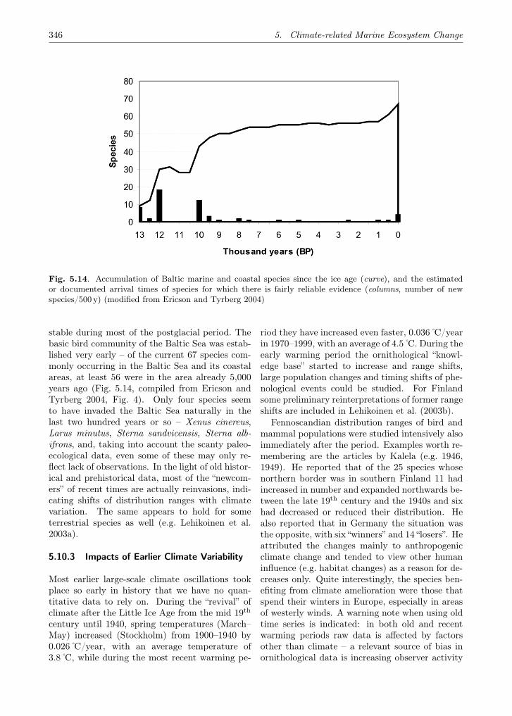
346 5. Climate-related Marine Ecosystem Change
Fig. 5.14. Accumulation of Baltic marine and coastal species since the ice age (curve), and the estimatedor documented arrival times of species for which there is fairly reliable evidence (columns, number of newspecies/500 y) (modified from Ericson and Tyrberg 2004)
stable during most of the postglacial period. Thebasic bird community of the Baltic Sea was estab-lished very early – of the current 67 species com-monly occurring in the Baltic Sea and its coastalareas, at least 56 were in the area already 5,000years ago (Fig. 5.14, compiled from Ericson andTyrberg 2004, Fig. 4). Only four species seemto have invaded the Baltic Sea naturally in thelast two hundred years or so – Xenus cinereus,Larus minutus, Sterna sandvicensis, Sterna alb-ifrons, and, taking into account the scanty paleo-ecological data, even some of these may only re-flect lack of observations. In the light of old histor-ical and prehistorical data, most of the “newcom-ers” of recent times are actually reinvasions, indi-cating shifts of distribution ranges with climatevariation. The same appears to hold for someterrestrial species as well (e.g. Lehikoinen et al.2003a).
5.10.3 Impacts of Earlier Climate Variability
Most earlier large-scale climate oscillations tookplace so early in history that we have no quan-titative data to rely on. During the “revival” ofclimate after the Little Ice Age from the mid 19th
century until 1940, spring temperatures (March–May) increased (Stockholm) from 1900–1940 by0.026 C/year, with an average temperature of3.8 C, while during the most recent warming pe-
riod they have increased even faster, 0.036 C/yearin 1970–1999, with an average of 4.5 C. During theearly warming period the ornithological “knowl-edge base” started to increase and range shifts,large population changes and timing shifts of phe-nological events could be studied. For Finlandsome preliminary reinterpretations of former rangeshifts are included in Lehikoinen et al. (2003b).
Fennoscandian distribution ranges of bird andmammal populations were studied intensively alsoimmediately after the period. Examples worth re-membering are the articles by Kalela (e.g. 1946,1949). He reported that of the 25 species whosenorthern border was in southern Finland 11 hadincreased in number and expanded northwards be-tween the late 19th century and the 1940s and sixhad decreased or reduced their distribution. Healso reported that in Germany the situation wasthe opposite, with six “winners” and 14 “losers”. Heattributed the changes mainly to anthropogenicclimate change and tended to view other humaninfluence (e.g. habitat changes) as a reason for de-creases only. Quite interestingly, the species ben-efiting from climate amelioration were those thatspend their winters in Europe, especially in areasof westerly winds. A warning note when using oldtime series is indicated: in both old and recentwarming periods raw data is affected by factorsother than climate – a relevant source of bias inornithological data is increasing observer activity

5.10. Sea Birds 347
and efficiency, which has been unaccounted for, sofar. In future studies it should be taken into ac-count.
5.10.4 Anthropogenic Climate ChangeImpacts on Birds – Predictions
Anthropogenic climate changes may influenceBaltic Sea bird populations by changes in:
• Distribution ranges during the breeding andnon-breeding seasons;
• Abundances during the breeding andnon-breeding seasons;
• Traits;• Migratory routes and stopover sites;• Timing of spring and autumn migration;• Migratory tendency within species/
populations.
In the following a short general description of thecurrent knowledge on each of these impact types isgiven. This summary is based on recent reviews,e.g. those by Møller et al. (2004), Crick (2004) andRehfisch et al. (2004):
1. Distribution changes
Range changes may be related to changes of habi-tat, but they need not be so, since factors otherthan suitable habitat may have constrained thedistribution of bird species in the past. Exten-sion of range is a different thing than a rangemargin shift, but both are expected to require asurplus of recruits in species where breeders showhigh site-tenacity. In the earlier warming period(in Fennoscandia from 1870 to 1940) many rangeshifts in birds were observed, both at the northernand the southern borders.
2. Changing abundances and community struc-tures
Change of abundance is a direct consequence ofthe difference between death and birth rates. Theunderstanding of the reasons and linkages betweenlong term changes in abundance of birds and an-thropogenic climate change is still very limited.
3. Evolutionary trait changes
Individual birds first react behaviourally tochanges in climate. The responses are phenotypic,i.e. plasticity of individuals is sufficient to fit the
behaviour to environmental changes. If the rate ofchange increases, selection comes into play. Rapidenvironmental change may cause strong selectioneffects, and, provided there is enough genetic vari-ability, combinations may exist that adapt thebirds evolutionarily to the changed condition. Itis only at this stage that population changes andrange shifts are likely to occur. For natural selec-tion to be efficient in adapting the population tochanged conditions there may be constraints thatarise from other counteracting selection pressures,even in a situation where anthropogenic climatechange is the driving force. For example, if theinitiation of spring migration is constrained eitherby conditions or by the internal clock (which itneed not be) selection effects can not be realisedin optimising timing of breeding.
4. Migratory pathways
Routes that the birds use between breeding andwintering areas are often habitual and are likelyto change if conditions at favoured stopover sitesdeteriorate. For species which require specialisedhabitat patches for refuelling, e.g. arctic waders,water level changes and other factors which changethe type and quality of coastal habitats may becritical. The intensively studied knot (Calidriscanutus) is one model species which may currentlysuffer locally from climate induced habitat changes(Baker et al. 2004). Within the Baltic Sea espe-cially arctic geese and seaducks may have to re-spond to anthropogenic climate change impacts.
5. Timing of migration
Timing of migration should be analysed in its en-tirety from initiation to end in both directions.Impacts at different phases may be different, be-cause anthropogenic climate change trends andstop-over conditions change both spatially andtemporally (e.g. Ahola et al. 2004). These highlydetailed analyses are only possible for species stud-ied by remote sensing techniques, and for suchspecies there are no long time series available yet.However, timing has been in the focus of researchon climate effects simply because it is rather easyto observe and long term data exist starting fromthe mid 18th century. Timing of critical annualevents is an important parameter, as time win-dows for optimal performance, e.g. in breeding,may change in length. It has been generally ex-pected that the length of suitable breeding pe-

348 5. Climate-related Marine Ecosystem Change
riod will increase, but this need not necessarily bethe case. Interactions between temperature andprecipitation may affect food availability, whichmay be more important than the expected longerbreeding periods.
6. Migratory tendency
Short distance, intra-European migrants are a spe-cial case which has not been the object of inten-sive studies. However, analyses of Fennoscandianwinter census data and ringing recovery analysiswill provide more knowledge on these effects in theyears to come (for the potential and problems ofringing recovery analyses, see Fiedler et al. 2004).
The documented recent changes in the popu-lations of birds in the Baltic Sea are discussedin relation to anthropogenic climate change andevaluated in relation to their possible impacts onthe population dynamics of the bird population inquestion. The impacts may be on adult survival,breeding effort, nestling survival/breeding successand dispersal.
5.10.5 Available Studies
Monitoring of population sizes covers the periodof recent climate variability rather well in Fin-land, Sweden and many other countries. Euro-pean monitoring programs have recently unitedin a pan-European monitoring program (seehttp://birdlife.cz/index.php?a=cat.101). Moni-toring programs usually only report the trends ofpopulation sizes and do not interpret or analysethe causes. Therefore, although we have a lot ofinformation on population variation, rather littlecan be said about the causes, because simultane-ous changes of many environmental factors mayhave parallel impacts.
Distributions are not monitored annually. Insome countries (e.g. Great Britain and Finland)bird atlas work (mapping of distributions) hasbeen done twice with similar methods in 1960–2000. In a recent paper Brommer (2004) sug-gested that in Finland range border shifts tookplace between the end of the 1970s and the end ofthe 1980s, and these might have been due to cli-mate impact. Southern species shifted their north-ern range borders northwards by 18 km in ca. tenyears, approximately double the speed shown bya similar British analysis (Thomas and Lennon1999). Rigid statistical analysis has yet to be doneto separate anthropogenic climate change impacts
from other causes in order to understand betterthe direct and indirect influences.
With respect to water birds, monitoring ofbreeding colonies has been carried out in mostcountries around the Baltic Sea during the periodof recent climate variability. However, few studieshave attempted to link trends to anthropogenic cli-mate change. Extensive monitoring of water birdsbreeding in the northern archipelagoes is takingplace in selected areas. In the Kaliningrad andSt. Petersburg regions of Russia only selected wa-ter bird species are monitored, and the same holdsfor Estonia. Monitoring of breeding water birdsis carried out annually in Latvia, Lithuania andPoland, and in all three countries counts are or-ganised in relation to specific areas. In Germany,monitoring of breeding water birds is organisedby the state administrations of Schleswig–Holsteinand Mecklenburg–Vorpommern, with a focus onprotected areas. Yearly monitoring data on breed-ing water birds in Denmark is currently organ-ised by one state only. In addition, game reservesand the breeding colony of auks at Christiansø arecounted regularly. The wetlands along the east-ern part of the Gulf of Finland are not currentlycovered by breeding monitoring programs.
Most recent counts of wintering water birds inthe Baltic Sea have been connected to the midwin-ter counts of Wetlands International. These countsgenerally cover birds of the coastal zone and la-goons, while offshore areas are surveyed only in-frequently. In 1992 and 1993, the first surveyscovering all major offshore areas were carried out(Durink et al. 1994). Since 1994, line transectcounts in offshore areas have not been undertakenas part of an internationally co-ordinated census.
5.10.6 Fluctuations in Population Levels
Direct influences of climate variability on Balticbird populations vary between terrestrial birds,water birds and seabirds, as well as between breed-ing and wintering bird faunas. Direct influenceson breeding bird populations are generally of lim-ited significance as compared to indirect influ-ences. The direct influences on breeding bird pop-ulations include reduced food availability due torising sea levels, increased mortality of chicks inlow-lying colonies due to rising sea levels, reduceddevelopment of the embryo due to low tempera-tures, abnormal development or death of the em-bryo due to excessive exposure to high tempera-tures and increased chick mortality due to over-
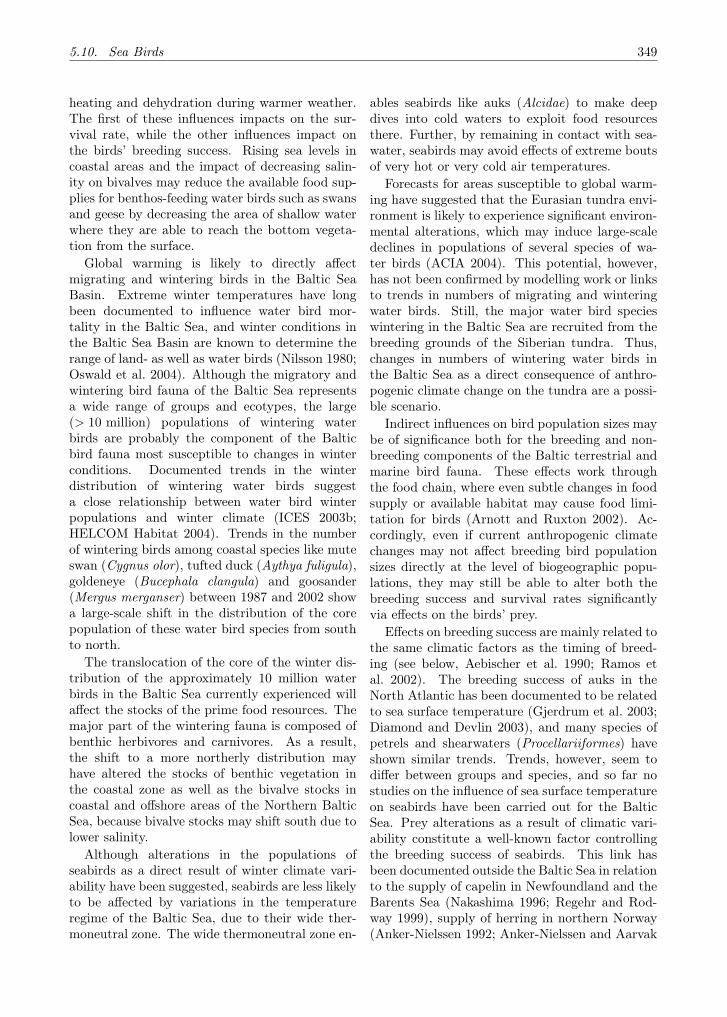
5.10. Sea Birds 349
heating and dehydration during warmer weather.The first of these influences impacts on the sur-vival rate, while the other influences impact onthe birds’ breeding success. Rising sea levels incoastal areas and the impact of decreasing salin-ity on bivalves may reduce the available food sup-plies for benthos-feeding water birds such as swansand geese by decreasing the area of shallow waterwhere they are able to reach the bottom vegeta-tion from the surface.
Global warming is likely to directly affectmigrating and wintering birds in the Baltic SeaBasin. Extreme winter temperatures have longbeen documented to influence water bird mor-tality in the Baltic Sea, and winter conditions inthe Baltic Sea Basin are known to determine therange of land- as well as water birds (Nilsson 1980;Oswald et al. 2004). Although the migratory andwintering bird fauna of the Baltic Sea representsa wide range of groups and ecotypes, the large(> 10 million) populations of wintering waterbirds are probably the component of the Balticbird fauna most susceptible to changes in winterconditions. Documented trends in the winterdistribution of wintering water birds suggesta close relationship between water bird winterpopulations and winter climate (ICES 2003b;HELCOM Habitat 2004). Trends in the numberof wintering birds among coastal species like muteswan (Cygnus olor), tufted duck (Aythya fuligula),goldeneye (Bucephala clangula) and goosander(Mergus merganser) between 1987 and 2002 showa large-scale shift in the distribution of the corepopulation of these water bird species from southto north.
The translocation of the core of the winter dis-tribution of the approximately 10 million waterbirds in the Baltic Sea currently experienced willaffect the stocks of the prime food resources. Themajor part of the wintering fauna is composed ofbenthic herbivores and carnivores. As a result,the shift to a more northerly distribution mayhave altered the stocks of benthic vegetation inthe coastal zone as well as the bivalve stocks incoastal and offshore areas of the Northern BalticSea, because bivalve stocks may shift south due tolower salinity.
Although alterations in the populations ofseabirds as a direct result of winter climate vari-ability have been suggested, seabirds are less likelyto be affected by variations in the temperatureregime of the Baltic Sea, due to their wide ther-moneutral zone. The wide thermoneutral zone en-
ables seabirds like auks (Alcidae) to make deepdives into cold waters to exploit food resourcesthere. Further, by remaining in contact with sea-water, seabirds may avoid effects of extreme boutsof very hot or very cold air temperatures.
Forecasts for areas susceptible to global warm-ing have suggested that the Eurasian tundra envi-ronment is likely to experience significant environ-mental alterations, which may induce large-scaledeclines in populations of several species of wa-ter birds (ACIA 2004). This potential, however,has not been confirmed by modelling work or linksto trends in numbers of migrating and winteringwater birds. Still, the major water bird specieswintering in the Baltic Sea are recruited from thebreeding grounds of the Siberian tundra. Thus,changes in numbers of wintering water birds inthe Baltic Sea as a direct consequence of anthro-pogenic climate change on the tundra are a possi-ble scenario.
Indirect influences on bird population sizes maybe of significance both for the breeding and non-breeding components of the Baltic terrestrial andmarine bird fauna. These effects work throughthe food chain, where even subtle changes in foodsupply or available habitat may cause food limi-tation for birds (Arnott and Ruxton 2002). Ac-cordingly, even if current anthropogenic climatechanges may not affect breeding bird populationsizes directly at the level of biogeographic popu-lations, they may still be able to alter both thebreeding success and survival rates significantlyvia effects on the birds’ prey.
Effects on breeding success are mainly related tothe same climatic factors as the timing of breed-ing (see below, Aebischer et al. 1990; Ramos etal. 2002). The breeding success of auks in theNorth Atlantic has been documented to be relatedto sea surface temperature (Gjerdrum et al. 2003;Diamond and Devlin 2003), and many species ofpetrels and shearwaters (Procellariiformes) haveshown similar trends. Trends, however, seem todiffer between groups and species, and so far nostudies on the influence of sea surface temperatureon seabirds have been carried out for the BalticSea. Prey alterations as a result of climatic vari-ability constitute a well-known factor controllingthe breeding success of seabirds. This link hasbeen documented outside the Baltic Sea in relationto the supply of capelin in Newfoundland and theBarents Sea (Nakashima 1996; Regehr and Rod-way 1999), supply of herring in northern Norway(Anker-Nielssen 1992; Anker-Nielssen and Aarvak

350 5. Climate-related Marine Ecosystem Change
2002) and supply of sandeel in the western NorthSea (Rindorf 2000). Similar controls via food re-sources have not been reported for water birds orterrestrial birds. The same prey alterations thatcause breeding success also may affect the survivalrate of adult birds. Mass mortality as a resultof potentially climate-induced large-scale fluctu-ations of prey has been reported in piscivorousseabirds feeding on schooling fish in the BarentsSea (Barrett and Krasnov 1996), the Bering Sea(Baduini et al. 2001) and the North Sea (Blake1984). Climatic effects were usually coupled toanomalous oceanographic conditions that changethe distribution and abundance of prey (Harrisand Wanless 1996; Piatt and Pelt 1997). Changesin the availability of benthic prey for water birdsas a result of anomalous oceanographic conditionshave not been documented in the Baltic Sea orneighbouring waters.
Many pelagic seabirds show a strong affinityto areas of strong stratification and stable frontalprocesses (Hunt and Harrison 1990; Skov and Dur-inck 2000). Changes in the stability of foragingareas for seabirds in the Baltic as a result of in-creased precipitation and runoff may alter the pos-sibilities for diving seabirds to find prey. The im-pact of changes in stratification and water col-umn structure in the Baltic Sea, which may beinduced by global warming, on feeding conditionsfor seabirds could be both positive (enhanced sta-bility) and negative (deepening of the pycnocline).
5.10.7 Phenological Changes
Birds use many cues to time the phases of annualcycle appropriately with the seasonally predictableenvironmental variation. In addition to this use ofcues, birds also possess a circannual clock, which isphotoperiodically regulated. In most species use ofcues other than photoperiod allows birds to plas-tically change their response to the environment.Temperature, precipitation, phenology of vegeta-tion and prey items can be such cues. Since 1990, alarge number of studies have shown that spring mi-gration of birds has become earlier in areas wherewinter/spring climates have become warmer, andno change has happened where climate has notameliorated. Several reviews are now availablethat serve as a background to the following gen-eral observations (Root et al. 2003; Lehikoinen etal. 2004; Crick 2004; Rehfisch et al. 2004).
Spring migration has generally become earlier,but there is a high degree of variability between
and within species. The phenology of migrationchanges relative to anthropogenic climate changeis also connected with (indirect) effects of NAO(e.g. Forchammer et al. 2002; Hüppop and Hüp-pop 2003; Vähätalo et al. 2004). Advancement ofspring migration to earlier dates does not meanthat fitness consequences exist. A frequent butinaccurate generalisation is that earlier migrationleads to earlier breeding that leads to higher breed-ing success. On average Southwest-Finnish breed-ing birds have advanced their spring migration by10 days in the period from 1965 to 2000 (whenmeasured by FAD, first arrival date). Largest ad-vances relate to short range migrants and partialmigrants; the smallest but still significant ones re-late to late arriving long distance migrants. Balticmarine and coastal species do not differ fromterrestrial ones in rate of advancement of FAD(Lehikoinen and Rainio, unpublished). Since FADis a rather problematic measure of spring arrival,other measures have been used (e.g. Lehikoinen etal. 2004; Sparks et al. 2004). Bird observatoriesand intensively studied breeding populations offerdata with which arrival of the whole populationcan be studied. These data suggest that not onlyare the earliest arriving individuals of a populationnow arriving earlier, but also the “median bird” inmany species arrives earlier, although the rate ofchange is significantly lower (Table 5.6)
Response of the earliest arriving individuals isgenerally stronger than the response of whole pop-ulations and that of the end tail of populations.FAD-data may be biased towards too high ratesof change, because it is likely that in more recentyears early individuals are observed earlier becauseof more intense observations and a denser networkof observers. MMT data (Table 5.6) are less bi-ased and provide a better basis for determiningchanges in spring migration patterns.
There is less information on autumn migration.SW-Finnish birds depart on average five days laternow than in the 1970s. There is, however, largevariability and quite a few species now leave earlierthan before. In Rybachi (Kola Peninsula), timingof autumn migration of long-distance migrants wasfound to be best explained by spring temperatures(Sokolov et al. 1998). This suggests that in thesespecies arrival in spring determines the whole sum-mer schedule including autumn departure – thewhole summer season is shifted earlier in thesespecies after warm springs. This is, however, nota general rule. Short distance migrants, which insmall passerine bird species can have two clutches
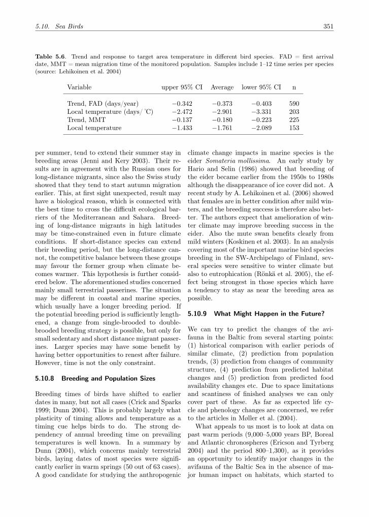
5.10. Sea Birds 351
Table 5.6. Trend and response to target area temperature in different bird species. FAD = first arrivaldate, MMT = mean migration time of the monitored population. Samples include 1–12 time series per species(source: Lehikoinen et al. 2004)
Variable upper 95% CI Average lower 95% CI n
Trend, FAD (days/year) −0.342 −0.373 −0.403 590Local temperature (days/ C) −2.472 −2.901 −3.331 203Trend, MMT −0.137 −0.180 −0.223 225Local temperature −1.433 −1.761 −2.089 153
per summer, tend to extend their summer stay inbreeding areas (Jenni and Kery 2003). Their re-sults are in agreement with the Russian ones forlong-distance migrants, since also the Swiss studyshowed that they tend to start autumn migrationearlier. This, at first sight unexpected, result mayhave a biological reason, which is connected withthe best time to cross the difficult ecological bar-riers of the Mediterranean and Sahara. Breed-ing of long-distance migrants in high latitudesmay be time-constrained even in future climateconditions. If short-distance species can extendtheir breeding period, but the long-distance can-not, the competitive balance between these groupsmay favour the former group when climate be-comes warmer. This hypothesis is further consid-ered below. The aforementioned studies concernedmainly small terrestrial passerines. The situationmay be different in coastal and marine species,which usually have a longer breeding period. Ifthe potential breeding period is sufficiently length-ened, a change from single-brooded to double-brooded breeding strategy is possible, but only forsmall sedentary and short distance migrant passer-ines. Larger species may have some benefit byhaving better opportunities to renest after failure.However, time is not the only constraint.
5.10.8 Breeding and Population Sizes
Breeding times of birds have shifted to earlierdates in many, but not all cases (Crick and Sparks1999; Dunn 2004). This is probably largely whatplasticity of timing allows and temperature as atiming cue helps birds to do. The strong de-pendency of annual breeding time on prevailingtemperatures is well known. In a summary byDunn (2004), which concerns mainly terrestrialbirds, laying dates of most species were signifi-cantly earlier in warm springs (50 out of 63 cases).A good candidate for studying the anthropogenic
climate change impacts in marine species is theeider Somateria mollissima. An early study byHario and Selin (1986) showed that breeding ofthe eider became earlier from the 1950s to 1980salthough the disappearance of ice cover did not. Arecent study by A. Lehikoinen et al. (2006) showedthat females are in better condition after mild win-ters, and the breeding success is therefore also bet-ter. The authors expect that amelioration of win-ter climate may improve breeding success in theeider. Also the mute swan benefits clearly frommild winters (Koskinen et al. 2003). In an analysiscovering most of the important marine bird speciesbreeding in the SW-Archipelago of Finland, sev-eral species were sensitive to winter climate butalso to eutrophication (Rönkä et al. 2005), the ef-fect being strongest in those species which havea tendency to stay as near the breeding area aspossible.
5.10.9 What Might Happen in the Future?
We can try to predict the changes of the avi-fauna in the Baltic from several starting points:(1) historical comparison with earlier periods ofsimilar climate, (2) prediction from populationtrends, (3) prediction from changes of communitystructure, (4) prediction from predicted habitatchanges and (5) prediction from predicted foodavailability changes etc. Due to space limitationsand scantiness of finished analyses we can onlycover part of these. As far as expected life cy-cle and phenology changes are concerned, we referto the articles in Møller et al. (2004).
What appeals to us most is to look at data onpast warm periods (9,000–5,000 years BP, Borealand Atlantic chronospheres (Ericson and Tyrberg2004) and the period 800–1,300), as it providesan opportunity to identify major changes in theavifauna of the Baltic Sea in the absence of ma-jor human impact on habitats, which started to

352 5. Climate-related Marine Ecosystem Change
take place around 5,000 BP. The unavoidably in-complete species list indicates a surprisingly sta-ble Baltic (Swedish) avifauna (Ericson and Tyr-berg 2004, p. 35). Practically all species currentlybreeding in the Baltic Sea were present alreadyduring the Atlantic period. Some, if not most oreven all, recent changes are reinvasions and reflectthe climate-dependent variability of distributionranges. On this basis there seems to be no majorspecies turnover to be expected, but the popula-tion sizes, regional distribution patterns and com-munity structures are likely to change. Howeverthese characteristics are affected by many otherfactors, not the least anthropogenic, and a thor-ough evaluation of likely relative changes as a re-sult of anthropogenic climate change is not cur-rently possible, due to the lack of comparativeanalyses of weather and habitat dependence inmost Baltic bird populations.
Since the early ‘predictions’ or rather educatedguesses by Berthold (1990), who classified a num-ber of European bird species in “winners” and“losers” separately into short- and long-distancemigratory categories, we have made little progressin predicting future development of bird popu-lations by species. Berthold’s general prediction(Berthold 1990) was that sedentary and short-distance species should win and long-distance mi-grants lose. Only a few Baltic marine, coastaland estuarine species were included in his study,but cormorant, heron, coot and black-headed gullwere listed as short distance migrants with highchances of population increase, while crane andlapwing had less chance of population increase ac-cording to Berthold (1990). Among long-distancemigrants he predicted strong declines for the littlebittern, white stork and garganey.
Although recent changes in the distributionand community structure of wintering water birdsseem to be driven by decadal climate changes, thefuture long-term changes of the Baltic water birdpopulations are very hard to predict. The rela-tionship between the warming of the winter cli-mate and the tendency for more water birds towinter in the northern parts is a good example forthe uncertainties regarding future water bird sce-narios (ICES 2003b; HELCOM Habitat 2004). Itseems a plausible prediction that more water birdswill concentrate in the north with amelioration ofwinter climate. However, this prediction dependson the availability of a surplus of benthic food, es-pecially bivalves in the northern Baltic Sea. Thissurplus may, in fact, be unlikely to be available,
as bivalve conditions generally will tend to worsen,also in the northern parts, as a function of increas-ing winter temperatures. Further, it is still un-certain whether the carrying capacity of benthicfood stocks for water birds has already reachedits limit due to changes in salinity, and adding tothat the future growth of bivalve stocks is uncer-tain due to the lack of reliable predictions aboutthe level of eutrophication in the northern BalticSea, especially in the coastal waters of the BalticStates and Russia. At the same time, warming ofthe tundra breeding areas may cause declines inthe populations of water birds visiting the BalticSea, enabling a higher proportion of birds to win-ter in the north. Accordingly, as for the terres-trial bird fauna only monitoring and comparativehabitat-weather dependence studies will provideus with the basis for making sound predictions onthe development of the water bird fauna in thefuture.
5.11 Summary
The Baltic Sea is not a steady state system, and,since its formation, it never has been. Externaldrivers acting on different time scales force ma-jor changes in the marine ecosystem structure andfunction. Postglacial isostatic and eustatic pro-cesses have shaped the Baltic Sea’s coastline, to-pography, basic chemistry and sedimentary envi-ronment on millennial scales (see Annex 2). Cli-mate variability acts on centennial and decadalscales, and, at least over the last 150 years (seeChap. 2), overlaps with human activities in thedrainage basin and the coastal zone, leading toconsiderable changes in the biogeochemistry ofthis semi-enclosed sea.
Changes in processes and functions in lagoons,estuaries and coastal waters observed over thelast 100 years have been generally assumed to besolely driven by anthropogenic forcing. However,to achieve a balanced classification of all driversacting on the Baltic Sea and to understand the in-ternal mechanisms and ecosystem response to cli-mate variability and anthropogenic climate changeon different trophic levels, the reactions to possibleanthropogenic climate change scenarios throughall trophic levels of the marine ecosystem are de-scribed in Chap. 5. Anthropogenic climate changescenarios for the Baltic Sea Basin (see Chap. 3)predict an increase in temperature especially dur-ing wintertime and an increase in rainfall in thenorthern part of the runoff area. The consequence
5.11. Summary 353
of increasing precipitation is twofold. Increasingprecipitation results in a decrease in salinity andin an increase of nutrient leakage and associatedeutrophication. The results of Chap. 5 are sum-marised in the following.
5.11.1 Increase of Nutrients
This is the most difficult topic to summarise, sinceso much has been written and is constantly beingpublished on it. The topic has been central toHELCOM activities and has interested Baltic Searesearchers and managers for decades. Many hy-pothetical ideas have been presented about limit-ing nutrients in different areas and circumstances.The topic is also of large economic interest, e.g.sewage water purification is certainly one of themost expensive outlays for cities and industry. Re-cently, also blooms of cyanobacteria have beenpresented as possible threat to recreation and thetourism industry.
Theoretically eutrophication is expected to en-hance the production and biodiversity in theecosystem up to a certain point, after which a col-lapse will occur due to several mechanisms such aschemical (anoxia) and biotic interactions (compe-tition, predation, exploitation). After this, a newecological balance will develop, which is charac-terised by low biodiversity and high variability dueto episodic outbursts of dominant species. Someeffects of eutrophication are clear and predictable,such as a general increase of primary production(HELCOM 2002), but others, such as interactionsbetween species and between individuals are ex-tremely hard to predict. There is evidence, how-ever, that some of this increase is transferred tohigher trophic levels.
Increasing eutrophication is an expected con-sequence of the anthropogenic climate change inthe region due to freshwater runoff determiningmost of the external nutrient load entering theBaltic Sea, especially in the near coastal areas(Stålnacke et al. 1999; HELCOM 2002). A furthereffect of eutrophication is the release of phospho-rus from anoxic sediments due to internal loading(see Sect. 5.5). The intensity of buoyant surfaceblooms of cyanobacteria might be enhanced dueto such internal eutrophication. They themselvespromote it by nitrogen fixation (see Sect. 5.5).This hypothesised situation means that, in orderto return to a previous state, nutrient removalfrom the Baltic Sea would need to be larger thanexpected on the basis of nutrient concentrations
at the time when symptoms of eutrophication firstbecame apparent.
The hypothesis that buoyant surface bloomsof cyanobacteria are a consequence of eutrophi-cation is under debate. Recently, Dippner andVoss (2004) have shown with stable isotopes of 15Nthat strong blooms of cyanobacteria appeared ina preindustrial period during the Medieval WarmPeriod, and Bianchi et al. (2000) demonstratedthat cyanobacterial blooms are nearly as old asthe present brackish water phase of the BalticSea, starting as far back as ∼ 7,000 BP. In addi-tion, the Baltic Proper, which of course receivesnutrients from direct precipitation, has a moreor less closed basinwide anticyclonic circulationcell (see also Annex 1.1) which reduces the trans-port of riverborne nutrients into the central BalticProper (Voss et al. 2005). The consequence is thatincreasing inputs of nutrients with higher riverrunoff will primarily remain in the near coastalareas rather than feed the cyanobacteria bloomsin the central Baltic Proper.
Available time-series studies suggest an overallincrease in mesozooplankton biomass, both in theopen sea and in the gulfs (see Sect. 5.6); however atspecies level some deviations of this general trendare found due to the influence of hydrographicchanges and selective planktivory.
Changes in the level of eutrophication due toanthropogenic climate change will affect the fish-eries indirectly through e.g. planktonic food sup-ply to developing larvae of practically all fishspecies (see Sect. 5.8). Furthermore, adult ben-thic fish (e.g. flounders and sculpins) will be indi-rectly affected by anoxia changing their environ-ment into a “benthic desert” (see Sect. 5.7). Gen-erally concerning benthos, biomasses are expectedto increase further in areas that are situated abovethe permanent pycnocline and to decrease in deepwater due to anoxia. Anoxia will also be partlyresponsible for some changes appearing in pelagicfish. Examples are the buoyancy characteristicsof the Baltic cod eggs rendering them subject tolethal deep-water concentrations of hydrogen sul-phide and low oxygen (see Sect. 5.8).
Predator-prey interactions are likely to changefish species relations e.g. between cod, herring andsprat (see Sect. 5.8). Decreased cod predationpressure on sprat during the last ten years has ledto substantially larger sprat stocks and catches.This development was apparently supported bybetter feeding conditions for sprat larvae feedingon small brackish water copepods (see Sect. 5.8).

354 5. Climate-related Marine Ecosystem Change
Indirect effects of eutrophication are also ex-pected due to changes in phytoplankton composi-tion and biomass as well as decreased transparencyof water, which are believed to subsequently causelack of vitamins in the pelagic food chain, leadingto the reproduction failure called M74 in juvenilesalmonid fish (see Sect. 5.8).
There already are signs that filamentous al-gae in the littoral zone have replaced the blad-der wrack, that anoxic bottoms with leaking ofnutrients exist even in shallow water and thatcyanobacteria will be responsible for changes inpelagic nutrient budgets. Generally speaking, nu-trient budgets will change with increasing eutroph-ication and we are likely to see annual plants re-place the perennials (HELCOM 1993b).
5.11.2 Increase of Temperature
Predicted increased temperatures, especially dur-ing winter, will change growth and reproductionof fauna and flora. It is important to note that asignificant part of the Baltic Sea biota, e.g. birds,is mostly of boreal origin, thus adapted to lowtemperatures in general. In the following we willshortly summarise main conclusions arrived at fordifferent taxa by the co-authors of this chapter.
Inter-annual variation of pelagic bacteriagrowth is partly dependent on temperature (alongwith the quality of available organic substrate andcompetitive relationships, Wikner and Hagström1999). Furthermore, the activity of pelagic bacte-ria is stimulated even more than primary produc-tion (Pomeroy and Deibel 1986), thus the ratiobetween bacteria biomass to phytoplankton is ex-pected to increase with temperature in eutrophicwaters (Laws 2003).
Recent monitoring data shows that diatomspring blooms are subject to species change whenwinters become milder (Hajdu et al. 1997). Fur-thermore, it has been suggested that the diatombloom itself will be reduced or perhaps even dis-appear after milder winters, to be replaced by di-noflagellates (see Sect. 5.5, Wasmund et al. 1998).There are signs that increasing summertime tem-peratures may enhance cyanobacterial blooms. Inaddition, higher than normal winter temperaturesmay prevent convection in late winter and earlyspring with the result that nutrients are not mixedinto the upper euphotic zone. In the Baltic Proper,with a salinity of 7 psu, the maximum density ofwater occurs at ∼ 2.5 C. If the winter tempera-ture is below 2.5 C, seasonal surface warming in
early spring will result in an unstable water col-umn with convective overturning. If the watertemperature is higher than 2.5 C, warming willresult in the development of a thermocline and noredistribution of nutrients due to convection willoccur. This process might also result in a shiftin species composition of phytoplankton in springand could counteract cyanobacteria blooms.
The natural annual range of variation in theBaltic Sea surface temperature is from below zeroup to over 20 C. Therefore, it is understandablethat so far only a few long-term studies have pro-vided examples of fauna reacting to temperaturechanges. In an 18-year time series from the north-ern Baltic Sea, annual peaks of the most abun-dant cladoceran species co-varied with the sea-sonal fluctuation of the surface water tempera-ture (Viitasalo et al. 1995, see Sect. 5.6). A shiftin dominance was observed within the open seacopepod community from Pseudocalanus acuspesto Acartia spp., coinciding with higher temper-atures during the 1990s (Möllmann et al. 2000,2003a). Increased production and survival rates ofsprat and herring populations during the last 5–10years covaried with high temperatures and highNAO indices (Kornilovs 1995; Axenrot and Hans-son 2003; MacKenzie and Köster 2004). Essen-tially the same conclusions are given in Sect. 5.8.
In the earlier warming period in Fennoscandiabetween 1870–1940, many range shifts in birdswere observed, both at the northern and southernborders and for spring as well as autumn migra-tion (see Sect. 5.10). Furthermore, extreme win-ter temperatures have long been documented toinfluence water bird mortality in the Baltic Sea,and winter conditions in the Baltic Sea Basin areknown to determine the ranges of land- as wellas water birds (Nilsson 1980). Spring migrationnow generally occurs earlier, although there is ahigh variation between and within species, andthe phenology of migration changes are also con-nected with effects of the NAO (e.g. Forchammeret al. 2002; Hüppop and Hüppop 2003; Vähätaloet al. 2004). A recent report places the ringed sealamong the species for which a global decline in dis-tribution is “very likely” (ACIA 2005). Modellingstudies project the probable extinction of southernsubpopulations of the Baltic ringed seal if ice suit-able for breeding declines drastically during thiscentury. The grey seal, which has been shown tohave the capability to breed extensively on landeven in the Baltic (see Sect. 5.9), should be lesssensitive.
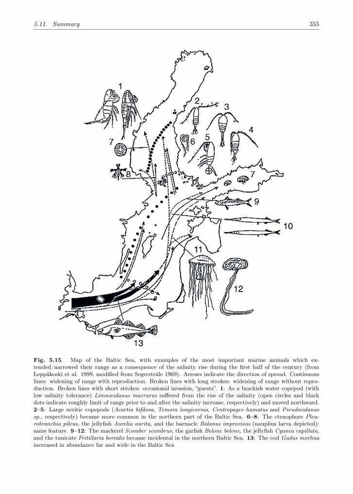
5.11. Summary 355
Fig. 5.15. Map of the Baltic Sea, with examples of the most important marine animals which ex-tended/narrowed their range as a consequence of the salinity rise during the first half of the century (fromLeppäkoski et al. 1999, modified from Segerstråle 1969). Arrows indicate the direction of spread. Continuouslines: widening of range with reproduction. Broken lines with long strokes: widening of range without repro-duction. Broken lines with short strokes: occasional invasion, “guests”. 1: As a brackish water copepod (withlow salinity tolerance) Limnocalanus macrurus suffered from the rise of the salinity (open circles and blackdots indicate roughly limit of range prior to and after the salinity increase, respectively) and moved northward.2–5: Large neritic copepods (Acartia bifilosa, Temora longicornis, Centropages hamatus and Pseudocalanussp., respectively) became more common in the northern part of the Baltic Sea. 6–8: The ctenophore Pleu-robranchia pileus, the jellyfish Aurelia aurita, and the barnacle Balanus improvisus (nauplius larva depicted):same feature. 9–12: The mackerel Scomber scombrus, the garfish Belone belone, the jellyfish Cyanea capillata,and the tunicate Fritillaria borealis became incidental in the northern Baltic Sea. 13: The cod Gadus morhuaincreased in abundance far and wide in the Baltic Sea

356 5. Climate-related Marine Ecosystem Change
5.11.3 Decrease of Salinity
A decrease of salinity of the Baltic Sea due to in-creasing precipitation will modify the ecosystemin several ways. The most important changes willprobably be seen in the distribution (both hori-zontal and vertical), although growth and repro-duction are also likely to be affected. The physi-ological effect of salinity variation was among thefirst problems to be studied in the early years ofBaltic Sea marine biology. Remane (1940) givesan overview of early osmoregulation studies andalso reports lower salinity limits for several speciesof the Baltic Sea fauna. Examples from variousphyla illustrate clearly the expected overall de-crease of Baltic Sea marine fauna. The decreasewill be more pronounced and will first be seenin the northern Baltic Sea surface area, the rivermouths and the Gulfs of Finland and Riga, if theincrease in rainfall in the northern part of the wa-tershed predicted in Chap. 3 of this book takesplace.
According to Remane (1940) the approximatelower limit of salinity tolerance is 2 psu for Praunusflexuosus, Neomysis vulgaris, and Gammarus lo-custa, 3 psu for Corophium volutator, 5.5 psufor Palaemon adspersus and Idotea baltica, 6 psufor Pontoporeia femorata and Harmothoe sarsi,7 psu for Pygospio elegans and Laomedea lovéni,and 7.5 psu for Terebellides strömii and Fabri-cia sabella. In the western Baltic Sea the com-mon starfish (Asterias rubens) and common shorecrab (Carcinus maenas) are among the speciesexpected to decrease if salinity decreases to lessthan 25–15 psu (Remane 1940, Segerstråhle 1957,Järvekülg 1979). Thus we can expect changes inspecies distribution along the complete range ofBaltic Sea surface salinity (for marine species adecrease) (see also Fig. A.1).
An increase in salinity during the first half ofthe 20th century resulted in a spread of severalmarine species (e.g. mesozooplankton, barnacle,jellyfish, larvaceans) towards the north and theeast in the Baltic Sea (Fig. 5.15, Segerstråle 1969).Correspondingly, the decrease in salinity after thelate 1970s in the northern Baltic Sea (Fig. 5.16)was reflected in biomass decline of the large ner-itic copepod species and increase of the freshwatercladoceran species (Vuorinen et al. 1998). In thedeep basins of the open Baltic Sea, the decreasein salinity resulted in reduced standing stocks ofPseudocalanus sp., an important component inthe pelagic food web. In contrast, populations of
species favored by high temperature (e.g. Acartiaspp.) increased.
We are likely to see a reversal of the changes ofthe 1950s. Some of this expected trend has alreadybeen documented as one of the key species in theBaltic Proper, the cod, which needs a certain levelof salinity during a certain life stage, now displayslow reproductive success in the Baltic Sea Basin.Cod eggs need a minimum salinity of 11.5 psu forbuoyancy, which they usually find in the haloclineregions of the deep Baltic Sea basins. Due to thereduced marine inflow in the last decades, whichresulted in low salinity but also low oxygen con-centrations in the deep water, cod eggs are fre-quently exposed to lethal oxygen conditions in thelayer in which they are neutrally buoyant (Kösteret al. 2005). It has further been indicated thatthe decrease in herring and sprat growth is due toa salinity-mediated change in the copepod com-munity (Rönkkönen et al. 2004; Möllmann et al.2003a, 2005). A parallel retreat towards the southhas been found in some benthic fauna, e.g. Scolo-plos armiger (see Sect. 5.7). In addition, the com-bination of decreasing salinity and increasing tem-perature will clearly reduce the general fitness ofnative benthic species and their adaptability tocope with other stressors, e.g. low oxygen or chem-ical pollution (see Sect. 5.3). Finally, decreasingsalinity enables all freshwater species to enlargetheir area of distribution in the Baltic Sea.
One of the key species in the Baltic Proper,the cod, has already been affected by decreasingsalinities. Fishing is the most important directanthropogenic effect on the Baltic Sea, and over-fishing of cod has contributed to the decrease ofstocks. Again, we are not able to evaluate therelative importance of decreasing salinity vs. over-fishing, when discussing the ultimate cause of thedecline in cod stocks. As a top predator in thepelagic food chain it used to control the sprat andherring stocks. Due to its decrease and climat-ically induced enhanced sprat reproduction, theecosystem has switched from cod-dominated tosprat-dominated (recent situation) states. We canpoint out, on the basis of zooplankton time seriesstudies, that there also is a deterioration of zoo-plankton quality in terms of larval food for cod,which further contributes to decreased survivaland growth of cod. Finally, increased sprat stocksmay compete for plankton food with cod larvae,which again would limit cod in the Baltic Sea.
The interaction of all these contributing factorsis, actually, result of peculiarities of the Baltic Sea

5.11. Summary 357
Sal
inity
(psu
)
10,60
11,00
11,40
11,80
12,20
12,60
13,00
13,40
5,80
6,00
6,20
6,40
6,60
6,80
7,00
7,20
5,60
1960
1955
Year
Cop
epod
a/C
lad
ocer
a-b
iom
ass
1965
1970
1975
1980
1985
1990
1995
2000
1.00
2.00
3.00
4.00
5.00
6.00
7.00
Sal
inity
(psu
)
a)
90,000
95,000
100,000
105,000
110,000
115,000
120,000
125,000
130,000
Riv
erru
noff
km3
a)
b)
c)
d)
b)
c)
d) No Data
Fig. 5.16. (a) Total freshwater runoff to the Baltic Sea (inverted scale), (b) variation of salinity at 200 metersdepth off Gotland, and (c) off the Island of Päiväluoto in Northern Baltic, and relation of copepoda/cladocerabiomass off Päiväluoto at the depth of 20 meters (modified from Vuorinen et al. 1998)
itself: low salinity, species living near lethally lowconcentrations of salt, a small water body render-ing cod subject to overfishing and the high impactof climatic factors.
Because of its ecological and evolutionary his-tory, the Baltic Sea predominantly is a receiverarea for introduced species, donor areas of whichare to be found both in the adjacent inland watersand oceanic coasts but also in remote seas. Most ofthe recent invaders in the Baltic Sea originate fromwarmer climates (Leppäkoski and Olenin 2001). Inconditions of increasing water temperature, notonly spontaneously spreading European invadersbut also more exotics from warmer regions of theworld can be expected to establish themselves inthe Baltic Sea.
Two target species known to cause severechanges in invaded ecosystems most likely willspread with climatic warming. The zebra mus-sel Dreissena polymorpha may penetrate to theGulf of Bothnia, into the areas presently devoidof large biofiltrators. The North American jellycomb Mnemiopsis leidyi, which recently invaded
the Black and Caspian Seas, has also invaded theBaltic Sea and possible changes in the pelagic sys-tem are not clear at the moment.
Finally, we would like to point out that mostof the animal and plant species in the Baltic Seaare incompletely, or not at all, monitored. Theexamples of time-series presented above are oftenbased on commercial (fish) or recreational (birds)observations, and are in this respect anecdotal andonly indicative of biotic consequences of the an-thropogenic climate change. It is noteworthy thatall climate indications: increase in winter temper-atures, precipitation and eutrophication have beenchanging in the predicted direction during the lastdecades.
We also want to point out that even with thislimited set of relatively short time series we seeclear indications of climate change, most likely atleast partly of anthropogenic origin in the BalticSea animals and plants. Natural and anthro-pogenic climate change tend to affect biota in thesame way, and future effects may turn out to besurprisingly rapid and extensive.

358 5. Climate-related Marine Ecosystem Change
5.12 References
Aaris-Sørensen K (1998) Danmarks forhistoriske dyreverden (Prehistoric animal world of Denmark).Gyldendal, Copenhagen (in Danish)
ACIA (2004) Arctic Climate Impact Assessment. Scientific Report, www.acia.uaf.edu/pages/scienti-fic.html
Ackefors H (1981) Zooplankton. In: Voipio A (ed) The Baltic Sea. Elsevier Oceanography Series 30.Elsevier, Amsterdam, pp. 238–254
Aebischer N, Coulson J, Colebrook J. (1990) Parallel long-term trends across four marine trophic lev-els and weather. Nature 347:753–755
Ahlbäck R (1955) Kökar. Näringslivet och dess organisation i en utskärssocken (Island of Kökar:Economic life and it’s organisation in an outer archipelago parish) Skrifter utgivna av SvenskaLitteratursällskapet i Finland 351 (in Swedish)
Ahola M, Laaksonen T, Sippola K, Eeva T, Rainio K, Lehikoinen E (2004) Variation in climate warm-ing along the migration route uncouples arrival and breeding dates. Glob Change Biol 10:1610-1617
Alaee M, Arias P, Sjödin A, Bergman Å (2003) An overview of commercially used brominated flameretardants, their applications, their use patterns in different countries/regions and possible modesof release. Env Int 29:683–689
Albalat A, Potrykus J, Pempkowiak J, Porte C (2002) Assessment of organotin pollution along thePolish coast (Baltic Sea) by using mussels and fish as sentinel organisms. Chemosphere 47:165–171
Alheit J, Hagen E (2001) Climate variability and northwest European fisheries. In: Proceedings ofthe Hanse Conference on “Past climate and its significance for human history in northwest Europe,the last 10,000 years”, Delmenhorst Germany, October 1999, pp. 9–14
Allsopp M, Erry B, Santillo D, Johnston P (2001) POPs in the Baltic – a review of persistent organicpollutants (POPs) in the Baltic Sea. Greenpeace International London, pp. 92
Amano M, Hayano A, Miayzaki N (2002) Geographic variation in the skull of the ringed seal Pusahispida. J Mammal 83,2:370–380
Andersin A-B, Sandler H (1991) Macrobenthic fauna and oxygen deficiency in the Gulf of Finland.Memoranda Societatis Pro Fauna et Flora Fennica 67:3–10
Andersin A-B, Lassig J, Parkkonen L, Sandler H (1978) The decline of macrofauna in the deeper partsof the Baltic Proper and Gulf of Finland. Kieler Meeresforschungen 4:23–52
Andrén E, Andrén T, Kunzendorff H (2000) Holocene history of the Baltic Sea as a background forassessing records of human impact in the sediments of the Gotland Basin. Holocene 10,6:687–702
Aneer G (1975) Composition of food of the Baltic herring (Clupea harengus v. membras L), four-horn sculpin (Myoxocephalus quadricornis L), and eel-pout (Zoarces vivparus L) from deep softbottom trawling in the Askö-landsort area in two consecutive years. Merentutkimuslait. Julk./Havsforskningsinst. Skrifter 239:146–154
Anker-Nielssen T (1992) Food-supply as a determinant of reproduction and population developmentin Norwegian Puffins Fratercula arctica. PhD Thesis, University of Trondheim, Norway
Anker-Nielssen T, Aarvak T (2002) The population ecology of Puffins at Røst. Status after the breed-ing season 2001. Norsk Institutt for Naturforskning: Oppdragsmelding 736:1–40
Arnosti C, Sagemann J, Jørgensen B, Thamdrup B (1998) Temperature dependence of microbialdegradation of organic matter in marine sediments: Polysaccharide hydrolysis, oxygen consump-tion, and sulfate reduction. Mar Ecol Prog Ser 165:59–70
Arnott SA, Ruxton GD (2002) Sandeel recruitment in the North Sea: Demographic, climatic andtrophic effects. Mar Ecol Prog Ser 238:199–210
Arntz WE, Brunswig D (1975) Studies on structure and dynamics of macrobenthos in the westernBaltic carried out by the joint research programme “Interaction sea–sea bottom” (SFB 95-Kiel).Proceedings of 10th European Symposium on Marine Biology. Ostend, Belgium, 17–23 Sept 1975,vol. 2
Aro E (2000) The spatial and temporal distribution patterns of cod (Gadus morhua callaris L.) in theBaltic Sea, and their dependence on environmental variability – Implications for fishery management.Finnish Game and Fisheries Research Institute, Helsinki.
5.12. References 359
Aschan M (1988) Soft bottom macrobenthos in a Baltic archipelago: Spatial variation and optimalsampling strategy. Ann Zool Fennici 25:153–164
Assmuth T, Jalonen P (2005) Risks and Management of Dioxin-like Compounds in Baltic Sea Fish:An Integrated Assessment. TemaNord 2005:568, Nordic Council of Ministers, Copenhagen 2005
Autio R (1998) Response of seasonally cold-water bacterioplankton to temperature and substratetreatments. Estuar Coast Shelf Sci 46:465–474
Axenrot T, Hansson S (2003) Predicting herring recruitment from young-of-the-year densities, spawn-ing stock biomass, and climate. Limnol Oceanogr 48:1716–1720
Baduini C, Hyrenbach K, Coyle K, Pinchuk A, Menenhall V, Hunt G (2001) Mass-mortality of short-tailed shearwaters in the south-eastern Bering Sea during summer 1997. Fish Oceanogr 10:117–130
Bagge O (1989) A review of investigations of the predation of cod in the Baltic. Rapp P-V Réun ConsInt Explor Mer 190:51–56
Bagge O, Thurow F, Steffensen E, Bay J (1994) The Baltic cod. Dana 10:1–28Baker AJ, González PM, Piersma T, Niles LJ, de Lima Serrano do Nascimento I, Atkinson PW, Clark
NA, Minton CDT, Peck MK, Aarts G (2004) Rapid population decline in red knots: Fitness con-sequences of decreased refuelling rates and late arrival in Delaware Bay. Proc Roy Soc London, B271:875–882
Banta GT, Giblin AE, Hobbie JE, Tucker J (1995) Benthic respiration and nitrogen release in Buz-zards Bay, Massachusetts. J Mar Res 53:107–135
Barber DG, Iacozza J (2004) Historical analysis of sea ice conditions in M’Clintoc Channel and theGulf of Boothia, Nunavut: Implications for ringed seal and polar bear habitat. Arctic 57,1:1–14
Barrett R, Krasnov Y (1996) Recent responses to changes in stocks of prey species by seabirds breed-ing in the southern Barents Sea. ICES J Mar Sci 53:713–722
Baumann H, Hinrichsen HH, Möllmann C, Köster FW, Malzahn AM, Temming A (2006) Recruitmentvariability in Baltic Sea sprat (Sprattus sprattus) is tightly coupled to temperature and transportpatterns affecting the larval and early juvenile stages. Can J Fish Aquat Sci 63:2191–2201
Begg GA, Marteinsdottir G (2002) Environmental and stock effects on spawning origins and recruit-ment of cod Gadus morhua. Mar Ecol Prog Ser 229:263–277
Bergman G (1956) Sälbeståndet vid våra kuster (The seal population at our coast). Nordenskiöld-samfundets tidskrift XVI:49–65 (in Swedish)
Berryman AA (1999) Principles of population dynamics and their application. Stanley Thornes Pub-lishers, Cheltenham, UK
Berthold P (1990) Patterns of avian migration in light of current global “greenhouse” effects: a CentralEuropean perspective. Acta XX Congressus Internationalis Ornithologici, vol. II:780–786
Bettarell Y, Amblard C, Sime-Ngando T, Carrias J-F, Sargos D, Garabetian F and Lavandier P (2003)Viral lysis, flagellate grazing potential, and bacterial production in lake Pavin. Microb Ecol 45:119–127
Beyer J, Lassen H (1994) The effect of size-selective mortality on size-at-age Baltic herring.Dana 10:203–234
Bianchi TS, Engelhaupt E, Westman P, Andrén T, Rolff C, Elmgren R (2000) Cyanobacterial bloomsin the Baltic Sea: Natural or human-induced? Limnol Oceanogr 45:716–726
Bignert A, Litzen K, Odsjö T, Olsson M, Persson W, Reutergårdh L (1995) Time-related factors in-fluence the concentration of sDDT, PCBs and shell parameters in eggs of Baltic Guillemot (Uriaaalge). Env Pollut 89:1861–1989
Bignert A, Asplund L, Willander A (2004) Comments Concerning the National Swedish ContaminantMonitoring Programme in Marine Biota. Rapport till Naturvårdsverket, 2004-04-30
Boeschker HTS, de Graf W, Köster M, Meyer-Reil L-A, Cappenberg TE (2001) Bacterial populationsand processes involved in acetate and propionate consumption in anoxic brackish sediment. FEMSMicrobiol Ecol 35:97–103
Bogovski S, Sergeyev B, Muzyka V, Karlova S (1998) Cytochrome P450 system and heme synthaseenzymes activity in flounder liver as biomarkers of marine environments pollution. Mar Env Res 46:13–16
360 5. Climate-related Marine Ecosystem Change
Bonner WN (1972) Grey seal and common seal in European waters. Oceanogr Mar Biol Ann Rev 10:461–507
Bonsdorff E (2006) Zoobenthic diversity-gradients in the Baltic Sea: Continuous post-glacial succes-sion in a stressed ecosystem. J Exp Mar Biol Ecol 330:383–391
Bonsdorff E, Pearson TH (1999) Variation in the sublittoral macrozoobenthos of the Baltic Sea alongenvironmental gradients: A functional-group approach. Austral Ecol 24:312–326
Bonsdorff E, Aarnio K, Sandberg E (1991) Temporal and spatial variability of zoobenthic communi-ties in archipelago waters of the northern Baltic Sea – consequences of eutrophication? Int Rev GesHydrobiol 76,3:433–449
Bonsdorff E, Blomquist EM, Mattila J, Norkko A (1997) Coastal Eutrophication: Cause, conse-quences and perspectives in the archipelago areas of the northern Baltic Sea. Estuar Coast ShelfSci 44:63–72
Borg H, Jonsson P (1996) Large-scale metal distribution in Baltic Sea sediments. Mar Pollut Bull 32:8–21
Brander K, Mohn B (2004) Effect of the North Atlantic Oscillation on recruitment of Atlantic cod(Gadus morhua). Can J Fish Aquat Sci 61:1558–1564
Brettar I, Rheinheimer G (1991) Dinitrification in the Central Baltic: Evidence for H2S-oxidation asmotor of denitrification in the oxic-anoxic interface. Mar Ecol Prog Ser 77:157–169
Brey T (1986) Increase in macrozoobenthos above the halocline in Kiel Bay comparing the 1960s withthe 1980s. Mar Ecol Prog Ser 28:299–302
Brommer J (2004) The range margins of northern birds shift polewards. Ann Zool Fennici 41:391–397Burris JE (1980) Vertical Migration of Zooplankton in the Gulf of Finland. Am Midland Nat 103:
316–321Burton JK (1995) Birds and Climate Change. Helm, LondonCanagaratnam P (1959) Growth of fishes in different salinities. J Fish Res Board Can 16:121–129Cardinale M, Arrhenius F (2000) Decreasing weight-at-age of Atlantic herring (Clupea harengus) from
the Baltic Sea between 1986 and 1996: A statistical analysis. ICES J Mar Sci 57:882–893Cardinale M, Casini M, Arrhenius F (2002) The influence of biotic and abiotic factors on the growth
of sprat (Sprattus sprattus) in the Baltic Sea. Aquat Living Resour 15:273–281Casini M, Cardinale M, Hjelm J (2006) Inter-annual variation in herring Clupea harengus, and sprat,
Sprattus sprattus, condition in the central Baltic Sea: What gives the tune? Oikos 112:638–650Cederwall H (1979) Energy flow and fluctuations of deeper soft bottom communities in the Baltic Sea.
Askö Laboratory and Department of Zoology, University of Stockholm, Sweden, pp. 1–23Cederwall H, Elmgren R (1980) Biomass increase of benthic macrofauna demonstrates eutrophication
of the Baltic Sea. Ophelia,Suppl 1:287–304Clarke A, Harris CM (2003) Polar marine ecosystems: Major threats and future change. Env Conser-
vat 30,1:1–25Cleveland WS, Devlin SJ (1988) Locally weighted regression: An approach to regression analysisi by
local fitting. J American Statistical Assoc 85:596–610Conley D, Humborg C, Rahm L, Savchuk OP, Wulff F (2002) Hypoxia in the Baltic Sea and basin-
scale changes in phosphorus biogeochemistry. Env Sci Technol 36:5315–5320Crick HQP (2004) The impact of climate change on birds. Ibis 146 (Suppl):48–56Crick HQP, Sparks TH (1999) Climate change related to egg-laying trends. Nature 399:423–424Crotty CM, Tyrrell PN, Espie GS (1994) Quenching of Chlorophyll a Fluorescence in Response to
Na+− Dependent HCO3− Transport-Mediated Accumulation of Inorganic Carbon in the Cyanobac-
terium Synechococcus UTEX 625. Plant Physiol 104:785–791Dalsgaard T, Canfield DE, Petersen J, Thamdrup B, Acuna-Gonzales L (2003) N-2 production by the
anammox reaction in the anoxic water column of Golfo Dulce, Costa Rica. Nature 442:606–608Dalsgaard T, Thamdrup B, Canfield DE (2005) Anaerobic ammonium oxidation (anammox) in the
marine environment. Res Microbiol 145:457–464Dalziel JA (1995) Reactive mercury in the eastern North Atlantic and southeast Atlantic. Mar Chem
49:307–314
5.12. References 361
Dannenberger D (1996) Chlorinated microcontaminants in surface sediments of the Baltic Sea: inves-tigations in the Belt Sea, the Arkona Sea and the Pomeranian Bight. Mar Pollut Bull 32:772–781
Davies JH (1957) The geography of the grey seal. J Mammal 38:297–310Davis AJ, Jenkinson LS, Lawton JH, Shorrocks B, Wood S (1998) Making mistakes when predicting
shifts in species range in response to global warming. Nature 391:783–786Davis BAS, Brewer S Stevenson AC, Guiot J, Data Contributors (2003) The temperature of Europe
during Holocene reconstructed from pollen data. Quat Sci Rev 22,15-17:1701–1716Daw T, Gray T (2005) Fisheries science and sustainability in international policy: a study of failure
in the European Union’s Common Fisheries Policy. Mar Pol 29:189–197Demel K, Mulicki Z (1954) Studia ilosciowe nad wydajnoscia biologiczna dna poludniowego Baltyku
(Quantitative studies on biological productivity of the southern Baltic bottom). Prace Morsk InstRyback w Gdyni 7:75–126 (in Polish)
Depledge M (1990) Interactions between heavy metals and physiological processes in estuarine inver-tebrates. In: Chambers PL, Chambers CM (eds) Estuarine Ecotoxicology. Japaga, pp. 89–100
de Swart RL, Ross PS, Vos JG, Osterhaus ADME (1996) Impaired immunity in harbour seals (Phocavitulina) exposed to bioaccumulated environmental contaminants: Review of a long-term feedingstudy. Env Health Perspect 104:823–828
Diamond AW, Devlin CM (2003) Seabirds as indicators of changes in marine ecosystems: Ecologicalmonitoring of Machias Seal Island. Env Monit Assess 88:153–175
Dippner JW, Ikauniece A (2001) Long-term zoobenthos variability in the Gulf of Riga in relation toclimate variability. J Mar Sys 30:155–164
Dippner JW, Voss M (2004) Climate reconstruction of the MWP in the Baltic Sea area based onbiogeochemical proxies from a sediment record. Baltica 17:5–16
Dippner JW, Kornilovs G, Sidrevics L (2000) Long-term variability of mesozooplankton in the Cen-tral Baltic Sea. J Mar Sys 25:23–31
Dippner JW, Hänninen J, Kuosa H, Vuorinen I (2001) The Influence on Climate Variability on zoo-plankton abundance in the Northern Baltic Archipelago Sea (SW Finland). ICES J Mar Sci 58:569–578
Doney SC (2006) Plankton in a warmer world. Nature 444:695–696Dunn P (2004) Breeding dates and reproductive performance. In: Møller A, Fiedler W, Berthold P
(2004) Birds and Climate Change. Adv Ecol Res 35:69–85Durink J, Skov H, Jensen FP, Pihl S (1994) Important Marine Areas for wintering Birds in the Baltic
Sea. Report to European Commission DG XI Research Contract 2242/90-09-01. Ornis Consult,Copenhagen, Denmark
Eero M, MacKenzie BR, Köster FW (2005) Developing biomass estimates for the eastern Baltic codpopulation for the entire 20th century. Havforskermødet 3–5 Feb 2005, Copenhagen, Denmark
Eero M, MacKenzie BR, Karlsdottir HM, Gaumiga R (2007) Development of international fisheriesfor the eastern Baltic cod (Gadus morhua) from the late 1880s until 1938. Fish Res (in press)
Elmgren R (1978) Structure and dynamics of Baltic benthos communities, with particular referenceto the relationship between macro- and meiofauna. Kieler Meeresforsch 4:1–22
Elmgren R (1989) Man’s impact on the ecosystem of the Baltic Sea: Energy flows today and at theturn of the century. Ambio 18:326–332
Elmgren R (2001) Understanding Human Impact on the Baltic Ecosystem, Changing views in RecentDecades. Ambio 30:222–231
Elmgren R, Rosenberg R, Andersin A-B, Evans S, Kangas P, Lassig J, Leppäkoski E, Varmo B (1984)Benthic macro- and meiofauna in the Gulf of Bothnia (Northern Baltic) Fin Mar Res 250:3–18
Engström P, Dalsgaard T, Huluth S, Aller RC (2005) Anaerobic ammonium oxidation by nitrite(anammox): Implications for N-2 production in coastal marine sediments. Geochim CosmochimActa 69:2057–2065
Enghoff IB (1999) Fishing in the Baltic region from the 5th century BC to the 16th century AD:Evidence from fish bones. Archaeofauna 8:41–85
Enghoff IB, MacKenzie BR, Nielsen EE (2007) The Danish fish fauna during the warm Atlantic period(ca. 7,000–3,900 BC): forerunner of future changes? Fish Res (in press)
362 5. Climate-related Marine Ecosystem Change
Ericson G, Lindesjöö E, Balk L (1998) DNA adducts and histopathological lesions in perch (Percafluviatilis) and northern pike (Esox lucius) along a polycyclic aromatic hydrocarbon gradient on theSwedish coastline of the Baltic Sea. Can J Fish Aquat Sci 55:815–824
Ericson PGP, Tyrberg T (2004) The early history of the Swedish avifauna. A review of the subfossilrecord and early written sources. Kungl Vitterhets Historie Och Antikvitets Akademien, Stockholm,Sweden
Falandysz J (2003) The Baltic Sea – Poland. Background document for the 1st Technical Workshop ofUNEP/GEF Project Regional Based Assessment of Persistent Toxic Substances- Region III- Europe.TOCOEN REPORT No 241, Brno
Falandysz J, Brzostowski A, Szpunar J, Rodriguez-Pereiro I (2002) Butyltins in sediments and three-spined stickleback (Gasterosteus aculleatus) from the marinas of the Gulf of Gdansk, Baltic Sea. JEnv Sci Health A 37:353–363
Fenchel T (1988) Marine plankton food chains. Ann Rev Ecol Syst 19:19–38Ferguson SH, Stirling I, McLoughlin P (2005) Climate change and ringed seal (Phoca hispida) recruit-
ment in western Hudson bay. Mar Mamm Sci 21,1:121–135Fiedler W, Bairlein F, Köppen U (2004) Using large-scale data from ringed bird for the investigation
of effects of climate change on migrating birds: pitfalls and prospects. In: Møller A, Fiedler W,Berthold P (eds) Birds and Climate Change. Adv Ecol Res 35: 49–68
FIMR (2003) Ice winter 2002/2003, www.fimr.fi/en/palvelut/jaapalvelu/jaatalvi2002-2003.htmlFinni T, Kononen K, Olsonen R, Wallström K (2001) The History of Cyanobacterial Blooms in the
Baltic Sea. Ambio 30:172–178Fisher UR, Velmirov B (2002) High control of bacterial production by viruses in an eutrophic oxbow
lake. Aquatic Microb Ecol 27:1–12Flinkman J (1999) Interactions between plankton and planktivores of the northern Baltic Sea: Se-
lective predation and predation avoidance. Walter and Andrée de Nottbeck Foundation ScientificReports 18
Flinkman J, Vuorinen I, Aro E (1992) Planktivorous Baltic Herring (Clupea harengus) prey selectivelyon reproducing copepods and cladocerans. Can J Fish Aquat Sci 49:75–77
Flinkman J, Aro E, Vuorinen I, Viitasalo M (1998) Changes in northern Baltic zooplankton and her-ring nutrition from 1980s to 1990s: Top-down and bottom-up processes at work. Mar Ecol Prog Ser165:127-136
Fonselius SH (1978) On nutrients and their role as production limiting factors in the Baltic. ActaHydrochim Hydrobiol 6:329–339
Fonselius SH, Valderrama J (2003) One hundred years of hydrographic measurements in the BalticSea. J Sea Res 49:229–241
Forchammer MC, Post E, Stenseth NC (2002) North Atlantic Oscillation timing of long- and short-distance migration. J Anim Ecol 71:1002–1014
Forstén A, Alhonen P (1975) The subfossil seals of Finland and their relations to the history of theBaltic Sea. Boreas 4:143–155
Franck H, Matthäus W (1992) The absence of effective major inflows and the present changes in thehydrographic conditions of the central Baltic deep water. In: Bjornestad, E, L Hagerman, K Jensen(eds) 12th Baltic Mar Biol Symp, Olsen and Olsen, Fredensborg
Frank KT, Petrie B, Choi JS, Leggett WC (2005) Trophic cascade in a formerly cod-dominatedecosystem. Science 308:1621–1623
Gerlach SA (1994) Oxygen conditions improve when the salinity in the Baltic Sea decreases. Mar PollBull 28:413–416
Gislason H (1999) Single and multispecies reference points for Baltic fish stocks. ICES J Mar Sci 56:571–583
Gjerdrum CG, Vallée AMJ, St Clair CC, Bertram DF, Ryder JL, Blackburn GS (2003) Tuften puffinreproduction reveals ocean climate variability. Proceedings of the National Academy of Science ofthe USA 100:9377–9388
5.12. References 363
Goodman SJ (1998) Patterns of extensive genetic differentation and variation among Europaean har-bour seals (Phoca vitulina vitulina) revealed using mitochondrial DNA polymorphisms. Mol BiolEvol 15:104–118
Gustafsson BG (2004) Sensitivity of Baltic Sea salinity to large perturbations in climate. Clim Res 27:237–251
Hänninen J, Vuorinen I, Hjelt P (2000) Climatic factors in the Atlantic control the oceanographic andecological changes in the Baltic Sea. Limnol Oceanogr 45:703–710
Hänninen J, Vuorinen I, Kornilovs G (2003) Atlantic climatic factors control decadal dynamics of aBaltic Sea Copepod, Temora longicornis. Ecography 26:672–678
Härkönen TO, Stenman O, Jüssi M, Jüssi I, Sagitov R, Verevkin M (1998) Population size and distri-bution of the Baltic ringed seal (Phoca hispida botnica). In: Heide-Jørgensen MP, Lydersen C (eds)Ringed seals in the North Atlantic NAMMCO Scientific publications, vol. I, Tromsø, Norway
Härkönen T, Harding KC, Goodman SJ, Johannesson K (2005) Colonization history of the Balticharbor seals: Integrating archaeological, behavioural, and genetic data. Mar Mamm Sci 21: 695–716
Hagström Å, Pinhassi J, Zweifel UL (2001) Marine bacterioplankton show bursts of rapid growth in-duced by substrate shifts. Aquat Microb Ecol 24:109–115
Hajdu S, Larsson U, Skärlund K (1997) Växtplankton. In: Elmgren R, Larsson U (Eds) Himmerfjär-den. Förändringar i ett näringsbelastat kustekosystem i Östersjön. (Phytoplankton. In: Himmer-fjärden. Changes in a nutrient-enriched coastal ecosystem of the Baltic Sea). Naturvårdsverket(SEPA) 4565:63-79 (in Swedish)
Hajdu S, Pertola S, Kuosa H (2005) Prorocentrum minimum (Dinophyceae) in the Baltic Sea: mor-phology, occurrence – a review. Harmful Algae 4:471–480
Halkka A, Helle E, Helander B, Jüssi I, Karlsson O, Soikkeli M, Stenman O, Verevkin MF (2005)Number of grey seals counted in censuses in the Baltic Sea 2000–2004. Symposium on Biology andManagement of Seals in the Baltic Area. Riista- ja kalaraportteja 346
Hall AJ, McConnell BJ, Barker RJ (2001) Factors affecting first-year survival in grey seals and theirimplications for life history strategy. J Anim Ecol 70,1:138–149
Hall LW Jr, Anderson RD (1995) The influence of salinity on the toxicity of various classes of chemi-cals to aquatic biota. Crit Rev Toxicol 25:281–346
Hammond PS, Berggren P, Benke H, Borchers DL, Collet A, Heide-Jørgensen MP, Heimlich S, HibyAR, Leopold MF, Øien N (2002) Distribution and abundance of the harbour porpoise and othercetaceans in the North Sea and adjacent waters. J Appl Ecol 39:361–376
Hansen FC, Möllmann C, Schütz U, Neumann T (2006) Spatio-temporal distribution and productionof calanoid copepods in the Central Baltic Sea. J Plankton Res 28:39–54
Hansen S, Lavigne DM (1997) Temperature effects on the breeding distribution of grey seals (Hali-choerus grypus). Physiol Zool 70,4:436–443
Hansen S, Lavigne DM, Innes S (1995) Energy metabolism and thermoregulation in juvanile harborseals (Phoca vitulina) in air. Physiol Zool 68,2:290–315
Hansson S (1985) Effects of eutrophication on fish communities with special reference to the BalticSea – a literature review. Rep Inst Freshw Res Drottningholm 62:36–56
Harding KC, Härkönen TJ (1999) Development in the Baltic grey seal (Halichoerus grypus and ringedseal (Phoca hispida) populations during the 20th century. Ambio 28,7:619–625
Harding KC, Fujiwara M, Axberg Y, Härkönen T (2005) Mass-dependent energetics and survival inharbour seal pups. Funct Ecol 19:129–135
Harding KC, Härkönen T, Helander B, Karlsson O (2007) Population assessment and risk analysis ofBaltic grey seals. In: Haug T, Hammill M. Olafsdottir D, Pike DG (eds) Grey Seals in the NorthAtlantic and the Baltic. NAMMCO Scientific Publications 6, in press
Hario M, Selin K (1986) Mitä pesinnän ajoittuminen kertoo haahkan menestymisestä Suomenlahdella(A 30 year change in the breeding time of the common eider in the Gulf of Finland). Suomen Riista33:19–25 (in Finnish)
Harris M, Wanless S (1996) Differential responses of Guillemots (Uria aalge) and Shag (Phalacrocoraxaristotelis) to a late winter wreck. Bird Study 43:220–230
364 5. Climate-related Marine Ecosystem Change
Heath MR, Gallego A (1998) Bio-physical modelling of the early life stages of haddock in the NorthSea. Fish Oceanogr 7:110–125
Hegseth EN, E Sakshaug (1983) Seasonal variation in light- and temperature-dependent growth ofmarine planktonic diatoms in in-situ dialysis cultures in the Trondheimsfjord, Norway (63◦ N).J Exp Mar Biol Ecol 67:199–220
Heiskanen A-S, Gran V, Lehtoranta J, Pitkänen H (2000) Fate of nutrients (N,P) along the estuarinegradient of the River Neva in the eastern Gulf of Finland, Baltic Sea. Short communication. ICESJ Mar Sci (Suppl) 56:161–164
HELCOM (1990) Second Periodic Assessment of the State of the Marine Environment of the BalticSea, 1984-1988. Background document – BSEP No 35B
HELCOM (1993) First assessment of the State of the Coastal Waters in the Baltic Sea. Baltic SeaEnvironment Proceedings No 54
HELCOM (1996) Third periodic assessment of the state of the marine environment of the Baltic Sea,1989–93. Background document. Baltic Sea Environment Proceedings 64B
HELCOM (2002) Fourth periodic assessment of the state of the marine environment of the Baltic Sea,1994–98. Background document. Baltic Sea Environment Proceedings 82B
HELCOM (2003a) Proceedings of the joint IMO/HELCOM/EU Workshop “Environmental impactsdue to the increased density of shipping in the Baltic Sea area – Copenhagen plus 1” Baltic SeaEnvironment Proceedings No 86
HELCOM (2003b) The Baltic Marine Environment 1999-2002. Baltic Sea Environment ProceedingsNo 87
HELCOM (2004) Dioxin in the Baltic Sea Helsinki Commission. Baltic Marine Environment Protec-tion Commission
HELCOM (2005) Nutrient Pollution to the Baltic Sea in 2000. Baltic Sea Environment ProceedingsNo 100
HELCOM HABITAT (2004) Development of Baltic waterbird monitoring strategy – Pilot Phase: eval-uation of available data and conclusion on necessary follow-up activities Document for HELCOMHABITAT 6, 2004
Herbert R (1999) Nitrogen cycling in coastal marine ecosystems. FEMS Microbiol Rev 23:563–590Hettler WF (1976) Influence of temperature and salinity on routine metabolic rate and growth of
young Atlantic menhaden. J Fish Biol 8:55–65Hiby L, Lundberg T, Karlsson O, Watkins J, Jüssi M, Jüssi I, Helander B (2007) Estimates of the
size of the Baltic grey seal population based on photo-identification data. In: Haug T, Hammill M.Olafsdottir D, Pike DG (eds) Grey Seals in the North Atlantic and the Baltic. NAMMCO ScientificPublications 6 (in press)
Hietanen S, Kuparinen J (2005) Nitrogen fluxes at the sediment-water interface (SEGUE-N). Tvär-minne Studies 10:33
Hinrichsen HH, Möllmann C, Voss R, Köster FW, Kornilovs G (2002) Bio-physical modelling of larvalBaltic cod (Gadus morhua) survival and growth. Can J Fish Aquat Sci 59:1958–1873
Hoar WS (1952) Thyroid function in some anadromous and landlocked teleosts. Transactions of theRoyal Society of Canada. VOL XLVI Ser III:39–53
Holm P, Bager M (2001) The Danish fisheries c. 1450–1800. Medieval and early modern sources andtheir potential for marine environmental history. In: Holm P, Smith TD (eds) Exploited Seas:Directions for Marine Environmental History. St John’s, Newfoundland
Holm P, Smith TD, Starkey DJ (2001) The exploited seas: New directions for marine environmentalhistory. Int Maritime Econ Hist Assoc, Maritime Studies Research Unit, Memorial University ofNewfoundland, St John’s, Newfoundland, Canada
Hook O, Johnels AG (1972) Breeding and distribution of the grey seal (Halichoerus grypus Fab) inthe Baltic Sea with observations of other seals of the area. Proc R Soc Lond B 182:37–58
Hoppe HG (1981) Blue-green algae agglomeration in surface water: A biotope of high algal activity.Kieler Meeresforsch 5:291–303
Horstmann U (1975) Eutrophication and mass production of blue-green algae in the Baltic. Meren-tutkimuslaitos Julk/Havsforskningsinst Skr 239:83–90

5.12. References 365
Hübel H, Hübel M (1980) Nitrogen fixation during blooms of Nodularia in coastal waters and back-waters of the Arkona Sea (Baltic Sea) in 1974. Int Rev Ges Hydrobiol 65:793–808
Hüppop O, Hüppop K (2003) North Atlantic Oscillation and timing of spring migration in birds. ProcR Soc Lond, Ser B: Biol Sci 270:233–240
Humborg C, Conley DJ, Rahm L, Wulff F, Cociasu A, Ittekkot V (2000) Silicon retention in riverbasins: Far-reaching effects on biogeochemistry and aquatic food webs in coastal marine environ-ments. Ambio 29:45–50
Hunt GL Jr, Harrison NM (1990) Foraging habitat and prey taken by least auklets at King Island,Alaska. Mar Ecolol Prog Ser 65:141–150
ICES (1997) Report of the Working Group on the Assessment of Pelagic Stocks in the Baltic ICESCM 1997/Assess: 12
ICES (2003a) Report of the Study Group on Multispecies Assessment in the Baltic ICES CM2003/H:03
ICES (2003b) A review of the status and trends of seabirds in the Baltic Sea. ICES CM 2003/C: 03Copenhagen
ICES (2004a) Report of the Advisory Committee on Fisheries Management and Advisory Committeeon Ecosystems. ICES Advice 1:1–1544
ICES (2004b) Report of the Baltic Fisheries Assessment Working Group ICES CM 2004/ACFM:22ICES (2004c) Report of the Baltic Salmon and Trout Assessment Working Group. ICES CM
2004/ACFM: 23Ikauniece A (2001) Long-term abundance dynamics of coastal zooplankton in the Gulf of Riga. Env
Internat 26:175–181Jackson JBC, Kirby MX, Berger WH, Bjorndal KA, Botsford LW, Bourque BJ, Bradbury RH, Cooke
R, Erlandson J, Estes JA, Hughes TP, Kidwell S, Lange CB, Lenihan HS, Pandolfi JM, PetersonCH, Steneck RS, Tegner MJ, Warner RW (2001) Historical overfishing and the recent collapse ofcoastal ecosystems. Science 293:629–638
Järvekülg A (1979) Donnaja fauna vosochnoj chasti Baltijskogo morja (Bottom fauna of the Easternpart of the Baltic Sea). Valgus, Tallinn (in Russian)
Janssen F, Neumann T, Schmidt M (2004) Inter-annual variability in cyanobacteria blooms in theBaltic Sea controlled by wintertime hydrographic conditions. Mar Ecol Prog Ser 275:59–68
Jarre-Teichmann A, Wieland K, MacKenzie BR, Hinrichsen HH, Plikshs M, Aro, E (2000) Stock-recruitment relationships for cod (Gadus morhua callarias L) in the central Baltic Sea incorporatingenvironmental variability. Arch Fish Mar Res 48:97–123
Jennings S, Kaiser MJ (1998) The effects of fishing on marine ecosystems. Adv Mar Biol 34:201–352Jenni L, Kéry M (2003) Timing of autumn bird migration under climate change: Advances in long-
distance migrants, delays in short-distance migrants. Proc R Soc Lond B 270:1467–1471Jørgensen BB (1977) Bacterial sulfate reduction within reduced microniches of oxic marine sediments.
Mar Biol 41:7–17Jørgensen BB (1996) Material flux in the sediment. In: Jørgensen BB, Richardson K (eds) Eutrophi-
cation in coastal marine ecosystems. American Geophysical Union Washington DCJonsson P (2000) Sediment Burial of PCBs in the offshore Baltic Sea. Ambio 29:260–267Jonsson P, Carman R, Wulff F (1990) Laminated sediments in the Baltic – A tool for evaluating nu-
trient mass balances. Ambio 19: 152–158Jonsson P, Grimvall A, Cederlof A, Hilden M (1996) Pollution threats to the Gulf of Bothnia. Ambio
Special Report 8:21–26Jonzen N, Cardinale M, Gardmark A, Arrhenius F, Lundberg P (2002) Risk of collapse in the eastern
Baltic cod fishery. Mar Ecol Prog Ser 240:225–233Jüssi I, Jüssi M (2001) Action plan for Grey Seals in Estonia 2001–2005. Eesti Ulikud (Estonian
Game) 7:64Kändler R (1949) Die Häufigkeit pelagischer Fischeier in der Ostsee als Maßstab für die Zu- und
Abnahme der Fischbestände (The abundance of pelagic fish eggs in the Baltic Sea as a measure forthe rise and decline of fish stocks). Kieler Meeresforsch VI:73–98 (in German)
366 5. Climate-related Marine Ecosystem Change
Kahru M (1997) Using satellites to monitor large-scale environmental change: a case study of cyano-bacteria blooms in the Baltic. In: Kahru M, Brown CW (eds) Monitoring algal blooms. Springer,Berlin Heidelberg New York
Kahru M, Horstmann U, Rud O (1994) Satellite detection of increased cyanobacteria blooms in theBaltic Sea: Natural fluctuations or ecosystem change? Ambio 23:469–472
Kahru M, Leppänen JM, Rud O, Savchuk OP (2000) Cyanobacteria blooms in the Gulf of Finlandtriggered by saltwater inflow into the Baltic Sea. Mar Ecol Prog Ser 207:13–18
Kalejs M, Tamsalu R (1984) Ocherki po biologicheskoj produktivnosti Baltijskogo morja (The salinityregime of the Baltic Sea. The temperature regime of the Baltic Sea, T.1). In: Essays on the BalticSea biological productivity. Moscow, pp. 33–67 (in Russian)
Kalela O (1946) Zur Ausbreitungsgeschichte der Vögel vegetationsreicher Seen (On the migration his-tory of birds from lakes with strong vegetation). Annales Academiae Scientiarum Fennicae. A.IV.Biologica 12:1–81 (in German)
Kalela O (1949) Changes in geographic ranges in the avifauna of northern and central Europe inrelation to recent changes in climate. Bird Banding 20:77-103
Kannan K, Falandysz J (1997) Butyltin residues in sediment, fish, fish-eating birds, harbour porpoiseand human tissues from the Polish coast of the Baltic Sea. Mar Pollut Bull 34:203–207
Kannan K, Senthilkumar K, Duda CA, Villeneuve DL, Falandysz J, Giesy J (1999) Butyltin com-pounds in sediment and fish from the Polish coast of the Baltic Sea. Env Sci Pollut Res 6:200–206
Karjalainen M (2005) Fate and effects of Nodularia spumigena and it’s toxin, Nodularin, in Baltic Seaplanktonic food webs. Contributions Finnish Institute of Marine Research 10:2005
Karlson K, Rosenberg R, Bonsdorff E (2002) Temporal and spatial large-scale effects of eutrophica-tion and oxygen deficiency on benthic fauna in Scandinavian and Baltic waters: A review. OceanogrMar Biol Ann Rev 40:427–489
Kelly BP (2001) Climate change and ice breeding pinnipeds. In: Walther GR, Burga CA, EdwardsPJ (eds) “Fingerprints” of climate change: Adapted behaviour and shifting species’ ranges. Kluwer,New York London, pp. 43–55
Kinze CC (1995) Exploitation of harbour porpoises (Phocoena phocoena) in Danish waters: a historicalreview. Rap Int Whal Comm Spec Issue 16:141–153
Kirkkala T, Helminen H, Erkkilä A (1998) Variability of nutrient limitation in the Archipelago Sea,SW Finland. Hydrobiologica 363:117–126
Köster FW, Möllmann C (2000a) Trophodynamic control by clupeid predators on recruitment successin Baltic cod? ICES J Mar Sci 57:310–323
Köster FW, Möllmann C (2000b) Egg cannibalism in Baltic sprat Sprattus sprattus. Mar Ecol ProgSer 196:269–277
Köster FW, Schnack D (1994) The role of predation on early life stages of cod in the Baltic. Dana 10:179–201
Köster FW, Hinrichsen HH, St John MA, Schnack D, MacKenzie BR, Tomkiewicz J, and Plikshs M(2001) Developing Baltic cod recruitment models. II. Incorporation of environmental variability andspecies interaction. Can J Fish Aquat Sci 58:1534–1556
Köster FW, Möllmann C, Neuenfeldt S, Vinther M, St John MA, Tomkiewicz J, Voss R, HinrichsenHH, Kraus G, Schnack D (2003) Fish stock development in the Central Baltic Sea (1976-2000) inrelation to variability in the physical environment. ICES Marine Science Symposia 219:294–306
Köster FW, Möllmann C, Hinrichsen HH, Tomkiewicz J, Wieland K, Kraus G, Voss R, MacKenzieBR, Schnack D, Makarchouk A, Plikshs M, Beyer JE (2005) Baltic cod recruitment – the impact ofclimate variability on key processes. ICES J Mar Sci 62:1408–1425
Kornilovs G (1995) Analysis of Baltic herring year-class strength in the Gulf of Riga. ICES CM1995/J:10
Kornilovs G, Sidrevics L, Dippner JW (2001) Fish and zooplankton interaction in the Central BalticSea. ICES J Mar Sci 58: 579–588
Koschinski S (2002) Current knowledge on harbour porpoises (Phocoena phocoena) in the Baltic Sea.Ophelia 55,3:167–197
5.12. References 367
Koskinen P, Saari L, Nummi P, Pellikka J (2003) Kannan tiheys ja sääolot vaikuttavat lisääntymis-menestykseen kyhmyjoutsenella (Stock density and weather conditions affect the reproduction suc-cess of the mute swan). Suomen Riista 49:17–24 (in Finnish)
Kostrichina EM (1977) Long-term dynamics of zooplankton in the Baltic sea in connection with thechanges in water regime. In: Rybokhozyajstvennye issledovanija (BaltNIIRKH) Issue 13 Riga,“Zwaigzne”:70–77 (in Russian with English summary)
Kostrichina E (1984) The dynamics of zooplankton abundance and biomass in the south-eastern, east-ern and north-eastern Baltic Articles on biological productivity of the Baltic Sea. Moscow 2:204–241(in Russian)
Kostrichina EM, Sidrevits LL (1977) Some regularities in zooplankton distribution in the Baltic Seaby regions. In: Rybokhozyajstvennye issledovanija (BaltNIIRKH) Issue 13 Riga, “Zwaigzne”:178–87(in Russian with English summary)
Kostrichina EM, Yurkovskis AK (1982) On the relation of the dynamics in zooplankton abundance inthe Baltic with phosphorus and Kattegat waters advection. In: Rybokhozyajstvennye issledovanija(BaltNIIRKH). Riga, Avots 17:3–10 (in Russian with English summary)
Kotta J, Kotta I (1995) The state of macrozoobenthos of Pärnu Bay in 1991 as compared to 1959–1960. Proc Estonian Acad Sci Ecol 5:26–37
Kousa H, Kuparinen J, Wikner J (1996) Pelagic Biology of the Gulf of Bothnia. In HELCOM 1996,Third Periodic Assessment of the State of the Baltic Sea, 1989–1993; Background document – BaltSea Env Proc No 64 B, p. 40
Kowalewska G, Konat J (1997) Distribution of polynuclear aromatic hydrocarbons (PAHs) in sedi-ments of the southern Baltic Sea. Oceanologia 39:83–104
Kremling K, Streu P (2000) Further evidence for a drastic decline of potentially hazardous trace met-als in Baltic Sea surface waters. Mar Poll Bull 40:674–679
Kremling K, Streu P (2001) The behavior of dissolved Cd, Co, Zn and Pb in North Atlantic near-surface waters (30◦ N/60◦ W to 60◦ N/2◦ W). Deep-Sea Res I, 48:2541–2567
Kube J, Gosselck F, Powilleit M, Warzocha J (1997) Long-term changes in the benthic communitiesof the Pomeranian Bay (southern Baltic Sea). Helgoländer Meeresuntersuchungen 51:399–416
Kuparinen J, Tuominen L (2001) Eutrophication and self-purification: Counteractions forced bylarge-scale cycles and hydrodynamic processes. Ambio 30:190–194
Kuypers MMM, Sliekers AO, Lavik G, Schmid M, Jørgensen BB, Kuenen JG, Damste JSS, Strous M,Jetten MSM (2003) Anaerobic ammonium oxidation by anammox bacteria in the Black Sea. Nature422:608–611
Laine AO (2003) Disrtibution of soft-bottom macrofauna in the deep open Baltic Sea in relation toenvironmental variability. Estuar Coast Shelf Sci 57:87–97
Laine AO, Sandler H, Andersin AB, Stigzelius J (1997) Long-term changes of macrozoobenthos in theEastern Gotland Basin and the Gulf of Finland (Baltic Sea) in relation to the hydrographical regime.J Sea Res 38:135–159
Lanning G, AS Cherkasiv, Sokolova IM (2006) Temperature-dependent effects of cadmium on mito-chondrial and whole-organism bioenergetics in Oysters. Mar Environ Res 62:S79–82
Larsson U, Elmgren R, Wulff F (1985) Eutrophication and the Baltic Sea: Causes and consequences.Ambio 14:9–14
Lassig J, Niemi A (1978) Vertical distribution and diurnal fluctuations of zooplankton in the GotlandDeep, June 1969. A Baltic year study. Kieler Meeresforsch 4:188–193
Lavigne DM (2002) Harp seal. In: Perrins WF, Würsig B, Thewissen JGM (eds) Encyclopedia ofMarine Mammals. Academic Press, New York
Laws EA (2003) Partitioning of microbial biomass in pelagic aquatic communities: Maximum re-siliency as a food web organizing construct. Aquat Microb Ecol 32:1–10
Laws EA, Falkowski PG, Smith WO, Ducklow H, McCarthy JJ (2000) Temperature effects on exportproduction in the open ocean. Glob Biogeochem Cy 14,4:1231–1246
Lee BG, Wallace WG, Luoma SN (1998) Uptake and loss kinetics of Cd, Cr and Zn in the bivalvesPoamocorbula amurenis and Macoma balthica: Effects of size and salinity. Mar Ecol Prog Ser 175:177–189
368 5. Climate-related Marine Ecosystem Change
Lee H, Swartz RC (1980) Biological processes affecting the distribution of pollutants in marine sedi-ments. Part II. Biodeposition and Bioturbation. In: Baker RA (ed) Contaminants and Sediments,vol 2. Ann Arbor Science Publ, Ann Arbor, Michigan
Lehikoinen E, Gustafsson E, Aalto T, Alho P, Laine J, Klemola H, Normaja J, Numminen T andRainio K (2003a) Varsinais-Suomen Linnut Turun (Birds of SW-Finland). Lintutieteellinen Yhdistysry, Turku
Lehikoinen E, Lemmetyinen R, Vuorisalo T (2003b) Linnuston ja lintututkimuksen historia Varsinais-Suomessa (History of birdlife and bird research in SW-Finland) In: Lehikoinen E, Gustafsson E,Aalto T, Alho P, Laine J, Klemola H, Normaja J, Numminen T, Rainio K (Eds) Varsinais-SuomenLinnut Turun (Birds of SW-Finland). Lintutieteellinen Yhdistys ry, Turku (in Finnish)
Lehikoinen E, Sparks T, Zalakevicius M (2004) Arrival and departure dates. In: Møller A, Fiedler W,Berthold P (2004) Birds and Climate Change. Adv Ecol Res 35:1–31
Lehikoinen A, Kilpi M, Öst M (2006) Winter climate affects subsequent breeding success of commoneiders. Glob Change Biol 12:1355–1365
Lehtonen KK, Schiedek D (2006) Monitoring biological effects of pollution in the Baltic Sea: Ne-glected – but still wanted? Mar Poll Bull 53:377–386
Lehtonen KK, Schiedek D, Koehler A, Lang T, Vuorinen PJ, Förlin L, Baršien? J, Pempkowiak J,Gercken J (2006) The BEEP project in the Baltic Sea: Overview of results and outlines for a regionalbiological effects monitoring strategy. Mar Pollut Bull 53:523–537
Leipe T, Hille S, Voss M, Bartholdy J, Christiansen C (2005) Sedimentary records of environmentalchanges of the central Baltic Sea during the past 1000 years. Sopot (Poland), 5th Baltic Sea ScienceCongress
Leonardsson K, Andersin AB, Mäkinen A, Rönnberg O (1997) Benthic biology. In: HELCOM (ed)Third periodic assessment of the State of the Baltic Sea, 1989–1993; Background document. BaltSea Env Proc No 64 B, pp. 42–46
Lepiksaar J (1986) The Holocene history of theriofauna in Fennoscandia and Baltic countries. Striae24:51–70
Leppäkoski E (1975) Assessment of degree of pollution on the basis of macrozoobenthos in marine andbrackishwater environments. Acta Acad Aboensis B 35 2:1–90
Leppäkoski E, Bonsdorff E (1989) Ecosystem variability and gradients: Examples from the Baltic Seaas a background for hazard assessment. In: Landner L (Ed) Chemicals in the aquatic environment:Advanced Hazard Assessment. Springer, Berlin Heidelberg New York, pp. 6–58
Leppäkoski E, Olenin S (2001) The meltdown of biogeographical peculiarities of the Baltic Sea: Theinteraction of natural and man made processes. Ambio 30,4–5:202–209
Leppäkoski E, Helminen H, Hänninen J, Tallqvist M (1999) Aquatic biodiversity under anthro-pogenic stress: An insight from the Archipelago Sea (SW Finland). Biodiversity and Conservation 8:55–70
Leppäkoski E, Gollasch S, Gruszka P, Ojaveer H, Olenin S, Panov V (2002) The Baltic – A sea ofinvaders. Can J Fis Aquat Sci 59:1175–1188
Lima M, Jaksic FM (2004) The impacts of ENSO on terrestrial ecosystems: A comparision with NAO.In: Stenseth NC, Ottersen G, Hurrell JW, Belgrano A (eds) Marine Ecosystems and Climate vari-ation. Oxford University Press
Lindqvist C, Possnert G (1997) The subsistence economy and diet at Jakob/Ajvide, Eksta parish andother prehistoric dwelling and burial sites on Gotland in long-term perspective. In: Burenhult G(ed) Remote Sensing: Applied techniques for the study of cultural resources and the localization,identification and documentation of sub-surface prehistoric remains in Swedisch Arcaealogly. IThesis and Papers in North-European Archaeology 19:a Hässleholm
Lindström G (1855) Bidrag till kännedomom Östersjöns invertebratfauna (Contribution to knowledgeof invertebrate fauna of the Baltic Sea). Öfversigt KVA:s Förh Arg 12 Stockholm:49–73 (in Swedish)
Line R, Sidrevics L (1995) Zooplankton in the Gulf of Riga. In: Ojaveer E (ed) Ecosystem of the Gulfof Riga between 1920 and 1990. Estonian Academy Publishers, Tallinn, pp. 175–186
Lõugas L (1997) Post-glacial development of vertebrate fauna in Estonian water bodies. A paleozoo-logical study. Dissertationes Biologicae Universitatis Tartuensis 32. Tartu University Press
5.12. References 369
Luckenbach T, Corsi I, Epel D (2004) Fatal attraction: Synthetic musk fragrances comprise multi-xenobiotic defence systems in mussels. Mar Env Res 58:215–219
Lumberg AJ (1976) On Zooplankton in the Guld of Finland. In: Rybokhozyajstvennye issledovanija(BaltNIIRKH) 12. Riga, “Zwaigzne” (in Russian with English summary)
Lumberg A, Ojaveer E (1991) On the Environment and Zooplankton Dynamics in the Gulf of Finlandin 1961–1990. Eesti Teaduste Akadeemia Toimetised. Ecology 40:131–140
Lumberg A, Ojaveer H (1997) Zooplankton dynamics in Muuga and Kolga Bays in 1975–1992, withparticular emphasis to the summer aspect. In: Ojaveer E (Ed) Proceedings of the 14th Baltic MarineBiologists Symposium, Pärnu, Estonia, 5–8 August 1995. Estonian Academy Publishers, Tallinn,pp. 139–148
MacKenzie BRM, FW Köster (2004) Fish production and climate: Sprat in the Baltic Sea. Ecology85,3:784–794
MacKenzie BR, Hinrichsen HH, Plikshs M, Wieland K, Zezera AS (2000) Quantifying environmentalheterogeneity: Estimating the size of habitat for successful cod egg development in the Baltic Sea.Mar Ecol Prog Ser 193:143–156
MacKenzie, BR, Alheit J, Conley DJ, Holm P, and Kinze CC (2002a) Ecological hypotheses for ahistorical reconstruction of upper trophic level biomass in the Baltic Sea and Skagerrak. Can J FishAquat Sci 59:173–190
MacKenzie, BR, Awebro K, Bager M, Holm P, Lajus J, Must A, Ojaveer H, Poulsen B, and Uzars D(2002b) Baltic Sea fisheries in previous centuries: Development of catch data series and preliminaryinterpretations of causes of fluctuations. ICES CM 2002 (2002/L: 02)
MacKenzie BR, Gislason H, Möllmann C, Köster FW (2007) Impact of fishing on fish biodiversity andthe ecosystem of the Baltic Sea during climate change. Glob Change Biol 13:1–20 doi:10.1111/j.1365-2486.2007.01369.x
Mannermaa K (2002) Bird bones from Jettböle I, a site in the Neolithic Åland – Archipelago in thenorthern Baltic. Acta Zoologica Cracoviensia 45:85–98
Marsh G, Athanasiadou M, Bergman A, Asplund L (2004) Identification of hydroxylated andmethoxylated polybrominated diphenyl ethers in Baltic Sea salmon (Salmo salar ) blood. Env SciTechnol 38:10–18
Marshall CT, O’Brien L, Tomkiewicz J, Köster FW, Kraus G, Marteinsdottir G, Morgan MJ,Saborido-Rey F, Blanchard JL, Secor DH, Wright PJ, Mukhina NV, Björnsson H (2003) Devel-oping Alternative Indices of Reproductive Potential for Use in Fisheries Management: Case Studiesfor Stocks Spanning an Information Gradient. J Northw Atl Fish Sci 33:161–190
Matthäus W, Franck H (1992) Characteristics of major Baltic inflows – a statistical analysis, ContShelf Res 12:1375–1400
Matthäus W, Lass HU (1995) The recent salt inflow into the Baltic Sea. J Phys Oceanogr 25:280–286Matthäus W, Nausch G (2003) Hydrographic-hydrochemical variability in the Baltic Sea during the
1990s in relation to changes during the 20th century. ICES Marine Science Symposia 219:132–143McLusky DD, Bryant V, Campell R (1986). The effect of temperature and salinity on the toxicity of
heavy metals to marine and estuarine invertebrates. Oceanogr Mar Biol Ann Rev 24:481–520Meier HEM, Döscher R, Halkka A (2004) Simulated distribututions of Baltic Sea-ice in warming cli-
mate and consequences for the Winter habitat of the Baltic Ringed Seal. Ambio 33,4–5:249–256Miettinen M, Halkka A, Högmander J, Keränen S, Mäkinen A, Nordström M, Nummelin J, Soikkeli M
(2005) The ringed seal in the Archipelago sea, SW-Finland, population size and survey techniques.Symposium on Biology and Management of Seals in the Baltic area, Riista- ja kalaraporteja 346
Miller K, Irving I (1975) Metabolism and temperature regulation in young harbor seals (Phoca vitulinarichardi ) in water. Am J Physiol 229:509–511
Milukaite A, Gulbinskas S (1997) Application of investigations of polycyclic aromatic hydrocarbonsfor the evaluation of sediments pollution in the Klaipeda Strait and the Baltic Sea coastal zone.Ekologija 2:44–49
Møhl U (1970) Fangstdyrene ved de danske strande (Seal and whale hunting on the danish coasts).Den zoologiske baggrund for harpunerne. KUML. Årbok for Jysk arkælogisk selskab 1970. Køben-havn 1971 (in Danish with English summary)
370 5. Climate-related Marine Ecosystem Change
Møller A, Fiedler W, Berthold P (eds) (2004) Birds and Climate Change. Advances in Ecological Re-search 35. Elsevier
Molinero JC, Ibanez F, Nival P (2005) North Atlantic climate and northwestern Mediterraneanplankton variability. Limnol Oceanogr 50:164–171
Möllmann C, Köster FW (1999) Food consumption by clupeids in the Central Baltic: Evidence fortop-down control? ICES J Mar Sci 56:100–113
Möllmann C, Köster FW (2002) Population dynamics of calanoid copepods and the implications oftheir predation by clupeid fish in the Central Baltic Sea. J Plankton Res 24:959–978
Möllmann C, Kornilovs G, Sidrevics L (2000) Long-term dynamics of main mesozooplankton speciesin the central Baltic Sea. J Plankton Res 22:2015-2038
Möllmann C, Köster FW, Kornilovs G, Sidrevics L (2002) Long-term trends in abundance of clado-cerans in the Central Baltic Sea. Mar Biol 141:434–452
Möllmann C, Köster FW, Kornilovs G, Sidrevics L (2003a) Interannual variability in population dy-namics of calanoid copepods in the Central Baltic Sea. ICES Marine Science Symposia 219:220–230
Möllmann C, Kornilovs G, Fetter M, Köster FW, Hinrichsen HH (2003b) The marine copepod, Pseu-docalanus elongatus, as a mediator between climate variability and fisheries in the Central BalticSea. Fish Oceanogr 12,4–5:360–368
Möllmann C, Kornilovs G, Fetter M, Köster FW (2004) Feeding ecology of central Baltic Sea herringand sprat. J Fish Biol 65:1563–1581
Möllmann C, Kornilovs G, Fetter M, Köster FW (2005) Climate, zooplankton and pelagic fish growthin the Central Baltic Sea. ICES J Mar Sci 62:1270–1280
Mudryk JM, Podgórska B, Bolalek J (2000) The occurrence and activity of sulphate-reducing bacteriain the bottom sediments of the Gulf of Gdansk. Oceanologia 42:150–117
Nakashima B (1996) The relationship between oceanographic conditions in the 1990s and changes inspawning behaviour, growth and early life history of capelin (Mallotus villosus). NAFO ScientificCouncil Research Document 94/74:18
Nausch G, Nehring D, Aertebjerg G (1999) Anthropogenic nutrient load of the Baltic Sea. Limnolog-ica 29:233–241
Nehring D (1984) The further development of the nutrient situation in the Baltic Proper. OpheliaSuppl 3:167–179
Nehring D (1989) Phosphate and nitrate trends and the ratio oxygen consumption to phosphate ac-cumulation in central Baltic deep waters with alternating oxic and anoxic conditions. Beiträge zurMeereskunde Berlin 59:47–58
Nehring D (1990) Die hydrographisch-chemischen Bedingungen in der westlichen und zentralen Ostseevon 1979 bis 1988 – ein Vergleich (The hydrographic-chemical conditions in the western and centralBaltic Sea from 1979 to 1988 – a comparison). Meereswiss Berichte des Instituts für Meereskunde,Warnemünde 2:3–45 (in German)
Nehring S (1994) First living Alexandrium minutum resting cysts in Western Baltic. Harmful AlgaeNews 9:1–2
Nehring S (1997) Giftalgen. Der Dinoflagellat Gymnodinium catenatum (Toxic Algae. The dinoflag-ellate Gymnodinium catenatum). Mikrokosmos 86:151–156 (in German)
Nehring S (1998) Establishment of thermophilic phytoplankton species in the North Sea: Biologicalindicators of climatic changes? J Mar Sci 55:818–823
Nielsen E, Richardson K (1996) Can changes in fisheries yield in the Kattegat (1950–1992) be linkedto changes in primary production? ICES J Mar Sci 53:988–994
Nielsen E, Møller Hansen M, Schmidt C, Meldrup D, and Grønkjær P (2001) Genetic differencesamong cod populations. Nature 413:272
Nilsson L (1980) Wintering diving duck populations and available food resources in the Baltic Wild-fowl 31:131–143
Nilsson P, Jansson M, Brydsten L (2003) Retention and long term accumulation of EOCI from pulpmill effluents in a Baltic Sea recipient. Water Air Soil Pollut 143:225–243
Nissling A (1994) Survival of eggs and yolk-sac larvae of Baltic cod (Gadus morhua L) at low oxygenlevels in different salinities. ICES Marine Science Symposium 198:626–631

5.12. References 371
Nissling A (2004) Effects of temperature on egg and larval survival of cod (Gadus morhua) and sprat(Sprattus sprattus) in the Baltic Sea – implications for stock development. Hydrobiologia 514:115–123
Nissling A, Westin L (1997) Salinity requirements for successful spawning of Baltic and Belt Sea codand the potential for cod stock interactions in the Baltic Sea. Mar Ecol Prog Ser 152:261–271
Nissling A, Kryvi H, Vallin L (1994) Variation in egg buoyancy of Baltic cod Gadus morhua and itsimplications for egg survival in prevailing conditions in the Baltic Sea. Mar Ecol Prog Ser 110:67–74
Nissling A, Larsson R, Vallin L, Frohlund K (1999) Assessment of egg and larval viability in cod,Gadus morhua – methods and results from an experimental study. Fish Res 38:169–186
Nissling A, Müller A, Hinrichsen HH (2003) Specific gravity and vertical distribution of sprat (Sprat-tus sprattus) eggs in the Baltic Sea. J Fish Biol 63:280–299
Nixon SW (1995) Coastal marine eutrophication: A definition, social causes, and future concerns.Ophelia 41:199–219
Nürnberg GK (1984) The prediction of internal phosphorus load in lakes with anoxic hypolimnia.Limnol Oceanogr 29:111–124
Nyman M, Bergknut M, Fant ML, Raunio H, Jestoi M, Bengs C, Murk A, Koistinen J, Backman C,Pelkonen O, Tysklind M, Hirvi T, Helle E (2003) Contaminant exposure and effects in Baltic ringedand grey seals as assessed by biomarkers. Mar Environ Res 55:73–99
Ojaveer E, Lumberg A, Ojaveer H (1998) Highlights of zooplankton dynamics in Estonian waters(Baltic Sea). ICES J Mar Sci 55:748–755
Ojaveer H, Simm H, Lankov A (2004) Population dynamics and ecological impacts of the non-indigenous Cercopagis pengoi in the Gulf of Riga (Baltic Sea). Hydrobiologia 522:261–269
Olenin S (1997) Benthic zonation of the Eastern Gotland Basin. Neth J Aquat Ecol 30,4:265–282Olsen EM, Heino M, Lilly GR, Morgan MJ, Brattey J, Ernande B, Dieckmann U (2004) Maturation
trends indicative of rapid evolution preceded the collapse of northern cod. Nature 428:932–935Oswald S, Huntley B, Hamer KC (2004) Exploring the impact of climate on the distribution of great
skuas breeding in the UK. Abstract, 8th International Seabird Group Conference, Aberdeen, 2–4April 2004
Otterlind G (1984) On fluctuations of the Baltic cod stock. ICES CM 1984/J:14Ottersen G, Stenseth NC, Hurrell JW (2004) Climatic fluctuations and marine systems: A general
introduction to the ecological effects. In: Stenseth NC, Ottersen G, Hurrell JW, Belgrano, A (eds)Marine Ecosystems and Climate Variation. Oxford University Press
Paerl H, Gallucci K (1985) Role of chemotaxis in establishing a specific cyanobacterial-bacterial asso-ciation. Science 227:647–649
Palo JU, Mäkinen HS, Helle E, Stenman O, Väinölä R (2001) Microsatellite variation in ringed seals(Phoca hispida): Genetic structure and history of the Baltic population. Heredity 86:609–617
Parmanne R, Rechlin O, Sjöstrand B (1994) Status and future of herring and sprat stocks in the BalticSea. Dana 10:29–59
Partensky F, Sournia A (1986) Le dinoflagellé Gyrodinium cf aureolum dans le plancton de l’Atlan-tique nord: identification, écologie, toxicité (The dinoflagellate Gyrodinium cf aureolum in the plank-ton of the North Atlantic: Identification, ecology, toxicity). Cryptogamie Algologie 7:251–275 (inFrench)
Pauly D (1995) Anecdotes and shifting baseline syndrome of fisheries. TREE 10:430Pauly D, Christensen V, Dalsgaard J, Froese R, Torres FJr (1998) Fishing down marine food webs.
Science 279:860–863Pearson TH (2001) Functional group ecology in soft-sediment marine benthos: The role of bioturba-
tion. Oceanogr Mar Biol Ann Rev 39:233-268Persson LE (1981) Were macrobenthic changes induced by thinning out of flatfish stocks in the Baltic
Proper? Ophelia 20,2:137–152Persson LE (1987) Baltic eutrophication: A contribution to the discussion. Ophelia 27,1:31–42
372 5. Climate-related Marine Ecosystem Change
Pershing AJ, Greene CH, Planque B, Fromentin JM (2004) The influences of climate variability onNorth Atlantic zooplankton populations. In: Stenseth NC, Ottersen G, Hurrell JW, Belgrano A(eds) Marine Ecosystems and Climate Variation. The North Atlantic: A Comparative Perspective.University Press, Oxford
Perus J, Bonsdorff E (2003) Long-term changes in macrozoobenthos in the Aland archipelago, north-ern Baltic Sea. J Sea Res 52:45–56
PEX (1989) Baltic Sea Patchiness Experiment – PEX 86 Part 1 (1,2) General report. ICES Cooper-ative Research Report 163
Pfeifer S, Schiedek D, Dippner JW (2005) Effect of temperature and salinity on acetylcholinesteraseactivity, a common pollution biomarker, in Mytilus sp from the south-western Baltic Sea. J ExpMar Biol Ecol 320:93–103
Piatt J, Pelt T (1997) Mass-mortality of Guillemots (Uria aalge) in the Gulf of Alaska in 1993. MarPollut Bull 34:656–662
Piskorska-Pliszczynska J, Grochowalski A, Wijaszka T, Kowalski B (2004) Levels of PCDD and PCDFin fish edible tissues from Polish coastal waters. Organohalogen Compounds 66:1947–1951
Pitkänen H, Kangas P, Miettinen V, and Ekholm P (1987) The state of the Finnish coastal waters in1979–1983. Vesi- ja ympäristöhallinnon julkaisuja 8
Pohl C, Hennings U (1999) The effect of redox processes on the partitioning of Cd, Pb, Cu, and Mnbetween dissolved and particulate phases in the Baltic Sea. Mar Chem 65:41–53
Pohl C, Kattner G, Schulz-Baldes M (1993) Cadmium, copper, lead and zinc on transects throughArctic and Eastern Atlantic surface and deep waters. J Mar Syst 4:17–29
Pomeroy LR, Deibel D (1986) Temperature regulation of bacterial activity during spring bloom inNewfoundland coastal waters. Science 233:359–361
Pomeroy LR, WJ Wiebe (2001) Temperature and substrates as interactive limiting factors for marineheterotrophic bacteria. Aquatic Microb Ecol 23:187–204
Pope JG, Macer CT (1996) An evaluation of the stock structure of North Sea cod, haddock, andwhiting since 1920, together with a consideration of the impacts of fisheries and predation effectsonthe biomass and recruitment. ICES J Mar Sci 53:1157–1169
Pouchet G, de Guerne J (1885) Sur la faune pelagique de la mer Baltique et du Golfe de Finlande (Onthe pelagic fauna of the Baltic Sea and the Gulf of Finland). Compt Rend Seances Acad Sciences100:919–921 (in French)
Poutanen EL, Nikkilä K (2001) Carotenoid pigments of tracers of cyanobacterial blooms in recent andpost-glacial sediments of the Baltic Sea. Ambio 30:179–183
Räisänen J, Hansson U, Ullerstig A, Döscher R, Graham LP, Jones C, Meier HEM, Samuelsson P,Willén U (2004) European climate in the late twenty-first century: Regional simulations with twodriving global models and two forcing scenarios. Clim Dyn 22:13–31
Ramos JA, Maul AM, Ayrton V, Bullock I, Hunter J, Bowler J, Castle G, Mileto R, Pacheco C (2002)Influence of local and large-scale weather events and timing of breeding on tropical roseate ternreproductive parameters Mar Ecol Prog Ser 243: 271–279
Ranta E, Vuorinen I (1990) Changes in species abundance relations in marine meso- zooplankton atSeili, Northern Baltic Sea, in 1967–1975. Aqua Fennica 20:171–180
Rasmussen H, Jørgensen BB (1992) Microelectrode studies of seasonal oxygen uptake in a coastal sed-iment: Role of molecular diffusion. Mar Ecol Progr Ser 81:289–303
Reeves RR (1998) Distribution, abundance and biology of ringed seals (Phoce hispida): An overview.NAMMCO Sci Publ 1:9–45
Regehr H, Rodway M (1999) Seabird breeding performance during two years of delayed Capelin arrivalin the Northwest Atlantic: A multi-species comparison. Waterbirds 22:60–67
Rehfisch MM, Feare CJ, Jones NV, Spray C (eds) (2004) Climate Change and Coastal Birds. Ibis 146(Suppl 1)
Reijnders PJH (2003) Reproductive and developmental effects of environmental organochlorines onmarine mammals. In: Vos J, Bossart G, Fournier M, O’Shea T (eds) Toxicology of Marine Mammals.Taylor & Francis LTD, London, pp. 55–56

5.12. References 373
Remane A (1940) Einführung in die zoologische Ökologie der Nord- und Ostsee. Die Tierwelt derNord- und Ostsee (Introduction to Zoological Ecology of the North and Baltic Sea), vol. I. Becker& Ehler, Leipzig, pp. 1–238 (in German)
Remane A, Schlieper K (1958) Die Biologie des Brackwassers. Die Binnengewässer (The Biology ofthe Brackish Water. The Inland Waters), vol. 22. E Schweizerbart’sche Verlagsbuchhandlung,Nägele u Obermiller, Stuttgart (in German)
Renssen H, Goosse H, Fichefet T, Brovkin V, Driesschaert E, Wolk F (2005) Simulating the Holoceneclimate evolution at northern high latitudes using a coupled atmosphere–sea ice–ocean-vegetationmodel. Clim Dyn 24:23–43
Renz J, Hirche HJ (2006) Life-cycle of Pseudocalanus acuspes Giesbrecht (Copepoda, Calanoida) inthe central Baltic Sea: I. Seasonal and spatial distribution. Mar Biol 148:567–580
Rice DL (1986) Early Diagenesis in Bioadvective Sediments: Relationships between the Diagenesisof Beryllium-7, Sediment Reworking Rates, and the Abundance of Conveyor-Belt Deposit-Feeders.J Mar Res 44,1:149–184
Rindorf A, Wanless S, Harris MP (2000) Effects of changes in sandeel availability on the reproductiveoutput of seabirds. Mar Ecol Prog Ser 202:241-252
Rönkä M, Saari L, Lehikoinen E, Suomela J, Häkkilä K (2005) Environmental changes and populationtrends of waterfowl. Ann Zool Fenn 42:587–602
Rönkkönen S, Ojaveer E, Raid T, Viitasalo M (2004) Long-term changes in Baltic herring (Clupeaharengus membras) growth in the Gulf of Finland. Can J Fish Aquat Sci 61:219–229
Rönner U, Sörensen F (1985) Denitrification rates in the low-oxygen waters of the stratified Balticproper. Appl Environ Microbiol 50: 801–806
Root TL, Price JT, Hall KR, Schneider SH, Rosenzweig C, Pounds JA (2003) Fingerprints of globalwarming on plants and animals. Nature 421:57–60
Roots O (2003) Environmental levels of PTS in Estonia. Background document for the 2nd TechnicalWorkshop of UNEP/GEF Project Regional Based Assessment of Persistent Toxic Substances –Region III – Europe TOCOEN REPORT No 243, Brno
Ross PS, De Swart RL, Reijnders PJH, van Loveren H, Vos JG, Osterhaus ADME (1995) Contami-nant-related suppression of delayed type hypersenisitivity and antibody responses in harbour sealsfed herring from the Baltic Sea. Environ Health Perspectives 103:162–167
Rothe F (1941) Quantitative Untersuchungen über die Planktonverteilung in der östlichen Ostsee(Quantitative investigations on the plankton distribution in the eastern Baltic Sea). Berichte derdeutschen wissenschaftlichen Kommission für Meeresforschung, Neue Folge 103:291–368 (in German)
Routti H, Nyman M, Bäckman C, Koistinen J, Helle E (2005) Accumulation of dietary organochlo-rines and vitamins in Baltic seals. Mar Env Res 60:267–287
Rudstam LG, Aneer G, Hildén M (1994) Top down control in the pelagic Baltic ecosystem. Dana 10:105–129
Rumohr H (1987) A. Hameier’s contribution to our knowledge of the benthos of the Baltic. Mitteilun-gen aus dem Zoologischen Museum der Universität Kiel, II, 5:1–32
Russak V (1994) Is the Radiation Climate in the Baltic Sea Region Changing. Ambio 23:160–163Sahrhage D, Lundbeck J (1992) A history of fishing. Springer, Berlin Heidelberg New YorkSandén P, Håkansson B (1996) Long-term trends in Secchi depth in the Baltic Sea. Limnol Oceanogr
4:346–351Sarmiento JL, Hughes TMC, Stouffer RJ, Manabe S (1998) Simulated response of the ocean carbon
cycle to anthropogenic climate warming. Nature 393:245–249Schinke H, Matthäus W (1998) On the causes of major Baltic inflows – an analysis of long time series
– trends, errors and discontinuities. Cont Shelf Res 18,1:67–97Schneider R, Schiedek D, Petersen GI (2000) Baltic cod reproductive impairment: Ovarian organo-
chlorine levels, hepatic EROD activity, development success of eggs and larvae, challenge tests.ICES CM 2000/S:09
Schnell S, Schiedek D, Schneider R, Balk L, Vuorinen PJ, Vuontisjärvi H, Lang T (2003) Some indi-cations of contaminant effects on Baltic cod (Gadus morhua L). ICES CM2003/M:09,1–12

374 5. Climate-related Marine Ecosystem Change
Segerstråle SG (1957) Baltic Sea. In: Hedgepeth JW (Ed) Treatise on Marine Ecology and Paleoecol-ogy. Geol Soc America Memoir 67:751–800
Segerstråle SG (1969) Biological fluctuations in the Baltic Sea. Prog Oceanogr 5:169–184Selin H, VanDeveer SD (2004) Baltic Sea hazardous substances management: Results and challenges.
Ambio 33:153–160Shapiro J (1990) Current beliefs regarding dominance by blue-greens: The case for the importance of
CO2 and pH. Verh Int Verein Limnol 24:38–54Shurin AT (1968) Status of bottom fauna during period from 1900 to 1962 in the changing conditions
of the Baltic Sea. In: Fishery Research (Rybokhozyaistvennye Issledovaniya, Baltniirkh) Riga,Zvaigzne 4:61–88 (in Russian)
Sidrevits LL (1980) Investigation on ecological characteristics of main zooplankton species in the cen-tral Baltic. In: Rybokhozyajstvennye issledovanija (BaltNIIRKH), Riga, Avots 65–70 (in Russianwith English summary)
Simm MA (1976) On Zooplankton. Ecology in the Bay of Pyarny. In: Rybokhozyajstvennye issle-dovanija (BaltNIIRKH). Issue 12. Riga, “Zwaigzne”, pp. 29–43 (in Russian with English summary)
Sjöblom V (1961) Wanderungen des Strömlings (Clupea harengus L) in einigen Schären- undHochseegebieten der Nördlichen Ostsee (Migration of the herring (Clupea harengus L) in archipela-gos and open waters of the northern Baltic Sea). Merentutkimuslaitoksen Julk./Havsforskningsin-stitutets Skr 199 (in German)
Skei J, Larsson P, Rosenberg R, Jonsson P, Olsson P and Broman D (2000) Eutrophication and Con-taminants in Aquatic Ecosystems. Ambio 29,4:184–194
Skov H, Durinck J (2000) Seabird distribution in relation to hydrography in the Skagerrak. Cont ShelfRes 20,2:169–187
Smith TG, Stirling I (1975) The breeding habitat of the ringed seal (Phoca hispida). The birth lairand associated structures. Can J Zool 53:1297–1305
Smith TG, Hammill MO, Taugbøl G (1991) A review of the developmental, behavioural and physio-logical adaptations of the ringed seal, Phoca hispida, to life in Arctic winter. Arctic 44,2:124–131
Sokolov LV, Markovets MY, Shapoval AP, Morozov YG (1998) Long-term trends in the timing ofspring migration of passerines on the Courish Spit of the Baltic Sea. Avian Ecol Behav 1:1–21
Somero G (2005) Linking biogeography to physiology: Evolutionary and acclimatory adjustments ofthermal limits. Front Zool 2, doi:10.1186/1742-9994-2-1
Sparholt H (1994) Fish species interactions in the Baltic Sea. Dana 10:131–162Sparholt H, Jensen IB (1992) The effect of cod predation on the weight-at-age of herring in the Baltic.
ICES Marine Science Symposia 195:448–491Sparks TH, Bairlein F, Bojarinova JG, Hüppop O, Lehikoinen EA, Rainio K, Sokolov LV, Walker D
(2004) Examining the total arrival distribution of migratory birds. Glob Change Biol 11:22–30Stal LJ, Albertano P, Bergman B, von Bröckel K, Gallon JR, Hayes PK, Sivonen K, and Walsby AE
(2003) BASIC: Baltic Sea Cyanobacteria. An investigation of the structure and dynamics of waterblooms of cyanobacteria in the Baltic Sea – responses to a changing environment. Cont Shelf Res 23:1695–1714
Stal LJ, Staal M, Villbrandt M (1999) Nutrient control of cyanobacterial blooms in the Baltic Sea.Aquat Microb Ecol 18:165–173
Stålnacke P, Grimvall A, Sundblad K, Tonderski A, (1999) Estimation of Riverine Loads of Nitrogenand Phosphorus to the Baltic Sea, 1970–1993. Env Monit Assess 58:173–200
Stenman O (1990) Hyljekuolemat itäisellä Suomenlahdella vähäjäisen talven 1988–1989 seurauksena(Seal deaths in the eastern Gulf of Finland as a consequence to scarcity of of ice in the winter1988–1989). Kalamies 4:12–13 (in Finnish)
Stenseth NC, Ottersen G, Hurrell JW, Belgrano A (2004) Marine Ecosystems and Climate variation.Oxford University Press
Stirling I, Smith TG (2004) Implications of warm temperatures, and an unusual rain event for thesurvival of ringed seals on the coast of southeastern Baffin Island. Arctic 57,1:59–67

5.12. References 375
Storå J (2002) Seal hunnting on Ajvide: A taphonomic study of seal remains from a pitted ware culturesite on Gotland. In: Burenhult G (ed) Remote sensing, vol. II. Theses and papers in North-EuropeanArchaeology 13:b
Storå J, Ericson PGP (2004) A prehistoric breeding population of harp seals (Phoca groenlandica) inthe Baltic sea. Mar Mamm Sci 20,1:115–133
Storå J, Lõugas L (2005) Human exploitation and history of seals in the Baltic during the lateHolocene. In: Monks G (ed) The exploitation and cultural importance of sea mammals. OxbowBooks, Oxford, pp. 95–106
STORE (2003) Environmental fisheries influences on fish stock recruitment in the Baltic Sea. EU-Project FAIR CT98 3959, Final Report
Storstrøms Amt, Teknik- og Miljøforvaltningen, Vandmiljøkontoret (2002) The “Baltic Carrier” OilSpill Monitoring and Assesment of Environmental Effects in Grønsund (DK)
Strand J, Jacobsen JA (2002) Imposex in two sublittoral neogastropods from the Kattegat and Ska-gerrak: The common whelk Buccinum undatum and the red whelk Neptunea antiqua. Mar EcolProg Ser 244:171–177
Strand J, Jacobsen JA, Pedersen B, Granmo A (2003) Butyltin compounds in sediment and molluscsfrom the shipping strait between Denmark and Sweden. Environ Pollut 124:7–15
Struck U, Pollehne F, Bauerfeind E, von Bodungen B (2004) Sources of nitrogen for the vertical par-ticle flux in the Gotland Sea (Baltic Proper) – results from sediment trap studies. J Mar Syst45:91–101
Suikkanen S, Laamanen M, Huttunen M (2007) Long-term changes in summer phytoplankton com-munities of the open northern Baltic Sea. Estuar Coast Shelf Sci 71,2-4:580–592
Szefer P (2002) Metal pollutants and radionuclides in the Baltic Sea – an overview. Oceanologica 44:129–178
Teilmann J, Lowry N (1996) Status of the harbour porpoise (Phocoena phocoena) in Danish waters.Rep Int Whal Commn 46:619–625
Thamdrup B, Hansen JW, BB Jørgensen (1998) Temperature dependence of aerobic respiration in acoastal sediment. FEMS Microbiol Ecol 25:189–200
Theede H (1984) Ökosystem Ostsee verändert sich ständig. (The Baltic Sea ecosystem is constantlychanging) Naturwiss Rundschau 37:225–227 (in German)
Theede H, Ponat A, Hiroki K, Schlieper C (1969) Studies on the resistance of marine bottom inverte-brates to oxygen-defiency and hydrogen sulphide. Mar Biol 2:325–337
Thomas LD, Lennon JJ (1999) Birds extend their ranges northwards. Nature 399:213Thurow F (1997) Estimation of the total fish biomass in the Baltic Sea during the 20th century. ICES
J Mar Sci 54:444–461Toresen R, Østvedt OJ (2000) Variation in abundance of Norwegian spring spawning herring (Clupea
harengus, Clupeidae) throughout the 20th century and the influence of climatic fluctuations. FishFish 1:231–256
Tortell PD, Reinfelder JR, Morel FMM (1997) Active uptake of bicarbonate by diatoms. Nature390:243–244
Tuomi T, Kuupo P (1999) Viral lysis and grazing loss of bacteria in nutrient- and carbon-manipulatedbrackish water enclosures. J Plankton Res 21:923–937
Tynan CT, DeMaster DP (1997) Observations and predictions of Arctic climate change: Potentialeffects on marine mammals. Arctic 50,4:308–322
Ukkonen P (2002) The early history of seals in the northern Baltic. Ann Zool Fenn 39:187–207UNEP (2002) Europe Regional Report: Regionally based assessment of persistent substances. GE03-
00167-January 2003-500, UNEP/CHEMICALS/2003/3, pp. 142Vähätalo A, Rainio K, Lehikoinen A, Lehikoinen E (2004) Spring arrival of birds depends on North
Atlantic Oscillation. J Avian Biol 35:210-216Vallin L, Nissling A (2000) Maternal effects on egg size and egg buoyancy of Baltic cod, Gadus
morhua: Implications for stock structure effects on recruitment. Fish Res 49:21–37Vallin L, Nissling A, Westin L (1999) Potential factors influencing reproductive success of Baltic cod,
Gadus morhua: A review. Ambio 28:92–99

376 5. Climate-related Marine Ecosystem Change
Viitasalo M (1992) Mesozooplankton in the Gulf of Finland and Northern Baltic Proper – a review ofmonitoring data. Ophelia 35:146–168
Viitasalo M, Katajisto T, Vuorinen I (1994) Seasonal dynamics of Acartia bifilosa and Eurytemoraaffinis (Copepoda, Calanoida) in relation to abiotic factors in the northern Baltic Sea. Hydrobiol292/293:415–422
Viitasalo M, Vuorinen I, Saesmaa S (1995) Mesozooplankton dynamics in the northern Baltic Sea:Implications of variations in hydrography and climate. J Plankton Res 17:1857–1878
Voipio A (1981) The Baltic Sea. Elsevier, AmsterdamVoss M, Emeis KC, Hille S, Neumann T, Dippner JW (2005) The nitrogen cycle of the Baltic Sea
from an isotopic perspective. Glob Biogeochem Cy 19, GB3001, doi:10.1029/2004GB002338Voss R, Köster FW, Dickmann M (2003) Comparing the feeding habits of co-occuring sprat (Sprattus
sprattus) and cod (Gadus morhua) larvae in the Bornholm Basin, Baltic Sea. Fish Res 63:97–111Voss R, Clemmesen C, Baumann H, Hinrichsen HH (2006) Baltic sprat larvae: Coupling food avail-
ability, larval condition and survival. Mar Ecol Prog Ser 308:243–254Vuorinen I, Ranta E (1987) Dynamics of marine mesozooplankton at Seili, Northern Baltic Sea, in
1967–1975. Ophelia 28,1:31–48Vuorinen I, Ranta E (1988) Can signs of eutrophication be found in the mesozooplankton of Seili,
Archipelago Sea? Kieler Meeresforsch Sonderh 6:126–139Vuorinen I, Hänninen J, Viitasalo M, Helminen U, Kuosa H (1998) Proportion of copepod biomass
declines together with decreasing salinities in the Baltic Sea. ICES J Mar Sci 55:767–774Vuorinen I, Hänninen J, Kornilovs G (2003) Transfer-function modelling between environmental vari-
ation and mesozooplankton in the Baltic Sea. Prog Oceanogr 59:339–356Vuorinen I, Hänninen J, Kornilovs G (2004) Erratum to: Transfer-function modelling between envi-
ronmental variation and mesozooplankton in the Baltic Sea. Prog Oceanogr 59:339-356Wasmund N (1994) Phytoplankton Periodicity in a Eutrophic Coastal Water of the Baltic Sea. Int
Rev Ges Hydrobiol 79:259–285Wasmund N (1996) Periodicity and trends in the phytoplankton of a shallow coastal water. Proceed-
ings of the 13th Symposium of the Baltic Marine Biologists: 63–66Wasmund N (1997) Occurrence of cyanobacterial blooms in the Baltic Sea in relation to environmental
conditions. Int Rev Ges Hydrobiol 82:169–184Wasmund N (2002) Harmful algal blooms in coastal waters of the south-eastern Baltic Sea. In: Scher-
newski G, Schiewer U (eds) Baltic coastal ecosystems. Springer, Berlin Heidelberg New York, pp.93–116
Wasmund N, Uhlig S (2003) Phytoplankton trends in the Baltic Sea. ICES J Mar Sci 60:177–186Wasmund N, Nausch G, Matthäus W (1998) Phytoplankton spring blooms in the southern Baltic Sea
– spatio-temporal development and long-term trends. J Plankton Res 20:1099–1117Wasmund N, Voss M, Lochte K (2001) Evidence of nitrogen fixation by non-heterocystous cyanobac-
teria in the Baltic Sea and re-calculation of a budget of nitrogen fixation. Mar Ecol Prog Ser 214:1–14
Wieland K, Zuzarte F (1991) Vertical distribution of cod and sprat eggs and larvae in the BornholmBasin (Baltic Sea) 1987–1990. ICES CM 1991/J:37
Wieland K, Waller U, Schnack D (1994) Development of Baltic cod eggs at different levels of temper-ature and oxygen content. Dana 10:163–177
Wieland K, Jarre-Teichmann A, Horbowa K (2000) Changes in the timing of spawning of Baltic cod:Possible causes and implications for recruitment. ICES J Mar Sci 57:452–464
Wikner J (2006) Bacterioplankton growth rate. HELCOM Indicator Fact Sheets 2006, www.hel-com.fi/environment2/ifs/ifs2006/en_GB/cover/
Wikner J, Hagström Å (1999) Bacterioplankton intra-annual variability: Importance of hydrologyand competition. Aquat Microb Ecol 20:245–260
Wiltshire KH, Manly BFJ (2004) The warming trend at Helgoland Roads, North Sea: Phytoplanktonresponse. Helgol Mar Res 58:269–273
Witt G, Trost E (1999) Polycyclic aromatic hydrocarbons (PAHs) in sediments of the Baltic Sea andof the German coastal waters. Chemosphere 38:1603–1614

5.12. References 377
Wodarg D, Komp P, McLachlan MS (2004) A baseline study of polychlorinated biphenyl and hex-achlorobenzene concentrations in the western Baltic Sea and Baltic Proper. Mar Chem 87:23–36
Wright DA (1995) Trace metals and major ion interactions in aquatic animals. Mar Pollut Bull 31:8–18
Wulff F, Rahm L (1993) Accumulation of chlorinated organic matter in the Baltic Sea from 50 yearsof use – A threat to the environment. Mar Pollut Bull 26:272–275
WWF (2005) Clean Baltic within reach? Baltic Ecoregion Action ProgrammeYurkovskis A (1998) Course and environmental consequences of eutrophication in the Gulf of Riga.
Proc Latvian Acad Sci, Section B (suppl) 52:56–61Zajaczkowski MJ, Legezynska J (2001) Estimation of zooplankton mortality caused by an Arctic
glacier outflow. Oceanologia 43:341–351Zmudzinski L (1978) The Evolution of Macrobenthic Deserts in the Baltic Sea. XI Conference of
Baltic Oceanographers, vol. 2. Rostock, pp. 780–794Zmudzinski L, Osowiecki A (1991) Long-term changes in macrozoobenthos of the Gdansk Deep. Int
Rev Ges Hydrobiol 76,3:465–471


A Annexes
A.1 Physical System Description
A.1.1 Baltic Sea Oceanography
Jüri Elken, Wolfgang Matthäus
A.1.1.1 General Features
The Baltic Sea is an intracontinental dilution basinwith a total area of 415,000 km2 (including Kat-tegat). Water exchange with the North Sea is re-stricted by the narrow straits (Little Belt, GreatBelt, Sound, with channel width 0.8, 16 and4 km, respectively) and the shallow sills (Darssand Drogden Sills, with maximum depths of 18and 8m, respectively). While saline water en-ters the Baltic Sea in the southwestern strait area,the freshwater surplus is concentrated in the largegulfs located in the opposite northeastern part ofthe sea. This leads to the general estuarine gra-dients, both in salinity (Fig. A.1) and ecosystemvariables. In the Baltic Proper, deep water ex-change is restricted by submarine sills and chan-nels connecting deep basins. Since the baroclinicRossby deformation radius is small (1.3–7 km, Fen-nel et al. 1991), advection-diffusion dynamics ofbasins and connecting channels is rather complex.
Despite the relatively small depths (meandepth is about 55 m), the water column of thecentral Baltic Proper is permanently stratified(Fig. A.2). During winter, the permanent halo-cline (C, Fig. A.2) separates the less saline coldwinter water (B) from the more saline and warmerdeep water (D). In the shallow western area, thereis a change between stratification and well-mixedconditions. The depth of the halocline increasesfrom about 40m in the Arkona Basin to 60–80min the eastern Gotland Basin. During summer,a seasonal thermocline develops at 25–30m depth(A2) separating the warm upper layer (A1) fromthe cold intermediate water (A3). During mild andnormal winters, ice cover occupies 15–50% of thesea area in its northeastern part, but may extendto the whole sea during the infrequently occurringsevere winters (Omstedt and Chen 2001).
The permanent halocline isolates the BalticProper deep layers to a great extent from the sur-face waters and their ventilation occurs mainly by
lateral advection of transformed North Sea water.Frequent but weak inflows (10–20 km3) interleavejust beneath the permanent halocline and preventstagnation there but they have little impact on thedeep and bottom waters. Episodic inflows of largervolumes (100–250 km3) of highly saline (17–25)and oxygenated water – termed major Baltic in-flows (MBIs) – represent the only mechanism bywhich the Baltic Sea deep water is displaced andrenewed to a significant degree (Matthäus andFranck 1992; Schinke and Matthäus 1998).
A total of 113 major inflows have been identifiedsince 1880 excluding the periods of the two WorldWars (Fig. A.3). All inflows have occurred be-tween the end of August and the end of April. Theseasonal frequency distribution of major inflows(Fig. A.3, top right corner) shows that such eventsare most frequent between October and February.They occur in clusters of several years, but somehave been isolated events.
During the first three-quarters of the past cen-tury, MBIs were observed more or less regularly(Fig. A.3). Since the mid-1970s, their frequencyand intensity has changed, and only a few ma-jor events have occurred since then. Oceano-graphic conditions in the central Baltic deep waterchanged drastically during this period which cul-minated between 1977 and 1992 in the most signif-icant and serious stagnation period (Nehring andMatthäus 1991; Matthäus and Franck 1992; cf.also Fig. A.4). Moreover, the major inflows in Jan-uary 1993 (Håkansson et al. 1993; Jakobsen 1995;Matthäus and Lass 1995) and January 2003 (Feis-tel et al. 2003) were only isolated events, and con-ditions in the central Baltic Sea deep water havesoon started to stagnate again although in 1997 asmall inflow (by the MBI index) led to an unusualincrease of deep water temperature (Fig. A.4) af-ter an exceptionally hot summer.
However, a similar stagnation period occurredearlier during 1920–1932 (cf. Fig. A.4). Thisnatural variation is well described by the meanBaltic Sea salinity (Winsor et al. 2001, 2003)which is strongly related to the large-scale atmo-spheric variability and the accumulated freshwaterinflow (Stigebrandt and Gustafsson 2003; Meierand Kauker 2003).
379

380 A. Annexes
Fig. A.1. Surface salinity distribution. Also indicated is runoff, Qf, to the Baltic Sea (15, 000 m3 s−1), toKattegat and Skagerrak (3, 000 m3 s−1), to the Danish, German, Dutch, and Belgian coasts (4, 000 m3 s−1),and to the east coast of England (2, 000 m3 s−1) (adapted from Rodhe 1998)
Fig. A.2. Typical thermohaline stratification in the central Baltic Sea during winter (full line) and summer(partly hatched )
20oC0
0
-50
-100
-150
-200
-250
4 8 12 16
15kg/m35 7 9 11 13
A1
A2
A3
B
C
D
Temperature Salinity

A.1. Physical System Description 381
Fig. A.3. Major Baltic inflows (MBIs) between 1880 and 2005 and their seasonal distribution (upper right )shown in terms of their relative intensity (Matthäus and Franck 1992; Fischer and Matthäus 1996; supplementedand updated)
Fig. A.4. Long-term variation of temperature, salinity, oxygen and hydrogen sulphide (expressed in terms ofnegative oxygen equivalents) concentrations in the deep water of the central Baltic Sea (Gotland Deep)

382 A. Annexes
A.1.1.2 External Water Budget and ResidenceTime
The average volume of the Baltic Sea – about21,000 km3 (excluding Kattegat and Belt Sea, e.g.HELCOM 2002) – is maintained by the exter-nal water budget, where dominating terms arewater import by river discharge, inflowing NorthSea water and net precipitation (precipitation mi-nus evaporation), and export by outflowing BalticSea water. Volume change due to thermal expan-sion contributes some 10% (order of magnitude) ofriver discharge in the seasonal heating and coolingcycle (Stigebrandt 2001) but is small on the annualscales. Minor terms in the long-term budget arevolume change by groundwater inflow (Peltonen2001), salt contraction (Omstedt and Nohr 2004),land uplift and ice export (Omstedt and Rutgers-son 2000). The water budget is closed by waterstorage variation due to the change of mean sealevel, which is important on time scales of weeksand months (Lehmann and Hinrichsen 2001).
The major water budget components have re-cently been reviewed by Omstedt et al. (2004).Magnitudes of river discharge, net precipitationand resulting net outflow to the North Sea are wellestablished (Table A.1) and various estimates dif-fer mainly by the period involved in the study andthe amount of data available. Regionally about80% of the river runoff and 85% of the net pre-cipitation enter the large gulfs (Gulfs of Bothnia,Finland and Riga), which thus represent the majorsource of freshwater input into the Baltic Sea andcontrol the low salinity in the Baltic Sea surfacewater (Omstedt and Axell 2003).
Water exchange with the North Sea throughthe Sound and the Belt Sea (average flow ra-tio 3:8 according to Jakobsen and Trebuchet2000) is highly variable in direction and magni-tude (±100, 000m3 s−1) even over short time pe-riods (e.g. Mattson 1996; Jakobsen and Trebuchet2000). During MBIs the accumulated volume mayexceed 200 km3 (50% of yearly river discharge)during a few weeks, e.g. in January 1993 (Håkans-son et al. 1993; Matthäus and Lass 1995; Jakob-sen 1995) and in January 2003 (Feistel et al. 2003;Piechura and Beszczynska-Möller 2004; Meier etal. 2004; Lehmann et al. 2004). In general, thewater entering the Baltic Sea may flow out againwithin a short time, thus not affecting the condi-tions in the larger sea area.
According to modelled Lagrangian trajectories,only 6% of the Great Belt water and 32% of the
Sound water remains after one year in the BalticSea (Döös et al. 2004). Therefore, summing upthe individual inflow and outflow events, calcu-lated from sea level difference along the straitswithout considering salinity, gives little informa-tion about water renewal in the sea. Flow in thestraits is often separated according to its salin-ity and the term “inflow” usually covers the wa-ters which form the deep layers below the primaryhalocline, i.e. waters entering the Arkona Basinwith S > 8–9. This treatment also includes BalticSea water that is entrained to the inflow. Theestimates of salinity-weighted inflows vary from19,000 to 43, 000m3 s−1 (Stigebrandt 1987; Kõutsand Omstedt 1993; Omstedt and Rutgersson 2000;Gustafsson 2001; Lehmann and Hinrichsen 2002;Meier and Kauker 2003; Omstedt and Nohr 2004)mainly depending on the methods/models usedand how the salt fluxes are adjusted.
The above inflow estimates yield the Baltic Seawater residence times of 11 to 22 years. Stige-brandt and Gustafsson (2003) have argued thatdeep water entering from the Kattegat and BeltSea is composed from the “true” Kattegat deepwater and recirculated Baltic Proper surface wa-ter. Only Kattegat deep water, with mean inflowrate 5, 000m3 s−1 contributes to the Baltic Sea wa-ter renewal, together with the freshwater supply,and the resulting residence time is 33 years. Thislatter estimate is consistent with the results fromclimatic scale runs with 3D models (Meier andKauker 2003; Döös et al. 2004; Meier 2005).
A.1.1.3 Processes and Patterns of Internal WaterCycle
The water effectively recirculates in the Baltic Sea,even with the relatively impermeable halocline.This overturning circulation may be called Baltichaline conveyor belt (Döös et al. 2004), analogousto the Wold Ocean climatic water cycle. Under-standing of the water cycle details is rapidly ad-vancing in the present period due to the devel-opments in high resolution measurements and 3Dclimatic scale modelling.
Calculation of water mass age, as refinement tothe bulk residence time, has started only recentlybased on the method by Deleersnijder et al. (2001).By that, additional Eulerian tracer is embeddedin the model to handle the age of seawater. Itis defined as time elapsed since a water particlehas left the source region that is kept constant intime. Meier (2005) investigated the spreading of

A.1. Physical System Description 383
Table A.1. Water budget components of the Baltic Sea (Kattegat and Belt Sea excluded) according toOmstedt et al. (2004)
Water budget component Long-term mean Interannual variability(m3 s−1) (m3 s−1)
River discharge 14,000 ±4, 000Net precipitation 1,500 ±1, 000Volume change 0 ±2, 000Net outflow to the North Sea 15,500 ±5, 000
surface water into the layers below by putting theconstant source on the surface. Median ages of thebottom water between one year in the BornholmBasin and 7 years in the northwestern GotlandBasin were found.
During 1903–1998 the oldest bottom water ofabout 11 years appeared at Landsort Deep. Asecondary age maximum was calculated in thehalocline of the deeper basins. In the east-ern Gotland Basin, three stagnation periods (inthe 1920/1930s, 1950/1960s, and 1980/1990s, cf.Fig. A.4) with residence times exceeding 8 yearswere found. Andrejev et al. (2004b) studiedspreading of the Neva River water in the Gulf ofFinland. The highest water ages (2 years) werefound in the southeastern part of the Gulf. Ittakes around 5 years to renew 98% of the watermasses of the Gulf of Finland.
Inflowing saline water (most frequently withsalinity 12–16, but during MBIs up to 22–25),driven barotropically by along-strait sea level dif-ference (e.g. Gustafsson and Andersson, 2001) isspread and transformed in the Baltic Proper inthe cascade of deep sub-basins. This process iscontrolled by the flow regime in the connection ar-eas (sills, deep channels) and depends on the “old”stratification of downstream basins relative to thevariable density of new incoming water. Sinkingwater masses (levels determined by the buoyancyof the downstream basin) entrain ambient surfacewaters, reducing their salinity and increasing theflowrate (e.g. Stigebrandt 1987; Kõuts and Om-stedt 1993). Saline water flowing to the ArkonaBasin, the first in the basin sequence, forms a thinnear-bottom dense water pool (Stigebrandt 1987)that leaks along the northern flanks as a baro-clinic geostrophic boundary current to the Born-holm Strait and further on into the BornholmBasin (Liljebladh and Stigebrandt 1996; Lass andMohrholz 2003).
Starting from the Bornholm Basin, the basinswork as buffers where incoming water may betrapped by the sill depth. Classical flow descrip-tion in the buffering Bornholm Basin distinguishesthree different modes of salt water intrusion (e.g.Grasshoff 1975): (1) regular inflow just below theprimary halocline interleaving on the level of neu-tral buoyancy; (2) occasional inflow of saline wa-ter, sinking to the bottom and exchanging theBornholm Basin deep water; (3) rather infre-quent occasional (major) inflow of large amountsof saline water, filling the whole Bornholm Basinabove Stolpe Sill level (60m) and exchanging theGotland Deep water. New observation techniqueswhich have become available during the recentdecade demonstrate the complex dynamics of theinflow process, which contains internal fronts withfine-scale intrusions, surface and subsurface ed-dies etc. The flow of higher-salinity water overthe Stolpe Sill frequently has a splash-like nature(Piechura et al. 1997). Behind the sill, the deeplayer often gets contracted, reflecting the internalhydraulic jump (hydraulically controlled transportover the sill). An example of a regular intrudingwater mass (identifiable by higher temperatures at50–70 m depths) is given in Fig. A.6 (Zhurbas etal. 2004).
The response of the Southern Baltic Sea to themajor inflow in January 2003 has been well doc-umented (e.g. Piechura and Beszczynska-Möller2004). The inflow water passed the western andsouthern slopes of the Bornholm Deep (as afterthe 1993 inflow, Jakobsen 1996) and detached inthe cyclonic eddy into the central part. In the cen-tral and western parts of the Bornholm Deep, theusual layering of temperature became totally dis-rupted. Instead, chaotic distribution of patches ofold-warm (> 10 C) and new-cold (< 2 C) waterwas clearly visible. By the end of April 2003, thenew-cold water mass reached the Gdansk Deep,
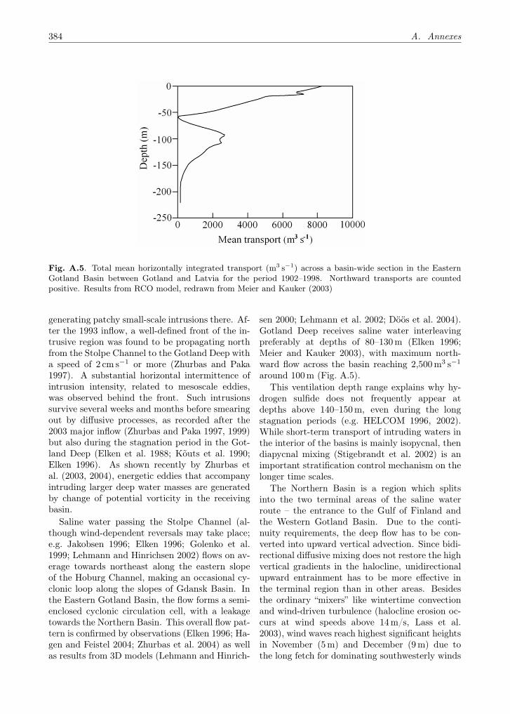
384 A. Annexes
Fig. A.5. Total mean horizontally integrated transport (m3 s−1) across a basin-wide section in the EasternGotland Basin between Gotland and Latvia for the period 1902–1998. Northward transports are countedpositive. Results from RCO model, redrawn from Meier and Kauker (2003)
generating patchy small-scale intrusions there. Af-ter the 1993 inflow, a well-defined front of the in-trusive region was found to be propagating northfrom the Stolpe Channel to the Gotland Deep witha speed of 2 cm s−1 or more (Zhurbas and Paka1997). A substantial horizontal intermittence ofintrusion intensity, related to mesoscale eddies,was observed behind the front. Such intrusionssurvive several weeks and months before smearingout by diffusive processes, as recorded after the2003 major inflow (Zhurbas and Paka 1997, 1999)but also during the stagnation period in the Got-land Deep (Elken et al. 1988; Kõuts et al. 1990;Elken 1996). As shown recently by Zhurbas etal. (2003, 2004), energetic eddies that accompanyintruding larger deep water masses are generatedby change of potential vorticity in the receivingbasin.
Saline water passing the Stolpe Channel (al-though wind-dependent reversals may take place;e.g. Jakobsen 1996; Elken 1996; Golenko et al.1999; Lehmann and Hinrichsen 2002) flows on av-erage towards northeast along the eastern slopeof the Hoburg Channel, making an occasional cy-clonic loop along the slopes of Gdansk Basin. Inthe Eastern Gotland Basin, the flow forms a semi-enclosed cyclonic circulation cell, with a leakagetowards the Northern Basin. This overall flow pat-tern is confirmed by observations (Elken 1996; Ha-gen and Feistel 2004; Zhurbas et al. 2004) as wellas results from 3D models (Lehmann and Hinrich-
sen 2000; Lehmann et al. 2002; Döös et al. 2004).Gotland Deep receives saline water interleavingpreferably at depths of 80–130m (Elken 1996;Meier and Kauker 2003), with maximum north-ward flow across the basin reaching 2,500 m3 s−1
around 100m (Fig. A.5).This ventilation depth range explains why hy-
drogen sulfide does not frequently appear atdepths above 140–150 m, even during the longstagnation periods (e.g. HELCOM 1996, 2002).While short-term transport of intruding waters inthe interior of the basins is mainly isopycnal, thendiapycnal mixing (Stigebrandt et al. 2002) is animportant stratification control mechanism on thelonger time scales.
The Northern Basin is a region which splitsinto the two terminal areas of the saline waterroute – the entrance to the Gulf of Finland andthe Western Gotland Basin. Due to the conti-nuity requirements, the deep flow has to be con-verted into upward vertical advection. Since bidi-rectional diffusive mixing does not restore the highvertical gradients in the halocline, unidirectionalupward entrainment has to be more effective inthe terminal region than in other areas. Besidesthe ordinary “mixers” like wintertime convectionand wind-driven turbulence (halocline erosion oc-curs at wind speeds above 14 m/s, Lass et al.2003), wind waves reach highest significant heightsin November (5 m) and December (9 m) due tothe long fetch for dominating southwesterly winds
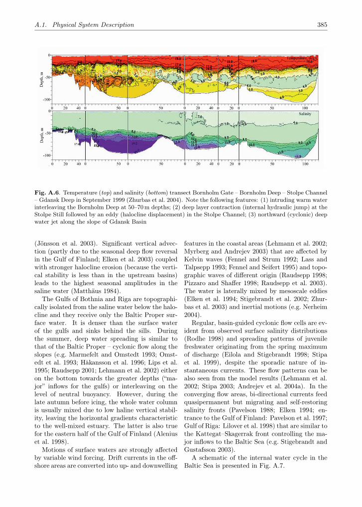
A.1. Physical System Description 385
Fig. A.6. Temperature (top) and salinity (bottom) transect Bornholm Gate – Bornholm Deep – Stolpe Channel– Gdansk Deep in September 1999 (Zhurbas et al. 2004). Note the following features: (1) intruding warm waterinterleaving the Bornholm Deep at 50–70 m depths; (2) deep layer contraction (internal hydraulic jump) at theStolpe Still followed by an eddy (halocline displacement) in the Stolpe Channel; (3) northward (cyclonic) deepwater jet along the slope of Gdansk Basin
(Jönsson et al. 2003). Significant vertical advec-tion (partly due to the seasonal deep flow reversalin the Gulf of Finland; Elken et al. 2003) coupledwith stronger halocline erosion (because the verti-cal stability is less than in the upstream basins)leads to the highest seasonal amplitudes in thesaline water (Matthäus 1984).
The Gulfs of Bothnia and Riga are topographi-cally isolated from the saline water below the halo-cline and they receive only the Baltic Proper sur-face water. It is denser than the surface waterof the gulfs and sinks behind the sills. Duringthe summer, deep water spreading is similar tothat of the Baltic Proper – cyclonic flow along theslopes (e.g. Marmefelt and Omstedt 1993; Omst-edt et al. 1993; Håkansson et al. 1996; Lips et al.1995; Raudsepp 2001; Lehmann et al. 2002) eitheron the bottom towards the greater depths (“ma-jor” inflows for the gulfs) or interleaving on thelevel of neutral buoyancy. However, during thelate autumn before icing, the whole water columnis usually mixed due to low haline vertical stabil-ity, leaving the horizontal gradients characteristicto the well-mixed estuary. The latter is also truefor the eastern half of the Gulf of Finland (Aleniuset al. 1998).
Motions of surface waters are strongly affectedby variable wind forcing. Drift currents in the off-shore areas are converted into up- and downwelling
features in the coastal areas (Lehmann et al. 2002;Myrberg and Andrejev 2003) that are affected byKelvin waves (Fennel and Strum 1992; Lass andTalpsepp 1993; Fennel and Seifert 1995) and topo-graphic waves of different origin (Raudsepp 1998;Pizzaro and Shaffer 1998; Raudsepp et al. 2003).The water is laterally mixed by mesoscale eddies(Elken et al. 1994; Stigebrandt et al. 2002; Zhur-bas et al. 2003) and inertial motions (e.g. Nerheim2004).
Regular, basin-guided cyclonic flow cells are ev-ident from observed surface salinity distributions(Rodhe 1998) and spreading patterns of juvenilefreshwater originating from the spring maximumof discharge (Eilola and Stigebrandt 1998; Stipaet al. 1999), despite the sporadic nature of in-stantaneous currents. These flow patterns can bealso seen from the model results (Lehmann et al.2002; Stipa 2003; Andrejev et al. 2004a). In theconverging flow areas, bi-directional currents feedquasipermanent but migrating and self-restoringsalinity fronts (Pavelson 1988; Elken 1994; en-trance to the Gulf of Finland: Pavelson et al. 1997;Gulf of Riga: Lilover et al. 1998) that are similar tothe Kattegat–Skagerrak front controlling the ma-jor inflows to the Baltic Sea (e.g. Stigebrandt andGustafsson 2003).
A schematic of the internal water cycle in theBaltic Sea is presented in Fig. A.7.

386 A. Annexes
Fig. A.7. A schematic of the large-scale internal water cycle in the Baltic Sea. The deep layer below thehalocline is given in the lower part of the figure. Green and red arrows denote the surface and bottom layercirculation, respectively. The light green and beige arrows show entrainment, the gray arrow denotes diffusion
A.1.2 Atmosphere
Hans-Jörg Isemer, Viivi Russak, Heikki Tuomen-virta
A.1.2.1 Atmospheric Circulation
The climate of the Baltic Sea Basin, located be-tween the 50th and 70th northern parallels in theEurasian continent’s coastal zone, is embedded inthe general atmospheric circulation system of thenorthern hemisphere, with its cyclonic circumpo-lar vortex providing for mean troposheric westerlyair flow with annually varying intensity (e.g. De-fant 1972). Strong westerly air flow provides formaritime, humid air mass transport in particularinto the southwestern and southern parts of thebasin, while in the east and north the maritimewesterly air flow is weakend due to friction anddrying processes providing for increasing continen-tal climate conditions.
The following two climatic types according toKöppen’s climate classification scheme dominatemuch of the Baltic Sea Basin: 1) Most of themiddle and northern parts of the basin are dom-inated by the temperate coniferous-mixed forestzone, with cold, wet winters, where the mean tem-
perature of the warmest month is not lower than10 C and that of the coldest month not higherthan −3 C, and where the rainfall is, on average,moderate in all seasons. 2) Much of the southwest-ern and southern region belongs to the marine westcoast climate, where prevailing west winds con-stantly bring in moisture from the oceans, and thepresence of a warm ocean current (the North At-lantic current system) provides for, in particular,moist and mild winters. Due to the influence of thewarm ocean currents on parts of mid- and northernEurope, the mean temperature of the Baltic SeaBasin is, on average, several degrees higher thanthat of other areas located in the same latitudes.In addition to the two climate types mentionedabove, the northeastern and eastern regions of thebasin are influenced by the moderate sub-arcticcontinental climate.
Major air pressure systems known to affect theweather and circulation in the Baltic Sea Basin arethe low-pressure system usually found near Iceland(Icelandic Low) and the high-pressure system inthe Azores Island region (Azores High). Also, thecontinental anticyclone over Russia may influenceclimate and circulation in the basin. The positionand strength of these systems vary on synoptictime scales, and any one of them can dominate
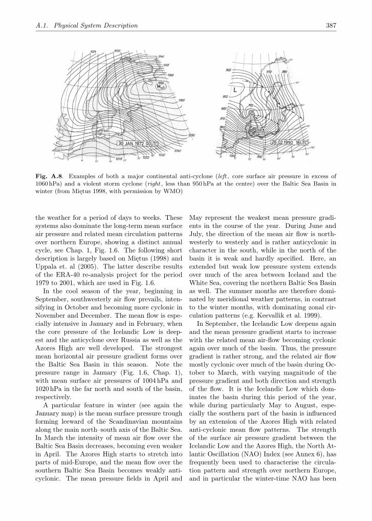
A.1. Physical System Description 387
Fig. A.8. Examples of both a major continental anti-cyclone (left , core surface air pressure in excess of1060 hPa) and a violent storm cyclone (right , less than 950 hPa at the centre) over the Baltic Sea Basin inwinter (from Miętus 1998, with permission by WMO)
the weather for a period of days to weeks. Thesesystems also dominate the long-term mean surfaceair pressure and related mean circulation patternsover northern Europe, showing a distinct annualcycle, see Chap. 1, Fig. 1.6. The following shortdescription is largely based on Miętus (1998) andUppala et. al (2005). The latter describe resultsof the ERA-40 re-analysis project for the period1979 to 2001, which are used in Fig. 1.6.
In the cool season of the year, beginning inSeptember, southwesterly air flow prevails, inten-sifying in October and becoming more cyclonic inNovember and December. The mean flow is espe-cially intensive in January and in February, whenthe core pressure of the Icelandic Low is deep-est and the anticyclone over Russia as well as theAzores High are well developed. The strongestmean horizontal air pressure gradient forms overthe Baltic Sea Basin in this season. Note thepressure range in January (Fig. 1.6, Chap. 1),with mean surface air pressures of 1004 hPa and1020 hPa in the far north and south of the basin,respectively.
A particular feature in winter (see again theJanuary map) is the mean surface pressure troughforming leeward of the Scandinavian mountainsalong the main north–south axis of the Baltic Sea.In March the intensity of mean air flow over theBaltic Sea Basin decreases, becoming even weakerin April. The Azores High starts to stretch intoparts of mid-Europe, and the mean flow over thesouthern Baltic Sea Basin becomes weakly anti-cyclonic. The mean pressure fields in April and
May represent the weakest mean pressure gradi-ents in the course of the year. During June andJuly, the direction of the mean air flow is north-westerly to westerly and is rather anticyclonic incharacter in the south, while in the north of thebasin it is weak and hardly specified. Here, anextended but weak low pressure system extendsover much of the area between Iceland and theWhite Sea, covering the northern Baltic Sea Basinas well. The summer months are therefore domi-nated by meridional weather patterns, in contrastto the winter months, with dominating zonal cir-culation patterns (e.g. Keevallik et al. 1999).
In September, the Icelandic Low deepens againand the mean pressure gradient starts to increasewith the related mean air-flow becoming cyclonicagain over much of the basin. Thus, the pressuregradient is rather strong, and the related air flowmostly cyclonic over much of the basin during Oc-tober to March, with varying magnitude of thepressure gradient and both direction and strengthof the flow. It is the Icelandic Low which dom-inates the basin during this period of the year,while during particularly May to August, espe-cially the southern part of the basin is influencedby an extension of the Azores High with relatedanti-cyclonic mean flow patterns. The strengthof the surface air pressure gradient between theIcelandic Low and the Azores High, the North At-lantic Oscillation (NAO) Index (see Annex 6), hasfrequently been used to characterise the circula-tion pattern and strength over northern Europe,and in particular the winter-time NAO has been

388 A. Annexes
shown to correlate with weather and climate inthe basin (e.g. Busuicoc et al. 2001; Cheng andHellström 1999; Jacobeit et al. 2001).
In summary, when westerly winds prevail, theweather may be warm and clear in much of, par-ticularly, the northern part of the basin due to the‘föhn’ phenomenon caused by the Scandinavianmountains. Despite the moderating effect of theocean, the Asian continental climate also extendsto the area at times, manifesting itself as severecold in winter and extreme heat in summer. Sincethe area is located in the zone of prevailing wester-lies where sub-tropical and polar air masses meet,weather types can change quite rapidly, particu-larly in winter. At synoptic time scales the indi-vidual air pressure and flow systems are drasticallyvariable and both storm cyclones and major con-tinental, sometimes long-lasting anticyclones maydominate the weather patterns in the region, seeFig. A.8.
A.1.2.2 Surface Air Temperature
The distribution of surface air temperature, Ta,is closely linked to the general climate and cir-culation regimes mentioned above. The generalnorth–south gradient is modulated by the south-west/northeast contrast of maritime versus conti-nental climate influences. In Fig. 1.9 (see Chap. 1),we show the annual cycle of Ta at four selected sta-tions which form a transect from north to souththrough the basin. Mean annual Ta differs bymore than 10 C in the Baltic Sea Basin. The cold-est regions are northeast Finland and the upper re-gions in the Scandinavian mountains, with meanannual surface air temperatures well below 0 C(e.g. −1 C in Sodankylä, and regions in northernSweden and Finland with mean annual Ta evenbelow −2 C). These are also the regions with thelargest amplitudes of the annual cycle (note themean July minus January difference of about 29 Cat Sodankylä, Fig. 1.9). The “most maritime” re-gion in the basin is the southwestern part (North-ern Germany and Denmark) of the basin, whichis less sheltered from the North Atlantic Ocean bythe Scandinavian mountains, where mean monthlyvalues of Ta exceed 0 C throughout the year (Mię-tus 1998, exemplified by the station Schleswig inFig. 1.9), but July mean temperatures are lowerthan in continental regions such as eastern Poland.
A.1.2.3 Precipitation
Precipitation in the Baltic Sea Basin shows botha distinct mean annual cycle and considerable re-gional variations. The latter are caused by theregionally varying circulation systems and the oro-graphic influence of the land surface. As forclouds, precipitation patterns over the Baltic Seamay differ considerably compared to land areas ofthe basin.
Recent estimates of the annual mean precipita-tion for the entire Baltic Sea Basin (both land andsea) vary between 620 mm/y (based on the Cli-mate Prediction Centre Merged Analysis of Pre-cipitation (CMAP) climatology, see e.g. Xie andArkin 1997) and 790mm/y (based on the GlobalPrecipitation Climatology Project (GPCP) clima-tology, see e.g. Huffman et al. 1997). Both es-timates given for the Baltic Sea Basin are refer-enced and discussed by Arpe et al. (2005), whoconcluded that the CMAP data are significantlyunderestimated while the GPCP estimates areslightly overestimated.
Both climatologies use a blend of gridded raingauge and satellite data. Earlier estimates basedexclusively on rain gauge data are mostly withinthe above-given range, e.g. the 728mm/y estimateof Kuusisto (1995), which is based on correcteddirect observations. Re-analysis products such asNCEP (e.g. Ruprecht and Kahl 2003) and NCEP-RII (e.g. Roads et al. 2002) yield 730mm/y and640 mm/y, respectively; however, re-analysis prod-ucts are known for several deficiencies which maycause significant biases in precipitation estimates(Ruprecht and Kahl 2003). Therefore, a reason-able current (i.e. for the recent 30 years) meanannual precipitation estimate is 750mm/y for theentire Baltic Sea Basin, including land and sea.
Rutgersson et al. (2001) give various estimatesof precipitation over the Baltic Sea. The SMHI(Swedish Meteorological and Hydrological Insti-tute) 1 degree gridded data set on the one handand estimates based on COADS (ComprehensiveOcean Atmosphere Data Set, see also Lindau2002) on the other hand, which are based on to-tally different data sources, agree astonishinglywell (600 and 606mm/y, respectively) and exhibita very similar annual cycle. Rutgersson et al.(2001) however present evidence that the SMHIdata may underestimate precipitation, because ofthe neglect of the rain gauges’ flow distortion andevaporation error correction. Based on the find-ings of Rubel and Hantel (1999, 2001), an annual
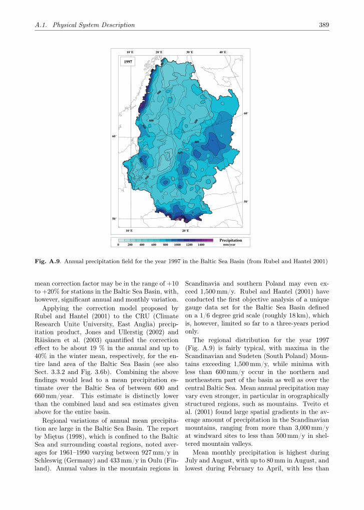
A.1. Physical System Description 389
200400
400
600
600
600
600
600
600
600
600
600
600
600
800800
800
800
800
800
800
800
800
800800
1000
1000
1000
1000
1200
1200
1200
1200
1400
1400
10 o E 20 o E 30 o E 40 o E
60 o
50 o
60 o
50 o
10 o E 20 o E
1997
0 200 400 600 800 1000 1200 1400 Precipitation
mm/year
Fig. A.9. Annual precipitation field for the year 1997 in the Baltic Sea Basin (from Rubel and Hantel 2001)
mean correction factor may be in the range of +10to +20% for stations in the Baltic Sea Basin, with,however, significant annual and monthly variation.
Applying the correction model proposed byRubel and Hantel (2001) to the CRU (ClimateResearch Unite University, East Anglia) precip-itation product, Jones and Ullerstig (2002) andRäisänen et al. (2003) quantified the correctioneffect to be about 19 % in the annual and up to40% in the winter mean, respectively, for the en-tire land area of the Baltic Sea Basin (see alsoSect. 3.3.2 and Fig. 3.6b). Combining the abovefindings would lead to a mean precipitation es-timate over the Baltic Sea of between 600 and660mm/year. This estimate is distinctly lowerthan the combined land and sea estimates givenabove for the entire basin.
Regional variations of annual mean precipita-tion are large in the Baltic Sea Basin. The reportby Miętus (1998), which is confined to the BalticSea and surrounding coastal regions, noted aver-ages for 1961–1990 varying between 927mm/y inSchleswig (Germany) and 433mm/y in Oulu (Fin-land). Annual values in the mountain regions in
Scandinavia and southern Poland may even ex-ceed 1,500 mm/y. Rubel and Hantel (2001) haveconducted the first objective analysis of a uniquegauge data set for the Baltic Sea Basin definedon a 1/6 degree grid scale (roughly 18 km), whichis, however, limited so far to a three-years periodonly.
The regional distribution for the year 1997(Fig. A.9) is fairly typical, with maxima in theScandinavian and Sudeten (South Poland) Moun-tains exceeding 1,500mm/y, while minima withless than 600 mm/y occur in the northern andnortheastern part of the basin as well as over thecentral Baltic Sea. Mean annual precipitation mayvary even stronger, in particular in orographicallystructured regions, such as mountains. Tveito etal. (2001) found large spatial gradients in the av-erage amount of precipitation in the Scandinavianmountains, ranging from more than 3,000mm/yat windward sites to less than 500 mm/y in shel-tered mountain valleys.
Mean monthly precipitation is highest duringJuly and August, with up to 80 mm in August, andlowest during February to April, with less than

390 A. Annexes
Janu
ary
Febr
uary
Mar
ch
Apr
il
May
June
July
Aug
ust
Sep
tem
ber
Oct
ober
Nov
embe
r
Dec
embe
r30
40
50
60
70
80
90
100
prec
ipita
tion
[mm
/mon
th]
Mean 1979-1998
Mean after Kuusisto, 1995
Fig. A.10. Annual cycle of precipitation calculated for the entire Baltic Sea Basin based on GPCP data(Huffman et al. 1997, thick line) and after Kuusisto (1995, dotted line), taken from Rubel and Hantel (2001).Vertical bars at the GPCP data indicate standard deviations of individual monthly values against the long-termmonthly means
45mm on average, see Fig. A.10. Figure A.10 alsoindicates inherent uncertainties even in our knowl-edge on long term means: While both data setsagree well during April to October, differences arenoticeable during winter months, with differencepeaks in December and January, which may be at-tributed at least partly to the different correctionalgorithms used for snow (Rubel and Hantel 2001).The interannual variability is large (Fig. A.10); thedetailed analyses of Rubel and Hantel (2001), forexample, yielded 646, 721 and 847mm/y in theyears 1996, 1997 and 1998, respectively.
A.1.2.4 Clouds
Changes and variability of clouds, as discussed inSect. 2.2 of this book, relate almost entirely to to-tal cloud cover, as “measured” by eye-observationsat synoptic stations. As with many other param-eters, information on mean annual and monthlycloud conditions is available either for individ-ual stations (e.g. Keevallik and Russak 2001; Ma-tuszko 2003) or only parts of the Baltic Sea Basin(e.g. Karlsson 2001; Raab and Vedin 1995).
Figure A.11 shows the annual cycle of totalcloud cover at different stations across the basinand for the Baltic Proper. For much of the basin,in particular the eastern continental part and alsofor much of the Baltic Sea, a prominent annual cy-cle with highest cloud amounts during winter and
lowest amounts during summer is clearly evident.Parts of the western and northern regions (mid-and northern Sweden and northern Finland in par-ticular) exhibit a reduced or almost no annual cy-cle (e.g. at Haparanda and Östersund, Fig. A.11).Karlsson (1999, 2001), using NOAA AVHRR dataover Scandinavia for 1991 to 2000, concluded that“with increasing distance from the central part ofthe Baltic Sea, the amplitude of the annual cycle ofcloudiness decreases for inland stations in Scandi-navia”. This is mostly due to the fact that duringsummer months no or little convective clouds formover the Baltic Sea, in contrast to the surroundingland areas. Areas in the Swedish mountains evenshow slightly higher values in summer comparedto winter. Karlsson (2001) showed distinct diurnaland inter-annual (Fig. 1.10, Chap. 1) variations oftotal cloudiness.
A.1.2.5 Surface Global Radiation
Global radiation, the solar radiation received by aunit horizontal surface, is usually measured at 1.5to 2m above the Earth’s surface. Its variation intime and space depends largely on solar elevationand length of day, both linked to the geographicallatitude of the site, and is considerably large in theBaltic Sea Basin. For example, in June, at 50◦ N,the sun is over the horizon for almost 16 hoursper day, while in the north at 70◦ N the polar day

A.1. Physical System Description 391
Fig. A.11. Mean annual cycle of total cloud cover (per cent) at various stations or regions in the Baltic SeaBasin. Red: Haparanda, northern Sweden; black: Östersund, mid-Sweden, both for 1951–2000 obtained fromSMHI (H. Alexandersson, pers. comm.); blue: for the Baltic Proper based on ship data for 1980 to 1992 (datataken from Isemer and Rozwadowska 1999); green: Lindenberg, eastern Germany (52.2◦ N/14.1◦ E) for 1951–2003 obtained from German Weather Service DWD (F. Beyrich, pers. comm.); and brown: Cracow, southernPoland for 1906–2000, redrawn from Matuszko (2003)
exists in this time. In winter, when in the southernpart of the basin the daylight lengths is about eighthours, the solar disk remains below the horizon inthe northern Baltic Sea Basin for weeks.
Besides these regular diurnal and annual cy-cles, the amount and genera of clouds are majorfactors determining the variations of global radi-ation across the basin. Totals of global radiationduring the warm season are higher in the coastalareas than in the hinterland. This is caused byless intensive formation and development of con-vective clouds over the sea and coastal region. An-other factor influencing the distribution of cloudsand, hence, global radiation is topography of theground. Favourable conditions for cloud forma-tion on slopes of mountain chains may result in adecrease of global radiation. On the other hand,on the elevated areas in mountains located higherthan the height of low clouds, global radiation usu-ally exceeds its value at lowland areas. The lat-ter is more evident during winter months. In thecold half year, global radiation may increase, re-sulting from multiple reflection of solar radiationbetween the surface and the atmosphere (base ofthe clouds) in regions with snow cover. Due to thehigh albedo of snow, monthly totals of global radi-
ation may increase by a factor of 1.4 to 1.8 (Toom-ing 2002). Global radiation may also be affectedby atmospheric transparency. Direct and diffuseradiations are highly sensitive to changes in atmo-spheric turbidity. But due to their opposite de-pendencies on transparency, the increase in globalradiation with increasing transparency is smaller.However, in highly polluted regions, totals of ra-diation may be noticeably smaller.
Unfortunately, long-term climatological solarradiation data for the Baltic Sea Basin are avail-able only for a small number of locations and par-ticularly few measurements are regularly made inthe northern regions. In December, monthly meanglobal radiation flux density varies between lessthan 15MJ/m2 north of about 65◦ N to more than90MJ/m2 in southern Poland with a rather strongorientation of isolines along latitudes. In June,the mean regional variation is between 550 and750MJ/m2, with a much stronger variation ac-cording to the difference between Baltic Sea versusland surfaces, and also according to the mountaineffect described above. Figure A.12 depicts 4 ex-amples of annual cycles of global radiation fluxdensities at different locations in the Baltic SeaBasin.

392 A. Annexes
Fig. A.12. Average global radiation (MJ/m2) at Sodankylä (northern Finland, 1971 to 2000), Tartu (Estonia,1981 to 2000), Lindenberg (eastern Germany, 1981 to 2000) and at the surface of the Baltic Proper (1980 to1992). The station data at Lindenberg, Tartu and Sodankylä are based on radiation measurements, while theBaltic Proper data set (taken from Rozwadowska and Isemer 1998) is based on parameterisations applied tocloud cover observations and humidity and air temperature measurements made aboard of voluntarily observingships
The contribution of diffuse radiation dependson cloudiness, surface albedo and turbidity of theatmosphere. The mean annual percentage of dif-fuse radiation to global radiation at the surfaceincreases from about 50% in the southern part ofthe basin to about 60–70% in the higher latitudes.This percentage of diffuse radiation varies season-ally: It is about 40–50% at 50–60◦ N in June, butmay reach about 80–90% in December (EuropeanSolar Radiation Atlas, Palz and Greif 1996).
A.1.3 Hydrology and Land Surfaces
Esko Kuusisto, Valery Vuglinsky, Raino Heino,Lev Kitaev
A.1.3.1 General Characteristics of the Baltic SeaBasin
The drainage area of the Baltic Sea (in this sec-tion also referred to as ‘Baltic Drainage’ or simply‘Drainage’), which is the land surface region of theBaltic Sea Basin, covers 1.74 million km2. It in-cludes territories from altogether 14 countries, thelargest areas belonging to Sweden (25.3%), Rus-sia (19.0%), Poland (17.8%) and Finland (17.4%).Three countries – Latvia, Lithuania and Estonia –
are completely within the Baltic Sea Basin, whileonly minor parts of Czech Republic, Germany,Norway, Slovakia and Ukraine drain towards theBaltic Sea.
The Baltic Sea Basin has about 80 lakes witha surface area larger than 100 km2. The numberof lakes larger than 1 km2 totals almost 10,000; ofthem 4,300 are located in Sweden and 2,300 in Fin-land. The total area of all lakes in the Baltic SeaBasin is around 123,000 km2 – one third of the areaof the Baltic Sea – and their volume 2,100 km3.
Forests cover about 54% of the Baltic Drainage.Agricultural land amounts to 26%, buildup land to4% (ECE 1993). Wetlands are a hydrologically im-portant feature of the Drainage; they still accountfor 20% of the total land area, although a consid-erable proportion of them have been drained andare today classified as forests or agricultural lands.
The climate varies considerably in the BalticDrainage (see also Annex 1.2.2). Long, cold win-ters dominate in the north, mean annual temper-atures being −2 . . . 0 C. In the southern part ofthe Drainage, thawing periods are frequent evenin midwinter, annual mean temperatures reachingup to 9 C. Precipitation is highest in the Scandesmountains, locally up to 2,000 mm/y, and exceed-
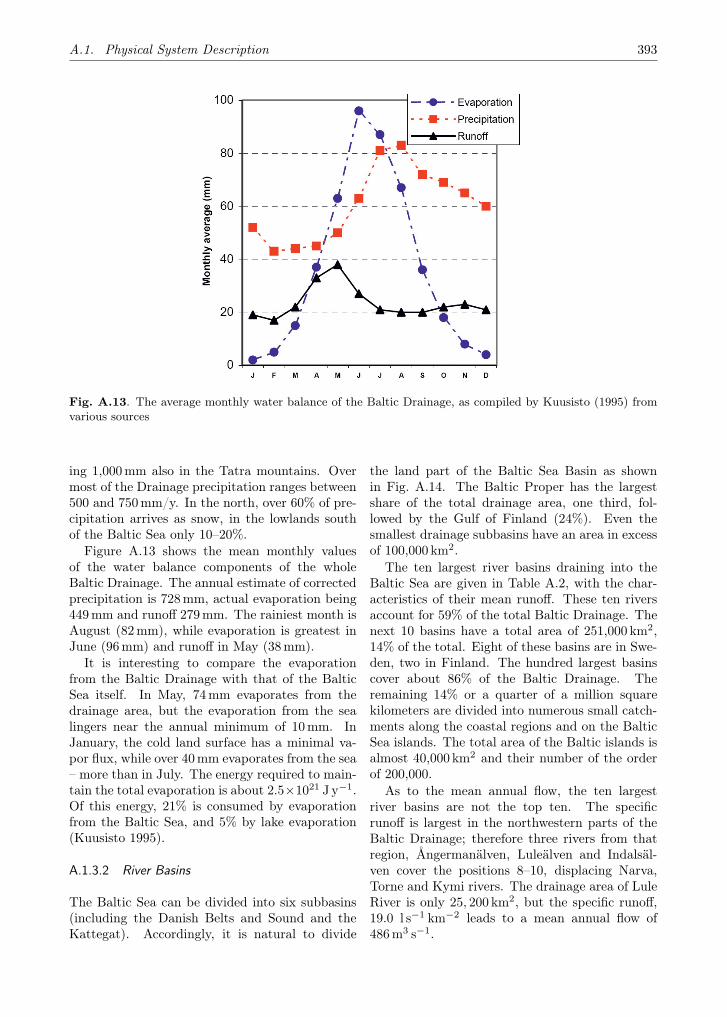
A.1. Physical System Description 393
Fig. A.13. The average monthly water balance of the Baltic Drainage, as compiled by Kuusisto (1995) fromvarious sources
ing 1,000mm also in the Tatra mountains. Overmost of the Drainage precipitation ranges between500 and 750mm/y. In the north, over 60% of pre-cipitation arrives as snow, in the lowlands southof the Baltic Sea only 10–20%.
Figure A.13 shows the mean monthly valuesof the water balance components of the wholeBaltic Drainage. The annual estimate of correctedprecipitation is 728mm, actual evaporation being449mm and runoff 279mm. The rainiest month isAugust (82mm), while evaporation is greatest inJune (96mm) and runoff in May (38mm).
It is interesting to compare the evaporationfrom the Baltic Drainage with that of the BalticSea itself. In May, 74mm evaporates from thedrainage area, but the evaporation from the sealingers near the annual minimum of 10mm. InJanuary, the cold land surface has a minimal va-por flux, while over 40mm evaporates from the sea– more than in July. The energy required to main-tain the total evaporation is about 2.5×10²¹ J y−1.Of this energy, 21% is consumed by evaporationfrom the Baltic Sea, and 5% by lake evaporation(Kuusisto 1995).
A.1.3.2 River Basins
The Baltic Sea can be divided into six subbasins(including the Danish Belts and Sound and theKattegat). Accordingly, it is natural to divide
the land part of the Baltic Sea Basin as shownin Fig. A.14. The Baltic Proper has the largestshare of the total drainage area, one third, fol-lowed by the Gulf of Finland (24%). Even thesmallest drainage subbasins have an area in excessof 100,000 km2.
The ten largest river basins draining into theBaltic Sea are given in Table A.2, with the char-acteristics of their mean runoff. These ten riversaccount for 59% of the total Baltic Drainage. Thenext 10 basins have a total area of 251,000 km2,14% of the total. Eight of these basins are in Swe-den, two in Finland. The hundred largest basinscover about 86% of the Baltic Drainage. Theremaining 14% or a quarter of a million squarekilometers are divided into numerous small catch-ments along the coastal regions and on the BalticSea islands. The total area of the Baltic islands isalmost 40,000 km2 and their number of the orderof 200,000.
As to the mean annual flow, the ten largestriver basins are not the top ten. The specificrunoff is largest in the northwestern parts of theBaltic Drainage; therefore three rivers from thatregion, Ångermanälven, Luleälven and Indalsäl-ven cover the positions 8–10, displacing Narva,Torne and Kymi rivers. The drainage area of LuleRiver is only 25, 200 km2, but the specific runoff,19.0 l s−1 km−2 leads to a mean annual flow of486m3 s−1.

394 A. Annexes
Fig. A.14. The subdivision of the Baltic Sea Basin, with areas and mean annual flows in 1950–1990 (fromBergström and Carlsson 1994)
Table A.2. The ten largest river basins of the Baltic Drainage. The runoff values refer to the period 1950–1990
River Drainage area (km2) Mean annual flow Specific runoff(m3 s−1) (l s−1 km−2)
Neva 281,000 2,460 8.8Vistula 194,400 1,065 5.5Odra 118,900 573 4.8Neman 98,200 632 6.4Daugava 87,900 659 7.5Narva 56,200 403 7.2Kemi 51,400 562 11.0Göta 50,100 574 11.5Torne 40,100 392 9.8Kymi 37,200 338 9.1
A.1. Physical System Description 395
A.1.3.3 Lakes and Wetlands
The total number of lakes in the Baltic Sea Basinmight be almost 400,000, most of them in Sweden,Finland and Russia. Poland has some 9,300 lakeswith surface areas over 1 ha; their total area isover 8,000 km2. Estonia has about 1,200 lakes,the largest completely within Estonian territory isVõrtsjärv, 270 km2. On the border of Estonia andRussia is the Lake Peipsi (3,555 km2), the largestinternational lake in Europe. Lithuania has 2,850lakes larger than 0.5 ha, covering 914 km2.
Looking into individual river basins, the RiverNeva has by far the largest lake area, almost50,000 km2, including two largest lakes in Eu-rope, Ladoga (18,130 km2) and Onega (9890 km2).As to the lake percentage, the basin of MotalaStröm (Sweden) is number one (22.3%), followedby Kymijoki (18.9%) and Göta älv (18.6%).
In addition to natural lakes, there are thou-sands of man-made ponds and reservoirs in theBaltic Sea Basin. Most of them are small ponds inPoland and the Baltic States, but the largest reser-voirs are in Sweden, with the exception of NarvaReservoir (200 km2) on the Estonian-Russianborder.
For centuries ago, all the countries around theBaltic Sea had large natural wetland areas. InDenmark, Germany, Latvia, Lithuania and Polandmost of the wetlands have been drained for agri-cultural purposes. Estonia and particularly Fin-land still have rather large natural wetlands. Innorthern Sweden exploitation has had a rela-tively small impact on wetlands, while utilisa-tion has been much more comprehensive farthersouth.
Even today the wetlands comprise one fifth ofthe Baltic Drainage. During the last few decades,the focus has changed from exploitation to conser-vation and preservation. Also the use of wetlandsin water quality issues, such as the retention ofnutrient leaching and cleaning of wastewater, hasbeen increasingly recognised.
A.1.3.4 Ice Regimes on Lakes and Rivers
Ice regimes in the water bodies (rivers and lakes)of the Baltic Sea Basin are formed predominantlyby the impact of Atlantic air masses producing awarming effect on the study area during the coldseason. The Baltic Sea itself stores much heatin wintertime and also warms the adjacent areas.Therefore, the closer the water body to the sea
coast, the later ice cover is formed and the earlierthe ice break-up occurs.
In the north, rivers are typically frozen in themiddle of October; rivers discharging to LakesLadoga and Onega are frozen in mid-November,and in southern and southeastern regions only latein December. In the rivers flowing towards thesouth-western coast of the Baltic Sea, permanentice cover may not be formed during some warmwinters. The duration of complete ice coverage inthe rivers flowing in the northern extremity of theBaltic Sea Basin may last 180 to 200 days. Icebreak-up in the rivers in the north usually occursearly in May; in the southeast of the area it hap-pens late in March. Mean long-term maximum icecover thickness on the rivers within the Baltic SeaBasin also differs greatly, depending on location.In the rivers discharging to the Gulf of Bothnia inthe north it may be 90 to 100 cm thick; in other re-gions such as the southeast of the Baltic Sea Basinit is no thicker than 30–40 cm.
Changes in ice regimes in lakes within the studyarea are similar to those in the rivers. But iceon lakes is usually formed later than that on therivers; ice break-up in lakes also occurs later.
On lakes in Poland (see e.g. Fig. 2.31), the icecover is formed in mid-November at the earliestand in mid-February at the latest. A considerablediversity was observed in mean dates of the icecover freeze-up depending on the lake depth. Theice cover formed earliest in the shallowest lakes(Lake Jeziorak – 12 December, Lake Lebsko – 19December) and at the latest in the deeper lakes(Lake Hancza – 2 January, Lake Charzykowskie –4 January). It is worth noting that the ice coveron Lake Studzieniczne froze up on the average 17days earlier than on Lake Hancza, which is only65 km away.
Ice characteristics of the Russian lakes differgreatly. This difference is mainly connected withthe lakes’ morphometry. The considerable influ-ence of the lakes’ morphometry is evident from thecomparison of the ice characteristics of the lakesLadoga and Onega. Mean ice cover duration, forexample, of the shallower Lake Onega is 20 dayslonger, and ice cover is 5 cm thicker.
A.1.3.5 Snow Cover
Snowfalls occur every winter in the Baltic SeaBasin and seasonal snow cover is formed exceptin the southwestern regions. Typical durations ofsnow cover over most areas are between four and
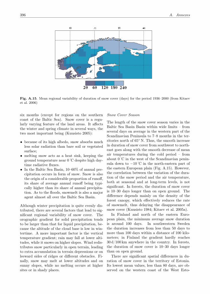
396 A. Annexes
Fig. A.15. Mean regional variability of duration of snow cover (days) for the period 1936–2000 (from Kitaevet al. 2006)
six months (except for regions on the southerncoast of the Baltic Sea). Snow cover is a regu-larly varying feature of the land areas. It affectsthe winter and spring climate in several ways, thetwo most important being (Kuusisto 2005):
• because of its high albedo, snow absorbs muchless solar radiation than bare soil or vegetatedsurface;
• melting snow acts as a heat sink, keeping theground temperature near 0 C despite high day-time radiative fluxes.
• In the Baltic Sea Basin, 10–60% of annual pre-cipitation occurs in form of snow. Snow is alsothe origin of a considerable proportion of runoff,its share of average annual runoff being typi-cally higher than its share of annual precipita-tion. As to the floods, snowmelt is also a majoragent almost all over the Baltic Sea Basin.
Although winter precipitation is quite evenly dis-tributed, there are several factors that lead to sig-nificant regional variability of snow cover. Theorographic gradient for solid precipitation tendsto be larger than that for liquid precipitation, be-cause the altitude of the cloud base is low in win-tertime. A more important factor is the verticaltemperature gradient; rain may fall at lower alti-tudes, while it snows on higher slopes. Wind redis-tributes snow particularly in open terrain, leadingto extra accumulation in terrain depressions or onleeward sides of ridges or different obstacles. Fi-nally, snow may melt at lower altitudes and onsunny slopes, while no melting occurs at highersites or in shady places.
Snow Cover Season
The length of the snow cover season varies in theBaltic Sea Basin Basin within wide limits – fromseveral days on average in the western part of theScandinavian Peninsula to 7–8 months in the ter-ritories north of 65◦ N. Thus, the smooth increasein duration of snow cover from southwest to north-east goes along with the smooth decrease of meanair temperatures during the cold period – fromabout 0 C in the west of the Scandinavian penin-sula down to −10 C in the north-eastern part ofthe eastern European plain (Fig. A.15). However,the correlation between the variation of the dura-tion of the snow period and the air temperature,both at seasonal and at long-term levels, is notsignificant. In forests, the duration of snow coveris 10–30 days longer than on open ground. Thedifference depends mainly on the density of theforest canopy, which effectively reduces the rateof snowmelt, thus delaying the disappearance ofsnow cover (Kuusisto 1984; Kitaev et al. 2005a).
In Finland and north of the eastern Euro-pean plain, the minimum average snow durationis around 100 days. In southwestern Swedenthe duration increases from less than 50 days tomore than 100 days within a distance of 100 kilo-meters; in Finland the gradient hardly reaches30 d/100 km anywhere in the country. In forests,the duration of snow cover is 10–30 days longerthan on open ground.
There are significant spatial differences in du-ration of snow cover in the territory of Estonia.Its lowest mean values, less than 80 days, are ob-served on the western coast of the West Esto-
A.1. Physical System Description 397
nian Archipelago, i.e. on the open coast of theBaltic Proper (Jaagus 1996, 1997; Tooming andKadaja 1999, 2000a,b). The highest mean dura-tion of snow cover, more than 130 days, is typicalfor north-eastern Estonia and for the uplands ofsouthern Estonia. Generally, snow cover durationincreases from west to east, similar to decreasingwinter air temperature.
Over the territory of Latvia there are remark-able spatial differences in snow cover duration:in the western part of Latvia along the coast ofthe Baltic Sea and in the proximity of the Gulfof Riga the duration is 70–90 days; it increasesto around 110 days moving away from the coast,and the longest snow duration, 114–134 days, isobserved in the uplands of eastern Latvia (Drave-niece 1998). In general, the duration of snow coverincreases from west to east-southeast, followingthe descending winter air temperature isotherms.
Snow Accumulation
In southern Sweden, maximum snow depths arebelow 20 cm, and it is below 40 cm in south-western Finland. Values exceeding 80 cm arereached everywhere north of the latitude 64◦ ex-cept along the coasts of the Gulf of Bothnia. InFinland and Russia the largest region with snowdepth exceeding this value extends from North-ern Karelia to south-eastern Lapland. The up-per slopes of the Scandinavian mountains in Swe-den typically have mean maximum snow depths of100–130 cm, while in Finland one meter is gener-ally exceeded only in the Kilpisjärvi area.
The smallest average maximum depths of snowcover in Poland are recorded in the western partof the country, at no more than 15 cm. The valuesgrow towards the northeast to more than 30 cm;in the mountains they generally increase with al-titude (depending strongly on the local topogra-phy). In the Tatra Mountains above the tree line,the average maximum seasonal snow depth ex-ceeds 150 cm and 200 cm at summits (Falarz 2004).
The water equivalent of snow is a hydrologi-cally much more important variable than the snowdepth. Although weather conditions during themelting period vary considerably from year toyear, the correlation coefficients between the max-imum areal water equivalent of snow and the vol-ume and peak of the spring flood are significant inalmost all major river basins in Fennoscandia.
In Finland in the period 1961–75, the meanmaximum water equivalent ranged from 80 to
140mm in the southern part and from 140 to200mm in the northern part (Kuusisto 1984). Upto the latitude of 66◦ N, the values were 40–60mmlarger in the eastern part of Finland than on thewestern coast. The year-to-year variation of max-imum water equivalent is highest in southwesternFinland, where the ratio between the high and lowmaximum water equivalent with a return period of20 years was 4–5, according to data used by Kuu-sisto (1984). In northern Finland the correspond-ing value was 1.6–2.0.
In Sweden, about one quarter of the countryhas mean maximum water equivalent in excess of200mm, while the corresponding fraction in Fin-land is only around 5 per cent. On the other hand,roughly one quarter of Sweden has less than 80 mmof water bound in snow cover during the maxi-mum accumulation; in Finland this fraction is alsoaround 5 per cent. In Norway, the countrywidesnow accumulation is still considerably more un-even than in Sweden. The variation of snow condi-tions from year to year is also quite large through-out Norway.
In western Estonia the mean maximum waterequivalent on fields remains below 50 mm, exceed-ing 70 mm in upland areas, and 90 mm in theHaanja region (Tooming and Kadaja 2000b). Themean maximum water equivalent in Poland ex-tends from below 30 mm in the west to above75 mm in the north-eastern part of the country;it is above 100/200mm in the highest part ofthe Sudeten/Carpathians, respectively (Sadowski1980).
Extreme Snow Conditions
In Finland the official record snow depth, 190 cm,was measured at the Kilpisjärvi climatological sta-tion on April 30th, 1997. It is clear that this valueis much lower than the true maximum in Finnishnature; accumulations of three to four meters arepossible in narrow gorges in the fjells of Laplandabove the tree line. Going further back in history,the snow cover of the winter of 1898–1899 was veryprobably much thicker than in any winter of the20th century. Snow depths exceeding 150 cm werereported from several observation sites in northernSavolax.
In Karelia (Russia), the maximum measuredsnow depth was recorded in the winter of 1983/84,when the average snow depth in March reached72 cm. Individual extreme measured values ofsnow depth in Karelia may reach 150 cm, which

398 A. Annexes
is more than twice the station standard deviationin this region. Both an increase in snow storageand in the number of winters with extreme snowdepth conditions were observed during the last twodecades (Kitaev et al. 2005b).
In Swedish lowlands, the highest official snowdepth is the same, 190 cm, as the record for Fin-land as a whole. This value was measured atDegersjö in Ångermanland, only 20 km from thecoast of the Gulf of Bothnia. Another coastal re-gion in Sweden with severe snowstorms is north-east Uppland (Dahlström 1995). In the Swedishfjells, snow depths in excess of two metres havebeen measured at all climatological stations be-tween the latitudes 62–68◦ N. The highest value,327 cm, was observed at Kopparåsen, 15 km eastof Riksgränsen, on the 28th of February in 1926.However, the variation of maximum snow depthis very high: There are winters when the maxi-mum remains clearly below one meter even at thesnowiest observations sites (Pershagen 1981).
Although the maximum snow depth of 77 cm asmean of route observation during the period 1962–2001 was recorded in Estonia on 20 December 1988in the Haanja upland, the winter periods 1981/82and 1965/66 can be considered as the snowiest,when the mean spatial (on the basis of land pointsof a 5 × 5 km grid) maximum water equivalentin February was 135.3 and 130.3mm, respectively(Tooming and Kadaja 2006). In Latvia, with abackground of average snow depth of 6–29 cm overthe territory, a high value, 126 cm, was observedin Gureli, Vidzeme Upland in the third decadeof March 1931. The variation of maximum snowdepth is very high: almost half of all winters arewarm and the others are colder than average oreven severe. There are years in Latvia with avery thin snow cover: going further back in his-tory such winters were 1948–1949, 1960–1961 and1971–1972. In the winter of 1972–1973 the depthof transitional snow cover was only 3–8 cm.
The absolute maximum of snow cover depth inPoland was observed in Dolina Pięciu Stawów Pol-skich (Tatras, 1670m a.s.l.; Falarz 2001). It was503 cm on March 26th 1967. It is highly probablethat the true maximum in highly located shieldedvalleys in the Tatras was much higher. Outsidethe mountains, the absolute maximum of snowcover depth was 85 (84) cm in Krakow (Suwałki)in February 1963 (1979). During the lowest-snowwinter seasons, the maximum snow depth did notexceed 10 cm in the lowlands, with some westernstations recording only 1–2 cm (Falarz 2004). In
the winter season 1991/92 in Słubice no snow coverof at least 1 cm depth was observed.
The maximum snow cover duration in south-western Poland (except for the mountains)reached 100 days, more than 140 days in thenortheastern region and 230–260 days in the TatraMountains above the tree line. In southern andeastern Poland, these maxima were recorded in thewinter of 1995/96, while in the rest of the coun-try, these maxima occured in the season 1969/70.There are permanent snow patches in the TatraMountains. The shortest snow cover duration inwestern Poland was just a few days per winterseason. Extremely short snow cover duration wasobserved in the winters of 1924/25, 1974/75 and1988/89.
A.2 The Late Quaternary Development ofthe Baltic Sea
Svante Björck
A.2.1 Introduction
Since the last deglaciation of the Baltic SeaBasin, which began 15,000–17,000 cal yr BP (cal-ibrated years Before Present) and ended 11,000–10,000 cal yr BP, the Baltic Sea Basin has under-gone many very different phases. The nature ofthese phases was determined by a set of forc-ing factors: a gradually melting Scandinavian IceSheet ending up into an interglacial environment,the highly differential glacio-isostatic uplift withinthe basin (from 9mm/yr to −1mm/yr; Ekman1996), changing the geographic position of thecontrolling sills (Fig. A.16), varying depths andwidths of the thresholds between the sea and theBaltic basin, and climate change. These fac-tors have caused large variations in salinity andwater exchange with the outer ocean, rapid togradual paleographic alterations with considerablechanges of the north-south depth profile with time.For example, the area north of southern Finland-Stockholm has never experienced transgressions,or land submergence, while the development southof that latitude has been very complex. The dif-ferent controlling factors are also responsible forhighly variable sedimentation rates, both in timeand space, and variations of the aquatic produc-tivity as well as faunal and floral changes. The ba-sic ideas in this article follow the lengthy, but lessup-dated version of the Baltic Sea history (Björck1995), a more complete reference list and, e.g., the

A.2. The Late Quaternary Development of the Baltic Sea 399
Fig. A.16. The Baltic Sea Basin, showing both land and submarine topography. The letters denote geograph-ical names used in the text. B = Billingen, Bl=Blekinge, D = Darss sill, F = Fehmarn Belt, G = Göta Älv rivervalley, GB = Great Belt, O = Otteid/Steinselva strait, S = Skagerrak, St = Stockholm, V= Lake Vättern andVn= Lake Vänern (by courtesy of Martin Jakobsson)
calendar year chronology of the different Baltic Seaphases can be found on the Internet1. Although Iwill focus on the postglacial history of the BalticSea in this restricted review, I think it is importantto inform the reader about the preceding stages tothe more modern Baltic Sea setting.
A.2.2 The Glacial to Late-Glacial Baltic Sea
Due to repetitive, more or less erosive, glacia-tions during the last glacial cycle, little de-tailed evidence exists about the glacial condi-tions in the Baltic before 15,000–14,000 cal yr BP.Based on lithostratigraphic correlations and alarge set of OSL (optically stimulated lumines-cence) and 14C dates, Houmark-Nielsen and Kjær(2003) have, however, indicated several ‘embry-onic’ glacial stages of the Baltic Sea during MIS3(Marine Isotope Stage 3 dated to about 25,000–60,000 cal yr BP). According to their model the dy-namic behavior of the southwestern part of the
1www.geol.lu.se/personal/seb/Maps%20of%20the-%20Baltic.htm
Scandinavian Ice Sheet between about 40,000–17,000 cal yr BP, produced several proglacial BalticIce lakes before the last Baltic Ice Lake proper be-tween about 15,000–11,600 cal yr BP (Björck 1995;Björck et al. 1996; Andrén et al. 1999). In-between glacial advances these proglacial stageshave been dated to about 40,000–35,000 and33,000–27,000 cal yr BP, but with changing con-figurations during these stages (Houmark-Nielsenand Kjær 2003). It is also postulated that thedeep northwest–southeast trending Esrum-Alnarpvalley, through Sjælland and Skåne, often func-tioned as the main connection between the BalticSea basin and the (glacio)marine waters of theKattegatt-Skagerrak. After the final advance sometime between 17,000–16,000 cal yr BP – the Öre-sund lobe (Kjær et al. 2003) – a rapid deglaciationof the southern Baltic Sea basin seems to havetaken place (Björck 1995; Lundqvist and Wohl-farth 2001; Houmark-Nielsen and Kjær 2003).
A proglacial lake – the Baltic Ice Lake (BIL) –was developed in front of the receding ice sheet.Due to glacial in-filling of the Esrum-Alnarp val-

400 A. Annexes
Fig. A.17. The configuration of the Baltic Ice Lake at about 14,000 cal yr BP. Note that the drainage throughÖresund and that today’s coast line is marked with a stiple line (from Björck 1995)
ley, the lowland in the Öresund region developedinto the connecting channel between the Baltic Seaand the sea in the northwest. Glaciolacustrine sed-iments, e.g., varved clays, were laid down in theBaltic as the ice sheet retreated northwards.
At this early stage of the BIL global sea levelwas situated at −100m (Lambeck and Chappell2001); more than 2/3 of the last glacial maximumice sheets still remained to be melted. Since the re-maining rebound of the loading effect from the icesheet was fairly small in the southernmost Baltic,the coast line was situated below today’s sea levelin southern Denmark, Germany and Poland. How-ever, further north both the total and remainingunloading effect – glacial isostatic uplift – waslarger than 100m, and therefore the coast linesof Sweden and the Baltic republics were above to-day’s sea level; the further north the higher.
As a consequence of the uplift the Öresundarea, which was now the threshold of the BIL,emerged faster than the rising sea level. Thisgradual shallowing of the outlet increased the ve-locity of the out-flowing water and thus also theerosion of the sill area. As long as loose Quater-nary deposits could be eroded, the erosion con-
tinued, and the present Öresund Strait was pos-sibly shaped, with the island of Ven being anerosional remnant of a previous till-covered land-scape. However, when the bedrock sill of flint-richbedrock between Malmö and Copenhagen was ex-posed, erosion ceased. The consequence of thiswas that the continuing uplift made the thresholdgradually shallower, until a critical water velocitywas reached. At this stage, about 14,000 cal yr BP(Fig. A.17), the water level inside the threshold,i.e. the BIL level, had to rise to compensate forthe decreased water depth of the sill. This causedthe BIL to rise above sea level; a gradually higherwater fall was created between the BIL level southof the threshold and sea level north of it. It alsomeant that coastal areas situated north of the Öre-sund isobase (isobases connect areas with the sameuplift/shoreline) continued to emerge, while areassouth of it submerged, the latter causing a trans-gression.
The melting Scandinavian Ice Sheet had astrong impact on the aquatic and sedimentary con-ditions in the Baltic; freshwater with a strongglacial influence produced clayey-silty sedimentsoften of varved (annual layering) type and with-

A.2. The Late Quaternary Development of the Baltic Sea 401
Fig. A.18. The configuration of the Baltic Ice Lake at about 13,000 cal yr BP. Note that it was drained northof Mt. Billingen and that Öresund was dry land. The arrow marks a possible subglacial drainage before Mt.Billingen was completely deglaciated (from Björck 1995)
out organic material. Diatoms are rarely foundin these sediments and it is doubtful if any faunaat all existed in this glacial lake. As the melt-ing continued northwards, an important water-shed melted out of the retreating ice sheet: theBillingen bedrock ridge in south central Swedenbetween the two large lakes Vättern and Vänern.The Billingen area almost formed a ‘wall’ betweenthe sea in the west and the up-dammed BIL in theeast.
However, when the ice retreated to thenorthern tip of Billingen around 13,000 cal yr BP(Fig. A.18), the BIL was drained west, initiallybeneath the ice. We think the BIL was loweredsome 10m at this event, but any morphologic ev-idence about this drainage would have been de-stroyed by the ice. The effect of the sudden lower-ing was that Öresund was abandoned as the out-flow and the BIL water flowed through the, at thetime glaciomarine, Vänern basin and out into theSkagerrak through several different valleys/fiords.However, there is no evidence from sediments thatsaline water managed to penetrate into the Baltic,east of Billingen.
At about 12,800 cal yr BP the North Atlantic re-gion experienced a fairly abrupt climatic change,the so-called Younger Dryas cooling. One effectof the lowered temperatures, especially in winter,was that the previously receding ice sheets of theregion began to expand again, and the Scandi-navian Ice Sheet advanced southwards to blockBillingen again. This would have dramatic effectson the BIL: the water level would once again riseabove sea level until Öresund began to function asthe outlet (Fig. A.19). This quick transgressionwould have continued slowly in areas south of thesill, while the remaining Baltic coasts experiencedregression, or emergence. The outlet/sill area wasstill rising quicker than the rising sea, which meantthat the BIL rose more and more above sea level;the waterfall in Öresund became gradually higher.During this time the sediments in the Baltic werestill very influenced by the glacial input, even inthe southern Baltic.
At the end of the Younger Dryas cool periodthe ice sheet started to retreat again, and some-time between 11,700 and 11,600 cal yr BP a second,and very dramatic, drainage occurred at Billin-
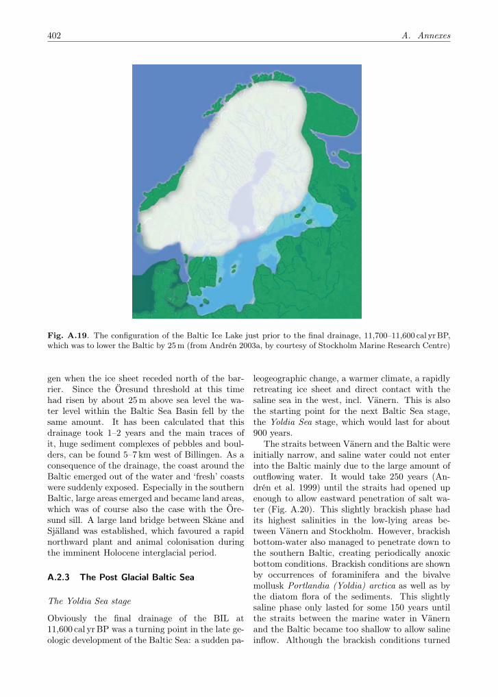
402 A. Annexes
Fig. A.19. The configuration of the Baltic Ice Lake just prior to the final drainage, 11,700–11,600 cal yr BP,which was to lower the Baltic by 25 m (from Andrén 2003a, by courtesy of Stockholm Marine Research Centre)
gen when the ice sheet receded north of the bar-rier. Since the Öresund threshold at this timehad risen by about 25 m above sea level the wa-ter level within the Baltic Sea Basin fell by thesame amount. It has been calculated that thisdrainage took 1–2 years and the main traces ofit, huge sediment complexes of pebbles and boul-ders, can be found 5–7 km west of Billingen. As aconsequence of the drainage, the coast around theBaltic emerged out of the water and ‘fresh’ coastswere suddenly exposed. Especially in the southernBaltic, large areas emerged and became land areas,which was of course also the case with the Öre-sund sill. A large land bridge between Skåne andSjälland was established, which favoured a rapidnorthward plant and animal colonisation duringthe imminent Holocene interglacial period.
A.2.3 The Post Glacial Baltic Sea
The Yoldia Sea stage
Obviously the final drainage of the BIL at11,600 cal yr BP was a turning point in the late ge-ologic development of the Baltic Sea: a sudden pa-
leogeographic change, a warmer climate, a rapidlyretreating ice sheet and direct contact with thesaline sea in the west, incl. Vänern. This is alsothe starting point for the next Baltic Sea stage,the Yoldia Sea stage, which would last for about900 years.
The straits between Vänern and the Baltic wereinitially narrow, and saline water could not enterinto the Baltic mainly due to the large amount ofoutflowing water. It would take 250 years (An-drén et al. 1999) until the straits had opened upenough to allow eastward penetration of salt wa-ter (Fig. A.20). This slightly brackish phase hadits highest salinities in the low-lying areas be-tween Vänern and Stockholm. However, brackishbottom-water also managed to penetrate down tothe southern Baltic, creating periodically anoxicbottom conditions. Brackish conditions are shownby occurrences of foraminifera and the bivalvemollusk Portlandia (Yoldia) arctica as well as bythe diatom flora of the sediments. This slightlysaline phase only lasted for some 150 years untilthe straits between the marine water in Vänernand the Baltic became too shallow to allow salineinflow. Although the brackish conditions turned

A.2. The Late Quaternary Development of the Baltic Sea 403
Fig. A.20. The configuration of the Yoldia Sea stage at 11,400–11,300 cal yr BP, when a short saline phase isabout to start. Note the large paleogeographic changes between Figs. A.19 and A.20 with the huge land-bridgein the south and the Närke Strait in the north (from Andrén 2003b, by courtesy of Stockholm Marine ResearchCentre)
into freshwater the Baltic was still at level withthe sea, and the sediments during the completeYoldia Sea stage were characterized by low organiccontent. As a contrast the western part of Vänernwas a fairly fauna-rich marine embayment (Fredén1986).
Owing to the on-going and still rapid uplift insouth central Sweden, the straits between Vänernand Skagerrak became gradually shallower, andeven some of them even emerged above sea level.The outflowing water from the Baltic had to passthrough Vänern and these straits, and in the endonly two straits functioned: the Göta Älv strait,which today is the Göta Älv river valley betweenVänern and Göteborg, and the Otteid/Steinselvastrait at the Swedish–Norwegian border east ofIdefjorden.
The Ancylus Lake stage
The gradual shallowing and narrowing of thesestraits resulted in increased water velocity in theseoutlets until a maximum was reached when they
could not ‘swallow’ the amount of water enteringthe Baltic Sea Basin (including meltwater from themelting ice sheet); the water level inside the nar-row straits had to rise to compensate for the de-creasing outflow area in the straits. Similar tothe up-damming of the Baltic Ice Lake, the wa-ter level had to rise in pace with the uplift of thesills/straits. South of the isobases for the outletregion this would result in a transgression, sincethe uplift here was smaller than the forced waterlevel rise, while to the north the situation wouldbe the opposite; a northwards increasing regres-sion. This tilting effect is the onset of the An-cylus Lake transgression, which started around10,700 cal yr BP.
The possibly already submerging coasts inthe southernmost Baltic experienced an increasedflooding, while the previously emerging coasts ofsouthern Sweden and the northern Baltic republicsnow changed into submergence. This sudden sub-mergence, or transgression, is witnessed by, e.g.,drowned pine forests east of Skåne and tree-ringanalyses show rapidly deteriorated living condi-

404 A. Annexes
Fig. A.21. The configuration of the Ancylus Lake stage at about 10,300 cal yr BP at the culmination of theAncylus transgression. Note the outlets west and southwest of Lake Vänern (from Andrén 2003c, by courtesyof Stockholm Marine Research Centre)
tions. The transgression is also clearly displayedby the Ancylus beach; a raised beach found inmany places in, e.g., southeast Sweden, on the is-land of Gotland, and in Latvia/Estonia showingtransgressive features.
The freshwater conditions with low primaryproductivity at the end of the Yoldia Sea andduring the Ancylus Lake, named after the fresh-water limpet Ancylus fluviatilis, resulted in goodmixing of water without permanent stratification.The sediments of the Ancylus Lake are also poorin organic material, and the further north themore glacially influenced they are. The amountof the Ancylus transgression varies between ar-eas/regions depending on the local uplift. Themaximum transgression probably occurred outsidethe Polish coast and amounted to about 20m,while a transgression of 10–12m characterisedthe Ancylus coast in the southwest, Denmark–Sweden–Germany. The latter amount was prob-ably also how much the Ancylus Lake was finallydammed-up above sea level. The transgressivephase of the Ancylus Lake lasted ca. 500 years,and was obviously governed by the possibility for
the Baltic water to find an alternative outflowarea. This meant that the transgression in thesouth continued as long as the constrained sillswest of Vänern functioned as outlets (Fig. A.21).
From independent studies we know that the An-cylus transgression ended abruptly with a fairlysudden lowering of the Baltic water level at about10,200 cal yr BP. The rate of the lowering, or re-gression, strongly implies that it is not only a grad-ual isostatic effect that shows up in the shore dis-placement curves, but rather a forced regression;the absolute water level fell. The most likely ex-planation for such a regression would be that theAncylus Lake level fell due to a lowering of thebase level. Since the base level was determined bythe sills/outlets, it would mean that the sill(s) waseroded.
We do, however, also know that the sills westof Vänern consist of crystalline bedrock, and it ishardly possible for water to suddenly erode 10 mof hard bedrock. It has therefore been assumedthat the water found a new outlet. Because ofthe transgression in the south, the most obviousthreshold/outlet candidate should be situated in

A.2. The Late Quaternary Development of the Baltic Sea 405
Fig. A.22. The configuration of the Ancylus Lake just prior to the first minor saline ingression at about10,000 cal yr BP. In comparison with Fig. A.21, note the regressive shore line as a consequence of both isostaticuplift and the lowering caused by the Ancylus drainage. Also note that Lake Vänern was no longer a part ofthe Ancylus Lake (from Jensen et al. 2002)
low-lying areas of the Danish–German area, whichis also characterized by lose Quaternary deposits.For a long time it has therefore been postulatedthat the water found its way over Darss Sill, intoMecklenburg Bay, over Fehmarn Belt and finallythrough the deep Great Belt, between the islandsof Själland and Fyn, the so-called Dana River.Parts of the submarine morphology along this pathhave been interpreted to be a remnant of such anerosive event.
However, recent German and Danish studies(e.g. Bennike et al. 1998; Jensen et al. 1999;Lemke et al. 1999) partly contradict such a sce-nario, although Bennike et al. (2004) recentlydated river deposits in the Great Belt channel toabout 10,200 cal yr BP, surrounded by levée andlake sediments. In fact, a compromise between therather dramatic picture of the Ancylus drainagepresented by Björck (1995) and Novak and Björck(1998) and the calm Danish–German solution maybe possible: an initial regression was caused by afew meters of erosion of the Darss Sill and pos-sibly also in the Great Belt channel lowering the
Baltic by up to 5m. This was followed by a fairlycalm fluvial phase; the gradient between the Kat-tegatt sea level and the Ancylus Lake level wasonly perhaps 5 m. As the region was now charac-terized by a rising sea level/base level this gradientdecreased and conditions gradually became evencalmer. We also know that the area outside themouth of the Great Belt channel in Kattegatt atthis time was not characterised by marine condi-tions, but was very influenced by freshwater (Ben-nike et al. 2004). Since the uplift of the area hadmore or less ceased, conditions were now controlledby the rapidly rising sea level (2–2.5 cm/yr). Itwould therefore last only 200–300 years before sealevel was at level with the Ancylus Lake, i.e. atabout 10,000 cal yr BP (Fig. A.22).
The transitional stage between the freshwaterof the Ancylus Lake and the following brackish-marine Littorina Sea (named after the marine gas-tropod Littorina littorea), named the Early Litto-rina Sea by Andrén et al. (2000), is also partlyan enigma. The first signs of marine influencehave usually been seen in sediments with an age

406 A. Annexes
of about 9,000 cal yr BP, usually in the southernBaltic area. This is also in accordance with thetime when we think that the Öresund Strait wasflooded by the global marine transgression; at thattime the sea level rise had exceeded the upliftrate in South Sweden. Therefore the youngerlimit of the Ancylus Lake, has often been setat about 8,500 cal yr BP, although geologists havebeen aware that the transition into the LittorinaSea is complex; the end of this transition stage hasoccasionally been named the Mastogloia Sea.
Lately, however, data from the Bornholm Basinand the archipelago of Blekinge in southeasternSweden imply that the first saline influence mayhave occurred already at about 9,800 cal yr BP(Andrén et al. 2000; Berglund et al. 2005).This indicates that saline water from Kattegatt,through the Great Belt–Fehmarn–Mecklenburg–Darss channel, could occasionally penetrate intothe Baltic fairly soon after the point in time whenthe rising sea level began to rise the Baltic level.However, this narrow and long outlet never did al-low large amounts of salt water into the Baltic. Itwould take another 1,500 years before a real ma-rine influence was felt inside the Baltic; then sealevel had finally reached up to the Öresund thresh-old between Limhamn and Dragør and a wide out-let/inlet area was created.
The Littorina Sea
If we disregard some of the uncertainties aboutthe initial outlet/inlet area during the Ancylus-Littorina transition, we can at least clearly docu-ment a rapid spread of saline influence throughoutthe Baltic basin around 8,500 cal yr BP. When thefirst clear signs of marine water appear, usuallydefining the onset of the Littorina Sea in the re-lated sediments, this is also usually reflected in thesediment composition as an increased organic con-tent. This implies that with the increased salineinfluence the aquatic primary productivity clearlyincreased in the Baltic. In the beginning of thisphase salinities were very low in the north, butbetween 8,500–7,500 cal yr BP the first and possi-bly most significant Littorina transgression set in.
The reason that the southern Baltic, up to ap-proximately the Stockholm–south Finland area,would experience transgressions during the forth-coming 2,500–3,000 years was that isostasy in thiswhole region was less rapid than the ongoing sealevel rise. While the causes for most of the sep-arate Littorina transgressions can possibly be re-
lated to sudden collapses of the Antarctic Ice Sheetand its huge ice shelves, the more or less steadilyrising sea level until 6,000 cal yr BP was mainlyan effect of the still melting North American icesheets. At this point in time the last remnants ofthe Labrador Ice Sheet melted.
During the first three successive Littorinatransgressions the water depths increased consid-erably (Berglund et al. 2005) in the, at the time,two functioning inlets, Öresund and Great Belt.The extent of these transgressions was in the or-der of at least 10 m in the inlet areas, with a largeincrease in water depth at any critical sill. In turn,this allowed a significant increase in the amount ofinflowing saline water into the Baltic, with highersalinities as an important consequence. The in-creasing salinity, in combination with the warmerclimate of the mid-Holocene, generated a fairly dif-ferent aquatic environment, compared to before.
In terms of richness and diversity of life, andtherefore also primary productivity, the biologicalculmination of the Baltic Sea was possibly reachedbetween 7,500–6,000 cal yr BP (Fig. A.23). Thehigh productivity, in combination with increasedstratification due to high salinities in the bot-tom water, caused anoxic conditions in the deeper(> 100m) parts of the Baltic Sea (Sohlenius et al.2001), especially in the central and northern partswith its larger distance to ‘fresh’ oxygenated At-lantic water.
A turning point in the Baltic development canbe seen after about 6,000 cal yr BP: the transgres-sive trend is broken around a large part of theBaltic coastline, although minor transgressionsmay have occurred until about 5,000 cal yr BP.While sea level had, generally speaking, ceased torise, the uplift pattern in the Baltic area was com-plex. In the southernmost Baltic area the sub-mergence continued, which meant that the trans-gression rate became less extensive than duringpeak Littorina time. In Sweden and along thecoast from northern Lithuania and northwards up-lift was still going on, which meant that the endof sea level rise resulted in a renewed regression.The regression caused shallower sills, which meantthat a gradually less amount of marine water couldenter the basin. Since the main sill areas, Öre-sund and Great Belt, are situated today aroundthe isobase −0.4mm/y (Ekman 1996), it impliesthat this shallowing ended perhaps a few hundredyears ago. Since then the inlet areas have becomeslightly deeper, causing more inflow of Atlanticwaters. Another consequence of the differential
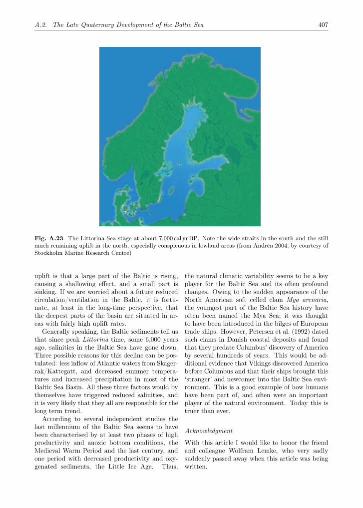
A.2. The Late Quaternary Development of the Baltic Sea 407
Fig. A.23. The Littorina Sea stage at about 7,000 cal yr BP. Note the wide straits in the south and the stillmuch remaining uplift in the north, especially conspicuous in lowland areas (from Andrén 2004, by courtesy ofStockholm Marine Research Centre)
uplift is that a large part of the Baltic is rising,causing a shallowing effect, and a small part issinking. If we are worried about a future reducedcirculation/ventilation in the Baltic, it is fortu-nate, at least in the long-time perspective, thatthe deepest parts of the basin are situated in ar-eas with fairly high uplift rates.
Generally speaking, the Baltic sediments tell usthat since peak Littorina time, some 6,000 yearsago, salinities in the Baltic Sea have gone down.Three possible reasons for this decline can be pos-tulated: less inflow of Atlantic waters from Skager-rak/Kattegatt, and decreased summer tempera-tures and increased precipitation in most of theBaltic Sea Basin. All these three factors would bythemselves have triggered reduced salinities, andit is very likely that they all are responsible for thelong term trend.
According to several independent studies thelast millennium of the Baltic Sea seems to havebeen characterised by at least two phases of highproductivity and anoxic bottom conditions, theMedieval Warm Period and the last century, andone period with decreased productivity and oxy-genated sediments, the Little Ice Age. Thus,
the natural climatic variability seems to be a keyplayer for the Baltic Sea and its often profoundchanges. Owing to the sudden appearance of theNorth American soft celled clam Mya arenaria,the youngest part of the Baltic Sea history haveoften been named the Mya Sea; it was thoughtto have been introduced in the bilges of Europeantrade ships. However, Petersen et al. (1992) datedsuch clams in Danish coastal deposits and foundthat they predate Columbus’ discovery of Americaby several hundreds of years. This would be ad-ditional evidence that Vikings discovered Americabefore Columbus and that their ships brought this‘stranger’ and newcomer into the Baltic Sea envi-ronment. This is a good example of how humanshave been part of, and often were an importantplayer of the natural environment. Today this istruer than ever.
Acknowledgment
With this article I would like to honor the friendand colleague Wolfram Lemke, who very sadlysuddenly passed away when this article was beingwritten.
408 A. Annexes
A.3 Ecosystem Description
A.3.1 Marine Ecosystem
A.3.1.1 The Seasonal Cycle of the Marine Ecosys-tems
Maiju Lehtiniemi
The specific characteristics of the Baltic Sea, itsshallowness, brackish water and partial ice coverduring winter, form a rather unique environmentfor the biota living in the sea. In addition, changesin salinity from south (almost seawater salinity) tonorth and east (near freshwater salinity) regulateeffectively the distribution of fauna and flora of lowdiversity. Permanent stratification, i.e. a haloclinebased on salinity differences between surface anddeep water, prevails in most of the Baltic Sea af-fecting the distribution of fauna. Water exchangeis restricted under the halocline, and thus bottomoxygen is often depleted, affecting animals livingin benthic habitats (Matthäus 1995). The Balticbiota is a mixture of marine and freshwater specieswith some genuine brackish water species (Remane1934). In addition to native species, the Baltic Seahosts about 100 nonindigenous species, more thanhalf of which have established reproducing popu-lations (Leppäkoski et al. 2002). The ecosystemchanges along latitudes and becomes simpler to-wards the north.
The location of the Baltic Sea at high lati-tudes affects the whole ecosystem through season-ality. Temperature and light conditions fluctuatealong the seasons, which regulate primary produc-tion and the length of the growing period, whichbecomes much shorter from the southern to thenorthern Baltic Sea. Annual ice cover in the north-ern parts, which shows large year-to-year varia-tions, requires special adaptations from all organ-isms.
Most of the invertebrates are specialised to livein either littoral, pelagic or benthic habitats, eachof which forms a distinct environment. However,food chains often overlap and these interrelatedfood chains are part of the broader food web. Cer-tain invertebrates, like mysid shrimps, utilise ef-fectively different systems, enhancing the energytransfer between them. In addition, fish, birds andmammals migrate/move regularly between differ-ent subsystems utilising them as feeding, winteringor spawning habitats. Millions of Arctic birds (wa-ter birds, geese, divers) migrate through the Baltic
Sea Basin twice a year on their migration be-tween Siberia and Europe. Hundreds of thousandsof them also overwinter in the Baltic Sea Basin,while most of the birds breeding in the Baltic SeaBasin, overwinter outside the area. Some of them,like Arctic Tern (Sterna paradisaea Pontoppidan),overwinter as far as on the Antarctic Ocean.
Spring Period – Intensive Primary Production andReproduction
Primary production and growth increase rapidlyduring spring when enough light reaches the sur-face waters, in the northern parts after the icebreak-up. Nutrients stored in the water columnduring winter are effectively utilised by the springbloom, which is mainly dominated by chain form-ing diatoms and dinoflagellates (Edler 1979; Lars-son et al. 1986). The highest biomasses are com-monly reached after a weak thermocline has devel-oped, which gives rise to a warmer well-lit surfacelayer. The development of thermal stratificationprevents mixing with deeper water layers and thussuppresses cell losses from the euphotic layer andgives the phytoplankton better survival opportu-nities.
The spring bloom declines after most of the ni-trate and phosphate are consumed from the wa-ter layer above the thermocline. After the bloom,most of the organic matter produced sinks out ofthe euphotic layer to the bottom because grazernumbers are still very low (Lignell et al. 1993).The most abundant species in the zooplanktoncommunity, which forms the next trophic level(Fig. A.24), are microprotozoans that have theirmaximum densities soon after the peak of the phy-toplankton bloom (Kivi 1986; Johansson et al.2004) and a few species of copepods and rotifers(Viitasalo et al. 1995; Möllmann et al. 2000).
The sedimenting organic material forms themain energy source for benthic secondary pro-duction (Kuparinen et al. 1984). The het-erotrophic benthic community is coupled to thepelagic and littoral systems through the seasonalpulse of sedimenting organic material. Suspen-sion feeders like barnacles (Balanus improvisusDarwin) and blue mussels (Mytilus edulis L.) onhard substrates or algae, and amphipods (Mono-poreia affinis Lindström, Pontoporeia femorataKröyer), isopods (Saduria entomon L.), bivalves(Macoma balthica L.) and polychaetes (e.g. Har-mothoe sarsi Kinberg, Marenzelleria viridis Ver-rill, Scoloplos armiger O.F. Müller) in/on the sed-

A.3. Ecosystem Description 409
Fig. A.24. Baltic Sea pelagic food web, grazing chain on the right and microbial loop on the left. The grazingchain prevails mainly under turbulent nutrient-rich circumstances e.g. during bloom periods (Kiørboe 1993)while the microbial loop dominates during summer in stratified conditions (Uitto et al. 1997) (from Vuorinen1994, figure by Juha Flinkman)
iment utilise the sinking organic material effec-tively. Mysid shrimps (Mysis mixta Lilljeborg,M. relicta Lovén), which are nektobenthic crus-taceans, feed omnivorously on abundant phyto-plankton and detritus and start to release theiryoung after the spring bloom (Salemaa et al. 1986;Rudstam and Hansson 1990; Viherluoto et al.2000). Also, many other invertebrates in thelittoral (e.g. Jaera sp. and prawns) and benthichabitats (e.g. M. affinis) release their young afterthe spring bloom (Segerstråle 1950). Zooplank-tivorous fish like Baltic herring (Clupea harengusmembras L.) and sprat (Sprattus sprattus L.) in-crease their feeding, which concentrates mainlyon large copepods (Fig. A.24; Möllmann et al.2004). Salmon smolts (Salmo salar L.) migratefrom spawning rivers to the coastal sea areasto feed on insects and invertebrates (Jutila andToivonen 1985).
Spring is the most active spawning time forBaltic fish. Sprat and cod (Gadus morhua L.) live
their whole life in the pelagial. They do not needcoastal waters, even at spawning, because theireggs and larvae are buoyant and thus survive inthe pelagial (Nissling and Westin 1991). Shal-low coastal areas are, however, favoured spawninggrounds of many littoral and pelagic fish species.For example herring, perch (Perca fluviatilis L.),roach (Rutilus rutilus Berg), pike (Esox lucius L.)and gobies (e.g. Pomatochistus spp.) lay eggson gravel or among macroalgae and macrophytes,which start their active growing period after win-ter. The littoral zone provides fish larvae withshelter, a diverse food supply and, thus, a goodstart for future growth (Urho 2002). Littoral areasare characterised by clear zonation, which gradu-ally changes from land to outer archipelagos andthe pelagial.
In the northern Baltic, shallow bays with standsof Phragmites australis (Cav.) and Charophytesare dominated by limnic fauna, while outer areaswith rocky shores covered with green and brown
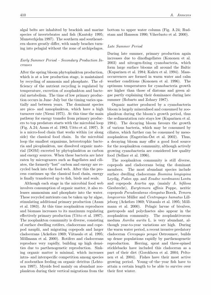
410 A. Annexes
algal belts are inhabited by brackish and marinespecies of invertebrates and fish (Kautsky 1995;Munsterhjelm 1997). The southern and southeast-ern shores greatly differ, with sandy beaches turn-ing into pelagial without the zone of archipelagos.
Early Summer Period – Secondary Production In-creases
After the spring bloom phytoplankton production,which is at a low production stage, is maintainedby recycling of ammonia and phosphate. The ef-ficiency of the nutrient recycling is regulated bytemperature, excretion of zooplankton and bacte-rial metabolism. The time of low primary produc-tion occurs in June–July but the timing varies spa-tially and between years. The dominant speciesare pico- and nanoplankton, which have a highturnover rate (Niemi 1975). At this time the mainpathway for energy transfer from primary produc-ers to top predators starts with the microbial loop(Fig. A.24; Azam et al. 1983; Uitto et al. 1997). Itis a micro-food chain that works within (or alongside) the classical food chain. In the microbialloop the smallest organisms, heterotrophic bacte-ria and picoplankton, use dissolved organic mate-rial (DOM) excreted by phytoplankton as carbonand energy sources. When these bacteria are latereaten by micrograzers such as flagellates and cili-ates, the formerly “lost” carbon and energy are re-cycled back into the food web. After this the pro-cess continues up the classical food chain, energyis finally transferred up to fish, birds and seals.
Although each stage in the microbial food webinvolves consumption of organic matter, it also re-leases ammonium and phosphate into the water.These recycled nutrients can be taken up by algae,stimulating additional primary production (Azamet al. 1983). At this time zooplankton reproducesand biomass increases to its maximum regulatingeffectively primary production (Uitto et al. 1997).The zooplankton community is diverse, consistingof surface dwelling rotifers, cladocerans and cope-pod nauplii, and migrating copepods and largercladocerans (Ackefors 1969; Viitasalo et al. 1995;Möllmann et al. 2000). Rotifers and cladoceransreproduce very rapidly, building up high densi-ties due to parthenogenetic reproduction. Sink-ing organic matter is minimal, which increasesintra- and interspecific competition among speciesof zoobenthos feeding on organic detritus (Lehto-nen 1997). Mysids feed mainly on abundant zoo-plankton during their vertical migrations from the
bottom to upper water column (Fig. A.24; Rud-stam and Hansson 1990; Viherluoto et al. 2000).
Late Summer Period
During late summer, primary production againincreases due to dinoflagellates (Kononen et al.2003) and nitrogen-fixing cyanobacteria, whichform large surface blooms all around the Baltic(Kuparinen et al. 1984; Kahru et al. 1994). Mass-occurrences are formed in warm water and calmweather conditions (Kononen et al. 1996). Theoptimum temperatures for cyanobacteria growthare higher than those of diatoms and green al-gae partly explaining their dominance during latesummer (Robarts and Zohary 1987).
Organic matter produced by a cyanobacteriabloom is largely mineralised and consumed by zoo-plankton during the bloom’s growth period, thusthe sedimentation rate stays low (Kuparinen et al.1984). The decaying bloom favours the growthof various bacteria, which may be consumed byciliates, which further can be consumed by meso-zooplankton (Engström-Öst et al. 2002). Thus,a decaying bloom may offer a good food sourcefor the zooplankton community, although activelygrowing cyanobacteria are considered low qualityfood (Sellner et al. 1996).
The zooplankton community is still diverse,copepods and cladocerans being the dominantmembers. The most abundant species includesurface dwelling cladocerans Bosmina longispinaLeydig, Podon spp. and Evadne nordmanni Lovénand copepods Acartia spp. (mainly A. bifilosaGiesbrecht), Eurytemora affinis Poppe, neriticcopepods Pseudocalanus elongatus Boeck, Temoralongicornis Müller and Centropages hamatus Lill-jeborg (Ackefors 1969; Viitasalo et al. 1995; Möll-mann et al. 2000). Pelagic larvae of bivalves,gastropods and polychaetes also appear in thezooplankton community. The zooplanktivorousmedusa Aurelia aurita L. is very abundant, al-though year-to-year variations are high. Duringthe warm water period, a recent invasive predatorycladoceran Cercopagis pengoi Ostroumov, buildsup dense populations rapidly by parthenogeneticreproduction. Herring, sprat and three-spinedsticklebacks have included this cladoceran as apart of their diet (Gorokhova et al. 2004; Pelto-nen et al. 2004). Fishes have their most activegrowing period. Young–of–the–year fish have toattain a certain length to be able to survive overtheir first winter.
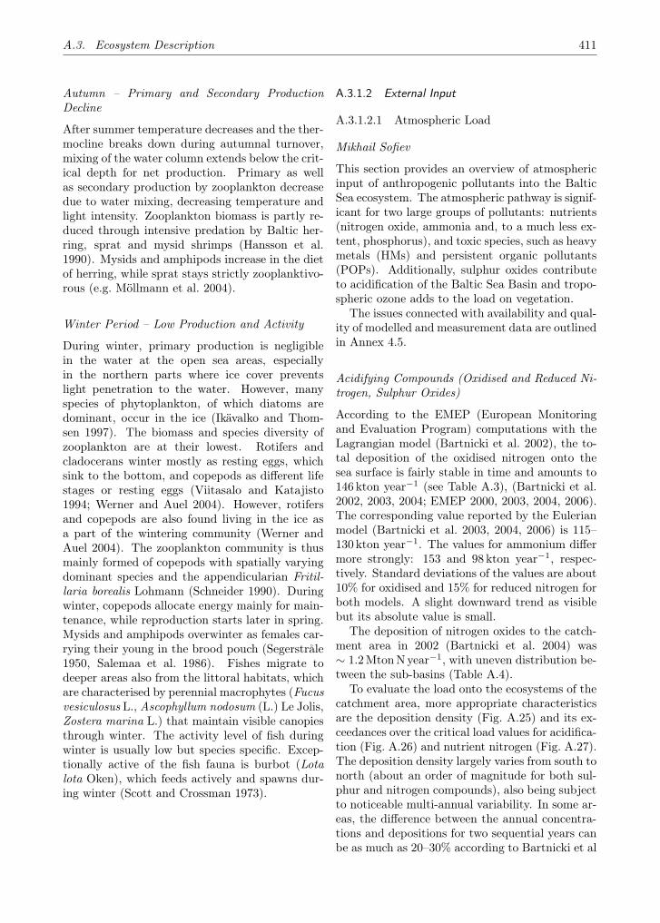
A.3. Ecosystem Description 411
Autumn – Primary and Secondary ProductionDecline
After summer temperature decreases and the ther-mocline breaks down during autumnal turnover,mixing of the water column extends below the crit-ical depth for net production. Primary as wellas secondary production by zooplankton decreasedue to water mixing, decreasing temperature andlight intensity. Zooplankton biomass is partly re-duced through intensive predation by Baltic her-ring, sprat and mysid shrimps (Hansson et al.1990). Mysids and amphipods increase in the dietof herring, while sprat stays strictly zooplanktivo-rous (e.g. Möllmann et al. 2004).
Winter Period – Low Production and Activity
During winter, primary production is negligiblein the water at the open sea areas, especiallyin the northern parts where ice cover preventslight penetration to the water. However, manyspecies of phytoplankton, of which diatoms aredominant, occur in the ice (Ikävalko and Thom-sen 1997). The biomass and species diversity ofzooplankton are at their lowest. Rotifers andcladocerans winter mostly as resting eggs, whichsink to the bottom, and copepods as different lifestages or resting eggs (Viitasalo and Katajisto1994; Werner and Auel 2004). However, rotifersand copepods are also found living in the ice asa part of the wintering community (Werner andAuel 2004). The zooplankton community is thusmainly formed of copepods with spatially varyingdominant species and the appendicularian Fritil-laria borealis Lohmann (Schneider 1990). Duringwinter, copepods allocate energy mainly for main-tenance, while reproduction starts later in spring.Mysids and amphipods overwinter as females car-rying their young in the brood pouch (Segerstråle1950, Salemaa et al. 1986). Fishes migrate todeeper areas also from the littoral habitats, whichare characterised by perennial macrophytes (Fucusvesiculosus L., Ascophyllum nodosum (L.) Le Jolis,Zostera marina L.) that maintain visible canopiesthrough winter. The activity level of fish duringwinter is usually low but species specific. Excep-tionally active of the fish fauna is burbot (Lotalota Oken), which feeds actively and spawns dur-ing winter (Scott and Crossman 1973).
A.3.1.2 External Input
A.3.1.2.1 Atmospheric Load
Mikhail Sofiev
This section provides an overview of atmosphericinput of anthropogenic pollutants into the BalticSea ecosystem. The atmospheric pathway is signif-icant for two large groups of pollutants: nutrients(nitrogen oxide, ammonia and, to a much less ex-tent, phosphorus), and toxic species, such as heavymetals (HMs) and persistent organic pollutants(POPs). Additionally, sulphur oxides contributeto acidification of the Baltic Sea Basin and tropo-spheric ozone adds to the load on vegetation.
The issues connected with availability and qual-ity of modelled and measurement data are outlinedin Annex 4.5.
Acidifying Compounds (Oxidised and Reduced Ni-trogen, Sulphur Oxides)
According to the EMEP (European Monitoringand Evaluation Program) computations with theLagrangian model (Bartnicki et al. 2002), the to-tal deposition of the oxidised nitrogen onto thesea surface is fairly stable in time and amounts to146 kton year−1 (see Table A.3), (Bartnicki et al.2002, 2003, 2004; EMEP 2000, 2003, 2004, 2006).The corresponding value reported by the Eulerianmodel (Bartnicki et al. 2003, 2004, 2006) is 115–130 kton year−1. The values for ammonium differmore strongly: 153 and 98 kton year−1, respec-tively. Standard deviations of the values are about10% for oxidised and 15% for reduced nitrogen forboth models. A slight downward trend as visiblebut its absolute value is small.
The deposition of nitrogen oxides to the catch-ment area in 2002 (Bartnicki et al. 2004) was∼ 1.2Mton Nyear−1, with uneven distribution be-tween the sub-basins (Table A.4).
To evaluate the load onto the ecosystems of thecatchment area, more appropriate characteristicsare the deposition density (Fig. A.25) and its ex-ceedances over the critical load values for acidifica-tion (Fig. A.26) and nutrient nitrogen (Fig. A.27).The deposition density largely varies from south tonorth (about an order of magnitude for both sul-phur and nitrogen compounds), also being subjectto noticeable multi-annual variability. In some ar-eas, the difference between the annual concentra-tions and depositions for two sequential years canbe as much as 20–30% according to Bartnicki et al

412 A. Annexes
Table A.3. Multi-annual deposition of pollutants onto the Baltic Sea surface (kton Nyear−1). L denotesresults from the EMEP Lagrangian, and E for the Eulerian model
1996L 1997L 1998L 1999L 2000L 2000E 2001E 2002E Aver.L Aver.E
NOx KtonN 140 138 158 150 145 147 128 113 146 129NHx KtonN 148 129 168 150 171 115 96 83 153 98N total. KtonN 288 267 326 300 316 262 224 196 299 227
Table A.4. Total nitrogen deposition onto the Baltic Sea catchment in 2002
N total, Kton N/year
Gulf of Bothnia Catchment 137Gulf of Finland Catchment 164Gulf of Riga Catchment 97Baltic Proper Catchment 698Belt Sea Catchment 54Kattegat Catchment 83Baltic Sea Catchment 1233
(2004, 2006). With regard to deposition variabil-ity, the precipitation amount and its distributionbetween the seasons plays one a major role.
For exceedances of acidification (Fig. A.26), thedownward trend is stronger – mainly due to reduc-tion of sulphur emission and, consequently, depo-sition during the last 20 years.
Comparison with HELCOM observations re-veals some spatial tendencies in the models’ qual-ity, which can be used to adjust the above esti-mates or at least evaluate their uncertainty.
For the Lagrangian model, comparison withmeasurements shows a spatially stochastic patternbut with an indication that the model overstatesthe deposition values for all years. The computedwet deposition is higher than the measured one for9 to 10 out of 14 HELCOM stations for both NOx
and NHx. The extent of over-estimation varies butcan be as much as a factor of 2 to 3 for some spe-cific stations and years. Therefore, the overall loadis probably also over-estimated.
For the Eulerian model, comparison for 2002shows that for most of southern Baltic Sae stations(DK5, DK8, DE9, EE9, PL4, SE11) the concen-trations of both oxidised and reduced nitrogen inprecipitation are overstated by the model by 20–50%. Such over-estimation is not visible for north-ern stations, which are located in less polluted ar-eas. There is no such tendency for concentrationsin air, which generally demonstrate a good agree-ment with observed levels.
There can be two reasons for such a trend: spa-tially inhomogeneous quality of precipitation in-formation and some nuances in parameterisationof scavenging. According to the EMEP status re-port 1/2004 (EMEP 2004), accumulated precipita-tion amount does not have a pronounced bias (al-though the difference for some stations can exceeda factor of 2). It is therefore possible to suggestthat the Eulerian model over-estimates by ∼ 20%the deposition onto the most-polluted sub-basinsof the Baltic Sea (Kattegat, Belt Sea, Gulf of Riga,southern-most part of the Baltic Proper) and is onaverage unbiased for the other sub-basins. Due tocomparatively small areas with such overestima-tion (Kattegat, Belt Sea and Gulf of Riga com-bined take ∼ 20% of the total deposition onto thesea surface), the overall over-estimation can hardlybe more than 5%. Comparison for 2001 leads toan even smaller number.
Within the scope of the EU project BalticSea System Study (BASYS) and a follow-up re-search, similar-type modelling assessments weremade using a semi-independent Eulerian modelHILATAR (Hongisto et al. 2003; Hongisto andJoffre 2005). This model, accepting the EMEPchemistry module, emission totals and, for partof the simulations, boundary conditions from theEMEP Lagrangian model, used a different advec-tion method, meteorological data and own timevariation of emission. The results appeared to bequite similar (Table A.5): mean total nitrogen de-

A.3. Ecosystem Description 413
Table A.5. Results of a semi-independent model study within the BASYS project
1993 1994 1995 1996 1997 1998 2000 2001 2002 Average
NOx Kton N 175 169 150 144 139 179 159NHx Kton N 115 103 105 114 99 117 109N total. Kton N 290 272 255 258 238 296 274 263 224 268
Fig. A.25. Map of total sulphur (upper left ), oxidised nitrogen (upper right ) and reduced nitrogen (lower)deposition in 2004. Unit is (mg S/N m−2 year−1) (from EMEP 2006)
position of 263 ktons year−1 for the period 1993–2002. The values are in between the results ofthe EMEP Eulerian and Lagrangian models, withNOx load being almost exactly on the half-way andNHx staying closer to the Eulerian model results.
Regarding the deposition density, the esti-mates for 1993–1998 showed practically the samemean value for sulphur oxides (for the Polishcoastline, the HILATAR model showed about1 g S m−2 year−1) but somewhat higher nitro-
gen values (total nitrogen amounted to 1.2–1.4 g Nm−2 year−1). The standard deviations ofthe monthly deposition values were 30–40% with atendency to grow towards the north. The compar-ison with measurements showed a limited overes-timation of the NOx wet deposition by HILATAR,while the ammonia fluxes are practically unbiased.
Another model-based estimate of Hertel etal. (2003) for 1999 resulted in slightly over300 ktons Nyear−1 of total nitrogen deposited onto
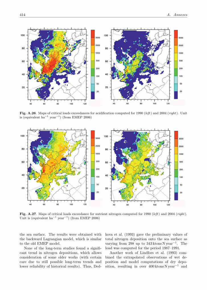
414 A. Annexes
Fig. A.26. Maps of critical loads exceedances for acidification computed for 1990 (left ) and 2004 (right ). Unitis (equivalent ha−1 year−1) (from EMEP 2006)
Fig. A.27. Maps of critical loads exceedance for nutrient nitrogen computed for 1990 (left ) and 2004 (right ).Unit is (equivalent ha−1 year−1) (from EMEP 2006)
the sea surface. The results were obtained withthe backward Lagrangian model, which is similarto the old EMEP model.
None of the long-term studies found a signifi-cant trend in nitrogen depositions, which allowsconsideration of some older works (with certaincare due to still possible long-term trends andlower reliability of historical results). Thus, Ded-
kova et al. (1993) gave the preliminary values oftotal nitrogen deposition onto the sea surface asvarying from 298 up to 343 ktons Nyear−1. Theload was computed for the period 1987–1991.
Another work of Lindfors et al. (1993) com-bined the extrapolated observations of wet de-position and model computations of dry depo-sition, resulting in over 400 ktons N year−1 and

A.3. Ecosystem Description 415
1.4–1.9 gNm−2 year−1 for total nitrogen deposi-tion at the southern Baltic coast (average over 7years 1980–1986). The total deposition onto thesea surface, however, can be challenged due to un-clear representativeness of coastal deposition mea-surements offshore.
The deposition of 0.5 g Nm−2 year−1 of oxidisednitrogen at the southern Baltic coast was also re-ported by MATCH model computations (Laurilaet al. 2004). That work has also considered po-tential developments of the situation in the futureclimate and predicted small and irregular changesin the pattern – the difference of the depositionvalues computed for various emission and climatescenarios from the reference estimates was mainlywithin 10%.
Studies of Sofiev and Grigoryan (1996) andSofiev et al. (1996) gave the values at the Polishcoast of 0.6–0.7mgNm−2 year−1 for oxidised and0.5mg Nm−2 year−1 for reduced nitrogen. The es-timates were computed by three different versionsof an independent model for the period 1991–94and appeared quite coherent.
It is seen that the results of the EMEP La-grangian model and decade-old independent as-sessments are quite close to each other, while theEulerian-model is closer to more modern applica-tions.
The following can therefore be concluded:
(i) Annual total deposition of oxidised nitrogenonto the Baltic Sea surface is 125± 20 kton Nyear−1 (a standard deviation range); for am-monia this estimate is 100±16 kton N year−1;
(ii) The deposition density varies from 0.5–0.6 gNm−2 year−1 at the southern coastdown to about 0.05 g Nm−2 year−1 in thenorth – for both oxidised and reduced ni-trogen (though ammonia trend is more pro-nounced). For oxidised sulphur compoundsthe present-time values are ∼ 1 g S m−2
year−1 and 0.1 g S m−2 year−1, respectively;
(iii) Inter-annual variability is comparativelysmall and has a standard deviation of 10–15%,thus accounting for the most of above uncer-tainty range;
(iv) No statistically significant trend for nitrogenoxides was observed by the above studies,while sulphur emission and deposition havestrongly decreased;
Table A.6. A share of deposition obtained by eachsub-basin of the Baltic Sea
NOx NHx
Belt Sea 8 14Kattegat 8 10Baltic Proper 58 54Gulf of Riga 4 4Gulf of Finland 6 4Gulf of Botnia 16 13
(v) A large spatial gradient of depositions is no-ticed by all computations. The typical distri-bution of deposition to the sea sub-basins ispresented in Table A.6
Tropospheric Ozone
There are several European models regularly com-puting the ozone level and its exceedance of thethresholds. The model formulations and their re-sults were extensively compared with each other,which allowed to derive consensus-based assess-ments of the present ozone level and its impor-tance for the Baltic Sea Basin (e.g. Roemer et al.2003; Hass et al. 2003; Laurila et al. 2004; Zlatevet al. 2002).
It is generally agreed that a high ozone levelduring the vegetation season is not yet a matterof primary concern for the Baltic Sea ecosystems,except for the most southwestern areas (Germanyand Denmark). It can, however, become more sig-nificant in future climate (Laurila et al. 2004). Atpresent, the maximum value for the AOT-40 ozoneindex (Accumulated Ozone above the Thresholdof 40 ppb) reaches 10 ppm-hours only in centralPoland and in Germany, which is still several timeslower than in the other parts of Europe. How-ever, there are warnings of a possible change ofthe situation due to warmer climate and increasingemissions. In particular, this problem can becomesevere if strongly increasing amounts of ozone inother parts of the Northern Hemisphere will be ad-vected towards the region (Derwent et al. 2002).
Toxic Species
Information about the toxic species is much lessprecise than that for nitrogen – both from observa-tional and from modelling points of view. All datacan be criticised for problems with quality and reli-
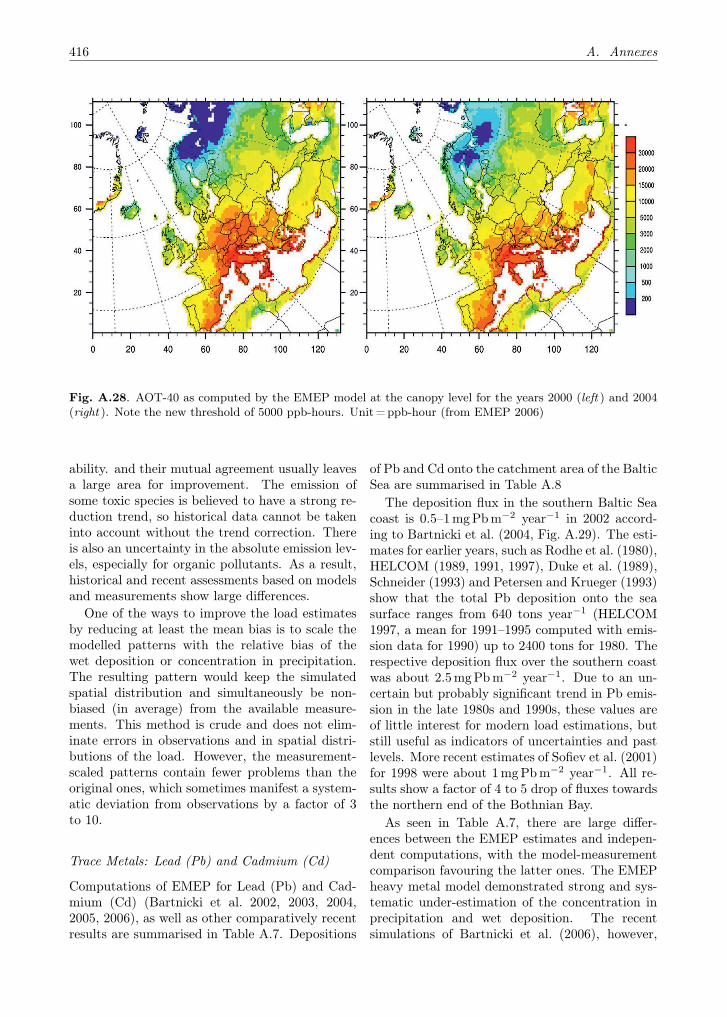
416 A. Annexes
Fig. A.28. AOT-40 as computed by the EMEP model at the canopy level for the years 2000 (left ) and 2004(right ). Note the new threshold of 5000 ppb-hours. Unit = ppb-hour (from EMEP 2006)
ability. and their mutual agreement usually leavesa large area for improvement. The emission ofsome toxic species is believed to have a strong re-duction trend, so historical data cannot be takeninto account without the trend correction. Thereis also an uncertainty in the absolute emission lev-els, especially for organic pollutants. As a result,historical and recent assessments based on modelsand measurements show large differences.
One of the ways to improve the load estimatesby reducing at least the mean bias is to scale themodelled patterns with the relative bias of thewet deposition or concentration in precipitation.The resulting pattern would keep the simulatedspatial distribution and simultaneously be non-biased (in average) from the available measure-ments. This method is crude and does not elim-inate errors in observations and in spatial distri-butions of the load. However, the measurement-scaled patterns contain fewer problems than theoriginal ones, which sometimes manifest a system-atic deviation from observations by a factor of 3to 10.
Trace Metals: Lead (Pb) and Cadmium (Cd)
Computations of EMEP for Lead (Pb) and Cad-mium (Cd) (Bartnicki et al. 2002, 2003, 2004,2005, 2006), as well as other comparatively recentresults are summarised in Table A.7. Depositions
of Pb and Cd onto the catchment area of the BalticSea are summarised in Table A.8
The deposition flux in the southern Baltic Seacoast is 0.5–1mgPb m−2 year−1 in 2002 accord-ing to Bartnicki et al. (2004, Fig. A.29). The esti-mates for earlier years, such as Rodhe et al. (1980),HELCOM (1989, 1991, 1997), Duke et al. (1989),Schneider (1993) and Petersen and Krueger (1993)show that the total Pb deposition onto the seasurface ranges from 640 tons year−1 (HELCOM1997, a mean for 1991–1995 computed with emis-sion data for 1990) up to 2400 tons for 1980. Therespective deposition flux over the southern coastwas about 2.5mgPb m−2 year−1. Due to an un-certain but probably significant trend in Pb emis-sion in the late 1980s and 1990s, these values areof little interest for modern load estimations, butstill useful as indicators of uncertainties and pastlevels. More recent estimates of Sofiev et al. (2001)for 1998 were about 1mgPb m−2 year−1. All re-sults show a factor of 4 to 5 drop of fluxes towardsthe northern end of the Bothnian Bay.
As seen in Table A.7, there are large differ-ences between the EMEP estimates and indepen-dent computations, with the model-measurementcomparison favouring the latter ones. The EMEPheavy metal model demonstrated strong and sys-tematic under-estimation of the concentration inprecipitation and wet deposition. The recentsimulations of Bartnicki et al. (2006), however,
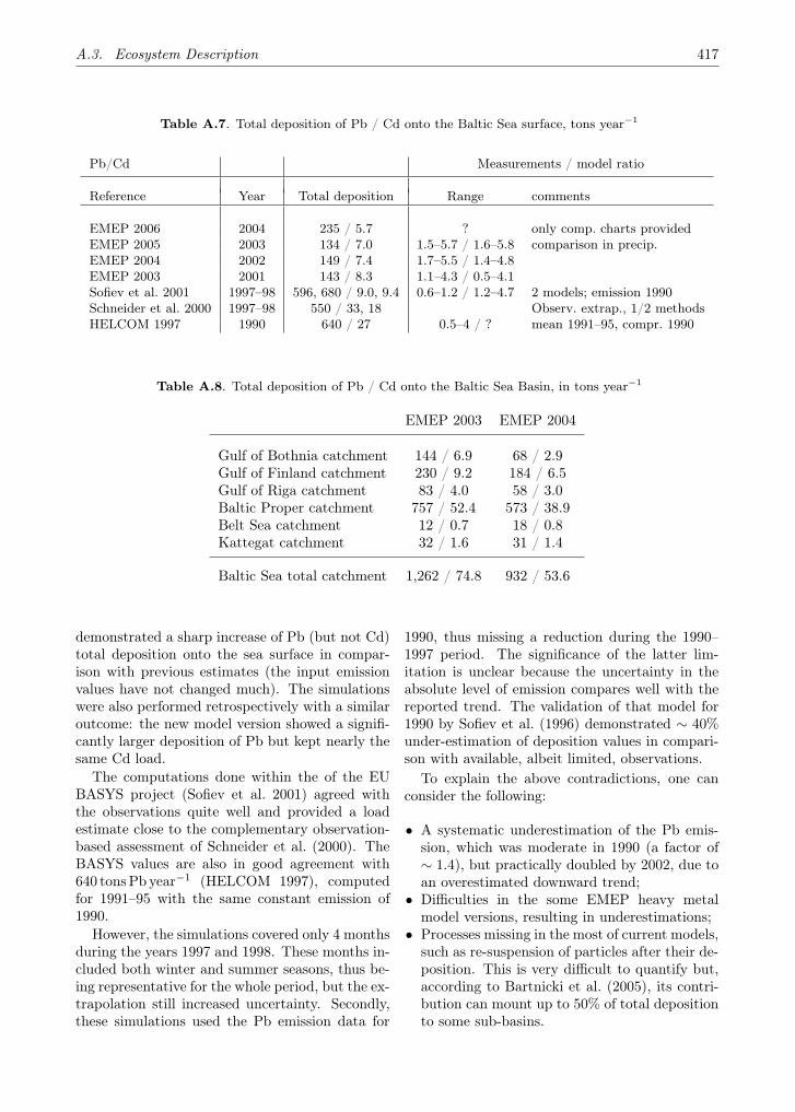
A.3. Ecosystem Description 417
Table A.7. Total deposition of Pb / Cd onto the Baltic Sea surface, tons year−1
Pb/Cd Measurements / model ratio
Reference Year Total deposition Range comments
EMEP 2006 2004 235 / 5.7 ? only comp. charts providedEMEP 2005 2003 134 / 7.0 1.5–5.7 / 1.6–5.8 comparison in precip.EMEP 2004 2002 149 / 7.4 1.7–5.5 / 1.4–4.8EMEP 2003 2001 143 / 8.3 1.1–4.3 / 0.5–4.1Sofiev et al. 2001 1997–98 596, 680 / 9.0, 9.4 0.6–1.2 / 1.2–4.7 2 models; emission 1990Schneider et al. 2000 1997–98 550 / 33, 18 Observ. extrap., 1/2 methodsHELCOM 1997 1990 640 / 27 0.5–4 / ? mean 1991–95, compr. 1990
Table A.8. Total deposition of Pb / Cd onto the Baltic Sea Basin, in tons year−1
EMEP 2003 EMEP 2004
Gulf of Bothnia catchment 144 / 6.9 68 / 2.9Gulf of Finland catchment 230 / 9.2 184 / 6.5Gulf of Riga catchment 83 / 4.0 58 / 3.0Baltic Proper catchment 757 / 52.4 573 / 38.9Belt Sea catchment 12 / 0.7 18 / 0.8Kattegat catchment 32 / 1.6 31 / 1.4
Baltic Sea total catchment 1,262 / 74.8 932 / 53.6
demonstrated a sharp increase of Pb (but not Cd)total deposition onto the sea surface in compar-ison with previous estimates (the input emissionvalues have not changed much). The simulationswere also performed retrospectively with a similaroutcome: the new model version showed a signifi-cantly larger deposition of Pb but kept nearly thesame Cd load.
The computations done within the of the EUBASYS project (Sofiev et al. 2001) agreed withthe observations quite well and provided a loadestimate close to the complementary observation-based assessment of Schneider et al. (2000). TheBASYS values are also in good agreement with640 tons Pb year−1 (HELCOM 1997), computedfor 1991–95 with the same constant emission of1990.
However, the simulations covered only 4 monthsduring the years 1997 and 1998. These months in-cluded both winter and summer seasons, thus be-ing representative for the whole period, but the ex-trapolation still increased uncertainty. Secondly,these simulations used the Pb emission data for
1990, thus missing a reduction during the 1990–1997 period. The significance of the latter lim-itation is unclear because the uncertainty in theabsolute level of emission compares well with thereported trend. The validation of that model for1990 by Sofiev et al. (1996) demonstrated ∼ 40%under-estimation of deposition values in compari-son with available, albeit limited, observations.
To explain the above contradictions, one canconsider the following:
• A systematic underestimation of the Pb emis-sion, which was moderate in 1990 (a factor of∼ 1.4), but practically doubled by 2002, due toan overestimated downward trend;
• Difficulties in the some EMEP heavy metalmodel versions, resulting in underestimations;
• Processes missing in the most of current models,such as re-suspension of particles after their de-position. This is very difficult to quantify but,according to Bartnicki et al. (2005), its contri-bution can mount up to 50% of total depositionto some sub-basins.

418 A. Annexes
Fig. A.29. Spatial distribution of total lead deposition flux (kg km−2 year−1) in the Baltic Sea Basin in 2002with resolution 50 × 50 km2 (adapted from Bartnicki et al. 2004)
Evaluation of these considerations requires furtherinvestigations.
Based on the above considerations, one canassume that current deposition of Pb onto theBaltic Sea surface accounts for at least 350–400tons year−1 but the uncertainty is large andits origin is not fully clear. The Pb deposi-tion flux at the southern coast does not exceed1mgPb m−2 year−1.
The case of Cd is similar to that of Pb: theunder-estimation of the current models is a fac-tor of a few times and the differences betweenthe independent estimates are large (Tables A.7and A.8). There is an agreement between almostall models, except for the old data of HELCOM(1997), for which the model-measurement compar-ison was not presented. All models show the totalload onto the sea surface to be somewhat below10 tons Cd year−1 and a factor of 2 to 3 of under-estimation of the wet deposition or concentrationin precipitation in comparison with observations.Scaling with this factor leads to the lower of thetwo observation-based estimates of Schneider et al.(2000).
It is therefore possible to suggest an uncertainemission as the main cause for the underestimationand conclude that the most probable depositionof Cd onto the Baltic Sea surface is about 20 tonsyear−1. There was no strong trend in the reportedCd emission during last decade.
Mercury (Hg)
Persistent toxic pollutants constitute the mostdifficult and the most uncertain set of species.Their emission data are typically not very accu-rate and complete, nor is the knowledge on phys-ical and chemical transformations in the environ-ment. Therefore, the estimates given below onlyshow an order of magnitude of the phenomena.
According to Bartnicki et al. (2004), Petersenet al. (2001) and Munthe et al. (2003), it is possi-ble to suggest that the order of magnitude of Hgdeposition onto the Baltic Sea surface is about 3tons year−1, but the input from the so-called “nat-ural background”, usually arbitrarily introducedinto the models in order to meet the observations,can constitute over 50% of this value.
The wet deposition flux of all mercury speciesstrongly varies over the region reaching its max-imum in Germany – over 5mg Hg m−2 year−1
– and falling below 0.1 µ g Hgm−2 year−1 in thenorthern part of the region (Lee et al. 2001). Thedry deposition flux could be a few times larger,mainly due to high dry deposition flux of the reac-tive Hg species. Munthe et al. (2003), to the con-trary, suggested that dry deposition is about 3 to6 µ g Hgm−2 year−1 all over the region with prac-tically no spatial trends. The estimates of Bart-nicki et al. (2004) for the total deposition fluxesvary from over 15 to below 5 µ g Hgm−2 year−1,

A.3. Ecosystem Description 419
Table A.9. Example of the budget of HCH isomers fort the Baltic Sea, in tons year−1
POPCYCLING model EMEP
α–HCH γ–HCH γ–HCH
Bothnian Bay 1.7 0.4Bothnian Sea 4.3 1.9 −0.2Gulf of Finland 1.1 0.5 −0.1Gulf of Riga −0.5 0.0 −0.08Baltic Proper 7.5 5.3 −0.7Danish Straits 0.5 0.4 −0.1Kattegat 1.3 0.7 −0.08
Baltic Sea 16.0 9.2 −1.26
with a strong decrease from south to north. Apossible explanation for the differences can againrefer to the model formulations and, in particu-lar, to treatment of the “background level”. Allthree models agree well with the mean air concen-trations of elemental mercury (the main observedHg-related parameter), as well as the few availableobservations of reactive Hg components.
Persistent Organic Pollutants (POP)
For the persistent organic pollutants, a verifiedquantitative information for the Baltic Sea Basinis available only for α- and γ-isomers of hex-achlorocyclohexane (HCH) and some polychlori-nated biphenyls (PCB). Recent simulations, suchas those of (Bartnicki et al. 2006), also providelump estimates for dioxins/furans. The mainsources of the information are: regional observa-tions (e.g. HELCOM 1997) for HCH and PCB, theEU POPCYCLING project results (Breivik andWania 2002) for α- and γ-HCH and the EMEPcomputations of Bartnicki et al. (2004, 2006) (Ta-ble A.9). The POPCYCLING project consid-ered an actual emission development over 30 years(1970–2000) and computed the mean flows (Ta-ble A.9). The EMEP POP model was run over 12years (1990–2002) to reach an equilibrium stageand then the last-year flux was taken as a result.
The HELCOM (1997) measurements of 7 PCBcongeners suggest that the mean deposition fluxat the Swedish west coast decreased from 0.9 to0.6 µ g PCB-sum m−2 year−1 during the periodfrom 1980 to 1996. Corresponding values for sumof α– and γ–HCH do not show a clear trend, fluctu-ating between 1 and 4 µ g HCH-sum m−2 year−1.
Two of the above models disagree on the di-rections of the net air-surface flux. The EMEPPOP model claimed that the region is a strongsource of γ-HCH (Bartnicki et al. 2004): it esti-mated that between 3.2 to 4.5 tons of γ-HCH gointo the air from the catchment area of the BalticSea. The POPCYCLING model showed that netvolatilization occurs only from agricultural soilsin the source areas: the Gulf of Riga for both iso-mers and the Danish Straits for Lindane. Forestsoils are always a strong sink for HCHs and canopyand coastal water compartments are close to equi-librium with overlying air, still being net receptorsof HCH. According to Breivik and Wania (2002b)these 30-years mean fluxes are also representativefor the latest years, such as 1998–2000, with somecorrection towards equilibrium between depositionand evaporation.
Validation of both models against measure-ments was done in a different manner as well. ThePOPCYLING model was verified against obser-vations in air, water, pine needles and sediments,with a general agreement to be within a factor of2 to 5 (Breivik and Wania 2002a). The EMEPmodel output was compared only with concentra-tions in air (very good agreement – within a factorof 1.5 to 2) and in precipitation (strong under-estimation by a factor of 3 to 12). Therefore, theresults of the POPCYCLING model are probablymore reliable, and they show that, on average, theBaltic Sea is a receptor of the HCH compounds.Over the catchment area of the Baltic Sea, onlysome agricultural fields serve as net emitters ofHCH. Absolute levels are uncertain but do notexceed the values shown in Table A.9.

420 A. Annexes
A.3.1.2.2 Aquaculture and Eutrophication
Marianne Holmer, Lars Håkanson
Aquaculture in the Baltic Sea is a relatively recentactivity, which was initiated at larger scales in thelate 1970s. In the Baltic Sea, the most importantcultured species is rainbow trout, which is grownin net cages anchored to the sea floor in shelteredas well as open areas. Aquaculture is considered animportant industry in the coastal zones around theworld, supporting the growing demand for marinefood products, but in the Baltic Sea marine aqua-culture is from a global perspective of rather lowimportance because of unfavourable biological andeconomical conditions. Due to low salinities only afew species, such as rainbow trout and some brack-ish water species, such as pike and perch, are com-mercially attractive, and shellfish cultures are lim-ited to the Swedish west coast and Danish waters.Whereas aquaculture production increased rapidlyin the Baltic Sea during the 1980s, the productionlevelled out and even declined in most Baltic Seacountries, such as Denmark, Sweden and Finland,in the 1990s due to falling economical benefitscaused by competitive imports of salmon, primar-ily from Norway and by environmental restrictionsin some countries, such as Denmark (Håkansonet al. 1988; de Pauw et al. 1989; Mäkinen 1991).Total annual production was somewhat less than57,000 tons in 2002 (Fig. A.30; FAO 2005).
The industry is now facing new challenges asnew species have been successfully cultured un-der experimental conditions and market prices onfish and shellfish for consumption have increasedso much that still more species have become at-tractive for cultivation. Aquaculture productionin the Baltic Sea is expected to increase duringthe next decade, as several “new” countries in theBaltic Sea Basin are investing in aquaculture (e.g.Estonia), and established countries are expand-ing through culturing new species (e.g. cod, plaiceand oyster) and increasing production of rainbowtrout and blue mussels encouraged by increasingmarket prices. Nevertheless, the overall growthrate in aquaculture is expected to be lower thanpredicted for other parts of the EU, such as theMediterranean, where fish farming is increasingvery rapidly (GESAMP 2001).
Whereas shellfish culturing is considered to beneutral or even to reduce the eutrophication ofthe coastal zones (Petersen and Loo 2004), the in-tensive culturing of finfish on artificial feeds leads
to a variety of environmental impacts, includingthe release of dissolved nutrients which may in-crease eutrophication of the Baltic Sea (Hall etal. 1990, 1992). Most of the nitrogen-containingwaste products are released in the dissolved form(primarily through fish excretion) and may leadto eutrophication events in the water column,whereas the phosphorus compounds are primar-ily released as particles and settle in the vicinityof the fish farms, contributing to the “footprint”of the farms (Brooks and Mahnken 2003). A Dan-ish survey shows that the release of waste nutrientsper kilo produced fish has been reduced by 54% forN and 64% for P, and although the production offish has been stable since the early 1990s, the totalrelease of N and P has been reduced by 26% and52% since 1987 (Havbrugsudvalget 2003). A simi-lar trend can be expected for the Baltic Sea due toimprovements of feed and feeding practices stim-ulated by increasing expenses and environmentalregulations.
Due to high organic contents of the settlingwaste products the oxygen demand in the sedi-ments increases and may impact the benthic faunabelow the net cages (Håkanson and Boulion 2002).The organic loading of the sediments increasesthe bacterial activity and regeneration of nutri-ents back to the water column, and both directrelease and regenerated nutrients may thus con-tribute to eutrophication (Hall et al. 1990, 1992).There have been quite a few environmental stud-ies of single farms, which have been able to showbenthic effects, and there are also several stud-ies of water column parameters in the Baltic Sea(Wallin et al. 1992; Nordvarg and Håkanson 2002;Gyllenhammar 2004; Håkanson et al. 2004).
Most fish farms are placed at locations withrapid water renewal, and the nutrients releasedare diluted to low concentrations within hoursof release. As the doubling rates of phytoplank-ton are in the order of days, blooms of phyto-plankton caused by nutrient release from singlefarms have not been observed. The benthic ef-fects are quite similar to observations from salmonfarms, as the feeding practices and general man-agement of the rainbow trout farms are similarto salmon farms (Hall et al. 1990, 1992; Holmerand Kristensen 1992; Brooks and Mahnken 2003),and estimates have shown that the overall nutri-ent release from fish farms will only decrease by2% by shifting from rainbow trout to salmon cul-ture, whereas the economical consequences prob-ably will be much larger due to the low prices
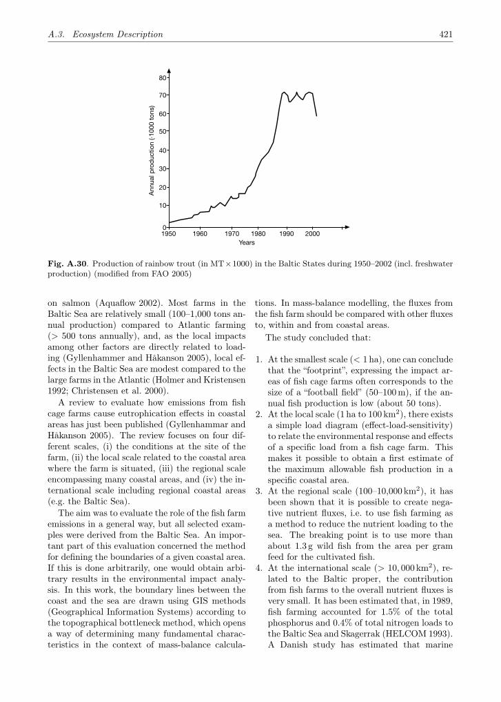
A.3. Ecosystem Description 421
��
��
��
��
�
Q�
�
��
����� ���� ���� ���� ���� ���
W����
!��
)�A�'
� �
)�(�
�����
����
( ��
�
Fig. A.30. Production of rainbow trout (in MT×1000) in the Baltic States during 1950–2002 (incl. freshwaterproduction) (modified from FAO 2005)
on salmon (Aquaflow 2002). Most farms in theBaltic Sea are relatively small (100–1,000 tons an-nual production) compared to Atlantic farming(> 500 tons annually), and, as the local impactsamong other factors are directly related to load-ing (Gyllenhammer and Håkanson 2005), local ef-fects in the Baltic Sea are modest compared to thelarge farms in the Atlantic (Holmer and Kristensen1992; Christensen et al. 2000).
A review to evaluate how emissions from fishcage farms cause eutrophication effects in coastalareas has just been published (Gyllenhammar andHåkanson 2005). The review focuses on four dif-ferent scales, (i) the conditions at the site of thefarm, (ii) the local scale related to the coastal areawhere the farm is situated, (iii) the regional scaleencompassing many coastal areas, and (iv) the in-ternational scale including regional coastal areas(e.g. the Baltic Sea).
The aim was to evaluate the role of the fish farmemissions in a general way, but all selected exam-ples were derived from the Baltic Sea. An impor-tant part of this evaluation concerned the methodfor defining the boundaries of a given coastal area.If this is done arbitrarily, one would obtain arbi-trary results in the environmental impact analy-sis. In this work, the boundary lines between thecoast and the sea are drawn using GIS methods(Geographical Information Systems) according tothe topographical bottleneck method, which opensa way of determining many fundamental charac-teristics in the context of mass-balance calcula-
tions. In mass-balance modelling, the fluxes fromthe fish farm should be compared with other fluxesto, within and from coastal areas.
The study concluded that:
1. At the smallest scale (< 1ha), one can concludethat the “footprint”, expressing the impact ar-eas of fish cage farms often corresponds to thesize of a “football field” (50–100 m), if the an-nual fish production is low (about 50 tons).
2. At the local scale (1 ha to 100 km2), there existsa simple load diagram (effect-load-sensitivity)to relate the environmental response and effectsof a specific load from a fish cage farm. Thismakes it possible to obtain a first estimate ofthe maximum allowable fish production in aspecific coastal area.
3. At the regional scale (100–10,000 km2), it hasbeen shown that it is possible to create nega-tive nutrient fluxes, i.e. to use fish farming asa method to reduce the nutrient loading to thesea. The breaking point is to use more thanabout 1.3 g wild fish from the area per gramfeed for the cultivated fish.
4. At the international scale (> 10, 000 km2), re-lated to the Baltic proper, the contributionfrom fish farms to the overall nutrient fluxes isvery small. It has been estimated that, in 1989,fish farming accounted for 1.5% of the totalphosphorus and 0.4% of total nitrogen loads tothe Baltic Sea and Skagerrak (HELCOM 1993).A Danish study has estimated that marine

422 A. Annexes
aquaculture in Denmark contributes with 0.4%and 1.3% of total Danish N and total P loading(including riverine load), respectively (Ærteb-jerg et al. 2003). Of the direct point sources,marine aquaculture contributed with 9.2% and8.1% N and P, respectively, but when the Dan-ish nutrient release from marine aquaculturewas compared with the total inputs to the Dan-ish coastal waters from the Baltic Sea, Swedenand Germany it only accounted for 4‰ and9‰ of the inputs of N and P, respectively (Ær-tebjerg et al. 2003). Although the release of nu-trients from marine aquaculture only has minoreffects on the total budgets, it is important tonote that it, together with other sources, con-tributes to the high loading of the Baltic Sea.
Due to the complexity of marine ecosystems, in-cluding spatial and temporal variabilities, com-plete studies using an ecosystem based approachto examine eutrophication effects of fish farming inthe Baltic Sea are difficult and expensive to carryout. Håkanson (2005) used a modelling approachto demonstrate ecosystem effects of fish farm emis-sion. The main questions in this study were: Howwould emissions of feed spill and faeces from afish farm influence the production and biomass ofkey functional organisms and how long would suchchanges remain if the fish farm is closed down?
The work is based on a comprehensive lakeecosystem model, LakeWeb, which accounts forproduction, biomass, predation, abiotic/biotic in-teractions of nine key functional groups of organ-isms, phytoplankton, bacterioplankton, two typesof zooplankton (herbivorous and predatory), twotypes of fish (prey and predatory), as well aszoobenthos, macrophytes and benthic algae. TheLakeWeb model gives seasonal variations (the cal-culation time is one week), and it has been cali-brated and critically tested using empirical dataand regressions based on data from many lakes.These tests have demonstrated that the model cancapture typical functional and structural patternsin lakes very well, lending credibility to the re-sults, and the model suggests that fish farm emis-sions cause significant increases in the biomass ofwild fish, without corresponding increases in algalvolume.
Thus, it is concluded that the fish farm emis-sions influence the secondary production moremarkedly than primary production. Although thisfinding might seem to be a paradox, it is relatedto the fact that wild fish directly consume food
spill and faeces from the fish farm, thereby creat-ing a specific foodweb pathway. Similar findingshave been done in the oligotrophic Mediterranean(Dempster et al. 2002), but remains to be vali-dated for fish farms in the Baltic Sea, althoughmany fish farmers support this hypothesis throughobservations of wild fish around their farms (K.M.Kjeldsen, pers. comm.).
The primary production in the Baltic Sea is lim-ited by nutrients during summer, and phosphate isthe typical limiting nutrient in the north, whereasnitrogen is argued to be limiting in the south (Elm-gren 2001). Fish farming in the Baltic Sea maythus, due to the release of dissolved nitrogen di-rectly through excretion of ammonium from thefish during summer and through the settling andregeneration of phosphorus, lead to a stimulationof the nutrient-limited primary producers. Oneimportant aspect when discussing mass-balances isthat the nutrients released from fish farms are im-mediately bioavailable, whereas up to 50% of thenitrogen in the Baltic Sea is considered to be non-bioavailable, as it is bound in humus compounds(Elmgren 2001).
Increased water column chlorophyll-a concen-trations and periphyton growth has been linkedto fish farming activities in the Archipelago Seain SW Finland (Honkanen and Helminen 2000).The study of the Archipelago Sea in Finland isone of the first to show an ecosystem effect on pri-mary production under eutrophic conditions, andsuggests that attached algae may be more sensi-tive indicators of nutrient release from fish farms.Although the nutrient release from fish farms ineutrophic regions is low compared to the othersources of nutrients as discussed above, the nutri-ents are released during the period, when the pri-mary producers often are limited by the availabil-ity of nutrients, which may explain the eutroph-ication effects in the Finnish archipelago duringsummer. Most of the run-off from land occurs inthe late autumn, winter and early spring (Håkan-son and Boulion 2002).
In conclusion, fish farming in the Baltic Seacontributes to the general eutrophication, and al-though the overall contributions are low (< 2% oftotal load), calculations from Denmark show thatfish farms account for up to 8–9% of the pointsources. Whereas large investments have beendone to reduce loads from point sources, only lim-ited research has been undertaken to develop tech-nology to reduce the environmental impacts of fishfarms. The loss of nutrients can be minimized by

A.3. Ecosystem Description 423
capture of wild fish for feed production or by in-troduction of extractive cultures such as shellfishand macroalgae.
At the local scale, nutrient release should becompared with imports and exports from the areaand the water residence time. If the water res-idence time is short, most nutrients will be ex-ported to the coastal area, whereas most of thenutrients may be turned over within the area if theresidence time is long. This may lead to increasedprimary and secondary production, in particularin periods with natural nutrient limitation in sum-mer and autumn. Such increased production mayresult in enhanced settling of organic matter withrisks of oxygen depletion events, in particular instratified water bodies. The location of futureaquaculture units has to be evaluated based on lo-cal conditions, such as nutrient limitation, waterresidence time and stratification.
A.3.1.3 External Pressures
A.3.1.3.1 Sea Traffic
Gerhard Dahlmann
Traffic and Navigational Situation
Shipping is steadily increasing in the Baltic Sea,reflecting intensifying international co-operationand economic prosperity. According to a more de-tailed statistical evaluation of the Baltic Sea ship-ping traffic, which was commissioned by Finland(Rytkönen et al. 2002), the sea-borne volume oftransported goods is expected to roughly doubleby the year 2017.
Concerning ferry traffic and passenger trans-ports the picture was a bit vague in the end ofthe 1990s because of the impact from the Belt-crossings and the abolition of duty free sales.Given data on the development during the lastfew years figures of ferry transport are still rising.
Around 2,000 sizeable ships are normally at seaat any time in the Baltic Sea. The Baltic Sea hassome of the busiest shipping routes in the world(HELCOM 2005)
Generally, it is difficult to obtain a reliable up-to-date overview of ship traffic in the Baltic Sea.The situation is expected to change when a moni-toring system for ships, based on AIS (AutomaticIdentification System) signals, which started in2005, will be routinely explored. This will allow allthe relevant statistics on shipping in the Baltic Sea
to be stored at the HELCOM server in Denmarkand displayed on the HELCOM website.
The AIS network is one of a package of 16 mea-sures adopted by the extra-ordinary HELCOMmeeting at ministerial level in Copenhagen inSeptember 2001, known as the “Copenhagen Dec-laration”. It includes incentives for IMO (Interna-tional Maritime Organisation), such as enhance-ment of pilots, routing measures and introductionof traffic separation schemes, as well as regionaland national activities, such as improved hydro-graphic services and use of Electronic NavigationalCharts. The Copenhagen Declaration has to beseen as one of the most important milestones ofthe HELCOM work in the field of improving mar-itime safety and thus preventing pollution fromships.
Maritime shipping can clearly be regarded asone of the most environmentally friendly meansof transportation. Nevertheless, steps to furtherenhance safety of navigation have to be consid-ered, among them enforced use of AIS onboardships and for monitoring systems in order to con-trol traffic, improved availability of electronic datato be used for sophisticated ships’ navigation sys-tems in order to support ships’ management, fur-ther needs of routing systems and traffic separa-tion schemes in order to support ships’ manage-ment and avoid as far as possible conflict situa-tions.
Impacts from Maritime Shipping
In order to minimise detrimental impacts of mar-itime shipping to the environment of the BalticSea, energetic measures have been taken byHELCOM as well as by the IMO. The most im-portant instruments for preventing marine pol-lution from ships are the world-wide applicableMARPOL Convention (International Conventionfor the Prevention of Pollution from Ships), andthe Helsinki Convention, which reflects, with re-spect to shipping, MARPOL Regulations. Theserules lead to a significant reduction of inter alia oildischarges form ships during operation and fromoil tankers, discharge of sewage and waste andemissions from ships by reducing sulphur contentof bunker fuel oil. A further international conven-tion which has to be mentioned in this context isthe Ballast Water Convention, aiming at the pre-vention of transfer of alien species through ships’ballast water (not yet in force).

424 A. Annexes
10˚
10˚
12˚
12˚
14˚
14˚
16˚
16˚
18˚
18˚
20˚
20˚
22˚
22˚
24˚
24˚
26˚
26˚
28˚
28˚
30˚
30˚
53˚ 53˚
54˚ 54˚
55˚ 55˚
56˚ 56˚
57˚ 57˚
58˚ 58˚
59˚ 59˚
60˚ 60˚
61˚ 61˚
62˚ 62˚
63˚ 63˚
64˚ 64˚
65˚ 65˚
66˚ 66˚
HELSINKI
RIGA
TALLINNSTOCKHOLM
KØBENHAVN
VILNIUS
Kemi
Oulu
Kokkola
Vaasa
Kaskinen
Turku
Pärnu
GöteborgVisby
MalmöMalmöMalmöMalmö
Szczecin
Klaipeda
Liepaja
Rostock
Ventspils
hus
havn
TravemündeTravemündeGdansk
g
Karlskrona
KielKiel
Luleå
Umeå
Härnösand
Gävle
Norrköping
Rauma
KaliningradKaliningrad
St. Petersburg
HELCOMLocation of oil spillages observed by aerialsurveillance within the Baltic Sea Area 2003
SYMBOLS Quantity Number
Category 1 > 0 - 1 m3 247Category 2 > 1- 10 m3 20Category 3 > 10-100 m3 6Category 4 > 100 m3 0Category ? unknown 19TOTAL NUMBER OF OBSERVATIONS: 292Data by: DE, DK, EE, FI, LV, PL and SE
made by S. Wilhelms BSH MUDAB (Meeresumwelt-Datenbank) UBA-UMPLIS/BSH
Fig. A.31. Location of oil spillages observed by aerial surveillance in 2003 (from HELCOM 2003b)
Oil Pollution
Oil is a serious threat to Baltic Sea ecosystemsand wildlife. The most visible effect of oil spills isthe oil contamination on the surface which causessmothing and death of birds and seals. As manyof the chemicals in the oil spills are toxic, oil pol-lution causes serious accumulative effects, for ex-ample on plankton, fish and animals living on theseafloor, as it builds up in the ecosystems. Faunaand flora close to the shipping lanes are also neg-atively affected. In the Baltic Sea, where the av-erage water temperature is only about 10 degrees,oil decomposes slowly due to the cold waters.
Illegal Discharges
About 10% of all the oil hydrocarbons in the BalticSea originate from intentional illegal dischargesfrom the machinery spaces or cargo tanks of ves-sels sailing in the Baltic Sea.
During 1988 to 2001, surveillance aircraft de-tected an average of 400 illegal oil discharges peryear in the Baltic Sea (HELCOM 2003a). In mostcases, the amount of oil discharged is less than1 cubic meter. Deliberate illegal oil dischargesfrom ships are regularly observed within the BalticSea since 1988. As from 1999 the number of ob-served illegal oil discharges has decreased from ap-
Exclusive Economic Zone Territorial border
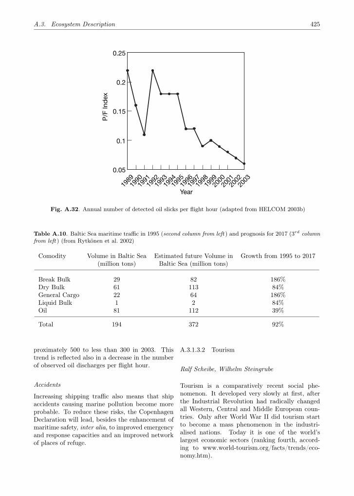
A.3. Ecosystem Description 425
0.2
0.1
0.05
0.15
198919
9019
9119
9219
9319
9419
9519
9619
9719
9819
9920
0020
0120
0220
03
0.25
Year
P/F
Ind
ex
Fig. A.32. Annual number of detected oil slicks per flight hour (adapted from HELCOM 2003b)
Table A.10. Baltic Sea maritime traffic in 1995 (second column from left ) and prognosis for 2017 (3rd columnfrom left ) (from Rytkönen et al. 2002)
Comodity Volume in Baltic Sea Estimated future Volume in Growth from 1995 to 2017(million tons) Baltic Sea (million tons)
Break Bulk 29 82 186%Dry Bulk 61 113 84%General Cargo 22 64 186%Liquid Bulk 1 2 84%Oil 81 112 39%
Total 194 372 92%
proximately 500 to less than 300 in 2003. Thistrend is reflected also in a decrease in the numberof observed oil discharges per flight hour.
Accidents
Increasing shipping traffic also means that shipaccidents causing marine pollution become moreprobable. To reduce these risks, the CopenhagenDeclaration will lead, besides the enhancement ofmaritime safety, inter alia, to improved emergencyand response capacities and an improved networkof places of refuge.
A.3.1.3.2 Tourism
Ralf Scheibe, Wilhelm Steingrube
Tourism is a comparatively recent social phe-nomenon. It developed very slowly at first, afterthe Industrial Revolution had radically changedall Western, Central and Middle European coun-tries. Only after World War II did tourism startto become a mass phenomenon in the industri-alised nations. Today it is one of the world’slargest economic sectors (ranking fourth, accord-ing to www.world-tourism.org/facts/trends/eco-nomy.htm).

426 A. Annexes
General development of tourism in the Baltic SeaBasin
Tourism developed properly in the 19th century.Its sudden rise was caused by the coincidenceof several factors, e.g. the developments in theEuropean transportation (steam boats, railways,road systems) and communication, and – deci-sively – the economic consequences of industriali-sation which brought a certain economic wealth tonew social groups and thus enabled them to travel.This new civic upper class immediately embracedthe developing spas, for new scientific and medi-cal insights confirmed their health benefits. In thecourse of the 19th century, the health interests ofthe bathers were soon joined by the economic in-terests of the local spa operators. However, thisearly form of tourism was restricted to relativelyfew spas and sea baths, and until the 20th cen-tury, the seaside repose remained a strict privilegeof the upper social classes.
In Germany, this quickly changed when the na-tional socialist system established the “Kraft durchFreude” movement and state-controlled recreationand holidays. Only the outbreak of the war in1939 prevented the plans for mass tourism frombeing realised.
In the German Democratic Republic (GDR) ofthe 1970s and 80s, the state newly created a risingpressure on the southern Baltic Sea coast. As aresult, that region had about 400,000 beds and 37million overnight stays in 1989 – about 40% of theGDR’s total volume (cf. Benthien 1996, p. 12).1990 saw a huge slump in this sector caused bythe reunification of Germany. The infrastructureof the East German socialistic tourism was notcompetitive, and new organisational and economicstructures had to be built from scratch. Althoughthe new infrastructure was quickly set up, tourismhas failed to reach the pre-Unification volume. To-day, the number of overnight stays in the German“Land” Mecklenburg-Vorpommern is about 22 mil-lion per year.
The development at the coasts of Poland,Lithuania, Latvia and Estonia took a similarcourse. But there, even more than in the GDR, thestate installed large tourism infrastructures whichwere alien to the landscape and, today, create con-siderable utilisation problems.
The development of tourism in Scandinaviatook a somewhat retarded and structurally dif-ferent course. Although there, too, its early
stage was shaped by the behaviour of the nobil-ity, Scandinavian noblemen began already in theearly 19th century to use their manors as summerresidences, exhibiting a particular preference forwaterside locations. As elsewhere, the assurgentcivic circles imitated upper-class behaviour andlooked for cheap summer lodgings in the country-side (Jäderholm and Steingrube 1996, p. 140 ff.).Thus, at an early time they already induced thebeginning of the cabins and related facilities whichare so typical of Scandinavia today.
Present and future situations in different tourismsectors
The present situation in the Baltic Sea Basin (cf.the up-to-date overview in Breitzmann 2004) ischaracterised by relative stability and can be sum-marised in the following points:
• Domestic tourism is dominant in all countriesboardering the Baltic Sea, i.e. most of thetourists come from the respective country.
• The cabin holiday has become an integral partof life in the Scandinavian countries and, there-fore, dominates domestic tourism. Because ofthe keen demand, domestic tourism is extend-ing into the “dry” countryside. Otherwise, thereis a clear local and regional trend: “to the wa-ter”, i.e. especially to the seaside, but also tothe lakes.
• In line with this trend, the southern Baltic Seacoast, with its typical sand beaches receivesmany bathing tourist.
• The intensively used areas are expanding con-tinuously. On the whole, however, there is lessof an addition in tourist numbers than a spatialredistribution:
– The pattern of locally centralised facilities inold, long-standing sea baths is replaced by ascatter of resorts along the entire coastline.
– Poland and the three Baltic states are slowlyjoining this market.
• The predominance of marine and other water-based activities creates a pronounced seasonal-ity.
• Business tourism provides some counter-balance, but concentrates on the tourist centresand cities.
• The Baltic Sea is of increasing interest for cruiseboat operators.

A.3. Ecosystem Description 427
Medium-term trends:
• Domestic visitors will continue to dominateBaltic Sea Basin tourism;
• The pronounced seasonality will hardly abate,because the many efforts to extend the seasonwill hardly have any quantitative effect.
• There are many current projects to diversifytourism. In rural regions, this will lead to theconstruction of a number of new facilities andto the provision of new visitor activities.
• In business tourism, the EU enlargement willcause an increase in travel volume and a shiftinto Poland and the Baltic States.
• The focus of the new developments will be onmaritime tourism which may cause visible ef-fects: creation of new marinas, more boat traf-fic, and an increasing number of “mini-cruises”.
• Ferry traffic will further increase in spite ofnewly built or planned bridges.
• In the Baltic Sea Basin in general, there willbe a slightly increasing travel volume caused bythe recent opening of the borders to the newEU member states.
• There will be a net redistribution at the expenseof the established destinations like Denmark,Schleswig-Holstein and Mecklenburg-Vorpom-mern, leading to more tourism in Poland andthe Baltic States.
Environment, climate, and tourism – generalobservations
Of course there is an intimate interrelationshipbetween tourism and the environment. On theone hand, the natural assets of a region are gen-erally recognised as the basis of tourism; and onthe other hand, (mass) tourism contributes to thedestruction of its own basis.
Nature, however, is a wide term, and climate isusually understood to be a part of it. However, itmakes sense to treat climate on its own. This isdue to, in the global dimension of climatic effects,the atmosphere’s high susceptibility to change, ascompared to other environmental factors, and thespecial impact of climate on the different prereq-uisites and aspects of tourism. As a schematic, wethus yield the simple relation shown in Fig. A.33.
The largest, i.e. most intensively discussed in-tersection (A) is doubtlessly covered by those is-sues that deal with global climate change. It isnot caused by specifically tourism-related activi-ties, but rather by other human economic activi-ties. Intersections B and C include all kinds of in-
Fig. A.33. Tourism, Environment and Climate – Ar-eas of Overlap
teractions between tourism and the environment,e.g. the waste problem in general, pollution causedby car traffic, as well as water supply and sewagetreatment, or direct impacts on animals and plants(not only in reserves) that are caused directly bytourists. It must be emphasised that these inter-actions occur invariably in both directions.
That tourism depends on the general natu-ral and environmental conditions is self-evident.Tourism requires nature both in the form of thelocal natural assets, as a space of action for ac-tivities, and simply as a backdrop. “Beautifulscenery”, “exotic nature” and similar attributes de-scribe the predominantly desired framework forpleasant, successful holidays.
Trend sports, in particular, which play an in-creasingly important role in tourism, make use ofnatural areas that until recently were completelyuninteresting for the leisure industry.
The opposite relationship – the impact oftourism on the environment – is easy to under-stand on a general level (Fig. A.34). The necessaryphysical infrastructure is the most obvious connec-tion. It is also self-evident that leisure activities,the traffic they induce, and finally, the behaviourof the tourists themselves are always accompaniedby environmental impacts. Equally easy to under-stand is the observation that tourism consumesresources like space, water, or energy.
The following, simple example gives an impres-sion of the complexity that characterises this re-

428 A. Annexes
Fig. A.34. Environmental implications of leisure and tourism
Fig. A.35. Infrastructure as a source of environmental impacts
lationship: To avoid tall hotel buildings that spoilthe scenery, new projects are subject to recom-mendations or regulations that demand an archi-tectural style in harmony with and typical of thescenery. But these buildings require, for the samenumber of beds, a floor space several times largerthan do multi-storey hotels.
Admittedly, this rather general list of themost important environmentally relevant “pres-sure zones” needs to be spelled out in greater de-tail. Figure A.35 gives some examples for the envi-ronmental impacts created by tourism infrastruc-ture, like lodging, catering trade, traffic infrastruc-ture, as well as supply and waste facilities. Butalso the activities themselves – ranging from sports(swimming pools, bicycle lanes, golf courses, etc.)to culture (museums, theatres, etc.) – require aspecific infrastructure.
These are the direct, immediately obvious envi-ronmental impacts. But we should not forget theindirect impacts:
• Tourism infrastructure requires a constructionindustry which, in turn, entails its own facilities,ranging from the gravel pit over the car pool tothe business building.
• Many seasonal workers in tourism require addi-tional lodgings and supply facilities.
• The gastronomic supply of the tourists impliesa row of special production plants, ranging fromfields or glasshouses to entire cattle herds andthe meat-processing businesses.
Of course, many of the implications mentioned aredesiderates of the economic policy of the respec-tive country, and of course not every environmen-tal impact is in itself destructive. The point hereis rather to demonstrate the intimacy and com-plexity of these relationships.
Interactions between climate change and tourism
The central issue of this paper is part of intersec-tion D (Fig. A.33), i.e. of the direct intersectionbetween climate and tourism. It is not intendedto separate it strictly from aspects which would beplaced in its vicinity but still within intersection C.
The “First International Conference on ClimateChange and Tourism” of the World Tourism Orga-nization (WTO) in Djerba, Tunesia (1993) iden-tified this subject area meanwhile as a sphere ofproblems too and focused on climate change re-

A.3. Ecosystem Description 429
lated impacts on water resources, at coastal andisland destinations, as well as mountain areas.The Djerba Declaration on Climate Change andTourism recognises that climate change impactsare already occurring at some tourism destinationsand the effects are expected to spread in the fu-ture2. Besides this, two other international meet-ings were held: at Milan (Italy) in 2003 on “Cli-mate Change, the Environment and Tourism: TheInteractions” and at Genoa (Italy) in 2004 on “Cli-mate Change, the Environment and Tourism inEurope’s Coastal Zones”3.
In the context of climate and tourism wemeet both directions of interdependencies: Conse-quences of climate change for tourism on the onehand, and the impact of tourism on climate changeon the other hand.
Consequences of climate change for tourism
The climate, as well as the weather, crucially in-fluences the choice of the holiday destination andduration. The decision pattern is shaped both bythe objective opportunity to conduct certain activ-ities (skiing, sailing, etc.) and by very subjectivewhims. Astonishingly, people often attach moreimportance to weather forecasts than to the actualweather (cf. Lohmann 2003, who also provides acomprehensive review of the literature). On theother hand, many tourists fail to catch up on theweather conditions in their holiday destination, orthey do so only shortly before they set off (Hamil-ton and Lau 2004). Referring to selected Europeancountries, Agnew and Palutikof (2001) conducteda study of climate impacts on the demand fortourism. In general, temperature is more stronglyperceived and considered in the decision-makingprocess than sunshine. Precipitation ranks onlythird. A certain “pleasant minimum temperature”should prevail, but the weather should also not betoo warm. In general, an average temperature of21 C can be regarded as attractive for tourists.In all countries under investigation, a one-degreerise in temperature resulted in an increase of thenumber of domestic tourists by one to five percent.
Because the many existing studies are, for thegreater part, not comparable, it became necessary
2cf. www.world-tourism.org/sustainable/climate/final-report.pdf
3cf. www.e-clat.org; more scientific information is avail-able via the very actual bibliography of “Climate, Tourismand Recreation” on www.fes.uwaterloo.ca/u/dj2scott/Do-cuments/CTREC%20Bibliography_FINAL.pdf
to establish an independent index which is free es-pecially of the interviewees’ subjective influence.The Tourism Climate Index (TCI) fulfills this re-quirement. It combines seven weighted monthlyaverages as mean and maximum temperatures, hu-midity, sum of precipitation, sun hours and windspeed. The TCI is also an appropriate tool for es-timating the attractiveness of a destination afterclimate change.
Scott and McBoyle (2001), who also provide amore detailed description of the TCI, attempted aforecast for selected North American cities, whichmay be quantified using the TCI in combinationwith models of climate change. They concludedthat approximately from 2070, many Canadianand northern United States cities will be affectedpositively. As a contrast, cities located furtherto the south, which even today stands out withunpleasant summer TCIs, will become even lessattractive. It is an obvious step to expect a sim-ilar development for Northern Europe and theMediterranean.
The studies by Bigano et al. (2005) are alsobased on simulations, but this time using theHamburg Tourism Model (HTM4), which predictsthe development of demand patterns in tourism.These authors’ predictions resemble those of Scottand McBoyle (2001): Tourism demand will doublein colder regions and decrease by 20% in warmercountries. In some regions, visitor numbers willeven drop to half their current level. There will bean increase, especially of international tourism, inthe currently colder regions.
Besides the direct consequences of climatechange, which can be immediately attributed tothe respective climate elements, there are numer-ous indirect effects. These may be quite diverse,effects on e.g. terrestrial and marine ecosystemsare covered in Chaps. 4 and 5 of this volume.
The most important effect for tourism, espe-cially for infrastructure, is the expected rise of thesea level. Its particular consequences, though, ap-pear to be less crucial than those of the general cli-mate change (Bigano et al. 2005). At first glance,it seems to be a great advantage that the sea levelwill not rise unexpectedly and within a very brieftime, but that this process will occur very slowlyin the course of many years. This leaves ample op-portunity to meet the effects with technical con-structions (dykes, barrages, etc.).
4www.uni-hamburg.de/Wiss/FB/15/Sustainability/htm.htm

430 A. Annexes
Tourism-relevant general impacts of a sea levelrise are (after Sterr et al. 1999):
• More available water surface. Not all extremelylow areas will be “defended” by dykes againstthe sea. This new water surface will be very at-tractive destinations for many people, i.e. theseareas create additional tourism.
• Increasing likelihood of (storm) flood events. Itsimpact concentrates on coastal facilities likemarinas, near-beach buildings, and the watervehicles themselves, even though the events ap-pear (at present) to occur more often in the lesstourism-relevant winter half year.
• Loss of land in floods and enforced erosion.This impact may extend to tourism-relevantareas, e.g. because buildings were erected inknown flood-prone and erosion-endangered ar-eas. Admittedly, most facilities are affected bysediment set free by erosion, the costs for theunsilting of harbour accesses would rise.
• Penetration of seawater into surface- andgroundwater bodies. This may especially con-cern isolated water catchments on islands,where water consumption increases consider-ably during the main tourist season.
• Biological changes in the coastal ecosystems.For example, they might affect the number anddistribution of fish species relevant for fishing,or, in combination with changes in water tem-perature and salinity, promote neozoa like thepiddock which causes considerable damage toharbour infrastructure and coastal protectionfacilities.
Against the background of these results, we mayexpect the following trends in the Baltic Sea Basin:The summer tourism will profit from the expectedclimate change, because the climate will generallybecome more tourism-friendly. The TCI (TourismClimate Index) will reach attractive levels evenin the northern part of the Baltic Sea Basin, aswell as the presently rather short tourist summerseason will be extended. There will be negativeimpacts on the winter tourism. Especially in themore continental regions of Northern Europe, win-ter temperatures will rise while snow certainty de-creases.
However, we should not forget that thesechanges will be much less effective than the socio-economic factors which define the general frame-work. The decision for the time and destination ofa holiday depends crucially on income, education,and age. Especially the habits of younger holiday-
makers (and, thus, their decision patterns) changevery quickly. These factors entail a much less pre-dictable risk than climate change (cf. Lise and Tol2005).
Impact of tourism on climate
Tourism is not only a “victim” of climate change,but itself influences climate development. How-ever, there is only one sector besides indirect ef-fects translated through general pressure on theenvironment (resource consumption, waste, soilsealing, etc.) that directly affects the climate:tourism-based traffic. It produces considerableamounts of exhaust gases and thus greatly con-tributes to climate change.
For many years, the trend in tourism has beentowards long-distance travel, which in turn causesan increase in flight traffic. Flight traffic is one ofthe strongest and most immediate sources of cli-mate change. In the Baltic, however, long-distancetraffic will increase “only” proportional to the gen-eral increase in long-distance travel. Because, ona global scale, the population size in this regionis comparatively low, this cause of environmen-tal pressure will be rather low-ranking. The in-crease in temperature could, under certain circum-stances, even have a contrary effect. A certain –though probably rather small – fraction of the pop-ulation in the Baltic Sea Basin will not travel tolong-distance destinations but rather spend theirholiday in the region itself. Thus, their contri-bution to the further increase of CO2 emissionswill be less than average. The present phase ofcheap flight travel causes very sizeable new touriststreams. This form of tourism also occurs in theBaltic Sea Basin, which is both source area anddestination. However, we can safely presume thatthe market will soon put an end to this phase andthus limit the present extreme emissions.
The primary form of tourism-related traffic inthe Baltic Sea Basin is individual transport, i.e.car traffic. Even in the medium-term, it will notlose its predominant position.
In general, the tourism-based traffic in theBaltic Sea Basin will grow – as a continuing ef-fect of the political opening of the East. Evenin the medium-term, we will continue to sensethat new source areas of travel traffic with anincreased action range have entered the market.The population of Poland and the Baltic Statesstill feel they have to catch up in terms of travel,and they will fulfil their desire as their economic

A.3. Ecosystem Description 431
wealth increases. On the other hand, these coun-tries present new destinations which – lacking al-ternatives – aggressively promote tourism in theirturn.
On a regional and local level, tourism- andleisure-based transport plays an especially impor-tant role. In Germany, 54% of the total trafficvolume is caused by leisure traffic, which, in turn,includes a share of problematic individual trafficof more than 80% (UBA 2003, p. 19). Especiallythe rise of the trend sports is regularly linked toan increase in traffic volume. Among these partic-ularly traffic-intensive leisure activities are diving,wind surfing, skiing, and climbing (Stettler 1998).Thus, in the medium-term tourism-based individ-ual traffic will considerably contribute to the in-crease of CO2 emissions.
Another source of increasing CO2 emissions isthe marine tourism. This form of tourism will gaineven more importance in future. Not only will thenumber of private motor boats rise, but the al-ready booming cruise market will continue to growin the Baltic Sea as it does elsewhere. In addition,the river cruise market has been developing witha higher than average rate for several years. Thus,in the medium-term marine tourism will also cre-ate considerable emissions.
Conclusions
The traffic volume in the Baltic Sea Basin willcontinue to rise in the medium-term. This devel-opment is primarily still an effect of the politicalopening of the East and the consequent EU en-largement. All of the new EU member states placegreat hopes in the tourism sector.
As a result, we will witness shifts of the touristdestinations within the Baltic Sea Basin - at thesouthern Baltic Sea coast the shift will be fromwest to east, i.e. from Denmark and Germanyto Poland and to some select seaside resorts inthe Baltic States. Large cities such as Gdansk,Riga, and St. Petersburg are also attracting moretourists.
This development will lead to more traffic – pre-dominantly individual traffic, but also ferry traffic– which can contribute considerably to climate-relevant emissions.
The trend towards marine tourism (more mo-tor boats, more cruises) will also strongly increaseemissions.
The remaining consequences are of a rathermore general, ecological nature (consumption of
space and resources, especially water, as well aswaste disposal problems). However, they will oc-cur predominantly as problems on the local andregional level – the total sum will hardly rise andcould perhaps be balanced by infrastructural andtechnical counter-measures.
The opposite relationship – the impact of cli-mate change on tourism in the Baltic Sea Basin –raises positive expectations. The probable changeof the sea level will hardly have any negative ef-fect. On the contrary, it might enhance the marinepotential, and the rise in temperature will improvethe natural basis for tourism. Consequently, thetotal volume of tourism will grow. But on thewhole, the changes will lead to more domestic andless long-distance tourism, thus contributing to areduction of the growth of climate-relevant emis-sions caused by tourism.
A.3.2 Terrestrial and Freshwater Ecosystems
Benjamin Smith, Thorsten Blenckner, ChristophHumborg, Seppo Kellomäki, Tiina Nõges, PeeterNõges
A.3.2.1 Catchment Area of the Baltic Sea
The catchment area of the Baltic Sea(1,735,000 km2), which constitutes the landsurface region of the Baltic Sea Basin, compriseswatersheds draining the Fennoscandian Alps inthe west and north, the Erzgebirge, Sudetesand western Carpathians in the south, uplandsalong the Finnish-Russian border and the centralRussian Highlands in the east. Politically, thisincludes most of Sweden, Finland, the BalticStates, Poland and part of Russia, Belarus,Ukraine and northern Germany (Fig. A.36). TheBaltic Sea Basin spans some 20 degrees of latitudeand climate types ranging from nemoral to alpineand subarctic. It can be roughly divided intoa south-eastern part, draining into the Gulf ofRiga and Baltic Proper, that is characterized bya cultivated landscape with a temperate climateand a northern boreal part characterized by conif-erous forests and peat. The natural vegetation ismainly broadleaved deciduous (nemoral) forestin lowland areas of the temperate southeast,and conifer-dominated boreal forest (taiga) innorthern Scandinavia. Cold-climate shrublandsand tundra occur in mountainous areas and inthe subarctic far north of the catchment region.Wetlands are a significant feature of the borealand subarctic zones.
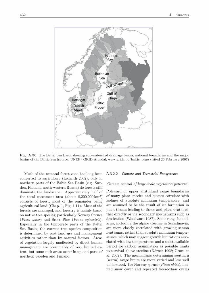
432 A. Annexes
Fig. A.36. The Baltic Sea Basin showing sub-watershed drainage basins, national boundaries and the majorbasins of the Baltic Sea (source: UNEP/ GRID-Arendal, www.grida.no/baltic, page visited 26 February 2007)
Much of the nemoral forest zone has long beenconverted to agriculture (Ledwith 2002); only innorthern parts of the Baltic Sea Basin (e.g. Swe-den, Finland, north-western Russia) do forests stilldominate the landscape. Approximately half ofthe total catchment area (about 8,200,000 km2)consists of forest, most of the remainder beingagricultural land (Chap. 1, Fig. 1.11). Most of theforests are managed, and forestry is mainly basedon native tree species; particularly Norway Spruce(Picea abies) and Scots Pine (Pinus sylvestris).Especially in the temperate parts of the BalticSea Basin, the current tree species compositionis determined by past land use and managementactivities rather than by natural factors. Areasof vegetation largely unaffected by direct humanmanagement are presumably of very limited ex-tent, but some such areas occur in upland parts ofnorthern Sweden and Finland.
A.3.2.2 Climate and Terrestrial Ecosystems
Climate control of large-scale vegetation patterns
Poleward or upper altitudinal range boundariesof many plant species and biomes correlate withisolines of absolute minimum temperature, andare assumed to be the result of ice formation inplant tissues leading to tissue and plant death, ei-ther directly or via secondary mechanisms such asdessication (Woodward 1987). Some range bound-aries, including the alpine treeline in Scandinavia,are more closely correlated with growing seasonheat sums, rather than absolute minimum temper-atures, which may suggest growth limitations asso-ciated with low temperatures and a short availableperiod for carbon assimilation as possible limitsto survival above treeline (Körner 1998; Grace etal. 2002). The mechanisms determining southern(warm) range limits are more varied and less wellunderstood. For Norway spruce (Picea abies), lim-ited snow cover and repeated freeze-thaw cycles

A.3. Ecosystem Description 433
have been suggested to interfere with the devel-opment and maintenance of winter-hardiness inseedlings, inhibiting natural regeneration of thisspecies in oceanic climates (Dahl 1990; Sykes etal. 1996; Bradshaw et al. 2000). In many temper-ate tree species, the timing of budburst appearsto be coupled to the duration and intensity of lowtemperatures in the winter. Budburst may thusbe delayed by several weeks following a warm win-ter, protecting the frost-sensitive new shoots fromdamage by late frosts (Murray et al. 1989; Sykeset al. 1996). This chilling mechanism has beenproposed to, for example, restrict the distributionof European beech (Fagus sylvatica) into the mostoceanic climates (Sykes and Prentice 1995).
In reality, temperature is only one of severalfactors controlling large-scale distributions of treespecies. Even if the seed dispersal of some speciesis able to keep up with climate change, local dom-inance shifts may be delayed by the long gen-eration times of trees, competition with residentspecies, required changes in soil structure, hydrol-ogy, chemistry, litter depth, requirements for my-corrhizae and other factors (Sykes and Prentice1996; Huntley 1991; Malanson and Cairns 1997).
Environmental control of ecosystem biogeochem-istry
Climate affects biogeochemical cycling within eco-systems by modifying the rates and modes of indi-vidual ecosystem processes. The most importantprocesses in terms of overall control of ecosystemfunctioning are the physiological processes under-lying net primary production (NPP): photosyn-thesis, autotrophic (plant) respiration, stomatalregulation and carbon allocation in plants. Car-bon assimilated in photosynthesis is eventually ei-ther respired or otherwise emitted (e.g. as biogenicvolatile organic compounds) directly to the atmo-sphere, or fed into the soil organic matter poolas litter, root exudates, or residues from distur-bance by fire. Productivity changes thus tendto propogate to litter and soil pools and impactdecomposition processes. Productivity changesmay also modify vegetation structure (e.g. leafarea index, LAI), changing the competitive bal-ance among individuals and species, and leading tofurther structural changes and feedbacks on pro-duction. Changes in disturbance regimes, for ex-ample, damage due to wind storms and wildfires,can be a further consequence of changed vegeta-tion structure.
The direct physiological effect of a temperatureincrease on plant carbon balance may be eitherpositive or negative, depending on the relativekinetic stimulation of photosynthesis and plantrespiration. However, NPP tends to be a con-stant proportion of GPP across biomes and cli-mate types, which suggests that respiration ratesare in the long term dependent on the supply of as-similates (i.e. net photosynthesis), and that accli-mation to a temperature change may occur (War-ing et al. 1998; Dewar et al. 1999).
Temperatures also affect annual productivityvia growing season length. Phenological eventssuch as budburst and leaf abscission in temper-ate and boreal plants are closely correlated withclimate indices, particularly temperature sums(Kramer 1995; Badeck et al. 2004). Both tempera-ture cues and photoperiod may determine growthcessation and the onset of hardening in the au-tumn. A uniform increase in average temperaturesthroughout the year implies that threshold tem-peratures for phenophase transitions in spring maybe achieved a number of days earlier, while laterautumn frosts may delay leaf abscission and win-ter hardening. However, many tree species requirean extended period of cold temperatures (chilling)to initiate budburst and, in these species, warmerwinter temperatures may delay the onset of growtheven once normal spring temperatures have beenachieved (Cannell 1989; Sykes et al. 1996). Theeffects of temperature changes on plant phenologymay be expected to impact NPP particularly athigh latitudes, where the growing season is short-est (Walker et al. 1995).
Soil nutrient status, particularly nitrogen avail-ability, is considered to limit productivity in manytemperate and boreal ecosystems (McGuire et al.1995; Bergh et al. 1999; Hungate et al. 2003).Increased soil temperatures will tend to stimu-late microbial activity and N-mineralisation rates,so long as soils remain moist, potentially releas-ing ecosystems from N-limitation (Melillo et al.2002). This effect may be particularly importantin the coldest boreal, arctic and alpine environ-ments (Jonasson et al. 1999; Strömgren and Lin-der 2002).
Soil water deficits occasionally limit production,even in many mesic ecosystem types. Althoughwater availability is not currently a major limit-ing factor for forest or agricultural production inthe Baltic Sea Basin, it does occur, e.g. on well-drained soils in southern Sweden (Bergh et al.1999). Increased temperatures lead to increased

434 A. Annexes
RAININTERCEPTION
RAIN
RELATIVEHUMIDITY
TEMPERATURE
LIGHTINTERCEPTION
ALLOCATION OFCARBOHYDRATES
EVAPORATION
TRANSPIRATION
STOMATALCONDUCTANCE
UNDERSTOREYEVAPOTRANSPIRATION
SOIL EVAPORATION
SOIL WATER
SOIL WATEROUTFLOW
LIGHT CO2
PHOTOSYNTHESIS
NITROGEN LITTERFALL
RESPIRATION
ROOT MASS
LEAF AREA
BRANCH MASS
STEM MASS
Fig. A.37. Conceptual diagram for the BIOMASS model (adapted from Freeman et al. 2005)
evaporative demand and depletion of soil watervia increased evapotranspiration, while changes inprecipitation patterns may exacerbate or amelio-rate moisture deficits and effects on production.
Rising atmospheric carbon dioxide (CO2) con-centrations are one of the most certain aspectsof global change. CO2 is a plant resource, andit has long been assumed that increased ambientCO2 levels would stimulate photosynthesis via re-duced photorespiration and improve plant waterbudgets through reduced stomatal conductance,in both cases tending to augment net carbon up-take (Bazzaz 1990). Laboratory and field experi-ments exposing plants or whole ecosystems to ele-vated CO2 levels confirm that production usuallyincreases by 15–50% for a doubling of CO2 abovepre-industrial levels (Poorter and Navas 2003); fortemperate forest ecosystems, the response acrossbroad productivity gradients is rather conservativeat a median of 23± 2% (Norby et al. 2005). How-ever, it has been suggested that, in many ecosys-tems, negative biogeochemical feedbacks may in-hibit plants from fully utilising the additional as-similates resulting from CO2-fertilisation on multi-decadal time scales (McGuire et al. 1995); reducedquality (lower N:C ratio) of the litter produced byCO2-fertilised plants could lead to immobilisation
of N by soil microbes, reducing plant N uptakeand NPP (McGuire et al. 1995). To a certain ex-tent, plants may compensate for nutrient limita-tions by an increased relative investment in belowground structures (roots) and functions (e.g. rootexudates, investment in mycorrhizae, Lloyd andFarquhar 1996).
Overall responses of ecosystem biogeochemistryto environmental changes are characterised bythe differential temporal signatures of many con-stituent processes. Short-term physiological re-sponses, such as the direct response of net pho-tosynthesis to a change in temperature, may bemodified by longer-term changes in, for example,plant structure, population dynamics, vegetationspecies composition and soil organic matter stoi-chiometry (Shaver et al. 2000).
A.3.2.3 Outline of the BIOMASS Forest GrowthModel
The BIOMASS model is based on sub-modelsdescribing radiation interception, canopy photo-synthesis, phenology, allocation of photosynthatesamong plant organs, growth, litter fall and wa-ter balance, including nitrogen effects on processes(Fig. A.37; Freeman et al. 2005). BIOMASS sim-
A.3. Ecosystem Description 435
ulates tree growth on a daily time step, which re-quires daily meteorological inputs of short-waveradiation, maximum and minimum air tempera-ture, precipitation, and humidity of the air. Grossprimary production is calculated from a radia-tion interception model requiring information oncanopy architecture and a biochemically-basedmodel of leaf photosynthesis by C3 plants. Netprimary production is obtained by subtracting theautotrophic respiration.
A.3.2.4 Outline of the EFISCEN Forest ResourceModel
EFISCEN is a large-scale matrix model, whichuses forest inventory data as input (Sallnäs 1990;Pussinen et al. 2001). EFISCEN can be used tocompile information on forest resources in Europeand to produce projections of the possible futuredevelopment of forests. The state of a forest isdepicted in the model as an area distribution overage and volume classes in matrices. Growth is de-scribed as area changes to higher volume classesand ageing of forest is incorporated as a functionof time up to the point of regeneration. The userdefines the level of fellings and the model imple-ments cuts according to predefined managementregimes.
The basic input data include forest area, grow-ing stock and increment by age classes, i.e. thedata available from national forest inventories.European-wide data are compiled in the EFIS-CEN European Forest Resource Database (EEFR)at the European Forest Institute (Schelhaas et al.1999). Country-level data consist of forest types,which are distinguished by region, owner class, siteclass and tree species, depending of the aggrega-tion level of the provided data.
The current version of EFISCEN can be used tostudy the carbon balance of the whole forest sec-tor. Stem-wood volumes are converted to carbonin the compartments stems, branches, leaves, andcoarse and fine roots using dry wood density, car-bon content and an age-dependent biomass distri-bution. Litter production is estimated using age-dependent turnover rates of each compartmentand is used as input to a dynamic soil carbon mod-ule. A dynamic wood products model enables theflow of carbon to be followed further through pro-cessing and wood products up to the time point atwhich carbon is released back to the atmosphere.The EFISCEN version used in the calculationspresented in Sect. 4.3.5 takes into account the im-
pact of changes in temperature and precipitationon forest growth, and thus forest structure, carbonbudget and fellings, as detailed by Pussinen et al.(2005).
A.3.2.5 Climate Scenarios Used in SilviStrat Calcu-lations
Three climate scenarios were used in the SilviS-trat project (Kellomäki and Leinonen 2005) toyield the predictions of change in forest growthpresented in Sect. 4.3.5.
• Current climate. Temperature and precipita-tion values are based on monthly time series1901–1995 and the CRU monthly climatology1961–1990, with a spatial resolution of 0.5 de-grees of latitude and longitude (Michell andJones 2005). The warming trend in the in-terpolated monthly time series 1961–1990 wasremoved to generate 30 years of climate datawith the typical interannual variability betweenyears. From this sample, individual years wererandomly drawn to generate the baseline cli-mate (‘current climate’) for the simulation pe-riod of 110 years.
• ECHAM4 climate. Values for the period be-tween 1990 and 2100 were used, taking the CRUmonthly climatology 1961–1990 as a baseline.It was based on output from the ECHAM4-OPYC3 GCM (cf. Chap. 3) which is availableas monthly means at a spatial resolution of2.81 × 2.76◦. The GCM simulation does notinclude the cooling effects of sulphate aerosolson climate.
• HadCM2 climate. The values were estimatedfor the period between 1990 and 2100 takingthe CRU monthly climatology 1961–1990 as abaseline. It was based on output from theHadCM2 GCM (Chap. 3) at a spatial resolutionof 2.5×3.75◦. The GCM simulation includes thecooling effects of sulphate aerosols on climate.
Climate scenarios from both GCMs were based onthe IS92a ‘business as usual’ emission scenario,which assumes a doubling of atmospheric CO2
concentrations in the 21st century. To generatemonthly surface climate data, GCM results weredownscaled to the sites by calculating the differ-ence for each parameter between the time period1990–2100 and the average values of the referenceperiod 1931–1960 using monthly time steps. Spa-tial interpolation of GCM data on the sites wasperformed with the Delaunay triangulation. The
436 A. Annexes
time series of these anomalies were then added tothe average values of baseline (CRU) data for thestudy sites.
A.4 Observational Data Used
A variety of data has been used for the descriptionand analyses of the atmosphere, the ocean, therunoff from rivers, and the ecology of the BalticSea and its surrounding area. Below follows ashort survey.
A.4.1 Atmosphere
Øyvind Nordli
Regular measurement with mercury in glass ther-mometers and barometers started at a few sites inthe Baltic Sea Basin already in the 18th century.As standard instruments at the meteorological ser-vices they were much improved as time passed.Now, the mercury instruments have been replacedin large numbers by sensors for automatic regis-tration. For long-term temperature trend analy-ses, the homogeneity of the series is a challengefor several reasons. Examples are improvementsof the thermometers themselves, and also, a bet-ter sheltering from short wave radiation (Nordli etal. 1997).
As site measurements grew denser, reliable gridbox mean values could be calculated. Advantage istaken of a work done by the Climate Research Unit(CRU) at the University of East Anglia (IPCC2001, Chap. 2). For this study of the Baltic SeaBasin (see Chap. 2), a subset of the CRU data setwith solely land stations is chosen. The datasetstarts in 1851, but only data after 1870 are usedin this book. The CRU data set includes manywell homogenised series from the Nordic countries(Jones and Moberg 2003).
Glass barometers with mercury are of about thesame age as the mercury thermometers. A chal-lenge has been to keep the calibration of the in-struments constant during transportation and alsoto keep them in good shape over long time spans.The readings of the barometers have to be ad-justed to standard gravity and temperature. Asstandards, 45◦ latitude and 0 C have been chosen,respectively. The pressure at station level is alsoadjusted to sea level. This operation may be chal-lenging for mountain stations and stations situatedin valleys where temperature inversions (tempera-ture increase with height) tend to develop. Thanks
to a network of radiosond stations also the heightof distinct pressure surfaces, as for example the500 hPa surface is mapped. During World WarII, the sonds were much improved in an increasingnumber, and a global data network from the upperatmosphere was established.
The pressure data sets have undergone two veryimportant procedures, namely reanalysis and grid-ding. This enables the study of circulation andcirculation changes. Data sets often used for dailydata are the ERA-40 (1957–2002) for Europe anda global data set from NCEP (1948–present).
The analyses of precipitation changes are basedupon measurements by rain gauges. Precipita-tion has larger spatial variability than tempera-ture and, in particular, pressure. This is oftensought to be compensated by a denser network.During wind a main problem is that the gaugesfail to catch all precipitation. The under-catch,which is largest under solid precipitation, is some-times adjusted for by empirical formulae (see morein Annex 1.2.3).
Cloud cover is manually observed at the me-teorological stations. The coverage of the sky isassessed in oktas, which has been standard sincethe 1st of January 1949. Solar radiation is alsomeasured at some stations (see Annex 1.2.5); thelength of reliable time series is now up to 40–50years. For Europe as a whole they amount toabout 300 (Kallis 1995).
A.4.2 Ocean
Philip Axe
A.4.2.1 Hydrographic Characteristics
Systematic temperature observations in the BalticSea extend back to measurements from lightshipsduring the 1880’s. Early observations of sea tem-perature were made using mercury thermometersand buckets. The invention of the reversing ther-mometer in 1874 made accurate (potentially bet-ter than 0.01 C) in-situ measurements possible.These thermometers continued in use until veryrecently, though are now largely replaced by elec-tronic ones offering better accuracy and ease ofuse. More detailed temperature profiles were ob-tained using bathythermographs – first mechani-cal, and later electronic. Claimed accuracies werebetter than 0.06 C though Emery and Thom-son (1997) suggest an accuracy of +/ − 0.1 Cis optimistic. Profiles (accurate to 0.002 C) are

A.4. Observational Data Used 437
now obtained by a combination of platinum resis-tance thermometers and thermistors mounted ina CTD (standing for ‘Conductivity, Temperatureand Depth’). The CTD is conventionally loweredthrough the water column, though can be towedbehind vessels. Sea surface temperature is mea-sured both by ships and from satellite borne ra-diometers.
Baltic Sea lightships also measured seawaterdensity using an aerometer – a form of hydrom-eter. Knowing the sample temperature, it is pos-sible to estimate the salinity. Salinity was alsoestimated from the chlorinity of seawater, deter-mined by titration. Now salinity is determined bycomparing the conductivity of a sample comparedto the conductivity of a reference solution. Thisis done both for water samples, and in situ usingthe CTD. A modern CTD is accurate to about0.005 psu (practical salinity unit). For more in-formation on the salinity scale, see for example,UNESCO 1985.
Together with changes in salinity, oxygen con-tent is used for identifying inflow events and forestimating seawater ventilation. The principlemethod of determination (Winkler titration) hasnot changed since 1889, and is capable of an accu-racy of 1%.
A.4.2.2 Sea Level Variability
Harbour authorities have collected sea level datasince at least the beginning of the eighteenth cen-tury. First measurements consisted of scratchingthe sea level on rocks, some of which are still ap-parent. Sea level observations in harbours weremade by visual observation of a graduated staff,before being superseded by float gauges. Floatgauges remain widely used. When well maintainedand used in conjunction with a properly designedstilling well they are accurate. More recently, sys-tems based on pressure gauges, acoustic time-of-flight and radar have been introduced. Pressuregauge systems require knowledge of the seawaterdensity to calculate the height of the sea surfaceabove the sensor. Acoustic and radar based sys-tems measure the distance between sensor and seasurface from the time taken by a signal to re-turn after reflection from the sea surface. Earlyacoustic systems had problems with changes in thespeed of sound in air due to temperature changes.Acoustic and pressure gauge systems can sufferfrom sensor drift, requiring good datum control.When regularly checked, these systems are also
capable of delivering high quality sea level data.Since 1991, the coastal observations have beenaugmented by satellite altimetry. These space-borne sensors provide sea level measurements overthe offshore Baltic Sea.
The world’s longest continuous sea level recordis from Stockholm, starting in 1774 (Ekman 1988),while data from Kronstadt extend back to 1777(Bogdanov et al. 2000). The IntergovernmentalOceanographic Commission’s GLOSS programme(IOC 1997) have identified a set of 175 tide gaugeswith sea level records of at least 60 years suitablefor climate research. Of these, 45 are located inthe Baltic.
Sea level recorded at Landsort, Sweden (estab-lished 1886) is considered a good proxy for thevolume of the Baltic Sea as a whole. The vol-ume of barotropic exchanges through the DanishStraits can be estimated using sea level gradientsin the Sound. These methods are now supple-mented by current (and hydrographic) measure-ments from automatic stations in the straits.
Though sea state observations have been madefrom ships, long-term wave measurements wereuncommon before the 1970’s. Swedish measure-ments started in 1978 (B. Broman, pers. comm).Methods used have included upward looking echosounders deployed near lighthouses (e.g. Alma-grundet). Systems based on pressure transducers,as well as accelerometer buoys, are currently inuse.
A.4.2.3 Optical Properties
A dataset consisting of more than 40,000 Secchidepth measurements, collected in the North andBaltic Seas between 1902 and 1999, was assembledby Aarup (2002). This data set is available fromICES (International Council for the Explorationof the Sea).
A.4.3 Runoff
Göran Lindström
Systematic runoff observations in the Baltic SeaBasin have been carried out since the early 1800s.The longest continuous data series is from the out-let of Lake Vänern, where observations started in1807. Since around the mid-1800s, data is avail-able from several other rivers, including Neva, Vis-tula, Neman, Daugava, Dalälven, Emajogi andVuoksi.

438 A. Annexes
Several systematic runoff datasets coveringmainly the last fifty years have been collected. TheBALTEX Hydrological Data Centre at SMHI inNorrköping has collected runoff data from the dif-ferent national institutes. The database extendsto the year 1950 and consists of data from over200 river flow stations, most of them near themouths of the rivers. The pan-Nordic datasetcreated in the CWE (Climate, Water and En-ergy, www.os.is/cwe) and CE (Climate and En-ergy, www.os.is/ce) Programmes consists of over150 streamflow records with an average length of84 years of daily data.
In addition, separate observation series fromdifferent countries have been utilised. These in-clude runoff, water level and water temperaturedata. Some historical data concerning majorfloods before systematic observations started havealso been available.
A.4.4 Marine Ecosystem Data
Ilppo Vuorinen, Joachim Dippner, Darius Dau-nys, Juha Flinkman, Antti Halkka, FriedrichW. Köster, Esa Lehikoinen, Brian R. MacKen-zie, Christian Möllmann, Flemming Møhlenberg,Sergej Olenin, Doris Schiedek, Henrik Skov, Nor-bert Wasmund
Observational evidence used in Chap. 5 (Climate-related marine ecosystem change ) is mainly, butnot completely, based on long term monitoringdata from various sources. Information on nu-trients, contaminants and phytoplankton is ex-clusively based on data from the “Convention onthe Protection of the Marine Environment of theBaltic Sea Area” – more usually known as theHelsinki Convention, or HELCOM5. HELCOM isalso the source for most of the data used on zoo-plankton. Information on fish, fisheries and mam-mals rely on data from the International Councilfor the Exploration of the Sea, ICES6 Bird data isbased on a Pan-European monitoring programmeestablished by the Royal Society for the Protectionof Birds (RSPB7).
Below is a short summary of both HELCOMand ICES monitoring programmes based on theseorganisations’ websites. In most cases also other,national data or data sets from different research
5www.helcom.fi6www.ices.dk/ocean/7www.rspb.org.uk/science/survey/2004/Europe.asp
projects have been used in Chap. 5. Their useis explained in Annex 4.4.3 below for sections ofChap. 5.
A.4.4.1 HELCOM
HELCOM works to protect the marine environ-ment of the Baltic Sea from all sources of pollu-tion through intergovernmental co-operation be-tween Denmark, Estonia, the European Com-munity, Finland, Germany, Latvia, Lithuania,Poland, Russia and Sweden. The Monitoringand Assessment Group (MONAS) looks after oneof HELCOM’s key tasks by assessing trends inthreats to the marine environment8, their impacts,the resulting state of the marine environment, andthe effectiveness of adopted measures. MONASaims to ensure that HELCOM’s monitoring pro-grammes9 are efficiently used through horizontalco-ordination between HELCOM’s five permanentworking groups.
HELCOM’s oldest monitoring program forphysical, chemical and biological variables of theopen sea started in 1979, followed in 1984 by themonitoring of radioactive substances in the BalticSea. Monitoring of inputs of nutrients and haz-ardous substances was initiated in 1998.
The HELCOM monitoring system consists ofseveral complementary programmes:
• The Pollution Load Compilation10 (PLC) pro-grammes (PLC-Air and PLC-Water) quantifyemissions of nutrients and hazardous substancesto the air, discharges and losses to inland sur-face waters, and the resulting air and water-borne inputs to the sea.
• The COMBINE programme11 quantifies the im-pacts of nutrients and hazardous substances inthe marine environment, also examining trendsin the various compartments of the marine en-vironment (water, biota, sediment). The pro-gramme also assesses physical forcing.
• Monitoring of radioactive substances (MORS)quantifies the sources and inputs of artificial ra-dionuclides, as well as the resulting trends inthe various compartments of the marine envi-ronment (water, biota, sediment).
8www.helcom.fi/environment2/en_GB/cover/9www.helcom.fi/groups/monas/en_GB/monas_moni-
toring/10www.helcom.fi/groups/monas/en_GB/plcwaterguide/11www.helcom.fi/groups/monas/CombineManual/
en_GB/main/
A.4. Observational Data Used 439
• HELCOM also coordinates the surveillance ofdeliberate illegal oil spills around the Baltic Sea,and assesses the numbers and distribution ofsuch spills on an annual basis.
A.4.4.2 ICES
ICES provides advice on the status of fish andshellfish stocks in the North Atlantic Ocean. Lastyear’s advice can be found in the ICES Advice re-port series12. The information forming the basisof this advice is collected by marine scientists inthe ICES 20 member countries. They collect datathrough sampling landings of fish at fish markets,sampling the amount of fish discarded from fishingboats and by targeted surveys with research ves-sels. The data is used by ICES Working Groups13to assess the status of fish and shellfish stocks.There also is a Working Group of Marine MammalEcology (WGMME), which has reported annualchanges in marine mammal species since 2001.
This information is then collated into adviceby the Advisory Committee on Fishery Manage-ment (ACFM). This Committee has representa-tives from each of the member countries and meetsevery year in summer and autumn. ICES advicecovers over 135 separate fish and shellfish stocks.The advice for each stock usually includes:
• An estimate of historical trends in landings,spawning stock biomass, recruitment and fish-ing mortality rate;
• A description of the ‘state of the stock’ in rela-tion to historical levels;
• The likely medium term development of thestock using different rates of fishing mortality;
• A short term forecast of spawning stock biomassand catch.
A.4.4.3 Other Observational Data used in Chap. 5
Nutrients, Contaminants (chemical pollution) andPhytoplankton
Information on sources and distribution of nutri-ents, contaminants (chemical pollution), and phy-toplankton is exclusively based on HELCOM data,see Annex 4.4.1 above.
12www.ices.dk/products/icesadvice.asp13www.ices.dk/iceswork/workinggroups.asp
Bacteria
Data and information on bacteria is based on re-search projects on both the Baltic Sea and othermarine areas. Regular monitoring of bacteriabiomass and production is carried out in the Both-nian Bay and the Bothnian Sea by the Umeå Ma-rine Sciences Centre, Sweden.
Zooplankton
Zooplankton has been monitored in a variety ofways in the Baltic Sea. There is no comprehensiveassessment of this data prior to 1979. However,after the commencement of HELCOM monitoringprograms, the zooplankton has been a standardissue. A recently established working group un-der the leadership of Dr. Lutz Postel at the BalticSea Research Institute Warnemünde (IOW), hasjust made an assessment on the current status ofzooplankton monitoring in the Baltic Sea.
Altogether, there are 122 regularly visited sta-tions where vertical net samples are taken. Themonitoring has been carried out once to severaltimes per annum. Sampling gear consists of ver-tical Juday nets (Baltic States) and WP-2 nets,which is the HELCOM standard today. Themesh size is 100 µ m. Hauls are usually takenseparately from close to the bottom to halocline,halocline to thermocline, and thermocline to sur-face. Ship-of-opportunity techniques have beenapplied to zooplankton monitoring in the BalticSea since 1998, when the Finnish Institute for Ma-rine Research (FIMR), in co-operation with theSir Alister Hardy Foundation for Ocean Science(SAHFOS) Plymouth and supported by the ship-ping company Transfennica Ltd, undertook Con-tinuous Plankton Recorder (CPR) experiments.
After experimental and gear comparison stud-ies conducted during 1998 to 2004, the Baltic SeaCPR survey is now operational on a route be-tween Lübeck, Germany and Hamina, Finland ona monthly basis. Another one is just being set upby the Baltic Sea Regional Programme (BSRP),running across the Baltic Sea between Sweden andPoland.
Benthos
Quantitative methods to study bottom macro-fauna in the Baltic Sea have been used sincethe early 1910s. Data used are referenced inChap. 5. No ICES or HELCOM materials on bot-

440 A. Annexes
tom macrofauna in the Baltic Sea were used be-cause they are not available in a form accessiblefor international use.
Fish
Only ICES data (see Annex 4.4.2 above) were usedfor fish and fisheries.
Marine Mammals
Until recently, marine mammal monitoring in theBaltic Sea was not well coordinated. An informalworking group on grey seals has coordinated an-nual surveys since 1999. Ringed seal monitoringin the Bothnian Bay started in the 1970s and isnow regularly performed by the Swedish Museumof Natural History, which also has the responsibil-ity for Swedish harbor seal surveys. Lack of icehas caused problems for ringed seal surveys in theGulf of Finland and Riga as aerial counts shouldpreferably take place in peak melting season (endof April to beginning of May). Surveys in theseareas have not been possible on an annual basis,and, in the Gulf of Finland, the border zone per-mission system has been additionally demanding.
Methodically sound data on ringed seal abun-dances in the Gulfs of Finland and Riga exist sincethe mid-1990s, and more limited data from theArchipelago Sea since 2001. A reliable trend es-timate for the ringed seal exists currently onlyfor the Bothnian Bay. Projected changes in iceclimate are very challenging for ringed seal sur-veys in especially the southern breeding areas, aswell timed aerial surveys of seals hauled on icehave been the standard method. Harbor por-poise abundances have been only sporadically es-timated in the Baltic Sea. The extensive SCANS(1994) and SCANS II (2005) surveys (biology.st-andrews.ac.uk/scans2/) have only partial cover-age, and the number of observed animals in tran-sects is necessarily very small because of limitednumbers.
Marine mammals data are based on informa-tion from the Working Group on Marine MammalEcolgy under the auspices of ICES14, which hasreviewed information on marine mammal speciessince 2001, and on advice on seal and harbor por-poise populations in the Baltic marine area (ICES2005). There are also national monitoring data in-cluded in the analysis. An expert group on seals
14www.ices.dk/iceswork/wgdetailace.asp?wg=WGMME
has also recently been established in HELCOM,and analysis initiated by this group will be avail-able in the coming years.
Sea Birds
The Pan-European Common Bird MonitoringProject was launched in January 2002 by the Eu-ropean Bird Census Council15. Its main projectgoal is to use common birds as indicators of thegeneral state of nature using scientific data onchanges in breeding populations across Europe. Itis a collection of national monitoring programs.In 2006, 20 countries reported monitoring resultsof 244 species. In this review published resultsof Swedish16 and Finnish17 monitoring programsand those directed to Baltic marine birds by Dan-ish authorities were used. Phenological changeswere described based on unpublished databasesobtained from the Jurmo and Hanko bird stations(run by Turku Ornithological Society and HelsinkiOrnithological Society Tringa, respectively) andphenology programs of ornithological societies ofTurku and Kemi-Tornio (Xenus).
A.4.5 Observational and Model Data for An-thropogenic Input
Mikhail Sofiev
Two most important sources of information aboutthe atmospheric pollution of the Baltic Sea Basinare the EMEP (European Monitoring and Evalua-tion Program) and HELCOM programmes, whichprovide regular assessments of concentration anddeposition of several species over Europe and overthe Baltic Sea Basin, respectively. Databases ofthese programmes contain both observations andmodel data (the latter ones are based on EMEPmodels). An advantage of these datasets is theirinternal consistency and long period of time cov-ered.
However, the data quality strongly depends onconsidered species. Some of the species are com-paratively well studied and there are both obser-vational and model assessments of their input tothe Baltic Sea, with uncertainties to be within afactor of 2 (first of all, oxidised nitrogen and am-monia). Some others are less known and available
15www.ebcc.info/16www.biol.lu.se/zooekologi/birgmonitoring/Eng/in-
dex.htm17www.fmnh.helsinki.fi/english/zoology/vertebrates/in-
fo/birds/index.htm
A.5. Data Homogeneity Issues 441
estimates have an uncertainty as large as a factorof 3 to 10 (most of toxic metals). Finally, somespecies are known poorly and the correspondingestimates are based on crude considerations show-ing an order of magnitude as the best or evenserving only as indicators of presence of the ef-fect (most of persistent multi-media pollutants).Therefore, the estimates from one source have tobe cross-verified with (semi-) independent sourcesof information, such as dedicated scientific stud-ies. Such studies are usually more concentratedon specific problems and processes and do not pro-vide that universal and long-term datasets as theEMEP/HELCOM ones: they cover limited periodof time, possibly only part of the sea, etc. Gen-eralization of their output might lead to large un-certainties in the final estimates and thus has tobe done with care.
Due to permanent development of all models,the estimates given by formally the same model indifferent years can vary significantly. For exam-ple, the nitrogen deposition onto the Baltic Seasurface estimated by Bartnicki et al. (2001) andBartnicki et al. (2002) for the same year 1998 us-ing the same EMEP Lagrangian model differ byas much as 36%. Similar concerns are valid forother modelling sources of information, althoughthe corresponding long-term data are rarely avail-able. Similar problems with observational data arediscussed in Annex 5. Therefore, a special atten-tion has to be paid to a synchronous considerationof model, observations and their mutual fitting.Should several estimates are available for the sameperiod made by the same tool the chronologicallylast ones should be taken.
A.5 Data Homogeneity Issues
Raino Heino
In practice it is difficult to obtain long homo-geneous data records. Various factors, such aschanges in (i) instruments and their exposure, (ii)observation times and averaging methods, and (iii)observation sites and their environments, intro-duce inhomogeneities into the data.
The inhomogeneities of climatological time se-ries may be in the form of (i) impulsive (or step-like) change of central tendency, (ii) progressivechange (or trend) or (iii) some kind of oscilla-tion. Most of the inhomogeneities fall typically inthe first category of impulsive change (includingchanges in instrumentation, observers or averag-
ing methods and station relocations) and typicallyalter the average value only, usually leaving thehigher statistical moments unchanged. An inho-mogeneity, however, may also contain changes invariability or in other distribution parameters. Inpractice, the inhomogeneity of a longer-term timeseries is usually a combination of many factors.
Climatic records, of course, contain variationsthat are due to several causative factors, such asvariations in incoming solar radiation and changesin atmospheric transparency, which may take anyof the above forms. Climatic records, at least thosethat are in their original form, are normally com-plex mixtures of both apparent and real variations.It is obvious that the apparent variations shouldbe detected and eliminated before proceeding toofar in the detection of real variations and theircauses.
Several statistical methods to study the homo-geneity can show whether any bias is included inthe data records. However, these do not provideany indication of its location or cause. Informationon the history of the measurements and stations isthus essential for a successful study of the data in-homogeneity. The importance of this “metadata”should also be emphasised.
A straightforward way to identify possiblepoints of inhomogeneity in records is a carefulstudy of the “methodological history” of the coun-try in question (e.g. country-wide changes in in-strumentation or times of observations and aver-aging methods). The background of each observ-ing station should also be checked from station in-spection reports or other relevant documents. Anychanges in instrumentation or observing methodsoccurring at a particular station should be checkedas a possible source of inhomogeneity.
Even if the observations were free of in-strumental or observational inhomogeneities, therecords may still show local step-like or progressivechanges. Major, as well as some minor relocationsof the stations, typically introduce severe inhomo-geneities. In addition to horizontal moves, a sta-tion relocation often includes a change in elevationand environment. Information on station historiesis of primary importance to the homogenisationprocess and can only be assessed station by sta-tion.
Progressive changes in the surroundings ofthe observation station also represent a frequentsource of inhomogeneity. Many of them are con-nected with urbanisation and/or industrialisationand they include (i) increase in artificial heat

442 A. Annexes
(thermal pollution), (ii) increase in gases, smokeand dust (atmospheric pollution) and (iii) decreasein natural surfaces, evaporation and snow.
In addition to urban and industrial effects, thereare many other obvious consequences of man’s ac-tivities for local climates (e.g. de/reforestation, ar-tificial lakes, etc.). Their detection and correction,however, are more difficult, because these, like realvariations in climate, are generally trend-like. Ap-parent cyclic changes are also generally gradualand hidden amongst the real changes.
A.5.1 Homogeneity of Temperature Records
The “true” temperature of the air (i.e. the ther-mometer bulb in thermodynamic equilibrium withthe surrounding air) cannot be measured realisti-cally in free air because of the effect of direct, dif-fuse and reflected solar radiation as well as long-wave radiation from the ground and surroundingobjects. Thus, thermometers need to be shelteredfrom radiation disturbances as well as from rainand snow. However, any shelter introduces its owndisturbing factors.
Although the first international meteorologi-cal congress (held in Vienna, 1873) took a some-what pessimistic view concerning the achievementof uniform, reliable arrangements for temperaturemeasurements, the majority of temperature obser-vations have been made in sufficiently similar anduniform ways to guarantee reasonably comparableresults in time and space. It is also noteworthythat the present regulations for temperature mea-surements do not differ much from the situationin the latter half of the 1800s.
Information on station relocations is of primaryimportance in estimating the homogeneity of tem-perature records at individual stations. A sitechange normally causes systematic changes in tem-perature. Parallel observations would help to esti-mate the corrections needed. Unfortunately suchmeasurements have been more an exception thanthe rule. Therefore, comparisons between the newand old sites have to be made with other stations,which are usually quite distant. Thus the resultsof comparisons, at least in the case of individualyears, cannot be wholly reliable.
A site change generally involves more than ageographical shift in location, however. In manycases, a change in height or a modification in thescreen/shelter may also occur. In addition, al-though the station might have remained at thesame location (according to the coordinates and
height information), minor relocations of the ther-mometer or screen sometimes take place, and mayhave an even larger effect than a major relocation.
The effects of site changes on a record are usu-ally found alongside urbanisation effects; the twosometimes counterbalancing each other, especiallyif the airport is situated near the sea or a largelake.
Considering that some of the longest-term(> 100 years) Baltic Sea Basin temperaturerecords are combinations of town and airportrecords, correcting for station relocations to air-ports in the 1940 and 1950s was one of the majorsteps in the homogenisation process. In all casesthe correction applied was negative on an annualbasis, but for monthly means the corrections weremore complicated. In addition, all these recordscontain one or two corrections due to relocationsof earlier town sites.
Despite relocations to airports, some of thelonger continuous observational records still comefrom towns. These records are thus expected tocontain a local apparent trend attributable to thedevelopment rate of the town.
A.5.2 Homogeneity of Precipitation Records
Measurements of precipitation are highly depen-dent on the structure of the precipitation gaugeand its exposure, and consequently introduce morecomplications than temperature measurements.The records of precipitation amounts are alwaysunderestimates of the real amounts and they canusually be expected to contain great inhomo-geneities in both space and time. In addition, mostof the random-type inhomogeneities are also neg-ative, resulting from reduction in the catch (e.g.due to a leaking gauge, spilling of water).
Of particular concern is the measurement ofsnowfall from conventional gauges, where large er-rors are known to occur. When precipitation er-rors are expressed as a percentage of the true pre-cipitation, they tend to be largest in windy highlatitude climates.
The principal errors in measuring precipitationare due to the following three causes: (i) wetting,i.e. the loss when transferring precipitation fromthe gauge (ii) evaporation from the gauge and (iii)wind (aerodynamic) effects.
The first loss is an instrument error and can beestimated quite accurately for different amountsof precipitation. Until now, very few of such cor-rections (see e.g. Hantel and Rubel 2001 and An-

A.6. Climate Models and Scenarios 443
nex 1.2.3) have been applied to the Baltic SeaBasin precipitation data and thus changes in thewetting error are due only to gauge changes. Evap-oration from the gauge depends on inter alia in-strument design and material, location of the sta-tion and other meteorological parameters (e.g. airtemperature, saturation deficit, wind). This er-ror is not accounted for in the Baltic Sea Basinroutine precipitation records, either. The largesterrors in precipitation measurements are due toaerodynamic causes.
The effect of instrumental errors on the homo-geneity of long-term precipitation records can beconsiderable for winter precipitation, although themagnitude of the error depends strongly on theamount of precipitation occurring in solid formsand on the openness of the observing site. Sincethis information was taken into account only verycrudely, the corrections should be regarded as pre-liminary until more exact information is available(especially regarding the openness of each station).
Precipitation measurements are extremely de-pendent on the local exposure of the gauge, soany changes in measuring sites or their surround-ings may introduce severe inhomogeneities into thedata records. This section describes relocations toairports, other types of relocations and urbanisa-tion.
A.5.3 Homogeneity of Other Climatic Records
Generally speaking, air pressure records arelikely to have been made with sufficiently goodinstruments and exposures. Relocations of sta-tions as well as environmental changes have no sig-nificant effect on pressure records, providing thatthe exact heights of the barometers (plus temper-ature data) are available. Specific points to notein the evaluation of the homogeneity of pressurerecords include (i) the date of introduction of thecorrection to standard gravity, and (ii) reductionto mean sea-level and information on the barome-ter height of each station.
Wind observations have been based on vari-ous wind vanes and anemometers. However, themost serious sources of inhomogeneities in long-term records arise from the relocation of observa-tion sites or from environmental changes in thevicinity of stations. Routine wind observationsmeasured about 10m above the surface are verysensitive to local topography and obstacles. Anychanges in these conditions should be checked asa possible break in data homogeneity.
Observations of total cloudiness are expectedto contain serious inhomogeneities. A change inthe estimation scales should also be noted whenusing the data. The considerable inhomogeneitiesthat occur in individual records are due to the sub-jectivity of cloudiness observations as well as to theopenness of the station.
It is also possible to study changes in cloudi-ness with the help of measurements of sunshineduration. Indeed, sunshine information providesa better indication of the incoming radiation tothe surface than cloudiness, because the cloudinessobservations do not discriminate between differenttypes and thicknesses of cloud, which can have alarge effect on the transmission of radiation. Com-pared with the other climatic elements, the inho-mogeneities of sunshine duration data, however,are relatively small and the data since the 1960sare quite reliable.
The examples selected above are from at-mospheric elements, but terrestrial and oceano-graphic elements contain similar types of incon-sistencies.
A.6 Climate Models and Scenarios
Burkhardt Rockel
Climate models are based on mathematical equa-tions that describe the physical behaviour andevolution of the atmosphere and ocean, includingmore or less complex parameterisations of physi-cal processes. With these models, future climatecan be predicted and past climate can be hind-casted to a certain precision. Besides the effect onthe accuracy that lies in the concept of the modelitself (e.g. numerical schemes, parameterisation ofprocesses), there are factors which influence the re-sults of the model simulations but cannot be pre-dicted by the model on its own. These factorsare called “external forcings” and can be of nat-ural (e.g. changes in incident solar radiation dueto variations in the activity of the sun, volcaniceruptions) or anthropogenic type.
The natural external forcings have been, at leastto some extent, known for the past centuries andcan be used in model simulations of the past cli-mate. However, they are unknown for the futureand can hardly be predicted. Anthropogenic ex-ternal forcings are also unknown for future times,but they can at least be assessed by assumptions ofdifferent kinds of future behaviour of man. The In-tergovernmental Panel on Climate Change (IPCC)

444 A. Annexes
!�( ��A���
!��( ��A���
F�( ��A���
F��( ��A���
!��������� � �&�A�
!�������� � �&�A�
F��������� � �&�A�
F�������� � �&�A�
! FF�!� � !�% !�F
!"X��
K��
+&'��(�� ��A
�K\�
Fig. A.38. SRES scenarios and climate models
developed different kinds of qualitative assump-tions, called story lines, for the future and deducedseveral quantitative future scenarios published inthe Special Report on Emission Scenarios (SRES).Figure A.38 shows a schematic sketch for the re-lationship between story lines, scenarios, and cli-mate models. In the following sections a conciseoverview is given on scenarios and climate models.
A.6.1 The SRES Emissions Scenarios
Emissions scenarios are plausible representationsof the future development of emissions of green-house gases and aerosol precursors, based on co-herent and internally consistent sets of assump-tions about demographic, socio-economic, andtechnological changes in the future.
The SRES scenarios (Nakićenović and Swart2000) were built around four narrative storylines,A1, A2, B1 and B2, each based on different as-sumptions about the factors that drive the de-velopment of human society in the 21st century.Several more detailed scenarios were formulatedwithin each storyline. Six of these, commonly re-ferred to as A1FI, A1T, A1B, A2, B1 and B2,were chosen by the IPCC as illustrative markerscenarios. In general, in the world described bythe A storylines people strive after personal wealth
rather than environmental quality. In the B story-lines, by contrast, sustainable development is pur-sued.
A.6.1.1 A1FI, A1T and A1B Scenarios
The A1 storyline describes a world of very rapideconomic growth and efficient international co-operation. Technological development is rapidand new innovations are distributed to developingcountries faster than today. Increasing economi-cal well-being leads to decreasing fertility in thedeveloping world, and the global population de-clines to 7.1 billion in the year 2050 after peakingat about 8.7 billion after the year 2050. The A1FI,A1T and A1B illustrative scenarios describe al-ternative directions of technological change in theenergy system, and are therefore quite different interms of the greenhouse gas emissions. In A1FI,energy production remains highly dependent onfossil fuels throughout the century, whereas A1Trepresents a rapid migration toward non-fossil en-ergy sources. A1B is intermediate between theseextreme cases.
A.6.1.2 A2 Scenario
In the A2 storyline scenarios, the world is char-acterised by economical blocks that are more in-

A.6. Climate Models and Scenarios 445
clined to defend their own special interests thanto co-operate with each other. As a result, eco-nomical growth is slower than in A1, particularlyin the developing world. The distribution of newenvironmentally efficient technologies to the devel-oping world is also slower. The global populationincreases continuously, reaching 15 billion in theyear 2100.
Although the per capita economic growth is rel-atively slow, the increasing population and slowintroduction of non-fossil energy sources lead to alarge increase in global greenhouse gas emissions.
A.6.1.3 B1 Scenario
The B1 storyline is characterized by efficient in-ternational co-operation and rapid distribution ofnew technologies and by the same evolution ofglobal population as A1. However, technologi-cal development is driven more strongly by envi-ronmental values than in the A1 and A2 story-lines. Economical growth is slightly slower, andthe gap between the developing and the indus-trialised world decreases more slowly than in A1,but the introduction of clean and resource-efficienttechnologies is faster. Furthermore, there is arapid change in economic structures toward a ser-vice and information society. As a result of thesechanges, greenhouse gas emissions are reduced be-low the present-day level by the end of the 21st
century.
A.6.1.4 B2 Scenario
The B2 storyline scenarios share features fromboth A2 and B1. International co-operation is lessefficient and the distribution of new technologiesis slower than in A1 and B1. The global popula-tion increases continuously but less rapidly thanin A2, reaching 10.4 billion in 2100. Like B1, theB2 scenario is also oriented towards environmentalprotection and social equity, but the developmentof environmentally friendly technologies proceedsmore slowly than in B1. As a result, greenhousegas emissions continue to grow throughout the 21st
century, although at a substantially slower ratethan in the A2 and A1FI scenarios.
A.6.2 Climate Models
The behaviour of the climate system can be stud-ied and simulated by using various types of cli-mate models. The results represented in this as-sessment report are mainly based on simulations
made with coupled atmosphere–ocean general cir-culations models (AOGCMs or GCMs, see alsoChap. 3) and regional climate models (RCMs).
A.6.2.1 Atmosphere–Ocean General CirculationModels (GCMs)
GCMs are the most advanced tool developed forstudying climate change on global and large re-gional scales. These models simulate the three-dimensional time evolution of atmospheric andoceanic conditions based upon physical laws ex-pressed by mathematical equations. The sub-models for the atmosphere and the ocean inter-act with each other and with separate model com-ponents simulating the sea ice and land surfaceconditions. The atmospheric components of theGCMs used for this assessment report typicallyhave a horizontal resolution of about 300 km withsome 10 to 30 levels in the vertical. The resolutionof the ocean models is similar or somewhat better.Some but not all GCMs use so-called flux adjust-ments to artificially add or remove energy, fresh-water and momentum at the atmosphere-oceaninterface. Flux adjustments improve the simula-tion of present-day climate, but many modellersfind them undesirable because of their unphysicalnature. Although the adjustments are kept con-stant with time, they may also indirectly modifythe simulated climate changes. However, there islittle evidence of any systematic differences in cli-mate change between flux-adjusted and non-flux-adjusted models. A list of global models referredto in this book is provided in Table 3.1.
A.6.2.2 Regional Climate Models (RCMs)
RCMs are used to simulate the climate in somearea with a higher horizontal resolution (typi-cally 20–50 km) than is computationally feasiblein global GCMs. This allows a more detailed rep-resentation of the local physical geography, such asmountain ranges and the land-sea distribution, aswell as a more detailed representation of weathersystems. An RCM only covers a limited part ofthe world and is therefore dependent on bound-ary conditions provided by a global climate model.For this atmospheric quantities (typically temper-ature, wind, moisture and cloud water) and sur-face quantities (typically pressure, temperature,moisture, snow amount, sea ice and others) of theGCM are at first interpolated onto the RCM grid.These boundary data are then used in the RCMin mainly two ways. The most common one is

446 A. Annexes
Fig. A.39. Mean sea level pressure SLP (hPa) in the North Atlantic – European sector (20◦ N to 80◦ N, 60◦ Wto 60◦ E) during a positive (left, January 1995) and a negative (right, January 1963) phase of the NAO. SLPdata from CRU (Jones 1997)
the lateral boundary formulation by Davis (1976),where a weighted mean of GCM and RCM datareplaces the actual RCM data in a zone of typi-cally 8–10 grid boxes at the lateral boundaries ofthe RCM area. This zone is called boundary orsponge zone. The weight for the GCM data de-creases from 1 at the outermost grid boxes to 0 atthe innermost of the boundary zone. The weightfor the RCM is vice versa. Additional informationof the GCM can be transferred to the RCM by thespectral nudging method (e.g. Waldron et al. 1996;von Storch et al. 2000; Miguez-Macho et al. 2004).In a first step GCM and RCM grid data are trans-ferred into spectral data. The low wave numbersof the RCM data fields are then replaced by thoseof the GCM. In the last step the combined spec-tral data are transferred back into grid data. Thesurface height and land/sea mask of a RCM gridbox are determined from high resolution observa-tional data sets. A list of regional models referredto in this report is provided in Table 3.2 (Chap. 3)
GCMs and RCMs provide future assessmentsof quantities like temperature, wind, precipitationand so forth. However, they cannot describe theinfluence of these changes e.g. on the environmentor the consequences for agriculture. This can beperformed by impact models (e.g. crop models,hydrology models) which generally run on a lo-cal scale and take the quantities provides by theclimate models as input.
A.7 North Atlantic Oscillation and ArcticOscillation
Joanna Wibig
The North Atlantic Oscillation (NAO) is a lead-ing mode of circulation variability over the NorthAtlantic mid-latitudes. At sea level it manifestsitself as a large scale mass alternation betweenthe Subtropical High and the Polar Low (Walker1924; van Loon and Rogers 1978). Because in theNorthern Hemisphere (NH) air flows counterclock-wise around cyclones and clockwise around anticy-clones, the high pressure gradient between the Ice-landic Low and the Azores High results in strongwesterly air flow over the eastern North Atlanticand Europe (Fig. A.39; January 1995). In the neg-ative phase of the NAO, both pressure systems areweak and so are the westerlies. Complete reversalof the pressure pattern, with pressure near Icelandhigher than in the vicinity of the Azores, some-times occurs but is very rare. Such a situation isconnected with easterly winds in the midlatitudesof the North Atlantic, blocking episodes and ex-tremely severe winters in Europe (Fig. A.39, Jan-uary 1963).
There is a great variety of concepts on how tomeasure the strength of the NAO. The two pointnormalized pressure difference is the one most of-ten used. Rogers (1984) used the SLP series fromPonta Delgada at the Azores and Stykkisholmuror Akureyri at Iceland, Hurrell (1995) made useof Lisbon and Stykkisholmur (Fig. A.40). Joneset al. (1997) used series from Gibraltar and com-piled records from the vicinity of Reykjavik andextended the NAOI record back to 1821.

A.7. North Atlantic Oscillation and Arctic Oscillation 447
1860 1880 1900 1920 1940 1960 1980 2000-6
-4
-2
0
2
4
Fig. A.40. Winter (DJFM) index of the NAO based on the difference of normalized sea level pressure (SLP)between Lisbon, Portugal and Stykkisholmur/Reykjavik, Iceland since 1864. The SLP anomalies at each stationwere normalized relative to the 120-year period 1864–1983. NAO Index Data provided by the Climate AnalysisSection, NCAR, Boulder, USA, see Hurrell (1995)
Fig. A.41. The monthly patterns of NAO presented as maps of correlation coefficients (×100) between prin-cipal component related to NAO and geopotential heights at the 500 hPa level (from www.cpc.ncep.noaa.gov/data/teledoc/; see also Bell 2007)

448 A. Annexes
Fig. A.42. The surface signature of the Northern Hemisphere annular node (NAM). The NAM is defined hereas the leading EOF of the Northern Hemisphere monthly mean 1000 hPa height anomalies. Units are m/stdof the principal component time series (adapted from Thompson and Wallace 2000)
Fig. A.43. Weather conditions during positive (left ) and negative (right ) phase of the NAO (from Wanner etal. 2001)

A.8. Statistical Background: Testing for Trends and Change Points (Jumps) 449
The NAO can also be distinguished as an at-mospheric teleconnection pattern. It is evidentthroughout the year in the NH, but its amplitudeis largest during winter, when it accounts for aboutone-third of total SLP variance over the North At-lantic. A lot of different methods allow for iden-tification of teleconnection patterns (Wallace andGutzler 1981; Barnston and Livezey 1987). TheNAO mode can be identified throughout the year,although its spatial pattern varies from season toseason (Fig. A.41). It reveals the seasonal shiftof the “centers of action”, because the eigenvectorsare constructed to explain maximum variance ofpressure or geopotential height field.
Recently, another pattern, closely related to theNAO has been distinguished (Thompson and Wal-lace 1998, 2001). It is known as the Arctic Oscilla-tion (AO) or Northern Hemisphere annular mode(NAM). AO is defined as a leading eigenvector ofthe monthly sea level pressure (SLP) field northof 20◦ N weighted by area (Fig. A.42). The spa-tial pattern of the AO in its positive phase has astrong low pressure center over the Arctic and azonal high pressure band in the subtropics withtwo distinct centers, over the North Atlantic andthe North Pacific. The spatial patterns of AO andNAO are very similar in the Atlantic sector. Someauthors state that the NAO is a regional represen-tation of the AO related with a more global pat-tern in the NH extratropics (Delworth and Dixon2000). Others suggest that the NAO and AO rep-resent the same phenomenon, for which differentdescriptions of dynamical processes are used (Wal-lace 2000).
The positive and negative phases of the NAOare associated with different spatial distributionsof temperature and precipitation anomalies, notonly across Europe, but across the whole NH ex-tratropics.
The well developed Icelandic Low results in aflow of warm and wet air into north-western Eu-rope whereas cold and relatively dry air comes toeastern Greenland. In the positive phase of theNAO in winter, temperature is above normal in allof Europe except its southern part, much of north-ern Eurasia and the central and western UnitedStates (US). The below normal temperature oc-curs in the northeastern part of the North Amer-ica, southern Europe and northern Africa and overthe Northern Pacific (Fig. A.43).
The NAO exerts a strong influence on winterprecipitation also. In its positive phase above nor-mal precipitation occurs in northern Europe and
the eastern US, whereas a water deficit occurs insouthern Europe, northern Africa and the north-eastern part of North America. The storm trackacross the North Atlantic is shifted north. Duringthe negative NAO phase, the storms wander moresoutherly along the Mediterranean region, bring-ing above normal precipitation to the Mediter-ranean area and Black Sea, whereas northern Eu-rope then has precipitation below the average.
The NAO exhibits considerable seasonal andinterannual variability, with prolonged periods ofdomination of positive or negative phases exert-ing a strong influence on different components ofthe ocean–atmosphere–sea-ice system: the locali-sation of warm and cool pools in the North At-lantic; the intensity of the subtropical and subpo-lar gyres, the Gulf Stream, the Mid-Atlantic andWest Norwegian currents; the formation of sea-icein the north (also in the Baltic Sea); runoff frombig Siberian and Canadian rivers and the fresh-water balance of the polar basin and many others(Wanner et al. 2001).
A.8 Statistical Background: Testing forTrends and Change Points (Jumps)
Hans von Storch, Anders Omstedt
A fundamental conceptual problem with trendsand change points is that the statistical expression“a significant trend” or “a significant change point”is understood by some not as formally defined butby the everyday language meaning of the words“change point” and “trend” (Annex 8.1). There arewell established procedures in the statistical litera-ture to determine whether a given limited time se-ries contains such instationarities as change pointsand trends. These tests almost always assume se-rially independent data, which for most physicaland ecological environmental variables is not ful-filled (Annex 8.2). Therefore, pre-whitening andMonte Carlo methods need to be employed (An-nex 8.3).
A.8.1 A Trend or a Change Point – a Propertyof a Random Process Generating Lim-ited Time Series
Two key concepts in the description of non-stationary time series are jumps, or change points,and trends. Intuitively, these terms are quite clear,since they have a meaning in every day language.For instance, in the American Heritage Dictionary,

450 A. Annexes
the word “trend” is explained as “the general di-rection in which something tends to move” and “ageneral tendency or inclination”, while a “changepoint” is explained as “a point of discontinuity,change, or cessation”.
The meanings of the everyday language expres-sions imply changes beyond the range of recordedexperience, in particular into the future. A trendmeans that we see the system of interest to haveundergone systematic changes in the recent, docu-mented past, and it is assumed that this tendencywill continue for some time into the foreseeable fu-ture. It is often a trend “towards” something, e.g.,higher prices or warmer temperatures. Similarly,if a development has a change point, then the newstate will continue into the future, at least for sometime. That is, in this language, the two terms con-tain a prediction of the foreseeable future.
The statistical definition of these terms is dif-ferent, and the continuous blending of the two of-ten causes difficulties in discussions about chang-ing conditions.
In statistical thinking, a time series X(t) oflength T has a trend if
X(t) = αt + n(t) with t = 0, . . . T
is a valid description of X(t); here α is a free pa-rameter, t usually the time, and n(t) a station-ary random variable18. “Stationary” means thatthe random process generating n(t) has the sameproperties for all considered t. Obviously, X(t) isnot stationary if α �= 0. Note that nothing is as-sumed about a state of X(t) at times t prior to 0or after T .
The time series X(t) has a change point at timet� if
X(t) = α1 + n(t) for t < t� andX(t) = α2 + n(t) for t ≥ t�
is a valid description19. Here, α1 and α2 are con-stants and n(t) a stationary process. Again, noth-ing is implied for the state of X prior to 0 andafter T .
The validity of the expressions for a trend ora change point is examined in the formalism of a
18This is a linear trend in the mean. Clearly, one mayconstruct also trends in the dispersion (variance) and otherstatistical parameters. Also, one may assume differentforms of the trend, such as a cyclic X(t) = sin(αt/P )+n(t)or any other form.
19In principle this may be seen also as a “trend” with astep-function as trend. One could also define change pointsin terms of variability and other statistical properties.
statistical test, which features the properties “notrend” or “no change point” as null hypothesis andthe properties “non-zero trend” or “existence of achange point at t� with 0 < t� < T ” as alternativehypothesis.
To do so, an arithmetic expression S(X,T )of the T + 1 data points X(0) to X(T ) named“test statistics” is derived, which results in largenumbers if the alternative hypothesis prevails andsmall numbers if the null hypothesis is a consis-tent description20. Then, the distribution of S isderived for the population of cases which satisfythe null hypothesis. If S95 is the 95%-ile of thedistribution of S21 then the null hypothesis is re-jected if S(X,T ) > S95.
Rejecting the null hypothesis means to acceptthe alternative hypothesis. Note that the alterna-tive hypothesis is not necessarily the negation ofthe null hypothesis. The latter is
X(t) = n(t)
so that the rejection would be
X(t) �= n(t)
or “X(t) is not a stationary process”, which is notequivalent to either
X(t) = αt + n(t) orX(t) = α1 + n(t) for t < t� andX(t) = α2 + n(t) for t ≥ t�
It needs other arguments, preferably physical orecological ones, to conclude that these specific al-ternative hypotheses are a rational choice. Also,the definition of S should be geared towards largevalues, when the specific alternative hypothesis isvalid.
Rejection of the null hypothesis or acceptance ofthe alternative hypothesis does not imply that thetrend or the state after the change point will con-tinue beyond T . Instead it means that we assignthe process, which has generated the finite time se-ries the property described by the alternative hy-pothesis. Thus, if we would generate another lim-ited time series, this would also have a trend, or a
20More precisely, S should attain numbers in a certainnumerical range, when the data are inconsistent with thenull hypothesis, and another range if they are consistent.For the sake of simpler language we assume that the formerrange contains small numbers, and the later large numbers.
21Or any other high percentile, which is subjectively cho-sen as sufficient to consider the data X(0) . . . X(T ) to beinconsistent with null hypothesis.
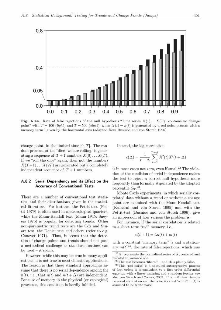
A.8. Statistical Background: Testing for Trends and Change Points (Jumps) 451
���
��
����
������ ��� �� ��Q �� ��� ��� ��� ��� ���
Fig. A.44. Rate of false rejections of the null hypothesis “Time series X(1) . . . X(T )” contains no changepoint” with T = 100 (light ) and T = 500 (black), when X(t) = n(t) is generated by a red noise process with amemory term l given by the horizontal axis (adapted from Busuioc and von Storch 1996)
change point, in the limited time [0, T ]. The ran-dom process, or the “dice” we are rolling, is gener-ating a sequence of T +1 numbers X(0) . . . X(T ).If we “roll the dice” again, then not the numbersX(T +1) . . . X(2T ) are generated but a completelyindependent sequence of T + 1 numbers.
A.8.2 Serial Dependency and its Effect on theAccuracy of Conventional Tests
There are a number of conventional test statis-tics, and their distributions, given in the statisti-cal literature. For instance the Pettit-test (Pet-tit 1979) is often used in meteorological quarters,while the Mann-Kendall text (Mann 1945; Sney-ers 1975) is popular for detecting trends. Othernon-parametric trend tests are the Cox and Stu-art test, the Daniel test and others (refer to e.g.Conover 1971). Thus, it seems that the detec-tion of change points and trends should not posea methodical challenge as standard routines canbe used – it seems.
However, while this may be true in many appli-cations, it is not true in most climatic applications.The reason is that these standard approaches as-sume that there is no serial dependence among then(t), i.e., that n(t) and n(t + ∆) are independent.Because of memory in the physical (or ecological)processes, this condition is hardly fulfilled.
Instead, the lag correlation
c(∆) =1
t − ∆
T−∆∑
t=0
X ′(t)X ′(t + ∆)
is in most cases not zero, even if small22 The viola-tion of the condition of serial independence makesthe test to reject a correct null hypothesis morefrequently than formally stipulated by the adoptedpercentile S95
23.Monte Carlo experiments, in which serially cor-
related data without a trend or without a changepoint are examined with the Mann-Kendall test(Kulkarni and von Storch 1995) and with thePettit-test (Busuioc and von Storch 1996), givean impression of how serious the problem is.
For instance, if the serial correlation is relatedto a short term “red” memory, i.e.,
n(t + 1) = λn(t) + m(t)
with a constant “memory term” λ and a station-ary m(t)24, the rate of false rejections, which was
22X′ represents the normalized series of X, centered andrescaled to variance one.
23The test becomes “liberal” – and thus plainly false.24This “red noise” is a so-called autoregressive process
of first order; it is equivalent to a first order differentialequation with a linear damping and a random forcing; seealso von Storch and Zwiers, 2002. If λ = 0 then there isno serial correlation and the noise is called “white”; m(t) isassumed to be white noise.

452 A. Annexes
�� � � �� �� ���
�
��
��
�
(�&����(�'��
Fig. A.45. Frequency (in per mille) of false detections of a change point at the t� values given at the horizontalaxis. 1000 Monte Carlo cases have been evaluated, all generated by a linear trend overlaid with white noise(α = 0.005; variance of noise = 1) (adapted from Busuioc and von Storch 1996)
����
������ ��� �� ��Q �� ��� ��� ��� ��� ���
����
����
���
�A'>�
(�&���������A��<(>����������������������������
Fig. A.46. Rate of false rejections of the null hypothesis “Time series X(1) . . . X(T ) contains no change point”with T = 100 (light ) and T = 500 (black), when X(t) = n(t) is generated by a red noise process with a memoryterm l given by the horizontal axis, when the Pettitt-test is applied to the pre-whitened, i.e., applied to Y (t)instead of X(t) (adapted from Busuioc and von Storch 1996)
stipulated to be 5%, of the Pettit-test dealing withthe detection of change points, is markedly largerthan 5% even for small λ ≥ 0.15 (Fig. A.44).
For large λ, say 0.8, in more than 50% of ap-plications of the Pettit test to a series without achange point and without other instationarities,the test indicates falsely that a change point is con-
tained in the data. A similar demonstration wasprovided by Kulkarni and von Storch (1995) forthe case of the Mann-Kendall test of linear trends(not shown).
When the serial correlation is related to a lineartrend, similarly false assessments of the alternativehypothesis happen. Figure A.45 shows the result

A.8. Statistical Background: Testing for Trends and Change Points (Jumps) 453
for 1,000 cases of series with a trend given by
X(t) = αt + n(t)
(Busuioc and von Storch, 1996). These series alldo not fulfil the null hypothesis of stationarity, butthey are all free of a change point. The time se-ries have a length of T = 100, and the diagramsdisplay how often a t� is falsely associated with achange point. They all cluster in the middle; forinstance the mid point t� = 50 is chosen in 1.5% ofall 1000 cases, while t�’s smaller than 40 or largerthan 60 are picked at a rate of on average 0.5%.t�’s smaller than 20 and larger than 80 never ap-pear. In total, a false change point is identified in38% of all cases.
A.8.3 Pre-whitening and Monte Carlo Ap-proaches to Overcome the Serial Depen-dency Problem
At least two possibilities exist to overcome theproblems related to serial dependence. One is pre-whitening and the other is Monte Carlo simula-tions.
“Pre-whitening” means to try to filter out theserial dependence. The detail of the filter dependson what is known, or assumed, about the serialdependence. For instance, if the serial dependence
originates from a linear trend, then a differencefilter, i.e.,
Y (t) = X(t + 1) − X(t)
would be appropriate. If the serial dependencemay be described by an auto-regressive processwith memory λ, then a suitable filter is
Y (t) = X(t + 1) − λX(t)
Figure A.46 shows as an example the frequency offalse rejections of the null hypothesis of no changepoint for different values of λ, when Y (t) is testedinstead of X(t). Figure A.44 has demonstratedthat with increasing λ’s this rejection rate growswell above the stipulated level (of 5%). Exceptfor very large values of λ, the test operates as re-quired.
Another possibility is to construct a large en-semble of limited time series X(0) . . . X(T ) withthe same statistical properties of the series to betested – without the specific property the test isdealing with, i.e., without a change point or with-out a trend. Then, by construction each memberof the ensemble fulfils the null hypothesis. Then,for each member the test statistic S is determined,and finally by polling all S-values, an empiricaldistribution of the test statistic is derived.

454 A. Annexes
A.9 References
Aarup T (2002) Transparency of the North Sea and Baltic Sea – a Secchi Depth data mining study.Oceanologia 44:323–337
Ackefors H (1969) Seasonal and vertical distribution of the zooplankton in the Askö area (northernBaltic proper) in relation to hydrographical conditions. Oikos 20:480–492
Ærtebjerg G, Andersen JH, Hansen OS (2003) Nutrients and eutrophication in Danish Marine Wa-ters. A challenge for science and management. Ministry of Environment, National EnvironmentalResearch Institute, Denmark
Agnew MD, Palutikof JP (2001) Impacts of climate on the demand for tourism. In: Matzarakis A, deFreitas CR (eds) Proceedings of the First International Workshop on Climate, Tourism and Recre-ation. International Society of Biometeorology, Commission on Climate, Tourism and Recreation.Porto Carras, Halkidiki, Greece. WP4:1–10
Alenius P, Myrberg K, Nekrasov A (1998) The physical oceanography of the Gulf of Finland: A re-view. Boreal Env Res 3:97–125
Andrejev O, Myrberg K, Alenius P, Lundberg PA (2004a) Mean circulation and water exchange inthe Gulf of Finland – A study based on three-dimensional modelling. Boreal Env Res 9:1–16
Andrejev O, Myrberg K, Lundberg PA (2004b) Age and renewal time of water masses in a semi-enclosed basin application to the Gulf of Finland. Tellus A 56:548–558
Andrén E, Andrén T, Sohlenius G (2000) The Holocene history of the southwestern Baltic Sea asreflected in a sediment core from the Bornholm Basin. Boreas 29:233–250
Andrén T (2003a) Baltiska Issjön – eller hur det började (The Baltic Ice Lake – or how it began).Havsutsikt 1/2003:4–5 (in Swedish)
Andrén T (2003b) Yoldiahavet – en viktig parentes (The Yoldia Sea – an important period). Havsut-sikt 2/2003:6–7 (in Swedish)
Andrén T (2003c) Ancylussjön – fortfarande ett mysterium (The Ancylus Lake – still a mystery).Havsutsikt 3/2003:8–9 (in Swedish)
Andrén T (2004) Littorinahavet – en salt historia (The Littorina Sea – A salt history). Havsutsikt1/2004:8–9
Andrén T, Björck J, Johnsen S (1999) Correlation of Swedish glacial varves with the Greenland(GRIP) oxygen isotope record. J Quat Sci 14:361–371
Aquaflow (2002) Miljøeffekter af havbrug i Finland (Environmental effects of aquacultures in Finland).Aquaflow ref: TL2002–088 (in Danish)
Arpe K, Hagemann S, Jacob D, Roeckner E (2005) The realisms of the ECHAM5 models to simulatethe hydrological cycle in the Arctic and north-European area. Nordic Hydrology 36:349–367
Azam F, Fenchel T, Field JG, Gray J, Meyer-Reil LA, Thingstad F (1983) The ecological role ofwater-column microbes in the sea. Mar Ecol Prog Ser 10:257–263
Badeck FW, Bondeau A, Böttcher K, Doktor D, Lucht W, Schaber J, Sitch S (2004) Response ofspring phenology to climate change. New Phytologist 162:295–309
Barnston AG, Livezey RE (1987) Classification seasonality and persistence of low frequency atmo-spheric circulation patterns. Mon Wea Rev 115:1083–1126
Bartnicki J, Gusev A, Lukewille A (2001) Atmospheric Supply of Nitrogen, Lead, Cadmium, Mercuryand Lindane to the Baltic Sea in 1998. Joint EMEP centres report for HELCOM 2001
Bartnicki J, Gusev A, Barret K, Simpson K (2002) Atmospheric Supply of Nitrogen, Lead, Cadmium,Mercury and Lindane to the Baltic Sea in the period 1996 – 2000. Joint EMEP centres report forHELCOM 2002
Bartnicki J, Gusev A, Berg T, Fagerli H (2003) Atmospheric Supply of Nitrogen, Lead, Cadmium,Mercury and Lindane to the Baltic Sea in 2001. EMEP/MSC-W note 3/2003
Bartnicki J, Gusev A, Berg T, Fagerli H (2004) Atmospheric Supply of Nitrogen. Lead. Cadmium.Mercury and Lindane to the Baltic Sea in 2002. EMEP/MSC-W technical report 3/2004
Bartnicki J, Gusev A, Berg T, Fagerli H (2005) Atmospheric Supply of Nitrogen, Lead, Cadmium,Mercury and Lindane to the Baltic Sea in 2003. EMEP/MSC-W note 3/2005

A.9. References 455
Bartnicki J, Gusev A, Aas W, Fagerli H (2006) Atmospheric Supply of Nitrogen, Lead, Cadmium,Mercury and Dioxines/Furanes to the Baltic Sea in 2004. EMEP/MSC-W TECHNICAL REPORT3/2006 OSLO, September 2006
Bazzaz FA (1990) The response of natural ecosystems to the rising global CO2 levels. Ann Rev EcolSystemat 21:167–196
Bell GD (2007) Climate Diagnostics Bulletin. Monthly Publication by U.S. Dept of Commerce, NOAAClimate Prediction Center
Bennike O, Jensen JB, Lemke W (1998) Fauna and flora in submarine early Holocene lake-marl de-posits from the southwestern Baltic Sea. The Holocene 8:353–358
Bennike O, Jensen JB, Lemke W, Kuijpers A, Lomholt S (2004) Late- and postglacial history of theGreat Belt, Denmark. Boreas 33:18–33
Benthien B (1996) Die Bäderlandschaft der südlichen Ostseeküste – ein Teil der zirkumbaltischen Er-holungszone (Seaside resorts at the southern Baltic Sea coast: Part of the circum-baltic recreationalzone). In: Greifswalder Beiträge zur Freizeit- und Tourismusforschung 7:7–13 (in German)
Bergh J, Linder S, Lundmark T, Elfving B (1999) The effect of water and nutrient availability on theproductivity of Norway spruce in northern and southern Sweden. Forest Ecol Manag 119:51–62
Berglund BE, Sandgren P, Barnekow L, Hannon G, Jiang H, Skog G, Yu S (2005) Early Holocenehistory of the Baltic Sea as reflected in coastal sediments in Blekinge, southeastern Sweden. QuatInt 130:111–139
Bergström S, Carlsson B (1994) River runoff to the Baltic Sea: 1950–1990. Ambio 23:280–287Bigano A, Goria A, Hamilton J, Tol R (2005): The Effect of Climate Change and Extreme Weather
Events on Tourism. Nota Di Lavoro 30.2005. The Fondazione Eni Enrico Mattei Note di LavoroSeries, www.feem.it/Feem/Pub/Publications/WPapers/default.htm
Björck S (1995) A review of the history of the Baltic Sea, 130–80 ka BP. Quat Int 27:19–40Björck S, Kromer B, Johnsen S, Bennike O, Hammarlund D, Lemdahl G, Possnert G, Rasmussen TL,
Wohlfarth B, Hammer CU, Spurk M (1996) Synchronized terrestrial-atmospheric deglacial recordsaround the North Atlantic. Science 274:1155–1160
Bogdanov VI, Medvedev M Yu, Solodov VA, Trapeznikov I, Yu A, Troshkov GA, Trubitsina AA,(2000) Mean monthly series of sea level observations (1777–1993) at the Kronstadt gauge. Reportsof the Finnish Geodetic Institute 2000:1
Bradshaw RHW, Holmqvist BH, Cowling SA, Sykes MT (2000) The effects of climate change on thedistribution and management of Picea abies in southern Scandinavia. Can J Forest Res 30:1992–1998
Breitzmann, KH (ed) (2004) Tourismus und Auslandstourismus im Ostseeraum (Tourism and tourismabroad in the Baltic Sea area). Selbstverlag des Ostseeinstituts, Beiträge und Informationen, Heft14. Rostock (in German)
Breivik K, Wania F (2002a) Evaluating a model of the historical behavior of two hexachlorocyclohex-anes in the Baltic Sea environment. Env Sci Technol 36:1014–1023
Breivik K, Wania F (2002b) Mass budgets pathways and equilibrium states of two hexachlorocyclo-hexanes in the Baltic Sea environment. Env Sci Technol 36:1024–1032
Brooks KM, Mahnken CVW (2003) Interactions of Atlantic salmon in the Pacific northwest environ-ment II. Organic wastes. Fish Res 62:255–293
Busuioc A, von Storch H (1996) Changes in the winter precipitation in Romania and its relation tothe large-scale circulation. Tellus 48A:538–552
Busuioc A, Chen D, Hellström C (2001) Temporal and spatial variability of precipitation in Swedenand its link with the large-scale atmospheric circulation. Tellus 53A:348–367
Cannell MGR (1989) Chilling thermal time and the date of flowering of trees. In: Wright C (ed) TheManipulation of Fruiting. Butterworths, London, pp. 99–113
Chen D, Hellström C (1999) The influence of the North Atlantic Oscillation on the regional tempera-ture variability in Sweden: Spatial and temporal variations. Tellus 51A:505–516
Christensen PB, Rysgaard S, Sloth NP, Dalsgaard T, Schwærter S (2000) Sediment mineralization,nutrient fluxes, denitrification and dissimilatory nitrate reduction to ammonium in an estuarinefjord with sea cage trout farms. Aquat Microb Ecol 21:73–84
Conover WJ (1971) Practical nonparametric statistics. Wiley & Sons

456 A. Annexes
Dahl E (1990) Probable effects of climatic change due to the greenhouse effect on plant productivityand survival in North Europe. In: Holten JI, Paulsen G, Oechel WC (eds) Effects of Climate Changeon Terrestrial Ecosystems, Norwegian Institute for Nature Research, Trondheim, Norway, pp 81–83
Dahlström B (1995) Snow cover. In: Raab B, Vedin H (eds) Climate, lakes and rivers. National Atlasof Sweden, pp. 91–97
Davis HC (1976) A lateral boundary formulation for multi-level prediction models. Q J Roy Met Soc102:405–418
de Pauw N, Jaspers E, Ackefors H, Wilkins N (1989) Aquaculture – A Biotechnology in Progress. ProcEurop Aquacult Soc, Bredene, Belgium, pp. 70–75
Dedkova I, Erdman L, Grigoryan S, Galperin M (1993) Assessment of airborne sulphur and nitrogenpollution of the Baltic Sea from European countries for 1987–1991. EMEP/MSC-E Moscow
Defant F (1972) Klima und Wetter der Ostsee (Climate and weather of the Baltic Sea). Kieler Meeres-forsch 28:1–130 (in German)
Deleersnijder E, Campin JM, Delhez E (2001) The concept of age in marine modelling: I Theory andpreliminary results. J Mar Sys 28:229–267
Delworth TL, Dixon KW (2000) Implications of the recent trend in the Arctic/North Atlantic Oscil-lation for the North Atlantic thermohaline circulation. J Clim 13:3721–3727
Dempster T, Sanchez-Jerez P, Bayle-Sempere JT, Gimenez-Casalduero F, Valle C (2002) Attractionof wild fish to sea-cage fish farms in the south-western Mediterranean Sea: Spatial and short-termtemporal variability. Mar Ecol Progr Ser 242:237–252
Derwent R, Collins W, Johnson C, Stevenson D (2002) Global ozone concentrations and regional airquality. Env Sci Technol 36:379A-382A
Dewar RC, Belinda EM, Mcmurtrie RE (1999) Acclimation of the respiration/photosynthesis ratio totemperature: Insights from a model. Glob Change Biol 5:615–622
Döös K, Meier HEM, Döscher R (2004) The Baltic haline conveyor belt or the overturning circulationand mixing in the Baltic. Ambio 33:261–266
Duke RA, Liss PS, Merrill JT, Buat-Menard P, Hicks BB, Miller JM, Prospero JM, Arimoto R,Church TM, Ellis W, Galloway JM, Hansen L, Jickells TD, Knap AH, Reinhardt KH, Schnei-der B, Soudine A, Tokos JJ, Tsunogai S, Wollast R, Zhou M (1989) The input of atmospheric tracespecies to the world ocean. Rep Stud GESAMP 38
ECE (1993) The Environment in Europe and North America. Annotated StatisticsEdler L (1979) Phytoplankton succession in the Baltic Sea. Acta Bot Fennici 110:75–78Eilola K, Stigebrandt A (1998) Spreading of juvenile freshwater in the Baltic proper. J Geophys Res
103,C12:27795–27807Ekman M (1988) The world’s longest continued series of sea level observations. Pure Appl Geophys
127:73–77Ekman M (1996) A consistent map of the postglacial uplift of Fennoscandia. Terra Nova 8:158–165Elken J (1994) Numerical study of fronts between the Baltic sub-basins. In: Proceedings of 19th
Conference of the Baltic Oceanographers, Sopot 1:438–446Elken J (1996) Deep water overflow circulation and vertical exchange in the Baltic proper. Estonian
Marine Institute Report Series 6Elken J, Pajuste M, Kõuts T (1988) On intrusive lenses and their role in mixing in the Baltic deep
layers. Proceedings of the 16th Conference of the Baltic Oceanographers, Kiel, pp. 367–376Elken J, Talpsepp L, Kõuts T, Pajuste M (1994) The role of mesoscale eddies and saline stratification
in the generation of spring bloom heterogeneity in the southeastern Gotland Basin: An examplefrom PEX ’86. In: Dybern BI (ed) ICES Cooperative Research Report 201: Patchiness in the BalticSea, pp. 40–48
Elken J, Raudsepp U, Lips U (2003) On the estuarine transport reversal in deep layers of the Gulf ofFinland. J Sea Res 49:267–274
Elmgren R (2001) Understanding human impact on the Baltic ecosystem: Changing views in recentdecades. Ambio 30:222–231
EMEP (2000) Transboundary acidification and eutrophication in Europe. EMEP Summary reportCCC and MSC-W, Oslo

A.9. References 457
EMEP (2003) Transboundary acidification eutrophication and ground level ozone in Europe. EMEPStatus report 2003, Oslo
EMEP (2004) Transboundary level of acidification eutrophication and ground-level ozone in Europe.Joint MSC-W CCC CIAM ICP-M&M and CCE report, Oslo
EMEP (2006) Transboundary acidification eutrophication and ground level ozone in Europe from1990 to 2004 in support for the review of the Gothenburg Protocol EMEP/MSC-W ETC/ACCICP-Forests CCE ICP M&M report EMEP status report, 2006
Emery WJ, Thomson RE (1997) Data analysis methods in physical oceanography. Pergamon PressEngström-Öst J, Koski M, Schmidt K, Viitasalo M, Jónasdóttir SH, Kokkonen M, Repka S, Sivonen
K (2002) Effects of toxic cyanobacteria on a plankton assemblage: Community development duringdecay of Nodularia spumigena. Mar Ecol Prog Ser 232:1–14
Falarz M (2001) Zmienność wieloletnia wyst powania pokrywy śnieżnej w polskich Tatrach (Long termvariability of snow cover in the Polish Tatra mountains). Folia Geogr Ser Geogr Phys 31–32:101–123(in Polish)
Falarz M (2004) Variability and trends in the duration and depth of snow cover in Poland in the 20th
century. Int J Climatol 24:1713–1727FAO (2005) Fisheries global information system, www.fao.orgFeistel R, Nausch G, Matthäus W, Hagen E (2003) Temporal and spatial evolution of the Baltic deep
water renewal in spring 2003. Oceanologia 45:623–642Fennel W, Seifert T (1995) Kelvin wave controlled upwelling in the western Baltic. J Mar Syst 6:289–
300Fennel W, Sturm M (1992) Dynamics of the western Baltic. J Mar Syst 3:183–205Fennel W, Seifert T, Kayser B (1991) Rossby radii and phase speeds in the Baltic Sea. Continent
Shelf Res 11:23–36Fischer H, Matthäus W (1996) The importance of the Drogden Sill in the Sound for major Baltic
inflows. J Mar Syst 9:137–157Fredén C (1986) Quaternary marine shell deposits in the region of Uddevalla and Lake Vänern.
Sveriges Geologiska Undersökning. Rapporter och Meddelanden 46Freeman M, Morén AS, Strömmer M, Linder S (2005) Climate change impacts on forests in Europe:
Biological impact mechanisms. In: Kellomäki S, Leinonen S (eds) Management of European forestsunder changing climatic conditions. University of Joensuu, Faculty of Forestry Research, Notes 163:46:115
GESAMP (2001) Planning and management for sustainable coastal aquaculture development.GESAMP Reports and Studies 68
Golenko NN, Beszczynska-Möller A, Piechura J, Walczowski W, Ameryk A (1999) Some results ofresearch on internal waves in the Stolpe Sill area. Oceanologia 41:537–551
Gorokhova E, Fagerberg T, Hansson S (2004) Predation by herring (Clupea harengus) and sprat(Sprattus sprattus) on Cercopagis pengoi in a western Baltic Sea bay. ICES J Mar Sci 61:959–965
Grace J, Berninger F, Nagy L (2002) Impacts of climate change on the tree line. Ann Bot 90:537–544Grasshoff K (1975) The hydrochemistry of landlocked basins and fjords. In: Riley JP, Skirrow G (eds)
Chemical Oceanography (2nd ed.), pp. 455–597. Academic Press, London New York San FransiscoGustafsson BG (2001) Quantification of water salt oxygen and nutrient exchange of the Baltic Sea
from observations in the Arkona Basin. Cont Shelf Res 21:1485–1500Gustafsson BG, Andersson HC (2001) Modelling the exchange of the Baltic Sea from the meridional
atmospheric pressure difference across the North Sea. J Geophys Res 106,C9:19731–19744Gyllenhammar A (2004) Predictive modelling of aquatic ecosystems at different scales using mass-
balances and GIS. PhD thesis, Uppsala UnivGyllenhammar A, Håkanson L (2005) Environmental consequence analyses of fish farms emissions re-
lated to different scales and exemplified by data from the Baltic – A review. Mar Env Res 60:211–243
Hagen E, Feistel R (2004) Observations of low-frequency current fluctuations in deep water of theEastern Gotland Basin/Baltic Sea. J Geophys Res 109 C03044 doi:101029/2003JC002017

458 A. Annexes
Håkanson L (2005) Changes to lake ecosystem structure resulting from fish cage farm emissions. Lakesand Reservoirs: Research and Management 10:71–80
Håkanson L, Boulion V (2002) The lake foodweb – modelling predation and abiotic/biotic interactions.Backhuys Publishers, Leiden
Håkanson L, Ervik A, Mäkinen T, Möller B (1988) Basic concepts concerning assessments of environ-mental effects of marine fish farms. Nordic Council of Ministers, NORD88:90, Copenhagen
Håkanson L, Gyllenhammar A, Brolin A (2004) A dynamic model to predict sedimentation and sus-pended particulate matter in coastal areas. Ecol Model 175:353–384
Håkansson B, Broman B, Dahlin H (1993) The flow of water and salt in the Sound during the Balticmajor inflow event in January 1993. ICES CM 1993/C:57
Håkansson B, Alenius P, Brydsten L (1996) The physical environment in the Gulf of Bothnia. AmbioSpecial Report No 8:5–12
Hall POJ, Anderson LG, Holby O, Kollberg S, Samuelsson M (1990) Chemical fluxes and mass bal-ances in a marine fish cage farm. I. Carbon. Mar Ecol Progr Ser 61:61–73
Hall POJ, Holby O, Kollberg S, Samuelsson MO (1992) Chemical fluxes and mass balances in a marinefish cage farm. 4. Nitrogen. Mar Ecol Progr Ser 89:81–91
Hamilton J, Lau M (2004) The role of climate information in tourist destination choice decision-making. Centre for Marine and Climate Research, Hamburg University, www.uni-hamburg.de/Wiss/FB/15/Sustainability/climinfo.pdf
Hansson S, Larsson U, Johansson S (1990) Selective predation by herring and mysids and zooplanktoncommunity structure in a Baltic Sea coastal area. J Plank Res 12:1099–1116
Hass H, van Loon M, Kessler K, Stern R, Matthijsen J, Sauter F, Zlatev Z, Langner J, Foltescu V,Schaap M (2003) Aerosol modelling: Results and intercomparison from European regional-scalemodelling systems. EUROTRAC-2 special report, EUROTRAC International Scientific Secretariat,GSF – National Research Center for Environment and Health. Munich, Germany
Havbrugsudvalget (2003) Bilag 4–11 til udvalgets rapport (Supplement 4–11 to Commission Report).Ministeriet for Fødevarer Landbrug og Fiskeri, (in Danish)
HELCOM (1989) Deposition of airborne pollution to the Baltic Sea area 1983–1985 and 1986. BalticSea Env Proc 32
HELCOM (1991) Airborne pollution load to the Baltic Sea 1986–1990. Baltic Sea Env Proc 39HELCOM (1993) The Baltic Sea Joint Comprehensive Environmental Action Programme. Helsinki,
1993. Baltic Sea Env Proc 48:2–20HELCOM (1996) Third Periodic Assessment of the State of the Marine Environment of the Baltic Sea
1989–1993. Background document. Baltic Sea Env Proc 64BHELCOM (1997) Airborne pollution load to the Baltic Sea 1991–1995. Baltic Sea Env Proc 69HELCOM (2002) Environment of the Baltic Sea Area 1994–1998. Baltic Sea Env Proc 82BHELCOM (2003a) The Baltic Marine Environment 1999–2002. Baltic Sea Env Proc 87HELCOM (2003b) HELCOM Report on Illegal Discharges Observed During Aerial Surveillance in
2003, www.helcom.fi/stc/files/shipping/spills2003.pdfHELCOM (2005) www.helcom.fi/stc/files/shipping/Overview%20of%20ships%20traffic.pdfHertel O, Ambelas SC, Brandt J, Christensen JH, Frohn M, Frydendall J (2003) Operational mapping
of atmospheric nitrogen deposition to the Baltic Sea. Atmos Chem Phys 3:2083–2099Holmer M, Kristensen E (1992) Impact of marine fish cage farming on sediment metabolism and sul-
fate reduction of underlying sediments. Mar Ecol Progr Ser 80:191–201Hongisto M, Joffre S (2005) Meteorological and climatological factors affecting transport and deposi-
tion of nitrogen compounds over the Baltic Sea. Boreal Env Res 10:1–17Hongisto M, Sofiev M, Joffre S (2003) Hilatar a limited area simulation model of acid contaminants:
II Model verification and long-tern simulation results. Atmos Env 37:1549–1560Honkanen T, Helminen H (2000) Impacts of fish farming on eutrophication: Comparisons among dif-
ferent characteristics of ecosystem. Intern Rev Hydrobiol 85:673–686Houmark-Nielsen M, Kjær K (2003) Southwest Scandinavia 40–15 kyr BP: Paleogeography and envi-
ronmental change. J Quat Sci 18:1–18

A.9. References 459
Hungate BA, Dukes JS, Shaw MR, Luo Y, Field CB (2003) Nitrogen and climate change. Science302:1512–1513
Huntley B (1991) How plants respond to climate change: Migration rates individualism and the con-sequences for plant communities. Ann Bot 67:15–22
Hurrell JW (1995) Decadal trends in the North Atlantic Oscillation: Regional temperatures and pre-cipitation. Science 269:676–679
Ikävalko J, Thomsen HA (1997) The Baltic Sea ice biota (March 1994): A study of the protistancommunity. Europ J Protistol 33:229–243
ICES (2005) ICES Advice Vol. 8, www.ices.dk/products/icesadvice2005.aspIOC (1997) Global sea level observing system (GLOSS) Implementation Plan – 1997. Intergovern-
mental Oceanographic Commission Technical Series, No 50, UNESCOIsemer HJ, Rozwadowska A (1999) Solar radiation fluxes at the surface of the Baltic Proper. Part 2:
Uncertainties and comparison with simple bulk parameterisations. Oceanologia 41:147–185Jaagus J (1996) Spatial and temporal variability of snow cover duration in Estonia. In: Punning JM
(ed) Estonia Geographical Studies. Estonian Academy Publishers, Tallinn, pp 43–59Jaagus J (1997) The impact of climate change on the snow cover pattern in Estonia. Climatic
Change 36:65–77Jacobeit J, Jönsson P, Bärring L, Beck C, Ekström M (2001) Zonal indices for Europe 1780–1995 and
running correlations with temperature. Climatic Change 48:219–241Jäderholm C, Steingrube W (1996) Das finnische Mökkiwesen – ein landestypischer Lebensstil im Um-
bruch? (The Finnish “Mökkis” – a change in typically Finnish life-style?). Erdkunde 50:138–148 (inGerman)
Jakobsen F (1995) The major inflow to the Baltic Sea during January 1993. J Mar Syst 6:227–240Jakobsen F (1996) The dense water exchange of the Bornholm Basin in the Baltic Sea. Dt Hydr Z
48,2: 133–145Jakobsen F, Trebuchet C (2000) Observations of the transport through the Belt Sea and an investi-
gation of momentum balance. Continent Shelf Res 20:293–311Jensen JB, Bennike O, Witkowski A, Lemke W, Kuijpers A (1999) Early Holocene history of the
southwestern Baltic Sea: The Ancylus Lake stage. Boreas 28:437–453Jensen JB, Kuijpers A, Bennike O, Lemke W (2002) Balkat – The Baltic Sea without frontiers. Ge-
ologi nyt fra GEUS 4/2002Johansson M, Gorokhova E, Larsson U (2004) Annual variability in ciliate community structure po-
tential prey and predators in the open northern Baltic Sea proper. J Plank Res 26:67–80Jonasson S, Michelsen A, Schmidt IK (1999) Coupling of nutrient cycling and carbon dynamics in the
Arctic integration of soil microbial and plant processes. Appl Soil Ecol 11:135–146Jones C, Ullerstig A (2002) The representation of precipitation in the RCA2 model. Rossby Centre
Atmosphere Model Version 2. SWECLIM Newsletter 12, pp. 27–39Jones PD, Moberg A (2003) Hemispheric and Large-Scale Surface Air Temperature Variations: An
Extensive Revision and an Update to 2001. J Clim 16:206–223Jones PD, Jónsson T, Wheeler D (1997) Extension to the North Atlantic Oscillation using early in-
strumental pressure observations from Gibraltar and south-west Iceland. Int J Climatol 17:1433–1450
Jönsson A, Broman B, Rahm L (2003) Variations in the Baltic Sea wave fields. Ocean Eng 30:107–126Jutila E, Toivonen J (1985) Food consumption of salmon post-smolts (Salmo salar L) in the northern
part of the Gulf of Bothnia. ICES CM 1985/M:21, p. 11Kahru M, Horstmann U, Rud O (1994) Satellite detection of increased cyanobacteria blooms in the
Baltic Sea: Natural fluctuation or ecosystem change. Ambio 23:469–472Kallis A (1995) Estonia’s place in the world of actinometry. In: Meteorology in Estonia in Johannes
Letzmann’s times and today. Estonian Academy Publishers, Tallinn, pp 95–100Karlsson KG (1999) Satellite sensing techniques and applications for the purpose of BALTEX. Meteo-
rol Z 9:111–116Karlsson KG (2001) A NOAA AVHRR cloud climatology over Scandinavia covering the period 1991–
2000. SMHI Reports Meteorology and Climatology 97

460 A. Annexes
Kautsky U (1995) Ecosystem processes in coastal areas of the Baltic Sea. PhD thesis, Dept of Zoology,Stockholm University
Keevallik S, Russak V (2001) Changes in the amount of low clouds in Estonia (1955–1995). Int JClimatol 21:389–397
Keevallik S, Post P, Tuulik J (1999) European circulation patterns and meteorological situation in Es-tonia. Theor Appl Climatol 63:117–127
Kellomäki S, Leinonen S (2005) Management of European forests under changing climatic conditions.Final Report of the Project “Silvicultural Response Strategies to Climatic Change in Managementof European Forests”. University of Joensuu, Faculty of Forestry Research, Notes 163:1– 4–27
Kiørboe T (1993) Turbulence phytoplankton cell size and the structure of pelagic food webs. AdvMar Biol 29:1–72
Kitaev L, Krueger O, Sherstyukov BG, Hobe H (2005a) Indications of influence of vegetation on thesnow cover distribution. Russian Meteorology and Hydrology. Allerton Press Inc, New York, 7,pp. 61–69
Kitaev L, Forland E, Razuvaev V, Tveito OE, Krueger O (2005b) Distribution of snow cover overNorthern Eurasia. Nordic Hydrology 36:311–319
Kitaev L, Razuvaev VN, Heino R, Forland E (2006) Duration of snow cover over Northern Europe.Russian Meteorology and Hydrology 3, Allerton Press Inc, New York, pp. 95–100
Kivi K (1986) Annual succession of pelagic protozoans and rotifers in the Tvärminne Storfjärden, SWcoast of Finland. Ophelia Suppl 4:101–110
Kjær K, Houmark-Nielsen M, Richardt N (2003) Ice-flow patterns and dispersal of Erratics at thesouthwestern margin of the last Scandinavian ice sheet: Imprint after paleo ice-streams. Boreas 32:130–148
Kononen K, Kuparinen J, Mäkelä K, Laanemets J, Pavelson J, Nômmann S (1996) Initiation ofcyanobacterial blooms in a frontal region at the entrance to the Gulf of Finland, Baltic Sea. LimnolOceanogr 41:98–112
Kononen K, Huttunen M, Hällfors S, Gentien P, Lunven M, Huttula T, Laanemets J, Lilover M, Pavel-son J, Stips A (2003) Development of a deep chlorophyll maximum of Heterocapsa triquetra Ehrenb.at the entrance to the Gulf of Finland. Limnol Oceanogr 48:594–607
Körner C (1998) A re-assessment of high elevation treeline positions and their explanation. Oecologia115:445–459
Kõuts T, Omstedt A (1993) Deep water exchange in the Baltic Proper. Tellus 45A:311–324Kõuts T, Elken J, Lips U (1990) Late autumn intensification of deep thermohaline anomalies and for-
mation of lenses in the Gotland Deep. Proceedings of the 17th Conference of the Baltic Oceanogra-phers, Norrköping 1990, pp. 280–293
Kramer K (1995) Phenotypic plasticity of the phenology of seven European species in relation toclimate warming. Plant Cell Env 18:93–104
Kulkarni A, von Storch H (1995) Monte Carlo experiments on the effect of serial correlation on theMann-Kendall-test of trends. Met Zeitschrift 4:82–85
Kuparinen J, Leppänen JM, Sarvala J, Sundberg A, Virtanen A (1984) Production and utilization oforganic matter in a Baltic ecosystem off Tvärminne, southwest coast of Finland. Rapp P v Réun.Cons. int. Explor. Mer. 193:180–192
Kuusisto E (1984) Snow accumulation and snowmelt in Finland. Publ of the Water Research Insti-tute 55
Kuusisto E (1995) Hydrology and hydroenergetics of the Baltic Drainage. Proceedings of the FirstStudy Conference of BALTEX, International BALTEX Secretariat Publication 3:18–27
Kuusisto E (2005) Snow as a geographic element. In: Seppälä M (ed) The Physical Geography ofFennoscandia. Oxford University Press, pp. 160–173
Lambeck K, Chappell J (2001) Sea level change through the last glacial cycle. Science 292:679–686Larsson U, Hobro R, Wulff F (1986) Dynamics of a phytoplankton spring bloom in a coastal area of
the northern Baltic Proper. Contributions from the Askö Laboratory 30:3–32Lass HU, Mohrholz V (2003) On the dynamics and mixing of inflowing saltwater in the Arkona Sea.
J Geophys Res 108,C2 3042 doi:101029/2002JC001465
A.9. References 461
Lass HU, Talpsepp L (1993) Observations of coastal jets in the Southern Baltic. Cont Shelf Res 13:2–3:189–203
Lass HU, Prandke H, Liljebladh B (2003) Dissipation in the Baltic proper during winter stratification.J Geophys Res 108 No C6 3187 doi:101029/2002JC001401 2003
Laurila T, Jonson JE, Langner J, Sundet J, Tuovinen JP, Bergström R, Foltescu V, Tarvainen V,Isaksen ISA (2004) Ozone exposure scenarios in the Nordic countries during the 21st century.EMEP/MSC-W Technical Report 2/2004
Ledwith M (2002) Land cover classification using SPOT Vegetation 10-day composite images – BalticSea Catchment basin. GLC2000 Meeting Ispra, Italy, April 18–22.2002
Lee DS, Nemitz E, Fowler D, Kingdon RD (2001) Modelling atmospheric mercury transport and de-position across Europe and the UK. Atmos Env 35:5455–5466
Lehmann A, Hinrichsen HH (2000) On the wind driven and thermohaline circulation of the Baltic Sea.Phys Chem Earth,B 25:183–189
Lehmann A, Hinrichsen HH (2001) The importance of water storage variations for water balance stud-ies of the Baltic Sea. Phys Chem Earth, B 26:383–389
Lehmann A, Hinrichsen HH (2002) Water heat and salt exchange between the deep basins of the BalticSea. Boreal Env Res 7:405–415
Lehmann A, Krauss W, Hinrichsen HH (2002) Effects of remote and local atmospheric forcing on cir-culation and upwelling in the Baltic Sea. Tellus 54A:299–316
Lehmann A, Lorenz P, Jacob D (2004) Modelling the exceptional Baltic Sea inflow events in 2002–2003. Geophys Res Lett, vol. 31, No. 21, L21308 101029/2004GL020830
Lehtonen KK (1997) Ecophysiology of two benthic amphipod species from the northern Baltic Sea.PhD thesis, University of Helsinki. Monogr Boreal Env Res No 7:1–33
Lemke W, Jensen JB, Bennike O, Witkowski A, Kuijpers A (1999) No indication of a deeply incisedDana River between Arkona Basin and Mecklenburg Bay. Baltica 12:66–70
Leppäkoski E, Gollasch S, Gruszka P, Ojaveer H, Olenin S, Panov V (2002) The Baltic – a sea ofinvaders. Can J Fish Aquat Sci 59:1175–1188
Lignell R, Heiskanen AS, Kuosa H, Gundersen K, Kuuppo-Leinikki P, Pajuniemi R, Uitto A (1993)Fate of a phytoplankton spring bloom: Sedimentation and carbon flow in the planktonic food webin the northern Baltic. Mar Ecol Prog Ser 94:239–252
Liljebladh B, Stigebrandt A (1996) Observations of deepwater flow into the Baltic Sea. J GeophysRes 101,C4:8895–8911
Lilover MJ, Lips U, Laanearu J, Liljebladh B (1998) Flow regime in the Irbe Strait. Aquat Sci 60:253–265
Lindau R (2002) Energy and water balance of the Baltic Sea derived from merchant ship observations.Boreal Env Res 7,4:417–424
Lindfors V, Joffre SM, Damski J (1993) Meteorological variability of the wet and dry deposition ofsulphur and nitrogen compounds over the Baltic Sea. Water Air Soil Pollut 66:1–28
Lips U, Lilover MJ, Raudsepp U, Talpsepp L (1995) Water renewal processes and related hydro-graphic structures in the Gulf of Riga. In: Hydrographic studies within the Gulf of Riga Project1993–1994. Estonian Marine Institute Report Series No 1, pp. 1–34
Lise W, Tol RSJ (2005) Impact of climate on tourist demand. Climatic Change 55:429–449Lloyd J, Farquhar GD (1996) The CO2 dependence of photosynthesis plant growth responses to ele-
vated atmospheric CO2 concentrations and their interactions with soil nutrient status. I. Generalprinciples and forest ecosystems. Funct Ecol 10:4–32
Lohmann M (2003) Über die Rolle des Wetters bei Urlaubsreiseentscheidungen (How weather affectsdecisions for holiday destinations). Jahrbuch der Tourismuswirtschaft Schweiz. Institut für öf-fentliche Dienstleistungen und Tourismus, Universität St. Gallen
Lundqvist J, Wohlfarth B (2001) Timing and east-west correlation of south Swedish ice marginal linesduring the Late Weichselian. Quat Sci Rev 20:1127–148
Mäkinen T (1991) Marine Aquaculture and Environment. Nordic Council of Minister, Nord, 1991, 22,pp. 9–23

462 A. Annexes
Malanson GP, Cairns DM (1997) Effects of dispersal population delays and forest fragmentation ontree migration rates. Plant Ecol 131:67–79
Mann HB (1945) Non-parametric test against trend. Econometrica 13:245–259Marmefelt E, Omstedt A (1993) Deep water properties in the Gulf of Bothnia. Cont Shelf Res 13:
169–187Matuszko D (2003) Cloudiness changes in Cracow in the 20th century. Int J Climatol 23:975–984Matthäus W (1984) Climatic and seasonal variability of oceanological parameters in the Baltic Sea.
Beiträge zur Meereskunde 51:29–49Matthäus W (1995) Natural variability and human impacts reflected in long-term changes in the Baltic
Deep Water conditions – a brief review. Dt Hydr Z 47:47–65Matthäus W, Franck H (1992) Characteristics of major Baltic inflows – a statistical analysis. Cont
Shelf Res 12:1375–1400Matthäus W, Lass HU (1995) The recent salt inflow into the Baltic Sea. J Phys Oceanogr 25:280–286Mattsson J (1996) Some comments on the barotropic flow through the Danish Straits and the division
of the flow between the Belt and the Öresund. Tellus 48:456–471McGuire AD, Melillo JM, Joyce LA (1995) The role of nitrogen in the response of forest net primary
production to elevated atmospheric carbon dioxide. Ann Rev Ecol Systemat 26:473–503Meier HEM (2005) Modeling the age of Baltic Seawater masses: Quantification and steady state sen-
sitivity experiments. J Geophys Res 110 C02006 doi:101029/2004JC002607Meier HEM, Kauker F (2003) Modeling decadal variability of the Baltic Sea. Part 2: The role of
freshwater inflow and large-scale atmospheric circulation for salinity. J Geophys Res 108 No C11doi: 10 1029/2003JC001799 2003; 32–1–32–10
Meier HEM, Döscher R, Broman B, Piechura J (2004) The major Baltic inflow in January 2003 andpreconditioning by smaller inflows in summer/autumn 2002: A model study. Oceanologia 46,4:557–579
Melillo JM, Steudler PA, Aber JD, Newkirk K, Lux H, Bowles FP, Catricala C, Magill A, AhrensT, Morrisseau S (2002) Soil warming and carbon-cycle feedbacks to the climate system. Science298:2173–2176
Miętus M (1998) The Climate of the Baltic Sea Basin. Marine Meteorology and Related Oceano-graphic Activities. Report 41. WMO/TD-No. 933. World Meteorological Organization
Miguez-Macho G, Stenchikov GL, Robock A (2004) Spectral nudging to eliminate the effects of do-main position and geometry in regional climate model simulations. J Geophys Res 109 D13104doi:101029/2003JD004495
Möllmann C, Kornilovs G, Sidrevics L (2000) Long-term dynamics of main mesozooplankton speciesin the central Baltic Sea. J Plankton Res 22:2015–2038
Möllmann C, Kornilovs G, Fetter M, Köster FW (2004) Feeding ecology of central Baltic Sea herringand sprat. J Fish Biol 65:1563–1581
Munsterhjelm R (1997) The aquatic macrophyte vegetation of flads and gloes, S coast of Finland.Acta Bot Fenn 157:1–68
Munthe J, Wangberg I, Iverfeldt A, Lindquist O, Stromberg D, Sommar J, Gardfeldt K, Petersen G,Ebinghaus R, Prestbo E (2003) Distribution of atmopsheric mercury species in Northern Europe:Final results from the MOE project. Atmos Env 37–1:9–20
Murray NB, Cannell MGR, Smith I (1989) Date of budburst of fifteen tree species in Britain followingclimatic warming. J Appl Ecol 26:693–700
Myrberg K, Andrejev O (2003) Main upwelling regions in the Baltic Sea – a statistical analysis basedon three-dimensional modelling. Boreal Env Res 8:97–112
Nakićenović N, Swart R (2000) Emissions Scenarios. A Special Report of Working Group III of theIntergovernmental Panel on Climate Change. Cambridge University Press
Nehring D, Matthäus W (1991) Current trends in hydrographic and chemical parameters and eutroph-ication in the Baltic Sea. Internationale Revue der gesamten Hydrobiologie 76:297–316
Nerheim S (2004) Shear-generating motions at various length scales and frequencies in the Baltic Sea– an attempt to narrow down the problem of horizontal dispersion. Oceanologia 46,4:477–503

A.9. References 463
Niemi Å (1975) Ecology of phytoplankton in the Tvärminne area SW coast of Finland. II. Primaryproduction and environmental conditions in the archipelago and the sea zone. Acta Bot Fennica 105:1–73
Nissling A, Westin L (1991) Egg buoyancy of Baltic cod (Gadus morhua) and its implications for codstock fluctuations in the Baltic. Mar Biol 111:33–35
Norby RJ, DeLucia EH, Gielen B, Calfapietra C, Giardina CP, King JS, Ledford J, McCarthy HR,Moore DJP, Ceulemans R, De Angelis P, Finzi AC, Karnosky DF, Kubiske ME, Lukac M, PregitzerKS, Scarascia-Mugnozza GE, Schlesinger WH, Oren R (2005) Forest response to elevated CO2 isconserved across a broad range of productivity. Proceedings of the National Academy of Sciences,USA 102:18052–18056
Nordli Ø, Alexandersson H, Frich P, Førland E, Heino R, Jónsson T, Tveito OE (1997) The effect ofradiation screens on Nordic time series of mean temperature. Int J Climatol 17:1667–1681
Nordvarg L, Håkanson L (2002) Predicting the environmental response of fish farming in coastal ar-eas of the Åland archipelago (Baltic Sea) using management models for coastal water planning.Aquaculture 206:217–243
Novak B, Björck S (1998) Marine seismic studies in southern Kattegatt with special emphasis on lon-gitudinal bars and their possible relationship to the drainage of the Ancylus Lake. GFF 120:293–302
Omstedt A, Axell LB (2003) Modeling the variations of salinity and temperature in the large Gulfs ofthe Baltic Sea. Continent Shelf Res 23:265–294
Omstedt A, Chen D (2001) Influence of atmospheric circulation on the maximum ice extent in theBaltic Sea. J Geophys Res 106,C3:4493–4500
Omstedt A, Nohr C (2004) Calculating the water and heat balances of the Baltic Sea using oceanmodelling and available meteorological hydrological and ocean data. Tellus 56A:400–414
Omstedt A, Rutgersson A (2000) Closing the water and heat cycles of the Baltic Sea. Meteorol Z 9:55–66
Omstedt A, Marmefelt E, Murthy CR (1993) Some flow charachteristics of the coastal boundary layerin the Bothnian Sea. Aqua Fennica 23,1:5–16
Omstedt A, Elken J, Lehmann A, Piechura J (2004) Knowledge of the Baltic Sea physics gained dur-ing the BALTEX and related programmes. Progr Oceanogr 63, Issues 1–2:1–28
Palz W, Greif J (1996) European Solar Radiation Atlas. Springer, Berlin Heidelberg New YorkPavelson J (1988) Nature and some characteristics of thermohaline fronts in the Baltic Proper. In:
Proceedings of the 16th Conference of the Baltic Oceanographers, Kiel, pp 796–805Pavelson J, Laanemets J, Kononen K, Nõmmann S (1997) Quasi-permanent density front at the en-
trance to the Gulf of Finland: Response to wind forcing. Cont Shelf Res 17,3:253–265Peltonen H, Vinni M, Lappalainen A, Pönni J (2004) Spatial distribution patterns of herring (Clupea
harengus L) sprat (Sprattus sprattus L) and the three-spined stickleback (Gasterosteus aculeatus L)in the Gulf of Finland, Baltic Sea. ICES J Mar Sci 61:966–971
Peltonen K (2002) Direct ground water inflow to the Baltic Sea. TemaNord 2002:503, Nordic Councilof Ministers, Copenhagen, Denmark
Pershagen H (1981) Maxisnödjup i Sverige 1905–76. (Maximum snow cover in Sweden 1905–76) SMHIReports Meteorology and Climatology, RMK 29 (in Swedish)
Petersen G, Krueger O (1993) Untersuchung und Bewertung des Schadstoffeintrags über die Atmo-sphäre im Rahmen von PARCOM (Nordsee) und HELCOM (Ostsee) – Teilvorhaben: Modellierungdes großräumigen Transports von Spurenmetallen (Investigation and assessment of atmospheric de-position of pollutants within the framework of PARCOM (North Sea) und HELCOM (Baltic Sea)– Subproject: Modelling large scale transport of trace metals). GKSS Research Centre Geesthacht,Germany, GKSS 93/E/28 (in German)
Petersen G, Bloxam R, Wong S, Munthe J, Krüger O, Schmolke SR, Vinod Kumar A (2001) A com-prehensive Eulerian modelling framework for airborne mercury species: Model development andapplications in Europe. Atmos Env 35,17:3063–3074
Petersen JK, Loo LO (2004) Miljøkonsekvenser af dyrkning af blåmuslinger (Environmental conse-quences of common mussel cultivation), www.fvm.dk (in Danish)

464 A. Annexes
Petersen KS, Rasmussen KL, Heinemeier J, Rud N (1992) Clams before Columbus. Nature 359:679Pettit AN (1979) A non-parametric approach to the change point problem. App Statist 26–135Piechura J, Beszczynska-Möller A (2004) Inflow waters in the deep regions of the southern Baltic sea-
transport and transformations. Oceanologia 46,1:113–141Piechura J, Walczowski W, Beszcynska-Möller A (1997) On the structure and dynamics of the water
in the Slupsk Furrow. Oceanologia 39,1:35–54Pizarro O, Shaffer G (1998) Wind-driven coastal-trapped waves off the Island of Gotland, Baltic Sea.
J Phys Oceanogr 28,11:2117–2129Poorter H, Navas ML (2003) Plant growth and competition at elevated CO2: On winners, losers, and
functional groups. New Phytologist 157:175–198Pussinen A, Meyer J, Zudin S, Lindner M (2005) European mitigation potential. In: Kellomäki S,
Leinonen S (eds) Management of European Forests Under Changing Climatic Conditions. Universityof Joensuu, Faculty of Forestry Research. Notes 163:383–400
Pussinen A, Schelhaas MJ, Verkaik E, Heikkinen E, Liski J, Karjalainen T, Päivinen R, Nabuurs GJ(2001) Manual for the European Forest Information Scenario Model (EFISCEN 20). EuropeanForest Institute, Joensuu, Finland, EFI, Internal Report 5:49
Raab B, Vedin H (1995) Climate, lakes, and rivers. National Atlas of SwedenRäisänen J, Hansson U, Ullerstig A, Döscher R, Graham LP, Jones C, Meier M, Samuelsson P, Willén
U (2003) GCM driven simulations of recent and future climate with the Rossby Centre coupledatmosphere – Baltic Sea regional climate model RCAO. SMHI Reports Meteorology and Climatology101, SMHI, Norrköping, Sweden
Raudsepp U (1998) Current dynamics of estuarine circulation in the Lateral Boundary Layer. EstuarCoast Shelf Sci 47:715–730
Raudsepp U (2001) Interannual and seasonal temperature and salinity variations in the Gulf of Rigaand corresponding saline water inflow from the Baltic Proper. Nordic Hydrology 32,2:135–160
Raudsepp U, Beletsky D, Schwab DJ (2003) Basin scale topographic waves in the Gulf of Riga. JPhys Oceanogr 33,5:1129–1140
Remane A (1934) Die Brackwasserfauna (Mit besonderer Berücksichtigung der Ostsee) (Brackish wa-ter fauna, with special emphasis on the Baltic Sea). Verhandlungen der Deutschen ZoologischenGesellschaft 36:34–74 (in German)
Roads J, Raschke E, Rockel B (2004) BALTEX water and energy budgets in the NCEP/DOE reanal-ysis. II. Boreal Env Res 7,4:307–318
Robarts RD, Zohary T (1987) Temperature effects on photosynthetic capacity, respiration, andgrowth rates of bloom-forming cyanobacteria. N.Z. J Mar Freshwat Res 21:391–399
Rodhe H, Soederlund R, Ekstedt J (1980) Depositon of airborne pollutants on the Baltic Sea. Am-bio 9: 168–173
Rodhe J (1998) The Baltic and the North Seas: A process-oriented review of the Physical Oceanog-raphy. In: Robinson A, Brink K (eds) The Sea, vol. 11. Wiley, New York, pp. 699–732
Roemer M, Beekmann M, Bergström R, Boersen G, Feldmann H, Flatøy F, Honore C, Langner J,Jonson JE, Matthijsen J, Memmesheimer M, Simpson D, Smeets P, Solberg S, Stern R, StevensonD, Zandveld P, Zlatev Z (2003) Ozone trends according to ten dispersion models. EUROTRAC-2special report, EUROTRAC International Scientific Secretariat, GSF – National Research Centerfor Environment and Health, Munich, Germany
Rogers JC (1984) The association between the North Atlantic Oscillation and the Southern Oscillationin the Northern Hemisphere. Mon Wea Rev 107:1999–2015
Rozwadowska A, Isemer HJ (1998) Solar radiation fluxes at the surface of the Baltic Proper. Part 1.Mean annual cycle and influencing factors. Oceanologia 40,4:307–330
Rubel F, Hantel M (1999) Correction of daily rain gauge measurements in the Baltic Sea drainagebasin. Nordic Hydrology 30:191–208
Rubel F, Hantel M (2001) BALTEX 1/6-degree daily precipitation climatology 1996–1998. Met At-mos Phys 77:155–166
Rudstam LG, Hansson S (1990) On the ecology of Mysis mixta (Crustacea, Mysidacea) in a coastalarea of the northern Baltic proper. Ann Zool Fennici 27:259–263

A.9. References 465
Ruprecht E, Kahl T (2003) Investigation of the atmospheric water budget of the BALTEX area usingNCEP/NCAR reanalysis data. Tellus 55A:426–437
Rutgersson A, Bumke K, Clemens M, Foltescu V, Lindau R, Michelson D, Omstedt A (2001) Precip-itation estimates over the Baltic Sea: Present state of the art. Nordic Hydrology 32:285–314
Rytkönen J, Siitonen L, Riipi T, Sassi J, Sukselainen J (2002) Statistical analyses of the Baltic mar-itime traffic. VTT Industrial Systems, Espoo. 108 s. + liitt. 44 s. VTT Research Report VAL34–012344
Sadowski M (1980) Rozkład przestrzenny zapasu wody w pokrywie śnieżnej w Polsce (Spatial distri-bution of water storage in the snow cover in Poland) Materiały Badawcze IMGW, ser Hydrologia iOceanologia (in Polish)
Salemaa H, Tyystjärvi-Muuronen K, Aro E (1986) Life histories distribution and abundance of Mysismixta and Mysis relicta in the northern Baltic Sea. Ophelia – Supplements 4:239–247
Sallnäs O (1990) A matrix model of the Swedish forest. Studia Forestalia Suecica 183:1– 23Schelhaas MJ, Varis S, Schuck A, Nabuurs GJ (1999) EFISCEN’s European Forest Resource Databa-
se European Forest Institute, Joensuu, Finland, www.efi.fi/projects/eefrSchinke H, Matthäus W (1998) On the causes of major Baltic inflows – an analysis of long time series.
Continent Shelf Res 18:67–97Schneider B (1993) Untersuchung und Bewertung des Schadstoffeintrags über die Atmosphäre im Rah-
men von PARCOM (Nordsee) und HELCOM (Ostsee) – Teilvorhaben: Messungen von Spuren-metallen (Investigation and assessment of atmospheric deposition of pollutants within the frame-work of PARCOM (North Sea) und HELCOM (Baltic Sea) – Subproject: Measurement of tracemetals). GKSS Research Centre Geesthacht, Germany, GKSS 93/E/53 (in German)
Schneider B, Ceburnis D, Marks R, Munthe J, Petersen G, Sofiev M (2000) Atmospheric Pb and Cdinput into the Baltic Sea: A new estimate based on measurements. Marine Chemistry 71:297–307
Schneider G (1990) Metabolism and standing stock of the winter mesozooplankton community in theKiel Bight/western Baltic. Ophelia 32:237–247
Scott D, McBoyle G (2001) Using a ‘tourism climate index’ to examine the implications of climatechange for climate as a tourism resource. In: Matzarakis A, de Freitas CR (eds) Proceedings ofthe First International Workshop on Climate Tourism and Recreation. International Society ofBiometeorology, Commission on Climate Tourism and Recreation, Porto Carras, Halkidiki, Greece,WP4, pp. 1–10
Scott WB, Crossman EJ (1973) Freshwater fishes of Canada. Fish Res Board Can Bull 184:641–645Segerstråle SG (1950) The amphipods on the coasts of Finland – some facts and problems. Soc Sci
Fenn Comm Biol 10:1–26Sellner KG, Olson MM, Olli K (1996) Copepod interactions with toxic and non-toxic cyanobacteria
from the Gulf of Finland. Phycologia Suppl 35:177–182Shaver GR, Canadell J, Chapin FS III, Gurevitch J, Harte J, Henry G, Ineson P, Jonasson S, Melillo
J, Pitelka L, Rustad L (2000) Global warming and terrestrial ecosystems: A conceptual frameworkfor analysis. BioScience 50:871–882
Sneyers R (1975) Sur l’analyse statistique des series d’observations (On the statistical analysis of ob-servation series). Note technique No 143, WMO
Sofiev M, Grigoryan S (1996) Numerical modelling of hemispheric air transport of acid compounds.Comparison of three approaches. MSC-E Report 6/96, Moscow
Sofiev M, Maslyaev A, Gusev A (1996) Heavy metal model intercomparison. Methodology and resultsfor Pb in 1990. MSC-E Report 2/96, Moscow
Sofiev M, Petersen G, Krueger O, Schneider B, Hongisto M, Jylha K (2001) Model simulations of theatmospheric trace metals concentrations and depositions over the Baltic Sea. Atmos Env 35,8:1395–1409
Sohlenius G, Emeis KC, Andrén E, Andrén T, Kohly A (2001) Development of anoxia during theHolocene fresh-brackish water transition in the Baltic Sea. Mar Geol 177:221–242
Sterr H, Ittekkot V, Klein RJT (1999) Weltmeere und Küsten im Wandel des Klimas (Oceans andcoasts in a changing climate). PGM 143:24–31
466 A. Annexes
Stettler J (1998) Natursport und Mobilität (Nature sports and mobility). In: Deutscher Sportbund(DSB) (ed): Sport und Mobilität. Dokumentation des 5. Symposiums zur ökologischen Zukunft desSports im September 1997 in Bodenheim. Selbstverlag, Frankfurt
Stigebrandt A (1987) Computations of the flow of dense water into the Baltic Sea from hydrographicalmeasurements in the Arkona Basin. Tellus 39A:170–177
Stigebrandt A (2001) Physical oceanography of the Baltic Sea. In: Wulff F, Rahm L, Larsson P (eds)A Systems Analysis of the Baltic Sea. Ecological Studies 148:19–68
Stigebrandt A, Gustafsson BG (2003) Response of Baltic Sea to climate change – Theory and obser-vations. J Sea Res 49,4:243–256
Stigebrandt A, Lass HU, Liljebladh B, Alenius P, Piechura J, Hietala R, Beszczynska A (2002)DIAMIX – an experimental study of diapycnal deepwater mixing in the virtually tideless BalticSea. Boreal Env Res 7,4:363–369
Stipa T (2003) Baroclinic adjustment in the Finnish coastal current. Tellus 56A,1:79–87Stipa T, Tamminen T, Seppälä J (1999) On the creation and maintenance of stratification in the Gulf
of Riga. J Mar Syst 23:27–46Strömgren M, Linder S (2002) Effects of nutrition and soil warming on stemwood production in a
boreal Norway spruce stand. Global Change Biol 8:1195–1204Sykes MT, Prentice IC (1995) Boreal forest futures: Modelling the controls on tree species range limits
and transient responses to climate change. Water Air Soil Pollut 82:415–428Sykes MT, Prentice IC, Cramer W (1996) A bioclimatic model for the potential distributions of north
European tree species under present and future climates. J Biogeogr 23:203–233Thompson DJW, Wallace JM (1998) The Arctic Oscillation signature in the wintertime geopotential
height and temperature fields. Geophys Res Lett 25:1297–1300Thompson DJW, Wallace JM (2000) Annular modes in the extratropical circulation. Part I: Month-
to-month variability. J Clim 13:1000–1016Thompson DJW, Wallace JM (2001) Regional Climate Impacts of the Northern Hemisphere Annular
Mode. Science 293:85–89Tooming H, Kadaja J (1999) Climate changes indicated by trends in snow cover duration and surface
albedo in Estonia. Meteorol Z, NF 8:16–21Tooming H, Kadaja J (2006) Handbook of Estonian snow cover. Estonian Meteorological and Hydro-
logical Institute, Tallinn-SakuTooming H, Kadaja J (2000a) Snow cover and surface albedo in Estonia. Meteorol Z, NF 9,2:97–102Tooming H, Kadaja J (2000b) Eesti lumikatte atlas (Snow cover atlas of Estonia). EMHI, Tallinn,
305 pp. (in Estonian)Tveito OE, Førland EJ, Alexandersson H, Drebs A, Jonsson T, Vaarby-Laursen E (2001) Nordic cli-
mate maps. DNMI report 06/01 KLIMAUBA (Umweltbundesamt) (2003) Mobilitätsstile in der Freizeit (Mobility styles during leisure time).
Berichte 2/03, Berlin (in German)Uitto A, Heiskanen AS, Lignell R, Autio R, Pajuniemi R (1997) Summer dynamics of the coastal
planktonic food web in the northern Baltic Sea. Mar Ecol Prog Ser 151:27–41UNESCO (1985) The International System of Units (SI) in Oceanography: Report of the IAPSO
Working Group on Symbols, Units, and Nomenclature in Physical Oceanography (SUN) IAPSOPublication Scientifique No 32; UNESCO technical papers in marine science No 45
Uppala SM, Kållberg PW, Simmons AJ, Andrae U, da Costa Bechtold V, Fiorino M, Gibson JK,Haseler J, Hernandez A, Kelly GA, Li X, Onogi K, Saarinen S, Sokka N, Allan RP, Andersson E,Arpe K, Balmaseda MA, Beljaars ACM, van de Berg L, Bidlot J, Bormann N, Caires S, ChevallierF, Dethof A, Dragosavac M, Fisher M, Fuentes M, Hagemann S, Hólm E, Hoskins BJ, IsaksenL, Janssen PAEM, Jenne R, McNally AP, Mahfouf JF, Morcrette JJ, Rayner NA, Saunders RW,Simon P, Sterl A, Trenberth KE, Untch A, Vasiljevic D, Viterbo P, Woollen J (2005) The ERA-40re-analysis. Q J Roy Met Soc 131:2961–3012doi:101256/qj04176
Urho L (2002) The importance of larvae and nursery areas for fish production. PhD thesis, Universityof Helsinki, pp. 118

A.9. References 467
van Loon H, Rogers JC (1978) The seesaw in winter temperatures between Greenland and northernEurope. Part I: General description. Mon Wea Rev 106:296–310
Viherluoto M, Kuosa H, Flinkman J, Viitasalo M (2000) Food utilisation of pelagic mysids Mysismixta and M. relicta during their growing season in the northern Baltic Sea. Mar Biol 136:553–559
Viitasalo M, Katajisto T (1994) Mesozooplankton resting eggs in the Baltic Sea: Identification andvertical distribution in laminated and mixed sediments. Mar Biol 120:455–465
Viitasalo M, Vuorinen I, Saesmaa S (1995) Mesozooplankton dynamics in the northern Baltic Sea:implications of variations in hydrography and climate. J Plank Res 17:1857–1878
von Storch H, Zwiers FW (2002) Statistical Analysis in Climate Research. Cambridge, CambridgeUniversity Press
von Storch H, Langenberg H, Feser F (2000) A spectral nudging technique for dynamical downscalingpurposes. Mon Wea Rev 128:3664–3673
Waldron KM, Paegle J, Horel JD (1996) Sensitivity of a spectrally filtered and nudged limited-areamodel to outer model options. Mon Wea Rev 124:529–547
Walker GT (1924) Correlation in seasonal variation of weather, IX Mem. Ind Met Dept 25:275–332Walker MD, Ingersoll RC, Webber PJ (1995) Effects of interannual climate variation on phenology
and growth of two alpine forbs. Ecology 76:1067–1083Wallace JM (2000) North Atlantic Oscillation /annular mode: Two paradigms – one phenomenon.
Q J Roy Met Soc 126:791–805Wallace JM, Gutzler DS (1981) Teleconnections in the geopotential height field during the Northern
Hemisphere winter. Mon Wea Rev 109:784–812Wallin M, Håkanson L, Persson J (1992) Belastningsmodeller för närsaltsutsäpp i kustvatten (Mod-
elling nutrient discharge in coastal waters). Speciellt fiskodlingars miljöpåverkan – Nordiska minis-terrådet, 1992:502 (in Swedish)
Wanner HS, Brönnimann S, Casty C, Gyalistras D, Luterbacher J, Schmutz C, Stephenson DB, Xo-plaki E (2001) North Atlantic Oscillation – concepts and studies. Survey Geophys 22:321–381
Waring RH, Landsberg JJ, Williams M (1998) Net primary production of forests: A constant fractionof gross primary production? Tree Physiology 18:129–134
Werner I, Auel H (2004) Environmental conditions and overwintering strategies of planktonic meta-zoans in and below coastal fast ice in the Gulf of Finland (Baltic Sea). Sarsia 89:102–116
Winsor P, Rodhe J, Omstedt A (2001) Baltic Sea ocean climate: An analysis of 100 yr of hydrographicdata with focus on the freshwater budget. Clim Res 18:5–15
Winsor P, Rodhe J, Omstedt A (2003) Erratum: Baltic Sea ocean climate: An analysis of 100 yr ofhydrographic data with focus on the freshwater budget. Clim Res 18:5–15, 2001, Clim Res 25:183
Woodward FI (1987) Climate and Plant Distribution. Cambridge University Press, CambridgeXie P, Arkin P (1997) Global precipitation: A 17-year monthly analysis based on gauge observations
satellite estimates and numerical model outputs. Bull Am Met Soc 78:2539–2558Zhurbas V, Paka VT (1997) Mesoscale thermohaline variability in the Eastern Gotland Basin follow-
ing the 1993 major Baltic inflow. J Geophys Res 102,C9:20917–20926Zhurbas V, Paka VT (1999) What drives thermohaline intrusions in the Baltic Sea? J Mar Syst 21,1–
4:229–241Zhurbas V, Oh IS, Paka VT (2003) Generation of cyclonic eddies in the Eastern Gotland Basin of the
Baltic Sea following dense water inflows: Numerical experiments. J Mar Syst 38:323–336Zhurbas V, Stipa T, Mälkki P, Paka V, Golenko N, Hense I, Sklyarov V (2004) Generation of sub-
surface cyclonic eddies in the southeast Baltic Sea: Observations and numerical experiments.J Geophys Res 109 C05033 doi:101029/2003JC002074
Zlatev Z, Bergstrom R, Brandt J, Hongisto M, Johnson JE, Langner J, Sofiev M (2002) Studying sen-sitivity of air pollution levels caused by variations of different key parameters. TemaNord 2001:569.Nordic Council of Ministers, Copenhagen 2001


Acronyms and Abbreviations
If an acronym or abbreviation is used once or twice only locally, it is not necessarily included in thislist.
3D Three-dimensionalACCELERATES Assessing Climate Change Effects on Land Use and Ecosystems – From Regional
Analyses to the European Scale, EU-funded projectACIA Arctic Climate Impact AssessmentAIS Automatic Identification SystemAO Arctic OscillationAOGCM Coupled Atmosphere-Ocean General Circulation ModelAOT-40 Ozone Index: Accumulated Ozone above the Threshold of 40 ppba.s.l above sea levelATEAM Advanced Terrestrial Ecosystem Analysis and Modelling, EU-funded projectBACC BALTEX Assessment of Climate Change for the Baltic Sea BasinBALTEX Baltic Sea ExperimentBaltic States Estonia, Latvia and LithuaniaBASYS Baltic Sea System Study, EU-funded projectBIL Baltic Ice LakeBP Before PresentBSH Bundesamt für Seeschifffahrt und Hydrography, GermanyC Carboncal yr BP Calibrated Years Before PresentCAVM Circumpolar Arctic Vegetation MapCC Cloud CoverCCEP Climate Change and Energy ProductionCCIRG UK Climate Change Impacts Review GroupCd CadmiumCDD Consecutive Duration of Dry Days with Precipitation less than 1mmCH4 MethaneCMAP Climate Prediction Centre Merged Analysis of PrecipitationCMIP2 Coupled Model Intercomparison Project, Phase 2CO2 Carbon DioxideCO3
2− CarbonateCI Confidence IntervalCPR Continuous Plankton RecorderCRU Climate Research Unit at the University of East AngliaCTD Oceanographic device to measure Conductivity, Temperature, DepthCu CopperCWP Clear-Water Phase
469

470 Acronyms and Abbreviations
DDT Dichloro-Diphenyl-Trichloroethane (a synthetic pesticide)DIN Dissolved Inorganic NitrogenDIP Dissolved Inorganic PhosphorusDJF December–January–FebruaryDOC Dissolved Organic CarbonDOM Dissolved Organic MatterDSi Dissolved SilicateDTR Daily Temperature RangeDWD Deutscher Wetterdienst (German Weather Service)ECA European Climate Assessment & Dataset, EU-funded projectECHAM Global climate model developed by Max-Plank-Institute Hamburg, GermanyECE Economic Commission for EuropeECMWF European Centre for Medium-Range Weather ForecastsEMEP European Monitoring and Evaluation ProgramEMHI Estonian Meteorological and Hydrological InstituteENSEMBLES Ensemble-based Predictions of Climate Changes and their Impacts, EU-funded
projectENSO El Niño / Southern OscillationERA-15 ECMWF Re-analysis Dataset 1978–1994ERA-40 ECMWF Re-analysis Dataset 1958–2001EU European UnionFAD First Arrival DateFAO Food and Agricultural Organisation (UN)FIMR Finnish Institute of Marine ResearchGCM Global Climate Model or General Circulation ModelGDR German Democratic RepublicGESAMP Joint Group of Experts on the Scientific Aspects of Marine Environmental
ProtectionGFDL Geophysical Fluid Dynamics LaboratoryGHG Greenhouse GasGIS Geographical Information SystemsGISS Goddard Institute for Space StudiesGPCP Global Precipitation Climatology ProjectGPP Gross Primary ProductionGPS Global Positioning SystemHCB Hexa-Chloro-Benzene (a synthetic pesticide)HCH Beta-Benzene-Hexa-Chloride (a synthetic pesticide)HCO3− Hydrogen CarbonateHELCOM Baltic Marine Environment Protection CommissionHIRHAM Regional climate model, based on HIRLAM and ECHAMHIRLAM High Resolution Limited Area ModelHg MercuryH2S Hydrogen Sulfide
Acronyms and Abbreviations 471
IBFSC International Baltic Sea Fisheries CommissionICES International Council for the Exploration of the SeaIDAG International ad-hoc Detection and Attribution GroupILMAVA Effect of Climate Change on Energy Resources in Finland, Finnish projectIMO International Maritime OrganizationINTAS The International Association for the Promotion of Co-operation with Scientists from
the New Independent States of the Former Soviet UnionIOC Intergovernmental Oceanographic CommissionIOW Baltic Sea Research Institute Warnemünde, GermanyIPCC Intergovernmental Panel on Climate ChangeIPG International Phenological GardensJJA June–July–AugustK PotassiumLAI Leaf Area IndexMAM March–April–MaiMARPOL International Convention for the Prevention of Pollution from ShipsMBI Major Baltic InflowMIB Maximum Annual Ice Extent in the Baltic SeaMICE Modelling the Impact of Climate Extremes, EU-funded projectMMT Mean Migration TimeN NitrogenN2 Molecular NitrogenN2O Nitrous OxideNAM Northern Hemisphere Annular ModeNAO North Atlantic OscillationNAOw Winter North Atlantic OscillationNCAR National Centre of Atmospheric ResearchNCEP National Centres for Environmental PredictionNDVI Normalized Differenced Vegetation IndexNGO Non-Governmental OrganisationNH Northern HemisphereNH4+ AmmoniumNO2− NitriteNO3− NitrateNOx Nitrogen OxidesNPP Net Primary ProductionO2 Molecular OxygenO3 OzoneP PhosphorusPAH Polycyclic Aromatic Hydrocarbons (organic pollutants)PAX Baltic Sea Patchiness ExperimentPb LeadPBDE Polybrominated Diphenyl Ethers (organic pollutants)
472 Acronyms and Abbreviations
PCB Polychlorinated Biphenyls (organic pollutants)PEN Potential Excess NitrogenPOP Persistent Organic PollutantPOPCYCLING Environmental Cycling of Persistent Organic Pollutants in the Baltic Region, EU-
funded projectPOSITIVE Phenological Observations and Satellite Data: Trends in the Vegetation Cycle in
Europe, EU-funded projectppb parts per billionppm parts per millionPRUDENCE Predictions of Regional Scenarios and Uncertainties for Defining European Cli-
mate Change Risks and Effects, EU-funded projectpsu Practical Salinity Unitq850 Absolute Humidity at 850 hPaRACCS Regionalisation of Anthropogenic Climate Change Simulations, EU-funded
projectRCA Regional Climate Atmosphere ModelRCAO Regional Climate Atmosphere Ocean ModelRCM Regional Climate ModelRCO Regional Climate Baltic Sea ModelRegClim Regional Climate Development under Global Warming, Nordic projectS SulphurSi SilicateSILMU Finnish Research Programme on Climate ChangeSilviStrat Silvicultural Response Strategies to Climatic Change in Management of European
Forests, EU-funded projectSLP Sea Level Air PressureSMHI Swedish Meteorological and Hydrological InstituteSO4
2− SulphateSON September–October–NovemberSRES Special Report on Emissions ScenariosSST Sea Surface TemperatureSTARDEX Statistical and Regional Dynamical Downscaling of Extremes for European Re-
gions, EU-funded projectSW South-WestSWECLIM Swedish Regional Climate Modelling ProgrammeTAR Third Assessment ReportTBT Tri-Butyl-Tin (an organic pollutant)TCI Tourism Climate IndexTHC Thermohaline CirculationTIN Total Inorganic NitrogenTn Daily Minimum Air TemperatureTOC Total Organic CarbonTx Daily Maximum Air Temperature

Acronyms and Abbreviations 473
UK United KingdomUKMO United Kingdom Meteorological OfficeUN United NationsUNFCCC United Nation’s Framework Convention on Climate ChangeUN-ECE United Nations Economic Commission for EuropeUNEP United Nations Environment ProgrammeUNESCO United Nations Educational, Scientific and Cultural OrganizationUS United StatesUSSR Union of Soviet Socialist RepublicsUV UltravioletVASClimO Variability Analysis of Surface Climate Observations, German research projectWASA Waves and Storms in the North Atlantic, EU-funded projectWMO World Meteorological OrganisationWWF World Wide Fund for NatureYOY Young of the YearZn Zinc