Azimuthal sound localization using coincidence of timing across frequency on a robotic platform

Azimuthal sound localization using coincidence of timing acrossfrequency on a robotic platform

Laurent Calmesa�

Knowledge-based Systems Group, Chair of Computer Science V and Institute for Biology II, RWTH-AachenUniversity, D-52056 Aachen, Germany

Gerhard LakemeyerKnowledge-based Systems Group, Chair of Computer Science V, RWTH-Aachen University, D-52056Aachen, Germany

Hermann WagnerInstitute for Biology II, RWTH-Aachen University, D-52056 Aachen, Germany

�Received 24 November 2005; revised 20 January 2007; accepted 26 January 2007�

An algorithm for localizing a sound source with two microphones is introduced and used inreal-time situations. This algorithm is inspired by biological computation of interaural timedifference as occurring in the barn owl and is a modification of the algorithm proposed by Liu et al.�J. Acoust. Soc. Am. 110, 3218–3231 �2001�� in that it creates a three-dimensional map ofcoincidence location. This eliminates localization artifacts found during tests with the originalalgorithm. The source direction is found by determining the azimuth at which the minimum of theresponse in an azimuth-frequency matrix occurs. The system was tested with a pan-tilt unit inreal-time in an office environment with signal types ranging from broadband noise to pure tones.Both open loop �pan-tilt unit stationary� and closed loop experiments �pan-tilt unit moving� wereconducted. In real world situations, the algorithm performed well for all signal types except puretones. Subsequent room simulations showed that localization accuracy decreases with decreasingdirect-to-reverberant ratio. © 2007 Acoustical Society of America. �DOI: 10.1121/1.2709866�

PACS number�s�: 43.60.Jn, 43.66.Pn, 43.66.Qp �AK� Pages: 2034–2048

I. INTRODUCTION

Sound localization is important in many behavioral situ-ations. Examples are conversations among humans, orienta-tion in space by animals and machines, avoidance of preda-tors, and localization of prey. The barn owl has a localizationprecision of some 3° in both azimuth and elevation �Bala etal., 2003; Knudsen et al., 1979�. Humans with their largerear separation can localize sound sources with a precision ofabout 1° in azimuth �for a review see Blauert �1997��. Arti-ficial sound localization systems reach localization preci-sions in the range of 1°–10° �Birchfield and Gillmor, 2002;Huang et al., 1999; Nakadai et al., 2002; Ward and William-son, 2002�.

There are several ways of constructing artificial sound-localization systems. Engineering approaches mostly involvemicrophone arrays acting as beamformers �Ward and Will-iamson �2002�; for a summary on beamforming arrays seevan Veen and Buckley �1988��. Such systems are usuallycomputationally intensive in that they have to process a mul-titude of signals. Other approaches involve cross correlationbetween microphone pairs �Huang et al., 1999; Nishiura etal., 2002; Svaizer et al., 1997�.

Biologically inspired approaches restrict themselves totwo inputs, equivalent to the two ears. One advantage ofsuch systems is that computations may be done online with

a�
Electronic mail: [email protected]
2034 J. Acoust. Soc. Am. 121 �4�, April 2007 0001-4966/2007/12

moderate computational costs. Additionally, for practical ap-plications �especially on mobile robots�, there is no need forspecial sound hardware providing more than two inputs.

In biological systems, binaural sound source localizationrelies on two major cues, interaural level differences �ILD�and interaural time differences �ITD�. ITDs arise from thedifference in conduction time a sound wave needs to reachthe two ear drums. ILDs are caused by the acoustic shadowof the head, attenuating the sound arriving at the eardrumwhich is farthest from the source �for an overview on spatialhearing in humans, see Blauert �1997��. Biologically inspiredsound-localization systems have either implemented one ofthese cues �ITD: Albani et al., 1994; Bodden, 1993; Braasch,2002; Lindemann, 1986a, 1986b; Nix and Hohmann, 2001;Peissig, 1993; ILD: Spence and Pearson 1990�, or both:Breebaart et al., 2001; Gaik, 1993; Viste and Evangelista,2004.

In searching for a simple, but effective algorithm oper-ating online on a robotic platform, we followed Liu et al.�2000�. These authors had taken a biological approach andhad implemented a variant of the Jeffress model �Jeffress,1948�. The Jeffress model works in a frequency-specificmanner and has two key elements: delay lines and coinci-dence detectors. The external ITDs are compensated in thebrain by delaying the ipsi- and contralateral signals in delaylines formed by axons. The axon terminals synapse oncoincidence-detector neurons, which are units that fire maxi-mally if the inputs from the left and right ear arrive simulta-
neously. Strong neurological evidence for the realization of
© 2007 Acoustical Society of America1�4�/2034/15/$23.00

the Jeffress model in nature has been found in birds �Carrand Konishi, 1988, 1990; Parks and Rubel, 1975; Sullivanand Konishi, 1986�. In these animals ipsi- and contralateralaxons from the nucleus magnocellularis function as the delaylines, while laminaris neurons are the coincidence detectors.The ability to represent ITDs implies that the cells can mea-sure relative time, which is achieved in the auditory systemby locking of action potentials to stimulus phase �Sullivanand Konishi, 1984�. Owls are specialists in this respect, asthey can achieve phase locking at high frequencies �up to9 kHz�. This also implies that the neurons in nucleus lami-naris, which are narrowly tuned to frequency, show a cyclicresponse to ITDs caused by phase ambiguities. These ambi-guities are preserved in the auditory pathway up to the lateralshell of the inferior colliculus �ICc LS�. It is only starting atthe level of the external nucleus of the inferior colliculus�ICx� that neurons are broadly tuned to frequency and re-spond maximally to a specific ITD. This is achieved by in-tegrating the responses of many narrowly frequency-tunedneurons with the same characteristic delay from ICc LS �Ta-kahashi and Konishi, 1986�. While it is clear that there arecoincidence detectors in mammals, it is currently debatedwhether these animals have delay lines at all �McAlpine andGrothe, 2003�.

Many successful models have dwelled on Jeffress’ ideas�for reviews and discussion see Colburn and Durlach �1978�,Joris et al. �1998�, McAlpine and Grothe �2003�, Stern andTrahiotis �1995��. The most basic implementation of the Jef-fress model consists of a correlation of the ear �or micro-phone� input signals. Such approaches have been used inrobotics �Murray et al., 2005�. More biologically orientedmodels perform frequency separation, include inhibition,normalization or thresholding instead of multiplication, rein-tegrate across frequency, and detect either peaks or troughs�e.g., Albani et al. �1994�, Cai et al. �1998�, Colburn andDurlach �1978�, Colburn et al. �1990�, Lindemann �1986a,1986b��. Recent complex simulations include precise neu-ronal models and inhibition �Zhou et al., 2005�, to take intoaccount the findings in the mammalian auditory system�McAlpine and Grothe, 2003�.

The model by Liu et al. �2000� performs an operationsimilar to the correlation in the frequency domain by exploit-ing interaural phase differences �IPDs�. This causes the sameproblems with phase ambiguities as in the barn owl. Thusfrequency integration has to be performed over the wholefrequency range in order to solve these ambiguities. We havemodified the Liu et al. �2000� algorithm using the “direct”method of frequency integration and implemented it on arobotic platform. The main difference to the original methodlies in taking into account the complete three-dimensionalcoincidence map for azimuth estimation. As with everymodel based solely on the evaluation of interaural time �orphase� differences, no statement on the elevation or the front/back position of a sound source can be made. Furthermore, itis assumed that the sound wave reaching the microphones isplanar �far field assumption�, meaning that the interauraltime differences are independent of sound source distance.

In Sec. II the mathematical model is described. Section
III describes the materials used as well as the experimental
J. Acoust. Soc. Am., Vol. 121, No. 4, April 2007

setup. In Sec. IV the results of testing the algorithm in ideal,real, and simulated environments are presented. The discus-sion and concluding remarks can be found in Sec. V. Part ofthis work has been published in abstract form �Calmes et al.,2003�.

II. MATHEMATICAL MODEL

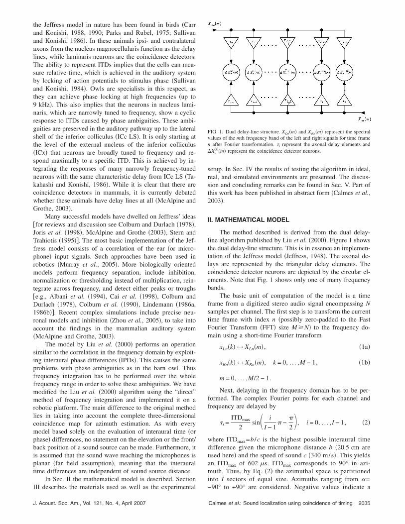
The method described is derived from the dual delay-line algorithm published by Liu et al. �2000�. Figure 1 showsthe dual delay-line structure. This is in essence an implemen-tation of the Jeffress model �Jeffress, 1948�. The axonal de-lays are represented by the triangular delay elements. Thecoincidence detector neurons are depicted by the circular el-ements. Note that Fig. 1 shows only one of many frequencybands.

The basic unit of computation of the model is a timeframe from a digitized stereo audio signal encompassing Nsamples per channel. The first step is to transform the currenttime frame with index n �possibly zero-padded to the FastFourier Transform �FFT� size M �N� to the frequency do-main using a short-time Fourier transform

xLn�k� ↔ XLn�m� , �1a�

xRn�k� ↔ XRn�m�, k = 0, . . . ,M − 1, �1b�

m = 0, . . . ,M/2 − 1.

Next, delaying in the frequency domain has to be per-formed. The complex Fourier points for each channel andfrequency are delayed by

�i =ITDmax

2sin� i

I − 1� −

�

2�, i = 0, . . . ,I − 1, �2�

where ITDmax=b /c is the highest possible interaural timedifference given the microphone distance b �20.5 cm areused here� and the speed of sound c �340 m/s�. This yieldsan ITDmax of 602 �s. ITDmax corresponds to 90° in azi-muth. Thus, by Eq. �2� the azimuthal space is partitionedinto I sectors of equal size. Azimuths ranging from �=

FIG. 1. Dual delay-line structure. XLn�m� and XRn�m� represent the spectralvalues of the mth frequency band of the left and right signals for time framen after Fourier transformation. �i represent the axonal delay elements and�Xn

�i��m� represent the coincidence detector neurons.

−90° to +90° are considered. Negative values indicate a

Calmes et al.: Sound localization using coincidence of timing 2035

sound source positioned in the left hemisphere, whilepositive azimuths point to a sound source in the righthemisphere.

The actual delaying is performed by adding a phase shiftcorresponding to the delay �i to the original phase of theinput signals in each frequency band

XLn�i��m� = XLn�m�e−j2�fm�i, �3a�

XRn�i� �m� = XRn�m�ej2�fm�i, i = 0, . . . ,I − 1, �3b�

m = 0, . . . ,M/2 − 1,

where M is the FFT size, �i specifies the delay in s, fm

=mfs /M is the center frequency of the mth frequency band,and n is the number of the current time frame.

As this operation is performed in the frequency domain,subsample accuracy is achieved without any additional ef-fort, because interpolation between samples is done implic-itly. In the time domain, interpolation would have to be doneexplicitly in order to shift the signals by an amount smallerthan one sample. Equation �2� may seem unintuitive as itallows for negative delays. However, this has no practicalimplications due to the periodic nature of the discrete Fouriertransform and thus can be safely ignored, as long as thedelayed signals are not meant to be transformed back into thetime domain.

The delays are symmetric around the 0-valued delay��I−1�/2. For the left channel, the negative internal delays aresituated to the left of the midline in the dual delay-line struc-ture, while positive internal delay values are situated to theright. For the right channel, the reverse is true. �0 has thevalue −ITDmax/2, while �I−1 has the value ITDmax/2. Thus,coincidence detection for external negative delays �soundsources positioned to the left� happens at the right side in thedelay-line structure, while coincidence detection for positiveexternal delays �sound sources positioned to the right� hap-pens at the left side in the dual delay-line structure. As can bededuced from Fig. 1, the delay value for the right channelcorresponding to the point i in the dual delay-line would be�I−i−1, whereas in Eq. �3b�, −�i is used. It can easily be shownby substituting I− i−1 in Eq. �2�, that �I−i−1=−�i.

The external time delay at the point i in the dual delay-line structure, which is compensated by the internal timedelay, corresponds to

ITDi = − ��i − �− �i�� = − 2�i. �4�

As the azimuth space has been partitioned into I sectorsby Eq. �2�, there exists a linear relationship between the azi-muth �i and the position i of a coincidence detector element

�i = 90 −i

I − 1180. �5�

In the ideal case, the time domain signals from bothchannels are identical except for a time difference. This re-sults in identical amplitude spectra in the frequency domain,whereas the time difference leads to a difference in the phasespectra for both channels. Equations �3a� and �3b� induce aphase change in the left and right channels, respectively, for
every point i in the dual delay line. At a given point �the
2036 J. Acoust. Soc. Am., Vol. 121, No. 4, April 2007

coincidence location�, the left and right phase spectra will beidentical �in the ideal case� or at least minimally different�for signals recorded by the microphones�. To detect thatpoint, first a coincidence map is built with

�Xn�i��m� = �XLn

�i��m� − XRn�i� �m��, i = 0, . . . ,I − 1, �6�

m = 0, . . . ,M/2 − 1.

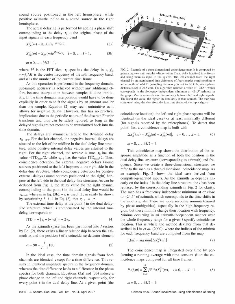
This coincidence map shows the distribution of the re-sponse amplitude as a function of both the position in thedual delay-line structure �corresponding to azimuth� and fre-quency. Since we create a three-dimensional structure, werefer to the map as a three-dimensional coincidence map. Asan example, Fig. 2 shows the ideal case derived fromcomputer-generated inputs. As the azimuth �i depends lin-early on the index i in the delay-line structure, the i has beenreplaced by the corresponding azimuth in Fig. 2 for clarity.The map has a frequency independent minimum at or closeto −24.5° of azimuth, which corresponds to the time shifts inthe input signals. There are more response minima �causedby phase ambiguities�, especially in the high-frequency re-gion, but these minima change their location with frequency.Minima occurring in an azimuth-independent manner overthe whole frequency range for a given i specify coincidencelocation. This is where the method deviates from that de-scribed in Liu et al. �2000�, where the indices of the minimafor each frequency band are computed from the map:

in�m� = arg mini

��Xn�i��m�� . �7�

The coincidence map is integrated over time by per-forming a running average with time constant � on the co-incidence maps computed for all time frames:

Pn�i,m� = �k=0

n

�n−k�Xk�i��m�, i = 0, . . . ,I − 1, �8�

FIG. 2. Example of a three-dimensional coincidence map. It is computed bygenerating two unit samples �discrete-time Dirac delta function� in softwareand using them as input to the system. The left channel leads the rightchannel by an interchannel time difference of four samples corresponding toan azimuth of −24.5° �sampling frequency is set to 16 kHz, microphonedistance is set to 20.5 cm�. The algorithm returned a value of −24.5°, whichcorresponds to the frequency-independent minimum at −24.5° azimuth inthe graph. Z-axis values denote dissimilarity between left and right signals.The lower the value, the higher the similarity at that azimuth. The map wascomputed using the data from the first time frame of the input signals.

m = 0, . . . ,M/2 − 1.

Calmes et al.: Sound localization using coincidence of timing

This again is in contrast to the algorithm used in Liu etal. �2000� where integration over time is done by accumulat-ing the coincidence locations of the minima for each fre-quency band �here, � refers to the Kronecker delta function�:

Pn�i,m� = �k=0

n

�n−k��i − ik�m�� . �9�

In our algorithm, integration over frequency is per-formed by summing up the coincidence map at the currenttime frame index n over all frequency bands

Hn�i� = �m=0

M/2−1

Pn�i,m�, i = 0, . . . ,I − 1. �10�

Liu et al. �2000� describe two methods for frequencyintegration. The first �called the “direct” method� is the sameas Eq. �10�. The second method �called the “stencil” filter� ismore complex. While the “direct” method only sums up co-incidence locations over frequency corresponding to a posi-tion i in the delay line, the stencil filter also takes into ac-count coincidence locations corresponding to phaseambiguities for the index i. This is possible, because thepattern of high-frequency phase ambiguities is unique foreach index i. To make this method computationally tractable,a broadband coincidence pattern has to be precomputed, pro-viding the theoretical positions of coincidence locations. Asthe delay values �i vary in a nonuniform manner, the coinci-dence pattern varies with the index i, thus requiring storagespace for I different patterns. To circumvent this disadvan-tage, Liu et al. �2000� chose to use uniform delays, thusrequiring only one precomputed theoretical broadband coin-cidence pattern. A sliding window, centered at the position iin the dual delay line, provides the coincidence positionsneeded for frequency integration. The tradeoff of this methodis, that with uniform delays, the angular resolution acrossazimuth positions is not constant. Positions close to the mid-line will have higher angular resolution than more lateralpositions, thus requiring a higher number I of coincidencedetectors to achieve a resolution equivalent to that obtainableby the direct method. We chose not to implement the stencilfilter, because we wanted to keep a constant angular resolu-tion and because the results obtained by using Eq. �10� weresufficient for our purposes.

The final localization function is obtained by normaliz-ing the function Hn�i� at the current time frame index n to therange 0–1 and by transforming the minima into maxima bysubtracting from 1,

Locn�i� = 1 −Hn�i� − min�Hn�i��

max�Hn�i�� − min�Hn�i��, �11�

i = 0, . . . ,I − 1.

To determine the points of coincidence location, the in-dices in

MAX of the local maxima of Locn�i� have to be foundsatisfying the following properties:

Locn�inMAX� � 0.5, �12a�

Locn�iMAX� Locn�iMAX − 1� , �12b�
n n

Locn�inMAX� Locn�in

MAX + 1� . �12c�

The threshold Eq. �12a� is necessary to suppress unwantedside peaks in the localization function which can result fromhigh-frequency phase ambiguities. A value of 0.5 proved tobe quite effective in suppressing side peaks not attributableto real sound sources. From in

MAX, the azimuth to the corre-sponding sound source can be computed with the help of Eq.�5�.

The final output of the localizer is an array of pairs ofazimuth with corresponding peak height

��inmax,heightin

MAX� = �90 −inMAX

I − 1180,Locn�in

MAX�� . �13�

An implementation using Eqs. �7�, �9�, and �10� was initiallytried, but this resulted in strong outliers at ±90° with noisyor nonbroadband signals. Finally the method of integrat-ing the complete three-dimensional coincidence map �in-stead of coincidence locations� over frequency �Eqs. �6�,�8�, and �10�� was chosen and this solved the problem.

III. MATERIALS AND METHODS

A. Hardware setup

Throughout the experiments—with the exception of thepan-tilt unit �PTU�—standard, readily available, off-the-shelfcomponents were used. The microphones were two SonyECM-F8 omnidirectional electret condenser microphones�frequency range: 50 Hz–12 kHz�, connected to twopreamplifiers built around an LF351N op-amp �frequencyrange: 50 Hz–20 kHz; obtained as kit from an electronicssupplier�. The preamplifiers were connected to the line-ininput of the on-board sound chip of a standard PC.

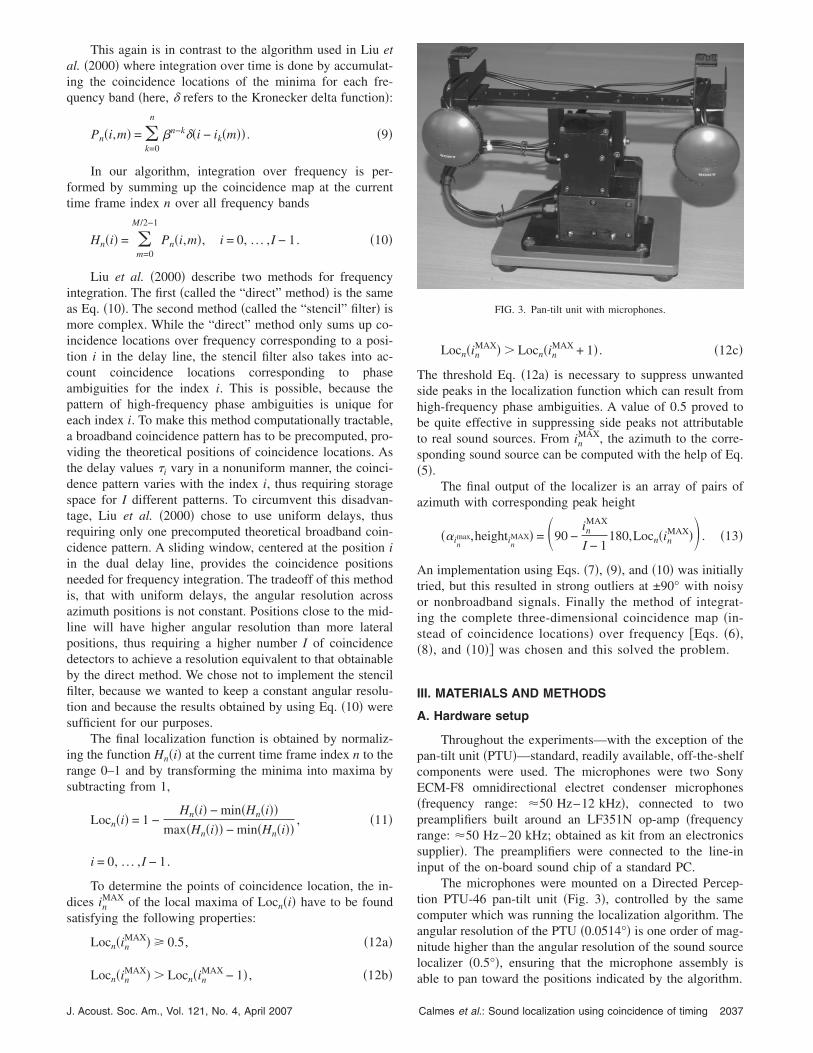
The microphones were mounted on a Directed Percep-tion PTU-46 pan-tilt unit �Fig. 3�, controlled by the samecomputer which was running the localization algorithm. Theangular resolution of the PTU �0.0514°� is one order of mag-nitude higher than the angular resolution of the sound sourcelocalizer �0.5°�, ensuring that the microphone assembly is

FIG. 3. Pan-tilt unit with microphones.

able to pan toward the positions indicated by the algorithm.


All the experiments were conducted in a normal officeenvironment, with background noise from computers andventilation. The sound source �a Sony SRS-57 loudspeaker;frequency range: 100 Hz–20 kHz� was placed at a dis-tance of approximately 1 m from the microphone assembly.The loudspeaker output volume was set in such a way thatthe signals recorded over the microphones �at the 0° azimuthsetting� had a maximal amplitude of about −2 dB with re-spect to the maximal input amplitude of the analog-to-digitalconverters. This ensured a high signal to noise ratio whileavoiding clipping in the input signals.

B. Software configuration

The algorithm was implemented in C on a LinuxOS. All signal processing was done in software. Wheneverpossible, the algorithm parameters mentioned in the Liu etal. �2000� article have been used. Due to hardware and real-time considerations, some parameters had to be changed. Thesampling frequency was 16 kHz. Signals were quantized at16 bits. The FFT size was 2048 points, yielding a frequencyresolution of 7.8125 Hz per frequency band. The system wasset up with 361 delay elements per delay line. With thisconfiguration, a linear angular resolution of 0.5° is achieved.A value of 340 m/s was used for the speed of sound. Thetime-integration constant � from Eq. �8� was set to 0.8.

As early versions of the software processed a time framein about 60 ms �on an AMD Athlon PC clocked at 1.3 GHz�,the time frame size was set to 62 ms �992 samples at16 kHz�, with no overlap. In this way, real-time operationwas achieved. Even though the latest, optimized version ofthe software completes the computation in less than 20 mson a newer computer �AMD Athlon XP 1800+�, the timeframe size was not reduced, in order to keep the data fromlater experiments consistent with earlier measurements.

After A/D conversion, the time frames were filtered witha 12th-order Butterworth band-pass filter �passband approxi-mately 100–4000 Hz� and weighted with a Hann window.The 992 samples were then zero-padded to the FFT size of2048 points.

In the case of click signals, a simple signal detector wasused to prevent the algorithm from producing azimuth esti-mations corresponding to background noise. Before the ex-periment, 2 s of background noise were recorded. As theclick was very short, it could be that the variance of a wholetime frame containing a click was still quite low. Therefore,for every time frame, the mean of the subframe �32 samples�variances was computed. The threshold was set to 1.7 �valuedetermined empirically� times the mean of the individualtime frame values. During the experiment, a time frame wasaccepted as containing a signal if the mean of the subframevariances was above the threshold computed from back-ground noise. In that case, localization computations wereperformed, otherwise the time frame was dropped. The solepurpose of this signal detection system was to ignore timeframes that did not contain samples belonging to the clickstimulus. We did not intend to develop a signal detector suit-able for practical applications.

Time was measured by reading out the processor cycle


counter at appropriate locations in the program. By subtract-ing two readouts enclosing a part of the code which is to betimed and dividing by the clock frequency, accurate timinginformation was obtained �within the limits of a non-real-time multitasking operating system�.

To obtain different sound source positions for the experi-ments, it was not the source loudspeaker that was movedwith respect to the microphone assembly, but rather the mi-crophone assembly was rotated with respect to the loud-speaker. This was done for practical reasons, as the spatialrequirements for moving the loudspeaker in an arc from−70° to +70° around the microphones exceed the spaceavailable in most office environments. In the following, forsimplicity, it will still be referred to a variation of the azi-muth of the sound source, but it should be kept in mind thatit was actually the microphones that were panned while thesound source position remained fixed.

IV. EXPERIMENTAL RESULTS

Four different types of tests of the algorithm were per-formed. Tests using the computer generated signals showedthe general correctness of the implementation of the algo-rithm. Tests using signals transmitted via loudspeaker andrecorded in open loop conditions demonstrated the robust-ness of the algorithm in real situations. Additionally, the per-formance of the algorithm was assessed in closed loop con-ditions on a robotic pan-tilt unit. Finally, to find anexplanation for the poor performance with low-frequency,narrowband signals, room simulations were conducted.

To assess the influence of spectral content of a signal onthe localization system, stimulus signals with increasingbandwidth were chosen, from pure tones to broadband noiseand clicks �Table I�. Because of the bandpass filter em-ployed, broadband here actually refers to a frequency rangeof 100 Hz–4 kHz.

It should be noted that multiple azimuths can be returnedby the system �especially for sine stimuli�, although only onestimulus source is present. In this case, the position withmaximal height was selected from the azimuths detected inEq. �13�. For sine stimuli, peaks not attributable to the realsource position corresponded to phase ambiguities and couldin some cases produce the maximal peak height. This re-sulted in the system localizing phase ambiguities instead ofthe real source position. For non-sine stimuli, spurious peaksabove the threshold imposed by Eq. �12a� were sometimes

TABLE I. Signal types used in the experiments.

Signal type Frequency range

Noise BroadbandClick BroadbandBandpass noise 1–4 kHzBandpass noise 500 Hz–4 kHzBandpass noise 100 Hz–1 kHzsine 1.5 kHzsine 1 kHzsine 500 Hz

detected. They were either caused by transient environmental


noise �e.g., door closing�, or they corresponded to phantomsources caused by the room acoustics. In either case theynever produced the azimuth with maximal peak height, sothat the azimuth estimation from the sound source localizercorresponded to the real source.

A. Tests using computer-generated signals directly

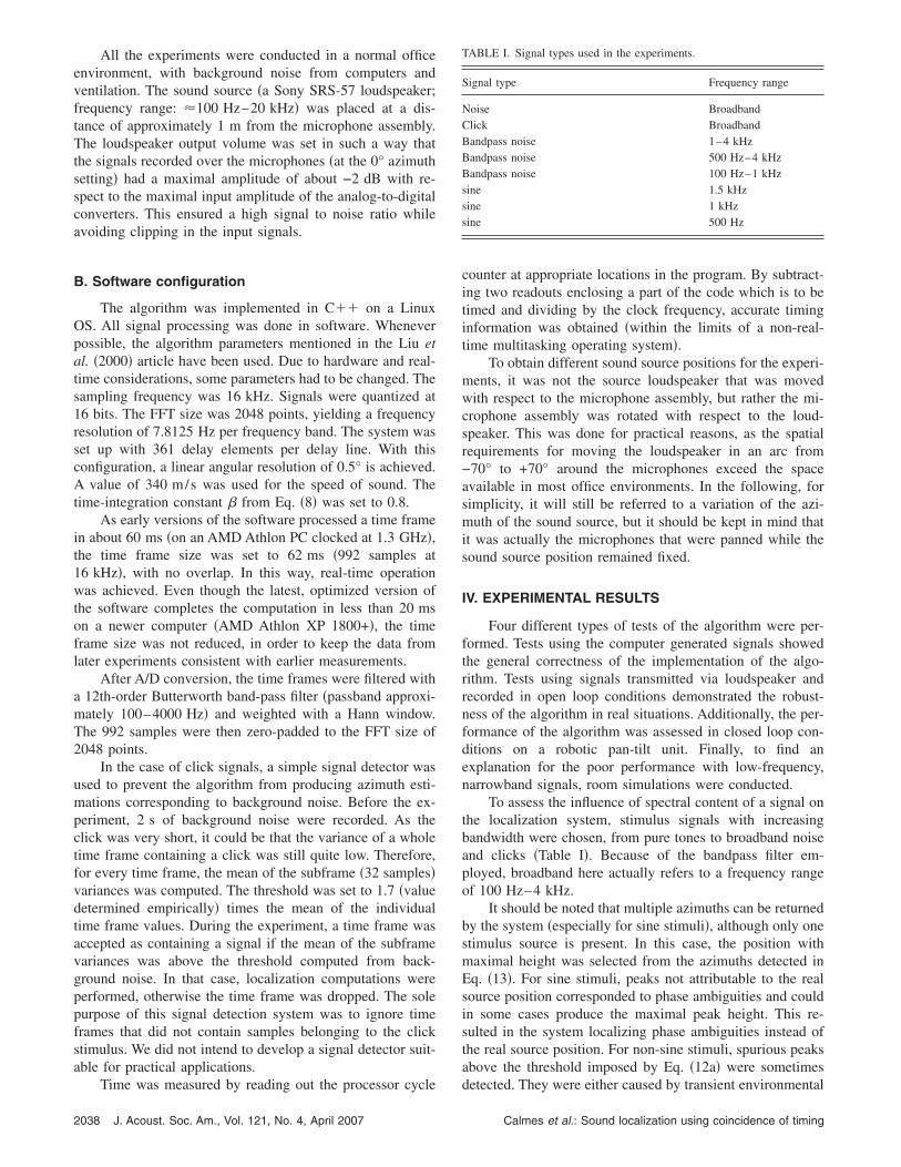
The coincidence map in Fig. 2 was created with twotime-shifted unit samples �the discrete-time version of theDirac delta function� generated in software. The frequency-independent minimum at −24.5° represents the simulated po-sition of the sound source. The output of the algorithm, in-deed yielded a sound-source position of −24.5°. In Fig. 4 asimilar coincidence map was created, but with broadbandnoise as stimulus. Again, one minimum, occurring at −24.5°was clearly frequency independent, while all other minimachanged their position with frequency. Although the mini-mum was less well defined than in Fig. 2, the algorithm hadno problem finding the position of the sound source.

Tests with many different ITDs and signal types wereconducted with computer-generated signals. The algorithmalways found the right peak corresponding to the originalITD with an error smaller than 1°. Moreover, the localizationestimate remained stable during the whole experiment. Evenfor sinusoidal stimuli, the correct ITD could be extracted.However, as expected for this type of input, for frequenciesabove 830 Hz, virtual peaks corresponding to phase ambi-guities were also detected.

B. Tests using microphone signals: Open loopexperiments

In these tests, the computer generated sound was trans-mitted via a loudspeaker and recorded by a pair of micro-phones. Stimulus presentation was continuous �with the ex-ception of the click stimulus�. The sound-source azimuthremained fixed during a localization run. The output of thealgorithm was not fed back to the PTU. Recorded data in-cluded source position, number of detected azimuths and thepairs of azimuth with corresponding peak heights from Eq.

FIG. 4. Example of a three-dimensional coincidence map of the first timeframe of a broadband noise signal with a time difference of 4 samplescorresponding to an azimuth of −24.5°. The algorithm computes the correctazimuth of −24.5°. Sampling rate is 16 kHz, microphone distance 20.5 cm.Z axis represents dissimilarity as in Fig. 2.

�13�.


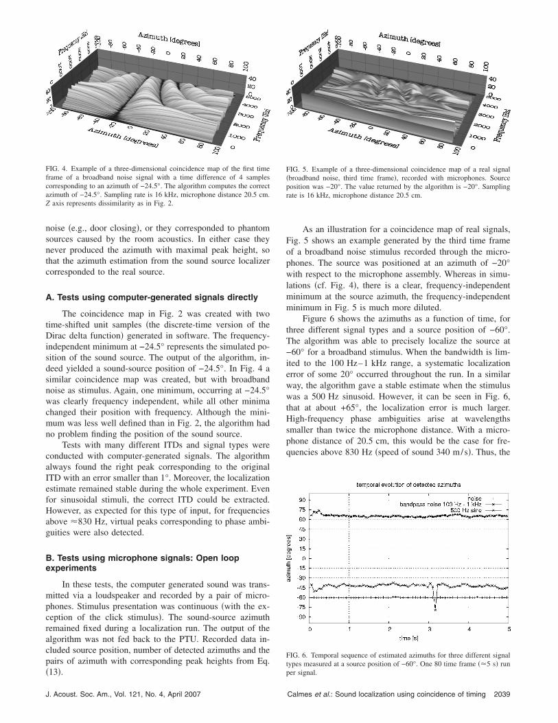
As an illustration for a coincidence map of real signals,Fig. 5 shows an example generated by the third time frameof a broadband noise stimulus recorded through the micro-phones. The source was positioned at an azimuth of −20°with respect to the microphone assembly. Whereas in simu-lations �cf. Fig. 4�, there is a clear, frequency-independentminimum at the source azimuth, the frequency-independentminimum in Fig. 5 is much more diluted.

Figure 6 shows the azimuths as a function of time, forthree different signal types and a source position of −60°.The algorithm was able to precisely localize the source at−60° for a broadband stimulus. When the bandwidth is lim-ited to the 100 Hz–1 kHz range, a systematic localizationerror of some 20° occurred throughout the run. In a similarway, the algorithm gave a stable estimate when the stimuluswas a 500 Hz sinusoid. However, it can be seen in Fig. 6,that at about +65°, the localization error is much larger.High-frequency phase ambiguities arise at wavelengthssmaller than twice the microphone distance. With a micro-phone distance of 20.5 cm, this would be the case for fre-quencies above 830 Hz �speed of sound 340 m/s�. Thus, the

FIG. 5. Example of a three-dimensional coincidence map of a real signal�broadband noise, third time frame�, recorded with microphones. Sourceposition was −20°. The value returned by the algorithm is −20°. Samplingrate is 16 kHz, microphone distance 20.5 cm.

FIG. 6. Temporal sequence of estimated azimuths for three different signaltypes measured at a source position of −60°. One 80 time frame �5 s� run
per signal.

mislocalization of the 500 Hz sinusoid �wavelength 68 cm�cannot be caused by the system locking onto a high-frequency phase ambiguity.

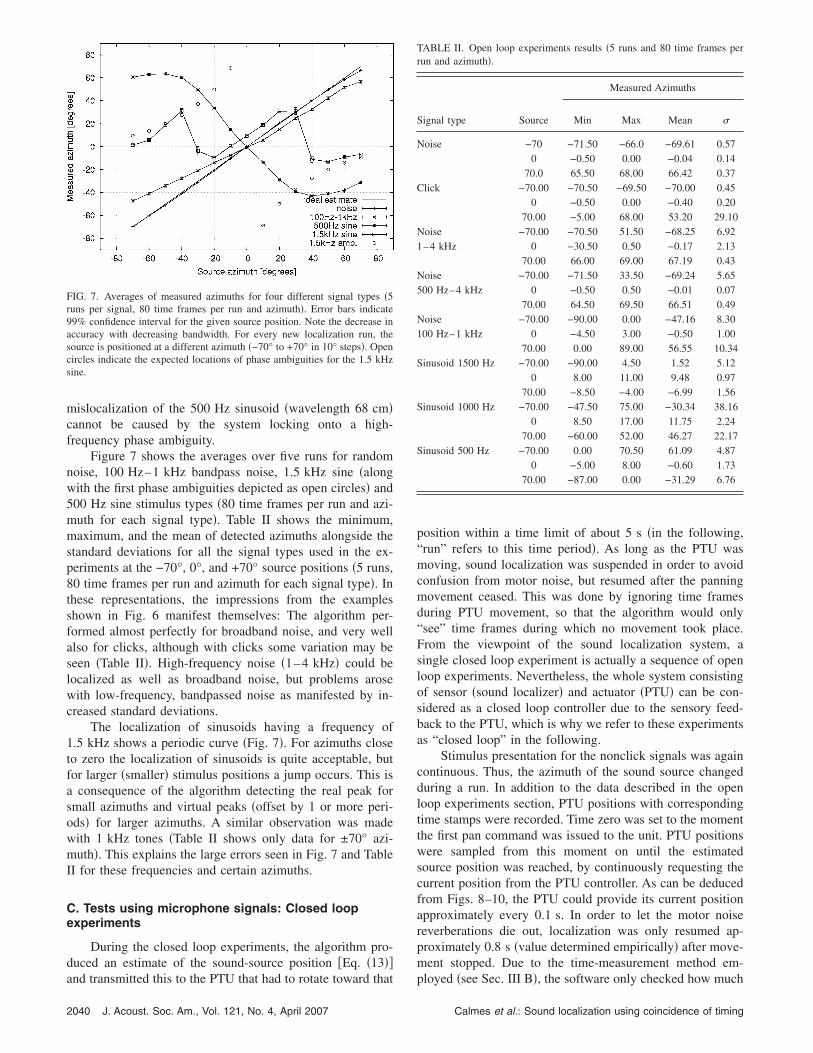
Figure 7 shows the averages over five runs for randomnoise, 100 Hz–1 kHz bandpass noise, 1.5 kHz sine �alongwith the first phase ambiguities depicted as open circles� and500 Hz sine stimulus types �80 time frames per run and azi-muth for each signal type�. Table II shows the minimum,maximum, and the mean of detected azimuths alongside thestandard deviations for all the signal types used in the ex-periments at the −70°, 0°, and +70° source positions �5 runs,80 time frames per run and azimuth for each signal type�. Inthese representations, the impressions from the examplesshown in Fig. 6 manifest themselves: The algorithm per-formed almost perfectly for broadband noise, and very wellalso for clicks, although with clicks some variation may beseen �Table II�. High-frequency noise �1–4 kHz� could belocalized as well as broadband noise, but problems arosewith low-frequency, bandpassed noise as manifested by in-creased standard deviations.

The localization of sinusoids having a frequency of1.5 kHz shows a periodic curve �Fig. 7�. For azimuths closeto zero the localization of sinusoids is quite acceptable, butfor larger �smaller� stimulus positions a jump occurs. This isa consequence of the algorithm detecting the real peak forsmall azimuths and virtual peaks �offset by 1 or more peri-ods� for larger azimuths. A similar observation was madewith 1 kHz tones �Table II shows only data for ±70° azi-muth�. This explains the large errors seen in Fig. 7 and TableII for these frequencies and certain azimuths.

C. Tests using microphone signals: Closed loopexperiments

During the closed loop experiments, the algorithm pro-duced an estimate of the sound-source position �Eq. �13��

FIG. 7. Averages of measured azimuths for four different signal types �5runs per signal, 80 time frames per run and azimuth�. Error bars indicate99% confidence interval for the given source position. Note the decrease inaccuracy with decreasing bandwidth. For every new localization run, thesource is positioned at a different azimuth �−70° to +70° in 10° steps�. Opencircles indicate the expected locations of phase ambiguities for the 1.5 kHzsine.

and transmitted this to the PTU that had to rotate toward that


position within a time limit of about 5 s �in the following,“run” refers to this time period�. As long as the PTU wasmoving, sound localization was suspended in order to avoidconfusion from motor noise, but resumed after the panningmovement ceased. This was done by ignoring time framesduring PTU movement, so that the algorithm would only“see” time frames during which no movement took place.From the viewpoint of the sound localization system, asingle closed loop experiment is actually a sequence of openloop experiments. Nevertheless, the whole system consistingof sensor �sound localizer� and actuator �PTU� can be con-sidered as a closed loop controller due to the sensory feed-back to the PTU, which is why we refer to these experimentsas “closed loop” in the following.

Stimulus presentation for the nonclick signals was againcontinuous. Thus, the azimuth of the sound source changedduring a run. In addition to the data described in the openloop experiments section, PTU positions with correspondingtime stamps were recorded. Time zero was set to the momentthe first pan command was issued to the unit. PTU positionswere sampled from this moment on until the estimatedsource position was reached, by continuously requesting thecurrent position from the PTU controller. As can be deducedfrom Figs. 8–10, the PTU could provide its current positionapproximately every 0.1 s. In order to let the motor noisereverberations die out, localization was only resumed ap-proximately 0.8 s �value determined empirically� after move-ment stopped. Due to the time-measurement method em-

TABLE II. Open loop experiments results �5 runs and 80 time frames perrun and azimuth�.

Signal type Source

Measured Azimuths

Min Max Mean �

Noise −70 −71.50 −66.0 −69.61 0.570 −0.50 0.00 −0.04 0.14

70.0 65.50 68.00 66.42 0.37Click −70.00 −70.50 −69.50 −70.00 0.45

0 −0.50 0.00 −0.40 0.2070.00 −5.00 68.00 53.20 29.10

Noise −70.00 −70.50 51.50 −68.25 6.921–4 kHz 0 −30.50 0.50 −0.17 2.13

70.00 66.00 69.00 67.19 0.43Noise −70.00 −71.50 33.50 −69.24 5.65500 Hz–4 kHz 0 −0.50 0.50 −0.01 0.07

70.00 64.50 69.50 66.51 0.49Noise −70.00 −90.00 0.00 −47.16 8.30100 Hz–1 kHz 0 −4.50 3.00 −0.50 1.00

70.00 0.00 89.00 56.55 10.34Sinusoid 1500 Hz −70.00 −90.00 4.50 1.52 5.12

0 8.00 11.00 9.48 0.9770.00 −8.50 −4.00 −6.99 1.56

Sinusoid 1000 Hz −70.00 −47.50 75.00 −30.34 38.160 8.50 17.00 11.75 2.24

70.00 −60.00 52.00 46.27 22.17Sinusoid 500 Hz −70.00 0.00 70.50 61.09 4.87

0 −5.00 8.00 −0.60 1.7370.00 −87.00 0.00 −31.29 6.76

ployed �see Sec. III B�, the software only checked how much


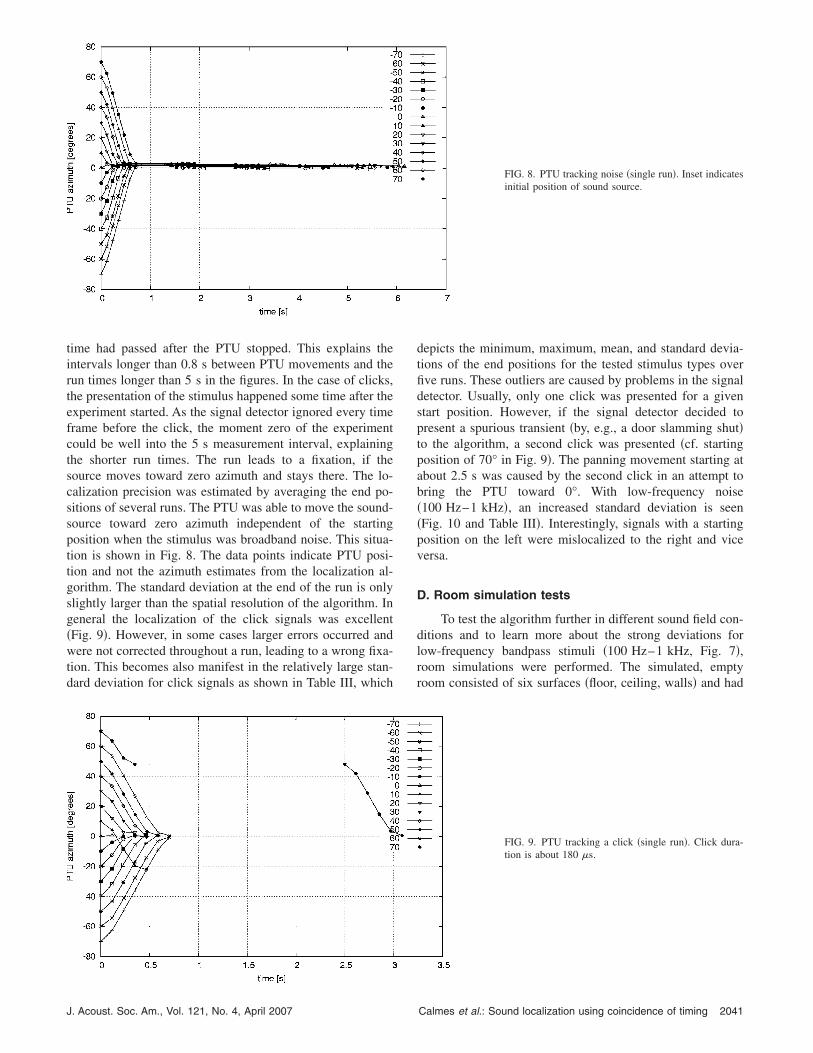
time had passed after the PTU stopped. This explains theintervals longer than 0.8 s between PTU movements and therun times longer than 5 s in the figures. In the case of clicks,the presentation of the stimulus happened some time after theexperiment started. As the signal detector ignored every timeframe before the click, the moment zero of the experimentcould be well into the 5 s measurement interval, explainingthe shorter run times. The run leads to a fixation, if thesource moves toward zero azimuth and stays there. The lo-calization precision was estimated by averaging the end po-sitions of several runs. The PTU was able to move the sound-source toward zero azimuth independent of the startingposition when the stimulus was broadband noise. This situa-tion is shown in Fig. 8. The data points indicate PTU posi-tion and not the azimuth estimates from the localization al-gorithm. The standard deviation at the end of the run is onlyslightly larger than the spatial resolution of the algorithm. Ingeneral the localization of the click signals was excellent�Fig. 9�. However, in some cases larger errors occurred andwere not corrected throughout a run, leading to a wrong fixa-tion. This becomes also manifest in the relatively large stan-dard deviation for click signals as shown in Table III, which


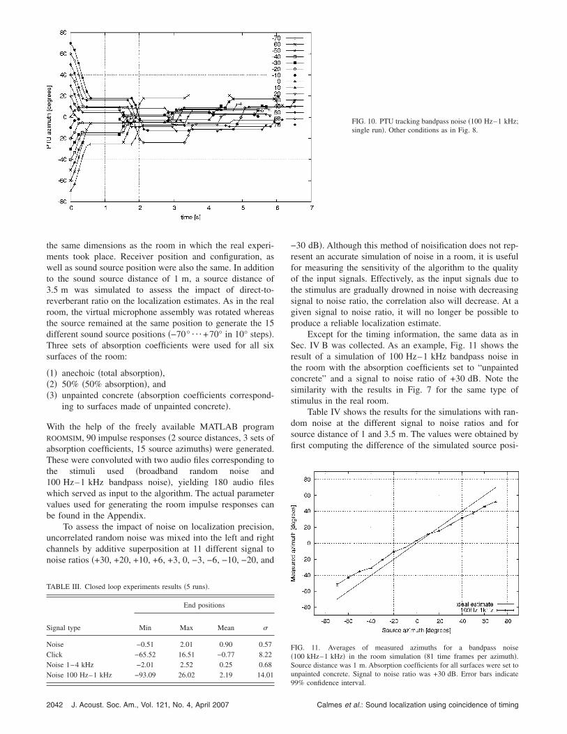
depicts the minimum, maximum, mean, and standard devia-tions of the end positions for the tested stimulus types overfive runs. These outliers are caused by problems in the signaldetector. Usually, only one click was presented for a givenstart position. However, if the signal detector decided topresent a spurious transient �by, e.g., a door slamming shut�to the algorithm, a second click was presented �cf. startingposition of 70° in Fig. 9�. The panning movement starting atabout 2.5 s was caused by the second click in an attempt tobring the PTU toward 0°. With low-frequency noise�100 Hz–1 kHz�, an increased standard deviation is seen�Fig. 10 and Table III�. Interestingly, signals with a startingposition on the left were mislocalized to the right and viceversa.

D. Room simulation tests

To test the algorithm further in different sound field con-ditions and to learn more about the strong deviations forlow-frequency bandpass stimuli �100 Hz–1 kHz, Fig. 7�,room simulations were performed. The simulated, emptyroom consisted of six surfaces �floor, ceiling, walls� and had

FIG. 9. PTU tracking a click �single run�. Click dura-tion is about 180 �s.

FIG. 8. PTU tracking noise �single run�. Inset indicatesinitial position of sound source.


the same dimensions as the room in which the real experi-ments took place. Receiver position and configuration, aswell as sound source position were also the same. In additionto the sound source distance of 1 m, a source distance of3.5 m was simulated to assess the impact of direct-to-reverberant ratio on the localization estimates. As in the realroom, the virtual microphone assembly was rotated whereasthe source remained at the same position to generate the 15different sound source positions �−70° ¯ +70° in 10° steps�.Three sets of absorption coefficients were used for all sixsurfaces of the room:

�1� anechoic �total absorption�,�2� 50% �50% absorption�, and�3� unpainted concrete �absorption coefficients correspond-

ing to surfaces made of unpainted concrete�.

With the help of the freely available MATLAB programROOMSIM, 90 impulse responses �2 source distances, 3 sets ofabsorption coefficients, 15 source azimuths� were generated.These were convoluted with two audio files corresponding tothe stimuli used �broadband random noise and100 Hz–1 kHz bandpass noise�, yielding 180 audio fileswhich served as input to the algorithm. The actual parametervalues used for generating the room impulse responses canbe found in the Appendix.

To assess the impact of noise on localization precision,uncorrelated random noise was mixed into the left and rightchannels by additive superposition at 11 different signal tonoise ratios �+30, +20, +10, +6, +3, 0, −3, −6, −10, −20, and

TABLE III. Closed loop experiments results �5 runs�.

Signal type

End positions

Min Max Mean �

Noise −0.51 2.01 0.90 0.57Click −65.52 16.51 −0.77 8.22Noise 1–4 kHz −2.01 2.52 0.25 0.68Noise 100 Hz–1 kHz −93.09 26.02 2.19 14.01


−30 dB�. Although this method of noisification does not rep-resent an accurate simulation of noise in a room, it is usefulfor measuring the sensitivity of the algorithm to the qualityof the input signals. Effectively, as the input signals due tothe stimulus are gradually drowned in noise with decreasingsignal to noise ratio, the correlation also will decrease. At agiven signal to noise ratio, it will no longer be possible toproduce a reliable localization estimate.

Except for the timing information, the same data as inSec. IV B was collected. As an example, Fig. 11 shows theresult of a simulation of 100 Hz–1 kHz bandpass noise inthe room with the absorption coefficients set to “unpaintedconcrete” and a signal to noise ratio of +30 dB. Note thesimilarity with the results in Fig. 7 for the same type ofstimulus in the real room.

Table IV shows the results for the simulations with ran-dom noise at the different signal to noise ratios and forsource distance of 1 and 3.5 m. The values were obtained byfirst computing the difference of the simulated source posi-

FIG. 10. PTU tracking bandpass noise �100 Hz–1 kHz;single run�. Other conditions as in Fig. 8.

FIG. 11. Averages of measured azimuths for a bandpass noise�100 kHz–1 kHz� in the room simulation �81 time frames per azimuth�.Source distance was 1 m. Absorption coefficients for all surfaces were set tounpainted concrete. Signal to noise ratio was +30 dB. Error bars indicate
99% confidence interval.

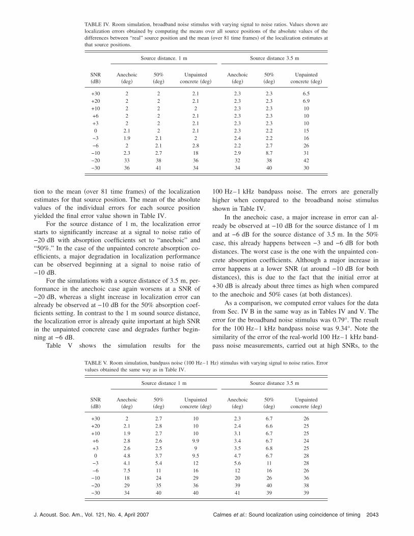
tion to the mean �over 81 time frames� of the localizationestimates for that source position. The mean of the absolutevalues of the individual errors for each source positionyielded the final error value shown in Table IV.

For the source distance of 1 m, the localization errorstarts to significantly increase at a signal to noise ratio of−20 dB with absorption coefficients set to “anechoic” and“50%.” In the case of the unpainted concrete absorption co-efficients, a major degradation in localization performancecan be observed beginning at a signal to noise ratio of−10 dB.

For the simulations with a source distance of 3.5 m, per-formance in the anechoic case again worsens at a SNR of−20 dB, whereas a slight increase in localization error canalready be observed at −10 dB for the 50% absorption coef-ficients setting. In contrast to the 1 m sound source distance,the localization error is already quite important at high SNRin the unpainted concrete case and degrades further begin-ning at −6 dB.

Table V shows the simulation results for the

TABLE IV. Room simulation, broadband noise stimulocalization errors obtained by computing the meandifferences between “real” source position and the mthat source positions.

SNR�dB�

Source distance. 1 m

Anechoic�deg�

50%�deg�

Unpaintconcrete �

+30 2 2 2.1+20 2 2 2.1+10 2 2 2+6 2 2 2.1+3 2 2 2.10 2.1 2 2.1

−3 1.9 2.1 2−6 2 2.1 2.8−10 2.3 2.7 18−20 33 38 36−30 36 41 34

TABLE V. Room simulation, bandpass noise �100 Hzvalues obtained the same way as in Table IV.

SNR�dB�

Source distance 1 m

Anechoic�deg�

50%�deg�

Unpaintconcrete �

+30 2 2.7 10+20 2.1 2.8 10+10 1.9 2.7 10+6 2.8 2.6 9.9+3 2.6 2.5 90 4.8 3.7 9.5

−3 4.1 5.4 12−6 7.5 11 16−10 18 24 29−20 29 35 36−30 34 40 40


100 Hz–1 kHz bandpass noise. The errors are generallyhigher when compared to the broadband noise stimulusshown in Table IV.

In the anechoic case, a major increase in error can al-ready be observed at −10 dB for the source distance of 1 mand at −6 dB for the source distance of 3.5 m. In the 50%case, this already happens between −3 and −6 dB for bothdistances. The worst case is the one with the unpainted con-crete absorption coefficients. Although a major increase inerror happens at a lower SNR �at around −10 dB for bothdistances�, this is due to the fact that the initial error at+30 dB is already about three times as high when comparedto the anechoic and 50% cases �at both distances�.

As a comparison, we computed error values for the datafrom Sec. IV B in the same way as in Tables IV and V. Theerror for the broadband noise stimulus was 0.79°. The resultfor the 100 Hz–1 kHz bandpass noise was 9.34°. Note thesimilarity of the error of the real-world 100 Hz–1 kHz band-pass noise measurements, carried out at high SNRs, to the

ith varying signal to noise ratios. Values shown arer all source positions of the absolute values of theover 81 time frames� of the localization estimates at

Source distance 3.5 m

Anechoic�deg�

50%�deg�

Unpaintedconcrete �deg�

2.3 2.3 6.52.3 2.3 6.92.3 2.3 102.3 2.3 102.3 2.3 102.3 2.2 152.4 2.2 162.2 2.7 262.9 8.7 3132 38 4234 40 30

z� stimulus with varying signal to noise ratios. Error


Anechoic�deg�

50%�deg�


2.3 6.7 262.4 6.6 253.1 6.7 253.4 6.7 243.5 6.8 254.7 6.7 285.6 11 2812 16 2620 26 3639 40 3841 39 39

lus ws oveean �

eddeg�

–1 H

eddeg�


simulation values for high SNR and a sound source distanceof 1 m in the unpainted concrete case �Table V�.

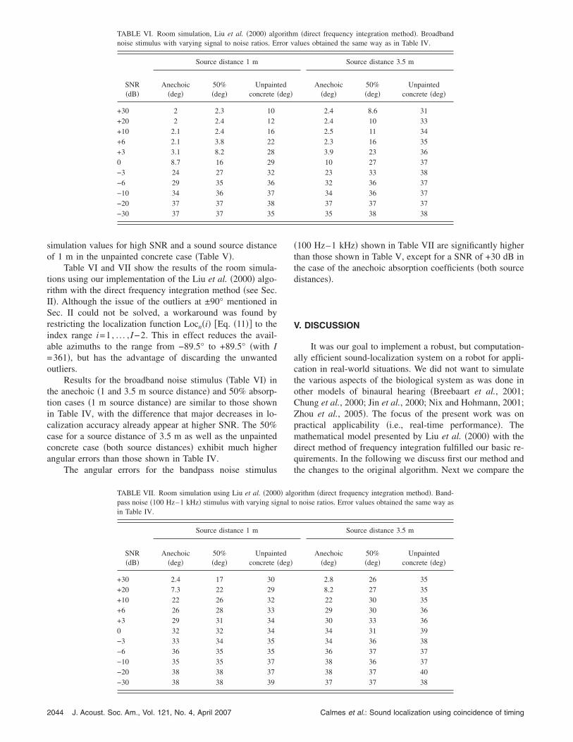
Table VI and VII show the results of the room simula-tions using our implementation of the Liu et al. �2000� algo-rithm with the direct frequency integration method �see Sec.II�. Although the issue of the outliers at ±90° mentioned inSec. II could not be solved, a workaround was found byrestricting the localization function Locn�i� �Eq. �11�� to theindex range i=1, . . . , I−2. This in effect reduces the avail-able azimuths to the range from −89.5° to +89.5° �with I=361�, but has the advantage of discarding the unwantedoutliers.

Results for the broadband noise stimulus �Table VI� inthe anechoic �1 and 3.5 m source distance� and 50% absorp-tion cases �1 m source distance� are similar to those shownin Table IV, with the difference that major decreases in lo-calization accuracy already appear at higher SNR. The 50%case for a source distance of 3.5 m as well as the unpaintedconcrete case �both source distances� exhibit much higherangular errors than those shown in Table IV.

The angular errors for the bandpass noise stimulus

TABLE VI. Room simulation, Liu et al. �2000� algnoise stimulus with varying signal to noise ratios. Er

SNR�dB�

Source distance 1 m

Anechoic�deg�

50%�deg�

Unpaintconcrete �

+30 2 2.3 10+20 2 2.4 12+10 2.1 2.4 16+6 2.1 3.8 22+3 3.1 8.2 280 8.7 16 29−3 24 27 32−6 29 35 36−10 34 36 37−20 37 37 38−30 37 37 35

TABLE VII. Room simulation using Liu et al. �2000pass noise �100 Hz–1 kHz� stimulus with varying sigin Table IV.

SNR�dB�

Source distance 1 m

Anechoic�deg�

50%�deg�

Unpaintconcrete �

+30 2.4 17 30+20 7.3 22 29+10 22 26 32+6 26 28 33+3 29 31 340 32 32 34−3 33 34 35−6 36 35 35−10 35 35 37−20 38 38 37−30 38 38 39


�100 Hz–1 kHz� shown in Table VII are significantly higherthan those shown in Table V, except for a SNR of +30 dB inthe case of the anechoic absorption coefficients �both sourcedistances�.

V. DISCUSSION

It was our goal to implement a robust, but computation-ally efficient sound-localization system on a robot for appli-cation in real-world situations. We did not want to simulatethe various aspects of the biological system as was done inother models of binaural hearing �Breebaart et al., 2001;Chung et al., 2000; Jin et al., 2000; Nix and Hohmann, 2001;Zhou et al., 2005�. The focus of the present work was onpractical applicability �i.e., real-time performance�. Themathematical model presented by Liu et al. �2000� with thedirect method of frequency integration fulfilled our basic re-quirements. In the following we discuss first our method andthe changes to the original algorithm. Next we compare the

�direct frequency integration method�. Broadbandalues obtained the same way as in Table IV.


Anechoic�deg�

50%�deg�


2.4 8.6 312.4 10 332.5 11 342.3 16 353.9 23 3610 27 3723 33 3832 36 3734 36 3737 37 3735 38 38

orithm �direct frequency integration method�. Band-noise ratios. Error values obtained the same way as


Anechoic�deg�

50%�deg�


2.8 26 358.2 27 3522 30 3529 30 3630 33 3634 31 3934 36 3836 37 3738 36 3738 37 4037 37 38

orithmror v

eddeg�

� algnal to

eddeg�


results of our tests with the localization performance of othersystems. Finally we present an outlook for further improve-ments of our system.

A. Method and control tests

While Liu et al. �2000� was a good starting point, wenoted that this algorithm, by taking into account only theminima of the coincidence map, does not use all of the in-formation available. We minimized information loss by per-forming the frequency integration over the whole three-dimensional coincidence map. The modified algorithmproduced excellent results without any indications of failureswith computer-generated signals. The ambiguities observedfor pure tones with a frequency higher than about 830 Hzwere expected, given the structure of the algorithm. Wechose not to implement the stencil filter method of frequencyintegration, because then we would have lost the constantangular resolution over the whole azimuth range. Further-more, we did not want to incur the additional computationaloverhead associated with the method.

It is difficult to compare the performance of our algo-rithm with the performance of the original method, becauseLiu et al. �2000� restricted their experiments to simulationsand anechoic chamber tests, and mainly conducted multi-source measurements. However, the one-speaker tests con-ducted in an anechoic chamber by Liu et al. �2000� seem tohave produced a similar localization accuracy as our open-loop tests in a laboratory environment. Our own tests withthe Liu et al. �2000� algorithm initially produced outliers at±90° �using the direct method�, which overshadowed thecorrect source azimuth �if it was present at all� in all casesexcept high SNR broadband stimuli. By restricting the rangeof estimated azimuths from −89.5° to +89.5° �thus ignoringthe outliers�, a workaround was found which could produceusable data. With high signal-to-noise and direct-to-reverberant ratios, the precision is quite good and seems toreflect the data from the original publication. Nevertheless,the Liu et al. �2000� algorithm with the direct method offrequency integration showed higher sensitivity to SNR andreverberation. We suppose that this is related to the minimumoperation performed on the coincidence values prior to fre-quency integration �Eq. �7��. For every frequency band, oneminimum is returned, indicating the location of coincidence.This assigns equal weights to all frequency bands. This is nota problem with high SNR broadband signals. But at lowsignal-to-noise ratios or with narrowband stimuli, givingequal weight to frequency bands containing little or no en-ergy pertaining to the signal seems to seriously corrupt thelocalization estimate.

One advantage of this type of algorithm is that they canachieve subsample accuracy for interaural delays without re-quiring explicit interpolation between samples. This is a con-sequence of carrying out all computations in the frequencydomain. Moreover, a high number of frequency bins may beimplemented without an increase in the data size. Algorithmsworking in the time domain are using filter banks for fre-quency separation �e.g., Roman and Wang �2003��. These
generate a high number of additional signals for the left and

right channels, which is computationally intensive. The algo-rithm presented here allows for efficient frequency filteringand, thus, restricting the computation of the coincidence mapto frequency ranges relevant to the intended practical appli-cation.

B. Open-loop and closed-loop tests

In the open-loop tests in real-world conditions, perfor-mance was excellent for broadband signals, but decreasedwith narrowing bandwidth of the stimuli. Specifically, prob-lems in the low-frequency range were observed. As initialsimulations �cf. Sec. IV A� showed that the software wasable to accurately determine the correct azimuth for all signaltypes, these high localization errors are not due to the algo-rithm but to reverberation as subsequent room simulationsshowed �cf. Sec. IV D�. Adding an echo-avoidance system�Huang et al., 1999� might improve the situation. These au-thors used three omni-directional microphones on a mobilerobotic platform. The localization was restricted to a singlefrequency band centered at 1 kHz and with a bandwidth of600 Hz in order to avoid phase ambiguities. ITDs were com-puted by the zero crossings of the wave forms from micro-phone pairs and from these, the direction to the sound sourcecould be computed. The localization accuracy was testedwith a 1 kHz sinusoid and a hand-clapping noise. The errorfor the sinusoid stimulus was within ±1° whereas for thehand-clapping noise, the accuracy was within ±7°. Althoughthis system is able to perform sound localization in threedimensions as well as resolving front-back confusions, this isonly possible through the use of three microphones. The re-striction to a single frequency band in order to avoid phaseambiguities in the ITD computation seems to be too much ofa constraint for practical applications. Additionally, extract-ing ITDs from several frequency bands with this methodwould entail a considerable additional computational over-head. In this respect, the algorithm described here is muchmore robust and suitable for future extensions.

In Nakadai et al. �2000, 2002� a frequency-domain al-gorithm for the sound localization subsystem of the human-oid torso SIG was used. The method performs ITD extractionby directly computing the phase difference between the leftand right channels from FFT frequency peaks. Additionally,interaural level differences were included in the azimuth es-timation. The error of the sound localization system waswithin ±5° from 0° to 30° and deteriorated for more lateralpositions �Nakadai et al., 2002�. Compared to this system,the method proposed here performs better for broadbandnoise.

The closed-loop experiments were performed to test thealgorithm in an environment closer to its later application ona mobile robotic platform. The results confirmed those ob-tained during the open loop tests. An excellent localizationwas achieved with broad-band signals. High-frequency sig-nals were localized better than low-frequency signals. Thisdemonstrated that the algorithm may be applicable to dy-namic, real-world situations.

Although comparisons are difficult, we have the impres-


sion that our system, despite its simplicity, does not performmuch worse in azimuth estimation than microphone arrayswith more than two microphones.

Omologo and Svaizer �1994� used 4 equispaced micro-phones with a separation of 15 cm. Three different localiza-tion algorithms were tested, with the so-called crosspower-spectrum phase algorithm providing the best results. For theexperiments, 97 stimuli were used with frequency contentranging from narrowband to wideband at various azimuthsand distances ranging from 1 to 3.6 m. Half of the stimulihad a noise component with an average SNR of 15 dB. Lo-calization accuracy was 66% with a tolerance �2°, 88%with a tolerance �5° and 96% with a tolerance �10°.

Brandstein and Silverman �1997� used a bilinear array of10 microphones with an intermicrophone separation of25 cm. Their system used a frequency-domain time-difference of arrival estimator designed for speech signalscombined with a speech source detector. For experimentswith single, nonmoving sources, 18 different source posi-tions were tested. Speech stimuli were used. The angularerror was approximately 2.5° over a range of 3 m.

Valin et al. �2003� used 8 microphones arranged on thesummits of a rectangular prism of dimensions 50 cm 40 cm 36 cm. The acoustic environment was noisy withmoderate reverberation. The localization system used thecrosspower-spectrum phase algorithm enhanced with a spec-tral weighting scheme. The angular error was approximately3° over a range of 3 m. The stimuli used for the experimentsconsisted of snapping fingers, tapping foot, and speaking.

C. Room simulations

The simple “shoebox” room model helped with under-standing the acoustic environment in which the real experi-ments took place. Three conclusions can be drawn fromthese simulations. First, the algorithm is relatively robustagainst noise, as important changes in localization error canonly be observed beginning at signal to noise ratios between−3 dB in the worst case and −20 dB in the best case. Second,the most important parameter degrading localization perfor-mance is direct-to-reverberant ratio. This becomes particu-larly apparent with the sound source at a distance of 3.5 mfrom the microphones and highly reflective surfaces �un-painted concrete�, where even the azimuth estimation of abroad-band stimulus produces rather large errors. Third, theroom simulations suggested that the systematic deviationsobserved with the low-frequency narrowband noise stimuluswere due to room reverberations. This is in accordance withfindings that binaural cues vary depending on the acousticenvironment and noise conditions �Nix and Hohmann, 2006�.

D. Conclusions and outlook

The relatively simple algorithm we used here with on-line capability performed surprisingly well in real-world situ-ations. It was less sensitive to adverse acoustical conditionsthan the algorithm by Liu et al. �2000� using the directmethod of frequency integration, while not being computa-tionally more complex. A further decrease in computation
time and memory requirements without a dramatic loss in

localization accuracy can be reached by reducing the criticalparameters of FFT size and number of delays per delay line.Thus the algorithm is easily adaptable to environments withreduced computational resources such as mobile robots. Thecurrent implementation is a good starting point for futureextensions. One aspect that will have to be considered isinteraural level differences caused by the mismatch of theleft and right microphone/preamplifier combinations. Al-though they are of an identical make, some asymmetries areintroduced by manufacturing and preamplifier adjustmenttolerances. By Eq. �6� we assume that the only differencesbetween the left and right signals will be phase differences,an assumption that is clearly violated in real environments.Even if in our experiments, localization accuracy was quitehigh, this mismatch could lead to problems in acousticallymore challenging environments. Specifically, source dis-crimination in the presence of multiple sources could be af-fected, requiring a mismatch compensation �Liu et al., 2001�.

We are currently working on a statistical source trackingmodule using a Bayes filter, which is expected to increase therobustness against motor noise from the PTU or the robot,among other things. This would make it possible to continuesound-source localization through motor activity of the mi-crophone platform. In the implementation presented here thelocalizer had to be interrupted during movement. Anotherextension would be a speech detector and a speech recog-nizer. The localizer would be working continuously, but itsoutput would be ignored as long as no speech was detected.As soon as there is speech, computation of the coincidencemap could be reduced to the relevant frequency components.This may be achieved, because all computations are done in

TABLE VIII. ROOMSIM parameters. Only those parameters differing fromthe program defaults are shown. Source coordinates are specified relative toreceiver coordinates.

Sampling frequency 16 kHz

Room depth �Lx� 4.95 mRoom width �Ly� 3.48 mRoom height �Lz� 4 mReceiver x position 0.8 mReceiver y position 1.5 mReceiver z position 1.0 mReceiver type Two sensorsReceiver sensor separation 0.205 mReceiver sensor directivity OmnidirectionalReceiver azimuth offset from −70° to +70° �10° steps�Source radial distance 1 or 3.5 mSource azimuth 0°Source elevation 0°

TABLE IX. Surface absorption coefficients used in the room simulations.Values shown are those provided by the ROOMSIM package.

Standard measurement frequencies

125 Hz 250 Hz 500 Hz 1 kHz 2 kHz 4 kHz

Anechoic 1 1 1 1 1 150% 0.75 0.75 0.75 0.75 0.75 0.75
Unpainted concrete 0.4 0.4 0.3 0.3 0.4 0.3

the frequency domain. In this way, localization accuracy ofthe source could be improved. The directional informationcould be used to steer a robot closer to the source and/or toperform directional filtering in order to increase signal-to-noise ratio for the speech recognizer.

ACKNOWLEDGMENTS

We thank Albert Feng, Chen Liu, and their co-workersfor discussions. This work was supported by the GermanScience Foundation �LA747/11�.

APPENDIX: ROOMSIM SETUP

Tables VIII and IX show the parameter values used inthe ROOMSIM program during the room simulation experi-ments. Table X shows reverberation times for the differentsimulation setups, estimated using the Eyring formula �Ey-ring, 1933�.

Albani, S., Peissig, J., and Kollmeier, B. �1994�. “Echtzeitimplementationund Test eines binauralen Lokalisationsmodells �“Realtime implementa-tion and test of a binaural localization model”�,” in Fortschritte derAkustik-DAGA 1994 �DPG Kongreß-GmbH, Bad Honnef, Germany�, pp.1393–1396.

Bala, A., Spitzer, M., and Takahashi, T. �2003�. “Prediction of auditory-spatial acuity from neural images on the owl’s auditory space map,” Na-ture �London� 424, 771–774.

Birchfield, S. T., and Gillmor, D. K. �2002�. “Fast Bayesian acoustic local-ization,” in Proceedings of the IEEE International Conference on Acous-tics, Speech, and Signal Processing �ICASSP�, Orlando, FL.

Blauert, J. �1997�. Spatial Hearing: The Psychophysics of Human SoundLocalization �MIT, Cambridge, MA�.

Bodden, M. �1993�. “Modeling human sound source localization and thecocktail-party-effect,” Acta Acust. 1, 43–55.

Braasch, J. �2002�. “Localization in the presence of a distracter and rever-beration in the frontal horizontal plane. II. Model algorithms,” Acust. ActaAcust. 88, 956–969.

Brandstein, M. S., and Silverman, H. F. �1997�. “A practical methodologyfor speech source localization with microphone arrays,” Speech Commun.11, 91–126.

Breebaart, J., van der Par, S., and Kohlrausch, A. �2001�. “Binaural process-ing model based on contralateral inhibition. I. Model structure,” J. Acoust.Soc. Am. 110, 1074–1088.

Cai, H., Carney, L. H., and Colburn, H. S. �1998�. “A model for binauralresponse properties of inferior colliculus neurons. I. A model with inter-aural time difference sensitive excitatory and inhibitory inputs,” J. Acoust.Soc. Am. 103, 475–493.

Calmes, L., Lakemeyer, G., and Wagner, H. �2003�. “A sound-localizationalgorithm for a mobile robot,” in Abstractband der 96. Jahresversam-mlung der Deutschen Zoologischen Gesellschaft �Humboldt-Universität zuBerlin, Berlin�.

Carr, C. E., and Konishi, M. �1988�. “Axonal delay lines for time measure-ment in the owls brain stem,” Proc. Natl. Acad. Sci. U.S.A. 85, 8311–8315.

TABLE X. Estimated reverberation times �s� �RT60� for the different con-figurations.

Standard measurement frequencies

125 Hz 250 Hz 500 Hz 1 kHz 2 kHz 4 kHz

Anechoic 0 0 0 0 0 050% 0.08 0.08 0.08 0.08 0.08 0.08Unpainted concrete 0.216 0.216 0.309 0.309 0.216 0.309

Carr, C. E., and Konishi, M. �1990�. “A circuit for detection of interaural


time differences in the brainstem of the barn owl,” J. Neurosci. 10, 3227–3246.

Chung, W., Carlile, S., and Leong, P. �2000�. “A performance adequatecomputational model for auditory localization,” J. Acoust. Soc. Am. 107,432–445.

Colburn, H. S., and Durlach, N. I. �1978�. “Models of Binaural Interaction,”in Handbook of Perception, edited by Carterette, E. C. and Friedman, M.P. �Academic, New York�, Vol. 4, Chap. 11.

Colburn, H. S., Han, Y. A., and Culotta, C. P. �1990�. “Coincidence model ofMSO responses,” Hear. Res. 49, 335–346.

Eyring, C. F. �1933�. “Methods of calculating the average coefficient ofsound absorption,” J. Acoust. Soc. Am. 4, 178–192.

Gaik, W. �1993�. “Combined evaluation of interaural time and intensitydifferences: Psychoacoustic results and computer modeling,” J. Acoust.Soc. Am. 94, 98–110

Huang, J., Supaongprapa, T., Terakura, I., Wang, F., Ohnishi, N., and Sugie,N. �1999�. “A model-based sound localization system and its applicationto robot navigation,” Robotics and Autonomous Systems 27, 199–209.

Jeffress, L. �1948�. “A place theory of sound localization,” J. Comp. Physiol.Psychol. 41, 35–39.

Jin, C., Schenkel, M., and Carlile, S. �2000�. “Neural system identificationmodel of human sound localization,” J. Acoust. Soc. Am. 108, 1215–1235.

Joris, P. X., Smith, P. H., and Yin, T. C. T. �1998�. “Coincidence detection inthe auditory system: 50 years after Jeffress,” Neuron 21, 1235–1238.

Knudsen, E. I., Blasdel, G. G., and Konishi, M. �1979�. “Sound localizationby the barn owl �tyto alba� measured with the search coil technique,” J.Comp. Physiol. 133, 1–11.

Lindemann, W. �1986a�. “Extension of a binaural cross-correlation modelby means of contralateral inhibition. I. Simulation of lateralization of sta-tionary signals,” J. Acoust. Soc. Am. 80, 1608–1622.

Lindemann, W. �1986b�. “Extension of a binaural cross-correlation modelby means of contralateral inhibition. II. The law of the first wave front,” J.Acoust. Soc. Am. 80, 1623–1630.

Liu, C., Wheeler, B. C., O’Brien, W. D. Jr., Bilger, R. C., Lansing, C. R.,and Feng, A. S. �2000�. “Localization of multiple sound sources with twomicrophones,” J. Acoust. Soc. Am. 108, 1888–1905.

Liu, C., Wheeler, B. C., O’Brien, W. D. Jr., Lansing, C. R., Bilger, R. C.,Jones, D. L., and Feng, A. S. �2001�. “A two-microphone dual delay-lineapproach for extraction of a speech sound in the presence of multipleinterferers,” J. Acoust. Soc. Am. 110, 3218–3231.

McAlpine, D., and Grothe, B. �2003�. “Sound localization and delaylines—Do mammals fit the model?,” Trends Neurosci. 26, 347–350.

Murray, J. C., Wermter, S., and Erwin, H. �2005�. “Auditory robotic track-ing of sound sources using hybrid cross-correlation and recurrent net-works,” Proceedings of the IEEE/RSJ International Conference on Intelli-gent Robots and Systems �IROS� �IEEE, Piscataway, NJ�.

Nakadai, K., Lourens, T., Okuno, H. G., and Kitano, H. �2000�. “Activeaudition for humanoid,” in Proceedings of the of 17th National Confer-ence on Artificial Intelligence �AAAI-2000�, pp. 832–839.

Nakadai, K., Okuno, H. G., and Kitano, H. �2002�. “Real-time sound sourcelocalization and separation for robot audition,” in Proceedings of the Sev-enth International Conference on Spoken Language Processing �ICSLP-2002�, Denver, Co, pp. 193–196.

Nishiura, T., Nakamura, M., Lee, A., Saruwatari, H., and Shikano, K.�2002�. “Talker tracking display on autonomous mobile robot with a mov-ing microphone array,” in Proceedings of the 2002 International Confer-ence on Auditory Display, Kyoto, Japan.

Nix, J., and Hohmann, V. �2001�. “Enhancing sound sources by use ofbinaural spatial cues,” in Proceedings of the Eurospeech 2001 Workshopon Consistent and Reliable Acoustical Cues �CRAC�, Aalborg, Denmark.

Nix, J., and Hohmann, V. �2006�. “Sound source localization in real soundfields based on empirical statistics of interaural parameters,” J. Acoust.Soc. Am. 119, 463–479.

Omologo, M., and Svaizer, P. �1994�. “Acoustic event localization using acrosspower-spectrum phase based technique,” in Proceedings of the IEEEInternational Conference on Acoustics, Speech, and Signal Processing �IC-ASSP�, Adelaide, Australia.

Parks, T. N., and Rubel, E. W. �1975�. “Organization of projections from n.magnocellularis to n. laminaris,” J. Comp. Neurol. 164, 435–448.

Peissig, J. �1993�. Binaurale Hörgerätestrategien in Komplexen Stör-schallsituationen (Binaural hearing aid strategies in complex noise envi-ronments), Fortschr.-Ber. VDI �VDI, Düsseldorf�.

Roman, N., and Wang, D. �2003�. “Binaural tracking of multiple moving


sources,” in Proceedings of the IEEE International Conference on Acous-tics, Speech, and Signal Processing �ICASSP�, Hong Kong, Vol. 5, pp.149–152.

Spence, C., and Pearson, J. C. �1990�. “The computation of sound sourceevaluation in the barn owl,” in Advances in Neural Information ProcessingSystems 2, NIPS Conference, Denver, Co, 27–30 November 1989, editedby D. S. Touretzky �Morgan Kaufmann, San Francisco, CA�, pp. 10–17.

Stern, R. M., and Trahiotis, C. �1995�. “Models of binaural interaction,” inHandbook of Perception and Cognition, edited by B. C. J. Moore �Aca-demic, New York�, Vol. 6, pp. 347–386.

Sullivan, W. E., and Konishi, M. �1984�. “Segregation of stimulus phase andintensity coding in the cochlear nucleus of the barn owl,” J. Neurosci. 4,1787–1799.

Sullivan, W. E., and Konishi, M. �1986�. “Neural map of interaural phasedifference in the owl’s brain stem,” Proc. Natl. Acad. Sci. U.S.A. 83,8400–8404.

Svaizer, P., Omologo, M., and Matassoni, M. �1997�. “Acoustic source lo-cation in a three-dimensional space using crosspower spectrum phase,” inProceedings of the IEEE International Conference on Acoustics, Speech,and Signal Processing �ICASSP�, Munich, Germany.


Takahashi, T., and Konishi, M. �1986�. “Selectivity for interaural time dif-ference in the owl’s midbrain,” J. Neurosci. 6, 3413–3422.

Valin, J.-M., Michaud, F., Rouat, J., and Létourneau, D. �2003�. “Robustsound source localization using a microphone array on a mobile robot,” inProceedings of the IEEE/RSJ International Conference on Intelligent Ro-bots and Systems �IROS�, Las Vegas, NV.

van Veen, B. D., and Buckley, K. M. �1988�. “Beamforming: A versatileapproach to spatial filtering,” IEEE ASSP Mag. 5, 4–24.

Viste, H., and Evangelista, G. �2004�. “Binaural source localization,” inProceedings of the Seventh International Conference on Digital AudioEffects �DAFx’04�, Naples, Italy, pp. 145–150.

Ward, D. B., and Williamson, R. C. �2002�. “Particle filter beamforming foracoustic source localization in a reverberant environment,” in Proceedingsof the IEEE International Conference on Acoustics, Speech, and SignalProcessing �ICASSP�, Orlando, FL, Vol. II, pp. 1777–1780.

Zhou, Y., Carney, L. H., and Colburn, H. S. �2005�. “A model for interauraltime difference sensitivity in the medial superior olive: Interaction of ex-citatory and inhibitory synaptic inputs, channel dynamics, and cellularmorphology,” J. Neurosci. 25, 3046–3058.


Azimuthal sound localization using coincidence of timing across frequency on a robotic platform

Documents

Transcript of Azimuthal sound localization using coincidence of timing across frequency on a robotic platform