Axial flow, multi-stage turbine and compressor models

This article appeared in a journal published by Elsevier. The attachedcopy is furnished to the author for internal non-commercial researchand education use, including for instruction at the authors institution

and sharing with colleagues.

Other uses, including reproduction and distribution, or selling orlicensing copies, or posting to personal, institutional or third party

websites are prohibited.

In most cases authors are permitted to post their version of thearticle (e.g. in Word or Tex form) to their personal website orinstitutional repository. Authors requiring further information

regarding Elsevier’s archiving and manuscript policies areencouraged to visit:

http://www.elsevier.com/copyright

http://www.elsevier.com/copyright

Author's personal copy

Axial flow, multi-stage turbine and compressor models

Jean-Michel Tournier, Mohamed S. El-Genk *

Institute for Space and Nuclear Power Studies and Chemical and Nuclear Engineering Department, University of New Mexico, Albuquerque, NM, USA

a r t i c l e i n f o

Article history:Received 8 December 2008Received in revised form 1 August 2009Accepted 12 August 2009Available online 29 September 2009

Keywords:Gas turbo-machineAxial-flow turbine and compressor designHeliumNoble gas binary mixturesClosed Brayton Cycle

a b s t r a c t

Design models of multi-stage, axial-flow turbine and compressor are developed for high temperaturenuclear reactor power plants with Closed Brayton Cycle for energy conversion. The models are basedon a mean-line through-flow analysis for free-vortex flow, account for the profile, secondary, end wall,trailing edge and tip clearance losses in the cascades, and calculate the geometrical parameters of theblade cascades. The effects of the mean-stage work coefficient, flow coefficient and stage reaction onthe design and performance of helium turbine and compressor are investigated. The results comparefavorably with those reported for 6 stages helium turbine and 20 stages helium compressor. Also pre-sented and discussed are the results of parametric analyses of a 530-MW helium turbine, and a 251-MW helium compressor.

� 2009 Elsevier Ltd. All rights reserved.

1. Introduction

Gas turbo-machines are widely used today throughout theworld for power generation and in mechanical drives, marineand aircraft engines [1]. Natural gas fired commercial power plantsuse axial-flow turbo-machines in a Closed Brayton Cycle (CBC) forelectricity generation at high thermal efficiency, with a growingcapacity of 30 GW per year worldwide. Recently, there is an inter-est in using CBC turbo-machine for energy conversion in futureHigh Temperature Reactor (HTR) power plants. In these plants,the graphite-moderated, helium-cooled nuclear reactor heatsource is coupled either directly or indirectly to a CBC for electric-ity generation. HTR power plants are being investigated in the USA,Europe, Russia, Japan and South Africa for electricity generation athigh thermal efficiency (>48%), and for providing process heat to ahost of industrial applications that include the co-generation ofhydrogen using thermo-chemical processes [2–5].

The design and optimization of HTR plants requires developingdetailed design and performance models of the axial-flow turbo-machines for CBC, which is the focus of this work. Very little workhas been reported on the subject, and the results of trade studies ofHTR power plants have often used simple thermodynamic modelswith simplifying assumptions such as constant turbine and com-pressor polytropic efficiencies (e.g., [4,6]). In addition to the plantperformance optimization, detailed turbo-machine models areneeded to investigate the effects of changing the reactor tempera-ture, type and molecular weight of the CBC working fluid, and the

rotation speed of the shaft on the turbo-machine size and plantperformance [7]. Thus, the objective of this work is to develop de-tailed design and performance models of gas turbo-machine forCBC in HTR nuclear power plants.

The developed models build on the extensive knowledge gainedin the design of open cycle systems and aircraft engines, exceptthat those of interest in this paper are for helium gas or binary mix-tures of He–Xe and He–N2 as CBC working fluids in HTR plants.These models are based on a mean-line through-flow analysis forfree-vortex flow [8–10]. They account for the profile, secondary,end wall, trailing edge and tip clearance losses in the cascades[11,12], and calculate the geometrical parameters of the blade cas-cades. Empirical correlations for the various losses are developedbased on the reported data in the literature, and used to selectthe values of the reaction, flow, and loading coefficients for opti-mizing the blades cascades and the performance of the compressorand turbine. The properties of the helium and binary mixtures ofhelium with other noble gases are incorporated into the presentmodels as function of temperature up to 1200 K and pressure upto 20 MPa [13,14]. The predictions of the models for the multi-stage, axial-flow turbine and compressor are validated using re-ported data for HTR power plant with helium working fluid [15].

The developed models could be used to perform preliminary de-sign optimization, and investigate the effects of design changes, thetype of working fluid and the shaft rotational speed on the poly-tropic efficiency, number of stages in and size of the axial-flow tur-bine and compressor in HTR plants. Parametric analyses performedin this work investigated the effects of the mean-stage work coef-ficient, reaction and flow coefficient on the design and perfor-mance of multi-stage helium turbine and compressor operatingat 3600 rpm.

0196-8904/$ - see front matter � 2009 Elsevier Ltd. All rights reserved.doi:10.1016/j.enconman.2009.08.005

* Corresponding author. Tel.: +1 505 277 5442; fax: +1 505 277 2814.E-mail address: [email protected] (M.S. El-Genk).

Energy Conversion and Management 51 (2010) 16–29

Contents lists available at ScienceDirect

Energy Conversion and Management

journal homepage: www.elsevier .com/locate /enconman


2. Models description

Fig. 1 illustrates the basic configuration of an axial-flow turbinewith inlet, exit and inner stages. Each stage has a cascade of sta-tionary blades, Inlet Guide Vanes (IGV) or Stator (S), which in-creases the swirl (tangential) velocity of the gas in the directionof rotation. The cascade of rotating blades, or Rotor (R), absorbsthe gas swirl velocity and converts it into torque for the rotatingshaft. An exit guide vanes cascade (EGV) following the last turbinestage removes any residual swirl velocity and converts the gas ki-netic energy into an increase in exit static pressure (Fig. 1). Fornearly constant axial flow velocity, the annular flow area increasesfrom inlet to outlet to accommodate the decreases in the gas pres-

sure and density (Fig. 1). The velocity triangles at the leading andtrailing edges of a turbine rotor blades cascade (Fig. 2) are usedin the aerodynamic design and analysis of turbo-machines.

Fig. 3 illustrates the basic configuration of an axial-flow com-pressor with inlet, exit and inner stages. Each inner stage has a cas-cade of stationary blades, or Stator (S), which decreases the swirl(tangential) velocity of the gas in the direction of rotation. As inthe turbine, the EGV removes the swirl velocity and converts thegas kinetic energy into an increase in exit static pressure (Fig. 3).The multi-stage compressor is also designed for nearly constantaxial flow velocity, thus, the annular flow area decreases from inletto outlet to accommodate the increases in the gas pressure anddensity (Fig. 3). Typical velocity triangles at the leading and trailing

Nomenclature

A cross-sectional flow area (m2)Aroot cross-sectional area of rotor blade root (m2)Atip cross-sectional area of rotor blade tip (m2)b maximum camber of blade (m)C actual chord length of blade (m)CL blades lift coefficient based on mean vector velocity,

Eqs. (41) and (78)Deq equivalent diffusion ratio, Wmax/W2 (>1)Ft tangential loading parameter, Eq. (30)h enthalpy per unit mass (J/kg)H height of blades (m)HTE boundary-layer shape factor, d�TE=hTE, Eq. (64)i incidence angle at blades leading edge (�)_m mass flow rate of working fluid through turbo-machine

(kg/s)M molecular weight (kg/mol)Ma gas Mach numberN number of blades in cascadeNsp stage specific speed, x

ffiffiffiffiffiffiffiffiffiffiffiA2Vx

p=jDhrotj3=4

nst number of rotor stages in turbo-machineO throat width between blades in cascade (m)P pressure (Pa)r radius (m)rm average radius of blade (m), 0.5 � (rhub + rtip)R stage reactionRe1C Reynolds number at the blade leading edge, (q1W1C)/l1

Re2C Reynolds number at the blade trailing edge, (q2W2C)/l2

S Pitch or distance between blades in cascade (m)S entropy per unit mass (J/kg K)tmax maximum blade thickness (m)tTE thickness of blades trailing edge (m)T temperature (K)U rotor tangential velocity (m/s), rx~V gas absolute velocity vector (m/s)Vx gas meridional velocity component (m/s)Vh gas tangential velocity component (m/s)~W gas relative velocity vector with respect to rotor wheel

(m/s), ð~V � ~UÞWmax peak velocity on suction surface of blade (m/s)_W rate of mechanical work (W)

Y pressure loss coefficient of a blades cascadeZ position of maximum camber, measured from blade

leading edge (m)ZTE spanwise penetration depth between primary and sec-

ondary loss regions (m)

Greek symbolsa angle between ~V and meridional plane (�)b blade angle relative to meridional plane (�)c ratio of specific heat capacities

C blade circulation parameter (dimensionless)d deviation angle at blade trailing edge (�)d* boundary layer displacement thickness (m)Dhrot total enthalpy change per rotor stage (J/kg)DbP total pressure loss (Pa)DU kinetic energy loss coefficientg turbo-machine polytropic efficiencyh blade camber (or turning) angle (�)h boundary-layer momentum thickness (m)j peak-to-valley surface roughness (m)k stage loading (work) coefficient, jDhrot j=U2

K stage boss ratio, rhub/rcas

l coolant dynamic viscosity (kg/m s)q density (kg/m3)r blade cascade solidity (C/S)rB maximum centrifugal stress of rotor blade (Pa)s blades clearance gap (m)u stage flow coefficient ðVx=UÞ/ angle between ~W and meridional plane (�)U blades stagger angle measured from axial direction (�)v blade angle measured from the chord line (�)x shaft angular speed (radians/s)

Subscript/superscripth tangential or ‘‘whirl” componentAM loss model of Ainley and Mathieson [11]B metallic bladeC compressorcas casing of turbo-machineryEW end wall lossesex exitgap gap losseshub hub of impellerin inletLE leading edge of bladesm median location of annular flow passagep profile lossesR rotating frame of referencerot rotors secondary lossessta statorT turbineTC tip clearance lossesTE trailing edge of bladestip tip of impellerx, z axial component0 inlet or leading edge of stator blades1 inlet or leading edge of rotor blades2 exit or trailing edge of rotor blades

J.-M. Tournier, M.S. El-Genk / Energy Conversion and Management 51 (2010) 16–29 17


edges of a compressor rotor cascade are shown in Fig. 4a and b. Thesmaller gas flow turning angle in the compressor limits the separa-tion of the boundary layer due to the positive pressure gradient.

The developed compressor and turbine models are based on amean-line analysis for free-vortex flow along the blades [8–10].With constant axial flow velocity, Vx and mean-line blade radius,rm, both the hub and tip radii vary from one stage to the next.The models assume constant mean flow coefficient, /m, and uni-form loading (work) coefficient, km and reaction, Rm in all stages,blades aspect ratio, H/C = 1.7 for the compressor stators, and 1.4for all other blades (Figs. 5 and 6). In addition, the maximum thick-ness ratio, tmax/C = 0.2 and 0.1 for the turbine and compressor

blades. The trailing edge thickness ratio, tTE/S is taken 0.02 for allturbine cascades, except the EGVs [11,12], and 0.00046 for all com-pressor cascades, and the blades tip clearance for all bladess = 1 mm. The turbine blades are assumed shrouded, with 2 tipseals, the compressor blades are unshrouded, and for all compres-sor blades and turbine EGVs the relative position of the maximumcamber, Z/C = 0.5. Semi-empirical relationships are used to deter-mine the thermodynamic and transport properties of the workingfluid as functions of both temperature and pressure from 300 K to1400 K and up to 20 MPa [13,14].

The mean blade tangential velocity, Um, the mean-line bladeradius, rm and the axial flow velocity, Vx are calculated by the

Turbine shroud / casing (stationary)

ω

Rotor

First stage 2nd stage Stage nst Exit stage

IGV R R RS S EGVInlet gasflow

Exit gasflowRS

{0} {1} {2}Turbine shroud / casing (stationary)Turbine shroud / casing (stationary)

ω

Rotor

First stage 2nd stage Stage nst Exit stage


Exit gasflowRS

Rotor

First stage 2nd stage Stage nst Exit stageFirst stage 2nd stage Stage nst Exit stage


Exit gasflowRS

{0} {1} {2}{0} {1} {2}

Fig. 1. A schematic of a multi-stage axial-flow turbine.

φ1

V1

W1

x

α1

U1

φ1

V1

W1

x

α1

U1

x

φ2

V2

W2

α2

U2

x

φ2

V2

W2

α2

U2

(a) Leading edge (b) Trailing edge

Fig. 2. Typical velocity triangles for the turbine rotor blades.

ω

Rotor

First stage Second stage Stage nst Exit stage

IGV R R RS S EGVInlet gas

flow

Exit gasflowRS

Compressor shroud / casing (stationary){0} {1} {2}

ω

Rotor

First stage Second stage Stage nst Exit stageFirst stage Second stage Stage nst Exit stage

IGV R R RS S EGVInlet gas

flow

Exit gasflowRSIGV R R RS S EGV

Inlet gasflow

Exit gasflowRS

Compressor shroud / casing (stationary){0} {1} {2}{0} {1} {2}

Fig. 3. A schematic of a multi-stage axial-flow compressor.

φ1 V1W1

x

α1

U1

φ1 V1W1

x

α1

U1

φ2

V2W2

x

α2

U2

φ2

V2W2

x

α2

U2

(a) Leading edge (b) Trailing edge

Fig. 4. Typical velocity triangles for the compressor rotor blades.

18 J.-M. Tournier, M.S. El-Genk / Energy Conversion and Management 51 (2010) 16–29


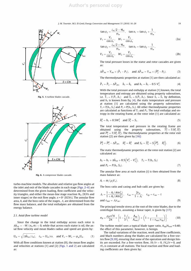
turbo-machine models. The absolute and relative gas flow angles atthe inlet and exit of the blade cascades in each stage (Figs. 2–6) aredetermined from the given loading, flow coefficient and the veloc-ity triangles, and either the mean-line stage reaction Rm (IGVs andinner stages) or the exit flow angle, a = 0� (EGVs). The annular flowarea, A, and the boss ratio of the stages, K, are determined from theflow mass balance, and the total enthalpies are obtained from theenergy balance.

2.1. Axial-flow turbine model

Since the change in the total enthalpy across each rotor isDhrot ¼ � _W=ðnst _mÞ < 0, while that across each stator is nil, the ax-ial flow velocity and mean blades radius and speed are given by:

Um ¼ffiffiffiffiffiffiffiffiffiffiffiffiffiffiffiffiffiffiffiffiffijDhrot=kmj

q; rm ¼ Um=x; and Vx ¼Wx ¼ umUm: ð1Þ

With all flow conditions known at station {0}, the mean flow anglesand velocities at stations {1} and {2} (Figs. 1 and 2) are calculatedas:

tan /1 ¼km=2�Rm

um; tan a1 ¼ tan /1 þ

1um

;

V1 ¼Vx

cos a1; W1 ¼

Vx

cos /1ð2aÞ

tan /2 ¼km=2þRm

um; tan a2 ¼ tan /2 �

1um

;

V2 ¼Vx

cos a2; W2 ¼

Vx

cos /2: ð2bÞ

The total pressure losses in the stator and rotor cascades are givenas:

DbPsta ¼ Ysta � ðbP1 � P1Þ; and DbProt ¼ Yrot � ðbPR2 � P2Þ: ð3Þ

The thermodynamic properties at station {1} are then calculated as:

bP1 ¼ bPo � DbPsta; h1 ¼ ho and h1 ¼ h1 � 0:5 V21: ð4Þ

With the total pressure and enthalpy at station {1} known, the totaltemperature and entropy are obtained using property subroutines,i.e. bT 1 ¼ TðbP1; h1Þ and bS1 ¼ SðbP1; h1Þ. Since S1 ¼ bS1 by definition,and h1 is known from Eq. (4), the static temperature and pressureat station {1} are calculated using the property subroutines:T1 = T(h1, S1) and P1 = P(h1, S1). All other thermodynamic propertiesare calculated as functions of T1 and P1. The total enthalpy and en-tropy in the rotating frame, at the rotor inlet {1} are calculated as:

hR1 ¼ h1 þ 0:5W2

1 and bSR1 ¼ S1: ð5Þ

The total temperature and pressure in the rotating frame areobtained using the property subroutines, bT R

1 ¼ TðhR1;bSR

1Þand bPR

1 ¼ TðhR1;bSR

1Þ. The thermodynamic properties at the rotor exitstation {2} are then given by [16]:

bPR2 ¼ bPR

1 � DbProt ; hR2 ¼ hR

1 and S2 ¼ bSR2 ¼ S bPR

2; hR2

� �: ð6Þ

The static thermodynamic properties at the rotor exit station {2} arecalculated as:

h2 ¼ h1 þ Dhrot þ 0:5 V21 � V2

2

� �; T2 ¼ Tðh2; S2Þ

and P2 ¼ Pðh2; S2Þ: ð7Þ

The annular flow area at each station {i} is then obtained from themass balance as:

Ai ¼ _m=ðqiVxÞ: ð8Þ

The boss ratio and casing and hub radii are given by:

Ki ¼1� Ai=ð4pr2

mÞ1þ Ai=ð4pr2

mÞ; rcas ¼

2rm

1þKi; rtip ¼ rcas � s

and rhub ¼ Kircas: ð9Þ

The principal tensile stress at the root of the rotor blades, due to thecentrifugal forces, assuming a linear taper, is given by [17]:

rB ¼qBx2A

2p� 1� 1

31� Atip

Aroot

� �� 1þ 1

1þ rhub=rtip

� �� : ð10Þ

The turbine model uses a typical blade taper ratio, Atip/Aroot = 0.40;the effect of this parameter, however, is benign.

The radial variations of the reaction, work and flow coefficients,and Mach numbers along the blades are calculated for a free-vor-tex flow [9,10], ensuring that none of the operation and design lim-its are exceeded. For a free-vortex flow, oh=or ¼ 0, oVx/or = 0, andrVh is constant at all stations. The local reaction and flow and load-ing coefficients are then given by:

Φφ1

β1

W1i

φ2

β2

C

S = C/σ

O

W2

tmax

δ

Z

Cx

Φφ1

β1

W1i

φ2

β2

C

S = C/σ

O

W2

tmax

δ

Z

Cx

Fig. 5. A turbine blades cascade.

Φ

φ1β1 W1i

φ2

β2

δ

C

O

W2

tmaxZ

S = C/σ

Cx

Φ

φ1β1 W1i

φ2

β2

δ

C

O

W2

tmaxZ

S = C/σ

Cx

Fig. 6. A compressor blades cascade.



1�RðrÞ ¼ ð1�RmÞrm

r

� �2; uðrÞ ¼ um

rm

r

� �;

kðrÞ ¼ kmrm

r

� �2: ð11Þ

The maximum flow and loading coefficients and minimum reactionall occur at the hub, and a positive reaction at the hub imposes aminimum value on the stage boss ratio of:

K � Kmin ¼2ffiffiffiffiffiffiffiffiffiffiffiffiffiffiffiffi

1�Rmp � 1� ��1

: ð12Þ

The local velocities at the blades leading and trailing edges and themaximum Mach number are then calculated and the polytropic effi-ciency is given [18] as:

gT ¼hin � hex

f nn�1� ðPin=qin � Pex=qexÞ

: ð13Þ

The non-ideal correction factor f, and exponents n and nS are givenby:

f ¼ hin � hSex

nSnS�1� ðPin=qin � Pex=qS

exÞ; n ¼ lnðPin=PexÞ

lnðqin=qexÞ;

nS ¼lnðPin=PexÞlnðqin=qS

exÞ: ð14Þ

The exit density and enthalpy for an isentropic expansion are calcu-lated as:

qSex ¼ qðPex; SinÞ and hS

ex ¼ hðPex; SinÞ: ð15Þ

Mallen and Saville [19] give a simpler expression as:

gT ¼hin � hex

hin � hex þ ðSex � SinÞ � ðTin � TexÞ= lnðTin=TexÞ: ð16Þ

For pressure ratios and inlet pressures up to 6.0 and 10 MPa, andbinary mixtures of noble gases and of helium and nitrogen, thepolytropic efficiencies predicted by Eqs. (13) and (16) are within0.1% of each other.

2.2. Pressure loss coefficient in turbine blades

The turbine model developed in this work incorporates the lat-est refinements proposed by Benner et al. [20,21] of Kacker andOkapuu’s model [12]. Reynolds and Mach numbers are based onthe relative gas flow velocities and the total pressure loss coeffi-cient is given as:

Y ¼ ðYp þ YsÞ þ YTE þ YTC : ð17Þ

Benner et al. proposed a loss scheme for the breakdown of the pro-file and secondary losses as:

ðYp þ YsÞ � ð1� ZTE=HÞ � Y 0p þ Y 0s: ð18Þ

The profile loss coefficient, based on recent turbine cascade data[22], is given by:

Y 0p ¼ 0:914� KinY 0p;AMKp þ Yshock

h i� KRe: ð19Þ

The factor Kin = 2/3, used by Kacker and Okapuu [12], underpredictsthe profile losses for blade rows with axial inflow. Zhu and Sjoland-er [22] introduced a higher correction, Kin = 0.825 for IGVs. For reac-tion blades, Kin = 2/3 is still used. Zhu and Sjolander have alsointroduced a Reynolds number correction factor based on their re-cent blade cascade data, as:

KRe ¼2� 105

Re2C

!0:575

; for Re2C < 2� 105;

and KRe ¼ 1:0; for Re2C � 2� 105: ð20Þ

The profile loss coefficient is multiplied by a factor 0.914 to obtainY 0p for zero trailing edge thickness [12]. The profile loss coefficient ofthe Ainley–Mathieson loss system, Y 0p;AM , was developed for vanesand blades having a trailing edge thickness to pitch ratio, tTE/S = 0.02 [11], and included the trailing edge losses. The factors Kp

and Yshock in Eq. (19) are identical to those introduced by Kackerand Okapuu [12] to account for the gas compressibility. The Machnumber correction factor, Kp in Eq. (19) is calculated as:

Kp ¼ 1� K2 � ð1� K1Þ; K1 ¼ 1; for Ma2 < 0:2;K1 ¼ 1� 1:25� ðMa2 � 0:2Þ for Ma2 > 0:2; and

K2 ¼ ðMa1=Ma2Þ2:ð21Þ

The shock losses occur at a relatively low average inlet Mach num-ber, due to the local flow acceleration at the highly curved leadingedges. These losses, appearing in Eq. (19), are calculated as [12]:

Yshock ¼q1W2

1

q2W22

� rhub

rtip� 3

4Mahub

1 � 0:4� �1:75

; for Mahub1 > 0:4 ð22aÞ

Yshock ¼ 0; for Mahub1 � 0:4 ð22bÞ

Also, the incident Mach number, always higher at the hub radiusthan at the midspan radius, is related to the mean incident Machnumber:

(a) For a reaction stage (rotor):

Mahub1

Ma1¼

5:716� rhubrtip

� �2�10:85� rhub

rtip

� �þ6:153; when rhub

rtip�0:95

1:0; when rhubrtip>0:95;

8<:ð23aÞ

(b) For a nozzle (stator):

Mahub1

Ma1¼

4:072� rhubrtip

� �2�6:644� rhub

rtip

� �þ3:705; when rhub

rtip�0:8

1:0; when rhubrtip>0:8:

8<:ð23bÞ

The profile loss coefficient, Y 0p;AM , by Ainley and Mathieson [11], aninterpolation between the results of two sets of cascade tests(b1 = 0 and b1 = /2), is given by:

Y 0p;AM ¼ Y ðb1¼0Þp;AM þ b1

/2

b1

/2

� �Y ðb1¼a2Þ

p;AM � Y ðb1¼0Þp;AM

h i �� tmax=C

0:2

� �Kmb1=/2

:

ð24Þ

The exponent Km is given by Zhu and Sjolander [22] as: Km = +1,when tmax/C < 0.2, and Km = �1, when tmax/C > 0.2. The results ofAinley and Mathieson using a comprehensive testing program ofcascades with b1 = 0 and tmax/C = 0.2 are correlated by the relation(Fig. 7):

Y ðb1¼0Þp;AM ¼ Aþ B� rþ 1

rC þ D

r

� �: ð25Þ

when /2 6 63:2�, the coefficients A, B, C and D are correlated asfunction of the trailing edge (TE) relative gas flow angle as:



A ¼ �5:58� 10�5 � /22 þ 1:03� 10�2 � /2 � 0:275;

B ¼ 1:553� 10�5 � /22 � 2:32� 10�3 � /2 þ 8:02� 10�2;

C ¼ �8:54� 10�3 � /2 þ 0:238;

D ¼ 4:83� 10�5 � /22 þ 2:83� 10�4 � /2 � 2:93� 10�2:

ð26aÞ

When /2 > 63.2�, these coefficients are correlated as:

A ¼ 2:44� 10�4 � /22 � 4:33� 10�2 � /2 þ 1:92;

B ¼ �4:02� 10�5 � /22 þ 6:94� 10�3 � /2 � 0:282;

C ¼ �2:23� 10�4 � /22 þ 4:96� 10�2 � /2 � 2:548;

D ¼ 5:39� 10�5 � /22 � 1:57� 10�2 � /2 þ 0:958:

ð26bÞ

The results of Ainley and Mathieson for a cascade with b1 = /2 andtmax/C = 0.2 are also well correlated by (Fig. 8):

Y ðb1¼a2Þp;AM ¼ Yp;min þ A� 1

r

� �� 1

r

� �min

n: ð27Þ

In this correlation, the optimum solidity for minimum losses is gi-ven by:

1r

� �min¼ �5:14� 10�4 � /2

2 þ 5:48� 10�2 � /2 � 0:798;

when /2 > 60�; ð28aÞ1r

� �min¼ �8:63� 10�6 � /3

2 þ 9:68� 10�4/22

� 3:76� 10�2 � /2 þ 1:272; when /2 � 60�:

The minimum value of the loss coefficient is then given as:

Yp;min ¼ 0:280� 1:0� 1r

� �min

� �: ð28bÞ

The coefficient A and the exponent n in Eq. (27) are given as:

(a) When 1r

� � 1

r

� min:

n ¼ 1:524� 10�4 � /22 � 0:031� /2 þ 2:992;

A ¼ 5:407� 10�3 � /2 � 0:19642; when /2 > 60�;

A ¼ �2:91� 10�3 � /2 þ 0:30260; when /2 � 60�:

ð28cÞ

(b) When 1r

� < 1

r

� min:

n ¼ 1:174� 10�2 � /22 � 1:5731� /2 þ 54:85; when /2 > 60�;

n ¼ 3:271� 10�3 � /22 � 0:3010� /2 þ 9:023; when /2 < 60�;

A ¼ 9:240� 10�3 � /22 � 1:2067� /2 þ 40:04; when /2 > 60�;

A ¼ 2:701� 10�3 � /22 � 0:2456� /2 þ 5:909; when /2 � 60�:

ð28dÞ

These results, for cascades with a maximum blade thickness, (tmax/C) = 0.2, are extended to different thicknesses using the last factoron the right-hand side of Eq. (24).

2.2.1. Spanwise penetration depth and secondary loss coefficientThe spanwise penetration depth (ZTE) of the separation line be-

tween the primary and the secondary loss regions, appearing in Eq.(18), is given [20] by:

ZTE

H¼ 0:10� jFtj0:79ffiffiffiffiffiffiffiffiffiffiffiffiffiffiffiffiffiffiffiffiffiffiffiffiffiffiffiffiffiffi

cos /1= cos /2

p� ðH=CÞ0:55 þ 32:7

d�

H

� �2

: ð29Þ

In this expression, the tangential loading parameter, Ft is given by:

Ft ¼ 2S

C � cos U� cos2ð/mÞ � ½tanð/1Þ þ tanð/2Þ: ð30Þ

The mean velocity vector angle is given by:

tanð/mÞ ¼12½tanð/1Þ � tanð/2Þ: ð31Þ

In Eq. (29), the boundary layer displacement thickness at the inletendwall, d*, is [23]:

d� ¼ d8¼ 0:0463x

ðq1W1x=l1Þ0:2 : ð32Þ

The reference length, x, in Eq. (32) is taken as half the bladeaxial chord. The secondary loss coefficient in Eq. (18) is given by[21]:

Y 0s ¼ FAR �0:038þ 0:41� tanhð1:2d�=HÞffiffiffiffiffiffiffiffiffiffiffiffi

cos Up

� ðcos /1= cos /2Þ � ðC cos /2=CxÞ0:55 : ð33Þ

The aspect ratio factor FAR is a function of the blade aspect ratio as:

FAR ¼ ðC=HÞ0:55; when H=C < 2:0 ð34aÞ

FAR ¼ 1:36604� ðC=HÞ; when H=C > 2:0 ð34bÞ

2.2.2. Trailing edge lossesThe trailing edge (TE) kinetic energy losses are expressed in

terms of the ratio of trailing edge thickness to the throat openingof the cascade. Kacker and Okapuu [12] have expressed theselosses in terms of the kinetic energy loss coefficient, DUTE, for axialentry nozzles (b1 = 0) and impulse blades (b1 = /2). The differencelies in the thicknesses of the profile boundary layers at the trailingedge of the blades. The impulse blades, with their thick boundarylayers, have lower trailing edge losses. For blades other than thetwo types above, the coefficient for the trailing edge kinetic energyloss is interpolated as:

0

0.02

0.04

0.06

0.08

0.10

0.3 0.5 0.7 0.9 1.1

Ainley and Mathieson [11]Present correlation, Eq. (25)

40506065

70

75

φ2 = 80 o

S / C Ratio

Y p,AM

for

β1 =

0

Fig. 7. Turbine blades profile loss coefficient for b1 = 0 and tmax/C = 0.2 [11].

0.060.080.100.120.140.160.180.200.220.24

0.3 0.5 0.7 0.9 1.1

Hainley & Mathieson [11]Present model,Eq. (27) 75

405055

60

65

φ2 = 70 o

S / C Ratio

Y p,AM

for

β 1 = φ

2

Fig. 8. Turbine blades profile loss coefficient for b1 = /2 and tmax/C = 0.2 [11].



DUTE ¼ DUðb1¼0ÞTE þ b1

/2

b1

/2

� �DUðb1¼a2Þ

TE � DUðb1¼0ÞTE

h i: ð35Þ

For an axial entry nozzle:

DUðb1¼0ÞTE ¼ 0:59563� tTE

O

� �2

þ 0:12264� tTE

O

� �� 2:2796� 10�3:

ð36aÞ

For an impulse blading:

DUðb1¼a2ÞTE ¼0:31066� tTE

O

� �2

þ0:065617� tTE

O

� ��1:4318�10�3:

ð36bÞ

The kinetic energy loss coefficient DUTE is converted to a pressureloss coefficient using the following relationship [10]:

YTE ¼1� c�1

2 Ma22 � 1

1�DUTE� 1

� �n o�c=ðc�1Þ� 1

1� 1þ c�12 Ma2

2

� ��c=ðc�1Þ : ð37Þ

2.2.3. Tip clearance lossesThe tip clearance (leakage) loss coefficient, YTC, in the turbine

blades cascade is calculated using the approach of Yaras and Sjo-lander [24] as:

YTC ¼ Ytip þ Ygap; ð38Þ

Ytip ¼ 1:4KEr�sH� cos2 /2

cos3 /m� C1:5

L ; and ð39Þ

Ygap ¼ 0:0049KGr�CH�

ffiffiffiffiffiCLp

cos /m: ð40Þ

The theoretical blade lift coefficient, CL, is given by [11]:

CL ¼2r� cosð/mÞ � ½tanð/1Þ þ tanð/2Þ: ð41Þ

For mid-loaded turbine blades, KE = 0.5 and KG = 1.0, and for front-or aft-loaded blades, KE = 0.566 and KG = 0.943 [24]. Eq. (39) is forunshrouded blades cascade. For shrouded blades [25], the sameexpression developed for unshrouded blades could be used byreplacing the tip clearance with an effective clearance value:seff = s/(n)0.42, and reducing the losses by 21.3%. Thus, the expres-sion used for the tip leakage losses in a shrouded blades cascade is:

Ytip ¼0:370:47

� 1:4KEr�seff

H� cos2 /2

cos3 /m� C1:5

L : ð42Þ

2.3. Turbine cascade geometry

The turbine blade profile follows the parabolic-arc camberline.However, the EGVs are designed using the compressor blades mod-el. Knowledge of (Z/C), the maximum camber (b/C), and the bladeangles measured from the chord line (v1 and v2) provides fourrelations that uniquely define the parabolic-arc profile (Figs. 5and 9). The blade camber (or turning) angle is expressed as,h = v1 + v2 = b1 + b2, and the maximum camber is given by [8]:

bC¼

ffiffiffiffiffiffiffiffiffiffiffiffiffiffiffiffiffiffiffiffiffiffiffiffiffiffiffiffiffiffiffiffiffiffiffiffiffiffiffiffiffiffiffiffiffiffiffiffiffiffiffiffiffiffiffiffiffiffiffiffiffiffiffiffiffi1þ ð4 tan hÞ2 � Z

C � ZC

� 2 � 316

h ir� 1

4 tan h: ð43Þ

The blade angles, with respect to the chord line, are given by:

tanðv1Þ ¼b=C

Z=C � 1=4; and tanðv2Þ ¼

b=C3=4� Z=C

: ð44Þ

The blade stagger angle with respect to the axial direction (Figs. 5and 9) is expressed as:

U ¼ ðv1 � b1Þ; or U ¼ ðb2 � v2Þ: ð45Þ

The number of blades in each row is determined using an empiricalmodel for the optimum solidity, based on matching the Ainley–Mathieson [11] minimum profile loss coefficients in Figs. 7 and 8.The optimum solidity for the axial-flow entry nozzles (b1 = 0�) is gi-ven by [9]:

1r

� �ðb1¼0Þ

opt

¼ 0:427þ 90� /2

58� 90� /2

93

� �2

: ð46Þ

Similarly, for impulse blading (b1 = /2):

1r

� �ðb1¼/2Þ

opt

¼ 0:224þ 0:575þ /2

90

� �� 1� /2

90

� �: ð47Þ

The optimum solidity for the turbine’s actual blade row, interpo-lated in the same manner used for the profile loss coefficient by Ain-ley and Mathieson (Eq. (24)), is given by:

1ropt¼ 1

r

� �ðb1¼0Þ

opt

þ b1

/2

b1

/2

� �� 1

r

� �ðb1¼/2Þ

opt

� 1r

� �ðb1¼0Þ

opt

" #: ð48Þ

The turbine blades are designed for zero incidence angle (i = 0), andthe deviation angle at the trailing edge is calculated using a recentcorrelation by Zhu and Sjolander [22] as:

d ¼ 17:3ð1=rÞ0:05 � ð/1 þ b2Þ

0:63 � cos2ðUÞ � ðtmax=CÞ0:29

ð30þ 0:01b2:071 Þ � tanhðRe2C=200; 000Þ

: ð49Þ

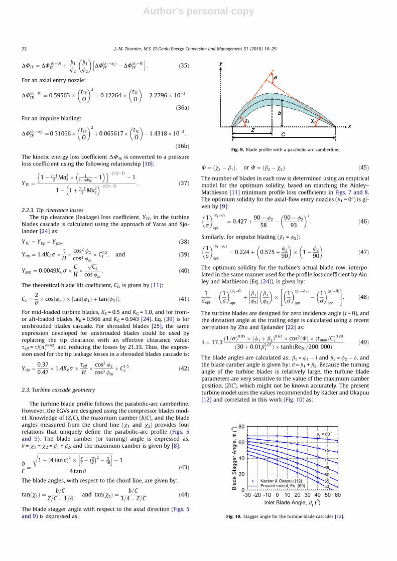
The blade angles are calculated as: b1 = /1 � i and b2 = /2 � d, andthe blade camber angle is given by: h = b1 + b2. Because the turningangle of the turbine blades is relatively large, the turbine bladeparameters are very sensitive to the value of the maximum camberposition, (Z/C), which might not be known accurately. The presentturbine model uses the values recommended by Kacker and Okapuu[12] and correlated in this work (Fig. 10) as:

χ1 χ2

ZC

b

θ

x

y

χ1 χ2

ZC

b

θ

x

y

Fig. 9. Blade profile with a parabolic-arc camberline.

0

20

40

60

80

-30 -20 -10 0 10 20 30 40 50 60

Kacker & Okapuu [12]Present model, Eq. (50) 50

5560

65

70

75

β2 = 80o

Inlet Blade Angle, β1 (o)

Blad

e St

agge

r Ang

le, Φ

(o )

Fig. 10. Stagger angle for the turbine blade cascades [12].



U ¼ Aþ B� b1 þ C � b21: ð50Þ

The coefficients A, B and C are functions of b2, and are given by:

A ¼ 0:710þ 0:2880� b2 þ 6:93� 10�3 � b22;

B ¼ 0:489� 0:0407� b2 þ 4:27� 10�4 � b22;

C ¼ �3:65� 10�3 þ 2:66� 10�5 � b2 þ 8:33� 10�8 � b22:

ð51Þ

Eq. (50) is used to determine the blade angles with respect to thechord line as:v1 ¼ Uþ b1 and v2 ¼ b2 �U. The location of maxi-mum camber is calculated by simultaneously solving Eqs. (44a)and (44b). Finally, the number of blades in the cascade is obtainedas:

N ¼ INT2prmr

H� H

C

� � �: ð52Þ

The blades pitch and chord are calculated as: S ¼ ð2prmÞ=Nand C ¼ rS: Iterations are performed until a convergence of thedeviation angle is achieved.

2.4. Axial-flow compressor design model

Aungier [8] recommended using a de Haller limit of 0.70 to rep-resent the stall condition for compressor blades cascade with tmax/C = 0.10, and developed an empirical relationship for this limit,which is used to obtain the mean-line flow coefficient as a functionof the loading coefficient, the reaction and the stall marginð1� KmÞ, as:

um ¼km=Km � 6=17 bRm

0:86�

bRm

0:50

!1:188<:

9=;1

2:0þ1=bRm

: ð53Þ

bRm ¼ 0:5þ jRm � 0:5j; and Km = 0.80 gives the flow coefficient for amean stall margin of 20%. With all flow conditions known at station{0} (the inlet of the stator blades cascade of the compressor stage),the mean flow angles and velocities at stations {1} and {2} are cal-culated as:

tan /1 ¼Rm þ km=2

um; tan a1 ¼

1um� tan /1;

V1 ¼Vx

cos a1; W1 ¼

Vx

cos /1ð54aÞ

tan /2 ¼Rm � km=2

um; tan a2 ¼

1um� tan /2;

V2 ¼Vx

cos a2; W2 ¼

Vx

cos /2: ð54bÞ

The total pressure losses in the stator and rotor cascades of thecompressor are given as:

DbPsta ¼ Ysta � ðbPo � PoÞ; and DbProt ¼ Yrot � ðbPR1 � P1Þ: ð55Þ

The thermodynamic properties at the leading and trailing edges ofthe rotor blades are calculated using Eqs. (4)–(7), and the annularflow areas, boss ratios and radii at each station {i} are calculatedusing Eqs. (8) and (9). The radial variations of the reaction, workand flow coefficients, Mach numbers and the de Haller ratios alongthe blades are calculated for a free-vortex flow [8,9], to ensure thatoperation and design limits are not exceeded. The maximum flowand loading coefficients and the minimum reaction all occur atthe hub. A positive reaction at the hub, and loading and flow coef-ficients <1.0 for surge stability, requires that:

K � Kmin ¼2

MAXffiffiffiffiffiffiffiffiffiffiffiffiffiffiffiffi1�Rmp

;ffiffiffiffiffiffikmp

;um

� � 1

!�1

: ð56Þ

The polytropic efficiency is calculated using the relationship [18] fornon-ideal gases, as:

gC ¼f n

n�1� ðPex=qex � Pin=qinÞhex � hin

: ð57Þ

The correction factor f, and exponents n and nS are given by:

f ¼ hSex � hin

nSnS�1� ðPex=qS

ex � Pin=qinÞ;

n ¼ lnðPex=PinÞlnðqex=qinÞ

; nS ¼lnðPex=PinÞlnðqS

ex=qinÞ: ð58Þ

The exit density and enthalpy for an isentropic compression are cal-culated as:

qSex ¼ qðPex; SinÞ; and hS

ex ¼ hðPex; SinÞ: ð59Þ

Mallen and Saville [19] give the following simpler expression for thepolytropic efficiency:

gC ¼hex � hin � ðSex � SinÞ � ðTex � TinÞ= lnðTex=TinÞ

hex � hin: ð60Þ

For pressure ratios up to 6.0, exit pressures up to 10 MPa, and bin-ary mixtures of noble gases and of helium and nitrogen, Eqs. (57)and (60) are within 0.1% of each other.

2.5. Pressure loss coefficient in compressor blades

In this Section, Reynolds and Mach numbers are based on therelative gas flow velocities. The total pressure loss coefficient inthe compressor cascade is given as:

Y ¼ Yp þ Ys þ YEW þ YTC : ð61Þ

Lieblein [26] expressed the blade-profile pressure loss coefficientas:

Yp ¼ 2h2

C

� �� r

cos /2� cos /1

cos /2

� �2

� 2HTE

3HTE � 1

� �� 1� h2

C

� �rHTE

cos /2

� ��3

: ð62Þ

The boundary-layer momentum thickness at the blade outlet, h2, isgiven [27] as:

h2

C¼ ho

2

C

� �� fM � fH � fRe: ð63Þ

The boundary layer trailing-edge shape factor, HTE, the ratio of theboundary layer displacement thickness to the momentum thick-ness, h2, is expressed as:

HTE ¼ HoTE � nM � nH � nRe: ð64Þ

The values of ho2 and Ho

TE are for inlet Mach numbers, Ma1 < 0.05, nocontraction in the height of the flow annulus, H, an inlet Reynoldsnumber, Re1C = 106 and hydraulically smooth blades. Based on theexperimental data of Koch and Smith [27] at these conditions, theboundary-layer momentum thickness at the blade outlet is corre-lated accurately as:

ho2

C¼ 2:644� 10�3 � Deq � 1:519� 10�4 þ 6:713� 10�3

2:60� Deq: ð65Þ

The shape factor for the boundary layer trailing-edge is correlatedas:



HoTE ¼

d�TE

ho2

¼ ð0:91þ 0:35� DeqÞ

� 1þ 0:48� Deq � 1� 4 þ 0:21� Deq � 1

� 6n o

: ð66Þ

A value of HoTE ¼ 2:7209 is used when Deq > 2.0. For conditions other

than nominal, Koch and Smith developed charts for determining thecorrection factors fM ; fH; fRe in Eq. (63) and nM; nH; nRe in Eq. (64). Thecorrection factor for inlet Mach number is correlated as:

fM ¼ 1:0þ ð0:11757� 0:16983� DeqÞ �Man1; ð67Þ

n ¼ 2:853þ Deqð�0:97747þ 0:19477� DeqÞ: ð68Þ

The correction factor for the flow area contraction is given by:

fH ¼ 0:53H1

H2þ 0:47: ð69Þ

The chart presented by Koch and Smith for the Reynolds correctionfactor is well approximated using the approach proposed by Aun-gier [9]. He introduced the critical blade chord Reynolds number,Recr = 100 � C/j, above which the effect of roughness become sig-nificant. When Re1C < Recr, the Reynolds correction factor is ex-pressed as:

fRe ¼106

Re1C

� �0:166; for Re1C � 2� 105;

1:30626� 2�105

Re1C

� �0:5; for Re1C < 2� 105:

8><>: ð70aÞ

When Re1C > Recr, the friction losses are controlled by the surfaceroughness and the Reynolds correction factor may be expressed as:

fRe ¼106

Recr

� �0:166; for Recr � 2� 105;

1:30626� 2�105

Recr

� �0:5; for Recr < 2� 105:

8><>: ð70bÞ

Typical ratios of the blade chord to surface roughness are:C/j = 10,000 to 20,000. When Re1C > 106 and C/j = 104, Recr = 106,and fRe = 1. The correction factor for the inlet Mach number is accu-rately fitted by:

nM ¼ 1:0þ 1:0725þ Deq � �0:8671þ 0:18043� Deq� � �

�Ma1:81 :

ð71Þ

The correction factor for the flow area contraction is calculated as:

nH ¼ 1:0þ H1

H2� 1:0

� �� 0:0026� D8

eq � 0:024� �

: ð72Þ

The correction factor for the inlet Reynolds number is given by:

nRe ¼106

Re1C

!0:06

; when Re1C < Recr; and

¼ 106

Recr

!0:06

; when Re1C � Recr: ð73Þ

The equivalent diffusion ratio, Deq is given by [27]:

Deq ¼W1

W2� 1þ K3

tmax

Cþ K4C

��

�

ffiffiffiffiffiffiffiffiffiffiffiffiffiffiffiffiffiffiffiffiffiffiffiffiffiffiffiffiffiffiffiffiffiffiffiffiffiffiffiffiffiffiffiffiffiffiffiffiffiffiffiffiffiffiffiffiffiffiffiffiffiffiffiffiffiffiffiffiffiffiffiffiffiffiffiffiffiffiffiffiffiffiffiffiffiffiffiffiffiffiffiðsin /1 � K1rC�Þ2 þ cos /1

A�throat � qthroat=q1

� �2s

: ð74Þ

In Eq. (74), the contraction ratio is given by:

A�throat ¼ 1:0� K2rtmax

C

� ��cosð0:5ð/1 þ /1ÞÞ

� �� Athroat

A1: ð75aÞ

The cascade throat area is assumed to occur at one-third of the axialchord, thus:

Athroat ¼ A1 �13ðA1 � A2Þ: ð75bÞ

The gas density at the throat is calculated as:

qthroat

q1¼ 1�

Ma2x1

1�Ma2x1

1� A�throat � K1rC�tan /1

cos /1

� �: ð75cÞ

The obtained constants in these equations from the experimentaldata of Koch and Smith are: K1 = 0.2445, K2 = 0.4458, K3 = 0.7688and K4 = 0.6024. The dimensionless blade circulation parameter inEqs. (74) and (75c) is given by:

C� ¼ r1mVh1 � r2mVh2

rW1 � ðr1m þ r2mÞ=2¼ ðtan /1 � tan /2Þ �

cos /1

r: ð76Þ

In the present compressor model, this parameter reduces to thesimpler expression on the right-hand side, since r1m = r2m = rm,which leads to U1m = U2m = Um.

The secondary flow loss coefficient is given by the correlationproposed by Howell [28] as:

Ys ¼ 0:018� r� cos2 /1

cos3 /m� C2

L : ð77Þ

The theoretical compressor blade lift coefficient, CL, is expressed as:

CL ¼2r� cosð/mÞ � ½tanð/1Þ � tanð/2Þ: ð78Þ

The mean velocity vector angle is given by:

tanð/mÞ ¼ 0:5½tanð/1Þ þ tanð/2Þ: ð79Þ

Based on a modified Howell’s model [28], Aungier [8] developed thefollowing expression for calculating the end wall loss coefficient, as:

YEW ¼ 0:0146� CH� cos /1

cos /2

� �2

: ð80Þ

The tip clearance (leakage) loss factor, YTC is calculated [24] as:

YTC ¼ Ytip þ Ygap; ð81Þ

Ytip ¼ 1:4KEr�sH� cos2 /1

cos3 /m� C1:5

L ; and ð82Þ

Ygap ¼ 0:0049KGr�CH

ffiffiffiffiffiCL

p= cos /m

� �: ð83Þ

For mid-loaded compressor blades (Z/C = 0.5), KE = 0.5 and KG = 1.0.

2.6. Compressor cascade geometry

The compressor blade profile is also a parabolic-arc camberline[8] (Fig. 9). The blade stagger angle, with respect to the axial direc-tion (Figs. 6 and 9), is expressed as:

U ¼ ðb1 � v1Þ; or U ¼ ðb2 þ v2Þ: ð84Þ

The location of the maximum camber is restricted to 0.25 < Z/C < 0.75, and the blade camber angle for a compressor cascade is re-stricted to: h = b1 � b2 < 90�. For the IGVs, b1 < b2 and the same pro-file and camberline are used, except for reversing the flow direction.In this case, Eqs. (43), (44), and (84) can be used for these blades,with the angles h, v1 and v2, and the parameter (b/C) being nega-tive. For example, for axial-compressor EGVs parameters: b1 = 40�,b2 = 0�, Z/C = 0.40, r = 1.0 and tmax/C = 0.20, Eqs. (43), (44), and(84) give h = 40�, b/C = 0.07792, v1 = 27.45�, v2 = 12.55�, andU = 12.55�. This blade profile can be inverted for IGVs as follows:b1 = 0�, b2 = 40�, Z/C = 0.60, r = 1.0 and tmax/C = 0.20, and Eqs. (43),(44), and (84) give h = �40�, b/C = �0.07792, v1 = �12.55�,v2 = �27.45�, and U = 12.55�.



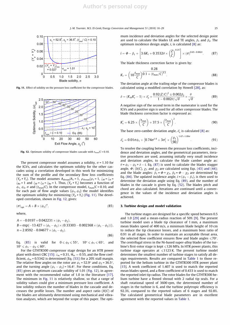
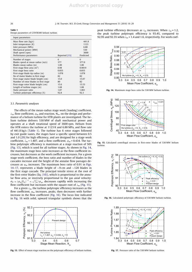
The present compressor model assumes a solidity, r = 1.10 forthe IGVs, and calculates the optimum solidity for the other cas-cades using a correlation developed in this work for minimizingthe sum of the profile and the secondary flow loss coefficients(Yp + Ys). The model assumes Athroat/A1 = 1, qthroat/q1 = 1, fM = fH =fRe = 1 and nM = nH = nRe = 1. Thus, (Yp + Ys) becomes a function of/1, /2, r and (tmax/C). In the compressor model, tmax/C = 0.10, andfor each pair of flow angle values {/1, /2} the model identifiesthe optimum solidity for minimizing (Yp + Ys) (Fig. 11). The devel-oped correlation, shown in Fig. 12, gives:

ðrÞopt ¼ Aþ B� ð/2Þn; ð85Þ

where,

A¼�0:0197þ0:042231�ð/1�/2Þ;B¼ expf�13:427þð/1�/2Þ� ð0:33303�0:002368�ð/1�/2ÞÞg;n¼ 2:8592�0:04677�ð/1�/2Þ:

ð86Þ

Eq. (85) is valid for 0 6 /2 6 55�, 10� 6 /1 6 65�, and10� 6 /1 � /2 6 60�.

For the GTHTR300 compressor stage design for an HTR powerplant with direct CBC [15]: km = 0.31, Rm ¼ 0:55, and the flow coef-ficient, /m = 0.5342 is determined (Eq. (53)) for a 20% stall margin.The relative flow angles on the rotor are /1 = 52.9� and /2 = 36.5�,and the turning angle (/1 � /2) = 16.4�. For these conditions, Eq.(85) gives an optimum cascade solidity of 1.01 (Fig. 12), in agree-ment with the recommended value of 1.0 in the literature [17].The minimum in Fig. 11 is relatively shallow, so that a range ofsolidity values could give a minimum pressure loss coefficient. Alow solidity reduces the number of blades in the cascade and de-creases the profile losses. The number and aspect ratio (H/C) ofthe blades are ultimately determined using mechanical and vibra-tion analyses, which are beyond the scope of this paper. The opti-

mum incidence and deviation angles for the selected design pointare used to calculate the blades LE and TE angles, b1 and b2. Theoptimum incidence design angle, i, is calculated [8] as:

i ¼ U� b1 þ 3:6Kt þ 0:3532h� ZC

� �0:25" #

� ðrÞ0:65�0:002h: ð87Þ

The blade thickness correction factor is given by:

Kt ¼ 10tmax

C

� � 0:28

0:1þ ðtmax=CÞ0:3 : ð88Þ

The deviation angle at the trailing edge of the compressor blades iscalculated using a modified correlation by Howell [28], as:

d ¼ ðKshK 0t � 1Þ � d�o þ0:92ðZ=CÞ2 0:002b2

1� 0:002h=ffiffiffiffirp � hffiffiffiffi

rp : ð89Þ

A negative sign of the second term in the numerator is used for theIGVs and a positive sign is used for all other compressor blades. Theblade thickness correction factor is expressed as:

K 0t ¼ 6:25� tmax

C

� �þ 37:5� tmax

C

� �2

: ð90Þ

The base zero-camber deviation angle, d�o is calculated [8] as:

d�o ¼ 0:01r/1 þ 0:74r1:9 þ 3r� �

� /1

90

� �1:67þ1:09r

: ð91Þ

To resolve the coupling between the pressure loss coefficients, inci-dence and deviation angles, and the geometrical parameters, itera-tive procedures are used, assuming initially very small incidenceand deviation angles, to calculate the blade camber angle as:h = /1 � /2 + d � i. Eq. (87) is used to calculate the blades staggerangle, U; (b/C), v1 and v2 are calculated using Eqs. (43) and (44);and the blade angles: b1 = U + v1, b2 = U � v2 are determined byEq. (84). The updated incidence angle, i = (/1 � b1), is then used todetermine the deviation angle using Eq. (89), and the number ofblades in the cascade is given by Eq. (52). The blades pitch andchord are also calculated. Iterations are continued until a conver-gence in the values of the incidence and deviation angles isachieved.

3. Turbine design and model validation

The turbine stages are designed for a specific speed between 0.5and 1.0 [29] and a mean-radius reaction of 50% [9]. The presentturbine model uses a blade tip clearance of 1 mm, a maximummean blades speed of 400 m/s, a minimum blade height of 10 cmto reduce the tip clearance losses, and a maximum boss ratio of0.91 in all stages. In order to maintain an acceptable throat area,the selected flow coefficient ensures flow and blade angles 670�.The centrifugal stress in the Ni-based super-alloy blades of the tur-bine’s first-rotor stage is kept 6126 MPa. In HTR power plants, thisturbine stage operates at 61123 K. The present turbine modeldetermines the smallest number of turbine stages to satisfy all de-sign requirements. Results are compared in Table 1 to those re-ported for the helium turbine in the GTHTR300 HTR power plant[15]. A work coefficient of 1.407 is used to match the reportedmean blades speed, and a flow coefficient of 0.433 is used to matchthe reported inlet tip radius. The rotor blades for the GTHTR300 he-lium turbine have a finned shroud with 2 radial tip seals. For ashaft rotational speed of 3600 rpm, the determined number ofstages in the turbine is 6, and the turbine polytropic efficiency is92.3%, compared to the reported values of 6 stages and 92.8%.The calculated geometrical blade parameters are in excellentagreement with the reported values in Table 1.

0

0.02

0.04

0.06

0.08

0.10

0 0.5 1.0 1.5 2.0 2.5 3.0

(Yp + Ys)min= 0.027 σopt = 1.01

φ1 = 52.9o, φ2 = 36.5o, (tmax/ C) = 0.10

Blade solidity, σ

( Yp +

Ys)

Fig. 11. Effect of solidity on the pressure loss coefficient for the compressor blades.

0

0.5

1.0

1.5

2.0

2.5

0 10 20 30 40 50 60

Eq. (85)tmax / C = 0.10

55o 50o45o

40o35o

30o

25o

20o

15o

φ1- φ2 = 10o

Exit Flow Angle, φ2 (o)

Opt

imum

Sol

idity

, (σ)

opt

Fig. 12. Optimum solidity of compressor blades cascade with tmax/C = 0.10.



3.1. Parametric analyses

The effects of the mean-radius stage work (loading) coefficient,km, flow coefficient, um and reaction, Rm, on the design and perfor-mance of a helium turbine for HTR plants are investigated. The he-lium turbine delivers 530 MW of shaft mechanical power andoperates at a shaft rotational speed of 3600 rpm. Helium fromthe HTR enters the turbine at 1123 K and 6.88 MPa, and flow rateof 441.8 kg/s (Table 1). The turbine has 6 rotor stages followedby exit guide vanes, the stages have a specific speed between 0.5and 1.0 [29] for high efficiency, and are designed for a stage workcoefficient, km = 1.407, and a flow coefficient, /m = 0.434. The tur-bine polytropic efficiency is maximum at a stage reaction of 50%(Fig. 13), which is used for all turbine stages. As shown in Fig. 14,the maximum stage boss ratio increases as the flow coefficient in-creases, but decreases as the work coefficient increases. For a givenstage work coefficient, the boss ratio and number of blades in thecascades increase and the height of the annular flow passages de-creases as um increases. The maximum boss ratio of 0.91 in Figs.14–17, represents a blade height of �9 cm and �120 blades inthe first stage cascade. The principal tensile stress at the root ofthe first-rotor blades (Eq. (10)), which is proportional to the annu-lar flow area, or inversely proportional to the gas axial velocity:rB / ðumUmÞ�1 /

ffiffiffiffiffiffikmp

=um, decreases rapidly with increasing theflow coefficient but increases with the square root of km (Fig. 15).

For a given km, the turbine polytropic efficiency increases as theflow coefficient, um increases, peaks, then decreases with furtherincrease in the flow coefficient (Fig. 16). The locus line indicatedin Fig. 16 with solid, upward triangular symbols shows that the

peak turbine efficiency decreases as km increases. When km = 1.2,the peak turbine polytropic efficiency is 93.4%, compared to92.9% and 92.3% when km = 1.4 and 1.6, respectively. For work coef-

Table 1Design parameters of GTHTR300 helium turbine.

Input parameters

Mass flow rate (kg/s) 441.8Inlet temperature (K) 1123Inlet pressure (MPa) 6.88Mechanical power (MW) 530Shaft speed (rpm) 3600Performance parameters Reported [15] Predicted

Number of stages 6 6Blades speed at mean radius (m/s) 377 377.0Blades mean radius (m) 1.00 1.00First-stage flow area (m2) 0.98 0.9819First stage boss ratio 0.855 0.855First-stage blade tip radius (m) 1.078 1.078No of stator blades in first stage 82 82First-stage stator blade height (cm) 15.0 15.07Number of rotor blades in first stage 80 82First-stage rotor blade height (cm) 15.6 15.53Length of turbine stages (m) 1.68 1.88Static pressure ratio 1.87 1.861Turbine polytropic efficiency (%) 92.8 92.3

91.9

92.0

92.1

92.2

92.3

0.3 0.4 0.5 0.6 0.7

Present design

He turbineλm = 1.407, φm = 0.434, nst = 6

Stage Mean Reaction, ℜm

Poly

topi

c Ef

ficie

ncy,

ηT (%

)

Fig. 13. Effect of mean stage reaction on the polytropic efficiency of helium turbine.

0.800.820.840.860.880.900.920.94

0.3 0.4 0.5 0.6 0.7 0.8 0.9 1.0

1.01.2

1.4

1.6

λ m= 1.8

He turbine (nst = 6, ℜm = 0.5)

0.91

φ2 =

70 o

Mean Flow Coefficient, ϕm

Stag

e Bo

ss R

atio

, Λm

ax

Fig. 14. Maximum stage boss ratio for 530 MW helium turbine.

40

60

80

100

120

140

0.3 0.4 0.5 0.6 0.7 0.8 0.9 1.0

Λmax = 0.91

1.01.2

1.41.6

λm = 1.8

He turbine (nst = 6, ℜm = 0.5)First stage rotor

φ2 = 70o


Cen

trifu

gal S

tress

, σB (M

Pa)

Fig. 15. Calculated centrifugal stresses in first-rotor blades of 530 MW heliumturbine.

90

91

92

93

94

0.3 0.4 0.5 0.6 0.7 0.8 0.9 1.0

Peak efficiencyΛmax = 0.91Present design

λ m=1.8

1.6

1.4

1.2

1.0He turbine (nst = 6, ℜm= 0.5)

φ2 =

70 o


Poly

tropi

c Ef

ficie

ncy,

ηT (%

)

Fig. 16. Calculated polytropic efficiency of 530 MW helium turbine.

1.84

1.85

1.86

1.87

1.88

1.89

0.3 0.4 0.5 0.6 0.7 0.8 0.9 1.0

Peak efficiencyΛmax = 0.91Present design

λm =1.8

1.6

1.4

1.2

1.0

He turbine (nst = 6, ℜm= 0.5)

φ 2=

70o


Turb

ine

Pres

sure

Rat

io

Fig. 17. Pressure ratio of the 530 MW helium turbine.



ficients of 1.2, 1.4 and 1.6, the turbine peak efficiency occurs atstage flow coefficients of 0.553, 0.639 and 0.707, respectively(Fig. 16). For a helium mass flow rate of 441.8 kg/s, total inlet tem-perature of 1123 K and turbine mechanical power of 530 MW, thetotal exit temperature of the turbine is constant = 893.7 K, but theexit pressure depends on the pressure losses in the turbine stages.For design work coefficients of 1.0–1.8, the turbine pressure ratiovaries from 1.846 to 1.88 (Fig. 17), for polytropic efficiencies of90.8–93.6% (Fig. 16). At mean-stage work and flow coefficients of1.4 and 0.6, the turbine’s pressure ratio is 1.856 and the polytropicefficiency of 92.8% is near optimum.

The mean blades radius, rm ¼ Um=x / 1=ffiffiffiffiffiffikmp

, decreases but theaxial flow velocity through the turbine, Vx ¼ umUm / um=


, in-creases slowly as the work coefficient increases (Fig. 18). The latteris due to the rapid increase in the mean flow coefficient withincreasing km along the locus of peak turbine polytropic efficiency(Fig. 16). As a result, the annular flow area through the turbine de-creases as km increases. The combination of lower mean blades ra-dius and lower annular flow area with increasing km decreases theturbine shroud radius (Fig. 18) and the volume of the stages, whichis true when the turbine is designed at the peak polytropicefficiency.

4. Compressor design and model validation

The results of the present model are compared in Table 2 withthose reported for an HTR plant helium compressor [15]. The com-

pressor stages are designed for a specific speed of 1.0–2.0 [29], ablade tip clearance of 1 mm [15], minimum blade height of6.7 cm for a tip clearance ratio s/H 6 1.5%, and maximum stageboss ratio of 0.93. The compressor stages have a 55% mean-radiusreaction [8]. The calculated parameters for the helium compressorare compared in Table 2 to those reported for the GTHTR300 HTRplant’s compressor. A work coefficient of 0.31 is used to matchthe reported mean blades speed, and a flow coefficient of 0.5342is used to ensure a 20% stall margin. For a shaft rotational speedof 3600 rpm, the number of compressor stages is 20, and the poly-tropic efficiency is 90.43%, compared to the reported values of 20stages and 90.5% [15]. The calculated geometrical blade parametersin the first stage are in excellent agreement with reported values(Table 2).

4.1. Parametric analyses

The effects of km and design surge margin on the performance ofa helium compressor are investigated. The compressor has 20 rotorstages, consumes 251 MW at a shaft rotational speed of 3600 rpm(Table 2). The helium working fluid enters the compressor at 301 K,3.52 MPa, and flow rate of 449.7 kg/s. For a mean stage reaction of55%, the mean flow coefficient (Eq. (53)) is calculated for mean stallmargins of 10%, 20% and 30% (Fig. 19). For a given stall margin, thegas velocities W1 and V2 in the stages are nearly constant, but um

increases rapidly with km. The gas flow angles decrease rapidlywith increasing the stage work coefficient; a limiting gas flow an-gle of 70� occurs at low km. The mean blades velocity, Um is inver-sely proportional to


; and decreases rapidly as the mean workcoefficient increases (Fig. 19). When Um > 400 m/s, the centrifugalstresses in the compressor rotor blades are excessive, limitingthe mean work coefficient to �0.20. The mean blades radius,rm = Um/x and the blades tip radius in the first stage decrease asthe work coefficient increases (Fig. 20). The largest stage boss ratio,

210

220

230

240

250

260

1.0 1.2 1.4 1.6 1.80.8

0.9

1.0

1.1

1.2

1.3

Mean blades radius

Maximum shroud radius

Stage Mean Work Coefficient, λm

Axia

l Vel

ocity

, Vx (m

/s)

Rad

ius

(m)

Fig. 18. Axial flow velocity and maximum shroud radius of 530 MW helium turbineat peak polytropic efficiency.

Table 2Design parameters of GTHTR300 helium compressor.

Input parameters

Mass flow rate (kg/s) 449.7Inlet temperature (K) 301Inlet pressure (MPa) 3.52Mechanical power (MW) 251Shaft speed (rpm) 3600Performance parameters Reported [15] Predicted

Number of stages 20 20Blades speed at mean radius (m/s) 299.2 300.0Blades mean radius (m) 0.794 0.796First-stage flow area (m2) 0.5133 0.5090First stage boss ratio 0.880 0.880First-stage blade tip radius (m) 0.852 0.847First-stage stator blade chord (cm) 6.0 5.98No. of stator blades in first stage 94 92First-stage stator blade height (cm) 10.2 10.18First-stage rotor blade chord (cm) 7.8 7.22Number of rotor blades in first stage 72 70First-stage rotor blade height (cm) 10.1 10.14Length of compressor stages (m) 3.80 3.53Static pressure ratio 2.0 1.981Compressor Polytropic efficiency (%) 90.5 90.43

0

0.2

0.4

0.6

0.8

1.0

0.1 0.2 0.3 0.4 0.5 0.6 0.7100

200

300

400

500

60030% surge margin20% surge margin10% surge margin

He compressor(nst = 20, ℜm = 0.55)

φ1 = 70 o

Λ1 = Λ

min

Work Coefficient, λm

Flow

Coe

ffici

ent,

φ m

Blad

es V

eloc

ity, U

m (m

/s)

Fig. 19. Flow coefficient and blades velocity of the helium compressor stages.

50

100

150

200

250

0.1 0.2 0.3 0.4 0.5 0.6 0.70.5

0.7

0.9

1.1

1.330% surge margin20% surge margin10% surge margin

He compressor(n

st= 20, ℜ

m= 0.55)

φ1 =

70 o

Λ1 = Λ

min

Rm


Axi

al V

eloc

ity, V

x (m

/s)

1st S

tage

Tip

Rad

ius,

Rtip

(m

)

Fig. 20. Axial flow velocity and blades tip radius of 251 MW helium compressor.



K, and the shortest rotor blades occur in the last stage of thecompressor.

The low molecular weight helium requires relatively short com-pressor blades (<11 cm) and high boss ratios >0.85 (Fig. 21). The ro-tor blades height in the last stage of the compressor first decreasesas km increases, reaching a minimum, then increases. The mini-mum blade height, however, occurs at a higher stage work coeffi-cient than the maximum value of the boss ratio (Fig. 20). Theminimum blades height minimizes the volume of the compressorblades and maximizes the polytropic efficiency, as shown later.The optimum solidity (r = C/S) of the last rotor cascade in the com-pressor for minimizing (Yp + Ys) (Eqs. (85) and (86)) varies from 0.7to 1.5, and increases almost linearly as the stage work coefficientincreases (Fig. 22). Since the blade chord length (C) is proportionalto the blade height, the number of blades in the last rotor cascadeinitially increases as km increases, reaching a maximum, then de-creases with further increase in km (Fig. 22). This trend is true forall other cascades of the axial-flow compressor. The compressor

with the highest polytropic efficiency has the largest number ofblades in the cascades (Figs. 22 and 23). At the peak efficiency,the compressor cascades have the largest number of shortestblades, and hence the lowest total blades volume. The calculatedcompressor peak polytropic efficiencies of 90.8%, 90.44% and 90%for stall margins of 10%, 20% and 30% occur at stage work coeffi-cients of 0.32, 0.30 and 0.25, respectively (Fig. 23). For design stallmargins of 10% to 30%, the compressor pressure ratio varies from1.941 to 1.985 (Fig. 24), and the polytropic efficiency from 88.1%to 90.8% (Fig. 23). For a 20% stall design margin and km = 0.18,the polytropic efficiency is 88.3%, and the total pressure lossesthrough the helium compressor stages are 0.440 MPa. For the samestall design margin, the peak efficiency of 90.4% and the peak pres-sure ratio of 1.981 occur at a work coefficient of 0.31, and totalpressure losses of only 0.369 MPa.

5. Summary and conclusions

To satisfy the need for detailed design and performance modelsfor noble gases turbo-machines for HTR plants with CBC, this workdeveloped multi-stage, axial-flow turbine and compressor models.The developed models, based on a mean-line through-flow analysisfor free-vortex flow along the blades, account for profile, second-ary, end wall, trailing edge and tip clearance (leakage) losses inthe cascades, and calculate the geometrical parameters of the bladecascades as functions of the flow conditions, mean-line flow coef-ficient, work coefficient and stage reaction. An empirical expres-sion is developed to determine the optimum solidity of thecompressor blades cascade for minimizing the sum of the profileand secondary pressure loss coefficients. The developed modelsare validated successfully using reported performance and hard-ware data of the helium compressor and turbine of the GTHTR300,HTR power plant, at a shaft speed of 3600 rpm. The determinednumber of stages in the helium turbine of 6 at a polytropic effi-ciency of the turbine of 92.3%, are in agreement with the reportedvalues of 6 stages and 92.8%. For 20% stall design margin in the he-lium compressor, the calculated minimum number of stages of 20at a polytropic efficiency of 90.43% for the compressor also com-pares well with the reported values of 20 stages and 90.5%. The cal-culated geometrical blade parameters for both the helium turbineand compressor are also in excellent agreement with the reportedvalues for the HTR plant turbo-machine.

Results of parametric analyses of the 6 stages, 530 MW heliumturbine show that the peak polytropic efficiency occurs at a meanstage reaction of 50%, and that increasing the stages work coeffi-cient decreases the turbine stages boss ratio, the shroud diameterand the rotor centrifugal stress, as well as the peak polytropic effi-ciency of the turbine. Presented results for a 251 MW helium com-pressor with 20 stages show that for a given stall margin,increasing the cascades mean-flow work coefficient increases the

6

7

8

9

10

11

12

0.1 0.2 0.3 0.4 0.5 0.6 0.70.82

0.84

0.86

0.88

0.90

0.92

0.9430% surge margin20% surge margin10% surge margin


φ 1=

70o

Λ 1= Λ min


Rot

or B

lade

Hei

ght,

HB (c

m)

Last

Sta

ge B

oss

Rat

io, Λ

Fig. 21. Rotor blades height and last stage boss ratio of 251 MW heliumcompressor.

60

70

80

90

100

110

0.1 0.2 0.3 0.4 0.5 0.6 0.70.6

0.8

1.0

1.2

1.4

1.6

30% surge margin20% surge margin10% surge margin

φ1 =

70 o

Λ 1= Λ min


Blad

es in

Rot

or

Rot

or C

asca

de S

olid

ity, σ

Fig. 22. Number of blades and last rotor solidity of 251 MW helium compressor.

88.0

88.5

89.0

89.5

90.0

90.5

91.0

0.1 0.2 0.3 0.4 0.5 0.6 0.7

Present design


30%

20%

10% surge margin

Λ 1= Λ min

φ 1=

70o


Poly

tropi

c Ef

ficie

ncy,

ηC (%

)

Fig. 23. Calculated polytropic efficiency of 251 MW helium compressor.

1.94

1.95

1.96

1.97

1.98

1.99

0.1 0.2 0.3 0.4 0.5 0.6 0.7

Present design

30%

20%

10% surge margin


Λ 1= Λ min

φ 1= 70

o


Com

pres

sor P

ress

ure

Rat

io

Fig. 24. Calculated pressure ratio of 251 MW helium compressor.



mean flow coefficient and blades cascade solidity, but decreasesthe blades centrifugal stresses and shroud diameter.

Results demonstrated that the present axial-flow turbine andcompressor models are versatile tools for performing preliminarydesign optimization of noble gases turbo-machines for HTR plantsand natural-gas commercial power plants for electricity generationusing CBCs. These models could also be used to investigate the im-pacts of changing the turbine and compressor design, the type ofworking fluid, the shaft rotational speed, and the CBC loop pressureon the polytropic efficiency, size, and the number of stages in andvolume of the turbine and the compressor. When integrated into athermodynamic model of the HTR plant, the resulting plant modelcould be used to conduct performance optimization and investi-gate the effects of using direct or indirect CBC and changing thetype and molecular weight of the CBC working fluid on the perfor-mance of the power plant.

Acknowledgments

This research is funded by the Institute for Space and NuclearPower Studies.

References

[1] Walsh PP, Fletcher P. Gas turbine performance. 2nd ed. Fairfield, NJ: BlackwellScience Ltd. and ASME Press; 2004 [chapter 1, p. 1–60, chapter 8, p. 345–66].

[2] Current status and future development of modular high temperature gascooled reactor technology, Report No. IAEA-TECDOC-1198. Vienna, Austria:International Atomic Energy Agency; 2001. p. 74–106, 154–67.

[3] Koster A, Matzner HD, Nicholsi DR. PBMR design for the future. Nucl Eng Des2003;222:231–45.

[4] Vasyaev AV, Golovko VF, Dimitrieva IV, Kodochigov NG, Kuzavkov NG, RulevVM. Substantiation of the parameters and layout solutions for an energyconversion unit with a gas-turbine cycle in a nuclear power plant with HTGR.Atomic Energy 2005;98(1):21–31.

[5] INEEL. Next generation nuclear plant – pre-conceptual design report, ReportNo. INEEL/EXT-07-12967 Rev. 1. ID: Idaho National Laboratory; 2007.

[6] Oh CH, Moore RL. Brayton cycle for high-temperature gas-cooled reactors. NuclTechnol 2005;149:324–36.

[7] El-Genk MS, Tournier J-M. Noble gas binary mixtures for gas-cooled reactorpower plants. Nucl Eng Des 2008;238:1353–72.

[8] Aungier RH. Axial-flow compressor – a strategy for aerodynamic design andanalysis. New York, NY: ASME Press; 2003 [chapter 6], p. 118–52, 221–4.

[9] Aungier RH. Turbine aerodynamics – axial-flow and radial-inflow turbinedesign and analysis. New York, NY: ASME Press; 2006. p. 69–79.

[10] Fielding L. Turbine design – the effect on axial flow turbine performance ofparameter variation. New York, NY: ASME Press; 2000. p. 130–2.

[11] Ainley DG, Mathieson GCR. A method of performance estimation for axial-flowturbines. British Aeronautical Research Council, Reports and Memoranda No.2974; December 1951.

[12] Kacker SC, Okapuu U. A mean line prediction method for axial flow turbineefficiency. J Eng Power 1982;104:111–9.

[13] Tournier J-M, El-Genk MS. Properties of noble gases and binary mixtures forclosed brayton cycle applications. J. Energy Convers Manag2008;49(3):469–92 [special issue on Space Nucl Power Propuls (El-Genk MS,editor)].

[14] Tournier J-M, El-Genk MS. Properties of helium, nitrogen, and He–N2 binarygas mixtures. J Thermophys Heat Transfer 2008;22(3):442–56.

[15] Takizuka T, Takada S, Yan X, Kosugiyama S, Katanishi S, Kunitomi K. R&D onthe power conversion system for gas turbine high temperature reactors. NuclEng Des 2004;233:329–46.

[16] Horlock JH. Losses and efficiencies in axial-flow turbines. Int J Mech Sci1960;2:48–75.

[17] Mattingly JD. Elements of gas turbine propulsion. AIAA educationseries. Reston, VA: American Institute of Aeronautics and Astronautics, Inc.;2005. p. 618–76, 924–9.

[18] Schultz JM. The polytropic analysis of centrifugal compressors. J Eng Power1962;84(1):69–82.

[19] Huntington RA. Evaluation of polytropic calculation methods forturbomachinery performance. J Eng Gas Turbines Power 1985;107:872–9.

[20] Benner MW, Sjolander SA, Moustapha SH. An empirical prediction method forsecondary losses in turbines – part I: a new loss breakdown scheme andpenetration depth correlation. J Turbomach 2006;128:273–80.

[21] Benner MW, Sjolander SA, Moustapha SH. An empirical prediction method forsecondary losses in turbines – part II: a new secondary loss correlation. JTurbomach 2006;128:281–91.

[22] Zhu J, Sjolander SA. Improved profile loss and deviation correlations for axial-turbine blade rows. In: Proceedings of GT2005 ASME turbo expo 2005: powerfor land, sea and air, June 6–9, 2005, Reno-Tahoe, Nevada, USA. AmericanSociety of Mechanical Engineers, New York, NY; 2005. Paper No. GT2005-69077. p. 783–92.

[23] Schlichting H. Boundary layer theory. 7th ed. New York, NY: McGraw-HillClassic Textbook Reissue; 1979 [translated by Dr. Kestin J] p. 158–61, 637–51,673.

[24] Yaras MI, Sjolander SA. Prediction of tip-leakage losses in axial turbines. JTurbomach 1992;114:204–10.

[25] Dunham J, Came PM. Improvements to the Ainley–Mathieson method ofturbine performance prediction. J Eng Power 1970;92:252–6.

[26] Lieblein S. Loss and stall analysis in compressor cascades. J Basic Eng1959;81:387–400.

[27] Koch CC, Smith Jr LH. Loss sources and magnitudes in axial-flow compressors. JEng Power 1976;A98:411–24.

[28] Howell AR. Fluid dynamics of axial compressors. Lectures on the Developmentof the British Gas Turbine Jet Unit, War Emergency Proceedings No. 12; 1947.Institution of Mechanical Engineers (Great Britain). p. 441–52.

[29] Wright T. Fluid machinery – performance, analysis, and design. Boca Raton,FL: CRC Press; 1999 [chapter 2] p. 56–65.


Axial flow, multi-stage turbine and compressor models

Documents

Transcript of Axial flow, multi-stage turbine and compressor models