Automatic image segmentation by dynamic region growth and ...
44
Rochester Institute of Technology Rochester Institute of Technology RIT Scholar Works RIT Scholar Works Theses 8-2007 Automatic image segmentation by dynamic region growth and Automatic image segmentation by dynamic region growth and multiresolution merging multiresolution merging Luis Enrique Garcia Ugarriza Follow this and additional works at: https://scholarworks.rit.edu/theses Recommended Citation Recommended Citation Garcia Ugarriza, Luis Enrique, "Automatic image segmentation by dynamic region growth and multiresolution merging" (2007). Thesis. Rochester Institute of Technology. Accessed from This Thesis is brought to you for free and open access by RIT Scholar Works. It has been accepted for inclusion in Theses by an authorized administrator of RIT Scholar Works. For more information, please contact [email protected].
-
Upload
khangminh22 -
Category
Documents
-
view
1 -
download
0
Transcript of Automatic image segmentation by dynamic region growth and ...

Rochester Institute of Technology Rochester Institute of Technology
RIT Scholar Works RIT Scholar Works
Theses
8-2007
Automatic image segmentation by dynamic region growth and Automatic image segmentation by dynamic region growth and
multiresolution merging multiresolution merging
Luis Enrique Garcia Ugarriza
Follow this and additional works at: https://scholarworks.rit.edu/theses
Recommended Citation Recommended Citation Garcia Ugarriza, Luis Enrique, "Automatic image segmentation by dynamic region growth and multiresolution merging" (2007). Thesis. Rochester Institute of Technology. Accessed from
This Thesis is brought to you for free and open access by RIT Scholar Works. It has been accepted for inclusion in Theses by an authorized administrator of RIT Scholar Works. For more information, please contact [email protected].
Automatic Image Segmentation by Dynamic Region
Growth and Multiresolution Merging
by
Luis Enrique Garcia U garriza
A Thesis Submitted in Partial Fulfillment of the Requirements for the Degree of Master of Science
Approved By:
Eli Saber Dr. Eli Saber Electrical Engineering Primary Adviser
In
Electrical Engineering
Vincent J. Amuso Dr. Vincent Amuso Electrical Engineering Department Head
Sohail Dianat Dr. Sohail Dianat Electrical Engineering
Imaging Science Laboratory Department of Electrical Engineering
Kate Gleason College of Engineering Rochester Institute of Technology
Rochester, New York
August 2007
Thesis Release Permission Form
Rochester Institute of Technology
Kate Gleason College of Engineering
Title: Automatic Image Segmentation by Dynamic Region Growth and
Multiresolution Merging
I, Luis Enrique Garcia U garriza, hereby grant permission to the Wallace Memorial
Library reporduce my thesis in whole or part.
Luis Enrique Garcia Ugarriza Luis Enrique Garcia U garriza
Date

Dedication
This thesis is dedicated to my family.
To my wife, Dr. Mary Mulcahey, for her continued support, patience, and inspiration.
To my father, Luis Garcia, who passed on to me his view that everything is possible.
To my mother, Lucy Ugarriza, for her never-failing love.
To my sisters, Monica and Tatiana, for always being there for me.
in

Acknowledgments
I would like to thank Professor Eli Saber, who gave me the opportunity to work on this
exciting project. Dr. Saber instructed me in the art of image processing, and also taughtme
valuable lessons on life, such as responsibility and integrity. He showed me the importance
of trying all possible approaches before asking questions. He showed me that there are
no bad ideas, just incorrect ways of promoting them. Most importantly, he inspired me to
pursue perfection and to always search for the next frontier. I also thank my co-advisor,
Dr. Vincent Amuso, without whose guidance, reviews, and recommendations this project
would not have come to its level of quality and importance. He has always been there to
talk aboutmy ideas, to proofread and mark up my papers and chapters, and to ask me good
questions to help me think through my problems, whether analytical, computational, or
even religious.
Besides my advisors, I thank the rest of the people that I have approached for different
questions: Professor Sohail Dianat, who provided insightful knowledge for any question
I would unexpectedly ask him; Professor Eric Peskin, for his continued insistency on im
proving the quality of segmentation; Mark Shaw, for his support and trust in the work
provided; and to all my colleagues, Mustafa Jaber, Sreenivas Patil, Manoj Reddy, Name
Harsha and Guru Balasubramanian, who made the "HPlab"
a fun place to be during the
many days and nights we spent together.
A special thanks goes to my friend, Professor Daniel Phillips, who is most responsible
for my choosing the field of signal processing. He showed me the fun of searching for
answers, the thrill of discovering new methods to achieve a purpose, and the satisfaction of
developing a useful and relevant invention for tomorrow.
IV

Abstract
Image segmentation is a fundamental task in many computer vision applications. We
present a novel unsupervised color image segmentation algorithm named GSEG, which
exploits the information obtained from detecting edges in color images. By using a color
gradient detection technique, pixels without edges are clustered and labeled individually to
identify the image content. Elements that contain higher gradient density are included by a
dynamic generation of clusters as the segmentation progresses. By quantizing the colors in
the image and extracting texture information from the neighborhood entropy of each pixel,
the proposed method obtains accurate models of texture that are highly effective to merge
regions that belong to the same object . Experimental results for various image scenarios
in comparison with state-of-the-art segmentation techniques demonstrate the performance
advantages of the proposed method.
Contents
Dedication iii
Acknowledgments iv
Abstract v
Table of Contents vii
List of Figures viii
List of Tables ix
List ofNomenclature 1
1 Introduction 1
2 Background 6
2.1 Edge detection in a vector field 6
2.2 One-Way Variance Analysis 8
2.3 Evaluation of Image Segmentation Algorithms 10
3 Proposed Algorithm 13
3.1 Region Growth and Dynamic Seed 13
3.1.1 Initial Seed Generation 14
3.1.2 Region Growth 15
3.1.3 Dynamic Seed Generation 18
3.1.4 Seed Growth Tracking and Classification 19
3.2 Texture Channel Generation 19
3.3 Multiresolution RegionMerging 22
4 Results 25
VI

5 Conclusion 31
References 32
vn

List of Figures
3.1 Flowchart ofRegion Growth Procedure 14
3.2 Histogram of Edge Values for Lena 19
3.3 Quantization of Colors 21
3.4 Flowchart ofMerging Procedure 24
4.1 Distribution NPR scores. (a)GRF; (b)JSEG; (c)GSEG 26
4.2 Balloon Results 27
4.3 China Results 28
4.4 Pilot Results 28
4.5 London Results 29
4.6 Tribal Results 29
4.7 Lady Results 29
Vlll

List of Tables
4.1 Segmentation algorithm results 25
IX
Chapter 1
Introduction
In recent years, automatic image segmentation has become a prominent objective in
image analysis and computer vision. Image segmentation is defined as the classification of
all the picture elements or pixels in an image into different clusters that exhibit similar fea
tures. Various image segmentation techniques have been proposed in past literature, where
color, edges, and texture are used as properties for classification. Using these properties,
the images can be analyzed for use in several applications including video surveillance,
image retrieval, medical imaging analysis, and object classification.
Initially, segmentation algorithms [1] were implemented using only gray levels, yield
ing regions without any significant information concerning the content of the image. The
advancement in color technology helped in obtaining meaningful color segmentation of
images as described in [2, 3]. Color provided definite advantages over gray-level seg
mentations, but these procedures consisted of only clustering pixels by the similarity of
colors. Location of pixels was not taken into account and, therefore, regions did not dis
play the compactness of objects containing varyingcolors throughout. This realization was
the beginning of a series of challenges that have proven to be some of the most difficult
and important steps in achieving effective image understanding. Different approaches have
been introduced to improve on the shortcomings of past algorithms.
The initial step is to assure that each region is not only clustered based on the color
similarity of pixels but also on other characteristics (e.g. location and distribution). This

problem was confronted in the gray-level domain in [4] by implementing the k-means clus
tering algorithm and Gibbs random-fieldmodel to obtain spatially contiguous regions. This
method was extended for multichannel images by Chang, et al, [5] by assuming that each
individual channel is conditionally independent. A good segmentation technique requires
that each region is bounded by continuous edges that separate individual objects in the
image. Saber, et al, dealt with this problem by extending the algorithm in [5] with a vector-
edge field and a split-and-merge procedure to obtain an improved segmentation and linked-
edge map. Images can have different content and cannot be restricted to a fixed number
of regions. The work in [6] uses a predetermined number of clusters at the beginning to
yield the final segmentation map. To this effect, the algorithm forces any type of scenario
to fit into a set number of clusters, yielding an incoherent segmentationmap in some cases.
Therefore, it is necessary to develop a technique to choose the number of clusters for each
image prior to segmentation.
Jianping et al. [7] proposed a method to select the number of clusters in an image by
acquiring the location of clusters between adjacent-edge regions. The challenge in this
method is to evaluate the correct threshold that differentiates edge pixels with false-edge
pixels. Jianping attempts to solve this problem using a fast, entropic-threshold technique in
a second-order neighborhood of each pixel. However, the final segmentation map obtained
by this procedure does not yield meaningful continuous edges. A different approach to
define the number of clusters needed was instituted byWan et al. [8] who developed a set
of rules that split or merge the clusters to obtain a final segmentation map with individual
meaningful regions.
By combining initial clustered regions, Liu et al. [9] proposed an approach to find the
best match with the predetermined shapes to obtain a final segmentation. There are two
problems with this approach: first, the algorithm always assumes that the initial segmen
tation has a larger number of clusters than required and proceeds with this assumption to
yield the final segmentation map. However, this is not true in every case, rendering this
assumption inconsistent. Second, the combination of over-segmented regions makes the

algorithm vulnerable to match with incorrect shapes. On the other hand, D'Elia et al. [10]
initiates the proposed algorithm by considering the entire image as a single region and
obtains the final segmentation map by combining the Bayesian classifier and theSplit-and-
Merge technique. This approach solves the problem of identifying the correct number of
initial clusters by investigating individual regions for further segmentation. The major set
back of the Bayesian approach is that it yields too many segments in a pattern or texture
region, which, in turn, produces a cluttered final segmentation map.
The task of segmenting images containing texture is an ongoing area of research in
image processing. Derin et al. [11] proposed a technique of comparing the Gibbs distribu
tion results to known textures. This technique was not applicable in the presence of noise
and proved to be computationally prohibiting. It became obvious that an alternate scheme
was required to identify patterns in images. Pyramid-structured wavelet transforms first
appeared in the work ofMallat et al.[12] and has become an important alternate approach
to identify patterns. Unser et al. [13] uses a variation of the discrete wavelet transform for
characterizing texture properties. In this study they limited their detection to a set of 12
Brodatz textures. Further analysis ofwavelet theory was completed by Fan et al. [14], who
showed that in natural textures the periodicity results in dependencies across the discrete
wavelet transform subbands. This approach was extended to 55 Brodatz textures. Chen
et al. [15] modified the approach of identifying textures without using Brodatz models by
simply classifying texture into a limited number of classes: smooth, horizontal, vertical,
and complex. This simplification made this approach difficult for images that contain mul
tiple textures that share common boundaries. Deng et al. [16] extended the work with
an automated method to identify texture regions without prior models of textures. This
method first quantizes the image into a few colors and filters them individually to deter
mine the smoothness of the local areas. The use of color quantization by this study causes
amajor problem when regions of varying shades, due to illumination, appear in the image.
For instance, the sky in panoramic images may change from light blue to dark blue in a
smooth transition, displaying no clear boundary of the sky. However, the quantization of

colors will often generate clusters for each shade of blue, which ultimately over-segments
the image.
We propose a segmentation algorithm that automatically selects clusters for images and
characterizes the texture present in each cluster to obtain the final segmentation. Using an
edge-color detection algorithm [17], which provides varying edge values according to color
differences, our procedure first created clusters on locations without edges. All the pixels
in a cluster are given a label, and the collection of these labeled pixels is referred to as
seeds. A limited area of an image is selected at this stage. The remaining area is segmented
by both growth of existent seeds and generation of new seeds, which is performed at in
creasingly higher values of color changes until all the pixels have received a segmentation
label. The characterization of texture is performed by quantizing the color in the image
and evaluating the entropic color information present at each seed. The seeds that are part
of textures have similar values of color entropy and consequently are merged to obtain the
final segmentation.
This effective procedure takes into account the fact that segmentation is a low-level
process and, as such, should not require a large amount of computational complexity. No
training or prior knowledge of the input image is part of the algorithm. The algorithm is
compiled in a MATLAB environment over a large database of diverse images. Compared
to other segmentation algorithms, and using the Berkeley manually segmented database as
a ground truth, the proposed algorithm consistently outperforms the segmentation results
from other segmentation techniques.
In chapter 2, a review of the necessary background required to effectively implement
and test our algorithm is presented. Our proposed algorithm is subdivided into three sec
tions: 3.1 introduces the Region Growth and Dynamic Seed procedure, 3.2 explains our
approach to characterize texture present on images, and 3.3 provides themethodology used
in our novel multiresolution merging of color and texture information. Results obtained
from testing our algorithm and comparisons to popular segmentation methods are provided

in chapter 4. Finally, chapter 5 provides the summary of our accomplishments in the cre
ation of this new segmentation algorithm referred to as GSEG
Chapter 2
Background
Years of research in the image and signal processing area have provided essential tools
in the implementation of various applications. This chapter will introduce techniques that
provide essential information required for the optimal implementation of our algorithm. We
will discuss an edge-detection algorithm that provides the intensity of the edges present in
the image. The edges are utilized to detect the individual regions in which the image is
segmented and the direction in which the region growth will take place. From the statis
tical field, we bring an effective method to analyze grouped data; analyzing the grouped
data is required to merge the regions that were over-segmented in the region growth proce
dure. And finally, a method for quantifying the quality of image segmentation techniques
is introduced to evaluate the robustness of our algorithm.
2.1 Edge detection in a vector field
The initial seeds or clusters are created by detecting areas with no edges inside them;
therefore, the first step of our algorithm is to employ an edge detection algorithm. Edge
detection has been extensively studied in two dimensional space and was generalized for
a multidimensional space by Lee and Cok [17]. Assuming that the image is a function
f(x, y), the edges can be defined as its first derivative Vf = [df/dx; df/dy]. Since it is
desired for the edges to be rotational invariant, themagnitude of the gradient is chosen. For

a vector field/, Lee and Cok expand the gradient vector to be defined as
D(*) =
>^(x) Ztyi(x) A/iM
Dtf2(x) Drf2(x) Drf2(x)(2.1)
D]/m(x) ZVm(x) JDJm(x)_
where >j/fe is the first partial derivative of thekth
component of / with respect to thejth
component of x. The distance from the point x with a unit vector u in the spatial domain
d = v uTDTDuwill be the corresponding distance traveled in the color domain. The vector
which maximizes given distance is the eigenvector of the matrix DTD that corresponds to
its largest eigenvalue.
In the special case of anRGB image, the gradient can be computed in the followingmanner:
let u, v, w denote each color channel and x, y the spatial coordinates for a pixel. Defining
the following variables to simplify the expression of the final solution:
q=
du
dx+
dv
dx+
dwVdx J
'dudu\ ( dv dv\ t dw dw
dy J \dxdyj \dx dy
du\ (dv\ ( dwY
dy) \dy) \dy J
the matrix DTD becomes
DrD =
q t
t h
and its largest eigenvalue A is
\ = (q + h + ,j(q + h)2-4(qh-tz)
(2.2)
(2.3)
(2.4)
(2.5)
(2.6)
by calculating A, the largest differentiation of colors is obtained, and the edges of the image
can be defined as
G = V\ (2.7)
2.2 One-Way Variance Analysis
One-way variance analysis allow us to take regions that have been separated due to
occlusion, or small texture differences and merge them together. The core of one-way
variance lies at highlighting the differences between groups that display multiple variables
to investigate the possibility that multiple groups are associated with a single factor [18].
We considered the general case in which p variables x1}x2,. . .
,xpare measured on
each individual group, and any direction in the p-dimensional sample of the groups is
specified by the p-tuple (ai,a2, . . . ,ap). We can convert each multivariate observation
x'i= {xn,xi2, . . .
, xip) into a univariate observation yt = a'x; wherea'
= (ai, a-i, . . .
,ap).
Since the samples are divided into g separate groups, it is useful to relabel each element
using the notation y^, where i refers to the group that the element belongs to, and j is the
location of the element on theith
group.
The objective of one-way variance is to find the optimal coefficients of the vector a
which will yield the largest differences across groups and minimize the distances of el
ements within the group. To do this, the between-groups sum-of-squares and products
matrix B0 and the within-groups sum-of-squares and products matrix W0 are define by
9
B0 = ^>i (x, -
X) (X;-
(2.8)1=1
and
wo = (x^-
*0 (*i-
(2-9)i=l ;=1
where the labeling x^ is analogous to that of yi3. x= ^ "ii x^, the sample mean vector
in theith
group, and x= \ Ef=i E"=i Xy = ^ Ef=i n%Xi is the overall sample mean vector.
Since ytj=
a'x^ ,it can be verified that the sum of between-groups and within-groups
become
SSB (a) = a'B0a and SSW (a) = a'W0a (2.10)
With n sample members and g groups, there are (g-
1) and (n-
g) degrees of freedom
between and within groups respectively. A test of the null hypothesis that there are no

differences in mean value among the g groups is obtained from the mean square ratio
where B =
^pxyBo is the between-group covariance matrix and W = t^-tW0 is the
within-groups covariance matrix. MaximizingF with respect to a is done by differentiating
F and setting the result to zero, yielding Ba-
(^) Wa = 0. But at the maximum of F,
f^ must be a constant I, so the required value of a must satisfy
(B-ZW)a = 0 (2.12)
This equation can be written (W_1B II) a = 0, so / must be an eigenvalue, and a
must be the eigenvector corresponding to the largest eigenvalue ofW_1B. This result will
provide the direction in the p-dimensional data space, which will tend to keep the distances
between each class small and simultaneously maintain the distances between classes as
large as possible.
In the case where g is large, or if the original dimensionality is large, a single direction
will provide a gross oversimplification of the true multivariate configuration. The term
in (2.12) will generally possess more than one eigenvalue/eigenvector pair which can be
used to generate multiple differentiating directions. Suppose that Ai > A2 > . . . As > 0
are the eigenvalues associated to the eigenvectors a^ a2, . . .
,as. If we define new variates
j/i, 2/2) by g/i = a^x, then the yt are termed canonical variates.
The eigenvalues A; and eigenvectors a, are gathered together so that a^ is theith
column
of a (p x s) matrix A, while A; is theith
diagonal element of the (s x s) diagonal matrix L.
Then, inmatrix terms, equation (2.12) may be written as BA= WAL, and the collection of
canonical variates is given by y = A'x. The space of all vectors y is termed the canonical
variate space. In this space, the mean of theith
group of individuals is yt= A%.
The Mahalanobis-squared distance between theith
andjth
group is given by
D2= (x; -
ij)'W"1
(ii -
xj) (2.13)
and compared to the Euclidean distance of the group means in the canonical variate space,
and substituting for yt and y we obtain
= (xi-x^AA'ixi-Xj) (2.14)
but it can be proven thatAA'
= W"1, thus substituting forAA'
above yields (2. 13). Hence,
by constructing the canonical variate space in the way described, the Euclidean distance
between the group means is equivalent to theMahalanobis distance of the original space.
Obtaining the Mahalanobis distance between groups is important, because it accounts
for the covariance between variables as well as differential variances, and it is now the
preferred measure of distance between two multivariate populations.
2.3 Evaluation of Image Segmentation Algorithms
To objectivelymeasure the quality of our segmentation algorithm we have implemented
a recently proposedmeasure of similarity, referred to as the Normalized Probabilistic Rand
(NPR) index [19]. This method compares segmentations obtained from the tested segmen
tation algorithms and compares them to a set of manual segmentations available for the
given image. The need of multiple manual segmentations for a single image is that there
is not a singular correct segmentation; therefore, the set of multiple perspectives of correct
segmentations becomes the ground-truth segmentations for the given image.
As its name implies, the NPR is a normalization of the Probabilistic Rand (PR) index.
The PR index allows comparison of a test segmentation to a set of multiple ground-truth
segmentation images through a soft nonuniform weighting of pixels pairs as a function of
the variability in the ground truth set [20].Assume that the ground-truth set is defined as
{Si, S2, . . .
, SK} of an image X = {xu x2, . . .
, xN} consisting of N pixels. Let Stest be
the segmentation that is to be compared with the manually labeled set. We denote the label
of pixel xn asl%test in the test segmentation and as Zf
* in the kth manual segmentation.
10
The PR models label relationships for each pixel pair, where each human segmenter pro
vides information (qj) about each pair of pixels (xi,Xj) as to whether the pair belongs
to the same group 1 or belongs to different groups 0. The set of all perceptually correct
segmentations defines a Bernoulli distribution for the pixel pair, giving a random variable
with expected value denoted as pi:j. The set {pi:j} for all unordered pairs (i,j) defines the
generative model of correct segmentations for the image X.
The Probabilistic Rand index is then defined as:
PR(Stest,{Sk}) = -4y [p$ (l-py)1-*] (2.15)
This measure takes values between 0 and 1, where 0 means Stest, {Si, S2, . . .
, Sk}
have no similarities, and 1 means all segmentations are equal. Although the summation in
(2. 15) is overall possible pairs ofN pixels, Unnikrishnan et al shows that the computational
complexity of the PR index is O (KN + fc Lk)-
The NPR index establishes a comparison method which meets the following require
ments for comparison correctness:
1. Images whose ground-truth segmentations are not well defined cannot provide ab
normally large values of similarity.
2. The comparison does not assume equal labeling of groups or same number of groups.
3. Boundaries that arewell defined by the humanmanual segmentation are given greater
importance than those regions that contain ill-defined boundaries.
4. Scores provide meaningful differences between segmentations of different images
and different segmentations of the same image.
The NPR is defined as
PR - E [PR]NPR=
MaX[PR)-nPR)(2'16)
11
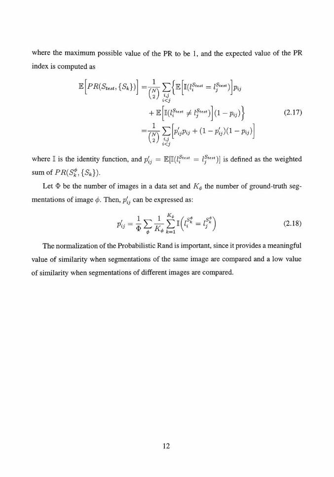
where the maximum possible value of the PR to be 1, and the expected value of the PR
index is computed as
E
PR(Stest,{Sk})]=-pyEJE[l(Zf-
= Zf-)J
i<j
Pij
+ E !(!?"# I/"")] (1-P)} (2-17)
3
i<j
EAjPa + tt-AW-Pii)
where I is the identity function, andp^- =E[I(lftest
= lfest)} is defined as the weighted
sum of PR(St,{Sk}).
Let $ be the number of images in a data set and K$ the number of ground-truth seg
mentations of image <j>. Then, p'^ can be expressedas:
^^ -"-^ fe=i
v y
The normalization of the ProbabilisticRand is important, since it provides ameaningful
value of similarity when segmentations of the same image are compared and a low value
of similarity when segmentations of different images are compared.
12
Chapter 3
Proposed Algorithm
An overview of the technique developed to segment images is provided here to serve as
a reference to the reader. The algorithm is composed of three different modules. The first
module uses an edge-detection algorithm to dynamically create regions composed of con
tiguous pixels that display similar gradient values. The second module consists of creating
an additional channel from the image. This channel contains the texture information of the
image. The lastmodule combines the texture information and the initial segmentation map
obtained in the first module to merge regions that display the same variance of colors and
texture. The following sections will describe the detailed technique for each of the three
modules.
3.1 Region Growth and Dynamic Seed
The quality of region-growing techniques is highly dependent on the initial locations
chosen to initialize the growing procedure. We propose an alternative process for region
growth that does not depend exclusively on the initial assignment of clusters for the final
segmentation. The procedure searches for regions in the image where no edges have been
detected. The selected regions form the initial set of clusters to segment the image. Sky,
skin, and in general, objects ofno strong colorvariance are selected in this step. Subsequent
clusters are incorporated with various levels of edge density during the growth procedure,
to account for all other objects that are found in natural images. A flowchart for this module
13
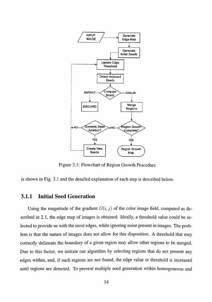
Figure 3.1: Flowchart ofRegion Growth Procedure
is shown in Fig. 3.1 and the detailed explanation of each step is described below.
3.1.1 Initial Seed Generation
Using the magnitude of the gradient G(i,j) of the color image field, computed as de
scribed in 2.1, the edge map of images is obtained. Ideally, a threshold value could be se
lected to provide us with themost edges, while ignoring noise present in images. The prob
lem is that the nature of images does not allow for this disposition. A threshold that may
correcdy delineate the boundary of a given region may allow other regions to be merged.
Due to this factor, we initiate our algorithm by selecting regions that do not present any
edges within, and, if such regions are not found, the edge value or threshold is increased
until regions are detected. To prevent multiple seed generation within homogeneous and
14

connected regions, the region selection at this stage is restricted to clusters of pixels which
are larger than 0.5% of the image. Each individual cluster is assigned a particular label for
differentiating purposes. This label map is referred as the Parent Seeds (PS). The labeling
procedure uses the general procedure outlined in reference [21].
1. Run-length encode the input image.
2. Scan the runs, assigning preliminary labels and recording label equivalences in a
local equivalence table.
3. Resolve the equivalence classes.
4. Relabel the runs based on the resolved equivalence classes.
3.1.2 Region Growth
The procedure continues by increasing the threshold found in the initial seed generation
and detecting new regions or child seeds that fall below the new threshold. These child
seeds need to be classified into adjacent-to-existent or non-adjacent seeds. In order to
make the region growth process efficient, it is important to also know the parent seed to
which the child is adjacent. The objective is to be able to process all adjacent child seeds
in a vectorized approach. To achieve this task we proceed to first detect the outside edges
of the PS map using a nonlinear spatial filter. The filter operates on the pixels of a 3 x
3 neighborhood, and the response of its operation is assigned at the center pixel of the
neighborhood. The size of neighborhoods being operated will be assumed to be 3 x 3
unless specified otherwise. The filter operates according to
F(i,j) = <
0 ifPS(i,j)>0,
0 if(min)e/3PS(7n,n)is0, (3.1)
1 otherwise
15

where /3 is the neighborhood being operated. The result of applying this filter is a mask
indicating the borders of the PS map.
The child seeds are individually labeled, and the ones adjacent to the parent seeds are
identified by performing an element-by-element multiplication of the parent seeds edge
mask and the labeled child map. The remaining pixels are referred to as the adjacent
child pixels. The pixels whose labels are members of the set of labels remaining after the
multiplication become part of the adjacent child seeds map. For the proper addition of
adjacent child seeds, it is necessary to compare their individual color differences to their
parents to assure a homogeneous segmentation. Reduction of the number of seeds to be
evaluated is accomplished by attaching to their parents the child seeds that have a size
smaller to the minimum seed size (MSS). In our algorithm, the MSS is set to 0.01% of
the image.
The child seed sizes are computed utilizing sparse matrix storage techniques to allow
for the creation of large matrices with low memory costs. Sparse matrices store only the
nonzero elements of the matrix, together with their location in the sparse matrix (indices).
The size of each child seed is computed by creating a matrix ofM x N columns by C rows,
where M is the number of columns of pixels in the image, N the number of rows, and C
the number of adjacent child seeds. The matrix is created by allocating a 1 at each column
in the row that matches the pixel label. The pixels that do not have a label are ignored. By
summing all the elements along each row,we obtain the number of pixels per child seed.
This procedure is useful for any operation that requires the knowledge of the number of
elements per group in the segmentationalgorithm.
To attach regions an association between child seeds and their parents is required. The
adjacent child pixels provide the child labels, but not the parent labels. A new spatial filter
is applied to the PS map to obtain the parent labels. The filter response at each center
point is equal to the maximum pixel value in its neighborhood. The association between
child and parent can now be obtained by creating a matrix with the first column composed
of the adjacent child pixels and the second column, with labels found at the location of the
16
adjacent child pixels in the matrix obtained after applying the maximum value filter to the
PSmap. It is important to note that non-linear filters are used to provide information about
the seeds and not to directly manipulate the image; therefore, it does not impair the final
result.
The functionality of the associationmatrix is manifold. It provides the number of child
pixels that are attached to parent seeds and also identifies which child seeds share edges
with more than one parent seed. Child seeds smaller than MSS can now be directly at
tached to their parents. Child seeds that share less than 5 pixels with their parents and are
larger than MSS are returned to the unsegmented region to be processed when the region
shares a more significant border. Finally, the remaining seeds are compared to their parents
to analyze if they should be added to a parent seed or not.
Given that spatial regions in images vary gradually, only the nearby area of adjacency
between parent and child is compared to provide a true representation of the color differ
ence. This objective is achieved by using two masks that will exclude the areas of both
parent and child seeds that are distant from their common boundaries. The first mask is a
dilation of the PS map using an octagonal structuring element with a distance of 15 pixels
between the center pixel to the sides of the octagon, as measured along the horizontal and
vertical axis. The second mask is the same dilation but this time applied to the adjacent
child seeds map. The two masks mutually exclude the pixels that fall beyond each other's
dilation masks. The values used in our algorithm are optimized to work with images that
range from 300 x 300 pixels of resolution to 1000 x 1000 pixels.
The comparison of regions is performed using the Euclidian distance between themean
colors of the groups. The reason for choosing this method is that only the nearby area of re
gions is being compared, and, therefore, the increased complexity ofusing theMahalanobis
distance does not improve the results, because the variance of the regions compared will
be small. Also, prior to comparing the colors, the image is converted to the CEE L*a*b*
color space, assuring that comparing colors usingthe Euclidean distance is similar to the
17

differentiation of colors by the human eye. The maximum color distance to allow the in
tegration of the child seed to the parent seed is set to 20. This distance is chosen to allow
the differentiation of at least 10 different colors along the range of thea*
channel orb*
channel.
3.1.3 Dynamic Seed Generation
When the parent seeds are created in the initial seed generation, the regions represented
by these seeds are characterized by areas of the image that have no texture. These areas
can be instances of sky, water, skin, and in general, regions where there is either no color
variance or a gradual transition from one color to the next. The dynamic addition of seeds
to the PS map is our answer to include the remaining regions that display different levels
of edge intensities through them but are part of the same identifiable object. Dynamic seed
generation consist of selecting a set of threshold values at which additional seeds are added
to the parent seeds. The threshold values are adjusted to account for the exponential decay
of edge values as seen in Fig. 3.2. Ranges in the low-edge values account for large areas
in the image. To incorporate new areas, the threshold values need to increment exponen
tially to include additional elements of considerable size into the segmentation map. The
threshold values selected for the addition of new seeds are: 15, 20, 30, 50, 85, and 120
accounting for an increment of 10% of the area of the image added at each interval.
At these intervals, the addition of new seeds follow a similar procedure to the method
explained in 3.1.2. The regions that fall below the selected edge threshold are detected.
All the regions that are not attached to any parent seeds and are larger than the MSS are
added to the PS map. For the addition of new seeds that share borders with existent seeds,
they are required to meet two qualifications: 1) the group must be large enough to become
a group by itself, and 2) the color differences between the region and its neighbor must be
greater than the maximum color difference allowed.
18
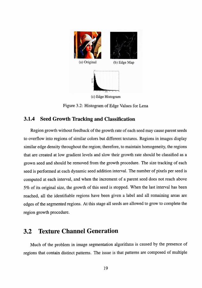
(a) Original (b) Edge Map
(c) Edge Histogram
Figure 3.2: Histogram ofEdge Values for Lena
3.1.4 Seed Growth Tracking and Classification
Region growthwithout feedback of the growth rate of each seedmay cause parent seeds
to overflow into regions of similar colors but different textures. Regions in images display
similar edge density throughout the region; therefore, to maintain homogeneity, the regions
that are created at low gradient levels and slow their growth rate should be classified as a
grown seed and should be removed from the growth procedure. The size tracking of each
seed is performed at each dynamic seed addition interval. The number of pixels per seed is
computed at each interval, and when the increment of a parent seed does not reach above
5% of its original size, the growth of this seed is stopped. When the last interval has been
reached, all the identifiable regions have been given a label and all remaining areas are
edges of the segmented regions. At this stage all seeds are allowed to grow to complete the
region growth procedure.
3.2 Texture Channel Generation
Much of the problem in image segmentation algorithms is caused by the presence of
regions that contain distinct patterns. The issue is that patterns are composed ofmultiple
19
shades of colors and cause over-segmentation andmisinterpretation of the edges surround
ing the patterned object. These objects are referred to in the computer vision industry as
textures. Texture regions may contain regular patterns such as a brick wall, to irregular
patterns such as leopard skins, bushes and many objects found in nature. The presence of
texture in images is so large and descriptive of objects that we have decided to generate an
additional channel containing this important information.
A method for obtaining information of patterns within an image is to evaluate the ran
domness present at various areas of the image. Entropy provides a measure of uncertainty
of a random variable [22]. If the random variable is composed from the pixel values of
a region, the entropy will define the randomness associated to the region being evaluated.
Texture regions contain various colors and shades; therefore, texture regions will contain a
specific value of uncertainty associated with them, providing a structure to merge regions
that display similar characteristics.
Information theory introduces entropy as the quantity which agrees with the intuitive
notion of what a measure of information should be [22]. In accordance with this supposi
tion, we can select a random group of pixels s from an image, with a set ofpossible values
{ai, a2, . . .
,aj}. The probability for a specific value a, to occur is P(dj), and it contains
I (aj) = l9p-(\ = ~l9p (aj) (3-2)
units of information. The quantity /(%) is referred to as the self-information of a,. If k
values are present on the set, the law of large numbers stipulates that, for a sufficiently
large value of k, symbol % will on average be output kP(dj) times. Thus the average
self-information obtained from k outputs is
-kP (ai) logP (ai) -...-kP (aj) logP (aj) (3.3)
or
j
-kJ2P(aj)logP(aj). (3.4)
20
Red
Green
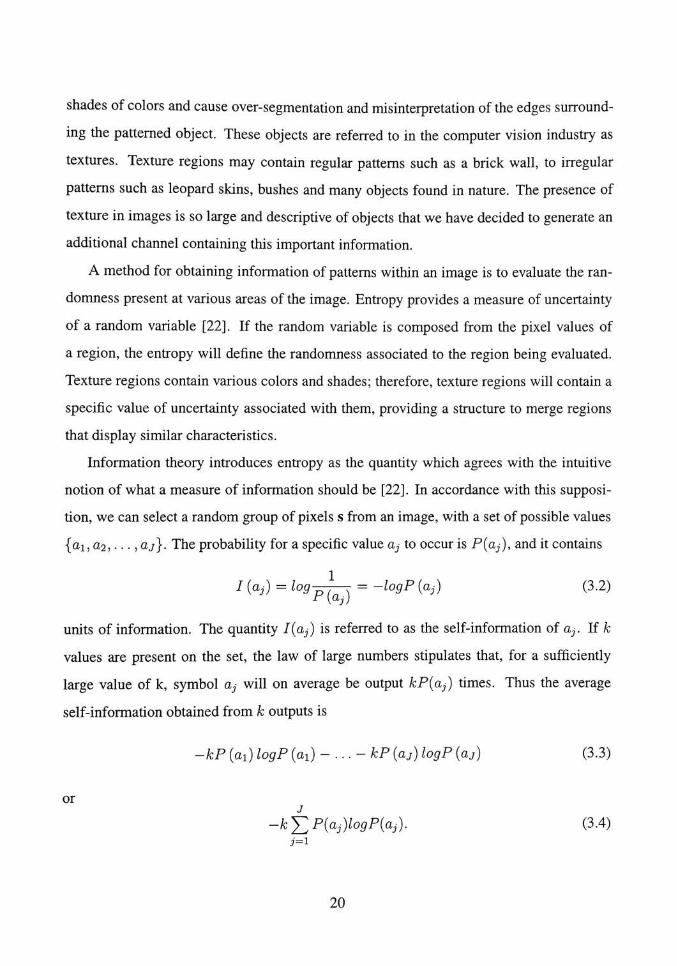
Figure 3.3: Quantization ofColors
The average information per source output, or entropy is defined by
H(s) = ~'P(aj)logP(aj) (3.5)
This quantity is defined for a single random variable, and for the case of color, multiple
variables are used. To take advantage of the color information without extending the pro
cess to compute the joint entropy, the colors in an image are quantized into 63, or 216
different colors. The quantization of colors can be done using uniform quantization which
cuts the RGB color cube into smaller boxes, and then maps all colors that fall within each
box to the color at the center of that box. Uniform quantization is represented in Fig. 3.3.
After the colors have been quantized, each pixel of the image can be indexed to one of
the 216 representative colors, effectively reducing the probability of each color occurring
to a one-dimensional random variable. To create the texture channel, the local entropy
is computed on a 9-by-9 neighborhood around each pixel in the indexed image, and the
resulting value is assigned to the center pixel of theneighborhood.
21
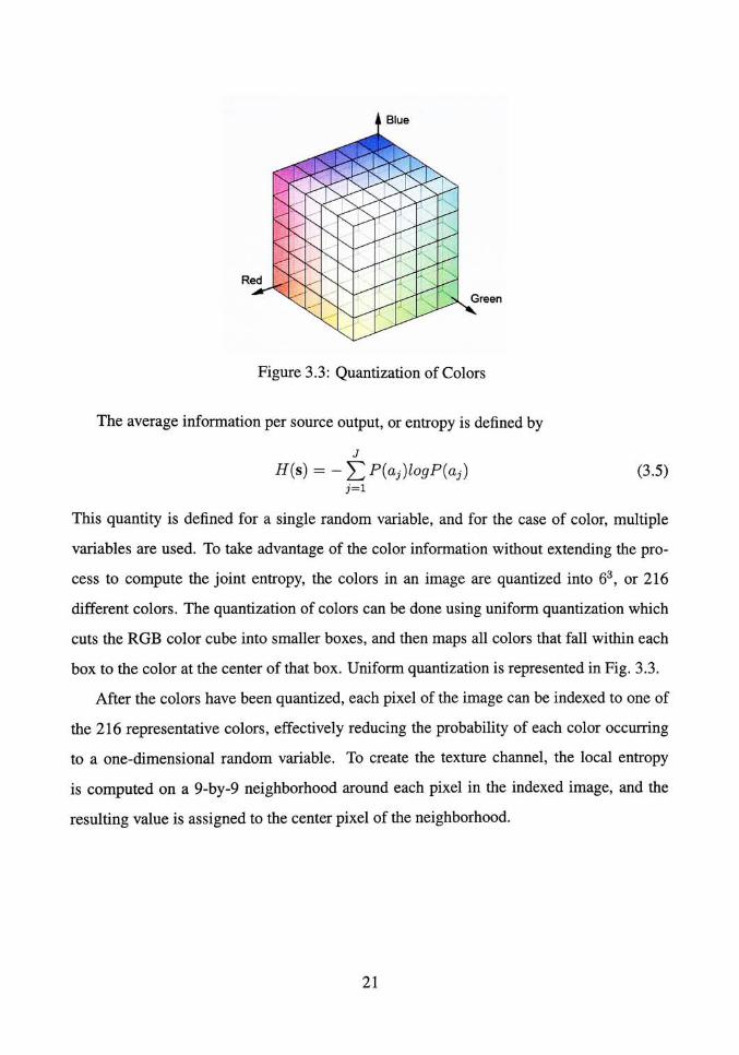
3.3 Multiresolution RegionMerging
The texture channel obtained from the second module is combined with the color infor
mation to describe the characteristics of each region segmented by the region growthmod
ule. Using a multivariate analysis of the independent regions, the resultant Mahalanobis
distances between groups is used to merge similar regions.
To this point the segmentation of the image has been performed with an absence of
information about the individual regions. Now that the image has been segmented into
different groups, information can be gathered from each individual region. Given that we
have four sources of information (Red, Green, Blue, and Texture) and individual regions
displaying a different number of pixels per group, we require a suitable method to display
the data in order to investigate relationships of the regions. The data can be modeled using
an (N * P) matrix, where N is the total number of pixels in the image, and P are the
total number of variables that contain information about each pixel. G is the total number
of groups in which the image has been segmented in the region growth procedure; then
the matrix is composed of G separate sets. The objective is to obtain a mean value for
each group that is used to compare the different groups. The method used to achieve this
objective is a one-way analysis of variance, which is explained in detail in section 2.2.
The Mahalanobis-squared distances are obtained for each pair of groups from the one
way analysis of the data. The algorithm uses these distances to find the similar groups and
merge them. Once a group has been merged, the similarity of this group to the others is
unknown, but required if the new group needs to be merged to other similar groups. To
prevent the need to re-evaluate the Mahalanobis distances for the groups after each region
merging has occurred, an alternateapproach was introduced.
Having the distances between groups, the smallest distance value is found. This value
only provides one pair of groups; therefore, the similarityvalue is increased until a larger
set of group pairs is obtained. Five group pairs were found to be anadequate number of
groups to reduce computation time without merging groups inadequately. We initiate by
merging the smaller group in this set and then continue to merge the next larger group.
22

After the first merge, a check is performed to see if one of the groups being merged is now
part of a larger group. In this case all the pair combinations of the groups should belong to
the pairs selected initially in the set to be merged together.
Once all the pairs of the set have been processed, the Mahalanobis distance is recom
puted for the new segmentation map, and the process is repeated until a desired number of
groups is achieved. The value of similarity obtained, after the desired numberof groups
has been achieved, should be used as a minimum value of merging to assure that all the
images display a similar level of segmentation. A flowchart of the procedure is shown in
Fig. 3.4.
23

Vectorize and
Concatenate Inputs:
[RGS,R,G,B,TX)
Apply One-WayMultivariate Analysis of
Variance
o
1 2 3 ...
v;
Xx~
x:
Mahalanobis
Distances \^
Merge Groups that
Display Small
Mahalanobis Distances
Figure 3.4: Flowchart ofMerging Procedure
24
Chapter 4
Results
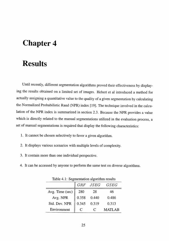
Until recently, different segmentation algorithms proved their effectiveness by display
ing the results obtained on a limited set of images. Hebert et al introduced a method for
actually assigning a quantitative value to the quality of a given segmentation by calculating
the Normalized Probabilistic Rand (NPR) index [19]. The technique involved in the calcu
lation of the NPR index is summarized in section 2.3. Because the NPR provides a value
which is directly related to the manual segmentations utilized in the evaluation process, a
set ofmanual segmentations is required that display the following characteristics:
1. It cannot be chosen selectively to favor a given algorithm.
2. It displays various scenarios with multiple levels of complexity.
3. It contain more than one individual perspective.
4. It can be accessed by anyone to perform the same test on diverse algorithms.
Table 4.1: Segmentation algorithm results
GRF JSEG GSEG
Avg. Time (sec) 280 28 46
Avg. NPR 0.358 0.440 0.486
Std. Dev. NPR 0.345 0.319 0.313
Environment C C MATLAB
25

GRF NPR distribution JSEG NPR distribution GSEG NPR distribution
ljaa-06 -04 -0.3 D 0.3 04 06 08 I $.6 -OB -0 4 -0.2 0 02 04 0.6 08
NPR index
(a) (b) (c)
Figure 4.1: Distribution NPR scores. (a)GRF; (b)JSEG; (c)GSEG
Such a set is available on the publicly accessible Berkeley Segmentation Database. This
database provides 1633 manual segmentations for 300 images created by 30 human sub
jects [23]. State-of-the-art algorithms were chosen to compare the quality of the segmen
tation results. These segmentation techniques are Fusion of Color and Edge Information
for improved Segmentation and Edge Linking (GRF) [6], the unsupervised segmentation
of color-texture regions in images and video (JSEG) [16], and the novel algorithm auto
matic segmentation by dynamic region growth and multiresolution merging (GSEG). To
prevent any discrepancy at the time of comparing the results, all the available images were
segmented using the available segmentation algorithms on the same machine. The testing
computer has a Pentium 4 CPU 3.20GHz, and 1.00 GB of RAM. The GRF and JSEG al
gorithms were run from the executable file provided by Rochester Institute of Technology
and the University of California respectively. The proposed method was processed using
MATLAB R2006a.
The normalization factor was computed by evaluating the Probabilistic Rand (PR) for
all available manual segmentations, and the expected index obtained was 0.6064. Results
obtained for the distinct methods are displayed in table 4.1. The results show that the
GSEG algorithm has the highest overall NPR results, and the variance of the results has the
narrowest spread, proving that the proposed algorithm performs consistently better than
the other algorithms. Fig. 4.1 display the distribution of the NPR scores for all the tested
images. It can be observed that 273 out of 300 images using the proposed algorithm are
26
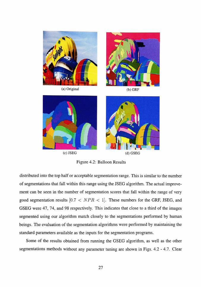
(a) Original (b)GRF
(c) JSEG (d) GSEG
Figure 4.2: Balloon Results
distributed into the top half or acceptable segmentation range. This is similar to the number
of segmentations that fall within this range using the JSEG algorithm. The actual improve
ment can be seen in the number of segmentation scores that fall within the range of very
good segmentation results [0.7 < NPR < 1]. These numbers for the GRF, JSEG, and
GSEG were 47, 74, and 98 respectively. This indicates that close to a third of the images
segmented using our algorithm match closely to the segmentations performed by human
beings. The evaluation of the segmentation algorithms were performed by maintaining the
standard parameters available as the inputs for the segmentation programs.
Some of the results obtained from running the GSEG algorithm, as well as the other
segmentations methods without any parameter tuning are shown in Figs. 4.2 - 4.7. Clear
27

(c) JSEG (d) GSEG
Figure 4.3: China Results
(a) Original (b)GRF
(c) JSEG (d) GSEG
Figure 4.4: Pilot Results
28
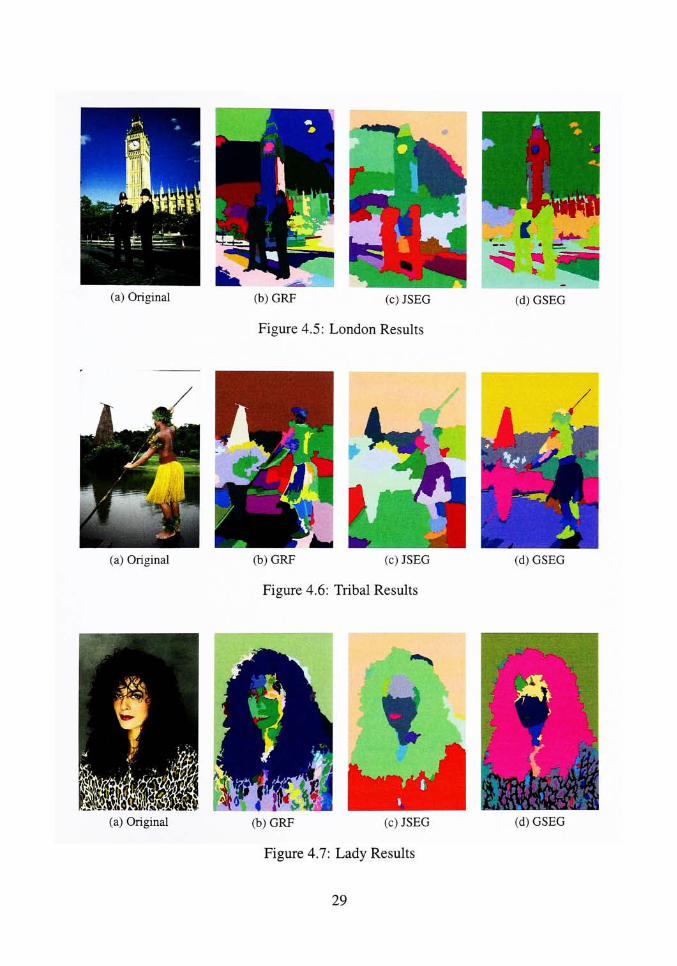
(a) Original (b) GRF (c) JSEG
Figure 4.5: London Results
(d) GSEG
(a) Original (b) GRF (c) JSEG
Figure 4.6: Tribal Results
(d) GSEG
(c) JSEG
Figure 4.7: Lady Results
(d) GSEG
29
advantages can be seen on the level of detail achieved from our segmentation in comparison
to the JSEG segmentation for all the images. The boundaries of the GRF procedure match
directly the boundaries of the object in the image. Fig. 4.4(c), and Fig. 4.5(c) displays
the disadvantage of guiding the segmentation method based on the quantization of colors
to create the initial clusters. In these images the sky has been oversegmented, because
the change of light provides different shades of blue. Advantages of the multiresolution
merging method can be seen on Figs. 4.3(d) and 4.7(d). In these results multiple regions
that create a pattern are assigned to the same class, allowing the algorithm to reduce the total
number of classes without losing information obtained from multiple similar regions that
are not adjacent to each other. The GRF results have the same level of detail as the GSEG
approach, but its lack of texture modeling does not allow it to differentiate objects with
similar colors but different texture. Figs. 4.4(b), 4.5(b), and 4.6(b) have regions merged
that display similar colors but contain substantially different textures.
30

Chapter 5
Conclusion
This work provides an effective method for automatic image segmentation on simple
to complex images. The algorithm is based on color edge-detection and dynamic region
growing, completed by a multiresolution region merging. The segmentation procedure has
been tested on the publicly available Berkeley database, and the quality of its results has
been measured. The robustness of our algorithm is displayed on the results, along with
those obtained on the same image when segmented by other methods. Future research
would be focused on object classification based on this segmentation algorithm.
31

References
[1] J. B. McQueen, "Some methods for classification and analysis ofmultivariate observations,"
in Proc. of 5th Berkeley Symp. on Mathematical Statistics and Probability,
vol. 1, pp. 281-296, 1967.
[2] J. Wu, H. Yan, and A. N. Chalmers, "Color image segmentation using fuzzy cluster
ing and suppervisedlearning,"
Journal ofElectronic Imaging, pp. 397^4-03, October
1994.
[3] P. Schmid, "Segmentation of digitized dermatoscopic images by two-dimensional
colorclustering,"
IEEE Transactions on Medical Imaging, vol. MI-18, pp. 164-171,
February 1999.
[4] T. N. Pappas, "An adaptive clustering algorithm for imagesegmentation,"
IEEE
Transactions on Signal Processing, vol. 40, pp. 901-914, April 1992.
[5] M. M. Chang, M. I. Sezan, and A. M. Tekalp, "Adaptive bayesian segmentation of
colorimages,"
Journal ofElectronic Imaging, vol. 3, pp. 404-414, October 1994.
[6] E. Saber, A. M. Tekalp, and G. Bozdagi, "Fusion of color and edge information for
improved segmentation and edgelinking,"
Image and Vision Computing, vol. 15,
pp. 769-780, 1997.
[7] J. Fan, D. K. Y. Yau, A. K. Elmagarmid, and W. G. Aref, "Automatic image seg
mentation by integrating color-edge extraction and seeded regiongrowing,"
IEEE
Transactions on Image Processing, vol. 10, pp. 1454-1466, October 2001.
[8] S. Y. Wanand and W. E. Higgins, "Symmetric regiongrowing,"
IEEE Transactions
on Image Processing, vol. 12, pp. 1007-1015, September 2003.
[9] L. Liu and S. Sclaroff, "Region segmentation via deformablemodel-guided split and
merge,"
in International Conference on Computer Vision, vol. 1, (Vancouver, BC,
Canada), pp. 98-104, 2001.
32
[10] C. D'Elia, G. Poggi, and G. Scarpa, "A tree-structured markov random field model
for bayesian imagesegmentation,"
IEEE Transactions on Image Processing, vol. 12,
pp. 1259-1273, October 2003.
[11] H. Derin and H. Elliott, "Modeling and segmentation of noisy and textured images
using gibbs randomfields,"
IEEE Transactions on Pattern Analysis andMachine In
telligence, vol. PAMI-9, pp. 39-55, January 1987.
[12] S. G. Mallat, "A theory for multiresolution signal decomposition: The wavelet representation,"
IEEE Transactions on PatternAnalysis andMachine Intelligence, vol. 1 1,
pp. 674-693, July 1989.
[13] M. Unser, "Texture classification and segmentation using waveletframes,"
IEEE
Transactions on Image Processing, vol. 4, pp. 1549-1560, November 1995.
[14] G. Fan and X.-G. Xia, "Wavelet-based texture analysis and synthesis using hidden
markovmodels,"
IEEE Transactions on Circuits and Systems, vol. 50, pp. 106-120,
January 2003.
[15] J. Chen, T. N. Pappas, A.Mojsilovic, andB. Rogowitz, "Adaptive image segmentation
based on color andtexture,"
in International Conference on Image Processing, vol. 3,
pp. 777-780, June 2002.
[16] Y Deng and B. S.Manjunath, "Unsupervised segmentation of color-texture regions in
images andvideo,"
IEEE Transactions on PatternAnalysis andMachine Intelligence,
vol. 23, pp. 800-810, August 2001.
[17] H.-C. Lee andD. R. Cok, "Detecting boundaries in a vectorfield,"
IEEE Transactions
on Signal Processing, vol. 39, pp. 1181-1194, May 1991.
[18] W. J. Krzanowski, Principles ofMultivariate Analysis, ch. 11. Oxford University
Press, 1988.
[19] R. Unnikrishnan, C. Pantofaru, andM. Hebert, "Toward objective evaluation of image
segmentationalgorithms."
Accepted for future publication in IEEE Transactions on
Pattern Analysis andMachine Intelligence.
[20] R. Unnikrishnan andM. Hebert, "Measures ofsimilarity,"
in IEEEProceedings Work
shop Computer VisionApllications, 2005.
33

[21] R. M. Haralick and L. G. Shapiro, Computer and Robot Vision, vol. 1, pp. 28^-8.
Addison-Wesley, 1992.
[22] T. M. Cover and J. A. Thomas, Elements ofInformation Theory. Wiley Interscience,
1991.
[23] D. Martin, C. Fowlkes, D. Tal, and J. Malik, "A database of human segmented nat
ural images and its application to evaluating segmentation algorithms and measuring
ecologicalstatistics,"
in IEEE International Conference on Computer Vision, vol. 2,
(Vancouver, BC, Canada), pp. 416^123, 2001.
34