University of CambridgeFaculty of Modern and Medieval Languages

Linguistics Tripos Part II 2015 Dissertation

Automatic Identification of SpellingVariation in Historical Texts

Alexander Robertson

AcknowledgementsI am sincerely grateful and indebted to my supervisor and Director of Studies for their invaluableadvice and encouragement, not only during this project but in everything that I have done overthese three happy years.

i

Contents

I Background 1

1 The variation problem 21.1 Desiderata . . . . . . . . . . . . . . . . . . . . . . . . . . . . . . . . . . . . . . . 4

2 Current approaches 52.1 Manual processing of historical texts . . . . . . . . . . . . . . . . . . . . . . . . 52.2 Norma . . . . . . . . . . . . . . . . . . . . . . . . . . . . . . . . . . . . . . . . . 62.3 VARD2 . . . . . . . . . . . . . . . . . . . . . . . . . . . . . . . . . . . . . . . . 62.4 Evaluating performance . . . . . . . . . . . . . . . . . . . . . . . . . . . . . . . 7

2.4.1 Norma . . . . . . . . . . . . . . . . . . . . . . . . . . . . . . . . . . . . . 72.4.2 VARD2 . . . . . . . . . . . . . . . . . . . . . . . . . . . . . . . . . . . . 8

2.5 Critical evaluation . . . . . . . . . . . . . . . . . . . . . . . . . . . . . . . . . . 9

II Theory 12

3 A framework for modelling variation 123.1 A formalism for representing text . . . . . . . . . . . . . . . . . . . . . . . . . . 12

3.1.1 Deriving a precise terminology from the formalism . . . . . . . . . . . . . 133.2 Summary . . . . . . . . . . . . . . . . . . . . . . . . . . . . . . . . . . . . . . . 15

III Practice 16

4 An automated approach to the variation problem 164.1 The type identification pipeline . . . . . . . . . . . . . . . . . . . . . . . . . . . 16

4.1.1 Feature extraction . . . . . . . . . . . . . . . . . . . . . . . . . . . . . . 174.1.2 Vectorisation . . . . . . . . . . . . . . . . . . . . . . . . . . . . . . . . . 174.1.3 Clustering . . . . . . . . . . . . . . . . . . . . . . . . . . . . . . . . . . . 17

4.2 Feature selection . . . . . . . . . . . . . . . . . . . . . . . . . . . . . . . . . . . 174.2.1 Form bigrams . . . . . . . . . . . . . . . . . . . . . . . . . . . . . . . . . 184.2.2 Part of speech . . . . . . . . . . . . . . . . . . . . . . . . . . . . . . . . . 184.2.3 Part of speech context . . . . . . . . . . . . . . . . . . . . . . . . . . . . 184.2.4 Pairwise similarity . . . . . . . . . . . . . . . . . . . . . . . . . . . . . . 19

4.3 Worked example . . . . . . . . . . . . . . . . . . . . . . . . . . . . . . . . . . . 20

5 Evaluating the automated approach 225.1 The performance evaluation pipeline . . . . . . . . . . . . . . . . . . . . . . . . 22

5.1.1 A toy example . . . . . . . . . . . . . . . . . . . . . . . . . . . . . . . . . 225.1.2 Statistical cluster comparison . . . . . . . . . . . . . . . . . . . . . . . . 24

6 Experimental implementation and evaluation 256.1 Experiment 1: Assessing the selected features . . . . . . . . . . . . . . . . . . . . 25

6.1.1 Design . . . . . . . . . . . . . . . . . . . . . . . . . . . . . . . . . . . . . 256.1.2 Results . . . . . . . . . . . . . . . . . . . . . . . . . . . . . . . . . . . . . 26

6.2 Experiment 2: Large-scale evaluation . . . . . . . . . . . . . . . . . . . . . . . . 27

ii

6.2.1 Results . . . . . . . . . . . . . . . . . . . . . . . . . . . . . . . . . . . . . 276.3 Experiment 3: Real historical text . . . . . . . . . . . . . . . . . . . . . . . . . . 27

6.3.1 Results . . . . . . . . . . . . . . . . . . . . . . . . . . . . . . . . . . . . . 286.4 Experiment 4: Chronology of the Great Vowel Shift . . . . . . . . . . . . . . . . 28

7 Discussion 30

8 Conclusion 32

Appendix A Experiment 3 - partial results 34

Appendix B Code: type identification pipeline 39

Appendix C Code: gold standard generation pipeline 47

Appendix D Code: evaluation pipeline 56

List of Figures

1 Variation decreases over time. Adapted from Baron, Rayson, and Archer (2009) 82 Visual comparison of equivalent historical and modern texts . . . . . . . . . . . 153 A pipeline for identifying types within a historical text . . . . . . . . . . . . . . 164 A pipeline for generating gold standard texts . . . . . . . . . . . . . . . . . . . . 235 Sample of automatically generated artificial “historical” text . . . . . . . . . . . 26

List of Tables

1 Issues with the Innsbruck Letter Corpus . . . . . . . . . . . . . . . . . . . . . . 52 Performance of Norma on historical texts. Adapted from Bollmann (2013) . . . . 83 Historical forms not classified as variants by VARD2 . . . . . . . . . . . . . . . 104 Appraisal of current methods against desiderata . . . . . . . . . . . . . . . . . . 115 Precise terminology derived from the formalism . . . . . . . . . . . . . . . . . . 146 Toy texts represented formally . . . . . . . . . . . . . . . . . . . . . . . . . . . . 147 Feature vector representation of formal variants in “the redd redde door” . . . . 218 Output of the type identification pipeline for a given toy input . . . . . . . . . . 219 Matrix of parameters used for each block in experiment 1 . . . . . . . . . . . . . 2610 p-scores for features . . . . . . . . . . . . . . . . . . . . . . . . . . . . . . . . . . 2711 Comparison of type assignment for three values of k. Coloured columns, from

left to right, k=6,000, k=8,342, k=10,000. . . . . . . . . . . . . . . . . . . . . . 2912 Appraisal of type identification pipeline against desiderata . . . . . . . . . . . . 3313 Type identification pipeline output for various k values (157 out of 16,684) . . . 34

1

Part I

Background

1 The variation problem

Languages in earlier stages of development differ from their modern analogues, reflecting syn-tactic, semantic and morphological changes over time. The study of these and other phenomenais the major concern of historical linguistics. The development of literacy and advances in tech-nology mean that human language has often been preserved in physical form. Whilst theseartefacts will eventually include video and sound recordings, the current life blood of historicallinguistics is text. The written word is the de facto source of evidence for earlier stages oflanguages and “the first-order witnesses to the more distance linguistic past are written texts.”(Lass, 1997)

Working with English texts presents both opportunities and problems. More recent stagesof English have more sources available, giving a fuller linguistic picture: the Old English (OE)period (600-1150) is survived by approximately 3,000 sources (Healey, 2002), mainly poetry andprose, whilst sources for the Present Day English (PDE) period (nominally 1900-2015) are likelyto number in the billions. Working with large amounts of data is increasingly easy, following thedevelopment of electronic corpora and automated methods for processing them. This has, inthe view of Rissanen (2000, p.7), “freed us from months and years of painstaking pencil work”.However, the freedom afforded by electronic corpora comes at a price: standardised input isrequired, such that each Saussurean signifiant is fixed in relation to the signifié. Colloquially,each word must be spelled the same way each time it is used.

This relation allows much of the tedious enterprise of linguistic annotation to be automated.Without it, the most basic corpus tasks, such as constructing word counts or calculating ngramfrequencies, become impossible and part-of-speech (POS) tagging accuracy is greatly reduced(Baron and Rayson, 2009). So whilst OE and PDE sources may differ dramatically in number,they at least share a common property in the consistency of their word forms. In OE, thiswas due to scribal tradition and the copying of texts by hand with the aim of producing afacsimile of an existing text. Inter-regional dialectal variation occurred but within-text wordforms were generally consistent. Similarly, little variation is present in PDE due to a processof standardisation, largely in place by the end of the 18th century (Görlach, 1991). Today, theconcept of spelling and the notion that it can be correct or incorrect is so pervasive that evenlinguists may refer to the spelling in pre-standardisation texts, though usually as a shorthandfor orthographic variation.

This dissertation is concerned with the word forms found in Early Modern English (EME)texts. These texts lack the consistency of word forms found in PDE but are available in sig-nificantly greater number than OE sources. The EME period, here taken to be from 1400 to1600, was a time of social and linguistic change. It is evidenced not only by poetry and prosebut also by personal correspondence in a volume unavailable for earlier epochs, providing a

2

view of language through a quite different lens, essentially creating the field of historical so-ciolinguistics (Bergs, 2005). Unfortunately, the volume of material and its pre-standardisationcharacteristics requires special effort to study. Currently, the creation of corpora from historicalsources is largely a manual process. Two examples are the Queen Elizabeth I Spelling Corpus(Evans, 2012) and the Parsed Corpus of Early English Correspondence (Taylor, Nurmi, Warner,Pintzuk, and Nevalainen, 2006). The QEISC, specifically constructed in order to study spelling,contains 22,400 words. Evans spent two months manually identifying and grouping variant wordforms and reports that for the creation of any larger corpus “an (semi)-automated system wouldbe imperative.” The PCEEC (Taylor et al., 2006), which was manually annotated with POSinformation, contains almost 2.6 million words. Nurmi (personal communication April 22nd,2014), reports: “It took me about three years to complete...I mechanically broke one keyboarddoing it.” Had these corpora been based on modern texts, their construction would have takenless time and effort, allowing the focus to be on the actual research aims.

Spelling variation presents problems even for researchers who are not specifically concernedwith historical texts as linguistic artefacts. Working on Enroller, a project to aggregate andindex multiple historical data sets, Anderson (2013) highlights the impossibility of even simplycross-referencing documents by keyword, a trivial task in PDE: “It is very difficult if not im-possible to identify all the probable spellings of a word in historical times or in dialectal texts.This problem is not addressed in the Enroller project but it is an important one that deserveseffort and funding to ameliorate.”

There are, then, two important issues regarding spelling variation in historical texts. Thefirst is the impact it has on the efficacy of natural language processing (NLP) techniques. Thesecond is the difficulty of analysing spelling variation on a large scale due to the unsuitability ofstandard corpus methods for analysing historical texts. Combined, these issues may be referredto as the variation problem.

Acknowledging this problem, and the value of addressing it, this dissertation presents anovel solution. It is arranged as follows:

• a table of desiderata for an idealised solution to the variation problem, against which anyapproach may be assessed;

• critical assessment of current approaches to the problem;

• a formalism for describing texts, allowing the variation problem to be precisely definedand restated;

• a technical implementation of the formalism;

• statistical and experimental assessment of the implementation.

A brief summary of the main findings closes this work.

3

1.1 Desiderata

The labels of these idealistic principles are a convenient shorthand. They will be referred towhen considering the properties of any approach to the variation problem.

Perfection Precision and recall should be 100%. All variants should be identifiedand each variant should be matched with its present-day form. Betweentwo systems, the better is that which correctly identifies more spellingvariation and correctly proposes modern day equivalents.

Least effort A major goal is to reduce the labour required to work with historicaltexts. Between two systems, that which requires the least labour (bysome sensible metric) is superior.

Explanatory adequacy A solution should be explicitly grounded in linguistic theory, able toexplain its success (or failure) with reference to the underlying structureof the language data.

Pure input The input to the solution should be the original text: either the actualoriginal artefact or a close facsimile. The closer a system is to the source,the better it is.

Language agnostic It should work on any language from any period. A system that onlyworks for one language is as useful as a theory of syntax, for example,that only applies to one language.

Epoch ignorant Variation should be detected purely on the basis of the input, with noreference to variation (or lack of) in another period. The ideal system issynchronic in its application but a series of such applications may wellinform diachronic study.

Preserve input The output should not replace variant forms with modern ones, but pre-serve them in-line or present them separately in an appropriate format.A system which acts like a modern-day spellchecker is inappropriate,as these variant forms are as historically relevant as syntactic structureeven if they are a gross inconvenience to corpus linguistics methods.

4

2 Current approaches

In addition to the manual approach taken by Evans (2012) and Taylor et al. (2006), tools existto assist researchers working with historical texts. The manual approach and two such toolswill now be assessed against the desiderata in section 1.1. Following this is a critical evaluation,highlighting crucial theoretical shortcomings. Table 4 (page 11) summarises this assessment.

2.1 Manual processing of historical texts

The traditional approach is to manually examine each word in a historical text and, where aword is not in modern spelling, emend or replace it. There is no standard procedure for manuallynormalising historical texts or investigating spelling variation, because the process is dependentupon the reason for normalising in the first place or the research questions underpinning theinvestigation. Where the aim is to create a modern analogue of a historical text, it may besufficient to simply read the text and replace any variant words by hand, based on the judgementof the reader. In addition to normalising the spelling, further changes may be applied during thisprocess – syntax may be modernised or archaic words updated. For Evans (2012) the purposewas to quantify spelling variation over time, so it was necessary not to replace historical wordsbut to group them together for counting. This was not just time-consuming – Evans (personalcommunication, December 2nd, 2014) reports it was “error-prone, and the corpus had to bechecked several times.”

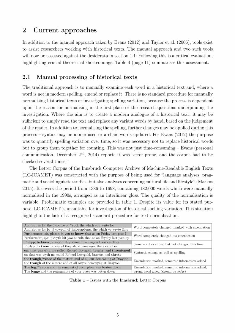
The Letter Corpus of the Innsbruck Computer Archive of Machine-Readable English Texts(LC-ICAMET) was constructed with the purpose of being used for “language analyses, prag-matic and sociolinguistic studies, but also analyses concerning cultural life and lifestyle” (Markus,2015). It covers the period from 1386 to 1698, containing 182,000 words which were manuallynormalised in the 1990s, arranged as an interlinear gloss. The quality of the normalisation isvariable. Problematic examples are provided in table 1. Despite its value for its stated pur-pose, LC-ICAMET is unsuitable for investigation of historical spelling variation. This situationhighlights the lack of a recognised standard procedure for text normalisation.

And Sir, as for the 6 couple of *cod, the which you write forAnd Sir, as for þe vj cowpull of haberndens, the which ye wryte ffore Word completely changed, marked with emendation

Furthermore, sir, pleases it you to know that as on Friday last past IFerthermore, syr, plesyth hit yow to wit that as on ffryday last past ay Word completely changed, no emendation

Philipp, to know, a way if they should have again their cattle orPhylyp, to know, a way yf they shuld have ayen there catell or Same word as above, but not changed this time

one that was with me called Roberd Lovegold, brazier, and threatenedon that was wyth me callid Roberd Lovegold, brasere, and threte Syntactic change as well as spelling

the trough/*core of the matter, and of all our demeaning at Draytonthe trough of the matere and of all owyre demenyng at Drayton Emendation marked, semantic information added

The log/*cabin and the remnant of your place was beaten downThe logge and the remenaunte of your place was betyn down

Emendation marked, semantic information added,wrong word given (should be lodge)

Table 1 – Issues with the Innsbruck Letter Corpus

5

2.2 Norma

This command-line tool (Bollmann, 2012) is written in Python 2. Norma has two operationalmodes, interactive and batch. First, variants are detected by comparing each word to a moderndictionary. Words with no match are highlighted as variants. The interactive mode iterates overeach word in a source text, prompting the user to confirm or reject candidates for normalisation,whereas batch mode automatically selects a candidate. Norma uses “normalisation modules”which allows the user to extend the functionality of the tool with custom normalisation tech-niques. Three modules are included as standard:

Word List Mapping

If the variant is in a list of historical:modern word mappings, it can be replaced by thismethod. The list must be compiled by hand.

Rule-Based Normalisation

Described in detail in Bollmann, Petran, and Dipper (2011), this employs a list of charac-ter rewrite rules, analogous to those seen in generative theories of syntax and phonology.Valid rules are applied, left to right, to the characters of a historical form and the resultingstring, if found in a target lexicon of modern words, becomes a normalisation candidate.The rewrite rules are generated automatically from a training corpus. This can eithertake the form of manually-compiled historical:modern word pairs or, as in Bollmann etal. (2011), from a portion of an aligned corpus set aside for use as training data.

Weighted Levenshtein Distance

The Levenshtein distance (Levenshtein, 1966) between two strings is defined as the num-ber of single character deletions, insertions or replacements required to transform onestring into another. For example, the distance between cat and bat is 1. A distance ofzero means the two strings are identical. The version used in Norma allows weights to beapplied to the deletions/insertions/replacements required to transform the input string,allowing them to be interpreted as more or less costly. Bollmann et al. (2011) gives v 7→ u

as an example of a low cost edit for Early New High German texts, as it is a common andvalid spelling variation, whilst v 7→ x should be a high cost edit given its implausibility.Weights can be specified manually (Bollmann, 2012) or learned automatically (Adesam,Ahlberg, and Bouma, 2012). This module performs pairwise Weighted Levenshtein Dis-tance comparisons between the words of the source text and a modern dictionary. Thecloser the score is to zero (i.e. no edits made), the more similar the two strings are.

2.3 VARD2

VARD2 (Baron and Rayson, 2008) is written in Java. It uses a graphical interface with the sameoperational modes as Norma. It uses the same dictionary method for detecting variants. In theword processor-style interactive mode, a user can click identified variants to select a replacement

6

from normalisation candidates. This operation can be automatically applied to all other tokensin the text which match the current variant. The choices made are tracked in order to updateconfidence scores – selecting the same replacement for a variant each time increases the futureconfidence score for that replacement. In batch mode, decisions about replacements are madebased on this score – the top-ranking candidate above a threshold of confidence automaticallyreplaces the variant. Four methods for determining replacement candidates are used:

Known Variants

This is the same as the Word List Mapping module of Norma.

Letter Replacement

This is the same as the Rule Based Normalisation module of Norma. The rule list isgenerated by the DICER tool (Baron and Rayson, 2009) using the interlinear gloss ofLC-ICAMET (see page 5) as an aligned corpus for training purposes.

Phonetic Matching

A code is generated by the Soundex algorithm (Russell and Odell, 1918) taking the variantas input. Codes are of the form A123, where A is the first character of the input and 123is generated based on the properties of the consonants in the input. For example, ‘today’is T300, “tomorrow” T560. The Soundex code for each variant is compared against thecodes for modern words in the dictionary. A matching code results in that modern wordbecoming a replacement candidate.

Edit Distance

For all candidates offered by the previous methods, the Levenshtein distance between thevariant and replacement candidates is calculated. This is the same algorithm as in Normabut without weighting and with a slight change to the output, which is normalised to avalue between 0 and 1 rather than being a count of edit operations.

2.4 Evaluating performance

Both Norma/VARD2 provide analysis of the performance of their methods. A direct quantita-tive comparison is not possible, since each uses quite different metrics. However, their assessmentmethodology is similar: historical text is normalised manually to create a gold standard, thenthe original historical text is processed. The output of this is compared to the gold standardand statistics generated. A brief summary of these will now be presented.

2.4.1 Norma

Bollmann (2013) manually normalised five German texts. The first 500 tokens of each corpuswas used as training data, though Bollmann also evaluated the impact of using 100, 250, 1000and 2000 tokens as training data. The remaining non-normalised tokens were then processed

7

in Norma. The results are reproduced in table 2. A metric called “accuracy” was used. Baselineaccuracy is the number of tokens in the pre-normalised text which already match modernspellings. This was re-calculated after processing in Norma.

Corpus Dating Size Baseline Word listMapping Rule-based WLD Combined

Berlin 15c 4,700 23.05% 62.05% 63.17% 60.71% 75.07%Melk 15c 4,541 39.32% 63.15% 64.14% 69.34% 74.49%

Sermon1 1677 2,178 72.71% 76.46% 78.67% 76.40% 79.56%Sermon2 1730 2,137 79.47% 85.22% 88.52% 88.15% 91.81%Sermon3 1770 1,953 83.41% 86.58% 90.50% 95.46% 95.73%

Table 2 – Performance of Norma on historical texts. Adapted from Bollmann (2013)

1450 1500 1550 1600 1650 1700 1750 18000

20

40

60

80

Year

%Variant

Typ

es

Percentage of variant types in selected corpora over time

ArcherInnsbruckLampeterEMEMT

Figure 1 – Variation decreases over time. Adapted from Baron, Rayson, and Archer (2009)

Two factors are notable. First, each text differed in baseline levels of variation. This is be-cause they are from different historical periods and there is a trend over time of decreasingvariation (fig. 1). Second, each corpus is quite small, likely due to the labour involved in man-ually normalising the texts. Performance improved with more training, but in some cases thiswas approaching 50% of the unseen data. Improvements over baseline were highly dependenton how much variation it contained.

2.4.2 VARD2

Baron and Rayson (2009) used LC-ICAMET for their gold standard, from which they extractedknown variants and letter replacement rules. How the quality of this source (see section 2.1)affected its suitability as an aligned corpus is unknown – Baron and Rayson do not mentionthis issue. LC-ICAMET was split into equally sized samples, then processed in batches to allow

8

VARD2 to learn more with each new batch of data. Performance was rated using precision andrecall:

recall =|{correct identifications} ∩ {possible identifications}|

|{correct identifications}|(1)

precision =|{correct normalisations} ∩ {possible normalisations}|

|{possible normalisations}|(2)

Recall (R) is the proportion of variants which have been successfully identified. Precision (P )is the proportion of those correct identifications which have been correctly normalised. Thebaseline with no training (besides the precompiled list of known variants and letter rules) wasR = 92%, P = 45%. After training, improvements in R and P plateaued at 93% and 65% once40,000 items of training data had been used. This represented 22% of the total data.

2.5 Critical evaluation

In the introduction, two major issues caused by spelling variation were highlighted, comprisingthe variation problem. Each will now be examined more closely, in the context of Norma/-VARD2.

If the purpose of working with a historical text is to “modernise” and make it suitable forNLP then, required effort aside, the methods described are valid solutions. The software toolsespecially are useful because they have been created not only for identifying but also “fixing”spelling variation. Therefore, Norma/VARD2 treat historical spelling variation in the sameway as Microsoft Word treats spelling errors. They make the same distinction as Kukich (1992)between error detection (through the use of dictionary look-up) and error correction (throughpairwise comparison of detected variants/errors to a modern dictionary, by some metric such asLevenshtein distance). But how appropriate are these distinctions in the context of analysinghistorical change through variation detection, the second part of the variation problem? It willnow be argued that they are inappropriate. This claim will be supported by showing that thetechnology behind Norma/VARD2 carries with it assumptions which make them unsuitable inthe fuller context of the variation problem.

First, the detection method used in Norma/VARD2 implicitly assumes historical word formsare deviant and modern ones are orthodox, as if writers in the 15th century had the modernform in mind each time but often mysteriously failed to produce it. The evidence for this is theuse of modern dictionaries for detecting variants. But this approach does not detect variants. Itonly detects non-modern words. Table 3 shows examples of historical words which are variantswithin the context of the time period they were written in, but which are not considered variantsby VARD2. This use of dictionaries violates the principle of epoch ignorance.

Second, the correction methods used by Norma/VARD2 explicitly make the same assump-tions that their detection method makes implicitly, that historical forms are errors. They at-tempt to undo these errors using string comparison metrics. However, the Levenshtein algorithmis based on the work of Damerau (1964). This looked at the types of spelling error producedwhen human operators were creating punch cards for a mainframe computer. 80% of errors

9

Historical Modern equivalent Other modern matchesbee be – verb bee – noun, an insectdon done – verb don – verb, to put ongoon gone – verb goon – noun, a foolpore poor – adj pore – noun, skin openingrite right – verb rite – noun, a ritualprey pray – verb prey – noun, hunted objectcaws cause – verb caws – noun, sounds made by crowswold would – modal wold – noun, a woodland

Table 3 – Historical forms not classified as variants by VARD2

were found to fall into four categories – character deletion, extra character insertion, charactersubstitution, and character transposition. “These are the errors one would expect as a result ofmisreading, hitting a key twice, or letting the eye move faster than the hand.” (Damerau, 1964,p.171)

This means that Norma/VARD2 use an algorithm which was designed based on the errorscreated by inaccurately inputting text on a computer keyboard. They do not take a linguistically-motivated approach to why historical and modern word forms differ. Instead, they operate un-der the belief that input errors on a keyboard are analogous to five hundred years of languagechange, as if the EME period were caused by clumsy typing. Levenshtein distance is at thevery core of Norma/VARD2 and its provenance subtly taints not only their performance butthe theoretical validity of that performance. So whilst approaches based on spell-checking tech-nology can achieve partially acceptable results, there is no scope for improving those resultswithout abandoning that fundamentally flawed method. They have no explanatory power.

10

Table 4 – Appraisal of current methods against desiderata

VARD2 Norma ManualPerfection No.

93% precision, 65% recall.No.75.07% accuracy on 4700 to-kens using 500 astraining data(baseline = 23.05%)95.73% accuracy on 1953 to-kens using 500 astraining data(baseline = 83.41%)

Possibly, de-pending on themethodology, butnot the case inthe LC-ICAMET.

Least effort Complexity O(n2) for WordList Mapping.Best case O(m × n) for eachindividual LD comparison,increasing linearly with textsize.Speed limited by computerpower.Up to 22% of data needsmanually tagged for optimaltraining (on large data set).Interactive mode requiresword-by-word checkingby user, complexity O(n)increasing linearly with textsize.Batch mode allows automaticacceptance of best-rankedcandidate.

Complexity O(n2) for WordList Mapping.Best case O(m × n) for eachindividual LD comparison,increasing linearly with textsize.Speed limited by computerpower.Requires manually createdtraining data, up to 50% ofsource on small data sets.Interactive mode requiresword-by-word checkingby user, complexity O(n)increasing linearly with textsize.Batch mode allows automaticacceptance of best-rankedcandidate.

Complexity O(n)for word-by-wordreplacement.Complexity O(n2)for groupingwords from textby variant.Speed limited byspeed of humanprocessor, butcan be massivelyparallelised withenough humans.

Explanatoryadequacy

Uncritically uses technologyfrom modern spellchecker re-search. Not grounded in the-ory.

Uncritically uses technologyfrom modern spellchecker re-search. Not grounded in the-ory.

Possibly.Depends on theperson doing themanual work.

Pure input No.Uses an optional list of knownvariants, without which per-formance is harmed.Requires a modern dictio-nary, without which no vari-ants can be detected.

No.Uses an optional list of knownvariants, without which per-formance is harmed.Requires a modern dictio-nary, without which no vari-ants can be detected.

Most likely.

Languageagnostic

Soundex phonetic algorithmis English-specific.

Yes. Possibly.Depends on theperson doing themanual work.

Epochignorant

No. Compares historicalforms directly with modernforms.

No. Compares historicalforms directly with modernforms.

Possibly.Depends on theperson doing themanual work.

Preserveoutput

Yes.Can output normalised textin XML format.

Yes.Outputs normalised text,word by word, to consolewhere it can be processedelsewhere.

Possibly.Depends on theperson doing themanual work.

11

Part II

Theory

3 A framework for modelling variation

It has been established that current non-manual approaches to the variation problem are basedon unsuitable modern spell checking technology and an assumption that historical words aredeviant in relation to modern ones. Further, each approach only addresses the first half ofthe variation problem – that of normalising historical texts for improving NLP efficacy. Theyprovide no useful way of investigating spelling variation in its own right and addressing thesecond half. This is part of a wider problem: the assumptions that constitute their theoreticaland methodological basis are mostly implicit, as demonstrated by the uncritical use of theLevenshtein algorithm. They are not grounded within a framework which precisely lays out theproblem they are trying to solve, instead relying on pragmatism – the problem is consideredsolved when a score of 100% is achieved in some metric for normalising a gold standard.

What is needed, and shall now be presented, is a schema for considering texts as formallinguistic entities rather than a series of words to be linearly processed in isolation by a bottom-up spell-checking process. The benefits of this are clear. First, it will provide a high level viewfrom which variation can be seen as a property of not just individual words but of entirehistorical texts. Second, it will permit the precise definition of the terminology in use. Finally,and most importantly, it will give a theoretically motivated way of approaching the variationproblem.

3.1 A formalism for representing text

A text, T , is a finite linear sequence of strings. From a variation perspective, it is formallydefined with the following parameters:

1. F = {f1, f2, f3, . . . , fn | f ∈ T}

The finite set of strings within T . Its elements are determined by tokenising the text.

2. P = {p1, p2, p3, . . . , pL | p ∈ N, L = |T |}

The finite set of positions within T . A position is a unique index of a string’s place withinT . The number of elements is determined by the cardinality of T .

3. S = {s1, s2, s3, . . . , sn | s ∈ T}

The finite set of senses used in the text. It is the collection of the semantic referencesmade by the text.

4. α = the instance relation over F , P , S

12

Describes a set of tuples, I. Each i ∈ I has the structure (f, p, s). These tuples link eachp ∈ P to some f ∈ F and some s ∈ S. A p can be associated with any f or s, and anf or s can be associated with one or more p, but each p is used only once. Associatingsenses with forms allows polysemy and homography to be represented.

5. γ = the variant function

With domain F , range ⊆ I.The set of all possible values is V ′. This set contains any i ∈ I which share the same valuefor f and s. These subsets of I are denoted by V(f,s).

6. λ = the type function.

With domain S and range ⊆ V ′.The set of all possible values is T ′, the members of which are subsets of V ′, such thatalthough they do not share the same f they have the same s. These subsets of V ′ aredenoted by Ts.

3.1.1 Deriving a precise terminology from the formalism

Discussion of spelling variation is hindered by overloaded terms which have both technical andcolloquial meanings. This claim will be justified by demonstrating how common terms maponto multiple elements of the formalism:

• F is a text’s types, vocabulary, words or lexicon. An isolated f is generally referred to asa word or token but can also be viewed as a spelling.

• Each i associates a word or spelling from the vocabulary with a unique position in thetext. This too can be referred to as a word.

• Each V(f,s) is a way of dividing the text into groups of words which have the same writtenform and semantics. This is one way of spelling a word.

• Each Ts groups those V(f,s) ∈ V ′ such that though they have different spellings, they arestill the same word based on semantics. For example, American and British English havedifferent words or spellings (e.g. favourite and favorite) with identical sense.

Accordingly, it will be productive to avoid these labels and to highlight the theoreticalcontrasts made by the formalism. The purpose of such contrasts is to explicitly lay out thestructure imposed on the variation problem by the schema and to propose testable solutions.Terminology derived from the formalism is presented in table 5 (page 14). Hereafter, only theseterms will be used.1 The distinctions made by the formalism are exemplified by toy examplesin table 6 (page 14).

1Special effort should be made to dissociate the upcoming usage of type from its technical meaning ininformation theory.

13

Formalism Terminology Descriptionf form the physical characteristics of a string in a textp position a location within the texti instance a form and sense linked to a unique locationV(f,s) variant a collection of instances with both a shared form and senseTs type a collection of variants with a shared sense but not shared form

Table 5 – Precise terminology derived from the formalism

Historical ModernText the redde redd door the red red doorForms {the, redde, redd, door} {the, red, door}Positions {1, 2, 3, 4} {1, 2, 3, 4}Senses {a, b, c} {a, b, c}

Instances {(1, the, a), (2, redde, b),(3, redd, b), (4, door, c)}

{(1, the, a), (2, red, b),(3, red, b), (4, door, c)}

Variants

V(the,a) = (1, the, a)V(redde,b) = (2, redde, b)V(redd,b) = (3, redd, b)V(door,c) = (4, door, c)

V(the,a) = (1, the, a)V(red,b) = (2, red, b),(3, red, b)V(door,c) = (4, door, c)

TypesTa = {V(the,a)}Tb = {V(redde,b), V(redd,b)}Tc = {V(door,c)}

Ta = {V(the,a)}Tb = {V(red,b)}Tc = {V(door,c)}

Table 6 – Toy texts represented formally

The locus of diachronic variation between two texts is not in the number of senses orpositions, but in how those senses and positions are distributed with relation to forms. Inmodern texts, there is a one-to-one mapping from types to variants and from variants to forms.The number of variants is therefore equal to the number of types, encapsulating the sameinformation in an essentially vacuous distinction. Historical texts differ in this respect, witha one-to-many mapping from types to variants being possible but preserving the one-to-onemapping from variants to forms. The type/variant distinction is meaningful in historical textsbecause it permits a technical perspective of variation without interference from the variation-free modern day situation that is generally found in standard texts. The original variationproblem can now be restated within this new framework:

• Investigating spelling variation within historical texts involves arranging the observablevariants into groups of types, such that each type maps to one sense, with as many wordforms as are present in the text representing that sense.

• For normalisation, the forms of the variants within each type must be made identical.

In the historical example of table 6, an investigation of spelling variation might involvestatistical analysis of the number of variants per type. Normalising this text to modern standardEnglish would involve examining the members of Tb and changing the instances within eachvariant to have modern forms, such that (2, redde, b) 7→ (2, red, b) and (3, redd, b) 7→ (3, red,

14

Historical T

Tc

V(door,c)

(4, door, c)

Tb

V(redd,b)

(3, redd, b)

V(redde,b)

(2, redde, b)

Ta

V(the,a)

(1, the, a)

Modern T

Tc

V(door,c)

(4, door, c)

Tb

V(red,b)

(3, red, b)(2, red, b)

Ta

V(the,a)

(1, the, a)

Figure 2 – Visual comparison of equivalent historical and modern texts

b). These new instances are then merged into a new variant, V(red,b), which replaces the historicalvariants, V(redde,b) and V(redd,b). The text is then ready for NLP processing. This normalisationprocedure can be visualised as reducing the branches within a tree whilst maintaining thenumber of leaves, as in fig. 2.

3.2 Summary

It has been demonstrated that historical texts, within the proposed framework, exhibit a one-to-many mapping from types to variants. Extracting the variants is trivial because they areapparent from the text and there is a one-to-one mapping from variants to forms regardlessof epoch. Identifying types is more challenging, since they represent a level of non-surfacestructure within the text, not directly observable. However, there exist computational methodsfor accessing hidden structure in data. What follows next is an example of how these can beapplied to the problem of identifying types. This will form a solution to the first part of thereformulated variation problem.

15

Part III

Practice

4 An automated approach to the variation problem

There are two major technical components within this dissertation. First, the technical imple-mentation of a solution to the first element of the reformulated variation problem (page 14).This maps variants to types but does not make any attempt to link the historical types totheir modern equivalents. Second, statistical evaluation of the accuracy of the implementedsolution. This evaluation is part of a feedback loop, allowing the technical implementation tobe adjusted in order to improve performance and efficiency. As shall be seen, multiple compo-nents were initially considered as part of the implementation but only the best were selected.These two technical components are the type identification pipeline (TI-pipeline) and the goldstandard generation pipeline. When combined, they form the performance evaluation pipeline.

4.1 The type identification pipeline

By treating the hidden types in a text as latent variables, it is possible to leverage the manifestproperties of a text’s variants using computational techniques. There are multiple techniquesavailable (Bishop, 2007) and determining which to use depends upon the problem under con-sideration. The variation problem can be viewed as a classification task, where variants mustbe classified according to which type they belong to. For example, in the case of the histori-cal text in fig. 2 (page 15) there are four variants to be classified into three types. This is anunsupervised learning task because types do not have labels – they are a theoretical constructpredicted to be in the data, rather than a concrete property of the data.

Historicaltext

Extractfeatures

Formsrepresentedas features

Vectorise

Formsrepresentedas binaryvectors

ClusterVariantssorted

into types

Figure 3 – A pipeline for identifying types within a historical text

Figure 3 shows the process by which a historical text is sorted into types. This was imple-mented in Python 3 (Appendices B to D). Each of the three key components shall be described

16

in turn, then a toy example presented.

4.1.1 Feature extraction

At this stage, the input text is tokenised into strings, which are equal to forms. For each form,a vector of features is constructed. These capture salient information about the forms fromwhich the latent variable, type, can be inferred. The choice of features is discussed afterwards,in section 4.2.

4.1.2 Vectorisation

This is a pre-processing step which converts components of feature vectors from categoricalforms into binary representations, through a process known as “one-of-K” encoding. For ex-ample, a feature colour=blue becomes colour_blue=1. This is necessary because the clusteringstep requires all vector components to be numerical rather than boolean truth values or strings.

4.1.3 Clustering

The binary vectors are arranged in an n-dimensional space, where n is the number of com-ponents per vector. Two vectors which are closer to each other, by some distance metric, areconsidered to be more similar than two which are, by the same metric, farther apart. Thereare many different types of clustering algorithm (Xu and Wunsch, 2005), with different mathe-matical properties which make them suitable for a range of applications. For current purposes,agglomerative hierarchical clustering (Zhao, Karypis, and Fayyad, 2005) was chosen. Multiplefactors contributed to this decision, mainly computational complexity and output characteris-tics. Complexity is an important consideration when working with large datasets, as it affectscomputation time. Furthermore, agglomerative hierarchical clustering can produce asymmetricclusters. This reflects the fact that some types can have many variants whilst others may onlyhave one.

The clustering process takes a parameter, k, and divides an n-dimensional space into x

partitions, where x is the number of vectors. For each cluster the distance to every other clusteris calculated. The clusters which are nearest to each other are merged. This process is repeateduntil the original x clusters are reduced to k clusters. Strategies for choosing a value for k arediscussed later, in section 6.

4.2 Feature selection

Clustering is an unsupervised machine learning algorithm. It requires no training phase. How-ever, it is necessary to select the features which comprise the vectors used by the algorithm.Intuitively, the more features of variants which share similar values, the more likely it is thatthose variants are members of the same type. The formalism can help determine which featureswill be informative, but a degree of pragmatism is required. For example, the instance tuplesof form, position and sense suggest three possible features. Of these only form is useful because

17

position is unique (i.e. maximally contrastive) to each instance and a type is not determined bythe positions of its variants’ instances within the text. Sense would be maximally informativebut is impossible to extract from text without doing exactly the kind of labour-intensive manuallabelling that this approach is designed to avoid. The features which were selected, and theirrationale, will now be presented.

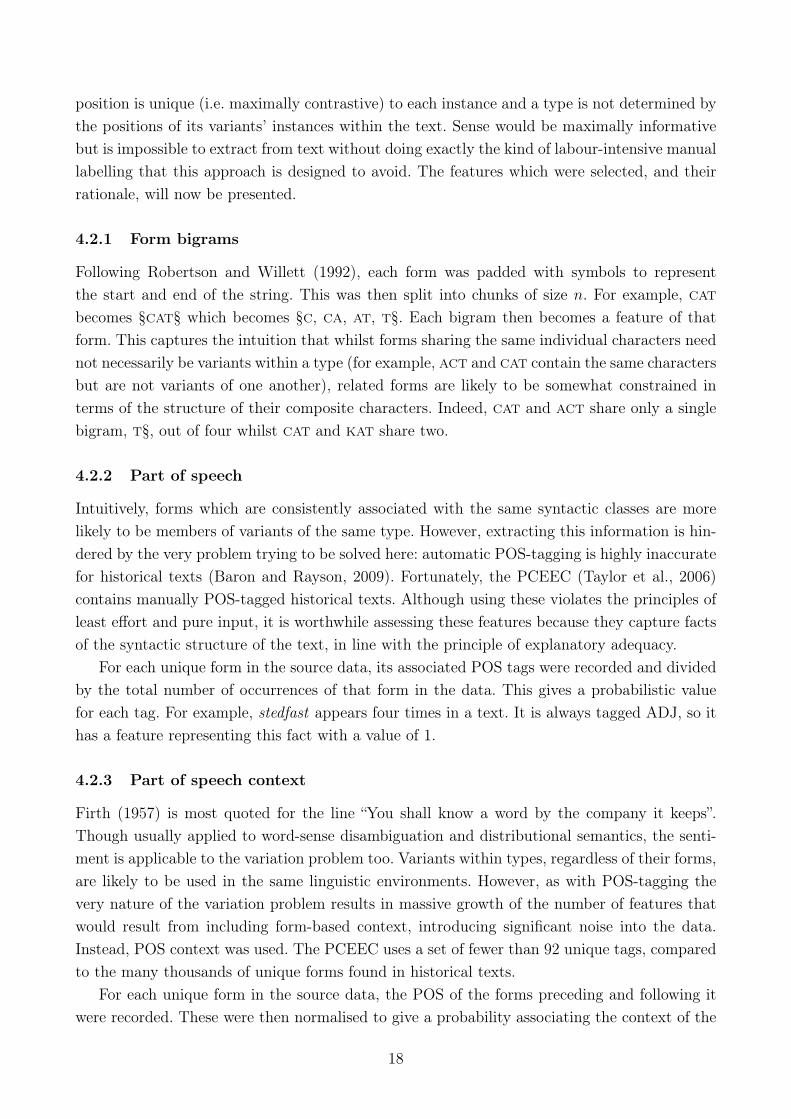
4.2.1 Form bigrams

Following Robertson and Willett (1992), each form was padded with symbols to representthe start and end of the string. This was then split into chunks of size n. For example, catbecomes §cat§ which becomes §c, ca, at, t§. Each bigram then becomes a feature of thatform. This captures the intuition that whilst forms sharing the same individual characters neednot necessarily be variants within a type (for example, act and cat contain the same charactersbut are not variants of one another), related forms are likely to be somewhat constrained interms of the structure of their composite characters. Indeed, cat and act share only a singlebigram, t§, out of four whilst cat and kat share two.

4.2.2 Part of speech

Intuitively, forms which are consistently associated with the same syntactic classes are morelikely to be members of variants of the same type. However, extracting this information is hin-dered by the very problem trying to be solved here: automatic POS-tagging is highly inaccuratefor historical texts (Baron and Rayson, 2009). Fortunately, the PCEEC (Taylor et al., 2006)contains manually POS-tagged historical texts. Although using these violates the principles ofleast effort and pure input, it is worthwhile assessing these features because they capture factsof the syntactic structure of the text, in line with the principle of explanatory adequacy.

For each unique form in the source data, its associated POS tags were recorded and dividedby the total number of occurrences of that form in the data. This gives a probabilistic valuefor each tag. For example, stedfast appears four times in a text. It is always tagged ADJ, so ithas a feature representing this fact with a value of 1.

4.2.3 Part of speech context

Firth (1957) is most quoted for the line “You shall know a word by the company it keeps”.Though usually applied to word-sense disambiguation and distributional semantics, the senti-ment is applicable to the variation problem too. Variants within types, regardless of their forms,are likely to be used in the same linguistic environments. However, as with POS-tagging thevery nature of the variation problem results in massive growth of the number of features thatwould result from including form-based context, introducing significant noise into the data.Instead, POS context was used. The PCEEC uses a set of fewer than 92 unique tags, comparedto the many thousands of unique forms found in historical texts.

For each unique form in the source data, the POS of the forms preceding and following itwere recorded. These were then normalised to give a probability associating the context of the

18

target form with a POS tag. For example, stedfast appears four times in a text. The formsimmediately preceding it are tagged ADVR, ADVR, D, D. The forms immediately following itare tagged P, P, ADJ+N, ADJ+N. Therefore, the probabilities of these tags are all 0.5.

4.2.4 Pairwise similarity

It has been argued that the use of modern dictionaries and spell-checking technology to identifyand normalise historical variation is inappropriate but it will now be demonstrated that, withsome revisions, it can be adapted to avoid criticisms based on a violation of the principle of epochignorance. Rather than comparing historical forms to a modern dictionary, they can instead becompared to the other historical forms within the same text. Words which are, in this context,more similar by some metric are more likely to be variants of a type. This approach is directlymotivated by considering the desiderata within the framework of the proposed formalism – agood example of the benefits that come from clearly defining a problem beforehand.

VARD2/Norma use a version of Levenshtein distance but many other metrics exist forcomparing strings. The algorithm that will be used here is Jaro distance (Jaro, 1989). Thisdiffers from Levenshtein distance in two important ways. First, it considers the number ofinsertions, deletions and transpositions required to transform one string into another rather thaninsertions, deletions and substitutions. Considering transpositions is theoretically motivated, inline with the desiderata, because transpositions are common in historical word forms (e.g.softely/softlye, chasde/chased), whilst substitutions can be accounted for by a chain operationof deletion and insertion. Second, the score generated by the Jaro algorithm is not a simplecount of edit operations but normalised from 0 to 1. This makes it more suitable for use as afeature value in clustering. The Jaro distance, dj, between two strings, s1 and s2, is defined:

19

dj =1

3

(m

|s1|+

m

|s2|+m− tm

)(3)

where:m =

⌊max(|s1|, |s2|)

2

⌋− 1 (4)

and:t =

m

2(5)

To generate features based on this, pairwise Jaro distances are first calculated for all words inthe input text. The top ten results are then encoded as feature-value pairs. For example, forstedfast some of the top-ranking comparisons are stedefaste, stedfastlie and stedfastnesse, withJaro distances of 0.933, 0.909 and 0.871 respectively.

The raw scores of the pairwise comparisons are not intended to be the main predictivefeature of similarity between variants. Jaro distance is a true metric function and satisfiescertain mathematical criteria. Such a function, d, must be:

• symmetric: d(x, y) = d(y, x)

• non-negative: d(x, y) ≥ 0

• coincident: d(x, y) = 0 if x = y

• subadditive: d(x, y) ≤ d(x, y) + d(y, z)

By pairwise comparing all variants within a text using Jaro distance, a metric space is created.Items which are closer to each other within this space are more similar but the property ofsubadditivity also captures relations of similarity between partitions of the metric space. Intu-itively, this mirrors assumptions of the formalism in that what variants have in common is somelatent variable, types, that connects them. Types, then, are equivalent to individual partitionsof the metric space.

4.3 Worked example

To demonstrate the TI-pipeline, a toy example will now be presented based on the text “the reddredde door”. First, forms are extracted by tokenisation. Each form is then tagged with its POSbefore values for the previously listed features are extracted to create feature vectors. Table 7shows how each of the forms found in the text is related to the structure of the formalism andhow this is information is represented within the TI-pipeline. These feature vectors are thenconverted to binary vectors and processed using agglomerative hierarchical clustering.

In this example, it is clear to see that the expected number of types is 3, so the k parameterof the clustering process is set to this value.2 The output of the clustering process is as seen intable 8 and can be interpreted as having successfully divided the input text into three types,assigning the two variants V(redd,b) and V(redde,b) to the same cluster, i.e. type.

2This is not always as easy to determine and is addressed in section 6.

20

V(the,a) V(redd,b) V(redde,b) V(door,c)

Pairwise Jarodistance score

redd=0.527redde=0.511door=0.0

the=0.527redde=0.933door=0.0

the=0.511redd=0.933door=0.0

the=0.0redd=0.0redde=0.0

Bigrams§t=1.0, th=1.0

he=1.0, e§=1.0

§r=1.0, re=1.0

ed=1.0, dd=1.0

d§=1.0

§r=1.0, re=1.0

ed=1.0, dd=1.0

de=1.0, e§=1.0

§d=1.0, do=1.0

oo=1.0, or=1.0

r§=1.0

Part of speech self_is_Det=1.0 self_is_Adj=1.0 self_is_Adj=1.0 self_is_Noun=1.0Part of speechcontext

prev_is_START=1.0next_is_Adj=1.0

prev_is_Det=1.0next_is_Adj=1.0

prev_is_Adj=1.0next_is_Noun=1.0

prev_is_Adj=1.0next_is_STOP=1.0

Table 7 – Feature vector representation of formal variants in “the redd redde door”

Form Clusterredd 0reddethe 1door 2

Table 8 – Output of the type identification pipeline for a given toy input

At this point, as intended, the first half of the restated variation problem has been fullyaddressed.

21

5 Evaluating the automated approach

The preceding example is interesting as a proof-of-concept for the proposed formalism and TI-pipeline. However, the accuracy of the method on a four instance text does not reasonably implythe same performance can be expected for a corpus of many more instances. Also, accuracy wasdetermined manually rather than mechanically. Two processes will now be presented. First, apipeline for generating gold standard texts which can be used to evaluate the output of theTI-pipeline. Second, a statistical method for evaluating pipeline performance on such generatedgold standard texts. Each will be demonstrated using a toy example.

5.1 The performance evaluation pipeline

As outlined in section 2.4 (page 7), VARD2/Norma make use of different methods for assessingtheir accuracy. However, neither of these are suitable for the proposed method because of thetype of output generated by the extraction pipeline – rather than map from historical to modernforms, it maps from variants to types. Although VARD2/Norma use different evaluation metrics(precision/recall, accuracy) they both use a similar methodology, taking a manually-normalisedcorpus as a gold standard against which the tools can be assessed. There is something tocriticise in each of the gold standards used. VARD2’s gold standard is based on LC-ICAMET,which suffers from issues relating to its compilation, whilst the very small size of Norma’sgold standard results in significant proportions of it being used as training data. Ironically, thevariation problem itself is to blame for the lack of large general purpose gold standards whichanyone working on the problem can use to assess solutions.

What is needed, and what will now be presented, is a process for automatically generatinggold standard data. This takes a modern text, replaces forms within it with historical forms andtracks the changes which have been made. It is then possible to use this artificial historical text,with the tracked changes acting as an answer key. Together, this key and the generated text forma gold standard. The output of this process can be used as the input to the type identificationprocess (fig. 3, page 16). Figure 4 provides an overview of the generation process. This processwill be described in detail, with a toy example demonstrating the joint generation/identificationpipeline.

5.1.1 A toy example

First a modern text is refactored in line with the structure of the formalism in section 3.1(page 13). The raw text is tokenised and each form associated with its unique position, tocreate an instance. These instances are underspecified, containing no semantic information,though this is not relevant to the task at hand. Instances with the same form are grouped intovariants, which are then grouped into types. This takes advantage of the fact that in moderntexts there is a one-to-one mapping of forms, variants and types – accordingly, there is no needto use semantics to group variants into types. The next step is to cause variation. This is doneby inducing the reverse of the normalisation process: rather than merge variants into types,

22

Moderntext

CreateTextObject

TextObjectvariation=false

Causevariation

Knownvariants list

Text Objectvariation=true

Recordvariation

List ofvariantsarrangedinto types

Use asinput to typeidentification

pipeline

Figure 4 – A pipeline for generating gold standard texts

types have their variants split. The instances contained within variants are renamed, takingnew names from a list of known variants, which has the effect of creating new variants. Duringthis process, a variety of useful data can be tracked, including the original and resultant numberof types and variants, which types have been split and how many times, which new forms havebeen inserted and at what position, how much variation is present (6) as well as how muchvariation has been added.

% variation = 100− 100

(number of types

number of variants

)(6)

Using the example of “the red red door”, three initial types would be created. The type con-taining a single variant for red, containing two instances, would then be targeted for variation.(There would be no point targeting the or door because they have only one instance per type –changing the form of those instances would be vacuous.) The modern form red is consulted ina dictionary of known variants, which maps modern forms to historical ones. The alternativeforms found there are then used to replace those found in the instances within the red variant.The effect of this is to create two new variants, containing one instance each, but which are stillheld within the same type. The instances are then called in the order of their position feature,resulting in the creation of a new text, for example “the redd redde door”. By (6), the originaltext has 0% variation, whilst the new one has 25%. Crucially, the location of this variation isknown, because instances connect forms to position, variants and types. Using this toy exampleas a gold standard would return two items: the “historicised” version “the redd redde door” andan expected cluster (i.e. type) assignment. matching that of table 8 (page 21).

This text can then be used as the input to the pipe identification pipeline. The output of thisis, naturally, the same as shown previously in table 8. The accuracy of this output, compared

23

to the gold standard, is easy to see because of the small size of the data. In order to assesslarger data sets a more principled and rigorous approach is required.

5.1.2 Statistical cluster comparison

The gold standards used by VARD2/Norma were constructed to assess their solution to thenormalisation aspect of the variation problem. The artificial gold standards generated here areintended to be used to assess the type identification aspect.3 As a result, statistical measuressuch as precision and recall are not suitable. This is because there is no label (i.e. a modernform) for each type represented by the clusters. Instead, a different metric must be used.

The output of the TI-pipeline is a list of cluster assignments, as is the output of the goldstandard creation pipeline. Each can be seen as the partition of a set, where the whole setis the collection of variants and each partition of that set represents a type. Each element ofthe set must be a member of one and only one subset and each subset must contain at leastone element. The gold standard partitioning represents the “ground truth”, against which thetype identification process can be externally validated. There are several information theoreticmethods for comparing the similarity of two possible partitions of a given set. An especiallyclear outline of these methods is to be found in Vinh, Epps, and Bailey (2010).

For current purposes Adjusted Mutual Information Score (AMIS) is ideal. This choice ismotivated by the argument presented in Vinh et al. (2010), namely that an ideal set partitioncomparison measure should (a) be a true metric (satisfying the properties of positive definite-ness, symmetry and triangle inequality), (b) be normalised to a fixed range such as [-1,1] or [0,1]and (c) have a constant baseline such that its expected value between a ground truth partitionand any random repartitioning should be zero thus indicating no similarity. AMIS satisfies onlythe second and third of these, not being a true metric, but this trade-off is acceptable becauseit is more important to adjust for chance, which is what the constant baseline does, since withlarge data sets it is possible to achieve high mutual information scores purely by random assign-ment of clusters. Therefore, when comparing the gold standard ground truth and the output ofthe TI-pipeline, an AMIS of 0 can be interpreted as the output being no better than randomlygrouping the variants into types. A score of 1 means that the two assignments are identical. Ascore between these values can be interpreted in line with Vinh et al. (2010, p.2839-2840), withscores closer to 1 meaning more information is mutual between the assignments than would bethe case if the AMIS were lower. Another attractive property of AMIS is that it is independentof any labels for the clusters, which is important here because the clusters have no labels –instead, the clusters themselves are the latent variables in the data, namely types.

In the toy example, the ground truth exactly matches the output of the type identificationprocess, giving an AMIS of 1. Experimental results, using more realistic data, will now bepresented.

3Although adapting the software to generate interlinear glosses would be trivial, texts generated this waywould not be a very rigorous test of the abilities of VARD2/Norma because the variation is generated by a listof known variants which those tools contain.

24

6 Experimental implementation and evaluation

Four experiments were run, evaluating the performance of the proposed formalism and pipelines.These are presented below, followed by a critical discussion of the output generated when agenuine historical text is used.

6.1 Experiment 1: Assessing the selected features

Before using the current model on real historical data, it will be useful to assess the predictivepowers of the features that drive the clustering process and ensure that all features correlatepositively with the latent variables being sought in the data. Another important consideration isthe time taken to compute the cluster assignments, because large data sets with many featurescan take a significant time to return results and this is wasteful of resources if some of thosefeatures do not perform any useful function. For example, using the full set of features detailedin section 4.2 (page 17) on a data set with 21,801 items results in the creation of feature vectorscontaining between 16 and 142 components. This becomes 61,459 binary vector componentsafter the 1-of-K encoding process. Arranging these 21,801 binary vectors in a 61,459-dimensionalspace and determining k clusters takes approximately ten hours on a MacBook Pro with a quad-core 2.3GHz i7 processor and 16GB of memory. Reducing the number of components in thefeature vectors reduces the number of binary vector components and therefore the computationtime.

6.1.1 Design

A 263,614 instance sample was selected from the POS-tagged version of the British NationalCorpus, comprising newspaper articles relating to sport and business and used to generate agold standard text (fig. 5). A dictionary of known variants, mapping 19,062 modern forms to36,233 historical forms, was generated from data made available by the DICER project.4 Themodern BNC data yielded 21,803 types, with an equal number of variants. 20,251 types wereinitially valid for variation – the forms within these types had at least three characters andwere alphabetic, with no special characters. Vacuous variation was avoided by selecting typeswhich contained more than one instance, whose form was in the known variant dictionary withat least two alternative forms available.

This resulted in 4,762 target types, 21.84% of the total. These types were induced to causevariation, redistributing their instances across more variants then changing the forms of theinstances within those variants using the known variants dictionary. The number of variantswithin these types increased by 152.14% from 4,762 to 12,007. The targeted types changedfrom holding one variant each to between 2 and 12 variants, with targeted types containing onaverage 2.52 variants. Across the whole text, the number of variants increased by 33.23% from21,803 to 29,048. By (6), the variation within the text changed from 0% to 24.94%. This levelof variation would date the created text to the 17th century (see fig. 1, page 8). The result is

4http://corpora.lancs.ac.uk/dicer/

25

Ian Botham can’t hev beene expectyng to hev such a vree wynter, bvt he’s certainly fillyng itinnovatively uuith a nationall tour of hs shevve, Ane Eueninge With Ian Botham. Clips of hsgreatest hits, varous filmed interviews ond other odde surprizal gueste are promist, folowed by‘Bothy’ taking questios trom the floore. Audiences myghte like to quiz hime about hs favouritesportyng momente. Wes it þe 1974 Benson ond Hedges quarter-final whe, as a 15-year-old, helost two teeths to te fearsome Andy Roberts before hitting þhe winning sicks?

Figure 5 – Sample of automatically generated artificial “historical” text

a large text with significant levels of variation, distributed unevenly across the types withinthe text. By comparison, the gold standard used in the VARD2 trials contained no more than30,000 tokens (i.e. instances within the proposed formalism). The largest single text used forassessing Norma was 4,700 tokens, though five standards containing 15,509 tokens in total wereused. The level of variation in those texts is unknown but can be estimated based on the ageof the text, with more modern texts having less variation.

This data set was divided into blocks. Each block contained all the types whose variantsshared an initial character, resulting in 24 blocks (no or very few words began with x or z).Each of these blocks was then processed multiple times by a parametrised instantiation ofthe TI-pipeline, using a different combination of features each time. Four binary features insixteen combinations (table 9) per block gave a total of 384 trials. All blocks were processedconcurrently on the Amazon EC2 cloud computing platform, with 32 Intel Xeon processorsrunning at 2.8GHz and 60GB of RAM. Running multiple trials is required because the outputof the agglomerative clustering algorithm is non-deterministic – an average is therefore needed.Each block was repeated ten times. Total computation time was approximately five hours.

1 2 3 4 5 6 7 8 9 10 11 12 13 14 15 16Bigram T T T T T T T T F F F F F F F FPOS T T T T F F F F T T T T F F F FPOS context T T F F T T F F T T F F T T F FPairwise comparison T F T F T F T F T F T F T F T F

Table 9 – Matrix of parameters used for each block in experiment 1

6.1.2 Results

AMIS for each trial was calculated by comparing the predicted cluster assignments to the goldstandard. p-scores were calculated to determine the correlation between AMIS and featuresettings. The results are shown in table 10. It can be seen that both POS and POS contextare negatively correlated with AMIS, harming the performance of the TI-pipeline. Removingthese features from future experiments has two benefits. First, it should reduce the time takento compute the types. Second, most crucially, it obviates any need for POS-tagged input. Thisallows the pipeline to adhere to the principle of pure input, since only unprocessed text isrequired.

26

Bigrams POS Context Pairwise comparisonp-score 0.197331736 -0.084754313 -0.223942882 0.797472663

Table 10 – p-scores for features

6.2 Experiment 2: Large-scale evaluation

Using the same automatically generated text from experiment 1 and a reduced feature set,the range of elements in each 21,801 feature vector fell from 16-142 to 12-31. The number ofcomponents in the equivalent binary feature vectors fell from 61,459 to 60,691. Computationtime was not noticeably reduced.

6.2.1 Results

The AMIS for the output of the TI-pipeline, compared to the gold standard, was 0.949. Thisis extremely close to a score of 1 but it should be noted that AMIS does not heavily penalisethe unnecessary division of sets of clusters. The score can be more accurately interpreted asmeaning that the output of the TI-pipeline is very similar to the gold standard and significantlymore similar than a random assignment of variants to types. The following experiment will usereal historical texts and examine the actual output of the TI-pipeline in order to provide a morepractical assessment of the procedure.

The text was processed again, this time using only the types to which variation had beenadded rather than all types. This is not a realistic process, as with a genuine historical textthere would be no way to make this differentiation between types. It does, however, give aninformative view of how successful the system is at identifying variant types without the addi-tional noise of “singleton” types that contain no variation. On this data set, AMIS was 0.707and therefore reasonably, but not completely, similar to the gold standard.

Overall, the identification pipeline is able to divide variants into types which are generallythe correct size.

6.3 Experiment 3: Real historical text

The Paston letters are a collection of correspondence between the members of a 15th centuryNorfolk family, written between 1422 to 1510, and are available as part of the PCEEC (Tayloret al., 2006), which takes as its source the seminal edition by Davis (1971). There are twocrucial differences between the Paston letters and an artificially generated text. First, there willbe no gold standard to provide a ground truth. Secondly, the degree of variation is not knownbeforehand so the k value for the clustering algorithm is unknown. This value declares howmany types should be identified within the data. There is no standard method for determiningk but machine learning techniques are an exploratory tool, not explanations in themselves.Therefore, it is to be expected that a degree of experimentation is required.

An informed estimate for k is possible. First, it will lie within [1, x] where x is the number ofvariants in the text, equal to the number of forms. The Paston letters contain 255,324 instances,

27

with 16,684 forms. Setting k closer to 1 will result in more variants per type. Setting it closer tox will result in fewer. Given a text from the 15th century, variation is likely to be high (as perfig. 1, page 8) and a suitable value for k for the Paston letters is therefore closer to 1 than to x.However, it does not make sense to set it too low – the letters are not a few types repeated overand over with thousands of different forms. By selecting a percentage of variation to expect(shown in fig. 1), (6) can be used to estimate how many types should be expected:

50% = 100− 100

(types16684

)(7)

Solving for types gives 8,342. Values for k above and below this, 6,000 and 10,000 respectively,were also used for comparison purposes.

6.3.1 Results

Table 11 shows the different output of the TI-pipeline using different values for k, focusing ontwo possible types (tidings and tiding). A fuller representation of the output is presented inAppendix A. Several features are noteworthy. First, setting k too high can cause fragmentationof types whilst too low causes over-clustering. For the Paston letters, k is likely to lie between6,000 and 8,342. Second, there is conflation of variants – the type identification process doesnot always distinguish between morphologically different forms (e.g. singular, plural, verbalinflection, adverbs). Third, some clusters contain forms which are arguably not variants of atype (caused/accused/chased/cursed), though many clusters are homogeneous.

6.4 Experiment 4: Chronology of the Great Vowel Shift

Whilst the ontological status of the Great Vowel Shift (GVS) is widely accepted, the details aredisputed. It is conceptualised as either a push-chain (Luick, 1903), pull-chain (Jespersen, 1928),or centre drift (Stockwell and Minkova, 1988). Its chronology is also uncertain. Attempting toanswer the latter, Lass (2000, Chapter 3) used the Paston Letters to show that /o:/ had begunraising to /u:/ by the 15th century. He reasoned that if /o:/ was raising, it might be writtenwith <ou> for /u:/ in words that etymologically had /o:/. Examples of this in the Letters weregiven: doun and goud for done and good. Similarly, raising of /u:/ to /au/ is supported by caw(cow) and ahawght. Lass claims that the top half of the GVS was well under way in the 15th

century, creating the conditions for a pull-chain.None of these forms actually appear in the Paston Letters. They are not in the seminal

Davis (1971) edition or the 1910 reprint of Gairdner (1895). The only examples of doun meandown. goud appears twice as goude but means could, written by Richard Calle, a servant of thePastons. There are no instances of any of the others. Lass also claims that /i:/ had dipthongisedin the Letters, evidenced by abeyd (abide) and creying (crying). Neither of these appear in theLetters, plus crying is of French or Latin origin.

Lass (personal communication April 23rd, 2014) attributes the error to “a conventionalsloppiness, which was part of praxis then”. This highlights the need for corpus tools for dealing

28

Type Usage of form in contexttidinges 1 1 1 As for tidinges elles, þe Kyng is at Shenetidingis 1 1 1 þat ye may bringe hym good tidingistidynges 1 2 2 And as for tidynges here in this contretidyngges 1 2 2 I merveyll that I here no tidyngges from yowtidyngys 1 1 3 As for tidyngys in this contre her be noontyding 1 1 4 and tyding wheder þer be any sech sutetydinges 1 2 2 As fore tydinges, here bee noon newetydingez 1 1 4 But of the fleet of shyppis there is no tydingeztydingis 1 1 4 But þe continuall tydingis of my seyd lordis coming hedertydingys 1 1 3 no tydingys in serteyn where the flet wastydyng 1 2 5 As for tydynges, the Kyng and the counsell is at Northamptontydynge 1 2 5 And as for tydynge, the berere heroff schall infforme yowtydynges 1 2 2 As for tydynges, my lorde Erchebysshop is at the Mooretydyngges 1 2 2 As for tydyngges, my lord Chaunceler is dischargedtydynggis 1 2 5 and I praye yow to sende me tydynggis from be-yond seetydynggys 1 2 5 As fore yowr syster, I can send yow no good tydynggys of heretydyngis 1 2 5 I prey yow lete my mastras your modere knowe these tydyngistydyngys 1 2 5 As for tydyngys owte of thys contreetythyngys 1 2 6 I vnderstond that ye had no tythyngys from me at that tymetytynges 1 2 2 schuld bere the Kyng certeyn lettres and juste tytyngestytyngges 1 2 2 blyssed be God, that he hath now good tytynggestytyngys 1 2 6 And as for tytyngys, in good feyth we haue non

Table 11 – Comparison of type assignment for three values of k. Coloured columns, from left toright, k=6,000, k=8,342, k=10,000.

with historical texts. Without them, researchers may instead rely on old scholarly sources,repeating mistakes and using them to support arguments which are then accepted, uncritically,by others. Although there is a great deal of debate over the theoretical construction of the GVS,there is very little checking of the “facts”. They are taken at face value because they have beenrepeated so often in the literature.

To test Lass’s chronology, the Letters were processed using the TI-pipeline. Clusters weremanually analysed to see which variants were grouped. These groups were then identified inthe Letters and date of authorship recorded. The digraphs <aw> and <ou> were highlighted.Most of the 236 <aw> forms were either of French origin (commandment, ransom, fault),etymologically did not have long vowels (land, Canterbury, hawk, worship) or were not part ofthe same syllable (award, away). Of the 695 <ou> forms, a similar situation was found withmostly French words, as well as <ou> representing <ov> (overcome, recovery). This makesit difficult to support a claim that /o:/ had raised to /u:/. Dipthongisation of /i:/ is also notsupported. All EME reflexes of OE abidan have <y> or <i> representing the stressed vowel:abidith, abideth, abydyth, abydyn, abyd, abydyng.

Setting aside Lass’s ghost words, the place name Hellesdon (OE: Hægelisdun) is well-attested. According to Lass, the etymological /u:/ should be represented with a digraph, toshow that it has dipthongised. The pipeline identified six variants for Hellesdon, across 53usages. Of these, only 2 have <ou>: Heylisdoune. The rest have <o>: Helesdon, Heylysdon,Heylesdon, Heilesdon, Heylisdon. The <ou> variants were used in 1461 and 1465 by John Pas-ton I, whilst the others are used between 1450 and 1476 by a range of authors. So even when

29

actual attestations are used to investigate Lass’s proposed GVS chronology, the claim that rais-ing of the high vowels was “well under way by around 1400” (Lass, 2000, p.80) is not supportedby the sources.

Establishing the extent of the GVS in 15th century Norfolk will require a full analysis of thehistorical sources. Such an analysis must cast aside traditional authorities on the evidence forsound change, to avoid repeating Lass’s error. Any theories of historical sound change wouldthen need to fully account for the entire range of explicitly attested facts, rather than cherry-picking examples which neatly support a chosen theory. The reason that this investigation hasnot been done yet is likely due to the sheer work required. Fortunately, the TI-pipeline hasshown that it can be useful in reducing the workload by making it easier to find orthographicvariants without completely manual checking of sources.

7 Discussion

There are multiple explanations for the classification errors in the results of experiment 3. Sincek is unknown, the partitioning of the metric space cannot be accurate. This naturally resultsin clusters being too small or too large. Only two features are used by the clustering algorithm(bigrams and pairwise similarity). More are likely to be needed, but these features could alsobe expanded, by using trigrams rather than bigrams or the entire set of pairwise comparisonsrather than just the top ten.5 Another explanation may be that some types lack sufficientvariants for the identification pipeline to capture their identify them by pairwise comparisonalone. Indeed, identifying types with many variants is a strength of the system.

The effectiveness of adding new features to overcome these issues would be easily assessed,using the demonstrated evaluation pipeline. Furthermore, the formalism can be used to guidefeature selection and it predicts that semantic information would be highly informative though,as discussed, this may violate the principle of pure input by requiring semantic tagging. Thisitself would negatively impact assessment of least effort, but novel methods of automaticallyextracting any semantic information from raw historical texts could be developed to do thisand incorporated into the TI-pipeline. For example, the latent semantic analysis methodologycould be adapted to use the initial output of the pipeline in order to extract semantic relations,which is then reprocessed by the pipeline.

The formalism assumes that the latent variable in historical texts is types and that this hid-den structure represents the “root” of variation (see fig. 2, page 15). In light of the morphologicalconflation observed, it may in fact be that lemmas are the latent variable. Any future workshould investigate this, because it hints at a connection between the proposed formalism andthe lexicon, in particular the nature of the lexicon’s contents. The lexicon is a core componentof linguistic theory but is often taken for granted. The Declarative Procedural model (Ullman,2001) merely stipulates it is part of the declarative system. The DRC model (Coltheart, Rastle,Perry, Langdon, and Ziegler, 2001) proposes a lexicon not only for sound but for orthography,

5Five were originally used, but the evaluation pipeline showed ten to be more effective. More were not useddue to the increased computation time.

30

but these too are underspecified. Models with orthography in the lexicon (e.g. Seidenberg andMcClelland, 1989) suffer from a synchronic bias because orthography, standard or otherwise,is a modern phenomenon. It seems unlikely that people in the 15th century stored multipleorthographic forms in their lexicons, selecting one at random. Rather, some psycholinguisticprocess for generating orthographic forms from the lexicon is implicated. Centuries later, westill have access to that process. This is evidenced by the ease with which modern readers“decode” historical forms and determine what modern forms they correspond to, even out ofcontext but especially if there is semantic understanding for that form.6 Within the proposedformalism, this may be accounted for by a decoding process using type-like information storedin the lexicon. Under this account, excluding orthographic information from the lexicon is asjustified as excluding different fonts and font sizes.

6retorne, peopell, bownde, contynew are easy, yepysweche, vowchesawf, scutys are trickier.

31

8 Conclusion

A working solution to one half of the original variation problem has been presented. It wasevaluated statistically and experimentally. It meets many desiderata (table 12). The proposedpipelines, which are fully automated and require no pre-processing of the source, could bethe first step to investigating linguistic phenomena in historical texts on a scale previouslynot possible due to the labour involved – as demonstrated by the investigation of the GreatVowel Shift’s chronology. Everything is based on a rigorous formalism, an approach that yieldednot only a novel view on an old problem but a precise technical vocabulary and a frameworkwithin which future improvements can be situated. Finally, analysis of the experimental resultssuggests that the formalism may be able to draw a connection between historical developmentsin orthography and psycholinguistic processes involving literacy and the lexicon.

32

Perfection No. Statistically strong results but type clusters oftencontain morphological variants.Clusters generally too small rather than too large.Does not normalise text.

See:section 6.2section 6.3

Least effort Completely automatic with no human input needed.No training needed.No preprocessing needed.Complexity O(n3) for agglomerative clustering, takingapproximately ten hours on 250,000 tokens.Speed is determined by hardware power but polyno-mial complexity makes larger data sets very slow.

See:section 6.1

Explanatoryadequacy

Completely grounded in a theoretical formalism whichmakes testable predictions as to the underlying struc-ture of texts.Uses suitable technology, critically chosen.Leverages form-internal structure (bigrams) to accessan underlying proposed type (possible lemma) struc-ture.Can be further adapted to better capture linguisticstructure.

See:section 3section 4.2

Pure input Yes.Requires only a historical source.POS-tagging is not required.No list of known variants is required.

See:section 6.1.2

Languageagnostic

No language-specific algorithms used – pairwise com-parison can be performed with any string metric suitedto the source language.

See:section 4.2.4

Epoch ignorant Yes.No modern dictionaries used.No comparisons to modern words made.Only within-source comparisons are used.

See:section 4.1section 4.2section 6.3

Preserveoutput

Yes.Returns a list of identified types without modifying thesource.

See:section 4.1section 6.3section 6.4

Table 12 – Appraisal of type identification pipeline against desiderata

33

A Experiment 3 - partial results

Table 13 – Type identification pipeline output for various k values (157 out of 16,684)

k = 6000 k = 8342 k = 10000FORM CLUSTER FORM CLUSTER FORM CLUSTERreuell 0 spekyth 0 charyté 0rewell 0 specyfyith 0 charité 0revell 0 spedyth 0 juge 1haxed 1 bowe 1 jugeis 1hadden 1 bower 1 juges 1hadde 1 bowez 1 dysshes 2haden 1 bowen 1 dysseys 2hade 1 thret 2 panell 3hadd 1 thrett 2 inpanell 3nepueu 2 threte 2 dowtere 4neuew 2 requyred 3 dowgtere 4nevewes 2 requyre 3 dowgteris 4nevoue 2 requyryd 3 babees 5nevewe 2 decesse 4 bees 5nevew 2 decesed 4 advyse 6neveu 2 decese 4 avysed 6gown 3 deceasse 4 advysed 6drownk 3 blodys 5 comown 7down 3 loodys 5 comonys 7nown 3 londys 5 comons 7fown 3 tydyngys 6 comowns 7mown 3 tydyng 6 comounly 7town 3 tythyngys 6 comoun 7dowun 3 tydynggis 6 comon 7

novembre 4 tytyngges 6 comouns 7nombere 4 tydinges 6 þidre 8nowmbere 4 tydyngges 6 þaire 8nouembere 4 tidynges 6 fauorabelye 9nouember 4 tydynggys 6 fauorably 9noumbir 4 tidyngges 6 favorably 9nouembre 4 tytyngys 6 fauorabely 9streyned 5 tytynges 6 countie 10strekyn 5 tydynges 6 counties 10streyne 5 tydyngis 6 countes 10

34

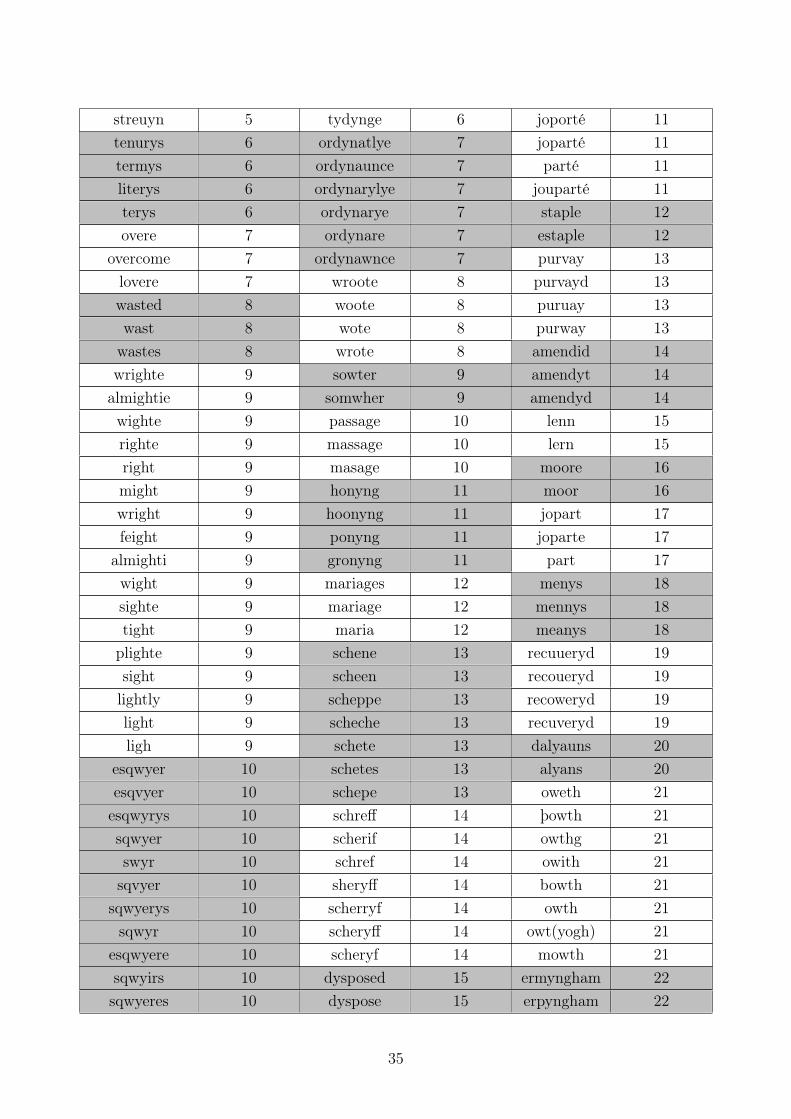
streuyn 5 tydynge 6 joporté 11tenurys 6 ordynatlye 7 joparté 11termys 6 ordynaunce 7 parté 11literys 6 ordynarylye 7 jouparté 11terys 6 ordynarye 7 staple 12overe 7 ordynare 7 estaple 12

overcome 7 ordynawnce 7 purvay 13lovere 7 wroote 8 purvayd 13wasted 8 woote 8 puruay 13wast 8 wote 8 purway 13wastes 8 wrote 8 amendid 14wrighte 9 sowter 9 amendyt 14almightie 9 somwher 9 amendyd 14wighte 9 passage 10 lenn 15righte 9 massage 10 lern 15right 9 masage 10 moore 16might 9 honyng 11 moor 16wright 9 hoonyng 11 jopart 17feight 9 ponyng 11 joparte 17

almighti 9 gronyng 11 part 17wight 9 mariages 12 menys 18sighte 9 mariage 12 mennys 18tight 9 maria 12 meanys 18plighte 9 schene 13 recuueryd 19sight 9 scheen 13 recoueryd 19lightly 9 scheppe 13 recoweryd 19light 9 scheche 13 recuveryd 19ligh 9 schete 13 dalyauns 20

esqwyer 10 schetes 13 alyans 20esqvyer 10 schepe 13 oweth 21esqwyrys 10 schreff 14 þowth 21sqwyer 10 scherif 14 owthg 21swyr 10 schref 14 owith 21sqvyer 10 sheryff 14 bowth 21

sqwyerys 10 scherryf 14 owth 21sqwyr 10 scheryff 14 owt(yogh) 21

esqwyere 10 scheryf 14 mowth 21sqwyirs 10 dysposed 15 ermyngham 22sqwyeres 10 dyspose 15 erpyngham 22

35

sqwyere 10 dysspytuose 15 gernyngham 22store 11 cast 16 gemyngham 22sorepe 11 casty 16 elyngham 22sorer 11 castyr 16 joystys 23sore 11 moungomerye 17 jostys 23soore 11 mongomeré 17 joperté 24

varyaunce 12 mongomery 17 pouerté 24clarance 12 montgomery 17 jupperté 24variaunce 12 wyte 18 mysch 25vareaunce 12 wytte 18 fysch 25varyance 12 wyttes 18 ocle 26claraunce 12 qwyte 18 cole 26deserve 13 daunger 19 ofys 27desyere 13 danger 19 otys 27desyerthe 13 dawnger 19 profet 28desyered 13 dangere 19 proff 28desert 13 dawngeres 19 profett 28deserue 13 wryton 20 smyth 29accusyd 14 wryting 20 symyth 29causyd 14 wrytin 20 syth 29chasyd 14 hate 21 comeners 30crasyd 14 thate 21 comenere 30cursyd 14 bull 22 avayll 31cawsyd 14 bullok 22 disavayll 31

jnquisytyff 15 jull 22 leve 32jnquietyng 15 juyll 22 leven 32jnquest 15 decembyre 23 talkyd 33jnquyet 15 december 23 balkyd 33qhen 16 indytement 24 walkyd 33whens 16 jndytementes 24 þedyr 34when 16 indytementes 24 þedyre 34sesyn 17 inditementes 24 athwyx 35soleyn 17 inditementis 24 atwyx 35sleyn 17 jnditement 24 breest 36seyn 17 inditementys 24 beest 36

borowyng 18 writ 25 secretory 37brochyng 18 write 25 secratory 37

vndereschetour 19 writell 25 wordy 38vnderstewerd 19 writene 25 wordys 38

36

busche 20 writen 25 woordys 38siche 20 fumowsly 26 beffore 39svche 20 fumows 26 before 39musche 20 dystrussyd 27 beffoore 39schep 20 dysstres 27 beffor 39soche 20 dystressys 27 pache 40suche 20 shepherdes 28 hache 40sche 20 shepherd 28 fore 41mette 21 scheperdes 28 force 41wette 21 schepeherd 28 afore 41yette 21 schepherd 28 forre 41detteez 21 goone 29 baptiste 42dette 21 agone 29 baptyste 42king 22 agoone 29 withowt 43þing 22 agonye 29 withowte 43kingz 22 curs 30 withoute 43keping 22 curse 30 without 43soch 23 colett 31 withouten 43such 23 colyet 31 withowth 43schuch 23 allweys 32 freyir 44recouere 24 alweys 32 frier 44recouery 24 alweye 32 freir 44recure 24 alweyis 32 freyr 44

recuuered 24 alwey 32 payth 45recuuere 24 allwey 32 fayth 45recouer 24 vicar 33 thinking 46recouered 24 vycare 33 thinkith 46

strawngenes 25 vycar 33 thinketh 46strawnge 25 conseill 34 thinkyth 46strange 25 counsellour 34 think 46

strangwysse 25 counseyll 34 launde 47straungerys 25 consell 34 lawnde 47strawngely 25 conseil 34 landes 47straunge 25 counsellyd 34 lande 47straung 25 counsel 34 writtes 48strangely 25 counseill 34 writtis 48straungiers 25 conseille 34 writt 48strawngys 25 counseyle 34 written 48straunger 25 counseal 34 writte 48

37

straungely 25 conseillour 34 writtys 48pasturys 26 cownsell 34 rosting 49pastures 26 counseil 34 bosting 49pasturs 26 counsell 34 repayment 50pasturen 26 counseyl 34 areyment 50

38

B Code: type identification pipeline

1 from nltk.tag import str2tuple

from collections import Counter, namedtuple, defaultdict, OrderedDict

3 from sklearn.feature_extraction import DictVectorizer

from copy import deepcopy

5 import pickle

from operator import itemgetter

7 import os

from itertools import product

9 import csv

11 from sklearn.cluster import AgglomerativeClustering as AC

13 from datetime import datetime as DT

15 class Corpus:

def __init__(self, **kwargs):

17 self.init_settings = OrderedDict()

’’’

19 Expected argument is just filename at this point.

**kwargs is a bit overkill, left over from previous versions

21 ’’’

for k,v in kwargs.items():

23 setattr(self, k, v)

self.init_settings[k] = v

25

def process_paston_data(filename):

27 ’’’

This takes the raw tagged Paston data from the PCEEC and converts

29 it to a list of (word, POS) tuples. Inserts start/end padding for

sentences.

31 ’’’

with open(filename) as file:

33 raw_text = file.read()

letters_temp = raw_text.split(’<Q’)

35 letters_temp.pop(0)

letters = ["<Q"+i for i in letters_temp]

37 letters2 = [i.splitlines() for i in letters]

letters3 = [i[8::6] for i in letters2]

39 for letter in letters3:

for index, sentence in enumerate(letter):

41 letter[index] = sentence.split()

for l in letters3:

43 for s in l:

s.append("ENDPAD_END")

45 s.insert(0,("STARTPAD_START"))

data = []

47 for letter in letters3:

39

for sent in letter:

49 data.append(sent)

data2 = []

51 for i in range(0,len(data)):

data2.append([str2tuple(x, sep="_") for x in data[i]])

53 data3 = []

for sent in data2:

55 for pair in sent:

data3.append(pair)

57 print(’Processing’, filename)

return [(x.lower(),y) for (x,y) in data3]

59

def process_bnc_data(filename):

61 ’’’

Loads the ~250k sample modern BNC text as (word, POS) tuples

63 and adds start/end padding for sentences.

’’’

65 with open(filename, ’rb’) as file:

raw_data = pickle.load(file)

67 for s in raw_data:

s.append(("ENDPAD" , ’END’))

69 s.insert(0,("STARTPAD" , ’START’))

71 data1 = []

for s in raw_data:

73 for pair in s:

data1.append(pair)

75 print(’Processing’, filename)

return [(x.lower(),y) for (x,y) in data1]

77

if self.filename == ’corpora/paston’:

79 ’’’

Processes Paston/BNC/Variation data, sets up some parameters

81 for stats which are used later.

’’’

83 self.data = process_paston_data(self.filename)

self.filename_nopath = self.filename.split(’/’)[1]

85 self.init_settings[’filename’] = self.filename_nopath

if self.filename == ’corpora/bnc’:

87 self.data = process_bnc_data(filename=self.filename)

self.filename_nopath = self.filename.split(’/’)[1]

89 self.init_settings[’filename’] = self.filename_nopath

if self.filename not in [’corpora/paston’, ’corpora/bnc’]:

91 self.data = self.filename

self.filename_nopath = "VarObjOutput"#FIX THIS AT SOME POINT

93 self.init_settings[’filename’] = self.filename_nopath

95 self.filename_for_saving = self.generate_filename()

40

97

print(’Creating word list’)

99 self.word_list = list(Counter([i[0] for i in self.data

if i[1] not in [’FW’, ’NUM’]]).keys())

101 self.word_list = [i for i in self.word_list if i not in

[’startpad’,’endpad’] and len(i) > 3 and i.isalpha() == True]

103 print(’Word list has’, len(self.word_list), ’entries’)

105 def populate_jwd(wordlist):

’’’

107 Called if using Variation or BNC data. Says JWD but actually

uses JD!

109 Loads a pre-compiled list of JD comparisons, because computing

them at call time takes hours.

111 ’’’

print(’Loading big JWD store - takes a while!’)

113 with open(’corpora/jwd_store.pickle’, ’rb’) as file:

storage = pickle.load(file)

115 print(’Loaded!’)

jwd_data = {}

117 print(’Extracting JWD data using wordlist:’,

len(self.word_list),

119 ’to process’)

for word in wordlist:

121 if len(storage[word]) > 10:

jwd_data[word] = sorted([i for i in storage[word].items()],

123 key=itemgetter(1), reverse=True)[0:10]

else:

125 jwd_data[word] = [i for i in storage[word].items()]

127 print(’JWD data all processed!’)

return jwd_data

129

’’’

131 The next part loads the right JD data file for the input.

Paston data is also precompiled.

133 ’’’

135 if self.filename == ’corpora/paston’:

with open(’data/paston_jaro_50.pickle’, ’rb’) as file:

137 self.jwd_data = pickle.load(file)

139 if self.filename == ’corpora/bnc’:

self.jwd_data = populate_jwd(self.word_list)

141

if self.filename not in [’corpora/paston’, ’corpora/bnc’]:

143 self.jwd_data = populate_jwd(self.word_list)

145 def padded_ngram_dict(word, n=2):

41

’’’

147 Ngram generator.

Takes a word and returns a dictionary where:

149 k = character bigram with padding (cat > $cat$ > $c, ca, at, t$)

v = count of each bigram in the word (usually=1)

151 Can parameterise for n (2 = bigrams, 3 = trigrams etc)

’’’

153 def bigrams_with_padding(word):

store = []

155 current_index = 0

padded = ’$’*(n-1) + word + ’$’*(n-1)

157 for i in range(0,len(padded)+1-n):

store.append(padded[i:current_index+n])

159 current_index += 1

return store

161

def padd_list_to_dict(list):

163 bigramdict = {}

for item in list:

165 bigramdict[item] = bigramdict.get(item, 0) + 1

return bigramdict

167

return padd_list_to_dict(bigrams_with_padding(word))

169

171 def compile_labels_and_features(

remove_empty=True,

173 length=False,

bigrams=self.bigrams):

175 ’’’

This turns each word into a feature vector.

177 Returns two matched lists.

First one is the words (i.e. lables)

179 Second one is the feature vectors for that word.

’’’

181 raw_features = []

labels = []

183

for word in self.word_list:

185 store = []

combo = {}

187 labels.append(word)

189 if length == True:

’’’

191 Include word length as a feature. Dumb idea.

’’’

193 store.append({’wordlength’:len(word)})

42

195 for jwditem in self.jwd_data[word]:

’’’

197 Include JD features (not JWD)

’’’

199 store.append({jwditem[0]:jwditem[1]})

201 if bigrams == True:

’’’

203 Include bigram features

’’’

205 store.append({k:v for k,v

in padded_ngram_dict(word, n=2).items()})

207

for d in store:

209 for k,v in d.items():

combo[k] = v

211 raw_features.append(combo)

213 if remove_empty == True:

’’’

215 Used to remove any raw components that are equal to 0.

Deprecated, I think?

217 ’’’

rf2 = []

219 for i in raw_features:

temp = {}

221 for k,v in i.items():

if v not in [0,0.0]:

223 temp[k] = v

rf2.append(temp)

225

raw_features = rf2

227

return labels, raw_features

229

print(’Creating label list’)

231

self.labels, self.raw_features = compile_labels_and_features()

233 ’’’

Use DictVectorizer to normalise the feature vectors for use in sklearn

235 using 1-of-k method.

’’’

237 self.vectoriserObject = DictVectorizer(sparse=False)

print(’All done’)

239

def find_by_start(self, n, vectors=True):

241 ’’’

Returns labels and features for words beginning with n

243 n can be one char or more.

43

’’’

245 l = []

f = []

247 for i,x in enumerate(self.labels):

if x[0][0:len(n)] == n:

249 l.append(x)

f.append(self.raw_features[i])

251 if vectors == True:

return l, self.vectoriserObject.fit_transform(f)

253 else:

return l, f

255

def find_by_list(self, items, vectors=True):

257 ’’’

As above, but takes list of items as input and returns the features for

259 them. Vectorises them to binary.

’’’

261 l = []

f = []

263 for index, label in enumerate(self.labels):

if label in items:

265 l.append(label)

f.append(self.raw_features[index])

267

if vectors == True:

269 return l, self.vectoriserObject.fit_transform(f)

else:

271 return l,f

273 def dump(self, labs, vects, filename):

’’’

275 Saves labels and vectors to file.

’’’

277 fname = ’csv/’ + filename + ".csv"

with open(fname, ’w’) as file:

279 out = csv.writer(file, delimiter=",", quoting=csv.QUOTE_ALL)

temp = zip(labs,vects)

281 temp = sorted(temp, key=itemgetter(1))

for i in temp:

283 out.writerow(i)

print(’Wrote to’, fname)

285

def generate_filename(self):

287 ’’’

Generates a filename for saving data to disk. Includes date and time

289 plus parameters from the model.

’’’

291 namestring = [str(k) + ’=’ + str(v)

for k,v in self.init_settings.items()]

44

293 return " ".join(namestring)

295 def do_KM(self, letter, k, dump=True):

’’’

297 This is called KM but actually uses AC!

Does the clustering.

299 Takes either a letter of the alphabet or a list.

If letter, clusters all words in the wordlist beginning with that. Used

301 for prototyping.

If list, clusters all the words in that list.

303 Dumps a CSV to disk, containing two columns. First is word, second is

cluster number.

305 ’’’

clusts = k

307

if type(letter) == str:

309 l,v = self.find_by_start(letter)

311 self.km_obj = AC(n_clusters=k, linkage=’average’)

313 results = self.km_obj.fit(v)

315 if dump == True:

filename = DT.now().strftime(’%d%m%y-%H%M%S’)

317 + self.filename_for_saving + ’-k’ + str(clusts)

self.dump(l, results.labels_, filename)

319 self.km_labels = l

self.km_clusters = results.labels_

321 print(’Stored KM output in self.km_labels, self.km_clusters’)

else:

323 self.km_labels = l

self.km_clusters = results.labels_

325 print(’Stored KM output in self.km_labels, self.km_clusters’)

327 if type(letter) == list:

l,v = self.find_by_list(letter)

329

self.km_obj = AC(n_clusters=k, linkage=’average’)

331

results = self.km_obj.fit(v)

333

self.predicted_clusters = {}

335

for v,k in zip(l, results.labels_):

337 self.predicted_clusters[v] = k

339 self.pred_prep = sorted(self.predicted_clusters.items(),

key=itemgetter(0))

341 self.predicted = [i[1] for i in self.pred_prep]

45

343 if dump == True:

filename = DT.now().strftime(’%d%m%y-%H%M%S’)

345 + self.filename_for_saving + ’-k’ + str(clusts)

self.dump(l, results.labels_, filename)

347 self.km_labels = l

self.km_clusters = results.labels_

349 print(’Stored KM output in self.km_labels, self.km_clusters’)

else:

351 self.km_labels = l

self.km_clusters = results.labels_

353 print(’Stored KM output in self.km_labels, self.km_clusters’)

identification.py

46

C Code: gold standard generation pipeline

from collections import defaultdict, Counter

2 from string import ascii_letters, ascii_lowercase, digits

from itertools import islice, product

4 import random

import pandas as pd

6 import pickle

from operator import itemgetter

8 from statistics import *

10 class Instance:

’’’

12 Equivalent to an instance from the formalism.

Has three properties (form, position, POS)

14 POS is not actually used though.

’’’

16 def __init__(self, form, position, PoS):

self.form = form

18 self.position = position

self.PoS = PoS

20

def get_position(self):

22 return self.position

def get_form(self):

24 return self.form

26 def __getitem__(self, key):

return [self.form,self.position][key]

28

def __repr__(self):

30 return "{}: {} {}".format(self.__class__.__name__,

self.form,

32 self.position)

34 class Container:

’’’

36 Base Class for something that will hold other stuff. Sets the basic

properties of a container.

38 ’’’

40 def __init__(self, *args):

self.contents = []

42 if len(args) > 0 and type(args[0]) == list:

for i in args[0]:

44 self.contents.append(i)

else:

46 if len(args) > 0:

self.contents.extend(args)

47

48

def add(self, *args):

50 if type(args[0]) == list:

for i in args[0]:

52 self.contents.append(i)

else:

54 self.contents.extend(args)

56 def __len__(self):

return len(self.contents)

58

def __getitem__(self,key):

60 return self.contents[key]

62 def __setitem__(self, key, value):

self.contents[key] = value

64

def __repr__(self):

66 if len(self.contents) == 0:

return ’An empty container’

68 else:

return "{}: holding {} itemsof class {}".format(

70 self.__class__.__name__, len(self.contents),

self.contents[0].__class__.__name__)

72

class Variant(Container):

74 ’’’

As per the formalism.

76 Inherits from Container object but overrides ’add’ method, to set

the Variant label based on form of its contents.

78 Also has split() method, used when variation is caused.

’’’

80 def __init__(self, *args):

super().__init__(*args)

82 if len(self) > 0:

self.name = self.contents[0].form

84

def add(self, *args):

86 if type(args[0]) == list:

for i in args[0]:

88 self.contents.append(i)

else:

90 self.contents.extend(args)

if len(self) > 0:

92 self.name = self.contents[0].form

94 def __repr__(self):

if len(self) == 0:

96 return "An empty Variant"

48

else:

98 return "A {} with name {} containing {} Instances".format(

self.__class__.__name__, self.name, len(self))

100

def split(self, known_variants, ID):

102 if len(self.contents) == 1:

return self

104

N = [i for i in known_variants[self.name]]

106

N.append(self.name)

108

V = [i for i in self.contents]

110

min_cuts = 1

112

if len(V) >= len(N):

114 if len(N) == 2:

max_cuts = 1

116 else:

max_cuts = len(N) - 1

118 if len(V) < len(N):

if len(V) == 2:

120 max_cuts = 1

else:

122 max_cuts = len(V) - 2

124 if max_cuts == 1:

num_cuts = 1

126 else:

num_cuts = random.randint(min_cuts, max_cuts)

128

if num_cuts == 1 and len(V) == 2:

130 cut_pos = [1]

else:

132 cut_pos = random.sample(range(1,len(V)), num_cuts)

134 cut_pos = sorted(cut_pos)

136 cut_pos.insert(0,0)

138 cut_pos.append(len(V))

140 new_chunks = []

142 for i, c in enumerate(cut_pos[0:-1]):

new_chunks.append(V[c:cut_pos[i+1]])

144

selected_new_names = random.sample(N, len(new_chunks))

49

146

for pair in zip(selected_new_names, new_chunks):

148 for inst in pair[1]:

inst.form = pair[0]

150

store = []

152 for x in new_chunks:

store.append(Variant(x))

154 for var in store:

var.ownerID = ID

156

return store

158

class Type(Container):

160 ’’’

Inherits from base Container class. Doesn’t override anything.

162 Extends functionality with methods for recording, causing and reporting

variation within its contents.

164 ’’’

def __init__(self, *args):

166 super().__init__(*args)

self.ID = "".join(

168 [random.choice(ascii_letters+digits) for x in range(15)])

for variant in self.contents:

170 variant.ownerID = self.ID

self.branches, self.leaves = self.get_foliage()

172

def get_foliage(self):

174 return len(self), sum([len(i) for i in self.contents])

176 def update_foliage(self):

self.branches, self.leaves = self.get_foliage()

178

def induce_split(self, known_variants):

180 self.pre = {}

self.pre[’Total Leaves’] = sum([len(v) for v in self.contents])

182 self.pre[’Total Branches’] = len(self.contents)

self.pre[’’’Average Leaves per

184 Branch’’’] = self.pre[’Total Leaves’]/self.pre[’Total Branches’]

186 if sum([

len(i) for i in self.contents

188 ]) > 1 and self.contents[0].name in known_variants:

x = self.contents[0].split(known_variants, ID=self.ID)

190 self.add(x)

self.contents = self.contents[1:]

192 self.update_foliage()

else:

194 pass

50

196 self.post = {}

self.post[’Total Leaves’] = sum([len(v) for v in self.contents])

198 self.post[’Total Branches’] = len(self.contents)

self.post[’Average Leaves per Branch’] = self.post[’’’Total

200 Leaves’’’] / self.post[’Total Branches’]

self.post[’% Leaves per Branch’] = 100-(self.post[’’’Average

202 Leaves per Branch’’’] / self.pre[’Average Leaves per Branch’] * 100)

self.post[’Variety % increase’] = 100*(self.post[’’’Total

204 Branches’’’] - self.pre[’Total Branches’])

206 def report_variation(self):

return 1.0/(float(len(self)))

208

def get_leaf_names(self):

210 return [v.contents[0].form for v in self.contents]

212 def __repr__(self):

return "{} {} ID {} branches {} leaves".format(

214 self.__class__.__name__, self.ID, self.get_foliage()[0],

self.get_foliage()[1])

216

218

class Text:

220 def __init__(self, *source, letter=None,

known_variants=’data/knownvariants.pickle’, aws=False):

222 ’’’

Creates Text object, based on formalism.

224 AWS settings are left over from file access issues on Amazon because

I couldn’t quickly find a way to deal with concurrent file access.

226 This should always be set to false now.

knownvariants.pickle is the dictionary of known variants generated

228 from the DICER website.

In addition to being the top level object, it tracks all the statistics

230 for variation.

’’’

232 print(’Importing known variants data’)

if aws == True:

234 self.known_variants = pickle.load(open(

known_variants + letter.upper(),’rb’))

236 if aws == False:

self.known_variants = pickle.load(open(

238 known_variants,’rb’))

240 self.source_data = source

self.data = []

242

for i in self.source_data:

51

244 for x in i:

self.data.append(x)

246

self.word_counts = dict(Counter(

248 i[0] for i in self.data if i[0].isalpha() == True and len(i[0])>3))

250 if source:

252 print(’Extracting Instances from source’)

self.contents = [Instance(f[0],

254 p, f[1]) for i in source for p,f in enumerate(i)]

256 print(’Folding Instances into Variants’)

self.variants = defaultdict(Variant)

258 for inst in self.contents:

self.variants[inst.form].add(inst)

260

self.variants = dict(self.variants)

262

print(’’’Constructing vocabulary of forms

264 with [a-z] as first character’’’)

self.vocabulary = set(

266 [i.form for i in self.contents if i.form[0] in ascii_lowercase])

268 print(’’’Generating Types from Instances: splitting

into in-vocab Types and junk Types’’’)

270 self.junk_types = set()

self.alpha_types = defaultdict(list)

272 for k,v in self.variants.items():

if v.name in self.vocabulary:

274 self.alpha_types[k[0]].append(Type(v))

else:

276 self.junk_types.add(Type(v))

278 self.alpha_types = dict(self.alpha_types)

280 print(’Merging junk Types and in-vocab types as all_types’)

alphaset = set()

282 for i in self.alpha_types.values():

for x in i:

284 alphaset.add(x)

self.all_types = self.junk_types.union(alphaset)

286

else:

288 ’’’

Used to create a blank text for testing purposes.

290 ’’’

self.contents = []

292 self.target_instances = []

52

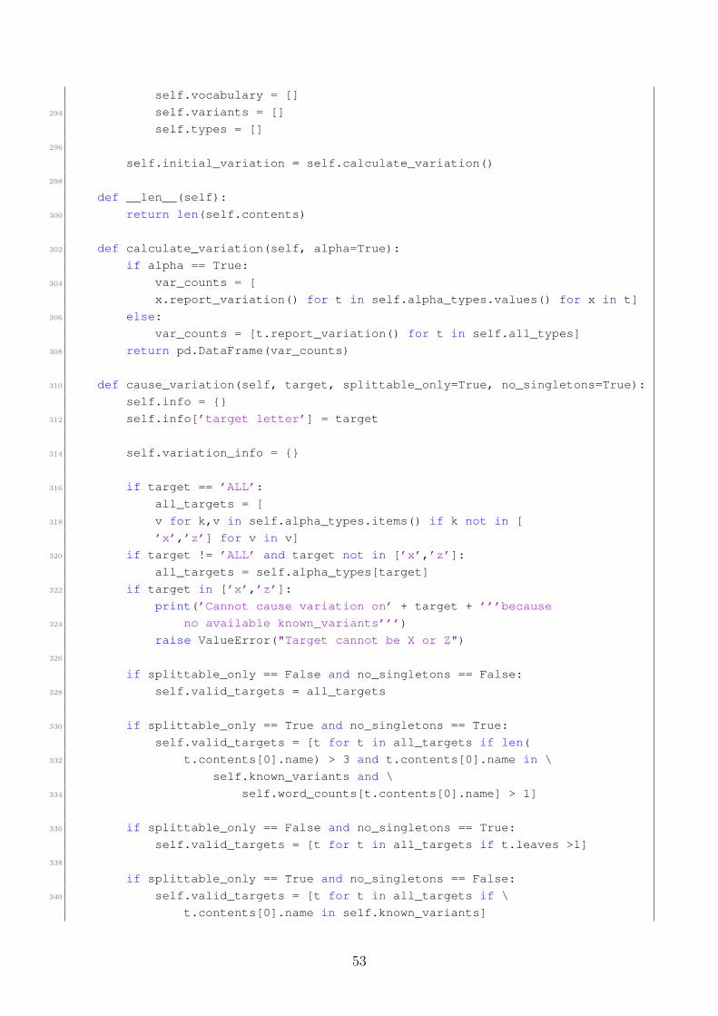
self.vocabulary = []

294 self.variants = []

self.types = []

296

self.initial_variation = self.calculate_variation()

298

def __len__(self):

300 return len(self.contents)

302 def calculate_variation(self, alpha=True):

if alpha == True:

304 var_counts = [

x.report_variation() for t in self.alpha_types.values() for x in t]

306 else:

var_counts = [t.report_variation() for t in self.all_types]

308 return pd.DataFrame(var_counts)

310 def cause_variation(self, target, splittable_only=True, no_singletons=True):

self.info = {}

312 self.info[’target letter’] = target

314 self.variation_info = {}

316 if target == ’ALL’:

all_targets = [

318 v for k,v in self.alpha_types.items() if k not in [

’x’,’z’] for v in v]

320 if target != ’ALL’ and target not in [’x’,’z’]:

all_targets = self.alpha_types[target]

322 if target in [’x’,’z’]:

print(’Cannot cause variation on’ + target + ’’’because

324 no available known_variants’’’)

raise ValueError("Target cannot be X or Z")

326

if splittable_only == False and no_singletons == False:

328 self.valid_targets = all_targets

330 if splittable_only == True and no_singletons == True:

self.valid_targets = [t for t in all_targets if len(

332 t.contents[0].name) > 3 and t.contents[0].name in \

self.known_variants and \

334 self.word_counts[t.contents[0].name] > 1]

336 if splittable_only == False and no_singletons == True:

self.valid_targets = [t for t in all_targets if t.leaves >1]

338

if splittable_only == True and no_singletons == False:

340 self.valid_targets = [t for t in all_targets if \

t.contents[0].name in self.known_variants]

53

342

# if target == ’ALL’ and len(self.valid_targets) > 2000:

344 # self.valid_targets = random.sample(self.valid_targets, 2000)

346 self.info[’splittable_only’] = splittable_only

self.info[’no_singletons’] = no_singletons

348

self.info[’Max Types available’] = len(all_targets)

350 self.info[’# Variants in max Types’] = len([t.branches \

for t in all_targets])

352

self.info[’# pre-var Type targets/Variants per Type’] = sum(

354 [t.branches for t in self.valid_targets])

356 for t in self.valid_targets:

t.induce_split(self.known_variants)

358

self.variation_info[’selection’] = self.valid_targets

360

self.info[’# Types post-var’] = len([t for t in self.valid_targets])

362 self.info[’# Variants in Types post-var’] = sum(

[t.branches for t in self.valid_targets])

364

366 self.expected_clustering = []

for t in self.variation_info[’selection’]:

368 self.expected_clustering.append(t.get_leaf_names())

370 self.words = []

for l in self.expected_clustering:

372 for x in l:

self.words.append(x)

374

for i in range(len(self.expected_clustering)):

376 for index, name in enumerate(self.expected_clustering[i]):

self.expected_clustering[i][index] = i

378

self.expected_temp = {}

380 for pair in zip(self.words, self.expected_clustering):

self.expected_temp[pair[0]] = pair[1]

382

self.expected_temp2 = sorted(self.expected_temp.items(), key=itemgetter

(0))

384

self.expected1 = [i[1] for i in self.expected_temp2]

386

self.expected = []

388 for i in list(self.expected_temp.values()):

for x in i:

54

390 self.expected.append(x)

392 self.k_to_use = len(self.valid_targets)

394

self.info[’k value’] = self.k_to_use

396 self.info[’Min +var cluster size’] = min([len(i) \

for i in self.expected_temp.values()])

398 self.info[’Max +var cluster size’] = max([len(i) \

for i in self.expected_temp.values()])

400 self.info[’Population variance +var cluster size’] = \

pvariance([len(i) for i in self.expected_temp.values()])

402 self.info[’Average +var cluster size’] = sum([len(i) \

for i in self.expected_temp.values()])/len([len(i) \

404 for i in self.expected_temp.values()])

self.info[’Ratio of Types to Variants after +var’] = \

406 self.k_to_use/self.info[’# Variants in Types post-var’]

self.info[’Ratio of +var Types to all Types’] = \

408 self.info[’# pre-var Type targets/Variants per Type’] / \

self.info[’Max Types available’]

410

def find(self,target):

412 store = []

for t in self.all_types:

414 if t.contents[0].name == target:

store.append(t)

416 return store

418 def output(self):

store = []

420 for inst in self.contents:

store.append((inst.form, inst.PoS, inst.position))

422 store = sorted(store, key=itemgetter(2))

return [(i[0], i[1]) for i in store]

goldstandard.py

55

D Code: evaluation pipeline

1 from CorpusObject1 import Corpus

from VariantObjects import Instance, Container, Variant, Type, Text

3 from itertools import product

from sklearn.metrics.cluster import *5 import pandas as pd

from collections import OrderedDict

7 from operator import itemgetter

from datetime import datetime as DT

9

def process(letter, sources, alg=’AC’, use_links=’average’, aws_setting=False,

11 use_affinity=’euclidean’):

’’’

13 This runs various parameterised versions of the Corpus object and extracts

the clustering output. Then it calculates various scores by comparing the

15 output to the expected gold standard.

This version here only works for the final model that uses JD info and

allows

17 bigrams to be turned on and off.

Saves it all to a pandas dataframe which can then have things like p-scores

19 done on it.

’’’

21

metrics = [adjusted_mutual_info_score, adjusted_rand_score,

23 mutual_info_score, normalized_mutual_info_score]

25 data = {letter:{}}

27 if aws_setting == True:

data[letter][’Post-var Text Object’] = [Text(source,

29 letter=letter, aws=True) for source in sources]

if aws_setting == False:

31 data[letter][’Post-var Text Object’] = [Text(source,

letter=letter, aws=False) for source in sources]

33

for text in data[letter][’Post-var Text Object’]:

35 text.cause_variation(letter)

37 data[letter][’Post-var Output’] = [x.output() for x in \

data[letter][’Post-var Text Object’]]

39 settings = [list(i) for i in product(letter, [True,False])]

41 data[letter][’settings’] = settings

43 results = OrderedDict()

results[letter] = OrderedDict()

45 for x in results:

for i in range(len(settings)):

56

47 results[x][i] = {}

49 for index, s in enumerate(settings):

temp = Corpus(filename=data[s[0]][’Post-var Output’][s[1]])

51 text = data[letter][’Post-var Text Object’][temp.windowsize]

print(’Starting clustering:’, index+1, ’out of’, len(settings))

53

temp.do_KM(letter=text.words, k=text.k_to_use, dump=False,

55 links=use_links, algorithm=alg)

print(’Finished clustering:’ + str(temp.generate_filename()))

57

results[letter][index][’SCORE adjusted_mutual_info_score’] = \

59 adjusted_mutual_info_score(temp.predicted, text.expected)

results[letter][index][’SCORE adjusted_rand_score’] = \

61 adjusted_rand_score(temp.predicted, text.expected)

results[letter][index][’SCORE mutual_info_score’] = \

63 mutual_info_score(temp.predicted, text.expected)

results[letter][index][’SCORE normalized_mutual_info_score’] = \

65 normalized_mutual_info_score(temp.predicted, text.expected)

67 for k,v in sorted(text.info.items(), key=itemgetter(0)):

results[letter][index][’STAT ’+k] = v

69

filename = temp.generate_filename()

71 filename = filename.split()

filename.pop(0)

73 filename = [i.split(’-’) for i in filename]

for pair in filename:

75 results[letter][index][’CONFIG ’+pair[0]] = pair[1]

77 for_dataframe = pd.DataFrame(results[letter])

for_dataframe = for_dataframe.T

79 name_to_save = ’stats/’ + DT.now().strftime(’%d%m%y-%H%M%S’) + \

letter + ’-alg-’ + alg + "-linktype-" + use_links +’-dataframe.csv’

81 for_dataframe.to_csv(name_to_save)

evaluation.py

57

References

Adesam, Yvonne, Malin Ahlberg, and Gerlof Bouma (2012). “bokstaffua, bokstaffwa, bokstafwa,bokstaua, bokstawa... Towards lexical link-up for a corpus of Old Swedish”. In: Proceedingsof the LTHist workshop at Konvens. url: http://www.oegai.at/konvens2012/proceedings/54_adesam12w/54_adesam12w.pdf.

Anderson, Jean (2013). “Enroller: an experiment in aggregating resources”. In: Language inScotland: Corpus-Based Studies. Ed. by W. Anderson. Vol. 19. Editions Rodopi B.V. url:http://eprints.gla.ac.uk/85487/1/85487.pdf.

Baron, Alistair and Paul Rayson (2008). “VARD 2: A tool for dealing with spelling variation inhistorical corpora”. In: Proceedings of the Postgraduate Conference in Corpus Linguistics.Aston University. Birmingham, UK. url: http://ucrel.lancs.ac.uk/people/paul/publications/BaronRaysonAston2008.pdf.

Baron, Alistair and Paul Rayson (2009). “Automatic standardisation of texts containing spellingvariation: How much training data do you need?” In: Proceedings of the Corpus LinguisticsConference. Ed. by Michaela Mahlberg, Victorina Gonzalez-Diaz, and Catherine Smith.Lancaster University. url: http://ucrel.lancs.ac.uk/publications/cl2009/314_FullPaper.pdf.

Baron, Alistair, Paul Rayson, and Dawn Archer (2009). “Word frequency and key word statisticsin corpus linguistics”. In: Anglistik 20.1, pp. 41–67. url: http://eprints.lancs.ac.uk/42528/1/IJES_-_final.pdf.

Bergs, Alexander (2005). Social networks and historical sociolinguistics: studies in morphosyn-tactic variation in the Paston letters (1421-1503). Vol. 51. Walter de Gruyter.

Bishop, Christopher M. (2007). Pattern recognition and machine learning. Vol. 4. 4. SpringerNew York.

Bollmann, Marcel (2012). “Automatic normalization of historical texts using distance measuresand the Norma tool”. In: Proceedings of the Second Workshop on Annotation of Corpora forResearch in the Humanities (ACRH-2), pp. 3–12. url: http://www.linguistics.ruhr-uni-bochum.de/anselm/pub/acrh12.pdf.

Bollmann, Marcel (2013). “Spelling Normalization of Historical German with Sparse TrainingData”. In: (Lancaster University). Corpus Analysis with Noise in the Signal. url: http://ucrel.lancs.ac.uk/cans2013/abstracts/Bollmann.pdf.

Bollmann, Marcel, Florian Petran, and Stefanie Dipper (2011). “Rule-based normalization ofhistorical texts”. In: Proceedings of the International Workshop on Language Technologies forDigital Humanities and Cultural Heritage, pp. 34–42. url: http://www.linguistics.rub.de/~petran/papers/ranlp2011.pdf.

58

Coltheart, Max et al. (2001). “DRC: A dual route cascaded model of visual word recognitionand reading aloud.” In: Psychological Review 108.1, pp. 204–256. url: http://dx.doi.org/10.1037/0033-295X.108.1.204.

Damerau, Fred J. (1964). “A technique for computer detection and correction of spelling errors”.In: Communications of the ACM 7.3, pp. 171–176.

Davis, Norman (1971). Paston letters and papers of the fifteenth century. Oxford UniversityPress.

Evans, Mel (2012). “A Sociolinguistics of Early Modern Spelling? An account of Queen Eliza-beth I’s correspondence”. In: Studies in Variation, Contacts and Change in English 10. url:http://www.helsinki.fi/varieng/series/volumes/10/evans/.

Firth, John Rupert (1957). A Synopsis of Linguistic Theory, 1930-1955.

Gairdner, James (1895). The Paston Letters, 1422-1509 AD. Vol. 1. A. Constable.

Görlach, M. (1991). Introduction to Early Modern English. Cambridge University Press. isbn:9780521310468.

Healey, Antonette diPaolo (2002). “The Dictionary of Old English: FromManuscripts to Megabytes”.In: Dictionaries: Journal of the Dictionary Society of North America 23.1, pp. 156–179. url:http://dx.doi.org/10.1353/dic.2002.0009.

Jaro, Matthew A. (1989). “Advances in Record-Linkage Methodology as Applied to Matchingthe 1985 Census of Tampa, Florida”. In: Journal of the American Statistical Association84.406, pp. 414–420. url: http://dx.doi.org/10.1080/01621459.1989.10478785.

Jespersen Otto, 1860-1943 (1928). Modern English grammar on historical principles. Part 1,Sounds and spellings. 4th ed. London: G. Allen & Unwin ltd.

Kukich, Karen (1992). “Techniques for Automatically Correcting Words in Text”. In: ACMComput. Surv. 24.4, pp. 377–439. issn: 0360-0300. url: http://dx.doi.org/10.1145/146370.146380 (visited on 12/23/2014).

Lass, Roger (1997). Historical Linguistics and Language Change (Cambridge Studies in Lin-guistics). Cambridge University Press. isbn: 0521459249.

Lass, Roger, ed. (2000). The Cambridge History of the English Language. Cambridge UniversityPress (CUP). url: http://dx.doi.org/10.1017/CHOL9780521264761.

Levenshtein, Vladimir I. (1966). “Binary codes capable of correcting deletions, insertions, andreversals”. In: Soviet physics doklady. Vol. 10, pp. 707–710.

Luick, Karl (1903). Studien zur englischen Lautgeschichte. Vol. 17. W. Braumüller.

59

Markus, Manfred (2015). Innsbruck Computer Archive of Machine-Readable English Texts.url: http://www.uibk.ac.at/anglistik/projects/icamet/ (visited on02/05/2015).

Rissanen, Matti (2000). “The world of English historical corpora”. In: Journal of English Lin-guistics 8.1, pp. 7–20.

Robertson, Alexander M. and Peter Willett (1992). “Searching for Historical Word-forms in aDatabase of 17Th-century English Text Using Spelling-correction Methods”. In: Proceedingsof the 15th Annual International ACM SIGIR Conference on Research and Development inInformation Retrieval. SIGIR ’92. New York, NY, USA: ACM, pp. 256–265. isbn: 0-89791-523-2. url: http://dx.doi.org/10.1145/133160.133208.

Russell, R. and M. Odell (1918). “Soundex”. In: US Patent 1.

Seidenberg, Mark S. and James L. McClelland (1989). “A distributed, developmental modelof word recognition and naming.” In: Psychological Review 96.4, pp. 523–568. url: http://dx.doi.org/10.1037/0033-295X.96.4.523.

Stockwell, Robert and Donka Minkova (1988). “The English Vowel Shift: problems of coherenceand explanation”. In: Luick Revisited. Tübingen: Gunter Narr Verlag, pp. 355–394.

Taylor, Ann et al. (2006). Parsed Corpus of Early English Correspondence. url: http://www-users.york.ac.uk/~lang22/PCEEC-manual/ (visited on 01/07/2015).

Ullman, Michael T. (2001). “A neurocognitive perspective on language: The declarative/proce-dural model”. In: Nature Reviews Neuroscience 2.10, pp. 717–726. url: http://dx.doi.org/10.1038/35094573.

Vinh, Nguyen Xuan, Julien Epps, and James Bailey (2010). “Information theoretic measuresfor clusterings comparison: Variants, properties, normalization and correction for chance”.In: The Journal of Machine Learning Research 11, pp. 2837–2854.

Xu, R. and D. Wunsch (2005). “Survey of Clustering Algorithms”. In: IEEE Trans. NeuralNetw. 16.3, pp. 645–678. url: http://dx.doi.org/10.1109/tnn.2005.845141.

Zhao, Ying, George Karypis, and Usama Fayyad (2005). “Hierarchical Clustering Algorithmsfor Document Datasets”. In: Data Mining and Knowledge Discovery 10.2, pp. 141–168. url:http://dx.doi.org/10.1007/s10618-005-0361-3.

60